Thesis for the degree of Doctor of Philosophy

Medium Access Control for Vehicular Ad Hoc Networks

Katrin Sjöberg

Göteborg, Sweden, 2013

School of Information Science,

Computer and Electrical Engineering

HALMSTAD UNIVERSITY

Department of Signals and Systems

CHALMERS UNIVERSITY OF TECHNOLOGY

Medium Access Control for Vehicular Ad Hoc Networks KATRIN SJÖBERG ISBN 978-91-7385-832-8

Copyright Katrin Sjöberg, 2013. All rights reserved.

Doktorsavhandlingar vid Chalmers tekniska högskola ISSN 1403-266X Ny serie nr 3513

Department of Signals and Systems CHALMERS UNIVERSITY OF TECHNOLOGY Hörsalsvägen 11 SE-412 96 Göteborg Sweden Telephone: +46 - (0)31 - 772 10 00 Fax: +46 - (0)31 - 772 36 63

Contact Information: Katrin Sjöberg School of Information Science, Computer and Electrical Engineering HALMSTAD UNIVERSITY SE-301 18 Halmstad Sweden Telephone: +46 - (0)35 - 16 71 00 Fax: +46 - (0)35 - 12 03 48 Email: Katrin.Sjoberg@hh.se

Printed in Sweden Chalmers Reproservice Göteborg, Sweden, 2013

i

Medium Access Control for Vehicular Ad Hoc Networks KATRIN SJÖBERG Department of Signals and Systems, Chalmers University of Technology

Abstract Cooperative intelligent transport systems (C-ITS), where vehicles cooperate by exchanging messages wirelessly to avoid, for example, hazardous road traffic situations, receive a great deal of attention throughout the world currently. Many C-ITS applications will utilize the wireless communication technology IEEE 802.11p, which offers the ability of direct communication between vehicles, i.e., ad hoc communication, for up to 1000 meters. In this thesis, medium access control (MAC) protocols for vehicular ad hoc networks (VANET) are scrutinized and evaluated. The MAC protocol decides when a station has the right to access the shared communication channel and schedules transmissions to minimize the interference at receiving stations. A VANET is a challenging network for the MAC proto-col because the number of stations in is unknown a priori and cannot be bounded. Therefore, the scalability of the MAC method has a major influence on the performance of C-ITS applications.

Two different MAC protocols are studied: carrier sense multiple access (CSMA) of 802.11p and self-organizing time division multiple access (STDMA). These two MAC methods are examined with re-spect to the communication requirements and protocol settings arising from C-ITS standardization. Based on these constraints, suitable performance measures are derived such as MAC-to-MAC delay and detection distance, where the former catches both the delay and reliability.

In STDMA, the channel access delay is upper-bounded and therefore known before transmission, since regardless of the number of stations within radio range, all stations are always guaranteed timely channel access. In CSMA, the channel access delay is not upper-bounded and it is unknown until transmission commences, as it is based on the instantaneous channel load and stations can experience a random delay when in backoff.

The evaluation of CSMA and STDMA is performed through extensive computer simulations, model-ling a 10 km highway with six lanes in each direction. Vehicles travel along the highway and broad-cast position messages periodically with different update rates. Two different channel models have been used during the evaluations, one distinguishing between a receiver being in line-of-sight (LOS) or obstructed LOS (OLOS) from the transceiver, while the other does not consider this.

The simulation results, for both channel models, show that CSMA has on average a smaller channel access delay than STDMA. However, the results also reveal that STDMA always achieves a better reliability than CSMA, especially for distances of 100-500 meters between transmitter and receiver. The distance, at which approaching stations receive the first messages from each other, is up to 100 meters longer for STDMA than CSMA. This thesis therefore concludes that STDMA is a very suitable MAC method for VANET-based C-ITS applications.

Keywords: CSMA, self-organizing TDMA, STDMA, SOTDMA, medium access control, MAC, vehicular ad hoc networks, VANET, vehicle-to-vehicle communications, V2V, V2X, IEEE 802.11p, WAVE, DSRC, ETSI ITS-G5, ISO CALM M5, real-time communications, scalability, traffic safety, cooperative system, cooperative ITS, C-ITS

ii

Acknowledgement

I am sitting here (exhausted), really late the day before the printing of the dissertation, and I must remember and thank all people that has in one way or another influenced me during my studies. It is really tricky. I have decided to only include two persons by names, which have had the greatest im-pact during this incredible journey. With these two persons I have had a tremendously enjoyable time as a PhD student, without them encouraging and inspiring me I would never had finished this dissertation. Therefore, my deepest thanks go to my supervisor and examiner Prof. Erik G. Ström at Chalmers University of Technology and my supervisor Assoc. Prof. Elisabeth Uhlemann at Halmstad University.

I also want to thank my colleagues at CC-lab, School of Information Science, Computer and Electrical Engineering at Halmstad University and at Communication Systems, Department of Signals and Sys-tems at Chalmers University of Technology.

Last but not least, I would like thank all my friends and my family that have been encouraging and understanding when I have not had time for them. Now, a new era of my life starts and I will try to catch up with you all .

This work was mainly funded by the Knowledge Foundation through the profile Center for Research on Embedded Systems (CERES), Halmstad University.

iii

List of papers The dissertation is based on the following peer-reviewed publications:

I. T. Abbas, F. Tufvesson, K. Sjöberg, and J. Karedal, “Measurement Based Shadowing Fading Model for Vehicle-to-Vehicle Network Simulations,” submitted to IEEE Transactions on Ve-hicular Technology.

II. K. Lidström, K. Sjöberg, U. Holmberg, J. Andersson, F. Bergh, M. Bjäde, and S. Mak, ”A Modu-lar CACC System Integration and Design,” in IEEE Transactions on Intelligent Transportations Systems, vol. 13, no. 3, pp. 1050-1061, Sept. 2012.

III. K. Sjöberg, E. Uhlemann, and E. G. Ström, “How severe is the hidden terminal problem in VANETs when using CSMA and STDMA?,” in Proc. of the 74th IEEE Vehicular Technology Con-ference (VTC2011-Fall), San Francisco, US, Sept. 2011, pp. 1-5.

IV. K. Sjöberg, E. Uhlemann, and E. G. Ström, “Delay and interference comparison of CSMA and self-organizing TDMA when used in VANETs,” in Proc. of the 7th Int. Wireless Communications and Mobile Computing Conference (IWCMC), Istanbul, Turkey, July 2011, pp. 1488-1493.

V. K. Sjöberg, J. Karedal, M. Moe, Ø. Kristiansen, R. Søråsen, E. uhlemann, F. Tufvesson, K. Even-sen, and E. G. Ström, ”Measuring and using the RSSI of IEEE 802.11p,” in Proc. of the 17th World Congress on Intelligent Transport Systems, Busan, Korea, Oct. 2010

VI. K. Sjöberg Bilstrup, E. Uhlemann, and E. G. Ström, “Scalability issues for the MAC methods STDMA and CSMA/CA of IEEE 802.11p when used in VANETs,” in Proc. of the IEEE Interna-tional Conference on Communications (ICC’10), Cape Town, South Africa, May 2010, pp. 1-5.

VII. K. Bilstrup, E. Uhlemann, E. G. Ström, and U. Bilstrup, “On the Ability of the 802.11p MAC Method and STDMA to Support Real-Time Vehicle-to-Vehicle Communication,” in EURASIP Journal on Wireless Communications and Networking, vol. 2009, Article ID 902414, 13 pages, doi:10.1155/2009/902414.

VIII. K. Bilstrup, E. Uhlemann, E. G. Ström, and U. Bilstrup, “On the ability of IEEE 802.11p and STDMA to provide predictable channel access,” in Proc. of 16th World Congress on ITS, Stock-holm, Sweden, Sept. 2009.

IX. K. Bilstrup, E. Uhlemann, and E. G. Ström, “Medium access control in vehicular networks based on the upcoming IEEE 802.11p standard”, in Proc. of the 15th World Congress on Intel-ligent Transport Systems, New York, US, Nov. 2008.

X. K. Bilstrup, E. Uhlemann, E. G. Ström, and U. Bilstrup, “Evaluation of the IEEE 802.11p MAC method for vehicle-to-vehicle communication,” in Proc. of the 68th IEEE Vehicular Technology Conference (VTC2008-Fall), Calgary, Canada, Sept. 2008, pp. 1-5.

XI. K. Bilstrup, “A survey regarding wireless communication standards intended for a high-speed vehicle environment,” Technical Report IDE0712, Halmstad University, Sweden, Feb. 2007.

v

Table of contents ABSTRACT ...................................................................................................................................................... I

ACKNOWLEDGEMENT .................................................................................................................................... II

LIST OF PAPERS ............................................................................................................................................ III

TABLE OF CONTENTS .................................................................................................................................... V

1 INTRODUCTION .................................................................................................................................... 1

1.1 VEHICULAR AD HOC NETWORKS ........................................................................................................................ 2

1.2 MEDIUM ACCESS CONTROL .............................................................................................................................. 3

1.3 SCOPE ......................................................................................................................................................... 4

1.4 PROBLEM DESCRIPTION ................................................................................................................................... 4

1.5 CONTRIBUTIONS ............................................................................................................................................ 5

1.6 METHOD ...................................................................................................................................................... 7

1.7 OUTLINE ...................................................................................................................................................... 7

2 STANDARDIZATION ON VEHICULAR COMMUNICATIONS ....................................................................... 9

2.1 IEEE WAVE ............................................................................................................................................... 10

2.1.1 Physical layer ................................................................................................................................. 12

2.1.2 Datalink layer ................................................................................................................................ 13

2.1.3 Network/Transport layers ............................................................................................................. 16

2.1.4 Security .......................................................................................................................................... 16

2.1.5 Message Set Dictionary ................................................................................................................. 17

2.1.6 General packet structure of a BSM message................................................................................. 17

2.2 ETSI TC ITS ............................................................................................................................................... 17

2.2.1 Access layer ................................................................................................................................... 18

2.2.2 Network/Transport layers ............................................................................................................. 19

2.2.3 Facilities and Application layers .................................................................................................... 22

2.2.4 General packet structure of a CAM ............................................................................................... 26

2.2.5 Decentralized congestion control .................................................................................................. 27

2.3 DIFFERENCES BETWEEN ETSI TC ITS AND IEEE WAVE ...................................................................................... 29

3 MEDIUM ACCESS CONTROL ................................................................................................................ 31

3.1 CARRIER SENSE MULTIPLE ACCESS .................................................................................................................... 31

3.1.1 Channel access procedure ............................................................................................................. 31

3.2 SELF-ORGANIZING TIME DIVISION MULTIPLE ACCESS ............................................................................................ 36

3.2.1 Channel access procedure ............................................................................................................. 37

3.2.2 Summary STDMA ........................................................................................................................... 41

vi

3.3 SIMULTANEOUS TRANSMISSIONS ..................................................................................................................... 41

3.4 RELATED WORK ........................................................................................................................................... 45

3.5 SUMMARY .................................................................................................................................................. 48

4 PERFORMANCE EVALUATION OF CSMA AND STDMA .......................................................................... 49

4.1 RADIO PROPAGATION MODEL ......................................................................................................................... 50

4.1.1 Nakagami model ........................................................................................................................... 50

4.1.2 LOS/OLOS model ........................................................................................................................... 51

4.1.3 Comparison of the deterministic parts of both channel models .................................................... 52

4.1.4 Signal-to-interference-plus-noise ratio .......................................................................................... 54

4.2 DATA TRAFFIC MODEL ................................................................................................................................... 54

4.3 MAC SPECIFIC PARAMETERS .......................................................................................................................... 54

4.3.1 CSMA ............................................................................................................................................. 54

4.3.2 STDMA ........................................................................................................................................... 55

4.4 VEHICLE TRAFFIC MODEL ............................................................................................................................... 55

4.5 PERFORMANCE METRICS ............................................................................................................................... 57

4.5.1 Channel access delay ..................................................................................................................... 57

4.5.2 Packet reception probability ......................................................................................................... 58

4.5.3 MAC-to-MAC delay ........................................................................................................................ 58

4.5.4 Packet inter-arrival time ................................................................................................................ 59

4.5.5 Detection distance ......................................................................................................................... 59

4.6 SIMULATION RESULTS ................................................................................................................................... 60

4.6.1 Channel access delay ..................................................................................................................... 60

4.6.2 Packet reception probability ......................................................................................................... 66

4.6.3 MAC-to-MAC delay ........................................................................................................................ 76

4.6.5 Packet inter-arrival time ................................................................................................................ 84

4.6.6 Detection distance ......................................................................................................................... 91

4.7 SUMMARY ................................................................................................................................................ 103

5 CONCLUSIONS .................................................................................................................................. 105

6 FUTURE OUTLOOK ............................................................................................................................ 107

REFERENCES .............................................................................................................................................. 109

APPENDIX A – ABBREVIATIONS .................................................................................................................. 115

1

1 Introduction Cooperative intelligent transport systems (C-ITS) [1], where vehicles cooperate by exchanging mes-sages wirelessly to avoid for example hazardous road traffic situations, receive a great deal of atten-tion throughout the world currently. There are intense research activities and standardization efforts on-going within this area. Further, major field operational tests (FOT) are planned and underway [2, 3]. Depending on application, there are mainly two wireless technologies considered for C-ITS; the short-range communication technology IEEE 802.11p [4] and cellular networks such as 3G/LTE. The latter depends on a centralized network topology where all data traffic must take a detour via the base station (BS) even though two stations are geographically co-located. IEEE 802.11p, on the other hand, offers the ability for direct communication between ITS stations, i.e., ad hoc communication, for up to 1000 meters. IEEE 802.11p1 is an amendment to the ubiquitous wireless local area network (WLAN) standard IEEE 802.11-2012 [5] tailored to the vehicular environment. IEEE 802.11-2012 spec-ifies the medium access control (MAC) sub-layer and several physical (PHY) layers. In 802.11p, ITS stations do not have to associate with each other before communication takes place therefore no network has to be established. Further, although no access point (AP) is present in 802.11p, there can be fixed ITS stations (e.g., ITS equipped traffic lights) offering services to mobile ITS stations (e.g., vehicles) and the distinction between mobile and fixed ITS stations is made at higher layers in the protocol stack.

C-ITS applications can roughly be categorized into road traffic safety, road traffic efficiency and value-added services [6]. Road traffic safety applications have stringent requirements on both bounded delay and high reliability, concurrently. Therefore, protocol stacks dedicated for supporting this type of applications have been developed in the USA and in Europe. The common denominators for these stacks are the communication technology 802.11p and simple network/transport protocols with low overhead allowing passing through the protocol stack faster. Road traffic efficiency applications and value-added services can use 802.11p technology and/or 3G/LTE together with the network protocol IPv6 supporting Internet connections. Value-added services may for example be announcements of commercial services such as advertisements for hotels, petrol stations, grocery stores etc. Examples of road traffic safety applications are lane change warning, emergency vehicle approaching, station-ary vehicle, road conditions, road work, etc. Efficiency applications aim at enhancing the road traffic flow, reducing CO2-emissions and pollution, through for example green light optimal speed advisory (GLOSA), traffic light optimization, in-vehicle signage, and enhanced route guidance. However, the border between road traffic safety and road traffic efficiency applications is not clear cut. If an acci-dent occurs, e.g., a vehicle suddenly breaks down in the middle of the street (stationary vehicle); the enhanced route guidance application can advise drivers to take an alternative route before they reach the stationary vehicle and end up in a queue with no possibility to turn around. In other words, the safety application can in certain situations trigger efficiency applications, and vice-versa.

Standardization on C-ITS specifies two types of messages that will be used to realize road traffic safe-ty applications; time-triggered position messages and event-driven hazard warnings. The former is

1 IEEE 802.11p [4] has been incorporated in the new version of IEEE 802.11-2012 [5] and it is therefore classi-fied as superseded. For simplicity the vehicular “profile” of 802.11 will be referred to as 802.11p throughout the thesis.

2

called cooperative awareness message (CAM) in Europe [7] and basic safety message (BSM) in the USA [8]. The event driven messages are called decentralized environmental notification message (DENM) in Europe [9] whereas USA does not have a distinct name for this type of message (although sometimes referred to as BSM type 2). CAM/BSM will be sent with an update rate of 1-10 Hz depend-ing on context and contain information about the vehicle speed, position, heading, path history, etc. They will roughly be around 200 bytes long without security overhead, which will add further bytes. A DENM will be issued when a road traffic safety application detects an upcoming potentially dan-gerous situation. Once triggered, the DENM will be sent periodically until the event is no longer valid (the situation was avoided or the situation has occurred) upon which a “stop” DENM will be transmit-ted.

Different C-ITS applications have different communication requirements and thus 3G/LTE and IEEE 802.11p are not two competing technologies they rather complement each other. One of the main advantages of 802.11p is the easy dissemination of information locally around the ITS station. Infor-mation can also be transmitted in a certain direction on the highway using geographical routing (georouting). The information contained in CAM/BSM is perishable with short life-time due to the movement of vehicles – the higher speed of the vehicle the shorter time the information is valid (in particular this concerns position information). By using the ad hoc communication of IEEE 802.11p, delays can be kept low since no detour around a BS is necessary. C-ITS applications that do not have short delay requirements or rely on information being spread regionally rather than locally can utilize 3G/LTE. For example, a fixed ITS station using 802.11p can act as an information provider to services offered by 3G/LTE by transmitting service announcements to surrounding vehicles, which in turn can connect to the 3G/LTE network themselves to retrieve more information. It should be noted, howev-er, that 3G/LTE networking currently requires subscription to a specific mobile telephone operator, which is not necessary for 802.11p used for C-ITS.

1.1 Vehicular ad hoc networks The majority of the data transmitted in the vehicular ad hoc network (VANET) supporting traffic safe-ty applications will be broadcasted (one-to-many communication) and no acknowledgements (ACK) will be sent in response if messages are received successfully. Many ITS stations are typically inter-ested in receiving the broadcasted messages and if everyone sent an ACK the communication chan-nel would be flooded. In the VANET using 802.11p (with no central coordination), there will be a set of predetermined frequency channels for communication, and the only way to state the presence of an ITS station is to broadcast CAM/BSM on one these channels.

The network establishment has been removed in 802.11p, i.e., a station is allowed to communicate outside the context of a basic service set (the smallest building block of an 802.11 network). This implies that whenever a station has a message to send it can transmit directly under the condition that the MAC protocol allows it. Ad hoc topologies without prior network establishment has ad-vantages such that a lower average delay can be achieved and no coverage by base stations is neces-sary – if there is someone to communicate with information exchange can take place. On the other hand, the ad hoc structure entails specific requirements for the communication protocols operating in this scenario. Specifically, the MAC protocol used in a VANET must be decentralized. It must cope with few stations as well as many stations without collapsing. Further, it should minimize simultane-ous transmissions in an attempt to keep the interference at an acceptable level for receiving stations.

3

The MAC protocol is a key component in cooperative systems because if channel access is not grant-ed in a timely fashion, cooperation cannot be achieved.

1.2 Medium access control The MAC method decides when a station has the right to access the shared communication channel. The regulation is made by scheduling transmissions in time, frequency, space or by using unique codes, constellations or interleavers to distinguish different stations. The type of MAC method to use in a particular communication network is selected based on network topology and application. Since all communications in a centralized network must traverse the AP/BS, it has knowledge of all nodes within range. A centralized network can therefore use a centralized MAC protocol that distributes available resources (frequencies, time slots or orthogonal codes) among all nodes currently within range. This implies that the AP/BS can use the MAC protocol to optimize performance based on spe-cific requirements. In ad hoc networks it is more difficult find such a resource efficient MAC method, especially since the number of stations can drastically vary from time to time. In a C-ITS operating in a VANET context, the requirements on the MAC method stem from three different parts namely (i) the ad hoc topology, (ii) road traffic safety applications, and (iii) the overall C-ITS.

The ad hoc topology requires the MAC protocol to be inherently:

• Self-organizing • Scalable

The road traffic safety applications have requirements on:

• Delay • Reliability

The overall C-ITS requirement on the MAC method is:

• Fairness

The ability to self-organize and scalability are two properties that the MAC method must have, to operate in an ad hoc topology. The ability of the MAC method to self-organize is a strict requirement, since no centralized coordination of the resources exists in VANETs. Scalability is defined in [10] as “A system is said to be scalable if it can handle the addition of users and resources without suffering a noticeable loss of performance or increase in administrative complexity.” In VANET-based road traf-fic safety applications, the number of stations cannot be restricted nor is it known in advance. The MAC protocol in a VANET therefore needs to fulfill the requirements on delay, reliability and fairness even though there are many stations in the system. Therefore, the scalability property of the MAC method is imperative since this significantly affects the delay, reliability and fairness jointly.

The delay does not necessarily need to be low to meet the requirements of VANET-based safety ap-plications. It is more important that it is predictable, i.e., there exists an upper bound on the channel access delay. With a predictable channel access delay, the station knows if it can meet the delay re-quirements of a certain message even in extreme cases, and it has the possibility to reorder and re-schedule messages depending on importance. Further, with a predictable channel access delay the station is given the possibility to optimize its message generation towards when the channel access is granted and thereby the information in the position message will be up-to-date.

4

Reliability is particularly cumbersome in broadcast communication scenarios since no ACKs are transmitted in response if a message was successfully received. In traditional unicast (one-to-one) communication, a message can be retransmitted until it is received correctly and reliability ap-proaches 100% when the delay grows to infinity. In other words, there is a trade-off between delay and reliability. Much like delay, reliability is addressed at several layers in the protocol stack. The PHY can enhance the reliability with suitable coding, modulation or/and diversity techniques tailored for the propagation environment. At the MAC layer reliability refers to the ability of the MAC method to schedule transmissions to reduce interference between stations.

The level of fairness between individual stations should be as high as possible in VANET-based safety applications. From a MAC perspective, fairness is translated into equal probability to access the channel given the same type of data traffic, i.e., the same Quality of Service (QoS) class should have the same probability of timely channel access for all stations in the system. Further, if the channel access delay and the interference during channel access vary greatly between transmissions, the MAC layer should try to distribute these variations among stations as fair as possible.

Consequently, the MAC protocol used in a VANET needs to be self-organizing such that unused re-sources are reclaimed regularly, it should be scalable such that no vehicles are excluded, it should provide a predictable delay such that channel access delay can be upper-bounded and fair, and it should schedule all transmissions to minimize interference for increased reliability.

1.3 Scope The focus of this thesis is to evaluate MAC methods for VANET with respect to the communication requirements arising from applications found within C-ITS, together with parameters and constraints stemming from C-ITS standardization. To this end, this thesis investigates the performance of two different MAC protocols, namely carrier sense multiple access (CSMA) of 802.11p and self-organizing time division multiple access (STDMA). The evaluated scenario is a case where all vehicles broadcast periodic position messages (CAM/BSM) with different update rates when travelling on a 10 km high-way with six lanes in each direction (no urban scenarios are used for evaluation and no unicast data traffic is present). In addition, suitable performance measures are defined, specifically for evaluating MAC methods in VANET, in which there can be no upper limit on the number of participating sta-tions.

1.4 Problem description The following research questions have been addressed in this thesis:

1. What type of communications requirements are imposed on the MAC layer of a VANET used for broadcasting road traffic safety data?

2. What performance metrics are suitable for evaluating MAC schemes for road traffic safety applications?

3. Given these performance metrics, what can we expect from the MAC in the current standard 802.11p?

4. Is there an alternative MAC scheme that can perform better? 5. How prominent is the scalability issue given the data traffic patterns derived from standardi-

zation?

5

6. How much does the channel model influence the evaluation of MAC schemes?

A VANET constitutes a particularly challenging communication environment due to the rapidly chang-ing station density. Further, the number of participating stations in a VANET is not always known and, more importantly, cannot be restricted. Since the decentralized network topology contains no AP or BS regulating access to the shared channel, scalability issues become more prominent. The concept of cells and reuse of frequency is not possible to use at the same extent as in cellular networks. In addition, the current proposal of both European and US standardization efforts is that all vehicles must share a common frequency channel for transmitting CAM/DENM/BSM. Therefore, many ve-hicular communication links will have to share the same radio spectrum in a limited geographical area, causing interference to one another.

1.5 Contributions Major contributions of this thesis are:

1. Up to date and comprehensive survey of C-ITS standardization, outlining requirements 2. New performance measures for evaluating MAC schemes for road traffic safety applications 3. Thorough evaluation study of the MAC scheme in the current standard 802.11p 4. Proposal of using alternative MAC scheme for VANETs fulfilling outlined requirements 5. Evaluation the impact of different network loads on MAC performance in VANET 6. Evaluating the impact of two different channel models on MAC performance in VANET

The research presented in this thesis started in 2006, which was before C-ITS standardization in Eu-rope had been initiated (ETSI Technical Committee on ITS was established in December 2007). In 1999, activities on ITS took off in the US when the Federal Communications Commission (FCC) allo-cated a 75 MHz band at 5.850-5.925 GHz especially intended for ITS: “to improve traveller safety, decrease congestion, facilitate the reduction of air pollution, and help to conserve vital fossil fuels” [11]. In 2004, IEEE begun its development of 802.11p and it was ratified in 2010. In [XI] from 2007, we surveyed several different wireless technologies for the high-speed vehicular environment and the only identified technology for ad hoc communication between vehicles, was 802.11p.

The MAC algorithm of 802.11p is based on CSMA, which faces problems with fairness when the number of stations increases within radio range as shown in [IX, X]. In [X], we also presented STDMA as an alternative MAC scheme for VANETs for the first time. STDMA is already in commercial use in a system called Automatic Identification System (AIS), which is a mandatory position reporting system for ships larger than 300 gross ton and passenger vessels. The AIS is very similar to what is currently under development for the vehicular environment. In AIS, ships keep track of each other through wirelessly communicated position messages and thereby accidents can be avoided. The AIS was de-veloped to combat the short-comings with conventional radar systems, such as the inability to see behind other objects and cluttered radar images due to bad weather situations. In [X], we adjusted the STDMA algorithm to fit the high-speed vehicular environment with respect to the PHY proposed in 802.11p and the carrier frequency of 5.9 GHz. In AIS, a carrier frequency of 160 MHz is employed together with a PHY based on Gaussian filtered minimum shift keying with frequency modulation (GMSK/FM).

In [VII, VIII], we studied channel access delay of CSMA and STDMA in VANETs, and showed that, when the network is overloaded, CSMA will start to drop packets at the sending side since newer packets

6

arrive at the MAC layer from the application before channel access had been granted for the earlier packet. The number of consecutive packet drops could result in lack of channel access for up to 10 seconds for some individual ITS stations. It was also shown that CSMA becomes unfair in overloaded situations, i.e., there was a major difference between the worst case channel access delay and the best case channel access delay in CSMA. In STDMA, however, all stations are guaranteed channel access regardless of the number of stations within radio range implying that the channel access delay is upper bounded. However, since STDMA allows more simultaneous transmissions, this leads to higher interference for certain stations. This is in contrast to CSMA, where stations instead start to drop packets at the sending side.

In [VI], we studied the occurrence of simultaneous transmissions within radio range for STDMA and CSMA. When the network load increases, STDMA allows simultaneous transmissions within radio range, but these are scheduled in space (using the position information contained in CAMs), i.e., STDMA aims to maximize the distance between two simultaneously transmitting stations. In CSMA, any stations that reach a backoff value of zero at the same time will cause simultaneous transmis-sions, and the backoff values do not depend on where in space the station is situated. In other words, STDMA strives to make the interference situation as favorable as possible for the closest neighbors, whereas in CSMA when simultaneous transmissions occur randomly and when they are co-located, packets are more likely lost. Simultaneous transmissions carried out outside the radio range of stations were studied in detail in [III], a.k.a. hidden terminal situations. Simulations of a highway scenario where carried out, in which all hidden terminal transmissions according to the def-inition in [III], were removed to determine their influence on performance. The results revealed that, even if no hidden terminal transmission occurred (due to being artificially removed), the packet re-ception probability did not increase drastically for CSMA or STDMA.

Given the communication requirements of VANET-based road traffic safety applications, we intro-duced a new performance metric called MAC-to-MAC delay in [IV], merging the channel access delay and reliability into one performance measure. In this measure the channel access delay goes to infini-ty when the message is not successfully decoded at receiver. The results revealed that even if CSMA on average has shorter channel access delay than STDMA, the reliability is not as high as for STDMA (i.e., fewer receptions goes towards infinity). The results in that, the cumulative distribution function (CDF) of the MAC-to-MAC delay is higher for STDMA than CSMA, after the initial delay.

While conducting the research presented in this thesis, standardization has evolved and much has changed throughout the years such as the generation rules of CAMs/BSMs, default data transfer rate and update rates. Back in 2006, a fixed update rate was foreseen. The discussion within standardiza-tion was then to use 2 Hz update rates and 800 byte long packets in Europe whereas similar discus-sions in US landed in 10 Hz and shorter packets around 300 bytes. The uncertainty regarding packet size stem mainly from the different security approaches investigated on both sides of the Atlantic. Further, position messages were initially thought to be sent using the highest priority queue of CSMA. These settings were used in all of the papers on which this thesis is based; reflect the on-going discussion within standardization at the time of publication. However, in this thesis the latest settings for default data transfer rate, packet length, update rates, priority queue for CSMA, etc., are all de-rived from current standardization as outlined in Chapter 2. These settings have also been the foun-dation for the performance evaluation of CSMA and STDMA conducted in Chapter 4. Further, a new channel model based on a recent channel sounding campaign is introduced [I] and compared with a

7

channel model based on the Nakagami-m model [12]. Five different performance metrics are derived and used for evaluating the MAC methods, including one previously unpublished: Detection Distance is established in this thesis.

1.6 Method The methodology has been:

1. Literature study 2. Interaction with industry in ETSI standardization to ensure industrial relevance and

knowledge transfer 3. Measurement campaigns and practical experiments 4. Careful development of performance metrics 5. Careful implementation of MAC methods in MATLAB and extensive computer simulations

The research direction was identified in [XI], where a literature study was performed on wireless technologies for the high-speed vehicular environment. Extensive system level computer simulations have been performed in MATLAB, where the MAC methods CSMA and STDMA have been evaluated in a highway scenario broadcasting CAMs/BSMs, resulting in several publications [III, IV, VI, VII, VIII, IX, X].

In January 2009, we were invited to ETSI Technical committee on ITS in Europe to present our ideas on an alternative MAC scheme for VANETs. Since then an active participation in standardization has remained. A Specialist Task Force 395 (STF395) within ETSI was put together in 2011 (led by the au-thor) which resulted in two published technical reports [13, 14] dealing with the suitability of time-slotted MAC approaches for road traffic safety applications. The author has also drafted the new version of the access layer technology, EN 302 663 [15], based on 802.11p with additional features tailored for the European frequency bands.

Practical work has also been part of the evaluation work presented in this thesis such as a measure-ment campaign using 802.11p hardware [V]. Further, an implementation of a cooperative adaptive cruise control (CACC) based on 802.11p communication was performed in [II].

1.7 Outline In Chapter 2, the standardization status for C-ITS in Europe and the USA is outlined, motivating the communication requirements on the MAC method presented in Chapter 3 and the parameter set-tings for the performance evaluation in Chapter 4. The two evaluated MAC schemes, CSMA and STDMA, are detailed in Chapter 3 together with related work on MAC schemes for VANETs. The per-formance metrics used for the MAC evaluation is outlined in Chapter 4, reflecting the requirements from C-ITS in Section 1.2. Simulation results are presented in Chapter 4, followed by conclusions and future outlook in Chapter 5 and Chapter 6, respectively.

9

2 Standardization on vehicular communications Much has happened during the last decade within all major standards development organizations (SDO) dealing with vehicular communications. The standardization on vehicular communications took off in 1999 when the U.S. Federal Communications Commission (FCC) allocated a 75 MHz band at 5.850-5.925 GHz especially intended for ITS: “to improve traveler safety, decrease traffic conges-tion, facilitate the reduction of air pollution, and help to conserve vital fossil fuels” [11]. The Ameri-can Society for Testing and Materials (ASTM) was commissioned to bring forward a standard and they did so by emanating from the WLAN standard IEEE 802.11 and made some minor changes to fit it to the high-speed vehicular environment. It was approved in 2003. The ASTM standard [16] made use of a simple mailbox application layer [17] and the resulting protocol stack contained three layers: application, data link and physical.

In 2003, IEEE took over the work from ASTM and they have extended the protocol stack with more layers for supporting Internet access and so forth. This more holistic view has been given the name wireless access in vehicular environment (WAVE) and it includes the physical layer up to the transport layer. The WAVE approach will be discussed in detail in Section 2.1. The Society for Auto-motive Engineers (SAE) is developing a message set dictionary [8] to be used by road traffic safety applications. The message set dictionary is technology agnostic, i.e., not relying on a particular wire-less access technology. The SAE is also developing a minimum performance requirements document J2945.1 [18], which will be the basis for road traffic safety applications.

The International Organization for Standardization (ISO) is developing a framework called communi-cations access for land mobiles (CALM) [19]. The idea with CALM is to use all types of already existing wireless access technologies such as 2G/3G/LTE, wireless broadband access (e.g., WiMAX), IEEE 802.11, CEN-DSRC (as defined in Europe and Japan supporting, e.g., electronic toll collection, ETC), to provide seamless wireless connection to the end users and applications. In the protocol stack above the different wireless carriers (i.e., network layer), the internet protocol version 6 (IPv6) is found, gluing together all different access technologies. For supporting vehicular ad hoc networking, CALM M5 [20] has been developed, which is based on IEEE 802.11p. Not all ITS applications can use IPv6 due to for example the rapidly changing environment. Therefore, a low overhead network and transport layer protocol has been developed called CALM – Non-IP networking [21].

In 2007, ETSI TC ITS was established, and it is responsible for bringing standards forward for all parts of the protocol stack. In 2009, the European Commission (EC) issued mandate M/453 “Standardisa-tion mandate addressed to CEN, CENELEC, and ETSI in the field of information and communication technologies to support the interoperability of co-operative systems for intelligent transport in the European community” [22]. ETSI and CEN responded to the mandate, which is legally binding. ETSI is responsible for developing the whole protocol stack including vehicle-centric road traffic safety ap-plications, whereas applications orienting towards road traffic efficiency utilizing road infrastructure are under the responsibility of CEN. In Europe, 30 MHz has been set aside for vehicular communica-tions at 5.875-5.905 GHz, solely intended for road traffic safety applications. Non-safety related ap-plications are directed to a 20 MHz band at 5.855-5.875 GHz. The dedicated frequency bands have been divided into 10 MHz frequency channels. Due to the proximity of these bands to the frequency band used for ETC in Europe (5.795-5.805 GHz) ETSI TC ITS must also develop mitigation techniques to avoid to interfere with the ETC systems [23]. There is no cost associated with using this frequency

10

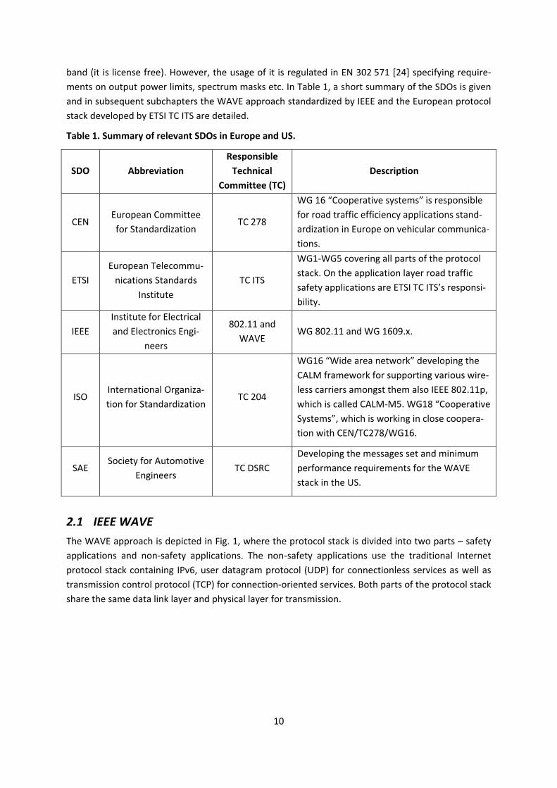
band (it is license free). However, the usage of it is regulated in EN 302 571 [24] specifying require-ments on output power limits, spectrum masks etc. In Table 1, a short summary of the SDOs is given and in subsequent subchapters the WAVE approach standardized by IEEE and the European protocol stack developed by ETSI TC ITS are detailed.

Table 1. Summary of relevant SDOs in Europe and US.

SDO Abbreviation Responsible

Technical Committee (TC)

Description

CEN European Committee for Standardization

TC 278

WG 16 “Cooperative systems” is responsible for road traffic efficiency applications stand-ardization in Europe on vehicular communica-tions.

ETSI European Telecommu-

nications Standards Institute

TC ITS

WG1-WG5 covering all parts of the protocol stack. On the application layer road traffic safety applications are ETSI TC ITS’s responsi-bility.

IEEE Institute for Electrical and Electronics Engi-

neers

802.11 and WAVE

WG 802.11 and WG 1609.x.

ISO International Organiza-tion for Standardization

TC 204

WG16 “Wide area network” developing the CALM framework for supporting various wire-less carriers amongst them also IEEE 802.11p, which is called CALM-M5. WG18 “Cooperative Systems”, which is working in close coopera-tion with CEN/TC278/WG16.

SAE Society for Automotive

Engineers TC DSRC

Developing the messages set and minimum performance requirements for the WAVE stack in the US.

2.1 IEEE WAVE The WAVE approach is depicted in Fig. 1, where the protocol stack is divided into two parts – safety applications and non-safety applications. The non-safety applications use the traditional Internet protocol stack containing IPv6, user datagram protocol (UDP) for connectionless services as well as transmission control protocol (TCP) for connection-oriented services. Both parts of the protocol stack share the same data link layer and physical layer for transmission.

11

The MAC sub-layer and the physical layer are derived from IEEE 802.11-2012 [5]. In July 2010, the vehicular “profile” of 802.11 was approved and termed 802.11p [4]. It has been incorporated in the latest version of IEEE 802.11-2012 and 802.11p is now classified as superseded. For simplicity the vehicular “profile” of 802.11 will be called 802.11p throughout this thesis to distinguish it from AP based WLAN operation.

IEEE 802.11p introduced a new management information base2 (MIB) parameter called dot11OCBActivated and when this is set to true a new capability is achieved namely the possi-bility to communicate outside the context of a basic service set (BSS), which is the smallest building block of a 802.11 network. The side effects of this is that the BSS authentication and association pro-cedures are removed because this is a time consuming process and in a VANET where stations are highly mobile this transaction may not be completed until the stations are out of the radio range of each other. The communication outside the BSS is ad hoc but it should not be confused with the in-dependent BSS which is one of the network topologies supported in 802.11. To distinguish between communication within a BSS and outside of it the network identification (basic service set id, BSSID) is set to a wildcard in every frame transmitted in an 802.11p network. The removal of authentication and association procedures implies further changes to 802.11, which will be discussed below.

IEEE 802.11-2012 contains two basic network topologies: the infrastructure BSS and the independent BSS (IBSS). The former contains an AP and data traffic usually takes a detour through the AP even when two stations are closely located. The IBSS is a set of stations communicating directly with each other and this is also called ad hoc network. Both these topologies are aimed for nomadic devices and synchronization is required between stations via beacons. Further, they are identified with a

2 The MIB is a virtual database containing a set of parameters that can be set in IEEE 802.11. The MIB parame-ters are given default values that can be changed depending on mode of operation.

Safety Appl. Non-Safety Applications

WSMP

1609.3

Secu

rity J2735

IEEE 802.11 Physical layer

Figure 1. An overview of the WAVE protocol stack containing both a road traffic safety applications’ part as well as a non-safety part.

IPv6

Physical layer

IEEE 802.11

WAVE 1609.4

IEEE 802.2

Data link layer

MAC sub-layer

MAC sub-layer ext.

LLC sub-layer

Network layer

Transport layer Network and transport layers

Message sub-layer

Application layer

TCP/UDP

Application layer

12

unique BSSID. Association and authentication are required in infrastructure BSS (containing AP) whereas in IBSS (ad hoc) association is not used and communication can take place in an unauthenti-cated mode. In 802.11p mode, authentication, association and security between stations are disa-bled at the MAC sub-layer. This implies that active and passive scanning of BSS and IBSS are disabled. The scanning on frequency channels for the station to join an existing network is no longer enabled. Therefore, the implementation of 802.11p in the vehicular environment requires predetermined frequency channels to be set in the management.

IEEE 802.11 offers several physical layers and one common MAC sub-layer with QoS support. IEEE 802.11p is using the orthogonal frequency division multiplexing (OFDM) physical layer detailed in Clause 18 of 802.11 [5] (a.k.a. IEEE 802.11a), and it has support for QoS through the former amend-ment called IEEE 802.11e (approved in 2004 and enrolled in the base standard 2007).

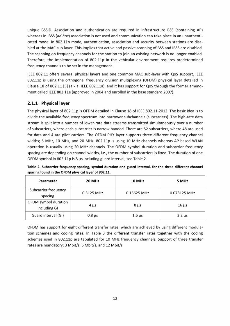
2.1.1 Physical layer The physical layer of 802.11p is OFDM detailed in Clause 18 of IEEE 802.11-2012. The basic idea is to divide the available frequency spectrum into narrower subchannels (subcarriers). The high-rate data stream is split into a number of lower-rate data streams transmitted simultaneously over a number of subcarriers, where each subcarrier is narrow banded. There are 52 subcarriers, where 48 are used for data and 4 are pilot carriers. The OFDM PHY layer supports three different frequency channel widths; 5 MHz, 10 MHz, and 20 MHz. 802.11p is using 10 MHz channels whereas AP based WLAN operation is usually using 20 MHz channels. The OFDM symbol duration and subcarrier frequency spacing are depending on channel widths, i.e., the number of subcarriers is fixed. The duration of one OFDM symbol in 802.11p is 8 µs including guard interval, see Table 2.

Table 2. Subcarrier frequency spacing, symbol duration and guard interval, for the three different channel spacing found in the OFDM physical layer of 802.11.

Parameter 20 MHz 10 MHz 5 MHz

Subcarrier frequency spacing

0.3125 MHz 0.15625 MHz 0.078125 MHz

OFDM symbol duration including GI

4 µs 8 µs 16 µs

Guard interval (GI) 0.8 µs 1.6 µs 3.2 µs

OFDM has support for eight different transfer rates, which are achieved by using different modula-tion schemes and coding rates. In Table 3 the different transfer rates together with the coding schemes used in 802.11p are tabulated for 10 MHz frequency channels. Support of three transfer rates are mandatory; 3 Mbit/s, 6 Mbit/s, and 12 Mbit/s.

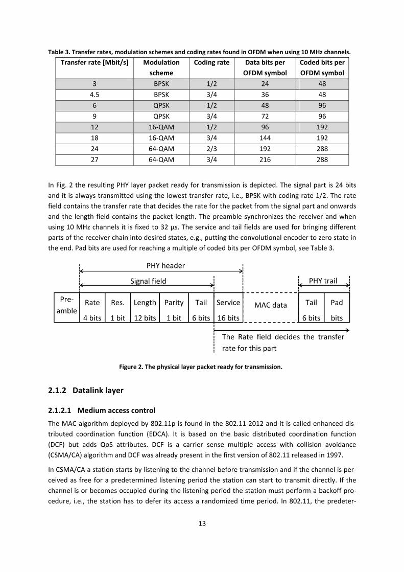
13

Table 3. Transfer rates, modulation schemes and coding rates found in OFDM when using 10 MHz channels. Transfer rate [Mbit/s] Modulation

scheme Coding rate Data bits per

OFDM symbol Coded bits per OFDM symbol

3 BPSK 1/2 24 48 4.5 BPSK 3/4 36 48 6 QPSK 1/2 48 96 9 QPSK 3/4 72 96

12 16-QAM 1/2 96 192 18 16-QAM 3/4 144 192 24 64-QAM 2/3 192 288 27 64-QAM 3/4 216 288

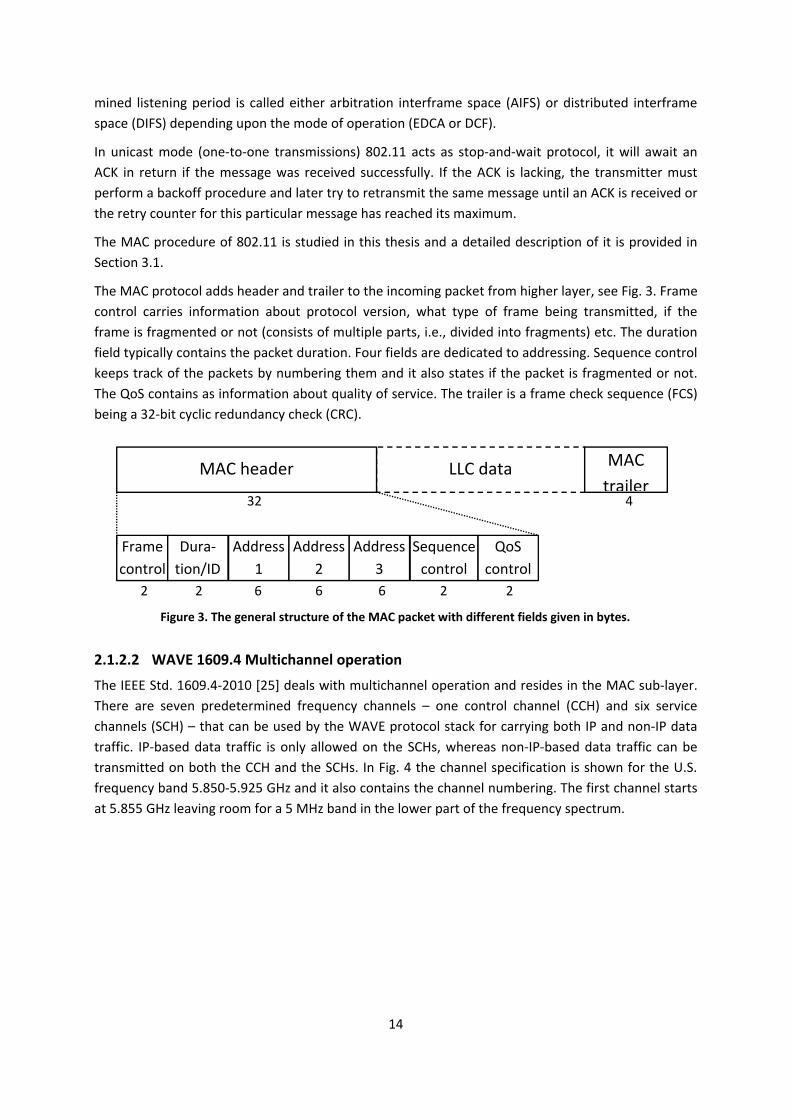
In Fig. 2 the resulting PHY layer packet ready for transmission is depicted. The signal part is 24 bits and it is always transmitted using the lowest transfer rate, i.e., BPSK with coding rate 1/2. The rate field contains the transfer rate that decides the rate for the packet from the signal part and onwards and the length field contains the packet length. The preamble synchronizes the receiver and when using 10 MHz channels it is fixed to 32 µs. The service and tail fields are used for bringing different parts of the receiver chain into desired states, e.g., putting the convolutional encoder to zero state in the end. Pad bits are used for reaching a multiple of coded bits per OFDM symbol, see Table 3.

2.1.2 Datalink layer

2.1.2.1 Medium access control The MAC algorithm deployed by 802.11p is found in the 802.11-2012 and it is called enhanced dis-tributed coordination function (EDCA). It is based on the basic distributed coordination function (DCF) but adds QoS attributes. DCF is a carrier sense multiple access with collision avoidance (CSMA/CA) algorithm and DCF was already present in the first version of 802.11 released in 1997.

In CSMA/CA a station starts by listening to the channel before transmission and if the channel is per-ceived as free for a predetermined listening period the station can start to transmit directly. If the channel is or becomes occupied during the listening period the station must perform a backoff pro-cedure, i.e., the station has to defer its access a randomized time period. In 802.11, the predeter-

MAC data

Figure 2. The physical layer packet ready for transmission.

Rate

4 bits

Res.

1 bit

Length

12 bits

Parity

1 bit

Tail

6 bits

Service

16 bits

Pad

bits

Tail

6 bits

Pre-amble

Signal field

PHY header

PHY trail

The Rate field decides the transfer rate for this part

14

mined listening period is called either arbitration interframe space (AIFS) or distributed interframe space (DIFS) depending upon the mode of operation (EDCA or DCF).

In unicast mode (one-to-one transmissions) 802.11 acts as stop-and-wait protocol, it will await an ACK in return if the message was received successfully. If the ACK is lacking, the transmitter must perform a backoff procedure and later try to retransmit the same message until an ACK is received or the retry counter for this particular message has reached its maximum.

The MAC procedure of 802.11 is studied in this thesis and a detailed description of it is provided in Section 3.1.

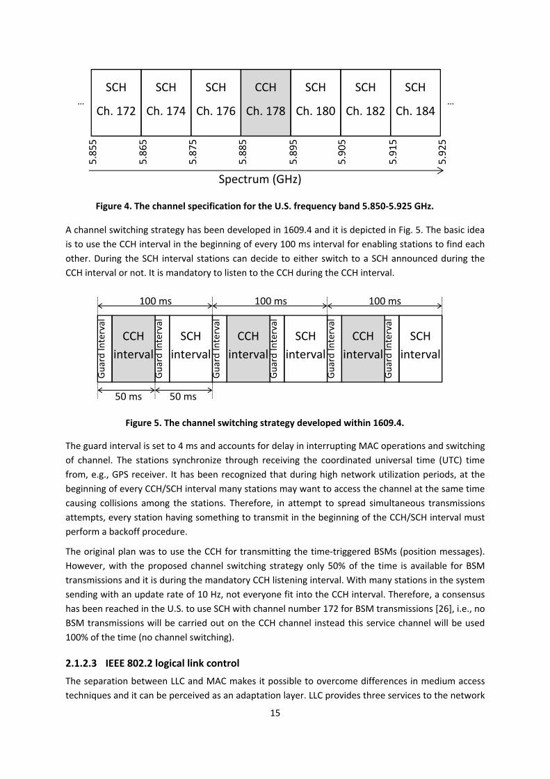
The MAC protocol adds header and trailer to the incoming packet from higher layer, see Fig. 3. Frame control carries information about protocol version, what type of frame being transmitted, if the frame is fragmented or not (consists of multiple parts, i.e., divided into fragments) etc. The duration field typically contains the packet duration. Four fields are dedicated to addressing. Sequence control keeps track of the packets by numbering them and it also states if the packet is fragmented or not. The QoS contains as information about quality of service. The trailer is a frame check sequence (FCS) being a 32-bit cyclic redundancy check (CRC).

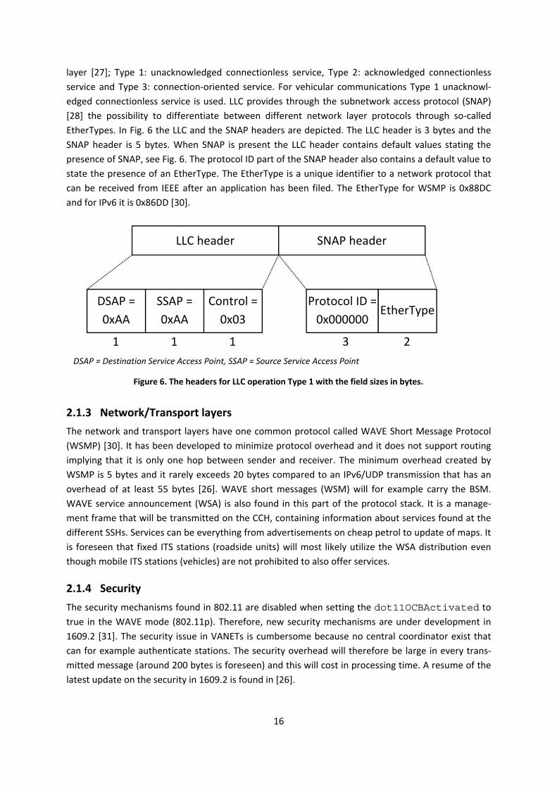
2.1.2.2 WAVE 1609.4 Multichannel operation The IEEE Std. 1609.4-2010 [25] deals with multichannel operation and resides in the MAC sub-layer. There are seven predetermined frequency channels – one control channel (CCH) and six service channels (SCH) – that can be used by the WAVE protocol stack for carrying both IP and non-IP data traffic. IP-based data traffic is only allowed on the SCHs, whereas non-IP-based data traffic can be transmitted on both the CCH and the SCHs. In Fig. 4 the channel specification is shown for the U.S. frequency band 5.850-5.925 GHz and it also contains the channel numbering. The first channel starts at 5.855 GHz leaving room for a 5 MHz band in the lower part of the frequency spectrum.

LLC data

Figure 3. The general structure of the MAC packet with different fields given in bytes.

MAC header MAC trailer

Frame control

Dura-tion/ID

Address 1

Address 2

Address 3

Sequence control

QoS control

32 4

2 2 6 6 6 2 2

15

A channel switching strategy has been developed in 1609.4 and it is depicted in Fig. 5. The basic idea is to use the CCH interval in the beginning of every 100 ms interval for enabling stations to find each other. During the SCH interval stations can decide to either switch to a SCH announced during the CCH interval or not. It is mandatory to listen to the CCH during the CCH interval.

The guard interval is set to 4 ms and accounts for delay in interrupting MAC operations and switching of channel. The stations synchronize through receiving the coordinated universal time (UTC) time from, e.g., GPS receiver. It has been recognized that during high network utilization periods, at the beginning of every CCH/SCH interval many stations may want to access the channel at the same time causing collisions among the stations. Therefore, in attempt to spread simultaneous transmissions attempts, every station having something to transmit in the beginning of the CCH/SCH interval must perform a backoff procedure.

The original plan was to use the CCH for transmitting the time-triggered BSMs (position messages). However, with the proposed channel switching strategy only 50% of the time is available for BSM transmissions and it is during the mandatory CCH listening interval. With many stations in the system sending with an update rate of 10 Hz, not everyone fit into the CCH interval. Therefore, a consensus has been reached in the U.S. to use SCH with channel number 172 for BSM transmissions [26], i.e., no BSM transmissions will be carried out on the CCH channel instead this service channel will be used 100% of the time (no channel switching).

2.1.2.3 IEEE 802.2 logical link control The separation between LLC and MAC makes it possible to overcome differences in medium access techniques and it can be perceived as an adaptation layer. LLC provides three services to the network

SCH

Ch. 172

Figure 4. The channel specification for the U.S. frequency band 5.850-5.925 GHz.

SCH

Ch. 174

SCH

Ch. 176

CCH

Ch. 178

SCH

Ch. 180

SCH

Ch. 182

SCH

Ch. 184 … …

5.85

5

5.86

5

5.87

5

5.88

5

5.89

5

5.90

5

5.91

5

5.92

5

Spectrum (GHz)

Guar

d In

terv

al

CCH interval

Guar

d In

terv

al

SCH interval

Guar

d In

terv

al

CCH interval

Guar

d In

terv

al

SCH interval

Guar

d In

terv

al

CCH interval

Guar

d In

terv

al

SCH interval

100 ms 100 ms 100 ms

Figure 5. The channel switching strategy developed within 1609.4.

50 ms 50 ms

16

layer [27]; Type 1: unacknowledged connectionless service, Type 2: acknowledged connectionless service and Type 3: connection-oriented service. For vehicular communications Type 1 unacknowl-edged connectionless service is used. LLC provides through the subnetwork access protocol (SNAP) [28] the possibility to differentiate between different network layer protocols through so-called EtherTypes. In Fig. 6 the LLC and the SNAP headers are depicted. The LLC header is 3 bytes and the SNAP header is 5 bytes. When SNAP is present the LLC header contains default values stating the presence of SNAP, see Fig. 6. The protocol ID part of the SNAP header also contains a default value to state the presence of an EtherType. The EtherType is a unique identifier to a network protocol that can be received from IEEE after an application has been filed. The EtherType for WSMP is 0x88DC and for IPv6 it is 0x86DD [30].

2.1.3 Network/Transport layers The network and transport layers have one common protocol called WAVE Short Message Protocol (WSMP) [30]. It has been developed to minimize protocol overhead and it does not support routing implying that it is only one hop between sender and receiver. The minimum overhead created by WSMP is 5 bytes and it rarely exceeds 20 bytes compared to an IPv6/UDP transmission that has an overhead of at least 55 bytes [26]. WAVE short messages (WSM) will for example carry the BSM. WAVE service announcement (WSA) is also found in this part of the protocol stack. It is a manage-ment frame that will be transmitted on the CCH, containing information about services found at the different SSHs. Services can be everything from advertisements on cheap petrol to update of maps. It is foreseen that fixed ITS stations (roadside units) will most likely utilize the WSA distribution even though mobile ITS stations (vehicles) are not prohibited to also offer services.

2.1.4 Security The security mechanisms found in 802.11 are disabled when setting the dot11OCBActivated to true in the WAVE mode (802.11p). Therefore, new security mechanisms are under development in 1609.2 [31]. The security issue in VANETs is cumbersome because no central coordinator exist that can for example authenticate stations. The security overhead will therefore be large in every trans-mitted message (around 200 bytes is foreseen) and this will cost in processing time. A resume of the latest update on the security in 1609.2 is found in [26].

Figure 6. The headers for LLC operation Type 1 with the field sizes in bytes.

LLC header SNAP header

Control = 0x03

1

SSAP = 0xAA

1

DSAP = 0xAA

1

Protocol ID = 0x000000

3

EtherType

2 DSAP = Destination Service Access Point, SSAP = Source Service Access Point

17

2.1.5 Message Set Dictionary SAE is standardizing a message set dictionary in J2735 [8]. This specification is not specifically tailored for the WAVE stack and can therefore be used by other wireless technologies as well. It contains fif-teen different types of messages. The most central message found herein is the BSM, which will be the basis for a diverse set of safety-related road traffic applications. It contains data about the vehicle itself such as position (latitude, longitude, and elevation), heading, steering wheel angle, vehicle size, etc. The BSM packet size will on average be 105 bytes and depending on driving context and the sta-tus of the wireless channel (i.e., channel busy ratio) it will be broadcasted 1 to 10 times per second (1-10 Hz).

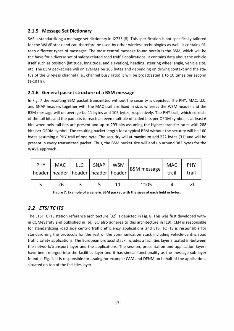
2.1.6 General packet structure of a BSM message In Fig. 7 the resulting BSM packet transmitted without the security is depicted. The PHY, MAC, LLC, and SNAP headers together with the MAC trail are fixed in size, whereas the WSM header and the BSM message will on average be 11 bytes and 105 bytes, respectively. The PHY trail, which consists of the tail bits and the pad bits to reach an even multiple of coded bits per OFDM symbol, is at least 6 bits when only tail bits are present and up to 293 bits assuming the highest transfer rates with 288 bits per OFDM symbol. The resulting packet length for a typical BSM without the security will be 160 bytes assuming a PHY trail of one byte. The security will at maximum add 222 bytes [31] and will be present in every transmitted packet. Thus, the BSM packet size will end up around 382 bytes for the WAVE approach.

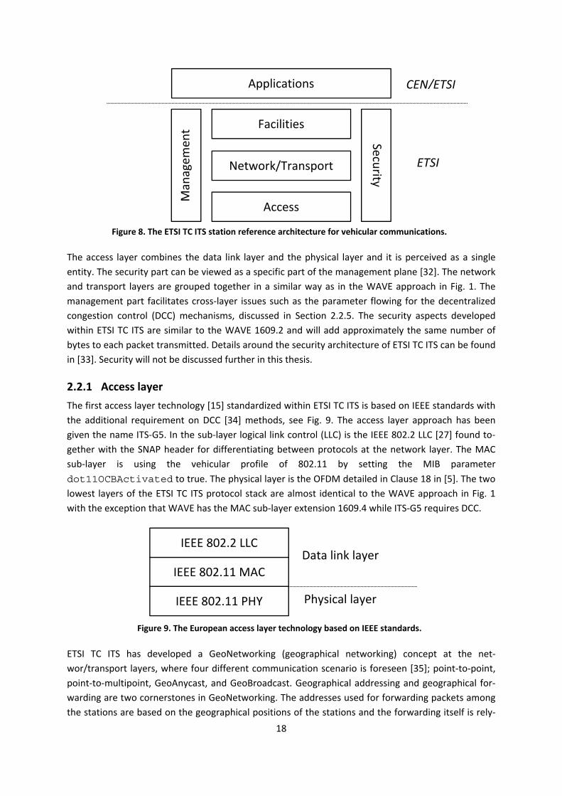
2.2 ETSI TC ITS The ETSI TC ITS station reference architecture [32] is depicted in Fig. 8. This was first developed with-in COMeSafety and published in [6]. ISO also adheres to this architecture in [19]. CEN is responsible for standardizing road side centric traffic efficiency applications and ETSI TC ITS is responsible for standardizing the protocols for the rest of the communication stack including vehicle-centric road traffic safety applications. The European protocol stack includes a facilities layer situated in-between the network/transport layer and the applications. The session, presentation and application layers have been merged into the facilities layer and it has similar functionality as the message sub-layer found in Fig. 1. It is responsible for issuing for example CAM and DENM on behalf of the applications situated on top of the facilities layer.

Figure 7. Example of a generic BSM packet with the sizes of each field in bytes.

PHY header

MAC header

LLC header

SNAP header

WSM header

BSM messageMAC trail

PHY trail

5 26 3 5 11 ~105 4 >1

18

The access layer combines the data link layer and the physical layer and it is perceived as a single entity. The security part can be viewed as a specific part of the management plane [32]. The network and transport layers are grouped together in a similar way as in the WAVE approach in Fig. 1. The management part facilitates cross-layer issues such as the parameter flowing for the decentralized congestion control (DCC) mechanisms, discussed in Section 2.2.5. The security aspects developed within ETSI TC ITS are similar to the WAVE 1609.2 and will add approximately the same number of bytes to each packet transmitted. Details around the security architecture of ETSI TC ITS can be found in [33]. Security will not be discussed further in this thesis.

2.2.1 Access layer The first access layer technology [15] standardized within ETSI TC ITS is based on IEEE standards with the additional requirement on DCC [34] methods, see Fig. 9. The access layer approach has been given the name ITS-G5. In the sub-layer logical link control (LLC) is the IEEE 802.2 LLC [27] found to-gether with the SNAP header for differentiating between protocols at the network layer. The MAC sub-layer is using the vehicular profile of 802.11 by setting the MIB parameter dot11OCBActivated to true. The physical layer is the OFDM detailed in Clause 18 in [5]. The two lowest layers of the ETSI TC ITS protocol stack are almost identical to the WAVE approach in Fig. 1 with the exception that WAVE has the MAC sub-layer extension 1609.4 while ITS-G5 requires DCC.

ETSI TC ITS has developed a GeoNetworking (geographical networking) concept at the net-wor/transport layers, where four different communication scenario is foreseen [35]; point-to-point, point-to-multipoint, GeoAnycast, and GeoBroadcast. Geographical addressing and geographical for-warding are two cornerstones in GeoNetworking. The addresses used for forwarding packets among the stations are based on the geographical positions of the stations and the forwarding itself is rely-

Network/Transport

Figure 8. The ETSI TC ITS station reference architecture for vehicular communications.

Access

Facilities

Applications

Man

agem

ent

Security

CEN/ETSI

ETSI

IEEE 802.11 MAC

Figure 9. The European access layer technology based on IEEE standards.

IEEE 802.11 PHY

IEEE 802.2 LLC Data link layer

Physical layer

19

ing upon that each and every station has a perception of its part of the network, in other words, the nearest neighbor of the station and their positions. The station does not maintain routing tables in-stead it keeps a list of neighbors it can hear (receive packets from) and based on the geographical address in an incoming packet the station forwards the packet if suitable. With GeoNetworking pack-ets can be addressed to certain geographical regions of interests without knowing if there are sta-tions in the destined area or not.

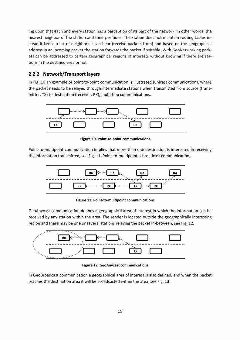
2.2.2 Network/Transport layers In Fig. 10 an example of point-to-point communication is illustrated (unicast communication), where the packet needs to be relayed through intermediate stations when transmitted from source (trans-mitter, TX) to destination (receiver, RX), multi-hop communications.

Point-to-multipoint communication implies that more than one destination is interested in receiving the information transmitted, see Fig. 11. Point-to-multipoint is broadcast communication.

GeoAnycast communication defines a geographical area of interest in which the information can be received by any station within the area. The sender is located outside the geographically interesting region and there may be one or several stations relaying the packet in-between, see Fig. 12.

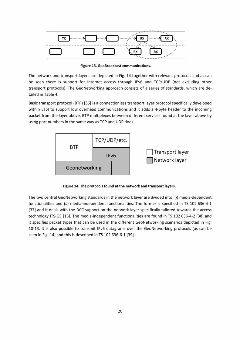
In GeoBroadcast communication a geographical area of interest is also defined, and when the packet reaches the destination area it will be broadcasted within the area, see Fig. 13.

TX

RX

Figure 10. Point-to-point communications.

RX

RX RX

RX

TX RX

RX RX

Figure 11. Point-to-multipoint communications.

RX

TX

Figure 12. GeoAnycast communications.

20

The network and transport layers are depicted in Fig. 14 together with relevant protocols and as can be seen there is support for Internet access through IPv6 and TCP/UDP (not excluding other transport protocols). The GeoNetworking approach consists of a series of standards, which are de-tailed in Table 4.

Basic transport protocol (BTP) [36] is a connectionless transport layer protocol specifically developed within ETSI to support low overhead communications and it adds a 4-byte header to the incoming packet from the layer above. BTP multiplexes between different services found at the layer above by using port numbers in the same way as TCP and UDP does.

The two central GeoNetworking standards in the network layer are divided into; (i) media-dependent functionalities and (ii) media-independent functionalities. The former is specified in TS 102 636-4-1 [37] and it deals with the DCC support on the network layer specifically tailored towards the access technology ITS-G5 [15]. The media-independent functionalities are found in TS 102 636-4-2 [38] and it specifies packet types that can be used in the different GeoNetworking scenarios depicted in Fig. 10-13. It is also possible to transmit IPv6 datagrams over the GeoNetworking protocols (as can be seen in Fig. 14) and this is described in TS 102 636-6-1 [39].

TX

RX RX

RX RX

Figure 13. GeoBroadcast communications.

Figure 14. The protocols found at the network and transport layers.

BTP Transport layer

TCP/UDP/etc.

Network layer IPv6

Geonetworking

21

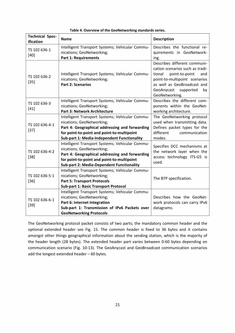
Table 4. Overview of the GeoNetworking standards series. Technical Spec-ification Name Description

TS 102 636-1 [40]

Intelligent Transport Systems; Vehicular Commu-nications; GeoNetworking; Part 1: Requirements

Describes the functional re-quirements in GeoNetwork-ing.

TS 102 636-2 [35]

Intelligent Transport Systems; Vehicular Commu-nications; GeoNetworking; Part 2: Scenarios

Describes different communi-cation scenarios such as tradi-tional point-to-point and point-to-multipoint scenarios as well as GeoBroadcast and GeoAnycast supported by GeoNetworking.

TS 102 636-3 [41]

Intelligent Transport Systems; Vehicular Commu-nications; GeoNetworking; Part 3: Network Architecture

Describes the different com-ponents within the GeoNet-working architecture.

TS 102 636-4-1 [37]

Intelligent Transport Systems; Vehicular Commu-nications; GeoNetworking; Part 4: Geographical addressing and forwarding for point-to-point and point-to-multipoint Sub-part 1: Media-Independent Functionality

The GeoNetworking protocol used when transmitting data. Defines packet types for the different communication modes.

TS 102 636-4-2 [38]

Intelligent Transport Systems; Vehicular Commu-nications; GeoNetworking; Part 4: Geographical addressing and forwarding for point-to-point and point-to-multipoint Sub-part 2: Media-Dependent Functionality

Specifies DCC mechanisms at the network layer when the access technology ITS-G5 is used.

TS 102 636-5-1 [36]

Intelligent Transport Systems; Vehicular Commu-nications; GeoNetworking; Part 5: Transport Protocols Sub-part 1: Basic Transport Protocol

The BTP specification.

TS 102 636-6-1 [39]

Intelligent Transport Systems; Vehicular Commu-nications; GeoNetworking; Part 6: Internet Integration Sub-part 1: Transmission of IPv6 Packets over GeoNetworking Protocols

Describes how the GeoNet-work protocols can carry IPv6 datagrams.

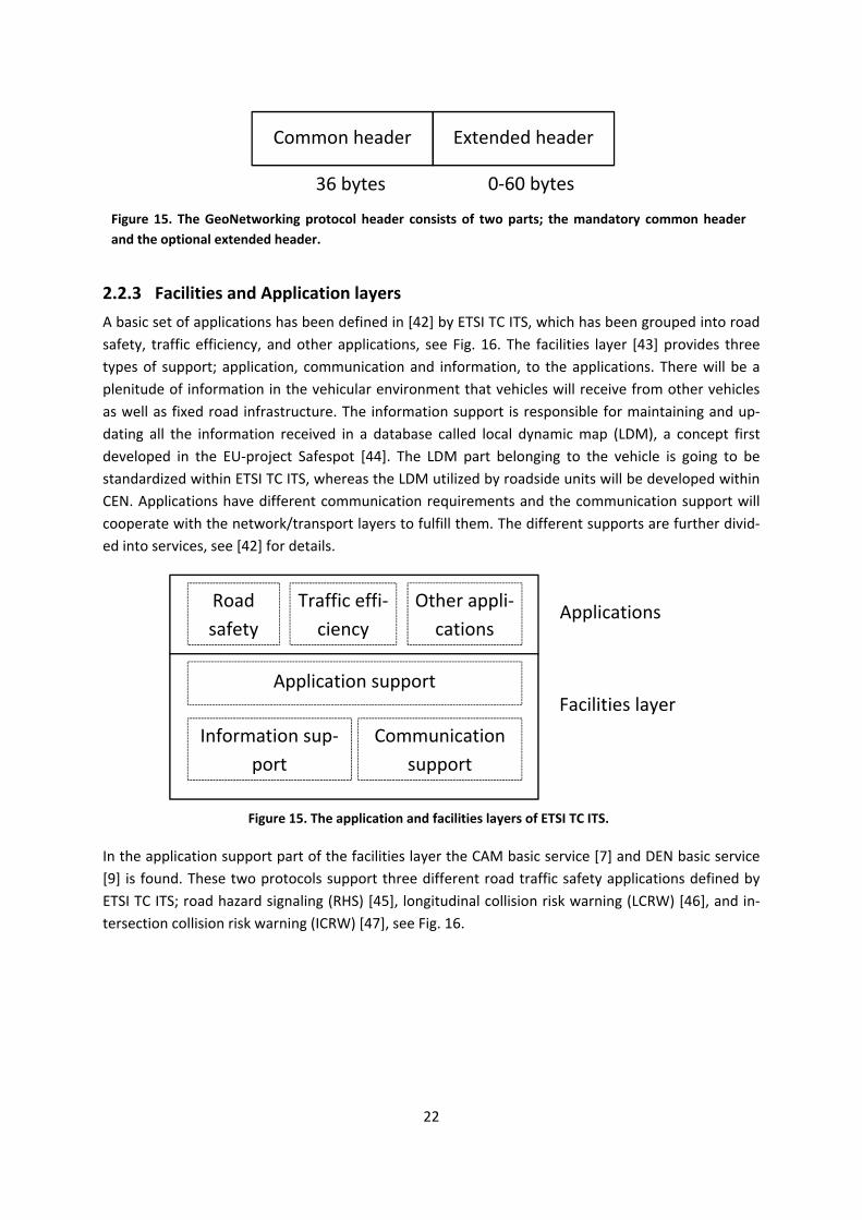
The GeoNetworking protocol packet consists of two parts; the mandatory common header and the optional extended header see Fig. 15. The common header is fixed to 36 bytes and it contains amongst other things geographical information about the sending station, which is the majority of the header length (28 bytes). The extended header part varies between 0-60 bytes depending on communication scenario (Fig. 10-13). The GeoAnycast and GeoBroadcast communication scenarios add the longest extended header – 60 bytes.

22

2.2.3 Facilities and Application layers A basic set of applications has been defined in [42] by ETSI TC ITS, which has been grouped into road safety, traffic efficiency, and other applications, see Fig. 16. The facilities layer [43] provides three types of support; application, communication and information, to the applications. There will be a plenitude of information in the vehicular environment that vehicles will receive from other vehicles as well as fixed road infrastructure. The information support is responsible for maintaining and up-dating all the information received in a database called local dynamic map (LDM), a concept first developed in the EU-project Safespot [44]. The LDM part belonging to the vehicle is going to be standardized within ETSI TC ITS, whereas the LDM utilized by roadside units will be developed within CEN. Applications have different communication requirements and the communication support will cooperate with the network/transport layers to fulfill them. The different supports are further divid-ed into services, see [42] for details.

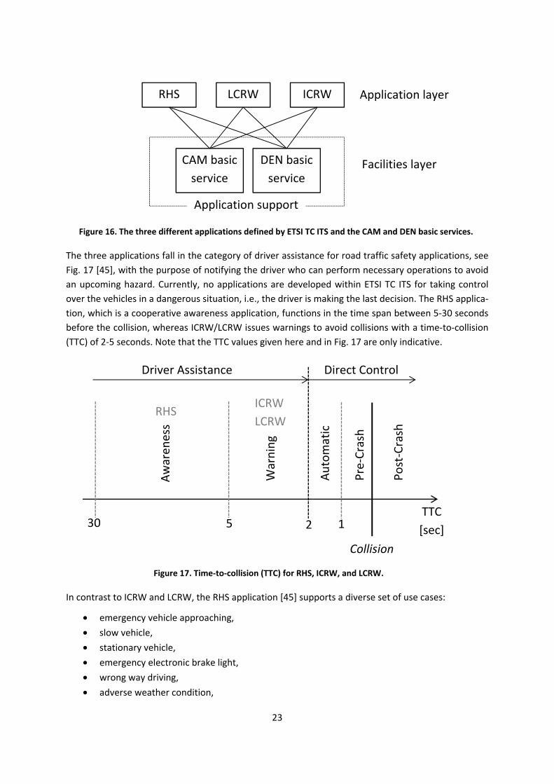
In the application support part of the facilities layer the CAM basic service [7] and DEN basic service [9] is found. These two protocols support three different road traffic safety applications defined by ETSI TC ITS; road hazard signaling (RHS) [45], longitudinal collision risk warning (LCRW) [46], and in-tersection collision risk warning (ICRW) [47], see Fig. 16.

Figure 15. The GeoNetworking protocol header consists of two parts; the mandatory common header and the optional extended header.

Common header Extended header

36 bytes 0-60 bytes

Figure 15. The application and facilities layers of ETSI TC ITS.

Applications Road safety

Traffic effi-ciency

Other appli-cations

Facilities layer

Application support

Information sup-port

Communication support

23

The three applications fall in the category of driver assistance for road traffic safety applications, see Fig. 17 [45], with the purpose of notifying the driver who can perform necessary operations to avoid an upcoming hazard. Currently, no applications are developed within ETSI TC ITS for taking control over the vehicles in a dangerous situation, i.e., the driver is making the last decision. The RHS applica-tion, which is a cooperative awareness application, functions in the time span between 5-30 seconds before the collision, whereas ICRW/LCRW issues warnings to avoid collisions with a time-to-collision (TTC) of 2-5 seconds. Note that the TTC values given here and in Fig. 17 are only indicative.

In contrast to ICRW and LCRW, the RHS application [45] supports a diverse set of use cases:

• emergency vehicle approaching, • slow vehicle, • stationary vehicle, • emergency electronic brake light, • wrong way driving, • adverse weather condition,

Figure 16. The three different applications defined by ETSI TC ITS and the CAM and DEN basic services.

Application layer RHS

Facilities layer

LCRW ICRW

Application support

DEN basic service

CAM basic service

TTC [sec]

Collision

Auto

mat

ic

Pre-

Cras

h

War

ning

Post

-Cra

sh

Awar

enes

s

Driver Assistance Direct Control

2

RHS ICRW LCRW

Figure 17. Time-to-collision (TTC) for RHS, ICRW, and LCRW.

1 30 5

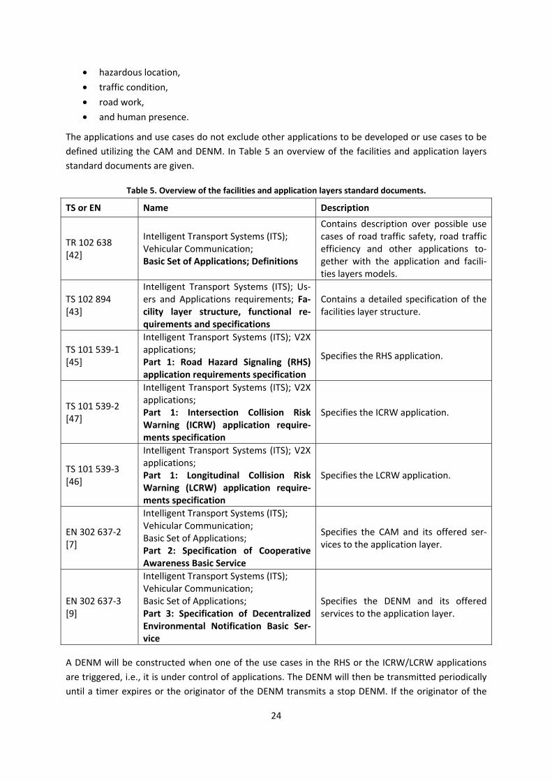
24

• hazardous location, • traffic condition, • road work, • and human presence.

The applications and use cases do not exclude other applications to be developed or use cases to be defined utilizing the CAM and DENM. In Table 5 an overview of the facilities and application layers standard documents are given.

Table 5. Overview of the facilities and application layers standard documents.

TS or EN Name Description

TR 102 638 [42]

Intelligent Transport Systems (ITS); Vehicular Communication; Basic Set of Applications; Definitions

Contains description over possible use cases of road traffic safety, road traffic efficiency and other applications to-gether with the application and facili-ties layers models.

TS 102 894 [43]

Intelligent Transport Systems (ITS); Us-ers and Applications requirements; Fa-cility layer structure, functional re-quirements and specifications

Contains a detailed specification of the facilities layer structure.

TS 101 539-1 [45]

Intelligent Transport Systems (ITS); V2X applications; Part 1: Road Hazard Signaling (RHS) application requirements specification

Specifies the RHS application.

TS 101 539-2 [47]

Intelligent Transport Systems (ITS); V2X applications; Part 1: Intersection Collision Risk Warning (ICRW) application require-ments specification

Specifies the ICRW application.

TS 101 539-3 [46]

Intelligent Transport Systems (ITS); V2X applications; Part 1: Longitudinal Collision Risk Warning (LCRW) application require-ments specification

Specifies the LCRW application.

EN 302 637-2 [7]

Intelligent Transport Systems (ITS); Vehicular Communication; Basic Set of Applications; Part 2: Specification of Cooperative Awareness Basic Service

Specifies the CAM and its offered ser-vices to the application layer.

EN 302 637-3 [9]

Intelligent Transport Systems (ITS); Vehicular Communication; Basic Set of Applications; Part 3: Specification of Decentralized Environmental Notification Basic Ser-vice

Specifies the DENM and its offered services to the application layer.

A DENM will be constructed when one of the use cases in the RHS or the ICRW/LCRW applications are triggered, i.e., it is under control of applications. The DENM will then be transmitted periodically until a timer expires or the originator of the DENM transmits a stop DENM. If the originator of the

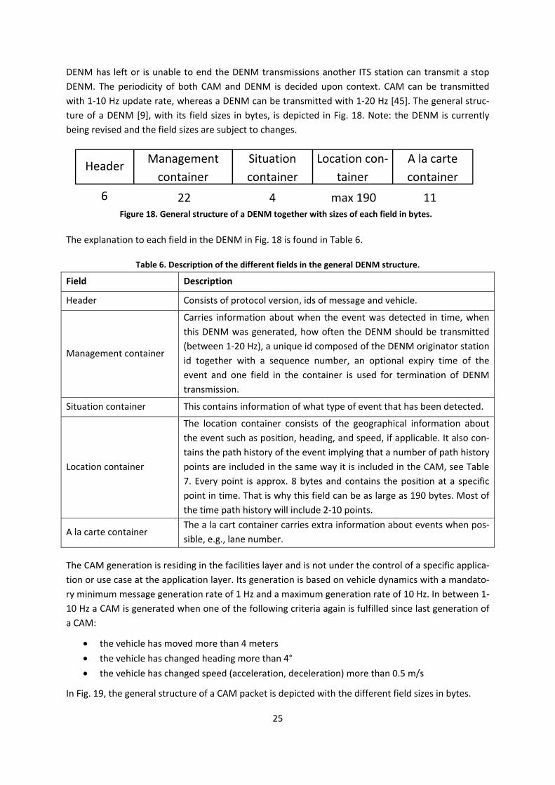
25

DENM has left or is unable to end the DENM transmissions another ITS station can transmit a stop DENM. The periodicity of both CAM and DENM is decided upon context. CAM can be transmitted with 1-10 Hz update rate, whereas a DENM can be transmitted with 1-20 Hz [45]. The general struc-ture of a DENM [9], with its field sizes in bytes, is depicted in Fig. 18. Note: the DENM is currently being revised and the field sizes are subject to changes.

The explanation to each field in the DENM in Fig. 18 is found in Table 6.

Table 6. Description of the different fields in the general DENM structure.

Field Description

Header Consists of protocol version, ids of message and vehicle.

Management container

Carries information about when the event was detected in time, when this DENM was generated, how often the DENM should be transmitted (between 1-20 Hz), a unique id composed of the DENM originator station id together with a sequence number, an optional expiry time of the event and one field in the container is used for termination of DENM transmission.

Situation container This contains information of what type of event that has been detected.

Location container

The location container consists of the geographical information about the event such as position, heading, and speed, if applicable. It also con-tains the path history of the event implying that a number of path history points are included in the same way it is included in the CAM, see Table 7. Every point is approx. 8 bytes and contains the position at a specific point in time. That is why this field can be as large as 190 bytes. Most of the time path history will include 2-10 points.

A la carte container The a la cart container carries extra information about events when pos-sible, e.g., lane number.

The CAM generation is residing in the facilities layer and is not under the control of a specific applica-tion or use case at the application layer. Its generation is based on vehicle dynamics with a mandato-ry minimum message generation rate of 1 Hz and a maximum generation rate of 10 Hz. In between 1-10 Hz a CAM is generated when one of the following criteria again is fulfilled since last generation of a CAM:

• the vehicle has moved more than 4 meters • the vehicle has changed heading more than 4° • the vehicle has changed speed (acceleration, deceleration) more than 0.5 m/s

In Fig. 19, the general structure of a CAM packet is depicted with the different field sizes in bytes.

Figure 18. General structure of a DENM together with sizes of each field in bytes.

Header

6

Management container

22 4 max 190 11

Situation container

Location con-tainer

A la carte container

26

The explanation to each field in the CAM in Fig. 19 is found in Table 7.

Table 7. Description of the different field in the general CAM structure.

Field Description

Header Consists of protocol version, ids of message and vehicle.

Basic container

Consists of position of the object received from a global navigation satellite system (GNSS) such as global positioning system (GPS), what kind of object (passenger car, motorcyclist, bus, heavy/light truck, pedestrian, etc.), and time stamp from GNSS receiver.

Basic vehicle con-tainer HF

This field is included in every CAM (high frequency, HF) and it contains infor-mation about heading, speed, curvature, driving direction (backward or for-ward), and the role of the vehicle if applicable (e.g., public transport, special transport, dangerous goods, road work).

Basic vehicle con-tainer LF

This field is not included in every CAM (low frequency, LF) and it contains more static data about the vehicle itself such as size, status of exterior lights, and path history. The path history is made up of a number of path history points, which can be at maximum 23 points. Every point is approx. 8 bytes and contains the position at a specific point in time. That is why this field can be as large as 176 bytes. Most of the time path history will include 2-10 points. It is at maximum transmitted with 2 Hz (included every 500 ms).

Special container

This field is included if the role of the vehicle contained in the basic vehicle container HF has indicated if it is public transport, dangerous goods etc., and then additional bytes (1-4 bytes depending on role) are included to describe the vehicle more precisely.

2.2.4 General packet structure of a CAM In Fig. 20 the resulting CAM packet transmitted without the security overhead is depicted. The PHY, MAC, LLC, SNAP, BTP and GeoNetworking (GN) headers together with the MAC trail are fixed in size. The CAM data will be 14 bytes when only the high frequency (HF) part is transmitted and when the low frequency (LF) part is present containing the path history the CAM will typically be 90 byte as-suming 10 points of path history. The PHY trail, which consists of the tail bits and the pad bits to reach an even multiple of coded bits per OFDM symbol, is at least 6 bits when only tail bits are pre-sent and up to 293 bits assuming the highest transfer rates with 288 bits per OFDM symbol. The re-sulting packet length for a HF CAM without the security will be 104 bytes assuming a PHY trail of one byte and for the LF CAM it will be 180 bytes. The security will at maximum add 222 bytes [31] and the security will be present in every transmitted packet. Thus, the resulting packet size will end up around 326 bytes for HF CAM (update rate of 1-10 Hz) and 402 bytes for LF CAM (update rate of 1-2 Hz).

Figure 19. General structure of a CAM together with sizes of each field in bytes.

Header

6

Basic container

Basic Vehiclecontainer HF

Basic Vehiclecontainer LF

Special con-tainer

18 14 max 176 1-4

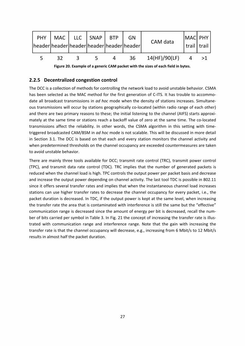
27

2.2.5 Decentralized congestion control The DCC is a collection of methods for controlling the network load to avoid unstable behavior. CSMA has been selected as the MAC method for the first generation of C-ITS. It has trouble to accommo-date all broadcast transmissions in ad hoc mode when the density of stations increases. Simultane-ous transmissions will occur by stations geographically co-located (within radio range of each other) and there are two primary reasons to these; the initial listening to the channel (AIFS) starts approxi-mately at the same time or stations reach a backoff value of zero at the same time. The co-located transmissions affect the reliability. In other words, the CSMA algorithm in this setting with time-triggered broadcasted CAM/BSM in ad hoc mode is not scalable. This will be discussed in more detail in Section 3.1. The DCC is based on that each and every station monitors the channel activity and when predetermined thresholds on the channel occupancy are exceeded countermeasures are taken to avoid unstable behavior.

There are mainly three tools available for DCC; transmit rate control (TRC), transmit power control (TPC), and transmit data rate control (TDC). TRC implies that the number of generated packets is reduced when the channel load is high. TPC controls the output power per packet basis and decrease and increase the output power depending on channel activity. The last tool TDC is possible in 802.11 since it offers several transfer rates and implies that when the instantaneous channel load increases stations can use higher transfer rates to decrease the channel occupancy for every packet, i.e., the packet duration is decreased. In TDC, if the output power is kept at the same level, when increasing the transfer rate the area that is contaminated with interference is still the same but the “effective” communication range is decreased since the amount of energy per bit is decreased, recall the num-ber of bits carried per symbol in Table 3. In Fig. 21 the concept of increasing the transfer rate is illus-trated with communication range and interference range. Note that the gain with increasing the transfer rate is that the channel occupancy will decrease, e.g., increasing from 6 Mbit/s to 12 Mbit/s results in almost half the packet duration.

Figure 20. Example of a generic CAM packet with the sizes of each field in bytes.

PHY header

MAC header

LLC header

SNAP header

BTP header

CAM data MAC trail

PHY trail

5 32 3 5 4 14(HF)/90(LF) 4 >1

GN header

36

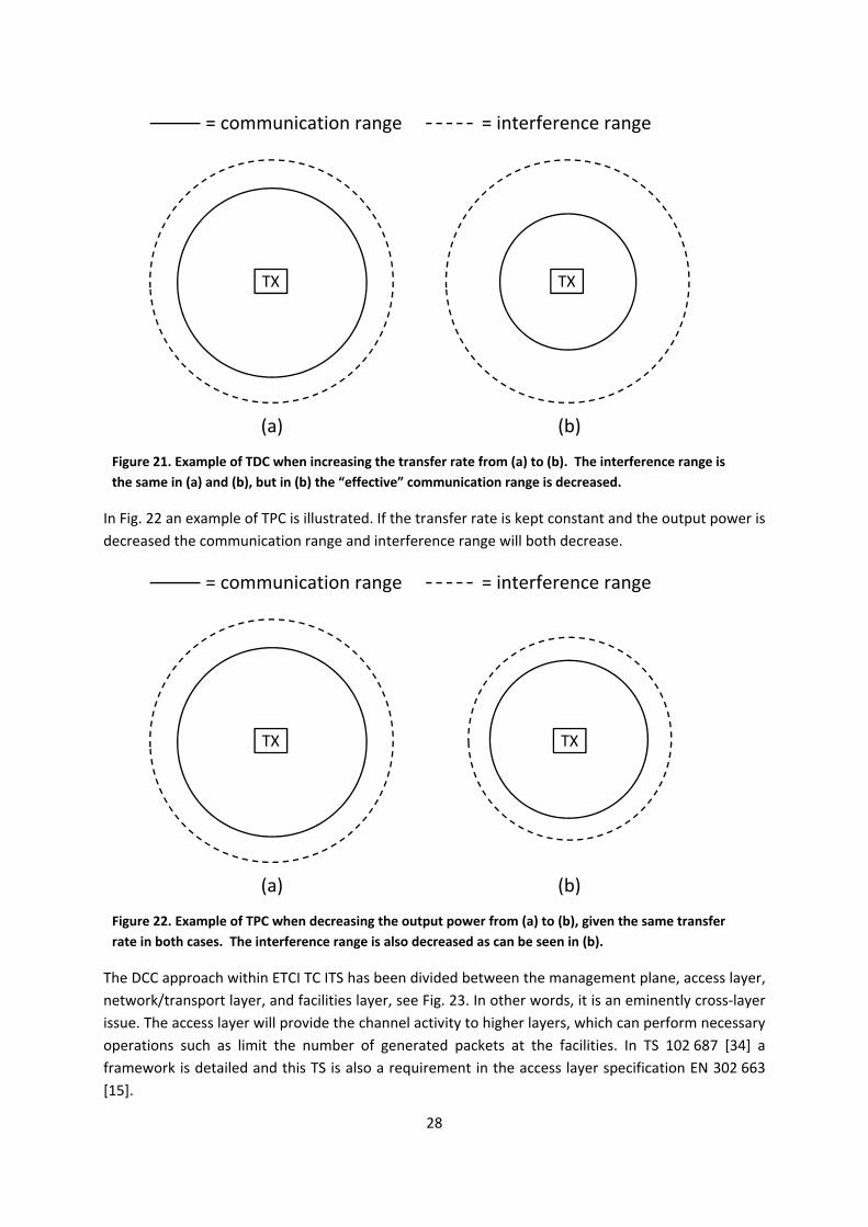
28

In Fig. 22 an example of TPC is illustrated. If the transfer rate is kept constant and the output power is decreased the communication range and interference range will both decrease.

The DCC approach within ETCI TC ITS has been divided between the management plane, access layer, network/transport layer, and facilities layer, see Fig. 23. In other words, it is an eminently cross-layer issue. The access layer will provide the channel activity to higher layers, which can perform necessary operations such as limit the number of generated packets at the facilities. In TS 102 687 [34] a framework is detailed and this TS is also a requirement in the access layer specification EN 302 663 [15].

TX

(a)

TX

(b)

= communication range = interference range

Figure 21. Example of TDC when increasing the transfer rate from (a) to (b). The interference range is the same in (a) and (b), but in (b) the “effective” communication range is decreased.

TX

(a) (b)

= communication range = interference range

Figure 22. Example of TPC when decreasing the output power from (a) to (b), given the same transfer rate in both cases. The interference range is also decreased as can be seen in (b).

TX

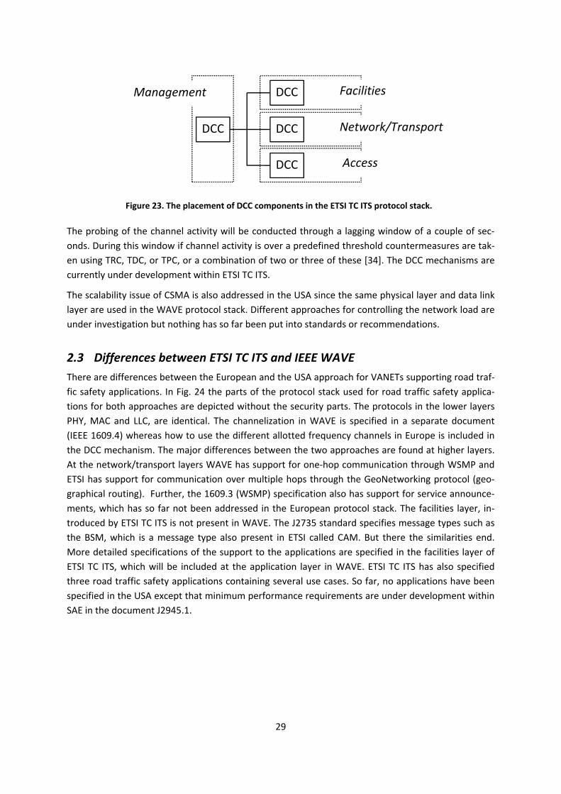
29

The probing of the channel activity will be conducted through a lagging window of a couple of sec-onds. During this window if channel activity is over a predefined threshold countermeasures are tak-en using TRC, TDC, or TPC, or a combination of two or three of these [34]. The DCC mechanisms are currently under development within ETSI TC ITS.

The scalability issue of CSMA is also addressed in the USA since the same physical layer and data link layer are used in the WAVE protocol stack. Different approaches for controlling the network load are under investigation but nothing has so far been put into standards or recommendations.

2.3 Differences between ETSI TC ITS and IEEE WAVE There are differences between the European and the USA approach for VANETs supporting road traf-fic safety applications. In Fig. 24 the parts of the protocol stack used for road traffic safety applica-tions for both approaches are depicted without the security parts. The protocols in the lower layers PHY, MAC and LLC, are identical. The channelization in WAVE is specified in a separate document (IEEE 1609.4) whereas how to use the different allotted frequency channels in Europe is included in the DCC mechanism. The major differences between the two approaches are found at higher layers. At the network/transport layers WAVE has support for one-hop communication through WSMP and ETSI has support for communication over multiple hops through the GeoNetworking protocol (geo-graphical routing). Further, the 1609.3 (WSMP) specification also has support for service announce-ments, which has so far not been addressed in the European protocol stack. The facilities layer, in-troduced by ETSI TC ITS is not present in WAVE. The J2735 standard specifies message types such as the BSM, which is a message type also present in ETSI called CAM. But there the similarities end. More detailed specifications of the support to the applications are specified in the facilities layer of ETSI TC ITS, which will be included at the application layer in WAVE. ETSI TC ITS has also specified three road traffic safety applications containing several use cases. So far, no applications have been specified in the USA except that minimum performance requirements are under development within SAE in the document J2945.1.

Figure 23. The placement of DCC components in the ETSI TC ITS protocol stack.

DCC Facilities

DCC Network/Transport

DCC Access

DCC

Management

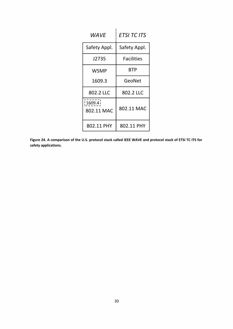
30

Safety Appl.

802.11 PHY

Figure 24. A comparison of the U.S. protocol stack called IEEE WAVE and protocol stack of ETSI TC ITS for safety applications.

GeoNet

802.11 MAC

802.2 LLC

BTP

Facilities

802.11 PHY

802.11 MAC

802.2 LLC

1609.4

Safety Appl.

WAVE ETSI TC ITS

WSMP

1609.3

J2735

31

3 Medium access control The MAC protocol, residing in the data link layer, is responsible for regulating access to the shared communication medium. The regulation is made by scheduling transmissions in time, frequency, space or by using unique codes, constellations or interleavers to distinguish different users. The re-search on MAC protocols is vast and dates back to the 70s, typically distinguishing between distribut-ed and centralized MAC protocols, which can provide random or guaranteed access [81]. In a random access protocol, stations contend for access to the medium and the channel access delay is not pre-dictable. A MAC method that falls into the category guaranteed access is predictable and channel access delay is upper-bounded. All stations will be allowed to transmit within a certain time period, regardless of the number of stations, and channel access can be made fair. Guaranteed access is more easily achieved in a centralized network topology, where a central controller, e.g., a BS or an AP, can distribute resources among all stations requiring access. In a distributed network like a VANET, the applied MAC protocol must not only be distributed, it must also self-organize such that it continuously adapts to changes in the data traffic patterns and network density.

From ongoing standardization activities as described in Chapter 2, it is clear that most road traffic safety applications will be based on VANETs where either event-driven hazard warning messages or time-triggered positioning messages are broadcasted. A MAC predictable with an upper bound on the channel access delay would therefore be preferable. Further, to maximize reliability, concurrent transmissions should be scheduled as far apart as possible to minimize interference. Finally, a MAC method that is fair and scalable in terms of the number of supported vehicles is desired.

As outlined in Chapter 2, CSMA is the proposed MAC method for the first generation of VANETs through IEEE 802.11p and it is also the basis for ISO CALM M5 as well as the European ETSI ITS-G5. As stated in Section 1.5 of this thesis, STDMA has the potential to fulfill most of the requirements im-posed by VANET-based C-ITS and consequently, the particular focus here is these two MAC schemes: CSMA and STDMA tailored towards VANETs. First, the functionality of CSMA and STDMA are detailed, followed by a detailed discussion of the causes and implications of simultaneous transmissions. Final-ly, a comparison with other MAC schemes is made, regarding ability to fulfill the requirements on the MAC method as outlined in Section 1.2.

3.1 Carrier sense multiple access There are two possible methods of channel access within 802.11 utilizing CSMA; enhanced distribut-ed channel access (EDCA) and distributed coordination function (DCF). EDCA has support for QoS by prioritizing data traffic at the MAC layer by placing packets into one of four different queues, each with its own predetermined listening period, arbitration inter-frame space (AIFS) and contention window setting. DCF is the basic access mechanism, without support for QoS, i.e., maintaining one queue at the MAC layer for all types of data traffic. For C-ITS, EDCA has been selected as MAC meth-od [5].

3.1.1 Channel access procedure In CSMA, each station initiates a transmission by listening to the channel, i.e., performs a carrier sense (CS) operation, during a predetermined listening period. If the sensing is successful, i.e., no channel activity is detected, the station transmits directly. If the channel is occupied or becomes oc-

32

cupied during the listening, the station must perform a backoff procedure, i.e., the station has to defer its access a randomized time period.

After a busy channel becomes clear, all stations must listen the predetermined listening period be-fore decrease of the backoff value can resume. Note that in broadcast mode, the backoff procedure will only be invoked once per packet and this occurs during the initial sensing of the channel. In unicast mode, however, where an ACK is sent in response to a successfully received packet, the backoff procedure can be invoked several times for the same packet if the transmitter does not re-ceive an ACK. Unsuccessful reception of an ACK can be caused by:

• RX did not receive the packet and therefore did not transmit ACK • RX did not decode the packet successfully and therefore did not transmit ACK • RX successfully decoded the packet and transmitted an ACK, but it was not received by TX. • RX successfully decoded the packet and transmitted an ACK, but it was not successfully de-

coded by TX.

The unsuccessful reception or decoding of packets can be due to path loss (weak signal because of large distance between transmitter and receiver), fading (multipath), or simultaneous transmissions (more than one transmission geographically co-located, e.g., hidden terminals). For every attempt to transmit a specific packet in unicast mode, CW will be increased until it reaches its maximum value, i.e., starting from the minimum value aCWmin until the maximum value aCWmax is reached. The PHY layer in use determines the values of aCWmin and aCWmax. For the OFDM PHY layer, they are aCWmin = 15 and aCWmax = 1023. In Fig. 26, the exponential increase of the contention window is depicted. This in turn implies that for the first backoff procedure, there are 16 values to uniformly select from ([0,15]), the second transmission attempt there are 32 values to select from ([0,31]), and so forth, until the maximum size of CW has been reached ([0,1023]). If the packet transmission is successful (an ACK is received in response), CW is set to its initial value again, i.e., aCWmin, for the next packet transmission.

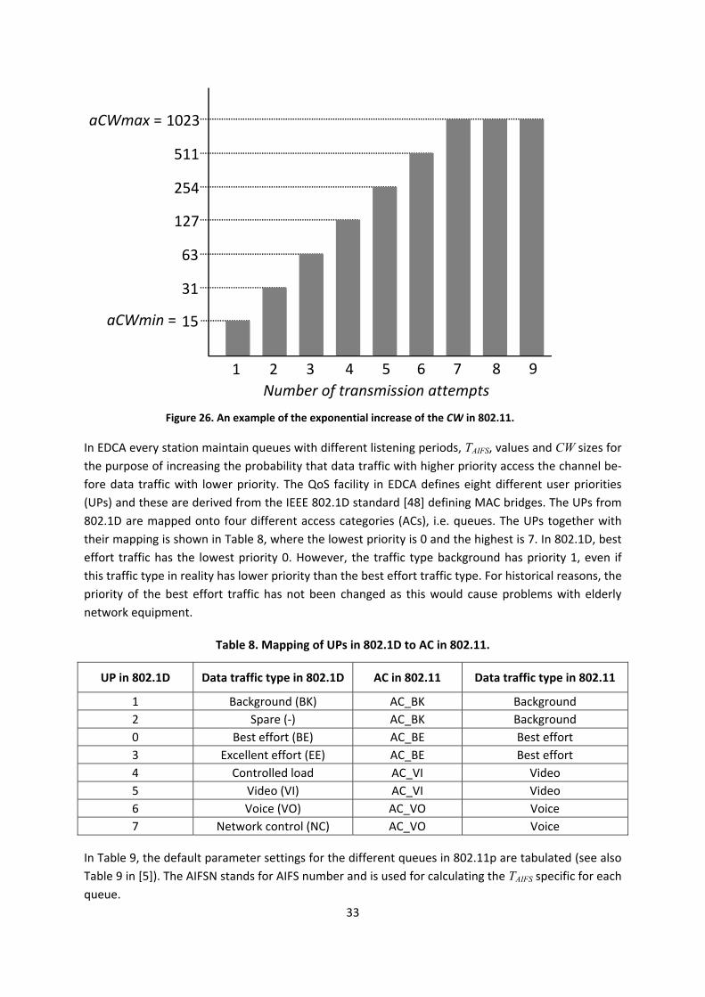
33

In EDCA every station maintain queues with different listening periods, TAIFS, values and CW sizes for the purpose of increasing the probability that data traffic with higher priority access the channel be-fore data traffic with lower priority. The QoS facility in EDCA defines eight different user priorities (UPs) and these are derived from the IEEE 802.1D standard [48] defining MAC bridges. The UPs from 802.1D are mapped onto four different access categories (ACs), i.e. queues. The UPs together with their mapping is shown in Table 8, where the lowest priority is 0 and the highest is 7. In 802.1D, best effort traffic has the lowest priority 0. However, the traffic type background has priority 1, even if this traffic type in reality has lower priority than the best effort traffic type. For historical reasons, the priority of the best effort traffic has not been changed as this would cause problems with elderly network equipment.

Table 8. Mapping of UPs in 802.1D to AC in 802.11.

UP in 802.1D Data traffic type in 802.1D AC in 802.11 Data traffic type in 802.11

1 Background (BK) AC_BK Background 2 Spare (-) AC_BK Background 0 Best effort (BE) AC_BE Best effort 3 Excellent effort (EE) AC_BE Best effort 4 Controlled load AC_VI Video 5 Video (VI) AC_VI Video 6 Voice (VO) AC_VO Voice 7 Network control (NC) AC_VO Voice

In Table 9, the default parameter settings for the different queues in 802.11p are tabulated (see also Table 9 in [5]). The AIFSN stands for AIFS number and is used for calculating the TAIFS specific for each queue.

15

31

63

127

254

511

1023

1 2 3 4 5 6 7 8 9

aCWmin =

aCWmax =

Number of transmission attemptsFigure 26. An example of the exponential increase of the CW in 802.11.

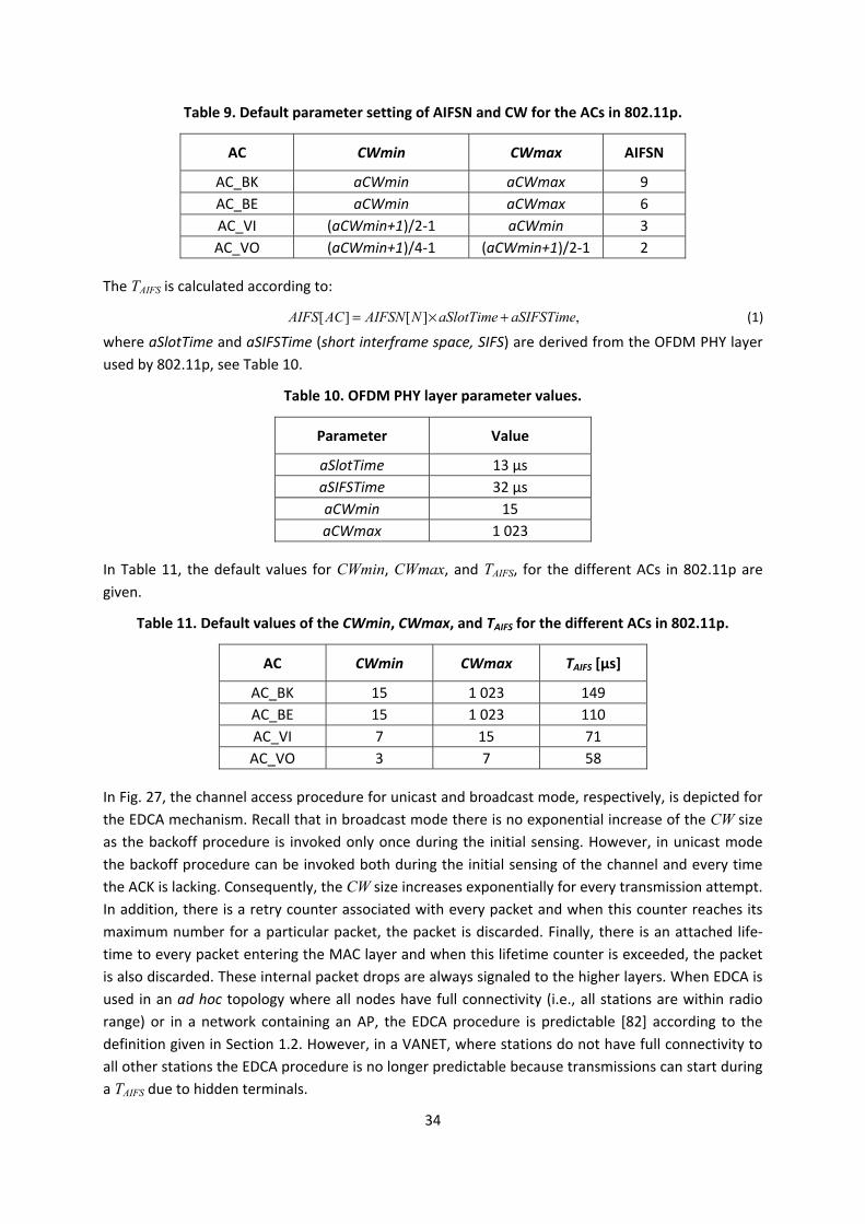
34

Table 9. Default parameter setting of AIFSN and CW for the ACs in 802.11p.

AC CWmin CWmax AIFSN

AC_BK aCWmin aCWmax 9 AC_BE aCWmin aCWmax 6 AC_VI (aCWmin+1)/2-1 aCWmin 3 AC_VO (aCWmin+1)/4-1 (aCWmin+1)/2-1 2

The TAIFS is calculated according to:

[ ] [ ] ,AIFS AC AIFSN N aSlotTime aSIFSTime= × + (1)

where aSlotTime and aSIFSTime (short interframe space, SIFS) are derived from the OFDM PHY layer used by 802.11p, see Table 10.

Table 10. OFDM PHY layer parameter values.

Parameter Value

aSlotTime 13 µs aSIFSTime 32 µs aCWmin 15 aCWmax 1 023

In Table 11, the default values for CWmin, CWmax, and TAIFS, for the different ACs in 802.11p are given.

Table 11. Default values of the CWmin, CWmax, and TAIFS for the different ACs in 802.11p.

AC CWmin CWmax TAIFS [µs]

AC_BK 15 1 023 149 AC_BE 15 1 023 110 AC_VI 7 15 71 AC_VO 3 7 58

In Fig. 27, the channel access procedure for unicast and broadcast mode, respectively, is depicted for the EDCA mechanism. Recall that in broadcast mode there is no exponential increase of the CW size as the backoff procedure is invoked only once during the initial sensing. However, in unicast mode the backoff procedure can be invoked both during the initial sensing of the channel and every time the ACK is lacking. Consequently, the CW size increases exponentially for every transmission attempt. In addition, there is a retry counter associated with every packet and when this counter reaches its maximum number for a particular packet, the packet is discarded. Finally, there is an attached life-time to every packet entering the MAC layer and when this lifetime counter is exceeded, the packet is also discarded. These internal packet drops are always signaled to the higher layers. When EDCA is used in an ad hoc topology where all nodes have full connectivity (i.e., all stations are within radio range) or in a network containing an AP, the EDCA procedure is predictable [82] according to the definition given in Section 1.2. However, in a VANET, where stations do not have full connectivity to all other stations the EDCA procedure is no longer predictable because transmissions can start during a TAIFS due to hidden terminals.

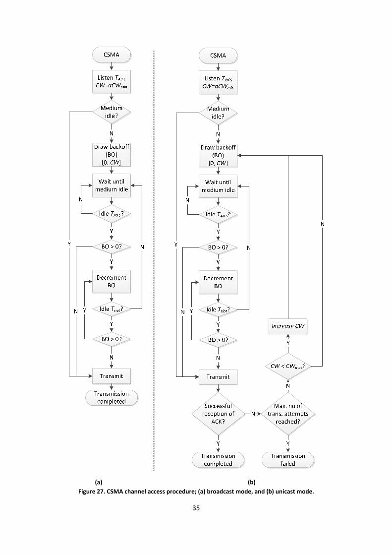
35

(a) (b)Figure 27. CSMA channel access procedure; (a) broadcast mode, and (b) unicast mode.

36

3.2 Self-organizing time division multiple access STDMA is already in commercial use in the AIS for the shipping industry with focus on surveillance applications, such as collision avoidance among ships using the VHF mobile maritime band. The AIS system is standardized in ITU-R Recommendation M.1371-4 [49] and its use is mandatory for all ships larger than 300 gross ton and all commercial passenger vessels regardless of size. These ships are required to carry a transponder that regularly transmits position messages using STDMA as its MAC method. The first release of the AIS standard was made in 1998 and the fourth revision was ratified in April 2010, which includes new features accommodating the leisure boat industry at a voluntary basis. Prior surveillance applications for ships have been based on ground infrastructure in harbors and along the coastline together with radar support. Radar has some shortcomings, such as the ina-bility to see behind large obstacles or incorrect radar images due to bad weather situations. By add-ing data communication, more solid information can be obtained about other ships in the vicinity and thereby accidents can be avoided. The update rate of the position messages broadcasted by ships using AIS depends on the speed of the ship.

In AIS, also base stations situated, e.g., at harbor entrances are used. These are connected to a back-office system allowing the authorities to follow ships in the harbor. The AIS base stations also trans-mit information about the harbor to the approaching ship. There are two different types of tran-sponders in AIS – Class A and Class B. The mandatory part of AIS for the large ships and passenger vessels use Class A transponders where STDMA is utilized as MAC method. Class B transponders are intended for the leisure boat industry and is not mandatory. Class B transponders use a carrier sense TDMA (CSTDMA) scheme for channel access. Consequently, the AIS system has introduced CSMA nodes into an already existing STDMA system.

In STDMA, time is divided into frames and further into time slots. In AIS the frame length is 1 minute and the number of slots in each frame is 2 250, giving a slot time slot of 26.6 ms. At start-up, the node decides upon a report rate, i.e., how many position messages that should be transmitted in each frame. The AIS standard has certain predetermined report rates depending on the speed of the ship. Anchored ships send one message every 3 minutes, whereas ships having a speed of 0 knots to 14 knots report every 10 seconds (6 messages per frame), and for higher speeds up to every 2 sec-onds (30 messages per frame).

The AIS transfer rate is 9.6 kbit/s and two different frequency channels are used, each with a band-width of 25 kHz and center frequencies of 161.975 MHz and 162.025 MHz, respectively. The tran-sponder uses both channels for transmissions and is capable of receiving on both channels at the same time, i.e., one transmitter and two receivers are required for each transponder. UTC synchroni-zation between nodes is required by AIS and is carried out using a GNSS such as GPS. A node reports in each transmission whether it has direct UTC or indirect UTC. The latter is used if a node does not have a working GPS due to poor signal quality or a faulty receiver. If this occurs, the node instead synchronizes using information obtained from other nodes that signal that they have direct UTC ca-pabilities. The AIS standard ITU-R Recommendation M.1371-4 [49] describes in detail the synchroni-zation in different scenarios and also fall back solutions.

Håkan Lans held a patent on STDMA [50], which expired in July 2012. The patent was also been re-examined in the US on March 30, 2010, cancelling all claims.

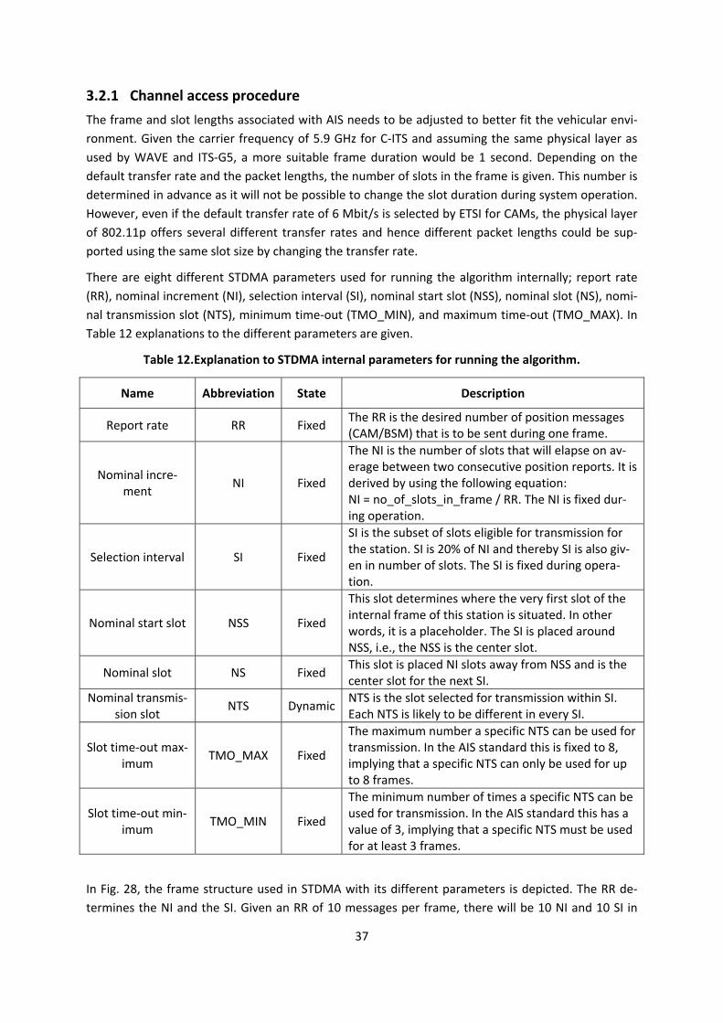
37

3.2.1 Channel access procedure The frame and slot lengths associated with AIS needs to be adjusted to better fit the vehicular envi-ronment. Given the carrier frequency of 5.9 GHz for C-ITS and assuming the same physical layer as used by WAVE and ITS-G5, a more suitable frame duration would be 1 second. Depending on the default transfer rate and the packet lengths, the number of slots in the frame is given. This number is determined in advance as it will not be possible to change the slot duration during system operation. However, even if the default transfer rate of 6 Mbit/s is selected by ETSI for CAMs, the physical layer of 802.11p offers several different transfer rates and hence different packet lengths could be sup-ported using the same slot size by changing the transfer rate.

There are eight different STDMA parameters used for running the algorithm internally; report rate (RR), nominal increment (NI), selection interval (SI), nominal start slot (NSS), nominal slot (NS), nomi-nal transmission slot (NTS), minimum time-out (TMO_MIN), and maximum time-out (TMO_MAX). In Table 12 explanations to the different parameters are given.

Table 12.Explanation to STDMA internal parameters for running the algorithm.

Name Abbreviation State Description

Report rate RR Fixed The RR is the desired number of position messages (CAM/BSM) that is to be sent during one frame.

Nominal incre-ment NI Fixed

The NI is the number of slots that will elapse on av-erage between two consecutive position reports. It is derived by using the following equation: NI = no_of_slots_in_frame / RR. The NI is fixed dur-ing operation.

Selection interval SI Fixed

SI is the subset of slots eligible for transmission for the station. SI is 20% of NI and thereby SI is also giv-en in number of slots. The SI is fixed during opera-tion.

Nominal start slot NSS Fixed

This slot determines where the very first slot of the internal frame of this station is situated. In other words, it is a placeholder. The SI is placed around NSS, i.e., the NSS is the center slot.

Nominal slot NS Fixed This slot is placed NI slots away from NSS and is the center slot for the next SI.

Nominal transmis-sion slot NTS Dynamic NTS is the slot selected for transmission within SI.

Each NTS is likely to be different in every SI.

Slot time-out max-imum TMO_MAX Fixed

The maximum number a specific NTS can be used for transmission. In the AIS standard this is fixed to 8, implying that a specific NTS can only be used for up to 8 frames.

Slot time-out min-imum TMO_MIN Fixed

The minimum number of times a specific NTS can be used for transmission. In the AIS standard this has a value of 3, implying that a specific NTS must be used for at least 3 frames.

In Fig. 28, the frame structure used in STDMA with its different parameters is depicted. The RR de-termines the NI and the SI. Given an RR of 10 messages per frame, there will be 10 NI and 10 SI in

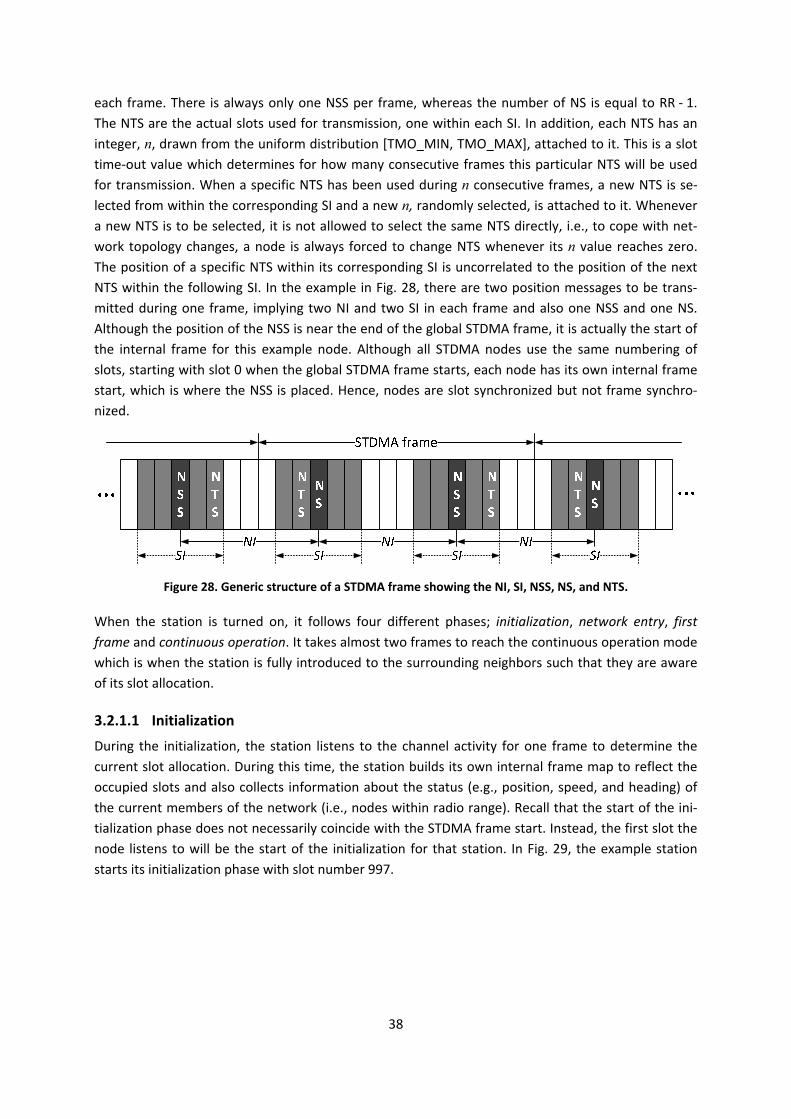
38

each frame. There is always only one NSS per frame, whereas the number of NS is equal to RR - 1. The NTS are the actual slots used for transmission, one within each SI. In addition, each NTS has an integer, n, drawn from the uniform distribution [TMO_MIN, TMO_MAX], attached to it. This is a slot time-out value which determines for how many consecutive frames this particular NTS will be used for transmission. When a specific NTS has been used during n consecutive frames, a new NTS is se-lected from within the corresponding SI and a new n, randomly selected, is attached to it. Whenever a new NTS is to be selected, it is not allowed to select the same NTS directly, i.e., to cope with net-work topology changes, a node is always forced to change NTS whenever its n value reaches zero. The position of a specific NTS within its corresponding SI is uncorrelated to the position of the next NTS within the following SI. In the example in Fig. 28, there are two position messages to be trans-mitted during one frame, implying two NI and two SI in each frame and also one NSS and one NS. Although the position of the NSS is near the end of the global STDMA frame, it is actually the start of the internal frame for this example node. Although all STDMA nodes use the same numbering of slots, starting with slot 0 when the global STDMA frame starts, each node has its own internal frame start, which is where the NSS is placed. Hence, nodes are slot synchronized but not frame synchro-nized.

When the station is turned on, it follows four different phases; initialization, network entry, first frame and continuous operation. It takes almost two frames to reach the continuous operation mode which is when the station is fully introduced to the surrounding neighbors such that they are aware of its slot allocation.

3.2.1.1 Initialization During the initialization, the station listens to the channel activity for one frame to determine the current slot allocation. During this time, the station builds its own internal frame map to reflect the occupied slots and also collects information about the status (e.g., position, speed, and heading) of the current members of the network (i.e., nodes within radio range). Recall that the start of the ini-tialization phase does not necessarily coincide with the STDMA frame start. Instead, the first slot the node listens to will be the start of the initialization for that station. In Fig. 29, the example station starts its initialization phase with slot number 997.

Figure 28. Generic structure of a STDMA frame showing the NI, SI, NSS, NS, and NTS.

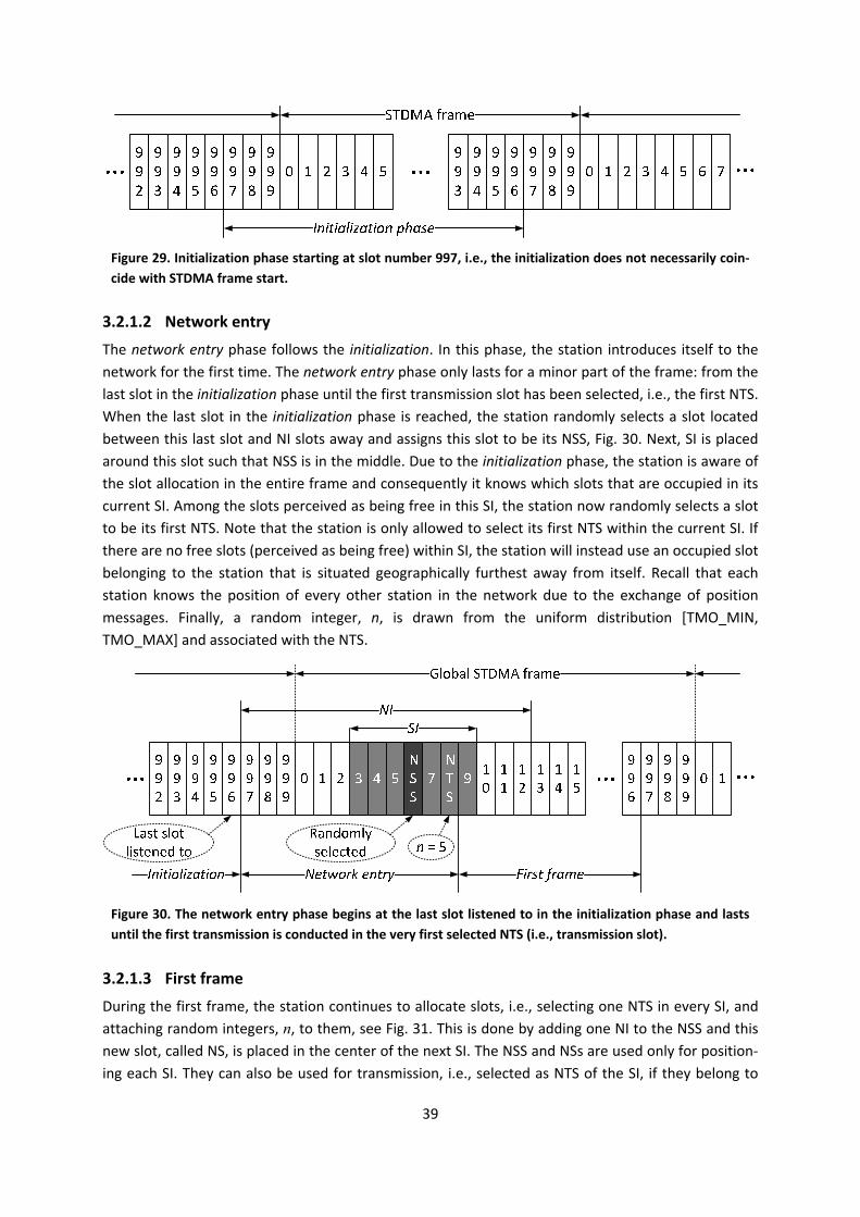
39

3.2.1.2 Network entry The network entry phase follows the initialization. In this phase, the station introduces itself to the network for the first time. The network entry phase only lasts for a minor part of the frame: from the last slot in the initialization phase until the first transmission slot has been selected, i.e., the first NTS. When the last slot in the initialization phase is reached, the station randomly selects a slot located between this last slot and NI slots away and assigns this slot to be its NSS, Fig. 30. Next, SI is placed around this slot such that NSS is in the middle. Due to the initialization phase, the station is aware of the slot allocation in the entire frame and consequently it knows which slots that are occupied in its current SI. Among the slots perceived as being free in this SI, the station now randomly selects a slot to be its first NTS. Note that the station is only allowed to select its first NTS within the current SI. If there are no free slots (perceived as being free) within SI, the station will instead use an occupied slot belonging to the station that is situated geographically furthest away from itself. Recall that each station knows the position of every other station in the network due to the exchange of position messages. Finally, a random integer, n, is drawn from the uniform distribution [TMO_MIN, TMO_MAX] and associated with the NTS.

3.2.1.3 First frame During the first frame, the station continues to allocate slots, i.e., selecting one NTS in every SI, and attaching random integers, n, to them, see Fig. 31. This is done by adding one NI to the NSS and this new slot, called NS, is placed in the center of the next SI. The NSS and NSs are used only for position-ing each SI. They can also be used for transmission, i.e., selected as NTS of the SI, if they belong to

Figure 29. Initialization phase starting at slot number 997, i.e., the initialization does not necessarily coin-cide with STDMA frame start.

Figure 30. The network entry phase begins at the last slot listened to in the initialization phase and lasts until the first transmission is conducted in the very first selected NTS (i.e., transmission slot).

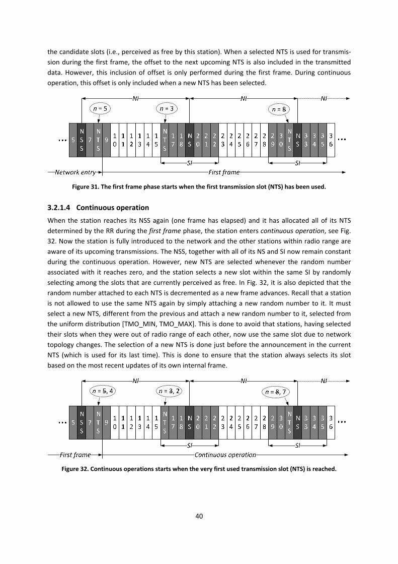
40

the candidate slots (i.e., perceived as free by this station). When a selected NTS is used for transmis-sion during the first frame, the offset to the next upcoming NTS is also included in the transmitted data. However, this inclusion of offset is only performed during the first frame. During continuous operation, this offset is only included when a new NTS has been selected.

3.2.1.4 Continuous operation When the station reaches its NSS again (one frame has elapsed) and it has allocated all of its NTS determined by the RR during the first frame phase, the station enters continuous operation, see Fig. 32. Now the station is fully introduced to the network and the other stations within radio range are aware of its upcoming transmissions. The NSS, together with all of its NS and SI now remain constant during the continuous operation. However, new NTS are selected whenever the random number associated with it reaches zero, and the station selects a new slot within the same SI by randomly selecting among the slots that are currently perceived as free. In Fig. 32, it is also depicted that the random number attached to each NTS is decremented as a new frame advances. Recall that a station is not allowed to use the same NTS again by simply attaching a new random number to it. It must select a new NTS, different from the previous and attach a new random number to it, selected from the uniform distribution [TMO_MIN, TMO_MAX]. This is done to avoid that stations, having selected their slots when they were out of radio range of each other, now use the same slot due to network topology changes. The selection of a new NTS is done just before the announcement in the current NTS (which is used for its last time). This is done to ensure that the station always selects its slot based on the most recent updates of its own internal frame.

Figure 31. The first frame phase starts when the first transmission slot (NTS) has been used.

Figure 32. Continuous operations starts when the very first used transmission slot (NTS) is reached.

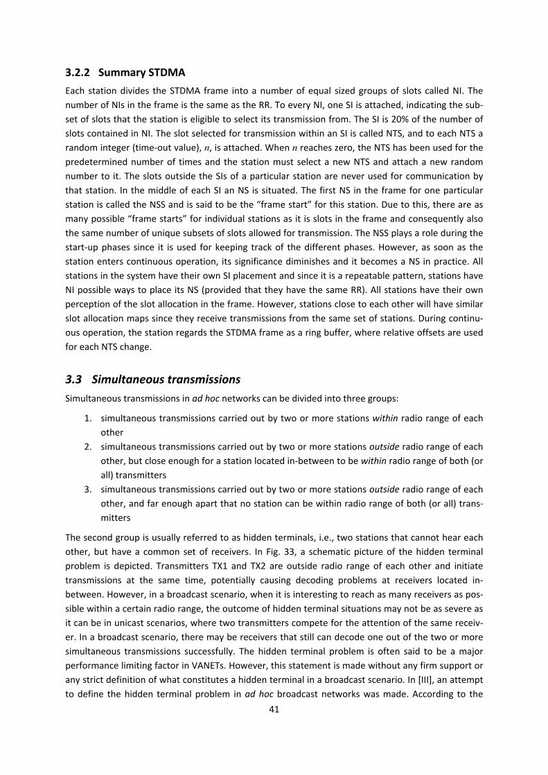
41

3.2.2 Summary STDMA Each station divides the STDMA frame into a number of equal sized groups of slots called NI. The number of NIs in the frame is the same as the RR. To every NI, one SI is attached, indicating the sub-set of slots that the station is eligible to select its transmission from. The SI is 20% of the number of slots contained in NI. The slot selected for transmission within an SI is called NTS, and to each NTS a random integer (time-out value), n, is attached. When n reaches zero, the NTS has been used for the predetermined number of times and the station must select a new NTS and attach a new random number to it. The slots outside the SIs of a particular station are never used for communication by that station. In the middle of each SI an NS is situated. The first NS in the frame for one particular station is called the NSS and is said to be the “frame start” for this station. Due to this, there are as many possible “frame starts” for individual stations as it is slots in the frame and consequently also the same number of unique subsets of slots allowed for transmission. The NSS plays a role during the start-up phases since it is used for keeping track of the different phases. However, as soon as the station enters continuous operation, its significance diminishes and it becomes a NS in practice. All stations in the system have their own SI placement and since it is a repeatable pattern, stations have NI possible ways to place its NS (provided that they have the same RR). All stations have their own perception of the slot allocation in the frame. However, stations close to each other will have similar slot allocation maps since they receive transmissions from the same set of stations. During continu-ous operation, the station regards the STDMA frame as a ring buffer, where relative offsets are used for each NTS change.

3.3 Simultaneous transmissions Simultaneous transmissions in ad hoc networks can be divided into three groups:

1. simultaneous transmissions carried out by two or more stations within radio range of each other

2. simultaneous transmissions carried out by two or more stations outside radio range of each other, but close enough for a station located in-between to be within radio range of both (or all) transmitters

3. simultaneous transmissions carried out by two or more stations outside radio range of each other, and far enough apart that no station can be within radio range of both (or all) trans-mitters

The second group is usually referred to as hidden terminals, i.e., two stations that cannot hear each other, but have a common set of receivers. In Fig. 33, a schematic picture of the hidden terminal problem is depicted. Transmitters TX1 and TX2 are outside radio range of each other and initiate transmissions at the same time, potentially causing decoding problems at receivers located in-between. However, in a broadcast scenario, when it is interesting to reach as many receivers as pos-sible within a certain radio range, the outcome of hidden terminal situations may not be as severe as it can be in unicast scenarios, where two transmitters compete for the attention of the same receiv-er. In a broadcast scenario, there may be receivers that still can decode one out of the two or more simultaneous transmissions successfully. The hidden terminal problem is often said to be a major performance limiting factor in VANETs. However, this statement is made without any firm support or any strict definition of what constitutes a hidden terminal in a broadcast scenario. In [III], an attempt to define the hidden terminal problem in ad hoc broadcast networks was made. According to the

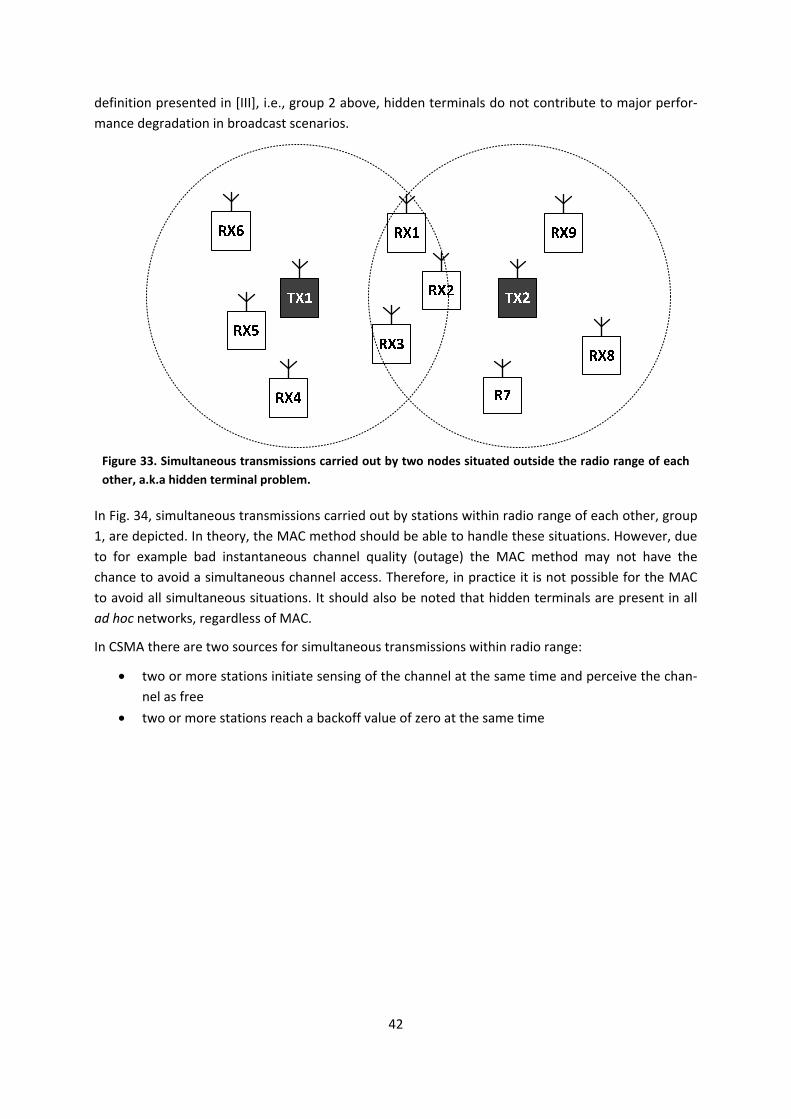
42

definition presented in [III], i.e., group 2 above, hidden terminals do not contribute to major perfor-mance degradation in broadcast scenarios.

In Fig. 34, simultaneous transmissions carried out by stations within radio range of each other, group 1, are depicted. In theory, the MAC method should be able to handle these situations. However, due to for example bad instantaneous channel quality (outage) the MAC method may not have the chance to avoid a simultaneous channel access. Therefore, in practice it is not possible for the MAC to avoid all simultaneous situations. It should also be noted that hidden terminals are present in all ad hoc networks, regardless of MAC.

In CSMA there are two sources for simultaneous transmissions within radio range:

• two or more stations initiate sensing of the channel at the same time and perceive the chan-nel as free

• two or more stations reach a backoff value of zero at the same time

Figure 33. Simultaneous transmissions carried out by two nodes situated outside the radio range of each other, a.k.a hidden terminal problem.

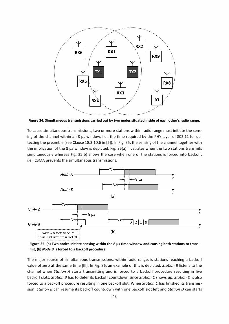
43

To cause simultaneous transmissions, two or more stations within radio range must initiate the sens-ing of the channel within an 8 µs window, i.e., the time required by the PHY layer of 802.11 for de-tecting the preamble (see Clause 18.3.10.6 in [5]). In Fig. 35, the sensing of the channel together with the implication of the 8 µs window is depicted. Fig. 35(a) illustrates when the two stations transmits simultaneously whereas Fig. 35(b) shows the case when one of the stations is forced into backoff, i.e., CSMA prevents the simultaneous transmissions.

The major source of simultaneous transmissions, within radio range, is stations reaching a backoff value of zero at the same time [III]. In Fig. 36, an example of this is depicted. Station B listens to the channel when Station A starts transmitting and is forced to a backoff procedure resulting in five backoff slots. Station B has to defer its backoff countdown since Station C shows up. Station D is also forced to a backoff procedure resulting in one backoff slot. When Station C has finished its transmis-sion, Station B can resume its backoff countdown with one backoff slot left and Station D can starts

Figure 34. Simultaneous transmissions carried out by two nodes situated inside of each other’s radio range.

Figure 35. (a) Two nodes initiate sensing within the 8 µs time window and causing both stations to trans-mit, (b) Node B is forced to a backoff procedure.

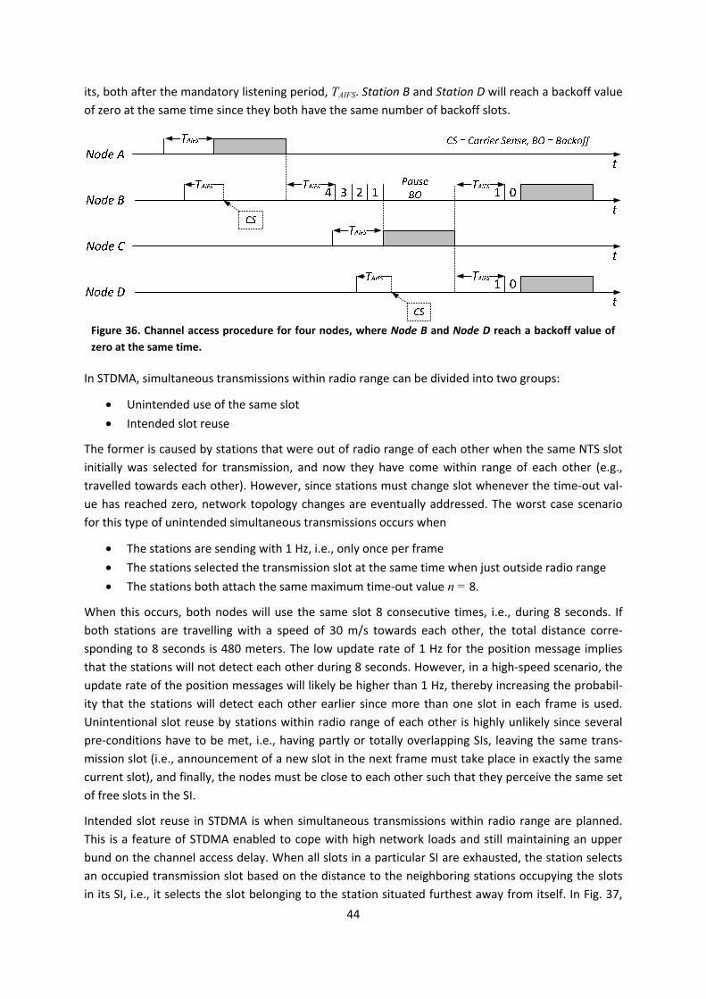
44

its, both after the mandatory listening period, TAIFS. Station B and Station D will reach a backoff value of zero at the same time since they both have the same number of backoff slots.

In STDMA, simultaneous transmissions within radio range can be divided into two groups:

• Unintended use of the same slot • Intended slot reuse

The former is caused by stations that were out of radio range of each other when the same NTS slot initially was selected for transmission, and now they have come within range of each other (e.g., travelled towards each other). However, since stations must change slot whenever the time-out val-ue has reached zero, network topology changes are eventually addressed. The worst case scenario for this type of unintended simultaneous transmissions occurs when

• The stations are sending with 1 Hz, i.e., only once per frame • The stations selected the transmission slot at the same time when just outside radio range • The stations both attach the same maximum time-out value n = 8.

When this occurs, both nodes will use the same slot 8 consecutive times, i.e., during 8 seconds. If both stations are travelling with a speed of 30 m/s towards each other, the total distance corre-sponding to 8 seconds is 480 meters. The low update rate of 1 Hz for the position message implies that the stations will not detect each other during 8 seconds. However, in a high-speed scenario, the update rate of the position messages will likely be higher than 1 Hz, thereby increasing the probabil-ity that the stations will detect each other earlier since more than one slot in each frame is used. Unintentional slot reuse by stations within radio range of each other is highly unlikely since several pre-conditions have to be met, i.e., having partly or totally overlapping SIs, leaving the same trans-mission slot (i.e., announcement of a new slot in the next frame must take place in exactly the same current slot), and finally, the nodes must be close to each other such that they perceive the same set of free slots in the SI.

Intended slot reuse in STDMA is when simultaneous transmissions within radio range are planned. This is a feature of STDMA enabled to cope with high network loads and still maintaining an upper bund on the channel access delay. When all slots in a particular SI are exhausted, the station selects an occupied transmission slot based on the distance to the neighboring stations occupying the slots in its SI, i.e., it selects the slot belonging to the station situated furthest away from itself. In Fig. 37,

Figure 36. Channel access procedure for four nodes, where Node B and Node D reach a backoff value of zero at the same time.

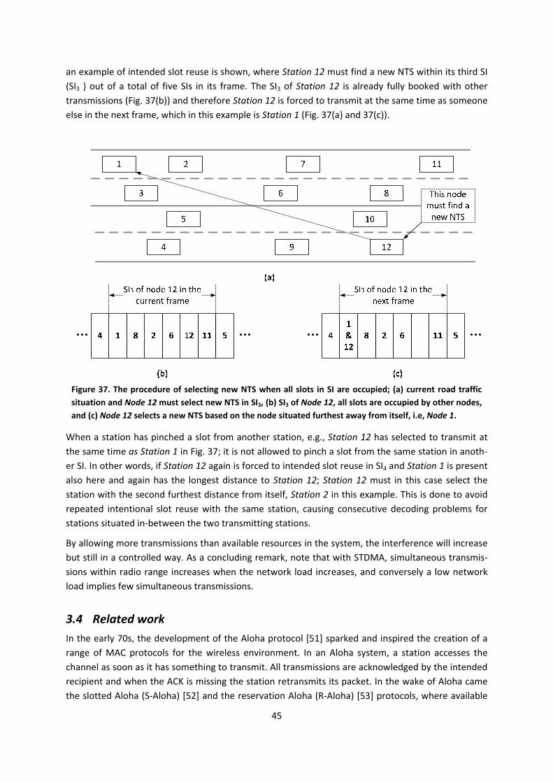
45

an example of intended slot reuse is shown, where Station 12 must find a new NTS within its third SI (SI3 ) out of a total of five SIs in its frame. The SI3 of Station 12 is already fully booked with other transmissions (Fig. 37(b)) and therefore Station 12 is forced to transmit at the same time as someone else in the next frame, which in this example is Station 1 (Fig. 37(a) and 37(c)).

When a station has pinched a slot from another station, e.g., Station 12 has selected to transmit at the same time as Station 1 in Fig. 37; it is not allowed to pinch a slot from the same station in anoth-er SI. In other words, if Station 12 again is forced to intended slot reuse in SI4 and Station 1 is present also here and again has the longest distance to Station 12; Station 12 must in this case select the station with the second furthest distance from itself, Station 2 in this example. This is done to avoid repeated intentional slot reuse with the same station, causing consecutive decoding problems for stations situated in-between the two transmitting stations.

By allowing more transmissions than available resources in the system, the interference will increase but still in a controlled way. As a concluding remark, note that with STDMA, simultaneous transmis-sions within radio range increases when the network load increases, and conversely a low network load implies few simultaneous transmissions.

3.4 Related work In the early 70s, the development of the Aloha protocol [51] sparked and inspired the creation of a range of MAC protocols for the wireless environment. In an Aloha system, a station accesses the channel as soon as it has something to transmit. All transmissions are acknowledged by the intended recipient and when the ACK is missing the station retransmits its packet. In the wake of Aloha came the slotted Aloha (S-Aloha) [52] and the reservation Aloha (R-Aloha) [53] protocols, where available

Figure 37. The procedure of selecting new NTS when all slots in SI are occupied; (a) current road traffic situation and Node 12 must select new NTS in SI3, (b) SI3 of Node 12, all slots are occupied by other nodes, and (c) Node 12 selects a new NTS based on the node situated furthest away from itself, i.e, Node 1.

46

time was divided into slots constituting a frame. The introduction of slots greatly increased the throughput compared to pure Aloha. In S-Aloha, a station randomly selects a slot in which to trans-mit as soon as it has something to send, without keeping track of which slots were used in the previ-ous frame. In R-Aloha, stations keep track of the slot occupation and whenever a station has some-thing to transmit it selects a slot that has been free in previous frames and it will keep it for as long as needed, i.e., it does not change transmissions slot every frame.

The first MAC protocols specifically designed for VANETs appeared in the 80s, during the first trials of C-ITS systems in Europe and the US [54] (e.g., PROMOTHEUS, IVHS). The concurrent slot assignment protocol (CSAP) [55] was proposed in 1988 to combat the hidden station problem encountered in R-Aloha. In CSAP, the frame is divided into two sub-frames; one part contains the slots for actual data transmission, whereas the other part is used for signaling if collisions are experienced by receivers, a.k.a. the collision slots. When a receiver recognizes a collision in a specific slot in the ordinary data frame part, it will transmit a high frequency signal in the corresponding collision slot to notify the concurrent transmitters. Along with the data, each transmitter also sends side information consisting of a simple slot allocation scheme, where free and occupied slots as experienced by this particular transmitter are marked with zeros and ones, respectively. When a station realizes that it has ac-cessed a specific slot concurrently with another station, it changes to a new slot.

The work on CSAP was extended in 1991 by Zhu et al. [56] through the MAC scheme termed decen-tral channel access protocol (DCAP), which supports higher station mobility than CSAP. The proce-dure of changing slots when collisions occur is enhanced in DCAP by including another protocol called the integrated service management (ISMA) protocol. The extra bits containing the collision infor-mation found at the end of the CSAP frame are removed and instead a handover request, based on lost connections to formerly adjacent stations (which still should be in radio range of each other ac-cording to their movement pattern) is issued. However, since the collision detection mechanism in both CSAP and in DCAP relies on a third party detecting and notifying about the event (two stations could have selected the same slot, while no other stations are within range of these two concurrently transmitting stations – and then no one can communicate the collision information), every transmis-sion is performed only with a certain probability, p, and deferred with 1– p in order to minimize un-detected concurrent transmissions.

The reliable R-Aloha (RR-Aloha) protocol proposed by Borgonovo et al. [57] in 2002 is almost identi-cal to the DCAP proposal but here every station also sends side information in each slot, containing the slot allocation chart as perceived by this particular station. The ADHOC-MAC [58], proposed by the same authors, is based on RR-Aloha with some additional features such as bandwidth allocation for point-to-point communication together with multicast support. Both in RR-Aloha and ADHOC-MAC, the frame length is fixed. In adaptive ADHOC (A-ADHOC) [59], however, the protocol is extend-ed to use a variable frame length to reduce the setup time and exploit the channel resources more efficiently. This implies that with few stations in the system, there are few slots and a short frame length, resulting in more frames per second, and when the number of stations increases, the frame length will be extended to accommodate the increase. Recall that in RR-Aloha, one bit is used in the slot allocation chart to denote whether a slot is perceived as free or occupied. However, the only time a slot is regarded as occupied is when a station has successfully received a packet in that partic-ular slot. Hence, a slot is said to be free if there has been a collision, i.e., a negative ACK is interpreted as a free slot in the slot allocation charts.

47

Also the decentralized TDMA (D-TDMA) protocol suggested in [60, 61], stations send side information containing the slot allocation chart. However, even if this scheme is denoted TDMA, it is almost iden-tical to the DCAP and ADHOC-MAC proposals.

In RR-Aloha+ [62], the RR-Aloha proposal was enhanced by introducing one more bit in the slot allo-cation chart transmitted by every station. This new bit is used for signaling the occurrence of a colli-sion, i.e., stations sending at the same time causing collisions somewhere in the network. During the performance evaluation of RR-Aloha+ it was discovered that the information about the slot allocation was propagating too far, such that it blocked transmissions that could have taken place, i.e., the ex-posed station problem. Therefore, the RR-Aloha+ protocol does not use slot charts that are more than one frame old, in order to maintain updated information. However, in RR-Aloha+ problems with scalability were detected. RR-Aloha+ was thus further developed into mobile slotted Aloha (MS-Aloha) [63]. Here, the slot chart information broadcasted by every station is limited to a certain number of hops. This greatly enhanced performance, especially at high vehicular speeds and rapidly changing network topology. By introducing MS-Aloha and thereby restricting the slot chart infor-mation, the scalability in terms of number of stations is improved as fewer transmissions are blocked.

Although slots are cleverly coordinated with slot allocation charts in all the extensions of RR-Aloha described above, the number of stations in the network is limited to the number of slots in the frame. When a station wants to join a network in which all slots are already occupied, it has to wait until a slot is released, either due to a station disappearing (moves away) or stops transmitting. This implies that the channel access delay is random. Also in the decentralized TDMA (D-TDMA) protocol, it is not possible to have more stations than available slots. Improvements in terms of increased pay-load in D-TDMA were made in [64], but the randomness for a large number of stations, larger than the number of slots, remains.

In space division multiple access (SDMA), access to the communication channel is based on the cur-rent location of the vehicle [65, 66, 67, 68]. Real-time location estimation is provided either through GNSS or using a magnetic positioning system [65]. Dead reckoning is also suggested as a counter measure for GPS errors [68]. The idea with SDMA is to divide all roads into different sectors and with-in each sector, e.g., TDMA or CDMA can be applied. In [68] each sector is five meters and has a one-to-one mapping to a specific time slot (TDMA). However, in an SDMA scenario there could be many unused slots due to sparse vehicle traffic or high relative speeds. The proposal from [68] is then to increase the channel utilization by allowing vehicles to use all time slots up to the next vehicle in front. However, position information must also be propagated in the network, i.e., all vehicles broad-cast their position information.

TDMA has traditionally been used in centralized networks where slots have been assigned to users by a static central controller. However, there exist decentralized TDMA schemes where stations group into clusters and elect a cluster head that divides the resources among the participating stations. In [69] a clustering scheme for stations in a highway scenario is proposed. Stations traveling in the same direction on the highway join in a cluster. The cluster head is responsible for the division of available bandwidth within the cluster as well as for communication between clusters. Within each cluster, a TDMA scheme is applied, whereas communication between clusters is performed using CSMA. To join or leave a cluster, a separate frequency channel is used and thus every vehicle is equipped with two transceivers. The cluster head searches for new stations on the separate frequency channel by

48

transmitting specific messages regularly. This proposal involves three separate MAC schemes and relies on the existence of several frequency channels.

Günter et al. [70] also proposes a clustering scheme where a cluster head is elected and within each cluster a TDMA scheme is applied. A part of the TDMA frame within each cluster is never allocated by the cluster members. Instead these slots are used by newly arrived stations to announce their pres-ence and to request transmission opportunities. When two clusters come within radio range of each other, the clusters are regrouped. This scheme is based on a single frequency channel and to de-crease the interference between clusters, a superframe between the clusters is proposed. This im-plies that nine ordinary cluster frames are grouped into a single superframe and only one ninth of the available time is allocated to a cluster.

3.5 Summary Most of the slotted MAC schemes reviewed in Section 3.4 have the advantage that each station knows in advance when it is allowed to transmit. Further, since synchronization is a prerequisite for slotted schemes, the problem with transmissions partly overlapping in time due to simultaneously transmitting stations that are out of radio range does not exist. It will be shown in Chapter 4, as ex-pected, that uncoordinated transmissions results in decreased performance. However, none of the slotted MAC schemes presented in Section 3.4 can accept more stations in the system than there are slots in the frame. Therefore, there is still an uncertainty about when channel access will take place when the network load increases beyond the number of slots.

The SDMA scheme, on the other hand, is based on station position on the road and as vehicles can-not be stacked on top of one another, channel access is always guaranteed. However, the SDMA scheme introduces a complex algorithm for division of the road network into suitable pieces. STDMA, described in Section 3.2, has a comparably low complexity and it scales well with an increasing num-ber of stations. When all resources are exhausted, a new station selects to transmit at the same time as someone else situated geographically furthest away from itself. Therefore, channel access delay is decoupled from the current network load.

Since CSMA is simple and does not require synchronization between stations, it is selected as the wireless technology for the first generation of C-ITS despite its scalability issues. However, there is a clear trend in on-going standardization towards controlling the data traffic injected into the network through DCC mechanisms. Several promising algorithms have been proposed recently [71, 72], where the application is aware of the network load and adjust its injected data traffic. Using this approach, every generated message (e.g., CAM/BSM/DENM) has a higher probability of being transmitted be-fore its deadline expires. Further, it also enables the application to prioritize between different mes-sages and only transmit messages critical to system performance.

Two strong candidates remain when evaluating MAC algorithms for VANETs; STDMA and CSMA. The former is interesting because it fulfils most of the criteria required by a MAC method used for traffic-safety, at a reasonably low complexity. The latter is interesting as it is the de facto standard for the first generation of VANETs. These two candidates are therefore investigated further in the next chap-ter, with respect to the criteria listed in Section 1.2.

49

4 Performance evaluation of CSMA and STDMA Since CSMA will be the prevailing MAC method of emerging standards for VANET based road traffic safety applications, as described in Chapter 2; it will be further studied in this chapter. In addition, STDMA as described in Chapter 3 will also be evaluated, since this MAC method has the potential to fulfill the requirements imposed by VANET based road traffic safety applications. Recall from Chapter 1, that the requirements deduced from road traffic safety applications are both delay and reliability concurrently. The overall C-ITS system requires that the probability for fairness is as high as possible, which can be translated into equal probability to access the channel for all involved stations. The ad hoc topology implies requirements on scalability, both in terms of the amount of data traffic, i.e., the network load, but most importantly in terms of the number of stations in the system.

To evaluate the requirements on predictable delay, reliability, fairness and scalability, five different performance metrics have been selected:

• Channel access delay

• Packet reception probability

• MAC-to-MAC delay

• Packet inter-arrival time

• Initial detection distance

The channel access delay highlights the ability of the MAC method to provide a predictable delay which is a functional requirement, i.e., either the delay is predictable or it is random. The packet re-ception probability is a non-functional requirement, i.e., a quality measure determining how well the MAC method schedules transmissions in time and space. The MAC-to-MAC delay captures both the channel access delay and the packet reception probability, and is further explained in Section 4.5. The packet inter-arrival time provides similar insight as the packet reception probability, but on an individual station basis, rather than averaged over several stations. Finally, the initial detection dis-tance is an important design parameter for ITS application developers, since this will determine the driver awareness horizon. Note that all five performance measures are evaluated for different net-work loads, to determine the scalability of the MAC methods, i.e., if the quality changes with in-creased network load.

The performance of CSMA and STDMA has been evaluated by means of computer simulations in MATLAB. The highway scenario was selected to model the vehicle traffic pattern since the highest relative speeds are found here and therefore it is likely the most stressing case for the MAC methods since stations can show up and quickly disappear again due to high velocities. Both CSMA and STDMA use parameters from the same PHY layer in the simulator, namely IEEE 802.11p, based on OFDM as described briefly in Section 2.1.1 and thoroughly in Clause 18 of [5]. Two different channel models have been used in the evaluations; one termed the LOS/OLOS model, which distinguishes between line-of-sight (LOS) and obstructed LOS (OLOS) transmissions, and the traditional Nakagami-m model, where the m value changes depending on distance between transmitter and receiver. The channel models are described further in Section 4.1. All vehicles broadcast 400 byte long position messages (e.g., CAM/BSM) using a data transfer rate of 6 Mbit/s and an output power of 100 mW (20 dBm). The broadcast mode implies that no acknowledgements are sent in a response to any received transmissions. This implies that the backoff procedure for CSMA will only be invoked once during the

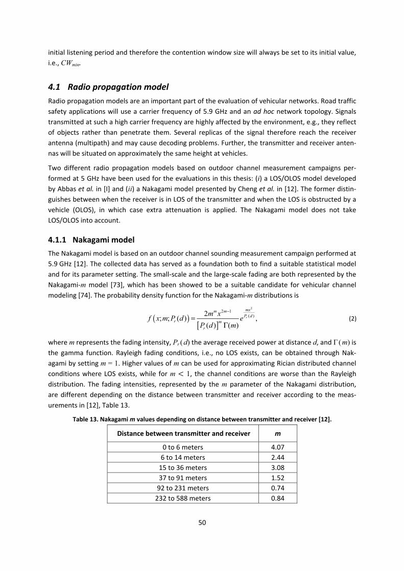
50

initial listening period and therefore the contention window size will always be set to its initial value, i.e., CWmin.

4.1 Radio propagation model Radio propagation models are an important part of the evaluation of vehicular networks. Road traffic safety applications will use a carrier frequency of 5.9 GHz and an ad hoc network topology. Signals transmitted at such a high carrier frequency are highly affected by the environment, e.g., they reflect of objects rather than penetrate them. Several replicas of the signal therefore reach the receiver antenna (multipath) and may cause decoding problems. Further, the transmitter and receiver anten-nas will be situated on approximately the same height at vehicles.

Two different radio propagation models based on outdoor channel measurement campaigns per-formed at 5 GHz have been used for the evaluations in this thesis: (i) a LOS/OLOS model developed by Abbas et al. in [I] and (ii) a Nakagami model presented by Cheng et al. in [12]. The former distin-guishes between when the receiver is in LOS of the transmitter and when the LOS is obstructed by a vehicle (OLOS), in which case extra attenuation is applied. The Nakagami model does not take LOS/OLOS into account.

4.1.1 Nakagami model The Nakagami model is based on an outdoor channel sounding measurement campaign performed at 5.9 GHz [12]. The collected data has served as a foundation both to find a suitable statistical model and for its parameter setting. The small-scale and the large-scale fading are both represented by the Nakagami-m model [73], which has been showed to be a suitable candidate for vehicular channel modeling [74]. The probability density function for the Nakagami-m distributions is

( )[ ]

22 1

( )2; ; ( ) ,( ) ( )

r

mxm mP d

r m

r

m xf x m P d e

P d m

−

=Γ

(2)

where m represents the fading intensity, Pr (d) the average received power at distance d, and Γ (m) is the gamma function. Rayleigh fading conditions, i.e., no LOS exists, can be obtained through Nak-agami by setting m = 1. Higher values of m can be used for approximating Rician distributed channel conditions where LOS exists, while for m < 1, the channel conditions are worse than the Rayleigh distribution. The fading intensities, represented by the m parameter of the Nakagami distribution, are different depending on the distance between transmitter and receiver according to the meas-urements in [12], Table 13.

Table 13. Nakagami m values depending on distance between transmitter and receiver [12].

Distance between transmitter and receiver m

0 to 6 meters 4.07 6 to 14 meters 2.44

15 to 36 meters 3.08 37 to 91 meters 1.52

92 to 231 meters 0.74 232 to 588 meters 0.84

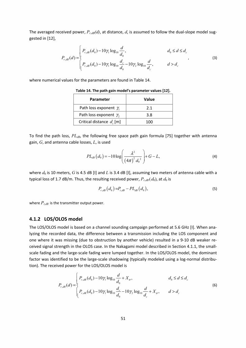
51

The averaged received power, Pr,dB(d), at distance, d, is assumed to follow the dual-slope model sug-gested in [12],

, 0 1 10 0

0,

, 0 1 10 2 100

( ) 10 log ,( )

( ) 10 log 10 log ,

r dB c

r dBc

r dB cc

dP d d d d

dP d

d dP d d d

d d

γ

γ γ

− ≤ ≤= − − >

, (3)

where numerical values for the parameters are found in Table 14.

Table 14. The path gain model’s parameter values [12].

Parameter Value

Path loss exponent 1γ 2.1 Path loss exponent 2γ 3.8 Critical distance cd [m] 100

To find the path loss, PLdB, the following free space path gain formula [75] together with antenna gain, G, and antenna cable losses, L, is used

( )( )

2

0 2 20

10log ,4

dBPL d G Ld

λπ

= − + −

(4)

where d0 is 10 meters, G is 4.5 dB [I] and L is 3.4 dB [I], assuming two meters of antenna cable with a typical loss of 1.7 dB/m. Thus, the resulting received power, Pr,dB (d0), at d0 is

( ) ( ), 0 , 0 ,r dB t dB dBP d P PL d= − (5)

where Pt,dB is the transmitter output power.

4.1.2 LOS/OLOS model The LOS/OLOS model is based on a channel sounding campaign performed at 5.6 GHz [I]. When ana-lyzing the recorded data, the difference between a transmission including the LOS component and one where it was missing (due to obstruction by another vehicle) resulted in a 9-10 dB weaker re-ceived signal strength in the OLOS case. In the Nakagami model described in Section 4.1.1, the small-scale fading and the large-scale fading were lumped together. In the LOS/OLOS model, the dominant factor was identified to be the large-scale shadowing (typically modeled using a log-normal distribu-tion). The received power for the LOS/OLOS model is

, 0 1 10 0

0,

, 0 1 10 2 100

( ) 10 log ,( )

( ) 10 log 10 log ,

r dB c

r dBc

r dB cc

dP d X d d d

dP d

d dP d X d d

d d

σ

σ

γ

γ γ

− + ≤ ≤= − − + >

(6)

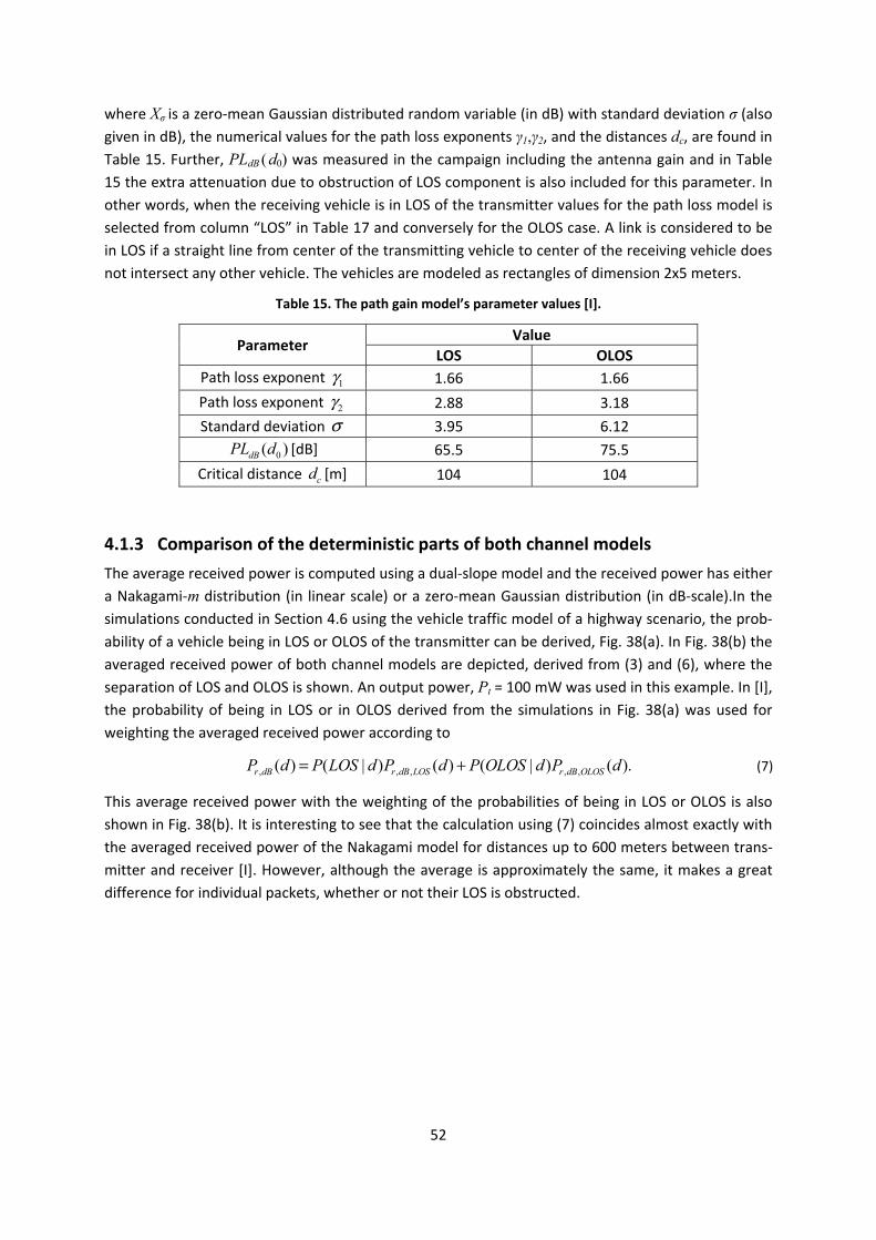
52

where Xσ is a zero-mean Gaussian distributed random variable (in dB) with standard deviation σ (also given in dB), the numerical values for the path loss exponents γ1,γ2, and the distances dc, are found in Table 15. Further, PLdB (d0) was measured in the campaign including the antenna gain and in Table 15 the extra attenuation due to obstruction of LOS component is also included for this parameter. In other words, when the receiving vehicle is in LOS of the transmitter values for the path loss model is selected from column “LOS” in Table 17 and conversely for the OLOS case. A link is considered to be in LOS if a straight line from center of the transmitting vehicle to center of the receiving vehicle does not intersect any other vehicle. The vehicles are modeled as rectangles of dimension 2x5 meters.

Table 15. The path gain model’s parameter values [I].

Parameter Value LOS OLOS

Path loss exponent 1γ 1.66 1.66 Path loss exponent 2γ 2.88 3.18 Standard deviation σ 3.95 6.12

0( )dBPL d [dB] 65.5 75.5 Critical distance cd [m] 104 104

4.1.3 Comparison of the deterministic parts of both channel models The average received power is computed using a dual-slope model and the received power has either a Nakagami-m distribution (in linear scale) or a zero-mean Gaussian distribution (in dB-scale).In the simulations conducted in Section 4.6 using the vehicle traffic model of a highway scenario, the prob-ability of a vehicle being in LOS or OLOS of the transmitter can be derived, Fig. 38(a). In Fig. 38(b) the averaged received power of both channel models are depicted, derived from (3) and (6), where the separation of LOS and OLOS is shown. An output power, Pt = 100 mW was used in this example. In [I], the probability of being in LOS or in OLOS derived from the simulations in Fig. 38(a) was used for weighting the averaged received power according to

, , , , ,( ) ( | ) ( ) ( | ) ( ).r dB r dB LOS r dB OLOSP d P LOS d P d P OLOS d P d= + (7)

This average received power with the weighting of the probabilities of being in LOS or OLOS is also shown in Fig. 38(b). It is interesting to see that the calculation using (7) coincides almost exactly with the averaged received power of the Nakagami model for distances up to 600 meters between trans-mitter and receiver [I]. However, although the average is approximately the same, it makes a great difference for individual packets, whether or not their LOS is obstructed.

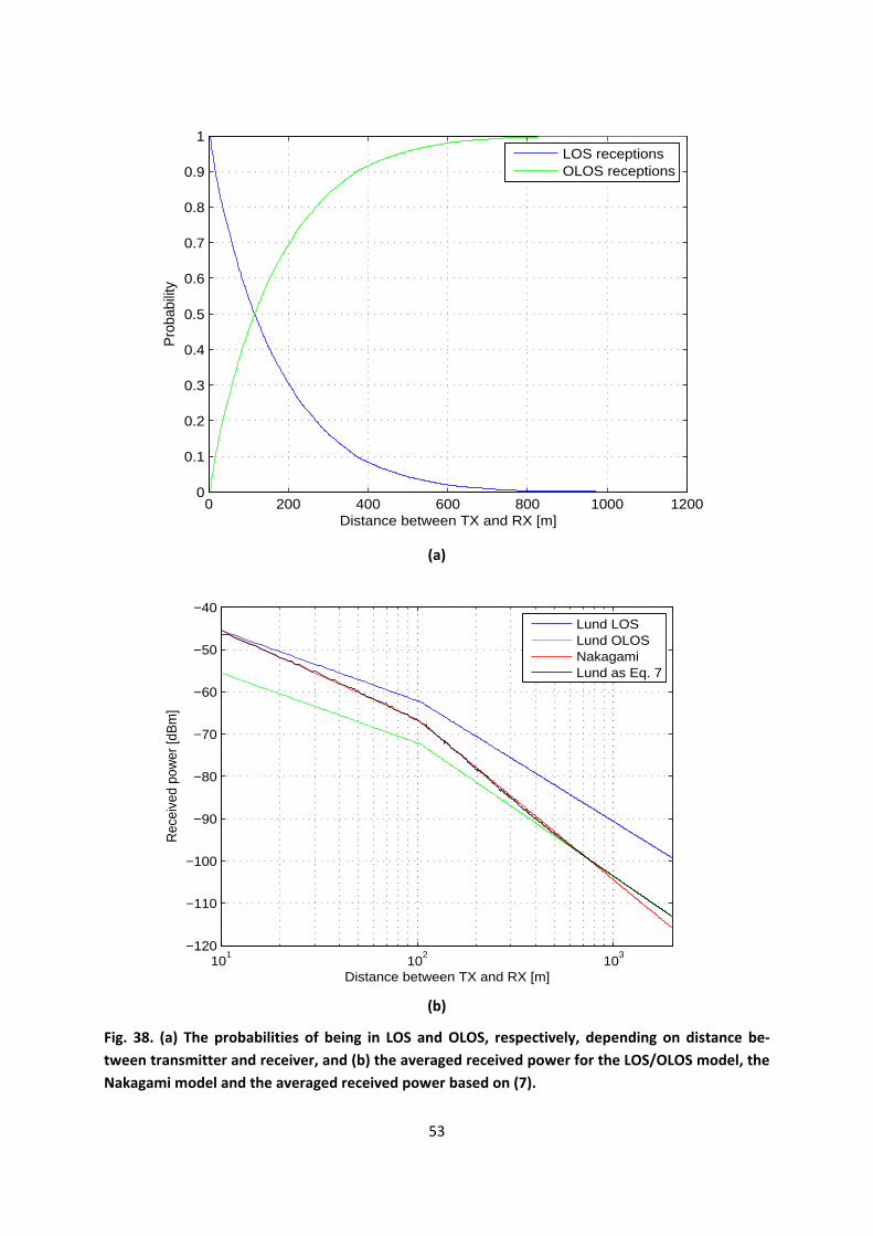
53

(a)

(b)

Fig. 38. (a) The probabilities of being in LOS and OLOS, respectively, depending on distance be-tween transmitter and receiver, and (b) the averaged received power for the LOS/OLOS model, the Nakagami model and the averaged received power based on (7).

0 200 400 600 800 1000 12000

0.1

0.2

0.3

0.4

0.5

0.6

0.7

0.8

0.9

1

Pro

babi

lity

Distance between TX and RX [m]

LOS receptionsOLOS receptions

101

102

103

−120

−110

−100

−90

−80

−70

−60

−50

−40

Distance between TX and RX [m]

Rec

eive

d po

wer

[dB

m]

Lund LOSLund OLOSNakagamiLund as Eq. 7

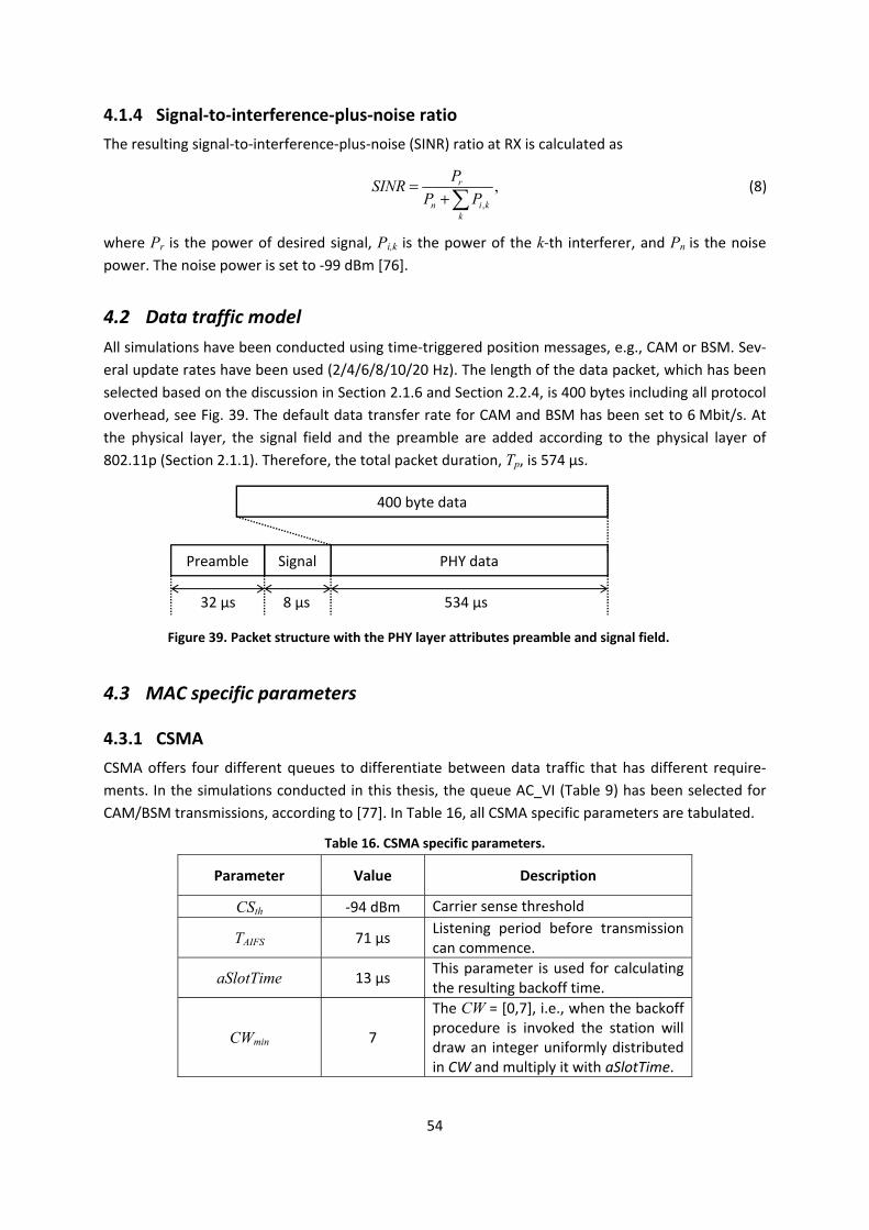
54

4.1.4 Signal-to-interference-plus-noise ratio The resulting signal-to-interference-plus-noise (SINR) ratio at RX is calculated as

,

,r

n i kk

PSINR

P P=

+ (8)

where Pr is the power of desired signal, Pi,k is the power of the k-th interferer, and Pn is the noise power. The noise power is set to -99 dBm [76].

4.2 Data traffic model All simulations have been conducted using time-triggered position messages, e.g., CAM or BSM. Sev-eral update rates have been used (2/4/6/8/10/20 Hz). The length of the data packet, which has been selected based on the discussion in Section 2.1.6 and Section 2.2.4, is 400 bytes including all protocol overhead, see Fig. 39. The default data transfer rate for CAM and BSM has been set to 6 Mbit/s. At the physical layer, the signal field and the preamble are added according to the physical layer of 802.11p (Section 2.1.1). Therefore, the total packet duration, Tp, is 574 µs.

4.3 MAC specific parameters

4.3.1 CSMA CSMA offers four different queues to differentiate between data traffic that has different require-ments. In the simulations conducted in this thesis, the queue AC_VI (Table 9) has been selected for CAM/BSM transmissions, according to [77]. In Table 16, all CSMA specific parameters are tabulated.

Table 16. CSMA specific parameters.

Parameter Value Description

CSth -94 dBm Carrier sense threshold

TAIFS 71 µs Listening period before transmission can commence.

aSlotTime 13 µs This parameter is used for calculating the resulting backoff time.

CWmin 7

The CW = [0,7], i.e., when the backoff procedure is invoked the station will draw an integer uniformly distributed in CW and multiply it with aSlotTime.

PHY dataSignal Preamble

400 byte data

32 µs 8 µs 534 µs

Figure 39. Packet structure with the PHY layer attributes preamble and signal field.

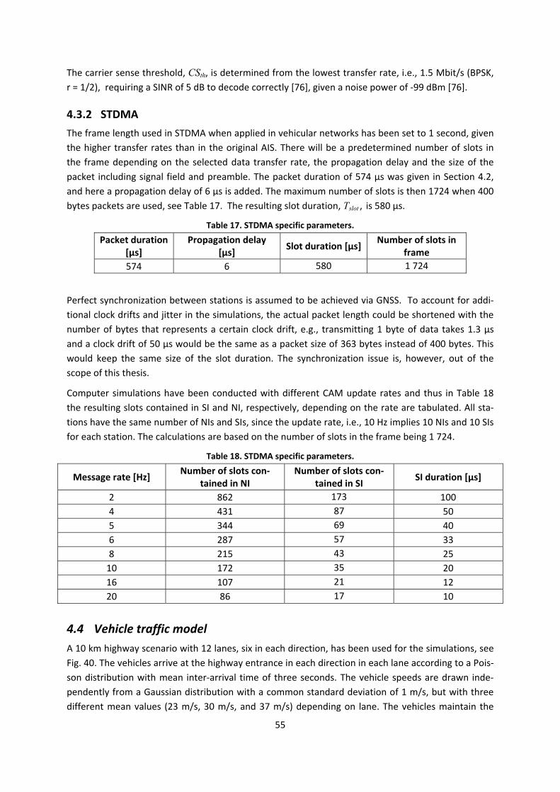
55

The carrier sense threshold, CSth, is determined from the lowest transfer rate, i.e., 1.5 Mbit/s (BPSK, r = 1/2), requiring a SINR of 5 dB to decode correctly [76], given a noise power of -99 dBm [76].

4.3.2 STDMA The frame length used in STDMA when applied in vehicular networks has been set to 1 second, given the higher transfer rates than in the original AIS. There will be a predetermined number of slots in the frame depending on the selected data transfer rate, the propagation delay and the size of the packet including signal field and preamble. The packet duration of 574 µs was given in Section 4.2, and here a propagation delay of 6 µs is added. The maximum number of slots is then 1724 when 400 bytes packets are used, see Table 17. The resulting slot duration, Tslot , is 580 µs.

Table 17. STDMA specific parameters. Packet duration

[µs] Propagation delay

[µs] Slot duration [µs] Number of slots in frame

574 6 580 1 724

Perfect synchronization between stations is assumed to be achieved via GNSS. To account for addi-tional clock drifts and jitter in the simulations, the actual packet length could be shortened with the number of bytes that represents a certain clock drift, e.g., transmitting 1 byte of data takes 1.3 µs and a clock drift of 50 µs would be the same as a packet size of 363 bytes instead of 400 bytes. This would keep the same size of the slot duration. The synchronization issue is, however, out of the scope of this thesis.

Computer simulations have been conducted with different CAM update rates and thus in Table 18 the resulting slots contained in SI and NI, respectively, depending on the rate are tabulated. All sta-tions have the same number of NIs and SIs, since the update rate, i.e., 10 Hz implies 10 NIs and 10 SIs for each station. The calculations are based on the number of slots in the frame being 1 724.

Table 18. STDMA specific parameters.

Message rate [Hz] Number of slots con-tained in NI

Number of slots con-tained in SI SI duration [µs]

2 862 173 100 4 431 87 50 5 344 69 40 6 287 57 33 8 215 43 25

10 172 35 20 16 107 21 12 20 86 17 10

4.4 Vehicle traffic model A 10 km highway scenario with 12 lanes, six in each direction, has been used for the simulations, see Fig. 40. The vehicles arrive at the highway entrance in each direction in each lane according to a Pois-son distribution with mean inter-arrival time of three seconds. The vehicle speeds are drawn inde-pendently from a Gaussian distribution with a common standard deviation of 1 m/s, but with three different mean values (23 m/s, 30 m/s, and 37 m/s) depending on lane. The vehicles maintain the

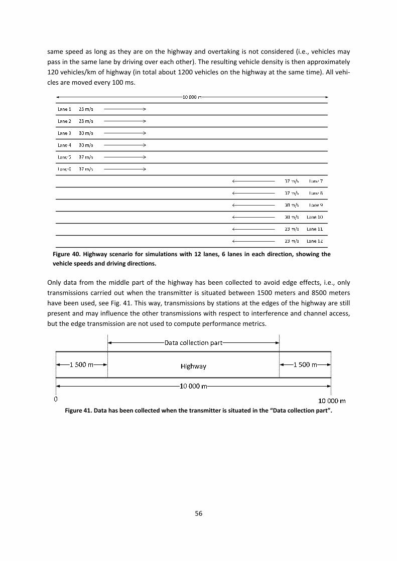
56

same speed as long as they are on the highway and overtaking is not considered (i.e., vehicles may pass in the same lane by driving over each other). The resulting vehicle density is then approximately 120 vehicles/km of highway (in total about 1200 vehicles on the highway at the same time). All vehi-cles are moved every 100 ms.

Only data from the middle part of the highway has been collected to avoid edge effects, i.e., only transmissions carried out when the transmitter is situated between 1500 meters and 8500 meters have been used, see Fig. 41. This way, transmissions by stations at the edges of the highway are still present and may influence the other transmissions with respect to interference and channel access, but the edge transmission are not used to compute performance metrics.

Figure 40. Highway scenario for simulations with 12 lanes, 6 lanes in each direction, showing the vehicle speeds and driving directions.

Figure 41. Data has been collected when the transmitter is situated in the “Data collection part”.

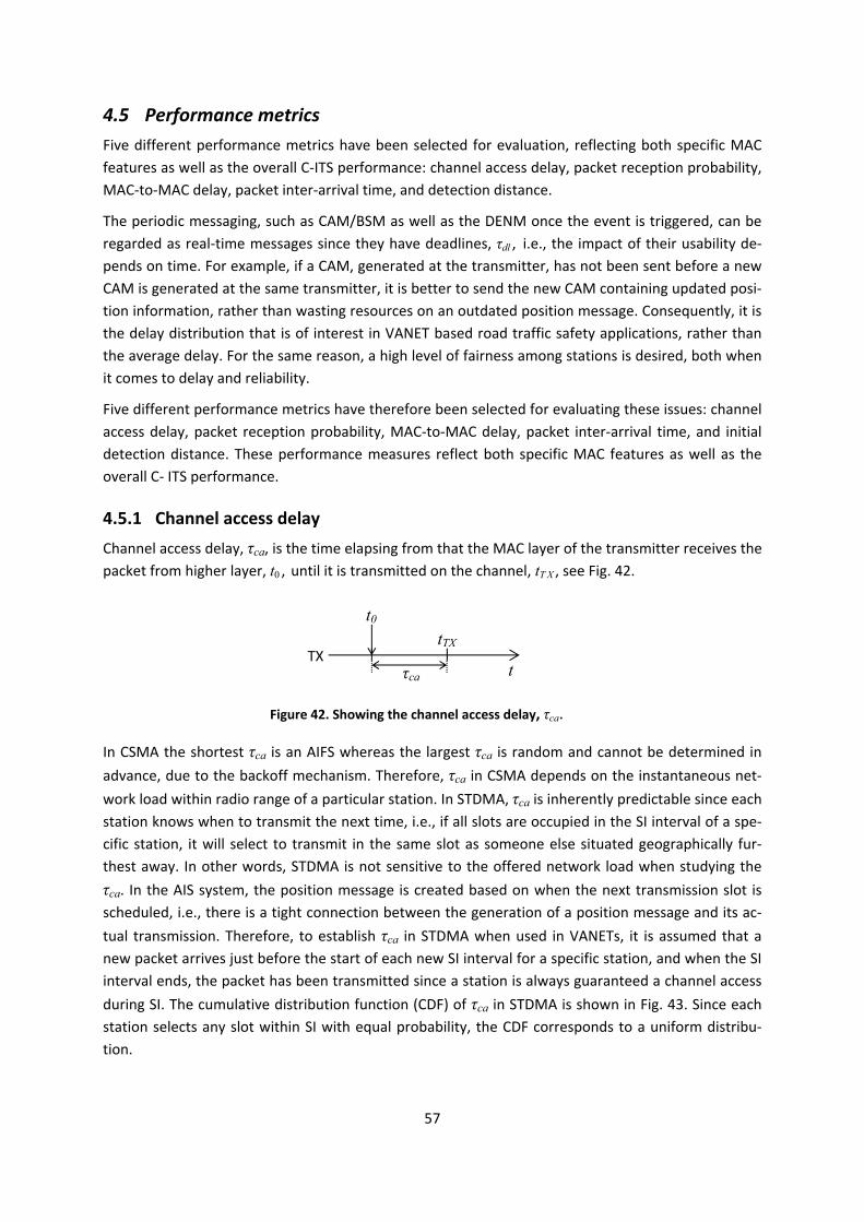
57

4.5 Performance metrics Five different performance metrics have been selected for evaluation, reflecting both specific MAC features as well as the overall C-ITS performance: channel access delay, packet reception probability, MAC-to-MAC delay, packet inter-arrival time, and detection distance.

The periodic messaging, such as CAM/BSM as well as the DENM once the event is triggered, can be regarded as real-time messages since they have deadlines, τdl , i.e., the impact of their usability de-pends on time. For example, if a CAM, generated at the transmitter, has not been sent before a new CAM is generated at the same transmitter, it is better to send the new CAM containing updated posi-tion information, rather than wasting resources on an outdated position message. Consequently, it is the delay distribution that is of interest in VANET based road traffic safety applications, rather than the average delay. For the same reason, a high level of fairness among stations is desired, both when it comes to delay and reliability.

Five different performance metrics have therefore been selected for evaluating these issues: channel access delay, packet reception probability, MAC-to-MAC delay, packet inter-arrival time, and initial detection distance. These performance measures reflect both specific MAC features as well as the overall C- ITS performance.

4.5.1 Channel access delay Channel access delay, τca, is the time elapsing from that the MAC layer of the transmitter receives the packet from higher layer, t0 , until it is transmitted on the channel, tT X , see Fig. 42.

In CSMA the shortest τca is an AIFS whereas the largest τca is random and cannot be determined in advance, due to the backoff mechanism. Therefore, τca in CSMA depends on the instantaneous net-work load within radio range of a particular station. In STDMA, τca is inherently predictable since each station knows when to transmit the next time, i.e., if all slots are occupied in the SI interval of a spe-cific station, it will select to transmit in the same slot as someone else situated geographically fur-thest away. In other words, STDMA is not sensitive to the offered network load when studying the τca. In the AIS system, the position message is created based on when the next transmission slot is scheduled, i.e., there is a tight connection between the generation of a position message and its ac-tual transmission. Therefore, to establish τca in STDMA when used in VANETs, it is assumed that a new packet arrives just before the start of each new SI interval for a specific station, and when the SI interval ends, the packet has been transmitted since a station is always guaranteed a channel access during SI. The cumulative distribution function (CDF) of τca in STDMA is shown in Fig. 43. Since each station selects any slot within SI with equal probability, the CDF corresponds to a uniform distribu-tion.

TX

t0 tTX

τca t

Figure 42. Showing the channel access delay, τca.

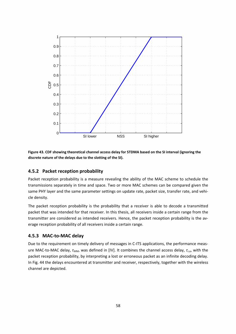
58

Figure 43. CDF showing theoretical channel access delay for STDMA based on the SI interval (ignoring the discrete nature of the delays due to the slotting of the SI).

4.5.2 Packet reception probability Packet reception probability is a measure revealing the ability of the MAC scheme to schedule the transmissions separately in time and space. Two or more MAC schemes can be compared given the same PHY layer and the same parameter settings on update rate, packet size, transfer rate, and vehi-cle density.

The packet reception probability is the probability that a receiver is able to decode a transmitted packet that was intended for that receiver. In this thesis, all receivers inside a certain range from the transmitter are considered as intended receivers. Hence, the packet reception probability is the av-erage reception probability of all receivers inside a certain range.

4.5.3 MAC-to-MAC delay Due to the requirement on timely delivery of messages in C-ITS applications, the performance meas-ure MAC-to-MAC delay, τMM, was defined in [IV]. It combines the channel access delay, τca, with the packet reception probability, by interpreting a lost or erroneous packet as an infinite decoding delay. In Fig. 44 the delays encountered at transmitter and receiver, respectively, together with the wireless channel are depicted.

SI lower NSS SI higher 0

0.1

0.2

0.3

0.4

0.5

0.6

0.7

0.8

0.9

1

CD

F

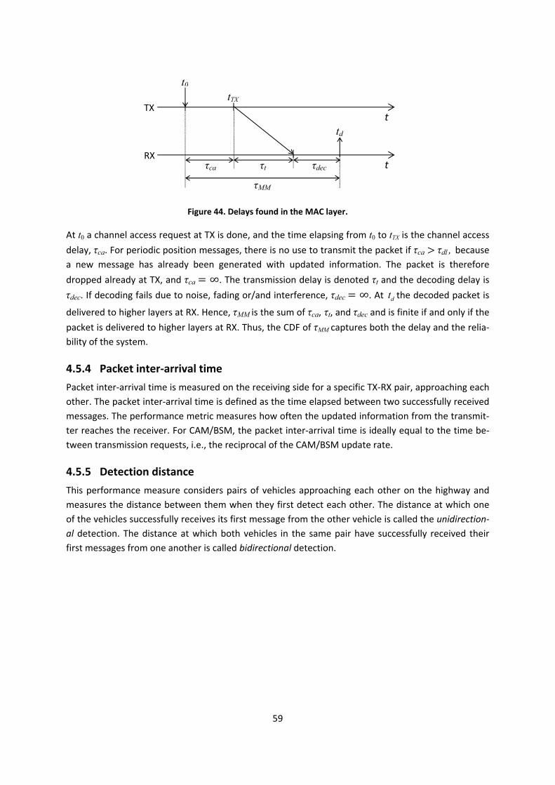
59

At t0 a channel access request at TX is done, and the time elapsing from t0 to tTX is the channel access delay, τca. For periodic position messages, there is no use to transmit the packet if τca > τdl , because a new message has already been generated with updated information. The packet is therefore dropped already at TX, and τca = ∞. The transmission delay is denoted τt and the decoding delay is τdec. If decoding fails due to noise, fading or/and interference, τdec = ∞. At dt the decoded packet is

delivered to higher layers at RX. Hence, τMM is the sum of τca, τt, and τdec and is finite if and only if the packet is delivered to higher layers at RX. Thus, the CDF of τMM captures both the delay and the relia-bility of the system.

4.5.4 Packet inter-arrival time Packet inter-arrival time is measured on the receiving side for a specific TX-RX pair, approaching each other. The packet inter-arrival time is defined as the time elapsed between two successfully received messages. The performance metric measures how often the updated information from the transmit-ter reaches the receiver. For CAM/BSM, the packet inter-arrival time is ideally equal to the time be-tween transmission requests, i.e., the reciprocal of the CAM/BSM update rate.

4.5.5 Detection distance This performance measure considers pairs of vehicles approaching each other on the highway and measures the distance between them when they first detect each other. The distance at which one of the vehicles successfully receives its first message from the other vehicle is called the unidirection-al detection. The distance at which both vehicles in the same pair have successfully received their first messages from one another is called bidirectional detection.

Figure 44. Delays found in the MAC layer.

TX

t0 tTX

τca

t

RX tτt

td

τdec

τMM

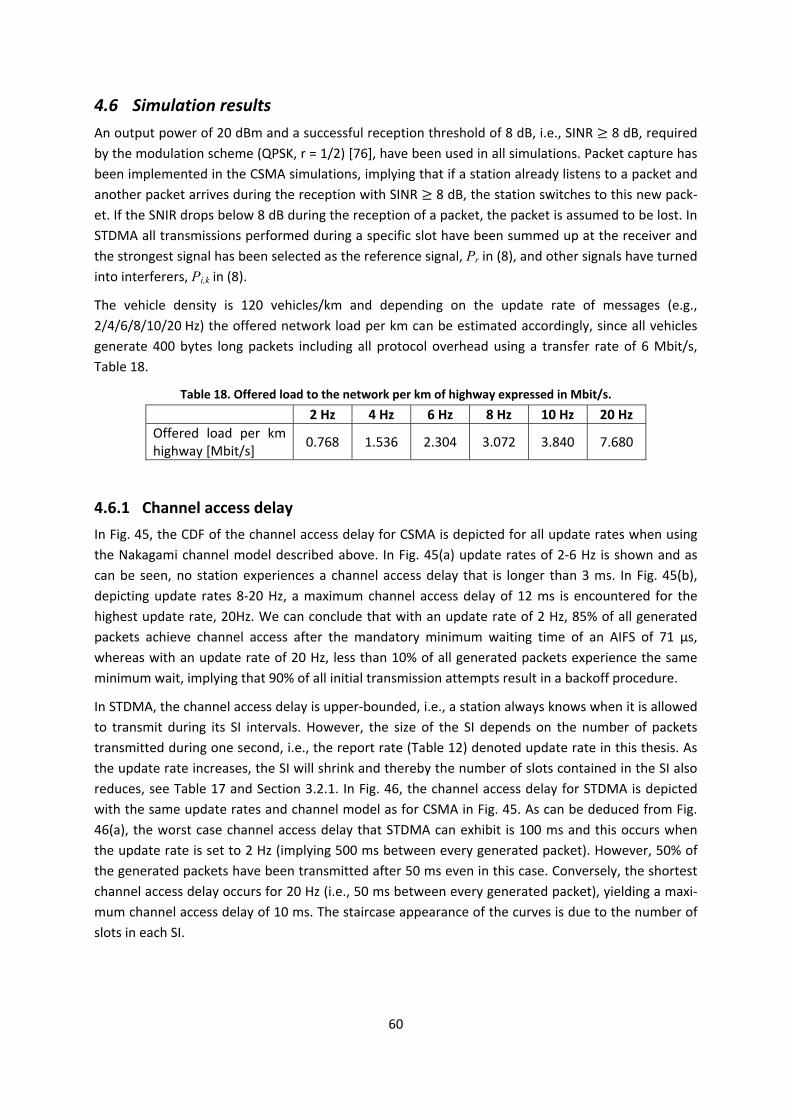
60

4.6 Simulation results An output power of 20 dBm and a successful reception threshold of 8 dB, i.e., SINR ≥ 8 dB, required by the modulation scheme (QPSK, r = 1/2) [76], have been used in all simulations. Packet capture has been implemented in the CSMA simulations, implying that if a station already listens to a packet and another packet arrives during the reception with SINR ≥ 8 dB, the station switches to this new pack-et. If the SNIR drops below 8 dB during the reception of a packet, the packet is assumed to be lost. In STDMA all transmissions performed during a specific slot have been summed up at the receiver and the strongest signal has been selected as the reference signal, Pr in (8), and other signals have turned into interferers, Pi,k in (8).

The vehicle density is 120 vehicles/km and depending on the update rate of messages (e.g., 2/4/6/8/10/20 Hz) the offered network load per km can be estimated accordingly, since all vehicles generate 400 bytes long packets including all protocol overhead using a transfer rate of 6 Mbit/s, Table 18.

Table 18. Offered load to the network per km of highway expressed in Mbit/s. 2 Hz 4 Hz 6 Hz 8 Hz 10 Hz 20 Hz

Offered load per km highway [Mbit/s] 0.768 1.536 2.304 3.072 3.840 7.680

4.6.1 Channel access delay In Fig. 45, the CDF of the channel access delay for CSMA is depicted for all update rates when using the Nakagami channel model described above. In Fig. 45(a) update rates of 2-6 Hz is shown and as can be seen, no station experiences a channel access delay that is longer than 3 ms. In Fig. 45(b), depicting update rates 8-20 Hz, a maximum channel access delay of 12 ms is encountered for the highest update rate, 20Hz. We can conclude that with an update rate of 2 Hz, 85% of all generated packets achieve channel access after the mandatory minimum waiting time of an AIFS of 71 µs, whereas with an update rate of 20 Hz, less than 10% of all generated packets experience the same minimum wait, implying that 90% of all initial transmission attempts result in a backoff procedure.

In STDMA, the channel access delay is upper-bounded, i.e., a station always knows when it is allowed to transmit during its SI intervals. However, the size of the SI depends on the number of packets transmitted during one second, i.e., the report rate (Table 12) denoted update rate in this thesis. As the update rate increases, the SI will shrink and thereby the number of slots contained in the SI also reduces, see Table 17 and Section 3.2.1. In Fig. 46, the channel access delay for STDMA is depicted with the same update rates and channel model as for CSMA in Fig. 45. As can be deduced from Fig. 46(a), the worst case channel access delay that STDMA can exhibit is 100 ms and this occurs when the update rate is set to 2 Hz (implying 500 ms between every generated packet). However, 50% of the generated packets have been transmitted after 50 ms even in this case. Conversely, the shortest channel access delay occurs for 20 Hz (i.e., 50 ms between every generated packet), yielding a maxi-mum channel access delay of 10 ms. The staircase appearance of the curves is due to the number of slots in each SI.

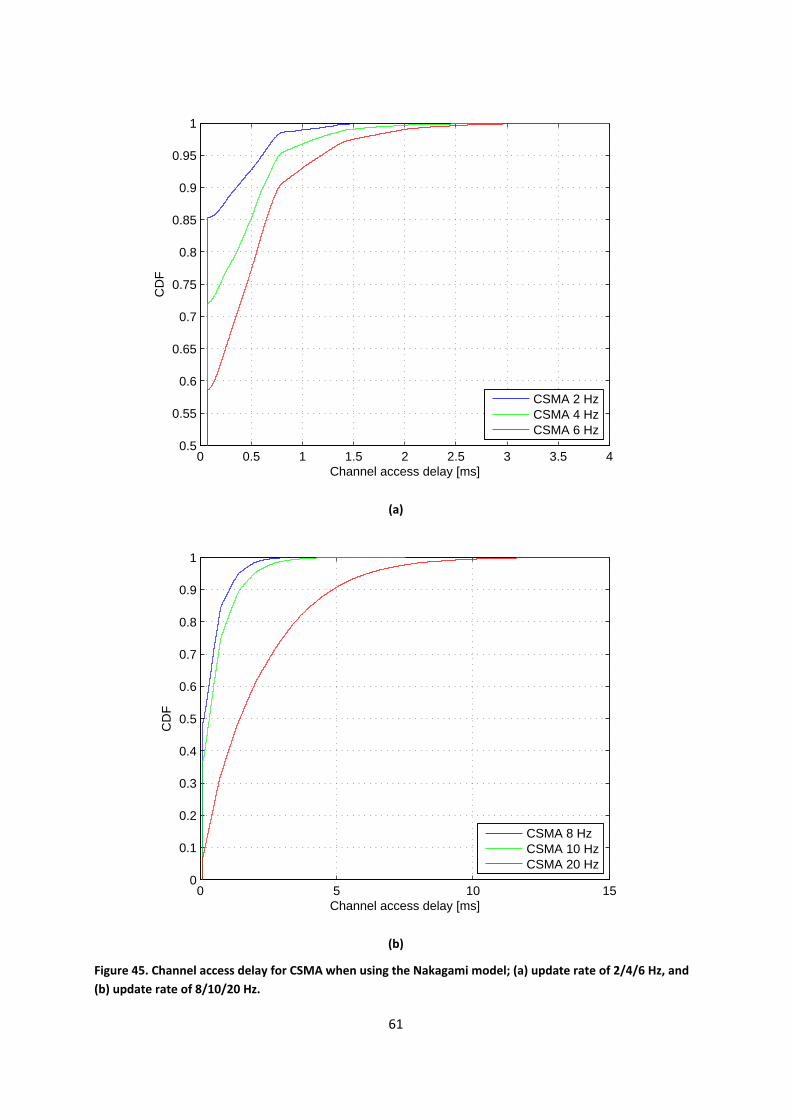
61

(a)

(b)

Figure 45. Channel access delay for CSMA when using the Nakagami model; (a) update rate of 2/4/6 Hz, and (b) update rate of 8/10/20 Hz.

0 0.5 1 1.5 2 2.5 3 3.5 40.5

0.55

0.6

0.65

0.7

0.75

0.8

0.85

0.9

0.95

1

Channel access delay [ms]

CD

F

CSMA 2 HzCSMA 4 HzCSMA 6 Hz

0 5 10 150

0.1

0.2

0.3

0.4

0.5

0.6

0.7

0.8

0.9

1

Channel access delay [ms]

CD

F

CSMA 8 HzCSMA 10 HzCSMA 20 Hz

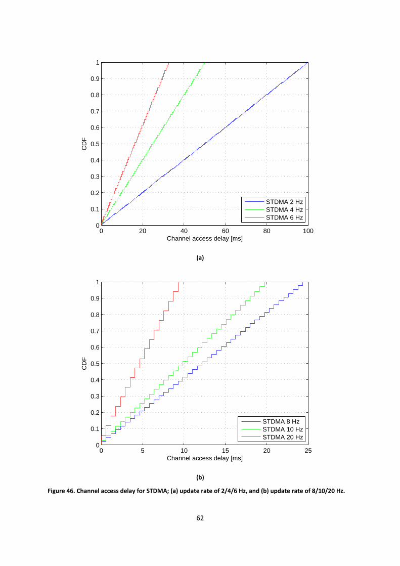
62

(a)

(b)

Figure 46. Channel access delay for STDMA; (a) update rate of 2/4/6 Hz, and (b) update rate of 8/10/20 Hz.

0 20 40 60 80 1000

0.1

0.2

0.3

0.4

0.5

0.6

0.7

0.8

0.9

1

Channel access delay [ms]

CD

F

STDMA 2 HzSTDMA 4 HzSTDMA 6 Hz

0 5 10 15 20 250

0.1

0.2

0.3

0.4

0.5

0.6

0.7

0.8

0.9

1

Channel access delay [ms]

CD

F

STDMA 8 HzSTDMA 10 HzSTDMA 20 Hz

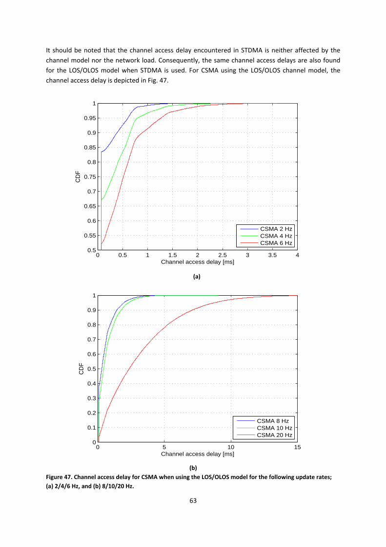
63

It should be noted that the channel access delay encountered in STDMA is neither affected by the channel model nor the network load. Consequently, the same channel access delays are also found for the LOS/OLOS model when STDMA is used. For CSMA using the LOS/OLOS channel model, the channel access delay is depicted in Fig. 47.

(a)

(b)Figure 47. Channel access delay for CSMA when using the LOS/OLOS model for the following update rates; (a) 2/4/6 Hz, and (b) 8/10/20 Hz.

0 0.5 1 1.5 2 2.5 3 3.5 40.5

0.55

0.6

0.65

0.7

0.75

0.8

0.85

0.9

0.95

1

Channel access delay [ms]

CD

F

CSMA 2 HzCSMA 4 HzCSMA 6 Hz

0 5 10 150

0.1

0.2

0.3

0.4

0.5

0.6

0.7

0.8

0.9

1

Channel access delay [ms]

CD

F

CSMA 8 HzCSMA 10 HzCSMA 20 Hz

64

In Fig. 48, the Nakagami and LOS/OLOS models are compared for CSMA. It can be concluded that the channel access delay is affected by the channel model in use and that the LOS/OLOS model implies longer channel access delays. This is due to the fact that the LOS/OLOS channel model has a success-ful packet reception range that is slightly longer than in the Nakagami case, implying that each sta-tion has slightly more stations within its radio range. These additional stations keep the channel oc-cupied more often, forcing more stations into the backoff procedure and thereby increasing the channel access delay. When evaluating the channel access delay for CSMA and STDMA it can be con-cluded that while the minimum delay is smaller for CSMA than for STDMA, the worst case delay is random for CSMA. For STDMA, the worst case channel access delay is known and independent on network load and channel type.

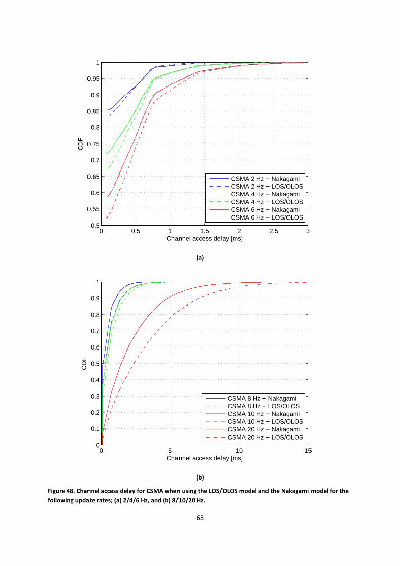
65

(a)

(b)

Figure 48. Channel access delay for CSMA when using the LOS/OLOS model and the Nakagami model for the following update rates; (a) 2/4/6 Hz, and (b) 8/10/20 Hz.

0 0.5 1 1.5 2 2.5 30.5

0.55

0.6

0.65

0.7

0.75

0.8

0.85

0.9

0.95

1

Channel access delay [ms]

CD

F

CSMA 2 Hz − NakagamiCSMA 2 Hz − LOS/OLOSCSMA 4 Hz − NakagamiCSMA 4 Hz − LOS/OLOSCSMA 6 Hz − NakagamiCSMA 6 Hz − LOS/OLOS

0 5 10 150

0.1

0.2

0.3

0.4

0.5

0.6

0.7

0.8

0.9

1

Channel access delay [ms]

CD

F

CSMA 8 Hz − NakagamiCSMA 8 Hz − LOS/OLOSCSMA 10 Hz − NakagamiCSMA 10 Hz − LOS/OLOSCSMA 20 Hz − NakagamiCSMA 20 Hz − LOS/OLOS

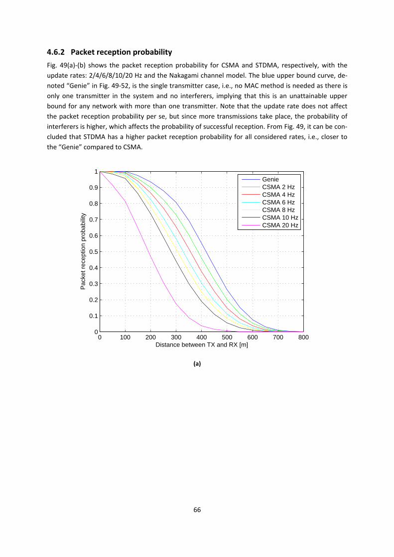
66

4.6.2 Packet reception probability Fig. 49(a)-(b) shows the packet reception probability for CSMA and STDMA, respectively, with the update rates: 2/4/6/8/10/20 Hz and the Nakagami channel model. The blue upper bound curve, de-noted “Genie” in Fig. 49-52, is the single transmitter case, i.e., no MAC method is needed as there is only one transmitter in the system and no interferers, implying that this is an unattainable upper bound for any network with more than one transmitter. Note that the update rate does not affect the packet reception probability per se, but since more transmissions take place, the probability of interferers is higher, which affects the probability of successful reception. From Fig. 49, it can be con-cluded that STDMA has a higher packet reception probability for all considered rates, i.e., closer to the “Genie” compared to CSMA.

(a)

0 100 200 300 400 500 600 700 8000

0.1

0.2

0.3

0.4

0.5

0.6

0.7

0.8

0.9

1

Distance between TX and RX [m]

Pac

ket r

ecep

tion

prob

abili

ty

GenieCSMA 2 HzCSMA 4 HzCSMA 6 HzCSMA 8 HzCSMA 10 HzCSMA 20 Hz

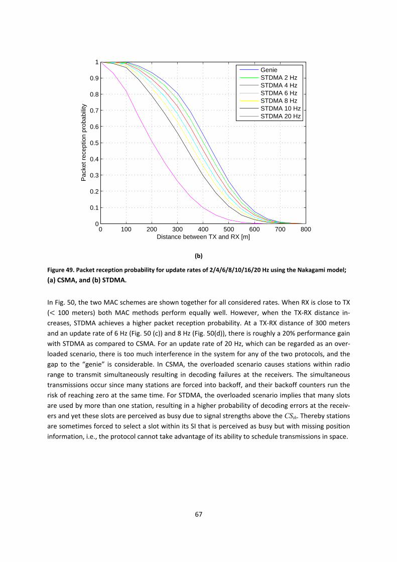
67

(b)

Figure 49. Packet reception probability for update rates of 2/4/6/8/10/16/20 Hz using the Nakagami model; (a) CSMA, and (b) STDMA.

In Fig. 50, the two MAC schemes are shown together for all considered rates. When RX is close to TX (< 100 meters) both MAC methods perform equally well. However, when the TX-RX distance in-creases, STDMA achieves a higher packet reception probability. At a TX-RX distance of 300 meters and an update rate of 6 Hz (Fig. 50 (c)) and 8 Hz (Fig. 50(d)), there is roughly a 20% performance gain with STDMA as compared to CSMA. For an update rate of 20 Hz, which can be regarded as an over-loaded scenario, there is too much interference in the system for any of the two protocols, and the gap to the “genie” is considerable. In CSMA, the overloaded scenario causes stations within radio range to transmit simultaneously resulting in decoding failures at the receivers. The simultaneous transmissions occur since many stations are forced into backoff, and their backoff counters run the risk of reaching zero at the same time. For STDMA, the overloaded scenario implies that many slots are used by more than one station, resulting in a higher probability of decoding errors at the receiv-ers and yet these slots are perceived as busy due to signal strengths above the CSth. Thereby stations are sometimes forced to select a slot within its SI that is perceived as busy but with missing position information, i.e., the protocol cannot take advantage of its ability to schedule transmissions in space.

0 100 200 300 400 500 600 700 8000

0.1

0.2

0.3

0.4

0.5

0.6

0.7

0.8

0.9

1

Distance between TX and RX [m]

Pac

ket r

ecep

tion

prob

abili

ty

GenieSTDMA 2 HzSTDMA 4 HzSTDMA 6 HzSTDMA 8 HzSTDMA 10 HzSTDMA 20 Hz

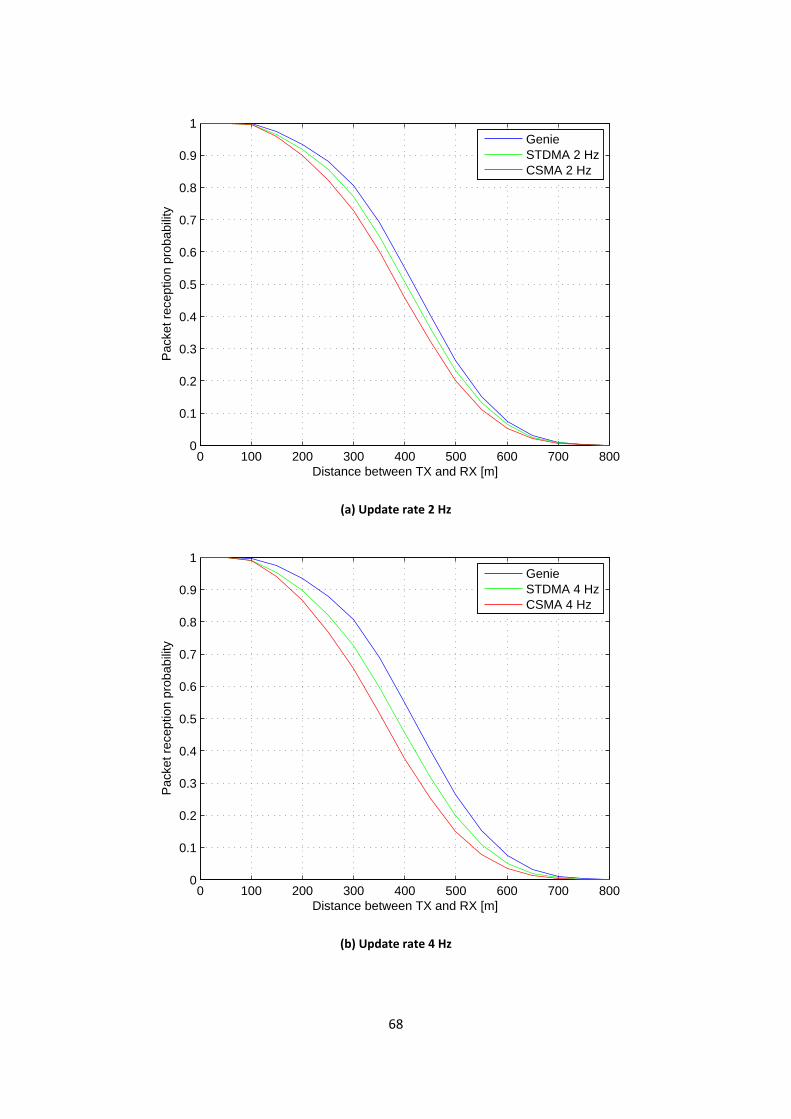
68

(a) Update rate 2 Hz

(b) Update rate 4 Hz

0 100 200 300 400 500 600 700 8000

0.1

0.2

0.3

0.4

0.5

0.6

0.7

0.8

0.9

1

Distance between TX and RX [m]

Pac

ket r

ecep

tion

prob

abili

ty

GenieSTDMA 2 HzCSMA 2 Hz

0 100 200 300 400 500 600 700 8000

0.1

0.2

0.3

0.4

0.5

0.6

0.7

0.8

0.9

1

Distance between TX and RX [m]

Pac

ket r

ecep

tion

prob

abili

ty

GenieSTDMA 4 HzCSMA 4 Hz

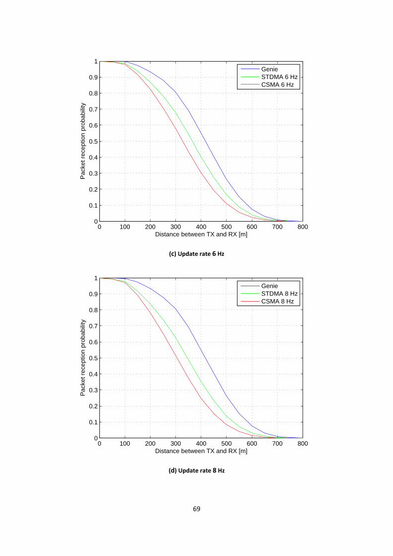
69

(c) Update rate 6 Hz

(d) Update rate 8 Hz

0 100 200 300 400 500 600 700 8000

0.1

0.2

0.3

0.4

0.5

0.6

0.7

0.8

0.9

1

Distance between TX and RX [m]

Pac

ket r

ecep

tion

prob

abili

ty

GenieSTDMA 6 HzCSMA 6 Hz

0 100 200 300 400 500 600 700 8000

0.1

0.2

0.3

0.4

0.5

0.6

0.7

0.8

0.9

1

Distance between TX and RX [m]

Pac

ket r

ecep

tion

prob

abili

ty

GenieSTDMA 8 HzCSMA 8 Hz

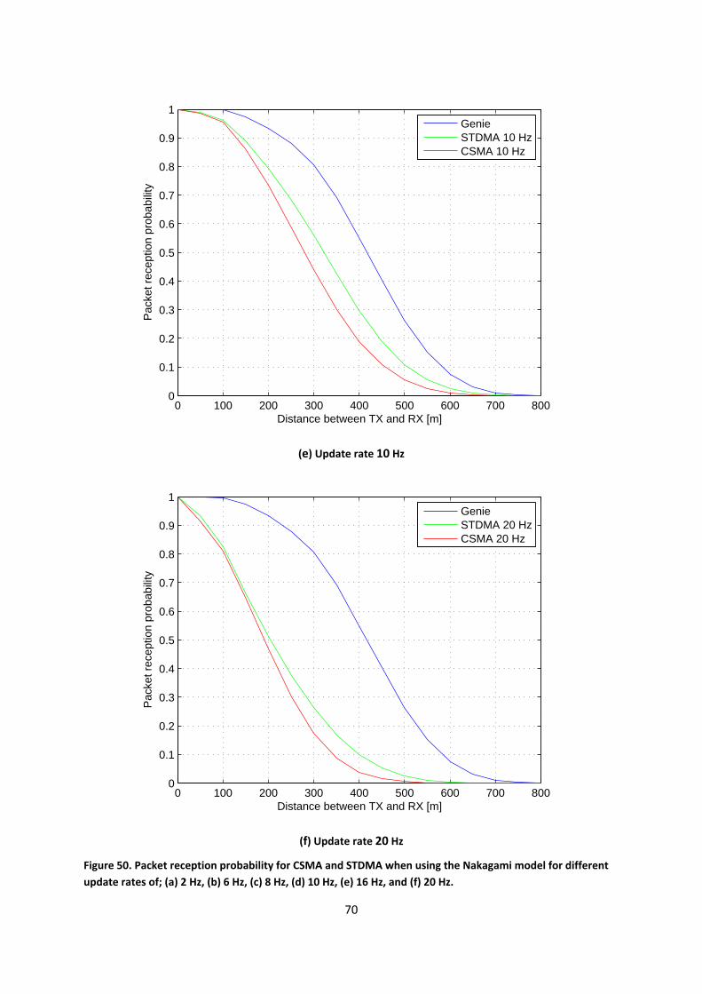
70

(e) Update rate 10 Hz

(f) Update rate 20 Hz

Figure 50. Packet reception probability for CSMA and STDMA when using the Nakagami model for different update rates of; (a) 2 Hz, (b) 6 Hz, (c) 8 Hz, (d) 10 Hz, (e) 16 Hz, and (f) 20 Hz.

0 100 200 300 400 500 600 700 8000

0.1

0.2

0.3

0.4

0.5

0.6

0.7

0.8

0.9

1

Distance between TX and RX [m]

Pac

ket r

ecep

tion

prob

abili

ty

GenieSTDMA 10 HzCSMA 10 Hz

0 100 200 300 400 500 600 700 8000

0.1

0.2

0.3

0.4

0.5

0.6

0.7

0.8

0.9

1

Distance between TX and RX [m]

Pac

ket r

ecep

tion

prob

abili

ty

GenieSTDMA 20 HzCSMA 20 Hz

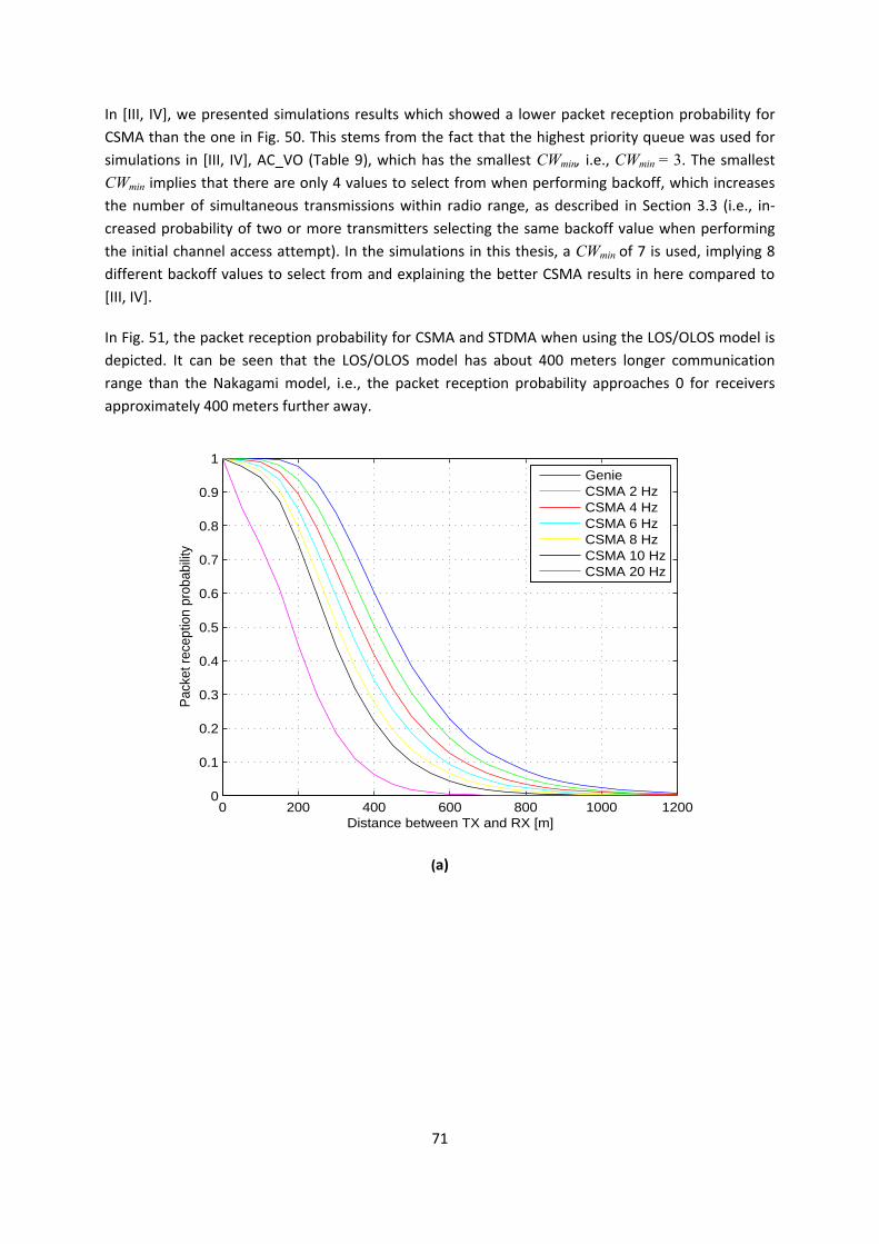
71

In [III, IV], we presented simulations results which showed a lower packet reception probability for CSMA than the one in Fig. 50. This stems from the fact that the highest priority queue was used for simulations in [III, IV], AC_VO (Table 9), which has the smallest CWmin, i.e., CWmin = 3. The smallest CWmin implies that there are only 4 values to select from when performing backoff, which increases the number of simultaneous transmissions within radio range, as described in Section 3.3 (i.e., in-creased probability of two or more transmitters selecting the same backoff value when performing the initial channel access attempt). In the simulations in this thesis, a CWmin of 7 is used, implying 8 different backoff values to select from and explaining the better CSMA results in here compared to [III, IV].

In Fig. 51, the packet reception probability for CSMA and STDMA when using the LOS/OLOS model is depicted. It can be seen that the LOS/OLOS model has about 400 meters longer communication range than the Nakagami model, i.e., the packet reception probability approaches 0 for receivers approximately 400 meters further away.

(a)

0 200 400 600 800 1000 12000

0.1

0.2

0.3

0.4

0.5

0.6

0.7

0.8

0.9

1

Distance between TX and RX [m]

Pac

ket r

ecep

tion

prob

abili

ty

GenieCSMA 2 HzCSMA 4 HzCSMA 6 HzCSMA 8 HzCSMA 10 HzCSMA 20 Hz

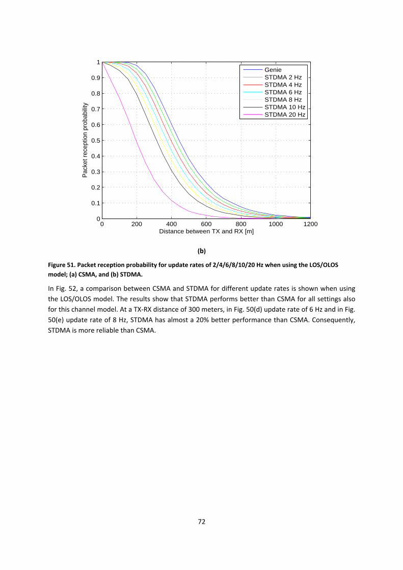
72

(b)

Figure 51. Packet reception probability for update rates of 2/4/6/8/10/20 Hz when using the LOS/OLOS model; (a) CSMA, and (b) STDMA.

In Fig. 52, a comparison between CSMA and STDMA for different update rates is shown when using the LOS/OLOS model. The results show that STDMA performs better than CSMA for all settings also for this channel model. At a TX-RX distance of 300 meters, in Fig. 50(d) update rate of 6 Hz and in Fig. 50(e) update rate of 8 Hz, STDMA has almost a 20% better performance than CSMA. Consequently, STDMA is more reliable than CSMA.

0 200 400 600 800 1000 12000

0.1

0.2

0.3

0.4

0.5

0.6

0.7

0.8

0.9

1

Distance between TX and RX [m]

Pac

ket r

ecep

tion

prob

abili

ty

GenieSTDMA 2 HzSTDMA 4 HzSTDMA 6 HzSTDMA 8 HzSTDMA 10 HzSTDMA 20 Hz

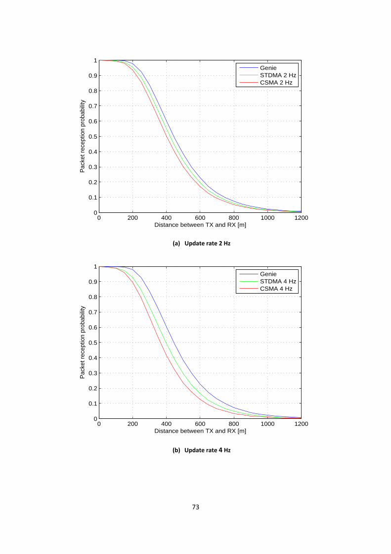
73

(a) Update rate 2 Hz

(b) Update rate 4 Hz

0 200 400 600 800 1000 12000

0.1

0.2

0.3

0.4

0.5

0.6

0.7

0.8

0.9

1

Distance between TX and RX [m]

Pac

ket r

ecep

tion

prob

abili

ty

GenieSTDMA 2 HzCSMA 2 Hz

0 200 400 600 800 1000 12000

0.1

0.2

0.3

0.4

0.5

0.6

0.7

0.8

0.9

1

Distance between TX and RX [m]

Pac

ket r

ecep

tion

prob

abili

ty

GenieSTDMA 4 HzCSMA 4 Hz

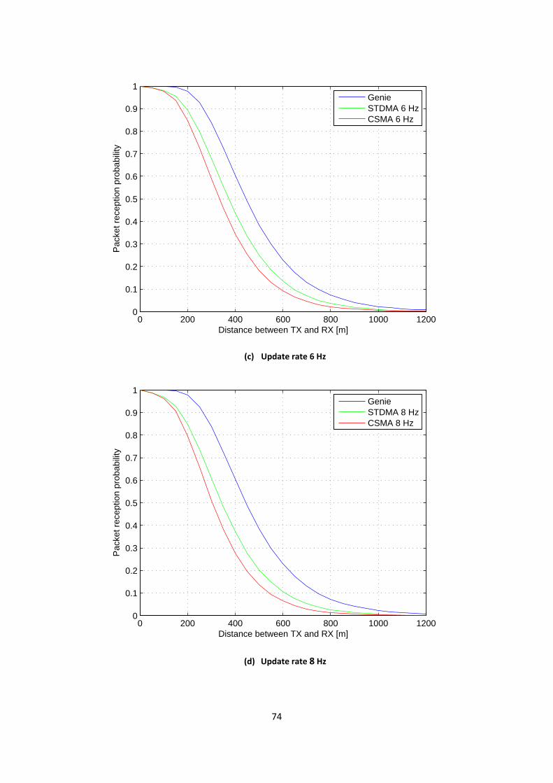
74

(c) Update rate 6 Hz

(d) Update rate 8 Hz

0 200 400 600 800 1000 12000

0.1

0.2

0.3

0.4

0.5

0.6

0.7

0.8

0.9

1

Distance between TX and RX [m]

Pac

ket r

ecep

tion

prob

abili

ty

GenieSTDMA 6 HzCSMA 6 Hz

0 200 400 600 800 1000 12000

0.1

0.2

0.3

0.4

0.5

0.6

0.7

0.8

0.9

1

Distance between TX and RX [m]

Pac

ket r

ecep

tion

prob

abili

ty

GenieSTDMA 8 HzCSMA 8 Hz

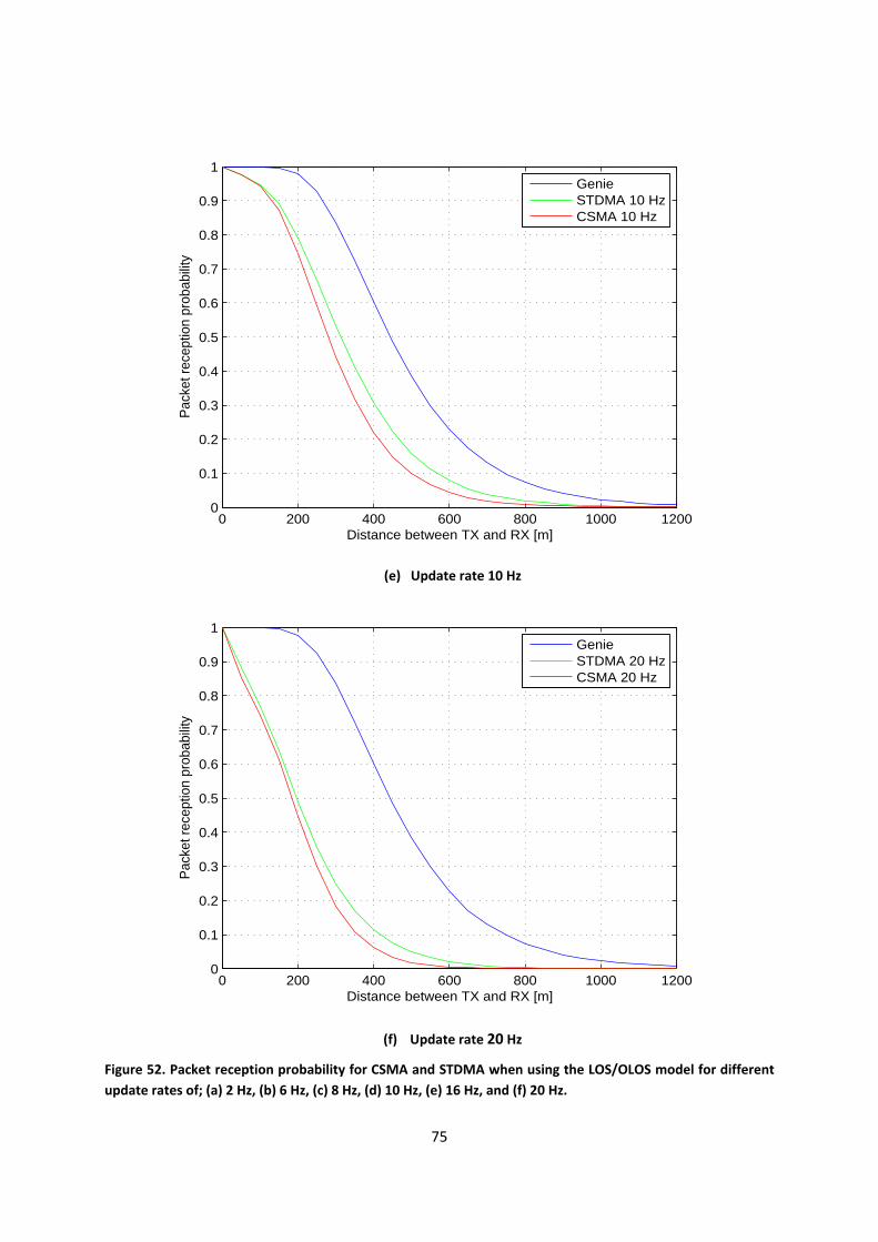
75

(e) Update rate 10 Hz

(f) Update rate 20 Hz

Figure 52. Packet reception probability for CSMA and STDMA when using the LOS/OLOS model for different update rates of; (a) 2 Hz, (b) 6 Hz, (c) 8 Hz, (d) 10 Hz, (e) 16 Hz, and (f) 20 Hz.

0 200 400 600 800 1000 12000

0.1

0.2

0.3

0.4

0.5

0.6

0.7

0.8

0.9

1

Distance between TX and RX [m]

Pac

ket r

ecep

tion

prob

abili

ty

GenieSTDMA 10 HzCSMA 10 Hz

0 200 400 600 800 1000 12000

0.1

0.2

0.3

0.4

0.5

0.6

0.7

0.8

0.9

1

Distance between TX and RX [m]

Pac

ket r

ecep

tion

prob

abili

ty

GenieSTDMA 20 HzCSMA 20 Hz

76

4.6.3 MAC-to-MAC delay MAC-to-MAC delay combines packet reception probability and channel access delay into one per-formance measure. The CDF for the MAC-to-MAC delay when using the Nakagami model for the up-date rates 2/4/6/8/10/20 Hz, is depicted in Fig. 53. Since the MAC-to-MAC delay is a function of the update rate, the range of the abscissa is selected based on the specific update rate in use, i.e., the time between two packet generations (e.g., 1/(2 Hz) = 0.5 s). According to the definitions in Section 4.5.3, we use the convention that packet drops of any kind cause the MAC-to-MAC delay to be infi-nite. Packet drops can occur at the transmitter (for CSMA when channel access is not granted until the packet has expired) or at the receiver (for both CSMA and STDMA when decoding fails). However, in Fig. 53, no packets have been dropped at the transmitting side. Therefore, the MAC-to-MAC delay is only infinite as a result of decoding failures. Every curve in the figure represents all cases when the distance between transmitter and receiver is within a certain range, i.e., “STDMA 100-200 m” implies all receivers that are between 100-200 meters away from a transmitter.

The channel access delay for CSMA increases with increased update rate, quite in contrast to STDMA, where it instead decreases. In Fig. 53(f), showing the highest update rate, the MAC-to-MAC delay reaches its maximum value after approximately the same time for both protocols for a TX-RX separa-tion of 0-100 meters. The largest difference in performance between the MAC protocols is found in Figure 53(d) for an update rate of 8 Hz, where CSMA shows a lower MAC-to-MAC delay for the suc-cessfully delivered packets, but where STDMA manages to deliver more packets to higher layers im-plying that the CDF converges to a higher value. This illustrates the basic trade-off between delay and reliability. STDMA offers better reliability than CSMA at the expense of a longer MAC-to-MAC delay. For the shortest TX-RX separation the MAC protocols perform equally well, which is consistent with the finding for the packet reception probability curves shown in Section 4.6.2.

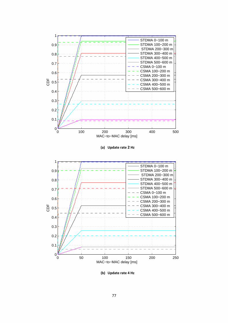
77

(a) Update rate 2 Hz

(b) Update rate 4 Hz

0 100 200 300 400 5000

0.1

0.2

0.3

0.4

0.5

0.6

0.7

0.8

0.9

1

MAC−to−MAC delay [ms]

CD

F

STDMA 0−100 mSTDMA 100−200 m STDMA 200−300 mSTDMA 300−400 mSTDMA 400−500 mSTDMA 500−600 mCSMA 0−100 mCSMA 100−200 mCSMA 200−300 mCSMA 300−400 mCSMA 400−500 mCSMA 500−600 m

0 50 100 150 200 2500

0.1

0.2

0.3

0.4

0.5

0.6

0.7

0.8

0.9

1

MAC−to−MAC delay [ms]

CD

F

STDMA 0−100 mSTDMA 100−200 m STDMA 200−300 mSTDMA 300−400 mSTDMA 400−500 mSTDMA 500−600 mCSMA 0−100 mCSMA 100−200 mCSMA 200−300 mCSMA 300−400 mCSMA 400−500 mCSMA 500−600 m

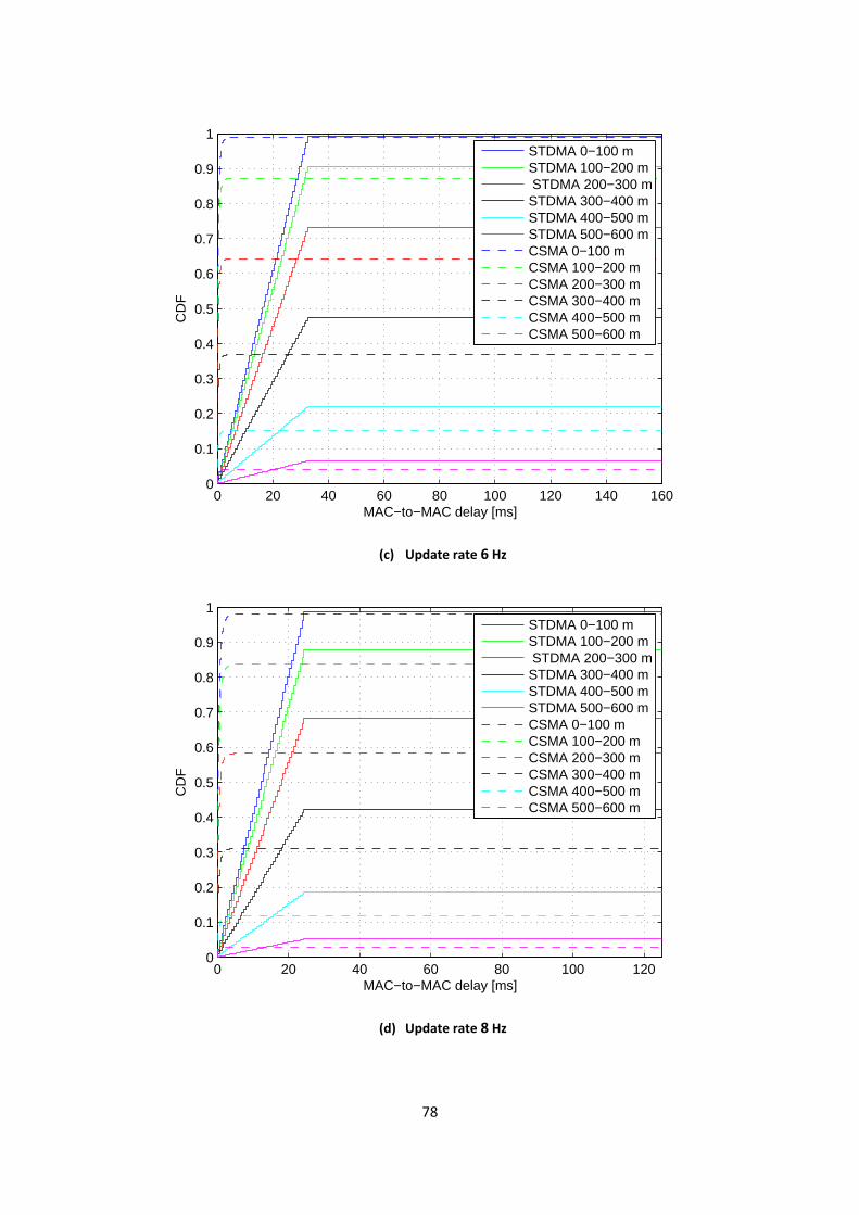
78

(c) Update rate 6 Hz

(d) Update rate 8 Hz

0 20 40 60 80 100 120 140 1600

0.1

0.2

0.3

0.4

0.5

0.6

0.7

0.8

0.9

1

MAC−to−MAC delay [ms]

CD

F

STDMA 0−100 mSTDMA 100−200 m STDMA 200−300 mSTDMA 300−400 mSTDMA 400−500 mSTDMA 500−600 mCSMA 0−100 mCSMA 100−200 mCSMA 200−300 mCSMA 300−400 mCSMA 400−500 mCSMA 500−600 m

0 20 40 60 80 100 1200

0.1

0.2

0.3

0.4

0.5

0.6

0.7

0.8

0.9

1

MAC−to−MAC delay [ms]

CD

F

STDMA 0−100 mSTDMA 100−200 m STDMA 200−300 mSTDMA 300−400 mSTDMA 400−500 mSTDMA 500−600 mCSMA 0−100 mCSMA 100−200 mCSMA 200−300 mCSMA 300−400 mCSMA 400−500 mCSMA 500−600 m

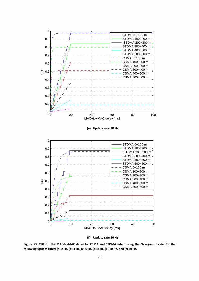
79

(e) Update rate 10 Hz

(f) Update rate 20 Hz

Figure 53. CDF for the MAC-to-MAC delay for CSMA and STDMA when using the Nakagami model for the following update rates: (a) 2 Hz, (b) 4 Hz, (c) 6 Hz, (d) 8 Hz, (e) 10 Hz, and (f) 20 Hz.

0 20 40 60 80 1000

0.1

0.2

0.3

0.4

0.5

0.6

0.7

0.8

0.9

1

MAC−to−MAC delay [ms]

CD

F

STDMA 0−100 mSTDMA 100−200 m STDMA 200−300 mSTDMA 300−400 mSTDMA 400−500 mSTDMA 500−600 mCSMA 0−100 mCSMA 100−200 mCSMA 200−300 mCSMA 300−400 mCSMA 400−500 mCSMA 500−600 m

0 10 20 30 40 500

0.1

0.2

0.3

0.4

0.5

0.6

0.7

0.8

0.9

1

MAC−to−MAC delay [ms]

CD

F

STDMA 0−100 mSTDMA 100−200 m STDMA 200−300 mSTDMA 300−400 mSTDMA 400−500 mSTDMA 500−600 mCSMA 0−100 mCSMA 100−200 mCSMA 200−300 mCSMA 300−400 mCSMA 400−500 mCSMA 500−600 m

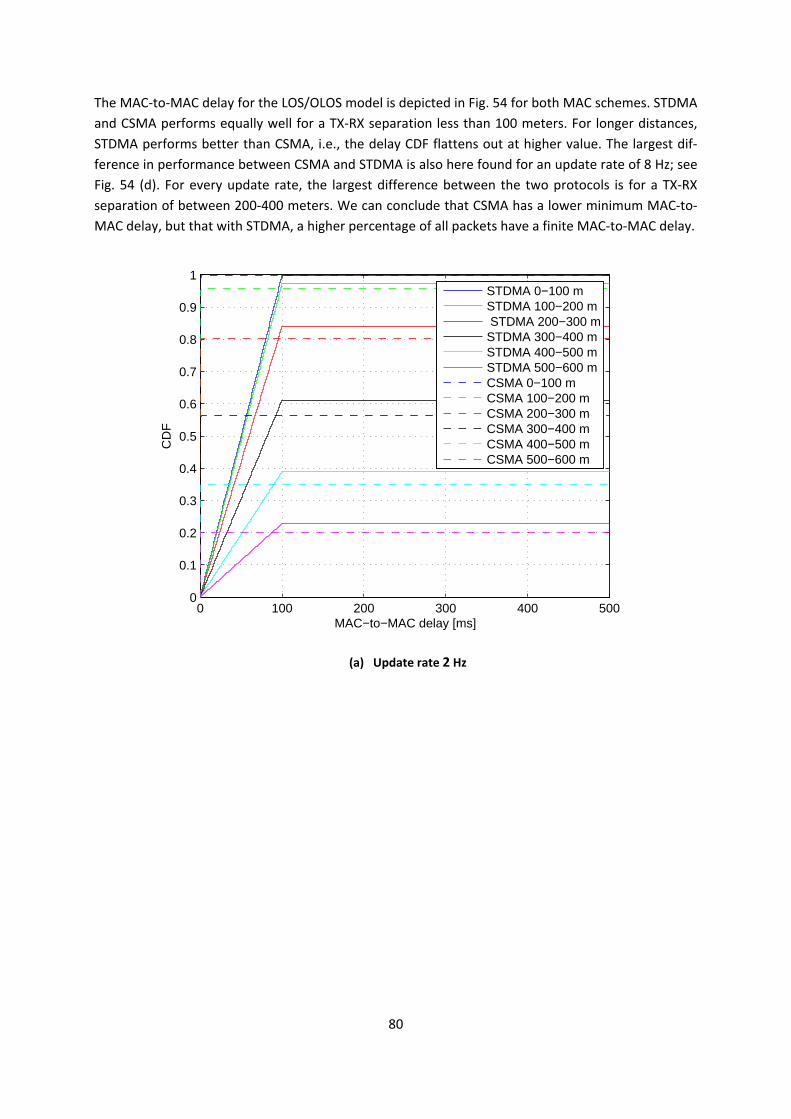
80

The MAC-to-MAC delay for the LOS/OLOS model is depicted in Fig. 54 for both MAC schemes. STDMA and CSMA performs equally well for a TX-RX separation less than 100 meters. For longer distances, STDMA performs better than CSMA, i.e., the delay CDF flattens out at higher value. The largest dif-ference in performance between CSMA and STDMA is also here found for an update rate of 8 Hz; see Fig. 54 (d). For every update rate, the largest difference between the two protocols is for a TX-RX separation of between 200-400 meters. We can conclude that CSMA has a lower minimum MAC-to-MAC delay, but that with STDMA, a higher percentage of all packets have a finite MAC-to-MAC delay.

(a) Update rate 2 Hz

0 100 200 300 400 5000

0.1

0.2

0.3

0.4

0.5

0.6

0.7

0.8

0.9

1

MAC−to−MAC delay [ms]

CD

F

STDMA 0−100 mSTDMA 100−200 m STDMA 200−300 mSTDMA 300−400 mSTDMA 400−500 mSTDMA 500−600 mCSMA 0−100 mCSMA 100−200 mCSMA 200−300 mCSMA 300−400 mCSMA 400−500 mCSMA 500−600 m

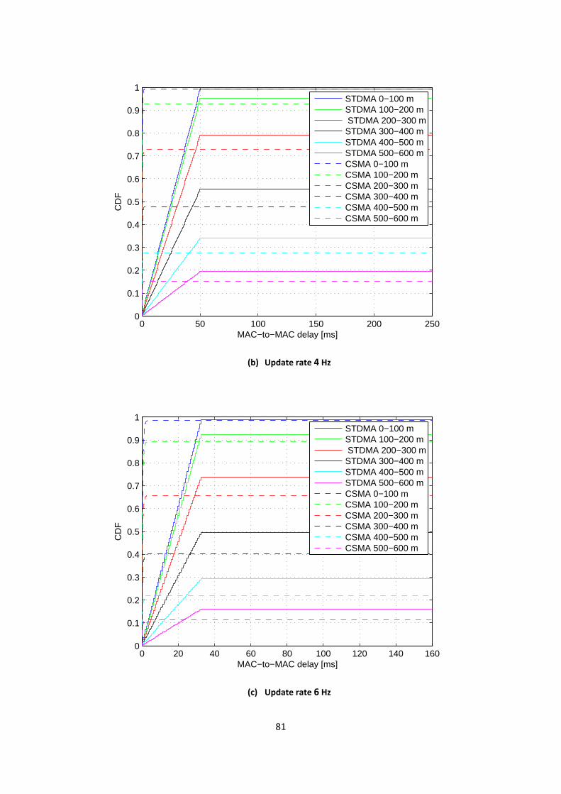
81

(b) Update rate 4 Hz

(c) Update rate 6 Hz

0 50 100 150 200 2500

0.1

0.2

0.3

0.4

0.5

0.6

0.7

0.8

0.9

1

MAC−to−MAC delay [ms]

CD

F

STDMA 0−100 mSTDMA 100−200 m STDMA 200−300 mSTDMA 300−400 mSTDMA 400−500 mSTDMA 500−600 mCSMA 0−100 mCSMA 100−200 mCSMA 200−300 mCSMA 300−400 mCSMA 400−500 mCSMA 500−600 m

0 20 40 60 80 100 120 140 1600

0.1

0.2

0.3

0.4

0.5

0.6

0.7

0.8

0.9

1

MAC−to−MAC delay [ms]

CD

F

STDMA 0−100 mSTDMA 100−200 m STDMA 200−300 mSTDMA 300−400 mSTDMA 400−500 mSTDMA 500−600 mCSMA 0−100 mCSMA 100−200 mCSMA 200−300 mCSMA 300−400 mCSMA 400−500 mCSMA 500−600 m

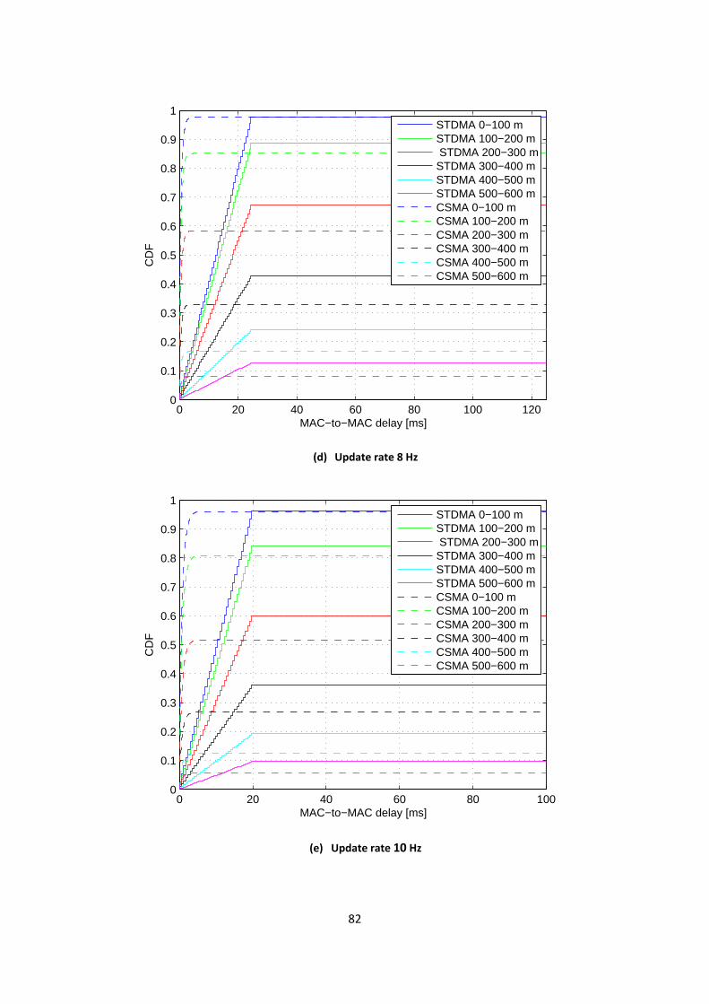
82

(d) Update rate 8 Hz

(e) Update rate 10 Hz

0 20 40 60 80 100 1200

0.1

0.2

0.3

0.4

0.5

0.6

0.7

0.8

0.9

1

MAC−to−MAC delay [ms]

CD

F

STDMA 0−100 mSTDMA 100−200 m STDMA 200−300 mSTDMA 300−400 mSTDMA 400−500 mSTDMA 500−600 mCSMA 0−100 mCSMA 100−200 mCSMA 200−300 mCSMA 300−400 mCSMA 400−500 mCSMA 500−600 m

0 20 40 60 80 1000

0.1

0.2

0.3

0.4

0.5

0.6

0.7

0.8

0.9

1

MAC−to−MAC delay [ms]

CD

F

STDMA 0−100 mSTDMA 100−200 m STDMA 200−300 mSTDMA 300−400 mSTDMA 400−500 mSTDMA 500−600 mCSMA 0−100 mCSMA 100−200 mCSMA 200−300 mCSMA 300−400 mCSMA 400−500 mCSMA 500−600 m

83

(f) Update rate 20 Hz

Figure 54. CDF for the MAC-to-MAC delay for CSMA and STDMA when using the LOS/OLOS model for the following update rates: (a) 2 Hz, (b) 4 Hz, (c) 6 Hz, (d) 8 Hz, (e) 10 Hz, and (f) 20 Hz.

0 10 20 30 40 500

0.1

0.2

0.3

0.4

0.5

0.6

0.7

0.8

0.9

1

MAC−to−MAC delay [ms]

CD

F

STDMA 0−100 mSTDMA 100−200 m STDMA 200−300 mSTDMA 300−400 mSTDMA 400−500 mSTDMA 500−600 mCSMA 0−100 mCSMA 100−200 mCSMA 200−300 mCSMA 300−400 mCSMA 400−500 mCSMA 500−600 m

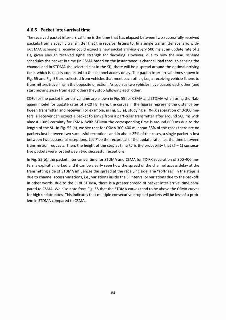
84

4.6.5 Packet inter-arrival time The received packet inter-arrival time is the time that has elapsed between two successfully received packets from a specific transmitter that the receiver listens to. In a single transmitter scenario with-out MAC scheme, a receiver could expect a new packet arriving every 500 ms at an update rate of 2 Hz, given enough received signal strength for decoding. However, due to how the MAC scheme schedules the packet in time (in CSMA based on the instantaneous channel load through sensing the channel and in STDMA the selected slot in the SI); there will be a spread around the optimal arriving time, which is closely connected to the channel access delay. The packet inter-arrival times shown in Fig. 55 and Fig. 56 are collected from vehicles that meet each other, i.e., a receiving vehicle listens to transmitters travelling in the opposite direction. As soon as two vehicles have passed each other (and start moving away from each other) they stop following each other.

CDFs for the packet inter-arrival time are shown in Fig. 55 for CSMA and STDMA when using the Nak-agami model for update rates of 2-20 Hz. Here, the curves in the figures represent the distance be-tween transmitter and receiver. For example, in Fig. 55(a), studying a TX-RX separation of 0-100 me-ters, a receiver can expect a packet to arrive from a particular transmitter after around 500 ms with almost 100% certainty for CSMA. With STDMA the corresponding time is around 600 ms due to the length of the SI. In Fig. 55 (a), we see that for CSMA 300-400 m, about 55% of the cases there are no packets lost between two successful receptions and in about 25% of the cases, a single packet is lost between two successful receptions. Let T be the reciprocal of the update rate, i.e., the time between transmission requests. Then, the height of the step at time kT is the probability that (k – 1) consecu-tive packets were lost between two successful receptions.

In Fig. 55(b), the packet inter-arrival time for STDMA and CSMA for TX-RX separation of 300-400 me-ters is explicitly marked and it can be clearly seen how the spread of the channel access delay at the transmitting side of STDMA influences the spread at the receiving side. The “softness” in the steps is due to channel access variations, i.e., variations inside the SI interval or variations due to the backoff. In other words, due to the SI of STDMA, there is a greater spread of packet inter-arrival time com-pared to CSMA. We also note from Fig. 55 that the STDMA curves tend to be above the CSMA curves for high update rates. This indicates that multiple consecutive dropped packets will be less of a prob-lem in STDMA compared to CSMA.

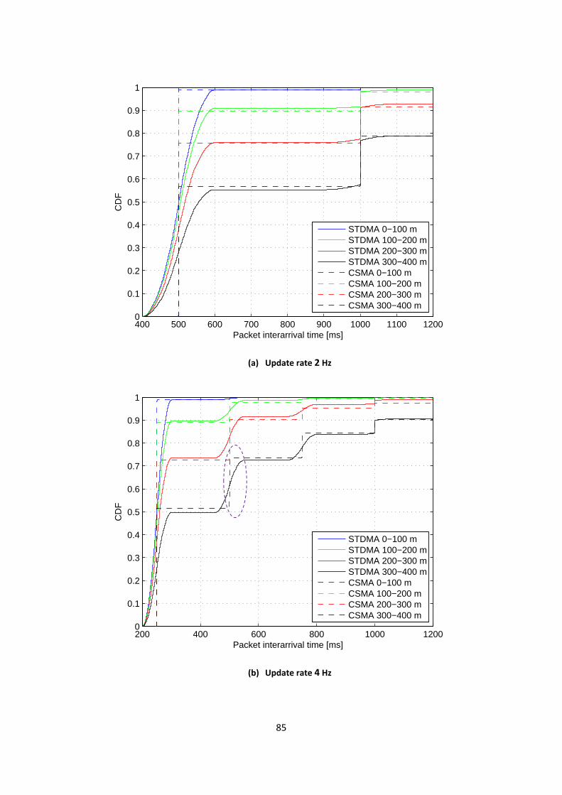
85

(a) Update rate 2 Hz

(b) Update rate 4 Hz

400 500 600 700 800 900 1000 1100 12000

0.1

0.2

0.3

0.4

0.5

0.6

0.7

0.8

0.9

1

Packet interarrival time [ms]

CD

F

STDMA 0−100 mSTDMA 100−200 mSTDMA 200−300 mSTDMA 300−400 mCSMA 0−100 mCSMA 100−200 mCSMA 200−300 mCSMA 300−400 m

200 400 600 800 1000 12000

0.1

0.2

0.3

0.4

0.5

0.6

0.7

0.8

0.9

1

Packet interarrival time [ms]

CD

F

STDMA 0−100 mSTDMA 100−200 mSTDMA 200−300 mSTDMA 300−400 mCSMA 0−100 mCSMA 100−200 mCSMA 200−300 mCSMA 300−400 m

86

(c) Update rate 6 Hz

(d) Update rate 8 Hz

200 400 600 800 1000 12000

0.1

0.2

0.3

0.4

0.5

0.6

0.7

0.8

0.9

1

Packet interarrival time [ms]

CD

F

STDMA 0−100 mSTDMA 100−200 mSTDMA 200−300 mSTDMA 300−400 mCSMA 0−100 mCSMA 100−200 mCSMA 200−300 mCSMA 300−400 m

200 400 600 800 1000 12000

0.1

0.2

0.3

0.4

0.5

0.6

0.7

0.8

0.9

1

Packet interarrival time [ms]

CD

F

STDMA 0−100 mSTDMA 100−200 mSTDMA 200−300 mSTDMA 300−400 mCSMA 0−100 mCSMA 100−200 mCSMA 200−300 mCSMA 300−400 m

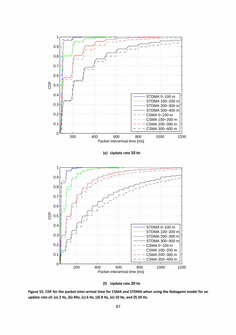
87

(e) Update rate 10 Hz

(f) Update rate 20 Hz

Figure 55. CDF for the packet inter-arrival time for CSMA and STDMA when using the Nakagami model for an update rate of; (a) 2 Hz, (b) 4Hz, (c) 6 Hz, (d) 8 Hz, (e) 10 Hz, and (f) 20 Hz.

200 400 600 800 1000 12000

0.1

0.2

0.3

0.4

0.5

0.6

0.7

0.8

0.9

1

Packet interarrival time [ms]

CD

F

STDMA 0−100 mSTDMA 100−200 mSTDMA 200−300 mSTDMA 300−400 mCSMA 0−100 mCSMA 100−200 mCSMA 200−300 mCSMA 300−400 m

200 400 600 800 1000 12000

0.1

0.2

0.3

0.4

0.5

0.6

0.7

0.8

0.9

1

Packet interarrival time [ms]

CD

F

STDMA 0−100 mSTDMA 100−200 mSTDMA 200−300 mSTDMA 300−400 mCSMA 0−100 mCSMA 100−200 mCSMA 200−300 mCSMA 300−400 m

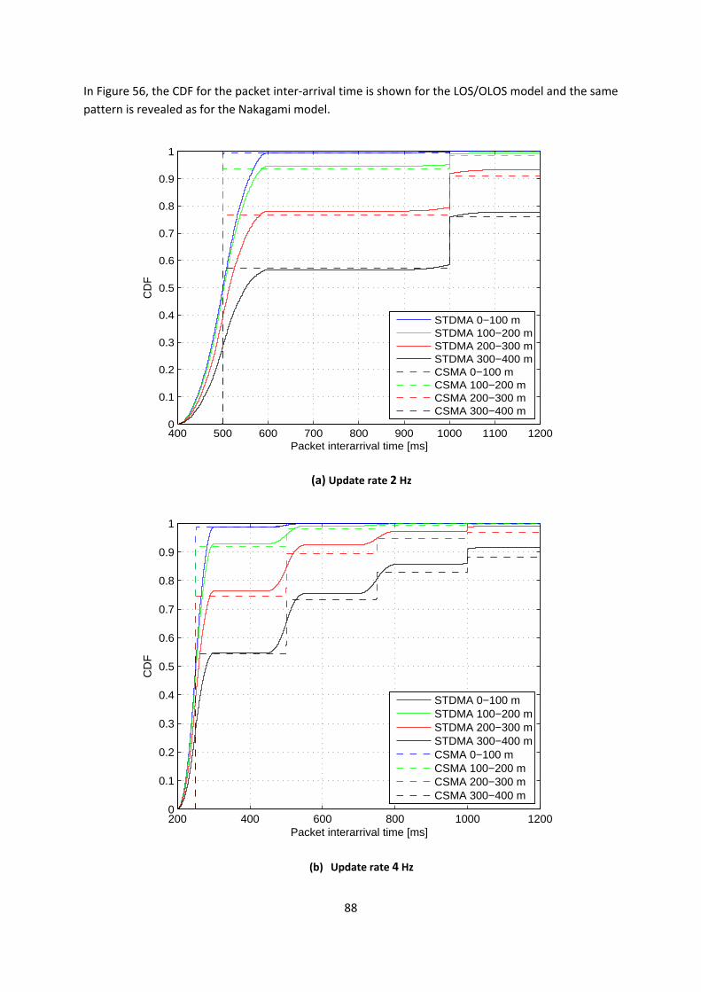
88

In Figure 56, the CDF for the packet inter-arrival time is shown for the LOS/OLOS model and the same pattern is revealed as for the Nakagami model.

(a) Update rate 2 Hz

(b) Update rate 4 Hz

400 500 600 700 800 900 1000 1100 12000

0.1

0.2

0.3

0.4

0.5

0.6

0.7

0.8

0.9

1

Packet interarrival time [ms]

CD

F

STDMA 0−100 mSTDMA 100−200 mSTDMA 200−300 mSTDMA 300−400 mCSMA 0−100 mCSMA 100−200 mCSMA 200−300 mCSMA 300−400 m

200 400 600 800 1000 12000

0.1

0.2

0.3

0.4

0.5

0.6

0.7

0.8

0.9

1

Packet interarrival time [ms]

CD

F

STDMA 0−100 mSTDMA 100−200 mSTDMA 200−300 mSTDMA 300−400 mCSMA 0−100 mCSMA 100−200 mCSMA 200−300 mCSMA 300−400 m

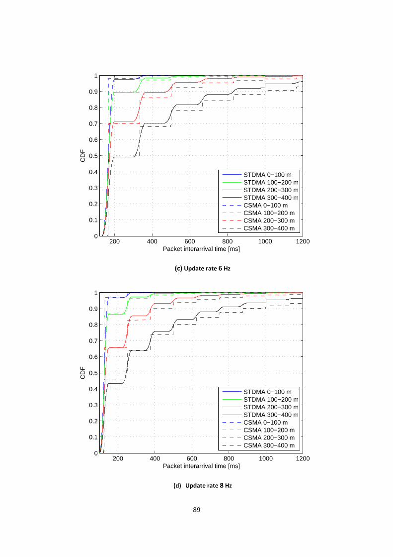
89

(c) Update rate 6 Hz

(d) Update rate 8 Hz

200 400 600 800 1000 12000

0.1

0.2

0.3

0.4

0.5

0.6

0.7

0.8

0.9

1

Packet interarrival time [ms]

CD

F

STDMA 0−100 mSTDMA 100−200 mSTDMA 200−300 mSTDMA 300−400 mCSMA 0−100 mCSMA 100−200 mCSMA 200−300 mCSMA 300−400 m

200 400 600 800 1000 12000

0.1

0.2

0.3

0.4

0.5

0.6

0.7

0.8

0.9

1

Packet interarrival time [ms]

CD

F

STDMA 0−100 mSTDMA 100−200 mSTDMA 200−300 mSTDMA 300−400 mCSMA 0−100 mCSMA 100−200 mCSMA 200−300 mCSMA 300−400 m

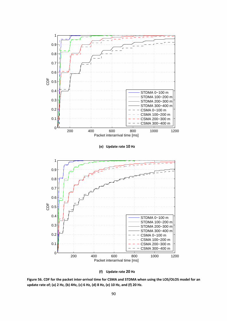
90

(e) Update rate 10 Hz

(f) Update rate 20 Hz

Figure 56. CDF for the packet inter-arrival time for CSMA and STDMA when using the LOS/OLOS model for an update rate of; (a) 2 Hz, (b) 4Hz, (c) 6 Hz, (d) 8 Hz, (e) 10 Hz, and (f) 20 Hz.

200 400 600 800 1000 12000

0.1

0.2

0.3

0.4

0.5

0.6

0.7

0.8

0.9

1

Packet interarrival time [ms]

CD

F

STDMA 0−100 mSTDMA 100−200 mSTDMA 200−300 mSTDMA 300−400 mCSMA 0−100 mCSMA 100−200 mCSMA 200−300 mCSMA 300−400 m

200 400 600 800 1000 12000

0.1

0.2

0.3

0.4

0.5

0.6

0.7

0.8

0.9

1

Packet interarrival time [ms]

CD

F

STDMA 0−100 mSTDMA 100−200 mSTDMA 200−300 mSTDMA 300−400 mCSMA 0−100 mCSMA 100−200 mCSMA 200−300 mCSMA 300−400 m

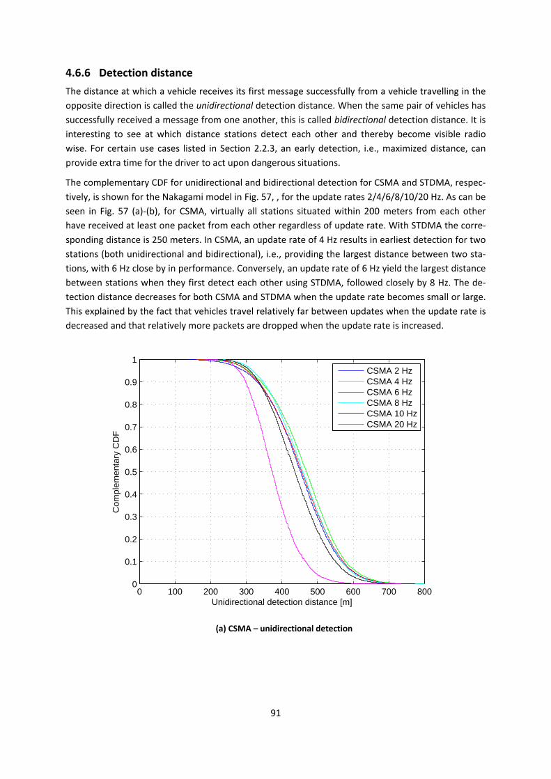
91

4.6.6 Detection distance The distance at which a vehicle receives its first message successfully from a vehicle travelling in the opposite direction is called the unidirectional detection distance. When the same pair of vehicles has successfully received a message from one another, this is called bidirectional detection distance. It is interesting to see at which distance stations detect each other and thereby become visible radio wise. For certain use cases listed in Section 2.2.3, an early detection, i.e., maximized distance, can provide extra time for the driver to act upon dangerous situations.

The complementary CDF for unidirectional and bidirectional detection for CSMA and STDMA, respec-tively, is shown for the Nakagami model in Fig. 57, , for the update rates 2/4/6/8/10/20 Hz. As can be seen in Fig. 57 (a)-(b), for CSMA, virtually all stations situated within 200 meters from each other have received at least one packet from each other regardless of update rate. With STDMA the corre-sponding distance is 250 meters. In CSMA, an update rate of 4 Hz results in earliest detection for two stations (both unidirectional and bidirectional), i.e., providing the largest distance between two sta-tions, with 6 Hz close by in performance. Conversely, an update rate of 6 Hz yield the largest distance between stations when they first detect each other using STDMA, followed closely by 8 Hz. The de-tection distance decreases for both CSMA and STDMA when the update rate becomes small or large. This explained by the fact that vehicles travel relatively far between updates when the update rate is decreased and that relatively more packets are dropped when the update rate is increased.

(a) CSMA – unidirectional detection

0 100 200 300 400 500 600 700 8000

0.1

0.2

0.3

0.4

0.5

0.6

0.7

0.8

0.9

1

Unidirectional detection distance [m]

Com

plem

enta

ry C

DF

CSMA 2 HzCSMA 4 HzCSMA 6 HzCSMA 8 HzCSMA 10 HzCSMA 20 Hz

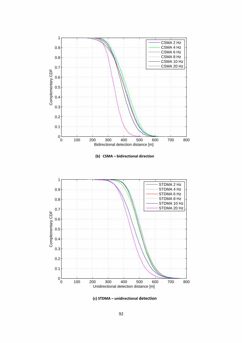
92

(b) CSMA – bidirectional direction

(c) STDMA – unidirectional detection

0 100 200 300 400 500 600 700 8000

0.1

0.2

0.3

0.4

0.5

0.6

0.7

0.8

0.9

1

Bidirectional detection distance [m]

Com

plem

enta

ry C

DF

CSMA 2 HzCSMA 4 HzCSMA 6 HzCSMA 8 HzCSMA 10 HzCSMA 20 Hz

0 100 200 300 400 500 600 700 8000

0.1

0.2

0.3

0.4

0.5

0.6

0.7

0.8

0.9

1

Unidirectional detection distance [m]

Com

plem

enta

ry C

DF

STDMA 2 HzSTDMA 4 HzSTDMA 6 HzSTDMA 8 HzSTDMA 10 HzSTDMA 20 Hz

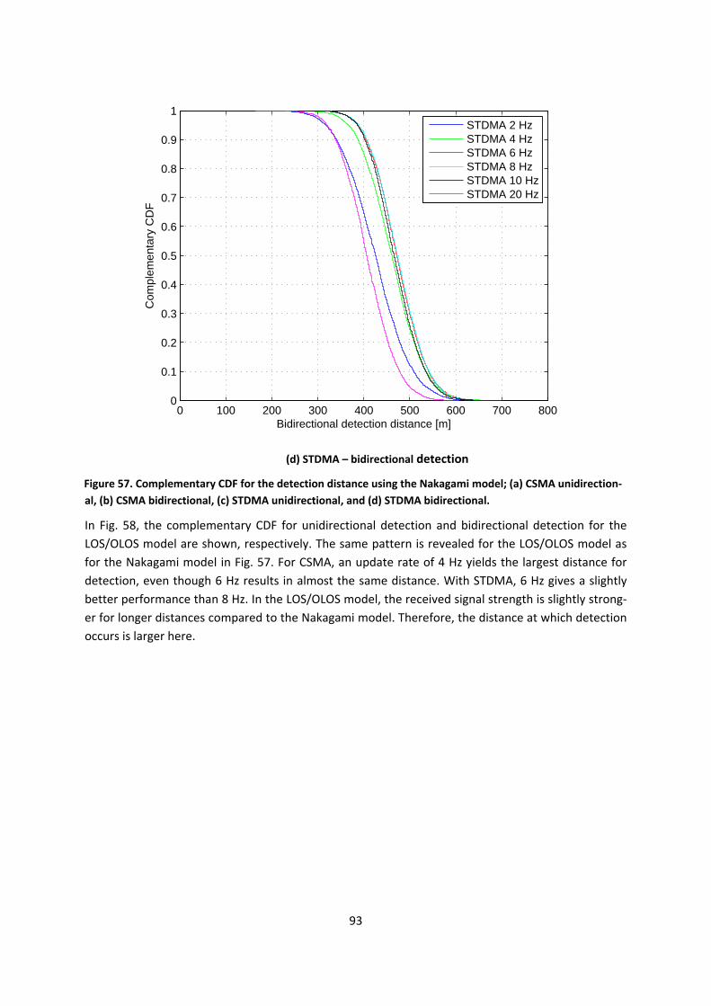
93

(d) STDMA – bidirectional detection

Figure 57. Complementary CDF for the detection distance using the Nakagami model; (a) CSMA unidirection-al, (b) CSMA bidirectional, (c) STDMA unidirectional, and (d) STDMA bidirectional.

In Fig. 58, the complementary CDF for unidirectional detection and bidirectional detection for the LOS/OLOS model are shown, respectively. The same pattern is revealed for the LOS/OLOS model as for the Nakagami model in Fig. 57. For CSMA, an update rate of 4 Hz yields the largest distance for detection, even though 6 Hz results in almost the same distance. With STDMA, 6 Hz gives a slightly better performance than 8 Hz. In the LOS/OLOS model, the received signal strength is slightly strong-er for longer distances compared to the Nakagami model. Therefore, the distance at which detection occurs is larger here.

0 100 200 300 400 500 600 700 8000

0.1

0.2

0.3

0.4

0.5

0.6

0.7

0.8

0.9

1

Bidirectional detection distance [m]

Com

plem

enta

ry C

DF

STDMA 2 HzSTDMA 4 HzSTDMA 6 HzSTDMA 8 HzSTDMA 10 HzSTDMA 20 Hz

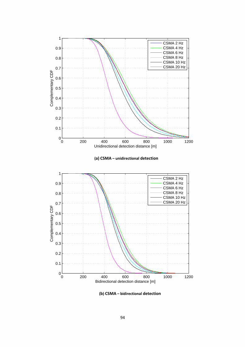
94

(a) CSMA – unidirectional detection

(b) CSMA – bidirectional detection

0 200 400 600 800 1000 12000

0.1

0.2

0.3

0.4

0.5

0.6

0.7

0.8

0.9

1

Unidirectional detection distance [m]

Com

plem

enta

ry C

DF

CSMA 2 HzCSMA 4 HzCSMA 6 HzCSMA 8 HzCSMA 10 HzCSMA 20 Hz

0 200 400 600 800 1000 12000

0.1

0.2

0.3

0.4

0.5

0.6

0.7

0.8

0.9

1

Bidirectional detection distance [m]

Com

plem

enta

ry C

DF

CSMA 2 HzCSMA 4 HzCSMA 6 HzCSMA 8 HzCSMA 10 HzCSMA 20 Hz

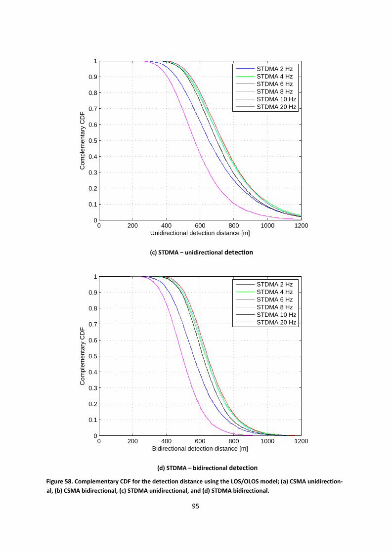
95

(c) STDMA – unidirectional detection

(d) STDMA – bidirectional detection

Figure 58. Complementary CDF for the detection distance using the LOS/OLOS model; (a) CSMA unidirection-al, (b) CSMA bidirectional, (c) STDMA unidirectional, and (d) STDMA bidirectional.

0 200 400 600 800 1000 12000

0.1

0.2

0.3

0.4

0.5

0.6

0.7

0.8

0.9

1

Unidirectional detection distance [m]

Com

plem

enta

ry C

DF

STDMA 2 HzSTDMA 4 HzSTDMA 6 HzSTDMA 8 HzSTDMA 10 HzSTDMA 20 Hz

0 200 400 600 800 1000 12000

0.1

0.2

0.3

0.4

0.5

0.6

0.7

0.8

0.9

1

Bidirectional detection distance [m]

Com

plem

enta

ry C

DF

STDMA 2 HzSTDMA 4 HzSTDMA 6 HzSTDMA 8 HzSTDMA 10 HzSTDMA 20 Hz

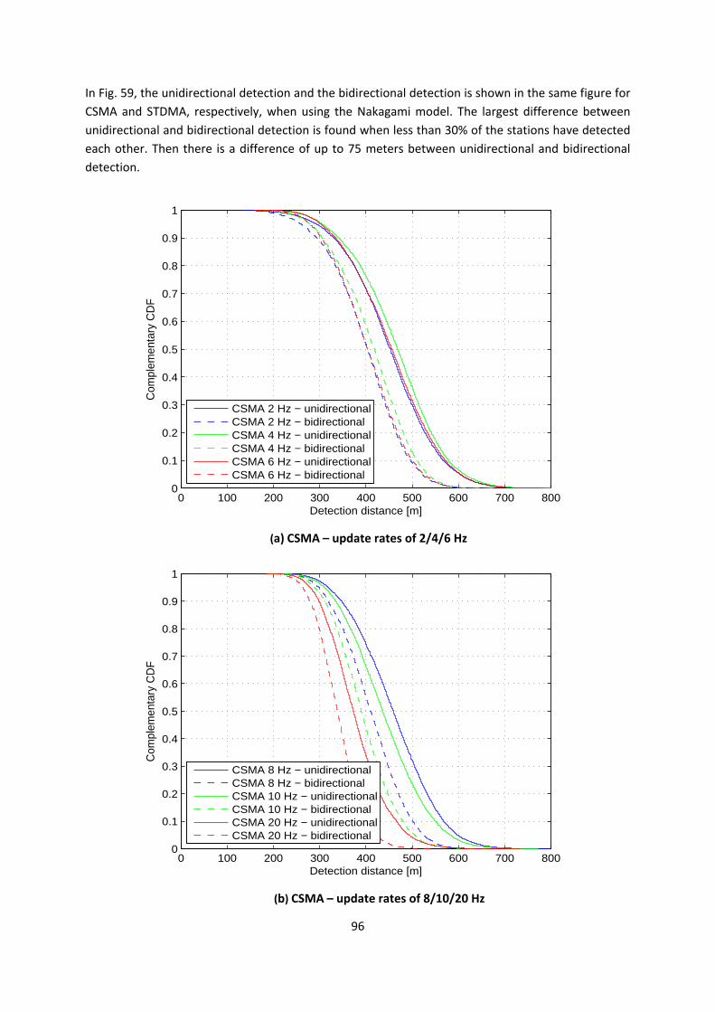
96

In Fig. 59, the unidirectional detection and the bidirectional detection is shown in the same figure for CSMA and STDMA, respectively, when using the Nakagami model. The largest difference between unidirectional and bidirectional detection is found when less than 30% of the stations have detected each other. Then there is a difference of up to 75 meters between unidirectional and bidirectional detection.

(a) CSMA – update rates of 2/4/6 Hz

(b) CSMA – update rates of 8/10/20 Hz

0 100 200 300 400 500 600 700 8000

0.1

0.2

0.3

0.4

0.5

0.6

0.7

0.8

0.9

1

Detection distance [m]

Com

plem

enta

ry C

DF

CSMA 2 Hz − unidirectionalCSMA 2 Hz − bidirectionalCSMA 4 Hz − unidirectionalCSMA 4 Hz − bidirectionalCSMA 6 Hz − unidirectionalCSMA 6 Hz − bidirectional

0 100 200 300 400 500 600 700 8000

0.1

0.2

0.3

0.4

0.5

0.6

0.7

0.8

0.9

1

Detection distance [m]

Com

plem

enta

ry C

DF

CSMA 8 Hz − unidirectionalCSMA 8 Hz − bidirectionalCSMA 10 Hz − unidirectionalCSMA 10 Hz − bidirectionalCSMA 20 Hz − unidirectionalCSMA 20 Hz − bidirectional

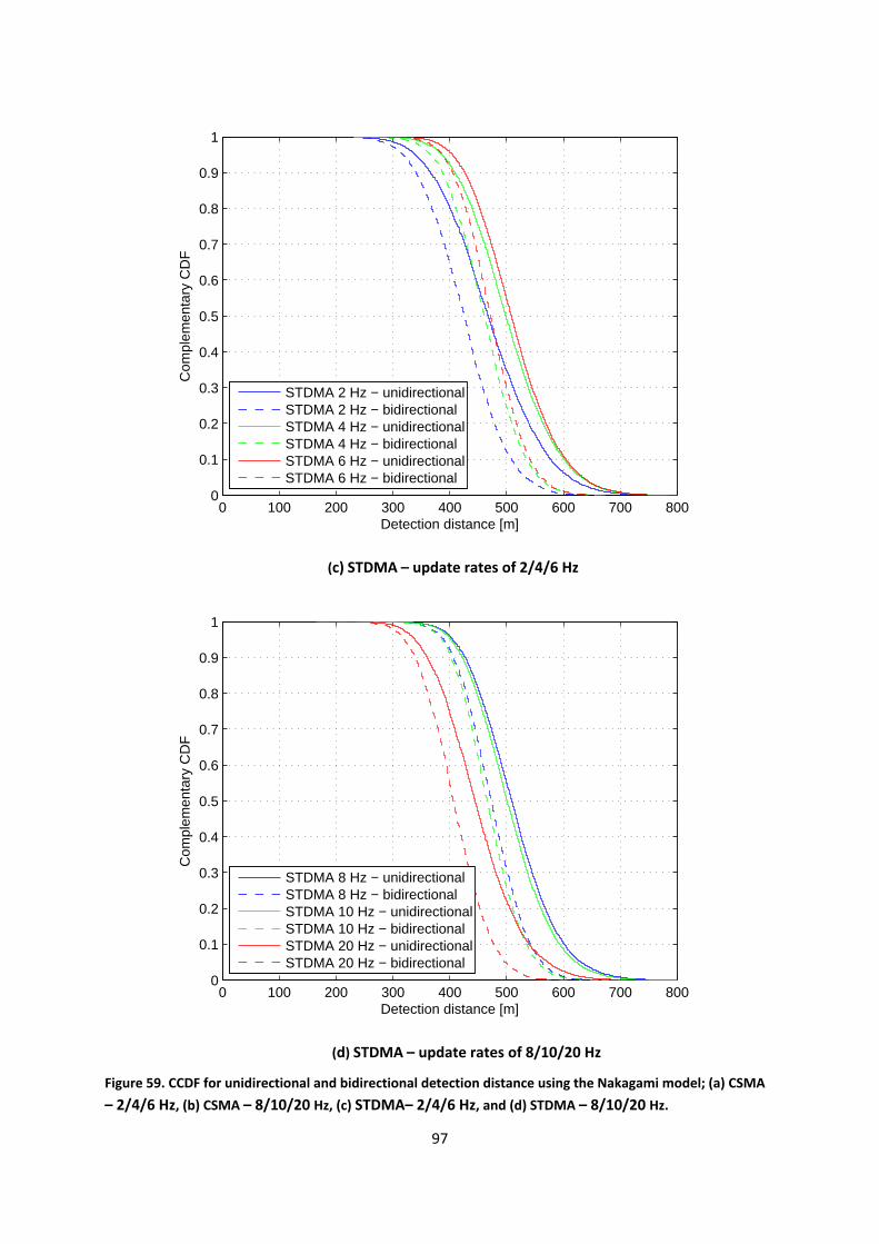
97

(c) STDMA – update rates of 2/4/6 Hz

(d) STDMA – update rates of 8/10/20 Hz

Figure 59. CCDF for unidirectional and bidirectional detection distance using the Nakagami model; (a) CSMA – 2/4/6 Hz, (b) CSMA – 8/10/20 Hz, (c) STDMA– 2/4/6 Hz, and (d) STDMA – 8/10/20 Hz.

0 100 200 300 400 500 600 700 8000

0.1

0.2

0.3

0.4

0.5

0.6

0.7

0.8

0.9

1

Detection distance [m]

Com

plem

enta

ry C

DF

STDMA 2 Hz − unidirectionalSTDMA 2 Hz − bidirectionalSTDMA 4 Hz − unidirectionalSTDMA 4 Hz − bidirectionalSTDMA 6 Hz − unidirectionalSTDMA 6 Hz − bidirectional

0 100 200 300 400 500 600 700 8000

0.1

0.2

0.3

0.4

0.5

0.6

0.7

0.8

0.9

1

Detection distance [m]

Com

plem

enta

ry C

DF

STDMA 8 Hz − unidirectionalSTDMA 8 Hz − bidirectionalSTDMA 10 Hz − unidirectionalSTDMA 10 Hz − bidirectionalSTDMA 20 Hz − unidirectionalSTDMA 20 Hz − bidirectional

98

In Fig. 60, the unidirectional detection and the bidirectional detection is shown in the same figure for CSMA and STDMA, respectively, when using the LOS/OLOS model. The largest difference between unidirectional and bidirectional detection is up to almost 100 meters. This is found when only 10% of the stations have detected each other for CSMA in Fig. 60(a) and STDMA for an update rate of 2 Hz in Fig. 60(c). Further, for an update rate of 20 Hz the smallest difference between unidirectional and bidirectional detection is seen.

In Fig. 61, a comparison between CSMA and STDMA for the bidirectional detection is shown for the Nakagami and LOS/OLOS models. Here it is obvious that in STDMA stations detect each other much earlier than in CSMA, the difference is up to 100 meters earlier detection for STDMA. The smallest difference in detection distance between CSMA and STDMA is found for an update rate of 2 Hz. However, none of the update rates 2/4/6 Hz for CSMA can reach the same detection distance as STDMA for 2 Hz.

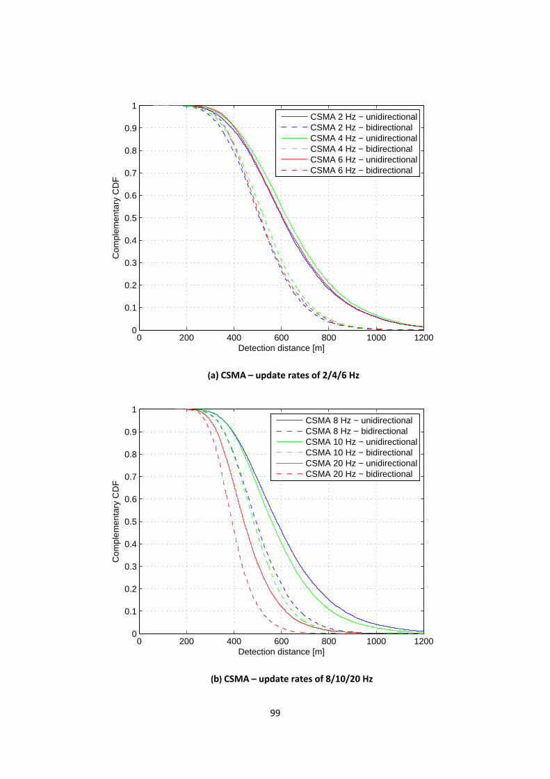
99

(a) CSMA – update rates of 2/4/6 Hz

(b) CSMA – update rates of 8/10/20 Hz

0 200 400 600 800 1000 12000

0.1

0.2

0.3

0.4

0.5

0.6

0.7

0.8

0.9

1

Detection distance [m]

Com

plem

enta

ry C

DF

CSMA 2 Hz − unidirectionalCSMA 2 Hz − bidirectionalCSMA 4 Hz − unidirectionalCSMA 4 Hz − bidirectionalCSMA 6 Hz − unidirectionalCSMA 6 Hz − bidirectional

0 200 400 600 800 1000 12000

0.1

0.2

0.3

0.4

0.5

0.6

0.7

0.8

0.9

1

Detection distance [m]

Com

plem

enta

ry C

DF

CSMA 8 Hz − unidirectionalCSMA 8 Hz − bidirectionalCSMA 10 Hz − unidirectionalCSMA 10 Hz − bidirectionalCSMA 20 Hz − unidirectionalCSMA 20 Hz − bidirectional

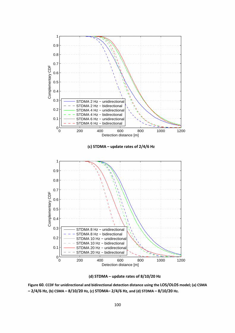
100

(c) STDMA – update rates of 2/4/6 Hz

(d) STDMA – update rates of 8/10/20 Hz

Figure 60. CCDF for unidirectional and bidirectional detection distance using the LOS/OLOS model; (a) CSMA – 2/4/6 Hz, (b) CSMA – 8/10/20 Hz, (c) STDMA– 2/4/6 Hz, and (d) STDMA – 8/10/20 Hz.

0 200 400 600 800 1000 12000

0.1

0.2

0.3

0.4

0.5

0.6

0.7

0.8

0.9

1

Detection distance [m]

Com

plem

enta

ry C

DF

STDMA 2 Hz − unidirectionalSTDMA 2 Hz − bidirectionalSTDMA 4 Hz − unidirectionalSTDMA 4 Hz − bidirectionalSTDMA 6 Hz − unidirectionalSTDMA 6 Hz − bidirectional

0 200 400 600 800 1000 12000

0.1

0.2

0.3

0.4

0.5

0.6

0.7

0.8

0.9

1

Detection distance [m]

Com

plem

enta

ry C

DF

STDMA 8 Hz − unidirectionalSTDMA 8 Hz − bidirectionalSTDMA 10 Hz − unidirectionalSTDMA 10 Hz − bidirectionalSTDMA 20 Hz − unidirectionalSTDMA 20 Hz − bidirectional

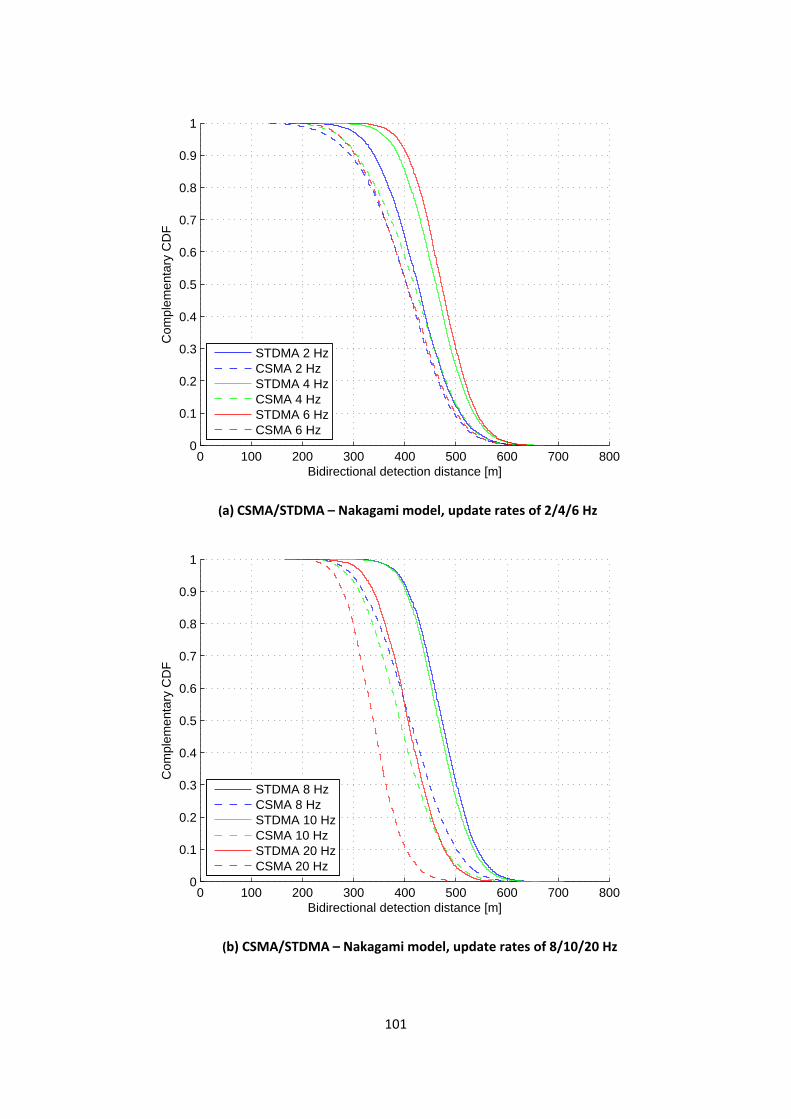
101

(a) CSMA/STDMA – Nakagami model, update rates of 2/4/6 Hz

(b) CSMA/STDMA – Nakagami model, update rates of 8/10/20 Hz

0 100 200 300 400 500 600 700 8000

0.1

0.2

0.3

0.4

0.5

0.6

0.7

0.8

0.9

1

Bidirectional detection distance [m]

Com

plem

enta

ry C

DF

STDMA 2 HzCSMA 2 HzSTDMA 4 HzCSMA 4 HzSTDMA 6 HzCSMA 6 Hz

0 100 200 300 400 500 600 700 8000

0.1

0.2

0.3

0.4

0.5

0.6

0.7

0.8

0.9

1

Bidirectional detection distance [m]

Com

plem

enta

ry C

DF

STDMA 8 HzCSMA 8 HzSTDMA 10 HzCSMA 10 HzSTDMA 20 HzCSMA 20 Hz

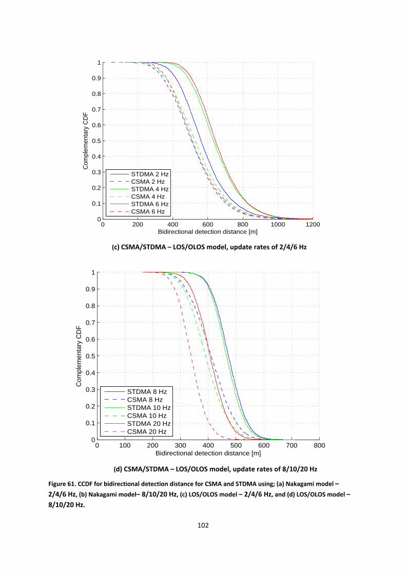
102

(c) CSMA/STDMA – LOS/OLOS model, update rates of 2/4/6 Hz

(d) CSMA/STDMA – LOS/OLOS model, update rates of 8/10/20 Hz

Figure 61. CCDF for bidirectional detection distance for CSMA and STDMA using; (a) Nakagami model – 2/4/6 Hz, (b) Nakagami model– 8/10/20 Hz, (c) LOS/OLOS model – 2/4/6 Hz, and (d) LOS/OLOS model – 8/10/20 Hz.

0 200 400 600 800 1000 12000

0.1

0.2

0.3

0.4

0.5

0.6

0.7

0.8

0.9

1

Bidirectional detection distance [m]

Com

plem

enta

ry C

DF

STDMA 2 HzCSMA 2 HzSTDMA 4 HzCSMA 4 HzSTDMA 6 HzCSMA 6 Hz

0 100 200 300 400 500 600 700 8000

0.1

0.2

0.3

0.4

0.5

0.6

0.7

0.8

0.9

1

Bidirectional detection distance [m]

Com

plem

enta

ry C

DF

STDMA 8 HzCSMA 8 HzSTDMA 10 HzCSMA 10 HzSTDMA 20 HzCSMA 20 Hz

103

4.7 Summary Both the minimum and the maximum channel access delay are of interest for VANET-based C-ITS applications. On average, the channel access delay is lower for CSMA than STDMA. For CSMA, the minimum channel access delay is known and depends on the length of the AIFS. In STDMA the chan-nel access delay depends on the number of slots contained in each SI. When the update rate increas-es, the number of slots in SI decreases; implying in turn that the channel access delay decreases. The shortest channel access delay with STDMA occurs for 20 Hz (i.e., 50 ms between every generated packet), yielding a maximum channel access delay of 10 ms.

The maximum channel access delay for CSMA is random, and depends on the instantaneous network load within radio range of a specific station. In the simulations conducted in this thesis work, all packets were transmitted in CSMA, i.e., no packet drops occurred at the sending side and the chan-nel access delay never exceeded 15 ms (see Fig. 45(b) and 47(b)). In STDMA, the station knows that it will be allowed to transmit within the predetermined SI and the channel access delay is not affected by the network load. The channel access delay is thus upper bounded and predictable since the sta-tion makes its own slot selections. As can be deduced from Fig. 46(a), the worst case channel access delay that STDMA can exhibit is 100 ms and this occurs when the update rate is set to 2 Hz (implying 500 ms between every generated packet). However, 50% of the generated packets have been trans-mitted after 50 ms even in this case.

STDMA has a better packet reception probability than CSMA for all considered update rates (Fig. 50 and Fig. 52) when the distance between transmitter and receiver is larger than 100 meters. This is due to the fact that all transmissions in STDMA are slot synchronized. In addition, when the network load increases, the benefits of scheduling transmissions in space comes into play. With CSMA, trans-missions may overlap in time, both completely and partially due to unsynchronized transmissions taking place outside the sensing range of concurrent transmitters. Also partially overlapping trans-missions are likely to cause decoding failures at receivers situated in between the concurrent trans-mitters (the hidden terminal problem). Further, when the network load increases, CSMA stations within radio range of each other are more likely to transmit at the same time due to reaching a backoff value of zero at the same time. This occurs since CSMA stations within radio range of each other are synchronized to some extent, through the channel sensing procedure, and therefore sta-tions tend to initiate their backoff counters at the same time, when a busy channel becomes free. The selection of backoff values is not scheduled in space and thus two or more stations can be geo-graphically co-located when reaching a backoff value of zero, reducing the packet reception probabil-ity for many receivers.

The MAC-to-MAC delay shows the overall reception performance, including both delay and reliabil-ity, for receivers located at distinct distances from the transmitter. For receivers located close to a transmitter, i.e., for distances below 100 meters, CSMA and STDMA perform equally well with re-spect to the MAC-to-MAC delay. For larger distances between transmitters and receivers, STDMA performs better than CSMA, due to its higher packet reception probability. However, since the chan-nel access delay with STDMA is more spread in time compared to CSMA (channel access is uniformly distributed over the SI in STDMA), this also affects the MAC-to-MAC delay. In other words, CSMA reacts faster than STDMA when a packet from the C-ITS application arrives at the MAC layer.

104

The packet inter-arrival time indicates how much time that has elapsed since the last periodic CAM/BSM was received from a particular transmitter. Hence, it also reveals how many consecutive packets that have been lost (due to excessive delay or interference). When the distance between transmitter and receiver is less than 100 meters, we can conclude that there will never be more than 400 ms between two successfully received packets for update rates 6/8/10/20 Hz. For update rates of 2 Hz and 4 Hz, this is longer due to the period T (being the reciprocal of the update rate). For an update rate of 20 Hz and a TX-RX distance of 300-400 meters, there is a probability of 20 consecutive packet drops of 2-3%.

The level of fairness in terms of channel access delay is also of importance. In STDMA, the overall ITS system achieves a higher level of fairness among the stations since all stations have equal probability to access the channel at a given time, given the same type of data traffic. With CSMA, some stations gain access to the channel directly after the mandatory listening period, while others have to wait up to 15 ms before channel access is granted in the worst case. Even though the level of fairness in terms of channel access delay is not as high in CSMA as for STDMA, it is still acceptable given the network load in the simulations presented in this thesis.

STDMA has better unidirectional and bidirectional detection distance than CSMA. The difference can be up to 100 meters for the benefit of STDMA. For both CSMA and STDMA, the detection distance decreases when the update rate becomes very small or very large. This explained by the fact that in the one extreme, very small rate, vehicles travel relatively far between two updates, thus reducing the detection distance, and in the other extreme, more packets are dropped due to increasing net-work load when the update rate is increased, which also leads to that vehicles travel relatively far between two successfully received updates. The largest detection distance for CSMA is achieved when using an update rate of 4 Hz, followed closely by 6 Hz. With STDMA the largest distance is achieved at 8 Hz, followed closely by 6 Hz. The smallest difference in performance is found for an update rate of 2 Hz.

Two different channel models have been used for simulations. The two examined MAC schemes are not noticeably performing differently under the two different models. In the LOS/OLOS model, transmissions reaches slightly longer, i.e., there is a stronger received signal at longer distances, than the Nakagami model. The stronger received signal implies that more stations within radio range and stations therefore perceive a higher network load. This affects the channel access delay for CSMA, which was seen in Fig. 48, and thereby also the MAC-to-MAC delay and packet inter-arrival time are also slightly affected. However, the relative performance between the two protocols under the two channel models are more or less the same.

105

5 Conclusions This thesis has scrutinized and evaluated two MAC methods, CSMA and STDMA, when used in VANETs supporting C-ITS applications. CSMA was selected for evaluation since it is the MAC method used by IEEE 802.11p, which has been adopted as the wireless access technology for the first genera-tion of C-ITS applications. STDMA was selected as it is already in commercial use through AIS, a man-datory position reporting system for large ships and passenger vessels with many similarities to VANETs. CSMA and STDMA are evaluated with respect to the communication requirements and the protocol settings arising from C-ITS standardization. Based on these constraints, suitable perfor-mance measures have been defined. Using these performance measures, CSMA and STDMA have been evaluated through extensive computer simulations, in a scenario where vehicles travel on a 10 km highway with 12 lanes (six lanes in each direction) broadcasting position messages (e.g., CAM/BSM) periodically with different update rates. The scenario was selected as it is expected to be one of the most challenging for the MAC algorithm.

The requirements on a MAC method for VANETs supporting C-ITS applications are that BSMs/CAMs should be transmitted periodically with low channel access delay and high reliability. Further, the achievable performance should be distributed fairly among all nodes. The low delay keeps the fresh-ness of the position data contained in the BSMs/CAMs as high as possible. The channel access delay should not exceed the time between two consecutive position messages, since a new message will then be ready for transmission before the old one has been granted channel access, causing the old message to be dropped. Finally, the overall system must be scalable such that all stations are allowed to transmit. The adopted performance measures: channel access delay, packet reception probability, MAC-to-MAC delay, packet inter-arrival time and detection distance, all contribute to the evaluation of a suitable MAC method for VANET-based C-ITS applications.

For CSMA, the maximum channel access delay is not bounded when EDCA is used in ad hoc mode. However, the simulations conducted in this thesis indicate that events causing longer delays than 15 ms are very unlikely for the considered update rates. From the simulation results, it can further be concluded that the channel access delay for CSMA is on average lower than for STDMA. For a rela-tively low update rate of 2 Hz, the upper bound on the channel access delay for STDMA is 100 ms whereas for CSMA the channel access delay never exceeds 2 ms. For a relatively high update rate of 20 Hz, the upper bound on STDMA is 10 ms, whereas CSMA never exceeds 15 ms for the evaluated highway scenario.

An advantage of STDMA is that the transmission slot in a certain SI is known some time before the actual transmission (from at least 80% of one frame duration up to as much as eight frames in ad-vance). This implies that the position message can be generated just in time for transmission (which is what is done in the AIS system). The channel access delay for STDMA, as derived in this thesis, does not take this into account and is therefore only a loose upper bound on the age of the position mes-sage. For CSMA, the time when the actual transmission takes place is harder to predict in advance. It can therefore be concluded that if the position messages in STDMA are generated just in time for the actual transmission, a considerably lower channel access delay can be achieved. Given the channel access delay derived from the CSMA simulations the age of the position messages will then be great-er in CSMA than in STDMA. However, it can also be concluded that the variation around the nominal

106

transmission times kT, where k is an integer and 1/T is the update rate, is larger in STDMA as com-pared to CSMA.

STDMA and CSMA achieve the same reliability for a TX-RX distance less than 100 meters. However, for increased distances between transmitters and receivers (100-500 meters), STDMA always achieve a higher reliability. The higher overall reliability for STDMA is due to the time slotting and its ability to schedule transmissions in space when the network load increases.

The MAC-to-MAC delay combines channel access delay and packet reception probability into one measure and thereby the requirements on delay and reliability from the C-ITS applications can be easily assessed by inspecting the CDF of the MAC-to-MAC delay. CSMA shows a lower MAC-to-MAC delay for the packets that are successfully delivered, but STDMA manages to deliver more packets to higher layers, such that the CDF of the MAC-to-MAC delay converges to a higher value for STDMA. This illustrates the basic trade-off between delay and reliability. STDMA offers better reliability than CSMA at the expense of a longer MAC-to-MAC delay.

The simulation results for the detection distance reveal that both the unidirectional and the bidirec-tional detection distances are much longer for STDMA than for CSMA, regardless of the update rate. An early detection, i.e., a large distance between two stations, is important for certain use cases, such as the emergency vehicle approaching, slow vehicle, and stationary vehicles as listed in Section 2.2.3. In a highway scenario (when vehicles travel at high speeds) an early notification can avoid pan-ic maneuvers by drivers and thereby greatly enhance traffic safety.

STDMA is better than CSMA for all evaluated performance measures, except for minimum channel access delay. STDMA is therefore more suitable for VANET-based C-ITS applications than CSMA be-cause it achieves a better performance and the channel access delay is predictable (implying that applications can be tailored towards to take this into account). STDMA was specifically developed for the AIS, which also is an ad hoc network concept with the aim of avoiding collisions between ships. Further, it has requirement on synchronization, however, the slot synchronization also improves the overall reliability. CSMA, on the other hand, is simple, well-known, and does not require synchroniza-tion between stations.

107

6 Future outlook The scalability issue of CSMA was addressed in 2009 within ETSI, which assembled an STF with the aim to DCC methods (see Section 2.2.5 for further details). The outcome of the STF was a toolbox, as outlined in TS 102 687 [34]. The toolbox is currently situated in the access layer and consists of four different knobs that can be used for controlling the network load; transmit rate control (TRC), trans-mit power control (TPC), transmit data rate control (TDC) and DCC sensitivity control (DSC). The latter is for controlling the carrier sense threshold in CSMA. Further, in TS 102 687 there is a suggestion of a state machine with three states; relaxed, active, and restrictive. Depending on network load meas-ured by the station, the station switches state and performs countermeasures to avoid injecting more data traffic into the network. In relaxed state the station can transmit whatever enters the MAC layer. When the network load increases to above 25% the station switches to active state and must start-up countermeasures such as TPC. When the network load increases to above 75% the station is forced into restrictive state, where it should avoid staying. The current approach in TS 102 687 gives the mandate to the access layer to for example drop packets that has been generated in the facilities layer. From a holistic point of view, this makes the system more unreliable than nec-essary. The control of packet drops should be moved to higher layers, i.e., all generated packets should be transmitted. Otherwise, this can further jeopardize an already unreliable system. Especial-ly, the C-ITS applications on the receiving side must be able to predict the behaviour of the other stations in the system.

Leaving the control to the applications generating the messages is an approach that has been re-searched lately. PULSAR and LIMERIC [71, 72] are two proposed algorithm for controlling the net-work load in CSMA when used in VANETs. They have their starting points in the BSM generation and the aim is to send as many messages as possible, converging towards a specific network load with an equal sharing of the bandwidth depending on driving context (i.e., driving with high speed requires more transmitted messages compared to a vehicle standing still in a traffic jam, simply due to the change of the vehicle’s dynamics). This generation with fair division of the bandwidth depending on driving context is also called the “cooperative awareness” approach. PULSAR and LIMERIC take into account also neighbouring stations’ sensed network load since a station perceiving a low network load can contribute to congested areas without knowing it otherwise.

In traditional networking, protocols in the communication stack are independent and not aware of what is going on at other layers. Usually, each protocol residing in each layer is optimized but vehicu-lar communications require joint optimization of all protocols to make the system to efficiently use the scarce resources. Methods for controlling the network load is a compelling example that joint optimization is needed in C-ITS. For instance, the PHY layer could provide the local channel busy ra-tio, which is conveyed to the facilities layer generating packets. The application can then determine based on the busy ratio if it is possible to generate a message or not. Once generated it should have a very high probability of being transmitted.

The carrier frequency of 5.9 GHz is cumbersome to work with, since the LOS component and the first order reflections from nearby scattering objects contribute most to the received power. Unfortu-nately, the diffracted components and higher order reflections do not carry significant power at this high frequency. Therefore, if the LOS component is missing and there are no nearby scatterers the received signal strength can drop significantly [78]. In “The great spectrum famine” Mitchell Lazaurus

108

[79] points out that the tractable carrier frequencies for mobile broadband are between 300 MHz and 3 500 MHz (3.5 GHz). Higher frequencies result in wavelengths shorter than 9 centimetres, which have trouble to penetrate walls and foliage. Lower carrier frequencies (< 300 MHz) yield antennas that are impractical in size (too large for handheld devices). For large vehicles, such as tractors with containers and rigids, the antenna placement is crucial for communication behind the vehicle at 5.9 GHz. One other aspect is also that the antenna cable cannot be too long because the signal will then be too attenuated before it reaches the decoder. A signal transmitted at a lower carrier frequency would reach longer due to reduced path loss and increased diffraction around, e.g., street corners.

The whole C-ITS world is an exciting area to study. When C-ITS becomes reality in our vehicle it has the potential to save lives and avoid accidents. The huge mass accidents occurring earlier this winter at Tranarpsbron outside Östra Ljungby [80] in the southern part of Sweden could have been avoided (or at least the impact could have been minimized) if C-ITS had been in place. Accidents cost the so-ciety enormous amount of grief and money every year.

In the latest CAM specification, generation rules depending on driving context have been developed (see Section 2.2.3). These new generation rules have not been used in this thesis, and it would be very interesting to investigate this further in the STDMA case. For instance, it would be interesting to see what STDMA can offer to control the network load, since it already keeps track of all neighbours in its frame. Even though STDMA offers predictable channel access delay and all stations are guaran-teed channel access, the interference level will at some point not allow for more data traffic.

109

References [1] ISO TR 17465-1:Draft, Intelligent transport systems – Terms, definitions, and guidelines

for Cooperative standards documents – Part 1: Terms, definitions and outline guidance for standards documents, May 2012.

[2] DRIVE C2X-project [online], http://www.drive-c2x.eu/project

[3] Safety Pilot Program [online], http://www.its.dot.gov/safety_pilot/index.htm

[4] IEEE Std. 802.11p-2010, Part 11: Wireless LAN Medium Access Control (MAC) and Physical Layer (PHY) specifications: Amendment 7: Wireless Access in Vehicular Environment, July 2010. Superseded.

[5] IEEE Std. 802.11-2012, Part 11: Wireless LAN Medium Access Control (MAC) and Physical Layer (PHY) specifications, March 2012.

[6] COMeSafety, “European ITS Communication Architecture: Overall Framework and Proof of Concept Implementation,” ver. 3.0, 2010.

[7] ETSI EN 302 637-2 Draft V.0.0.5, Intelligent Transport Systems (ITS); Vehicular Commu-nications; Basic Set of Applications; Part 2: Specification of Cooperative Awareness Basic Service, June 2012.

[8] SAE Std. J2735, Dedicated Short Range Communications (DSRC) Message Set Diction-ary, DSRC Committee, Nov. 2009.

[9] ETSI EN 302 637-3: Draft V0.0.7, Intelligent Transport Systems (ITS); Vehicular Commu-nications; Basic Set of Applications; Part 3: Specification of Decentralized Environmen-tal Notification Basic Service, June 2012.

[10] B. Clifford Neumann, “Readings in distributed computing systems,” in chapter Scale in Distributed, IEEE Computer Society, Los Alamitos, CA, 1994, pp. 463-489.

[11] Homepage of FCC [online], http://transition.fcc.gov/Bureaus/Engineering_Technology/Orders/1999/fcc99305.txt

[12] L. Cheng, B. E. Henty, D. D. Stancil, F. Bai, and P. Mudalige, “Mobile Vehicle-to-Vehicle Narrow-Band Channel Measurement and Characterization of the 5.9 GHz Dedicated Short Range Communication (DSRC) Frequency Band,” in IEEE Journal on Selected Are-as in Communications, vol. 25, no. 8, pp. 1501-1516, Oct. 2007.

[13] ETSI TR 102 861 (V.1.1.1), Intelligent Transport Systems (ITS); STDMA recommended parameters and settings for cooperative ITS; Access layer part.

[14] ETSI TR 102 862 (V.1.1.1), Intelligent Transport Systems (ITS); Performance Evaluation of Self-Organizing TDMA as Medium Access Control Method Applied to ITS; Access layer part.

[15] ETSI EN 302 663:Draft V1.3.2 , Intelligent Transport Systems (ITS); Access Layer Speci-fication for Intelligent Transport Systems operating in the 5 GHz frequency band, De-cember 2012.

110

[16] ASTM E2213-03, Standard Specification for Telecommunications and Information Exchange between Roadside and Vehicle Systems – 5 GHz Band Dedicated Short-Range Communications (DSRC) Medium Access Control (MAC) and Physical Layer (PHY) Specifications, 2003.

[17] IEEE Std. 1455-1999, IEEE Standard for Message Sets for Vehicle/Roadside Communi-cations, 1999.

[18] SAE Draft J2945.1, DSRC Message Communication Minimum Performance Require-ments – Basic Safety Message for Vehicle Safety Applications.

[19] ISO 21217:2010, Intelligent Transport Systems – Communications access for land mobiles (CALM) – Architecture, 2010.

[20] ISO 21215:2010, Intelligent Transport Systems – Communications access for land mobiles (CALM) – M5, 2010.

[21] ISO 29281:2011, Intelligent Transport Systems – Communications access for land mobiles (CALM) – Non-IP networking, 2011.

[22] European Commission M/453, Standardisation mandate addressed to CEN, CENELEC, and ETSI in the field of information and communication technologies to support the interoperability of co-operative systems for intelligent transport in the European Community, Oct. 2009.

[23] ETSI TS 102 792:Draft, Intelligent Transport Systems (ITS); Mitigation techniques to avoid interference between the European CEN Dedicated Short Range Communica-tion (CEN DSRC) and Intelligent Transport Systems (ITS) operating in the 5 GHz fre-quency range.

[24] ETSI EN 302 571:Draft V1.2.6, Intelligent Transport Systems (ITS), Radio communica-tions equipment operating in the 5 855 MHz to 5 925 MHz frequency band: Harmo-nized EN covering the essential requirements o farticle 3.2 of the R&TTE Directive, December 2012.

[25] IEEE Std. 1609.4-2010, IEEE Standard for Wireless Access in Vehicular Environments (WAVE) – Multi-channel operation, February 2011.

[26] John B. Kenney, “Dedicated Short-Range Communications (DSRC) Standards in the United States,” in Proceedings of the IEEE, vol. 99, no.7, pp. 1162-1182, July 2011.

[27] ANSI/IEEE Std. 802.2-1998, Information technology – Telecommunications and infor-mation exchange between systems – Local and metropolitan area networks – Specific requirements – Part 2: Logical Link Control, 1998.

[28] IEEE 802-2001, IEEE Standard for Local and Metropolitan Area Networks: Overview and Architecture.

[30] IEEE Std. 1609.3, IEEE Standard for Wireless Access in Vehicular Environments (WAVE) – Networking Services, December 2010.

111

[31] IEEE P1609.2/D15, IEEE Draft Standard for Wireless Access in Vehicular Environment (WAVE) – Security Services for Applications and Management Messages, Draft 15, May 2012.

[32] ETSI EN 302 665, Intelligent Transport Systems (ITS); Communications Architecture, 2010.

[33] ETSI TS 102 940 (V.1.1.1), Intelligent Transport Systems (ITS), Security, ITS communi-cations security architecture and security management, June 2012.

[34] ETSI TS 102 687 (V1.1.1), Intelligent Transport Systems (ITS); Decentralized Conges-tion Control Mechanism for Intelligent Transport Systems operating the 5 GHz range; Access layer part, 2011.

[35] ETSI TS 102 636-2, Intelligent Transport Systems; Vehicular Communications; GeoNetworking; Part 2: Scenarios, 2010.

[36] ETSI TS 102 636-5-1, Intelligent Transport Systems; Vehicular Communications; GeoNetworking; Part 5: Transport Protocols; Sub-part 1: Basic Transport Protocol, 2011.

[37] ETSI TS 102 636-4-1:Draft V.0.0.9, Intelligent Transport Systems; Vehicular Communi-cations; GeoNetworking; Part 4: Geographical addressing and forwarding for point-to-point and point-to-multipoint; Sub-part 1: Media-Dependent Functionality, April 2012.

[38] ETSI TS 102 636-4-2, Intelligent Transport Systems; Vehicular Communications; GeoNetworking; Part 4: Geographical addressing and forwarding for point-to-point and point-to-multipoint; Sub-part 2: Media-Independent Functionality, 2011.

[39] ETSI TS 102 636-5-1, Intelligent Transport Systems; Vehicular Communications; GeoNetworking; Part 6: Internet integration; Sub-part 1: Transmission of IPv6 Packets over GeoNetworking Protocols, 2011.

[40] ETSI TS 102 636-1, Intelligent Transport Systems; Vehicular Communications; GeoNetworking; Part 1: Requirements, 2010.

[41] ETSI TS 102 636-5-1, Intelligent Transport Systems; Vehicular Communications; GeoNetworking; Part 3: Network Architecture, 2010.

[42] ETSI TR 102 638 (V.1.1.1), Intelligent Transport Systems (ITS); Vehicular Communica-tions; Basic Set of Applications; Definitions, 2009.

[43] ETSI TS 102 894: Draft V.1.0.2, Intelligent Transport Systems (ITS), Users and applica-tions requirements; Facility layer structure, functional requirements and specifica-tions.

[44] Safespot’s homepage [online], http://www.safespot-eu.org/

[45] ETSI DTS 101 539-1:Draft V.0.0.6, Intelligent Transport Systems (ITS); V2X Applica-tions; Part 1: Road Hazard Signaling (RHS); Application requirements specification, May 2012.

112

[46] ETSI TS 101 539-3:Draft V.0.0.4, Intelligent Transport Systems (ITS); V2X applications; Part 1: Longitudinal Collision Risk Warning (LCRW) application requirements specifi-cation, June 2012.

[47] ETSI TS 101 539-2:Draft V.0.0.4, Intelligent Transport Systems (ITS); V2X applications; Part 1: Intersection Collision Risk Warning (ICRW) application requirements specifica-tion, June 2012.

[48] ANSI/IEEE Std. 802.1D-1998: IEEE Standard for Information technology - Telecommu-nications and information exchange between systems - Local and metropolitan area networks - Common specifications- Part 3: Media Access Control (MAC) Bridges.

[49] ITU-R Recommendation M.1371-4:2010: Technical characteristics for universal ship-borne automatic identification system using time division multiple access in the VHF maritime mobile band.

[50] H. Lans, "Position Indicating System", US patent 5,506,587, issued 1996.

[51] N. Abramson, "The Aloha system – another alternative for computer communica-tions," in Proc. of the AFIPS Joint Computer Conferences, Houston, TX, 1970, pp. 281-285.

[52] L. G. Roberts, "Aloha packet system with and without slots and capture," ACM SIGCOMM Computer Communication Review, vol. 5, no. 2, pp. 28-42, April 1975.

[53] W. Crowther, R. Rettberg, D. Walden, S. Crustein, and F. Heart, "A system for broad-cast communication: Reservation Aloha," in Proc. of the 6th Hawaii International Con-ference on System Sciences, Honolulu, HI, January 1973, pp. 371-374.

[54] I. Catling ed., Advanced Technology for Road Transport: IVHS and ATT, Artech house, 1994.

[55] A. Mann and J. Rückert, "A new concurrent slot assignment protocol for traffic in-formation exchange," in Proc. of the 38th IEEE Vehicular Technology Conference (VTC’88), Philadelphia, PA, June 1988, pp. 503-508.

[56] W. Zhu, T. Hellmich, and B. Walke, "DCAP, a decentral channel access protocol: per-formance analysis," in Proc. of the 41st IEEE Vehicular Technology Conference (VTC’91), Orlando, FL, May 1991, pp. 463-468.

[57] F. Borgonovo, A. Capone, M. Cesana, and L. Fratta, "RR-Aloha, a reliable R-Aloha broadcast channel for ad-hoc inter-vehicle communication networks," in Proc. 1st Annual Mediterranean Ad Hoc Networking Workshop (Med-Hoc-Net 2002), Baia Chia, Italy, Sept. 2002.

[58] F. Borgonovo, A. Capone, M. Cesana, and L. Fratta, "ADHOC MAC: a New MAC Archi-tecture for Ad-Hoc Networks Providing Efficient and Reliable Point-to-Point and Broadcast Services," ACM Wireless Networks (WINET), vol. 10, no. 4, pp. 359-366, Ju-ly 2004.

[59] L. Miao, F. Ren, C. Lin, and A. Luo, "A-ADHOC: an adaptive real-time distributed MAC protocol for vehicular ad hoc networks," in Proc. of 4th International Conference on

113

Communications and Networking in China 2009 (CHINACOM), Xi’an, China, August 2009, pp. 1-6.

[60] Y. Tadokoro, K. Ito, J. Imai, N. Suzuki, and N. Itoh, "Advanced transmission cycle con-trol scheme for autonous decentralized TDMA protocol in safe driving support sys-tems," in Proc. of 2008 IEEE Intelligent Vehicle Symposium, Eindhoven, The Nether-lands, June 2008, pp. 1062-1067.

[61] S. Makido, N. Suzuki, T. Harada, and J. Muramatsu, "Decentralized TDMA protocol for real-time vehicle-to-vehicle communications," Journal of Information Processing So-ciety of Japan (IPSJ) vol. 48, no. 7, pp. 2257-2266, July 2007.

[62] H. A. Cozzetti and R. Scopigno, "RR-Aloha+: a slotted and distributed MAC protocol for vehicular communications," in Proc. of the IEEE Vehicular Networking Conference, Tokyo, Japan, Oct. 2009, pp. 1-6.

[63] R. Scopigno and H. A. Cozzetti, "Mobile slotted Aloha for VANETs," in Proc. of the 70th IEEE Vehicular Technology Conference (VTC 2009-Fall), Anchorage, AK, September 2009, pp. 1-6.

[64] M. Lenoble, K. Ito, T. Tadokor, M. Takanashi, and K. Sanda, "Header reduction to increase the throughput in decentralized TDMA-based vehicular networks," in Proc. of 2009 IEEE Vehicular Networking Conference, Tokyo, Japan, Oct. 2009, pp. 1-6.

[65] S. V. Bana and P. Varaiya, "Space division multiple access (SDMA) for robust ad hoc vehicle communication networks," in Proc. of the IEEE Intelligent Transportation Sys-tems Conference, Oakland, CA, Aug. 2001, pp. 962-967.

[66] S. Katragadda, C. N. S. Ganesh Murthy, M. S. Ranga Rao, M. K. S., and R. Sachin, "A decentralized location-based channel access protocol for inter-vehicle communica-tion," in Proc. of the 57th IEEE Vehicular Technology Conference (VTC2003-Spring), Je-ju Island, Korea, April 2003, pp. 1831-1835.

[67] X. Chen, H. H. Refai, and X. Ma, "SDMA: on the suitability for VANET," in Proc. 3rd International Conference on Information and Communication Technologies (ICTTA 2008), Damascus, Syria, April 2008.

[68] J. J. Blum and A. Eskandarian, "A Reliable Link-Layer Protocol for Robust and Scalable Inter-Vehicle Communications," IEEE Transactions on Intelligent Transportation Sys-tems, vol. 8, no. 1, pp. 4-13, Jan. 2007.

[69] H. Su and X. Zhang, "Clustering-Based Multichannel MAC Protocols for QoS Provision-ing over Vehicular Ad Hoc Networks," in IEEE Transactions on Vehicular Technology, vol. 56, no. 6, pp. 3309-3323, Nov. 2007.

[70] Y. Günter, W. B., and H. P. Grossmann, "Medium access concept for VANETs based on clustering," in Proc. of the 66th IEEE Vehicular Technology Conference (VTC2007-Fall), Baltimore, MD, Oct. 2007, pp. 2189-2193.

[71] T. Tielert, D. Jiang, Q. Chen, L. Delgrossi, and H. Hartenstein, ”Design methodology and evaluation of rate adaptation based congestion control for vehicle safety com-

114

munications,” in Proc. of the 2011 IEEE Vehicular Networking Conference (VNC), Am-sterdam, The Netherlands, Nov. 2011, pp. 116-123.

[72] J. B. Kenney, G. Bansal, and C. E. Rohrs, “LIMERIC: A linear message rate control algo-rithm for vehicular DSCR systems,” in Proc. of the eighth ACM International Work-shop on Vehicular Inter-Networking (VANET’11), Las Vegas, NV, USA, Sept. 2011, pp. 21-30.

[73] M. Nakagami, The m-distribution, a general formula of intensity distribution of the rapid fading, Oxford, England, Pergamon, 1960.

[74] V. Taliwal, D. Jiang, H. Mangold, C. Chen, and R. Sengupta, “Empirical determination of channel characteristics for DSRC vehicle-to-vehicle communication,” in Proc. ACM Workshop on Vehicular Ad Hoc Networks (VANET), Philadephia, PA, USA, Oct. 2004, pp. 88-88.

[75] T.S. Rappaport, Wireless Communications – Principles and Practice, Prentice-Hall, 1996.

[76] D. Jiang, Q. Chen, and L. Delgrossi, “Optimal data rate selection for vehicle safety communications,” in Proc. of the fifth ACM International Workshop on Vehicular In-ter-Networking (VANET’08), San Francisco, CA, USA, Sept. 2008, pp. 30-38.

[77] ETSI TS 102 724 (V.1.1.1), Intelligent Transport Systems (ITS); Harmonized Channel Specifications for Intelligent Transport Systems operating in the 5 GHz frequency band.

[78] T. Abbas, J. Karedal, F. Tufvesson, A. Paier, L. Bernadó, and A. F. Molisch, ”Directional Analysis of Vehicle-to-Vehicle Propagation Channels,” in Proc. of the 73rd IEEE Vehic-ular Technology Conference (VTC2011-Spring), Budapest, Hungary, May 2011, pp. 1-5.

[79] M. Lazarus, “The Great Spectrum Famine,” in IEEE Spectrum, vol. 47, no. 10, pp. 26-31, Oct. 2010.

[80] Accident at Tranarpsbron [online], http://www.svt.se/nyheter/regionalt/sydnytt/jattelik-trafikolycka-pa-tranarpsbron

[81] A. Chandra, V. Gummalla, and J. O. Limb, "Wireless medium access control proto-cols," IEEE Communications Surveys and Tutorials, vol. 3, no. 2, pp. 2-15, April 2000.

[82] G.-H. Hwang, and D.-H. Cho, “Performance Analysis on Coexistence of EDCA and Leg-acy DCF Stations in IEEE 802.11 Wireless LANs,” in IEEE Transactions on Wireless Communications, vol. 5, no. 12, pp. 3355-3359, Dec. 2006.

115

Appendix A – Abbreviations AC Access Category ACK ACKnowledgement AIFS Arbitration InterFrame Space AIFSN AIFS Number AIS Automatic Identification System AP Access Point ASTM American Society for Testing and Materials BE Best Effort BK Background BSA Basic Set of Applications BSM Basic Safety Message BPSK Binary Phase Shift Keying BS Base Station BSS Basic Service Set BTP Basic Transport Protocol C-ITS Cooperative ITS CALM Communication Access for Land Mobiles CAM Cooperative Awareness Message CALM Communication Access for Land Mobiles CDF Cumulative Distribution Function CEN European Committee for Standardization (French: Comité Européen de Normalisation) CRC Cyclic Redundancy Check CSMA Carrier Sense Multiple Access CSMA/CA CSMA with Collision Avoidance CSTDMA Carrier Sense TDMA CW Contention Window DCC Decentralized Congestion Control DCF Distributed Coordination Function DENM Decentralized Environmental Notification Message DIFS Distributed InterFrame Space DSAP Destination Service Access Point DSRC Dedicated Short-Range Communicaton DSC DCC Sensitivity Control EDCA Enhanced Distributed Coordination Function EE Excellent Effort EN European Norm ES ETSI Standard ETC Electronic Toll Collection ETSI European Telecommunications Standards Institute EU European Union FCC Federal Communications Commission FCS Frame Check Sequence

116

FOT Field Operational Test GLOSA Green Light Optimal Speed Advisory GN GeoNetworking GNSS Global Navigation Satellite System GPS Global Positioning System HF High Frequency IBSS Independent BSS ICRW Intersection Collision Risk Warning IEEE Institute of Electrical and Electronics Engineers IPv6 Internet Protocol version 6 ISO International Organization for Standardization ITS Intelligent Transport Systems ITU International Telecommunications Union ITU-R ITU Radio communication sector LCRW Longitudinal Risk Collision Warning LDM Local Dynamic Map LF Low Frequency LLC Logical Link Control LTE Long Term Evolution MAC Medium Access Control MIB Management Information Base QAM Quadrature Amplitude Modulation QoS Quality of Service QPSK Quadrature Phase Shift Keying PHY Physical layer RHS Road Hazard Signaling SAE Society of Automotive Engineers SIFS Short InterFrame Space SINR Signal-to-Inteference-plus-Noise Ratio SNAP SubNetwork Access Protocol SSAP Source Service Access Point STDMA Self-organizing TDMA TC Technical Committee TCP Transmission Control Protocol TDMA Time Division Multiple Access TR Technical Report TS Technical Specification TTC Time-To-Collision UDP User Datagram Protocol UP User Priority UTC Coordinated Universal Time VANET Vehicular Ad hoc NETworks VI Video VO Voice

117

WAVE Wireless Access in Vehicular Environment WG Working Group WLAN Wireless Local Area Network WSA WAVE Service Announcement WSM WAVE Short Message WSMP WAVE Short Message Protocol