Embed Size (px)
Citation preview
Vehicular Ad hoc Networks (VANET)
(Engineering and simulation of mobile ad hoc routing protocols
for VANET on highways and in cities)
Master’s Thesis in Computer Science Rainer Baumann, ETH Zurich 2004
[email protected], http://hypert.net/education

Rainer Baumann, ETH Zurich 2004 Master’s Thesis Vehicular Ad hoc Networks (VANET) [email protected] 3/128
Contents 1. Abstract .............................................................................................. 6
1.1. Structure of this thesis ................................................................... 6 2. Introduction ......................................................................................... 7 3. Wireless technology .............................................................................. 8
3.1. The IEEE 802 family....................................................................... 8 3.2. The IEEE 802.11............................................................................ 9 3.3. The Mac Layer..............................................................................10 3.4. The PHY Layer..............................................................................16 3.5. Antennas .....................................................................................18 3.6. Propagation, reflection, and transmission losses through common building materials (2.4 GHz versus 5 GHz)..........................18 3.7. Which to take, 802.11a or 802.11g .................................................19 3.8. Characteristics of available hardware ..............................................20 3.9. IEEE 802.11 Security ....................................................................21
4. Ad hoc On demand Distance Vector routing protocol (AODV) .....................22 4.1. Mobile ad hoc routing protocols ......................................................22 4.2. Introduction .................................................................................22 4.3. Unicast routing .............................................................................23 4.4. Multicast routing...........................................................................25 4.5. Security.......................................................................................26 4.6. Implementations ..........................................................................26
5. Network Simulator – NS-2 ....................................................................27 5.1. About NS-2 ..................................................................................27 5.2. NS-2, implementing languages.......................................................27 5.3. Architecture of ns-2 ......................................................................28 5.4. Usage of ns-2...............................................................................31 5.5. TCL simulation scripts ...................................................................32 5.6. Wireless simulations based on 802.11 .............................................33 5.7. Trace files....................................................................................38 5.8. Limitations of ns-2 ........................................................................42 5.9. Extensions to ns-2 ........................................................................42 5.10. Utilities........................................................................................43 5.11. Used machine for simulations.........................................................44
6. Car traffic simulator .............................................................................45 6.1. Multi-agent traffic simulator ...........................................................46
7. Connectivity in vehicular ad hoc networks ...............................................48 7.1. Simulation setup ..........................................................................48 7.2. Metrics ........................................................................................51 7.3. Results ........................................................................................51 7.4. Conclusions..................................................................................53 7.5. Summary ....................................................................................54
8. Secure ring broadcasting ......................................................................55 8.1. Broadcasting in ad hoc networks ....................................................55 8.2. Secure Ring Broadcasting (SRB) .....................................................56 8.3. Metrics ........................................................................................61 8.4. Simulation setup ..........................................................................61 8.5. Results ........................................................................................62 8.6. Conclusions..................................................................................65 8.7. Verification under random interference............................................66 8.8. Summary ....................................................................................67
Rainer Baumann, ETH Zurich 2004 Master’s Thesis Vehicular Ad hoc Networks (VANET) [email protected] 4/128
9. Directed route node selection ................................................................68 9.1. Directed Route Node Selection (DRNS) ............................................69 9.2. Metrics ........................................................................................69 9.3. Simulation setup ..........................................................................69 9.4. Results ........................................................................................70 9.5. Conclusions..................................................................................71 9.6. Summary ....................................................................................72 9.7. Comparison and combination of SRB and DRNS................................72
10. Hybrid internet access..........................................................................76 10.1. Hybrid ad hoc networks .................................................................76 10.2. The Hybrid Internet Access extension (HIA) .....................................76 10.3. Simulation setup ..........................................................................82 10.4. Metrics ........................................................................................84 10.5. Results ........................................................................................84 10.6. Conclusions..................................................................................86 10.7. Summary ....................................................................................87
11. ARP, a relict ? .....................................................................................88 11.1. The address resolution protocol (ARP) .............................................88 11.2. Why ARP ? ...................................................................................88 11.3. Simulation setup ..........................................................................89 11.4. Metrics ........................................................................................89 11.5. Results ........................................................................................89 11.6. Conclusion ...................................................................................91 11.7. Summary ....................................................................................91
Appendix A - Master's thesis description .......................................................92 A.1. Introduction .................................................................................92 A.2. Tasks ..........................................................................................92 A.3. Remarks......................................................................................93
Appendix B - List of figures .........................................................................94 Appendix C - List of tables ..........................................................................95 Appendix D - List of equations .....................................................................97 Appendix E - References .............................................................................98
E.1. Books..........................................................................................98 E.2. Papers.........................................................................................98 E.3. Company publications ...................................................................99 E.4. Standards and drafts...................................................................100 E.5. Lecture Notes.............................................................................100 E.6. Talks.........................................................................................100 E.7. Websites ...................................................................................100
Appendix F - Source codes ........................................................................102 F.1. Used TCL script ..........................................................................102
Appendix G - Detailed results ....................................................................106 G.1. Connectivity in vehicle ad hoc networks (Chapter 7) .......................106 G.2. Secure ring broadcasting (Chapter 8) ............................................109 G.3. SRB verification under random interference ...................................115 G.4. Directed route node selection (Chapter 9)......................................118 G.5. SRB-DRNS combination ...............................................................122 G.6. Hybrid Internet Access (Chapter 10) .............................................125 G.7. ARP a relict? (Chapter 11) ...........................................................127

Rainer Baumann, ETH Zurich 2004 Master’s Thesis Vehicular Ad hoc Networks (VANET) [email protected] 5/128
Preface This paper originates from my master’s thesis at the Swiss Federal Institute of Technology Zurich ETH (www.ethz.ch), Department of Computer Science (www.inf.ethz.ch), Computer Systems Institute (www.cs.inf.ethz.ch), Laboratory for Software Technology (www.lst.inf.ethz.ch) Prof. Dr. Thomas Gross. I would like to thank very much my adviser Valery Naumov for his great support and my professor Thomas Gross for his input and giving me the opportunity to write this thesis. I would also like to say thank you to the group of Prof. Kai Nagel for generating the traffic files for my simulations and to my fellow students Patrick Leuthold, Sibylle Aregger, Arianne Ibig and Antonia Schmidig for their support and interesting discussions. © Rainer Baumann, [email protected], ETH Zurich 2004
Rainer Baumann, ETH Zurich 2004 Master’s Thesis Vehicular Ad hoc Networks (VANET) [email protected] 6/128
1. Abstract In this thesis the performance and usability of wireless Vehicular Ad hoc Networks (VANET) are studied. For investigation we use the network simulator ns-2 with a car traffic movement file of the larger region of the canton of Zurich, simulating the current WLAN hardware with the Ad hoc On Demand Distance Vector routing protocol (AODV). The connectivity tests have shown that it is a realistic option to use ad hoc networks for vehicular communication. But our simulations also have drawn out that several protocol improvements and extensions would lead to much better performance, especially for broadcasting. In this thesis we propose two new broadcasting mechanisms that try to minimize the number of broadcasting messages and to get more stable routes: the Secure Ring Broadcasting (SRB) and the Directed Route Node Selection (DRNS). SRB establishes routes over intermediate nodes that have a preferred distance between each other. This is beneficial for fast moving nodes with high density as in city scenarios during rush hours. DRNS has been developed for highway scenarios. It takes in account that nodes driving in opposite directions are a bad choice to be intermediate nodes in a route. Since the Internet is becoming more and more popular, we also have a look at the possibility of offering access to it. For this purpose, a multi hop hybrid internet access protocol based on AODV has been developed. Finally a study on the influences of the Address Resolution Protocol (ARP) on the performance of ad hoc networks is presented.
1.1. Structure of this thesis This thesis is mainly divided into three parts. In the first chapters (2-6) an overview over the used technologies and standards is given. In the following chapters (7-11) some protocol improvements and extensions are discussed. Finally, in appendix some additional information can be found. In chapter three the current wireless technologies are presented, continued by an introduction to AODV and the network simulator ns-2. From chapter seven on, we have a look at some protocol improvements and extensions. First of all an analysis about the connectivity of vehicular ad hoc networks was done. Based on this a new broadcasting system called Secure Ring Broadcasting (SRB – chapter 8) was developed. We also propose an improvement for fast moving nodes (Directed Route Node Selection DRNS – chapter 9). A multi hop ad hoc on demand internet access protocol based on AODV is presented in chapter 10. Some thoughts and tests concerning ARP can be found in chapter 11.
Rainer Baumann, ETH Zurich 2004 Master’s Thesis Vehicular Ad hoc Networks (VANET) [email protected] 7/128
2. Introduction Driving means changing constantly location. This means a constant demand for information on the current location and specifically for data on the surrounding traffic, routes and much more. This information can be grouped together in several categories. A very important category is driver assistance and car safety. This includes many different things mostly based on sensor data from other cars. One could think of brake warning sent from preceding car, tailgate and collision warning, information about road condition and maintenance, detailed regional weather forecast, premonition of traffic jams, caution to an accident behind the next bend, detailed information about an accident for the rescue team and many other things. One could also think of local updates of the cars navigation systems or an assistant that helps to follow a friend’s car. Another category is infotainment for passengers. For example internet access, chatting and interactive games between cars close to each other. The kids will love it. Next category is local information as next free parking space (perhaps with a reservation system), detailed information about fuel prices and services offered by the next service station or just tourist information about sights. A possible other category is car maintenance. For example online help from your car mechanic when your car breaks down or just simply service information. So far no inter-vehicle communication system for data exchange between vehicles and between roadside and vehicles has been put into operation. But there are several different research projects going on [39] [40].
Rainer Baumann, ETH Zurich 2004 Master’s Thesis Vehicular Ad hoc Networks (VANET) [email protected] 8/128
3. Wireless technology Over the last years, the technology for wireless communications has made tremendous advantages. It allows very high mobility, efficient working and is almost extreme economical. Today we divide wireless technologies into two main groups. On one side we have large area technologies as GSM, GPRS or UMTS, which have moderate bandwidth. On the other side we have the local area technologies as WLAN (Wireless Local Area Network) with much higher bandwidth. In this thesis we will focus on the second one, the WLAN. There exist two different standards for Wireless LAN: HIPERLAN from European Telecommunications Standards Institute (ETSI) and 802.11 from Institute of Electrical and Electronics Engineers (IEEE). Nowadays the 802.11 standard totally dominates the market and the implementing hardware is well engineered. So it is adjacency to concentrate on this one.
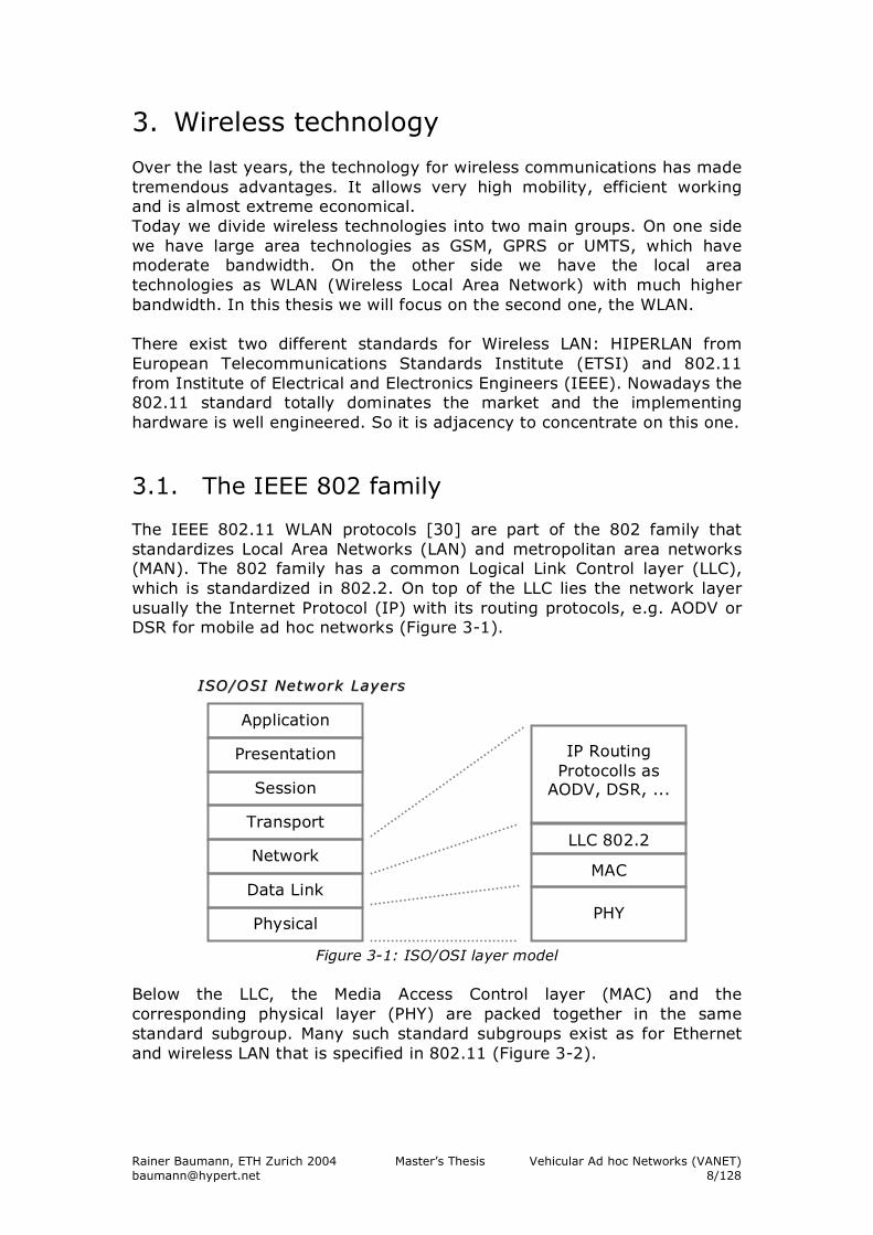
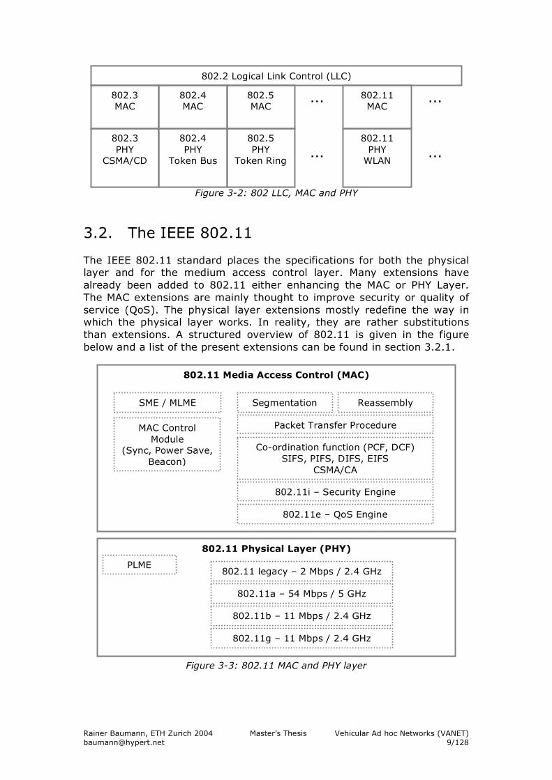
3.1. The IEEE 802 family The IEEE 802.11 WLAN protocols [30] are part of the 802 family that standardizes Local Area Networks (LAN) and metropolitan area networks (MAN). The 802 family has a common Logical Link Control layer (LLC), which is standardized in 802.2. On top of the LLC lies the network layer usually the Internet Protocol (IP) with its routing protocols, e.g. AODV or DSR for mobile ad hoc networks (Figure 3-1).
Figure 3-1: ISO/OSI layer model Below the LLC, the Media Access Control layer (MAC) and the corresponding physical layer (PHY) are packed together in the same standard subgroup. Many such standard subgroups exist as for Ethernet and wireless LAN that is specified in 802.11 (Figure 3-2).
Application
Presentation
Session
Transport
Network
Data Link
Physical
ISO/OSI Network LayersISO/OSI Network Layers
PHY
LLC 802.2
MAC
IP Routing Protocolls as
AODV, DSR, ...
Rainer Baumann, ETH Zurich 2004 Master’s Thesis Vehicular Ad hoc Networks (VANET) [email protected] 9/128
Figure 3-2: 802 LLC, MAC and PHY
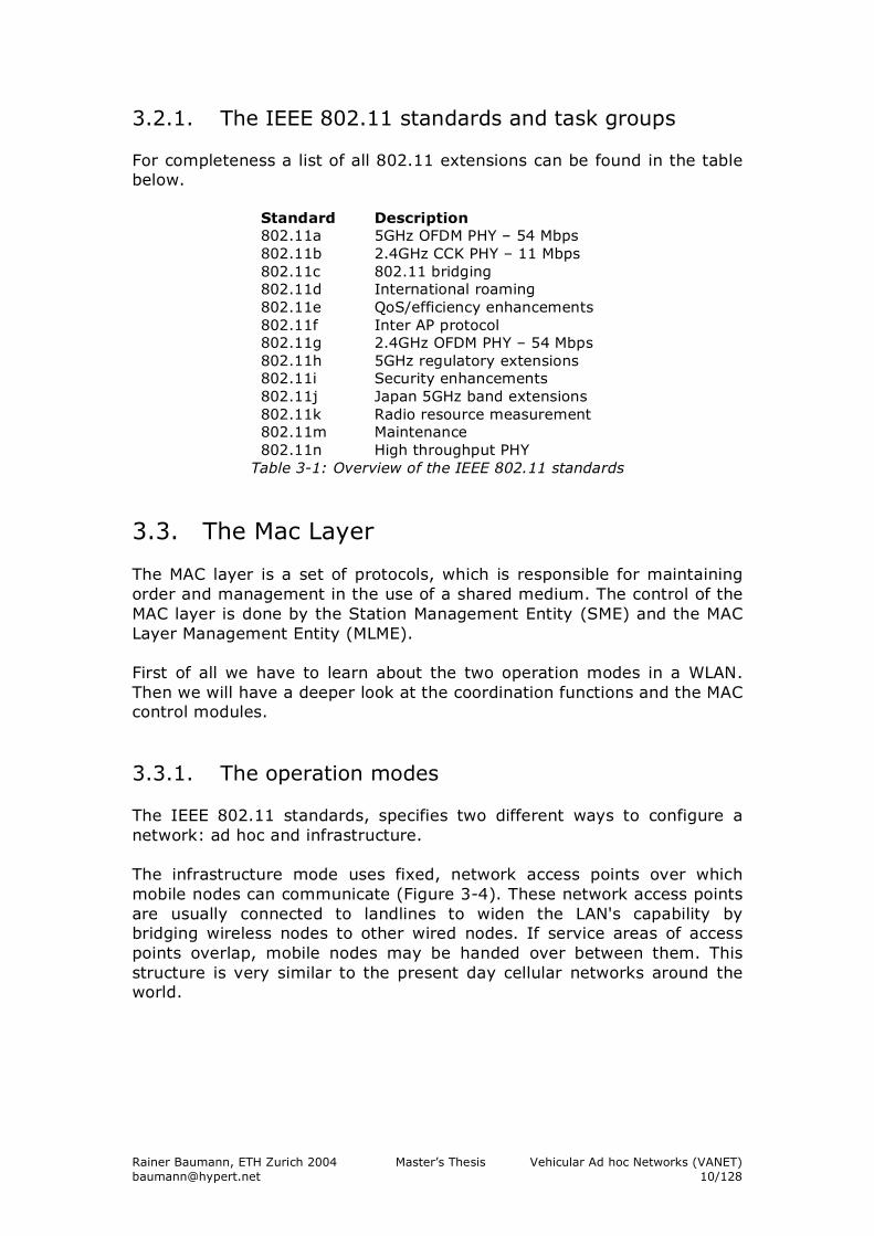
3.2. The IEEE 802.11 The IEEE 802.11 standard places the specifications for both the physical layer and for the medium access control layer. Many extensions have already been added to 802.11 either enhancing the MAC or PHY Layer. The MAC extensions are mainly thought to improve security or quality of service (QoS). The physical layer extensions mostly redefine the way in which the physical layer works. In reality, they are rather substitutions than extensions. A structured overview of 802.11 is given in the figure below and a list of the present extensions can be found in section 3.2.1.
Figure 3-3: 802.11 MAC and PHY layer
802.11 Media Access Control (MAC)
802.11 Physical Layer (PHY)
802.11a – 54 Mbps / 5 GHz
802.11b – 11 Mbps / 2.4 GHz
802.11g – 11 Mbps / 2.4 GHz
802.11 legacy – 2 Mbps / 2.4 GHz
802.11i – Security Engine
802.11e – QoS Engine
Packet Transfer Procedure
Co-ordination function (PCF, DCF) SIFS, PIFS, DIFS, EIFS
CSMA/CA
SME / MLME
MAC Control Module
(Sync, Power Save, Beacon)
PLME
Segmentation Reassembly
802.2 Logical Link Control (LLC)
802.3 MAC
802.3 PHY
CSMA/CD
802.4 MAC
802.4 PHY
Token Bus
802.5 PHY
Token Ring
802.11 PHY
WLAN
802.5 MAC
802.11 MAC
...
...
...
...
Rainer Baumann, ETH Zurich 2004 Master’s Thesis Vehicular Ad hoc Networks (VANET) [email protected] 10/128
3.2.1. The IEEE 802.11 standards and task groups For completeness a list of all 802.11 extensions can be found in the table below.
Standard Description 802.11a 5GHz OFDM PHY – 54 Mbps 802.11b 2.4GHz CCK PHY – 11 Mbps 802.11c 802.11 bridging 802.11d International roaming 802.11e QoS/efficiency enhancements 802.11f Inter AP protocol 802.11g 2.4GHz OFDM PHY – 54 Mbps 802.11h 5GHz regulatory extensions 802.11i Security enhancements 802.11j Japan 5GHz band extensions 802.11k Radio resource measurement 802.11m Maintenance 802.11n High throughput PHY
Table 3-1: Overview of the IEEE 802.11 standards
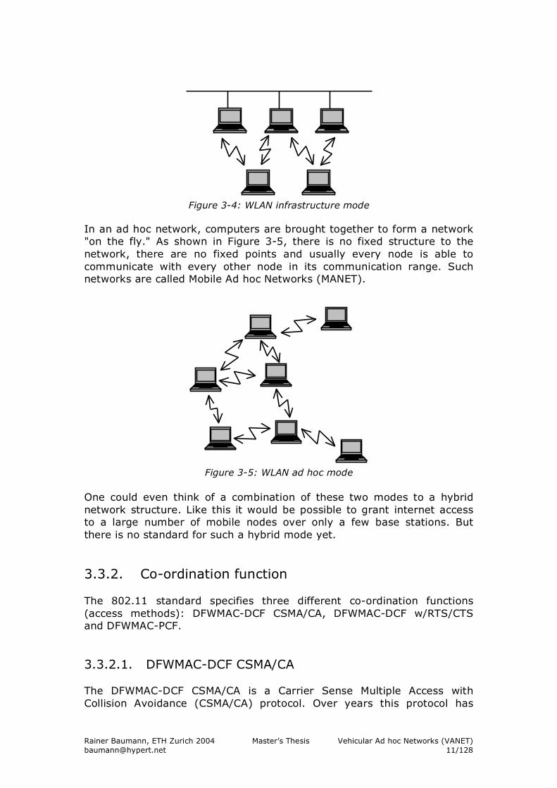
3.3. The Mac Layer The MAC layer is a set of protocols, which is responsible for maintaining order and management in the use of a shared medium. The control of the MAC layer is done by the Station Management Entity (SME) and the MAC Layer Management Entity (MLME). First of all we have to learn about the two operation modes in a WLAN. Then we will have a deeper look at the coordination functions and the MAC control modules. 3.3.1. The operation modes The IEEE 802.11 standards, specifies two different ways to configure a network: ad hoc and infrastructure. The infrastructure mode uses fixed, network access points over which mobile nodes can communicate (Figure 3-4). These network access points are usually connected to landlines to widen the LAN's capability by bridging wireless nodes to other wired nodes. If service areas of access points overlap, mobile nodes may be handed over between them. This structure is very similar to the present day cellular networks around the world.
Rainer Baumann, ETH Zurich 2004 Master’s Thesis Vehicular Ad hoc Networks (VANET) [email protected] 11/128
Figure 3-4: WLAN infrastructure mode
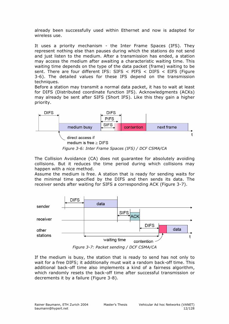
In an ad hoc network, computers are brought together to form a network "on the fly." As shown in Figure 3-5, there is no fixed structure to the network, there are no fixed points and usually every node is able to communicate with every other node in its communication range. Such networks are called Mobile Ad hoc Networks (MANET).
Figure 3-5: WLAN ad hoc mode One could even think of a combination of these two modes to a hybrid network structure. Like this it would be possible to grant internet access to a large number of mobile nodes over only a few base stations. But there is no standard for such a hybrid mode yet. 3.3.2. Co-ordination function The 802.11 standard specifies three different co-ordination functions (access methods): DFWMAC-DCF CSMA/CA, DFWMAC-DCF w/RTS/CTS and DFWMAC-PCF. 3.3.2.1. DFWMAC-DCF CSMA/CA The DFWMAC-DCF CSMA/CA is a Carrier Sense Multiple Access with Collision Avoidance (CSMA/CA) protocol. Over years this protocol has
Rainer Baumann, ETH Zurich 2004 Master’s Thesis Vehicular Ad hoc Networks (VANET) [email protected] 12/128
already been successfully used within Ethernet and now is adapted for wireless use. It uses a priority mechanism - the Inter Frame Spaces (IFS). They represent nothing else than pauses during which the stations do not send and just listen to the medium. After a transmission has ended, a station may access the medium after awaiting a characteristic waiting time. This waiting time depends on the type of the data packet (frame) waiting to be sent. There are four different IFS: SIFS < PIFS < DIFS < EIFS (Figure 3-6). The detailed values for these IFS depend on the transmission techniques. Before a station may transmit a normal data packet, it has to wait at least for DIFS (Distributed coordinate function IFS). Acknowledgments (ACKs) may already be sent after SIFS (Short IFS). Like this they gain a higher priority.
Figure 3-6: Inter Frame Spaces (IFS) / DCF CSMA/CA
The Collision Avoidance (CA) does not guarantee for absolutely avoiding collisions. But it reduces the time period during which collisions may happen with a nice method. Assume the medium is free. A station that is ready for sending waits for the minimal time specified by the DIFS and then sends its data. The receiver sends after waiting for SIFS a corresponding ACK (Figure 3-7).
Figure 3-7: Packet sending / DCF CSMA/CA
If the medium is busy, the station that is ready to send has not only to wait for a free DIFS; it additionally must wait a random back-off time. This additional back-off time also implements a kind of a fairness algorithm, which randomly resets the back-off time after successful transmission or decrements it by a failure (Figure 3-8).
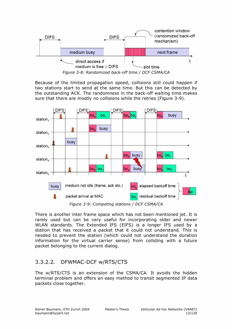
Rainer Baumann, ETH Zurich 2004 Master’s Thesis Vehicular Ad hoc Networks (VANET) [email protected] 13/128
Figure 3-8: Randomized back-off time / DCF CSMA/CA
Because of the limited propagation speed, collisions still could happen if two stations start to send at the same time. But this can be detected by the outstanding ACK. The randomness in the back-off waiting time makes sure that there are mostly no collisions while the retries (Figure 3-9).
Figure 3-9: Competing stations / DCF CSMA/CA
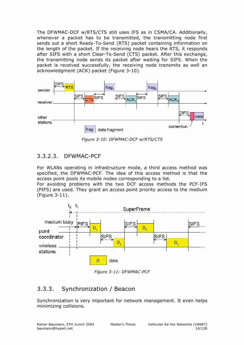
There is another inter frame space which has not been mentioned jet. It is rarely used but can be very useful for incorporating older and newer WLAN standards. The Extended IFS (EIFS) is a longer IFS used by a station that has received a packet that it could not understand. This is needed to prevent the station (which could not understand the duration information for the virtual carrier sense) from colliding with a future packet belonging to the current dialog. 3.3.2.2. DFWMAC-DCF w/RTS/CTS The w/RTS/CTS is an extension of the CSMA/CA. It avoids the hidden terminal problem and offers an easy method to transit segmented IP data packets close together.
Rainer Baumann, ETH Zurich 2004 Master’s Thesis Vehicular Ad hoc Networks (VANET) [email protected] 14/128
The DFWMAC-DCF w/RTS/CTS still uses IFS as in CSMA/CA. Additionally, whenever a packet has to be transmitted, the transmitting node first sends out a short Ready-To-Send (RTS) packet containing information on the length of the packet. If the receiving node hears the RTS, it responds after SIFS with a short Clear-To-Send (CTS) packet. After this exchange, the transmitting node sends its packet after waiting for SIFS. When the packet is received successfully, the receiving node transmits as well an acknowledgment (ACK) packet (Figure 3-10).
Figure 3-10: DFWMAC-DCF w/RTS/CTS
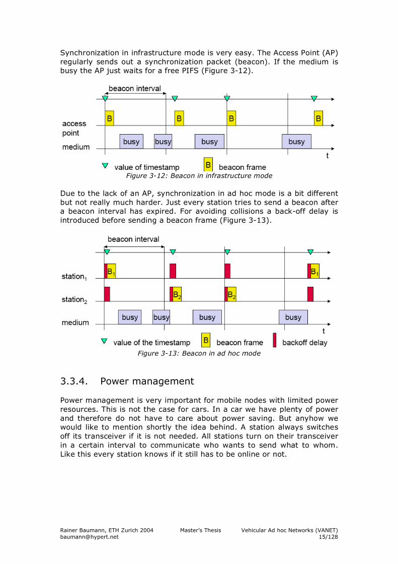
3.3.2.3. DFWMAC-PCF For WLANs operating in infrastructure mode, a third access method was specified, the DFWMAC-PCF. The idea of this access method is that the access point pools its mobile nodes corresponding to a list. For avoiding problems with the two DCF access methods the PCF-IFS (PIFS) are used. They grant an access point priority access to the medium (Figure 3-11).
Figure 3-11: DFWMAC-PCF
3.3.3. Synchronization / Beacon Synchronization is very important for network management. It even helps minimizing collisions.
Rainer Baumann, ETH Zurich 2004 Master’s Thesis Vehicular Ad hoc Networks (VANET) [email protected] 15/128
Synchronization in infrastructure mode is very easy. The Access Point (AP) regularly sends out a synchronization packet (beacon). If the medium is busy the AP just waits for a free PIFS (Figure 3-12).
Figure 3-12: Beacon in infrastructure mode
Due to the lack of an AP, synchronization in ad hoc mode is a bit different but not really much harder. Just every station tries to send a beacon after a beacon interval has expired. For avoiding collisions a back-off delay is introduced before sending a beacon frame (Figure 3-13).
Figure 3-13: Beacon in ad hoc mode
3.3.4. Power management Power management is very important for mobile nodes with limited power resources. This is not the case for cars. In a car we have plenty of power and therefore do not have to care about power saving. But anyhow we would like to mention shortly the idea behind. A station always switches off its transceiver if it is not needed. All stations turn on their transceiver in a certain interval to communicate who wants to send what to whom. Like this every station knows if it still has to be online or not.
Rainer Baumann, ETH Zurich 2004 Master’s Thesis Vehicular Ad hoc Networks (VANET) [email protected] 16/128
3.4. The PHY Layer The physical layer itself can again be divided into two parts: the Physical Layer Convergence Protocol (PLCP) and the Physical Medium Dependent (PMD). Responsible for the control of these sublayers is the Physical Layer Management Entity (PLME). The PLCP provides a method for mapping the MAC sublayer protocol data Units (MPDU) into a framing format suitable for sending and receiving data and management information using the associated PMD system. Beside it is also responsible for carrier sensing, clear channel assessment and basic error correction. The PMD interacts directly with the physical medium and performs the most basic bit transmission functions of the network. It is mainly responsible for encoding and modulation. For making the signal less vulnerable to narrowband interference and frequency dependent fading, spread spectrum technologies are used. They spread the narrow band signal into a broadband signal using a special code. In older systems Frequency Hopping Spread Spectrum (FHSS) has been used while in newer Direct Sequence Spread Spectrum (DSSS) or Orthogonal Frequency Division Modulation (OFDM) is implemented [10] [8]. At the moment there are four physical layers specified in IEEE 802.11: 802.11 legacy was the original one. With 802.11b the story of success for 802.11 began. It was the first widely accepted wireless networking standard, followed, paradoxically, by 802.11a and 802.11g.
3.4.1. 802.11 legacy The original version of the standard IEEE 802.11 released in 1997 and sometimes called "802.11 legacy" specifies two data rates of 1 and 2 megabits per second (Mbps) to be transmitted via infrared (IR) signals or in the Industrial, Scientific and Medical (ISM) band at 2.4 GHz. IR has been dropped from later revisions of the standard, because it could not succeed against the well established IrDA protocol and had no known implementations. For encoding Differential Phase Shift Keying (DPSK, for 1Mbps) and Differential Quaternary Phase Shift Keying (DQPSK, for 2Mbps) are used. Legacy 802.11 was rapidly succeeded by 802.11b.
3.4.2. 802.11b 802.11b has a range up to several hundreds meters with the low-gain omni directional antennas typically used in 802.11b devices. 802.11b has a maximum throughput of 11 Mbps, however a significant percentage of this bandwidth is used for communication overhead; in practice the maximum throughput is about 5.5 Mbps. For this extension the CCK (Complementary Code Keying) encoding is used.
Rainer Baumann, ETH Zurich 2004 Master’s Thesis Vehicular Ad hoc Networks (VANET) [email protected] 17/128
Extensions have been made to the 802.11b protocol in order to increase speed to 22, 33, and 44 Mbps, but the extensions are proprietary and not endorsed by the IEEE. Many companies call enhanced versions "802.11b+". 3.4.3. 802.11a In 2001 a faster relative started shipping, 802.11a, even though the standard was already ratified in 1999. The 802.11a standard uses the 5 GHz band, and operates at a raw speed of 54 Mbps, and more realistic speeds in the mid-20 Mbps. The speed is reduced to 48, 36, 34, 18, 12, 9 then 6 Mbps if required. 802.11a has 12 nonoverlapping channels, 8 dedicated to indoor and 4 channels dedicated to point-to-point usage. Different countries have different ideas about support, although a 2003 World Radiotelecommunciations Conference made it easier for use worldwide. A mid-2003 FCC decision may open more spectrums to 802.11a channels as well. The major problem in Europe is that most frequencies in the 5 GHz band are assigned to the military or to radar applications. 802.11a has not seen wide adoption because of the high adoption rate of 802.11b, and concerns about range: at 5 GHz, 802.11a cannot reach as far with the same power limitations, and may be absorbed more readily. We will come back to this later on in section 3.6.
3.4.4. 802.11g In June 2003, a third extension to the physical layer was ratified: 802.11g. This flavor works in the 2.4 GHz band like 802.11b, but operates at up to 54 Mbps raw or about 24.7 Mbps net throughput and a range comparable to 802.11b. It is fully backwards compatible with 802.11b. Details of making b and g work together occupied much of the time required for the standardization process. The 802.11g standard swept the consumer world of early adopters starting in January 2003, well before ratification. The corporate users held back and Cisco and other big equipment makers waited until ratification. By summer 2003, announcements were flourishing. Today hardware supporting 802.11g is available almost from all manufacturers. Also some extensions have already been made to the 802.11g protocol in order to increase speed to 108 Mbps and ranges up to 300 meters (Atheros Super G/802.11g+) [25] [27].
Rainer Baumann, ETH Zurich 2004 Master’s Thesis Vehicular Ad hoc Networks (VANET) [email protected] 18/128
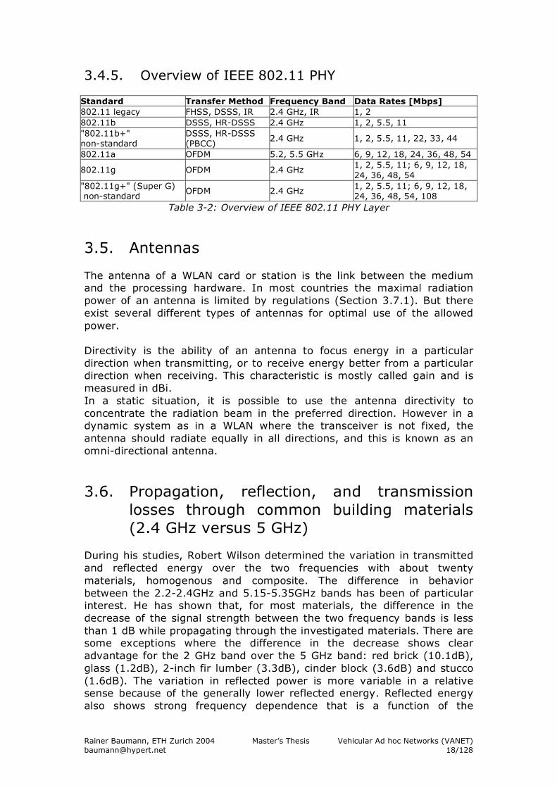
3.4.5. Overview of IEEE 802.11 PHY
Standard Transfer Method Frequency Band Data Rates [Mbps] 802.11 legacy FHSS, DSSS, IR 2.4 GHz, IR 1, 2 802.11b DSSS, HR-DSSS 2.4 GHz 1, 2, 5.5, 11 "802.11b+" non-standard
DSSS, HR-DSSS (PBCC)
2.4 GHz 1, 2, 5.5, 11, 22, 33, 44
802.11a OFDM 5.2, 5.5 GHz 6, 9, 12, 18, 24, 36, 48, 54
802.11g OFDM 2.4 GHz 1, 2, 5.5, 11; 6, 9, 12, 18, 24, 36, 48, 54
"802.11g+" (Super G) non-standard
OFDM 2.4 GHz 1, 2, 5.5, 11; 6, 9, 12, 18, 24, 36, 48, 54, 108
Table 3-2: Overview of IEEE 802.11 PHY Layer
3.5. Antennas The antenna of a WLAN card or station is the link between the medium and the processing hardware. In most countries the maximal radiation power of an antenna is limited by regulations (Section 3.7.1). But there exist several different types of antennas for optimal use of the allowed power. Directivity is the ability of an antenna to focus energy in a particular direction when transmitting, or to receive energy better from a particular direction when receiving. This characteristic is mostly called gain and is measured in dBi. In a static situation, it is possible to use the antenna directivity to concentrate the radiation beam in the preferred direction. However in a dynamic system as in a WLAN where the transceiver is not fixed, the antenna should radiate equally in all directions, and this is known as an omni-directional antenna.
3.6. Propagation, reflection, and transmission losses through common building materials (2.4 GHz versus 5 GHz)
During his studies, Robert Wilson determined the variation in transmitted and reflected energy over the two frequencies with about twenty materials, homogenous and composite. The difference in behavior between the 2.2-2.4GHz and 5.15-5.35GHz bands has been of particular interest. He has shown that, for most materials, the difference in the decrease of the signal strength between the two frequency bands is less than 1 dB while propagating through the investigated materials. There are some exceptions where the difference in the decrease shows clear advantage for the 2 GHz band over the 5 GHz band: red brick (10.1dB), glass (1.2dB), 2-inch fir lumber (3.3dB), cinder block (3.6dB) and stucco (1.6dB). The variation in reflected power is more variable in a relative sense because of the generally lower reflected energy. Reflected energy also shows strong frequency dependence that is a function of the
Rainer Baumann, ETH Zurich 2004 Master’s Thesis Vehicular Ad hoc Networks (VANET) [email protected] 19/128
thickness of the sample, as well as its permittivity. Concluding one can say that the 2.4 GHz band has clear advantages over the 5 GHz band [5] [6].
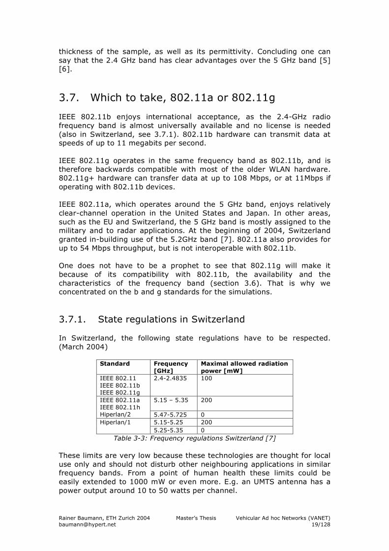
3.7. Which to take, 802.11a or 802.11g IEEE 802.11b enjoys international acceptance, as the 2.4-GHz radio frequency band is almost universally available and no license is needed (also in Switzerland, see 3.7.1). 802.11b hardware can transmit data at speeds of up to 11 megabits per second. IEEE 802.11g operates in the same frequency band as 802.11b, and is therefore backwards compatible with most of the older WLAN hardware. 802.11g+ hardware can transfer data at up to 108 Mbps, or at 11Mbps if operating with 802.11b devices. IEEE 802.11a, which operates around the 5 GHz band, enjoys relatively clear-channel operation in the United States and Japan. In other areas, such as the EU and Switzerland, the 5 GHz band is mostly assigned to the military and to radar applications. At the beginning of 2004, Switzerland granted in-building use of the 5.2GHz band [7]. 802.11a also provides for up to 54 Mbps throughput, but is not interoperable with 802.11b. One does not have to be a prophet to see that 802.11g will make it because of its compatibility with 802.11b, the availability and the characteristics of the frequency band (section 3.6). That is why we concentrated on the b and g standards for the simulations. 3.7.1. State regulations in Switzerland In Switzerland, the following state regulations have to be respected. (March 2004)
Standard Frequency [GHz]
Maximal allowed radiation power [mW]
IEEE 802.11 IEEE 802.11b IEEE 802.11g
2.4-2.4835 100
5.15 – 5.35
200
IEEE 802.11a IEEE 802.11h Hiperlan/2 5.47-5.725 0
5.15-5.25 200 Hiperlan/1 5.25-5.35 0
Table 3-3: Frequency regulations Switzerland [7] These limits are very low because these technologies are thought for local use only and should not disturb other neighbouring applications in similar frequency bands. From a point of human health these limits could be easily extended to 1000 mW or even more. E.g. an UMTS antenna has a power output around 10 to 50 watts per channel.
Rainer Baumann, ETH Zurich 2004 Master’s Thesis Vehicular Ad hoc Networks (VANET) [email protected] 20/128
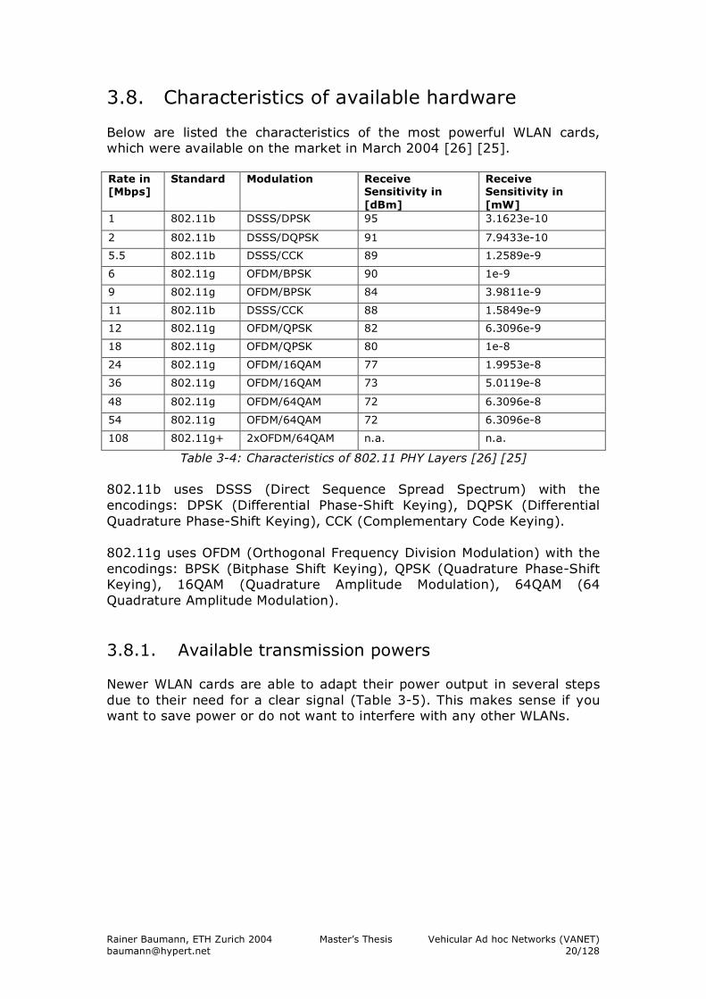
3.8. Characteristics of available hardware Below are listed the characteristics of the most powerful WLAN cards, which were available on the market in March 2004 [26] [25]. Rate in [Mbps]
Standard Modulation Receive Sensitivity in [dBm]
Receive Sensitivity in [mW]
1 802.11b DSSS/DPSK 95 3.1623e-10
2 802.11b DSSS/DQPSK 91 7.9433e-10
5.5 802.11b DSSS/CCK 89 1.2589e-9
6 802.11g OFDM/BPSK 90 1e-9
9 802.11g OFDM/BPSK 84 3.9811e-9
11 802.11b DSSS/CCK 88 1.5849e-9
12 802.11g OFDM/QPSK 82 6.3096e-9
18 802.11g OFDM/QPSK 80 1e-8
24 802.11g OFDM/16QAM 77 1.9953e-8
36 802.11g OFDM/16QAM 73 5.0119e-8
48 802.11g OFDM/64QAM 72 6.3096e-8
54 802.11g OFDM/64QAM 72 6.3096e-8
108 802.11g+ 2xOFDM/64QAM n.a. n.a.
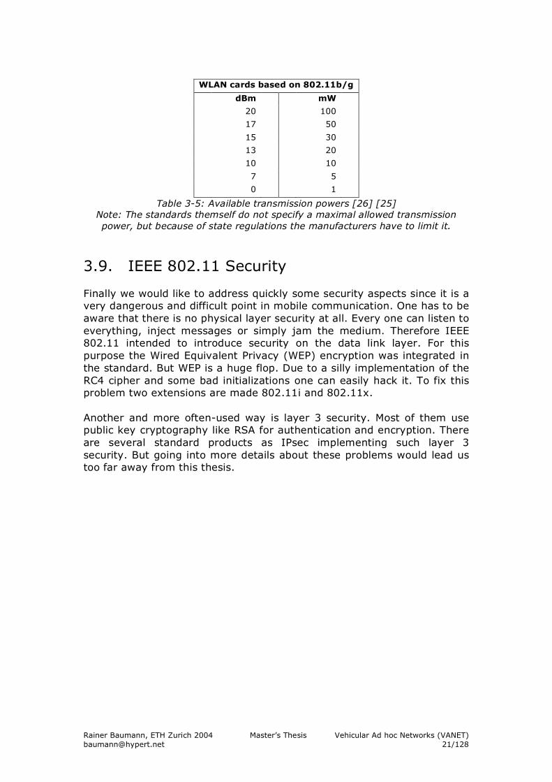
Table 3-4: Characteristics of 802.11 PHY Layers [26] [25] 802.11b uses DSSS (Direct Sequence Spread Spectrum) with the encodings: DPSK (Differential Phase-Shift Keying), DQPSK (Differential Quadrature Phase-Shift Keying), CCK (Complementary Code Keying). 802.11g uses OFDM (Orthogonal Frequency Division Modulation) with the encodings: BPSK (Bitphase Shift Keying), QPSK (Quadrature Phase-Shift Keying), 16QAM (Quadrature Amplitude Modulation), 64QAM (64 Quadrature Amplitude Modulation). 3.8.1. Available transmission powers Newer WLAN cards are able to adapt their power output in several steps due to their need for a clear signal (Table 3-5). This makes sense if you want to save power or do not want to interfere with any other WLANs.
Rainer Baumann, ETH Zurich 2004 Master’s Thesis Vehicular Ad hoc Networks (VANET) [email protected] 21/128
WLAN cards based on 802.11b/g
dBm mW
20 100
17 50
15 30
13 20
10 10
7 5
0 1
Table 3-5: Available transmission powers [26] [25] Note: The standards themself do not specify a maximal allowed transmission power, but because of state regulations the manufacturers have to limit it.
3.9. IEEE 802.11 Security Finally we would like to address quickly some security aspects since it is a very dangerous and difficult point in mobile communication. One has to be aware that there is no physical layer security at all. Every one can listen to everything, inject messages or simply jam the medium. Therefore IEEE 802.11 intended to introduce security on the data link layer. For this purpose the Wired Equivalent Privacy (WEP) encryption was integrated in the standard. But WEP is a huge flop. Due to a silly implementation of the RC4 cipher and some bad initializations one can easily hack it. To fix this problem two extensions are made 802.11i and 802.11x. Another and more often-used way is layer 3 security. Most of them use public key cryptography like RSA for authentication and encryption. There are several standard products as IPsec implementing such layer 3 security. But going into more details about these problems would lead us too far away from this thesis.
Rainer Baumann, ETH Zurich 2004 Master’s Thesis Vehicular Ad hoc Networks (VANET) [email protected] 22/128
4. Ad hoc On demand Distance Vector routing protocol (AODV)
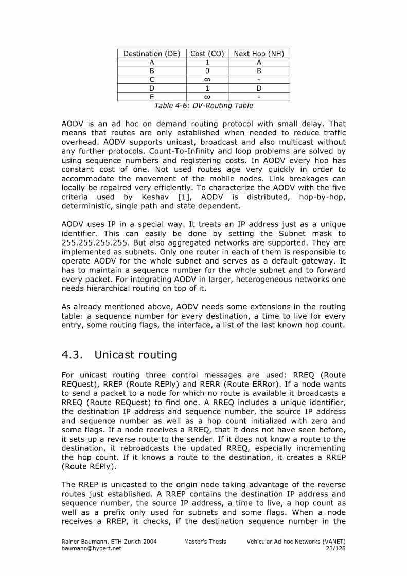
4.1. Mobile ad hoc routing protocols There exist hundreds of routing protocols for many different purposes. Mobile ad hoc routing protocols are very specialized in their task. There are two main characteristics to distinguish them. The first characteristic is when they gather their routing information. On one hand we have the proactive (table driven) protocols, which always try to have complete, up-to-date routing information. This automatically implies a certain overhead, which dramatically increases with high mobility. On the other hand we have the group of reactive (on demand) protocols, which only try to gather routing information when it is needed. The second characteristic is how they route data towards the destination. We distinguish here the destination based (link state) protocols from the topology based (distance vector). In a destination based protocol a node knows all details about the used routes. It includes the complete information about the routing path in every sent data packet. In a topology based protocol a node knows only about its neighbors and the next hop toward a destination. Like this a data packet only has to carry the destination address. This can be an important advantage for large networks with long routes. When we think of our inter vehicle communication scenario, we have to face high mobility and large networks. The best combination for this situation would be an on demand topology based routing protocol.
4.2. Introduction In November 2001 the MANET (Mobile Ad hoc Networks) Working Group for routing of the Internet Engineering Task Force (IEFT) community published the first version of the AODV routing protocol (Ad hoc On demand Distance Vector) [5]. In July 2003 the latest draft was published under the number RFC3561 [29]. AODV belongs to the class of Distance Vector routing protocols (DV). In a DV every node knows its neighbors and the costs to reach them. A node maintains its own routing table, storing all nodes in the network, the distance and the next hop to them. Such a routing table is shown in Table 4-6. If a node is not reachable, the distance to it is set to infinity. Every node periodically sends its whole routing table to its neighbors. So they can check if there is a useful route to another node using this neighbor as next hop. When a link breaks, a misbehavior called Count-To-Infinity may occur.
Rainer Baumann, ETH Zurich 2004 Master’s Thesis Vehicular Ad hoc Networks (VANET) [email protected] 23/128
Destination (DE) Cost (CO) Next Hop (NH) A 1 A B 0 B C ∞ - D 1 D E ∞ -
Table 4-6: DV-Routing Table AODV is an ad hoc on demand routing protocol with small delay. That means that routes are only established when needed to reduce traffic overhead. AODV supports unicast, broadcast and also multicast without any further protocols. Count-To-Infinity and loop problems are solved by using sequence numbers and registering costs. In AODV every hop has constant cost of one. Not used routes age very quickly in order to accommodate the movement of the mobile nodes. Link breakages can locally be repaired very efficiently. To characterize the AODV with the five criteria used by Keshav [1], AODV is distributed, hop-by-hop, deterministic, single path and state dependent. AODV uses IP in a special way. It treats an IP address just as a unique identifier. This can easily be done by setting the Subnet mask to 255.255.255.255. But also aggregated networks are supported. They are implemented as subnets. Only one router in each of them is responsible to operate AODV for the whole subnet and serves as a default gateway. It has to maintain a sequence number for the whole subnet and to forward every packet. For integrating AODV in larger, heterogeneous networks one needs hierarchical routing on top of it. As already mentioned above, AODV needs some extensions in the routing table: a sequence number for every destination, a time to live for every entry, some routing flags, the interface, a list of the last known hop count.
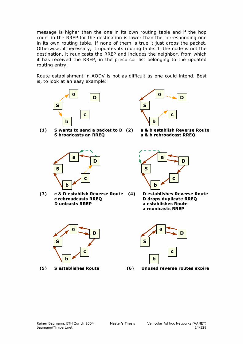
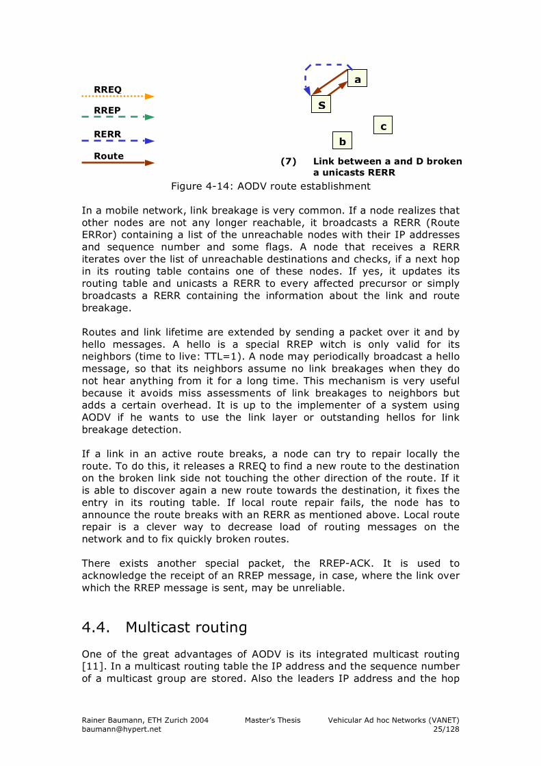
4.3. Unicast routing For unicast routing three control messages are used: RREQ (Route REQuest), RREP (Route REPly) and RERR (Route ERRor). If a node wants to send a packet to a node for which no route is available it broadcasts a RREQ (Route REQuest) to find one. A RREQ includes a unique identifier, the destination IP address and sequence number, the source IP address and sequence number as well as a hop count initialized with zero and some flags. If a node receives a RREQ, that it does not have seen before, it sets up a reverse route to the sender. If it does not know a route to the destination, it rebroadcasts the updated RREQ, especially incrementing the hop count. If it knows a route to the destination, it creates a RREP (Route REPly). The RREP is unicasted to the origin node taking advantage of the reverse routes just established. A RREP contains the destination IP address and sequence number, the source IP address, a time to live, a hop count as well as a prefix only used for subnets and some flags. When a node receives a RREP, it checks, if the destination sequence number in the
Rainer Baumann, ETH Zurich 2004 Master’s Thesis Vehicular Ad hoc Networks (VANET) [email protected] 24/128
message is higher than the one in its own routing table and if the hop count in the RREP for the destination is lower than the corresponding one in its own routing table. If none of them is true it just drops the packet. Otherwise, if necessary, it updates its routing table. If the node is not the destination, it reunicasts the RREP and includes the neighbor, from which it has received the RREP, in the precursor list belonging to the updated routing entry. Route establishment in AODV is not as difficult as one could intend. Best is, to look at an easy example:
S
b
c
a D
(1) S wants to send a packet to D S broadcasts an RREQ
(2) a & b establish Reverse Route a & b rebroadcast RREQ
S
b
c
a D
S
b c
a D
(3) c & D establish Reverse Route c rebroadcasts RREQ D unicasts RREP
S
b c
a D
(4) D establishes Reverse Route D drops duplicate RREQ a establishes Route a reunicasts RREP
S
b
c
a D
(5) S establishes Route
S
b
c
a D
(6) Unused reverse routes expire
Rainer Baumann, ETH Zurich 2004 Master’s Thesis Vehicular Ad hoc Networks (VANET) [email protected] 25/128
Figure 4-14: AODV route establishment In a mobile network, link breakage is very common. If a node realizes that other nodes are not any longer reachable, it broadcasts a RERR (Route ERRor) containing a list of the unreachable nodes with their IP addresses and sequence number and some flags. A node that receives a RERR iterates over the list of unreachable destinations and checks, if a next hop in its routing table contains one of these nodes. If yes, it updates its routing table and unicasts a RERR to every affected precursor or simply broadcasts a RERR containing the information about the link and route breakage. Routes and link lifetime are extended by sending a packet over it and by hello messages. A hello is a special RREP witch is only valid for its neighbors (time to live: TTL=1). A node may periodically broadcast a hello message, so that its neighbors assume no link breakages when they do not hear anything from it for a long time. This mechanism is very useful because it avoids miss assessments of link breakages to neighbors but adds a certain overhead. It is up to the implementer of a system using AODV if he wants to use the link layer or outstanding hellos for link breakage detection. If a link in an active route breaks, a node can try to repair locally the route. To do this, it releases a RREQ to find a new route to the destination on the broken link side not touching the other direction of the route. If it is able to discover again a new route towards the destination, it fixes the entry in its routing table. If local route repair fails, the node has to announce the route breaks with an RERR as mentioned above. Local route repair is a clever way to decrease load of routing messages on the network and to fix quickly broken routes. There exists another special packet, the RREP-ACK. It is used to acknowledge the receipt of an RREP message, in case, where the link over which the RREP message is sent, may be unreliable.
4.4. Multicast routing One of the great advantages of AODV is its integrated multicast routing [11]. In a multicast routing table the IP address and the sequence number of a multicast group are stored. Also the leaders IP address and the hop
RREQ
RREP
Route
S
b c
a
(7) Link between a and D broken a unicasts RERR
RERR
Rainer Baumann, ETH Zurich 2004 Master’s Thesis Vehicular Ad hoc Networks (VANET) [email protected] 26/128
count to him are stored as well as the next hop in the multicasting tree and the lifetime of the entry. To join a multicast group a node has to send an RREQ to the group address with the join flag set. Any node in the multicast tree, which receives the RREQ, can answer with a RREP. Like this, a requester could receive several RREP from which he can choose the one with the shortest distance to the group. A MACT (Multicast ACTivation) Message is send to the chosen tree node to activate this branch. If a requester does not receive a RREP, the node supposes, that there exists no multicast tree for this group in this network segment and it becomes the group leader. A multicast RREP contains additional the IP of the group leader and the hop count to the next group member. The group leader periodically broadcasts a group hello message (a RREP) and increments each time the sequence number of the group. When two networks segments become connected, two partitioned group trees have to be connected. Every group member receiving two group hello messages from different leaders will detect a tree connection. Then this node emits an RREQ with the repair flag set to the group. If a node in the group tree does not receive any group hello or other group message, it has to repair the group tree with a RREQ and has to ensure, that not a RREP from a node in its own sub tree is chosen. If a group member wants to leave the group and it is a leaf, it can prune the branch with a MACT and the flag prune set. If it is not a leaf, it must continue to serve as a tree member. A good tutorial to AODV multicasting can be found in [11].
4.5. Security AODV defines no special security mechanisms. So an impersonation attack can easily be done. Or even simpler, a misbehaving node is planted in the network. There are a few proposals how to solve this problem, but it is very hard because AODV is not a source based routing protocol and such a solution would introduce a tremendous overhead [28].
4.6. Implementations There are two types of different implementations, user space daemons and kernel modules. The first implementation requires to maintain an own routing table and was first implemented in the Mad hoc Implementation [36] by Fredrik Lilieblad, Oskar Mattsson, Petra Nylund, Dan Ouchterlony, Anders Roxenhag running on a Linux 2.2 kernel but does not supports multicast. A bit later the University of Uppsala published user space daemon implementation called AODV-UU [37], which runs fairly well on Linux with a 2.4 kernel. Today many different implementations of AODV exist [35].
Rainer Baumann, ETH Zurich 2004 Master’s Thesis Vehicular Ad hoc Networks (VANET) [email protected] 27/128
5. Network Simulator – NS-2
5.1. About NS-2 NS-2 is an open-source simulation tool running on Unix-like operating systems [33]. It is a discreet event simulator targeted at networking research and provides substantial support for simulation of routing, multicast protocols and IP protocols, such as UDP, TCP, RTP and SRM over wired, wireless and satellite networks. It has many advantages that make it a useful tool, such as support for multiple protocols and the capability of graphically detailing network traffic. Additionally, NS-2 supports several algorithms in routing and queuing. LAN routing and broadcasts are part of routing algorithms. Queuing algorithm includes fair queuing, deficit round robin and FIFO. NS-2 started as a variant of the REAL network simulator in 1989 [38]. REAL is a network simulator originally intended for studying the dynamic behavior of flow and congestion control schemes in packet-switched data networks. In 1995 ns development was supported by Defense Advanced Research Projects Agency DARPA through the VINT project at LBL, Xerox PARC, UCB, and USC/ISI. The wireless code from the UCB Daedelus and CMU Monarch projects and Sun Microsystems have added the wireless capabilities to ns-2. Valery Naumov proposed a list-based improvement for ns-2 involving maintaining a double linked list to organize mobile nodes based on their X-coordinates. When sending a packet, only those neighbor nodes are considered, which are within a circle corresponding to the carrier-sense threshold energy level, below which a node cannot hear the packet. Compared to the original version, where all nodes in the topology are considered, its considerable gain in run-time, performance goes down by about 4 to 20 times, depending on the size of the topology. The larger the topology and greater the number of nodes, the greater is the improvement seen with the list-based implementation [2]. NS-2 is available on several platforms such as FreeBSD, Linux, SunOS and Solaris. NS-2 also builds and runs under Windows with Cygwin. Simple scenarios should run on any reasonable machine; however, very large scenarios benefit from large amounts of memory and fast CPU’s.
5.2. NS-2, implementing languages NS-2 is basically written in C++, with an OTcl (Object Tool Command Language) interpreter as a front-end. It supports a class hierarchy in C++, called compiled hierarchy and a similar one within the OTcl interpreter, called interpreter hierarchy. Some objects are completely implemented in C++, some others in OTcl and some are implemented in
Rainer Baumann, ETH Zurich 2004 Master’s Thesis Vehicular Ad hoc Networks (VANET) [email protected] 28/128
both. For them, there is a one-to-one correspondence between classes of the two hierarchies. But why should one use two languages? The simulator can be viewed as doing 2 different things. While on one hand detailed simulations of protocols are required, we also need to be able to vary the parameters or configurations and quickly explore the changing scenarios. For the first case we need a system programming language like C++ that effectively handles bytes, packet headers and implements algorithms efficiently. But for the second case iteration time is more important than the run-time of the part of task. A scripting language like Tcl accomplishes this.
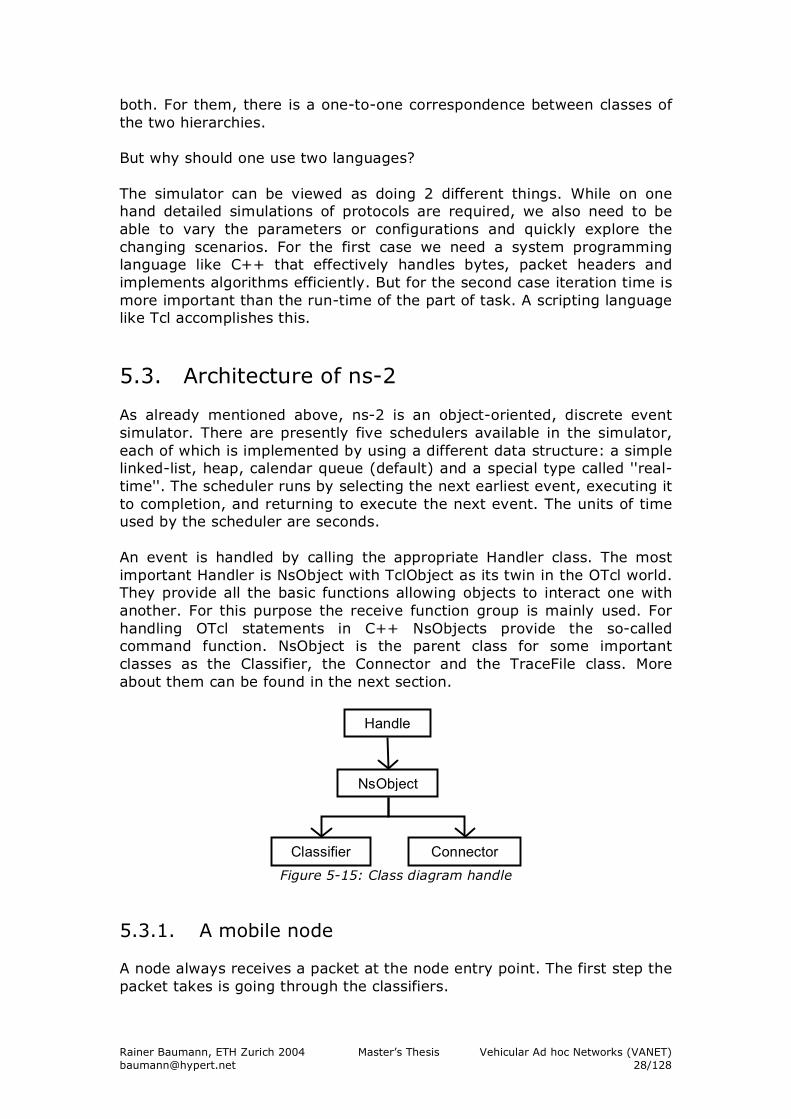
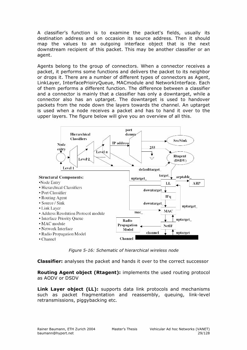
5.3. Architecture of ns-2 As already mentioned above, ns-2 is an object-oriented, discrete event simulator. There are presently five schedulers available in the simulator, each of which is implemented by using a different data structure: a simple linked-list, heap, calendar queue (default) and a special type called ''real-time''. The scheduler runs by selecting the next earliest event, executing it to completion, and returning to execute the next event. The units of time used by the scheduler are seconds. An event is handled by calling the appropriate Handler class. The most important Handler is NsObject with TclObject as its twin in the OTcl world. They provide all the basic functions allowing objects to interact one with another. For this purpose the receive function group is mainly used. For handling OTcl statements in C++ NsObjects provide the so-called command function. NsObject is the parent class for some important classes as the Classifier, the Connector and the TraceFile class. More about them can be found in the next section.
Figure 5-15: Class diagram handle
5.3.1. A mobile node A node always receives a packet at the node entry point. The first step the packet takes is going through the classifiers.
Handle
NsObject
Classifier Connector
Rainer Baumann, ETH Zurich 2004 Master’s Thesis Vehicular Ad hoc Networks (VANET) [email protected] 29/128
A classifier’s function is to examine the packet's fields, usually its destination address and on occasion its source address. Then it should map the values to an outgoing interface object that is the next downstream recipient of this packet. This may be another classifier or an agent. Agents belong to the group of connectors. When a connector receives a packet, it performs some functions and delivers the packet to its neighbor or drops it. There are a number of different types of connectors as Agent, LinkLayer, InterfacePrioiryQueue, MACmodule and NetworkInterface. Each of them performs a different function. The difference between a classifier and a connector is mainly that a classifier has only a downtarget, while a connector also has an uptarget. The downtarget is used to handover packets from the node down the layers towards the channel. An uptarget is used when a node receives a packet and has to hand it over to the upper layers. The figure below will give you an overview of all this.
Figure 5-16: Schematic of hierarchical wireless node
Classifier: analyses the packet and hands it over to the correct successor Routing Agent object (Rtagent): implements the used routing protocol as AODV or DSDV Link Layer object (LL): supports data link protocols and mechanisms such as packet fragmentation and reassembly, queuing, link-level retransmissions, piggybacking etc.
Rainer Baumann, ETH Zurich 2004 Master’s Thesis Vehicular Ad hoc Networks (VANET) [email protected] 30/128
Address Resolution Protocol module (ARP): finds and resolves the IP address of the next – hop/node into the correct MAC address. The MAC destination address is set into the MAC header of the packet Interface Priority Queue (IFq): gives a priority to routing protocol packets by running a filter over the packets and removing those with a specified destination address Medium Access Protocol module (MAC): provides multiple functionalities such as carrier sense, collision detection and avoidance etc Network Interface (NetIF): is an interface for a mobile node to access the channel. Each packet leaving the NetIF is stamped with the meta-data in its header and the information of the transmitting interface such as transmission power, wavelength etc. to be used by the propagation model of the receiving NetIF.
Radio Propagation Model: uses Free-space attenuation (1/r2) at near
distances and an approximation to two rays ground (1/r4) at far distances by default. It decides whether a mobile node with a given distance, power of transmission and wavelength can receive a packet. By default, it implements an omni directional antenna, which has unit gain for all directions.
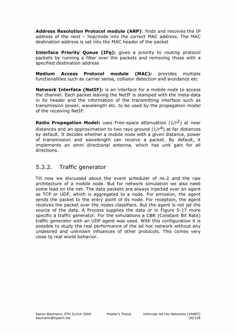
5.3.2. Traffic generator Till now we discussed about the event scheduler of ns-2 and the raw architecture of a mobile node. But for network simulation we also need some load on the net. The data packets are always injected over an agent as TCP or UDP, which is aggregated to a node. For emission, the agent sends the packet to the entry point of its node. For reception, the agent receives the packet over the nodes classifiers. But the agent is not jet the source of the data. A Process supplies the data or in Figure 5-17 more specific a traffic generator. For the simulations a CBR (Constant Bit Rate) traffic generator with an UDP agent was used. With this configuration it is possible to study the real performance of the ad hoc network without any undesired and unknown influences of other protocols. This comes very close to real world behavior.
Rainer Baumann, ETH Zurich 2004 Master’s Thesis Vehicular Ad hoc Networks (VANET) [email protected] 31/128
Figure 5-17: Schematic of traffic generator and packet flow
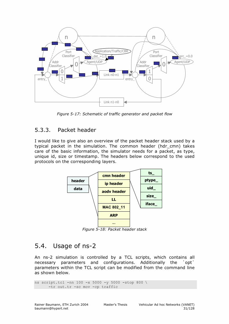
5.3.3. Packet header I would like to give also an overview of the packet header stack used by a typical packet in the simulation. The common header (hdr_cmn) takes care of the basic information, the simulator needs for a packet, as type, unique id, size or timestamp. The headers below correspond to the used protocols on the corresponding layers.
Figure 5-18: Packet header stack
5.4. Usage of ns-2 An ns-2 simulation is controlled by a TCL scripts, which contains all necessary parameters and configurations. Additionally the ΄opt΄ parameters within the TCL script can be modified from the command line as shown below. ns script.tcl -nn 100 -x 5000 -y 5000 -stop 800 \
-tr out.tr -sc mov -cp traffic
header
data ip header
aodv header
LL
MAC 802_11
cmn header
ARP
ts_
ptype_
uid_
size_
iface_
...
Application/Traffic/CBR
0 1
n0
n1
Addr Classifier
Port Classifier
entry_
0 Agent/UDP Addr Classifier
Port Classifier
entry_
1 0
Link n0-n1
Link n1-n0
0 Agent/UDP
dst_=1.0 src_=0.0
Rainer Baumann, ETH Zurich 2004 Master’s Thesis Vehicular Ad hoc Networks (VANET) [email protected] 32/128
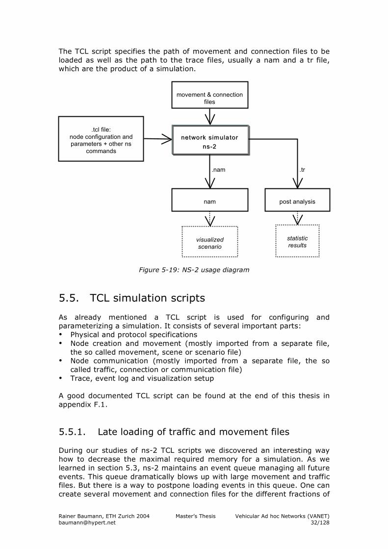
The TCL script specifies the path of movement and connection files to be loaded as well as the path to the trace files, usually a nam and a tr file, which are the product of a simulation.
Figure 5-19: NS-2 usage diagram
5.5. TCL simulation scripts As already mentioned a TCL script is used for configuring and parameterizing a simulation. It consists of several important parts: • Physical and protocol specifications • Node creation and movement (mostly imported from a separate file,
the so called movement, scene or scenario file) • Node communication (mostly imported from a separate file, the so
called traffic, connection or communication file) • Trace, event log and visualization setup A good documented TCL script can be found at the end of this thesis in appendix F.1.
5.5.1. Late loading of traffic and movement files During our studies of ns-2 TCL scripts we discovered an interesting way how to decrease the maximal required memory for a simulation. As we learned in section 5.3, ns-2 maintains an event queue managing all future events. This queue dramatically blows up with large movement and traffic files. But there is a way to postpone loading events in this queue. One can create several movement and connection files for the different fractions of
network simulatornetwork simulator nsns --22
.tcl file:
node configuration and parameters + other ns
commands
movement & connection
files
nam
post analysis
.tr file
.nam file
visualized scenario
statistic results
Rainer Baumann, ETH Zurich 2004 Master’s Thesis Vehicular Ad hoc Networks (VANET) [email protected] 33/128
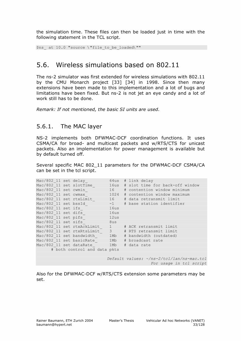
the simulation time. These files can then be loaded just in time with the following statement in the TCL script. $ns_ at 10.0 "source \"file_to_be_loaded\""
5.6. Wireless simulations based on 802.11 The ns-2 simulator was first extended for wireless simulations with 802.11 by the CMU Monarch project [33] [34] in 1998. Since then many extensions have been made to this implementation and a lot of bugs and limitations have been fixed. But ns-2 is not jet an eye candy and a lot of work still has to be done. Remark: If not mentioned, the basic SI units are used.
5.6.1. The MAC layer NS-2 implements both DFWMAC-DCF coordination functions. It uses CSMA/CA for broad- and multicast packets and w/RTS/CTS for unicast packets. Also an implementation for power management is available but by default turned off. Several specific MAC 802_11 parameters for the DFWMAC-DCF CSMA/CA can be set in the tcl script. Mac/802_11 set delay_ 64us # link delay Mac/802_11 set slotTime_ 16us # slot time for back-off window Mac/802_11 set cwmin_ 16 # contention window minimum Mac/802_11 set cwmax_ 1024 # contention window maximum Mac/802_11 set rtxLimit_ 16 # data retransmit limit Mac/802_11 set bssId_ -1 # base station identifier Mac/802_11 set ifs_ 16us Mac/802_11 set difs_ 16us Mac/802_11 set pifs_ 12us Mac/802_11 set sifs_ 8us Mac/802_11 set rtxAckLimit_ 1 # ACK retransmit limit Mac/802_11 set rtxRtsLimit_ 3 # RTS retransmit limit Mac/802_11 set bandwidth_ 1Mb # bandwidth (outdated) Mac/802_11 set basicRate_ 1Mb # broadcast rate Mac/802_11 set dataRate_ 1Mb # data rate # both control and data pkts
Default values: ~/ns-2/tcl/lan/ns-mac.tcl For usage in tcl script
Also for the DFWMAC-DCF w/RTS/CTS extension some parameters may be set.
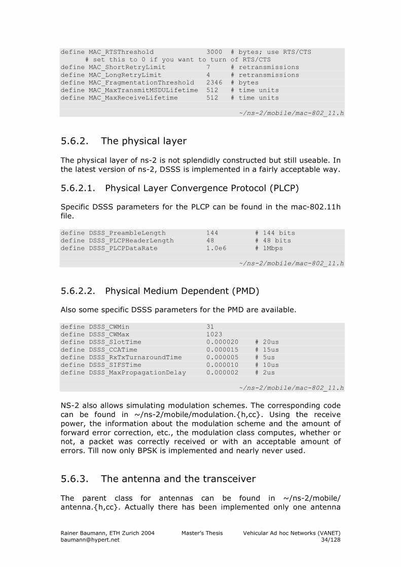
Rainer Baumann, ETH Zurich 2004 Master’s Thesis Vehicular Ad hoc Networks (VANET) [email protected] 34/128
define MAC_RTSThreshold 3000 # bytes; use RTS/CTS # set this to 0 if you want to turn of RTS/CTS define MAC_ShortRetryLimit 7 # retransmissions define MAC_LongRetryLimit 4 # retransmissions define MAC_FragmentationThreshold 2346 # bytes define MAC_MaxTransmitMSDULifetime 512 # time units define MAC_MaxReceiveLifetime 512 # time units
~/ns-2/mobile/mac-802_11.h
5.6.2. The physical layer The physical layer of ns-2 is not splendidly constructed but still useable. In the latest version of ns-2, DSSS is implemented in a fairly acceptable way. 5.6.2.1. Physical Layer Convergence Protocol (PLCP) Specific DSSS parameters for the PLCP can be found in the mac-802.11h file. define DSSS_PreambleLength 144 # 144 bits define DSSS_PLCPHeaderLength 48 # 48 bits define DSSS_PLCPDataRate 1.0e6 # 1Mbps
~/ns-2/mobile/mac-802_11.h
5.6.2.2. Physical Medium Dependent (PMD) Also some specific DSSS parameters for the PMD are available. define DSSS_CWMin 31 define DSSS_CWMax 1023 define DSSS_SlotTime 0.000020 # 20us define DSSS_CCATime 0.000015 # 15us define DSSS_RxTxTurnaroundTime 0.000005 # 5us define DSSS_SIFSTime 0.000010 # 10us define DSSS_MaxPropagationDelay 0.000002 # 2us
~/ns-2/mobile/mac-802_11.h
NS-2 also allows simulating modulation schemes. The corresponding code can be found in ~/ns-2/mobile/modulation.{h,cc}. Using the receive power, the information about the modulation scheme and the amount of forward error correction, etc., the modulation class computes, whether or not, a packet was correctly received or with an acceptable amount of errors. Till now only BPSK is implemented and nearly never used.
5.6.3. The antenna and the transceiver The parent class for antennas can be found in ~/ns-2/mobile/ antenna.{h,cc}. Actually there has been implemented only one antenna
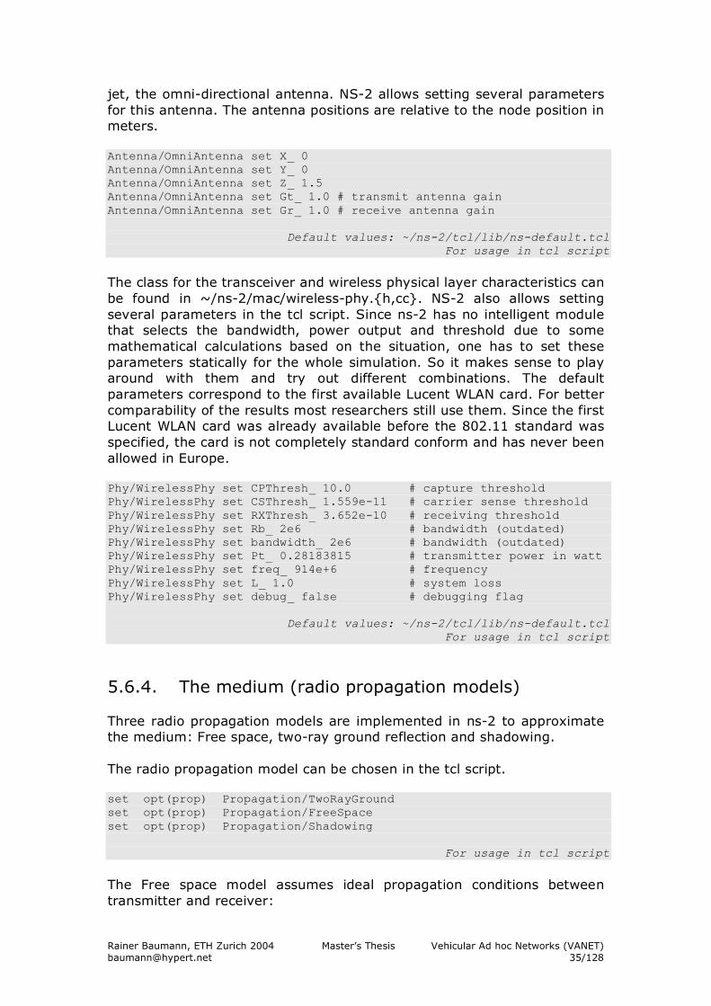
Rainer Baumann, ETH Zurich 2004 Master’s Thesis Vehicular Ad hoc Networks (VANET) [email protected] 35/128
jet, the omni-directional antenna. NS-2 allows setting several parameters for this antenna. The antenna positions are relative to the node position in meters. Antenna/OmniAntenna set X_ 0 Antenna/OmniAntenna set Y_ 0 Antenna/OmniAntenna set Z_ 1.5 Antenna/OmniAntenna set Gt_ 1.0 # transmit antenna gain Antenna/OmniAntenna set Gr_ 1.0 # receive antenna gain
Default values: ~/ns-2/tcl/lib/ns-default.tcl For usage in tcl script
The class for the transceiver and wireless physical layer characteristics can be found in ~/ns-2/mac/wireless-phy.{h,cc}. NS-2 also allows setting several parameters in the tcl script. Since ns-2 has no intelligent module that selects the bandwidth, power output and threshold due to some mathematical calculations based on the situation, one has to set these parameters statically for the whole simulation. So it makes sense to play around with them and try out different combinations. The default parameters correspond to the first available Lucent WLAN card. For better comparability of the results most researchers still use them. Since the first Lucent WLAN card was already available before the 802.11 standard was specified, the card is not completely standard conform and has never been allowed in Europe. Phy/WirelessPhy set CPThresh_ 10.0 # capture threshold Phy/WirelessPhy set CSThresh_ 1.559e-11 # carrier sense threshold Phy/WirelessPhy set RXThresh_ 3.652e-10 # receiving threshold Phy/WirelessPhy set Rb_ 2e6 # bandwidth (outdated) Phy/WirelessPhy set bandwidth_ 2e6 # bandwidth (outdated) Phy/WirelessPhy set Pt_ 0.28183815 # transmitter power in watt Phy/WirelessPhy set freq_ 914e+6 # frequency Phy/WirelessPhy set L_ 1.0 # system loss Phy/WirelessPhy set debug_ false # debugging flag
Default values: ~/ns-2/tcl/lib/ns-default.tcl For usage in tcl script
5.6.4. The medium (radio propagation models) Three radio propagation models are implemented in ns-2 to approximate the medium: Free space, two-ray ground reflection and shadowing. The radio propagation model can be chosen in the tcl script. set opt(prop) Propagation/TwoRayGround set opt(prop) Propagation/FreeSpace set opt(prop) Propagation/Shadowing
For usage in tcl script The Free space model assumes ideal propagation conditions between transmitter and receiver:
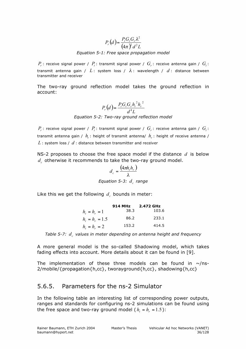
Rainer Baumann, ETH Zurich 2004 Master’s Thesis Vehicular Ad hoc Networks (VANET) [email protected] 36/128
( )( ) Ld
GGPdP
rtt
r 22
2
4!
"=
Equation 5-1: Free space propagation model
rP : receive signal power /
tP : transmit signal power /
rG : receive antenna gain /
tG :
transmit antenna gain / L : system loss / ! : wavelength / d : distance between transmitter and receiver The two-ray ground reflection model takes the ground reflection in account:
( )Ld
hhGGPdP
rtrtt
r 4
22
=
Equation 5-2: Two-ray ground reflection model
rP : receive signal power /
tP : transmit signal power /
rG : receive antenna gain /
tG :
transmit antenna gain / th : height of transmit antenna/
rh : height of receive antenna /
L : system loss / d : distance between transmitter and receiver
NS-2 proposes to choose the free space model if the distance d is below
cd otherwise it recommends to take the two-ray ground model.
( )!
"rt
c
hhd
4=
Equation 5-3:
cd range
Like this we get the following
cd bounds in meter:
914 MHz 2.472 GHz
1==rthh 38.3 103.6
5.1==rthh 86.2 233.1
2==rthh 153.2 414.5
Table 5-7: cd values in meter depending on antenna height and frequency
A more general model is the so-called Shadowing model, which takes fading effects into account. More details about it can be found in [9]. The implementation of these three models can be found in ~/ns-2/mobile/{propagation{h,cc}, tworayground{h,cc}, shadowing{h,cc}
5.6.5. Parameters for the ns-2 Simulator In the following table an interesting list of corresponding power outputs, ranges and standards for configuring ns-2 simulations can be found using the free space and two-ray ground model ( 5.1==
rthh ):
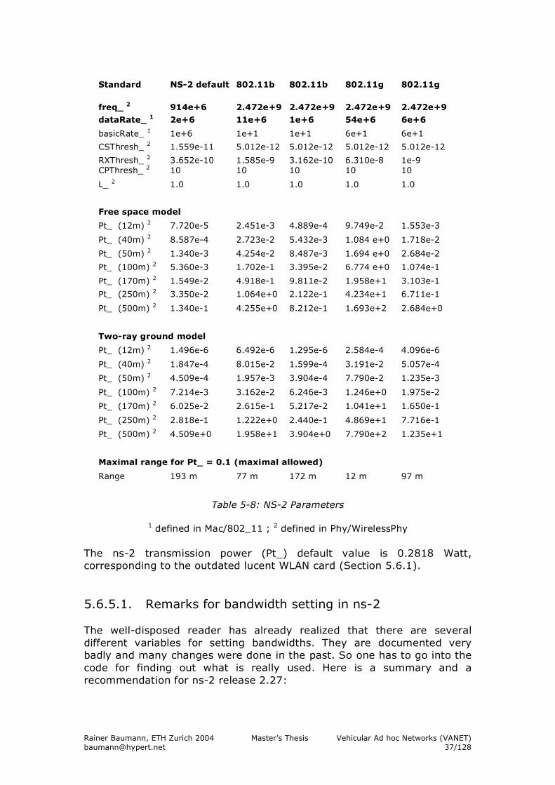
Rainer Baumann, ETH Zurich 2004 Master’s Thesis Vehicular Ad hoc Networks (VANET) [email protected] 37/128
Standard NS-2 default 802.11b 802.11b 802.11g 802.11g
freq_ 2 914e+6 2.472e+9 2.472e+9 2.472e+9 2.472e+9
dataRate_ 1 2e+6 11e+6 1e+6 54e+6 6e+6
basicRate_ 1 1e+6 1e+1 1e+1 6e+1 6e+1
CSThresh_ 2 1.559e-11 5.012e-12 5.012e-12 5.012e-12 5.012e-12
RXThresh_ 2 3.652e-10 1.585e-9 3.162e-10 6.310e-8 1e-9 CPThresh_ 2 10 10 10 10 10
L_ 2 1.0 1.0 1.0 1.0 1.0
Free space model
Pt_ (12m) 2 7.720e-5 2.451e-3 4.889e-4 9.749e-2 1.553e-3
Pt_ (40m) 2 8.587e-4 2.723e-2 5.432e-3 1.084 e+0 1.718e-2
Pt_ (50m) 2 1.340e-3 4.254e-2 8.487e-3 1.694 e+0 2.684e-2
Pt_ (100m) 2 5.360e-3 1.702e-1 3.395e-2 6.774 e+0 1.074e-1
Pt_ (170m) 2 1.549e-2 4.918e-1 9.811e-2 1.958e+1 3.103e-1
Pt_ (250m) 2 3.350e-2 1.064e+0 2.122e-1 4.234e+1 6.711e-1
Pt_ (500m) 2 1.340e-1 4.255e+0 8.212e-1 1.693e+2 2.684e+0
Two-ray ground model
Pt_ (12m) 2 1.496e-6 6.492e-6 1.295e-6 2.584e-4 4.096e-6
Pt_ (40m) 2 1.847e-4 8.015e-2 1.599e-4 3.191e-2 5.057e-4
Pt_ (50m) 2 4.509e-4 1.957e-3 3.904e-4 7.790e-2 1.235e-3
Pt_ (100m) 2 7.214e-3 3.162e-2 6.246e-3 1.246e+0 1.975e-2
Pt_ (170m) 2 6.025e-2 2.615e-1 5.217e-2 1.041e+1 1.650e-1
Pt_ (250m) 2 2.818e-1 1.222e+0 2.440e-1 4.869e+1 7.716e-1
Pt_ (500m) 2 4.509e+0 1.958e+1 3.904e+0 7.790e+2 1.235e+1
Maximal range for Pt_ = 0.1 (maximal allowed)
Range 193 m 77 m 172 m 12 m 97 m
Table 5-8: NS-2 Parameters
1 defined in Mac/802_11 ; 2 defined in Phy/WirelessPhy The ns-2 transmission power (Pt_) default value is 0.2818 Watt, corresponding to the outdated lucent WLAN card (Section 5.6.1). 5.6.5.1. Remarks for bandwidth setting in ns-2 The well-disposed reader has already realized that there are several different variables for setting bandwidths. They are documented very badly and many changes were done in the past. So one has to go into the code for finding out what is really used. Here is a summary and a recommendation for ns-2 release 2.27:
Rainer Baumann, ETH Zurich 2004 Master’s Thesis Vehicular Ad hoc Networks (VANET) [email protected] 38/128
Phy/WirelessPhy set Rb_ # is obsolete. It is no where used any more. Phy/WirelessPhy set bandwidth_ # is outdated. It is only used in Phy but no longer in WirelessPhy. WirelseePhy uses the Mac function txtime() for corresponding calculations. Mac/802_11 set bandwidth_ # is outdated. It is used in Mac but a bad choice for 802_11. The use of this variable in 802_11 can lead to misbehavior. It is recommended to use basicRate_ and dataRate_ Mac/802_11 set basicRate_ # is current. It sets the basic rate for the used standard, e.g. for 802.11b 1Mpbs and for 802.11g 6Mbps. Mac/802_11 set dataRate_ # is current. It is responsible for the transmission rate of data and control packets.
5.7. Trace files As already mentioned above, one gets two trace files as a result of a simulation: a normal trace file (created by $ns_ trace-all commands) and a nam trace file ($ns_ nam-traceall). The nam trace file is a subset of a normal trace file with the suffix ".nam". It contains information for visualizing packet flow and node movement for use with the homonymous nam tool. Nam is a Tcl/TK based animation tool for viewing network simulation traces and real world packet trace data. The design theory behind nam was to create an animator that is able to read large animation data sets and be extensible enough, so that it could be used in different network visualization situations [33]. For studying protocol behavior one has to refer to the normal trace file with the suffix ".tr". It contains all requested trace data produced by a simulation. In the TCL configuration script one can tell the simulator which kind of trace information shall be printed out: agent, route and mac trace. They can separately be turned on or off for every node in the node-config. $ns_ node-config -agentTrace ON/OFF $ns_ node-config -routerTrace ON/OFF $ns_ node-config -macTrace ON/OFF
In the original cmu trace implementation, which can be found in ~/ns-2/trace/cmu-trace.{h,cc}, two trace file formats exists: the 'old' and the 'new' one. If one wants to use the new trace file format, one has to turn it on explicitly by using the Tcl script. $ns_ use-newtrace
For understanding the trace files, first of all one has to know that one line in a trace file corresponds to one event traced by the simulator. A line
Rainer Baumann, ETH Zurich 2004 Master’s Thesis Vehicular Ad hoc Networks (VANET) [email protected] 39/128
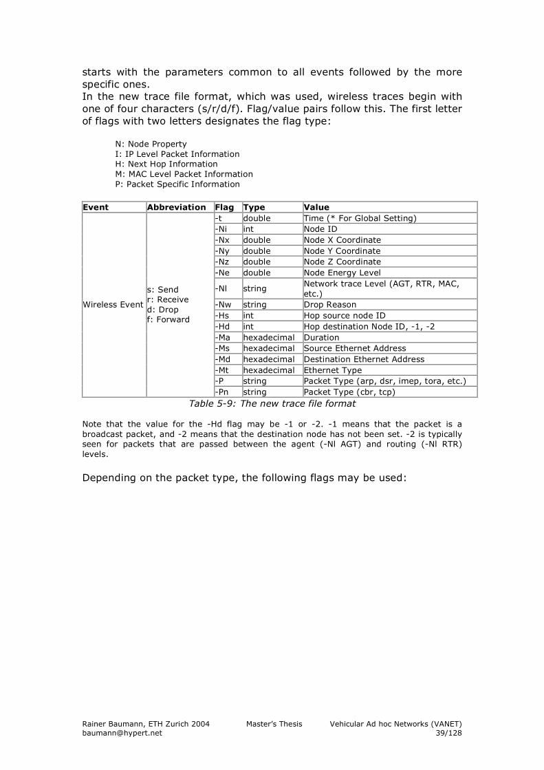
starts with the parameters common to all events followed by the more specific ones. In the new trace file format, which was used, wireless traces begin with one of four characters (s/r/d/f). Flag/value pairs follow this. The first letter of flags with two letters designates the flag type:
N: Node Property I: IP Level Packet Information H: Next Hop Information M: MAC Level Packet Information P: Packet Specific Information
Event Abbreviation Flag Type Value
-t double Time (* For Global Setting) -Ni int Node ID -Nx double Node X Coordinate -Ny double Node Y Coordinate -Nz double Node Z Coordinate -Ne double Node Energy Level
-Nl string Network trace Level (AGT, RTR, MAC, etc.)
-Nw string Drop Reason -Hs int Hop source node ID -Hd int Hop destination Node ID, -1, -2 -Ma hexadecimal Duration -Ms hexadecimal Source Ethernet Address -Md hexadecimal Destination Ethernet Address -Mt hexadecimal Ethernet Type -P string Packet Type (arp, dsr, imep, tora, etc.)
Wireless Event
s: Send r: Receive d: Drop f: Forward
-Pn string Packet Type (cbr, tcp) Table 5-9: The new trace file format
Note that the value for the -Hd flag may be -1 or -2. -1 means that the packet is a broadcast packet, and -2 means that the destination node has not been set. -2 is typically seen for packets that are passed between the agent (-Nl AGT) and routing (-Nl RTR) levels. Depending on the packet type, the following flags may be used:
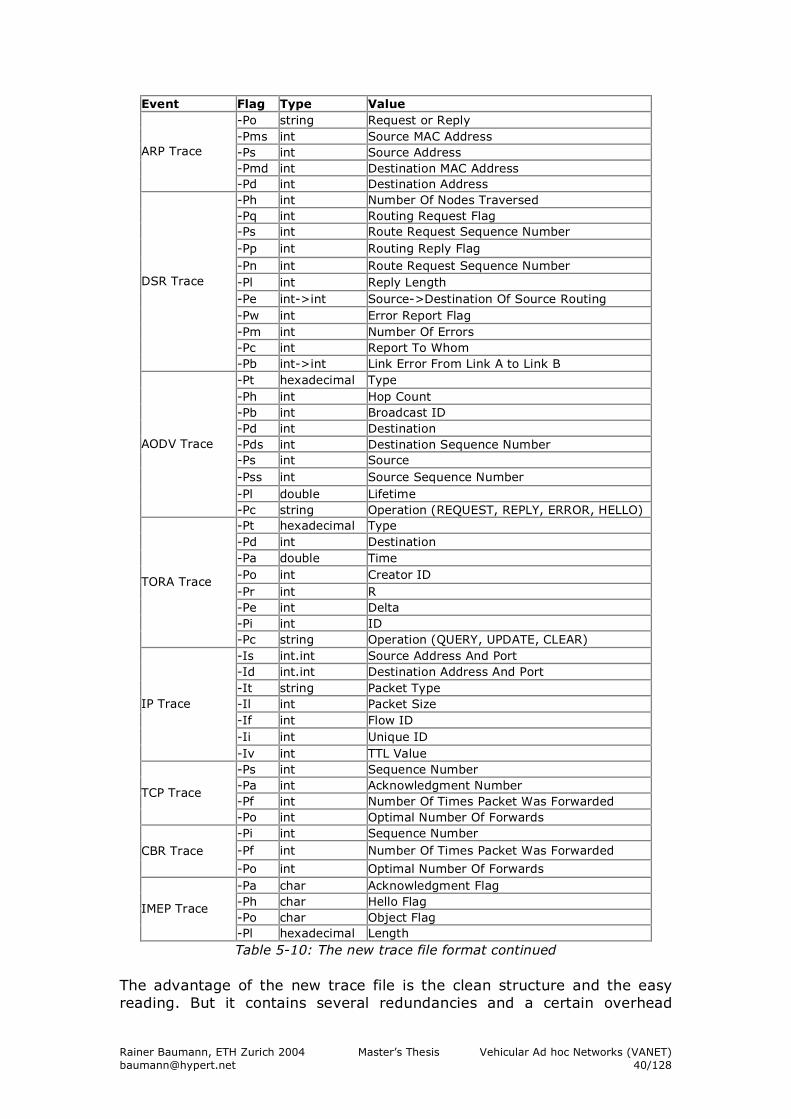
Rainer Baumann, ETH Zurich 2004 Master’s Thesis Vehicular Ad hoc Networks (VANET) [email protected] 40/128
Event Flag Type Value -Po string Request or Reply -Pms int Source MAC Address -Ps int Source Address -Pmd int Destination MAC Address
ARP Trace
-Pd int Destination Address -Ph int Number Of Nodes Traversed -Pq int Routing Request Flag -Ps int Route Request Sequence Number -Pp int Routing Reply Flag -Pn int Route Request Sequence Number -Pl int Reply Length -Pe int->int Source->Destination Of Source Routing -Pw int Error Report Flag -Pm int Number Of Errors -Pc int Report To Whom
DSR Trace
-Pb int->int Link Error From Link A to Link B -Pt hexadecimal Type -Ph int Hop Count -Pb int Broadcast ID -Pd int Destination -Pds int Destination Sequence Number -Ps int Source -Pss int Source Sequence Number -Pl double Lifetime
AODV Trace
-Pc string Operation (REQUEST, REPLY, ERROR, HELLO) -Pt hexadecimal Type -Pd int Destination -Pa double Time -Po int Creator ID -Pr int R -Pe int Delta -Pi int ID
TORA Trace
-Pc string Operation (QUERY, UPDATE, CLEAR) -Is int.int Source Address And Port -Id int.int Destination Address And Port -It string Packet Type -Il int Packet Size -If int Flow ID -Ii int Unique ID
IP Trace
-Iv int TTL Value -Ps int Sequence Number -Pa int Acknowledgment Number -Pf int Number Of Times Packet Was Forwarded
TCP Trace
-Po int Optimal Number Of Forwards -Pi int Sequence Number -Pf int Number Of Times Packet Was Forwarded CBR Trace
-Po int Optimal Number Of Forwards -Pa char Acknowledgment Flag -Ph char Hello Flag -Po char Object Flag
IMEP Trace
-Pl hexadecimal Length Table 5-10: The new trace file format continued
The advantage of the new trace file is the clean structure and the easy reading. But it contains several redundancies and a certain overhead
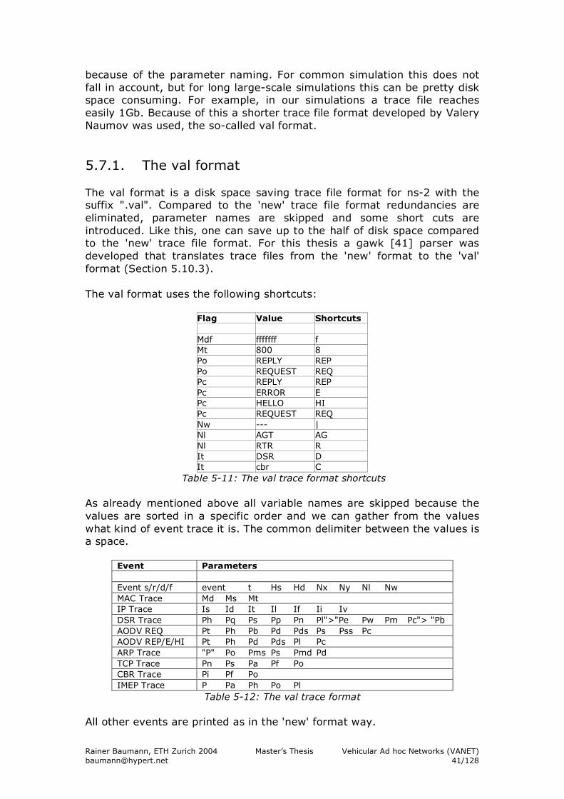
Rainer Baumann, ETH Zurich 2004 Master’s Thesis Vehicular Ad hoc Networks (VANET) [email protected] 41/128
because of the parameter naming. For common simulation this does not fall in account, but for long large-scale simulations this can be pretty disk space consuming. For example, in our simulations a trace file reaches easily 1Gb. Because of this a shorter trace file format developed by Valery Naumov was used, the so-called val format.
5.7.1. The val format The val format is a disk space saving trace file format for ns-2 with the suffix ".val". Compared to the 'new' trace file format redundancies are eliminated, parameter names are skipped and some short cuts are introduced. Like this, one can save up to the half of disk space compared to the 'new' trace file format. For this thesis a gawk [41] parser was developed that translates trace files from the 'new' format to the 'val' format (Section 5.10.3). The val format uses the following shortcuts:
Flag Value Shortcuts Mdf fffffff f Mt 800 8 Po REPLY REP Po REQUEST REQ Pc REPLY REP Pc ERROR E Pc HELLO HI Pc REQUEST REQ Nw --- | Nl AGT AG Nl RTR R It DSR D It cbr C
Table 5-11: The val trace format shortcuts As already mentioned above all variable names are skipped because the values are sorted in a specific order and we can gather from the values what kind of event trace it is. The common delimiter between the values is a space.
Event Parameters Event s/r/d/f event t Hs Hd Nx Ny Nl Nw MAC Trace Md Ms Mt IP Trace Is Id It Il If Ii Iv DSR Trace Ph Pq Ps Pp Pn Pl">"Pe Pw Pm Pc"> "Pb AODV REQ Pt Ph Pb Pd Pds Ps Pss Pc AODV REP/E/HI Pt Ph Pd Pds Pl Pc ARP Trace "P" Po Pms Ps Pmd Pd TCP Trace Pn Ps Pa Pf Po CBR Trace Pi Pf Po IMEP Trace P Pa Ph Po Pl
Table 5-12: The val trace format All other events are printed as in the 'new' format way.
Rainer Baumann, ETH Zurich 2004 Master’s Thesis Vehicular Ad hoc Networks (VANET) [email protected] 42/128
5.8. Limitations of ns-2 A simulator model of a real-world system is necessarily a simplification of the real-world system itself. Especially for WLAN simulations one has to be very generous, because there are tremendously many quick changing parameters, which cannot be handled up to now and in the near future. There are also some practical limitations. We found out that the maximum number of mobile nodes, ns-2 allows, is 16250 (nn_max). Processor speed is also a problem. For example, on a 2 GHz machine a 500 node simulation, with the random way point movement model, in an area of 5x1 km2 with 100 connections over 600 seconds, easily takes several days and requires easily a GB of RAM.
5.9. Extensions to ns-2 5.9.1. Switch ON/OFF An extension, we integrated into ns-2, is a switch ON/OFF function for mobile nodes. For example, when a car parks and switches of its WLAN card or when a car leaves the simulation area, one has to make sure that the node does no longer participate in the mobile ad hoc network. $ns_ at 10.0 "$node_(5) switch ON" $ns_ at 20.0 "$node_(5) switch OFF"
5.9.2. ARP ON/OFF Another feature, we added to ns-2, is ARP ON/OFF. It allows to switch of the Address Resolution Protocol (ARP). When ARP is switched off, the same addresses will be used for layer two and three. #define arpOFF // switches off arp
~/ns2/mac/arp.h
Rainer Baumann, ETH Zurich 2004 Master’s Thesis Vehicular Ad hoc Networks (VANET) [email protected] 43/128
5.10. Utilities
5.10.1. Creating random traffic-pattern for wireless scenarios
Random traffic connections of TCP and CBR (Constant Bit Rate) can be setup between mobile nodes using a traffic scenario generator script. This traffic generator script is available under ~/ns-2/indep-utils/cmu-scen-gen and is called cbrgen.tcl. The command line looks like the following: ns cbrgen.tcl [-type cbr|tcp] [-nn nodes] [-seed seed] [-mc connections] [-rate rate]
5.10.2. Creating node-movements for wireless scenarios The random node movement generator is available under ~/ns-2/indep-utils/cmu-scen-gen/setdest directory and consists of setdest{.cc,.h} and Makefile. Setdest can be run with arguments as shown below: ./setdest [-n num_of_nodes] [-p pausetime] [-s maxspeed] [-t simtime] [-x maxx] [-y maxy] > [outdir/movement-file]
5.10.3. Trace file converter, new to val In section 5.7.1 the val trace file format was described, which allows us nearly to cut in half the required disk space for a trace file. For easy conversion of trace files in the new format to the val format an awk parser was written. gawk –f tr-parser-new-to-val NEWTRFILE
5.10.4. Movement to nam file converter Often one quickly wants to generate a nam file for having a look at the node movements. But for this, one had to run a time consuming ns simulation with no traffic setup. For example, we often had to explore and evaluate some areas from the main movement source file. With an ns-2 simulation this would take about half a day up to a full day. So we developed an ns-2 movement file to nam file converter. It consists of a bash script at_nam_converter.exe and an awk script parser at_nam_converter.awk, which is called from the bash script. With this converter it takes just a couple of minutes to convert a movement file with ten thousand nodes and hundred thousand events. ./at_nam_converter.exe MOVMENTFILE NAMFILE
Rainer Baumann, ETH Zurich 2004 Master’s Thesis Vehicular Ad hoc Networks (VANET) [email protected] 44/128
5.10.5. Movement file area and time cutter The movement file cutter allows cutting out a part of a movement file in the time and space dimension. It can be configured giving the X, Y and T minima and maxima as parameters. gawk -f at_filter.awk -v X_min=10 X_max=99 Y_min=10 Y_max=99 T_min=10 T_max=99 V_min=2 INPUTFILE > OUTPUTFIL
5.10.6. Movement file adjuster Another tool we developed is a movement file adjuster. It allows resetting time and space coordinates as well as it offers a possibility to scale the time. X_min, Y_min and T_min just can be given the coordinates of the new origin. gawk -f at_adjust.awk -v X_min=10 Y_min=10 T_min=10 T_scalar=1 INPUTFILE > OUTPUTFIL
5.10.7. Movement file statistic generator There are two movement file statistic generators. At_stat generates a statistic for a movement file including the minimum, maximum and average for all dimensions. The at_event_stat allows producing a summary for the number of events in a time slot. The slot size is 100 second by default but can be changed by resetting the value as shown below. gawk -f at_stat.awk MOVFILE gawk -f at_event_stat.awk –v slot=100 MOVFILE
5.11. Used machine for simulations For the simulations carried out for this thesis we used the following machines: gavia.inf.ethz.ch • Genuine Intel Dual Processor • 2x Intel® Xenon™ CPU 1.70GHz • 2x L2 Cache 256kb • Memory 1510 Mb • Linux 2.4.20-24.9smp (Red Hat Linux 3.2.2-5) During execution of simulation we often phased the limitation of this machine. Due to this, we had to reduce the number of simulations resulting in a bit weaker statistics.
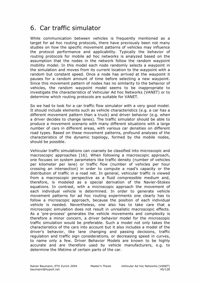
Rainer Baumann, ETH Zurich 2004 Master’s Thesis Vehicular Ad hoc Networks (VANET) [email protected] 45/128
6. Car traffic simulator While communication between vehicles is frequently mentioned as a target for ad hoc routing protocols, there have previously been not many studies on how the specific movement patterns of vehicles may influence the protocol performance and applicability. Typically the behavior of routing protocols for mobile ad hoc networks is analyzed based on the assumption that the nodes in the network follow the random waypoint mobility model. In this model each node randomly selects a waypoint in the simulation and moves from its current location to the waypoint with a random but constant speed. Once a node has arrived at the waypoint it pauses for a random amount of time before selecting a new waypoint. Since this movement pattern of nodes has no similarity to the behavior of vehicles, the random waypoint model seems to be inappropriate to investigate the characteristics of Vehicular Ad hoc Networks (VANET) or to determine which routing protocols are suitable for VANET. So we had to look for a car traffic flow simulator with a very good model. It should include elements such as vehicle characteristics (e.g. a car has a different movement pattern than a truck) and driver behavior (e.g. when a driver decides to change lanes). The traffic simulator should be able to produce a movement scenario with many different situations with a large number of cars in different areas, with various car densities on different road types. Based on these movement patterns, profound analyses of the characteristics of the dynamic topology, formed by the mobile nodes, should be possible. Vehicular traffic simulations can coarsely be classified into microscopic and macroscopic approaches [16]. When following a macroscopic approach, one focuses on system parameters like traffic density (number of vehicles per kilometer per lane) or traffic flow (number of vehicles per hour crossing an intersection) in order to compute a road’s capacity or the distribution of traffic in a road net. In general, vehicular traffic is viewed from a macroscopic perspective as a fluid compressible medium and, therefore, is modeled as a special derivation of the Navier-Stokes equations. In contrast, with a microscopic approach the movement of each individual vehicle is determined. In order to generate vehicle movement patterns for ad hoc routing experiments one clearly has to follow a microscopic approach, because the position of each individual vehicle is needed. Nevertheless, one also has to take care that a microscopic simulation does not result in unrealistic macroscopic effects. As a ‘pre-process’ generates the vehicle movements and complexity is therefore a minor concern, a driver behavior model for the microscopic traffic simulation would be preferable. Such a model not only takes the characteristics of the cars into account but it also includes a model of the driver’s behavior, like lane changing and passing decisions, traffic regulation and traffic sign considerations, or decreasing speed in curves, to name only a few. Driver Behavior Models are known to be highly accurate and are therefore used by vehicle manufacturers, e.g. to determine the lifetime of certain parts of the car.
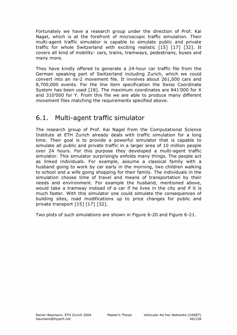
Rainer Baumann, ETH Zurich 2004 Master’s Thesis Vehicular Ad hoc Networks (VANET) [email protected] 46/128
Fortunately we have a research group under the direction of Prof. Kai Nagel, which is at the forefront of microscopic traffic simulation. Their multi-agent traffic simulator is capable to simulate public and private traffic for whole Switzerland with exciting realistic [15] [17] [32]. It covers all kind of mobility: cars, trains, tramways, pedestrians, buses and many more. They have kindly offered to generate a 24-hour car traffic file from the German speaking part of Switzerland including Zurich, which we could convert into an ns-2 movement file. It involves about 261,000 cars and 8,700,000 events. For the line item specification the Swiss Coordinate System has been used [18]. The maximum coordinates are 841’000 for X and 310’000 for Y. From this file we are able to produce many different movement files matching the requirements specified above.
6.1. Multi-agent traffic simulator The research group of Prof. Kai Nagel from the Computational Science Institute at ETH Zurich already deals with traffic simulation for a long time. Their goal is to provide a powerful simulator that is capable to simulate all public and private traffic in a larger area of 10 million people over 24 hours. For this purpose they developed a multi-agent traffic simulator. This simulator surprisingly enfolds many things. The people act as linked individuals. For example, assume a classical family with a husband going to work by car early in the morning, two children walking to school and a wife going shopping for their family. The individuals in the simulation choose time of travel and means of transportation by their needs and environment. For example the husband, mentioned above, would take a tramway instead of a car if he lives in the city and if it is much faster. With this simulator one could simulate the consequences of building sites, road modifications up to price changes for public and private transport [15] [17] [32]. Two plots of such simulations are shown in Figure 6-20 and Figure 6-21.
Rainer Baumann, ETH Zurich 2004 Master’s Thesis Vehicular Ad hoc Networks (VANET) [email protected] 47/128
Figure 6-20: Traffic flow example Zurich [32]
Legend: green: driving cars / red: waiting car in a traffic jam / yellow: parked cars:
Figure 6-21: Traffic flow example Switzerland [15]
Legend: yellow: low car density / green: moderate car density /
red: critical cat density -> traffic jams
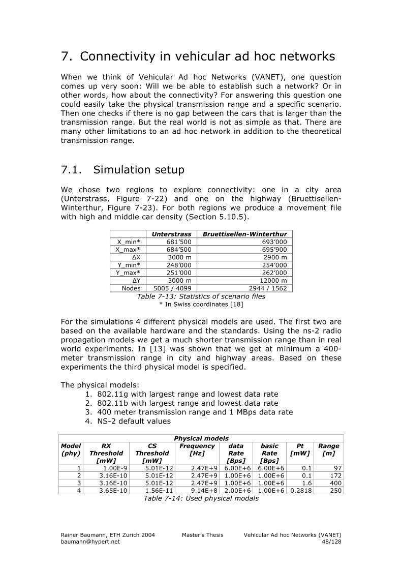
Rainer Baumann, ETH Zurich 2004 Master’s Thesis Vehicular Ad hoc Networks (VANET) [email protected] 48/128
7. Connectivity in vehicular ad hoc networks When we think of Vehicular Ad hoc Networks (VANET), one question comes up very soon: Will we be able to establish such a network? Or in other words, how about the connectivity? For answering this question one could easily take the physical transmission range and a specific scenario. Then one checks if there is no gap between the cars that is larger than the transmission range. But the real world is not as simple as that. There are many other limitations to an ad hoc network in addition to the theoretical transmission range.
7.1. Simulation setup We chose two regions to explore connectivity: one in a city area (Unterstrass, Figure 7-22) and one on the highway (Bruettisellen-Winterthur, Figure 7-23). For both regions we produce a movement file with high and middle car density (Section 5.10.5).
Unterstrass Bruettisellen-Winterthur X_min* 681’500 693’000 X_max* 684’500 695’900
ΔX 3000 m 2900 m Y_min* 248’000 254’000 Y_max* 251’000 262’000
ΔY 3000 m 12000 m Nodes 5005 / 4099 2944 / 1562
Table 7-13: Statistics of scenario files * In Swiss coordinates [18]
For the simulations 4 different physical models are used. The first two are based on the available hardware and the standards. Using the ns-2 radio propagation models we get a much shorter transmission range than in real world experiments. In [13] was shown that we get at minimum a 400-meter transmission range in city and highway areas. Based on these experiments the third physical model is specified. The physical models:
1. 802.11g with largest range and lowest data rate 2. 802.11b with largest range and lowest data rate 3. 400 meter transmission range and 1 MBps data rate 4. NS-2 default values
Physical models
Model (phy)
RX Threshold
[mW]
CS Threshold
[mW]
Frequency [Hz]
data Rate [Bps]
basic Rate [Bps]
Pt [mW]
Range [m]
1 1.00E-9 5.01E-12 2.47E+9 6.00E+6 6.00E+6 0.1 97 2 3.16E-10 5.01E-12 2.47E+9 1.00E+6 1.00E+6 0.1 172 3 3.16E-10 5.01E-12 2.47E+9 1.00E+6 1.00E+6 1.6 400 4 3.65E-10 1.56E-11 9.14E+8 2.00E+6 1.00E+6 0.2818 250
Table 7-14: Used physical modals
Rainer Baumann, ETH Zurich 2004 Master’s Thesis Vehicular Ad hoc Networks (VANET) [email protected] 49/128
For the simulation, AODV is used as a routing protocol. In this simulation we want to evaluate the connectivity of the specified scenarios. So they are turned off: TTL_START=255, TTL_THRESHOLD=255, TTL_INCREMENT=0 and MAX_RREQ_TIMEOUT=1.0 Finally we have to look at the traffic pattern. Since we only want to evaluate connectivity and not connection stability, 1 data packet with 512 Bits CBR payload per connection is sent. For the city scenario we set up 6 different connections (Table 7-15) and for the highway 4 (Table 7-16). Per simulation only one connection is established to eliminate possible interference between the different connections. A map of the scenarios with the connection and the connection statistic can be found in Figure 7-22 and Figure 7-23.
Figure 7-22: City of Zurich, region Unterstrass, connection 0 to 5, (3x3km)
3
5
2 4
0
1
500m
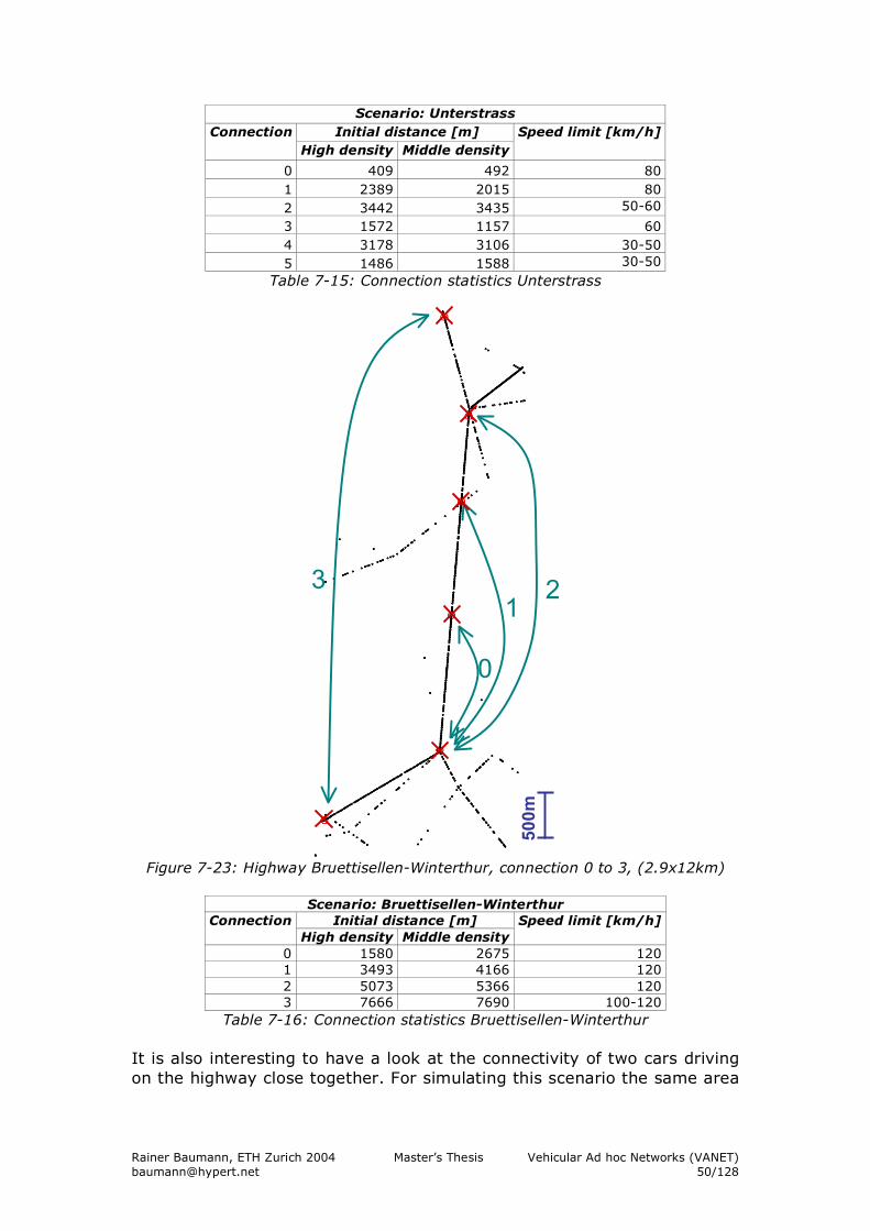
Rainer Baumann, ETH Zurich 2004 Master’s Thesis Vehicular Ad hoc Networks (VANET) [email protected] 50/128
Scenario: Unterstrass Initial distance [m] Connection
High density Middle density Speed limit [km/h]
0 409 492 80 1 2389 2015 80 2 3442 3435 50-60
3 1572 1157 60 4 3178 3106 30-50 5 1486 1588 30-50
Table 7-15: Connection statistics Unterstrass
Figure 7-23: Highway Bruettisellen-Winterthur, connection 0 to 3, (2.9x12km)
Scenario: Bruettisellen-Winterthur
Initial distance [m] Connection High density Middle density
Speed limit [km/h]
0 1580 2675 120 1 3493 4166 120 2 5073 5366 120 3 7666 7690 100-120
Table 7-16: Connection statistics Bruettisellen-Winterthur It is also interesting to have a look at the connectivity of two cars driving on the highway close together. For simulating this scenario the same area
0
1 2 3
500m
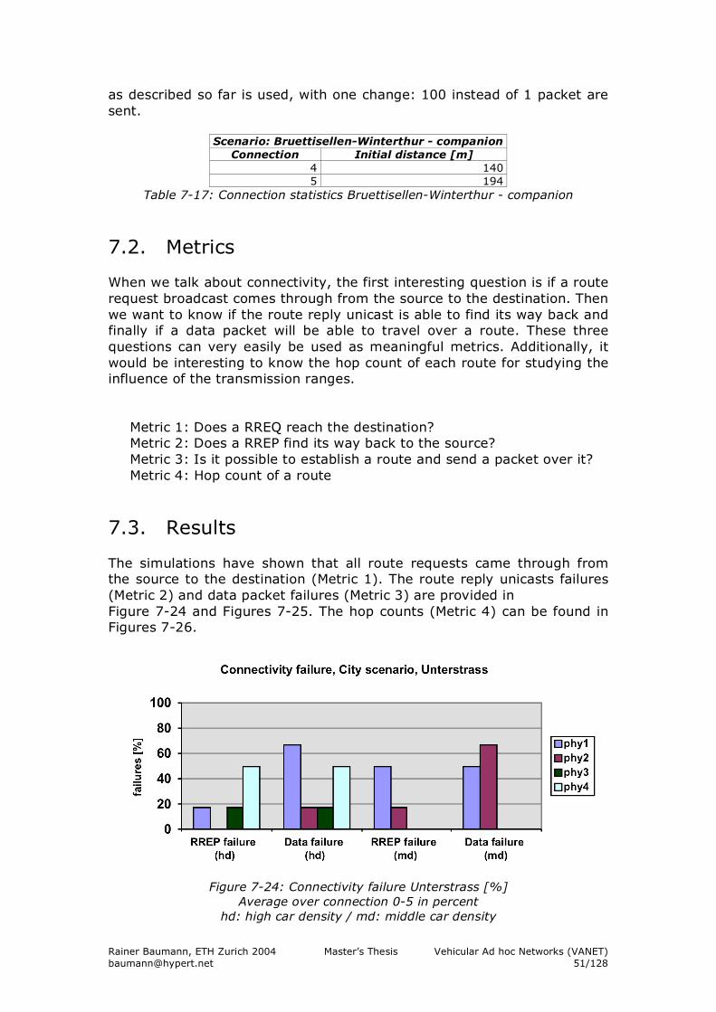
Rainer Baumann, ETH Zurich 2004 Master’s Thesis Vehicular Ad hoc Networks (VANET) [email protected] 51/128
as described so far is used, with one change: 100 instead of 1 packet are sent.
Scenario: Bruettisellen-Winterthur - companion Connection Initial distance [m]
4 140 5 194
Table 7-17: Connection statistics Bruettisellen-Winterthur - companion
7.2. Metrics When we talk about connectivity, the first interesting question is if a route request broadcast comes through from the source to the destination. Then we want to know if the route reply unicast is able to find its way back and finally if a data packet will be able to travel over a route. These three questions can very easily be used as meaningful metrics. Additionally, it would be interesting to know the hop count of each route for studying the influence of the transmission ranges.
Metric 1: Does a RREQ reach the destination? Metric 2: Does a RREP find its way back to the source? Metric 3: Is it possible to establish a route and send a packet over it? Metric 4: Hop count of a route
7.3. Results The simulations have shown that all route requests came through from the source to the destination (Metric 1). The route reply unicasts failures (Metric 2) and data packet failures (Metric 3) are provided in Figure 7-24 and Figures 7-25. The hop counts (Metric 4) can be found in Figures 7-26.
Figure 7-24: Connectivity failure Unterstrass [%]
Average over connection 0-5 in percent hd: high car density / md: middle car density
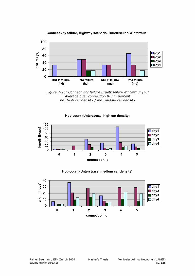
Rainer Baumann, ETH Zurich 2004 Master’s Thesis Vehicular Ad hoc Networks (VANET) [email protected] 52/128
Figure 7-25: Connectivity failure Bruettisellen-Winterthur [%]
Average over connection 0-3 in percent hd: high car density / md: middle car density
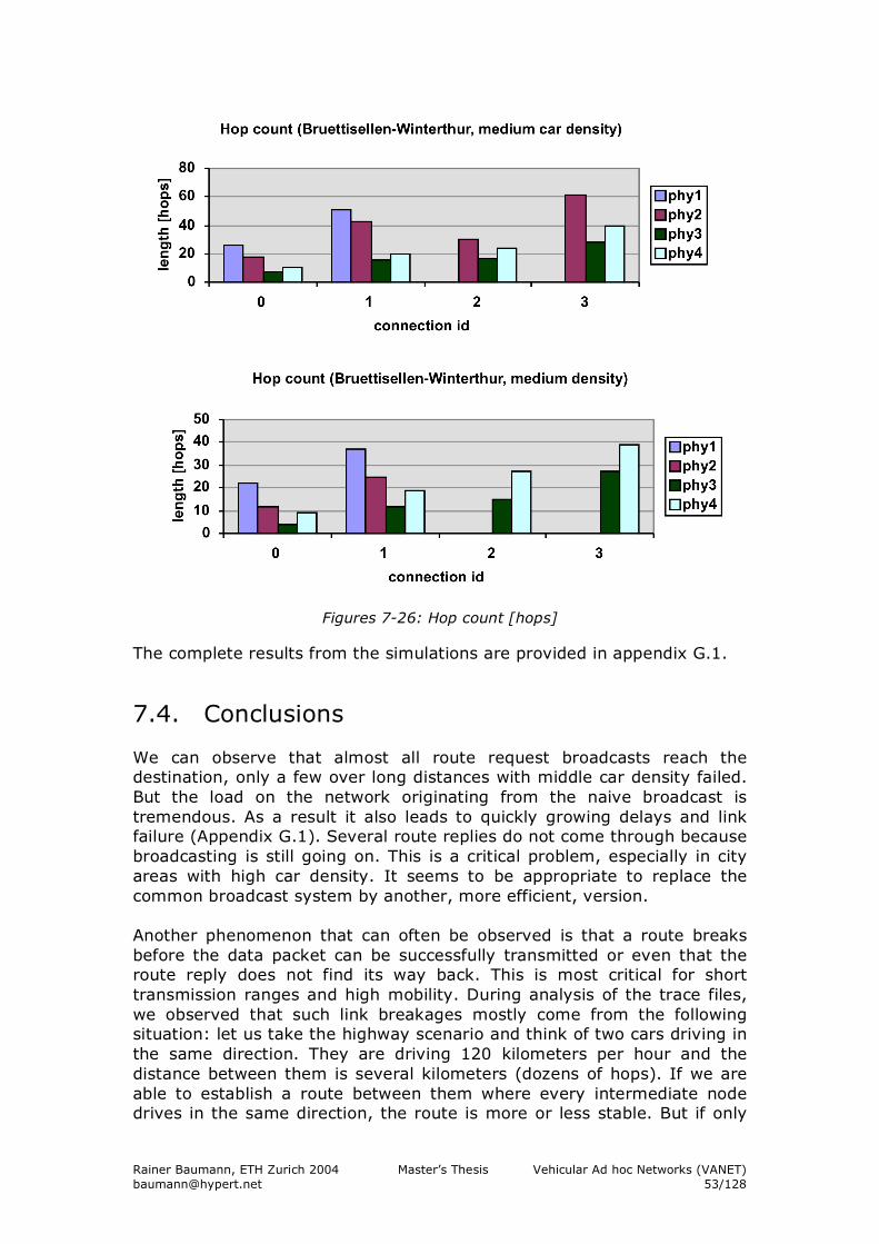
Rainer Baumann, ETH Zurich 2004 Master’s Thesis Vehicular Ad hoc Networks (VANET) [email protected] 53/128
Figures 7-26: Hop count [hops]
The complete results from the simulations are provided in appendix G.1.
7.4. Conclusions We can observe that almost all route request broadcasts reach the destination, only a few over long distances with middle car density failed. But the load on the network originating from the naive broadcast is tremendous. As a result it also leads to quickly growing delays and link failure (Appendix G.1). Several route replies do not come through because broadcasting is still going on. This is a critical problem, especially in city areas with high car density. It seems to be appropriate to replace the common broadcast system by another, more efficient, version. Another phenomenon that can often be observed is that a route breaks before the data packet can be successfully transmitted or even that the route reply does not find its way back. This is most critical for short transmission ranges and high mobility. During analysis of the trace files, we observed that such link breakages mostly come from the following situation: let us take the highway scenario and think of two cars driving in the same direction. They are driving 120 kilometers per hour and the distance between them is several kilometers (dozens of hops). If we are able to establish a route between them where every intermediate node drives in the same direction, the route is more or less stable. But if only
Rainer Baumann, ETH Zurich 2004 Master’s Thesis Vehicular Ad hoc Networks (VANET) [email protected] 54/128
one intermediate node drives in the opposite direction we have a serious problem. Such a node covers about 35 meter per second or 70 meters per second relative to the cars driving in the opposite direction. This is about 20 to 50 percent of the simulated transmission ranges. Since we know from the simulations above that a transmission of a single data packet with route establishment over such a distance takes about a second, it is logically that this leads to a link breakage. If one wants to use AODV on highways, it is essential to extend it in a way that avoids such link breakages.
7.5. Summary The connectivity simulation for highway and city areas has shown that ad hoc networks as proposed, can very well be used for inter vehicle communication. But it seems appropriate to use a clever broadcasting system for avoiding network jams in areas with high car density. It is also advisable to use a routing protocol that takes into account driving directions for fast moving vehicles for reducing link breakage.
Rainer Baumann, ETH Zurich 2004 Master’s Thesis Vehicular Ad hoc Networks (VANET) [email protected] 55/128
8. Secure ring broadcasting
8.1. Broadcasting in ad hoc networks Broadcasting is defined to be an one-to-all communication. I.e. a mobile node sends a message that should be received by all other nodes in the network (provided they are connected). A broadcasting mechanism is the core of every mobile ad hoc routing protocol for route discovery or announcement. It is responsible for the lion’s share of the administrative network load. This is already a sufficient motivation for analyzing it in more detail. The most basic broadcasting protocol is known as the blind flooding, in which a source node transmits the message to all its neighbors, and then each node that receives it for the first time reemits it. Assuming an ideal MAC layer, this protocol is reliable, that is, every node in the network will receive at least once the message. However, because of its simplicity, this protocol leads to a lot of duplicated packets and jams the whole network. Especially in a very dense network, as in car city scenarios, this setup leads to a tremendous overhead. A more intelligent protocol, named Neighbor Elimination Scheme (NES) has been proposed in [19] [20]. Its principle is as follows. Each node that receives a message for the first time does not retransmit it immediately, but waits for a given duration, which can be computed or randomly generated. While waiting, the node monitors its neighborhood and after each received copy of the broadcast message, it eliminates from its rebroadcast list neighbors that are assumed to have correctly received it. If the list becomes empty before the node decides to relay the message, the reemission is canceled. This protocol allows some bandwidth savings by canceling redundant emissions, while still insuring an entire coverage of the network. But every node needs to know its neighbors. In turn, this can be bandwidth consuming in a fast changing network as in vehicular ad hoc networks. Another category of protocols is based on the computation of a connected dominating set S. A set is a dominating one if each node in the graph is either in S or a neighbor of a node in S. The broadcasting step, in its simplest variant, can be described as follows. When a node receives a broadcast message for the first time, it drops the message if it is not in the considered connected dominating set or retransmits it otherwise [20]. Nodes ignore subsequent receptions of the same message. When the neighbor elimination scheme is applied, some transmissions may be avoided. A node that is in the dominating set, but observes that all its neighbors have already received the same message, can also drop the packet without retransmitting it. But calculating such a dominating set requires a lot of bandwidth. Even worse, once such a dominating set is calculated, it is already out dated because of the fast changing scenario.
Rainer Baumann, ETH Zurich 2004 Master’s Thesis Vehicular Ad hoc Networks (VANET) [email protected] 56/128
A further broadcast improvement is the so-called geoflood [12]. The geoflood algorithm assumes that each node can discern its own location, but it does not require each node to know the location of its neighbors. This is an important distinction because learning the location of other nodes is usually done by means of a “hello” protocol, which adds additional protocol messages. Today, nodes can easily obtain their location through already popular GPS devices. It makes sense to assume that a car, which is equipped with a WLAN system, also has an onboard GPS system for example for a navigation system. In geoflood each node waits a short period of time before forwarding on the first reception of the message as in NES. A node abstains from forwarding a message when it receives the same message from all geographic directions. A location field carrying the position of the sender extends a routing packet. Each node defines a Cartesian plane with its own location as the origin. A node will abstain from forwarding only when it has received the message from all four quadrants (NE, NW, SE and SW). Thus the algorithm works as follows: If the local node has forwarded the received message earlier, the message is dropped. If this is the first reception of the message, the quadrant from which the message arrived is recorded, and a packet holding time t is chosen. The message is temporarily put on hold until either the message is received from all four quadrants or t time has passed. If the message arrives from all four quadrants before time t, then the message is dropped, otherwise it is forwarded and the (source, sequence) pair is stored in the forwarding cache to filter future duplicates. An important part of the algorithm is the selection of packet holding time. Nodes furthest away from the local sender should select the smallest packet holding times. These are the nodes located near the perimeter of the sender’s transmission range. Holding times increase as the distance to the sender decreases, with those nodes closest to the sender waiting the longest. For cars, the geoflood algorithm has one major disadvantage. A car on a straight route will nearly never be able to receive a packet from all for quadrants. One now can tend to propose to reduce the four quadrants only to two. But this will lead to serious problems at crossings. For both situations, we run some short simulation for verifying our thoughts and the results are very clear: geoflood is no option for vehicular ad hoc networks. So we have decided to develop our own broadcasting mechanism for avoiding unnecessary route request, the Secure Ring Broadcasting (SRB).
8.2. Secure Ring Broadcasting (SRB) Secure Ring Broadcasting (SRB) is specialized for broadcasting route requests. The main target of it is not only to minimize broadcasting messages but also to get more stable routes.
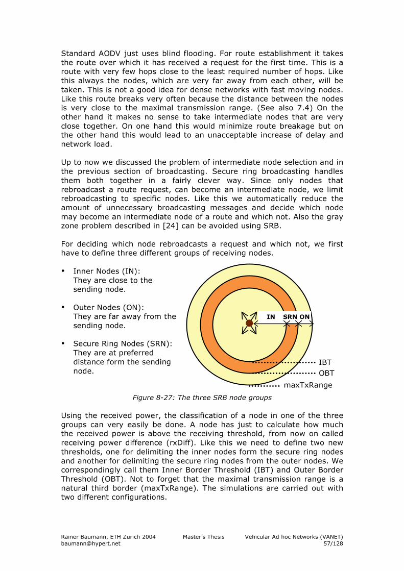
Rainer Baumann, ETH Zurich 2004 Master’s Thesis Vehicular Ad hoc Networks (VANET) [email protected] 57/128
Standard AODV just uses blind flooding. For route establishment it takes the route over which it has received a request for the first time. This is a route with very few hops close to the least required number of hops. Like this always the nodes, which are very far away from each other, will be taken. This is not a good idea for dense networks with fast moving nodes. Like this route breaks very often because the distance between the nodes is very close to the maximal transmission range. (See also 7.4) On the other hand it makes no sense to take intermediate nodes that are very close together. On one hand this would minimize route breakage but on the other hand this would lead to an unacceptable increase of delay and network load. Up to now we discussed the problem of intermediate node selection and in the previous section of broadcasting. Secure ring broadcasting handles them both together in a fairly clever way. Since only nodes that rebroadcast a route request, can become an intermediate node, we limit rebroadcasting to specific nodes. Like this we automatically reduce the amount of unnecessary broadcasting messages and decide which node may become an intermediate node of a route and which not. Also the gray zone problem described in [24] can be avoided using SRB. For deciding which node rebroadcasts a request and which not, we first have to define three different groups of receiving nodes. • Inner Nodes (IN):
They are close to the sending node.
• Outer Nodes (ON): They are far away from the sending node.
• Secure Ring Nodes (SRN): They are at preferred distance form the sending node.
Figure 8-27: The three SRB node groups Using the received power, the classification of a node in one of the three groups can very easily be done. A node has just to calculate how much the received power is above the receiving threshold, from now on called receiving power difference (rxDiff). Like this we need to define two new thresholds, one for delimiting the inner nodes form the secure ring nodes and another for delimiting the secure ring nodes from the outer nodes. We correspondingly call them Inner Border Threshold (IBT) and Outer Border Threshold (OBT). Not to forget that the maximal transmission range is a natural third border (maxTxRange). The simulations are carried out with two different configurations.
IBT OBT
maxTxRange
IN ON SRN
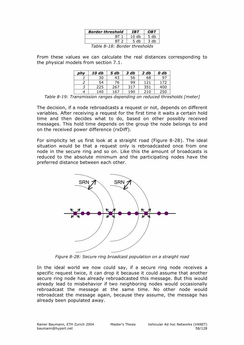
Rainer Baumann, ETH Zurich 2004 Master’s Thesis Vehicular Ad hoc Networks (VANET) [email protected] 58/128
Border threshold IBT OBT BT 1 10 db 5 db BT 2 5 db 3 db
Table 8-18: Border thresholds From these values we can calculate the real distances corresponding to the physical models from section 7.1.
phy 10 db 5 db 3 db 2 db 0 db 1 30 43 56 68 97 2 54 76 99 121 172 3 225 267 317 351 400 4 140 167 190 210 250
Table 8-19: Transmission ranges depending on reduced thresholds [meter] The decision, if a node rebroadcasts a request or not, depends on different variables. After receiving a request for the first time it waits a certain hold time and then decides what to do, based on other possibly received messages. This hold time depends on the group the node belongs to and on the received power difference (rxDiff). For simplicity let us first look at a straight road (Figure 8-28). The ideal situation would be that a request only is rebroadcasted once from one node in the secure ring and so on. Like this the amount of broadcasts is reduced to the absolute minimum and the participating nodes have the preferred distance between each other.
Figure 8-28: Secure ring broadcast population on a straight road In the ideal world we now could say, if a secure ring node receives a specific request twice, it can drop it because it could assume that another secure ring node has already rebroadcasted this message. But this would already lead to misbehavior if two neighboring nodes would occasionally rebroadcast the message at the same time. No other node would rebroadcast the message again, because they assume, the message has already been populated away.
SRN SRN
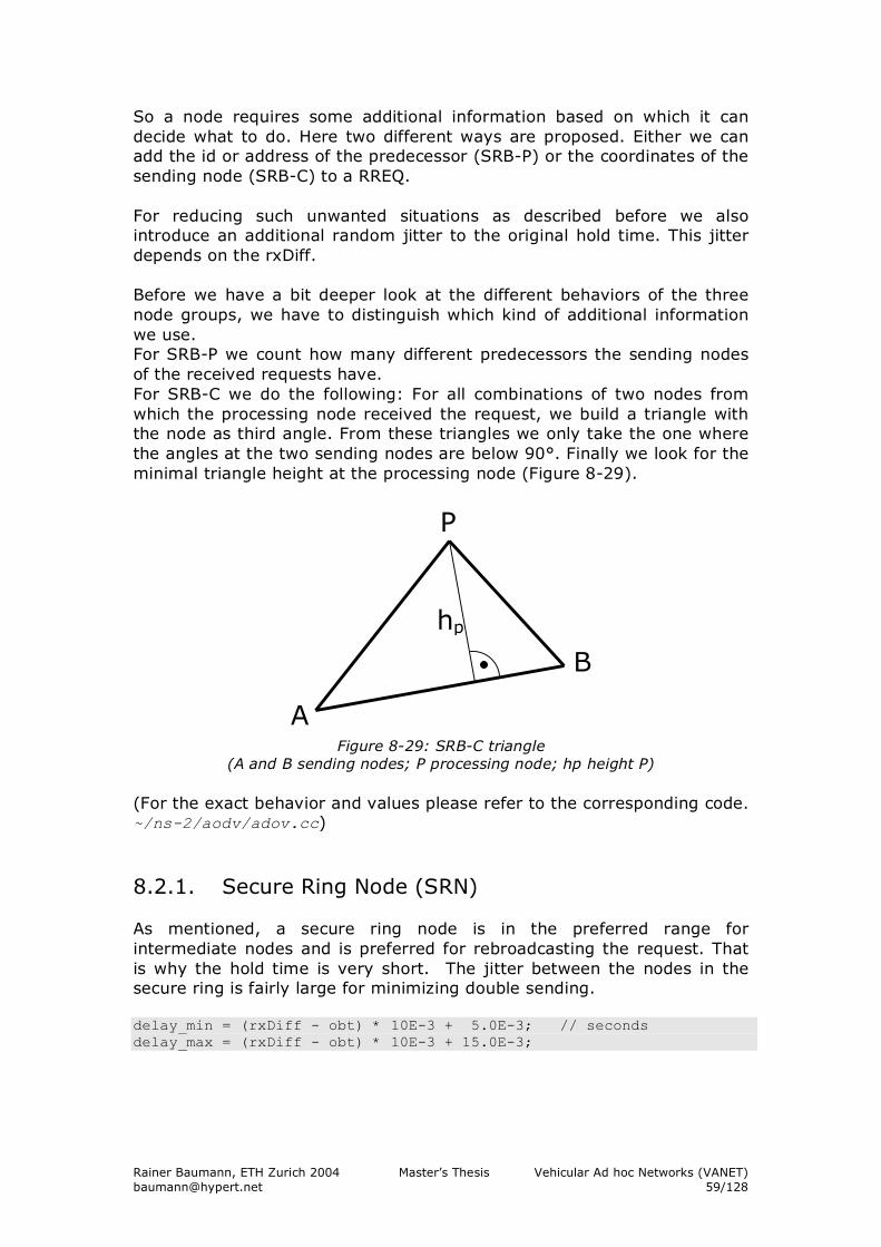
Rainer Baumann, ETH Zurich 2004 Master’s Thesis Vehicular Ad hoc Networks (VANET) [email protected] 59/128
So a node requires some additional information based on which it can decide what to do. Here two different ways are proposed. Either we can add the id or address of the predecessor (SRB-P) or the coordinates of the sending node (SRB-C) to a RREQ. For reducing such unwanted situations as described before we also introduce an additional random jitter to the original hold time. This jitter depends on the rxDiff. Before we have a bit deeper look at the different behaviors of the three node groups, we have to distinguish which kind of additional information we use. For SRB-P we count how many different predecessors the sending nodes of the received requests have. For SRB-C we do the following: For all combinations of two nodes from which the processing node received the request, we build a triangle with the node as third angle. From these triangles we only take the one where the angles at the two sending nodes are below 90°. Finally we look for the minimal triangle height at the processing node (Figure 8-29).
Figure 8-29: SRB-C triangle (A and B sending nodes; P processing node; hp height P)
(For the exact behavior and values please refer to the corresponding code. ~/ns-2/aodv/adov.cc)
8.2.1. Secure Ring Node (SRN) As mentioned, a secure ring node is in the preferred range for intermediate nodes and is preferred for rebroadcasting the request. That is why the hold time is very short. The jitter between the nodes in the secure ring is fairly large for minimizing double sending. delay_min = (rxDiff - obt) * 10E-3 + 5.0E-3; // seconds delay_max = (rxDiff - obt) * 10E-3 + 15.0E-3;
P
A
B
hp
Rainer Baumann, ETH Zurich 2004 Master’s Thesis Vehicular Ad hoc Networks (VANET) [email protected] 60/128
SRB-P (predecessor of sender) If we receive the same request from two nodes with different predecessors in the hold time, we drop the request otherwise we rebroadcast it. SRB-C (coordinates of sender) If the minimal height value is below a certain threshold (e.g. 50 meter) we drop the packet, otherwise we rebroadcast it. 8.2.2. Outer Node (ON) If no secure ring node rebroadcasts the request, it is up to an outer node to rebroadcast it. delay_min = (obt - rxDiff) * 2E-3 + 72.0E-3; // seconds delay_max = (obt - rxDiff) * 2E-3 + 74.0E-3;
The behavior of an outer node is the most complex of all three node groups. This is because we do not want SRB to reduce the maximal transmission range. In an ideal situation, an ON hears a request three times, because after the first received broadcast it should hear the rebroadcast of the SRN and also the rebroadcast from the next node. If an ON hears the rebroadcast twice, it makes sense to wait again for another hold time since we can assume that the packet was just rebroadcasted from a SRN or another ON. delay_min = min( rxDiff * 5E-3 + 20.0E-3 , 110E-3 ); // seconds delay_max = min( rxDiff * 5E-3 + 25.0E-3 , 115E-3 );
But if the node has still not detected a third broadcast of the request after waiting for the second hold time, it rebroadcasts the message itself. SRB-P (predecessor of sender) If we receive the same request from three nodes with different predecessors in the hold time, we drop the request. If we hear it only twice we wait for an additional hold time. If we have heard it a third time after the second hold time with another predecessor, we drop the request as well. In all other cases the request will be rebroadcasted. SRB-C (coordinates of sender) We only consider nodes with height below a certain threshold (e.g. 50 meter). If we receive the same request from three nodes in the hold time, we drop the request. If we hear it only twice, we wait for an additional hold time. If we hear it a third time after the second hold time, we drop the request as well. In all other cases the request will be rebroadcasted.
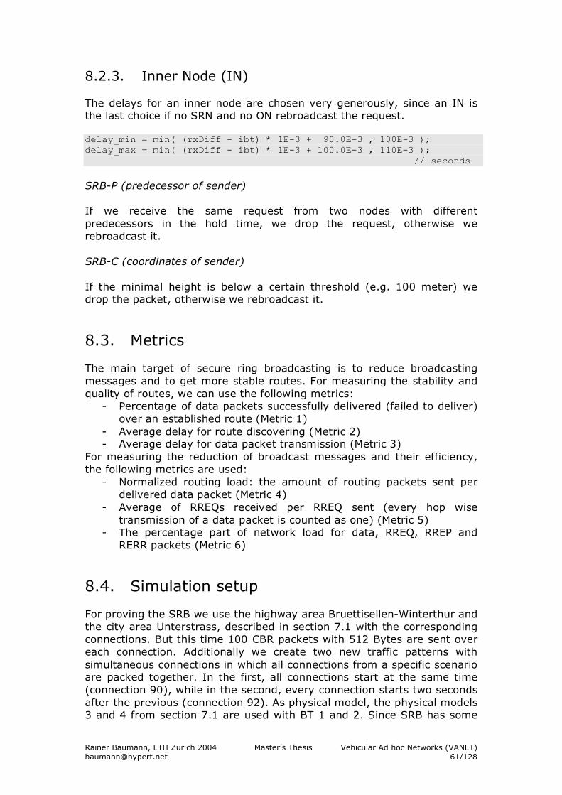
Rainer Baumann, ETH Zurich 2004 Master’s Thesis Vehicular Ad hoc Networks (VANET) [email protected] 61/128
8.2.3. Inner Node (IN) The delays for an inner node are chosen very generously, since an IN is the last choice if no SRN and no ON rebroadcast the request. delay_min = min( (rxDiff - ibt) * 1E-3 + 90.0E-3 , 100E-3 ); delay_max = min( (rxDiff - ibt) * 1E-3 + 100.0E-3 , 110E-3 ); // seconds
SRB-P (predecessor of sender) If we receive the same request from two nodes with different predecessors in the hold time, we drop the request, otherwise we rebroadcast it. SRB-C (coordinates of sender) If the minimal height is below a certain threshold (e.g. 100 meter) we drop the packet, otherwise we rebroadcast it.
8.3. Metrics The main target of secure ring broadcasting is to reduce broadcasting messages and to get more stable routes. For measuring the stability and quality of routes, we can use the following metrics:
- Percentage of data packets successfully delivered (failed to deliver) over an established route (Metric 1)
- Average delay for route discovering (Metric 2) - Average delay for data packet transmission (Metric 3)
For measuring the reduction of broadcast messages and their efficiency, the following metrics are used:
- Normalized routing load: the amount of routing packets sent per delivered data packet (Metric 4)
- Average of RREQs received per RREQ sent (every hop wise transmission of a data packet is counted as one) (Metric 5)
- The percentage part of network load for data, RREQ, RREP and RERR packets (Metric 6)
8.4. Simulation setup For proving the SRB we use the highway area Bruettisellen-Winterthur and the city area Unterstrass, described in section 7.1 with the corresponding connections. But this time 100 CBR packets with 512 Bytes are sent over each connection. Additionally we create two new traffic patterns with simultaneous connections in which all connections from a specific scenario are packed together. In the first, all connections start at the same time (connection 90), while in the second, every connection starts two seconds after the previous (connection 92). As physical model, the physical models 3 and 4 from section 7.1 are used with BT 1 and 2. Since SRB has some
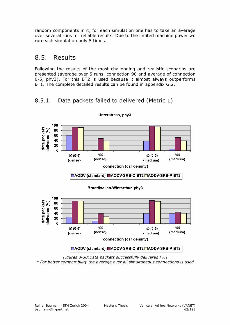
Rainer Baumann, ETH Zurich 2004 Master’s Thesis Vehicular Ad hoc Networks (VANET) [email protected] 62/128
random components in it, for each simulation one has to take an average over several runs for reliable results. Due to the limited machine power we run each simulation only 5 times.
8.5. Results Following the results of the most challenging and realistic scenarios are presented (average over 5 runs, connection 90 and average of connection 0-5, phy3). For this BT2 is used because it almost always outperforms BT1. The complete detailed results can be found in appendix G.2. 8.5.1. Data packets failed to delivered (Metric 1)
Figures 8-30:Data packets successfully delivered [%]
* For better comparability the average over all simultaneous connections is used
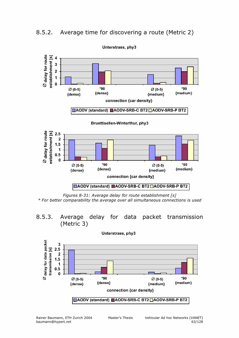
Rainer Baumann, ETH Zurich 2004 Master’s Thesis Vehicular Ad hoc Networks (VANET) [email protected] 63/128
8.5.2. Average time for discovering a route (Metric 2)
Figures 8-31: Average delay for route establishment [s]
* For better comparability the average over all simultaneous connections is used 8.5.3. Average delay for data packet transmission
(Metric 3)
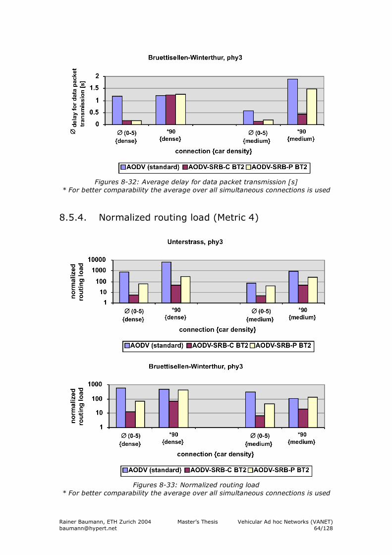
Rainer Baumann, ETH Zurich 2004 Master’s Thesis Vehicular Ad hoc Networks (VANET) [email protected] 64/128
Figures 8-32: Average delay for data packet transmission [s]
* For better comparability the average over all simultaneous connections is used
8.5.4. Normalized routing load (Metric 4)
Figures 8-33: Normalized routing load
* For better comparability the average over all simultaneous connections is used
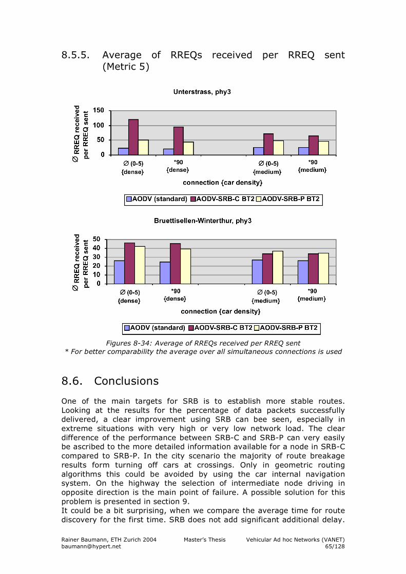
Rainer Baumann, ETH Zurich 2004 Master’s Thesis Vehicular Ad hoc Networks (VANET) [email protected] 65/128
8.5.5. Average of RREQs received per RREQ sent (Metric 5)
Figures 8-34: Average of RREQs received per RREQ sent
* For better comparability the average over all simultaneous connections is used
8.6. Conclusions One of the main targets for SRB is to establish more stable routes. Looking at the results for the percentage of data packets successfully delivered, a clear improvement using SRB can bee seen, especially in extreme situations with very high or very low network load. The clear difference of the performance between SRB-C and SRB-P can very easily be ascribed to the more detailed information available for a node in SRB-C compared to SRB-P. In the city scenario the majority of route breakage results form turning off cars at crossings. Only in geometric routing algorithms this could be avoided by using the car internal navigation system. On the highway the selection of intermediate node driving in opposite direction is the main point of failure. A possible solution for this problem is presented in section 9. It could be a bit surprising, when we compare the average time for route discovery for the first time. SRB does not add significant additional delay.
Rainer Baumann, ETH Zurich 2004 Master’s Thesis Vehicular Ad hoc Networks (VANET) [email protected] 66/128
In contrast, SRB-C even reduces the delay for networks with low load. The load is also the relevant factor for the delay using blind flooding. Due to the congested network a packet obtains a delay comparable with the specific random delays introduced by SRB. A main target for SRB is to reduce the amount of network load resulting form broadcast messages. For measuring this, the ratio of the amount of routing packets transmitted per delivered data packet is calculated. Note that a logarithmic scale has been used for the plot in Figures 8-33. For SRB-C a reduction up to two magnitudes can be observed. Due to some boarder effects, the reduction for SRB-P is not that impressive. At the sharp cute boarder, every node rebroadcasts the message with the hop, that some other node further away is just able to receive the message. But there is no further node answering, so every node at the boarder will try it as well. This is necessary for not limiting the range of the network by the routing protocol. The average of received RREQs per RREQ sent confirms the much higher efficiency of SRB especially in city scenarios. If we compare the results of the two border thresholds (BT1 and BT2) with each other, one can easily see that this parameter in combination with the car density has a strong impact on the performance of SRB. In the simulations BT2 mostly outperforms BT1. More detailed analysis of several different border thresholds still have to be done in a future project. It is also interesting to compare the results for the physical model 3 and 4. The interested reader will recognize that model 4 with the shorter transmission range some times has outperformed model 3. This points out, that a larger transmission range also has some disadvantages for ad hoc networks. The larger the range, the more nodes are affected by a unicast what increases the probability of a collision.
8.7. Verification under random interference In real world, signal propagation is often influenced by uncontrollable random factors as for example other cars or weather. Since SRB operates with the signal propagation range we wanted to check up on the influence of these random factors. For verifying SRB under such conditions some random variability in the received power up to 3 dB is introduced. For simulation the same setup and metrics as proposed earlier in this chapter are used (Section 8.3 and 8.4). The detailed results can be found in appendix G.3. The percentage of successful delivered data packets for SRB decreased slightly up to 20%. For standard AODV the decrease is much more impressive with a maximum of 100%. For both, SRB and standard AODV, the delays increase a bit but not dramatically because of the shorter communication ranges. On the normalized routing load, the variation has almost no influence.
Rainer Baumann, ETH Zurich 2004 Master’s Thesis Vehicular Ad hoc Networks (VANET) [email protected] 67/128
8.8. Summary Secure Ring Broadcasting (SRB) has accomplished the expectations. It markedly reduces the amount of broadcasting messages and establishes more stable routes. SRB with coordinates (SRB-C) outperforms SRB with predecessors (SRB-P) in almost all situations clearly as result of the availability of more detailed information. SRB has a large amount of tunable parameters: the various delays, the boarder thresholds and not to forget the transmission range. A detailed study of their effects still has to be done in a future project.
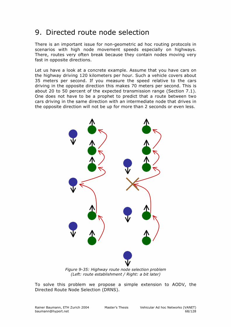
Rainer Baumann, ETH Zurich 2004 Master’s Thesis Vehicular Ad hoc Networks (VANET) [email protected] 68/128
9. Directed route node selection There is an important issue for non-geometric ad hoc routing protocols in scenarios with high node movement speeds especially on highways. There, routes very often break because they contain nodes moving very fast in opposite directions. Let us have a look at a concrete example. Assume that you have cars on the highway driving 120 kilometers per hour. Such a vehicle covers about 35 meters per second. If you measure the speed relative to the cars driving in the opposite direction this makes 70 meters per second. This is about 20 to 50 percent of the expected transmission range (Section 7.1). One does not have to be a prophet to predict that a route between two cars driving in the same direction with an intermediate node that drives in the opposite direction will not be up for more than 2 seconds or even less.
Figure 9-35: Highway route node selection problem (Left: route establishment / Right: a bit later)
To solve this problem we propose a simple extension to AODV, the Directed Route Node Selection (DRNS).
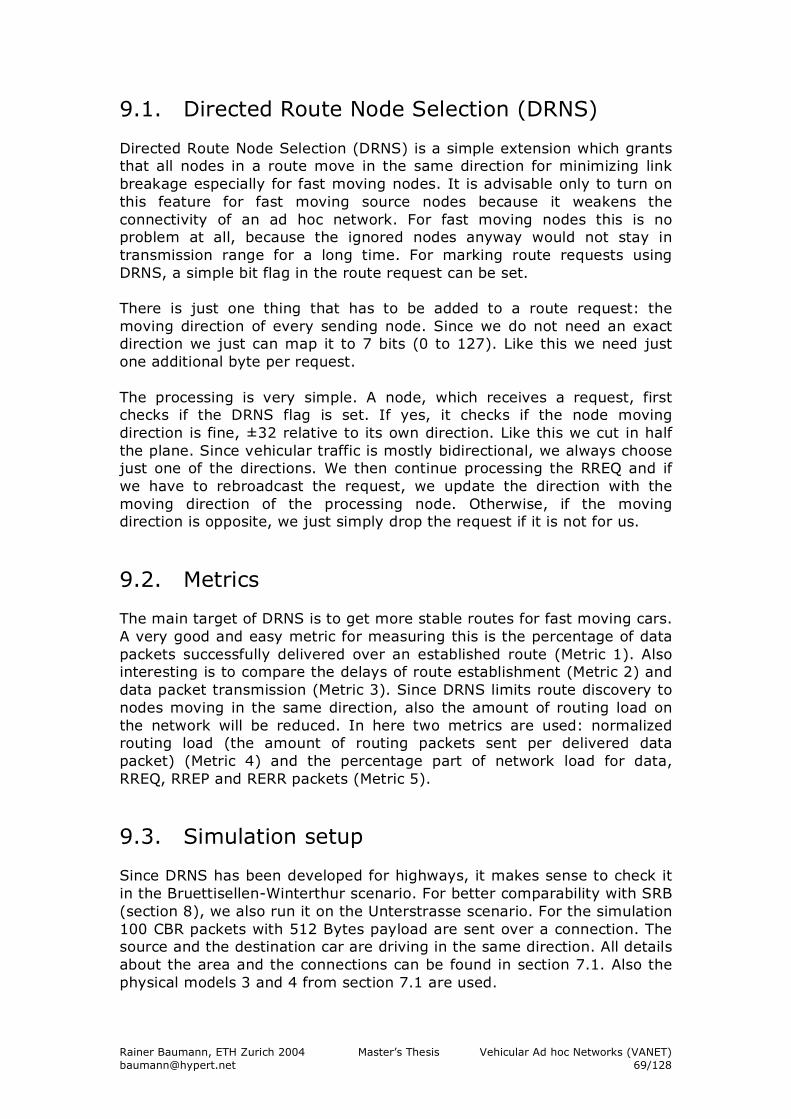
Rainer Baumann, ETH Zurich 2004 Master’s Thesis Vehicular Ad hoc Networks (VANET) [email protected] 69/128
9.1. Directed Route Node Selection (DRNS) Directed Route Node Selection (DRNS) is a simple extension which grants that all nodes in a route move in the same direction for minimizing link breakage especially for fast moving nodes. It is advisable only to turn on this feature for fast moving source nodes because it weakens the connectivity of an ad hoc network. For fast moving nodes this is no problem at all, because the ignored nodes anyway would not stay in transmission range for a long time. For marking route requests using DRNS, a simple bit flag in the route request can be set. There is just one thing that has to be added to a route request: the moving direction of every sending node. Since we do not need an exact direction we just can map it to 7 bits (0 to 127). Like this we need just one additional byte per request. The processing is very simple. A node, which receives a request, first checks if the DRNS flag is set. If yes, it checks if the node moving direction is fine, ±32 relative to its own direction. Like this we cut in half the plane. Since vehicular traffic is mostly bidirectional, we always choose just one of the directions. We then continue processing the RREQ and if we have to rebroadcast the request, we update the direction with the moving direction of the processing node. Otherwise, if the moving direction is opposite, we just simply drop the request if it is not for us.
9.2. Metrics The main target of DRNS is to get more stable routes for fast moving cars. A very good and easy metric for measuring this is the percentage of data packets successfully delivered over an established route (Metric 1). Also interesting is to compare the delays of route establishment (Metric 2) and data packet transmission (Metric 3). Since DRNS limits route discovery to nodes moving in the same direction, also the amount of routing load on the network will be reduced. In here two metrics are used: normalized routing load (the amount of routing packets sent per delivered data packet) (Metric 4) and the percentage part of network load for data, RREQ, RREP and RERR packets (Metric 5).
9.3. Simulation setup Since DRNS has been developed for highways, it makes sense to check it in the Bruettisellen-Winterthur scenario. For better comparability with SRB (section 8), we also run it on the Unterstrasse scenario. For the simulation 100 CBR packets with 512 Bytes payload are sent over a connection. The source and the destination car are driving in the same direction. All details about the area and the connections can be found in section 7.1. Also the physical models 3 and 4 from section 7.1 are used.
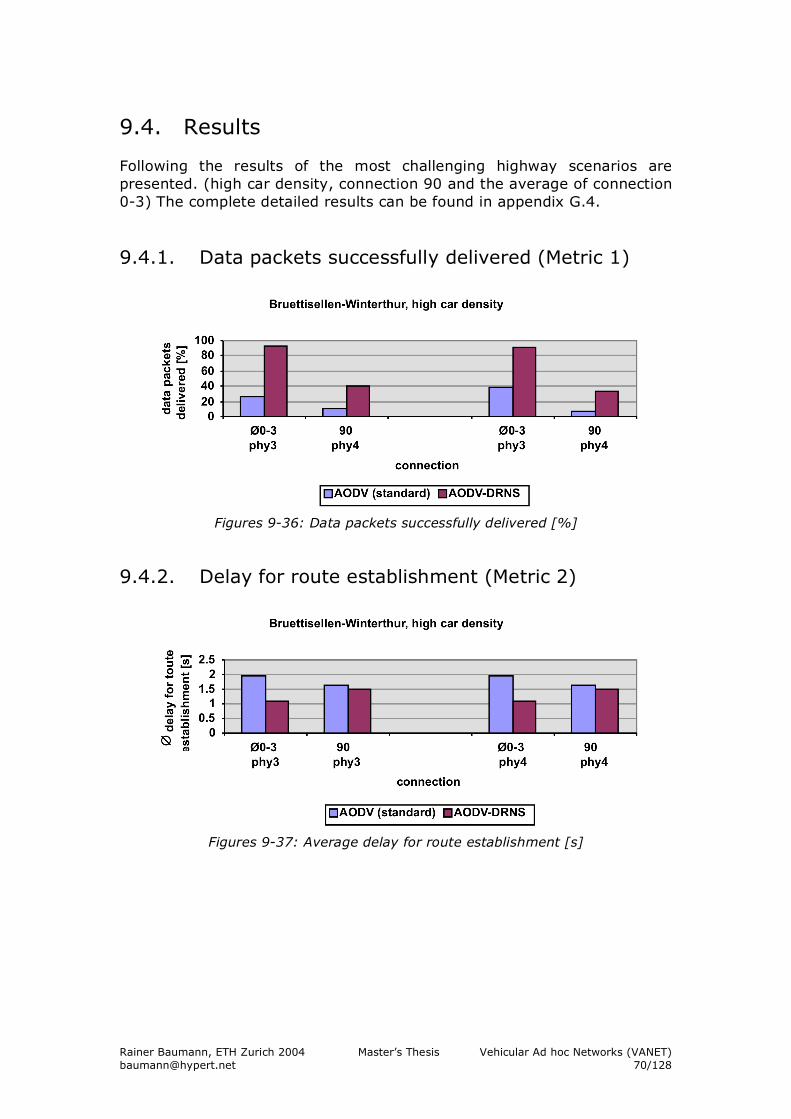
Rainer Baumann, ETH Zurich 2004 Master’s Thesis Vehicular Ad hoc Networks (VANET) [email protected] 70/128
9.4. Results Following the results of the most challenging highway scenarios are presented. (high car density, connection 90 and the average of connection 0-3) The complete detailed results can be found in appendix G.4.
9.4.1. Data packets successfully delivered (Metric 1)
Figures 9-36: Data packets successfully delivered [%]
9.4.2. Delay for route establishment (Metric 2)
Figures 9-37: Average delay for route establishment [s]
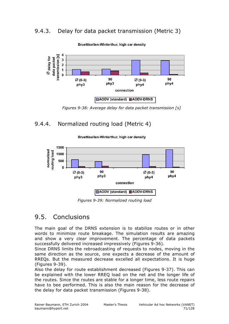
Rainer Baumann, ETH Zurich 2004 Master’s Thesis Vehicular Ad hoc Networks (VANET) [email protected] 71/128
9.4.3. Delay for data packet transmission (Metric 3)
Figures 9-38: Average delay for data packet transmission [s]
9.4.4. Normalized routing load (Metric 4)
Figures 9-39: Normalized routing load
9.5. Conclusions The main goal of the DRNS extension is to stabilize routes or in other words to minimize route breakage. The simulation results are amazing and show a very clear improvement. The percentage of data packets successfully delivered increased impressively (Figures 9-36). Since DRNS limits the rebroadcasting of requests to nodes, moving in the same direction as the source, one expects a decrease of the amount of RREQs. But the measured decrease excelled all expectations. It is huge (Figures 9-39). Also the delay for route establishment decreased (Figures 9-37). This can be explained with the lower RREQ load on the net and the longer life of the routes. Since the routes are stable for a longer time, less route repairs have to bee performed. This is also the main reason for the decrease of the delay for data packet transmission (Figures 9-38).
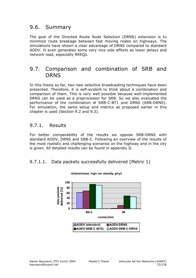
Rainer Baumann, ETH Zurich 2004 Master’s Thesis Vehicular Ad hoc Networks (VANET) [email protected] 72/128
9.6. Summary The goal of the Directed Route Node Selection (DRNS) extension is to minimize route breakage between fast moving nodes on highways. The simulations have shown a clear advantage of DRNS compared to standard AODV. It even generates some very nice side effects as lower delays and network load, especially RREQs.
9.7. Comparison and combination of SRB and DRNS
In this thesis so far, two new selective broadcasting techniques have been presented. Therefore, it is self-evident to think about a combination and comparison of them. This is very well possible because well-implemented DRNS can be used as a preprocessor for SRB. So we also evaluated the performance of the combination of SRB-C-BT1 and DRNS (SRB-DRNS). For simulation, the same setup and metrics as proposed earlier in this chapter is used (Section 9.2 and 9.3).
9.7.1. Results For better comparability of the results we oppose SRB-DRNS with standard AODV, DRNS and SRB-C. Following an overview of the results of the most realistic and challenging scenarios on the highway and in the city is given. All detailed results can be found in appendix G. 9.7.1.1. Data packets successfully delivered (Metric 1)
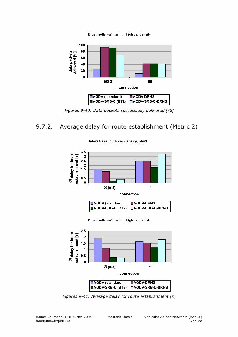
Rainer Baumann, ETH Zurich 2004 Master’s Thesis Vehicular Ad hoc Networks (VANET) [email protected] 73/128
Figures 9-40: Data packets successfully delivered [%]
9.7.2. Average delay for route establishment (Metric 2)
Figures 9-41: Average delay for route establishment [s]
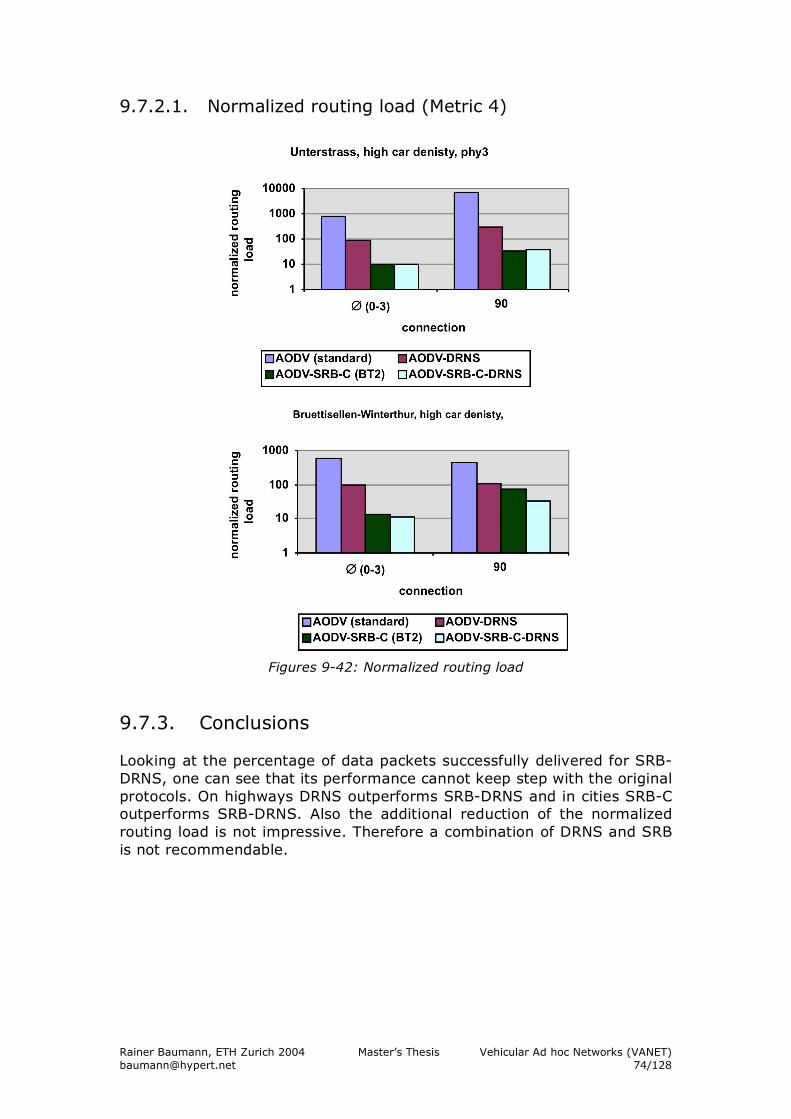
Rainer Baumann, ETH Zurich 2004 Master’s Thesis Vehicular Ad hoc Networks (VANET) [email protected] 74/128
9.7.2.1. Normalized routing load (Metric 4)
Figures 9-42: Normalized routing load
9.7.3. Conclusions Looking at the percentage of data packets successfully delivered for SRB-DRNS, one can see that its performance cannot keep step with the original protocols. On highways DRNS outperforms SRB-DRNS and in cities SRB-C outperforms SRB-DRNS. Also the additional reduction of the normalized routing load is not impressive. Therefore a combination of DRNS and SRB is not recommendable.
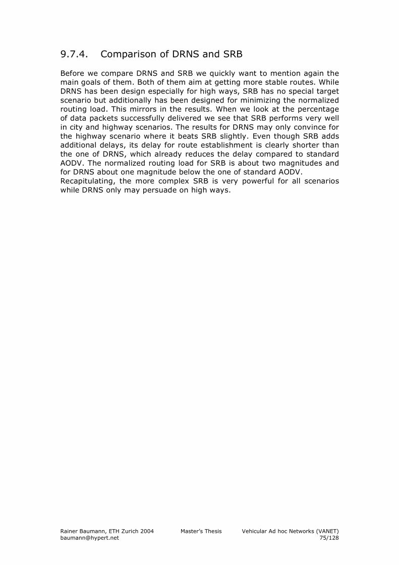
Rainer Baumann, ETH Zurich 2004 Master’s Thesis Vehicular Ad hoc Networks (VANET) [email protected] 75/128
9.7.4. Comparison of DRNS and SRB Before we compare DRNS and SRB we quickly want to mention again the main goals of them. Both of them aim at getting more stable routes. While DRNS has been design especially for high ways, SRB has no special target scenario but additionally has been designed for minimizing the normalized routing load. This mirrors in the results. When we look at the percentage of data packets successfully delivered we see that SRB performs very well in city and highway scenarios. The results for DRNS may only convince for the highway scenario where it beats SRB slightly. Even though SRB adds additional delays, its delay for route establishment is clearly shorter than the one of DRNS, which already reduces the delay compared to standard AODV. The normalized routing load for SRB is about two magnitudes and for DRNS about one magnitude below the one of standard AODV. Recapitulating, the more complex SRB is very powerful for all scenarios while DRNS only may persuade on high ways.
Rainer Baumann, ETH Zurich 2004 Master’s Thesis Vehicular Ad hoc Networks (VANET) [email protected] 76/128
10. Hybrid internet access
10.1. Hybrid ad hoc networks Today internet access became a standard commodity, and many users do not want to do without even in cars. As mentioned in the introduction, one could think of many useful services, which could be offered, having an internet connection in a vehicle e.g. car maintenance. Wireless LAN is the ideal technology to provide such connections. But if we would use common access points, the building of such an infrastructure would be unaffordable. Due to the short communication ranges, a huge number of access points would be needed to install a seamless wireless network. To allow greater mobility, and to reduce the impact of collisions with multiple users attached to the same access point, multi-hop access mode is being considered. Instead of direct communication with access points, it may be beneficial, extended coverage and bandwidth capacity, to contact access points via other users in multi-hop fashion. Such combined infrastructure and ad hoc networks are so called hybrid networks (Section 3.3.1). The WLAN standard specifies two different operation modes: infrastructure and ad hoc (Section 3.3.1). The two modes already differ in their design target. On one side the infrastructure mode is thought for mobile nodes offering access to a wired network (e.g. the Internet). The main component in an infrastructure WLAN is the access point, which manages everything. For communication always a direct link between a node and an access point is required (single hop). On the other hand we have the ad hoc mode, which is thought for infrastructure less networking in a group of mobile nodes, which is by nature multi hop. The ideal thing would be to combine this two operation modes getting a multi hop WLAN, which offers access to a wired network. Since the two modes already differ on the very low MAC layer, there is no way to combine them. But there is still a possibility how to get such a desired WLAN. We could run the WLAN in the ad hoc mode and additionally attach some nodes with a second network card connected to a wired network. These nodes have to act as a gateway between the wireless and wired world. They are some kind of base station. Based on this idea, the Hybrid Internet Access extension for AODV (HIA) has been developed.
10.2. The Hybrid Internet Access extension (HIA) Hybrid Internet Access (HIA) is an extension for AODV making possible multi-hop internet access over hybrid WLANs. It surprisingly requires few changes in AODV. There are two kinds of nodes: common mobile nodes and gateway nodes. The affiliation of a node must be recognizable by its IP address. It is advised to use a block of private IP addresses (e.g. 10.0.0.0 up to 10.255.255.255) and divide it into two parts, one part for the gateway
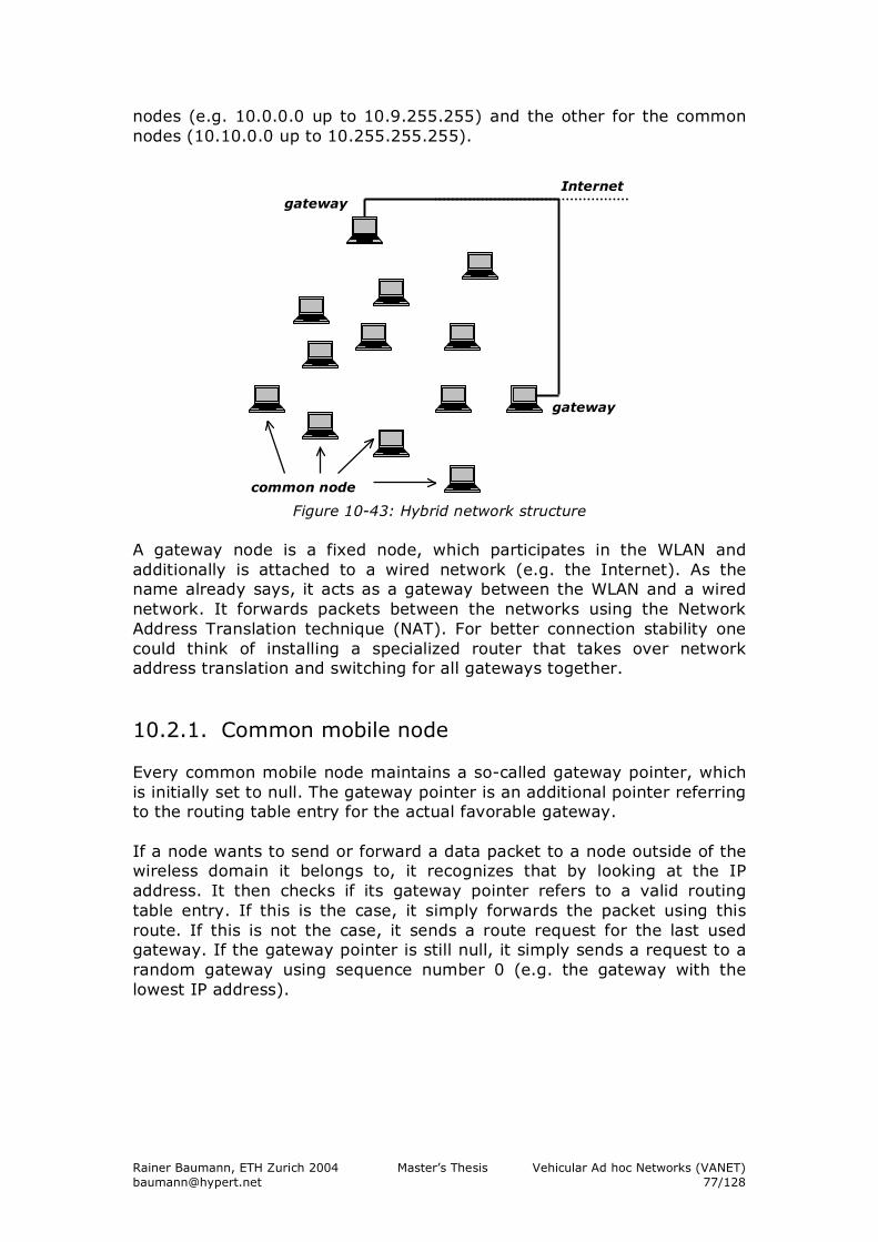
Rainer Baumann, ETH Zurich 2004 Master’s Thesis Vehicular Ad hoc Networks (VANET) [email protected] 77/128
nodes (e.g. 10.0.0.0 up to 10.9.255.255) and the other for the common nodes (10.10.0.0 up to 10.255.255.255).
Figure 10-43: Hybrid network structure A gateway node is a fixed node, which participates in the WLAN and additionally is attached to a wired network (e.g. the Internet). As the name already says, it acts as a gateway between the WLAN and a wired network. It forwards packets between the networks using the Network Address Translation technique (NAT). For better connection stability one could think of installing a specialized router that takes over network address translation and switching for all gateways together. 10.2.1. Common mobile node Every common mobile node maintains a so-called gateway pointer, which is initially set to null. The gateway pointer is an additional pointer referring to the routing table entry for the actual favorable gateway. If a node wants to send or forward a data packet to a node outside of the wireless domain it belongs to, it recognizes that by looking at the IP address. It then checks if its gateway pointer refers to a valid routing table entry. If this is the case, it simply forwards the packet using this route. If this is not the case, it sends a route request for the last used gateway. If the gateway pointer is still null, it simply sends a request to a random gateway using sequence number 0 (e.g. the gateway with the lowest IP address).
gateway
gateway
Internet
common node
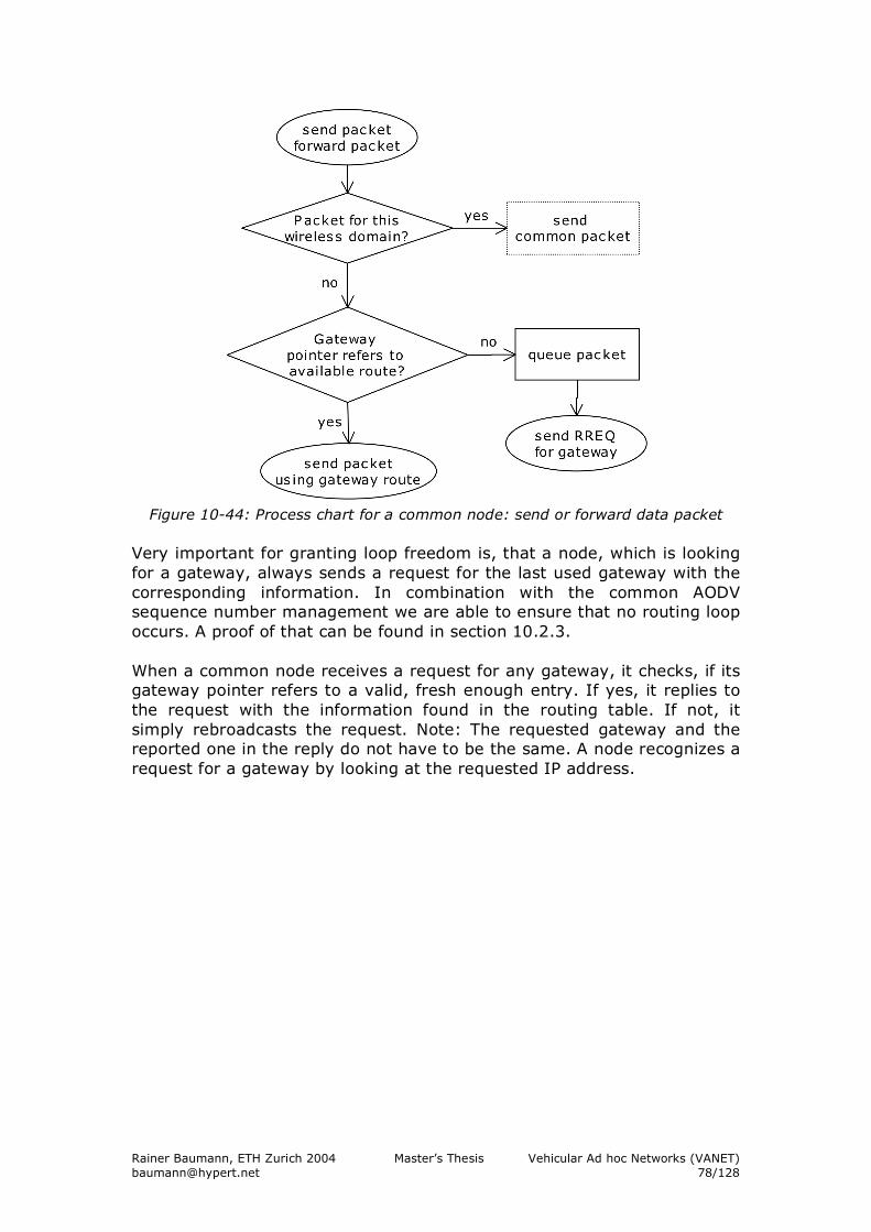
Rainer Baumann, ETH Zurich 2004 Master’s Thesis Vehicular Ad hoc Networks (VANET) [email protected] 78/128
Figure 10-44: Process chart for a common node: send or forward data packet
Very important for granting loop freedom is, that a node, which is looking for a gateway, always sends a request for the last used gateway with the corresponding information. In combination with the common AODV sequence number management we are able to ensure that no routing loop occurs. A proof of that can be found in section 10.2.3. When a common node receives a request for any gateway, it checks, if its gateway pointer refers to a valid, fresh enough entry. If yes, it replies to the request with the information found in the routing table. If not, it simply rebroadcasts the request. Note: The requested gateway and the reported one in the reply do not have to be the same. A node recognizes a request for a gateway by looking at the requested IP address.
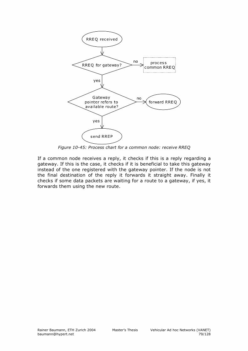
Rainer Baumann, ETH Zurich 2004 Master’s Thesis Vehicular Ad hoc Networks (VANET) [email protected] 79/128
Figure 10-45: Process chart for a common node: receive RREQ
If a common node receives a reply, it checks if this is a reply regarding a gateway. If this is the case, it checks if it is beneficial to take this gateway instead of the one registered with the gateway pointer. If the node is not the final destination of the reply it forwards it straight away. Finally it checks if some data packets are waiting for a route to a gateway, if yes, it forwards them using the new route.
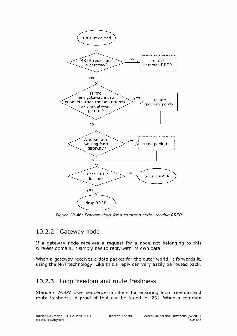
Rainer Baumann, ETH Zurich 2004 Master’s Thesis Vehicular Ad hoc Networks (VANET) [email protected] 80/128
Figure 10-46: Process chart for a common node: receive RREP
10.2.2. Gateway node If a gateway node receives a request for a node not belonging to this wireless domain, it simply has to reply with its own data. When a gateway receives a data packet for the outer world, it forwards it, using the NAT technology. Like this a reply can very easily be routed back.
10.2.3. Loop freedom and route freshness Standard AODV uses sequence numbers for ensuring loop freedom and route freshness. A proof of that can be found in [23]. When a common
Rainer Baumann, ETH Zurich 2004 Master’s Thesis Vehicular Ad hoc Networks (VANET) [email protected] 81/128
node requests a route to a gateway, we have to distinguish two different situations.
1. The node reestablishes the route to the gateway it used last. Such a reestablishment is automatically loop free since it obeys the same rules as for common route reestablishment in AODV including sequence number usage. To the same reason such a rebuilt route is also granted to be fresh.
2. The node establishes a route to another gateway. This is very similar to the establishment of a new route to a node to which it has not jet established any route. The only difference is that at start time the requesting node has not known yet to which gateway it will establish a route. But this does not fall in account since there is no difference in the additional information packed in such a request. From this, it follows that such a route is also loop free and fresh.
Note that the correct usage of route error messages (RERR) is very important for granting route freshness. The argumentation for loop freedom above can be formulated as a proof by induction. This proof is based on the proof of the loop-free property of AODV presented in [23].
Definition 1: Suppose that nodes Xi (i=1, 2, ..., n) are the nodes on a existing route from a source X1 to a destination Xn. We say Xi points to Xi+1, (symbolically Xi->Xi+1) if node Xi+1 is the next hop for the destination in the corresponding routing table of node Xi. Definition 2: Let Si be the actual sequence number for the destination Xn in the routing table of node Xi (i=1, 2, ..., n). And let Si,old be the corresponding sequence number before a new route to Xn has been established using this node. Definition 3: For Xi, Xj with i<j holds Si<=Sj, since Sj:=max(Si,Sj,old+1). Definition 4: A routing loop is defined by
!
" Xi==Xj, i≠j. Lemma 1: A new established or reestablished route is loop free. Proof: Suppose there is a routing loop in the new established route. Then for Xi->Xj holds that Si<=Sj and Sj,old<=Si. But this is a contradiction since Sj,old<=Sj+1 implies that Si=Si+1. Definition 5: The gateway pointer for node i is Gi. Lemma 2: A new established gateway route is loop free. Proof: If Gi,old=Gi,new we have simply reestablished a route to a gateway what is nothing else then a common route reestablishment and by lemma 1 loop free. If Gi,old≠Gi,new we have established a new route what is also loop free by lemma 1.
Rainer Baumann, ETH Zurich 2004 Master’s Thesis Vehicular Ad hoc Networks (VANET) [email protected] 82/128
Theorem 1: The whole ad hoc network, including the routes to the gateways, is loop free for the entire time. Base: At initial point there exists no routes and all gateway pointers are set to NULL. Induction: Every additionally established route is loop free by lemma 1. Definition 6: A route is fresh, iff Si,old<Si,new. Lemma 2: A new established route to a gateway is always fresh. Proof: If Gi,old=Gi,new then Si,old<Si,new since we increased Si before initiating the route request. If Gi,old≠Gi,new it is trivial since always 0<Si,new. Equations 10-4: Proof of loop freedom and freshness for AODV-HIA
10.3. Simulation setup For the simulation there are several leading questions. First of all we want to know about the usability of AODV-HIA. Then it is interesting to know what is the required base station density for a sufficient cover of the simulation area. For the simulations we chose the city scenario Unterstrass with high car density (Section 7.1.). Additionally we place once 24, 15 and 3 gateways at prominent places over the scene (Figure 10-47).
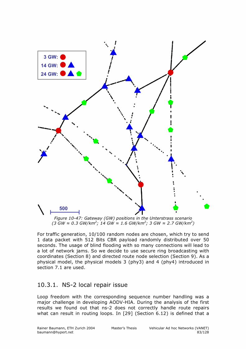
Rainer Baumann, ETH Zurich 2004 Master’s Thesis Vehicular Ad hoc Networks (VANET) [email protected] 83/128
Figure 10-47: Gateway (GW) positions in the Unterstrass scenario (3 GW ≈ 0.3 GW/km2; 14 GW ≈ 1.6 GW/km2; 3 GW ≈ 2.7 GW/km2)
For traffic generation, 10/100 random nodes are chosen, which try to send 1 data packet with 512 Bits CBR payload randomly distributed over 50 seconds. The usage of blind flooding with so many connections will lead to a lot of network jams. So we decide to use secure ring broadcasting with coordinates (Section 8) and directed route node selection (Section 9). As a physical model, the physical models 3 (phy3) and 4 (phy4) introduced in section 7.1 are used.
10.3.1. NS-2 local repair issue Loop freedom with the corresponding sequence number handling was a major challenge in developing AODV-HIA. During the analysis of the first results we found out that ns-2 does not correctly handle route repairs what can result in routing loops. In [29] (Section 6.12) is defined that a
500m
3 GW:
14 GW:
24 GW:
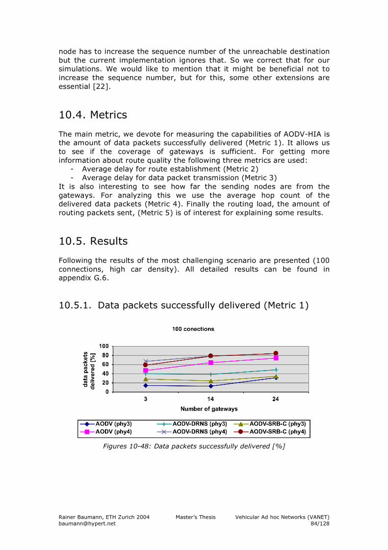
Rainer Baumann, ETH Zurich 2004 Master’s Thesis Vehicular Ad hoc Networks (VANET) [email protected] 84/128
node has to increase the sequence number of the unreachable destination but the current implementation ignores that. So we correct that for our simulations. We would like to mention that it might be beneficial not to increase the sequence number, but for this, some other extensions are essential [22].
10.4. Metrics The main metric, we devote for measuring the capabilities of AODV-HIA is the amount of data packets successfully delivered (Metric 1). It allows us to see if the coverage of gateways is sufficient. For getting more information about route quality the following three metrics are used:
- Average delay for route establishment (Metric 2) - Average delay for data packet transmission (Metric 3)
It is also interesting to see how far the sending nodes are from the gateways. For analyzing this we use the average hop count of the delivered data packets (Metric 4). Finally the routing load, the amount of routing packets sent, (Metric 5) is of interest for explaining some results.
10.5. Results Following the results of the most challenging scenario are presented (100 connections, high car density). All detailed results can be found in appendix G.6. 10.5.1. Data packets successfully delivered (Metric 1)
Figures 10-48: Data packets successfully delivered [%]
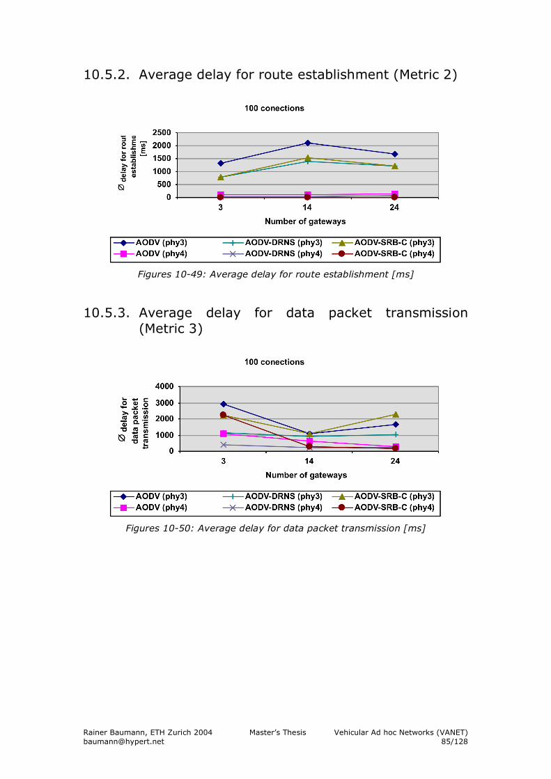
Rainer Baumann, ETH Zurich 2004 Master’s Thesis Vehicular Ad hoc Networks (VANET) [email protected] 85/128
10.5.2. Average delay for route establishment (Metric 2)
Figures 10-49: Average delay for route establishment [ms]
10.5.3. Average delay for data packet transmission (Metric 3)
Figures 10-50: Average delay for data packet transmission [ms]
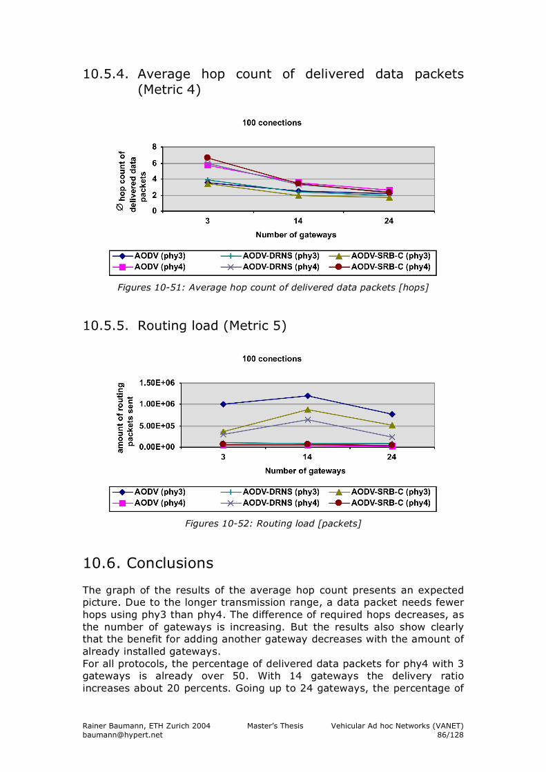
Rainer Baumann, ETH Zurich 2004 Master’s Thesis Vehicular Ad hoc Networks (VANET) [email protected] 86/128
10.5.4. Average hop count of delivered data packets (Metric 4)
Figures 10-51: Average hop count of delivered data packets [hops]
10.5.5. Routing load (Metric 5)
Figures 10-52: Routing load [packets]
10.6. Conclusions The graph of the results of the average hop count presents an expected picture. Due to the longer transmission range, a data packet needs fewer hops using phy3 than phy4. The difference of required hops decreases, as the number of gateways is increasing. But the results also show clearly that the benefit for adding another gateway decreases with the amount of already installed gateways. For all protocols, the percentage of delivered data packets for phy4 with 3 gateways is already over 50. With 14 gateways the delivery ratio increases about 20 percents. Going up to 24 gateways, the percentage of
Rainer Baumann, ETH Zurich 2004 Master’s Thesis Vehicular Ad hoc Networks (VANET) [email protected] 87/128
delivered data packets rises again about 10 percents. Here also a flattening of the curves can be observed. The corresponding delays for phy4 are surprisingly short, especially the delays for route establishment. For phy3 the results do not look as good as for phy4. The ratio of data packets successfully delivered is much lower because of the greater interference caused by the larger transmission range. This leads to a much higher routing load resulting in longer delays. The influence of the larger transmission range is much stronger than expected and should be investigated in a future project. The difference between phy3 and phy4 shows that the longest possible transmission range is not the optimal for multi hop hybrid internet access.
10.7. Summary The Hybrid Internet Access extension for AODV (HIA) is a real option for offering multi hop hybrid internet access in cars. The simulations have shown that the choice of physical model has a strong impact on the achieved performance. More detailed studies on that still have to be done.
Rainer Baumann, ETH Zurich 2004 Master’s Thesis Vehicular Ad hoc Networks (VANET) [email protected] 88/128
11. ARP, a relict ?
11.1. The address resolution protocol (ARP) The Address Resolution Protocol (ARP) performs the mapping of an IP address belonging to layer 3 to a physical machine address (MAC address), which belongs to layer 2 that is recognized in the local network. For example, in IP Version 4, an address is 32 bits long. In an Ethernet local area network, MAC addresses for attached devices are 48 bits long. A table, usually called the ARP cache, is used to maintain a correlation table between each MAC address and its corresponding IP address. The address resolution protocol provides the rules for making this correlation and providing address conversion in both directions. Since protocol details differ for each type of local area network, there are separate ARP specifications for Ethernet, Frame Relay, ATM, Fiber Distributed-Data Interface, HIPPI, and other protocols.
11.2. Why ARP ? The ISO/OSI layer model defines the seven layers as independent interchangeable. This allows free combination between various protocols of different layers and divers hardware. In a network packet, the layer three addresses usually denote the originator and the final destination while the layer two addresses normally refer to the intermediate sender and intermediate destination. In an ad hoc multi hop WLAN the diversity is much smaller. Only a few different layer two standards are available and they all use the same address system. On the layer three it is even simpler. Since an ad hoc network is one domain, we have to use one single protocol. Almost all available layer three routing protocols are based on IP, which became a quasi standard in the past years. So the question comes up, why to use two different addressing systems. This only adds additional overhead, especially because of ARP. There are many ways how the two address systems could be unified. The easiest one would be, if we think of IPv6, just to include the MAC address in the IP address. A completely different approach, but with the same target, omitting ARP, is cross-layer feedback. The main idea is to use all received messages for learning about IP to MAC address mappings. Since we never unicast a message to a node from which we have not yet received any packets, ARP would simply be obsolete. But such a cross-layer feedback violates the layering theory and would require new specific implementations of the affected layers. Before a lot of effort is putted in the realization of address unification or cross-layer feedback, one is certainly interested to know how much is the performance gain by omitting ARP.
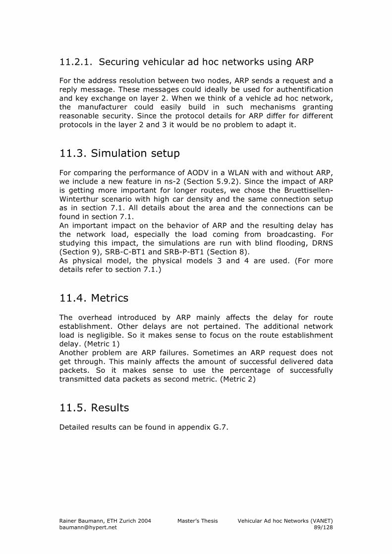
Rainer Baumann, ETH Zurich 2004 Master’s Thesis Vehicular Ad hoc Networks (VANET) [email protected] 89/128
11.2.1. Securing vehicular ad hoc networks using ARP For the address resolution between two nodes, ARP sends a request and a reply message. These messages could ideally be used for authentification and key exchange on layer 2. When we think of a vehicle ad hoc network, the manufacturer could easily build in such mechanisms granting reasonable security. Since the protocol details for ARP differ for different protocols in the layer 2 and 3 it would be no problem to adapt it.
11.3. Simulation setup For comparing the performance of AODV in a WLAN with and without ARP, we include a new feature in ns-2 (Section 5.9.2). Since the impact of ARP is getting more important for longer routes, we chose the Bruettisellen-Winterthur scenario with high car density and the same connection setup as in section 7.1. All details about the area and the connections can be found in section 7.1. An important impact on the behavior of ARP and the resulting delay has the network load, especially the load coming from broadcasting. For studying this impact, the simulations are run with blind flooding, DRNS (Section 9), SRB-C-BT1 and SRB-P-BT1 (Section 8). As physical model, the physical models 3 and 4 are used. (For more details refer to section 7.1.)
11.4. Metrics The overhead introduced by ARP mainly affects the delay for route establishment. Other delays are not pertained. The additional network load is negligible. So it makes sense to focus on the route establishment delay. (Metric 1) Another problem are ARP failures. Sometimes an ARP request does not get through. This mainly affects the amount of successful delivered data packets. So it makes sense to use the percentage of successfully transmitted data packets as second metric. (Metric 2)
11.5. Results Detailed results can be found in appendix G.7.
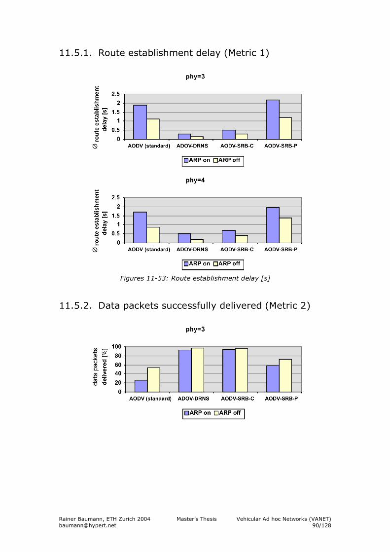
Rainer Baumann, ETH Zurich 2004 Master’s Thesis Vehicular Ad hoc Networks (VANET) [email protected] 90/128
11.5.1. Route establishment delay (Metric 1)
Figures 11-53: Route establishment delay [s]
11.5.2. Data packets successfully delivered (Metric 2)
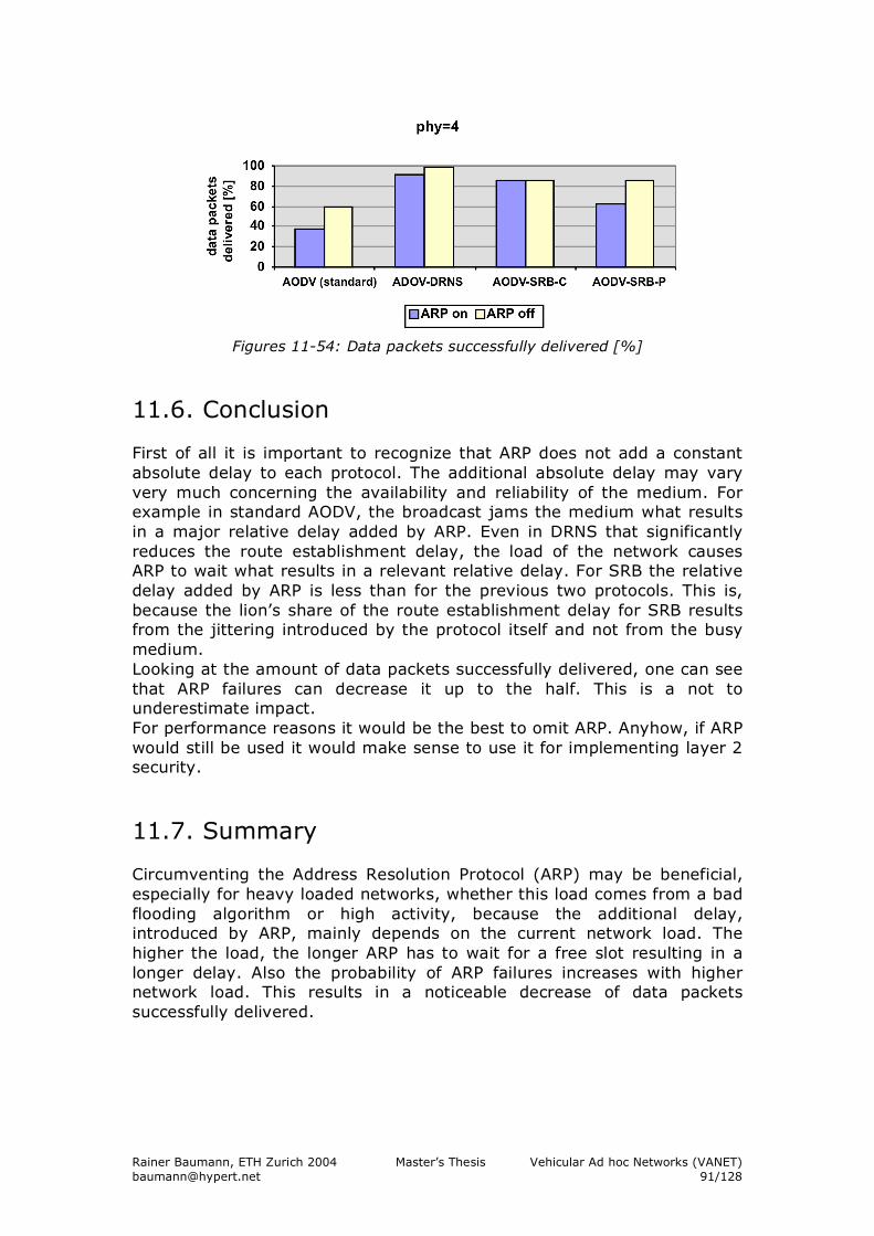
Rainer Baumann, ETH Zurich 2004 Master’s Thesis Vehicular Ad hoc Networks (VANET) [email protected] 91/128
Figures 11-54: Data packets successfully delivered [%]
11.6. Conclusion First of all it is important to recognize that ARP does not add a constant absolute delay to each protocol. The additional absolute delay may vary very much concerning the availability and reliability of the medium. For example in standard AODV, the broadcast jams the medium what results in a major relative delay added by ARP. Even in DRNS that significantly reduces the route establishment delay, the load of the network causes ARP to wait what results in a relevant relative delay. For SRB the relative delay added by ARP is less than for the previous two protocols. This is, because the lion’s share of the route establishment delay for SRB results from the jittering introduced by the protocol itself and not from the busy medium. Looking at the amount of data packets successfully delivered, one can see that ARP failures can decrease it up to the half. This is a not to underestimate impact. For performance reasons it would be the best to omit ARP. Anyhow, if ARP would still be used it would make sense to use it for implementing layer 2 security.
11.7. Summary Circumventing the Address Resolution Protocol (ARP) may be beneficial, especially for heavy loaded networks, whether this load comes from a bad flooding algorithm or high activity, because the additional delay, introduced by ARP, mainly depends on the current network load. The higher the load, the longer ARP has to wait for a free slot resulting in a longer delay. Also the probability of ARP failures increases with higher network load. This results in a noticeable decrease of data packets successfully delivered.
Rainer Baumann, ETH Zurich 2004 Master’s Thesis Vehicular Ad hoc Networks (VANET) [email protected] 92/128
Appendix A - Master’s thesis description Cars as ad hoc network hosts Master’s Thesis for Rainer Baumann Institute for Computer Systems, Prof. Dr. Th. Gross
A.1. Introduction Using the potential of ad hoc networks to exchange information between cars in a city or on a highway can be very attractive: in a car unlimited power supply is available, effective antennas can be used; the density of hosts is usually high enough to maintain the connection, etc. More and more cars have now GPS systems installed. The convenience of such systems is evident, but there are many possibilities to improve the service, e.g. an ad hoc network may be used to transmit warnings about traffic jams, ice-on-road, accidents, construction sites, etc. This message could force GPS system to recalculate the route to avoid the problem or to warn the driver about the danger, if it is unavoidable. Cars can be used also for monitoring the environmental conditions, gathering the data on their way and uploading them to some fixed access points. In this project we are interested in the investigation of the possibility to use ad hoc network to exchange information between cars. Since real experiments are impossible, the ns-2 simulator should be used. To keep research close to reality, we provide realistic cars movement patterns on the map of Zurich-city and on some highways in Switzerland. The data is obtained from the traces of car simulator, developed by the group of Prof. Kai Nagel (ETH Zurich). The goal of this work is to adjust one of the existing protocols (or to design and implement a new one) for effective routing in city- and/or highway-like scenarios with the following evaluation of the changes.
A.2. Tasks 1. Understand the available 802.11 MAC protocols (the advantages,
disadvantages, available hardware). 2. Understand AODV routing protocol. 3. Investigate the related work. 4. Develop and integrate your changes to AODV for best performance of
this protocol when used for routing between cars. 5. Evaluation. Evaluate your changes on a variety of different scenarios
(city, highway) with different density of cars (different map regions) under different data loads.
Rainer Baumann, ETH Zurich 2004 Master’s Thesis Vehicular Ad hoc Networks (VANET) [email protected] 93/128
A.3. Remarks • At the end of the period the following documents have to be handed in:
the source code, a report as well as a short abstract of the work done. The report shall follow the rules of a scientific article.
• A diploma project serves as an example for projects in the professional life of a computer scientist and includes a presentation of the project towards the end of the project, at a mutually agreed-upon date.
• Development Environment: Linux, C, awk, ns-2. Professor: Prof. Th. Gross Start: March 1, 2004 Assistant: Valeri Naoumov End: September 1, 2004
Rainer Baumann, ETH Zurich 2004 Master’s Thesis Vehicular Ad hoc Networks (VANET) [email protected] 94/128
Appendix B - List of figures Figure 3-1: ISO/OSI layer model ............................................................. 8 Figure 3-2: 802 LLC, MAC and PHY........................................................... 9 Figure 3-3: 802.11 MAC and PHY layer ..................................................... 9 Figure 3-4: WLAN infrastructure mode.....................................................11 Figure 3-5: WLAN ad hoc mode ..............................................................11 Figure 3-6: Inter Frame Spaces (IFS) / DCF CSMA/CA ...............................12 Figure 3-7: Packet sending / DCF CSMA/CA..............................................12 Figure 3-8: Randomized back-off time / DCF CSMA/CA ..............................13 Figure 3-9: Competing stations / DCF CSMA/CA........................................13 Figure 3-10: DFWMAC-DCF w/RTS/CTS .....................................................14 Figure 3-11: DFWMAC-PCF.......................................................................14 Figure 3-12: Beacon in infrastructure mode ...............................................15 Figure 3-13: Beacon in ad hoc mode .........................................................15 Figure 5-15: Class diagram handle............................................................28 Figure 5-16: Schematic of hierarchical wireless node...................................29 Figure 5-17: Schematic of traffic generator and packet flow .........................31 Figure 5-18: Packet header stack..............................................................31 Figure 5-19: NS-2 usage diagram .............................................................32 Figure 6-20: Traffic flow example Zurich [32].............................................47 Figure 6-21: Traffic flow example Switzerland [15] .....................................47 Figure 7-22: City of Zurich, region Unterstrass, connection 0 to 5, (3x3km)...49 Figure 7-23: Highway BruettisellenWinterthur, connection 0 to 3, (2.9x12km)50 Figure 7-24: Connectivity failure Unterstrass [%] .......................................51 Figure 7-25: Connectivity failure Bruettisellen-Winterthur [%] .....................52 Figures 7-26: Hop count [hops] .................................................................53 Figure 8-27: The three SRB node groups ...................................................57 Figure 8-28: Secure ring broadcast population on a straight road .................58 Figure 8-29: SRB-C triangle .....................................................................59 Figures 8-30: Data packets successfully delivered [%]..................................62 Figures 8-31: Average delay for route establishment [s] ...............................63 Figures 8-32: Average delay for data packet transmission [s] ........................64 Figures 8-33: Normalized routing load ........................................................64 Figures 8-34: Average of RREQs received per RREQ sent ..............................65 Figure 9-35: Highway route node selection problem ....................................68 Figures 9-36: Data packets successfully delivered [%]..................................70 Figures 9-37: Average delay for route establishment [s] ...............................70 Figures 9-38: Average delay for data packet transmission [s] ........................71 Figures 9-39: Normalized routing load ........................................................71 Figures 9-40: Data packets successfully delivered [%]..................................73 Figures 9-41: Average delay for route establishment [s] ...............................73 Figures 9-42: Normalized routing load ........................................................74 Figure 10-43: Hybrid network structure.......................................................77 Figure 10-44: Process chart for a common node: send or forward data packet .78 Figure 10-45: Process chart for a common node: receive RREQ......................79 Figure 10-46: Process chart for a common node: receive RREP ......................80 Figure 10-47: Gateway (GW) positions in the Unterstrass scenario .................83 Figures 10-48: Data packets successfully delivered [%]..................................84 Figures 10-49: Average delay for route establishment [ms] ............................85 Figures 10-50: Average delay for data packet transmission [ms] .....................85 Figures 10-51: Average hop count of delivered data packets [hops] .................86 Figures 10-52: Routing load [packets] ..........................................................86 Figures 11-53: Route establishment delay [s]................................................90 Figures 11-54: Data packets successfully delivered [%]..................................91
Rainer Baumann, ETH Zurich 2004 Master’s Thesis Vehicular Ad hoc Networks (VANET) [email protected] 95/128
Appendix C - List of tables Table 3-1: Overview of the IEEE 802.11 standards...................................10 Table 3-2: Overview of IEEE 802.11 PHY Layer........................................18 Table 3-3: Frequency regulations Switzerland [7] ....................................19 Table 3-4: Characteristics of 802.11 PHY Layers [26] [25] ........................20 Table 3-5: Available transmission powers [26] [25] .................................21 Table 4-6: DV-Routing Table .................................................................23 Table 5-7:
cd values in meter depending on antenna height and frequency 36
Table 5-8: NS-2 Parameters..................................................................37 Table 5-9: The new trace file format ......................................................39 Table 5-10: The new trace file format continued........................................40 Table 5-11: The val trace format shortcuts ...............................................41 Table 5-12: The val trace format .............................................................41 Table 7-13: Statistics of scenario files ......................................................48 Table 7-14: Used physical modals............................................................48 Table 7-15: Connection statistics Unterstrass ............................................50 Table 7-16: Connection statistics Bruettisellen-Winterthur ..........................50 Table 7-17: Connection statistics Bruettisellen-Winterthur - companion........51 Table 8-18: Border thresholds.................................................................58 Table 8-19: Transmission ranges depending on reduced thresholds [meter]..58 Table G.1-20: Connectivity failure Unterstrass (max 6) ...............................106 Table G.1-21: Connectivity failure Bruettisellen-Winterthur (max 4)..............106 Tables G.1-22: Connectivity results Unterstrass – high density [ms]...............107 Tables G.1-23: Connectivity results Unterstrass – medium density [ms] .........108 Tables G.1-24: Connectivity results Bruettisellen-Winterthur – high density [ms] ...............................................................108 Tables G.1-25: Connectivity results Bruettisellen-Winterthur – medium density109 Tables G.1-26: Connectivity results Bruettisellen-Winterthur – companion [ms]
........................................................................................109 Tables G.2-27: Data packets successfully delivered [%]................................110 Tables G.2-28: Average delay for route establishment [s] .............................111 Tables G.2-29: Average delay for data packet transmission [s] ......................112 Tables G.2-30: Normalized routing load ......................................................113 Tables G.2-31: Average of RREQs received per RREQ sent ............................113 Tables G.2-32: Percentage of network load for data, RREQ, RREP and RERR
packets [%/%/%/%]..........................................................115 Tables G.3-33: Data packets successfully delivered [%]................................115 Tables G.3-35: Average delay for data packet transmission [s] ......................116 Tables G.3-36: Normalized routing load ......................................................117 Tables G.3-37: Average of RREQs received per RREQ sent ............................117 Tables G.4-38: Data packets successfully delivered [%]................................118 Tables G.4-40: Average delay for data packet transmission [s] ......................120 Tables G.4-41: Normalized routing load ......................................................121 Tables G.4-42: Percentage part of network load for data, rreq, rrep and rerr
packets [%/%/%/%]..........................................................121 Tables G.4-43: Average of RREQs received per RREQ sent ............................122 Tables G.5-44: Data packets successfully delivered [%]................................122 Tables G.5-45: Average delay for route establishment [s] .............................123 Tables G.5-46: Average delay for data packet transmission [s] ......................123 Tables G.5-47: Normalized routing load ......................................................124 Tables G.5-48: Average of RREQs received per RREQ sent ............................124 Tables G.6-49: Data packets successfully delivered [%]................................125 Tables G.6-50: Average delay for route establishment [ms] ..........................125
Rainer Baumann, ETH Zurich 2004 Master’s Thesis Vehicular Ad hoc Networks (VANET) [email protected] 96/128
Tables G.6-51: Average delay for data packet transmission [ms] ...................126 Tables G.6-52: Average hop count of a data packet [hops]............................126 Tables G.6-53: Routing load [packets] ........................................................127 Tables G.7-54: Average delay for route establishment [s] .............................127 Tables G.7-55: Data packets successfully delivered [%]................................128
Rainer Baumann, ETH Zurich 2004 Master’s Thesis Vehicular Ad hoc Networks (VANET) [email protected] 97/128
Appendix D - List of equations Equation 5-1: Free space propagation model..............................................36 Equation 5-2: Two-ray ground reflection model ..........................................36 Equation 5-3:
cd range ...........................................................................36
Equations 10-4: Proof of loop freedom and freshness for AODV-HIA .................82
Rainer Baumann, ETH Zurich 2004 Master’s Thesis Vehicular Ad hoc Networks (VANET) [email protected] 98/128
Appendix E - References
E.1. Books [1] An Engineering Approach to Computer Network, S. Keshav, Addison
Wesly / AT&T, 1997
E.2. Papers [2] Valery Naumov, Thomas Gross; Simulation of Large Ad Hoc
Networks; ETH Zurich [3] Valery Naumov, Thomas Gross; Performance Comparison of Two
Routing Protocols in Large Ad Hoc Networks; Technical report, 2003 [4] Daniel L. Lough, T. Keith Blankenship, Kevin J. Krizman; A Short
Tutorial on Wireless LANs and IEEE 802.11; The Bradley Department of Electrical and Computer Engineering; Virginia Polytechnic Institute and State University
[5] Charles E. Perkins, Elizabeth M. Royer; Ad hoc On Demand Distance
Vector Routing; Sun Microsystems Laboratories, University of California
[6] Robert Wilson; Propagation Losses Through Common Building
Materials 2.4 GHz vs 5 GHz Reflection and Transmission Losses Through Common Building Materials; University of Southern California; November 2003
[7] Faktenblatt Radio Local Are Network (RLAN) Version 2.4b; Swiss
Federal office of communications [8] Benjamin E. Henty; A Brief Tutorial on the PHY and MAC layers of
the IEEE 802.11b Standard; July 12, 2001 [9] Kevin Fall, Kannan Varadhan; The ns Manual; UC Berkeley December
2003 [10] Denis Bakin; Evolution of 802.11 (physical layer) [11] Janne Salmi; AODV Multicast Features; Helsinki University of
Technology; April 2000 [12] J. Arango, M. Gegermark, A. Efrat, S. Pink; An Efficient Flooding
Algorithm for Mobile Ad hoc Networks; University of Arizona [13] J. P. Singh, N. Bambos; Wireless LAN Performance Under Varied
Stress Conditions in Vehicle Traffic Scenarios; Stanford University
Rainer Baumann, ETH Zurich 2004 Master’s Thesis Vehicular Ad hoc Networks (VANET) [email protected] 99/128
[14] T. Kosch, C. Schwingenschlögl, L. Ai; Information Dissemination in
Multihop Inter-Vehicel Netwoks; University of Munich [15] Kai Nagel; Modeling and Simulation; Institute for Computer Science
ETH Zurich 2004 [16] D. Helbing, Traffic and related self-driven many particle systems,
rev. Modern Physics vol. 73, 2001 [17] Bryan Raney, Nurhan Cetin, Andreas Völlmy, Milenko Vrtic, Kay
Axhausen, Kai Nagel; An agent-based microsimulation model of Swiss travel; Institute for Computer Science ETH Zurich 2002
[18] Formeln und Konstanten für die Berechung der Schweizerischen
schiefachsigen Zylinderprojektion und der Transformation zwischen Koordinatensystemen; Bundesamt für Landestopographie; September 2001
[19] W. Peng and X.C. Lu; On the reduction of broadcast redundancy in
mobile ad hoc networks; In ACM MobiHoc 2000, pages 129 – 130, Boston, Massachusetts, USA, August 2000
[20] I. Stojmenovic and M. Seddigh; Broadcasting algorithms in wireless
networks. In Proceedings of the International Conference on Advances in Infrastructure for Electronic Business, Science, and Education on the Internet SSGRR, L’Aquila, Italy, July 31-Aug. 6 2000.
[21] P. Ratanchnani, R. Kravets; A hybrid approach to internet
connectivity for mobile ad hoc networks [22] K. Kim, H. Seo; The Effects of Local Repair Schemes of AODV in Ad
Hoc Networks; Department of Computer Engineering Yenugnam University
[23] C. E. Perkins and E. M. Royer; Ad-hoc On-Demand Distance Vector
Routing; In Proceedings of the 2nd IEEE Workshop on Mobile Computing Systems and Applications, pages 90–100, New Orleans, LA; February 1999
[24] H. Lundgren, E. Nordstöm, C. Tschudin; The Gray Zone Problem in
IEEE 802.11b based Ad hoc Networks;Uppsala University Sweden
E.3. Company publications [25] NETGEAR 108 Mbps Wireless Solution: Technology Overview;
netgear.com; October 2003
Rainer Baumann, ETH Zurich 2004 Master’s Thesis Vehicular Ad hoc Networks (VANET) [email protected] 100/128
[26] Cisco Aironet 802.11g 1100 and 1200 Series Access Point Upgrade Kit Data Sheet; cisco.com; 2003
[27] Atheros Demonstrates Super G™; atheros.com; 2003
E.4. Standards and drafts [28] Manel Guerrero Zapata; Secure Ad hoc On-Demand Distance Vector
(SAODV) Routing; Nokia Research Center [29] C. Perkins, E. Belding-Royer, S. Das; RFC3561; Ad hoc On-Demand
Distance Vector (AODV) Routing; July 2003 [30] LAN MAN Standards Committee of the IEEE Computer Society.
Wireless LAN Medium Access Control (MAC) and Physical Layer (PHY) Specifications. IEEE Standard 802.11. Technical report, 1999
E.5. Lecture Notes [31] Roger Wattenhofer; Mobile Computation; Distributed Computing
Group ETH Zurich; 2003
E.6. Talks [32] Kai Nagel; Multi-agent traffic simulations; Institute for Computer
Science ETH Zurich 2004
E.7. Websites [33] The Network Simulator - ns-2; www.isi.edu/nsnam/ns [34] CMU/Monarch project; Rice University; November 1998;
www.monarch.cs.rice.edu [35] AODV; Standardization RFC3561; UC Santa Barbara;
www.ietf.org/rfc/rfc3561.txt [36] Flying Linux; MAD HOC; mad hoc.flyinglinux.net [37] AODV-UU routing protocol implementation; Uppsala University;
user.it.uu.se/~henrikl/aodv [38] REAL; S. Keshav; Cornell University; minnie.tuhs.org/REAL [39] FleetNet: www.et2.tu-harburg.de/fleetnet

Rainer Baumann, ETH Zurich 2004 Master’s Thesis Vehicular Ad hoc Networks (VANET) [email protected] 101/128
[40] CarTalk: www.cartalk2000.net [41] gawk: www.gnu.org/software/gawk/gawk.html
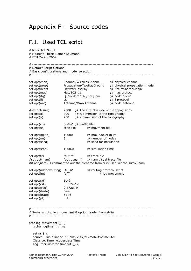
Rainer Baumann, ETH Zurich 2004 Master’s Thesis Vehicular Ad hoc Networks (VANET) [email protected] 102/128
Appendix F - Source codes
F.1. Used TCL script # NS-2 TCL Script # Master’s Thesis Rainer Baumann # ETH Zurich 2004 # -------------------------------------------------------------------------------------------- # Default Script Options # Basic configurations and model selection # -------------------------------------------------------------------------------------------- set opt(chan) Channel/WirelessChannel ;# physical channel set opt(prop) Propagation/TwoRayGround ;# physical propagation model set opt(netif) Phy/WirelessPhy ;# NetIf/SharedMedia set opt(mac) Mac/802_11 ;# mac protocol set opt(ifq) Queue/DropTail/PriQueue ;# node queue set opt(ll) LL ;# ll protocol set opt(ant) Antenna/OmniAntenna ;# node antenna #set opt(size) 2000 ;# The size of a side of the topography set opt(x) 700 ;# X dimension of the topography set opt(y) 700 ;# Y dimension of the topography set opt(cp) br-file" ;# traffic file set opt(sc) scen-file" ;# movment file set opt(ifqlen) 10000 ;# max packet in ifq set opt(nn) 3 ;# number of nodes set opt(seed) 0.0 ;# seed for imsulation set opt(stop) 1000.0 ;# simulation time set opt(tr) "out.tr" ;# trace file #set opt(nam) "out.tr.nam" ;# nam visual trace file #if opt(nam) is commented out the filename from tr is used wit the suffix .nam set opt(adhocRouting) AODV ;# routing protocol script set opt(lm) "off" ;# log movement set opt(rxt) 1e-9 set opt(cst) 5.012e-12 set opt(freq) 2.472e+9 set opt(drate) 6e+6 set opt(brate) 6e+6 set opt(pt) 0.1 # -------------------------------------------------------------------------------------------- # Some scripts: log movement & option reader from stdin # -------------------------------------------------------------------------------------------- proc log-movement {} { global logtimer ns_ ns set ns $ns_ source ~/ns-allinone-2.17/ns-2.17/tcl/mobility/timer.tcl Class LogTimer -superclass Timer LogTimer instproc timeout {} {
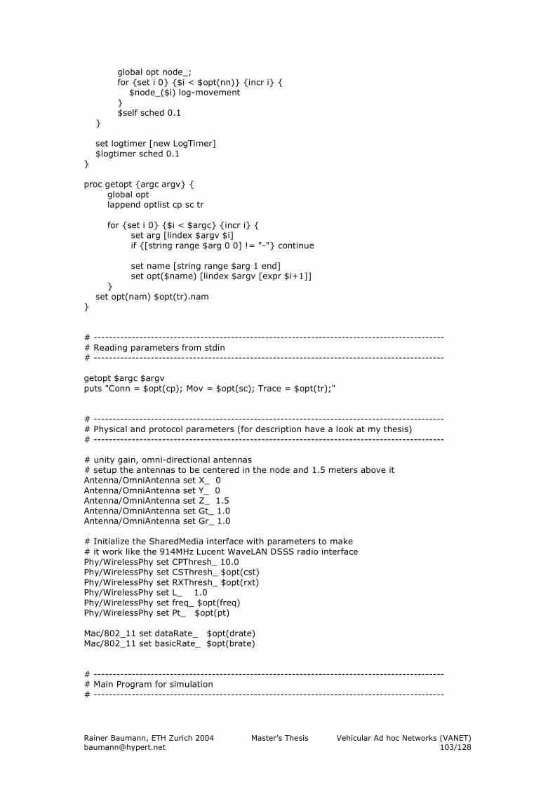
Rainer Baumann, ETH Zurich 2004 Master’s Thesis Vehicular Ad hoc Networks (VANET) [email protected] 103/128
global opt node_; for {set i 0} {$i < $opt(nn)} {incr i} { $node_($i) log-movement } $self sched 0.1 } set logtimer [new LogTimer] $logtimer sched 0.1 } proc getopt {argc argv} { global opt lappend optlist cp sc tr for {set i 0} {$i < $argc} {incr i} { set arg [lindex $argv $i] if {[string range $arg 0 0] != "-"} continue set name [string range $arg 1 end] set opt($name) [lindex $argv [expr $i+1]] } set opt(nam) $opt(tr).nam } # -------------------------------------------------------------------------------------------- # Reading parameters from stdin # -------------------------------------------------------------------------------------------- getopt $argc $argv puts "Conn = $opt(cp); Mov = $opt(sc); Trace = $opt(tr);" # -------------------------------------------------------------------------------------------- # Physical and protocol parameters (for description have a look at my thesis) # -------------------------------------------------------------------------------------------- # unity gain, omni-directional antennas # setup the antennas to be centered in the node and 1.5 meters above it Antenna/OmniAntenna set X_ 0 Antenna/OmniAntenna set Y_ 0 Antenna/OmniAntenna set Z_ 1.5 Antenna/OmniAntenna set Gt_ 1.0 Antenna/OmniAntenna set Gr_ 1.0 # Initialize the SharedMedia interface with parameters to make # it work like the 914MHz Lucent WaveLAN DSSS radio interface Phy/WirelessPhy set CPThresh_ 10.0 Phy/WirelessPhy set CSThresh_ $opt(cst) Phy/WirelessPhy set RXThresh_ $opt(rxt) Phy/WirelessPhy set L_ 1.0 Phy/WirelessPhy set freq_ $opt(freq) Phy/WirelessPhy set Pt_ $opt(pt) Mac/802_11 set dataRate_ $opt(drate) Mac/802_11 set basicRate_ $opt(brate) # -------------------------------------------------------------------------------------------- # Main Program for simulation # --------------------------------------------------------------------------------------------
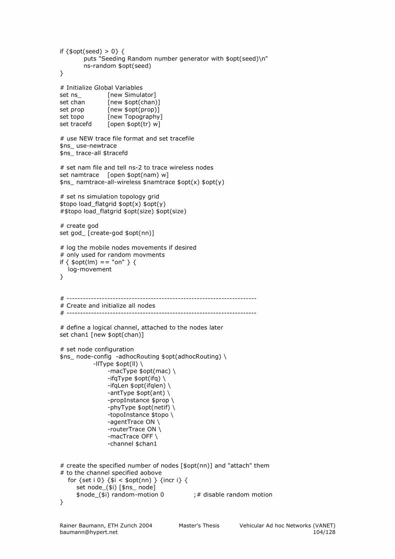
Rainer Baumann, ETH Zurich 2004 Master’s Thesis Vehicular Ad hoc Networks (VANET) [email protected] 104/128
if {$opt(seed) > 0} { puts "Seeding Random number generator with $opt(seed)\n" ns-random $opt(seed) } # Initialize Global Variables set ns_ [new Simulator] set chan [new $opt(chan)] set prop [new $opt(prop)] set topo [new Topography] set tracefd [open $opt(tr) w] # use NEW trace file format and set tracefile $ns_ use-newtrace $ns_ trace-all $tracefd # set nam file and tell ns-2 to trace wireless nodes set namtrace [open $opt(nam) w] $ns_ namtrace-all-wireless $namtrace $opt(x) $opt(y) # set ns simulation topology grid $topo load_flatgrid $opt(x) $opt(y) #$topo load_flatgrid $opt(size) $opt(size) # create god set god_ [create-god $opt(nn)] # log the mobile nodes movements if desired # only used for random movments if { $opt(lm) == "on" } { log-movement } # ---------------------------------------------------------------------- # Create and initialize all nodes # ---------------------------------------------------------------------- # define a logical channel, attached to the nodes later set chan1 [new $opt(chan)] # set node configuration $ns_ node-config -adhocRouting $opt(adhocRouting) \ -llType $opt(ll) \ -macType $opt(mac) \ -ifqType $opt(ifq) \ -ifqLen $opt(ifqlen) \ -antType $opt(ant) \ -propInstance $prop \ -phyType $opt(netif) \ -topoInstance $topo \ -agentTrace ON \ -routerTrace ON \ -macTrace OFF \ -channel $chan1 # create the specified number of nodes [$opt(nn)] and "attach" them # to the channel specified aobove for {set i 0} {$i < $opt(nn) } {incr i} { set node_($i) [$ns_ node] $node_($i) random-motion 0 ;# disable random motion }
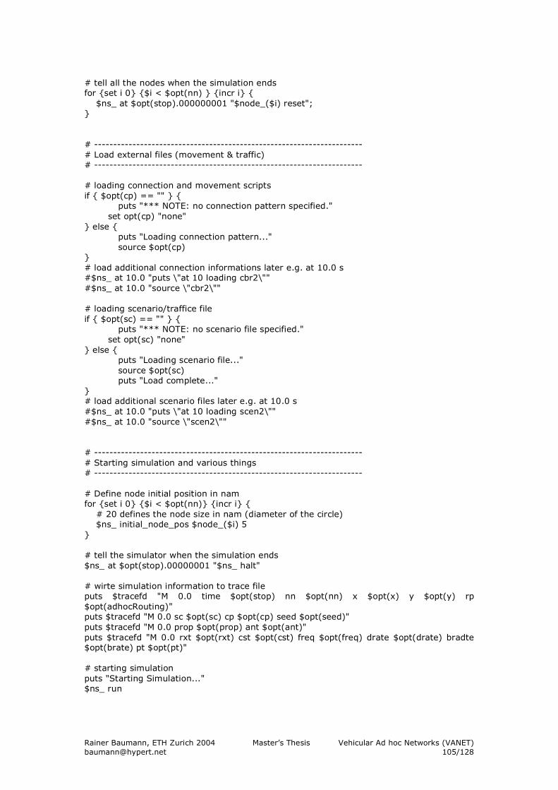
Rainer Baumann, ETH Zurich 2004 Master’s Thesis Vehicular Ad hoc Networks (VANET) [email protected] 105/128
# tell all the nodes when the simulation ends for {set i 0} {$i < $opt(nn) } {incr i} { $ns_ at $opt(stop).000000001 "$node_($i) reset"; } # ---------------------------------------------------------------------- # Load external files (movement & traffic) # ---------------------------------------------------------------------- # loading connection and movement scripts if { $opt(cp) == "" } { puts "*** NOTE: no connection pattern specified." set opt(cp) "none" } else { puts "Loading connection pattern..." source $opt(cp) } # load additional connection informations later e.g. at 10.0 s #$ns_ at 10.0 "puts \"at 10 loading cbr2\"" #$ns_ at 10.0 "source \"cbr2\"" # loading scenario/traffice file if { $opt(sc) == "" } { puts "*** NOTE: no scenario file specified." set opt(sc) "none" } else { puts "Loading scenario file..." source $opt(sc) puts "Load complete..." } # load additional scenario files later e.g. at 10.0 s #$ns_ at 10.0 "puts \"at 10 loading scen2\"" #$ns_ at 10.0 "source \"scen2\"" # ---------------------------------------------------------------------- # Starting simulation and various things # ---------------------------------------------------------------------- # Define node initial position in nam for {set i 0} {$i < $opt(nn)} {incr i} { # 20 defines the node size in nam (diameter of the circle) $ns_ initial_node_pos $node_($i) 5 } # tell the simulator when the simulation ends $ns_ at $opt(stop).00000001 "$ns_ halt" # wirte simulation information to trace file puts $tracefd "M 0.0 time $opt(stop) nn $opt(nn) x $opt(x) y $opt(y) rp $opt(adhocRouting)" puts $tracefd "M 0.0 sc $opt(sc) cp $opt(cp) seed $opt(seed)" puts $tracefd "M 0.0 prop $opt(prop) ant $opt(ant)" puts $tracefd "M 0.0 rxt $opt(rxt) cst $opt(cst) freq $opt(freq) drate $opt(drate) bradte $opt(brate) pt $opt(pt)" # starting simulation puts "Starting Simulation..." $ns_ run
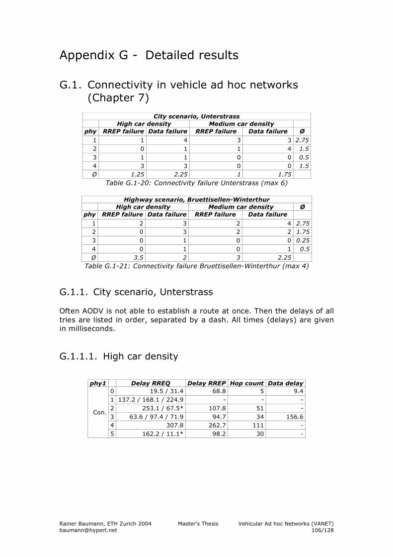
Rainer Baumann, ETH Zurich 2004 Master’s Thesis Vehicular Ad hoc Networks (VANET) [email protected] 106/128
Appendix G - Detailed results
G.1. Connectivity in vehicle ad hoc networks (Chapter 7)
Table G.1-20: Connectivity failure Unterstrass (max 6)
Highway scenario, Bruettisellen-Winterthur High car density Medium car density Ø
phy RREP failure Data failure RREP failure Data failure
1 2 3 2 4 2.75 2 0 3 2 2 1.75 3 0 1 0 0 0.25 4 0 1 0 1 0.5 Ø 3.5 2 3 2.25
Table G.1-21: Connectivity failure Bruettisellen-Winterthur (max 4)
G.1.1. City scenario, Unterstrass Often AODV is not able to establish a route at once. Then the delays of all tries are listed in order, separated by a dash. All times (delays) are given in milliseconds. G.1.1.1. High car density
phy1 Delay RREQ Delay RREP Hop count Data delay 0 19.5 / 31.4 68.8 5 9.4 1 137.2 / 168.1 / 224.9 - - - 2 253.1 / 67.5* 107.8 51 - 3 63.6 / 97.4 / 71.9 94.7 34 156.6 4 307.8 262.7 111 -
Con.
5 162.2 / 11.1* 98.2 30 -
City scenario, Unterstrass High car density Medium car density
phy RREP failure Data failure RREP failure Data failure Ø
1 1 4 3 3 2.75 2 0 1 1 4 1.5 3 1 1 0 0 0.5 4 3 3 0 0 1.5 Ø 1.25 2.25 1 1.75
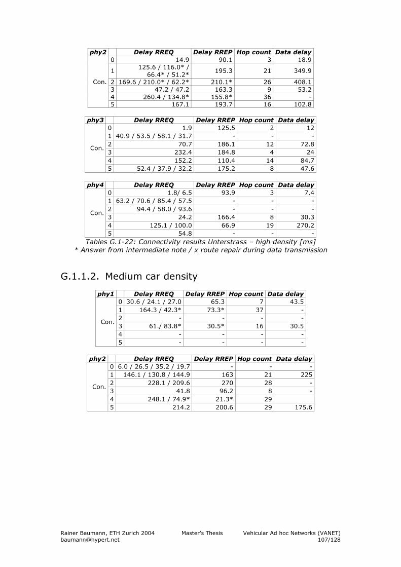
Rainer Baumann, ETH Zurich 2004 Master’s Thesis Vehicular Ad hoc Networks (VANET) [email protected] 107/128
phy2 Delay RREQ Delay RREP Hop count Data delay 0 14.9 90.1 3 18.9
1 125.6 / 116.0* / 66.4* / 51.2*
195.3 21 349.9
2 169.6 / 210.0* / 62.2* 210.1* 26 408.1 3 47.2 / 47.2 163.3 9 53.2 4 260.4 / 134.8* 155.8* 36 -
Con.
5 167.1 193.7 16 102.8
phy3 Delay RREQ Delay RREP Hop count Data delay 0 1.9 125.5 2 12 1 40.9 / 53.5 / 58.1 / 31.7 - - - 2 70.7 186.1 12 72.8 3 232.4 184.8 4 24 4 152.2 110.4 14 84.7
Con.
5 52.4 / 37.9 / 32.2 175.2 8 47.6
phy4 Delay RREQ Delay RREP Hop count Data delay 0 1.8/ 6.5 93.9 3 7.4 1 63.2 / 70.6 / 85.4 / 57.5 - - - 2 94.4 / 58.0 / 93.6 - - - 3 24.2 166.4 8 30.3 4 125.1 / 100.0 66.9 19 270.2
Con.
5 54.8 - - - Tables G.1-22: Connectivity results Unterstrass – high density [ms]
* Answer from intermediate note / x route repair during data transmission
G.1.1.2. Medium car density
phy1 Delay RREQ Delay RREP Hop count Data delay 0 30.6 / 24.1 / 27.0 65.3 7 43.5 1 164.3 / 42.3* 73.3* 37 - 2 - - - - 3 61./ 83.8* 30.5* 16 30.5 4 - - - -
Con.
5 - - - -
phy2 Delay RREQ Delay RREP Hop count Data delay 0 6.0 / 26.5 / 35.2 / 19.7 - - - 1 146.1 / 130.8 / 144.9 163 21 225 2 228.1 / 209.6 270 28 - 3 41.8 96.2 8 - 4 248.1 / 74.9* 21.3* 29
Con.
5 214.2 200.6 29 175.6
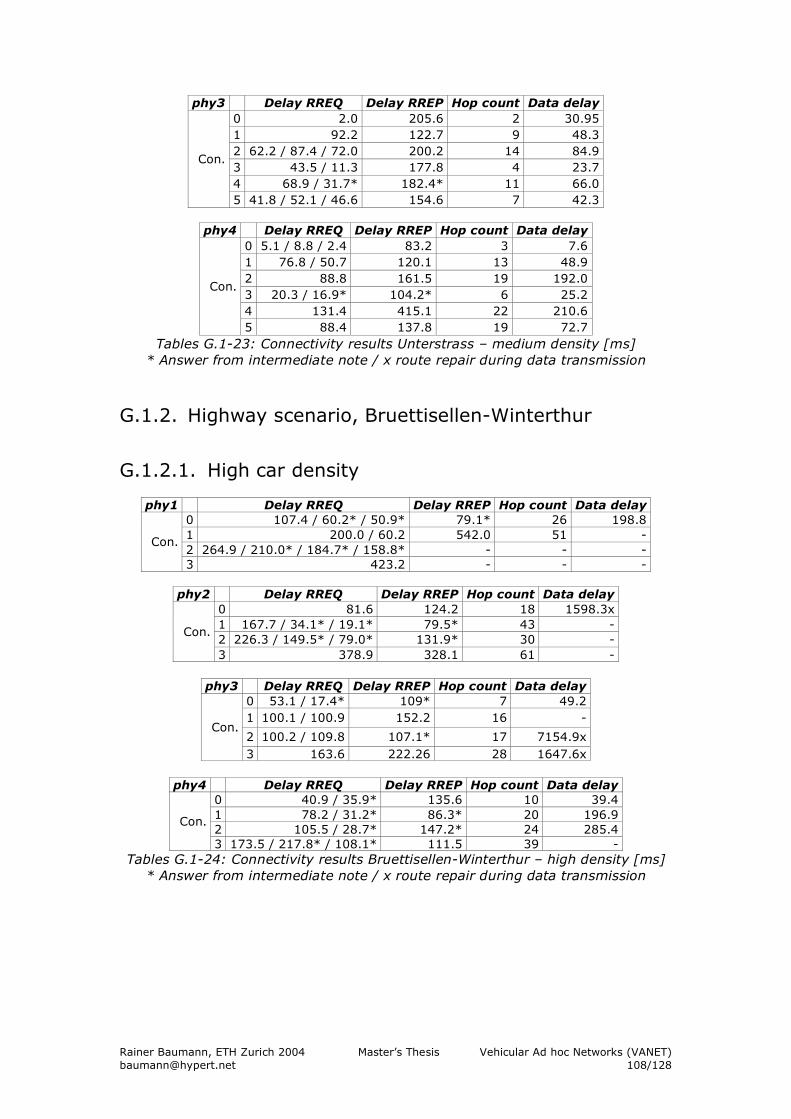
Rainer Baumann, ETH Zurich 2004 Master’s Thesis Vehicular Ad hoc Networks (VANET) [email protected] 108/128
phy3 Delay RREQ Delay RREP Hop count Data delay 0 2.0 205.6 2 30.95 1 92.2 122.7 9 48.3 2 62.2 / 87.4 / 72.0 200.2 14 84.9 3 43.5 / 11.3 177.8 4 23.7 4 68.9 / 31.7* 182.4* 11 66.0
Con.
5 41.8 / 52.1 / 46.6 154.6 7 42.3
phy4 Delay RREQ Delay RREP Hop count Data delay 0 5.1 / 8.8 / 2.4 83.2 3 7.6 1 76.8 / 50.7 120.1 13 48.9 2 88.8 161.5 19 192.0 3 20.3 / 16.9* 104.2* 6 25.2 4 131.4 415.1 22 210.6
Con.
5 88.4 137.8 19 72.7 Tables G.1-23: Connectivity results Unterstrass – medium density [ms]
* Answer from intermediate note / x route repair during data transmission
G.1.2. Highway scenario, Bruettisellen-Winterthur
G.1.2.1. High car density
phy1 Delay RREQ Delay RREP Hop count Data delay 0 107.4 / 60.2* / 50.9* 79.1* 26 198.8 1 200.0 / 60.2 542.0 51 - 2 264.9 / 210.0* / 184.7* / 158.8* - - -
Con.
3 423.2 - - -
phy2 Delay RREQ Delay RREP Hop count Data delay 0 81.6 124.2 18 1598.3x 1 167.7 / 34.1* / 19.1* 79.5* 43 - 2 226.3 / 149.5* / 79.0* 131.9* 30 -
Con.
3 378.9 328.1 61 -
phy3 Delay RREQ Delay RREP Hop count Data delay 0 53.1 / 17.4* 109* 7 49.2 1 100.1 / 100.9 152.2 16 -
2 100.2 / 109.8 107.1* 17 7154.9x Con.
3 163.6 222.26 28 1647.6x
phy4 Delay RREQ Delay RREP Hop count Data delay 0 40.9 / 35.9* 135.6 10 39.4 1 78.2 / 31.2* 86.3* 20 196.9 2 105.5 / 28.7* 147.2* 24 285.4
Con.
3 173.5 / 217.8* / 108.1* 111.5 39 - Tables G.1-24: Connectivity results Bruettisellen-Winterthur – high density [ms]
* Answer from intermediate note / x route repair during data transmission
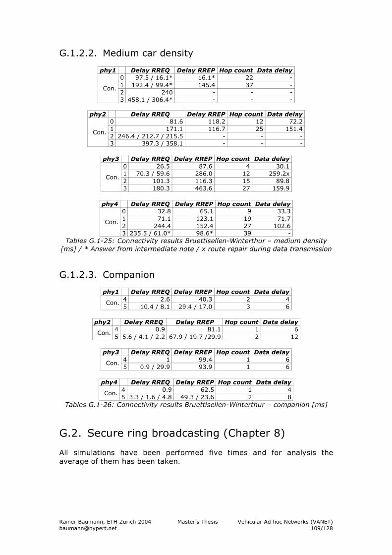
Rainer Baumann, ETH Zurich 2004 Master’s Thesis Vehicular Ad hoc Networks (VANET) [email protected] 109/128
G.1.2.2. Medium car density
phy1 Delay RREQ Delay RREP Hop count Data delay 0 97.5 / 16.1* 16.1* 22 - 1 192.4 / 99.4* 145.4 37 - 2 240 - - -
Con.
3 458.1 / 306.4* - - -
phy2 Delay RREQ Delay RREP Hop count Data delay 0 81.6 118.2 12 72.2 1 171.1 116.7 25 151.4 2 246.4 / 212.7 / 215.5 - - -
Con.
3 397.3 / 358.1 - - -
phy3 Delay RREQ Delay RREP Hop count Data delay 0 26.5 87.6 4 30.1 1 70.3 / 59.6 286.0 12 259.2x 2 101.3 116.3 15 89.8
Con.
3 180.3 463.6 27 159.9
phy4 Delay RREQ Delay RREP Hop count Data delay 0 32.8 65.1 9 33.3 1 71.1 123.1 19 71.7 2 244.4 152.4 27 102.6
Con.
3 235.5 / 61.0* 98.6* 39 - Tables G.1-25: Connectivity results Bruettisellen-Winterthur – medium density
[ms] / * Answer from intermediate note / x route repair during data transmission
G.1.2.3. Companion
phy1 Delay RREQ Delay RREP Hop count Data delay 4 2.6 40.3 2 4 Con. 5 10.4 / 8.1 29.4 / 17.0 3 6
phy2 Delay RREQ Delay RREP Hop count Data delay
4 0.9 81.1 1 6 Con. 5 5.6 / 4.1 / 2.2 67.9 / 19.7 /29.9 2 12
phy3 Delay RREQ Delay RREP Hop count Data delay
4 1 99.4 1 6 Con. 5 0.9 / 29.9 93.9 1 6
phy4 Delay RREQ Delay RREP Hop count Data delay
4 0.9 62.5 1 4 Con. 5 3.3 / 1.6 / 4.8 49.3 / 23.6 2 8
Tables G.1-26: Connectivity results Bruettisellen-Winterthur – companion [ms]
G.2. Secure ring broadcasting (Chapter 8) All simulations have been performed five times and for analysis the average of them has been taken.
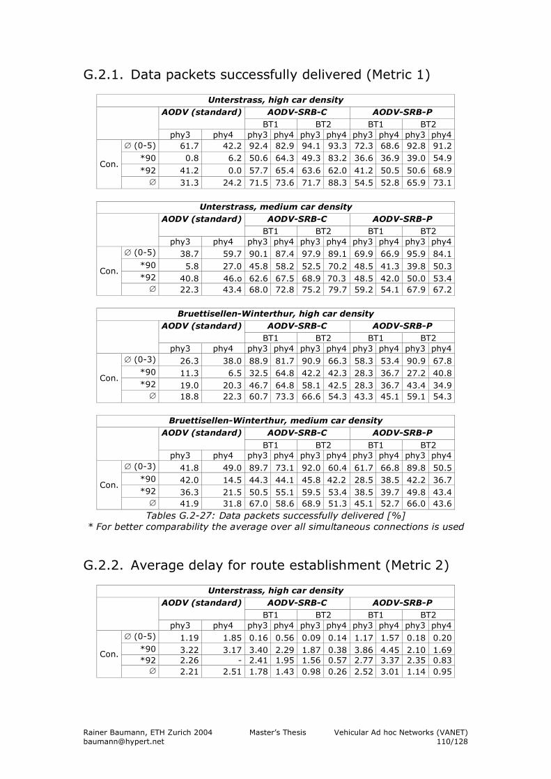
Rainer Baumann, ETH Zurich 2004 Master’s Thesis Vehicular Ad hoc Networks (VANET) [email protected] 110/128
G.2.1. Data packets successfully delivered (Metric 1)
Unterstrass, high car density AODV-SRB-C AODV-SRB-P AODV (standard)
BT1 BT2 BT1 BT2 phy3 phy4 phy3 phy4 phy3 phy4 phy3 phy4 phy3 phy4
∅ (0-5) 61.7 42.2 92.4 82.9 94.1 93.3 72.3 68.6 92.8 91.2 *90 0.8 6.2 50.6 64.3 49.3 83.2 36.6 36.9 39.0 54.9
*92 41.2 0.0 57.7 65.4 63.6 62.0 41.2 50.5 50.6 68.9 Con.
∅ 31.3 24.2 71.5 73.6 71.7 88.3 54.5 52.8 65.9 73.1
Unterstrass, medium car density
AODV-SRB-C AODV-SRB-P AODV (standard) BT1 BT2 BT1 BT2
phy3 phy4 phy3 phy4 phy3 phy4 phy3 phy4 phy3 phy4 ∅ (0-5) 38.7 59.7 90.1 87.4 97.9 89.1 69.9 66.9 95.9 84.1
*90 5.8 27.0 45.8 58.2 52.5 70.2 48.5 41.3 39.8 50.3 *92 40.8 46.o 62.6 67.5 68.9 70.3 48.5 42.0 50.0 53.4
Con.
∅ 22.3 43.4 68.0 72.8 75.2 79.7 59.2 54.1 67.9 67.2
Bruettisellen-Winterthur, high car density
AODV-SRB-C AODV-SRB-P AODV (standard) BT1 BT2 BT1 BT2
phy3 phy4 phy3 phy4 phy3 phy4 phy3 phy4 phy3 phy4 ∅ (0-3) 26.3 38.0 88.9 81.7 90.9 66.3 58.3 53.4 90.9 67.8
*90 11.3 6.5 32.5 64.8 42.2 42.3 28.3 36.7 27.2 40.8 *92 19.0 20.3 46.7 64.8 58.1 42.5 28.3 36.7 43.4 34.9
Con.
∅ 18.8 22.3 60.7 73.3 66.6 54.3 43.3 45.1 59.1 54.3
Bruettisellen-Winterthur, medium car density
AODV-SRB-C AODV-SRB-P AODV (standard)
BT1 BT2 BT1 BT2 phy3 phy4 phy3 phy4 phy3 phy4 phy3 phy4 phy3 phy4
∅ (0-3) 41.8 49.0 89.7 73.1 92.0 60.4 61.7 66.8 89.8 50.5 *90 42.0 14.5 44.3 44.1 45.8 42.2 28.5 38.5 42.2 36.7 *92 36.3 21.5 50.5 55.1 59.5 53.4 38.5 39.7 49.8 43.4
Con.
∅ 41.9 31.8 67.0 58.6 68.9 51.3 45.1 52.7 66.0 43.6 Tables G.2-27: Data packets successfully delivered [%]
* For better comparability the average over all simultaneous connections is used G.2.2. Average delay for route establishment (Metric 2)
Unterstrass, high car density AODV-SRB-C AODV-SRB-P AODV (standard)
BT1 BT2 BT1 BT2 phy3 phy4 phy3 phy4 phy3 phy4 phy3 phy4 phy3 phy4
∅ (0-5) 1.19 1.85 0.16 0.56 0.09 0.14 1.17 1.57 0.18 0.20 *90 3.22 3.17 3.40 2.29 1.87 0.38 3.86 4.45 2.10 1.69 *92 2.26 - 2.41 1.95 1.56 0.57 2.77 3.37 2.35 0.83
Con.
∅ 2.21 2.51 1.78 1.43 0.98 0.26 2.52 3.01 1.14 0.95
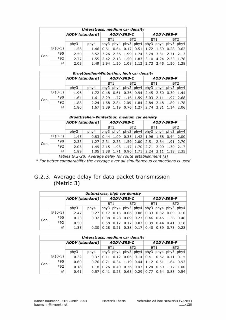
Rainer Baumann, ETH Zurich 2004 Master’s Thesis Vehicular Ad hoc Networks (VANET) [email protected] 111/128
Unterstrass, medium car density AODV-SRB-C AODV-SRB-P AODV (standard)
BT1 BT2 BT1 BT2 phy3 phy4 phy3 phy4 phy3 phy4 phy3 phy4 phy3 phy4
∅ (0-5) 1.56 1.46 0.61 0.64 0.17 0.51 1.72 1.59 0.28 0.62 *90 2.50 3.52 3.26 2.36 1.99 1.74 3.74 3.31 2.71 2.13 *92 2.77 1.55 2.42 2.13 1.50 1.83 3.10 4.24 2.33 1.78
Con.
∅ 2.03 2.49 1.94 1.50 1.08 1.13 2.73 2.45 1.50 1.38
Bruettisellen-Winterthur, high car density
AODV-SRB-C AODV-SRB-P AODV (standard)
BT1 BT2 BT1 BT2 phy3 phy4 phy3 phy4 phy3 phy4 phy3 phy4 phy3 phy4
∅ (0-3) 1.96 1.72 0.48 0.61 0.36 0.94 2.45 2.50 0.30 1.44 *90 1.64 1.61 2.29 1.77 1.16 1.59 3.03 2.11 1.97 2.68 *92 1.88 2.24 1.68 2.84 2.09 1.84 2.84 2.48 1.89 1.78
Con.
∅ 1.80 1.67 1.39 1.19 0.76 1.27 2.74 2.31 1.14 2.06
Bruettisellen-Winterthur, medium car density
AODV (standard) AODV-SRB-C AODV-SRB-P BT1 BT2 BT1 BT2
phy3 phy4 phy3 phy4 phy3 phy4 phy3 phy4 phy3 phy4 ∅ (0-3) 1.45 0.83 0.44 1.09 0.33 1.42 1.96 1.58 0.44 2.00
*90 2.33 1.27 2.31 2.33 1.59 2.00 2.51 2.64 1.91 2.70 *92 2.03 1.49 2.15 1.93 1.47 1.70 2.71 2.99 1.30 2.17
Con.
∅ 1.89 1.05 1.38 1.71 0.96 1.71 2.24 2.11 1.18 2.35 Tables G.2-28: Average delay for route establishment [s]
* For better comparability the average over all simultaneous connections is used
G.2.3. Average delay for data packet transmission (Metric 3)
Unterstrass, high car density
AODV-SRB-C AODV-SRB-P AODV (standard)
BT1 BT2 BT1 BT2 phy3 phy4 phy3 phy4 phy3 phy4 phy3 phy4 phy3 phy4
∅ (0-5) 2.47 0.27 0.17 0.13 0.06 0.06 0.33 0.32 0.09 0.10 *90 0.23 0.32 0.38 0.28 0.69 0.27 0.46 0.45 1.36 0.46 *92 0.50 - 0.58 0.17 0.17 0.07 0.39 0.44 0.41 0.18
Con.
∅ 1.35 0.30 0.28 0.21 0.38 0.17 0.40 0.39 0.73 0.28
Unterstrass, medium car density
AODV-SRB-C AODV-SRB-P AODV (standard) BT1 BT2 BT1 BT2
phy3 phy4 phy3 phy4 phy3 phy4 phy3 phy4 phy3 phy4 ∅ (0-5) 0.22 0.37 0.11 0.12 0.06 0.14 0.41 0.67 0.11 0.15
*90 0.60 0.76 0.71 0.34 1.19 0.44 1.12 0.61 1.64 0.93 *92 0.18 1.18 0.26 0.40 0.36 0.47 1.24 0.50 1.17 1.00
Con.
∅ 0.41 0.57 0.41 0.23 0.63 0.29 0.77 0.64 0.88 0.54
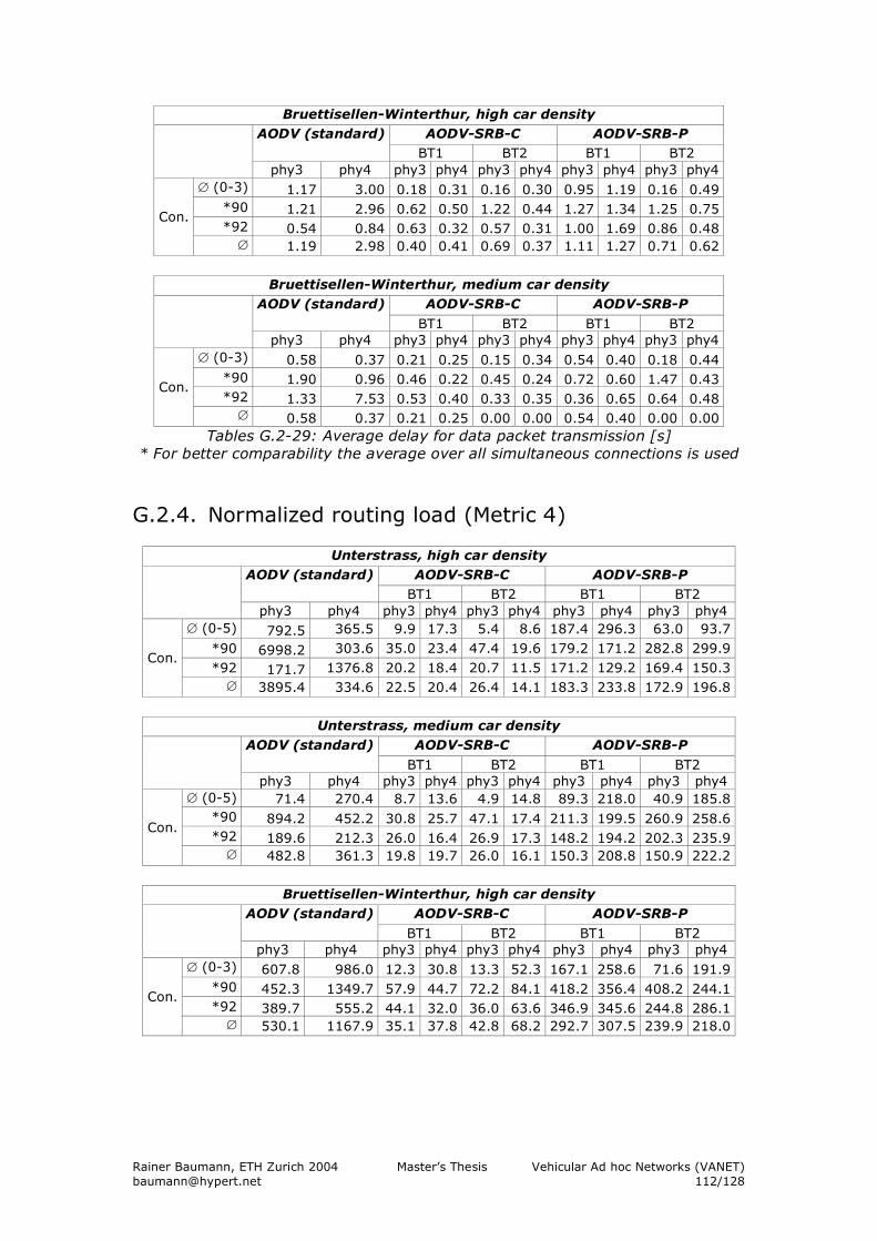
Rainer Baumann, ETH Zurich 2004 Master’s Thesis Vehicular Ad hoc Networks (VANET) [email protected] 112/128
Bruettisellen-Winterthur, high car density AODV-SRB-C AODV-SRB-P AODV (standard)
BT1 BT2 BT1 BT2 phy3 phy4 phy3 phy4 phy3 phy4 phy3 phy4 phy3 phy4
∅ (0-3) 1.17 3.00 0.18 0.31 0.16 0.30 0.95 1.19 0.16 0.49 *90 1.21 2.96 0.62 0.50 1.22 0.44 1.27 1.34 1.25 0.75 *92 0.54 0.84 0.63 0.32 0.57 0.31 1.00 1.69 0.86 0.48
Con.
∅ 1.19 2.98 0.40 0.41 0.69 0.37 1.11 1.27 0.71 0.62
Bruettisellen-Winterthur, medium car density
AODV-SRB-C AODV-SRB-P AODV (standard)
BT1 BT2 BT1 BT2 phy3 phy4 phy3 phy4 phy3 phy4 phy3 phy4 phy3 phy4
∅ (0-3) 0.58 0.37 0.21 0.25 0.15 0.34 0.54 0.40 0.18 0.44 *90 1.90 0.96 0.46 0.22 0.45 0.24 0.72 0.60 1.47 0.43 *92 1.33 7.53 0.53 0.40 0.33 0.35 0.36 0.65 0.64 0.48
Con.
∅ 0.58 0.37 0.21 0.25 0.00 0.00 0.54 0.40 0.00 0.00 Tables G.2-29: Average delay for data packet transmission [s]
* For better comparability the average over all simultaneous connections is used G.2.4. Normalized routing load (Metric 4)
Unterstrass, high car density AODV-SRB-C AODV-SRB-P AODV (standard)
BT1 BT2 BT1 BT2 phy3 phy4 phy3 phy4 phy3 phy4 phy3 phy4 phy3 phy4
∅ (0-5) 792.5 365.5 9.9 17.3 5.4 8.6 187.4 296.3 63.0 93.7 *90 6998.2 303.6 35.0 23.4 47.4 19.6 179.2 171.2 282.8 299.9 *92 171.7 1376.8 20.2 18.4 20.7 11.5 171.2 129.2 169.4 150.3
Con.
∅ 3895.4 334.6 22.5 20.4 26.4 14.1 183.3 233.8 172.9 196.8
Unterstrass, medium car density
AODV-SRB-C AODV-SRB-P AODV (standard)
BT1 BT2 BT1 BT2 phy3 phy4 phy3 phy4 phy3 phy4 phy3 phy4 phy3 phy4
∅ (0-5) 71.4 270.4 8.7 13.6 4.9 14.8 89.3 218.0 40.9 185.8 *90 894.2 452.2 30.8 25.7 47.1 17.4 211.3 199.5 260.9 258.6 *92 189.6 212.3 26.0 16.4 26.9 17.3 148.2 194.2 202.3 235.9
Con.
∅ 482.8 361.3 19.8 19.7 26.0 16.1 150.3 208.8 150.9 222.2
Bruettisellen-Winterthur, high car density
AODV-SRB-C AODV-SRB-P AODV (standard)
BT1 BT2 BT1 BT2 phy3 phy4 phy3 phy4 phy3 phy4 phy3 phy4 phy3 phy4
∅ (0-3) 607.8 986.0 12.3 30.8 13.3 52.3 167.1 258.6 71.6 191.9 *90 452.3 1349.7 57.9 44.7 72.2 84.1 418.2 356.4 408.2 244.1 *92 389.7 555.2 44.1 32.0 36.0 63.6 346.9 345.6 244.8 286.1
Con.
∅ 530.1 1167.9 35.1 37.8 42.8 68.2 292.7 307.5 239.9 218.0
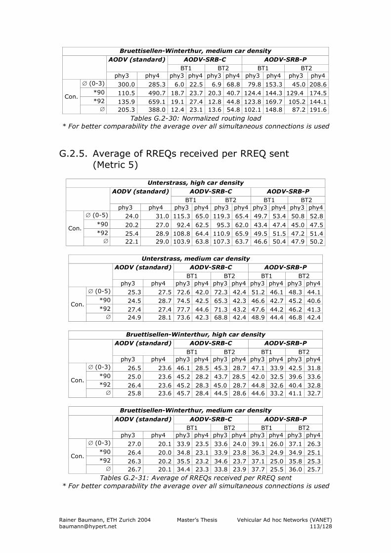
Rainer Baumann, ETH Zurich 2004 Master’s Thesis Vehicular Ad hoc Networks (VANET) [email protected] 113/128
Bruettisellen-Winterthur, medium car density AODV-SRB-C AODV-SRB-P AODV (standard)
BT1 BT2 BT1 BT2 phy3 phy4 phy3 phy4 phy3 phy4 phy3 phy4 phy3 phy4
∅ (0-3) 300.0 285.3 6.0 22.5 6.9 68.8 79.8 153.3 45.0 208.6 *90 110.5 490.7 18.7 23.7 20.3 40.7 124.4 144.3 129.4 174.5 *92 135.9 659.1 19.1 27.4 12.8 44.8 123.8 169.7 105.2 144.1
Con.
∅ 205.3 388.0 12.4 23.1 13.6 54.8 102.1 148.8 87.2 191.6
Tables G.2-30: Normalized routing load * For better comparability the average over all simultaneous connections is used
G.2.5. Average of RREQs received per RREQ sent
(Metric 5)
Unterstrass, high car density AODV-SRB-C AODV-SRB-P AODV (standard)
BT1 BT2 BT1 BT2 phy3 phy4 phy3 phy4 phy3 phy4 phy3 phy4 phy3 phy4
∅ (0-5) 24.0 31.0 115.3 65.0 119.3 65.4 49.7 53.4 50.8 52.8 *90 20.2 27.0 92.4 62.5 95.3 62.0 43.4 47.4 45.0 47.5 *92 25.4 28.9 108.8 64.4 110.9 65.9 49.5 51.5 47.2 51.4
Con.
∅ 22.1 29.0 103.9 63.8 107.3 63.7 46.6 50.4 47.9 50.2
Unterstrass, medium car density
AODV-SRB-C AODV-SRB-P AODV (standard) BT1 BT2 BT1 BT2
phy3 phy4 phy3 phy4 phy3 phy4 phy3 phy4 phy3 phy4 ∅ (0-5) 25.3 27.5 72.6 42.0 72.3 42.4 51.2 46.1 48.3 44.1
*90 24.5 28.7 74.5 42.5 65.3 42.3 46.6 42.7 45.2 40.6 *92 27.4 27.4 77.7 44.6 71.3 43.2 47.6 44.2 46.2 41.3
Con.
∅ 24.9 28.1 73.6 42.3 68.8 42.4 48.9 44.4 46.8 42.4
Bruettisellen-Winterthur, high car density
AODV-SRB-C AODV-SRB-P AODV (standard)
BT1 BT2 BT1 BT2 phy3 phy4 phy3 phy4 phy3 phy4 phy3 phy4 phy3 phy4
∅ (0-3) 26.5 23.6 46.1 28.5 45.3 28.7 47.1 33.9 42.5 31.8 *90 25.0 23.6 45.2 28.2 43.7 28.5 42.0 32.5 39.6 33.6 *92 26.4 23.6 45.2 28.3 45.0 28.7 44.8 32.6 40.4 32.8
Con.
∅ 25.8 23.6 45.7 28.4 44.5 28.6 44.6 33.2 41.1 32.7
Bruettisellen-Winterthur, medium car density
AODV-SRB-C AODV-SRB-P AODV (standard) BT1 BT2 BT1 BT2
phy3 phy4 phy3 phy4 phy3 phy4 phy3 phy4 phy3 phy4 ∅ (0-3) 27.0 20.1 33.9 23.5 33.6 24.0 39.1 26.0 37.1 26.3
*90 26.4 20.0 34.8 23.1 33.9 23.8 36.3 24.9 34.9 25.1 *92 26.3 20.2 35.5 23.2 34.6 23.7 37.1 25.0 35.8 25.3
Con.
∅ 26.7 20.1 34.4 23.3 33.8 23.9 37.7 25.5 36.0 25.7 Tables G.2-31: Average of RREQs received per RREQ sent
* For better comparability the average over all simultaneous connections is used
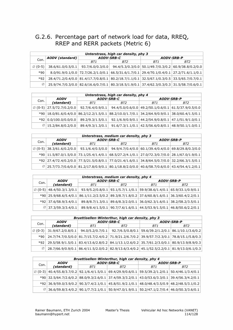
Rainer Baumann, ETH Zurich 2004 Master’s Thesis Vehicular Ad hoc Networks (VANET) [email protected] 114/128
G.2.6. Percentage part of network load for data, RREQ, RREP and RERR packets (Metric 6)
Unterstrass, high car density, phy 3
AODV-SRB-C AODV-SRB-P Con.
AODV (standard) BT1 BT2 BT1 BT2
∅ (0-5) 38.6/61.0/0.5/0.1 93.7/6.0/0.3/0.0 94.4/5.3/0.3/0.0 50.1/49.7/0.3/0.2 60.9/38.8/0.2/0.0
*90 8.0/91.9/0.1/0.0 72.7/26.2/1.0/0.1 66.5/31.6/1.7/0.1 29.4/70.1/0.4/0.1 27.2/71.6/1.1/0.1
*92 28.4/71.2/0.4/0.0 81.4/17.7/0.8/0.1 80.2/18.7/1.1/0.1 32.5/67.1/0.3/0.5 33.5/65.7/0.7/0.1
∅ 25.9/74.7/0.3/0.0 82.6/16.6/0.7/0.1 80.3/18.5/1.9/0.1 37.4/62.3/0.3/0.3 31.5/58.7/0.6/0.1
Unterstrass, high car density, phy 4
AODV-SRB-C AODV-SRB-P Con.
AODV (standard) BT1 BT2 BT1 BT2
∅ (0-5) 27.5/72.7/0.2/0.0 92.7/6.4/0.9/0.1 94.4/5.0/0.6/0.0 49.2/50.1/0.6/0.1 61.5/37.9/0.5/0.0
*90 18.0/81.6/0.4/0.0 86.2/12.2/1.5/0.1 88.2/10.0/1.7/0.1 34.2/64.9/0.9/0.1 38.0/60.4/1.5/0.1
*92 0.0/100.0/0.0/0.0 89.2/9.3/1.5/0.1 92.1/6.9/0.9/0.1 44.2/54.9/0.8/0.1 47.1/51.9/1.0/0.1
∅ 15.2/84.8/0.2/0.0 89.4/9.3/1.3/0.1 91.6/7.3/1.1/0.1 42.5/56.6/0.8/0.1 48.9/50.1/1.0/0.1
Unterstrass, medium car density, phy 3
AODV-SRB-C AODV-SRB-P Con.
AODV (standard) BT1 BT2 BT1 BT2
∅ (0-5) 38.3/61.6/0.2/0.0 93.1/6.4/0.5/0.0 94.9/4.7/0.4/0.0 60.1/39.4/0.4/0.0 69.8/29.8/0.3/0.0
*90 11.5/87.0/1.5/0.0 73.1/25.4/1.4/0.1 68.5/27.2/4.1/0.1 27.0/72.3/0.7/0.0 28.1/67.0/1.9/0.1
*92 27.4/72.4/0.2/0.0 77.5/21.5/0.8/0.1 77.0/21.4/1.6/0.1 34.8/64.5/0.7/0.0 32.2/66.3/1.5/0.1
∅ 25.7/73.7/0.6/0.0 81.2/17.8/0.9/0.1 80.1/18.8/2.0/0.0 40.6/58.7/0.6/0.0 43.4/54.4/1.2/0.1
Unterstrass, medium car density, phy 4
AODV-SRB-C AODV-SRB-P Con.
AODV (standard) BT1 BT2 BT1 BT2
∅ (0-5) 48.4/50.3/1.3/0.1 93.9/5.2/0.8/0.1 93.1/5.7/1.1/0.1 59.9/38.6/1.4/0.1 65.9/33.1/0.9/0.1
*90 25.9/68.6/5.4/0.1 86.1/11.2/2.5/0.2 89.3/8.7/1.8/0.2 37.6/60.8/1.6/0.1 36.3/60.4/2.2/0.1
*92 37.6/58.9/3.4/0.1 89.8/8.7/1.3/0.1 89.6/8.3/2.0/0.1 36.0/62.3/1.6/0.1 38.2/58.2/3.5/0.1
∅ 37.3/59.3/3.4/0.1 89.9/8.4/1.5/0.1 90.7/7.6/1.6/0.1 44.5/53.9/1.5/0.1 46.8/50.6/2.2/0.1
Bruettisellen-Winterthur, high car density, phy 3
AODV-SRB-C AODV-SRB-P Con.
AODV (standard) BT1 BT2 BT1 BT2
∅ (0-3) 31.9/67.2/0.8/0.1 94.0/5.2/0.7/0.1 92.7/6.5/0.8/0.1 59.6/39.2/1.2/0.1 86.1/10.1/3.6/0.2
*90 24.7/74.7/0.5/0.0 81.7/15.7/2.4/0.2 71.9/21.2/6.7/0.2 39.9/57.7/2.3/0.1 78.8/15.1/5.8/0.3
*92 29.5/58.9/1.5/0.1 83.4/13.6/2.8/0.2 84.1/13.1/2.6/0.2 35.7/61.2/3.0/0.1 80.9/13.9/8.9/0.3
∅ 28.7/66.9/0.9/0.1 86.4/11.5/2.0/0.2 82.9/13.6/3.4/0.2 45.1/52.5/2.2/0.1 81.9/13.0/6.1/0.3
Bruettisellen-Winterthur, high car density, phy 4
AODV-SRB-C AODV-SRB-P Con.
AODV (standard) BT1 BT2 BT1 BT2
∅ (0-3) 40.4/55.8/3.7/0.2 92.1/6.4/1.5/0.1 69.4/29.9/0.6/0.1 59.5/39.2/1.2/0.1 50.4/46.1/3.4/0.1
*90 32.5/64.7/2.6/0.2 88.0/9.3/2.6/0.1 37.4/59.3/3.2/0.1 43.0/53.6/3.3/0.1 39.4/56.3/4.2/0.1
*92 36.9/59.0/3.9/0.2 90.3/7.4/2.1/0.1 45.8/51.9/2.1/0.1 48.0/48.4/3.5/0.9 48.2/48.5/3.1/0.2
∅ 36.6/59.8/3.4/0.2 90.1/7.7/2.1/0.1 50.9/47.0/1.9/0.1 50.2/47.1/2.7/0.4 46.0/50.3/3.6/0.1
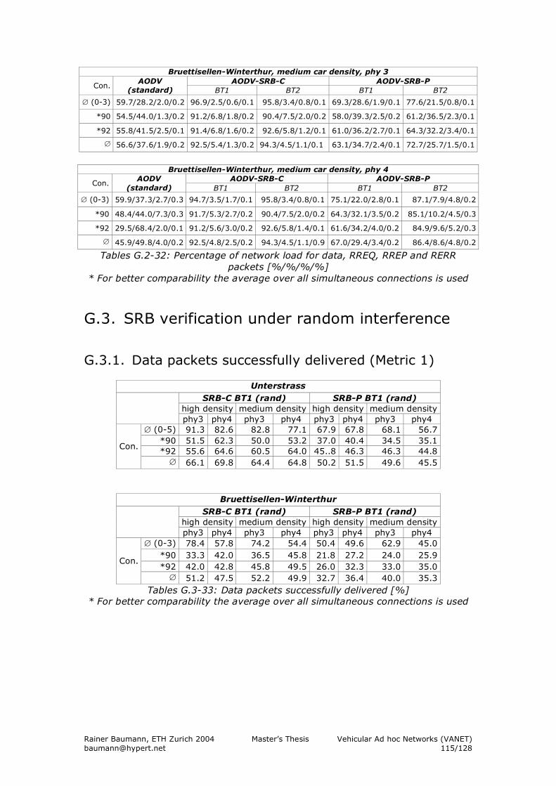
Rainer Baumann, ETH Zurich 2004 Master’s Thesis Vehicular Ad hoc Networks (VANET) [email protected] 115/128
Bruettisellen-Winterthur, medium car density, phy 3 AODV-SRB-C AODV-SRB-P
Con. AODV
(standard) BT1 BT2 BT1 BT2
∅ (0-3) 59.7/28.2/2.0/0.2 96.9/2.5/0.6/0.1 95.8/3.4/0.8/0.1 69.3/28.6/1.9/0.1 77.6/21.5/0.8/0.1
*90 54.5/44.0/1.3/0.2 91.2/6.8/1.8/0.2 90.4/7.5/2.0/0.2 58.0/39.3/2.5/0.2 61.2/36.5/2.3/0.1
*92 55.8/41.5/2.5/0.1 91.4/6.8/1.6/0.2 92.6/5.8/1.2/0.1 61.0/36.2/2.7/0.1 64.3/32.2/3.4/0.1
∅ 56.6/37.6/1.9/0.2 92.5/5.4/1.3/0.2 94.3/4.5/1.1/0.1 63.1/34.7/2.4/0.1 72.7/25.7/1.5/0.1
Bruettisellen-Winterthur, medium car density, phy 4
AODV-SRB-C AODV-SRB-P Con.
AODV (standard) BT1 BT2 BT1 BT2
∅ (0-3) 59.9/37.3/2.7/0.3 94.7/3.5/1.7/0.1 95.8/3.4/0.8/0.1 75.1/22.0/2.8/0.1 87.1/7.9/4.8/0.2
*90 48.4/44.0/7.3/0.3 91.7/5.3/2.7/0.2 90.4/7.5/2.0/0.2 64.3/32.1/3.5/0.2 85.1/10.2/4.5/0.3
*92 29.5/68.4/2.0/0.1 91.2/5.6/3.0/0.2 92.6/5.8/1.4/0.1 61.6/34.2/4.0/0.2 84.9/9.6/5.2/0.3
∅ 45.9/49.8/4.0/0.2 92.5/4.8/2.5/0.2 94.3/4.5/1.1/0.9 67.0/29.4/3.4/0.2 86.4/8.6/4.8/0.2
Tables G.2-32: Percentage of network load for data, RREQ, RREP and RERR packets [%/%/%/%]
* For better comparability the average over all simultaneous connections is used
G.3. SRB verification under random interference
G.3.1. Data packets successfully delivered (Metric 1)
Unterstrass SRB-C BT1 (rand) SRB-P BT1 (rand)
high density medium density high density medium density
phy3 phy4 phy3 phy4 phy3 phy4 phy3 phy4 ∅ (0-5) 91.3 82.6 82.8 77.1 67.9 67.8 68.1 56.7
*90 51.5 62.3 50.0 53.2 37.0 40.4 34.5 35.1 *92 55.6 64.6 60.5 64.0 45..8 46.3 46.3 44.8 Con.
∅ 66.1 69.8 64.4 64.8 50.2 51.5 49.6 45.5
Bruettisellen-Winterthur SRB-C BT1 (rand) SRB-P BT1 (rand)
high density medium density high density medium density
phy3 phy4 phy3 phy4 phy3 phy4 phy3 phy4 ∅ (0-3) 78.4 57.8 74.2 54.4 50.4 49.6 62.9 45.0
*90 33.3 42.0 36.5 45.8 21.8 27.2 24.0 25.9 *92 42.0 42.8 45.8 49.5 26.0 32.3 33.0 35.0
Con.
∅ 51.2 47.5 52.2 49.9 32.7 36.4 40.0 35.3 Tables G.3-33: Data packets successfully delivered [%]
* For better comparability the average over all simultaneous connections is used

Rainer Baumann, ETH Zurich 2004 Master’s Thesis Vehicular Ad hoc Networks (VANET) [email protected] 116/128
G.3.2. Average delay for route establishment (Metric 2)
Unterstrass SRB-C BT1 (rand) SRB-P BT1 (rand)
high density medium density high density medium density
phy3 phy4 phy3 phy4 phy3 phy4 phy3 phy4 ∅ (0-5) 0.22 0.50 0.89 1.48 1.47 1.63 2.05 2.06
*90 3.09 2.53 2.59 2.79 4.57 4.30 3.71 3.65 *92 1.66 1.70 2.35 3.10 4.00 3.58 4.49 3.74
Con.
∅ 1.66 1.58 1.94 2.46 3.35 3.17 3.42 3.15
Bruettisellen-Winterthur
SRB-C BT1 (rand) SRB-P BT1 (rand) high density medium density high density medium density
phy3 phy4 phy3 phy4 phy3 phy4 phy3 phy4 ∅ (0-3) 0.56 0.99 0.72 1.62 2.07 1.70 1.90 2.00
*90 2.60 2.28 3.13 2.64 2.90 3.25 2.31 2.37 *92 2.37 2.42 1.94 2.46 2.74 2.00 2.42 2.47
Con.
∅ 1.84 1.90 1.93 2.24 2.57 2.32 2.21 2.28 Tables G.3-34: Average delay for route establishment [s]
* For better comparability the average over all simultaneous connections is used
G.3.3. Average delay for data packet transmission (Metric 3)
Unterstrass
SRB-C BT1 (rand) SRB-P BT1 (rand) high density medium density high density medium density
phy3 phy4 phy3 phy4 phy3 phy4 phy3 phy4 ∅ (0-5) 0.16 0.25 0.60 0.30 0.60 1.23 0.73 1.43
*90 0.59 0.50 0.77 0.28 0.54 0.54 1.32 0.97 *92 0.24 0.54 0.35 0.60 0.53 0.75 0.87 1.32
Con.
∅ 0.33 0.43 0.57 0.39 0.56 0.84 0.97 1.24
Bruettisellen-Winterthur
SRB-C BT1 (rand) SRB-P BT1 (rand) high density medium density high density medium density
phy3 phy4 phy3 phy4 phy3 phy4 phy3 phy4 ∅ (0-3) 0.34 1.15 0.46 0.39 0.99 0.87 0.75 1.31
*90 0.75 1.02 1.44 0.76 1.39 1.60 1.25 1.48 *92 0.77 1.26 1.14 1.14 0.76 1.73 2.20 0.89
Con.
∅ 0.62 1.14 1.01 0.76 1.05 1.40 1.40 1.23
Tables G.3-35: Average delay for data packet transmission [s] * For better comparability the average over all simultaneous connections is used

Rainer Baumann, ETH Zurich 2004 Master’s Thesis Vehicular Ad hoc Networks (VANET) [email protected] 117/128
G.3.4. Normalized routing load (Metric 4)
Unterstrass SRB-C BT1 (rand) SRB-P BT1 (rand)
high density medium density high density medium density
phy3 phy4 phy3 phy4 phy3 phy4 phy3 phy4 ∅ (0-5) 5.9 15.2 15.0 19.7 123.3 249.0 140.9 137.2
*90 25.4 21.7 30.3 23.3 207.3 194.6 227.1 194.6 *92 19.8 18.7 18.1 20.7 172.1 174.9 163.7 242.9
Con.
∅ 15.7 18.5 22.7 21.5 165.3 221.8 184.0 165.9
Bruettisellen-Winterthur
SRB-C BT1 (rand) SRB-P BT1 (rand) high density medium density high density medium density
phy3 phy4 phy3 phy4 phy3 phy4 phy3 phy4 ∅ (0-3) 23.5 112.4 11.9 51.4 259.1 450.2 79.4 337.5
*90 49.8 49.9 22.0 32.1 337.3 323.0 175.6 176.1 *92 42.1 47.4 18.0 26.5 296.9 282.1 127.3 141.6
Con.
∅ 36.7 81.2 17.0 41.8 298.2 386.6 127.5 256.8 Tables G.3-36: Normalized routing load
* For better comparability the average over all simultaneous connections is used
G.3.5. Average of RREQs received per RREQ sent (Metric 5)
Unterstrass
SRB-C BT1 (rand) SRB-P BT1 (rand) high density medium density high density medium density
phy3 phy4 phy3 phy4 phy3 phy4 phy3 phy4 ∅ (0-5) 106.6 57.5 63.8 37.0 52.1 51.8 49.9 43.1
*90 91..2 56.9 70.4 39.4 44.3 47.3 46.3 40.1 *92 102.0 56.7 67.8 39.9 50.4 49.9 47.9 40.8
Con.
∅ 98.9 57.2 67.1 38.2 48.2 49.6 48.1 41.6
Bruettisellen-Winterthur
SRB-C BT1 (rand) SRB-P BT1 (rand) high density medium density high density medium density
phy3 phy4 phy3 phy4 phy3 phy4 phy3 phy4 ∅ (0-3) 41.1 24.6 30.8 20.9 44.2 31.3 36.77 23.6
*90 40.5 24.6 31.3 20.7 40.8 29.7 33.8 22.6 *92 41.2 24.6 30.9 20.4 30.0 35.1 23.1 23.1
Con.
∅ 40.8 24.6 31.1 20.8 42.5 30.5 35.3 23.1 Tables G.3-37: Average of RREQs received per RREQ sent
* For better comparability the average over all simultaneous connections is used
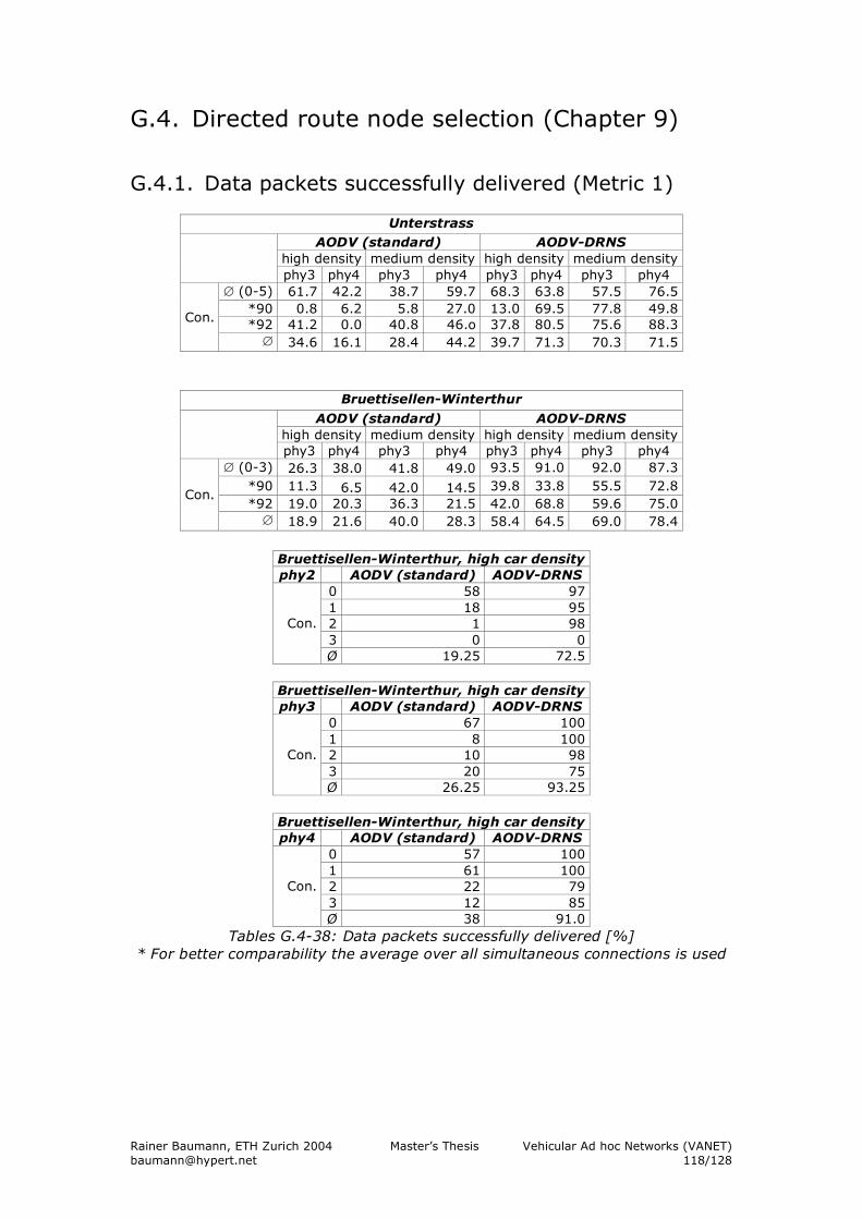
Rainer Baumann, ETH Zurich 2004 Master’s Thesis Vehicular Ad hoc Networks (VANET) [email protected] 118/128
G.4. Directed route node selection (Chapter 9) G.4.1. Data packets successfully delivered (Metric 1)
Unterstrass AODV (standard) AODV-DRNS
high density medium density high density medium density
phy3 phy4 phy3 phy4 phy3 phy4 phy3 phy4 ∅ (0-5) 61.7 42.2 38.7 59.7 68.3 63.8 57.5 76.5
*90 0.8 6.2 5.8 27.0 13.0 69.5 77.8 49.8 *92 41.2 0.0 40.8 46.o 37.8 80.5 75.6 88.3 Con.
∅ 34.6 16.1 28.4 44.2 39.7 71.3 70.3 71.5
Bruettisellen-Winterthur
AODV (standard) AODV-DRNS high density medium density high density medium density
phy3 phy4 phy3 phy4 phy3 phy4 phy3 phy4 ∅ (0-3) 26.3 38.0 41.8 49.0 93.5 91.0 92.0 87.3
*90 11.3 6.5 42.0 14.5 39.8 33.8 55.5 72.8 *92 19.0 20.3 36.3 21.5 42.0 68.8 59.6 75.0
Con.
∅ 18.9 21.6 40.0 28.3 58.4 64.5 69.0 78.4
Bruettisellen-Winterthur, high car density phy2 AODV (standard) AODV-DRNS
0 58 97 1 18 95 2 1 98 3 0 0
Con.
Ø 19.25 72.5
Bruettisellen-Winterthur, high car density phy3 AODV (standard) AODV-DRNS
0 67 100 1 8 100 2 10 98 3 20 75
Con.
Ø 26.25 93.25
Bruettisellen-Winterthur, high car density phy4 AODV (standard) AODV-DRNS
0 57 100 1 61 100 2 22 79 3 12 85
Con.
Ø 38 91.0 Tables G.4-38: Data packets successfully delivered [%]
* For better comparability the average over all simultaneous connections is used
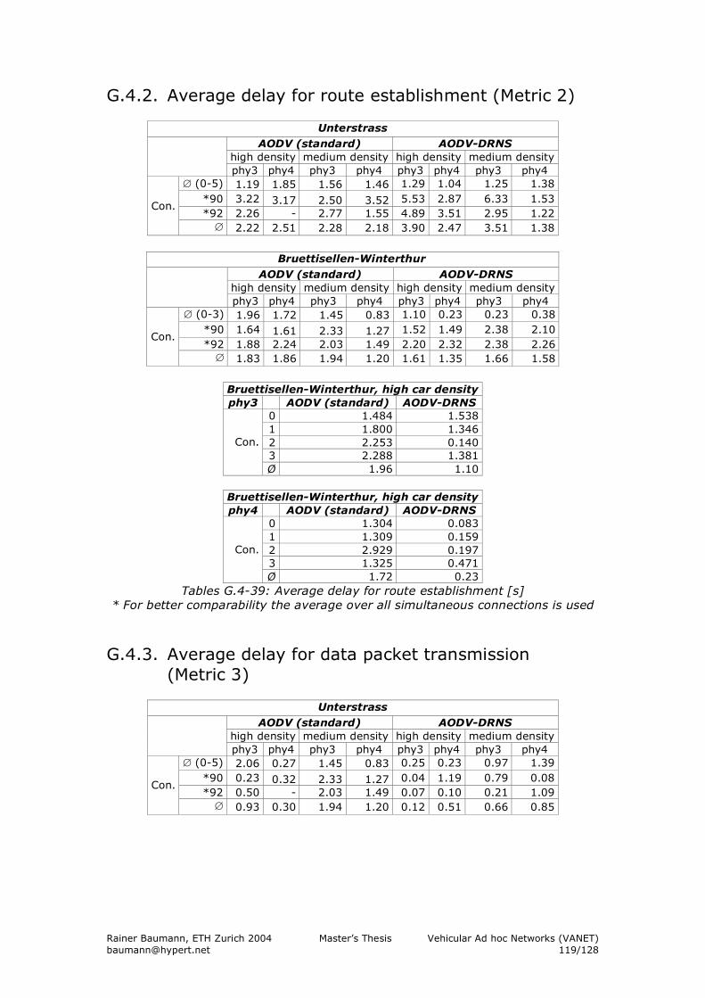
Rainer Baumann, ETH Zurich 2004 Master’s Thesis Vehicular Ad hoc Networks (VANET) [email protected] 119/128
G.4.2. Average delay for route establishment (Metric 2)
Unterstrass AODV (standard) AODV-DRNS
high density medium density high density medium density
phy3 phy4 phy3 phy4 phy3 phy4 phy3 phy4 ∅ (0-5) 1.19 1.85 1.56 1.46 1.29 1.04 1.25 1.38
*90 3.22 3.17 2.50 3.52 5.53 2.87 6.33 1.53 *92 2.26 - 2.77 1.55 4.89 3.51 2.95 1.22
Con.
∅ 2.22 2.51 2.28 2.18 3.90 2.47 3.51 1.38
Bruettisellen-Winterthur
AODV (standard) AODV-DRNS high density medium density high density medium density
phy3 phy4 phy3 phy4 phy3 phy4 phy3 phy4 ∅ (0-3) 1.96 1.72 1.45 0.83 1.10 0.23 0.23 0.38
*90 1.64 1.61 2.33 1.27 1.52 1.49 2.38 2.10 *92 1.88 2.24 2.03 1.49 2.20 2.32 2.38 2.26
Con.
∅ 1.83 1.86 1.94 1.20 1.61 1.35 1.66 1.58
Bruettisellen-Winterthur, high car density phy3 AODV (standard) AODV-DRNS
0 1.484 1.538 1 1.800 1.346 2 2.253 0.140 3 2.288 1.381
Con.
Ø 1.96 1.10
Bruettisellen-Winterthur, high car density phy4 AODV (standard) AODV-DRNS
0 1.304 0.083 1 1.309 0.159 2 2.929 0.197 3 1.325 0.471
Con.
Ø 1.72 0.23 Tables G.4-39: Average delay for route establishment [s]
* For better comparability the average over all simultaneous connections is used G.4.3. Average delay for data packet transmission
(Metric 3)
Unterstrass AODV (standard) AODV-DRNS
high density medium density high density medium density
phy3 phy4 phy3 phy4 phy3 phy4 phy3 phy4 ∅ (0-5) 2.06 0.27 1.45 0.83 0.25 0.23 0.97 1.39
*90 0.23 0.32 2.33 1.27 0.04 1.19 0.79 0.08 *92 0.50 - 2.03 1.49 0.07 0.10 0.21 1.09
Con.
∅ 0.93 0.30 1.94 1.20 0.12 0.51 0.66 0.85
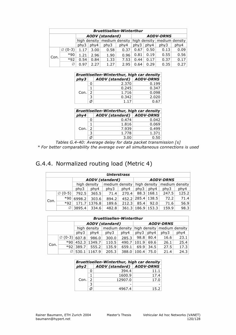
Rainer Baumann, ETH Zurich 2004 Master’s Thesis Vehicular Ad hoc Networks (VANET) [email protected] 120/128
Bruettisellen-Winterthur AODV (standard) AODV-DRNS
high density medium density high density medium density
phy3 phy4 phy3 phy4 phy3 phy4 phy3 phy4 ∅ (0-3) 1.17 3.00 0.58 0.37 0.67 0.50 0.13 0.09
*90 1.21 2.96 1.90 0.96 0.81 0.19 0.55 0.56 *92 0.54 0.84 1.33 7.53 0.44 0.17 0.37 0.17
Con.
∅ 0.97 2.27 1.27 2.95 0.64 0.29 0.35 0.27
Bruettisellen-Winterthur, high car density phy3 AODV (standard) AODV-DRNS
0 2.370 0.199 1 0.245 0.347 2 1.716 0.098 3 0.342 2.020
Con.
Ø 1.17 0.67
Bruettisellen-Winterthur, high car density phy4 AODV (standard) AODV-DRNS
0 0.474 0.042 1 1.816 0.069 2 7.939 0.499 3 1.778 1.371
Con.
Ø 3.00 0.50 Tables G.4-40: Average delay for data packet transmission [s]
* For better comparability the average over all simultaneous connections is used G.4.4. Normalized routing load (Metric 4)
Unterstrass AODV (standard) AODV-DRNS
high density medium density high density medium density
phy3 phy4 phy3 phy4 phy3 phy4 phy3 phy4 ∅ (0-5) 792.5 365.5 71.4 270.4 88.3 168.1 247.5 125.2
*90 6998.2 303.6 894.2 452.2 285.4 138.5 72.2 71.4 *92 171.7 1376.8 189.6 212.3 85.4 92.0 71.6 56.9
Con.
∅ 3895.4 334.6 482.8 361.3 186.9 153.3 159.9 98.3
Bruettisellen-Winterthur
AODV (standard) AODV-DRNS high density medium density high density medium density
phy3 phy4 phy3 phy4 phy3 phy4 phy3 phy4 ∅ (0-3) 607.8 986.0 300.0 285.3 98.8 80.4 16.6 23.1
*90 452.3 1349.7 110.5 490.7 101.9 69.6 26.1 25.4 *92 389.7 555.2 135.9 659.1 69.9 34.5 27.5 17.3
Con.
∅ 530.1 1167.9 205.3 388.0 100.4 75.0 21.4 24.3
Bruettisellen-Winterthur, high car density phy2 AODV (standard) AODV-DRNS
0 394.4 11.1 1 1600.9 17.4 2 12907.0 17.0 3 - -
Con.
Ø 4967.4 15.2
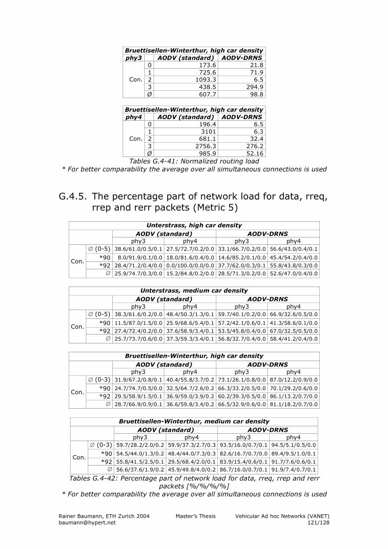
Rainer Baumann, ETH Zurich 2004 Master’s Thesis Vehicular Ad hoc Networks (VANET) [email protected] 121/128
Bruettisellen-Winterthur, high car density phy3 AODV (standard) AODV-DRNS
0 173.6 21.8 1 725.6 71.9 2 1093.3 6.5 3 438.5 294.9
Con.
Ø 607.7 98.8
Bruettisellen-Winterthur, high car density phy4 AODV (standard) AODV-DRNS
0 196.4 6.5 1 3101 6.3 2 681.1 32.4 3 2756.3 276.2
Con.
Ø 985.9 52.16 Tables G.4-41: Normalized routing load
* For better comparability the average over all simultaneous connections is used
G.4.5. The percentage part of network load for data, rreq, rrep and rerr packets (Metric 5)
Unterstrass, high car density
AODV (standard) AODV-DRNS phy3 phy4 phy3 phy4
∅ (0-5) 38.6/61.0/0.5/0.1 27.5/72.7/0.2/0.0 33.1/66.7/0.2/0.0 56.6/43.0/0.4/0.1
*90 8.0/91.9/0.1/0.0 18.0/81.6/0.4/0.0 14.6/85.2/0.1/0.0 45.4/54.2/0.4/0.0
*92 28.4/71.2/0.4/0.0 0.0/100.0/0.0/0.0 37.7/62.0/0.3/0.1 55.8/43.8/0.3/0.0 Con.
∅ 25.9/74.7/0.3/0.0 15.2/84.8/0.2/0.0 28.5/71.3/0.2/0.0 52.6/47.0/0.4/0.0
Unterstrass, medium car density
AODV (standard) AODV-DRNS phy3 phy4 phy3 phy4
∅ (0-5) 38.3/61.6/0.2/0.0 48.4/50.3/1.3/0.1 59.7/40.1/0.2/0.0 66.9/32.6/0.5/0.0
*90 11.5/87.0/1.5/0.0 25.9/68.6/5.4/0.1 57.2/42.1/0.6/0.1 41.3/58.6/0.1/0.0
*92 27.4/72.4/0.2/0.0 37.6/58.9/3.4/0.1 53.5/45.8/0.4/0.0 67.0/32.5/0.5/0.0 Con.
∅ 25.7/73.7/0.6/0.0 37.3/59.3/3.4/0.1 56.8/32.7/0.4/0.0 58.4/41.2/0.4/0.0
Bruettisellen-Winterthur, high car density
AODV (standard) AODV-DRNS phy3 phy4 phy3 phy4
∅ (0-3) 31.9/67.2/0.8/0.1 40.4/55.8/3.7/0.2 73.1/26.1/0.8/0.0 87.0/12.2/0.9/0.0
*90 24.7/74.7/0.5/0.0 32.5/64.7/2.6/0.2 66.3/33.2/0.5/0.0 70.1/29.2/0.6/0.0
*92 29.5/58.9/1.5/0.1 36.9/59.0/3.9/0.2 60.2/39.3/0.5/0.0 86.1/13.2/0.7/0.0 Con.
∅ 28.7/66.9/0.9/0.1 36.6/59.8/3.4/0.2 66.5/32.9/0.6/0.0 81.1/18.2/0.7/0.0
Bruettisellen-Winterthur, medium car density
AODV (standard) AODV-DRNS phy3 phy4 phy3 phy4
∅ (0-3) 59.7/28.2/2.0/0.2 59.9/37.3/2.7/0.3 93.5/16.0/0.7/0.1 94.5/5.1/0.5/0.0
*90 54.5/44.0/1.3/0.2 48.4/44.0/7.3/0.3 82.6/16.7/0.7/0.0 89.4/9.5/1.0/0.1
*92 55.8/41.5/2.5/0.1 29.5/68.4/2.0/0.1 83.9/15.4/0.6/0.1 91.7/7.6/0.6/0.1 Con.
∅ 56.6/37.6/1.9/0.2 45.9/49.8/4.0/0.2 86.7/16.0/0.7/0.1 91.9/7.4/0.7/0.1
Tables G.4-42: Percentage part of network load for data, rreq, rrep and rerr packets [%/%/%/%]
* For better comparability the average over all simultaneous connections is used
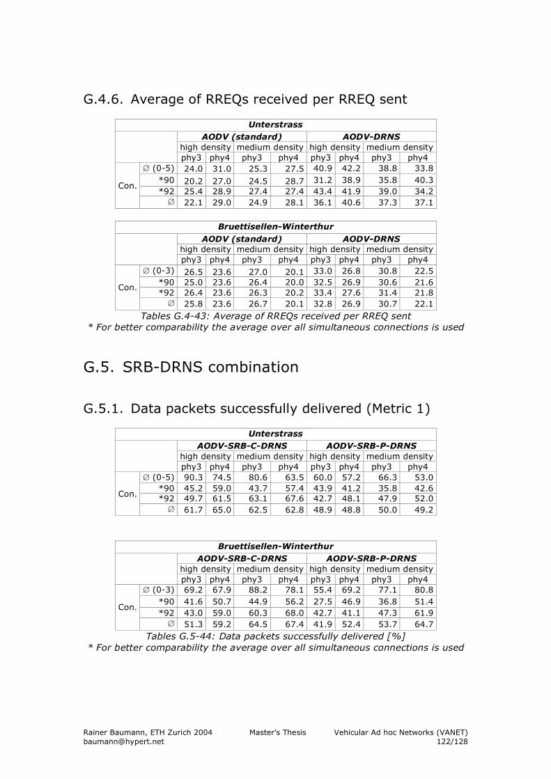
Rainer Baumann, ETH Zurich 2004 Master’s Thesis Vehicular Ad hoc Networks (VANET) [email protected] 122/128
G.4.6. Average of RREQs received per RREQ sent
Unterstrass AODV (standard) AODV-DRNS
high density medium density high density medium density
phy3 phy4 phy3 phy4 phy3 phy4 phy3 phy4 ∅ (0-5) 24.0 31.0 25.3 27.5 40.9 42.2 38.8 33.8
*90 20.2 27.0 24.5 28.7 31.2 38.9 35.8 40.3 *92 25.4 28.9 27.4 27.4 43.4 41.9 39.0 34.2
Con.
∅ 22.1 29.0 24.9 28.1 36.1 40.6 37.3 37.1
Bruettisellen-Winterthur
AODV (standard) AODV-DRNS high density medium density high density medium density
phy3 phy4 phy3 phy4 phy3 phy4 phy3 phy4 ∅ (0-3) 26.5 23.6 27.0 20.1 33.0 26.8 30.8 22.5
*90 25.0 23.6 26.4 20.0 32.5 26.9 30.6 21.6 *92 26.4 23.6 26.3 20.2 33.4 27.6 31.4 21.8
Con.
∅ 25.8 23.6 26.7 20.1 32.8 26.9 30.7 22.1
Tables G.4-43: Average of RREQs received per RREQ sent * For better comparability the average over all simultaneous connections is used
G.5. SRB-DRNS combination
G.5.1. Data packets successfully delivered (Metric 1)
Unterstrass AODV-SRB-C-DRNS AODV-SRB-P-DRNS
high density medium density high density medium density
phy3 phy4 phy3 phy4 phy3 phy4 phy3 phy4 ∅ (0-5) 90.3 74.5 80.6 63.5 60.0 57.2 66.3 53.0
*90 45.2 59.0 43.7 57.4 43.9 41.2 35.8 42.6 *92 49.7 61.5 63.1 67.6 42.7 48.1 47.9 52.0 Con.
∅ 61.7 65.0 62.5 62.8 48.9 48.8 50.0 49.2
Bruettisellen-Winterthur AODV-SRB-C-DRNS AODV-SRB-P-DRNS
high density medium density high density medium density
phy3 phy4 phy3 phy4 phy3 phy4 phy3 phy4 ∅ (0-3) 69.2 67.9 88.2 78.1 55.4 69.2 77.1 80.8
*90 41.6 50.7 44.9 56.2 27.5 46.9 36.8 51.4 *92 43.0 59.0 60.3 68.0 42.7 41.1 47.3 61.9
Con.
∅ 51.3 59.2 64.5 67.4 41.9 52.4 53.7 64.7 Tables G.5-44: Data packets successfully delivered [%]
* For better comparability the average over all simultaneous connections is used
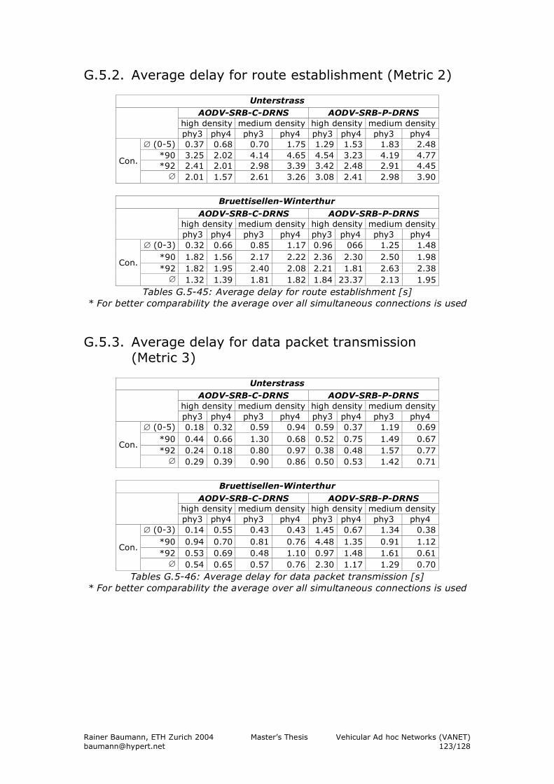
Rainer Baumann, ETH Zurich 2004 Master’s Thesis Vehicular Ad hoc Networks (VANET) [email protected] 123/128
G.5.2. Average delay for route establishment (Metric 2)
Unterstrass AODV-SRB-C-DRNS AODV-SRB-P-DRNS
high density medium density high density medium density
phy3 phy4 phy3 phy4 phy3 phy4 phy3 phy4 ∅ (0-5) 0.37 0.68 0.70 1.75 1.29 1.53 1.83 2.48
*90 3.25 2.02 4.14 4.65 4.54 3.23 4.19 4.77 *92 2.41 2.01 2.98 3.39 3.42 2.48 2.91 4.45 Con.
∅ 2.01 1.57 2.61 3.26 3.08 2.41 2.98 3.90
Bruettisellen-Winterthur
AODV-SRB-C-DRNS AODV-SRB-P-DRNS high density medium density high density medium density
phy3 phy4 phy3 phy4 phy3 phy4 phy3 phy4 ∅ (0-3) 0.32 0.66 0.85 1.17 0.96 066 1.25 1.48
*90 1.82 1.56 2.17 2.22 2.36 2.30 2.50 1.98 *92 1.82 1.95 2.40 2.08 2.21 1.81 2.63 2.38
Con.
∅ 1.32 1.39 1.81 1.82 1.84 23.37 2.13 1.95 Tables G.5-45: Average delay for route establishment [s]
* For better comparability the average over all simultaneous connections is used
G.5.3. Average delay for data packet transmission (Metric 3)
Unterstrass
AODV-SRB-C-DRNS AODV-SRB-P-DRNS high density medium density high density medium density
phy3 phy4 phy3 phy4 phy3 phy4 phy3 phy4 ∅ (0-5) 0.18 0.32 0.59 0.94 0.59 0.37 1.19 0.69
*90 0.44 0.66 1.30 0.68 0.52 0.75 1.49 0.67 *92 0.24 0.18 0.80 0.97 0.38 0.48 1.57 0.77
Con.
∅ 0.29 0.39 0.90 0.86 0.50 0.53 1.42 0.71
Bruettisellen-Winterthur
AODV-SRB-C-DRNS AODV-SRB-P-DRNS high density medium density high density medium density
phy3 phy4 phy3 phy4 phy3 phy4 phy3 phy4 ∅ (0-3) 0.14 0.55 0.43 0.43 1.45 0.67 1.34 0.38
*90 0.94 0.70 0.81 0.76 4.48 1.35 0.91 1.12 *92 0.53 0.69 0.48 1.10 0.97 1.48 1.61 0.61
Con.
∅ 0.54 0.65 0.57 0.76 2.30 1.17 1.29 0.70 Tables G.5-46: Average delay for data packet transmission [s]
* For better comparability the average over all simultaneous connections is used
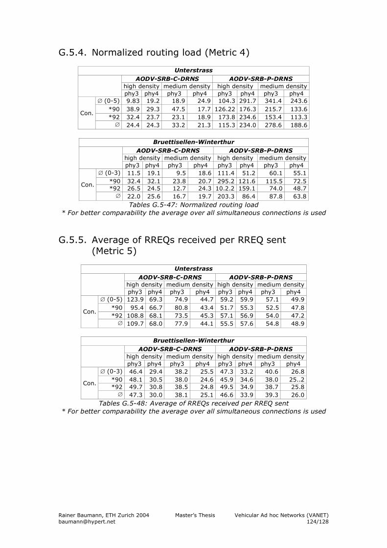
Rainer Baumann, ETH Zurich 2004 Master’s Thesis Vehicular Ad hoc Networks (VANET) [email protected] 124/128
G.5.4. Normalized routing load (Metric 4)
Unterstrass AODV-SRB-C-DRNS AODV-SRB-P-DRNS
high density medium density high density medium density
phy3 phy4 phy3 phy4 phy3 phy4 phy3 phy4 ∅ (0-5) 9.83 19.2 18.9 24.9 104.3 291.7 341.4 243.6
*90 38.9 29.3 47.5 17.7 126.22 176.3 215.7 133.6 *92 32.4 23.7 23.1 18.9 173.8 234.6 153.4 113.3
Con.
∅ 24.4 24.3 33.2 21.3 115.3 234.0 278.6 188.6
Bruettisellen-Winterthur
AODV-SRB-C-DRNS AODV-SRB-P-DRNS high density medium density high density medium density
phy3 phy4 phy3 phy4 phy3 phy4 phy3 phy4 ∅ (0-3) 11.5 19.1 9.5 18.6 111.4 51.2 60.1 55.1
*90 32.4 32.1 23.8 20.7 295.2 121.6 115.5 72.5 *92 26.5 24.5 12.7 24.3 10.2.2 159.1 74.0 48.7
Con.
∅ 22.0 25.6 16.7 19.7 203.3 86.4 87.8 63.8 Tables G.5-47: Normalized routing load
* For better comparability the average over all simultaneous connections is used
G.5.5. Average of RREQs received per RREQ sent (Metric 5)
Unterstrass
AODV-SRB-C-DRNS AODV-SRB-P-DRNS high density medium density high density medium density
phy3 phy4 phy3 phy4 phy3 phy4 phy3 phy4 ∅ (0-5) 123.9 69.3 74.9 44.7 59.2 59.9 57.1 49.9
*90 95.4 66.7 80.8 43.4 51.7 55.3 52.5 47.8 *92 108.8 68.1 73.5 45.3 57.1 56.9 54.0 47.2
Con.
∅ 109.7 68.0 77.9 44.1 55.5 57.6 54.8 48.9
Bruettisellen-Winterthur
AODV-SRB-C-DRNS AODV-SRB-P-DRNS high density medium density high density medium density
phy3 phy4 phy3 phy4 phy3 phy4 phy3 phy4 ∅ (0-3) 46.4 29.4 38.2 25.5 47.3 33.2 40.6 26.8
*90 48.1 30.5 38.0 24.6 45.9 34.6 38.0 25..2 *92 49.7 30.8 38.5 24.8 49.5 34.9 38.7 25.8
Con.
∅ 47.3 30.0 38.1 25.1 46.6 33.9 39.3 26.0 Tables G.5-48: Average of RREQs received per RREQ sent
* For better comparability the average over all simultaneous connections is used
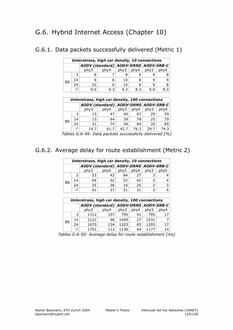
Rainer Baumann, ETH Zurich 2004 Master’s Thesis Vehicular Ad hoc Networks (VANET) [email protected] 125/128
G.6. Hybrid Internet Access (Chapter 10) G.6.1. Data packets successfully delivered (Metric 1)
Unterstrass, high car density, 10 connections AODV (standard) AODV-DRNS AODV-SRB-C
phy3 phy4 phy3 phy4 phy3 phy4 3 8 7 8 9 9 8
14 9 6 10 8 9 9 24 10 6 10 8 9 8
BS
∅ 9.0 6.3 9.3 8.3 9.0 8.3
Unterstrass, high car density, 100 connections
AODV (standard) AODV-DRNS AODV-SRB-C phy3 phy4 phy3 phy4 phy3 phy4
3 15 47 40 67 29 59 14 13 64 39 78 25 79 24 31 74 49 84 35 85
BS
∅ 19.7 61.7 42.7 76.3 29.7 74.3 Tables G.6-49: Data packets successfully delivered [%]
G.6.2. Average delay for route establishment (Metric 2)
Unterstrass, high car density, 10 connections AODV (standard) AODV-DRNS AODV-SRB-C
phy3 phy4 phy3 phy4 phy3 phy4 3 33 42 84 27 3 4
14 54 32 52 42 3 4 24 35 38 16 25 3 3
BS
∅ 41 37 51 31 3 4
Unterstrass, high car density, 100 connections
AODV (standard) AODV-DRNS AODV-SRB-C phy3 phy4 phy3 phy4 phy3 phy4
3 1312 107 795 41 795 17 14 2121 96 1409 27 1531 7 24 1670 134 1203 65 1205 17
BS
∅ 1701 112 1136 44 1177 14 Tables G.6-50: Average delay for route establishment [ms]
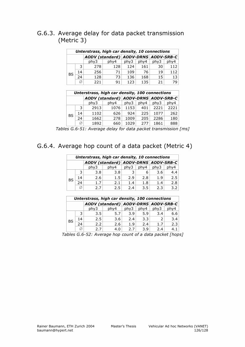
Rainer Baumann, ETH Zurich 2004 Master’s Thesis Vehicular Ad hoc Networks (VANET) [email protected] 126/128
G.6.3. Average delay for data packet transmission (Metric 3)
Unterstrass, high car density, 10 connections
AODV (standard) AODV-DRNS AODV-SRB-C phy3 phy4 phy3 phy4 phy3 phy4
3 278 128 124 161 30 112 14 256 71 109 76 19 112 24 128 73 136 168 15 13
BS
∅ 221 91 123 135 21 79
Unterstrass, high car density, 100 connections
AODV (standard) AODV-DRNS AODV-SRB-C phy3 phy4 phy3 phy4 phy3 phy4
3 2913 1076 1153 401 2221 2221
14 1102 626 924 225 1077 262 24 1662 278 1009 205 2286 180
BS
∅ 1892 660 1029 277 1861 888
Tables G.6-51: Average delay for data packet transmission [ms]
G.6.4. Average hop count of a data packet (Metric 4)
Unterstrass, high car density, 10 connections AODV (standard) AODV-DRNS AODV-SRB-C
phy3 phy4 phy3 phy4 phy3 phy4 3 3.8 3.8 3 6 3.6 4.4
14 2.6 1.5 2.9 2.8 1.9 2.5 24 1.7 2.1 1.4 1.8 1.4 2.8
BS
∅ 2.7 2.5 2.4 3.5 2.3 3.2
Unterstrass, high car density, 100 connections
AODV (standard) AODV-DRNS AODV-SRB-C phy3 phy4 phy3 phy4 phy3 phy4
3 3.5 5.7 3.9 5.9 3.4 6.6 14 2.5 3.6 2.4 3.3 2 3.4 24 2.2 2.6 1.9 2.4 1.7 2.3
BS
∅ 2.7 4.0 2.7 3.9 2.4 4.1 Tables G.6-52: Average hop count of a data packet [hops]
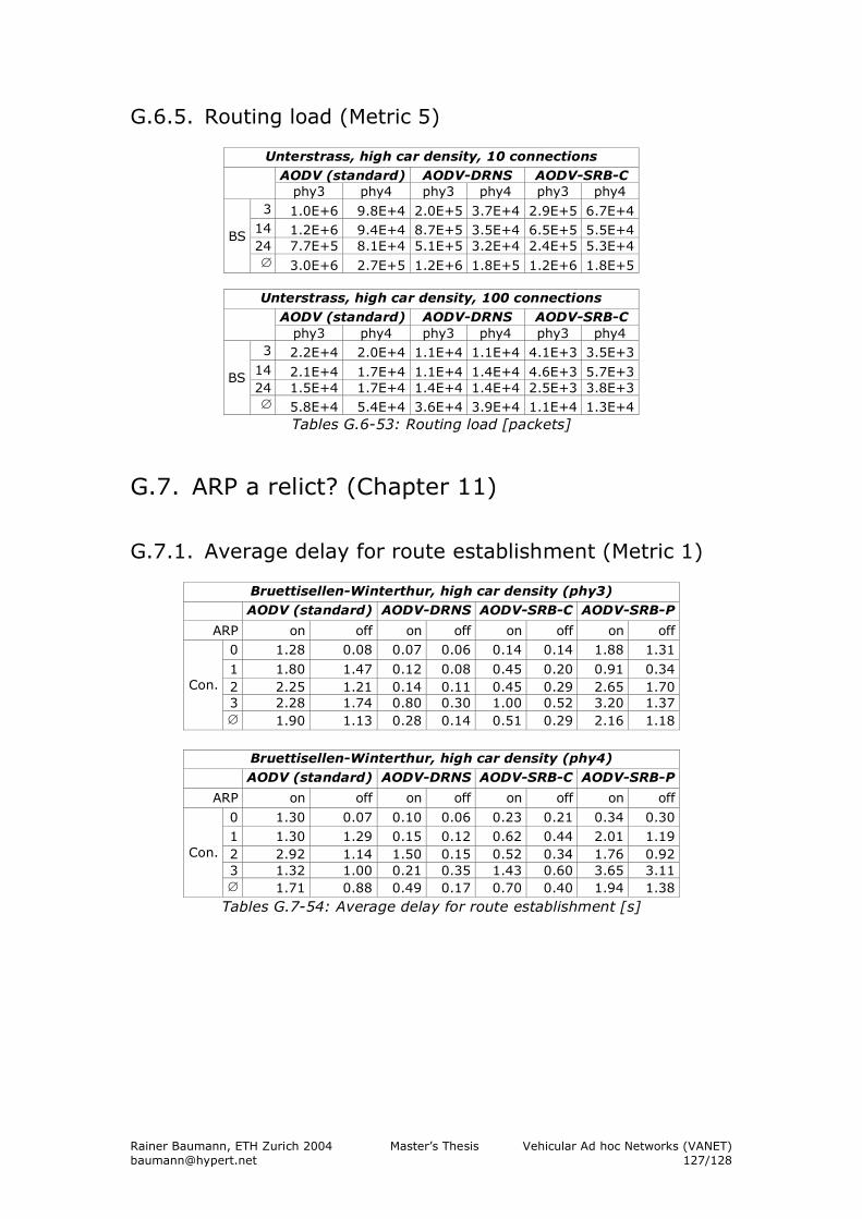
Rainer Baumann, ETH Zurich 2004 Master’s Thesis Vehicular Ad hoc Networks (VANET) [email protected] 127/128
G.6.5. Routing load (Metric 5)
Unterstrass, high car density, 10 connections AODV (standard) AODV-DRNS AODV-SRB-C
phy3 phy4 phy3 phy4 phy3 phy4 3 1.0E+6 9.8E+4 2.0E+5 3.7E+4 2.9E+5 6.7E+4
14 1.2E+6 9.4E+4 8.7E+5 3.5E+4 6.5E+5 5.5E+4 24 7.7E+5 8.1E+4 5.1E+5 3.2E+4 2.4E+5 5.3E+4
BS
∅ 3.0E+6 2.7E+5 1.2E+6 1.8E+5 1.2E+6 1.8E+5
Unterstrass, high car density, 100 connections AODV (standard) AODV-DRNS AODV-SRB-C
phy3 phy4 phy3 phy4 phy3 phy4 3 2.2E+4 2.0E+4 1.1E+4 1.1E+4 4.1E+3 3.5E+3
14 2.1E+4 1.7E+4 1.1E+4 1.4E+4 4.6E+3 5.7E+3 24 1.5E+4 1.7E+4 1.4E+4 1.4E+4 2.5E+3 3.8E+3
BS
∅ 5.8E+4 5.4E+4 3.6E+4 3.9E+4 1.1E+4 1.3E+4 Tables G.6-53: Routing load [packets]
G.7. ARP a relict? (Chapter 11)
G.7.1. Average delay for route establishment (Metric 1)
Bruettisellen-Winterthur, high car density (phy3) AODV (standard) AODV-DRNS AODV-SRB-C AODV-SRB-P
ARP on off on off on off on off 0 1.28 0.08 0.07 0.06 0.14 0.14 1.88 1.31
1 1.80 1.47 0.12 0.08 0.45 0.20 0.91 0.34 2 2.25 1.21 0.14 0.11 0.45 0.29 2.65 1.70 3 2.28 1.74 0.80 0.30 1.00 0.52 3.20 1.37
Con.
∅ 1.90 1.13 0.28 0.14 0.51 0.29 2.16 1.18
Bruettisellen-Winterthur, high car density (phy4)
AODV (standard) AODV-DRNS AODV-SRB-C AODV-SRB-P
ARP on off on off on off on off
0 1.30 0.07 0.10 0.06 0.23 0.21 0.34 0.30 1 1.30 1.29 0.15 0.12 0.62 0.44 2.01 1.19 2 2.92 1.14 1.50 0.15 0.52 0.34 1.76 0.92 3 1.32 1.00 0.21 0.35 1.43 0.60 3.65 3.11
Con.
∅ 1.71 0.88 0.49 0.17 0.70 0.40 1.94 1.38 Tables G.7-54: Average delay for route establishment [s]
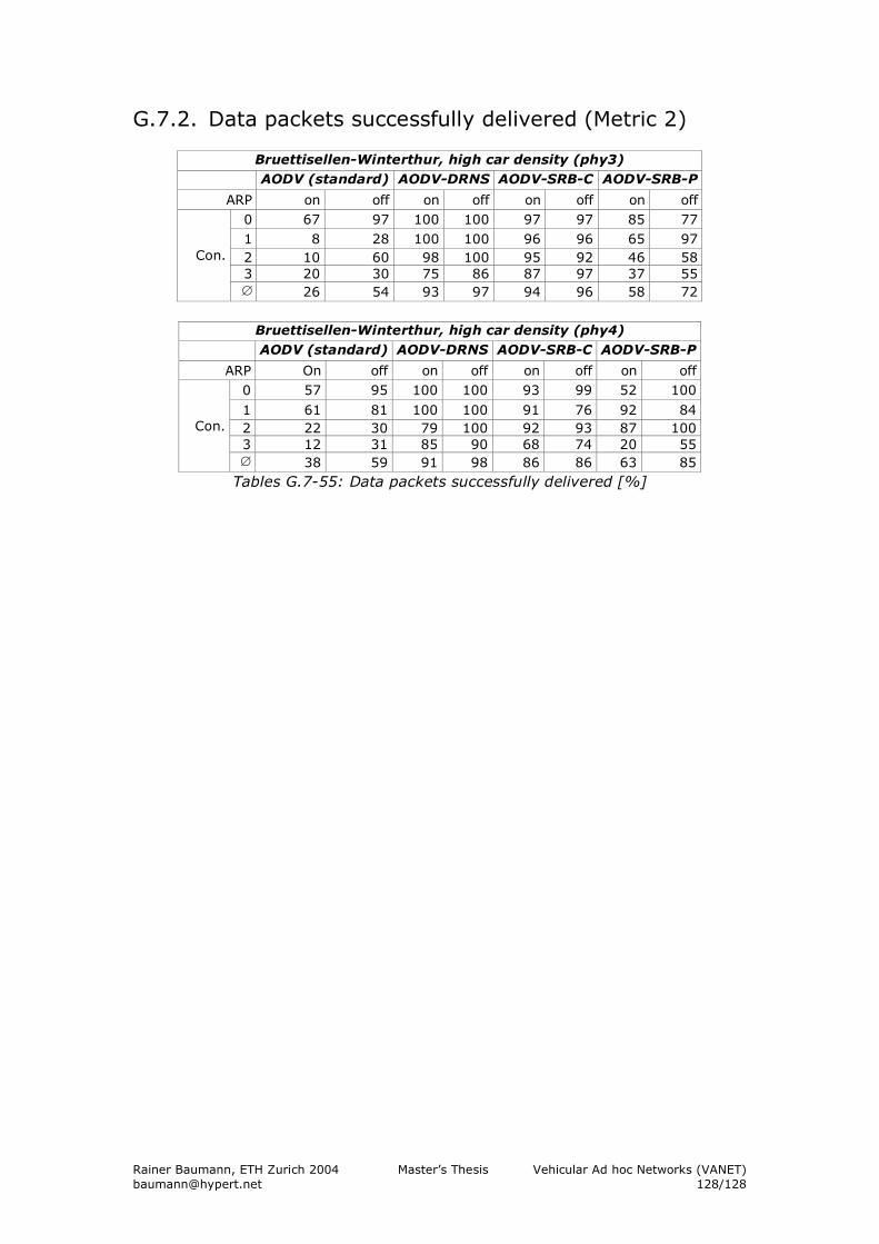
Rainer Baumann, ETH Zurich 2004 Master’s Thesis Vehicular Ad hoc Networks (VANET) [email protected] 128/128
G.7.2. Data packets successfully delivered (Metric 2)
Bruettisellen-Winterthur, high car density (phy3) AODV (standard) AODV-DRNS AODV-SRB-C AODV-SRB-P
ARP on off on off on off on off 0 67 97 100 100 97 97 85 77 1 8 28 100 100 96 96 65 97 2 10 60 98 100 95 92 46 58 3 20 30 75 86 87 97 37 55
Con.
∅ 26 54 93 97 94 96 58 72
Bruettisellen-Winterthur, high car density (phy4) AODV (standard) AODV-DRNS AODV-SRB-C AODV-SRB-P
ARP On off on off on off on off 0 57 95 100 100 93 99 52 100
1 61 81 100 100 91 76 92 84 2 22 30 79 100 92 93 87 100 3 12 31 85 90 68 74 20 55
Con.
∅ 38 59 91 98 86 86 63 85 Tables G.7-55: Data packets successfully delivered [%]