Embed Size (px)
Citation preview
Cell States and Cell Fate: Statistical and Computational Models in (Epi)Genomics
CitationFernandez, Daniel. 2015. Cell States and Cell Fate: Statistical and Computational Models in (Epi)Genomics. Doctoral dissertation, Harvard University, Graduate School of Arts & Sciences.
Permanent linkhttp://nrs.harvard.edu/urn-3:HUL.InstRepos:14226043
Terms of UseThis article was downloaded from Harvard University’s DASH repository, and is made available under the terms and conditions applicable to Other Posted Material, as set forth at http://nrs.harvard.edu/urn-3:HUL.InstRepos:dash.current.terms-of-use#LAA
Share Your StoryThe Harvard community has made this article openly available.Please share how this access benefits you. Submit a story .
Accessibility

Cell States and Cell Fate: Statistical andComputational models in (Epi)Genomics
A dissertation presented
by
Daniel Fernandez
to
The Department of Statistics
in partial fulfillment of the requirements
for the degree of
Doctor of Philosophy
in the subject of
Statistics
Harvard University
Cambridge, Massachusetts
October 2014

c©2014 - Daniel Fernandez
All rights reserved.
Professor Jun S. Liu Daniel Fernandez
Cell States and Cell Fate: Statistical and Computational models
in (Epi)Genomics
Abstract
This dissertation develops and applies several statistical and computational methods to
the analysis of Next Generation Sequencing (NGS) data in order to gain a better under-
standing of our biology. In the first chapter we introduce key concepts in molecular biology,
and recent technological developments that help us better understand this complex science
which, in turn, provide the foundation and motivation for the subsequent chapters.
In the second chapter we present the problem of estimating gene/isoform expression at
the allelic level, and different models to solve this problem. First, we describe the observed
data and the computational workflow to process the data. Next, we propose frequentist and
bayesian models motivated by the central dogma of molecular biology and the data generating
process (DGP) for RNA-Seq. We develop EM and Gibbs sampling approaches to estimate
gene and transcript-specific expression from our proposed models. Finally, we present the
performance of our models in simulations and we end with the analysis of experimental
RNA-Seq data at the allelic level.
In the third chapter we present our paired factorial experimental design to study parentally
biased gene/isoform expression in the mouse cerebellum, and dynamic changes of this pattern
between young and adult stages of cerebellar development. We present a bayesian variable
selection model to estimate the difference in expression between the paternal and maternal
genes, while incorporating relevant factors and its interactions into the model. Next, we
apply our model to our experimental data, and further on we validate our predictions using
iii

pyrosequencing follow-up experiments. We subsequently applied our model to the pyrose-
quencing data across multiple brain regions. Our method, combined with the validation
experiments, allowed us to find novel imprinted genes, and investigate, for the first time,
imprinting dynamics across brain regions and across development.
In the fourth chapter we move from the controlled-experiments in mouse isogenic lines
to the highly variant world of human genetics in observational studies. In this chapter
we introduce a Bayesian Regression Allelic Imbalance Model, BRAIM, that estimates the
imbalance coming from two major sources: cis-regulation and imprinting. We model the
cis-effect as an additive effect for the heterozygous group and we model the parent-of-origin
effect with a latent variable that indicates to which parent a given allele belongs to. Next,
we show the performance of the model under simulation scenarios, and finally we apply the
model to several experiments across multiple tissues and multiple individuals.
In the fifth chapter we characterize the transcriptional regulation and gene expression of
in-vitro Embryonic Stem Cells (ESCs), and two-related in-vivo cells; the Inner Cell Mass
(ICM) tissue, and the embryonic tissue at day 6.5. Our objective is two fold. First we would
like to understand the differences in gene expression between the ESCs and their in-vivo
counterpart from where these cells were derived (ICM). Second, we want to characterize the
active transcriptional regulatory regions using several histone modifications and to connect
such regulatory activity with gene expression. In this chapter we used several statistical and
computational methods to analyze and visualize the data, and it provides a good showcase
of how combining several methods of analysis we can delve into interesting developmental
biology.
iv
Contents
Title Page . . . . . . . . . . . . . . . . . . . . . . . . . . . . . . . . . . . . . . . . iAbstract . . . . . . . . . . . . . . . . . . . . . . . . . . . . . . . . . . . . . . . . . iiiTable of Contents . . . . . . . . . . . . . . . . . . . . . . . . . . . . . . . . . . . . vCitations to Previously Published Work . . . . . . . . . . . . . . . . . . . . . . . viiiAcknowledgments . . . . . . . . . . . . . . . . . . . . . . . . . . . . . . . . . . . . ixDedication . . . . . . . . . . . . . . . . . . . . . . . . . . . . . . . . . . . . . . . . xi
1 Introduction 11.1 The Cell: its components and the central dogma of MB . . . . . . . . . . . . 2
1.1.1 The genome . . . . . . . . . . . . . . . . . . . . . . . . . . . . . . . . 41.1.2 The Transcriptome and the Proteome . . . . . . . . . . . . . . . . . . 51.1.3 Cell regulation via Protein-Binding . . . . . . . . . . . . . . . . . . . 6
1.2 Chromatin Structure and epigenetics . . . . . . . . . . . . . . . . . . . . . . 81.2.1 Chromatin Structure . . . . . . . . . . . . . . . . . . . . . . . . . . . 91.2.2 Cell regulation via Epigenetics . . . . . . . . . . . . . . . . . . . . . . 101.2.3 DNA methylation . . . . . . . . . . . . . . . . . . . . . . . . . . . . . 111.2.4 Histone Modification . . . . . . . . . . . . . . . . . . . . . . . . . . . 11
1.3 Sequencing Technologies and Experimental Protocols . . . . . . . . . . . . . 121.3.1 PyroSequencing . . . . . . . . . . . . . . . . . . . . . . . . . . . . . . 131.3.2 Illumina: Sequencing-by-Synthesis with Reversible Fluorescent Termi-
nators . . . . . . . . . . . . . . . . . . . . . . . . . . . . . . . . . . . 141.3.3 Whole-Genome Sequencing . . . . . . . . . . . . . . . . . . . . . . . . 151.3.4 RNA-Seq . . . . . . . . . . . . . . . . . . . . . . . . . . . . . . . . . 171.3.5 ChIP-Seq . . . . . . . . . . . . . . . . . . . . . . . . . . . . . . . . . 19
2 Allelic Imbalance and Allele-specific expression 212.1 Introduction . . . . . . . . . . . . . . . . . . . . . . . . . . . . . . . . . . . . 22
2.1.1 Biological mechanisms of Allelic Imbalance . . . . . . . . . . . . . . . 232.1.2 Our Estimand of Interest, and the Data . . . . . . . . . . . . . . . . 262.1.3 Normalized Measures of RNA expression . . . . . . . . . . . . . . . . 28
2.2 Computational Workflow . . . . . . . . . . . . . . . . . . . . . . . . . . . . . 302.3 Frequentist Model of Allele-Specific Expression . . . . . . . . . . . . . . . . . 32
v
2.3.1 Maximum Likelihood Estimation . . . . . . . . . . . . . . . . . . . . 332.3.2 Bootstrap approach to obtain Confidence Intervals . . . . . . . . . . 35
2.4 Bayesian Model of Allele-Specific Expression . . . . . . . . . . . . . . . . . . 362.4.1 Gibbs Sampler . . . . . . . . . . . . . . . . . . . . . . . . . . . . . . 38
2.5 Hierarchical Model of Allele-Specific Expression across Multiple Experiments 392.6 Identifiability Issues . . . . . . . . . . . . . . . . . . . . . . . . . . . . . . . . 402.7 Simulation Results: To Count or not to Count? . . . . . . . . . . . . . . . . 422.8 Discussion . . . . . . . . . . . . . . . . . . . . . . . . . . . . . . . . . . . . . 46
3 Design of Experiments in the study of Parental-Specific Expression 493.1 Experimental Design . . . . . . . . . . . . . . . . . . . . . . . . . . . . . . . 523.2 BRAIM: Bayesian Regression Allelic Imbalance Model . . . . . . . . . . . . 55
3.2.1 Gibbs Sampling . . . . . . . . . . . . . . . . . . . . . . . . . . . . . . 593.3 Choice of Prior Parameters . . . . . . . . . . . . . . . . . . . . . . . . . . . . 633.4 Analysis and Results . . . . . . . . . . . . . . . . . . . . . . . . . . . . . . . 64
Independent Validation using PyroSequencing . . . . . . . . . . . . . 68Isoform-Specific Imprinting . . . . . . . . . . . . . . . . . . . . . . . . 70Developmental Regulation of Genomic Imprinting in the Cerebellum . 73Genomic Locations of Imprinted Genes . . . . . . . . . . . . . . . . . 77Spatial Regulation of Genomic Imprinting . . . . . . . . . . . . . . . 80
3.5 Sensitivity Analysis . . . . . . . . . . . . . . . . . . . . . . . . . . . . . . . . 833.5.1 Single Model across all genes, and correlation structure . . . . . . . . 85
3.6 Discussion . . . . . . . . . . . . . . . . . . . . . . . . . . . . . . . . . . . . . 87
4 Allele-Specific Regulation in Human Population across Multiple Tissues 924.1 The GTEx Project Consortium . . . . . . . . . . . . . . . . . . . . . . . . . 924.2 Experimental Design and Computational Workflow . . . . . . . . . . . . . . 934.3 Hi-Braim . . . . . . . . . . . . . . . . . . . . . . . . . . . . . . . . . . . . . . 97
4.3.1 Definining cis and trans eQTL and ASE . . . . . . . . . . . . . . . . 974.3.2 Hi-Braim with No Imprinting . . . . . . . . . . . . . . . . . . . . . . 99
Detecting Imprinting . . . . . . . . . . . . . . . . . . . . . . . . . . . 1034.3.3 Hi-Braim with Imprinting . . . . . . . . . . . . . . . . . . . . . . . . 103
Adaptive MCMC within Gibbs Sampling . . . . . . . . . . . . . . . . 1054.4 Simulations . . . . . . . . . . . . . . . . . . . . . . . . . . . . . . . . . . . . 1094.5 Results . . . . . . . . . . . . . . . . . . . . . . . . . . . . . . . . . . . . . . . 1134.6 Discussion . . . . . . . . . . . . . . . . . . . . . . . . . . . . . . . . . . . . . 116
5 Single and Small Cell Clustering Methods in Developmental Biology 1195.1 Transcriptomic and genomic chromatin structure in early mammalian devel-
opment using small cell experiments . . . . . . . . . . . . . . . . . . . . . . . 1195.1.1 Introduction . . . . . . . . . . . . . . . . . . . . . . . . . . . . . . . . 1195.1.2 Experimental design . . . . . . . . . . . . . . . . . . . . . . . . . . . 1215.1.3 Results . . . . . . . . . . . . . . . . . . . . . . . . . . . . . . . . . . . 123
vi

ChIP-seq data processing - Enhancer regions . . . . . . . . . . . . . . 123Transcriptomic Analysis of a Developmental Trajectory . . . . . . . . 125Differential gene Expression (DE) . . . . . . . . . . . . . . . . . . . . 126Clustering of Enhancer and Promoter Regions . . . . . . . . . . . . . 127
5.1.4 Discussion . . . . . . . . . . . . . . . . . . . . . . . . . . . . . . . . . 1285.2 Finding Heterogeneous population in Single-cell Experiments . . . . . . . . . 130
5.2.1 Introduction . . . . . . . . . . . . . . . . . . . . . . . . . . . . . . . . 130Limitations of simple clustering algorithms . . . . . . . . . . . . . . . 131
5.2.2 BASIC algorithm . . . . . . . . . . . . . . . . . . . . . . . . . . . . . 132Statistical model . . . . . . . . . . . . . . . . . . . . . . . . . . . . . 132Gibbs sampling algorithm . . . . . . . . . . . . . . . . . . . . . . . . 137
5.2.3 Selecting the number of groups K . . . . . . . . . . . . . . . . . . . . 144Approximating marginal likelihood functions . . . . . . . . . . . . . . 144Selecting K with marginal likelihoods . . . . . . . . . . . . . . . . . . 147
5.2.4 Simulation studies . . . . . . . . . . . . . . . . . . . . . . . . . . . . 1495.2.5 Application on real hematopoietic stem cell data . . . . . . . . . . . . 168
A ASE Models 171
B Mathematical Derivations 172
C Examples of MCMC chains for BRAIM model 173
D MCMC chains for Hi-BRAIM 191D.1 Simulations . . . . . . . . . . . . . . . . . . . . . . . . . . . . . . . . . . . . 191
Bibliography 191
vii

Citations to Previously Published Work
Chapter 2, chapter 3 and chapter 5 are based on the following (in preparation) papers
(they can also be found at the website http://www.dnaiel.com).
Julio D. Perez, Nimrod D. Rubinstein, Daniel Fernandez, Stephen W. Santoro,Leigh A. Needleman, John J Choi, Mariela Zirlinger, Jun S. Liu and Cather-ine Dulac. Dynamic Regulation and Functional significance of Parent-of-OriginAllelic Expression in the Adult and Developing Brain. Submitted. (2014)
Fernandez, D., Rubinstein, N., Jun Li, M., Perez J., Dulac C. and Liu, JS. Allele-specific Expression across Multiple Tissues in human studies. In preparation.(2014)
Goren A., Xing J., Dixit A., Fernandez D., Velenich A., Durham T., Liu, JS.,Regev, A. and Bernstein BE. Faithfulness of stem cell models: comparative anal-ysis of transcriptome and genomic chromatin structure in early mammalian de-velopment. In preparation. (2014)
Chapter 2 and 3 is based on collaborative work with Professor Catherine Dulac, and her
lab members Nimrod Rubinstein and Julio Perez. Chapter 4 is based on collaborative work
with Professor Catherine Dulac, Nimrod Rubinstein, Jiexing Wu, and Jun Li. Chapter 5
is based on collaborative work with Professor Aviv Regev and Bradley Bernstein labs, and
their lab members Alon Goren, Atray Dixit and Yang Li (member of Jun Liu lab).
viii

Acknowledgments
I want to start by thanking my advisor, professor Jun Liu. I am extremely honored,
grateful and lucky for the opportunity to work and learn from him. His Bayesian eye and
his Monte Carlo ’moves’ very much resemble the one of an eagle: sharp, fast, accurate and
precise. He showed me how to do research by setting up an example of integrity, and high
standards of research himself, and by questioning my ideas, assumptions and models with
an inquisitive mind.
I also wanted to thank my statistical committee members professors Joseph Blitzstein
and Tirthnakar Dasgupta. I thank Professor Joseph Blitzstein for teaching me 210, 211 and
many other statistical ideas, for writing amazing posts in Quora (I am his follower there), and
for showing me how complex ideas can be translated into beautiful, not necesarily simple,
but rather simpler, levels of abstraction. I thank Tirthankar for his patience and great
support throughout my PhD., for teaching me about experimental design, and for being a
great contributor to my research.
I also want to thank our scientific collaborators in biology and my biological comittee
member, Professor Catherine Dulac and her lab members Julio Perez and Nimrod Rubinstein
for their constant support, helpful discussions and hard work in validating the results, and
understanding the relevance of the findings.
Moreover, I am forever indebt with my first biological and medical collaborator Dr.
Bradley Bernstein and his lab members Atray Dixit, Alon Goren, Birgit Knoechel and Ryan
Russell. In their lab I first saw a sequencing machine and ’bench’ work; and their ambition,
and ability to look at a scientific problem from many different angles will always resonate
with me.
But the life of a PhD. is a rich one, and teaching what we have learnt is a core part of
our statistics department. I would also like to thank the CompBio course team, professors
ix

Jun Liu and Shirley Liu, and TFs Alejandro and Lin, from whom I learned how to combine
ideas from statistics, computer science and biology, I was extremely lucky to TF for them,
and learn from them.
Also, I wanted to thank all members of Jun’s lab, we had great moments together, smart
discussions, and always helped one another. I want to especially thank Ke Deng, Ming
Hu, Jun Li, Yang Li and Jiexing Wu. But I was also part of a bigger community, the
statistics department at Harvard and I thank all members of the department. I especially
thank my classmates Valeria Espinoza, Simeng Han, Jonathan Hennessy, Bo Jiang, Joseph
Kelly, Nathan Stein, Xiao Tong, Samuel Wong and Xiaojin Xu; and our own department
administrator Betsey Cogswell and the staff members Steven Finch, Jimmy Matejek, Alice
Moses, Dale Rinkel, Maureen Stanton.
Lastly, but not least, thanks to my family: my noble wife Jane, my parents Arturo and
Magdalena, my brothers Arturo and Juan Cristobal and my sister Magdalena, my in laws
Pedro, Cata and Maca, my godsons R2D2 and Pedrito, and all my nephews and nieces.
Also thanks to my in-laws, Dr. and Ms. Hong, my little sister-in-law Anne Hong and my
brother-in-law el Jefe. I am glad to have a big and loving family, that very much cares for
me, and is there for me unconditionally.
x

To my joyful and caring Jane, who inspires me everyday, and brings me the joy
and peace needed to focus on my research.
xi

Chapter 1
Introduction
A technological advance of a major sort almost always is overestimated in the
short run for its consequences - and underestimated in the long run.
- Francis Collins
The ability to read the whole DNA (whole genome) and to accurately measure the molec-
ular state of a cell(s)1 is now possible due to major technological achievements over the past
few decades, beginning with early Sanger sequencing in the 70s, Sanger and Coulson (1975)
and Sanger et al. (1977) to the Next Generation Sequencing Technologies (NGS) of today,
Metzker (2009) and Koboldt et al. (2013). These technologies, in turn, have allowed us to
read the entire human genome (HGP, the International Human Genome Sequencing Con-
sortium (2001) and Venter et al. (2001)). The HGP opened a pandora’s box of possibilities
to the study of our biology, and to the study of disease. Now, sequencing technologies can
be used to study the proteome, the transcriptome (RNA-Seq), transcriptional regulation
1Note that in this thesis we interchangeably refer to a cell as a single cell, or as a population of cells (be-lieved to be in a similar condition/state or coming from the same tissue). Note that most of our experimentswere done in tissues containing on the order of thousands to million of cells, but the methods could be easilyapplied to single-cell experiments.
1
via protein binding (ChIP-Seq), the epigenetic landscape (ChIP-Seq, DNAse-Seq, WGBS,
Chia-Pet, DNAase-Seq, DamID-Seq), and the chromatin structure of a cell (Hi-C), among
several other molecular measures of a cell’s activity (or current state).
This gives us a much more comprehensive understanding of cell and molecular biology,
allowing us to tackle a variety of questions starting from fundamental biology such as the
basis of epigenetic inheritance, the study of cell identity, cell differentiation, embryonic and
stem cell development, to the importance of genetics and epigenetics in maintaining the
proper state of cells.
In this thesis we present several statistical and computational models that help us under-
stand and properly analyze genomics and epigenomics data, and thus the title of the thesis:
Cell States and Cell Fate: Statistical and Computational models in (Epi)Genomics. How-
ever, before describing the models we present a brief introduction of molecular biology and
the sequencing technologies used throughout this thesis. This serves a two fold objective;
on one hand, it helps the reader to better understand the concepts and the motivation for
our research, making this thesis more or less self-contained, and on the other hand, it helps
motivate the statistical models that are presented. Much like the words of George Box, ”all
models are wrong, but some are useful,” I would further fine tune them to say that ”models
that do not take the data generating process into consideration are most likely not useful.”
2
1.1 The Cell: its components and the central dogma
of MB
A eukaryotic cell is an extremely complex and dynamic system, with millions of molecules
interacting with each other in order to maintain its function and state2.
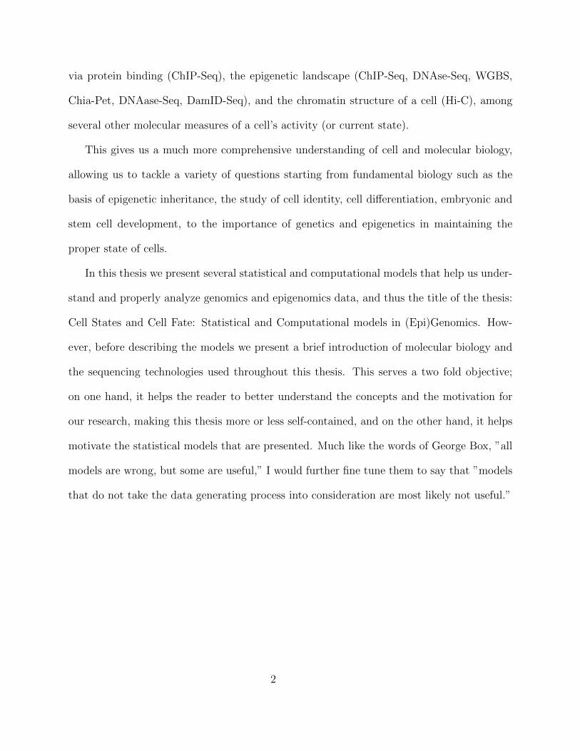
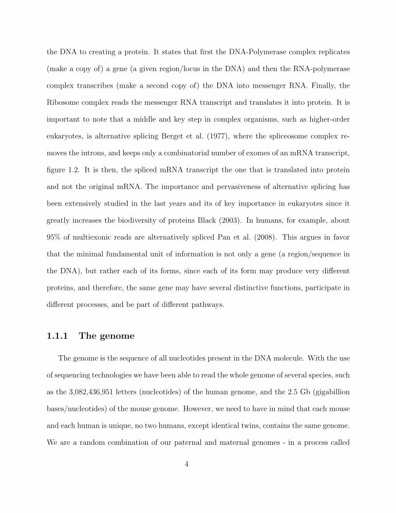
Nonetheless, part of this complexity can be explained through the central dogma of
molecular biology, and its key actors: the DNA, the chromosome, the chromatin, the RNA,
the RNA-polymerase, the proteins, and the Ribosome. The central dogma states that the
information on how to make a protein is codified inside the DNA, and it flows from DNA to
RNA to protein.
Figure 1.1: The central dogma of molecular biology.
The DNA can be viewed as the information required for a cell to live, divide, differen-
tiate, and maintain its state and function. The fundamental dogma of MB explains how
such information is read, copied, and translated into molecular machinery called proteins.
In broad terms the central dogma describes, in great detail, all the steps to go from reading
2By function we mean the physiological function the cell has in the organism, i.e., hemoglobin is a cellwhich major purpose is to carry oxygen. By cell state we mean the physiological condition of the cell at agiven time.
3
the DNA to creating a protein. It states that first the DNA-Polymerase complex replicates
(make a copy of) a gene (a given region/locus in the DNA) and then the RNA-polymerase
complex transcribes (make a second copy of) the DNA into messenger RNA. Finally, the
Ribosome complex reads the messenger RNA transcript and translates it into protein. It is
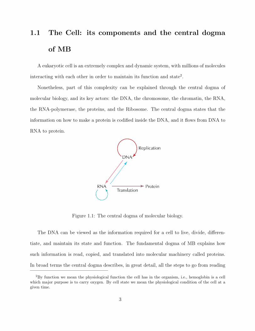
important to note that a middle and key step in complex organisms, such as higher-order
eukaryotes, is alternative splicing Berget et al. (1977), where the spliceosome complex re-
moves the introns, and keeps only a combinatorial number of exomes of an mRNA transcript,
figure 1.2. It is then, the spliced mRNA transcript the one that is translated into protein
and not the original mRNA. The importance and pervasiveness of alternative splicing has
been extensively studied in the last years and its of key importance in eukaryotes since it
greatly increases the biodiversity of proteins Black (2003). In humans, for example, about
95% of multiexonic reads are alternatively spliced Pan et al. (2008). This argues in favor
that the minimal fundamental unit of information is not only a gene (a region/sequence in
the DNA), but rather each of its forms, since each of its form may produce very different
proteins, and therefore, the same gene may have several distinctive functions, participate in
different processes, and be part of different pathways.
1.1.1 The genome
The genome is the sequence of all nucleotides present in the DNA molecule. With the use
of sequencing technologies we have been able to read the whole genome of several species, such
as the 3,082,436,951 letters (nucleotides) of the human genome, and the 2.5 Gb (gigabillion
bases/nucleotides) of the mouse genome. However, we need to have in mind that each mouse
and each human is unique, no two humans, except identical twins, contains the same genome.
We are a random combination of our paternal and maternal genomes - in a process called
4
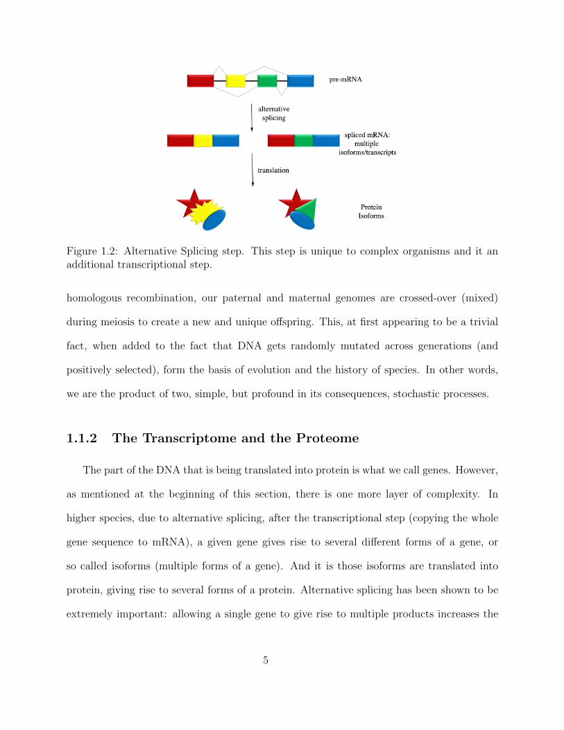
Figure 1.2: Alternative Splicing step. This step is unique to complex organisms and it anadditional transcriptional step.
homologous recombination, our paternal and maternal genomes are crossed-over (mixed)
during meiosis to create a new and unique offspring. This, at first appearing to be a trivial
fact, when added to the fact that DNA gets randomly mutated across generations (and
positively selected), form the basis of evolution and the history of species. In other words,
we are the product of two, simple, but profound in its consequences, stochastic processes.
1.1.2 The Transcriptome and the Proteome
The part of the DNA that is being translated into protein is what we call genes. However,
as mentioned at the beginning of this section, there is one more layer of complexity. In
higher species, due to alternative splicing, after the transcriptional step (copying the whole
gene sequence to mRNA), a given gene gives rise to several different forms of a gene, or
so called isoforms (multiple forms of a gene). And it is those isoforms are translated into
protein, giving rise to several forms of a protein. Alternative splicing has been shown to be
extremely important: allowing a single gene to give rise to multiple products increases the
5
diversity of proteins allowed by our more or less 20,000 genes, and in turn allowing us to
differentiate from other species for which we share great part of our genome.
As proteins form the basis of cell regulation and cell function, we are mostly interested
in estimating protein abundance but current technologies are more suitable for estimating
isoform/transcript abundances. This is how two genomic concepts came to existence: the
transcriptome and the proteome. The transcriptome is the set of all transcripts inside a cell,
and the proteome is the set of all proteins inside a cell. The degree to which the transcriptome
is a proxy for the proteome is still a matter of debate but proteome technologies still have a
long road before we can accurately measure all the proteins inside a eukaryotic cell.
1.1.3 Cell regulation via Protein-Binding
We have explained the process by which proteins are synthesized, but all cells carry the
same genomic information, and all cells from our body come from a single cell, the zygote.
Thus, Why cells with the exact same DNA can be of very different type, exhibiting completely
different morphology, state and function? We have more than 200 different cells-types in
our body, and certainly no one would argue that a neuron looks and acts extremely different
from a blood cell, but what biological mechanism allows the existence and maintenance of
such differences between cell types?
This can be partially understood through gene regulation, i.e., the rate at which different
genes are being expressed in a given cell. In other words, through gene regulation a cell can
control its state and function by ’expressing’ (being translated into protein) different genes,
with in turn perform different function, at different time and space.
A well-known mechanism for gene regulation is the interaction between protein and DNA,
by which a protein/enzyme binds to the DNA in order to control the expression level of a
6
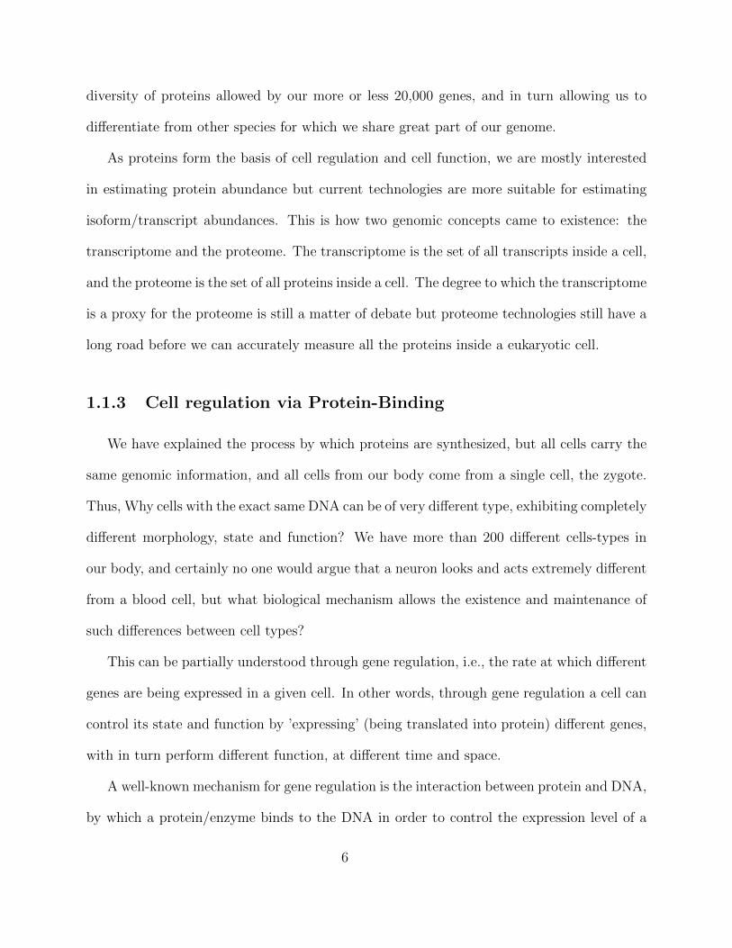
gene or a set of genes. Base on the role of such proteins they have been named: specificity
factors, repressors, general transcription factors, activators and silencers, figure 1.3.
Figure 1.3: Diagram of classes of transcription factors and their activity.
Specificity factors alter the specificity of RNA polymerase for a given promoter or set
of promoters, making it more or less likely to bind to them (i.e. sigma factors used in
prokaryotic transcription). Repressors bind to non-coding sequences on the DNA strand that
are close to or overlapping the promoter region, impeding RNA polymerase’s progress along
the strand, thus impeding the expression of the gene. General transcription factors position
RNA polymerase at the start of a protein-coding sequence and then release the polymerase
to transcribe the mRNA. Activators enhance the interaction between RNA polymerase and a
particular promoter, encouraging the expression of the gene. Activators do this by increasing
the attraction of RNA polymerase for the promoter, through interactions with subunits of
the RNA polymerase or indirectly by changing the structure of the DNA. Enhancers are
sites on the DNA helix that are bound to by activators in order to loop the DNA bringing
7
a specific promoter to the initiation complex. Silencers are regions of DNA that are bound
by transcription factors in order to silence gene expression. The mechanism is very similar
to that of enhancers.
Although transcription factors play a major role in gene regulation, one could imagine
that there must be an inheritable mechanism that activates/repress different transcription
factors in different cells; and that stably maintains different regulatory networks across
different cell types. Such mechanism is called epigenetics. In order to better understand
epigenetics we first introduce the chromatin and chromosome structure, and then explain
how the epigenome is believed to play a major role in gene regulation and ultimately, cell
differentiation, cell identity and cell function.
1.2 Chromatin Structure and epigenetics
Each living eukaryotic cell needs to solve an extremely hard problem: how to fit an
approximately 1.5 meters long molecule (DNA) into a 1 nano meter cell nucleus. The DNA
is only part of the story. The whole DNA molecule is contained within a larger superstructure.
This superstructure was firstly discovered by Walther Flemming in 1879 by using staining
techniques and the microscope to observe the contents inside the nucleus of a cell. He
would stain the ”fibrous network” inside the nucleus, which he termed chromatin, ”stainable
material” (from the greek word chroma, meaning color).
Later on it was discovered that the hard task of packaging DNA is accomplished by
specialized proteins that bind to and fold the DNA, generating a series of coils and loops
that provide increasingly higher levels of organization, preventing the DNA from becoming
an unmanageable tangle. Thus, chromatin can be described as the complex of DNA and
8
protein that make up the contents of the nucleus of a cell. Amazingly, although the DNA is
very tightly folded, it is compacted in a way that allows it to easily become available to the
many proteins in the cell that replicate it, repair it, and use its genes to produce proteins.
Nowadays it is well accepted the high importance of chromatin in packaging the DNA
inside the nucleus in a way that is dynamic and accessible to other proteins. Furthermore
chromatin plays a major role in strengthening the DNA to allow mitosis, and to prevent DNA
damage, and ultimately, it is believed to be central in gene regulation and in maintaining
the state and function of a given cell.
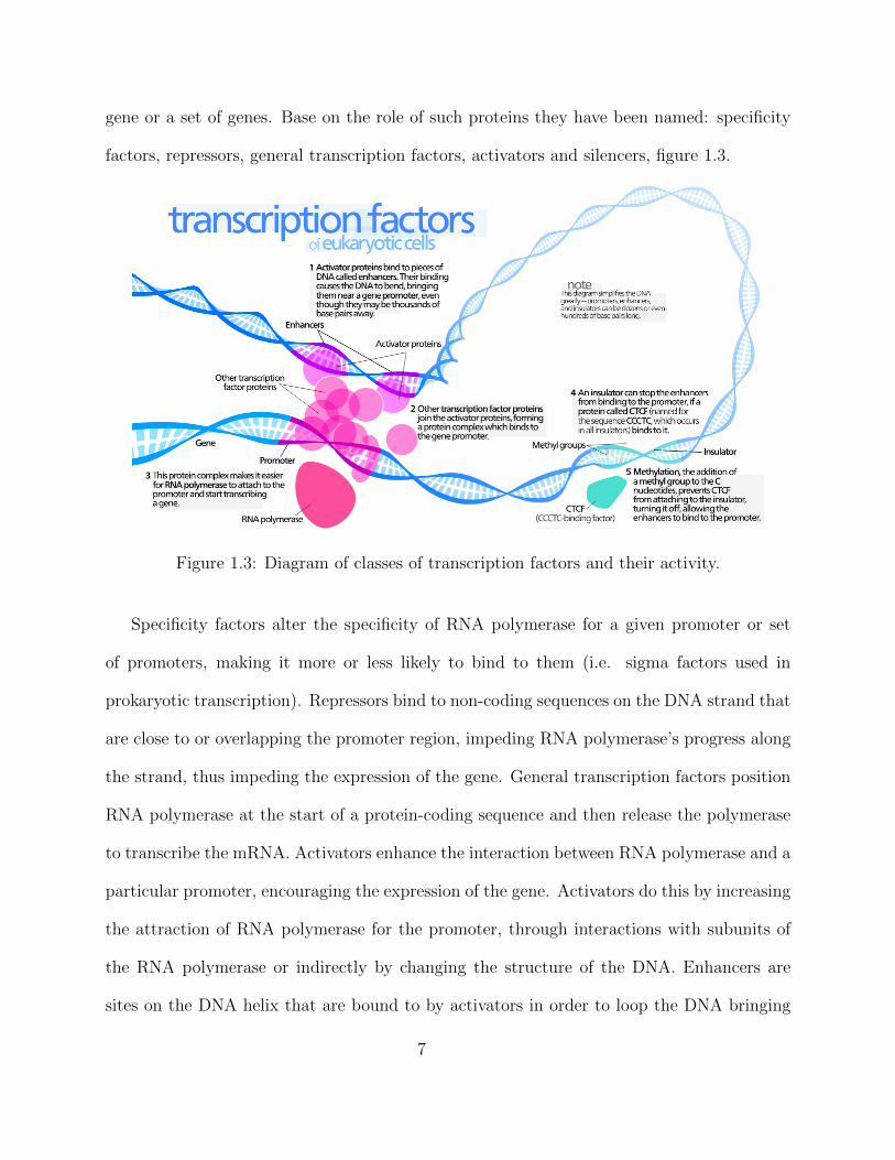
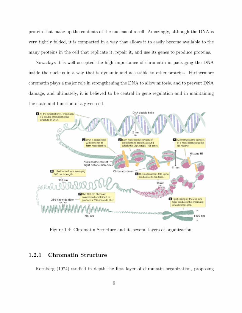
Figure 1.4: Chromatin Structure and its several layers of organization.
1.2.1 Chromatin Structure
Kornberg (1974) studied in depth the first layer of chromatin organization, proposing
9
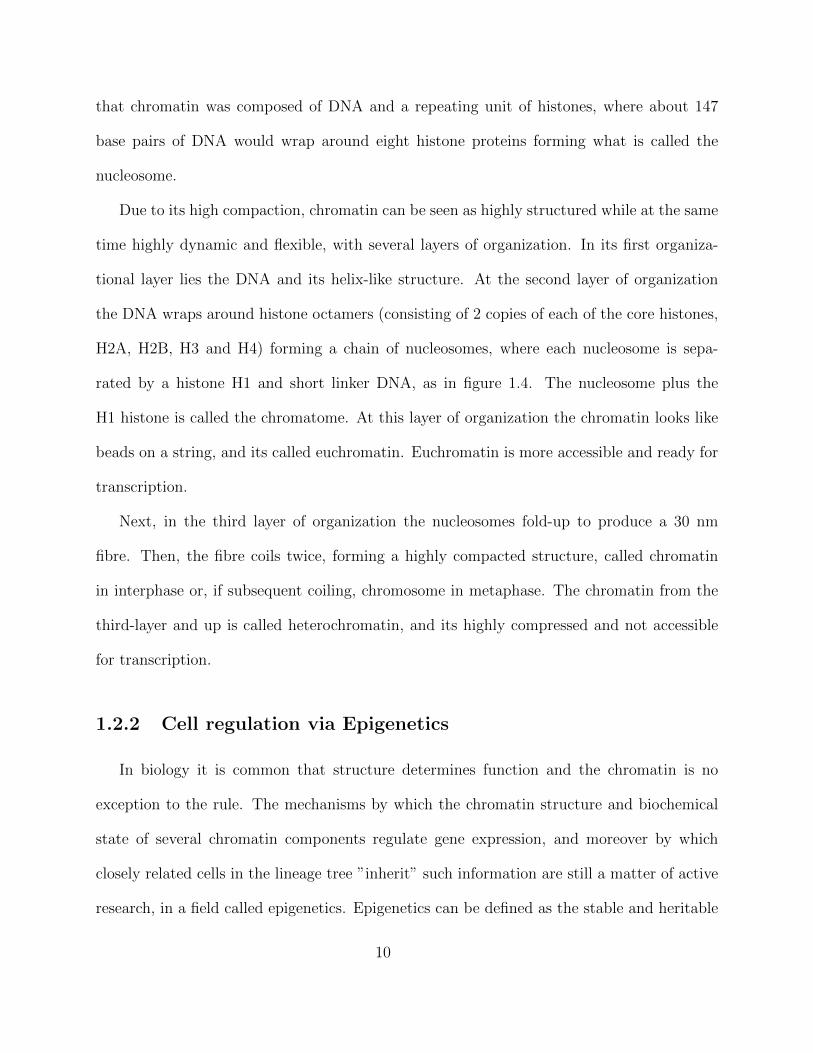
that chromatin was composed of DNA and a repeating unit of histones, where about 147
base pairs of DNA would wrap around eight histone proteins forming what is called the
nucleosome.
Due to its high compaction, chromatin can be seen as highly structured while at the same
time highly dynamic and flexible, with several layers of organization. In its first organiza-
tional layer lies the DNA and its helix-like structure. At the second layer of organization
the DNA wraps around histone octamers (consisting of 2 copies of each of the core histones,
H2A, H2B, H3 and H4) forming a chain of nucleosomes, where each nucleosome is sepa-
rated by a histone H1 and short linker DNA, as in figure 1.4. The nucleosome plus the
H1 histone is called the chromatome. At this layer of organization the chromatin looks like
beads on a string, and its called euchromatin. Euchromatin is more accessible and ready for
transcription.
Next, in the third layer of organization the nucleosomes fold-up to produce a 30 nm
fibre. Then, the fibre coils twice, forming a highly compacted structure, called chromatin
in interphase or, if subsequent coiling, chromosome in metaphase. The chromatin from the
third-layer and up is called heterochromatin, and its highly compressed and not accessible
for transcription.
1.2.2 Cell regulation via Epigenetics
In biology it is common that structure determines function and the chromatin is no
exception to the rule. The mechanisms by which the chromatin structure and biochemical
state of several chromatin components regulate gene expression, and moreover by which
closely related cells in the lineage tree ”inherit” such information are still a matter of active
research, in a field called epigenetics. Epigenetics can be defined as the stable and heritable
10
information that is distinct from DNA sequences and fostered by specialized mechanisms.
These mechanisms include DNA methylation, small interfering RNAs, histone variants,
histone post-translational modifications (PTMs). To date, however, only DNA methylation
has been shown to be stably inherited between cell divisions. Although some histone PTMs
are expected to contribute to the transmission of epigenetic information, others participate
in the process of transcription - the so-called active marks - and others are likely to be
restricted to structural functions.
1.2.3 DNA methylation
DNA methylation is the biochemical process by which a methyl group is added to the
cytosine or adenine DNA nucleotides. In multicellular eukaryotes, DNA methylation seems
to be confined to cytosine bases and is associated with a repressed chromatin state and
inhibition of gene expression. In adult somatic cells, DNA methylation typically occurs in a
CpG dinucleotide context; non-CpG methylation is prevalent in embryonic stem cells, and
has also been indicated in neural development.
DNA methylation is essential for viability in mice, because targeted disruption of the
DNA methyltransferase enzymes results in lethality. There are two general mechanisms by
which DNA methylation inhibits gene expression: first, modification of cytosine bases can
inhibit the association of some DNA binding factors with their cognate DNA recognition
sequences; and second, proteins that recognize methyl-CpG can elicit the repressive potential
of methylated DNA. Methyl-CpG-binding proteins (MBPs) use transcriptional co repressor
molecules to silence transcription and to modify surrounding chromatin, providing a link
between DNA methylation and chromatin remodelling and modification.
11
1.2.4 Histone Modification
Another type of epigenetic mechanism for gene regulation are the biochemical modifica-
tions of the histone tails. Histones undergo posttranslational modifications that alter their
interaction with DNA and nuclear proteins. The H3 and H4 histones have long tails protrud-
ing from the nucleosome, which can be covalently modified at several places. Modifications
of the tail include methylation, acetylation, phosphorylation, ubiquitination, SUMOylation,
citrullination, and ADP-ribosylation. The core of the histones H2A, H2B, and H3 can also be
modified. Combinations of modifications are thought to constitute a code, the so-called ”his-
tone code”. Histone modifications act in diverse biological processes such as gene regulation,
DNA repair, chromosome condensation (mitosis) and spermatogenesis (meiosis).
In summary, the epigenome plays a major role in gene regulation and how cells differ-
entiate and maintain their identity across the lineage tree. It is analogous to the hardware
and the software in computer systems, where the genome is the same for all the cells, but
the epigenome changes from cell to cell in order to control what the hardware is doing.
1.3 Sequencing Technologies and Experimental Proto-
cols
Sequencing technologies could be loosely define as the set of technologies that allow us
to read, at a single nucleotide level, the information contained in DNA molecules. However,
in order to achieve such goal several human and automated machine steps must be done.
Thus, sequencing technologies include a number of methods that are grouped broadly as
template preparation, sequencing and imaging. The unique combination of specific protocols
12
distinguishes one technology from another and determines the type of data produced from
each platform. Currently the major platforms available include Life Sciences Technology
(Roche), Applied Biosystems SOLiD, Illumina, Pacific Biosciences, IonTorrent among several
others. In the recent years Illumina has become one of the most widely used sequencing
technologies, and in this thesis we mainly use sequencing data generated from the Illumina
sequencing platform, in combination with specific experimental protocols depending on the
question of interest.
It is worth mentioning that we do not have any preference in terms of sequencing tech-
nologies, and each technology has its limitations and advantages. Illumina for example has
to go under several PCR amplifications steps but it has a lower per-base error rate than
PacBio. On the other hand, PacBio can sequence at the single molecule level with no need
for amplification steps but it has a higher per-base error rate than illumina. We believe that
the appropriate choice of technology should be an integral part of the experimental design;
and therefore understanding the limitations of each technology is very important.
1.3.1 PyroSequencing
Pyrosequencing is based on iteratively complementing single strands and simultaneously
reading out the signal emitted from the nucleotide being incorporated (also called sequencing
by synthesis, sequencing during extension). Electrophoresis is therefore no longer required to
generate an ordered read out of the nucleotides, as the read out is now done simultaneously
with the sequence extension.
In the pyrosequencing process, one nucleotide at a time is washed over several copies of
the sequence to be determined, causing polymerases to incorporate the nucleotide if it is com-
plementary to the template strand. The incorporation stops if the longest possible stretch
13
of complementary nucleotides has been synthesized by the polymerase. In the process of in-
corporation, one pyrophosphate per nucleotide is released and converted to ATP by an ATP
sulfurylase. The ATP drives the light reaction of luciferases present and the emitted light
signal is measured. To prevent the dATP provided for sequencing reaction from being used
directly in the light reaction, deoxy-adenosine-50-(a-thio)- triphosphate (dATPaS), which
is not a substrate of the luciferase, is used for the base incorporation reaction. Standard
deoxyribose nucleotides are used for all other nucleotides. After capturing the light inten-
sity, the remaining unincorporated nucleotides are washed away and the next nucleotide is
provided.
In our thesis we used pyrosequencing methods for validation, but Roche 454 life sciences
uses pyrosequencing methods for high-throughput sequencing.
1.3.2 Illumina: Sequencing-by-Synthesis with Reversible Fluores-
cent Terminators
Here we present an overview of the Illumina sequencing technology and the steps neces-
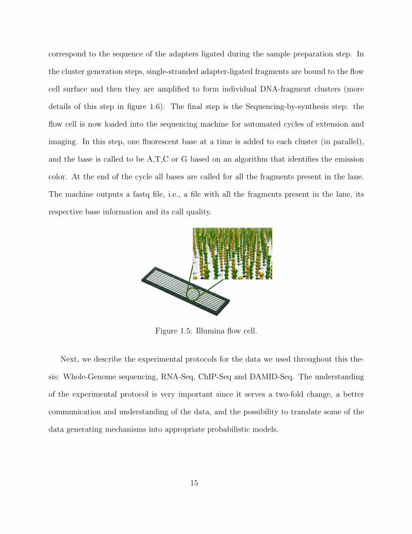
sary to sequence millions of DNA molecules per run, ECO (2007). The first step is to pre-
pare the sample to be sequenced, this varies depending on the experimental protocol (whole
genome sequencing, ChIP-Seq, etc.) but it almost always end with a so-called library, i.e.,
a large number of 200-500 bp double-stranded DNA molecule fragments. Then, illumina-
specific adapters are ligated to the end of each of the fragments and the fragments are isolated
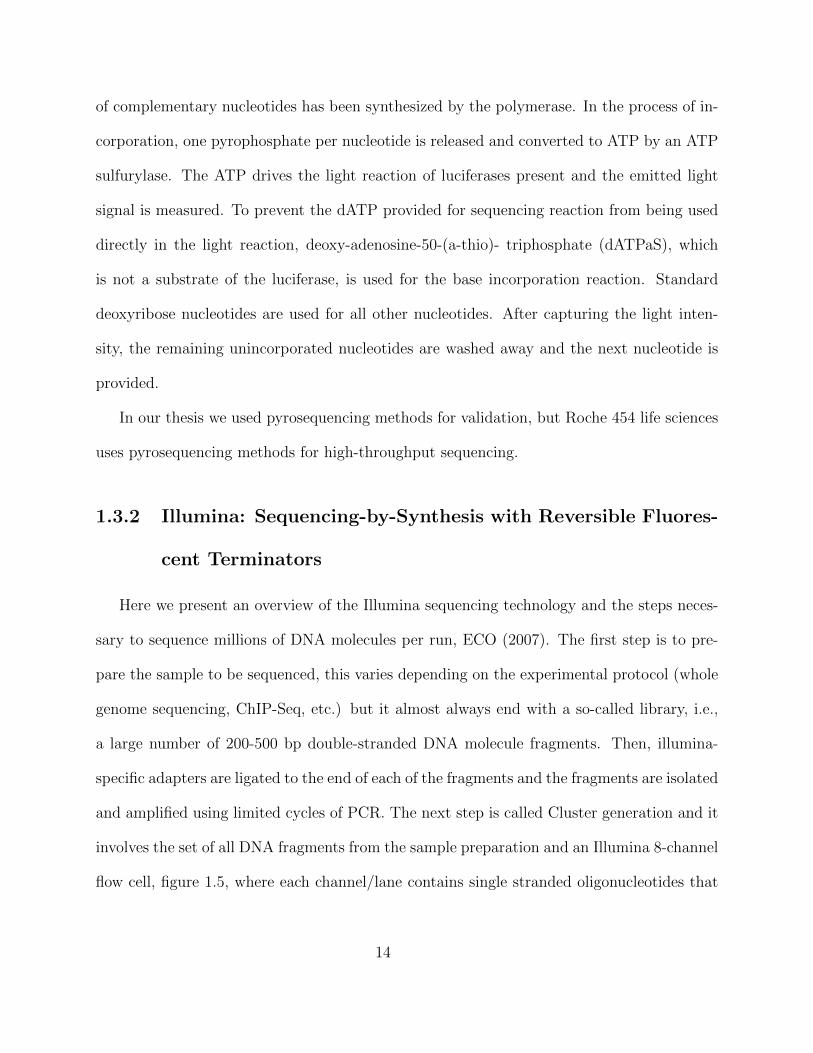
and amplified using limited cycles of PCR. The next step is called Cluster generation and it
involves the set of all DNA fragments from the sample preparation and an Illumina 8-channel
flow cell, figure 1.5, where each channel/lane contains single stranded oligonucleotides that
14
correspond to the sequence of the adapters ligated during the sample preparation step. In
the cluster generation steps, single-stranded adapter-ligated fragments are bound to the flow
cell surface and then they are amplified to form individual DNA-fragment clusters (more
details of this step in figure 1.6). The final step is the Sequencing-by-synthesis step: the
flow cell is now loaded into the sequencing machine for automated cycles of extension and
imaging. In this step, one fluorescent base at a time is added to each cluster (in parallel),
and the base is called to be A,T,C or G based on an algorithm that identifies the emission
color. At the end of the cycle all bases are called for all the fragments present in the lane.
The machine outputs a fastq file, i.e., a file with all the fragments present in the lane, its
respective base information and its call quality.
Figure 1.5: Illumina flow cell.
Next, we describe the experimental protocols for the data we used throughout this the-
sis: Whole-Genome sequencing, RNA-Seq, ChIP-Seq and DAMID-Seq. The understanding
of the experimental protocol is very important since it serves a two-fold change, a better
communication and understanding of the data, and the possibility to translate some of the
data generating mechanisms into appropriate probabilistic models.
15
Figure 1.6: Illumina Workflow.
1.3.3 Whole-Genome Sequencing
The human genome project was a Whole Genome Sequencing project. The whole DNA
information contained in a mix of individuals DNA was sequenced, and transformed into a
large string of A, T, C and Gs, separated by chromosome. This information is now publicly
available for everyone online in UCSD Genome Browser and many other sites. However,
the human genome project was not the only genome to be sequenced, many more species
were sequenced. As of today more than 200 species have been sequenced and there are still
16
ongoing major sequencing projects, such as the Metagenome project, Cancer Genome Atlas,
Personal Genomes, and 1KGP.
It is worth mentioning that although most whole genome sequencing projects use similar
technologies the objective may vary, for example in the early days of sequence the main
objective was to assemble several species (among them humans), genomes. This is a hard
computational problem and requires the use of several sequencing technologies in addition
with efficient dynamic programming alignment algorithms - analogous to completing a jigsaw
puzzle. Many computational and statistical developments came from this area in the early
90s and early 2000s. Now that we have most reference sequences, projects like the TCGA
project relies on the human genome sequence information to characterize non-heritable ge-
nomic variations in cancer samples. On the other hand, the metagenome project aims is
to create a reference set of genomes of all the microorganisms living in certain environment
(Gut, liver, etc.).
The technology to sequence whole genomes used today is also based on Illumina sequenc-
ing technologies, a whole DNA is sheared into fragments and a library is prepared for it to be
the input to sequencing machines, such as the Illumina Machine described in section 1.3.2.
1.3.4 RNA-Seq
RNA-Seq is an experimental protocol based on sequencing technologies that allows us
to estimate the abundance of all the RNA transcripts in a cell. It has quickly become
the standard protocol for quantifying gene expression, largely replacing microarray-based
experiments. This is due to a variety of reasons but, to us, the most compelling is the
analysis flexibility that RNA-Seq based experiments provide. With RNA-Seq experiment
the application of NGS data expanded considerably to studies of transcriptome assembly,
17
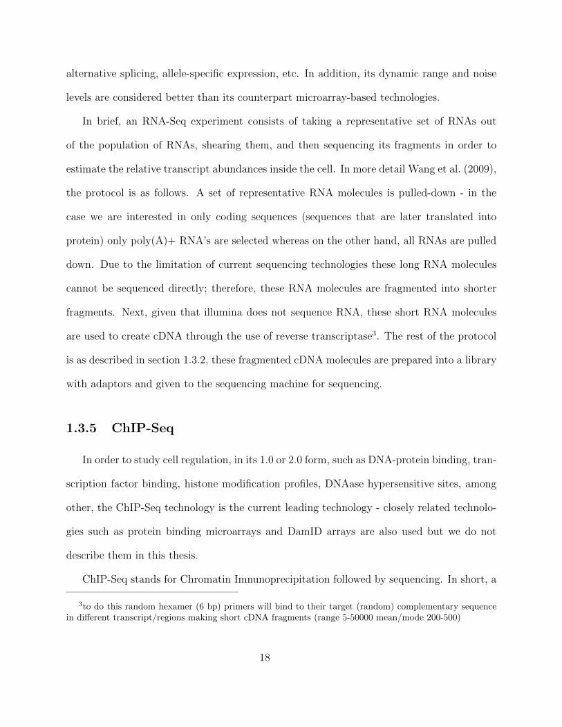
alternative splicing, allele-specific expression, etc. In addition, its dynamic range and noise
levels are considered better than its counterpart microarray-based technologies.
In brief, an RNA-Seq experiment consists of taking a representative set of RNAs out
of the population of RNAs, shearing them, and then sequencing its fragments in order to
estimate the relative transcript abundances inside the cell. In more detail Wang et al. (2009),
the protocol is as follows. A set of representative RNA molecules is pulled-down - in the
case we are interested in only coding sequences (sequences that are later translated into
protein) only poly(A)+ RNA’s are selected whereas on the other hand, all RNAs are pulled
down. Due to the limitation of current sequencing technologies these long RNA molecules
cannot be sequenced directly; therefore, these RNA molecules are fragmented into shorter
fragments. Next, given that illumina does not sequence RNA, these short RNA molecules
are used to create cDNA through the use of reverse transcriptase3. The rest of the protocol
is as described in section 1.3.2, these fragmented cDNA molecules are prepared into a library
with adaptors and given to the sequencing machine for sequencing.
1.3.5 ChIP-Seq
In order to study cell regulation, in its 1.0 or 2.0 form, such as DNA-protein binding, tran-
scription factor binding, histone modification profiles, DNAase hypersensitive sites, among
other, the ChIP-Seq technology is the current leading technology - closely related technolo-
gies such as protein binding microarrays and DamID arrays are also used but we do not
describe them in this thesis.
ChIP-Seq stands for Chromatin Imnunoprecipitation followed by sequencing. In short, a
3to do this random hexamer (6 bp) primers will bind to their target (random) complementary sequencein different transcript/regions making short cDNA fragments (range 5-50000 mean/mode 200-500)
18
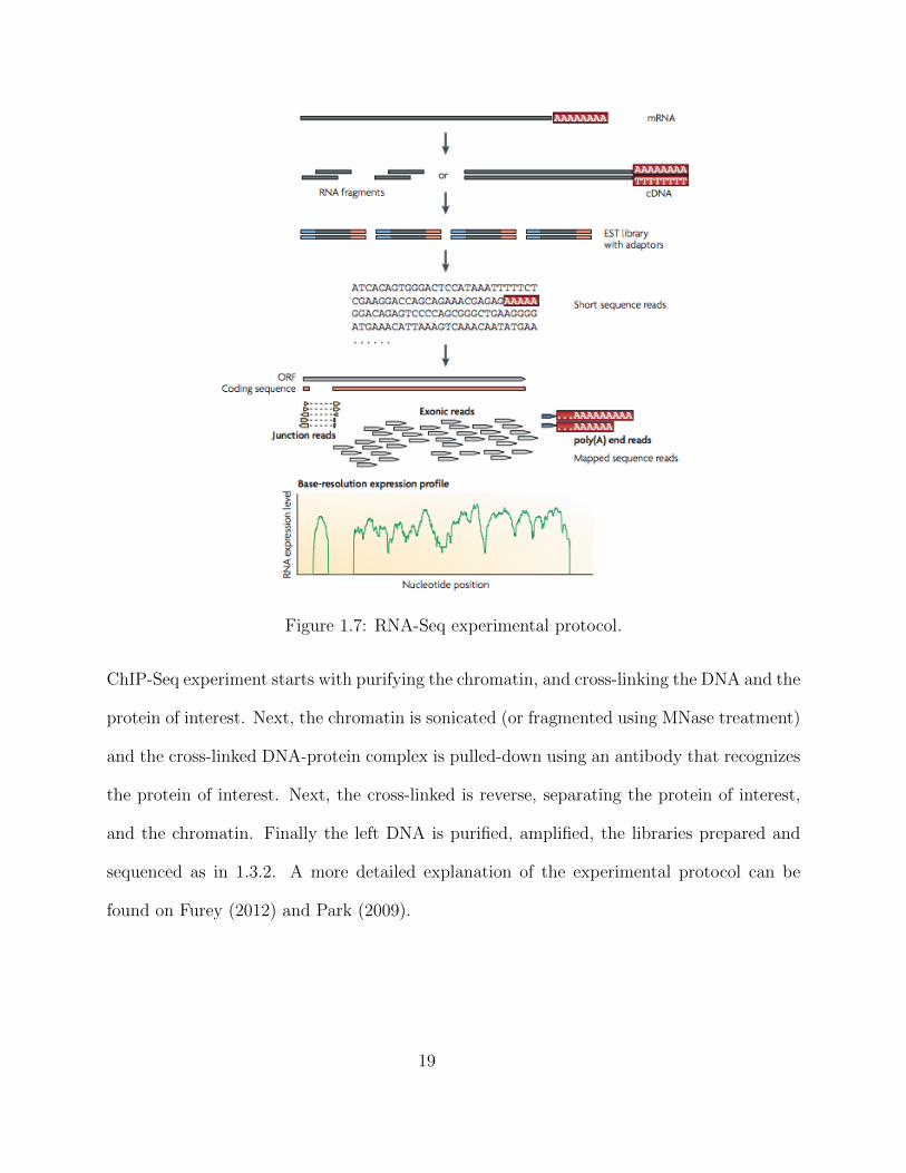
Figure 1.7: RNA-Seq experimental protocol.
ChIP-Seq experiment starts with purifying the chromatin, and cross-linking the DNA and the
protein of interest. Next, the chromatin is sonicated (or fragmented using MNase treatment)
and the cross-linked DNA-protein complex is pulled-down using an antibody that recognizes
the protein of interest. Next, the cross-linked is reverse, separating the protein of interest,
and the chromatin. Finally the left DNA is purified, amplified, the libraries prepared and
sequenced as in 1.3.2. A more detailed explanation of the experimental protocol can be
found on Furey (2012) and Park (2009).
19
Figure 1.8: ChIP-Seq experimental protocol.
20
Chapter 2
Allelic Imbalance and Allele-specific
expression
Every complete set of chromosomes contains the full code; so there are, as a
rule, two copies of the latter in the fertilized egg cell, which forms the earliest
stage of the future individual.
- Erwin Schrodinguer
In this chapter we extend several RNA-Seq models, such as Trapnell et al. (2010) and Glaus
et al. (2011), to the case of allele-specific gene/isoform expression. In the case of experiments
for which we have the individual’s genotype, and its respective haplotype-blocks, our method
can estimate the expression for each gene/isoform at the allelic level, but we loose the parent-
of-origin information. Moreover, in the case of experiments for which we have the paternal
and maternal genomes our method can estimate the expression for each of the parental
alleles.
We present bayesian and frequentist models of allelic expression in an RNA-Seq experi-
ment, combined with phasing information, such as paternal/maternal phasing in the study of
21
imprinting; or haplotype phasing in the case of population-level studies. Next, we provide a
computationally efficient EM algorithm to estimate allelic expression, and its bayesian coun-
terpart, a gibbs sampling approach to sample the allelic expression from its posterior. Next,
we define a differential-expression test to test for differences between the haplotypes, and
we provide a simulation study to show the performance of our approach in comparison with
other popular published methods, Robinson et al. (2010). The methods presented in this
chapter serve as basis for the study of imprinting in chapter 3 and the study of ase-cis-eQTL
and imprinting in chapter 4.
2.1 Introduction
Several models have been proposed for the estimation of gene/transcript expression,
and/or alternative splicing using RNA-Seq experiments. The state-of-the-art methods can
be divided into two major groups. On the one side, a set of models, that we call count-based
methods estimate gene expression by creating an artificial ”gene model”, where a gene is
defined as the intersection (or union) of all its possible transcripts, and then the expression
is estimated as the sum of all reads that map to such ”gene model”. It has been pointed by
several authors that such models are undesirable since they do not take into consideration
the data generating process of RNA-Seq.
On the other side, several models such as Jiang and Wong (2009), Trapnell et al. (2010),
Glaus et al. (2011) and Turro et al. (2011), that we call transcript-based models, model the
RNA-seq data at the transcript-level, assigning reads to each of the transcripts (alternative
isoforms) of a gene according to their probabilities in the model. In such models, in order
to estimate the expression of a gene, one has to first estimate the expression of each of its
22

transcripts, and then the expression of a gene can be estimated as the weighted average
expression of each of the transcripts coming from such gene.
We believe that the transcript-based models are more in line with the biological reality
since they model the data at the transcript-level. As Sidney Brenner pointed out with respect
to the discovery of genes: ”I think the most important thing there was that immediately you
could say, boy if we could find out how the sequence of bases corresponds to the sequence of
amino acids, because now we could define the gene not just as a blob, not just as a bead on a
string, but we could define the gene now as a length of DNA”. In other words the transcript-
based models adhere to the physical reality of a gene, by which a specific sequence is copied
into an RNA transcript, and not a ”hypothetical construct”, or so-called ”gene model”.
Furthermore, since in transcript-based models the data is modeled at the molecular level
of transcripts, they incorporate an explicit parameter for the relative abundance of tran-
scripts in their likelihood, making the results easier to interpret. In other words, cells have
transcripts inside the nucleus, not reads, nor counts, and having a parameter that estimate
the relative abundance of transcripts is definitely an advantage.
However, most transcript-based models, except Turro et al. (2011), can only quantify
transcript expression at the single chromosome case, where only a single measure of expres-
sion per transcript is calculated. This is a simplification of the biology since we are a diploid
organism, and we have two allelic copies of each transcript: the one inherited from the father
and the one inherited from the mother. More specifically, we have 23 pairs of chromosomes,
where each of the 23 pairs were inherited from our parents.
23
2.1.1 Biological mechanisms of Allelic Imbalance
Allelic imbalance (AI) is a phenomenon where the two alleles of a given gene are expressed
at different levels in a given cell, either because of epigenetic inactivation of one of the two
alleles, or because of genetic variation in regulatory regions. The major known phenomena
of allelic-imbalance are X-chromosome inactivation, mitotically stable autosomal monoallelic
expression, imprinting and cis-regulation at the allele-specific level.
X-inactivation is a process by which cells in the epiblast (cells that give rise to the
embryo) randomly choose one of the X-chromosomes to become inactive, and such decision
is mantained throughout the lineage of a given cell - giving rise to mosaich patterns of
expression across tissues in the developed organism. The icon of X-inactivation is the female
calico cat, which exhibits patches of black and orange fur due to the random inactivation
of one of the alleles of the X-located gene responsible for the coloration of its fur, in which
one allele gives rise to black fur and the other allele gives rise to orange fur. Autosomal
monoallelic expression is similar to X-inactivation in the sense that some cells randomly
choose to inactivate one of the alleles, while other cells of the same type choose the opposite
allele. Also, as in X-inactivation such decision is mantained throughout cell division of the
same cell, but different clonal populations choose the inactive alleles randomly. Imprinting
on the other side is a very different mechanism, it occurs for the cells in the germline, and
its parent-of-origin specfifc, in the sense that either the paternal or the maternal allele is
inactivated. Finally, the last source of allelic imbalance is cis-regulation at the allele-specific
level.
In summary, in a single cell, in females, one would always observe all of the genes of
a randomly chosen X-chromosomes to be inactive, several autosomal genes to be randomly
silenced, hundreds of genes to be silenced in the germline in a parent-of-origin manner, and on
24
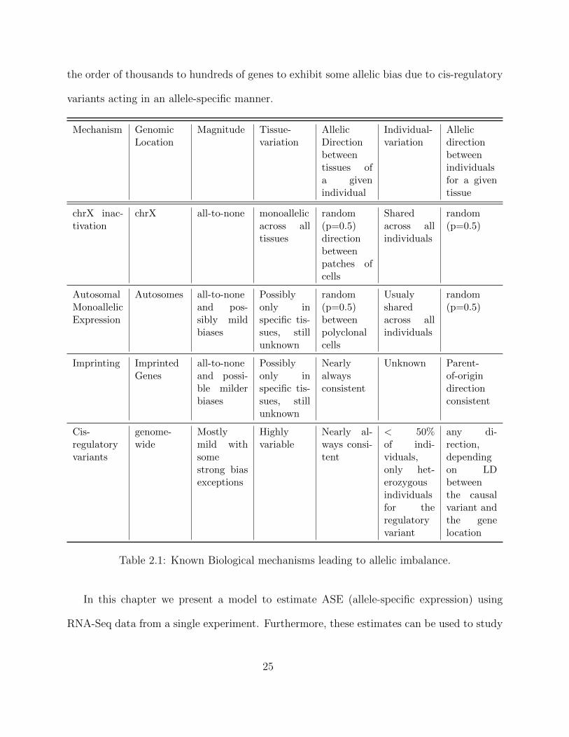
the order of thousands to hundreds of genes to exhibit some allelic bias due to cis-regulatory
variants acting in an allele-specific manner.
Mechanism GenomicLocation
Magnitude Tissue-variation
AllelicDirectionbetweentissues ofa givenindividual
Individual-variation
Allelicdirectionbetweenindividualsfor a giventissue
chrX inac-tivation
chrX all-to-none monoallelicacross alltissues
random(p=0.5)directionbetweenpatches ofcells
Sharedacross allindividuals
random(p=0.5)
AutosomalMonoallelicExpression
Autosomes all-to-noneand pos-sibly mildbiases
Possiblyonly inspecific tis-sues, stillunknown
random(p=0.5)betweenpolyclonalcells
Usualysharedacross allindividuals
random(p=0.5)
Imprinting ImprintedGenes
all-to-noneand possi-ble milderbiases
Possiblyonly inspecific tis-sues, stillunknown
Nearlyalwaysconsistent
Unknown Parent-of-origindirectionconsistent
Cis-regulatoryvariants
genome-wide
Mostlymild withsomestrong biasexceptions
Highlyvariable
Nearly al-ways consi-tent
< 50%of indi-viduals,only het-erozygousindividualsfor theregulatoryvariant
any di-rection,dependingon LDbetweenthe causalvariant andthe genelocation
Table 2.1: Known Biological mechanisms leading to allelic imbalance.
In this chapter we present a model to estimate ASE (allele-specific expression) using
RNA-Seq data from a single experiment. Furthermore, these estimates can be used to study
25
some of the described mechanisms of allelic imbalance in a more detailed, genome-wide
manner. In population studies, for which we have genotypic information, it can help us
understand allele-specific effects across several individuals, and how allelic1 differences affect
expression. It has been shown that there are several allelic differences that affect disease risk,
and potentially, response to drug treatment. This is of key importance in GWAS, eQTL,
drug response, and the still pending promise of personalized medicine. We dedicate such
effort in chapter 4 of this thesis.
Furthermore, in chapter 3 we show how when combining RNA-Seq data and whole genome
sequencing of the offspring parents we can quantify parent-of-origin expression and, therefore
delve into the biology (and effects) of impriting.
Nevertheless, it has been a long road to be able to study allele-specific expression and
parent-of-origin expression at a genome-wide scale. In the earlier days of microarray exper-
iments for gene expression this was not feasible since one would have needed allele-specific
probes to quantify differential expression of alleles. However with NGS technologies, by com-
bining RNA-Seq experiments with SNP arrays or whole genome sequencing of the parents,
studies of allele-specific expression, or parent-of-origin expression, respectively, have become
more common. Albeit conceptually possible such studies present several computational and
statistical challenges that have been addressed in this thesis: mapping bias to a reference
genome, Degner et al. (2009), phasing of the reads high-uncertainty due to read ambiguity
with respect to the allele-of-origin.
1by different alleles we mean different sequences of a transcript due to natural variation in the population
26
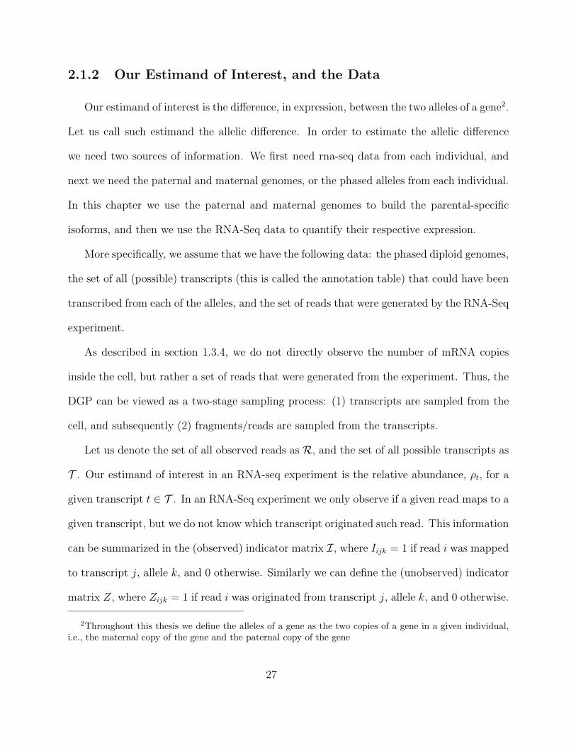
2.1.2 Our Estimand of Interest, and the Data
Our estimand of interest is the difference, in expression, between the two alleles of a gene2.
Let us call such estimand the allelic difference. In order to estimate the allelic difference
we need two sources of information. We first need rna-seq data from each individual, and
next we need the paternal and maternal genomes, or the phased alleles from each individual.
In this chapter we use the paternal and maternal genomes to build the parental-specific
isoforms, and then we use the RNA-Seq data to quantify their respective expression.
More specifically, we assume that we have the following data: the phased diploid genomes,
the set of all (possible) transcripts (this is called the annotation table) that could have been
transcribed from each of the alleles, and the set of reads that were generated by the RNA-Seq
experiment.
As described in section 1.3.4, we do not directly observe the number of mRNA copies
inside the cell, but rather a set of reads that were generated from the experiment. Thus, the
DGP can be viewed as a two-stage sampling process: (1) transcripts are sampled from the
cell, and subsequently (2) fragments/reads are sampled from the transcripts.
Let us denote the set of all observed reads as R, and the set of all possible transcripts as
T . Our estimand of interest in an RNA-seq experiment is the relative abundance, ρt, for a
given transcript t ∈ T . In an RNA-Seq experiment we only observe if a given read maps to a
given transcript, but we do not know which transcript originated such read. This information
can be summarized in the (observed) indicator matrix I, where Iijk = 1 if read i was mapped
to transcript j, allele k, and 0 otherwise. Similarly we can define the (unobserved) indicator
matrix Z, where Zijk = 1 if read i was originated from transcript j, allele k, and 0 otherwise.
2Throughout this thesis we define the alleles of a gene as the two copies of a gene in a given individual,i.e., the maternal copy of the gene and the paternal copy of the gene
27
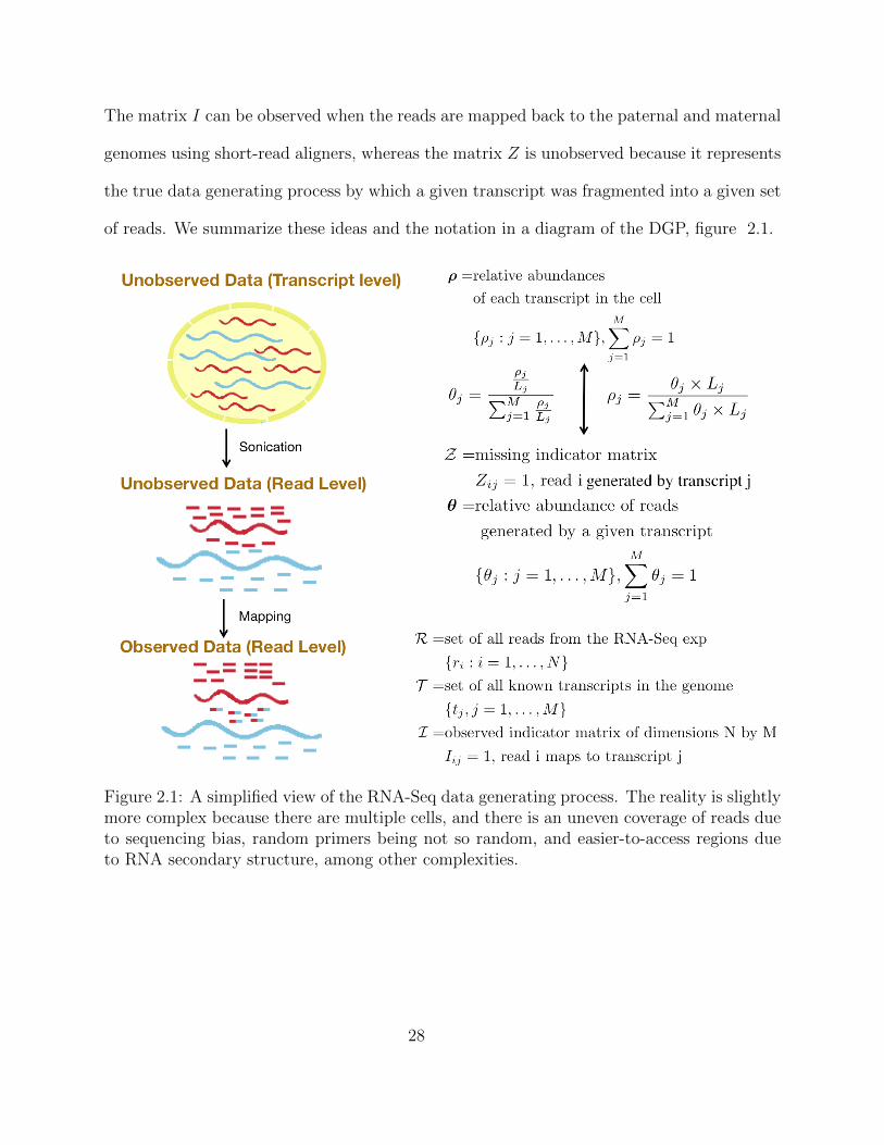
The matrix I can be observed when the reads are mapped back to the paternal and maternal
genomes using short-read aligners, whereas the matrix Z is unobserved because it represents
the true data generating process by which a given transcript was fragmented into a given set
of reads. We summarize these ideas and the notation in a diagram of the DGP, figure 2.1.
Figure 2.1: A simplified view of the RNA-Seq data generating process. The reality is slightlymore complex because there are multiple cells, and there is an uneven coverage of reads dueto sequencing bias, random primers being not so random, and easier-to-access regions dueto RNA secondary structure, among other complexities.
28
2.1.3 Normalized Measures of RNA expression
It follows from the description of the DGP that without knowledge (spike-ins) of the
total abundance of transcripts molecules inside the cell is not possible to estimate absolute
abundance of transcripts, and therefore, RNA-Seq experiments at best can only provide
measures of the relative abundance of transcripts. We called this measure as ρt in the
description of the DGP, and we defined it as the relative abundance of transcript t in the
cell.
In the current literature there are two widely accepted normalized (across samples) mea-
sures of expression for ρt, Reads per Kilobase per Million mapped reads (RPKM), and
Transcripts Per Million (TPM). However, studies have shown on solid theoretical grounds
that RPKM is less interpretable, its biased when comparing abundances between samples,
and it may inflate the number of false positives when comparing two samples, Wagner et al.
(2012).
We can go one step further and define this mesure in physical terms. ρt is the relative
molar RNA concentration (rmc) of each transcript t, defined as, rmct = mRNAtmRNAtotal
, with,
RNAtotal =∑
t∈T mRNAt. It is straightforward to show that, ˆrmc = 1|T | , i.e., the average
rmc is a constant equals to 1 over the total number of transcripts in the experiment. In
theory, we would like ρt to be directly proportional to rmc. Thus, our interest is to know,
which of the two measures, TPM or RPKM exhibits such property? Let us forget about the
multiple alignment issue for the sake of comparing the two measures. Then,
RPKMt = 109 × ciL′tN
(2.1)
where ct is the number of reads mapping to transcript t, L′t is the effective length of transcript
29
t, and N is the number of mappable reads in the sequencing experiment. It is easy to show
that the sum of RPKMs depends on N , the number of mapped reads, therefore it is platform
dependent and thus not directly proportional to rmct.
On the other side, TPM is defined as:
TPMt = 106 × Z × ciL′tN
(2.2)
where, Z is added in order to make this measure technology-independent, and it is a nor-
malization factor. It can easily be shown that such measure is now directly proportional to
rmct and it is thus our prefered measure of expression.
In the case of allele-specific effects we are interested in measuring, yt = ρtp − ρtm, i.e.,
the difference, in expression, between the paternal and maternal alleles. For such cases, has
been argued that it is not important which measure to use. Nevertheless, such assumption
is not true. Let us assume we did E experiments and we know that the allelic-specific effect
is the same in each of the experiments. Then, if we use RPKM as the measure for ρt, we
have, y(i)t = α(i) × (rmctp − rmctm), i = 1, . . . , E, and therefore our final estimate for the
allele-specific effect will have a bias factor given by α. The bias factor α is a function of the
sequencing depth in each of the experiments so it follows that the difference between the
paternal and maternal RPKMs is not directly proportional to the difference of the paternal
and maternal relative molar concentrations.
2.2 Computational Workflow
A key-step in any analysis of next generation sequencing data is the computational work-
flow to properly process the data. One has to develop computationally efficient, robust and
30
carefully design computational workflows because these experiments tend to produce large
amounts of data. In this thesis, we analyzed more than 100 terabytes of data and without
the aid of high performance computing clusters, and other well-established algorithms many
of the proposed models would not be feasible to implement. Here we describe what we con-
sider the optimal approach to process large amounts of RNA-Seq data into a format that is
suitable for our model, and can serve as an input for our algorithm.
As we mentioned earlier, we assume that we have the set of all reads generated by the
RNA-Seq experiment - this is standard and is contained within a fastq file, where each 4 lines
contains the read id, the read sequence and the per-base read quality. Then, such file needs
to be inspected for quality control, such that reads contaminated with library preparation
steps, and/or reads of low quality bases are filtered out. Once such QC is done we have
a new, higher confidence set of reads, but we still do not know where they were generated
from the genome. Thus, a key step is the alignment of the reads to the reference genome.
In this step one has to have in mind that such reads were originated from transcripts, and
therefore, the reads that cover exon junctions will map to far apart regions in the genome.
Because of this, it is recommended to map the reads to the genome using ’transcriptome-
aware’ aligners, such as Tophat and STAR. Another common strategy is to create a file
with all the annotated transcripts and their respective sequence and map the reads to the
sequence of all transcripts. In our workflow we decided to use transcriptome-aware aligners.
However, in our case we are interested in allele-specific expression and therefore our
transcriptome is double the size of the haploid transcriptome. Therefore, we need to use
’in-silico’ parental genomes and map our reads generated from the RNA-Seq experiment to
each genome independently. This approach has two advantages: it allows us to phase the
reads, meaning to identify from which genome, paternal or maternal, the reads came from;
31
and at the same time it helps us overcome the mapping bias associated when mapping reads
to a haploid genomic reference.
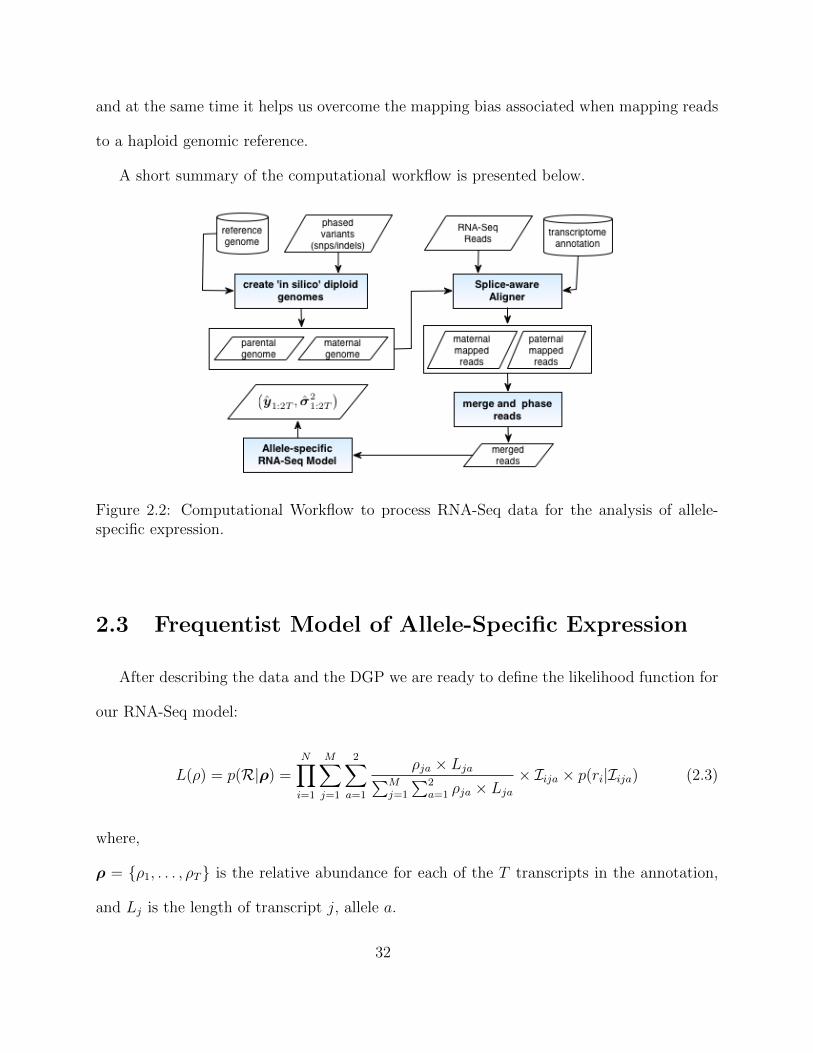
A short summary of the computational workflow is presented below.
Figure 2.2: Computational Workflow to process RNA-Seq data for the analysis of allele-specific expression.
2.3 Frequentist Model of Allele-Specific Expression
After describing the data and the DGP we are ready to define the likelihood function for
our RNA-Seq model:
L(ρ) = p(R|ρ) =N∏i=1
M∑j=1
2∑a=1
ρja × Lja∑Mj=1
∑2a=1 ρja × Lja
× Iija × p(ri|Iija) (2.3)
where,
ρ = {ρ1, . . . , ρT} is the relative abundance for each of the T transcripts in the annotation,
and Lj is the length of transcript j, allele a.
32
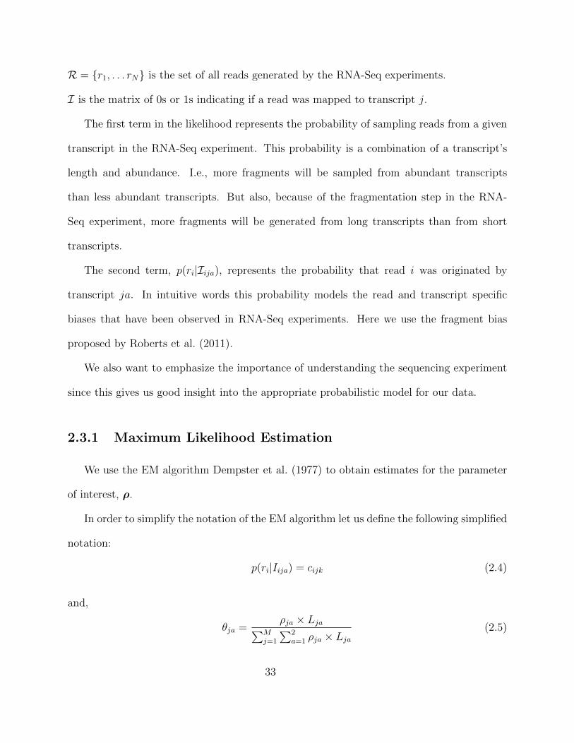
R = {r1, . . . rN} is the set of all reads generated by the RNA-Seq experiments.
I is the matrix of 0s or 1s indicating if a read was mapped to transcript j.
The first term in the likelihood represents the probability of sampling reads from a given
transcript in the RNA-Seq experiment. This probability is a combination of a transcript’s
length and abundance. I.e., more fragments will be sampled from abundant transcripts
than less abundant transcripts. But also, because of the fragmentation step in the RNA-
Seq experiment, more fragments will be generated from long transcripts than from short
transcripts.
The second term, p(ri|Iija), represents the probability that read i was originated by
transcript ja. In intuitive words this probability models the read and transcript specific
biases that have been observed in RNA-Seq experiments. Here we use the fragment bias
proposed by Roberts et al. (2011).
We also want to emphasize the importance of understanding the sequencing experiment
since this gives us good insight into the appropriate probabilistic model for our data.
2.3.1 Maximum Likelihood Estimation
We use the EM algorithm Dempster et al. (1977) to obtain estimates for the parameter
of interest, ρ.
In order to simplify the notation of the EM algorithm let us define the following simplified
notation:
p(ri|Iija) = cijk (2.4)
and,
θja =ρja × Lja∑M
j=1
∑2a=1 ρja × Lja
(2.5)
33
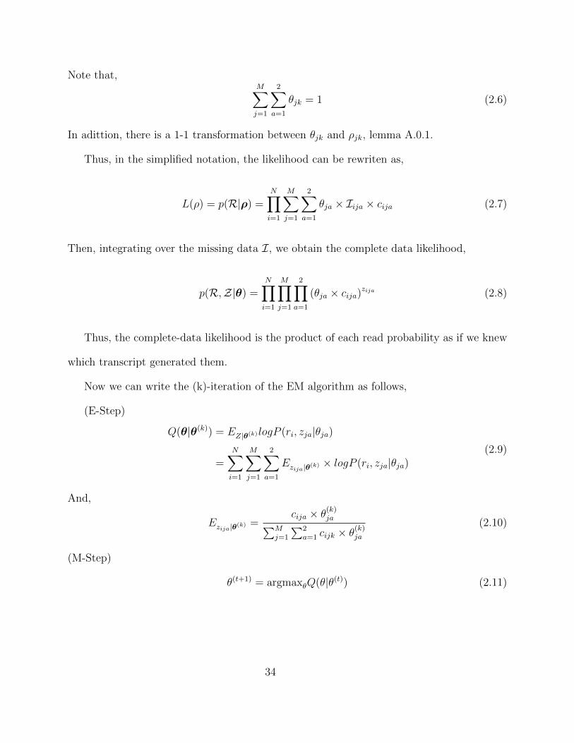
Note that,M∑j=1
2∑a=1
θjk = 1 (2.6)
In adittion, there is a 1-1 transformation between θjk and ρjk, lemma A.0.1.
Thus, in the simplified notation, the likelihood can be rewriten as,
L(ρ) = p(R|ρ) =N∏i=1
M∑j=1
2∑a=1
θja × Iija × cija (2.7)
Then, integrating over the missing data I, we obtain the complete data likelihood,
p(R,Z|θ) =N∏i=1
M∏j=1
2∏a=1
(θja × cija)zija (2.8)
Thus, the complete-data likelihood is the product of each read probability as if we knew
which transcript generated them.
Now we can write the (k)-iteration of the EM algorithm as follows,
(E-Step)
Q(θ|θ(k)) = EZ|θ(k)logP (ri, zja|θja)
=N∑i=1
M∑j=1
2∑a=1
Ezija|θ(k) × logP (ri, zja|θja)(2.9)
And,
Ezija|θ(k) =cija × θ(k)
ja∑Mj=1
∑2a=1 cijk × θ
(k)ja
(2.10)
(M-Step)
θ(t+1) = argmaxθQ(θ|θ(t)) (2.11)
34
Thus,
θ(t+1)jk =
∑ni=1E(Zijk|θ(t))
N(2.12)
where E(Zijk|θ(t)) is the same as in 2.12.
Note. This model may be weakly identifiable in cases where the two alleles have few
differences, in terms of number of SNPs, or INDELS. In such cases, the EM still guaran-
tees convergence to, at least, a local maxima. Moreover, the identifiable pair, θj1 + θj2 is
guaranteed to be the maximum likelihood estimate.
2.3.2 Bootstrap approach to obtain Confidence Intervals
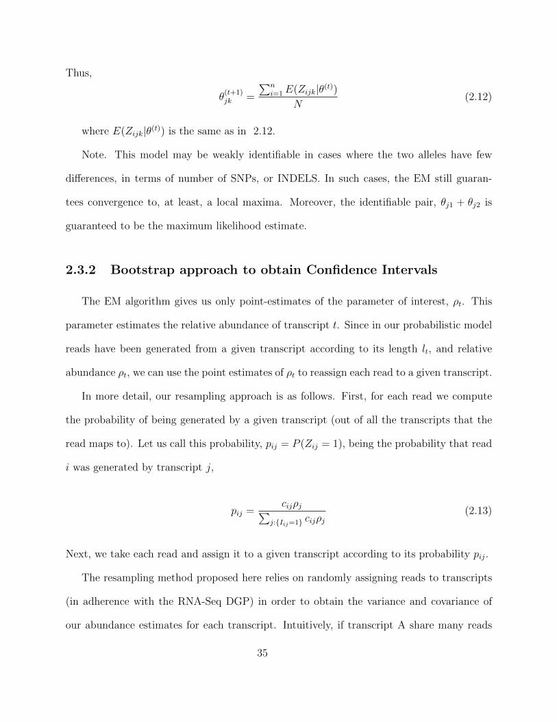
The EM algorithm gives us only point-estimates of the parameter of interest, ρt. This
parameter estimates the relative abundance of transcript t. Since in our probabilistic model
reads have been generated from a given transcript according to its length lt, and relative
abundance ρt, we can use the point estimates of ρt to reassign each read to a given transcript.
In more detail, our resampling approach is as follows. First, for each read we compute
the probability of being generated by a given transcript (out of all the transcripts that the
read maps to). Let us call this probability, pij = P (Zij = 1), being the probability that read
i was generated by transcript j,
pij =cijρj∑
j:{Iij=1} cijρj(2.13)
Next, we take each read and assign it to a given transcript according to its probability pij.
The resampling method proposed here relies on randomly assigning reads to transcripts
(in adherence with the RNA-Seq DGP) in order to obtain the variance and covariance of
our abundance estimates for each transcript. Intuitively, if transcript A share many reads
35

with transcript B they will be highly correlated, and if transcript A has very few reads
and/or many shared sequences with other genomic regions it will exhibit high variance in its
abundance estimate.
Note: Without loss of generality we specified one transcript per locus but in the allele-
specific case we always deal with two alleles per transcript.
2.4 Bayesian Model of Allele-Specific Expression
One advantage of defining a bayesian model for allele-specific expression is that we can
directly sample from the posterior, thus avoiding the use of a bootstrap approach to obtain
the standard error of our expression estimates.
The model presented here is an expansion of the BitSeq model, Glaus et al. (2011), for
the allele-specific case, where the main difference is that now the indicator matrix I has
twice the number of transcripts than in the non-allele case.
In order to build the allele-specific expression model we use the same notation as in
figure 2.1. We define our model in terms of θ, instead of in terms of ρ in order to sim-
plify the sampling steps. However, there is a 1-1 transformation between both parameters,
lemma A.0.1. Also, to simplify the notation, we refer to the number of transcripts as T ,
which in the allele-specific setting is equivalent to twice the number of transcripts than in
the haploid setting of the BitSeq model.
Thus, we can write the joint distribution of the observed data, the missing data and the
36
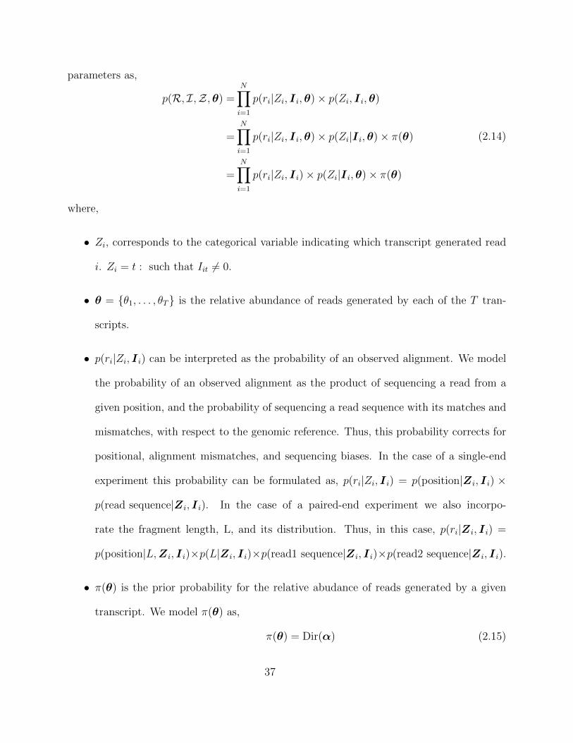
parameters as,
p(R, I,Z,θ) =N∏i=1
p(ri|Zi, I i,θ)× p(Zi, I i,θ)
=N∏i=1
p(ri|Zi, I i,θ)× p(Zi|I i,θ)× π(θ)
=N∏i=1
p(ri|Zi, I i)× p(Zi|I i,θ)× π(θ)
(2.14)
where,
• Zi, corresponds to the categorical variable indicating which transcript generated read
i. Zi = t : such that Iit 6= 0.
• θ = {θ1, . . . , θT} is the relative abundance of reads generated by each of the T tran-
scripts.
• p(ri|Zi, I i) can be interpreted as the probability of an observed alignment. We model
the probability of an observed alignment as the product of sequencing a read from a
given position, and the probability of sequencing a read sequence with its matches and
mismatches, with respect to the genomic reference. Thus, this probability corrects for
positional, alignment mismatches, and sequencing biases. In the case of a single-end
experiment this probability can be formulated as, p(ri|Zi, I i) = p(position|Zi, I i) ×
p(read sequence|Zi, I i). In the case of a paired-end experiment we also incorpo-
rate the fragment length, L, and its distribution. Thus, in this case, p(ri|Zi, I i) =
p(position|L,Zi, I i)×p(L|Zi, I i)×p(read1 sequence|Zi, I i)×p(read2 sequence|Zi, I i).
• π(θ) is the prior probability for the relative abudance of reads generated by a given
transcript. We model π(θ) as,
π(θ) = Dir(α) (2.15)
37

The general version of the model also incorporate the probability that a given read was
generated by noise and not by any of the transcripts it aligned to. In order to do so,
we define a latent variable Znoise, and the associated probability for the read to not have
been generated by any transcript, θnoise - when adding this extra latent variable and noise
parameter, the joint distribution of the data becomes,
p(R, I,Z,θ, Znoise, θnoise) =N∏i=1
p(ri|Zi, I i)×p(Zi|I i, Znoise,θ)×p(Znoise|θ)×π(θ)×π(θnoise)
(2.16)
Without loss of generalization we will work with the model without the extra noise term in
the next sections, but our model runs with the noise term.
2.4.1 Gibbs Sampler
Let us write the joint distribution of the observed data, the latent variables, and the
model parameters,
p(R, I,Z,θ) =N∏i=1
p(ri|Zi, I i)× p(Zi|I i,θ)× π(θ) (2.17)
In the Gibbs sampler we first assign a read to a given transcript, i.e., we sample Zi|I i,θ,
and next we sample the transcript abudance given the read assignment, i.e., θ|Zi - doing
this iteratively we guarantee convergence to the joint distribution.
Nevertheless, such strategy can be quite slow since we need to assign have to sample
reads and trasncripts abundances in a read-by-read manner. A faster approach would be to
use the collapsed gibbs sampler version of this algorithm.
38

Algorithm 1 Gibbs Sampler for estimating Allele-specific expression parameters θ
1. Initialize the parameters.
2. Sample each parameter iterative (until convergence) from their full condi-tionals, as follows,For alignment of read i = 1, . . . , n
(a) Sample Zi|I i,θ ∼ Cat(Zi|φi), where φit ∝ p(ri|I i, Zi) × θt, t = 1, . . . , T . Notethat φit needs to be normalized such that
∑t:{Iit 6=0} φit = 1. I.e., the read can
have only been generated by one of the transcripts it aligned to.
(b) Sample θ|Zi ∼ Dir (θ|α + C1, . . . α + CT ), where Ct =∑N
i=1 δ(Zi = t). I.e., Ctcounts the total number of reads that were assigned as generated by transcript tin a given iteration.
3. Take only the samples after the burn-in and compute posterior statistics for the pa-rameters of interest.
2.5 Hierarchical Model of Allele-Specific Expression
across Multiple Experiments
We have presented methods to obtain expression estimates per-experiment, but in several
situations we may want to estimate the grand-mean across all experiments. In the hierarchi-
cal model we assume exchangeability across experiments with the same factors, since there
is no reason to believe experimental-level differences when the factors are shared. The Hi-
erarchical model borrows information from exchangeable experiments, and it tends to give
better predictions than complete-pooling or no-polling, Gelman (2006).
This model is similar to the previous model but now we impose a common hyperprior
distribution for each θ(e), i.e., the abundance of reads coming from a given transcript in a
given experiment. We show a graphical representation of the model in figure 2.3. Thus, we
can write the joint distribution of the parameters and the observed data as,
39

p (R, I,Z,θ,µ, σ) = p(σ)× p(µ)×E∏e=1
{π(θ(e)|(µ, σ)
)×
N∏i=1
p(r(e)i |Z
(e)i , I
(e)i
)× p
(Z
(e)i |I
(e)i ,θ(e)
)}(2.18)
where,
• Z(e)i , corresponds to the categorical variable indicating which transcript generated read
i in the eth experiment. Z(e)i = t : such that I
(e)it 6= 0.
• θ(e) = {θ(e)1 , . . . , θ
(e)T } is the relative abundance of reads generated by each of the T
transcripts in experiment e.
• p(r(e)i |Z
(e)i , I
(e)i ) can be interpreted as the probability of an observed alignment for a
given read in a given experiment.
• π(θ(e)|(µ, σ)
)is the prior probability for the relative abudance of reads generated by
a given transcript in a given experiment. We model this probability as, Dir (µ� σ).
• p(µ) is the prior probabily for the hyperparameter µ. The hyperparameters µ can be
interpreted as the grand-mean for the abundance of reads for each transcripts across
all experiments. This parameter is shared among all the same experiments.
• p(σ) is the prior probabily for the hyperparameter σ. The hyperparameter σ can be
interpreted as a scaling factor, allowing different scaling between different experiments.
Now, using the joint distribution we derive a Metropolis-within-Gibbs sampler to obtain
the posterior estimates for each of the parameters in the model,
40

Algorithm 2 Metropolis-within-Gibbs Sampler for estimating grand-mean across all exper-iments
1. Initialize the parameters.
2. Sample each parameter iterative (until convergence) from their full condi-tionals, as follows,For experiment e = 1, . . . , EFor alignment of read i = 1, . . . , ne
(a) Sample Z(e)i |I
(e)i ,θ(e) ∼ Cat
(Z
(e)i |φ
(e)i
), where φit ∝ p(r
(e)i |I
(e)i , Z
(e)i ) × θ(e)
t , t =
1, . . . , T
(b) Sample θ(e)|Z(e)i ∼ Dir
(θ(e)|µ1σ + C
(e)1 , . . . , µTσ + C
(e)T
), where C
(e)t =∑N
i=1 δ(Z(e)i = t). I.e., C
(e)t counts the total number of reads that were assigned
as generated by transcript t in a given experiment e, in a given iteration.
End of iteration over read and experiments, now we sample the hyperpa-rameters:
(c) Sample µ|θ(1), . . . ,θ(E), σ from its posterior using Metropolis-Hasting’s algo-rithm and a proposal distribution given by µ∗|µ(s) ∼ Dir
(µ∗|µ(s)
)- the posterior
was obtained by discarding all terms not involving µ in the joint distribution,
p(µ|θ(1), . . . ,θ(E), σ
)∝
E∏e=1
Dir(θ(e)|µ, σ
)×Dir(1)
(d) Sample σ|θ(1), . . . ,θ(E),µ from its posterior using Metropolis-Hasting’s algo-rithm and a proposal distribution given by σ∗|σ(s) ∼ LN
(σ(s), 1
)- the posterior
was obtained by discarding all terms not involving σ in the joint distribution,
p(σ|θ(1), . . . ,θ(E),µ
)∝
E∏e=1
Dir(θ(e)|µ, σ
)×Gamma(λ1, λ2)
3. Take only the samples after the burn-in and compute posterior statistics for the pa-rameters of interest.
41
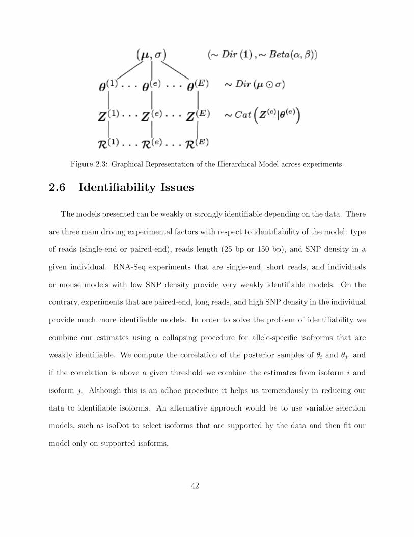
Figure 2.3: Graphical Representation of the Hierarchical Model across experiments.
2.6 Identifiability Issues
The models presented can be weakly or strongly identifiable depending on the data. There
are three main driving experimental factors with respect to identifiability of the model: type
of reads (single-end or paired-end), reads length (25 bp or 150 bp), and SNP density in a
given individual. RNA-Seq experiments that are single-end, short reads, and individuals
or mouse models with low SNP density provide very weakly identifiable models. On the
contrary, experiments that are paired-end, long reads, and high SNP density in the individual
provide much more identifiable models. In order to solve the problem of identifiability we
combine our estimates using a collapsing procedure for allele-specific isofrorms that are
weakly identifiable. We compute the correlation of the posterior samples of θi and θj, and
if the correlation is above a given threshold we combine the estimates from isoform i and
isoform j. Although this is an adhoc procedure it helps us tremendously in reducing our
data to identifiable isoforms. An alternative approach would be to use variable selection
models, such as isoDot to select isoforms that are supported by the data and then fit our
model only on supported isoforms.
42
2.7 Simulation Results: To Count or not to Count?
As mentioned earlier, transcript-based models provide interpretable estimates of transcript-
specific expression and a straightforward way to combine such estimates into gene expression
estimates. In this section we compare our methods with the, up to now, commonly used
method of counting the number of reads per SNP in a given transcript, Robinson et al.
(2010).
We used tuxSimAllele to simulate an RNA-Seq experiment, a diploid version of the
published simulator TuxSim, Trapnell et al. (2013). Our simulator, TuxSimAllele, takes as an
input an expression file, and a parameters file containing RNA-Seq experimental parameters,
as well as dna-specfic parameters. The expression file contains the target expression for each
of the annotated transcripts for each allele. The RNA-Seq specific parameters are related
to the technical parameters of the experiment: the length of the reads, the type of reads
(single-end or paired-end), the mean cDNA fragment length and its variance, and the total
number of cDNA fragments that were sequenced (sequencing depth). The genome-specific
parameters are the genome of the individual and the set of variations (SNPs and Indels)
in the individual’s genome. Here we assumed a SNP density (in exons) in line with the
biological reality and the current technology - human alleles vary about 1 SNP per 1 Kb
(0.001 SNP density), and mouse isogenic lines alleles vary about 1 SNP per 100 bp (0.01).
Since our objective is to identify allele-specific bias across multiple experiments, we de-
cided to simulate allele-specific bias across multiple experiments. In order to do so we create
a base expression file for all allelic-transcripts in the annotation. In the base expression file
we specify the RPKM, ρt, for each of the allelic transcripts in the annotation. Also in the
base expression file we select a subset of genes that will exhibit allele-specific bias in an iso-
43
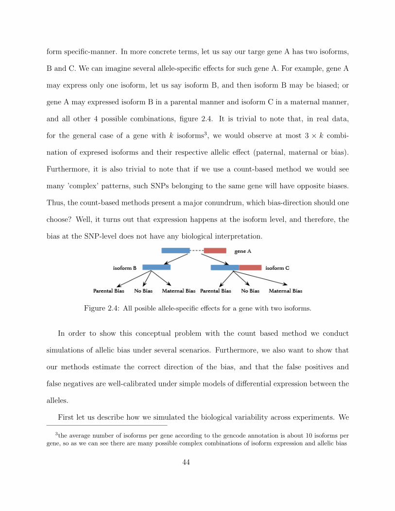
form specific-manner. In more concrete terms, let us say our targe gene A has two isoforms,
B and C. We can imagine several allele-specific effects for such gene A. For example, gene A
may express only one isoform, let us say isoform B, and then isoform B may be biased; or
gene A may expressed isoform B in a parental manner and isoform C in a maternal manner,
and all other 4 possible combinations, figure 2.4. It is trivial to note that, in real data,
for the general case of a gene with k isoforms3, we would observe at most 3 × k combi-
nation of expresed isoforms and their respective allelic effect (paternal, maternal or bias).
Furthermore, it is also trivial to note that if we use a count-based method we would see
many ’complex’ patterns, such SNPs belonging to the same gene will have opposite biases.
Thus, the count-based methods present a major conundrum, which bias-direction should one
choose? Well, it turns out that expression happens at the isoform level, and therefore, the
bias at the SNP-level does not have any biological interpretation.
Figure 2.4: All posible allele-specific effects for a gene with two isoforms.
In order to show this conceptual problem with the count based method we conduct
simulations of allelic bias under several scenarios. Furthermore, we also want to show that
our methods estimate the correct direction of the bias, and that the false positives and
false negatives are well-calibrated under simple models of differential expression between the
alleles.
First let us describe how we simulated the biological variability across experiments. We
3the average number of isoforms per gene according to the gencode annotation is about 10 isoforms pergene, so as we can see there are many possible complex combinations of isoform expression and allelic bias
44
assume, in line with empirical data, that the number of reads in a given isoform, Xt, follows
a NB[µt, σ2t ], with µt = ρt × Lt
1000× D
1000000, and a variance, fitted with a lowess (using real
data), to be a function of the mean. Thus for each experiment, given our base expression
file, that specifies ρt, and the parameters files that specifies D, we can simulate the RNA-Seq
experiment, and generate reads accordingly.
We simulated expression data for all the genes/isoforms in the gencode annotation and we
perturbed (simulated as having parental/maternal bias) only about 0.5% of the genes (in line
with the numbers previously reported). We perform the simulations under several scenarios,
and we compare the EM and bayesian approaches described in this chapter, in addition with
the most commonly used count-methods for estimating allelic-biases. Table 2.2 explains the
different simulated scenarios, and table 2.3 and figure 2.5 show the performance for each
of the methods under all the simulated scenarios. We can see that under the assumption
that the paternal and maternal effects are consistent across all isoforms of a gene the count
method performs in line with the EM and Bayesian allele-specific models described earlier,
nevertheless under any other scenario our proposed models perform preferably.
2.8 Discussion
We presented a model and an efficient computational workflow for finding allele-specific
expression estimates at the transcript-level, and that also allows us to compute estimates
at the gene-level by taking the weighted sum of all the transcripts present in a given gene.
Nevertheless, the model is as good as the data is and in order to reduce the uncertainty of
our estimates several experimental decisions can be made. First, one would ideally estimate
allele-specific expression for individuals with a well-sequenced genome, and with large DNA
45
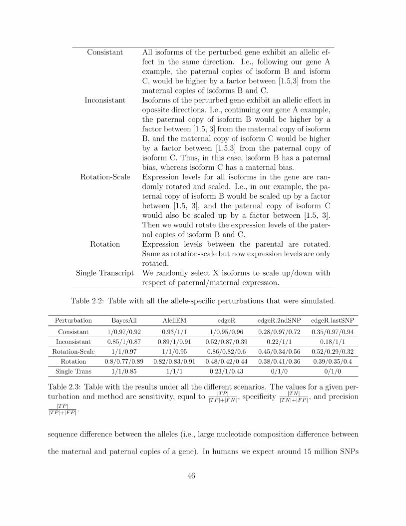
Consistant All isoforms of the perturbed gene exhibit an allelic ef-fect in the same direction. I.e., following our gene Aexample, the paternal copies of isoform B and isformC, would be higher by a factor between [1.5,3] from thematernal copies of isoforms B and C.
Inconsistant Isoforms of the perturbed gene exhibit an allelic effect inopossite directions. I.e., continuing our gene A example,the paternal copy of isoform B would be higher by afactor between [1.5, 3] from the maternal copy of isoformB, and the maternal copy of isoform C would be higherby a factor between [1.5,3] from the paternal copy ofisoform C. Thus, in this case, isoform B has a paternalbias, whereas isoform C has a maternal bias.
Rotation-Scale Expression levels for all isoforms in the gene are ran-domly rotated and scaled. I.e., in our example, the pa-ternal copy of isoform B would be scaled up by a factorbetween [1.5, 3], and the paternal copy of isoform Cwould also be scaled up by a factor between [1.5, 3].Then we would rotate the expression levels of the pater-nal copies of isoform B and C.
Rotation Expression levels between the parental are rotated.Same as rotation-scale but now expression levels are onlyrotated.
Single Transcript We randomly select X isoforms to scale up/down withrespect of paternal/maternal expression.
Table 2.2: Table with all the allele-specific perturbations that were simulated.
Perturbation BayesAll AlellEM edgeR edgeR.2ndSNP edgeR.lastSNP
Consistant 1/0.97/0.92 0.93/1/1 1/0.95/0.96 0.28/0.97/0.72 0.35/0.97/0.94
Inconsistant 0.85/1/0.87 0.89/1/0.91 0.52/0.87/0.39 0.22/1/1 0.18/1/1
Rotation-Scale 1/1/0.97 1/1/0.95 0.86/0.82/0.6 0.45/0.34/0.56 0.52/0.29/0.32
Rotation 0.8/0.77/0.89 0.82/0.83/0.91 0.48/0.42/0.44 0.38/0.41/0.36 0.39/0.35/0.4
Single Trans 1/1/0.85 1/1/1 0.23/1/0.43 0/1/0 0/1/0
Table 2.3: Table with the results under all the different scenarios. The values for a given per-turbation and method are sensitivity, equal to |TP |
|TP |+|FN | , specificity |TN ||TN |+|FP | , and precision
|TP ||TP |+|FP | .
sequence difference between the alleles (i.e., large nucleotide composition difference between
the maternal and paternal copies of a gene). In humans we expect around 15 million SNPs
46
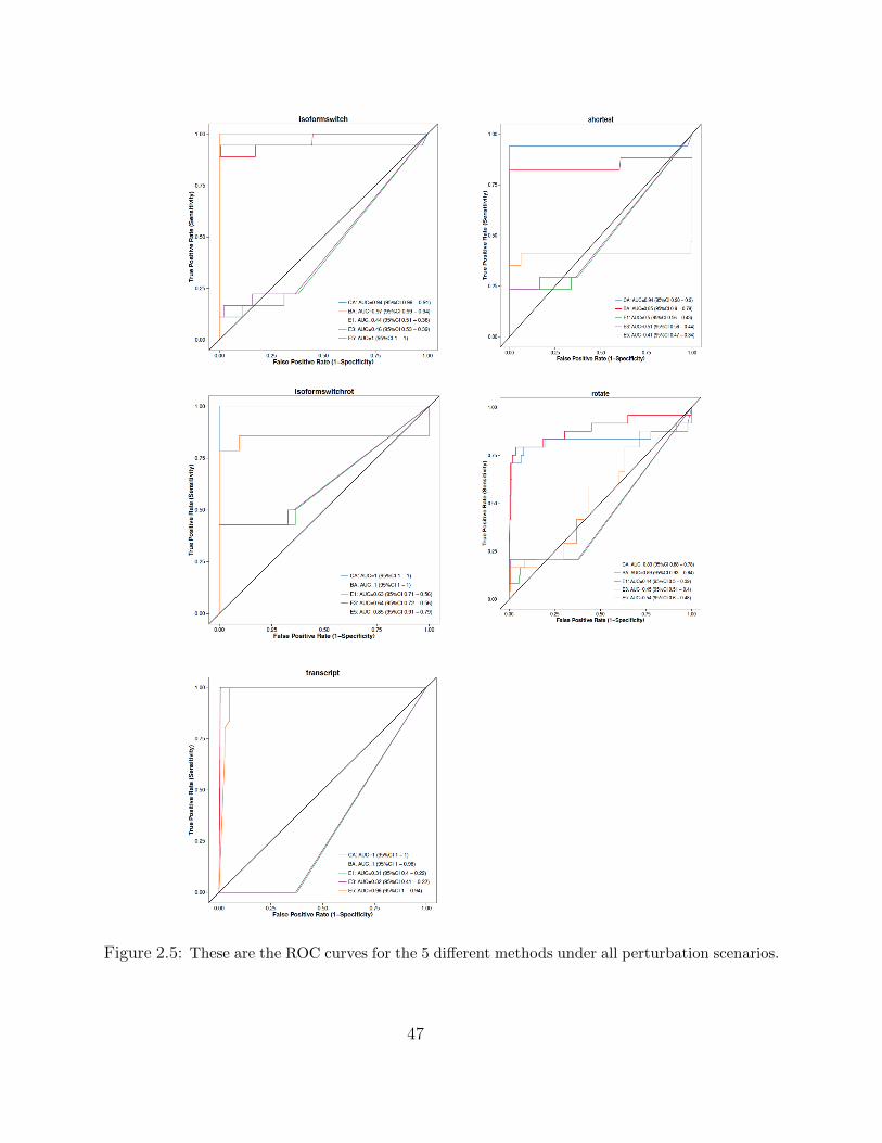
Figure 2.5: These are the ROC curves for the 5 different methods under all perturbation scenarios.
47

between two individuals, while the difference in two mouse strains can be higher ( 1% of the
genome, or equivalently 30 million SNPs).
Second, we would ideally be able to sequence large molecules and thus, reducing the
mapping uncertainty. Illumina current technologies can easily sequence 100 bp paired-end
reads, and PacBio technologies can sequence much longer reads but with a much higher
error rate. We expect that in the longer term this will be less of an issue and we will be able
to sequence much longer molecules, thus reducing the posterior variance of our estimates
considerably.
Third, sequencing depth can helps us considerably in being able to estimate allele-specific
expression for lowly expressed genes, and also helps us in having more reproducible and
robust estimates of the allelic epxression difference.
48
Chapter 3
Design of Experiments in the study of
Parental-Specific Expression
To consult the statistician after an experiment is finished is often merely to ask
him to conduct a post-mortem examination. He can perhaps say what the
experiment died of.
- Ronald Fisher
In this chapter we study parentally-biased gene/isoform expression across several brain
regions1 during early and adult developmental stages, and in other tissues such as liver and
muscle. Traditionally, parentally-biased gene expression, when observed across most cell
types and in an all-to-none fashion is called imprinting. Imprinting is an epigenetic phenom-
ena by which we parentally inherit only one ’working’ copy of a the so-called imprinted gene.
I.e., either the maternal or the paternal copy is actively transcribed in the offspring, and the
other copy (paternal or maternal, respectively) is silenced, and therefore, not transcribed,
1we analyzed rna-seq data for the cerebellum, dorsal raphe and arcuate; and pyrosequencing data forvalidation in at least 10 different brain regions
49
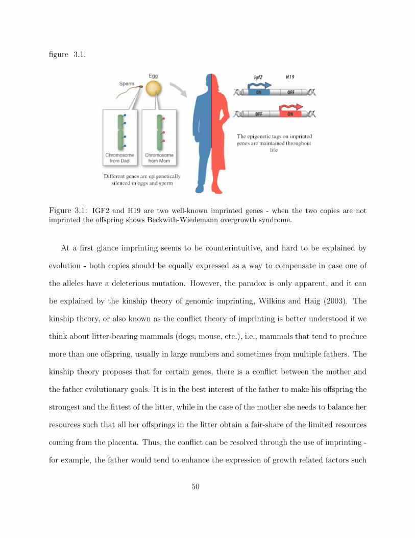
figure 3.1.
Figure 3.1: IGF2 and H19 are two well-known imprinted genes - when the two copies are notimprinted the offspring shows Beckwith-Wiedemann overgrowth syndrome.
At a first glance imprinting seems to be counterintuitive, and hard to be explained by
evolution - both copies should be equally expressed as a way to compensate in case one of
the alleles have a deleterious mutation. However, the paradox is only apparent, and it can
be explained by the kinship theory of genomic imprinting, Wilkins and Haig (2003). The
kinship theory, or also known as the conflict theory of imprinting is better understood if we
think about litter-bearing mammals (dogs, mouse, etc.), i.e., mammals that tend to produce
more than one offspring, usually in large numbers and sometimes from multiple fathers. The
kinship theory proposes that for certain genes, there is a conflict between the mother and
the father evolutionary goals. It is in the best interest of the father to make his offspring the
strongest and the fittest of the litter, while in the case of the mother she needs to balance her
resources such that all her offsprings in the litter obtain a fair-share of the limited resources
coming from the placenta. Thus, the conflict can be resolved through the use of imprinting -
for example, the father would tend to enhance the expression of growth related factors such
50
that his offspring is the strongest, and the mother to compensate such effect would tend to
repress growth-related genes.
To better understand the kinship theory let us take as an example two well-known im-
printed genes, the growth-related genes HG19 and IGF2 shown in figure 3.1. It is known
that in mammals only the paternal copy of IGF2 is expressed in the offspring, and in the
case of H19 only the maternal copy is expressed. Since both are growth related factors,
IGF2 being a growth-enhancing gene and H19 being a growth-supressor gene this shows the
kinship theory in action.
It has also been shown that imprinting plays a major role in development and its key to
the proper function of an organism. In some cases the lack of imprinting can be lethal to the
mother and the offspring and in other cases is associated with major disorders. It has been
shown to be strongly associated with the Prader-Willis, Angelman and Beckwith-Wiedemann
syndromes, and it has also been shown to play an important role in several types of cancer,
such as leukemia, prostate cancer, and colorectal cancer. Moreover, several studies suggest
that imprinting may play an active role in the brain and in social behavior, Garfield et al.
(2011). Thus, imprinting is a strong candidate for a better understanding of socially-related
diseases such as autism and schizophrenia, Badcock and Crespi (2008).
However, few studies have looked at imprinting in a systematic, and genome-wide manner.
Thus, our interest to understand its effects using a more general approach, by measuring its
effect across several developmental time-points, several tissues and in a genome-wide manner.
In this chapter we assume that we have estimates of the parental-specific gene expression
for each experiment - one possible model for achieving such goal is to use the models proposed
in the previous chapter, but as technology evolves there may be more accurate ways to
estimate parental-specific expression. Next, we propose a model on such estimates to help
51
us identify reproducible and consistent differences in expression between the two allele’s of
a gene, the maternal and the paternal copies.
In order to estimate genes that exhibit parent-of-origin effects we present a careful exper-
imental design that accounts for many of the important factors. Next, we fit the Bayesian
Regression and variable selection model to our data and obtain estimates of the main and
interaction effects. Finally, we compare our results with known imprinted genes, and we
validate some of our predictions using pyro-sequencing follow-up experiments.
3.1 Experimental Design
To properly study parent-of-origin bias one has to consider a careful experimental design
or it could lead to misleading/wrong conclusions. First, it is well-known that the DNA
sequence has a large effect over expression, given that sequence differences in promoter,
enhancer and/or insulator regions give rise to different transcriptional regulation programs.
In our design we control for sequence-specific differences in expression by using two
reciprocal mouse crosses. In the initial cross the paternal genome comes from one strain,
and the maternal genome from a different strain. In the reciprocal cross the paternal and
maternal strains are inverted. The mouse cross is one of the 2-level factors in the experiment.
The cross is not the only factor that could likely affect parental bias. This bias may vary
across tissues, ages, and/or gender. In order to exemplify this, let us take the gender factor.
Males have one copy of chromosome X, and females have two copies of chromosome X. Thus,
at the very least, there cannot be imprinting in X-chromosome genes for males.
Moreover, several studies have suggested that imprinting does not exhibit an homoge-
neous pattern across cell types, Garfield et al. (2011). With this in mind, we did experiments
52
in several brain regions, such as Cerebellum, Arcuate and Dorsal Raphe, and an even larger
survey of brain regions during the validation step. It is also well known that DNA methyla-
tion, a key mechanism associated with genomic imprinting and gene-silencing, its dynamic
and likely to change between different developmental stages.
Although we repeated the experimental design across several tissues, without loss of
generality, we shall focus on the design for one brain region, the cerebellum.
With all these factors in mind, we conducted a paired 23 factorial design with several
replicates per pair. The experimental units are mice reciprocal crosses, F1i and F1r, of two
mouse strains, C57 and CAST. Then, for each cross we take cells from their cerebellum at
two-stages of development, 8 days and 8 weeks; and each experiment consists of a single-end
59 bp RNA-Seq experiment (section 1.3.4). The three 2-level factors are Sex (S): M (1), F
(−1); Cross (C): F1i (1), F1r (−1) and Age (A): P8 (1), P64 (−1).
Our estimand of interest is the difference, in expression, between the paternal copy of
the gene and the maternal copy of the gene. Thus, ideally, we would measure the paternal
expression, zp, and maternal expression, zm directly and our response would be the difference
between the two copies2, z = zp−zm. Intuitively, if the difference (z) is 0 across all replicates
we can conclude that there is no parent-of-origin effect, but if such difference is greater or
less than 0 there is a parent-of-origin effect.
However, the problem is slightly more complex and in an RNA-Seq experiment one cannot
directly observe the number of copies coming from each of the alleles, but rather we observe
reads coming from each of the alleles. Therefore, to circumvent this issue, we use an RNA-
Seq model to estimate the allele-specific expression for each gene (chapter 2). Let us denote
2by paternal expression we mean the number of RNA molecules that have been transcribed from thepaternal DNA, and by maternal expression we mean the number of molecules that have been transcribedfrom the maternal DNA
53
our paramater (estimand) of interest as z (equivalent to θ in our RNA-Seq model, equation
2.17). Let us also denote its posterior mean as y = E(z|RNA-seq data) and its posterior
variance as ε = V ar(z|RNA-Seq data), then using bayesian asymptotic theory we know that,
z ∼ N(y, ε). Moreover, under a vague prior for z we can further assume that y and ε closely
approximate the maximum likelihood estimator and fisher information of z. Consequently,
approximately, y ∼ N(z, ε).
We can think of our response as a response y with known measurement errors ε. It is
analogous to measuring the response in an experimental design where we do not directly
observe the response, but rather an estimate of the response plus some error3.
The table describing the full experimental design is presented below, table 3.1. As one
can see in the table, the design is a balance design with 6 replicates per factor combination.
Thus, for example, the first row in the table corresponds to the first factor combination where
the tissue-sample for the RNA-Seq experiment was extracted from a male offspring (S = 1),
coming from an F1i cross (C = 1), and a cerebellum with 8 days of development (A = 1).
Furthermore, y1:6 represents the estimated vector of responses (y1, . . . , y6); ε1:6 = (ε1, . . . , ε6)
represents the estimated errors associated with each estimated response, and nrep = 6 means
that the experiment was repeated (independently) for 6 different biological replicates of such
factor combination.
We are mainly interested in computing the main effect of the difference between the
paternal and the maternal gene expression, after controlling for all the factors mentioned
3Note that the expression estimate and its standard error were estimated from the probabilistic modelin chapter 2. Albeit not perfect, in the sense that a full model across replicates where we estimate theexpression and the factor effects simultaneously may have been more appropriate, this is a tractable andreasonable way to simplify the problem. Furthermore, for a single replicate estimating the expression andits standard errors takes about 6 to 7 hours on 6 cores and it uses about 10 to 20 Gb of Ram, thus a fullmodel would probably be highly impractical.
54

Experiment S C A y ε(y) nrep
1:6 1 1 1 y1:6 ε1:6 67:12 1 -1 1 y7:12 ε7:12 613:18 -1 1 1 y13:18 ε13:18 619:24 -1 -1 1 y19:24 ε19:24 625:30 1 1 -1 y25:30 ε25:30 631:36 1 -1 -1 y31:36 ε31:36 637:42 -1 1 -1 y37:42 ε37:42 643:48 -1 -1 -1 y43:48 ε43:48 6
Table 3.1: Paired 23 factorial design with repeated measurements - six replicates per factorcombination.
above. In order to do so we propose a Bayesian Regression Allelic Imbalance Model, with
the acronym of BRAIM. The model name serves two purposes, one the one hand it stresses
the fact that the model is a bayesian regression on the difference between the alleles, and on
the other hand it serves the purpose to stress that most of our studies of imprinted genes
were done across several Brain regions.
In this model we model all the main effects and interaction effects of each factor over the
response (difference in expression between the alleles). Continuing with the example in the
table, we model the main effects of S,C and A; and its interaction effects SC, SA,CA; plus
an intercept term that estimates the average gene/isoform expression difference (across all
factors) between the paternal and maternal alleles.
3.2 BRAIM: Bayesian Regression Allelic Imbalance Model
Our proposed model, BRAIM, has two key features, on the one side it is not just a simple
linear regression model, but it also incorporates a variable selection feature to estimate and
select the relevant main effects and interaction effects. In addition, it incorporates into the
model the fact that our observations are estimates of the true allelic expression, and thus it is
55
necessary to propagate the uncertainty of our estimates into the model - genes/isoforms with
fewer reads and few SNPs will have higher uncertainty than gene/isoforms with more reads
and many SNPs thus avoiding the uncertainty in our estimates will lead to high number of
false positives and biased conclusions.
A relatively similar model in the context of variable selection was first proposed by George
and McCulloch (1993), and later on extended to experimental designs that involves complex
aliasing by Chipman et al. (1997). Our model takes this ideas and extends it to a 23 factorial
paired design, with measurements errors.
Let us denote the estimate of our response as y. Let us also denote the standard error
of our response estimate as, ε4.
Then, we can model y as normally distributed,
y|z ∼ MVN (z, E) (3.1)
where, y is an estimate of the response, of dimension n × 1, z can be interpreted as the
unobserved/latent true value of the response and is of dimension n× 1, and E = diag(ε2i ) is
the covariance matrix of the response estimate, modeled as independent and of dimension
n×n. Note that n represents the total number of observations. Continuing with the example
from the previous section, n would correspond to 2k × nrep = 23 × 6 = 48, since that is the
total number of samples for our given paired 3-factor (2-level each factor) experimental
design.
4Here it is important to note that in RNA-Seq data we do not directly observe the expression of agene/isoform since our observed data are reads, and we do not directly observe which isoform generatedthem. This uncertainty must be propagated into our model for allele-specific expression and thus, as describedearlier, our observed response y is an estimate of the true difference in expression between the paternal andmaternal allele.
56
Next, we model the unobserved true value of the response, z, as,
z|β, σ2 ∼ MVN (Xβ,Σ) (3.2)
where, X = (X1, . . . , Xp) is the experimental design matrix, with X1 being a column vector
of 1s, and β = (β1, . . . , βp) the regression parameters for the intercept, plus the main and
interaction effects; and Σ = diag (σ2). Note that in our model β1 is the intercept and it
can be interpreted as the average difference between the paternal and maternal expression
values. Continuing with our example, p = k +(k2
)+ 1 = 3 + 3!
2!1!+ 1 = 7. Let us also add an
additional notation, p = m + 1 + m∗, where m is the number of main effects and m∗ is the
number of interaction effects. Note that in a balanced design as in our example, m = k, but
in other experimental designs such coincidence may not always hold true.
Next, we take a similar approach to the aforementioned models and model the βs as a
mixture of normals, such that the first normal is centered around zero with a small variance,
representing a non-significant effect, and the second normal is centered around the estimated
effect of β, and considers the effect to be significant.
βk|τk, ck, δk ∼
N (0, τ 2
k ) , δk = 0
N (0, (ckτk)2) , δk = 1
(3.3)
The δs can be interpreted as an indicator random variable that indicates if a given factor
has an effect on the response. In the case we are interested only in the main effects, we can
57

model the δs as Bernoulli i.i.d., with probability pi.
π(δ) ∝k∏i=1
pi (3.4)
In case we are interested in main effects and interaction effects, we should have in mind the
principles of effect sparsity, effect hierarchy and effect heredity. Thus, our model for δ in
such case is,
π(δ) ∝m+1∏i=1
pi
m∗∏i=1
p(δi|pa(δi)) (3.5)
where, m is the number of main effects, m∗ is the number of interactions in the model
(m + m∗ = k, i.e., the total number of effects incorporated into the model). Also, pa(δi)
represents all the parents of effect i.
We can also write the distribution of β as a multivariate normal,
β|σ2, τ , c, δ ∼ MVN (0,Σδ) (3.6)
where,
Σδ = diag
((σcδkk τk
)2)
(3.7)
Finally, we put a conjugate prior on σ2,
σ2 ∼ IG (ν/2, νλ/2) (3.8)
58

3.2.1 Gibbs Sampling
Let us write the joint distribution of the observed data, y = (y1, . . . , yn), the covariance
diagonal matrix with observation errors, E = diag (ε2i ), and the vector of parameters and
latent variables, θ = (z,β, σ2, δ),
f(y, E;θ) = f(y|z, E)π(z|β, σ2)π(β|δ, σ2)π(δ)π(σ2) (3.9)
where,
f (y|z, E) ∝ |E|−1/2 exp
{−1
2(y − z)TE(y − z)
}(3.10)
π(z|β, σ2
)∝ |Σ|−1/2 exp
{−1
2(z −Xβ)TΣ−1(z −Xβ)
}(3.11)
π(β|δ, σ2
)∝ (σ)−(k+1) exp
{−1
2βTΣ−1
δ β
}(3.12)
with, Σ = diag(σ2), and, Σδ = diag(σcδkk τk
)2
.
The priors for σ2 is proportional to,
π(σ2)∝(σ2)− ν
2+1
exp
{− νλ
2σ2
}(3.13)
and, in the case we are only interested in the main effects, the prior for δ is a multinomial
with probabilities pi.
π (δ) ∼ multinom(p) (3.14)
Note that each probability pk is the prior probability that factor k will have a main effect
on the response.
Now we derive the full conditionals so we can define the Gibbs Sampling algorithm,
59

1. Full Conditional for z - Obtained by dropping the terms not involving z in the joint
distribution.
f(z|σ2,β, y
)∝ f (y|z, E) π
(z|β, σ2
)∝ |E|−1/2 exp
{−1
2(y − z)T E−1 (y − z)
}× |Σ|−1/2 exp
{−1
2(z −Xβ)T Σ−1 (z −Xβ)
}∝ exp
{−1
2
[(y − z)T E−1 (y − z) + (z −Xβ)T Σ−1 (z −Xβ)
]}
Now, using the expansion form of the multivariate normal, lemma B.0.2, we obtain,
f(z|σ2,β, y
)∝ exp
{−1
2
[(z − µz)
T Λ−1z (z − µz)
]}
where,
µz = Λz
(Σ−1Xβ + E−1y
)
Λz =(E−1 + Σ−1
)−1
Thus,
z|σ2,β, y ∼MVN (µz,Λz)
2. Full conditional for β - Obtained by dropping the terms not involving β in the joint
60

distribution.
f(β|z, σ2, δ
)∝
π(z|β, σ2
)π(β|δ, σ2
)∝
|Σ|−1/2 exp
{−1
2(z −Xβ)T Σ−1 (z −Xβ)
}× σ−(k+1) exp
{−1
2βTΣ−1
δ β
}∝
exp
{−1
2
[(z −Xβ)T Σ−1 (z −Xβ) + βTΣ−1
δ β]}
Now, using the expansion form of the multivariate normal with regression coefficients,
lemma B.0.2, we obtain,
f(β|z, σ2, δ
)∝ exp
{−1
2
[(β − µβ
)TΛ−1β
(β − µβ
)]}
where,
µβ = Λβ
(XTΣ−1z
)
Λβ =(XTΣ−1X + Σ−1
δ
)−1
Thus,
β|z, σ2, δ ∼MVN(µβ,Λβ
)
3. Full conditional for σ2 - Obtained by dropping the terms not involving σ2 in the joint
61

distribution.
f(σ2|z,β, δ
)∝
π(z|β, σ2
)π(β|δ, σ2
)π(σ2)∝[
σ2]−N/2
exp
{− 1
2σ2(z −Xβ)T (z −Xβ)
}× [σ]−(k+1) exp
{− 1
2σ2βTΣ−1
δ β
}×[σ2]−ν/2−1
exp
{− νλ
2σ2
}∝
[σ2]−(N+k+1+ν)/2−1
exp
{− 1
2σ2
[νλ+ (z −Xβ)T (z −Xβ) + βTΣ−1
δ β]}
Thus,
σ2|z,β, δ ∼ IG
(1
2(N + k + 1 + ν) ,
1
2
[νλ+ (z −Xβ)T (z −Xβ) + βTΣ−1
δ β])
.
4. Full conditional for δ - Obtained by dropping all the terms not involving δ in the joint
distribution.
f(δ|z,β, σ2
)∝ π
(β|δ, σ2
)π (δ)
However, the joint conditional for δ is unknown, and therefore, it is more suitable
to sample each δi independently, given the set δ[−i] = {δ1, . . . , δi−1, δi+1, . . . , δk+1}.
Using the equation above, we obtain,
f(δi|δ[−i], z,β, σ2) ∝ π
(δi|δ[−i],β, σ
2)π(δi, δ[−i]
)
62

Algorithm 3 BRAIM Gibbs Sampler.
1. Initialize the parameters.
2. Sample each parameter iterative (until convergence) from their full condi-tionals, as follows,
(a) Sample z|σ2,β, y ∼ Nn (µz,Λz),with µz = Λz (Σ−1Xβ + E−1y), and Λz = (E−1 + Σ−1)
−1
(b) Sample β|z, σ2, δ ∼ Nk(µβ,Λβ
),
with µβ = Λβ
(XTΣ−1z
)and Λβ =
(XTΣ−1X + Σ−1
δ
)−1
(c) Sample
σ2|z,β, δ ∼ IG(
12
(N + k + 1 + ν) , 12
[νλ+ (z −Xβ)T (z −Xβ) + βTΣ−1
δ β])
(d) For i = 1, . . . , k + 1, Sample δi with probability as in equation 3.15.
3. Take only the samples after the burn-in and compute posterior statistics for the pa-rameters of interest.
Thus,
p(δi = 1|δ[−i],β, σ
2, z)
=π(β|δi = 1, δ[−i], σ
2)π(δi, δ[−i]
)π(β|δi = 1, δ[−i], σ2
)π(δi = 1, δ[−i]
)+ π
(β|δi = 0, δ[−i], σ2
)π(δi = 0, δ[−i]
)=
π(δi, δ[−i]
)π(δi = 1, δ[−i]
)+
π(β|δi=0,δ[−i],σ2)π(β|δi=1,δ[−i],σ2)
π(δi = 0, δ[−i]
) (3.15)
where,π(β|δi=0,δ[−i],σ
2)π(β|δi=1,δ[−i],σ2)
is the ratio of the normal mixture for β, equation 3.12.
3.3 Choice of Prior Parameters
Several prior parameters need to be specified. The normal mixture prior on β has pa-
rameters τ and c, the inverse gamma prior for σ has parameters ν and λ, and each δ has
63
prior probability pk to be selected. Since we are mainly interested in a good ranking of
the probability of a factor being significant we need to tune this parameters to make the
posteriors comparable across isoforms/genes. Thus, we treat these parameters as tunning
constants as well as representations of our prior information.
Let us focus on τ and c now. The parameter c acts as a multipying constant that
determines how much higher a null effect from an important effect has to be in order to be
considered siginificant. I.e., if we fix c = 10 it means that an important effect is around
10 times larger than a neligible one. With this in mind we tune the value of τ such that
significant effects has a high posterior probability of being selected. If τ is too large then
almost no effect would be considered significant, and if τ is too small also almost no effect
would be considered significant. Thus, a good tunning point for τ is key.
An improper prior for σ, i.e., ν = 0 deems inappropriate, since this allows σ to be close
to 0 and results in overinflated posteriors for selecting a variable as significant. Thus a
relatively unimformative prior would be a good choice - it has been suggested to use a value
for ν close to 2 and then choose λ such that the prior mean for σ equals√V ar(y)/5.
Finally, the prior probability for δ = 1 has a very straightforward interpretation. pk is
the probability that a given factor can be considered as significant.
3.4 Analysis and Results
We applied the main effects BRAIM model to our response. As described earlier, the
response was the difference between paternal and maternal expression for a given transcript,
and for each transcript, we estimated the posterior probabilities of each factor being selected
in the model and their main effects. The factors considered in the model were Sex (S), Cross
64

(C) and Age (A).
Before fitting the model we filtered lowly-expressed transcripts. We considered a tran-
script to be expressed if there was at least one replicate with more than 10 reads mapping
to it. Thus, transcripts that did not have more than 10 reads mapping to them in at least
one replicate were discarded from further analysis. We used the ensembl annotation of
transcripts5, and we added retrotransposons and functional RNAs, totaling approximately
140,000 transcripts. After filtering for lowly expressed transcripts, we obtained 47, 676 tran-
scripts (from 26, 651 genes) with higher expression levels that we used for our analysis.
We fitted the model, independently, for each of the 47,676 transcripts, using the gibbs
sampling procedure described in Algorithm 1. Thus, for each of the transcripts we obtained,
Ns number of MCMC samples, for the following parameters: βI , βS, βC , βA, δI , δS, δC , δA,
where,
• βI correspond to the intercept samples, and represents the average difference between
the paternal and maternal transcripts across all possible factor combinations. Thus,
βI can be interpreted as the parent-of-origin effect for a given transcript.
• βS, βC and βA correspond to the main effects of Sex, Cross and Age. The main effect
of Cross can be interpreted as a strain effect, or a haplotype-specific effect as opposed
to the parent-of-origin effect we are mostly interested in.
•∑δI=1Ns
,∑δS=1Ns
,∑δC=1Ns
,∑δA=1Ns
correspond to the posterior probability of the intercept
being selected into the model; and the posterior probability of the Cross, Sex and Age
factors to be selected into the model. If the intercept has a high probability of being
selected we are more confident that there is a strong difference between the paternal
5http://www.ensembl.org/index.html
65

and maternal transcripts across any factor combination.
Let us take three illustrative examples, where the estimates of βI and their posterior
probability of being selected varies from negligible to highly significant. Our first example
is gene A530017D24Rik, transcript ENSMUST00000101077. We chose this gene because it
is a very common example in our data, it shows a strong strain effect but it exhibits no
parent-of-origin effect. In figure C.1 we show the paternal and maternal expression for each
of the replicates, in addition with the posterior probabilities for each of the factors to be
selected into the model. The MCMC samples for each of the variables in the model are
shown in the pages following the main figure (figures C.2 to C.6).
A second example is two different transcripts for the same gene, H13. Let us focus on
transcript ENSMUST00000109825, figure C.7. This example shows the canonical imprinting
pattern, where the paternal copy of the transcript is highly expressed and the maternal copy
is silenced. The MCMC samples for each of the variables in the model are shown in the
pages following the main figure (figures C.8 to C.12).
Now let us focus on another transcript, ENSMUST00000148156, figure C.13 of gene H13.
This examples is also a canonical imprinting pattern, where in this case the maternal copy
of the transcript is highly expressed and the paternal copy is silenced. The MCMC samples
for each of the variables in the model are shown in the pages following the main figure
(figures C.14 to C.18).
We could show such figures for each of the 47, 676 MCMC traces for each transcripts
analyzed but this would surely use too many pages. Thus, we decided to compute the
median posterior value for each of the samples in each transcript, i.e., we obtain 47, 676
median posterior values for each of the transcripts/parameter combination. Since there
are βI , βS, βC , βA, δI , δS, δC , δA different parameters we plot the histogram of the posterior
66
medians across all transcripts in 3.2. In the figure we can appreciate that,
• βI is centered around 0 and the majority of the genes shows very little parent-of-origin
effects, with the exception of some interesting outliers.
• βS is centered around 0 and the majority of the genes shows very little Sex effects.
• βC is centered around 0 but a large number of genes exhibit a strong cross-effect.
• βA is centered around 0 and the majority of the genes shows almost no Age effects,
except for a small minority.
•∑δI=1Ns
, i.e., the posterior probability of the intercept being included in the model.
We can see that for most genes the posterior probability is below 0.95. However
an interesting pattern arise, there are several genes with posterior probability 1, and
for those we are extremely confident on the mean difference being significant across
all factors. There are about 150 transcripts with PP > 0.95. We call these genes
significant, and we select them for subsequent sensitivity analysis.
•∑δS=1Ns
, i.e., the posterior probability of the sex factor being included in the model. We
can see that for almost all genes the posterior probability is below 0.95, and we can
conclude that Sex is almost never a significant factor.
•∑δC=1Ns
i.e., the posterior probability of the cross factor being included in the model.
We can see that for many transcripts the PP > 0.95, and more than 200 genes show
a significant cross effect. This is expected and in line with the biology, since differ-
ent strains will contain differences in sequence and therefore very different regulation
programs.
67
•∑δC=1Ns
i.e., the posterior probability of the age factor being included in the model.
We can see that for a few transcripts the PP > 0.95. These transcripts exhibit an
age-specific effect over imprinting.
The distribution of the PPs (Posterior Probabilties) of the parental effect shows that
most transcripts are not inferred to be under imprinting regulation, figure 3.2. It also clearly
shows a group of transcripts with PP > 0.95 of the parental effect, which we set as our
cutoff for calling an effect significant, i.e., calling the parental bias imprinting. Notably, the
distribution of the PPs of the cross effect, figure 3.2, clearly shows how widely prevalent it is
in these hybrids indicating that both crosses are necessary for inferring genomic imprinting or
monoallelic expression (as opposed to Deng et al., 2014). In addition, none of the transcripts
imprinted are reported to have a sex-effect with PP above our 0.95 cutoff, indicating that
genomic imprinting is sex invariant in the mouse cerebellum. Conversely, a small group
of imprinted transcripts are found to have age-effect PPs above the 0.95 cutoff indicating
age-regulated imprinting (detailed below).
Independent Validation using PyroSequencing
Among the 124 genes inferred to be imprinted (represented by 169 transcripts), 74 were
previously reported as such (either identified before 2010 or independently validated by De-
Veale et al., 2012; or Gregg et al., 2010). The remaining 50 genes had not been described
as imprinted before (figure 3.3A). To independently evaluate imprinting in all these candi-
dates we used pyrosequencing, a real-time sequence-by-synthesis approach relying on light
emissions after nucleotide incorporation (Wang and Elbein, 2007). As positive and negative
controls, we respectively tested 11 known imprinted genes and 11 randomly selected genes
with no significant parental effects according to our RNA-seq analysis. We tested an average
68
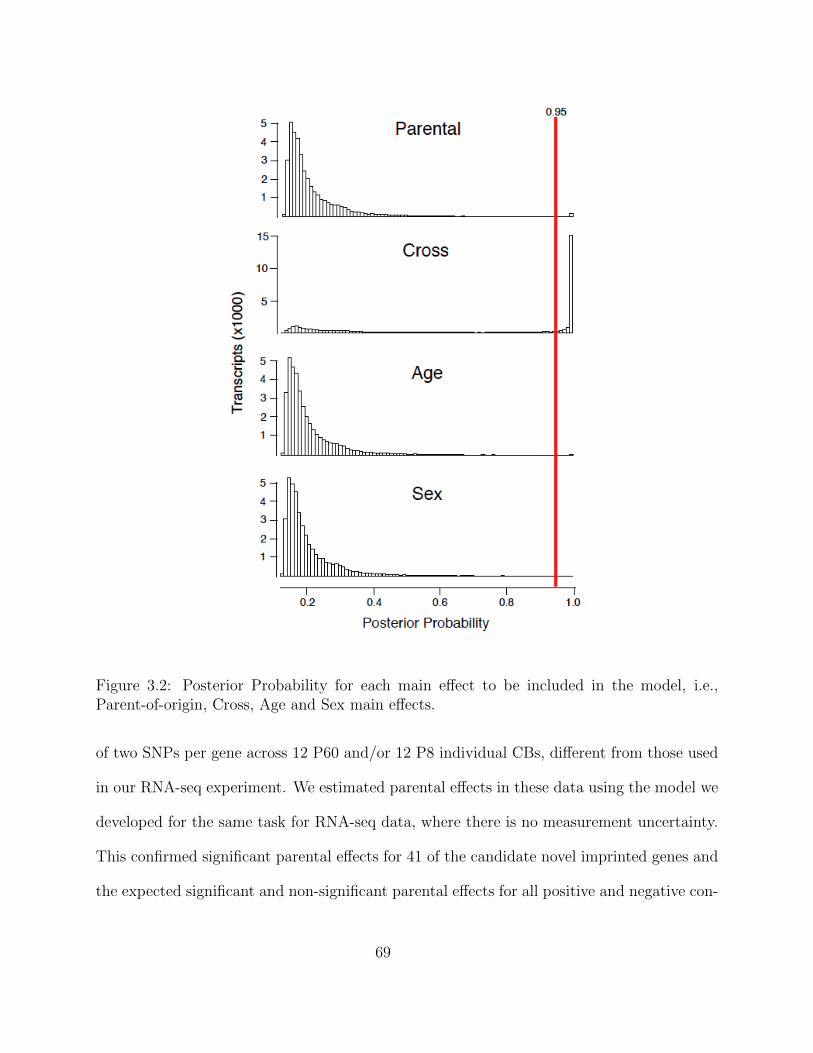
Figure 3.2: Posterior Probability for each main effect to be included in the model, i.e.,Parent-of-origin, Cross, Age and Sex main effects.
of two SNPs per gene across 12 P60 and/or 12 P8 individual CBs, different from those used
in our RNA-seq experiment. We estimated parental effects in these data using the model we
developed for the same task for RNA-seq data, where there is no measurement uncertainty.
This confirmed significant parental effects for 41 of the candidate novel imprinted genes and
the expected significant and non-significant parental effects for all positive and negative con-
69
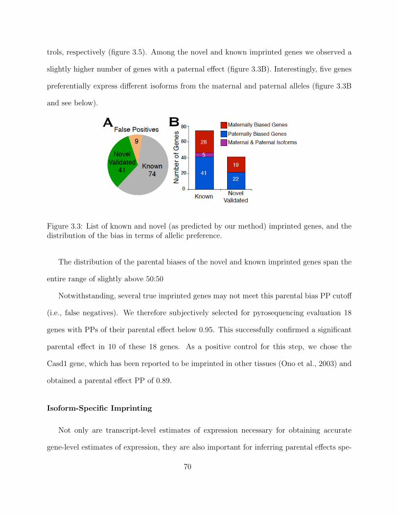
trols, respectively (figure 3.5). Among the novel and known imprinted genes we observed a
slightly higher number of genes with a paternal effect (figure 3.3B). Interestingly, five genes
preferentially express different isoforms from the maternal and paternal alleles (figure 3.3B
and see below).
Figure 3.3: List of known and novel (as predicted by our method) imprinted genes, and thedistribution of the bias in terms of allelic preference.
The distribution of the parental biases of the novel and known imprinted genes span the
entire range of slightly above 50:50
Notwithstanding, several true imprinted genes may not meet this parental bias PP cutoff
(i.e., false negatives). We therefore subjectively selected for pyrosequencing evaluation 18
genes with PPs of their parental effect below 0.95. This successfully confirmed a significant
parental effect in 10 of these 18 genes. As a positive control for this step, we chose the
Casd1 gene, which has been reported to be imprinted in other tissues (Ono et al., 2003) and
obtained a parental effect PP of 0.89.
Isoform-Specific Imprinting
Not only are transcript-level estimates of expression necessary for obtaining accurate
gene-level estimates of expression, they are also important for inferring parental effects spe-
70
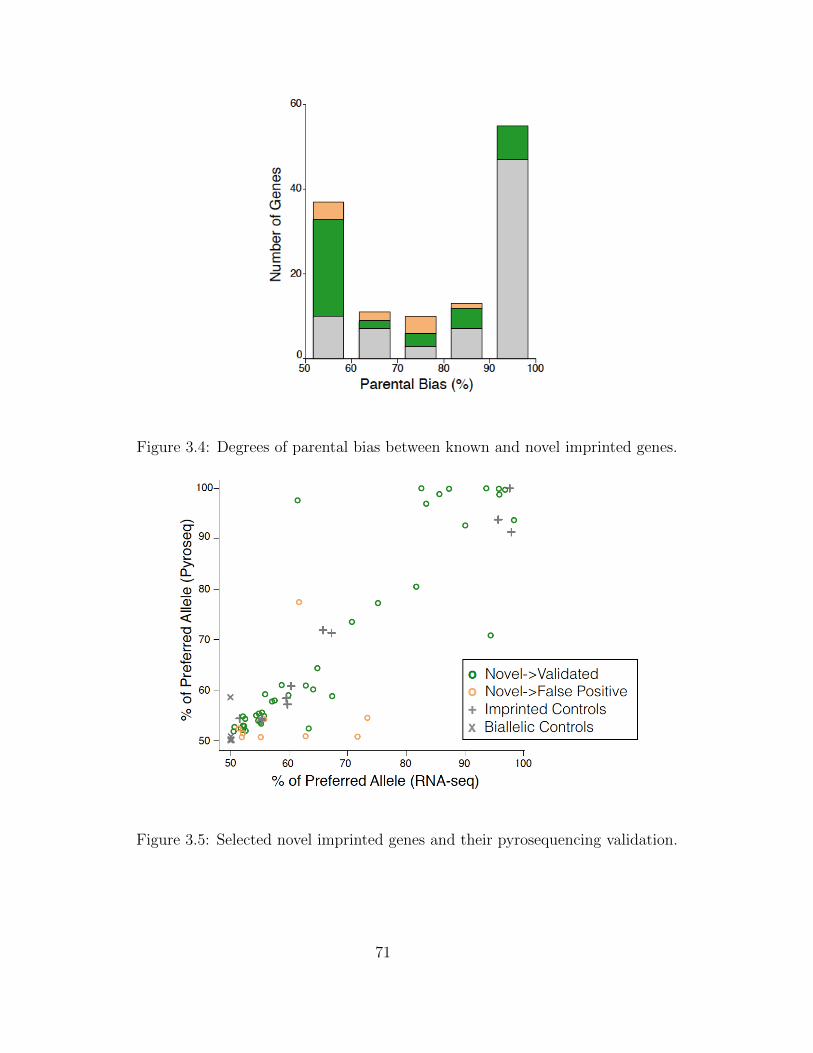
Figure 3.4: Degrees of parental bias between known and novel imprinted genes.
Figure 3.5: Selected novel imprinted genes and their pyrosequencing validation.
71
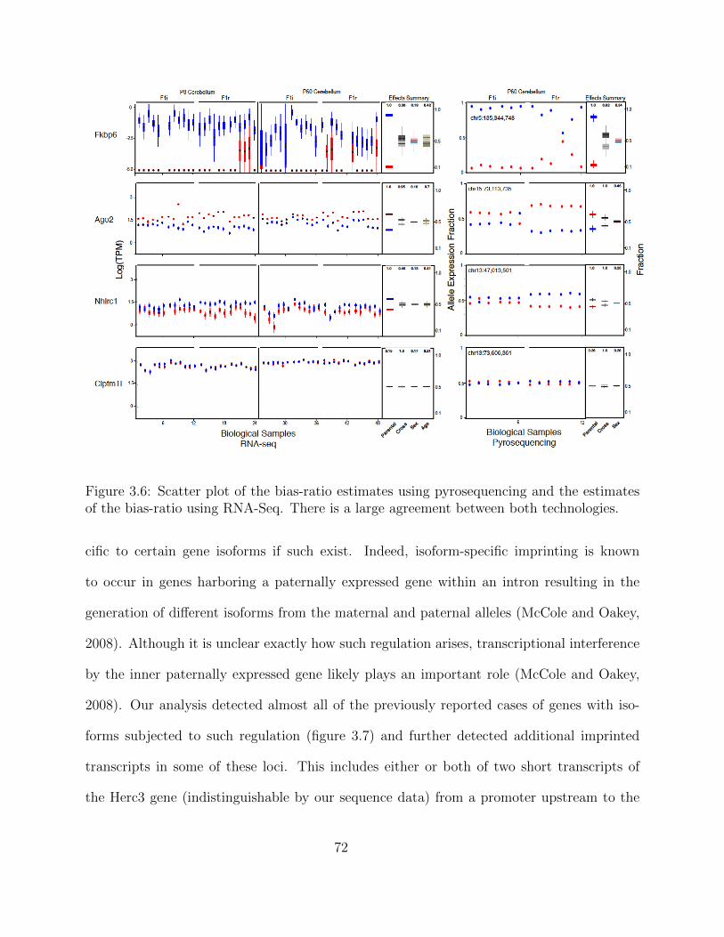
Figure 3.6: Scatter plot of the bias-ratio estimates using pyrosequencing and the estimatesof the bias-ratio using RNA-Seq. There is a large agreement between both technologies.
cific to certain gene isoforms if such exist. Indeed, isoform-specific imprinting is known
to occur in genes harboring a paternally expressed gene within an intron resulting in the
generation of different isoforms from the maternal and paternal alleles (McCole and Oakey,
2008). Although it is unclear exactly how such regulation arises, transcriptional interference
by the inner paternally expressed gene likely plays an important role (McCole and Oakey,
2008). Our analysis detected almost all of the previously reported cases of genes with iso-
forms subjected to such regulation (figure 3.7) and further detected additional imprinted
transcripts in some of these loci. This includes either or both of two short transcripts of
the Herc3 gene (indistinguishable by our sequence data) from a promoter upstream to the
72
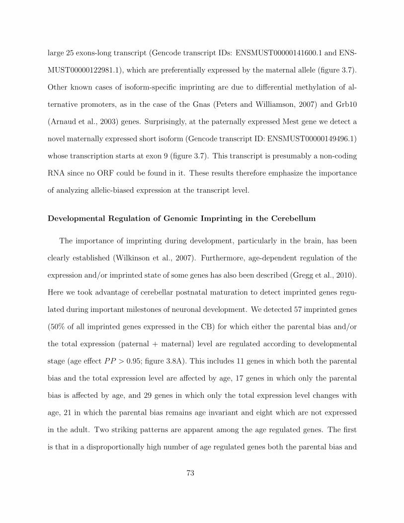
large 25 exons-long transcript (Gencode transcript IDs: ENSMUST00000141600.1 and ENS-
MUST00000122981.1), which are preferentially expressed by the maternal allele (figure 3.7).
Other known cases of isoform-specific imprinting are due to differential methylation of al-
ternative promoters, as in the case of the Gnas (Peters and Williamson, 2007) and Grb10
(Arnaud et al., 2003) genes. Surprisingly, at the paternally expressed Mest gene we detect a
novel maternally expressed short isoform (Gencode transcript ID: ENSMUST00000149496.1)
whose transcription starts at exon 9 (figure 3.7). This transcript is presumably a non-coding
RNA since no ORF could be found in it. These results therefore emphasize the importance
of analyzing allelic-biased expression at the transcript level.
Developmental Regulation of Genomic Imprinting in the Cerebellum
The importance of imprinting during development, particularly in the brain, has been
clearly established (Wilkinson et al., 2007). Furthermore, age-dependent regulation of the
expression and/or imprinted state of some genes has also been described (Gregg et al., 2010).
Here we took advantage of cerebellar postnatal maturation to detect imprinted genes regu-
lated during important milestones of neuronal development. We detected 57 imprinted genes
(50% of all imprinted genes expressed in the CB) for which either the parental bias and/or
the total expression (paternal + maternal) level are regulated according to developmental
stage (age effect PP > 0.95; figure 3.8A). This includes 11 genes in which both the parental
bias and the total expression level are affected by age, 17 genes in which only the parental
bias is affected by age, and 29 genes in which only the total expression level changes with
age, 21 in which the parental bias remains age invariant and eight which are not expressed
in the adult. Two striking patterns are apparent among the age regulated genes. The first
is that in a disproportionally high number of age regulated genes both the parental bias and
73
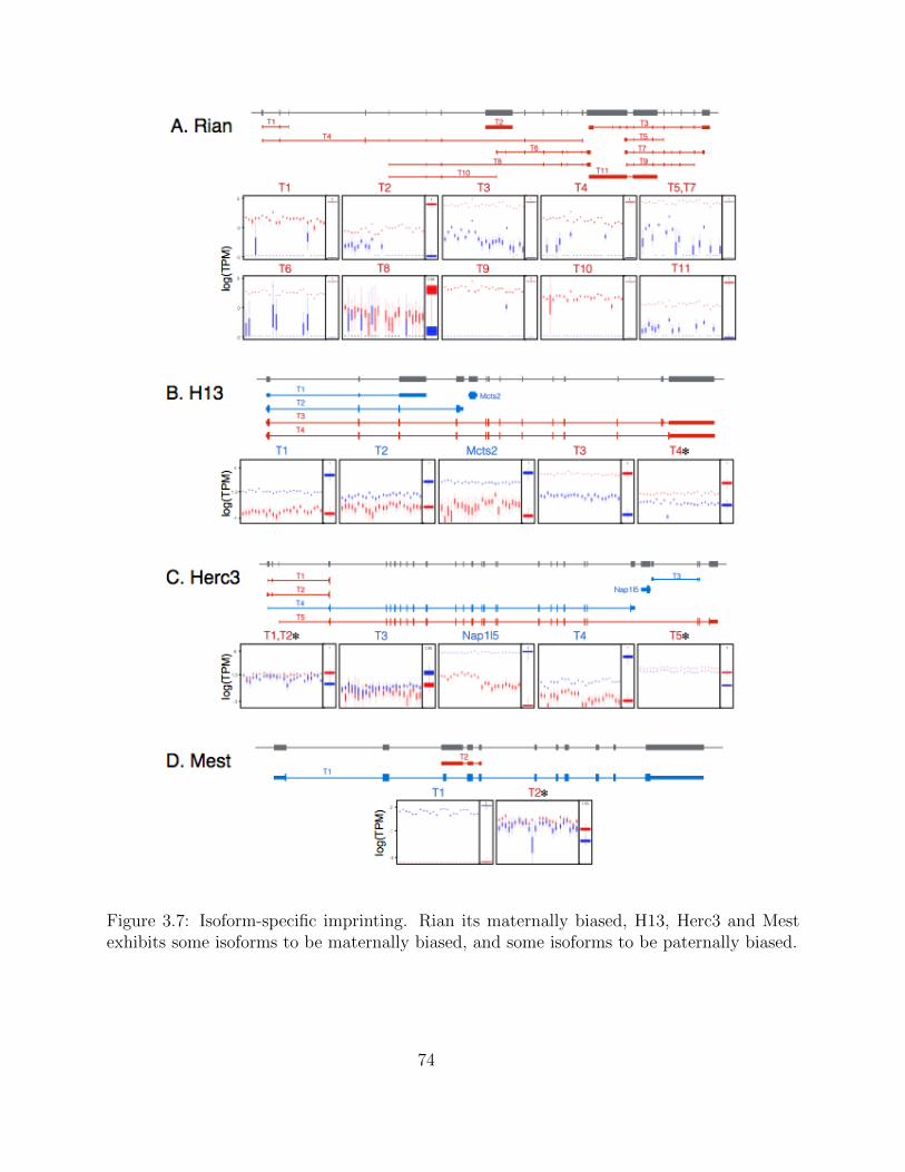
Figure 3.7: Isoform-specific imprinting. Rian its maternally biased, H13, Herc3 and Mestexhibits some isoforms to be maternally biased, and some isoforms to be paternally biased.
74
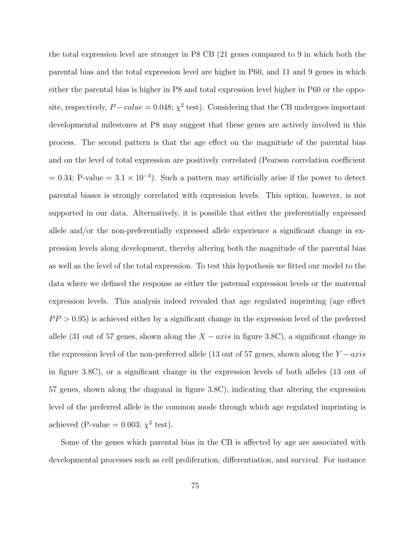
the total expression level are stronger in P8 CB (21 genes compared to 9 in which both the
parental bias and the total expression level are higher in P60, and 11 and 9 genes in which
either the parental bias is higher in P8 and total expression level higher in P60 or the oppo-
site, respectively, P −value = 0.048; χ2 test). Considering that the CB undergoes important
developmental milestones at P8 may suggest that these genes are actively involved in this
process. The second pattern is that the age effect on the magnitude of the parental bias
and on the level of total expression are positively correlated (Pearson correlation coefficient
= 0.34; P-value = 3.1 × 10⁻⁴). Such a pattern may artificially arise if the power to detect
parental biases is strongly correlated with expression levels. This option, however, is not
supported in our data. Alternatively, it is possible that either the preferentially expressed
allele and/or the non-preferentially expressed allele experience a significant change in ex-
pression levels along development, thereby altering both the magnitude of the parental bias
as well as the level of the total expression. To test this hypothesis we fitted our model to the
data where we defined the response as either the paternal expression levels or the maternal
expression levels. This analysis indeed revealed that age regulated imprinting (age effect
PP > 0.95) is achieved either by a significant change in the expression level of the preferred
allele (31 out of 57 genes, shown along the X − axis in figure 3.8C), a significant change in
the expression level of the non-preferred allele (13 out of 57 genes, shown along the Y −axis
in figure 3.8C), or a significant change in the expression levels of both alleles (13 out of
57 genes, shown along the diagonal in figure 3.8C), indicating that altering the expression
level of the preferred allele is the common mode through which age regulated imprinting is
achieved (P-value = 0.003; χ2 test).
Some of the genes which parental bias in the CB is affected by age are associated with
developmental processes such as cell proliferation, differentiation, and survival. For instance
75
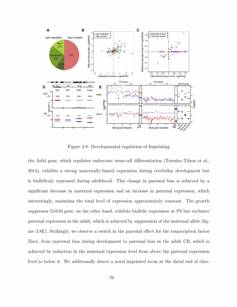
Figure 3.8: Developmental regulation of Imprinting
the Asb4 gene, which regulates embryonic stem-cell differentiation (Townley-Tilson et al.,
2014), exhibits a strong maternally-biased expression during cerebellar development but
is biallelicaly expressed during adulthood. This change in parental bias is achieved by a
significant decrease in maternal expression and an increase in paternal expression, which
interestingly, maintains the total level of expression approximately constant. The growth
suppressor Grb10 gene, on the other hand, exhibits biallelic expression at P8 but exclusive
paternal expression in the adult, which is achieved by suppression of the maternal allele (fig-
ure 3.8E). Strikingly, we observe a switch in the parental effect for the transcription factor
Zim1, from maternal bias during development to paternal bias in the adult CB, which is
achieved by reduction in the maternal expression level from above the paternal expression
level to below it. We additionally detect a novel imprinted locus at the distal end of chro-
76
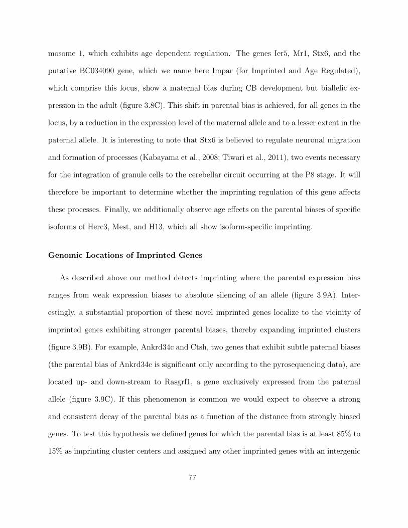
mosome 1, which exhibits age dependent regulation. The genes Ier5, Mr1, Stx6, and the
putative BC034090 gene, which we name here Impar (for Imprinted and Age Regulated),
which comprise this locus, show a maternal bias during CB development but biallelic ex-
pression in the adult (figure 3.8C). This shift in parental bias is achieved, for all genes in the
locus, by a reduction in the expression level of the maternal allele and to a lesser extent in the
paternal allele. It is interesting to note that Stx6 is believed to regulate neuronal migration
and formation of processes (Kabayama et al., 2008; Tiwari et al., 2011), two events necessary
for the integration of granule cells to the cerebellar circuit occurring at the P8 stage. It will
therefore be important to determine whether the imprinting regulation of this gene affects
these processes. Finally, we additionally observe age effects on the parental biases of specific
isoforms of Herc3, Mest, and H13, which all show isoform-specific imprinting.
Genomic Locations of Imprinted Genes
As described above our method detects imprinting where the parental expression bias
ranges from weak expression biases to absolute silencing of an allele (figure 3.9A). Inter-
estingly, a substantial proportion of these novel imprinted genes localize to the vicinity of
imprinted genes exhibiting stronger parental biases, thereby expanding imprinted clusters
(figure 3.9B). For example, Ankrd34c and Ctsh, two genes that exhibit subtle paternal biases
(the parental bias of Ankrd34c is significant only according to the pyrosequencing data), are
located up- and down-stream to Rasgrf1, a gene exclusively expressed from the paternal
allele (figure 3.9C). If this phenomenon is common we would expect to observe a strong
and consistent decay of the parental bias as a function of the distance from strongly biased
genes. To test this hypothesis we defined genes for which the parental bias is at least 85% to
15% as imprinting cluster centers and assigned any other imprinted genes with an intergenic
77
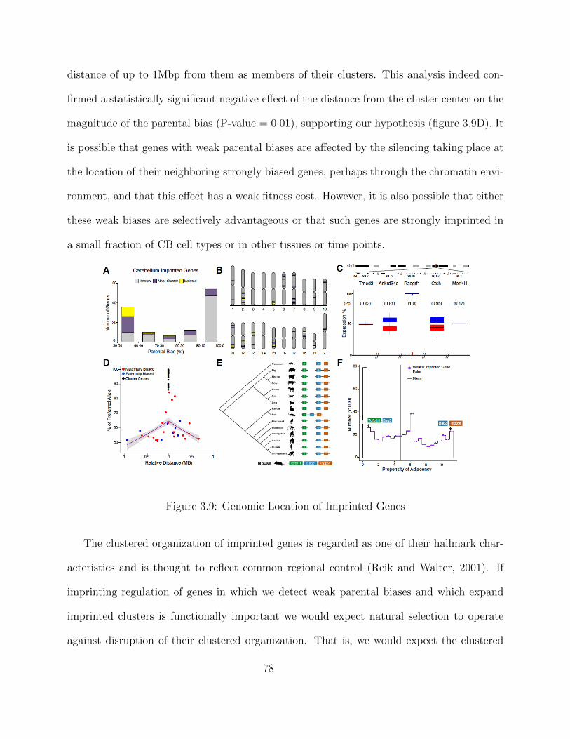
distance of up to 1Mbp from them as members of their clusters. This analysis indeed con-
firmed a statistically significant negative effect of the distance from the cluster center on the
magnitude of the parental bias (P-value = 0.01), supporting our hypothesis (figure 3.9D). It
is possible that genes with weak parental biases are affected by the silencing taking place at
the location of their neighboring strongly biased genes, perhaps through the chromatin envi-
ronment, and that this effect has a weak fitness cost. However, it is also possible that either
these weak biases are selectively advantageous or that such genes are strongly imprinted in
a small fraction of CB cell types or in other tissues or time points.
Figure 3.9: Genomic Location of Imprinted Genes
The clustered organization of imprinted genes is regarded as one of their hallmark char-
acteristics and is thought to reflect common regional control (Reik and Walter, 2001). If
imprinting regulation of genes in which we detect weak parental biases and which expand
imprinted clusters is functionally important we would expect natural selection to operate
against disruption of their clustered organization. That is, we would expect the clustered
78
organization, or micro-synteny, of such genes to be conserved during mammalian evolution.
On the other hand, if imprinting regulation of these genes is not functionally important
we would not expect the micro-synteny of these genes to be conserved across mammalian
genomes. To test these hypotheses, we derived all pairs of adjacent genes in the mouse
genome and estimated the propensity of their mammalian orthologs to be adjacent as well
(figure 3.9E), using a probabilistic phylogenetic model analyzing phyletic patterns of presence
and absence (Cohen and Pupko, 2011). This revealed that the mean propensity of adjacency
of orthologs of mouse adjacent imprinted gene pairs, with parental biases lower than 85% to
15%, is significantly higher than the mean propensity of adjacency of orthologs of all mouse
adjacent gene pairs (P-value = 4.8× 10⁻⁵, figure 3.9F). This finding therefore supports the
hypothesis that imprinting regulation of mouse genes, for which we detect weak parental
biases, is functionally important. It also suggests that the orthologs of many of these genes
are imprinted in the analyzed comparative mammalian species.
Notwithstanding, the genomic locations of several novel imprinted genes exhibiting mild
parental biases are isolated from any other imprinted gene (> 2Mbp away). Indeed, previous
studies have reported differential methylation between the two alleles for some of these genes.
For example, differential methylation was observed in a region of chromosome 13 immediately
downstream of Nhlrc1 (Xie et al., 2012), a novel paternally biased gene in our results. In
humans, mutations in Nhlrc1 cause Lafora progressive myoclonic epilepsy (RomMateo et
al., 2012), a fatal neurological disorder characterized by the presence of massive intracellular
inclusions observed in several neuronal cell types across the brain including the cerebellar
granule cells. Differential methylation but not parentally biased expression was also reported
within the Actinin alpha 1 (Actn1) gene at chromosome 12 (Calaway and Domnguez, 2012),
which codes for a protein that regulates cytoskeleton interactions with the membrane. Our
79
results show that this gene is indeed preferentially expressed from the paternal allele.
Spatial Regulation of Genomic Imprinting
Tissue-dependent regulation has been described for several imprinted genes (Prickett
and Oakey, 2012). We chose to extend the survey of tissue-specific imprinting patterns
by analyzing parentally-biased expression of 28 imprinted genes (20 known and 8 novel),
from pyrosequencing data obtained from 16 brain macro-regions and seven non-brain tis-
sues, all from adult animals (figure 3.10A). This revealed several striking patterns of shared
parentally-biased expression among genes and across tissues (figure 3.10B). These patterns,
by and large, include two main spatial clades, non-brain and brain, where in the latter the
parental bias is much more consistent and robust. The brain is further subdivided into
additional sub-clades which roughly group developmentally related regions. One sub-clade
clusters most of the telencephalon, the thalamus, and cerebellum. The other sub-clade is
further split into a clade that groups mesencephalic and rhombencephalic regions and a clade
that groups diencephalic and basal ganglia regions.
Imprinted genes clearly cluster into three main clades, one that includes maternally
biased genes, one that includes paternally biased genes, and one that includes genes that
are sporadically biased in the brain, most of which are maternally biased. Several genes
exhibit sharp contrasts in their parental bias between the brain and body. This includes
genes which are exclusively or nearly exclusively biased in and throughout the brain, such
as the maternally biased Ube3a (Rougeulle et al., 1997), Trappc9, Bag3, and B3gnt2 and
the paternally biased BclX long isoform (Bcl2l1L), Inpp5f (Choi et al., 2005), and Begain.
Interestingly, Igf2, which is maternally biased in the brain (Gregg et al., 2010) but paternally
biased outside the brain (figure 3.10B), stands in contrast to the brain paternally biased
80

and body maternally biased Grb10 (Hikichi et al., 2003). The Igf2r gene, which during
developmental periods is maternally expressed and exerts a function that is antagonistic to
that of the paternally expressed Igf2 (Haig, 2004), maintains a strong maternal bias in the
body which is relaxed in most of the brain (figure 3.10B). The fact that these three genes
regulate growth in the tissues in which they are expressed (Haig, 2004), suggests different
contributions from the parental genomes to the brain and body. In addition, the Kcnk9
gene is robustly maternally biased throughout the brain whereas in the body it is either
not expressed, biallelicaly expressed, or paternally biased. Finally, the Zim1 gene shows an
intriguing pattern of both paternal and maternal biases both in the brain and in the body.
Notwithstanding the contrasting imprinting patterns between the body and the brain,
the brain itself shows considerable imprinting dynamics. We therefore repeated the previous
clustering analysis, this time confined to the brain. This revealed that the Trappc9L, Chrac1,
and Ago2 genes, which co-localize to an imprinted cluster in the distal end of chromosome
15, exhibit a very similar pattern of maternal bias across the brain, which is stronger in the
cortex and weaker in the olfactory bulb, hippocampus, and Cb. The Copg2 and Mest geness
which co-localize near the centromeric region of chromosome 6, exhibit a strongly similar
pattern to that of genes on the distal end of chromosome 15. The Zim1, Asb4, and Herc3
genes, which are located in the proximal end of chromosome 7, the proximal end chromosome
6, and near the centromeric region of chromosome 6, respectively, also exhibit shared patterns
of biallelic expression (or in the case of Zim1 weak paternal biases) in telencephalic regions
and Cb but strong maternal biases in other brain regions. These results suggest that the
brain executes region-specific programs of imprinting. Moreover, the genes utilized in these
programs are not necessarily from the same imprinted cluster, suggesting a higher order of
regulation.
81
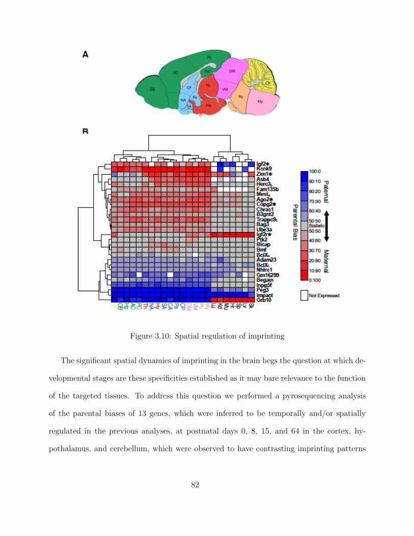
Figure 3.10: Spatial regulation of imprinting
The significant spatial dynamics of imprinting in the brain begs the question at which de-
velopmental stages are these specificities established as it may bare relevance to the function
of the targeted tissues. To address this question we performed a pyrosequencing analysis
of the parental biases of 13 genes, which were inferred to be temporally and/or spatially
regulated in the previous analyses, at postnatal days 0, 8, 15, and 64 in the cortex, hy-
pothalamus, and cerebellum, which were observed to have contrasting imprinting patterns
82
in the previous analysis. We additionally analyzed the parental bias of these genes in the
entire E15 brain. This revealed substantial spatio-temporal dynamics of the parental bias of
several genes (figure 3.11). For instance, Blcap experiences a gradual decrease in maternal
bias along the age axis, which is consistent across the three analyzed brain regions. In con-
trast, the switch from maternal to paternal bias of Zim1 during Cb development, mentioned
above, occurs gradually along development in both the Cb and cortex, yet is not mirrored in
the hypothalamus where maternal bias is strongly maintained up to adulthood. Moreover,
this analysis revealed that the sharp contrast between the parental biases of Igf2 and Grb10,
observed across the brain, seem to be co-temporally regulated. The switch in the expressed
allele for both genes happens earlier in the cortex and hypothalamus than in the Cb, which
roughly coincides with the completion of their development. These results highlight that
imprinting needs to be considered as a spatio-temporally dynamic process in the context of
the specific targeted pathways.
3.5 Sensitivity Analysis
We follow Chipman et al. (1997) in setting ν to a value near two (specifically 2.5) and
setting λ =2√
(var(y))
51ν
(v2− 1). Since var(y) = 1 for all transcripts, for ν we get λ = 0.04.
We chose τ and c of all transcripts to have empirical values of 0.1 and 4.25, respectively, in
order to provide a good separation between imprinted and non-imprinted transcripts at the
selected PP = 0.95 cutoff. In addition, we set to p of all effects to 0.1, reflecting our prior
belief of the effects being significant. Although the choice of these hyper-parameter values
is arbitrary to some extent, if the model is robust this choice should not affect the ranking
of the δ estimates but merely their values. Therefore, in order to evaluate how the inference
83
of genomic imprinting by our model is affected by our choice of empirical hyper-parameter
values we performed the following sensitivity analysis. The empirical value that we chose
for each of the five hyper-parameters: τ , c, ν, λ and p, was perturbed by selecting four
other values. Specifically, we perturbed the empirical τ = 0.1 value with 0.005, 0.01, 1, and
2 thus both lowering and elevating the posterior probability of an effect begin significant;
we perturbed the empirical value c = 4.25 only with the higher values: 1.7, 3.4, 5.3125, and
10.625 as 4.25 was found to be around the minimal value for detecting significant effects; we
perturbed the empirical value ν = 2.5 with 5, 12.5, 25, and 50 as ν cannot assume values lower
than 2; we perturbed the empirical value λ = 0.04 with 0.002, 0.004, 0.4, and 0.8 shifting the
prior distribution from informative to uninformative; and finally, we perturbed the empirical
value p = 0.1 with higher prior probabilities of 0.2, 0.3, 0.4, and 0.5.
In each such perturbation we re-fitted our model to the data where all other hyper-
parameter values are held fixed at their original empirical unperturbed values (thereby
achieving a one-at-a-time sensitivity analysis). We assessed the perturbed results using
a receiver operating characteristic (ROC) analysis in which the imprinted transcripts ob-
tained by the unperturbed inferences were used as the ground-truth positives, and all other
non-imprinted transcripts were used as ground-truth negatives. For practical computational
considerations, for all perturbations we used a random sample of 10% of the 38, 112 tran-
scripts in our data set. For this sample to reflect the transcripts proportionally with respect
to the PP of their parental effect, we binned the 38, 112 parental effect PP distribution to a
100 bin histogram and randomly sampled 10% from each bin. In all perturbations the area
under the ROC curve (AUC) was found to be 1, except for the τ = 1 and τ = 2 perturbations
which obtained AUCs of 0.99 and 0.95, respectively (figure 3.12). These results therefore
indicate that the ranking of transcripts according to the PP of the parental effect, obtained
84

by our model, is robust to the choice of hyper-parameter empirical values. Therefore, the
practice employed in this study of selecting empirical values, setting a parental effect PP
cutoff, and experimentally confirming all transcripts with a PP of parental effect above that
cutoff, is a reasonable choice for obtaining reliable inference of genomic imprinting from
RNA-seq data.
3.5.1 Single Model across all genes, and correlation structure
In order to asses our confidence in our posterior estimates and our model we propose
a full model across all genes. We believe that a pontentially sensible assumptions is the
independence between the expression estimates for each gene/isoform. Thus here we propose
to fit a model that does not assume independence between gene/isoform expression. We also
try different priors for σ, since we would like our model to be robust to different assumptions
with respect to the error term in the regression part of the model. We believe that the
assumption of normality of the response, and the linear relationship between the response
and the factors are robust enough so we did not try change such assumptions in our sensitivity
models.
Let us focus now on how to incorporate the covariance structure in the model, since some
non-trivial calculations must be made to the model and the gibbs sampler to fit this new
model.
Let us now write the response as y = (y1, . . . ,yG) is a vector of dimensions (N ×G)× 1,
and now we model all the genes as coming from a common multivariate normal distribution,
y ∼ Nn×g (z, E)
85

where, z = (z1, . . . ,zG), and E a matrix of dimensions (N ×G)× (N ×G), of the form,
E =
diag (ε11) · · · diag (ε1G)
.... . .
...
diag (εG1) · · · diag (εGG)
with, diag (εij) a diagonal matrix of dimensions N ×N containing the estimated covariance
between gene/isoform i and j for each of the N replicates. Thus, the major change is in the
dimensions of the combined (across all genes) data, and in the structure of the covariance
matrix E. We also use the following notation for the other variables in the model,
β = (β1, . . . ,βG)
δ = (δ1, . . . , δG)
and we also write the design matrix X as a block diagonal matrix of dimensions (N ×G)×
(K ×G),
X =
X1 · · · 0
.... . .
...
0 · · · XG
Xβ =
X1β1
...
XGβG
86
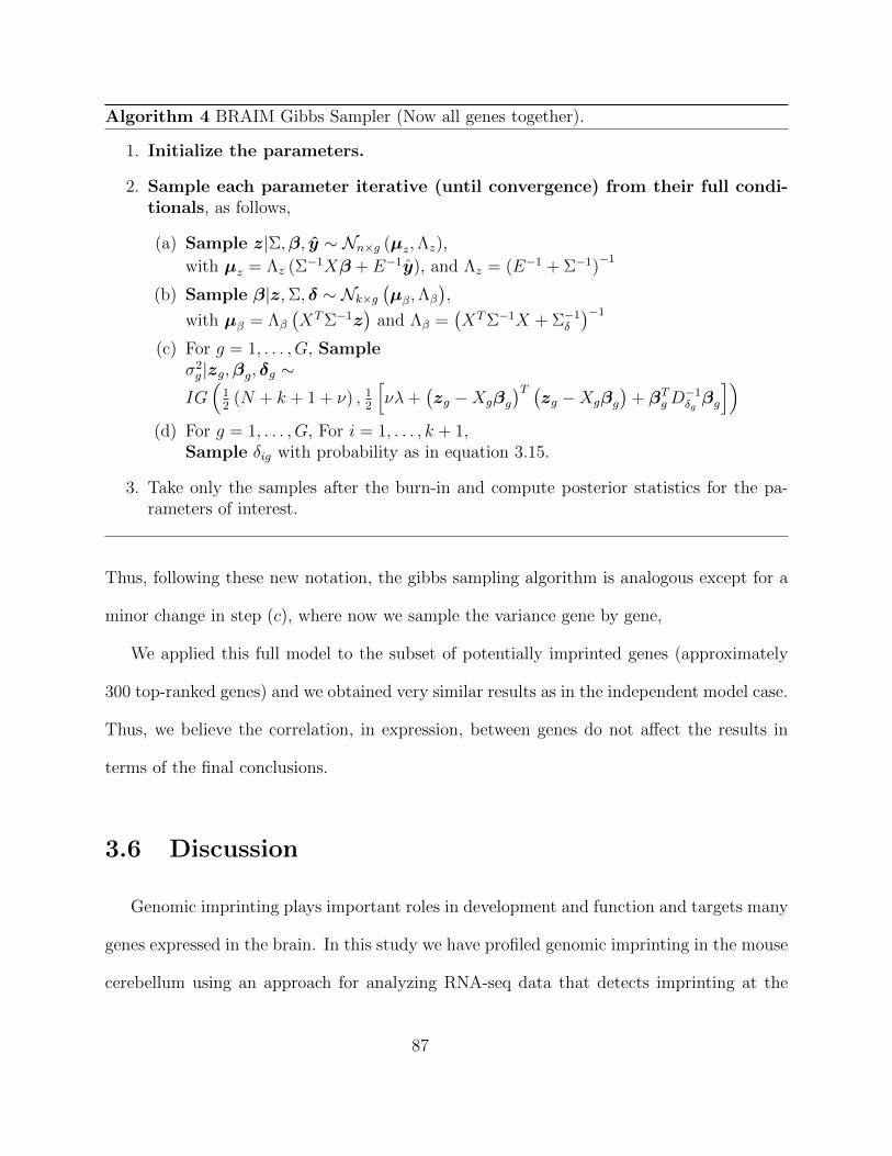
Algorithm 4 BRAIM Gibbs Sampler (Now all genes together).
1. Initialize the parameters.
2. Sample each parameter iterative (until convergence) from their full condi-tionals, as follows,
(a) Sample z|Σ,β, y ∼ Nn×g (µz,Λz),
with µz = Λz (Σ−1Xβ + E−1y), and Λz = (E−1 + Σ−1)−1
(b) Sample β|z,Σ, δ ∼ Nk×g(µβ,Λβ
),
with µβ = Λβ
(XTΣ−1z
)and Λβ =
(XTΣ−1X + Σ−1
δ
)−1
(c) For g = 1, . . . , G, Sampleσ2g |zg,βg, δg ∼IG(
12
(N + k + 1 + ν) , 12
[νλ+
(zg −Xgβg
)T (zg −Xgβg
)+ βTgD
−1δgβg
])(d) For g = 1, . . . , G, For i = 1, . . . , k + 1,
Sample δig with probability as in equation 3.15.
3. Take only the samples after the burn-in and compute posterior statistics for the pa-rameters of interest.
Thus, following these new notation, the gibbs sampling algorithm is analogous except for a
minor change in step (c), where now we sample the variance gene by gene,
We applied this full model to the subset of potentially imprinted genes (approximately
300 top-ranked genes) and we obtained very similar results as in the independent model case.
Thus, we believe the correlation, in expression, between genes do not affect the results in
terms of the final conclusions.
3.6 Discussion
Genomic imprinting plays important roles in development and function and targets many
genes expressed in the brain. In this study we have profiled genomic imprinting in the mouse
cerebellum using an approach for analyzing RNA-seq data that detects imprinting at the
87
individual transcript level and simultaneously estimates the effects that all factors in the
experimental design, namely age, sex, and the mouse cross, have on it. The most relevant
experimental factor in question was the cross-effect, since approximately 18% of the genes
showed an strong cross-effect when explaining their allelic imbalance. In addition the high
sequencing depth allowed us to detect imbalances for lowly expressed genes that otherwise
we would have potentially dismissed as non-imprinted genes. Finally, the large number of
replicates was a very important step since it allowed us to have a much stronger confidence
in our findings.
Importantly, in our data, most of the newly discovered imprinted genes and a considerable
number of the known imprinted genes show parental expression biases with magnitudes
weaker than the traditionally accepted all-to-none. This higher resolution of detection is
clearly contributed both by our powerful experimental design as well as by our sensitive
approach. Currently, our experiments cannot distinguish whether the weak parental biases
are uniform across the tissues we sampled or result from averaging variable magnitudes of
parental biases specific to individual cell types, as in the case of a nephron-specific cell
type imprinting of the Gnas gene (Weinstein et al., 2000) and neuron-specific imprinting
of the Snx14 gene (Huang et al., 2014). Resolving between the two options for all the
weakly biased imprinted genes clearly requires more sensitive high-throughput approaches.
However, the imprinting regulation of these genes, in at least some of the CB cell types,
is corroborated by several lines evidence. First, many of these genes are located by or at
known imprinted clusters and this localization is observed to be evolutionarily conserved
suggesting it is under purifying selection. In addition, some of the isolated weakly biased
genes have putative imprinting control regions. Second, the parental biases of many of these
genes show both tissue and developmental-stage specificities. Third, many of these genes
88

are implicated to participate in the same biological pathways, including cell survival and
apoptosis, as strongly biased genes.
89
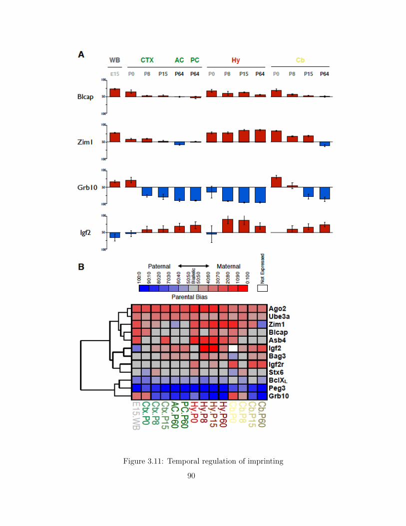
Figure 3.11: Temporal regulation of imprinting
90
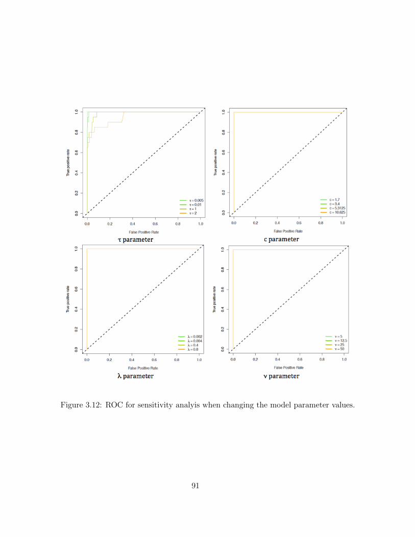
Figure 3.12: ROC for sensitivity analyis when changing the model parameter values.
91
Chapter 4
Allele-Specific Regulation in Human
Population across Multiple Tissues
About 99 percent of genes in humans have counterparts in the mouse. Eighty
percent have identical, one-to-one counterparts.
- Eric Lander
4.1 The GTEx Project Consortium
During my PhD., thanks to my advisor, I was lucky to have access to genotype data for
many individuals (185),and their respective gene-expression across multiple ex-vivo tissues
(10). The project I am referring to is the Genotype-Tissue Expression project (GTEx) and
the overarching aim of the project, as stated in their website, is to provide to the scientific
community a resource with which to study human gene expression and regulation and its
relationship to genetic variation.
This is an ambitious goal but the data certainly provides enough information, for at
92
least, in a given population of individuals, be able to identify wich variants may regulate the
expression of a gene - such type of variants are called eQTLs, and it stands for expression
quantitative trait loci. There is a clear limitation in the sense that it is not an ATLAS of
ALL the regulatory elements in the genome, since the data will certainly miss regulatory
regions that do not span a genetic variant, or will miss regulatory regions for SNPs with very
low MAF (minor allele frequency) due to low number of replicates.
Nevertheless, several other projects have tried to map the regulatory activity, though the
use of ChIP sequencing methods in order to better understand gene regulation across multiple
cell types. For example the ENCODE project used several cell lines to identify TF binding
sites, Histone modification sites, DNA methylation regions and DNA hypersensitivity sites.
Another project closely related, but with the aim to identify regulatory regions in ex-vivo
tissues as opossed to cultured-in-vitro cell lines is the Epigenomics Roadmap project. Finally,
it is worth mentioning the FANTOM project, wich just published an ATLAS of enhancers
across multiple tissues. These projects are complimentary to the GTEx consortium since
they can help us in the interpretation of the eQTL results.
In this chapter of the thesis we extend our allelic imbalance models from previous chapters
to its applications in the context of population studies, such as the GTEx project.
4.2 Experimental Design and Computational Workflow
The GTEx project collected gene expression across multiple tissues, and genotype data
from blood samples across multiple post-mortem donors (individuals). For a graphical ver-
sion of the GTEx experimental design please refer to figure 4.1.
More specifically, the GTEx project consortium has collected RNA-Seq sample from as
93
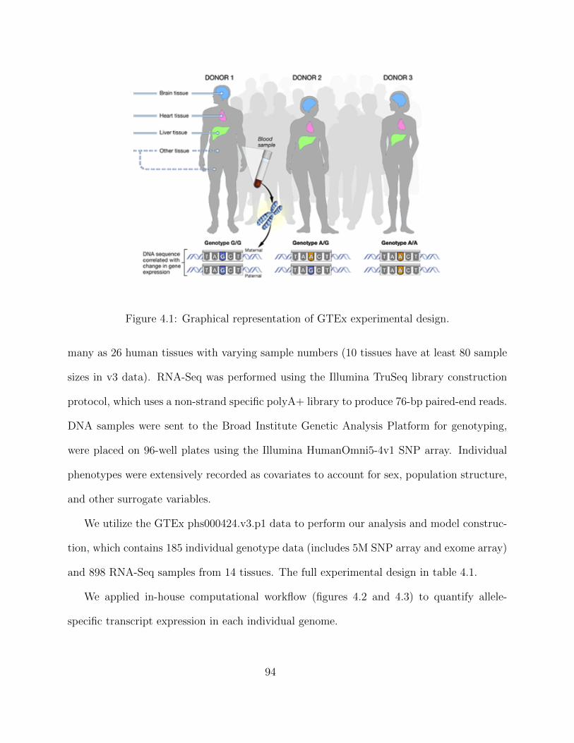
Figure 4.1: Graphical representation of GTEx experimental design.
many as 26 human tissues with varying sample numbers (10 tissues have at least 80 sample
sizes in v3 data). RNA-Seq was performed using the Illumina TruSeq library construction
protocol, which uses a non-strand specific polyA+ library to produce 76-bp paired-end reads.
DNA samples were sent to the Broad Institute Genetic Analysis Platform for genotyping,
were placed on 96-well plates using the Illumina HumanOmni5-4v1 SNP array. Individual
phenotypes were extensively recorded as covariates to account for sex, population structure,
and other surrogate variables.
We utilize the GTEx phs000424.v3.p1 data to perform our analysis and model construc-
tion, which contains 185 individual genotype data (includes 5M SNP array and exome array)
and 898 RNA-Seq samples from 14 tissues. The full experimental design in table 4.1.
We applied in-house computational workflow (figures 4.2 and 4.3) to quantify allele-
specific transcript expression in each individual genome.
94
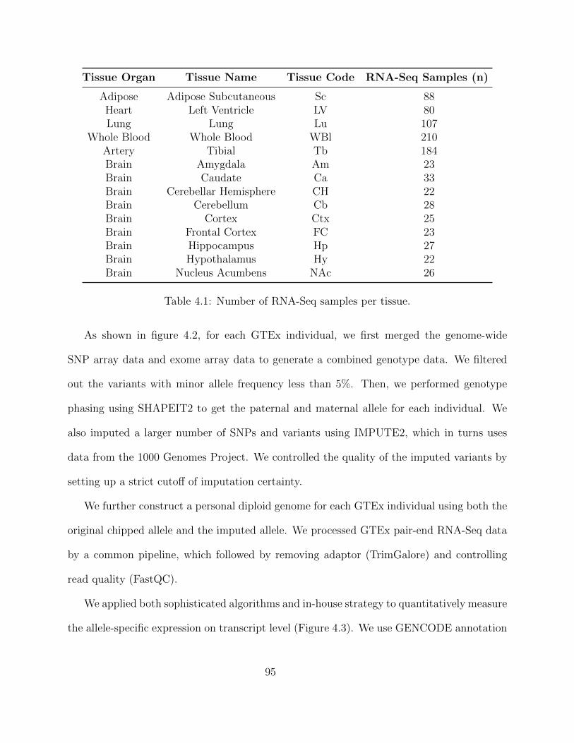
Tissue Organ Tissue Name Tissue Code RNA-Seq Samples (n)
Adipose Adipose Subcutaneous Sc 88Heart Left Ventricle LV 80Lung Lung Lu 107
Whole Blood Whole Blood WBl 210Artery Tibial Tb 184Brain Amygdala Am 23Brain Caudate Ca 33Brain Cerebellar Hemisphere CH 22Brain Cerebellum Cb 28Brain Cortex Ctx 25Brain Frontal Cortex FC 23Brain Hippocampus Hp 27Brain Hypothalamus Hy 22Brain Nucleus Acumbens NAc 26
Table 4.1: Number of RNA-Seq samples per tissue.
As shown in figure 4.2, for each GTEx individual, we first merged the genome-wide
SNP array data and exome array data to generate a combined genotype data. We filtered
out the variants with minor allele frequency less than 5%. Then, we performed genotype
phasing using SHAPEIT2 to get the paternal and maternal allele for each individual. We
also imputed a larger number of SNPs and variants using IMPUTE2, which in turns uses
data from the 1000 Genomes Project. We controlled the quality of the imputed variants by
setting up a strict cutoff of imputation certainty.
We further construct a personal diploid genome for each GTEx individual using both the
original chipped allele and the imputed allele. We processed GTEx pair-end RNA-Seq data
by a common pipeline, which followed by removing adaptor (TrimGalore) and controlling
read quality (FastQC).
We applied both sophisticated algorithms and in-house strategy to quantitatively measure
the allele-specific expression on transcript level (Figure 4.3). We use GENCODE annotation
95
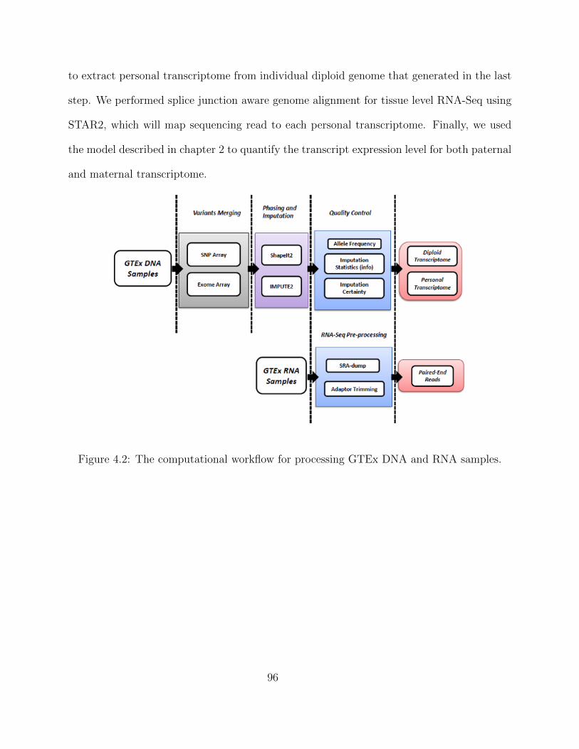
to extract personal transcriptome from individual diploid genome that generated in the last
step. We performed splice junction aware genome alignment for tissue level RNA-Seq using
STAR2, which will map sequencing read to each personal transcriptome. Finally, we used
the model described in chapter 2 to quantify the transcript expression level for both paternal
and maternal transcriptome.
Figure 4.2: The computational workflow for processing GTEx DNA and RNA samples.
96
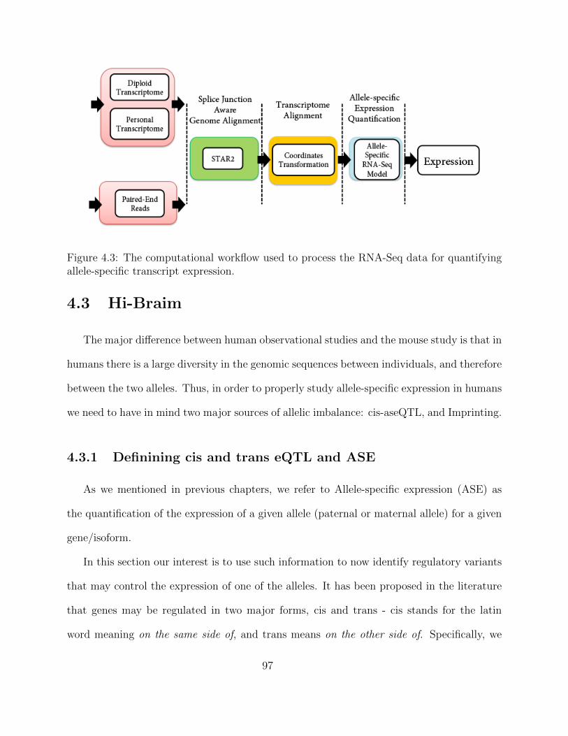
Figure 4.3: The computational workflow used to process the RNA-Seq data for quantifyingallele-specific transcript expression.
4.3 Hi-Braim
The major difference between human observational studies and the mouse study is that in
humans there is a large diversity in the genomic sequences between individuals, and therefore
between the two alleles. Thus, in order to properly study allele-specific expression in humans
we need to have in mind two major sources of allelic imbalance: cis-aseQTL, and Imprinting.
4.3.1 Definining cis and trans eQTL and ASE
As we mentioned in previous chapters, we refer to Allele-specific expression (ASE) as
the quantification of the expression of a given allele (paternal or maternal allele) for a given
gene/isoform.
In this section our interest is to use such information to now identify regulatory variants
that may control the expression of one of the alleles. It has been proposed in the literature
that genes may be regulated in two major forms, cis and trans - cis stands for the latin
word meaning on the same side of, and trans means on the other side of. Specifically, we
97
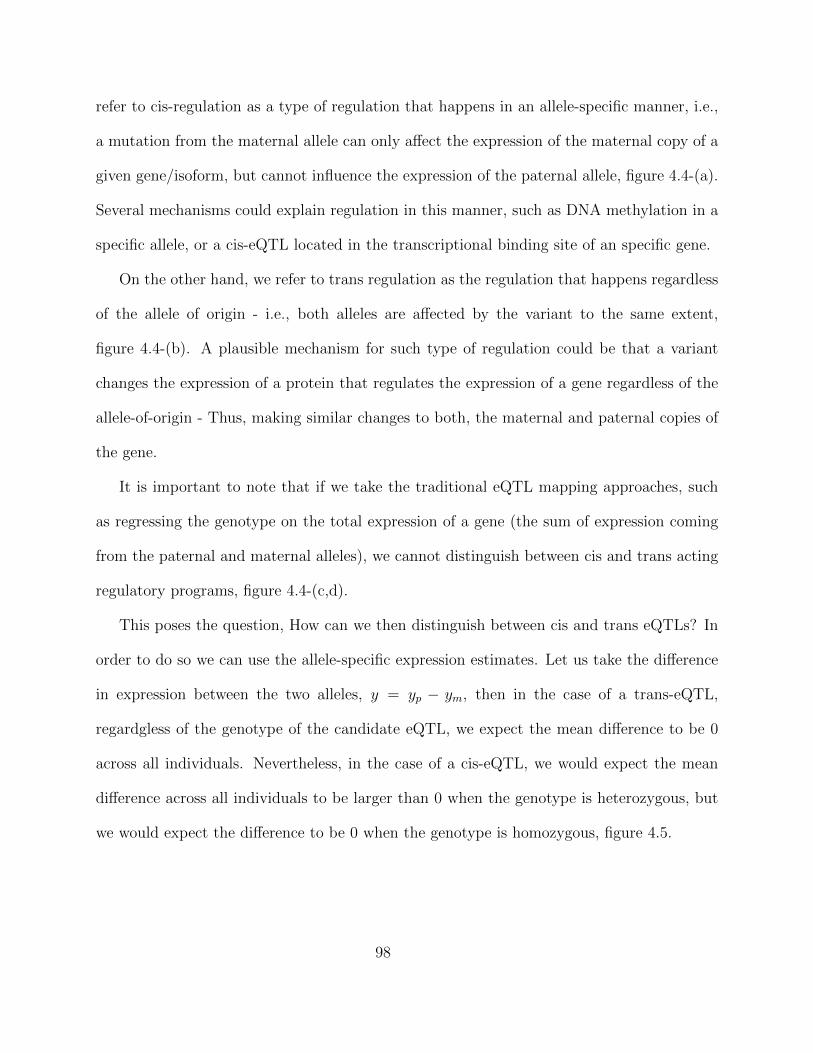
refer to cis-regulation as a type of regulation that happens in an allele-specific manner, i.e.,
a mutation from the maternal allele can only affect the expression of the maternal copy of a
given gene/isoform, but cannot influence the expression of the paternal allele, figure 4.4-(a).
Several mechanisms could explain regulation in this manner, such as DNA methylation in a
specific allele, or a cis-eQTL located in the transcriptional binding site of an specific gene.
On the other hand, we refer to trans regulation as the regulation that happens regardless
of the allele of origin - i.e., both alleles are affected by the variant to the same extent,
figure 4.4-(b). A plausible mechanism for such type of regulation could be that a variant
changes the expression of a protein that regulates the expression of a gene regardless of the
allele-of-origin - Thus, making similar changes to both, the maternal and paternal copies of
the gene.
It is important to note that if we take the traditional eQTL mapping approaches, such
as regressing the genotype on the total expression of a gene (the sum of expression coming
from the paternal and maternal alleles), we cannot distinguish between cis and trans acting
regulatory programs, figure 4.4-(c,d).
This poses the question, How can we then distinguish between cis and trans eQTLs? In
order to do so we can use the allele-specific expression estimates. Let us take the difference
in expression between the two alleles, y = yp − ym, then in the case of a trans-eQTL,
regardgless of the genotype of the candidate eQTL, we expect the mean difference to be 0
across all individuals. Nevertheless, in the case of a cis-eQTL, we would expect the mean
difference across all individuals to be larger than 0 when the genotype is heterozygous, but
we would expect the difference to be 0 when the genotype is homozygous, figure 4.5.
98
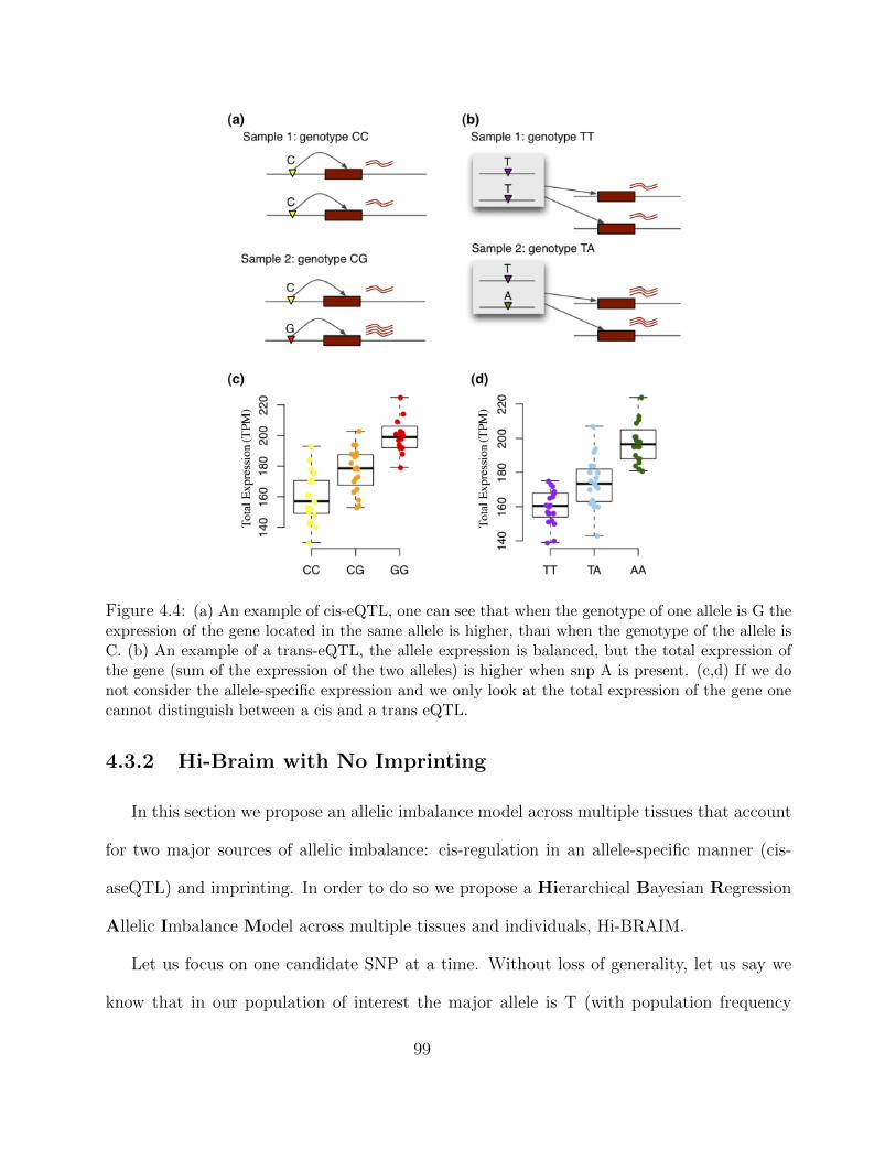
Figure 4.4: (a) An example of cis-eQTL, one can see that when the genotype of one allele is G theexpression of the gene located in the same allele is higher, than when the genotype of the allele isC. (b) An example of a trans-eQTL, the allele expression is balanced, but the total expression ofthe gene (sum of the expression of the two alleles) is higher when snp A is present. (c,d) If we donot consider the allele-specific expression and we only look at the total expression of the gene onecannot distinguish between a cis and a trans eQTL.
4.3.2 Hi-Braim with No Imprinting
In this section we propose an allelic imbalance model across multiple tissues that account
for two major sources of allelic imbalance: cis-regulation in an allele-specific manner (cis-
aseQTL) and imprinting. In order to do so we propose a Hierarchical Bayesian Regression
Allelic Imbalance Model across multiple tissues and individuals, Hi-BRAIM.
Let us focus on one candidate SNP at a time. Without loss of generality, let us say we
know that in our population of interest the major allele is T (with population frequency
99
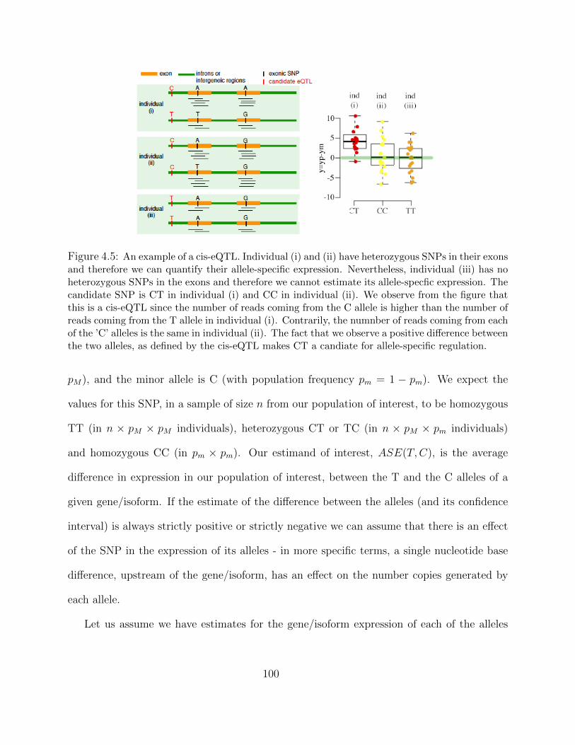
Figure 4.5: An example of a cis-eQTL. Individual (i) and (ii) have heterozygous SNPs in their exonsand therefore we can quantify their allele-specific expression. Nevertheless, individual (iii) has noheterozygous SNPs in the exons and therefore we cannot estimate its allele-specfic expression. Thecandidate SNP is CT in individual (i) and CC in individual (ii). We observe from the figure thatthis is a cis-eQTL since the number of reads coming from the C allele is higher than the number ofreads coming from the T allele in individual (i). Contrarily, the numnber of reads coming from eachof the ’C’ alleles is the same in individual (ii). The fact that we observe a positive difference betweenthe two alleles, as defined by the cis-eQTL makes CT a candiate for allele-specific regulation.
pM), and the minor allele is C (with population frequency pm = 1 − pm). We expect the
values for this SNP, in a sample of size n from our population of interest, to be homozygous
TT (in n × pM × pM individuals), heterozygous CT or TC (in n × pM × pm individuals)
and homozygous CC (in pm × pm). Our estimand of interest, ASE(T,C), is the average
difference in expression in our population of interest, between the T and the C alleles of a
given gene/isoform. If the estimate of the difference between the alleles (and its confidence
interval) is always strictly positive or strictly negative we can assume that there is an effect
of the SNP in the expression of its alleles - in more specific terms, a single nucleotide base
difference, upstream of the gene/isoform, has an effect on the number copies generated by
each allele.
Let us assume we have estimates for the gene/isoform expression of each of the alleles
100
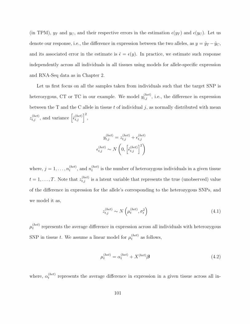
(in TPM), yT and yC , and their respective errors in the estimation ε(yT ) and ε(yC). Let us
denote our response, i.e., the difference in expression between the two alleles, as y = yT − yC ,
and its associated error in the estimate is ε = ε(y). In practice, we estimate such response
independently across all individuals in all tissues using models for allele-specific expression
and RNA-Seq data as in Chapter 2.
Let us first focus on all the samples taken from individuals such that the target SNP is
heterozygous, CT or TC in our example. We model y(het)t,j , i.e., the difference in expression
between the T and the C allele in tissue t of individual j, as normally distributed with mean
z(het)t,j , and variance
[ε
(het)t,j
]2
,
y(het)t,j = z
(het)t,j + ε
(het)t,j
ε(het)t,j ∼ N
(0,[ε
(het)t,j
]2)
where, j = 1, . . . , n(het)t , and n
(het)t is the number of heterozygous individuals in a given tissue
t = 1, . . . , T . Note that z(het)t,j is a latent variable that represents the true (unobserved) value
of the difference in expression for the allele’s corresponding to the heterozygous SNPs, and
we model it as,
z(het)t,j ∼ N
(µ
(het)t , σ2
t
)(4.1)
µ(het)t represents the average difference in expression across all individuals with heterozygous
SNP in tissue t. We assume a linear model for µ(het)t as follows,
µ(het)t = α
(het)t +X(het)β (4.2)
where, α(het)t represents the average difference in expression in a given tissue across all in-
101
dividuals with a heterozygous target SNP, and we put a prior on α(het)t ∼ N(µα, σ
2α) with
hyperprior parameters µα and σ2α.
The matrix X(het) is of dimension nhett ×p and it represents the matrix of covariates for all
individuals with heterozygous target SNP in a given tissue, and, β is a vector of dimension
p and we assume a non-informative prior for each of its entries.
Nevertheless, in our sample population not all individuals are heterozygous for the target
SNP. Thus, for the individuals with homozygous target SNP, i.e., with target SNP values of
CC and TT in our example, we model them as having mean 0 but sharing the same variance
as in the heterozygous SNPs, thus,
y(hom)t,j = z
(hom)t,j + ε
(hom)t,j
ε(hom)t,j ∼ N
(0,[ε
(hom)t,j
]2)
Moreover, we assume that the true difference in expression between alleles also has mean
0 in the homozygous case, z(hom)tj ∼ N(0, σ2
t ). This is the key difference between the two
groups of individuals. In the case of the heterozygous group we assumed the difference to be
positive, with parameter α(het)t , and in the case of the homozygous group we assumed their
mean difference to be 0.
Note that σ2t represents the variance of the (true) difference between the alleles for tissue t
and we assume it to be a common variance for individuals with homozygous and heterozygous
target SNPs. The advantage of such assumption is that we gain in sample size, and the
individuals with homozygous target SNPs aid us in estimating the variance for the group of
interest, the heterozygous group.
Finally, we put a prior on σ2t ∼ IG(a, b), with hyperparameters a and b; and we put a
102
prior on σα ∼ IG(a∗, b∗) with hyperparameters a∗ and b∗.
Detecting Imprinting
The previous model would work for genes that do not exhibit any parent-of-origin effect,
which is roughly 97% or more of the genes in the human genome. However, for the small
percentage of genes that may exhibit some parental bias in their expression the previous
model would be oversimplified and would not detect such effects. Let us define our response
as y = δ ∗ (yp − ym), where δ is an indicator that takes the value 1 if yp actually correponds
to the paternal genome, and −1 otherwise. Then, the intermediate sign random variable δ
helps us estimate the parental bias, but since δ is missing, we would ideally integrate over δ
in our model so to obtain an estimate of the parent-of-origin effect.
4.3.3 Hi-Braim with Imprinting
In this section we propose an allelic imbalance model across multiple tissues that ac-
count for two major sources of allelic imbalance: cis-regulation in an allele-specific manner
(cis-aseQTL) and imprinting. In order to do so we extend the previous model to a Hier-
archical Mixture model, where we model imprinting using a latent variable (missing data)
that indicates if the difference corresponds to the paternal allele minus the maternal allele,
or viceversa.
Let us define the difference, in expression, between the two alleles for tissue t, individual
j as, ytj = y(p)t,j − y
(m)t,j . Then, we can model ytj ∼ N(zt,j, εt,j). Next, we model the true
difference in expression, zt,j as a mixture of normals1 with a linear imprinting effect νt,
1the mixture comes from the fact that the true paternal allele is unknown. Thus, for example a 0/100imprinted gene will look like a mixture since some of the response will correspond to the difference betweenthe paternal minus the maternal allele, and some of the different will correspond exactly to the opossite case
103
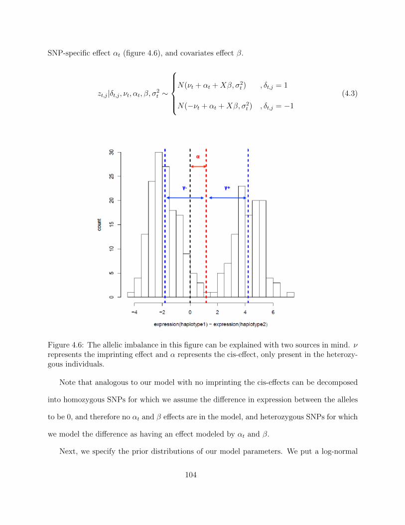
SNP-specific effect αt (figure 4.6), and covariates effect β.
zt,j|δt,j, νt, αt, β, σ2t ∼
N(νt + αt +Xβ, σ2
t ) , δt,j = 1
N(−νt + αt +Xβ, σ2t ) , δt,j = −1
(4.3)
Figure 4.6: The allelic imbalance in this figure can be explained with two sources in mind. νrepresents the imprinting effect and α represents the cis-effect, only present in the heterozy-gous individuals.
Note that analogous to our model with no imprinting the cis-effects can be decomposed
into homozygous SNPs for which we assume the difference in expression between the alleles
to be 0, and therefore no αt and β effects are in the model, and heterozygous SNPs for which
we model the difference as having an effect modeled by αt and β.
Next, we specify the prior distributions of our model parameters. We put a log-normal
104

prior on νt ∼ LN (log µν , σ2ν) because νt can only take positive values. We put a normal prior
on αt ∼ N(µα, σ2α), and a noninformative prior on β, p(β) = 1. We put an inverse-gamma
prior on σ2t ∼ IG(a, b), and we assume p(δtj = 1) = 1/2.
Finally, we specify the hyperprior distributions. We assume a non-informative hyperprior
on µα, an inverse-gamma hyperprior on σ2α ∼ IG(a∗, b∗) and on σ2
ν ∼ IG(c∗, d∗). And lastly,
a log-normal hyperprior on log µν ∼ LN(0, 102).
Adaptive MCMC within Gibbs Sampling
Let us write the joint density of the observed data, y = (y(het), y(hom)), the covariance
diagonal matrix with observation errors, E = diag
([ε(het)
]2
,[ε(hom)
]2)
, and the vector of
parameters and latent variables, θ =(z(hom), z(het),ν,α,β,σ2, µα, σ
2α, a, b, a
∗, b∗, c∗, d∗),
f(y, E;θ) =T∏t=1
n(hom)t∏j=1
[f(y
(hom)t,j |z(hom)
t,j ,[ε(hom)
]2)f(z
(hom)t,j |δ(hom)
t,j , µ(hom)t,j , σ2
t
)f(δ
(hom)t,j
)]n(het)t∏j=1
[f(y
(het)t,j |z
(het)t,j ,
[ε(het)
]2)f(z
(het)t,j |δ
(het)t,j , µ
(het)t,j , σ2
t
)f(δ
(het)t,j
)]f(νt|σ2
ν
)f(α
(het)t |µα, σ2
α
)f(σ2t |a, b
)f(σ2ν |c∗, d∗
)f(σ2α|a∗, b∗
)
where,
µ(hom)t,j = δ
(hom)t,j νt, and
µ(het)t,j = α
(het)t +Xβ + δ
(het)t,j νt
We derived a Gibbs Sampler approach first but it had a very slow convergence to the true
values. Thus we decided to reduce the number of parameters in our model by integrating
105

the joint density over the δ and z latent variables. Let us focus on the posterior part that
depends on δ and z, for such part we can write the posterior as,
f1(y, E;θ)
∝T∏t=1
nt∏j=1
[f(yt,j |zt,j , [εt,j ]2
)f(zt,j |δt,j , µt,j , σ2
t
)f (δt,j)
]
∝T∏t=1
nt∏j=1
exp
{− (yt,j − zt,j)2
2 [εt,j ]2
}(exp
{− (zt,j − µt,j)2
2σ2t,j
})δt,j (exp
{− (zt,j − µt,j)2
2σ2t,j
})1−δt,j
Let us first integrate (sum) over all the possible values of δ. Since δ can only take two
values, the integration corresponds merely to the sum of the two mixtures,
f2(y, E;θ) ∝T∏t=1
nt∏j=1
exp
{− (yt,j − zt,j)2
2 [εt,j ]2
}(exp
{−(zt,j − µ+
t,j
)22σ2
t,j
}+ exp
{−(zt,j − µ−
t,j
)22σ2
t,j
})
∝T∏t=1
nt∏j=1
exp
{− (yt,j − zt,j)2
2 [εt,j ]2
}exp
{−(zt,j − µ+
t,j
)22σ2
t,j
}+
exp
{− (yt,j − zt,j)2
2 [εt,j ]2
}exp
{−(zt,j − µ−
t,j
)22σ2
t,j
}
Now we have the sum of the multiplication of two-normal densities. We can integrate
over z, obtaining,
f3(y, E;θ) = f(yt,j|µt,j, [ε]2 + σ2
t
)∝
T∏t=1
nt∏j=1
exp
{−(yt,j − µ+
t,j
)2
2([εt,j]
2 + σ2t,j
)}+ exp
{−(yt,j − µ−t,j
)2
2([εt,j]
2 + σ2t,j
)}
where, µ+t,j = νt + αt +Xβ, and µ−t,j = −νt + αt +Xβ
106
Finally, the joint density without the δ and z parameters can be writen as,
f(y, E;θ) =T∏t=1
n(hom)t∏j=1
f(y
(hom)t,j |µ(hom)
t,j ,[ε(hom)
]2+ σ2
t
) n(het)t∏j=1
f(y
(het)t,j |µ
(het)t,j ,
[ε(het)
]2+ σ2
t
)f(νt|µν , σ2
ν
)f(α
(het)t |µα, σ2
α
)f(σ2t |a, b
)f(σ2ν |c∗, d∗
)f(σ2α|a∗, b∗
)
Now, we derive the sampling scheme for the full posterior. We used an adaptive MCMC, Vi-
hola (2012), within Gibbs approach, where we sample ν|θ−ν , then α|θ−α, then σ2t |θ−σ2
t, then
β|θ−β, σ2ν using adaptive metropolis, and we sample σ2
α, µν , µα using their closed-form con-
ditional posterior distributions.
In order to simplify notation let us denote,
f∗(yt,j |µt,j , E + σ2t ) =
n(hom)t∏j=1
f
(y(hom)t,j |µ(hom)
t,j ,[ε(hom)
]2+ σ2
t
) n(het)t∏j=1
f
(y(het)t,j |µ
(het)t,j ,
[ε(het)
]2+ σ2
t
)
Thus, the adaptive MCMC within Gibbs sampler algorithm is as follows,
107

Algorithm 5 H-BRAIM Adaptive MCMC within Gibbs.
1. Initialize the parameters.
2. Sample each parameter iterative (until convergence) from their full condi-tionals, as follows,
(a) Sample ν|α,β,σ2t , E, µν , σ
2ν from its posterior density f(ν|α,β,σ2
t , E, µν , σ2ν)
using k adaptive MCMC steps.
f(ν|α,β,σ2t , E, µν , σ
2ν) ∝
T∏t=1
f ∗(yt,j|µt,j, E + σ2t )f(νt|µν , σ2
ν
)(b) Sample α|ν,β,σ2
t , E, µα, σ2α from its posterior density f(α|ν,β,σ2
t , E, µν , σ2ν)
using k adaptive MCMC steps.
f(α|ν,β,σ2t , E, µν , σ
2ν) ∝
T∏t=1
f ∗(yt,j|µt,j, E + σ2t )f(αt|µα, σ2
α
)(c) Sample β|ν,α,σ2
t , E from its posterior density f(β|ν,α,σ2t , E) using k adaptive
MCMC steps.
f(β|ν,α,σ2t , E) ∝
T∏t=1
f ∗(yt,j|µt,j, E + σ2t )
(d) Sampleσ2t |ν,α,β, E, a, b from its posterior density f(σ2
t |ν,α,β, E, a, b) using k adaptiveMCMC steps.
f(β|ν,α,σ2t , E, µν , σ
2ν) ∝
T∏t=1
f ∗(yt,j|µt,j, E + σ2t )f(σ2t |a, b
)(e) Sample σ2
ν ∼ IG (0.5nt + c∗, 0.5∑nt
t=1(log νt − µν)2 + d∗)
(f) Sample σ2α ∼ IG (0.5nt + a∗, 0.5
∑ntt=1(log νt − µα)2 + b∗)
(g) Sample µν ∼ N (var∗ν × µ∗ν ,√var∗ν),
with var∗ν =(ntσ2ν
+ 1102
)−1
and µ∗ν = var∗ν ×(
log νtntσ2ν
+ 0 1102
)(h) Sample µα ∼ N (var∗α × µ∗α,
√var∗α),
with var∗α =(ntσ2α
+ 1102
)−1
and µ∗α = var∗α ×(αt
ntσ2α
+ 0 1102
)3. Take only the samples after the burn-in and compute posterior statistics for the pa-
rameters of interest.
108
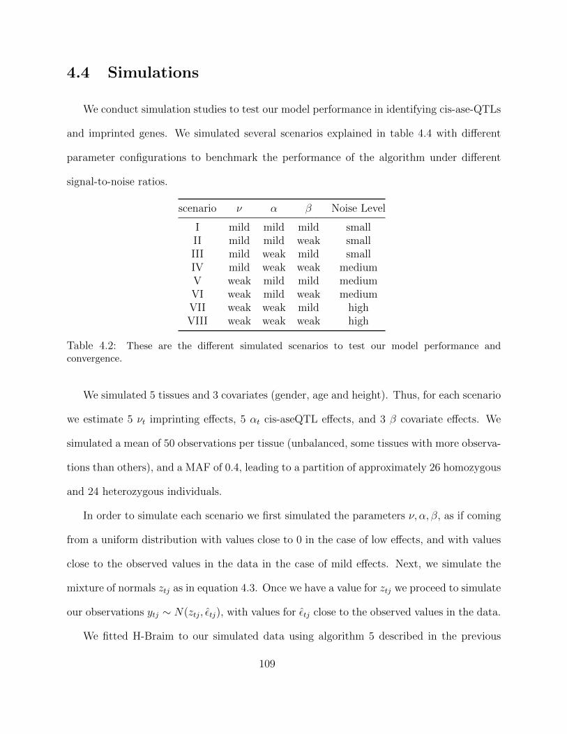
4.4 Simulations
We conduct simulation studies to test our model performance in identifying cis-ase-QTLs
and imprinted genes. We simulated several scenarios explained in table 4.4 with different
parameter configurations to benchmark the performance of the algorithm under different
signal-to-noise ratios.
scenario ν α β Noise Level
I mild mild mild smallII mild mild weak smallIII mild weak mild smallIV mild weak weak mediumV weak mild mild mediumVI weak mild weak mediumVII weak weak mild highVIII weak weak weak high
Table 4.2: These are the different simulated scenarios to test our model performance andconvergence.
We simulated 5 tissues and 3 covariates (gender, age and height). Thus, for each scenario
we estimate 5 νt imprinting effects, 5 αt cis-aseQTL effects, and 3 β covariate effects. We
simulated a mean of 50 observations per tissue (unbalanced, some tissues with more observa-
tions than others), and a MAF of 0.4, leading to a partition of approximately 26 homozygous
and 24 heterozygous individuals.
In order to simulate each scenario we first simulated the parameters ν, α, β, as if coming
from a uniform distribution with values close to 0 in the case of low effects, and with values
close to the observed values in the data in the case of mild effects. Next, we simulate the
mixture of normals ztj as in equation 4.3. Once we have a value for ztj we proceed to simulate
our observations ytj ∼ N(ztj, εtj), with values for εtj close to the observed values in the data.
We fitted H-Braim to our simulated data using algorithm 5 described in the previous
109

section. In the main text we show the posterior credible intervals for each of the 13 estimated
parameters under each of the simulated scenarios, as well as the true value of the simulation,
figures 4.7 to 4.9. We can see that in most cases the true simulated value is within the
range of the posterior credible interval. In addition, in the appendix we show the MCMC
diagnostics and convergence plots, appendix figures D.1 to D.8.
110
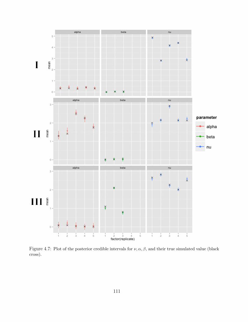
Figure 4.7: Plot of the posterior credible intervals for ν, α, β, and their true simulated value (blackcross).
111
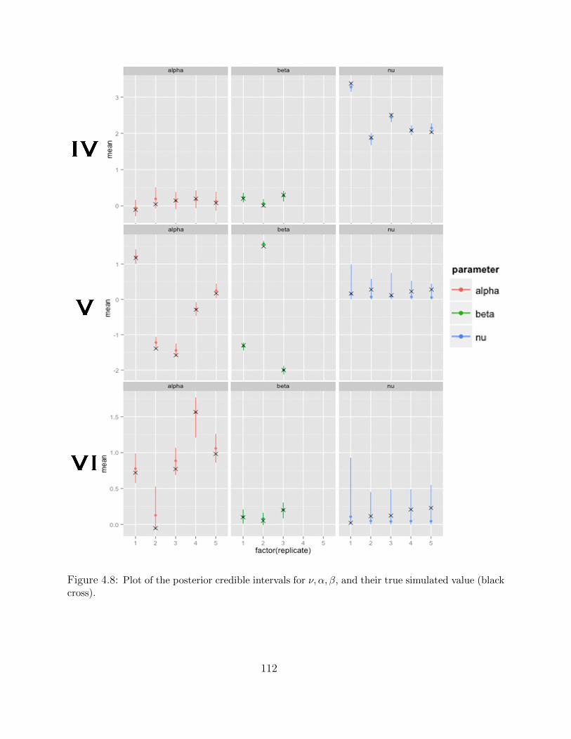
Figure 4.8: Plot of the posterior credible intervals for ν, α, β, and their true simulated value (blackcross).
112
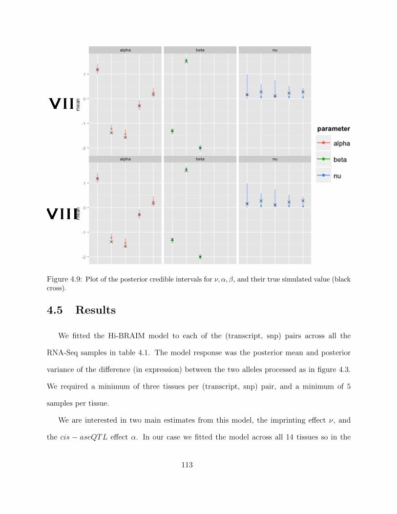
Figure 4.9: Plot of the posterior credible intervals for ν, α, β, and their true simulated value (blackcross).
4.5 Results
We fitted the Hi-BRAIM model to each of the (transcript, snp) pairs across all the
RNA-Seq samples in table 4.1. The model response was the posterior mean and posterior
variance of the difference (in expression) between the two alleles processed as in figure 4.3.
We required a minimum of three tissues per (transcript, snp) pair, and a minimum of 5
samples per tissue.
We are interested in two main estimates from this model, the imprinting effect ν, and
the cis − aseQTL effect α. In our case we fitted the model across all 14 tissues so in the
113
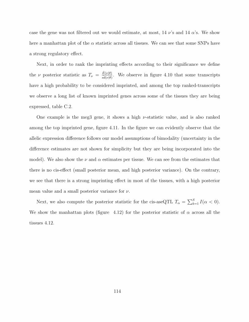
case the gene was not filtered out we would estimate, at most, 14 ν’s and 14 α’s. We show
here a manhattan plot of the α statistic across all tissues. We can see that some SNPs have
a strong regulatory effect.
Next, in order to rank the imprinting effects according to their significance we define
the ν posterior statistic as Tν = E(ν|θ)sd(ν|θ) . We observe in figure 4.10 that some transcripts
have a high probability to be considered imprinted, and among the top ranked-transcripts
we observe a long list of known imprinted genes across some of the tissues they are being
expressed, table C.2.
One example is the meg3 gene, it shows a high ν-statistic value, and is also ranked
among the top imprinted gene, figure 4.11. In the figure we can evidently observe that the
allelic expression difference follows our model assumptions of bimodality (uncertainty in the
difference estimates are not shown for simplicity but they are being incorporated into the
model). We also show the ν and α estimates per tissue. We can see from the estimates that
there is no cis-effect (small posterior mean, and high posterior variance). On the contrary,
we see that there is a strong imprinting effect in most of the tissues, with a high posterior
mean value and a small posterior variance for ν.
Next, we also compute the posterior statistic for the cis-aseQTL Tα =∑S
k=1 I(α < 0).
We show the manhattan plots (figure 4.12) for the posterior statistic of α across all the
tissues 4.12.
114
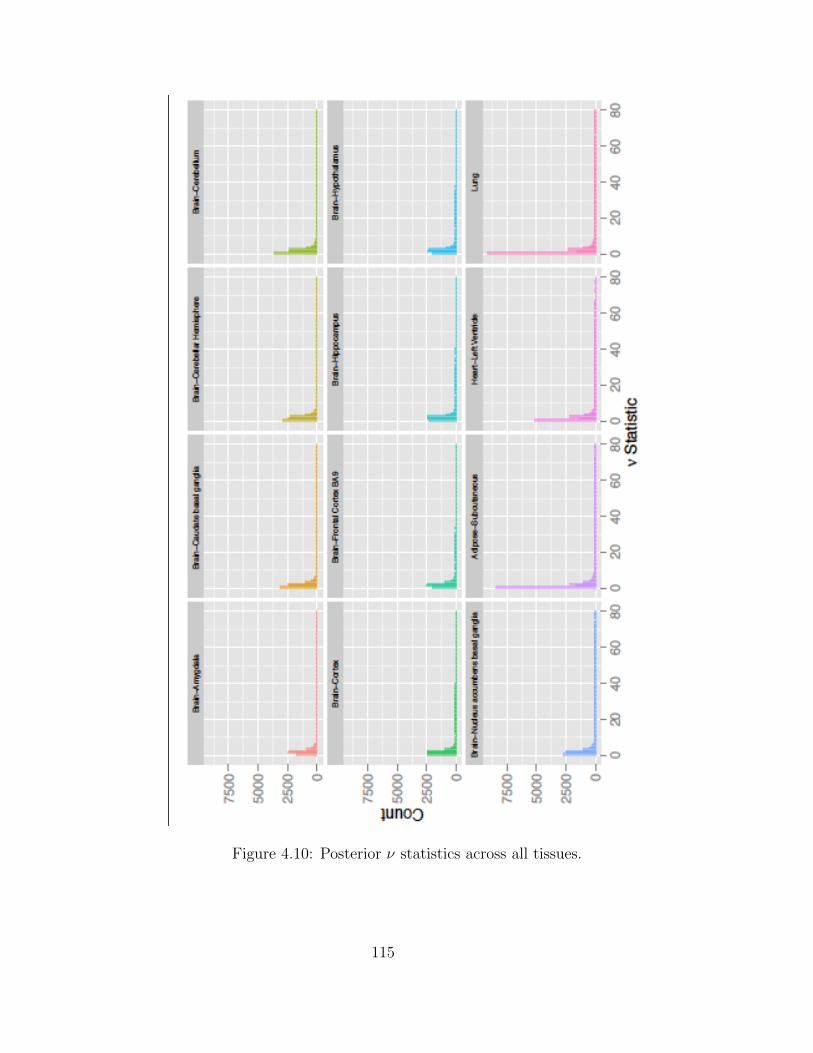
Figure 4.10: Posterior ν statistics across all tissues.
115
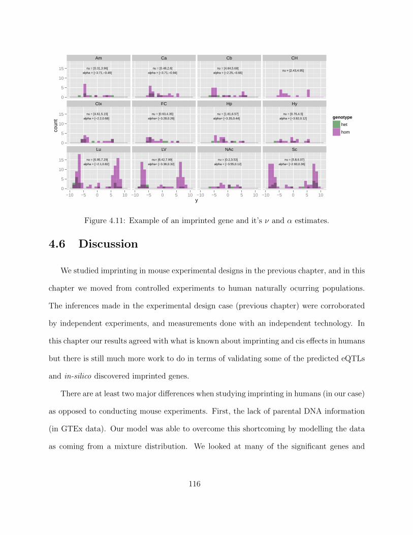
nu = [0.31,3.96]
alpha = [−3.71,−0.49]
nu = [0.48,2.6]
alpha = [−3.71,−0.94]
nu = [4.84,5.68]
alpha = [−2.25,−0.66]nu = [2.43,4.95]
nu = [4.61,5.15]
alpha = [−2.2,0.68]
nu = [0.93,4.35]
alpha = [−3.28,0.26]
nu = [1.81,6.57]
alpha = [−3.35,0.44]
nu = [0.76,4.5]
alpha = [−3.92,0.12]
nu = [6.95,7.29]
alpha = [−2.1,0.82]
nu = [6.42,7.99]
alpha = [−3.36,0.32]
nu = [0.2,3.53]
alpha = [−3.55,0.12]
nu = [5.8,6.07]
alpha = [−2.93,0.36]
Am Ca Cb CH
Ctx FC Hp Hy
Lu LV NAc Sc
0
5
10
15
0
5
10
15
0
5
10
15
−10 −5 0 5 10 −10 −5 0 5 10 −10 −5 0 5 10 −10 −5 0 5 10y
coun
t genotype
het
hom
Figure 4.11: Example of an imprinted gene and it’s ν and α estimates.
4.6 Discussion
We studied imprinting in mouse experimental designs in the previous chapter, and in this
chapter we moved from controlled experiments to human naturally ocurring populations.
The inferences made in the experimental design case (previous chapter) were corroborated
by independent experiments, and measurements done with an independent technology. In
this chapter our results agreed with what is known about imprinting and cis effects in humans
but there is still much more work to do in terms of validating some of the predicted eQTLs
and in-silico discovered imprinted genes.
There are at least two major differences when studying imprinting in humans (in our case)
as opposed to conducting mouse experiments. First, the lack of parental DNA information
(in GTEx data). Our model was able to overcome this shortcoming by modelling the data
as coming from a mixture distribution. We looked at many of the significant genes and
116
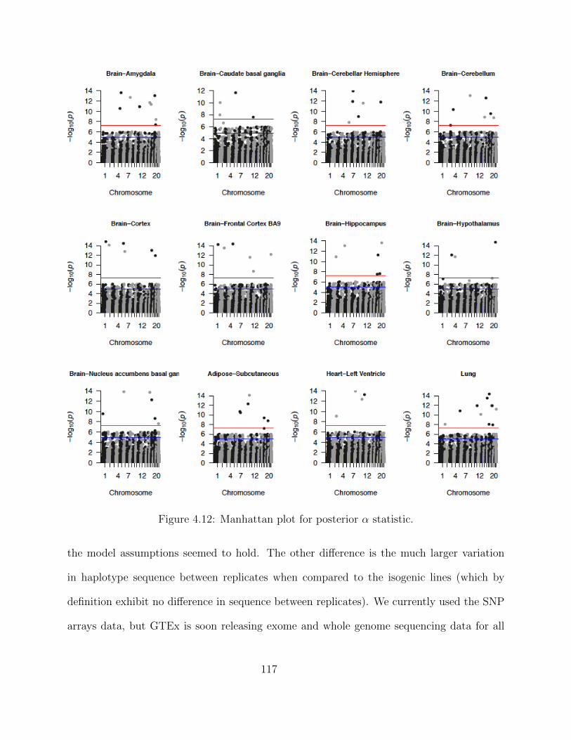
Figure 4.12: Manhattan plot for posterior α statistic.
the model assumptions seemed to hold. The other difference is the much larger variation
in haplotype sequence between replicates when compared to the isogenic lines (which by
definition exhibit no difference in sequence between replicates). We currently used the SNP
arrays data, but GTEx is soon releasing exome and whole genome sequencing data for all
117

the individuals in the study. This will provide a much richer dataset in terms of genetic
variation among the individuals. We suggest adding an individual effect in this case since
we wil have a much better resolution of the sequence differences betweeen the two alleles of
a gene.
Our model has two major advantages. On the one hand it models the data across multiple
tissues, allowing us to borrow information across tissues. On the other hand it is based on
accurate estimates of transcript expression at the allele level, allowing us to differentiate
between different transcripts of the same gene, while propagating the uncertainty in our
expression estimates.
118
Chapter 5
Single and Small Cell Clustering
Methods in Developmental Biology
omnis cellula e cellula - every living cell comes from another living cell
- Rudolf Virchow
5.1 Transcriptomic and genomic chromatin structure
in early mammalian development using small cell
experiments
5.1.1 Introduction
Stem cells possess the ability to self-renew and give rise to differentiated cells types. In
vitro culture conditions have enabled the derivation of an assortment of cell lines that possess
these properties. However, there is a wide-range of stem-like phenotypes that exist along
the differentiation cascade. Additionally, stem cells with phenotypic similarity have been
119
derived in vitro based on a multiplicity of signaling paradigms.
Recent findings suggest that human embryonic stem cells (hESCs) and induced pluripo-
tent stem cells (hiPS) have greater morphologic and signaling dependencies to mouse epi-
blast derived stem cells (mEpiSC) than their logical counterparts, mouse embryonic stem
cells (mESCs). These two categories of stem models rely on different signaling pathways to
achieve stemness.
ESCs are derived from a period in early mammalian development marked by prominent
cellular and molecular changes as the totipotent zygotic cell transitions into the blastocyst.
The outer, trophectoderm cells of the blastocyst will give rise to the placenta, while its inner
cell mass (ICM) forms the precursor of the fetus and part of the extra-embryonic tissues
(Wang and Dey, 2006). In contrast, in vitro stem cells are generally sustained in a relatively
static pluripotent state through the use of inhibitors and/or the over-expression of transcrip-
tion factors. These exogenous factors have the ability to regulate transcriptional paradigms
to drive cells towards a stem-like state. A high-quality comparative study of transcriptional
programs across early developmental tissues would allow a direct quantification of how faith-
ful in vitro stem models are. While driven by external factors, the transcriptional paradigm
is fully realized through cis-regulatory elements. The differential usage of these elements is
intimately connected to chromatin organization. Poised and repressed regions can also pre-
dict future states as the stem cell differentiates. Although chromatin organization is known
to have a pivotal role in developmental transitions (Ho and Crabtree, 2010), it has been dif-
ficult to study these principles in in vivo early developmental tissues due to limited amount
of sample. Studies of the distribution of histone modifications across the genome of their
in vitro counterpart, ESC reveal a unique organization where bivalent domains form with
repressive and active marks on the same promoter (Bernstein et al., 2006); generally open,
120
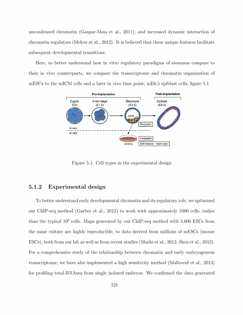
uncondensed chromatin (Gaspar-Maia et al., 2011); and increased dynamic interaction of
chromatin regulators (Melcer et al., 2012). It is believed that these unique features facilitate
subsequent developmental transitions.
Here, to better understand how in vitro regulatory paradigms of stemness compare to
their in vivo counterparts, we compare the transcriptome and chromatin organization of
mESCs to the mICM cells and a later in vivo time point, mE6.5 epiblast cells, figure 5.1
Figure 5.1: Cell types in the experimental design
5.1.2 Experimental design
To better understand early developmental chromatin and its regulatory role, we optimized
our ChIP-seq method (Garber et al., 2012) to work with approximately 5000 cells, rather
than the typical 106 cells. Maps generated by our ChIP-seq method with 5,000 ESCs from
the same culture are highly reproducible, to data derived from millions of mESCs (mouse
ESCs), both from our lab as well as from recent studies (Marks et al., 2012; Shen et al., 2012).
For a comprehensive study of the relationship between chromatin and early embryogenesis
transcriptome, we have also implemented a high sensitivity method (Malboeuf et al., 2013)
for profiling total-RNAseq from single isolated embryos. We confirmed the data generated
121
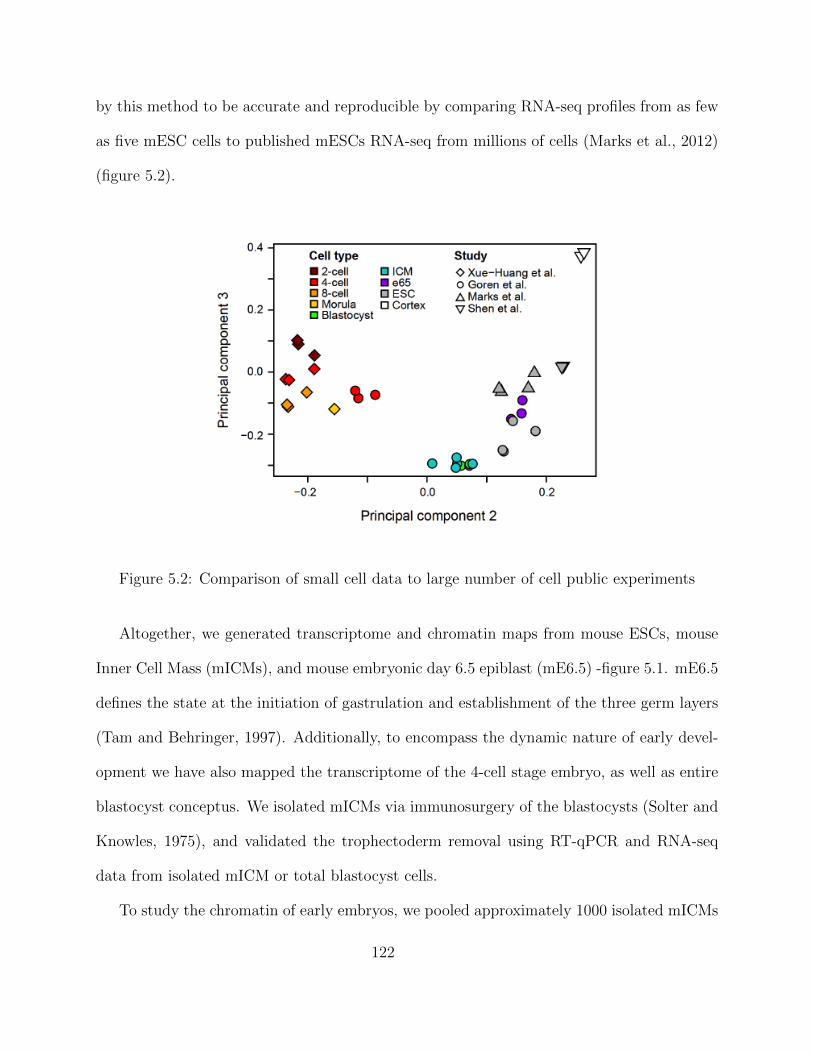
by this method to be accurate and reproducible by comparing RNA-seq profiles from as few
as five mESC cells to published mESCs RNA-seq from millions of cells (Marks et al., 2012)
(figure 5.2).
Figure 5.2: Comparison of small cell data to large number of cell public experiments
Altogether, we generated transcriptome and chromatin maps from mouse ESCs, mouse
Inner Cell Mass (mICMs), and mouse embryonic day 6.5 epiblast (mE6.5) -figure 5.1. mE6.5
defines the state at the initiation of gastrulation and establishment of the three germ layers
(Tam and Behringer, 1997). Additionally, to encompass the dynamic nature of early devel-
opment we have also mapped the transcriptome of the 4-cell stage embryo, as well as entire
blastocyst conceptus. We isolated mICMs via immunosurgery of the blastocysts (Solter and
Knowles, 1975), and validated the trophectoderm removal using RT-qPCR and RNA-seq
data from isolated mICM or total blastocyst cells.
To study the chromatin of early embryos, we pooled approximately 1000 isolated mICMs
122
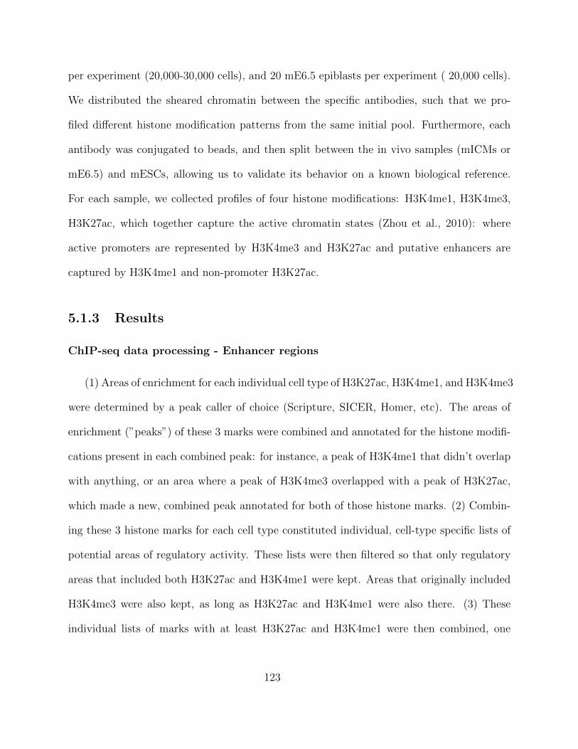
per experiment (20,000-30,000 cells), and 20 mE6.5 epiblasts per experiment ( 20,000 cells).
We distributed the sheared chromatin between the specific antibodies, such that we pro-
filed different histone modification patterns from the same initial pool. Furthermore, each
antibody was conjugated to beads, and then split between the in vivo samples (mICMs or
mE6.5) and mESCs, allowing us to validate its behavior on a known biological reference.
For each sample, we collected profiles of four histone modifications: H3K4me1, H3K4me3,
H3K27ac, which together capture the active chromatin states (Zhou et al., 2010): where
active promoters are represented by H3K4me3 and H3K27ac and putative enhancers are
captured by H3K4me1 and non-promoter H3K27ac.
5.1.3 Results
ChIP-seq data processing - Enhancer regions
(1) Areas of enrichment for each individual cell type of H3K27ac, H3K4me1, and H3K4me3
were determined by a peak caller of choice (Scripture, SICER, Homer, etc). The areas of
enrichment (”peaks”) of these 3 marks were combined and annotated for the histone modifi-
cations present in each combined peak: for instance, a peak of H3K4me1 that didn’t overlap
with anything, or an area where a peak of H3K4me3 overlapped with a peak of H3K27ac,
which made a new, combined peak annotated for both of those histone marks. (2) Combin-
ing these 3 histone marks for each cell type constituted individual, cell-type specific lists of
potential areas of regulatory activity. These lists were then filtered so that only regulatory
areas that included both H3K27ac and H3K4me1 were kept. Areas that originally included
H3K4me3 were also kept, as long as H3K27ac and H3K4me1 were also there. (3) These
individual lists of marks with at least H3K27ac and H3K4me1 were then combined, one
123
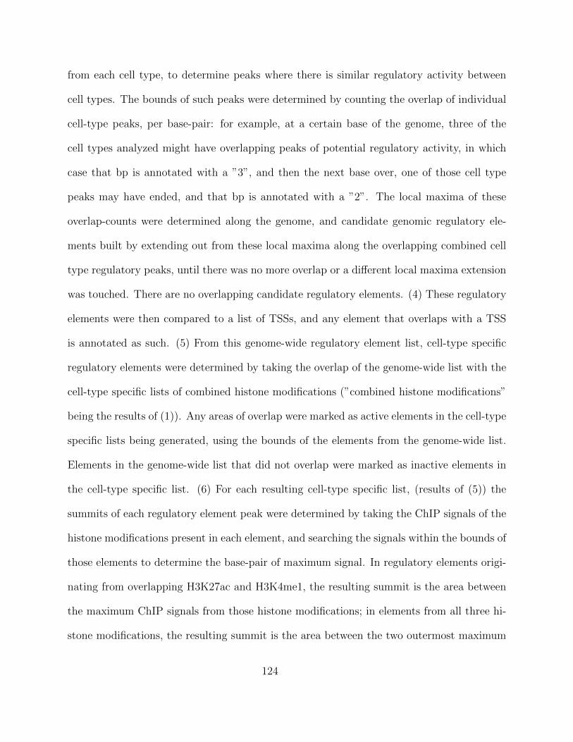
from each cell type, to determine peaks where there is similar regulatory activity between
cell types. The bounds of such peaks were determined by counting the overlap of individual
cell-type peaks, per base-pair: for example, at a certain base of the genome, three of the
cell types analyzed might have overlapping peaks of potential regulatory activity, in which
case that bp is annotated with a ”3”, and then the next base over, one of those cell type
peaks may have ended, and that bp is annotated with a ”2”. The local maxima of these
overlap-counts were determined along the genome, and candidate genomic regulatory ele-
ments built by extending out from these local maxima along the overlapping combined cell
type regulatory peaks, until there was no more overlap or a different local maxima extension
was touched. There are no overlapping candidate regulatory elements. (4) These regulatory
elements were then compared to a list of TSSs, and any element that overlaps with a TSS
is annotated as such. (5) From this genome-wide regulatory element list, cell-type specific
regulatory elements were determined by taking the overlap of the genome-wide list with the
cell-type specific lists of combined histone modifications (”combined histone modifications”
being the results of (1)). Any areas of overlap were marked as active elements in the cell-type
specific lists being generated, using the bounds of the elements from the genome-wide list.
Elements in the genome-wide list that did not overlap were marked as inactive elements in
the cell-type specific list. (6) For each resulting cell-type specific list, (results of (5)) the
summits of each regulatory element peak were determined by taking the ChIP signals of the
histone modifications present in each element, and searching the signals within the bounds of
those elements to determine the base-pair of maximum signal. In regulatory elements origi-
nating from overlapping H3K27ac and H3K4me1, the resulting summit is the area between
the maximum ChIP signals from those histone modifications; in elements from all three hi-
stone modifications, the resulting summit is the area between the two outermost maximum
124
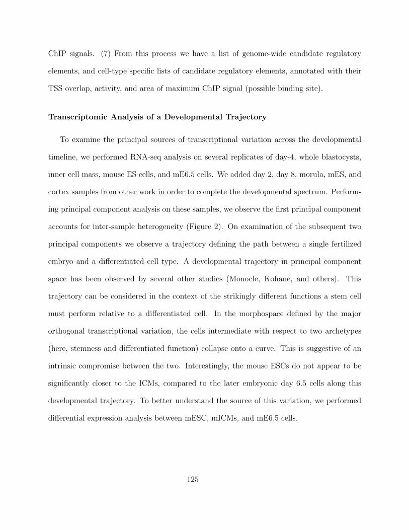
ChIP signals. (7) From this process we have a list of genome-wide candidate regulatory
elements, and cell-type specific lists of candidate regulatory elements, annotated with their
TSS overlap, activity, and area of maximum ChIP signal (possible binding site).
Transcriptomic Analysis of a Developmental Trajectory
To examine the principal sources of transcriptional variation across the developmental
timeline, we performed RNA-seq analysis on several replicates of day-4, whole blastocysts,
inner cell mass, mouse ES cells, and mE6.5 cells. We added day 2, day 8, morula, mES, and
cortex samples from other work in order to complete the developmental spectrum. Perform-
ing principal component analysis on these samples, we observe the first principal component
accounts for inter-sample heterogeneity (Figure 2). On examination of the subsequent two
principal components we observe a trajectory defining the path between a single fertilized
embryo and a differentiated cell type. A developmental trajectory in principal component
space has been observed by several other studies (Monocle, Kohane, and others). This
trajectory can be considered in the context of the strikingly different functions a stem cell
must perform relative to a differentiated cell. In the morphospace defined by the major
orthogonal transcriptional variation, the cells intermediate with respect to two archetypes
(here, stemness and differentiated function) collapse onto a curve. This is suggestive of an
intrinsic compromise between the two. Interestingly, the mouse ESCs do not appear to be
significantly closer to the ICMs, compared to the later embryonic day 6.5 cells along this
developmental trajectory. To better understand the source of this variation, we performed
differential expression analysis between mESC, mICMs, and mE6.5 cells.
125
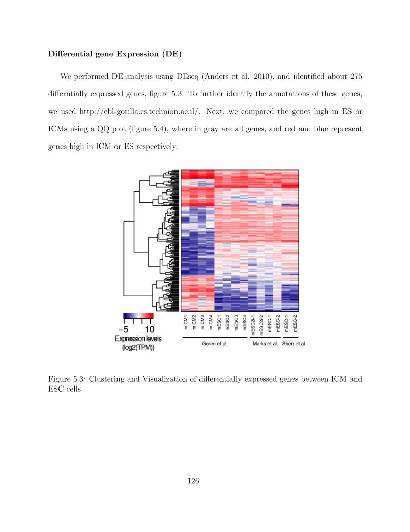
Differential gene Expression (DE)
We performed DE analysis using DEseq (Anders et al. 2010), and identified about 275
differntially expressed genes, figure 5.3. To further identify the annotations of these genes,
we used http://cbl-gorilla.cs.technion.ac.il/. Next, we compared the genes high in ES or
ICMs using a QQ plot (figure 5.4), where in gray are all genes, and red and blue represent
genes high in ICM or ES respectively.
Figure 5.3: Clustering and Visualization of differentially expressed genes between ICM andESC cells
126
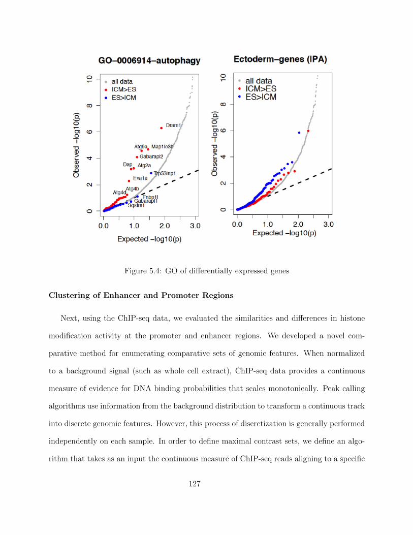
Figure 5.4: GO of differentially expressed genes
Clustering of Enhancer and Promoter Regions
Next, using the ChIP-seq data, we evaluated the similarities and differences in histone
modification activity at the promoter and enhancer regions. We developed a novel com-
parative method for enumerating comparative sets of genomic features. When normalized
to a background signal (such as whole cell extract), ChIP-seq data provides a continuous
measure of evidence for DNA binding probabilities that scales monotonically. Peak calling
algorithms use information from the background distribution to transform a continuous track
into discrete genomic features. However, this process of discretization is generally performed
independently on each sample. In order to define maximal contrast sets, we define an algo-
rithm that takes as an input the continuous measure of ChIP-seq reads aligning to a specific
127
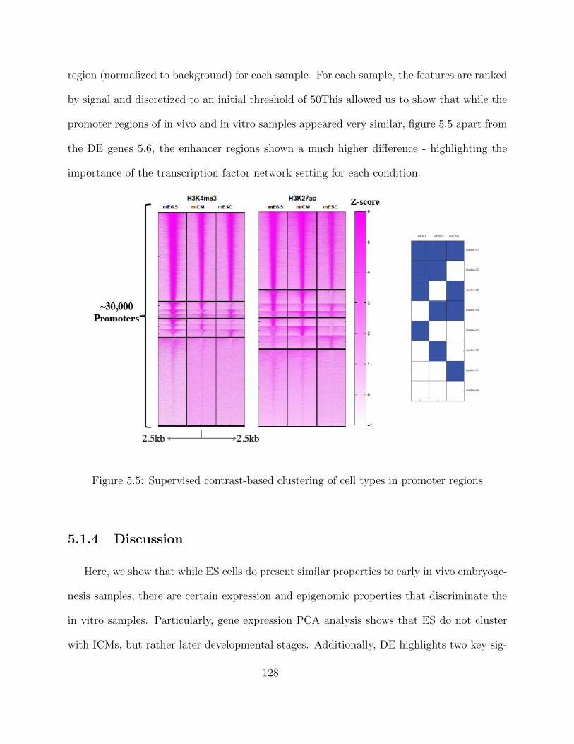
region (normalized to background) for each sample. For each sample, the features are ranked
by signal and discretized to an initial threshold of 50This allowed us to show that while the
promoter regions of in vivo and in vitro samples appeared very similar, figure 5.5 apart from
the DE genes 5.6, the enhancer regions shown a much higher difference - highlighting the
importance of the transcription factor network setting for each condition.
Figure 5.5: Supervised contrast-based clustering of cell types in promoter regions
5.1.4 Discussion
Here, we show that while ES cells do present similar properties to early in vivo embryoge-
nesis samples, there are certain expression and epigenomic properties that discriminate the
in vitro samples. Particularly, gene expression PCA analysis shows that ES do not cluster
with ICMs, but rather later developmental stages. Additionally, DE highlights two key sig-
128
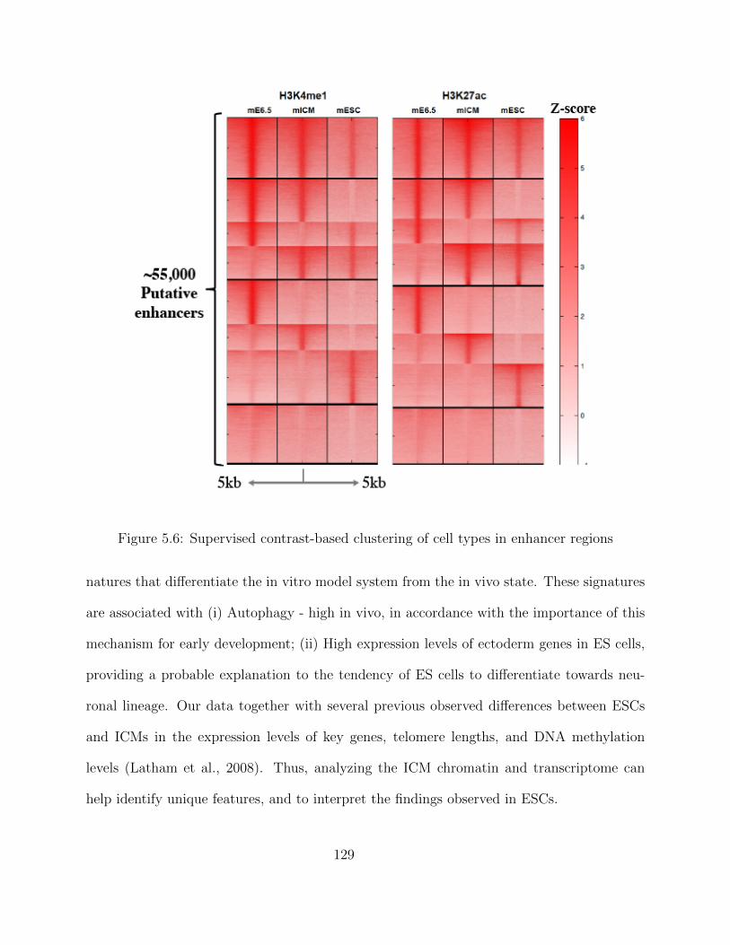
Figure 5.6: Supervised contrast-based clustering of cell types in enhancer regions
natures that differentiate the in vitro model system from the in vivo state. These signatures
are associated with (i) Autophagy - high in vivo, in accordance with the importance of this
mechanism for early development; (ii) High expression levels of ectoderm genes in ES cells,
providing a probable explanation to the tendency of ES cells to differentiate towards neu-
ronal lineage. Our data together with several previous observed differences between ESCs
and ICMs in the expression levels of key genes, telomere lengths, and DNA methylation
levels (Latham et al., 2008). Thus, analyzing the ICM chromatin and transcriptome can
help identify unique features, and to interpret the findings observed in ESCs.
129
5.2 Finding Heterogeneous population in Single-cell Ex-
periments
5.2.1 Introduction
Recent advancements in single cell capture, library preparation methods, and RNA se-
quencing technologies allows us to estimate the expression levels of RNA transcripts in a
single cell. Biological applications range from the identification of heterogenous subpopu-
lations within a population, such as immune cells and cancer cells to the ability to profile
rare and scarce cell types, such as circulating tumor cells or inner cell mass cells. Re-
cent molecular studies have shown that, even when derived from a seemingly homogeneous
population, single cells can exhibit substantial differences in gene expression and protein
concentrations, Shalek et al. (2013).
Several studies have showed the heterogeneity of gene expression for a given gene across
all randomly sampled single cells coming from a cell population. Nevertheless, observing
systematic and coordinated heterogeneity for a set of genes across all sampled single cells,
would give us further evidence of the heterogeneity at the single cell level in a cell population.
However, finding a group of genes that are differentially expressed between subpopulations
is a tricky problem, analogous to the chicken or the egg paradox. On the one hand we
need to, 1) Find a set of genes that are differentially expressed between two (or more)
sub-populations, and on the oher hand we need to 2) Assign each single cell to their sub-
population of origin. These two tasks convolve and confound with each other tightly. For
example, given a predefined assignment of the single cells, we could always rank the genes
by the difference in expression across sub-populations. On the other hand, given a set of
130
genes that are believed to be differentially expressed between sub-populations, we could
assign each of the cells to their subpopulation of origin by their similarity of expression
on such set of genes. Therefore in order to solve this problem we need a model that can
identify the optimal partitioning of the single cells, as well as selecting a ’signature’ gene set
that is differentially expressed in sub-populations. This motivates our approach that uses a
Bayesian probabilistic model and, subsequently a Gibbs sampler to sample the parameters
and assignment indicators from the full posterior distribution of our model.
Limitations of simple clustering algorithms
There are some previous attempts to identify the heterogeneous cell populations from
single cell gene expression data. For example, Guo et al. (2013) analyzed a dataset with 6
cell populations on about 200 genes. For each cell population, they picked the top 4 genes
ranked according to the highest variance of expression in the population and then they did
a hierarchical clustering of cells on those 4 genes. They did observe that the cells can be
clustered into 2 or 3 sub-populations by this approach. However, this approach seems rather
arbitrary and can lead to misleading results because of two reasons. First, this approach
ranks the genes by their variance in absolute scale rather than binary active/inactive states.
It is possible that some genes are inactive in all cells but simply have high variance in
their expression. Because these genes are not expressed in all cells, clustering cells based
on those genes will not help us to identify the heterogeneous cell sub-populations. Second,
it is still problematic even if we can identify the genes with bimodality by ranking their
variances, because the selected top genes with highest variances may not be systematically
heterogeneous in sub-populations. Consider a simple example with two genes, G1 and G2,
in 40 cells, labeled as C1, C2, ..., C40. G1 and G2 are selected by the approach due to their
131
high variances. Gene 1 is active in C1, ..., C20, and inactive in C21, ..., C40. If Gene 2
is also active in C1, ..., C20, and inactive in C21, ..., C40, or the opposite, then there is a
strong evidence of coordination between G1 and G2, and evidence of heterogeneity on gene
group {G1, G2} between the two sub-populations C1, ..., C20, and C21, ..., C40. However,
it is also possible that G2 is active in C1, ..., C10, C31, ..., C40 and inactive in C11, ...,
C30, then the expression states of G1 and G2 are completely independent with each other.
The approach proposed in Guo et al. (2013) cannot distinguish these two scenarios when
selecting genes that are used to partition cells, therefore the results by that approach may
lead to misleading results.
5.2.2 BASIC algorithm
Here we propose a novel Bayesian-model based variable selection and clustering algo-
rithm, called BASIC, to identify heterogeneous subpopulations. Instead of fitting a model
on the gene expression levels, which tend to be noisy and subject to PCR amplification is-
sues, we propose a model on a rather less subject to noise data, the active or inactive infered
states for each gene. This approach is also in agreement with the concept of transcriptional
bursting and therefore it is more robust to variability in gene expression for which there may
not be any biological difference.
Statistical model
Let us consider an experiment for which we estimate the gene expression of G genes, in
TPM or RPKM values, for each of the C cells randomly sampled from a given cell population.
Let us define Yc,g as the expression level measured for gene g in cell c, where g = 1, . . . , G
and c = 1, . . . , C. Here we propose a Bayesian hierarchical mixture model to characterize
132
the gene expression heterogeneity in the population of interest (a given cancer tumor, the
immune response of a tissue, etc.). We assume a bimodal distribution for the expression
levels of each gene g across all C cells. More specifically, we assume that the two possible
states for a gene are a so-called inactive state that follows an Exponential distribution and
an active state that follows a Normal distribution. To gain flexibility we assume that the
parameters of both distributions can be different for each gene. It is important to note that
when a gene is in a single state (active or inactive) across all C cells is a special case of the
bimodal distribution.
Now let us define the unobserved indicator variable Zc,g to take the value 1 if gene g is
transcribed in cell c, and the value 0 if gene g is untranscribed in cell c. Morevoer, if the
gene is active (Zc,g = 1), then Yc,g follows a Normal distribution with mean µg and variance
σ2g ; and if the gene is repressed (Zc,g = 0), the measured expression level is mostly noise
and is modeled by an Exponential distribution with mean parameter λg. We impose non-
informative prior distributions for this Bayesian model. We put an inverse-Gamma(ασ, βσ)
prior distribution on σ2g and a Normal with mean µ0 and variance σ2
g prior for µg. . We
know in prior that the expression level of an inactive gene is low, so we adopt conjugate
Gamma (αλ, βλ) prior for λg.
We want to classify each of the single cells into several, let us say K, heterogenous sub-
populations. A heterogeneous subpopulation is defined as the coordinated expression of a
set of signature genes within a subpopulation. Further, we assume that this set of genes is
differentialy expressed with respect to the otherK-1 subpopulations. In general, it is common
to find that a large proportion of genes are bimodally distributed, but their active/inactive
states are not coordinated. We assume that within a heterogenous sub-population only a
small proportion of genes are synchronized.
133
Let us define K as the number of sub-populations and let us define Ic = 1, . . . , K as the
assignment indicator for each cell c. We usually do not know K and we need to estimate it
from the data. Specifically, we adopt a Bayesian mixture of finite mixtures (MFM) model
to estimate K. We assume that a set of genes are differentially expressed between single cell
populations with coordinated active/inactive states. We call such set of genes “biomarker”
genes. Let us define Sg = {1, 0} as the indicator for whether gene g is selected as a biomarker.
For the biomarker genes, we model them as having different rate of active/inactive states
in each single cell, while we model the non-biomarker genes as having a homogeneous rate
across all cells. If gene g is a biomarker, we define the vector θg = (θg,1, . . . , θg,K) as the
probability of observing gene g to be active in each of the K sub-populations. If gene g is
not a biomarker, ωg denote the overall probability of gene g being active in all cells. We
build a Bayesian hierarchical model for jointly modeling the expression level, active/inactive
states, and partitioning of single cells. A MFM model is adopted where we assume K − 1
134
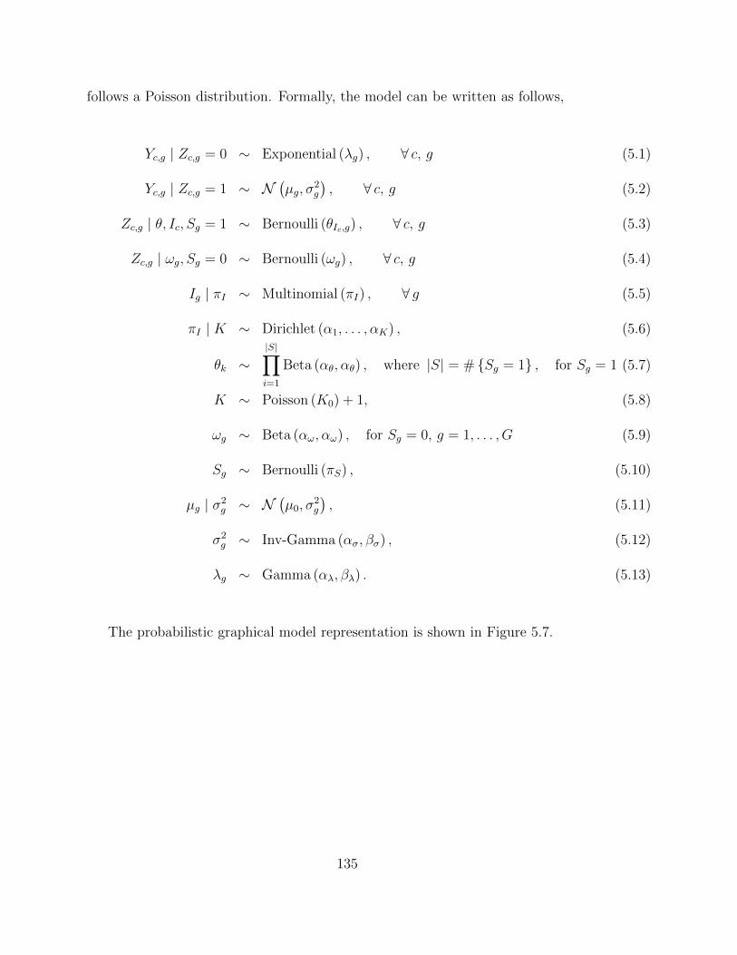
follows a Poisson distribution. Formally, the model can be written as follows,
Yc,g | Zc,g = 0 ∼ Exponential (λg) , ∀ c, g (5.1)
Yc,g | Zc,g = 1 ∼ N(µg, σ
2g
), ∀ c, g (5.2)
Zc,g | θ, Ic, Sg = 1 ∼ Bernoulli (θIc,g) , ∀ c, g (5.3)
Zc,g | ωg, Sg = 0 ∼ Bernoulli (ωg) , ∀ c, g (5.4)
Ig | πI ∼ Multinomial (πI) , ∀ g (5.5)
πI | K ∼ Dirichlet (α1, . . . , αK) , (5.6)
θk ∼|S|∏i=1
Beta (αθ, αθ) , where |S| = # {Sg = 1} , for Sg = 1 (5.7)
K ∼ Poisson (K0) + 1, (5.8)
ωg ∼ Beta (αω, αω) , for Sg = 0, g = 1, . . . , G (5.9)
Sg ∼ Bernoulli (πS) , (5.10)
µg | σ2g ∼ N
(µ0, σ
2g
), (5.11)
σ2g ∼ Inv-Gamma (ασ, βσ) , (5.12)
λg ∼ Gamma (αλ, βλ) . (5.13)
The probabilistic graphical model representation is shown in Figure 5.7.
135
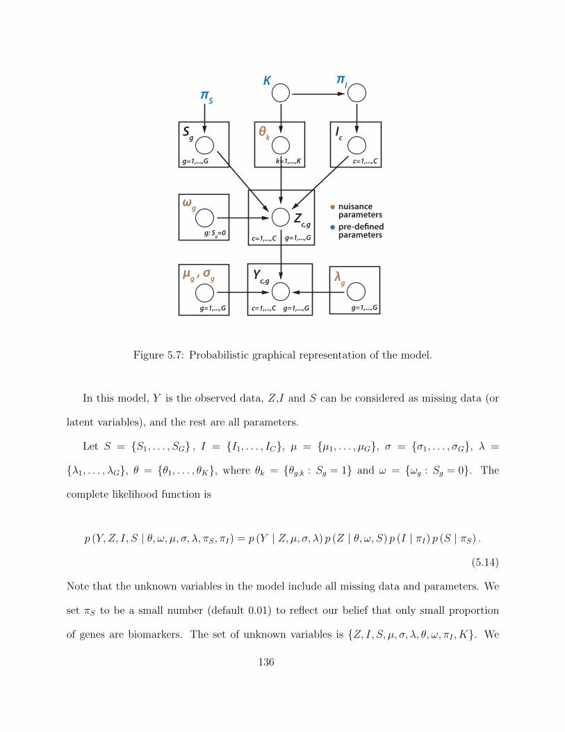
Sg
πS
πI
g=1,...,G
g=1,...,G
θk
k=1,...,K
K
nuisanceparameters
Ic
c=1,...,C
λg
g=1,...,G
ωg
g: Sg=0
μg , σg
Zc,g
g=1,...,Gc=1,...,C
Yc,g
g=1,...,Gc=1,...,C
pre-de�nedparameters
Figure 5.7: Probabilistic graphical representation of the model.
In this model, Y is the observed data, Z,I and S can be considered as missing data (or
latent variables), and the rest are all parameters.
Let S = {S1, . . . , SG} , I = {I1, . . . , IC}, µ = {µ1, . . . , µG}, σ = {σ1, . . . , σG}, λ =
{λ1, . . . , λG}, θ = {θ1, . . . , θK}, where θk = {θg,k : Sg = 1} and ω = {ωg : Sg = 0}. The
complete likelihood function is
p (Y, Z, I, S | θ, ω, µ, σ, λ, πS, πI) = p (Y | Z, µ, σ, λ) p (Z | θ, ω, S) p (I | πI) p (S | πS) .
(5.14)
Note that the unknown variables in the model include all missing data and parameters. We
set πS to be a small number (default 0.01) to reflect our belief that only small proportion
of genes are biomarkers. The set of unknown variables is {Z, I, S, µ, σ, λ, θ, ω, πI , K}. We
136
propose an efficient Gibbs sampler to sample from the posterior distribution of missing data
and parameters. We integrated out µ, σ, λ and θ for the Gibbs sampler and developed an
efficient collapsed Gibbs sampler.
Gibbs sampling algorithm
To derive the collapsed Gibbs sampling algorithm, let us first assume Z is known and
look at the conditional posterior distribution of S and I. The likelihood function for missing
data Z is
p (Z | I, S, θ, ω) =∏
g:Sg=0
ωng,1g (1− ωg)ng,0∏
g:Sg=1
K∏k=1
θng,k,1g,k (1− θg,k)ng,k,0 , (5.15)
where {ng,0, ng,1} are the number of cells being active or inactive across all cells, and
{ng,k,0, ng,k,1} are the number active or inactive cells in sub-population k for each gene i.
We adopt a Beta (αω, αω) prior for ωg and a Beta (αθ, αθ) prior for θg,k, where the default
values of αω and αθ are set to be 0.5. We integrate out ω’s and θ’s and obtain the marginal
likelihood,
p (Z | I, S) =∏
i:Sg=0
B (αω + ng,1, αω + ng,0)
B (αω, αω)
∏i:Si=1
K∏k=1
B (αθ + ng,k,1, αθ + ng,k,0)
B (αθ, αθ)
=∏
i:Sg=0
[Γ (αω + ng,1) Γ (αω + ng,0)
Γ (2αω + C)
Γ (2αω)
Γ (αω) Γ (αω)
]∏
i:Sg=1
K∏k=1
[Γ (αθ + ng,k,1) Γ (αθ + ng,k,0)
Γ (2αθ + Ck)
Γ (2αθ)
Γ (αθ) Γ (αθ)
](5.16)
where Ck denotes the number of cells in sub-population k according to current I, B (·, ·) and
Γ (·) denote beta and gamma function. The posterior distribution of I and S is proportional
137
to the product of likelihood function P (Z|I, S) and the prior distributions of I and S,
P (I, S | Z) ∝ p (Z | I, S) p (I) p (S) . (5.17)
We let p (Sg = 1) = πS, where πS reflects our prior knowledge on the proportion of genes
differentially expressed in sub-populations. By default (in the current implementation), we
assume that a small proportion of genes are differentially expressed (biomarkers) across
sub-populations and we set the prior probability πS = 0.05.
Our goal is to draw S (the biomarker selection indicators) and I (cell sub-population
indicators) from its marginal posterior distribution, p (S, I | Z). We initialize Z, S and I
according to their prior distributions and use the Gibbs sampling algorithm to update each Sg
and Ic. Here we derive the conditional distributions for updating Sg and Ic. The probability
of selecting gene g as a biomarker conditional on Z and I, can be calculated as follows,
p (Sg = 1 | Z, I) ∝ p (Sg = 1) p (Z | Sg = 1, I)
= πS
K∏k=1
[Γ (αθ + ng,k,1) Γ (αθ + ng,k,0)
Γ (2αθ + Ck)
Γ (2αθ)
Γ (αθ) Γ (αθ)
], (5.18)
p (Sg = 0 | Z, I) ∝ p (Sg = 0) p (Z | Sg = 0, I)
= (1− πS)
(Γ (αω + ng,1) Γ (αω + ng,0)
Γ (2αω + C)
Γ (2αω)
Γ (αω) Γ (αω)
). (5.19)
In the sampler, once we have sampled the the set of biomarkers according to their posterior
probability we want to assign each of the cells into a given subpopulation. In order to do
so, we need to update the posterior for the cell population indicator Ic for each cell c, given
the new set of biomarkers.
In a mixture of finite mixture model, the prior probability of cell c joining an existing
138
sub-population k, conditional on the sub-population assignments of other cells, is
p(Ic = k | I[−c]
)∝ (Ck + 1)κ (C,K) , (5.20)
and the prior probability of forming a new sub-population is
p(Ic = K + 1 | I[−c]
)∝ κ (C,K + 1) , (5.21)
where K+1 represents the new sub-population, and function κ (c, k) = E[K(c)/K
(k)]. Here,
K(t) = K (K − 1) · · · (K − t+ 1) , (5.22)
K(n) = K (K + 1) · · · (K + n− 1) . (5.23)
The numbers κ (c, k) can be precomputed efficiently using the following recursion,
κ (c, k) = κ (c− 1, k − 1)− (c+ t− 2)κ (c, k − 1) , (5.24)
κ (c, 0) = E[1/K(n)
]= P (S > n) /γn, (5.25)
where γ is the Poisson distribution parameter for K.
The conditional distribution of Ic given Z, S and I[−c] is
p(Ic = k | Z, S, I[−c]
)∝ p
(Ic = k | I[−c]
)p(Z | Ic = k, I[−c], S
), (5.26)
∝ (Ck + 1)κ (C,K) p(Z | Ic = k, I[−c], S
), (5.27)
139

and
p(Ic = K + 1 | Z, S, I[−c]
)∝ p
(Ic = K + 1 | I[−c]
)p(Z | Ic = K + 1, I[−c], S
), (5.28)
∝ κ (C,K + 1) p(Z | Ic = K + 1, I[−c], S
), (5.29)
where
p(Z | Ic = k, I[−c], S
)∝
∏g:Sg=1
K∏l=1
[Γ(αθ + n∗g,l,1
)Γ(αθ + n∗g,l,0
)Γ (2αθ + C∗l )
Γ (2αθ)
Γ (αθ) Γ (αθ)
]. (5.30)
where{n∗g,l,0, n
∗g,l,1
}are the number of cells being active or inactive in sub-population l of
each gene g, and C∗l denotes the number of cells in sub-population l - all conditional on
current sub-population assignments I except that Ic = k.
Conditional on a given Z, we can use the conditional distribution above to update S and
I. To complete one Gibbs sampling iteration, we also need to update Z conditional on S,
I, θ, ω, Y , µ, σ and λ. In previous calculations of conditional distribution of S and I, we
integrated out parameters θ and ω. Fortunately, we apply the same scheme to integrate out
θ, ω, µ, σ and λ from the conditional distribution of Z. Therefore, in the Gibbs sampling
process we only need to sample from the joint posterior distribution of Z, S and I. This
collapsed Gibbs sampling scheme dramatically helps the mixing of the Markov chain and
improves computational efficiency.
The observed likelihood function of Yg = {Y1,g, . . . , YC,g} conditional on
Zg = {Z1,g, · · · , ZC,g} and other parameters is
140
p (Yg | Zg , µg , σg , λg) =
C∏c=1
[E (Yc,g | λ)]I(Zc,g=0) [N (Yc,g | µg , σ2g
)]I(Zc,g=1)(5.31)
=
C∏c=1
[λ exp (−λYc,g)]I(Zc,g=0)
[(2πσ2
g
)−1/2exp
(−
1
2σ2g
(Yc,g − µg)2
)]I(Zc,g=1)
, (5.32)
where E (· | ·) and N (· | ·, ·) are Exponential and Normal distribution density functions.
First, by Exponential-Gamma conjugacy, we can integrate out λg from the likelihood function
over the prior distribution Gamma (1, 1),
p (Yg | Zg , µg , σg) =
∫p (Yg | Zg , µg , σg , λg) p (λg) dλg (5.33)
=βαλλ
Γ (αλ)
Γ (αλ + ng,0)(βλ +
∑c:Zc,g=0 yc,g
)αλ+ng,0 · C∏c=1
[(2πσ2
g
)−1/2exp
(−
1
2σ2g
(Yc,g − µg)2
)]I(Zc,g=1)
.(5.34)
Then, we integrate µg and σg out from the likelihood function by their prior distribution,
p (Yg | Zg) (5.35)
=
∫p (Yg | Zg , µg , σg , λ) p (µg) p
(σ2g
)dµgdσ
2g (5.36)
=βαλλ
Γ (αλ)
Γ (αλ + ng,0)(βλ +
∑c:Zc,g=0 yc,g
)αλ+ng,0 · (5.37)
βασσ (2π)−ng,1
2
Γ (ασ)√ng,1 + 1
Γ(ng,1
2+ ασ
)βσ + 1
2
∑c:Zc,g=1
Y 2c,g + µ20 −
∑c:Zc,g=1
Yc,g+µ0
2
ng,1+1
ng,1
2+ασ
. (5.38)
141
Now we have the marginal likelihood of Yg given Zg, and we can update each Zc,g by the
following conditional distribution. The conditional probability of Zc,g being 1 is
p(Zc,g = 1 | Yg , Z[−c],g , Sg , Ic, θ, ω
)(5.39)
=p(Zc,g = 1, Yg , Z[−c],g | Sg , Ic, θ, ω
)p(Zc,g = 0, Yg , Z[−c],g | Sg , Ic, θ, ω
)+ p
(Zc,g = 1, Yg , Z[−c],g | Sg , Ic, θ, ω
) (5.40)
=p(Zc,g = 1, Yg | Z[−c],g , Sg , Ic, θ, ω
)p(Zc,g = 0, Yg | Z[−c],g , Sg , Ic, θ, ω
)+ p
(Zc,g = 1, Yg | Z[−c],g , Sg , Ic, θ, ω
) (5.41)
=p(Yg | Zc,g = 1, Z[−c],g
)p (Zc,g = 1 | Sg , Ic, θ, ω)
p(Yg | Zc,g = 0, Z[−c],g
)p (Zc,g = 0 | Sg , Ic, θ, ω) + p
(Yg | Zc,g = 1, Z[−c],g
)p (Zc,g = 1 | Sg , Ic, θ, ω)
. (5.42)
Let z be either 1 or 0; Note that if we can find p(Zc,g = z | Z[−c],g, Sg, Ic
)by integrating
out θ andω from p (Zc,g = z | Sg, Ic, θ, ω), then the conditional distribution of Zc,g being z
can be simplified to
p(Zc,g = z | Yg , Z[−c],g , Sg , Ic
)(5.43)
=p(Zc,g = z, Yg | Z[−c],g , Sg , Ic
)p(Zc,g = 0, Yg | Z[−c],g
)+ p
(Zc,g = 1, Yg | Z[−c],g
) (5.44)
=p(Yg | Zc,g = z, Z[−c],g
)p(Zc,g = z | Z[−c],g , Sg , Ic
)p(Yg | Zc,g = 0, Z[−c],g
)p(Zc,g = 0 | Z[−c],g , Sg , Ic
)+ p
(Yg | Zc,g = 1, Z[−c],g
)p(Zc,g = 1 | Z[−c],g , Sg , Ic
) .(5.45)
The analytical form of p(Zc,g = z | Z[−c],g, Sg, Ic
)is simply the conditional mean of θg,Ic
given Z[Ic/c],g of due to Bernoulli-Beta conjugacy, where Z[Ic/c],g = {Zc′,g : Ic′ = Ic and c′ 6= c}.
When gene g is selected as biomarker, i.e. Sg = 1,
142
p(Zc,g = 1 | Z[−c],g , Sg = 1, Ic
)=
∫p(Zc,g = z | Sg = 1, θg,Ic
)p(θg,Ic | Z[Ic/c],g
)dθg,Ic (5.46)
=
∫θg,Icp
(θg,Ic | Z[Ic/c],g
)dθg,Ic (5.47)
=αθ + ng,[Ic/c],1
2αθ + ng,[Ic/c], (5.48)
where ng,[Ic/c] is the total number of elements in Z[Ic/c],g and ng,[Ic/c],1 is the total number
of 1s in Z[Ic/c],g. When Sg = 0,
p(Zc,g = 1 | Z[−c],g , Sg = 0, Ic
)=
∫p (Zc,g = z | Sg = 0, ωg) p
(ωg | Z[−c],g
)dωg (5.49)
=
∫ωgp
(ωg | Z[−c],g
)dωg (5.50)
=αω + ng,[−c],1
2αω + C − 1, (5.51)
where ng,[−c],1 is the number of 1s in Zg except Zc,g. Note that integrating (5.48), (5.51)
and (5.38) we can already evaluate (5.45).
The Gibbs sampling algorithm is straightforward with the calculated conditional distri-
butions. In iteration t of the Gibbs sampler, we conduct the following conditional updates:
1. Draw Sg from p (Sg | Z, I), for all g = 1, . . . , G,
2. Draw Ic from p(Ic | Z, S, I[−c]
), for all c = 1, . . . , C.
3. Draw Zc,g from p(Zc,g | Yg, Z[−c],g, Sg, Ic
), for all g = 1, . . . , G and c = 1, . . . , C.
143
5.2.3 Selecting the number of groups K
Approximating marginal likelihood functions
In this part, we show how to select the number of subpopulations, K. The confidence
of observing heterogeneity can be evaluated by checking if K > 1 is supported by the data.
There are multiple ways of selecting the number of groups K. The first one is using Dirichlet
process mixture model to simultaneously sample from the space of K and I. However, it has
been proved that the estimation of number of groups K is inconsistent by Dirichlet process
mixture model. Another natural way for estimating K is by Bayesian model selection, i.e.
calculating the marginal likelihoods p (Z | Mk), where Mk denotes the model in which the
mixture model is constrained to have K groups. The calculation of marginal likelihood
p (Z | Mk) involves integrating out all parameters from their prior distribution,
p (Z | Mk) =
∫ ∫ ∑S
∑I
p (Z | S, I, θ, ω,Mk) p (S) p (I | Mk) p (θ | Mk) p (ω) dθdω, (5.52)
where∑
S
∑I represents the summation over all possible values of discrete variables S
and I. Note that integration in Eq. 5.52 does not have analytical solution and the numerical
integration is also infeasible to calculate due to the high dimension. However, we could
use the samples drawn from Gibbs sampling to approximate the marginal likelihood by the
method in Chib (1995). In particular, conditional on a specific S, we have the following
equation holds for an arbitrary (θ∗, ω∗),
ln p (Z | S,Mk) = ln p (Z | S, θ∗, ω∗,Mk) + ln p (θ∗) + ln p (ω∗)− ln p (θ∗, ω∗ | S,Z,Mk) (5.53)
144

In the above equation p (Z | S, θ∗, ω∗,Mk) can be calculated analytically as the product
of observed likelihood functions,
p (Z | S, θ∗, ω∗,Mk) =
∏Sg=0
C∏c=1
(ω∗g)Zc,g (1− ω∗g)1−Zc,g
C∏c=1
1
K
K∑k=1
∏Sg=1
(θ∗g,k
)Zc,g (1− θ∗g,k
)1−Zc,g . (5.54)
We approximate ln p (θ∗, ω∗ | S,Z,Mk) by fixing S and running Gibbs sampler for M
iterations to draw samples{I(1), . . . , I(M)
}from p (I | S,Z,Mk), then
p (θ∗, ω∗ | S,Z,Mk) =∑I
p (θ∗, ω∗ | S, I, Z,Mk) p (I | S,Z,Mk)
≈1
M
M∑m=1
p(θ∗, ω∗ | S, I(m), Z,Mk
), (5.55)
where
p (θ∗, ω∗ | S, I, Z,Mk) =∏Sg=0
p(ω∗g | S, I, Z,Mk
) ∏Sg=1
p(θ∗g | S, I, Z,Mk
)(5.56)
=∏Sg=0
Beta(ω∗g |αω + ng,1, αω + ng,0
)· (5.57)
∏Sg=1
K∏k=1
Beta(θ∗g,k
∣∣αθ + ng,k,1, αθ + ng,k,0
). (5.58)
Plug 5.55 in 5.53, we get the approximation for marginal likelihood ln p (Z | S,Mk).
Even though 5.53 is valid for any valid θ∗ and ω∗, arbitrary choice can lead to very bad
approximation. Here we choose each θ∗g,k or ω∗g to be their posterior mean given S, which ω∗g
145

can be calculated exactly
ω∗g ≡ E [ωg | S,Z] =ng,1
2αω + C, (5.59)
and θ∗g,k can be calculated from the samples I(1), . . . , I(M) from collapsed Gibbs sampler,
θ∗g,k ≡ E[θg,k | S,Z,Mk
](5.60)
= E[E[θg,k | S, I, Z,Mk
]| Z, S,Mk
](5.61)
=1
M
M∑m=1
E[θg,k | S,Z, I(m)
](5.62)
=1
M
M∑m=1
αθ + n(m)g,k,1
2αθ + Ck. (5.63)
It is extremely difficult to further integrate out S from p (Z | S,Mk) since different
S gives different dimensionality of (θ, ω). Therefore instead of p (Z | Mk) we calculate
p(Z | Sk,Mk
)where Sk is an estimator of S under model Mk. We choose estimator for
gene g, Sk,g, to be the marginal mode of posterior distribution, i.e.,
Sk,g = 1, p (Sg | Z,Mk) > 0.5, (5.64)
Sk,g = 0, p (Sg | Z,Mk) < 0.5. (5.65)
146
Selecting K with marginal likelihoods
In previous section we proposed to approximate p(Z | Sk,Mk
)by MCMC samples,
where notation Sk indicates that each k should have different estimator Sk. p(Z | Sk,Mk
)quantifies the overall fitting of model Sk and Mk to the data. Therefore we can use
p(Z | Sk,Mk
)to compare models under different group number k. In particular, we can
use p(Z | Sk,M1
), the marginal likelihood for one single population, as the baseline and
calculate ∆k, which is defined as the following Bayes factor,
∆k = ln p(Z | Sk,Mk
)− ln p
(Z | Sk,M1
). (5.66)
Note that if θ and ω has the same prior distribution, i.e. αω = αθ in our setting, θs and ωs
will be equivalent underM1, therefore Z will be independent of S, i.e. ln p(Z | Sk,M1
)=
ln p (Z | M1). Let’s call M1 as the “homogeneous model” because it allows only one single
cluster. ∆k quantifies how much better a model with k sub-populations fits the data than
the homogeneous model. Note that the calculation of ∆k can be simplified due to the
cancellations of likelihood functions for Zg with Sg = 0,
147
∆k = lnp(Z | Sk,Mk
)p(Z | Sk,M1
) (5.67)
= ln
∫ ∫ ∑I p(Z | Sk, I, θ, ω,Mk
)p (I | Mk) p (θ | Mk) p (ω) dθdω∫ ∫ ∑
I p(Z | Sk, I, θ, ω,M1
)p (I | M1) p (θ | M1) p (ω) dθdω
(5.68)
= ln
∫ ∫ ∑I
∏Sk,g=0 p (Zg | ωg)
∏Sk,g=1 p (Zg | I, θ,Mk) p (I | Mk) p (θ | Mk) p (ω) dθdω∫ ∫ ∑
I
∏Sk,g=0 p (Zg | ωg)
∏Sk,g=1 p (Zg | I, θ,M1) p (I | M1) p (θ | M1) p (ω) dθdω
(5.69)
= ln
[∫ ∑I
∏Sk,g=0 p (Zg | ωg) p (ω) dω
] ∫ ∫ ∑I
∏Sk,g=1 p (Zg | I, θ,Mk) p (I | Mk) p (θ | Mk) dθ[∫ ∑
I
∏Sk,g=0 p (Zg | ωg) p (ω) dω
] ∫ ∫ ∑I
∏Sk,g=1 p (Zg | I, θ,M1) p (I | M1) p (θ | M1) dθ
(5.70)
= ln
∫ ∫ ∑I
∏Sk,g=1 p (Zg | I, θ,Mk) p (I | Mk) p (θ | Mk) dθ∫ ∫ ∑
I
∏Sk,g=1 p (Zg | I, θ,M1) p (I | M1) p (θ | M1) dθ
(5.71)
= lnp({Zg : Sk,g = 1
}| Sk,g ,Mk
)p({Zg : Sk,g = 1
}| Sk,g ,M1
) . (5.72)
Note that since M1 is essentially a single component model, we could calculate
p({Zg : Sk,g = 1
}| Sk,g,M1
)analytically,
p({Zg : Sk,g = 1
}| Sk,g ,M1
)=
∫ ∏Sg=1
p (Zg | θ,M1) p (θ | M1) dθ (5.73)
=∏Sg=1
∫p (Zg | θg,1) p (θg,1) dθg,1 (5.74)
=∏Sg=1
[Γ (αθ + ng,1) Γ (αθ + ng,0)
Γ (2αθ + C)
Γ (2αθ)
Γ (αθ) Γ (αθ)
]. (5.75)
Therefore, we only need to approximate marginal likelihood
p({Zg : Sk,g = 1
}| Sk,g,Mk
). Additionally, Equation 5.72 also indicates that if Sk,g = 0
for all g, then ∆k = 0.
148
5.2.4 Simulation studies
We conduct simulation studies to test our algorithm performance in identifying biomarker
genes and partition the cells into sub-populations. In the following five scenarios we sim-
ulated data with different parameter configurations to benchmark the performance of the
algorithm under different signal-to-noise ratios. For each scenario, we simulated the binary
active/inactive states for G genes across C cells. Without loss of generality, we let K = 2 for
number of simulated sub-populations and each cell is randomly assigned to each of the two
sub-populations. Among the G genes, GS genes are differentially expressed in the two sub-
populations, and other genes are homogeneous across all cells. For heterogeneously expressed
genes, we let their probability of being active to be pE and (1− pE) in two sub-populations.
These two probabilities do not necessarily sum to be one, but here we simulate data in
this way to guarantee the contrast between sub-populations. For homogeneously expressed
genes, we randomly draw their probability of being active from a Beta (a, a) distribution,
where in current study we let a = 1 and the resulting Beta (1, 1) distribution is simply the
Uniform distribution on [0, 1]. For each of the simulated scenarios, we run 1000 iterations
of our Gibbs sampling for each simulated data set, and the estimated posterior distributions
of parameters S = (S1, . . . , SG) and I = (I1, . . . , IC). In the display of results, we rank the
genes by their posterior probability of being selected, p (Si = 1 | Z).
Scenario 1: C = 100, G = 200, NS = 0. We still simulated the expression 200
genes across 100 homogeneous cells. Specifically, there is no sub-population across the 200
cells. The heatmap of simulated data is shown in Figure 5.8. One can see clearly that
the partitioning by hierarchical clustering was random because there is no sub-population
in the data. We run our Gibbs sampling on this simulated data. The estimated posterior
probabilities for the 200 genes being selected are plotted in top of Figure 5.9. We can see
149
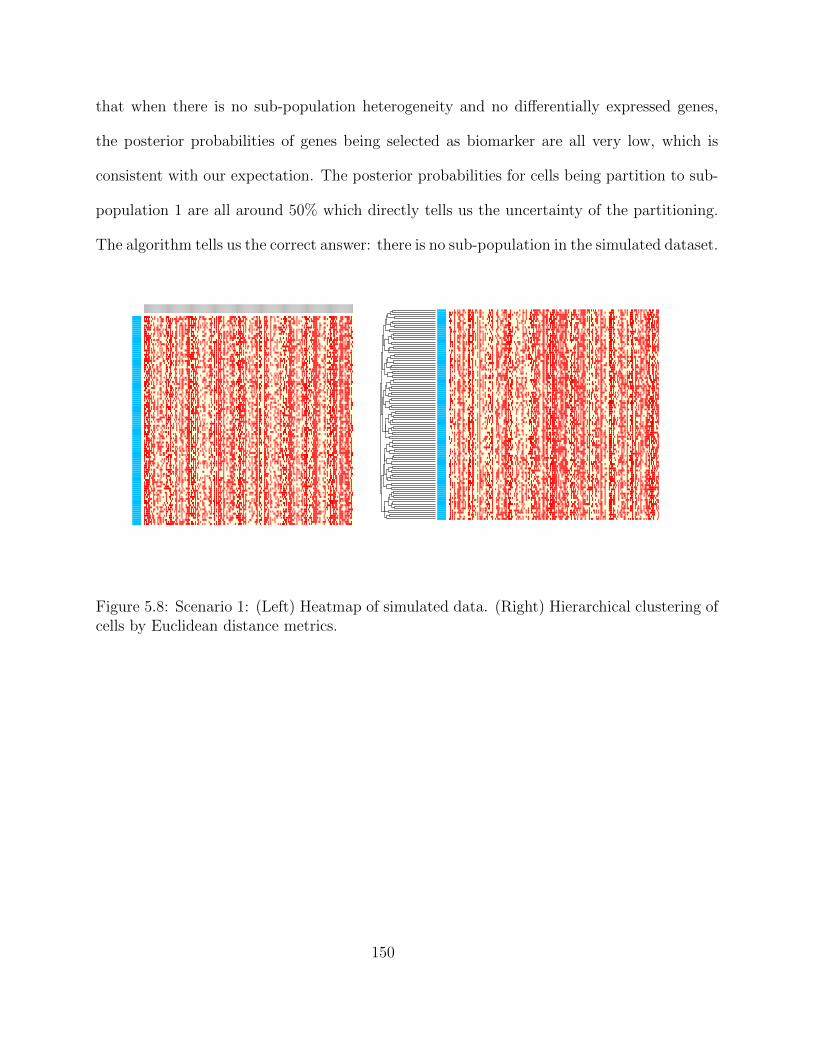
that when there is no sub-population heterogeneity and no differentially expressed genes,
the posterior probabilities of genes being selected as biomarker are all very low, which is
consistent with our expectation. The posterior probabilities for cells being partition to sub-
population 1 are all around 50% which directly tells us the uncertainty of the partitioning.
The algorithm tells us the correct answer: there is no sub-population in the simulated dataset.
Figure 5.8: Scenario 1: (Left) Heatmap of simulated data. (Right) Hierarchical clustering ofcells by Euclidean distance metrics.
150
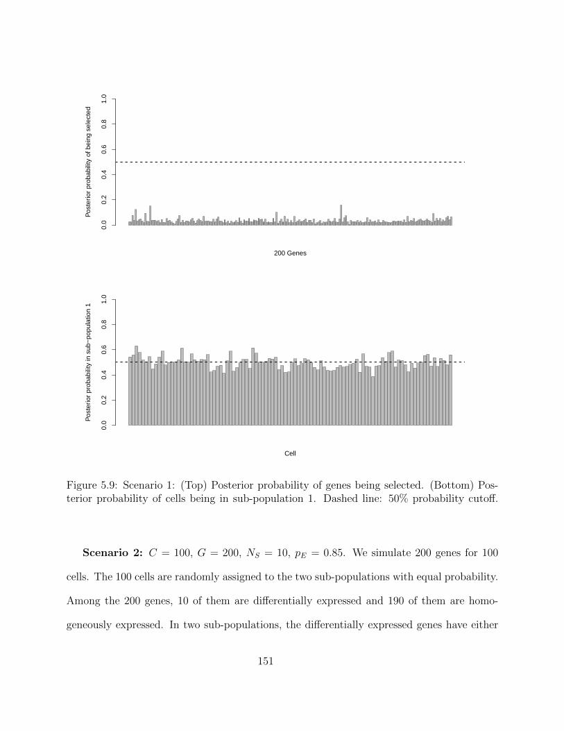
200 Genes
Pos
terio
r pr
obab
ility
of b
eing
sel
ecte
d
0.0
0.2
0.4
0.6
0.8
1.0
Cell
Pos
terio
r pr
obab
ility
in s
ub−
popu
latio
n 1
0.0
0.2
0.4
0.6
0.8
1.0
Figure 5.9: Scenario 1: (Top) Posterior probability of genes being selected. (Bottom) Pos-terior probability of cells being in sub-population 1. Dashed line: 50% probability cutoff.
Scenario 2: C = 100, G = 200, NS = 10, pE = 0.85. We simulate 200 genes for 100
cells. The 100 cells are randomly assigned to the two sub-populations with equal probability.
Among the 200 genes, 10 of them are differentially expressed and 190 of them are homo-
geneously expressed. In two sub-populations, the differentially expressed genes have either
151
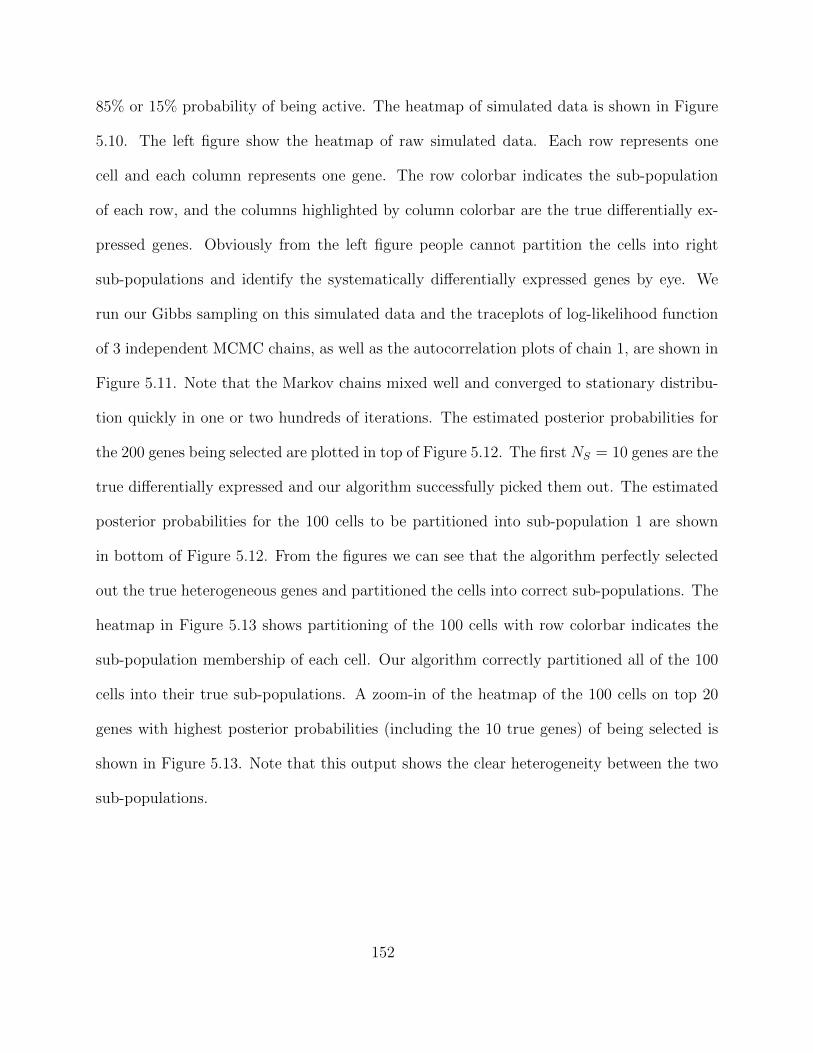
85% or 15% probability of being active. The heatmap of simulated data is shown in Figure
5.10. The left figure show the heatmap of raw simulated data. Each row represents one
cell and each column represents one gene. The row colorbar indicates the sub-population
of each row, and the columns highlighted by column colorbar are the true differentially ex-
pressed genes. Obviously from the left figure people cannot partition the cells into right
sub-populations and identify the systematically differentially expressed genes by eye. We
run our Gibbs sampling on this simulated data and the traceplots of log-likelihood function
of 3 independent MCMC chains, as well as the autocorrelation plots of chain 1, are shown in
Figure 5.11. Note that the Markov chains mixed well and converged to stationary distribu-
tion quickly in one or two hundreds of iterations. The estimated posterior probabilities for
the 200 genes being selected are plotted in top of Figure 5.12. The first NS = 10 genes are the
true differentially expressed and our algorithm successfully picked them out. The estimated
posterior probabilities for the 100 cells to be partitioned into sub-population 1 are shown
in bottom of Figure 5.12. From the figures we can see that the algorithm perfectly selected
out the true heterogeneous genes and partitioned the cells into correct sub-populations. The
heatmap in Figure 5.13 shows partitioning of the 100 cells with row colorbar indicates the
sub-population membership of each cell. Our algorithm correctly partitioned all of the 100
cells into their true sub-populations. A zoom-in of the heatmap of the 100 cells on top 20
genes with highest posterior probabilities (including the 10 true genes) of being selected is
shown in Figure 5.13. Note that this output shows the clear heterogeneity between the two
sub-populations.
152
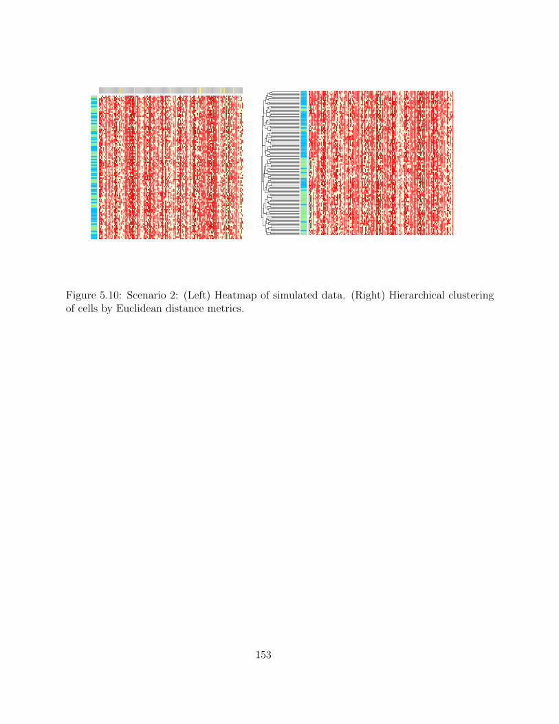
Figure 5.10: Scenario 2: (Left) Heatmap of simulated data. (Right) Hierarchical clusteringof cells by Euclidean distance metrics.
153
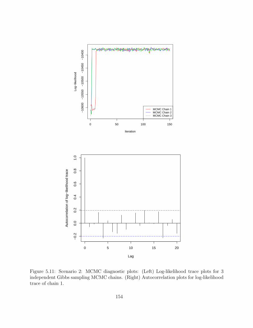
0 50 100 150
−10
600
−10
550
−10
500
−10
450
−10
400
Iteration
Log−
likel
ihoo
d
MCMC Chain 1MCMC Chain 2MCMC Chain 3
0 5 10 15 20
−0.
20.
00.
20.
40.
60.
81.
0
Lag
Aut
ocor
rela
tion
of lo
g−lik
elih
ood
trac
e
Figure 5.11: Scenario 2: MCMC diagnostic plots: (Left) Log-likelihood trace plots for 3independent Gibbs sampling MCMC chains. (Right) Autocorrelation plots for log-likelihoodtrace of chain 1.
154
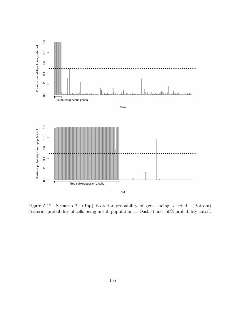
Gene
Pos
terio
r pr
obab
ility
of b
eing
sel
ecte
d
0.0
0.2
0.4
0.6
0.8
1.0
True heterogeneous genes
Cell
Pos
terio
r pr
obab
ility
in s
ub−
popu
latio
n 1
0.0
0.2
0.4
0.6
0.8
1.0
True sub−population 1 cells
Figure 5.12: Scenario 2: (Top) Posterior probability of genes being selected. (Bottom)Posterior probability of cells being in sub-population 1. Dashed line: 50% probability cutoff.
155
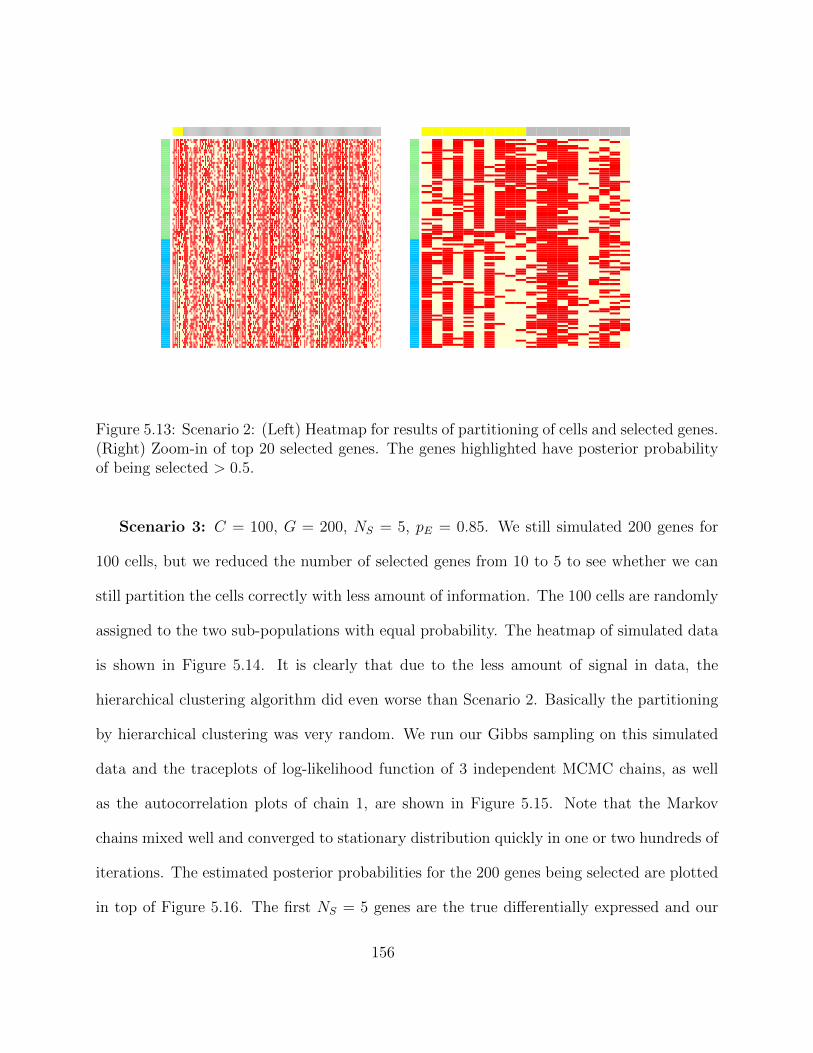
Figure 5.13: Scenario 2: (Left) Heatmap for results of partitioning of cells and selected genes.(Right) Zoom-in of top 20 selected genes. The genes highlighted have posterior probabilityof being selected > 0.5.
Scenario 3: C = 100, G = 200, NS = 5, pE = 0.85. We still simulated 200 genes for
100 cells, but we reduced the number of selected genes from 10 to 5 to see whether we can
still partition the cells correctly with less amount of information. The 100 cells are randomly
assigned to the two sub-populations with equal probability. The heatmap of simulated data
is shown in Figure 5.14. It is clearly that due to the less amount of signal in data, the
hierarchical clustering algorithm did even worse than Scenario 2. Basically the partitioning
by hierarchical clustering was very random. We run our Gibbs sampling on this simulated
data and the traceplots of log-likelihood function of 3 independent MCMC chains, as well
as the autocorrelation plots of chain 1, are shown in Figure 5.15. Note that the Markov
chains mixed well and converged to stationary distribution quickly in one or two hundreds of
iterations. The estimated posterior probabilities for the 200 genes being selected are plotted
in top of Figure 5.16. The first NS = 5 genes are the true differentially expressed and our
156
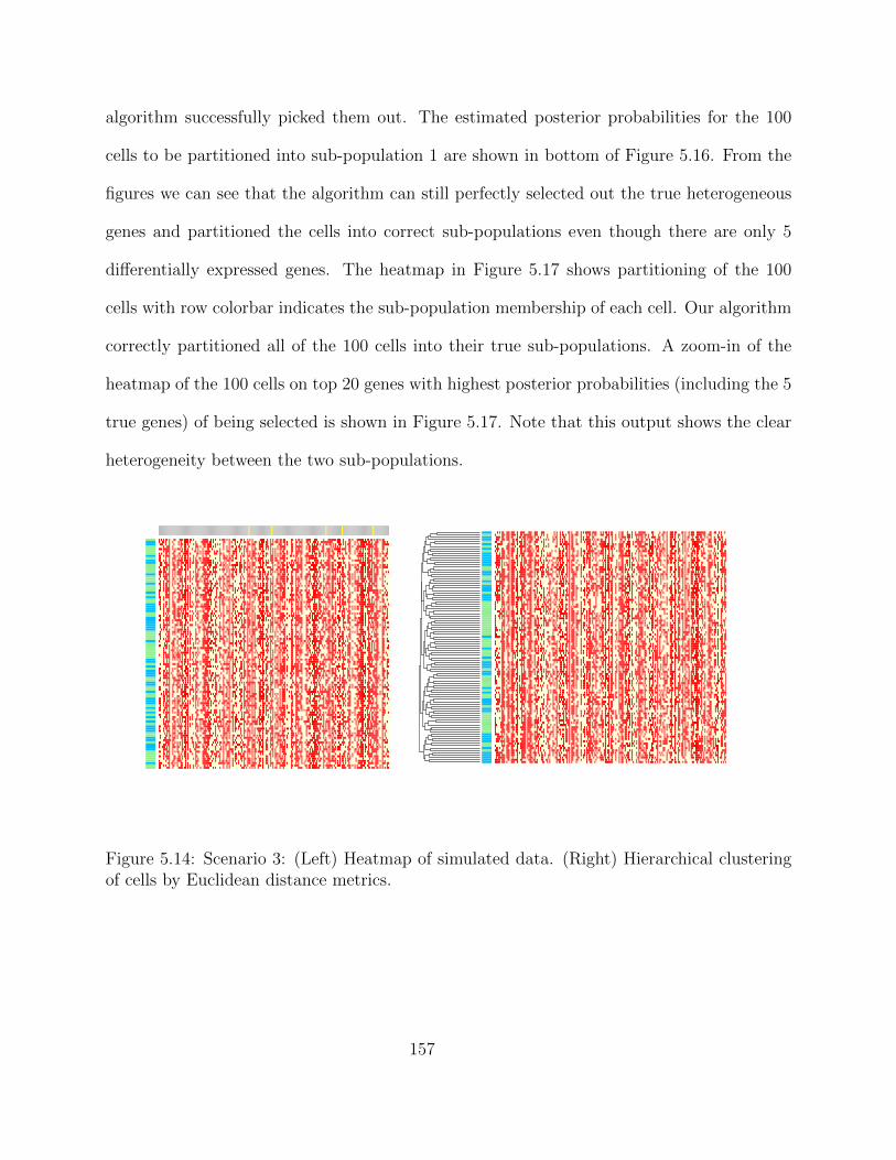
algorithm successfully picked them out. The estimated posterior probabilities for the 100
cells to be partitioned into sub-population 1 are shown in bottom of Figure 5.16. From the
figures we can see that the algorithm can still perfectly selected out the true heterogeneous
genes and partitioned the cells into correct sub-populations even though there are only 5
differentially expressed genes. The heatmap in Figure 5.17 shows partitioning of the 100
cells with row colorbar indicates the sub-population membership of each cell. Our algorithm
correctly partitioned all of the 100 cells into their true sub-populations. A zoom-in of the
heatmap of the 100 cells on top 20 genes with highest posterior probabilities (including the 5
true genes) of being selected is shown in Figure 5.17. Note that this output shows the clear
heterogeneity between the two sub-populations.
Figure 5.14: Scenario 3: (Left) Heatmap of simulated data. (Right) Hierarchical clusteringof cells by Euclidean distance metrics.
157
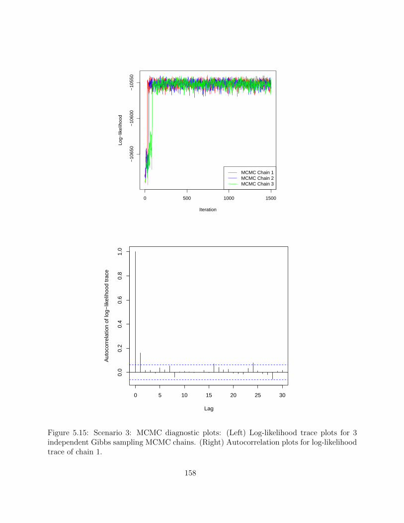
0 500 1000 1500
−10
650
−10
600
−10
550
Iteration
Log−
likel
ihoo
d
MCMC Chain 1MCMC Chain 2MCMC Chain 3
0 5 10 15 20 25 30
0.0
0.2
0.4
0.6
0.8
1.0
Lag
Aut
ocor
rela
tion
of lo
g−lik
elih
ood
trac
e
Figure 5.15: Scenario 3: MCMC diagnostic plots: (Left) Log-likelihood trace plots for 3independent Gibbs sampling MCMC chains. (Right) Autocorrelation plots for log-likelihoodtrace of chain 1.
158
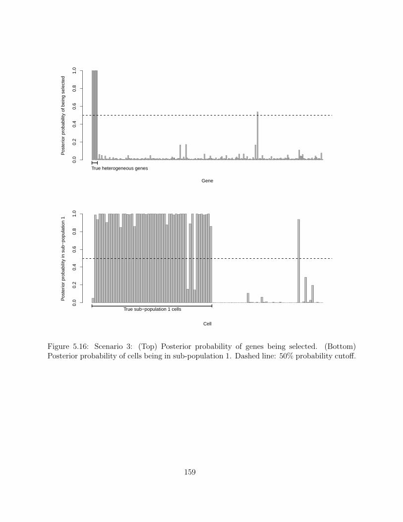
Gene
Pos
terio
r pr
obab
ility
of b
eing
sel
ecte
d
0.0
0.2
0.4
0.6
0.8
1.0
True heterogeneous genes
Cell
Pos
terio
r pr
obab
ility
in s
ub−
popu
latio
n 1
0.0
0.2
0.4
0.6
0.8
1.0
True sub−population 1 cells
Figure 5.16: Scenario 3: (Top) Posterior probability of genes being selected. (Bottom)Posterior probability of cells being in sub-population 1. Dashed line: 50% probability cutoff.
159
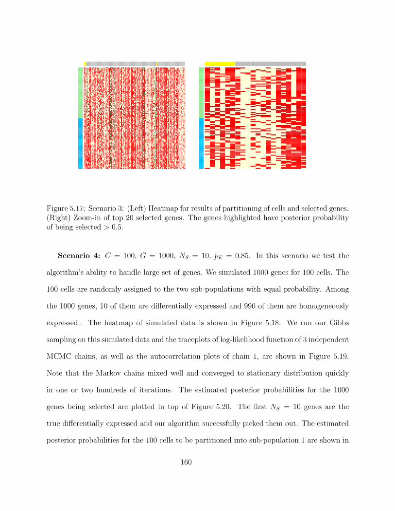
Figure 5.17: Scenario 3: (Left) Heatmap for results of partitioning of cells and selected genes.(Right) Zoom-in of top 20 selected genes. The genes highlighted have posterior probabilityof being selected > 0.5.
Scenario 4: C = 100, G = 1000, NS = 10, pE = 0.85. In this scenario we test the
algorithm’s ability to handle large set of genes. We simulated 1000 genes for 100 cells. The
100 cells are randomly assigned to the two sub-populations with equal probability. Among
the 1000 genes, 10 of them are differentially expressed and 990 of them are homogeneously
expressed.. The heatmap of simulated data is shown in Figure 5.18. We run our Gibbs
sampling on this simulated data and the traceplots of log-likelihood function of 3 independent
MCMC chains, as well as the autocorrelation plots of chain 1, are shown in Figure 5.19.
Note that the Markov chains mixed well and converged to stationary distribution quickly
in one or two hundreds of iterations. The estimated posterior probabilities for the 1000
genes being selected are plotted in top of Figure 5.20. The first NS = 10 genes are the
true differentially expressed and our algorithm successfully picked them out. The estimated
posterior probabilities for the 100 cells to be partitioned into sub-population 1 are shown in
160
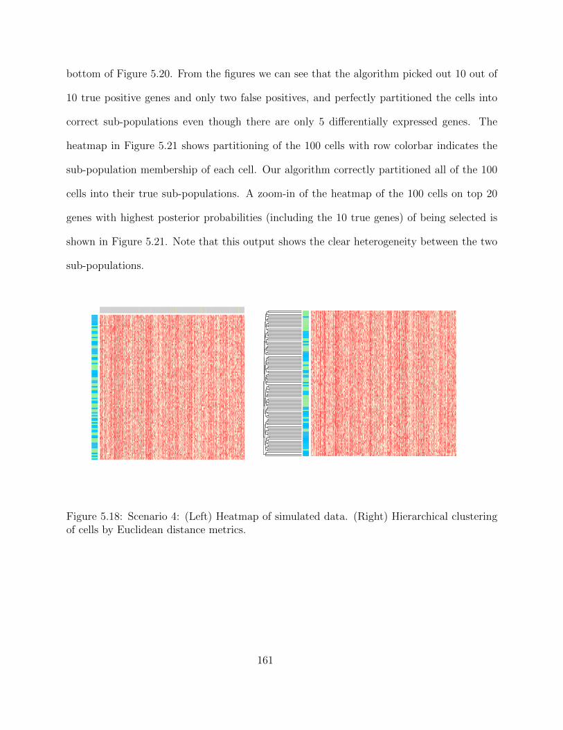
bottom of Figure 5.20. From the figures we can see that the algorithm picked out 10 out of
10 true positive genes and only two false positives, and perfectly partitioned the cells into
correct sub-populations even though there are only 5 differentially expressed genes. The
heatmap in Figure 5.21 shows partitioning of the 100 cells with row colorbar indicates the
sub-population membership of each cell. Our algorithm correctly partitioned all of the 100
cells into their true sub-populations. A zoom-in of the heatmap of the 100 cells on top 20
genes with highest posterior probabilities (including the 10 true genes) of being selected is
shown in Figure 5.21. Note that this output shows the clear heterogeneity between the two
sub-populations.
Figure 5.18: Scenario 4: (Left) Heatmap of simulated data. (Right) Hierarchical clusteringof cells by Euclidean distance metrics.
161
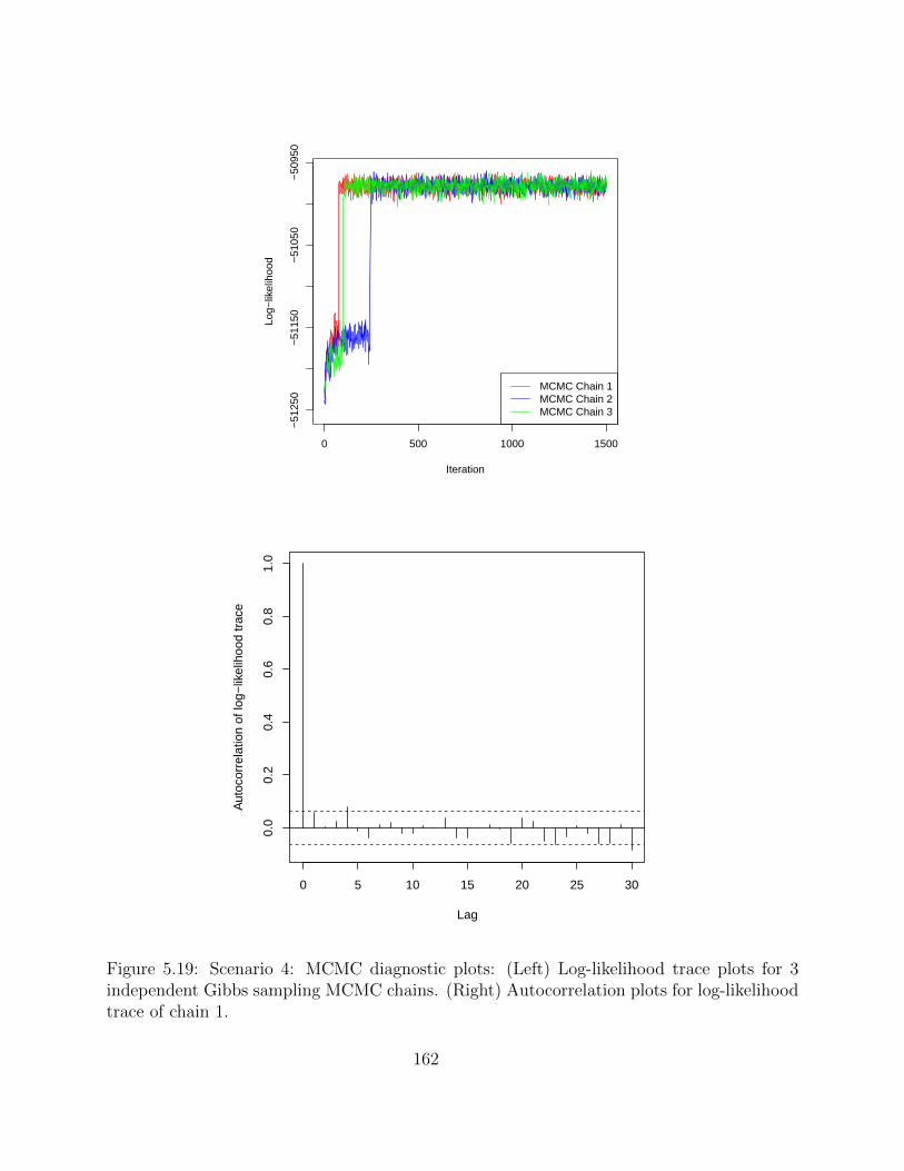
0 500 1000 1500
−51
250
−51
150
−51
050
−50
950
Iteration
Log−
likel
ihoo
d
MCMC Chain 1MCMC Chain 2MCMC Chain 3
0 5 10 15 20 25 30
0.0
0.2
0.4
0.6
0.8
1.0
Lag
Aut
ocor
rela
tion
of lo
g−lik
elih
ood
trac
e
Figure 5.19: Scenario 4: MCMC diagnostic plots: (Left) Log-likelihood trace plots for 3independent Gibbs sampling MCMC chains. (Right) Autocorrelation plots for log-likelihoodtrace of chain 1.
162
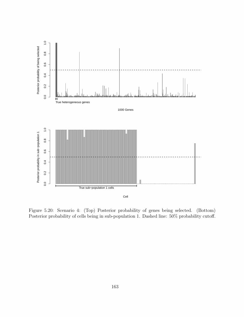
1000 Genes
Pos
terio
r pr
obab
ility
of b
eing
sel
ecte
d
0.0
0.2
0.4
0.6
0.8
1.0
True heterogeneous genes
Cell
Pos
terio
r pr
obab
ility
in s
ub−
popu
latio
n 1
0.0
0.2
0.4
0.6
0.8
1.0
True sub−population 1 cells
Figure 5.20: Scenario 4: (Top) Posterior probability of genes being selected. (Bottom)Posterior probability of cells being in sub-population 1. Dashed line: 50% probability cutoff.
163
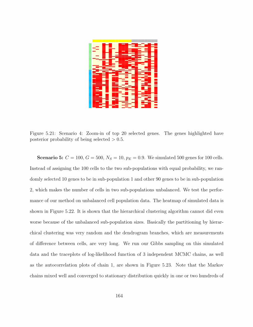
Figure 5.21: Scenario 4: Zoom-in of top 20 selected genes. The genes highlighted haveposterior probability of being selected > 0.5.
Scenario 5: C = 100, G = 500, NS = 10, pE = 0.9. We simulated 500 genes for 100 cells.
Instead of assigning the 100 cells to the two sub-populations with equal probability, we ran-
domly selected 10 genes to be in sub-population 1 and other 90 genes to be in sub-population
2, which makes the number of cells in two sub-populations unbalanced. We test the perfor-
mance of our method on unbalanced cell population data. The heatmap of simulated data is
shown in Figure 5.22. It is shown that the hierarchical clustering algorithm cannot did even
worse because of the unbalanced sub-population sizes. Basically the partitioning by hierar-
chical clustering was very random and the dendrogram branches, which are measurements
of difference between cells, are very long. We run our Gibbs sampling on this simulated
data and the traceplots of log-likelihood function of 3 independent MCMC chains, as well
as the autocorrelation plots of chain 1, are shown in Figure 5.23. Note that the Markov
chains mixed well and converged to stationary distribution quickly in one or two hundreds of
164
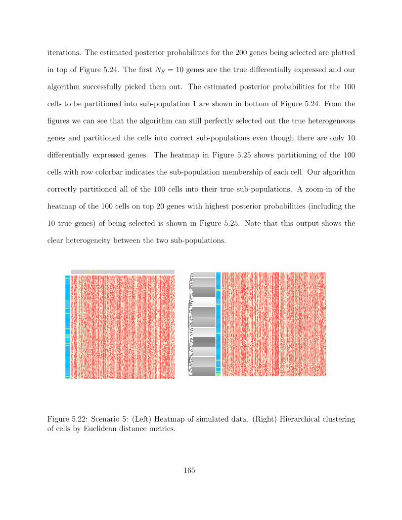
iterations. The estimated posterior probabilities for the 200 genes being selected are plotted
in top of Figure 5.24. The first NS = 10 genes are the true differentially expressed and our
algorithm successfully picked them out. The estimated posterior probabilities for the 100
cells to be partitioned into sub-population 1 are shown in bottom of Figure 5.24. From the
figures we can see that the algorithm can still perfectly selected out the true heterogeneous
genes and partitioned the cells into correct sub-populations even though there are only 10
differentially expressed genes. The heatmap in Figure 5.25 shows partitioning of the 100
cells with row colorbar indicates the sub-population membership of each cell. Our algorithm
correctly partitioned all of the 100 cells into their true sub-populations. A zoom-in of the
heatmap of the 100 cells on top 20 genes with highest posterior probabilities (including the
10 true genes) of being selected is shown in Figure 5.25. Note that this output shows the
clear heterogeneity between the two sub-populations.
Figure 5.22: Scenario 5: (Left) Heatmap of simulated data. (Right) Hierarchical clusteringof cells by Euclidean distance metrics.
165

0 500 1000 1500
−51
250
−51
150
−51
050
−50
950
Iteration
Log−
likel
ihoo
d
MCMC Chain 1MCMC Chain 2MCMC Chain 3
0 5 10 15 20 25 30
0.0
0.2
0.4
0.6
0.8
1.0
Lag
Aut
ocor
rela
tion
of lo
g−lik
elih
ood
trac
e
Figure 5.23: Scenario 5: MCMC diagnostic plots: (Left) Log-likelihood trace plots for 3independent Gibbs sampling MCMC chains. (Right) Autocorrelation plots for log-likelihoodtrace of chain 1.
166
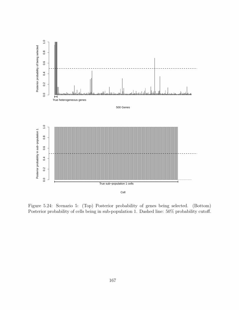
500 Genes
Pos
terio
r pr
obab
ility
of b
eing
sel
ecte
d
0.0
0.2
0.4
0.6
0.8
1.0
True heterogeneous genes
Cell
Pos
terio
r pr
obab
ility
in s
ub−
popu
latio
n 1
0.0
0.2
0.4
0.6
0.8
1.0
True sub−population 1 cells
Figure 5.24: Scenario 5: (Top) Posterior probability of genes being selected. (Bottom)Posterior probability of cells being in sub-population 1. Dashed line: 50% probability cutoff.
167
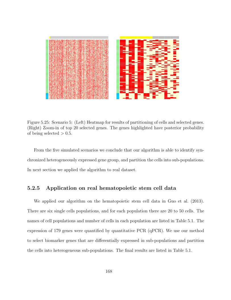
Figure 5.25: Scenario 5: (Left) Heatmap for results of partitioning of cells and selected genes.(Right) Zoom-in of top 20 selected genes. The genes highlighted have posterior probabilityof being selected > 0.5.
From the five simulated scenarios we conclude that our algorithm is able to identify syn-
chronized heterogeneously expressed gene group, and partition the cells into sub-populations.
In next section we applied the algorithm to real dataset.
5.2.5 Application on real hematopoietic stem cell data
We applied our algorithm on the hematopoietic stem cell data in Guo et al. (2013).
There are six single cells populations, and for each population there are 20 to 50 cells. The
names of cell populations and number of cells in each population are listed in Table 5.1. The
expression of 179 genes were quantified by quantitative PCR (qPCR). We use our method
to select biomarker genes that are differentially expressed in sub-populations and partition
the cells into heterogeneous sub-populations. The final results are listed in Table 5.1.
168
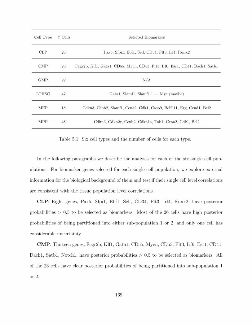
Cell Type # Cells Selected Biomarkers
CLP 26 Pax5, Sfpi1, Ebf1, Sell, CD34, Flt3, Irf4, Runx2
CMP 23 Fcgr2b, Klf1, Gata1, CD55, Mycn, CD53, Flt3, Irf6, Esr1, CD41, Dach1, Satb1
GMP 22 N/A
LTHSC 47 Gata1, Slamf1, Slamf1.1 — Myc (maybe)
MEP 18 Cdkn3, Ccnb2, Slamf1, Ccna2, Cdk1, Casp9, Bcl2l11, Erg, Ccnd1, Bcl2
MPP 48 Cdkn3, Cdkn2c, Ccnb2, Cdkn1a, Tob1, Ccna2, Cdk1, Bcl2
Table 5.1: Six cell types and the number of cells for each type.
In the following paragraphs we describe the analysis for each of the six single cell pop-
ulations. For biomarker genes selected for each single cell population, we explore external
information for the biological background of them and test if their single cell level correlations
are consistent with the tissue population level correlations.
CLP: Eight genes, Pax5, Sfpi1, Ebf1, Sell, CD34, Flt3, Irf4, Runx2, have posterior
probabilities > 0.5 to be selected as biomarkers. Most of the 26 cells have high posterior
probabilities of being partitioned into either sub-population 1 or 2, and only one cell has
considerable uncertainty.
CMP: Thirteen genes, Fcgr2b, Klf1, Gata1, CD55, Mycn, CD53, Flt3, Irf6, Esr1, CD41,
Dach1, Satb1, Notch1, have posterior probabilities > 0.5 to be selected as biomarkers. All
of the 23 cells have clear posterior probabilities of being partitioned into sub-population 1
or 2.
169
GMP: No genes in this cell population, have posterior probabilities > 0.5 to be se-
lected as biomarkers. All of the 22 cells have high uncertainty in posterior probabilities of
being partitioned into sub-population 1 or 2, which suggests that the whole population is
homogeneous and no sub-population exists in this data.
LTHSC: Three genes, Gata1, Slamf1, Slamf1.1, have posterior probabilities > 0.5 and
one gene, Myc, has posterior probability ∼ 0.4 to be selected as biomarkers. All of the 47
cells have clear posterior probabilities of being partitioned into sub-population 1 or 2.
MEP: Ten genes, Cdkn3, Ccnb2, Slamf1, Ccna2, Cdk1, Casp9, Bcl2l11, Erg, Ccnd1,
Bcl2, have posterior probabilities > 0.4 to be selected as biomarkers. All of the 18 cells have
clear posterior probabilities of being partitioned into sub-population 1 or 2.
MPP: Ten genes, Cdkn3, Cdkn2c, Ccnb2, Cdkn1a, Tob1, Ccna2, Cdk1, Bcl2, have
posterior probabilities > 0.5 to be selected as biomarkers. All of the 48 cells have clear
posterior probabilities of being partitioned into sub-population 1 or 2.
170
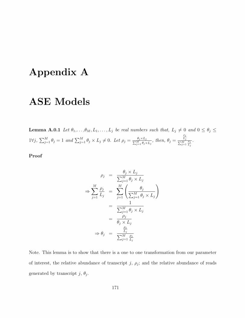
Appendix A
ASE Models
Lemma A.0.1 Let θ1,. . . ,θM , L1, . . . , Lj be real numbers such that, Lj 6= 0 and 0 ≤ θj ≤
1∀j,∑M
j=1 θj = 1 and∑M
j=1 θj × Lj 6= 0. Let ρj =θj×Lj∑Mj=1 θj×Lj
, then, θj =
ρjLj∑Mj=1
ρjLj
.
Proof
ρj =θj × Lj∑Mj=1 θj × Lj
⇒M∑j=1
ρjLj
=M∑j=1
(θj∑M
j=1 θj × Lj
)
=1∑M
j=1 θj × Lj
=ρj
θj × Lj
⇒ θj =
ρjLj∑Mj=1
ρjLj
Note. This lemma is to show that there is a one to one transformation from our parameter
of interest, the relative abundance of transcript j, ρj; and the relative abundance of reads
generated by transcript j, θj.
171

Appendix B
Mathematical Derivations
Proposition B.0.2 If
f(z|µ,y, S,Σ) ∝ exp{−1
2
[(z − µ)T S−1 (z − µ) + (y − z)T Σ−1 (y − z)
]},
then, z ∼ N (µz,Λz), with µz = Λz (S−1µ+ Σ−1y) and Λz = (S−1 + Z−1)−1
Proof The proof can be found in Gelman et al. (2013), pp85.
Proposition B.0.3 If y|β,Σ ∼ Nn (Xβ,Σ), and β|D ∼ Nk(0, D),
then, β|y,Σ, D ∼ Nk(µβ,Λz
), with µβ = ΛβX
TΣ−1y and Λβ =(XTΣ−1X +D−1
)−1
Proof The proof can be found at Lindley and Smith (1972).
172
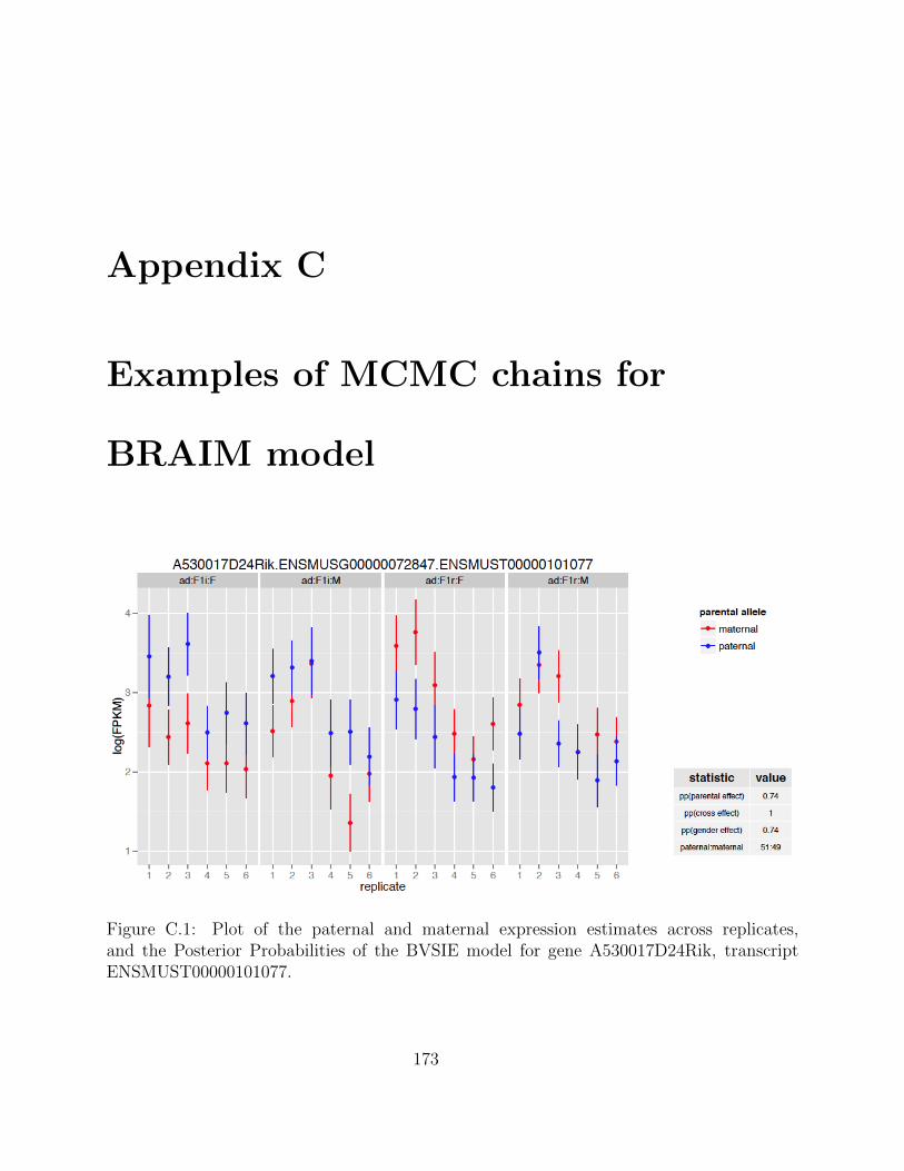
Appendix C
Examples of MCMC chains for
BRAIM model
Figure C.1: Plot of the paternal and maternal expression estimates across replicates,and the Posterior Probabilities of the BVSIE model for gene A530017D24Rik, transcriptENSMUST00000101077.
173
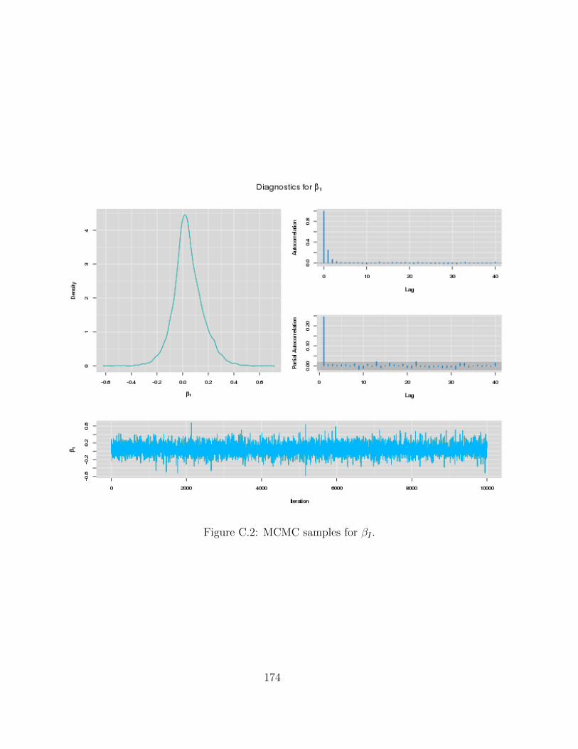
Figure C.2: MCMC samples for βI .
174
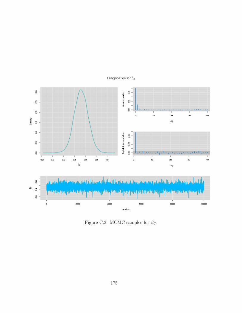
Figure C.3: MCMC samples for βC .
175
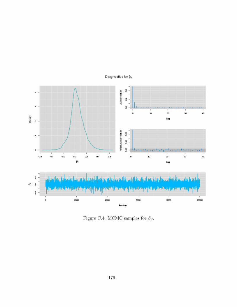
Figure C.4: MCMC samples for βS.
176
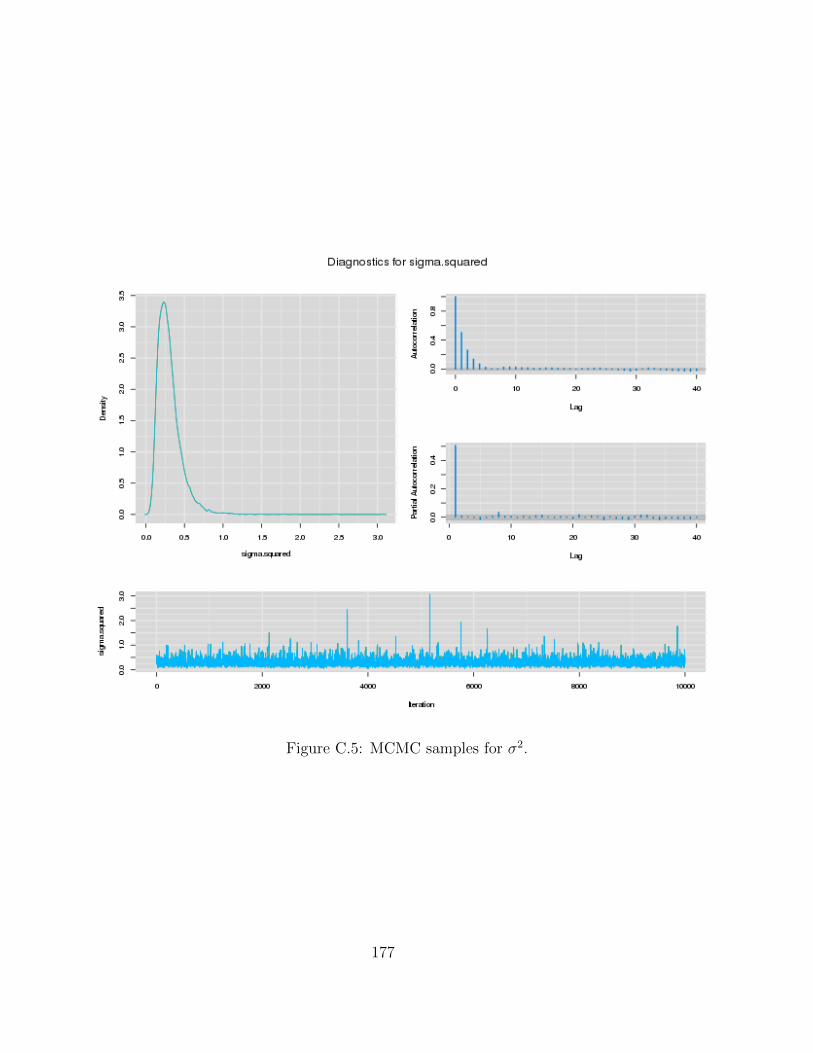
Figure C.5: MCMC samples for σ2.
177
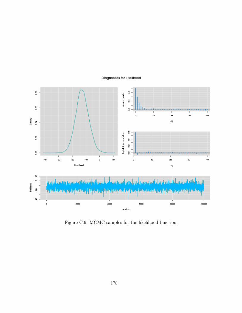
Figure C.6: MCMC samples for the likelihood function.
178
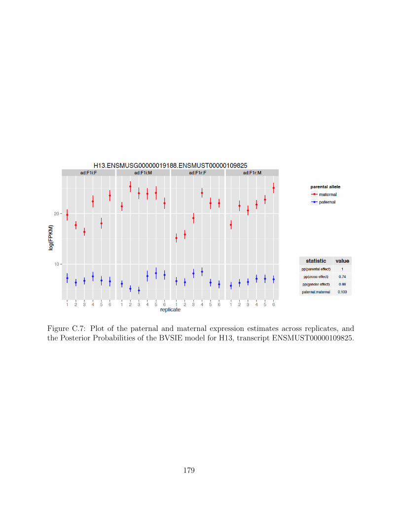
Figure C.7: Plot of the paternal and maternal expression estimates across replicates, andthe Posterior Probabilities of the BVSIE model for H13, transcript ENSMUST00000109825.
179
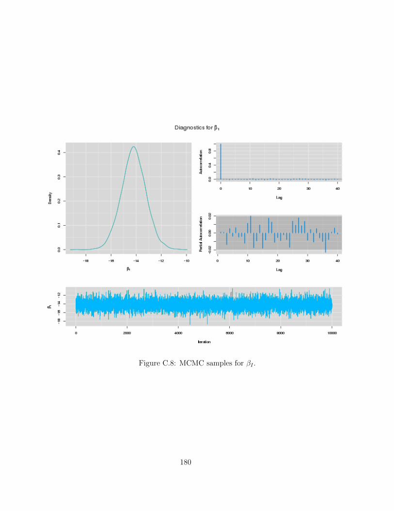
Figure C.8: MCMC samples for βI .
180
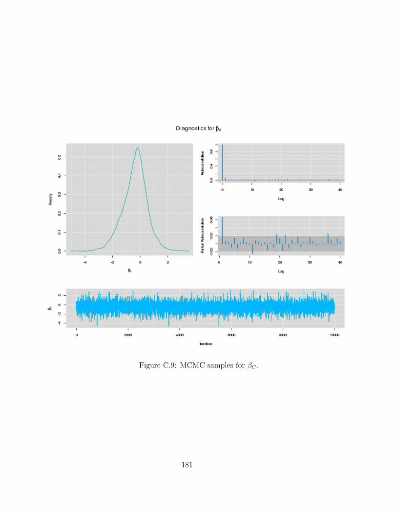
Figure C.9: MCMC samples for βC .
181
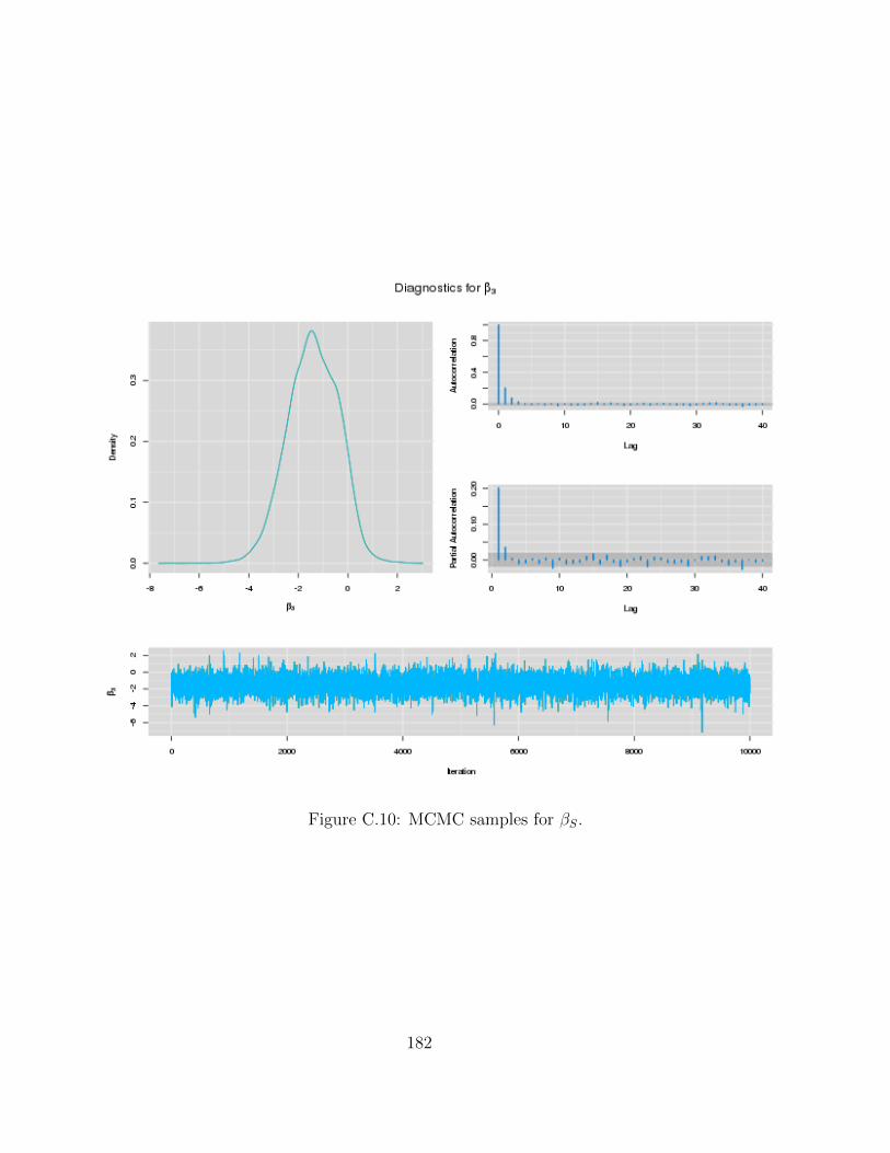
Figure C.10: MCMC samples for βS.
182
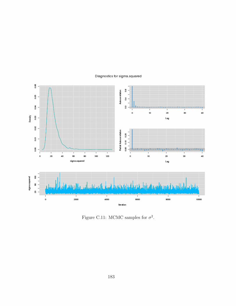
Figure C.11: MCMC samples for σ2.
183
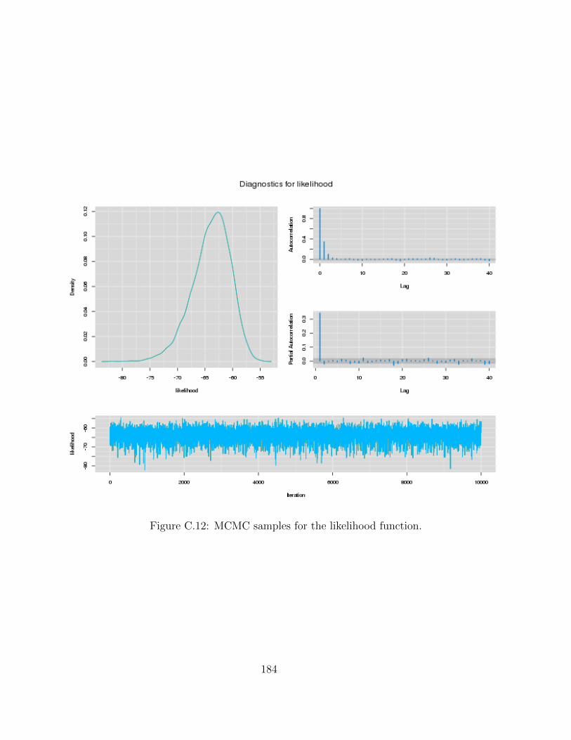
Figure C.12: MCMC samples for the likelihood function.
184
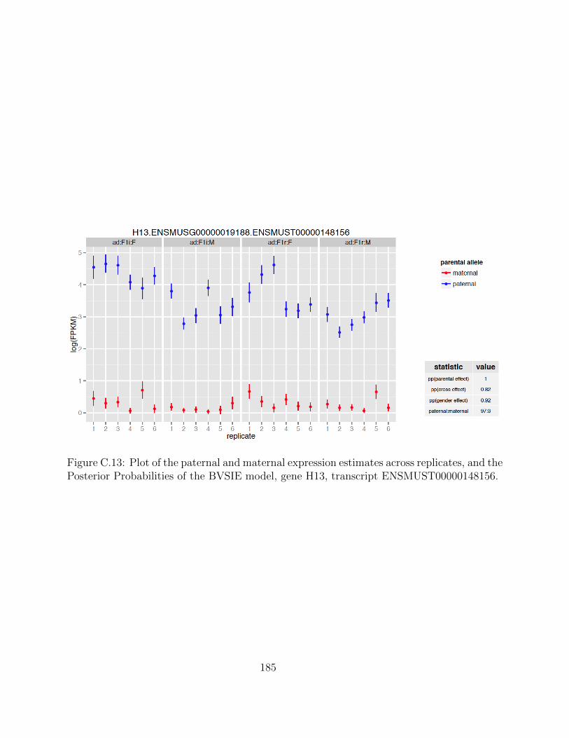
Figure C.13: Plot of the paternal and maternal expression estimates across replicates, and thePosterior Probabilities of the BVSIE model, gene H13, transcript ENSMUST00000148156.
185
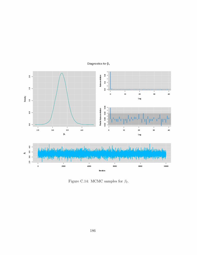
Figure C.14: MCMC samples for βI .
186
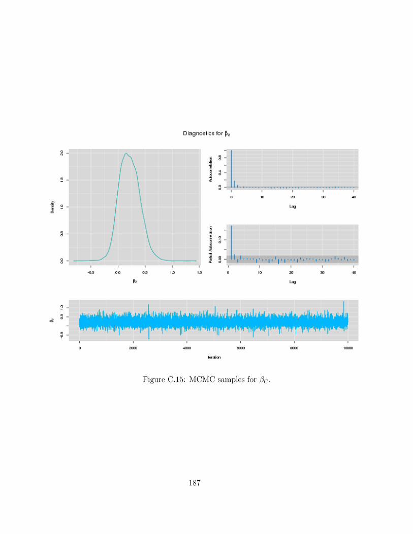
Figure C.15: MCMC samples for βC .
187
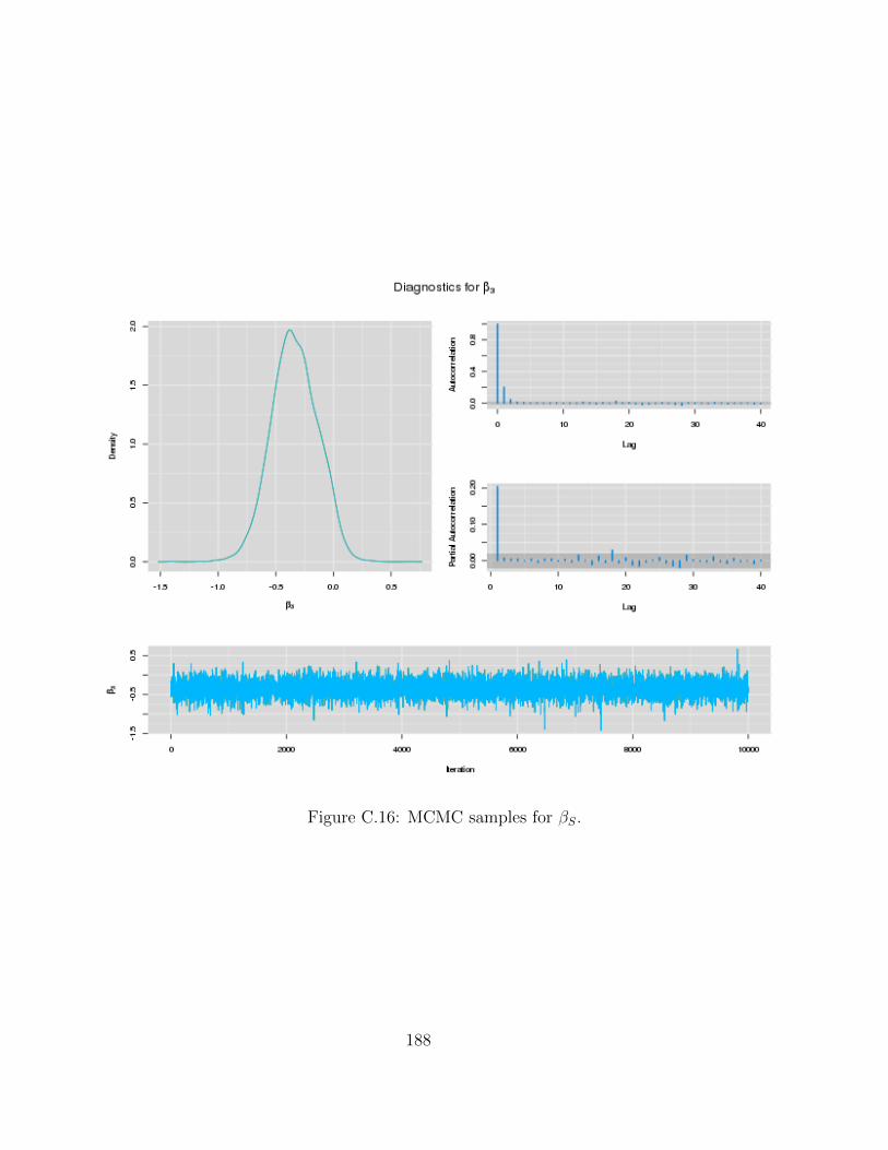
Figure C.16: MCMC samples for βS.
188
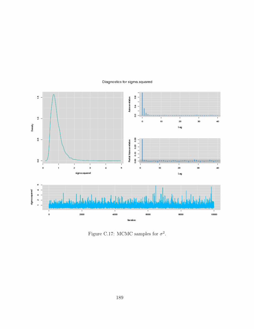
Figure C.17: MCMC samples for σ2.
189
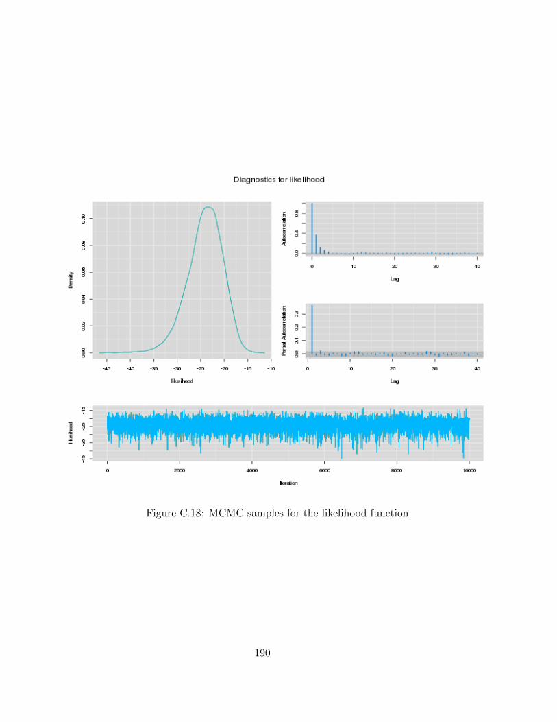
Figure C.18: MCMC samples for the likelihood function.
190

Appendix D
MCMC chains for Hi-BRAIM
D.1 Simulations
191
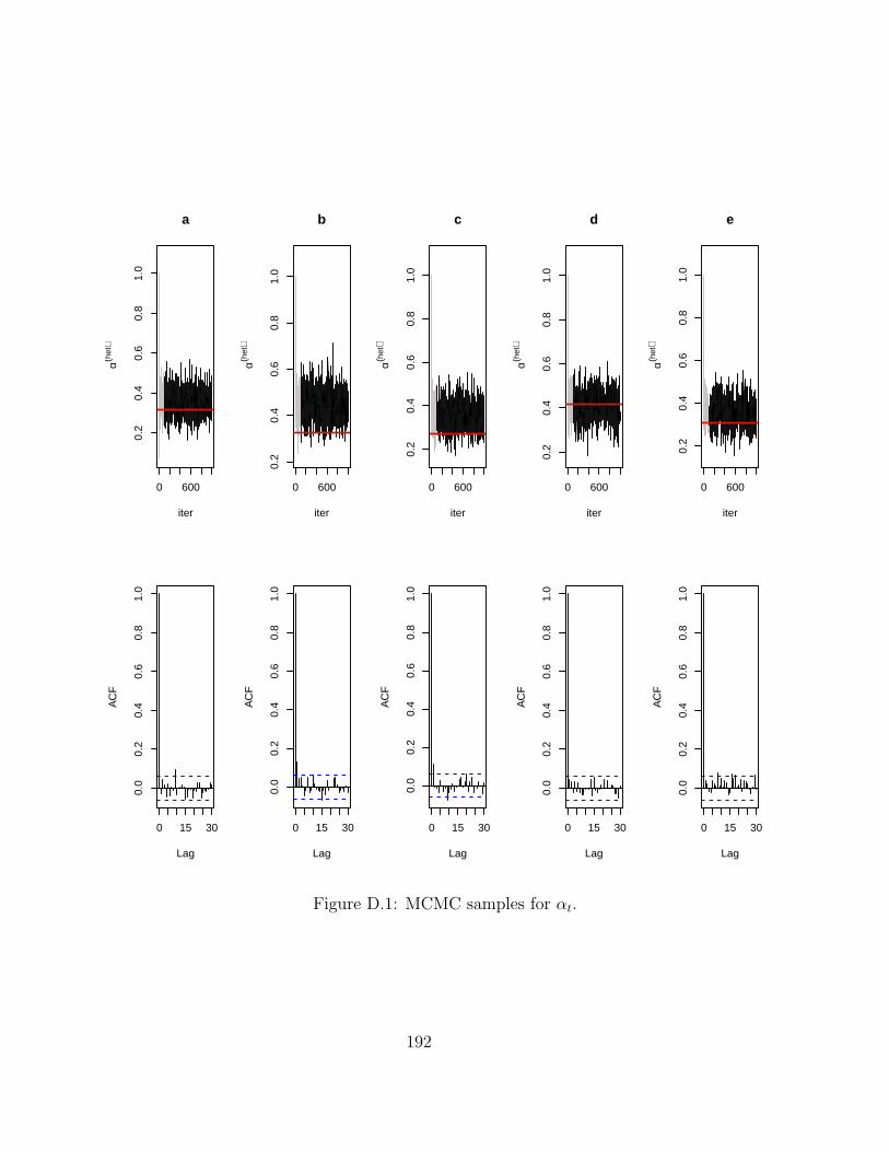
0 600
0.2
0.4
0.6
0.8
1.0
a
iter
α(het
)
0 600
0.2
0.4
0.6
0.8
1.0
b
iter
α(het
)
0 600
0.2
0.4
0.6
0.8
1.0
c
iter
α(het
)
0 600
0.2
0.4
0.6
0.8
1.0
d
iterα(h
et)
0 600
0.2
0.4
0.6
0.8
1.0
e
iter
α(het
)
0 15 30
0.0
0.2
0.4
0.6
0.8
1.0
Lag
AC
F
0 15 30
0.0
0.2
0.4
0.6
0.8
1.0
Lag
AC
F
0 15 30
0.0
0.2
0.4
0.6
0.8
1.0
Lag
AC
F
0 15 30
0.0
0.2
0.4
0.6
0.8
1.0
Lag
AC
F
0 15 30
0.0
0.2
0.4
0.6
0.8
1.0
Lag
AC
F
Figure D.1: MCMC samples for αt.
192
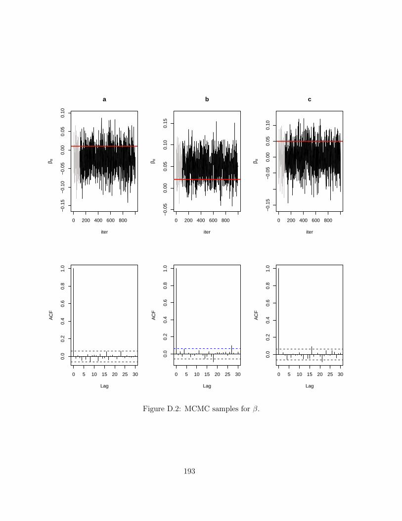
0 200 400 600 800
−0.
15−
0.10
−0.
050.
000.
050.
10
a
iter
β α
0 200 400 600 800
−0.
050.
000.
050.
100.
15
b
iter
β α
0 200 400 600 800
−0.
15−
0.05
0.00
0.05
0.10
c
iter
β α
0 5 10 15 20 25 30
0.0
0.2
0.4
0.6
0.8
1.0
Lag
AC
F
0 5 10 15 20 25 30
0.0
0.2
0.4
0.6
0.8
1.0
Lag
AC
F
0 5 10 15 20 25 30
0.0
0.2
0.4
0.6
0.8
1.0
Lag
AC
F
Figure D.2: MCMC samples for β.
193
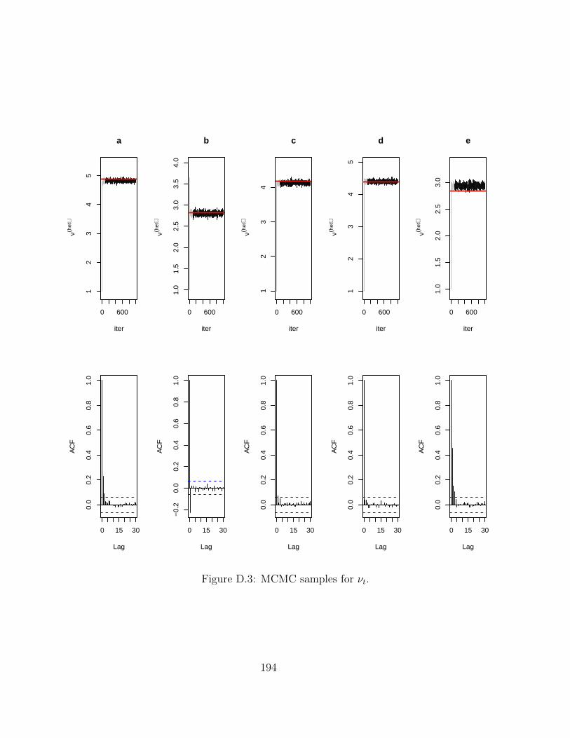
0 600
12
34
5
a
iter
ν(het
)
0 600
1.0
1.5
2.0
2.5
3.0
3.5
4.0
b
iter
ν(het
)
0 600
12
34
c
iter
ν(het
)
0 600
12
34
5
d
iterν(h
et)
0 600
1.0
1.5
2.0
2.5
3.0
e
iter
ν(het
)
0 15 30
0.0
0.2
0.4
0.6
0.8
1.0
Lag
AC
F
0 15 30
−0.
20.
00.
20.
40.
60.
81.
0
Lag
AC
F
0 15 30
0.0
0.2
0.4
0.6
0.8
1.0
Lag
AC
F
0 15 30
0.0
0.2
0.4
0.6
0.8
1.0
Lag
AC
F
0 15 30
0.0
0.2
0.4
0.6
0.8
1.0
Lag
AC
F
Figure D.3: MCMC samples for νt.
194
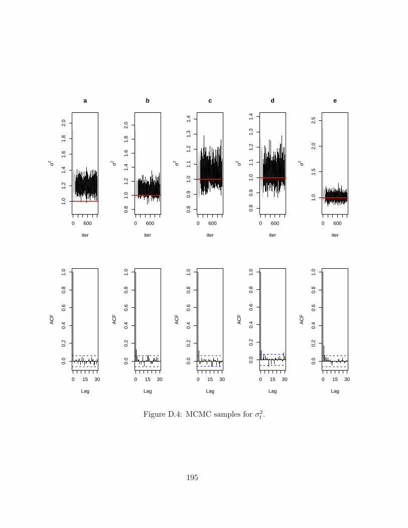
0 600
1.0
1.2
1.4
1.6
1.8
2.0
a
iter
σ2
0 600
0.8
1.0
1.2
1.4
1.6
1.8
2.0
b
iter
σ2
0 600
0.8
0.9
1.0
1.1
1.2
1.3
1.4
c
iter
σ2
0 600
0.8
0.9
1.0
1.1
1.2
1.3
1.4
d
iterσ2
0 600
1.0
1.5
2.0
2.5
e
iter
σ2
0 15 30
0.0
0.2
0.4
0.6
0.8
1.0
Lag
AC
F
0 15 30
0.0
0.2
0.4
0.6
0.8
1.0
Lag
AC
F
0 15 30
0.0
0.2
0.4
0.6
0.8
1.0
Lag
AC
F
0 15 30
0.0
0.2
0.4
0.6
0.8
1.0
Lag
AC
F
0 15 30
0.0
0.2
0.4
0.6
0.8
1.0
Lag
AC
F
Figure D.4: MCMC samples for σ2t .
195
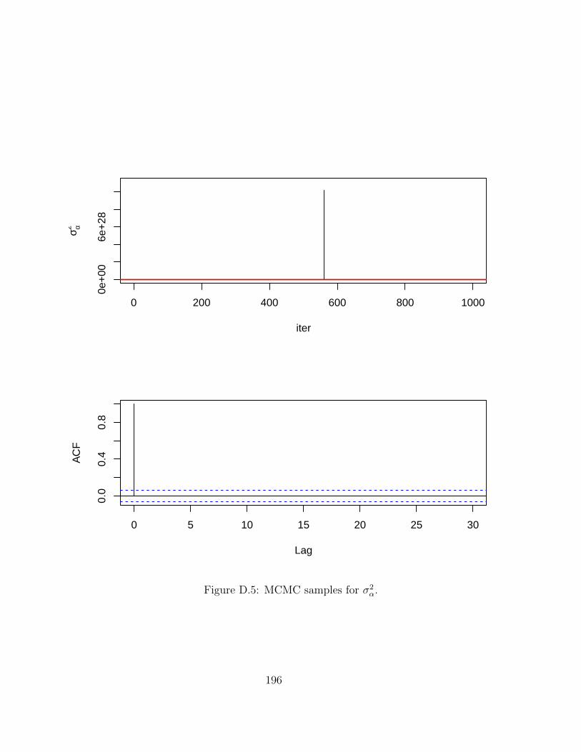
0 200 400 600 800 1000
0e+
006e
+28
iter
σ α2
0 5 10 15 20 25 30
0.0
0.4
0.8
Lag
AC
F
Figure D.5: MCMC samples for σ2α.
196
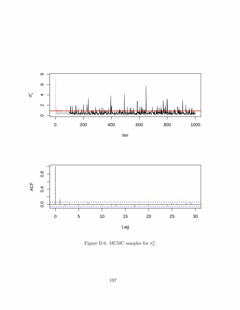
0 200 400 600 800 1000
02
46
8
iter
σ ν2
0 5 10 15 20 25 30
0.0
0.4
0.8
Lag
AC
F
Figure D.6: MCMC samples for σ2ν .
197
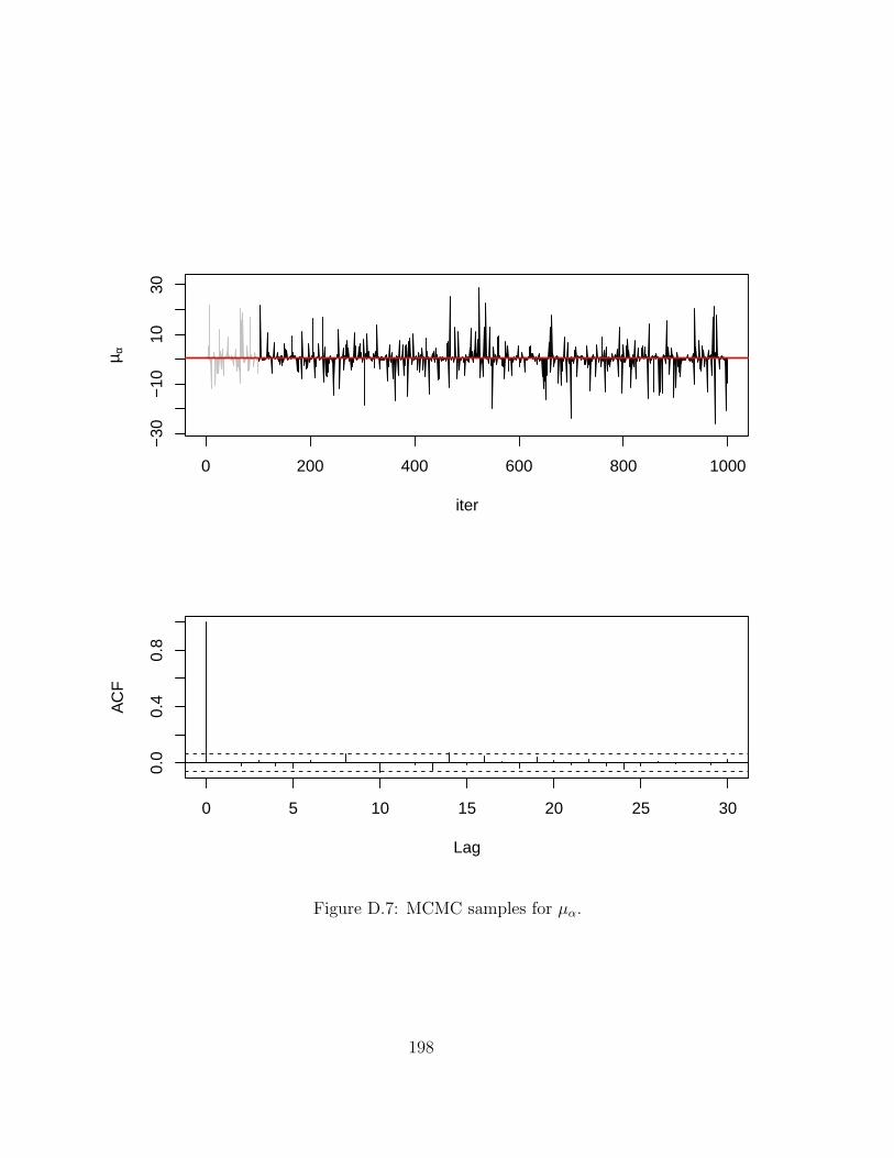
0 200 400 600 800 1000
−30
−10
1030
iter
µ α
0 5 10 15 20 25 30
0.0
0.4
0.8
Lag
AC
F
Figure D.7: MCMC samples for µα.
198
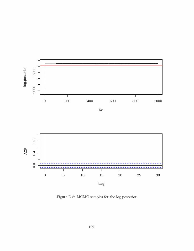
0 200 400 600 800 1000
−90
00−
6000
iter
log.
post
erio
r
0 5 10 15 20 25 30
0.0
0.4
0.8
Lag
AC
F
Figure D.8: MCMC samples for the log posterior.
199

Bibliography
Christopher Badcock and Bernard Crespi. Battle of the sexes may set the brain. Nature,454(7208):1054–1055, 2008.
Susan M Berget, Claire Moore, and Phillip A Sharp. Spliced segments at the 5’terminus ofadenovirus 2 late mrna. Proceedings of the National Academy of Sciences, 74(8):3171–3175,1977.
Douglas L Black. Mechanisms of alternative pre-messenger rna splicing. Annual review ofbiochemistry, 72(1):291–336, 2003.
Siddhartha Chib. Marginal likelihood from the gibbs output. Journal of the AmericanStatistical Association, 90(432):1313–1321, 1995.
Hugh Chipman, Michael Hamada, and CFJ Wu. A bayesian variable-selection approachfor analyzing designed experiments with complex aliasing. Technometrics, 39(4):372–381,1997.
Jacob F Degner, John C Marioni, Athma A Pai, Joseph K Pickrell, Everlyne Nkadori, YoavGilad, and Jonathan K Pritchard. Effect of read-mapping biases on detecting allele-specificexpression from rna-sequencing data. Bioinformatics, 25(24):3207–3212, 2009.
Arthur P Dempster, Nan M Laird, and Donald B Rubin. Maximum likelihood from in-complete data via the em algorithm. Journal of the Royal Statistical Society. Series B(Methodological), pages 1–38, 1977.
ECO. Seqanswers, October 2007. http://seqanswers.com/forums/showthread.php?t=21.
Terrence S Furey. Chip–seq and beyond: new and improved methodologies to detect andcharacterize protein–dna interactions. Nature Reviews Genetics, 13(12):840–852, 2012.
Alastair S Garfield, Michael Cowley, Florentia M Smith, Kim Moorwood, Joanne E Stewart-Cox, Kerry Gilroy, Sian Baker, Jing Xia, Jeffrey W Dalley, Laurence D Hurst, et al.Distinct physiological and behavioural functions for parental alleles of imprinted grb10.Nature, 469(7331):534–538, 2011.
Andrew Gelman. Multilevel (hierarchical) modeling: what it can and cannot do. Techno-metrics, 48(3), 2006.
200

Andrew Gelman, John B Carlin, Hal S Stern, David B Dunson, Aki Vehtari, and Donald BRubin. Bayesian data analysis. CRC press, 2013.
Edward I George and Robert E McCulloch. Variable selection via gibbs sampling. Journalof the American Statistical Association, 88(423):881–889, 1993.
Peter Glaus, Antti Honkela, and Magnus Rattray. Bayesian model of transcript differentialexpression in rna-seq data with biological variation. 2011.
Guoji Guo, Sidinh Luc, Eugenio Marco, Ta-Wei Lin, Cong Peng, Marc A Kerenyi, SemirBeyaz, Woojin Kim, Jian Xu, Partha Pratim Das, et al. Mapping cellular hierarchy bysingle-cell analysis of the cell surface repertoire. Cell stem cell, 13(4):492–505, 2013.
Hui Jiang and Wing Hung Wong. Statistical inferences for isoform expression in rna-seq.Bioinformatics, 25(8):1026–1032, 2009.
Daniel C Koboldt, Karyn Meltz Steinberg, David E Larson, Richard K Wilson, and Elaine RMardis. The next-generation sequencing revolution and its impact on genomics. Cell, 155(1):27–38, 2013.
Roger D Kornberg. Chromatin structure: a repeating unit of histones and dna. Science, 184(4139):868–871, 1974.
Dennis V Lindley and Adrian FM Smith. Bayes estimates for the linear model. Journal ofthe Royal Statistical Society. Series B (Methodological), pages 1–41, 1972.
Michael L Metzker. Sequencing technologies?the next generation. Nature Reviews Genetics,11(1):31–46, 2009.
Qun Pan, Ofer Shai, Leo J Lee, Brendan J Frey, and Benjamin J Blencowe. Deep sur-veying of alternative splicing complexity in the human transcriptome by high-throughputsequencing. Nature genetics, 40(12):1413–1415, 2008.
Peter J Park. Chip–seq: advantages and challenges of a maturing technology. Nature ReviewsGenetics, 10(10):669–680, 2009.
Adam Roberts, Cole Trapnell, Julie Donaghey, John L Rinn, Lior Pachter, et al. Improvingrna-seq expression estimates by correcting for fragment bias. Genome Biol, 12(3):R22,2011.
Mark D Robinson, Davis J McCarthy, and Gordon K Smyth. edger: a bioconductor packagefor differential expression analysis of digital gene expression data. Bioinformatics, 26(1):139–140, 2010.
Fred Sanger and Alan R Coulson. A rapid method for determining sequences in dna byprimed synthesis with dna polymerase. Journal of molecular biology, 94(3):441–448, 1975.
201
Frederick Sanger, Steven Nicklen, and Alan R Coulson. Dna sequencing with chain-terminating inhibitors. Proceedings of the National Academy of Sciences, 74(12):5463–5467, 1977.
Alex K Shalek, Rahul Satija, Xian Adiconis, Rona S Gertner, Jellert T Gaublomme, RaktimaRaychowdhury, Schragi Schwartz, Nir Yosef, Christine Malboeuf, Diana Lu, et al. Single-cell transcriptomics reveals bimodality in expression and splicing in immune cells. Nature,2013.
the International Human Genome Sequencing Consortium. Initial sequencing and analysisof the human genome. Nature, 409(6822):860–921, February 2001. ISSN 0028-0836. doi:10.1038/35057062. URL http://dx.doi.org/10.1038/35057062.
Cole Trapnell, Brian A Williams, Geo Pertea, Ali Mortazavi, Gordon Kwan, Marijke J vanBaren, Steven L Salzberg, Barbara J Wold, and Lior Pachter. Transcript assembly andquantification by rna-seq reveals unannotated transcripts and isoform switching duringcell differentiation. Nature biotechnology, 28(5):511–515, 2010.
Cole Trapnell, David G Hendrickson, Martin Sauvageau, Loyal Goff, John L Rinn, and LiorPachter. Differential analysis of gene regulation at transcript resolution with rna-seq.Nature biotechnology, 31(1):46–53, 2013.
Ernest Turro, Shu-Yi Su, Angela Goncalves, LJ Coin, Sylvia Richardson, and Alex Lewin.Haplotype and isoform specific expression estimation using multi-mapping rna-seq reads.Genome Biol, 12(2):R13, 2011.
J. C. Venter, M. D. Adams, E. W. Myers, P. W. Li, R. J. Mural, G. G. Sutton, H. O. Smith,M. Yandell, C. A. Evans, and R. A. Holt. The Sequence of the Human Genome. Science,291(5507):1304–1351, February 2001. ISSN 1095-9203. doi: 10.1126/science.1058040. URLhttp://dx.doi.org/10.1126/science.1058040.
Matti Vihola. Robust adaptive metropolis algorithm with coerced acceptance rate. Statisticsand Computing, 22(5):997–1008, 2012.
Gunter P Wagner, Koryu Kin, and Vincent J Lynch. Measurement of mrna abundance usingrna-seq data: Rpkm measure is inconsistent among samples. Theory in Biosciences, 131(4):281–285, 2012.
Zhong Wang, Mark Gerstein, and Michael Snyder. Rna-seq: a revolutionary tool for tran-scriptomics. Nature Reviews Genetics, 10(1):57–63, 2009.
Jon F Wilkins and David Haig. What good is genomic imprinting: the function of parent-specific gene expression. Nature Reviews Genetics, 4(5):359–368, 2003.
202