‘-

1

Chemical Engineering Plant Design

Lecture 18 Piping Systems

Instructor: David Courtemanche

CE 408

‘-

2

Piping Systems

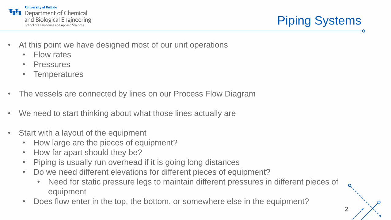
• At this point we have designed most of our unit operations

• Flow rates

• Pressures

• Temperatures

• The vessels are connected by lines on our Process Flow Diagram

• We need to start thinking about what those lines actually are

• Start with a layout of the equipment

• How large are the pieces of equipment?

• How far apart should they be?

• Piping is usually run overhead if it is going long distances

• Do we need different elevations for different pieces of equipment?

• Need for static pressure legs to maintain different pressures in different pieces of

equipment

• Does flow enter in the top, the bottom, or somewhere else in the equipment?

‘-

3

Piping Systems

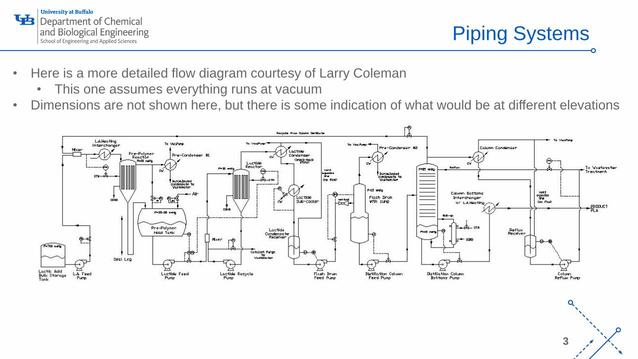
• Here is a more detailed flow diagram courtesy of Larry Coleman

• This one assumes everything runs at vacuum

• Dimensions are not shown here, but there is some indication of what would be at different elevations

‘-

4

Piping Systems

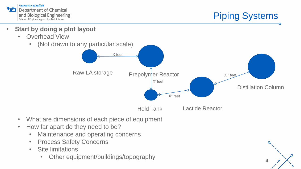
• Start by doing a plot layout

• Overhead View

• (Not drawn to any particular scale)

• What are dimensions of each piece of equipment

• How far apart do they need to be?

• Maintenance and operating concerns

• Process Safety Concerns

• Site limitations

• Other equipment/buildings/topography

Raw LA storage Prepolymer Reactor

Hold Tank Lactide Reactor

Distillation Column

X feet

X’ feet

X’’ feet

X’’’ feet

‘-

5

Piping Systems

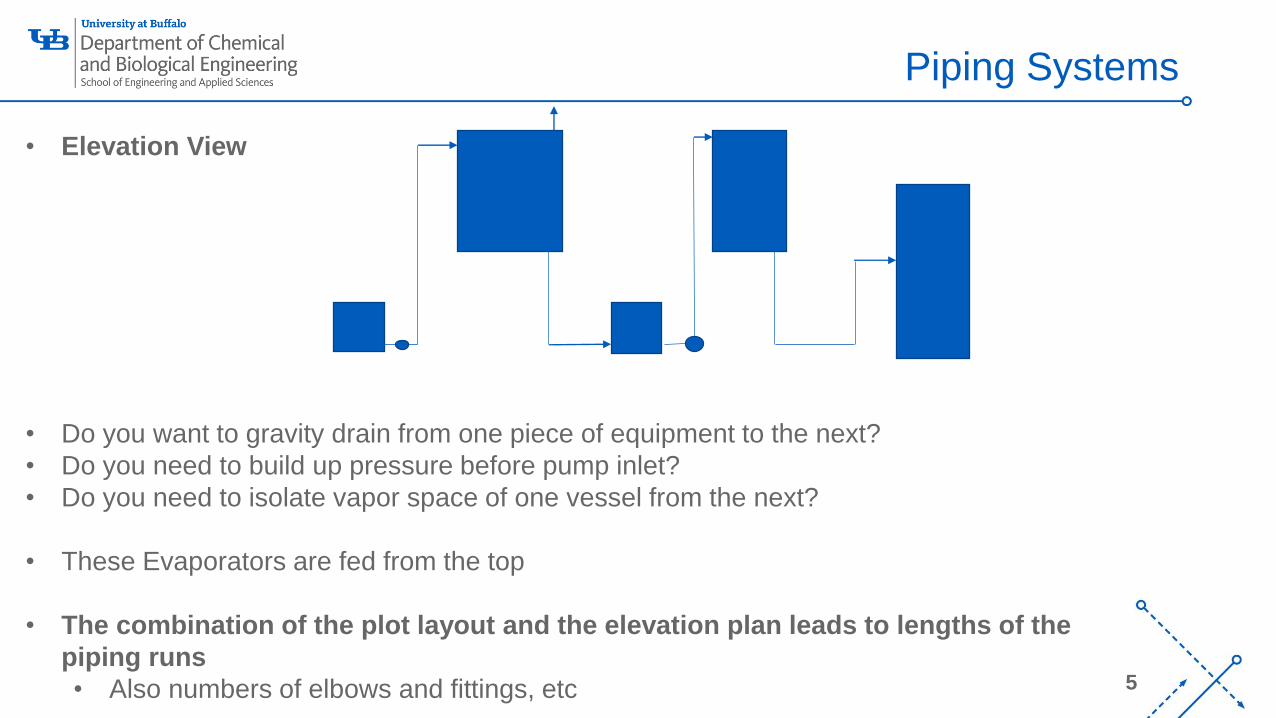
• Elevation View

• Do you want to gravity drain from one piece of equipment to the next?

• Do you need to build up pressure before pump inlet?

• Do you need to isolate vapor space of one vessel from the next?

• These Evaporators are fed from the top

• The combination of the plot layout and the elevation plan leads to lengths of the

piping runs

• Also numbers of elbows and fittings, etc

‘-

6

Piping Systems

• After we have a layout and an idea about the piping paths we need to determine a few more things:

• Pipe diameter

• Pumping requirements

• These are very much connected to one another

‘-

7

Piping Systems

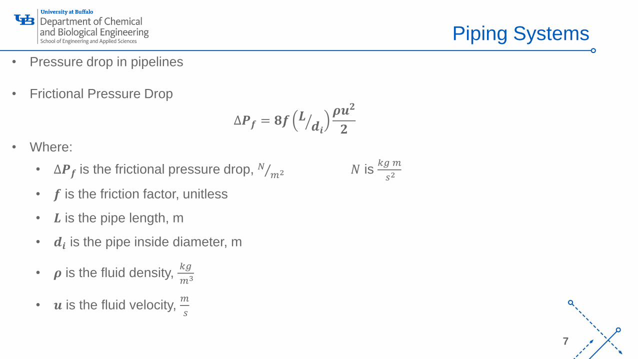
• Pressure drop in pipelines

• Frictional Pressure Drop

∆𝑷𝒇 = 𝟖𝒇 ൗ𝑳 𝒅𝒊

𝝆𝒖𝟐

𝟐

• Where:

• ∆𝑷𝒇 is the frictional pressure drop, Τ𝑁 𝑚2 𝑁 is𝑘𝑔 𝑚

𝑠2

• 𝒇 is the friction factor, unitless

• 𝑳 is the pipe length, m

• 𝒅𝒊 is the pipe inside diameter, m

• 𝝆 is the fluid density, 𝑘𝑔

𝑚3

• 𝒖 is the fluid velocity, 𝑚

𝑠

‘-

8

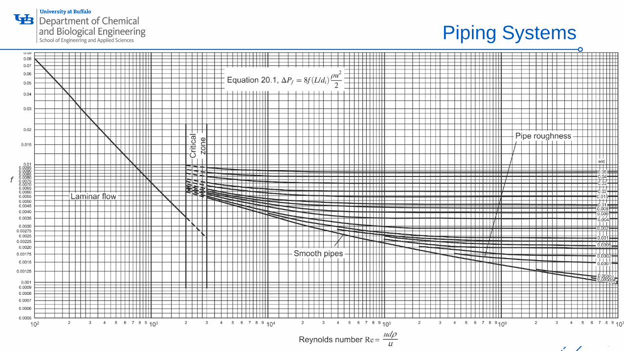
Piping Systems

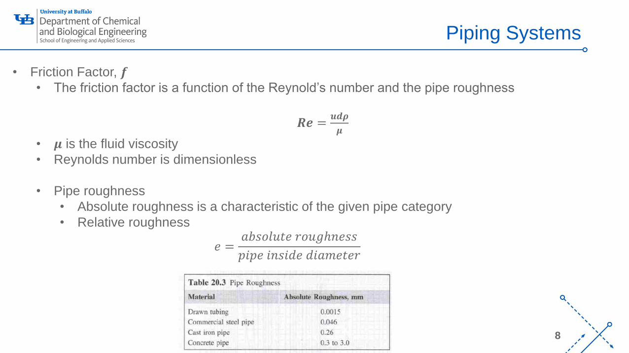
• Friction Factor, 𝒇• The friction factor is a function of the Reynold’s number and the pipe roughness

𝑹𝒆 =𝒖𝒅𝝆

𝝁

• 𝝁 is the fluid viscosity

• Reynolds number is dimensionless

• Pipe roughness

• Absolute roughness is a characteristic of the given pipe category

• Relative roughness

𝑒 =𝑎𝑏𝑠𝑜𝑙𝑢𝑡𝑒 𝑟𝑜𝑢𝑔ℎ𝑛𝑒𝑠𝑠

𝑝𝑖𝑝𝑒 𝑖𝑛𝑠𝑖𝑑𝑒 𝑑𝑖𝑎𝑚𝑒𝑡𝑒𝑟

‘-

9

Piping Systems

‘-

10

Piping Systems

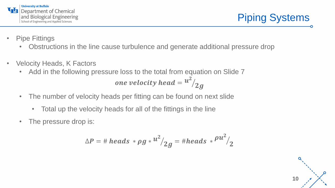
• Pipe Fittings

• Obstructions in the line cause turbulence and generate additional pressure drop

• Velocity Heads, K Factors

• Add in the following pressure loss to the total from equation on Slide 7

𝒐𝒏𝒆 𝒗𝒆𝒍𝒐𝒄𝒊𝒕𝒚 𝒉𝒆𝒂𝒅 = ൗ𝒖𝟐𝟐𝒈

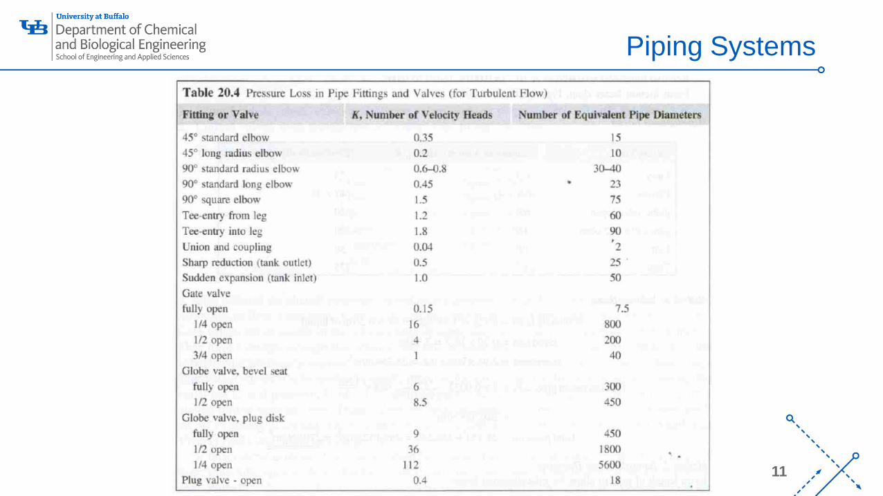
• The number of velocity heads per fitting can be found on next slide

• Total up the velocity heads for all of the fittings in the line

• The pressure drop is:

∆𝑷 = # 𝒉𝒆𝒂𝒅𝒔 ∗ 𝝆𝒈 ∗ ൗ𝒖𝟐𝟐𝒈 = #𝒉𝒆𝒂𝒅𝒔 ∗ ൗ𝝆𝒖𝟐

𝟐

‘-

11

Piping Systems

‘-

12

Piping Systems

• Pipe Fittings

• Equivalent Pipe Diameters

• Total up the number of equivalent pipe diameters for all of the fittings

• Multiply by the pipe diameter

• Increase the length of pipe by the calculated length

‘-

13

Piping Systems

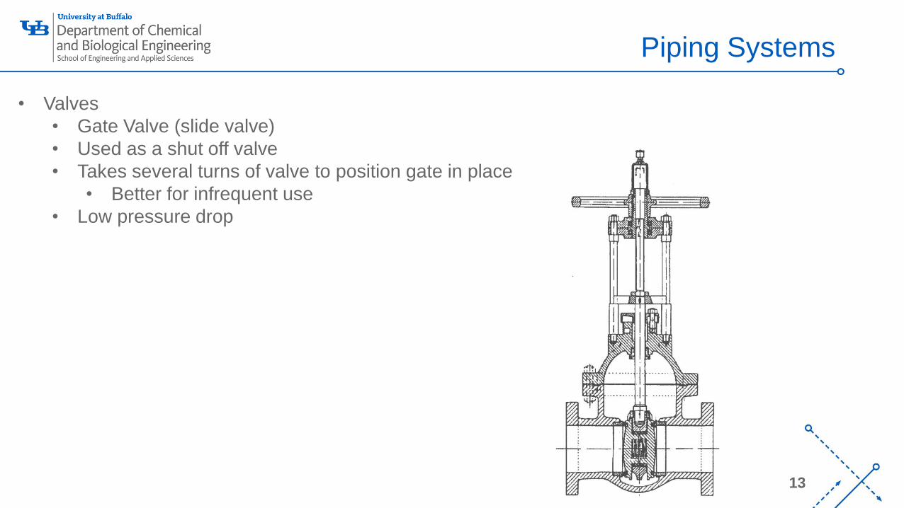
• Valves

• Gate Valve (slide valve)

• Used as a shut off valve

• Takes several turns of valve to position gate in place

• Better for infrequent use

• Low pressure drop

‘-

14

Piping Systems

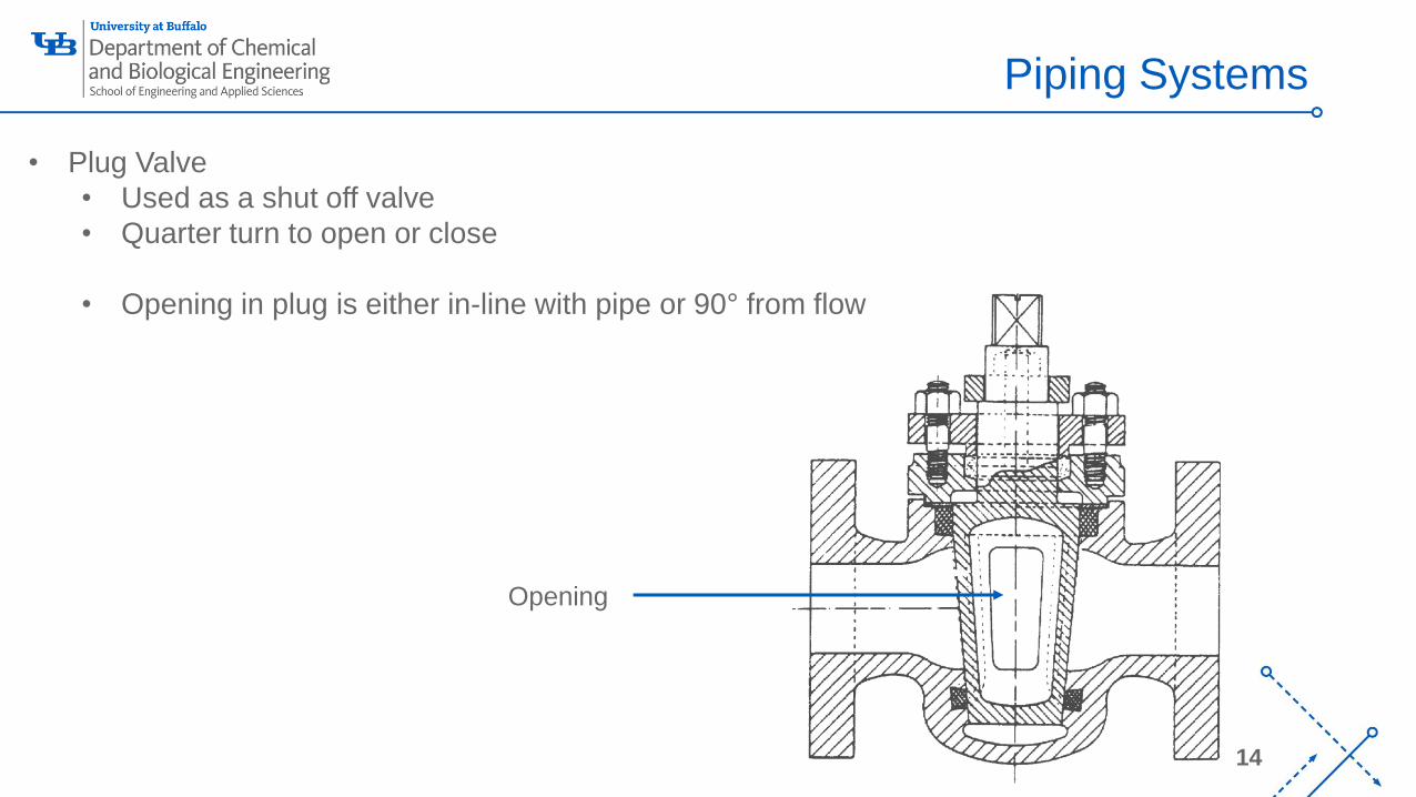
• Plug Valve

• Used as a shut off valve

• Quarter turn to open or close

• Opening in plug is either in-line with pipe or 90° from flow

Opening

‘-

15

Piping Systems

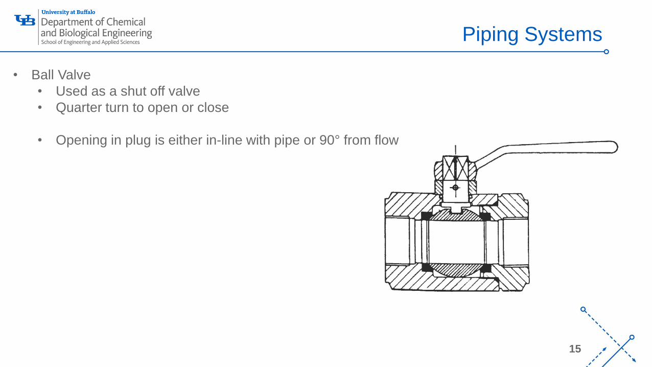
• Ball Valve

• Used as a shut off valve

• Quarter turn to open or close

• Opening in plug is either in-line with pipe or 90° from flow

‘-

16

Piping Systems

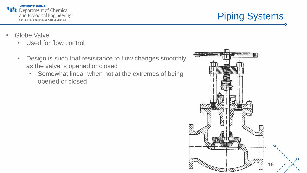
• Globe Valve

• Used for flow control

• Design is such that resisitance to flow changes smoothly

as the valve is opened or closed

• Somewhat linear when not at the extremes of being

opened or closed

‘-

17

Piping Systems

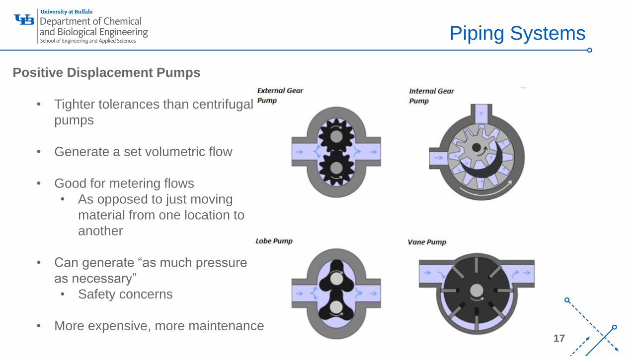
Positive Displacement Pumps

• Tighter tolerances than centrifugal

pumps

• Generate a set volumetric flow

• Good for metering flows

• As opposed to just moving

material from one location to

another

• Can generate “as much pressure

as necessary”

• Safety concerns

• More expensive, more maintenance

‘-

18

Piping Systems

Lobe Pump

‘-

19

Piping Systems

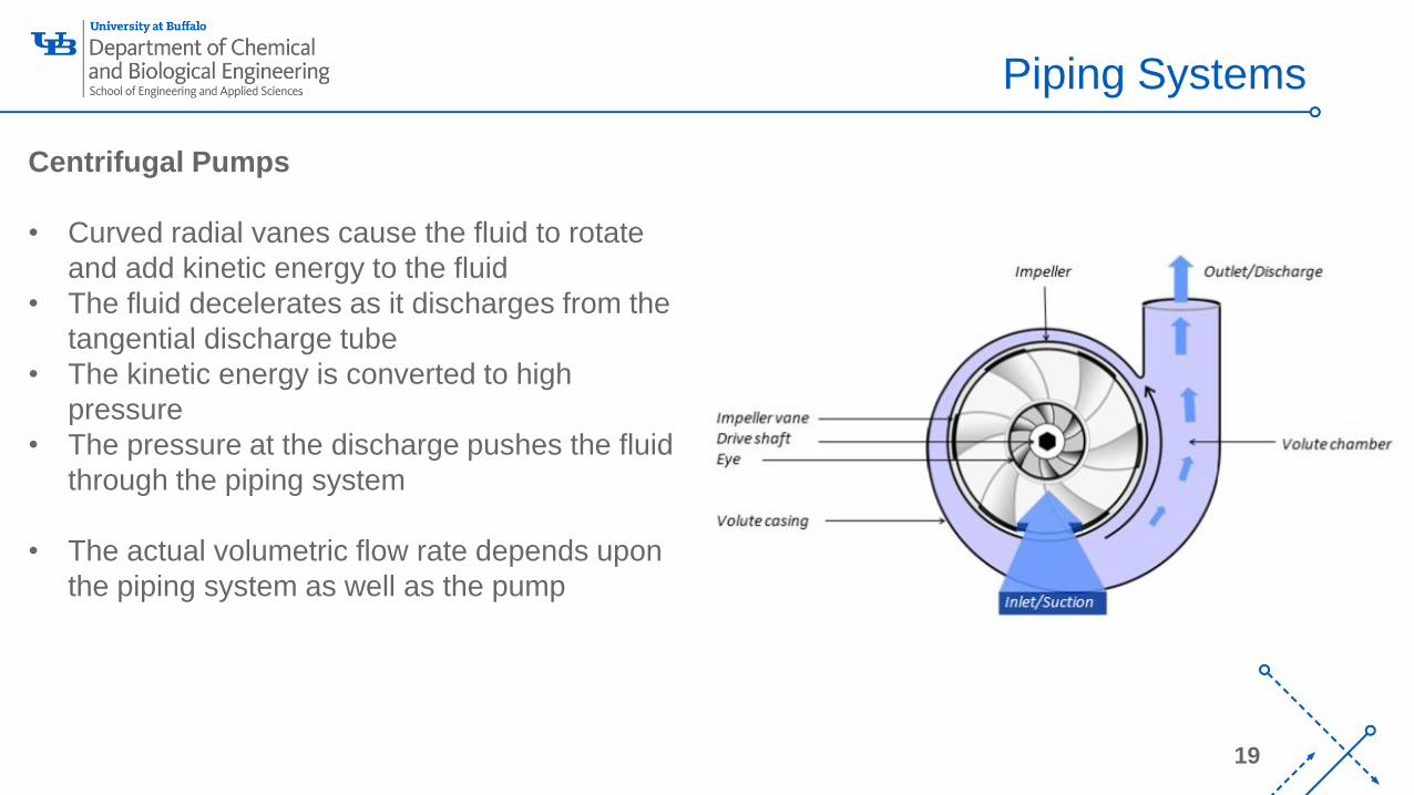
Centrifugal Pumps

• Curved radial vanes cause the fluid to rotate

and add kinetic energy to the fluid

• The fluid decelerates as it discharges from the

tangential discharge tube

• The kinetic energy is converted to high

pressure

• The pressure at the discharge pushes the fluid

through the piping system

• The actual volumetric flow rate depends upon

the piping system as well as the pump

‘-

20

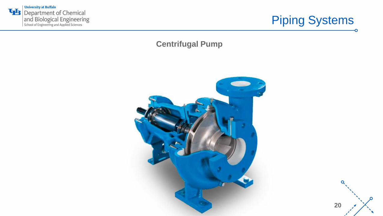
Piping Systems

Centrifugal Pump

‘-

21

Piping Systems

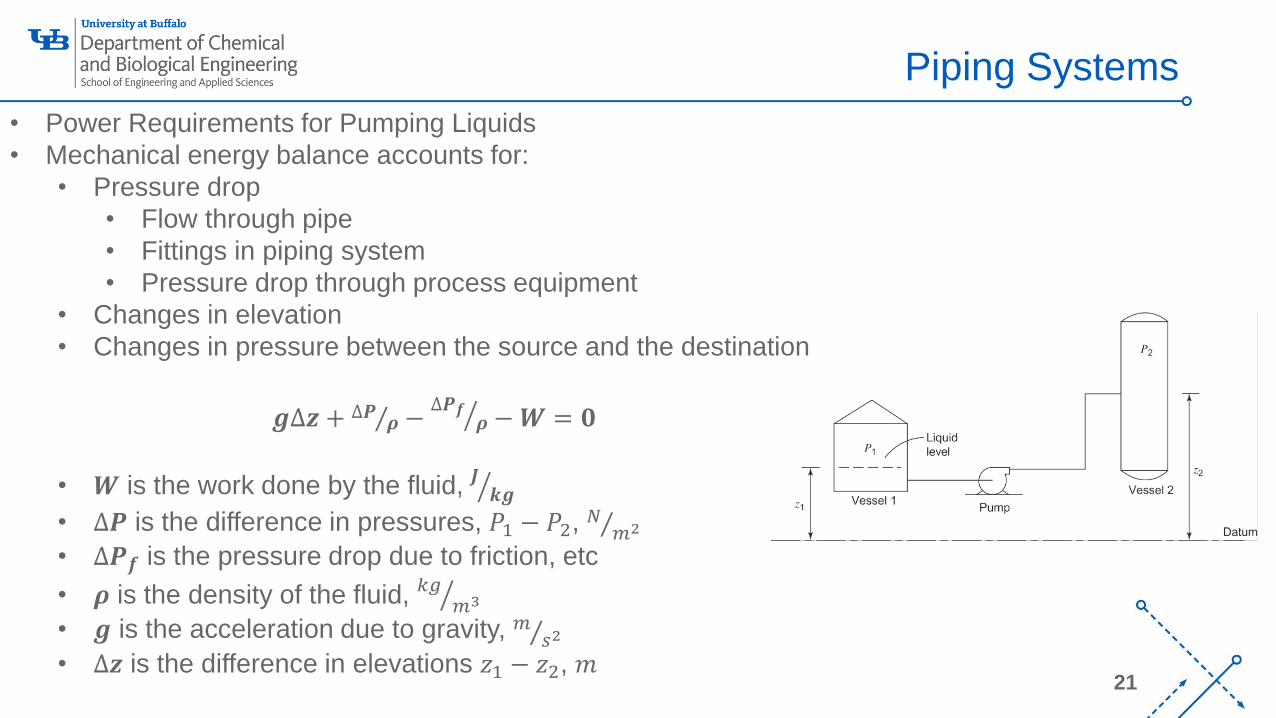
• Power Requirements for Pumping Liquids

• Mechanical energy balance accounts for:

• Pressure drop

• Flow through pipe

• Fittings in piping system

• Pressure drop through process equipment

• Changes in elevation

• Changes in pressure between the source and the destination

𝒈∆𝒛 + Τ∆𝑷𝝆− ൗ∆𝑷𝒇

𝝆−𝑾 = 𝟎

• 𝑾 is the work done by the fluid, ൗ𝑱 𝒌𝒈

• ∆𝑷 is the difference in pressures, 𝑃1 − 𝑃2, Τ𝑁 𝑚2

• ∆𝑷𝒇 is the pressure drop due to friction, etc

• 𝝆 is the density of the fluid, ൗ𝑘𝑔𝑚3

• 𝒈 is the acceleration due to gravity, Τ𝑚 𝑠2

• ∆𝒛 is the difference in elevations 𝑧1 − 𝑧2, 𝑚

‘-

22

Piping Systems

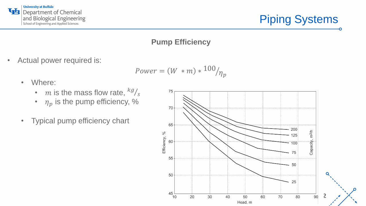
Pump Efficiency

• Actual power required is:

𝑃𝑜𝑤𝑒𝑟 = 𝑊 ∗𝑚 ∗ ൗ100𝜂𝑝

• Where:

• 𝑚 is the mass flow rate, Τ𝑘𝑔𝑠

• 𝜂𝑝 is the pump efficiency, %

• Typical pump efficiency chart

‘-

23

Piping Systems

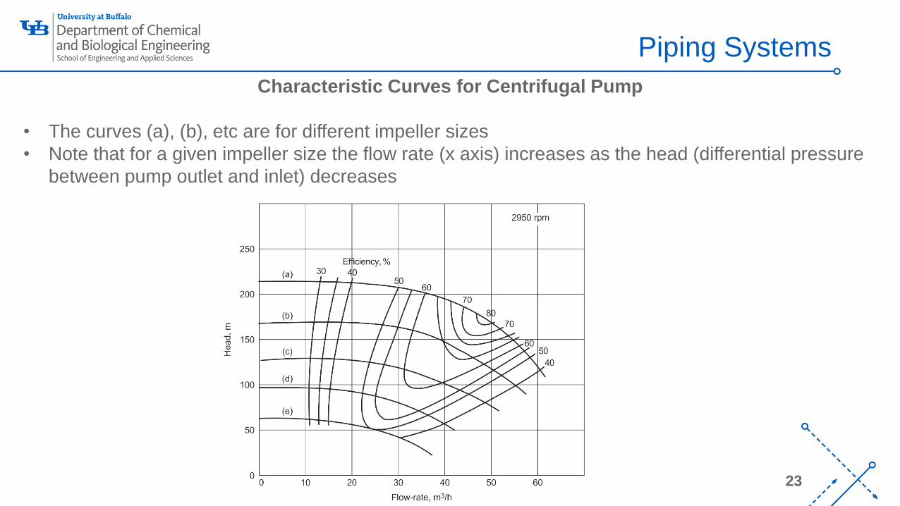
Characteristic Curves for Centrifugal Pump

• The curves (a), (b), etc are for different impeller sizes

• Note that for a given impeller size the flow rate (x axis) increases as the head (differential pressure

between pump outlet and inlet) decreases

‘-

24

Piping Systems

Pump Head

• Mechanical Energy balance

𝒈∆𝒛 + Τ∆𝑷𝝆− ൗ∆𝑷𝒇

𝝆−𝑾 = 𝟎

• 𝑾 is the work done BY the fluid• We are interested in 𝑾𝒔, the work done by the pump ON the fluid (per unit volume)• Lets rearrange the equation:

𝝆𝒈 𝒛𝟏 − 𝒛𝟐 + 𝑷𝟏 − 𝑷𝟐 − ∆𝑷𝒇 = 𝝆𝑾

• Shaft work is:

𝑾𝒔 = −𝝆𝑾

• Therefore,

𝑾𝒔 = 𝑷𝟐 − 𝑷𝟏 + 𝝆𝒈 𝒛𝟐 − 𝒛𝟏 + ∆𝑷𝒇

• Pump Head is:

𝑯𝒑𝒖𝒎𝒑 =𝑾𝒔

𝝆𝒈

‘-

25

Piping Systems

Cavitation and Net Positive Suction Head (NPSH)

• The inlet to pump will generate a lower pressure

• If the pressure at the inlet drops below the bubble point of the liquid then bubbles will form

• This is called cavitation and will lead to erratic flow and damage to the pump

• As the bubbles form they create micro-explosions

• The net positive head required 𝑵𝑷𝑺𝑯𝒓𝒆𝒒𝒅 is a function of the pump design and will be specified by

the manufacturer

• Typically 3 m for pump capacities up to 100 ൗ𝑚3

ℎ and 6 m above that capacity

• You need to calculate the available NPSH, 𝑵𝑷𝑺𝑯𝒂𝒗𝒂𝒊𝒍 :

‘-

26

Piping Systems

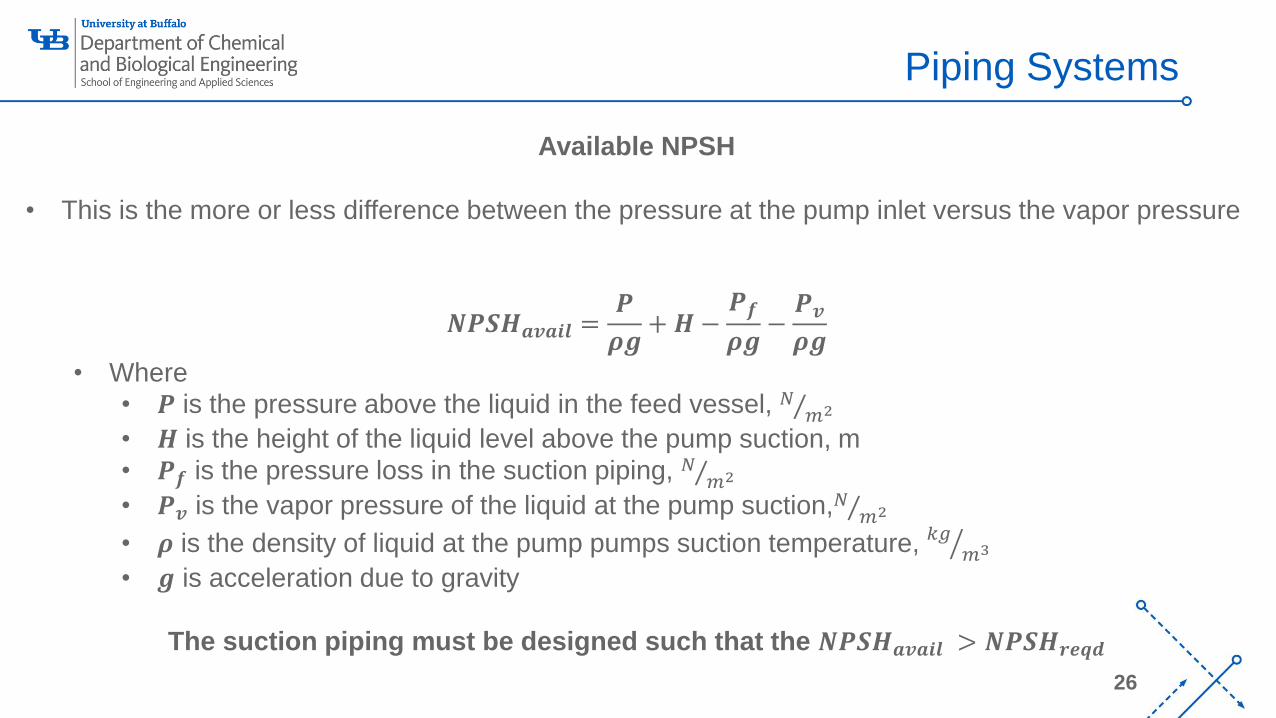
Available NPSH

• This is the more or less difference between the pressure at the pump inlet versus the vapor pressure

𝑵𝑷𝑺𝑯𝒂𝒗𝒂𝒊𝒍 =𝑷

𝝆𝒈+𝑯−

𝑷𝒇

𝝆𝒈−𝑷𝒗

𝝆𝒈• Where

• 𝑷 is the pressure above the liquid in the feed vessel, Τ𝑁 𝑚2

• 𝑯 is the height of the liquid level above the pump suction, m

• 𝑷𝒇 is the pressure loss in the suction piping, Τ𝑁 𝑚2

• 𝑷𝒗 is the vapor pressure of the liquid at the pump suction, Τ𝑁 𝑚2

• 𝝆 is the density of liquid at the pump pumps suction temperature, ൗ𝑘𝑔𝑚3

• 𝒈 is acceleration due to gravity

The suction piping must be designed such that the 𝑵𝑷𝑺𝑯𝒂𝒗𝒂𝒊𝒍 > 𝑵𝑷𝑺𝑯𝒓𝒆𝒒𝒅

‘-

27

Piping Systems

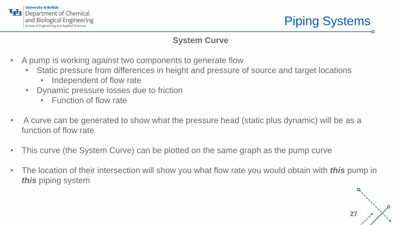
System Curve

• A pump is working against two components to generate flow

• Static pressure from differences in height and pressure of source and target locations

• Independent of flow rate

• Dynamic pressure losses due to friction

• Function of flow rate

• A curve can be generated to show what the pressure head (static plus dynamic) will be as a

function of flow rate

• This curve (the System Curve) can be plotted on the same graph as the pump curve

• The location of their intersection will show you what flow rate you would obtain with this pump in

this piping system

‘-

28

Piping Systems

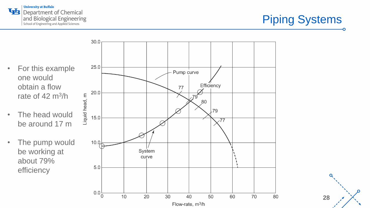
• For this example

one would

obtain a flow

rate of 42 m3/h

• The head would

be around 17 m

• The pump would

be working at

about 79%

efficiency

‘-

29

Piping Systems

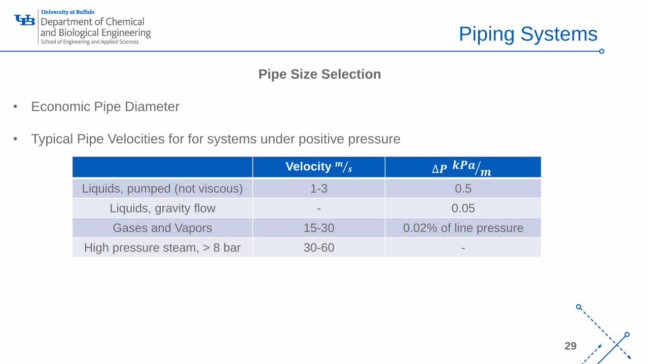
Pipe Size Selection

• Economic Pipe Diameter

• Typical Pipe Velocities for for systems under positive pressure

Velocity Τ𝒎 𝒔 ∆𝑷 ൗ𝒌𝑷𝒂𝒎

Liquids, pumped (not viscous) 1-3 0.5

Liquids, gravity flow - 0.05

Gases and Vapors 15-30 0.02% of line pressure

High pressure steam, > 8 bar 30-60 -

‘-

30

Piping Systems

Pipe Size Selection, Vacuum Systems

• For vacuum systems below 60 mm Hg allow max of 5% of absolute pressure

• You may see 50 m/s listed as a guideline

• You can start there but it is recommended to use pressure drop as your guiding principle

• Not that the low density of vapor under vacuum means that the mass flow rate is very low for a

similar velocity

• This means that vacuum lines are LARGE