Case Selection via Matching - MIT

Article

Case Selection viaMatching

Richard A. Nielsen1

Abstract

This article shows how statistical matching methods can be used to select‘‘most similar’’ cases for qualitative analysis. I first offer a methodologicaljustification for research designs based on selecting most similar cases. I thendiscuss the applicability of existing matching methods to the task of selectingmost similar cases and propose adaptations to meet the unique requirementsof qualitative analysis. Through several applications, I show that matchingmethods have advantages over traditional selection in ‘‘most similar’’ casedesigns: They ensure that most similar cases are in fact most similar; theymake scope conditions, assumptions, and measurement explicit; and theymake case selection transparent and replicable.

Keywords

case selection, matching, most similar systems, qualitative methods, researchdesign

Can statistical matching methods be used for selecting cases in qualitative

case study research? Qualitative methodologists have used matching as an

analogy for the logic of ‘‘most similar’’ case study research and some suggest

that it is a viable way of selecting cases for paired analysis (Gerring 2007;

Levy 2008; Lieberman 2015; Seawright and Gerring 2008; Tarrow 2010).

1 Department of Political Science, Massachusetts Institute of Technology, Cambridge, MA, USA

Corresponding Author:

Richard A. Nielsen, Department of Political Science, Massachusetts Institute of Technology,

77 Massachusetts Avenue, Room E53-470, Cambridge, MA 02139, USA.

Email: [email protected]

Sociological Methods & Research2016, Vol. 45(3) 569-597

ª The Author(s) 2014Reprints and permission:

sagepub.com/journalsPermissions.navDOI: 10.1177/0049124114547054

smr.sagepub.com

at Massachusetts Institute of Technology on July 4, 2016smr.sagepub.comDownloaded from

http://www.sagepub.com/journalsPermissions.nav

http://smr.sagepub.com

http://smr.sagepub.com/

Yet to my knowledge, only one qualitative study—Madrigal, Alpızar, and

Schluter (2011)—has explicitly used matching to select cases, indicating that

either the analytic benefits are not clear or the methods are not sufficiently

developed to meet researcher needs. This article offers a methodological jus-

tification for most similar case designs, explains the benefits of using match-

ing for qualitative case selection, shows how existing matching algorithms

can be adapted to meet the needs of qualitative analysts, and walks through

examples in which these methods are be applied to real case selection prob-

lems using new, freely available software.

Selecting cases with statistical matching methods has several advantages.

First, researchers can be confident that selected cases that are in fact similar,

especially when there are many relevant variables. When identical cases are

not available, researchers must trade off similarity on some variables for

similarity on others. Statistical matching offers a principled way to make

these trade-offs and provides tools for assessing the quality of the resulting

case pairings. Selecting cases with matching is transparent, replicable, and

protects researchers against the criticism that the cases were intentionally

chosen in ways that might bias the findings. Importantly, it does not require

that researchers adopt a ‘‘statistical worldview’’ when analyzing cases

(Mahoney and Goertz 2006). In fact, although statistical matching is closely

associated with causal inference and the counterfactual model of causation

(Neyman 1923; Rubin 1973), researchers do not have to adopt this counter-

factual model, or even the broad goal of causal inference. Instead, the

machinery of matching can be co-opted for a different purpose: to select most

similar cases that are, in fact, most similar.

I begin by arguing for a new understanding of the inferential logic that

motivates most similar case selection strategies and the process tracing anal-

ysis that typically follows. I then give an overview of statistical matching

methods. Because most existing matching algorithms are not ideally suited

for qualitative case selection, I explain which methods can be most usefully

adapted to the needs of case study analysts. I illustrate the benefits of match-

ing with applications to the work of Madrigal et al. (2011), Haverland (2006),

and Lieberman (2003), followed by a summary of the benefits and costs to

researchers.

Design and Inference With Most Similar Cases

Case selection is the process of choosing cases for case study research. Fol-

lowing Gerring (2004), I define a case is ‘‘a spatially bounded phenomenon

. . . observed at a single point in time or over some delimited period of time’’

570 Sociological Methods & Research 45(3)



(p. 342). A case study is ‘‘an intensive study of a single unit for the purpose of

understanding a larger class of (similar) units’’ (p. 342). Virtually, all quali-

tative methodologists agree that systematic, nonrandom case selection is cru-

cial to case study research, although there is disagreement about which

selection strategies have the most merit.1 Seawright and Gerring (2008)

describe seven general strategies of case selection for causal inference: typ-

ical, diverse, extreme, deviant, influential, most similar, and most different.2

Statistical matching methods will primarily be useful for designs that pair (or

group) cases based on similarity—namely, most similar and ‘‘most differ-

ent’’ case selection. In this article, I focus on applications of matching to

most similar case selection, leaving most different case selection and other

strategies for future research.3

Most similar case selection entails choosing two or more cases that have

similar characteristics. This strategy is genealogically related to Mill’s

(1858) method of difference and was developed and clarified by Przeworski

and Teune (1970) as the method of ‘‘most similar systems,’’ and Lijphart

(1971) as the Comparative Method.4 It features prominently in recent texts

on case selection (Gerring 2007) and is a relatively common strategy for

designing research in several disciplines.5 Most similar case selection pro-

ceeds by (1) defining the relevant universe of cases, (2) identifying key vari-

ables of interest that should be similar across the target cases, (3) identifying

a variable or variables that should vary meaningfully across the target cases,

and (4) selecting the desired number of cases—often a pair but sometimes

more—that have the specified similarities and differences. Often, analysts

begin this process with one case already in mind and follow the steps men-

tioned previously to identify a second case that is similar.

Are Credible Inferences Possible With Most Similar Case Designs?

Despite the popularity of most similar case designs, defenses of this approach

in the methodological literature are surprisingly weak, and some argue that

the approach is less helpful than other approaches (Seawright n.d.). Given

that the purpose of this study is to improve the execution of these designs,

I begin by presenting a stronger justification.

Texts on qualitative methodology often treat most similar case selection

as a precursor to a correlational analysis—essentially an ‘‘intuitive regres-

sion’’ with very few cases. From this perspective, the paired cases serve as

mutual counterfactuals, answering the question ‘‘what might have happened

under different circumstances?’’ By comparing very similar cases, qualita-

tive methodologists have argued that they can approximate the logic of a

Nielsen 571



randomized experiment (Lieberman 2003:8; Tarrow 2010:244). Assuming

that plausible ‘‘natural experiments’’ can be identified, the resulting similar-

ity between cases ‘‘controls’’ for potential confounding of the relationship of

theoretical interest. Any remaining correlation between a variable of interest

and the outcome is causal.6

This characterization of most similar case selection as a precursor to small-n

intuitive regression is misleading because it is not methodologically sound and it

is not what most researchers actually do. If researchers did primarily use intui-

tive regression to analyze small numbers of similar cases, the results would be

unpersuasive for the same reasons that a randomized experiment with a handful

of cases would be uninformative—the design is statistically underpowered.

Additionally, researchers would have to argue that any random error in the pro-

cess of generating outcomes is negligible relative to the magnitude of the causal

effect and that there are no unobserved confounders.7 Finally, this characteriza-

tion does not recognize that many most similar case designs also condition on

the outcome variable in some way during the case selection process (e.g., ensur-

ing that the outcome of interest occurs in at least one case).

Luckily, most similar case analysis is not small-n regression. Instead of

merely reporting correlations, case study analysts almost universally

describe the process by which each outcome came about in each case (Capor-

aso 2009; Tarrow 2010; Tilly 2002). Tarrow (2010:238) argues that parallel

process tracing is an integral part of most similar case analysis and that it

gives greater inferential leverage than the ‘‘logic of correlation’’ because pro-

cess tracing can unpack the causal mechanisms that underlie a correlation.

George and Bennett (2005) further explain the role of process tracing in most

similar case analysis, which they refer to as ‘‘controlled comparison:’’

[P]rocess-tracing can serve to make up for the limitations of a particular con-

trolled comparison. When it is not possible to find cases similar in every

respect but one—the basic requirement of controlled comparisons—one or

more of the several independent variables identified may have causal impact.

Process-tracing can help to assess whether each of the potential causal vari-

ables in the imperfectly matched cases can, or cannot, be ruled out as having

causal significance. If all but one of the independent variables that differ

between the two cases can be ruled out via a process-tracing procedure . . .

a stronger (though still not definitive) basis exists for attributing causal signif-

icance to the remaining variable. (p. 215)

But what specifically is process tracing, and how does it strengthen a most

similar case design? George and Bennett (2005) define process tracing as




‘‘attempts to identify the intervening causal process—the causal chain and

causal mechanism—between an independent variable (or variables) and the

outcome of the dependent variable’’ (p. 207). Because it is causal inference,

process tracing must rely on inferences about counterfactual states of the

world (Neyman 1923; Pearl 2000; Rubin 1973).8 At each step of a causal

chain, the scholar must infer what would have happened if the proceeding links

had been different. And at each step, confounders might lead the researcher to

conclude that a false pathway is in fact real. In short, each step in a process tra-

cing chain requires a causal estimate with nonexperimental data.

Seen from this light, it is surprising that process tracing is possible at all,

given the difficulty of obtaining even a single unbiased causal estimate in

many nonexperimental settings. Process tracing requires many such esti-

mates; how does it achieve causal inference without the quantitative machin-

ery that allows other cases to serve as counterfactuals? Some methodologists

have argued that process tracing overcomes this challenge by replacing data

set observations with one or more causal process observations—defined as

an ‘‘insight or piece of data that provides information about context, process

or mechanism, and that contributes distinctive leverage in causal inference’’

(Brady and Collier 2004:227). These often resemble a ‘‘smoking gun’’ that

points to the operation of some causal mechanism. Subsequent work has tried

to unpack whether and how causal process observations facilitate causal

inference (Beck 2006, 2010; Collier, Brady, and Seawright 2010; Mahoney

2012), but this is an active area of research and methodologists do not yet agree.

I argue that process tracing primarily uses thought experiments, rather

than data, to inform counterfactual statements.9 Observing a smoking gun

is powerful because a researcher can imagine a world without the smoking

gun, not because the researcher is comparing the this instance of a smoking

gun with other noninstances in a specific data set. Instead, the researcher

makes counterfactual assumptions, based on experience, of how things

‘‘typically’’ behave and thus how alternative worlds might have played out.

Because these counterfactual assumptions are based on experience, causal

links in the process tracing chain are most believable if they are ‘‘short’’ and

can be reduced to common experiences. In defense of this position, George

and Bennett (2005) quote historian Clayton Roberts arguing that a proper

causal explanation involves ‘‘minute tracing of the explanatory narrative to

the point where the events to be explained are microscopic and the covering

laws correspondingly more certain’’ (Roberts 1996:66).

Effective process tracing requires two types of evidence. First, it requires

‘‘measurement evidence’’ that the events in the purported causal chain hap-

pened. Case studies are ideal for measurement because researchers can focus

Nielsen 573



their efforts on discerning what events actually occurred in a particular case.

This descriptive inference does not rely on counterfactual claims. Second, it

requires ‘‘identifying evidence’’ that identifies the causal relationship (in the

statistical sense) by ruling out confounding variables and processes. Unfor-

tunately, ‘‘proving the negative and demonstrating that a particular process

did not occur can be notoriously difficult’’ (George and Bennett

2005:218). This is where a research design featuring carefully matched cases

helps to rule out alternative causes. The case selection and process tracing

components of the typical most similar case analysis can thus complement

each other to produce more reliable inferences than either could achieve in

isolation.

Properly understood, most similar case analysis is analogous to the two

stage empirical strategy proposed by Ho et al. (2007a) for making causal

inference in quantitative observational studies: (1) use statistical matching

to create a sample in which units have similar background characteristics and

(2) use a parametric model (such as regression) to account for the confound-

ing due to remaining differences between units. Intuitively, step 1 attempts to

find a subset of observations in an observational data set that looks as if they

could have come from a randomized experiment. Practically, this means con-

structing a subsample in which the units vary meaningfully on the key vari-

able of interest—the treatment—but are similar in all other ways. In most

cases, this matching procedure creates a subsample that looks more similar

than the original data. However, differences may persist between the treat-

ment and control groups that cannot be fixed without the matched subset

becoming too small for the subsequent analysis to be informative. To account

for remaining differences in a matched data set, Ho et al. (2007a) propose

using a parametric model such as ordinary least square to estimate causal

quantities of interest in the matched sample. This research procedure is ‘‘dou-

bly robust’’—causal inference is possible if either the matching works or the

parametric model works.

I argue that qualitative scholars are doing something similar when com-

bining most similar case selection with process tracing. First, they condition

on some confounders when selecting cases to ensure that those confounders

are not the cause of any effect they see. Then, they deal with the rest of the

empirical variation among the cases by using process tracing in the same way

that quantitative analysts use regression to interpolate between nonidentical

cases. Although this design is no longer a ‘‘natural experiment’’ because

some covariates could be correlated with treatment assignment, it reduces the

inferential burden at the process tracing stage. Rather than contending with

all potential alternative causes through process tracing, the analyst must only




contend with those not addressed at the matching stage. In some sense, the

procedure follows the logic of double robustness because the case selection

and process tracing guard against each other’s failures. Although this ana-

logy is informal, it suggests a strong justification for most similar case

analysis.

Statistical Matching for Case Selection

How can statistical matching help advance the analytical goals of case study

researchers using most similar case designs? As shown previously, the infer-

ential leverage in a most similar case design relies partially (though not

solely) on the similarity of the cases. Finding sufficiently similar cases can

be challenging, and the analyst must persuade the reader that the paired cases

are indeed the most similar. Matching helps with these challenges.

A Review of Statistical Matching Methods

Statistical matching is an approach to purposeful case selection in large-n

studies with the goal of finding comparable units within a data set. Matching

is useful for making causal inferences in large-n data sets (Rosenbaum 2002;

Rubin 1973) and is closely associated with the Neyman-Rubin causal model

(Neyman 1923; Rubin 1973). The logic is simple: If units A and B are iden-

tical and A receives a treatment while B receives control, then subsequent dif-

ferences between the units can be attributed to the treatment. Matching, like

regression, is a way of conditioning on covariates. Rather than ‘‘controlling

for’’ a variable by including it in a regression model, matching ‘‘controls for’’

a variable by only allowing comparisons between units that have sufficiently

similar levels of the variable.

Although matching was developed to facilitate causal inference via statis-

tical analysis, the primary role of matching is to create matched samples with

similar units, a goal shared by qualitative researchers using most similar case

designs. Qualitative researchers can use matching to find similar cases with-

out adopting the assumptions or quantitative machinery that follows match-

ing in quantitative studies.

Before describing specific matching methods, I describe the general fea-

tures of the problem that matching is trying to solve. Matching identifies

treated and control units that are ‘‘close’’ to each other in a k-dimensional

space defined by the k covariates that need to be conditioned on to estimate

unbiased causal effects. In general, as the number of covariates grows, the

distance between units in the covariate space also grows, so matching with

Nielsen 575



more covariates means that matched pairs are further apart.10 For this reason,

it can be detrimental to condition on variables that are not confounders

because matching on these variables makes reduces similarity on actual con-

founders. On the other hand, analysts rarely have enough information to defi-

nitively declare that a variable is not a confounder.

There are many matching methods, primarily distinguishable by the dis-

tance metrics they use to determine similarity. Here, I describe the most com-

mon and most important methods.

Exact matching. Exact matching identifies units that are identical on observed

covariates. It is ideal for both quantitative studies and qualitative controlled

comparison, but it is often difficult to find exact matches, especially when the

covariates used for matching take on many values.

Coarsened exact matching. Coarsened exact matching (CEM; Iacus, King, and

Porro 2011, 2012) follows a similar logic to exact matching but works for

data sets where exact matches are not possible. Matching proceeds by first

coarsening each continuous variable into categories preferably based on sub-

stantive knowledge. For example, one might reasonably coarsen years of

education into categories corresponding to primary school, secondary

school, and college. This would allow a freshman in high school to match

with a senior in high school, but not with someone who had started college.

Each covariate is coarsened based on these user-defined categories and exact

matching is done on the coarsened variables. Units are matched together if

they fall within the same stratum of the coarsenings. Observations that fall

a stratum with no units in the opposite treatment are discarded.

Mahalanobis matching. This family of algorithms identifies similar units by

minimizing pairwise Mahalanobis distance,11 a generalization of Euclidean

distance that accounts for correlations between variables (Rubin 1973).

Propensity score matching. Propensity score matching (Rosenbaum and Rubin

1983) relies on the insight that the propensity of each observation to receive

treatment is a balancing score, meaning that conditioning on the true propen-

sity score will, in expectation, balance the covariate distributions of treat-

ment and control groups. In practice, analysts typically estimate propensity

scores using logistic regression and match observations that have similar pro-

pensity scores.




Genetic matching. Genetic matching (Diamond and Sekhon 2013) uses a

genetic algorithm to optimally choose weights for each matching variable.

These variable weights imply a distance metric that is then used to produce

a matched sample that minimizes a loss function based on global differences

between treated and control distributions.12 At each iteration, the algorithm

starts with a proposal for the variable weights, introduces many random ver-

sions of this vector, and tests to see which version improves covariate simi-

larity the most. The starting proposal for each iteration is the best set of

weights from the previous iteration; this repeats until balance is optimized.

Genetic matching takes as its inputs the matrix of matching variables aug-

mented with a column that is the estimated propensity score. Because of this,

genetic matching is a generalization of Mahalanobis and propensity score

matching and will reproduce the results of these algorithms if they are

optimal.

Adapting Matching Methods for Case Selection Goals

Which matching methods are most useful for qualitative case selection?

Matching methods are not inherently good or bad on their own merits—their

utility is based entirely on whether they can help the analyst find a subsample

of similar units. A matching method that works well for one application may

perform poorly for others. In general, I find that versions of exact matching

and Mahalanobis matching are most likely to be helpful for case selection.

Propensity score matching is unlikely to be helpful (contrary to Seawright

and Gerring 2008).

Exact matching is ideal for selecting most similar cases because it mirrors

what qualitative scholars are already doing when possible. Exact matching

creates pairs of cases that are identical on the matching variables—the exact

procedure described in qualitative methods texts as the proper way of select-

ing most similar cases. Using exact matching for case selection is thus simply

taking what qualitative scholars already are doing, but carrying out the

matching on a computer (which has benefits, described subsequently). Exact

matching should be the first tool that any analyst should turn to. Quantitative

analysts rarely use exact matching because they need substantial sample

sizes for subsequent analysis and often only a few exact matches can

be found in a data set. In contrast, case study researchers only need a small

number of exact matches for analysis, so exact matching may be more fea-

sible for case study research.

Which methods are most useful for selecting similar cases when exact

matches are not available? When confronting this situation, case study

Nielsen 577



practitioners often take the step of coarsening or dichotomizing variables on

which they cannot find exact matches (Gerring 2007:133). This is exactly the

same procedure as CEM, so CEM offers a principled way of thinking about

these choices and selecting matches. CEM implements the method that most

qualitative scholars already choose when there are no exact matches avail-

able. Thus, analysts can garner the benefits of using statistical software to

perform the case selection while retaining exactly the same procedure that

they would have used if selecting cases by hand.

Mahalanobis matching offers a different way of matching cases when

exact matches do not exist. Mahalanobis matching identifies units located

close together in the k-dimensional space defined by the covariates. Although

this does not exactly mirror what qualitative scholars typically do when there

are no exact matches, it does provide the outcome that analysts typically

want: the paired cases will be as close together as the existing data allow.

This method can be combined with other methods. If it is particularly impor-

tant to condition on some covariate X1, then exact matching can be used for

this covariate, followed by Mahalanobis matching on the other covariates

within the strata defined by exact matches on X1.

Propensity score matching is probably not ideal for selecting similar cases

for qualitative analysis because it first summarizes the k covariate values for

a single case using a scalar (the propensity score) and then matches units on

this scalar. Although matching on propensity scores may balance aggregate

covariate distributions, individual matches are often far apart in the covariate

space. As such, selecting two cases with similar propensity scores may not

produce matches that have similar values of the control variables. Similarly,

Genetic matching (as currently implemented) minimizes a loss function

defined in terms of global balance, so paired units are not necessarily close

in the covariate space. However, genetic matching provides technology for

weighting covariates by their importance that is useful to case study analysts.

Matching methods rarely work ‘‘off the shelf’’ for qualitative case selec-

tion because they are intended to precede statistical analysis rather than pro-

cess tracing. The most obvious problem is that existing computer software

for matching is not tailored to the specific needs of case study scholars. Soft-

ware for matching is readily available (Ho et al. 2007a, 2007b) but is tailored

to producing an entire data set of matched treatment and control units rather

than answering questions such as ‘‘which three cases are most like case x?’’ I

provide software that implements matching routines specifically for case

selection.13 With this software, users can find one or more cases that best

match a particular case of interest using matching methods described in this

article. If the researcher does not have a particular case in mind, the software




can find the closest possible matched pairs in terms of specified covariates.

Unlike statistical matching software, I do not require users to specify a

‘‘treatment’’ variable because some qualitative analysts do not have one at

the case selection stage. Other analysts do have a treatment variable in mind;

my software has options to maximize the variance or ‘‘spread’’ of a contin-

uous variable of particular interest while matching as closely as possible on

several other variables (King, Keohane, and Verba 1994:140).

One difference between case selection for quantitative and qualitative

research is that case study analysts often condition on the outcome variable

during case selection, most frequently by choosing cases where a rare out-

come of interest is present. This differs from the statistical matching frame-

work and requires modification to existing matching routines. Conditioning

on the outcome no longer allows unbiased estimation of the correlation

between treatment and outcome (Geddes 1990), but may still meet the ana-

lytical goals of case study researchers. If so, the methods mentioned previ-

ously can be adapted to maximize case similarity subject to some

constraint on the values of the outcome variable, although researchers should

be aware that constraints will often reduce the number or quality of available

matches.

Analysts often know that some covariates are more likely than others to be

important alternative causes of the phenomenon of interest. This type of

information is easily incorporated into the matching framework, and match-

ing can help researchers express to readers the extent to which one variable

matters more than another. This can be done by weighting the variable highly

in the matching analysis, or even requiring that it be matched exactly.

Because readers might question the relative importance of these variables,

researchers could check the robustness of their case selection to alternative

weights. There is no ‘‘correct’’ weighting—generally, variables that are

strong confounds and difficult to account for in the subsequent process tra-

cing should receive the most weight when matching.

In some settings, researchers can use existing data sets to match cases. In

others, the researcher needs data that are partially or completely unavailable.

If the missing information can be coded in general terms, then analysts can

code the variables themselves and pass this data set to the matching routine.

This does not mean that every variable must be quantified—categorical cod-

ing is adequate for matching.

If missing information is difficult to collect for more than a few cases, one

viable strategy is to first match on easily measured variables and then mea-

sure difficult variables for the cases that are most promising. However, it is

crucial to note that if information is missing for many cases, then the analyst

Nielsen 579



does not have enough information to pursue a most similar case design with

respect to the missing information. Any matching of cases, whether carried

out mentally by the researcher or using statistical software requires data to

make the comparison. If the criteria for matching cases are too vague to be

written down, they are probably too vague to be used at all.

Another strategy for dealing with missing information is match on proxy

variables or comparing cases that are widely considered to be ‘‘natural

pairs.’’ For example, matching countries by geographic region can hold

many confounders constant, even though geography itself may not be a con-

founder. This is also a solution for situations when data are ‘‘missing’’

because analysts do not know which variables are confounders. If the con-

founder set is partially unknown, controlling for categories that of broad

similarity between cases can increase similarity on a large number of known

and unknown dimensions. However, if the major confounders can be speci-

fied and data are available, analysts should demonstrate that matching on

these types of broad proxy variables does not compromise the goal of finding

the best matches on the specific matching variables.

Taking the idea of ‘‘natural pairs’’ to its logical conclusion, the best match

for unit it (where t indexes time) may be it – 1.14 In quantitative settings, ana-

lysts sometimes avoid matching the same unit in different time periods

because it might violate a crucial assumption of the Neyman-Rubin causal

model that the potential outcomes of compared units are independent.15

However, qualitative researchers might wish to focus on such pairings, either

because they can account for the independence or because their analytic

goals do not require independent cases. A design that compares units it and

it – 1 will control for any time-invariant factors whether information is miss-

ing or not.

Illustrations

In this section, I illustrate the process of case selection via matching on two

applied examples.

Madrigal, Alpızar, and Schluter (2011)

Madrigal et al. (2011) seek to explain the performance of community-based

drinking water provision organizations (CBDWOs) in rural Costa Rica. To

my knowledge, their study is the only published research that uses statistical

matching for case selection, so it is instructive to see how matching was

implemented and whether it improves the study.




Madrigal et al. (2011) are explicit that their primary goal is to ‘‘study cau-

sal pathways instead of measuring the causal effect of selected variables on

outcomes’’ (p. 1665). Because of their theoretical approach, they are most

interested in the influence of CBDWO governance structures on water infra-

structure condition, consumer satisfaction, and financial health. Citing Sea-

wright and Gerring (2008), they use matching as a case selection method

to ‘‘reduce the number of potential explicative variables [and] focus on the

role of governance structures’’ (p. 1665).

Madrigal et al. (2011) use modified propensity score matching to select

four cases that meet several constraints. They restrict the sample to cases

in the Metropolitan Region of Costa Rica (one of seven administrative

regions) on substantive grounds: that it allows ‘‘better control of geographi-

cal and climatic characteristics’’ and eliminates the possibility that ‘‘peculia-

rities of the relationship between ICAA regional administrative units and

local CBDWO might affect their performance’’ (p. 1665).16 Within this sub-

set, they estimate a propensity score model with organizational type as the

outcome and cases characteristics as predictors. They then ‘‘[reduce] the

population of cases to those located within a 95 percent confidence interval

around the median propensity score’’ and select ‘‘the four cases closest to the

median assuring that they differ in terms of water quality’’ (see Note 6).

Thus, they condition on the outcome—specifically selecting a high- and

low-performing CBDWO from each of the two types of CBDWO govern-

ance.17 Their goal with this procedure is to analyze cases that are similar

to each other and representative of the other cases in some sense.

Unfortunately for replication purposes, the identities of the selected cases

are obscured to protect the communities, so we cannot evaluate the perfor-

mance of this case selection method relative to other possibilities. However,

this serves to illustrate that matching helps readers evaluate the quality of

case selection, even when standards of ethical research require that the iden-

tities of cases remain secret. This may be one of matching’s greatest benefits

for qualitative work.

The authors provide replication data for most of the matching procedure,

although the final selection stage is omitted and key indicators that would

identify the selected cases are either missing or modified. I use this data set

to illustrate why the propensity score matching used by Madrigal et al. (2011)

may be less than ideal. For comparison, I identify the best match in terms of

the propensity scores estimated by the authors and the best match in terms of

Mahalanobis distance. Table 1 shows case information about the best pairing

generated by each distance metric. I find that Mahalanobis matching pro-

duces a matched pair that is more similar in the scale of the covariates, with

Nielsen 581



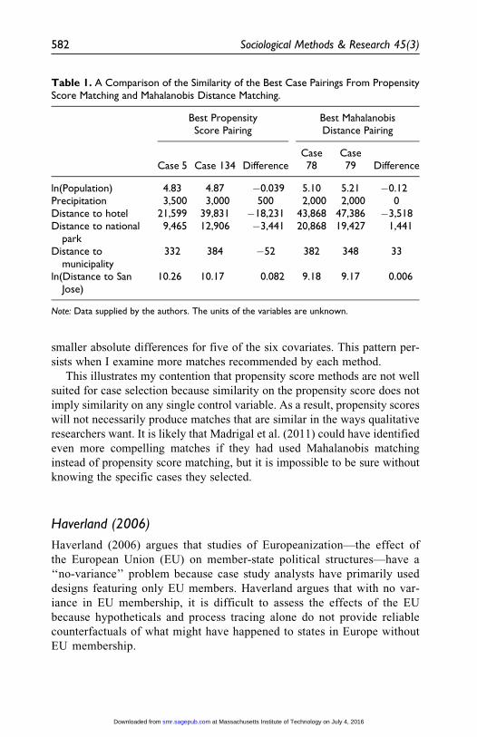
smaller absolute differences for five of the six covariates. This pattern per-

sists when I examine more matches recommended by each method.

This illustrates my contention that propensity score methods are not well

suited for case selection because similarity on the propensity score does not

imply similarity on any single control variable. As a result, propensity scores

will not necessarily produce matches that are similar in the ways qualitative

researchers want. It is likely that Madrigal et al. (2011) could have identified

even more compelling matches if they had used Mahalanobis matching

instead of propensity score matching, but it is impossible to be sure without

knowing the specific cases they selected.

Haverland (2006)

Haverland (2006) argues that studies of Europeanization—the effect of

the European Union (EU) on member-state political structures—have a

‘‘no-variance’’ problem because case study analysts have primarily used

designs featuring only EU members. Haverland argues that with no var-

iance in EU membership, it is difficult to assess the effects of the EU

because hypotheticals and process tracing alone do not provide reliable

counterfactuals of what might have happened to states in Europe without

EU membership.

Table 1. A Comparison of the Similarity of the Best Case Pairings From PropensityScore Matching and Mahalanobis Distance Matching.

Best PropensityScore Pairing

Best MahalanobisDistance Pairing

Case 5 Case 134 DifferenceCase78

Case79 Difference

ln(Population) 4.83 4.87 �0.039 5.10 5.21 �0.12Precipitation 3,500 3,000 500 2,000 2,000 0Distance to hotel 21,599 39,831 �18,231 43,868 47,386 �3,518Distance to national

park9,465 12,906 �3,441 20,868 19,427 1,441

Distance tomunicipality

332 384 �52 382 348 33

ln(Distance to SanJose)

10.26 10.17 0.082 9.18 9.17 0.006

Note: Data supplied by the authors. The units of the variables are unknown.




Haverland is skeptical that a most similar design will produce good infer-

ences. The non-EU states he considers most similar to EU members—Norway

and Switzerland—are enmeshed in the European milieu and may be influenced

by Europeanization without formal membership. Instead, he argues that future

research might profitably analyze ‘‘moderately similar’’ cases such as Austra-

lia, Canada, New Zealand, and the United States (p. 141). His criterion for

these cases is that they are ‘‘stable and liberal democracies with a capitalist

economy’’ that are ‘‘so ‘remote’ from the EU that often it can be plausibly

argued that indirect EU effects also do not reach them’’ (p. 141).

I use matching to implement the case selection strategy advocated by

Haverland. I operationalize Haverland’s matching criteria by collecting data

on political freedom, civil liberties (Freedom House 2006), gross domestic

product (GDP) per capita, trade (Gleditsch 2004), and socialism averaged

between 1980 and 1992 (prior to the signing of the Treaty of Maastricht) for

26 of the 28 current EU members,18 and 151 non-EU states. It would be

exceptionally taxing to manually consider each of the 3,926 possible pairings

between EU and non-EU states. I use the software described previously to

identify pairs of similar EU and non-EU cases based on Mahalanobis dis-

tance calculated for these five variables.

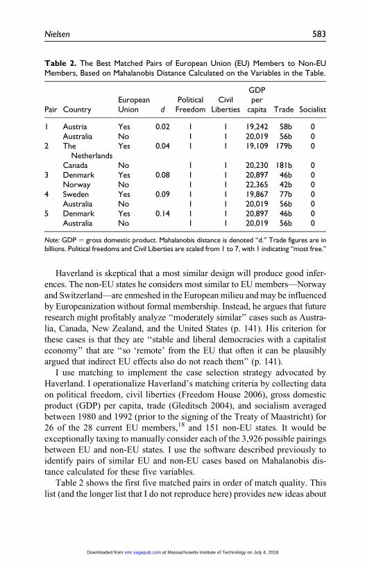
Table 2 shows the first five matched pairs in order of match quality. This

list (and the longer list that I do not reproduce here) provides new ideas about

Table 2. The Best Matched Pairs of European Union (EU) Members to Non-EUMembers, Based on Mahalanobis Distance Calculated on the Variables in the Table.

Pair CountryEuropeanUnion d

PoliticalFreedom

CivilLiberties

GDPper

capita Trade Socialist

1 Austria Yes 0.02 1 1 19,242 58b 0Australia No 1 1 20,019 56b 0

2 TheNetherlands

Yes 0.04 1 1 19,109 179b 0

Canada No 1 1 20,230 181b 03 Denmark Yes 0.08 1 1 20,897 46b 0

Norway No 1 1 22,365 42b 04 Sweden Yes 0.09 1 1 19,867 77b 0

Australia No 1 1 20,019 56b 05 Denmark Yes 0.14 1 1 20,897 46b 0

Australia No 1 1 20,019 56b 0

Note: GDP ¼ gross domestic product. Mahalanobis distance is denoted ‘‘d.’’ Trade figures are inbillions. Political freedoms and Civil Liberties are scaled from 1 to 7, with 1 indicating ‘‘most free.’’

Nielsen 583



which countries might serve as cases to evaluate the effects of Europeaniza-

tion. I find that some expert intuitions may be incorrect. Haverland identifies

Norway and Switzerland as the two cases that are obviously most similar to

EU members, but although Norway appears high on the list (as a match for

Denmark), Switzerland is only the 45th best match for any EU country.19

Although Haverland considers Australia to be a moderately similar case to

the EU countries, I find that it is the best possible non-EU pairing for three

of the five EU cases—Austria, Sweden, and Denmark. It is in fact a legiti-

mately most similar case based on a reasonable operationalization of Haver-

land’s own criteria. There is no need to settle for moderately similar cases.

Table 2 does not feature any of the largest economies in the EU because

these countries do not have non-EU counterparts that are as similar as the

pairs listed. There may be other reasons to analyze these large economies

(including intrinsic importance). I illustrate how to find matches for a spe-

cific case by using the same variables to identify matches for Germany using

Mahalanobis distance matching. The resulting top matches—Japan, the

United States, Canada, Union of Soviet Socialist Republics (USSR)/Russia,

and South Korea—corroborate Haverland’s intuition that Canada is similar

to Germany (p. 141) and offer some additional options for consideration.

However, the Mahalanobis distances between these matches range from

5.4 to 30.9, indicating that these matches are substantially less similar than

those in Table 2.20

If any of the above-mentioned matches are surprising, it indicates that

either the analyst’s heuristic sense of similarity is wrong or that additional

matching criteria should be considered. Matching methods can help analysts

elicit their own beliefs about which variables ought to be matched to make a

pair of case studies persuasive. Perhaps new variables should be included, the

current variables should be transformed to account for nonlinearities, or

some variables should be weighted more heavily than others to construct

matches that better fit a heuristic sense of similarity.

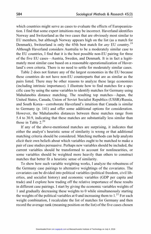
To show how such variable weighting works, I analyze the robustness of

the Germany case pairings to alternative weightings of the covariates. The

covariates can be divided into political variables (political freedom, civil lib-

erties, and socialist history) and economic variables (GDP per capita and

trade) and I explore how trading off the relative importance of these results

in different case pairings. I start by giving the economic variables weights of

1 and gradually decreasing these weights to 0 while simultaneously starting

the weights of the political variables at 0 and increasing them to 1.21 For each

weight combination, I recalculate the list of matches for Germany and then

record the average rank (meaning position on the list) of the five cases chosen




originally: Japan, the United States, Canada, USSR/Russia, and South Korea.

For any weighting that ranks these cases at the top, the average rank will be

3.5. If these cases are poor matches, they will appear further down the list and

the average rank will increase.

The results in Figure 1 show that the case selection depends on the

relative weight assigned to economic and political variables. The eco-

nomic variables appear to dominate, so the top matches are stable as long

as at least 40 percent of the weight is on economic variables. However, if

the political variables are weighted highly, then the matches change sub-

stantially. The original matches move far down the list, while other cases

take their place at the top. With all of the weight placed on the political

variables, the best matches for Germany are Saint Lucia, Kiribati, Vene-

zuela, the Bahamas, and Botswana. These matches surprise me, indicat-

ing that (1) I do not have an accurate sense of which cases have Freedom

House scores similar to Germany between 1980 and 1993 and (2) the

economic variables are important to my own heuristic sense of what it

means for a country to be ‘‘like Germany.’’ This style of robustness anal-

ysis could accompany any presentation of most similar case selection to

show whether the cases chosen are sensitive to the importance placed on

each matching variable.

1 : 0 .75 : .25 .5 : .5 .25 : .75 0 : 1

60

40

20

0

Economic variable weights : Political variable weights

Avg.

Ran

k of

Japa

n, U

SA,

Can

ada,

USS

R, a

nd K

orea

amon

g al

l cas

e pa

iring

s

Best 5: Japan, USA, Canada, USSR, Korea

Best 5: St. Lucia, Kiribati, Venezuela, Bahamas, Botswana

Best 5: Japan, India, USA, Thailand, Honduras

Figure 1. Changes in the average positions of Japan, United States, Canada, Unionof Soviet Socialist Republics (USSR), and Korea on the list of best matches forGermany depending on different weights for economic and political variables. Thefive best matches for Germany are listed for the weighting combinations 0.5:0.5,0.25:0.75, and 0:1.

Nielsen 585



How Can Matching Improve Case Selection?

The previous sections show that several statistical matching methods can be

adapted to serve the goals of case study researchers; this section discusses

how matching improves upon current case selection practices.

Matching Aids Transparency and Replicability

One of the well-known adages of small-n research is that ‘‘the cases you

choose affect the answer you get’’ (Geddes 1990:131). Analysts can

strengthen confidence in their findings by providing precise information

on how cases were selected, preferably in the form of a publicly available

replication archive (Dafoe 2014).

It is almost universal in most similar case studies to spend at least some

portion of the research describing the case selection. However, scholars

rarely provide any discussion or data on alternative cases they considered but

did not choose. Matching improves the credibility of case selection by pro-

viding comparisons to the cases not selected.

To illustrate, I reexamine Evan Lieberman’s (2003) study comparing how

definitions of ‘‘national political community’’ influenced the politics and

outcomes of tax collection in South Africa and Brazil. Lieberman is con-

cerned that economic development and tax revenues from international trade

might have influenced tax policy, so he sets out to show that these factors are

virtually identical for the South African and Brazilian cases and cannot be the

causes of the differences he observes.22 Lieberman’s extensive discussion

(pp. 106-121) describes compelling similarities between the cases and his

figures show that GDP per capita and tax revenue from trade in Brazil and

South Africa have trended similarly over time. However, there is no discus-

sion of alternative case pairings and without comparisons to other countries,

it is difficult to tell just how similar these trends are.

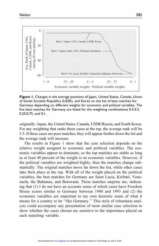
To illustrate how comparison to other countries could make Lieberman’s

case selection more even more persuasive, Figure 2 shows cross-national

GDP per capita data from 1950 to 1990 for 175 countries, with South Africa

and Brazil highlighted for comparison. This figure is directly analogous to

Lieberman’s figure 4.1 (2003:114), except that other countries are included

as well.23 Although it is difficult to pick out the individual trend lines for the

other 173 countries, it appears that Brazil and South Africa are indeed rela-

tively similar.

To formalize this comparison, I use statistical matching methods to show

how close Brazil and South Africa’s GDP per capita trend lines are relative to




other possible cases that could have been chosen. I first discard any countries

that do not have a complete GDP per capita time series between 1950 and

1990, which leaves 85 countries for matching. I reformat the time-series

cross-sectional data into a cross section, with countries in the rows of the data

matrix and yearly values of GDP per capita in the columns. I then calculate

Euclidean distance24 between each observation, producing a measure of

similarity between trends in the same scale as Figure 2.

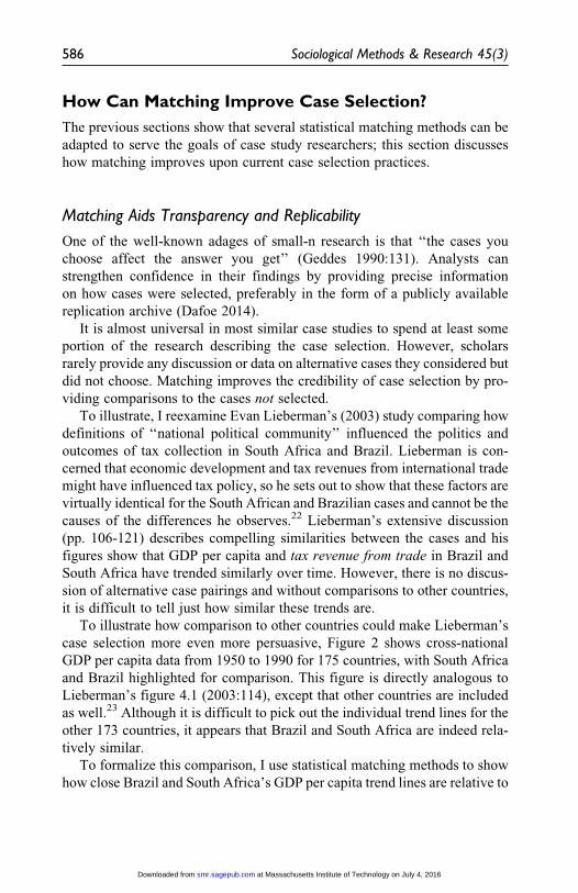
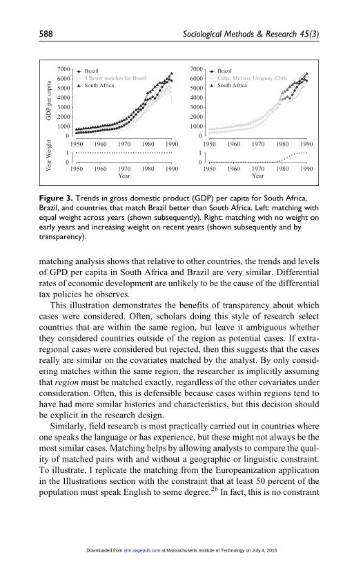
The left panel of Figure 3 shows the resulting matches if I begin with Bra-

zil and identify the most similar countries based on GDP per capita trends.

For a most similar case design, South Africa should be the best match for

Brazil among the possible matched pairs we could have chosen (or nearly

so). South Africa ranks highly, but there are nine other countries25 that are

better matches. However, rather than weighing all years equally, it may be

preferable to give greater weight to the more recent past. The right panel

of Figure 3 shows the results of a revised matching procedure with very little

weight given to the distant past and logistically increasing weight over time.

This produces a different ordering of matches; South Africa is now the fifth

best match for Brazil out of 85 possible matches.

Given that similar GDP per capita trends are only one of several criteria

that Lieberman uses for case selection, this result is quite encouraging. The

GD

P pe

r cap

ita

Year1950 1960 1970 1980 1990

0

2000

4000

6000

8000

10000

● ● ● ● ● ● ● ● ● ● ● ● ● ● ● ● ● ● ● ● ● ●●

●●

●●

●●

●

● ●● ●

●

●●

● ●● ●

Brazil173 Other countriesSouth Africa

●

Figure 2. Trends in gross domestic product (GDP) per capita between 1950 and1990 for 175 countries including South Africa and Brazil.Source: Gleditsch (2004).

Nielsen 587



matching analysis shows that relative to other countries, the trends and levels

of GPD per capita in South Africa and Brazil are very similar. Differential

rates of economic development are unlikely to be the cause of the differential

tax policies he observes.

This illustration demonstrates the benefits of transparency about which

cases were considered. Often, scholars doing this style of research select

countries that are within the same region, but leave it ambiguous whether

they considered countries outside of the region as potential cases. If extra-

regional cases were considered but rejected, then this suggests that the cases

really are similar on the covariates matched by the analyst. By only consid-

ering matches within the same region, the researcher is implicitly assuming

that region must be matched exactly, regardless of the other covariates under

consideration. Often, this is defensible because cases within regions tend to

have had more similar histories and characteristics, but this decision should

be explicit in the research design.

Similarly, field research is most practically carried out in countries where

one speaks the language or has experience, but these might not always be the

most similar cases. Matching helps by allowing analysts to compare the qual-

ity of matched pairs with and without a geographic or linguistic constraint.

To illustrate, I replicate the matching from the Europeanization application

in the Illustrations section with the constraint that at least 50 percent of the

population must speak English to some degree.26 In fact, this is no constraint

GD

P pe

r cap

ita

1950 1960 1970 1980 19900

1000200030004000500060007000

●●●●●●●●●●●●●●●●●●●●●●●

●●

●●

●●

●

●●●

●●

●●

●●●●

Brazil9 Better matches for BrazilSouth Africa

●

Year

Wei

ght

Year

●● ● ● ● ● ● ● ● ● ● ● ● ● ● ● ● ● ● ● ● ● ● ● ● ● ● ● ● ● ● ● ● ● ● ● ● ● ● ● ● ●

1950 1960 1970 1980 199001

1950 1960 1970 1980 19900

1000200030004000500060007000 Brazil

Cuba, Mexico, Uruguay, ChileyySouth Africa

●

Year

● ● ● ● ● ● ● ● ● ● ● ● ● ● ● ● ● ● ● ● ● ● ● ● ● ● ● ● ● ●●

●

●

●●

● ● ● ● ● ●

1950 1960 1970 1980 199001

Figure 3. Trends in gross domestic product (GDP) per capita for South Africa,Brazil, and countries that match Brazil better than South Africa. Left: matching withequal weight across years (shown subsequently). Right: matching with no weight onearly years and increasing weight on recent years (shown subsequently and bytransparency).




at all—the list of best matches is essentially identical to Table 2. In contrast, when

I consider a similar constraint that all cases must have an adequate Francophone

population, I get a drastically different set of best matches—namely, Luxem-

bourg–Switzerland, Belgium–Switzerland, France–Switzerland, and the improb-

able combinations of Luxembourg–Djibouti and Luxembourg–Congo.27

Analysts and readers might rightly worry that this language-constrained case

selection strategy will not result in sufficiently similar cases.

The use of matching for case selection can also help researchers by tying

their hands during the case selection process. Analysts often know something

about the cases they are considering and could be accused of selecting cases

that seem likely to lend additional support to a preferred hypothesis. Match-

ing offers an additional way to reassure readers against such claims. A

researcher looking for a second fieldwork site to confirm findings from a first

case can avoid concerns about cherry-picking by specifying a list of covari-

ates for matching, a list of cases to consider, and a list of constraints (such as

language requirements or countries that are prohibitive for field work), and

then selecting the case most similar to their first case given the constraints.

Costs and Limitations

Selecting cases with statistical matching also entails costs and has limita-

tions, but I argue that most of these are actually benefits in disguise. The first

obvious cost is the need to acquire matching software and learn how to use it.

This is easily mitigated: I provide software for each of the routines discussed

in this article, along with annotated code to recreate all of the illustrations

mentioned previously.

A second cost is that the data for matching must be entered into a machine-

readable format. This is easy for researchers using preexisting data sets, but it

can be taxing for scholars who are relying on their own personal knowledge of

cases to enter all of that knowledge into a spreadsheet. The benefit of this effort

is that by transferring the data from one’s head to a spreadsheet, the criteria for

case selection are explicit rather than implicit, aiding both the researcher and

subsequent readers evaluating the research design.

Perhaps the most severe limitation is missing data. In many instances,

case study researchers are undertaking small-n analysis precisely because

they lack the large, cross-case data sets that seem ideal for case selection via

matching. Often, key pieces of information are missing for some of the cases

that otherwise would be eligible for selection. Statistical matching methods

cannot calculate the similarity of cases with missing data, meaning that only

cases with no missing data on the matching variables can be considered.

Nielsen 589



I have suggested solutions to this problem in Statistical Matching for Case

Selection section. Here, I will argue that this ‘‘problem’’ is a feature rather

than a bug. One benefit of using matching is that it reveals the limits of what

the researcher knows about the world and avoids the false pretense of a most

similar case design when such a design is impossible. By definition, paired

cases cannot be most similar unless other cases were also considered that were

less similar. Only cases without missing data can be fully compared, meaning

that only units with no missing data are eligible for selection regardless of how

the researcher actually chooses the cases. Matching makes this eligibility cri-

terion transparent but the problem lurks even if matching is not used.

Some researchers who have incomplete data nevertheless argue that their

cases are ‘‘similar enough’’ to rule out confounding from one or more factors.

By stating that cases are ‘‘similar enough,’’ researchers are appealing to aux-

iliary information about the strength of the confounding that might be

induced by the control variables. If two cases are not identical, but still seem

‘‘close enough,’’ this indicates that the researcher’s priors tell them that

minor differences in a potential confounder are not worrisome. Although

common in practice, this approach differs substantially from the formal logic

of most similar case design. Using matching for case selection makes it clear

when this shift in the logic of inquiry occurs.

Case selection via matching can also be criticized from the opposite direc-

tion: When enough data are available to select cases from a relatively large pool,

perhaps regression analysis should be preferred over qualitative case studies.

This critique ignores the goals of case study researchers, most of whom are try-

ing to trace causal mechanisms. This focus on mechanisms is almost entirely lost

in a regression analysis of the pool of eligible cases. In fact, the advice to ‘‘just

run a regression’’ lays bare some of the trade-offs for researchers choosing

between process tracing and regression. Process tracing of mechanisms offers

substantial information about individual cases but is too costly to carry out for

more than a few cases. In contrast, a large-n regression is easy to implement but

provides dubious causal inferences in most observational settings and gives lit-

tle insight into mechanisms. The choice to select cases and process trace reveals

the researcher’s belief that tracing mechanisms will ultimately lend more sup-

port for a theory than correlating inputs with outcomes.

Conclusion

Statistical matching methods have much to offer qualitative researchers fac-

ing the task of most similar case selection. Several existing matching meth-

ods are formalized versions of the case selection rules already used by many




qualitative researchers, but case selection via matching does not require

adoption of a ‘‘statistical worldview.’’ Statistical matching methods offer

substantial improvements over traditional practices of case selection: They

ensure that most similar cases are in fact most similar, they make scope con-

ditions, assumptions, and measurement explicit, and they make case selec-

tion transparent and replicable. The costs of using matching to select cases

are modest and surmountable. I provide freely available software that makes

the matching methods in this article accessible to researchers, along with

code to walk readers through each of the examples mentioned previously.

Matching requires researchers to enter data about their cases into a

computer-readable form, but this promotes transparency and makes the

resulting scholarship more credible. Case study analysts would do well to

consider matching when selecting most similar cases.

Author’s Note

Replication data are available at http://dx.doi.org/10.7910/DVN/26581.

Acknowledgment

Thanks to Andrew Bennett, Oliver Bevan, Dan Carpenter, John Gerring, Adam

Glynn, Peter Hall, Darren Hawkins, Nahomi Ichino, Gary King, Dan Nielson, Jay

Seawright, John Sheffield, Brandon Stewart, Vera Troeger, David Waldner, and

reviewers at Sociological Methods and Research for helpful discussions and

comments.

Declaration of Conflicting Interests

The author(s) declared no potential conflicts of interest with respect to the research,

authorship, and/or publication of this article.

Funding

The author(s) disclosed receipt of the following financial support for the research,

authorship, and/or publication of this article: This research was supported in part

by a National Science Foundation Graduate Research Fellowship.

Notes

1. The primary advocates for random sampling are Fearon and Laitin (2008) who

randomly sample 25 cases for qualitative analysis of the causes of civil wars.

Random sampling is more problematic with fewer cases.

2. Others suggest additional the criteria of data availability, ‘‘large within-case var-

iance in values on the independent, dependent, or condition variables,’’ and

‘‘intrinsic importance’’ (Van Evera 1997:77).

Nielsen 591



3. An interesting twist on most similar and most different research designs are case

selection strategies that use most different cases with the same outcome (MDSO)

and most similar cases with a different outcome (MSDO; Berg-Schlosser and De

Meur 2009; De Meur and Berg-Schlosser 1996). These authors have a rather differ-

ent matching method for pairing cases, using a Boolean distance metric after discre-

tizing the variables of interest. Matching could also be modified to fit this situation

and would allow the user to use continuous covariates without discretizing them.

4. See also Collier (1993) and Meckstroth (1975).

5. A search in Google Scholar for ‘‘most similar systems’’ returned 2,260 search

results. The same search on JSTOR returns 149 results, mostly in Political Sci-

ence, Sociology, and International Relations (as of January 24, 2014).

6. In practice, credible natural experiments can be hard to find (Dunning 2012;

Sekhon and Titiunik 2012).

7. We can be much more confident about the conclusions of most similar case anal-

ysis when testing deterministic theories (Dion 1998).

8. For discussion and contrasting views, see Woodward (2007), Bogen (2004), and

Salmon (1994).

9. See Fearon (1991) for a methodological statement on the links between counter-

factuals with and without case comparisons.

10. I refer to ‘‘matched pairs,’’ but statistical matching can also incorporate varying

treatment-control ratios.

11. Squared Mahalanobis distance is defined for two p � 1 vectors x and y as

D2 ¼ ðx� yÞ0P �1ðx� yÞ where S is the covariance matrix of the p � p

distribution.

12. The matched sample is produced by using the k � k diagonal weight matrix W in

a generalization of the mahalanobis distance formula D2� ¼ ðx� yÞ0

ðP �1=2Þ0W

P �1=2ðx� yÞ to match observations whereP �1/2 is a Cholesky

decomposition such thatP �1=2

P �1=2� �0¼

P. The default loss function is to

minimize the largest p value from paired t-tests and Kolmogorov–Smirnov tests

for all matching variables.

13. Matching software is available at http://cran.r-project.org/web/packages/case-

Match/index.html.

14. This is the small-n equivalent of fixed effects regression.

15. The Neyman-Rubin causal model requires the stable unit treatment value

assumption which is that the potential outcomes of each unit are independent

of the treatment assignment of the other units. Both qualitative and quantitative

researchers must account for learning and interactions between units to make

credible inference.

16. ICAA stands for the ‘‘Costa Rican Institute of Water and Sewerage,’’ a govern-

ment institution that oversees provision of drinking water.




17. The two governance structures are CAAR—Comites de Acueductos y Alcantar-

illados Rurales, and ASADAS—Asociaciones Administradoras de Sistemas de

Acueductos y Alcantarillados Sanitarios

18. The Czech Republic and Slovakia are excluded because they were unified during

this time period.

19. Switzerland is the seventh best match for Denmark, after Norway, Australia, Ice-

land, San Marino, New Zealand, and Liechtenstein. Switzerland matches poorly

because it has a combination of trade and gross domestic product (GDP) per

capita that is relatively far from others in the data.

20. Mahalanobis distance does not have interpretable units, so it cannot be used as an

absolute measure of match quality, but when calculated over the same variables

in a single data set, higher distances indicate worse matches.

21. I implement weights following the approach of Greevy et al. (2012).

22. Lieberman’s study is an example of both most similar case selection (Lieberman

2003:8) and ‘‘nested analysis’’ (Lieberman 2005, 2003:32-34), suggesting that

these designs are not mutually exclusive.

23. I change the analysis slightly by extending the data to 1990 and not correcting for

purchasing power parity. Starting with 1950 is comparable to Lieberman’s anal-

ysis because he extrapolated all of the data prior to 1950. Data are from Gleditsch

(2004).

24. Euclidean distance is a special case of Mahalanobis distance where the covar-

iance matrix is substituted with an identity matrix of the same dimensions. My

software implements both Euclidean and Mahalanobis distance matching.

25. The nine better matches are Mexico, Costa Rica, Cuba, Yugoslavia/Serbia,

Panama, Czechoslovakia, Romania, and Chile.

26. Data on the approximate number of English speakers by country are from

http://en.wikipedia.org/wiki/List_of_countries_by_English-speaking_popula-

tion (available on request).

27. Data on the approximate number of French speakers by country are from http://en.

wikipedia.org/wiki/List_of_countries_where_French_is_an_official_language

(available on request).

References

Beck, Nathaniel. 2006. ‘‘Is Causal-process Observation an Oxymoron?’’ Political

Analysis 14:347-52.

Beck, Nathaniel. 2010. ‘‘Causal Process ‘‘Observation’’: Oxymoron or (Fine) Old

Wine.’’ Political Analysis 18:499-505.

Berg-Schlosser, Dirk and Gisele De Meur. 2009. ‘‘Comparative Research Design:

Case and Variable Selection.’’ Pp. 19-32 in Configurational Comparative Meth-

ods, edited by Benoit Rihoux and Charles Ragin. Thousand Oaks, CA: Sage.

Nielsen 593


http://en.wikipedia.org/wiki/List_of_countries_by_English-speaking_population

http://en.wikipedia.org/wiki/List_of_countries_by_English-speaking_population

http://en.wikipedia.org/wiki/List_of_countries_where_French_is_an_official_language

http://en.wikipedia.org/wiki/List_of_countries_where_French_is_an_official_language


Bogen, Jim. 2004. ‘‘Analysing Causality: The Opposite of Counterfactual is Factual.’’

International Studies in the Philosophy of Science 18:3-26.

Brady, Henry E. and David C. Collier, eds. 2004. Rethinking Social Inquiry: Diverse

Tools, Shared Standards. Lanham, MD: Rowman and Littlefield.

Caporaso, James A. 2009. ‘‘Is There a Quantitative-qualitative Divide in Com-

parative Politics? The Case of Process Tracing.’’ Pp. 67-83 in Sage Handbook

of Comparative Politics, edited by Todd Landman and Neil Robinson. Thou-

sand Oaks, CA: Sage.

Collier, David. 1993. ‘‘The Comparative Method.’’ Pp. 105-19 in Political Science:

State of the Discipline II, edited by Ada Finifter. Washington, DC: American

Political Science Association.

Collier, David, Henry Brady, and Jason Seawright. 2010. ‘‘Outdated Views of Qua-

litative Methods: Time to Move On.’’ Political Analysis 18:506-13.

Dafoe, Allan. 2014. ‘‘Science Deserves Better: The Imperative to Share Complete

Replication Files.’’ PS: Political Science & Politics 47:60-66.

De Meur, Gisele and Dirk Berg-Schlosser. 1996. ‘‘Conditions of Authoritarian-

ism, Fascism, and Democracy in Interwar Europe: Systematic Matching and

Contrasting of Cases for ‘‘Small N’’ Analysis.’’ Comparative Political Studies

29:423-68.

Diamond, Alexis and Jasjeet S. Sekhon. 2013. ‘‘Genetic Matching for Estimating

Causal Effects: A General Multivariate Matching Method for Achieving Balance

in Observational Studies.’’ The Review of Economics and Statistics 95:932-45.

Dion, Douglas. 1998. ‘‘Evidence and Inference in the Comparative Case Study.’’

Comparative Politics 30:127-54.

Dunning, Thad. 2012. Natural Experiments in the Social Sciences: A Design-based

Approach. New York: Cambridge University Press.

Fearon, James D. 1991. ‘‘Counterfactuals and Hypothesis Testing in Political Sci-

ence.’’ World Politics 43:169-95.

Fearon, James D. and David D. Laitin. 2008. ‘‘Integrating Qualitative and Quantita-

tive Methods.’’ Pp. 756-78 in The Oxford Handbook of Political Methodology,

edited by Janet M. Box-Steffensmeier, Henry E. Brady, and David Collier. New

York: Oxford University Press.

Freedom House. 2006. Freedom in the World Country Rating 1972-2007. Washing-

ton, DC: Freedom House.

Geddes, Barbara. 1990. ‘‘How the Cases You Choose Affect the Answers You Get:

Selection Bias in Comparative Politics.’’ Political Analysis 2:131-50.

George, Alexander L. and Andrew Bennett. 2005. Case Studies and Theory Develop-

ment in the Social Sciences. Cambridge, MA: MIT Press.

Gerring, John. 2004. ‘‘What Is a Case Study and What Is It Good for?’’ American

Political Science Review 98:341.




Gerring, John. 2007. Case Study Research: Principles and Practices. Cambridge,

UK: Cambridge University Press.

Gleditsch, Kristian Skrede. 2004. ‘‘Expanded Trade and GDP Data, version 4.0.

Accessed February 26, 2008. http://privatewww.essex.ac.uk/~ksg/exptradegdp.

html.

Greevy, Robert A.Jr., , Carlos G. Grijalva, Christianne L. Roumie, Cole Beck, Adri-

ana M. Hung, Harvey J. Murff, Xulei Liu, and Marie R. Griffin. 2012.

‘‘Reweighted Mahalanobis Distance Matching for Cluster-randomized Trials with

Missing Data.’’ Pharmacoepidemiology and Drug Safety 21:148-54.

Haverland, Markus. 2006. ‘‘Does the EU Cause Domestic Developments?

Improving Case Selection in Europeanisation Research.’’ West European Pol-

itics 29:134-46.

Ho, Daniel E., Kosuke Imai, Gary King, and Elizabeth A. Stuart. 2007a. ‘‘Matching

as Nonparametric Preprocessing for Reducing Model Dependence in Parametric

Causal Inference.’’ Political Analysis 15:199-236.

Ho, Daniel E., Kosuke Imai, Gary King, and Elizabeth A. Stuart. 2007b. ‘‘MatchIt:

Nonparametric Preprocessing for Parametric Causal Inference.’’ Journal of Statis-

tical Software. Accessed September 16, 2014. http://gking.harvard.edu/matchit/.

Iacus, Stefano M., Gary King, and Giuseppe Porro. 2011. ‘‘Multivariate Matching

Methods that are Monotonic Imbalance Bounding.’’ Journal of the American Sta-

tistical Association 106:354-61.

Iacus, Stefano M., Gary King, and Giuseppe Porro. 2012. ‘‘Causal Inference without

Balance Checking: Coarsened Exact Matching.’’ Political Analysis 20:1-24.

King, Gary, Robert O. Keohane, and Sidney Verba. 1994. Designing Social Inquiry: Sci-

entific Inference in Qualitative Research. Princeton, NJ: Princeton University Press.

Levy, Jack S. 2008. ‘‘Case Studies: Types, Designs, and Logics of Inference.’’ Con-

flict Management and Peace Science 25:1-18.

Lieberman, Evan S. 2003. Race and Regionalism in the Politics of Taxation in Brazil

and South Africa. New York: Cambridge University Press.

Lieberman, Evan S. 2005. ‘‘Nested Analysis as a Mixed-method Strategy for Com-

parative Research.’’ American Political Science Review 99:435-52.

Lieberman, Evan S. 2015. ‘‘Nested Analysis: Towards the Integration of Comparative

Historical Analysis with Other Social Science Methods.’’ In Advances in Com-

parative Historical Analysis, edited by Kathleen Thelen. Cambridge, UK: Cam-

bridge University Press.

Lijphart, Arend. 1971. ‘‘Comparative Politics and Comparative Method.’’ American

Political Science Review 65:682-93.

Madrigal, Roger, Francisco Alpızar, and Achim Schluter. 2011. ‘‘Determinants of

Performance of Community-based Drinking Water Organizations.’’ World Devel-

opment 39:1663-75.

Nielsen 595


http://privatewww.essex.ac.uk/&tilde;ksg/exptradegdp.html



http://gking.harvard.edu/matchit/


Mahoney, James. 2012. ‘‘The Logic of Process Tracing Tests in the Social Sciences.’’

Sociological Methods and Research 41:570-97.

Mahoney, James and Gary Goertz. 2006. ‘‘A Tale of Two Cultures: Contrasting

Quantitative and Qualitative Research.’’ Political Analysis 14:227-49.

Meckstroth, Theodore W. 1975. ‘‘‘Most Different Systems’ and ‘Most Similar Sys-

tems’: A Study in the Logic of Comparative Inquiry.’’ Comparative Political

Studies 8:132-57.

Mill, John Stuart. 1858. A System of Logic, Ratiocinative and Inductive. New York:

Harper & Brothers. First published in 1843.

Neyman, Jerzy. 1923. ‘‘On the Application of Probability Theory to Agricultural

Experiments. Essay on Principles. Section 9.’’ Statistical Science 5:465-72. Trans-

lated by Dorota M. Dabrowska and Terence P. Speed.

Pearl, Judea. 2000. Causality: Models, Reasoning, and Inference. New York: Cam-

bridge University Press.

Przeworski, Adam and Henry Teune. 1970. The Logic of Comparative Social Inquiry.

New York: John Wiley.

Roberts, Clayton. 1996. The Logic of Historical Explanation. University Park: The

Pennsylvania State University Press.

Rosenbaum, Paul R. 2002. Observational Studies. Springer Series in Statistics New

York: Springer-Verlag.

Rosenbaum, Paul R. and Donald B. Rubin. 1983. ‘‘The Central Role of the Propensity

Score in Observational Studies for Causal Effects.’’ Biometrika 70:41-55.

Rubin, Donald B. 1973. ‘‘Matching to Remove Bias in Observational Studies.’’ Bio-

metrics 29:159-83.

Salmon, Wesley C. 1994. ‘‘Causality without Counterfactuals.’’ Philosophy of Sci-

ence 61:297-312.

Seawright, Jason. n.d. ‘‘Aligning Quantitative Case Selection Procedures with Case-Study

Analytic Goals.’’ Unpublished manuscript. Accessed September 16, 2014. http://berke

leyroundtable.weebly.com/uploads/2/1/9/9/21997192/seawright_case_selection.pdf.

Seawright, Jason and John Gerring. 2008. ‘‘Case Selection Techniques in Case Study

Research: A Menu of Qualitative and Quantitative Options.’’ Political Research

Quarterly 61:294-308.

Sekhon, Jasjeet and Rocio Titiunik. 2012. ‘‘When Natural Experiments Are Neither

Natural nor Experiments.’’ American Political Science Review 106:35-57.

Tarrow, Sidney. 2010. ‘‘The Strategy of Paired Comparison: Toward a Theory of

Practice.’’ Comparative Political Studies 43:230-59.

Tilly, Charles. 2002. Stories, Identities and Political Change. Lanham, MD: Rowman

& Littlefield.

Van Evera, Stephan. 1997. Guide to Methods for Students of Political Science. Ithaca,

NY: Cornell University Press.



http://berkeleyroundtable.weebly.com/uploads/2/1/9/9/21997192/seawright_case_selection.pdf

http://berkeleyroundtable.weebly.com/uploads/2/1/9/9/21997192/seawright_case_selection.pdf


Woodward, Jim. 2007. ‘‘Interventionist Theories of Causation in Psychological Per-

spective.’’ Pp. 19-36 in Causal Learning. New York: Oxford University Press.

Author Biography

Richard A. Nielsen is an asssistant professor of political science at the Massachusetts

Institute of Technology. His research interests include Islam, political violence,

human rights, economic development, and research design.

Nielsen 597



Documents

Case Selection via Matching - MIT