Larry Samuelson-Evolutionary Games and Equilibrium Selection -MIT Press (1998).pdf

title:Evolutionary Games and Equilibrium Selection MITPress Series On Economic Learning and SocialEvolution

author: Samuelson, Larry.publisher: MIT Press

isbn10 | asin: 0262692198print isbn13: 9780262692199

ebook isbn13: 9780585087184language: English

subject Game theory, Noncooperative games (Mathematics) ,Equilibrium (Economics)

publication date: 1998lcc: HB144.S26 1998eb

ddc: 519.3/02433

subject: Game theory, Noncooperative games (Mathematics) ,Equilibrium (Economics)

Page i

Evolutionary Games and Equilibrium Selection

Page ii

MIT Press Series on Economic Learning and Social Evolution

General Editor

Ken Binmore, Director of the Economic Learning and Social

Evolution Centre, University College London.

1. Evolutionary Games and Equilibrium Selection, Larry Samuelson, 1997

Page iii

Evolutionary Games and Equilibrium Selection

Larry Samuelson

The MIT PressCambridge, Massachusetts

London, England

Page iv

First MIT Press paperback edition, 1998

© 1997 Massachusetts Institute of Technology

All rights reserved. No part of this publication may be reproduced in any form by anyelectronic or mechanical means (including photocopying, recording, or informationstorage and retrieval) without permission in writing from the publisher.

This book was set in Palatino by Windfall Software using ZzTEX.

Printed and bound in the United States of America.

Library of Congress Cataloging-in-Publication Data

Samuelson, Larry, 1953-Evolutionary games and equilibrium selection / Larry Samuelson.p. cm.(MIT Press series on economic learning and socialevolution)Includes bibliographical references and index.ISBN 0-262-19382-5 (hc: alk. paper), 0-262-69219-8 (pb)1. Game theory. 2. Noncooperative games (Mathematics)3. Equilibrium (Economics) I. Title. II. Series.HB144.S26 1997519.3'02433dc20 96-41989

CIP

Page v

To my parents

Page vii

Contents

Series Foreword xi

Preface xiii

1 Introduction 1

1.1 Game Theory 1

1.2 Equilibrium 5

1.3 Evolutionary Games 12

1.4 Evolution 17

1.5 Evolution and Equilibrium 21

1.6 The Path Ahead 34

2 The Evolution of Models 37

2.1 Evolutionarily Stable Strategies 38

2.2 Alternative Notions of Evolutionary Stability 50

2.3 Dynamic Systems 62

3 A Model of Evolution 83

3.1 The Aspiration and Imitation Model 84

3.2 Time 88

3.3 Sample Paths 95

3.4 Stationary Distributions 100

3.5 Limits 103

3.6 Appendix: Proofs 108

4 The Dynamics of Sample Paths 113

4.1 Dynamics 113

4.2 Equilibrium 118

4.3 Strictly Dominated Strategies 121

Page viii

4.4 Weakly Dominated Strategies 123


5 The Ultimatum Game 139

5.1 The Ultimatum Game 140

5.2 An Ultimatum Minigame 142

5.3 Numerical Calculations 149

5.4 Relevance to Experimental Data? 158

5.5 Leaving Money on the Table 162


6 Drift 169

6.1 Introduction 169

6.2 The Model 170

6.3 When Can Drift Be Ignored? 180

6.4 When Drift Matters 187

6.5 Examples 192

6.6 Discussion 203

7 Noise 205

7.1 The Model 207

7.2 Limit Distributions 210

7.3 Alternative Best Replies 222

7.4 Trembles 230


8 Backward and Forward Induction 239

8.1 Introduction 239

8.2 The Model 241

8.3 Recurrent Outcomes 246

8.4 Backward Induction 250

8.5 Forward Induction 2558.6 Markets 259


9 Strict Nash Equilibria 267

9.1 A Muddling Model 269

9.2 Dynamics 273

9.3 Equilibrium Selection 278

Page ix

9.4 Risk Dominance 285

9.5 Discussion 287

10 Conclusion 291

References 293

Index 307

Page xi

Series Foreword

The MIT Press series on Economic Learning and Social Evolution reflects the widespreadrenewal of interest in the dynamics of human interaction. This issue has provided a broadcommunity of economists, psychologists, philosophers, biologists, anthropologists, andothers with a sense of common purpose so strong that traditional interdisciplinaryboundaries have begun to melt away.

Some of the books in the series will be works of theory. Others will be philosophical orconceptual in scope. Some will have an experimental or empirical focus. Some will becollections of papers with a common theme and a linking commentary. Others will havean expository character. Yet others will be monographs in which new ideas meet the lightof day for the first time. But all will have two unifying features. The first will be arejection of the outmoded notion that what happens away from equilibrium can safely beignored. The second will be a recognition that it is no longer enough to speak in vagueterms of bounded rationality and spontaneous order. As in all movements, the timecomes to put the beef on the tableand the time for us is now.

Authors who share this ethos and would like to be part of the series are cordially invitedto submit outlines of their proposed books for consideration. Within our frame ofreference, we hope that a thousand flowers will bloom.

KEN BINMOREDIRECTORECONIMIC LEARNING AND SOCIAL EVOLUTION CENTREUNIVERSITY COLLEGE LONDONGOWER STREETLONDON WC1E 6BT, ENGLAND

Page xiii

Preface

This book began as simply a collection of my recent articles in evolutionary game theory.As the book has evolved, I have done some rewriting of these articles in an attempt tomake clear the connections between them and the common themes that run throughthem. At the same time, I have endeavored to retain the ability of each chapter to standalone.

There are already several good texts or surveys, listed at the beginning of chapter 1,devoted to evolutionary game theory. In light of these, I do not attempt a comprehensivetreatment of the subject in this book. A brief review is given of the background materialthat is particularly relevant, some guidance is given as to where a more detailedtreatment can be found in the literature, and then the book concentrates on my work.

The articles forming the basis for this work have been written with Ken Binmore, JohnGale, Georg Nö1deke, Richard Vaughan, and Jianbo Zhang. I am fortunate to have hadthe opportunity to work with these coauthors and I have learned much from them. Theespecially large role that Ken Binmore and Georg Nö1deke have played will be apparentin the pages that follow. Any remaining errors are my responsibility.

I am thankful to Ken Binmore, George Mailath, Phil McCalman, Georg Nö1deke, and twoanonymous reviewers for helpful comments and discussions on this manuscript, and I amthankful to Bonnie Rieder for drawing the figures. Part of this work was done whilevisiting the CentER for Economic Research at Tilburg University, the Departments ofEconomics at the Universities of Alicante, Bonn and Melbourne, and the Institute forAdvanced Studies at the Hebrew University of Jerusalem. I am grateful to each of themfor their support and hospitality. Financial support from the National Science Foundation(SES 9122176 and SBR 9320678) and the Deutsche Forschungsgemeinschaft (SFB 303) isgratefully acknowledged.

Page 1

1Introduction

This book examines the interplay between evolutionary game theory and the equilibriumselection problem in noncooperative games. It is motivated by the belief thatevolutionary techniques have much to tell us about equilibrium selection. The analysisfocuses on this theme, leaving to others the task of presenting more comprehensivecoverage of either evolutionary game theory or equilibrium selection.1

This chapter provides an introduction to equilibrium selection and evolutionary modelsbeginning with the most basic of questions, including what game theory is and what onemight hope to accomplish with it. A discussion of these seemingly elementary issues mayappear unnecessary, but I am convinced that paying careful attention to such questions isimportant to making progress in game theory.

1.1 Game Theory

Game theory is the study of interactive derision making, in the sense that those involvedin the decisions are affected by their own choices and by the decisions of others. Thisstudy is guided by two principles. First, people's choices are motivated by well-defined,stable preferences over the outcomes of their decisions. Second, people act strategically.When making their decisions, they take into account the relationship between theirchoices and the decisions of others.

The assumption that people have stable preferences, and make choices guided by thesepreferences, has long played a central role in

1. For book-length introductions to evolutionary game theory, see Bomze and Pötscher [42], Fudenberg andLevine [95], Hofbauer and Sigmund [119], Maynard Smith [149], Vega-Redondo [242], and Weibull [248]. A moreconcise introduction appears in van Damme [240]. The survey articles of Crawford [67] and Mailath [145] are alsohelpful. For a discussion of equilibrium selection, see van Damme [241].

Page 2

economics. This feature is often identified as the defining characteristic of economicinquiry. Contrary to the second principle, however, much of economic theory isconstructed on the assumption that people do not act strategically. Instead, the linksbetween an agent's decisions and the decisions of others are assumed to be sufficientlyweak as to be safely ignored, allowing the agent to act as if he is the isolated inhabitantof an unresponsive world.2 The consistent exploitation of this assumption leads to one ofeconomic theory's most elegant achievements, general equilibrium theory; as well as toone of its most commonly used, partial equilibrium supply-and-demand analysis.

That game theory and conventional or ''nonstrategic" economic theory are both built uponpreference-based individual decision theories ensures that they have much in common.The nonstrategic approach to economics has been quite successful. It has passed themarket test of berg used, both within and outside of academia. I believe that, wheneverpossible, game theory should be guided by the same principles of inquiry that haveworked for conventional economics.

Three characteristics of a conventional economic model are noteworthy. First, the heartof such a model is an equilibrium. The equilibrium provides a convenient tool fororganizing the information contained in the model even if we do not believe that theworld is always in equilibrium. Second, the usefulness of the model generally lies in itsability to yield comparative static results showing how this equilibrium changes asparameters of the model change. Finally; behind this equilibrium analysis lie implicitassumptions about out-of-equilibrium behavior, designed to address the questions of howan equilibrium is reached or why the equilibrium is interesting.

In equilibrium, the agents that inhabit a traditional economic model are rationalflawlessly making choices that maximize their profits or utility. However, if one examinesthe out-of-equilibrium story that lurks behind the scenes, one often finds that theseagents are anything but rational. Instead, their decisions may be driven by rules of thumbthat have very little to do with optimization. However, market forces select in favor ofthose whose decisions happen to be optimal while eliminating those making suboptimalchoices. The standard defense of profit maximization, for example, is that firms employ awide variety

2. It is perhaps for this reason that Robinson Crusoe often appears on graduate qualifying exams in microeconomictheory.

Page 3

of pricing rules, but only those whose rules happen to provide good approximations ofprofit maximization survive. Similarly; consumers may behave rationally in a Walrasianequilibrium, but are typically quite myopic in the adjustment process that is thought toproduce that equilibrium. The behavior that persists in equilibrium then looks as if it isrational, even though the motivations behind it may be quite different. An equilibriumdoes not appear because agents are rational, but rather agents appear rational becausean equilibrium has been reached.

As successful as the nonstrategic approach has been, some economic problems involvestrategic considerations in such a central way that the latter cannot be ignored. Forexample, consider the discussion of markets that commonly appears in intermediatemicroeconomics textbooks. As long as one side of the market has sufficiently manyagents that each individual can approximately ignore strategic considerations, thentraditional economic theory encounters no difficulties. It is straightforward to discussperfect competition, monopoly, and monopsony. But once these three have beenconsidered, an obvious fourth case remains, namely bilateral monopoly; as well asintermediate cases involving markets in which the number of buyers or sellers exceedsone, but is not large. There is no escaping strategic considerations in these cases, and noescaping a need for game theory.

How can we use game theory to address strategic issues? There are two possibilities. Forsome, game theory is a normative exercise investigating how decisions should be made.The players that inhabit this game theory are hypothetical "perfectly rational agents."The task for game theory is to formulate a notion of rationality; derive the implications ofthis notion for the outcomes of games, and then ensure that the resulting theory isconsistent, in the sense that we would be willing to call the behavior that produces suchoutcomes rational. The intricacy of this problem grows out of the self-reference that isbuilt into the notion of rationality, with all of its attendant logical paradoxes. The richnessof the problem grows out of our having no a priori notion of what it means to be rational,substituting instead a mixture of intuition, analogy, and ideology. The resulting modelshave a solid claim to being philosophy and art as well as science.3 This version of gametheory

3. Game theory has experienced considerable success as a nonnative pursuit. For example, one can finddiscussions of moral philosophy (Binmore [20], Gauthier [98], and Harsanyi [114]) and social choice (Moulin [159])carried out in game-theoretic terms.

Page 4

departs from conventional economic inquiry in that rational behavior is the point ofdeparture, rather than being the outcome of the adjustments that produce anequilibrium.

For others, game theory is a positive exercise in investigating how decisions are made.The players that inhabit this game-theoretic world are people rather than hypotheticalbeings. The goal is a theory providing insight into how people are observed to behaveand how they are likely to behave in new situations. In taking people as its object ofinquiry and taking insight into behavior as its goal this use of game theory followssquarely in the footsteps of traditional economic theory.

We shall be concerned with the positive uses of game theory. It is therefore important tobe clear on what is being sought from game theory. I do not expect the formal structureof the theory, by itself, to have positive implications. Instead, I expect to deriveimplications from the combination of game theory and additional assumptions aboutplayers' utilities, beliefs, rules for making decisions, and so on. We can then never "test"pure game theory. Instead, game theory by itself consists of a collection of tautologiesthat neither require nor admit empirical testing. It is accordingly more appropriate toview game theory as a language than a theory. At best, we can test joint hypotheses thatinvolve assumptions beyond game theory. The true test of game theory is not a statisticalinvestigation of whether it is "right" but rather a more practical test of whether it isuseful, just as the success of nonstrategic economic theories is revealed in their havingbeen found to be useful. Those pursuing game theory as a positive exercise mustdemonstrate that it is a valuable tool for investigating behavior.

The example of traditional economic theory; and especially expected utility theory, isinstructive in this respect. Utility maximization by itself has no positive implications forbehavior. One can make any behavior the outcome of a utility maximization problem bycleverly constructing the model primarily by choosing the appropriate preferences. Inspite of this, utility maximization retains its place as the underlying model for virtually allof economics. This is partly because utility maximization provides a convenient languagein which to conduct economic analysis. To a much greater extent, however, utilitymaximization retains its central place in economic analysis because the addition of somesimple further structure, such as the assumption that

Page 5

people prefer more to less, yields a model with sufficient power to be useful.4

Game theory has experienced some success as a positive tool by providing a frameworkfor thinking precisely about strategic interactions. Even seemingly simple strategicsituations contain subtle traps for the unwary, and even the clearest of thinkers can find itdifficult to avoid these traps in the absence of game-theoretic tools to guide theirthinking. At an abstract level familiar choice problems such as Newcomb's paradox, thesurprise test paradox, and the paradox of the twins are less paradoxical when one hasused the tools of game theory to model the strategic situation (see Binmore [20]). Ineconomic applications, game theory has provided the tools for understanding a widevariety of behavior. For example, it was once common to construct models of limit pricingin which incumbent firms manipulated their current prices to deter new firms fromentering the market, even though, as observed by Friedman [84], there was no linkbetween current prices and entrants' postentry profitability. An understanding of theseissues appeared only with the use of game-theoretic techniques (e.g., Milgrom andRoberts [154]). Porter [184] uses game theory to describe the price-setting behavior ofAmerican railroads in the 1880s; Hendricks, Porter, and Wilson [117] find game-theoreticmodels useful in explaining the behavior of bidders in auctions for offshore oil and gasdrilling rights; and Roberts and Samuelson [191] use game theory to describe theadvertising behavior of American cigarette manufacturers.

1.2 Equilibrium

Along with some successes, game theory has encountered difficulties. As withnonstrategic analyses, a game-theoretic investigation typically

4. The observation might be made here that utility maximization at least implies the generalized axiom of revealedpreference (GARP), and we can check for violations of GARP, either by observing actual choices or conductingexperiments. However, there is a sufficiently large leap from the theoretical world where GARP is derived to eventhe most tightly controlled experimental or empirical exercise as to allow sufficient room for an apologist torationalize a failure of GARP. For example, the choices that we can observe are necessarily made sequentially,which in turn causes different choices to be made in slightly different situations and with slightly differentendowments, allowing enough latitude for apparent violations of GARP to be explained. The attraction of expected-utility theory arises because the additional assumptions needed to give it predictive power, such as that smallchanges in endowments do not matter too much, often appear plausible.

Page 6

proceeds by formulating a model and then finding an equilibrium, in this case a Nashequilibrium.5 However, many games have more than one equilibrium, and for anequilibrium analysis to be successful, we must have some way of proceeding in suchcases. Making progress on the problem of equilibrium selection is essential to the successof game theory.

This is not to say that we must choose a unique equilibrium for every game. Instead,there may be some games in which our best guess is that the outcome will be one ofseveral equilibria. If the game is a coordination game in which people are decidingwhether to drive on the right or the left side of the road, for example, then it seemspointless to argue about which side it will be without seeking further information. Simplygiven the game, our best statement is that one of these outcomes will appear. This isconsistent with the evidence, as we observe driving on the right in some countries anddriving on the left in others. We could construct a theory explaining which countries driveon the right and which on the left, but the most likely places to look for explanationsinclude factors such as historical precedents and accidents that lie outside of thedescription of the coordination game commonly used to model this problem. If we haveonly the information contained in the specification of the game, our best "solution" is tooffer both equilibria.

This may suggest that we resolve the equilibrium-selection problem simply by offeringthe set of all Nash equilibria as solutions. This is an approach often taken by nonstrategiceconomic theories, where multiple equilibria also arise, but recourse can be found inshowing that all of the equilibria share certain properties. For example, the fundamentalwelfare theorems establish properties shared by all Walrasian equilibria, reducing theneed to worry about selecting particular equilibria. In game-theoretic analyses, however,this approach usually does not work. Instead, some equilibria appear to be obviously lessinteresting than others. In the driving game, for example, we readily dismiss the mixed-strategy equilibrium in which each driver drives on each side of the road with equalprobability. As the following paragraphs show, there are other games in which somepure-strategy equilibria are commonly dismissed.

5. A Nash [164] equilibrium is a collection of strategies, one for each player, that are mutual best replies in thesense that each agent's strategy is optimal given the strategies of the other agents.

Page 7

Figure 1.1Chain-Store Game

Figure 1.2Chain-Store Game, extensive form

Much of the recent work in game theory has been concerned with the question of what todo when there are multiple equilibria, with particular attention devoted to characterizingproperties that might help distinguish equilibria worthy of our attention from lessinteresting equilibria. To illustrate the issues, consider the game shown in figure 1.1.6 Itis most convenient to think of this game in its extensive form, shown in figure 1.2. This isa one-period version of Selten's Chain-Store Game [209]. Player I is a potential entrantinto a market. If player I stays out of the market (N, or "Not enter"), then player II is amonopolist and earns a payoff of 4. If player I enters (E, or "Enter"), then player II canacquiesce (A), causing the two firms to share the market for profits of 2 each, or player IIcan retaliate (R), causing a price war that drives both players' payoffs to -4.

The Chain-Store Game has two pure-strategy Nash equilibria, given by (E, A) and (N, R).Traditional game theory typically endorses (E, A) and rejects (N, R). The difficulty withthe latter is that it calls for

6. The convention is adopted throughout that player I is the row player and player II the column player

Page 8

player II to retaliate if the entrant enters, even though retaliating gives player II a lowerpayoff than acquiescing. Notice that retaliating is a best reply for player II in the Nashequilibrium (N, R), because the mere "threat" of retaliation induces player I to stay outand ensures that player II does not actually have to carry through on this threat. But thisthreat does not appear to be "credible," in the sense that player II would prefer to notretaliate if player I actually chose E.

Not only do some equilibria appear to be less plausible than others, such as (N, R) in theChain-Store Game, but the implications of the analysis can depend crucially on whichequilibrium we choose. I have suggested limit pricing as a case in which ourunderstanding was significantly enhanced by the use of game theory. But Milgrom andRoberts's game-theoretic analysis of equilibrium limit pricing [153] yields multipleequilibria. Entry is affected by limit pricing in some of these equilibria, but not others.Some firms distort their preentry prices in some equilibria, but not others. This isprecisely the type of multiple equilibrium problem that we must address if game theory isto be a useful, positive tool. Is the absence of entry in a market an indication that entry isnot profitable, or that incumbents are taking anticompetitive actions? What are thewelfare effects of the actions firms take in response to potential entry, and what shouldbe our policy toward these actions? Insight into these questions hinges upon which of themany possible equilibria we expect to appear.

The initial response to the problem of multiple equilibria, the equilibrium refinementsliterature, refined the definition of Nash equilibrium by adding additional criteria. Thesecriteria are designed to exclude equilibria such as (N, R) in the Chain-Store Game, in theprocess offering precise specifications of what it means for a "threat" not to be "credible."

The difficulty with (N, R) in the Chain-Store Game appears to be obvious. In the normalform of the game, R is a weakly dominated strategy.7 In the extensive form, theequilibrium is supported by a threat of responding to entry by playing Ra threat thatplayer II would prefer not to carry out should entry occur. Equivalently; when player I

7. It is becoming increasingly common to use the phrase "strategic form" rather than "normal form," perhaps inresponse to a fear that "normal form" carries with it the presumption that this is the preferred way to examine agame. ''Normal form" is a shortening of von Neumann and Morgenstern's "normalized form" [245, p. 85], whichdoes not signal a priority for examining such games; von Neumann and Morgenstern identify the "normalized form"as being better suited to some purposes and the "extensive form" to others. I use "normal form" throughout.

Page 9

chooses N, player II has a collection of alternative best replies available, including thepure strategies A and R, all of which maximize player II's payoffs. The equilibrium (N, R)is supported by a particular choice from this collection that appears to be the wrongchoice.

The initial building blocks of equilibrium refinements were stipulations that dominatedstrategies must not be played or that choices at out-of-equilibrium information sets mustbe equilibrium choices in the counterfactual circumstance that these information sets arereached. For example, one of the first and most familiar refinements, Selten's notion of asubgame-perfect equilibrium [207, 208], is built around the requirement that equilibriumplay occur even at out-of-equilibrium subgames. The effect of such requirements is toplace restrictions on which strategy from a collection of alternative best replies can beused as part of a Nash equilibrium, in the process eliminating equilibria such as (N, R) inthe Chain-Store Game.

The restrictions to be placed on out-of-equilibrium behavior may appear to be obvious inthe Chain-Store Game, but more formidable challenges for an equilibrium refinement areeasily constructed, involving more complicated out-of-equilibrium possibilities as well asmore intricate challenges to our intuition as to what is a "good" equilibrium. The resulthas been a race between those who construct examples to highlight the flaws of existingrefinements and those who construct refinements. This race has produced an ever-growing collection of contending refinements, many of which are quite sensitive tovarious fine details in the construction of the model but the race has produced very littlebasis for interpreting these refinements or choosing between them.8

The possibility that different refinements will choose different equilibria is only one of thedifficulties facing the refinements program. In other games the conventional refinementsagree, only to produce a counterintuitive outcome, where the refinements appear to misssome important ideas about how games are played. Consider the Coordination Gameshown in figure 1.3. There are again two pure-strategy Nash equilibria, given by (T, L)and (B, R). These are both strict Nash

8. The equilibrium refinements literature has been successful in forcing game theorists to make precise theirarguments for choosing one equilibrium over another. Intuition and judgment may still be the best guide toequilibrium selection, but refinements provide the means for identifying and isolating the features of an equilibriumthat make it intuitively attractive. One of the first refinements of sequential equilibrium was named the "IntuitiveCriterion" by Cho and Kreps [64] in recognition of its being designed to capture what they found intuitively appealingabout certain equilibria.

Page 10

Figure 1.3Coordination Game

Figure 1.4Coordination Game

equilibria and hence involve no alternative best replies. As a result, both equilibria survivevirtually all of the equilibrium concepts in the refinements literature. Yet we would besurprised to see anything other than (T, L) from this game.

In the course of concentrating on evaluating Nash equilibria in which some players playweak best replies, such as (N, R) in the Chain-Store Game, the refinements literature hasavoided the relative merits of strict Nash equilibria.9 The choice between such equilibriais often described as a separate question of equilibrium selection rather than refinement.Kohlberg and Mertens [135, note 2] go so far as to maintain that the choice betweenstrict Nash equilibria lies outside the purview of noncooperative game theory. However, Iprefer not to separate the question of choosing an equilibrium into two separate pieces,using a refinement theory to deal with Nash equilibria involving alternative best repliesand a selection theory to deal with choices between strict Nash equilibria. Instead, I joinHarsanyi and Selten [116] in thinking that behavioral considerations relevant to one ofthese issues must be relevant to the other as well. The title of this book accordinglyrefers only to equilibrium selection (as does the title of Harsanyi and Selten's).

In yet other games, there are often no Nash equilibria that appear to be a likelydescription of behavior. Consider the Coordination Game shown in figure 1.4. This gamehas two pure-strategy Nash equilibria, given by (T, R) and (B, L), and a mixed-strategyequilibrium in which each player attaches probability to each pure strategy. Whichequilib-

9. The most notable exception is Harsanyi and Selten [116].

Page 11

rium should we expect? In the absence of a clear answer to this question, do we haveany reason to believe that players confronted with this game will manage to coordinatetheir actions on a pure-strategy Nash equilibrium, or on any equilibrium? In some cases,as in the choice of which side of the road to drive on, historical precedent or something inthe description or environment of the game may focus players' attention on a particularNash equilibrium. In other cases, there may no be obvious clues as to how to play thegame. The Nash equilibrium concept then seems to be too strong.10

In response to such concerns, Bernheim [14] and Pearce [182] chose the oppositedirection of the refinements literature, introducing the concept of "rationalizable"strategies.11 In figure 1.4 all strategies are rationalizable. More generally, any strategiesthat are part of a Nash equilibrium are rationalizable, but there may be otherrationalizable strategies. Rationalizability is designed to capture precisely the implicationsof the common assumptions that the players know the game, are Bayesian rational, andall of this is common knowledge, and it is accordingly significant that the implications ofrationalizability fall short of Nash equilibrium.12

In some cases, it may even be too demanding to insist on rational-izable strategies. Forexample, the only rationalizable outcome in the finitely repeated Prisoners' Dilemma is todefect in every round, but we do not always expect relentless defection. The apparentlesson to be learned here is that the common knowledge of rationality is a verydemanding assumption. There may be cases where players do not know even that theiropponents are rational, much less that this is common knowledge, and such cases maywell take us outside the set of rationalizable strategies.13

10. One might appeal to the mixed-strategy equilibrium in this case, but this raises the question of why playersshould use or believe in precisely the required mixtures.

11. A strategy for player I is rationalizable if it is a best response to some belief about player II's strategy that putspositive probability only on player-II strategies that are best responses to some belief about player I's strategy thatputs positive probability only on player-I strategies that are best responses and so on.

12. A flourishing literature has grown around the question of rationalizable strategies, including work on alternativenotions of rationalizability, especially in extensive-form games (Bernheim [14], Battigalli [10, 11], Börgers [45, 46], andPearce [182]) and work using the concept of rationalizability in applications (Cho [63], Watson [247]).

13. Kreps and Wilson [137] and Milgrom and Roberts [154] exploit the lack of common knowledge of rationality toexplain entry deterrence in Selten's Chain-Store Game [209]. Kreps et al. [136] analogously explain cooperation in thefinitely repeated Prisoners' Dilemma. Fudenberg and Maskin [96] provide a similar argument for general finitelyrepeated games.

Page 12

The difficulties that arise in choosing between equilibria, or in deciding whether anyequilibrium is applicable, reflect a deeper lack of consensus among game theorists onhow to interpret a Nash equilibrium. One interpretation is that players are to be viewedas having no idea who their opponents are or how the game has been played in the past,either by themselves or others, and are locked into separate cubicles that isolate themfrom any observations of the outside world. Each must choose a strategy while in thiscubicle and without any knowledge of others' choices, though perhaps armed with thecommon knowledge that all players are rational. Here, it is hard to see how we couldimpose any requirement stronger than rationalizability. In particular, it is hard to see howwe can expect an equilibrium in figure 1.4 in such circumstances.

Alternatively; the Nash equilibrium concept is often motivated by assuming that theplayers have unlimited opportunities to communicate, but then must independentlychoose their strategies (perhaps in the cubicles of the previous paragraph). Thepresumed outcome of this communication is an agreement on how the game should beplayed. Here, it is generally assumed that a Nash equilibrium agreement must result: theplayers will understand that if they agree on strategies that are not a Nash equilibrium,then at least one of them will have an incentive not to honor the agreement. It isgenerally further assumed that once an agreement on a Nash equilibrium has beenstruck, the fact it is a best reply for each player to perform her part of this agreementsuffices to ensure the agreement will be executed.14 If this motivation for Nashequilibrium is persuasive, however, then it would seem to have much strongerimplications than simply Nash equilibrium or various of its refinements. For example, it ishard to imagine the equilibrium (B, R) emerging in figure 1.3 in such circumstances.

1.3 Evolutionary Games

The one constant that runs throughout conventional game theory, including especially theequilibrium refinements and equilibrium selec-

14. What happens in the absence of an agreement is left unspecified. But this is important, because thecommunication phase itself is a game that may well have multiple equilibria as well as many nonequilibriumoutcomes. An interesting device for surmounting this difficulty is to replace the conversation and resultingagreement with a recommendation made by an exogenous authority. One might think of this authority as being"Game Theory." Greenberg's theory of social situations [106] is motivated in this way.

Page 13

tion literature, is the belief that players are rational, and this rationality is commonknowledge. The common knowledge of rationality is often informally regarded as anecessary condition for there to be any hope that equilibrium play will appear. However,this same rationality immediately creates tension for an equilibrium theory. Players usetheir equilibrium strategies because of what would happen if they did not. But rationalplayers are certain to play their equilibrium strategies. One is then forced to confrontcounterfactual hypotheses of the type: what happens if a player who is sure to play hisequilibrium strategy does not do so?15

Philosophers have long wrestled with the meaning of counterfactuals. Lewis [141]discusses the meaning of counterfactuals in terms of "possible worlds." No player willdeviate from her equilibrium strategy in this world, meaning the world in which theequilibrium is indeed an equilibrium, but there are other possible worlds in which shewould deviate. She does not deviate because doing so would have adverse consequencesin these other worlds. For example, we can be confident that in this world, we will notleap off the edge of a tall building because there are possible worlds in which we canimagine taking such a leap and in which the consequences are undesirable.

Considerable care must be taken in contemplating the other worlds required to evaluatecounterfactuals. We can readily imagine possible worlds in which we leap off a buildingand fall to destruction. However, there are yet other possible worlds in which a leap off atall building does not have undesirable consequences, perhaps because the laws ofgravity work somewhat differently in these worlds. We are persuaded not to leap, in spiteof being able to imagine these latter worlds, because the worlds with undesirableconsequences somehow seem "closer" to our own world than do those with benignconsequences. Our task in evaluating counterfactuals is to find the closest possible worldto our own in which the deviation giving rise to the counterfactual occurs. An equilibriumis a collection of strategies that are optimal when the consequences of deviations areevaluated in the closest possible world.

The difficulty here is that there is no objective way of determining which possible worldsare closest. Logic alone makes no distinction between the world in which we leap to ourdeaths and the world in which we happily float in midair. Instead, an equilibrium selection

15. The discussion in section 1.3 is based on Binmore and Samuelson [23].

Page 14

theory assigns meaning to the concept of closest as part of the process of determininghow out-of-equilibrium moves are to be evaluated.

Where should we look for insight into which alternative possible worlds are close? Thisagain depends upon our view of game theory. If game theory is a normative exercise,this amounts to asking what a rational player should think when confronted with animpossibly irrational play. There appears to be very little to guide our thinking in thisrespect, though equilibrium concepts such as justifiable equilibrium (McLennan [152]) andexplicable equilibrium (Reny [185]) are built around versions of requirements that agentsshould believe their opponents are as rational as possible.

If game theory is a positive exercise, then it is important to realize that the models withwhich we work are simplified representations of more complicated real-world problems.The obvious place to look when considering close alternative worlds is then the featuresof the actual problem that have been assumed away in constructing the model. The worldis rife with imperfections that we ignore when constructing models, and an equilibriumconcept implicitly chooses among these imperfections to explain out-of-equilibriumbehavior.

Assumptions about closest worlds are typically built into equilibrium concepts in the formof trembles. The original game is replaced by a new game that matches the original withhigh probability, but that with some small probability is actually a different game. Anyaction that should not have occurred in an equilibrium of the original game is thenexplained as indicating that the players are really playing the altered game, which iscarefully chosen so that any such action is consistent with the play of the game. Selten'strembling hand perfection [208], for example, adds chance moves to the originalspecification of the game so that players intending to choose an equilibrium action playthat action most of the time, but occasionally play something completely different. Facedwith an action that would not occur in equilibrium, an agent assumes that Natureintervened to replace the intended equilibrium action with the actual action.

Economists are often reluctant to abandon the perfectly rational optimizing agents thatfrequent economic models. The trembles upon which an equilibrium refinement is builtare often introduced with an appeal to the possibility that players might make mistakes,or that one can only understand "complete rationality as a limiting case of incompleterationality" (Selten [208, p. 35]). However, the resulting trembles typically affect therules of the game (as in Selten's trembling hand perfection), the preferences of theplayers, or the beliefs of the players. The

Page 15

common practice is to ask a player to stubbornly persist in the belief that her opponent isrational, even after observing a tremble that would provide good evidence to the contraryif trembles really represented departures from rationality.

The point of departure for an evolutionary model is the belief that people are not alwaysrational. Rather than springing into life as the result of a perfectly rational reasoningprocess in which each player, armed with the common knowledge of perfect rationality,solves the game, strategies emerge from a trail-and-error learning process in whichplayers find that some strategies perform better than others. The agents may do verylittle reasoning in the course of this learning process. Instead, they simply take actions,sometimes with great contemplation and sometimes with no thought at all. Theirbehavior is driven by rules of thumb, social norms, conventions, analogies with similarsituations, or by other, possibly more complex, systems for converting stimuli intoactions. In games that are played rarely and that are relatively unimportant, there willrarely be any discipline brought to bear on such behavior; we will have little to say aboutthem. In games that are sufficiently important to attract players' attention, however, andthat are played repeatedly, players will adjust their behavior, rejecting choices thatappear to give low payoffs in favor of choices that give high payoffs. The result is aprocess of experimenting and groping about for something that seems to work, a processin which strategies that bring high payoffs tend to crowd out strategies that do not.

In adopting this approach, evolutionary game theory follows the example set bynonstrategic economic models. Nonstrategic equilibrium theories insist on rationalitywhen describing their equilibria, but resort to less-than-rational behavior when telling thestories that motivate equilibrium. Evolutionary game theory similarly assumes that thebehavior driving the process by which agents adjust their strategies may not be perfectlyrational, even though it may lead to "rational" equilibrium behavior. In particular, theadjustment process driving evolutionary game theory sounds much like the process bywhich competitive markets are typically described as reaching equilibrium, with high-profit behavior being rewarded at the expense of low-profit behavior The evolutionaryapproach thus marks not a new departure for economists but rather a return to theirroots.

Like traditional game theory, evolutionary models again produce a tremble-based theoryof equilibrium, but with a new notion of tremble. If a player makes a choice that wouldnot be made in equilibrium, the most likely tremble to which an evolutionary gametheorist appeals is

Page 16

that the player's reasoning does not match the reasoning specified by the equilibriumanalysis. If we are involved in a game of chess and believe that play is proceedingaccording to some equilibrium, what should we believe when our opponent makes anunexpected move? Traditional game theory calls for us to believe that the opponentmeant to make the equilibrium move, but Nature intervened in its execution, perhaps bycausing the player's hand to slip. Alternatively; we might believe that the player hasdifferent beliefs about the rules of the game or preferences over the outcome.Evolutionary game theory would suggest that we consider the possibility that the playerhas reasoned differently about the game and has some other path of play in mind.16

The example of chess provides some interesting insights into the interplay betweenevolutionary game theory and equilibrium. Chess is a finite, zero-sum game of perfectinformation. As a result, either White has a pure strategy that forces a victory (i.e., thatallows While to win no matter how Black plays), or Black has a pure strategy that forces avictory, or each player has a pure strategy that forces a draw.17 Which of these is thecase is not yet known, and chess is accordingly still an interesting game, but a perfectlyrational player would know which was the case. A perfectly rational player then neednever draw any inferences about her opponent. Her strategy prescribes an action forevery contingency; and she need only pursue this strategy; without giving any thought toher opponent, to ensure the outcome she can force. If the opponent is rational, there isno point in doing anything else. Against the type of opponent found in evolutionary gametheory, however, it may pay quite well to do something else. Suppose the solution tochess is that each player can force a draw. Let the players begin with strategies thatforce this outcome, but let Black make an unanticipated move. This move may reveal anunexpected way of thinking about the game that will lead to more unorthodox moves inthe future. It may also be that White will draw if White simply continues with herstrategy, but will win if, after recognizing the implications of Black's unexpected move,she plays in a way that exploits Black's future play,

16. This alternative path of play may be characterized as a mistake on the part of the opponent, meaning that theopponent would do better to stick to the equilibrium we had in mind, or perhaps more usefully, as a mistake on ourpart, meaning that the supposed "mistake" on the part of the opponent is simply an indication that the path wehave in mind does not provide a good model of our opponent's behavior.

17. This result dates back to Zermelo [254] and is often identified as the beginning of game theory.

Page 17

even though such attempted exploitation would be disastrous against a rational Black.The failure to act accordingly puts one in the situation of the "unlucky expert" who losesat poker or bridge or chess, only to explain that he would have won if only his opponentshad played better.18

1.4 Evolution

How do we translate these ideas about equilibrium and out-of-equilibrium play into toolsthat can be used to analyze games? There is no biology in this book, and yet the word"evolution" is used throughout. Evolutionary game theory takes both its name and itsbasic techniques from work in biology. In a biological application, the players in the gameare genes; the strategies are the characteristics of behavior with which these genesendow their host organism. The payoff to a gene is the number of offspring carrying thatgene. The link between strategies and payoffs arises because some characteristics willmake their host organisms better able to reproduce than others.

In some cases, the payoff to a gene will depend only on its own characteristic or behaviorand will not depend upon the genes carried by other organisms. This is the case offrequency-independent selection and is the counterpart of a nonstrategic approach ineconomics. In other cases, the success of one gene will depend upon the other genespresent in the population of organisms. This is likely to occur whenever the hostorganisms must compete for resources such as food, shelter, or mates. This is the case offrequency-dependent selection, and it is here that evolutionary game theory is especiallyuseful.

Evolutionary game theory proceeds in one of two ways. The original approach, pioneeredby Maynard Smith and Price [150] and Maynard Smith [149], is to work with the conceptof an evolutionarily stable strategy (ESS). An ESS is a Nash equilibrium satisfying an additionalstability property. This stability property is interpreted as ensuring that if an ESS isestablished in a population, and if a small proportion of the population adopts somemutant behavior, then the process of selection arising out of differing rates ofreproduction will eliminate the latter. Once an ESS becomes established in a population, itshould therefore be able

18. The Connecticut Yankee in King Arthur's court (Twain [236]) is consistently led to ruin by assuming that hisbumbling opposition is rational. He observes that the worst enemy of the best swordsman in France is by nomeans the second best swordsman in France but rather the worst swordsman in France because the latter'sirrational play cannot be anticipated by one trained in the art of rational swordsmanship.

Page 18

to withstand the pressures of mutation and selection. Biologists have found the ESS conceptuseful. A good example is provided by Hammerstein and Riechert [112], who show thatthe ESS concept provides a good description of the behavior of spiders when contestingownership of territories.

The alternative is to construct a dynamic model of the process by which the proportionsof various strategies in a population change. This will typically be a stochastic process,but if the random events affecting individual payoffs are independent, and the populationsufficiently large, a good approximation is obtained by examining the expected value ofthis process. In a biological context, such approximations typically lead to the often-usedreplicator dynamics.19 The best-known form of the replicator dynamics was introduced byTaylor and Jonker [232] and by Zeeman [253], but similar ideas have been used inearlier applications. Hofbauer and Sigmund [119] discuss one of the earliest analyses touse similar ideas, in which the mathematician Volterra [244] constructed a dynamicmodel to explain population fluctuations of predator and prey fish species in the AdriaticSea. Similar equations had previously been studied by Lotka [144], and are now knownas ''the Lotka-Volterra equations."

The agents in biological applications of evolutionary game theory never choose strategiesand never change their strategies. Instead, they are "hard-wired" to play a particularstrategy, which they do until they die. Variations in the mix of strategies within apopulation are caused by differing rates of reproduction. In economic applications, wehave a different process in mind. The players in the game are people, who choose theirstrategies and may change strategies.20 An evolutionary approach in economics beginswith a model of this strategy adjustment process. In some cases, this model lies implicitlybehind the scenes and the analysis proceeds by applying static solution concepts to thegame, such as ESS, that are designed to characterize the outcomes of

19. Dawkins [71, p. 15] introduces the term replicator to refer to a collection of molecules capable of producing acopy of itself, or replicating, using raw materials either from itself or from other sources. Hofbauer and Sigmund[119, pp. 147-148] note the central role played by the replicator dynamics in a variety of biological applications,including models of sociobiology, macromolecular evolution, mathematical ecology, and population genetics.

20. Dawkins [71] suggests a view of the evolution of human behavior in which the place of genes is taken by"memes," which are rules of thumb for making decisions. Dawkins interprets the study of evolution to include theprocess by which people make selections from the pool of memes.

Page 19

Figure 1.5Prisoners' Dilemma

the strategy adjustment model. In other cases, an explicitly dynamic approach is pursued.

The use of evolutionary techniques in economics is often associated with Robert Axelrod[3] and his Prisoners' Dilemma tournaments. A typical Prisoners' Dilemma is shown infigure 1.5, where we interpret strategy C as cooperation and D as defection. ThePrisoners' Dilemma has gained notoriety as a game in which we have a particularlycompelling solution concept, namely strictly dominant strategies, yielding an outcome,(D, D), that is to some disconcertingly inefficient (because the nonequilibrium outcomestrategies (C, C) give both players higher payoffs).

Allowing agents to play an infinitely repeated version of the Prisoners' Dilemma opens thepossibility for cooperation as an equilibrium outcome.21 However, the repeated game alsoopens the door to a multitude of other equilibria, including one in which playersrelentlessly defect. Which should we expect, and do we have any reason to expectcooperation to appear?

Axelrod [3] addressed this question by staging a tournament. Invitations were issued forgame theorists and others to submit computer programs capable of playing the repeatedPrisoners' Dilemma. Each program submitted played every other program in a round-robintournament, including a game against itself and a game against an additional strategythat played randomly in each period. In the first of Axelrod's tournaments, fourteensubmitted strategies played a version of the repeated Prisoners' Dilemma that lastedexactly two hundred rounds. The winner of the tournament, meaning the strategy withthe highest payoff in the round-robin tournament, was the strategy TIT-FOR-TAT.22

21. Elements of cooperative outcomes in repeated games also appear in the biological literature under the guise ofreciprocal altruism.

22. TIT-FOR-TAT cooperates on its first move and thereafter plays whichever strategy its opponent played in the previousperiod.

Page 20

A second and better-known tournament attracted sixty-two submissions (in addition toincluding the random strategy). In this case, contestants were not told the length of thegame, but were told that in each period there would be a probability of .00346 that thegame would end after that period and a probability of .99654 that the game wouldcontinue. Axelrod made this stopping rule operational by taking five draws from thedistribution over game lengths implied by these probabilities, producing lengths of 63, 77,151, 156, and 308. Each match then consisted of five games, one of each of theselengths. The winner of this tournament was again TIT-FOR-TAT.

Axelrod followed this tournament with an evolutionary analysis. His interpretation wasthat if future tournaments were held, then less successful strategies would be submittedless often, and more successful strategies resubmitted more often. Axelrod accordinglyconstructed a dynamic model to simulate this strategy selection process. Each strategybegan each period with a weight. Using these weights, Axelrod calculated the averagepayoff of each strategy against all other strategies. He then adjusted the weights,increasing the weight on those strategies with relatively high average payoffs anddecreasing the weights on strategies with low average payoffs. These weights might beinterpreted as the proportions of a population consisting of the various strategies, with aprocess of selection increasing the proportion of high-payoff strategies and decreasing theproportion of low-payoff strategies. When the simulation halted, TIT-FOR-TAT had the highestpopulation proportion, about 15%.

The success of TIT-FOR-TAT was initially attributed to TIT-FOR-TAT'S being an evolutionarily stablestrategy for the infinitely repeated Prisoners' Dilemma, though it is now clear that theinfinitely repeated Prisoners' Dilemma has no ESS. Linster [142, 143] and Nachbar [162]have analyzed and extended Axelrod's work; a growing list of studies simulateevolutionary models of the Prisoners' Dilemma.23 Linster and Nachbar's work shows thatthe identity of the most successful strategy in the repeated Prisoners' Dilemma can bequite dependent upon the pool of available strategies, and identifies cases in whichstrategies other than TIT-FOR-TAT are most successful. Linster [142], for example, examining amodel containing the twenty-six strategies that can

23. See, for example, Bruch [52], Huberman and Glance [122], Nowak [171], Nowak, Bonhoeffer, and May[172], Nowak and May [173, 174], Nowak and Sigmund [175, 176, 177, 178, 179], and Nowak, Sigmund, and El-Sedy [180].

Page 21

be implemented by one- or two-stage finite automata, finds that if the evolutionaryprocess is subjected to constant perturbations, then GRIM, which prescribes cooperation untilthe first instance of defection, after which it prescribes relentless defection, is the mostsuccessful strategy. Together with the simulations, Linster and Nachbar's work indicatesthat the repeated Prisoners' Dilemma is a complicated environment in which TIT-FOR-TAT

sometimes but not always fares well.

1.5 Evolution and Equilibrium

The use of evolutionary game theory in economics has now spread well beyond thePrisoners' Dilemma. In the process, attention has turned to the implications ofevolutionary processes for equilibrium selection. Do evolutionary models yield outcomesin which agents appear to act rationally; in the sense that they avoid dominatedstrategies or choose rationalizable strategies? Are the outcomes of evolutionary modelsNash equilibria? Are evolutionary models helpful in choosing refinements of Nashequilibria, or in selecting between strict Nash equilibria?

Our approach to these questions will be characterized by four themes: (1) the use ofdynamic models, (2) the consideration of the time span over which these models arerelevant, (3) a focus on the stability properties of the outcomes, and (4) an interest in theequilibrium implications of these outcomes.

Dynamics

I work primarily with dynamic models. Whenever possible, I construct these dynamicmodels from explicit specifications of how individuals choose their strategies. It istempting to claim that the result is less arbitrary models, but we have no nonarbitraryway of choosing some models as being less arbitrary than others. However, an advantageof an explicit foundation is that it forces us to be specific about the forces behind ourmodel and result, just as equilibrium refinements brought precision to assessments ofalternative equilibria. This appears to be our best hope for interpreting the analysis.Although it will do little to resolve questions about what is the right model it may at leastfocus the discussion on the right questions.

The models employed in this book are extraordinarily simple. One cannot hope that suchmodels literally capture the way people make

Page 22

decisions. Instead, like all models, they are at best approximations of how agentsbehave. Better approximations would be valuable, and it is important that we makeprogress on the question of how people learn to use certain strategies.24 At the sametime, it is important to investigate the implications of various learning rules, andespecially the extent to which these implications are driven by broad properties of thelearning rules rather than idiosyncratic details. Among other insights, this will help focusour attention on the interesting issues when examining how people learn.

There is very little that one would recognize as "rational" in the way the agents modeledin this book behave. One approach to adaptive behavior is to construct models in whichagents are fully rational Bayesian expected-utility maximizers, but are uncertain aboutsome aspect of their environment. Their behavior then adapts as new informationprompts the updating of their expectations. We have much to learn from such models,but I suspect that real-world choices are often guided by quite different considerations.The starkly dear theoretical models with which we work may look much different to thepeople actually facing the situations approximated by these models. They may not evenrecognize that they are involved in a game and may not know what strategies areavailable or what their payoffs are, much less be able to form a consistent model of thissituation and act as Bayesian expected-utility maximizers. Instead, I suspect that theiractions will often be driven by imitation, either of others or of their own behavior insituations they perceive to be similar. Their behavior may then be quite mechanical,bearing little resemblance to that of a Bayesian utility maximizer facing uncertainty.

I describe the forces guiding agents' strategy choices as "selection" or "learning." I usethese terms interchangeably, though the former has a more biological flavor, while thelatter is commonly used in economic contexts. Given the mechanical behavior describedin the previous paragraph, is it reasonable to characterize the agents modeled in thisbook as learning? A committed Bayesian would answer with a clear no. In order to becalled learning, a Bayesian would demand a specification of what the agents are learning,and would then want to see this specification captured in a model of Bayesian updating.The

24. Psychologists have been concerned with such issues for a much longer time than have economists, and weundoubtedly have much to learn from the psychological learning literature.

Page 23

behavior described in this book would perhaps be described as adaptation, but notlearning.

If you were to replace "learning" with "adaptive behavior" throughout this book, I wouldnot object. The key point is that people adapt their behavior to their circumstances. Is amodel of Bayesian updating the best way to capture this behavior? Perhaps sometimes,but in many cases, Bayesian models divert attention from the important aspects ofbehavior A Bayesian analysis requires the agents to begin with a consistent model oftheir environment, which can then be mechanically adjusted as new information isreceived. Attention is directed away from the process by which this consistent model isachieved and focused on the subsequent adjustments. However, I think the crucialaspects of the learning process often occur as agents attempt to construct their models ofthe strategic situation they face. These attempts may often fail to produce consistentmodels, with agents unknowingly relying upon a contradictory specification, until someevent exposes the inconsistency and sends the agents scurrying back to the modelconstruction stage. The models people use may often be so simple as to make theBayesian analysis of the model trivial but to make the model construction and revisionprocess extremely important.

I do not have a model of how people construct the models that guide their behavior.Instead, I rely upon crude and often arbitrary specifications of how choices are made.However, if we are interested in people, rather than ideally rational agents, then Isuspect that working with such specifications will be useful.

Time

The typical procedure in evolutionary game theory is to examine the limiting behavior ofa dynamic model either explicitly or implicitly, through an equilibrium concept such as anESS. Is this an appropriate way to proceed?25

A good start on answering this question is provided by asking when an evolutionarymodel can be expected to be useful. Many of the difficulties with interpreting Nashequilibrium and its refinements arise out of a failure to identify the circumstances inwhich it is relevant, or out of attempts to apply a single concept in widely differentcircumstances. I have mentioned two common motivations for Nash equilibrium, one

25. This section expands upon a discussion in Binmore and Samuelson [26].

Page 24

allowing virtually no coordination and one explicitly allowing for coordination. It is then nosurprise that some object to the Nash equilibrium concept as magically assuming toomuch coordination, while others regard it as naively assuming too little.

It makes no sense to apply an evolutionary analysis to games that are played onlyoccasionally, or to situations in which agents rarely find themselves. Behavior in suchsituations is likely to be driven by a host of factors we would traditionally identify aseconomically insignificant, including seemingly unimportant differences in the way peopleperceive the problem they must solve; evolutionary considerations will be renderedirrelevant by the lack of opportunity to adjust behavior in light of experience. I suspectthat psychology has more to tell us about such situations than does economics.

It also makes no sense to apply an evolutionary analysis in cases where the game iscomplicated and the rewards from learning how to play the game optimally are small. Inthe course of our daily affairs, we make so many decisions that we cannot subject eachone to a careful analysis. Many decisions are made with the benefit of very littleconsideration at all in order to concentrate on seemingly more important decisions. Littleattention has been devoted to the question of which decisions command our attentionand which do not, but we cannot expect people to devote resources to problems that areeither too difficult to solve or not worth solving.

In the circumstances just described, the arguments against an evolutionary analysis arealso arguments against an equilibrium analysis. It is hard to see how agents can beexpected to coordinate on equilibrium actions in situations that are only rarelyencountered, or in cases where players do not devote critical attention to the game.Where an evolutionary analysis does not apply, we can then hope, at best, to restrictattention to rationalizable strategies.

Given a case where an evolutionary model is useful meaning a strategic situation that isfrequently encountered and sufficiently simple and important to command attention, wemust next ask how this model is to be used. In particular, we can examine the stationarydistributions or steady states of the model or we can examine the path along which themodel travels on its way to such a stationary distribution.

Economists devote the bulk of their attention to long-run behavior. This is reflected in thetremendous energy devoted to studying the equilibria of models, and the very little tounderstanding the process that produces these equilibria. Even dynamic models aretypically

Page 25

studied by examining the long-run behavior captured by a steady state analysis.

Evolutionary game theorists are similarly interested in the long run, although here it isless dear what is meant by the "long run." The extent to which a long-run analysis isinteresting, and the relationship between the long-run outcome of a model and thebehavior the model is designed to study, depends crucially on choices made whenconstructing the model. For example, Hammerstein and Riechert [112] are interested inthe long-run behavior of spiders in territorial contests. But even without further modeling,we know the stationary distribution of the actual process governing the spiders' behavior,which is that the spiders are extinct. In particular, we know that with positive probabilitythere will come a period of time when all spider offspring will be born male, and that theperiod will be long enough for this outcome to ensure extinction. In spite of thisprediction, we continue to study spiders.26 The long run in which we are interested issome period of time sufficiently short that such an event occurs only with extraordinarilysmall probability, but sufficiently long for other forces to have produced a stable patternof behavior among the spiders. This is typically studied by constructing a model thatexcludes such unlikely events as an accidental extinction caused by a prolonged period ofall-male births, and then studying the long-run behavior of this new, stripped-downmodel.

Studying the long-run behavior, or equivalently the stationary distributions, of theresulting model corresponds to studying part of the path along which the underlyingsystem travels on its way to its stationary distributions. This path is relevant because theevents that shape a stationary distribution of the underlying system occur with such lowprobability, and the expected time until such an event occurs is so long, that theintervening behavior is worthy of study.

We are thus interested in the paths along which behavior evolves. Which aspects of thesepaths are to be studied? We are unlikely to have much to say about the behaviorcharacterizing the initial segments of such paths. In a biological system, this behavior willbe determined by the initial genetic structure of the population, which in turn will havebeen determined by the past effects of selection on the population. In an economiccontext, initial behavior when faced with a new problem

26. A similar calculation predicts that the fate of the human race is extinction, but this has not halted social science.

Page 26

is likely to be determined by rules of thumb or social norms that people are used toapplying in similar but more familiar situations. Which situations are considered similar,and hence which rules are used, is likely to depend upon the way the new problem isdescribed and presented, and may have little to do with the economics of the problem.

I use terms such as rule of thumb, convention, and social norm to describe the factorsdetermining the initial behavior in a decision problem or game. Questions such as whatconstitutes a convention or norm, how one is established, how it shapes behavior, andhow it might be altered, have attracted considerable attention. In contrast, I do not evendefine these terms, and frequently use them interchangeably. The important point is thatbehavior in a newly encountered strategic situation is often not the result of a carefulstrategic analysis. Many factors may influence this behavior, including especially the waythe player would behave in similar, more familiar situations. These are the factors towhich I refer when speaking of rules of thumb, norms, and conventions. I often use morethan one term because the factors in question are likely to be quite varied. I refrain froma more thorough analysis of these factors because my interest lies primarily in whathappens as they are displaced by strategic considerations.

If we allow sufficient time to pass, then the state of the system will respond to the forcesof selection or learning. Given our currently primitive understanding of learning, it is notclear that we can expect evolutionary models to usefully describe the initial phases of thislearning process, during which the rules of thumb that produced the initial behavior in thegame contend with the economic considerations that players learn in the course ofplaying the game.

If we are lucky, the learning or selection process will approach a seemingly stationarystate and remain in the vicinity of that state for a long time. It is in studying this aspectof a path that simple evolutionary models are most likely to be useful. At this point, theoriginal rules of thumb and social norms guiding behavior will have given way toeconomic considerations. We may then be able to approximate the learning process withsimple models sufficiently closely that the models provide useful information about thesuch states.

If we are unlucky, the learning dynamics may lead to cyclic behavior or more complicatedbehavior, such as chaos, that has nothing to do with stationary points. Although we knowfrom work in dynamic systems that cyclic or complicated behavior is a very realpossibility, appearing in seemingly simple models and excluded only at the cost

Page 27

of strong assumptions, I shall restrict my attention to sufficiently simple games that suchbehavior does not occur. This approach dearly excludes many games, but it seems wiseto understand simple cases first before proceeding to more complicated ones. Similarly, astationary distribution will exist in all of my models.

Even though we shall be examining models in which behavior approaches a stationaryconfiguration, it is important to remember this is not the study of the stationarydistributions of the underlying evolutionary process. These will typically depend upon theoccurrence of rare events that have been excluded from the model, such as the possibilityof a sex ratio realization that is sufficiently peculiar as to ensure extinction. For example,suppose we are interested in a coordination game in which drivers must decide whetherto drive on the right or the left side of the road and must also decide upon a unit in whichto measure the distances they drive. After some initial experience, we would expect somestandard of behavior to be established, though there are several possibilities for such astandard, and we may not be able to limit attention to just one of these. People in theUnited States have coordinated on driving on the right side of the road and measuringtheir distances in miles; in England people drive on the left and measure in miles, while inFrance they drive on the right and measure in kilometers. Whichever standard of behavioris established, we would expect the system to linger in the vicinity of such behavior for anextended period of time. This may accordingly be a stationary distribution of the modelwe have constructed. However, this behavior need not characterize a stationarydistribution of the underlying process. Countries have been known to change both theside of the road on which they drive and the units in which they measure.

When examining the sample paths of an evolutionary process, we may be working witheither a stationary distribution of the model we have constructed or the sample paths ofthe model. If we have reason to believe that the expected waiting time until reaching astationary distribution of the model is relatively short, then we are more likely to beinterested in the stationary distribution. In other cases, however, reaching a stationarydistribution of the model will require an extraordinarily long waiting time. This is likely tobe the case if the model captures the events whose improbability leads to an interest inthe paths rather than the stationary distribution of the underlying evolutionary process. Inthese cases, we will be especially interested in the sample paths of

Page 28

the model including the states near which these paths linger for long periods of time.

Returning to the coordination game in which people must choose the side of the road onwhich they will drive, one possible model would consist simply of best-responsedynamics. The sample path of such a model will lead to coordination on one of the twopossible outcomes, and then will exhibit no further change. Faced with this model wewould be interested in stationary distributions. However, evolutionary game theoristshave recently made great use of models in which an adjustment process, such as thebest-response dynamics, is subjected to perturbations that are very rare but can causelarge changes in behavior.27 The sample path of such a model will again initially producecoordination on one of the two possible sides of the road, such as the right side, and willremain in the vicinity of such an outcome for a very long time. However, this state willnot provide a good description of the stationary distribution of the model. At some point aperturbation will shift the model to the vicinity of the state in which everyone drives onthe left, where the system will then linger for an extended time. Over the course of time,an infinite number of such shifts between sides of the road will occur, between which thesystem spends long periods of time when very little movement occurs. A stationarydistribution is a distribution over states induced by such shifts. However, the timerequired to establish the stationary distribution of the model is likely to be extraordinarilylong. In this case, we will often be interested in the sample path behavior of the model.

It will be helpful to have terms to describe the various phases of an evolutionary process.In Binmore. and Samuelson [26], we referred to the initial behavior of the system as the''short run." We referred to the period of time during which learning is adjusting thestrategies of the agents but before behavior has approached a state near which it willspend an extended period of time as the "medium run." Roth and Erev [195] use"medium run" similarly.

Kandori, Mailath, and Rob [128] and Young [250] use "long run" to refer to a stationarydistribution of their processes in which best response dynamics are subjected to rareperturbations. However, these stationary distributions are driven primarily by large burstsof mutations that happen very rarely and for which we must wait a very long time. Wehave just seen that when faced with such a process, we may

27. For example, Kandori, Mailath, and Rob [128] and Young [250].

Page 29

be most interested in studying the limiting outcome of a model from which these rarebursts of mutations are excluded. As shown in chapter 3, removing the perturbations fromthe underlying process can lead to the study of a system of differential equations. Butstudying the limiting outcome of such a model is also often described as a "long-runanalysis" (as in Weibull [248]).

The phrase "long run" thus has two masters to serve. In Binmore and Samuelson [26],we responded by using "ultralong run" to refer to the stationary distributions of anevolutionary process, including the influence of possibly very rare events that may giverise to long waiting times before this stationary distribution is relevant. "Long run" wasused to refer to a study of the limiting outcomes of a model from which the rareperturbations of the underlying process have been removed. The long run is then a periodof time long enough for the process to have converged to a stable pattern of behavior.This behavior may not characterize a stationary distribution of the underlying process, butit will characterize the behavior of the process for a long time. The short, medium, andlong runs are all sample path phenomena of the underlying process, while the ultralongrun is characterized by a stationary distribution of that process, though the long run maybe characterized by a stationary distribution of a model constructed to approximate theunderlying process by excluding certain very unlikely events.

Stability

The primary technique for examining sample paths of the underlying model will be toapproximate these paths by systems of differential equations and then to examine thestationary states of these equations. Does this provide a relevant guide to long-runbehavior? This depends upon the stability properties of these stationary states. Forexample, mathematicians generally regard a stationary state that is a sink as havingreassuring stability properties, while remaining skeptical of a saddle or a source.

The difficulty is that when working with games, we frequently encounter stationary statesthat are neither sinks, saddles, nor sources. In the language of the theory of differentialequations, these stationary states are not hyperbolic.28 In the eyes of a mathematician,to fail to

28. The Jacobian of the system of differential equations has eigenvalues with zero real parts at these states.

Page 30

be hyperbolic is one of the most serious sins for a stationary state. Two difficulties arisewith a nonhyperbolic stationary state. First, examining the eigenvalues of the associatedJacobian does not reveal the stability properties of the stationary state. It might or mightnot be a sink, and more information is required to determine which is the case. This is asignal that the first-order approximation captured by examining the Jacobian does notprovide enough information to answer stability questions. More importantly, whatever thestability properties of this stationary state, they are not "structurally stable." Instead, anarbitrarily small perturbation in the specification of the system of differential equationscan completely alter the properties of the stationary state. Some perturbations may turnthe state into a sink, others into a source, and still others may destroy the stationarystate altogether

Mathematicians often respond by identifying nonhyperbolic stationary states as beinguninteresting. To bolster this point of view, theorems have been developed identifyingconditions under which "almost all" dynamic systems, in some suitable sense, have onlyhyperbolic stationary states. It is then no surprise that mathematicians commonly answerquestions about nonhyperbolic stationary states with the question, "Why worry aboutsuch exceptional cases?"

Economists also often make use of genericity conditions. I agree that we should workwith generic models. A result driven by a nongenericity places too much faith in ourability to capture exactly the strategic situation in a model. However, it is important thatwe work with an appropriate concept of genericity. For example, we often encountereconomic questions that are best modeled as extensive-form games, and in such gameswe often encounter equilibria where some information sets are unreached. Theseequilibria are familiar as the breeding ground for equilibrium refinements, which revolvearound specifications of what players can believe and do at unreached information sets.In the strategy space an equilibrium outcome with an unreached information set givesrise to a component of equilibria, with different points in the component corresponding todifferent specifications of behavior off the equilibrium path. In the state space of a systemof differential equations describing evolutionary behavior, this gives rise to a componentof stationary states. It is well known, however, that hyperbolic stationary states areisolated. We then cannot dismiss nonhyperbolic stationary states as exceptional cases, nomore than we can insist that all Nash equilibria should be strict simply because we canfind a space in which such a property is generic. We are forced to consider non-

Page 31

hyperbolic stationary states, with no prospect of rescue by a genericity argument.

The finding that a stationary state is not hyperbolic forces us to question not only thestability properties of the stationary state but also the specification of the evolutionarymodel that gave rise to such a state. The failure of the stationary state to be structurallystable indicates that important considerations were excluded when constructing themodel out of the mistaken belief that these were sufficiently unimportant to be safelyignored. There are several ways that one might respond, but my preference is toincorporate these neglected factors into the model and then reconsider the stabilityproperties of the stationary states. I refer to this process as "incorporating drift" into themodel, with the word "drift" being borrowed from biologists such as Kimura [134].29

If we find a stationary state that is not structurally stable, could it be that thephenomenon we are trying to model is simply not structurally stable? It could. Despitethe common attempts by economists to force everything into an equilibrium analysis, wehave no reason to believe that every evolutionary process is structurally stable. However,no model can establish the conclusion that an underlying process fails to be stable.Instead, there always remains the possibility that the incorporation of currently excludedfactors will yield a structurally stable model and only when we have exactly investigatedthe underlying process can we conclude that structural stability fails. In the meantime, afinding of instability in a model is an indication that we must look further. Drift must beincorporated into the model to either achieve structural stability or to confirm that theapparent instablity is real.

What should we make of the observation that drift matters? At one level, this appearsmerely to be the statement that we need better models. Perhaps more importantly; itappears that the outcomes of evolutionary models are quite sensitive to the details of themodels. Neither statement seems to be good news for the theory. Much like therefinements literature, there is ample opportunity for the results of evolutionary modelsto depend upon the models' fine details, all of which

29. Kimura popularized the idea of genetic drift, which refers to variations in the genetic composition of a populationarising not out of selection pressures but out of the random realizations of the process of reproduction in a finitepopulation. The drift appearing in the models in this book arises from different sources, but shares with Kimura thefeature that it has little effect on a population when selection pressures are strong, but potentially great effectswhen selection pressures are weak.

Page 32

are likely to be very difficult to observe in applied work. In one respect, even lessprogress on equilibrium selection is made here than in the refinements literature becauseevolutionary models introduce a collection of new factors upon which equilibriumselection might depend, including history. However, evolutionary models make progressin two ways. First, the models direct attention to factors that are missed in traditionalanalyses of games and refinements, and which I suspect play a larger role in shapingequilibria than the rationality considerations found in refinement theories. Second, thatdrift matters does not mean that we can say nothing about equilibrium, even though weare unlikely to be able to observe the details of drift. Instead, subsequent chapters showthat an understanding of how drift matters can be exploited to extract implications forequilibrium selection.

Earlier in this chapter, I compared evolutionary models to the implicit adjustmentprocesses that conventional economic theories use to motivate their focus on equilibriumbehavior. The attempt of the tâtonnement literature to provide an adaptive foundationfor Walrasian equilibrium is often regarded as a failure because the only generalconditions found to be sufficient for convergence were unpalatably strong.30 There isevery indication that evolutionary game theory will also fail to produce strong, generallyapplicable results. However, I regard this as a virtue rather than a vice. I expect theoutcome of a game to depend upon the process by which the players learn to play thegame, the specification of the game, and the setting in which the game is played. Onlysome of these factors are captured by the models of games with which we commonlywork, and we accordingly should not expect general results based on these models.Evolutionary game theory provides insight into how outcomes are likely to differ indifferent classes of games, into what factors outside our models are likely to beimportant, and into the roles played by these factors.31

I have characterized game theory as a language and indicated that the test of thelanguage of game theory is whether it is useful. What does "useful" mean? I take this tomean that without requiring exces-

30. See Hahn [110]. For example, the assumptions that the excess demand function satisfies the weak axiom ofrevealed preference or that all goods are gross substitutes can be used to obtain uniqueness and convergenceresults, but these assumptions are very demanding.

31. See Mailath [145, p. 263] for similar sentiments.

Page 33

sively convoluted additional assumptions, such as assumptions about preferences,evolutionary models can produce results describing behavior.32 Returning to the exampleset by nonstrategic economic theory, comparative static results describing how behaviorcan be expected to change as the specification of the game is changed would beespecially interesting. The following chapters exploit the nature of drift to make a start onsuch results. I think this type of work is rendered all the more important by the prospectof using recent developments in experimental economics to evaluate the results.

Equilibrium

Certain basic conclusions concerning equilibrium selection will recur throughout theanalysis. The models used will continually lead to Nash equilibria or, in extensive-formgames, self-confirming equilibria. This is expected. Attention is focused on the limitingoutcomes of dynamic processes that converge. One of the more robust results inevolutionary game theory is the "folk theorem" result that convergence or stabilityimplies Nash equilibrium. However, we shall find little support beyond this for familiarrefinements of Nash equilibrium.

The cornerstone of many refinements is the assumption that players will not play weaklydominated strategies, whether this requirement appears explicitly or as an implication ofa requirement that players optimize in a world of trembles. Despite the intuitive appeal ofa recommendation to avoid weakly dominated strategies, rigorous foundations for such arequirement have been elusive.33 The evolutionary models below similarly yield outcomesthat need not eliminate weakly dominated strategies.

The failure to eliminate weakly dominated strategies is characteristic of a wide variety ofevolutionary models. I suspect that if there is any general implication to emerge fromevolutionary game theory, it will be that we should be much less eager to discard weaklydominated strategies and should place less emphasis on dominance arguments in

32. This is still a subjective definition. I doubt that a more objective definition of "useful" exists, but at the sametime have no doubt that subjective criteria of this type lie behind a great deal of the current practice in economics.

33. Examinations of Bayesian rationality, for example, immediately yield the recommendation that one should eliminatestrictly dominated strategies, and even iteratively eliminate strictly dominated strategies, but provide much weakersupport for weak dominance arguments.

Page 34

selecting equilibria. This in turn may lead to reconsideration of applied work in a widevariety of areas.

1.6 The Path Ahead

Chapter 2 sets the stage by briefly examining related current work in evolutionary gametheory. Chapter 3 introduces a learning model, designed to be the simplest setting inwhich the relevant points can be made, sacrificing realism for a starker exposition. It thennotes that the stationary distribution of the stochastic learning process can be calculatedby following the lead of Young [250] and of Kandori, Mailath, and Rob [128], althoughthe behavior of the model over very long periods of time is well approximated (if thepopulation is large) by the deterministic replicator dynamics.

Chapters 4-6 investigate evolutionary models based on deterministic differentialequations. Given the results of chapter 3, I interpret this as an analysis of the paths ofplay generated by an underlying evolutionary process over finite but long periods of time.Chapter 4 establishes conditions ensuring that such dynamics eliminate strictly dominatedstrategies, but shows that they generally do not eliminate weakly dominated strategiesfrom consideration. Weakly dominated strategies persist even when the dynamics areadjusted so as always to remain in the interior of the state space and hence always tomaintain some payoff pressure against dominated strategies. This adjustment is the firstappearance of "drift" in the analysis.

The finding that weakly dominated strategies are not eliminated provides the first hintthat the outcomes of evolutionary models may bear little resemblance to traditionalrefinements. Chapter 5 pursues this finding in the context of the Ultimatum Game, agame where the plausibility of equilibrium refinements has been debated. In theUltimatum Game, player I first makes a proposal as to how a surplus should be splitbetween players I and II. Player II either accepts, implementing the proposed division, orrejects, causing the game to end with payoffs of zero for both players. This game has aunique subgame-perfect equilibrium in which player I demands all of the surplus andplayer II accepts.34 In experiments, player I typically offers between and of

34. This is the case if the surplus is infinitely divisible. If instead divisions must be made in multiples of a monetaryunit, such as a penny, then other subgame-perfect equilibria exist, but player II receives at most a penny in anysuch equilibrium.

Page 35

the surplus to player II; offers of or less of the surplus stand at least an equal chance ofbeing rejected. Conventional game theory thus provides a clear equilibrium prediction ina simple game that fares quite badly in experimental settings. In chapter 5, I argue thatevolutionary models readily direct attention to Nash equilibria of the Ultimatum Gamethat are not subgame-perfect and that, like the experimental outcomes, allocate asignificant fraction of the surplus to player II.35

Chapter 6 examines the forces lying behind the survival of dominated strategies, theimplications of these forces for equilibrium selection, and the important role drift plays indeveloping comparative static predictions.

Chapters 7-9 explore the stationary distributions of learning models that incorporate rareperturbations. It is important to assess how the re-suits of chapters 4-6 hold up overlonger periods of time. For example, are weakly dominated strategies eliminated in thesestationary distributions? Can we expect to see only subgame-perfect equilibria in thestationary distributions?

Chapter 7 presents the techniques for examining the stationary distribution, based onmethods developed by Freidlin and Wentzell [81] and popularized in economics by Fosterand Young [79], by Kandori, Mailath, and Rob [128] and by Young [250]. It then conductsa preliminary examination of normal-form games, finding that weakly dominatedstrategies are in general not eliminated.

Chapter 8 extends this analysis to very simple extensive-form games. The first findinghere is that the evolutionary process directs attention not to Nash equilibria but rather tothe self-confirming equilibria of Fudenberg and Levine [91]. We then examine self-confirming equilibria satisfying a subgame consistency property of the type thatdistinguishes subgame-perfect equilibria from Nash equilibria. In the limited class ofgames examined (extensive-form games of perfect information in which each playermoves only once along each path of play), the stationary distribution always containssuch an equilibrium. However, there may well be many other outcomes appearing in thestationary distribution. We then have a reason to be interested in the equivalent of asubgame-perfect equilibrium, but not to make that the sole object of our interest.

Chapter 8 shows that the evolutionary model respects forward induction arguments insome simple games. To see why this may be the

35. Alternative explanations for the experimental findings are discussed in chapter 5.

Page 36

case, notice that the motivation for a forward induction argument typically involves aplayer choosing an action in order to convey information or send a message to anotherplayer. The specifics of a forward induction formulation revolve around ensuring that themeaning of the action is unambiguous. In an evolutionary model, the "meaning" attachedto an action is determined endogenously by the agents who happen to choose orexperiment with the action in the course of the evolutionary process. This meaning willoften fluctuate over time and will often not be the one required to drive the forwardinduction argument. However, it is highly likely that at some point, a meaning getsattached to the message that is sufficient for the forward induction re-suit. If the forwardinduction equilibrium that appears has sufficiently strong stability properties, theappropriate meaning will be stuck to the message, and the forward induction outcomewill persist.

We shall be mostly concerned with the equilibrium refinement issue of evaluatingequilibria when players have alternative best replies available. Chapter 9 turns to anexamination of the equilibrium selection problem of choosing between strict Nashequilibria. Although it examines a model quite similar to that of Kandori, Mailath, and Rob[128], the chapter assumes that the learning process is noisy; meaning that when playersrevise their strategies, they sometimes mistakenly switch away from a best reply. Suchbehavior may be quite likely in the complicated world in which games are actually played.The introduction of such noise has two effects. First, the length of time that must passbefore the stationary distribution becomes relevant can be shorter than in models whereagents flawlessly switch to best replies. Second, it affects equilibrium selection results,causing the model to select sometimes the payoff-dominant equilibrium and sometimesthe risk-dominant equilibrium.

Chapter 10 closes with some thoughts-on the additional work required before it is clearwhether evolutionary game theory will change the way we think about games or will be apassing fancy. My view here is that the best chance for game theory as a whole to retainits central position in economics is to demonstrate that it is useful in describing howpeople behave, and that our current best chance of doing this is through evolutionaryarguments.

Page 37

2The Evolution of Models

This chapter discusses three aspects of evolutionary game theory that play key roles inmotivating subsequent chapters. The material in this chapter will be familiar to thoseworking in evolutionary game theory, and is developed in much greater detail in theexisting literature on evolutionary games cited at the beginning of chapter 1.

First, although we have much to learn from biological evolutionary models, we must domore than simply borrow techniques from biologists, who have built a theory around thenotion of an evolutionarily stable strategy. The difficulty is that evolutionarily stablestrategies too often fail to exist. More importantly, they often fail to exist in games thatare interesting from an economic point of view and in which one expects evolutionaryarguments to have implications.

Second, the response to the existence problem includes a growing list of alternativenotions of evolutionary stability, in which many considerations familiar from conventionalgame-theoretic equilibrium refinements, especially trembles, play a prominent role. Thedifferences in these alternative notions are most readily interpreted as differences in theimplicit, dynamic models of the underlying evolutionary process they represent, directingattention to dynamic considerations.

Finally, our best hope for understanding the relationship between evolutionary argumentsand equilibrium selection lies in understanding explicitly dynamic evolutionary models,whose literature includes work that borrows heavily from biological models as well asanalyses tailored to economic applications. The argument of this book begins with thischapter's observation that two of the most common models can give quite differentconclusions for very simple games.

Page 38

2.1 Evolutionarily Stable Strategies

Symmetric Games

The basic tool for work in evolutionary game theory is the notion of an evolutionarilystable strategy (ESS). The most common setting in which to discuss evolutionary stability isa two-player, symmetric game. Let denote a finite set of pure strategies for agame G. Two players are to play G, each of whom must make a choice from S. Payoffsare specified by the function with being the payoff to either player fromusing strategy si, given that the opponent chooses sj. Let DS denote the set of probabilitymeasures on S and interpret an element as a mixed strategy. Then we can extend pto in the usual way by letting be the payoff to a player choosing mixed strategys, given that the opponent chooses s'.1

An evolutionarily stable strategy is defined as follows:

Definition 2.1

Strategy s* is an evolutionarily stable strategy if there exists such that for everystrategy with and for every ,

To interpret this definition, we think of this game as being played by a large population ofagents. These agents are repeatedly, randomly matched into pairs for a single, static playof the underlying game. Treatments of evolutionarily stable strategies are oftensomewhat vague as to just how this matching takes place, and there are several points inthe story where one might want to see a more precise model. We can think of asequence of discrete points in time, with every agent being matched with an opponent toplay the game once in every period, and with the various configurations in which theagents can be matched being equally likely in any given period.

In each time period, each agent in the population is characterized by a strategy for thegame G, either pure or mixed, that the agent plays in that period. Notice that agents arecharacterized by strategies for G and not for the larger, repeated game created by thematching process.

1. Hence, for s and , we have .

Page 39

This is typically motivated by some combination of the assumptions that the population isvery large, so that the probability of playing a given player twice is so small as to benegligible, and that the matching is anonymous, so that agents are unable to conditiontheir choices on the identity of their current opponent. Current actions then seeminglyhave no effect on future play, allowing agents to concentrate on strategies of G. Whenmatched to play the game, one of the agents in the pair is randomly assigned to beplayer I in the game, with the other agent becoming player II and with either assignmentbeing equally likely. Agents do not know which role they fill and hence cannot conditiontheir strategies on the role assignment.

The next step in the story is to assume that there exists some process by which agentschoose their strategies and subsequently revise these choices. It suffices to consider aparticularly simple case. Suppose that there are just two strategies, s*and s, present inthe population, with proportion 1 - Î of the population playing s*. Given the assumptionsthat all matches are equally likely and that the population is sufficiently large, we cantreat the distribution of strategies in the population and the distribution of strategiesamong an agent's opponents as being approximately equal.2 The expected payoff frombeing matched and playing the game, to an agent playing strategy s*, is then

, while the expected payoff to s is

Now suppose that the strategy revision process causes the proportion of the populationplaying s* to increase if the expected payoff to s* exceeds that of s. In a biologicalmodel, the underlying strategy revision process is generally described as one of asexualreproduction, with each agent producing a number of offspring, who play the samestrategy, equal to the agent's expected payoff. In an economic context, this process isone in which agents learn that some strategies yield higher payoffs than others andswitch to the former. In either case, if s* is an ESS, then by definition s* earns a higherpayoff than any other strategy a whenever most of the population plays s*. Theappearance of a small group of agents playing strategy a in a population of agentsplaying the ESS strategy s*, whether arising from mutations in a biological model orexperimentation in an economic model, will then give rise to adjustments that increasethe proportion of the population

2. Boylan [49] and Gilboa and Matsui [100] examine the technical issues involved in constructing a model of largepopulations with equally likely matches.

Page 40

playing strategy s*, eventually eliminating a and restoring a state in which all agents plays*. The strategy s* can thus repulse a sufficiently small invasion of strategy s.

As its name suggests, the concept of an ESS is a stability condition. The interpretation ofthe concept begins with a state in which all of the population plays strategy s*. Nocomment is made as to how such a state has been reached. In addition, the strategy s*

is asked to be stable only in the face of isolated bursts of mutations. The model implicitlyallows a mutant s to be purged from the population before the appearance of the nextmutant. This would be an especially serious limitation if mutants were required to playpure strategies. It appears less demanding when we recognize that, by playing a mixedstrategy, a mutant can capture some of the effect of the simultaneous appearance ofmutants playing a number of different strategies.

The significance of the evolutionarily stable strategy concept is thus that if nature (in abiological model) or some process of learning (in an economic model) has a tendency toproduce monomorphic population states, and if occasional mutations also occur, then thestates we should expect to observe are ESSS, which can persist in the face of suchmutations.

The bilinearity of the payoff function can be used to derive the following equivalent andcommonly used definition of an ESS:

Definition 2.2

Strategy is an evolutionarily stable strategy if, for all :

This, the original definition of an ESS offered by Maynard Smith [149] and by Maynard Smithand Price [150] has the advantage of making it clear that the ESS condition is thecombination of a Nash equilibrium requirement, given by (2.1), and a stabilityrequirement, given by (2.2). The latter ensures that the ESSs* can repel mutants. In orderto vanquish a mutant, the strategy s* must fare better than a mutant s in a populationalmost entirely composed of s*s but with a few s s, where ''few" can be made as small aswe would like. Because the population is almost all s*s, this requires that s* be a bestreply against itself. It suffices that s* be a strict best reply to itself. If an alternative bestreply s exists, then s* must be a better reply to s than is s itself. If conditions (2.1)-(2.2)fail then the strategy s is said to be able to invade s*.

Page 41

Asymmetric Games

In many cases, we will be interested in asymmetric games. In biological applications,asymmetries may arise because two animals in a game are of different sizes, or haveidentities as the owner of a territory and the intruder into that territory. In economicapplications, asymmetries will often arise because the agents in a transaction haveidentities such as buyer and seller, firm and union, principal and agent, employed andunemployed, or informed and uninformed.

There are two ways an asymmetry can appear First, the players in a game may havedifferent strategy sets or different payoff functions. In a biological contest, the game maybe played by different species, one of whom might be predator and one of whom mightbe prey. In an economic context, we might be dealing with firms and workers. Second,the players may have identical strategy sets and payoff functions, but may know whetherthey are player I or II and may be able to condition their strategies on this information.For example, the labels "player I" and "player II" may correspond to characteristics suchas age, size, height, or occupation. Even if these characteristics have no effect on payoffs,they can potentially be used by players to create asymmetries on which they cancondition their strategies. This seemingly minor difference can have importantimplications. When discussing the coordination game of figure 1.4, for example, Iassumed that the game was asymmetric, so that (T, R) was a pure Nash equilibrium,even though the players have identical strategy sets and payoff functions. If this were asymmetric game (with strategies T and L perhaps relabeled as A, and strategies B and Rrelabeled as B), then there is a unique Nash equilibrium (and ESS) in which each playermixes equally between the two strategies.

In order to apply the ESS concept to asymmetric games, we now think of agents, whencalled upon to play the game, being randomly (with equal probabilities) assigned to beeither player I or player II. The agents are informed of the role to which they have beenassigned and are allowed to condition their choice upon this assignment. Hence, theunderlying asymmetric game (denoted by G) has been embedded in a larger symmetricgame (denoted by G). The first move in the latter game is Nature's, who decides which ofthe two agents is player I and which is player II. A strategy in game G is then a choice ofa strategy to be played in the role of player I in game G and a strategy to be played inthe role of player II in game G. Payoffs in G are given by the

Page 42

expectation over the payoffs attained as each of the players in game G. We then applythe standard ESS condition to game G.3

While this is the most common method for applying ideas of evolutionary stability toasymmetric games, it is dearly inappropriate in some cases. If the asymmetry arises outof the agents being members of different species, then it is unrealistic to think of a givenagent sometimes filling the role of player I and sometimes filling the role of player II. Ifthe asymmetry involves buyers and sellers, and the good in question is a financial assetor a used car, then it may well be realistic to model an agent as sometimes buying andsometimes selling. If the good is a new car or a service such as extinguishing oil wellfires, then it is probably more appropriate to model agents as always being on only oneside of the transaction. If the asymmetries arise out of the ability of agents to conditiontheir strategies on factors such as age, size, height, or occupation, with conventions suchas always choosing the older agent in a pair to be player II, then it may be unrealistic tomodel all agents as being equally likely to fill either role.4

Equilibrium

Biologists have made frequent use of models based on evolutionarily stable strategies, insome cases finding the models to be remarkably good tools for describing behavior (cf.Hammerstein and Riechert [112] and Maynard Smith [149]). Much of the interest inevolutionary game theory in economics arises out of the possible connections betweenevolutionary theories and more traditional game-theoretic solution concepts. What arethe equilibrium properties of an ESS?

It will be convenient to consider only symmetric games. A connection betweenevolutionarily stable strategies and Nash equilibrium has already been noted:5

3. This extends the ESS concept to asymmetric normal-form games. The question remains of how to apply theconcept of extensive-form games. One possibility is to simply work with the corresponding normal form. Selten[211, 212] presents an alternative approach that explicitly exploits the extensive-form structure of the game.

4. A notion of evolutionary stability for the case of an asymmetry arising because the game is played by two distinctgroups of agents, such as predator and prey or buyers and sellers, is given by Cressman [68]. A more commonapproach to asymmetric games in economics is to work with dynamic models. This chapter touches on dynamicmodels in section 2.3.

5. Because the results in this chapter are well known, I do not present proofs of its propositions.

Page 43

Proposition 2.1

If s* is an evolutionarily stable strategy of game G, then is a Nash equilibrium of Gthat is isolated in the set of symmetric Nash equilibria. If is a strict Nash equilibrium,then s* is an evolutionarily stable strategy.

That every ESS is a Nash equilibrium follows immediately from condition (2.1) of definition2.2, which requires that the evolutionarily stable strategy be a best reply to itself. To seethat a strict Nash equilibrium must be an ESS, we note that condition (2.2) in definition 2.2comes into play only in the case of alternative best replies. Because a strict Nashequilibrium has no alternative best replies, it then must be an ESS. Hofbauer and Sigmund[119, p. 121] show that an ESSs* must be contained in a neighborhood with the propertythat s* is a better reply to s than is s itself, for any other strategy s in the neighborhood.This leads to the confusion that an ESS must be an isolated Nash equilibrium.

Definition 2.2 makes it clear that evolutionary stability is a stronger equilibrium conceptthan Nash equilibrium. An indication of how much stronger is the ESS concept is provided bythe following, taken from van Damme [240, theorem 9.3.4]:

Proposition 2.2

If s* is an evolutionarily stable strategy, then is a proper equilibrium.

It is useful to sketch the intuition behind this result, for a particularly transparent specialcase, because it provides the first indication of how refinement ideas can appear in anevolutionary context. Let s1 be a pure strategy that is an ESS. If (s1, s1) is a strict Nashequilibrium, then it is certainly proper. What if there are alternative best replies? Let thestrategy set be denoted by with the numbering chosen so that

Hence, in this special case there is just one alternative best reply (namely, s2) and noother payoff ties against s1. This is the simplest context in which a pure-strategyequilibrium might fail to be proper.

Is (s1, s1) a proper equilibrium? This is essentially the question of whether choosing s1 isthe right way to break the payoff tie between strategies s1 and s2. From the standpoint ofproper equilibrium, this tie

Page 44

has been broken correctly if s1 continues to be a best reply when an appropriate type oftremble is introduced into the game. More precisely, (s1, s1) is proper (Myerson [160]) ifwe can find a sequence sn, where each sn is a mixed strategy with full support on S andwhere , and if we can also find a corresponding sequence În with and with

for all . The motivation behind these trembles is that players should be less likely tomake small mistakes than big ones. Condition (2.5) is the statement that the probabilitywith which players tremble to low-payoff strategies must be much smaller than theprobability with which they tremble to higher-payoff strategies.

Conditions (2.3)-(2.4) establish a payoff ranking among strategies, and the obviousapproach to showing that (s1, s1) is proper is to mimic this ranking in the specification oftrembles. Fix a sequence În with and, as a candidate for sn, let , for with sn(s1) comprising the remaining probability. This ensures that low-payoff strategiesreceive smaller tremble probabilities; from (2.4), it is then immediate that (2.5) holds forall sufficiently large n and for all strategies, except possibly the case of s1 and s2. That is,the key issue in determining whether (s1, s1) is proper involves the alternative best replys2 and not the other, inferior replies.

We are then left with breaking the tie between s1 and s2, which means we must establishthat . Given that the trembles make s1 the most likely strategy, the desiredinequality will certainly hold if . However, the assumption (2.3) that s2 is analternative best reply gives equality here. We accordingly appeal to the next most likelystrategy, which is s2, and it suffices that . But this inequality must holdbecause s1 is an ESS, and condition (2.2) then ensures that . Hence (s1, s1) isproper.

The key observation here is that both the ESS concept and properness subject s1 to alexicographic test. It suffices in each case that s1 be a strict best reply to itself. If it is onlya weak best reply because s2 is also a best reply, then properness asks us to regard s2 asthe next most likely strategy, and it suffices that s1 be a better reply to this next mostlikely strategy of s2 than is s2. But the ESS concept also requires s1 to be a better reply to s2

that is s2 itself, as does the ESS concept for each alternative strategy, and hence ESS sufficesfor

Page 45

properness.6 More generally, an equilibrium refinement requires an equilibrium to survivetrembles that inject out-of-equilibrium strategies into the game. The notion of anevolutionarily stable strategy analogously requires a strategy to survive mutations thatinject unplayed strategies into the game. More sophisticated refinements placerestrictions on the trembles, such as the properness requirement that players are lesslikely to tremble to lower-payoff strategies. If the evolutionary process is more effectiveat quickly eliminating low-payoff strategies, then we would similarly expect relativelyhigh-payoff mutations to have more effect than lower-payoff mutations. It is then nosurprise that many refinement ideas should reappear in an evolutionary setting.

Van Damme [237] and Kohlberg and Mertens [135] have shown that a proper equilibriuminduces a sequential equilibrium in every corresponding extensive form. An evolutionarilystable strategy thus has strong refinement properties, yielding a proper equilibrium in thenormal form and sequential equilibrium in the extensive form, and does so without thetedium of finding sequences of trembles.

Existence

The ESS concept dearly leads us back to equilibrium concepts that have occupied centerstage in the refinements literature. However, another characteristic of evolutionarilystable strategies has limited their use in studying equilibrium issues: an ESS often fails toexist.

The existence of an evolutionarily stable strategy poses no difficulties in symmetricgames. van Damme [240, theorem 9.2.3] shows

Proposition 2.3

Let G be a two-player symmetric game with and with and .Then G has an evolutionarily stable strategy.

To motivate the payoff inequalities that are assumed in this proposition, consider themost extreme case where they fail, namely, where all of the payoffs in the game are thesame. In this case there is no hope for an inequality in either of (2.1)-(2.2), and hence nohope for an ESS.

6. In the simple case just considered, the properness story stops with the consideration of s2 because of threefactors: the ESS is a pure strategy, there is only one alternative best reply, and no two inferior best replies receiveequal payoffs against the ESS. Relaxing any of these introduces some payoff ties that must be handled carefullywhen constructing the sequence of trembles sn. Doing so introduces some new technical issues but no newconceptual ones.

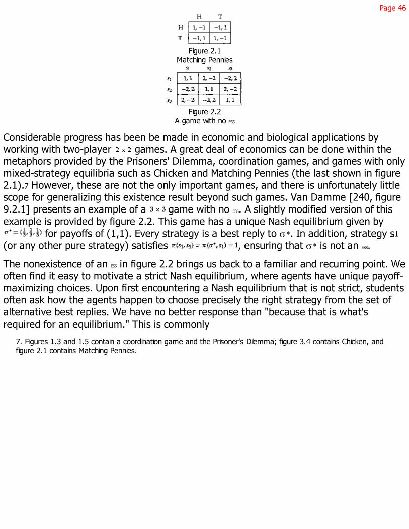
Page 46

Figure 2.1Matching Pennies

Figure 2.2A game with no ESS

Considerable progress has been be made in economic and biological applications byworking with two-player games. A great deal of economics can be done within themetaphors provided by the Prisoners' Dilemma, coordination games, and games with onlymixed-strategy equilibria such as Chicken and Matching Pennies (the last shown in figure2.1).7 However, these are not the only important games, and there is unfortunately littlescope for generalizing this existence result beyond such games. Van Damme [240, figure9.2.1] presents an example of a game with no ESS. A slightly modified version of thisexample is provided by figure 2.2. This game has a unique Nash equilibrium given by

for payoffs of (1,1). Every strategy is a best reply to s*. In addition, strategy s1

(or any other pure strategy) satisfies , ensuring that s* is not an ESS.

The nonexistence of an ESS in figure 2.2 brings us back to a familiar and recurring point. Weoften find it easy to motivate a strict Nash equilibrium, where agents have unique payoff-maximizing choices. Upon first encountering a Nash equilibrium that is not strict, studentsoften ask how the agents happen to choose precisely the right strategy from the set ofalternative best replies. We have no better response than "because that is what'srequired for an equilibrium." This is commonly

7. Figures 1.3 and 1.5 contain a coordination game and the Prisoner's Dilemma; figure 3.4 contains Chicken, andfigure 2.1 contains Matching Pennies.

Page 47

followed by some dynamic intuition about how other choices would prompt adjustmentsin strategies until, one hopes, an equilibrium is reached.

The ESS concept, and its potential nonexistence, tells us something about this dynamicintuition. Inspecting figure 1.4 shows that if we consider this to be a symmetric game(with strategies labeled T = L = A and B = R = B), then injecting a nonequilibriumstrategy, such as playing A with probability , into a population playing the equilibriumhalf-half mixture, causes the former to receive a strictly lower payoff. This suggests thatsome pressure will be brought to bear against nonequilibrium strategies in this case, andthe equal mixture is an ESS as well as a Nash equilibrium.8 There may then be some basisfor the dynamic intuition behind the selection of the best replies required to support theNash equilibrium. In figure 2.2, however, the introduction of a nonequilibrium strategydoes not introduce a similar payoff pressure. This challenges the intuition offered insupport of the Nash equilibrium in this case, and precludes the existence of an ESS.

It may not appear particularly troubling that the game in figure 2.2 has no ESS. Theintuitive stories offered as a defense of Nash equilibrium in the presence of alternativebest replies may be less convincing in this case, and it may not be clear how anevolutionary process should be expected to behave on this game. However, the ESS

concept encounters more serious existence difficulties. An ESS can fail to exist even thoughthe Nash equilibrium concept is convincing, and even though the implications of anevolutionary process appear to be intuitively obvious. Consider figure 2.3. There is asingle component of Nash equilibria in this game, including any mixture over s1 and s2.The unique Nash equilibrium in undominated strategies is (s1, s1). There is no ESS. Inparticular, s1 fails to be an ESS because s2 gives equality in both of (2.1)-(2.2). However,strategy s3 always earns strictly less than any other strategy in the population, and itseems clear that an evolutionary model will at least agree with the Nash equilibriumconcept in yielding the prediction that strategy s3 will be eliminated. The ESS concept canthus fail to exist in cases where evolutionary arguments have implications we would likeour model to capture.

8. Notice that the same is not true of Matching Pennies (figure 2.1) because this is not a symmetric game. An ESS

must then be a strict Nash equilibrium (see proposition 2.4 below), which does not exist for this game.

Page 48

Figure 2.3A game with no ESS

The games in figures 2.2 and 2.3 are not generic, where the word "generic" is given itscommonly used, informal meaning of involving no payoff ties. I am sympathetic to thecontention that game theory should be confined to generic games. The models withwhich we work are approximations, including the numbers we choose to representpayoffs. We may find it convenient in constructing the model to assign the same payoff totwo seemingly similar outcomes. But if this payoff tie turns out to play a major role indriving the results, then we must reconsider our modeling assumptions. It is unlikely thetwo out comes have literally identical payoffs; that the relative magnitude of their payoffsmatters is a signal we should calculate these payoffs more carefully and adjust our modelaccordingly. We should then be suspicious of any results driven by a nongenericity in thespecification of the game.

At the same time, care must be taken in formulating a genericity requirement. It is wellknown that we could dispense with most equilibrium refinement considerations entirely;simply by restricting attention to games that are "generic" in the sense that there are noties in their normal-form payoff matrices. This observation has failed to forestall work onequilibrium refinements because the genericity requirement is too strong. Normal-formpayoff ties can appear because two normal-form strategy profiles lead to the sameterminal node in a generic extensive-form game. We cannot avoid a tie in this case andcannot raise genericity-based objections to such a game. Even asking for no ties toappear in extensive-form payoffs can be too strong. The appropriate place in which torequire genericity is not necessarily the space of payoffs, in either the normal orextensive forms, but rather the mapping from economic outcomes into utilities. Thismapping may be generic, and yet we may have to contend with ties in payoffs. These tiesmay appear in both the normal and extensive form because different strategies give riseto the same economic outcome. For example, I consider Rubinstein's alternating offersbargaining game [197] to be

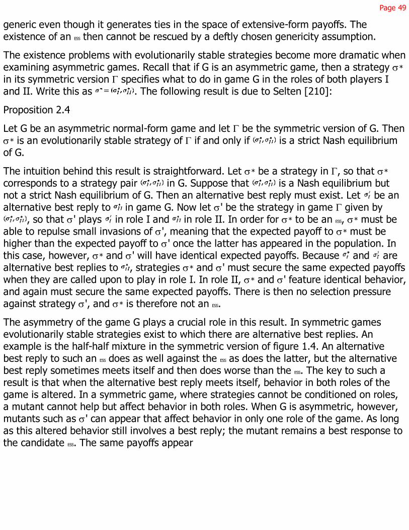
Page 49

generic even though it generates ties in the space of extensive-form payoffs. Theexistence of an ESS then cannot be rescued by a deftly chosen genericity assumption.

The existence problems with evolutionarily stable strategies become more dramatic whenexamining asymmetric games. Recall that if G is an asymmetric game, then a strategy s*

in its symmetric version G specifies what to do in game G in the roles of both players Iand II. Write this as . The following result is due to Selten [210]:

Proposition 2.4

Let G be an asymmetric normal-form game and let G be the symmetric version of G. Thens* is an evolutionarily stable strategy of G if and only if is a strict Nash equilibriumof G.

The intuition behind this result is straightforward. Let s* be a strategy in G, so that s*

corresponds to a strategy pair in G. Suppose that is a Nash equilibrium butnot a strict Nash equilibrium of G. Then an alternative best reply must exist. Let be analternative best reply to in game G. Now let s' be the strategy in game G given by

, so that s' plays in role I and in role II. In order for s* to be an ESS, s* must beable to repulse small invasions of s', meaning that the expected payoff to s* must behigher than the expected payoff to s' once the latter has appeared in the population. Inthis case, however, s* and s' will have identical expected payoffs. Because and arealternative best replies to , strategies s* and s' must secure the same expected payoffswhen they are called upon to play in role I. In role II, s* and s' feature identical behavior,and again must secure the same expected payoffs. There is then no selection pressureagainst strategy s', and s* is therefore not an ESS.

The asymmetry of the game G plays a crucial role in this result. In symmetric gamesevolutionarily stable strategies exist to which there are alternative best replies. Anexample is the half-half mixture in the symmetric version of figure 1.4. An alternativebest reply to such an ESS does as well against the ESS as does the latter, but the alternativebest reply sometimes meets itself and then does worse than the ESS. The key to such aresult is that when the alternative best reply meets itself, behavior in both roles of thegame is altered. In a symmetric game, where strategies cannot be conditioned on roles,a mutant cannot help but affect behavior in both roles. When G is asymmetric, however,mutants such as s' can appear that affect behavior in only one role of the game. As longas this altered behavior still involves a best reply; the mutant remains a best response tothe candidate ESS. The same payoffs appear

Page 50

when two mutants meet as when a mutant and the candidate ESS meet, ensuring that thelatter is not an ESS. A candidate for an ESS can then be sure of repelling all mutants only if nomutant is a best reply, implying that an ESS must be a strict Nash equilibrium.

Restricting attention to strict Nash equilibria is a sufficiently strong requirement toseverely limit the usefulness of the ESS concept in asymmetric games. Mixed strategies,such as the unique Nash equilibrium of Matching Pennies (figure 2.1), are immediatelyprecluded. In extensive-form games this requires that equilibrium strategies be pure andreach every information set. However, interesting economic problems readily lead togames and equilibria in which some information sets are not reached. Our intuition is thatgame theory in general and evolutionary game theory in particular should havesomething to say about such games. Making progress on refining and selecting equilibriathen requires some alternative to working with the notion of an evolutionarily stablestrategy.

It is important to note what is not being asserted in the previous paragraph. It is not thecase that I have already selected a favorite equilibrium concept and am now disappointedbecause evolutionary stability, in insisting on strict Nash equilibria, fails to agree with thatconcept. To the contrary, I think there is little to be gained from seeking a singleequilibrium concept to be ordained on abstract grounds as the ''right" one. Instead, theappropriate equilibrium is likely to vary across games and settings, and may often dependupon institutional considerations that are not captured in the specification of the game.As a result, we are often faced with the task of interpreting and evaluating equilibria, andthese equilibria are typically not strict Nash equilibria. We need some help in evaluatingthese equilibria, and this is what I seek from an evolutionary model. A model that cannothelp in this task is disappointing not because if fails to select the right equilibrium butbecause it fails to provide information that might help identify some equilibria as moreinteresting than others.

2.2 Alternative Notions of Evolutionary Stability

The previous section contains good news and bad news. The concept of evolutionarystability captures considerations familiar from the refinements literature, but does so in away that all too easily leads to nonexistence. One response to the potential nonexistenceof evolutionarily stable strategies has been to propose alternative notions of evo-

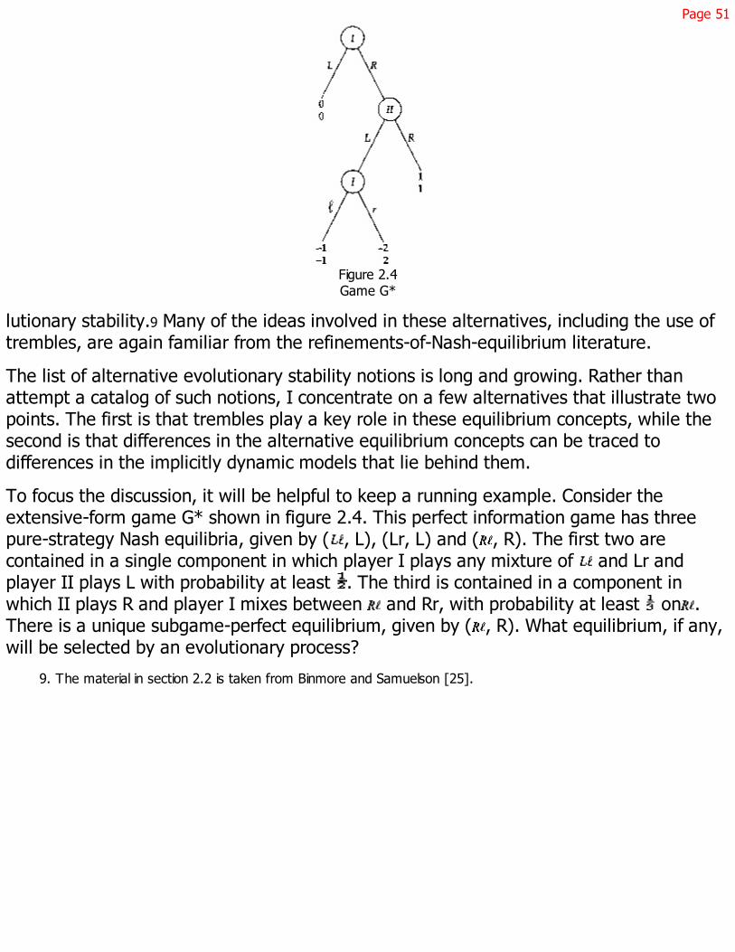
Page 51

Figure 2.4Game G*

lutionary stability.9 Many of the ideas involved in these alternatives, including the use oftrembles, are again familiar from the refinements-of-Nash-equilibrium literature.

The list of alternative evolutionary stability notions is long and growing. Rather thanattempt a catalog of such notions, I concentrate on a few alternatives that illustrate twopoints. The first is that trembles play a key role in these equilibrium concepts, while thesecond is that differences in the alternative equilibrium concepts can be traced todifferences in the implicitly dynamic models that lie behind them.

To focus the discussion, it will be helpful to keep a running example. Consider theextensive-form game G* shown in figure 2.4. This perfect information game has threepure-strategy Nash equilibria, given by ( , L), (Lr, L) and ( , R). The first two arecontained in a single component in which player I plays any mixture of and Lr andplayer II plays L with probability at least . The third is contained in a component inwhich II plays R and player I mixes between and Rr, with probability at least on .There is a unique subgame-perfect equilibrium, given by ( , R). What equilibrium, if any,will be selected by an evolutionary process?

9. The material in section 2.2 is taken from Binmore and Samuelson [25].

Page 52

We can first ask about evolutionarily stable strategies for game G*. This requires workingwith the symmetrized version G* of game G*, in which a strategy for an agent includes astrategy for both players I and II and an agent is equally likely to fill the role of eitherplayer I or player II. Because an ESS of G* must be a strict Nash equilibrium of G* and thelatter has no strict Nash equilibria, we immediately have10

Remark 2.1

An evolutionarily stable strategy does not exist for Game G*.

For example, the subgame-perfect equilibrium ( , R) is not evolutionarily stable becausethe strategy (Rr, R) can invade. More precisely, taking s* to be ( , R) and s to be (Rr, R)yields equality throughout conditions (2.1)-(2.2). The strategy (Rr, R) can invade becauseit differs from the subgame-perfect equilibrium strategy ( , R) only at information setsthat are never reached when ( , R) and (Rr, R) play each other or themselves. Thedifferent behavior specified by the mutant (Rr, R) then has no effect on play. There is noobvious way for an evolutionary process to bring pressure against this strategy, and thesubgame-perfect equilibrium cannot be evolutionarily stable.

Neutrally Stable Strategies

The strategies ( , R) and (Rr, R) give identical outcomes in game G*. Then why do wecare whether (Rr, R) can invade? More generally, we may not want to discard anequilibrium, even if it is not evolutionarily stable, as long as the only invaders are thosewhose behavior and payoffs match that of the candidate strategy. Why worry aboutchanges in behavior off the equilibrium path? Toward this end, Maynard Smith [149, p.107] defines the concept of a neutrally stable strategy. Let S be the set of pure strategiesin an asymmetric game G, so that is the set of mixed strategies for thesymmetrized game G.11 Then we have12

10. It is common to say that G* has no ESS, though the asymmetry of G* forces the ESS concept to be applied tothe symmetrized version of the game given by G*. Analogous references to G* are made for subsequentequilibrium concepts.

11. As usual, a mixed strategy for G is taken to be two independent mixtures over S, one for each player in game G.

12. Because G* is asymmetric, I state definitions in this section in terms of strategies for asymmetric games. Theusual symmetrization is involved in computing payoffs. The profit functions that appear in this definition are then theexpected profits, with the expectation taken over the identity of the opponent and the role to be occupied whenplaying the game.

Page 53

Definition 2.3

A neutrally stable strategy for an asymmetric game G is a strategy such that,for all :

Comparing these conditions with (2.1)-(2.2), we see that the final strict inequality in (2.2)has been replaced with a weak inequality. The effect of this change is that we do notrequire a neutrally stable strategy to receive a strictly higher payoff than any mutant, andhence cannot be sure that every mutant will be driven out once it appears. At the sametime, (2.6)-(2.7) ensure that a mutant cannot earn a higher payoff than the neutrallystable strategy, and hence that the mutant cannot displace the neutrally stable strategy.It thus may be that after a mutant appears, the mutant and the neutrally stable strategycoexist.

It is straightforward to verify that neutrally stable strategies exist for game G*:

Remark 2.2

In Game G*, every Nash equilibrium (sI, sII) is a neutrally stable strategy except (i) theNash equilibrium in which player II plays R and player I plays with probability and Rrwith probability ; and (ii) any Nash equilibrium in which player I mixes between andLr, while player II plays L with probability .

Every Nash equilibrium is thus neutrally stable except those teetering just on the brink ofnot being Nash equilibria.

The difficulty with neutrally stable strategies is that they may not be "stable enough."Consider the subgame-perfect equilibrium of Game G*. How reassuring do we find it thatthis strategy is neutrally stable? Beginning in a state in which all agents in the populationplay their part of the subgame-perfect equilibrium, changes in behavior can occur that donot give rise to any evolutionary pressure to adjust strategies. In particular, mutationscan introduce the strategy (Rr, R). An outcome in which ( , R) is played can then bedisplaced by one in which player II plays R and player I mixes between and Rr, as longas suitably large probability (i.e., at least ) is still placed on . This shift has noimplications for observed behavior. However, this may lead to a population polymorphismin which of the agents in population I play Rr. At this point, small infusions of mutantsplaying Rr and L will cause L to receive a higher payoff for player II than R, causingstrategy L to grow and potentially disrupting the subgame-perfect equilibrium outcome.Neutral stability may then be

Page 54

too weak a requirement to be interesting. At the very least, it seems that when workingwith neutral stability, one should address polymorphic populations and should assess thestability of entire components of equilibria.

Trembles

The objection to the neutral stability of the subgame-perfect equilibrium in the previousparagraph is based on the possibility that mutations can lead the system to an outcomein which Rr is played by a proportion of the population approaching . How probable aresuch mutations? If the mutations needed to cause stability problems for a neutrally stablestrategy are quite unlikely, then the neutrally stable strategy may not be problematic.Alternatively, we might accept a component of neutrally stable strategies as stable aslong as mutations will direct the system to the "more stable" part of the component.

Maynard Smith [149] suggests that small perturbations in either the game or theevolutionary process will eliminate the effect of mutations on off-the-equilibrium-pathbehavior. In particular, perturbations in Game G* might take the form of some player-IIagents occasionally playing L, even though the strategy of each such agent is to play R.These perturbations would cause player I agents to earn a higher payoff from playing than from Rr and hence should push player I back to , interrupting any movementtoward Rr.

Selten [211, 212] pursues a similar intuition in introducing the concept of a limitevolutionarily stable strategy.13 To find a limit ESS of an asymmetric game G, we firstconstruct a perturbed game G(Î), where is a vector containing a nonnegativenumber for each of the pure strategies for each of players I and II. The players and payofffunctions are unchanged, but players in G(Î) must choose mixed strategies from the sets

and , where for any pure strategy , with a similarcharacterization of DII. Hence players can be forced to attach positive probability tocertain pure strategies in the perturbed game. Notice, however, that is notrequired, so that strategies in the perturbed game need

13. The limit ESS concept is Selten's first step in the construction of evolutionary stability ideas that explicitly takeaccount of the extensive-form structure of a game [211, 212]. Elementary extensive-form considerations reappearin chapter 8 below.

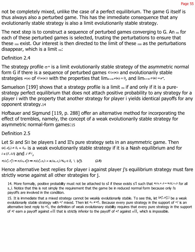
Page 55

not be completely mixed, unlike the case of a perfect equilibrium. The game G itself isthus always also a perturbed game. This has the immediate consequence that anyevolutionarily stable strategy is also a limit evolutionarily stable strategy.

The next step is to construct a sequence of perturbed games converging to G. An ESS foreach of these perturbed games is selected, trusting the perturbations to ensure thatthese ESSS exist. Our interest is then directed to the limit of these ESSS as the perturbationsdisappear, which is a limit ESS:

Definition 2.4

The strategy profile s* is a limit evolutionarily stable strategy of the asymmetric normalform G if there is a sequence of perturbed games and evolutionarily stablestrategies of with the properties that lim , and lim .

Samuelson [199] shows that a strategy profile is a limit ESS if and only if it is a pure-strategy perfect equilibrium that does not attach positive probability to any strategy for aplayer i with the property that another strategy for player i yields identical payoffs for anyopponent strategy.14

Hofbauer and Sigmund [119, p. 288] offer an alternative method for incorporating theeffect of trembles, namely, the concept of a weak evolutionarily stable strategy forasymmetric normal-form games:15

Definition 2.5

Let SI and SII be players I and II's pure strategy sets in an asymmetric game. Then is a weak evolutionarily stable strategy if it is a Nash equilibrium and for

and ,

Hence alternative best replies for player i against player j's equilibrium strategy must farestrictly worse against all other strategies for j.

14. More formally, positive probability must not be attached to sI if these exists s'I such that for alls_i. Notice that this is not simply the requirement that the game be in reduced normal form because only i'spayoffs are involved in the condition.

15. It is immediate that a mixed strategy cannot be weakly evolutionarily stable. To see this, let be a weakevolutionarily stable strategy with mixed. Then let . Because every pure strategy in the support of is analternative best reply to , the definition of weak evolutionary stability requires that every pure strategy in the supportof earn a payoff against sII that is strictly inferior to the payoff of against sII, which is impossible.

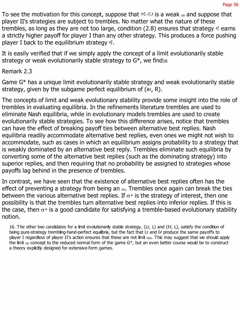
Page 56

To see the motivation for this concept, suppose that is a weak ESS and suppose thatplayer II's strategies are subject to trembles. No matter what the nature of thesetrembles, as long as they are not too large, condition (2.8) ensures that strategy earnsa strictly higher payoff for player I than any other strategy. This produces a force pushingplayer I back to the equilibrium strategy .

It is easily verified that if we simply apply the concept of a limit evolutionarily stablestrategy or weak evolutionarily stable strategy to G*, we find16

Remark 2.3

Game G* has a unique limit evolutionarily stable strategy and weak evolutionarily stablestrategy, given by the subgame perfect equilibrium of ( , R).

The concepts of limit and weak evolutionary stability provide some insight into the role oftrembles in evaluating equilibria. In the refinements literature trembles are used toeliminate Nash equilibria, while in evolutionary models trembles are used to createevolutionarily stable strategies. To see how this difference arises, notice that tremblescan have the effect of breaking payoff ties between alternative best replies. Nashequilibria readily accommodate alternative best replies, even ones we might not wish toaccommodate, such as cases in which an equilibrium assigns probability to a strategy thatis weakly dominated by an alternative best reply. Trembles eliminate such equilibria byconverting some of the alternative best replies (such as the dominating strategy) intosuperior replies, and then requiring that no probability be assigned to strategies whosepayoffs lag behind in the presence of trembles.

In contrast, we have seen that the existence of alternative best replies often has theeffect of preventing a strategy from being an ESS. Trembles once again can break the tiesbetween the various alternative best replies. If s* is the strategy of interest, then onepossibility is that the trembles turn alternative best replies into inferior replies. If this isthe case, then s* is a good candidate for satisfying a tremble-based evolutionary stabilitynotion.

16. The other two candidates for a limit evolutionarily stable strategy, (Lr, L) and ( , L), satisfy the condition ofbeing pure-strategy trembling-hand-perfect equilibria, but the fact that Lr and produce the same payoffs toplayer I regardless of player II's action ensures that these are not limit ESSS. This may suggest that we should applythe limit ESS concept to the reduced normal form of the game G*, but an even better course would be to constructa theory explicitly designed for extensive-form games.

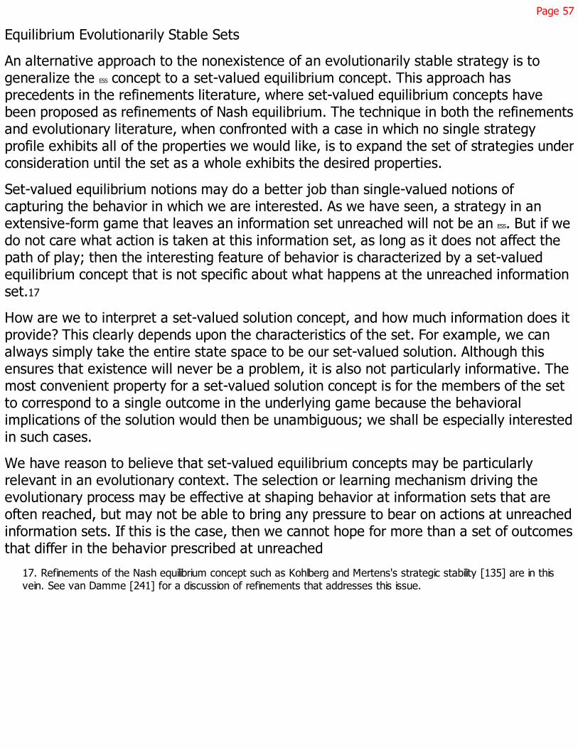
Page 57

Equilibrium Evolutionarily Stable Sets

An alternative approach to the nonexistence of an evolutionarily stable strategy is togeneralize the ESS concept to a set-valued equilibrium concept. This approach hasprecedents in the refinements literature, where set-valued equilibrium concepts havebeen proposed as refinements of Nash equilibrium. The technique in both the refinementsand evolutionary literature, when confronted with a case in which no single strategyprofile exhibits all of the properties we would like, is to expand the set of strategies underconsideration until the set as a whole exhibits the desired properties.

Set-valued equilibrium notions may do a better job than single-valued notions ofcapturing the behavior in which we are interested. As we have seen, a strategy in anextensive-form game that leaves an information set unreached will not be an ESS. But if wedo not care what action is taken at this information set, as long as it does not affect thepath of play; then the interesting feature of behavior is characterized by a set-valuedequilibrium concept that is not specific about what happens at the unreached informationset.17

How are we to interpret a set-valued solution concept, and how much information does itprovide? This clearly depends upon the characteristics of the set. For example, we canalways simply take the entire state space to be our set-valued solution. Although thisensures that existence will never be a problem, it is also not particularly informative. Themost convenient property for a set-valued solution concept is for the members of the setto correspond to a single outcome in the underlying game because the behavioralimplications of the solution would then be unambiguous; we shall be especially interestedin such cases.

We have reason to believe that set-valued equilibrium concepts may be particularlyrelevant in an evolutionary context. The selection or learning mechanism driving theevolutionary process may be effective at shaping behavior at information sets that areoften reached, but may not be able to bring any pressure to bear on actions at unreachedinformation sets. If this is the case, then we cannot hope for more than a set of outcomesthat differ in the behavior prescribed at unreached

17. Refinements of the Nash equilibrium concept such as Kohlberg and Mertens's strategic stability [135] are in thisvein. See van Damme [241] for a discussion of refinements that addresses this issue.

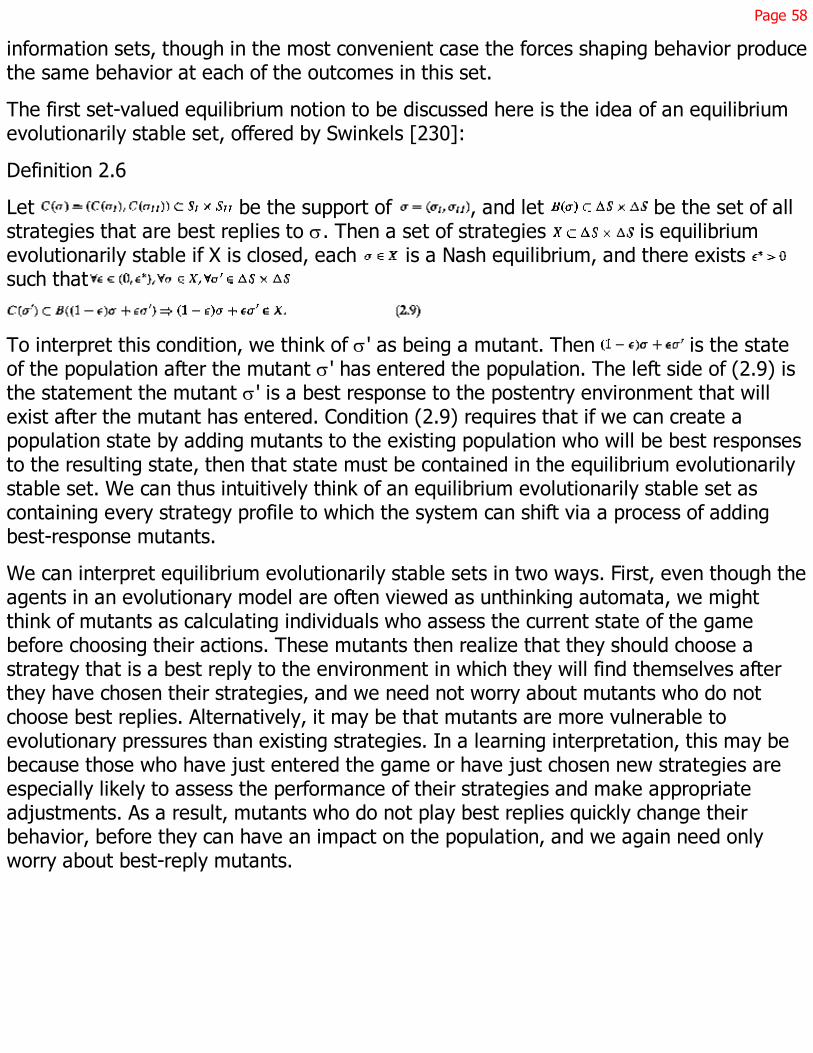
Page 58

information sets, though in the most convenient case the forces shaping behavior producethe same behavior at each of the outcomes in this set.

The first set-valued equilibrium notion to be discussed here is the idea of an equilibriumevolutionarily stable set, offered by Swinkels [230]:

Definition 2.6

Let be the support of , and let be the set of allstrategies that are best replies to s. Then a set of strategies is equilibriumevolutionarily stable if X is closed, each is a Nash equilibrium, and there exists such that

To interpret this condition, we think of s' as being a mutant. Then is the stateof the population after the mutant s' has entered the population. The left side of (2.9) isthe statement the mutant s' is a best response to the postentry environment that willexist after the mutant has entered. Condition (2.9) requires that if we can create apopulation state by adding mutants to the existing population who will be best responsesto the resulting state, then that state must be contained in the equilibrium evolutionarilystable set. We can thus intuitively think of an equilibrium evolutionarily stable set ascontaining every strategy profile to which the system can shift via a process of addingbest-response mutants.

We can interpret equilibrium evolutionarily stable sets in two ways. First, even though theagents in an evolutionary model are often viewed as unthinking automata, we mightthink of mutants as calculating individuals who assess the current state of the gamebefore choosing their actions. These mutants then realize that they should choose astrategy that is a best reply to the environment in which they will find themselves afterthey have chosen their strategies, and we need not worry about mutants who do notchoose best replies. Alternatively, it may be that mutants are more vulnerable toevolutionary pressures than existing strategies. In a learning interpretation, this may bebecause those who have just entered the game or have just chosen new strategies areespecially likely to assess the performance of their strategies and make appropriateadjustments. As a result, mutants who do not play best replies quickly change theirbehavior, before they can have an impact on the population, and we again need onlyworry about best-reply mutants.

Page 59

In G*, equilibrium evolutionarily stable sets have the attractive feature of correspondingto a single outcome:

Remark 2.4

Game G* has a unique equilibrium evolutionarily stable set in which player II alwaysplays R, yielding the subgame-perfect equilibrium outcome.

In particular, the strategy profile ( , L) cannot be contained in an equilibriumevolutionarily stable set because the set would also have to contain the strategy profile inwhich player I chooses and player II mixes equally between L and R, at which pointthere are mutant strategies (placing higher probabilities on R for player II) that pass thetest of being best replies to their postentry environment, but take the system outside theset of Nash equilibria.18

Nonequilibrium Evolutionarily Stable Sets

A different outcome is provided by Sobel's nonequilibrium evolutionarily stable sets[223].19 The common assumption in evolutionary analyses is that the populations arelarge, so that we can treat them as being essentially infinite, in the sense that samplingwith and without replacement gives equivalent results. Sobel, however, explicitlyassumes that agents are drawn from two finite populations, one of player I's and one ofplayer II's. We then have

Definition 2.7

Strategy profile s, identifying a pure strategy for each agent of each population, canreplace s' if s and s' differ only in the strategy of a single agent, with that agent'sexpected payoff against a randomly selected agent of the opposing population being atleast as high under s as it is under s'. A set X is a nonequilibrium evolutionarily stable setif it is nonempty and minimal with respect to the property that and s able to replaces' implies .

18. Thomas [234, 235] offers the related set-valued equilibrium concept of an evolutionarily stable set, obtained bydirectly extending the definition of an ESS to sets. An evolutionarily stable set differs from an equilibrium evolutionarilystable set in that any strategy in a neighborhood of an evolutionarily stable set that does as least as well as thestrategies in the set must also be in the set, whereas equilibrium evolutionarily stable sets impose a similarrequirement only for strategies that are best responses in the neighborhood. The unique evolutionarily stable set ingame G* coincides with the equilibrium evolutionarily stable set. See Balkenborg [6], Balkenborg and Schlag [7, 8],and Schlag [204, 205] for further development.

19. Predecessors of Sobel include Kim and Sobel [133] and Blume, Kim, and Sobel [34]. Related ideas appear in theformulation of cyclically stable sets by Gilboa and Matsui [99] and Matsui [148].

Page 60

Hence a nonequilibrium evolutionarily stable set must contain any population profile towhich it can move via a process of having one player at a time shift in a direction thatdoes not decrease the player's payoff. It follows immediately from the definition that

Remark 2.5

In Game G*, there is a single nonequilibrium evolutionarily stable set, containing (amongother strategy profiles) every strategy profile in which player I chooses any mixturebetween and Lr as well as every strategy profile in which player I mixes between and Rr, while player II chooses R.

Both of the Nash equilibrium outcomes of G* are included in the nonequilibriumevolutionary state set, as are some profiles that are not equilibria. To see how thisoccurs, consider a state in which all agents play their part of the subgame-perfectequilibrium ( , R). This state can be replaced by a state in which a member of populationI plays Rr because the shift from to r does not decrease the agent's payoff. This statecan in turn be replaced by one in which yet another agent in population I plays Rr;continuing in this way we can successively replace states until we have all agents inpopulation I paying Rr. At this point, we have a state that does not correspond to a Nashequilibrium because agents in population II are playing R but L is a best reply. However,this state must be contained in the nonequilibrium evolutionarily stable set, at least if thelatter is to contain the subgame-perfect equilibrium, because we have moved to thecurrent state from the subgame-perfect equilibrium via a series of replacements. Nowadditional replacements can occur that cause agents in population II to switch from R to Lbecause such switches increase the payoffs of these agents (given that agents inpopulation I play Rr). These replacements again yield states that are not equilibria; thiscan continue until we reach a state in which agents in population I play Rr and those inpopulation II play L. Further replacements can then cause agents in population I to switchto L, which is now a payoff-increasing switch, and can lead to a state in which agents inpopulation I play , while those in population II play L. We have then reached a Nashequilibrium that is not subgame-perfect.

Dynamic Interpretations

The list of alternative notions of evolutionary stability has been steadily growing. Whataccounts for the differences in these various stability notions? I think the most revealingway to assess these notions is to

Page 61

recognize that behind each concept lies an implicitly dynamic model just as manyconventional equilibrium refinements are motivated by implicitly dynamic models of whatplayers will do when confronted with an out-of-equilibrium event. These dynamic modelsdiffer most noticeably in the different provisions they make for the treatment of mutants.

To see the differing dynamic foundations lying behind static equilibrium concepts,compare the concepts of a weak evolutionarily stable strategy and equilibriumevolutionarily stable set, both of which support the subgame-perfect outcome. The weakevolutionarily stable strategy concept assumes that mutations switching agents fromstrategy to Rr are immediately repulsed. Hence attention can be limited to the singlestrategy profile ( , R), which appears to involve an assumption to the effect thatperturbations causing player II to play L occur frequently enough to eradicate anyswitches from to Rr. In contrast, the concept of an equilibrium evolutionarily stable setallows mutations introducing Rr to proceed unchecked until the boundary is approachedat which R ceases to be a best reply for player II. Here, further mutations are impossible.The assumption appears to be that it is not perturbations but best-reply behavior thatdisciplines mutations. As long as R is a best reply for player II, there is no disciplineimposed on mutations toward Rr. Once the edge is reached at which L is a best reply,however, then a rush of player-II agents to L pushes player I back to , which in turnmakes R once again a best reply for player II.

In light of this interpretation, consider the difference between equilibrium andnonequilibrium evolutionarily stable sets. Attention is again. directed at the treatment ofmutants in the dynamic models that implicitly lie behind the two concepts. Begin with thesubgame-perfect equilibrium ( , R) in game G*. Both the equilibrium and nonequi-librium evolutionarily stable set concepts allow mutations to switch agents in population Itoward Rr, to the point that L can become a weak best reply for player II. Here, however,the two part company. As we have seen, one interpretation of an equilibriumevolutionarily stable set is that mutants adjust faster than incumbents. Any further drifttoward Rr now prompts player II to adjust toward the best reply of L, which immediatelypushes the mutant agent I's back to (and then player II back to R) and restores theNash equilibrium. A nonequilibrium evolutionarily stable set, in contrast, admits thepossibility that once sufficient mutation toward Rr has occurred to make L a best reply forplayer II, the primary adjustments may first be for

Page 62

player-II agents to switch to L, with this movement continuing until player-I agents nolonger find it a best reply to play R at their first move and hence switch to or Lr,leading away from the subgame-perfect equilibrium.

Despite the contrast in the terms, namely, equilibrium evolutionarily stable sets andnonequilibrium evolutionarily stable sets, these are quite similarly motivated andconstructed concepts. Lying behind both is a presumption that agents in the populationflow toward higher-payoff strategies and away from lower-payoff strategies, but can beswitched by mutations among equal-payoff strategies. Starting from the subgame-perfectequilibrium, both agree that mutations from to Rr can occur They differ only on whathappens when these mutations lead the system to the brink of no longer being a Nashequilibrium, where they make different assumptions as to the relative rates at whichagents in the two populations adjust their strategies. But this seemingly subtle differenceleads one concept to restrict attention to the subgame-perfect equilibrium, while leadingthe other to include other Nash equilibria and nonequilibrium outcomes as well.

2.3 Dynamic Systems

The finding that the various stability notions, offered as alternatives to the concept of anevolutionarily stable strategy, differ in their implicit, underlying dynamics, directs ourattention to dynamic evolutionary models. I believe that the study of such models willplay a central role in assessing evolutionary stability concepts.

Because biologists working with evolutionary models have a clear idea of how theevolutionary process operates, it is only natural that they would investigate directly thedynamic process whose outcome the ESS is supposed to describe. With the help of somesimplifying assumptions, the resulting models lead to the replicator dynamics, a system ofdeterministic difference or differential equations that plays a central role in biologicalmodels.

Economists have similarly studied dynamic models, both in an effort to motivate solutionconcepts such as ESS, and its alternatives, and in response to the observation that an ESS

often fails to exist. In many cases, economists have simply worked with the replicatordynamics. Given their original biological motivation, it is not obvious that the replicatordynamics should command attention in economic applications. However, several authorshave recently noted that the replicator dynamics can emerge from simple learningmodels. Although

Page 63

the learning models in question are stylized and arbitrary in many respects, and certainlyprovide no reason to claim that the replicator dynamics are in any sense the ''right"model they do suggest that the replicator should not be automatically dismissed ineconomic applications.20 The process by which agents choose their strategies in alearning context is more likely to resemble the replicator dynamics if imitation is animportant component of the learning process; a process driven by imitation shares manyof the features of biological reproduction, with agents who are successful giving rise toadditional agents playing the same strategy.

This section presents the basic results concerning the replicator dynamics and theirrelationship to evolutionarily stable strategies.21 Economists have also examined a widevariety of dynamic evolutionary models using other techniques. This section doses with abrief discussion of a frequently used model whose techniques of analysis and outcomeprovide a sharp contrast with those of models based on the replicator dynamicstheMarkov model of Kandori, Mailath, and Rob [128].

Replicator Dynamics

In discussing the replicator dynamics, I shall often interpret the system in biologicalterms. Consider first the most common model containing a single large population ofagents who will be matched in pairs to play a symmetric game. Unlike the case of anevolutionarily stable strategy, each agent is now associated with a pure strategy. Thecounterpart of a mixed strategy in this model is a polymorphic population in whichdifferent agents play different pure strategies. One could easily allow the agents to playmixed strategies as long as only a finite number of such strategies could occur in thepopulation at any single time, whereas allowing an infinite number of different

20. One such derivation is presented in chapter 3. See also Börgers and Sarin [47], Cabrales [54], and Schlag[206]. Cressman [69] shows that if a state is a hyperbolic stationary state under both the replicator dynamics andan arbitrary dynamic from a more general class of "monotonic" dynamics (that includes the replicator dynamics),then it is a source, saddle, or sink under the monotonic dynamic if and only if it is a source, saddle, or sink underthe replicator dynamics. This is a reflection of the fact that the properties of stationary states are relativelyinsensitive to alterations in the specification of a dynamic system that preserve the qualitative nature of its localbehavior. The implication is that we can often learn much from studying the replicator dynamics.

21. This material is well covered by Weibull [248] and by van Damme [240], as well as by Hofbauer and Sigmund[119], and the treatment here will be brief.

Page 64

strategies requires more advanced techniques. Notice that a model in which agents playpure strategies and mixed-strategy outcomes appear as population polymorphisms issimilar in spirit to Harsanyi's purification model of mixed strategies [115].

Let be the number of agents playing pure strategy i at time t and let N(t) be the totalnumber of agents at time t. Let be the proportion of agents playing pure strategy i attime t, so . Let x(t) be the vector of proportions playing the various purestrategies. x(t) is then a member of the mixed-strategy simplex, and we will ofteninterpret x(t) as a mixed strategy.

There are several versions of the replicator dynamics and even more methods for derivingand motivating these versions. First, consider discrete-time models. Van Damme [240,section 9.4] suggests the following argument, based on a nonoverlapping generationsmodel of the population.22 In each period, agents in the population are paired at randomto each play exactly one game. At the end of the period, each agent is replaced byagents who play the same strategy and whose number is given by the payoff the originalagent received in the game played in that period. Then let the expected number ofreplacements for each agent playing strategy i be denoted by and let the expectednumber of agents next period be For convenience, let the average payoff in thepopulation be denoted by, where

If we assume that actual outcomes will match expected outcomes, then the proportion ofthe population playing strategy i next period will be

We can than represent the evolution of the population as

This discrete replicator dynamic is examined by Dekel and Scotchmer [72], Hofbauer andSigmund [119], Maynard Smith [149, p. 183], and van Damme [240]. The assumptionthat actual and expected outcomes

22. Hofbauer and Sigmund [119, p. 13] present a similar argument.

Page 65

will coincide is commonly motivated by observing that the population is assumed to belarge, so that one can appeal to the law of large numbers. The next chapter returns tothis issue.

The derivation of (2.10) is based on the assumption that generations do not overlap, sothat all agents reproduce at the same time and parents do not survive the reproductionprocess.23 For some biological applications, where reproduction occurs in a fixed breedingseason and organisms live only from birth to the next breeding season, this may be themost appropriate model. In other applications, in which reproduction is not synchronized,an overlapping generations model may be more appropriate. This may especially be thecase in the learning applications that interest us, where there may be no reason for allagents to assess their strategies at the same time, and hence agents who have justselected a new strategy will coexist with others who have maintained their currentstrategy for some time.

Binmore [19] examines the overlapping generations case; a similar derivation appears inTaylor and Jonker [232]. Suppose that in each period of time of length t, a fraction t ofthe population gives birth, with an individual playing strategy i giving birth to offspring who also play strategy i. Then the expected number of agents playing strategy iin period is given by . Dividing each side by the total numberof agents next period (given by ) and then dividing the numerator anddenominator of the right side by the total number of agents this period, we have

and hence

Equations (2.10) and (2.11) are the two most common discrete replicator dynamics.Cabrales and Sobel [55] consider a variation of (2.11) given by

23. Mailath [145, p. 268] notes the importance of the nonoverlapping generations assumption.

Page 66

Hofbauer and Sigmund [119, p. 133], considering the case of , suggest a version thatincludes (2.11) as a special case:

The constant C is interpreted as the rate of "background fitness," which is the rate offitness that would prevail in the absence of the strategic interaction in question. Thoughbackground fitness notions have played only a minor role in economic applications ofevolutionary game theory, similar notions will make an appearance in chapter 9.

It is often convenient to work in continuous time. Van Damme [240] invokes anassumption that time periods are very short to pass from (2.10) to

van Damme then observes that by a rescaling of time, this can be converted to thefollowing system, which has identical solution trajectories:

Alternatively, one can obtain (2.14) directly by taking the limit as the length of a timeperiod t approaches zero in (2.12), and can obtain (2.15) directly by taking the limit in (2.11) (or (2.13) with C = 1).24

In many cases, it does not matter which replicator dynamic we use. However, Hofbauerand Sigmund [119, p. 133] note that with , the outcome of (2.13) can depend on C.This in turn indicates that (2.10) and (2.11) can give different results. The results inSamuelson and Zhang [202] and in Dekel and Scotchmer [72] show that (2.10) and(2.15) can give different outcomes. Cabrales and Sobel [55] and Weibull [248] explorethe forces behind this difference. Boylan [49] shows that (2.10) and either of (2.14) or(2.15) can give different results. Finally, Bomze and Eichberger [41] and Hofbauer andSigmund [119, p. 273] note that the transformation leading from (2.14) to (2.15) canbreak down when there is more than one population, and that the two continuousdynamic systems can give different outcomes

24. Hofbauer and Sigmund [119, section 16.1] and Weibull [248, chapter 3] provide direct derivations of (2.15)without the intermediate step of a discrete-time model.

Page 67

in this case. Some of these differences are explored further by Seymour [215].25

Equilibrium

Once a formulation for the replicator dynamics is chosen, what can we learn from it? Thereplicator dynamics are related to the ESS concept as well as to the Nash equilibriumconcept. In exploring these relations, I restrict attention to the case that has dominatedthe literature, especially the biological literature, namely, symmetric games played by asingle population of players and with the replicator dynamic given by (2.15).

Let denote a solution to (2.15). The interpretation is that gives thestate of the population at time t given that its state at time zero, or initial condition, is x0.The right side of (2.15) is a polynomial in the population shares, and hence is Lipschitz-continuous. This in turn suffices to ensure that for any initial condition x0, there is aunique solution .26 Given a state x0, the set is the trajectory or the orbitpassing through x0. This trajectory is periodic with period t if there exists a time t with

. A set X is invariant if implies that for all . The set X is forward-invariant if implies that for all .

Because the selection mechanism lying behind the replicator dynamics is based onreproduction, strategies that are currently not played by any agent in the populationcannot be introduced into the population by the replicator dynamics. At the same time, itis evident from (2.15) that the growth rate of the proportion of the population playing anygiven strategy is finite. The proportion of the population playing a strategy can get verysmall, but never reaches zero. Literally speaking, there is no extinction, though cases canarise in which the proportion of the population playing a particular strategy approacheszero. As a result, the strategy simplex DS is invariant under the replica-tot dynamics. Inaddition, any boundary face (i.e., any set obtained by setting the population proportionsof one or more strategies equal

25. Things become more complicated if one adds perturbations to the replicator dynamics. Foster and Young [79],Fudenberg and Harris [85], and Cabrales [54] examine models based on stochastic differential equations.

26. This is the Picard-Lindelöf theorem. See Hirsch and Smale [118] or Hale [111].

Page 68

to zero) is also invariant. In the extreme, any monomorphic population state obtained byattaching all agents to the same strategy is invariant.

We now require some stability notions. The following are standard:

Definition 2.8

The state x* Î X is a stationary state of the differential equation dx/dt = f(x) defined on if is stable if it is a stationary point with the property that for every

neighborhood V of x*, there exists a neighborhood with the property that if ,then for all t > 0. And x* is asymptotically stable if it is stable and there exists aneighborhood W of x* such that implies limt .

Stationary states, also sometimes called "rest points" or "dynamic equilibria," have theproperty that if the dynamic system begins at such a state, then it remains there.However, a stationary state can still be unstable. For example, x* may be stationary butmay be a source, meaning that for every initial condition close to x*, the dynamic systemmoves away from x*. A stable state is a stationary point with the property that if atrajectory starts nearby, then it stays nearby; though it need not converge to x*. Anasymptotically stable state satisfies the additional property that trajectories beginningfrom all nearby states converge to x*.27

A first familiar result is then

Proposition 2.5.1

If (x, x) is a Nash equilibrium of a symmetric game G, then x is a stationary state of thereplicator dynamic (2.15).

Proposition 2.5.2

If x is a stationary state of (2.15), (x, x) need not be a Nash equilibrium of G.

Proposition 2.5.1 is easily established. A Nash equilibrium has the property that allstrategies played with positive probability receive the same payoff, which must be as highas the payoff to any strategy that does not receive positive probability. The right side of(2.15) must then be zero for every strategy, either because the strategy is played withzero probability ( ) or the strategy receives the same payoff as

27. Weibull [248] contains an example showing that the requirement that a stationary state x* be stable is notredundant in the definition of asymptotic stability. In particular, one can find a stationary state x* with the propertythat the trajectories from all nearby initial conditions converge to x*, but stray far away in the process, so thattrajectories that start nearby do not remain nearby.

Page 69

every other, and hence receives the average payoff (giving )

A state x can be stationary and yet (x, x) can fail to be a Nash equilibrium because thesuperior best replies that prevent (x, x) from being a Nash equilibrium are played by zeroproportion of the population in state x. As an extreme example, recall that everymonomorphic population state is a stationary state of the replicator dynamics, eventhough some of these states may not be Nash equilibria.

The ability of a point x to be stationary without (x, x) being a Nash equilibrium, becauseall of the strategies that are better replies are absent from the population and hencecannot increase in proportion, exploits one of the less attractive features of the replicatordynamics, namely their inability to introduce new strategies into the population. Imitationmay be important, but if payoffs can be increased by introducing a currently unusedstrategy into play, then we would expect some agent to eventually choose such astrategy, either by design or by mistake. As a result, it is important to investigate howoutcomes of the replicator dynamics fare when currently unused strategies are injectedinto the population. A first step is to examine stability.

A natural conjecture is that a stationary state that is not a Nash equilibrium cannot bestable. Instead, any perturbation that introduces a better reply than the existing strategyinto the population, no matter how small must cause the better reply to increase inproportion and hence must lead away from the original state. Making this precise gives

Proposition 2.6

If x is stable, then (x, x) is a Nash equilibrium; but there exist Nash equilibria (x, x) suchthat x is not stable.

Theorems establishing some form of the claim that "stability implies Nash" appearthroughout evolutionary game theory. In conventional game theory, the conditions for aNash equilibrium are often described as being necessary for behavior to be self-enforcingbecause otherwise some agents would have incentives to alter their behavior. Proposition2.6 and related results provide a version of this necessity in a dynamic model.

The argument establishing that stable states are Nash equilibria is straightforward,exploiting the fact that if better replies exist, then perturbations introducing those bestreplies must yield dynamics that lead away, though the proof requires some attention todetail. To show

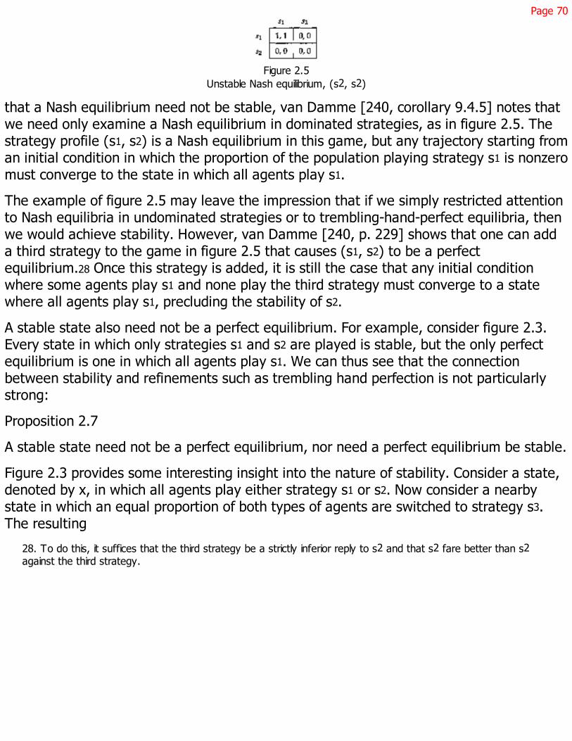
Page 70

Figure 2.5Unstable Nash equilibrium, (s2, s2)

that a Nash equilibrium need not be stable, van Damme [240, corollary 9.4.5] notes thatwe need only examine a Nash equilibrium in dominated strategies, as in figure 2.5. Thestrategy profile (s1, s2) is a Nash equilibrium in this game, but any trajectory starting froman initial condition in which the proportion of the population playing strategy s1 is nonzeromust converge to the state in which all agents play s1.

The example of figure 2.5 may leave the impression that if we simply restricted attentionto Nash equilibria in undominated strategies or to trembling-hand-perfect equilibria, thenwe would achieve stability. However, van Damme [240, p. 229] shows that one can adda third strategy to the game in figure 2.5 that causes (s1, s2) to be a perfectequilibrium.28 Once this strategy is added, it is still the case that any initial conditionwhere some agents play s1 and none play the third strategy must converge to a statewhere all agents play s1, precluding the stability of s2.

A stable state also need not be a perfect equilibrium. For example, consider figure 2.3.Every state in which only strategies s1 and s2 are played is stable, but the only perfectequilibrium is one in which all agents play s1. We can thus see that the connectionbetween stability and refinements such as trembling hand perfection is not particularlystrong:

Proposition 2.7

A stable state need not be a perfect equilibrium, nor need a perfect equilibrium be stable.

Figure 2.3 provides some interesting insight into the nature of stability. Consider a state,denoted by x, in which all agents play either strategy s1 or s2. Now consider a nearbystate in which an equal proportion of both types of agents are switched to strategy s3.The resulting

28. To do this, it suffices that the third strategy be a strictly inferior reply to s2 and that s2 fare better than s2against the third strategy.

Page 71

replicator dynamics trajectory will (asymptotically) eliminate the strategy s3, decreasethe proportion of agents playing s2, and increase the proportion playing s1. Thesedynamics do not return the system to the original state x, but such a return is notrequired in order for us to pronounce x stable. Instead, stability requires only that as longas the initial perturbation away from x is not too large the system not stray too far fromx, and this condition is satisfied in this case.

A state in which a population playing the game in figure 2.3 is split between strategies s1

and s2 may be stable, but it is not asymptotically stable . One might conjecture that ifstability is increased to asymptotic stability, then we would recover perfection. We have

Proposition 2.8

If x is asymptotically stable, then (x,x) is a perfect and isolated equilibrium. However,neither perfect nor perfect and isolated equilibria need be asymptotically stable.

Bomze [39] proves that asymptotically stable states are perfect and isolated. Figure 2.3provides a perfect equilibrium, in which all agents play s1, that is not asymptoticallystable. Asymptotic stability fails in this case because there are arbitrarily close stateswhere almost all agents play s1 but some play s2 that are also stationary states of thedynamics, and hence from which the dynamics do not converge to s1. However, suchstates exist because the perfect equilibrium in this case is not isolated. To see that anisolated, perfect equilibrium need not be asymptotically stable, we need only recall thatthe game in figure 2.5 can be augmented by a third strategy to produce an isolated,perfect equilibrium, namely (s2, s2), that is not even stable.

The finding that asymptotically stable equilibria are isolated and perfect recalls thesimilar characterization of evolutionarily stable strategies. What is the relationshipbetween the two? Taylor and Jonker [232] and Zeeman [253] show the following:29

Proposition 2.9.1

Every ESS is asymptotically stable, but asymptotically stable states need not be ESSS.

29. Hopkins [121] shows that for the class of "positive definite" dynamic processes (which includes the replicator)on symmetric games, any regular ESS is asymptotically stable, thus extending proposition 2.9.1 for regular ESSS.(Hopkins defines an ESS to be regular if it contains all best replies within its support, a property also sometimes called"quasi-strictness.") Bomze and Weibull [44] establish a counterpart of proposition 2.9.1 for neutrally stablestategies and stable states of the replicator dynamics.

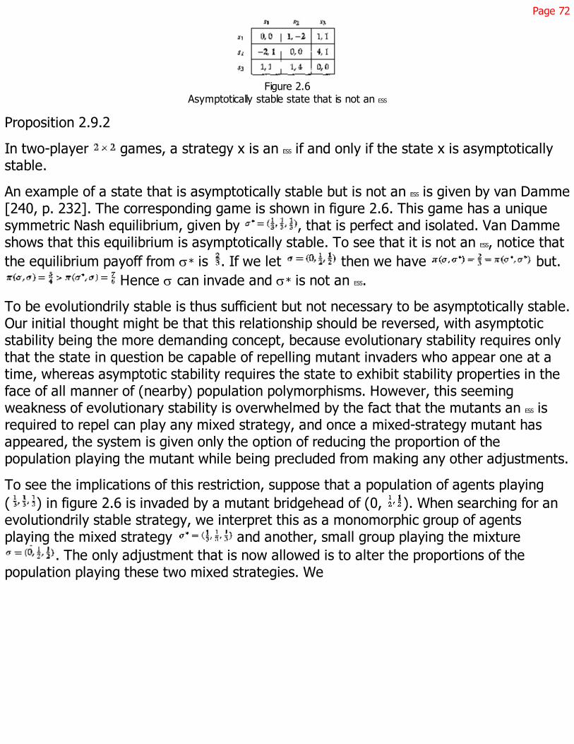
Page 72

Figure 2.6Asymptotically stable state that is not an ESS

Proposition 2.9.2

In two-player games, a strategy x is an ESS if and only if the state x is asymptoticallystable.

An example of a state that is asymptotically stable but is not an ESS is given by van Damme[240, p. 232]. The corresponding game is shown in figure 2.6. This game has a uniquesymmetric Nash equilibrium, given by , that is perfect and isolated. Van Dammeshows that this equilibrium is asymptotically stable. To see that it is not an ESS, notice thatthe equilibrium payoff from s* is . If we let then we have but.

Hence s can invade and s* is not an ESS.

To be evolutiondrily stable is thus sufficient but not necessary to be asymptotically stable.Our initial thought might be that this relationship should be reversed, with asymptoticstability being the more demanding concept, because evolutionary stability requires onlythat the state in question be capable of repelling mutant invaders who appear one at atime, whereas asymptotic stability requires the state to exhibit stability properties in theface of all manner of (nearby) population polymorphisms. However, this seemingweakness of evolutionary stability is overwhelmed by the fact that the mutants an ESS isrequired to repel can play any mixed strategy, and once a mixed-strategy mutant hasappeared, the system is given only the option of reducing the proportion of thepopulation playing the mutant while being precluded from making any other adjustments.

To see the implications of this restriction, suppose that a population of agents playing( ) in figure 2.6 is invaded by a mutant bridgehead of (0, ). When searching for anevolutiondrily stable strategy, we interpret this as a monomorphic group of agentsplaying the mixed strategy and another, small group playing the mixture

. The only adjustment that is now allowed is to alter the proportions of thepopulation playing these two mixed strategies. We

Page 73

Figure 2.7Derived game between candidate ESS and mutant

then essentially have a two-strategy game, involving s* and s, with payoffs given infigure 2.7. The strategy s is dominant in this game, causing s to push s* to extinctionand hence ensuring that the latter is not an ESS.

This can be contrasted with the case of the replicator dynamics. Here an initial statecharacterized by s* is viewed as a polymorphic population where one-third of thepopulation is playing each of the pure strategies s1, s2 and s3. The introduction of themutant s is interpreted as a perturbation that increases the proportions of the populationplaying strategies s2 and s3 by like amounts, while reducing the proportion playing s1. Thereplicator dynamics are now free to make whatever adjustments in the populationproportions are induced by the payoffs attached to this new state. This perturbationdecreases the payoff to s3, increases the payoff to s1, and increases the payoff to s2 evenmore, causing the replicator dynamics to increase the proportion of the populationplaying s2 at the expense of s3. As this movement continues, however, the payoffs of thethree strategies change. The relative payoff to strategy s1 will increase to such an extentthat the proportion of the population playing s1 will increase. This in turn can increase therelative payoff to s3 to the extent that the proportion playing strategy s3 begins toincrease. This process continues until the replicator dynamics spiral back into state s*.Such a spiral is implicitly excluded by the ESS calculation.

This difference in the behavior of the replicator dynamics and the ESS concept dependscrucially on the existence of at least three strategies. Suppose that a mixture s* isasymptotically stable under the replicator dynamics in a game with two pure strategies,s1 and s2. A perturbation that leads to a state a where the proportion playing strategy sis in creased must lead to a relatively higher payoff for strategy s1, in order for thereplicator dynamics to push the system back toward s*. But this increased payoff forstrategy s1 ensures that s* is a better reply than is

Page 74

s (because s* places more weight on s1), which is the requirement for s* to beevolutionarily stable. This suggests that evolutionary stability and asymptotic stability inthe replicator dynamics are equivalent games with only two strategies, as is confirmed byproposition 2.9.2.

The distinction between asymptotic stability and evolutionary stability thus arises out ofthe richer dynamic forces that can appear when there are three or more strategies. Wecan see this in the re-suits of Bomze and van Damme [43], who provide acharacterization of evolutionarily stable strategies in terms of dynamic systems. Inparticular, fix a symmetric game G with a finite number of strategies and fix a strategys*, where s* may be a pure or mixed strategy. For any alternative pure or mixed strategy

, we consider a ''derived" game . This is a game in which there are twostrategies, s* and s, and whose payoff function is given by restricting the payoff functionof game G to these two strategies. An example of such a derived game is given in figure2.7. Bomze and van Damme [43, theorem 1] show

Proposition 2.10

State s* is evolutionarily stable in a symmetric game G if and only if for every strategy, the state in which all agents play s* is asymptotically stable under the replicator

dynamic (2.15) in the derived game .

These results are encouraging. Asymptotically stable states have some equilibriumrefinement properties. When an ESS exists, then it corresponds to an asymptotically stablestate, providing a convenient algorithm for finding the latter. In addition, asymptoticallystable states can exist even when an ESS does not, potentially allowing some relief fromthe existence problems of evolutionarily stable strategies.

How much relief has been obtained from the possibility that an ESS might not exist? Inanswering this question, it is helpful to move beyond. the symmetric games, with whichthis section has been concerned thus far, to asymmetric games. The existence problemswith evolutionary stable strategies become especially apparent in asymmetric games.How do the replicator dynamics fare in such games? Strong results for this case havebeen established by Ritzberger and Vogelsberger [189] and by Ritzberger and Weibull[190].30 In particular, let s now be a population profile for an asymmetric game, so thats identifies, for each

30. Ritzberger [188] obtains similar results. Hofbauer and Sigmund [119, p. 282, exercise 1] note thatasymptotically stable states cannot be completely mixed.

Page 75

population, the proportion of that population playing each of the available purestrategies. Then, according to Ritzberger and Vogelsberger [189, proposition 1] and toRitzberger and Weibull [190, theorem 1]:

Proposition 2.11

A stationary point s of an asymmetric game G is asymptotically stable under thereplicator dynamic (2.15) if and only if s is a strict Nash equilibrium of G.

An investigation of the replicator dynamics thus leads to results reminiscent of those thatemerge from consideration of evolutionarily stable strategies. Asymptotically stablestates are Nash equilibria that possess refinement properties. However, asymptoticallystable states often fail to exist. The possibility of nonexistence is especially apparent inasymmetric games, where only strict Nash equilibria can be asymptotically stable. If weare to seek relief from the nonexistence of asymptotically stable states or therequirement of a strict Nash equilibria, we must follow the lead of those who have soughtalternatives to the evolutionarily stable strategy concept, examining either alternativestability notions or alternative dynamic models.

Micro foundations

It will be helpful to briefly consider the possibility of alternative dynamic models.31 Thebiological analogies that lie behind the replicator dynamics are often helpful, but we areespecially interested in how people learn to play games. Suppose we begin with a modelof how the agents in a game make and revise their choices. Will the resulting dynamicsystem bear any relationship to the replicator dynamics or similar systems of equations?What will be the equilibrium implications?

The work of Boylan [49, 51] is quite instructive in this regard, and also serves as awarning that choice models may give behavior that differs markedly from systems ofdifference or differential equations that seem to be derived from the models in astraightforward way. Consider the game in figure 2.8. Boylan examines a model in whichthis game is played by a finite population of agents. Each agent is matched to playexactly one game with a single opponent in each period, with

31. Swinkels [231], Ritzberger and Weibull [190], Balkenborg [6], Blume [33], and Hurkens [123] examinealternative stability notions, examining sets of outcomes with the property that the set as a whole satisfies aversion of asymptotic stability.

Page 76

Figure 2.8Boylan's Game

each of the finite number of possible matching configurations being equally likely. Aftereach such match, the agents in that match die and are replaced by two new agents. Thepayoffs of the game identify the strategies played by these new agents. For example, amatch between an s2 and an s3 agent gives the payoffs (2, 0), meaning that two of thenew agents play strategy s2 (and none plays s3). A more economic inter pretation of thisprocess would view the agents not as dying and being replaced by new agents but ratheras either retaining their own strategies or switching to the strategy of their opponent intheir most recent match. Notice that the population size remains constant. We thus havea finite stochastic process.

Boylan [49] derives a deterministic, discrete replicator dynamic from the limit of thismodel as the population size goes to infinity. Boylan [49, 51] also derives a continuousreplicator dynamic from the limit as the population size goes to infinity and the length ofa time period goes to zero. In each case, Boylan shows that these dynamic systemsprovide good approximations of the behavior of the stochastic process over any finitetime interval.32 At the same time, the limiting behaviors of these models are quitedifferent. For any fixed population size, the limiting distribution of the underlyingstochastic choice process attaches probability to at most three states, consisting of thosestates in which all population members play the same strategy. Hence the stochasticprocess always produces a monomorphic population state in which two strategies areextinct. The limiting outcomes of the discrete replicator dynamic attach positiveprobability to these three states but also to an infinite number of other states in whichtwo strategies sur-

32. More precisely, fix an initial condition, a time T, and an . Then for population sizes sufficiently large, therealization of the stochastic process and the solution of the deterministic replicator equation at any time arewithin Î of each other with probability at least .

Page 77

vive and one is extinct. The continuous replicator dynamic produces cyclical behavior,with periodic orbits that pass through the initial condition. If all strategies are initiallypresent, then no strategy becomes extinct.

The important point here is that examining what appears to be the obvious deterministicdifference or differential equation can give outcomes quite different than the underlyingstochastic process. The derivations of the various versions of the replicator dynamicdiscussed above involved a number of approximations, "smoothing" arguments, andlimiting operations. It is clear from Boylan's results that these procedures are notinnocuous. When working with a dynamic system, it is accordingly important tounderstand clearly the model from which the dynamic behavior emerges.

Boylan's analysis takes as its point of departure a model that identities, for each pair ofstrategies played by the agents in a match, the number of offspring of each agent. Onereadily interprets this in biological terms, but economic applications are more strained.For the latter, we need a model of the learning process that converts experience in thegame into decisions to adopt certain strategies. A number of such models have recentlyappeared. Most prominent among these are the models of Young [250] and of Kandori,Mailath, and Rob [128]. Their popularity has been fueled by the fact that they typicallyyield strong results with a minimum of analytical complication. The forces driving themodels are similar, though they differ considerably in the details of their construction. Itwill be useful to briefly examine the simpler model of Kandori, Mailath, and Rob [128],hereafter called the "KMR" model; we shall further restrict our attention to the simplestform of this model.

The model begins with a symmetric normal-form game, played by a single population ofN players, each of whom is characterized by a pure strategy. In each period, theseplayers are matched in pairs to play the game an infinite number of times. At eachiteration of play, each player is equally likely to be matched with each of the N 1opponents. As a result, there is no randomness in the average payoffs received in eachperiod, with each player receiving the expected payoff of playing against the mixedstrategy given by the proportions of opponents playing the various pure strategies.

At the end of each period, all players "learn," meaning that they change their strategy tothe best response to the current population

Page 78

state.33 It is not essential that this learning process be so rigid as to switch every agentto a best reply. The results would be unchanged if some agents are randomly drawn ineach period to switch to a best reply. Similarly, the model could be built around a numberof alternative specifications, as long as they increase the proportion of agents playing abest response.

After learning, "mutations" occur. Each player takes an independent draw from a randomvariable that produces the outcome "mutant" with probability l. If the agent is not amutant (probability ), then the agent retains her current strategy. If a mutant, thenthe agent randomly chooses a strategy, with each of the strategies being equally likely.

The KMR model yields a Markov process. In the most commonly studied application, thegame has only two strategies. Let these be denoted by X and Y. The state space of theKMR model is the set {0,1,..., N}, where a state identifies the number of agents playingstrategy X. The transition matrix for this process is strictly positive, meaning that theprobability of moving from any given state to any other is positive. To verify this, oneneed only note that beginning in any state, there is a positive probability that afterlearning has occurred, all agents are drawn to be mutants and happen to make thestrategy choices that yield the new state in question.

Because its transition matrix is strictly positive, the KMR model has a unique stationarydistribution that is independent of initial conditions and that will attach positiveprobability to all states in the state space. However, Kandori, Mailath, and Rob [128]show that if the mutation probability l is sufficiently small, then the stationarydistribution will concentrate almost all of its probability on only a few states. Theyaccordingly direct our attention to the limit of the stationary distribution as l get small,which I refer to as the "limiting distribution." Young [250] and Kandori, Mailath, and Rob[128] show that this limit is often easily computed and often produces powerful results.

33. If there is more than one best reply and agents are already playing a best reply, then they do not changestrategies. If they are not choosing a best reply, then a rule for selecting among the best replies must be imposed.The specifics of this rule typically do not have a significant impact on the results. The most common rule is toassume that agents randomly choose a best reply, with each possible best reply being equally likely. This discussionwill consider only games with two pure strategies, so that the issue of choosing among multiple best replies doesnot arise.

Page 79

Figure 2.9Stag-Hunt Game

How do the KMR model and a model based on deterministic differential equations, suchas the replicator dynamics, compare? Consider the Stag-Hunt Game of figure 2.9. This isa symmetric game played by a single population of players, each of whom may chooseeither X or Y. The game has two Nash equilibria in pure strategies, (X, X) and (Y, Y). Italso has a mixed Nash equilibrium in which both players use X with probability .Harsanyi and Selten [116] call (X, X) the "payoff-dominant equilibrium" because it isPareto-superior to the other Nash equilibria of the game, and they call (Y, Y) the "risk-dominant equilibrium." In a symmetric game with two symmetric, strict Nashequilibria, the risk-dominant equilibrium is characterized by having the larger basin ofattraction under either the best-reply or the replicator dynamics.

Which of the Nash equilibria in the Stag-Hunt Game should be selected? The mixed-strategy equilibrium is commonly dismissed, but the choice between the two pure-strategy equilibria has provoked much debate. Conventional equilibrium refinementstypically shy away from choosing between strict Nash equilibria, and most of the debatehas accordingly been conducted in an evolutionary context.34

The phase diagram for the replicator dynamics is shown in figure 2.10. The equilibria (X,X) and (Y, Y), or more precisely, the state in which all agents play X and the state inwhich all agents play Y, are both asymptotically stable with respect to the replicatordynamics. The same is true of any dynamic in which population shares are positivelyrelated to average payoffs, including best-reply dynamics. The outcome of the replicatordynamics then depends critically on their

34. Among nonevolutionary theories that do discriminate between the two strict Nash equilibria of this game,Harsanyi and Selten's equilibrium selection theory [116] proposes the payoff-dominant equilibrium as the rationalchoice in the Stag-Hunt Game. Anderlini's theory of Turing machines engaged in cheap talk [1] also selects thepayoff-dominant equilibrium. Carlsson and van Damme [60, 61] show that the risk-dominant equilibrium is the onlyone that is robust to a specific type of uncertainty about payoffs.

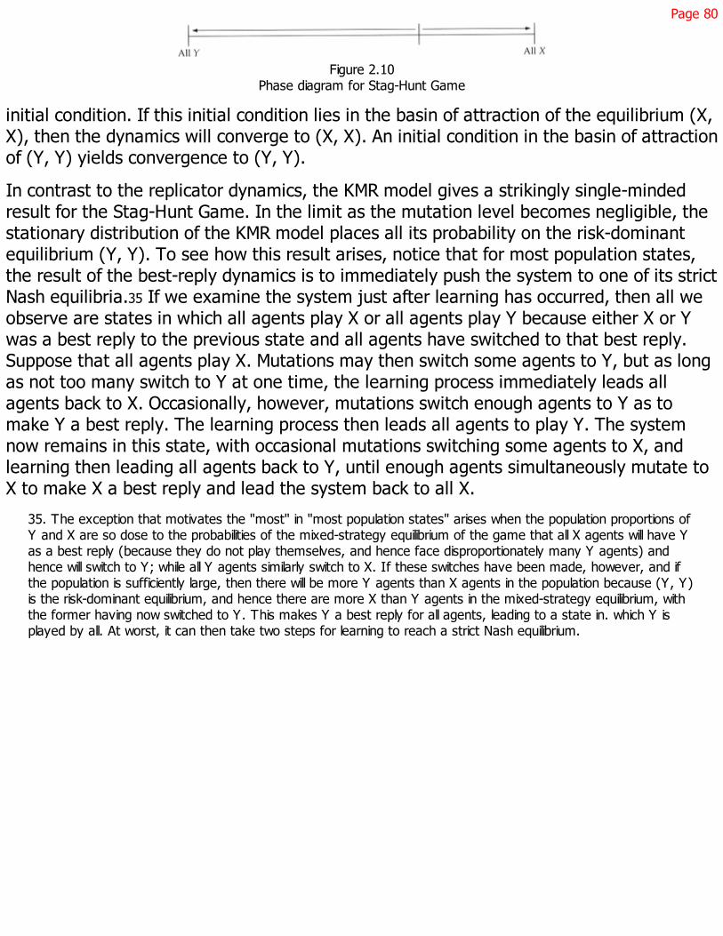
Page 80

Figure 2.10Phase diagram for Stag-Hunt Game

initial condition. If this initial condition lies in the basin of attraction of the equilibrium (X,X), then the dynamics will converge to (X, X). An initial condition in the basin of attractionof (Y, Y) yields convergence to (Y, Y).

In contrast to the replicator dynamics, the KMR model gives a strikingly single-mindedresult for the Stag-Hunt Game. In the limit as the mutation level becomes negligible, thestationary distribution of the KMR model places all its probability on the risk-dominantequilibrium (Y, Y). To see how this result arises, notice that for most population states,the result of the best-reply dynamics is to immediately push the system to one of its strictNash equilibria.35 If we examine the system just after learning has occurred, then all weobserve are states in which all agents play X or all agents play Y because either X or Ywas a best reply to the previous state and all agents have switched to that best reply.Suppose that all agents play X. Mutations may then switch some agents to Y, but as longas not too many switch to Y at one time, the learning process immediately leads allagents back to X. Occasionally, however, mutations switch enough agents to Y as tomake Y a best reply. The learning process then leads all agents to play Y. The systemnow remains in this state, with occasional mutations switching some agents to X, andlearning then leading all agents back to Y, until enough agents simultaneously mutate toX to make X a best reply and lead the system back to all X.

35. The exception that motivates the "most" in "most population states" arises when the population proportions ofY and X are so dose to the probabilities of the mixed-strategy equilibrium of the game that all X agents will have Yas a best reply (because they do not play themselves, and hence face disproportionately many Y agents) andhence will switch to Y; while all Y agents similarly switch to X. If these switches have been made, however, and ifthe population is sufficiently large, then there will be more Y agents than X agents in the population because (Y, Y)is the risk-dominant equilibrium, and hence there are more X than Y agents in the mixed-strategy equilibrium, withthe former having now switched to Y. This makes Y a best reply for all agents, leading to a state in. which Y isplayed by all. At worst, it can then take two steps for learning to reach a strict Nash equilibrium.

Page 81

These isolated bursts of rare mutations will continually switch the system between thetwo ends of the state space. Where will the system spend most of its time, in the statewhere all agents play X or the state where all agents play Y? This depends upon therelative probabilities of switching between these two states. Because (Y, Y) is the risk-dominant equilibrium and hence has the larger basin of attraction, the number ofmutations from Y to X required to switch the system from all-Y to all-X is more than thenumber of mutations from X to Y required to make the reverse switch. The system thenspends more of its time in the state where all agents play Y than in the state where allplay X. As the probability of a mutation gets small, the probability of switching from all-Yto all-X gets arbitrarily small relative to the probability of a switch in the reversedirection, and the system spends virtually all of its time in equilibrium, where all agentsplay Y.

How do we interpret these results? The search for the evolutionary foundations of game-theoretic solution concepts leads from the notion of an evolutionarily stable strategy toalternative notions of evolutionary stability to dynamic models of evolutionary processes.I believe dynamic models represent our best hope for making progress on understandingequilibrium concepts, although they also present some difficult puzzles. The commonlyused technique of modeling the evolutionary process as a system of deterministicdifference or differential equations may tell us little about equilibrium concepts other thanthat "strict Nash equilibria are good." We can attempt to probe deeper into these issuesby modeling the choices made by the agents. However, if we do so by investigating thecommonly used models of Young [250] and of Kandori, Mailath, and Rob [128], we findquite different results, including the finding that "not all strict Nash equilibria are good."What is the relationship between these two types of models, one based on difference ordifferential equations and one on perturbed best-response dynamics? Under whatcircumstances are they applicable? The exploration of these questions begins in the nextchapter.

Page 83

3A Model of Evolution

This chapter explores the relationship between (1) an explicit selection model; (2)deterministic differential equations, such as the classical replicator dynamics; and (3) themutation-counting methodology of Freidlin and Wentzell [81], on which the models ofKandori, Mailath, and Rob [128] and of Young [250] are based. The learning modelinvolved in this exploration is deliberately kept as simple as possible in order to focusattention on the main points. More general models are considered in subsequentchapters.1

This chapter concludes that whether differential equations or mutation-counting methodsare useful in studying the evolutionary processes depends primarily on the length of timeover which one chooses to study the selection model. If the population is sufficientlylarge, then the replicator dynamics provide a good approximation of the behavior of thepopulation along any finite interval of time. However, the replicator dynamics do notprovide a good description of the model's limiting behavior, which is captured by themutation-counting methods of Freidlin and Wentzell [81].

The replicator dynamics are often dismissed by economists as being of purely biologicalinterest, while other models based on differential equations are sometimes criticized fornot having been derived from models of individual behavior. The emergence of thereplicator dynamics from the "Aspiration and Imitation" model considered in this chaptersuggests that such dynamics should not be automatically

1. The Aspiration and Imitation model considered in this chapter is taken from Binmore, Gale, and Samuelson [21]and Binmore and Samuelson [24]. The consideration of lengths of time is taken from discussions that firstappeared in Binmore and Samuelson [26] and were pursued in Binmore, Samuelson, and Vaughan [28], fromwhich the remainder of the chapter is taken.

Page 84

rejected as models of how people behave. At the same time, the Aspiration and Imitationmodel is quite special. Other models will give rise to other approximations and we haveno reason to believe the replicator dynamics have any particular significance. Theimportant point is that systems of deterministic differential equations, like the replicatordynamics, can serve as useful approximations for the behavior of evolutionary processesover long but finite intervals of time.

The model examined in this chapter is a symmetric one in which agents are drawn from asingle population to play the game without knowing which role in the game they arefilling. Chapter 2 showed that symmetric and asymmetric models can behave differently.For example, the difficulties with conventional approaches, such as static notions ofevolutionary stability, are especially apparent in asymmetric games. In the chapters thatfollow, I shall often shift between symmetric and asymmetric models, choosing whichevermost effectively makes the point, noting in the process any results that are tied to aparticular case.

3.1 The Aspiration and Imitation Model

The learning model to be studied is based on a process of comparing realized payoffs toan aspiration payoff level and, as a result, sometimes choosing new strategies byimitating others.2 Consider the symmetric game G * of figure 3.1. Let there be asingle population containing N agents, where N is finite. Time is divided into discreteintervals of length t. In each time period, an agent is characterized by the pure strategy Xor Y that she is programmed to use in that period. In each period of length t, pairs ofagents are randomly drawn (independently

2. Binmore, Samuelson, and Vaughan [28] present a model that leads to similar behavior in a biological setting. Thespecification of how agents learn is both an important area of research and one that has recently attractedtremendous attention. A careful discussion of this literature would require a book of its own (such as Fudenberg andLevine [95]). I shall be content here to note that models of learning in games are examined by, among manyothers, Banerjee and Fudenberg [9], Bendor, Mookherjee, and Ray [12], Bin-more, Gale, and Samuelson [21],Binmore and Samuelson [24], Blume [33], Bomze and Eichberger [41], Börgers and Sarin [47], Canning [56, 57,58], Cheung and Friedman [62], Crawford [66], Eichberger, Haller, and Milne [73], Ellison [75], Foster and Vohra[77, 78], Fudenberg and Kreps [86, 87, 88, 89], Fudenberg and Levine [91, 92, 93, 94], Jordan [124, 125], Kalaiand Lehrer [127], Kaniovski and Young [129], Milgrom and Roberts [155, 156], Nachbar [163], Roth and Erev[195, 196], Selten [213], and Stahl [227, 228].

Page 85

Figure 3.1Game G *

and without replacement) to play the game, with each agent playing one game and withthe various ways agents can be matched being equally probable.3

The payoffs A, B, C, and D that appear in the specification of game G* given by figure 3.1are taken to be expected payoffs. Realized payoffs are random, being given by theexpected payoff in the game G* plus the outcome R of a random variable R*. I interpretthis random variable as capturing a variety of random shocks that perturb payoffs. Iregard this randomness as a crucial feature of many real-world games, where payoffs arelikely to be affected by a wide assortment of forces that have been excluded whenconstructing the model G*. These forces may be sufficiently complicated that playersencounter difficulties simply identifying their payoffs precisely, much less determiningthose payoffs exactly by simply choosing between strategies X and Y. Payoffs are thennaturally modeled as being random. The expected value of R* is zero, and thedistribution of G* does not depend upon the strategy chosen by a player or heropponent.4

An agent playing X and meeting an opponent who plays X receives an expected payoff ofA and an actual payoff of A + R. If an agent plays

3. Because we shall take , this assumption requires that the game be played arbitrarily rapidly. I view this as anapproximation of the case when play is frequent relative to strategy revision, which I consider the natural settingfor evolutionary models. Kandori, Mailath, and Rob [128] examine periods of fixed length and assume that eitheragents play an infinite number of times or agents play a round-robin tournament in each period. Nöoldeke andSamuelson [168] assume a round-robin tournament in each period. Young's model [250] is less demanding in thisrespect, though it still assumes that the result of each game is made known to all agents as soon as it is played.Robson and Vega-Redondo [193] examine periods of fixed length and assume that each agent plays once in eachperiod.

4. For all strategy choices, the distribution F of R* is then independent and identically distributed across players. Itwould be interesting to study cases in which the distribution of R* differs across players or strategies, or in which thissource of noise is correlated across individuals, perhaps as a result of environmental factors that impose a commonrisk on all agents. The latter type of uncertainty is discussed by Fudenberg and Harris [85] and by Robson [192].

Page 86

X in a population where proportion k of her opponents play X, then the agent's expectedpayoff, denoted by , is given by

where the expectation is taken with respect to the likely identity of the agent's opponentand the likely realization of R *. The expected payoff of an agent playing Y in apopulation where proportion k of her opponents pay X, denoted by , is given by

In each period of length t, each agent takes a draw from an independently distributedBernoulli random variable. Let the units in which time is measured be chosen so that withprobability t, this distribution produces the outcome ''learn." With the complementaryprobability, the agent does not learn. An agent who receives the learn draw recalls herrealized payoff in the last period and assesses it as being either "satisfactory" or "notsatisfactory."5 If the realized payoff exceeds an aspiration level, then the strategy isdeemed satisfactory and the agent makes no change in strategy. If instead the realizedpayoff falls short of the aspiration level, then the agent loses faith in her current strategyand abandons it. If an agent plays strategy X in a population in which everyone plays X,for example, and then receives the learn draw, the corresponding probability that thisagent abandons her strategy is given by

where D is the aspiration level, R is the realization of the random payoff variable R*, andF is the cumulative distribution of R*. Similar expressions hold for the payoffs B, C, and D.

I assume that F is a Uniform distribution on the interval [-w, w], where. Two properties of the Uniform distribution make it especially

convenient. First, it satisfies the monotone likelihood ratio property, which is a necessaryand sufficient condition for it to be more likely that low average realized payoffs areproduced

5. Satisficing models have long been a prominent alternative to models of fully rational behavior, being pioneered ineconomics by Simon [217, 218, 219] and in psychology by Bush and Mosteller [53], and pursued, for example, byWinter [249] and by Nelson and Winter [166]. More recently, satisficing models built on aspiration levels have beenexamined by Bendor, Mookherjee, and Ray [12] and by Gilboa and Schmeidler [102, 103, 104].

Page 87

by low average expected payoffs, and hence for realized payoffs to provide a useful basisfor evaluating strategies (see Milgrom [157]). If this were not the case, then I would notexpect to encounter agents using learning processes in which low-payoff realizationsprompt them to seek new strategies.6 Second, the linearity of the Uniform distributionallows us to pass expectations inside the function g defined in (3.3). Hence, if an agentplays a strategy that gives an expected payoff of p, then the probability she abandons herstrategy is given by

If the agent plays X and proportion k of the opponents play strategy X, then the p thatappears in (3.4) is given by , defined in (3.1). If the agent chooses Y, then p is givenby , defined in (3.2).

The assumption that F is the Uniform distribution, as well as the strong independenceassumption on F, plays an important role in leading to the replicator dynamics. Anapproximation result similar to proposition 3.1 below could be established for otherspecifications, but the approximating differential equations would not be the replicatordynamics, which are thus a quite special example of a more general phenomenon.Perhaps the strongest assumption in this model is that the aspiration level is exogenouslyfixed and does not change over time. Relaxing this assumption introduces a new elementof history dependence that qualitatively changes the analysis.7

If agent i has abandoned her strategy as unsatisfactory, she must now choose a newstrategy. I assume that she randomly selects a member j of the population. Withprobability 1 l, agent i imitates agent j's strategy.8 With probability l, agent i is a"mutant" who chooses the strategy that agent j is not playing.

6. I view the learning rule as being the product of an evolutionary process in which agents have discovered thatsome rules for choosing and rejecting strategies work better than others. The evolutionary process shaping therules by which agents learn about strategies is likely to proceed at a slower pace than the rate at which agents usethese rules to choose strategies, perhaps even being a biological phenomenon, and attention is restricted here tothe question of how agents behave given a fixed learning rule. However, if a low payoff does not lead to theexpectation that a strategy is likely to yield low payoffs in the future, then evolution is unlikely to produce a learningrule centered around abandoning strategies with low payoffs.

7. Models with endogenous aspiration levels include those of Bendor, Mookherjee, and Ray [12], Börgers and Sarin[48], and Karandikar et al. [130].

8. She may thereby end up playing the strategy with which she began, having perhaps had her faith in it restored byseeing it played by the person she chose to copy.

Page 88

3.2 Time

How we examine this evolutionary model depends to a large extent on which time periodwe are interested in. To focus the discussion, let A > C and B > D, so that (X, X) and (Y,Y) are Nash equilibria of game G *.

Stationary Distributions

The Aspiration and Imitation model is a Markov model. The state space is given by{0,1,...,N}, where a state identifies the number of agents in the population playingstrategy X. The transition probabilities, derived from the process by which agentsabandon their existing strategies and adopt new ones, will be calculated in the nextsection.

One approach to the Aspiration and Imitation model then, is to study its stationarydistributions. This study is made easier by the fact that the model has only one stationarydistribution. In particular, it is possible for the Aspiration and Imitation model to reachany state from any other state. With the help of just the right combination of learn draws,imitation draws, and mutations, such a transition can always occur in a single step,though it may be most likely to occur through a sequence of steps. It is a standard resultthat such a Markov process has a unique stationary distribution. The Markov modelconverges to this distribution from any initial position, in the sense that the distributiondescribing the likely state of the system at time t approaches the stationary distributionas t gets large. In addition, the distribution of realized states along any sample pathapproaches the stationary distribution almost surely. Hence the stationary distribution isindependent of initial conditions. We can study the outcome of the learning processwithout having to devote any attention to its point of departure. In the most convenientcase, the stationary distribution will concentrate virtually all of its probability on a singleequilibrium, which we can then refer to as the outcome or the selected outcome of thestationary distribution.

The models of Kandori, Mailath, and Rob [128] and of Young [250] similarly have theproperty that for any two states, the probability of a transition from one state to anotheris positive, and these models accordingly also have unique stationary distributions. Youngand Kandori, Mailath, and Rob show that techniques taken from Freidlin and Wentzell[81] can be used to conveniently calculate the stationary dis-

Page 89

tribution. In other models, there may be multiple stationary distributions. We then facethe task of characterizing the set of stationary distributions, but an evolutionary analysiscan still concentrate on these distributions.

The extent to which a stationary distribution is interesting depends upon the length oftime required for it to be a good approximation of the behavior of the Markov process. Tosee the issues involved here, notice that in the Aspiration and Imitation model, theprocess of rejecting strategies whose payoffs fall short of the aspiration level andimitating the strategies of others will tend to push agents toward best replies. This in turntends to push the process toward the state in which either all agents play X or all agentsplay Y, whichever is currently a best reply. Once the system reaches the vicinity of such astate, where all agents play X, for example, it will tend to remain there. Occasionally, thesystem will move away from the endpoint of the state space as the randomness inpayoffs causes agents to abandon X or mutations introduce strategy Y. These departuresfrom the endpoint will usually be small, and will give rise to forces pushing back towardthe endpoint. On rare occasions, however, a combination of mutations and realizations ofthe aspiration and imitation process will switch enough agents to strategy Y as to makethe latter a best response, and the expected movement of the system will be toward thestate in which all agents play Y. The system is then likely to linger in the vicinity of thestate where all agents play Y for a long time, with occasional slight departures, untilanother coincidental sequence of learning outcomes and mutations restores the statewhere all agents play X. Similar behavior emerges in Kandori, Mailath, and Rob [128],whose learning process spends most of its time near an endpoint of the state space,being occasionally pushed away by mutations that are usually followed by a movementback to the end of the state space, but which on rare occasions are followed by a switchto the other end of the state space.

In both the Aspiration and Imitation and the Kandori, Mailath, and Rob models, thestationary distribution becomes relevant only after there has been enough time, andenough transitions from one end of the state space to the other, to establish a stableproportion of time spent at each end of the state space. Because the transitions from oneend of the state space to the other require a very special combination of events, they canbe quite unlikely, and the time required for the stationary distribution to be relevant canbe very long.

Page 90

Although these considerations suggest that the stationary distribution may sometimesrefer to too long a time period to be relevant, they also suggest that much can be learnedby examining the behavior of the system over periods of time too short for the stationarydistribution to be relevant. I refer to such behavior as "sample path" behavior. The timerequired to reach the stationary distribution can be very long because the sample path islikely to approach one end of the state space and remain in the vicinity of this end,though subjected to frequent, small perturbations, for a long time. But then sample pathbehavior is likely to remain approximately unchanged over long periods of time. Thisinitial long period of stable behavior may be the most interesting aspect of the learningprocess and may be the most important target of study.

Sample Paths

It is helpful to organize our thinking about sample paths of learning processes aroundthree aspects of these paths. First, even if the stationary distribution is unique and henceindependent of initial conditions, the strategies with which agents happen to begin playwill make a difference for the behavior of sample paths. If most agents initially play X ingame , our expectation is that the learning model will increase the proportion of agentsplaying X. If most agents initially play Y, then we expect the proportion playing Y toincrease. The first case leads to the equilibrium (X, X) being played in most matches for along period, while the second leads to (Y, Y).

The choices agents make when faced with the task of determining their initial play in anew situation may have little to do with the considerations captured by game theoristswhen modeling such situations. In particular, I suspect that people seldom have asufficiently good grasp of the strategic realities, even of situations they encounterfrequently, as to analyze these situations in game-theoretic terms.9 Instead, they simplyadopt whatever behavior they typically use or whatever behavior is customary or is thesocial norm in such situations. If they appear to be optimizing, it is because the socialnorm has had a

9. For example, experiments with second-price auctions reveal that even when people are good at choosing optimalbids, players seldom provide an account of why such a bid is optimal that would be deemed coherent by a gametheorist. Similarly, successful poker players are often unable to provide a strategic theory of why bluffing is a goodidea.

Page 91

long time to become adapted to the situations in which it is commonly applied.

We must therefore expect that players faced with a novel situation will choose theiraction by calling on their experience in similar situations they have faced in the past andthen applying the rule of thumb or social norm that guides their behavior in suchsituations. However, players' assessments of what is similar may not coincide with thejudgment of a game theorist, especially as players actually faced with the prospect ofmaking choices in games may find the actual environment much more complicated thanthe game theorist's corresponding model. The social norm invoked in a novel situationmay then be a function of superficial features of the way the problem is posed rather thanthe strategic aspects of the problem, and a social norm may be triggered that is not at alladapted to the current game. Initial behavior may accordingly be heavily dependent uponthe way a new social situation is framed and may bear little relationship to the structureof the problem.

It has become common to offer evolutionary interpretations of the behavior of subjects inlaboratory experiments. The evolutionary approach seems natural in light of theobservation that subjects' behavior often changes as they gain experience with the game.However, experimental subjects are typically thrust into a quite unfamiliar setting. Theirinitial behavior may then depend upon a host of details that game theorists would regardas strategically irrelevant. It is thus unsurprising that framing effects are important inexperiments and that evolutionary interpretations of experimental results may have littleto tell us about initial play.10

As experience with a game is accumulated, a player's behavior is likely to adapt to thenew circumstances posed by a game. Players begin to learn. This is the secondinteresting aspect of sample path behavior.

How quickly does learning proceed, and how soon does it lead to seemingly stablebehavior? This depends upon three features of the context in which the learning occurs.The first is the extent to which

10. To avoid this problem, one might follow Crawford [66] and Roth and Erev [195, 196] in taking the initialbehavior as determined by considerations lying outside the model and concentrating on explaining the learningprocess that appears as this initial behavior gives way to strategic considerations learned in the course ofaccumulating experience with the game. Other examinations of learning in experimental contexts include Andreoniand Miller [2], Crawford [65], and Miller and Andreoni [158].

Page 92

the social norm triggered by the framing of the situation has been reinforced in the pastand appears to work in the current game. A weakly held norm will be much more easilydisplaced by learning than a strongly held norm. If different norms are adopted bydifferent players, as-may occur when the framing of the problem is relatively abstract,then the subsequent interaction among the players will produce unexpected behavior.None of the norms will seem to work well prompting reconsideration of the norms thathave been adopted and facilitating learning. A norm that is strongly held by all players,however, may be very difficult to dislodge and may cause behavior to respond to learningonly very slowly.

Second, learning will be faster the more important the game is to the players. I believethat in their daily lives people face sufficiently many choices to make it impossible forthem to analyze all of them. Many, perhaps most, choices are made according to rules ornorms that receive occasional scrutiny at best. The full power of our decision-makingmachinery is reserved only for the most important choices. A choice can fail to beimportant either because it is rarely made or because the stakes in making the choice aresimply too small to bother with. In either case, learning is likely to proceed quite slowly.

Finally, learning will be faster the simpler the task is that the players must learn. It is acommon practice for game theorists to assume that players will solve any problem thatcan be solved. This may be appropriate if the agents can accumulate enough experiencewith the game to learn the optimal behavior, but we must recognize that in the case of adifficult task, the length of time required to generate this experience may be very long.

The learning process may lead to a state in which the learning dynamics exert no furtherpressure. For example, this will happen when the Aspiration and Imitation model or theKandori, Mailath, and Rob model is applied to Game G *, with the system approaching astate where nearly all players choose X or nearly all players choose Y. Because (X, X) and(Y, Y) are Nash equilibria of Game G*, there is very little incentive for further changes inbehavior. The system may then remain in the vicinity of this equilibrium for a very longperiod of time.

The previous discussion of the stationary distribution shows that the first sojourn in thevicinity of an equilibrium is not the end of the story. The learning dynamics may lead to astate in which they place no more pressure on the system, but there may be othersources of "noise" capable of moving the system between states. This noise may take theform

Page 93

of mutations that perturb a deterministic learning process, as in Kandori, Mailath, andRob [128], or unexpected realizations of a stochastic learning process such as theAspiration and Imitation model. Occasional1y, these perturbations will be sufficientlysevere as to cause the system to jump out of the basin of attraction, under the learningdynamics, of the existing equilibrium and into the basin of attraction of anotherequilibrium. The learning dynamics will then cause the system to spend a long time nearthis new equilibrium. Given sufficient time, shocks of this nature will give rise to adistribution describing the relative lengths of time the system spends near each of thepossible equilibria. This distribution is a stationary distribution of the system.

How Long Is Long?

It will be helpful to have some terms to describe the various aspects of behavior thatpotentially emerge from learning models. Binmore and Samuelson [26] describe theseaspects of behavior in terms of lengths of time. Like the "short run" and "long run" thatare familiar from the theory of the firm, these periods of time are relative terms designedto organize our thinking rather than identify precise lengths of time. They involve notabsolute units of time but rather the periods of time it takes certain things to happen. Asa result, the length of the various "runs'' will vary from setting to setting. Which length isinteresting depends upon the game to be played and the setting where it is played.

As do Binmore and Samuelson [26], I shall use "short run" to describe the initial play ofthe system. I follow both Binmore and Samuelson [26] and Roth and Erev [195] in using"medium run" to describe the behavior of the system as learning begins to have its effectbut before the system reaches an equilibrium.

We now might proceed by referring to a stationary distribution of the model as the "longrun." This would be consistent with the terms used by Roth and Erev [195] and byKandori, Mailath, and Rob [128]; it would also be consistent with "long run" as used ineconomics to mean a period of time long enough for all adjustments to have taken placeand as used in mathematics to mean a limiting result as the system is allowed to runarbitrarily long. However, such a usage does not take into account that before astationary distribution becomes applicable, the sample path of the process may spend avery long time in one place, and the length of time for a stationary distribution to berelevant may be very much longer. In recognition of this, I shall use "long

Page 94

run" to refer to the length of time required for the sample path to reach an equilibrium,near which it will linger for a long time, and "ultralong run" to refer to the length of timerequired for mutations and other rare events to occur with sufficient frequency to make astationary distribution relevant.

The issue in determining how to use "long run" is one of modeling. Models are alwaysapproximations, and one never literally believes there is nothing else that can happenand that has not been captured by the model. This chapter will show that learningprocesses, such as the Aspiration and Imitation process or the processes examined byKandori, Mailath, and Rob [128], are well approximated over potentially very long periodsof time by systems of differential equations that miss only certain very improbableevents, such as certain very special realizations of the stochastic learning process or largebursts of mutations. A common approach is then to work with such models and to takethe resulting differential equations to be an effectively complete specification of theunderlying process. Once an equilibrium is reached, there is nothing more in the modelthat can possibly happen. This is commonly called a "long-run analysis" (see Weibull[248], for example), and this is the sense in which I use ''long run." In the underlyingprocess, however, there are more things that can and eventually will happen, thoughthey happen with low probability and their occurrence will require waiting a long time. Ananalysis of a stationary distribution of the process must take account of thesepossibilities, and the need to characterize such an investigation in terms of lengths oftime prompts the introduction of the phrase "ultralong run."

An analogy from the theory of the firm will be useful. The "long run" in the theory of thefirm describes the outcome for a fixed specification of the market structure. Over longerperiods of time, this long-run outcome will be rendered irrelevant by technologicalinnovations and new product developments that produce large changes in the nature ofthe market. We know that these will happen, but also expect them to occur soinfrequently that a given market equilibrium is likely to persist for a long time. A usefulanalytical approximation is then to work with models in which market structure is simplyfixed, and to refer to the equilibria of these models as "long-run behavior" Someoneinterested in new product innovations might then object that we have used "long run" torefer to a period of time too short to capture everything that can happen in the market,and that "long run" should be reserved only for behavior emerging from models that allowinnovation. At one level,

Page 95

this argument is compelling, but if we are convinced that the resulting lengths of time aretoo long to be relevant, the most useful approach is to exclude innovation from the modeland study the long-run behavior of the resulting model. This is the counterpart of thelong-run analysis we shall be undertaking.

This discussion assumes that the sample path of the process will converge to something.We shall concentrate on sufficiently simple games that convergence problems do notarise. However, Shapley's celebrated demonstration that fictitious play need not convergein a normal-form game [216] has since been joined by a number of examplesshowing that complicated behavior can appear even in seemingly simple games.11

3.3 Sample Paths

This section establishes a link between the replicator dynamics and the long-run behaviorof the Aspiration and Imitation model. If the population is sufficiently large and the lengthof a time period is sufficiently short, then the sample path behavior of the Aspiration andImitation model is approximated arbitrarily closely by a solution of the replicatordynamics. More general1y, deterministic differential equations can be good tools forstudying the long-run behavior of stochastic selection processes.

The variant of the replicator dynamic to be studied has the form

where is interpreted as the fraction of an infinite population playing strategy X ingame G *, is the expected payoff in the population, K is a constant thatdoes not depend on the state, and where

The more familiar form of the replicator dynamic given by (2.15) is obtained by followingthe standard practice of considering the case in which the probability l of a mutation iszero.

Equations (3.6)-(3.7) match equations (3.1)-(3.2), with z replacing k. As a result, identifies the payoff to an agent playing strategy X

11. For example, see Skyrms [220, 221].

Page 96

given that proportion z of the agent's opponents play X. If the state of a finite populationwere z, meaning that proportion z of the population plays strategy X, then each individualplaying strategy X faces opponents who play X in slightly smaller proportion than z. Asthe size of the population grows, this distinction disappears and z becomes both thecurrent state and the proportion of opponents playing strategy X.

When the population size is N and the length of a time period is t, the Aspiration andImitation model is a Markov process with N + 1 population states , wherev=1/N and xN is the number of agents characterized by strategy X in state x. Thepassage from this model to a differential equation in which z is modeled as taking onvalues in [0,1], as in (3.5), will be accomplished by examining the limit as N gets largeand t gets small.

The key transitions in this Markov process are those that lead from an existing state to anadjacent state, meaning a state in which either one more or one fewer agents playstrategy X. Because attention will be focussed on short time periods, the probability thattwo agents receive the learn draw. in any single period, and hence that the systempotentially moves more than one step in a period, will be negligible. For fixed N, we cancalculate the probability of moving one step to the right in a single period, from astate x with to the state x + v:

To see how this probability is constructed, notice that for the population to move fromstate x to state x + v, in which the number of agents characterized by strategy X hasincreased by one, four things must happen. First, at least one agent must receive thelearn draw. The probability that exactly one agent receives the learn draw is .The probability that two or more agents receive the learn draw, and that the result is tomove the state one step to the right, is .12 Second, the agent receiving the learndraw must currently be playing strategy Y, the probability of which is 1 - x. Third, theresult of this

12. The probability that two or more learn draws occur and move the state one step to the fight is less than orequal to the probability of two or more learn draws, which is given by where is the relevantbinomial coefficient. This is in turn bounded above by where the inequality requires ,which is ensured by taking the limit before .

Page 97

agent's strategy assessment must be to abandon strategy Y. An agent playing strategy Yfaces opponents who play strategy X in proportion xN/(N - 1) and play strategy Y inproportion (N - xN - 1)/(N - 1). The probability of abandoning Y is then given by

, where this equality follows from (3.3) and from F being theUniform distribution.13 Finally, when choosing a new strategy, the agent must choosestrategy X, either by correctly imitating an agent playing X or by mistakenly imitating anagent playing Y. The probability of choosing X is given by

.

Similarly, the probability of moving one step to the left in a single period from astate x with to the state x - v is given by

Note that (3.8) and (3.9) implicitly define R(x, v) and L(x, v) by

These probabilities of moving one step to the left or fight can now be used to constructan approximate characterization of sample path behavior. The first step is to estimate theexpectation and variance of , conditional on x(t) = x. To this end, we canintroduce the quantities

where .

It is useful to note that (3.12)-(3.13) allow us to write the replicator equation (3.5) in theform

13. This uses the fact that N/(N-1)=1+1/(N-1) and 1/(N-1)=1/N + 1/(N(N - 1)).

Page 98

To obtain the result in (3.14), we recall that F is a Uniform distribution on [ ], andhence and then calculate

Letting , rescaling time to eliminate the 2w in the denominators, noting that, and replacing the discrete variable x with the continuous

variable z then gives (3.14).

Returning to the estimation of the expectation and variance of let. Then, since and the probability of moving more than one

step in a single period is , (3.12) and (3.13) lead to the following:

Rewrite equation (3.16) as

When in (3.19) so that , the fight side converges to . Notice thattwo limits are involved here, namely; and , and that the relative rates at whichthese limits are taken are not arbitrary. Instead, t must approach zero sufficiently fastthat t approaches zero. If one limit is taken after the other, the order must be first,and then . I return to the order in which various limits are taken in section 3.5.

When and then , the left side of (3.19) converges to a derivative that informalderivations of the replicator dynamics often identify with x(t) without further comment. Ifthis identification is appropriate, (3.19) would produce the replicator equation in the limit.Börgers and Satin [47] point out that some care must be taken in per-

Page 99

forming this limiting operation and that a formal argument is necessary. The proof of thefollowing proposition is constructed along the lines of Boylan [49, 51].14 In thisproposition, it is important to distinguish between the state x(t) of the system describedby the Aspiration and Imitation model and the state z(t) of the system governed by thereplicator equation (3.14). The former is a random variable defined on the discrete set ofpoints , while the latter is the deterministic solution to a differential equationwhose state space is the interval [0,1]. Section 3.6 proves

Proposition 3.1

Fix x(0) and let z(t) be the solution of the replicator equation subject to theboundary condition z(0) = x (0). Then for any and any integer T > 0, there arepositive constants N0 and such that if and , then

for any t satisfying at which x(t) is defined.

Because proposition 3.1 holds for finite values of t, it is not a characterization of thestationary distribution of the Aspiration and Imitation Markov process. Instead, itestablishes properties of the sample paths of the model. I refer to these sample pathproperties as "having long-run implications." To see what is meant by this and to explorethe implications, suppose that z(t) is governed by the replicator dynamic (3.5) (or (3.14))with the boundary condition z(0) = x(0). Figure 3.2 shows a phase diagram for thereplicator dynamic (3.5) when l is small and when A > B and D > C, so there are twostrict Nash equilibria, given by (X, X) and (Y, Y), and one mixed-strategy equilibrium.There are three stationary states x, k and z satisfying . The inner stationarystate is unstable, but x and z are asymptotically stable with basins of attraction [0, k)and (k, 1] respectively. As , the stationary states x, k, and z converge to the threeNash equilibria of game G *. The stationary state x converges to the equilibrium in whichall agents play Y. The stationary state z converges to the equilibrium in which all agentsplay X. The stationary state k converges to the mixed equilibrium.

14. I thank Rob Seymour for his help in understanding these methods. Börgers and Sarin [47] establish a similarresult by appealing to theorem 1.1 of Norman [170, p. 118], deriving the replicator dynamics in a model in whichthe "population size" is infinite from the outset.

Page 100

Figure 3.2Phase diagram for game G *

Suppose that z(0) = x (0) happens to lie in the basin of attraction of z. The replicatordynamics will then move close to z and remain in the vicinity of z forever. For sufficientlylarge N and small t, we have from proposition 3.1 that with probability at least

for . With high probability, the Aspiration and Imitation model thus also movesclose to z and remains in the vicinity of z for an extended time. Upon observing suchbehavior, we would be tempted to say that the process has converged to z or has"selected" the equilibrium z. This long period of time spent in the vicinity of a state suchas z qualifies this as a long-run result.

In examining limiting behavior, the limit was applied to the process z(t) and not tothe process x(t). As the next section on the ultralong-run behavior of x(t) demonstrates,the ultralong-run behavior of the Aspiration and Imitation model may be quite differentfrom that described by the replicator dynamics in the long run. The larger is thepopulation size N, the longer will the approximation provided by the replicator dynamicsbe a good one, but the size of the population required for this approximation increases asthe interval of time increases, and the replicator dynamics will not be a goodapproximation forever.

3.4 Stationary Distributions

This section studies the stationary distribution over states given by the Aspiration andImitation model. In the terms given above, this is an ultralong-run analysis.

Again, the analysis begins with the observation that for fixed values of t, v and l, theAspiration and Imitation model is a Markov process on the state space {0, v, 2v, ..., 1}with a single ergodic set consisting of the entire state space. Hence the followingstandard result for Markov processes is immediate (see Billingsley [17], Seneta [214], orKemeny and Snell [132, theorems 4.1.4, 4.1.6, and 4.2.1]):

Page 101

Proposition 3.2

Fix t, v, and l. Then there exists a unique probability distribution on {0, v, 2v,...,1} that is a stationary distribution for the Aspiration and Imitation Markov process. Therelative frequencies of the various states realized along a sample path approach thedistribution almost surely as . For any initial condition x(0), the probabilitydistribution describing the likely state of the process at time t converges to as tgets large.

The distribution is referred to as either the "stationary distribution" or the"asymptotic distribution" of the Markov process, where gives the probabilityattached to state x given v and t.

Let us now turn to characterizing the stationary distribution. For the case of small valuesof t, we can derive a particularly convenient representation for . Let be theprobability attached to state x by the Markov process at time t, given v and t. Then forsmall values of t, this satisfies

where and are defined by (3.8)-(3.9), where , and where. The error term in (3.20) arises from the possibility that

there may be multiple recipients of the learn draw in a single period. The stationarydistribution is then characterized by the following version of (3.20):

Rearranging (3.21) gives

Now take the limit , As the probability of more than one agent receiving thelearn draw in a single period becomes negligible. Transitions then consist of either asingle step to the left or a single step to the right. The result is a birth-death chain (cf.Gardiner [97] and Karlin and Taylor [131, chapter 4]). The following description of thestationary

Page 102

Figure 3.3Significant x-tree

distribution is standard for such chains. In particular, (3.23) follows immediately from(3.22), (3.10)-(3.11), and .

Proposition 3.3

Let Then for any state , we have

An alternative route to this conclusion, which highlights the nature of the limitingargument as ; uses the method of Freidlin and Wentzell [81], as employed by Young[250] and by Kandori, Mailath, and Rob [128]. One first constructs, for each state x in thefinite Markov process, the collection of all x-trees, where an x-tree is a collection oftransitions between states with the property that each state other than x is the origin ofone and only one transition, x is the origin of no transition, and there is a path oftransitions to x from every state other than x. Fixing a state x, one then computes theproducts of the transition probabilities in each x-tree and adds these products (for all ofthe x-trees) to obtain a number Z(x). The exact ultralong-run probabilities P(x, v) and

of being at states x and x are then proportional to Z(x) and . In the Aspirationand Imitation model, products of order greater than can be neglected because the limit

is to be taken.15 Only the single x-tree of order illustrated in figure 3.3 thenneed be retained. When the products for x and x + v are divided, only one factor fromeach fails to cancel, leaving (3.23).

Yet another path to this conclusion is provided by the following. First, rewrite equation(3.20) in the form

15. For similar reasons, Young [250] and Kandori, Mailath, and Rob [128] can neglect products that do notminimize the order of l because the limit is taken.

Page 103

Now take the limit . The error term on the right disappears and we are left with theprobability P(x, v, t) that satisfies

A stationary distribution is defined by the property that . Writing in (3.24) leads us to equation (3.22) with a zero error term. Proposition 3.3 therefore stillapplies.

What is the relationship between the replicator approximation of the Aspiration andImitation model and the asymptotic distribution? To bring this question into sharperfocus, suppose that the initial condition lies in the basin of attraction of z relative to thereplicator dynamics (see figure 3.2). As a result, the system will initially be highly likely toapproach p and spend an extended period of time in the neighborhood of z. The larger Ngets, the more likely this will be a good description of the behavior of the system and thelonger the time span over which it will be valid.

Chapter 9 shows that, in spite of this initial behavior, there are payoff specifications forwhich the asymptotic distribution attaches almost all of its probability mass on x. Toreconcile these observations, we notice that a transition from a state near z to a state inthe basin of attraction of x requires a rather special realization of random events. Theseevents require a much larger proportion of X agents to abandon their strategies andadopt Y than the system is expected to produce. During any bounded time interval, theprobability of such a combination of strategy revisions, and hence the probability that theAspiration and Imitation population will reach the basin of attraction of x, is arbitrarilysmall. However, "arbitrarily small" is not the same as "zero." The probability that such acombination of strategy revisions will eventually occur is unity. As a result, the systemwill, with certainty; visit states near x and spend most of its time in such states, thoughfor some initial conditions and population sizes one will have to wait an extraordinarilylong time for this to occur.

3.5 Limits

The taking of limits plays an important role in many evolutionary analyses. The Aspirationand Imitation model is no exception. In the course of examining the model, two limitshave been taken: the length

Page 104

of a time period t has been allowed to approach zero and the population size N hasapproached infinity. We may also be interested in allowing the mutation probability l toapproach zero, as do Young [250] and Kandori, Mailath, and Rob [128].

The limit allows the convenience of working in continuous time. In particular, itallows us to ignore the possibility of more than one agent revising a strategy at once, sothat strategy assessments are isolated, idiosyncratic events. This will not always beappropriate. In a biological context, reproduction may be coordinated by breedingseasons, and hence may be best captured by a discrete-time model with simultaneousreproduction. In a learning context, the arrival of information or other public events maycoordinate strategy assessments. In other cases, however, the times when strategies arerevised will not be coordinated, leading to a model in which we can usefully let tapproach zero.

The limit allows us to concentrate on the expected value of the process, at leastover finite periods of time. This is typical of evolutionary analyses, which commonlyappeal to large-population assumptions not only to work with expected values but also toeliminate repeated-game effects.

What about the order in which the limits and are taken? Here we shall takethe limit first, to reflect our interest in an overlapping generations model wherestrategy revisions occur at uncoordinated times.

After , we have the limits and possibly . In many cases, I think it isinappropriate to take the limit . Instead, I believe that the world is an inherentlynoisy environment, and the most realistic model retains mutations. If we are to take ,however, I believe that this limit should be taken last. In some cases, the order of theselimits does not matter. Section 9.4 shows that in games with two strict Nashequilibria, reversing the order of limits has no effect and the order is arbitrary. This is notalways the case, however. The order matters in games with a single, mixed-strategyNash equilibrium.

To illustrate this point, consider the game of Chicken shown in figure 3.4. The phasediagram under either the replicator or best-reply dynamics is shown in figure 3.5. Thisgame is a special case of the Hawk-Dove Game of Maynard Smith [149], prompting thestrategy labels of D (for ''Dove") and H (for "Hawk"). Chicken has a unique symmetricequilibrium in which each player plays D and H with

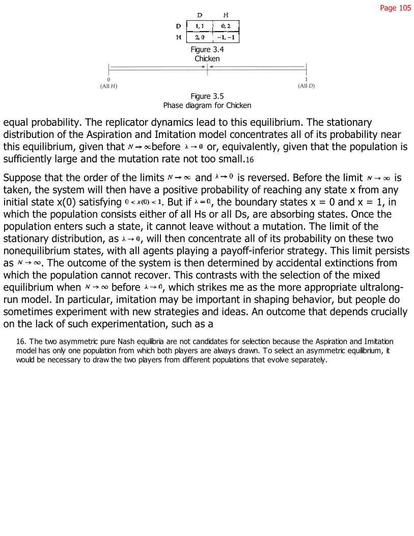
Page 105

Figure 3.4Chicken

Figure 3.5Phase diagram for Chicken

equal probability. The replicator dynamics lead to this equilibrium. The stationarydistribution of the Aspiration and Imitation model concentrates all of its probability nearthis equilibrium, given that before or, equivalently, given that the population issufficiently large and the mutation rate not too small.16

Suppose that the order of the limits and is reversed. Before the limit istaken, the system will then have a positive probability of reaching any state x from anyinitial state x(0) satisfying . But if , the boundary states x = 0 and x = 1, inwhich the population consists either of all Hs or all Ds, are absorbing states. Once thepopulation enters such a state, it cannot leave without a mutation. The limit of thestationary distribution, as , will then concentrate all of its probability on these twononequilibrium states, with all agents playing a payoff-inferior strategy. This limit persistsas . The outcome of the system is then determined by accidental extinctions fromwhich the population cannot recover. This contrasts with the selection of the mixedequilibrium when before , which strikes me as the more appropriate ultralong-run model. In particular, imitation may be important in shaping behavior, but people dosometimes experiment with new strategies and ideas. An outcome that depends cruciallyon the lack of such experimentation, such as a

16. The two asymmetric pure Nash equilibria are not candidates for selection because the Aspiration and Imitationmodel has only one population from which both players are always drawn. To select an asymmetric equilibrium, itwould be necessary to draw the two players from different populations that evolve separately.

Page 106

stationary distribution concentrated on the endpoints of the state space, should beviewed with suspicion. As a result, if one is interested in large populations and smallmutation rates, the limit should be taken last (or not taken at all).

This fixes the order of limits as first , next , and then . But when, in thecourse of taking these limits, do we examine the limiting outcome of the system? Thedistinction between the long run and the ultralong run hinges on the answer to thisquestion.

The key issue here is whether we examine the system before or after letting thepopulation size approach infinity. First, we might examine the limiting outcome of thesystem after letting . Letting " " be a shorthand representation of "examine thelimiting outcome of the system," we then have two possibilities:

Case 1:

Case 2:

These two cases correspond to a long-run analysis. In particular, by first letting timeperiods get short and then the population get large,17 we obtain a deterministicdifferential equation. In the Aspiration and Imitation Model, this equation is a version ofthe classical replicator dynamics (with an extra term added to take account of theexistence of mutations). After obtaining this equation, we let , which is a shorthandfor the statement that we study the limiting behavior of the differential equation.18 Thereplicator dynamics are commonly used to examine the limiting outcome of the systemwith the simplifying assumption that , giving case 1. Case 2 obtains if we retainmutations when studying the limiting outcome of the replicator dynamics.

We must interpret the notation carefully. By assumption, this denotes the operationof examining a limiting outcome, which is ac-

17. From proposition 3.1, the precise operation here is , so that

18. Cases 1 and 2 can be contrasted with the traditional story (outlined in section 2.3) that is associated with informalmotivations of the replicator dynamics: first , next , next , then . In particular, by first dispensingwith mutations ) and then letting the population size get large ( ), a model is obtained in which large numbersof simultaneous births occur at discrete intervals. This model is described by a deterministic difference equation knownas the "discrete replicator dynamic." This difference equation is commonly approximated by a differential equation( ). The limiting behavior of the differential equation is then studied ( ).

Page 107

complished by literally taking the limit in the replicator dynamics. However, thisdoes not correspond to taking the limit in the underlying model. Instead, we haveseen that the replicator dynamics provide a good guide to the behavior of the underlyingmodel only for finite, though possibly very long, time periods. Taking the limit in thereplicator dynamics is then a convenient way of approximating the behavior of theAspiration and Imitation over long, but not infinitely long, periods of time.

The second possibility is that we examine the limiting outcome of the system beforetaking the limit . There are two possibilities here, depending upon whether we takethe limit before or after allowing the length of a time period to approach zero,yielding two cases:

Case 3:

Case 4:

Cases 3 and 4 correspond to an analysis of the stationary distribution. Here, the first stepis to derive the stationary distribution of the discrete-time (case 4) or continuous-time(case 3) Markov process for fixed values of the parameters. We have seen that the orderof the limits and is immaterial in the Aspiration and Imitation Model and hencethese two approaches yield identical results. In particular, we examine this stationarydistribution before limiting arguments involving the population size or mutation rateobscure any of the randomness of the Markov process. The remaining limits arecomparative static exercises that allow the derivation of particularly sharp approximationsof the limiting distribution.

Which of these two approaches, which can give quite different outcomes, is theappropriate one? Should we be interested in the long run or the ultralong run? The easyway out of this question is to claim that both can be interesting, and subsequent chaptersare devoted to both. The important point here is that the replicator dynamics and thestochastic models of Young [250] and of Kandori, Mailath, and Rob [128] need not beviewed as competing models or methods, despite their potentially differing outcomes.Instead, they are alternative approximations for examining the outcome of a singlemodel, with one approximation being appropriate when addressing the long run and theother, when addressing the ultralong run.

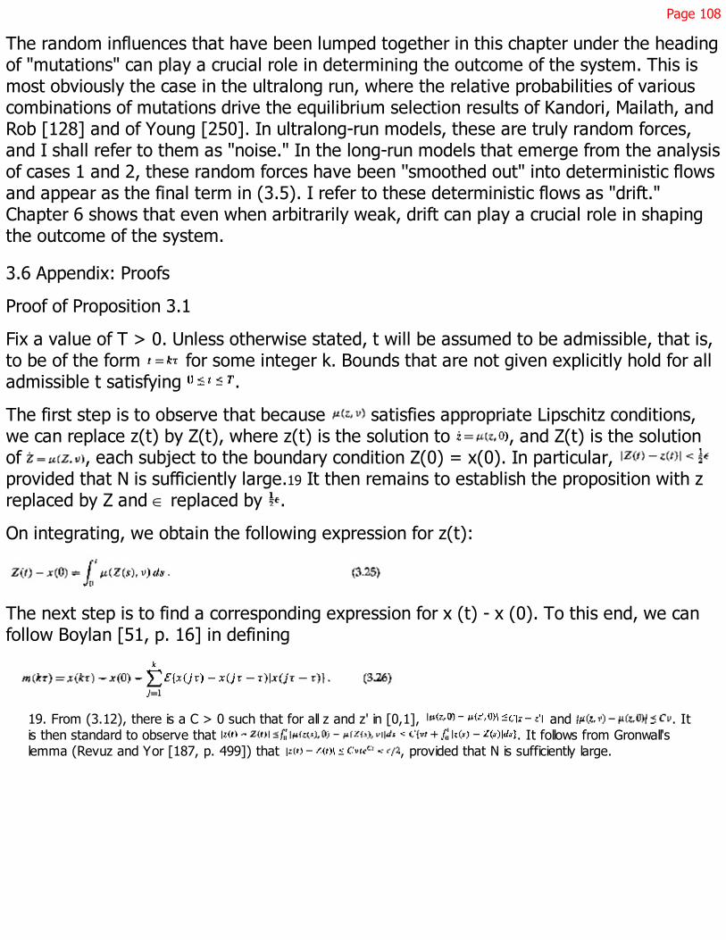
Page 108

The random influences that have been lumped together in this chapter under the headingof "mutations" can play a crucial role in determining the outcome of the system. This ismost obviously the case in the ultralong run, where the relative probabilities of variouscombinations of mutations drive the equilibrium selection results of Kandori, Mailath, andRob [128] and of Young [250]. In ultralong-run models, these are truly random forces,and I shall refer to them as "noise." In the long-run models that emerge from the analysisof cases 1 and 2, these random forces have been ''smoothed out" into deterministic flowsand appear as the final term in (3.5). I refer to these deterministic flows as "drift."Chapter 6 shows that even when arbitrarily weak, drift can play a crucial role in shapingthe outcome of the system.

3.6 Appendix: Proofs

Proof of Proposition 3.1

Fix a value of T > 0. Unless otherwise stated, t will be assumed to be admissible, that is,to be of the form for some integer k. Bounds that are not given explicitly hold for alladmissible t satisfying .

The first step is to observe that because satisfies appropriate Lipschitz conditions,we can replace z(t) by Z(t), where z(t) is the solution to , and Z(t) is the solutionof , each subject to the boundary condition Z(0) = x(0). In particular, provided that N is sufficiently large.19 It then remains to establish the proposition with zreplaced by Z and Î replaced by .

On integrating, we obtain the following expression for z(t):

The next step is to find a corresponding expression for x (t) - x (0). To this end, we canfollow Boylan [51, p. 16] in defining

19. From (3.12), there is a C > 0 such that for all z and z' in [0,1], and . Itis then standard to observe that . It follows from Gronwall'slemma (Revuz and Yor [187, p. 499]) that , provided that N is sufficiently large.

Page 109

Boylan notes that is a martingale, which is a fact that will be needed later. For themoment, it is important to note only that .

On rearranging (3.26) and making use of (3.16), we obtain

where [s] is the integer part of s.

The next step is to subtract (3.27) from (3.25) to obtain

where C has been chosen independently of v so that Since wehave . Hence, on writing

inequality (3.28) implies that

where

The final error term O (v) has been added to the expression for M(t), so that (3.29) holdsfor all t satisfying and not just t of the form kt. The supremum in the expressionM(t) ensures that M increases. We can then appeal directly to Gronwall's lemma, fromwhich we deduce that

for all t satisfyring .

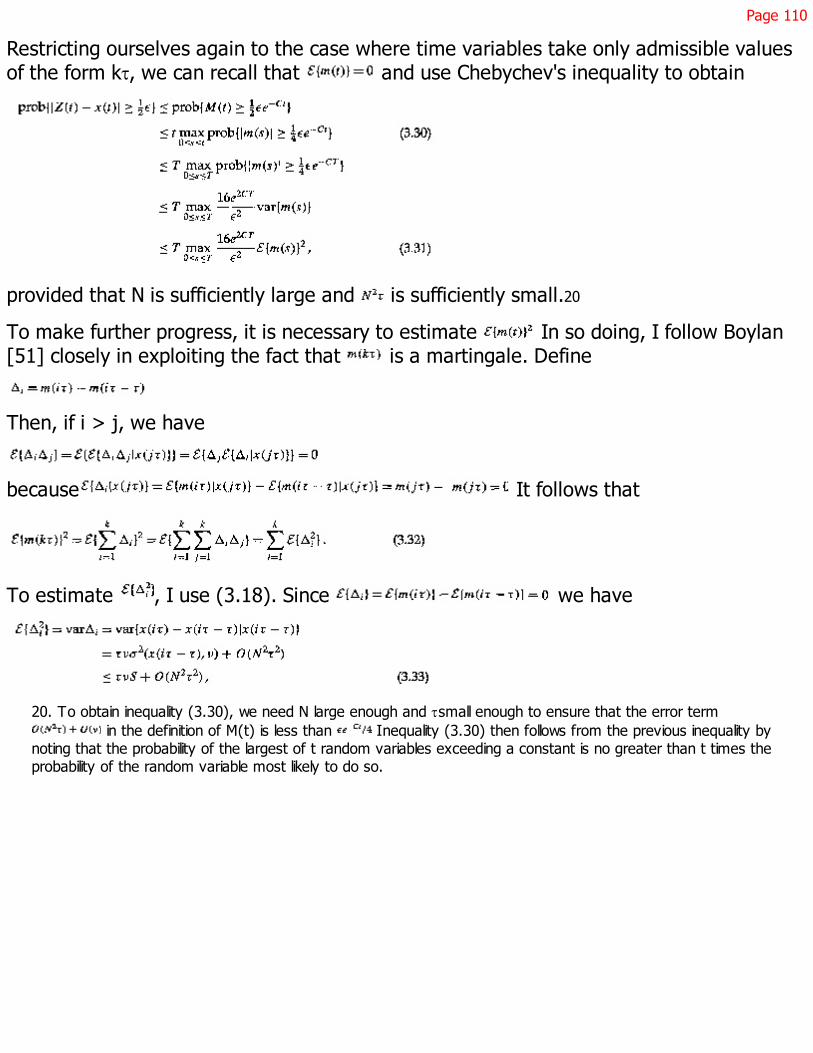
Page 110

Restricting ourselves again to the case where time variables take only admissible valuesof the form kt, we can recall that and use Chebychev's inequality to obtain

provided that N is sufficiently large and is sufficiently small.20

To make further progress, it is necessary to estimate In so doing, I follow Boylan[51] closely in exploiting the fact that is a martingale. Define

Then, if i > j, we have

because It follows that

To estimate , I use (3.18). Since we have

20. To obtain inequality (3.30), we need N large enough and tsmall enough to ensure that the error term in the definition of M(t) is less than Inequality (3.30) then follows from the previous inequality by

noting that the probability of the largest of t random variables exceeding a constant is no greater than t times theprobability of the random variable most likely to do so.

Page 111

where S is an upper bound for that is independent of x and v. Inserting the estimate(3.33) into (3.32), we obtain

provided that N is sufficiently large and is sufficiently small.

On using the estimate (3.34) in (3.31), we find that

which yields the conclusion of the proposition.

Page 113

4The Dynamics of Sample Paths

Chapter 3 showed that if the population is sufficiently large, then a good approximation ofthe behavior of the Aspiration and Imitation model over finite periods of time, can beobtained by examining the deterministic differential equation describing the expectedbehavior of the system. In the particular case of the Aspiration and Imitation model, therelevant differential equation is a version of the replicator dynamics. A similarapproximation result holds for other models, though these will typically give rise to otherdifferential equations. This chapter is devoted to the study of evolutionary models builtaround systems of differential equations.1

4.1 Dynamics

Attention is restricted to two-player, asymmetric games. Let the players be named I andII. The notation easily becomes burdensome, and it will be convenient to let the finitesets of pure strategies for player I and II be denoted by and An element of willtypically be denoted by i and an element of by j. Payoff functions are then given by

and . Let the number of strategies in and be denoted n1 andn11. Let x and y be elements of and where is the (n1 - 1)-dimensional simplex.We can interpret x and y as vectors identifying the proportions of populations I and IIplaying each of the pure strategies in and .

Let the expected payoff to a randomly chosen agent in population I given thatpopulation proportions are (x, y).2 In more conventional terms, this is the expectedpayoff to player I from using mixed

1. The analysis in this chapter is taken from Samuelson and Zhang [202].

2. Hence

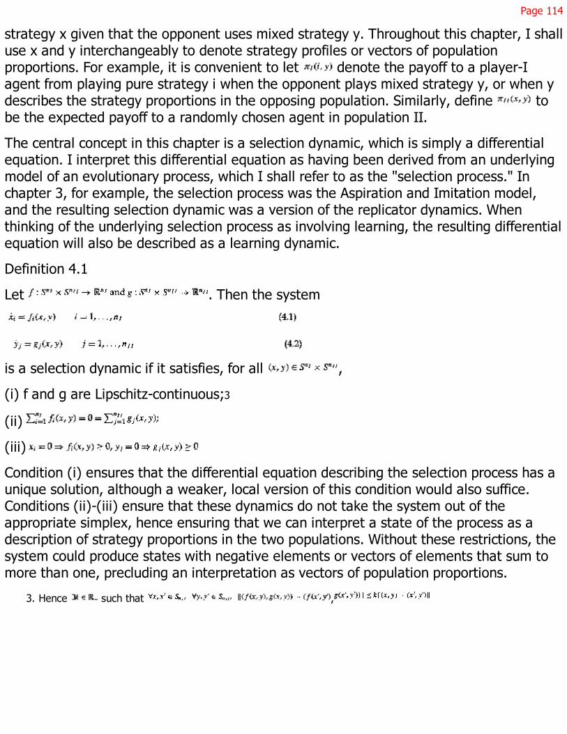
Page 114

strategy x given that the opponent uses mixed strategy y. Throughout this chapter, I shalluse x and y interchangeably to denote strategy profiles or vectors of populationproportions. For example, it is convenient to let denote the payoff to a player-Iagent from playing pure strategy i when the opponent plays mixed strategy y, or when ydescribes the strategy proportions in the opposing population. Similarly, define tobe the expected payoff to a randomly chosen agent in population II.

The central concept in this chapter is a selection dynamic, which is simply a differentialequation. I interpret this differential equation as having been derived from an underlyingmodel of an evolutionary process, which I shall refer to as the "selection process." Inchapter 3, for example, the selection process was the Aspiration and Imitation model,and the resulting selection dynamic was a version of the replicator dynamics. Whenthinking of the underlying selection process as involving learning, the resulting differentialequation will also be described as a learning dynamic.

Definition 4.1

Let . Then the system

is a selection dynamic if it satisfies, for all ,

(i) f and g are Lipschitz-continuous;3

(ii)

(iii)

Condition (i) ensures that the differential equation describing the selection process has aunique solution, although a weaker, local version of this condition would also suffice.Conditions (ii)-(iii) ensure that these dynamics do not take the system out of theappropriate simplex, hence ensuring that we can interpret a state of the process as adescription of strategy proportions in the two populations. Without these restrictions, thesystem could produce states with negative elements or vectors of elements that sum tomore than one, precluding an interpretation as vectors of population proportions.

3. Hence such that ,

Page 115

I shall write x(t) and y(t) to denote the time t values of x and y, but will suppress twhenever possible. Note that is the growth rate of the proportion of population Iplaying strategy i. It will be helpful to define f/x to denote the vector of growth rates

. We shall be interested in selection dynamics that satisfy the followingproperties:

Definition 4.2

A selection dynamic (f, g) is regular if, for any state (x, y) with there is a finitevalue, denoted by , such that

for any sequence with and with with a similar condition holdingfor player II.

A selection dynamic (f, g) is monotonic if, for all

with a similar condition for player II.

A selection dynamic is aggregate monotonic if, for all

with a similar condition for player II.

Regularity ensures that the growth rates f/x and g/y, which are continuous on the interiorof as a result of definition 4.1, are continuous on all of This in turn ensuresthat if x(0) and y(0) are strictly positive, then x(t) and y(t) are strictly positive for all t.Hence strategies never literally become extinct, though the proportion of a populationplaying a strategy can approach zero. In cases where x(0) and y(0) are strictly positive, Ishall refer to the initial conditions as "strictly interior" or "completely mixed." Notice thatregularity and monotonicity together have the implication that if , then encethe dynamics cannot introduce new strategies into the population even if they would givehigher payoffs than all strategies currently being played. This is not a surprising propertyfor a model based on imitation; though it precludes best-response dynamics. Whileimitation may be important, the assumption that people playing a game can never have anew idea, in the sense that they can never introduce a strategy that is currently notplayed, is severe.

Page 116

Section 4.4 accordingly examines the effect of introducing mutations that continuallyinject all strategies into the system.

Monotonicity ensures that if pure strategy i receives a higher payoff than i' and theproportion of the population playing both strategies is positive, then xi grows faster thanxi'. A monotonicity condition lies at the heart of this type of analysis because it providesthe link between the payoffs of the game and the dynamics of the selection process.4 Aloose interpretation of monotonicity is that, on average, players are able to switch fromworse to better strategies. Regularity and mono-tonicity together ensure that if one takesa sequence of states along which the expected payoff of strategy i is higher than that of i,with the expected profit difference bounded away from zero, then the difference ingrowth rates of xi and xi', does not deteriorate to zero along this sequence. This in turnensures that the proportion of the population playing strategy i' will approach zero.

Aggregate monotonicity requires that if (for example) the population II vector y is suchthat a mixed strategy p would receive a higher payoff against y than would p, then onaverage, those pure strategies to which p attaches relatively high probability haverelatively high growth rates. By taking p and p' to attach all of their probability to purestrategies, we obtain the implication that aggregate monotonicity implies monotonicity.Examples are easily constructed to show that the converse fails.5

It is clear that the replicator dynamics are monotonic and that the converse need nothold, so that monotonicity is a generalization of

4. This monotonicity property is referred to as "relative monotonicity" by Nachbar [161]. Friedman [82] applies asimilar requirement to the absolute rates of change (rather than growth rates) of the population proportionsattached to the various pure strategies, and refers to qualifying dynamics as "order compatible." Swinkels [231]works with ''myopic" adjustment processes, by which he means processes for which , with a similarcondition for population II. Hence the strategy adjustments of population I must have the effect of increasing theaverage payoff, provided that the strategy of population II is held fixed. It is immediate that monotonic selectiondynamics are myopic but that the converse fails. Given the central role of monotonicity conditions in evolutionarymodels, it is clearly important to investigate the conditions under which selection processes give rise toapproximating differential equations that are monotonic.

5. In Samuelson and Zhang [202], we incorrectly stated the definition of aggregate monotonicity without the "(=)" oneach side of implication (4.4). In this case, aggregate monotonicity does not imply monotonicity, as can be seen bynoting that every dynamic on the trivial game whose payoffs are all zero would then be aggregate monotonic, butwould be monotonic only if every state were stationary. I am grateful to Klaus Ritzberger for bringing this to myattention.

Page 117

the replicator dynamics. Aggregate monotonicity is also a generalization of the replicatordynamics, but one which retains more of the replicator structure. To explain this remark,we first recall that the replicator dynamics are given by

with a similar specification for player II. We can then solve for

leading us to conclude that the replicator dynamics are aggregate monotonic.6

Next, we observe that aggregate monotonic dynamics are simply transformations of thereplicator dynamics. Let (f*, g*) denote the replicator dynamics. Section 4.5 contains theproof of the following, taken from Samuelson and Zhang [202]:

Proposition 4.1

If (f, g) is a regular, aggregate monotonic selection dynamic, then there exist functions and with and such that

This proposition indicates that aggregate monotonic dynamics are positive multiples ofthe replicator dynamics, though the multiple may depend on the current state. Theabsolute growth rates that prevail at any state may then differ from the replicator, butthe ratios of the growth rates of strategies from a given population must be preserved.Hence the only freedom we gain in passing from the replicator dynamics to an aggregatemonotonic dynamic is to alter the rates at which the two populations learn.7

6. Ritzberger and Weibull [190] work with a generalization of aggregate monotonicity which they refer to as "sign-preserving dynamics." A dynamic is sign-preserving if the growth rate of strategy i is positive (negative) if and onlyif the payoff of strategy i is greater than (less than) the average payoff in the population.

7. The proposition and its proof involve only local arguments, and hence can be extended to the statement that if aselection dynamic is locally aggregate monotonic then it is locally a multiple of the replicator dynamics.

Page 118

42. Equilibrium

What are the equilibrium implications of monotonic dynamics? It is immediate from thedefinitions that a Nash equilibrium must be a stationary state of a monotonic dynamic.8In particular, all strategies played with positive probability in a Nash equilibrium mustreceive the same payoff, which suffices for a state to be a stationary state of a monotonicdynamic. Chapter 2 noted that the replicator dynamics provide examples of cases inwhich stationary states under a monotonic dynamic are not Nash equilibria.

If a state is stationary under a monotonic dynamic but is not a Nash equilibrium, then itcannot be stable, yielding yet another instance of the result that "stability implies Nash."By straightforward intuition, the superior replies that prevent a strategy profile from beinga Nash equilibrium in the underlying game introduce pressures that disrupt stability in theassociated dynamic. In particular, if (x, y) is a stationary state but is not a Nashequilibrium because player 1 has a strategy i that is a better response than x to playerII's strategy y, then there must exist a neighborhood of (x, y) with the property that iearns a strictly higher payoff in this neighborhood than does at least one strategy, say i',in the support of x. Furthermore, this neighborhood can be chosen so that the payoffdifference between i and i' is bounded away from zero. This in turn implies that thegrowth rate of strategy i under a monotonic, regular dynamic must exceed that of i' onthis neighborhood, with the difference again bounded away from zero. But if this is thecase, then any trajectory that remains in the vicinity of (x, y) must cause the proportionof the population playing strategy i' to go to zero, a contradiction to the claim that (x, y)is a stationary state. Thus we have9

Proposition 4.2

Let (f, g) be a regular, monotonic selection dynamic and let (x*, y*) be stable. Then (x*,y*) is a Nash equilibrium.

How much more can we gain if we work with asymptotic stability rather than stability?Friedman [82] confirms that asymptotically stable

8. "Nash equilibrium" here has the obvious meaning of a state in which a positive proportion of one of thepopulations is attached to a strategy only if it is a best response to the opposing population.

9. Somanathan [224] establishes a partial converse of this theorem by establishing a sufficient condition for the stabilityof pure-strategy Nash equilibria under monotonic dynamics.

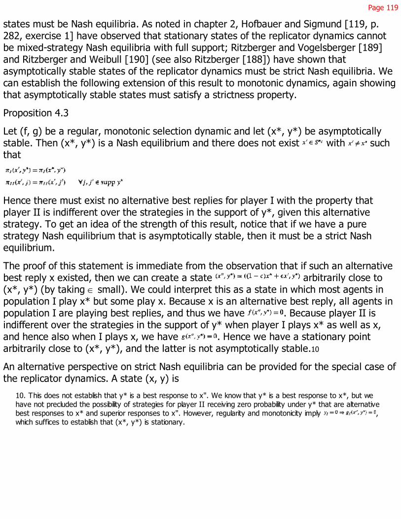
Page 119

states must be Nash equilibria. As noted in chapter 2, Hofbauer and Sigmund [119, p.282, exercise 1] have observed that stationary states of the replicator dynamics cannotbe mixed-strategy Nash equilibria with full support; Ritzberger and Vogelsberger [189]and Ritzberger and Weibull [190] (see also Ritzberger [188]) have shown thatasymptotically stable states of the replicator dynamics must be strict Nash equilibria. Wecan establish the following extension of this result to monotonic dynamics, again showingthat asymptotically stable states must satisfy a strictness property.

Proposition 4.3

Let (f, g) be a regular, monotonic selection dynamic and let (x*, y*) be asymptoticallystable. Then (x*, y*) is a Nash equilibrium and there does not exist with suchthat

Hence there must exist no alternative best replies for player I with the property thatplayer II is indifferent over the strategies in the support of y*, given this alternativestrategy. To get an idea of the strength of this result, notice that if we have a purestrategy Nash equilibrium that is asymptotically stable, then it must be a strict Nashequilibrium.

The proof of this statement is immediate from the observation that if such an alternativebest reply x existed, then we can create a state arbitrarily close to(x*, y*) (by taking Î small). We could interpret this as a state in which most agents inpopulation I play x* but some play x. Because x is an alternative best reply, all agents inpopulation I are playing best replies, and thus we have . Because player II isindifferent over the strategies in the support of y* when player I plays x* as well as x,and hence also when I plays x, we have . Hence we have a stationary pointarbitrarily close to (x*, y*), and the latter is not asymptotically stable.10

An alternative perspective on strict Nash equilibria can be provided for the special case ofthe replicator dynamics. A state (x, y) is

10. This does not establish that y* is a best response to x". We know that y* is a best response to x*, but wehave not precluded the possibility of strategies for player II receiving zero probability under y* that are alternativebest responses to x* and superior responses to x". However, regularity and monotonicity imply ,which suffices to establish that (x*, y*) is stationary.

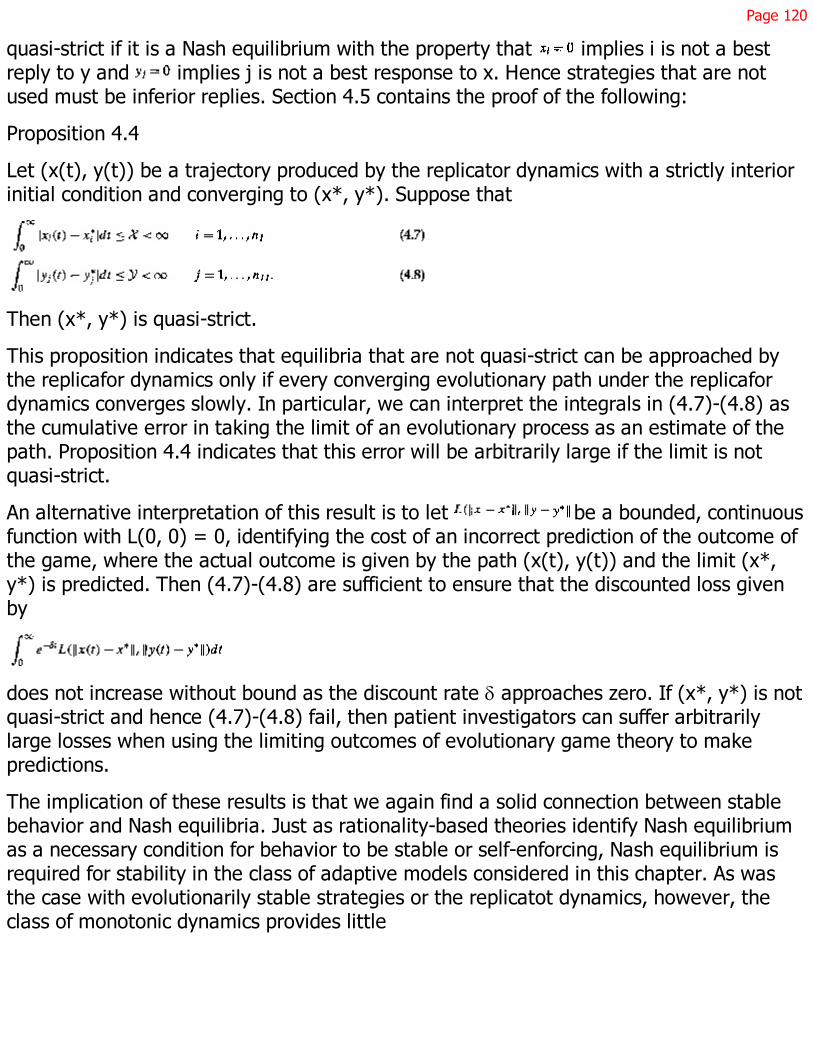
Page 120

quasi-strict if it is a Nash equilibrium with the property that implies i is not a bestreply to y and implies j is not a best response to x. Hence strategies that are notused must be inferior replies. Section 4.5 contains the proof of the following:

Proposition 4.4

Let (x(t), y(t)) be a trajectory produced by the replicator dynamics with a strictly interiorinitial condition and converging to (x*, y*). Suppose that

Then (x*, y*) is quasi-strict.

This proposition indicates that equilibria that are not quasi-strict can be approached bythe replicafor dynamics only if every converging evolutionary path under the replicafordynamics converges slowly. In particular, we can interpret the integrals in (4.7)-(4.8) asthe cumulative error in taking the limit of an evolutionary process as an estimate of thepath. Proposition 4.4 indicates that this error will be arbitrarily large if the limit is notquasi-strict.

An alternative interpretation of this result is to let be a bounded, continuousfunction with L(0, 0) = 0, identifying the cost of an incorrect prediction of the outcome ofthe game, where the actual outcome is given by the path (x(t), y(t)) and the limit (x*,y*) is predicted. Then (4.7)-(4.8) are sufficient to ensure that the discounted loss givenby

does not increase without bound as the discount rate d approaches zero. If (x*, y*) is notquasi-strict and hence (4.7)-(4.8) fail, then patient investigators can suffer arbitrarilylarge losses when using the limiting outcomes of evolutionary game theory to makepredictions.

The implication of these results is that we again find a solid connection between stablebehavior and Nash equilibria. Just as rationality-based theories identify Nash equilibriumas a necessary condition for behavior to be stable or self-enforcing, Nash equilibrium isrequired for stability in the class of adaptive models considered in this chapter. As wasthe case with evolutionarily stable strategies or the replicatot dynamics, however, theclass of monotonic dynamics provides little

Page 121

insight into refinements of Nash equilibria. In particular, monotonic dynamics readilydirect attention to strict Nash equilibria, but appear to have little to say about the casesin which equilibrium refinements become an issue, namely the gap between Nashequilibria and strict Nash equilibria.

4.3 Strictly Dominated Strategies

Some insight into the interaction between monotonic dynamics and equilibriumrefinements can be gained by examining the fate of dominated strategies undermonotonic dynamics. First, consider strictly dominated strategies. The following notionsare familiar and intuitively clear, but some care is required in their formulation becausethe difference between pure and mixed strategies will be important.

A strategy is strictly dominated by if for all Let D(XI, XII) bethe set of pure strategies in that are not strictly dominated by any pure strategy in, given that player II chooses strategies from . Let be the set of mixed

strategies in that are not strictly dominated by any strategies in Sn1, given thatplayer II chooses from . Similar definitions apply to player 11.

Definition 4.3

The strategy survives pure strict iterated admissibility if there exist sequences of sets

with and with

and where the sequence terminates, in the sense that and .The strategy survives strict iterated admissibility if we replace D by D * and X by Min this definition.

This definition is unambiguous, in the sense that every sequence satisfying the conditionsof the definition yields the same set of surviving strategies (Pearce [182]). Pearce alsoshows that the set of strategies surviving strict iterated admissibility is nonempty andcoincides with the set of rationalizable strategies in two-player games.

Page 122

Monotonic selection dynamics eliminate strategies that do not survive pure strict iteratedadmissibility while aggregate monotonic dynamics eliminate strategies that do notsurvive strict iterated admissibility. In particular, section 4.5 proves11

Proposition 4.5.1

Let (f, g) be a regular, monotonic selection dynamic and suppose does not survivepure strict iterated admissibility. Then for any trajectory (x(t), y(t)) with (x(0), y(0))completely mixed, we have

Proposition 4.5.2

Let (f, g) be a regular, aggregate monotonic selection dynamic. Let the strategy failstrict iterated admissibility. Then for any trajectory (x(t), y(t)) with (x(0), y(0))completely mixed, there exists a function such that for every t, thereexists a pure strategy i (t) in the support of x' such that .

The intuition behind propositions 4.5.1 and 4.5.2 is straightforward. If strategy i is strictlydominated by the pure strategy i', then i must always receive a strictly lower payoff, andhence must always be characterized by a strictly lower growth rate under a monotonicdynamic. This can be the case only if the proportion of the population playing iapproaches zero. Hence strategies strictly dominated by other pure strategies will beeliminated. Once the original collection of strictly dominated strategies has been nearlyeliminated, the same forces operate on a new collection of strategies that is now strictlydominated (by pure strategies). Continuing in this way, a monotonic dynamic performsthe iterated elimination of strategies that are strictly dominated by pure strategies.

Additional complications arise if strategy i is dominated by the mixed strategy x. Strategyi will always earn a lower payoff than some other pure strategy, but the identity of thisdominating pure strategy may change over time, preventing a simple repetition of theprevious argument. However, it is straightforward to construct an analogous argument forthe case of an aggregate monotonic selection dynamic.

Nachbar [161] used similar considerations to show that if pure strict iterated admissibilityremoves all but a single strategy for each player, than a monotonic adjustment processmust converge to the surviving

11. Vives [243] and Milgrom and Roberts [155] obtain a similar result for supermodular games.

Page 123

strategy profile. Hofbauer and Weibull [120] have recently shown that a condition called"convex monotonicity" is both weaker than aggregate monotonicity and suffices for theelimination of any pure strategy that fails strict iterated admissibility. Convexmonotonicity is also necessary for pure strict iterated admissibility in the sense that forevery selection dynamic failing convex monotonicity, there exists a game with a purestrategy that survives in spite of being strictly dominated by a (possibly mixed) strategy.In one of Björnerstedt's examples [31], a strategy strictly dominated by a mixed strategysurvives in a continuous-time dynamic that is monotonic but not aggregate monotonic,showing that the assumption of aggregate monotonicity in proposition 4.5.2 cannot bereplaced with monotonicity.

Dekel and Scotchmer [72] present an example in which a strategy strictly dominated by amixed strategy survives under a discrete-time replicator dynamic. Coupled withpropositions 4.5.1 and 4.5.2, this indicates the continuous and discrete formulations cangive different re-suits. Cabrales and Sobel [55] explore this difference, showing thatstrictly dominated strategies can survive if the time periods for the discrete dynamic aresufficiently long that the dynamic takes relatively large jumps. In particular, they showthat if one formulates the continuous and discrete dynamics so that the former is the limitof the latter as the length of a time period shrinks, then strictly dominated strategies areeliminated for all sufficiently short time periods. Weibull [248] expands upon this issue.Björnerstedt et al. [32] present an alternative perspective, formulating the discretereplicator dynamics as an overlapping generations model and showing that dominatedstrategies will be eliminated if the degree of generation overlap is sufficiently high.

4.4 Weakly Dominated Strategies

Propositions 4.5.1 and 4.5.2 show that monotonic dynamics yield outcomes that respectat least the iterated removal of pure strategies strictly dominated by other purestrategies. Attention now turns to weak dominance.

An immediate observation concerning weakly dominated strategies is that a monotonicprocess cannot converge from an interior initial condition to an outcome that places all ofthe probability in one population on a pure strategy dominated by another pure strategy.Suppose that pure strategy i is weakly dominated by strategy i'. Suppose further that theselection dynamic is regular and monotonic and converges to

Page 124

(x*, y*) with . Then for every t, strategy i' earns a higher payoff than i. Hence wehave

for all t. Then the system cannot converge to (x*, y*). This argument gives

Proposition 4.6

Let (f, g) be a regular, monotonic select-ion dynamic and let (x*, y*) be a limitingoutcome of (f, g) with (x(0), y(0)) completely mixed. Then (x*, y*) cannot attach unitaryprobability to a pure strategy that is weakly dominated by another pure strategy.

At the same time, the outcomes of regular, monotonic dynamics need not eliminatedominated strategies entirely. The difficulty here is that the difference between thegrowth rates in (4.9) may approach zero as the selection dynamics converge, relievingthe pressure against the weakly dominated strategy i and allowing i to survive. This canbe contrasted with the case of strictly dominated strategies, where the key step inshowing that such strategies cannot survive is the observation that the difference in (4.9)can be bounded away from zero.

Van Damme [240, example 9.4.3] shows that there exist stable outcomes in symmetricgames that attach positive probability to weakly dominated strategies. For a simpleasymmetric example, consider the game shown in figure 4.1. The phase diagram for thisgame, under the replicator dynamics, is given in figure 4.2.12 It is straightforward tocalculate that under the replicator dynamics, any state in which player II plays L andplayer I mixes between T and B, with strictly positive probability attached to T, is stableand is the limiting outcome of some nontrivial trajectory. These are Nash equilibria inwhich player I attaches positive probability to a weakly dominated strategy B. Thedifficulty is that T dominates B, but only weakly and the payoff difference between T andB disappears as population II becomes concentrated on L. It is then possible thatpopulation II can converge to L so rapidly

12. I have followed the standard practice of letting the row player in a bimatrix game be player I and using x todenote this population's strategy proportions. When drawing the phase diagram, it would be natural to representplayer I's strategies on the horizontal axis. However, I find it helpful to orient the phase diagram so that the cornercorresponding to the pure strategy combination (T, L) is the upper left corner, as it is in the bimatrix. As a result,the phase diagram measures the probability that player I plays T along the vertical axis and the probability thatplayer II plays R along the horizontal axis. A similar convention is adopted for subsequent phase diagrams.

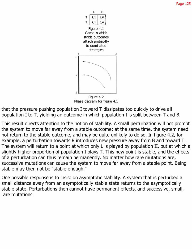
Page 125

Figure 4.1Game in which

stable outcomesattach probability

to dominatedstrategies

Figure 4.2Phase diagram for figure 4.1

that the pressure pushing population I toward T dissipates too quickly to drive allpopulation I to T, yielding an outcome in which population I is split between T and B.

This result directs attention to the notion of stability. A small perturbation will not promptthe system to move far away from a stable outcome; at the same time, the system neednot return to the stable outcome, and may be quite unlikely to do so. In figure 4.2, forexample, a perturbation towards R introduces new pressure away from B and toward T.The system will return to a point at which only L is played by population II, but at which aslightly higher proportion of population I plays T. This new point is stable, and the effectsof a perturbation can thus remain permanently. No matter how rare mutations are,successive mutations can cause the system to move far away from a stable point. Beingstable may then not be "stable enough."

One possible response is to insist on asymptotic stability. A system that is perturbed asmall distance away from an asymptotically stable state returns to the asymptoticallystable state. Perturbations then cannot have permanent effects, and successive, small,rare mutations

Page 126

cannot lead the system far away. However, we have seen that insisting on asymptoticallystable states rejects pure-strategy equilibria that are not strict. One suspects that whilenone of these equilibria is asymptotically stable, some of them are ''more stable" thanothers. We must then investigate the properties of equilibria that are stable but notasymptotically stable.

Asymptotic stability requires robustness to all perturbations. The appropriateness of sucha requirement depends upon the source of the perturbations. If the model given by

and is a literal description of the phenomenon to be studied, then wehave no clues. as to the likely nature of perturbations and no reason to suspect sometypes of perturbation as being more important than others. There accordingly appears tobe no alternative to asking for robustness to all perturbations. This is especially likely tobe the case in a normative analysis, where one might reasonably argue that all aspects ofthe problem should be captured in the model.

In a positive analysis, however, our models are never literal descriptions of the underlyingprocess, but are instead approximations chosen in a process that attempts to balancerealism and tractability. Chapter 3's justification for working with systems of differentialequations as models of an evolutionary process involved an explicit approximationtheorem. Perturbations are then likely to be the product of aspects of the underlyingprocess that have been excluded from the model.

An analogous situation arises when working with tremble-based equilibrium concepts inconventional game theory. An equilibrium is trembling-hand-perfect if there are nearbyequilibria in at least one converging sequence of perturbed games. But why is thatparticular sequence of interest? One way to avoid this question is to ask for robustness inthe face of all trembles, leading to the notion of a strictly perfect equilibrium. Becausesuch equilibria often fail to exist, Kohlberg and Mertens [135] have constructed a set-valued counterpart driven by the criterion of robustness to all perturbations. It isinteresting to note that Kohlberg and Mertens also take the position that the model of thegame is a complete, literal description of the strategic interaction. In this case we againhave no reason to suspect some types of perturbation as being more important thanothers, and are accordingly prompted to ask for robustness to all perturbations. As withevolutionary models, this may be appropriate for a normative theory, but is notnecessarily an appropriate standard for a positive theory, where various features of the

Page 127

strategic interaction excluded from the model may again cause some trembles to bemore likely than others.

In light of this, we turn our attention to whether stable states of the selection dynamicswill retain their stability properties when faced with certain types of perturbations thatreflect unmodeled aspects of the underlying stochastic selection process. Theseperturbations will appear as random movements between states in the selection processand as deterministic adjustments to the differential equations that approximate thatprocess in the long run. Suppose, for example, that the underlying process was theAspiration and Imitation model and that we were studying the common replicatordynamics given by (2.15). Perturbations appear in the Aspiration and Imitation model inthe form of mutations, which have been excluded in deriving (2.15). Taking them intoconsideration leads to a new long-run approximation given by (3.5).

These considerations suggest that we investigate dynamics of the following form:13

where (f, g) is a selection dynamic and and satisfy

We can interpret this as a situation in which most of the population, that is, the ( )and ( ) proportions of populations I and II, evolve according to the original selectiondynamic. The terms and can be interpreted as the proportions of the populations thatare subject to perturbations and whose choices are described by the distributions x and h.In the Aspiration and Imitation model, these perturbations might arise out of mutationsor out of unexpected realizations of the random learning process. In other models, analternative interpretation could be that these are new entrants into the game, replacingexisting players, who thus do not have experience with the game and choose theirstrategies according to the exogenously given x and h.

13. Hotbauer and Sigmund [119, chapter 9] present a similar model, with the perturbations motivated astransmission errors in the evolutionary process. Boylan [50] examines an analogous process in symmetric games.Bomze and Bürger [40] provide an alternative approach to stability based on perturbations.

Page 128

The precise form of x and h will not be specified in this chapter. Given that the motivationfor these terms arises out of aspects of the selection process not captured in the modelwe would in general expect to gain insight into the nature of x and h by examining theunderlying learning process. Because these elements of the underlying stochasticselection process originally seemed unimportant, we will be interested in the case inwhich and are small, and will be especially interested in the limiting case in whichthey approach zero.

The specification in (4.10)-(4.11) differs from that of the Aspiration and Imitation modelin two respects. First, we now have two populations in an asymmetric game, and allowasymmetries across the two populations in the form of differing values of and . Inaddition, the perturbations x and h are assumed to be independent of the current state.Inspection of (3.5) shows that this is not the case for the Aspiration and Imitation model.This independence is convenient for the present purposes, and will be generalized inchapter 6. Notice also that the specification of the perturbations is given by x and hindependently of the values of and . Although not important to the results, this makesthe exposition more convenient.

We shall maintain the assumption that x and h are completely mixed, meaning that and are positive for all i and j. Hence the perturbations can switch agents to any of theavailable strategies, which is important when examining games such as the one in figure4.1. The dominated strategy B survives among some members of the population onlybecause R is eliminated by the selection process, and in assessing the stability of pointsin which B is played it is important that perturbations be able to introduce strategy R.

I shall refer to the dynamic in (4.10)-(4.11) as the "perturbed selection dynamic." We areinterested in the stationary states of the perturbed selection dynamic. I shall refer to thelimit of these stationary states, as the perturbations become arbitrarily small, as "limitstationary states." Section 4.5 confirms the following expected result:

Proposition 4.7

A limit stationary state of a regular, monotonic dynamic is a Nash equilibrium.

To see why we expect such a result to hold, notice that stationary states of unperturbed,regular, monotonic dynamics can fail to be Nash equilibria only because a superior replymight be played by a zero proportion of the population, and hence be unable to grow inspite of its payoff advantage. In the perturbed dynamics every strategy is always

Page 129

played by at least some small fraction of the population. Any superior reply to the currentstate will then grow. A stationary state of the perturbed dynamics will thus be a statewhere almost all agents are playing strategies from some Nash equilibrium, while theperturbations distribute some agents among the remaining strategies. As we approach alimit stationary state by taking the size of the perturbations to zero, the latter strategiesdisappear and we obtain a Nash equilibrium.

I have drawn an analogy between (4.10)-(4.11) and tremble-based equilibriumrefinements. While the motivation for (4.10)-(4.11) and for Selten's trembling handperfection [208] might be similar, the two types of perturbation have quite differenteffects in their respective models. For example, weakly dominated strategies can survivein limit stationary states, unlike trembling hand perfection. In addition, it can be the casethat only under exceptional conditions does a limit stationary state exist that attacheszero probability to dominated strategies.

To verify this last statement, consider the game in figure 4.1. Let (f, g) be the replicatordynamic. I shall conserve on notation by letting z denote the proportion of population Iplaying T and v the proportion of population II playing R. Similarly, let x and h be theprobabilities attached to T and R by the perturbations. Then we have

A stationary state must satisfy , and we can then solve (4.12)-(4.13) for

Now examine the limit as and . Will the result be the Nash equilibrium inundominated strategies, given by (T, L) and corresponding to ? The left side of(4.14) approaches ¥ as , and (0,1) can then be the limit stationary state only ifthe right side of (4.14) also approaches infinity, or only if . A necessary (andsufficient) condition to eliminate dominated strategies is then that population II besubject to perturbations that are arbitrarily large compared to those of population I.

Why must ? Perturbations exert two conflicting forces on population I. By causingsome of population II to play R, perturbations ensure that T earns a higher payoff than B,introducing

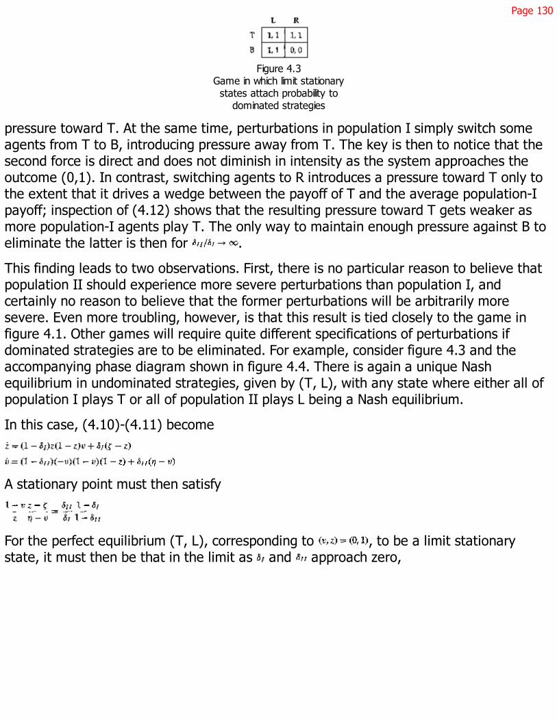
Page 130

Figure 4.3Game in which limit stationary

states attach probability todominated strategies

pressure toward T. At the same time, perturbations in population I simply switch someagents from T to B, introducing pressure away from T. The key is then to notice that thesecond force is direct and does not diminish in intensity as the system approaches theoutcome (0,1). In contrast, switching agents to R introduces a pressure toward T only tothe extent that it drives a wedge between the payoff of T and the average population-Ipayoff; inspection of (4.12) shows that the resulting pressure toward T gets weaker asmore population-I agents play T. The only way to maintain enough pressure against B toeliminate the latter is then for .

This finding leads to two observations. First, there is no particular reason to believe thatpopulation II should experience more severe perturbations than population I, andcertainly no reason to believe that the former perturbations will be arbitrarily moresevere. Even more troubling, however, is that this result is tied closely to the game infigure 4.1. Other games will require quite different specifications of perturbations ifdominated strategies are to be eliminated. For example, consider figure 4.3 and theaccompanying phase diagram shown in figure 4.4. There is again a unique Nashequilibrium in undominated strategies, given by (T, L), with any state where either all ofpopulation I plays T or all of population II plays L being a Nash equilibrium.

In this case, (4.10)-(4.11) become

A stationary point must then satisfy

For the perfect equilibrium (T, L), corresponding to , to be a limit stationarystate, it must then be that in the limit as and approach zero,

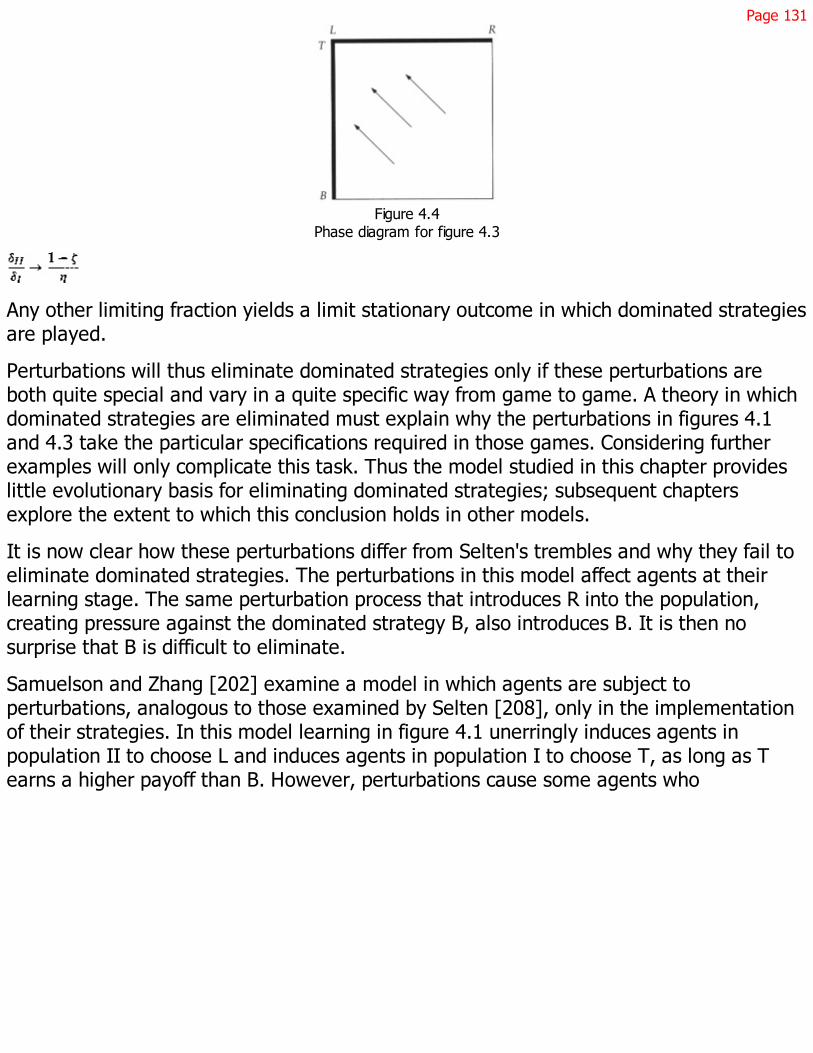
Page 131


Any other limiting fraction yields a limit stationary outcome in which dominated strategiesare played.

Perturbations will thus eliminate dominated strategies only if these perturbations areboth quite special and vary in a quite specific way from game to game. A theory in whichdominated strategies are eliminated must explain why the perturbations in figures 4.1and 4.3 take the particular specifications required in those games. Considering furtherexamples will only complicate this task. Thus the model studied in this chapter provideslittle evolutionary basis for eliminating dominated strategies; subsequent chaptersexplore the extent to which this conclusion holds in other models.

It is now clear how these perturbations differ from Selten's trembles and why they fail toeliminate dominated strategies. The perturbations in this model affect agents at theirlearning stage. The same perturbation process that introduces R into the population,creating pressure against the dominated strategy B, also introduces B. It is then nosurprise that B is difficult to eliminate.

Samuelson and Zhang [202] examine a model in which agents are subject toperturbations, analogous to those examined by Selten [208], only in the implementationof their strategies. In this model learning in figure 4.1 unerringly induces agents inpopulation II to choose L and induces agents in population I to choose T, as long as Tearns a higher payoff than B. However, perturbations cause some agents who

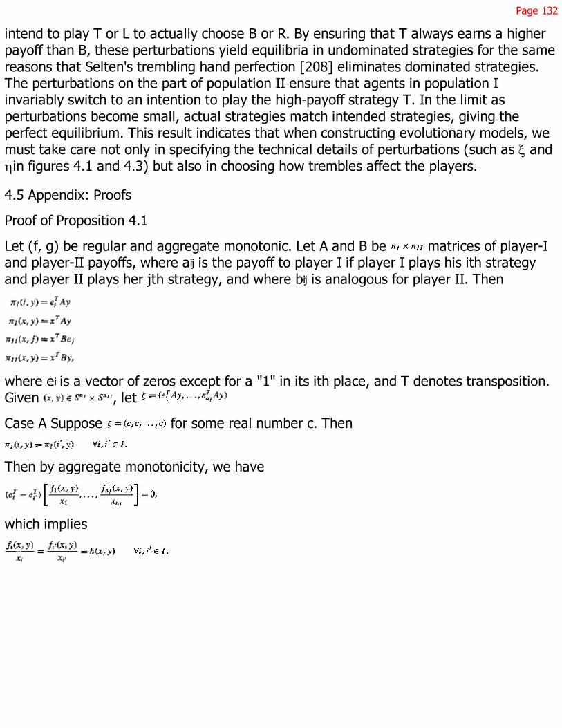
Page 132

intend to play T or L to actually choose B or R. By ensuring that T always earns a higherpayoff than B, these perturbations yield equilibria in undominated strategies for the samereasons that Selten's trembling hand perfection [208] eliminates dominated strategies.The perturbations on the part of population II ensure that agents in population Iinvariably switch to an intention to play the high-payoff strategy T. In the limit asperturbations become small, actual strategies match intended strategies, giving theperfect equilibrium. This result indicates that when constructing evolutionary models, wemust take care not only in specifying the technical details of perturbations (such as x andhin figures 4.1 and 4.3) but also in choosing how trembles affect the players.



Let (f, g) be regular and aggregate monotonic. Let A and B be matrices of player-Iand player-II payoffs, where aij is the payoff to player I if player I plays his ith strategyand player II plays her jth strategy, and where bij is analogous for player II. Then

where ei is a vector of zeros except for a "1" in its ith place, and T denotes transposition.Given , let

Case A Suppose for some real number c. Then

Then by aggregate monotonicity, we have

which implies

Page 133

Because f is a selection dynamic, we have

Therefore, for any , we have

where the final equality holds because and f*is the replicator dynamic.

Case B Suppose there is no such that . By aggregate monotonicity, for all,

Let Then the orthogonal complement of X in is span, and we have

Thus there exist Å(x, y) and a(x, y) such that

Because , there exists such that . Then aggregate monotonicityimplies

Therefore, . Because (f, g) is a selection dynamic, we have

Therefore,

and

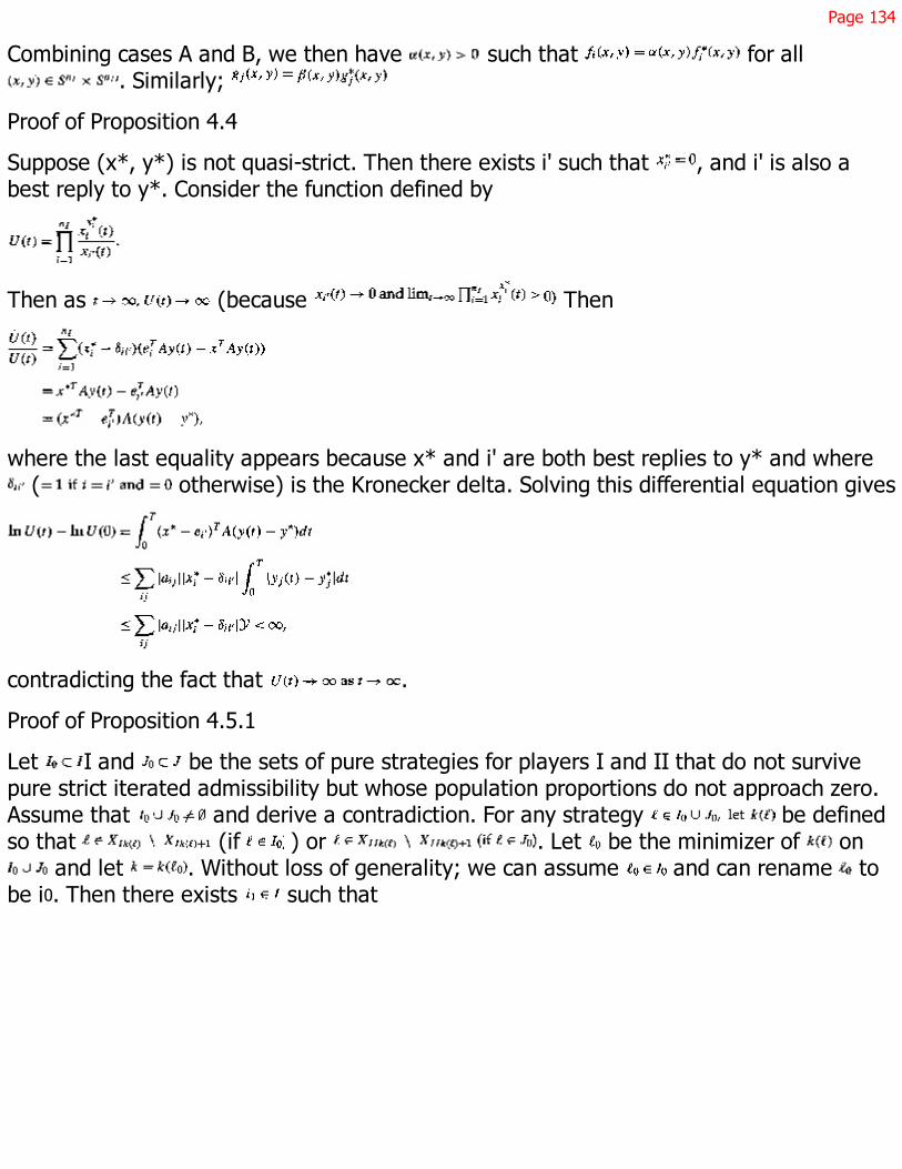
Page 134

Combining cases A and B, we then have such that for all. Similarly;


Suppose (x*, y*) is not quasi-strict. Then there exists i' such that , and i' is also abest reply to y*. Consider the function defined by

Then as (because Then

where the last equality appears because x* and i' are both best replies to y* and where ( otherwise) is the Kronecker delta. Solving this differential equation gives

contradicting the fact that .

Proof of Proposition 4.5.1

Let I and be the sets of pure strategies for players I and II that do not survivepure strict iterated admissibility but whose population proportions do not approach zero.Assume that and derive a contradiction. For any strategy be definedso that (if ) or . Let be the minimizer of on

and let . Without loss of generality; we can assume and can rename tobe i0. Then there exists such that

Page 135

for all . Because k minimizes , we have for all . Then

As ( ), the second term in (4.15) approaches zero while the first term is negative andbounded away from zero. Therefore, there exist and such that

By monotonicity and regularity, we then have, for some ,

and hence , contradicting the assumption that .

Proof of Proposition 4.5.2

Let p be a mixed strategy for player I (without loss of generality) that fails strict iteratedadmissibility and let (x(t), y(t)) be a trajectory with (x(0), y(0)) completely mixed. Itsuffices to show that14

Assume that (4.16) fails and derive a contradiction. Let A1 be the set of mixed strategies that fail to survive iterated strict dominance and for which . Let AII

be similarly defined for population II. Because we assume that (4.16) fails, isnonempty. For , let be such that or dependingupon whether or . Let a be the minimizer of k on . Without loss ofgenerality, assume and let k(a) be written simply k. Then since , thereexists such that b strictly dominates a for all y in MIIK, that is,

14. I use the assumption of a strictly interior initial condition here to ensure that the product in (4.16) is nonzero forany finite t.

Page 136

Let Y consist of all those with the property that only if . Then

By aggregate monotonicity, we have

Because Y is a closed subset of Sn11, regularity ensures that there exists such that

Now given y(t), define y *(t) by

where lt is chosen such that Because (by definition of k), we have Let

Then differentiating gives

The first part of (4.18) is bounded above byÎ (from (4.17)), while the second part isbounded by when t is large. Thus there exists such that

for , or equivalent1y,

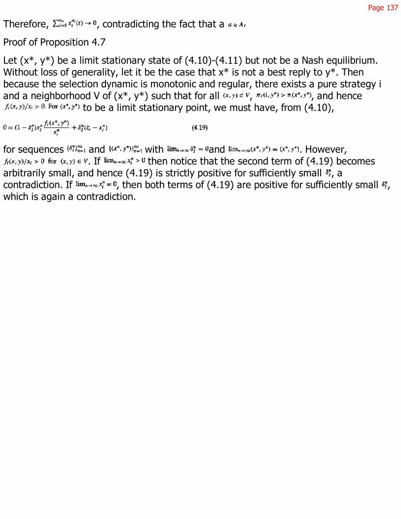
Page 137

Therefore, , contradicting the fact that a


Let (x*, y*) be a limit stationary state of (4.10)-(4.11) but not be a Nash equilibrium.Without loss of generality, let it be the case that x* is not a best reply to y*. Thenbecause the selection dynamic is monotonic and regular, there exists a pure strategy iand a neighborhood V of (x*, y*) such that for all , , and hence

to be a limit stationary point, we must have, from (4.10),

for sequences and with and . However,. If then notice that the second term of (4.19) becomes

arbitrarily small, and hence (4.19) is strictly positive for sufficiently small , acontradiction. If , then both terms of (4.19) are positive for sufficiently small ,which is again a contradiction.

Page 139

5The Ultimatum Game

In continuing our investigation of evolutionary models based on systems of deterministicdifferential equations, let us move now from the abstract models of the previous chapterto the consideration of a particular game, the Ultimatum Game.1

The Ultimatum Game is especially simple and has an unambiguous equilibrium prediction,at least if we are willing to believe in backward induction. However, there is considerableexperimental evidence showing that Ultimatum Game outcomes in the laboratory do notmatch the unique, subgame-perfect equilibrium of the game. As this chapter will show, anevolutionary analysis can lead to conclusions that differ from those of the traditionalequilibrium refinements literature and that match the qualitative nature of experimentaloutcomes better than does the subgame-perfect equilibrium.

There are already many explanations for observed outcomes in the Ultimatum Game.Most of these are some variant on the claim that the model is misspecified. Generally, itis the preferences of the players that are thought to be misspecified, with the players saidto be affected by fairness or relative income considerations in addition to the amount ofmoney they receive. I do not claim that such forces are absent. They may operatealongside the evolutionary forces described here, and may have a hand in explaining whythe quantitative match between the model in this chapter and observed experimentaloutcomes is not particularly close. It may also be the case that evolutionary forces aloneexplain the results and the model in this chapter, while on the right track, may be thewrong evolutionary model. Yet again, evolution may have nothing to do with the results.

1. This chapter is taken from Binmore, Gale, and Samuelson [21].

Page 140

At this point, all of these must remain possibilities. We shall assume away all otherfactors to demonstrate that evolutionary forces alone can yield outcomes thatsignificantly differ from the subgame-perfect equilibrium. Questions of how we mightassess the importance of evolutionary arguments, and how we might determine whetherthey are relevant at all, are taken up in the next chapter.

The simplicity of the Ultimatum Game makes it an ideal context in which to discuss a keyissue. Evolutionary analyses are motivated by thoughts of players learning to play games.But the Ultimatum Game is so simple, what could there be to learn? This question issufficiently compelling for some, especially when applied to responders, as to promptstatements that responders in the Ultimatum Game cannot possibly have anything tolearn. I confront this issue at the end of the chapter, arguing that there are indeed thingsfor responders to learn.

5.1 The Ultimatum Game

Consider two players with a dollar to divide. The rules of the Ultimatum Game specifythat player I begins by making an offer of to player II, who then accepts or refuses.If player II accepts, player I gets 1 - x, and player II gets x. If player II refuses, both getnothing.

This game has a unique subgame-perfect equilibrium in which player II plans to acceptany offer she might receive and player I offers player II nothing. If offers must be made inmultiples of some monetary unit, such as a penny, then there are other subgame-perfectequilibria, but player II gets at most a penny in any such equilibrium.

In the first of many experiments on this and related games, Güth, Schmittberger, andSchwarze [108] found that the modal offer was nd that player I had roughly half achance of being rejected if he offered about of the sum of money available. Binmore,Shaked, and Sutton [29] reported qualitatively similar results in their replication of theUltimatum Game experiment. There have been many related studies in the interim,surveyed by Bolton and Zwick [38], Güth and Tietz [109], Roth [194] and Thaler [233].

The discussion prompted by these experimental results has proceeded in two directions.Critics of traditional economic theory have added these results to a list that includes thefinitely repeated Prisoners' Dilemma and games involving the private provision of public

Page 141

goods; they have interpreted the results as demonstrating that the optimizing paradigmon which conventional economic models and game-theoretic equilibrium concepts arebased is fundamentally mistaken. Instead, behavior. is often explained in terms of socialnorms. Frank [80] is particularly eloquent on this subject. In bargaining games, forexample, it is popular to assert that people ''just play fair."

Many game theorists, on the other hand, have responded by dismissing laboratory resultsas irrelevant to actual behavior. The assertion is made that poorly motivatedundergraduates in the artificial and unfamiliar situations often found in experiments arenot reliable indicators of how people actually behave when making important economicdecisions. There appears to be little doubt that experimentalists or game theorists shouldbe cautious about making predictions unless the game is reasonably simple, theincentives are adequate, and subjects have sufficient opportunity for gaining experiencewith the game.2 More and more experiments satisfy these criteria, however, and gametheorists cannot ignore well-run experiments that persistently refute their predictions. Inthe case of the Ultimatum Game, the relevant experiments have been replicated toooften for doubts about the data to persist. The theory must be reconsidered.

At first glance, the case for subgame perfection in the Ultimatum Game seems ironclad.This is a two-player game of perfect information in which each player moves only once.3Player I need only believe that player II will not play a weakly dominated strategy toarrive at the subgame-perfect offer However, chapter 4 showed that evolutionaryprocesses typically do not eliminate weakly dominated strategies, and this observationprovides the motivation for an evolutionary analysis of the Ultimatum Game.

We shall assume that the replicator dynamics provide a good approximation of the long-run behavior of the learning process. Chapter 3 explains why it might be reasonable towork with some system of deterministic differential equations. Although there is noparticular reason

2. These circumstances, stressed by Binmore [19, p. 51], appeared in chapter 3 as conditions under which initialbehavior in an evolutionary process is likely to give way to strategic considerations. Smith [222] discusses the needto offer experimental subjects large incentives. Ledyard [139] examines the effects of increasing the incentivesand allowing subjects to accumulate experience in experimental treatments of the private provision of public goods.

3. In particular, the criticism that subgame perfection calls for players to regard their opponents as perfectly rationalafter having received evidence to the contrary (cf. Binmore [18]) has no force in the Ultimatum Game.

Page 142

Figure 5.1Ultimatum Minigame

Figure 5.2Ultimatum Minigame, normal form

to expect the replicator dynamics to be especially applicable, it will be clear from theanalysis that other regular, monotonic dynamics will give qualitatively the same results,though the specifics of the calculations will differ.

5.2 An Ultimatum Minigame

The structure of this chapter's argument is most easily isolated by examining thesimplified version of the Ultimatum Game shown in figure 5.1. In this UltimatumMinigame, player I can make a high offer (H) or a low offer (L) to player II. If he makes ahigh offer, it is assumed that player II accepts and the surplus of 4 is split evenly. If hemakes a low offer, player II may accept (Y, for payoffs (3,1)) or refuse (N, for payoffs(0,0)). The normal form of this game is shown in figure 5.2.

The Ultimatum Minigame is highly stylized, but it captures the basic dilemma facingplayer I in the Ultimatum Game: should player I make an aggressive offer, obtaining ahigh payoff if it is accepted but

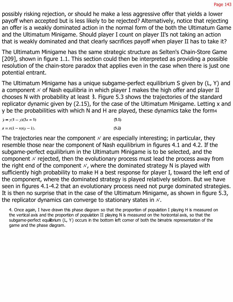
Page 143

possibly risking rejection, or should he make a less aggressive offer that yields a lowerpayoff when accepted but is less likely to be rejected? Alternatively, notice that rejectingan offer is a weakly dominated action in the normal form of the both the Ultimatum Gameand the Ultimatum Minigame. Should player I count on player II's not taking an actionthat is weakly dominated and that clearly sacrifices payoff when player II has to take it?

The Ultimatum Minigame has the same strategic structure as Selten's Chain-Store Game[209], shown in figure 1.1. This section could then be interpreted as providing a possibleresolution of the chain-store paradox that applies even in the case when there is just onepotential entrant.

The Ultimatum Minigame has a unique subgame-perfect equilibrium S given by (L, Y) anda component of Nash equilibria in which player I makes the high offer and player IIchooses N with probability at least . Figure 5.3 shows the trajectories of the standardreplicator dynamic given by (2.15), for the case of the Ultimatum Minigame. Letting x andy be the probabilities with which N and H are played, these dynamics take the form4

The trajectories near the component are especially interesting; in particular, theyresemble those near the component of Nash equilibrium in figures 4.1 and 4.2. If thesubgame-perfect equilibrium in the Ultimatum Minigame is to be selected, and thecomponent rejected, then the evolutionary process must lead the process away fromthe right end of the component , where the dominated strategy N is played withsufficiently high probability to make H a best response for player I, toward the left end ofthe component, where the dominated strategy is played relatively seldom. But we haveseen in figures 4.1-4.2 that an evolutionary process need not purge dominated strategies.It is then no surprise that in the case of the Ultimatum Minigame, as shown in figure 5.3,the replicator dynamics can converge to stationary states in .

4. Once again, I have drawn this phase diagram so that the proportion of population I playing H is measured onthe vertical axis and the proportion of population II playing N is measured on the horizontal axis, so that thesubgame-perfect equilibrium (L, Y) occurs in the bottom left comer of both the bimatrix representation of thegame and the phase diagram.

Page 144

Figure 5.3Phase diagram, no drift

We summarize the key properties of these trajectories as follows:

Proposition 5.1

The subgame-perfect equilibrium S is the unique asymptotically stable stationary state ofthe unperturbed replicator dynamics. With the exception of the state in which player Iplays H and player II plays Y with probability , the Nash equilibria in the set arestable.

The replicator dynamics can thus converge to stable outcomes that are not the subgame-perfect equilibrium. However, the mere fact that interior points of can attracttrajectories of the replicator dynamics does not seem to be an adequate reason forregarding them as alternatives to the subgame-perfect equilibrium S. As was the case infigures 4.1-4.2, perturbations can shift the system between states in the component .No single, small perturbation can shift the system very far, which is to say, the states in are stable. However, the effects of successive, small perturbations can accumulate tohave a large, permanent impact. The survival of states in is allowed only by theextinction of the strategy L. If the perturbations continually introduce the strategy L, thenthere is always pressure against strategy N and the fate of states in is not clear.

Page 145

Figure 5.4Phase diagram, comparable drift

To regard the states in as serious candidates for long-run outcomes, they should thensurvive in the presence of such perturbations. Accordingly; we now turn to the perturbedreplicator dynamics, introduced in (4.10)-(4.11) and given, for the Ultimatum Minigame,by

These equations are analogues to (5.7)-(5.8) of section 5.3 below. I call dI and dII the"levels of drift" in the two populations. Notice that the perturbations are assumed tointroduce each of the two strategies in each population with equal frequency; reflected inthe that appear in (5.3)-(5.4). The effect of alternative specifications will be discussedin the next section.

Figures 5.4 and 5.5 show trajectories for the perturbed replicator dynamics. These figuresindicate that the outcome of the perturbed dynamics depends in an important way on thespecification of the perturbations. Most of this specification has been fixed in (5.3)-(5.4),but the relative magnitudes of dI and dII remain open. These magnitudes

Page 146

Figure 5.5Phase diagram, more drift in population

determine which population, proposers or responders, experience a higher incidence ofdrift.

In figure 5.4, responders and proposers are equally prone to drift . In this case,there are no stationary states near the component . Instead, there is a single,asymptotically stable stationary state that lies very close to the subgame-perfectequilibrium and that differs from the subgame-perfect equilibrium only because theperturbations continually introduce the strategies H and N into populations I and II, andlearning can accordingly never entirely eradicate such behavior. In this case of equal driftin the two populations, the perturbations inject the strategy L into population I withsufficient frequency, and hence exert enough pressure against the strategy N inpopulation II, to ensure that stationary states near the component cannot survive.Strategy N is effectively eliminated and the system converges to the subgame-perfectequilibrium.

In figure 5.5, responders are subject to more drift than proposers. In this case, there aretwo asymptotically stable states. Although one again lies near the subgame-perfectequilibrium, the other lies near

Page 147

the component . This state, denoted by x, corresponds to a Nash equilibrium in whichproposers choose H. In this case, perturbations do not exert sufficient pressure againstthe strategy N to ensure that the subgame-perfect equilibrium appears.

To make the results suggested by these figures more precise, consider the dynamicsgiven by (5.3)-(5.4) and let drift be small, so that is close to (0,0). Let

be fixed and consider the limit as (at rates which preserve f)in two cases:

Case 1:

Case 2:

Since , responders are subject to more drift than proposers in the second case.Section 5.6 contains the proofs of the following, including details of the specification of and .

Lemma 5.1

Let be the set of stationary states of the system (5.3)-(5.4) given .

In case 1, the set has at most one limit point as >, which is thesubgame-perfect equilibrium S.

In case 2, the set has three limit points as , consisting of the subgame-perfect equilibrium S and two states contained in the component of Nash equilibria , inwhich agents from population I all play H. Agents from population II play N withprobability and in these latter two states.

Proposition 5.2

Let be the set of asymptotically stable states of the system (5.3)-(5.4) givenvalues .

In case 1, the set has a unique limit point as , which is the subgame-perfect equilibrium S.

In case 2, the set has two limit points as , which are the subgame-perfect equilibrium S and the Nash equilibrium in which population I plays H andpopulation II plays N with probability . (The state in which I plays H and II plays N withprobability is a limit of saddles.)

The first case gives rise to the phase diagram in figure 5.4; the second case to the phasediagram in figure 5.5. In figure 5.5, it is the asymptotically stable state x that convergesto the Nash equilibrium in which player I plays H and player II plays Y with probability .

Page 148

In the presence of drift, asymptotically stable states can thus arise near Nash equilibria ofthe Ultimatum Minigame that are not subgame-perfect. In the long run, we cannotrestrict our attention to subgame-perfect equilibrium. We have good reason to expectother Nash equilibrium to appear.

How do we interpret these results? The forces behind them, including the important roleplayed by the relative rates of drift in the two populations, are familiar from the previouschapter. In the Ultimatum Minigame, states in the component are stationary because Lhas disappeared from the system, allowing Y and N to both be best replies, just as thestrategy B persists in the game of figure 4.1 because R is eliminated. Perturbations in theUltimatum Minigame introduce L into the population, exerting a pressure against N, butalso introduce N into the population. The outcome depends upon the relative strengths ofthese two forces.

In figure 4.1, the perturbation introducing R is the only force exerted against strategy B.Eliminating B is then difficult, and B is entirely purged from the outcome only if theperturbations injecting R into the system are arbitrarily large compared to those injectingB. In the Ultimatum Minigame, the burden of eliminating dominated strategies does notentirely fall to perturbations. Rather than completely eliminating N, the perturbationsneed only reduce the frequency of N to the point that L is a best response for proposers,which is to say, perturbations need only lead to the left end of the component . Thelearning process will then lead to the subgame-perfect equilibrium. The dominatedstrategy N can then survive, if at all, only in sufficiently high proportion, unlike the gameof figure 4.1. If the two populations are equally subject to drift, then the perturbationscannot maintain strategy N in sufficiently high frequency; instead allowing the proportionof N in the population to fall to the point that L is a best response for player I, and onlythe subgame-perfect equilibrium survives. The existence of asymptotically stable statesnear then requires that responders be subject to drift at a sufficiently high rate relativeto proposers.

The effects of drift, including the appearance of asymptotically stable states near thecomponent , appear no matter how small are the drift parameters dI and dII. What isimportant is the relative sizes of these parameters and not their absolute value. Verysmall amounts of drift can have large effects on the outcome of the system because thecrucial feature of drift is its behavior near the component . Because is a component ofNash equilibria, almost all agents are playing

Page 149

almost best replies when the system is near this component. The learning dynamics thenexert very little pressure, and even arbitrarily small amounts of drift can be decisive indetermining whether the system is pushed toward the component , yielding anasymptotically stable state near , or is pushed away from and toward the subgame-perfect equilibrium.

5.3 Numerical Calculations

Let us now turn to the full Ultimatum Game. Abstract versions of the Ultimatum Gametypically allow player I to choose offers from the interval [0,1]. If the game is to beactually played, as in experiments, we must work instead with a finite set of offers. Thissection studies a version of the Ultimatum Game in which the players must split a "pie" ofsize 40. The set of offers available to the proposer is .5 Notice that an offer i Î is the amount that player I proposes player II should get rather than the amount player

I demands for himself. An action for player II is a choice from the set {Y, N}. Herstrategies are therefore functions . This is an unmanageably largestrategy set, however, and we therefore assume that player II is restricted to functions ofthe form f(i) = Y (for ) and f(i) = N (for ), for some . We can thenidentify player II's strategy with the minimum acceptable offer j and the set of pure-strategy pairs can be identified with . There are forty pure-strategy Nash equilibria,given by (i,i), where (i = 1,2,...,40). Because i = 0 is excluded, the unique subgame-perfect equilibrium is (1,1).6

Let the fraction of proposers who make offer i at time t be denoted by . Let denotethe payoff of a proposer using offer i at time t when his opponent is drawn at randomfrom the population of responders at time t. The average payoff in the population ofproposers at time t is then . The standard replicator equation forthe evolution of , given by (2.15), is

5. In crucial cases, solutions were also computed for games with I = {1, 2,...,100} without significantly altering theresults.

6. These strategies force player II to accept the whole pie if it is offered. They also force player II to play strategiesthat are "monotonic" in the sense that player II must accept all high offers and reject all low ones, and has availableonly the choice of a dividing line between the two sets. I do not expect these restrictions to play a role in driving theresults. For an analysis of a simple case that does not impose these restrictions, see Harms [113].

Page 150

Similarly, let be the fraction of responders playing strategy j at time t, with beingthe fitness of a responder using strategy j and be the average fitness of responders,so that

The evolution of the system is determined by the eighty equations given by (5.5) and(5.6).

The results of chapter 4 and the analysis of the Ultimatum Minigame direct attention tothe case in which (5.5)-(5.6) are subject to perturbations. It is also apparent from chapter4 and the previous section that the manner in which these perturbations enter the modelcan be very important. In light of this, it is useful to have some idea of the source of theperturbation to be studied.

I view an agent as a stimulus-response mechanism with two modes of operation: aplaying mode and a learning mode. An agents' playing mode operates when it is calledupon to choose a strategy in one of a large number of games that it repeatedly playsagainst different opponents. Its behavior, when in playing mode and when confrontedwith a game, is triggered by a stimulus that is determined by the manner in which thegame is framed. Absent the learning mode, an agent could therefore be identified with afixed decision rule that maps a set of stimuli into a set of strategies. However, sometimesan agent will enter its learning mode between games to adjust its current decision rule.This is the equivalent of receiving the learn draw in chapter 3. When learning, the agenttakes a stimulus and some information about the relative success of strategies in thegame labeled by this stimulus and uses them to modify its reaction to the stimulus. Thelearning rule that it uses for this purpose is assumed to be fixed, and is assumed in thischapter to be approximated by the replicator dynamics.

Noise may perturb an agent either in its decision mode or in its learning mode. Theperturbations in an agent's playing mode are analogous to the trembles of Selten'strembling hand perfection [208] and commonly appear in the equilibrium refinementsliterature. However, as chapter 1 explained, much of the noise in agents' behavior occursin their learning process. As in chapter 4, we shall pursue the implications of noisylearning by considering only trembles in an agent's learning mode.

Page 151

Let us simplify further by assuming that the only source of error lies in the possibility thatan agent may mistakenly learn to play a strategy adapted to the wrong game. Peoplemake many more decisions and play many more games than they have time to analyze.These decisions must then be guided by a relatively small number of rules, and in manycases choices in a game will be guided by a rule that has been developed for use inseemingly similar but strategically different situations. In the case of a misguidedproposer, we simply assume that he makes each offer i in the Ultimatum Game withsome probability qi. If the fraction of proposers at time t who misread the game is alwaysdI, and the usual arguments leading to the replicator equation apply to the fraction 1 - dI

of the proposing population who do not misread the game, then we are led to theperturbed replicator dynamics of (4.10)-(4.11), in this case given by

where (5.7) describes the evolution of the fraction of agents in the proposingpopulation who play strategy i. The corresponding equation for the population ofresponders is

where dII is the fraction of the responding population who misread the game and y j

describes the choices of such agents. As with the Ultimatum Minigame, dI and dII are the''drift levels" of populations I and II.

What determines qi and y j? These reflect rules of thumb or behavior learned in othergames. Considerations arising in the Ultimatum Game may then tell us very little abouttheir precise form. In this section, we shall base most of the calculations on a uniformdistribution over strategies and shall look briefly at how the specification of qi and y j

affects the results.

Equations (5.7)-(5.8) have not been solved analytically, but instead by numericalcalculations. Table 5.1 reports calculations for various values of dI and dII.7 The rows intable 5.1 correspond to different values of dI; the columns correspond to different valuesof dII. In each

7. I thank John Gale for performing the calculations. The difference equation is used to approximate equation (5.7), where . The robustness of the approximation was tested by repeatinga sample of the calculations with much smaller values of t.

Page 152

Table 5.1Fixed noise calculations

dII

0.1 0.01 0.001 0.0001 0

0.1 7 2 1 1 1

0.01 9 7 3 1 1

dI 0.001 9 9 7 3 1

0.0001 9 9 9 7 1

0 9 9 9 9 9

case, the system was initialized with each of the forty possible strategies being played by of each population. The mistake probabilities were also taken to be uniform, so that

.

The entries in table 5.1 are the modal offers made by player I after the system hasconverged to a point where the proportion of each population playing each strategy isunchanging in its first fifteen decimal places. In each case, the frequency with which themodal offer is played at this point is 1.00 to at least two decimal places. The equilibriumbehavior of responders is much more diffuse, but is very highly concentrated on strategiesless than or equal to the modal offer. Hence offers are rejected with only a very tinyprobability. For example, in the cases when the modal equilibrium offer made by player Iis 9, a significant fraction of responders would accept each of the offers between 1 and 9in equilibrium (with virtually no responders insisting on more than 9)but the fraction ofresponders who will refuse anything lower than 9 is high enough to make it unprofitablefor proposers to reduce their offer.

Table 5.1 shows that if there is no drift , then the result is an outcome in whichresponders receive a little more than 20% of the pie. This is a Nash equilibrium but not asubgame-perfect equilibrium of the Ultimatum Game; it is accordingly analogous to aNash equilibrium contained in the component of the Ultimatum Minigame. It is notsurprising that, from some initial conditions, the system can con verge to such anequilibrium. The identity of the equilibrium to which the system converges is an accidentof the initial conditions. From other initial conditions, the system will converge to otherNash equilibria that are not subgame-perfect, while some initial conditions will lead

Page 153

to convergence to the subgame-perfect equilibrium. The uniform initial condition happensto lead to an outcome in which proposers make the offer 9.

How do these equilibria fare in the presence of drift? If the drift level among respondersis sufficiently small relative to that of proposers, then the subgame-perfect equilibriumappears; if the responders' relative drift level fails to be small enough, however, thenoutcomes appear that are far from the subgame-perfect equilibrium. If responders aresubject to enough drift compared with proposers, then player II gets a little more than20% of the pie.8

This type of result is familiar from the Ultimatum Minigame, and the intuition for theresult is straightforward. It is, for example, weakly dominated for player II to refuse anoffer of 10%; there will therefore always be some evolutionary pressure against thisstrategy because, in the presence of drift, the proportion of proposers who make such lowoffers may be small but is continually renewed. However, if this fraction of the proposingpopulation becomes sufficiently small, the pressure against refusals of 10% will benegligible compared with the drift engendered by the noise in the responding population.Hence, if responders experience enough drift relative to proposers, then sufficiently manyresponders can reject offers of 10% that it is not a best response for proposers to offermore, and we can reach outcomes that are not subgame-perfect.

Why should we anticipate that there will be at least as much drift in the population ofresponders as in the population of proposersor more? Recall that drift has been motivatedas a result of an agent misreading the game when learning and hence acquiring aninappropriate behavior. The context is that of a boundedly rational agent withoutsufficient computational power to devote full attention to all of the many games thatcompete for its attention. However, the frequency with which learning errors are made isunlikely to be independent of the potential costs; instead, we can expect the likelihood ofa learning error to depend on how much it currently matters in payoff terms what

8. For the dynamic , Binmore and Samuelson [26] find results that are much the same asreported here, though they find that player I's drift level need only be at least as high as player II's in order to givesubgame perfection. This difference arises because, near the subgame-perfect equilibrium, the divisor becomesespecially small for responders. This accentuates the learning portion of the noisy replicator dynamic, causing theresponding population to be less affected by drift. The outcome for cases in which player II's drift level is higher isagain 9.

Page 154

strategy is played in the game. Players are likely to be more diligent in identifying gamescorrectly when their potential gains and losses are large, and more prone to misreadinggames when their potential gains or losses are small. McKelvey and Palfrey [151]similarly suggest modeling players as being more likely to make mistakes or experimentwith new choices if the payoff implications are small. The idea goes back to Myerson'sproper equilibrium [160], which refines the idea of a trembling-hand equilibrium bymaking more costly mistakes less likely.9

In the Ultimatum Game, the result of making such an assumption is that responders willexperience higher drift levels when proposers are making low offers because theresponders will then have less at stake. In particular, such endogenously determined driftwill lead responders to be subject to larger perturbations than proposers if the systemshould get close to the subgame-perfect equilibrium.

To explore this question further, we can perform calculations in which the drift levels areendogenized to bear a relationship to payoffs. Let

where a and b are constant and is the difference between the maximum andminimum of the expected payoffs attached to player k's strategies, given the currentdistribution of strategies in the opposing population. When this difference is zero, as isnearly the case for responders at the subgame-perfect equilibrium, the drift level takes itshighest value of b. If the difference could increase all the way to infinity, woulddecrease to zero.

The difference between the maximum and minimum payoff is an arbitrary measure of thepayoffs that are at stake in a game. Calculations using alternative measures, such as thevariance of the payoffs to player k's strategies, with each strategy taken to be equallylikely in the variance calculation, produced analogous results (Binmore and Samuelson[26]). A more realistic measure would also incorporate a sample of past payoffs ratherthan employing all current payoffs, but this leads to a much more complicated process.On the other hand, I suspect that people are indeed often able to make educatedguesses

9. Chapter 2 noted that the concept of an evolutionarily stable strategy selects proper equilibria, providing anevolutionary setting in which more costly mistakes are made less often.

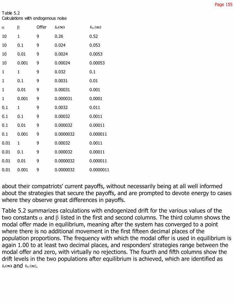
Page 155

Table 5.2Calculations with endogenous noise

a b Offer

10 1 9 0.26 0.52

10 0.1 9 0.024 0.053

10 0.01 9 0.0024 0.0053

10 0.001 9 0.00024 0.00053

1 1 9 0.032 0.1

1 0.1 9 0.0031 0.01

1 0.01 9 0.00031 0.001

1 0.001 9 0.000031 0.0001

0.1 1 9 0.0032 0.011

0.1 0.1 9 0.00032 0.0011

0.1 0.01 9 0.000032 0.00011

0.1 0.001 9 0.0000032 0.000011

0.01 1 9 0.00032 0.0011

0.01 0.1 9 0.000032 0.00011

0.01 0.01 9 0.0000032 0.000011

0.01 0.001 9 0.0000032 0.0000011

about their compatriots' current payoffs, without necessarily being at all well informedabout the strategies that secure the payoffs, and are prompted to devote energy to caseswhere they observe great differences in payoffs.

Table 5.2 summarizes calculations with endogenized drift for the various values of thetwo constants a and b listed in the first and second columns. The third column shows themodal offer made in equilibrium, meaning after the system has converged to a pointwhere there is no additional movement in the first fifteen decimal places of thepopulation proportions. The frequency with which the modal offer is used in equilibrium isagain 1.00 to at least two decimal places, and responders' strategies range between themodal offer and zero, with virtually no rejections. The fourth and fifth columns show thedrift levels in the two populations after equilibrium is achieved, which are identified as

and .

Page 156

Table 5.3Calculations with varying initial conditions

As table 5.2 shows, endogenizing drift leads to an equilibrium in which the responderpopulation is subject to more drift than the pro poser population. It is therefore notsurprising that the equilibrium outcome is not subgame-perfect. The equilibrium offer isagain close to 20%.

How robust are these results? First, consider the question of initial conditions. Thecalculations reported in tables 5.1 and 5.2 are based on a uniform initial distribution ofoffers over . One certainly expects the outcome of the system to be sensitive to initialconditions. Table 5.3 shows the results for some alternative initial conditions, reportingthe modal equilibrium offers for the case of endogenous drift with and . Theentry in row i and column j of table 5.3 is the modal equilibrium offer when the system isstarted from an initial condition in which all proposers play i and all responders play j.Hence the "10"

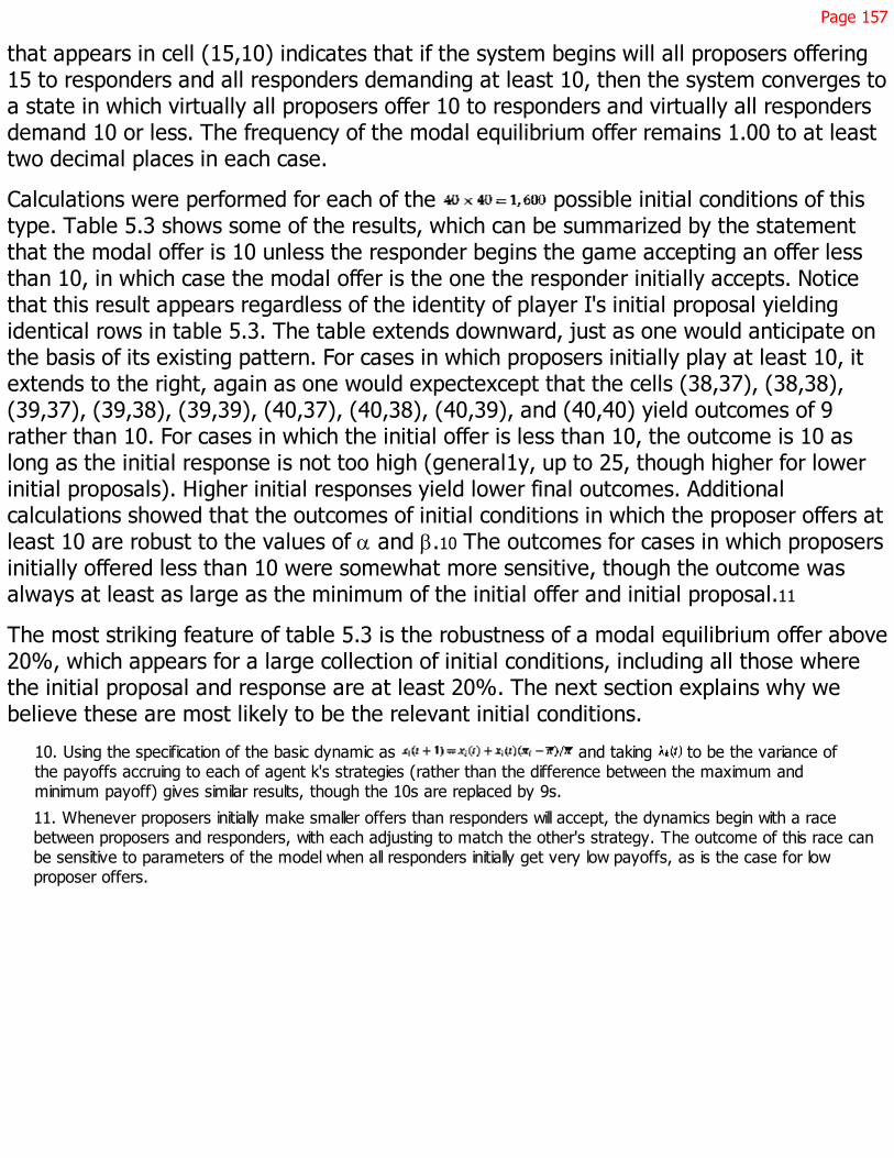
Page 157

that appears in cell (15,10) indicates that if the system begins will all proposers offering15 to responders and all responders demanding at least 10, then the system converges toa state in which virtually all proposers offer 10 to responders and virtually all respondersdemand 10 or less. The frequency of the modal equilibrium offer remains 1.00 to at leasttwo decimal places in each case.

Calculations were performed for each of the possible initial conditions of thistype. Table 5.3 shows some of the results, which can be summarized by the statementthat the modal offer is 10 unless the responder begins the game accepting an offer lessthan 10, in which case the modal offer is the one the responder initially accepts. Noticethat this result appears regardless of the identity of player I's initial proposal yieldingidentical rows in table 5.3. The table extends downward, just as one would anticipate onthe basis of its existing pattern. For cases in which proposers initially play at least 10, itextends to the right, again as one would expectexcept that the cells (38,37), (38,38),(39,37), (39,38), (39,39), (40,37), (40,38), (40,39), and (40,40) yield outcomes of 9rather than 10. For cases in which the initial offer is less than 10, the outcome is 10 aslong as the initial response is not too high (general1y, up to 25, though higher for lowerinitial proposals). Higher initial responses yield lower final outcomes. Additionalcalculations showed that the outcomes of initial conditions in which the proposer offers atleast 10 are robust to the values of a and b.10 The outcomes for cases in which proposersinitially offered less than 10 were somewhat more sensitive, though the outcome wasalways at least as large as the minimum of the initial offer and initial proposal.11

The most striking feature of table 5.3 is the robustness of a modal equilibrium offer above20%, which appears for a large collection of initial conditions, including all those wherethe initial proposal and response are at least 20%. The next section explains why webelieve these are most likely to be the relevant initial conditions.

10. Using the specification of the basic dynamic as and taking to be the variance ofthe payoffs accruing to each of agent k's strategies (rather than the difference between the maximum andminimum payoff) gives similar results, though the 10s are replaced by 9s.

11. Whenever proposers initially make smaller offers than responders will accept, the dynamics begin with a racebetween proposers and responders, with each adjusting to match the other's strategy. The outcome of this race canbe sensitive to parameters of the model when all responders initially get very low payoffs, as is the case for lowproposer offers.

Page 158

How do the results depend upon the specification of drift, that is, on qi and y j? Bychanging these specifications, we can obtain different results. The distribution of driftamong the responders is especially important. If we alter y j to put relatively more weighton offers and responses near zero, equilibrium outcomes can be achieved in which theresponder gets less that 20% of the pie. Causing more weight to be put on somewhathigher offers gives outcomes in which the responders get more than 20% of the pie.

It is interesting to note, however, that changing the values of qi and y j that are attachedto relatively high offers has virtually no effect on the outcome. For example, we canchange the mistake probabilities so that q20 and y20, the probabilities of the "fair" offerand response, take various values up to 0.95 (with the remaining values of qi and y j

remaining equal to one another). We might view this as a case in which the rule of thumbto which most noisy players resort when not paying attention to the game is to split thepie evenly, with a minority of such players adopting completely random rules of thumbthat attach equal probability to all strategies. This change leaves the results of thecalculations virtually unaffected.

It is clear that we cannot place too much significance on the particular value of theequilibrium offer of a little more than 20% that repeatedly emerges in the calculations;and it is important that the re-suits not be remembered for this number Differentspecifications of the model can give different numbers. The important feature of theresults is that the equilibrium offer is frequently far from subgame-perfect; as is the casewith the Ultimatum Minigame, these results persist even when the drift levels are madevery small. Reaching an outcome that is not subgame-perfect requires primarily that theresponding population experience at least as much drift as the proposing population, ormore. But this is the configuration of drift that appears if players are less likely tosuccumb to drift when making decisions that are more important.

5.4 Relevance to Experimental Data?

This chapter opened with an argument that the Ultimatum Game was interesting becauseof the contrast between the theoretical prediction offered by the subgame-perfectequilibrium and experimental results. How do we think the calculations of the previoussection might be rel-

Page 159

evant to the experimental data? This requires a return to the distinction between theshort, medium, long, and ultralong runs, restated briefly as follows:

1. In the short run, experimental behavior is driven primarily by norms that are triggeredby the framing of the problem. If these norms have been strongly reinforced outside thelaboratory, they may be hard to shift. Short-run behavior may accordingly be quitesensitive to framing effects.

2. In the medium run, subjects begin to learnas emphasized by Andreoni and Miller [2],Crawford [65, 66], Miller and Andreoni [158], Roth and Erev [195, 196], and numerousothers.

3. In the long run, this interactive learning process may converge on an equilibrium of thegame.

4. In the ultralong run, there may be jumps between equilibria when random shocks joltthe system from one basin of attraction to another.

In the ultralong run, we can expect an evolutionary process to select the subgame-perfectequilibrium in our version of the Ultimatum Game.12 However, given that ten periods is atypical length for experiments, while fifty periods is a relatively long experiment, it seemsquite unlikely that ultralong-run considerations are relevant to experimental outcomes.

I regard the replicator dynamics as being potentially relevant to the long-run outcome oflearning in the laboratory. In particular, I think the observation that learning can lead toequilibria that are not subgame-perfect, especially in a noisy environment, is analternative to modifications of agents' preferences as an explanation of why thesubgame-perfect equilibrium might not appear in experimental outcomes.

This last statement requires the consideration of two points. First, the claim that we canobtain Nash equilibria that are not subgame-perfect depends upon beginning with initialconditions or with short-run behavior that is not too close to the subgame-perfectequilibrium. Why might we expect this to be the case?

12. This statement relies on proposers being forced to offer responders at least 1, so that accepting is a strict bestresponse in the subgame perfect equilibrium. The outcome is less obvious if zero offers are allowed.

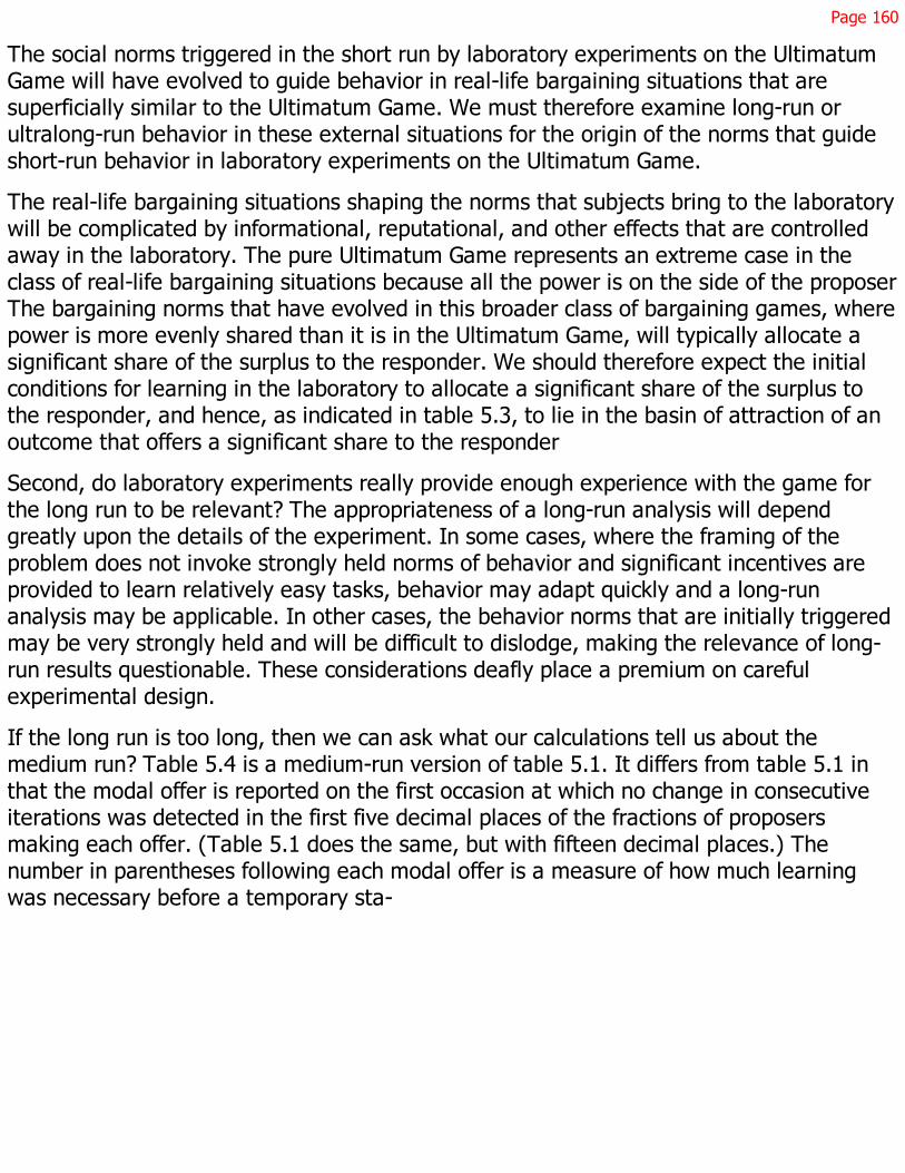
Page 160

The social norms triggered in the short run by laboratory experiments on the UltimatumGame will have evolved to guide behavior in real-life bargaining situations that aresuperficially similar to the Ultimatum Game. We must therefore examine long-run orultralong-run behavior in these external situations for the origin of the norms that guideshort-run behavior in laboratory experiments on the Ultimatum Game.

The real-life bargaining situations shaping the norms that subjects bring to the laboratorywill be complicated by informational, reputational, and other effects that are controlledaway in the laboratory. The pure Ultimatum Game represents an extreme case in theclass of real-life bargaining situations because all the power is on the side of the proposerThe bargaining norms that have evolved in this broader class of bargaining games, wherepower is more evenly shared than it is in the Ultimatum Game, will typically allocate asignificant share of the surplus to the responder. We should therefore expect the initialconditions for learning in the laboratory to allocate a significant share of the surplus tothe responder, and hence, as indicated in table 5.3, to lie in the basin of attraction of anoutcome that offers a significant share to the responder

Second, do laboratory experiments really provide enough experience with the game forthe long run to be relevant? The appropriateness of a long-run analysis will dependgreatly upon the details of the experiment. In some cases, where the framing of theproblem does not invoke strongly held norms of behavior and significant incentives areprovided to learn relatively easy tasks, behavior may adapt quickly and a long-runanalysis may be applicable. In other cases, the behavior norms that are initially triggeredmay be very strongly held and will be difficult to dislodge, making the relevance of long-run results questionable. These considerations deafly place a premium on carefulexperimental design.

If the long run is too long, then we can ask what our calculations tell us about themedium run? Table 5.4 is a medium-run version of table 5.1. It differs from table 5.1 inthat the modal offer is reported on the first occasion at which no change in consecutiveiterations was detected in the first five decimal places of the fractions of proposersmaking each offer. (Table 5.1 does the same, but with fifteen decimal places.) Thenumber in parentheses following each modal offer is a measure of how much learningwas necessary before a temporary sta-

Page 161

Table 5.4Medium-run calculations

0.1 0.01 0.001 0.0001 0

0.1 9(13) 7(74) 7(69) 7(69) 7(69)

0.01 9(15) 9(12) 9(12) 9(12) 9(12)

0.001 9(15) 9(12) 9(12) 9(12) 9(12)

0.0001 9(15) 9(12) 9(12) 9(12) 9(12)

0 9(15) 9(12) 9(12) 9(12) 9(12)

bility in the first five decimal places was achieved.13 In table 5.1, the frequency withwhich modal offers were used was 1.00 to at least two decimal places. The frequencywith which the modal offers were used at the time reported in table 5.4 is at least .98.14

Table 5.4 shows that for all combinations of drift levels, and with uniform initialconditions and perturbations, the system quickly approaches a modal offer of about 20%.But table 5.1 shows this to be a medium-run result; in the long run, the systemsometimes moves away to the subgame-perfect equilibrium. Only when is themedium run behavior a useful guide to the long-run behavior of the system.

Roth and Erev [195] report Ultimatum Game simulations that spend extended periods oftime, in the medium run, near equilibria that are Nash but not subgame-perfect.Explaining the experimental data on the Ultimatum Game as a set of medium-runobservations of a learning process, they apply similar learning models to two othergames, the Best-Shot Game and a market game, in which experimental out comesresemble the subgame-perfect equilibrium much more closely and for which theirsimulations show relatively rapid convergence to the subgame-perfect equilibrium. Thisbolsters the hope that evolutionary models might have something to say aboutexperimental behavior.

13. The measure is the number of iterations of the discrete dynamic described in note 5.3 multiplied by the stepsize t, where t of the population has an opportunity to change strategies in each iteration of the discrete equation.This measure therefore provides a crude approximation to the aggregate number of times that members of theentire population have assessed their strategies.

14. If we ask for stability in only the first three decimal places, the first line of table 5.4 would read 9 (7) 9 (6) 9 (6) 9(6) 9 (6), with the modal offer being played with frequency at least .85 in each case. The remaining lines would beessentially unchanged.

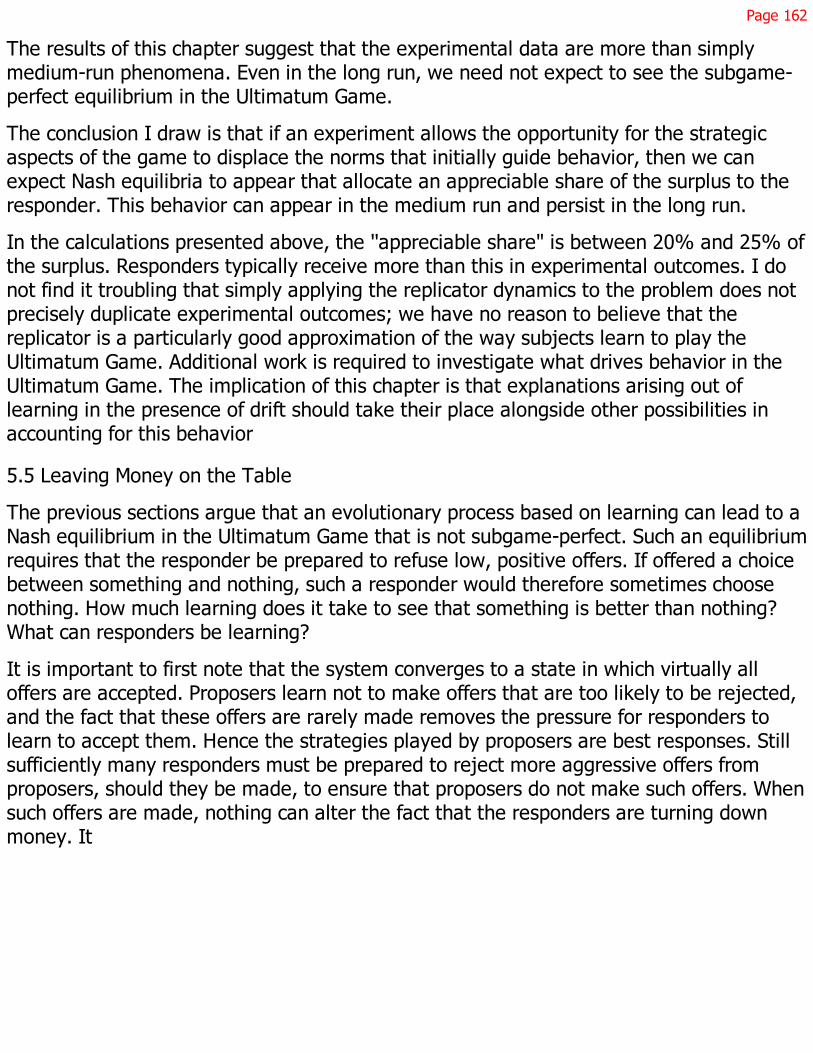
Page 162

The results of this chapter suggest that the experimental data are more than simplymedium-run phenomena. Even in the long run, we need not expect to see the subgame-perfect equilibrium in the Ultimatum Game.

The conclusion I draw is that if an experiment allows the opportunity for the strategicaspects of the game to displace the norms that initially guide behavior, then we canexpect Nash equilibria to appear that allocate an appreciable share of the surplus to theresponder. This behavior can appear in the medium run and persist in the long run.

In the calculations presented above, the ''appreciable share" is between 20% and 25% ofthe surplus. Responders typically receive more than this in experimental outcomes. I donot find it troubling that simply applying the replicator dynamics to the problem does notprecisely duplicate experimental outcomes; we have no reason to believe that thereplicator is a particularly good approximation of the way subjects learn to play theUltimatum Game. Additional work is required to investigate what drives behavior in theUltimatum Game. The implication of this chapter is that explanations arising out oflearning in the presence of drift should take their place alongside other possibilities inaccounting for this behavior

5.5 Leaving Money on the Table

The previous sections argue that an evolutionary process based on learning can lead to aNash equilibrium in the Ultimatum Game that is not subgame-perfect. Such an equilibriumrequires that the responder be prepared to refuse low, positive offers. If offered a choicebetween something and nothing, such a responder would therefore sometimes choosenothing. How much learning does it take to see that something is better than nothing?What can responders be learning?

It is important to first note that the system converges to a state in which virtually alloffers are accepted. Proposers learn not to make offers that are too likely to be rejected,and the fact that these offers are rarely made removes the pressure for responders tolearn to accept them. Hence the strategies played by proposers are best responses. Stillsufficiently many responders must be prepared to reject more aggressive offers fromproposers, should they be made, to ensure that proposers do not make such offers. Whensuch offers are made, nothing can alter the fact that the responders are turning downmoney. It

Page 163

seemingly takes very little learning to know that this is not a good thing to do.

Because the issues appear to be so dear, behavior such as rejecting a positive offer isoutlawed in conventional economic modeling. Perhaps for this reason, a commonresponse to this chapter's argument is an incredulous "Why would anyone leave moneyon the table?" This comment is generally followed by an assertion that we must look toalternative models of players' preferences to explain such behavior. It is always useful toremind ourselves that all models are approximations; thus the commonly used, simplemodel of the Ultimatum Game is unlikely to capture players' preferences exactly. While itis important to develop richer models of preferences, it is also important to realize thatresponders do have something to learn in the Ultimatum Game and that the outcome ofthe learning process may not be a subgame-perfect equilibrium, even if players'preferences are exactly captured by the monetary payoffs of the game.

That positive offers should be refused in the short run is easy to understand. Short-runbehavior in the Ultimatum Game is likely to be governed by social norms that aretriggered by the framing of the laboratory experiment. Rather than being adapted to thepure Ultimatum Game, such social norms will have evolved for use in everyday relativesof the Ultimatum Game. In everyday life, however, we rarely play pure take-it-or-leave-itgames. In particular, real-life games are seldom played under conditions of totalanonymity; a refusal of something positive may therefore serve to maintain a reputationfor toughness. For example, in the take-it-or-leave-it auction used by stores to sell theirgoods, a refusal of something positive may simply indicate a willingness to preserve areputation for not taking such offers. Norms that call for refusals in commonly occurring"take it or leave it" situations therefore make good evolutionary sense. Given that suchnorms exist, it is unsurprising if they are sometimes inappropriately triggered inlaboratory experiments. Short-run refusals of positive offers in the pure Ultimatum Gametherefore create no problem for orthodox game theory.

I have argued, however, that Nash equilibria that are not subgame-perfect should betaken seriously even in the long run. This requires that responders in a noisy environmentstand ready to reject some positive offers. On this subject, it is useful first to observe thatpeople clearly do sometimes leave money on the table. Frank

Page 164

[80], for example, reminds us that nearly everyone, including economists, leave tips inrestaurants, even in restaurants they do not plan to revisit.

One may ask why we leave money on the table. In the case of tipping, most people aresatisfied with the explanation that leaving a tip is a custom it would be uncomfortable toviolate. If pressed, they might again appeal to modifications of the utility function,perhaps attributing the discomfort to the unfairness involved in disappointing the server'sexpectations.

Such considerations have led a number of authors to downplay strategic explanations ofexperimental behavior in favor of various theories of "fair play." Sophisticated versions ofthis approach sometimes build a taste for "fairness" into the utility functions attributed tothe subjects. Ochs and Roth [181] discuss such considerations in explaining the results ofan alternating offers bargaining experiment. Bolton [37] and Levine [140] explicitlyconstruct such utility functions for this purpose.15

I agree that subjects find their emotions engaged in bargaining situations. They alsofrequently explain their bargaining behavior in the laboratory in terms of "fairness." Butan approach that takes these facts at their face value is in danger of explaining too muchand too little. Fairness theories explain too much because, by choosing one's fairnessnotion with sufficient care, one can justify a very wide range of outcomes. At the sametime, such theories explain too little because they provide no insight into the origin of thefairness norms to which appeal is made.

A more fruitful approach is to ask how the custom of leaving money on the table cansurvive. I think the answer is quite simple. The amounts involved and the frequency withwhich the situation arises are too small to provide sufficient evolutionary pressure toeliminate the phenomenon in a noisy environment.

If this is the case, what of the folk explanation in terms of the discomfort felt at violatinga fairness norm? In responding to such a question, it is important to appreciate that theevolutionary approach reverses the standard explicans and explicandum of the folkexplanation and of an optimizing interpretation of economic theory. The players in anevolu-

15. Fudenberg and Levine [90] provide a method for investigating how irrational subjects must be if experimentalresults are generated by a process in which subjects are learning to play a self-confirming (Fudenberg and Levine[91]) equilibrium.

Page 165

tionary model are not members of the species Homo economicus. They do not optimizerelative to fixed preferences. They simply have decision rules for playing games. When aplayer switches from a less profitable to a more profitable strategy, he does not do sobecause he thinks that the switch is optimalhe is simply acting as a stimulus-responsemechanism.

If people are simply stimulus-response machines, what role is left for feelings such asanger or discomfort that are often invoked to explain actions? In answering this question,we must again keep careful track of what causes what. It is easy to say that I preferredto take this foolish action rather than that wise action because I got angry. But angryfeelings are a reflex to certain stimuli; such reflexes survive because the behaviors theyinduce have evolutionary advantages. Rather than seeking to explain a particularbehavior in terms of the angry feelings that accompany it, we would do better to explainthe angry feelings in terms of the evolutionary advantages of the behavior. In brief, beingangry or fearful or amorous is how it feels to be a stimulus-response mechanism. Anger isuseful because it often leads us to reject offers when there are good reasons for doing so.Unfortunately, players sometimes misread the strategic situation in which they findthemselves, with the counterproductive result that an inappropriate response is triggeredand reinforced by rising emotions.

Of course, none of us likes to admit that much of our behavior is little more than a set ofconditioned reflexes; we prefer to offer more flattering rationalizations of the behavior.For example, the stimulus of receiving an offer of only 10% in the Ultimatum Game maybe sufficiently irritating that we turn the offer down. If asked why we refused, we maythen rationalize our behavior by arguing that irritation is an entirely appropriate responseto an "unfair" offer of 10%. Such an explanation may become institutionalized and thusmay reinforce the behavior that it "explains." But I see no reason to believe that fairnessnorms are fixed and immutable. I believe that players usually find their way to a long-runequilibrium by trial-and-error learning without having any dear understanding of thestrategic realities of the game they are playing. They simply learn that certain stimulus-response behaviors are effective; after the game, they may rationalize their behavior invarious ways. In bargaining experiments, they often say that the long-run equilibrium towhich they found their way is fair. But, from an evolutionary perspective, how theyexplain their own behavior to themselves and others is beside the point. If they hadfound their way

Page 166

to another equilibrium, they would be offering some other explanation.16 Economists whofit a particular utility function to observed behavior would similarly find themselvesproposing a different utility function.

Because I think notions such as fairness are affected by behavior, I believe that attentionis most usefully focused on the evolution of behavior. If a type of behavior that promptspeople to leave money on the table survives, it will be because there is insufficientevolutionary pressure to remove it. Fairness explanations may be offered asrationalizations of the behavior. Such stories may even be incorporated into the workingsof the stimulus-response mechanism. But the details of how the mechanism actuallyworks or how we explain its workings to ourselves are secondary. The primaryconsideration is why some behavior patterns survive in a population, while othersnecessarily perish.

All of this leaves unanswered the question, what do agents have to learn? I haveappealed to insignificant evolutionary pressure as the reason for refusing money, but whydoes it take any pressure to learn to accept something rather than nothing? What playershave to learn is that the Ultimatum Game is different from the situations in which theyusually find themselves, and that it is worthy of an independent analysis rather than theapplication of an "off-the-shelf" decision rule that evolved for use in other games. I do notthink the Ultimatum Game, nor any game, is so simple that this need not be learned.Instead, people are constantly engaged in so many decisions that very few are analyzed,with most being made by applying one of a relatively short list of existing decision rules.People have learned from experience that it generally works better to apply a familiar,seemingly appropriate decision rule to a problem than to do a more thorough analysis.17

Only through experience with a game do players come to recognize it as being sufficientlydifferent and sufficiently important to warrant its own

16. In Binmore et al. [30], the median long-run equilibrium claim in a laboratory implementation of the NashDemand Game turns out to be a very good predictor of the median claim said to be fair in a computerizedpostexperimental debriefing, even though subjects are randomly chosen for an initial conditioning that directs theirsubsequent play to different long-run equilibrium claims.

17. For example, most computer users have learned that when unpacking a new computer, it generally works betterto plug the machine in and turn it on rather than first read the folder prominently marked "READ ME FIRST."

Page 167

analysis.18 By the time such experience has been accumulated with the Ultimatum Game,proposers may already have learned not to make aggressive offers, and the faintincentives remaining for responders to analyze and accept such offers may beinadequate.

Do the replicator dynamics capture this learning process? Perhaps not, nor do I have analternative model of the process. However, the replicator shares with the process the keycharacteristics that responders cannot be expected to automatically accept all offers,even without appealing to other models of preferences. I regard additional work on thistype of learning as being very important, and I suspect that it may take us well outsidethe usual realm of both Bayesian and adaptive learning models.


Proof of Lemma 5.1

Writing and in (5.3)-(5.4) yields (x, y) equal to (1, 0), (0, 0) and (x, 1)as candidates for the limit points of R. Recall that y is the probability with which player Iplays H and x is the probability with which player II plays Y, so that (0, 0) is thesubgame-perfect equilibrium. The first point is a source for the unperturbed dynamics andis easily excluded as a limit point of R. We now consider the possible values of x. To thisend, write in (5.3)-(5.4) and then set y = 1. We then obtain the equation

,

where . This equation has two solutions, and , satisfying, when . In this case, ( , 1) and ( , 1) are contained in the

component of Nash equilibria . When , the equation has no solutions x satisfying.


The proof of the first statement is straightforward, and we consider only the second. Theright side of (5.3)-(5.4) defines a function F: for which

18. Interestingly, the realization that a new problem requires analysis may be more likely to appear when the gameis an obvious departure from ordinary experience than with a seemingly familiar game. As a result, performance onnew problems may actually be better if they are less familiar.

Page 168

DF(y,x)

.

The trace of this matrix is negative when and . We therefore consider thelimiting value of its determinant.

Multiply the second column of detDF(y,x) by 1 - 2x and then make the substitution, which holds at a rest point by virtue of (5.3)-(5.4). Factor out

the term and write and y = 1 in what remains. We then have tosign the determinant

.

The roots of the quadratic equation are and . It follows that thedeterminant is positive when and negative when . Thus isasymptotically stable and is not.

Page 169

6Drift

6.1 Introduction

Chapter 5 argued that while simple models of learning can direct players to Nashequilibria in the Ultimatum Game in which player II receives a significant share of thesurplus, this alone is insufficient to justify an interest in such equilibria. The equilibriahave a compelling claim on our attention only if they satisfy an appropriate stabilityproperty. In the case of the Ultimatum Game, the stability of such equilibria initially looksdoubtful. Perturbations in the offers made by proposers can only bring pressure onresponders to accept offers, pushing the system toward the subgame-perfect equilibrium.We also have good reason to take such perturbations seriously. The world contains manyimperfections that we conceal when formulating a game, but which reappear in the formof perturbations to any equilibrating process used to model how interactive learning leadssubjects to an equilibrium of a game.

Chapter 5 then argued that in order to investigate these questions, we should expand ourmodel to include such perturbations. Upon doing so, we find that the nature of theperturbations can be very important, and the perturbations can play a key role instabilizing Nash equilibria that are not subgame-perfect.

This chapter broadens the study of perturbed equilibriating processes. Retaining the termdrift to summarize the imperfections that may perturb an equilibriating process, thechapter investigates when drift matters and what we can say about equilibrium selectionwhen it does.1

1. This chapter reports work in progress; for a more detailed report, including proofs, see Binmore and Samuelson[27].

Page 170

The question of refining a Nash equilibrium typically arises when equilibrium strategiesare accompanied by alternative best replies, which raise the question of whether theplayer can reasonably or "plausibly" be expected to choose her equilibrium strategyrather than some other best reply. If a refinement answers this question negatively, thenit rejects the Nash equilibrium. In learning models these same alternative best replieslead to stationary states of the adjustment dynamics that occur in components ratherthan being isolated. The experience of the Ultimatum Minigame is typical where we find acomponent containing the pure strategy equilibrium (H, N). The learning dynamics oftenlead toward some parts of such a component and away from other parts. As a result, thestability properties of the component hinge upon the small shocks that cause the systemto drift between equilibria within the component. If this drift pushes the system towardstates where the learning dynamics lead away from the component, then the componentas a whole will not be stable. If the drift pushes the system toward equilibria where thelearning dynamics lead toward the component, then the component will be stable, andthe component of equilibrium is potentially a long-run prediction of how the game will beplayed.

The recognition that drift can be important might appear to vanquish all hopes forempirical applications of game theory. What good is a theory whose implications dependupon the details of perturbations that may be very small and hence very difficult toobserve? To answer this question, let us return to the example set by work withnonstrategic economic theories. Conventional economics regularly works with theoriesinvolving unobservable elements; it calculates the effect of altering observable aspects ofa particular model while assuming unobservable features remain constant. Accordingly,we shall investigate the implications of manipulating the aspects of a game that we canreasonably hope to observe, namely the payoffs, while maintaining the hypothesis thatthe process by which players learn and the specification of drift remain constant. Thisleads to comparative statics predictions, concerning how the long-run outcome of playvaries as the payoffs of the game vary, that may be useful in applied work.Understanding drift may then open rather than close the door to applications of gametheory.

6.2 The Model

Let G denote a game with n players. As usual, we will think of this game being played byagents drawn from n populations. However, it

Page 171

will often be convenient to say simply that "player I plays strategy B with probability a"when the precise statement would be that "a proportion of the agents in population Iplay B."

Let be the strategy set for player . Then a state for population is an -dimensional vector of nonnegative numbers whose sum equals one.2 Such a vector isinterpreted as listing the fraction of agents in population playing each of the purestrategies in . A state of the entire system is a vector identifying the state ofeach population. Let Z be the set of such states.

Selection

We now think of the choices made by the agents in this game as being determined by anevolutionary process in which agents drawn from finite populations are repeatedlymatched to play the game and adjust their strategies in light of their experience. TheAspiration and Imitation model of chapter 3 is one example of such a process. Thischapter will allow a broader class of models, though the assumption will be maintainedthat the choices resulting from this process can be described by a Markov process overthe state space Z. Hence the state in which the system will next be found is a randomvariable that depends only upon the current strategies played by the various agents.Notice that strategy adjustments are potentially noisy; in the sense that knowing thestate at time t may allow us to identify only a probability measure describing the likelyidentity of the next state.

We shall be focusing on the long-run behavior of our model when the populations arelarge. Chapter 3 indicates that the point of departure for such an analysis is aspecification of the expected state at time , given that the state at time t is . Letthis expectation be given by

To interpret (6.1), we can think of F as capturing the important forces that govern agents'strategy revisions. I refer to F as the "selection process." In a biological context, F modelsa process of natural

2. Chapter 3 generally used x to refer to a state drawn from a one-dimensional state space, while the next twochapters used x and y to refer to the strategy vectors of two populations. The analysis in this chapter is notrestricted to either one dimension or two players, and uses z to denote a state.

Page 172

selection driven by differences in fitness. The primary force behind the selection processhere is that agents playing some strategies are likely to have more offspring than others.In the models of Young [250] and of Kandori, Mailath, and Rob [128], F models a best-response learning process driven by differences in payoffs, where the primary forcedriving selection is that when agents choose their strategies, they switch to bestresponses given the current population state. In the Aspiration and Imitation model Fmodels the result of agents periodically receiving payoff realizations that fall short of theiraspiration level prompting the agents to imitate others.

To study the evolutionary process, we might then begin by simply examining theselection process F, taking this to be a good model of the underlying process. Forexample, we could study best-response dynamics in an economic setting or the replicatordynamics in a biological setting. However, we must recognize that, like any model theselection process is an approximation, designed to capture the important features of aproblem, while excluding other considerations. Our hope when constructing the model isto include sufficiently few features of the actual situation in the specification of F as tomake the model tractable, but sufficiently many to make the model a usefulapproximation.

The features that have been excluded from the selection mechanism F are described byG. In a biological application, G models mutations, which are random alterations in thegenetic structure of an individual. In the models of Young [250] and of Kandori, Mailath,and Rob [128], G models random alterations in agents' strategies. In the Aspiration andImitation model, G is again described as mutations, though these are viewed as mistakesin copying the strategies of others rather than biological phenomena. I shall refer to theforces captured by G as ''noise."

Given that the selection mechanism F is designed to capture the important forces behindstrategy choices, the events represented by G are likely to be relatively improbable.Hence we are interested in the case of small noise. The difficult issue of determining howsmall is "small" is generally handled by examining the limit as the events captured by thenoise G become arbitrarily improbable. It is helpful to have notation that facilitatesexamining this limit; hence, instead of thinking of reductions in the amount of noise aschanging the specification of G, we can think of G as being fixed and insert the parameterl in (6.1). Reductions in the amount of noise are then taken to be reduc-

Page 173

tions in l. I shall refer to l as either the "noise level" or the "drift level."3

The stochastic selection process and the expression in (6.1) for its expected outcomemay be quite complicated. It would be helpful to have some simple techniques availablefor studying this process. If we assume that the derivatives of F and G exist and arebounded, then we can take a Taylor expansion of (6.1) to obtain

where f and g are the appropriate derivatives of F and G. It will be useful to bear in mindthat the original stochastic process (6.1) is written as and not simply F. Hence theterm ) that appears in (6.2) is not the remainder from a Taylor expansion of theunderlying selection process F, capturing errors that arise out of replacing F by a localapproximation. Instead, we can view the selection process F itself as an approximationrather than an exact model of the underlying stochastic evolutionary process, with G andhence representing factors excluded from F.

Long-Run Dynamics

To study long-run behavior, we can now rearrange (6.2) to give

The next step is to follow the example of chapter 3 in taking the limits t and ,where N is the size of each of the populations. The latter limit suggests that, by the lawof large numbers, we should be able to remove the expectation from the left side of(6.3); the former limit suggests we should then be able to replace the left side of (6.3)with a derivative, yielding

a deterministic differential equation defined on the set given by theproduct of the n simplexes , where

3. This specification clearly imposes some restrictions on the way in which noise becomes small. As Bergin andLimpan [13] show, these restrictions can be important in an ultralong-run analysis. I return to this point in chapter7. This restriction could easily be eliminated from this chapter, but only at the expense of replacing statements ofthe form "for all sufficiently small drift levels" with slightly more cumbersome statements.

Page 174

z(t) is the population state at time t. In chapter 3, the counterpart of (6.4) was theperturbed replicator dynamic given by (3.5).

The step from (6.3) to (6.4) is often justified informally. Chapter 3 showed that this stepcan be made formally; with the deterministic differential equation (6.4) providing anarbitrarily good long-run approximation of the behavior of the stochastic process by whichstrategies are adjusted, so long as we are interested in large populations.4

If we assume that f and g are continuously differentiable, and also Lipschitz-continuous,on an open set containing the state space Z, we ensure that there exists a unique,continuously differentiable solution z = z(t, z(0)), specifying the state at time t, giveninitial condition z(0), that satisfies (6.4) (Hale [111, chapter 1]; Hirsch and Smale [118,chapter 8]). Let us further assume that the state space Z is forward-invariant under thissolution, so that once the solution is an element of Z, it never leaves Z. Coupled withdifferentiability and the compactness of Z, this ensures that we encounter no boundaryproblems when working with the dynamic. Similarly, there exists a unique solution to theequation dz/dt = f(z), which we can again assume renders the state space Z forward-invariant. Common examples such as the replicator dynamics satisfy these assumptions.

What are the crucial assumptions in this development? First, the underlying stochasticselection process is a Markov process, with strategy revisions depending on only thecurrent state. This is potentially a very strong assumption, which may require players toforsake a long history of experience in order to react to an idiosyncratic current state. Theextent to which this assumption is reasonable depends upon the nature of the selectionprocess we have in mind. If agents are occasionally collecting information about others'play and choosing best responses, it is quite likely that they most readily collectinformation about current or recent play, and the Markov assumption may then not be toounrealistic. If strategy revisions are a response to one's own payoffs, as in the Aspirationand Imitation model, then the Markov assumption is more demanding. Much of thelearning literature focuses on Markov models because of their tractability. The relaxationof this assumption is an important topic for future work.

4. The long-run approximation result is established in chapter 3 for the special case of a one-dimensional statespace, but the argument is easily adapted to our more general case. The result is that for any time T and any Î,we can choose sufficiently large N and sufficiently small t (in particular, small enough that is small enough) thatthe outcome of the stochastic strategy adjustment model at time , is within of the expected value given by(6.4) with probability at least .

Page 175

The second assumption is that the differential equation (6.4) is continuouslydifferentiable. This smoothness requirement excludes pure best-response behavior,where even an arbitrarily small difference in payoffs suffices to switch all agents to thehigh-payoff strategy (and in the process may make the Markov assumption moredemanding). I consider this a realistic assumption. I do not think that dramatic changes inbehavior are prompted by arbitrarily small differences in payoffs; instead, I expect smallpayoff differences to prompt small or slow shifts in behavior, with people being morelikely to switch strategies as the payoff differences from doing so increase. A smoothlearning process provides a good first approximation of this behavior.

If the model is well constructed, meaning that the payoffs are a good representation ofpreferences and f captures the important forces behind strategy revisions, then we canexpect f to be closely linked to payoffs. The drift term g, however, may have little ornothing to do with the payoffs of the game. Instead, considerations excluded from themodel when specifying the game and its payoffs may play a major role in shaping g. Insome circumstances, drift may be completely unrelated to payoffs. This is the case inmany biological models of mutation as well as in the models of Young [250] and ofKandori, Mailath, and Rob [128].

The relative importance of drift is measured by l. I shall refer to G and l as "noise" andthe "noise level," when working with the underlying stochastic evolutionary process, butshall refer to g and l as ''drift" and the "drift level" when working with the approximation(6.4), where all of the randomness in the system has been smoothed away. In theprevious two chapters, the possibility of different drift levels in different populations wasemphasized; the role of l was played by and . In this chapter, any such asymmetrieswill be captured in the specification of g.

Drift

We shall think of l as being small, reflecting the belief that important considerationshave been captured by the selection process f. This follows in the footsteps of biologicalmodels and especially the models of Young [250] and of Kandori, Mailath, and Rob [128],where the mutations that introduce noise into the models are taken to be arbitrarilyimprobable.

Page 176

Given that we are interested in the case in which drift is very small two questions arise.When can we simplify our analysis further by ignoring drift? This would involve replacing(6.4) with

If drift cannot be ignored, then what can be said about the outcomes of the model?

In a biological model, ignoring drift often takes the from of ignoring the possibility ofmutations and simply examining the replicator dynamics. As long as the initial conditionsof the latter are modeled as being in the interior of the state space, so that all strategiesare initially present, this often creates no problems. In an economic context, ignoring driftoften takes the from of concentrating on the pure best-response dynamics, ignoring otherforces that may perturb strategy choices. In the analysis of the Ultimatum Game of theprevious chapter, ignoring drift took form of setting and examining theunperturbed replicator dynamics.

The answer to the question of whether drift can be ignored depends upon what length oftime we are interested in. If the ultralong run is of interest, then the question must bereformulated. To study the ultralong run, we must examine the asymptotic behavior ofthe original Markov process directlyrather than studying the deterministic approximation(6.4) obtained by taking expectations. The question is then not whether the drift given byg matters, but whether the noise captured by G matters. Chapter 2 noted that thestationary distribution of a Markov process can be radically changed by minute changes inone of its transition probabilities, especially if this makes a zero probability positive.Young [250] and Kandori, Mailath, and Rob [128] exploit precisely this dependence toobtain their strong, ultralong-run, equilibrium selection results.

Alternatively, we may be interested in medium-run results. To study the medium run, itsuffices to fix a value of T > 0 and to study the behavior of (6.5) for . Over such arestricted range, the solutions to (6.4) and (6.5) are arbitrarily close if l is sufficientlysmall. The following is a well-known continuity property of differential equations:

Lemma 6.1

Let z(t, z(0), l) solve (6.4), given initial condition z(0) and drift level l, and let z(t, z(0),0) solve (6.5) with the identical initial condition z(0). Then for any and , thereexists such that for if and , then .

Page 177

This result indicates that we can ensure that the trajectories of the system with drift andthe system without drift can be kept as dose together as we want for as long as we want,provided the drift level is sufficiently small. Small amounts of drift can then be ignored.

Sánchez [203, theorem 6.3.1] provides a proof based on the following intuition. If bothsystems start from a common initial condition, and if l is small, then the solutions to fand cannot diverge too quickly. They will diverge, however, so that f and willsoon be evaluated at nearby but different states. As long as l is sufficiently small,however, the Lipschitz continuity of f ensures that the behavior of the two systems is nottoo different when evaluated at states that are not too far apart, and hence the twosystems still do not grow apart too fast. There is then an upper bound on how far apartthe two solutions can grow over the time interval [0, T], with this bound decreasing tozero as l decreases to zero.

Lemma 6.1 does not tell us that the long-run behaviors of (6.4) and (6.5) are similarwhen l is small. For example, the analysis of the Ultimatum Minigame of the previouschapter indicates that the asymptotic behavior of the solution to (6.5) need notapproximate the asymptotic behavior of a solution to (6.4), no matter how small is l.5This indicates that the limits and do not commute. First taking to obtain(6.5) and then studying the limiting behavior of this system ( ) need not lead to thesame conclusions as first studying the limiting behavior of (6.4) and then allowing .

The Chain-Store Game

To clarify the relationship between drift and the long run, consider the game shown infigure 6.1. Assume that the payoffs in this game satisfy the inequalities , so thatthe player I prefers E if player II chooses A, but player I prefers N if player II chooses R.In addition, b > d, so that if player I chooses E, then player II prefers A. This game thenhas the same qualitative features as Selten's Chain-Store Game [209], shown in figure1.1: a weakly dominated strategy for player II (given by R), a strict Nash equilibrium(given by (E, A)), and a component of weak Nash equilibria in which player I chooses

5. For example, (6.5) corresponds to the phase diagram shown in figure 5.3, while an appropriately specifiedversion of (6.4) corresponds to figure 5.4. The former has a component of stationary states, and potential long-run outcomes, while the latter has only S as a stationary state.

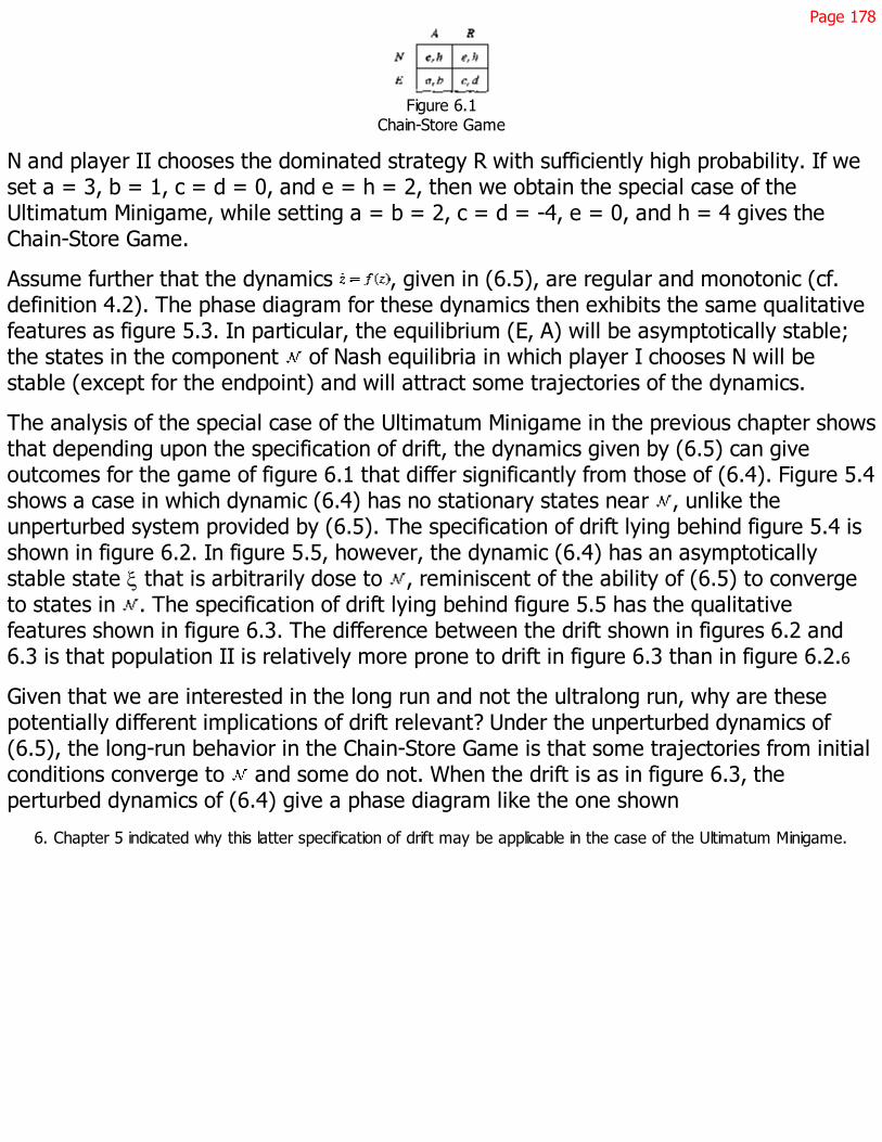
Page 178

Figure 6.1Chain-Store Game

N and player II chooses the dominated strategy R with sufficiently high probability. If weset a = 3, b = 1, c = d = 0, and e = h = 2, then we obtain the special case of theUltimatum Minigame, while setting a = b = 2, c = d = -4, e = 0, and h = 4 gives theChain-Store Game.

Assume further that the dynamics , given in (6.5), are regular and monotonic (cf.definition 4.2). The phase diagram for these dynamics then exhibits the same qualitativefeatures as figure 5.3. In particular, the equilibrium (E, A) will be asymptotically stable;the states in the component of Nash equilibria in which player I chooses N will bestable (except for the endpoint) and will attract some trajectories of the dynamics.

The analysis of the special case of the Ultimatum Minigame in the previous chapter showsthat depending upon the specification of drift, the dynamics given by (6.5) can giveoutcomes for the game of figure 6.1 that differ significantly from those of (6.4). Figure 5.4shows a case in which dynamic (6.4) has no stationary states near , unlike theunperturbed system provided by (6.5). The specification of drift lying behind figure 5.4 isshown in figure 6.2. In figure 5.5, however, the dynamic (6.4) has an asymptoticallystable state x that is arbitrarily dose to , reminiscent of the ability of (6.5) to convergeto states in . The specification of drift lying behind figure 5.5 has the qualitativefeatures shown in figure 6.3. The difference between the drift shown in figures 6.2 and6.3 is that population II is relatively more prone to drift in figure 6.3 than in figure 6.2.6

Given that we are interested in the long run and not the ultralong run, why are thesepotentially different implications of drift relevant? Under the unperturbed dynamics of(6.5), the long-run behavior in the Chain-Store Game is that some trajectories from initialconditions converge to and some do not. When the drift is as in figure 6.3, theperturbed dynamics of (6.4) give a phase diagram like the one shown

6. Chapter 5 indicated why this latter specification of drift may be applicable in the case of the Ultimatum Minigame.

Page 179

Figure 6.2Drift for figure 5.4

Figure 6.3Drift for figure 5.5

in figure 5.5. Once again, the conclusion is that some trajectories converge to andsome do not. When drift is as in figure 6.2, the perturbed dynamics of (6.4) give a phasediagram like that of figure 5.4. Some trajectories in figure 5.4 converge to S withoutcoming near ; other trajectories do not converge to , but do come very close to . Inaddition, the rate of movement of the dynamic system is very slow near the component of Nash equilibria because payoff differences are small, and hence learning forces areweak near such a component, while drift is also assumed to be small. As a result, thetrajectories that come close to will spend a very long time near . Thus is interestingin the medium run, even when the equilibrium that will be selected in the long run is S.Because the medium run can be very

Page 180

long, why must we go further to a long-run analysis?7 Why do we care whether somespecifications of drift lead to asymptotically stable states near ?

The difference between the cases shown in figures 5.4 and 5.5, and the relevance of drift,hinges on what is meant by small and by long run. In figure 5.4 an argument for therelevance of over a long period of time must presume that drift is sufficiently small andthe initial condition places sufficient weight on the strategies H and N because otherwisethe system will leave the neighborhood of too quickly. The longer the time period ofinterest, the more stringent are these requirements. In contrast, the conditions for theapplicability of are much less demanding in figure 5.5, requiring only that the initialcondition lie in the basin of attraction of x, at which point we can be confident that thesystem will not stray from the vicinity of over any arbitrarily long time period. Studyingdrift is then important because drift can make an outcome such as a good prediction oflong-run behavior under a much wider range of circumstances.

6.3 When Can Drift Be Ignored?

The Chain-Store Game, including the special case of the Ultimatum Minigame, shows thatthere are cases in which drift matters. When does it matter?

Structurally Stable Stationary States

A stationary state of a differential equation is hyperbolic if the Jacobian matrix of thedifferential equation, evaluated at the stationary state, has no eigenvalues with zero realparts. Hyperbolic stationary states are isolated and are either sources, saddles, or sinks(Hirsch and Smale [118, chapter 9]). Stationary states that appear as members ofconnected components are thus not hyperbolic, although there are also isolatedstationary states that are not hyperbolic.

For our purposes, the important characteristic of hyperbolic stationary states is that theyare "structurally stable." Small perturbations of the specification of the dynamic systemcannot destroy a hyperbolic stationary state and cannot alter its stability properties. Inparticular,

7. The analysis of Roth and Erev [195] is based on speed-of-adjustment arguments of this type.

Page 181

proposition 6.1.1 follows immediately from the continuity of f and g on the compact set Z,while proposition 6.1.2 follows from Hirsch and Smale [118, theorems 1-2, p. 305]:8

Proposition 6.1.1

For any , there exists such that for any , every stationary state of lieswithin Î of a stationary state of f.

Proposition 6.1.2

Let z be a hyperbolic stationary state of f. Then has a hyperbolic stationary statez(l) that converges to z as l converges to zero, with each z(l) being a sink (saddle)[source] if and only if z is a sink (saddle) [source].

Propositions 6.1.1and 6.1.2 indicate that, if we are working with hyperbolic stationarystates of f, then we can ignore drift and work with rather than . Thestationary states of f provide approximate information concerning stationary states of

that lie nearby and are of the same type. The approximation becomes arbitrarilysharp as l gets small. The considerations that are excluded when is replaced by f donot have a signficant effect on the results, at least if l is small, and might reasonably beignored in the interest of tractability.

Nonhyperbolic stationary states do not have this structural stability. An arbitrarily smallchange in the dynamic system, or equivalently an arbitrarily small amount of drift, cancompletely change the nature of a nonhyperbolic stationary state.

For some, these observations resolve the issue of whether drift is important. It is oftensaid that almost all dynamic systems have only hyperbolic stationary states. The Peoxitotheorem (Hirsch and Smale [118, p. 314]) shows that for two-dimensional systems, thereis a precise sense of "almost all" for which this statement holds; a similar re-suit holds inhigher dimensions for certain classes of dynamic systems, such as linear and gradientsystems [118, pp. 313-315]. In the words of a mathematician, "Why worry about theexceptional cases" in which stationary states are not hyperbolic?

The answer is that the economics of the applications to which learning models areapplied often forces us to confront nonhyperbolic stationary states. To see this, we needonly recall that hyperbolic stationary states must be isolated. As a result, a Nashequilibrium that

8. For convenience, I shall often write simply f and for and , respectively.

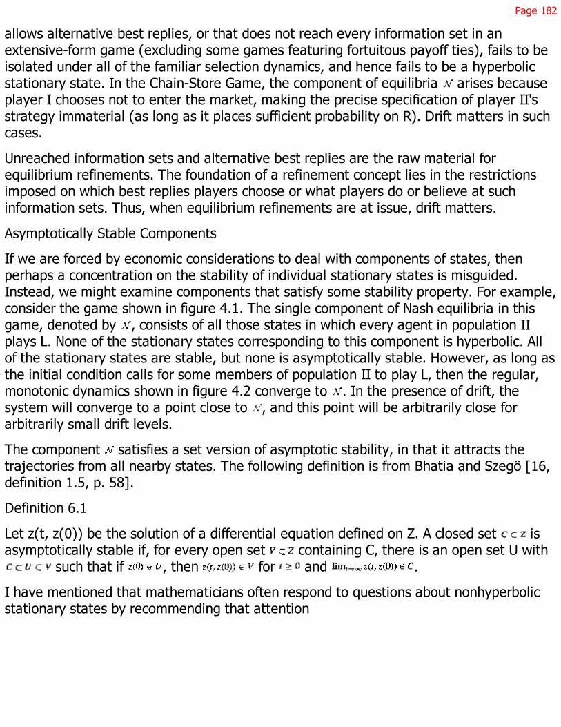
Page 182

allows alternative best replies, or that does not reach every information set in anextensive-form game (excluding some games featuring fortuitous payoff ties), fails to beisolated under all of the familiar selection dynamics, and hence fails to be a hyperbolicstationary state. In the Chain-Store Game, the component of equilibria arises becauseplayer I chooses not to enter the market, making the precise specification of player II'sstrategy immaterial (as long as it places sufficient probability on R). Drift matters in suchcases.

Unreached information sets and alternative best replies are the raw material forequilibrium refinements. The foundation of a refinement concept lies in the restrictionsimposed on which best replies players choose or what players do or believe at suchinformation sets. Thus, when equilibrium refinements are at issue, drift matters.

Asymptotically Stable Components

If we are forced by economic considerations to deal with components of states, thenperhaps a concentration on the stability of individual stationary states is misguided.Instead, we might examine components that satisfy some stability property. For example,consider the game shown in figure 4.1. The single component of Nash equilibria in thisgame, denoted by , consists of all those states in which every agent in population IIplays L. None of the stationary states corresponding to this component is hyperbolic. Allof the stationary states are stable, but none is asymptotically stable. However, as long asthe initial condition calls for some members of population II to play L, then the regular,monotonic dynamics shown in figure 4.2 converge to . In the presence of drift, thesystem will converge to a point close to , and this point will be arbitrarily close forarbitrarily small drift levels.

The component satisfies a set version of asymptotic stability, in that it attracts thetrajectories from all nearby states. The following definition is from Bhatia and Szegö [16,definition 1.5, p. 58].

Definition 6.1

Let z(t, z(0)) be the solution of a differential equation defined on Z. A closed set isasymptotically stable if, for every open set containing C, there is an open set U with

such that if , then for and .

I have mentioned that mathematicians often respond to questions about nonhyperbolicstationary states by recommending that attention

Page 183

be restricted to hyperbolic stationary states. In contrast, Guckenheimer and Holmes [107,pp. 258-259] suggest that if stationary states fail to be hyperbolic, then we should notnecessarily abandon or embellish the model in an attempt to achieve hyperbolicity.Instead, we should consider the possibility that the existing model is the best descriptionof the physical system to be studied. If so, the failure of hyperbolicity should serve not asa signal to seek a new model but as a caution to place confidence only in those featuresof the model which are robust to all perturbations. This last comment is analogous to thestatement that if one cannot examine asymptotically stable points, then one should studyasymptotically stable sets.

The asymptotic stability of in the figure 4.1 is a statement about equilibrium outcomes,namely; that the payoff (1,1) will appear, rather than a statement about strategies. Inparticular, nothing has been said about what strategy player I will play. In other cases,different states in a component of equilibrium will correspond to differences in behavior atunreached information sets. The asymptotic stability of the component then tells usnothing about out-of-equilibrium behavior. In many cases, we will be unconcerned withsuch behavior because it is unobserved and has no economic consequences. In othercases, we may encounter asymptotically stable components with the property that thepayoffs of at least some players vary across states in the component. We must then beconcerned about which element in the component appears, for which there is noalternative to delving into the details of the drift process.

Relatively Asymptotically Stable Components

Asymptotic stability is a sufficiently strong notion that we will often be unable to findasymptotically stable components. At the same time, asymptotic stability may bestronger than necessary for a component of equilibria to be deemed worthy of attention.

Figure 6.4 shows a modification of the Chain-Store Game. The incumbent is now "tough"in the sense of Milgrom and Roberts [154] or Kreps and Wilson [138], meaning that theincumbent receives a higher payoff from resisting entry than from acquiescing. There is aunique component of Nash equilibria in which the entrant does not enter and the chainstore fights entry with probability at least . This component is not asymptotically stable.Instead, any state in which no entry occurs is a stationary state, so that there existstationary states arbitrarily close to that are not contained in . However, every initial

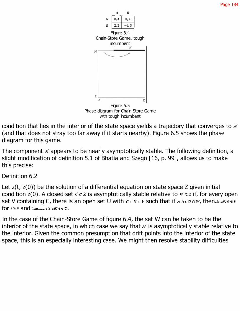
Page 184

Figure 6.4Chain-Store Game, tough

incumbent

Figure 6.5Phase diagram for Chain-Store Game

with tough incumbent

condition that lies in the interior of the state space yields a trajectory that converges to (and that does not stray too far away if it starts nearby). Figure 6.5 shows the phasediagram for this game.

The component appears to be nearly asymptotically stable. The following definition, aslight modification of definition 5.1 of Bhatia and Szegö [16, p. 99], allows us to makethis precise:

Definition 6.2

Let z(t, z(0)) be the solution of a differential equation on state space Z given initialcondition z(0). A closed set is asymptotically stable relative to if, for every openset V containing C, there is an open set U with such that if , thenfor and .

In the case of the Chain-Store Game of figure 6.4, the set W can be taken to be theinterior of the state space, in which case we say that is asymptotically stable relative tothe interior. Given the common presumption that drift points into the interior of the statespace, this is an especially interesting case. We might then resolve stability difficulties

Page 185

Figure 6.6Centipede Game

by simply seeking components that are asymptotically stable with respect to the interior.

There is reason to believe that such an approach will be quite effective in some cases.Cressman and Schlag [70] study the replicator dynamic in a class of generic extensive-form games of perfect information in which no path through the game involves more thanthree moves and in which there are at most two actions at each node. Such games mayhave multiple Nash equilibria, but Cressman and Schlag show that any such game has aunique component of equilibria that is asymptotically stable with respect to the interior,and this component corresponds to the subgame-perfect equilibrium outcome. As long asthe initial condition is interior, we are then assured of convergence to the subgame-perfect equilibrium outcome.

On the other hand, Cressman and Schlag [70] present counterexamples to show that thisresult does not extend to longer games. More importantly; the relationship betweenasymptotic stability with respect to the interior and the importance of drift requires somefurther investigation. If a component is asymptotically stable with respect to the interior,than any perturbation of the system away from this component and into the interior ofthe state space will give rise to convergence back to the component. This does not imply,however, that drift is unimportant. For example, consider the Centipede Game, whosenormal form is shown in figure 6.6. Figure 6.7 shows the extensive form of this game,while figure 6.8 shows the state space, indicating the direction of the dynamics in twofaces of the state space spanned by and . Notice that in the face ofthis state space corresponding to the strategies , the phase diagram has thesame qualitative features as the Chain-Store Game. Then there exists a specification ofdrift such that, in this face, the phase diagram matches that of figure 5.4 and everytrajectory converges to (Aa, a). There accordingly exist some specifications of drift suchthat some trajectories

Page 186

Figure 6.7Centipede Game, extensive form space

Figure 6.8Centipede Game, state space

in the resulting dynamics with drift start arbitrarily close to the component containing thesubgame-perfect equilibrium but converge to states that are far away. These trajectories,however, are confined to the face of the state space spanned by , and the driftin question never pushes the system out of this face. The same reasons prompting us tobe interested in asymptotic stability with respect to the interior suggest that we shouldconsider only trajectories with

Page 187

interior origins and interior-pointing drift. But lemma 6.1 can then be invoked to ensurethat there are states in the interior of the state space, and arbitrarily close to thecomponent containing the subgame-perfect equilibrium, that give rise to trajectoriesleading far away from that component (though they may eventually converge to thecomponent).9 The details of the drift process can thus be relevant, even when dealingwith components that are asymptotically stable with respect to the interior.

6.4 When Drift Matters

In the Chain-Store Game of figure 6.1, a component of nonhyperbolic stationary statesarises that is neither asymptotically stable nor asymptotically stable relative to theinterior. In these cases, drift matters. The forces captured by g(z) are not negligible forthe purposes of long-run prediction, and we cannot evade studying the model .What can be said about such cases?

In addition to assuming that f and g are continuously differentiable, let us assume thatthe stationary states of are hyperbolic for sufficiently small l. This latterassumption would be natural if we were interested in a fixed value of l. If the stationarystates of were not hyperbolic, then we would argue that yet more unmodeledsources of drift need to be incorporated into the model. The assumption that thestationary states of are hyperbolic for all sufficiently small l is stronger, but isnecessary if we are to examine small drift levels without committing to how small issmall. Let us simplify further by assuming that the basin of attraction of the set of allstationary points of is the entire space Z; this excludes cycles and other complicatedor chaotic trajectories. Although cycles or even more exotic behavior must be importantin some cases, it is important to begin by understanding cases in which the dynamics arerelatively well behaved.

The indication that drift matters is that the unperturbed dynamic has stationarystates that occur in a component C rather than being isolated. When does this componentpossess sufficient stability to be a possible prediction of long-run behavior for a learningdynamic with drift? The component can be considered a potentially relevant prediction oflong-run behavior if, in the presence of drift, we can find

9. Ponti [183] provides numerical calculations of such trajectories.

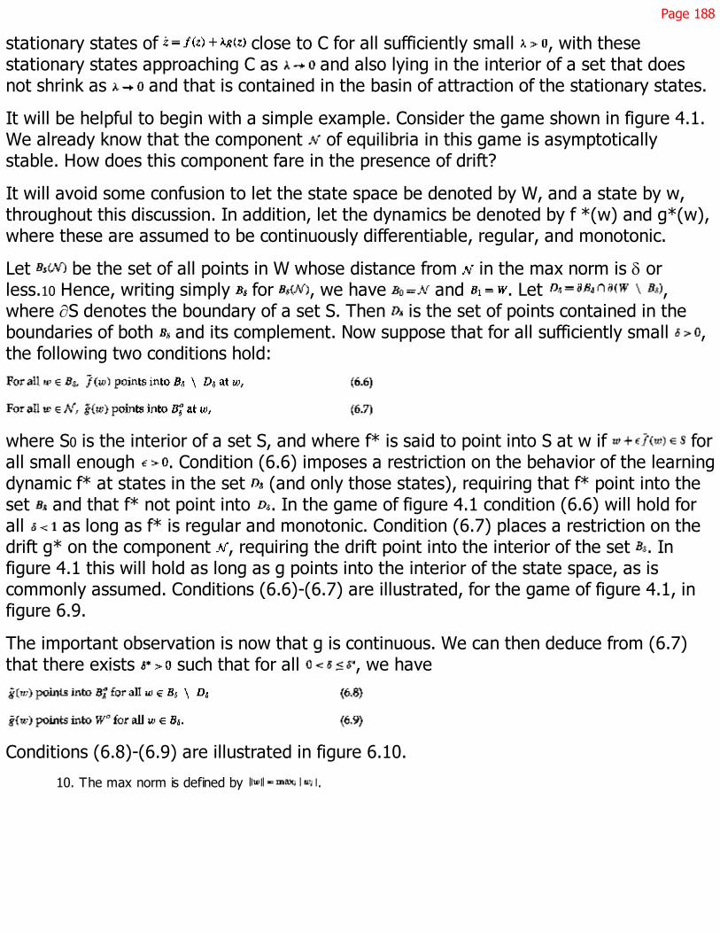
Page 188

stationary states of close to C for all sufficiently small , with thesestationary states approaching C as and also lying in the interior of a set that doesnot shrink as and that is contained in the basin of attraction of the stationary states.

It will be helpful to begin with a simple example. Consider the game shown in figure 4.1.We already know that the component of equilibria in this game is asymptoticallystable. How does this component fare in the presence of drift?

It will avoid some confusion to let the state space be denoted by W, and a state by w,throughout this discussion. In addition, let the dynamics be denoted by f *(w) and g*(w),where these are assumed to be continuously differentiable, regular, and monotonic.

Let be the set of all points in W whose distance from in the max norm is d orless.10 Hence, writing simply for , we have and . Let ,where ¶S denotes the boundary of a set S. Then is the set of points contained in theboundaries of both and its complement. Now suppose that for all sufficiently small ,the following two conditions hold:

where S0 is the interior of a set S, and where f* is said to point into S at w if forall small enough . Condition (6.6) imposes a restriction on the behavior of the learningdynamic f* at states in the set (and only those states), requiring that f* point into theset and that f* not point into . In the game of figure 4.1 condition (6.6) will hold forall as long as f* is regular and monotonic. Condition (6.7) places a restriction on thedrift g* on the component , requiring the drift point into the interior of the set . Infigure 4.1 this will hold as long as g points into the interior of the state space, as iscommonly assumed. Conditions (6.6)-(6.7) are illustrated, for the game of figure 4.1, infigure 6.9.

The important observation is now that g is continuous. We can then deduce from (6.7)that there exists such that for all , we have

Conditions (6.8)-(6.9) are illustrated in figure 6.10.

10. The max norm is defined by .

Page 189

Figure 6.9Illustration of conditions (6.6)-6.7)

Figure 6.10Illustration of conditions (6.8)-(6.9)

This observation allows us to conclude that if conditions (6.6)-(6.7) hold, then thereexists a l(d) with the property that stationary points of can be found in whenever and . To verify that such a exists, fix . Then observe thatf * is continuous on W and, for sufficiently small d* ( in the game of figure 4.1, thoughsmaller values of d* may be required when we generalize to other games), has zeros in only on . Combined with (6.6) and (6.8), this allows us to conclude that there existsl(d) such that points into for all and all . In addition, from (6.6)and (6.9), we can conclude that there exists l(d) such that points into for all

and all . Hence, for sufficiently small l, points into for all . Thissituation is illustrated in figure 6.11.

Page 190

Figure 6.11Interior-pointing perturbed dynamics

The next step is to apply Brouwer's theorem to the function defined, for smallenough Î, by , where and , and where Î is chosensufficiently small to ensure that for all . A fixed point w* of Y(w) is astationary state of ; any such stationary state is contained in .

As , proposition 6.1.1 indicates that these stationary states approach . Because alltrajectories through points of do not leave , and nonconverging trajectories areexcluded by hypothesis, the basin of attraction of the set of all stationary states of theperturbed dynamics inside contains , no matter how small l is. The component thus satisfies the criteria for being a potential description of the long-run behavior of theperturbed system.

The dynamics in figure 4.2 are sufficiently simple that the component could hardly failto have well-behaved stability properties, and this is evident without the machinery of thepreceding argument. We must now use this argument to extend the result to morecomplex situations. To do this, we can first note that the argument holds for a broaderrange of cases than the component in the game of figure 4.1. All that is required is acomponent of equilibria that is the face of a state space W and that satisfies (6.6)-(6.7). The result will then hold regardless of the dimension of W.

The next step is to look for cases in which components of equilibria may not be faces ofthe phase diagram but are structurally equivalent to a face. Let Z be a state space,though not necessarily the state space of figure 4.2. Let be a closed component ofstationary states of

Page 191

. We need to specify what it means for C to have properties similar to those of inthe previous discussion, and to identify the implications of this similarity.

Some notation is required. Let the state space be denoted by W as well as Z. Let be continuously differentiable on Z. If is a face of the state space, recall that

is the set of points whose distance from in the max norm is d or less. Binmore andSamuelson [27] present the proof of the following.11

Proposition 6.2

Let be continuously differentiable on the state space Z. Let be a face of the statespace W (= Z). Suppose there exists a differentiable injection with differentiableinverse F such that and such that the dyamics and

, together with the face and the state space W, satisfy (6.6)-(6.7).Then there exist and for all such that stationary states of canbe found in whenever and . The basin of attraction of the set ofsuch stationary points contains . As , these stationary points converge to

.

To see why this result holds, notice that the mapping f is a diffeomorphism, meaningthat it is a differentiable bijection with a differentiable inverse, between the state space(denoted by W) and a subset of the state space containing the component C. From thepreceding analysis of and W, we know there exist and such that has astationary state w* in for and , given the condition that f * and g*satisfy (6.6)-(6.7). But f is differentiable and hence F' is nonsingular. This implies that

is a stationary state of contained in and whose basin of attractioncontains .

If the conditions of proposition 6.2 are satisfied, how does this imply that the set C isworthy of attention? For any small d and sufficiently small l, the system hasstationary states that lie within distance d of C. In addition, these stationary states havea basin of attraction that contains and hence that does not shrink as l shrinks. Theset C thus provides an approximation of the local limiting behavior of the dynamic for small l.

In the two applications of this result that follow, the mapping f will be chosen so that theset will be the set of points in the basin of

11. F ' is the Jacobian of the differentiable function F .

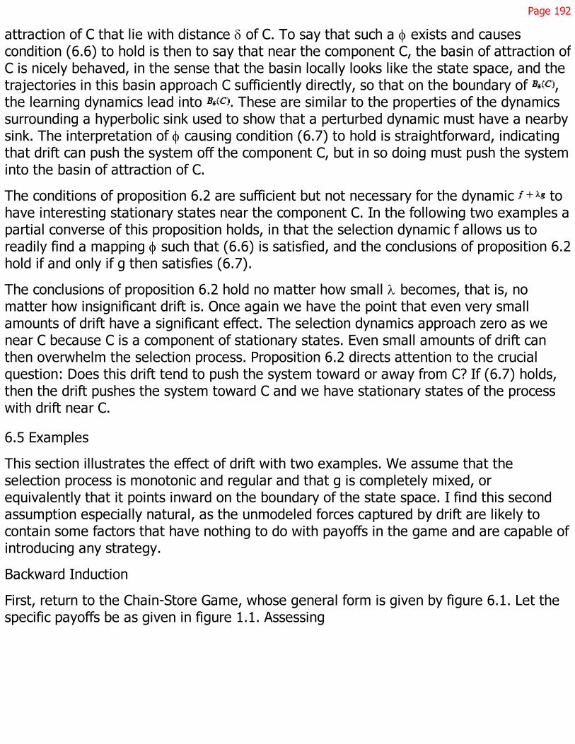
Page 192

attraction of C that lie with distance d of C. To say that such a f exists and causescondition (6.6) to hold is then to say that near the component C, the basin of attraction ofC is nicely behaved, in the sense that the basin locally looks like the state space, and thetrajectories in this basin approach C sufficiently directly, so that on the boundary of ,the learning dynamics lead into . These are similar to the properties of the dynamicssurrounding a hyperbolic sink used to show that a perturbed dynamic must have a nearbysink. The interpretation of f causing condition (6.7) to hold is straightforward, indicatingthat drift can push the system off the component C, but in so doing must push the systeminto the basin of attraction of C.

The conditions of proposition 6.2 are sufficient but not necessary for the dynamic tohave interesting stationary states near the component C. In the following two examples apartial converse of this proposition holds, in that the selection dynamic f allows us toreadily find a mapping f such that (6.6) is satisfied, and the conclusions of proposition 6.2hold if and only if g then satisfies (6.7).

The conclusions of proposition 6.2 hold no matter how small l becomes, that is, nomatter how insignificant drift is. Once again we have the point that even very smallamounts of drift have a significant effect. The selection dynamics approach zero as wenear C because C is a component of stationary states. Even small amounts of drift canthen overwhelm the selection process. Proposition 6.2 directs attention to the crucialquestion: Does this drift tend to push the system toward or away from C? If (6.7) holds,then the drift pushes the system toward C and we have stationary states of the processwith drift near C.

6.5 Examples

This section illustrates the effect of drift with two examples. We assume that theselection process is monotonic and regular and that g is completely mixed, orequivalently that it points inward on the boundary of the state space. I find this secondassumption especially natural, as the unmodeled forces captured by drift are likely tocontain some factors that have nothing to do with payoffs in the game and are capable ofintroducing any strategy.

Backward Induction

First, return to the Chain-Store Game, whose general form is given by figure 6.1. Let thespecific payoffs be as given in figure 1.1. Assessing

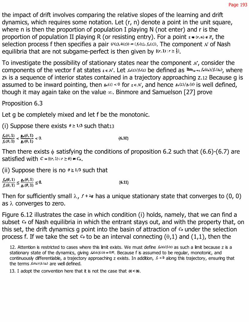
Page 193

the impact of drift involves comparing the relative slopes of the learning and driftdynamics, which requires some notation. Let (r, n) denote a point in the unit square,where n is then the proportion of population I playing N (not enter) and r is theproportion of population II playing R (or resisting entry). For a point , theselection process f then specifies a pair . The component of Nashequilibria that are not subgame-perfect is then given by .

To investigate the possibility of stationary states near the component , consider thecomponents of the vector f at states . Let be defined as , wherezk is a sequence of interior states contained in a trajectory approaching z.12 Because g isassumed to be inward pointing, then for , and hence is well defined,though it may again take on the value ¥. Binmore and Samuelson [27] prove

Proposition 6.3

Let g be completely mixed and let f be the monotonic.

(i) Suppose there exists such that13

Then there exists f satisfying the conditions of proposition 6.2 such that (6.6)-(6.7) aresatisfied with .

(ii) Suppose there is no such that

Then for sufficiently small l, has a unique stationary state that converges to (0, 0)as l converges to zero.

Figure 6.12 illustrates the case in which condition (i) holds, namely, that we can find asubset of Nash equilibria in which the entrant stays out, and with the property that, onthis set, the drift dynamics g point into the basin of attraction of under the selectionprocess f. If we take the set to be an interval connecting (q,1) and (1,1), then the

12. Attention is restricted to cases where this limit exists. We must define as such a limit because z is astationary state of the dynamics, giving . Because f is assumed to be regular, monotonic, andcontinuously differentiable, a trajectory approaching z exists. In addition, along this trajectory, ensuring thatthe terms are well defined.

13. I adopt the convention here that it is not the case that .

Page 194

Figure 6.12Condition (i) of proposition 6.3

key to verifying that drift points into the basin of attraction under the selection process isverifying this property at the endpoint (q,1). The existence of such a set then hinges uponfinding a value of q for which (6.10) holds.

It is important to note that in figure 6.12, has been chosen to be a subset of the Nashequilibrium component . It will typically be the case that conditions (6.6)-(6.7) can besatisfied not by an entire component of Nash equilibria but by a subset of thatcomponent.14 In the case of the replicator dynamics, the endpoint of the component ,given by ( , 1), gives , precluding the possibility that (6.10) holds. At thispoint, interior-pointing drift cannot point into the basin of attraction under the learningdynamics.

If there exists a set q satisfying (6.10), then the component has robust stabilityproperties in the perturbed dynamic , even though there are stationary states of thedynamic f, contained in that are arbitrarily dose to . The drift g pushes the systemfrom points in back into the basin of attraction of and away from points in . Thisis where drift plays its essential role.

Proposition 6.3 indicates that when examining the Chain-Store Game, we can simplycheck the relative slopes of the learning and drift processes on the component of Nashequilibria . The component is worthy of our attention if and only if there are states in

where the slope of the drift process is flatter than the learning dynamics, in the sensethat the drift process points into the basin of attraction, under the dynamics without drift,of a subset of the component of Nash equilibria. ''Worthy of attention" means that thereare nearby stationary states

14. I will often say that "conditions (6.6)-(6.7) are satisfied" rather than the more precise but cumbersomestatement that "there exists a diffeomorphism f such that the induced dynamics f * and g* satisfy (6.6)-(6.7)."

Page 195

of the process with drift whose basin of attraction does not shrink as the drift levelshrinks. For the case of the replicator dynamics and the Ultirnatum Minigame, chapter 5showed that if condition (i) of proposition 6.3 holds, then there is a unique stationarypoint close to , which is asymptotically stable.

Comparative Statics

One motivation for an interest in drift is the observation that conventional theoreticalpredictions often do not match how people (or at least experimental subjects) playgames. How does proposition 6.2 help? In particular, what are the potentially testablepredictions we could extract from proposition 6.2?

In thinking about testing, it is useful to consider the way that applied work is pursued inconventional economic theory, which consistently uses comparative statics results as abasis for empirical work. Models are used to generate statements about the directions inwhich variables move in response to changes in observable parameters, whilemaintaining ceteris paribus assumptions that unobserved parameters do not change.

This suggests that game theorists similarly seek predictions based on comparative staticsexercises in which one or more observable parameters are varied while the remainingunobservable parameters are held fixed. If these predictions are violated in thelaboratory; then the theory on which they are based must be reconsidered. Notice,however, that this reconsideration may take many forms. The predictions will inescapablydepend on maintained hypotheses about unobservables. If a prediction fails, it may thenbe a reflection of a faulty model or a faulty maintained hypothesis. This is again a familiarcharacteristic of empirical work.

The payoff function p of a game is the obvious observable, something that can becontrolled and varied in an experimental design. In the case of the Chain-Store Game,payoffs are determined by the parameters a, b, c, d, e, and h of figure 6.1. The strategiccharacter of the Chain-Store Game is preserved by subjecting the parameters to theconstraints

In claiming that payoffs can be manipulated and are given by the parameters a, b, c, d, e,and h, I do not claim that players are motivated

Page 196

only by monetary payoffs. While I think that both game theorists and their critics areoften too quick to construct new models of preferences in order to explain unexpectedexperimental results, I also do not think that monetary payoffs are always the only thingthat matters. Instead, some middle ground must be appropriate. But it remains the casethat the parameters a, b, c, d, e, and h can be observed and manipulated. Rather thandebating whether the forces shaping behavior are better described as preferences orlearning, the more useful approach is to derive the implications of the various models andsee which is most useful.

The process will be treated as unobservable. This is not to say that datacannot be gathered that is relevant to how people learn. The problem is that we do notknow how to incorporate these data into the theory in a reliable manner, much less howto make the next step from theory into experiments. For example, it is common in somequarters to insist that if a learning theory is to be useful or convincing, then it mustexplain the variation in behavior over the rounds of an experiment. I think this insistenceis appropriate only if the laboratory experiment provides sufficiently many trials for thelearning theory to be applicable. This often fails to be the case, given the necessarilyshort lengths of many experiments and the emphasis of many learning models on limitingresults.

Learning models may capture the process by which players learn to play the games theyfrequently encounter outside of the laboratory. If the laboratory setting is successful intriggering analogies in the players' thinking to the appropriate games, then we canobserve the outcome of this learning process in the experimental behavior. It is thisoutcome that is addressed by the comparative statics presented here. If the experimentfails in triggering behavior rules among the players that have evolved in the real-lifecounterpart of the experimental game, perhaps because framing effects direct attentionto superficially similar but strategically quite different games, then we can expect toobserve very little about the players' learning processes.15

A maintained hypothesis about the learning process f, derived as an approximation of, will be that it is not only regular and mono-

15. This emphasis on avoiding framing effects does not imply that we can dispense with the provision of experiencein a laboratory setting. It is only by providing such experience that we can collect any hint at all as to howcontaminated the results are by framing considerations.

Page 197

tonic, but also comparatively monotonic.16 To define the latter, denote the ith strategy ofplayer by and let be the coordinate of f corresponding to strategy i for player .Let be the average payoff to strategy for player in state z. Now consider twopayoff functions and and fix a state z. Suppose there exists a strategy

for player such that , for all s-h, whenever or , and such that. If , then it is assumed that , and if for , then it is

assumed that , while fhi for is unaffected. This assumption ensures that ifwe fix a state z and then consider a change in the payoffs to player from strategy i thatincreases the average payoff of strategy i in state z, then the rate at which strategy igrows increases, and the rates at which other strategies grow for player i decrease.

We know even less about the drift process g, derived as an approximation of , thanabout f, and the process of drift clearly goes into the unobservables list. I expect drift todepend upon a host of factors in addition to the payoffs in the game. As a result, drift willoften have little to do with the payoffs. In most of what follows, the maintainedhypothesis is that g is independent of the payoffs in the game. I refer to this as "the caseof exogenous drift."

There remains the question of the initial condition z(0). The comparative statics resultsderived below are predicated on the assumption that z(0) is independent of payoffs. Thepredictions will therefore not apply to games for which z(0) turns out to vary significantlywith p. Again, we have the point that if framing effects are important, then the theorymay have nothing to say.

Applying these considerations leads to the suggestion that experiments compare versionsof the Chain-Store Game with varying payoffs. The first task is to determine which payoffconfigurations are more likely to give stable stationary points near the component .Binmore and Samuelson [27] prove

Proposition 6.4

Fix payoffs a, b, c, d, e, and h satisfying (6.12) for the Chain-Store Game of figure 6.1. Letthe selection dynamic f be monotonic, regular, and comparatively monotonic, and let thedrift g be exogenous. If there exists a subset C of the component of Nash

16. I now replace by to capture the dependence of the selection process on payoffs.

Page 198

Figure 6.13Dalek Game

equilibria for which a mapping f exists satisfying the conditions of proposition 6.2, thensuch a subset also exists when either or e or d is increased or when either a, b, or c isdecreased, provided that (6.12) is preserved. The converse can fail in each case.

Chain-Store Game experiments can thus be conducted with varying values of the payoffsa and b. An outcome consistent with the theory would be the observation of thesubgame-perfect equilibrium for large values of a and b and the Nash, non-subgame-perfect equilibrium for small values of a and b. Violations of this relationship wouldchallenge the theory. Similar experiments can be done with other combinations ofpayoffs.

Drift has been taken to be exogenously fixed throughout this exercise, which is often asuitable first approximation, as in biological examples. In the Ultimatum Game, however,we have seen that the drift process may be related to payoffs, in that a population mayhave a higher drift rate because the payoff differences between its strategies are smaller.The particular drift process examined in chapter 5 reinforces the effects of movements inpayoffs, and proposition 6.4 continues to hold for this drift process. An analysis like thatleading to proposition 6.4 can be performed for any process of drift, though it will bemore complicated and the results will be clearer in some cases than in others, dependingupon what is assumed about drift.

Outside Options and Forward Induction

Consider the "Dalek Game" shown in figure 6.13. The extensive form of this game isshown in figure 6.14. Kohlberg and Mertens [135] use this game to illustrate forwardinduction reasoning.

The Dalek Game has two components of Nash equilibria, including a strict Nashequilibrium given by (M, L) with payoffs (9, 3) and a

Page 199

Figure 6.14Dalek Game, extensive form

component of equilibria with payoffs (7, 4) in which player I takes the outside option(plays T) and player II plays R with probability at least . The former is a (hyperbolic)sink under regular, monotonic dynamics while the stationary states in the lattercomponent are not hyperbolic.

It is common to argue that forward induction restricts attention to the equilibrium (M, L)in this game. For example, we might appeal to the iterated elimination of weaklydominated strategies (cf. Kohlberg and Mertens [135]). B is strictly dominated for playerI. Removing B causes R to be weakly dominated for player II, the removal of whichcauses T to be weakly dominated for player I, leaving (M, L). Alternatively, we couldappeal to the never-weak-best-response criterion (Kohlberg and Mertens [135]) or to theforward induction reasoning of van Damme [238, 239] (in an equivalent but differentextensive form in which player I first chooses between T and {M, B} and then choosesbetween M and B) or to the normal form variant of this reasoning given in Mailath,Samuelson, and Swinkels [146].

How does this forward induction argument fare in our terms? First, it is straightforward toapply proposition 6.2 to the component . Letting zR be the proportion of population IIplaying strategy R in state z we have

Proposition 6.5

If there is a state such that g(Z*) points into the interior of the basin of attraction,under the dynamic f, of the set , then there exists a mapping f satisfyingthe conditions of proposition 6.2.

Page 200

In the presence of drift, we thus have good reasons to be interested in Nash equilibriathat fail conventional forward induction arguments. However, it would be nice to have acondition that is more revealing than the requirement that "g(Z*) points into the interiorof the basin of attraction of the set ." The key to finding such a condition isthe observation that strategy B is strictly dominated by T for player I in the Dalek Game.Proposition 4.5 shows that any monotonic dynamic will eliminate B. Hence, everytrajectory of the dynamics must approach the boundary face spanned by .But if attention is restricted to this face, the Dalek Game is a special case of the Chain-Store Game.

Can we use what we know about the Chain-Store Game to identify sufficient conditionsfor existence of stationary points near the component in the Dalek Game? In particular,suppose that condition (i) of proposition 6.3 holds when the dynamics of the Dalek Gameare restricted to the face Z-B. Can this fact be used to conclude that the Dalek Game hasa stationary point dose to ? The answer is yes, as long as drift does not create toopowerful a force toward strategy B.

If z is a point in the state space of this game, let zT, zB, and zR denote the probabilitieswith which strategies T, B and R are played at z, with the residual probabilities beingattached to M and L. Similarly, let be the element of the vector f corresponding to T,and so on. Then is the set of states corresponding to the componentof Nash equilibria that are not subgame-perfect.

Let f *, g*, and be the dynamics f, g and on Z-B defined by letting (this ispossible because Z-B is forward-invariant under f) and letting (and hence

, making Z-B forward-invariant). Call and the state space Z-B the "restricteddynamics." Binmore and Samuelson [27] prove

Proposition 6.6

Suppose that for all , there is a sufficiently small l such that the restricted dynamicshave a sink (saddle) [source] within d of . Then for all , there is a function and a sufficiently small l such that if , then the unrestricted dynamics have a sink (saddle) [saddle] within d of in the Dalek Game.

To interpret this result, note that proposition 6.3 provides sufficient conditions for therestricted dynamics to have stationary points close

Page 201

to the component of Nash equilibria in the state space Z-B, as well as sufficientconditions for no such stationary point to exist. Proposition 6.6 indicates that if the formersufficient conditions are met, then we need look no further. As long as drift does notintroduce the strategy B into the game with too much force, the unrestricted dynamics inthe Dalek Game also have a stationary point near .

This result holds because the learning dynamic f pushes the system toward the face Z-B.If perturbations never introduced strategy B into the population, then the system wouldeventually be governed by the forces that appear in this face; hence the system wouldeventually have behavior specified by the restricted dynamics on Z-B. Proposition 6.3could then be applied to gain insight into this behavior. Proposition 6.6 indicates that thiscontinues to hold in the presence of drift that also introduces the strategy B into thepopulation, as long as it does not do so too vigorously.17

Comparative Statics

Turning now to comparative statics considerations similar to those of the Chain-StoreGame, we could construct a general form of the Dalek Game, the first two rows of whichwould match the Chain-Store Game of figure 6.1 and the final row of which wouldcorrespond to a strictly dominated strategy for player I. From propositions 6.4 and 6.6,we will then have results that are consistent with the model if we observe outcomes nearthe Nash equilibrium that fails forward induction, in which the outside option is taken, forsmall values of a, b, and c and large values of d and e. Violations of this pattern wouldagain challenge the theory. One implication is that we should observe Nash equilibria thatfail forward induction when the value to player II of taking the outside option is relativelylarge.

In light of this, it is interesting to note that Balkenborg [5], when conducting experimentswith a version of the Dalek Game, finds that the outside option is virtually always chosen.This provides the beginnings of a comparative statics exercise, but additional insight intothe model requires additional experiments with different payoffs.

17. Notice that if the conditions of proposition 6.6 are met, a source in the restricted dynamics corresponds to asaddle in the unrestricted dynamics. This reflects the fact that f must reduce the proportion of the populationplaying B and hence must approach the face Z-B.

Page 202

Binmore et al. [22] examine a related game in which players I and II have ten dollars todivide. Player I demands a share of the ten dollars; player II simultaneously eitherdemands a share of the ten dollars or elects to take an outside option. If player II takesthe outside option, then player II receives a payoff of a, where , while player Ireceives nothing. If player II makes a demand rather than taking the outside option and ifthe two players' demands are incompatible, meaning that the total of their demandsexceeds ten dollars, then each receives nothing. If the demands sum to less than tendollars, then each player receives his demand as well as half of the remaining surplus.

This game has many Nash equilibria. Pure-strategy Nash equilibria include efficientequilibria, in which player II forgoes the outside option and players I and II makedemands that exactly exhaust the ten dollars and allocate at least a to player II, as wellas inefficient equilibria, in which player II opts out and player I demands more than .There are also mixed-strategy Nash equilibria, all of which are inefficient. Notice thatefficiency requires player II to forgo the outside option, even if a is large, though player IImust be compensated for doing so with a payoff at least as large as a.

Forward induction arguments do not exclude any of these equilibria, although it iscommon to focus on the efficient equilibria of such a game, sometimes with differingopinions as to how player II should be compensated for surrendering the outside option.What if we examine the long-run outcomes of an evolutionary model? Binmore et al. [22]show that, in the presence of drift, the long-run outcomes in this game tend to involvedivisions of the surplus that are not too extreme. The more important drift is, thestronger this centralizing tendency, that is, the larger the set of asymmetric divisions ofthe surplus that do not appear as long-run outcomes. This centralizing tendency appearseven though the drift itself is not biased toward symmetric divisions, and for much thesame reason that perturbations in the Nash [165] demand game push players toward theNash bargaining solution.18 If player II's outside option is not too attractive, thiscentralizing tendency poses no problems for efficiency, but if the outside option issufficiently attractive, then the centralizing tendency can make it more

18. Similar forces appear in Young's evolutionary model of play in the Nash demand game [251].

Page 203

attractive for player II to take the outside option than divide the surplus with player I.

The implication of learning with drift, then, is that the outside option is more likely to bechosen, and an inefficient result more likely to appear, when player II's outside option isrelatively lucrative. The experimental results of Binmore et al. [22] show that the outsideoption is often taken, and is taken much more often when it is more lucrative.

6.6 Discussion

The central idea behind this chapter is simple: for a model to be successful, it mustinclude important factors and exclude unimportant ones. But how do we know what isimportant and what is not? In the case of evolutionary games, the model itself providesthe answers. If the model produces stationary states that are not hyperbolic and do notoccur in components satisfying some variation of asymptotic stability, then it hasexcluded important factors.

The factors to be added to the model can have a significant impact on the behavior of thedynamic system, but they also may be very small in magnitude. It is presumably becausethey are small that they are excluded from the model in the first analysis. How can amodel whose behavior is shaped by arbitrarily small factors be of any use in applications?One conclusion of this chapter is that, while the factors themselves may be small, theirexistence can nevertheless be used to derive comparative statics results that do notdepend upon observing arbitrarily small magnitudes.

Page 205

7Noise

We begin our investigation of ultralong-run models. As in chapter 3, our point ofdeparture is a model of the stochastic process by which agents adjust their strategies. Weshall maintain the convention of previous chapters that this is a Markov process, where astate is a specification of how many of the agents in a finite population are playing eachof the strategies available in the underlying game. The Aspiration and Imitation model ofchapter 3 is an example of such a Markov model, but less structure will be assumed inthis chapter.1

We shall be focusing on the stationary distribution of the Markov process. Two familiarforces act on agents' strategies. One is selection. In an economic context, selectionoccurs via a process of learning; in a biological context, this would be a process of naturalselection driven by different strategies leading to different rates of reproduction. Thesecond process is mutation. In a biological context, these are literally mutations,consisting of random alterations in genetic codes; in economic contexts, it is againcommon to use the term mutation, where this refers to an agent randomly switching to anew strategy. We might think of this as an agent experimenting with a new strategy orbeing replaced by a new agent unfamiliar with the game who initially chooses a strategyat random.

What is the difference between selection and mutation? As in chapter 6, we can think ofselection as capturing the important forces affecting strategy choices, while mutation is aresidual, capturing whatever has been excluded when modeling selection. As a result, wecan expect selection to occur with a higher probability or at a faster rate than mutation,and also to be related to the payoffs in the game. This link

1. This chapter is taken from Samuelson [200, 201].

Page 206

between payoffs and selection is often captured by building the selection mechanismaround a tendency for agents to switch toward a best reply to the current state. Such atendency may take the form of a deterministic selection mechanism in which every agentswitches to a best reply to the current state in every period, or it may take the form of astochastic process in which it is simply more likely that agents switch to a best reply;when they do happen to switch, than the reverse. The relative importance of selection iscaptured by focusing on the case where the probability of a mutation is very small. Togive meaning to the phrase ''very small," we shall follow the common practice ofexamining the limiting outcome as the probability of a mutation approaches zero.

Unlike the selection mechanism, there is little reason to believe that mutations have aparticularly strong connection with the payoffs of the game. Thus mutations areconventionally modeled as being completely random, in the sense that they may switch aplayer to any of the existing strategies and are unaffected by payoffs.

The innovation of Foster and Young [79], developed further by Kandori, Mailath, and Rob[128] and by Young [250], was to show that even arbitrarily improbable mutations canplay a crucial role in shaping the stationary distribution of the model. They showed thattechniques developed by Freidlin and Wentzell [81] could be used to derive particularlystrong conclusions about the limiting case as the probability of a mutation goes to zero.Chapter 6 used "noise" to refer to relatively improbable, stochastic events such asmutations. The message of Young and of Kandori, Mailath, and Rob is simple: noisematters.

This chapter presents a straightforward generalization of the model of Kandori, Mailath,and Rob [128] beyond the two-player games and the specific learning and mutationprocesses they consider, as well as the tools needed to characterize the stationarydistribution of this model. These lead to the first result concerning equilibrium selection,namely; that we cannot always expect weakly dominated strategies to be excluded fromthe stationary distribution. The finding of previous chapters, that dominated strategiesare not eliminated by the deterministic differential equations used to approximate thelong-run behavior of the strategy adjustment process, is then not an artifact of examininginsufficiently long time periods. Dominated strategies persist even in the stationarydistribution.

Page 207

7.1 The Model

Selection

Consider a finite, normal-form game, denoted , where t is a finite set of players, is the joint strategy set, and is the payoff function.

Assume that G is an asymmetric game and there exist n populations, one for each playerin the game. The model is easily adapted to handle the common alternative in which G issymmetric and is played by agents drawn from a single population.

Each population is composed of N identical agents, where N is finite. The agents fromthese populations are randomly matched to play game G in each period .Chapter 3 mentioned ways of making this "random matching" assumption precise. Thekey characteristic in each case is that an agent's expected payoff equals the payoff theagent would receive against a mixed strategy whose probabilities are given by thefractions in which the various pure strategies appear in the opposing populations.

At each time t, each agent will be characterized by a pure strategy. The state x of thesystem at time t identifies, for each population and each strategy , the number ofagents of population playing pure strategy i (denoted or , but with t generallysuppressed). Let x, y, and z refer to states and let X denote the set of all possible states.

In each period, after agents have played the game, they potentially switch strategies. Letthe process by which agents switch between strategies be called "selection" or a"selection mechanism." A selection mechanism is then a transition matrix defined on thestate space X that identifies, for each state the system might occupy at time t, theprobability that the system moves to each of the various states in X in period . Hencea selection mechanism is a transition matrix, denoted by F, that identifies the transitionprobability Fxy for all states x and y in X.

For example, suppose that in each period t, each agent in each population takes anindependent draw from a Bernoulli trial. With probability , this draw produces theoutcome "do not learn" and the agent does not change strategies. With probability m, thisdraw produces the outcome "learn." In this case, the agent switches to a best responseto the period t actions of the agents in other populations (if there is more

Page 208

than one best response, the agent switches to each of them with positive probability).From this model of individual agent behavior, the probabilities Fxy that describe theaggregate behavior of the system can be calculated. I refer to these as the "best-response dynamics with inertia." If , then we have the deterministic best-responsedynamics in which every agent switches to a best reply in every period.

The best-response dynamics with inertia may be applicable in situations wherecalculating optimal actions is costly, difficult, or time-consuming, so that agents willusually simply repeat the actions they have taken in the past. Occasionally, however,agents in such an environment will assess their strategies. When doing so, they may beable to collect considerable information, perhaps by observing and consulting others,thereby attaining knowledge of the current state. The best-response dynamics withinertia assume that agents then choose a best reply to this state.

The selection mechanism is a Markov process with a transition matrix F and state spaceX. A stationary distribution, denoted , is a probability measure on X thatsatisfies . It would be most convenient if the Markov process defined by F had aunique stationary distribution, but we cannot expect this to be the case. Consider, forexample, a two-player normal-form game with two strict Nash equilibria. Let theselection mechanism be given by the best-response dynamics with inertia. Then there willbe at least two. stationary distributions, with each attaching unitary probability to a statethat corresponds to one of the game's two strict Nash equilibria. The stationarydistribution to which the system converges will depend upon initial conditions.

Noise

The key insight of Foster and Young [79] is that adding noise to an evolutionary system,in the form of stochastic mutations, can yield a unique stationary distribution.

The process of mutation is assumed to be independent across agents. Consider an agentfrom population playing strategy at the end of period t (i.e., after the agents havebeen matched, played the game, and possibly switched strategies via the selectionmechanism). With probability , for , no mutation occurs on this agent and theagent continues to play strategy i. With probability l, this agent undergoes a mutation, inwhich case the agent switches to each strategy

Page 209

with the exogenously fixed probability . This mutation process bears asuperficial resemblance to the selection mechanism given by the best-response dynamicswith inertia, with the crucial difference that the mutations need not bear any relationshipto payoffs and are "completely mixed," meaning that a mutation may Switch an agent toany strategy.

The results will not depend on the specification of the function g as long as it is retainsthe property of being completely mixed and as long as g is independent of l, so that theeffect of a mutation is independent of the probability of a mutation. This assumptioncould be relaxed, and g allowed to depend on l, as long as the relative probabilities ofthe strategies to which a mutation might switch an agent remain nonzero and boundedas l, approaches zero. This assumption on ratios of mutation-induced 'transitionprobabilities would also allow a more general formulation in which the effect of amutation on an agent varied across states. For examinations of how other mutationprocesses might affect the results, see Blume [36] and Bergin and Lip-man [13]. Berginand Lipman, for example, show that virtually any outcome can be obtained, in the limit asthe probability of a mutation approaches zero, if in the process the relative probabilitiesof the strategies to which a mutation switches an agent can approach zero or infinity.

Let Gyz denote the probability that mutations move the system from state y to state z.The conjunction of the selection and mutation mechanisms gives us an overall transitionmatrix between states, denoted by G, where

Notice that for all y, and hence for all x, .

The state space X and the transition matrix G again define a Markov process. We areinterested in the stationary distributions of this process. Chapter 3 observed that thefollowing is standard for a transition matrix such as G that has only positive elements(see Billingsley [17], Seneta [214], or Kemeny and Snell [132, theorems 4.1.4, 4.1.6, and4.2.1]):

Proposition 7.1

(i) The Markov process defined by G has a unique stationary distribution, that is, aprobability measure g* on X such that .

Page 210

(ii) The relative frequencies with which the states in X are realized along a sample pathof the process approach g* almost surely as .

(iii) For any initial distribution over states g0, we have .

Hence, independently of the initial condition, the distribution of the population isasymptotically given by g*. This stationary distribution can be interpreted both as theproportion of time that any realization of the process spends in each state and as theprobability that the process will be in each state at any (sufficiently distant) future time.

For many the attraction of this result lies in the stationary distribution of the system beingindependent of the initial conditions. Alternatively we say that history does not matterThis greatly simplifies our investigation of the system.

7.2 Limit Distributions

The transition matrix G and the stationary distribution g* depend on the mutation rate l,and will sometimes be written as G(l) and g*(l). We shall consider the case of raremutations, and hence the limit of the distribution g* (l) as l approaches zero, denoted by

. This is the distribution examined by Foster and Young [79], Young [250],and Kandori, Mailath, and Rob [128]. Foster and Young refer to g** as the "stochasticallystable distribution," while Kandori, Mailath, and Rob refer to an equilibrium as a "long-runequilibrium" if this distribution puts a probability mass of one on the equilibrium. I shallrefer to it as the ''limit distribution" or "limiting distribution."

Counting Mutations

The basic tool used to investigate the limit distribution is a result from Freidlin andWentzell [81] that was applied in models of evolutionary games by Kandori, Mailath, andRob [128] and by Young [250]. Consider the following class of directed graphs on thestate space X:

Definition 7.1

Let x be a state in X. Then an x-tree on X is a tree with each state in X as a node andwith x with its initial node, that is, a x-tree is a binary relation on X with the followingproperties:

(i) For all with , there is one and only one element of the form (y, z) in therelation.

Page 211

(ii) For every , the relation contains a sequence of the form .(iii) The relation contains no element of the form (x, y).

If we think of an element of the relation (y, z) as denoting an arrow from y to z, then anx-tree is a tree or collection of arrows such that each element other than x is the initialpoint of one and only one arrow and there is a path of arrows from each element of X \{x} to x. Notice that there are no cycles in such a tree. For each , let hx denote an x-tree and define the set of x-trees by Hx. It will often be convenient to denote the element(y, z) of an x-tree as ( ).

We can now construct the following vector. For a fixed state x and for each x-tree,associate with each (y, z) in the tree the transition probability from y to z, or Gyz. Thentake the product of these probabilities for the tree, and sum these products over the setof all x-trees. This gives a number of the form

We can collect these numbers to construct a vector of the form . Then theresult of Freidlin and Wentzell [81, lemma 3.1, p. 177] is

Proposition 7.2

g*(l) is proportional to x(l).

Freidlin and Wentzell's proof is surprisingly straightforward, involving some simplealgebraic manipulations of the condition that g*(l) is a stationary distribution (i.e, thecondition ).

Proposition 7.2 allows us to derive some properties of the limit distribution from (7.2).First, we can calculate Gwz, which identifies the probability that mutations take thesystem from state w to z. Let Mwz identify the various combinations of mutations that canmove the state from w to z. Then define to be the total number of mutationsrequired of agents in population under mutation combination Let be thebinomial coefficient corresponding to the total number of ways that these population mutants can be drawn from population given state y and let be the product ofthe probabilities (., .) for the mutations required of population under mwz. Then wehave

Page 212

and from (7.2), we have

The key property of this equation is that the only terms that depend on l are those inwhich l explicitly appears.

Second, let and

Then we can interpret k(x, y) as the least number of mutations required to get from statex to y, in the sense there is positive probability that starting from state x, the selectionmechanism will move the system to a state z from which k(x, y) mutations can move thesystem to state y (with a similar statement holding for no number less than k(x, y)).

Section 7.5 proves the following:2

Proposition 7.3

(i) A limit distribution g** exists and is unique.

(ii) The states appearing in the limit distribution are those which can be reached with thefewest mutations. In particular, if and only if x satisfies

If we interpret the term in parentheses in (7.6) as the cost, in terms of mutations, oflinking all other states to the state x, we then have the states easiest to reach from otherstates appearing in the limit distribution, with "easiest" interpreted as requiring thefewest mutations.

Proposition 7.3 indicates that in order to obtain results on the limit distribution g**, wecan look for counting arguments, where the counting concerns the least number ofmutations, that is, the highest power attached to ( ), required to accomplish thetransitions contained in an x-graph. The fewer the mutations, the more likely x is toappear in the limit distribution, in the sense that only mutation-minimizing

2. This result (proposition 7.3) is standard. For example, see theorem 1 of Kandori, Mailath, and Rob [128] ortheorem 2 of Young [250].

Page 213

states will appear. Notice that the only relevant property of the selection probabilities Fxy

in this calculation is whether they are zero (yielding k(x, y)>0) or positive (yielding k(x,y=0), with the magnitude of positive Fxy being irrelevant. This ability to replacecalculation with counting and to restrict attention to the two-member partition of the unitinterval into zero and nonzero elements is a great simplification and the gain achieved byworking with the limiting case as . Hence I shall say that the transition ( )"requires k(x, y) mutations" and, similarly, that the transition ( ) "does not require amutation" if and only if .

Absorbing Sets

A nonempty set of states is absorbing if it is a minimal set with respect to theproperty of being closed under the selection mechanism. Hence there is zero probabilitythat the selection mechanism can cause the process to exit A (though mutations may stillmove the system out of an absorbing set). In addition, the minimality requirementensures that there is a positive probability of moving from any state in A to any otherstate in A in a finite number of time periods. If this were not the case, a strict subset of Acould be found that is dosed under the selection mechanism, and A would not beabsorbing. An absorbing set may contain many states or may contain only a single state.In the latter case, I shall refer to the state as simply an "absorbing state." Because thestate space is finite and dosed under the selection mechanism, it is immediate that atleast one absorbing set exists, and there may be more than one absorbing set.

The basin of attraction of an absorbing set is the set of states from which there is positiveprobability that the selection mechanism (without mutations) moves the system to theabsorbing set in a finite number of time periods. Let B(A) and B(x) denote the basin ofattraction of an absorbing set A or an absorbing state x. The union of the basins ofattraction of the absorbing sets in X must equal X. If the selection mechanism F isdeterministic, meaning that only the probabilities zero and one appear in the transitionmatrix, then the basins of attraction of two absorbing sets must be disjoint. Ifprobabilities other than zero and one appear in F, then the basins of attraction ofabsorbing sets A and A' may intersect, meaning that there are states from which theselection mechanism may lead to A but may also lead to A'.

Proposition 7.3 leads immediately to the following (proved in section 7.5):

Page 214

Proposition 7.4

(i) State appears in the support of the limit distribution only if x is contained in anabsorbing set A of the selection mechanism.

(ii) If one state in an absorbing set A of the selection mechanism is contained in thesupport of the limit distribution, so are all other states in A.

It is a standard result that for a Markov process G, the stationary distribution of Gattaches probability only to states contained in absorbing sets of G. Proposition 7.4indicates that as the probability of a mutation becomes small, the stationary distributionof F becomes concentrated on absorbing sets of the selection mechanism F.3 To see whythis holds, we need only note that the selection mechanism leads from any state notcontained in an absorbing set to an absorbing set, without requiring any mutations; onlywith the help of a mutation can the system leave an absorbing set. The number ofmutations required in an x-tree that links the remaining states to state x is thus lower if xis a member of an absorbing set than if it is not. The result then follows from proposition7.3. The proof in section 7.5 makes this intuition precise.

Proposition 7.4 indicates that adding mutations to the selection process F provides ameans of choosing between the stationary distributions of the Markov process F. Inparticular, F may have many stationary distributions. For every absorbing set of F, there isa stationary distribution whose support coincides with that absorbing set.4 For any l,however, the process G has a unique absorbing set consisting of the entire state spaceand has a unique stationary distribution. As , this stationary distribution converges toone of the stationary distributions of F.

To illustrate propositions 7.3 and 7.4, let us apply the argument behind the result ofKandori, Mailath, and Rob [128], that the limit distribution contains only the risk-dominant equilibrium in symmetric games with two strict Nash equilibria, to the Stag-Hunt Game shown in figure 2.9. The two strict Nash equilibria of this game consist of (X,X) and (Y, Y). In the terms of Harsanyi and Selten [116], the former equilibrium is payoff-dominant while the latter is risk-dominant. As do

3. Gilboa and Samet [101] introduce the concept of an absorbent stable set, which is analogous to the concept ofan absorbing set.

4. We can create other stationary distributions by taking combinations of these.

Page 215

Figure 7.1Phase diagram for best-response dynamics, Stag-Hunt Game

Kandori, Mailath, and Rob, let this game be played by a single population of N agents.The state space is then the set {0,1,..., N}, where a state identifies the number of agentsplaying strategy X.

Following Kandori, Mailath, and Rob [128], let the selection mechanism F be given by thebest-response dynamics, so that in each period every agent switches to a best responseto the distribution of strategies played by that agent's opponents in the previous period.Figure 7.1 shows the phase diagram for the Stag-Hunt Game under the deterministicbest-reply dynamics for the case in which there are five agents.5 There are two absorbingsets of the selection mechanism, each of which is a singleton, consisting of the state 0and the state 5, which correspond to the game's two strict Nash equilibria. The mixed-strategy equilibrium is given by . The relative position of this point is marked on thestate space in figure 7.1; it does not correspond to a state, and hence cannot be anabsorbing set. It is important to note, however, that even if the number of agents in thepopulation were chosen so that we could exactly duplicate the probabilities of the mixed-strategy equilibrium in population proportions, the mixed-strategy equilibrium would notbe an absorbing state. This is because in single-population models, each agent samplesopponents from a slightly different distribution.6

5. These transitions are easily computed from the rule that all agents switch to a best reply to the current state.Notice that if the current state is 3, so that two agents play Y and three play X, then Y agents face opponents inproportion and find X a best reply while X agents face and find Y a best reply, switching the systemto state 2.

6. To see this, suppose we have a population of 300 agents and assign 200 to X and 100 to Y. Then an X-agent seesa population of opponents consisting of 199 X-agents and 100 Y-agents, making Y a best reply. Similarly, agentscurrently playing Y find X a best reply. If, instead of working with a single population, we allow each player to berepresented by a separate population, then each agent can face population frequencies of strategies that match theprobabilities of a mixed-strategy equilibrium, and hence the mixed-strategy equilibrium can be an absorbing state.

Page 216

Figure 7.2Mutation-minimizing 0-tree , Stag-Hunt Game

Figure 7.3Mutation-minimizing 5-tree , Stag-Hunt Game

Figures 7.2 and 7.3 show the mutation-minimizing 0-tree and 5-tree, denoted by and ,along with an identification of how many mutations each transition requires. These arethe trees that potentially achieve the minimum in parenthesis in (7.6). Fewer mutationsare required in , which is to say, state 0 satisfies (7.6), while state 5 does not. The limitdistribution then places a probability of one on state 0.

It is no coincidence that state 0 is the risk-dominant equilibrium. In a symmetricgame, figure 7.1 shows that the key calculation is the number of mutations required tomake a transition from one of the equilibria to the basin of attraction of the other. Theequilibrium with the highest such number will be the only one that appears in the limitdistribution. But this will be the equilibrium with the largest basin of attraction, which bydefinition is the risk-dominant equilibrium.7

7. similar ideas are used in a much different setting by Glance and Huberman [105] to examine the repeatedPrisoners' Dilemma. They examine a model in which a group of n players repeatedly meets to play an n-playerPrisoners' Dilemma. Players are independently, randomly selected to revise their strategies. When doing so, eachplayer chooses an action that maximizes the player's payoff from the remainder of the game. To evaluate thispayoff, each player holds an expectation of how the choices of future players are related to his current choice.Finally, the system is perturbed by random fluctuations in choices. In the most interesting case, expectations areconstructed so that for sufficiently long horizons, the proportion of players cooperating in each period is dose to oneof two levels, a high level and a low level. These are "locally stable," in the sense

(Footnote continued on next page)

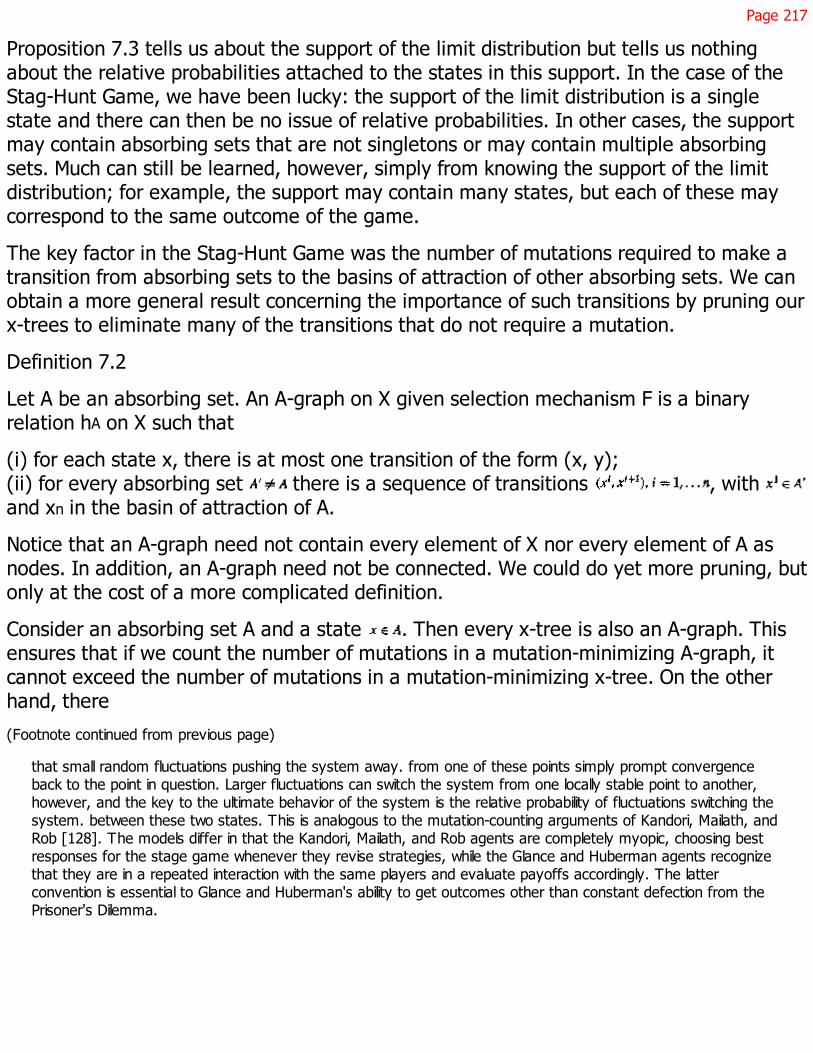
Page 217

Proposition 7.3 tells us about the support of the limit distribution but tells us nothingabout the relative probabilities attached to the states in this support. In the case of theStag-Hunt Game, we have been lucky: the support of the limit distribution is a singlestate and there can then be no issue of relative probabilities. In other cases, the supportmay contain absorbing sets that are not singletons or may contain multiple absorbingsets. Much can still be learned, however, simply from knowing the support of the limitdistribution; for example, the support may contain many states, but each of these maycorrespond to the same outcome of the game.

The key factor in the Stag-Hunt Game was the number of mutations required to make atransition from absorbing sets to the basins of attraction of other absorbing sets. We canobtain a more general result concerning the importance of such transitions by pruning ourx-trees to eliminate many of the transitions that do not require a mutation.

Definition 7.2

Let A be an absorbing set. An A-graph on X given selection mechanism F is a binaryrelation hA on X such that

(i) for each state x, there is at most one transition of the form (x, y);(ii) for every absorbing set there is a sequence of transitions , with and xn in the basin of attraction of A.

Notice that an A-graph need not contain every element of X nor every element of A asnodes. In addition, an A-graph need not be connected. We could do yet more pruning, butonly at the cost of a more complicated definition.

Consider an absorbing set A and a state . Then every x-tree is also an A-graph. Thisensures that if we count the number of mutations in a mutation-minimizing A-graph, itcannot exceed the number of mutations in a mutation-minimizing x-tree. On the otherhand, there

(Footnote continued from previous page)

that small random fluctuations pushing the system away. from one of these points simply prompt convergenceback to the point in question. Larger fluctuations can switch the system from one locally stable point to another,however, and the key to the ultimate behavior of the system is the relative probability of fluctuations switching thesystem. between these two states. This is analogous to the mutation-counting arguments of Kandori, Mailath, andRob [128]. The models differ in that the Kandori, Mailath, and Rob agents are completely myopic, choosing bestresponses for the stage game whenever they revise strategies, while the Glance and Huberman agents recognizethat they are in a repeated interaction with the same players and evaluate payoffs accordingly. The latterconvention is essential to Glance and Huberman's ability to get outcomes other than constant defection from thePrisoner's Dilemma.

Page 218

are many A-graphs that are not x-trees because they are missing transitions. Notice,however, that any minimal A-graph can be converted into an x-tree for some byadding transitions that do not require mutations.8 This then gives us the converse, thatthe number of mutations in a mutation-minimizing A-graph cannot exceed the number ina mutation-minimizing x-tree for , from which we immediately have

Proposition 7.5

State x appears in the limit distribution if and only if x is contained in an absorbing set Afor which

where hA is an A-graph, HA is the set of A-graphs, and A is the set of absorbing sets.9

Nash Equilibria

Without making assumptions about the selection mechanism F, we have no reason tobelieve that the outcome of the model will bear any relationship to familiar equilibriumconcepts. This section investigates the consequences of a common assumption, namely,that agents do not switch away from best responses and do not play inferior responseseternally. To formalize this, let (i.x)be the expected payoff to an agent in population playing strategy , given that x is the current state.10 Then the system is Nash-compatible if, for any state ,

Statement (7.8) indicates that there is positive probability that the state of the systemchanges if and only if some agent is not playing a best

8. This holds because each state z that is not the origin of a transition in an A-graph is either contained in the basinof attraction of A or is contained in the basin of attraction of an absorbing set that has a state y as the origin of atransition, and transitions can then be added linking state z to x, or z to y, without requiring mutations.

9. Because hx is an x-tree and hA an A-graph, some room for ambiguity arises as to what hx or hA means when A isa singleton absorbing set containing the element x. The meaning will be clear from the context.

10. This calculation is well defined because x includes a specification of the strategies played by agents in populationsother than , and the matching process ensures that the expected payoff to an agent in population matches theexpected payoff from playing a single agent whose mixed strategy duplicates these population proportions.

Page 219

reply. Although this is a common assumption, it is not immediately clear what ensuresthat the system will work so flawlessly. Chapter 9 explores the implications of relaxingthis assumption in a particular setting. I shall abuse notation somewhat by saying that astate is a Nash equilibrium if each agent in the state is playing a best response to thedistribution of strategies in the other populations. Hence state x is a Nash equilibrium ifand only if, for all and any strategy ,

From (7.8), we immediately have

Proposition 7.6

Let the selection mechanism be Nash-compatible. Then the state x is a Nash equilibriumif and only if x is a singleton absorbing set.

Therefore, if the absorbing sets constituting the support of the limit distribution are allsingletons, then the support consists of Nash equilibria.

Proposition 7.6 is another version of the "folk theorem" of evolutionary game theory that"stability implies Nash," with the requirement that the limit distribution contain onlysingleton absorbing sets supplying the stability condition. It stops short of simplyasserting that the limit distribution consists only of Nash equilibria because in general wecannot exclude nonsingleton absorbing sets from the limit distribution. This should comeas no surprise. Many evolutionary models yield the result that outcomes will be Nashequilibria if they exhibit some stability property; but conditions ensuring convergence tostable outcomes are much more elusive.11

Recurrent Sets

The basic task of characterizing the limit distribution of the Markov process has beenreplaced with that of characterizing the support of the limit distribution, in the hopes thatthere are enough interesting cases in which the support alone provides sufficientinformation that we need look no further. How do we characterize the support? We can

11. Young's assumption that the game is weakly acyclic [250] is motivated by the need to exclude nonsingletonabsorbing sets. Crawford [66], Marimon and McGrattan [147], and Milgrom and Roberts [155, 156] examineconditions under which certain dynamic systems converge.

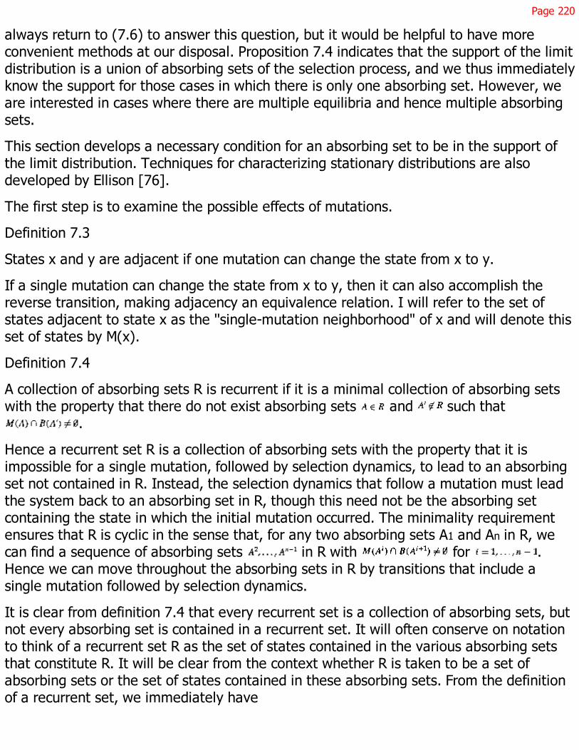
Page 220

always return to (7.6) to answer this question, but it would be helpful to have moreconvenient methods at our disposal. Proposition 7.4 indicates that the support of the limitdistribution is a union of absorbing sets of the selection process, and we thus immediatelyknow the support for those cases in which there is only one absorbing set. However, weare interested in cases where there are multiple equilibria and hence multiple absorbingsets.

This section develops a necessary condition for an absorbing set to be in the support ofthe limit distribution. Techniques for characterizing stationary distributions are alsodeveloped by Ellison [76].

The first step is to examine the possible effects of mutations.

Definition 7.3

States x and y are adjacent if one mutation can change the state from x to y.

If a single mutation can change the state from x to y, then it can also accomplish thereverse transition, making adjacency an equivalence relation. I will refer to the set ofstates adjacent to state x as the ''single-mutation neighborhood" of x and will denote thisset of states by M(x).

Definition 7.4

A collection of absorbing sets R is recurrent if it is a minimal collection of absorbing setswith the property that there do not exist absorbing sets and such that

.

Hence a recurrent set R is a collection of absorbing sets with the property that it isimpossible for a single mutation, followed by selection dynamics, to lead to an absorbingset not contained in R. Instead, the selection dynamics that follow a mutation must leadthe system back to an absorbing set in R, though this need not be the absorbing setcontaining the state in which the initial mutation occurred. The minimality requirementensures that R is cyclic in the sense that, for any two absorbing sets A1 and An in R, wecan find a sequence of absorbing sets in R with for .Hence we can move throughout the absorbing sets in R by transitions that include asingle mutation followed by selection dynamics.

It is clear from definition 7.4 that every recurrent set is a collection of absorbing sets, butnot every absorbing set is contained in a recurrent set. It will often conserve on notationto think of a recurrent set R as the set of states contained in the various absorbing setsthat constitute R. It will be clear from the context whether R is taken to be a set ofabsorbing sets or the set of states contained in these absorbing sets. From the definitionof a recurrent set, we immediately have

Page 221

Lemma 7.1

At least one recurrent set exists. Recurrent sets are disjoint.

The basic result is now that the limit distribution contains only absorbing sets that arecontained in recurrent sets, and includes all of the absorbing sets in any recurrent set thatcontributes to the limit distribution. The limit distribution is thus a union of recurrent sets.Section 7.5 proves

Proposition 7.7

Let state x be contained in the support of the limit distribution. Then

(i) x is contained in a recurrent set R;(ii) all states are contained in the support of the limit distribution.

A necessary condition for being contained in the limit distribution is then that a state becontained in a set that is robust to single mutations, which is to say, the selectiondynamics that follow a single mutation must at least eventually lead back to the set.

Where we encounter multiple recurrent sets and know only that at least one of themappears in the support of the limit distribution, there is no substitute for returning toproposition 7.3 and either doing the complete mutation-counting analysis or looking forfurther necessary conditions that might allow us to discriminate between the recurrentsets. Where we encounter a unique recurrent set, but one so large and containing statescorresponding to such a variety of outcomes as to be uninformative, there is no substitutefor seeking information on the shape of the limit distribution on its support. In manycases, however, we will find a unique recurrent set with much to be learned simply byknowing that the support of the limit distribution is confined to that recurrent set.

The results that emerge in the presence of a unique, "well-behaved" recurrent set aremore robust than many mutation-counting arguments. We may be uncomfortable withresults driven by the relative likelihoods of such highly improbable events (as l getssmall) as the simultaneous occurrence of enough mutations to move the system from oneabsorbing set to the basin or attraction of another. For example, we may hesitate toeliminate an absorbing set A from consideration on the strength of the argument that the10, 001 (highly improbable) mutations needed to get from absorbing set A to A' are muchless likely than

Page 222

the 10, 000 mutations needed to get from A' to A. In contrast, results based solely on thecomposition of recurrent sets are results driven by the fact that it takes only a singlemutation to escape from a set that is not recurrent, while it takes more than a singlemutation to escape from a recurrent set. I regard comparisons of this type as the mostrobust to emerge from the model and regard games in which such comparisons are usefulas the natural games to examine with the model.12

7.3 Alternative Best Replies

The tools developed in the previous section can now be applied to questions ofequilibrium selection. Particular attention will be devoted to Nash equilibria withalternative best replies, that is, Nash equilibria in which at least one agent hasalternative strategies that yield payoffs equal to those of the equilibrium strategy.

Alternative best replies are a natural application of these tools. As previous chapters havenoted, many equilibrium refinement questions arise out of the presence of alternativebest replies. More importantly the mutation-counting arguments that arise in connectionwith alternative best replies often involve simply checking whether the equilibria inquestion are contained in a recurrent set; hence single-mutation arguments suffice toexclude such equilibria from consideration.

The following will help characterize recurrent sets:

Definition 7.5

A set of states is a mutation-connected component of Nash equilibria if X' is minimalwith respect to the properties that every element of X' is a Nash equilibrium and no Nashequilibrium is adjacent to any element of X'.

A mutation-connected component is thus a maximal collection of Nash equilibria with theproperty that one can move from any state in the component to any other state in thecomponent, without leaving the component, by moving between adjacent states.

A mutation-connected component may appear to be simply a component of Nashequilibria, translated from the joint strategy set of the game into the state space, but thisneed not be the case. To illustrate

12. A complete consideration of "robustness" must include a careful examination of the issue of waiting times. Inparticular, dissatisfaction arises with results driven by large numbers of mutations because they can require verylong periods of time before the stationary distribution is an applicable description of the process. Chapter 9 offerssome brief remarks on waiting times.

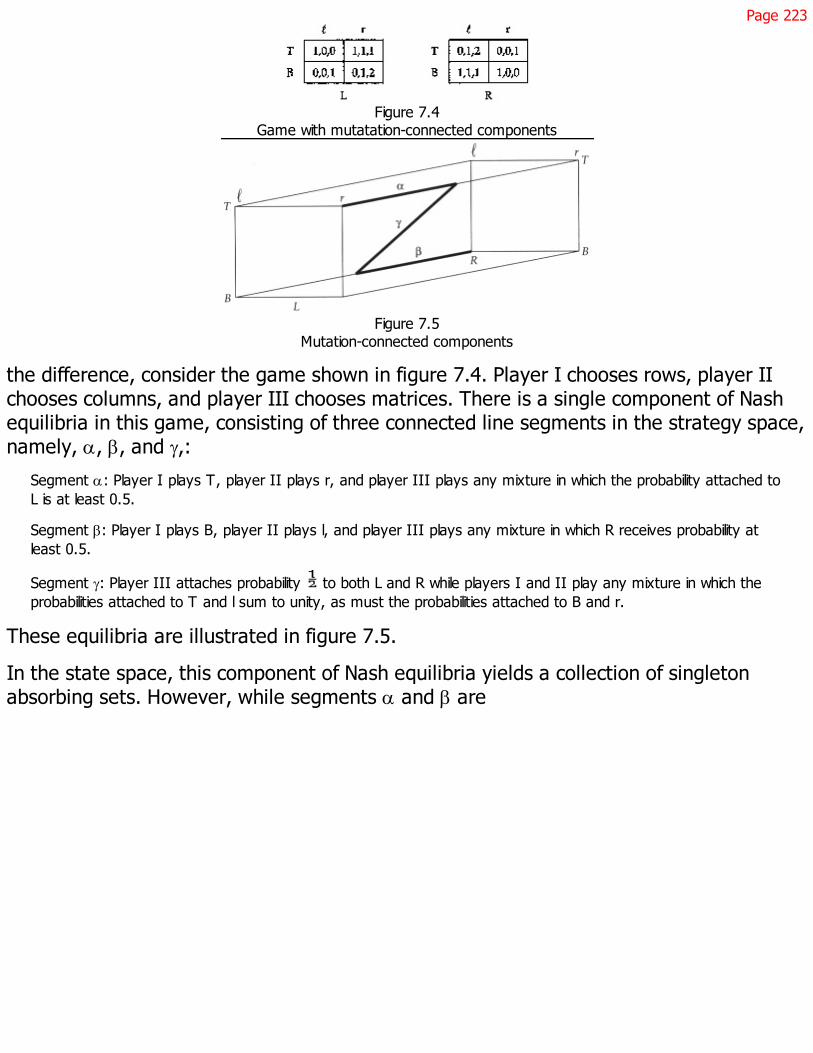
Page 223

Figure 7.4Game with mutatation-connected components

Figure 7.5Mutation-connected components

the difference, consider the game shown in figure 7.4. Player I chooses rows, player IIchooses columns, and player III chooses matrices. There is a single component of Nashequilibria in this game, consisting of three connected line segments in the strategy space,namely, a, b, and g,:

Segment a: Player I plays T, player II plays r, and player III plays any mixture in which the probability attached toL is at least 0.5.

Segment b: Player I plays B, player II plays l, and player III plays any mixture in which R receives probability atleast 0.5.

Segment g: Player III attaches probability to both L and R while players I and II play any mixture in which theprobabilities attached to T and l sum to unity, as must the probabilities attached to B and r.

These equilibria are illustrated in figure 7.5.

In the state space, this component of Nash equilibria yields a collection of singletonabsorbing sets. However, while segments a and b are

Page 224

each (separately) mutation-connected components, segment g, is not contained in amutation-connected component. In particular, a movement between two "neighboring"absorbing sets in segments a and b requires only one mutation, switching apopulation-III agent between L and R or vice versa. A movement between twoneighboring states in segment g, requires two mutations, one from population I and onefrom population II.

For the purposes of our analysis, mutation-connected components are the relevantobject. For example, let the learning dynamics in figure 7.4 be given by the best-responsedynamics. Then segments a and b are in recurrent sets, but there is no recurrent setcontaining g,. To verify this, we first note that beginning with a state in segment g, asingle mutation, causing an agent in population III to switch from L to R (or R to L) yieldsa state where B and l (or T and r) are best replies, which then yields a switch to a statewhere all agents in populations I and II play B or l (or T or r), contained in segment b (ora). If, however, we begin with a state in segment a or b, no single mutation can yield astate in the interior of segment g, (because the actions of at least two agents mustchange, one from population I and one from population II); each state in the interior ofsegment g, has only itself as its basin of attraction (because all populations mix at suchstates and at no state outside of g, are all populations indifferent, so the best-responsedynamics, from any state not in g, switch at least one population to a pure strategy). Thisestablishes that segments a and b can be contained in recurrent sets, but g, cannot be.This argument is easily extended to show that there is a unique recurrent set consistingof the union of a and b.

The definitions of a mutation-connected component and recurrent set ensure that if onestate of a mutation-connected component is contained in a recurrent set, then so are allstates. From these definitions, we immediately have

Proposition 7.8

Let the selection mechanism be Nash-compatible. If x is a Nash equilibrium contained inthe support of the limit distribution, then the entire mutation-connected component ofNash equilibria containing x is contained in the support of the limit distribution.

Six examples will serve to illustrate proposition 7.8. In the first five, the selectionmechanism is assumed to be the best-response dynamics with inertia; in the final slightlymore complicated example, it will be convenient to switch to another form of the best-response dynamics.

Page 225

For the first example, consider the game shown in figure 4.1, where strategy L strictlydominates R for player II. There is a unique component of Nash equilibria in which playerII plays L and player I chooses any mixture between T and B. There is similarly a uniquemutation-connected component in the state space, consisting of all those states in whichall agents in population II play L, namely, the unique recurrent set. The support of thelimit distribution then consists of all those states in which player II plays L. In all but oneof these states, some agents in Population I play B, and hence play a weakly dominatedstrategy.

This, the first of several examples in which we find that dominated strategies need not beexcluded from the limit distribution, raises three questions. First, how does strategy Bsurvive? The answer is familiar from chapter 4. T dominates B, but only weakly so, with Tearning a strictly higher payoff than B as long as some agents in population II play R. Inaddition, L strictly dominates R, and agents in population II are thus switching to L. Wethen have a race between agents in population II switching to L and agents in populationI switching to T. If the former switch sufficiently quickly; then the pressure against B iseliminated and an outcome appears in which the dominated strategy B persists.

Second, why do mutations not eliminate strategy B? Considerations from chapter 4 againreappear. By continually introducing R into the population, mutations should create weakbut persistent pressure against B. In particular, the selection dynamics near thecomponent of equilibria are always pushing population I away from B and toward T.Given that mutations constantly push us away from this component and bring thesedynamics into play; we should then expect the limit distribution at least to concentrate itsprobability on states in which the proportion of agents playing T is high. Notice, however,that at the same time these mutations introduce a pressure against B arising out of theappearance of R, they also introduce pressure toward B in the form of mutations thatswitch agents in population I to strategy B. If we simply left mutations in population I tooperate unchecked, the re-suit would be a force toward equal numbers of agents playingT and B. The net effect of these two forces is then unclear. Samuelson [201] shows thatwe will obtain outcomes in which the dominated strategy B is eliminated if we are willingto examine the limiting case of an arbitrarily large population and if, at states wherealmost all agents play L (formally; at states where all but one agent play L), theprobability

Page 226

the selection mechanism switches an agent from B to T becomes arbitrarily large, relativeto the probability an agent switches from R to L, as the population grows.

The palatability of this last condition depends upon our view of the selection mechanism.As the population becomes large, the payoff difference between strategies T and B, atstates where all but one agent play L, goes to zero. If we are to obtain an outcome inwhich dominated strategies are eliminated, the probability that agents switch from B to Tmust not go to zero. Hence the selection mechanism must exhibit a discontinuity; with azero probability of switching from B to T when the payoff difference is zero (if Nashcompatibility is to be preserved) while even an arbitrarily small payoff difference yields aswitching probability that is bounded away from zero. I have referred to selectionmechanisms with this property as "ordinal selection mechanisms" (Samuelson [198])because strategy switches appear to be driven by the relative payoff rankings ofstrategies rather than the magnitudes of the payoff differences involved. On the otherhand, we might expect the probability of switching between strategies to be increasing inthe payoff difference between the two strategies, yielding a cardinal system. I aminclined toward cardinal mechanisms, an inclination already indulged in chapter 6, wherethe selection process f was assumed to be continuously differentiable. If we choosecardinal mechanisms, however, we must be willing to live with ultralong-run outcomes inwhich dominated strategies appear.

Third, why do we care if strategy B survives? The payoffs are the same regardless ofwhether (T, L) or (B, L) is played. More generally, we would be unconcerned with thedetails of the limit distribution as long as all the states in its support give the sameeconomic outcome. However, by changing player II's payoffs in figure 4.1, we can obtaina case with the same limit distribution where the outcome does matter.

In making this change, we obtain a game that is not genetic even in its extensive form,much less being genetic in the space of normal-form payoffs. As noted in chapter 2, mypreference is to restrict analysis to generic games. However, as chapter 2 also noted, thespace in which the genericity argument is formulated must be carefully chosen. In manycases it is even too demanding to insist that if two outcomes give one player the samepayoff, then they give all players the same payoff because the economic outcomes at thetwo nodes may differ in details relevant to one player and not the other. Hence a beliefthat analysis

Page 227

should be restricted to generic games does not obviate the need to seriously considergames with ties between payoffs and games with payoff ties for some but not all players.

For the second example, let us turn to the game shown in figure 4.3, where again there isa unique Nash equilibrium in undominated strategies, given by (T, L). The absorbing setsare all singletons and consist of every state in which either all agents in population I playT or all agents in population II play L. These sets together constitute a mutation-connected component and are a recurrent set; all are then contained in the support of thelimit distribution. Once again, we limit our attention to Nash equilibria, but dominatedstrategies may appear. Notice that some coordination is introduced into the limitoutcome. Both strategies B and R can appear, but no state appears in which bothstrategies are played.

For the third example, consider the game shown in figure 6.4. where, as before, theabsorbing sets are singletons corresponding to the Nash equilibria of the game andconsist of all those states in which all agents in population I play N and at least of theagents in population II play R. These are again contained in a single recurrent set that isthe support of the limit distribution.

For the fourth example, we can present a single-population game with features similar tothose of figure 6.4. Young and Foster [252] consider a version of the infinitely repeatedPrisoners' Dilemma played by three strategies: TIT-FOR-TAT (TFT), COOPERATE (C), and DEFECT (D).Taking the payoffs of the stage game in the Prisoners' Dilemma to be given by figure 1.5and using the limit of the means to calculate payoffs, the payoff matrix for this three-strategy game is given by figure 7.6. The phase diagram for this game under a regular,monotonic dynamic is given in figure 7.7. There is again a single recurrent set containingall of the game's Nash equilibria, in which no agents play D and at least half of the agentsplay TFT. This set is the support of the limit distribution under the best-responsedynamics with inertia.

For the fifth example, consider the game shown in figure 7.8, where the Nash equilibriaconsist of two mutation-connected components. Component a contains those states inwhich all agents in population II play L and all agents in population I play M or T, with atleast playing M. Component b consists of a single state corresponding to the Nashequilibrium (B, R), which, because M dominates B, is an equilibrium in dominatedstrategies; hence every equilibrium in component b involves dominated strategies.

Page 228

Figure 7.6Repeated Prisoners' Dilemma

with three strategies


Figure 7.8Game with a single recurrent setcontaining dominated strategies

Calculating the recurrent sets for this example requires greater precision in thespecification of the best-response dynamics with inertia. What if an agent who receivesthe learn draw already plays a best response strategy, but other best responses are alsoavailable?

One likely outcome is that the agent will simply retain the current strategy. If this is thecase, then the selection mechanism can never cause agents to switch away from strategyM in figure 7.8, and the unique recurrent set consists of component a.

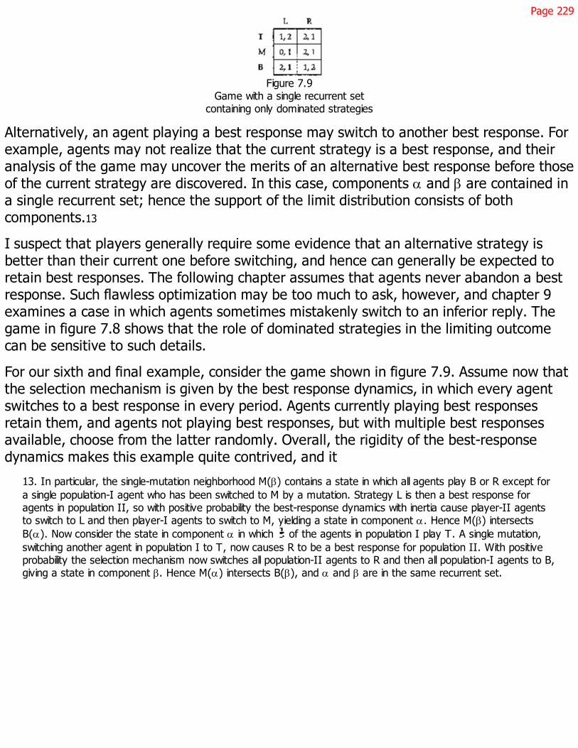
Page 229

Figure 7.9Game with a single recurrent set

containing only dominated strategies

Alternatively, an agent playing a best response may switch to another best response. Forexample, agents may not realize that the current strategy is a best response, and theiranalysis of the game may uncover the merits of an alternative best response before thoseof the current strategy are discovered. In this case, components a and b are contained ina single recurrent set; hence the support of the limit distribution consists of bothcomponents.13

I suspect that players generally require some evidence that an alternative strategy isbetter than their current one before switching, and hence can generally be expected toretain best responses. The following chapter assumes that agents never abandon a bestresponse. Such flawless optimization may be too much to ask, however, and chapter 9examines a case in which agents sometimes mistakenly switch to an inferior reply. Thegame in figure 7.8 shows that the role of dominated strategies in the limiting outcomecan be sensitive to such details.

For our sixth and final example, consider the game shown in figure 7.9. Assume now thatthe selection mechanism is given by the best response dynamics, in which every agentswitches to a best response in every period. Agents currently playing best responsesretain them, and agents not playing best responses, but with multiple best responsesavailable, choose from the latter randomly. Overall, the rigidity of the best-responsedynamics makes this example quite contrived, and it

13. In particular, the single-mutation neighborhood M(b) contains a state in which all agents play B or R except fora single population-I agent who has been switched to M by a mutation. Strategy L is then a best response foragents in population II, so with positive probability the best-response dynamics with inertia cause player-II agentsto switch to L and then player-I agents to switch to M, yielding a state in component a. Hence M(b) intersectsB(a). Now consider the state in component a in which of the agents in population I play T. A single mutation,switching another agent in population I to T, now causes R to be a best response for population II. With positiveprobability the selection mechanism now switches all population-II agents to R and then all population-I agents to B,giving a state in component b. Hence M(a) intersects B(b), and a and b are in the same recurrent set.

Page 230

provides an extreme outcome: every state in the support of the limit distribution involvesdominated strategies. However unreasonable or unlikely such an outcome is, it effectivelyexposes the mechanics of the model.

Two absorbing sets exist here, each of which is a singleton. Let these absorbing states bedenoted by x and y, where state x corresponds to the Nash equilibrium (M, R), whichinvolves the dominated strategy M. State y then corresponds to the mixed equilibrium inwhich agents in population I are evenly divided between T and B, while those inpopulation II are evenly divided between L and R. To show that the unique recurrent setcontains only set x, we can first note that the basin of attraction of state y can onlycontain states in which player II is indifferent between L and R and attaches an equalproportion of the population to each of these strategies. This in turn is a feature of thewell-known difficulty of having best-response dynamics converge to a mixed-strategyNash equilibrium. However, the best-response dynamics, beginning from any state thatcan be reached from x by a single mutation, cannot reach a state in which L and R giveequal payoffs and are played in equal proportions. The basin of attraction of y is thus nota single mutation away from x.14 As a special case of the observation that every stateexcept y is in the basin of attraction of x, a single mutation suffices to transform y into astate in the basin of attraction of x.15 The result is a limit distribution in which onlyequilibria involving dominated strategies are played.

7.4 Trembles

The previous section shows that dominated strategies can survive in the limit distribution.Chapter 4 has already touched on the differ-

14. Any mutation in population I transforms state x into a state in which either L or R is a strict best response forpopulation II. A mutation in population II makes either T or B a strict best response, and once all population-Iagents have switched to this best response, either L or R will be a best response for player II. In either case, wereach a state in which all population-II agents play the same strategy. But then population II must thereafteralways be monomorphic. In each period, either all population-II agents play a (possibly weak) best response andretain their strategy, or all play an inferior response and switch to the other strategy. This precludes convergenceto state y.

15. For example, let this single mutation switch an agent in population II from R to L. Then all agents in population Iswitch to B, at which point all agents in population II switch to R. Strategies M and T are now both unplayed bestresponses for player I, allowing some probability that all agents in population I switch to M.

Page 231

Figure 7.10Selection mechanism

ences between perturbations to the process by which agents select their strategies, suchas the mutations that appear in this chapter, and trembles in the implementation of astrategy. To explore the difference between mutations and trembles in the currentcontext, I add trembles to the model.16

Let us begin with an example built around the game of figure 4.1. To make explicit thecalculations that characterize the limit distribution, we must work with a simple statespace. We therefore assume that each of the two populations consists of a single agent.There are then four states, consisting of {TL, TR; BL, BR}, where the first element of astate specifies player I's choice and the second element specifies player II's choice. Let l.be the probability an agent undergoes a mutation that switches the agent's strategy, andlet l be constant across agents and states.

The selection mechanism without trembles will be constructed to create the strongestpossible pressure against the dominated strategy B consistent with payoff-driven strategychoices. We shall therefore assume that if player II plays R in period t, then player IIswitches to L in period . Player I switches strategies if and only if a payoff of zero isrealized, in which case player I switches to T. The transition matrix for the selectionmechanism is then given in figure 7.10. Notice that states TL and BL are adjacentsingleton absorbing sets and hence together constitute the unique recurrent set. In theabsence of trembles, the limit distribution will thus include TL and BL.

Now let us consider trembles. Before the play of the game in each period, each playertakes a draw from a Bernoulli trial that with probability d produces the outcome ''tremble"and with probability

16. Canning [58, 59] examines evolutionary models with trembling hand trembles but without mutations.

Page 232

Figure 7.11Selection mechanism with trembles

produces no tremble. In the latter case, the agent plays her current strategy; in theformer, the agent's strategy is chosen from a tremble distribution that depends upon theagent's current strategy.

Given the selection mechanism, trembles on the part of player I can do nothing to speedthe elimination of strategy B. Accordingly, let us assume that trembles never distortplayer I's choices, so that the tremble distributions for player I simply put unitary mass onplayer I's current strategy. Player II's tremble distribution when playing R similarly putsunitary mass on R because having player II play L instead of R can never increase thepressure to play B. However, when player II chooses L, the result is to play L withprobability and to play R with probability d. These trembles ensure that T receives anexpected payoff higher than B in every state. Together, the trembles and selectionmechanism appear to present the best case possible for the elimination of B.

The selection mechanism with trembles is shown in figure 7.11. There is now a uniqueabsorbing set consisting of the state TL, and the limit distribution will place probabilityonly on TL. Trembles thus have the effect of excluding dominated strategies from thelimit.

We are interested, however, not in trembles that occur with some fixed probability d butin trembles that can be taken to be arbitrarily small, just as trembling-hand perfectequilibria are obtained by taking the limit as trembles approach zero. We are theninterested in two limits, with both the probability of a tremble and the probability of amutation approaching zero. Once again, the order of these limits is an issue. To addressthis, let d(l) identify the probability of a tremble as a function of the probability of amutation, where . The complete transition matrix, with both trembles andmutations, is then given in figure 7.12.

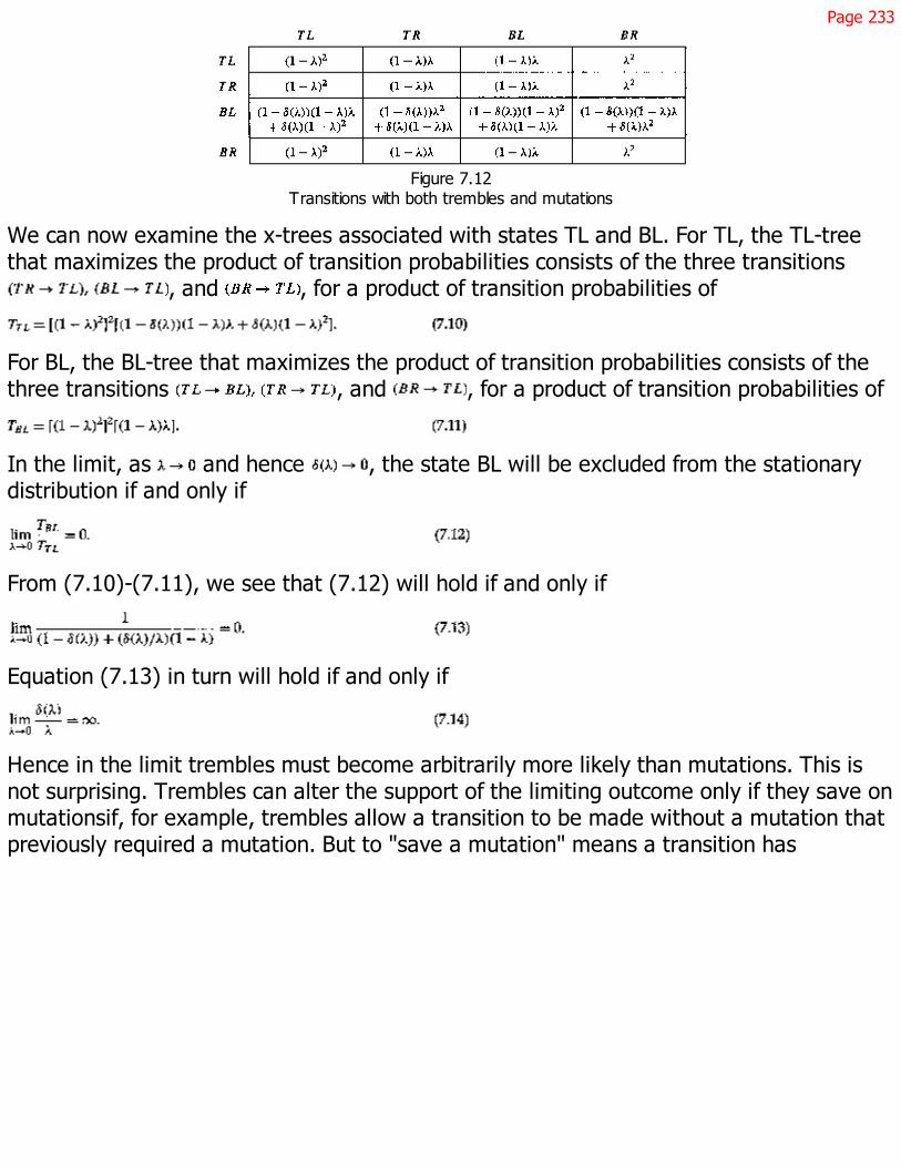
Page 233

Figure 7.12Transitions with both trembles and mutations

We can now examine the x-trees associated with states TL and BL. For TL, the TL-treethat maximizes the product of transition probabilities consists of the three transitions

, and , for a product of transition probabilities of

For BL, the BL-tree that maximizes the product of transition probabilities consists of thethree transitions , and , for a product of transition probabilities of

In the limit, as and hence , the state BL will be excluded from the stationarydistribution if and only if

From (7.10)-(7.11), we see that (7.12) will hold if and only if

Equation (7.13) in turn will hold if and only if

Hence in the limit trembles must become arbitrarily more likely than mutations. This isnot surprising. Trembles can alter the support of the limiting outcome only if they save onmutationsif, for example, trembles allow a transition to be made without a mutation thatpreviously required a mutation. But to "save a mutation" means a transition has

Page 234

to occur with a probability an order of magnitude higher than that of a mutation, andhence (7.14) must hold.

This relationship between trembles and mutations goes beyond our simple example.17

Let be the selection mechanism with trembles, where . Let bethe "limit distribution with trembles," where d(l) gives the probability of a tremble as afunction of the probability of a mutation, gives the stationary distribution for fixedl and hence fixed d(l), and where is the limit of these distributions as . Lettrembles and mutations be independent.

Proposition 7.9

Let x and y be adjacent absorbing states. Let x but not y appear in the support of ,the limit distribution with trembles. Then .

Proposition 7.9 is proven in section 7.5. The intuition is familiar from our example.Trembles matter because they create new transitions between states and hence save onmutations, allowing some paths in the state space to be traversed with fewer mutations.If it is to make a difference in the support of the limit distribution, however, "saving amutation" must involve creating a transition probability an order of magnitude higherthan the probability of a mutation. Hence trembles must become arbitrarily more likelythan mutations in the limit. The "small" trembles of trembling hand perfection may not beas small as they initially appear.



Statement (i)

Because is proportional to Á(l), it suffices for the existence of to showthat for all , that has a limit as l converges to zero. This follows immediatelyfrom (7.4), which implies that is a ratio of polynomials in l.

Statement (ii)

From (7.4), can be written as the sum over Hx of terms of the form , where aand b are constant in l. From proposition 7.2, we then have if and only if thesummation over

17. The version of the following argument that appeared in Samuelson [201] was unnecessarily complicated andcontained errors. I am thankful to Philippe Rivière for bringing this to my attention.

Page 235

Hx appearing in contains a term that maximizes (over the summations over Hy

appearing in the expressions for , ) the exponent attached to . From the definitionof k(x, y) given in (7.5), this is the set of x satisfying (7.6).


Statement (i)

Let

We interpret N(hx) as the minimum number of mutations required to accomplish thetransitions in the x-tree hx. Let . Then N*(x) is the value of the minimumcontained in parentheses in (7.6). We assume throughout the remainder of this sectionthat all sequences of states are chosen so that their members are unique, without loss ofgenerality.

Now let not be contained in an absorbing set. Let be an x1-tree for which. There exists a sequence of distinct states such that for and such that xn is contained in an absorbing set A and is the first such state in

the sequence. There also exists a state such that contains a transition forsome state ; and there exists a sequence of states , contained in A with

and .

It suffices to show that because this will ensure, from (7.6), that x1 is notcontained in the limit distribution. Now remove from each transition of the form (xi, wi)and (yi, zi), (i.e., remove all transitions beginning with xi and yi, ) and addthe transitions , and (yn, xn). The result is an xn-tree.None of the added transitions requires a mutation, while the deleted transition (y1, z) didrequire a mutation (because y1 but not z is contained in the absorbing set A). Hence

as required.

Statement (ii)

Let y1 and yn be contained in an absorbing set A. We show , which (because yl

and yn are arbitrary) suffices for the result. Let . Note that A must contain asequence of states with none of the transitions requiring a mutation. Thenconstruct a yn-tree by deleting from each transition of the form (yi, zi) and adding

. The result is a yn-tree with , giving the result.

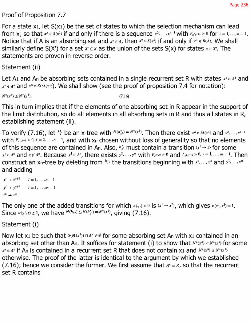
Page 236


For a state x1, let S(x1) be the set of states to which the selection mechanism can leadfrom xl, so that if and only if there is a sequence with for .Notice that if A is an absorbing set and , then if and only if . We shallsimilarly define S(X') for a set as the union of the sets S(x) for states . Thestatements are proven in reverse order.

Statement (ii)

Let A1 and An be absorbing sets contained in a single recurrent set R with states and and ). We shall show (see the proof of proposition 7.4 for notation):

This in turn implies that if the elements of one absorbing set in R appear in the support ofthe limit distribution, so do all elements in all absorbing sets in R and thus all states in R,establishing statement (ii).

To verify (7.16), let be an x-tree with . Then there exist and with , and with xn chosen without loss of generality so that no elementsof this sequence are contained in An. Also, must contain a transition for some

and . Because , there exists with and . Thenconstruct an xn-tree by deleting from the transitions beginning with and and adding

The only one of the added transitions for which is , which gives .Since , we have , giving (7.16).

Statement (i)

Now let x1 be such that for some absorbing set An with x1 contained in anabsorbing set other than An. It suffices for statement (i) to show that for some

if An is contained in a recurrent set R that does not contain x1 and otherwise. The proof of the latter is identical to the argument by which we established(7.16); hence we consider the former. We first assume that , so that the recurrentset R contains

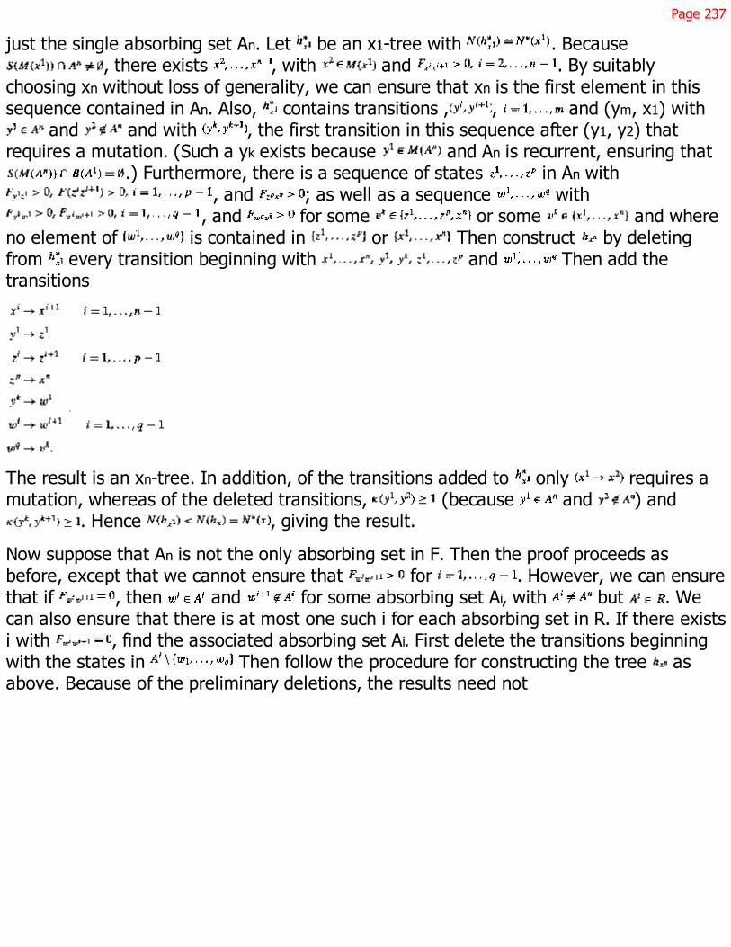
Page 237

just the single absorbing set An. Let be an x1-tree with . Because, there exists , with and . By suitably

choosing xn without loss of generality, we can ensure that xn is the first element in thissequence contained in An. Also, contains transitions , , and (ym, x1) with

and and with , the first transition in this sequence after (y1, y2) thatrequires a mutation. (Such a yk exists because and An is recurrent, ensuring that

.) Furthermore, there is a sequence of states in An with, and ; as well as a sequence with

, and for some or some and whereno element of is contained in or Then construct by deletingfrom every transition beginning with and Then add thetransitions

The result is an xn-tree. In addition, of the transitions added to only requires amutation, whereas of the deleted transitions, (because and ) and

. Hence , giving the result.

Now suppose that An is not the only absorbing set in F. Then the proof proceeds asbefore, except that we cannot ensure that for . However, we can ensurethat if , then and for some absorbing set Ai, with but . Wecan also ensure that there is at most one such i for each absorbing set in R. If there existsi with , find the associated absorbing set Ai. First delete the transitions beginningwith the states in Then follow the procedure for constructing the tree asabove. Because of the preliminary deletions, the results need not

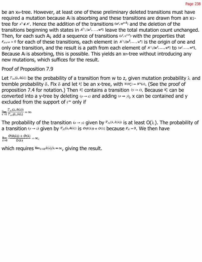
Page 238

be an xn-tree. However, at least one of these preliminary deleted transitions must haverequired a mutation because Ai is absorbing and these transitions are drawn from an x1-tree for . Hence the addition of the transitions and the deletion of thetransitions beginning with states in leave the total mutation count unchanged.Then, for each such Ai, add a sequence of transitions with the properties that

for each of these transitions, each element in is the origin of one andonly one transition, and the result is a path from each element of to .Because Ai is absorbing, this is possible. This yields an xn-tree without introducing anynew mutations, which suffices for the result.


Let be the probability of a transition from w to z, given mutation probability l andtremble probability d. Fix d and let be an x-tree, with . (See the proof ofproposition 7.4 for notation.) Then contains a transition . Because can beconverted into a y-tree by deleting and adding , x can be contained and yexcluded from the support of only if

The probability of the transition given by is at least O(l). The probability ofa transition given by is because . We then have

which requires , giving the result.

Page 239

8Backward and Forward Induction

8.1 Introduction

This chapter puts the tools developed in chapter 7 to work. We shall focus on whether thelimit distributions in very simple extensive-form games restrict attention to outcomes thatexhibit backward or forward induction properties.1

To examine extensive-form games, two modifications in the previous analysis arerequired.2 First, the notions of what characterizes a player and a state must be expanded.A player, instead of being described simply by strategy will now be characterized by astrategy and a conjecture as to the strategies of other players; a state, by a specificationof how many agents in each population hold each possible conjecture and strategy.

I think it most natural to assume that players in an extensive-form game can observe thepath of play through. the game but cannot observe what opponents would have chosenat unreached information sets, and hence cannot observe opponents' strategies. To makechoices based on their observations of current outcomes, players need some conjecturesas to what behavior will appear if these choices cause information sets to be reached thatare not included in the current path of play. As a result, a process in which players choosebest responses to current strategies can require players to know the details of behavior atinformation sets that cannot be observed under current play. Endowing players withconjectures allows them to choose best responses to observable information and to theirbeliefs about things they cannot observe.

1. This chapter is taken from Nöldeke and Samuelson [168].

2. Canning [58, 59] confronts similar issues in examining evolutionary processes on extensive-form games.

Page 240

Second, once conjectures are introduced into the model the evolutionary "folk theorem"that "stability implies Nash" must be reconsidered. Singleton absorbing states will nowcorrespond to self-confirming equilibria rather than to Nash equilibria. Absorbing setsexist in which each agent is playing a best reply to the observed behavior of otheragents, but which fail to be Nash equilibria because conjectures about what opponentswould do off the equilibrium path are not correct.

Given that we are going to be working with self-confirming equilibria, the notion ofbackward induction also requires some modification. A self-confirming equilibrium will besaid to be "subgame-consistent" if the strategies and conjectures yield a self-confirmingequilibrium on every subgame. Notice that this notion of consistency could be applied toany equilibrium concept, and a subgame-perfect equilibrium is simply a Nash equilibriumthat is subgame-consistent.

The examination begins with the study of recurrent outcomes. An outcome is recurrent ifthere exists a recurrent set with the property that every state in that set produces theoutcome in question. There may be many states producing a given outcome, where thesestates differ in their specifications of conjectures or behavior off the equilibrium path inways that do not affect realized behavior. This chapter shows that recurrent outcomesexhibit both backward and forward induction properties. In extensive-form games inwhich each player moves at most once along any path, every recurrent outcome is asubgame-consistent self-confirming equilibrium outcome. Furthermore, every recurrentoutcome must satisfy a forward induction property. In two-player games from our class,this property implies the never-weak-best-response property.

Our analysis cannot halt with this result, however, because recurrent outcomes may failto exist. Instead, recurrent sets may contain states yielding a variety of outcomes.3 Thechapter continues by considering two simple classes of games.

First, we examine backward induction in games of perfect information in which eachplayer moves at most once along any path. In these games there is a unique recurrentset, which contains the subgame-perfect equilibrium outcome. However, the subgame-perfect equilib-

3. It is also possible for recurrent outcomes to exist without the corresponding recurrent set appearing in thesupport of the limit distribution or constituting the entire support of the limit distribution.

Page 241

rium outcome will be the only outcome in this set, and hence will be a recurrent outcome,only under stringent conditions. If these conditions are not met, the subgame-perfectequilibrium still appears in the limiting distribution, but is accompanied by other self-confirming that yield different outcomes.

Next, we examine forward induction in games where player I has a choice betweenexercising an outside option or playing a normal-form game with player II. If there is anystrict Nash equilibrium of the sub-game yielding a higher payoff to player I than theoutside option, then equilibria in which the latter is played cannot appear in the limitingdistribution.

8.2 The Model

Consider a game denoted by G, where G is now taken to be a finite, extensive-form gamewith perfect recall and without moves by nature. Let denote the set of playersand the set of terminal nodes, or outcomes. An assignment of payoffs to terminal nodesis given by the function .

Our attention will be restricted to games G satisfying the condition that no path throughthe game tree intersects two or more information sets of a single player. This is a naturalclass of games in which to examine subgame perfection because questions of rationalbehavior after evidence of irrationality do not arise (cf. Binmore [18] and Reny [186]).More important, restricting attention to this class of games allows the specification ofstraightforward rules for updating strategies and conjectures.4

Learning

Given an extensive form game G, assume that, for every player , there is a finitepopulation consisting of N > 1 agents. At each time , every possible combinationof agents capable of playing the game meets and plays.

At time t, each agent of each population is described by a characteristic, consisting of apure behavior strategy and a conjecture. A conjecture for an agent specifies, for eachpopulation representing an opponent and for each action such an opponent may take atone of his

4. See notes 6 and 8 for details.

Page 242

information sets, the number of agents in the population taking that action5.A state of thesystem is a specification of how many agents in each population have each possiblecharacteristic. Let X denote the set of possible states of the system, and let x denote anelement of X. Associated with every state is a distribution over terminal nodes, denotedby sx, that results from the matching process and play of the game.

The selection mechanism will be given by a form of the best-response dynamics withinertia. Hence, in each period, after agents have been matched, each agent of eachpopulation independently takes a random draw from a Bernoulli trial. With probability

, the agent's characteristic does not change. With probability m, the drawproduces the outcome ''learn." An agent who learns is able to observe the outcomes of allmatches of the current round of play. Notice that players cannot observe actions atinformation sets that are not reached during the course of play.

Given this information, the agent first updates his conjectures to match the observedfrequency of actions at all information sets that were reached during period t. Updatedconjectures about play at information sets that are reached are uniquely determined andthe same for all agents who learn.6 Conjectures at unreached information sets areunchanged.7

Given his new conjecture, the agent updates his behavior strategy. At all information setswhere his current action is a best response,

5. Notice that these conjectures describe opponents' actions rather than beliefs about nodes in information sets, asin the usual specification of a sequential equilibrium (see Kreps and Wilson [138]).

6. This specification uses the assumptions that every player moves at most once along each path and that learningplayers observe the outcomes of all matches. In particular, suppose player i's information set h is reached in somematch. Whether h is reached depends only on the choices of player i's opponents, so it must be that for all agentsfrom population i, there is a matching that allows their behavior at h to be observed. All learning agents then observethis behavior and update their conjectures to match the actual distribution of actions by player-i agents at informationset h. The assumption that learning agents observe the current state is strong, but allows a convenientcharacterization of conjectures.

7. Because agents update conjectures to match the most recently observed play, an agent's conjecture aboutanother agent is a strategy rather than a probability distribution over strategies. Assuming that learning agents observethe most recent play and change their conjectures to match this play yields a finite state space, which simplifies theanalysis.

Page 243

his action remains unchanged.8 At all information sets where his current action is not abest response against his conjecture, the agent changes to an action that is chosenaccording to some probability distribution (which depends only on the agent's informationabout the current state) that puts positive probability on all actions that are bestresponses.

In chapter 6 the assumption that the selection mechanism is "smooth" was identified asan important and appealing assumption. The most common specification violating thisassumption is best-response dynamics. Best-response dynamics with inertia would satisfythis smoothness assumption if the degree of inertia were related to payoffs, so thatagents were less likely to evaluate their strategies and switch to a best response whendifferences in payoffs were small. The specification of this chapter, however, where theprobability of an agent's switching to a best response is m, regardless of payoffs, is notsmooth.

This chapter shows that even in the ultralong run, we cannot expect evolutionary modelsto select subgame-perfect equilibria. Using a best-response-based learning processmakes it as difficult as possible to obtain this result because it ensures that the pressureto switch to best responses, which is crucial to obtaining subgame-perfect equilibria,remains strong even as the payoff differences driving this pressure shrink. The result thatthe subgame-perfect equilibrium is not selected is most powerful in such a setting.

The best-response dynamics with inertia have the property that an agent can hold aconjecture while experiencing outcomes that contradict that conjecture, and yet still notalter the conjecture. Only when the learn draw is next received does an agent checkwhether her conjectures are consistent with her own play. It may not be unusual foragents to only occasionally evaluate their beliefs by collecting information about the stateof the world, but why does an agent not immediately incorporate into her conjecturesinformation provided by the outcome of her own plays? To answer this, I again appeal tothe belief

8. Again, whether one of the agent's own information sets is reached does not depend on the agent's behaviorstrategy. Therefore his conjectures and hence action remains unchanged at any information set that was notreached in the previous state. In particular, changes in an agent's actions at an information set h cannot causethat agent to now potentially reach and hence choose a new action at the previously unreached information set. h'

Page 244

that people are typically involved in many strategic situations, each of which requiresthem to form conjectures about the situation they face and choose an action based onthat conjecture. It is impossible to conduct a full analysis of every choice, and mostchoices are made on the basis of decision rules that involve little or no analysis. Thesechoices may not be best replies and may be based on conjectures that are inconsistentwith observed outcomes or even internally inconsistent. Only when the occasionalopportunity is taken to conduct an analysis of a problem can we expect people to formconsistent models. These models may subsequently be rendered obsolete by changes inthe strategic environment, and the agent will again persist in using a model that iscontradicted by her experience, until the next time she brings her reasoning to bear onthe problem.

The learning mechanism defines a collection of probabilities of the form Fxy for all x and yin X. These probabilities in turn constitute a Markov process on the state space X.

Mutations

Mutations now make their appearance. At the end of each time t, each agent takesanother independent draw from a Bernoulli trial. With probability , this drawproduces no change in this agent's characteristic. With probability l, this draw producesthe outcome "mutate," where the agent changes to a characteristic randomly determinedaccording to a probability distribution that puts positive probability on each of thecharacteristics possible for this agent.

The learning and mutation processes together yield a Markov process, denoted by é, withtransition probabilities . We again have the standard result that the Markov process

has a unique stationary distribution g*(l). We are interested in the limitdistribution .

Limit Distribution

The study of the limit distribution begins with a characterization of singleton absorbingsets.

Definition 8.1

A state is a self-confirming equilibrium if each agent's strategy is a best response tothat agent's conjecture and if

Page 245

each agent's conjecture about opponents' strategies matches the opponents' choices atany information set that is reached in the play of some match.

This is the analogue of Fudenberg and Levine's notion of a self-confirming equilibrium[91], except that it is defined directly in the state space of the Markov process ratherthan in the strategy space of the game.9

The definition then immediately implies (where absorbing states were introduced in theprevious chapter):

Proposition 8.1

State is an absorbing state if and only if x is a self-confirming equilibrium.

As expected, this establishes equivalence between singleton absorbing sets and self-confirming equilibria rather than Nash equilibria. Limit distributions composed of singletonabsorbing sets will then be composed of self-confirming equilibria.10

Proposition 7.7 can be adapted to this model to ensure that the limit distribution containsonly recurrent sets and all of the absorbing sets in any recurrent set that contributes tothe limiting distribution. Then what can be said about recurrent sets? Consider a self-confirming equilibrium. A key observation is that any recurrent set containing thisabsorbing state will also contain states corresponding to the same path through theextensive-form game, but a variety of out-of-equilibrium behavior and out-of-equilibriumconjectures. Some additional terminology is helpful in making this precise. Given a self-confirming equilibrium outcome, player can force entry into a subgame if there

9. See Kalai and Lehrer [126] for a similar equilibrium concept. There may be self-confirming equilibria in the gameG that cannot be supported as self-confirming equilibria in the state space of the Markov process é because theformer require mixed strategies that cannot be duplicated as population proportions in the finite populations playinggame G. A similar difficulty arises when considering subgame-perfect equilibria. In the following analysis we shall notdistinguish between equilibria in the game G and in the state space of the Markov process. This is appropriate if thepopulation size is such that we can achieve any desired equilibrium on every subgame in the state space. Similar re-suits can be obtained for pure-strategy versions of the equilibrium concepts without this assumption.

10. Nöldeke and Samuelson [167] provide an example of a simple signaling game in which a self-confirming equilibriumthat is not a Nash equilibrium appears in the limiting distribution of the evolutionary process, ensuring that theconsideration of self-confirming equilibria that are not Nash equilibria is necessary.

Page 246

exists an information set h belonging to player that is reached in at least some matchduring the play of the self-confirming equilibrium and if there also exists an action forplayer at h that is not chosen by any player- agent and is such that the decision noderesulting from the choice of is the root of subgame . We then have

Proposition 8.2

(i) Let be an absorbing state. Let x' differ from x only in actions prescribed atinformation sets that are not reached in any matchings in state x (i.e., every agent in xcan be paired with a distinct agent in x' such that the two agents hold identicalconjectures at all information sets and play identical actions at all information setsreached in any matching under x). Then x' is also an absorbing state and a recurrent setthat contains x also contains x'.

(ii) Suppose that, given an absorbing state x, player can force entry into a subgame. If x' differs from x only in the conjectures that agents from populations other than

hold over choices at information sets in , then a recurrent set that contains x alsocontains x'.

The proof is given in section 8.7. Part (i) of proposition 8.2 indicates that if a self-confirming equilibrium is contained in an absorbing set, then so is any state that can beobtained by altering actions at unreached information sets, while holding conjecturesfixed. That conjectures are fixed and actions are affected at unreached information setsensures that any such new state is also a self-confirming equilibrium and can be reachedfrom the original state by a series of mutations. This implies that the states are containedin the same recurrent set. Part (ii) indicates that the absorbing set will also include anystates that can be reached by altering the conjecture of a player about an unreachedsubgame into which the player cannot force entry. The implication of this result is thatthe evolutionary process is not effective at imposing discipline at unreached informationsets. If a self-confirming equilibrium appears in a recurrent set, so does any state thatcan be reached by perturbing actions at unreached information sets.

8.3 Recurrent Outcomes

We now examine recurrent sets that are composed of singleton absorbing sets. The onlyhope for single-valued equilibrium predictions clearly lies with recurrent sets that arecomposed of absorbing states,

Page 247

all of which correspond to the same self-confirming equilibrium outcome. We call theoutcome involved a "recurrent outcome:"11

Definition 8.2

An outcome s* is recurrent if there exists a recurrent set R such that for all , it is thecase that .

Studying such outcomes allows us to characterize the limiting distribution when the latteris "nicely behaved" and also provides some clue as to when it will be so behaved.

We can first establish a backward induction property for recurrent outcomes. Let x be aself-confirming equilibrium. Then x is a subgame-consistent self-confirming equilibrium if,for any subgame, the actions and conjectures specified by x for this subgame are a self-confirming equilibrium.12 We then have13

Proposition 8.3

Let G* be an extensive-form game with each player moving at most once along eachpath. Then every recurrent outcome is a subgame-consistent self-confirming equilibriumoutcome.

The proof is given in section 8.7. The intuition is that if the absorbing states in a recurrentset giving outcome s* do not correspond to a subgame-consistent self-confirmingequilibrium, then there must exist a subgame not reached in outcome s* that can beentered by some player and that has the property that every self-confirming equilibriumof this subgame gives a higher payoff than does s*. In addition, proposition 8.2 ensuresthat the recurrent set R contains states in which the actions on this subgame correspondto a self-confirming equilibrium, though agents' conjectures do not match those actions(otherwise, agent would not be playing a best reply, and the state would not be anabsorbing state). Now let a mutation cause a player- agent to enter this subgame, andlet all agents learn. Whatever else happens, the result will be a self-confirmingequilibrium in the subgame, and subsequent learning cannot change this behavior. Thelearning process

11. It is clear that a nonsingleton absorbing set must contain states corresponding to different outcomes, that is,must contain states x and x' such that , because only then can the learning dynamic cause the system tocycle between the states in the absorbing set.

12. Because attention is restricted to games with the property that every path of play intersects at most oneinformation set for every player, the actions and conjectures specified by x for a subgame are unambiguous.

13. In Nöldeke and Samuelson [168], we incorrectly claimed to have shown that recurrent outcomes were simplysubgame-perfect, or equivalently subgame-consistent Nash equilibria. We are grateful to Pierpaolo Battigalli for bringingthis to our attention.

Page 248

then cannot lead back to a state with an outcome s* because player prefers enteringthe subgame to playing her part of the outcome s*. Hence the learning process cannotlead back to R, which cannot then be recurrent. This establishes that recurrent outcomesmust be subgame-consistent self-confirming equilibria.

Turning now to forward induction, the following proposition shows that some self-confirming equilibrium outcomes can be subgame-consistent but still fail to be recurrentbecause they lack a forward induction property. This failure occurs because the statessupporting the subgame-consistent equilibrium outcome again allow a variety of behavioroff the equilibrium path, including behavior that, once revealed, will tempt agents awayfrom the equilibrium in quest of a higher payoff. The ability to pull agents away from anequilibrium requires only that an agent can cause a subgame to be reached that has atleast one self-confirming equilibrium promising the player a higher payoff than thesubgame-consistent self-confirming equilibrium. It may be impossible to support thishigher payoff as an equilibrium in the entire game, so that subsequent adjustments maylead away from this payoff, but these adjustments cannot lead back to the originalequilibrium. The proof of proposition 8.3 establishes the following:

Proposition 8.4

Let G be an extensive-form game with each player moving at most once along each path.Suppose outcome s* is recurrent. If, given a state yielding outcome s*, player can forceentry into a subgame , then no self-confirming equilibrium of can give player ahigher payoff than does s*.

The result in proposition 8.4 associates a strong forward induction property with locallystable outcomes. For example, this property is stronger than that of van Damme [239],which rejects an equilibrium if player can force entry into a subgame with a uniqueequilibrium that gives a higher payoff than the original equilibrium, but that (unlikeproposition 8.4) makes no comment about the case in which there are multiple suchequilibria in the subgame In many games, the conditions of proposition 8.4 will be toostringent to be satisfied by any of the subgame-consistent self-confirming equilibriumoutcomes. A recurrent outcome fails to exist in such a case.

In two-player games (with each player moving at most once along any path), theseresults can be sharpened. We can think of such a game

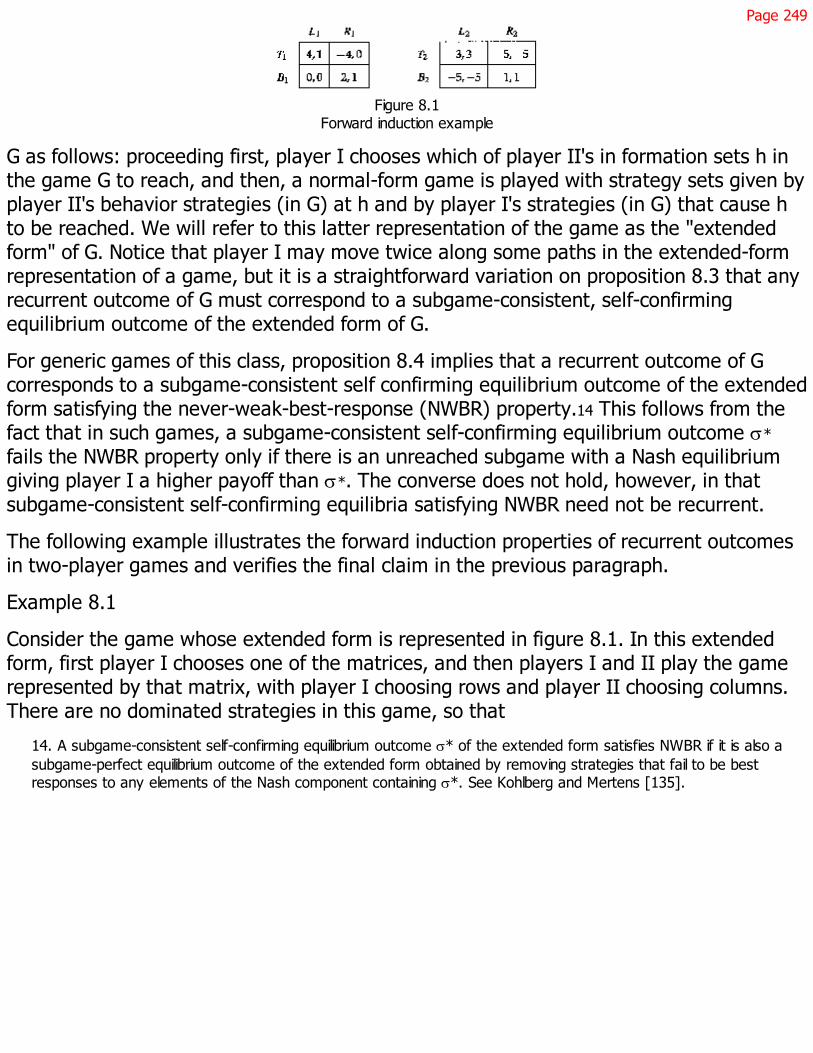
Page 249

Figure 8.1Forward induction example

G as follows: proceeding first, player I chooses which of player II's in formation sets h inthe game G to reach, and then, a normal-form game is played with strategy sets given byplayer II's behavior strategies (in G) at h and by player I's strategies (in G) that cause hto be reached. We will refer to this latter representation of the game as the "extendedform" of G. Notice that player I may move twice along some paths in the extended-formrepresentation of a game, but it is a straightforward variation on proposition 8.3 that anyrecurrent outcome of G must correspond to a subgame-consistent, self-confirmingequilibrium outcome of the extended form of G.

For generic games of this class, proposition 8.4 implies that a recurrent outcome of Gcorresponds to a subgame-consistent self confirming equilibrium outcome of the extendedform satisfying the never-weak-best-response (NWBR) property.14 This follows from thefact that in such games, a subgame-consistent self-confirming equilibrium outcome s*

fails the NWBR property only if there is an unreached subgame with a Nash equilibriumgiving player I a higher payoff than s*. The converse does not hold, however, in thatsubgame-consistent self-confirming equilibria satisfying NWBR need not be recurrent.

The following example illustrates the forward induction properties of recurrent outcomesin two-player games and verifies the final claim in the previous paragraph.

Example 8.1

Consider the game whose extended form is represented in figure 8.1. In this extendedform, first player I chooses one of the matrices, and then players I and II play the gamerepresented by that matrix, with player I choosing rows and player II choosing columns.There are no dominated strategies in this game, so that

14. A subgame-consistent self-confirming equilibrium outcome s* of the extended form satisfies NWBR if it is also asubgame-perfect equilibrium outcome of the extended form obtained by removing strategies that fail to be bestresponses to any elements of the Nash component containing s*. See Kohlberg and Mertens [135].

Page 250

iterated weak dominance fails to eliminate any strategies. NWBR eliminates thesubgame-perfect equilibrium (T2, L2). In particular, B1 is a best response to no element inthe component supporting outcome (T2, L2). Once B1 is eliminated, subgame consistencyrequires player II to choose L1 at her first information set, at which point (T2, L2) ceasesto be an equilibrium. Notice that NWBR cannot eliminate the subgame-perfect equilibriumgiven by (B2, R2) because every strategy is a best response to some element in thecomponent supporting this outcome.

In contrast, the only recurrent outcome in this game is (T1, L1). To see this, consider asingleton absorbing set x supporting either outcome (B2, R2) or (T2, L2). By proposition8.2, any recurrent set containing x contains a state y in which all player-II agents chooseL1 at their first information set. Now let a mutation occur that causes a player-I agent toplay T1. Then with positive probability, all player-I agents learn and switch to T1, yieldinga new singleton absorbing set x' that supports outcome (T1, L1). This establishes

(cf. definition 7.4). However, the equilibrium (T1, L1) gives player I thehighest possible payoff in the game, and action L1 is a strict best reply for player II at therelevant information set. There is then a set R, containing x', that contains only statesyielding the outcome (T1, L1) and that is recurrent for all sufficiently large populationsizes. This implies that the state x supporting outcome (B2, R2) is not contained in arecurrent set. Furthermore, (T1, L1) is the unique recurrent outcome because anargument similar to the one just given shows that neither the outcome (B1, R1) nor amixed-strategy equilibrium outcome is recurrent.

8.4 Backward Induction

Even if a game admits a unique subgame-consistent self-confirming equilibrium outcomes*, the results of the previous section do not allow us to conclude that s* appears in thelimit distribution, much less that s* is the only outcome in that distribution. The onlypossible recurrent outcome is s*, but a recurrent outcome may fail to exist, or thecorresponding recurrent set may not constitute the entire support of the limit distribution.To address these issues, we shall consider extensive-form games with each playermoving at most once along each path, as before, but now restrict attention to genericgames of perfect information. The result of this section is that the subgame-perfectequilibrium

Page 251

must appear in the limiting distribution, but only under stringent conditions will it be theonly outcome in the limiting distribution.15

The genericity condition is that for every player and every payoff of distinct terminalnodes x and x', . It is well known that such games have a unique subgame-perfect equilibrium.16

A useful preliminary result is that such games have only singleton absorbing sets, whichin turn implies that the evolutionary process converges to a recurrent set containing onlystates yielding self-confirming equilibrium outcomes:17

Proposition 8.5

Let G be a generic extensive form game of perfect information with each player movingat most once along each path. Then all absorbing sets are singletons.

(This and all subsequent propositions in this chapter are proved in section 8.7.)

Next, we can show that there is a unique recurrent set, and that recurrent set containsthe subgame-perfect equilibrium outcome. From proposition 7.7, this implies that thelimit distribution satisfies a backward induction property in the sense that it must assignstrictly positive probability to the subgame perfect equilibrium. Furthermore, if thesubgame-perfect equilibrium outcome is recurrent, then it must be the unique outcomeappearing in the support of the limiting distribution. The proof of this result, whichcombines ideas from the proof of propositions 7.7 and 8.3, exploits the fact thatabsorbing sets are singletons.

Proposition 8.6

Let G be a generic extensive-form game of perfect information with each player movingat most once along each path.

15. An equilibrium is subgame-perfect in such a game if and only if it is a subgame-consistent self-confirmingequilibrium, and we can accordingly speak simply of subgame-perfect equilibria. These games are dominance-solvable, so that the subgame-perfect equilibrium is the outcome of the iterated elimination of weakly dominatedstrategies in the normal form. The finding that the subgame-perfect equilibrium will often not be the only outcomein the limiting distribution is then related to the finding in chapter 7 that a similar model need not eliminate weaklydominated strategies in the normal form.

16. Notice that the unique subgame-perfect equilibrium will always be in pure strategies, so that the question ofwhether mixed strategies can be duplicated by population proportions does not arise.

17. Canning [59] shows that all the absorbing sets for a fictitious play process in extensive-form games of perfectinformation are singletons. In a model with "trembling hand" trembles of the type introduced by Selten [208], butwithout mutations, Canning finds the subgame-perfect equilibrium is the unique limiting outcome (as trembles becomesmall).

Page 252

Then there is a unique recurrent set and that recurrent set contains the subgame-perfectequilibrium outcome.

Proposition 8.6 establishes that the subgame-perfect equilibrium is the only candidate fora recurrent outcome. When will it be recurrent? Proposition 8.4 showed that thesubgame-perfect equilibrium outcome will not be recurrent if some player can be temptedaway from the equilibrium path by a self-confirming equilibrium in a sub-game thatpromises that player a higher payoff. This suggests that if no such opportunities arise, sothat no player can force entry into a sub-game with at least one self-confirmingequilibrium offering the player a higher payoff than the subgame-perfect equilibrium, thenthe latter will be recurrent. The following example shows that this conjecture is false.

Example 8.2

Consider the three-player game G* shown in figure 8.2.18 The unique subgame-perfectequilibrium is given by the strategy combination (R, R, R), for a payoff of (1, 1, 1). Let xR

be the state in which all agents from all populations play R, and let xL. be a state in whichall agents play L, with conjectures matching these actions. Note that xL is a self-confirming equilibrium, and gives payoffs (0, 0, 0). We can now show that xL must becontained in the support of the limit distribution.

By proposition 8.6, xR is in the support of the limit distribution, and so (by proposition8.2) is the state in which all agents from populations I and II play R and all agents frompopulation III play L, with conjectures matching the behavior of agents at reacheddecision nodes and with agents from population I and II conjecturing that all agents frompopulation III play R. Now let a single mutation cause an agent from population II to playL. With positive probability all agents from population II (but no other agents) nowreceive the learn draw, update their conjectures to match the observation that all agentsfrom population III play L, and switch to playing a best reply of L. Suppose in the nextstage of the evolutionary process all agents from population I (but no other agents)learn. They update their conjectures to match the observed behavior of other agents,which is that agents from population II are playing L, and then switch to their best replyof playing L.

18. It is easy to establish that for all two-player games (from the class of games under consideration) thesubgame-perfect equilibrium outcome is recurrent for every sufficiently large population size, and is thus the onlyoutcome in the limiting distribution of the evolutionary process.

Page 253

Figure 8.2Game G*

It is easily checked that the resulting state is a singleton absorbing set yielding the sameoutcome as xL. Beginning with a state contained in the recurrent set containing xR, asingle mutation thus reaches the basin of attraction of a state yielding the outcomecorresponding to xL. From the fact that xR is contained in a recurrent set and fromproposition 8.2 again, it thus follows that xL and xR are contained in the same recurrentset, and consequently the self-confirming equilibrium xL must appear in the support of thelimit distribution.

This example illustrates the differences between the outcomes of this model and variousnotions of evolutionary stability. It will be helpful to illustrate these differences byconsidering Swinkels's equilibrium evolutionarily stable (EES) sets [230]. It is easy to showthat in game G*, the (unique) EES set and the limiting distribution of the current modelboth contain a set of strategies corresponding to the payoff (1, 1, 1). In our case, therecurrent set containing these states also contains states corresponding to any possiblemixture on the part of player III, including mixtures that violate the conditions for a Nashequilibrium. It is the presence of these states that prevents the subgame-perfectequilibrium from being a recurrent outcome because single mutations

Page 254

can lead from these states to learning dynamics that draw the system away from thesubgame-perfect outcome. The corresponding EES set allows only Nash equilibria, andhence includes mixtures on the part of player III only if a probability of or less is placedon L. The dynamic intuition behind the EES set is that deviations from Nash equilibrium,even at unreached subgames, prompt immediate responses that push the system back tothe EES set, so that the system is not free to drift away from Nash equilibria via movementsat unreached information sets.

Swinkels [231] examines a dynamic model in which he obtains re-suits similar to those ofthe current chapter in a much different context. Swinkels considers an asymptotic stabilitynotion for sets of outcomes under a dynamic process specified by a deterministicdifferential equation, and shows that for a broad class of deterministic dynamics, setssatisfying this assumption must contain a Kohlberg and Mertens stable and hyperstableset [135]. The current model thus shares with Swinkels the characteristic that ''good"outcomes, such as subgame-perfect or stable equilibria, are contained in the limitingoutcome, but the limit outcome will generally not be restricted to include only such goodoutcomes. In the current model if any self-confirming equilibrium strategy profile appearsin the limiting distribution, then so do any other strategy profiles created by alteringbehavior at unreached subgames. These can include strategy profiles that are not self-confirming equilibria but are surrounded by learning dynamics that lead to quite differentoutcomes, causing the latter to also appear in the limiting distribution. In Swinkels'sdynamic model similar forces appear Every equilibrium appearing in the outcome isaccompanied by a host of strategy profiles that give the same outcome, in some casesincluding profiles surrounded by dynamics that lead to other outcomes. Swinkels observesthat his model holds some hope of yielding asymptotically stable sets that contain onlysubgame-perfect outcomes if the dynamics have rest points only at Nash equilibria (asopposed, for example, to having rest points at all self-confirming equilibria, as in thecurrent model).19

Proposition 8.4 and example 2 suggest that the subgame-perfect equilibrium outcome willbe the unique outcome in the limit distribution of the evolutionary process if no playercan be "tempted" away from the subgame-perfect equilibrium by a higher payoff, even

19. The potential difficulty with such an assumption is that it seemingly requires players to react to changes inactions at information sets that are not reached during play.

Page 255

a nonequilibrium payoff. To make this intuition precise, it is helpful to have a bit moreterminology. The subgame-perfect equilibrium outcome, identified by the terminal nodex*, is a strict outcome (cf. Balkenborg [4]) if no player can force entry into a subgamethat has a terminal node with a higher payoff than the subgame-perfect equilibrium. Moreformally; suppose that, given the subgame-perfect equilibrium outcome, player canforce entry into the subgame . Let denote the set of terminal nodes contained in

. If x* is a strict outcome, then for all ,

must hold. And we have20

Proposition 8.7

Let the game be as in proposition 8.6. If the subgame-perfect equilibrium outcome isstrict, it is the unique outcome in the limiting distribution for all sufficiently largepopulation sizes.

These results provide both good and bad news for backward induction. Subgameperfection presents the only possibility for a recurrent outcome, and the subgame-perfectequilibrium always appears in the limit distribution of our simple games. In many games,however, the limit distribution contains states that do not yield the subgame-perfectoutcome path. This suggests a reinterpretation of the role of backward induction in finiteextensive-form games of perfect information, with subgame perfection being a sufficientbut not necessary condition for an outcome to be interesting.

8.5 Forward Induction

In the spirit of the previous section, this section examines a class of games simpleenough to give us some insight into the question of when the forward inductionproperties of recurrent outcomes carry over to the limiting distribution of the evolutionaryprocess. Our attention will be restricted to two-player games whose extended form firstcalls for player I to choose between an outside option, yielding payoff vector p*, andentering a normal-form game G *.

20. Notice that propositions 8.4 and 8.7 are not converses of one another because proposition 8.7 requires that noterminal node in give player a higher payoff than , while proposition 8.4 requires that a serf-confirmingequilibrium outcome in give a higher payoff than .

Page 256

The analysis of these games is complicated by the fact that they may have nonsingletonabsorbing sets. Considerable progress can still be made, but the following assumptionsstrengthen the results.

Assumption 8.1.1

If an agent a from population receives the learn draw, and (after updating conjectures)finds that she is not playing a best reply, and if other player agents are playing bestreplies, then agent a switches to a best reply played by one of the other player agents.

Assumption 8.1.2

No Nash equilibrium of game G * gives player I the same payoff as the outside option.

Assumption 8.1.1 introduces some further inertia into the learning process, indicating thatwhen switching strategies, agents will choose best replies that are already played byother members of their population if such strategies exist. This assumption is likely to bereasonable in contexts where learning is at least partly driven by imitation. Assumption8.1.2 is a mild genericity assumption.

Proposition 8.8

Suppose that there exists a strict Nash equilibrium of the game G* providing player I witha payoff higher than .

(i) Then for all sufficiently large population sizes, the limiting distribution does not containa state in which all agents in population I choose the outside option.

(ii) If assumptions 8.1.1-8.1.2 hold, then for all sufficiently large population sizes, thelimiting distribution does not contain a state in which any agent from population Ichooses the outside option.

The intuition behind this result will by now be familiar. Consider a state where all agentsin population I take the outside option. If a recurrent set contained this state, it wouldalso contain a state where the outside option is taken, but where play in game G*corresponds to the Nash equilibrium of the game that gives player I a higher payoff than

. A mutation causing an agent from population I to enter game G*, followed bylearning, will then cause the outside option to be abandoned.

Proposition 8.8 can be contrasted with the forward induction concept introduced by vanDamme [238, 239]. Van Damme's notion stipulates that if there is one and only one Nashequilibrium of the subgame that offers player I a higher payoff than the outside option(with other Nash

Page 257

equilibria of the subgame offering lower payoffs), then equilibria in which player Ichooses the outside option will not appear.

The result established in proposition 8.8 differs in two respects. First, it does not requirethat the equilibrium in the game G * providing i with a higher payoff than adhering to theoutside option be unique.21 The uniqueness requirement appears in van Damme'sdefinition because of a presumption that if there are multiple equilibria in the sub-gamethat dominate the outside option for player I, then entering the subgame provides anambiguous signal and the forward induction argument loses its force. Ambiguity is not adifficulty in the evolutionary approach. The evolutionary process "assigns" a meaning tothe event of entering the subgame, even if this meaning is a priori ambiguous.

Second, although the existence of a Nash equilibrium in the subgame exhibiting certainproperties appears as a condition of the proposition, the result does not require anassumption of equilibrium play in the subgame, and hence requires no assumption ofequilibrium play after nonequilibrium actions. In particular, even though the resultestablishes that the outside option cannot appear in the limiting distribution, it does notfollow that the limiting distribution must correspond to an equilibrium of G*. Instead, thepossibility cannot be excluded that the limit distribution corresponds to a recurrent setcontaining some non-singleton absorbing set (that contains only states in which player Ienters G* and receives a higher payoff than the outside option).

One of the apparent successes of evolutionary game theory has been the use of eitherrefinements of the evolutionarily stable strategy concept or dynamic models to establishforward induction properties for outcomes of cheap talk games. Bhaskar [15], Blume,Kim, and Sobel [34], Kim and Sobel [133], Matsui [148], Sobel [223], and Wärneryd[246] establish conditions under which the evolutionary process, operating on the cheaptalk game, selects efficient equilibria of the underlying game. The forces behind theseresults are quite similar to those behind proposition 8.8.

To see this similarity, suppose that the underlying game is the Stag-Hunt Game of figure2.9. This game has two Nash equilibria, (X, X, ) and (Y, Y), with the former being payoff-dominant and the latter risk-dominant. Now suppose that before playing the game, eachplayer has

21. Our requirement that this equilibrium be strict plays a role similar to van Damme's assumption that the game isgeneric [238, 239].

Page 258

an opportunity to announce either "X" or "Y," with the announcements being madesimultaneously. These can be interpreted as announcements of strategies that the agentsclaim they will play, but the announcements are "cheap talk" in the sense that theyimpose no restriction on the action that the player actually takes. A strategy is now anannouncement and a specification of what the player will do for each possibleannouncement configuration. Hence the strategy "XYX'' is interpreted as "Announce X,play Y if the opponent announces X, and play X if the opponent announces Y." Let thisgame be played by a single population of players who are randomly chosen to be row orcolumn players when matched.

Consider an outcome in which everyone sends the message Y and then plays theinefficient equilibrium (Y, Y). This is the counterpart of all agents choosing the outsideoption in proposition 8.8. Now let mutations switch all agents to strategies in whichmessage Y is sent and action Y played, but specifying that the strategy X would beplayed in any match where at least one agent sent the message X. These mutations donot affect realized play, do not give rise to any learning pressure on the system, and donot take the system outside the mutation-connected component of absorbing statescontaining the original state in which all agents send Y and play Y. Now let a mutationintroduce a strategy in which an agent sends the currently unused message X. Theresulting dynamics will lead to an outcome with only the efficient equilibrium beingplayed. As in the case of proposition 8.8, this argument has proceeded by noting that therecurrent set supporting the inefficient equilibrium includes states in which an unreachedsubgame exhibits equilibrium behavior yielding higher payoffs than current play, and thennoting that a mutation, leading to that subgame, causes agents to adopt this behavior.

The key step in making this argument for the cheap talk case is ensuring that an unusedmessage exists. This is especially problematic if agents are allowed to use mixedstrategies, where they can attach positive probability to all messages while playing thesame inefficient equilibrium after any message pair, effectively babbling away theopportunity to coordinate. An important ingredient in evolutionary analyses of cheap talkis then typically some variant. of a "large message space" assumption ensuring thatunused messages exist.

The sequence of mutations required to produce an efficient outcome in a game of cheaptalk, or to produce the forward induction outcome

Page 259

in proposition 8.8, may be quite special. The length of time required for such a sequenceto appear may accordingly be very long; these are then clearly ultralong-run results.Chapter 6 shows that forward induction arguments may fare quite differently in the longrun.

8.6 Markets

Backward and forward induction are the two basic building blocks of equilibriumrefinements. The results of this chapter's ultralong-run evolutionary model offer mixedsupport for backward induction. We have examined the class of games in which backwardinduction is most likely to work, namely, finite extensive-form games of perfectinformation in which each player moves at most once along any equilibrium path, using abest-reply-based learning model that is also conducive to backward induction. Althoughthe limit distribution of the resulting evolutionary process will include the uniquesubgame-perfect equilibrium of such a gamethe only possibility for a unique limitingoutcomein the absence of strong conditions, it will also include self-confirming equilibriathat are not subgame-perfect.

Self-confirming equilibria that are not subgame-perfect appear in the limiting distributionbecause the evolutionary system can be tempted away from the subgame-perfectequilibrium outcome by the lure of higher payoffs. In games with multiple subgame-perfect equilibria, these same forces, by allowing the system to be drawn away fromsome of the equilibria, can produce forward induction properties. This suggests that in anevolutionary analysis, backward induction is likely to play a role somewhat different fromits usual one, being sufficient but not necessary to identify an outcome as interesting,while forward induction is likely to play a larger than usual role.

This characterization is based on a quite specific model, and a wide variety of othermodels must be investigated before general conclusions can be drawn. An immediatechallenge facing such an investigation is the examination of more complicated games.The games we have examined in this chapter are simple enough that the ability ofplayers to observe only outcomes and not strategies has not caused great difficulties, butthe issues become more complicated in larger games.

The key to constructing useful models of more complicated games may involve moredetailed modeling of the process by which agents

Page 260

interact. An integral feature of an evolutionary model is the possibility that players maylearn both from their own experience and the experience of others. Our evolutionarymodel like most, does not discuss the details of how players acquire information aboutthe outcomes of games played by others.22 It is assumed that players are randomlymatched in groups, with one representative from each population, to play games, and isthen further assumed that players who learn automatically observe or know the outcomesof all matches.

In practice, the mechanism by which agents are brought together to play a game maybear little resemblence to a random matching process that arranges agents intotemporary, isolated groups, with each such group being equally likely and each possiblegroup forming in each period. The alternative arrangements by which the game is playedmay play an important role in determining how information is transferred betweenagents. For example, it may often be more useful to think of agents as interacting inmarkets rather than in pairs. Information may then be conveyed by the market outcome,such as the market price.

Nöldeke and Samuelson [169] examine an evolutionary model of play in signaling games.Rather than assuming that players meet in pairs or triplets to play the game, the modelcalls for all players to participate in a single market in each period. A key aspect of theinformation transmission process is then the senders' observation of market prices, whichnot only imposes some useful structure on the evolutionary process but, in this modelalso produces a dynamic model virtually identical to that outlined by Spence [225, 226] inhis introduction of signaling. As a result, the forces driving the equilibrium selectionresults in the evolutionary analysis can be directly linked to ideas appearing in Spence'sanalysis and the subsequent equilibrium refinements literature. I suspect great progresscan be made in applying evolutionary models through additional work on modeling themarket mechanisms by which agents are matched to play games and by whichinformation is transferred.

22. The assumption that all agents play all other agents in each period does not suffice to provide this information.Some of agent i's actions may be revealed only when agent i plays agent j, ensuring that agent k cannot learneverything there is to be learned about agent i simply from observing the outcomes reached, when agent k playsagent i.

Page 261



Part (i)

Let x and x' have the specified property. Then x and x' feature identical conjectures at allinformation sets and identical actions at every information set reached during the play ofany match. Because all of the actions taken in state x are best replies to agents'conjectures, the same is true of x', ensuring that x' is a singleton absorbing set. To showthat x' lies in R(x), the recurrent set containing x, we need only note that we canconstruct a sequence of singleton absorbing sets beginning with x and leading to x', eachsuccessive pair of which is adjacent; by altering, one agent at a time, the actions atunreached information sets that prevail in state x to match those of state x'.

Part (ii)

A similar argument establishes that x' in this case is contained in R(x) because alteringthe conjectures of agents from populations other than , in a subgame that they cannotcause to be reached, does not affect the optimality of their actions at reached informationsets.


Let ors* be a recurrent outcome generated by the recurrent set R consisting of singletonabsorbing sets. From proposition 8.1, the outcome s* must then be the outcome of a self-confirming equilibrium. Suppose s* does not correspond to a subgame-consistent self-confirming equilibrium. Then every state satisfies the condition that there exists aplayer who can force entry into a subgame such that every self-confirmingequilibrium of yields a higher payoff than does s*. Proposition 8.2 ensures that Rcontains a state z in which the actions and conjectures of all players who have aninformation set in correspond to a self-confirming equilibrium of .23 Now considera mutation in the actions of a player agent that causes to be reached. Then withpositive probability, all player agents learn. These agents will switch their actions so asto enter . The learning mechanism then cannot further adjust actions or conjectures in

because these constitute a self-confirming equilibrium on . This in turn ensuresthat the

23. This step uses the assumption that each player moves at most once along every path, which ensures thatplayer has no information set in . Proposition 8.2 then implies that we can choose the desired conjectures forall players having an information set in .

Page 262

learning mechanism leads to an absorbing set, say A, that contains at least one state notresulting in the outcome s*. We then have and , contradicting the claimthat R is recurrent (cf. definition 7.4).


Let x be a state that is not a self-confirming equilibrium. It suffices to show that withpositive probability, the learning mechanism leads from x to a state that yields a self-confirming equilibrium (and is hence a singleton absorbing set). This implies that everystate that is not a self-confirming equilibrium lies in the basin of attraction of a self-confirming equilibrium, and thus the only absorbing sets are singletons consisting of self-confirming equilibria. To show this, fix x and consider the evolutionary sequence in which,in each period, all agents receive the learn draw. Let be a sequence of sets ofnodes constructed by letting X1 consist of all nodes that are followed only by terminalnodes, and letting Xi for i > 1 consist of all nodes not contained in and followedonly by nodes contained in or terminal nodes. Let t1 be large enough that if x1 isa node of X1 and if there are at least two periods in which some match reaches node x1,then xl has already been reached in at least two periods prior to t1 (since X1 is finite andthe sequence of learn draws has been fixed, t1 exists). Then no conjectures about actionsat any node can change after period tl: either node xl has already been twicereached, in which case actions (after the first time the node is reached) and conjectures(after the second time) must match the unique optimal action at this node and cannotsubsequently be changed (because the actions in question can never be suboptimal);24 orthe node is never again reached, in which case conjectures cannot be subsequentlychanged by the learning process. Now let X2 be the collection of nodes followed only byeither terminal nodes or nodes in X1. A similar argument shows that there exists a time t2after which conjectures at nodes in X2 cannot change. Continuing this argumentestablishes the existence of a (finite) period tm after which no conjectures can change. Inperiod , all agents will switch to best responses to these conjectures, with these bestresponses confirming the conjectures (because there is no further conjectureadjustment), yielding a

24. This step uses the assumption that each player moves only once along each path, so that if player movesat this node, then conjectures about player behavior at this node cannot subsequently be altered by havingplayer change an action at a prior node that previously made this node unreachable.

Page 263

self-confirming equilibrium. Hence the learning process leads to a self-confirmingequilibrium with strictly positive probability, establishing the desired result.


Let R be a recurrent set. It is first shown that R must contain a state yielding thesubgame-perfect equilibrium outcome. A simple extension of the argument establishingproposition 8.2 then implies that R must contain all singleton absorbing statescorresponding to the subgame-perfect equilibrium outcome, thus ensuring that no otherrecurrent set exists and yielding the result. To show that R must contain a state yieldingthe subgame-perfect equilibrium outcome, consider an arbitrary singleton absorbing set xcontained in R. Let be the sequence of nodes constructed in the proof ofproposition 8.5. Let nx be the smallest integer such that state x prescribes play at a nodeqnx', reached in the course of play, that is contained in the set Xnx but does not matchplay prescribed by the subgame-perfect equilibrium. (If there is no such nx, then x yieldsthe subgame-perfect equilibrium outcome and we are done). By proposition 8.2, Rcontains an element, say x', with and with x and x' yielding identical play andconjectures and with x' prescribing actions corresponding to the subgame-perfectequilibrium at every node that is not reached. Consider x'. Let a single mutation occurthat causes an agent at node to switch to the subgame-perfect equilibrium action.Then with positive probability, all agents who move at node learn and switch to thesubgame-perfect equilibrium action at node . Any subsequent learning, because itcannot alter actions following node (or any other nodes followed by subgame-perfectequilibrium actions) will then lead to a state x1, which is either the subgame-perfectequilibrium or satsifies . (This inequality follows from noting that x must correspondto a pure strategy, given our genericity assumption and that x is self-confirming; thus allnodes in other than are unreached.) Because R is recurrent, we have x1 in R. As thisargument can be applied to any and the set of nodes (and hence m) is finite, thisensures that the subgame-perfect equilibrium is in R.


Let be the maximal payoff that could result for player if he deviates from thesubgame-perfect equilibrium path. Let be the subgame-perfect equilibrium outcome.Because the subgame-perfect equilibrium outcome is a strict outcome, we have

, that is, is the worst possible

Page 264

payoff player could receive. Define and let Consider a population size and a singleton absorbing set x* yielding the subgame-perfect equilibrium outcome.

By propositions 8.5 and 8.6 it suffices to show that, given x*, a single mutation cannotyield a state lying in the basin of attraction of a self-confirming equilibrium that does notyield the subgame-perfect equilibrium outcome. This ensures that the subgame-perfectequilibrium outcome is the only outcome in any recurrent set, yielding the result. Supposethat a single mutation occurs and call the resulting state x'. If this mutation changes thecharacteristic of an agent of player who cannot force entry into a subgame, then x'yields the subgame-perfect equilibrium outcome. Hence we may assume that themutation changes the characteristic of an agent, whom we refer to as the "affectedagent," of player who could force entry into a subgame . Suppose this mutationdoes not cause the affected agent to change his strategy on the equilibrium path. Thenthe current state remains unchanged until the affected agent receives the learn draw,and if he does so, he will update his conjecture to match the observed behavior of otheragents. Because the subgame-perfect equilibrium outcome is a strict outcome, theresulting state must be a self-confirming equilibrium yielding the subgame-perfectequilibrium path. Finally, suppose the mutation causes the affected agent to force entryinto a subgame . By construction, it is the case that for any , all agents but theaffected agent will, upon receiving the learn draw, not change their action. Hence theonly adjustment in actions that can be caused by the learning process is that the affectedagent eventually switches back to the subgame-perfect equilibrium path, completing theproof that the subgame-perfect equilibrium outcome is the only outcome in a recurrentset.


Statement (i)

Let x' be a singleton absorbing set corresponding to the Nash equilibrium of the game G *that yields player I a higher payoff than Because this Nash equilibrium is assumed tobe strict, {x'} is a recurrent set for sufficiently large N. To show that the limitingdistribution excludes states in which all player I agents play the outside option, it sufficesto show that if an absorbing set A containing such a state y is contained in a recurrent setR(y), then , a contradiction. Thus consider a state y in which all player Iagents play the outside option. If y is a singleton absorbing set, then it follows by asimple variation of the argument in proposition 8.6 that

Page 265

(In particular, R(y) contains a state in which all player II agents play theirpart of the equilibrium of G * whose player-I payoff exceeds ; a single mutation causinga player-I agent to enter G* then yields a state in the basin of attraction of x'.) Hence asingleton absorbing set in which all agents from population 1 choose the outside optioncannot appear in the limit distribution. To complete the proof, it suffices to show that astate y in which all player-I agents choose the outside option cannot be part of anonsingleton absorbing set. Suppose that it is. Then this absorbing set, denoted A, mustcontain a state y' in which not all player-I agents play the outside option (becauseotherwise A would be a singleton), with (because the learning mechanism leadswith positive probability from any state in a nonsingleton absorbing set to any other).

can hold only if the outside option is a strict best reply in state y' or if it is a weakbest reply and no player-I agents currently play best replies. Let either of theseconditions hold. Then there is a positive probability that all (and only) player-I agentslearn in state y', with these agents switching to the outside option. This yields a singletonabsorbing set (because the outside option is by hypothesis a best reply for player-Iagents and any strategies for player-II agents are best replies to the outside option).Because y is a singleton absorbing set, it cannot be that A is a nonsingleton absorbing setbecause , yielding a contradiction.

Statement (ii)

Let assumptions 8.1.1-8.1.2 hold. Then we show that there cannot exist a nonsingletonabsorbing set containing a state in which some (though possibly not all) player-I agentsplay the outside option. Suppose such a set exists, denoted A. Then A must contain twostates, say x and x', such that no player-I agent plays the outside option in state x', someplayer-I agents play the outside option in state x, and Then the outside optionmust be a best reply for player-I agents in state x'. If it is a unique best reply (or if it is aweak best reply, but no other best reply is currently played), then with positiveprobability all (and only) player-I agents learn and the learning mechanism

25. If not, then the outside option must be a best reply in every state in A. However, there cannot exist a set ofstrategies for a player that are best replies in every state of a nonsingleton absorbing set. If such a set S existed,then there must exist a state in the absorbing set A where all player-I agents play strategies in S. However, nosubsequent adjustments in player-I strategies can occur because the strategies in S are best replies in every statein A. With positive probability, the other player's agents then all learn and switch to best replies, yielding a self-confirming equilibrium and hence a singleton absorbing set, contradicting the fact that A is an absorbing set.

Page 266

leads to a self-confirming equilibrium and hence singleton absorbing set in which allplayer-I agents choose the outside option, contradicting the assumption that A is anonsingleton absorbing set. If some other best reply is currently played, then underassumption 8.1.1 no player-I agents can switch to the outside option, contradicting .Hence no nonsingleton absorbing set can contain states in which some player-I agentsplay the outside option. The proof is then completed by noting that, given assumption8.1.2, there cannot exist a singleton absorbing set in which some but not all player-Iagents play the outside option.

Page 267

9Strict Nash Equilibria

Chapters 7-8 have shown that even small amounts of noise, in the form of mutations thatrandomly switch agents between strategies, can have important implications for thestationary distributions of evolutionary models. This echoes the findings of Kandori,Mailath, and Rob [128] and of Young [250], who show that accounting for the effects ofimprobable mutations leads to the prediction that the limit distribution concentrates all ofits probability on the risk-dominant equilibrium in symmetric games.

These results raise two questions. (1) What happens if we incorporate other sources ofnoise, besides arbitrarily improbable mutations, into the model? (2) How long is theultralong run to which these limit distribution calculations can be applied?

To motivate question 1, notice that like all models, an evolutionary model is anapproximation of complicated phenomena, ideally including salient features of theunderlying process and excluding unimportant ones. These unimportant, excludedfeatures will cause the performance of the underlying process to deviate from that of themodel in a variety of ways, which is to say, the model excludes various sorts of noise.One hopes that this uncaptured noise is sufficiently small relative to the forces included inthe model as to have only a minor effect on outcomes. Mutation-counting models,however, examine the limit as the probability of a mutation goes to zero. As this sourceof noise becomes small, might it not be overwhelmed by other factors excluded from themodel? Can this cause the process to yield results that differ from the predictions of amodel based solely on mutations?

The relevance of question 2 is straightforward. In order for the limit distribution to be anapplicable description of the state of the process, we must wait long enough formutations to induce transitions between

Page 268

states that cannot occur under the learning process alone. But if the probability of amutation is very small, this may entail waiting a very long time.

In this chapter we shall introduce another source of noise into the model.1 The point ofdeparture for the analysis is the observation that in the models of Young [250] and ofKandori, Mailath, and Rob [128] as well as in our model of chapter 8, agents choose bestresponses given their information whenever the selection mechanism (but not mutations)prompts them to choose strategies. I shall describe such agents as ''maximizers."

We shall consider a selection mechanism that is motivated by a simple belief: peoplemake mistakes. It may be that people are more likely to switch to a best reply thanotherwise, but they are unlikely to be so flawless that they always switch to a best replywhen reassessing their strategies. Furthermore, I do not expect these mistakes to benegligible, and hence do not think it appropriate to examine the limiting case as themistakes become arbitrarily small. I refer to agents who are plagued by such mistakes as"muddlers." These mistakes might seem absurd in the stark models with which weusually work, but arise quite naturally in the noisy world where games are actuallyplayed.

The Aspiration and Imitation model introduced in chapter 3, is a muddling model becausean unlucky draw from the random variables determining realized payoffs or aspirationlevels may prompt agents to switch away from a best response. Much of the analysis ofchapter 7 was conducted within the context of a muddling model because there neededto be only positive probability that the selection mechanism move agents in the directionof a best response, though the agents of the previous chapter were maximizers.

This chapter examines the effect of muddling agents in symmetric games played by asingle population. Examining muddlers rather than maximizers has the consequence thatthe expected waiting time before the ultralong-run predictions of the model becomerelevant is reduced. To see why, consider the possibility that a population of agents hasfound its way to an equilibrium not selected in the ultralong run. In the maximizingmodels of Young [250] and of Kandori, Mailath, and Rob [128], a large number ofsimultaneous mutations are now necessary for the system to escape from theequilibrium's basin

1. The chapter reports work in progress; for a more detailed report, including proofs, see Binmore and Samuelson[24].

Page 269

of attraction. In contrast, the Muddling model requires only one mutation to escape fromthe equilibrium, after which the agents may muddle their way out of its basin ofattraction.

Incorporating noisy learning into the model also has implications for equilibrium selection:muddling models do not always select the same equilibria as maximizing models. In thesymmetric games studied in this chapter, the maximizing models of Young [250] andof Kan-dori, Mailath, and Rob [128] choose between two strict Nash equilibria byselecting the risk-dominant equilibrium. When risk dominance and payoff dominanceconflict, the Muddling model sometimes selects the payoff-dominant equilibrium.

The world is an inherently noisy place, and the results of this chapter again lead to theconclusion that noise matters2 and that we must exercise some caution in performing theconvenient limiting operations that lie at the heart of many evolutionary analyses. Whenexamining the limit as noise disappears, attention must be devoted to the question ofwhether the way has not simply been cleared for some other source of noise, currentlyexcluded from the model, to take its place.

As in chapter 6, the conclusion that outcomes can be quite sensitive to differentspecifications of very small perturbations appears to pose a serious challenge toevolutionary theories. What hope is there for using these models to describe behavior? Inchapter 6 the response was to develop comparative static implications of the model thatwould hold regardless of the specification of drift, as long as drift was fixed. The finalsections of this chapter develop some implications of the model that can potentially becompared to how agents play games.

9.1 A Muddling Model

Consider the symmetric game G * of figure 3.1, reproduced in figure 9.1. Assume thatthere is a single population containing N agents. As in chapters 7-8, our interest isdirected to the stationary distribution of the learning process.

This , single-population game is much simpler than the games examined in chapter 7,although the question of interest is now the choice between strict Nash equilibria ratherthan evaluating equilibria with alternative best replies. The former question is sufficientlymore

2. Another perspective on how noise matters in the model of Kandori, Mailath, and Rob [128] is provided by Berginand Lipman [13].

Page 270

Figure 9.1Game G *

difficult, especially in a muddling model where we do not have available the convenientassumption that strategy adjustments are always in the direction of a best response, thatwe cannot simply apply the techniques developed in chapter 7. To gain some additionalstructure, this chapter examines the continuous-time limit in which time intervals arearbitrarily short and agents' strategy adjustments are independent, idiosyncratic events.

Time is divided into discrete intervals of length t. In each time period, an agent ischaracterized by the strategy X or Y she is pro grammed to use in that period. The modelwill again be a Markov model in that only the current state affects the actions of an agentwho evaluates her strategy and potentially chooses a new strategy.

The model has four parameters: the time t at which the system is observed, the length tof a time period, the population size N, and the mutation rate l. The analysis will involvetaking limits with respect to at least three of these parameters (possibly excepting l).Chapter 3 focused on the importance of the order in which these limits are taken. In thischapter, we shah study the ultralong-run behavior of the system, represented by takingthe limit . We then take the limit . This gives a model in which agents revise theirstrategies at uncoordinated, idiosyncratic times. Finally, we take the limits andpossibly in order to sharpen the results.

A population state x will now refer to the number of agents currently playing strategy X.The fraction of such agents is denoted by k = x/N. Learning is taken to be an infrequentoccurrence compared with the play of the game. At the end of each period of length t, amental bell rings inside each player's head, an event I refer to as "receiving the learndraw." Let the units in which time is measured be chosen so that the probability ofreceiving the learn draw in a period of length t is given by t.

Learn draws are independent across agents and across time. An agent who does notreceive the learn-draw retains her current strategy, while an agent receiving the learndraw potentially changes strategies.

Page 271

As t approaches 0, occurrences in which more than one agent receives the learn draw ina single period will be very rare. As a result, the system can be described in terms of theprobabilities that, when a learn draw is received, the number of agents currently playingstrategy X increases or decreases by one. Let be the probability that, givenpopulation size N and mutation rate l, and given that a single player (and only a singleplayer) receives the learn draw, the re-suit is to cause a player currently playing strategyY to switch to X. Hence . Similarly; let be the probability that, given a singleplayer receives the learn draw, the result is to cause a player currently playing X toswitch to Y. Hence

The parameter that appears in and will be interpreted as the rate ofmutation. For example, this is the equivalent of the mutation rate in the models of Young[250] and of Kandori, Mailath, and Rob [128], where a mutation causes an agent toabandon her current strategy in order to be randomly assigned to another one. Moregenerally; mutations may capture a variety of minor disturbances, many of whichmodelers would often suppress in the belief that they are too small to be relevant.Because the focus will sometimes be on what happens as , it is assumed that and are continuous on the right at . I refer to and as the "selection"or "learning process."

We assume that the learning process satisfies assumptions 9.1.1-9.1.5, 9.2, and 9.3.1-9.3.3.

Assumption 9.1.1

;

Assumption 9.1.2

;

Assumption 9.1.3

;

Assumption 9.1.4

;

Assumption 9.1.5

,

where hN(x) is a positive-valued function on { } and h and H are constants.Assumption 9.1.1, which asserts that the learning process alone cannot cause an agent toswitch to a strategy not already present in the population, is common in biologicalmodels, where changes in the composition of the population are caused by death

Page 272

and reproduction. It may be appropriate in a learning context if learning is drivenprimarily by imitation; it will not hold for best-response learning. This assumption couldbe easily relaxed, but it helps focus attention on the role of mutations in the model.Assumptions 9.1.2-9.1.3 are the essence of the Muddling model. By ensuring that both

and are positive (except in the pure population states x = 0 and x = N), theyensure that the learning process may either increase or decrease the number of agentsplaying strategy X, and hence may either move agents toward or away from best replies,in any state in which both strategies are present in the population. Assumption 9.1.4ensures that the muddling agents are not too close to being maximizers, in the sensethat the probability of moving in the direction of a best response cannot be arbitrarilylarge compared to the probability of moving away from a best response. It is importanthere that h and H do not depend on l or N, so that the model does not collapse to amaximizing model as the probability of a mutation gets small or the population getslarge. Assumption 9.1.5, which states that mutations can push the population away froma state in which all agents play the same strategy, ensures that the probability ofswitching away from a monomorphic state is of the same order of magnitude (for smallmutation probabilities) as the probability of a mutation. The interpretation here is that asingle mutation suffices to introduce a new strategy into a monomorphic population.

Assumption 9.2

There exist functions and that are continuous in l and k for and suchthat

(i) ;

(ii) .

Assumption 9.2 is the requirement that as the population gets large, the behavior of anagent who has received the learn draw depends only on the agent's current strategy andthe fraction of the population playing X. This reflects the fact that as the population getslarge, the fraction of an agent's opponents playing a particular strategy and the fractionof the population playing that strategy are nearly identical, causing sampling effects todisappear.

Assumption 9.3.1

and ;

Assumption 9.3.2

;

Page 273

Assumption 9.3.3

Assumption 9.3.1 ensures that the propensity for agents to switch strategies does notdisappear as the population grows large. Assumptions 9.3.2-9.3.3 require that thelearning process be always more likely to move the system in the direction of a best replythan away from it. This builds in a link between payoffs and strategy selection, thoughthe muddling nature of the learning ensures that this is an imperfect link.3

An example of a muddling model satisfying assumptions 9.1.1-9.1.5, 9.2, and 9.3.1-9.3.3is the Aspiration and Imitation model of chapter 3. Binmore and Samuelson [24] workwith a more general version of the Aspiration and Imitation model which again satisfiesthese same assumptions, in which the distribution F of the random variable R * thatperturbs payoffs is assumed to be log-concave rather than Uniform.

9.2 Dynamics

Stationary Distribution

Examining the ultralong-run behavior of the Muddling model requires a study of thestationary distribution of the system. Fix the game G*. For a fixed set of values of theparameters t, l, and N, we then have a homogeneous Markov process on a finitestate space. In addition, the Markov process is irreducible, because assumptions 9.1.2,9.1.3, and 9.1.5 ensure that for any state , there is a positive probability boththat the Markov process moves to the state x + 1 (if ), where the number of agentsplaying X is increased by one, and that the process moves to the state x - 1 (if x > 0),where the number of agents playing X is decreased by one. The following result is thenboth standard and familiar from propositions 3.2 and 7.1:

Proposition 9.1

The Markov process has a unique stationary distribution. The proportion of time todate t spent in each state converges to the corresponding stationary probability almostsurely as ; and the distribution over states at a given time t converges to thestationary distribution as .

3. Blume [35] examines a model satisfying assumptions 9.3.1-9.3.3, with agents being more likely (but not certain)to switch to high-payoff strategies and with switching probabilities being smoothly related to payoffs.

Page 274

Let be the probability measure given by the stationary distribution, hereafter simplycalled the "stationary distribution." Then is the probability attached by thestationary distribution to state x. This chapter studies the distribution obtained from

by taking the limit .

As , the event in which more than one agent receives the learn draw occurs withnegligible probability. The model is thus a birth-death process, as studied in Gardiner [97]and by Karlin and Taylor [131, chapter 4]. The following result is standard, where (9.1) isknown as the "detailed balance" equation:

Proposition 9.2

Consider states x and x + 1. Then the limiting stationary distribution existsand satisfies

To interpret (9.1), consider a game with two strict Nash equilibria. Let k* be theprobability attached to X by the mixed-strategy Nash equilibrium of the game and let

. Notice that x* need not be an integer, in which case there will be no populationstate that exactly corresponds to the mixed-strategy equilibrium. Then if , we musthave if l is sufficiently small and N large because strategy X must be abest reply here, and hence assumption 9.3.2 gives ; and assumptions 9.2 and9.3.1 can then be invoked to conclude Hence the stationary distribution

increases on [x*, N]. Similarly, from assumption 9.3.3, , and must decrease on [0, x*].4 The graph of g therefore reaches maxima at the endpoints ofthe state space. These endpoints correspond to the strict Nash equilibria of the game atwhich either all agents play X or all agents play Y. Its minimum is achieved at x*.5

Convergence

How long is the ultralong run, and is it too long? One way of answering this is to comparethe convergence properties of the Muddling

4. The precise statement here is that for fixed , there is sufficiently large N and small l such that increases on [ ] and decreases on [ ], and whose minimum and maximum on [ ] differ byless than .

5. The convenience of the detailed balance equation (9.1) is available because attention has been restricted to two-player games. Extending the analysis to larger games will require new techniques, though some of the basic ideaswill reappear.

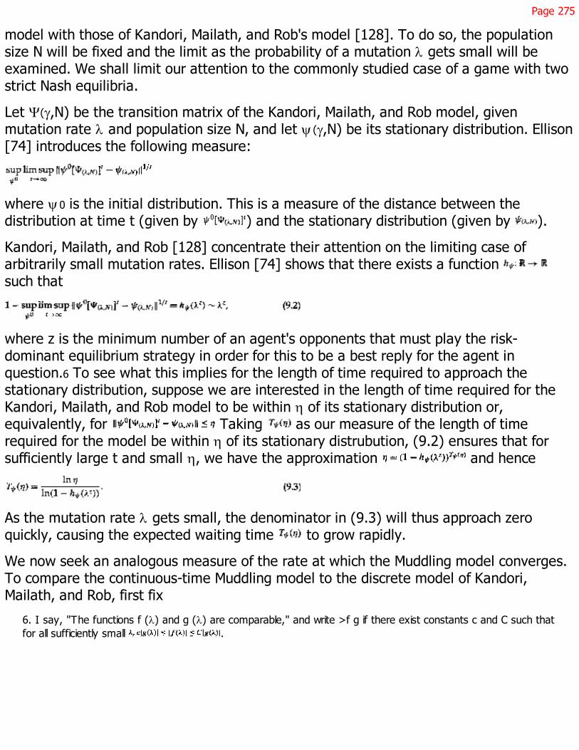
Page 275

model with those of Kandori, Mailath, and Rob's model [128]. To do so, the populationsize N will be fixed and the limit as the probability of a mutation l gets small will beexamined. We shall limit our attention to the commonly studied case of a game with twostrict Nash equilibria.

Let Y(g,N) be the transition matrix of the Kandori, Mailath, and Rob model, givenmutation rate l and population size N, and let y (g,N) be its stationary distribution. Ellison[74] introduces the following measure:

where y0 is the initial distribution. This is a measure of the distance between thedistribution at time t (given by ) and the stationary distribution (given by ).

Kandori, Mailath, and Rob [128] concentrate their attention on the limiting case ofarbitrarily small mutation rates. Ellison [74] shows that there exists a function such that

where z is the minimum number of an agent's opponents that must play the risk-dominant equilibrium strategy in order for this to be a best reply for the agent inquestion.6 To see what this implies for the length of time required to approach thestationary distribution, suppose we are interested in the length of time required for theKandori, Mailath, and Rob model to be within h of its stationary distribution or,equivalently, for Taking as our measure of the length of timerequired for the model be within h of its stationary distrubution, (9.2) ensures that forsufficiently large t and small h, we have the approximation and hence

As the mutation rate l gets small, the denominator in (9.3) will thus approach zeroquickly, causing the expected waiting time to grow rapidly.

We now seek an analogous measure of the rate at which the Muddling model converges.To compare the continuous-time Muddling model to the discrete model of Kandori,Mailath, and Rob, first fix

6. I say, "The functions f (l) and g (l) are comparable," and write >f g if there exist constants c and C such thatfor all sufficiently small .

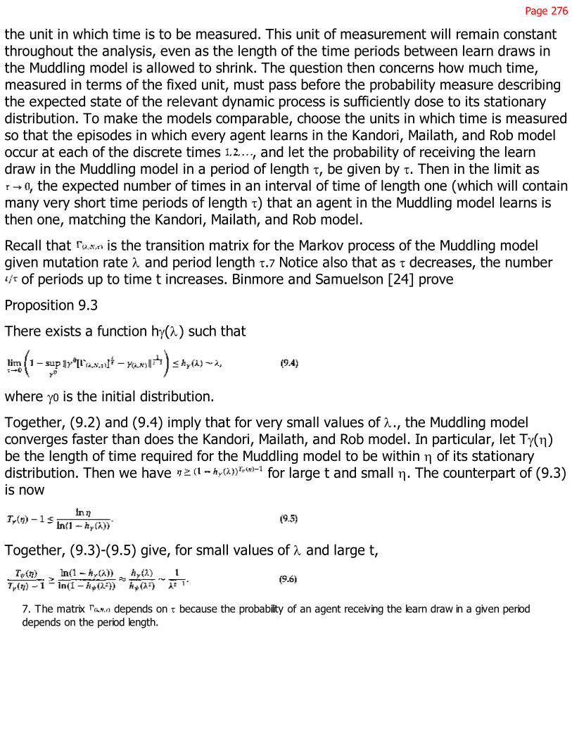
Page 276

the unit in which time is to be measured. This unit of measurement will remain constantthroughout the analysis, even as the length of the time periods between learn draws inthe Muddling model is allowed to shrink. The question then concerns how much time,measured in terms of the fixed unit, must pass before the probability measure describingthe expected state of the relevant dynamic process is sufficiently dose to its stationarydistribution. To make the models comparable, choose the units in which time is measuredso that the episodes in which every agent learns in the Kandori, Mailath, and Rob modeloccur at each of the discrete times , and let the probability of receiving the learndraw in the Muddling model in a period of length t, be given by t. Then in the limit as

, the expected number of times in an interval of time of length one (which will containmany very short time periods of length t) that an agent in the Muddling model learns isthen one, matching the Kandori, Mailath, and Rob model.

Recall that is the transition matrix for the Markov process of the Muddling modelgiven mutation rate l and period length t.7 Notice also that as t decreases, the number

of periods up to time t increases. Binmore and Samuelson [24] prove

Proposition 9.3

There exists a function hg(l) such that

where g0 is the initial distribution.

Together, (9.2) and (9.4) imply that for very small values of l., the Muddling modelconverges faster than does the Kandori, Mailath, and Rob model. In particular, let Tg(h)be the length of time required for the Muddling model to be within h of its stationarydistribution. Then we have for large t and small h. The counterpart of (9.3)is now

Together, (9.3)-(9.5) give, for small values of l and large t,

7. The matrix depends on t because the probability of an agent receiving the learn draw in a given perioddepends on the period length.

Page 277

Condition (9.6) implies that if, for example, N = 100 and z = 33, so that of one'sopponents must play the risk-dominant strategy in order for it to be a best reply, then itwill take times as long for the Kandori, Mailath, and Rob model to be within h of itsstationary distribution as it takes the Muddling model. Ellison [74] obtains a similarcomparison for the Kandori, Mailath, and Rob model and his "two neighbor" matchingmodel. Ellison notes that if N = 100 and z = 33, then halving the mutation rate causes histwo-neighbor matching model (and hence the Muddling model) to take about twice aslong to converge, while the Kandori, Mailath, and Rob model will take 233 (> 8 billion)times as long to converge.

What lies behind the result established in proposition 9.3? The Kandori, Mailath, and Robmodel relies upon mutations to accomplish its transitions between equilibria. Forexample, the stationary distribution may put all of its probability on state 0, but the initialcondition may lie in the basin of attraction of state N. Best-reply learning then takes thesystem immediately to state N, and convergence requires waiting until the burst of zsimultaneous mutations, required to jump over the basin of attraction of N and reach thebasin of attraction of 0, becomes a reasonably likely event. Because the probability ofsuch an event is of the order of lz, this requires waiting a very long time when themutation rate is small. In contrast, the Muddling model requires mutations only to escapeboundary states (see assumptions 9.1.1-9.1.5). Once a single mutation has allowed thisescape (cf. assumption 9.1.5), then the noisy learning dynamics can allow the system to"swim upstream" out of its basin of attraction.8 The probability of moving from state N tostate 0 is given by When mutation rates are small, the learning dynamicsproceed at a much faster rate than mutations occur, so that only one term in thisexpression ( ) is of order l. Convergence then requires waiting only for a singlemutation, rather than z simultaneous mutations, and hence relative waiting times differby a factor of lz-1.

The difference in rates of convergence for these two models will be most striking whenthe mutation rate is very small, and examining an arbitrarily small mutation rate focusesattention on the worst possible case for the Kandori, Mailath, and Rob [128] model.Binmore, Samuelson, and Vaughan [28] present an example in which N = 100, z = 33,

8. Fudenberg and Harris [85] make a similar distinction, including the "swimming upstream" analogy.

Page 278

and . The expected waiting time in the Kandori, Mailath, and Rob model isapproximately , while that of the Muddling model is approximately 5,000.However, waiting times are likely to be much closer for larger mutation rates, becauseincreasing l makes the Kandori, Mailath, and Rob model noisier, reducing its waitingtime. The waiting times are also likely to be closer if we force the noise in the Muddlingmodel process to become negligible. This comparison thus cannot be viewed as anindictment of the Kandori, Mailath, and Rob model but rather as an illustration of animportant point: incorporating nonnegligible noise into a model can hasten itsconvergence. Even if unexplained, exogenously determined perturbations (mutations) areto be treated as negligible, expected waiting times can still be short if noise appears inthe learning process itself.

This examination of waiting times has held the population size N fixed. The Muddlingmodel yields sharp equilibrium selection results as , but need not do so for smallvalues of N. In addition, the expected waiting time diverges in the Muddling model as Nincreases, becoming arbitrarily long as N gets large.9 There accordingly remains plenty ofroom for skepticism as to the applicability of ultralong-run analyses based on examiningstationary distributions. In particular, the Muddling model obtains crisp equilibriumselection results only at the cost of long waiting times, and the finding that waiting timescan be short must be tempered by the realization that the resulting stationary distributionmay give noisy equilibrium selection results. In many cases, however, a population that isnot arbitrarily large and a stationary distribution that allocates probability to more thanone state may be the most appropriate model even though it does not give unambiguousequilibrium selection results.10

9.3 Equilibrium Selection

We turn now to equilibrium selection, concentrating on the case of large populations andsmall mutation rates. In particular, we begin

9. Hence convergence in this model is not fast in the second sense that Ellison [74, pp. 1060-1063] discussesbecause waiting times in the Muddling model do not remain bounded as N gets large.

10. The population size N often need not be very large before most of the mass of the stationary distribution isattached to a single state. In the Binmore, Samuelson, and Vaughan [28] example, where N = 100, z = 33, and

, the stationary distribution places more than .97 probability on states in which at most .05 of the populationplays strategy X.

Page 279

with the limiting stationary distribution of the Markov process as and then study thelimits and . The order in which these two limits are taken is one of the issuesto be examined. Of these two limiting operations, I consider restricting attention to smallmutation rates to be especially unrealistic. Allowing the mutation rate to be boundedaway from zero complicates the analysis but affects neither the techniques nor the basicnature of the results.11 I consider the assumption of a large population to be morerealistic of the two limits in many applications, but it clearly does not apply to all cases ofinterest. It is assumed throughout this section that assumptions 9.1.1-9.1.5, 9.2, and9.3.1-9.3.3 hold.

Two Strict Nash Equilibria

First assume that A> B and D> C, so that the game G * has two strict Nash equilibria. Asin the previous section, let g(l,N) denote the limiting stationary distribution of the Markovprocess on { } as Abusing notation, let g(l,N) also denote the correspondingBorel measure on [0,1]. Thus, for an open interval , g(l,N)(A) is the probability offinding the system at a state x with . To avoid a tedious special case, assume

where assumptions 9.1.4 and 9.2 ensure that the integral exists. Bin-more andSamuelson [24] prove

Proposition 9.4

Let (9.7) hold. Then there exists a unique Borel probability measure g* on [0,1] with

,

where the limits refer to the weak convergence of probability measures. In addition,.

This result states that, in the limit as mutation probabilities get small and the populationgets large (in any order), the stationary

11. Consider, for example, the case of two strict Nash equilibria. If the mutation rate is positive, then taking thelimit as the produces a stationary distribution that concentrates all of its probability near one of the strictNash equilibria, being closer as the mutation rate is smaller. The criterion for which equilibrium is ''selected" in thisway is a variant of (9.8), with the limits on the integral being adjusted to account for the positive mutation rate.

Page 280

distribution of the Markov process attaches probability only to the two pure-strategyequilibria. In "generic" cases, for which (9.7) holds, probability will be attached to onlyone of these equilibria, which I refer to as the "selected equilibrium."

Which Equilibrium?

A number of papers have recently addressed the problem of equilibrium selection insymmetric games. Young [250] and Kandori, Mailath, and Rob [128] are typical infinding that the risk-dominant equilibrium is always selected. Robson and Vega Redondo[193] offer a model in which the payoff-dominant equilibrium is always selected.However, condition (9.8) below provides a criterion showing that the Muddling modelsometimes selects the payoff-dominant equilibrium and sometimes selects the risk-dominant equilibrium.

Proposition 9.5.1

The selected equilibrium will be (X, X) [(Y, Y)] if

Proposition 9.5.2

The payoff-dominant equilibrium in game G * can be selected even if it fails to be risk-dominant.

Proposition 9.5.1 is established in the course of proving proposition 9.4. In particular,proposition 9.4 ensures that only states 0 and N, which correspond to the two strict Nashequilibria of the game, receive positive probability in the limit of the stationarydistribution as and . To then see why we can expect the integral (9.8) todetermine which of these two equilibria is selected, recall that the stationary distributionsatisfies the detailed balance equation given by (9.1). This in turn implies that theprobabilities attached to states 0 and N are given by

Now, taking logarithms of this expression and taking limits gives

,

and hence

Page 281

which in turn leads to (9.8).

To establish proposition 9.5.2, consider the Aspiration and Imitation model. Let

Then neither of the two pure-strategy Nash equilibria, given by (X, X) and (Y, Y), risk-dominates the other, but (X, X) is the payoff-dominant equilibrium. In order to computethe outcome, let F be a Uniform distribution on the interval [-2, 2]. Then the probabilityof abandoning a strategy is linear in the expected payoff of the strategy, with

, , , .

Inserting these probabilities in the expressions for transition probabilities for theAspiration and Imitation model given by (3.8)-(3.11), taking the limits and ,and inserting in (9.8) gives

ensuring that (X, X) is selected. The game can then be perturbed slightly to make (Y, Y)risk-dominant while still keeping (X, X) payoff-dominant and without altering the fact that(X, X) is selected.

Why does this result differ from that of Kandori, Mailath, and Rob [128], whose modelselects the equilibrium with the larger basin of attraction under best-reply dynamics,namely, the risk-dominant equilibrium? In the perturbed version of the game consideredin the previous proof, the equilibrium (X, X) has a basin of attraction smaller than (Y,Y)'s, but in (X, X)'s basin the probability of switching away from strategy X, relative to thecorresponding probability for strategy Y, is exceptionally small being nearly zero forstates in which nearly all agents play X. This makes it very difficult to leave (X, X)'s basin,and yields a selection in which all agents play X. Only the size of

Page 282

the basin of attraction matters in Kandori, Mailath, and Rob, while in the Muddling modelthe strength of the learning flows matters as well.

Best-Response Dynamics

If it is the relative strengths of the learning flows that cause the Muddling model tosometimes select the payoff-dominant equilibrium, then the model should be more likelyto select the risk-dominant equilibrium if the learning process is closer to best-responselearning, so that "strength of flow" issues are less important. This can be confirmed.

Let A > B and D > C, and let , where k* is the probability attached to X by themixed-strategy equilibrium, so that there are two strict Nash equilibria, with (Y, Y) beingthe risk-dominant equilibrium. Fix and satisfying assumptions 9.1.1-9.1.5, 9.2, and9.3.1-9.3.3. Then let

,

where Bx(k) equals 1 if X is a best response ( ), and zero otherwise, and By(k) equalsone if Y is a best response ( ), and zero otherwise. Then and are a convexcombination of the best-response dynamics and and . As f increases to unity and approach best-response dynamics. Binmore and Samuelson [24] prove:

Proposition 9.6

If and satisfy assumptions 9.1.1-9.1.5, 9.2, and 9.3.1-9.3.3, then the selectedequilibrium in game G * is the risk-dominant equilibrium for any convex combination ofthe best-response dynamics and and that puts sufficient weight on the former.

Random Imitation Dynamics

Best-response dynamics have the property that strategy adjustments are preciselydetermined by payoffs. At another end of the spectrum are dynamics in which strategyadjustments have nothing to do with payoffs. Suppose that those who receive the learndraw imitate a randomly chosen opponent, regardless of payoff considera-

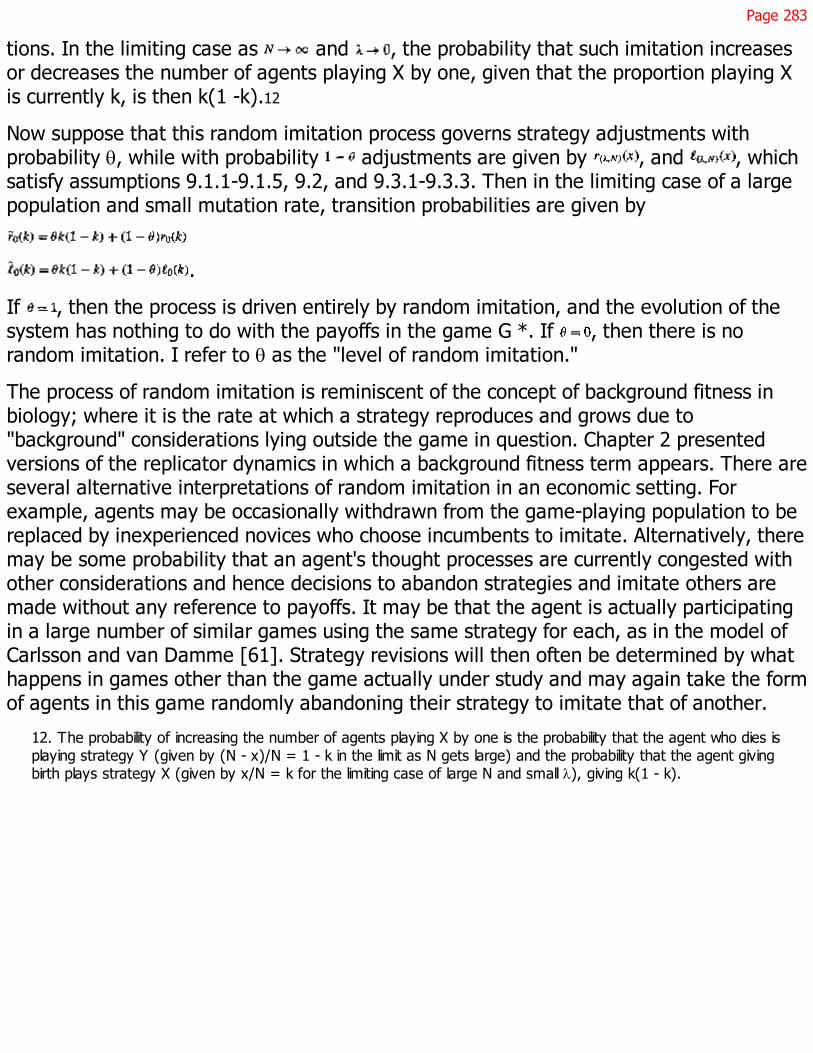
Page 283

tions. In the limiting case as and , the probability that such imitation increasesor decreases the number of agents playing X by one, given that the proportion playing Xis currently k, is then k(1 -k).12

Now suppose that this random imitation process governs strategy adjustments withprobability q, while with probability adjustments are given by , and , whichsatisfy assumptions 9.1.1-9.1.5, 9.2, and 9.3.1-9.3.3. Then in the limiting case of a largepopulation and small mutation rate, transition probabilities are given by

.

If , then the process is driven entirely by random imitation, and the evolution of thesystem has nothing to do with the payoffs in the game G *. If , then there is norandom imitation. I refer to q as the "level of random imitation."

The process of random imitation is reminiscent of the concept of background fitness inbiology; where it is the rate at which a strategy reproduces and grows due to"background" considerations lying outside the game in question. Chapter 2 presentedversions of the replicator dynamics in which a background fitness term appears. There areseveral alternative interpretations of random imitation in an economic setting. Forexample, agents may be occasionally withdrawn from the game-playing population to bereplaced by inexperienced novices who choose incumbents to imitate. Alternatively, theremay be some probability that an agent's thought processes are currently congested withother considerations and hence decisions to abandon strategies and imitate others aremade without any reference to payoffs. It may be that the agent is actually participatingin a large number of similar games using the same strategy for each, as in the model ofCarlsson and van Damme [61]. Strategy revisions will then often be determined by whathappens in games other than the game actually under study and may again take the formof agents in this game randomly abandoning their strategy to imitate that of another.

12. The probability of increasing the number of agents playing X by one is the probability that the agent who dies isplaying strategy Y (given by (N - x)/N = 1 - k in the limit as N gets large) and the probability that the agent givingbirth plays strategy X (given by x/N = k for the limiting case of large N and small l), giving k(1 - k).

Page 284

Proposition 9.7

If the level of random imitation q is sufficiently large, then the equilibrium (X, X) isselected if

and (Y, Y) is selected if (9.11) is positive.


Let (X,X) and (Y, Y) be Nash equilibria, with (Y, Y) being risk dominant. From (9.8), theselected equilibrium will be (X, X) if

As , the left side of (9.12) approaches zero. Then consider the first derivative of theleft side of (9.12). A negative derivative ensures that (9.12) approaches zero from above,so that (9.12) is positive and hence the payoff-dominant equilibrium is selected for q near1. Evaluated at , this derivative is given by the left side of (9.11). The selectedequilibrium, for large background fitness, is thus (X, X) if (9.11) is negative and (Y, Y) if(9.11) is positive.

What is the interpretation of condition (9.11)? It is straightforward to evaluate (9.11) forthe case of the Aspiration and Imitation model finding

Corollary 9.1

In the Aspiration and Imitation model (9.11) is negative and hence the risk-dominantequilibrium of game G * is selected, for sufficiently large q.

This provides another condition for the risk-dominant equilibrium to be selected. In thecase of the Aspiration and Imitation model the condition is that changes in strategy mustbe driven primarily by random imitation and not payoffs in the game. Hence the risk-dominant equilibrium is selected in relatively unimportant gamesthose whose payoffshave little to do with agents' behavior.

No Pure-Strategy Equilibria

The previous findings establish equilibrium selection results for the case of two strict Nashequilibria. These can be contrasted with the case of games in which B > A and C > D, sothat there is a unique, mixed-

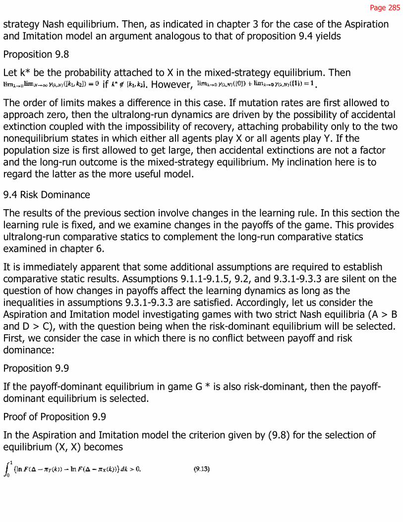
Page 285

strategy Nash equilibrium. Then, as indicated in chapter 3 for the case of the Aspirationand Imitation model an argument analogous to that of proposition 9.4 yields

Proposition 9.8

Let k* be the probability attached to X in the mixed-strategy equilibrium. Then if . However, .

The order of limits makes a difference in this case. If mutation rates are first allowed toapproach zero, then the ultralong-run dynamics are driven by the possibility of accidentalextinction coupled with the impossibility of recovery, attaching probability only to the twononequilibrium states in which either all agents play X or all agents play Y. If thepopulation size is first allowed to get large, then accidental extinctions are not a factorand the long-run outcome is the mixed-strategy equilibrium. My inclination here is toregard the latter as the more useful model.

9.4 Risk Dominance

The results of the previous section involve changes in the learning rule. In this section thelearning rule is fixed, and we examine changes in the payoffs of the game. This providesultralong-run comparative statics to complement the long-run comparative staticsexamined in chapter 6.

It is immediately apparent that some additional assumptions are required to establishcomparative static results. Assumptions 9.1.1-9.1.5, 9.2, and 9.3.1-9.3.3 are silent on thequestion of how changes in payoffs affect the learning dynamics as long as theinequalities in assumptions 9.3.1-9.3.3 are satisfied. Accordingly, let us consider theAspiration and Imitation model investigating games with two strict Nash equilibria (A > Band D > C), with the question being when the risk-dominant equilibrium will be selected.First, we consider the case in which there is no conflict between payoff and riskdominance:

Proposition 9.9

If the payoff-dominant equilibrium in game G * is also risk-dominant, then the payoff-dominant equilibrium is selected.


In the Aspiration and Imitation model the criterion given by (9.8) for the selection ofequilibrium (X, X) becomes

Page 286

Let (X, X) and (Y, Y) be risk-equivalent in game G *, so that A+C=B+D, and let A=D.Then from the linearity of and , we have that (9.13) holds with equality. Nowmake (X, X) the payoff-dominant equilibrium by increasing A and decreasing C so as topreserve A+C+B+D (and hence to preserve the risk-equivalence of the two strategies).Because F is Uniform, this adjustment causes to decrease. The payoff-dominant equilibrium (X, X) is then selected. Next, note that adding a constant to A andC or subtracting a constant from D and B, so as to also make (X, X) risk-dominant,increases the function on [0, 1], which strengthens the inequalityin (9.13) and hence preserves the result that the payoff-dominant equilibrium is selected.

Now consider cases where the payoff and risk dominance criteria conflict. We havealready seen that sometimes the payoff-dominant equilibrium will be selected andsometimes the risk-dominant equilibrium will be selected. The question of interest is howthe likelihood of choosing the risk-dominant equilibrium in the game G* varies with thepayoffs in the game. To pose this question precisely, let k* be the probability attached toX in the mixed strategy equilibrium. Let (Y, Y) be the risk-dominant equilibrium (so )but let (X, X) be payoff-dominant. Let p* be the payoff in game G* from the mixed-strategy equilibrium. We can then consider variations in the payoffs A, B, C, D that leavek* and p* unchanged. For example, we can consider a decrease in D accompanied by anincrease in B calculated so as to preserve k* and p*, as illustrated in figure 9.2. We thusrestrict our attention to variations in the payoffs A, B, C, and D for which C=C(A) andB=B(D), where .

Proposition 9.10

If the payoff-dominant equilibrium is selected given payoffs A, B, C, and D, with mixed-strategy equilibrium k* and mixed-strategy equilibrium payoff p*, and if D>>B, then thepayoff-dominant equilibrium is also selected for any payoffs A, B', C, and D' that preservek* and p* and for which .

Proposition 9.10 tells us that if D > B and the payoff-dominant equilibrium is selected,then the payoff-dominant equilibrium continues to be selected as D is decreased (and Bincreased), at least until . The proof establishes that the payoff-dominant equilibriumwill continue to be selected for at least some range of values of D < B. Hence, if thepayoff-dominant equilibrium is selected for any value , then it is selected for aninterval of values of D that includes p* in its inte-

Page 287

Figure 9.2Payoff variations

rior. If the payoff-dominant equilibrium is not selected for any value of , then it maystill be selected for some value of . Movements in the payoffs to strategy Y thatincrease B and decrease D then make the payoff-dominant equilibrium more likely to beselected. The best case for the payoff-dominant equilibrium occurs when D = B or D < B.The payoff-dominant equilibrium is thus favored by reducing the variation in payoffs tostrategy Y or even "inverting" them, so that while (Y, Y) is an equilibrium, the highestreward to strategy Y is obtained if the opponent plays X.


Fix . Fix A and hence C (A). If we set D = A, then proposition 9.9 ensures that (Y, Y)will be selected, since it is risk dominant and payoff undominated. Now let D decline.Because F is Uniform, (9.13) increases until D reaches p*, and is increasing at .Hence, if the payoff-dominant equilibrium is selected for any value of , then it is alsoselected for any smaller value of D that preserves .

9.5 Discussion

Given proposition 9.10, it is interesting to note that Straub [229] has conductedexperiments to investigate the conditions under which

Page 288

risk-dominant and payoff-dominant equilibria are selected in symmetric games withtwo strict Nash equilibria. He finds that the risk-dominant equilibrium is the most commonequilibrium played in seven out of eight of the experiments. The exception, in which thepayoff-dominant equilibrium appeared, is the only game in which D << B. This isconsistent with the statement that the payoff-dominant equilibrium is most likely to beselected when .

Friedman [83] also reports experiments with symmetric games having two strict Nashequilibria. Friedman finds that altering a game in which D < B to achieve D = B, whilepreserving the basins of attraction of the Nash equilibria, causes the risk-dominantequilibrium to be selected more often and the payoff-dominant equilibrium to be selectedless often. This is consistent with the statement that the risk-dominant equilibrium maybe selected for all values , but there may exist values D << B for which the payoff-dominant equilibrium is selected.

The experiments of Straub [229] and Friedman [83] were designed for other purposes,and are at best suggestive concerning the circumstances under which risk-dominant orpayoff-dominant equilibria will appear. More specifically designed experiments arerequired to provide more precise insights. Suppose such experiments produce the resultthat setting D > B yields the risk-dominant equilibrium, while reducing D and increasingB, in such a way as to preserve p* and the basins of attraction, leads to the payoff-dominant equilibrium. Do we have any reason to suspect that the considerations capturedby the Muddling model of this chapter have anything to do with the outcome? To thecontrary, we probably have some reason to suspect that this chapter's model does not liebehind the outcome. Proposition 9.10 describes the implications of variations in payoffsfor the stationary distribution of the Muddling model. The stationary distribution is anultralong-run phenomenon. We can safely expect the ultralong run to be longer than thenumber of trials typically allowed in laboratory experiments. We must then question therelevance of the theory to experiments (though we then also have a convenient apologyif experimental outcomes do not match the predictions of the theory).

There remains some hope for the theory. The experiences of experimental subjectsoutside the laboratory will have directed them to strategies that produce sometimes therisk-dominant equilibrium and sometimes the payoff-dominant equilibrium. If the forcesdriving this process bear a sufficient relationship to those driving the Mud-

Page 289

dling model, and if the choices subjects must make in the laboratory sufficiently resemblethose they make outside as to trigger behavior appropriately suited to the experimentalgame, then we can expect the theoretical and laboratory results to be related and hencecan expect the theory to be relevant. This link between theoretical and experimentaloutcomes clearly places a great premium on successful experimental design.

On the one hand, it would seem an extraordinary coincidence that a model as simple asthe Muddling model could actually hope to describe how people behave. Notice, however,that traditional game theory tells us that when examining a symmetric game withtwo strict Nash equilibria, only the best-reply structure of the game matters forequilibrium selection, that is, only the sizes of the basins of attraction of the two Nashequilibria matter. The evolutionary models of Kandori, Mailath, and Rob [128] and ofYoung [250] also produce a result where only the best-reply structure matters. Thecommon intuition is that other considerations, such as the magnitudes of payoffs, alsomatter. The Muddling model directs our attention to one way in which suchconsiderations might matter

Page 291

10Conclusion

What remains to be done? Two areas for further work strike me as particularly important.First, work on the structure of evolutionary models is needed. An evolutionary analysisbegins with a model of how players make their choices in games and how they learn thatsome choices work better than others. This process makes a more explicit appearance insome models than in others, but is always lurking in the background. Learning is acomplicated phenomenon even in a stationary environment. An added layer of complexityappears in games because players can be attempting to learn a moving target. We haveonly very simple and preliminary ideas about what drives learning, and there is much tobe done in this respect.

Additional work is also required on developing techniques to analyze learning models.The current practice relies heavily on being able to restrict attention to either verysimaple games or simple dynamic processes. Much can be learned by examining thereplicator dynamics or Markov processes with one-dimensional state variables, but wemust also move beyond such models. In connection with this, it is important to note thatexisting models typically call for players to be repeatedly matched in pairs to play a fixedgame. It is very difficult to think of cases in which one is repeatedly matched withdifferent opponents to play a large number of literally identical games. One possibility inthis regard is to argue that people are constantly faced with making decisions in a varietyof strategic situations that they sort into a relatively small number of basic categories,such as coordination games, bargaining games, prisoners' dilemmas, and so on. Theevolutionary process may then operate within these classes of games, with agentsapplying a single decision rule to each class that is adjusted in light of their experience insuch games. While the general outlines of this story seem plausible, it has not beensubjected to the scrutiny of a model.

Page 292

What of the future of evolutionary game theory? I think an analogy with generalequilibrium theory is useful. After establishing the existence and basic properties ofWalrasian equilibrium, economists turned considerable attention to the interpretation ofthis equilibrium. How was an equilibrium achieved, who set prices, how stable was anequilibrium, what happened when there was no Walrasian auctioneer? The resultinganalysis produced adjustment models, disequilibrium models, stability analyses, strategicmodels, models with imperfect competition, and a variety of other investigations. Butlittle change has occurred in the way most economists think about general equilibriumtheory, where Walrasian equilibrium remains the standard tool.

Game theorists have established the existence and basic properties of Nash equilibriumand its various refinements. Some variant of sequential equilibrium, including perfectBayesian equilibrium, is the standard concept. The use of game theory has spreadthroughout applied fields in economics such as industrial organization and internationaltrade. Evolutionary game theory is now probing many of the same questions that generalequilibrium theorists considered. One possibility is that evolutionary game theory followsthe alternatives to Walrasian general equilibrium theory in having little effect on howeconomists think about equilibrium. Evolutionary game theory is especially in danger ofsuffering this fate if it does no more than produce an ever-growing list of alternativemodels with differing results.

The future for .evolutionary game theory is more hopeful if the theory can demonstrateits ability to provide insights that are useful to economists working with game-theoreticmodels. One first step to such a demonstration would be to show that evolutionarymodels can be useful in interpreting and predicting the results of laboratory experiments.A complementary step would be work designed to replace the randomly matched pairsand abstract games of most evolutionary models with patterns of interaction that moreclosely resemble activities in the markets to which the models are applied. The modelscould then be used as a standard tool in applied work. Notice that this may requiredifferent models for different applications, bringing institutional features into theeconomic analysis that are currently often thought to be important but are commonlyignored. I expect both avenues of inquiry to play important roles in shaping the future ofevolutionary game theory.

Page 293

References

1. L. Anderlini. Communication, computability, and common interest games. EconomicTheory discussion paper 159, St. John's College, Cambridge, 1990.

2. James Andreoni and John H. Miller. Auctions with artificial adaptive agents. Games andEconomic Behavior 10:39-64, 1995.

3. Robert Axelrod. The evolution of cooperation. Basic Books, New York, 1984.

4. Dieter Balkenborg. Strictness, evolutionary stability and repeated games with commoninterests. CARESS working paper 93-20, University of Pennsylvania, 1993.

5. Dieter Balkenborg. An experiment on forward versus backward induction. SFBdiscussion paper B-268, University of Bonn, 1994.

6. Dieter Balkenborg. Strictness and evolutionary stability. Center for Rationality andInteractive Decision Theory discusssion paper 52, Hebrew University of Jerusalem, 1994.

7. Dieter Balkenborg and Karl Schlag. Evolutionarily stability in asymmetric populationgames. SFB discussion paper B-314, University of Bonn, 1995.

8. Dieter Balkenborg and Karl Schlag. On the interpretation of evolutionarily stable sets.SFB discussion paper B-313, University of Bonn, 1995.

9. Abhijit Banerjee and Drew Fudenberg. Word-of-mouth learning. Mimeo, MassachusettsInstitute of Technology and Harvard University, 1995.

10. Pierpaolo Battigalli. Strategic rationality orderings and the best rationalizationprinciple. Mimeo, Princeton University, 1993.

11. Pierpaolo Battigalli. On rationalizability in extensive games. Journal of EconomicTheory, 1996. Forthcoming.

12. Jonathan Bendor, Dilip Mookherjee, and Debraj Ray. Aspirations, adaptive learning,and cooperation in repeated games. Mimeo, Indian Statistical Institute, 1994.

13. James Bergin and Bart Lipman. Evolution with state-dependent mutations.Econometrica 64:943-956, 1996.

14. Douglas Bernheim. Rationalizable strategic behavior. Econometrica 52:1007-1028,1984.

Page 294

15. V. Bhaskar. Noisy communication and the evolution of cooperation. Mimeo, DelhiSchool of Economics, 1995.

16. N. E Bhatia and G. E Szegö. Stability theory of dynamical systems. Springer, NewYork, 1970.

17. Patrick Billingsley. Probability and measure. Wiley, New York, 1986.

18. Ken Binmore. Modelling rational players: I and II. Economics and Philosophy 3:9-55,4:179-214, 1987-1988.

19. Ken Binmore. Fun and games. D.C. Heath, Lexington, MA, 1992.

20. Ken Binmore. Game theory and the social contract. Vol. 1. Playing fair. MIT Press,Cambridge, MA, 1993.

21. Ken Binmore, John Gale, and Larry Samuelson. Learning to be imperfect: Theultimatum game. Games and Economic Behavior 8:56-90, 1995.

22. Ken Binmore, Chris Proulx, Larry Samuelson, and Joe Swierzbinski. Hard bargains andlost opportunities. SSRI working paper 9517, University of Wisconsin, 1995.

23. Ken Binmore and Larry Samuelson. Evolutionary stability in repeated games playedby finite automata. Journal of Economic Theory 57:278-305,1992.

24. Ken Binmore and Larry Samuelson. Muddling through: Noisy equilibrium selection.SSRI working paper 9410R, University of Wisconsin, 1993.

25. Ken Binmore and Larry Samuelson. Drift. European Economic Review 38:859-867,1994.

26. Ken Binmore and Larry Samuelson. An economist's perspective on the evolution ofnorms. Journal of Institutional and Theoretical Economics 150:45-63, 1994.

27. Ken Binmore and Larry Samuelson. Evolutionary drift and equilibrium selection. SSRIworking paper 9529, University of Wisconsin, 1994.

28. Ken Binmore, Larry Samuelson, and Richard Vaughan. Musical chairs: Modelling noisyevolution. Games and Economic Behavior 11:1-35, 1995.

29. Ken Binmore, Avner Shaked, and John Sutton. Testing noncooperative bargainingtheory: A preliminary study. American Economic Review 75:1178-1180, 1985.

30. K. Binmore, J. Swierzbinski, S. Hsu, and C. Proulx. Focal points and bargaining.International Journal of Game Theory 22:381-409, 1993.

31. Jonas Björnerstedt. Experimentation, imitation and evolutionary dynamics. Mimeo,Stockholm University, 1995.

32. Jonas Björnerstedt, Martin Dufwenberg, Peter Norman, and Jörgen Weibull.

Evolutionary selection dynamics and irrational survivors. Research Papers in Economics1994:7 WE, University of Stockholm, 1994.

33. Andreas Blume. Learning, experimentation and long-run behavior in games. Mimeo,University of Iowa, 1994.

34. Andreas Blume, Yong-Gwan Kim, and Joel Sobel. Evolutionary stability in games ofcommunication. Games and Economic Behavior 5:547-575, 1993.

Page 295

35. Lawrence E. Blume. The statistical mechanics of strategic interaction. Games andEconomic Behavior 5:387-424, 1993.

36. Lawrence E. Blume. How noise matters. Mimeo, Cornell University, 1994.

37. Gary E. Bolton. A comparative model of bargaining: Theory and evidence. AmericanEconomic Review 81:1096-1136,1991.

38. Gary E. Bolton and Rami Zwick. Anonymity versus punishment in ultimatumbargaining. Games and Economic Behavior 10:95-121, 1995.

39. Immanuel Bomze. Non-cooperative 2-person games in biology: A classification.International Journal of Game Theory 15:31-59, 1986.

40. Immanuel Bomze and Reinhard Bürger. Stability by mutation in evolutionary games.Games and Economic Behavior 11:145-173, 1995.

41. Immanuel Bomze and Jurgen Eichberger. Evolutive versus naive Bayesian learning.Institute of Statistics and Computer Science technical report 118, University of Vienna,1992.

42. Immanuel M. Bomze and Benedikt M. Pötscher. Game theoretical foundations ofevolutionary stability. Springer, Berlin, 1989.

43. Immanuel M. Bomze and Eric van Damme. A dynamical characterization ofevolutionarily stable states. CentER for Economic Research discussion paper 9045, TilburgUniversity, 1990.

44. Immanuel M. Bomze and Jörgen Weibull. Does neutral stability imply Lyapunovstability? Games and Economic Behavior 11:173-192, 1995.

45. Tilman Börgers. On the definition of rationalizability in extensive games. Discussionpaper 91-22, University College London, 1991.

46. Tilman Börgers. A formalization of ''forward induction." Mimeo, University CollegeLondon, 1992.

47. T. Börgers and R. Satin. Learning through reinforcement. and replicator dynamics.Mimeo, University College London, 1995.

48. T. Börgers and R. Sarin. Naive reincorcement learning with endogenous aspirations.Mimeo, University College London, 1996.

49. Richard T. Boylan. Laws of large numbers for dynamical systems with randomlymatched individuals. Journal of Economic Theory 57:473-504, 1992.

50. Richard T. Boylan. Evolutionary equilibria resistant to mutations. Games andEconomic Behavior 7:10-34,1994.

51. Richard T. Boylan. Continuous approximation of dynamical systems with randomlymatched individuals. Journal of Economic Theory 66:615-625, 1995.

52. Eva Bruch. The evolution of cooperation in neighborhood structures. Master's thesis,University of Bonn, 1993.

53. Robert R. Bush and Frederick Mosteller. Stochastic models for learning. Wiley, NewYork, 1955.

Page 296

54. Antonio Cabrales. Stochastic replicator dynamics. Mimeo, Universitat Pompeu Fabra,Barcelona, 1995.

55. Antonio Cabrales and Joel Sobel. On the limit points of discrete selection dynamics.Journal of Economic Theory 57:407-419, 1992.

56. David Canning. Convergence to equilibrium in a sequence of games with learning.STICERD discussion paper 89/190, London School of Economics, 1989.

57. David Canning. Average behavior in learning models. Journal of Economic Theory57:442-472, 1992.

58. David Canning. Learning language conventions in common interest signaling games.Department of Economics discussion paper 607, Columbia University, 1992.

59. David Canning. Learning the subgame-perfect equilibrium. Department of Economicsdiscussion paper 608, Columbia University, 1992.

60. Hans Carlsson and Eric van Damme. Equilibrium selection in Stag-Hunt games. In KenBinmore, Alan Kirman, and Piero Tani, eds., Frontiers of Game Theory, pp. 237-254. MITPress, Cambridge, MA, 1993.

61. Hans Carlsson and Eric van Damme. Global games and equilibrium selection.Econometrica 61:989-1018, 1993.

62. Yin-Wong Cheung and Daniel Friedman. Learning in evolutionary games: Somelaboratory results. UCSC Economics Department working paper 303, University ofCalifornia, Santa Cruz, 1994.

63. In-Koo Cho. Stationarity, rationalizability and bargaining. Review of Economic Studies61:357-374, 1994.

64. In-Koo Cho and David M. Kreps. Signaling games and stable equilibria. QuarterlyJournal of Economics 102:179-221,1987.

65. Vincent P. Crawford. An "evolutionary" interpretation of Van Huyck, Battalio, andBeil's experimental results on coordination. Games and Economic Behavior 3:25-59, 1991.

66. Vincent P. Crawford. Adaptive dynamics in coordination games. Econometrica 63:103-143, 1995.

67. Vincent P. Crawford. Theory and experimentation in the analysis of strategicinteraction. Discussion paper 95-37, University of California, San Diego, 1995.

68. Ross Cressman. Evolutionary game theory with two groups of individuals. Games andEconomic Behavior 11:237-253, 1995.

69. Ross Cressman. Local stability of smooth selection dynamics for normal-form games.Mimeo, Wilfrid Laurier University, 1996.

70. Ross Cressman and Karl H. Schlag. The dynamic (in)stability of backwards induction.Discussion paper B-347, University of Bonn, 1995.

71. R. Dawkins. The selfish gene. Oxford University Press, Oxford, 1976.

72. Eddie Dekel and Suzanne Scotchmer. On the evolution of optimizing behavior. Journalof Economic Theory 57:392-406, 1992.

Page 297

73. Jurgen Eichberger, Hans Hailer, and Frank Milne. Naive Bayesian learning in matrix games. Journal of Economic Behavior and Organization 21:69-90,1993.

74. Glenn Ellison. Learning, local interaction, and coordination. Econometrica 61:1047-1072, 1993.

75. Glenn Ellison. A little rationality and learning from personal experience. Mimeo,Massachusetts Institute of Technology, 1993.

76. Glenn Ellison. Basins of attraction and long run equilibria. Mimeo, MassachusettsInstitute of Technology, 1995.

77. Dean Foster and Rakesh V. Vohra. Asymptotic calibration. Mimeo, University ofPennsylvania and Ohio State University, 1995.

78. Dean Foster and Rakesh V. Vohra. Calibrated learning and correlated equilibrium.Mimeo, University of Pennsylvania and Ohio State University, 1995.

79. Dean Foster and Peyton Young. Stochastic evolutionary game dynamics. Journal ofTheoretical Biology 38:219-232,1990.

80. R. H. Frank. Passions within reason. Norton, New York, 1988.

81. M. I. Freidlin and A.D. Wentzell. Random perturbations of dynamical systems.Springer, New York, 1984.

82. D. Friedman. Evolutionary games in economics. Econometrica 59:637-666,1991.

83. Daniel Friedman. Equilibrium in evolutionary games: Some experimental results.Economic Journal 106:1-25,1996.

84. James W. Friedman. On entry preventing behavior. In S. J. Brams, A. Schotter, and G.Schwodiauer, eds., Applied game theory, pp. 236-253. Physica, Vienna, 1979.

85. Drew Fudenberg and Chris Harris. Evolutionary dynamics with aggregate shocks.Journal of Economic Theory 57:420-441, 1992.

86. Drew Fudenberg and David M. Kreps. A theory of learning, experimentation, andequilibrium in games. Mimeo, Stanford University and Massachusetts Institute ofTechnology, 1988.

87. Drew Fudenberg and David M. Kreps. Learning mixed equilibria. Games and EconomicBehavior 5:320-367, 1993.

88. Drew Fudenberg and David M. Kreps. Learning in extensive-form games. 1. Self-confirming equilibrium, Harvard Institute for Economic Development discussion paper 20,Harvard University, 1994.

89. Drew Fudenberg and David M. Kreps. Learning in extensive-form games. 2.

Experimentation and Nash equilibrium. Harvard Institute for Economic Developmentdiscussion paper 20, Harvard University, 1994.

90. Drew Fudenberg and David K. Levine. How irrational are subjects in extensive-formgames? Economic Theory discussion paper 14, Harvard University, 1993.

91. Drew Fudenberg and David K. Levine. Self-confirming equilibrium. Econometrica61:523-546,1993.

Page 298

92. Drew Fudenberg and David K. Levine. Steady state learning and Nash equilibrium.Econometrica 61:547-574, 1993.

93. Drew Fudenberg and David K. Levine. Consistency and cautious fictitious play.Harvard Institute of Economic Research discussion paper 21, Harvard University, 1994.

94. Drew Fudenberg and David K. Levine. Conditonal universal consistency. Mimeo,Harvard University and University of California at Los Angeles, 1995.

95. Drew Fudenberg and David K. Levine. Theory of learning in games. Mimeo, HarvardUniversity and University of California at Los Angeles, 1995.

96. Drew Fudenberg and Eric Maskin. The folk theorem in repeated games withdiscounting and incomplete information. Econometrica 54:533-554, 1986.

97. C. W. Gardiner. Handbook of stochastic methods. Springer, Berlin, 1985.

98. D. Gauthier. Morals by agreement. Clarendon Press, Oxford, 1986.

99. Itzhak Gilboa and Akihiko Matsui. Social stability and equilibrium. Econometrica59:859-868, 1991.

100. Itzhak Gilboa and Akihiko Matsui. A model of random matching. Journal ofMathematical Economics 21:185-198, 1992.

101. Itzhak Gilboa and Dov Samet. Absorbent stable sets. Center for MathematicalStudies in Economics and Management Science discussion paper 935, NorthwesternUniversity, 1991.

102. Itzhak Gilboa and David Schmeidler. Case-based consumer theory. Mimeo,Northwestern University, 1993.

103. Itzhak Gilboa and David Schmeidler. Case-based decision theory. Quarterly Journalof Economics 110:605-640,1995.

104. Itzhak Gilboa and David Schmeidler. Case-based optimization. Games and EconomicBehavior, 1996. Forthcoming.

105. Natalie S. Glance and Bernardo A. Huberman. The outbreak of cooperation. Journalof Mathematical Sociology 17:281-302, 1993.

106. Joseph Greenberg. The theory of social situations. Cambridge University Press,Cambridge, 1990.

107. J. Guckenheimer and E Holmes. Nonlinear oscillations, dynamical systems, andbifurcations of vector fields. Springer, New York, 1983.

108. W. Güth R. Schmittberger, and B. Schwarze. An experimental analysis of ultimatumbargaining. Journal of Economic Behavior and Organization 3:367-388, 1982.

109. Werner Güth and Reinhard Tietz. Ultimatum bargaining behavior: A survey andcomparison of experimental results. Journal of Economic Psychology 11:417-449, 1990.

110. Frank Hahn. Stability. In Kenneth J. Arrow and Michael D. Intriligator, eds.,Handbook of mathematical economics, vol. 2, pp. 745-794. North Holland, New York,1982.

111. J. Hale. Ordinary differential equations. Wiley, New York, 1969.

112. Peter Hammerstein and Susan E. Riechert. Payoffs and strategies in territorial con-

Page 299

tests: ESS analyses of two ecotypes of the spider Agelenopsis aperta. EvolutionaryEcology 2:115-138, 1988.

113. William Harms. Discrete replicator dynamics for the Ultimatum Game. Mimeo,University of California, Irvine, 1994.

114. J. Harsanyi. Rational behavior and bargaining equilibrium in games and socialsituations. Cambridge University Press, Cambridge, 1977.

115. John C. Harsanyi. Games with randomly distributed payoffs: A new rationale formixed-strategy equilibrium points. International Journal of Game Theory 2:1-23, 1973.

116. John C. Harsanyi and Reinhard Selten. A general theory of equilibrium selection ingames. MIT Press, Cambridge, MA, 1988.

117. Kenneth Hendricks, Robert H. Porter, and Charles A. Wilson. Auctions for oil and gasleases with an informed bidder and a random reservation price. Econometrica 62:1415-1452, 1994.

118. Morris W. Hirsch and Stephen Smale. Differential equations, dynamical systems, andlinear algebra. Academic Press, New York, 1974.

119. J. Hofbauer and K. Sigmund. The theory of evolution and dynamical systems.Cambridge University Press, Cambridge, 1988.

120. Josef Hofbauer and Jörgen Weibull. Evolutionary selection against dominatedstrategies. Journal of Economic Theory, 1995. Forthcoming.

121. Ed Hopkins. Learning, matching and aggregation. EUI working paper ECO 95/19,European University Institute, 1995.

122. Bernardo A. Huberman and Natalie S. Glance. Evolutionary games and computersimulations. Proceedings of the National Academy of Sciences 90:7712-7715, 1993.

123. S. Hurkens. Learning by forgetful players. Games and Economic Behavior 11:304-329, 1995.

124. James S. Jordan. Bayesian learning in normal-form games. Games and EconomicBehavior 3:60-81,1991.

125. James S. Jordan. Three problems in learning mixed-strategy Nash equilibria. Gamesand Economic Behavior 5:368-386, 1993.

126. Ehud Kalai and Ehud Lehrer. Private-beliefs equilibrium. Center for MathematicalStudies in Economics and Management Science discussion paper 926, NorthwesternUniversity, 1991.

127. Ehud Kalai and Ehud Lehrer. Rational learning leads to Nash equilibria. Econometrica61:1019-1046, 1993.

128. Michihiro Kandori, George J. Mailath, and Rafael Rob. Learning, mutation, and long-run equilibria in games. Econometrica 61:29-56, 1993.

129. Yuri Kaniovski and Peyton Young. Learning dynamics in games with stochasticperturbations. Games and Economic Behavior 11:330-363, 1995.

130. Rajeeva Karandikar, Dilip Mookherjee, Debraj Ray, and Fernando Vega-Redondo.Evolving aspirations and cooperation. Mimeo, Boston University, 1995.

Page 300

131. Samuel Karlin and Howard M. Taylor. A first course in stochastic processes.Academic Press, New York, 1975.

132. John G. Kemeny and J. Laurie Snell. Finite Markov chains. Van Nostrand, Princeton,NJ, 1960.

133. Yong-Gwan Kim and Joel Sobel. An evolutionary approach to pre-playcommunication. Econometrica 63:1181-1194, 1992.

134. Motoo Kimura. The neutral theory of molecular evolution. Cambridge UniversityPress, Cambridge, 1983.

135. Elon Kohlberg and Jean-François Mertens. On the strategic stability of equilibria.Econometrica 54:1003-1038, 1986.

136. David M. Kreps, Paul Milgrom, John Roberts, and Robert J. Wilson. Rationalcooperation in the finitely repeated Prisoners' Dilemma. Journal of Economic Theory27:245-252, 1982.

137. David M. Kreps and Robert J. Wilson. Reputation and imperfect information. Journalof Economic Theory 27:253-279, 1982.

138. David M. Kreps and Robert J. Wilson. Sequential equilibrium. Econometrica 50:863-894, 1982.

139. John O. Ledyard. Public goods: A survey of experimental research. In John Kagel andAlvin E. Roth, eds., Handbook of Experimental Economics, pp. 111-194. PrincetonUniversity Press, Princeton, NJ, 1995.

140. David K. Levine. Modeling altruism and spitefulness in experiments. Mimeo,University of California at Los Angeles, 1995.

141. D. Lewis. Counterfactuals. Basil Blackwell, Oxford, 1976.

142. Bruce G. Linster. Evolutionary stability in the infinitely repeated Prisoners' Dilemmaplayed by two-state Moore machines. Southern Economic Journal 58:880-903, 1992.

143. Bruce G. Linster. Stochastic evolutionary dynamics in the repeated Prisoners'Dilemma. Economic Inquiry 32:342-357, 1994.

144. A. J. Lotka. Undamped oscillations derived form the law of mass action. Journal ofthe American Chemical Society 42:1595-1598, 1920.

145. George J. Mailath. Introduction: Symposium on evolutionary game theory. Journal ofEconomic Theory 57:259-277, 1992.

146. George J. Mailath, Larry Samuelson, and Jeroen M. Swinkels. Extensive-formreasoning in normal games. Econometrica 61:273-302, 1993.

147. Ramon Marimon and Ellen McGratten. On adaptive learning in strategic games. InAlan Kirman and Mark Salmon, eds., Learning and rationality in economics, pp. 63-101.Basil Blackwell, 1995.

148. Akihiko Matsui. Cheap-talk and cooperation in society. Journal of Economic Theory54:245-258, 1991.

Page 301

149. John Maynard Smith. Evolution and the theory of games. Cambridge UniversityPress, Cambridge, 1982.

150. John Maynard Smith and G. R. Price. The logic of animal conflict. Nature 246:15-18,1973.

151. Richard D. McKelvey and Thomas R. Palfrey. An experimental study of the CentipedeGame. Econometrica 60:803-836, 1992.

152. A. McLennan. Justifiable beliefs in sequential equilibrium. Econometrica 53:889-904,1985.

153. Paul Milgrom and John Roberts. Limit pricing and entry under incompleteinformation: An equilibrium analysis. Econometrica 50:443-460, 1982.

154. Paul Milgrom and John Roberts. Predation, reputation, and entry deterrence. Journalof Economic Theory 27:280-312, 1982.

155. Paul Milgrom and John Roberts. Rationalizability, learning, and equilibrium in gameswith strategic complementarities. Econometrica 58:1255-1278, 1990.

156. Paul Milgrom and John Roberts. Adaptive and sophisticated learning in normal-formgames. Games and Economic Behavior 3:82-100, 1991.

157. Paul R. Milgrom. Good news and bad news: Representation theorems andapplications. Bell Journal of Economics 12:380-391, 1981.

158. John H. Miller and James Andreoni. Can evolutionary dynamics explain free riding inexperiments? Economics Letters 36:9-15, 1991.

159. Hervé Moulin. Social choice. In Robert J. Aumann and Sergiu Hart, eds., Handbook ofgame theory, vol. 2, pp. 1091-1126. North Holland, New York, 1994.

160. Roger B. Myerson. Proper equilibria. International Journal of Game Theory 7:73-80,1978.

161. John H. Nachbar. "Evolutionary" selection dynamics in games: Convergence and limitproperties. International Journal of Game Theory 19:59-89, 1990.

162. John H. Nachbar. Evolution in the finitely repeated Prisoner's Dilemma. Journal ofEconomic Behavior and Organization 19:307-326, 1992.

163. John H. Nachbar. Predition, optimization, and rational learning in games. Mimeo,Washington University, St. Louis, 1995.

164. John E Nash. Equilibrium points in n-person games. Proceedings of the NationalAcademy of Sciences 36:48-49, 1950.

165. John F. Nash. Two-person cooperative games. Econometrica 21:128-140, 1953.

166. R. Nelson and S. Winter. An evolutionary theory of economic change. HarvardUniversity Press, Cambridge, MA, 1982.

167. Georg Nö1deke and Larry Samuelson. The evolutionary foundations of backward andforward induction. SFB discussion paper B-216, University of Bonn, 1992.

168. Georg Nö1deke and Larry Samuelson. An evolutionary analysis of backward andforward induction. Games and Economic Behavior 5:425-454, 1993.

Page 302

169. Georg Nöldeke and Larry Samuelson. A dynamic model of equilibrium selection insignaling markets. SSRI working paper 9518, University of Wisconsin, 1995.

170. M. Frank Norman. Markov processes and learning models. Academic Press, NewYork, 1972.

171. Martin A. Nowak. Stochastic stategies in the Prisoner's Dilemma. TheoreticalPopulation Biology 38:93-112, 1990.

172. Martin A. Nowak, Sebastian Bonhoeffer, and Robert M. May. More spatial games.International Journal of Bifurcation and Chaos 4:33-56, 1994.

173. Martin A. Nowak and Robert M. May. Evolutionary games and spatial chaos. Nature359:826-829, 1992.

174. Martin A. Nowak and Robert M. May. The spatial dilemmas of evolution.International Journal of Bifurcation and Chaos 3:35-78, 1993.

175. Martin A. Nowak and Karl Sigmund. The evolution of stochastic strategies in thePrisoner's Dilemma. Acta Applicandae Mathematica 20:247-265, 1990.

176. Martin A. Nowak and Karl Sigmund. TIT-FOR-TAT in heterogeneous populations.Nature 355:250-252, 1992.

177. Martin A. Nowak and Karl Sigmund. The alternating Prisoner's Dilemma. Mimeo,University of Oxford, 1993.

178. Martin A. Nowak and Karl Sigmund. Chaos and the evolution of cooperation.Proceedings of the National Academy of Sciences 90:5091-5094, 1993.

179. Martin A. Nowak and Karl Sigmund. A strategy of win-stay, lose-shift thatoutperforms TIT-FOR-TAT in the Prisoner's Dilemma game. Nature 364:56-58, 1993.

180. Martin A. Nowak, Karl Sigmund, and Esam E1-Sedy. Automata, repeated games, andnoise. Journal of Mathematical Biology 33:703-722, 1993.

181. Jack Ochs and Alvin E. Roth. An experimental study of sequential bargaining.American Economic Review 79:355-384, 1989.

182. David Pearce. Rationalizable strategic behavior and the problem of perfection.Econometrica 52:1029-1050, 1984.

183. Giovanni Ponti. Cycles of learning in the Centipede Game. Mimeo, University CollegeLondon, 1996.

184. Robert H. Porter. A study of cartel stability: The joint executive committee, 1880-1886. Bell Journal of Economics 14:301-314, 1983.

185. Philip J. Reny. Backward induction, normal-form perfection, and explicable equilibria.

Econometrica 60:627-650, 1992.

186. Philip J. Reny. Common belief and the theory of games with perfect information.Journal of Economic Theory 59:257-274, 1993.

187. D. Revuz and M. Yor. Continuous martingales and Brownian motion. Springer, Berlin,1991.

188. Klaus Ritzberger. The theory of normal-form games from the differentiableviewpoint. International Journal of Game Theory 23:207-236, 1993.

Page 303

189. Klaus Ritzberger and Karl Vogelsberger. The Nash field. IAS research memorandum263, Institute for Advanced Studies, 1990.

190. Klaus Ritzberger and Jörgen Weibull. Evolutionary selection in normal-form games.Econometrica 63:1371-1400, 1995.

191. Mark J. Roberts and Larry Samuelson. An empirical analysis of dynamic non-pricecompetition in an oligopolistic industry. RAND Journal of Economics 19:200-219, 1988.

192. Arthur J. Robson. A biological basis for expected and non-expected utility. Journal ofEconomic Theory 68:397-424, 1996.

193. Arthur J. Robson and Fernando Vega-Redondo. Efficient equilibrium selection inevolutionary games with random matching. Journal of Economic Theory 70:65-92, 1996.

194. Alvin E. Roth. Bargaining experiments. In John Kagel and Alvin E. Roth, eds.,Handbook of experimental economics, pp. 253-348. Princeton University Press, Princeton,NJ, 1995.

195. Alvin E. Roth and Ido Erev. Learning in extensive-form games: Experimental dataand simple dynamic models in the intermediate term. Games and Economic Behavior8:164-212, 1995.

196. Alvin E. Roth and Ido Erev. On the need for low-rationality, cognitive game theory:Reinforcement learning in experimental games with unique, mixed-strategy equilibria.Mimeo, University of Pittsburgh and Technion, 1995.

197. Ariel Rubinstein. Perfect equilibrium in a bargaining model. Econometrica 50:97-109,1982.

198. Larry Samuelson. Evolutionary foundations of solution concepts for finite, two-player,normal-form games. In Moshe Y. Vardi, ed., Theoretical aspects of reasoning aboutknowledge. Morgan Kaufmann, 1988.

199. Larry Samuelson. Limit evolutionarily stable strategies in two-player, normal-formgames. Games and Economic Behavior 3:110-119, 1991.

200. Larry Samuelson. Does evolution eliminate dominated strategies. In Ken Binmore,Alan Kirman, and Piero Tani, eds., Frontiers of game theory, pp. 213-236. MIT Press,Cambridge, MA, 1993.

201. Larry Samuelson. Stochastic stability in games with alternative best replies. Journalof Economic Theory 64:35-65, 1994.

202. Larry Samuelson and Jianbo Zhang. Evolutionary stability in asymmetric games.Journal of Economic Theory 57:363-391, 1992.

203. David A. Sánchez. Ordinary differential equations and stability theory: An

introduction. Freeman, San Francisco, 1968.

204. Karl H. Schlag. Evolution in partnership games: An equivalence result. SFBdiscussion paper B-298, University of Bonn, 1994.

205. Karl H. Schlag. When does evolution lead to efficiency in communication games? SFBdiscussion paper B-299, University of Bonn, 1994.

206. Karl H. Schlag. Why imitate, and if so, how? SFB discussion paper B-361, Universityof Bonn, 1996.

Page 304

207. Reinhard Selten. Spieltheoretische Behandlung eines Oligopolmodells mitNachfragetragheit. Zeitschrift für die gesamte Staatswissenschaft 121:301-324, 667-689,1965.

208. Reinhard Selten. Reexamination of the perfectness concept for equilibrium points inextensive-form games. International Journal of Game Theory 4:25-55, 1975.

209. R. Selten. The chain-store paradox. Theory and Decision 9:127-159, 1978.

210. Reinhard Selten. A note on evolutionarily stable strategies in asymmetric animalcontests. Journal of Theoretical Biology 84:93-101, 1980.

211. Reinhard Selten. Evolutionary stability in extensive two-person games. MathematicalSocial Sciences 5:269-363, 1983.

212. Reinhard Selten. Evolutionary stability in extensive two-person games: Correctionand further development. Mathematical Social Sciences 16:223-266, 1988.

213. Reinhard Selten. Anticipatory learning in two-person games. In Reinhard Selten, ed.,Game Equilibrium Models. Vol. 1, Evolution and game dynamics, pp. 98-154. Springer,New York, 1991.

214. E. Seneta. Non-negative matrices and Markov chains. Springer, New York, 1981.

215. R. Seymour. Continuous-time models of evolutionary games. 1. Populations of fixedsize. Mathematics working paper, University College London, 1993.

216. Lloyd Shapley. Some topics in two-person games. Advances in Game Theory: Annalsof Mathematical Studies 5:1-28, 1964.

217. Herbert Simon. A behavioral model of rational choice. Quarterly Journal ofEconomics 69:99-118, 1955.

218. Herbert Simon. Models of man. Wiley, New York, 1957.

219. Herbert Simon. Theories of decision making in economics and behavioral science.American Economic Review 49:253-283, 1959.

220. Brian Skyrms. Chaos in game dynamics. Journal of Logic, Language, and Information1:111-130, 1992.

221. Brian Skyrms. Chaos and the explanatory significance of equilibrium: Strange at-tractors in evolutionary game theory. Mathematical Behavior Sciences working paper 93-1, University of California, Irvine, 1993.

222. V. Smith. Experimental economics: Induced value theory. American EconomicReview 66:274-279, 1976.

223. Joel Sobel. Evolutionary stabiliy in communication games. Economics Letters 42:301-

312, 1993.

224. E. Somanathan. Evolutionary stability of pure-strategy equilibria in finite games.Mimeo, Emory University, 1995.

225. A. M. Spence. Job market signaling. Quarterly Journal of Economics 90:225-243,1973.

226. A. M. Spence. Market signaling. Harvard University Press, Cambridge, MA, 1974.

227. Dale O. Stahl. The evolution of Smartn players. Games and Economic Behavior5:604-617, 1993.

Page 305

228. Dale O. Stahl. Rule learning in a guessing game. Center for Applied Research inEconomics working paper 9415, University of Texas, Austin, 1994.

229. Paul G. Straub. Risk dominance and coordination failures in static games. DisputeResolution Research Center working paper 106, Northwestern University, 1993.

230. Jeroen M. Swinkels. Evolutionary stability with equilibrium entrants. Journal ofEconomic Theory 57:306-332, 1992.

231. Jeroen M. Swinkels. Adjustment dynamics and rational play in games. Games andEconomic Behavior 5:455-484, 1993.

232. Peter D. Taylor and Leo B. Jonker. Evolutionarily stable strategies and gamedynamics. Mathematical Biosciences 40:145-156, 1978.

233. Richard H. Thaler. Anomalies: The Ultimatum Game. Journal of EconomicPerspectives 2:195-206, 1988.

234. B. Thomas. Evolutionarily stable sets in mixed-strategist models. TheoreticalPopulation Biology 28:332-341, 1985.

235. B. Thomas. On evolutionarily stable sets. Journal of Mathematical Biology 22:105-115, 1985.

236. Mark Twain. A Connecticut Yankee in King Arthur's court. In Mark Twain: GreenwichUnabridged Library Classics, pp. 489-690. Chatham River Press, New York, 1982.

237. Eric van Damme. A relation between perfect equilibria in extensive-form games andproper equilibria in normal-form games. International Journal of Game Theory 13:1-13,1984.

238. Eric van Damme. Stable equilibria and forward induction. SFB discussion paper A-128, University of Bonn, 1987.

239. Eric van Damme. Stable equilibria and forward induction. Journal of EconomicTheory 48:476-596, 1989.

240. Eric van Damme. Stability and perfection of Nash equilibria. Springer, Berlin, 1991.

241. Eric van Damme. Refinements of Nash equilibrium. In Jean-Jacques Laffont, ed.,Advances in Economic Theory: Sixth World Congress. Cambridge University Press,Cambridge, 1992.

242. Fernando Vega-Redondo. Evolution in games: Theory and economic applications.Mimeo, University of Alicante, 1995.

243. Xavier Vives. Nash equilibrium with strategic complementarities. Journal ofMathematical Economics 19:305-321, 1990.

244. V. Volterra. Leçons sur la théorie mathématique de la lutte pour la vie. Gauthier-Villars, Paris, 1931.

245. John von Neumann and Oskar Morgenstern. Theory of games and economicbehavior. Princeton University Press, Princeton, NJ, 1944.

246. Karl Wärneryd. Cheap talk, coordination, and evolutionary stability. Games andEconomic Behavior 5:532-546, 1990.

Page 306

247. Joel Watson. A ''reputation" refinement without equilibrium. Econometrica 61:199-206, 1993.

248. Jürgen Weibull. Evolutionary game theory. MIT Press, Cambridge, MA, 1995.

249. S. Winter. Satisficing, selection, and the innovating remnant. Quarterly Journal ofEconomics 85:237-260, 1971.

250. Peyton Young. The evolution of conventions. Econometrica 61:57-84, 1993.

251. Peyton Young. An evolutionary model of bargaining. Journal of Economic Theory59:145-168, 1993.

252. Peyton Young and Dean Foster. Cooperation in the short and in the long run. Gamesand Economic Behavior 3:145-156, 1991.

253. E. C. Zeeman. Population dynamics from game theory. In Z. Nitecki and C. Robinson,eds., Global theory of dynamical systems, pp. 471-497. Springer, Berlin, 1992. LectureNotes in Mathematics No. 819.

254. E. Zermelo. Über eine Anwendung der Mengenlehre auf die Theorie desSchachspiels. Proceedings of the Fifth International Congress of Mathematicians 2:501-504, 1912.

Page 307

Index

A

Absorbing sets, 213, 245

Adjacent states, 220, 245

Aggregate monotonic dynamic, 115

Alternative best replies, 170, 222

Aspiration and Imitation model, 84

Asymmetric games, 41, 49

Asymptotically stable components, 182

Asymptotically stable stationary state, 68, 118

Asymptotic stability relative to the interior, 184

Axelrod, Robert, 19

B

Background fitness, 66, 283

Backward induction, 192, 250

Balkenborg, Dieter, 201

Basin of attraction, 213

Battigalli, Pierpaolo, 247

Bayesian learning, 22

Bergin, James, 209

Best reply, 89

Best response dynamics, 208, 243, 282

Best Shot Game, 161

Binmore, Ken, 5, 65, 202, 241

Birth-death process, 101, 274

Björnerstedt, Jonas, 123

Blume, Lawrence, E., 209

Börgers, Tilman, 98

Boylan, Richard, 75, 99

C

Cabrales, Antonio, 123

Cardinal selection mechanism, 226

Centipede Game, 185

Chain Store Game, 7, 143, 177, 192

Characteristic, 241

Cheap talk, 257

Chess, 16

Chicken, 46, 104

Comparative statics, 195, 201

Conjectures, 241

Continuous time, 104

Convention, 26

Convergence, 274

Coordination game, 9

Counterfactuals, 13

Cressman, Ross, 185

D

Dalek game, 198

Dekel, Eddie, 123

Detailed balance, 274

Deterministic differential equations, 113, 173

Drift, 145, 169

Dynamic systems, 62, 113

E

Ellison, Glenn, 275

Emotions, 164

Equilibrium evolutionarily stable sets, 57, 254

Equilibrium refinements, 8, 170

Equilibrium selection, 10

Erev, Ido, 161

Evolutionarily stable strategy, 17, 38

Experiments

relationship to perturbed dynamics, 158

risk dominance, 288

Ultimatum Game, 140

Extended form, 249

F

Fairness, 164

Forward induction, 198, 248, 255

Foster, Dean, 208

Frank, Robert H., 141, 163

Freidlin, M. I., and Wentzell, A. D., 83, 211

Page 308

Friedman, D., 118, 288

Friedman, James, 5

Frequency dependent selection, 17

Frequency independent selection, 17

Fudenberg, Drew, 245

G

Genericity, 30, 48

Graph, 217

H

Hammerstein, Peter, 25

Harsanyi, John C., 10, 64

Hawk-Dove game, 104

Hofbauer, Josef, 43, 119

Hyperbolic stationary states, 180

I

Interactive decision making, 1

Iterated admissibility, 121

J

Jonker, Leo B., 18, 71

K

Kandori, Mailath, and Rob model, 28, 77, 83, 172, 206, 267

Kandori, Michihiro. See Kandori, Mailath, and Rob model

Kimura, Motoo, 31

Kohlberg, Elon, 10, 45, 126, 198

L

Levine, David K., 245

Lewis, David, 13Limit distribution, 210, 244

Limit evolutionarily stable strategy, 54

Limit pricing, 5

Limits, order of, 103

Limit stationary state, 128

Linster, Bruce G., 20

Lipman, Bart, 209

Lotka, A. J., 18

M

Mailath, George. See Kandori, Mailath, and Rob model

Markov model, 88, 174, 208

Matching pennies, 46

Maximizers, 268

Maynard Smith, John, 17, 40, 42, 54

McKelvey, Richard D., 154

McLennan, Andrew, 14

Mertens, Jean-Francois, 10, 45, 126, 198

Milgrom, Paul, 87

Monotone likelihood ratio property, 86

Monotonic dynamic, 115

Muddlers, 268

Muddling model, 269

Mutation-connected component, 222

Mutations, 208, 210, 244

N

Nachbar, John H., 20, 122

Nash-compatible selection, 218

Nash demand game, 202Nash equilibrium, 6, 118, 218

Neutrally stable strategies, 52

Never-weak-best-response, 249

Noise, 175, 208

Nonequilibrium evolutionarily stable sets, 59

Nonstrategic economic theory, 2

O

Ordinal selection mechanism, 226

Outside options, 202

Overlapping generations, 65

P

Palfrey, Thomas R., 154

Payoff dominant equilibrium, 79, 214

Pearce, David, 121

Perfect equilibrium, 54-55, 70

Perturbations, 126-127, 144

Perturbed replicator dynamic, 145, 151

Possible worlds, 13

Price, G. R., 17, 40

Prisoners' Dilemma, 19, 227

Profit maximization, 2

Proper equilibrium, 43, 154

Q

Quasi-strict equilibrium, 120

R

Random imitation dynamics, 282

Rationalizability, 11, 121

Recurrent outcome, 246Recurrent set, 219

Regular dynamic, 115

Relatively asymptotically stable components, 183

Reny, Philip J., 14, 241

Replicator dynamics, 18, 63, 95, 143

Riechert, Susan E., 25

Risk dominant equilibrium, 79, 214, 285

Ritzberger, Klaus, 74, 116n, 119

Rivière, Philippe, 234n

Rob, Rafael. See Kandori, Mailath, and Rob model

Roth, Alvin E., 161

Rubinstein bargaining model, 48

Rule of thumb, 26

Documents

Larry Samuelson-Evolutionary Games and Equilibrium Selection -MIT Press (1998).pdf