Embed Size (px)
Citation preview
ERD
C/S
L TR
-00-
8
Case Histories of Mass Concrete ThermalStudiesStephen B. Tatro, Anthony A. Bombich, andJohn R. Hess
September 2000
Stru
ctur
es L
abor
ator
y
Approved for public release; distribution is unlimited.

PRINTED ON RECYCLED PAPER
The contents of this report are not to be used for advertising,publication, or promotional purposes. Citation of trade namesdoes not constitute an official endorsement or approval of the useof such commercial products.
The findings of this report are not to be construed as an officialDepartment of the Army position, unless so designated by otherauthorized documents.
ERDC/SL TR-00-8September 2000
Case Histories of Mass Concrete ThermalStudiesby Stephen B. Tatro
U.S. Army Engineer District, Walla Walla201 North Third StreetWalla Walla, WA 99362-1876
Anthony A. BombichStructures LaboratoryU.S. Army Engineer Research and Development Center3909 Halls Ferry RoadVicksburg, MS 39180-6199
John R. HessU.S. Army Engineer District, Sacramento111 222 Street, NWSacramento, CA 99999
Final report
Approved for public release; distribution is unlimited
Prepared for U.S. Army Corps of EngineersWashington, DC 20314-1000
iii
Contents
Preface ................................................................................................................. vii
Conversion Factors, Non-SI to SI Units of Measurement ................................... viii
1—Introduction...................................................................................................... 1
What the Report Contains................................................................................ 1Concept............................................................................................................ 1Thermal Analysis Objectives........................................................................... 2Thermal Cracking Prevention Measures.......................................................... 3General Thermal Analysis Process .................................................................. 3
2—Level 1 Thermal Study Analysis ...................................................................... 6
General ............................................................................................................ 6Input Properties and Parameters ...................................................................... 6Temperature Analysis...................................................................................... 7Cracking Analysis............................................................................................ 7Conclusions and Recommendations ................................................................ 8
3—Level 1 Analysis, Cache Creek Detention Basin Weir ..................................... 9
Introduction ..................................................................................................... 9Input Properties and Parameters ...................................................................... 9Temperature Analysis.................................................................................... 13Cracking Analysis.......................................................................................... 13Conclusions and Recommendations .............................................................. 14
4—Level 2 Thermal Analysis .............................................................................. 17
General .......................................................................................................... 17Input Properties and Parameters .................................................................... 17Temperature Analysis.................................................................................... 19Cracking Analysis.......................................................................................... 20Conclusions and Recommendations .............................................................. 21
5—Level 2 Analysis, American River RCC Gravity Dam................................... 22
General .......................................................................................................... 22Input Properties and Parameters .................................................................... 22Temperature Analysis.................................................................................... 26
iv
Compute Temperature Histories.................................................................... 28Cracking Analysis.......................................................................................... 34Conclusions and Recommendations .............................................................. 39
6—Level 2 Analysis, Locks and Dams 2, 3, and 4 Monongahela River .............. 41
General .......................................................................................................... 41Input Properties and Parameters .................................................................... 41Temperature Analysis.................................................................................... 44Cracking Analysis.......................................................................................... 49Conclusions and Recommendations .............................................................. 60
References............................................................................................................ 61
Appendix A: Determination of Tensile Strain Capacity (TSC)........................... A1
Purpose ......................................................................................................... A1Background .................................................................................................. A1Description of Test Method .......................................................................... A2Tensile Strain Capacity Test Results ............................................................ A2Use of TSC for Mass Gradient Cracking Analyses....................................... A2Use of TSC for Surface Gradient Cracking Analyses................................... A3
SF 298
List of Figures
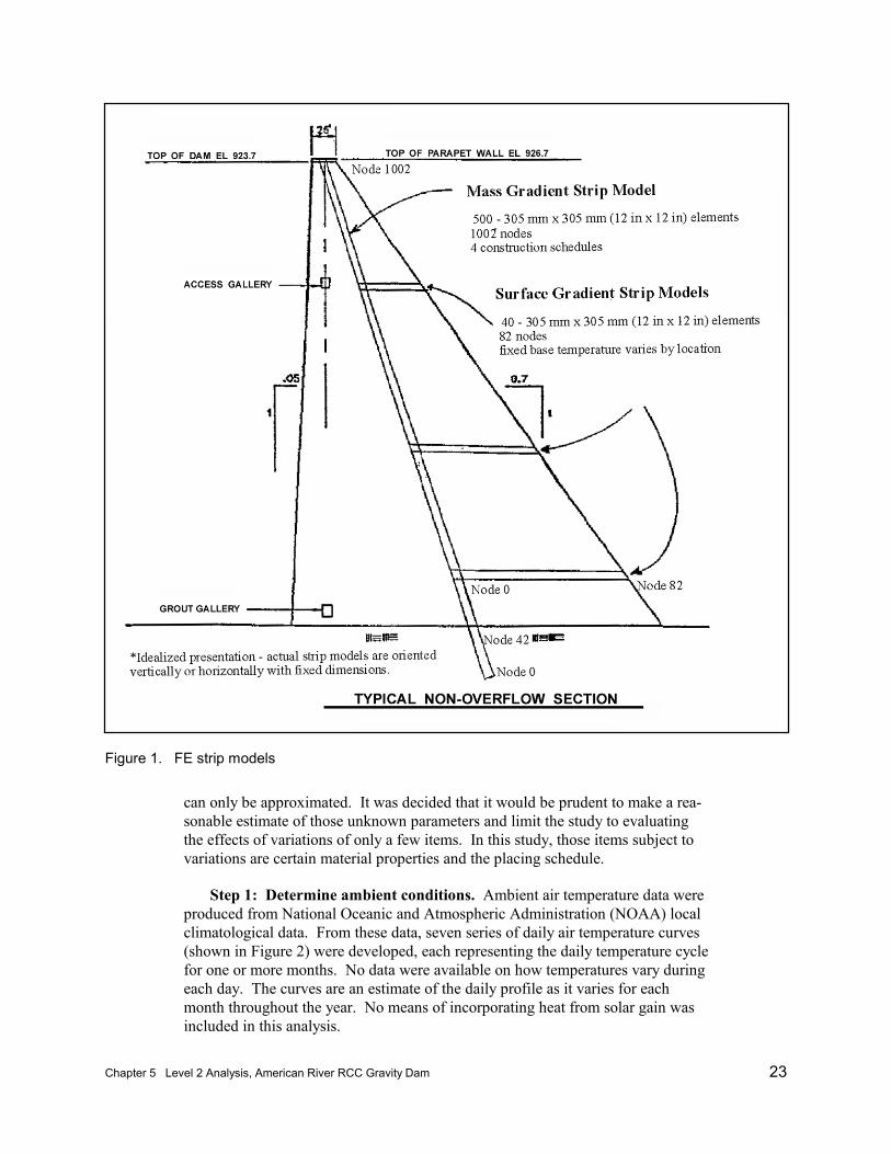
Figure 1. FE strip models................................................................................... 23
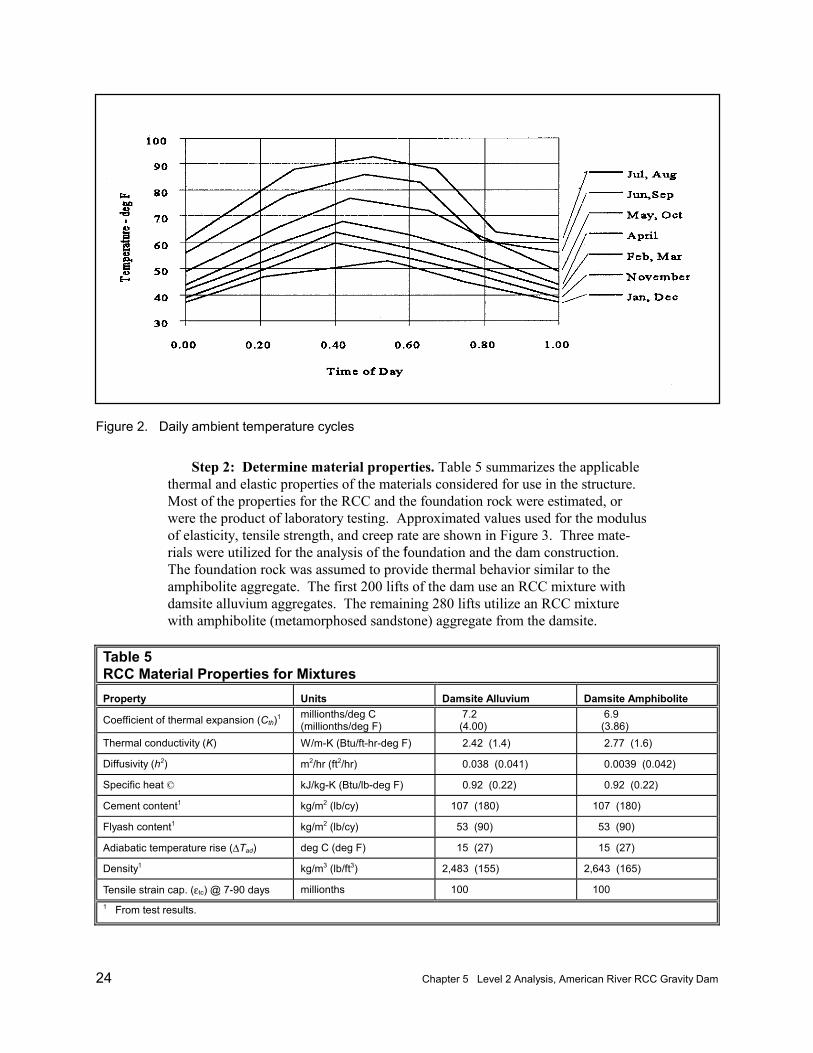
Figure 2. Daily ambient temperature cycles ....................................................... 24
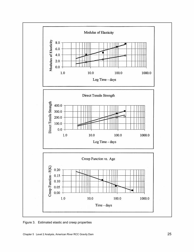
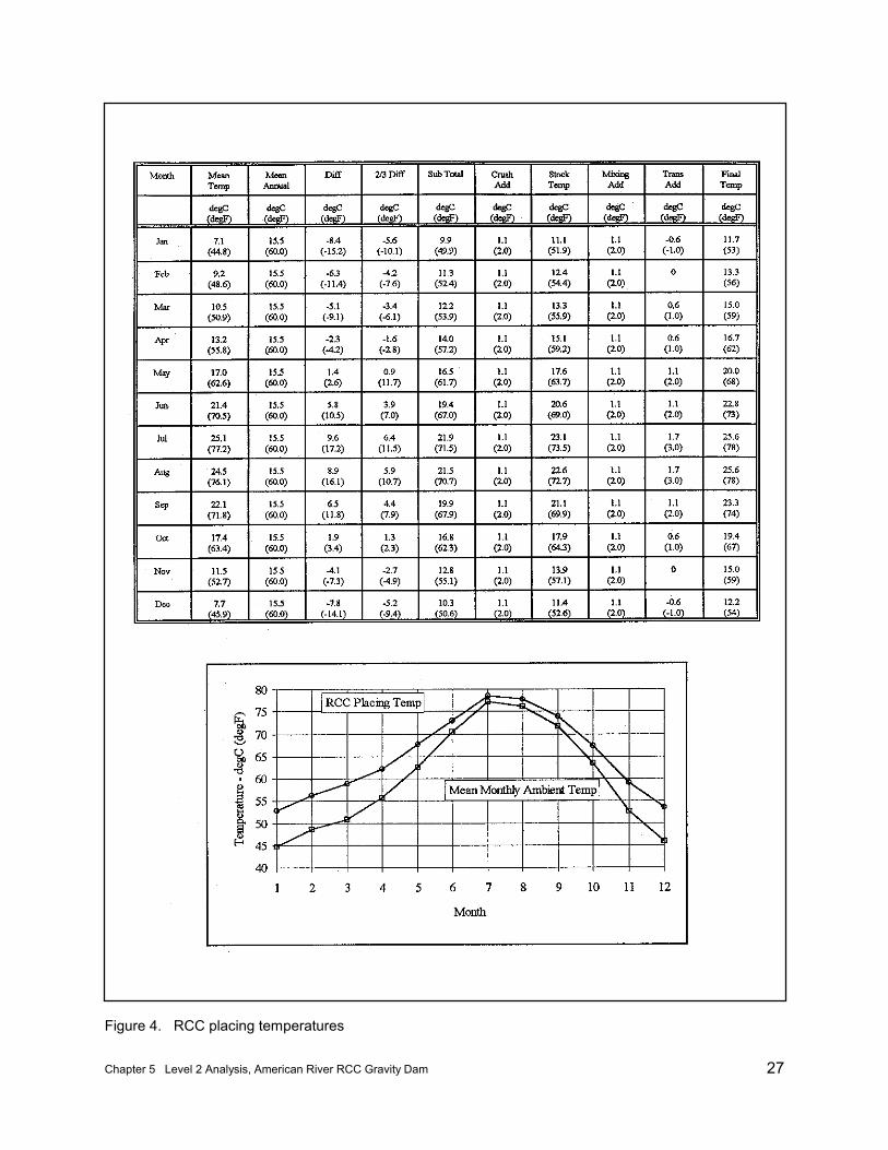
Figure 3. Estimated elastic and creep properties ................................................ 25
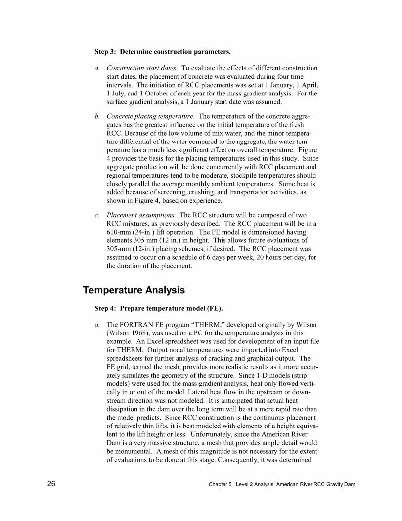
Figure 4. RCC placing temperatures .................................................................. 27
Figure 5. Mass gradient temperature histories for 1 January start ...................... 29
Figure 6. Mass gradient peak temperatures for 1 January start ......................... 29
Figure 7. Mass gradient temperature histories for 1 October start ..................... 30
Figure 8. Mass gradient peak temperatures for 1 October start ......................... 30
Figure 9. Mass gradient temperature histories for 1 July start ........................... 31
Figure 10. Mass gradient peak temperatures for 1 July start ............................. 31
Figure 11. Mass gradient temperature histories for 1 April start ........................ 32
Figure 12. Mass gradient peak temperatures for 1 April start ............................ 32
v
Figure 13. Temperature history for selected nodes from surface gradientmodel................................................................................................ 33
Figure 14. Surface gradient temperature distribution ......................................... 33
Figure 16. Lock wall section used in example ................................................... 42
Figure 17. Mean daily ambient temperatures and concrete placementtemperatures ..................................................................................... 42
Figure 18. Adiabatic temperature rise for Level 2 thermal analysis 2-Dexample ............................................................................................ 43
Figure 19. Finite element model of lock wall example ...................................... 45
Figure 20. Typical temperature histories at locations of mass gradientanalysis ............................................................................................. 46
Figure 21. Temperature distributions across lift 6 used in surfacegradient analysis ............................................................................... 49
Figure 22. Temperature differences in lift 6 for surface gradient analysis ......... 52
Figure 23. Balanced temperature difference distributions in lift 6 forsurface gradient analysis................................................................... 57
Figure 24. Evaluation of surface gradient cracking potential bycomparing induced tensile strain with slow-load tensile straincapacity............................................................................................. 59
List of Tables
Table 1. Thermal Study Process ....................................................................... 4
Table 2. NOAA Temperature Data, Woodland, CA....................................... 10
Table 3. Cache Creek Weir Placing Temperature Computation ..................... 11
Table 4. Cache Creek Weir Thermal Analysis Summary ............................... 12
Table 5. RCC Material Properties for Mixtures.............................................. 24
Table 6. Summary of Locations of Mass Gradient Thermal Cracks ............... 36
Table 7. Concrete and Foundation Thermal Properties .................................. 43
Table 8. Concrete and Foundation Mechanical Properties ............................. 43
Table 9. Summary of Surface Heat Transfer Coefficients for FEThermal Analyses ............................................................................. 45
vi
Table 10. Temperature Distribution in Lift 6 for Surface GradientAnalysis ............................................................................................ 47
Table 11. Temperature Differences Referenced to Temperature at 0.5Day ................................................................................................... 50
Table 12. Temperature Differences Normalized in Reference to SurfaceTemperature Differences for Surface Gradient Analysis .................. 53
Table 13. Balanced or Effective Temperature Differences to Determine“H” and Surface Gradients Strains ................................................... 55
Table 14. Mass Gradient Cracking Analysis .................................................... 57
Table 15. Surface Gradient Cracking Analysis................................................. 58
vii
Preface
This report contains examples of Level 1 and Level 2 thermal analyses. Theanalyses were conducted in conjunction with U.S. Army Corps of Engineersprojects and individually funded from project funds. These analyses wereoriginally assembled as annexes to ETL 1110-2-542, Thermal Studies of MassConcrete Structures.
The analyses were performed over a period of several years during the designof Cache Creek Detention Basin Weir by Sacramento District, the preliminarydesign of American River Dam for Sacramento District, and for various designefforts for Locks 2, 3, and 4 for Pittsburgh District.
Mr. Stephen B. Tatro, Walla Walla District, was responsible for the thermalanalysis of Cache Creek Detention Basin Weir and for American River Dam. Mr. John R. Hess, Sacramento District, provided consultation during certainphases of the work. Mr. Tatro and Mr. Anthony A. Bombich, StructuresLaboratory (SL), U.S. Army Engineer Research and Development Center(ERDC), were responsible for various phases of the Locks 2, 3, and 4 analyses. Messrs. Tatro and Bombich prepared the major element of this report. Finalreview was provided by Mr. Hess. Dr. Michael J. O’Connor was Acting Directorof SL.
At the time of publication of this report, Dr. James R. Houston was Directorof ERDC, and COL James S. Weller, EN, was Commander.
The contents of this report are not to be used for advertising,publication, or promotional purposes. Citation of trade names doesnot constitute an official endorsement or approval of the use of suchcommercial products.

viii
Conversion Factors, Non-SI toSI Units of Measurement
Non-SI units of measurement used in this report can be converted to SI unitsas follows:
Multiply By To Obtain
Fahrenheit degrees 5/9 Celsius degrees or kelvins1
feet 0.3048 meters
inches 0.0254 meters1 To obtain Celsius (C) temperature readings from Fahrenheit (F) readings use the followingformula: C = (5/9) (F-32). To obtain kelvin (K) readings, use K = (5/9) – (F-32) + 273.15.
Chapter 1 Introduction 1
1 Introduction
What the Report ContainsThis report presents examples of mass concrete thermal studies performed for
several U.S. Army Corps of Engineers projects. The examples are preceded by abrief explanation of the components of each study and other relevant information.This chapter provides an introduction to the concepts, objectives, and process forperforming a thermal analysis and identifies measures to control thermal cracking.
The example thermal studies were generally performed as outlined in Engi-neer Technical Letter (ETL) 1110-2-542, Thermal Studies of Mass ConcreteStructures. This ETL is no longer in print, but the major elements of the docu-ment are now contained in Engineer Manual (EM) 1110-2-2000, Standard Prac-tice for Concrete for Civil Works Structures. This report serves as a companiondocument to the EM. More detailed explanations of the general provisions forperforming mass concrete thermal studies are contained in EM 1110-2-2000.
The procedure for a Level 1 analysis is presented herein along with an exam-ple of the thermal study conducted for Cache Creek Sedimentation Basin. Theprocedure for a Level 2 analysis is also presented. The preliminary thermalanalysis for the American River Dam provides an example of a one-dimensionalLevel 2 thermal analysis, including an example using simple finite element (FE),one-dimensional (1-D) strip models. The thermal analysis for Locks and Dams 2,3, and 4 on the Monongahela River provides an example of a Level 2 analysisusing more complex two-dimensional (2-D), FE methodology. Appendix Apresents the current practice for determination of concrete tensile strain capacity(TSC) for use in cracking analysis.
ConceptMass concrete is defined by the American Concrete Institute (ACI) as “any
volume of concrete with dimensions large enough to require that measures betaken to cope with generation of heat from hydration of the cement and attendantvolume change to minimize cracking.” When portland cement combines withwater, the ensuing exothermic (heat-releasing) chemical reaction causes a tem-perature rise in the concrete mass. The actual temperature rise in a mass concretestructure (MCS) depends upon the heat-generating characteristics of the mass
2 Chapter 1 Introduction
concrete mixture, its thermal properties, environmental conditions, geometry ofthe MCS, and construction conditions. Usually the peak temperature is reached ina few days to weeks after placement, followed by a slow reduction in temperature.Over a period of several months to several years, the mass eventually cools tosome stable temperature, or to a stable temperature cycle for thinner structures. Achange in volume occurs in the MCS proportional to the temperature change andthe coefficient of thermal expansion of the concrete. If volume change isrestrained during cooling of the mass by the foundation, the previously placedconcrete, or the exterior surfaces, sufficient tensile strain can develop to causecracking. Cracking generally occurs in the main body or at the surface of theMCS. These two principal cracking phenomena are termed mass gradient andsurface gradient cracking, respectively. ACI 207.1R contains detailed informationon heat generation, volume change, restraint, and cracking in mass concrete.
Thermal Analysis ObjectivesA thermal analysis is necessary to attain any of the following design
objectives:
To develop materials and structural and construction procedure requirementsfor use in feasibility evaluation, design, cost engineering, specifications, and con-struction of new MCS. Thermal studies provide a rational basis for specifyingconstruction requirements. A thermal study provides a guide for formulatingadvantageous design features, optimizing concrete mixture proportions, andimplementing necessary construction requirements.
To provide cost savings by revising the structural configuration, materialrequirements, or construction sequence. Construction requirements for concreteplacement temperature, mixture proportions, placement rates, insulation require-ments, and schedule constraints that are based on arbitrarily selected parameterscan create costly operations. Cost savings may be achieved through items such aseliminating unnecessary joints, allowing increased placing temperatures, increasedlift heights, and reduced insulation requirements.
To develop structures with improved performance where existing similarstructures have exhibited unsatisfactory behavior (such as extensive cracking)during construction or operation. Cracking which requires remedial repairs wouldbe considered unsatisfactory behavior. Cracking which does not affect the overallstructural behavior or some function of the structure would not be classified asunsatisfactory behavior.
To more accurately predict behavior of unprecedented structures for whichlimited experience is available, such as structures with unusual structural con-figuration, extreme loadings, unusual construction constraints, or severeoperational requirements.
Chapter 1 Introduction 3
Thermal Cracking Prevention MeasuresProvisions to counteract predicted thermal cracking are discussed in ACI 207
documents and typically include:
a. Changes in construction procedures, including placing times andtemperatures.
b. Changes in concrete materials and thermal properties.
c. Precooling of concrete materials.
d. Limit concrete placement temperatures.
e. Postcooling of concrete.
f. Construction of joints (with waterstops where necessary) to controllocation of cracks.
g. Construction of water barrier membranes to prevent water from enteringcracks.
h. Alteration of structure geometry to avoid or control cracking.
i. Use and careful removal of insulation.
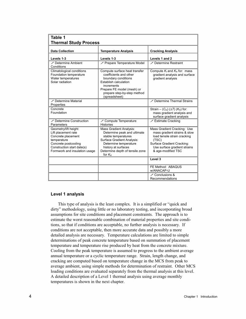
General Thermal Analysis ProcessThe thermal study process at any level consists of several steps that are sum-
marized in Table 1. These steps are similar for all three levels of analysis. Thesteps can be subdivided among three general tasks: data collection, temperatureanalysis, and cracking analysis. The specific efforts within each of these tasks canvary considerably, depending upon the level of analysis selected for the thermalstudy. Data collection includes those steps that provide input data and preparationof input for subsequent analysis tasks. Data collection may include informationretrieval and testing. Temperature analysis generates the temperatures or temper-ature histories for the MCS, which are possible scenarios of thermal loadingsduring construction and subsequent cooling. Cracking evaluation uses tempera-ture data from the temperature analysis, other sources of loading, material proper-ties, concrete/foundation interaction, geometry, construction parameters, etc., tocompute strains and evaluate the potential for cracking in the MCS. This processis directly applicable for evaluating mass gradient and surface gradient crackingfor thermal studies (Levels 1 and 2) and for advanced FE thermal studies such asnonlinear incremental structural analysis (NISA) (Level 3). At all levels of ther-mal analysis, parametric studies are an important part of thermal analysis and areused to assist the engineer in making proper decisions for design and construction.
4 Chapter 1 Introduction
Table 1Thermal Study Process
Data Collection Temperature Analysis Cracking Analysis
Levels 1-3 Levels 1-3 Levels 1 and 2 Determine Ambient
Conditions Prepare Temperature Model Determine Restraint
Climatological conditionsFoundation temperatureWater temperaturesSolar radiation
Compute surface heat transfercoefficients and otherboundary conditions
Establish calculationincrements
Prepare FE model (mesh) orprepare step-by-step method(spreadsheet)
Compute Kf and KR for: massgradient analysis and surfacegradient analysis
Determine MaterialProperties
Determine Thermal Strains
ConcreteFoundation
Strain – (Cth) (∆T) (KR) for: mass gradient analysis andsurface gradient analysis
Determine ConstructionParameters
Compute TemperatureHistories
Estimate Cracking
Geometry/lift heightLift placement rateConcrete placementtemperatureConcrete postcoolingConstruction start date(s)Formwork and insulation usage
Mass Gradient Analysis: Determine peak and ultimatestable temperatures
Surface Gradient Analysis: Determine temperaturehistory at surfaces
Determine depth of tensile zonefor KR
Mass Gradient Cracking: Usemass gradient strains & slowload tensile strain cracking(TSC)
Surface Gradient Cracking: Use surface gradient strains& age-modified TSC
Level 3
FE Method: ABAQUSw/ANACAP-U
Conclusions &Recommendations
Level 1 analysis
This type of analysis is the least complex. It is a simplified or “quick anddirty” methodology, using little or no laboratory testing, and incorporating broadassumptions for site conditions and placement constraints. The approach is toestimate the worst reasonable combination of material properties and site condi-tions, so that if conditions are acceptable, no further analysis is necessary. Ifconditions are not acceptable, then more accurate data and possibly a moredetailed analysis are necessary. Temperature calculations are limited to simpledeterminations of peak concrete temperature based on summation of placementtemperature and temperature rise produced by heat from the concrete mixture. Cooling from the peak temperature is assumed to progress to the ambient averageannual temperature or a cyclic temperature range. Strain, length change, andcracking are computed based on temperature change in the MCS from peak toaverage ambient, using simple methods for determination of restraint. Other MCSloading conditions are evaluated separately from the thermal analysis at this level.A detailed description of a Level 1 thermal analysis using average monthlytemperatures is shown in the next chapter.
Chapter 1 Introduction 5
Level 2 analysis
Level 2 thermal analysis is characterized by a more rigorous determination ofconcrete temperature history in the structure and the use of a wide range of tem-perature analysis tools. Placement temperatures are usually determined based onambient temperatures and anticipated material processing and handling measures.The temperature history of the concrete mass is approximated by using step-by-step iteration using the Schmidt or Carlson methods or by FE analysis usingsimple 1-D models, termed “strip” models, or using 2-D models representingcross sections of a structure. Evaluation of thermal cracking within the interior ofan MCS, termed mass gradient cracking, and cracking at the surface of an MCS,termed surface gradient cracking, are appropriate at this level. Detailed crackingevaluation of complex shapes or loading conditions other than thermal loads is notperformed at this level.
Level 3 analysis
A Level 3 analysis is also known as a nonlinear incremental structural analysis(NISA). NISA is performed using the FE method, exclusively, to compute incre-mental temperature histories, thermal stress-strain, stress-strain from other load-ing, and cracking prediction results. Significant effort is necessary to collectenvironmental data, assess and implement applicable construction parameters,acquire foundation materials properties, determine appropriate constructionscenarios, and perform testing required for thermal and nonlinear material proper-ties input. Preparation of FE models and conducting temperature and thermalstress analyses which generate significant volumes of data are generally extensiveand costly efforts. ETL 1110-2-365 describes the computational methodology andapplication of Level 3 (NISA) analysis. Hollenbeck and Tatro (2000) present anexample of a 2-D NISA application to analyze cracking for Zintel Canyon Dam, aroller compacted concrete (RCC) dam constructed in 1992.
6 Chapter 2 Level 1 Thermal Study Analysis
2 Level 1 Thermal StudyAnalysis
GeneralThis chapter summarizes each step in a Level 1 thermal study mass gradient
analysis of a MCS. An example of how this procedure was applied for a modest-size MCS is presented in Chapter 3. Although alternative approaches can beused, this method is in common use for this level MCS thermal analysis. Surfacegradient thermal analysis is seldom conducted at this level of analysis.
Input Properties and ParametersStep 1: Determine ambient conditions. Simple analyses conducted for a
Level 1 analysis are typically based on average monthly temperature data.
Step 2: Determine material properties. Laboratory test results on materialproperties are seldom available for this level of thermal analysis. Material prop-erties are generally estimated from published data in sources such as ACI docu-ments, technical publications, and engineering handbooks. Often knowninformation such as compressive strength and aggregate type is used to predictother material properties from published data. The minimum properties requiredare the coefficient of thermal expansion (Cth), the adiabatic temperature rise(ΔTad), and the tensile strain capacity (εtc).
Step 3: Determine construction parameters. Concrete placement temper-ature is the essential construction parameter needed for this level of thermalanalysis. A first approximation is to assume that concrete placement tempera-tures (Tp) directly parallel the average monthly temperature. A more accuratemethod is to modify the average monthly temperature based upon production timeperiod and extent of production or to use actual placement temperature data fromsimilar projects.
Chapter 2 Level 1 Thermal Study Analysis 7
Temperature AnalysisStep 4: Mass gradient temperature analysis. For Level 1 mass gradient
analysis, no elaborate “model” is used to develop temperature history. The long-term temperature change is simply calculated as the peak concrete temperatureminus the ultimate stable concrete temperature.
a. Determine peak temperature. This is the sum of the concrete placementtemperature and the adiabatic temperature rise.
b. Determine ultimate stable temperature. Large structures cool to a stabletemperature equal to the average ambient temperature. However, smallerconcrete structures cool to a stable annual temperature cycle, since there isinsufficient mass to provide complete insulation of the interior. ACI207.1R provides a plot relating temperature variation with depth to deter-mine this internal temperature cycle. It is assumed that the concrete tem-perature cycles about the average annual temperature.
c. Determine long-term temperature change. The sum of the placingtemperature plus adiabatic temperature rise provides a quick peaktemperature of the MCS. Then subtracting the ultimate stabletemperature provides the long-term temperature change used for strainand cracking evaluation.
Cracking AnalysisStep 5: Mass gradient cracking analysis. Using long-term temperature
change and ACI formulas, mass gradient strain is approximated. These strains arecompared to estimates of tensile strain capacity to determine if and when crackingmay occur.
a. Determine mass gradient restraint conditions. The structure restraintfactor (KR) and the foundation restraint factor (Kf)(in ACI 207.2R termed“Multiplier for foundation rigidity”) are determined as described inEquation 5 (see Chapter 6) and in ACI 207.2R.
b. Determine mass gradient thermal strain. The total induced strain is theproduct of the long-term temperature change, the coefficient of thermalexpansion, and restraint factors.
Total strain = (Cth) (dT) (KR) (Kf) (1)
where
Total strain = induced strain (millionths)
Cth = coefficient of thermal expansion
dT = temperature differential
8 Chapter 2 Level 1 Thermal Study Analysis
KR = structure restraint factor
Kf = foundation restraint factor
Cracking strain is computed by subtracting tensile strain capacity from thetotal strain. The remainder is the strain that must be accommodated incracks at some spacing and width across the MCS.
c. Estimate mass gradient cracking. Foundation conditions (restraint) con-trol the spacing of cracks and the crack width. If the foundation is stiffer,tightly spaced cracks of small width can be expected. If the foundation isrelatively soft (low restraint), widely spaced and wider cracks can beanticipated. Multiply the MCS length by the cracking strain to determinethe total width of cracking to be accommodated in the MCS. Estimate acrack width based on foundation conditions and divide the total width ofcracking by the assumed crack width to determine the total number ofcracks.
Conclusions and RecommendationsThese typically include expected maximum temperatures for starting place-
ment in different seasons, expected transverse and longitudinal cracking withouttemperature or other controls, recommended concrete placement temperaturelimitations, anticipated concrete precooling measures, need for adjustment inconcrete properties, joint spacing, and sensitivity of the thermal analysis tochanges in parameters.
Chapter 3 Level 1 Analysis, Cache Creek Detention Basin Weir 9
3 Level 1 Analysis, CacheCreek Detention Basin Weir
IntroductionThis example, based on a thermal study for the Cache Creek Detention Basin
Weir, illustrates one way to estimate concrete placing temperature based on ambi-ent air temperatures and material processing schemes and schedules. The studyevaluates mass gradient cracking only. The Cache Creek Detention Basin inCalifornia is a RCC overflow weir section in a levee system. The structure is4.6 m (15 ft) high, 3.6 m (12 ft) wide at the top, has 0.8 to 1 slopes upstream anddownstream, and is 530 m (1,740 ft) long. Compacted sands and silts were placedagainst the full height of the upstream face. The purpose of the study was todetermine the adequacy of contraction joints spaced at 30-m (100-ft) intervalsand, if necessary, provide recommendations for alternate configurations. Alsoaddressed is the adequacy of a maximum placing temperature of 29 deg C (85 degF) for the RCC. The following paragraphs provide explanation on the selectioncriteria and determination of the parameters used to summarize thermal study.
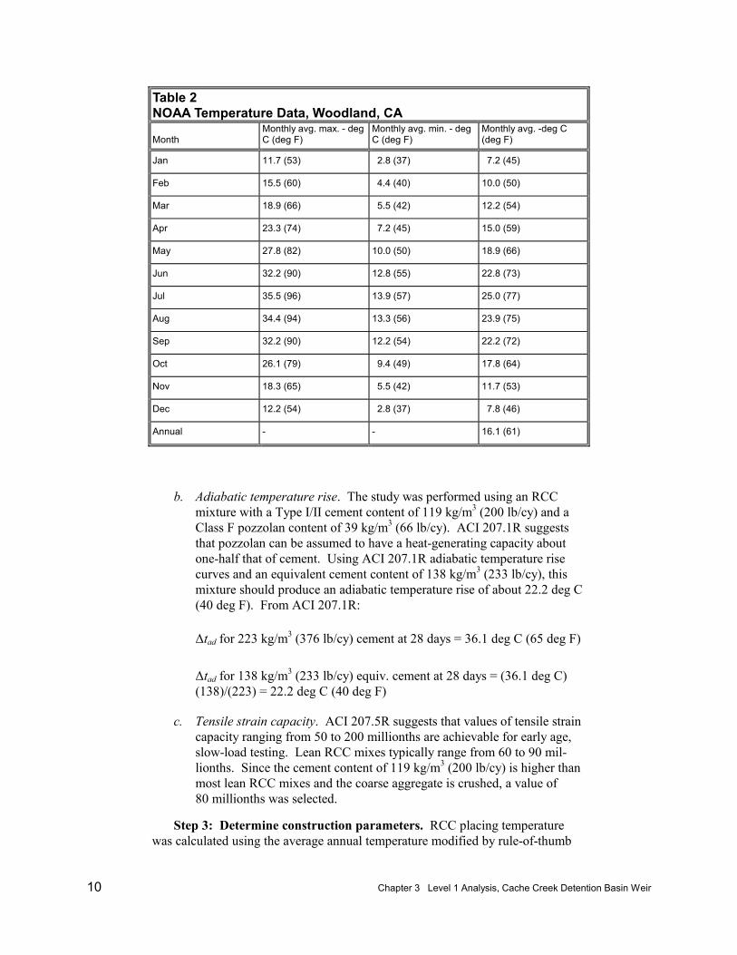
Input Properties and ParametersStep 1: Determine ambient conditions. Data were provided from climato-
logical data summaries for Woodland, CA, prepared by the National Oceanic andAtmospheric Administration (NOAA), shown in Table 2. The average annualtemperature used was 16.1 deg C ( 61 deg F), and monthly mean and averagemonthly maximum and minimum temperatures were used for other computations.
Step 2: Determine material properties.
a. Coefficient of thermal expansion. Coefficient of thermal expansion wasestimated using handbook data (Fintel 1985) for the sandstone and meta-sandstone aggregate concrete planned for the project:
Cth = 9.9 millionths/deg C (5.5 millionths/deg F)
10 Chapter 3 Level 1 Analysis, Cache Creek Detention Basin Weir
Table 2NOAA Temperature Data, Woodland, CA
MonthMonthly avg. max. - degC (deg F)
Monthly avg. min. - degC (deg F)
Monthly avg. -deg C(deg F)
Jan 11.7 (53) 2.8 (37) 7.2 (45)
Feb 15.5 (60) 4.4 (40) 10.0 (50)
Mar 18.9 (66) 5.5 (42) 12.2 (54)
Apr 23.3 (74) 7.2 (45) 15.0 (59)
May 27.8 (82) 10.0 (50) 18.9 (66)
Jun 32.2 (90) 12.8 (55) 22.8 (73)
Jul 35.5 (96) 13.9 (57) 25.0 (77)
Aug 34.4 (94) 13.3 (56) 23.9 (75)
Sep 32.2 (90) 12.2 (54) 22.2 (72)
Oct 26.1 (79) 9.4 (49) 17.8 (64)
Nov 18.3 (65) 5.5 (42) 11.7 (53)
Dec 12.2 (54) 2.8 (37) 7.8 (46)
Annual - - 16.1 (61)
b. Adiabatic temperature rise. The study was performed using an RCCmixture with a Type I/II cement content of 119 kg/m3 (200 lb/cy) and aClass F pozzolan content of 39 kg/m3 (66 lb/cy). ACI 207.1R suggeststhat pozzolan can be assumed to have a heat-generating capacity aboutone-half that of cement. Using ACI 207.1R adiabatic temperature risecurves and an equivalent cement content of 138 kg/m3 (233 lb/cy), thismixture should produce an adiabatic temperature rise of about 22.2 deg C(40 deg F). From ACI 207.1R:
Δtad for 223 kg/m3 (376 lb/cy) cement at 28 days = 36.1 deg C (65 deg F)
Δtad for 138 kg/m3 (233 lb/cy) equiv. cement at 28 days = (36.1 deg C)(138)/(223) = 22.2 deg C (40 deg F)
c. Tensile strain capacity. ACI 207.5R suggests that values of tensile straincapacity ranging from 50 to 200 millionths are achievable for early age,slow-load testing. Lean RCC mixes typically range from 60 to 90 mil-lionths. Since the cement content of 119 kg/m3 (200 lb/cy) is higher thanmost lean RCC mixes and the coarse aggregate is crushed, a value of80 millionths was selected.
Step 3: Determine construction parameters. RCC placing temperaturewas calculated using the average annual temperature modified by rule-of-thumb
Chapter 3 Level 1 Analysis, Cache Creek Detention Basin Weir 11
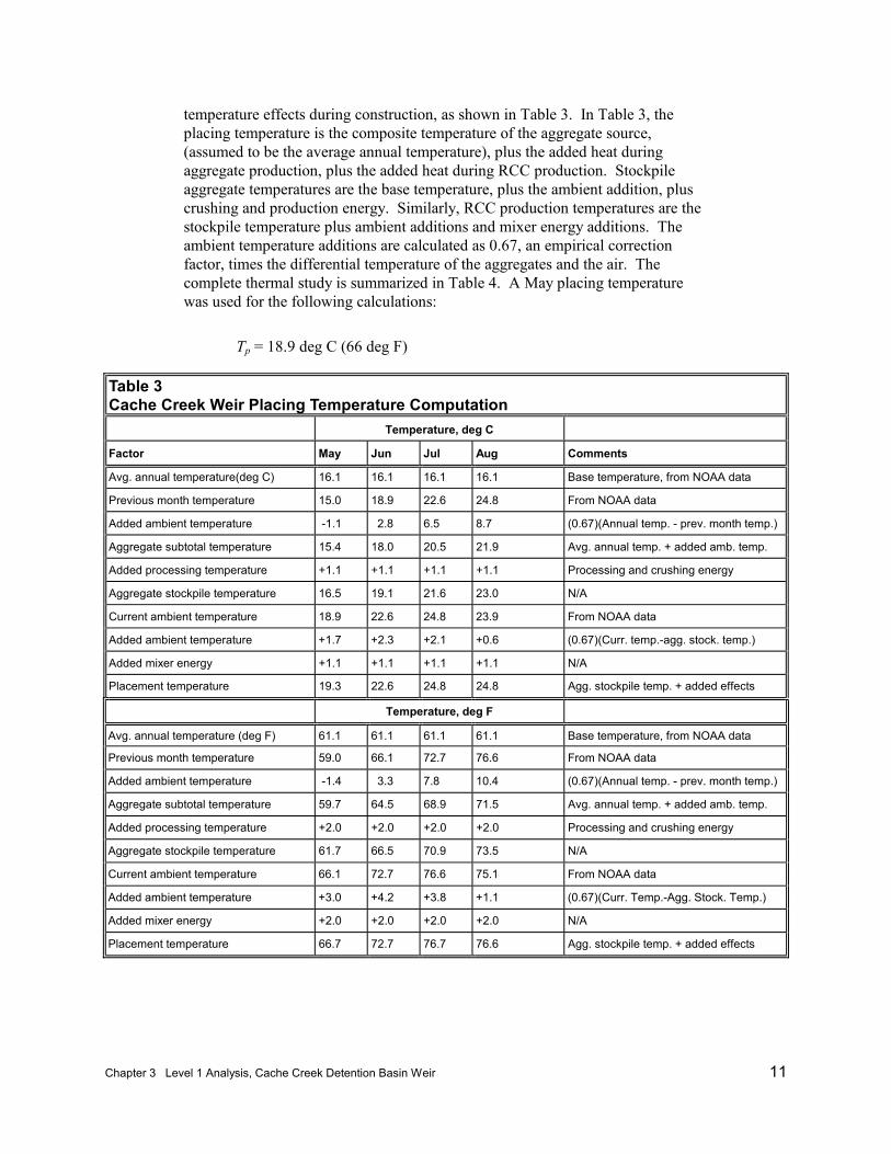
temperature effects during construction, as shown in Table 3. In Table 3, theplacing temperature is the composite temperature of the aggregate source,(assumed to be the average annual temperature), plus the added heat duringaggregate production, plus the added heat during RCC production. Stockpileaggregate temperatures are the base temperature, plus the ambient addition, pluscrushing and production energy. Similarly, RCC production temperatures are thestockpile temperature plus ambient additions and mixer energy additions. Theambient temperature additions are calculated as 0.67, an empirical correctionfactor, times the differential temperature of the aggregates and the air. Thecomplete thermal study is summarized in Table 4. A May placing temperaturewas used for the following calculations:
Tp = 18.9 deg C (66 deg F)
Table 3Cache Creek Weir Placing Temperature Computation
Temperature, deg C
Factor May Jun Jul Aug Comments
Avg. annual temperature(deg C) 16.1 16.1 16.1 16.1 Base temperature, from NOAA data
Previous month temperature 15.0 18.9 22.6 24.8 From NOAA data
Added ambient temperature -1.1 2.8 6.5 8.7 (0.67)(Annual temp. - prev. month temp.)
Aggregate subtotal temperature 15.4 18.0 20.5 21.9 Avg. annual temp. + added amb. temp.
Added processing temperature +1.1 +1.1 +1.1 +1.1 Processing and crushing energy
Aggregate stockpile temperature 16.5 19.1 21.6 23.0 N/A
Current ambient temperature 18.9 22.6 24.8 23.9 From NOAA data
Added ambient temperature +1.7 +2.3 +2.1 +0.6 (0.67)(Curr. temp.-agg. stock. temp.)
Added mixer energy +1.1 +1.1 +1.1 +1.1 N/A
Placement temperature 19.3 22.6 24.8 24.8 Agg. stockpile temp. + added effects
Temperature, deg F
Avg. annual temperature (deg F) 61.1 61.1 61.1 61.1 Base temperature, from NOAA data
Previous month temperature 59.0 66.1 72.7 76.6 From NOAA data
Added ambient temperature -1.4 3.3 7.8 10.4 (0.67)(Annual temp. - prev. month temp.)
Aggregate subtotal temperature 59.7 64.5 68.9 71.5 Avg. annual temp. + added amb. temp.
Added processing temperature +2.0 +2.0 +2.0 +2.0 Processing and crushing energy
Aggregate stockpile temperature 61.7 66.5 70.9 73.5 N/A
Current ambient temperature 66.1 72.7 76.6 75.1 From NOAA data
Added ambient temperature +3.0 +4.2 +3.8 +1.1 (0.67)(Curr. Temp.-Agg. Stock. Temp.)
Added mixer energy +2.0 +2.0 +2.0 +2.0 N/A
Placement temperature 66.7 72.7 76.7 76.6 Agg. stockpile temp. + added effects
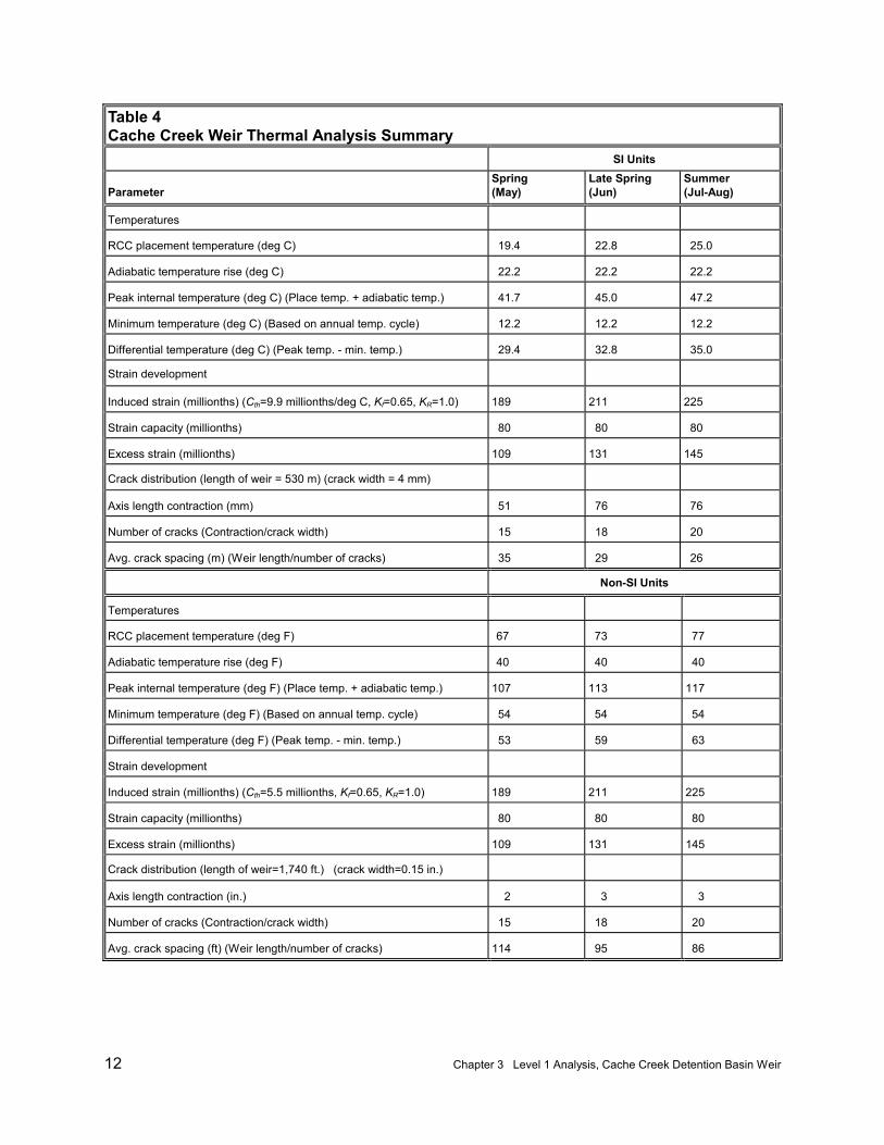
12 Chapter 3 Level 1 Analysis, Cache Creek Detention Basin Weir
Table 4Cache Creek Weir Thermal Analysis Summary
SI Units
ParameterSpring(May)
Late Spring(Jun)
Summer(Jul-Aug)
Temperatures
RCC placement temperature (deg C) 19.4 22.8 25.0
Adiabatic temperature rise (deg C) 22.2 22.2 22.2
Peak internal temperature (deg C) (Place temp. + adiabatic temp.) 41.7 45.0 47.2
Minimum temperature (deg C) (Based on annual temp. cycle) 12.2 12.2 12.2
Differential temperature (deg C) (Peak temp. - min. temp.) 29.4 32.8 35.0
Strain development
Induced strain (millionths) (Cth=9.9 millionths/deg C, Kf=0.65, KR=1.0) 189 211 225
Strain capacity (millionths) 80 80 80
Excess strain (millionths) 109 131 145
Crack distribution (length of weir = 530 m) (crack width = 4 mm)
Axis length contraction (mm) 51 76 76
Number of cracks (Contraction/crack width) 15 18 20
Avg. crack spacing (m) (Weir length/number of cracks) 35 29 26
Non-SI Units
Temperatures
RCC placement temperature (deg F) 67 73 77
Adiabatic temperature rise (deg F) 40 40 40
Peak internal temperature (deg F) (Place temp. + adiabatic temp.) 107 113 117
Minimum temperature (deg F) (Based on annual temp. cycle) 54 54 54
Differential temperature (deg F) (Peak temp. - min. temp.) 53 59 63
Strain development
Induced strain (millionths) (Cth=5.5 millionths, Kf=0.65, KR=1.0) 189 211 225
Strain capacity (millionths) 80 80 80
Excess strain (millionths) 109 131 145
Crack distribution (length of weir=1,740 ft.) (crack width=0.15 in.)
Axis length contraction (in.) 2 3 3
Number of cracks (Contraction/crack width) 15 18 20
Avg. crack spacing (ft) (Weir length/number of cracks) 114 95 86
Chapter 3 Level 1 Analysis, Cache Creek Detention Basin Weir 13
Temperature AnalysisStep 4: Mass gradient temperature analysis.
a. Determine peak temperature. This is the sum of the initial RCCplacement temperature and the adiabatic temperature rise:
Tp + ΔTad = 18.9 + 22.2 = 41.1 deg C (106 deg F)
b. Determine ultimate stable temperature. Since the weir is a relatively thinMCS, it is expected to develop a stable temperature cycle, rather than asingle stable temperature as in larger MCS’s. The temperatures belowwere determined using the methodology in ACI 207.1R (“Temperaturevariation with depth”). Typical distance from the RCC surface to theinterior was determined to be 4.6 m (15 ft). From ACI 207.1R figure:
24.0surfaceat range Temp
concrete through change Temp =
Temp range at surface
Temp range at surface = 24.8 - 7.3 = 17.5 deg C (31.5 deg F)
Temp change in concrete interior = (0.24) (17.5 deg C) = 4.2 deg C (7.6 deg F)
Temp range in concrete interior = 16.2 ± 4.2 deg C (61.1 ± 7.6 deg F)
Tmin = minimum interior concrete temp. = 16.2- 4.2 = 12 deg C (53.5 deg F)
c. Determine long-term temperature change. This value is simply the peakRCC placement temperature less the stable minimum temperature. Assuming a May placement:
ΔT = Tp + Tad - Tmin = 41.1 - 11.9 = 29.2 deg C (53 deg F)
Cracking AnalysisStep 5: Mass gradient cracking analysis.
a. Determine mass gradient restraint conditions. Geometric restraint isconservatively set at KR=1.0, since the structure has a low profile. Foun-dation restraint is set at Kf= 0.65, since the base is not rock but rathercompacted structural backfill.
14 Chapter 3 Level 1 Analysis, Cache Creek Detention Basin Weir
KR = 1.0 Kf = 0.65
b. Determine mass gradient thermal strain. The total induced strain in themass RCC is the product of the long-term temperature change, thecoefficient of thermal expansion, and restraint factors:
Total induced strain = (Cth)(ΔT)(KR)(Kf) = (9.9 millionths/deg C )(29.2 deg C)(1.0)(0.65) = 189 millionths
c. Estimate mass gradient cracking. The strain that results in cracking ofthe structure is the total induced strain less the tensile strain capacity (εsc)of the material. The total crack width in the length of the structure is thecracking strain multiplied by the length of the structure. The estimatednumber of cracks are based on the assumed crack widths. Typical crackwidths range from 0.002 to 5 mm (0.01 to 0.2 in.). The larger crackwidths are typical of structures founded on flexible or yielding founda-tions. Since such a foundation exists here, a typical crack width of 4 mm(0.15 in.) was assumed:
Cracking strain = total induced strain - εsc = 189 - 80 = 109 millionths
Total crack width = (weir length)(cracking strain) = (530 m)(1,000mm/m)(109 millionths) = 58 mm (2.3 in.)
Assumed crack widths = 4 mm (0.15 in.)
Estimated cracks = 58 mm/4 mm = 15 cracks
Estimated crack spacing = 530 m/15 cracks= 35 m (116 ft)
Since contraction joints will be installed at 30-m (100-ft) spacing, additionalcracking is not expected. Occasional center cracks can be expected where condi-tions and restraint factors vary from those assumed.
Conclusions and RecommendationsConclusions
Based on calculations similar to those shown above and on previous temper-ature analysis figures, and experience, the following conclusions were provided:
a. May placement schedule. RCC placement temperatures should be 19.4 to21.1 deg C (67 to 70 deg F) if aggregates are produced the precedingmonth. If aggregate processing is performed earlier, lower placementtemperatures may result. Crack spacing in an unjointed structure is
Chapter 3 Level 1 Analysis, Cache Creek Detention Basin Weir 15
calculated to be 35 m (116 ft). The 30-m (100-ft) contraction jointinterval easily accommodates this volume change with joint widths ofapproximately 3 mm (0.13 in.).
b. June placement schedule. RCC placement temperatures should be 22.2 to23.9 deg C (72 to 75 deg F) if aggregates are produced the precedingmonth. If aggregate processing is performed earlier, lower placementtemperatures may result. Crack spacing in an unjointed structure is calcu-lated to be 29 m (97 ft). The 30-m (100-ft) contraction joint interval justaccommodates this volume change with joint widths of approximately4 mm (0.15 in.).
c. July and August placement schedules. RCC placement temperaturesshould be 23.9 to 26.7 deg C (75 to 80 deg F) if aggregates are producedthe preceding month. If aggregate processing is performed earlier, lowerplacement temperatures may result. Crack spacing in an unjointed struc-ture is calculated to be 26 m (87 ft). The 30-m (100-ft) contraction jointinterval is not quite adequate to accommodate this volume change at afixed joint width of 4 mm (0.15 in.). Joint widths will increase or addi-tional cracking will occur.
d. Since the anticipated period for RCC construction is during the late springor summer months, the 29.4-deg C (85-deg F) placement temperaturelimitation specified could be a factor if unusually hot weather shouldoccur. Under normal weather conditions, uncontrolled placing tempera-tures should range from 19.4 to 24.4 deg C (67 to 76 deg F) from Maythrough August. In the event that abnormal weather causes average dailyambient temperature in excess of 29.4 deg C (85 deg F), RCC tempera-tures could exceed 29.4 deg C (85 deg F). Aggregate stockpile coolingand possible use of batch water chillers would be the most expedientsolutions to this problem.
e. The current joint spacing of 30 m (100 ft) is adequate for RCC place-ments during May and June. Later placements in July and August willresult in occasional centerline cracking of monoliths, possibly in as manyas three or four monoliths. Lesser cracking is very probable since mate-rial properties were conservatively estimated.
f. During construction, RCC placement temperature was maintained atabout 29.4 deg C (85 deg F), and transverse contraction joints werespaced at 30-m (100-ft) intervals. All the contraction joints openedproperly during the first few months after construction, with no inter-mediate cracking. Crack widths varied from 1.5 to 6 mm (0.06 to0.25 in.).
g. Several material properties were applied conservatively. Small reductionsof adiabatic temperature rise and coefficient of thermal expansion andsmall increases in tensile strain capacity could improve thermal crackingperformance. If each of these properties were individually changed10 percent, summer crack spacing would be around 30 m (100 ft). If

16 Chapter 3 Level 1 Analysis, Cache Creek Detention Basin Weir
these changes were cumulative, crack spacing would be over 40 m(130 ft).
Recommendations
a. Maintain current 29.4-deg C (85-deg F) maximum placement temperaturelimitation. Consider allowing minor temperature violations so long as thetime-weighted average of the RCC placement temperature is maintainedbelow 26.7 deg C (80 deg F).
b. Maintain current contraction joint spacing of 30 m (100 ft). The currentcontraction joint configuration of 30-m (100-ft) joint intervals is sufficientto accommodate the total anticipated axial contractions due to cementinduced temperature fluctuations during May and June placements. Sometransverse cracking will occur during the July and August placementschedule; however, the extent of cracking should not be of concernconsidering the upstream backfill and the frequency of use.
Chapter 4 Level 2 Thermal Analysis 17
4 Level 2 Thermal Analysis
GeneralThis chapter summarizes typical steps in a Level 2 mass gradient and surface
gradient thermal analysis of a MCS. Two examples of the procedure are pre-sented in Chapters 5 and 6. Example 1 (Chapter 5) covers a simple one-dimensional (1-D) (strip model) finite element (FE) mass gradient and surfacegradient thermal analysis. Example 2 (Chapter 6) presents a more complex two-dimensional (2-D) mass gradient and surface gradient thermal analysis. Thisprocedure uses FE methodology only because of the widespread availability anduse of this technology. Although other methods of conducting a Level 2 thermalanalysis are available, these procedures are most commonly used.
Input Properties and ParametersThe level of data detail depends on the complexity of a Level 2 thermal analy-
sis. Parametric analysis should be routinely conducted at this level, using arational number and range of input properties and parameters to evaluate likelythermal problems.
Step 1: Determine ambient conditions. Level 2 analyses may be basedupon average monthly temperatures for a less complex analysis, or on averageexpected daily temperatures for each month for a complex analysis. Wind vel-ocity data are generally needed for computing heat transfer coefficients. Extremeambient temperature input conditions, such as cold fronts and sudden cold res-ervoir temperatures, can and should be considered when appropriate to identifypossible problems.
Step 2: Determine material properties. Thermal properties required for FEthermal analysis include thermal conductivity, specific heat, adiabatic temperaturerise of the concrete mixture(s), and density of the concrete and foundation materi-als. Coefficient of thermal expansion is required for computing induced strainfrom temperature differences. Moduli of elasticity of concrete and foundationmaterials are required for determination of foundation restraint factors. Tensilestrain capacity test results are important for cracking evaluation. When tensilestrain capacity data are not available, the methodology presented in Appendix Amay be used to estimate probable tensile strain capacity performance of the
18 Chapter 4 Level 2 Thermal Analysis
concrete. Creep test results are necessary to determine the sustained modulus ofelasticity (or an estimate of Esus is made) if stress-based cracking analysis is used.
Step 3: Determine construction parameters. Construction parametersmust be compiled which include information about concrete placement tempera-ture, structure geometry, lift height, construction start dates, concrete placementrates, and surface treatment such as formwork and insulation that are possibleduring construction of the MCS. To determine concrete placement temperature, afirst approximation is to assume that concrete placement temperatures directlyparallel the mean daily ambient temperature curve for the project site. Actualplacement temperature data from other projects can be used for prediction, modi-fied by ambient temperature data differences between the different sites. Thetemperature of the aggregate stockpiles may change more slowly than does theambient temperature in the spring and fall. Hence, placement temperatures duringspring months may lag several degrees below mean daily air temperatures, whileplacement temperatures in the fall may lag several degrees above mean daily airtemperatures.
a. Surface heat transfer coefficients. Surface heat transfer coefficients (filmcoefficients) are applied to all exposed surfaces to represent the convec-tion heat transfer effect between a fluid (air or water) and a concrete sur-face, in addition to the conduction effects of formwork and insulation. The following equations are taken from the American Society of Heating,Refrigerating and Air Conditioning Engineers (ASHRAE) (1977). Theseequations may be used for computing the surface heat transfer coefficientsto be included in any of the FE codes for modeling convection.
For surfaces without forms, the coefficients should be computed based onthe following:
).deg./(
:)9.10(5.172
2
FindayBtuK
W/maVhmphkm/hVfor b
−−−
=<(2)
)F.deg.inday/Btu(
(dc:)9.10(5.17for2
2
−−−
+=>
K
W/mV)hmphkm/hV(3)
where
V = wind velocity in km/h (mph)
h = surface heat transfer coefficient or film coefficient
a = 2.6362 (0.1132)
b = 0.8 (0.8)
c = 5.622 (0.165)
d = 1.086 (0.0513)
Chapter 4 Level 2 Thermal Analysis 19
The wind velocity may be based on monthly average wind velocities atthe project site. Data can be obtained for a given location and thengeneralized over a period of several months for input into the analysis.
b. Forms and insulation. If forms and insulation are in place, then thevalues for h computed in the equations above should be modified asfollows:
++
=′
+
+
=′
hRR
h
hkb
kb
h
11
11
insulationformwork
insulationformwork(4)
where
h' = revised surface heat transfer coefficient
b = thickness of formwork or insulation
k = conductivity of formwork or insulation
Rformwork= R value of formwork
Rinsulation= R value of insulation
Temperature AnalysisStep 4: Prepare temperature model.
a. Various temperature analysis methods suitable for Level 2 thermal analy-sis are discussed in EM 1110-2-2000. Either step-by-step integrationmethods or FE models may be used for Level 2 temperature analysis ormass and surface gradients. If step-by-step integration methods are used,the computation or numerical model should be programmed into a per-sonal computer spreadsheet. The decision on whether to use FE 1-D stripmodels or 2-D section analysis is generally based on complexity of thestructure, complexity of the construction conditions, and on the stage ofproject design. Often 1-D strip models are used first for parametricanalyses to identify concerns for more detailed 2-D analysis.
b. Compute temperature histories. Once computed, temperature data shouldbe tabulated as temperature-time histories and temperature distributions toobtain good visual representations of temperature distribution in the struc-ture. Hollenbeck and Tatro (2000) provide examples of temperaturedistribution plots. Appropriate locations can then be selected for
20 Chapter 4 Level 2 Thermal Analysis
temperature distribution histories at which mass gradient and surfacegradient analyses will be conducted.
Step 5: Mass gradient temperature analysis. Temperature-time histories,showing the change in temperature with time at specific locations after placing,are generally used to calculate temperature differences for mass gradient crackinganalysis. Temperature differences for mass gradient cracking analysis are gen-erally computed as the difference between the peak concrete temperatures and thefinal stable temperatures that the cooling concrete will eventually reach.
Step 6: Surface gradient temperature analysis. The objective of surfacegradient temperature analysis is to determine at desired critical locations the varia-tion of surface temperatures with depth and with time. This can be performedeffectively with 1-D strip models or with 2-D analysis. Thinner sections mayrequire temperature distributions entirely across the structure, while large sectionsoften only require temperature to be evaluated to some depth where temperaturechanges are relatively slow. Ideally, temperature distribution histories are gener-ated for a single lift, tabulated from one surface to the other (or a stable interior)with each distribution representing temperatures for a specific time afterplacement.
Cracking AnalysisStep 7: Mass gradient cracking analysis. The mass gradient temperature
differences are used with Cth and restraint factors (Kf and KR) to evaluate massgradient cracking potential, using Equation 1. Computed mass gradient strains arecompared against tensile strain capacity to evaluate cracking potential. For astress-based mass gradient cracking analysis, the sustained modulus of elasticitycorresponding to the time frame of the analysis is used to convert strains calcu-lated by Equation 1 to stresses. The use of the sustained modulus allows for therelief of temperature-induced stress due to creep. These stresses are compared tothe tensile strength of the concrete at the appropriate age to determine where andwhen cracking may occur.
Step 8: Surface gradient cracking analysis. Surface gradient crackinganalysis is based on higher temperature differences in the surface concrete com-pared to the more slowly cooling interior which creates areas of tension in thesurface to some depth, H. Tensile strain is calculated based on Cth, the tempera-ture difference at some depth of interest, and the degree of restraint based on H.
a. Temperature differences are calculated using as a basis the temperaturewhen the concrete first begins hardening, rather than a peak temperatureas used in mass gradient computations. These temperature differences,with time and depth, allow determination of tensile and compressionzones near the concrete surfaces. The point at which tension and com-pression zones balance is considered a stress-strain free boundary (locatedat H from the surface) used to compute restraint for surface gradient
Chapter 4 Level 2 Thermal Analysis 21
analysis. This point is generally calculated by evaluating temperaturedifferences at depth with respect to temperature differences at the surface.
b. Reference or initial temperatures for a surface gradient analysis aredefined as the temperatures in the structure at the time when the concretebegins to harden and material properties begin to develop. Generally, thistime is established at concrete ages of 0.25, 0.5, or 1.0 day. This age isdependent upon the rate at which the concrete achieves final set, the rateof subsequent cement hydration, and the properties of the mixture. Forvery lean concrete mixtures at normal temperature, a baseline time of1.0 day may be reasonable. Mixtures that gain strength more rapidly atearly ages may be better approximated by an earlier reference time of0.25 or 0.33 day (6 or 8 hours).
c. Internal restraint factors, KR, are computed using Equation 4.1 or 4.2 inACI 207.2R, depending upon the ratio of L/H, where L is the horizontaldistance between joints or ends of the structure, and H is the depth of thetension block. Induced tensile strains are computed at each analysis timefrom Equation 1 using the coefficient of thermal expansion, the tempera-ture differences between the surface and interior concrete, and the com-puted internal restraint factors. KR is assumed to be equal to 1.0 forinternal restraint conditions. These strains are compared with slow-loadtensile strain capacity (selected or tested to correspond to the time thatstrains are generated) to determine cracking potential.
d. Stress-based surface gradient cracking analysis is often handled in aslightly different way, particularly in the way creep is accounted for in theanalysis. Commonly, incremental temperature differences at differentdepths and times are computed. These incremental temperature differ-ences are converted to incremental stresses, including creep effects, usingthe Cth, Esus, and KR. The incremental stresses generated during each timeperiod are summed to determine the cumulative tensile stress in the sur-face concrete at various depths. These stresses are compared to the tensilestrength of the concrete at the appropriate age to determine crackingpotential.
Conclusions and RecommendationsConclusions and recommendations typically include expected maximum
temperatures for starting placement in different seasons, expected transverse andlongitudinal cracking without temperature or other controls, recommended con-crete placement temperature limitations, anticipated concrete precooling measures,need for adjustment in concrete geometry, properties, joint spacing, and the sensi-tivity of the thermal analysis to changes in parameters. Typical temperature con-trol measures evaluated might include reduced lift heights, use of insulated forms,and reduction in mix cement content. The potential for thermal shock may beaddressed. In addition, recommendations for further or more advanced thermalanalysis should be provided and justified.
22 Chapter 5 Level 2 Analysis, American River RCC Gravity Dam
5 Level 2 Analysis, AmericanRiver RCC Gravity Dam
GeneralAn example of a 1-D mass gradient and a surface gradient analysis in a
Level 2 thermal study of an MCS is presented below. This example is based onpreliminary 1-D analyses performed during feasibility studies on a proposed largeflood-control RCC gravity dam on the American River in California. This damwas planned to be 146 m (480 ft) high, 792 m (2,600 ft) long, with a downstreamface slope of 0.7H:1.0V.
The 1-D analysis was used as a screening tool only to provide preliminaryevaluation of several concerns and to develop information for more detailed analy-ses. These studies were conducted to ascertain the general extent of thermalcracking (cracking due to mass thermal gradients and surface thermal gradients),for guidance in selecting an appropriate joint spacing to accommodate transversethermal cracking, to evaluate the possibility of longitudinal cracking in the struc-ture, and for early planning and cost-estimating purposes. Figure 1 illustrates the1-D strip models employed in this analysis and the overall dam proportions.
FE analysis in this study was used only to determine temperature history forthe various schedule alternatives, using the FORTRAN program “THERM”(Wilson 1968). Stresses were determined by manual computational methods,based on temperature change computed by the FE temperature analysis, the coef-ficient of thermal expansion, the sustained modulus of elasticity, and the degree ofrestraint. To account for stress relief due to creep and because the mass concretemodulus of elasticity is very low at early ages, the analysis is segmented into sev-eral time spans, 1 to 3 days, 3 to 7 days, and 7 to 28 days. This allows use ofchanging material properties (modulus and creep) to be used for each time span,as well as changing h and H dimensions of the surface gradient tension block withtime. Consequently, temperature changes were determined for each time span.
Input Properties and ParametersAt this early stage in the planning process, many of the details of the structure,
materials performance, and placement constraints have not been determined and
Chapter 5 Level 2 Analysis, American River RCC Gravity Dam 23
Figure 1. FE strip models
can only be approximated. It was decided that it would be prudent to make a rea-sonable estimate of those unknown parameters and limit the study to evaluatingthe effects of variations of only a few items. In this study, those items subject tovariations are certain material properties and the placing schedule.
Step 1: Determine ambient conditions. Ambient air temperature data wereproduced from National Oceanic and Atmospheric Administration (NOAA) localclimatological data. From these data, seven series of daily air temperature curves(shown in Figure 2) were developed, each representing the daily temperature cyclefor one or more months. No data were available on how temperatures vary duringeach day. The curves are an estimate of the daily profile as it varies for eachmonth throughout the year. No means of incorporating heat from solar gain wasincluded in this analysis.
24 Chapter 5 Level 2 Analysis, American River RCC Gravity Dam
Figure 2. Daily ambient temperature cycles
Step 2: Determine material properties. Table 5 summarizes the applicablethermal and elastic properties of the materials considered for use in the structure. Most of the properties for the RCC and the foundation rock were estimated, orwere the product of laboratory testing. Approximated values used for the modulusof elasticity, tensile strength, and creep rate are shown in Figure 3. Three mate-rials were utilized for the analysis of the foundation and the dam construction. The foundation rock was assumed to provide thermal behavior similar to theamphibolite aggregate. The first 200 lifts of the dam use an RCC mixture withdamsite alluvium aggregates. The remaining 280 lifts utilize an RCC mixturewith amphibolite (metamorphosed sandstone) aggregate from the damsite.
Table 5RCC Material Properties for MixturesProperty Units Damsite Alluvium Damsite Amphibolite
Coefficient of thermal expansion (Cth)1 millionths/deg C(millionths/deg F)
7.2 (4.00)
6.9 (3.86)
Thermal conductivity (K) W/m-K (Btu/ft-hr-deg F) 2.42 (1.4) 2.77 (1.6)
Diffusivity (h2) m2/hr (ft2/hr) 0.038 (0.041) 0.0039 (0.042)
Specific heat © kJ/kg-K (Btu/lb-deg F) 0.92 (0.22) 0.92 (0.22)
Cement content1 kg/m2 (lb/cy) 107 (180) 107 (180)
Flyash content1 kg/m2 (lb/cy) 53 (90) 53 (90)
Adiabatic temperature rise (∆Tad) deg C (deg F) 15 (27) 15 (27)
Density1 kg/m3 (lb/ft3) 2,483 (155) 2,643 (165)
Tensile strain cap. (εtc) @ 7-90 days millionths 100 1001 From test results.
Chapter 5 Level 2 Analysis, American River RCC Gravity Dam 25
Figure 3. Estimated elastic and creep properties
26 Chapter 5 Level 2 Analysis, American River RCC Gravity Dam
Step 3: Determine construction parameters.
a. Construction start dates. To evaluate the effects of different constructionstart dates, the placement of concrete was evaluated during four timeintervals. The initiation of RCC placements was set at 1 January, 1 April,1 July, and 1 October of each year for the mass gradient analysis. For thesurface gradient analysis, a 1 January start date was assumed.
b. Concrete placing temperature. The temperature of the concrete aggre-gates has the greatest influence on the initial temperature of the freshRCC. Because of the low volume of mix water, and the minor tempera-ture differential of the water compared to the aggregate, the water tem-perature has a much less significant effect on overall temperature. Figure4 provides the basis for the placing temperatures used in this study. Sinceaggregate production will be done concurrently with RCC placement andregional temperatures tend to be moderate, stockpile temperatures shouldclosely parallel the average monthly ambient temperatures. Some heat isadded because of screening, crushing, and transportation activities, asshown in Figure 4, based on experience.
c. Placement assumptions. The RCC structure will be composed of twoRCC mixtures, as previously described. The RCC placement will be in a610-mm (24-in.) lift operation. The FE model is dimensioned havingelements 305 mm (12 in.) in height. This allows future evaluations of305-mm (12-in.) placing schemes, if desired. The RCC placement wasassumed to occur on a schedule of 6 days per week, 20 hours per day, forthe duration of the placement.
Temperature AnalysisStep 4: Prepare temperature model (FE).
a. The FORTRAN FE program “THERM,” developed originally by Wilson(Wilson 1968), was used on a PC for the temperature analysis in thisexample. An Excel spreadsheet was used for development of an input filefor THERM. Output nodal temperatures were imported into Excelspreadsheets for further analysis of cracking and graphical output. TheFE grid, termed the mesh, provides more realistic results as it more accur-ately simulates the geometry of the structure. Since 1-D models (stripmodels) were used for the mass gradient analysis, heat only flowed verti-cally in or out of the model. Lateral heat flow in the upstream or down-stream direction was not modeled. It is anticipated that actual heatdissipation in the dam over the long term will be at a more rapid rate thanthe model predicts. Since RCC construction is the continuous placementof relatively thin lifts, it is best modeled with elements of a height equiva-lent to the lift height or less. Unfortunately, since the American RiverDam is a very massive structure, a mesh that provides ample detail wouldbe monumental. A mesh of this magnitude is not necessary for the extentof evaluations to be done at this stage. Consequently, it was determined
Chapter 5 Level 2 Analysis, American River RCC Gravity Dam 27
Figure 4. RCC placing temperatures
28 Chapter 5 Level 2 Analysis, American River RCC Gravity Dam
that a reasonable determination of internal temperatures could be doneusing strip models. A strip model is simply a vertical or horizontal “strip”of elements, usually only one element wide. Heat flows through the endsof the strip, but no heat flows from the sides. The model is located wherenecessary to simulate the thermal activity at that location. While theeffects of many factors cannot be easily modeled using this method, gen-eralized behavior can be determined.
b. The primary mesh for mass gradient analysis, shown in Figure 1, is com-posed of 500 elements and 1,002 nodes. It simulates a strip through across section of the dam originating 6 m (20 ft) in the foundation rock. Elements 1 to 20 form the rock foundation with the bottom row of nodesset at a fixed temperature of 115.5 deg C (60 deg F), the mean annual airtemperature for the area. An arbitrary time of 30 days is allowed to elapseprior to concrete placement to allow the rock temperatures to stabilize.
c. The RCC at about dam midheight was evaluated for a surface temperaturegradient. The surface gradient strip model spans from the exposed sur-face along a single lift to a point inside the structure where temperaturesare assumed to not be influenced by ambient conditions. A small FEmodel was generated of approximately 82 nodes and 40 elements. Tem-perature histories of these nodes were then determined. The exterior sur-face of the surface gradient strip model was assumed to be fully exposed,with no insulation, using a heat transfer coefficient of 28.45 W/m2-K(5.011 Btu/ft2-hr-deg F).
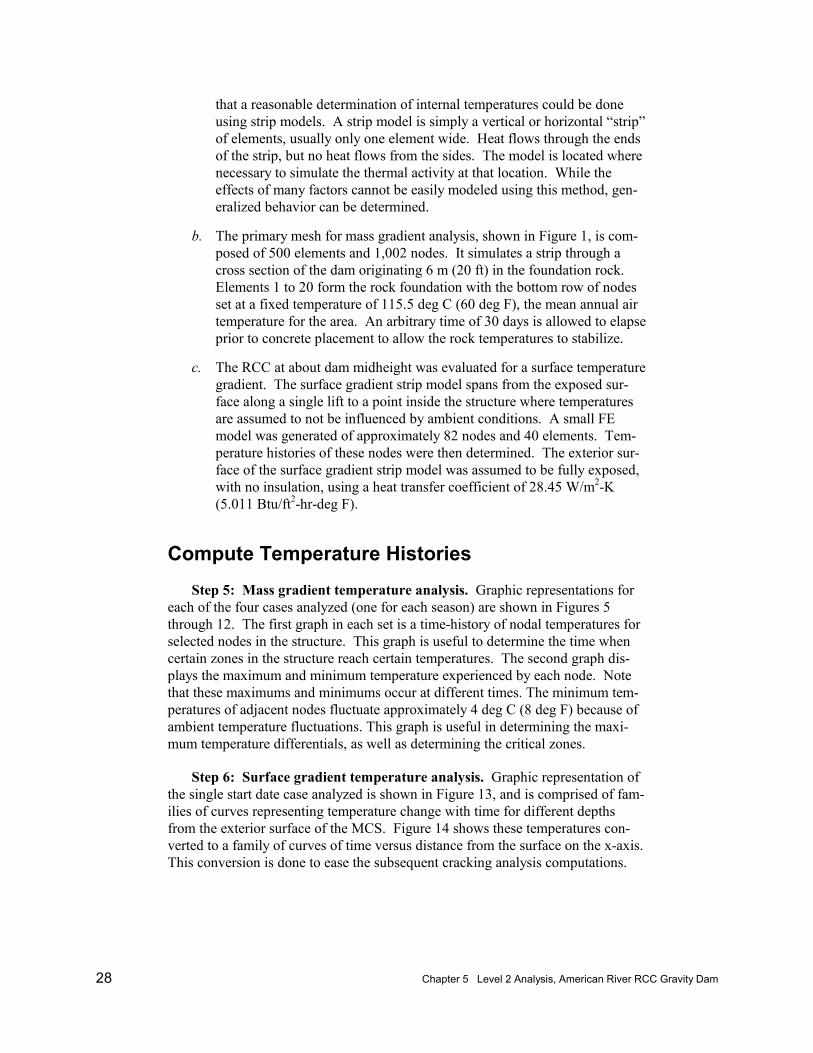
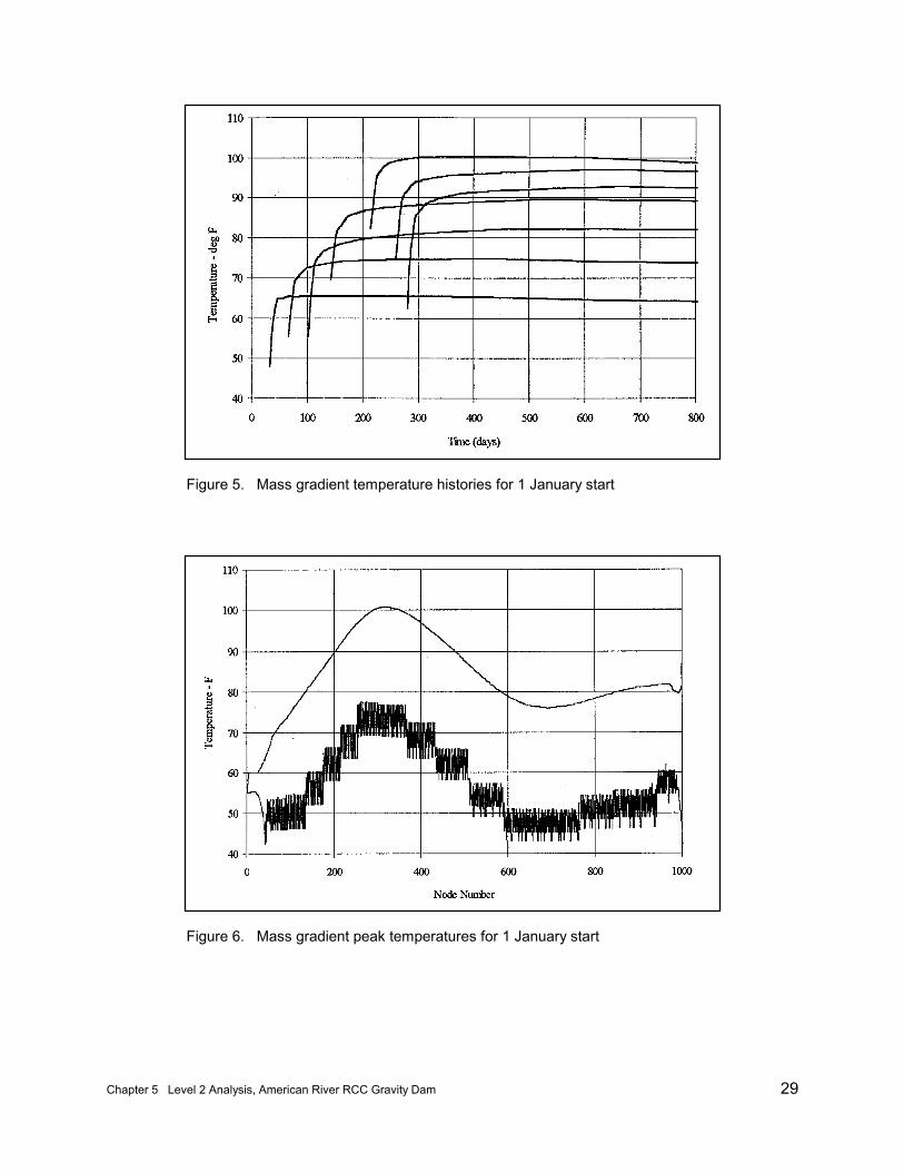
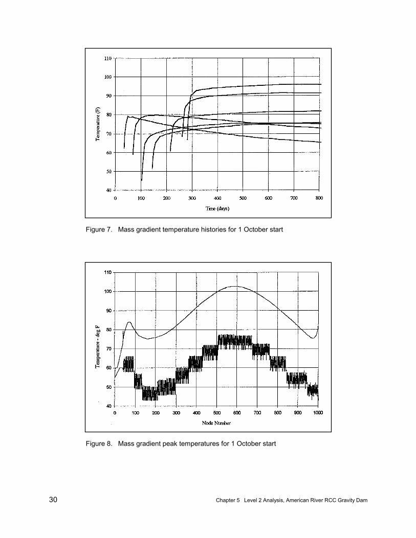
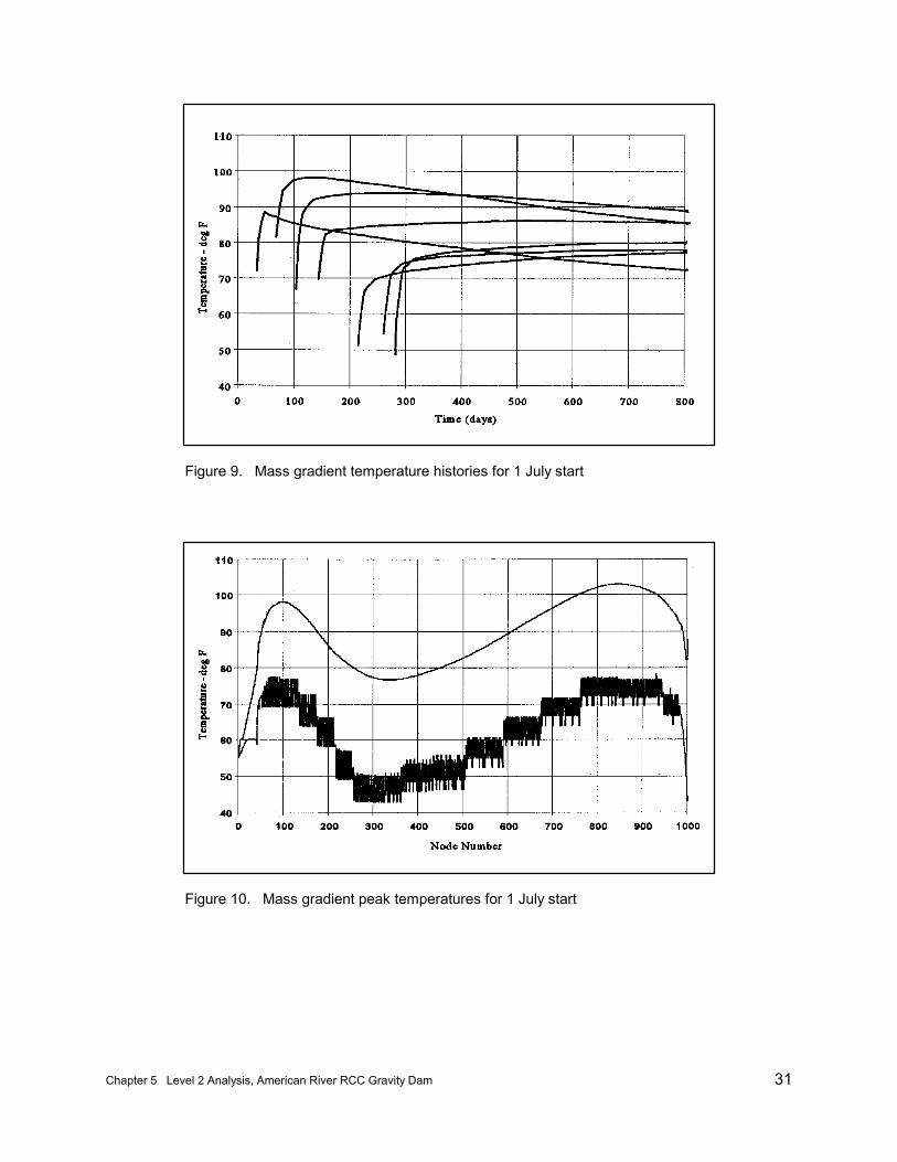
Compute Temperature HistoriesStep 5: Mass gradient temperature analysis. Graphic representations for
each of the four cases analyzed (one for each season) are shown in Figures 5through 12. The first graph in each set is a time-history of nodal temperatures forselected nodes in the structure. This graph is useful to determine the time whencertain zones in the structure reach certain temperatures. The second graph dis-plays the maximum and minimum temperature experienced by each node. Notethat these maximums and minimums occur at different times. The minimum tem-peratures of adjacent nodes fluctuate approximately 4 deg C (8 deg F) because ofambient temperature fluctuations. This graph is useful in determining the maxi-mum temperature differentials, as well as determining the critical zones.
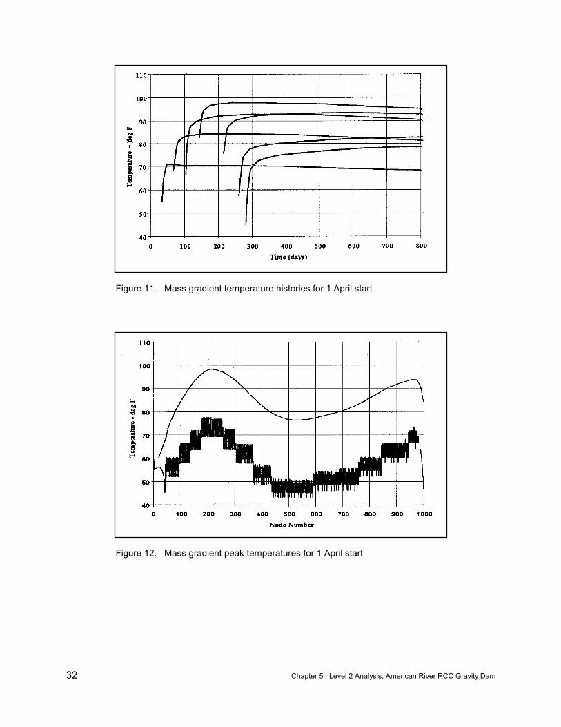
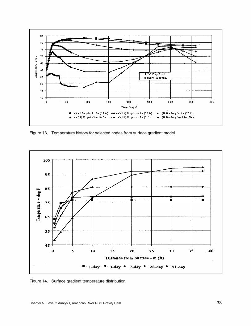
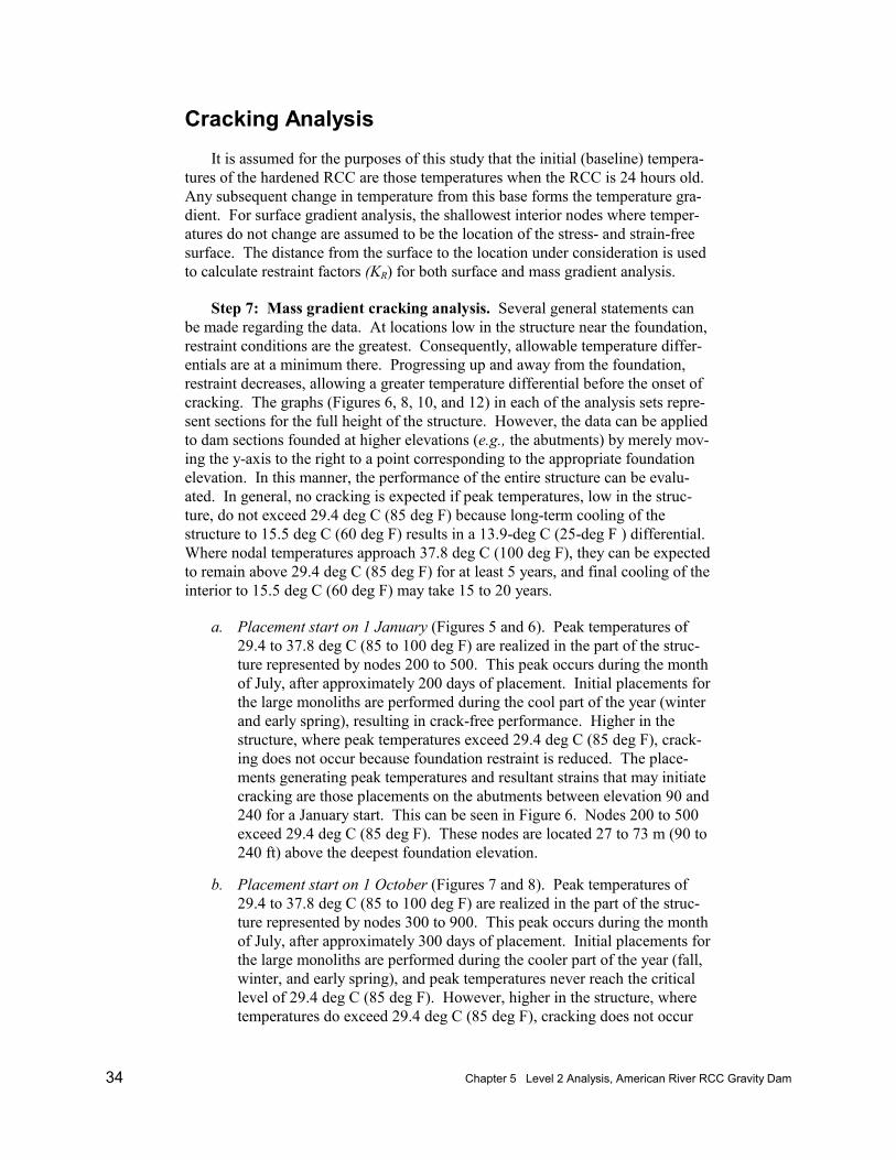
Step 6: Surface gradient temperature analysis. Graphic representation ofthe single start date case analyzed is shown in Figure 13, and is comprised of fam-ilies of curves representing temperature change with time for different depthsfrom the exterior surface of the MCS. Figure 14 shows these temperatures con-verted to a family of curves of time versus distance from the surface on the x-axis.This conversion is done to ease the subsequent cracking analysis computations.
Chapter 5 Level 2 Analysis, American River RCC Gravity Dam 29
Figure 5. Mass gradient temperature histories for 1 January start
Figure 6. Mass gradient peak temperatures for 1 January start
30 Chapter 5 Level 2 Analysis, American River RCC Gravity Dam
Figure 7. Mass gradient temperature histories for 1 October start
Figure 8. Mass gradient peak temperatures for 1 October start
Chapter 5 Level 2 Analysis, American River RCC Gravity Dam 31
Figure 9. Mass gradient temperature histories for 1 July start
Figure 10. Mass gradient peak temperatures for 1 July start
32 Chapter 5 Level 2 Analysis, American River RCC Gravity Dam
Figure 11. Mass gradient temperature histories for 1 April start
Figure 12. Mass gradient peak temperatures for 1 April start
Chapter 5 Level 2 Analysis, American River RCC Gravity Dam 33
Figure 13. Temperature history for selected nodes from surface gradient model
Figure 14. Surface gradient temperature distribution
34 Chapter 5 Level 2 Analysis, American River RCC Gravity Dam
Cracking AnalysisIt is assumed for the purposes of this study that the initial (baseline) tempera-
tures of the hardened RCC are those temperatures when the RCC is 24 hours old. Any subsequent change in temperature from this base forms the temperature gra-dient. For surface gradient analysis, the shallowest interior nodes where temper-atures do not change are assumed to be the location of the stress- and strain-freesurface. The distance from the surface to the location under consideration is usedto calculate restraint factors (KR) for both surface and mass gradient analysis.
Step 7: Mass gradient cracking analysis. Several general statements canbe made regarding the data. At locations low in the structure near the foundation,restraint conditions are the greatest. Consequently, allowable temperature differ-entials are at a minimum there. Progressing up and away from the foundation,restraint decreases, allowing a greater temperature differential before the onset ofcracking. The graphs (Figures 6, 8, 10, and 12) in each of the analysis sets repre-sent sections for the full height of the structure. However, the data can be appliedto dam sections founded at higher elevations (e.g., the abutments) by merely mov-ing the y-axis to the right to a point corresponding to the appropriate foundationelevation. In this manner, the performance of the entire structure can be evalu-ated. In general, no cracking is expected if peak temperatures, low in the struc-ture, do not exceed 29.4 deg C (85 deg F) because long-term cooling of thestructure to 15.5 deg C (60 deg F) results in a 13.9-deg C (25-deg F ) differential.Where nodal temperatures approach 37.8 deg C (100 deg F), they can be expectedto remain above 29.4 deg C (85 deg F) for at least 5 years, and final cooling of theinterior to 15.5 deg C (60 deg F) may take 15 to 20 years.
a. Placement start on 1 January (Figures 5 and 6). Peak temperatures of29.4 to 37.8 deg C (85 to 100 deg F) are realized in the part of the struc-ture represented by nodes 200 to 500. This peak occurs during the monthof July, after approximately 200 days of placement. Initial placements forthe large monoliths are performed during the cool part of the year (winterand early spring), resulting in crack-free performance. Higher in thestructure, where peak temperatures exceed 29.4 deg C (85 deg F), crack-ing does not occur because foundation restraint is reduced. The place-ments generating peak temperatures and resultant strains that may initiatecracking are those placements on the abutments between elevation 90 and240 for a January start. This can be seen in Figure 6. Nodes 200 to 500exceed 29.4 deg C (85 deg F). These nodes are located 27 to 73 m (90 to240 ft) above the deepest foundation elevation.
b. Placement start on 1 October (Figures 7 and 8). Peak temperatures of29.4 to 37.8 deg C (85 to 100 deg F) are realized in the part of the struc-ture represented by nodes 300 to 900. This peak occurs during the monthof July, after approximately 300 days of placement. Initial placements forthe large monoliths are performed during the cooler part of the year (fall,winter, and early spring), and peak temperatures never reach the criticallevel of 29.4 deg C (85 deg F). However, higher in the structure, wheretemperatures do exceed 29.4 deg C (85 deg F), cracking does not occur
Chapter 5 Level 2 Analysis, American River RCC Gravity Dam 35
because foundation restraint is reduced. For an October start, the place-ments generating peak temperatures and resultant strains that may initiatecracking are those placements on the abutments at elevations 43 to 134 m(140 to 440 ft) from the lowest foundation elevation.
c. Placement start on 1 July (Figures 9 and 10). Peak temperatures of 29.4to 37.8 deg C (85 to 100 deg F) are realized in the part of the structurerepresented by nodes 50 to 200 and 500 to 1000. This peak occurs afterapproximately 100 days of placement (during the month of July) for theearly placements, and 1 year later for the upper dam placements. Initialplacements for the large monoliths are performed during the warmest partof the year (the summer and early fall months), and peak temperaturesexceed the critical level of 29.4 deg C (85 deg F). However, higher in thestructure, where temperatures do exceed 29.4 deg C (85 deg F), crackingdoes not occur because foundation restraint is reduced. For a July start,the additional placements generating peak temperatures and resultantstrains that may initiate cracking are those placements on the abutments atelevations 73 to 146 m (240 to 480 ft) above the lowest foundationelevation.
d. Placement start on 1 April (Figures 11 and 12). Peak temperatures of29.4 to 37.8 deg C (85 to 100 deg F) are realized in the part of the struc-ture represented by nodes 100 to 400 and 800 to 1000. This peak occursduring the month of July, after approximately 100 days of placement forthe early placements, and 1 year later for the upper dam placements. Initial placements for the large monoliths are performed during themoderate part of the year (the spring), avoiding cracking. Higher in thestructure, where temperatures exceed 29.4 deg C (85 deg F), crackingdoes not occur because foundation restraint is reduced. Additional place-ments generating peak temperatures and resultant strains that may initiatecracking are those placements on the abutments from an elevation 12 to49 m (40 to 160 ft) above the lowest foundation elevation and placementsnear the top of the dam.
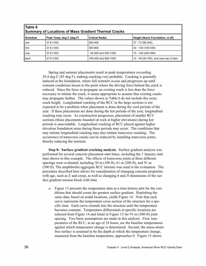
e. Mass gradient cracking analysis results. Table 6 summarizes, for eachplacing schedule evaluated, the nodes and the node locations where massgradient thermal cracking is expected. The “Height Above Foundation”refers to those abutment foundation locations at elevations above thelowermost foundation elevation. For example, a January-start scheduleresults in probable cracking of nodes 200 to 400, and foundation eleva-tions located 27 to 73 m (90 to 240 ft) above the lowest foundationelevation.
Uncontrolled RCC placing temperatures will result in peak temperatures of37.8 deg C (100 deg F) and ultimate temperature differentials of 22.2 deg C(40 deg F). The maximum temperature differential calculated from tensile straincapacity and the coefficient of thermal expansions is 13.9 deg C (25 deg F) for thenear term, increasing to near 16.7 deg C (30 deg F) for cooling periods of15 years. Fall and winter placements result in cool placing temperatures, withpeak temperatures for those placements of less than 29.4 deg C (85 deg F).
36 Chapter 5 Level 2 Analysis, American River RCC Gravity Dam
Table 6Summary of Locations of Mass Gradient Thermal CracksSchedule Peak Temp, deg C (deg F) Critical Nodes Height Above Foundation, m (ft)
Jan 37.8 (100) 200-400 27 - 73 (90-240)
Oct 37.8 (100) 300-900 43 - 134 (140-440)
July 37.8 (100) 50-200 and 500-1000 73 - 146 (240-480)
April 37.8 (100) 100-400 and 800-1000 12 - 49 (40-160) and near top of dam
Spring and summer placements result in peak temperatures exceeding29.4 deg C (85 deg F), making cracking very probable. Cracking is generallyinduced at the foundation, where full restraint occurs and progresses up untilrestraint conditions lessen to the point where the driving force behind the crack isreduced. Since the force to propagate an existing crack is less than the forcenecessary to initiate the crack, it seems appropriate to assume that existing cracksmay propagate further. The values shown in Table 6 do not include this extracrack height. Longitudinal cracking of the RCC in the large sections is notexpected to be a problem when placement is done during the cool periods of theyear. If these placements are done during the hot periods of the year, longitudinalcracking may occur. As construction progresses, placement of smaller RCCsections (those placements founded on rock at higher elevations) during hotperiods is unavoidable. Longitudinal cracking of RCC placed against higherelevation foundation areas during these periods may occur. The conditions thatmay initiate longitudinal cracking may also initiate transverse cracking. Theoccurrence of transverse cracks can be reduced by installing transverse joints,thereby reducing the restraint.
Step 8: Surface gradient cracking analysis. Surface gradient analysis wasperformed for several concrete placement start times, including the 1 January starttime shown in this example. The effects of transverse joints at three differentspacings were evaluated, including 30 m (100 ft), 61 m (200 ft), and 91 m(300 ft). The amphibolite aggregate RCC mixture was used in the evaluation. Theprocedure described here allows for consideration of changing concrete propertieswith age, such as E and creep, as well as changing h and H dimensions of the sur-face gradient tension block with time.
a. Figure 13 presents the temperature data as a time-history plot for the con-ditions that should create the greatest surface gradient. Replotting thesame data, based on nodal locations, yields Figure 14. Note that eachcurve represents the temperature cross section of the structure for a spe-cific time. Each curve extends into the structure until the temperaturebecomes constant. Temperature differentials at specific locations areselected from Figure 14 and listed in Figure 15 for 91-m (300-ft) jointspacing. Two basic assumptions are made in this analysis. First, tem-peratures of the RCC, at an age of 24 hours, are the baseline temperaturesagainst which temperature change is determined. Second, the stress-strainfree surface is assumed to be the depth at which the temperature change,measured from the baseline temperature, approaches 0. Figure 15 shows
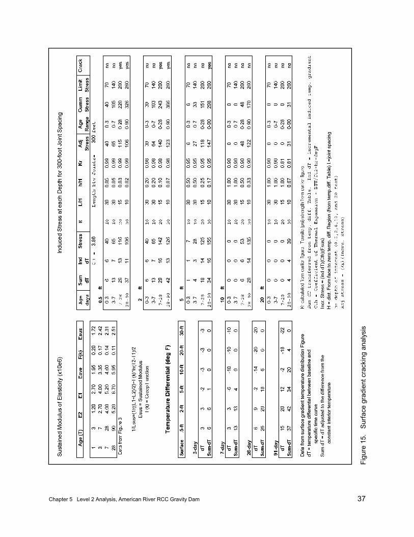
Chapter 5 Level 2 Analysis, American River RCC Gravity Dam 37
Figu
re 1
5.
Surfa
ce g
radi
ent c
rack
ing
anal
ysis
38 Chapter 5 Level 2 Analysis, American River RCC Gravity Dam
the temperature deviations (dT) from the baseline temperature, as well asthe depth at which the temperature gradient approaches 0. The Sum dTtemperature differences are included in Figure 15 as a starting point forcalculating induced stresses. “Induced dT,” or the individual incrementsof temperature gradient induced with each age period, is calculated fromthe “Sum dT’s.” Sustained modulus of elasticity (Esus) is determined inFigure 15 for each age increment. To calculate incremental stressgenerated by temperature gradients:
Incremental stress = (Ind dT)(Cth)(Esus)
b. To determine KR, Figure 4.1 of ACI 207.2R or Equation 4.1 or 4.2 of ACI207.2R are used, requiring calculation of H, L, and h. H is the distancefrom the exterior surface to the stress- and strain-free surface at eachincremental time period and is determined from the Temperature Differ-ential Table in Figure 15 (note H for each age increment is the same). Lis the joint spacing. h is the distance from the surface to the depth ofinterest (near surface, 0.6 , 1.5, 3, and 6 m (2, 5, 10, and 20 ft) in thefigures), and h/H is the proportion of H from the surface to the depth ofinterest. h/H largely determines the amount of restraint at any location. For L/H 2.5, KR is calculated as follows:
h/H
R
HLHL
K
−
−=
1
2
“Adj stress” is calculated by:
Adj stress = (KR)(Incremental stress)
Cumulative stresses are then summed by superposition of stress from eachage interval. Crack development is judged by whether the cumulativestress exceeds the tensile strength.
c. From Figure 15 and similar computations for 30- and 61-m (100- and200-ft) joint spacings, the computations indicate that surface cracking isnot likely for a 30-m (100-ft) joint spacing. Surface cracking mayincrease to a depth of 0.6 m (2 ft) for joint spacings up to 61 m (200 ft)and up to 1.5 m (5 ft) for joint spacings of 91 m (300 ft). The full extentof surface cracking is controlled by the formation of the initial surfacecracks. For example, at a joint spacing of 91 m (300 ft), the surface maycrack at the midpoint. The analysis shows that this crack may propagateto a depth of 1.5 m (5 ft) after several weeks to months. However, theoccurrence of this crack forms a new joint pattern at a spacing of 46 m(150 ft). While the depth of cracking may not be sufficient to change therestraint conditions (L/H), it may be enough to relieve induced stressesand stabilize the crack growth to depths of 0.6 m (2 ft). A joint spacing of
Chapter 5 Level 2 Analysis, American River RCC Gravity Dam 39
61 m (200 ft) may be an optimum spacing for this project based on theoccurrence of surface cracking. Evaluation of the combined effects ofsurface gradient strains with mass gradient strains was not pursued, sincethe surface gradient strain contribution is not considered to be significantto the overall cracking performance of the structure using joint spacingsof 30 and 61 m (100 and 200 ft).
Conclusions and RecommendationsThe maximum temperature differential under full restraint conditions (KR
= 1.0) that will not result in cracking of the RCC is 13.9 deg C (25 deg F). Sincethe final temperature of the RCC will be 15.5 deg C (60 deg F) (the averageannual temperature), a crack-free peak RCC temperature is 29.4 deg C (85 deg F). This allowable differential of 13.9 deg C (25 deg F) increases as thedistance of the RCC placements from the foundation increases. After evaluatingseveral placing schedules, it was apparent that the most beneficial conditionsoccurred when the RCC placement of the lower third of the dam commenced inthe fall of the year and was completed during late spring. This means that, for thelarger dam sections, the upper two-thirds would then be placed during a hottertime period. The reduction in foundation restraint at this height in the structure,however, more than offsets the effects of the higher temperatures.
Surface gradients were evaluated for several transverse joint intervals. Because the site is located in a relatively temperate area, where cold temperaturesare rare, stresses from surface gradients were of little consequence for joint spac-ings up to 61 m (200 ft). Greater joint spacings increase the depth of surfacecracking.
For contraction joints set at a spacing of approximately 61 m (200 ft), trans-verse cracking of the structure may occur in the lower 6 to 12 m (20 to 40 ft) ofthe structure. Similarly, longitudinal cracking may occur in the lower 6 to 12 m(20 to 40 ft) of the structure for sections of the dam having an upstream-downstream dimension greater than 61 m (200 ft). Since the occurrence of alongitudinal crack could create serious stability concerns, more rigorous analysescoupling the effects of other simultaneous loadings are necessary to better evalu-ate the extent of cracking.
An alternate rock source, a nearby quarried limestone aggregate, provides anRCC with a very low coefficient of thermal expansion of 4.5 millionths/deg C(2.5 millionths/deg F). The net effect of using this aggregate instead of the dam-site amphibolite is to raise the allowable maximum peak temperature from 29.4 to37.8 deg C (85 to 100 deg F). It appears that if this aggregate is used, no furthercontrol of aggregate temperatures may be necessary. Without this aggregate, mea-sures are necessary to control placing temperatures so that peak temperatures donot exceed 29.4 deg C (85 deg F). This requires a 15.5-deg C (60-deg F) placingtemperature for certain placements. This placing temperature could be raised to23.9 deg C (75 deg F), if the limestone aggregate was used.
40 Chapter 5 Level 2 Analysis, American River RCC Gravity Dam
Completion of RCC placements up to a minimum elevation during a fall andwinter time period should be required in the construction contract. Otherwise, ifthese low elevation placements are placed during the spring and summer period,the RCC placing temperature should be specified not to exceed 26.7 to 29.4 deg C(80 to 85 deg F). This will require the use of additional cooling measures. Stock-pile sprinkling, water chilling, and possible shading may be sufficient to achievethese temperatures.
The scope of this study was of a limited nature: to identify the potentialextent of thermal cracking in the structure. Only generalized conclusions arepossible. For a structure of this height, volume, and seismic loadings, a morerigorous study should be performed during design of the structure. Full-sectionmodeling, incorporating foundation properties, restraint conditions, and early-agematerial properties (time- and temperature-dependent properties) should be done. The structure should be analyzed in sections to ascertain the strain developmentthat may lead to longitudinal cracking and in elevation to ascertain strain devel-opment that may lead to transverse cracking. The results of these studies shouldguide the designer as to whether a 3-D model is necessary. It is presumed that a3-D analysis will indicate better cracking performance of the structure than a 2-Dmodel would indicate. This analysis should quantify the effects of several loadconditions in addition to the thermal loads. It may be that the combined action ofthese factors will initiate cracking.
Chapter 6 Level 2 Analysis, Locks and Dams 2, 3, and 4 Monongahela River 41
6 Level 2 Analysis, Locksand Dams 2, 3, and 4Monongahela River
GeneralAn example of each step in the performance of a relatively complex mass
gradient and a surface gradient analysis in a Level 2 thermal study of an MCS ispresented. This example is based on 2-D analyses performed during design stud-ies for locks and dam facilities on the Monongahela River in Pennsylvania. Thesestudies were conducted to maximize lift heights and determine optimum place-ment temperatures and to expedite construction and minimize costs. Althoughnumerous lock monolith configurations exist in the project, the most massivesection was selected for analysis. Conclusions and recommendations from thisanalysis could be applied to the other project monoliths. Figure 16 shows a crosssection representation of the geometry of a river wall monolith with nominal 3-m(10-ft) lifts used in this example analysis. Two-dimensional FE analysis was usedto determine temperature histories and temperature distribution during and follow-ing construction. FE analysis was not applied for cracking analysis. Crackinganalysis was performed using a strain-based criteria similar to proceduresdescribed in ACI 207.2R. Slow-load tensile strain capacity test results (whichinclude creep effects) were used to determine the extent of cracking. Analysiswas performed on 15 combinations of several parameters, including three liftheights, two maximum concrete placement temperatures, three construction starttimes, two lift placement rates, and insulated forms for fall placement.
Input Properties and ParametersStep 1: Determine ambient conditions. These data were gathered from
local records. Ambient temperature data are shown in Figure 17.
Step 2: Determine material properties. Table 7 contains thermal prop-erties used in the example thermal analysis. Adiabatic temperature rise is shown inFigure 18. This adiabatic temperature rise is characteristic of the heat generationof an exterior concrete in a mass concrete structure and is not characteristic ofinterior mass concrete. The foundation material is assumed to be limestone of
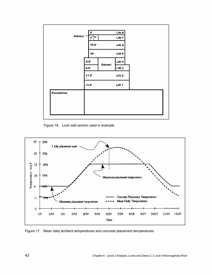
42 Chapter 6 Level 2 Analysis, Locks and Dams 2, 3, and 4 Monongahela River
Figure 16. Lock wall section used in example
Figure 17. Mean daily ambient temperatures and concrete placement temperatures
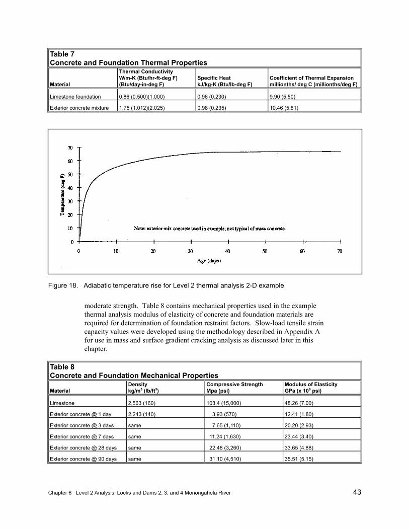
Chapter 6 Level 2 Analysis, Locks and Dams 2, 3, and 4 Monongahela River 43
Table 7Concrete and Foundation Thermal Properties
Material
Thermal ConductivityW/m-K (Btu/hr-ft-deg F)(Btu/day-in-deg F)
Specific HeatkJ/kg-K (Btu/lb-deg F)
Coefficient of Thermal Expansionmillionths/ deg C (millionths/deg F)
Limestone foundation 0.86 (0.500)(1.000) 0.96 (0.230) 9.90 (5.50)
Exterior concrete mixture 1.75 (1.012)(2.025) 0.98 (0.235) 10.46 (5.81)
Figure 18. Adiabatic temperature rise for Level 2 thermal analysis 2-D example
moderate strength. Table 8 contains mechanical properties used in the examplethermal analysis modulus of elasticity of concrete and foundation materials arerequired for determination of foundation restraint factors. Slow-load tensile straincapacity values were developed using the methodology described in Appendix Afor use in mass and surface gradient cracking analysis as discussed later in thischapter.
Table 8Concrete and Foundation Mechanical Properties
MaterialDensitykg/m3 (lb/ft3)
Compressive StrengthMpa (psi)
Modulus of ElasticityGPa (x 106 psi)
Limestone 2,563 (160) 103.4 (15,000) 48.26 (7.00)
Exterior concrete @ 1 day 2,243 (140) 3.93 (570) 12.41 (1.80)
Exterior concrete @ 3 days same 7.65 (1,110) 20.20 (2.93)
Exterior concrete @ 7 days same 11.24 (1,630) 23.44 (3.40)
Exterior concrete @ 28 days same 22.48 (3,260) 33.65 (4.88)
Exterior concrete @ 90 days same 31.10 (4,510) 35.51 (5.15)
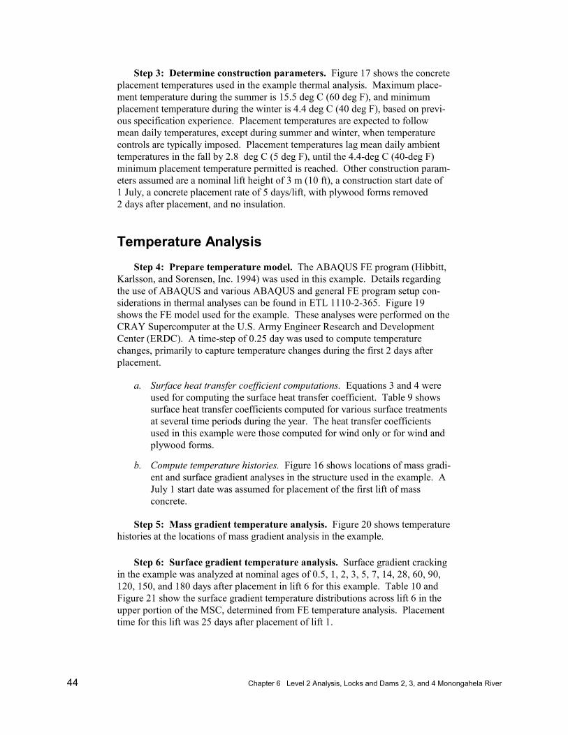
44 Chapter 6 Level 2 Analysis, Locks and Dams 2, 3, and 4 Monongahela River
Step 3: Determine construction parameters. Figure 17 shows the concreteplacement temperatures used in the example thermal analysis. Maximum place-ment temperature during the summer is 15.5 deg C (60 deg F), and minimumplacement temperature during the winter is 4.4 deg C (40 deg F), based on previ-ous specification experience. Placement temperatures are expected to followmean daily temperatures, except during summer and winter, when temperaturecontrols are typically imposed. Placement temperatures lag mean daily ambienttemperatures in the fall by 2.8 deg C (5 deg F), until the 4.4-deg C (40-deg F)minimum placement temperature permitted is reached. Other construction param-eters assumed are a nominal lift height of 3 m (10 ft), a construction start date of1 July, a concrete placement rate of 5 days/lift, with plywood forms removed2 days after placement, and no insulation.
Temperature AnalysisStep 4: Prepare temperature model. The ABAQUS FE program (Hibbitt,
Karlsson, and Sorensen, Inc. 1994) was used in this example. Details regardingthe use of ABAQUS and various ABAQUS and general FE program setup con-siderations in thermal analyses can be found in ETL 1110-2-365. Figure 19shows the FE model used for the example. These analyses were performed on theCRAY Supercomputer at the U.S. Army Engineer Research and DevelopmentCenter (ERDC). A time-step of 0.25 day was used to compute temperaturechanges, primarily to capture temperature changes during the first 2 days afterplacement.
a. Surface heat transfer coefficient computations. Equations 3 and 4 wereused for computing the surface heat transfer coefficient. Table 9 showssurface heat transfer coefficients computed for various surface treatmentsat several time periods during the year. The heat transfer coefficientsused in this example were those computed for wind only or for wind andplywood forms.
b. Compute temperature histories. Figure 16 shows locations of mass gradi-ent and surface gradient analyses in the structure used in the example. AJuly 1 start date was assumed for placement of the first lift of massconcrete.
Step 5: Mass gradient temperature analysis. Figure 20 shows temperaturehistories at the locations of mass gradient analysis in the example.
Step 6: Surface gradient temperature analysis. Surface gradient crackingin the example was analyzed at nominal ages of 0.5, 1, 2, 3, 5, 7, 14, 28, 60, 90,120, 150, and 180 days after placement in lift 6 for this example. Table 10 andFigure 21 show the surface gradient temperature distributions across lift 6 in theupper portion of the MSC, determined from FE temperature analysis. Placementtime for this lift was 25 days after placement of lift 1.
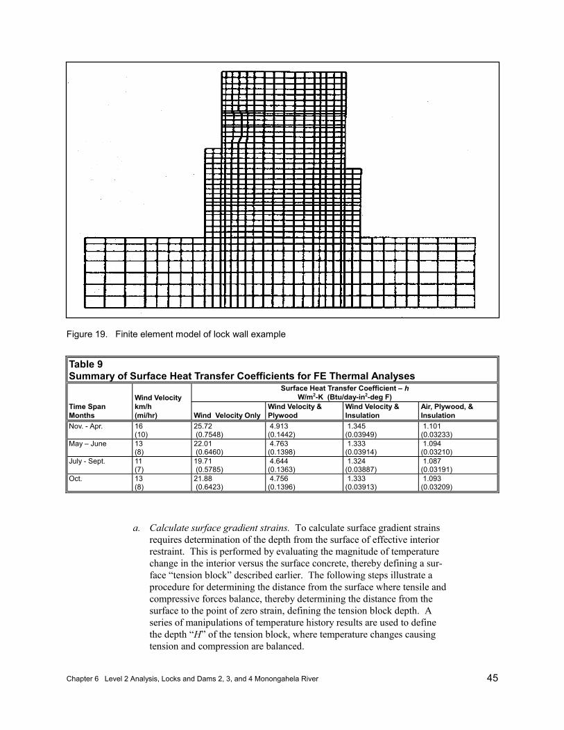
Chapter 6 Level 2 Analysis, Locks and Dams 2, 3, and 4 Monongahela River 45
Figure 19. Finite element model of lock wall example
Table 9Summary of Surface Heat Transfer Coefficients for FE Thermal Analyses
Surface Heat Transfer Coefficient – hW/m2-K (Btu/day-in2-deg F)
Time SpanMonths
Wind Velocitykm/h(mi/hr) Wind Velocity Only
Wind Velocity &Plywood
Wind Velocity &Insulation
Air, Plywood, &Insulation
Nov. - Apr. 16(10)
25.72 (0.7548)
4.913(0.1442)
1.345(0.03949)
1.101(0.03233)
May – June 13(8)
22.01 (0.6460)
4.763(0.1398)
1.333(0.03914)
1.094(0.03210)
July - Sept. 11(7)
19.71 (0.5785)
4.644(0.1363)
1.324(0.03887)
1.087(0.03191)
Oct. 13(8)
21.88 (0.6423)
4.756(0.1396)
1.333(0.03913)
1.093(0.03209)
a. Calculate surface gradient strains. To calculate surface gradient strainsrequires determination of the depth from the surface of effective interiorrestraint. This is performed by evaluating the magnitude of temperaturechange in the interior versus the surface concrete, thereby defining a sur-face “tension block” described earlier. The following steps illustrate aprocedure for determining the distance from the surface where tensile andcompressive forces balance, thereby determining the distance from thesurface to the point of zero strain, defining the tension block depth. Aseries of manipulations of temperature history results are used to definethe depth “H” of the tension block, where temperature changes causingtension and compression are balanced.
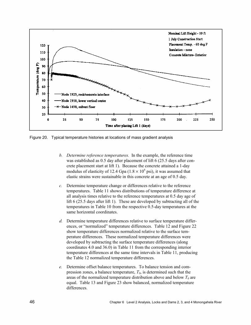
46 Chapter 6 Level 2 Analysis, Locks and Dams 2, 3, and 4 Monongahela River
Figure 20. Typical temperature histories at locations of mass gradient analysis
b. Determine reference temperatures. In the example, the reference timewas established as 0.5 day after placement of lift 6 (25.5 days after con-crete placement start at lift 1). Because the concrete attained a 1-daymodulus of elasticity of 12.4 Gpa (1.8 × 10⁶ psi), it was assumed thatelastic strains were sustainable in this concrete at an age of 0.5 day.
c. Determine temperature change or differences relative to the referencetemperatures. Table 11 shows distributions of temperature difference atall analysis times relative to the reference temperatures at 0.5 day age oflift 6 (25.5 days after lift 1). These are developed by subtracting all of thetemperatures in Table 10 from the respective 0.5-day temperatures at thesame horizontal coordinates.
d. Determine temperature differences relative to surface temperature differ-ences, or “normalized” temperature differences. Table 12 and Figure 22show temperature differences normalized relative to the surface tem-perature differences. These normalized temperature differences weredeveloped by subtracting the surface temperature differences (alongcoordinates 4.0 and 36.0) in Table 11 from the corresponding interiortemperature differences at the same time intervals in Table 11, producingthe Table 12 normalized temperature differences.
e. Determine offset balance temperatures. To balance tension and com-pression zones, a balance temperature, T0, is determined such that theareas of the normalized temperature distribution above and below T0 areequal. Table 13 and Figure 23 show balanced, normalized temperaturedifferences.
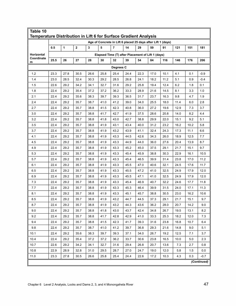
Chapter 6 Level 2 Analysis, Locks and Dams 2, 3, and 4 Monongahela River 47
Table 10Temperature Distribution in Lift 6 for Surface Gradient Analysis
Age of Concrete in Lift 6 placed 25 days after Lift 1 (days)
0.5 1 2 3 5 7 14 29 59 91 121 151 181
Elapsed Time (T) after Placement of Lift 1 (days)HorizontalCoordinatem 25.5 26 27 28 30 32 39 54 84 116 146 176 206
Degrees C
1.2 23.3 27.8 30.5 26.6 25.8 25.4 24.4 22.3 17.0 10.1 4.1 0.1 -0.9
1.4 23.0 28.5 32.4 30.3 29.2 28.5 26.8 24.1 18.2 11.2 5.1 0.9 -0.4
1.5 22.6 29.2 34.2 34.1 32.7 31.6 29.2 25.8 19.4 12.4 6.2 1.8 0.1
1.8 22.4 29.2 35.4 37.2 37.2 36.2 33.3 28.9 21.6 14.5 8.1 3.3 1.0
2.1 22.4 29.2 35.6 38.3 39.7 39.3 36.5 31.7 23.7 16.3 9.8 4.7 1.9
2.4 22.4 29.2 35.7 38.7 41.0 41.2 39.0 34.0 25.5 18.0 11.4 6.0 2.8
2.7 22.4 29.2 35.7 38.8 41.5 42.3 40.8 36.0 27.2 19.6 12.9 7.3 3.7
3.0 22.4 29.2 35.7 38.8 41.7 42.7 41.9 37.5 28.6 20.8 14.0 8.2 4.4
3.2 22.4 29.2 35.7 38.8 41.8 43.0 42.7 38.8 29.9 22.0 15.1 9.2 5.1
3.5 22.4 29.2 35.7 38.8 41.9 43.1 43.4 40.0 31.2 23.2 16.2 10.2 5.8
3.7 22.4 29.2 35.7 38.8 41.9 43.2 43.9 41.1 32.4 24.3 17.3 11.1 6.6
4.1 22.4 29.2 35.7 38.8 41.9 43.3 44.5 42.6 34.3 26.0 18.9 12.5 7.7
4.5 22.4 29.2 35.7 38.8 41.9 43.3 44.9 44.0 36.0 27.6 20.4 13.9 8.7
4.9 22.4 29.2 35.7 38.8 41.9 43.3 45.2 45.0 37.5 29.1 21.7 15.1 9.7
5.3 22.4 29.2 35.7 38.8 41.9 43.3 45.4 45.9 38.8 30.3 22.9 16.1 10.5
5.7 22.4 29.2 35.7 38.8 41.9 43.3 45.4 46.5 39.9 31.4 23.8 17.0 11.2
6.1 22.4 29.2 35.7 38.8 41.9 43.3 45.5 47.0 40.6 32.1 24.5 17.6 11.7
6.5 22.4 29.2 35.7 38.8 41.9 43.3 45.5 47.2 41.0 32.5 24.9 17.9 12.0
6.9 22.4 29.2 35.7 38.8 41.9 43.3 45.5 47.1 41.0 32.5 24.9 17.9 12.0
7.3 22.4 29.2 35.7 38.8 41.9 43.3 45.4 46.9 40.7 32.2 24.6 17.7 11.8
7.7 22.4 29.2 35.7 38.8 41.9 43.3 45.3 46.4 39.9 31.5 24.0 17.1 11.3
8.1 22.4 29.2 35.7 38.8 41.9 43.3 45.1 45.7 38.8 30.5 23.0 16.2 10.6
8.5 22.4 29.2 35.7 38.8 41.9 43.2 44.7 44.5 37.3 29.1 21.7 15.1 9.7
8.7 22.4 29.2 35.7 38.8 41.9 43.2 44.3 43.6 36.2 28.0 20.7 14.2 9.0
9.0 22.4 29.2 35.7 38.8 41.8 43.0 43.7 42.4 34.8 26.7 19.5 13.1 8.2
9.2 22.4 29.2 35.7 38.8 41.7 42.8 42.9 41.0 33.3 25.3 18.2 12.0 7.3
9.4 22.4 29.2 35.7 38.8 41.5 42.3 41.7 39.3 31.6 23.8 16.8 10.7 6.4
9.8 22.4 29.2 35.7 38.7 41.0 41.2 39.7 36.8 29.3 21.6 14.8 9.0 5.1
10.1 22.4 29.2 35.6 38.3 39.7 39.3 37.1 34.0 26.7 19.2 12.5 7.1 3.7
10.4 22.4 29.2 35.4 37.2 37.2 36.2 33.7 30.6 23.8 16.5 10.0 5.0 2.3
10.7 22.6 29.2 34.2 34.1 32.7 31.6 29.4 26.8 20.7 13.6 7.3 2.7 0.8
10.8 22.9 28.9 32.8 31.0 29.5 28.7 27.0 24.7 19.0 12.0 5.8 1.5 0.0
11.0 23.3 27.8 30.5 26.6 25.8 25.4 24.4 22.6 17.2 10.3 4.3 0.3 -0.7
(Continued)
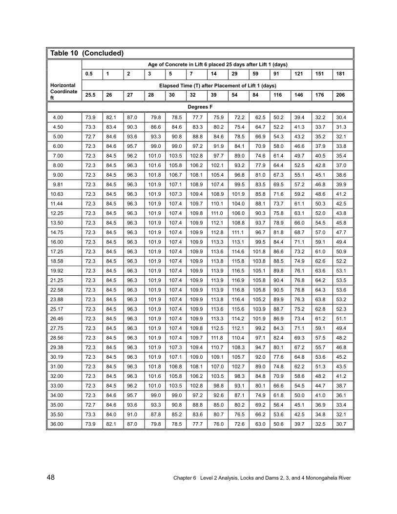
48 Chapter 6 Level 2 Analysis, Locks and Dams 2, 3, and 4 Monongahela River
Table 10 (Concluded)Age of Concrete in Lift 6 placed 25 days after Lift 1 (days)
0.5 1 2 3 5 7 14 29 59 91 121 151 181
Elapsed Time (T) after Placement of Lift 1 (days)HorizontalCoordinateft 25.5 26 27 28 30 32 39 54 84 116 146 176 206
Degrees F
4.00 73.9 82.1 87.0 79.8 78.5 77.7 75.9 72.2 62.5 50.2 39.4 32.2 30.4
4.50 73.3 83.4 90.3 86.6 84.6 83.3 80.2 75.4 64.7 52.2 41.3 33.7 31.3
5.00 72.7 84.6 93.6 93.3 90.8 88.8 84.6 78.5 66.9 54.3 43.2 35.2 32.1
6.00 72.3 84.6 95.7 99.0 99.0 97.2 91.9 84.1 70.9 58.0 46.6 37.9 33.8
7.00 72.3 84.5 96.2 101.0 103.5 102.8 97.7 89.0 74.6 61.4 49.7 40.5 35.4
8.00 72.3 84.5 96.3 101.6 105.8 106.2 102.1 93.2 77.9 64.4 52.5 42.8 37.0
9.00 72.3 84.5 96.3 101.8 106.7 108.1 105.4 96.8 81.0 67.3 55.1 45.1 38.6
9.81 72.3 84.5 96.3 101.9 107.1 108.9 107.4 99.5 83.5 69.5 57.2 46.8 39.9
10.63 72.3 84.5 96.3 101.9 107.3 109.4 108.9 101.9 85.8 71.6 59.2 48.6 41.2
11.44 72.3 84.5 96.3 101.9 107.4 109.7 110.1 104.0 88.1 73.7 61.1 50.3 42.5
12.25 72.3 84.5 96.3 101.9 107.4 109.8 111.0 106.0 90.3 75.8 63.1 52.0 43.8
13.50 72.3 84.5 96.3 101.9 107.4 109.9 112.1 108.8 93.7 78.9 66.0 54.5 45.8
14.75 72.3 84.5 96.3 101.9 107.4 109.9 112.8 111.1 96.7 81.8 68.7 57.0 47.7
16.00 72.3 84.5 96.3 101.9 107.4 109.9 113.3 113.1 99.5 84.4 71.1 59.1 49.4
17.25 72.3 84.5 96.3 101.9 107.4 109.9 113.6 114.6 101.8 86.6 73.2 61.0 50.9
18.58 72.3 84.5 96.3 101.9 107.4 109.9 113.8 115.8 103.8 88.5 74.9 62.6 52.2
19.92 72.3 84.5 96.3 101.9 107.4 109.9 113.9 116.5 105.1 89.8 76.1 63.6 53.1
21.25 72.3 84.5 96.3 101.9 107.4 109.9 113.9 116.9 105.8 90.4 76.8 64.2 53.5
22.58 72.3 84.5 96.3 101.9 107.4 109.9 113.9 116.8 105.8 90.5 76.8 64.3 53.6
23.88 72.3 84.5 96.3 101.9 107.4 109.9 113.8 116.4 105.2 89.9 76.3 63.8 53.2
25.17 72.3 84.5 96.3 101.9 107.4 109.9 113.6 115.6 103.9 88.7 75.2 62.8 52.3
26.46 72.3 84.5 96.3 101.9 107.4 109.9 113.3 114.2 101.9 86.9 73.4 61.2 51.1
27.75 72.3 84.5 96.3 101.9 107.4 109.8 112.5 112.1 99.2 84.3 71.1 59.1 49.4
28.56 72.3 84.5 96.3 101.9 107.4 109.7 111.8 110.4 97.1 82.4 69.3 57.5 48.2
29.38 72.3 84.5 96.3 101.9 107.3 109.4 110.7 108.3 94.7 80.1 67.2 55.7 46.8
30.19 72.3 84.5 96.3 101.9 107.1 109.0 109.1 105.7 92.0 77.6 64.8 53.6 45.2
31.00 72.3 84.5 96.3 101.8 106.8 108.1 107.0 102.7 89.0 74.8 62.2 51.3 43.5
32.00 72.3 84.5 96.3 101.6 105.8 106.2 103.5 98.3 84.8 70.9 58.6 48.2 41.2
33.00 72.3 84.5 96.2 101.0 103.5 102.8 98.8 93.1 80.1 66.6 54.5 44.7 38.7
34.00 72.3 84.6 95.7 99.0 99.0 97.2 92.6 87.1 74.9 61.8 50.0 41.0 36.1
35.00 72.7 84.6 93.6 93.3 90.8 88.8 85.0 80.2 69.2 56.4 45.1 36.9 33.4
35.50 73.3 84.0 91.0 87.8 85.2 83.6 80.7 76.5 66.2 53.6 42.5 34.8 32.1
36.00 73.9 82.1 87.0 79.8 78.5 77.7 76.0 72.6 63.0 50.6 39.7 32.5 30.7
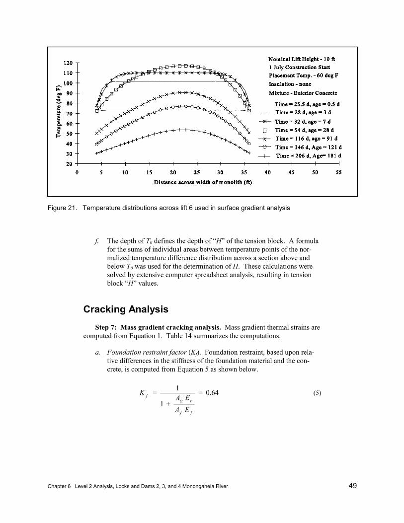
Chapter 6 Level 2 Analysis, Locks and Dams 2, 3, and 4 Monongahela River 49
Figure 21. Temperature distributions across lift 6 used in surface gradient analysis
f. The depth of T0 defines the depth of “H” of the tension block. A formulafor the sums of individual areas between temperature points of the nor-malized temperature difference distribution across a section above andbelow T0 was used for the determination of H. These calculations weresolved by extensive computer spreadsheet analysis, resulting in tensionblock “H” values.
Cracking AnalysisStep 7: Mass gradient cracking analysis. Mass gradient thermal strains are
computed from Equation 1. Table 14 summarizes the computations.
a. Foundation restraint factor (Kf). Foundation restraint, based upon rela-tive differences in the stiffness of the foundation material and the con-crete, is computed from Equation 5 as shown below.
0.64 = + 1
1 =
ff
cgf
EAEA
K (5)
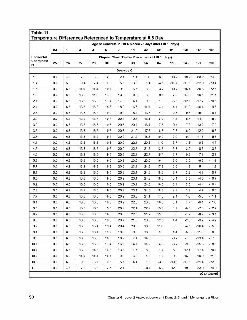
50 Chapter 6 Level 2 Analysis, Locks and Dams 2, 3, and 4 Monongahela River
Table 11Temperature Differences Referenced to Temperature at 0.5 Day
Age of Concrete in Lift 6 placed 25 days after Lift 1 (days)
0.5 1 2 3 5 7 14 29 59 91 121 151 181
Elapsed Time (T) after Placement of Lift 1 (days)HorizontalCoordinatem 25.5 26 27 28 30 32 39 54 84 116 146 176 206
Degrees C
1.2 0.0 4.6 7.2 3.3 2.5 2.1 1.1 -1.0 -6.3 -13.2 -19.2 -23.2 -24.2
1.4 0.0 5.6 9.4 7.4 6.3 5.5 3.9 1.1 -4.8 -11.7 -17.8 -22.0 -23.4
1.5 0.0 6.6 11.6 11.4 10.1 9.0 6.6 3.2 -3.2 -10.2 -16.4 -20.8 -22.6
1.8 0.0 6.8 13.0 14.8 14.8 13.8 10.9 6.5 -0.8 -7.9 -14.3 -19.1 -21.4
2.1 0.0 6.8 13.3 16.0 17.4 17.0 14.1 9.3 1.3 -6.1 -12.5 -17.7 -20.5
2.4 0.0 6.8 13.3 16.3 18.6 18.9 16.6 11.6 3.1 -4.4 -11.0 -16.4 -19.6
2.7 0.0 6.8 13.3 16.4 19.2 19.9 18.4 13.7 4.9 -2.8 -9.5 -15.1 -18.7
3.0 0.0 6.8 13.3 16.4 19.4 20.4 19.5 15.1 6.2 -1.5 -8.4 -14.1 -18.0
3.2 0.0 6.8 13.3 16.5 19.5 20.6 20.4 16.4 7.5 -0.4 -7.3 -13.2 -17.2
3.5 0.0 6.8 13.3 16.5 19.5 20.8 21.0 17.6 8.8 0.8 -6.2 -12.2 -16.5
3.7 0.0 6.8 13.3 16.5 19.5 20.9 21.5 18.8 10.0 2.0 -5.1 -11.3 -15.8
4.1 0.0 6.8 13.3 16.5 19.5 20.9 22.1 20.3 11.9 3.7 -3.5 -9.8 -14.7
4.5 0.0 6.8 13.3 16.5 19.5 20.9 22.6 21.6 13.6 5.3 -2.0 -8.5 -13.6
4.9 0.0 6.8 13.3 16.5 19.5 20.9 22.8 22.7 15.1 6.7 -0.6 -7.3 -12.7
5.3 0.0 6.8 13.3 16.5 19.5 20.9 23.0 23.5 16.4 8.0 0.5 -6.3 -11.9
5.7 0.0 6.8 13.3 16.5 19.5 20.9 23.1 24.2 17.5 9.0 1.5 -5.4 -11.2
6.1 0.0 6.8 13.3 16.5 19.5 20.9 23.1 24.6 18.2 9.7 2.2 -4.8 -10.7
6.5 0.0 6.8 13.3 16.5 19.5 20.9 23.1 24.8 18.6 10.1 2.5 -4.5 -10.7
6.9 0.0 6.8 13.3 16.5 19.5 20.9 23.1 24.8 18.6 10.1 2.5 -4.4 -10.4
7.3 0.0 6.8 13.3 16.5 19.5 20.9 23.1 24.6 18.3 9.8 2.3 -4.7 -10.6
7.7 0.0 6.8 13.3 16.5 19.5 20.9 23.0 24.1 17.6 9.1 1.6 -5.3 -11.1
8.1 0.0 6.8 13.3 16.5 19.5 20.9 22.8 23.3 16.5 8.1 0.7 -6.1 -11.8
8.5 0.0 6.8 13.3 16.5 19.5 20.9 22.4 22.2 15.0 6.7 -0.6 -7.3 -12.7
8.7 0.0 6.8 13.3 16.5 19.5 20.8 22.0 21.2 13.8 5.6 -1.7 -8.2 -13.4
9.0 0.0 6.8 13.3 16.5 19.5 20.7 21.3 20.0 12.5 4.4 -2.8 -9.2 -14.2
9.2 0.0 6.8 13.3 16.4 19.4 20.4 20.5 18.6 11.0 3.0 -4.1 -10.4 -15.0
9.4 0.0 6.8 13.3 16.4 19.2 19.9 19.3 16.9 9.3 1.4 -5.6 -11.6 -16.0
9.8 0.0 6.8 13.3 16.3 18.6 18.9 17.4 14.5 7.0 -0.7 -7.6 -13.4 -17.3
10.1 0.0 6.8 13.3 16.0 17.4 16.9 14.7 11.6 4.3 -3.2 -9.9 -15.3 -18.6
10.4 0.0 6.8 13.0 14.8 14.8 13.8 11.3 8.2 1.4 -5.9 -12.4 -17.4 -20.1
10.7 0.0 6.6 11.6 11.4 10.1 9.0 6.8 4.2 -1.9 -9.0 -15.3 -19.9 -21.8
10.8 0.0 6.0 9.9 8.1 6.6 5.7 4.1 1.8 -3.9 -10.9 -17.1 -21.4 -22.9
11.0 0.0 4.6 7.2 3.3 2.5 2.1 1.2 -0.7 -6.0 -12.9 -19.0 -23.0 -24.0
(Continued)
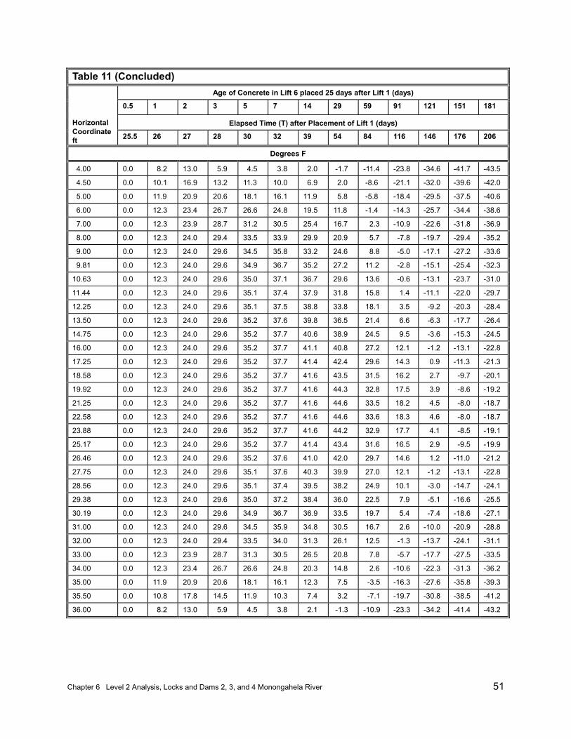
Chapter 6 Level 2 Analysis, Locks and Dams 2, 3, and 4 Monongahela River 51
Table 11 (Concluded)Age of Concrete in Lift 6 placed 25 days after Lift 1 (days)
0.5 1 2 3 5 7 14 29 59 91 121 151 181
Elapsed Time (T) after Placement of Lift 1 (days)HorizontalCoordinateft 25.5 26 27 28 30 32 39 54 84 116 146 176 206
Degrees F
4.00 0.0 8.2 13.0 5.9 4.5 3.8 2.0 -1.7 -11.4 -23.8 -34.6 -41.7 -43.5
4.50 0.0 10.1 16.9 13.2 11.3 10.0 6.9 2.0 -8.6 -21.1 -32.0 -39.6 -42.0
5.00 0.0 11.9 20.9 20.6 18.1 16.1 11.9 5.8 -5.8 -18.4 -29.5 -37.5 -40.6
6.00 0.0 12.3 23.4 26.7 26.6 24.8 19.5 11.8 -1.4 -14.3 -25.7 -34.4 -38.6
7.00 0.0 12.3 23.9 28.7 31.2 30.5 25.4 16.7 2.3 -10.9 -22.6 -31.8 -36.9
8.00 0.0 12.3 24.0 29.4 33.5 33.9 29.9 20.9 5.7 -7.8 -19.7 -29.4 -35.2
9.00 0.0 12.3 24.0 29.6 34.5 35.8 33.2 24.6 8.8 -5.0 -17.1 -27.2 -33.6
9.81 0.0 12.3 24.0 29.6 34.9 36.7 35.2 27.2 11.2 -2.8 -15.1 -25.4 -32.3
10.63 0.0 12.3 24.0 29.6 35.0 37.1 36.7 29.6 13.6 -0.6 -13.1 -23.7 -31.0
11.44 0.0 12.3 24.0 29.6 35.1 37.4 37.9 31.8 15.8 1.4 -11.1 -22.0 -29.7
12.25 0.0 12.3 24.0 29.6 35.1 37.5 38.8 33.8 18.1 3.5 -9.2 -20.3 -28.4
13.50 0.0 12.3 24.0 29.6 35.2 37.6 39.8 36.5 21.4 6.6 -6.3 -17.7 -26.4
14.75 0.0 12.3 24.0 29.6 35.2 37.7 40.6 38.9 24.5 9.5 -3.6 -15.3 -24.5
16.00 0.0 12.3 24.0 29.6 35.2 37.7 41.1 40.8 27.2 12.1 -1.2 -13.1 -22.8
17.25 0.0 12.3 24.0 29.6 35.2 37.7 41.4 42.4 29.6 14.3 0.9 -11.3 -21.3
18.58 0.0 12.3 24.0 29.6 35.2 37.7 41.6 43.5 31.5 16.2 2.7 -9.7 -20.1
19.92 0.0 12.3 24.0 29.6 35.2 37.7 41.6 44.3 32.8 17.5 3.9 -8.6 -19.2
21.25 0.0 12.3 24.0 29.6 35.2 37.7 41.6 44.6 33.5 18.2 4.5 -8.0 -18.7
22.58 0.0 12.3 24.0 29.6 35.2 37.7 41.6 44.6 33.6 18.3 4.6 -8.0 -18.7
23.88 0.0 12.3 24.0 29.6 35.2 37.7 41.6 44.2 32.9 17.7 4.1 -8.5 -19.1
25.17 0.0 12.3 24.0 29.6 35.2 37.7 41.4 43.4 31.6 16.5 2.9 -9.5 -19.9
26.46 0.0 12.3 24.0 29.6 35.2 37.6 41.0 42.0 29.7 14.6 1.2 -11.0 -21.2
27.75 0.0 12.3 24.0 29.6 35.1 37.6 40.3 39.9 27.0 12.1 -1.2 -13.1 -22.8
28.56 0.0 12.3 24.0 29.6 35.1 37.4 39.5 38.2 24.9 10.1 -3.0 -14.7 -24.1
29.38 0.0 12.3 24.0 29.6 35.0 37.2 38.4 36.0 22.5 7.9 -5.1 -16.6 -25.5
30.19 0.0 12.3 24.0 29.6 34.9 36.7 36.9 33.5 19.7 5.4 -7.4 -18.6 -27.1
31.00 0.0 12.3 24.0 29.6 34.5 35.9 34.8 30.5 16.7 2.6 -10.0 -20.9 -28.8
32.00 0.0 12.3 24.0 29.4 33.5 34.0 31.3 26.1 12.5 -1.3 -13.7 -24.1 -31.1
33.00 0.0 12.3 23.9 28.7 31.3 30.5 26.5 20.8 7.8 -5.7 -17.7 -27.5 -33.5
34.00 0.0 12.3 23.4 26.7 26.6 24.8 20.3 14.8 2.6 -10.6 -22.3 -31.3 -36.2
35.00 0.0 11.9 20.9 20.6 18.1 16.1 12.3 7.5 -3.5 -16.3 -27.6 -35.8 -39.3
35.50 0.0 10.8 17.8 14.5 11.9 10.3 7.4 3.2 -7.1 -19.7 -30.8 -38.5 -41.2
36.00 0.0 8.2 13.0 5.9 4.5 3.8 2.1 -1.3 -10.9 -23.3 -34.2 -41.4 -43.2
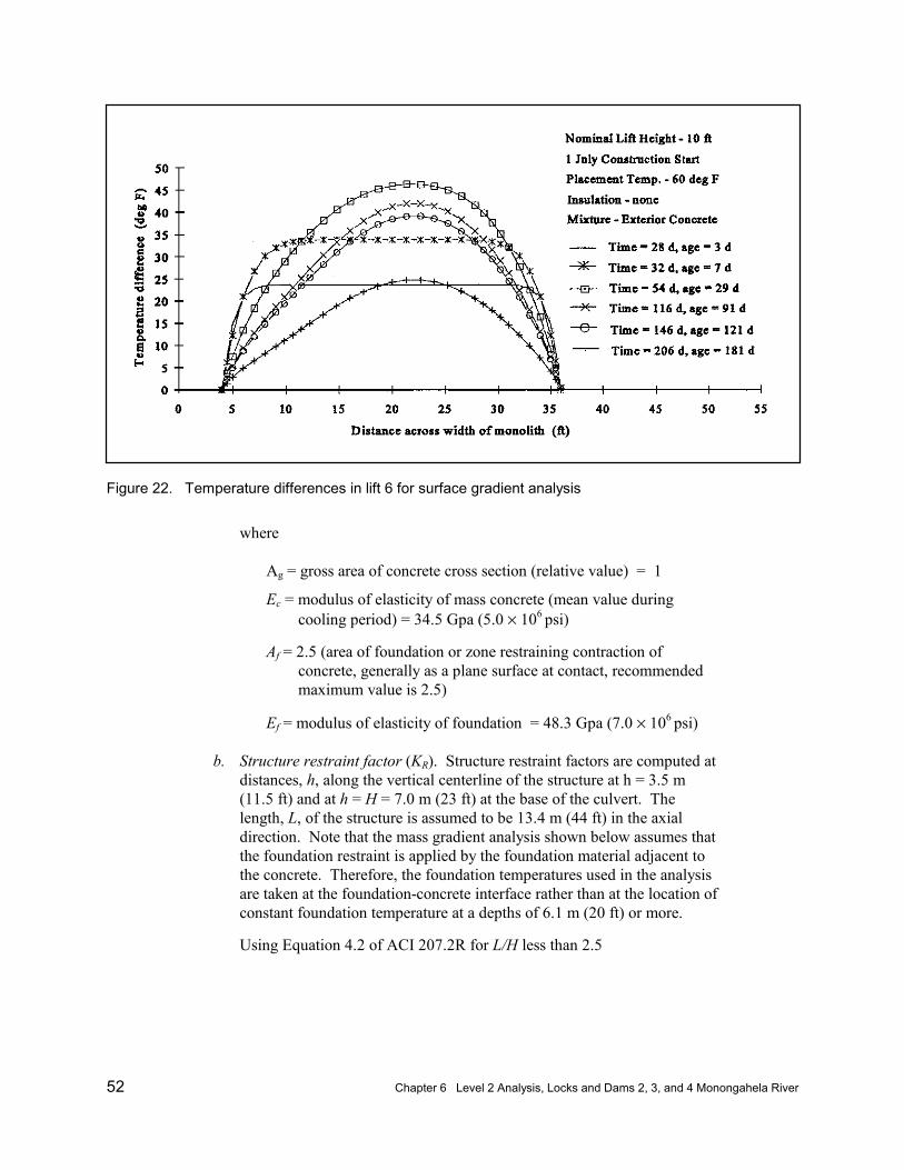
52 Chapter 6 Level 2 Analysis, Locks and Dams 2, 3, and 4 Monongahela River
Figure 22. Temperature differences in lift 6 for surface gradient analysis
where
Ag = gross area of concrete cross section (relative value) = 1
Ec = modulus of elasticity of mass concrete (mean value duringcooling period) = 34.5 Gpa (5.0 × 10⁶ psi)
Af = 2.5 (area of foundation or zone restraining contraction ofconcrete, generally as a plane surface at contact, recommendedmaximum value is 2.5)
Ef = modulus of elasticity of foundation = 48.3 Gpa (7.0 × 10⁶ psi)
b. Structure restraint factor (KR). Structure restraint factors are computed atdistances, h, along the vertical centerline of the structure at h = 3.5 m(11.5 ft) and at h = H = 7.0 m (23 ft) at the base of the culvert. Thelength, L, of the structure is assumed to be 13.4 m (44 ft) in the axialdirection. Note that the mass gradient analysis shown below assumes thatthe foundation restraint is applied by the foundation material adjacent tothe concrete. Therefore, the foundation temperatures used in the analysisare taken at the foundation-concrete interface rather than at the location ofconstant foundation temperature at a depths of 6.1 m (20 ft) or more.
Using Equation 4.2 of ACI 207.2R for L/H less than 2.5

Chapter 6 Level 2 Analysis, Locks and Dams 2, 3, and 4 Monongahela River 53
Table 12Temperature Differences Normalized in Reference to Surface Temperature Differencesfor Surface Gradient Analysis
Age of Concrete in Lift 6 placed 25 days after Lift 1 (days)
0.5 1 2 3 5 7 14 29 59 91 121 151 181
Elapsed Time (T) after Placement of Lift 1 (days)HorizontalCoordinatem 25.5 26 27 28 30 32 39 54 84 116 146 176 206
Degrees C
1.2 0.0 0.0 0.0 0.0 0.0 0.0 0.0 0.0 0.0 0.0 0.0 0.0 0.0
1.4 0.0 1.0 2.2 4.1 3.8 3.4 2.8 2.1 1.6 1.5 1.4 1.2 0.8
1.5 0.0 2.1 4.3 8.2 7.6 6.9 5.5 4.2 3.1 3.0 2.8 2.3 1.6
1.8 0.0 2.3 5.7 11.6 12.3 11.7 9.8 7.5 5.6 5.3 4.9 4.0 2.7
2.1 0.0 2.3 6.0 12.7 14.8 14.9 13.0 10.2 7.6 7.1 6.7 5.5 3.7
2.4 0.0 2.3 6.1 13.1 16.1 16.8 15.5 12.6 9.5 8.8 8.2 6.8 4.6
2.7 0.0 2.3 6.1 13.2 16.6 17.8 17.3 14.6 11.2 10.4 9.7 8.1 5.5
3.0 0.0 2.3 6.1 13.2 16.8 18.3 18.4 16.1 12.6 11.6 10.8 9.0 6.2
3.2 0.0 2.3 6.1 13.2 16.9 18.5 19.3 17.4 13.9 12.8 11.9 10.0 6.9
3.5 0.0 2.3 6.1 13.2 17.0 18.7 19.9 18.6 15.1 14.0 13.0 11.0 7.6
3.7 0.0 2.3 6.1 13.2 17.0 18.8 20.4 19.7 16.4 15.1 14.1 11.9 8.4
4.1 0.0 2.3 6.1 13.2 17.0 18.8 21.0 21.2 18.2 16.9 15.7 13.3 9.5
4.5 0.0 2.3 6.1 13.2 17.0 18.8 21.5 22.6 19.9 18.5 17.2 14.7 10.5
4.9 0.0 2.3 6.1 13.2 17.0 18.8 21.7 23.6 21.5 19.9 18.6 15.9 11.5
5.3 0.0 2.3 6.1 13.2 17.0 18.8 21.9 24.5 22.8 21.2 19.7 16.9 12.3
5.7 0.0 2.3 6.1 13.2 17.0 18.8 22.0 25.1 23.8 22.2 20.7 17.8 13.0
6.1 0.0 2.3 6.1 13.2 17.0 18.8 22.0 25.5 24.6 22.9 21.4 18.4 13.5
6.5 0.0 2.3 6.1 13.2 17.0 18.8 22.0 25.7 24.9 23.3 21.7 18.7 13.7
6.9 0.0 2.3 6.1 13.2 17.0 18.8 22.0 25.7 25.0 23.3 21.7 18.7 13.8
7.3 0.0 2.3 6.1 13.2 17.0 18.8 22.0 25.5 24.6 23.0 21.5 18.5 13.5
7.7 0.0 2.3 6.1 13.2 17.0 18.8 21.9 25.0 23.9 22.3 20.8 17.9 13.1
8.1 0.0 2.3 6.1 13.2 17.0 18.8 21.7 24.3 22.8 21.3 19.9 17.0 12.4
8.5 0.0 2.3 6.1 13.2 17.0 18.8 21.3 23.1 21.3 19.9 18.6 15.9 11.5
8.7 0.0 2.3 6.1 13.2 17.0 18.7 20.9 22.1 20.1 18.8 17.5 15.0 10.8
9.0 0.0 2.3 6.1 13.2 16.9 18.6 20.2 21.0 18.8 17.6 16.4 13.9 10.0
9.2 0.0 2.3 6.1 13.2 16.8 18.3 19.4 19.6 17.3 16.2 15.1 12.8 9.1
9.4 0.0 2.3 6.1 13.2 16.6 17.8 18.2 17.9 15.6 14.6 13.6 11.5 8.2
9.8 0.0 2.3 6.1 13.1 16.1 16.8 16.3 15.4 13.3 12.5 11.6 9.8 6.9
10.1 0.0 2.3 6.0 12.7 14.8 14.9 13.6 12.5 10.7 10.0 9.3 7.9 5.5
10.4 0.0 2.3 5.7 11.6 12.3 11.7 10.2 9.1 7.8 7.3 6.8 5.7 4.1
10.7 0.0 2.1 4.3 8.2 7.5 6.9 5.7 5.1 4.4 4.2 3.9 3.3 2.3
10.8 0.0 1.4 2.6 4.8 4.1 3.6 3.0 2.7 2.4 2.3 2.1 1.8 1.3
11.0 0.0 0.0 0.0 0.0 0.0 0.0 0.1 0.2 0.3 0.2 0.2 0.2 0.1
(Continued)
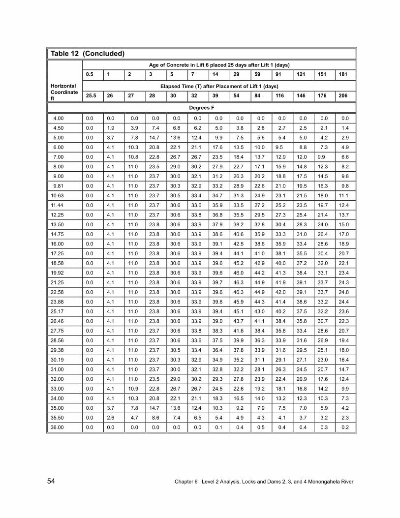
54 Chapter 6 Level 2 Analysis, Locks and Dams 2, 3, and 4 Monongahela River
Table 12 (Concluded)Age of Concrete in Lift 6 placed 25 days after Lift 1 (days)
0.5 1 2 3 5 7 14 29 59 91 121 151 181
Elapsed Time (T) after Placement of Lift 1 (days)HorizontalCoordinateft 25.5 26 27 28 30 32 39 54 84 116 146 176 206
Degrees F
4.00 0.0 0.0 0.0 0.0 0.0 0.0 0.0 0.0 0.0 0.0 0.0 0.0 0.0
4.50 0.0 1.9 3.9 7.4 6.8 6.2 5.0 3.8 2.8 2.7 2.5 2.1 1.4
5.00 0.0 3.7 7.8 14.7 13.6 12.4 9.9 7.5 5.6 5.4 5.0 4.2 2.9
6.00 0.0 4.1 10.3 20.8 22.1 21.1 17.6 13.5 10.0 9.5 8.8 7.3 4.9
7.00 0.0 4.1 10.8 22.8 26.7 26.7 23.5 18.4 13.7 12.9 12.0 9.9 6.6
8.00 0.0 4.1 11.0 23.5 29.0 30.2 27.9 22.7 17.1 15.9 14.8 12.3 8.2
9.00 0.0 4.1 11.0 23.7 30.0 32.1 31.2 26.3 20.2 18.8 17.5 14.5 9.8
9.81 0.0 4.1 11.0 23.7 30.3 32.9 33.2 28.9 22.6 21.0 19.5 16.3 9.8
10.63 0.0 4.1 11.0 23.7 30.5 33.4 34.7 31.3 24.9 23.1 21.5 18.0 11.1
11.44 0.0 4.1 11.0 23.7 30.6 33.6 35.9 33.5 27.2 25.2 23.5 19.7 12.4
12.25 0.0 4.1 11.0 23.7 30.6 33.8 36.8 35.5 29.5 27.3 25.4 21.4 13.7
13.50 0.0 4.1 11.0 23.8 30.6 33.9 37.9 38.2 32.8 30.4 28.3 24.0 15.0
14.75 0.0 4.1 11.0 23.8 30.6 33.9 38.6 40.6 35.9 33.3 31.0 26.4 17.0
16.00 0.0 4.1 11.0 23.8 30.6 33.9 39.1 42.5 38.6 35.9 33.4 28.6 18.9
17.25 0.0 4.1 11.0 23.8 30.6 33.9 39.4 44.1 41.0 38.1 35.5 30.4 20.7
18.58 0.0 4.1 11.0 23.8 30.6 33.9 39.6 45.2 42.9 40.0 37.2 32.0 22.1
19.92 0.0 4.1 11.0 23.8 30.6 33.9 39.6 46.0 44.2 41.3 38.4 33.1 23.4
21.25 0.0 4.1 11.0 23.8 30.6 33.9 39.7 46.3 44.9 41.9 39.1 33.7 24.3
22.58 0.0 4.1 11.0 23.8 30.6 33.9 39.6 46.3 44.9 42.0 39.1 33.7 24.8
23.88 0.0 4.1 11.0 23.8 30.6 33.9 39.6 45.9 44.3 41.4 38.6 33.2 24.4
25.17 0.0 4.1 11.0 23.8 30.6 33.9 39.4 45.1 43.0 40.2 37.5 32.2 23.6
26.46 0.0 4.1 11.0 23.8 30.6 33.9 39.0 43.7 41.1 38.4 35.8 30.7 22.3
27.75 0.0 4.1 11.0 23.7 30.6 33.8 38.3 41.6 38.4 35.8 33.4 28.6 20.7
28.56 0.0 4.1 11.0 23.7 30.6 33.6 37.5 39.9 36.3 33.9 31.6 26.9 19.4
29.38 0.0 4.1 11.0 23.7 30.5 33.4 36.4 37.8 33.9 31.6 29.5 25.1 18.0
30.19 0.0 4.1 11.0 23.7 30.3 32.9 34.9 35.2 31.1 29.1 27.1 23.0 16.4
31.00 0.0 4.1 11.0 23.7 30.0 32.1 32.8 32.2 28.1 26.3 24.5 20.7 14.7
32.00 0.0 4.1 11.0 23.5 29.0 30.2 29.3 27.8 23.9 22.4 20.9 17.6 12.4
33.00 0.0 4.1 10.9 22.8 26.7 26.7 24.5 22.6 19.2 18.1 16.8 14.2 9.9
34.00 0.0 4.1 10.3 20.8 22.1 21.1 18.3 16.5 14.0 13.2 12.3 10.3 7.3
35.00 0.0 3.7 7.8 14.7 13.6 12.4 10.3 9.2 7.9 7.5 7.0 5.9 4.2
35.50 0.0 2.6 4.7 8.6 7.4 6.5 5.4 4.9 4.3 4.1 3.7 3.2 2.3
36.00 0.0 0.0 0.0 0.0 0.0 0.0 0.1 0.4 0.5 0.4 0.4 0.3 0.2
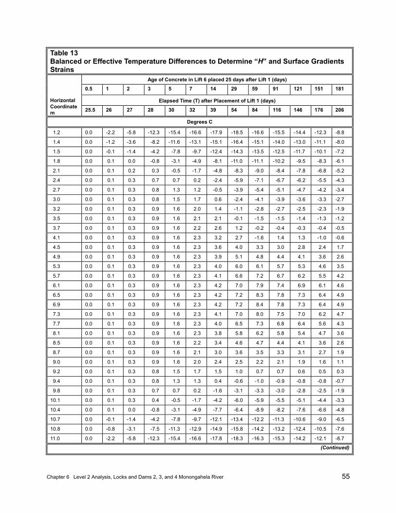
Chapter 6 Level 2 Analysis, Locks and Dams 2, 3, and 4 Monongahela River 55
Table 13Balanced or Effective Temperature Differences to Determine “H” and Surface GradientsStrains
Age of Concrete in Lift 6 placed 25 days after Lift 1 (days)
0.5 1 2 3 5 7 14 29 59 91 121 151 181
Elapsed Time (T) after Placement of Lift 1 (days)HorizontalCoordinatem 25.5 26 27 28 30 32 39 54 84 116 146 176 206
Degrees C
1.2 0.0 -2.2 -5.8 -12.3 -15.4 -16.6 -17.9 -18.5 -16.6 -15.5 -14.4 -12.3 -8.8
1.4 0.0 -1.2 -3.6 -8.2 -11.6 -13.1 -15.1 -16.4 -15.1 -14.0 -13.0 -11.1 -8.0
1.5 0.0 -0.1 -1.4 -4.2 -7.8 -9.7 -12.4 -14.3 -13.5 -12.5 -11.7 -10.1 -7.2
1.8 0.0 0.1 0.0 -0.8 -3.1 -4.9 -8.1 -11.0 -11.1 -10.2 -9.5 -8.3 -6.1
2.1 0.0 0.1 0.2 0.3 -0.5 -1.7 -4.8 -8.3 -9.0 -8.4 -7.8 -6.8 -5.2
2.4 0.0 0.1 0.3 0.7 0.7 0.2 -2.4 -5.9 -7.1 -6.7 -6.2 -5.5 -4.3
2.7 0.0 0.1 0.3 0.8 1.3 1.2 -0.5 -3.9 -5.4 -5.1 -4.7 -4.2 -3.4
3.0 0.0 0.1 0.3 0.8 1.5 1.7 0.6 -2.4 -4.1 -3.9 -3.6 -3.3 -2.7
3.2 0.0 0.1 0.3 0.9 1.6 2.0 1.4 -1.1 -2.8 -2.7 -2.5 -2.3 -1.9
3.5 0.0 0.1 0.3 0.9 1.6 2.1 2.1 -0.1 -1.5 -1.5 -1.4 -1.3 -1.2
3.7 0.0 0.1 0.3 0.9 1.6 2.2 2.6 1.2 -0.2 -0.4 -0.3 -0.4 -0.5
4.1 0.0 0.1 0.3 0.9 1.6 2.3 3.2 2.7 -1.6 1.4 1.3 -1.0 -0.6
4.5 0.0 0.1 0.3 0.9 1.6 2.3 3.6 4.0 3.3 3.0 2.8 2.4 1.7
4.9 0.0 0.1 0.3 0.9 1.6 2.3 3.9 5.1 4.8 4.4 4.1 3.6 2.6
5.3 0.0 0.1 0.3 0.9 1.6 2.3 4.0 6.0 6.1 5.7 5.3 4.6 3.5
5.7 0.0 0.1 0.3 0.9 1.6 2.3 4.1 6.6 7.2 6.7 6.2 5.5 4.2
6.1 0.0 0.1 0.3 0.9 1.6 2.3 4.2 7.0 7.9 7.4 6.9 6.1 4.6
6.5 0.0 0.1 0.3 0.9 1.6 2.3 4.2 7.2 8.3 7.8 7.3 6.4 4.9
6.9 0.0 0.1 0.3 0.9 1.6 2.3 4.2 7.2 8.4 7.8 7.3 6.4 4.9
7.3 0.0 0.1 0.3 0.9 1.6 2.3 4.1 7.0 8.0 7.5 7.0 6.2 4.7
7.7 0.0 0.1 0.3 0.9 1.6 2.3 4.0 6.5 7.3 6.8 6.4 5.6 4.3
8.1 0.0 0.1 0.3 0.9 1.6 2.3 3.8 5.8 6.2 5.8 5.4 4.7 3.6
8.5 0.0 0.1 0.3 0.9 1.6 2.2 3.4 4.6 4.7 4.4 4.1 3.6 2.6
8.7 0.0 0.1 0.3 0.9 1.6 2.1 3.0 3.6 3.5 3.3 3.1 2.7 1.9
9.0 0.0 0.1 0.3 0.9 1.6 2.0 2.4 2.5 2.2 2.1 1.9 1.6 1.1
9.2 0.0 0.1 0.3 0.8 1.5 1.7 1.5 1.0 0.7 0.7 0.6 0.5 0.3
9.4 0.0 0.1 0.3 0.8 1.3 1.3 0.4 -0.6 -1.0 -0.9 -0.8 -0.8 -0.7
9.8 0.0 0.1 0.3 0.7 0.7 0.2 -1.6 -3.1 -3.3 -3.0 -2.8 -2.5 -1.9
10.1 0.0 0.1 0.3 0.4 -0.5 -1.7 -4.2 -6.0 -5.9 -5.5 -5.1 -4.4 -3.3
10.4 0.0 0.1 0.0 -0.8 -3.1 -4.9 -7.7 -6.4 -8.9 -8.2 -7.6 -6.6 -4.8
10.7 0.0 -0.1 -1.4 -4.2 -7.8 -9.7 -12.1 -13.4 -12.2 -11.3 -10.6 -9.0 -6.5
10.8 0.0 -0.8 -3.1 -7.5 -11.3 -12.9 -14.9 -15.8 -14.2 -13.2 -12.4 -10.5 -7.6
11.0 0.0 -2.2 -5.8 -12.3 -15.4 -16.6 -17.8 -18.3 -16.3 -15.3 -14.2 -12.1 -8.7
(Continued)
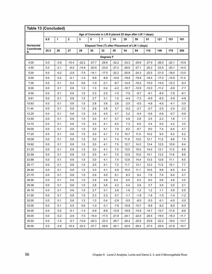
56 Chapter 6 Level 2 Analysis, Locks and Dams 2, 3, and 4 Monongahela River
Table 13 (Concluded)Age of Concrete in Lift 6 placed 25 days after Lift 1 (days)
0.5 1 2 3 5 7 14 29 59 91 121 151 181
Elapsed Time (T) after Placement of Lift 1 (days)HorizontalCoordinateft 25.5 26 27 28 30 32 39 54 84 116 146 176 206
Degrees F
4.00 0.0 -3.9 -10.4 -22.2 -27.7 -29.8 -32.2 -33.3 -29.9 -27.9 -26.0 -22.1 -15.9
4.50 0.0 -2.1 -6.5 -14.8 -20.9 -23.6 -27.2 -29.6 -27.1 -25.2 -23.5 -20.1 -14.5
5.00 0.0 -0.2 -2.6 -7.5 -14.1 -17.5 -22.2 -25.8 -24.3 -22.5 -21.0 -18.0 -13.0
6.00 0.0 0.2 -0.1 -1.4 -5.6 -8.8 -14.6 -19.8 -19.9 -18.4 -17.2 -14.9 -11.0
7.00 0.0 0.1 0.4 0.6 -1.0 -3.1 -8.7 -14.9 -16.2 -15.0 -14.0 -12.3 -9.3
8.00 0.0 0.1 0.6 1.3 1.3 0.4 -4.2 -10.7 -12.9 -12.0 -11.2 -9.9 -7.7
9.00 0.0 0.1 0.6 1.5 2.3 2.2 -1.0 -7.0 -9.7 -9.1 -8.5 -7.6 -6.1
9.81 0.0 0.1 0.6 1.5 2.7 3.1 1.0 -4.4 -7.3 -6.9 -6.5 -5.9 -4.8
10.63 0.0 0.1 0.6 1.5 2.8 3.6 2.6 -2.0 -5.0 -4.8 -4.5 -4.1 -3.5
11.44 0.0 0.1 0.6 1.5 2.9 3.8 3.7 -0.2 -2.7 -2.7 -2.5 -2.4 -2.2
12.25 0.0 0.1 0.6 1.5 2.9 4.0 4.7 2.2 -0.4 -0.6 -0.6 -0.7 -0.9
13.50 0.0 0.1 0.6 1.5 3.0 4.1 5.7 4.9 2.9 2.5 2.3 1.8 1.1
14.75 0.0 0.1 0.6 1.5 3.0 4.1 6.5 7.3 6.0 5.4 5.0 4.2 3.0
16.00 0.0 0.1 0.6 1.5 3.0 4.1 7.0 9.2 8.7 8.0 7.4 6.4 4.7
17.25 0.0 0.1 0.6 1.5 3.0 4.1 7.3 10.7 11.0 10.2 9.5 8.3 6.2
18.58 0.0 0.1 0.6 1.5 3.0 4.1 7.4 11.9 13.0 12.1 11.2 9.8 7.5
19.92 0.0 0.1 0.6 1.5 3.0 4.1 7.5 12.7 14.3 13.4 12.5 10.9 8.4
21.25 0.0 0.1 0.6 1.5 3.0 4.1 7.5 13.0 15.0 14.0 13.1 11.5 8.8
22.58 0.0 0.1 0.6 1.5 3.0 4.1 7.5 13.0 15.0 14.1 13.2 11.6 8.9
23.88 0.0 0.1 0.6 1.5 3.0 4.1 7.4 12.6 14.4 13.5 12.6 11.1 8.5
25.17 0.0 0.1 0.6 1.5 3.0 4.1 7.2 11.7 13.1 12.3 11.5 10.1 7.7
26.46 0.0 0.1 0.6 1.5 3.0 4.1 6.9 10.4 11.1 10.5 9.8 8.5 6.4
27.75 0.0 0.1 0.6 1.5 2.9 4.0 6.1 8.3 8.4 7.9 7.4 6.4 4.7
28.56 0.0 0.1 0.6 1.5 2.9 3.8 5.4 6.5 6.3 6.0 5.6 4.8 3.5
29.38 0.0 0.1 0.6 1.5 2.8 3.6 4.3 4.4 3.9 3.7 3.5 3.0 2.1
30.19 0.0 0.1 0.6 1.5 2.7 3.1 2.8 1.9 1.2 1.2 1.1 0.9 0.5
31.00 0.0 0.1 0.6 1.5 2.3 2.3 0.7 -1.1 -1.8 -1.6 -1.5 -1.4 -1.2
32.00 0.0 0.1 0.6 1.3 1.3 0.4 -2.9 -5.5 -6.0 -5.5 -5.1 -4.5 -3.5
33.00 0.0 0.1 0.5 0.6 -1.0 -3.1 -7.6 -10.8 -10.7 -9.8 -9.2 -8.0 -6.0
34.00 0.0 0.2 -0.1 -1.4 -5.6 -8.8 -13.8 -16.9 -15.9 -14.7 -13.7 -11.8 -8.6
35.00 0.0 -0.2 -2.6 -7.5 -14.0 -17.5 -21.8 -24.1 -22.0 -20.4 -19.0 -16.3 -11.7
35.50 0.0 -1.4 -5.7 -13.6 -20.3 -23.3 -26.7 -28.4 -25.6 -23.8 -22.2 -19.0 -13.7
36.00 0.0 -3.9 -10.4 -22.2 -27.7 -29.8 -32.1 -32.9 -29.4 -27.5 -25.6 -21.8 -15.7
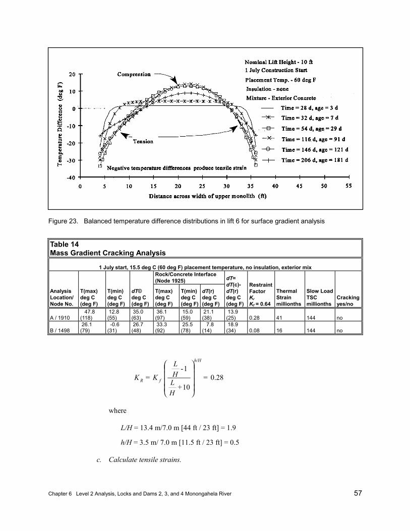
Chapter 6 Level 2 Analysis, Locks and Dams 2, 3, and 4 Monongahela River 57
Figure 23. Balanced temperature difference distributions in lift 6 for surface gradient analysis
Table 14Mass Gradient Cracking Analysis
1 July start, 15.5 deg C (60 deg F) placement temperature, no insulation, exterior mixRock/Concrete Interface(Node 1925)
AnalysisLocation/Node No.
T(max)deg C(deg F)
T(min)deg C(deg F)
dT©deg C(deg F)
T(max)deg C(deg F)
T(min)deg C(deg F)
dT(r)deg C(deg F)
dT=dT(c)-dT(r)deg C(deg F)
RestraintFactorKrKf = 0.64
ThermalStrainmillionths
Slow LoadTSCmillionths
Crackingyes/no
A / 1910 47.8(118)
12.8(55)
35.0(63)
36.1(97)
15.0(59)
21.1(38)
13.9(25) 0.28 41 144 no
B / 1498 26.1(79)
-0.6(31)
26.7(48)
33.3(92)
25.5(78)
7.8(14)
18.9(34) 0.08 16 144 no
0.28 = 10 +
1 - =
HLHL
KK
h/H
fR
where
L/H = 13.4 m/7.0 m [44 ft / 23 ft] = 1.9
h/H = 3.5 m/ 7.0 m [11.5 ft / 23 ft] = 0.5
c. Calculate tensile strains.
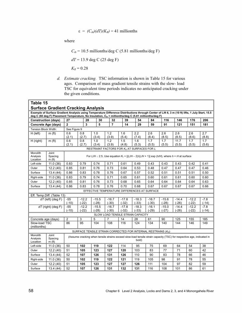
58 Chapter 6 Level 2 Analysis, Locks and Dams 2, 3, and 4 Monongahela River
ε = (Cth)(dT)(KR) = 41 millionths
where
Cth = 10.5 millionths/deg C (5.81 millionths/deg F)
dT = 13.9 deg C (25 deg F)
KR = 0.28
d. Estimate cracking. TSC information is shown in Table 15 for variousages. Comparison of mass gradient tensile strains with the slow- loadTSC for equivalent time periods indicates no anticipated cracking underthe given conditions.
Table 15Surface Gradient Cracking AnalysisExample of Surface Gradient Analysis using Temperature Difference Distributions through Center of Lift 6, 3 m (10 ft) lifts, 1 July Start, 15.5deg C (60 deg F) Placement Temperature, No Insulation, Cth = millionths/deg C (5.81 millionths/deg F)Construction (days) 27 28 30 32 39 54 84 116 146 176 206Concrete Age (days) 2 3 5 7 14 29 59 91 121 151 181Tension Block Width: See Figure 9H (left) m (ft) 0.6
(2.1)0.8(2.7)
1.0(3.4)
1.2(3.9)
1.6(5.4)
2.2(7.4)
2.6(8.4)
2.6(8.5)
2.6(8.5)
2.6(8.6)
2.7(8.8)
H (right) m (ft) 0.6(2.1)
0.8(2.7)
1.0(3.4)
1.2(3.9)
1.5(4.8)
1.6(5.3)
1.7(5.5)
1.7(5.5)
11.7(5.5)
1.7(5.5)
1.7(5.6)
RESTRAINT FACTORS FOR KR AT SURFACES FOR LMonolithAnalysisLocation
JointSpacingm (ft)
For L/H 2.5, Use equation Kr = [(L/H – 2)/(L/H + 1)] exp (h/H), where h = H at surface
Left-side 11.0 (36) 0.83 0.79 0.74 0.71 0.61 0.49 0.43 0.43 0.43 0.42 0.41Outer 12.2 (40) 0.85 0.81 0.76 0.73 0.64 0.53 0.48 0.47 0.47 0.47 0.46Surface 13.4 (44) 0.86 0.83 0.78 0.76 0.67 0.57 0.52 0.51 0.51 0.51 0.50Right-side 11.0 (36) 0.83 0.79 0.74 0.71 0.65 0.61 0.60 0.61 0.61 0.60 0.60Outer 12.2 (40) 0.85 0.81 0.76 0.73 0.68 0.65 0.64 0.64 0.64 0.64 0.63Surface 13.4 (44) 0.86 0.83 0.78 0.76 0.70 0.68 0.67 0.67 0.67 0.67 0.66
EFFECTIVE TEMPERATURE DIFFERENCES AT SURFACEEff. Temp.Diff. (Table 13)
dT (left) (deg F) -55(-10)
-12.2(-22)
-15.5(-28)
-16.7(-30)
-17.8(-32)
-18.3(-33)
-16.7(-30)
-15.6(-28)
-14.4(-26)
-12.2(-22)
-7.8(-14)
dT (right) (deg F) -55(-10)
-12.2(-22)
-15.5(-28)
-16.7(-30)
-17.8(-32)
-18.3(-33)
-16.1(-29)
-15.0(-27)
-14.4(-26)
-12.2(-22)
-7.8(-14)
SLOW LOAD TENSILE STRAIN CAPACITYConcrete age (days) 2 3 5 7 14 28 61 90 125 155 185Slow-load TSC(millionths)
86 95 104 108 116 124 134 140 144 146 149
SURFACE TENSILE STRAIN CORRECTED FOR INTERNAL RESTRAINS (KR)MonolithAnalysisLocation
JointSpacingm (ft)
(Assume cracking when tensile strains exceed slow-load tensile strain capacity (TSC) for respective age, indicated inbold)
Left-side 11.0 (36) 50 102 119 122 114 95 75 69 64 54 38Outer 12.2 (40) 51 105 123 127 120 103 83 77 71 60 42Surface 13.4 (44) 52 107 126 131 126 110 90 83 78 66 46Right-side 11.0 (36) 50 102 119 122 121 119 105 98 91 78 55Outer 12.2 (40) 51 105 123 127 127 126 111 104 97 82 59Surface 13.4 (44) 52 107 126 131 132 131 116 108 101 86 61
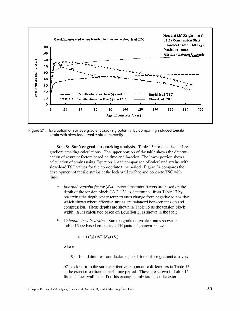
Chapter 6 Level 2 Analysis, Locks and Dams 2, 3, and 4 Monongahela River 59
Figure 24. Evaluation of surface gradient cracking potential by comparing induced tensilestrain with slow-load tensile strain capacity
Step 8: Surface gradient cracking analysis. Table 15 presents the surfacegradient cracking calculations. The upper portion of the table shows the determi-nation of restraint factors based on time and location. The lower portion showscalculation of strains using Equation 1, and comparison of calculated strains withslow-load TSC values for the appropriate time period. Figure 24 compares thedevelopment of tensile strains at the lock wall surface and concrete TSC withtime.
a. Internal restraint factor (KR). Internal restraint factors are based on thedepth of the tension block, “H.” “H” is determined from Table 13 byobserving the depth where temperatures change from negative to positive,which shows where effective strains are balanced between tension andcompression. These depths are shown in Table 15 as the tension blockwidth. KR is calculated based on Equation 2, as shown in the table.
b. Calculate tensile strains. Surface gradient tensile strains shown inTable 15 are based on the use of Equation 1, shown below:
ε = (Cth) (dT) (KR) (Kf)
where
Kf = foundation restraint factor equals 1 for surface gradient analysis
dT is taken from the surface effective temperature differences in Table 13,at the exterior surfaces at each time period. These are shown in Table 15for each lock wall face. For this example, only strains at the exterior
60 Chapter 6 Level 2 Analysis, Locks and Dams 2, 3, and 4 Monongahela River
surface are calculated and are shown in Table 15. Exterior surface strainsare shown in this table for KR = 1.0, for comparison assuming the surfaceis completely restrained, and for various lengths (L = 11.0, 12.2, and13.4 m) (L = 36, 40, and 44 ft) between vertical joints in the lock wall,where the surface restraint is less than 1.0. Strain variation with depthfrom the surface could be developed using corresponding KR for interiorlocations.
c. Estimate cracking. Comparison of strains with slow-load TSC providesan estimation of where and when surface gradient cracking may develop,as shown in Table 14. The estimated depth of cracking could beevaluated using KR at varying depths from the surface, and comparingwith slow-load TSC.
Conclusions and RecommendationsSome of the conclusions and recommendations from this thermal study
included the following:
Conclusions
a. Maximum lift height = 1.5 m (5 ft).
b. Maximum concrete placement temperature = 15.5 deg C (60 deg F)producing a 35.0 deg C (95 deg F) interior temperature.
Recommendations
a. Conduct additional mixture proportioning studies to further reduce thecement content.
b. Insulate all exposed concrete surfaces placed between 15 October and1 March.
c. Remove insulation only when ambient temperatures are above mean dailytemperatures, to aid thermal shock.
d. Open culvert space to cool air slowly to avoid thermal shock.
References 61
References
American Concrete Institute. ACI manual of concrete practice. Detroit, MI.
ACI 116R-90, “Cement and concrete terminology,” Part 1.
ACI 207.1R-87, “Mass concrete for dams and other massive structures,” Part 1.
ACI 207.2R-90, “Effect of restraint, volume change, and reinforcement ofcracking of massive concrete,” Part 1.
ACI 207.4R-93, “Cooling and insulating systems for mass concrete,” Part 1.
ACI 207.5R-89, “Roller compacted mass concrete,” Part 1.
American Society of Heating, Refrigerating and Air-Conditioning Engineers. (1977). ASHRAE handbook and product directory - 1977 fundamentals,New York.
Fintel, M. (1985). Handbook of concrete engineering. 2nd ed., Van NostrandReinhold, New York.
Headquarters, Department of the Army. “Standard practice for concrete for civilworks structures,” EM 1110-2-2000, Washington, DC.
__________. “Nonlinear, incremental structural analysis of massive concretestructures,” ETL 1110-2-365, Washington, DC.
Hibbitt, Karlsson, and Sorensen, Inc. (1994). ABAQUS user’s manual, version5.3., Pawtucket, RI.
Hollenbeck, R. E., and Tatro, S. B. (2000). “Nonlinear, incremental structuralanalysis of Zintel Canyon Dam,” ERDC/SL TR-00-7, U.S. Army EngineerResearch and Development Center, Vicksburg, MS.
Houghton, D. L. (1976). “Determining tensile strain capacity of mass concrete.”ACI Journal Proceedings, Vol 73, No. 12, 691-700.

62 References
U.S. Army Engineer Waterways Experiment Station. (1949). “Standard testmethod for ultimate tensile strain capacity of concrete.” Handbook forConcrete and Cement (with periodic supplements), Designation CRDC 71-80. Vicksburg, MS.
Wilson, E. L. (1968). “The determination of temperatures within mass concretestructures,” SESM Report No. 68-17, University of California, Berkeley.
Appendix A Determination of Tensile Strain Capacity (TSC) A1
Appendix ADetermination of Tensile StrainCapacity (TSC)
PurposeTensile strain capacity (TSC) is the change in length per unit length that can
be sustained in concrete prior to cracking. This property is used with the resultsof temperature analysis to determine whether a mass concrete structure (MCS)will crack and the extent of cracking. This appendix describes testing to deter-mine TSC, methods to estimate TSC, and methodology for its use in thermalanalysis.
BackgroundThe Corps of Engineers introduced TSC testing of concrete several decades
ago to provide a basis for evaluating crack potential for strain-based thermalstudies of MCS (Houghton 1976). This property is also used to compare differentaggregates and different concrete mix proportions in MCS. TSC varies primarilybased on age, strength, aggregate type, shape, and texture. TSC tests are con-ducted on large concrete beams instrumented to measure strain to failure. TSC isdetermined in a series of tests, including rapid and slow loading of beams. Theslow-load test was designed to simulate the strain conditions occurring in a massconcrete structure during long-term cooling. By conducting tests at severalloading ages, TSC data can be used to evaluate mass gradient cracking resistancein a structure under long-term cooling. Surface gradients generally develop dur-ing the first several days or weeks after placement of concrete, particularly follow-ing the removal of insulated forms. Hence, strains due to surface gradientsdevelop more rapidly than tested using the slow-load TSC test, and more slowlythan a standard TSC test failed at a normal loading rate. This appendix describesone method used to estimate TSC for surface gradient analyses.
A2 Appendix A Determination of Tensile Strain Capacity (TSC)
Description of Test Method
Tensile strain capacity is determined according to test method CRD-C 71(WES 1949). The test method requires a minimum of three beams for each test,and generally a minimum of three tests is recommended for each test set to allowfor variation in the test results. Rapid-load (0.28 Mpa/min) (40 psi/min) andslow-load (0.17 Mpa/week) (25 psi/week) tests are usually conducted in test seriesconsisting of three beam tests each. TSC test specimens are 300-mm by 300-mmby 1,680-mm-long (12-in. by 12-in. by 66-in.-long) beams tested in third-pointloading. Strain gauges are located at or near the top and bottom (compression andtension) surfaces to measure strain during the tests. At the age of test, a rapid-loadtest is conducted and a slow-load test is begun. Loading continues at the pre-scribed rate until failure. During the slow-load beam test, strain measurements aremade on the beam under load. In addition, measurements of autogenous strain aremade on the third beam. The autogenous shrinkage strains are used to correct thestrain measurements on the beam under slow load. Upon failure of the slowlyloaded beam, a rapid-load test is performed on the third beam. A TSC test seriesusually contains a suite of rapid- and slow-load tests typically initiated at 3, 7,28 days, and/or other ages. The differences in TSC capacity from the slow- andrapid-load beams provide an indication of the cumulative creep strain during theslow-load test. The strains measured in the slow-load beam test containing bothelastic and creep strains are expressed in millionths (1 × 10⁻⁶ in./in.).
Tensile Strain Capacity Test ResultsTSC test results can vary widely depending on a variety of factors. Test
results for the specific materials and mixture(s) to be used in an MCS should beused whenever possible. Actual values for TSC of mass concrete for slow-loadtests for specimens loaded at 7 days and failing at about 90 days range from 88 to237 millionths. Corresponding values for rapid-load tests conducted at 7 daysrange from 40 to 105 millionths. For tests conducted upon failure of the slow-load beam, rapid-load results range from 73 to 136 millionths. Ratios of slow-load tensile strain capacity to rapid-load tensile strain capacity tested at the sameage as the slow-load specimens range from 1.0 to 2.0 and averages 1.4. Thisaverage is relatively insensitive to age.
Use of TSC for Mass Gradient Cracking AnalysesMass gradient tensile loading in an MCS occurs over an extended period of
time. The standard slow-load TSC test was specifically designed for this condi-tion. Standard slow-load TSC tests provide a reasonable limiting strain in massgradient cracking analyses for the condition of restrained slow loading of massconcrete which occurs in a slowly cooling mass. Using an appropriate loadingtime period, the slow-load TSC can be used directly for mass gradient crackinganalysis.
Appendix A Determination of Tensile Strain Capacity (TSC) A3
Use of TSC for Surface Gradient CrackingAnalysesSurface gradient strains
Surface gradient strains can be initiated at a very early age, particularly afterthe removal of insulated formwork, and can develop over a few days or weeks ofloading due to the initial temperature rise and subsequent development of the sur-face temperature gradient. Because loading under surface gradient conditions ismore rapid than the standard TSC slow-load test, the results of that test may notwell represent surface gradient conditions. Very accurate TSC values may not benecessary for surface gradient analysis, except for critical situations. For mostsituations, the standard test values will suffice for surface gradient cracking analy-sis as well as mass gradient cracking analysis. In some structures, concrete mix-tures placed near the surface of the MCS may differ significantly from internalconcrete mixtures. Tests for TSC used in surface gradient analysis should beconducted on the appropriate concrete mixture(s).
Simulated surface gradient strains
For critical situations, slow-load TSC tests conducted at more rapid rates ofloading than the standard slow-load test may be conducted to simulate the devel-opment of surface gradient thermal strains. In lieu of such special load ratetesting, an estimate can be made of TSC for use in preliminary surface gradientTSC determinations, using the ratio of 1.4 described above. An estimate of TSCfor surface gradient analysis is determined by testing TSC at the rapid load rateand at the age of interest. This value is then multiplied by 1.4, to determine aTSC under the slow loading reflective of surface gradient strain development. This estimate is believed to be reasonably conservative at ages from 1 to 14 days.Because creep rates are greatest at early ages, it is possible that slow-load TSCmay be considerably higher especially from 1 to 7 days. Until test data are avail-able, this may be used for developing surface gradient tensile strain capacityvalues.
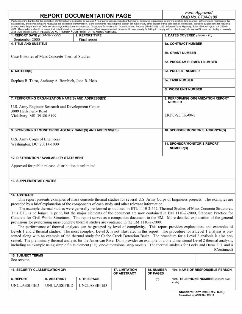
REPORT DOCUMENTATION PAGE Form ApprovedOMB No. 0704-0188
Public reporting burden for this collection of information is estimated to average 1 hour per response, including the time for reviewing instructions, searching existing data sources, gathering and maintaining thedata needed, and completing and reviewing this collection of information. Send comments regarding this burden estimate or any other aspect of this collection of information, including suggestions for reducingthis burden to Department of Defense, Washington Headquarters Services, Directorate for Information Operations and Reports (0704-0188), 1215 Jefferson Davis Highway, Suite 1204, Arlington, VA 22202-4302. Respondents should be aware that notwithstanding any other provision of law, no person shall be subject to any penalty for failing to comply with a collection of information if it does not display a currentlyvalid OMB control number. PLEASE DO NOT RETURN YOUR FORM TO THE ABOVE ADDRESS.1. REPORT DATE (DD-MM-YYYY) September 2000
2. REPORT TYPE Final report
3. DATES COVERED (From - To)
5a. CONTRACT NUMBER
5b. GRANT NUMBER
4. TITLE AND SUBTITLE
Case Histories of Mass Concrete Thermal Studies5c. PROGRAM ELEMENT NUMBER
6. AUTHOR(S) 5d. PROJECT NUMBER
Stephen B. Tatro, Anthony A. Bombich, John R. Hess 5e. TASK NUMBER
5f. WORK UNIT NUMBER
7. PERFORMING ORGANIZATION NAME(S) AND ADDRESS(ES) 8. PERFORMING ORGANIZATION REPORT NUMBER
U.S. Army Engineer Research and Development Center3909 Halls Ferry RoadVicksburg, MS 39180-6199 ERDC/SL TR-00-8
9. SPONSORING / MONITORING AGENCY NAME(S) AND ADDRESS(ES) 10. SPONSOR/MONITOR’S ACRONYM(S)
U.S. Army Corps of EngineersWashington, DC 20314-1000 11. SPONSOR/MONITOR’S REPORT
NUMBER(S)
12. DISTRIBUTION / AVAILABILITY STATEMENT
Approved for public release; distribution is unlimited.
13. SUPPLEMENTARY NOTES
14. ABSTRACT This report presents examples of mass concrete thermal studies for several U.S. Army Corps of Engineers projects. The examples arepreceded by a brief explanation of the components of each study and other relevant information. The example thermal studies were generally performed as outlined in ETL 1110-2-542, Thermal Studies of Mass Concrete Structures.This ETL is no longer in print, but the major elements of the document are now contained in EM 1110-2-2000, Standard Practice forConcrete for Civil Works Structures. This report serves as a companion document to the EM. More detailed explanation of the generalprovisions for performing mass concrete thermal studies are contained in the EM 1110-2-2000. The performance of thermal analyses can be grouped by level of complexity. This report provides explanations and examples ofLevels 1 and 2 thermal studies. The most complex, Level 3, is not illustrated in this report. The procedure for a Level 1 analysis is pre-sented along with an example of the thermal study for Cache Creek Detention Basin. The procedure for a Level 2 analysis is also pre-sented. The preliminary thermal analysis for the American River Dam provides an example of a one-dimensional Level 2 thermal analysis,including an example using simple finite element (FE), one-dimensional strip models. The thermal analysis for Locks and Dams 2, 3, and 4
(Continued)15. SUBJECT TERMSSee reverse.
16. SECURITY CLASSIFICATION OF: 17. LIMITATIONOF ABSTRACT
18. NUMBEROF PAGES
19a. NAME OF RESPONSIBLE PERSON
a. REPORT
UNCLASSIFIED
b. ABSTRACT
UNCLASSIFIED
c. THIS PAGE
UNCLASSIFIED75 19b. TELEPHONE NUMBER (include area
code)
Standard Form 298 (Rev. 8-98)Prescribed by ANSI Std. 239.18

14. (Concluded)
on the Monongahela River provides an example of a Level 2 analysis using more complex two-dimensional FEmethodology. Appendix A presents the current practice for determination of concrete tensile strain capacity for usein cracking analysis. The analyses illustrated by the examples in this report are recommended to evaluate thermal behavior of massconcrete structures. The analyses are useful in establishing the type and degree of control measures necessary tocontrol thermal cracking.
15. SUBJECT TERMS
Adiabatic temperature riseAmerican River DamCache Creek Detention Basin WeirConcreteCrackingDamsFinite element methodInsulationJointsLock and Dam 2,3,4Mass concreteMass gradientRestraintRoller compacted concreteSurface gradientTemperatureThermal analysisTensile strain capacityThermal strainThermal stress