IEEE TRANSACTIONS ON INTELLIGENT TRANSPORTATION SYSTEMS, VOL. 12, NO. 1, MARCH 2011 73

Cascade Architecture for Lateral Control inAutonomous Vehicles

Joshué Pérez, Vicente Milanés, and Enrique Onieva

Abstract—Research on intelligent transport systems (ITSs) issteadily leading to safer and more comfortable control for vehi-cles. Systems that permit longitudinal control have already beenimplemented in commercial vehicles, acting on throttle and brake.Nevertheless, lateral control applications are less common in themarket. Since a too-sudden turn of the steering wheel can causean accident in a few seconds, good speed and position control ofthe steering wheel is essential. We present here a new cascadecontrol architecture based on fuzzy logic controllers that emulatea human driver’s behavior. The control architecture was tested ona real vehicle at different vehicle speeds. The results showed theuse of a straightforward and intuitive fuzzy controller to give goodperformance.

Index Terms—Autonomous vehicles, fuzzy logic, intelligenttransportation systems (ITSs), lateral control, system analysis anddesign.

I. INTRODUCTION

AUTONOMOUS vehicles, once a utopia, are now poisedto become a reality. As engineers, we have a broad range

of possibilities of participation, since there are several fieldsinvolved in the control and automation of vehicles: controlmaneuvers, vehicle and infrastructure instrumentation, vehiclesimulation, etc. [1].

One of the first developments in the field of advancedvehicle-control systems took place in the early 1960s by theGeneral Motors Research Group. They developed and demon-strated the automatic control of the steering, speed, and brakingof automobiles [2] on test tracks. Later, other research groupsbegan to improve the lateral and longitudinal control of au-tonomous vehicles. In the late 1960s, Ohio State Universityand the Massachusetts Institute of Technology (MIT) beganworking on the application of these techniques to urban trans-portation problems [3]. The first broad-scale investigation of theapplication of automation technologies to urban transportationproblems appeared in MIT’s Project METRAN [4].

Manuscript received October 7, 2009; revised February 26, 2010 andMay 23, 2010; accepted July 14, 2010. Date of current version March 3,2011. This work was supported by in part by CYCIT (Spain), Plan Na-cional (Spain), and MICINN (Spain) under the projects GUIADE (P9/08),TRANSITO (TRA2008-06602-C03-01), and City-Elec (PS-370000-2009-4).The Associate Editor for this paper was L. Li.

The authors are with the Industrial Computer Science Department, Cen-tre of Automation and Robotics (CAR), Universidad Politécnica de Madrid,Consejo Superior de Investigaciones Científicas, (UPM-CSIC), La Poveda-Arganda del Rey, 28500 Madrid, Spain (e-mail: joshue.perez@car.upm-csic.es;vicente.milanes@car.upm-csic.es; enrique.onieva@car.upm-csic.es).

Color versions of one or more of the figures in this paper are available onlineat http://ieeexplore.ieee.org.

Digital Object Identifier 10.1109/TITS.2010.2060722

Recent years have seen significant advances in research inthis area, with several applications to commercial vehicles. Theleading vehicle manufacturers are investigating the develop-ment of new advanced driver-assistance systems (ADASs) [5].The goal of ADAS is to aid drivers in critical situations ratherthan to replace them. The most important advances have beencruise control [6], dynamic stability control [7], antilock brakes(ABS) [8], pedestrian detection with night-vision systems [9],collision avoidance [10], and semiautonomous parking andwarning signals [11], among others. These applications havemainly been implemented on the longitudinal control (actionsof acceleration and braking).

Lateral control concerns the action on the steering wheel.One of the pioneers on work on lateral control wasAckermann [12]. His approach was to merge active steeringwith yaw rate feedback to robustly decouple the yaw and lateralmotions. Another useful method for performing lateral controlis based on a predefined reference trajectory [13]. Throughtechniques that allow quick, smooth, and high-quality control,it is possible to control such nonlinear dynamic systems such asthe steering in a car. Techniques including fuzzy logic [14], lin-ear matrix inequality optimization (in automated snowblower)[15], and yaw rate control [16] have been used to keep thevehicle following the reference trajectory.

Choi [17] developed an adaptive control law and a distancerate observer for the lateral control of autonomous vehiclesusing magnetic sensors in the vehicle’s front wheels. In aparallel line of work, the Nissan Research Center has achievedsignificant advances in lateral control using error-cancelingfeedback control to estimate the next point on the track and togenerate the possible steering outputs [18].

Another significant change in the steering wheel system hasbeen the inclusion of electric-power-assisted steering (EPS)as a replacement for the traditional hydraulic power steering(HPS) systems in new-generation vehicles. There have beensimulations of the advanced control of this kind of system [19].Guvenc and Guvenc [20] present a two-controller structureproposal for the generic EPS system, addressing motor torqueand steering motion.

Yih and Gerdes [21] of Stanford University modified areal vehicle so that it could use a steer-by-wire system andreceive Global Positioning System (GPS) data. They used abicycle model and real-time estimation for the control and thecancelation of the effects of steering system dynamics andtire disturbance forces. Furthermore, there have been severalapplications for automated highway systems (AHSs) targetedat heavy vehicles [22]. Those authors incorporated an innerloop controller into the nested lateral control architecture forautonomous driving.

1524-9050/$26.00 © 2011 IEEE

74 IEEE TRANSACTIONS ON INTELLIGENT TRANSPORTATION SYSTEMS, VOL. 12, NO. 1, MARCH 2011

In the control of dynamic systems, there is, however, a largegap between the design of a controller using simulations andits implementation in a real system. This gap is gradually beingreduced with advances in different simulators [23], [24], butthese simulators still depend on the level of complexity and thedifferent constraints imposed by the systems. In this context,intelligent control offers powerful techniques for the control ofsuch highly complex systems such as autonomous vehicles.

In 1985, Sugeno and Nishida published a landmark paper.They demonstrated that any industrial process whatsoever canbe controlled with a simple model of human operation orhuman experience [14]. The problem was reduced to finding theproper control rules and fine-tuning them based on a driver’sexperience. Various studies have compared fuzzy control andclassical control techniques in autonomous vehicles [25], withthe fuzzy controllers showing good results.

The AUTOPIA program was begun in 1998 at the Instituteof Industrial Automation of the Spanish National ResearchCouncil (IAI-CSIC). The experiments to be described in thispaper were conducted with an electric Citroen Berlingo, imple-menting a new lateral control scheme for the steering wheel. Itis a continuation of previous studies carried out by the group[26], [27] but considerably improving the results achieved sofar. In brief, the improvements, both hardware and software,with respect to previous works are the following.

1) The power stage based on the ISA Bus card wasremoved for a new-generation power stage connected toan onboard PC through Ethernet connection. With thenew proportional–integral–derivative (PID) controller,the delay times were reduced, and a faster time responsewas achieved [28]. A new motor and a gear ratio wereinstalled [29].

2) Moreover, the advance of this new steering control per-mits using a new output control variable, i.e., the steeringwheel’s angular speed, which had never been used inprevious works.

3) Taking into account this new output variable, two fuzzyinputs have been included, i.e., the actual speed and thedistance to the bend, to perform a new fuzzy controllerthat permits smooth steering wheel control.

4) A low speed was previously used in bends (8 km/h) [30].With the new angular speed and position controller, thecorners can be taken up to 24 km/h.

5) Finally, a unique fuzzy controller capable of driving inboth straight and bend segments has been developed,substituting the two previous controllers. The new outputvariable—the steering wheel’s angular speed—permitsusing the same rule base for these two scenarios. Previ-ously, two steering controllers were needed [26].

The lateral controller described in this paper considers theangular speed and position as output variables. A cascadesteering control architecture performs well over different rangesof speeds and difficult urban curves (i.e., cornering). The maincontribution is the use of the position and angular speed ofthe steering wheel controlled through fuzzy logic to carry outsmooth and comfortable control aimed at emulating a humandriver.

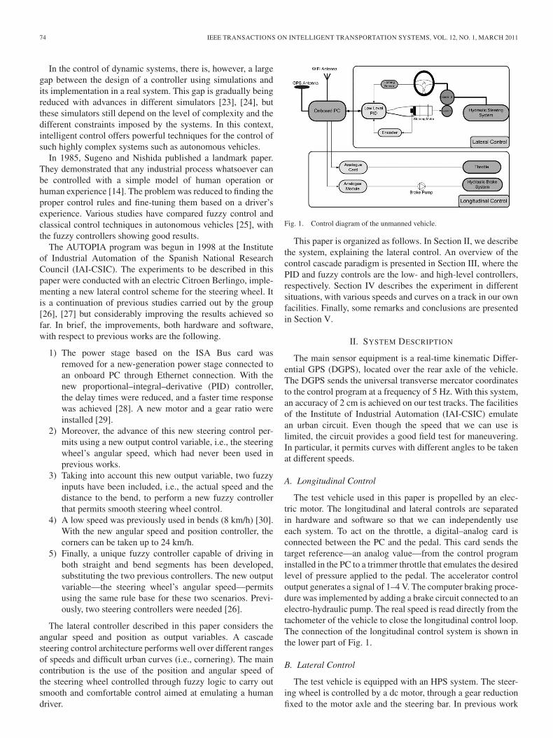
Fig. 1. Control diagram of the unmanned vehicle.

This paper is organized as follows. In Section II, we describethe system, explaining the lateral control. An overview of thecontrol cascade paradigm is presented in Section III, where thePID and fuzzy controls are the low- and high-level controllers,respectively. Section IV describes the experiment in differentsituations, with various speeds and curves on a track in our ownfacilities. Finally, some remarks and conclusions are presentedin Section V.

II. SYSTEM DESCRIPTION

The main sensor equipment is a real-time kinematic Differ-ential GPS (DGPS), located over the rear axle of the vehicle.The DGPS sends the universal transverse mercator coordinatesto the control program at a frequency of 5 Hz. With this system,an accuracy of 2 cm is achieved on our test tracks. The facilitiesof the Institute of Industrial Automation (IAI-CSIC) emulatean urban circuit. Even though the speed that we can use islimited, the circuit provides a good field test for maneuvering.In particular, it permits curves with different angles to be takenat different speeds.

A. Longitudinal Control

The test vehicle used in this paper is propelled by an elec-tric motor. The longitudinal and lateral controls are separatedin hardware and software so that we can independently useeach system. To act on the throttle, a digital–analog card isconnected between the PC and the pedal. This card sends thetarget reference—an analog value—from the control programinstalled in the PC to a trimmer throttle that emulates the desiredlevel of pressure applied to the pedal. The accelerator controloutput generates a signal of 1–4 V. The computer braking proce-dure was implemented by adding a brake circuit connected to anelectro-hydraulic pump. The real speed is read directly from thetachometer of the vehicle to close the longitudinal control loop.The connection of the longitudinal control system is shown inthe lower part of Fig. 1.

B. Lateral Control

The test vehicle is equipped with an HPS system. The steer-ing wheel is controlled by a dc motor, through a gear reductionfixed to the motor axle and the steering bar. In previous work

PÉREZ et al.: CASCADE ARCHITECTURE FOR LATERAL CONTROL IN AUTONOMOUS VEHICLES 75

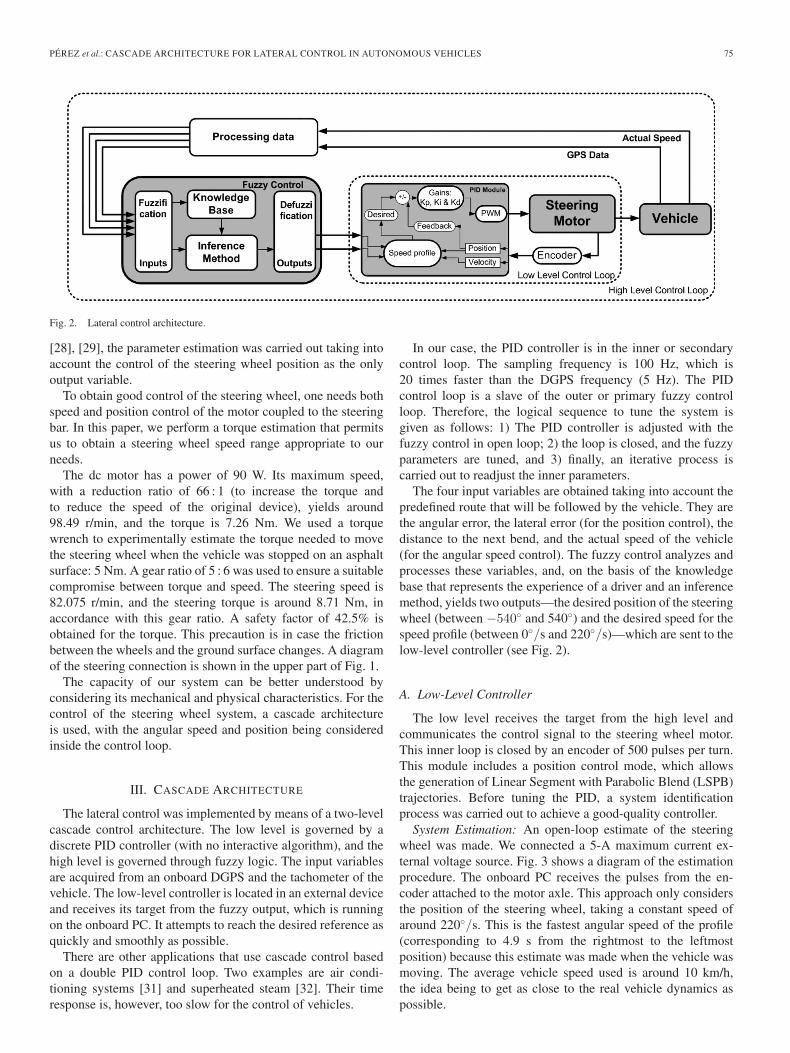
Fig. 2. Lateral control architecture.

[28], [29], the parameter estimation was carried out taking intoaccount the control of the steering wheel position as the onlyoutput variable.

To obtain good control of the steering wheel, one needs bothspeed and position control of the motor coupled to the steeringbar. In this paper, we perform a torque estimation that permitsus to obtain a steering wheel speed range appropriate to ourneeds.

The dc motor has a power of 90 W. Its maximum speed,with a reduction ratio of 66 : 1 (to increase the torque andto reduce the speed of the original device), yields around98.49 r/min, and the torque is 7.26 Nm. We used a torquewrench to experimentally estimate the torque needed to movethe steering wheel when the vehicle was stopped on an asphaltsurface: 5 Nm. A gear ratio of 5 : 6 was used to ensure a suitablecompromise between torque and speed. The steering speed is82.075 r/min, and the steering torque is around 8.71 Nm, inaccordance with this gear ratio. A safety factor of 42.5% isobtained for the torque. This precaution is in case the frictionbetween the wheels and the ground surface changes. A diagramof the steering connection is shown in the upper part of Fig. 1.

The capacity of our system can be better understood byconsidering its mechanical and physical characteristics. For thecontrol of the steering wheel system, a cascade architectureis used, with the angular speed and position being consideredinside the control loop.

III. CASCADE ARCHITECTURE

The lateral control was implemented by means of a two-levelcascade control architecture. The low level is governed by adiscrete PID controller (with no interactive algorithm), and thehigh level is governed through fuzzy logic. The input variablesare acquired from an onboard DGPS and the tachometer of thevehicle. The low-level controller is located in an external deviceand receives its target from the fuzzy output, which is runningon the onboard PC. It attempts to reach the desired reference asquickly and smoothly as possible.

There are other applications that use cascade control basedon a double PID control loop. Two examples are air condi-tioning systems [31] and superheated steam [32]. Their timeresponse is, however, too slow for the control of vehicles.

In our case, the PID controller is in the inner or secondarycontrol loop. The sampling frequency is 100 Hz, which is20 times faster than the DGPS frequency (5 Hz). The PIDcontrol loop is a slave of the outer or primary fuzzy controlloop. Therefore, the logical sequence to tune the system isgiven as follows: 1) The PID controller is adjusted with thefuzzy control in open loop; 2) the loop is closed, and the fuzzyparameters are tuned, and 3) finally, an iterative process iscarried out to readjust the inner parameters.

The four input variables are obtained taking into account thepredefined route that will be followed by the vehicle. They arethe angular error, the lateral error (for the position control), thedistance to the next bend, and the actual speed of the vehicle(for the angular speed control). The fuzzy control analyzes andprocesses these variables, and, on the basis of the knowledgebase that represents the experience of a driver and an inferencemethod, yields two outputs—the desired position of the steeringwheel (between −540◦ and 540◦) and the desired speed for thespeed profile (between 0◦/s and 220◦/s)—which are sent to thelow-level controller (see Fig. 2).

A. Low-Level Controller

The low level receives the target from the high level andcommunicates the control signal to the steering wheel motor.This inner loop is closed by an encoder of 500 pulses per turn.This module includes a position control mode, which allowsthe generation of Linear Segment with Parabolic Blend (LSPB)trajectories. Before tuning the PID, a system identificationprocess was carried out to achieve a good-quality controller.

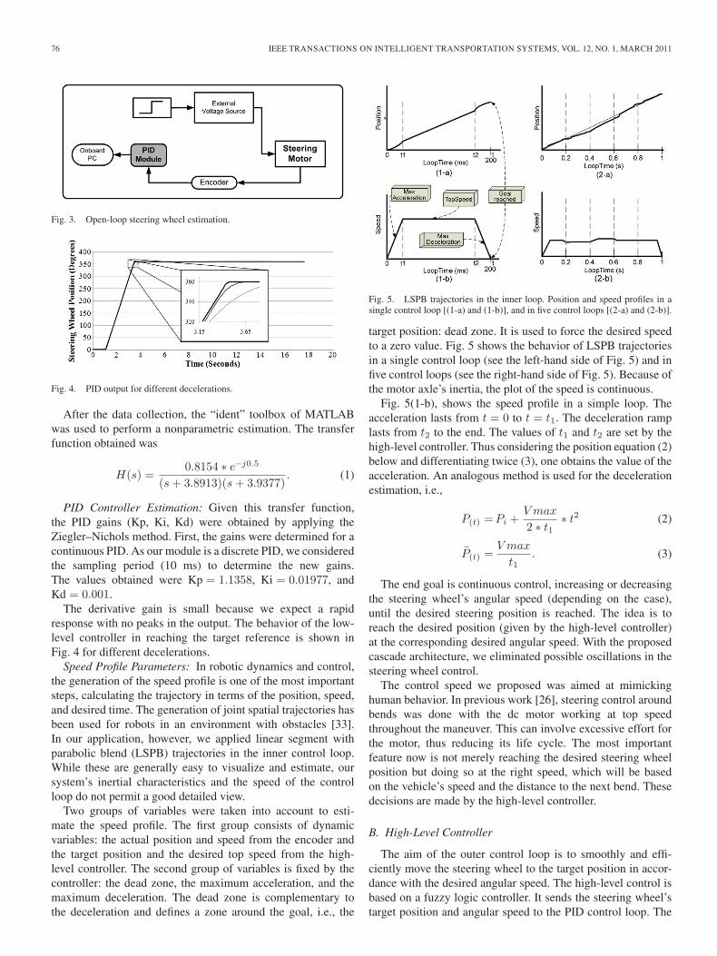
System Estimation: An open-loop estimate of the steeringwheel was made. We connected a 5-A maximum current ex-ternal voltage source. Fig. 3 shows a diagram of the estimationprocedure. The onboard PC receives the pulses from the en-coder attached to the motor axle. This approach only considersthe position of the steering wheel, taking a constant speed ofaround 220◦/s. This is the fastest angular speed of the profile(corresponding to 4.9 s from the rightmost to the leftmostposition) because this estimate was made when the vehicle wasmoving. The average vehicle speed used is around 10 km/h,the idea being to get as close to the real vehicle dynamics aspossible.

76 IEEE TRANSACTIONS ON INTELLIGENT TRANSPORTATION SYSTEMS, VOL. 12, NO. 1, MARCH 2011

Fig. 3. Open-loop steering wheel estimation.

Fig. 4. PID output for different decelerations.

After the data collection, the “ident” toolbox of MATLABwas used to perform a nonparametric estimation. The transferfunction obtained was

H(s) =0.8154 ∗ e−j0.5

(s + 3.8913)(s + 3.9377). (1)

PID Controller Estimation: Given this transfer function,the PID gains (Kp, Ki, Kd) were obtained by applying theZiegler–Nichols method. First, the gains were determined for acontinuous PID. As our module is a discrete PID, we consideredthe sampling period (10 ms) to determine the new gains.The values obtained were Kp = 1.1358, Ki = 0.01977, andKd = 0.001.

The derivative gain is small because we expect a rapidresponse with no peaks in the output. The behavior of the low-level controller in reaching the target reference is shown inFig. 4 for different decelerations.

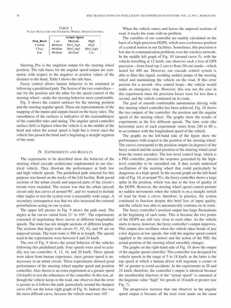
Speed Profile Parameters: In robotic dynamics and control,the generation of the speed profile is one of the most importantsteps, calculating the trajectory in terms of the position, speed,and desired time. The generation of joint spatial trajectories hasbeen used for robots in an environment with obstacles [33].In our application, however, we applied linear segment withparabolic blend (LSPB) trajectories in the inner control loop.While these are generally easy to visualize and estimate, oursystem’s inertial characteristics and the speed of the controlloop do not permit a good detailed view.

Two groups of variables were taken into account to esti-mate the speed profile. The first group consists of dynamicvariables: the actual position and speed from the encoder andthe target position and the desired top speed from the high-level controller. The second group of variables is fixed by thecontroller: the dead zone, the maximum acceleration, and themaximum deceleration. The dead zone is complementary tothe deceleration and defines a zone around the goal, i.e., the

Fig. 5. LSPB trajectories in the inner loop. Position and speed profiles in asingle control loop [(1-a) and (1-b)], and in five control loops [(2-a) and (2-b)].

target position: dead zone. It is used to force the desired speedto a zero value. Fig. 5 shows the behavior of LSPB trajectoriesin a single control loop (see the left-hand side of Fig. 5) and infive control loops (see the right-hand side of Fig. 5). Because ofthe motor axle’s inertia, the plot of the speed is continuous.

Fig. 5(1-b), shows the speed profile in a simple loop. Theacceleration lasts from t = 0 to t = t1. The deceleration ramplasts from t2 to the end. The values of t1 and t2 are set by thehigh-level controller. Thus considering the position equation (2)below and differentiating twice (3), one obtains the value of theacceleration. An analogous method is used for the decelerationestimation, i.e.,

P(t) =Pi +V max

2 ∗ t1∗ t2 (2)

P̈(t) =V max

t1. (3)

The end goal is continuous control, increasing or decreasingthe steering wheel’s angular speed (depending on the case),until the desired steering position is reached. The idea is toreach the desired position (given by the high-level controller)at the corresponding desired angular speed. With the proposedcascade architecture, we eliminated possible oscillations in thesteering wheel control.

The control speed we proposed was aimed at mimickinghuman behavior. In previous work [26], steering control aroundbends was done with the dc motor working at top speedthroughout the maneuver. This can involve excessive effort forthe motor, thus reducing its life cycle. The most importantfeature now is not merely reaching the desired steering wheelposition but doing so at the right speed, which will be basedon the vehicle’s speed and the distance to the next bend. Thesedecisions are made by the high-level controller.

B. High-Level Controller

The aim of the outer control loop is to smoothly and effi-ciently move the steering wheel to the target position in accor-dance with the desired angular speed. The high-level control isbased on a fuzzy logic controller. It sends the steering wheel’starget position and angular speed to the PID control loop. The

PÉREZ et al.: CASCADE ARCHITECTURE FOR LATERAL CONTROL IN AUTONOMOUS VEHICLES 77

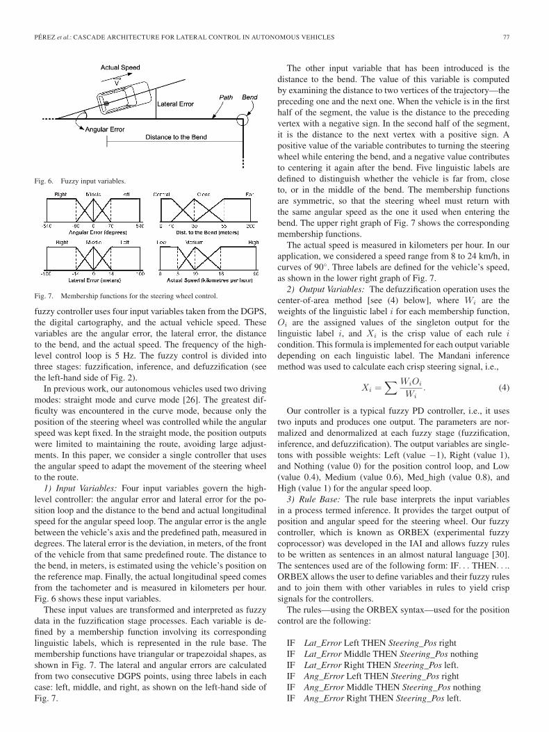
Fig. 6. Fuzzy input variables.

Fig. 7. Membership functions for the steering wheel control.

fuzzy controller uses four input variables taken from the DGPS,the digital cartography, and the actual vehicle speed. Thesevariables are the angular error, the lateral error, the distanceto the bend, and the actual speed. The frequency of the high-level control loop is 5 Hz. The fuzzy control is divided intothree stages: fuzzification, inference, and defuzzification (seethe left-hand side of Fig. 2).

In previous work, our autonomous vehicles used two drivingmodes: straight mode and curve mode [26]. The greatest dif-ficulty was encountered in the curve mode, because only theposition of the steering wheel was controlled while the angularspeed was kept fixed. In the straight mode, the position outputswere limited to maintaining the route, avoiding large adjust-ments. In this paper, we consider a single controller that usesthe angular speed to adapt the movement of the steering wheelto the route.

1) Input Variables: Four input variables govern the high-level controller: the angular error and lateral error for the po-sition loop and the distance to the bend and actual longitudinalspeed for the angular speed loop. The angular error is the anglebetween the vehicle’s axis and the predefined path, measured indegrees. The lateral error is the deviation, in meters, of the frontof the vehicle from that same predefined route. The distance tothe bend, in meters, is estimated using the vehicle’s position onthe reference map. Finally, the actual longitudinal speed comesfrom the tachometer and is measured in kilometers per hour.Fig. 6 shows these input variables.

These input values are transformed and interpreted as fuzzydata in the fuzzification stage processes. Each variable is de-fined by a membership function involving its correspondinglinguistic labels, which is represented in the rule base. Themembership functions have triangular or trapezoidal shapes, asshown in Fig. 7. The lateral and angular errors are calculatedfrom two consecutive DGPS points, using three labels in eachcase: left, middle, and right, as shown on the left-hand side ofFig. 7.

The other input variable that has been introduced is thedistance to the bend. The value of this variable is computedby examining the distance to two vertices of the trajectory—thepreceding one and the next one. When the vehicle is in the firsthalf of the segment, the value is the distance to the precedingvertex with a negative sign. In the second half of the segment,it is the distance to the next vertex with a positive sign. Apositive value of the variable contributes to turning the steeringwheel while entering the bend, and a negative value contributesto centering it again after the bend. Five linguistic labels aredefined to distinguish whether the vehicle is far from, closeto, or in the middle of the bend. The membership functionsare symmetric, so that the steering wheel must return withthe same angular speed as the one it used when entering thebend. The upper right graph of Fig. 7 shows the correspondingmembership functions.

The actual speed is measured in kilometers per hour. In ourapplication, we considered a speed range from 8 to 24 km/h, incurves of 90◦. Three labels are defined for the vehicle’s speed,as shown in the lower right graph of Fig. 7.

2) Output Variables: The defuzzification operation uses thecenter-of-area method [see (4) below], where Wi are theweights of the linguistic label i for each membership function,Oi are the assigned values of the singleton output for thelinguistic label i, and Xi is the crisp value of each rule icondition. This formula is implemented for each output variabledepending on each linguistic label. The Mandani inferencemethod was used to calculate each crisp steering signal, i.e.,

Xi =∑ WiOi

Wi. (4)

Our controller is a typical fuzzy PD controller, i.e., it usestwo inputs and produces one output. The parameters are nor-malized and denormalized at each fuzzy stage (fuzzification,inference, and defuzzification). The output variables are single-tons with possible weights: Left (value −1), Right (value 1),and Nothing (value 0) for the position control loop, and Low(value 0.4), Medium (value 0.6), Med_high (value 0.8), andHigh (value 1) for the angular speed loop.

3) Rule Base: The rule base interprets the input variablesin a process termed inference. It provides the target output ofposition and angular speed for the steering wheel. Our fuzzycontroller, which is known as ORBEX (experimental fuzzycoprocessor) was developed in the IAI and allows fuzzy rulesto be written as sentences in an almost natural language [30].The sentences used are of the following form: IF. . . THEN. . ..ORBEX allows the user to define variables and their fuzzy rulesand to join them with other variables in rules to yield crispsignals for the controllers.

The rules—using the ORBEX syntax—used for the positioncontrol are the following:

IF Lat_Error Left THEN Steering_Pos rightIF Lat_Error Middle THEN Steering_Pos nothingIF Lat_Error Right THEN Steering_Pos left.IF Ang_Error Left THEN Steering_Pos rightIF Ang_Error Middle THEN Steering_Pos nothingIF Ang_Error Right THEN Steering_Pos left.

78 IEEE TRANSACTIONS ON INTELLIGENT TRANSPORTATION SYSTEMS, VOL. 12, NO. 1, MARCH 2011

TABLE IFUZZY RULE FOR THE STEERING WHEEL SPEED CONTROL

Steering_Pos is the singleton output for the steering wheelposition. The rule bases for the angular speed output are sym-metric with respect to the negative or positive values of thedistance to the bend. Table I shows the rule base.

Fuzzy control allows human behavior to be emulated infollowing a predefined path. The fusion of the two controllers—one for the position and the other for the speed control of thesteering wheel—make the steering behavior more comfortable.

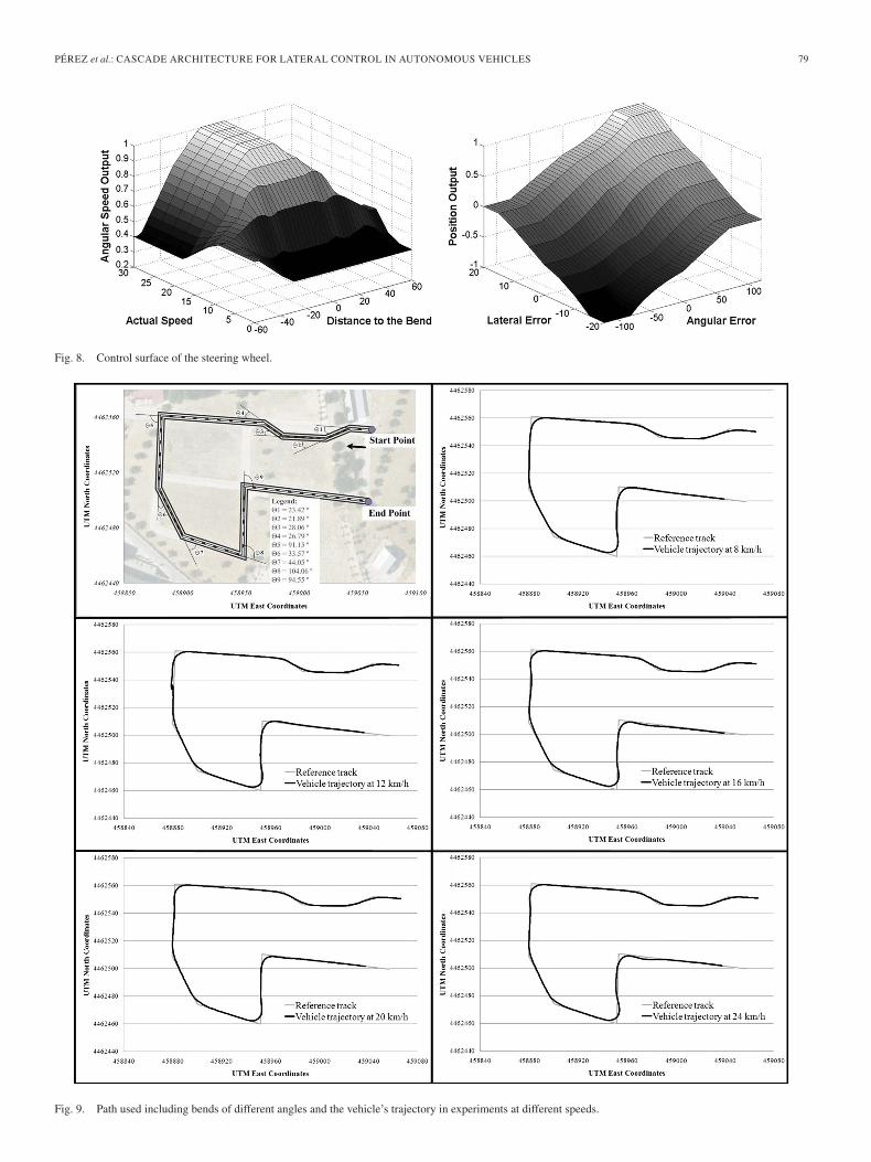
Fig. 8 shows the control surfaces for the steering positionand the steering angular speed. These are representations of themapping of the inputs and outputs based on the fuzzy rules. Thesmoothness of the surfaces is indicative of the reasonablenessof the controller rules and tuning. The angular speed controllersurface (left) is highest when the vehicle is in the middle of thebend and when the actual speed is high but is lower once thevehicle has passed the bend and is beginning a straight segmentof the route.

IV. EXPERIMENTS AND RESULTS

The experiments to be described show the behavior of thesteering wheel cascade architecture implemented in our elec-trical vehicle. They illustrate the performance at both lowand high vehicle speeds. The predefined path selected for thispurpose was based on the tracks of the IAI facility. Both pavedsections of the urban circuit and unpaved parts of the circuit’sterrain were included. The reason was that the urban (paved)circuit only has curves of around 90◦, and we wanted to includeother angles to test the system over a reasonably wide range. Asecondary consequence was that we also increased the externalperturbations acting on our system.

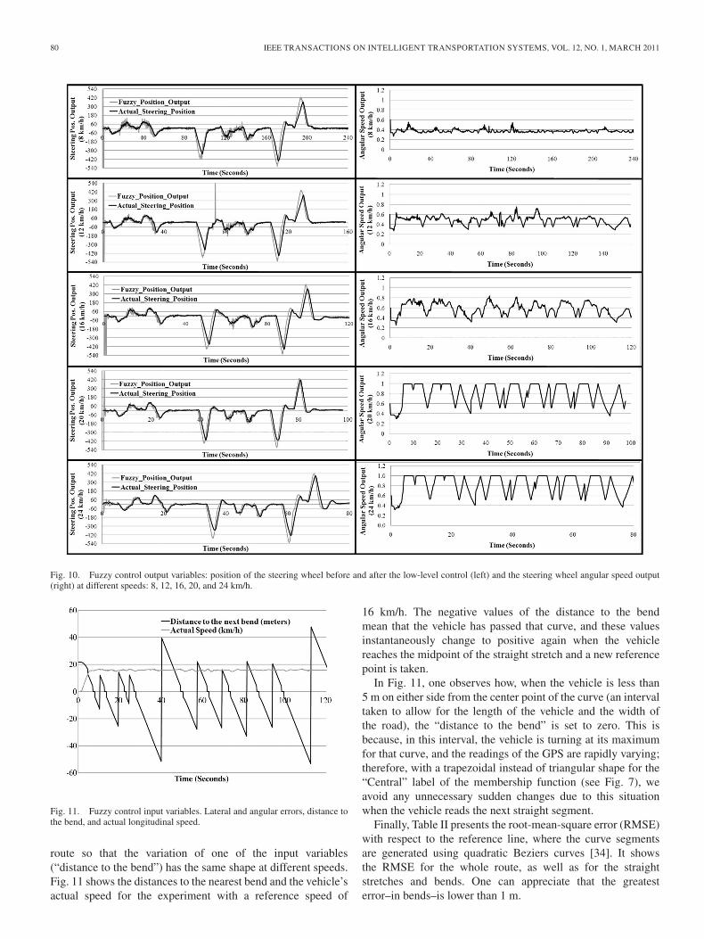
The upper left picture in Fig. 9 shows the path used. Theangles at the curves varied from 21◦ to 105◦. The experimentsconsisted of negotiating these curves at different longitudinalspeeds. The route has ten straight sections of different lengths.The sections that begin with curves θ1, θ2, θ3, and θ6 are onunpaved terrain. The total route is 500 m in length. The speedsused in the experiments were between 8 and 24 km/h.

The rest of Fig. 9 shows the actual behavior of the vehiclesfollowing this predefined path. Four speeds were used to actu-ally test our controller: 8, 12, 16, and 20 km/h. These speedswere taken from human experience, since greater speed is un-necessary in an urban circuit. These experiments showed goodperformance of the steering wheel angular speed and positioncontroller. Also shown is an extra experiment at a greater speed(24 km/h) to test the robustness of the controller. In this test, al-though the vehicle keeps to the road, one observes that the erroris greater as it follows the path, particularly around the sharpestcurve (θ8; see the lower right graph of Fig. 9). Indeed, this wasthe most difficult curve, because the vehicle must turn 105◦.

When the vehicle enters and leaves the unpaved sections ofroad, it tracks the route with no problem.

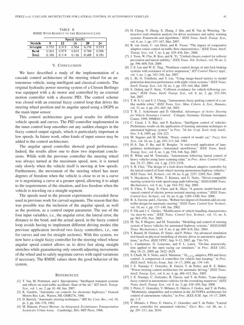
The variables of our controller are mainly calculated on thebasis of a high-precision DGPS, which uses a reference positionof a central station in our facilities. Sometimes, this precision islost due to communication problems over the wireless network.In the middle left graph of Fig. 10 (around curve 5), with thevehicle travelling at 12 km/h, one observes such a loss of GPSprecision—from fixed (up 2 cm) to float (50 cm) mode—whichlasted for 400 ms. However, our cascade control system isable to filter this signal, avoiding sudden jumps of the steeringwheel and maintaining the vehicle on the road. If this errorpersists for a second—five control loops—the vehicle wouldmake an emergency stop. However, this was not the case inthis experiment since the precision losses were for less than asecond, and the vehicle continued on its route.

The goal of smooth comfortable autonomous driving withthis steering wheel controller has been achieved. Fig. 10 showsthe two outputs of the controller: the position and the angularspeed of the steering wheel. The graphs show the results ofexperiments at the five different speeds. The time scale (thehorizontal axis) of each experiment varies from 240 to 80 s,in accordance with the longitudinal speed of the vehicle.

The graphs on the left-hand side of the figure show theperformance with respect to the position of the steering wheel.The curves correspond to the position output (in degrees) of thefuzzy control and the actual position of the steering wheel (readfrom the motor encoder). The low-level control loop, which isa PID controller, permits the response generated by the high-level controller to be smoothed out. It thus avoids undesiredoscillations of the steering wheel that could particularly bedangerous at a high speed. In the second graph on the left-handside of Fig. 10, at around 70 s, the fuzzy controller shows a largespike in the position, which was due to the loss of quality ofthe DGPS. However, the steering wheel speed control permitsno sudden movements when the vehicle is on a straight stretchof road far from a curve; therefore, in practice, the systemcontinued to function despite this brief loss of input quality,and the vehicle was able to automatically continue on its route.

The fuzzy controller’s position output has large fluctuationsat the beginning of each route. This is because the two pointsof the DGPS are still very close to each other. As the vehiclestarts to move, however, the fuzzy controller’s output improves.This output also oscillates when the vehicle takes bends of justa few degrees at low speeds, but with the angular speed control(applied to the steering motor) and the action of the PID, theactual position of the steering wheel smoothly changes.

The graphs on the right-hand side of Fig. 10 show the outputof the angular speed controller. This controller was designed forvehicle speeds in the range of 5 to 18 km/h, as the latter is thetop speed at which a human driver will negotiate a corner of90◦ or greater to avoid accidents. In the experiments at 20 and24 km/h, therefore, the controller’s output is identical becausethe membership function of the “actual speed” is saturated atthe linguistic value “high” for speeds of 18 km/h or greater (seeFig. 7).

The progressive increase that one observes in the angularspeed output is because all the tests were made on the same

PÉREZ et al.: CASCADE ARCHITECTURE FOR LATERAL CONTROL IN AUTONOMOUS VEHICLES 79

Fig. 8. Control surface of the steering wheel.

Fig. 9. Path used including bends of different angles and the vehicle’s trajectory in experiments at different speeds.

80 IEEE TRANSACTIONS ON INTELLIGENT TRANSPORTATION SYSTEMS, VOL. 12, NO. 1, MARCH 2011

Fig. 10. Fuzzy control output variables: position of the steering wheel before and after the low-level control (left) and the steering wheel angular speed output(right) at different speeds: 8, 12, 16, 20, and 24 km/h.

Fig. 11. Fuzzy control input variables. Lateral and angular errors, distance tothe bend, and actual longitudinal speed.

route so that the variation of one of the input variables(“distance to the bend”) has the same shape at different speeds.Fig. 11 shows the distances to the nearest bend and the vehicle’sactual speed for the experiment with a reference speed of

16 km/h. The negative values of the distance to the bendmean that the vehicle has passed that curve, and these valuesinstantaneously change to positive again when the vehiclereaches the midpoint of the straight stretch and a new referencepoint is taken.

In Fig. 11, one observes how, when the vehicle is less than5 m on either side from the center point of the curve (an intervaltaken to allow for the length of the vehicle and the width ofthe road), the “distance to the bend” is set to zero. This isbecause, in this interval, the vehicle is turning at its maximumfor that curve, and the readings of the GPS are rapidly varying;therefore, with a trapezoidal instead of triangular shape for the“Central” label of the membership function (see Fig. 7), weavoid any unnecessary sudden changes due to this situationwhen the vehicle reads the next straight segment.

Finally, Table II presents the root-mean-square error (RMSE)with respect to the reference line, where the curve segmentsare generated using quadratic Beziers curves [34]. It showsthe RMSE for the whole route, as well as for the straightstretches and bends. One can appreciate that the greatesterror–in bends–is lower than 1 m.

PÉREZ et al.: CASCADE ARCHITECTURE FOR LATERAL CONTROL IN AUTONOMOUS VEHICLES 81

TABLE IIRMSE WITH RESPECT TO THE REFERENCE LINE

V. CONCLUSION

We have described a study of the implementation of acascade control architecture of the steering wheel for an au-tonomous vehicle, using intelligent and classical controls. Theoriginal hydraulic power steering system of a Citroen Berlingowas equipped with a dc motor and controlled by an externalmotion controller with a discrete PID. The control schemewas closed with an external fuzzy control loop that drives thesteering wheel position and its angular speed using a DGPS asthe main input sensor.

This control architecture gave good results for differentvehicle speeds and curves. The PID controller implemented inthe inner control loop smoothes out any sudden changes in thefuzzy control output signals, which is particularly important atlow speeds. In future work, other kinds of input sensor may beadded to the control architecture.

The angular speed controller showed good performance.Indeed, the results allow one to draw two important conclu-sions. While with the previous controller the steering wheelwas always turned at the maximum speed, now, it is turnedonly slowly when the vehicle itself is moving at low speeds.Furthermore, the movement of the steering wheel has moredegrees of freedom when the vehicle is close to or in a curveor is negotiating a curve at a greater speed, allowing it to adaptto the requirements of the situation, and less freedom when thevehicle is traveling on a straight segment.

The speeds used in the present experiments exceeded thoseused in previous work for curved segments. The reason that thiswas possible was the inclusion of the angular speed, as wellas the position, as a control output parameter. The use of thefour input variables, i.e., the angular error, the lateral error, thedistance to the bend, and the actual speed, in the fuzzy controlloop avoids having to implement different driving modes (theprevious application involved two fuzzy controllers, i.e., onefor curves and one for straight sections). With this system, wenow have a single fuzzy controller for the steering wheel whoseangular speed control allows us to drive fast along straightstretches while guaranteeing only smooth adjusting movementsof the wheel and to safely negotiate curves with rapid variationsif necessary. The RMSE values show the good behavior of thesystem.

REFERENCES

[1] T. Vaa, M. Penttinen, and I. Spyropoulou, “Intelligent transport systemsand effects on road traffic accidents: State of the art,” IET Intell. Transp.Syst., vol. 1, no. 2, pp. 81–88, Jun. 2007.

[2] K. Gardels, “Automatic car controls for electronic highways,” GeneralMotors Res. Lab., Warren, MI, GMR276, 1960.

[3] D. Barrick, “Automatic steering techniques,” IRE Int. Conv. Rec., vol. 10,pt. 2, pp. 166–178, 1962.

[4] M. Hanson, Projest Metran: An Integrated, Evolutionary TransportationSystem for Urban Areas. Cambridge, MA: MIT Press, 1966.

[5] H. Cheng, N. Zheng, X. Zhang, J. Qin, and H. Van de Wetering, “In-teractive road situation analysis for driver assistance and safety warningsystems: Framework and algorithms,” IEEE Trans. Intell. Transp. Syst.,vol. 8, no. 1, pp. 157–167, Mar. 2007.

[6] B. van Arem, C. van Driel, and R. Visser, “The impact of cooperativeadaptive cruise control on traffic-flow characteristics,” IEEE Trans. Intell.Transp. Syst., vol. 7, no. 4, pp. 429–436, Dec. 2006.

[7] J. Yoon, W. Cho, B. Koo, and K. Yi, “Unified chassis control for rolloverprevention and lateral stability,” IEEE Trans. Veh. Technol., vol. 58, no. 2,pp. 596–609, Feb. 2009.

[8] J.-S. Lin and W.-E. Ting, “Nonlinear control design of anti-lock brakingsystems with assistance of active suspension,” IET Control Theory Appl.,vol. 1, no. 1, pp. 343–348, Jan. 2007.

[9] L. Bi, O. Tsimhoni, and Y. Liu, “Using image-based metrics to modelpedestrian detection performance with night-vision systems,” IEEE Trans.Intell. Transp. Syst., vol. 10, no. 1, pp. 155–164, Mar. 2009.

[10] S. Gehrig and F. Stein, “Collision avoidance for vehicle-following sys-tems,” IEEE Trans. Intell. Transp. Syst., vol. 8, no. 2, pp. 233–244,Jun. 2007.

[11] T. H. S. Li and S.-J. Chang, “Autonomous fuzzy parking control of a car-like mobile robot,” IEEE Trans. Syst., Man, Cybern. A, Syst., Humans,vol. 33, no. 4, pp. 451–465, Jul. 2003.

[12] T. B. J. Ackermann and D. Odenthal, Advantages of Active Steeringfor Vehicle Dynamics Control. Cologne, Germany: German AerospaceCenter, 1999, 99ME013.

[13] C. Unsal, J. S. Bay, and P. Kachroo, “Intelligent control of vehicles:Preliminary results on the application of learning automata techniques toautomated highway system,” in Proc. 7th Int. Conf. Tools Artif. Intell.,Nov. 5–8, 1995, pp. 216–223.

[14] M. Sugeno and M. Nishida, “Fuzzy control of model car,” Fuzzy SetsSyst., vol. 16, no. 2, pp. 103–113, Jul. 1985.

[15] H.-S. Tan, F. Bu, and B. Bougler, “A real-world application of lane-guidance technologies—Automated snowblower,” IEEE Trans. Intell.Transp. Syst., vol. 8, no. 3, pp. 538–548, Sep. 2007.

[16] R. White and M. Tomizuka, “Autonomous following lateral control ofheavy vehicles using laser scanning radar,” in Proc. Amer. Control Conf.,Jun. 25–27, 2001, vol. 3, pp. 2333–2338.

[17] S. B. Choi, “The design of a look-down feedback adaptive controller forthe lateral control of front-wheel-steering autonomous highway vehicles,”IEEE Trans. Veh. Technol., vol. 49, no. 6, pp. 2257–2269, Nov. 2000.

[18] Y. Hayakawa, R. White, T. Kimura, and G. Naito, “Driver-compatiblesteering system for wide speed-range path following,” IEEE/ASME Trans.Mechatronics, vol. 9, no. 3, pp. 544–552, Sep. 2004.

[19] X. Chen, T. Yang, X. Chen, and K. Zhou, “A generic model-based ad-vanced control of electric power-assisted steering systems,” IEEE Trans.Control Syst. Technol., vol. 16, no. 6, pp. 1289–1300, Nov. 2008.

[20] B. A. Guvenc and L. Guvenc, “Robust two degree-of-freedom add-on con-troller design for automatic steering,” IEEE Trans. Control Syst. Technol.,vol. 10, no. 1, pp. 137–148, Jan. 2002.

[21] P. Yih and J. C. Gerdes, “Modification of vehicle handling characteristicsvia steer-by-wire,” IEEE Trans. Control Syst. Technol., vol. 13, no. 6,pp. 965–976, Nov. 2005.

[22] M. Tai, P. Hingwe, and M. Tomizuka, “Modeling and control of steeringsystem of heavy vehicles for automated highway systems,” IEEE/ASMETrans. Mechatronics, vol. 9, no. 4, pp. 609–618, Dec. 2004.

[23] T. Bauml, H. Giuliani, D. Simic, and F. Pirker, “An advanced simulationtool based on physical modelling of electric drives in automotive applica-tions,” in Proc. IEEE VPPC, Sep. 9–12, 2007, pp. 736–741.

[24] L. Cardamone, D. Loiacono, and P. L. Lanzi, “On-line neuroevolu-tion applied to the open racing car simulator,” in Proc. IEEE CEC,May 18–21, 2009, pp. 2622–2629.

[25] S. Chaib, M. S. Netto, and S. Mammar, “ Hinfty adaptive, PID and fuzzycontrol: A comparison of controllers for vehicle lane keeping,” in Proc.IEEE Intell. Vehicles Symp., Jun. 14–17, 2004, pp. 139–144.

[26] J. E. Naranjo, C. Gonzalez, R. Garcia, T. de Pedro, and R. E. Haber,“Power-steering control architecture for automatic driving,” IEEE Trans.Intell. Transp. Syst., vol. 6, no. 4, pp. 406–415, Dec. 2005.

[27] J. E. Naranjo, C. Gonzalez, R. Garcia, and T. de Pedro, “Lane-changefuzzy control in autonomous vehicles for the overtaking maneuver,” IEEETrans. Intell. Transp. Syst., vol. 9, no. 3, pp. 438–450, Sep. 2008.

[28] J. Perez, C. Gonzalez, V. Milanes, E. Onieva, J. Godoy, and T. de Pedro,“Modularity, adaptability and evolution in the AUTOPIA architecture forcontrol of autonomous vehicles,” in Proc. IEEE ICM, Apr. 14–17, 2009,pp. 1–5.

[29] V. Milanés, J. Pérez, E. Onieva, C. González, and T. de Pedro, “Lateralpower controller for unmanned vehicles,” Elect. Rev., vol. 86, no. 1,pp. 207–211, Jan. 2010.

82 IEEE TRANSACTIONS ON INTELLIGENT TRANSPORTATION SYSTEMS, VOL. 12, NO. 1, MARCH 2011

[30] R. García, T. de Pedro, J. Naranjo, J. Reviejo, and C. Gonzalez, “Frontaland lateral control for unmanned vehicles in urban tracks,” in Proc. IEEEIV , Versailles, France, 2002, pp. 583–588.

[31] K. Xie, W. Hao, and J. Xie, “Superheated steam temperature cascadecontrol system based on fuzzy-immune PID,” in Proc. 4th Int. Conf.FSKD, Aug. 24–27, 2007, vol. 2, pp. 624–628.

[32] J. Wang, Y. Jing, and C. Zhang, “Robust cascade control system design forcentral airconditioning system,” in Proc. 7th WCICA, Jun. 25–27, 2008,pp. 1506–1511.

[33] Z. Y. Guo and T. C. Hsia, “Joint trajectory generation for redundant robotsin an environment with obstacles,” in Proc. IEEE Int. Conf. Robot. Autom.,May 13–18, 1990, pp. 157–162.

[34] I. Skog and P. Händel, “In-car positioning and navigation technologies—A survey,” IEEE Trans. Intell. Transp. Syst., vol. 10, no. 3, pp. 4–21,Sep. 2009.

Joshué Pérez was born in Coro, Venezuela, in 1984.He received the B.E. degree in electronic engineer-ing from the Simón Bolívar University, Caracas,Venezuela, in 2007 and the M.E. degree in systemengineering and automatic control from the Univer-sity Complutense of Madrid, Madrid, Spain, in 2009.He is currently working toward the Ph.D. degree withthe Centre of Automation and Robotics, ConsejoSuperior de Investigaciones Científicas, Madrid.

His research interest includes fuzzy logic, mod-eling, control, and cooperative maneuvers among

autonomous vehicles.

Vicente Milanés was born in Badajoz, Spain, in1980. He received the B.E. and M.E. degrees in elec-tronic engineering from the Extremadura University,Caceres, Spain, in 2002 and 2006, respectively, andthe Ph.D. degree in electronic engineering from theAlcala University, Madrid, Spain, in 2010.

Since 2006, he has been with the Indus-trial Computer Science Department (currently theCentre of Automation and Robotics), Instituto deAutomática Industrial, Consejo Superior de Investi-gaciones Científicas, Madrid. His research interests

include autonomous vehicles, fuzzy-logic control, and intelligent transportationsystems.

Enrique Onieva was born in Priego de Córdoba,Spain, in 1983. He received the B.E. degree incomputer science engineering and the M.E. degreein soft computing and intelligent systems from theUniversity of Granada, Granada, Spain, in 2006, and2008, respectively.

Since 2007, he has been with the Indus-trial Computer Science Department (currently theCentre of Automation and Robotics), Instituto deAutomática Industrial, Consejo Superior de Inves-tigaciones Científicas, Madrid, Spain. His research

interests include autonomous vehicles, fuzzy-logic control, and intelligenttransportation systems.