VISION BASED AUTONOMOUS LATERAL AND LONGITUDINAL CONTROL ... · VISION BASED AUTONOMOUS LATERAL AND LONGITUDINAL CONTROL ... Kalman filter with PID steer control ... are used to guide

International Journal of Instrumentation and Control Systems (IJICS) Vol.2, No.4, October 2012

DOI : 10.5121/ijics.2012.2407 73

VISION BASED AUTONOMOUS LATERAL AND

LONGITUDINAL CONTROL SYSTEM

D.Sivaraj1 A.Kandaswamy2 V.Rajasekar3 P.B.SankarGanesh4

1,3,4Department of Elec. & Comm. Engg., PSG College of Technology, Coimbatore

[email protected] 2Department of Bio-Medical Engg., PSG College of Technology, Coimbatore

[email protected]

ABSTRACT

Automation combined with the increasing market penetration of on-line communication, navigation, and

advanced driver assistance systems will ultimately result in Intelligent Vehicle Highway Systems. Advanced

Vehicle Control Systems (AVCS) is a key technology for Intelligent Transportation System (ITS) and

Intelligent Vehicle Control System (IVCS). The unmanned control of the steering wheel is one of the most

important challenges faced by the researchers. This paper proposes 1D sensor calibration algorithm which

makes the vehicle to identify the track independent of various lighting conditions. Pre-processing algorithm

helps in finding the position and orientation of the vehicle in the track. A novel control architecture for

automatic steering, acceleration and braking control of a self guided vehicle has been proposed which

consists of cascaded Kalman filter with PID steer control algorithm. It provides smooth tracking over the

entire track. Adaptive speed control based on speed difference and acceleration control algorithm based on

steer error are used. These algorithms make the vehicle to optimally manoeuvre the track. The

experimental results show that the combination of Kalman filter with PID for lateral control reduces

trajectory error to a minimum level and adaptive speed control algorithm for longitudinal control provides

smooth speed over the entire track.

KEYWORDS

1 D Camera, Kalman filter, PID control, lateral and longitudinal control

1. INTRODUCTION

Due to increasing traffic demand, modern societies with well-planned road management systems and sufficient infrastructures for transportation still face the problem of traffic congestion. This results in loss of travel time, and huge economic cost. Constructing new roads will be one of the solutions for handling the traffic congestion problem but it is often less feasible because of political and environmental concerns. The projected ITS infrastructure benefits over the duration from 1996 to 2015 are savings in cost due to accidents up to 44%, time savings of 41%, emissions/fuel can be reduced by 6%, operating cost savings of 5%, cost savings to agencies contributing a factor of 4% and others providing less than 1% (Beverly Kuhn, Presentation). Congestion costs in the United States are estimated to be


74

$100 billion annually, traffic accidents caused by congestion drains away another $70 billion per year. At the same time, new pavement construction is no longer in itself a complete solution to address the transportation needs [6]. In technology perspective six major categories of ITS are reviewed[17]; Advanced Traffic Management Systems (ATMS), Advanced Traveller Information Systems (ATIS), Advanced Public Transportation Systems (APTS), Fleet Management and Control Systems (FMCS), Advanced Rural Transportation systems and Advanced Vehicle Control Systems (AVCS). The components of AVCS in ITS hierarchy [6] are shown in the figure 1. AVCS integrates sensors, computers and control systems to assist and alert drivers or to take a part of vehicle driving. The main purposes of these systems are to increase safety, to decrease congestions on roads and highways, and to improve road systems productivity [21]. AVCS also includes advanced cruise control, automated steering control for lane keeping and autonomous behaviour, including automated stopping and lane changes in reaction to other vehicles [6]. There are two ways to design steering controllers: imitating human drivers and using dynamic models of the car and control methods based on linear theory. Controllers for lateral and longitudinal control have been developed based on classical geometric control Global Positioning System (GPS) and inter-vehicle communications [19], using fuzzy logic techniques to address both challenges and incorporate human procedural knowledge into the vehicle control algorithms [16]. Image processing techniques are used to guide the autonomous vehicles from losing the track when the guide line is missing [10] and to identify obstacles and to traverse them accordingly. Artificial vision systems and the neural network based rapidly adapting lateral position handler (RALPH) were used in Navlab vehicle series [7].

Figure 1 AVCS in ITS Hierarchy

This paper is organized as follows: Section 2 presents the vehicle instrumentation of the autonomous self guided vehicle covering the hardware organization. Section 3 describes about the line scanning camera to identify black line from white surface. Since these values are unpredictable without camera calibration, a novel calibration algorithm is proposed. Section 4 deals with a pre-processing technique for effective identification of the vehicle in the track and it covers the lateral control algorithm and its organization which is based upon Kalman filter and PID controller for steering control. Section 5 describes about the longitudinal control organization which covers the adaptive speed control and acceleration control of the vehicle and finally section 6 addresses the simulation and experimentation results.

ITS

ATMS ATIS APTS FMCS ARTS AVCS

LATERAL

CONTROL

LONGITUDINAL

CONTROL

SENSORS AND

COMMUNICATION

SAFETY AND FAULT

TOLERANCE


75

2. HARDWARE MODULE OF VEHICLE

The proposed prototype vehicle is a 1/17 scale down version of the on-road vehicle which is battery driven. Its vision system is 128 X 1 linear sensor array (line-scan camera) with an amplifier. Servo motor with front axle for front wheel steer mechanism and two DC motors attached to rear axle with final drive gear arrangement are used in the prototype vehicle. The vehicle is controlled by Freescale 5604B microcontroller. The self guided vehicle and its block diagram are shown in figure 2 and 3 respectively. The hardware specifications of the vehicle are as shown in table 1.

3. TRACK SCANNING METHODOLOGIES

The use of line-scanning cameras for the measurement in the areas such as automotive industry is increasing. In many applications line-scanning cameras are replacing 2-D cameras because of the increased efficiency and the accuracy. The 1-D data that line scanning camera provide is easier and faster to process than 2-D images. The amount of light reflected depends on the smoothness of the surface, smoother surface reflects better than the rougher. The amount absorbed also depends on the color of the surface, dark colors absorb better than light. Flat black absorbs best of all and the white surface.

Figure 2 Self Guided Vehicle Figure 3 Block Diagram of the Vehicle

Table 1 Hardware Specification

Length 28.5 cm Min. Right turn radius 17.5 cm

Width 16 cm Min left turn radius 17 cm

Height 9 cm Centre duty cycle 1500

Wheel circumference 18 cm Extreme left duty cycle 1150

Max. Right turn angle 35 ⁰ Extreme right duty cycle 1860

Max. Left turn angle 38.6 ⁰ PWM duty per degree turn 9.65

Also, the angle at which the light strikes the object has an effect on the amount absorbed and/or reflected. The camera is positioned at an elevation of 4.8 cm to obtain better view of the track that lay ahead. The forward scanning distance ahead of the vehicle is set to be 11 cm and the scanning

CAMERA

LM 2940

5V POWER

BATTERY

LM 2940

5V POWER

MC 33931

H - DRIVES

FEEDBACK

5604B

CPU

DRIVE

MOTORS

STEER

MOTOR


76

span of 7 cm width. Each pixel value is equal to the intensity value of 0.547 mm space in the track. The angle of depression of the camera and its view point is 23.5 degrees. The test track has a black track of 2.5 cm in the white background. The intensity level of the measured 7 cm scan area is plotted in Figure 4,5 & 6. Sensor voltages representing white are relatively large which helps us to differentiate the black line from the white background. Around 48 pixels corresponds to the black line in the track gives a dip in the output voltage. The output obtained from the sensors for various positions of the track is shown in figures 6, 7 and 8.

Figure 4 (a) Black Line in the Center (b) Equivalent Line-Scan Camera Output

Figure 5 (a) Black line in the Right (b) Equivalent Line-Scan Camera Output

Figure 6 (a) Black Line in the Left (b) Equivalent Line-Scan Camera Output

The integration time of the line scanning camera is the period during which light is sampled and charge accumulates on each pixel’s integrating capacitor. By changing the integration time, a desired output voltage can be obtained on the output pin while avoiding saturation for a wide range of light levels. The minimum time needed to guarantee the sampling capacitor for pixel ‘n’ will charge to the voltage level of the integrating capacitor is the charge transfer time of 20 µs. Therefore, after n + 1 clocks, an extra 20 µs wait must occur before the next SI pulse to start a new integration and output cycle. The minimum integration time for any given array is determined by time required to clock out all the pixels in the array and the time to discharge the pixels. The minimum integration time can be calculated from the equation, where, n is the number of pixels.


77

-------- (1)

3.1 Sensor Calibration Algorithm

Integration time is one of the important factors deciding the accuracy and the reliability of the input obtained from the sensor array. It plays a crucial role in fixing the optimal value that ought to be fixed for maximized performance. It cannot be made too large, since it will take much time to read the individual values and the overall sampling rate decreases. Thereby making vulnerable to miss the necessary corrections and thus making undesired deviations from the track. It can neither be made too low as it becomes much difficult to distinguish between white background and black line which are already contaminated with the light noise when the difference that marks their difference is very small. Thus, the integration time plays a key role in deciding the tracking efficiency and hence in the algorithm used, the integration time is varied dynamically so as to adjust for the unpredicted light intensity variations and fluctuations. The sensor analog values before and after calibration are shown in figure 7 and 8. The plot describing the adaptive variation of the integration time with respect to the sensed values of black and white and is also made to increase/decrease on each iteration as the condition remains.

Figure 7 (a)Track under 1000 lux (b) Equivalent Output (c) After Adaptive Calibration

Figure 8 (a)Track under 10 lux (b)Equivalent Output (c) After Adaptive Calibration

Our proposed adaptive sensor calibration algorithm suitably calibrates the camera to get reliable results. The sensor calibration algorithm varies the integration time with respect to the difference in the recognizable black and the white values, which are plotted as shown in figure 9. From figure 9 it is clear that when the difference between the black and white values is in the optimal range of 20 to 30 the integration time remains same. Due to light intensity variation if the difference between the black and white values is decreased, the integration time is increased to adapt to the current intensity level and vice versa. This process is iteratively repeated as shown in figure 9. From the experimental analysis as shown in figure 10 it is evident that adaptive sensor calibration technique adapts to the various light intensity conditions and facilitates the identification of black line from the white background at any intensity level between 10 lux – 1000 lux.


78

Figure 9 Adaptive Calibration Plot

Figure 10 Plot of Dynamic Integration Time Vs Light Intensity

4. POSITION IDENTIFICATION AND LATERAL CONTROL ORGANIZATION

After sensor calibration the sensor values are used to identify the position and orientation of the vehicle. Based on the position and orientation the control action is applied by the control algorithm for servo steer correction. The analog output obtained from the camera after calibration is given to the on-chip ADC for pre-processing (position identification) followed by a two layer cascaded control structure which makes the overall lateral control of the vehicle as shown in figure 11. After sensor calibration the sensor values are used to identify the position and orientation of the vehicle. Based on the position and orientation the control action is applied by the control algorithm for servo steer correction.

Figure 11 Lateral Control Methodology


79

4.1 Pre – Processing Techniques

The process of detecting the position of the vehicle in the test bed track from the centre black line is done by obtaining the values from the sensor using the pre processing techniques which are as in figure 11 and 12. Due to the high sensitive nature of the sensor, the readings will not be crisp as it is more likely to be affected by random noise. In order to remove it and linear out the sensor readings, Kalman filter is used. Kalman filter is an adaptive filter. It is mainly used where the measurements observed over time contains, noise and other inaccuracies. It computes a weighted average between the predicted value and the measured value. Kalman filter works recursively and requires only the last "best guess" to calculate a new state. The equations of Kalman filter are given from equations 2 through 6, [22]

tt1- t|1-tt1- t|t u B xF x += -----------(2)

Q F P F P tt1- t|1-tt1- t|t +=T -----------(3)

)y ( K x x 1|tt1- t|t t|t −−+= ttt xH -----------(4)

1-

1|t

T

t1- t|tt )H ( H P K t

T

ttt RHP +=−

-----------(5)

1- t|tt t|t P )K - 1 ( P tH= -----------(6)

The readings from the sensor is sent to the Kalman filter which will remove the deviations from the readings, for this the system is modeled as,

t1 t x x =+ -----------(7)

The next state of the system is same as the present state so that filter will be insensitive to the small deviations thus removing their effect. Kalman filter parameters for the proposed model are Error of Estimation P=10,Error Due to process Q=0.007 and Error from measurements R=0.05. The deviation of the vehicle from the centre of the black line is considered to be the error. In order to detect the position of the vehicle from the sensor readings various image processing algorithms like first difference, second difference, Prewitt operator and Sobel operators have been considered and the mask similar to that of the Sobel operator is being used and satisfactory results have been obtained through it.


80

Figure 12 Pre – processing

The Sobel operator is used in image processing algorithms, particularly for edge detection. It is a discrete differentiation operator which computes the gradient of the image intensity function. An edge detecting operator similar to the Sobel operator’s mask is used for the edge detection. The operator calculates the gradient of the image intensity at each point, giving the direction of the largest possible increase from light to dark and the rate of change in that direction. The result therefore shows how "abruptly" or "smoothly" the image changes at the point, and therefore how likely it is that part of the image represents an edge, as well as how that edge is likely to be oriented. A one dimensional mask similar to the 2D Sobel operator has been employed. The result of this operator will give the position, where there is a sudden or smooth change in readings. Operator used here is,

Edge detection mask = [-1 2 -1] ------------(8)

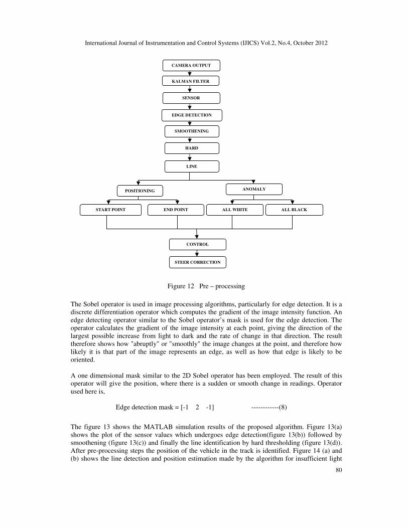
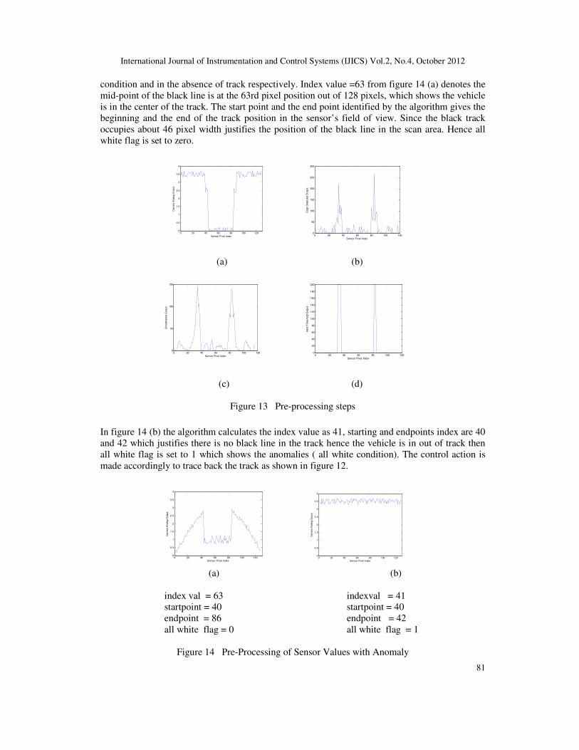
The figure 13 shows the MATLAB simulation results of the proposed algorithm. Figure 13(a) shows the plot of the sensor values which undergoes edge detection(figure 13(b)) followed by smoothening (figure 13(c)) and finally the line identification by hard thresholding (figure 13(d)). After pre-processing steps the position of the vehicle in the track is identified. Figure 14 (a) and (b) shows the line detection and position estimation made by the algorithm for insufficient light

CAMERA OUTPUT

SENSOR

CALIBRATION

EDGE DETECTION

MASK

KALMAN FILTER

SMOOTHENING

MASK

HARD

THRESHOLDING

LINE

IDENTIFICATION

POSITIONING ANOMALY

DETECTION

START POINT

DETECTION

END POINT

DETECTION

ALL WHITE

CONDITION

ALL BLACK

CONDITION

CONTROL

ALGORITHM

STEER CORRECTION


81

condition and in the absence of track respectively. Index value =63 from figure 14 (a) denotes the mid-point of the black line is at the 63rd pixel position out of 128 pixels, which shows the vehicle is in the center of the track. The start point and the end point identified by the algorithm gives the beginning and the end of the track position in the sensor’s field of view. Since the black track occupies about 46 pixel width justifies the position of the black line in the scan area. Hence all white flag is set to zero.

(a) (b)

(c) (d)

Figure 13 Pre-processing steps

In figure 14 (b) the algorithm calculates the index value as 41, starting and endpoints index are 40 and 42 which justifies there is no black line in the track hence the vehicle is in out of track then all white flag is set to 1 which shows the anomalies ( all white condition). The control action is made accordingly to trace back the track as shown in figure 12.

(a) (b)

index val = 63 indexval = 41 startpoint = 40 startpoint = 40 endpoint = 86 endpoint = 42 all white flag = 0 all white flag = 1

Figure 14 Pre-Processing of Sensor Values with Anomaly

0 20 40 60 80 100 1200

50

100

150

200

250

300

Sensor Pixel Index

Edge D

ete

cte

d O

utp

ut

0 20 40 60 80 100 1200

0.5

1

1.5

2

2.5

3

3.5

4

Sensor Pixel Index

Cam

era

Analo

g O

utp

ut

0 20 40 60 80 100 1200

20

40

60

80

100

120

140

160

180

200

Sensor Pixel Index

Hard

Th

resh

old

Outp

ut

0 20 40 60 80 100 1200

50

100

150

Sensor Pixel Index

Sm

ooth

ened O

utp

ut

0 20 40 60 80 100 1200

0.5

1

1.5

2

2.5

3

3.5

4

Sensor Pixel Index

Cam

era

Analo

g O

utp

ut

0 20 40 60 80 100 1200

0.5

1

1.5

2

2.5

3

3.5

4

Sensor Pixel Index

Cam

era

Analo

g O

utp

ut


82

4.2 Lateral Control Algorithm

Two layer control architecture is proposed to manage the steer of the vehicle. The high level layer consists of Kalman filter which is used to act upon the Pre-processed sensor inputs and to generate the necessary steer value [5]. The low level layer is composed of PID controller that receives the high level layer’s command and controls the servo motor. This two level architecture has been organized on the basis of the cascade controlled architecture. Kalman filter, as in section 2 is an adaptive filter and is mainly used where the measurements observed over time contains noise and other inaccuracies.

As depicted in the figure 15, for better steering control, the index value of the black line is obtained from pre-processing techniques and the pre-processed error is then given to the high level control architecture (i.e.) Kalman filter. It eliminates the effect of noise and other disturbances in the input error values and provides with the necessary steer that has to be made for smooth response. The high level architecture’s output is then fed to the low level architecture which has PID controller. PID controller consists of three separate modules namely the Proportional, Derivative and the Integral controller. PID controllers are widely used in feedback control of industrial processes. PID advantages include simplicity, robustness and their familiarity in the field of control applications. The process of selecting the various coefficient values to make a PID controller perform correctly is called PID Tuning [11].

Figure 15 Lateral Control Flow

In figure 15 Ei denote the present error and Ei-1 denote the error of previous iteration. If the absolute value of Ei is greater than the absolute value of Ei-1, the vehicle is deviating away from the track else the vehicle is retracing back to the track. PID controller enhances the steer as done by PI controller when the vehicle is deviating away from the track and diminishes the steer as in

CAMERA OUTPUT

ERROR PRE-PROCESSING

KALMAN FILTER P

E i

> 0 Ei < 0 E i >

E i-1

Ei <

Ei-1

∑

I I

D D

CENTRE STEER VALUE

SERVO STEER VALUE

Y

No

Y Y Y

No

No

No


83

PD controller in-order to make a smooth retrace back to the track once the vehicle is aligned with the track. This filtered and controlled value is the correction that has to be accumulated with the centre PWM value in order to obtain the steer of desired angle. Hence the correction value added with the centre value is given as the PWM duty value for the servo motor thus giving us the required steering action throughout the track with greater accuracy. The presence of Kalman filter also protects the steering action from external disturbances such as varying lighting conditions, sudden flashes and sensor misreading which if otherwise may cause instability to the vehicle and thereby making it to relinquish tracing the track. Thus the two level architecture of Kalman Filter and PID controller manages the lateral control of the autonomous self guided vehicle effectively.

5 LONGITUDINAL CONTROL ORGANIZATION

The longitudinal control of a vehicle includes various aspects regarding the speed of the vehicle. It covers adaptive speed control, adaptive cruise control, platooning and various other techniques. Due to various inescapable reasons the speed of the vehicle might get varied than the expected value for a given input duty cycle of the dc motor. Some major instance that vary the speed of the vehicle is the effect of changes in the power supplied by the battery, variation in the friction produced between the wheels and the track as the vehicle takes a turn, etc. This effect worsens if the vehicle takes a sharp turn. Presence of turns in the track is unavoidable and hence a suitable alternate algorithm has to be developed and employed to overcome this impediment. Thus adaptive speed control becomes mandatory in the automated self guided vehicle.

Figure 16 Current Feedback

The information about the speed of the vehicle during the run is obtained by the current feedback. The current drawn by the dc motor after converting it into digital values using on-chip ADC for various speed levels are as plotted in figure 16. Table 2 and 3 shows the DC motor PWM value under no-load condition and full-load condition for the differential drive DC motors. The present speed of the vehicle is calculated from the feedback current value and compared with the base speed. If the present speed is slower than the base speed PWM is increased iteratively to get the desired speed and vice versa. The proposed adaptive speed control algorithm is shown in figure 17.


84

Table 2 DC Motors drive current

Table 3 Feedback from DC motors

CURRENT FEED BACK VALUES (FROM ADC ( AS HEXA DECIMAL) )

NO LOAD CONDITION

CONDITION ON THE TRACK

LEFT MOTOR ONLY 38 9B

RIGHT MOTOR ONLY 3A A4

DUAL DRIVE (LEFT, RIGHT)

(39, 3C) (9D, A0)

5.1 Adaptive Speed Control Algorithm

The speed of the motors vary involuntarily while making curves due to various reasons such as friction, centripetal force etc. and to compensate the above effect and to make the vehicle be in steady speed during turns, a boosting algorithm is employed as shown in figure 17.

Figure 17 Adaptive Speed Algorithm

LEFT MOTOR (NO LOAD) RIGHT MOTOR (NO LOAD)

DC MOTOR

PWM

CURRENT FEEDBACK

DC MOTOR

PWM

CURRENT FEEDBACK

50 05 h 50 06 h

100 0D h 100 0E h

150 18 h 150 17 h

200 24 h 200 25 h

250 2D h 250 2E h

300 38 h 300 3A h

Y

N

SET BASE SPEED

CURRENT FB

FIND TRUE

TS

>

BS

INCREASE

DUTY CYCLE

SET BASE SPEED

SET DUTY

CYCLE TO BASE

VALUE


85

Table 4 Speed Boost Vs Iteration Table

Boost\

PWM Increment for Iteration

1

2

3

4

5

6

0 BS BS BS BS BS BS

1 BS+5 BS+10 BS+15 BS+20 BS+25 BS+30

2 BS+10 BS+20 BS+30 BS+40 BS+50 BS+60

3 BS+15 BS+30 BS+45 BS+60 BS+75 BS+90

4 BS+20 BS+40 BS+60 BS+80 BS+100 BS+120

5 BS+25 BS+50 BS+75 BS+100 BS+125 BS+150

The table 4 shows how the dc motor’s PWM is varied in order to maintain the constant speed. In the table ‘BS’ denotes the base speed and ‘TS’ the true speed of the vehicle. The ‘Boost’ is computed as the difference between the base speed and the true speed and depending upon the boost value the duty cycle is increased/decreased for every iterations in order to compensate the increase/reduction in speed as in table 4.

Boost = BS – TS New Speed = BS + (Boost * No. of Iterations) The result of employing the boost algorithm rectifies the speed reduction problem. The performance of the above algorithm is shown in the figure 18.

5.2 Adaptive acceleration control algorithm

In order to have efficient performance from the vehicle the acceleration of the vehicle is varied according to the steer error value. The algorithm is similar to adaptive delta algorithm where the delta change is made adaptive to the input signal.


86

Figure 19 Adaptive Acceleration Control Plot

When the correlation between the previous steer values and the present steer value is high and also the error is minimum, then the vehicle is accelerated so as to optimize the speed. Conversely when the correlation among the previous and the present error values is low or the deviation from the track is high, then the vehicle is decelerated to as to optimize the control. Thus both speed and steer control of the vehicle is optimized by the use of adaptive acceleration control algorithm. The graph plotted between the acceleration and the error values is shown in the figure 19.

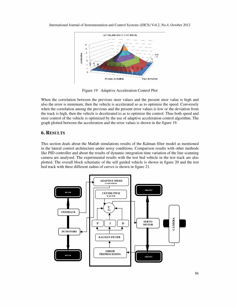
6. RESULTS

This section deals about the Matlab simulations results of the Kalman filter model as mentioned in the lateral control architecture under noisy conditions. Comparison results with other methods like PID controller and about the results of dynamic integration time variation of the line scanning camera are analysed. The experimental results with the test bed vehicle in the test track are also plotted. The overall block schematic of the self guided vehicle is shown in figure 20 and the test bed track with three different radius of curves is shown in figure 21.

ADAPTIVE SPEED

CONTROL

DCMOTORS

ERROR

PREPROCESSING

CA

ME

RA

SERVO

MOTOR

KALMAN FILTER

P I D

∑

REAR

FEEDBACK

CENTRE PWM

VALUE

REAR

FRONT

FRONT


87

Figure 20 Block Schematic of Self Guided Vehicle

Figure 21 Test Bed Track

Figure 22 shows the Kalman filtered output for small and relatively large curves in the track which is simulated using matlab for the proposed model. For smaller curves the sensor value changes is small and the system is smoothly aligned and reaches its zero error position. The same is applicable for sharper curves.

Figure 22 Simulation Results of Kalman Filter for Lateral Error Correction

Thus the Kalman filter smoothens out the sensor values and gives us relatively smooth response for controlling the servo motor which in turn steers the car.


88

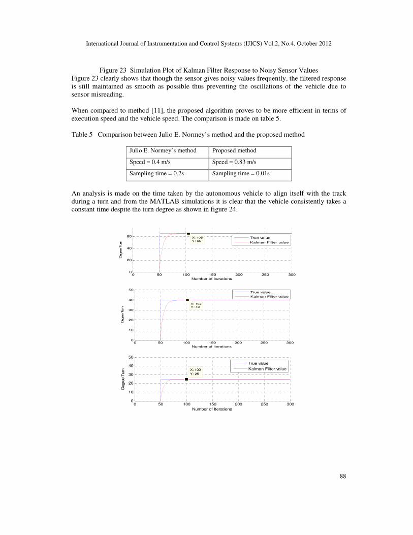
Figure 23 Simulation Plot of Kalman Filter Response to Noisy Sensor Values

Figure 23 clearly shows that though the sensor gives noisy values frequently, the filtered response is still maintained as smooth as possible thus preventing the oscillations of the vehicle due to sensor misreading. When compared to method [11], the proposed algorithm proves to be more efficient in terms of execution speed and the vehicle speed. The comparison is made on table 5. Table 5 Comparison between Julio E. Normey’s method and the proposed method

Julio E. Normey’s method Proposed method

Speed = 0.4 m/s Speed = 0.83 m/s

Sampling time = 0.2s Sampling time = 0.01s

An analysis is made on the time taken by the autonomous vehicle to align itself with the track during a turn and from the MATLAB simulations it is clear that the vehicle consistently takes a constant time despite the turn degree as shown in figure 24.

0 50 100 150 200 250 3000

20

40

60

X: 105

Y: 65

Number of Iterations

Degre

e T

urn

True value

Kalman Filter value

0 50 100 150 200 250 3000

10

20

30

40

50

X: 102

Y: 40


Degre

e T

urn

True value

Kalman Filter value

0 50 100 150 200 250 3000

10

20

30

40

50

X: 100

Y: 25


Degre

e T

urn

True value

Kalman Filter value


89

0 50 100 150 200 250 3000

10

20

30

40

50

X: 101

Y: 9.999


Degre

e T

urn

True value

Kalman Filter value

Figure 24 Number of Iterations to Settle vs. Degree Turn Unlike [11], where the turning time varies with respect to the turn angle, the proposed algorithm maintains almost constant time to turn all kinds of curves however sharp or blunt they might be as shown from figure 24. The time required to turn is given by the number of iterations required to settle multiplied by the time taken for one iteration and in this case the time taken to align with any kind of curve is always nearly 0.5 seconds. This proves that, the proposed method will be of great advantage when a track with multiple sharp curves is encountered. Various tracking methods such as Kalman filter, PID Controller and the proposed method are implemented and their results are compared. The lap completion time is plotted against the duty cycle and the graph is obtained as shown in figure 25. Where * denotes the point from which the car becomes unstable. It is clear from the graph that PID and Kalman becomes unstable as the speed of the car is increased and the proposed model remains stable even at higher speeds.

Figure 25 Results of the Experiment taken in Test Bed Track using Test Vehicle

From the experimental results it has been seen that the proposed method is more stable than other algorithms and it works well even at high speeds where all the other algorithms failed. In Kalman filter based design, the parameter P plays a vital role as it gives the error in the estimation of the state [12]. The value of P should be maintained as low as possible towards 0. Lower the P value towards 0, more accurate the estimated state of the system is, in the proposed model the value of P is around 0.003 which is obtained from test results and it justifies that the proposed model is more accurate.

7. CONCLUSION

Thus from the proposed model, the adaptive sensor calibration technique, adapts to the various light intensity conditions and facilitating the identification of black line from the white


90

background at any intensity level (10 lux – 1000 lux). Pre processing algorithm helps to identify the position and orientation of the vehicle in the track. Kalman filter helps to reduce the environmental noise. PID controller reduces the oscillations and makes the vehicle to track smoothly. The proposed speed control algorithm makes the vehicle to maintain the speed over the entire track. Finally the adaptive acceleration control algorithm optimizes the vehicle speed in straight line and in the curves appropriately. The combination of proposed sensor calibration algorithm, pre-processing algorithm, cascaded Kalman and PID steer control algorithm, adaptive speed and acceleration control algorithm together makes the test bed vehicle to complete the test bed track in a shortest time. The proposed models and algorithms can be extended to real time vehicles by making suitable modifications.

REFERENCES [1] ‘A Case study of Advanced Vehicle Control and Safety Systems’, Systems, Man, and Cybernetics,

1999. IEEE Systems, Man and Cybernetics '99 Conference Proceedings, Tokyo, Japan, (12 October 1999).

[2] A.H. Ismail, H. R. Ramli, M. H. Ahmad, and M. H. Marhaban, 2009 ‘Vision-based System for Line Following Mobile Robot’, 2009 IEEE Symposium on Industrial Electronics and Applications (ISIEA 2009), Kuala Lumpur, Malaysia, (October 4-6, 2009).

[3] Alberto Martin, Hector Marini and Sabri Tosunoglu, ‘Intelligent Vehicle / Highway System: A Survey’, Florida International University, Department of Mechanical Engineering.

[4] Andrisano O., Verdone R., Nakagawa M. 2000 ‘Intelligent Transportation Systems: The Role of Third Generation Mobile Radio Networks’, IEEE Communication Magazine, 38, (9), pp. 144–151.

[5] B.S. Rao, H.F. Durrant-Whyte, 1991 ‘Fully Decentralised algorithm for Multisensory Kalman filtering’, Paper 7901D (C8), IEEE proceedings-d, vol. 138, no.5, (September 1991).

[6] Centennial Engineering, inc., 1992 ‘Survey on Intelligent Vehicle High-way System, Denver metro Area’, for the Coloroda Department of Transportation, (October 1992).

[7] D. Pomerleau, 1995 ‘RALPH: Rapidly adapting lateral position handler’, in Proceedings of IEEE Intelligent Vehicles Symposium, Detroit, MI, pp. 506–511.

[8] European Transport Policy for 2010: Time to Decide, White Paper, Luxembourg: Office for Official Publications of the European Communities, 2001. L-2985.

[9] Frank J. Mammano and J. Richard Bishop Jr., ‘Status of IVHS Technical Developments in the United States’, Turner – Fairbank Highway Research Center, Federal Highway Administration.

[10] Jose E. Naranjo, Carlos González, Ricardo García, Teresa de Pedro, and Rodolfo E. Haber, 2005 ‘Power-Steering Control Architecture for Automatic Driving’, IEEE transactions on Intelligent Transportation Systems, vol. 6, no. 4, (December 2005).

[11] Julio E.Normey-Rico, Ismael Alcal!a, Juan Glomez-Ortega, Eduardo F. Camacho, 2001 ‘Mobile robot path tracking using a robust PID controller’, Control Engineering Practice journal, (September 2001).

[12] Leonie Freeston, ‘Applications of the Kalman Filter Algorithm to Robot Localisation and World Modelling’, Electrical Engineering Final Year Project 2002 University of Newcastle, NSW, Australia.

[13] M. El koursi, Ching-Yao Chan and Wei-Bin Zhang, ‘Preliminary Hazard Analyses’, 2008 IEEE symposium on Intelligent Vehicles, (4th June 2008).

[14] Oscar Laureano Casanova, Fragaria Alfissima, Franz Yupanqui Machaca, 2008 ‘Robot Position Tracking Using Kalman Filter’, Proceedings of the World Congress on Engineering, Vol. II, London, U.K, (July 2 - 4, 2008).

[15] Presentation on Intelligent Transportation System by Beverly Kuhn. [16] S. Kato, S. Tsugawa, K. Tokuda, T.Matsui, and H. Fujiri, 2002 ‘Vehicle control algorithms for

cooperative driving with automated vehicles and inter-vehicle communications’, IEEE Transactions on Intelligent Transportation System, vol. 3, no. 3,pp. 155–161, (September 2002).

[17] S.L. Toral M.R, Martı´nez Torres, F.J. Barrero M.R, Arahal , 2010 ‘Current paradigms in Intelligent Transportation Systems’, IET Intelligent Transport Systems, 12th May 2010.

[18] Sadayuki Tsugawa, Takaharu Saito, Akio Hosaka, ‘Super Smart Vehicle System: AVCS Related Systems for the Future’, AIST, MITI, Toyota Motor Corporation and Nissan Motor Co. Ltd.

[19] Steven E. Shladover, 1993 ‘Research and Development Needs for Advanced Vehicle Control Systems’, Micro IEEE, volume 13, issue 1, (February 1993).


91

[20] Toral S., Vargas M., Barrero F. 2009 ‘Embedded Multimedia Processors for Road-Traffic Parameter Estimation’, Computer, 42, (12), pp. 61–68.

[21] T.C. Goldsmith, Automated Vehicle Guidance (AVCS) – The Real Automobile (online) http://www.azinet.com/articles/real98.htm

[22] Kalman Filter Applications, (online) http://www.cs.auckland.ac.nz/ TeachAuckland.html/ mm/MI63slides.pdf

Documents

VISION BASED AUTONOMOUS LATERAL AND LONGITUDINAL CONTROL ... · VISION BASED AUTONOMOUS LATERAL AND LONGITUDINAL CONTROL ... Kalman filter with PID steer control ... are used to guide