Capturing Market Dynamics Rolf Riedi - Rice Universityriedi/Publ/TALKS/Riedi-TUK-FinanceWeb.pdf · Capturing Market Dynamics ... Mandelbrot’s cascades and beyond. • Muzy et al

Capturing Market Dynamics

Stochastic Systems and Modelling in Networking and FinancePart V

Dependable Adaptive Systems and Mathematical ModelingKaiserslautern, August 2006

Rolf Riedi

Dept of Statistics

Market models

The ongoing discussionabout the role of

LRD, fBm and cascades in Financial data

Rudolf Riedi Rice University stat.rice.edu/~riedi

History

• Bachelier 1900– Computes “Barrier Option” for price modeled by Brownian motion

• Mandelbrot 1962: – self-similarity of Cotton prices

• Samuelson– Foundations of Economic Analysis (1947)– keep only minumum of simple economic relations; – rewrite it as a constrained optimization problem.

• Black-Scholes(’73)-Merton(’70s) (Nobel 1997)– Log returns are BM (returns are geometric Brownian motion)– Derive partial differential equation for option price

• Girsanov (’60) theorem– Equivalent martingale measure (pricing measure) simplifies the

computation of option prices

• Engle (Nobel 2003) – ARCH, Cond.Duration and other time series models


Ongoing

• Estimating Fractal Dimension Of S&P 500 Using Wavelet Analysis • Bayraktar, Poor, Sircar 2003

• Dynamics of financial markets – Mandelbrot’s cascades and beyond.

• Muzy et al 2005

• London Stock Exchange: signs of orders obey LRD with H = 0.7. – This would suggest a very strong market inefficiency.– However, compensated for by anti-correlated fluctuations in

transaction size and liquidity• Lillo, Farmer 2004

• Why Stock Markets Crash – Local logarithmic chirps

• Sornette


fBm and arbitrage

• Arbitrage strategy for Black-Scholes model driven by – fractional Brownian motion or – by a time changed fractional Brownian motion, – when the volatility is stochastic.

• Bayraktar, Poor 2005

– fBm is not semi-martingale, nor a Markov process– Black-Scholes differential equation not well-defined– No equivalent martingale measure for fBm, and therefore in a

frictionless market where continuous trading is possible there exist arbitrage strategies.


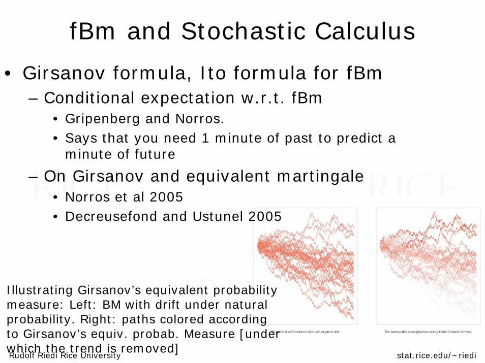
fBm and Stochastic Calculus

• Girsanov formula, Ito formula for fBm– Conditional expectation w.r.t. fBm

• Gripenberg and Norros. • Says that you need 1 minute of past to predict a

minute of future

– On Girsanov and equivalent martingale• Norros et al 2005• Decreusefond and Ustunel 2005

Illustrating Girsanov’s equivalent probability measure: Left: BM with drift under naturalprobability. Right: paths colored according to Girsanov’s equiv. probab. Measure [underwhich the trend is removed]

Conclusion: we need

• Estimation proceduresFor LRD and multifractal scaling

• new improved models

Multifractal estimation

Large DeviationsMultifractal formalismLegendre transform


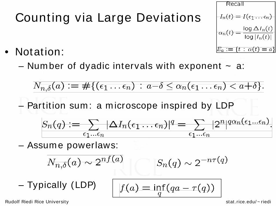
Counting via Large Deviations

• Notation:– Number of dyadic intervals with exponent ~ a:

– Partition sum: a microscope inspired by LDP

– Assume powerlaws:

– Typically (LDP)


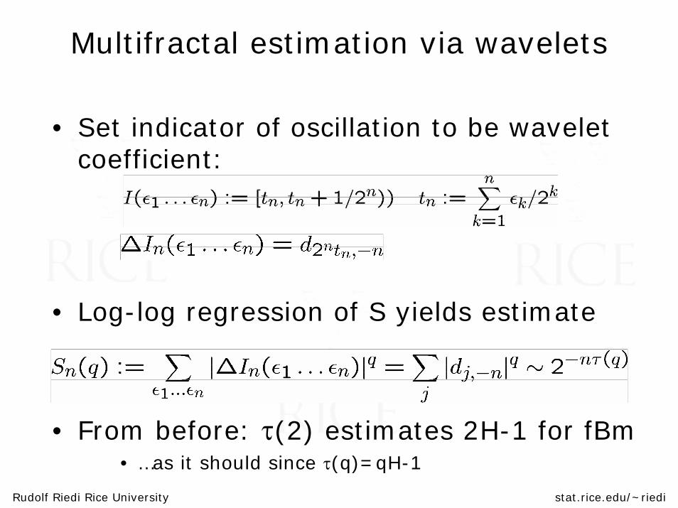
Multifractal estimation via wavelets

• Set indicator of oscillation to be wavelet coefficient:

• Log-log regression of S yields estimate

• From before: τ(2) estimates 2H-1 for fBm• …as it should since τ(q)=qH-1

fBm simulation


Fractional ARIMA

• Recall the definition which allows for sequential simulation

• …and has simpler spectral density than fGn


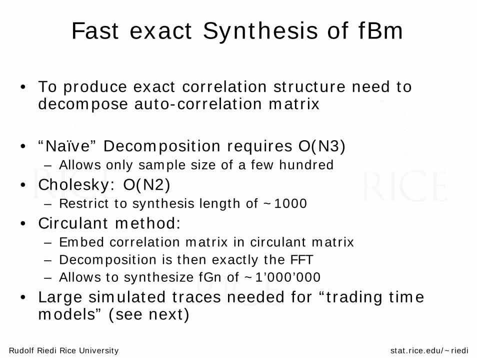
Fast exact Synthesis of fBm

• To produce exact correlation structure need to decompose auto-correlation matrix

• “Naïve” Decomposition requires O(N3)– Allows only sample size of a few hundred

• Cholesky: O(N2)– Restrict to synthesis length of ~1000

• Circulant method: – Embed correlation matrix in circulant matrix– Decomposition is then exactly the FFT– Allows to synthesize fGn of ~1’000’000

• Large simulated traces needed for “trading time models” (see next)

Multifractal Subordination

Processes with multifractal oscillations


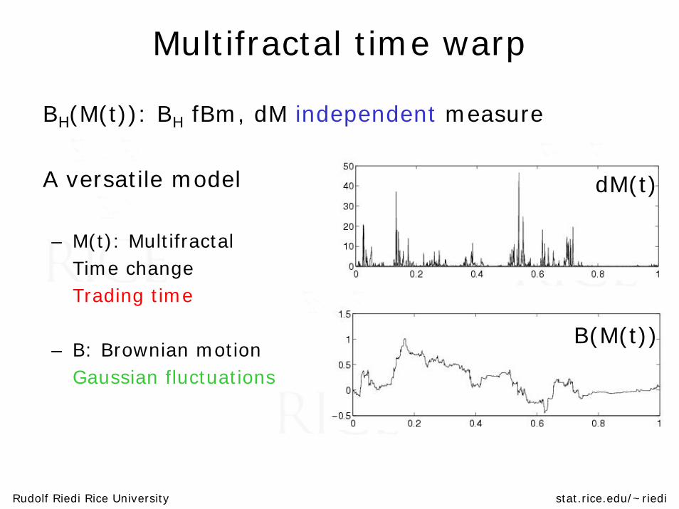
Multifractal time warp

BH(M(t)): BH fBm, dM independent measure

A versatile model

– M(t): MultifractalTime changeTrading time

– B: Brownian motionGaussian fluctuations

dM(t)

B(M(t))


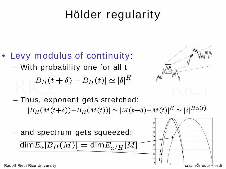
Hölder regularity

• Levy modulus of continuity:– With probability one for all t

– Thus, exponent gets stretched:

– and spectrum gets squeezed:


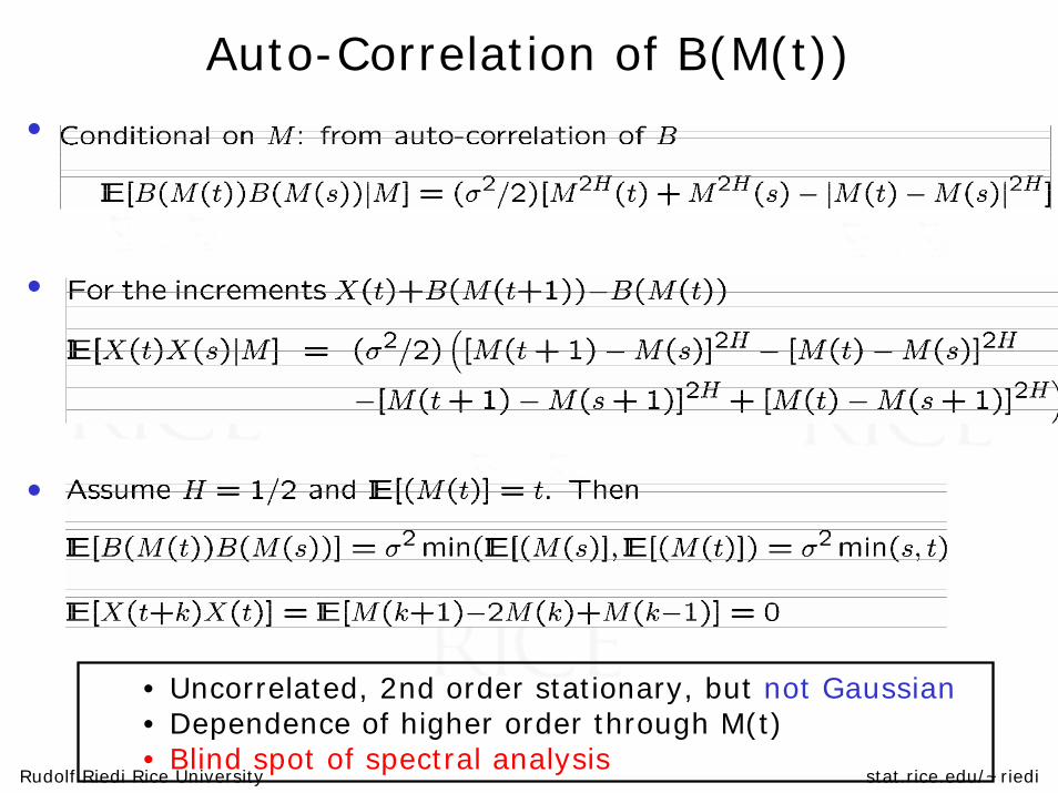
Auto-Correlation of B(M(t))

•

•

•

• Uncorrelated, 2nd order stationary, but not Gaussian• Dependence of higher order through M(t)• Blind spot of spectral analysis


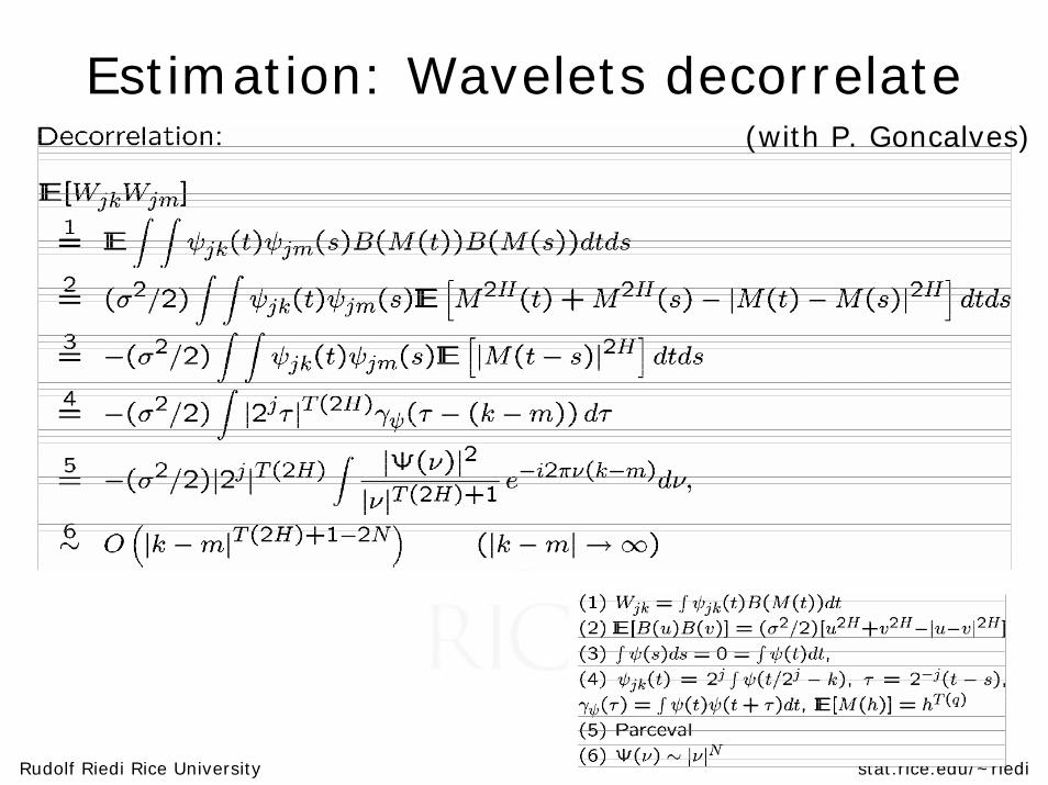
Estimation: Wavelets decorrelate(with P. Goncalves)


Multifractal Estimation for B(M(t))

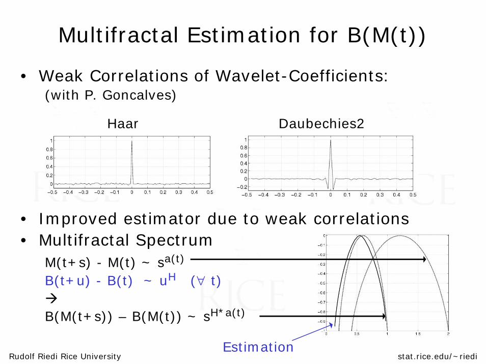
• Weak Correlations of Wavelet-Coefficients:(with P. Goncalves)

Haar Daubechies2

• Improved estimator due to weak correlations• Multifractal Spectrum

M(t+s) - M(t) ~ sa(t)

B(t+u) - B(t) ~ uH (∀ t)

B(M(t+s)) – B(M(t)) ~ sH*a(t)

Estimation


Multifractal time in Zoology

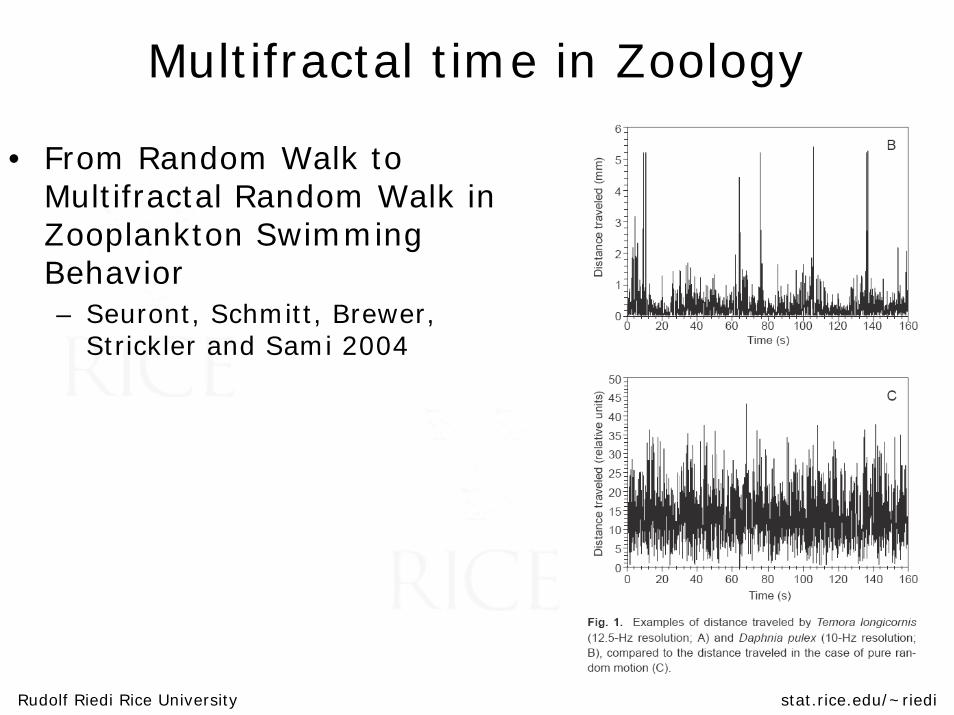
• From Random Walk to Multifractal Random Walk in Zooplankton Swimming Behavior– Seuront, Schmitt, Brewer,

Strickler and Sami 2004

Tail estimation

And diverging moments


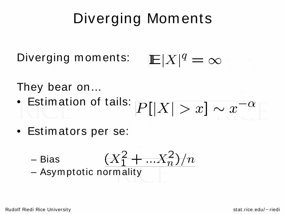
Diverging Moments

Diverging moments:

They bear on…• Estimation of tails:

• Estimators per se:

– Bias– Asymptotic normality

Theory


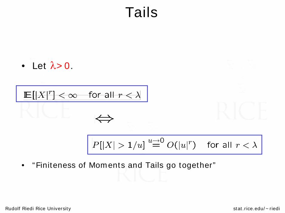
Tails

• Let λ>0.

• “Finiteness of Moments and Tails go together”


Characteristic function 101

• Characteristic function:

• Char Fct and Moments 101: If E|X|n is exists then

• Vice versa: If φ has 2p derivates then E|X|2p exists


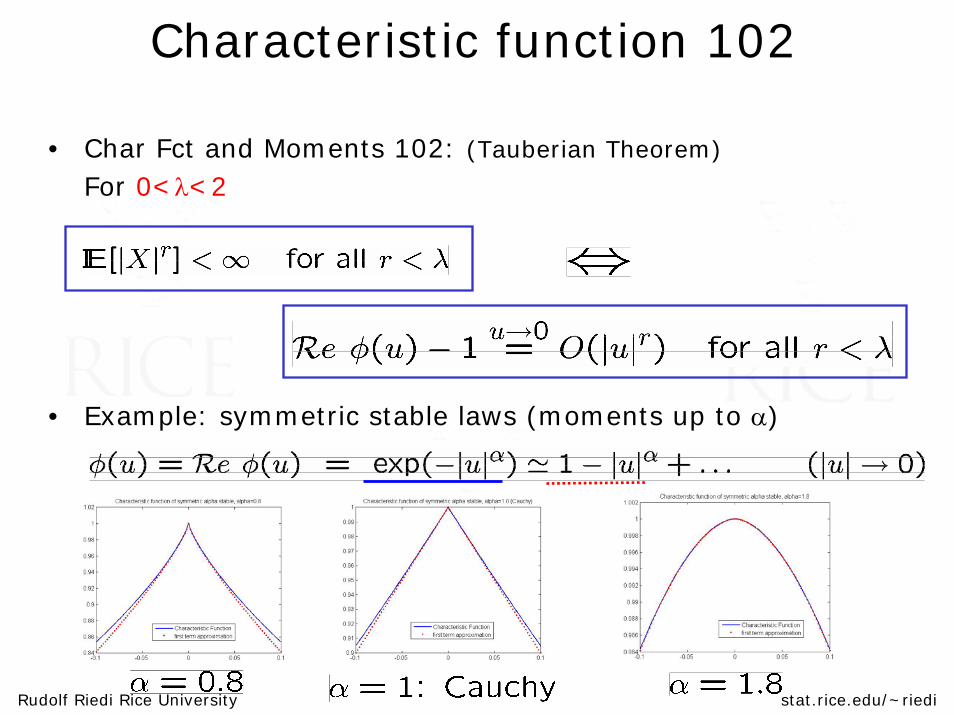
Characteristic function 102

• Char Fct and Moments 102: (Tauberian Theorem)

For 0<λ<2

• Example: symmetric stable laws (moments up to α)


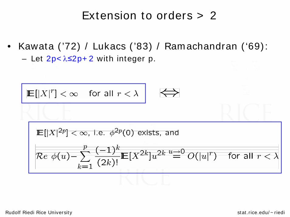
Extension to orders > 2

• Kawata (’72) / Lukacs (’83) / Ramachandran (‘69): – Let 2p<λ≤2p+2 with integer p.


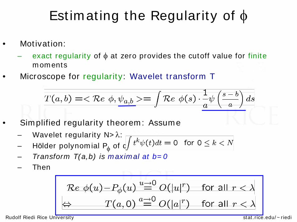
Estimating the Regularity of φ

• Motivation: – exact regularity of φ at zero provides the cutoff value for finite

moments

• Microscope for regularity: Wavelet transform T

• Simplified regularity theorem: Assume– Wavelet regularity N>λ:– Hölder polynomial Pφ of degree ≤N– Transform T(a,b) is maximal at b=0– Then


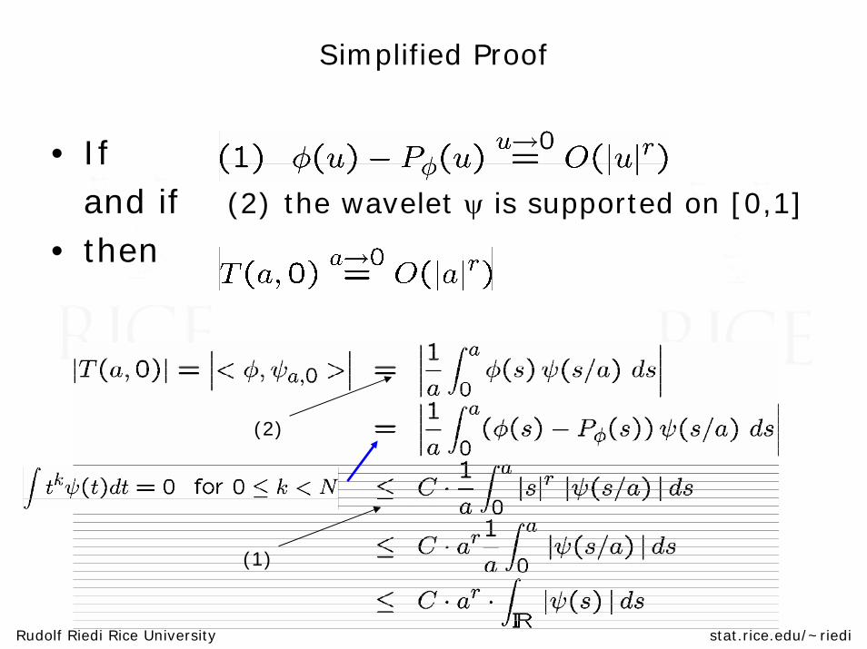
Simplified Proof

• If and if (2) the wavelet ψ is supported on [0,1]

• then

(2)

(1)


Wavelet Transform of φ• Fourier transform:

• Parseval:

• Assume: Fourier Transform Ψ of ψ is real positive.– then:

– in other words: |T(a,b)| maximal at b=0

• Ex:


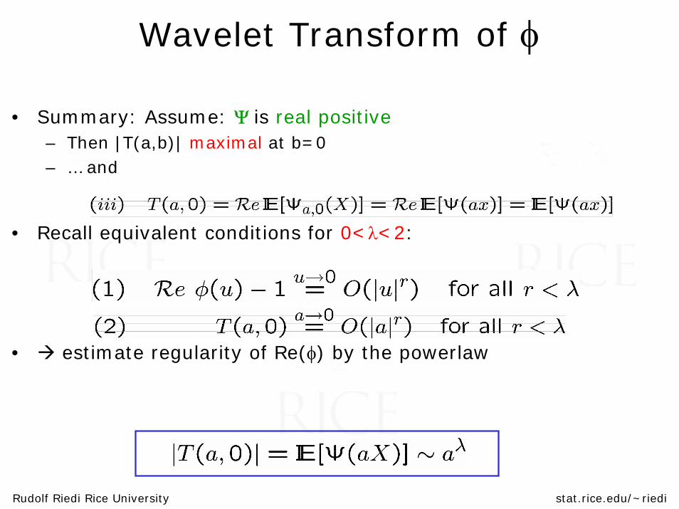
Wavelet Transform of φ

• Summary: Assume: Ψ is real positive– Then |T(a,b)| maximal at b=0– … and

• Recall equivalent conditions for 0<λ<2:

• estimate regularity of Re(φ) by the powerlaw

Implementationand

Performance


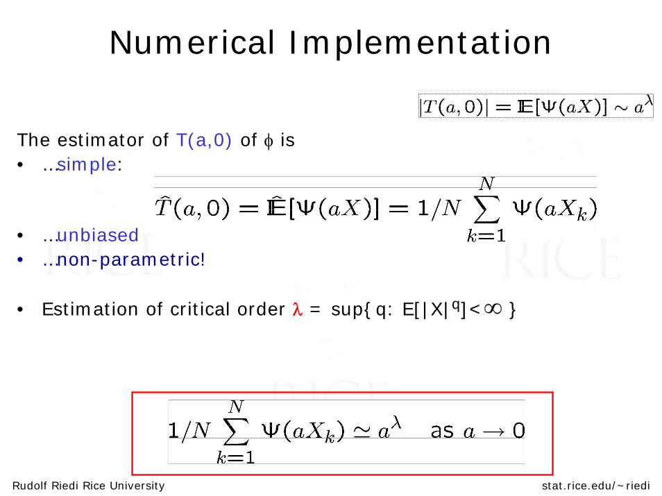
Numerical Implementation

The estimator of T(a,0) of φ is• …simple:

• …unbiased• …non-parametric!

• Estimation of critical order λ = sup{q: E[|X|q]<∞ }


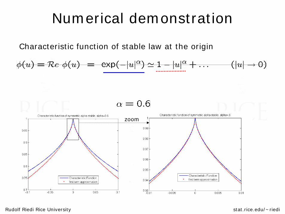
Numerical demonstration

Characteristic function of stable law at the origin

zoom


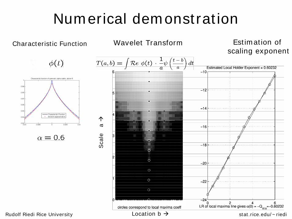
Numerical demonstrationWavelet Transform Estimation of

scaling exponent

Sca

le a

Location b

Characteristic Function


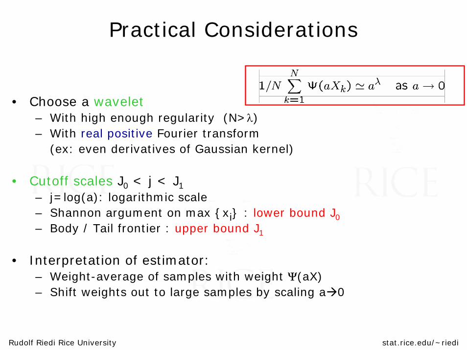
Practical Considerations

• Choose a wavelet– With high enough regularity (N>λ)– With real positive Fourier transform

(ex: even derivatives of Gaussian kernel)

• Cutoff scales J0 < j < J1– j=log(a): logarithmic scale– Shannon argument on max {xi} : lower bound J0

– Body / Tail frontier : upper bound J1

• Interpretation of estimator:– Weight-average of samples with weight Ψ(aX)– Shift weights out to large samples by scaling a 0


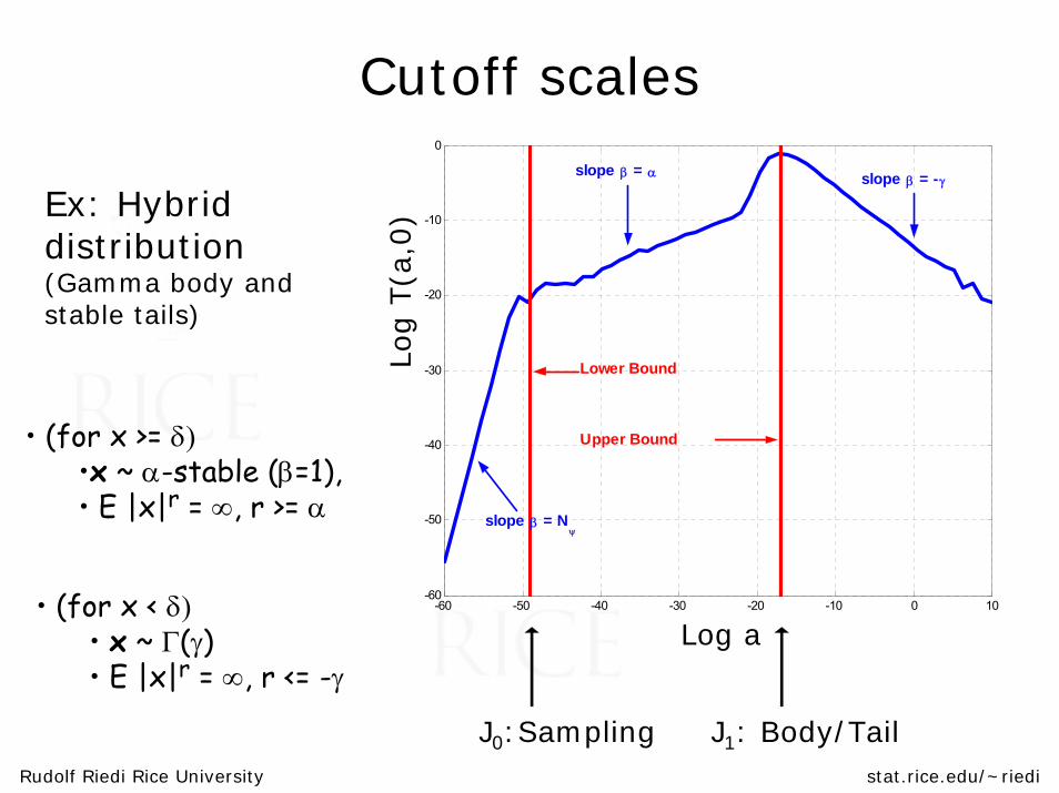
Cutoff scales

Ex: Hybrid distribution(Gamma body and stable tails)

• (for x < δ)• x ~ Γ(γ)• E |x|r = ∞, r <= -γ

-60 -50 -40 -30 -20 -10 0 10-60

-50

-40

-30

-20

-10

0

Lower Bound

Upper Bound

slope β = α slope β = -γ

slope β = Nψ

Log T

(a,0

)

Log a

• (for x >= δ)•x ~ α-stable (β=1), • E |x|r = ∞, r >= α

J0:Sampling J1: Body/Tail


Competing for stable parameter

Alpha-stable Laws:• compare with Koutrouvelis’80 and McCullogh’86 are parametric (stable distribution)• non-parametric wavelet based estimator is

• competitive• especially for intermediate to small a

αα

λ

α± ± ± ± ±

± ± ± ±

± ± ± ± ±

Wavelet based


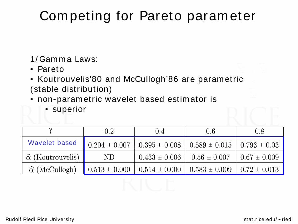
Competing for Pareto parameter

γ

Wavelet based

αα

± ± ± ±

± ± ±

± ± ±±

1/Gamma Laws:• Pareto• Koutrouvelis’80 and McCullogh’86 are parametric (stable distribution)• non-parametric wavelet based estimator is

• superior

Model identification

…through scaling of moments


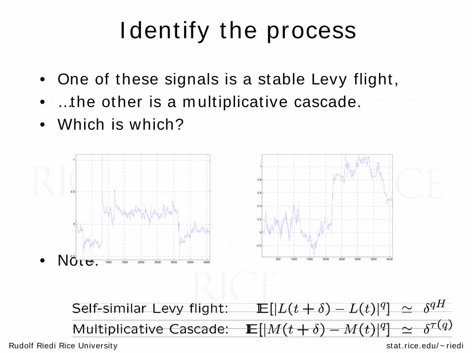
Identify the process

• One of these signals is a stable Levy flight,• …the other is a multiplicative cascade.• Which is which?

• Note:500 1000 1500 2000 2500 3000 3500 4000

-0.5

0

0.5

1

500 1000 1500 2000 2500 3000 3500 4000

-0.2

0

0.2

0.4

0.6

0.8

1


1000 2000 3000 4000 5000 6000 7000 8000

10

20

30

40

50

60

1000 2000 3000 4000 5000 6000 7000 8000

10

20

30

40

50

60

1000 2000 3000 4000 5000 6000 7000 8000

10

20

30

40

50

60

1000 2000 3000 4000 5000 6000 7000 8000

10

20

30

40

50

60

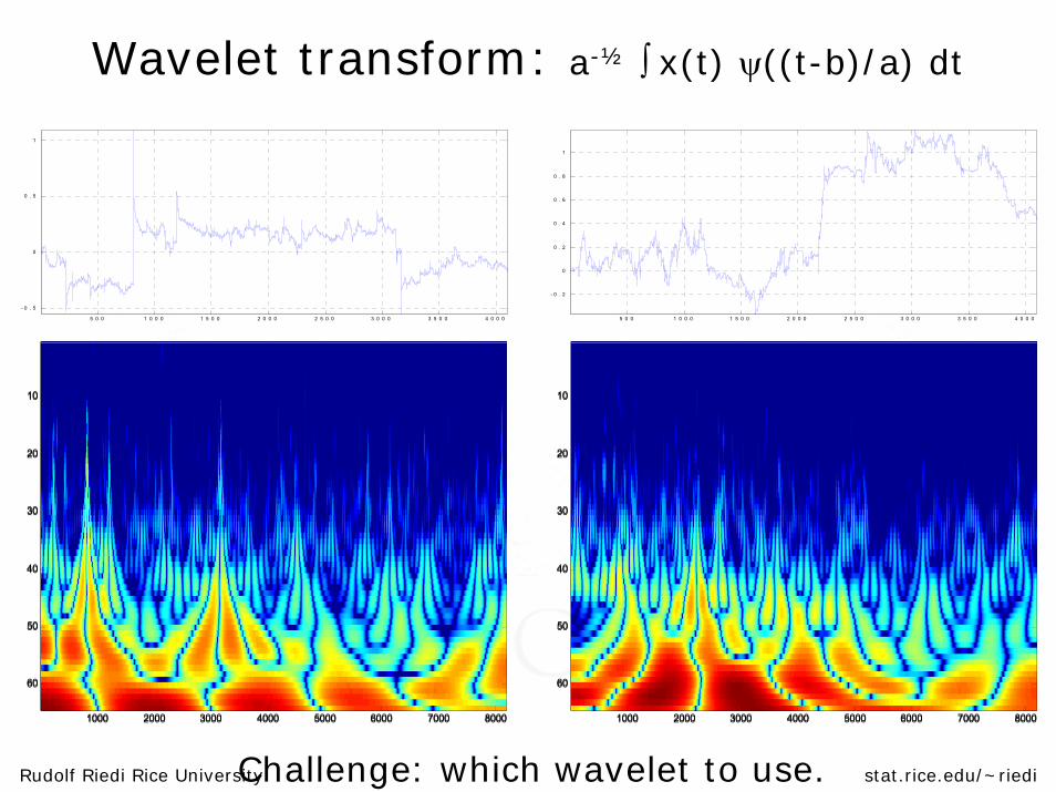
Wavelet transform: a-½ ∫ x(t) ψ((t-b)/a) dt

5 0 0 1 0 0 0 1 5 0 0 2 0 0 0 2 5 0 0 3 0 0 0 3 5 0 0 4 0 0 0

- 0 . 5

0

0 . 5

1

5 0 0 1 0 0 0 1 5 0 0 2 0 0 0 2 5 0 0 3 0 0 0 3 5 0 0 4 0 0 0

- 0 . 2

0

0 . 2

0 . 4

0 . 6

0 . 8

1

Challenge: which wavelet to use.


Estimating

0 1 2 3 4 5 6-1 5

-1 0

-5

0

5

1 0

00 . 5 11 . 5 22 . 5 33 . 5 44 . 5 5

0 1 2 3 4 5 6-5 0

-4 0

-3 0

-2 0

-1 0

0

1 0

2 0

00 . 5 11 . 5 22 . 5 33 . 5 44 . 5 5

S(a,q), q>0 S(a,q), q>0

0 1 2 3 4 5 60

5

1 0

1 5

2 0

2 5

3 0 - 5-4 . 5 - 4-3 . 5 - 3-2 . 5 - 2-1 . 5 - 1-0 . 5 0

0 1 2 3 4 5 6-5

0

5

1 0

1 5

2 0

2 5

3 0

3 5

4 0 - 5-4 . 5 - 4-3 . 5 - 3-2 . 5 - 2-1 . 5 - 1-0 . 5 0

S(a,q), q<0 S(a,q), q<0

Challenge: which orders to use.


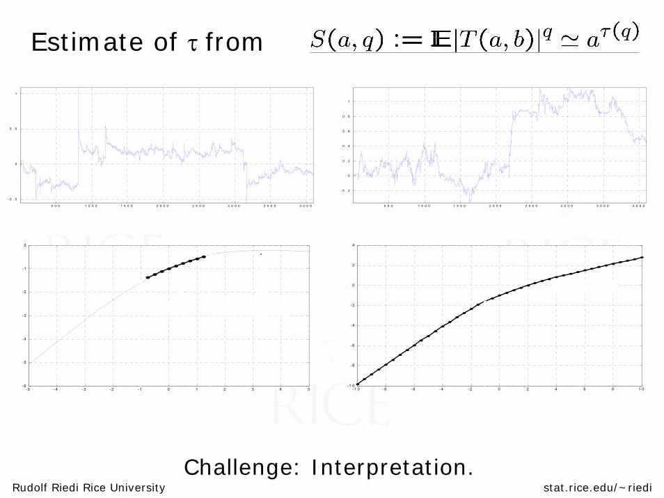
Estimate of τ from

Challenge: Interpretation.

5 0 0 1 0 0 0 1 5 0 0 2 0 0 0 2 5 0 0 3 0 0 0 3 5 0 0 4 0 0 0

- 0 . 5

0

0 . 5

1

5 0 0 1 0 0 0 1 5 0 0 2 0 0 0 2 5 0 0 3 0 0 0 3 5 0 0 4 0 0 0

- 0 . 2

0

0 . 2

0 . 4

0 . 6

0 . 8

1

- 5 - 4 - 3 - 2 - 1 0 1 2 3 4 5- 6

- 5

- 4

- 3

- 2

- 1

0

τ ( q ) = H q θ ( q ) = 1 - q ( H - 1 / α )

- 1 0 - 8 - 6 - 4 - 2 0 2 4 6 8 1 0- 1 0

- 8

- 6

- 4

- 2

0

2

4

λ + + ∞


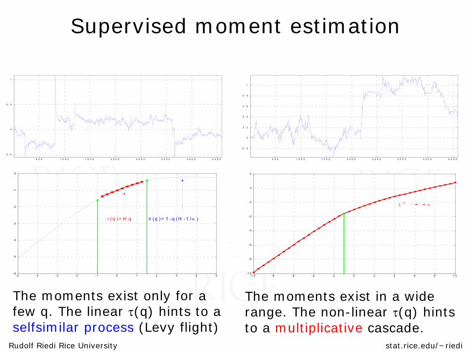
Supervised moment estimation

The moments exist only for a few q. The linear τ(q) hints to a selfsimilar process (Levy flight)

- 5 - 4 - 3 - 2 - 1 0 1 2 3 4 5- 6

- 5

- 4

- 3

- 2

- 1

0

τ ( q ) = H q θ ( q ) = 1 - q ( H - 1 / α )

- 1 0 - 8 - 6 - 4 - 2 0 2 4 6 8 1 0- 1 0

- 8

- 6

- 4

- 2

0

2

4

λ + + ∞

The moments exist in a wide range. The non-linear τ(q) hints to a multiplicative cascade.

5 0 0 1 0 0 0 1 5 0 0 2 0 0 0 2 5 0 0 3 0 0 0 3 5 0 0 4 0 0 0

- 0 . 5

0

0 . 5

1

5 0 0 1 0 0 0 1 5 0 0 2 0 0 0 2 5 0 0 3 0 0 0 3 5 0 0 4 0 0 0

- 0 . 2

0

0 . 2

0 . 4

0 . 6

0 . 8

1

Documents

Capturing Market Dynamics Rolf Riedi - Rice Universityriedi/Publ/TALKS/Riedi-TUK-FinanceWeb.pdf · Capturing Market Dynamics ... Mandelbrot’s cascades and beyond. • Muzy et al