CAPITAL MARKET EXPECTATIONS - Research … | CAPITAL MARKET EXPECTATIONS This expected returns forecasting starts with the asset classes of most interest to investors (which also happen

CAPITAL MARKET EXPECTATIONS

Methodology Overview

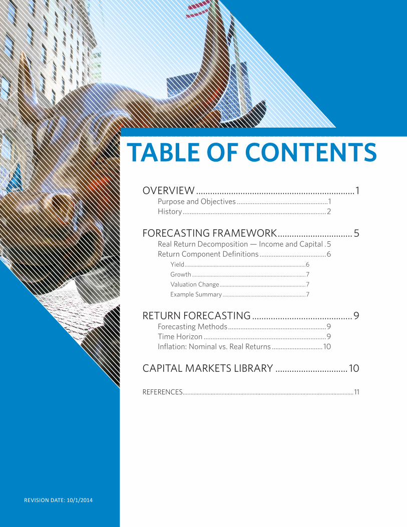
TABLE OF CONTENTSOVERVIEW .................................................................... 1

Purpose and Objectives ....................................................1History ..................................................................................2

FORECASTING FRAMEWORK ................................ 5Real Return Decomposition — Income and Capital .5Return Component Definitions ......................................6

Yield ...................................................................................6Growth ..............................................................................7Valuation Change ...........................................................7Example Summary .........................................................7

RETURN FORECASTING ...........................................9Forecasting Methods ........................................................9Time Horizon ......................................................................9Inflation: Nominal vs. Real Returns ............................. 10

CAPITAL MARKETS LIBRARY ............................... 10

REFERENCES .............................................................................................................. 11

REVISION DATE: 10/1/2014

“We understand that some of our insights will never find their way into products, but we provide them in support of investors and the finance community.”

— ROB ARNOTTCHAIRMAN & CEO

CAPITAL MARKET EXPECTATIONS | 1

Purpose and Objectives

Sharing our insights is one of the core tenets of Research Affiliates’ philosophy and a key part of our mission. We strive to fill gaps in the marketplace when we think our insights will be useful to investors. We saw such a gap

with respect to long-term capital market expectations by asset class, and decided to undertake the task of making such expectations freely available to the investor community. In undertaking this initiative, we did so with three criteria in mind: 1) transparency, 2) robustness, and 3) timeliness.

In addition to sharing our capital market expectations, we think it’s important to explain the conceptual framework and the calculations behind those results. This is the focus of this document and others in the white paper library. Too often in modern finance, results come from black-box models. The black-box approach is detrimental both to the model creators, who can never receive feedback to improve the model, and to the end users, who never have an understanding of the assumptions underlying their activities. That being said, achieving sufficient transparency, without inundating the reader with unnecessary information, is not easy. We, therefore, realize the correct level of detail is something that will be reached over time as we work with our clients to gain feedback.

The objective of robustness does not mean that our models will include, or attempt to address, every new finding or complexity that comes up in the study and practice of finance. In fact, the opposite is true: We wish to focus on building simple, economically sound models that are suitable for forecasting with a long-term timeframe in mind. We strive to adhere to a principle attributed to Albert Einstein: “Everything must be made as simple as possible, but not simpler.” We will then continually review our models to look for areas where they can be improved. When such areas are discovered, our methodology will adapt and continually become more efficacious.

Being timely means that we want to provide updates to our capital market expectations at a frequency that is useful to our readers. Initially this will be quarterly, but may change in the future.

The remainder of this document explains how we think about asset class returns from a building block perspective, and provides transparency into the methods employed to develop these return expectations.

OVERVIEW

2 | CAPITAL MARKET EXPECTATIONS

This expected returns forecasting starts with the asset classes of most interest to investors (which also happen to be the most liquid). Over time this list will undoubtedly expand to cover less liquid asset classes. For now, there are five asset class groups:

• Domestic & Foreign Cash: Short-term cash instruments • Fixed Income• Equity• Real Estate Investment Trusts (REITS)• Commodities

History

Before developing a model for future expected returns, it is important to revisit the recent past. Figure 1 shows the real return and risk of 15 asset classes over the past 25 years. These 15 asset classes, which we

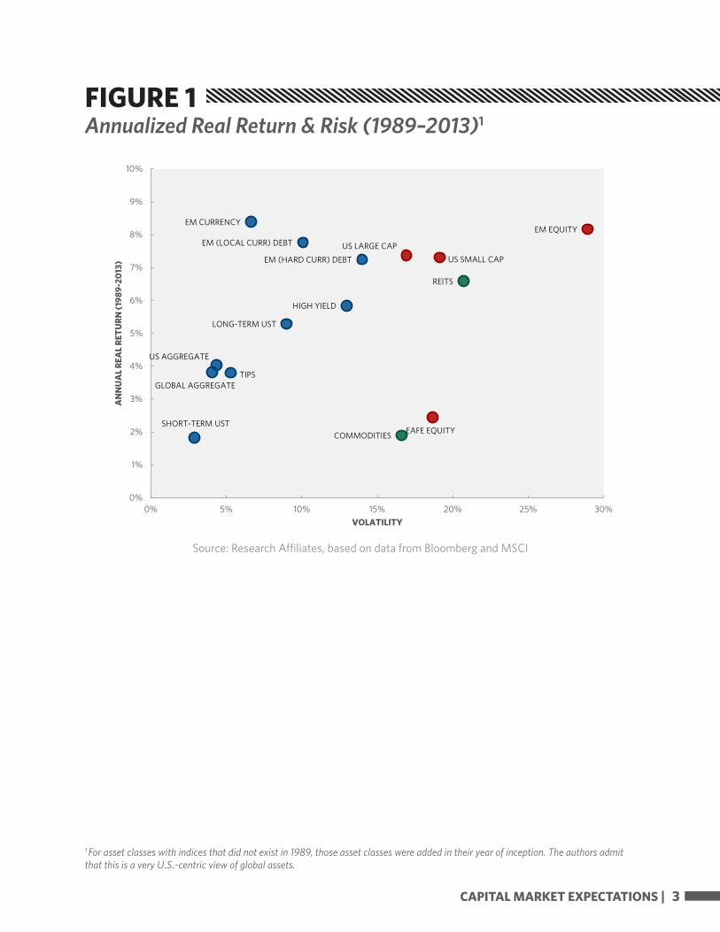
will refer to as the Core Asset Classes, were chosen to give a broad overview of the investment universe. They are represented by the industry indices listed in Table 1. In cases where the representative index has not been in existence for 25 years, the values in the chart represent the risk and return since the inception of the index.

From Figure 1 , it’s clear that over half the asset classes had a real return greater than 5%. Add inflation of 2.5% to that real return, and it’s clear why many investors choose a nominal 7% discount rate (future return expectation) for their portfolios. If past were prologue, the story would end here, with future expected returns taken directly from this chart; however, it’s not hard to imagine a future world very different from that of the last 25 years. Low, and often negative, real interest rates, continued development of emerging and frontier markets, and rising debt levels across the globe, among a slew of other differences, mean there is good reason to expect the next 25 years to differ greatly from the recent past.

Given that past is not prologue, it is imperative to construct a framework with which to estimate future capital market expectations. The foremost objective in creating an asset allocation framework is internal consistency in the treatment of each asset class. It is very difficult, if not impossible, to create a model that results in perfect absolute forecasts, but if the model is internally consistent, the results will allow for relative comparison between asset classes, even if the estimated absolute returns prove to be inaccurate. Therefore, in constructing the asset allocation framework, we use a structural approach that clearly defines the economic drivers of return and risk for each asset class. Regarding the impetus for a structural approach, Nevo and Whinston (2010, page 71) had this to say:

“When sources of credible identification are available, structural modeling can provide a way to extrapolate observed responses to environmental changes to predict responses to other not-yet-observed changes. In an ideal research environment, this would be unnecessary….Unfortunately, the real world is not always so ideal. The change we are interested in may literally never have occurred before, and even if it has, it may have been in different circumstances, so the previously observed effects may not provide a good prediction of the current one.Structural analysis gives us a way to relate observations of responses to changes in the past to predict the responses to different changes in the future.”

Following a structural approach also leads to sensible, economically understandable results that can ultimately be used to make long-term strategic portfolio construction and management decisions.


US LARGE CAPUS SMALL CAP

EAFE EQUITY

EM EQUITY

SHORT-TERM UST

LONG-TERM UST

HIGH YIELD

US AGGREGATE

GLOBAL AGGREGATE

EM (HARD CURR) DEBT

EM (LOCAL CURR) DEBT

EM CURRENCY

TIPS

REITS

COMMODITIES

0%

1%

2%

3%

4%

5%

6%

7%

8%

9%

10%

0% 5% 10% 15% 20% 25% 30%

AN

NU

AL

REA

L RE

TURN

(198

9-20

13)

VOLATILITY

Source: Research Affiliates, based on data from Bloomberg and MSCI

FIGURE 1Annualized Real Return & Risk (1989–2013)1

1 For asset classes with indices that did not exist in 1989, those asset classes were added in their year of inception. The authors admit that this is a very U.S.-centric view of global assets.


Asset Class Representative Index Inception Date

Commodities Bloomberg Commodity 1991

EAFE Equity MSCI EAFE 1970

Emerging Mkt Equity MSCI Emerging Markets 1988

Emerging Mkt Currency JP Morgan ELMI+ 1994

Emerging Mkt (Hard Currency) Debt JP Morgan EMBI+ 1994

Emerging Mkt (Local Currency) Debt JP Morgan GBI-EM 2002

Global Aggregate Barclays Global Aggregate 1990

High Yield Barclays High Yield 1983

Long-Term UST Barclays US Treasury Long 1990

REITs FTSE NAREIT 1972

Short-Term UST Barclays 1-3Yr US Treasury 1992

TIPS Barclays US TIPS 1997

US Aggregate Barclays US Aggregate 1976

US Large Cap Equity S&P 500 (TR index) 1926

US Small Cap Equity Russell 2000 1979

Source: Research Affiliates

TABLE 1Asset Class Representative Indices


Forecasting FrameworkThe goal of any sound forecasting framework is to identify the set of intuitive, mutually exclusive, cumulatively

exhaustive (MECE) components which collectively capture the drivers of change in the dependent target. The overall framework employed here for forecasting returns is based on the fundamental drivers of income and capital change of an investment. To motivate the idea that the chosen set of building blocks achieves this goal, we can work backwards by decomposing realized total return into its component parts.

Real Return Decomposition — Income and Capital

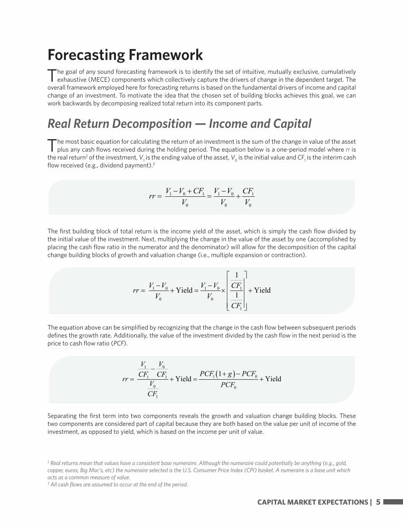
The most basic equation for calculating the return of an investment is the sum of the change in value of the asset plus any cash flows received during the holding period. The equation below is a one-period model where rr is

the real return2 of the investment, V1 is the ending value of the asset, V0 is the initial value and CF1 is the interim cash flow received (e.g., dividend payment).3

The first building block of total return is the income yield of the asset, which is simply the cash flow divided by the initial value of the investment. Next, multiplying the change in the value of the asset by one (accomplished by placing the cash flow ratio in the numerator and the denominator) will allow for the decomposition of the capital change building blocks of growth and valuation change (i.e., multiple expansion or contraction).

The equation above can be simplified by recognizing that the change in the cash flow between subsequent periods defines the growth rate. Additionally, the value of the investment divided by the cash flow in the next period is the price to cash flow ratio (PCF).

Separating the first term into two components reveals the growth and valuation change building blocks. These two components are considered part of capital because they are both based on the value per unit of income of the investment, as opposed to yield, which is based on the income per unit of value.

2 Real returns mean that values have a consistent base numeraire. Although the numeraire could potentially be anything (e.g., gold, copper, euros, Big Mac’s, etc) the numeraire selected is the U.S. Consumer Price Index (CPI) basket. A numeraire is a base unit which acts as a common measure of value.3 All cash flows are assumed to occur at the end of the period.

( )01

1 01 1

0 0

1

1 Yield Yield

VVPCF g PCFCF CFrr V PCF

CF

−+ −

= + = +

1 0 1 1 0 1

0 0 0

V V CF V V CFrrV V V

− + −= = +

1 0 1 0 1

0 0

1

1

Yield Yield1V V V V CFrr

V VCF

− − = + = × +


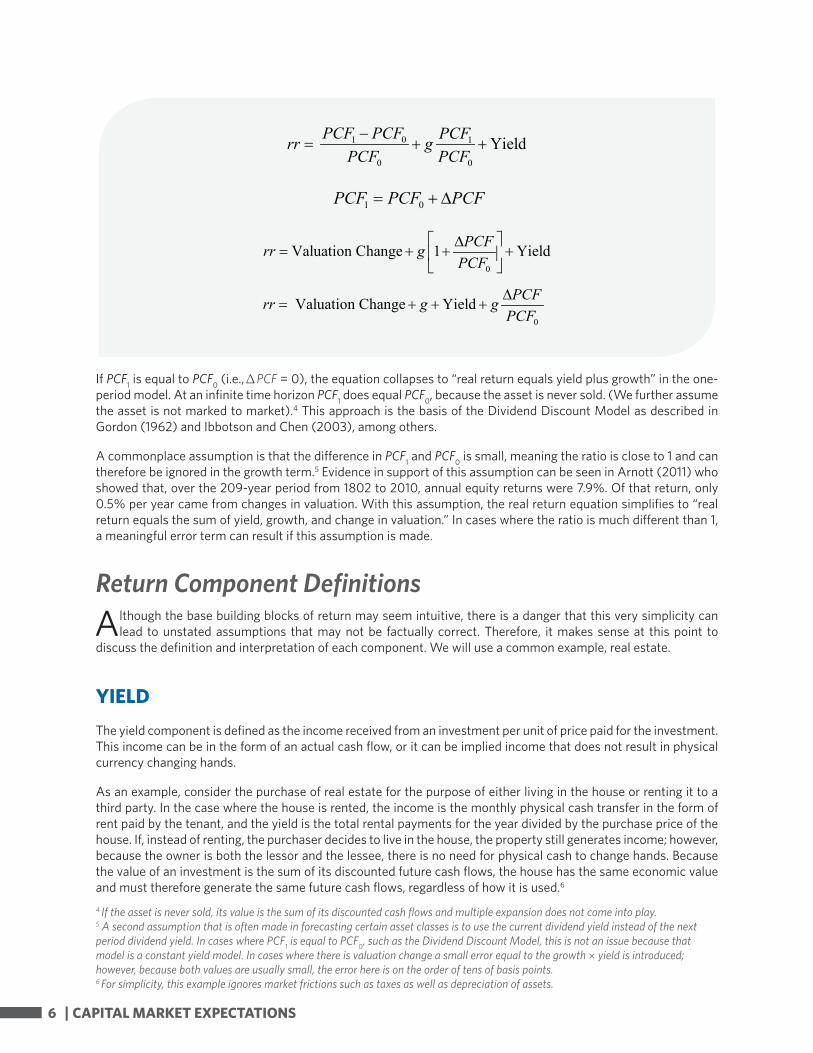
If PCF1 is equal to PCF0 (i.e.,∆ PCF = 0), the equation collapses to “real return equals yield plus growth” in the one-period model. At an infinite time horizon PCF1 does equal PCF0, because the asset is never sold. (We further assume the asset is not marked to market).4 This approach is the basis of the Dividend Discount Model as described in Gordon (1962) and Ibbotson and Chen (2003), among others.

A commonplace assumption is that the difference in PCF1 and PCF0 is small, meaning the ratio is close to 1 and can therefore be ignored in the growth term.5 Evidence in support of this assumption can be seen in Arnott (2011) who showed that, over the 209-year period from 1802 to 2010, annual equity returns were 7.9%. Of that return, only 0.5% per year came from changes in valuation. With this assumption, the real return equation simplifies to “real return equals the sum of yield, growth, and change in valuation.” In cases where the ratio is much different than 1, a meaningful error term can result if this assumption is made.

Return Component Definitions

Although the base building blocks of return may seem intuitive, there is a danger that this very simplicity can lead to unstated assumptions that may not be factually correct. Therefore, it makes sense at this point to

discuss the definition and interpretation of each component. We will use a common example, real estate.

YIELDThe yield component is defined as the income received from an investment per unit of price paid for the investment. This income can be in the form of an actual cash flow, or it can be implied income that does not result in physical currency changing hands.

As an example, consider the purchase of real estate for the purpose of either living in the house or renting it to a third party. In the case where the house is rented, the income is the monthly physical cash transfer in the form of rent paid by the tenant, and the yield is the total rental payments for the year divided by the purchase price of the house. If, instead of renting, the purchaser decides to live in the house, the property still generates income; however, because the owner is both the lessor and the lessee, there is no need for physical cash to change hands. Because the value of an investment is the sum of its discounted future cash flows, the house has the same economic value and must therefore generate the same future cash flows, regardless of how it is used.6 4 If the asset is never sold, its value is the sum of its discounted cash flows and multiple expansion does not come into play.5 A second assumption that is often made in forecasting certain asset classes is to use the current dividend yield instead of the next period dividend yield. In cases where PCF1 is equal to PCF0, such as the Dividend Discount Model, this is not an issue because that model is a constant yield model. In cases where there is valuation change a small error equal to the growth × yield is introduced; however, because both values are usually small, the error here is on the order of tens of basis points.6 For simplicity, this example ignores market frictions such as taxes as well as depreciation of assets.

1 0 1

0 0

YieldPCF PCF PCFrr gPCF PCF−

= + +

0

Valuation Change 1 YieldPCFrr gPCF

∆= + + +

0

Valuation Change Yield PCFrr g gPCF∆

= + + +

1 0PCF PCF PCF= + ∆


Confusion often arises with respect to yield because practitioners fail to incorporate another extremely important part of the story, the time horizon of the investment. Returning to the house example, the implicit assumption is that the investment period, the length of time the house is owned, is sufficiently long with respect to the time horizon over which return is being measured. If the return time horizon is shorter—say five years, and the house is owned for 10 years—yield would be defined as the starting rental income in the first five years, and the change in that income over the subsequent years would be defined as growth.

But what happens when the investment life is less than the return time horizon? As a second example, consider the case of a canoe rental company. A person buys a canoe for $5,000 and then rents it out on an annual lease for $500. The twist in this example is that the canoe is only seaworthy for three years, at which point the investor has to purchase a new canoe to rent to customers. Prior to starting this canoe rental business, the investor would like to estimate the annual return of the business over the next 10 years. The initial yield is 10% ($500/$5000); however, this initial yield is not sufficient to estimate the yield for the entire 10-year period. In three years, canoe prices may rise to $6,000, but the rental market may still only be able to support prices of $500 per year. In this case the future yield is less than 10%. The opposite could also occur.

Therefore, where the return time horizon is greater than the life of the investment, the current yield tells only part of the story, because yield is the cash flow per unit of investment and the unit of investment may change in the future.

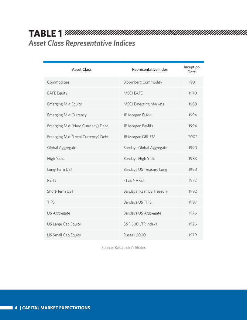
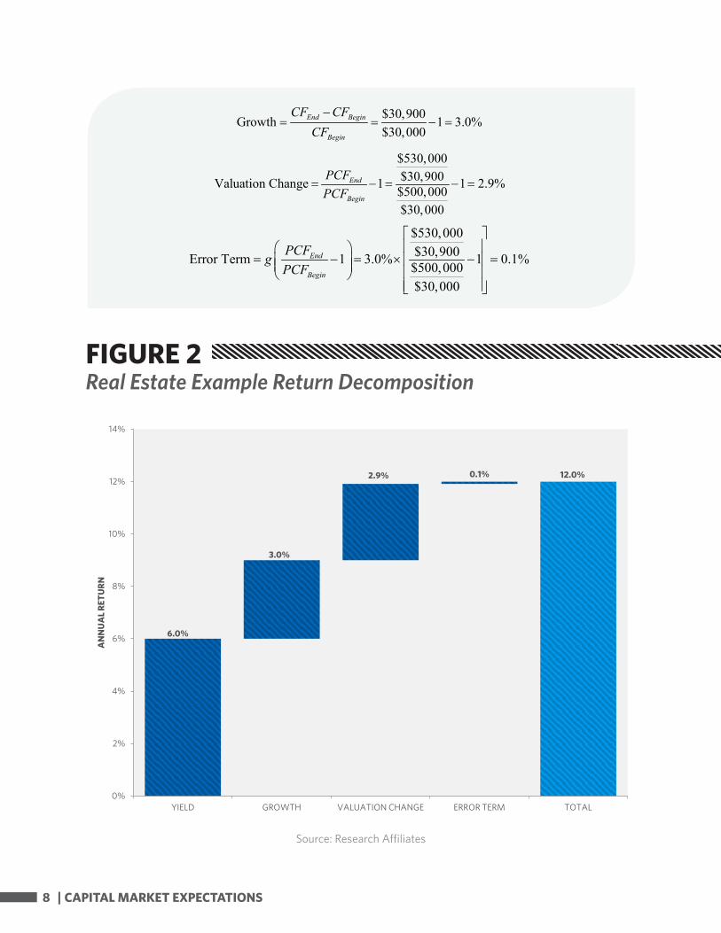
GROWTHThe growth building block represents the capital change in the value of the investment, based on the change in cash flow, to keep the value per unit of cash flow constant. For example, assume the house discussed previously is purchased for $500,000 and rented out to a third party who pays $30,000 per year ($2,500 per month) in rent. Assume in the next year, the market rate for similar apartments will increase to $30,900 per year ($2,575 per month). The landlord will realize growth in income of 3.0% per year [($500,000/$30,000) x ($30,900/$500,000) – 1].

VALUATION CHANGEAn investment’s valuation change captures the capital gain or loss in excess of the underlying cash flow’s growth rate. In the house example, annual rental income on the $500,000 property is $30,000. Thus the price of the property is 16.7 times the cash flow. If the value of the property increases to $530,000, the price to cash flow ratio increases to 17.2. Therefore, the investor earns an extra 2.9% [(17.2/16.7) – 1] from the increase in the property’s valuation multiple.

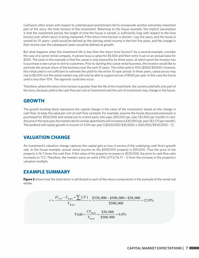
EXAMPLE SUMMARYFigure 2 shows how the total return is attributed to each of the return components in the example of the rental real estate.

( ) $530,000 $500,000 $30,000 12.0%$500,000

End Begin i

Begin

V V CFr

V− + − +

= = =∑

$30,000Yield 6.0%$500,000

Begin

Begin

CFV

= = =


6.0%

3.0%

2.9% 0.1% 12.0%

0%

2%

4%

6%

8%

10%

12%

14%

YIELD GROWTH VALUATION CHANGE ERROR TERM TOTAL

AN

NU

AL

RETU

RN

Source: Research Affiliates

FIGURE 2Real Estate Example Return Decomposition

$530,000$30,900Valuation Change 1 1 2.9%$500,000$30,000

End

Begin

PCFPCF

= − = − =

$530,000$30,900Error Term 1 3.0% 1 0.1%$500,000$30,000

End

Begin

PCFgPCF

= − = × − =

$30,900Growth 1 3.0%$30,000

End Begin

Begin

CF CFCF−

= = − =


Return ForecastingForecasting Methods

Before delving into the manner in which each return component is forecasted for each asset class, it is worthwhile to describe some of the most common methods of forecasting used today. Multiple forecasting methods can be

used for the same building block, and there is large overlap in the methods that can be used across building blocks.

• Current Value: For assets with time horizons longer than the return horizon, the current yield level is the proper yield to consider for the entire time horizon.

• Historical Trends: In situations where the future is expected to resemble the past, or in cases where a structural change is either not probable or the forecaster does not have any information with which to forecast a structural change, a continuation of the past trend can be appropriate. The most important decision when choosing to employ the historical trend is the length of the look-back. The forecaster must decide how much history is still relevant today, as well as the cost/benefit of obtaining additional historical data.

• Constant Value: Sometimes the expectation is for a variable to be volatile in the future and therefore difficult to predict, and sometimes the modeler is unable to extract any meaningful information from the data with which to make a defensible forecast. In these cases, often the best forecast is to model the average rate of the variable and assume this constant rate going forward. Some modelers, when faced with limited information, will assume a prospective value of zero; however, it’s important to consider that no information should not be confused with no value in the variable going forward (i.e., zero is often a bad choice).

• Hand Waving: Hand waving is possibly the most common approach used by soothsayers, and it results in an indefensible guess wrapped in a lot of complex language for the purpose of feigning knowledge where little exists. This should never be done; however, the reality of the situation is that it is an approach practiced by many prognosticators.

Time Horizon

One of the major considerations when embarking on the journey to generate asset class return expectations is the issue of time horizon. Because the focus here is on generating capital market expectations for strategic

asset allocation, and not tactical overlays, a significantly long time horizon of 10 years was selected.

The 10-year time horizon is not meant to imply a 10-year buy-and-hold strategy, but instead incorporates a strategy consisting of asset classes with constant duration targets. Said another way, asset classes with shorter durations (e.g., fixed income) need to be periodically rebalanced to maintain the constant duration. The rebalance period chosen here is one year which means that a two-year bond, for example, will be held for one year, at which time the bond with one year remaining to maturity would be sold and the proceeds used to purchase a new two-year bond. Asset classes with significantly long duration (e.g., equities) can be considered buy-and-hold because the change in duration from the passage of 1, 2, or even 10 years on these types of assets is minimal.

FIGURE 2Real Estate Example Return Decomposition


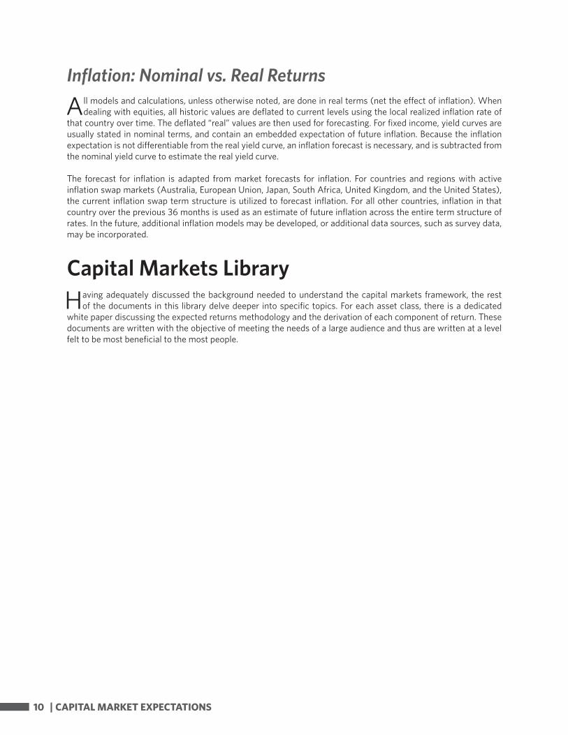
Inflation: Nominal vs. Real Returns

All models and calculations, unless otherwise noted, are done in real terms (net the effect of inflation). When dealing with equities, all historic values are deflated to current levels using the local realized inflation rate of

that country over time. The deflated “real” values are then used for forecasting. For fixed income, yield curves are usually stated in nominal terms, and contain an embedded expectation of future inflation. Because the inflation expectation is not differentiable from the real yield curve, an inflation forecast is necessary, and is subtracted from the nominal yield curve to estimate the real yield curve.

The forecast for inflation is adapted from market forecasts for inflation. For countries and regions with active inflation swap markets (Australia, European Union, Japan, South Africa, United Kingdom, and the United States), the current inflation swap term structure is utilized to forecast inflation. For all other countries, inflation in that country over the previous 36 months is used as an estimate of future inflation across the entire term structure of rates. In the future, additional inflation models may be developed, or additional data sources, such as survey data, may be incorporated.

Capital Markets LibraryHaving adequately discussed the background needed to understand the capital markets framework, the rest

of the documents in this library delve deeper into specific topics. For each asset class, there is a dedicated white paper discussing the expected returns methodology and the derivation of each component of return. These documents are written with the objective of meeting the needs of a large audience and thus are written at a level felt to be most beneficial to the most people.


REFERENCES

Arnott, Rob. 2011. “Equity Risk Premium Myths.” In Rethinking the Equity Risk Premium, by P. Brett Hammond Jr., Martin L. Leibowitz, and Laurence B. Siegel. Charlottesville, VA: Research Foundation of CFA Institute.

Gordon, Myron. 1962. The Investment, Financing and Valuation of a Corporation. Homewood, IL: Irwin.Ibbotson, Roger, and Peng Chen. 2003. “Long-Run Stock Returns: Participating in the Real Economy.” Financial Analysts Journal, vol. 59, no. 1 (January/February):88–98.

Ibbotson, Roger, and Peng Chen. 2003. “Long-Run Stock Returns: Participating in the Real Economy.” Financial Analysts Journal, vol. 59, no. 1 (January/February):88–98.

Nevo, Aviv, and Michael Whinston. 2010. “Taking the Dogma out of Econometrics: Structural Modeling and Cred-ible Inference.” Journal of Economic Perspectives, vol. 24, no. 2 (Spring):69–82.


DISCLAIMER

The information contained herein regarding Asset Allocation and Expected Returns may represent real return forecasts for several asset classes and not for any Research Affiliates (“RA”) fund or strategy. These forecasts are forward-looking statements based upon the reasonable beliefs of RA and are not a guarantee of future performance. Forward-looking statements speak only as of the date they are made, and RA assumes no duty to and does not undertake to update forward-looking statements. Forward-looking statements are subject to numerous assumptions, risks, and uncertainties, which change over time. Actual results may differ materially from those anticipated in forward-looking statements.

All projections provided are estimates and are in U.S. dollar terms, unless otherwise specified. Given the complex risk-reward trade-offs involved, one should always rely on judgment as well as quantitative optimization approaches in setting strategic allocations to any or all of the above asset classes. Please note that all information shown is based on qualitative analysis. Exclusive reliance on the above is not advised. This information is not intended as a recommendation to invest in any particular asset class or strategy or as a promise of future performance. Note that these asset class and strategy assumptions are passive only–they do not consider the impact of active management. References to future returns are not promises or even estimates of actual returns a client portfolio may achieve. Assumptions, opinions and estimates are provided for illustrative purposes only. They should not be relied upon as recommendations to buy or sell any securities, commodities, derivatives or financial instruments of any kind. Forecasts of financial market trends that are based on current market conditions or historical data constitute a judgment and are subject to change without notice. We do not warrant its accuracy or completeness. This material has been prepared for information purposes only and is not intended to provide, and should not be relied on for, accounting, legal, tax, investment or tax advice. There is no assurance that any of the target prices mentioned will be attained. Any market prices are only indications of market values and are subject to change.

Hypothetical or simulated performance results have certain inherent limitations. Unlike an actual performance record, simulated results do not represent actual trading, but are based on the historical returns of the selected investments, indices or investment classes and various assumptions of past and future events. Simulated trading programs in general are also subject to the fact that they are designed with the benefit of hindsight. Also, since the trades have not actually been executed, the results may have under or over compensated for the impact of certain market factors. In addition, hypothetical trading does not involve financial risk. No hypothetical trading record can completely account for the impact of financial risk in actual trading. For example, the ability to withstand losses or to adhere to a particular trading program in spite of the trading losses are material factors which can adversely affect the actual trading results. There are numerous other factors related to the economy or markets in general or to the implementation of any specific trading program which cannot be fully accounted for in the preparation of hypothetical performance results, all of which can adversely affect trading results.

The asset classes are represented by broad-based indices which have been selected because they are well known and are easily recognizable by investors. Indices have limitations because indices have volatility and other material characteristics that may differ from an actual portfolio. For example, investments made for a portfolio may differ significantly in terms of security holdings, industry weightings and asset allocation from those of the index. Accordingly, investment results and volatility of a portfolio may differ from those of the index. Also, the indices noted in this presentation are unmanaged, are not available for direct investment, and are not subject to management fees, transaction costs or other types of expenses that a portfolio may incur. In addition, the performance of the indices reflects reinvestment of dividends and, where applicable, capital gain distributions. Therefore, investors should carefully consider these limitations and differences when evaluating the index performance.

No investment process is risk free and there is no guarantee of profitability; investors may lose all of their investments. No investment strategy or risk management technique can guarantee returns or eliminate risk in any market environment. Diversification does not guarantee a profit or protect against loss. Investing in foreign securities presents certain risks not associated with domestic investments, such as currency fluctuation, political and economic instability, and different accounting standards. This may result in greater share price volatility. The prices of small- and mid-cap company stocks are generally more volatile than large-company stocks. They often involve higher risks because smaller companies may lack the management expertise, financial resources, product diversification and competitive strengths to endure adverse economic conditions.

Bond prices fluctuate inversely to changes in interest rates. Therefore, a general rise in interest rates can result in the decline of the value of your investment. High-yield bonds, also known as junk bonds, are subject to greater risk of loss of principal and interest, including default risk, than higher-rated bonds. Investing in fixed-income securities involves certain risks such as market risk if sold prior to maturity and credit risk especially if investing in high-yield bonds which have lower ratings and are subject to greater volatility. All fixed-income investments may be worth less than original cost upon redemption or maturity. Income from municipal securities is generally free from federal taxes and state taxes for residents of the issuing state. While the interest income is tax-free, capital gains, if any, will be subject to taxes. Income for some investors may be subject to the


federal alternative minimum tax (AMT).

There are special risks associated with an investment in real estate, including credit risk, interest-rate fluctuations and the impact of varied economic conditions. Distributions from REIT investments are taxed at the owner’s tax bracket.

Hedge funds or alternative investments are complex, speculative investment vehicles and are not suitable for all investors. They are generally open to qualified investors only and carry high costs and substantial risks and may be highly volatile. There is often limited (or even nonexistent) liquidity and a lack of transparency regarding the underlying assets. They do not represent a complete investment program. The investment returns may fluctuate and are subject to market volatility so that an investor’s shares, when redeemed or sold, may be worth more or less than their original cost. Hedge funds are not required to provide investors with periodic pricing or valuation and are not subject to the same regulatory requirements as mutual funds. Investing in hedge funds may also involve tax consequences. Speak to your tax advisor before investing. Investors in funds of hedge funds will incur asset-based fees and expenses at the fund level and indirect fees, expenses and asset-based compensation of investment funds in which these funds invest. An investment in a hedge fund involves the risks inherent in an investment in securities as well as specific risks associated with limited liquidity, the use of leverage, short sales, options, futures, derivative instruments, investments in non-U.S. securities, junk bonds and illiquid investments. There can be no assurances that a manager’s strategy (hedging or otherwise) will be successful or that a manager will use these strategies with respect to all or any portion of a portfolio. Please carefully review the Private Placement Memorandum or other offering documents for complete information regarding terms, including all applicable fees, as well as other factors you should consider before investing.

Buying commodities allows for a source of diversification for those sophisticated persons who wish to add commodities to their portfolios and who are prepared to assume the risks inherent in the commodities market. Any purchase represents a transaction in a non-income producing commodity and is highly speculative. Therefore, commodities should not represent a significant portion of an individual’s portfolio. Buying gold, silver, platinum and palladium allows for a source of diversification for those sophisticated persons who wish to add precious metals to their portfolios and who are prepared to assume the risks inherent in the bullion market. Any bullion or coin purchase represents a transaction in a non-income-producing commodity and is highly speculative. Therefore, precious metals should not represent a significant portion of an individual’s portfolio.

Trading foreign exchange involves a high degree of risk. Exchange rates between foreign currencies change rapidly do to a wide range of economic, political and other conditions, exposing one to risk of exchange rate losses in addition to the inherent risk of loss from trading the underlying financial product. If one deposits funds in a currency to trade products denominated in a different currency, one’s gains or losses on the underlying investment therefore may be affected by changes in the exchange rate between the currencies. If one is trading on margin, the impact of currency fluctuation on that person’s gains or losses may be even greater.

Investments that are concentrated in a specific sector or industry increase their vulnerability to any single economic, political or regulatory development. This may result in greater price volatility.

This information has been prepared by RA based on data and information provided by internal and external sources. While we believe the information provided by external sources to be reliable, we do not warrant its accuracy or completeness.

Research Affiliates is the owner of the trademarks, service marks, patents and copyrights related to the Fundamental Index methodology. The trade names Fundamental Index®, RAFI®, the RAFI logo, and the Research Affiliates corporate name and logo among others are the exclusive intellectual property of Research Affiliates, LLC. Any use of these trade names and logos without the prior written permission of Research Affiliates, LLC is expressly prohibited. Research Affiliates, LLC reserves the right to take any and all necessary action to preserve all of its rights, title and interest in and to these terms and logos.

Various features of the Fundamental Index® methodology, including an accounting data-based non-capitalization data processing system and method for creating and weighting an index of securities, are protected by various patents, and patent-pending intellectual property of Research Affiliates, LLC. (See all applicable US Patents, Patent Publications, and Patent Pending intellectual property located at http://www.researchaffiliates.com/Pages/legal.aspx#d, which are fully incorporated herein.)

© Research Affiliates, LLC. All rights reserved. Duplication or dissemination prohibited without prior written permission.

© 2014 Research Affiliates, LLC. All Rights Reserved.

620 Newport Center Drive Suite 900

Newport Beach, CA 92660Main: +1 949.325.8700

www.ResearchAffiliates.com

@RA_Insights

Documents

CAPITAL MARKET EXPECTATIONS - Research … | CAPITAL MARKET EXPECTATIONS This expected returns forecasting starts with the asset classes of most interest to investors (which also happen