Can an increase in public investment sustainably lift output? · Can an increase in public investment sustainably lift economic growth? This paper seeks to identify the conditions

Unclassified ECO/WKP(2016)75 Organisation de Coopération et de Développement Économiques Organisation for Economic Co-operation and Development 24-Nov-2016

___________________________________________________________________________________________

_____________ English - Or. English ECONOMICS DEPARTMENT

CAN AN INCREASE IN PUBLIC INVESTMENT SUSTAINABLY LIFT ECONOMIC GROWTH?

ECONOMICS DEPARTMENT WORKING PAPERS No. 1351

By Annabelle Mourougane, Jarmila Botev, Jean-Marc Fournier, Nigel Pain and Elena Rusticelli

OECD Working Papers should not be reported as representing the official views of the OECD or of its member

countries. The opinions expressed and arguments employed are those of the author(s).

Authorised for publication by Christian Kastrop, Director, Policy Studies Branch, Economics Department.

All Economics Department Working Papers are available at www.oecd.org/eco/workingpapers.

JT03406120

Complete document available on OLIS in its original format

This document and any map included herein are without prejudice to the status of or sovereignty over any territory, to the delimitation of

international frontiers and boundaries and to the name of any territory, city or area.

EC

O/W

KP

(20

16)7

5

Un

classified

En

glish

- Or. E

ng

lish

Cancels & replaces the same document of 23 November 2016

ECO/WKP(2016)75

2

OECD Working Papers should not be reported as representing the official views of the OECD or of its member countries. The opinions expressed and arguments employed are those of the author(s). Working Papers describe preliminary results or research in progress by the author(s) and are published to stimulate discussion on a broad range of issues on which the OECD works. Comments on Working Papers are welcomed, and may be sent to the Economics Department, OECD, 2 rue André-Pascal, 75775 Paris Cedex 16, France. Comment on the Papers is invited, and may be sent to OECD Economics Department, 2 rue André Pascal, 75775 Paris Cedex 16, France, or by e-mail to [email protected]. All Economics Department Working Papers are available at www.oecd.org/eco/workingpapers. Recent working papers on the same topics include: Fournier, J.-M. and Å. Johansson (2016), “The Effect of the Size and the Mix of Public Spending on Growth and Inequality”, OECD Economics Department Working Papers, No. 1344, OECD Publishing, Paris.

Fournier, J. (2016), “The Positive Effect of Public Investment on Potential Growth”, OECD Economics Department Working Papers, No. 1347, OECD Publishing, Paris.

Bloch, D., Fournier, J., Gonzales, D. and Pina, A. (2016), “Trends in Public Finances: Insights from a New Detailed Dataset”, OECD Economic Department Working Papers, No. 1345, OECD Publishing, Paris.

This document and any map included herein are without prejudice to the status of or sovereignty over any territory, to the delimitation of international frontiers and boundaries and to the name of any territory, city or area. The statistical data for Israel are supplied by and under the responsibility of the relevant Israeli authorities. The use of such data by the OECD is without prejudice to the status of the Golan Heights, East Jerusalem and Israeli settlements in the West Bank under the terms of international law.

© OECD (2016)

You can copy, download or print OECD content for your own use, and you can include excerpts from OECD publications, databases and multimedia products in your own documents, presentations, blogs, websites and teaching materials, provided that suitable acknowledgment of OECD as source and copyright owner is given. All requests for commercial use and translation rights should be submitted to [email protected]

ECO/WKP(2016)75

3

ABSTRACT/RÉSUMÉ

Can an increase in public investment sustainably lift economic growth?

This paper seeks to identify the conditions under which raising public investment can sustainably lift

growth without deteriorating public finances. To do so, it relies on a range of simulations using three

different macro-structural models. According to the simulations, OECD governments could finance a ½

percentage point of GDP investment-led stimulus for three to four years on average in OECD countries

without raising the debt-to-GDP ratio in the medium term, provided projects are sound. After one year, the

average output gains for the large advanced economies of such a stimulus amount to 0.4-0.6%. However,

the gains are particularly uncertain for Japan. Reprioritising spending in later years would lead to average

long-term output gains of between 0.5 to 2% in the large advanced economies. Those gains depend on the

assumptions made on the rate of return. Hysteresis reinforces the case for an investment-led stimulus.

Output gains will also be higher if the stimulus is combined with structural reforms and if countries act

collectively.

JEL Classification: C3, E6

Keywords: public investment, public debt, fiscal multiplier

******

Une augmentation de l'investissement public peut-elle durablement augmenter la croissance?

Ce document de travail cherche à déterminer les conditions dans lesquelles l'augmentation de

l'investissement public peut soutenir la croissance durablement sans détériorer les finances publiques. Pour

ce faire, il s'appuie sur une série de simulations utilisant trois modèles macro-structurels différents. Selon

les simulations, les gouvernements des pays de l'OCDE pourraient financer une augmentation de

l'investissement de ½ point de PIB pendant trois à quatre ans en moyenne dans les pays de l'OCDE sans

augmenter le ratio dette sur PIB à moyen terme, à condition que les projets soient de bonne qualité. Après

un an, les gains moyens de production pour les grandes économies avancées d'un tel stimulus s'élèvent à

0,4-0,6%. Cependant, ces gains sont particulièrement incertains pour le Japon. Une réallocation des

dépenses vers celles qui sont les plus productives les années suivantes, se traduirait par des gains moyens à

long terme de production entre 0,5 et 2% dans les grandes économies avancées. Ces gains dépendent des

hypothèses retenues sur le taux de rendement. Les effets d'hystérésis renforcent l'argument en faveur d'une

augmentation de l'investissement public. Les gains de production seront également plus élevés si le

stimulus est combiné à des réformes structurelles et si les pays agissent collectivement.

Classification JEL: C3, E6

Mots clés: investissement public, dette publique, multiplicateur budgétaire

ECO/WKP(2016)75

4

TABLE OF CONTENTS

1. Introduction and summary .................................................................................................................... 6 2. Public investment has been weak ......................................................................................................... 8 3. Simulation design ............................................................................................................................... 10 4. In the short term an investment-led stimulus boosts output and reduce the debt-to-GDP ratio ......... 16 5. Public investment has a positive long-term effect on growth ............................................................. 18

The outcomes depend markedly on assumptions about the rate of return on public investment ........... 20 Hysteresis reinforces the case for an investment-led stimulus ............................................................... 21 The effect of stimulus on debt dynamics appears to be stronger at the zero-lower bound ..................... 22 An increase in public investment reduces uncertainties around public debt .......................................... 23

6. What are the gains of going collective? .............................................................................................. 24 7. Combining an investment stimulus with structural reform enhances growth impacts ....................... 27

REFERENCES .............................................................................................................................................. 30

ANNEX 1. DESCRIPTION OF THE MODELS .......................................................................................... 33

1. The Fall & Fournier model ................................................................................................................. 33 2. The Fiscal Maquette model ................................................................................................................ 34

Specification of the main equations ....................................................................................................... 34 Parameters and calibration ..................................................................................................................... 36

Tables

Table 1. Country-specific conditions and the impact of public investment stimulus on output .................. 8

Figures

Figure 1. Public investment in selected OECD countries ............................................................................ 9 Figure 2. Infrastructure investment has been weak across the OECD ...................................................... 10 Figure 3. Estimates of returns to public investment ................................................................................... 11 Figure 4. Average annual increase in public investment during episodes of investment expansion ......... 12 Figure 5. Number of years during which a permanent growth-enhancing investment

increase can be funded with temporary deficits ......................................................................... 14 Figure 6. The short-term effect of a sustained increase in public investment by 0.5% of GDP ................ 17 Figure 7. One-year output gains of a ½ per cent of GDP increase in investment

under different assumptions on fiscal multipliers ...................................................................... 18 Figure 8. Long-term output gains of a permanent increase in public investment of ½ per cent of GDP ... 19 Figure 9. Long-term output effects of different assumptions on the rate of return on public investment . 20 Figure 10. Long-term effects of a lower public investment elasticity to potential output ......................... 21 Figure 11. Effects of hysteresis on long-term output and public debt ratios-preliminary ......................... 22 Figure 12. Effects of the zero-lower bound on debt dynamics .................................................................. 23 Figure 13. Reduction in public debt uncertainty ........................................................................................ 24 Figure 14. Number of OECD countries which significantly increase public investment during

at least two years ....................................................................................................................... 25 Figure 15. Gains of collective action in the OECD countries according to the FM model ....................... 26 Figure 16. Gains from collective action in the OECD countries according to the NiGEM model ............ 27 Figure 17. The addition of product market reforms and a public investment increase .............................. 28 Figure 18. Additional output gains from structural reforms after one year after one year ........................ 29

ECO/WKP(2016)75

5

Boxes

Box 1. Brief comparison of the different models ....................................................................................... 13 Box 2. Debt -financed public investment with no long-term effect on the debt to GDP ratio ................... 15

ECO/WKP(2016)75

6

CAN AN INCREASE IN PUBLIC INVESTMENT SUSTAINABLY

LIFT ECONOMIC GROWTH?

Annabelle Mourougane, Jarmila Botev, Jean-Marc Fournier, Nigel Pain and Elena Rusticelli1

1. Introduction and summary

1. The recovery from the crisis has repeatedly proved weaker than expected, with the current

conjuncture characterised by modest demand growth, subdued investment, low inflation and weak

productivity growth. Experience to date also suggests that reliance on monetary policy alone will fail to

deliver a rebound in growth, and that the scope for additional monetary policy measures is increasingly

limited. Interest rates are now at the zero lower bound or negative in many advanced economies and

unconventional measures, such as quantitative easing and negative policy rates, may face decreasing

returns and give rise to anomalies in financial markets.

2. Very low interest rates offer most OECD countries extremely favourable borrowing conditions to

increase productive public spending. These favourable conditions are best used by locking-in low interest

rates with long-maturity borrowing (OECD, 2016). Well-targeted spending on education, health or

research and development brings significant output gains in the long run. Infrastructure needs are also

sizeable in OECD countries, especially as fiscal consolidation in recent years has pushed down public

capital spending to very low levels in many countries. In such a situation, additional public investment

should generate high rates of return if good governance and framework conditions are in place. In a view to

mitigating and adapting to climate change, these new investment projects could focus on low-carbon,

climate resilient options.

3. Against this background, the OECD has recommended an increase in public investment to

support demand and employment in the short run and catalyse private investment and innovation so as to

increase potential output in the long term. Still, questions remain open about the size of public investment

multipliers and the long-term returns on public capital, both of which play a role in determining how public

debt-to-GDP ratios will evolve in response to higher public investment. The objective of this paper is to

identify the conditions under which raising public investment can sustainably lift growth without

deteriorating public finances. To do so, it relies on a range of simulations using three different macro-

structural models.

4. Simulation results suggest that:

There is room for deficit-financed public investment-led stimulus of ½ percentage point of GDP

for three- to four years on average in OECD countries without raising the debt-to-GDP ratio in

the medium term, provided projects are sound. Subsequently a reprioritisation of tax and

spending would also help support economic growth.

1. The authors are members of the Economics Department of the OECD. They would like to thank

OECD Economics Department colleagues Mark Baker, Sven Blondal, Claude Giorno, Catherine Mann for

their comments and suggestions, as well as Sylvie Foucher-Hantala for statistical support and Veronica

Humi (also from Economics Department) for editorial assistance.

ECO/WKP(2016)75

7

After one year, the average output gains for the large advanced economies of such a stimulus

amount to 0.4-0.6%. The gains are particularly uncertain for Japan. Moving to a deficit-neutral

stimulus would shave off the one-year growth impact by about 0.2 percentage point.

Looking forward, a sustained investment stimulus of ½ percentage point of GDP is estimated to

lead to an average long-term output gains between 0.5 to 2% in the large advanced economies.

Those gains depend on the assumptions made on the rate of returns, the elasticity of output with

regard to public investment and the depreciation rate.

Countries where the initial level of public capital is low are likely to benefit the most from the

stimulus on the assumption that additional investment has a high risk-adjusted rate of return in

these economies. Assuming that all public investment projects in a given country have the same

rates of return at the margin, the effect on output would be, amongst the large advanced

economies, above average in Germany and the United Kingdom, where the stock of public

capital is estimated to be relatively low. On the other hand, the output gains could be negative for

Japan, reflecting a large initial public capital stock and associated low and even negative rates of

return at the margin for conventionally-defined public capital.

If persistent demand weakness gradually undermines the productive capacity of the economy

(“hysteresis”), the case for an investment-led stimulus is reinforced, as the stimulus would lead to

stronger long-term gains on output. The amplitude of these gains depends on the initial position

in the cycle, and, to a lesser extent, on the degree of labour-market rigidity. They would be

particularly strong for Italy and France.

Collective action among the large advanced economies to raise high-quality public investment is

estimated to bring additional output gains of about 0.2 percentage point on average after one year

in the economies concerned compared with a scenario where countries act individually. As a

consequence, the debt-to-GDP ratio would also fall more in the short term than otherwise.

Germany would be, amongst the large advanced economies, the country that benefits the most

from collective action to boost public investment relative to undertaking additional investment by

itself.

Combining an investment-led stimulus with product-market structural reforms can lead to a

stronger short-term growth impact and accentuate the reduction of the public debt-to-GDP ratio.

In particular, reforms targeted at frictions that hold back demand for investment can lower the

opportunity costs of investing. Easing product-market regulations by the average improvement

over two years in a typical OECD country could add around 0.3 percentage point to the growth

impact after the first year. Reducing the regulatory burden stemming from anti-competitive

product market regulations in upstream sectors would have on average an impact of the same

amplitude and would be particularly beneficial in Canada, France and Italy.

A sustained rise in the stock of public capital and potential output reduces the public debt-to-

GDP ratio as the denominator increases. It thus reduces risks on debt as current debt to GDP ratio

moves further away from its default limit, notably in the small European economies.

Table 1 provides a summary of these main results for the large advanced economies.

ECO/WKP(2016)75

8

Table 1. Country-specific conditions and the impact of public investment stimulus on output

Low level of public capital/high rate of

return Hysteresis Collective action

Reduction in uncertainty

around public debt

Structural reforms

United States + + + + + Japan -- = + -- ++ Germany ++ = ++ + + France + ++ + + +++ Italy + ++ + ++ +++ United Kingdom ++ = + + + Canada + + + + +++

Note: signs summarise the amplitude of the output gains following an investment-led stimulus. For instance the existence of hysteresis in France and Italy makes these countries gain more from such a measure than other advanced economies. Uncertainty around public debt is assessed by the inter-quantile range of the debt level in 2040 in the stochastic Fall &Fournier model.

Source: OECD calculations based on F&F, FM and NiGEM models.

5. This paper is organised as follows. The first part discusses the scope for boosting public

investment in a context of ultra-low interest rates that reduce financing costs and of large infrastructure

needs in some OECD countries. The following sections present model simulations, provide estimates of

the impact of sustained increase in public investment on growth and public finances and identify the

conditions for this increase to significantly boost long-term growth.

2. Public investment has been weak

6. In recent years, the share of public investment in output has decreased in many OECD countries

(Figure 1). Some euro area countries under market pressure have cut public investment substantially to

help meet their fiscal consolidation objectives in the aftermath of the sovereign crisis. Public investment in

fixed capital declined by an average 0.6% of GDP between 2010 and 2013 in OECD countries, accounting

for one-quarter of fiscal consolidation in this period. The decline was much larger in some countries,

exceeding 2.5% of GDP in Greece, Spain and Ireland and accounting for just around half of the

consolidation in Spain. On average in OECD countries, 1% of GDP consolidation was associated with a

0.3% of GDP cut in public investment (OECD, 2015a).

7. Although recent levels of infrastructure spending are not very low compared with pre-crisis

capital spending (Figure 2), there is evidence in many OECD countries, including the United States, that

gross investment has not been sufficient to make up for capital depreciation (Dobbs et al., 2013). As a

result, a backlog of replacement and maintenance investment has been building up, and the quality of

public infrastructure has deteriorated, hampering productivity and socio-economic opportunities (OECD,

2016b).

8. Additional capital spending is also required to help achieve long-term objectives such as those

related to climate change and environmental quality. Greater spending on other form of investment, such as

education or health, also supports long-term growth (Fournier and Johansson, 2016; Barbiero and

Cournède, 2013). In particular, recent evidence based on OECD countries suggests that increasing the

quality of, and the time spent in, education yields large growth gains by raising skills and thereby

productivity. Growth gains from public investment in health (e.g. in hospitals and medical equipment and

prevention) are also found to be strong, as such an investment may improve workers’ health and well-being

and, in turn, productivity.

9. Output gains from increased public spending on research and development are potentially large,

particularly if spending is directed to basic research where widespread market failures lead to

ECO/WKP(2016)75

9

under-investment by the private sector (OECD, 2015b). Higher public spending on basic research can also

enhance the ability of economies to learn from innovations at the global frontier (Saia et al., 2015).

Figure 1. Public investment in selected OECD countries

Per cent of potential output

Source: OECD Economic Outlook database.

10. Infrastructure investment is likely to have high returns in countries where the initial stock of

public capital and investment is low (Fournier, 2016). This is particularly the case for the United Kingdom

and Germany. By contrast, rate of returns are likely to be very low, and even negative, in Japan, where the

stock of public capital as traditionally defined already exceeds 100% of potential output (Figure 3).

11. Good governance and reliable ex ante assessment of projects’ social rates of return are crucial to

ensure that high returns materialise and to prevent the cost overruns and overestimation of future demand

that have occurred in a number of past infrastructure projects (Persson and Song, 2010). More generally,

regulation and other framework conditions, including access to markets and pricing regimes, will also

affect the return on investment (Sutherland et al., 2011).

ECO/WKP(2016)75

10

12. Against this background, a number of countries have announced a boost in public infrastructure

spending in the coming years. In late 2014, the European Commission presented its Investment Plan for

Europe – the so-called Juncker Plan -- which aimed at unlocking public and private investment. It was

officially estimated to amount to at least € 315 bn (around 2% of EU GDP in 2015) over the period

2015-17. In Canada, the government plans to invest more than CAD 120 bn in infrastructure (6% GDP)

over 10 years (Canada Federal Budget, 2016). Japan has announced a stimulus package for 2016-17 that

includes infrastructure spending for the 21st century (about 0.3% of GDP) and reconstruction and

prevention spending following the recent earthquakes (about 0.5% of GDP). In addition, 1.2% of GDP has

been earmarked for the Fiscal Investment and Loan Programme, outside government accounts, to enhance

private infrastructure investment. However, public investment as a share of GDP is expected to remain

broadly stable in most OECD countries in the next two years (OECD, 2016a).

Figure 2. Infrastructure investment has been weak across the OECD

Per cent of GDP

Note: IP stands for intellectual properties.

Source: Economic Outlook Database and National Statistical Offices.

3. Simulation design

13. This section investigates the economic and fiscal impacts of an increase in public investment in

the OECD economies. Public investment should be understood in a very broad sense here and

encompasses both soft and hard infrastructure, including in particular education health, and R&D. The

rationale for such investments is that they could help to push economies onto a higher growth path than

might otherwise be the case, at a time when private investment growth remains modest. While an increase

in public investment supports aggregate demand in the short term, efficient public investment also

contributes to higher potential output by increasing the stock of capital. Moreover, to the extent that public

investment catalyses private investment, the gains are further multiplied. Public investment could crowd

out private investment through higher interest rates, but if monetary policy remains accommodative, as is

likely in current circumstances, this channel would be muted.

2.0

2.5

3.0

3.5

4.0

4.5

1997 1998 1999 2000 2001 2002 2003 2004 2005 2006 2007 2008 2009 2010 2011 2012 2013 2014

OECD Euro area Japan United States

0.5

1.0

1.5

2.0

2.5

3.0

3.5

4.0

4.5

1997 1998 1999 2000 2001 2002 2003 2004 2005 2006 2007 2008 2009 2010 2011 2012 2013 2014

United States United States Public United States Private excluding IP

ECO/WKP(2016)75

11

Figure 3. Estimates of returns to public investment

Note: The dashed line indicates the 95 % confidence interval. The measure of the capital stock depends on assumptions on the rate of depreciation of capital and on the level of disaggregation at which the calculation is made. The IMF database of public stock series, which may differ from national sources, has been used to compute these estimates. This database is used here because the capital stock is computed in all countries with the same methodology. Light shading indicates a positive not significant investment effect and darker shading indicates a negative not significant investment effect.

Source: Fournier (2016).

ECO/WKP(2016)75

12

14. The impacts on GDP growth and government debt ratios of an investment-led stimulus are

assessed through a range of scenarios using three macro-structural models which cast different lights on the

issues: the Fall and Fournier (2015) model (the F&F model); the Fiscal Maquette, developed in Botev and

Mourougane (forthcoming) (the FM model); and the NiGEM macroeconomic model developed and

maintained by NIESR (see Box 1). The use of several models allows the main mechanisms at play to be

highlighted, as well as the uncertainties surrounding the results.

15. In these exercises the size of the stimulus package is set at 0.5% of GDP, which implies an

increase in the volume of government investment of around 15% in the typical OECD member state. This

is close to the average of the annual increase in public investment observed over the period 1995-2015 in

the OECD countries in the years when public investment increased (0.6 % of GDP) (Figure 4). In some

countries, this may be challenging to achieve immediately. The projects undertaken are assumed to be

economically worthwhile.

Figure 4. Average annual increase in public investment during episodes of investment expansion

1995 - 2015

Note: Only public investment increases that is higher than ¼ of the standard deviation of the level of public investment share in GDP are considered unless it is part of a longer-lasting investment episode, so that very tiny isolated changes in investment-to-GDP ratios that may be due to movements in the denominator, are excluded.


ECO/WKP(2016)75

13

Box 3. Brief comparison of the different models

The three models employed in the analysis share a number of common features. In particular, the transmission mechanisms of an increase in public investment to the economy are very similar. In addition to the short-term boost in demand, such a shock increases output in the long run when it is permanent. When the shock is temporary, the long-term impact on output is close to zero in the three models.

Each model has specific features that cast different lights on the examined issues.

The F&F model is a long-term stochastic model and allows examining the impact of uncertainties on simulation outcomes. Twenty-six OECD economies are modelled. The efficiency of investment is estimated to be a decreasing function of the initial capital stock level (Fournier, 2016). In addition, interest rates are assumed to be more sensitive to public debt levels in the euro area countries than in the other OECD countries.

The FM model encompasses structural features (such as hysteresis) and some international dimensions, through trade volumes linkages. Only the large advanced economies and the rest of the world are modelled. As in the F&F model, a rise in public debt increases the credit risks premium faced by governments.

NiGEM is a full-fledged international model. All economies, including large emerging-market economies, are modelled. Individual country models are linked through trade (via world demand and price competiveness) and financial flows (gross foreign assets and liabilities). The model also encompasses a number of options in terms of monetary policy or fiscal rules and can be run in backward and forward-looking modes.

The definition of the public sector differs across countries and partly explains observed differences in government investment across countries. One major source of difference is the extent to which governments subcontract the delivery of public services to private firms.

A more detailed description of the first two models is provided in Annex 1. More information on the NiGEM model can be found in Barrell et al. (2012).

16. The investment-led stimulus is deficit-financed for a certain period, before turning to budget-

neutral. This period of time has been computed using the F&F model. It corresponds to the number of

years during which a country can finance a permanent 0.5% of GDP stimulus by increasing its deficit,

without raising its public debt-to-GDP above the value it would have had without the stimulus by 2040

(Box 2). Japan is estimated not to have fiscal space to finance such a stimulus (Botev et al., 2016), and to

have no room for further public investment anymore (Fournier, 2016). Simulations suggest this number

ranges between one year in Korea to six in Ireland or the United Kingdom (Figure 5). It is a function of the

country's initial level of public capital stocks, public investment and the interest rate to growth rate

differential, as well as the initial level of debt. For instance, the lower the initial public stock of capital the

higher the return on public investment and thus the higher the GDP impact, which provides room for

longer lasting deficit. Conversely, for a given percentage increase in GDP the higher the initial debt-to-

GDP ratio the stronger the decline in this debt ratio, which also provides for room for longer lasting deficit.

ECO/WKP(2016)75

14

Figure 5. Number of years during which a permanent growth-enhancing investment increase can be funded with temporary deficits

Note: A no-policy change scenario is compared to a scenario with a permanent increase of public investment by 0.5% of GDP and a temporary deficit increase of the same amount during the number of years reported in this figure. The number of years is set so that the debt level in 2040 is the same in the no-policy change scenario and in the investment shift scenario. Public investment has decreasing marginal returns as estimated in Fournier (2016), and the other structural parameters estimated in Fall and Fournier (2015) are homogenous across countries. The most important country-specific parameters that can influence the computation are the initial public investment level, the initial capital stock level, the initial public debt level and the interest rate to growth rate gap. The computation assumes countries have access to markets.

Source: F&F model.

17. The scenarios have been designed to increase the comparability of the simulations across models.

For the sake of simplicity the number of years during which a country can finance an investment stimulus

through deficit has been assumed to be the same in the three models. Still, the comparability is not total,

given the specific features of each model, and the results should thus be interpreted with great care. In

particular, convergence to the long term is generally achieved through market and policy mechanisms,

including the use of a Taylor rule, whereby monetary authorities respond to changes in output gaps and in

inflation. Those mechanisms and the specification of this rule, however, differ from one model to another.

In addition, budget solvency rules are also modelled differently. In all three models, the increase in public

investment is financed through an increase in tax or a cut in other spending. Furthermore, the assumption is

made that additional tax revenues resulting from the demand effect of the investment stimulus are

exclusively used for debt reduction in the F&F and FM models, whereas the budget balance target is fixed

in NiGEM. As a consequence, simulations are strictly budget-neutral in the second regime in the F&F and

FM models only. Finally, international spillovers are fully accounted for in the NiGEM model, only

partially in the FM model and not at all in the F&F model.

ECO/WKP(2016)75

15

Box 4. Debt -financed public investment with no long-term effect on the debt to GDP ratio

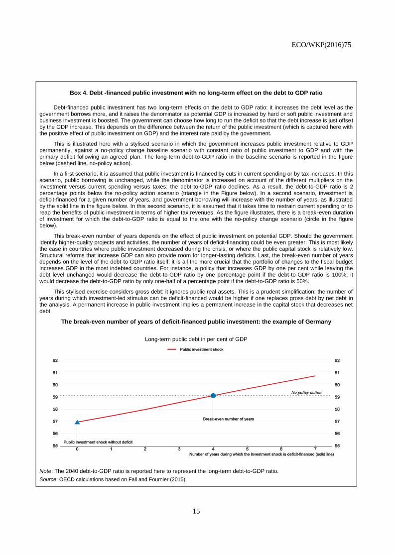
Debt-financed public investment has two long-term effects on the debt to GDP ratio: it increases the debt level as the government borrows more, and it raises the denominator as potential GDP is increased by hard or soft public investment and business investment is boosted. The government can choose how long to run the deficit so that the debt increase is just offset by the GDP increase. This depends on the difference between the return of the public investment (which is captured here with the positive effect of public investment on GDP) and the interest rate paid by the government.

This is illustrated here with a stylised scenario in which the government increases public investment relative to GDP permanently, against a no-policy change baseline scenario with constant ratio of public investment to GDP and with the primary deficit following an agreed plan. The long-term debt-to-GDP ratio in the baseline scenario is reported in the figure below (dashed line, no-policy action).

In a first scenario, it is assumed that public investment is financed by cuts in current spending or by tax increases. In this scenario, public borrowing is unchanged, while the denominator is increased on account of the different multipliers on the investment versus current spending versus taxes: the debt-to-GDP ratio declines. As a result, the debt-to-GDP ratio is 2 percentage points below the no-policy action scenario (triangle in the Figure below). In a second scenario, investment is deficit-financed for a given number of years, and government borrowing will increase with the number of years, as illustrated by the solid line in the figure below. In this second scenario, it is assumed that it takes time to restrain current spending or to reap the benefits of public investment in terms of higher tax revenues. As the figure illustrates, there is a break-even duration of investment for which the debt-to-GDP ratio is equal to the one with the no-policy change scenario (circle in the figure below).

This break-even number of years depends on the effect of public investment on potential GDP. Should the government identify higher-quality projects and activities, the number of years of deficit-financing could be even greater. This is most likely the case in countries where public investment decreased during the crisis, or where the public capital stock is relatively low. Structural reforms that increase GDP can also provide room for longer-lasting deficits. Last, the break-even number of years depends on the level of the debt-to-GDP ratio itself: it is all the more crucial that the portfolio of changes to the fiscal budget increases GDP in the most indebted countries. For instance, a policy that increases GDP by one per cent while leaving the debt level unchanged would decrease the debt-to-GDP ratio by one percentage point if the debt-to-GDP ratio is 100%; it would decrease the debt-to-GDP ratio by only one-half of a percentage point if the debt-to-GDP ratio is 50%.

This stylised exercise considers gross debt: it ignores public real assets. This is a prudent simplification: the number of years during which investment-led stimulus can be deficit-financed would be higher if one replaces gross debt by net debt in the analysis. A permanent increase in public investment implies a permanent increase in the capital stock that decreases net debt.

The break-even number of years of deficit-financed public investment: the example of Germany

Long-term public debt in per cent of GDP

Note: The 2040 debt-to-GDP ratio is reported here to represent the long-term debt-to-GDP ratio.

Source: OECD calculations based on Fall and Fournier (2015).

ECO/WKP(2016)75

16

18. The results reported in this section are based on the assumption that interest rates are fixed for six

years. Subsequently, monetary policy is assumed to follow a Taylor rule in the F&F and FM models, and a

two-pillar rule based on the deviation of inflation and nominal GDP from target in the NiGEM model.

Simulations were run in forward-looking mode in NiGEM and in backward-looking mode in the two other

models.

4. In the short term an investment-led stimulus boosts output and reduce the debt-to-GDP

ratio

19. In the short term, an increase in the public investment of ½ percentage point of GDP in each

single economy, assuming it is temporary deficit-financed in the short term and interest rates are fixed,

increases output by 0.4-0.6% in the first year on average in the large advanced countries (Figure 6).

20. Short-term output gains are particularly unclear for Japan where the evidence points to lower, and

much more uncertain, fiscal multipliers in the most recent period (Auerbach and Gorodnichenko, 2014;

Figure 7).

21. Differences regarding the other countries are smaller. In particular, the growth impact is

estimated to be higher in the United States than in Canada and the European economies, which are more

open. A stronger impact on growth in Canada, the United Kingdom and the United States is found in

NiGEM than in the FM simulations. Being global, NiGEM includes international spillovers from

emerging-market economies and smaller OECD economies. These spillovers are included for large

advanced economies in the FM model, but the latter incorporates the marked increase in import penetration

observed since 2010 in all these economies but Canada.

22. On the fiscal side, the stimulus impact on the public debt-to-GDP ratio depends essentially on

growth dynamics. The public debt-to-GDP ratio is expected to fall in the short term in the United States,

and to a lesser extent in the euro area.

23. In the simulations presented in the paper, interest rates do not react to the changes in growth and

associated inflation pressures in the first six years following the increase in public investment. This would

seem to be an appropriate assumption in the current environment of modest growth and low inflation.

However, if central banks were to tighten policy to respond to the faster closing of output gaps or the

emergence of inflationary pressures, the investment stimulus would lead to smaller output gains in the

short term. Under these circumstances, the fall in the public-debt ratio would be less pronounced compared

with a situation when monetary policy remains unchanged. The strength of the effect would be contingent

on the details of the monetary policy reaction (i.e. the way the Taylor rules are specified and in particular

on the respective weights assigned to the inflation and the growth objectives). Any monetary policy

response is likely to be muted in euro area countries as long as an individual country is implementing

stimulus, as monetary policy reacts to area-wide conditions.

ECO/WKP(2016)75

17

Figure 6. The short-term effect of a sustained increase in public investment by 0.5% of GDP

Note: The increase in public investment is deficit financed for a few years and subsequently budget neutral in all countries but Japan. It is budget neutral over the whole simulation period for Japan.

Source: OECD calculations using the NiGEM and FM models.

24. The impact of the fiscal stimulus depends on the way it is financed. Assuming a deficit-neutral

rather than a debt-financed stimulus would decrease the first-year impact on growth by about 0.2

percentage point on average in the large advanced economies, according to the FM model. The positive

deficit-neutral multiplier reflects the assumption of higher multipliers on the spending than on the tax side

(Gechert et al., 2015).

25. Simulations using the NiGEM model suggest that raising public investment lifts business

investment by a median of 0.7% in the most advanced economies after one year and, with corresponding

increases in the business sector capital stock and potential output. These effects could be even stronger if

the additional public investment were to be concentrated in network industries, particularly in the European

Union, where there is a greater possibility of crowding in private investment (OECD, 2015a).

ECO/WKP(2016)75

18

Figure 7. One-year output gains of a ½ per cent of GDP increase in investment under different assumptions on fiscal multipliers

Difference to baseline, percentage

Note: The multiplier used in the simulation is 0.7 for Japan and 1.1 for all the other countries.

Source: OECD calculations using the FM model.

5. Public investment has a positive long-term effect on growth

26. Contrary to other fiscal instruments such as transfers or some forms of public consumption, an

investment-led stimulus has not only a short-term demand effect but also a longer-term supply effect. This

is most likely the cases in fields for which the social rate of return is above the private rate of return, so that

without public intervention, investment is below its welfare optimum. Empirical estimates confirm a

positive supply effect, which depends on the type of investment (see for instance Fournier, 2016, for public

investment and functional subcomponents, or Bom and Ligthart, 2014, for investment in core

infrastructure, such as roads, rails and telecommunications). Evidence that social rate of return is above the

private rate of return also support the argument that public investment can boost growth, and the

externality is particularly large in the case of research and development (Jones and Williams, 1998).

27. In the simulations, the long-term impact of a permanent investment increase (of 0.5% of GDP) on

the productive capacity of the economy reflects essentially direct capital accumulation in the production

function. Technical progress is exogenous in the three models. However, some spillovers from the higher

public capital stock on potential output are implicitly captured through a relatively high elasticity of output

to public capital in the F&F and in FM models. This additional effect has been estimated to be positive for

infrastructure spending in the United States and in the European Union (White House, 2016; European

Commission, 2014).

28. The long-term impact depends in part on the way budget neutrality is achieved in the medium to

long term. While a reduction in consumption and transfer spending or an increase in non-distortionary

taxes is unlikely to have a permanent negative effect, an increase in distortionary taxes (that will affect

ECO/WKP(2016)75

19

investment or savings) will do so (Gemmell et al., 2011; Johansson et al., 2008). A reduction in public

spending that holds down potential output (e.g. subsidies as shown in Fournier and Johansson, 2016) could

even provide an additional positive effect on potential output.

29. In the simulations, it is assumed that the stimulus is financed through an increase in non-

distortionary tax or a cut in other spending, with neither of these factors affecting potential output in the

F&F and FM models. In the NiGEM simulations, the stimulus is financed through an increase in direct

taxes on households, which reduces household disposable income and spending.

30. The magnitude of the effect on long-term growth is estimated to be broadly similar in the FM and

F&F models, except for Japan, reflecting in particular the assumptions of the relatively high elasticity of

potential output with respect to public capital and the depreciation rate. In the FM model, the shock to

public investment increases long-term output by about 2% in most of the large advanced economies

compared with the baseline (Figure 9). In the F&F model, the stimulus would raise output in the long term

by 1.8% on average in OECD countries and 1.6% in the large advanced economies. The existing high level

of public investment Japan explains the negative output effect in the F&F model, while this effect is not

accounted for in the FM model.

31. Compared with these two models, simulations based on the NiGEM model point to a smaller

long-term impact on output, around 0.5% on average in the large advanced economies. In this model,

several mechanisms serve to damp the speed at which actual output catches up with potential and the size

of the overall response. First, the investment stimulus is offset by higher direct taxes on households,

constraining private consumption. Second, competitiveness losses also crowd out some activity in the

economy in which the investment expansion occurs, and the increase in final demand results in higher

imports. Third, after six years, monetary policy tightening raises long-run interest rates, damping private

investment and initially causing equity prices to decline. Finally, the rise in the output gap has an impact

on the price level, via price-cost mark-ups. In the FM model, this final effect also operates but is relatively

small.

Figure 8. Long-term output gains of a permanent increase in public investment of ½ per cent of GDP

Difference to baseline

Note: FM and F&F assume budget neutrality is achieved by increasing non-distortionary taxes, while it is achieved through an increase in labour tax in NiGEM. The increase in public investment is deficit financed for a few years and subsequently budget neutral in all countries but Japan. It is budget neutral over the whole simulation period for Japan.

Source: OECD calculations using F&F, NiGEM and FM models (see Annex 2).

ECO/WKP(2016)75

20

The outcomes depend markedly on assumptions about the rate of return on public investment

32. The long-term impacts of the investment-led stimulus reflect the assumptions made on the rate of

return, which in turn are assumed to depend on the initial stock of public capital and the level of public

investment (Fournier, 2016). As discussed above, countries where public capital stocks are estimated to be

low would benefit from a high rate of return on an incremental increase in public investment. Thus,

amongst the large advanced economies, the impact of the investment stimulus is above average in

Germany (2.5%) and the United Kingdom (2.4%), where the stock of public capital is estimated to be

relatively low. The effect could be negative for Japan, where the initial public capital stock exceeds 100%

of potential output.

33. To a large extent, simulation outcomes reflect the assumption that all public investment projects

in a given c have the same social rate of return, while there is evidence that the returns depend on

institutional factors, such as the quality of project selection and the regulatory and operational frameworks

(Gupta et al., 2014; Agénor, 2010). Increasing the marginal returns to public capital by one standard

deviation would significantly increase the long-term effect on output, with an average impact on growth of

around 2.8% for the OECD countries and 2.6% for the large advanced economies (Figure 9). If, by

contrast, the marginal returns to public capital are lower by one standard deviation, the average stimulus

effect would amount to only 0.7% on average for the OECD countries and 0.5% for the large advanced

economies. In the same vein, assuming a lower elasticity of GDP to public capital would in the FM model

lead to lower long-term output gains of around 1% on average in the large advanced economies (Figure

11). The outcomes will also depend on the assumptions on the depreciation rate.

Figure 9. Long-term output effects of different assumptions on the rate of return on public investment



Source: OECD calculations using the F&F model.

ECO/WKP(2016)75

21

Figure 10. Long-term effects of a lower public investment elasticity to potential output




Hysteresis reinforces the case for an investment-led stimulus

34. The presence of hysteresis reinforces the case for an investment-led stimulus as it leads to

stronger long-term gains on output. The amplitude of these gains depends on the initial position in the

cycle and, to a lesser extent, on the degree of labour-market rigidity.

35. Hysteresis in a weak economy alters the impacts on growth and public finances of a public

investment stimulus as it changes the dynamics of labour demand and of capital investment, which in turn

have persisting negative effects on supply (Delong and Summers, 2012). First, a cyclical change in labour

demand can lead to a supply adjustment through insiders/outsiders effects (Blanchard and Summers, 1987;

Lindbeck and Snower, 1988) or skill losses (Pissarides, 1992). In the insider/outsider model, trade unions

or lobbies defend the interest of their employed members in wage negotiations, which leads to a higher

level of unemployment. Skill losses can occur when the long-term unemployed and discouraged job

seekers experience a decline in their human or social capital. Second, a cut in investment prompted by

weak aggregate demand also leads to negative supply-side effects, with a lower stock of capital reducing

potential output and total factor productivity when new technology is embodied in capital investment.

36. In the FM model, labour-market hysteresis is modelled following Kapadia (2005) and is the

combination of two factors, the degree of labour-market rigidity and the position in the business cycle (i.e.

the sign and the amplitude of the output gap). The degree of hysteresis is calibrated to be stronger in

continental European than in English-speaking countries, for a given level of the output gap. Hysteresis is

assumed to be asymmetric, as only negative shocks leading to large and persistent long-term

unemployment impact the level of potential output through skill losses.

37. The first-year effect of an investment-led stimulus is little affected by the presence of hysteresis.

Hysteresis matters essentially in the long term and when the stimulus is sustained (Figure 11). An

investment-led fiscal stimulus is found to have a stronger long-term effect on the output level of about ½

percentage point in France and Italy than it would be in the absence of labour-market hysteresis. The

differences are lower, of around ¼ percentage point, in the United States and Canada. Starting from an

ECO/WKP(2016)75

22

output gap that is close to zero, the United Kingdom does not benefit from additional output gains when

hysteresis is taken into account.

Figure 11. Effects of hysteresis on long-term output



The effect of stimulus on debt dynamics appears to be stronger at the zero-lower bound

38. One argument put forward in the debate about the desirability of boosting public investment is

that such a stimulus measure would be particularly useful when the zero-lower bound (ZLB) prevents

monetary policy from playing its counter-cyclical role in full. In the simulations presented thus far, central

banks are assumed to keep policy interest rates unchanged for six years and then to react to changes in

inflation and output according to a standard Taylor rule.

39. In this section, a budget-neutral sustained increase in public investment of ½ percentage point of

GDP is simulated both without and with a binding ZLB using the F&F model. The ZLB can be hit even

when there is a fiscal stimulus as other macroeconomic shocks may depress inflation. This is captured in

the Monte-Carlo simulations with an idiosyncratic shock to inflation. The effect of the ZLB is evaluated

through the difference in the impact on growth and the debt-to-GDP ratios in these two scenarios. In the

case of large adverse shocks, the simulation without a binding ZLB implies a negative short-term interest

rate, assuming implicitly that central banks are able to react whatever the circumstance (e.g. with a

quantitative easing programme that is equivalent to the negative interest rate suggested by the Taylor rule).

In the case of large adverse shocks, with a binding ZLB, interest rates cannot go below zero. As the

simulations are undertaken in a low-inflation environment, the probability to hit the ZLB is not negligible.

Other assumptions are similar to baseline simulations to preserve comparability. In particular, the short-

term interest rate is constant during the first 6 years of the simulation. Unchanged fiscal multipliers are also

assumed. A higher fiscal multiplier in the ZLB environment, as argued in Christiano et al. (2011) or

Miyamoto et al. (2015), would mechanically increase the growth effect of the public-investment stimulus.

40. In practice, the assumption that monetary policy is constrained by a ZLB has only a small impact

on the long-term growth effect of an increase in public investment. By contrast, the changes in the patterns

ECO/WKP(2016)75

23

of debt-to-GDP ratios are noticeable (Figure 12). With the simulations considered here, the probability to

hit the ZLB is quite high in the euro area, and this explains why the ZLB has stronger effects in countries

in this area, especially in those with elevated public debt. Indeed, in a ZLB environment, the higher

probability of experiencing episodes of large increase in real interest rates when economies are subject to

deflationary shocks exacerbates adverse debt dynamics.

Figure 12. Effects of the zero-lower bound on debt dynamics

Additional debt change in 2040 caused by an investment shock under the ZLB


An increase in public investment reduces uncertainties around public debt

41. Additional public investment is estimated to reduce the uncertainties surrounding public debt in

most OECD countries (Figure 13). The decline is marked in peripheral European countries (Ireland and

Portugal), as it helps those economies to move away from the critical debt threshold that could trigger

adverse market reactions. In addition, the mechanical effect of a rise of output is larger for heavily indebted

countries. In sum, the bigger the debt, the more critical it is to find ways to increase output. However, in

Japan, where the high public capital stock suggests that the effect of public investment stimulus on output

could even be negative, other policies may be better suited to raise output.

ECO/WKP(2016)75

24

Figure 13. Reduction in public debt uncertainty

Public debt change, per cent of GDP

Note: Uncertainty is reduced when the 75th percentile goes done more than the 25

th percentile.


6. What are the gains of going collective?

42. Episodes of collective fiscal action have rarely been observed in the past, the coordinated

response to the 2008 financial crisis and the period of fiscal austerity that followed in the euro area being

two notable exceptions (Figure 14). The number of OECD countries which simultaneously injected a

sustained large public-investment stimulus was around four per year on average in the pre-crisis period,

and in general these were not coordinated. By contrast, more than 15 countries made a large increase in

public investment spending in 2008 and 17 did so in 2009.

43. With globalisation and tighter links between countries, collective action may be increasingly

more powerful than taking fiscal action alone. Several channels could be at play:

Demand spillovers whereby policy action in one country influences investment and export flows

with partner economies (Barrell et al., 2012; OECD, 2015). Such spillovers will thus be higher in

more open economies and will depend on the trade structure. Such spillovers are found to be

significant in a case of synchronised fiscal stimulus (Auerbach and Gorodnichenko, 2013).

Competitiveness effects, e.g. resulting from measures that reduce factor costs or mark-ups in one

country and improve its competitiveness. As these measures make other countries relatively less

competitive, these effects reduce the positive demand spillover effect. However, in the case of a

public investment stimulus these effects are likely to be second-order.

ECO/WKP(2016)75

25

Figure 14. Number of OECD countries which significantly increased public investment during at least two years

Note: Only public investment increases that is higher than ¼ of the standard deviation of the level of public investment share in GDP are considered unless it is part of a longer-lasting investment episode, so that very tiny isolated changes in investment-to-GDP ratios that may be due to movements in the denominator, are excluded.


Knowledge spillovers, resulting from the international diffusion of innovations and higher trade

levels, will raise the benefits to other countries from higher public investment in each economy.

While these spillovers are less important in the short term, they play a role in the long term.

In Europe, a possible additional spillover relates to risk premia on government debt. A collective

improvement in fiscal positions could reduce fears of defaults or debt restructuring throughout

the euro area, possibly resulting in an additional decline in risk premia.

44. This section seeks to examine the extent of these benefits and to identify which countries are

likely to benefit the most from collective action. Only some of the possible spillovers are captured in the

simulations: the demand spillovers in the FM model and the demand and competitiveness spillovers in the

NiGEM model.

45. In order to quantify those spillover effects, the impact of an increase of ½ percentage point of

GDP in public investment for each country acting alone is compared with a scenario where all the

countries act simultaneously (OECD countries for the NiGEM model, large advanced economies for the

FM model). Monetary policy is assumed to remain unchanged for six years.

46. Overall, after one year, collective action to raise high-quality public investment is estimated to

raise the output impact in each country, bringing additional output gains of about 0.2 percentage point on

average in the large advanced economies compared with a scenario where countries act individually. This

would represent a gain in the output impact of around one-third on average in the large advanced

economies according to the NiGEM simulation and around one-half according to the FM model. However,

most of the difference can be explained by the outcome for Japan, where, as mentioned above, the growth

impact of the stimulus is uncertain. Excluding Japan, the average gain would be around one-half in both

simulations. As a consequence, the debt-to-GDP ratio would also fall more in all countries compared with

the outcome when each country acts alone.

ECO/WKP(2016)75

26

Figure 15. Gains from collective action in the OECD countries according to the FM model



47. Although the average output gains would be broadly of the same order of magnitude in the two

models, there are differences in the outcome across countries (Figure 15, Figure 16). This is a reflection of

the nature of the shock (collective action in OECD versus G7 countries) rather than of the model

characteristics. In both simulations, though, Germany would be, amongst the large advanced economies,

the country that benefits the most from participating in collective action to boost public investment.

ECO/WKP(2016)75

27

Figure 16. Gains from collective action in the OECD countries according to the NiGEM model


Source: OECD calculations using the NiGEM model.

7. Combining an investment stimulus with structural reform enhances growth impacts

48. The implementation of product-market reforms can enhance the impact of an investment-led

stimulus on growth and public finances, through their impact on total factor productivity and potential

output. This is illustrated in a simulation in which a product market reform package is added on top of the

permanent investment boost temporarily financed with debt as simulated earlier. By increasing potential

output in the long run, this package reduces uncertainties surrounding public debt, especially in the most

indebted European countries (Figure 17). In this stylised exercise, the product market regulation reform is

not explicitly interacted with the public investment initiative. In practice, their benefits could be even

higher as product market reforms can reduce frictions that hold back demand for investment.

ECO/WKP(2016)75

28

Figure 17. The addition of product market reforms to a public investment increase

Reduction of debt in 2040 relative to a no change scenario

Note: Uncertainty is reduced when the 75th percentile goes done more than the 25

th percentile.


49. To illustrate the output impact of structural reforms, two scenarios are presented in this section,

using the FM model.

The first scenario is a 10% reduction in the regulatory burden stemming from anti-competitive

product-market regulation in upstream sectors as measured by the OECD indicators (Egert and

Wanner, 2016). Its effect on total factor productivity has been derived from Bourlès et al. (2010),

where total factor productivity depends on institutions and the distance to the frontier country

(the United States).

The second scenario is a reduction in product-market regulation in all the large advanced

economies. The reduction has been calibrated using the average improvement of this indicator

over two years for an average country (-0.3 percentage point). This reform is estimated to boost

the level of total factor productivity by 0.5% after 5 years and 0.74% after ten years, with a very

long-term effect of 1.2% (Égert and Gal, forthcoming). In the simulation, the impact is assumed

to be the same on all the countries covered. The possible broader effects of such a reform on

employment and capital stock have been omitted. It is possible that the short-term effect of the

reform could be over-estimated, as competition-enhancing reforms can negatively impact

employment in the initial years following a reform (OECD, 2016b). However, the effect may be

under-estimated over the long run as there is evidence of a strong direct effect of product-market

regulation for household incomes, which suggests sizeable employment gains at this horizon

(Causa et al., 2015).

Structural reforms are also assumed to increase the speed of adjustment of the economy

following a shock. For illustration purposes, the adjustment speed has been doubled when

structural reforms are implemented.

ECO/WKP(2016)75

29

Figure 18. Additional output gains from structural reforms after one year

Note: In the scenario with structural reform, the regulatory burden stemming from anti-competitive product-market regulation in upstream sectors is assumed to be reduced by 10%. Its effect on total factor productivity has been derived from Bourlès et al. (2010), where total factor productivity depends on institutions and the distance to the frontier country (the United States). Structural reforms are also assumed to increase the speed of adjustment of the economy following a shock. For illustration purposes, the adjustment speed has been doubled when structural reforms are implemented. The possible broader effects of such a reform on employment and capital stock have been omitted, suggesting possible over-estimation of the reform in the short term (OECD, 2016c). Also, the budgetary costs of reforms are not considered, as the latter are hard to quantify.


50. In the short term, a combined reduction in the regulatory burden as captured by OECD indicators

by 10% and an investment-led stimulus would raise growth by an additional 0.3 percentage point

compared to a scenario with fiscal stimulus only. The growth effect would be reduced by 0.1 percentage

point had the structural reforms not raised the country speed of adjustment. The overall effect would differ

from one country to another, depending on the initial level of the regulatory burden (Figure 18). Countries

such as France and Italy and, to a lesser extent, Canada, where the regulatory burden is relatively high,

would benefit the most from the reform. Easing product-market regulations by past average improvement

over two years in a typical OECD country would also add around 0.3 percentage point to growth in the

first year. The resulting effects on the public debt ratio would be marked in Italy and France.

51. A number of caveats should be kept in mind when interpreting these results. While the focus is

mainly on GDP and government balances, there could also be important distributional consequences, with

some reforms affecting certain household groups more than others. A reduction in barriers to competition

has been found to lift incomes of the lower-middle class more than GDP per capita, pointing to some

synergies between growth and equity (Causa et al., 2015). Also, the budgetary costs of reforms are not

considered, as the latter are hard to quantify. To the extent that reform measures have additional costs

which would have to be financed through higher taxes, their macroeconomic impacts could be smaller than

those presented here.

52. In the long run, the overall impact on output is predominantly explained by the effect of

structural reforms, and therefore reflects the estimation of their impacts on total factor productivity in Égert

and Gal (forthcoming) and Bourlès et al. (2010). More generally, structural reforms create fiscal space by

increasing potential output, which in turn may generate structural budget improvements, depending on how

those reforms affect productivity and potential growth.

ECO/WKP(2016)75

30

REFERENCES

Agénor, P-R. (2010), “A Theory of Infrastructure-led Development”, Journal of Economic Dynamics and

Control, Elsevier, Vol. 34(5).

Auerbach, A.J. and Y. Gorodnichenko (2012), “Measuring the Output Responses to Fiscal Policy",

American Economic Journal: Economic Policy, Vol. 4: 1–27.

Barrell, R., D. Holland and I. Hurst (2012), “Fiscal Multipliers and Prospects for Consolidation”, OECD

Economic Studies, Vol. 2012, OECD Publishing, Paris. DOI: http://dx.doi.org/10.1787/eco_studies-

2012-5k4dpmw9hphc.

Barbiero, O. and B. Cournède (2013), “New Econometric Estimates of Long-term Growth Effects of

Different Areas of Public Spending”, OECD Economics Department Working Papers, No. 1100.

DOI: http://dx.doi.org/10.1787/5k3txn15b59t-en

Blanchard, O. and L. Summers (1987), “Hysteresis in Unemployment ”, European Economic Review, 31

(1-2), 288-295.

Bom, P. and J. Ligthart (2014), “What Have we Learned from Three Decades of Research on the

Productivity of Public Capital? ”, Journal of Economic Surveys, Vol. 28, No. 5, 889-916.

Botev, J. and A. Mourougane (forthcoming), “Fiscal Consolidation: What are the Breakeven Fiscal

Multipliers?”, OECD Economics Department Working Papers.

Botev, J., J-M Fournier and A. Mourougane, "A Reassessment of Fiscal Space", OECD Economics

Department Working Papers, No. 1351, OECD Publishing, Paris..

Bourlès, R., G. Cette, J. Lopez, J. Mairesse and G. Nicoletti (2010), “ The Impact of Growth of Easing

Regulations in Upstream Sectors”, CESifo Dice Report, Journal of International Comparisons, Vol.

8, No. 3.

Canada Federal Budget (2016), “Growing the Middle Class”, Department of Finance Canada, Ottawa,

http://www.budget.gc.ca/2016/docs/plan/budget2016-en.pdf

Causa, O., A. de Serres and N. Ruiz (2015), “Can Pro-Growth Policies lift all Boats? An Analysis based on

Household Disposable Income”, OECD Journal: Economic Studies, Vol. 2015, OECD Publishing,

Paris. DOI: http://dx.doi.org/10.1787/eco_studies-2015-5jrqhbb1t5jb

Christiano, L., M. Eichenbaum and S. Rebelo (2011), “When is the Government Spending Multiplier

Large?”, Journal of Political Economy, Vol. 119, No. 1.

Coenen, G., C. J. Erceg, C. Freedman, D. Furceri, M. Kumhof, R. Lalonde, D. Laxton, J. Lindé, A.

Mourougane, D. Muir, S. Mursula, C. de Resende, J. Roberts, W. Roeger, S. Snudden, M. Trabandt

and J. in’t Veld (2012), “Effects of Fiscal Stimulus in Structural Models”, American Economic

Journal: Macroeconomics , Vol. 4(1).

Delong, J. and L. Summers (2012), “Fiscal Policy in a Depressed Economy”, Brookings Papers on

Economic Activity, Spring 2012.

http://www.budget.gc.ca/2016/docs/plan/budget2016-en.pdf

ECO/WKP(2016)75

31

Dobbs, R. H. Pohl, D. Lin, J. Mischke, N. Garemo, J. Hexter, S. Matzinger, R. Palter and R. Nanavatty

(2013), “Infrastructure Productivity: How to save $1 trillion a year”, McKinsey Global Institute

Report, January.

Égert, B. and I. Wanner (2016), "Regulations in services sectors and their impact on downstream

industries: The OECD 2013 Regimpact Indicator", OECD Economics Department Working Papers,

No. 1303, OECD Publishing, Paris. DOI: http://dx.doi.org/10.1787/5jlwz7kz39q8-en

Égert B. and P. Gal (forthcoming), “The Quantification of Structural Reforms: A new Framework”, OECD

Economics Department Working Papers.

European Commission (2014), “Infrastructure in the EU: Developments and Impact on Growth”,

Occasional Papers 203.

Fall, F. and J.M. Fournier J. (2015), “Macroeconomic Uncertainties, Prudent Debt Targets and Fiscal

Rules”, OECD Economics Department Working Papers, No. 1230, OECD Publishing, Paris.

DOI: http://dx.doi.org/10.1787/5jrxv0bf2vmx-en

Fournier, J.M. (2016), “The positive effect of public investment on potential growth”, OECD Economics

Department Working Paper, forthcoming.

Fournier, J.M. and A. Johansson (2016), “The Effect of the Size and the Mix of Public Spending on

Growth and Inequality”, OECD Economics Department Working Paper, No. 1344.

Gechert S., A. Hughes Hallet and A. Rannenberg (2015), “Fiscal Multipliers in Downturns and the Effects

of Eurozone Consolidation”, CEPR Policy Insight.

Gemmell, N. R. Kneller and I. Sanz (2011), “The Timing and Persistence of Fiscal Policy Impacts on

Growth: Evidence from OECD Countries”, The Economic Journal, 121, F33–F58, February.

Gupta, S., A. Kangur, C. Papageorgiou and A. Wane (2014), “Efficiency-adjusted public capital and

growth”, World Development, 57:164–178.

Johansson, A., C. Heady, J. Arnold, B. Brys and L. Vartia (2008), “Tax and Economic Growth”, OECD

Economics Department Working paper, No. 620.

Jones, C. I. and J. C. Williams (1998), “Measuring the Social Return to R & D”, The Quarterly Journal of

Economics, Vol. 113, No. 4, pp. 1119-1135.

Kapadia, S. (2005), “Optimal Monetary Policy under Hysteresis”, Economics Series Working Papers 205,

University of Oxford, Department of Economics.

Lindbeck, A. and D. Snower (1988), “Long-Term Unemployment and Macroeconomic Policy”,

American Economic Review, Vol. 78(2), 38-43.

Miyamoto, W., T. L. Nguyen and D. Sergeyev (2015), “Government Spending Multipliers under the Zero

Lower Bound: Evidence from Japan”, mimeo, December.

Mourougane, A. (2016), “Crisis, Potential Output and Hysteresis”, International Economics, DOI:

http://dx.doi.org/10.1016/j.inteco.2016.07.001.

OECD (2016a), Economic Outlook, forthcoming.

ECO/WKP(2016)75

32

OECD (2016b), OECD Economic Surveys: United States 2016, forthcoming.

OECD (2016c), Employment Outlook, Ch. 3 “Short-Term Effects of Structural Reforms: Pain before

Gain?”, forthcoming.

OECD (2015a), “Lifting Investment for Higher Sustainable Growth”, Ch. 3 in OECD Economic Outlook,

Vol. 2015/1, OECD Publishing, Paris.

OECD (2015b), OECD Economic Outlook, Vol. 2015/2, OECD Publishing, Paris.

Persson, J. and D. Song (2010), “The Land Transport Sector: Policy and Performance”, OECD Economics

Department Working Papers, No. 817, OECD Publishing, Paris.

DOI: http://dx.doi.org/10.1787/5km3702v78d6-en

Pissarides, C. (1992), “Loss of Skill during Unemployment and the Persistence of Employment

Shocks”, The Quarterly Journal of Economics, 107 (4), 1371-1391.

Price, R.W., T. Dang and J. Botev (2015), “Adjusting Fiscal Balances for the Business Cycle: New Tax

and Expenditure Elasticity Estimates for OECD countries”, OECD Economics Department Working

Papers, No. 1275, OECD Publishing, Paris. DOI: http://dx.doi.org/10.1787/5jrp1g3282d7-en

Rawdanowicz, Ł. (2012), “Choosing the Pace of Fiscal Consolidation”, OECD Economics Department

Working Papers, No. 992, OECD Publishing, Paris. DOI: http://dx.doi.org/10.1787/5k92n2xg106g-

en

Saia, A., D. Andrews and S. Albrizio (2015), “Productivity Spillovers from the Global Frontier and Public

Policy: Industry-Level Evidence”, OECD Economics Department Working Papers, No. 1238,

OECD Publishing, Paris. DOI: http://dx.doi.org/10.1787/5js03hkvxhmr-en

Sorbe, S. (2012), “Portugal - Assessing the Risks Around the Speed of Fiscal Consolidation in an

Uncertain Environment”, OECD Economics Department Working Papers, No. 984, OECD

Publishing, Paris. DOI: http://dx.doi.org/10.1787/5k92smzp0b6h-en

Sutherland, D., S. Araújo, B. Égert and T. Kozluk (2011), “Public Policies and Investment in Network

Infrastructure”, OECD Journal: Economic Studies, Vol. 2011/1.

White House (2016), “The Economic Benefit of Investing in US Infrastructure”, ch. 6 ERP 2016.

ECO/WKP(2016)75

33

ANNEX 1. DESCRIPTION OF THE MODELS

1. The Fall & Fournier model

A set of nine equations is used to simulate jointly eight variables and public debt dynamics. The eight

variables are the growth rate, git, of country i at year t; the potential output, Yitpot

; the inflation rate

measured by the GDP deflator, πit; the overnight nominal interest rate, rits ; the long-term nominal

interest rate, ritl ; the primary balance, PBit; the structural primary balance, PBit

st; and the public capital

stock-to-GDP ratio. PCAPit. The public investment-to-GDP ratio, PINVit , is added as an exogenous

variable. This is the framework of Fall and Fournier (2015), in which the effect of public investment

on potential growth with decreasing marginal returns as reported in Fournier (2016), is added.2 An

adverse effect of negative output gap on potential GDP is also added to reflect the hysteresis effect of

long-term unemployment, as in the FM model.

The framework of Fall and Fournier (2015) includes three deterministic equations and four estimated

stochastic equations, which provide the main coefficients for the simulations. The first deterministic

equation is the fiscal reaction function. In the fiscal reaction function used here, the government lets

the automatic stabilisers play during the year around a primary balance target. This target varies across

countries from 0 to 2.5 per cent of GDP, depending on consolidation needs. The structural balance is

defined as the primary balance minus about 0.4 times the output gap, consistent with the estimates of

the impact of the business cycle on the primary balance reported in Sorbe (2012). Four estimated

stochastic equations capture short-term shocks on growth, inflation, monetary policy and on long-term

interest rates:

where emuit is a dummy equal to one for the countries that are a member of the euro area, πtar is the

inflation target of the central bank assumed to be equal to 2%, and πitc denotes core inflation. ui and αt

are country and year fixed effects, ε1,it, ε3,it and ε4,it follow an AR(1) process and ε2,it is a white noise

error term.

Country-specific residuals of each of these equations are combined with output gap revisions and the

time fixed effect of the first equation to capture four country specific short-term shocks, a country-

specific potential output shock and a common growth shock. Shocks are jointly-drawn from the

estimated co-variance of the residuals of these equations.

2. This assumption of decreasing marginal returns is critical for Japan, where the public capital stock is

the highest. It is worth noting that according to this analysis public investment was already ineffective

in the 1990s in Japan as public capital stock was already close to GDP in 1990.

git = β1,1GAPit−1 + β1,2(rit−1l −πit−1) + β1,3∆PBit

st + β1,4∆PBitst1t≥2009 + β1,5∆PBit

st1t≥2009 + β1,6emuit1t≥2009 +

β1,7∆PBitstGAPit−1 + β1,8GAPit−11t≥2009 + u1,i + α1,t + ε1,it (1)

πit = β2,1

πit−1 + β2,2

πit−2 + β2,3

πit−3 + β2,4

GAPit−1 + u2,i + α2,t + ε2,it (2)

rits = β3,1GAPit−1 + β3,2(πit−1 − πtar) + u3,i + α3,t + ε3,it (3)

ritl = β4,1rit

s + β4,2git−1 + β4,3πit−1c + β4,4Dit−1 + β3,5emu itDit−1 + u4,i + ε4,it (4)

ECO/WKP(2016)75

34

The estimates in Fournier (2016) are added to capture the effect of public investment on potential

growth. The estimated returns of public investment decrease with the level of capital stock. In

countries with a high public capital stock, high-return public investment projects may be scarce: the

risk to invest in cost-inefficient projects is higher. The estimation results are simplified to model the

difference between a baseline public investment scenario and an alternative one:

ln (Yitpot

) − ln (Yit,baselinepot

) = (β5,1 + β5,2 ∗ PCAPit−1d ) ∗ (PINVit−1 − PINVit−1,baseline) (1)

Where β5,1, β5,2 and d are the parameters estimated in column 5 of Table 4 in Fournier (2016). This is

combined with a public capital accumulation equation in which the depreciation rate is 4.2%,

consistently with the one used by the IMF to compute the historical data.

In the results used in this paper, public investment has a positive effect on potential growth if public

capital is below about 85% of GDP. The effect of public investment on potential growth is surrounded

by uncertainties, and these uncertainties reflect to some extent the variability of quality across

investment projects. In a stylised scenario of public investment in lower quality projects, the average

estimates is replaced by the estimates minus one standard deviation to give insights on the risk

associated with poor selection and management of public investment projects.

The simulations are run with gross debt. The mechanisms at work are the same if one replaces gross

by net debt. The level of debt is modified substantially for those governments with large financial

assets and hence the primary balance needed to keep debt at a prudent level is lower (see Fall and

Fournier, 2015 for an example of net debt dynamics). However, the simulations with net debt do not

take into account the uncertainties surrounding financial asset valuation.

Countries differ in terms of initial positions, the size of shocks and long-term growth potential.

Heterogeneous structural features are captured by country-specific fixed effects. The initial level of

public investment and public capital in particular affect the long-term effect on additional public

spending on potential output. Two specific features capture the specificities of the euro area. First, the

short-term interest rate is set jointly, based on the average output gap and average inflation. Second,

the long-term interest rate reacts more to public debt in the euro area. This second feature reflects the

observed market behaviour and captures a different scope of the capacity of the central bank to act as a

lender of last resort and the higher risk of debt restructuring when devaluation is not possible.

2. The Fiscal Maquette model

The model draws on previous OECD work, especially Sorbe (2012), Rawdanowicz (2012) and more

recently Fall and Fournier (2015).

Specification of the main equations

Economic growth is modelled as a reduced form and depends on potential growth, real interest rates

and discretionary fiscal policy.

yt = yt∗ + ay,gapgapt−1 + ay,rrt + 1igt + 2cgt − 3taxt + εy,t

(1)

with yt the log of actual output, yt∗ the log of potential output, rt the real long-term interest rate, ig,

cg and tax are respectively public investment, public consumption and tax in percentage of potential

GDP, and gapt the output gap. s are fiscal multipliers. The gap term is necessary to make the model

converge and captures the effect of other market mechanisms and stabilisation policies that are not

ECO/WKP(2016)75

35

explicitly modelled (e.g. unconventional monetary policy) and/or the effect of the external sector

(which is exogenous in the model).

When the model is simulated jointly for several countries (linked mode), international trade spillovers

are introduced in the growth equation.

Potential output is affected by past developments in demand. Hysteresis has a permanent impact on the

level of potential:

yt∗ = yt−1

∗ + μ ∗ Min(gapt−1, 0) +ϵ

deprecigt + δ ∗ (yt−1

∗ − yss∗ ) + εy∗,t (2)

with μ > 0 the degree of labour market hysteresis, ϵ is the elasticity of public capital in the production

function, deprec the depreciation rate, δ the speed of convergence of potential output to the steady

state, yss∗ and εy∗,t a supply shock.

Inflation is driven by an expectation-augmented Phillips curve where expectations are anchored to an

inflation target.

πt = aπ,ππt−1 + (1 − aπ,π)πtT + aπ,gap ∗ gapt + επ,t (3)

With πt inflation, πtT inflation target and επ,t an inflation shock. The specification assumes dynamic

homogeneity.

Monetary policy settings follow a Taylor rule

it = Max(θ1it−1+(1 − θ1) ∗ (i∗ + σ1(πt − πtT) + σ2 ∗ gapt), i)̅ (4)

With it nominal short-term interest rate, i ̅a lower threshold under which it cannot go and i* the neutral

rate which is supposed to be time-varying. The neutral rate is recomputed so that it is always

consistent with targeted inflation and potential output developments. In euro area countries, monetary

policy is supposed to respond to euro area-wide inflation and output gap, so that country-specific

inflation and output gap affect monetary policy to the extent of the weight of the respective country in

euro area nominal GDP.

The long-term nominal interest rate on public debt is assumed to follow the short-term rate with a term

premium and a fiscal risk. The latter increases by φ1 basis points for each percentage point of gross

debt. This implicit assumption here is that financial markets impose a risk premium on the interest rate

applied to debt, that is function of the level of debt.

irlt = it + termt + riskf + εi,t (5)

with termt = ϑtermt−1 + term (6)

and riskf = φdt−1 (7)

With irlt long-term nominal interest rate bearing on public debt, term the term premium, riskf fiscal

risk, dt public debt-to GDP ratio, εi,t a shock. The term premium is time-varying, with an auto-

regressive component, and in the medium term it converges to its historical average (term).

The real interest rate is computed as the difference between the nominal interest rate and inflation.

ECO/WKP(2016)75

36

rt = irlt − πt (8)

Public balance is broken down into a structural component and a cyclical one, which moves in line

with the output gap.

pbt = ig̅t + cg̅t + tax̅̅ ̅̅ t + (αcg + αtax)gapt + εpb,t (9)

With pbt public balance, in percentage of GDP and α semi-elasticity of the respective fiscal variable

to the output gap. pb̅̅̅̅t is the cyclically adjusted primary balance and is composed of cyclically-

adjusted public investment, public consumption and tax. One option in the model is to activate a fiscal

reaction function whereby the primary balance is derived to stabilise the debt-to-GDP ratio over the

long term.

Finally, the debt-to-GDP ratio is calculated using a standard debt accumulation formula.

∆dt =(rt−yt )

(1+yt )dt−1 − pbt (10)

Parameters and calibration

The model has been constructed for the large advanced economies. Parameters have been, to the extent

possible, estimated. This is in particular the case for the growth and the Phillips curve equations (Table

1). Those coefficients have been estimated using annual Economic Outlook data, released in

November 2015.

In some cases, parameters were calibrated using existing literature. Fiscal multipliers have been

calibrated using Coenen et al. (2012).

The hysteresis parameter measures the effect of persistent weak demand on potential output. It is

calibrated following Kapadia (2005) and Delong and Summers (2012) to 0.1 in English-speaking

economies and 0.2 in continental European countries and in Japan. These values are consistent, though

on the low side, with those estimated by Mourougane (2016) using a panel of OECD countries.

Although there is now a broad recognition that it is important to incorporate the feedback effect of

financial markets, no consensus has emerged on the best way to model fiscal risks. The approach

adopted in this paper is to opt for simplicity and assume the premium depends on the level of the debt-

to-GDP ratio.

The parameters entering the Taylor rule are standard. The inflation target is set at 2% for all the

countries. It is supposed that central banks avoid abrupt jump in the policy rate by smoothing its

adjustment. It is assumed the ECB reaction function is consistent with its de jure mandate and that the

central bank targets only inflation.

The cyclical part of the budget is calculated using the semi-elasticity of the budget to the output gap

derived in Price et al. (2015). The resulting budget semi-elasticity ranges between 0.41 in Japan to

0.61 in France and has been estimated using disaggregated spending and revenue data and error-

correction models.

The steady-state term premium is computed using the average of the observed difference between

short and long-term rates over the period 1999 to 2014 in the euro area countries and from 1995 to

2014 in the other G7 economies.

ECO/WKP(2016)75

37

Table 1. Calibration

Parameter or variable Value Source

Equation g*

μ Degree of labour-market hysteresis

0.1 in the United States, the

United Kingdom and Canada

0.2 in European countries and in

Japan

Calibrated using Kapadia

(2005); Delong Summer

(2012)

ϵ Elasticity of public capital in the production

function 0.2 Bom and Ligthart (2014)

deprec Depreciation rate 5%

Average general

government capital in the

United States (4.6%)

δ Potential output speed of convergence -0.3 Calibrated

yss∗ Steady state of potential output

2% for the United States, 0.5%

for Japan and 1% for the euro

area countries

Calibrated

1 Fiscal multiplier public investment 1.1 (0.7 for Japan)

Calibrated using Gechert

et al. (2015) and

Auerbach and

Gorodnichenko (2014)

2 Fiscal multiplier other public spending 1

3 Fiscal multiplier tax 0.3

Taylor rule and interest rates

θ1 Inertia in interest premium in the Taylor

rule 0.5 Calibrated

σ1 Weight on inflation in the Taylor rule 1 Calibrated

σ2 Weight on the gap in the Taylor rule 0.5 Calibrated

πtT Inflation target 2% Calibrated

i ̅ Lower limit on the interest rate -5% Calibrated

φ Influence of debt on interest premium 0.5 basis point; 0.1 basis point for

Japan Calibrated

Term Steady-state term premium Average difference between long

and short-term rates

Public deficit

αcg, αtax Elasticity of fiscal variables to the output

gap

Country-specific value, their sum

is around 0.4-0.6 and takes into

account changing share of each

component in GDP and in total

government spending/revenue

Calibrated using Price et

al. (2015)

Equation g Panel with same coefficient for all the countries , s are calibrated Sure Estimation 1990-

2014

Equation Phillips Panel with same coefficient for all the countries Sure Estimation 1990-

2014

Documents

Can an increase in public investment sustainably lift output? · Can an increase in public investment sustainably lift economic growth? This paper seeks to identify the conditions