Embed Size (px)
Citation preview

CALIFORNIA STATE UNIVERSITY, NORTHRIDGE
DISTANCE AND OVERCURRENT PROTECTION
OF FEEDERS AT DISTRIBUTION SUBSTATION
A graduate project submitted in partial fulfillment of the requirements
For the degree of Master of Science in
Electrical Engineering
By
Youssef Pierre Chedid
December 2013
ii
The graduate project of Youssef Pierre Chedid is approved by:
_________________________________ ___________________
Professor Xiyi Hang Date
_________________________________ __________________
Professor Benjamin Mallard Date
_________________________________ _________________
Professor Bruno Osorno, Chair Date
California State University, Northridge
iii
Table of Contents
Signature Page…………………………………………………………………………….ii
List of Figures……………………………………………………………………..…...…iv
List of Tables……………………………………………………………………..…….…v
Abstract………………………………………………………………………………...…vi
1. Introduction…………………………………………………………………….....1
2. Background Theory
2.1.Microprocessor vs. Electromechanical Relays……………………………..…2
2.2.Overcurrent Protection………………………………………………………..5
2.3.TCC Curves…………………………………………………………………...6
2.4.Directional Overcurrent Protection………………………………………..…10
2.5.Distance Protection………………………………………………………..…14
2.6.Comparison and Selection…………………………………………………...16
2.7.Fuses…………………………………………………………………………17
2.8.Fault Location…………………………………………………………….…18
3. System Application
3.1.Entire GUI……………………………………………………….……….….21
3.2.GUI - Windows…………………………………………………………..….22
3.3.Substation Design…………………………………………………………....27
3.4.GUI - Overcurrent Example……………………………………………….…29
3.5.GUI – Distance Protection Example…………………………………………32
3.6.GUI – Fault Location Example……………………………………………....34
4. Conclusion…………………………………………………………………...…..36
References………………………………………………………………………………..37
Appendix A. Fuse Curves Data …………………………………………………………38
Appendix B. Partial GUI Code ……………………………………….............................39
iv
List of Figures
Figure 2.11 - Westing House electromechanical time overcurrent relay………………….3
Figure 2.12 - SEL-751A Feeder Relay…………………………………………………....4
Figure 2.13 - SEL-351 Overcurrent Relay………………………………………………...4
Figure 2.31 - U2 Curve (TD: 0.5 to 15)…………………………………………………...8
Figure 2.32 - U3 Curve (TD: 0.5 to 15)…………………………………………………...9
Figure 2.33 - U4 Curve (TD: 0.5 to 15)………………………………………………….10
Figure 2.41 - Single Source System with Relay…………………………………………12
Figure 2.42 - Two Source System……………………………………………………….13
Figure 2.51 - Distance Protection example………………………………………………14
Figure 2.71 - S&C Standard Speed………………………………………………………18
Figure 3.11 - Entire GUI…………………………………………………………………21
Figure 3.21 - GUI-Window 1…………………………………………………………….22
Figure 3.22 - GUI-Window 2…………………………………………………………….23
Figure 3.23 - GUI-Window 3…………………………………………………………….24
Figure 3.24 - GUI-Window 4…………………………………………………………….25
Figure 3.25 - GUI-Window 5……………………………………………………….........26
Figure 3.26 - GUI-Window 6……………………………………………………….........27
Figure 3.31 - Operating Single Line of 12kV Distribution Substation…………………..28
Figure 3.41 - Main and Backup relay coordination……………………………………...30
Figure 3.42 - AcSELerator Software (SEL-351)………………………………………...31
Figure 3.51 - GUI_ Zone Protection……………………………………………………..33
Figure 3.52 - AcSELerator Software (SEL-421)………………………………………...34
Figure 3.61 - Fault Location using Algorithm I………………………………………….35
Figure 3.62 - Fault Location using Algorithm II………………………………………...35
v
List of Tables
Table 2.21 - Overcurrent Protection Elements……………………………………………5
Table 2.51 - SEL Zone Protection……………………………………………………….15
Table 2.71 - Fuse Manufacturers and Types……………………………………………..17
Table A1.1 - S&C Standard Curves Data Points………………………………………...38
vi
ABSTRACT
DISTANCE AND OVERCURRENT PROTECTION
OF FEEDERS AT DISTRIBUTION SUBSTATION
By
Youssef Pierre Chedid
Master of Science in Electrical Engineering
The “Distance and Overcurrent Protection of Feeders at Distribution Substation” report
will discuss protection of distribution feeders at a substation. The paper will discuss the
three types of protection that can be implemented on a distribution feeder. Also, this
paper presents an in depth analysis and comparison of the overcurrent, directional
overcurrent, and distance protection. Using AutoCAD, a substation’s operating single
line was constructed as an example of an actual substation. Also, a “Protection
Assistance” graphical User Interface (GUI) was created to assist in feeder protection. The
GUI will include SEL overcurrent time-current curves, overcurrent relay coordination,
fuse relay coordination, mho graph for distance protection, and fault location using
Wavelet Transform.
1
1. Introduction
Distribution Feeders are a crucial part of the electric grid. They deliver power from the
transmission line to the customers. Applying proper protection on distribution feeders is
critical since a small fault (without proper protection) can affect the whole feeder and
cause a huge outage. Feeders usually exist in a distribution substation, and a substation
usually contains approximately 5 to 10 feeders. In newer substations, feeders are usually
rated at 12kV but 4kV feeders might exist. Protection on feeders at substation exists
through relays, usually two relays per feeder; the first is the main protection and the other
acts as a backup. Usually microprocessor relays are used but electromechanical and solid
state relays still exist.
The three types of protection that can be applied to feeders are overcurrent protection,
directional overcurrent protection, and distance protection. The overcurrent protection is
much more applicable in the industry than the directional and distance protection. In
situations where a distributed generator (DG) is present, power is reversed at some
instances. Since overcurrent protection protects from faults in one direction, it cannot be
implemented in these circumstances. In such a situation directional overcurrent or
distance protection would be the ideal protection. Directional overcurrent detects fault in
forward and reverse directions and distance protection uses zones to protect the feeder.
2
2. Background Theory
2.1 Microprocessor vs. Electromechanical Relays
Overcurrent Protection can be applied in microprocessor relays and electromechanical
relays. The theory behind overcurrent protection is when extremely large current is found
in the electric circuit caused by electric grid faults. The excessive current can be caused
by single line to ground faults, double line to ground faults, line to line faults, and three
phase faults. [4] In protection there are two types of overcurrent protection, instantaneous
overcurrent protection (ANSI Device No. 50) and time overcurrent protection (ANSI
Device No. 51). Overcurrent protection is used in many equipment protection
applications. Some of these applications are:
Feeder protection and backup feeder protection
Transmission/Sub-transmission lines backup protection
Transformer backup protection
Bus Tie, Bus Sectionalizer, & Capacitor Banks
Generators and motors
Originally overcurrent protection was implemented in electromechanical relays. Some
manufacturer’s that produce electromechanical relay are General Electric, ABB, and
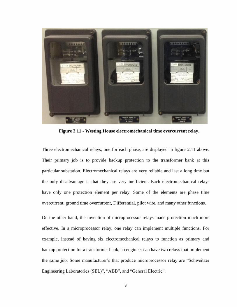
Westing House. Figure 2.11, shown below displays a “General Electric”
electromechanical relay implementing phase time overcurrent.
3
Figure 2.11 - Westing House electromechanical time overcurrent relay.
Three electromechanical relays, one for each phase, are displayed in figure 2.11 above.
Their primary job is to provide backup protection to the transformer bank at this
particular substation. Electromechanical relays are very reliable and last a long time but
the only disadvantage is that they are very inefficient. Each electromechanical relays
have only one protection element per relay. Some of the elements are phase time
overcurrent, ground time overcurrent, Differential, pilot wire, and many other functions.
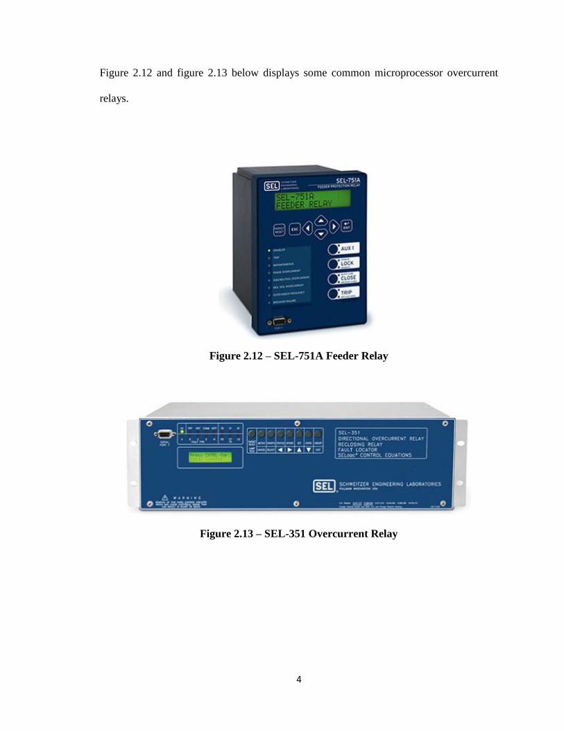
On the other hand, the invention of microprocessor relays made protection much more
effective. In a microprocessor relay, one relay can implement multiple functions. For
example, instead of having six electromechanical relays to function as primary and
backup protection for a transformer bank, an engineer can have two relays that implement
the same job. Some manufacturer’s that produce microprocessor relay are “Schweitzer
Engineering Laboratories (SEL)”, “ABB”, and “General Electric”.
4
Figure 2.12 and figure 2.13 below displays some common microprocessor overcurrent
relays.
Figure 2.12 – SEL-751A Feeder Relay
Figure 2.13 – SEL-351 Overcurrent Relay
5
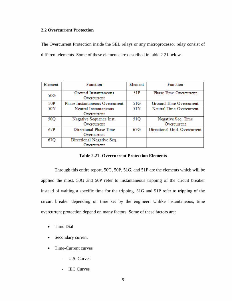
2.2 Overcurrent Protection
The Overcurrent Protection inside the SEL relays or any microprocessor relay consist of
different elements. Some of these elements are described in table 2.21 below.
Table 2.21- Overcurrent Protection Elements
Through this entire report, 50G, 50P, 51G, and 51P are the elements which will be
applied the most. 50G and 50P refer to instantaneous tripping of the circuit breaker
instead of waiting a specific time for the tripping. 51G and 51P refer to tripping of the
circuit breaker depending on time set by the engineer. Unlike instantaneous, time
overcurrent protection depend on many factors. Some of these factors are:
Time Dial
Secondary current
Time-Current curves
- U.S. Curves
- IEC Curves
6
Current Transformer
Maximum fault Current
Tripping time (Tp)
Reset time (TR)
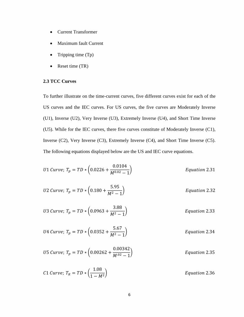
2.3 TCC Curves
To further illustrate on the time-current curves, five different curves exist for each of the
US curves and the IEC curves. For US curves, the five curves are Moderately Inverse
(U1), Inverse (U2), Very Inverse (U3), Extremely Inverse (U4), and Short Time Inverse
(U5). While for the IEC curves, there five curves constitute of Moderately Inverse (C1),
Inverse (C2), Very Inverse (C3), Extremely Inverse (C4), and Short Time Inverse (C5).
The following equations displayed below are the US and IEC curve equations.
(
)
(
)
(
)
(
)
(
)
(
)
7
(
)
(
)
(
)
(
)
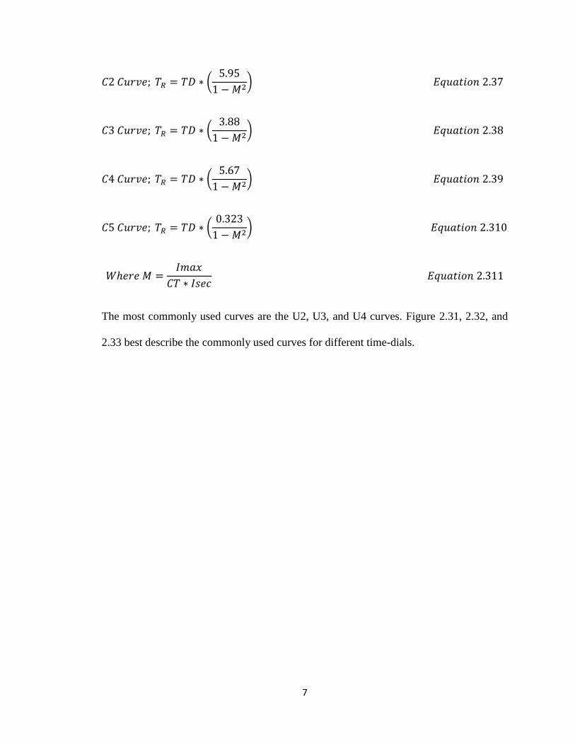
The most commonly used curves are the U2, U3, and U4 curves. Figure 2.31, 2.32, and
2.33 best describe the commonly used curves for different time-dials.
8
Figure 2.31 – U2 Curve (TD: 0.5 to 15) [2]
9
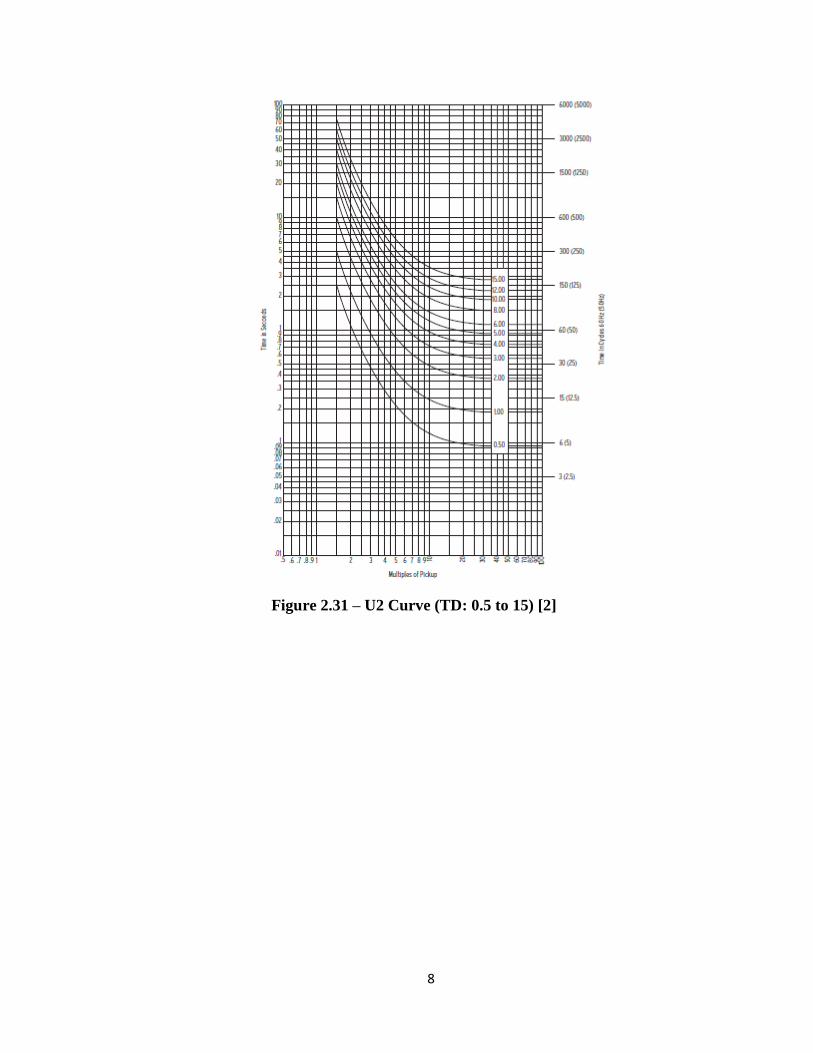
Figure 2.32 – U3 Curve (TD: 0.5 to 15) [2]
As shown in figure 2.32 above, different curves are displayed for varying time dial. “The
tripping time duration of the overcurrent relay (SEL) can vary due to relay type, time-dial
setting (TDS) and magnitude fault currents.”[3] The U3 curve will be used in a
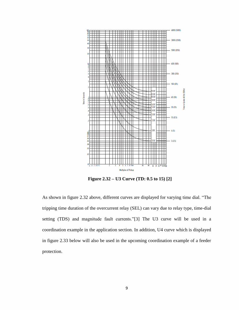
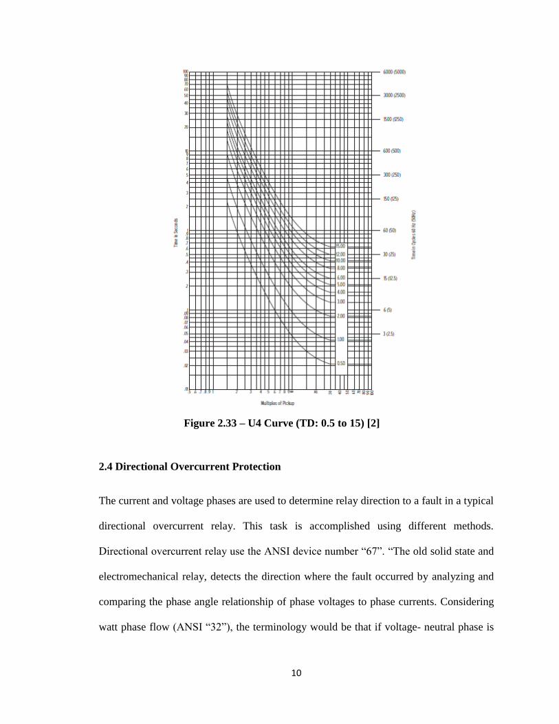
coordination example in the application section. In addition, U4 curve which is displayed
in figure 2.33 below will also be used in the upcoming coordination example of a feeder
protection.
10
Figure 2.33 – U4 Curve (TD: 0.5 to 15) [2]
2.4 Directional Overcurrent Protection
The current and voltage phases are used to determine relay direction to a fault in a typical
directional overcurrent relay. This task is accomplished using different methods.
Directional overcurrent relay use the ANSI device number “67”. “The old solid state and
electromechanical relay, detects the direction where the fault occurred by analyzing and
comparing the phase angle relationship of phase voltages to phase currents. Considering
watt phase flow (ANSI “32”), the terminology would be that if voltage- neutral phase is
11
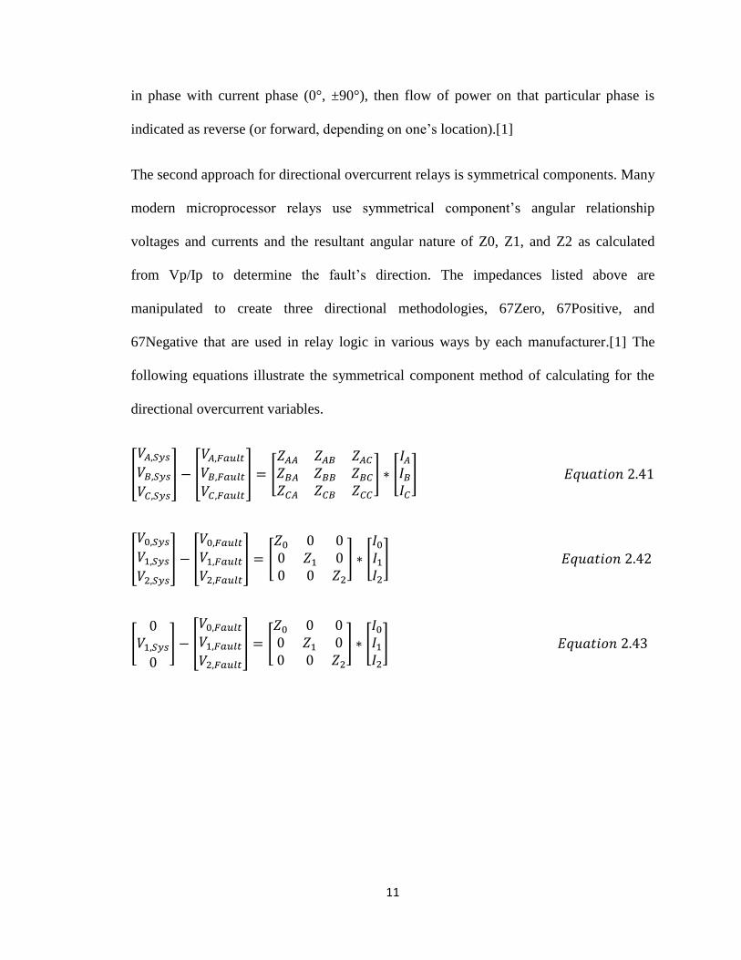
in phase with current phase (0°, ±90°), then flow of power on that particular phase is
indicated as reverse (or forward, depending on one’s location).[1]
The second approach for directional overcurrent relays is symmetrical components. Many
modern microprocessor relays use symmetrical component’s angular relationship
voltages and currents and the resultant angular nature of Z0, Z1, and Z2 as calculated
from Vp/Ip to determine the fault’s direction. The impedances listed above are
manipulated to create three directional methodologies, 67Zero, 67Positive, and
67Negative that are used in relay logic in various ways by each manufacturer.[1] The
following equations illustrate the symmetrical component method of calculating for the
directional overcurrent variables.
[
] [
] [
] [
]
[
] [
] [
] [
]
[
] [
] [
] [
]
12
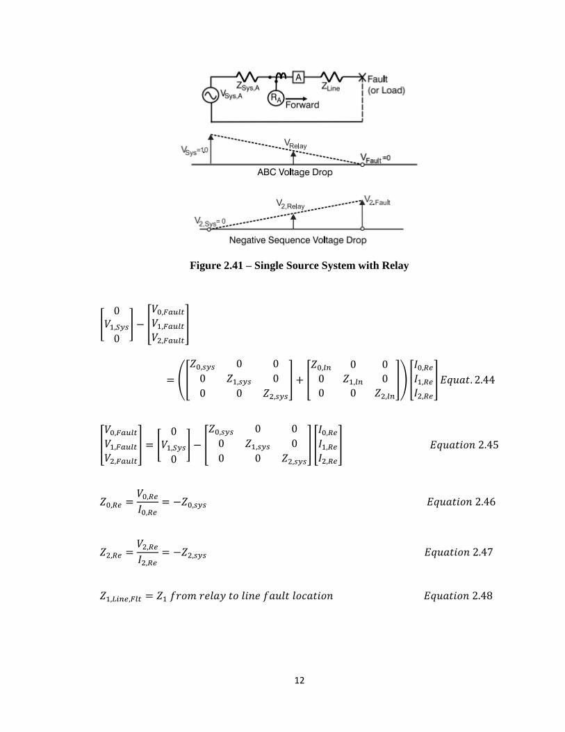
Figure 2.41 – Single Source System with Relay
[
] [
]
([
] [
]) [
]
[
] [
] [
] [
]
13
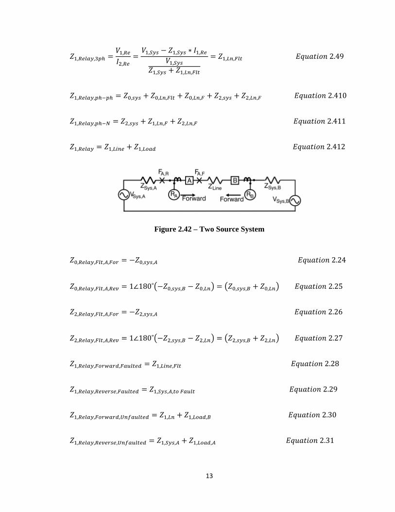
Figure 2.42 – Two Source System
( ) ( )
( ) ( )
14
2.5 Distance Protection
Distance protection is a crucial type of protection that varies from overcurrent protection.
It occupies the ANSI number of 21. Selectivity and fast operation is why some electrical
engineers prefer distance relay over overcurrent relays. Distance relays are generally
implemented for transmission line protection, sub-transmission lines backup protection,
and primary phase-fault protection. Overcurrent relays are commonly used for all type of
fault primary and back-up protection, but in today’s market there is a huge demand
toward distance relays for phase to ground protection.[5]
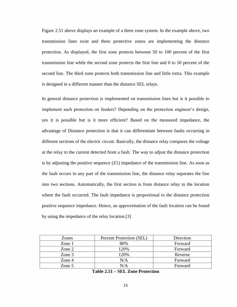
The basic distance protection is based on Zones. Usually the first zone protects 80% of
the electric circuit, while the second zone protects 120% of the circuit (Table 2). The
third zone is equal to the second zone and it is upside down. The SEL relay design
implements up to five zones. These values can vary depending on the design but they are
used as default values for SEL relays that implement distance protection. The reason for
using 80% for the first zone is to avoid nuisance trips. The extra 20% that is implemented
on zone 2 is used to fasten protection towards the end of the line. The third zone is upside
down to protect the line from reverse current.
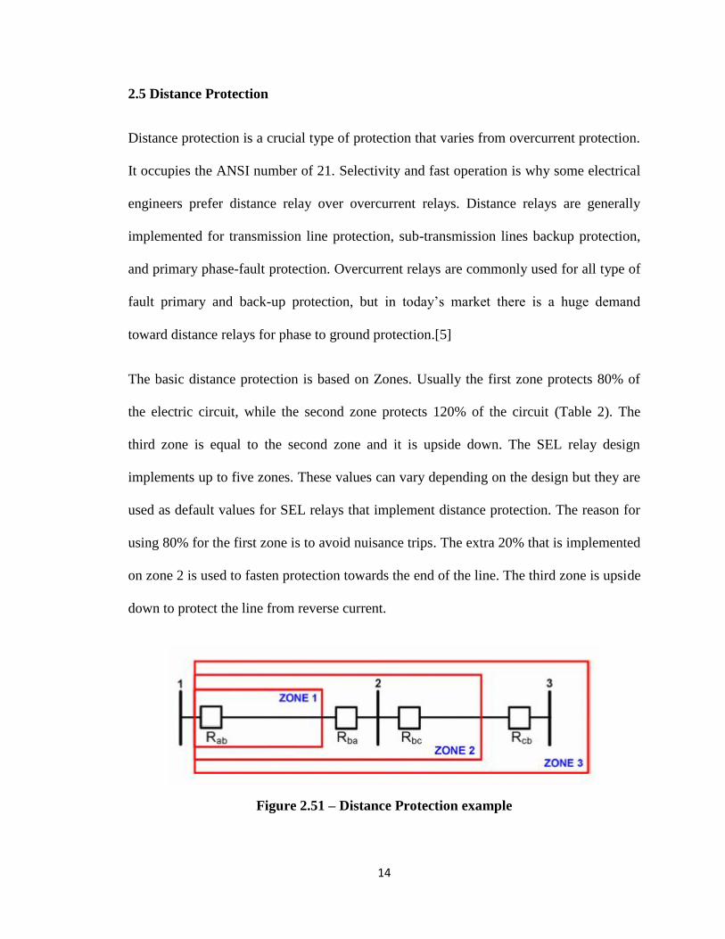
Figure 2.51 – Distance Protection example
15
Figure 2.51 above displays an example of a three zone system. In the example above, two
transmission lines exist and three protective zones are implementing the distance
protection. As displayed, the first zone protects between 50 to 100 percent of the first
transmission line while the second zone protects the first line and 0 to 50 percent of the
second line. The third zone protects both transmission line and little extra. This example
is designed in a different manner than the distance SEL relays.
In general distance protection is implemented on transmission lines but is it possible to
implement such protection on feeders? Depending on the protection engineer’s design,
yes it is possible but is it more efficient? Based on the measured impedance, the
advantage of Distance protection is that it can differentiate between faults occurring in
different sections of the electric circuit. Basically, the distance relay compares the voltage
at the relay to the current detected from a fault. The way to adjust the distance protection
is by adjusting the positive sequence (Z1) impedance of the transmission line. As soon as
the fault occurs in any part of the transmission line, the distance relay separates the line
into two sections. Automatically, the first section is from distance relay to the location
where the fault occurred. The fault impedance is proportional to the distance protection
positive sequence impedance. Hence, an approximation of the fault location can be found
by using the impedance of the relay location.[3]
Zones Percent Protection (SEL) Direction
Zone 1 80% Forward
Zone 2 120% Forward
Zone 3 120% Reverse
Zone 4 N/A Forward
Zone 5 N/A Forward
Table 2.51 – SEL Zone Protection
16
2.6 Comparison and Selection
After analyzing the three types of protection, it is time to analyze feeder protection. All
three types of protections can be implemented in feeder protection. The most common
feeder protection is overcurrent protection. One problem with overcurrent protection is
that it is a one way protection, which means that if power reversed direction the feeder
would be unprotected. Power can reverse direction if a distributed generator (DG) is
connected to the grid. In order to provide overcurrent feeder protection even when power
is reversed, directional overcurrent is implemented. One disadvantage of directional
overcurrent protection is the settings are too complicated. As shown from equation X to
equation Y, directional overcurrent equations are much more involved with multiple
variables to account for. If overcurrent protection is not to be implemented, distance
protection can be used. Distance protection will protect a given feeder or line regardless
of the direction of the power. At a renewable energy source, distance protection can be
implemented to feeders since it is common to have a DG connected to the grid.
17
2.7 Fuses
Fuses are essential part of feeder protection; they are usually placed to interrupt faults
without tripping the breaker. A fuse is basically a low value resistor which works as a
device that melts when the current rating exceeds the fuse rating. It is commonly used
downstream in a distribution feeder. One of the advantages of fuses are that they protect
the feeder from a huge outage [6]
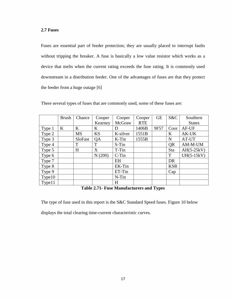
There several types of fuses that are commonly used, some of these fuses are:
Brush Chance Cooper
Kearney
Cooper
McGraw
Cooper
RTE
GE S&C Southern
States
Type 1 K K K D 1406B 9F57 Coor AF-UF
Type 2 MS KS K-silver 1551B K AK-UK
Type 3 SloFast QA K-Tin 1555B N AT-UT
Type 4 T T S-Tin QR AM-M-UM
Type 5 H X T-Tin Sta AH(5-25kV)
Type 6 N (200) C-Tin T UH(5-15kV)
Type 7 EH DR
Type 8 EK-Tin KSR
Type 9 ET-Tin Cap
Type10 N-Tin
Type11 H
Table 2.71- Fuse Manufacturers and Types
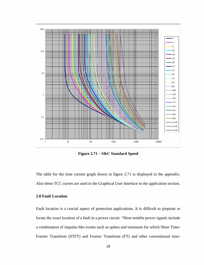
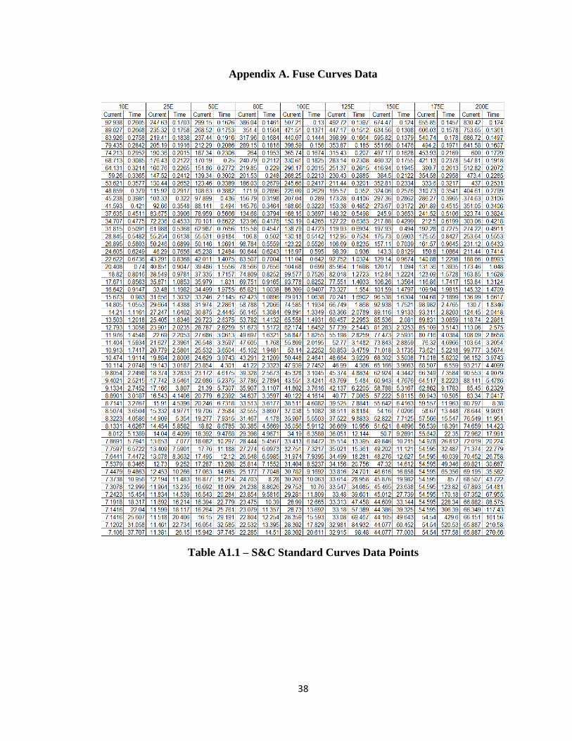
The type of fuse used in this report is the S&C Standard Speed fuses. Figure 10 below
displays the total clearing time-current characteristic curves.
18
Figure 2.71 – S&C Standard Speed
The table for the time current graph drawn in figure 2.71 is displayed in the appendix.
Also these TCC curves are used in the Graphical User Interface in the application section.
2.8 Fault Location
Fault location is a crucial aspect of protection applications. It is difficult to pinpoint or
locate the exact location of a fault in a power circuit. “Most notable power signals include
a combination of impulse-like events such as spikes and transients for which Short Time-
Fourier Transform (STFT) and Fourier Transform (FT) and other conventional time-
19
frequency methods are not as suitable for analysis.” [2] “The Wavelet Transform (WT) is
one of the best ways for analyzing transient signals.”[2] Therefore the Wavelet analysis
that is based on two Algorithms is the best solution for accurate fault location.
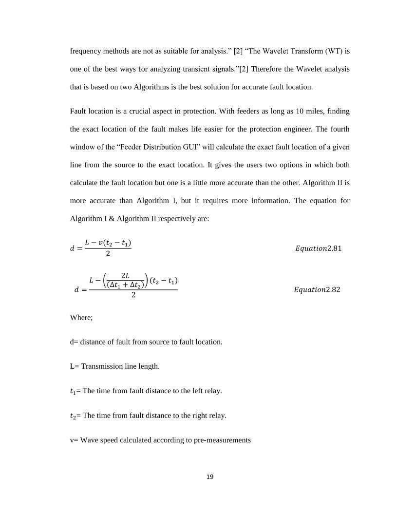
Fault location is a crucial aspect in protection. With feeders as long as 10 miles, finding
the exact location of the fault makes life easier for the protection engineer. The fourth
window of the “Feeder Distribution GUI” will calculate the exact fault location of a given
line from the source to the exact location. It gives the users two options in which both
calculate the fault location but one is a little more accurate than the other. Algorithm II is
more accurate than Algorithm I, but it requires more information. The equation for
Algorithm I & Algorithm II respectively are:
(
)
Where;
d= distance of fault from source to fault location.
L= Transmission line length.
= The time from fault distance to the left relay.
= The time from fault distance to the right relay.
v= Wave speed calculated according to pre-measurements

20
= The difference in the main and reflected waves for the relay left of fault.
= The difference in the main and reflected waves for the relay right of fault.
A simple example will solved using hand calculation to illustrate the difference between
the two methods and the level of accuracy.
21
3. System Application
3.1 Entire GUI
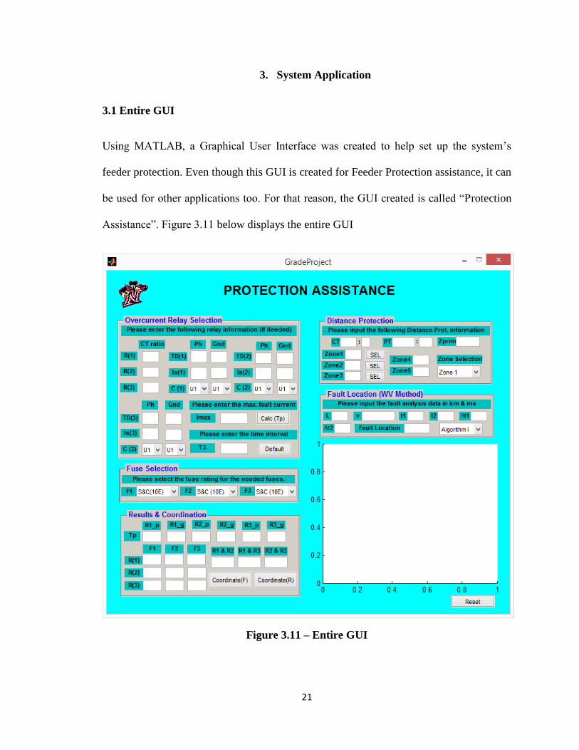
Using MATLAB, a Graphical User Interface was created to help set up the system’s
feeder protection. Even though this GUI is created for Feeder Protection assistance, it can
be used for other applications too. For that reason, the GUI created is called “Protection
Assistance”. Figure 3.11 below displays the entire GUI
Figure 3.11 – Entire GUI
22
3.2 GUI - Windows
“Protection Assistance” GUI is consist of six main windows. The first three windows
help assist with Overcurrent relay coordination. The Fourth window is involved in
Distance Protection while the fifth window assists the user with fault location using the
WV method. The sixth window is the axes window which allows the user to view the
plots generated by the other windows.
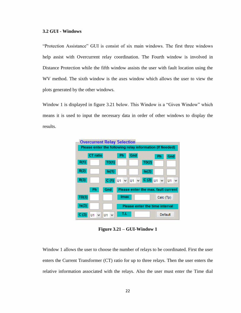
Window 1 is displayed in figure 3.21 below. This Window is a “Given Window” which
means it is used to input the necessary data in order of other windows to display the
results.
Figure 3.21 – GUI-Window 1
Window 1 allows the user to choose the number of relays to be coordinated. First the user
enters the Current Transformer (CT) ratio for up to three relays. Then the user enters the
relative information associated with the relays. Also the user must enter the Time dial
23
(TD) and the secondary current (Is) associated with the relay used. All the symbols
followed by “(1)” are associated with the first relays used. Also, “(2)” and “(3)” are
associated with the second and third relay respectively. After providing the necessary
information, the user has to select the time-current characteristic curve to be used for
phase and ground at each relay selected. The curves that are available for selection are the
U.S. curves and the I.E.C. curves. A code was written for each “curve selection” pop up
menu in order to display the graph associated with the curve right after the curve type is
selected.
This process will only display the curves related to a specific design but in order to
coordinate the relays together couple of additional steps have to be followed. The first
step is to run the short circuit analysis on a separate program and display the maximum
fault “Imax” in the edit box in window 1. Clicking the push bottom “Calc (Tp)” located
next to “Imax” will calculate the Tripping time for each relay in Window 3 displayed in
figure 3.23. The last edit box in window 1 is the coordination “Time Interval (T.I.)”. The
“Default” push bottom, located next to the “Time Interval” edit box, is used to input a
default value of 0.25 for the time interval.
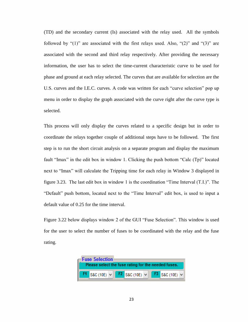
Figure 3.22 below displays window 2 of the GUI “Fuse Selection”. This window is used
for the user to select the number of fuses to be coordinated with the relay and the fuse
rating.
24
Figure 3.22 - GUI-Window 2
Window 2 allows the user to integrate in the design up to three fuses. A code was written
for each “Fuse selection” pop up menu in order to display the graph associated with the
rated fuse. The SMU Fuse Units-S&C Standard Speed time overcurrent characteristic
curves were used with the rating varying from 10E to 250E. Coordination between the
relays selected in window 1 and the fuses selected in window 2 will be done in window 3.
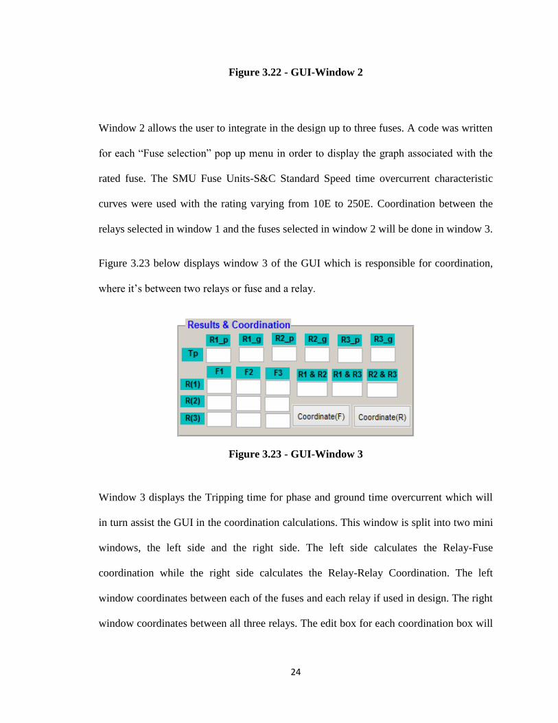
Figure 3.23 below displays window 3 of the GUI which is responsible for coordination,
where it’s between two relays or fuse and a relay.
Figure 3.23 - GUI-Window 3
Window 3 displays the Tripping time for phase and ground time overcurrent which will
in turn assist the GUI in the coordination calculations. This window is split into two mini
windows, the left side and the right side. The left side calculates the Relay-Fuse
coordination while the right side calculates the Relay-Relay Coordination. The left
window coordinates between each of the fuses and each relay if used in design. The right
window coordinates between all three relays. The edit box for each coordination box will
25
display a “YES” or “NO” respond upon pushing the “Coordinate (F)” or “Coordinate
(R)” push bottoms depending on application.
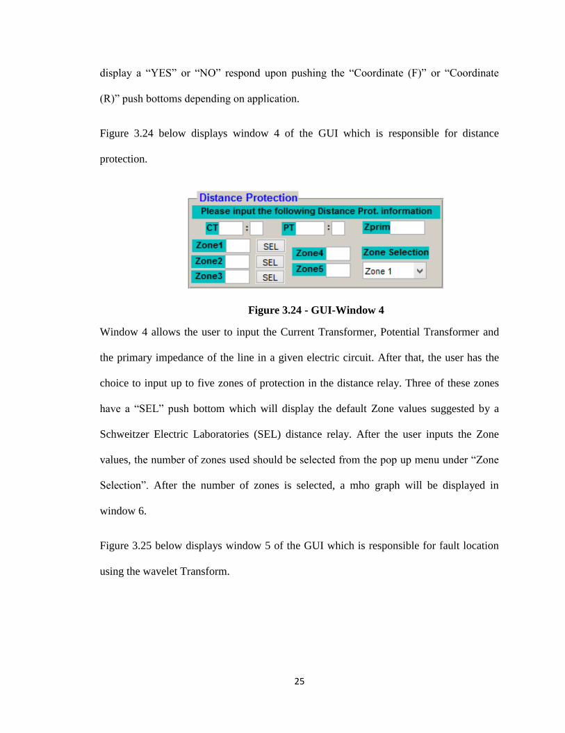
Figure 3.24 below displays window 4 of the GUI which is responsible for distance
protection.
Figure 3.24 - GUI-Window 4
Window 4 allows the user to input the Current Transformer, Potential Transformer and
the primary impedance of the line in a given electric circuit. After that, the user has the
choice to input up to five zones of protection in the distance relay. Three of these zones
have a “SEL” push bottom which will display the default Zone values suggested by a
Schweitzer Electric Laboratories (SEL) distance relay. After the user inputs the Zone
values, the number of zones used should be selected from the pop up menu under “Zone
Selection”. After the number of zones is selected, a mho graph will be displayed in
window 6.
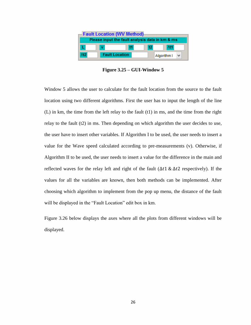
Figure 3.25 below displays window 5 of the GUI which is responsible for fault location
using the wavelet Transform.
26
Figure 3.25 – GUI-Window 5
Window 5 allows the user to calculate for the fault location from the source to the fault
location using two different algorithms. First the user has to input the length of the line
(L) in km, the time from the left relay to the fault (t1) in ms, and the time from the right
relay to the fault (t2) in ms. Then depending on which algorithm the user decides to use,
the user have to insert other variables. If Algorithm I to be used, the user needs to insert a
value for the Wave speed calculated according to pre-measurements (v). Otherwise, if
Algorithm II to be used, the user needs to insert a value for the difference in the main and
reflected waves for the relay left and right of the fault ( respectively). If the
values for all the variables are known, then both methods can be implemented. After
choosing which algorithm to implement from the pop up menu, the distance of the fault
will be displayed in the “Fault Location” edit box in km.
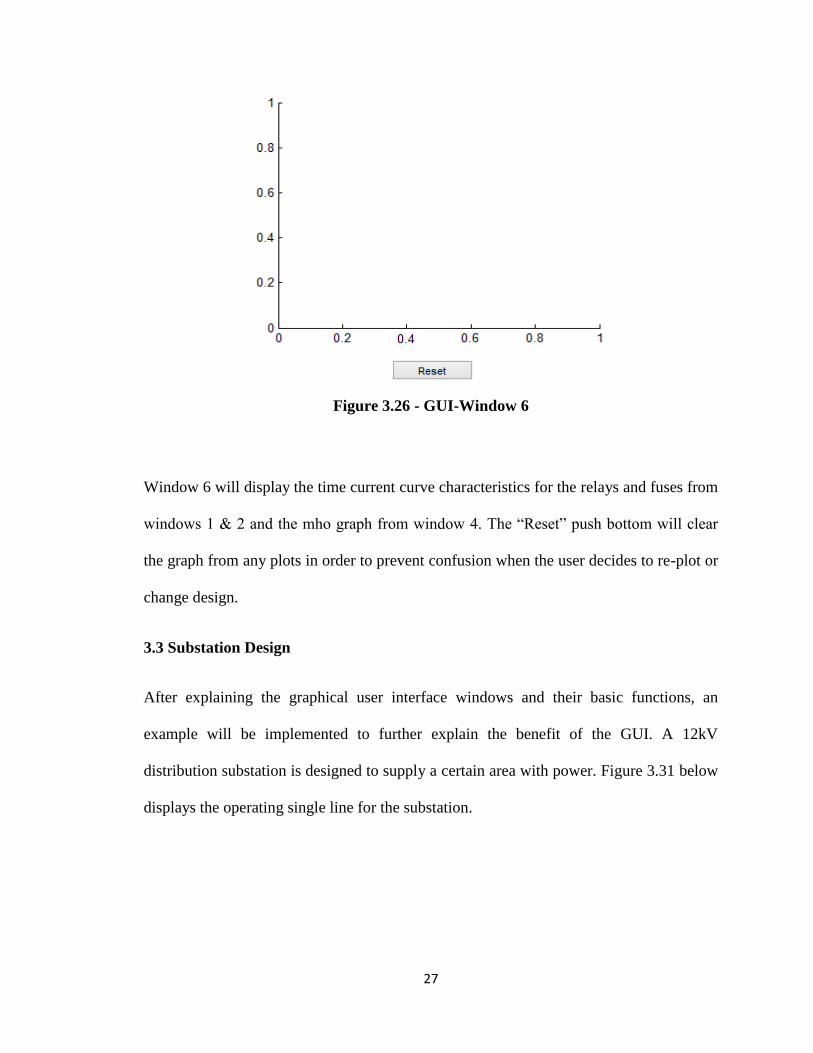
Figure 3.26 below displays the axes where all the plots from different windows will be
displayed.
27
Figure 3.26 - GUI-Window 6
Window 6 will display the time current curve characteristics for the relays and fuses from
windows 1 & 2 and the mho graph from window 4. The “Reset” push bottom will clear
the graph from any plots in order to prevent confusion when the user decides to re-plot or
change design.
3.3 Substation Design
After explaining the graphical user interface windows and their basic functions, an
example will be implemented to further explain the benefit of the GUI. A 12kV
distribution substation is designed to supply a certain area with power. Figure 3.31 below
displays the operating single line for the substation.
28
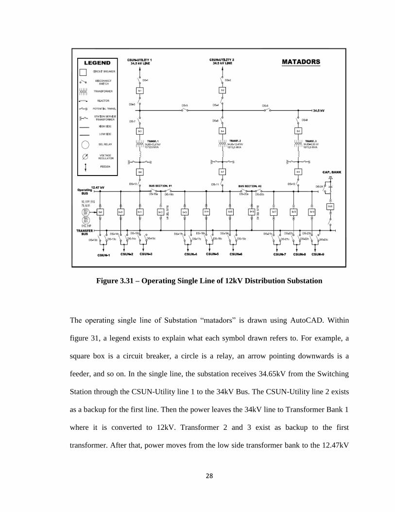
Figure 3.31 – Operating Single Line of 12kV Distribution Substation
The operating single line of Substation “matadors” is drawn using AutoCAD. Within
figure 31, a legend exists to explain what each symbol drawn refers to. For example, a
square box is a circuit breaker, a circle is a relay, an arrow pointing downwards is a
feeder, and so on. In the single line, the substation receives 34.65kV from the Switching
Station through the CSUN-Utility line 1 to the 34kV Bus. The CSUN-Utility line 2 exists
as a backup for the first line. Then the power leaves the 34kV line to Transformer Bank 1
where it is converted to 12kV. Transformer 2 and 3 exist as backup to the first
transformer. After that, power moves from the low side transformer bank to the 12.47kV
29
operating bus. Then power transfers from the operating bus to the feeders. The transfer
bus exists as backup to the operating bus. After the feeders, power is sent downstream to
supply residential and businesses.
3.4 GUI - Overcurrent Example
As displayed on the single lines, the protection on the feeders consists of two relays
connected to the circuit breaker. The main relay is SEL-351 while the backup relay is
SEL-501. The functions used as protection on the main relay (SEL-351) are 50, 50P,
50G, 79, and 81.The functions used for protection on the backup relay (SEL-501) are
51G and 51P. One problem exists with the current protection which is coordination
between the main relay and the backup relays. The GUI designed in this section will
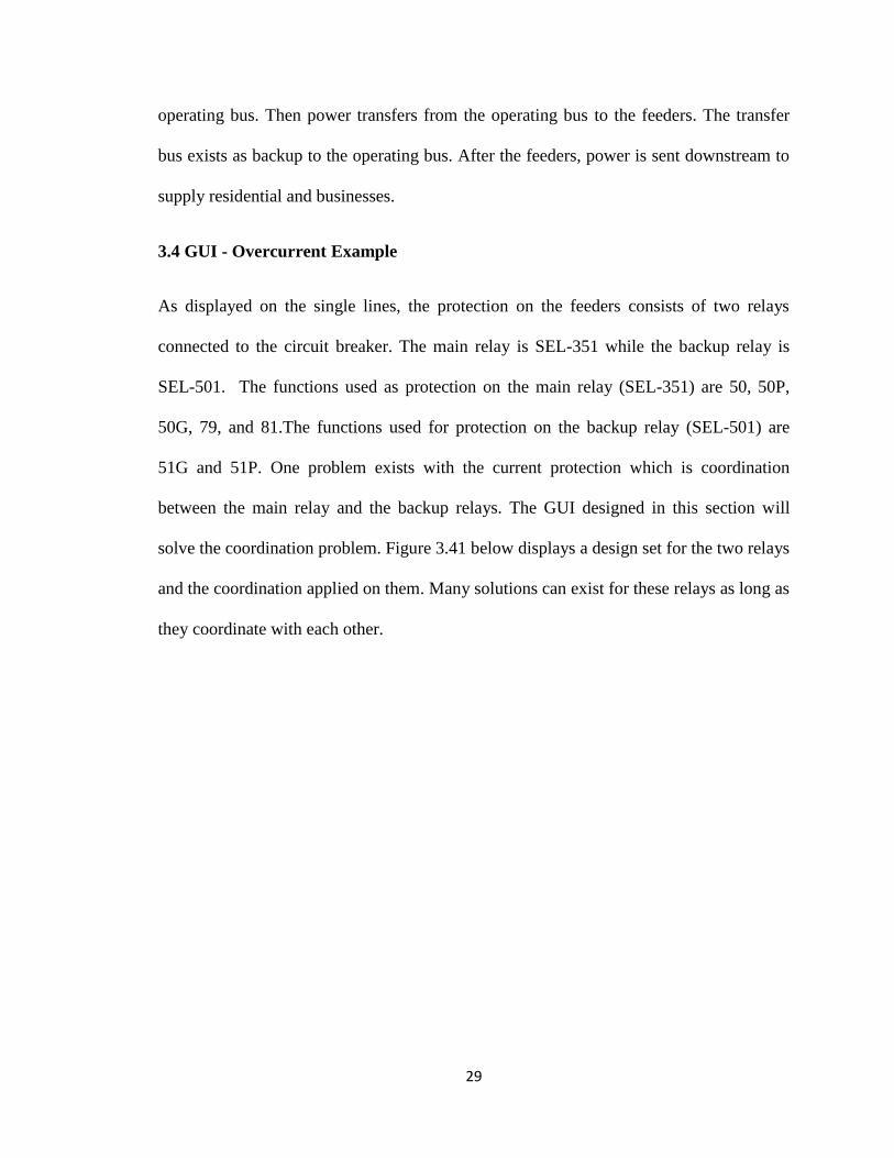
solve the coordination problem. Figure 3.41 below displays a design set for the two relays
and the coordination applied on them. Many solutions can exist for these relays as long as
they coordinate with each other.
30
Figure 3.41- Main and Backup relay coordination
As displayed in window 1, the given CT is 400:5 so the CT ratio is 80 for both relays.
The design for the main relay consists of time dial of 3 and secondary current is set at 7A
which sets the minimum pickup current at 560A.The curve chosen is the extremely
inverse (U4) curve. The design for the backup relay consists of time dial of 3 and
secondary current is set at 10A which makes the minimum pickup current at 300A. The
curve chosen is the inverse curve (U2). After running the short circuit analysis using
31
computer software, the maximum fault was found to be 20,000A so Imax in window 1
was set to 20,000. The curves for the two relays are displayed in window 6, the blue is
the main relay and the green is the backup relay. After plotting the graphs, for
coordination purposes the time interval (window 1) was set to 0.25. Clicking on
“Coordinate(R)” bottom in window 3 displayed a “YES” which means both relays are
coordinated. If “NO” was displayed that means both relays were not coordinated and the
designed to be altered.
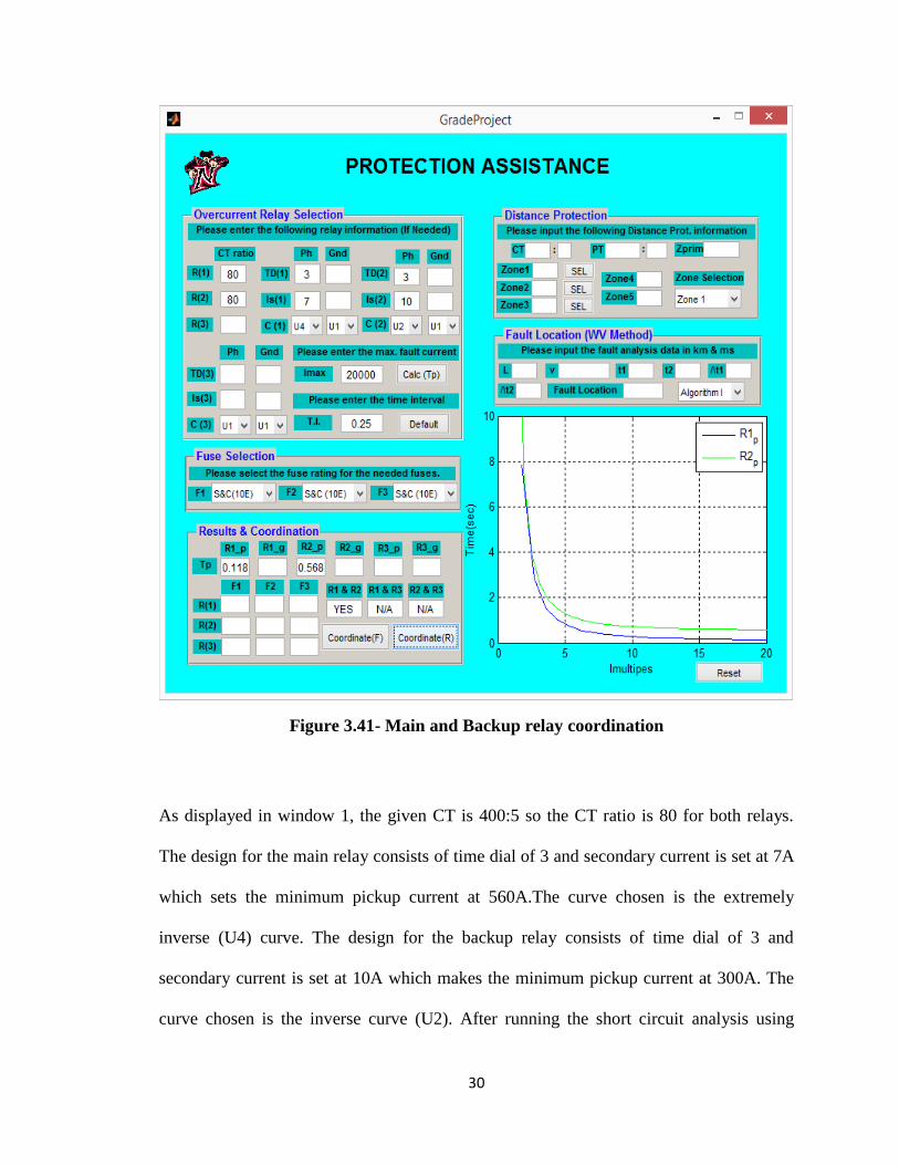
After having both relays coordinated, the next step would be to input the data used in the
SEL software “AcSELerator”.
Figure 3.42 - AcSELerator Software (SEL-351)
32
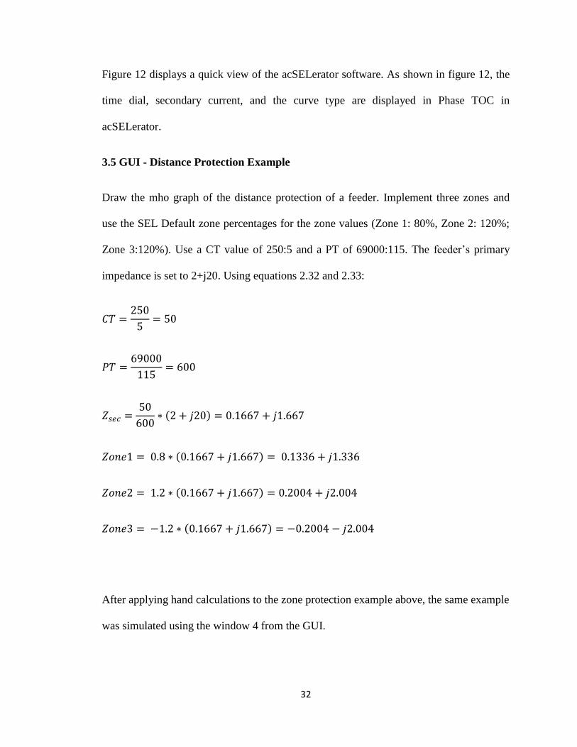
Figure 12 displays a quick view of the acSELerator software. As shown in figure 12, the
time dial, secondary current, and the curve type are displayed in Phase TOC in
acSELerator.
3.5 GUI - Distance Protection Example
Draw the mho graph of the distance protection of a feeder. Implement three zones and
use the SEL Default zone percentages for the zone values (Zone 1: 80%, Zone 2: 120%;
Zone 3:120%). Use a CT value of 250:5 and a PT of 69000:115. The feeder’s primary
impedance is set to 2+j20. Using equations 2.32 and 2.33:
After applying hand calculations to the zone protection example above, the same example
was simulated using the window 4 from the GUI.
33
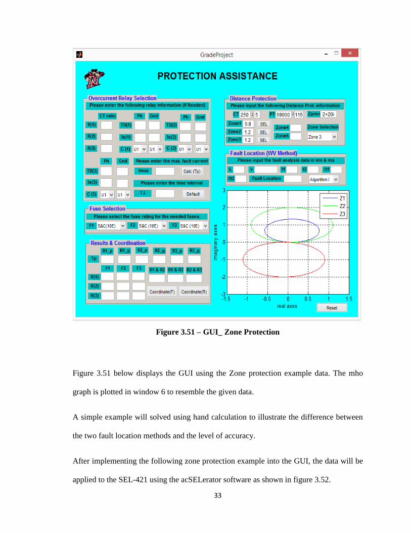
Figure 3.51 – GUI_ Zone Protection
Figure 3.51 below displays the GUI using the Zone protection example data. The mho
graph is plotted in window 6 to resemble the given data.
A simple example will solved using hand calculation to illustrate the difference between
the two fault location methods and the level of accuracy.
After implementing the following zone protection example into the GUI, the data will be
applied to the SEL-421 using the acSELerator software as shown in figure 3.52.
34
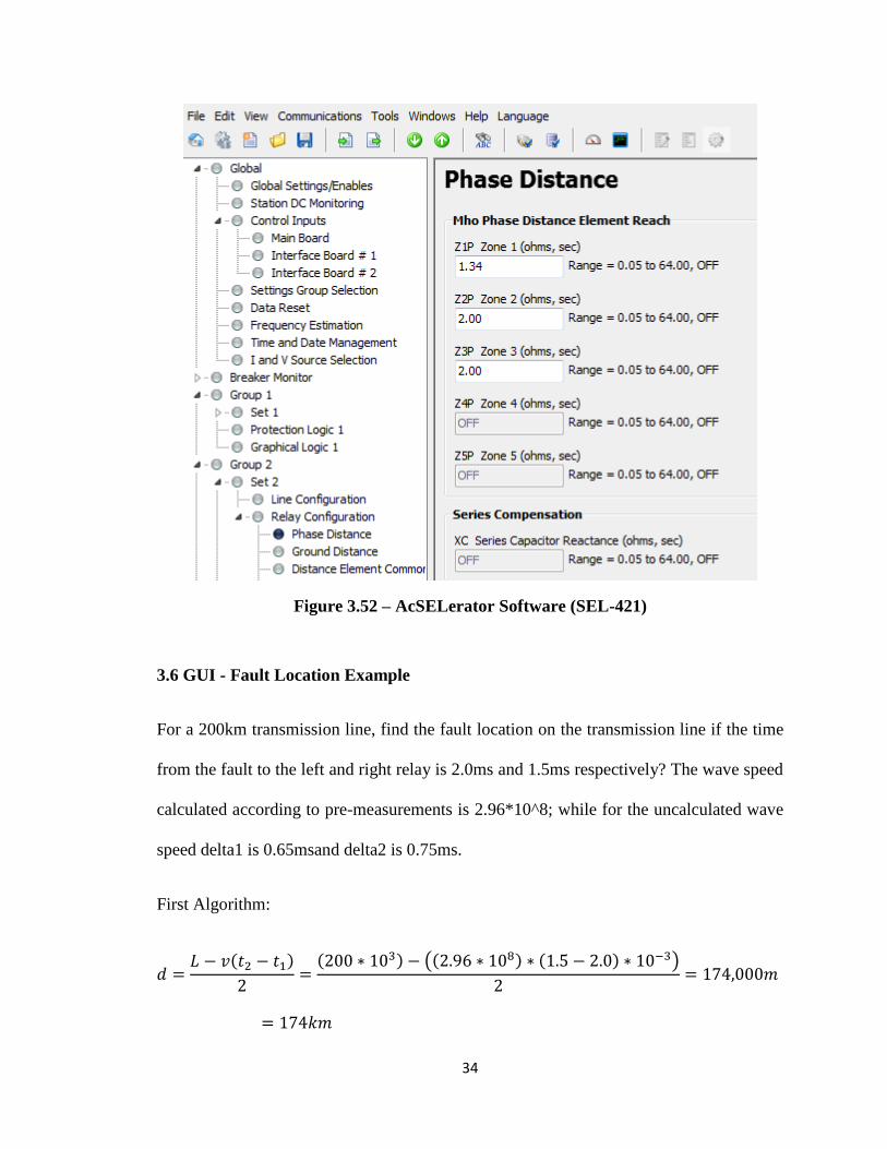
Figure 3.52 – AcSELerator Software (SEL-421)
3.6 GUI - Fault Location Example
For a 200km transmission line, find the fault location on the transmission line if the time
from the fault to the left and right relay is 2.0ms and 1.5ms respectively? The wave speed
calculated according to pre-measurements is 2.96*10^8; while for the uncalculated wave
speed delta1 is 0.65msand delta2 is 0.75ms.
First Algorithm:
( )
35
Therefore, the fault location using the second algorithm is 174km.
Second Algorithm:
(
)
(
( ))
Therefore, the fault location using the second algorithm is 171km. The second algorithm
is much more accurate than the first because more variables are involved.
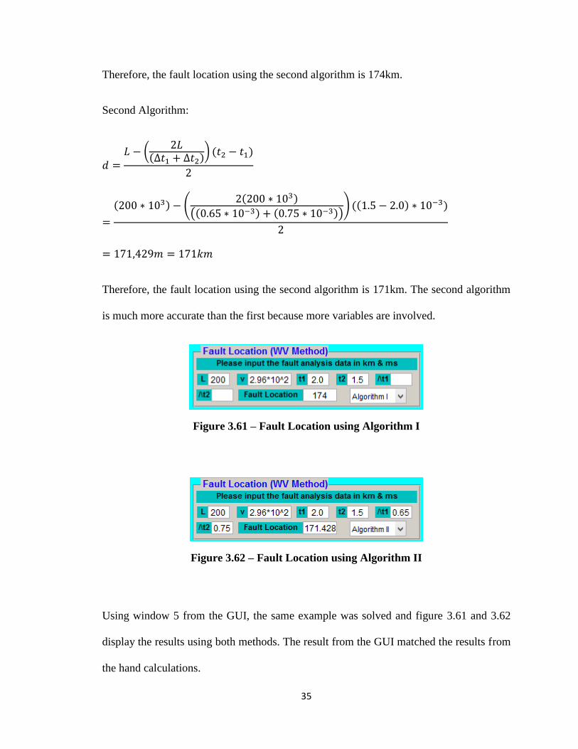
Figure 3.61 – Fault Location using Algorithm I
Figure 3.62 – Fault Location using Algorithm II
Using window 5 from the GUI, the same example was solved and figure 3.61 and 3.62
display the results using both methods. The result from the GUI matched the results from
the hand calculations.
36
4. Conclusion
The paper discussed the three types of protection that can be implemented on a
distribution feeder.
This paper presented an in depth analysis and comparison of the overcurrent,
directional overcurrent, and distance protection.
In addition, this paper presented two new fault location detection algorithms.
The most commonly used protection on feeders is Overcurrent protection.
Schweitzer Engineering Laboratories relays and time-current curves (TCC) were
used in this report.
An operating single line diagram of a fictional substation was drawn using
AutoCAD to display feeder location in a substation.
A Graphical User Interface “Protection Assistance” was created using MATLAB
to help assist with Overcurrent and distance protection.
Coordination between the main relay and backup relay was implemented using
TCC curves in the GUI
Also, the GUI included a window to assist in fault location calculation using the
Algorithm of choice.
Zone protection and directional overcurrent protection are crucial and necessary
in certain cases especially when reverse power is present.
A study was implemented on zone protection and the mho graph was displayed in
the GUI.
It all comes down to the engineer’s choice to what design to implement.
37
References
[1] J. Horak and W. Babic, “Directional Overcurrent Relaying (67) Concepts”, IEEE
Rural Electric Power Conference, 2006.
[2] A. Tabatabaei, M.R. Mosavi, & A. Rahmati, “Fault Location Techniques in Power
System based on Traveling Wave using Wavelet Analysis and GPS Timing”, Iran
University of Science and Technology.
[3] D. Uthitsunthorn, and T. Kulworawanichpong, “Distance Protection of a Renewable
Energy Plant in Electric Power Distribution Systems”, International Conference on
Power System Technology, 2010
[4] Linear Technology. “Overvoltage & Overcurrent Protection”. Internet:
www.linear.com/products/overvoltage__*_overcurrent_protection, 2013 [Nov. 2, 2013].
[5] Distance Protection. “Line Protection with Distance Relay”. Internet:
www.gedigitalenergy.com/multilin/notes/artsci/art14.pdf, Nov, 2013 [Nov. 5, 2013].
[6] Online Electrical Engineering Study Site. “Electrical Fuse HRC Fuse High Rupturing
Capacity”. Internet: www.electrical4u.com/electrical-fuse-hrc-fuse-high-rupturing-
capacity/, Nov, 2013 [Nov. 1, 2013].
[7] I. Chilvers and N. Jenkins, "Distance relaying of 1l kV circuits to increase the
installed capacity of distributed generation", IEEE Proceedings - Generation,
Transmission and Distribution.
[8] H. Shateri and S. Jamali, "Measured impedance by distance relay in second protective
zone", The International Universities Power Engineering Conference, September 2007
[9] L.G. Perez, and A.1 Urdaneta, "Optimal Computation of Distance Relays Second
Zone Timing in a Protection Scheme with Directional Overcurrent Relays", IEEE
Power Engineering Review.
[10] T Smith, M.E. Lacedonia, S. Pitts and Z. Zhang, “Review of Application of Ground
Distance Protection”,
[11] 1 Cho, C. Jung and 1 Kim, "Adaptive setting of digital relay for transmission line
protection", International Conference on Power System Technology.
38
Appendix A. Fuse Curves Data
Table A1.1 – S&C Standard Curves Data Points
39
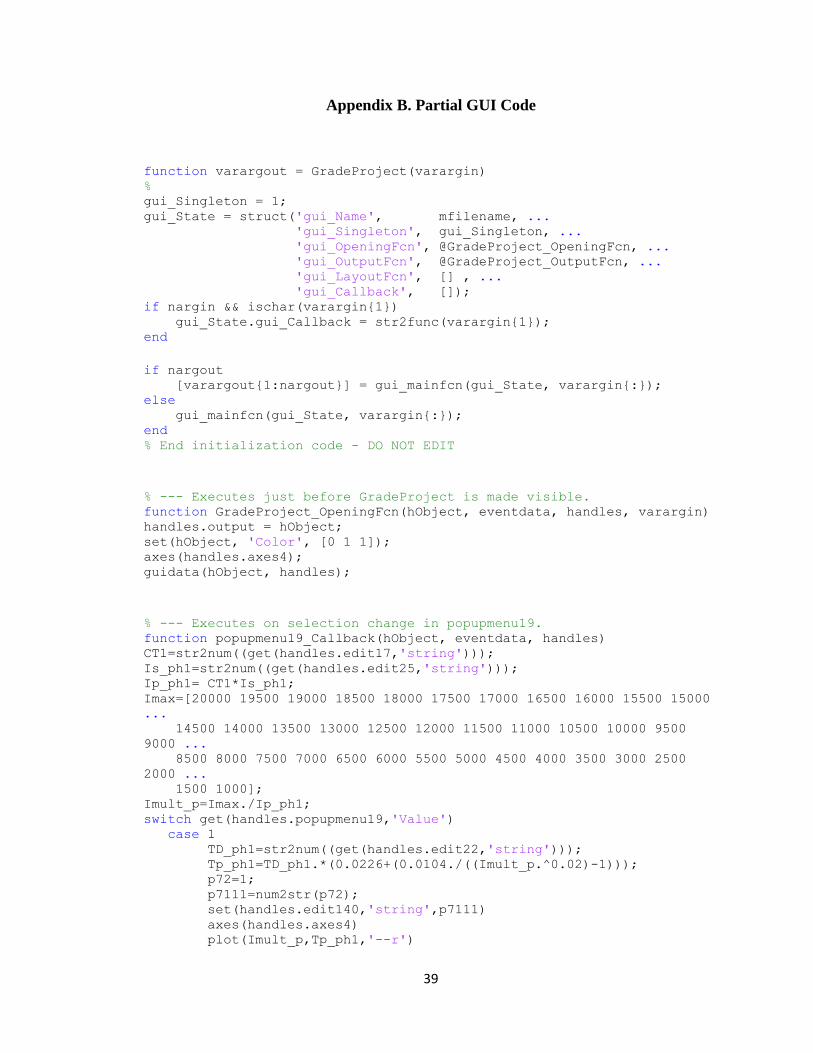
Appendix B. Partial GUI Code
function varargout = GradeProject(varargin) % gui_Singleton = 1; gui_State = struct('gui_Name', mfilename, ... 'gui_Singleton', gui_Singleton, ... 'gui_OpeningFcn', @GradeProject_OpeningFcn, ... 'gui_OutputFcn', @GradeProject_OutputFcn, ... 'gui_LayoutFcn', [] , ... 'gui_Callback', []); if nargin && ischar(varargin{1}) gui_State.gui_Callback = str2func(varargin{1}); end
if nargout [varargout{1:nargout}] = gui_mainfcn(gui_State, varargin{:}); else gui_mainfcn(gui_State, varargin{:}); end % End initialization code - DO NOT EDIT
% --- Executes just before GradeProject is made visible. function GradeProject_OpeningFcn(hObject, eventdata, handles, varargin) handles.output = hObject; set(hObject, 'Color', [0 1 1]); axes(handles.axes4); guidata(hObject, handles);
% --- Executes on selection change in popupmenu19. function popupmenu19_Callback(hObject, eventdata, handles) CT1=str2num((get(handles.edit17,'string'))); Is_ph1=str2num((get(handles.edit25,'string'))); Ip_ph1= CT1*Is_ph1; Imax=[20000 19500 19000 18500 18000 17500 17000 16500 16000 15500 15000
... 14500 14000 13500 13000 12500 12000 11500 11000 10500 10000 9500
9000 ... 8500 8000 7500 7000 6500 6000 5500 5000 4500 4000 3500 3000 2500
2000 ... 1500 1000]; Imult_p=Imax./Ip_ph1; switch get(handles.popupmenu19,'Value') case 1 TD_ph1=str2num((get(handles.edit22,'string'))); Tp_ph1=TD_ph1.*(0.0226+(0.0104./((Imult_p.^0.02)-1))); p72=1; p7111=num2str(p72); set(handles.edit140,'string',p7111) axes(handles.axes4) plot(Imult_p,Tp_ph1,'--r')
40
hold on
case 2 TD_ph1=str2num((get(handles.edit22,'string'))); Tp_ph1=TD_ph1.*(0.18+(5.95./((Imult_p.^2)-1))); p72=2; p7111=num2str(p72); set(handles.edit140,'string',p7111) axes(handles.axes4) plot(Imult_p,Tp_ph1,'--r') hold on
case 3 TD_ph1=str2num((get(handles.edit22,'string'))); Tp_ph1=TD_ph1.*(0.0963+(3.88./((Imult_p.^2)-1))); p72=3; p7111=num2str(p72); set(handles.edit140,'string',p7111) axes(handles.axes4) plot(Imult_p,Tp_ph1,'--r') hold on
case 4 TD_ph1=str2num((get(handles.edit22,'string'))); Tp_ph1=TD_ph1.*(0.0352+(5.67./((Imult_p.^2)-1))); p72=4; p7111=num2str(p72); set(handles.edit140,'string',p7111) axes(handles.axes4) plot(Imult_p,Tp_ph1,'--r') hold on
case 5 TD_ph1=str2num((get(handles.edit22,'string'))); Tp_ph1=TD_ph1.*(0.00262+(0.00342./((Imult_p.^0.02)-1))); p72=5; p7111=num2str(p72); set(handles.edit140,'string',p7111) axes(handles.axes4) plot(Imult_p,Tp_ph1,'--r') hold on
case 6 TD_ph1=str2num((get(handles.edit22,'string'))); Tp_ph1=TD_ph1.*(0.14./((Imult_p.^0.02)-1)); p72=6; p7111=num2str(p72); set(handles.edit140,'string',p7111) axes(handles.axes4) plot(Imult_p,Tp_ph1,'--r') hold on
case 7 TD_ph1=str2num((get(handles.edit22,'string'))); Tp_ph1=TD_ph1.*(13.5./((Imult_p)-1)); p72=7;
41
p7111=num2str(p72); set(handles.edit140,'string',p7111) axes(handles.axes4) plot(Imult_p,Tp_ph1,'--r') hold on
case 8 TD_ph1=str2num((get(handles.edit22,'string'))); Tp_ph1=TD_ph1.*(80./((Imult_p.^2)-1)); p72=8; p7111=num2str(p72); set(handles.edit140,'string',p7111) axes(handles.axes4) plot(Imult_p,Tp_ph1,'--r') hold on
case 9 TD_ph1=str2num((get(handles.edit22,'string'))); Tp_ph1=TD_ph1.*(120./((Imult_p)-1)); p72=9; p7111=num2str(p72); set(handles.edit140,'string',p7111) axes(handles.axes4) plot(Imult_p,Tp_ph1,'--r') hold on
case 10 TD_ph1=str2num((get(handles.edit22,'string'))); Tp_ph1=TD_ph1.*(0.05./((Imult_p.^0.04)-1)); p72=10; p7111=num2str(p72); set(handles.edit140,'string',p7111) axes(handles.axes4) plot(Imult_p,Tp_ph1,'--r') hold on
otherwise end
% --- Executes during object creation, after setting all properties. function axes13_CreateFcn(hObject, eventdata, handles) imshow('matadors.gif')
function pushbutton7_Callback(hObject, eventdata, handles) CT1=str2num((get(handles.edit2,'string'))); Is_ph1=str2num((get(handles.edit6,'string'))); Ip_ph1= CT1*Is_ph1; TD_ph1=str2num((get(handles.edit1,'string'))); Imax=str2num((get(handles.edit29,'string'))); Imult_p=Imax./Ip_ph1; R1_p=str2num((get(handles.edit135,'string'))); if R1_p==1 Tp_ph1=TD_ph1.*(0.0226+(0.0104./((Imult_p.^0.02)-1)));
42
Tp_ph11=num2str(Tp_ph1); set(handles.edit135,'string',Tp_ph11) elseif R1_p==2 Tp_ph1=TD_ph1.*(0.18+(5.95./((Imult_p.^2)-1))); Tp_ph11=num2str(Tp_ph1); set(handles.edit135,'string',Tp_ph11) elseif R1_p==3 Tp_ph1=TD_ph1.*(0.0963+(3.88./((Imult_p.^2)-1))); Tp_ph11=num2str(Tp_ph1); set(handles.edit135,'string',Tp_ph11) elseif R1_p==4 Tp_ph1=TD_ph1.*(0.0352+(5.67./((Imult_p.^2)-1))); Tp_ph11=num2str(Tp_ph1); set(handles.edit135,'string',Tp_ph11) elseif R1_p==5 Tp_ph1=TD_ph1.*(0.00262+(0.00342./((Imult_p.^0.02)-1))); Tp_ph11=num2str(Tp_ph1); set(handles.edit135,'string',Tp_ph11) elseif R1_p==6 Tp_ph1=TD_ph1.*(0.14./((Imult_p.^0.02)-1)); Tp_ph11=num2str(Tp_ph1); set(handles.edit135,'string',Tp_ph11) elseif R1_p==7 Tp_ph1=TD_ph1.*(13.5./((Imult_p)-1)); Tp_ph11=num2str(Tp_ph1); set(handles.edit135,'string',Tp_ph11) elseif R1_p==8 Tp_ph1=TD_ph1.*(80./((Imult_p.^2)-1)); Tp_ph11=num2str(Tp_ph1); set(handles.edit135,'string',Tp_ph11) elseif R1_p==9 Tp_ph1=TD_ph1.*(120./((Imult_p)-1)); Tp_ph11=num2str(Tp_ph1); set(handles.edit135,'string',Tp_ph11) elseif R1_p==10 Tp_ph1=TD_ph1.*(0.05./((Imult_p.^0.04)-1)); Tp_ph11=num2str(Tp_ph1); set(handles.edit135,'string',Tp_ph11) end Is_gd1=str2num((get(handles.edit7,'string'))); Ip_gd1= CT1*Is_gd1; TD_gd1=str2num((get(handles.edit3,'string'))); Imult_p1=Imax./Ip_gd1; R1_g=str2num((get(handles.edit136,'string'))); if R1_g==1 Tp_ph1=TD_ph1.*(0.0226+(0.0104./((Imult_p1.^0.02)-1))); Tp_ph11=num2str(Tp_ph1); set(handles.edit136,'string',Tp_ph11) elseif R1_g==2 Tp_ph1=TD_ph1.*(0.18+(5.95./((Imult_p1.^2)-1))); Tp_ph11=num2str(Tp_ph1); set(handles.edit136,'string',Tp_ph11) elseif R1_g==3 Tp_ph1=TD_ph1.*(0.0963+(3.88./((Imult_p1.^2)-1))); Tp_ph11=num2str(Tp_ph1); set(handles.edit136,'string',Tp_ph11) elseif R1_g==4
43
Tp_ph1=TD_ph1.*(0.0352+(5.67./((Imult_p1.^2)-1))); Tp_ph11=num2str(Tp_ph1); set(handles.edit136,'string',Tp_ph11) elseif R1_g==5 Tp_ph1=TD_ph1.*(0.00262+(0.00342./((Imult_p1.^0.02)-1))); Tp_ph11=num2str(Tp_ph1); set(handles.edit136,'string',Tp_ph11) elseif R1_g==6 Tp_ph1=TD_ph1.*(0.14./((Imult_p1.^0.02)-1)); Tp_ph11=num2str(Tp_ph1); set(handles.edit136,'string',Tp_ph11) elseif R1_g==7 Tp_ph1=TD_ph1.*(13.5./((Imult_p1)-1)); Tp_ph11=num2str(Tp_ph1); set(handles.edit136,'string',Tp_ph11) elseif R1_g==8 Tp_ph1=TD_ph1.*(80./((Imult_p1.^2)-1)); Tp_ph11=num2str(Tp_ph1); set(handles.edit136,'string',Tp_ph11) elseif R1_g==9 Tp_ph1=TD_ph1.*(120./((Imult_p1)-1)); Tp_ph11=num2str(Tp_ph1); set(handles.edit136,'string',Tp_ph11) elseif R1_g==10 Tp_ph1=TD_ph1.*(0.05./((Imult_p1.^0.04)-1)); Tp_ph11=num2str(Tp_ph1); set(handles.edit136,'string',Tp_ph11) end CT2=str2num((get(handles.edit16,'string'))); Is_ph2=str2num((get(handles.edit20,'string'))); Ip_ph2= CT2*Is_ph2; TD_ph2=str2num((get(handles.edit19,'string'))); Imult_p3=Imax./Ip_ph2; R2_p=str2num((get(handles.edit137,'string'))); if R2_p==1 Tp_ph1=TD_ph1.*(0.0226+(0.0104./((Imult_p3.^0.02)-1))); Tp_ph11=num2str(Tp_ph1); set(handles.edit137,'string',Tp_ph11) elseif R2_p==2 Tp_ph1=TD_ph1.*(0.18+(5.95./((Imult_p3.^2)-1))); Tp_ph11=num2str(Tp_ph1); set(handles.edit137,'string',Tp_ph11) elseif R2_p==3 Tp_ph1=TD_ph1.*(0.0963+(3.88./((Imult_p3.^2)-1))); Tp_ph11=num2str(Tp_ph1); set(handles.edit137,'string',Tp_ph11) elseif R2_p==4 Tp_ph1=TD_ph1.*(0.0352+(5.67./((Imult_p3.^2)-1))); Tp_ph11=num2str(Tp_ph1); set(handles.edit137,'string',Tp_ph11) elseif R2_p==5 Tp_ph1=TD_ph1.*(0.00262+(0.00342./((Imult_p3.^0.02)-1))); Tp_ph11=num2str(Tp_ph1); set(handles.edit137,'string',Tp_ph11) elseif R2_p==6 Tp_ph1=TD_ph1.*(0.14./((Imult_p3.^0.02)-1)); Tp_ph11=num2str(Tp_ph1);
44
set(handles.edit137,'string',Tp_ph11) elseif R2_p==7 Tp_ph1=TD_ph1.*(13.5./((Imult_p3)-1)); Tp_ph11=num2str(Tp_ph1); set(handles.edit137,'string',Tp_ph11) elseif R2_p==8 Tp_ph1=TD_ph1.*(80./((Imult_p3.^2)-1)); Tp_ph11=num2str(Tp_ph1); set(handles.edit137,'string',Tp_ph11) elseif R2_p==9 Tp_ph1=TD_ph1.*(120./((Imult_p3)-1)); Tp_ph11=num2str(Tp_ph1); set(handles.edit137,'string',Tp_ph11) elseif R2_p==10 Tp_ph1=TD_ph1.*(0.05./((Imult_p3.^0.04)-1)); Tp_ph11=num2str(Tp_ph1); set(handles.edit137,'string',Tp_ph11) end Is_gd2=str2num((get(handles.edit21,'string'))); Ip_gd2= CT2*Is_gd2; TD_gd2=str2num((get(handles.edit18,'string'))); Imult_p4=Imax./Ip_gd2; R2_g=str2num((get(handles.edit138,'string'))); if R2_g==1 Tp_ph1=TD_ph1.*(0.0226+(0.0104./((Imult_p4.^0.02)-1))); Tp_ph11=num2str(Tp_ph1); set(handles.edit138,'string',Tp_ph11) elseif R2_g==2 Tp_ph1=TD_ph1.*(0.18+(5.95./((Imult_p4.^2)-1))); Tp_ph11=num2str(Tp_ph1); set(handles.edit138,'string',Tp_ph11) elseif R2_g==3 Tp_ph1=TD_ph1.*(0.0963+(3.88./((Imult_p4.^2)-1))); Tp_ph11=num2str(Tp_ph1); set(handles.edit138,'string',Tp_ph11) elseif R2_g==4 Tp_ph1=TD_ph1.*(0.0352+(5.67./((Imult_p4.^2)-1))); Tp_ph11=num2str(Tp_ph1); set(handles.edit138,'string',Tp_ph11) elseif R2_g==5 Tp_ph1=TD_ph1.*(0.00262+(0.00342./((Imult_p4.^0.02)-1))); Tp_ph11=num2str(Tp_ph1); set(handles.edit138,'string',Tp_ph11) elseif R2_g==6 Tp_ph1=TD_ph1.*(0.14./((Imult_p4.^0.02)-1)); Tp_ph11=num2str(Tp_ph1); set(handles.edit138,'string',Tp_ph11) elseif R2_g==7 Tp_ph1=TD_ph1.*(13.5./((Imult_p4)-1)); Tp_ph11=num2str(Tp_ph1); set(handles.edit138,'string',Tp_ph11) elseif R2_g==8 Tp_ph1=TD_ph1.*(80./((Imult_p4.^2)-1)); Tp_ph11=num2str(Tp_ph1); set(handles.edit138,'string',Tp_ph11) elseif R2_g==9 Tp_ph1=TD_ph1.*(120./((Imult_p4)-1));
45
Tp_ph11=num2str(Tp_ph1); set(handles.edit138,'string',Tp_ph11) elseif R2_g==10 Tp_ph1=TD_ph1.*(0.05./((Imult_p4.^0.04)-1)); Tp_ph11=num2str(Tp_ph1); set(handles.edit138,'string',Tp_ph11) end CT3=str2num((get(handles.edit17,'string'))); Is_ph3=str2num((get(handles.edit24,'string'))); Ip_ph3= CT3*Is_ph3; TD_ph3=str2num((get(handles.edit23,'string'))); Imult_p5=Imax./Ip_ph3; R3_p=str2num((get(handles.edit139,'string'))); if R3_p==1 Tp_ph1=TD_ph1.*(0.0226+(0.0104./((Imult_p5.^0.02)-1))); Tp_ph11=num2str(Tp_ph1); set(handles.edit139,'string',Tp_ph11) elseif R3_p==2 Tp_ph1=TD_ph1.*(0.18+(5.95./((Imult_p5.^2)-1))); Tp_ph11=num2str(Tp_ph1); set(handles.edit139,'string',Tp_ph11) elseif R3_p==3 Tp_ph1=TD_ph1.*(0.0963+(3.88./((Imult_p5.^2)-1))); Tp_ph11=num2str(Tp_ph1); set(handles.edit139,'string',Tp_ph11) elseif R3_p==4 Tp_ph1=TD_ph1.*(0.0352+(5.67./((Imult_p5.^2)-1))); Tp_ph11=num2str(Tp_ph1); set(handles.edit139,'string',Tp_ph11) elseif R3_p==5 Tp_ph1=TD_ph1.*(0.00262+(0.00342./((Imult_p5.^0.02)-1))); Tp_ph11=num2str(Tp_ph1); set(handles.edit139,'string',Tp_ph11) elseif R3_p==6 Tp_ph1=TD_ph1.*(0.14./((Imult_p5.^0.02)-1)); Tp_ph11=num2str(Tp_ph1); set(handles.edit139,'string',Tp_ph11) elseif R3_p==7 Tp_ph1=TD_ph1.*(13.5./((Imult_p5)-1)); Tp_ph11=num2str(Tp_ph1); set(handles.edit139,'string',Tp_ph11) elseif R3_p==8 Tp_ph1=TD_ph1.*(80./((Imult_p5.^2)-1)); Tp_ph11=num2str(Tp_ph1); set(handles.edit139,'string',Tp_ph11) elseif R3_p==9 Tp_ph1=TD_ph1.*(120./((Imult_p5)-1)); Tp_ph11=num2str(Tp_ph1); set(handles.edit139,'string',Tp_ph11) elseif R3_p==10 Tp_ph1=TD_ph1.*(0.05./((Imult_p5.^0.04)-1)); Tp_ph11=num2str(Tp_ph1); set(handles.edit139,'string',Tp_ph11) end Is_gd3=str2num((get(handles.edit25,'string'))); Ip_gd3= CT3*Is_gd3; TD_gd3=str2num((get(handles.edit22,'string')));
46
Imult_p6=Imax./Ip_gd3; R3_g=str2num((get(handles.edit140,'string'))); if R3_g==1 Tp_ph1=TD_ph1.*(0.0226+(0.0104./((Imult_p6.^0.02)-1))); Tp_ph11=num2str(Tp_ph1); set(handles.edit140,'string',Tp_ph11) elseif R3_g==2 Tp_ph1=TD_ph1.*(0.18+(5.95./((Imult_p6.^2)-1))); Tp_ph11=num2str(Tp_ph1); set(handles.edit140,'string',Tp_ph11) elseif R3_g==3 Tp_ph1=TD_ph1.*(0.0963+(3.88./((Imult_p6.^2)-1))); Tp_ph11=num2str(Tp_ph1); set(handles.edit140,'string',Tp_ph11) elseif R3_g==4 Tp_ph1=TD_ph1.*(0.0352+(5.67./((Imult_p6.^2)-1))); Tp_ph11=num2str(Tp_ph1); set(handles.edit140,'string',Tp_ph11) elseif R3_g==5 Tp_ph1=TD_ph1.*(0.00262+(0.00342./((Imult_p6.^0.02)-1))); Tp_ph11=num2str(Tp_ph1); set(handles.edit140,'string',Tp_ph11) elseif R3_g==6 Tp_ph1=TD_ph1.*(0.14./((Imult_p6.^0.02)-1)); Tp_ph11=num2str(Tp_ph1); set(handles.edit140,'string',Tp_ph11) elseif R3_g==7 Tp_ph1=TD_ph1.*(13.5./((Imult_p6)-1)); Tp_ph11=num2str(Tp_ph1); set(handles.edit140,'string',Tp_ph11) elseif R3_g==8 Tp_ph1=TD_ph1.*(80./((Imult_p6.^2)-1)); Tp_ph11=num2str(Tp_ph1); set(handles.edit140,'string',Tp_ph11) elseif R3_g==9 Tp_ph1=TD_ph1.*(120./((Imult_p6)-1)); Tp_ph11=num2str(Tp_ph1); set(handles.edit140,'string',Tp_ph11) elseif R3_g==10 Tp_ph1=TD_ph1.*(0.05./((Imult_p6.^0.04)-1)); Tp_ph11=num2str(Tp_ph1); set(handles.edit140,'string',Tp_ph11) end