CALIFORNIA STATE UNIVERSITY, NORTHRIDGE

TRIAXIAL COMPRESSION TESTS

LABORATORY PROCEDURES AND

TRIAL TEST RESULTS ON A COHESIONLESS SOIL

A graduate project submitted in partial satisfaction of the requirements for the degree of Master of Science in

Engineering

by

Jean Carlisle Russell

August, 1987

This Graduate Project of Jean Carlisle Russell is approved:

stepfie4 Gadoms~

California State University, Northridge

ii

ACKNOWLEDGEMENTS

I dedicate this project to my husband Rob whose love,

patience, support, and help with the household chores

allowed the large amount of time and space so needed for its

accomplishment. I also wish to thank my sister Sue who was

always there to encourage and uplift me when the going got

rough and who spent many hours using her computer graphic

skills to print the final version of this project.

iii

TABLE OF CONTENTS

List of Tables

List of Figures

List of Photographs

List of Symbols and Abbreviations

Abstract

Introduction

Chapter

1. Triaxial Compression Tests

I. Introduction .

II. Alternative Test Procedures

III. Interpretation of Test Data

IV. Soil Properties Which Influence the Results

Page

vii

viii

ix

X

xi

1

2

2

5

9

9

Soil Density 10

Grain Shape 13

Mineral Contact Surface 13

Grain Size and Mineral Composition 13

Coefficient of Uniformity 14

V. Sources of Experimental Error 14

Elastic Membrane 14

Proving Ring 15

Dial Gauge . 16

Bedding Movements 16

Stress Intensity 17

iv

TABLE OF CONTENTS (continued)

End Restraints . . . . .

Soil Specimen Dimensions

Rate of Deformation

Energy Loss due to Friction

Volume Change Measurements

Entrapped Air

2. The Laboratory Equipment

3. The Trial Tests

I. Soil Description

II. Test Procedures

4. Results of the Trial Tests

5. Discussion of the Results

I. Trial Test Results

II. Test Procedures

III. The Influence of Soil Properties

IV. Sources of Experimental Error

Page

17

18

18

19

19

20

21

26

26

28

31

46

46

48

49

50

Elastic Membrane 50

Proving Ring 50

Dial Gauge . 51

End Restraints and Soil Specimen Dimensions . . . . . . . . 51

Rate of Deformation and Energy Loss 52

Entrapped Air 52

6. Summary and Recommendations 53

v

References

Appendices

TABLE OF CONTENTS (continued)

Page

. 57

A. Triaxial Test Procedures (Cohesionless Soi-l) 59

I. Preparation of the Sample 59

II. Installation of the Cell on the Load Frame 61

III. Application of Cell Pressure 62

IV. Filling the Pedestal Burettes . 62

V. Increase Initial Vacuum by Saturation 62

VI. Back Pressure Saturation 63

VII. Determination of the Degree of Saturation. . . . 64

VIII. Shearing of the Specimen 65

IX. End of Test 66

B. Soil Properties 68

C. Equipment Information 71

D. Data Measurements and Calculations 75

E. Data Tables and Calculations 83

vi

LIST OF TABLES

Table Page

1. Trial Test Results 32

2. Sieve Analysis Data 68

3. Moisture Content Data 68

4. Dial Readings Conversion Chart 71

5. Correlation Chart for the 500# Capacity Proving.'Ring .73

6. Summary of Data: Dense Sand at a-3 = 70 kPa 83

7. Summary of Data: Dense Sand at 0"3 = 220 kPa 84

8. Summary of Data: Dense Sand at 0"3 = 420 kPa 85

9. Summary of Data: Loose Sand at 0""3 = 70 kPa 86

10. Summary of Data: Loose Sand at 0:3 = 220 kPa 87

11. sunm1ary of Data: Loose Sand at a-3 = 420 kPa 88

12. Trial Test Data Calculations 89

vii

LIST OF FIGURES

Figure Page

1. Typical Principal Stress Orientation . . . . 3

2. Determination of the Mohr Strength Envelope 5

3. Effect of Rate of Loading on Shear Strength 7

4. Failure Shapes for Various Soil Densities 10

5. Stress-Strain-Volume Change Curves, Cohesionless Materials 11

6. Effect of Normal Stress on the Friction Angle 12

7. The Triaxial Control Panel 22

8. Sample Site Location Map . 27

9. Trial Test Results for Dense Sand at o3 = 70 kPa . 33

10. Trial Test Results for Dense Sand at o

3 = 220 kPa 34

11. Trial Test Results for Dense Sand at ~3 = 420 kPa 35

12. Trial Test Results for Loose Sand at ~3 = 70 kPa 36

13. Trial Test Results for Loose Sand at ~3 = 220 kPa 37

14. Trial Test Results for Loose Sand at ~3 = 420 kPa. 38

15. Mohr Circles and Mohr Envelope at 20~ Strain 45

16. Gradation Curve 70

17. The Triaxial Control Panel 72

18. Dial Readings Conversion Graph for the 10,000# Capacity Proving Ring 74

viii

LIST OF PHOTOGRAPHS

Photograph Page

1. The Triaxial Control Panel 23

2. Specimen at 20% Axial Strain - Dense Sand: Cf3 = 70 kPa 39

3. Specimen at 20% Axial Strain - Dense Sand: <:;=3 = 220 kPa . . 40

4. Specimen at 20% Axial Strain - Dense Sand: 0"3 = 420 kPa 41

5. Specimen at 20% Axial Strain - Loose Sand:

~ = 70 kPa 42

6. Specimen at 20% Axial Strain - Loose Sand: <T3 = 220 kPa 43

7. Specimen at 20% Axial Strain - Loose Sand: ?f3 = 420 kPa 44

ix

Symbol

(jl

CT3

uu test

CD test

cu test

c

cc

Oft

crff

LIST OF SYMBOLS AND ABBREVIATIONS

Definition

major principal effective stress

minor principal effective stress or cell chamber pressure

unconsolidated­undrained test

consolidated­drained test

consolidated­undrained test

effective angle of internal friction

soil cohesion

original length

length of "x"

original volume

volume of "x"

coefficient of uniformity

compression index

cubic centimeters

effective shear stress on the failure plane at failure

normal effective stress on the failure plane at failure

X

Symbol

Accum.

SW

SM

w

in.

Deform.

sq. in.

lb.

eff.

e

No.

kPa

v

Definition

accumulated

grain size at "#" percent finer by weight

weight of "x"

weight

well-graded sand, gravelly sands, little or no fines

silty sand, sand­silt mixtures

water content

inches

deformation

square inches

pounds

effective

void ratio

specific gravity

Mercury

number

kilopascals

original diameter

length

volume

ABSTRACT

TRIAXIAL COMPRESSION TESTS

LABORATORY PROCEDURES

AND

TRIAL TEST RESULTS ON A COHESIONLESS SOIL

by

Jean Carlisle Russell

Master of Science in Engineering

Recently acquired triaxial compression test equipment at

California State University, Northridge was assembled and

placed in operation. A series of trial tests on a

cohesionless soil was conducted to check the operation of

the equipment and to provide a basis for developing a set of

laboratory test procedures. A review of the literature

regarding commonly used laboratory test procedures and

possible sources for error has suggested modifications to

the trial test procedures which yield more accurate test

results. For example, in the trial tests it was difficult

to prepare a soil specimen with a high densty; suggested

improvements are included in this report. Also, because it

was impossible to obtain complete saturation of the soil

specimen prior to testing, changes in the saturation

technique are proposed. Lastly, because reuse of the

saturation water increased the amount of dissolved air and

xi

resulted in soil particles in suspension, changes in the

plumbing are proposed so that fresh water can be used for

each test.

xii

Introduction

The Department of Civil and Industrial Engineering at

the C.S.U.N. received delivery of triaxial compression test

equipment in the fall semester of 1985. The purposes of

this project were the following:

1. Review the available literature on triaxial

compression testing and the possible sources for test error.

2. Assemble and connect the various components of

the test system.

3. Develop step-by-step laboratory test procedures

which would allow undergraduate students to conduct a

triaxial test on cohesionless soil.

4. Run a series of six trial tests on cohesionless

soil in both the loose and dense condition.

5. Present and discuss the results of these trial

tests.

6. Make recommendations for changes in the test

equipment.

7. Propose modifications of the laboratory test

procedures.

il .

CHAPTER 1

Triaxial Compression Tests

I. Introduction

The triaxial compression test is one of the most common

strength tests used in geotechnical laboratorys today. The

test is used in routine engineering investigations as an aid

to design (Means and Parcher 317). This introduction

describes the general procedures used to perform a triaxial

test and the specific procedures used for the drained test.

Following the description of these procedures is a

discussion of the interpretation and value of the test

results.

The goal of the triaxial test is to determine the

strength characteristics of soil as well as the

stress/strain behavior of soil under controlled conditions.

Sometimes failure is indicated by the appearance of a

failure plane which divides the specimen. A common standard

for specimens that do not show a definite failure plane

during shearing is to deform the specimen to 80 percent of

its original height. In other words, shear the specimen to

reach 20 percent strain. Once a rate of loading and a

confining chamber pressure is selected, the amount of axial

load needed to reach the desired 20 percent strain will

become apparent as the test is performed.

The test utilizes a cylindrical soil specimen which is

enclosed in an impermeable membrane which, in turn, is

2

securely bound to a base and cap. Next, the testing

apparatus is assembled and a pressure chamber is filled with

a liquid (usually water) through which hydrostatic pressure

is applied to the surface of the specimen. Axial load is

applied through a piston acted on by the loading crosshead.

Vertical movement of the crosshead is measured by means of a

dial gauge. The magnitude of the load is measured by a

proving ring. Drainage of water from the pores of the soil

may or may not be permitted during some phase of testing

(Means and Parcher 317).

a1 = a3+

'

- a 3 (Chamber pressure)

' a

Figure 1

Typical Principal Stress Orientation

The application of the all-round cell pressure (~3 ) and

the application of the axial load generally form the two

separate loading stages of the test. The stress caused by

the axial load is commonly refered to the deviator stress

(~~ ), sho~~ in Figure 1, since it is the difference

between ~1 (the major principal stress) and ~3 (the minor

3

principal stress). The magnitude of the deviator stress at

failure is referred to as the compressive strength of the

soil (Means and Parcher 317).

The results of a series of at least three tests at

varying cell pressures and/or axial loads can be plotted to

produce a strength envelope as shown in Figure 2. The curve

which is drawn tangent to the Mohr circles, represents

combinations of shear strength and normal stress at failure

for the particular soil tested. This curve can often be

approximated as a straight line with an angle "¢" called the

angle of internal friction and an intercept on the vertical

axis "c" called the cohesion of the soil. For cohesionless

soils c is typically equal to zero.

"When properly used, the values of c and ~ are useful

for estimating the carrying capacity of a foundation. The

difficulty in the application of these values as determined

by shear tests lies in making the test approximate the

complex conditions encountered in the [actual soil]

foundation. Different values of these shear factors can be

obtained from the same type of test on the same sample of

soil depending on how the test is conducted." The engineer

must know how to interpret ". . the influence of such

factors as drainage and rate of loading upon the properties

determined from the test. Laboratory tests at best do not

exactly determine the properties of the soil under working

conditions, but they can often serve as valuable aids to the

judgement when properly interpreted" (Means 66-67).

4

Shear Stress

( T tt )

c

Normal Effective Stress

Figure 2

Determination of the the Mohr Strength Envelope

II. Alternative Test Procedures

There are three types of tests commonly used for

determining the shear strength of a soil. They are:

1. Unconsoidated-undrained (UU) test.

2. Consolidated-undrained (CU) test.

3. Consolidated-drained (CD) test.

Therefore, the engineer has the choice of allowing or

preventing drainage of the specimen during testing.

The undrained test is performed by loading the specimen

to failure with drainage outlets closed. An excess pore

pressure (positive or negative) may develop when a specimen

is tested in undrained shear. If pore-pressure measurements

5

are taken, the effective parameters for stress can be

computed (Bowles 52-53).

During the drained test, if the specimen is tested at a

sufficiently slow rate· of strain, complete drainage will

occur. For this type of test, the applied stress equals the

effective stress since no pore water pressure is built up.

Drainage can occur from either the cap only, the base only,

or both the cap and base of the specimen. The choice of

drainage locations may be determined for the ease of

recording data.

In the drained test, it is best that the specimen be

fully saturated before shearing. However, complete

saturation is extremely difficult to obtain if the sample is

placed dry and subsequently flooded. Bishop and Henkel have

found that one method to achieve complete saturation is to

deposit the sand under water through a funnel (90-92). (This

method is explained in more detail in Chapter 6,

recommendation #2.)

In drained tests on cohesive soils where pore pressure

may build up if the test is conducted too rapidly, pore

pressure dissipation becomes the governing factor when

choosing the rate of loading. "If in a triaxial test the

deviator stress is applied too rapidly with the drainage

valve open, an appreciable excess hydrostatic pore pressure

may exist at the middle of the sample .... [Also,] during

rapid strain the individual soil particles have less freedom

to choose a path of least resistance than during slow

6

strain. Hence, more particles are forced to override

neighboring particles and this leads to ... "an erroneous

increase in the apparent strength of the specimen (Wu 15).

Figure 3 shows how strain rate can affect the test results.

stress

strain

Figure 3

Effect of Rate of Loading on Shear Strength (Wu 16)

For medium grained sands tested in drained shear the

water is essentially free draining. In other words,

"drainage will occur rapidly enough that the applied stress

will be carried by the soil grains as rapidly as the load

can be applied" (Means 74). The rate of loading for medium

grained sands is governed by the speed with which the

operator can record accurate readings of load and volume

change. "Fine [grained] sands and silts drain more slowly

than the coarser materials and care should be taken during

the test to see that there has been complete consolidation

"during the entire course of the test (74).

7

Regardless of the type of test, similar methods are

available for the collection of data. The data include the

pre-test data describing the soil specimen and the data

generated during testing. The pre-test data needed is the

weight, size, volume, and air/water composition of the soil

sample. The diameter of the specimen, once prepared for

shearing in the flexible membrane, can be measured by the

use of calipers or a circumferential tape. Measurements are

normally taken at the upper, lower and mid-section of the

specimen. Tests have "found that the diameter computed from

the average measurements obtained by the calipers agreed

reasonably well with that obtained by the use of the

circumferential tape. However, since the . tape

measures the average diameter at any one location on the

specimen whereas the calipers measure a 'two-point·

diameter, the use of the circumferential tape will result in

more accurate diameter [measurements]" (Mulilis, Townsend

and Horz 268).

The data generated during the test include the amount

of deformation, the proving ring readings, and the volume of

water released from or absorbed into the specimen.

Typically, data is taken at regular intervals of deformation

although data can also be taken at set time intervals. The

rate of load build up occurs rapidly at first and decreases

with time. Hence, the data is typically taken at shorter

intervals during the initial portion of the test. The

initial rapid portion of deformation will vary in length

8

depending upon the rate of loading and the value of

confining pressure selected for the test.

III. Interpretation of Test Data

The test data can be presented in various ways. For

each test a graph of the stress vs. strain and change in

volume vs. strain can be plotted. Axial strain is normally

displayed as a percent strain equal to:

~l/L0x100. Stress is displayed as either the deviator stress equal to:

~-~

or the stress ratio:

~~~·

Change in volume can be displayed as the total volume change

in cubic centimeters at any instant or as volumetric strain

equal to:

~v/V0 .

Finally, the Mohr circle describing the state of stress at

failure can be plotted for each test. The Mohr circles for

a series of tests on the same soil can be interpreted to

produce a strength envelope as shown previously in Figure 2.

IV. Soil Properties Which Influence the Results

various properties of the soil sample influence the

triaxial test results. They include: (1} the density and

void ratio of the cohesionless soil sample (which can be

varied), (2J the grain shape, (3) the mineral contact

9 ~ '

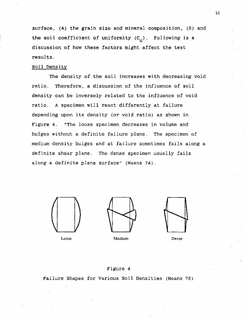
surface, (4) the grain size and mineral composition, (5) and

the soil coefficient of uniformity (Cu>· Following is a

discussion of how these factors m.ight affect the test

results.

Soil Density

The density of the soil increases with decreasing void

ratio. Therefore, a discussion of the influence of soil

density can be inversely related to the influence of void

ratio. A specimen will react differently at failure

depending upon its density (or void ratio) as shown in

Figure 4. "The loose specimen decreases in volume and

bulges without a definite failure plane. The specimen of

medium density bulges and at failure sometimes fails along a

definite shear plane. The dense specimen usually fails

along a definite plane surface" (Means 74).

Loose Medium Dense

Figure 4

Failure Shapes for Various Soil Densities (Means 75)

10

Soil density also has an influence on the percent

volume change of the specimen during shear in the drained

test as shown in Figure 5. The loose specimen continuously

decreases in volume until near failure. The dense specimen

continuously increases in volume during shear. The medium

dense specimen shows little change in volume during shear

until near failure.

+ Dense

Volume 0 Change

Loose

Strain

Figure 5

Stress-Strain-Volume Change Curves

Cohesionless Materials (Means 75)

11

Soil density will significantly influence the resulting

angle of internal friction (~) as determined by the test.

"The value of $ is not constant for any one material but

increases with density" (Means 75). Increasing density

causes a rise in the resistance to movement of the soil

grains because of the interlocking of grains. (Interlocking

is the process of individual soil grains resisting shear;

some grains must be lifted and rolled over others as sliding

occurs along the failure plane.) A greater portion of the

shear strength is due to interlocking for dense sands than

for loose sands. This interlocking adds a larger portion of

the shear strength at lower shear stress than at higher

shear stress.

Shear Strength

Loose Sand

Shear <I> L Strength

~--......

l"ormal Stress

Figure 6

Dense Sand

03 03 01

Normal Stress

Effect of Normal Stress on the Friction Angle (Means 76)

12

When the deformation of the sand is greater, the

density is reduced, in turn reducing the influence of

interlocking of grains. The resulting Mohr envelope is

usually a straight line (constant ~) for loose sands and a

curve (decreasing ~ with increasing stress) for dense sands

as shown in Figure 6. The minimum value of~ at failure for

the sand in the dense state would be the same as the value

of~ for the sand in the loose state (Means 75).

Grain Shape

The grain shape of the sand particles will affect the

resulting angle of internal friction(~). The interlocking

phenomenon described previously becomes more significant

when soils have angular shaped grains. "Since the motion of

individual particles has a component normal to the plane of

failure, a considerable amount of the work required to

produce failure must be used in overcoming the resistance

which the normal force offers to this motion" (Means and

Parcher 323) .

Mineral Contact Surface

The term "angle of internal friction" can be inferred

to mean that the shearing resistance in a soil is caused by

mineral to mineral contact between two grain surfaces. In

fact, most soil grains are coated with a moisture film that

inhibits mineral contact except at very high normal stress

(Means and Parcher 321). Therefore, mineral contact surface

has typically little influence on the test results and it

would seem appropriate to refer to ~ as the "angle of

13

shearing resistance" due to interlocking of grains rather

than the "angle of internal friction" (Means and Parcher

322).

Grain Size and Mineral Composition

The influence of grain size on ~ was investigated by

A.Casagrande. His results have shown that grain size has

little affect on ~- Also, since mineral grains of sand

consist largely of quartz and feldspar it is rare to find

that ~ varies appreciably due to differences in

mineralogical properties (Means and Parcher 323-324).

Coefficient of Uniformity

"Soils having higher coefficients of uniformity [ "Cu",

well graded soils] have higher values of ¢. Such soils tend

to have lower void ratios ... than do more uniform soils"

(Means and Parcher 325). In other words, a soil composed of

a diverse size of soil grains (well graded soils) can fit

together more compactly than one of uniform sized grains.

In turn, these well graded soils will result in possessing

greater shear resistance.

In summary, "the value of <t> varies from about 25° for

loose sands with well rounded grains to about 50° for dense,

well graded sands with irregular shaped grains" (Means 76).

v. Sources of Experimental Error

There are many possible sources of experimental error.

This section examines some of these sources of error and how

they might affect the test results. Also examined is how

14

these errors can be accounted for or avoided. Sources for

error examined are: (1) the elastic membrane, (2) the

proving ring, (3) the dial gauge, (4) the bedding movements,

(5) the stress intensity, (6) the end restraints, (7) the

soil specimen dimensions, (8) the rate of deformation, (9)

the energy loss, (10) the change in volume measurements, and

(11) the entrapped air.

Elastic Membrane

The sample specimen is confined by a thin elastic

membrane that attempts to allow free deformation during

shear. The physical properties of the membrane itself have

a slight affect on the measured strength of the.specimen.

Gilbert and Henkel found that "the strength contributed by

the membrane at failure . was found to depend upon the

thickness of the membrane and the strain at failure; but to

be independent of the confining pressure and the strength of

the specimen." In routine soil testing, this effect is

usually neglected (cited in Means and Parcher 363).

Proving Ring

The axial load is applied by a proving ring with its

own gauge and by a piston. Provided the proving ring is of

a good-quality and calibra~ed regularly, the only source of

error may arise from friction between the sleeve/seal and

the piston. Bishop and Henkel have shown that errors due to

friction may be between one and five percent of the load.

One alternative to avoid the affect of friction on the value

of the proving ring gauge reading is to measure the load

15 ' '

inside the triaxial cell. Tests have been conducted with

the proving ring mounted between the piston and the top cap

and also with the proving ring incorporated into the

pedestal. Of these two locations, "the latter seems to be

the best, since it is insensitive to cell-pressure variation

and sufficiently stiff to require no correction to measured

deflections as the load varies" (cited in Morgan and Moore

313).

Dial Gauge

The common method of measuring axial deformation of the

sample is by using a dial gauge attached to the base of the

proving ring and acting on a pillar supported from the top

of the cell. According to Lee, this method of attachment

can be a source of error due to tilting of the proving ring

during the course of the test. Bishop and Green have found

that this error may be eliminated by attaching the dial

gauge rigidly to the piston itself and allowing it to bear

on a pillar supported from the base of the cell (cited in

Morgan and Moore 318-319).

Bedding Movements

Lee has also found that the amount of axial deformation

measured by the dial gauge may be in error due to bedding

movements. Bedding movements can occur at various

interfaces such as between the proving ring and the piston,

the piston and the end cap, and the end caps and the porous

stone end platens. Bedding errors may be taken into account

by calibrating the system for bedding movements using a

16 ~ '

dummy steel sample (Morgan and Moore 318-319).

Stress Intensity

When wide ranges of stress are imposed on a soil it

behaves such that the correlation between strength and the

normal stress (~ff=afftan~') is not a linear relationship.

In the coarser granular materials under very high stress

approaching 900 psi (as compared to a maximum of 232 psi in

the trial tests in this study) the lack of a linear

relationship is clearly associated with the crushing of

particles, initially local crushing at interparticle

contacts, and ultimately shattering of complete particles.

In dense materials under very high stress, this shattering

effect greatly reduces the rate of volume increase at

failure which leads to a marked reduction in the overall

value of~ at failure (Bishop 146).

End Restraints

In the triaxial application of stress on a soil

specimen it is impossible to recreate the in-situ occurrence

of uniformity in the distribution of stresses as they occur.

The most obvious indication of non-uniform conditions is the

common "barreling" of a soil specimen during shear. These

non-uniformities are due to the end restraint imposed

between the platens and the soil specimen. To alleviate

some of this restraint "free" or "frictionless" ends can be

utilized. An enlarged, polished, end platen is covered by a

thin layer of silicone grease and a latex rubber disc of

about 0.010" thickness (Morgan and Moore 309-310). Sarsby,

17

Kalterziotis, and Haddad have found that "bedding error" due

to the compression and distortion of the rubber/grease layer

may account for up to 80 percent of the recorded axial

deformation (83). Even so, strain distributions are

markedly improved by the use of these frictionless ends.

"The technique of using frictionless ends is so simple and

the benefits are so great that there appears to be no reason

why they should not be used for all laboratory testing"

(Morgan and Moore 309-310).

Soil Specimen Dimensions

Considering the stress distribution in the sheared

specimen, the state of stress adjacent to the head and base

is unknown and differs from the state of stress elsewhere in

the specimen. If a failure plane occurs which intersects

either the loading head or the base, the test results will

likely indicate an unreliable strength. A common practice

besides frictionless ends used to overcome the effects of

this lateral restraint is to use samples with a height-to­

breadth ratio of two-to-one so that deformation is

approximately uniform at sample midheight and the failure

plane occurs near the center without hinderance (Means and

Parcher 362).

Rate of Deformation

The voids in the soil specimen are filled with air

and/or water. During rapid deformation of the specimen, the

water pressure may influence the apparent strength of the

soil. Soil in a loose state has deformation which is

18

accompanied by a decrease in volume as explained in Chapter

Three. " Rapid deformation produces pressure in the

pore water which reduces the pressure between the soil

grains thereby reducing the shear resistance. Dense

cohesionless materials expand when deformed. [Rapid]

deformation of these dense saturated materials produces

tension in the pore water which increases the shear

resistance" (Means 77). Selecting an appropriate rate of

deformation to ailow the water to drain so that the applied

load is carried only by the soil grains will eliminate the

influence of pore water pressure on the test results.

Energy Loss due to Friction

To maintain zero pore pressure (as described previously

in reference to the drained test) there is an associated

change in volume. From a conservation of energy viewpoint,

this change in volume indicates that additional work (as

compared to the undrained test) has been done to shear the

sample due to friction (Lee and Ingles 205). "For sands

(except in a very loose state) the drained test will lead to

slightly higher values of . ~-, due to the work done by

the increase in volume of the sample during shear and to the

smaller strain at failure" (Bishop and Henkel 19).

Volume Change Measurements

The results of the triaxial test include data and

graphs presenting the change in volume of the specimen

during shear. "Volume-change measurements on saturated

samples are normally carried out by measuring the expelled

19

water in a burette. Errors in this method can arise from

leakage of the cell fluid into the drainage line through

either the membrane or past the $ ring seals on the platens,

by evaporation of water from the burette and by air coming

out of solution in the pore fluid." For tests carried out

over several days, the difference in results may be

noticeable, but for short term tests these errors are likely

to be small (Morgan and Moore 310-312).

Entrapped Air

The final source of error arises when air is entrapped

in the specimen. This problem may occur when the attempt to

reach 100% saturation before conducting the triaxial test is

not successful. Air can also be introduced into the

specimen if the water used for saturation is not de-aired.

Voids with negative pore pressure behave in a fashion

similar to the soil skeleton, supporting the axial load and

falsely increasing the soil strength in the test results.

Also, air is a compressible substance. Therefore, volume

changes measured merely by the expelled water will not

account for the change in volume due to the compression of

trapped air when excessive pore pressure exists in the soil

specimen.

20

CHAPTER 2

The Laboratory Equipment

The laboratory equipment used for the triaxial soil

tests was commercially available from Geotest Instrument

Corporation (Chicago, Illinois). It includes a control

panel, a load frame, a triaxial cell, and a vacuum pump. The

air and water supply are provided at the laboratory. This

chapter includes a brief description of each of these

components used for the sample tests and any problems that

were encountered in their use.

The triaxial control panel (Geotest Model #55423)

includes dial gauges for the various cell, back, and head

pressures, pressure regulators, pressure supply and vent

valves, a digital pore pressure gauge, burettes and water

supply controls, and a vacuum regulator and gauge. The main

panel has two attaching side panels that can be used for

running more than one test at a time. These add-on panels

were not utilized in this project. The following page has a

diagram of the control panel (Figure 7) with a listing of

its components. The pressure gauges on the panel use

various units of measurement (see Appendix C for a

conversion chart). No problems were encountered in the use

of the control panel.

The load frame (Geotest Model #55720) consists of a

main cabinet with a control console. The base cabinet has a

hand crank with a high speed, low speed, and manual

21

I 0, 0 Power I PORE PRE kPa I Fuse

10 ~ ~ 8 o·8

~ ~ 33 34

(lj) ~

22 20 [!] ([) ([)

• 30-2

• • • t

31

32 2 L..

L..

• 30-3

'~ • • •

Control Panel Components: t); 3Q~ I~

1. Cell pressure supply valve 18. Transducer selector 2. Cell pressure regulator 19. (none) 3. Cell pressure vent valve 20. Pedestal selector 4. Head pressure supply valve 21. Pedestal selector 5. Head pressure regulator 22. Cap selector 6. Head pressure vent valve 23. Cap selector 7. Back pressure supply valve 24. Test gauge selector 8. Back pressure regulator 25. Test gauge selector 9. Back pressure vent valve 26. Cap burette (45cc)

10. Vacuum regulator 27. Pedestal burette (45cc) 11. Mercury shut off valve 28. Pedestal burette (3cc) 12. Transducer de-air valve 29. Mercury trap 13. Pedestal saturation valve 30. Cell overflow valve 14. Filling valves burette 31. Back pressure gauge 15. Selector valves burette 32. Common test gauge 16. Filling valves burette 33. Head pressure gauge 17. Cap saturation valve 34. Vacuum gauge

Figure 7

The Triaxial Control Panel (Geotest Model #S5423)

22

23

Photograph 1

The Triaxial Control Panel (Geotest Model #S5423)

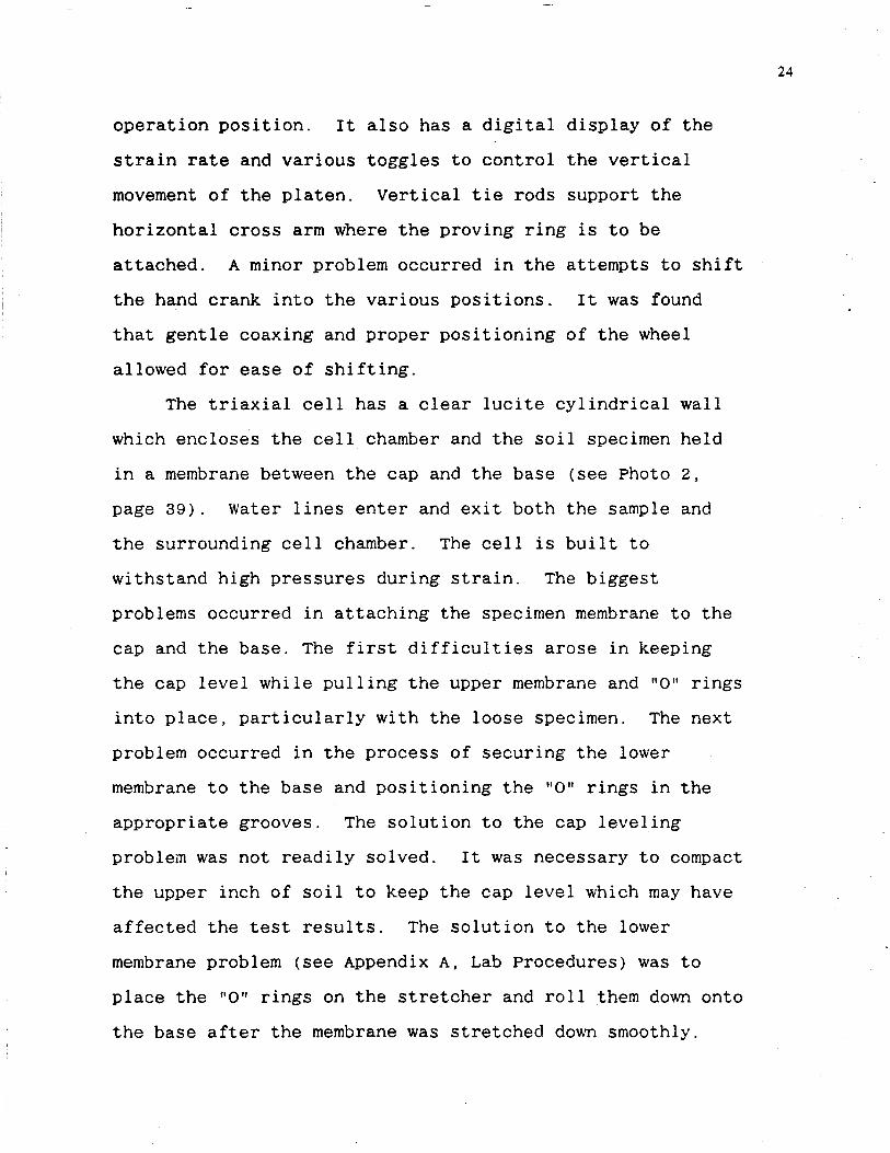
operation position. It also has a digital display of the

strain rate and various toggles to control the vertical

movement of the platen. Vertical tie rods support the

horizontal cross arm where the proving ring is to be

attached. A minor problem occurred in the attempts to shift

the hand crank into the various positions. It was found

that gentle coaxing and proper positioning of the wheel

allowed for ease of shifting.

The triaxial cell has a clear lucite cylindrical wall

which encloses the cell chamber and the soil specimen held

in a membrane between the cap and the base (see Photo 2,

page 39). Water lines enter and exit both the sample and

the surrounding cell chamber. The cell is built to

withstand high pressures during strain. The biggest

problems occurred in attaching the specimen membrane to the

cap and the base. The first difficulties arose in keeping

the cap level while pulling the upper membrane and "0" rings

into place, particularly with the loose specimen. The next

problem occurred in the process of securing the lower

membrane to the base and positioning the "0" rings in the

appropriate grooves. The solution to the cap leveling

problem was not readily solved. It was necessary to compact

the upper inch of soil to keep the cap level which may have

affected the test results. The solution to the lower

membrane problem (see Appendix A, Lab Procedures) was to

place the "0'' rings on the stretcher and roll them down onto

the base after the membrane was stretched down smoothly.

24

The vacuum pump (Marvac Model #AAI) is attached to the

control panel. Once the pump is activated, the vacuum

regulator and gauge on the panel are used for its operation.

The only problem encountered with the pump was its tendency

to overheat. For this reason, the pump was turned off when

it wasn·t in use.

The available air supply in the soils lab was 40 psi

and was sufficient pressure for running the trial tests. The

water supply was jerry-rigged using a two gallon jug of

purified (not de-aired) water perched upon a tall stool

sitting on the lab counter. The low water pressure made the

filling of the cell chamber slow. The water lines were

attached such that the same water was used to fill the cell,

the panel burettes and, in turn, the soil sample. Most

significantly, this water was then recirculated back into

the jug for reuse. As a result, not only was additional air

introduced into the water, but soil particles were washed

into the burettes as the water passed through the soil

specimen slightly decreasing the total volume of soil solids

under test.

25

CHAPTER 3

The Trial Tests

I. Soil Description

A natural, medium-grained soil was utilized for the

sample tests. Soil samples were collected for testing at a

local foothill site in the San Fernando Valley, north of Los

Angeles (see map.Figure 8.) The soil was removed from an

undeveloped hilltop overlooking Hansen Dam at Los Angeles

Reservoir outside a housing tract. The surrounding

vegetation was dry, sparse chaparral. The ground surface

was gravelly and light tan in color. The soil was removed

at a depth of approximately four to eight inches. The soil

was dry and difficult to penetrate. Therefore, the soil was

greatly disturbed in the process of hammering away sample

material with a shovel.

Analysis according to the Unified Soil Classification

System yielded an SW primary designation. A sieve analysis

and gradation curve of the sample (see Appendix B) resulted

in 6.87 percent finer than the No.200 pan, a coefficient of

uniformity, Cu = 7.0, and a compression index, Cc = 1.37.

Because the fines in the sample exceeded the five percent

limit, a dual symbol classification was required to include

designation for the fines. The fines, by visual inspection,

appeared to be silty in nature. Therefore, the complete

analysis yielded an SW-SM designation: gravelly, silty,

well-graded sand. Examination of particles with a microscope

26

0 0

.Q

0 CJ)

Rinaldi St

~ ~

NORTH • Mission Hills

Figure 8

Sample Site Location Map

San Fernando

•

27

revealed an angular shape for the gravel grains. The

moisture content of the sample was tested one day after

collection and rated 2.9 percent.

II. Test Procedures

A general description of the test procedures used for

the trial tests follows. (More detailed, step-by-step

procedures can be found in Appendix A.) The trial tests

allowed for drainage during both the chamber pressure and

axial load application stages of the test. First, full

consolidation was reached under the applied chamber

pressure. The deviator stress was then applied and

increased slowly so that no significant pore pressure was

built up while the specimen was under test. This type of

test is called a consolidated-drained (CD) test.

The soil sample was prepared by stretching the membrane

smoothly within the stretcher mold. The mold was then

placed over the pedestal cap (with hoses attached) on the

base of the cell. Dry sand was then deposited into the

stretched membrane. The loose sample was not tamped during

placement, while the dense sample was tamped 25 times for

every five spoonfuls of sand. The top cap (with hoses

attached) was positioned squarely on top of the soil

specimen. A vacuum was then applied to the specimen to

maintain its shape while removing the stretcher mold.

The appropriate proving ring was installed to the load

frame. The triaxial cell was then placed over the base and

28

installed on the load frame. The deformation dial was set

into position between a flat bar attached to the plunger and

a vertical rod attached to the base of the cell. Next, the

cell was filled with water and a cell pressure of 40 kPa was

applied at the same time the vacuum was removed.

To begin saturation of the specimen, the pedestal

burettes were filled. Water was run slowly by gravity into

the base of the sample allowing it to fill the sample voids

until it spilled.from the cap. The goal of this technique

was to avoid trapping pockets of air in the voids. A vacuum

of 10 inches Hg was applied to the cap to help draw the

water upwards and remove the air. This saturation was then

increased by applying a back pressure to the sample ends and

allowing it to consolidate for no less than half an hour

prior to testing. The degree of saturation was tested by

raising the cell pressure and watching for an equal rise in

the pore pressure.

The specimen was finally compressed at an axial speed

of 0.063 inches per minute. A set of trail tests for

specimens in both the loose and dense condition were run at

chamber pressures equal to 70, 220 and 240 kPa. Drainage

was allowed only at the pedestal. Recordings of changes in

volume and axial load measurements were then taken at

regular intervals of deformation; for the first 0.10 inch in

0.01 inch intervals; for the next 0.20 inch in 0.02 inch

intervals; and for the remaining deformation in 0.05 inch

intervals. Compression continued until 20 percent strain

29 @ '

was reached. The sheared sample was then photographed and

measured for its final height and diameter. Once the test

data was accumulated, it was entered into spread sheets for

further calculations (see Appendix E) and graphic display.

30 p '

CHAPTER 4

Results of the Trial Tests

The experimental results are presented in Table 1. The

results are also presented in Figures 9-14 where effective

stress versus axial strain and change in volume versus axial

strain are plotted. Photographs of the specimens at 20

percent strain are shown in Photograghs 2-7. Finally,

Figure 15 summarizes all the data in a plot of shear stress

versus normal effective stress. Chapter 5 presents a

discussion and interpretation of the ~est results.

31

32

CHAMBER PRESSURE

SOIL 70 kPa 220 kPa 420 kPa PROPERTIES (10.2 psi) (31. 9 psi) (60.9 psi)

eo 0.684 0.684 0.702

D efinal 0.654 0.637 0.635 E N s /j.v IV

0 max -0.0209 -0.0316 -0.0401 E

s /j.o max 154.5 kPa 590.2 kPa 1185 kPa A (22.36 psi) (85.6 psi) (171.9 psi) N D

cr1 /cr3max 3.21 3.68 3.82

J'ff 224.5 kPa 810.2 kPa 1605 kPa (32.56 psi) (117.5 psi) (232.8 psi)

eo 0.692 0.680 0.734

L efinal 0.628 0.603 0.652 0 0 s 6vtv

0 max -0.0380 -0.0463 -0.0475 E

s 6cr max 167.9 kPa 605.2 kPa 1117 kPa A (24.31 psi) (87.8 psi) (161.9 psi) N D

cr1 /o-3max 3.40 3.75 3.66

::rff 237.9 kPa 825.2 kPa 1536 kPa (34.51 psi) (119.7 psi) (222.8 psi)

Table 1

Trial Test Results

:5.-4

:5.:!

- J.D

lb"

' :!.B

lb :!.B -

en :!.-4 en w 0::: 2.2 r Ul

w :!.D

>

t 1.B

w 1.8 ~ ~ w 1.-4

1.:!

1.0 0.0

,...,. -1.0

0 -2.0 0 -J.Il d -f.ll X

-5.0 0

> -B.D

' > -7.0 <l -B.O - -B.Il

~ -1D.Il <! 0::: -11.[1 1- -12.1l Ul -1:5.1l

U -H.O

0::: -15.0

ti -18.0

~ -17.0

:::l-1Bil ....J .

0 -1B.Il > -2D.Il

-:!1.0

0 5.0 10.0 15.0

AXIAL STRAIN ( 0/o)

Figure 9

Trial Test Results for Dense Sand at cr3 = 70 kPa (e

0 = 0.684)

33

20.0

3.8

3.6

3.-4 ,.....

•t:r 3.2

' ::S.D lb ~ 2.8

Ul 2.6 Ul

w 0:: 2.-4 t-Ul :2.2 w > ::!.D -1- 1.8 u w u... 1.6 u... w

1 .-4

1.::!

1.D D.D

,..... -:!.ll

a --4.1l a c5 -8.1l X

0 -ltD > '- -10.1l >

<J -12.1l \...J

-14.0 z :;{ -18.0

.~ -1B.Il Ul -::!ll.ll u - -22.1l 0::: 1- -24.0 w ~ -:!B.Il :::> ...1 -2B.D a > -:50.0

-3:!.0

0 5.0 10.0 15.0

AXIAL STRAIN ( 0/o)

Figure 10

Trial Test Results for Dense Sand at ~3 = 220 kPa (e

0 = 0.684)

34

20.0

-4.0

3.6

3.6 ........

I~ 3.4

' 3.:! IC

3.0 .......

Ul :'.1.6 Ul w :'.1.6 0:: 1- 2.4 (/)

w l.:! > - 2.0 1--u 1.6 w LL. LL. 1.6 w

1.4

1.2

1.0 D.D

,......

0 -S.D 0 d X -1D.D

0 >

' > -15.0 <J '-'

z -:!D.IJ

<t a:: -'15 I] f- •. (/)

U -3D.D a:: 1--w -35.0 ~ ::J -l -40 D 0 .

>· --4-S.D

0 5.0 10.0 15.0

A X I A L STR A IN ( o/o)

Figure 11

Trial Test Results for Dense Sand at cr3 = 420 kPa (e

0 = 0.702)

35

20.0

36 Q '

l.-4

3.::! c D

,....,. 3.0 '\. 1Uju6tcd Str.o\in Gt.lu,. lt:r '

::1.8

lli ::!.6 ...... Ul ::!.-4 Ul LU a::: :!.:! ...... U1 ::!.D LU > 1 .B

t 1.6 LU LL. LL. LU 1.-4

1.2

1.0 D.D

,.....,

0 -2.0

0 --4.0 d

X 0 -Ei.O > ' -B.D > <J ........,

-10.0

z < -12.0 IY t; -1-4.0

U -1Ei.O

IY ..... -18.0 LU

~ -20.0 _J

0-22.0 >

-2-4.0 .I

0 5.0 10.0 15.0 20.0

AXIAL STRAIN (D/o)

Figure 12

Trial Test Results for Loose Sand at 03 = 70 kPa (eo = 0.692)

37

:5.8

:S.Ei

:S.-4 ,....

,!J" 3.2

' 3.0 lb - 2.8 (/) (/) 2.6 L&.J 0::: 2.4 I-U1 2.2 L&.J > 2.0 -.....

1 .f.l u L&.J I.&.. 1.Ei I.&.. L&.J

1.~

1.::!

1.0 D.D

~

0 -5.0 0 0 X-1D.U

0

> ,-Hi.D >

<J --2D.D

z ::;( -25.0 0:: ..... en -:so.n u 0:: -35.0

..... L&.J ~ --4{1.0

:J _J 0--45.0

> -50.0

0 5.0 10.0 15.0 20.0

A X I A L STRAIN ( 0/o)

Figure 13

Trial Test Results for Loose Sand at a3 = 220 kPa (e

0 = 0.680)

:5.B

3.6

,.....

lt:r 3.:!

' 3.0 Jtl - :!.B

(J) :!.B (J)

1.&.1 a:: 2.-4 1-Ul 2.2 1.&.1

::!.D > -I- 1.8 u ~ 1.1'1 L.. 1.&.1 1.-4

1.2

1.0 D.D

r---.

0 0

c:j -1 D.D X

0

>

' > <l \o...J-2D.D

z < a: I-(f) -30.0

u -lY I-1.&.1 ~ -4-D.D

:J _J

0 >

-SD.D

0 5.0 10.0 15.0

AXIAL STRAIN ( 0/o)

Figure 14

Trial Test Results for Loose Sand at cr3 = 420 kPa (e

0 = 0.734)

38

20.0

------~ ------- - - ----- ------- ------

TeSI NO. I Df:. A /NED

c-3 -= 7 0 1::-f ()..... r,f;ojr;;~

Photograph 2

Specimen at 20% Axial Strain Dense Sand: ~3 = 70 kPa

39

rt~T Nr 2-

Photograph 3

Specimen at 20% Axial Strain Dense Sand : a

3 = 220 kPa

40

/E~T No.3 : r.~.l·i£!

~·; =- q.;. r ~ ,.__ J

I I

v.IJ ; '"

Photograph 4

Specimen at 20% Axial Strain Dense Sand : a

3 = 420 kPa

41

re~r No.

Photograph 5

Specimen at 20% Axial Strain Loose Sand: rr3 = 70 kPa

42

NO. ~ • .._ '" I " • I

:1 • .. •

. .

Photograph 6

Specimen at 20% Axial Strain Loose Sand: cr3 = 220 kPa

43

- -- ~-- -- - - ----- - -- - - - ---- - - - ---- - --- - - -- - ---

, . , ..- ·' • ::. '? - .. ,. "'\

, .. . f ' • fl. - • ~· ..

/ . - - . ,. ~ I ~ - 't ... . !:-- " -.

Photograph 7

Specimen at 20% Axail Strain Loose Sand : rr3 = 420 kPa

p .

44

7

6

5

Shear Stress"' (kPa)

3 (x 1 02

) 2

0 2 3 "' 5

--.....

L

6 7 8 9 10 11 12

Normal Effective Stress (kPa)

(x 102)

Figure 15

..... ' Jf',

' ' \ \

\

13 1-1

Mohr Circles and Mohr Envelope at 20~ Strain

45

\ \ \ I

15 16 17

CHAPTER 5

Discussion of the Results

This chapter discusses the results of the trial tests

and relates the previous discussion of: (1) the test

procedures, (2) the influence of soil properties on the

series of trial tests, and (3) the sources of experimental

error.

I. Trial Test Results

Figures 9-14 for sand in both the loose and dense

condition show an increase in effective stress as the

chamber pressure increases from 70 to 420 kPa. Similarly,

the volumetric strain measured by expelled water decreases

with increasing chamber pressure for each test. In

comparing the stress versus strain graphs of sand in the

dense condition to the loose condition, only slight

differences in the values are apparent.

Interruptions during the test are indicated on the

stress versus strain graphs in Figures 9-14. These

interruptions resulted from the need to: (1) adjust the arm

on the strain gauge dial when it reached its maximum travel,

(2) empty the pedestal burettes when they became filled to

capacity, and (3) change proving rings to allow for

measurement of greater axial loads during higher chamber

pressures.

The adjustment of the strain gauge dial shows a slight

46

dip in the curve. It is apparent only because once the dial

arm reached its maximum travel, for a short instant, the

dial rather than the soil specimen began to support the

axial load. The replacement of the proving ring caused a

sudden increase in the axial load shown by an upward jump in

the curve. For the tests with higher chamber pressures, it

was necessary to stop the test and switch to a higher

capacity proving ring.

In comparing the volumetric strain versus axial strain

graphs for sand in the dense to the loose condition (Figures

9-14), two trends are apparent. The dense condition tests

show an upward curve of increasing volume after reaching the

minimum volume point of the test. On the other hand, the

loose condition tests show a flattening of the curve beyond

the minimum volume point. Also, the volume decrease for the

loose condition tests is consistently greater than the

decrease of volume for the dense condition tests at the same

chamber pressure.

The photographs of the six sample tests show that all

specimens failed by bulging (a barrel shape). For the sand

in the dense condition, the buldging is more prominent at

all three chamber pressures.

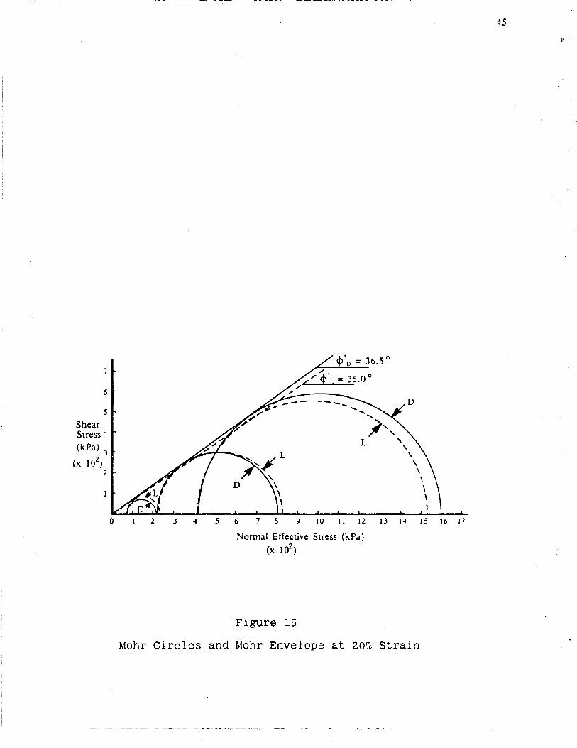
Examination of Figure 15, Mohr Circles and Mohr

Envelope at 20% Strain, yields very slight differences in

the strength envelopes from the sand in the dense to the

loose condition. In fact, the tests with low and medium

chamber pressure indicate a slightly higher value of shear

47

strength for the loose condition test and a slightly lower

value of shear strength for the loose condition test at the

high chamber pressure.

II. Test Procedures

A consolidated-drained (CD) test was used to conduct

the trial tests. The tests allowed for drainage only at the

pedestal. This option was chosen for ease of recording

data.

The soil sample was placed dry in the membrane and

subsequently flooded. A back pressure was then applied for

a time span varying from 30 minutes to 24 hours. The degree

of saturation in both cases was less than complete indicated

by experimental procedure VII, Determination of the Degree

of Saturation (see Appendix A). The techniques used to

prepare the soil specimen as well as the air trapped within

were both contributors to the saturation problem.

The rate of loading used for the sample tests was 0.063

inches per minute. This rate was based on the need to take

accurate readings of load and volume changes. This rate was

sufficiently slow to record data and resulted in tests of 30

to 45 minutes in length.

The recording of data for the sample tests was straight

forward. Typical weight, volume, and moisture content

measurements were utilized. The calipers used to measure

the sample diameter were awkward to hold level and did not

give consistent results.

48

III. The Influence of Soil Properties

The photographs of the failed samples show a barrel

failure shape for all six of the sample tests. This shape

indicates, as shown in Figure 4 (page 10), that all these

soil samples were prepared, contrary to the original intent,

with loose density.

The graphs of volumetric strain versus axial strain

(Figures 9-14) all show an immediate and significant

decrease in volume. As indicated by Figure 5 (page 11),

this behavior again is associated with a loose density

specimen for all six trial tests. The specimens in the more

dense condition do show a sharper turn of increasing volume

after reaching the minimum volume point and less total

decrease in volume as would be expected for a more dense

soil specimen. However, this effect does not override the

fact that the results indicate all six specimens were

prepared in the loose condition.

The shape of the strength envelope is also an indicator

of sample density. This graph (Figure 15, page 45) again

indicates that the samples are of very similar density. In

fact, the loosely prepared specimen shows a slight dropping

of shear strength at the highest chamber pressure. As sho~n

in Figure 6 (page 12), this effect is normally associated

with a high density specimen due to interlocking of grains.

The occurrence of this effect for the specimen in the loose

condition is so slight that it is not significant nor is it

likely due to interlocking of grains. What is significant

49

is the absence of this peaking effect in the strength

envelope for the densely prepared soil specimen. In fact,

there occurs a very close proximity of the two curves.

The angle of internal friction is an indicator of grain

shape, soil gradation and density. From Figure 15 (page

45), the angle of internal friction (~') is approximately

equal to 35°. This angle falls somewhat less than half way

between the 25° expected for loose, poorly graded, round

grained sands and the 50° expected for dense, well graded,

angular grained sands. The well graded nature of the soil

sample and its angular shaped grains rather than its density

likely contributes to this higher than expected ~ for the

trial tests which were apparently all of loose soil density.

IV. Sources of Experimental Error

Elastic Membrane

The thin elastic membranes used in the sample tests

were supplied by the triaxial testing machine manufacturer.

The affect of these membranes on the test results is small

enough to be neglected.

Proving Ring

Both a 500# and 10,000# capacity proving ring were

utilized during the conduct of the tests. These rings were

of significantly different capacity and degrees of accuracy.

It was necessary to trade rings midway through the 220 kPa

and 420 kPa tests. As previously noted, the jump in the

stress/strain curves indicates the effect changing proving

50

rings. This effect may be caused by the lessening of stress

as the 500# capacity proving ring reached its working

maximum. This effect may also be the result of the

difficulty in calculating a start point for the existing

stress when trading rings and the difference in accuracy of

the two rings. A single proving ring of 1500# capacity

would have been adequate to conduct all six sample tests.

Dial Gauge

The compression dial gauge also made it necessary to

make adjustments during the conduct of the test. This

problem resulted from the dial gauge being too large to

accommodate the compression distance needed to reach 20

percent axial strain. Otherwise, the compression dial

gauge, being attached rigidly to the piston and bearing on a

pillar supported from the base of the cell (as described in

Chapter 1, page 15), did not contribute to test error.

End Restraints and Soil

Specimen Dimensions

The trial test results may have been influenced by the

use of the porous stone end platens. These cause non­

uniform stress conditions in the soil specimen during shear

and the barreling failure shape effect. The use of

frictionless end platens, as described in Chapter 1 (page

17), may result in a better simulation of soil specimen

failure. Otherwise, the two-to-one ratio of height-to­

breadth was generally used and was likely not a source of

test error.

51

Rate of Deformation and

Energy Loss

The sample sand, being of medium sized grains, was

easily free draining at a deformation rate of 0.063 inches

per minute. It was likely not a candidate for the

occurrence of pore water pressure build up which would

introduce error in the test results. Also, the decrease in

volume occuring during shear indicates a loose density soil

specimen. Therefore, since no work was done by the specimen

against friction as it would if it were expanding during

shear, it is not necessary to adjust o for energy loss.

Entrapped Air

The final possible source of error is the entrapment of

air in the soil specimen. The use and recirculation of

non-de-aired water and the fact that the sample did not

reach full saturation prior to testing both contributed to

the problem of air entrapment. This trapped air may not

have had an influence on the test results because all the

tests were drained during shear. Assuming no negative pore

pressure was established, no additional shear strength was

added to the specimen. Also, assuming that no excessive

pore pressure was built up, the change in volume measured by

consistently air entrapped water was a fair gauge both in

entering and being expelled from the sample. Therefore, the

entrapped air likely had no effect on the test results.

52 f! •

CHAPTER 6

Summary and Recommendations

A set of test procedures to be used by undergraduate

students conducting triaxial compression tests on

cohesionless soils is presented in this report. This report

describes options the student can choose from in conducting

the tests. Also, this report discusses the influence of

soil properties, and laboratory techniques and equipment on

the test results. Finally, this report includes the results

and analysis of six trial tests. In conclusion, the

following items are recommended for application to future

tests:

1. During the trial tests each specimen was allowed

to drain only at the pedestal to make it easier for one

person to record data. If two students record data, it

would be possible to allow drainage at both the cap and

pedestal.

2.

This approach is recommended for future tests.

Although both the technique of saturating the soil

sample from the bottom upwards and subsequently applying a

back pressure was used, complete saturation was not

achieved. Future research is recommended to investigate

other techniques such as preparing the sample in a wetted

state to achieve 100% saturation prior to testing. As

mentioned previously, Bishop and Henkel have found that

complete saturation can be achieved by depositing the sand

under water through a funnel. The funnel is clamped at the

53

top of the membrane stretcher with the membrane in position.

The membrane and the funnel are then filled with de-aired

water. The sand is first prepared by mixing it in a beaker

with water and boiling the mixture under a vacuum to remove

trapped air; the mixture is then placed into the stopped

funnel. To minimize segregation, the sample is built up by

quickly releasing the stopper and allowing a continuous

rapid flow of the mixture into the stretcher (90-92).

3. Measurement of the soil diameter was difficult and

unreliable using only one measurement with the calipers.

Better results can be attained by using a circumferential

tape and measuring at the top, middle, and lower sections of

the sample.

4. Attempts to prepare both loose and dense soil

specimens yielded specimens of similar density, an alternate

approach to achieve high density soil is recommended.

Tapping of each and every spoonful of soil placed into the

membrane and/or utilizing electronic vibration may result in

a significantly higher density soil specimen than the loose

specimen which is tapped minimally or not at all.

5. The switching of proving rings during testing was

inconvenient and a source for error. The utilization of a

single 1500# capacity proving ring will provide the needed

accuracy for all the chamber pressures utilized in the

sample tests.

6. The compression dial gauge with a three inch face

was too large to accommodate the necessary distance to reach

54

20 percent strain. A dial gauge with a two and a half inch

or smaller face and a travel of one and a half inches would

give more room for the arm to contract without adjustment

while shearing the specimen.

7. As described in Chapter 1 (page 17), the end caps

restrain the specimen ends and inhibit the even distribution

of stresses through the specimen. The use of frictionless

end caps is easily accommodated and will reduce the error

introduced by this phenomenon.

8. The water used for the tests was purified but not

de-aired. Future tests using de-aired water may result in

more accurate measurements of the change in volume and shear

strength of the specimen during shear for the undrained

test. The use of de-aired water will also assist in

reaching full saturation of the specimen prior to testing.

9. The problem of keeping the top cap level when

preparing a loose sample for testing needs to be

investigated. The technique of consolidating the upper

layer of soil (as used in the trial tests) is not ideal

because it gives the specimen more shear resistance than it

otherwise would attain.

10. The placement of the water source on a stool

perched on top of the laboratory counter did achieve

sufficient water pressure to conduct the test . However,

higher water pressure would aid with the speed in which the

test could be accomplished and may be considered for future

tests.

55

11. Most significantly, the water line assembly needs

to be reworked so that the water that leaves the sample and

the burettes is not reused. It is important to assure that

fresh, purified, de-aired water is entering the soil

specimen for saturation.

It is the author's hope that the research and

experimentation contained herein will help pave the way for

the undergraduate student in his or her first introduction

to the triaxial compression test. In giving consideration

to the recommended test procedures from Appendix A and the

suggested adjustments above, the student should make strides

towards more accurate and reliable test results.

56

REFERENCES

"Back Pressure Test." Geotest Instrument Corporation Manual. Chicago, Illinois: Geotest Instrument Corp., October 24, 1985.

Bishop, A.W. "The Strength of Soils as Engineering Materials." Milestones in Soil Mechanics; The First Ten Rankine Lectures. Edinburgh: Thomas Telford LTD, 1975.

Bishop, Alan w. and Henkel, D.J. The Measurement of Soil Properties in the Triaxial Test. London, Great Britain: Edward Arnold LTD, 1957.

Lambe, T. William. Soil Testing for Engineers. New York, N.Y.: John Wiley & Sons, Inc., 1951.

Lee, I.K. and Ingles, O.G. "Strength and Deformation of Soils and Rocks." Soil Mechanics Selected Topics. Ed. I.K. Lee. New York, N.Y.: American Elsevier Publishing Company, Inc., 1968.

Means, R.E. Soil Investigation for Building Foundations. Oklahoma State University Engineering Experiment Station Publication, March, 1961.

Means, R.E. and Parcher, J.V. Physical Properties of Soils. Columbus, Ohio: Charles E. Merrill Books Inc., 1963.

Morgan, J.R. and Moore, P.J. "Experimental Techniques." Soil Mechanics Selected Topics. Ed. I K. Lee. ~ew York, N.Y.: American Elsevier Publishing Company, Inc., 1968.

:\!ulilis, J.P. and Townsend, F.C. and Horz, R.C. "Triaxial Testing Techniques and Sand Liquefaction." Dynamic Geotechnical Testing. Ed. Jane B. Wheeler, Helen M. Hoersch, Ellen J. McGlinchey and Helen Mahy. Baltimore, Maryland: American Society for Testing and Materials, September, 1978.

Patten, Authur. "Instructions S5710, 55720 Controlled Strain Load Frames." Geotest Instrument Corporation Manual. Chicago, Illinois: Geotest Instrument Corp., January 31, 1986.

Sarsby, R.W. and Kalterziotis, Nikolas and Haddad, Essam H. "Compression of "Free-Ends" During Triaxial Testing." Journal of Geotechnical Engineering, ASCE, Vol. 108, January, 1982.

57

REFERENCES (continued)

Sowers, George F. "Strength Testing of Soils." Laboratory Shear Testing of Soils. Baltimore, Maryland: American Society for Testing and Materials, December, 1964.

Wu, S. and others. "Capillary Effects on the Dynamic Modulus of Sands and Silts." Journal of Geotechnical Engineering, ASCE, Vol. 110, September, 1984.

wu, Tien Hsing. Soil Dynamics. Boston, Mass.: Allyn and Bacon, Inc., 1971.

58 0 .

APPENDIX A

Triaxial Test Procedures

(Cohesionless Soil)

I: Preparation of the Sample

1. Obtain thickness of the membrane (Lambe 102).

(Current CSUN lab membranes for the 2 3/4 inch diameter

specimens are 0.012 inches thick.)

2. Remove cell from base by a) removing top nut on

vertical rod, b) removing pin lock on lock ring on the lip

of the cell, and c) prying at bottom of cell with a

screwdriver in the supplied slot.

3. Install two "0" rings on the stretcher bottom.

4. Thread two "0" rings above the cap with the cap

hoses in place.

5. Place membrane in split stretcher with about 1

inch projecting from each end. Fold membrane over outside

of stretcher both top and bottom. (Membrane will cover "0"

rings on the bottom of the stretcher.)

6. Apply vacuum to stretcher by hand pumping on the

attached hose and seal it tightly by folding tubing with a

clamp. Make certain the membrane is perfectly smooth with

no wrinkles.

7. Place stretcher on base which contains the lower

porous brass plate. Support the stretcher with 5/8 inch

wooden blocks to sit above the base.

8. Weigh to 0.1 gram a dish with dry soil which is to

59

,, .

be tested (Lambe 102). You will need approximately 1000

grams for the 2 3/4 inch diameter specimen.

9. Place the sand within the membrane by tamping

spoonfuls of soil, taking care not to pinch the membrane

with the tamper (Lambe 102). The amount of tamping depends

on the denseness of the soil desired. For loose sand no

tamping is needed. For dense sand use 25 tamps for every

five spoonfuls of soil.* Fill membrane with soil until

level with the top of the stretcher.

10. Again weigh dish of soil. The difference in

weights is the weight of the soil used (Lambe 102).

11. Put the upper porous brass plate (wider diameter

do~n) and cap on top of the specimen and level.

12. Stretch the membrane over the top and bottom caps.

Seal membrane by rolling the "0" rings into the grooves

provided on the caps and level the top cap.

13. Turn on vacuum pump and turn No.10 to set vacuum

to five inches Mercury. Turn No.22 to vacuum position.

Apply five inches Mercury vacuum to specimen by opening cap

saturate on base and No.17 on panel. The vacuum pump will

now continue in operation until the specimen is ready for

shearing.

14. Remove the two stretcher clamps. Check the level

of the cap and carefully remove the sample mold (Lambe 103).

15. After the mold is removed, increase the vacuum to

ten inches Mercury (Lambe 103).

16. Measure the length of the specimen with a ruler

60

and the diameter with calipers at its mid-height to 1/32

inch.*

17. Pull the plunger on the cell up as far as it will

go and lock it in place.

18. Apply Vaseline to the "0" ring on the base

19. Place the cell on the base, push it down over the

"0" ring.

20. Place the lock ring on the lip of the cell and

secure it by the pin lock.

II. Installation of the Cell on the Load Frame

1. Install the appropriate proving ring to the load

frame.

2. Check that the load frame pedestal has been

returned to the lowest position.

3. Place the cell on the center of the load frame

pedestal. Lower the proving ring until it just makes

contact with the plunger.

4. Install the deformation dial into the vertical rod

with the top nut in place and secure between the top nut and

the flat bar on the plunger.

5. Check that overflow No.30 on the panel is open and

open vent No.3 to allow air to be vented from the top of the

cell. Check that vents No.6 & 9 are closed.

6. Fill cell with water by opening cell water on

base. You may need to siphon air from the inlet hose on the

cell base by suction. Let the overflow from the cell fill

the lucite reservoir on the panel about half way up and

61

close fill valve on cell base and the "T" to the cell water

supply.

7. Close No.30 and vent No.3.

8. Close red supply valves No.1,4 & 7, mercury No.ll

and transducer No.l2. Hook up supply pressure to the panel.

III. Application of Cell Pressure

1. Turn selector No.24 to cell position.

2. Open cell pressure supply No.1 slowly. Set the

cell pressure regulator to 40 kPa.

3. Open No.30 to apply the 40 kPa confining pressure

to the cell.

IV. Filling the Pedestal Burettes

1. Close saturation valve No.l3, cap saturate on cell

base, and filling valves No.l4 & 16. Turn No.22 to vent and

empty cap burette of water at front of panel.

2. Turn selector No.20 into vacuum position.

3. Open No.l5-B and close No.l5-A.

4. Open "T" to the panel water supply. Fill burette

by opening No.l4 slightly until filled. Let vacuum remove

any air that might be in the water.

5. Turn No.20 into back pressure position. If water

is well de-aired, small bubbles on the side of burettes

should disappear instantly.

6. Fill small burette by opening No.l5-A while 15-B

is still .open until filled.

v. Increase Initial Vacuum bv Saturation

1. Close de-air ·No.l2 on panel and pedestal purge on

62

cell base.

2. Turn pore pressure selector No.l8 into cell No.1

position.

3. Can temporarily turn off vacuum pump EXCEPT to

refill pedestal burette (see step V.7).

4. Open pedestal saturate on cell base and No.l3.

5. Open pedestal purge on cell base and let water

flow through to flush air out of pedestal circuit. When no

more air is coming out, close pedestal purge valve while

leaving pedestal saturation valve open.

6. Open No.l2 to flush air out of transducer (first

make sure small hose behind panel is set in a container).

When no more air is coming out, close No.12.

7. Re-fill pedestal burette as necessary by closing

No.13 and turning No.20 from back to vacuum position. Then

open No.14 until burette is filled. Return to sample

saturation by reverse order of these steps.

8. Check that cap purge valve is closed.

9. Turn No.22 to vacuum position and turn vacuum pump

on at ten inches Mercury.

10. Open No.17 on panel and cap saturation valve on

cell base.

11. Give enough time for vacuum to pull water through

the specimen from the pedestal to the cap. When water

begins to fill cap burette, close cap saturate on cell base

and No.17. Turn No.22 to vent position.

63

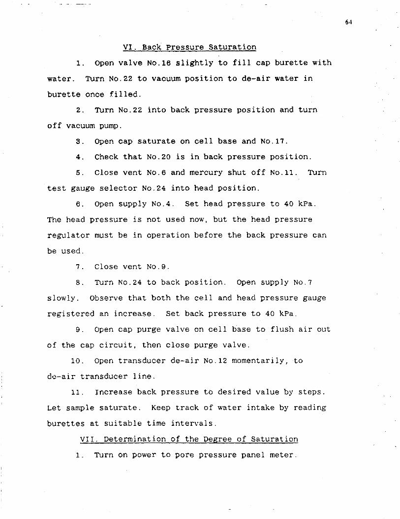
VI. Back Pressure Saturation

1. Open valve No.16 slightly to fill cap burette with

water. Turn No.22 to vacuum position to de-air water in

burette once filled.

2. Turn No.22 into back pressure position and turn

off vacuum pump.

3. Open cap saturate on cell base and No.17.

4. Check that No.20 is in back pressure position.

5. Close vent No.6 and mercury shut off No.11. Turn

test gauge selector No.24 into head position.

6. Open supply No.4. Set head pressure to 40 kPa.

The head pressure is not used now, but the head pressure

regulator must be in operation before the back pressure can

be used.

7. Close vent No.9.

8. Turn No.24 to back position. Open supply No.7

slowly. Observe that both the cell and head pressure gauge

registered an increase. Set back pressure to 40 kPa.

9. Open cap purge valve on cell base to flush air out

of the cap circuit, then close purge valve.

10. Open transducer de-air No.12 momentarily, to

do-air transducer line.

11. Increase back pressure to desired value by steps.

Let sample saturate. Keep track of water intake by reading

burettes at suitable time intervals.

VII. Determination of the Degree of Saturation

1. Turn on power to pore pressure panel meter.

64

2. Close saturation valves No.13 and 17.

3. Raise cell pressure by 40 kPa. If specimen is

completely saturated the pore pressure will also show an

increase of 40 kPa. If pore pressure increase is less, back

pressure may be increased further. Perform steps 4 and 5.

4. Reduce cell pressure to the previous value.

5. Open saturation valves and increase back pressure.

To retest specimen return to steps 2 & 3.

Note: If pore pressure reaction is only slightly less

than it should be, the specimen may become fully saturated

during consolidation.

VIII. Shearing of the Specimen

1. Close cap saturate on cell base.

2. Check that pedestal saturate on cell base and

No.13 are open, and No.20 is in back position.

3. RELEASE PLUNGER LOCK.

4. Place the hand wheel in the high speed position as

well as the "Hi-Lo Range" toggle.

5. Put "start-stop" toggle on stop and "test-return"

on test.

6. Turn machine ON.

7. Turn controlled speed pot counterclockwise until

it stops and put "start-stop" toggle on start.

8. Set exact speed desired by turning controlled

speed pot clockwise to increase speed.

9. Proving ring dial will advance slightly and then

stop. Set this position to zero on the dial.

65

10. When proving ring dial begins to increase again

record pedestal burette level and STOP machine when ten

divisions have passed on the compression dial. Quickly

record load dial reading and burette position.

11. Reset compression dial so that it reads ten

divisions and reset bar on the plunger to allow for maximum

travel of the compression gauge rod.

12. Turn machine back ON. Record load dial reading

and pedestal burette reading at regular intervals on the

compression dial.

IX. End of Test

1. Stop mach1ne at final deformation dial reading. It

is customary to deform the sample 20 percent of the original

length.

2. Close saturation valves on cell base.

3. Turn selector No.24 to cell position.

4. Reduce cell pressure to 40 kPa above the back

pressure.

5. Tighten plunger lock.

6. Flip "test-return" toggle to return, turn

"start-stop" toggle to start, and turn the controlled pot

knob to maximum speed. (The machine will automatically turn

off when it reaches the lower limit.)

7. Empty cap burette by leaving No.22 on back

position, closing No.l7 and opening No.16 until empty.

8. Adjust "T" to close the water supply to the panel

and open the cell supply line.

66

9. Start draining water off from cell while pressure

is still on. After about a quarter of the water is out

close overflow valve No.30 on panel. Let the remaining

water flow out under the effect of residual pressure. When

empty, close cell water valve on cell base.

10. Check that the head pressure is only about 40 kPa

above the back pressure.

11. Reduce the back pressure to a minimum.

12. Close supply valve No.7 and open vent valve No.9.

13. Reduce head pressure to minimum.

14. Close supply valve No.4 and open vent valve No.6.

15. Reduce cell pressure to a minimum.

16. Close supply valve No.4 and open vent valve No.3.

17. Turn off electric power to panel.

18. Remove the cell from the load frame.

19. Release the plunger lock and relock in the upper

most position.

20. Remove the dial indicator and lock nut.

21. Separate the cell from the base as described

previously (see 1.2.)

22. Proceed to obtain whatever additional data is

necessary regarding the condition of the specimen after

failure such as:

a) Photograph or sketch of the failure shape.

b) Final diameter of the specimen.

c) Final length of the specimen.

* These items are recommended for change (see Chapter 6).

67

APPENDIX B

Soil Properties

Table 2 ·

Sieve Analysis Data

Sieve Wt. Wt.Sieve + Soil(g)

Wt. % % No. Sieve(g) Soil(g) Retained Accum.

4 582.33 586.77 4.44 0.84 0.84

10 439.88 473.82 33.94 6.44 7.28

20 413.22 541.26 128.04 24.30 31.58

50 445.14 658.55 213.41 40.50 72.08

100 353.82 428.05 74.33 14.09 86.17

200 347.14 383.84 36.70 6.96 93.13

pan 334.53 370.76 36.23 6.87 100.00

Sum = 526.99 g

~container= 292.24 g C+S = 818.64 g

wsoil = 526.40 g

Table 3

Moisture Content Data

Test No. 1 2

Wt. of cup +wet soil(g) 251.73 283.65

Wt. of cup + dry soil(g) 248.31 279.62

Wt. of cup(g) 134.53 135.52

Wt. of dry soil(g) 113.78 144.10

Wt. of water(g) 3.42 4.03

Water content, w% 2.9% 2.8~

68

% Finer

99.16

92.72

68.42

27.92

13.83

6.87

0.00

3

240 .. 93

237.84

134.69

103.15

3.09

3.0%

69

Sample Moisture Content Calculation for Test 1:

Wt. of water 3.42 w =----------------X 100% = -------- X 100% = 2.9%

Wt. of dry soil 113.78

Calculations for Unified Soil Classification:

(see Figure 16 for Gradation curve data)

010 = 0.10 in cu

060 030

= ------- = 7.0 = 0.31 in 010

060 = 0.70 in (030)2

cc = ---5~~~~~~--- = 1.37

For sw classification the following must be met:

cu > 6 and 1 < Cc < 3 Sample meets the above requirements.

U.S. STANDARD SIEV! Ol'fNING IN INCHES U.S. STANOAID SIM NUMI£15

100 6 A 3 2 IYJ I % YJ lll 3 .. 6 I 10 1A 16 20 30 .ao SO 70 100 lAO 200 I I I I fU' """" '

I I I I I I' 1-1--1-· l!l

- - ·-·· -- -·-1--

90

\ 10 \

' - -. -- !-

70 . s -· _j_ j 60

C) t-1 P' 0. ..., P' ~· c-t ~ ~·

IIi ~-r--fso

' I E

i AO \ ! v

0 t-1 ::1 <D

0 ..... c Q)

t-1 < <D

• !

r \ I

. 130 ~~ 't I ' r-\ 20

~ '----

10 I .

1-- -- ·- -- --- . - -r-0 soo 100 so 10 s o.s 0.1

G~IN SIZE MllliMfTOS

I COIIliS I GRAm I COAIR I SAND I COMH I - -- I -S-f NO ftfV a. llf"" ClASStri(AflON NATW'IC. u I\ "

OIADATMJN CUIY!S

HYOitOMm•

0

10

20

- I-- t--· t--

. 30s AO j

~ • -+- I-- • so !

~ v

60§ • 70r

.. _ 10

-90

--1--· ·-- r----100

o.os 0.01 o.oos 0.001

SllTOICUT I IIIIOIKT MASTER5 · 'Tr+~\ T«sts Ot\ il cohe.sion I e.s• so·, l •• San Fernando Valle'j. CA

1 {

..-.GNO.

DAft b/8h

-..J 0

APPENDIX C

Equipment Information

Table 4

Dial Readings Conversion Chart

Units of Pressure

Hg( in) psi kPa

0.00 0 0.00 4.07 2 13.79 8.14 4 27.58

12.22 6 41.37 16.29 8 55.16 20.36 10 68.95 24.43 12 82.74 28.50 14 96.53 32.58 16 110.32

20 137.90 40 275.80 60 413.70 80 551.60

100 689.50 120 827.40 140 965.30 160 1103.20 180 1241.10 200 1379.00 220 1516.90 240 1654.80 260 1792.70 280 1930.60 300 2068.50

psi X 2.036 = Hg( inches)

psi X 6.895 = kPa

71

-~ ~ ~

~ 0 -Power I PORE PRE lr.Pa I Fuse

~ 10

0 0 0 33 34

~ @) [!] 12 20

()) ()) ,..

• 30-2

'J:G • • •

31

32

I I

I

2

t

• 30-3

~ • • •

17/ control Panel Components. #

30~ I~

1. Cell pressure supply valve 18. Transducer selector 2. Cell pressure regulator 19. (none) 3. Cell pressure vent valve 20. Pedestal selector 4. Head pressure supply valve 21. Pedestal selector 5. Head pressure regulator 22. Cap selector 6. Head pressure vent valve 23. Cap selector 7. Back pressure supply valve 24. Test gauge selector 8. Back pressure regulator 25. Test gauge selector 9. Back pressure vent valve 26. Cap burette (45cc)

10. Vacuum regulator 27. Pedestal burette (45cc) 11. Mercury shut off valve 28. Pedestal burette (3cc) 12. Transducer de-air valve 29. Mercury trap 13. Pedestal saturation valve 30. Cell overflow valve 14. Filling valves burette 31. Back pressure gauge 15. Selector valves burette 32. Common test gauge 16. Filling valves burette 33. Head pressure gauge 17. Cap saturation valve 34. Vacuum gauge

Figure 17

The Triaxial Control Panel (Geotest Model #85423)

72 ~ '

73 ~ '

\MLUE IN P&UGIS DJYJ8JDN8 0 I 2 3 4 IJ 6 7 • 9 ------------·---·---·--·-·---·---·---·-------·-no • 10 10 10 11 11 IJ1 12 12 12 IJ3 160. 13 13 14 14 14 IJ5 IJ5 IJ5 15 16 170 • 16 16 17 17 17 18 18 18 19 19 lBO • " 60 60 60 61 61 61 62 62 62 190 • 63 63 63 64 64 64 65 65 65 66 aoo • 66 66 67 67 67 67 68 68 68 69 210 • 69 69 70 '70 '70 '71 71 71 72 72 220. 72 73 '73 '73 74 '74 74 75 75 75 230. '76 '76 76 '77 77 '77 '78 '78 '78 79 240. '79 '79 ., ., ., ., 81 81 81 82 210. 82 82 83 83 83 84 84 84 85 8:5 260. 85 86 86 86 87 87 87 - - -270• .. .. .. 90 90 90 91 91 91 92 1180 • 92 92 92 93 93 93 94 94 94 95 290. 95 95 96 96 96 97 97 97 ft ft 300. ft .. .. .. 100 100 100 101 101 101 310 • 102 102 102 103 103 103 104 104 104 lOS :120 • 105 105 10:5 106 106 106 107 107 107 lOB 330. lOB lOB 109 109 109 110 110 uo 111 Ill 340• Ill 112 IS2 112 113 113 113 114 114 114 310. 115 115 IS5 116 116 116 117 117 117 117 360 • 118 118 118 119 119 119 120 120 120 121 370• 121 121 122 122 122 123 123 123 124 124 380. 124 125 125 125 126 126 126 127 127 127 390. 128 129 130 130 131 132 133 134 134 135 400. 136 137 137 138 139 140 141 141 142 143 410 • 144 145 145 146 147 148 149 149 110 151 420. 152 152 183 114 15:5 156 156 157 IH 159 430. 160 160 161 162 163 164 164 16:5 166 167 440 • 167 168 169 170 171 171 172 173 174 17:5 410. 175 176 177 178 179 179 180 181 1112 182 460. 183 184 18:5 186 186 187 188 189 190 190 470 • 191 192 193 194 194 19:5 196 197 197 lft 480. 199 200 201 201 202 203 204 205 20:5 206 490. 207 208 209 209 ;uo 211 212 212 213 214 ltOO • 215 216 216 217 218 219 220 220 221 222 510• 223 224 224 22:5 226 227 227 228 229 230 520. 231 231 232 233 234 235 23:5 236 237 238 530. 239 239 240 241 242 242 243 244 24S 246 140• 246 247 248 249 2:50 210 251 252 2:53 254 ISO • 254 25:5 256 2:57 2:57 258 2S9 260 261 261 560. 262 263 264 265 26:5 266 267 268 269 269 170 • 270 271 272 272 273 274 27:5 276 276 'C77 sao • 278 279 280 280 'C81 a;! C83 284 284 'C85 190. 286 C87 C87 288 'C89 290 291 291 292 293 600. 294 295 295 296 297 298 298 299 300 301 610 • 302 302 303 304 30:5 306 306 307 308 309 620. 310 :uo 311 312 313 313 314 31:5 316 317 630. 317 318 319 320 321 321 322 323 32~ 325 640• 325 326 327 :an 328 329 '330 331 332 332 650 • 333 334 335 336 336 337 338 339 340 340

~· 341 342 343 :143 344 345 :M6 :M7 :M7 348 670 • 349 350 351 3:51 352 353 354 35:5 355 356 680. 357 3:58 358 359 360 361 362 362 363 364 690. 365 366 366 367 368 369 370 370 371 372 700. 373 373 374 37:5 376 377 377 378 379 380 710 • 381 381 :1112 383 3114 38:5 3115 386 387 389 720. :188 389 390 391 392 392 393 394 395 396 730. 396 397 3ft 3ft 400 400 401 402 403 403 740. 404 40:5 406 407 407 408 409 410 411 411 750 • 412 413 414 415 415 416 417 418 418 419 760. GO 421 422 422 423 4c4 4'CS 4c6 426 427 770 • 4CB 429 430 430 431 432 433 433 434 435 780. 436 437 437 438 439 440 441 441 442 443 790. 444 445 445 446 447 448 448 449 450 451 BOO • 412 412 453 454 415 456 456 457 4H 459 810 • 460 460 461 462 463 463 464 465 466 467 820. 467 468 469 470 471 471 472 473 474 47:5 830. 475 476 477 478 478 479 480 481 482 482 840• 483 484 485 486 486 487 4BB 489 490 490 850 • 491 492 493 493 494 49:5 4196 497 497 4198 860. 499 100 101 101 102 103 IJ04 105 105 106 870• 107 108 108 109 110 511 112 IU2 113 514

Table 5

Correlation Chart for the 500# Capacity Proving Ring

I : --4 ~- - : • :';~ :~f'l Ji:il, J ,,, ' - : :l 'r, -::J.:~: .. _:+.:; ~,_.~~-- .: :~~!'_~.:_'.:_'_· ..• -,. :_.Jl''-,'',-_.,: <;. 1 r··~- ~--..,--- -;:-· --- .. ·-:--;. : .:: _:. ::;:: ; :O::p: ·r .. L :r:. :::T ;: I . . '"I' .. - _- :;

Figure 18

Dial Readings Conversion Graph for the 10,000# Capacity Proving Ring

74

·APPENDIX D

Data Measurements and Calculations

Dense Sand Soil Sample at ~3 = 70 kPa

Dimensions of test specimen (from manual measurements):

Initial

Do = 2.786 in Dfinal = 3.122 in

Lo = 6.563 in Lfinal = 5.219 in

vo = 655.63 cc vfinal = 654.70 cc

weight of test specimen:

wcontainer + sand before formation= 1949 · 74 g

wcontainer + sand after formation = 888 · 22 g

wsand used in specimen= 1061 · 52 g

Other sample data before testing:

wsoil solids = 1031 · 60 g

vsoil solids= 389 · 28 cc

vvoids = 266.35 cc

e0

= 0.684

Other sample data after testing:

Vfinal = 643.83 cc (based on expelled water)

v - 254.55 cc voids-final -

efinal = 0.654

Dense Sand Soil Sample at a3 = 220 kPa

Dimensions of test specimen (from manual measurements):

Do = 2.786 in Dfinal = 3.226 in

Lo = 6.750 in Lfinal = 4.938 in

vo = 674.31 cc vfinal = 661.41 cc

75

Initial weight of test specimen:

wcontainer +sand before formation= 2017 · 98 g

wcontainer + sand after formation = 926 · 31 g

wsand used in specimen = 1091 · 67 g

Other sample data before testing:

wsoil solids = 1060 · 90 g

vsoil solids = 400 · 34 cc

vvoids = 273.97 cc

e0

= 0.684

Other sample data after testing:

Vfinal = 655.51 cc (based on expelled water)

v - 255.17 cc voids-final -

efinal = 0.637

Dense Sand Soil Sample at cr3 = 420 kPa

Dimensions of test specimen (from manual measurements):

Do = 2.785 in Dfinal = 3.126 in

Lo = 6.719 in Lfinal = 5.063 in

vo = 670.71 cc vfinal = 636.76 cc

Initial weight of test specimen:

wcontainer +sand before formation= 1887 · 53 g

Wcontainer + sand after formation = 812 · 95 g

wsand used in specimen = 1074 · 58 g

Other sample data before testing:

wsoil solids = 1044 · 30 g

vsoil solids = 394 · 07 cc

vvoids = 276.64 cc

76

e0

= 0.702

Other sample data after testing:

Vfinal = 644.41 cc (based on expelled water)

vvoids-final = 250 · 34 cc

efinal = 0.635

Loose Sand Soil Sample at ~3 = 70 kPa

Dimensions of test specimen {from manual measurements):

Do = 2.636 in Dfinal = 2.940 in

Lo = 6.500 in Lfinal = 5.063 in

v = 581.30 cc vfinal = 563.24 cc 0

Initial weight of test specimen:

wcontainer +sand before formation= 1857 · 12 g

wcontainer + sand after formation= 920 · 19 g

wsand used in specimen= 936 · 93 g

Other sample data before testing:

w "1 solids = 910.52 g SOl

v "1 solids = 343.59 cc ·sol v voids = 237.71 cc

eo = 0.692

Other sample data after testing:

Vfinal = 559.40 cc (ba~ed on expelled water)

v - 215.81 cc voids-final -

efinal = 0.628

77

Loose Sand Soil Sample at ~3 = 220 kPa

Dimensions of test specimen (from manual measurements):

Initial

D = 2.651 in Dfinal = 2.976 0

Lo = 6.500 in Lfinal = 4.844 in

vo = 587.97 cc vfinal = 552.16 cc

weight of test specimen:

Wcontainer + sand before formation = 1914 · 95 g

Wcontainer + sand after formation= 960 · 55 g

wsand used in specimen = 954 · 40 g

Other sample data before testing:

w = 927.50 g soil solids

vsoil solids = 350 · 00 cc

vvoids = 237.97 cc

e0

= 0.680

Other sample data after testing:

Vfinal = 561.17 cc (based on expelled water)

v - 211.17 cc voids-final -

efinal = 0.603

Loose Sand Soil Sample at o3 = 420 kPa

Dimensions of test specimen (from manual measurements):

Do = 2.673 in D = 3.008 in final

Lo = 6.500 in L = 4.844 in final

vo = 597.77 cc vfinal = 564.09 cc

Initial weight of test specimen:

Wcontainer + sand before formation= 1679 · 84 g

Wcontainer + sand after formation = 739 · 60 g

78

wsand used in specimen = 940 · 24 g

Other sample data before testing:

w = 913.74 g soil solids

vsoil solids = 344 · 81 00

vvoids = 252.96 cc

e0

= 0.734

Other sample data after testing:

Vfinal = 569.47 cc (based on expelled water)

v - 224.66 cc voids-final -

efinal = 0.652

Sample Calculations for the Loose Soil Sample at

o=-3 = 70 kPa

Dimensions of test specimen (from manual measurements):

D0

= 2.810- (0.012 X 2) = 2.786 in (where 0.012" is the

thickness of the membrane)

V 0

= - D 0

2 I 4 X L 0

= - ( 2 . 7 8 6) 2 I 4 X 6 . 56 3 = 4 0 . 0 1 i.n 3

v0

= 40.01 in3 X ((2.54) 3 ccl1 in3 ) = 655.63 cc

Initial weight of test specimen:

wsand used in specimen = wcontainer + sand before formation

- Wcontainer + sand after formation

wsand used in specimen= 1949.74- 888.22 = 1061.52 g

Other sample data before testing:

Assume Gs = 2.65 and w = 2.9%

Wsoil solids = W0 1(w + 1) = 1061.521(0.029 + 1) = 1031.60 g

vsoil solids = wsoil solids 1Gs = 1031 · 6012 · 65 = 389.28 cc

79

vvoids = vo- vsoil solids = 655.63 - 389.28 = 266.35 cc

eo = vvoids/Vsoil solids = 266.35/389.28 = 0.684

Other sample data after testing:

vfinal = vo - vexpelled water at 20% strain

= 655.63 - 11.8 = 643.83 cc

vvoids-final = vfinal - vsoil solids = 643.83 - 389.28 = 254.55 cc

efinal = vvoids-final 1Vsoil solids = 254 · 551389 · 28 = 0.654

80

DATA MEASUREMENTS AND CALCULATIONS

(Triaxial Compression Test on a Cohesionless Soil)

Page __ of __

Tested by ___________________ _ Date of testing ________ __

Description of soil ________________ __ Sample no. ________ __

-------------- Density Sand Soil Sample at G3 = _______ kPa

Dimensions of test specimen (from manual measurements) :

Do = em Dfinal = em

Lo = em Lfinal = em

vo = ec vfinal = ce

Initial weight of test specimen:

wcontainer sand before formation = g +

wcontainer sand after formation = g +

wsand used in specimen = g

Other sample data before testing:

wsoil solids = g

vsoil solids = ec

vvoids = cc

eo =

Other sample data after testing:

Vfinal = _______ cc (based on expelled water)

vvoids-final = ------- ec

efinal = -------

81

TRIAXIAL COMPRESSION TEST (with volume changes) Page_ of __

Tested by D&,te of Testing Descl"iption of Soil _________________ _

Samt>le No. Confining Pressure m = Rate of loading = Initial burette reading = ------

Area Corrected Burette

Volumetric Deviator

Effective Vertical I Deform dial Load dial Unit strain correction strain vertical horizontal reading reading factor area (sq.in.) reading (cc) (x 0.001) load (lh} stress (kPn) eff. stress

00 IV

Deform. Load Unit Area Corr·ec. ted Burette Volumetric Deviator Effective Vertical/ dial dial strain correction area reading strain load vertical horizontal

readinq reading factor <sq.in.l <eel <>: o. (101) <lbl stress <kPal eff.stress (I 0 0.000 1 • 00(1 6.107 26.0 o.oo 0.0 70.0 1.000

10 85 0.0(12 0.998 6. 116 25.6 -0.61 28.0 101.~; 1. 451 20 105 0.003 0.997 6.1:.:6 ~"' -.t...;:J. -· -1.07 34.5 108.8 1.555 30 1 ,, .. , ._._ 0.005 0.995 6.135 24.8 -1.83 40.0 114.9 1.642 40 136 0.006 0.994 6.144 24.2 -2.75 44.b 120.0 1. 715 50 148 0.008 0.992 6.154 23.8 -3.36 48.5 124.3 1. 776

0 (1) ;:I rn (1)

en

60 160 0.009 0.991 6.163 23.4 -3.97 52.4 128.6 1.838 70 172 0.011 LD.989 6.173 23.0 -4.58 56.:!, 132.9 1.899 80 184 0.012 0.988 6.182 .., .. , c:: -5.34 60.2 137.1 1.959' ..c....c...:.J

90 195 0.014 0.986 6.192 22.0 -6.10 63.7 140.9 2.014j 100 205 0.015 0.985 6.201 21.5 -6.86 67.0 144.5 2.064 120 227 0.018 0.982 6.221 20.6 -8.24 74.1 152.1 2.174

0 I» c+ I»

t-i I»

cnc g§

t-f 0.1» t; I»

I»'< o' c+ .......

00 q~8, (1) ......

(A) 0)

0 II I»

rt -.Ill' 0··

~ '1j I»

140 245 0.021 0.979 6.24(1 20.0 -9.15 80.0 158.4 2.263 160 264 0.024 0.976 6.260 19.2 -10.37 86.1 164.8 2.355: 180 282 0.027 0.973 6.279 18.5 -11.44 92.0 171.0 2.4431 200 300 0.030 (1.970 6.299 17.7 -12.66 97.8 177.0 2.5301 250 338 0.038 0.962 6.349 16.3 -14.80 111.(1 190.5 ., ., ... ...... 7""" ...... 300 352 0.046 0.954 6.41.10 15.2 -16.47 115.0 193.9 2.770 350 364 o.os~~. 0.947 6.451 14.2 -18.(10 119.0 197.2 2.8171 400 376 0.061 0.939 6.503 13.5 -19.07 123.0 200.4 2.863! 450 385 0.069 o. 9::'.1 6.557 13.0 -19.83 126.0 202.5 2.8931 500 394 0.076 0.924 6. 611 12.6 -20.44 131.0 206.6 2.952!

550 400 0.084 0.916 6.66b 12.5 -20.59 136.0 210.7 3. 0101 600 406 0.091 0.909 6.722 12.3 -20.90 141.0 214.6 3.067

650 412 0.099 0.901 6. 778 12.3 -20.90 145.(1 217.5 3. 10B 1

700 417 0.107 0.893 6.836 12.3 -20.90 149.0 220.3 3.147

750 420 0.114 0.886 6.895 12.5 -20.59 152.0 222.0 3.172

BOO 423 0.122 0.878 6.955 12.6 -20.44 154.0 222.7 3.182

cJ ....... (1) > rn "1j

'1j I» M ;:I z 0. 0

1-4 (') X I» ~ M 0 c ....... I» c+ ..... 0 ;:I

850 426 0.130 0.870 7.01b 12.8 -20.13 156.0 223.3 3.191 rn 900 428 0.137 0.1:'16.:. 7.078 13.0 -19.B3 158.0 223.9 3.199

950 430 0.14~_; 0.85~_, 7. 141 13. 1 -19.6B 160.0 224.5 3.208 100(1 431 0.152 0.848 7.205 13.3 -19.37 160.0 223.1 3.1BB

1050 432 0.160 0.84U 1. :;:~7u 13.5 -19.07 161.0 222.7 3.182 1100 43:. o. 168 0.852 7. :.-:o.7 13.b -1B.91 162.0 222.2 3.175

1150 435 0.175 o. a~~j '7.405 13.8 -18.61 164.0 222.7 3.182

1200 436 o. 183 0.817 7.474 14.0 -18.30 164.0 221.3 3.162 1250 437 0.190 0.810 7.::.44 14. 1 -1B.15 165.0 220.8 3.155

1300 438 0.198 O.RU2 7.616 14.2 . -18.00 166.0 220.3 3.148 __ 1350 438 0.206 0.794 7.689 14.3 -17.B5 166.0 218.8 3.127

OP.form. ILo~d Unit ArE'<~

dial dial strain correction neading readinq factor

u (I 0.000 1. (1(10 10 91 0.001 0.999 2(1 180 (1.003 0.997 30 229 0.004 0.996 40 274 0.006 (1.994 50 317 0.007 0.993 60 347 0.009 0.991 70 363 0.010 0.990

0 <D

80 378 0.012 0.988 90 393 0.013 0.987

;J too 408 0.015 0.985 (/1 120 438 0.018 0.982 <D

C/J C/JC:

g§ 140 465 0.021 0.979 160 491 0.024 0.976 180 517 0.027 0.973 200 541 0.030 0.970

0.1» .., '1 I»

!»"<: 0" c-t ......

220 566 0.033 0.967 240 589 0.036 0.964 260 61)7 0.039 0.961

0 <D QlH,

-.1 w 0

280 636 0.041 0.959 300 656 0.044 0.956 350 703 0.052 0.948

II I» 400 745 0.059 0.941 c-t 450 782 0.067 0.933

"'I» "' .. 0

500 817 (1. 074 (1.926 550 847 0.081 0.91<;1 600 872 0.089 0.911

~ '"t1 I»

650 34 0.096 0.904 7•JO ::;s o. 104 0.896 750 36 o. 111 0.88<;1 81)(1 37 0.119 0.881 850 37 0.126 0.874 9(10 37 0.133 0.867 950 38 0.141 0.859

1000 2>8 0.148 0.852 1050 38 0.156 0.844 11 (1(1 38 0.163 0.837 1150 38 0.170 0.830 ILOO 39 0.178 0.822 1250 39 0.185 0.815 130(1 39 0.193 0.807 1350 39 0.200 0.800

CorrPcted Bttrette Volumetric arPa r·eoadt nq strain <sq. in.) <ccl (X 0.001)

6.096 14.4 u.o 6. 105 14.0 -0.6 6. 114 13.3 -1.6 6.123 12.8 -2.4 6.132 12.0 -3.6 6.141 11.3 -4.6 6. 151 10.6 -5.6 b. 1 6(1 9.9 -6.7 6.169 9.2 -7.7 6.178 8.6 -8.6 6.188 8.0 -9.5 6.206 6.8 -11.3 6.225 5.7 -12.9 6.244 4.6 -14.5 6.263 3.7 -15.9 6.28~ 2.8 -17.2 6.301 2.0 -18.4 6.321 1. 2 -19.6 6.340 o.::: -20.9 6.360 25.0 -22.1 6.380 24.3 -23.1 6.429 23.1 -24.9 6.480 21.7 -27.0 6.5.::1 20.8 -28.3 6.584 20.1 -29.4 6.637 19.6 -30.1 6.691 19.2 -30.7 6. 746 18.6 -31.6 6.801 18.6 -31.6 6.858 18.6 -31.6 6.916 18.8 -31.3 6.974 18.9 -31.1 7.034 19. 1 -30.8 7.094 19. ::; -30.5 7.156 19.5 -30.3 7.219 19.7 -30.0 7.283 19.9 -29.7 7.340 20.2 -29.2 7.414 2(J. 3 -2<;1.1 7.481 20.5 -28.8 7.550 20.7 -28.5 7.620 20.8 -28._3_

DPviator F.ffective load vertical (1 bl stress CI<Pal

(1.(1 2~!0. n .30. (I 253.9 58.9 286.4 74.8 304.2 89.4 320.5

103.0 335.7 114.0 347.8 119.0 353.2 124.0 358.6 130.0 365.1 142.0 379.3 166.0 404.4 187.0 427.1 208.0 449.7 228.0 471.0 247.0 491.1 267.0 512.2 285.0 530.9 29G'.O 545.2 322.0 569.1 338.0 585.3 375.0 622.2 408.0 654.1 437.0 681.3 465.0 707.0 489.0 728.0 508.0 743.5 547.0 779.1 564.0 791.8 580.0 803.1 588.{1 806.3 597.0 810.2 600.0 808.2 605.0 808.0 611.0 808.7 613.0 805.5 616.0 803.2 618.0 "799. 9 623.0 799.4 624.0 795.1 628.0 7G'3.5 t.29. 0 - 789.2

-----

Vertical/ horizontal eff.stress

1. (1(1(1

1.154 1.302 1.383 1.457 1.526 1.581 1. 605 1.630 1.659 1. 719 1.838 1.941 2.044 2.141 2.232 2.328 2.413 2.478 2.587 2.660 2.828 2.973 3.097 3.213 3.309 3.379 3.541 3.599 3.650 3.665 3.683 3.673 3.672 3.676 3.661 3.651 3.636 3.633 3.614 3.607 3.587

00

"""

Deform. Load Unit Area Corrected dial dial strain corrlll'ction area readina readina factor <sq. in.)

0 0 o.ooo 1. (1(1(1 b.092 10 200 0.001 0.999 b. 101 20 330 0.003 0.997 b.110 30 3b5 0.004 0.99b b. 119 40 395 o.OOb 0.994 b.12B 50 425 0.007 0.993 b.138 bO 453 0.009 0.991 b.147 70 480 0.010 0.990 b.15b

0 (1)

=='

80 500 0.012 0.988 b.1b5 90 530 0.013 0.987 b.175

100 553 0.015 0.985 6.184 VI 120 603 0.018 0.982 6.203 (1)

fl> cnc g§ 0.1» t-3 ...., I» !»'<: 0" c+ 1-'

140 650 0.021 0.979 6.222 160 695 0.024 0.97b 6.241 180 738 0.027 0.973 b.260 200 780 0.030 0.970 6.279 220 823 0.033 0.9b7 6.298 240 8b4 1).036 0.964 6.318 2b0 904 0.039 0.9b1 6.337

0 (1) qp-t,

00 w 0

II I»

280 930 0.042 0.958 6.357 300 40.0 0.045 0.955 b.377 350 45.0 0.052 0.948 b.427 400 49.0 O.ObO 0.940 b.478

c+ til-l» N·· 0

450 52.5 0.067 0.933 6.52q 500 Sb.O 0.074 0.92b b.582 550 59.0 0.082 0.918 6.635 600 61.5 0.089 0.911 6.689

~ '11 I»

650 64.0 0.097 0.903 b.744 700 6b.O 0.104 0.896 b.801 750 68.0 0.112 0.888 b.857 BOO 70.0 0.119 0.881 b.915 850 71.5 0.127 0.873 b.974 900 73.0 0.134 0.8bb 7.034 950 74.0 0.141 0.859 7.095

1000 7!5.0 0.149 0.851 7.157 1050 77.0 o. 156 O.B44 7.220 1100 77.0 o.1b4 0.83b 7.285 1150 77.0 0.171 0.829 7.350 1200 77.0 (1.179 0.821 7.417 1250 78.0 0.18b (1.814 7.484 1300 78.0 0.193 0.807 7.554 1350 78.5 0.201 0.799 7.6~4

-- ----

Burette Volumetric reading strain <cc) h: o. 001)

30.b o.o 29.7 -1.3 29.0 -2.4 28.b -3.0 28.2 -3.b 27.2 -5.1 26.5 -b.1 2b.O -b.9 25.2 -8.1 24.5 -9.1 23.8 -10.1 22.7 -11.8 21.6 -13.4 20.4 -15.2 19.2 -17.0 18.2 -18.5 17.2 -20.0 16.2 -21.5 15.2 -23.0 14.2 -24.5 13.2 -25.9 11.6 -28.3 10.2 -30.4 8.8 -32.5 7.b -34.3 6.b -35.8 5.8 -37.0 5.1 -38.0 4.6 -38.8 4.3 -39.2 4.0 -39.7 3.8 -40.0 3.7 -40.1 3.7 -40.1 3.7 -40.1 3.7 -40.1 3.7 -40.1 3.9 -39.8 4.0 -39.7 4. 1 -39.5 4.2 -39.4 4.3 -39.2

Deviator load (lb)

o.o b5.4

108.0 119.0 132.0 15b.O 178.0 199.0 215.0 239.0 257.0 296.0 333.0 377.0 403.0 43b.O 470.0 502.0 533.0 554.0 646.0 728.0 793.0 850.0 908.0 957.0 998.0

1039.0 1072.0 1105. (I 1138.0 llb2.0 1187. (I 1203.0 1220.0 1236.(1 1252.0 1252.0 1252.0 12b9.0 1269.0 1277.0

Effective v!ll'rtic.al stress H:Pal

420.(1 493.9 541.8 554.1 5b8.5 595.2 b19.b 642.9 bb0.4 b86.9 70b.5 749.0 789.0 83b.5 8b3.9 898.8 934.5 967.8 999.9

1020.9 1118.5 1201.0 1264.1 1317.6 1371.2 1414.5 1448.7 1482.2 1506.9 1531.0 1554.b 1568.8 1583.5 1589.0 1595.3 1600.3 1605.0 1594.5 1583.9 158q.o 1578.3 1574.9

Vertical/ horizontal eff. stress,

1. OOOj 1.17b 1.290 1. 319 1.354 1.417, 1. 4751 1. 531 1.573 1.635 1.682 1.783 1.879 1.992 2.057 2.140 2.225 2.305 2.381 2.431 2.663 2.860 3.010 3.137 3.2b5 3.368 3.449 3.529 3.588 3.64b 3.702 3.735 3. 77(11 3.784 3.798 3. 810, 3.922! 3. 797' 3.771 3.784 3. 758; 3. 7501

00 v.

,,,,., t:lrm. Luoi~r1 litH t Art"a Cnr r r·c t E·d

didl d1al strain cor·Tectior• c4rr~a

t·eddinq n~adi ng f ac: lor 1sq.1n. l n 0 O. OO•J 1. 000 5. 4!::.7

11..1 64 fJ. t.UJ~ 1..1.998 5. 46~i :LtJ 86 o. oo::; 0.997 5.4/4 :.o 98 0.005 0.995 5. 48:;~ 40 lOB 0.006 0.994 5.491 5U 124 o.uo8 (1. 99'.:.' 5.499 bU 1:53 0.(11)9 0.991 5.508 70 141 0.011 0.989 5.516 80 148 0.012 0.988 5 1:.,1: • :.J..::.. .. J

t""' 90 156 0.014 0.986 5.534 0 0 Vl

100 163 0.015 0.985 5.54:.' 120 171 0.018 0.982 5.560

<D 140 184 0.022 0.97B 5.5'17 C/J

C/JC

g§ O.P> .,

160 198 0.025 0.975 5.595 180 212 0.028 0.972 5.612 200 224 0.031 0.969 5.630 220 236 0.034 0.966 5.648

t; P> P>'<: 0" rt ~

0 <D

240 248 0.1..137 0.963 5.666 :0:60 261 0.040 0.960 5.684 :.!80 272 0.043 0.957 5. 71..13

qp-~ (() 00

t:J II P>

rt

300 283 0.046 0.954 5.7:21 350 311 0.1)54 0.946 5. 761:1 4UO 337 0.062 0.938 5.815 450 362 0.069 o. 9:31 5.863

--.Ill' 500 373 0.077 o. 92:2· 5 .. 91~ 0·· 550 .382 (1.085 0.915 5.961 .,.... '1:1

600 389 0.092 0.908 6.012 65(1 395 0.100 0.900 6.063

P> 700 402 0.108 0.892 6. 116 750 407 o. 115 0.8B5 6.169 8(10 412 0.123 0.877 6 . .,...,.,.

• 44.-•J

850 416 0.131 0.869 6.278 9(1(1 420 0.138 0.862 6. :3:':4 950 423 0.146 0.854 b • . :::91

1000 425 0.154 0.846 6.449 1050 428 0.162 0.838 6.508 tlUU 4::.u 0.169 0.831 6.::.6<1 1150 432 0.177 0.823 6.630 1200 43?. O. HIS 0.815 6.693 1250 436 o. 192 li.BUB 6.756 1300 437 0.200 0.800 6.821

1-lun.·t t r· '.Jnl••mtctr i r: Ueviator r f:adi nq strdin loc.d (CC) (>: o. out l (}b)

42.0 o.u u.o 41.5 -0.9 21.2 41.0 -1.7 .. ,..., c , ..... ~ 40.5 -2.6 32.3 .39. II -5.2 35.5 38.5 -6.0 40.1 ::;u.u -6.9 43.6 37.5 -7.7 46.2 37.(1 -8.6 48.5 36.4 -9.6 5t.t 35.9 -10.5 53.4 35.3 -11.5 56.0 34. :.) -13.2 60.2 "?"? ... . ..:,.._ .... ""' -15.1 64.7 ·:.~. 4 -16.5 69.3 3t. 5 -18.1 73.2 30.3 -20.1 77.1 30.0 -20.6 81. (I 2CI.~ -22.0 85.2 28.5 -23.2 88.7 27.8 -24.4 92.3 26.3 -27.0 102.0 24.9 -29.4 110.0 23.8 -31.3 118.0 22.,9 -32.9 122.0 22.1 -34.2 125.0 21.5 -35.3 127.0 21.0 -36.1 132.0 20.6 -36.8 137.0 20.3 -37.3 141.(1 20.1 -37.7 145.0 20.0 -37.8 149.0 20.0 -37.8 152.0 19.9 -38. (l 154.0 19.9 -38.0 156.0 19.9 -:.a. o 158.0 '20. (t -37.8 160.0 20.0 -37.8 161.(1 20.0 -37.8 162.0 20.0 -2.7. 8 164.0 20.1 -37.7 165.0

Effective vertical stress <kPal

70.0 96.7 98.3

110.6 114.6 121.0 124.6 127.7 130.5 133.7 136.4 139.4 144.4 149.7 155.1 159.6 164.1 168.6 173.3 177.2 181.2 191.9 200.4 208.8 212.3 214.6 215.6 220.1 224.4 227.6 230.6 233.6 235.4 236.1 236.8 237.4 237.9 237.4 236.9 237.4 :.::36.8

Vertical/ horizontal eff.stress

1.000 1.382 1 4 .. .,1 • '-'"'1 1.580 1

1.637 1.729 1. 780 1.825 1. 865, l.91ol 1.949 1.992 2.063 2.139 2.217 2.281 2.345 2. 4081 2. 4771

2.5321 2.589 2.742 2.864 2.9831

3. 0331 3.066 3. 081' 3.145! 3.207' 3.~52 3.296 3.338 3.364 3.374 3.383 3.392 3.400 3.392 3.385 3.391 3._383

00 0\

Deform. Load Unit Area Corrected dial dial strain correction area reading reading factor (sq.in.l

u !) 0.000 1.000 5.612 10 178 0.002 0.998 5.621 20 288 0.003 0.997 5.629 30 336 o.oos 0.995 5.638 40 360 0.006 0.994 5.647 50 .383 0.008 0.992 5.656 60 405 0.009 0.991 5.664 70 426 0.011 0.989 5.673

l' 80 447 0.012 0.988 5.682 0 90 467 0.014 0.986 5.691 0 rn <tl

100 485 0.015 0.985 5.1(10 12U 523 0.018 0.98:Z 5.718

CJ) 140 562 0.022 0.978 5.736 cnc 160 600 0.025 0.975 5.754

~§ O.Pl 1--J

'1 Pl

180 634 0.028 0.972 5.772 200 668 0.031 0.969 5.790 220 703 o.o:34 0.966 5.809

Pl'<: c::J' 240 735 0.037 0.963 5.827 {"'t 1-'

0 <tl ql H)

(A) I-'

260 770 0.040 0.960 5.846 280 803 o. (143 (1. 957 5.865 300 835 0.046 0.954 5.884

0 0 350 36.0 0.054 0.946 5.931 II Pl

rt NP'

400 39.8 0.062 0.938 5.980 450 43.2 1).069 0.931 6.029

1\.) •• 500 46.3 0.077 o.q23 6.080 0 550 49.5 0.085 0.915 6.131

~ '"C1

600 52.2 0.092 0.908 6.183 650 54.7 0.100 0.900 6.236

Pl 700 56.9 0.108 0.892 6.289 750 58.7 0.115 0.885 6.344 BOO 60.5 0.123 0.877 6.400 850 62.0 0.131 0.869 6.456 9UO 63.3 0.138 0.862 6.514 950 64.5 0.146 0.854 6.5.73

1000 65.'1 0.154 0.846 6.632 1050 66.2 0.162 0.838 6.693 1100 67.1 0.169 0.831 6. '755 1150 67.9 0.177 0.823 6.818 1200 68.2 0.185 0.815 6.883 1250 68.9 0.192 0.8••8 6.948 1::;oo 69.4 0.200 0.800 7.Ul~'i

Burette Volume>tric DP-viator reading strain 1 oc.d (eel (}: l). (1(11 ) ((b)

42.7 o.o o.o 42.3 -0.7 58.2 41.3 -2.3 93.9 40./ -3.3 110.0 40.0 -4.5 118.0 39.3 -5.7 125.0 38.6 -6.9 140.0 38.0 -7.9 156.0 3'7 .2 -9.2 173.0 36.5 -10.4 189.0 36.(1 -11.2 203.0 34.8 -13.2 233.0 33.6 -15.2 264.0 32.5 -17.1 294.0 31.4 -18.9 321. (I 30.5 -20.4 347.0 29.5 -22.1 375.0 28.6 -23.6 400.0 27.6 -25.3 428.0 26.7 -26.8 454.0 26.0 -27.9 479.0 24. 1 -31.1 585.4 22.5 -33.8 647.2 :z 1. 2 -36.0 702.4 19.8 -38.3 752.8 18.7 -40.1 804.9 17.7 -41.8 848.8 17.0 -43.(1 889.4 16.2 -44.3 •n5.2 15.7 -45.2 954.5 15.3 -45.8 983.7 15.0 -46.3 1008.1 14.7 -46.8 1029.3 14.5 -47.2 1048.8 14.4 -47.3 1068.3 14.3 -47.5 1076.4 14.3 -47.5 1091.1 14.3 -47.5 1104.1 14.3 -47.5 1108.9 14.4 -47.3 1120.3

--~-H_._4 -47.3 1128.5

E:tfective vertical stress CkPal

4:..0.0 491.4 535.0 554.5 564.1 572.4 590.4 609.6 629.,9 649.0 665.5 701. (I 737.3 772.3 803.4 833.2 865.1 893.3 924.8 953.7 981.3

1100.4 1166.2 1223.3 1273.8 1325.2 1366.5 1403.5 1434.3 1457.3 1479.9 1496.6 1509.5 1520.2 1530.6 1528.8 1533.6 1536.5 1530.9 1531. 7 1529.1

Vertical/ horizontal eft.stress

1.000 1.170 1.274 1.320 1.343 1. 363 1.406 1.451 1; 500 1.545 1.585 1.669 1.756 1.839 1.913 1.984 2.060 2.127 2.202 2.271 2.337 2.620 2.777 2.913 3.033 3.155 3.254 3.342 3.415 3.470 3.524 3.564 3.594 3.620 3.644 3.640 3.652 3.658 3.645 3.647 3.641

00 -l

Deform. Load Unit Area Corrected d1al dial strain correction area reading reading factor <sq. in. l

1_1 (I 0.000 1. 000 ;;J. -J.: .

to 1~0 0.002 0.998 5.529 20 1"16 0.003 0.997 5.537 30 210 o.oos (1. 995 5.546 40 240 0.006 0.994 5.554 50 ~67 0.008 0.992 5.563 60 296 0.009 0.991 5.571 70 325 0.011 0.989 5.580

r-- 80 351 0.012 0.988 5.589 0 0 {/) (b

90 362 0.014 0.986 5.598 100 372 0.015 0.985 5.606 120 392 0.018 0.982 5.624

en 140 412 0.022 0.978 5.642 cnc ~§ O..Pl ~

160 433 0.025 0.975 5.659 180 453 0.028 0.972 5.677 200 471 0.031 0.969 5.695

11 Pl 220 489 0.034 0.966 5.713 P>'< 0" ("I- .......

0 (b ql H,

(.c) ~

240 507 0.037 0.963 5.732 :l60 524 0.040 0.960 5.750 280 543 0.043 (1'. 957 5.768 300 560 0.046 0.954 5.787

0 ~

II P' ("I-

~P'

350 602 0.054 0.946 5.834 400 640 0.06~ 0.938 5.882 450 675 0.069 (1.931 5.931

N·· 500 708 0.077 0.923 5.980 0 550 736 0.085 0.915 6.030 .,.... '1:1

600 765 0.092 0.908 6.081 650 789 o.1oo 0.900 6.1:::;3

P' 700 812 0.108 0.892 6.186 750 833 0.115 0.885 6.240 800 852 0.123 0.877 6.295 850 866 o. 131 0.869 6.350 900 33.8 0.138 0.862 b.407 950 34.4 0.146 0.854 6.465

1000 35.0 0.154 0.846 6.524 1050 35.5 0.162 0.838 b. sa:::. 1100 35.8 o. 169 0.831 6.644 1150 36.2 0.177 0.823 6.707 1200 36.3 0.185 0.815 6.770 1250 36.5 0.192 0.808 6. 9:::.4 13UO 3?.7 0.201) o.sou 6.900

---- -------------

Burette Volumetric Deviator reading strain load <cc) (x o. (II) 1 ) (1 b)

_\9.1 o.o 0.0 38.5 -1.0 39.4 37.0 -3.6 57.6 36.5 -4.4 68.b 36.0 -5.3 78.4 35.1 -6.8 87.1 34.5 -7.8 96.5 33.8 -9.0 106.(1 33.1 -10.2 115.0 32.5 -11.2 118.0 31.9 -12.2 122.0 30.7 -14.3 130.0 29.6 -16.2 145.0 28.5 -18.0 162.0 27.5 -19.7 178.0 26.4 -21.6 192.0 25.5 -23.1 206.0 24.5 -24.8 220.0 23.6 -26.4 234.0 22.9 -27.6 249.0 22.0 -29.1 262.0 20.4 -31.8 295.0 18.7 -34.7 325.0 17.4 -36.9 353.0 16.2 -38.9 379.0 15.2 -40.6 4(11.0 14.4 -42.0 424.0 13.8 -43.0 443.0 13.2 -44.0 461 • (I 12.9 -44.6 418.0 12.b -45.1 493.0 ...... a':

""-•"' -45.2 504.0 11.9 -46.3 549.6 11.9 -46.3 559.3 11.9 -46.3 569.1 12.0 -46.1 577.2 12.0 -46.1 582.1 12. 1 -45.9 5138.6 1'> "':) ··"' -45.8 590.2 12.3 -45.6 593.5 12.3 -45.6 613.0

Effective vert 1 coal stress <kP•>

2:20.0 269.2 291.7 305.3 317.3 328.0 339.4 351.0 361.9 365.4 370.1 379.4 397.2 417.4 436.2 452.5 468.6 484.7 500.6 517.6 532.2 568.7 601.0 630.4 657.0 678.5 700.7 718.0 733.8 748.2 7b0.0 767.2 811.5 816.6 821.5 824.6 824.1 825.2 821.2 818.8 83~.6

Vertical/ horizontal ef+.stress

1. 000 1 .., .. ,..,..

...... ....>

1.326 1.388 1.442 1. 491 1.543 1.~9~

1.645 1.661 1.682 1.724 1.805 1.897 1.983 2.056 2.130 2.203 2.275 2.353 2.419 2.585 2.732 2.865 2.986 3.084 3.185 3.263 3.335 3.401 3.454 3.487i 3.688 3. 711 3.734 3.748 3.746 3.750 3.732 3.721 3.784

00 00

Table 12

Trial Test Data Calculations

Sample Calculations for Table 6, Summary of Data; Dense Sand at o3 = 70 kPa for the deformation dial reading of 100.

Deformation dial reading (A)

Load dial reading (B)

Unit strain (C)

Area correction factor (D)

Corrected area (sq.in.) (E)

Burette reading (CC) (F)

Volumetric strain (X 0.001) (G)

Deviator load (lb) (H)

Effective vertical stress (kPa) (I)

Vertical/horizontal effective stress (J)

100 (Read from dial gauge)

205 (Read from proving ring gauge)

100(A) X 0.001 I 6.5625 (L0

) = 0.015

1 - 0.015(C) = 0.985

6.107(A0

) I 0.985(0) = 6.201

21.5 (Read from burette)

21.6(F) - 26.0(Initial reading) I 0.65558(V

0 X 0.001) = -6.86

67.0 (Read from Table 5, Correlation Chart)

((67.0(H) I 6.201(E)] + 10.15(CJ3 )] x 6.895(kPa/psi) = 144.5

[144.5(1) I 10.15(a3 )] I 6.895(kPa/psi) = 2.064

89