Embed Size (px)
Citation preview
CALCULUSMULTIVARIABLE
Giovanni Viglino
RAMAPO COLLEGE OF NEW JERSEYSeptember, 2017

CHAPTER 11 FUNCTIONS OF SEVERAL VARIABLES
11.1 Limits and Continuity 427
11.2 Graphing Functions of Two Variables 435
11.3 Double Integrals 444
11.4 Double Integrals in Polar Coordinates 457
11.5 Triple Integrals 464
11.6 Cylindrical and Spherical Coordinates 472
Chapter Summary 483
CHAPTER 12 VECTORS AND VECTOR-VALUED FUNCTIONS
12.1 Vectors in the Plane and Beyond 487
12.2 Dot and Cross Products 501
12.3 Lines and Planes 514
12.4 Vector-Valued Functions 523
12.5 Arc Length and Curvature 534
Chapter Summary 545
CHAPTER 13 DIFFERENTIATING FUNCTIONS OF SEVERAL VARIABLES
13.1 Partial Derivatives and Differentiability 549
13.2 Directional Derivatives, Gradient Vectors, and Tangent Planes 560
13.3 Extreme Values 574
Chapter Summary 588
CHAPTER 14 VECTOR CALCULUS
14.1 Line Integrals 591
14.2 Conservative Fields and Path-Independence 604
14.3 Green’s Theorem 617
14.4 Curl and Div 626
14.5 Surface Integrals 633
14.6 Stoke’s Theorem 644
14.7 The Divergence Theorem 653
Chapter Summary 659
CONTENTSMULTIVARIABLE CALCULUS
APPENDIX A CHECK YOUR UNDERSTANDING SOLUTIONS CHAPTERS 11 THROUGH 14
APPENDIX B ADDITIONAL THEORETICAL DEVELOPMENT
CHAPTERS 11 THROUGH 14
APPENDIX C ANSWERS TO ODD-NUMBERED EXERCISES
CHAPTERS 11 THROUGH 14
CHAPTER 1 PRELIMINARIES
1.1 Sets and Functions 1
1.2 One-To-One Functions and their Inverses 11
1.3 Equations and Inequalities 18
1.4 Trigonometry 29
Chapter Summary 39
CHAPTER 2 LIMITS AND CONTINUITY
2.1 The Limit: An Intuitive Introduction 43
2.2 The Definition of a Limit 53
Chapter Summary 63
CHAPTER 3 THE DERIVATIVE
3.1 Tangent lines and the Derivative 65
3.2 Differentiation Formulas 78
3.3 Derivatives of Trigonometric Functions and the Chain Rule 89
3.4 Implicit Differentiation 103
3.5 Related Rates 110
Chapter Summary 119
CHAPTER 4 THE MEAN VALUE THEOREM AND APPLICATIONs
4.1 The Mean-Value Theorem 121
4.2 Graphing Functions 131
4.3 Optimization 149
Chapter Summary 164
SINGLE VARIABLE CALCULUS
CHAPTER 5 INTEGRATION
5.1 The Indefinite Integral 167
5.2 The Definite Integral 177
5.3 The Substitution Method 189
5.4 Area and Volume 195
5.5 Additional Applications 208
Chapter Summary 219
CHAPTER 6 ADDITIONAL TRANSCENDENTAL FUNCTIONS
6.1 The Natural Logarithmic Function 223
6.2 The Natural Exponential Function 231
6.3 and 242
6.4 Inverse Trigonometric Functions 250
Chapter Summary 258
CHAPTER 7 TECHNIQUES OF INTEGRATION
7.1 Integration by Parts 261
7.2 Completing the Square and Partial Fractions 270
7.3 Powers of Trigonometric Functions andTrigonometric Substitution 280
7.4 A Hodgepodge of Integrals 291
Chapter Summary 298
CHAPTER 8 L’HÔPITAL’S RULE AND IMPROPER INTEGRALS
8.1 L’Hôpital’s Rule 301
8.2 Improper Integrals 310
Chapter Summary 318
CHAPTER 9 SEQUENCES AND SERIES
9.1 Sequences 321
9.2 Series 332
9.3 Series of Positive Terms 345
9.4 Absolute and Conditional Convergence 356
9.5 Power Series 364
9.6 Taylor Series 373
Chapter Summary 387
ax logax
CHAPTER 10 PARAMETRIZATION OF CURVES AND
POLAR COORDINATES
10.1 Parametrization of Curves 393
10.2 Polar Coordinates 405
10.3 Area and Length 416
Chapter Summary 424
APPENDIX A CHECK YOUR UNDERSTANDING SOLUTIONS CHAPTERS 1 THROUGH 10
APPENDIX B ADDITIONAL THEORETICAL DEVELOPMENT
CHAPTERS 1 THROUGH 10
APPENDIX C ANSWERS TO ODD-NUMBERED EXERCISES
CHAPTERS 1 THROUGH 10
PREFACEAcknowledgements typically appear at the end of a preface. In this case, however, myindebtedness to Professor Marion Berger for her invaluable input throughout the develop-ment of this text is such that I am compelled to express my gratitude for her contributionsat the beginning: Thank you, dear colleague and friend.
That said:Our text consists of two volumes. Volume I addresses those topics typically covered instandard Calculus I and Calculus II courses; which is to say, the Single Variable Calculus.Multivariable Calculus is covered in Volume II.
Our primary goal all along has been to write a readable text, without compromising math-ematical integrity. Along the way you will encounter numerous Check Your Understand-ing boxes designed to challenge your understanding of each newly-introduced concept.Complete solutions to the problems in those boxes appear in Appendix A, but please don’tbe in too much of a hurry to look at those solutions. You should TRY to solve the problemson your own, for it is only through ATTEMPTING to solve a problem that one grows math-ematically. In the words of Descartes:
WE NEVER UNDERSTAND A THING SO WELL, AND MAKE IT
OUR OWN, WHEN WE LEARN IT FROM ANOTHER, AS WHEN
WE HAVE DISCOVERED IT FOR OURSELVES.
You will encounter a few graphing calculator glimpses in the text. In the final analysis,however, one can not escape the fact that:
MATHEMATICS DOES NOT RUN ON BATTERIES

11.1 Limits and Continuity 427
11
CHAPTER 11FUNCTIONS OF SEVERAL VARIABLES
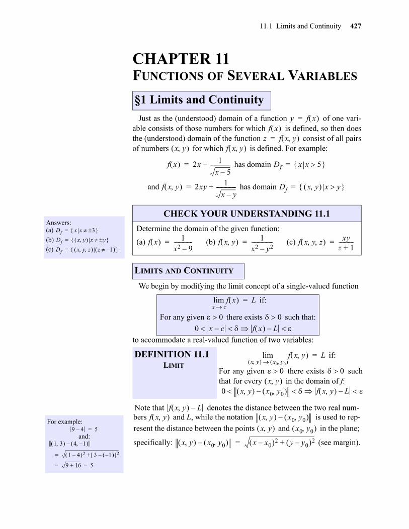
Just as the (understood) domain of a function of one vari-able consists of those numbers for which is defined, so then doesthe (understood) domain of the function consist of all pairsof numbers for which is defined. For example:
has domain
and has domain
We begin by modifying the limit concept of a single-valued function
to accommodate a real-valued function of two variables:
Note that denotes the distance between the two real num-bers and L, while the notation is used to rep-
resent the distance between the points and in the plane;
specifically: (see margin).
§1 Limits and Continuity
y f x =f x
z f x y =x y f x y
f x 2x 1
x 5–---------------+= Df x x 5 =
Answers:(a)
(b)
(c)
Df x x 3 =
Df x y x y =
Df x y z z 1– =
CHECK YOUR UNDERSTANDING 11.1
Determine the domain of the given function:
(a) (b) (c)
LIMITS AND CONTINUITY
if:
For any given there exists such that:
f x y 2xy 1
x y–---------------+= Df x y x y =
f x 1x2 9–--------------= f x y 1
x2 y2–----------------= f x y z xy
z 1+-----------=
f x x clim L=
0 00 x c– f x L–
For example:
and:9 4– 5=
1 3 4 1– –
1 4– 2 3 1– – 2+=
9 16+ 5= =
DEFINITION 11.1LIMIT
if:
For any given there exists suchthat for every in the domain of f:
f x y x y x0 y0
lim L=
0 0x y
0 x y x0 y0 – f x y L–
f x y L–f x y x y x0 y0 –
x y x0 y0
x y x0 y0 – x x0– 2 y y0– 2+=
gio
428 Chapter 11 Functions of Several Variables
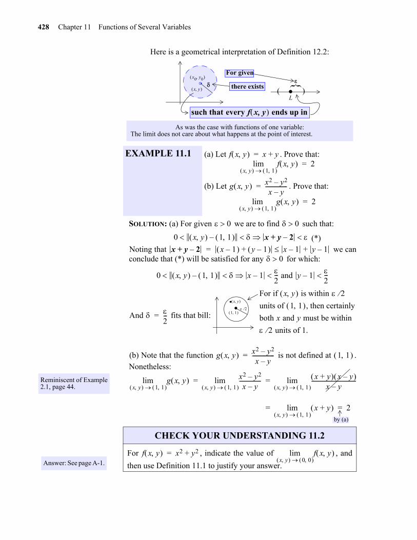
Here is a geometrical interpretation of Definition 12.2:
SOLUTION: (a) For given we are to find such that:
Noting that we canconclude that (*) will be satisfied for any for which:
And fits that bill:
(b) Note that the function is not defined at .
Nonetheless:
As was the case with functions of one variable: The limit does not care about what happens at the point of interest.
EXAMPLE 11.1 (a) Let . Prove that:
(b) Let . Prove that:
there exists
x0 y0
.L
( )
}For given
x y
such that every f x y ends up in
f x y x y+=f x y
x y 1 1 lim 2=
g x y x2 y2–x y–
----------------=
g x y x y 1 1
lim 2=
0 0
0 x y 1 1 – x y 2–+ (*)x y 2–+ x 1– y 1– + x 1– y 1–+=
0
0 x y 1 1 – x 1–2--- and y 1–
2---
Reminiscent of Example2.1, page 44.
Answer: See page A-1.
CHECK YOUR UNDERSTANDING 11.2
For , indicate the value of , and
then use Definition 11.1 to justify your answer.
2---=
. 21 1
x y . For if x y is within 2units of 1 1 , then certainly
both x and y must be within
2 units of 1.
g x y x2 y2–x y–
----------------= 1 1
by (a)
g x y x y 1 1
lim x2 y2–x y–
----------------x y 1 1
lim x y+ x y– x y–
---------------------------------x y 1 1
lim= =
x y+ x y 1 1
lim 2= =by (a)
f x y x2 y2+= f x y x y 0 0
lim
gio
11.1 Limits and Continuity 429
Theorem 2.3, of page 55, holds for functions of two variables:
PROOF: We content ourselves by establishing (a). The proof is “iden-tical” to that of Theorem 2.3(a), page 55 (see margin).
For a given we are to find such that:
By virtue of the triangle inequality we have:
It follows that (*) will hold for any for which
implies that BOTH and
. Let’s find such a :
Since , there is a such that
.
Since there is a such that
.
It follows that for the smaller of and :
.
THEOREM 11.1LIMIT THEOREMS
If and , then:
(a) .
(b)
(c) .
(d) .
(e) for any number c.
f x y x y x0 y0
lim L= g x y x y x0 y0
lim M=
f x y g x y + x y x0 y0
lim L M+=
f x y g x y – x y x0 y0
lim L M–=
f x y g x y x y x0 y0
lim LM=
f x y g x y ----------------
x y x0 y0 lim
LM----- if M 0=
cf x y x y x0 y0
lim cL=
The only difference is thatthe distance notation on page 55 is adjusted torepresent the distancebetween points in the plane;namely: .
x c–
x y x0 y0 –
0 0
0 x y x0 y0 – f g+ x y L M+ –
0 x y x0 y0 – f x y g x y L– M–+
0 x y x0 y0 – f x y L– g x y M– + (*)
f x y L– g x y M– + f x y L– g x y M–+
0
0 x y x0 y0 – f x y L–2---
g x y M–2---
f x y x y x0 y0
lim L= 1 0
0 x y x0 y0 – 1 f x y L–2---
g x y x y x0 y0
lim M= 2 0
0 x y x0 y0 – 2 g x y M–2---
1 2
0 x y x0 y0 – f x y L–2--- and g x y M–
2---
gio
430 Chapter 11 Functions of Several Variables
gio
As might be anticipated (see page 19):
As is the case with functions of one variable:
A polynomial function oftwo variables (or simply apolynomial function) is a sumof terms of the form ,where c is a constant and n andm are nonnegative integers.Moreover, a rational func-tion is a ratio of two polyno-mials.
cxnym
In the exercises you are invited to verify that for:
:
for any constant c.
It then follows, from Theorem 11.1, that for any polynomial of two variables (see margin):
Thus:
Moreover, for any polynomials , :
(providing ).
Thus:
f x y x= f x y x y x0 y0
lim x0=
f x y y= f x y x y x0 y0
lim y0=
cx y x0 y0
lim c=
p x y p x y
x y x0 y0 lim p x0 y0 =
2x2
x y 2 3 lim y x 3y–+ 2 22 3 2 3 3–+ 17= =
p x y q x y p x y q x y ----------------
x y x0 y0 lim
p x0 y0 q x0 y0 ---------------------= q x0 y0 0
x2 y+xy 1–--------------
x y 3 4– lim 9 4–
12– 1–------------------- 5
13------–= =
Answers: (a) See page A-1 (b) 20
CHECK YOUR UNDERSTANDING 11.3
(a) Prove Theorem 11.1(e).
(b) Use Theorem 11.1, along with Example 11.1, to evaluate
CONTINUITY
DEFINITION 11.2CONTINUITY
The real-valued function is continu-ous at if:
A function that is continuous at every pointin its domain is said to be a continuousfunction.
THEOREM 11.2
If f and g are continuous at then soare the functions:(a) (b) (c)
(d) [providing ]
(e) (for any real number c)
5 x y+ x2 y2–x y–
----------------
x y 1 1 lim
f x y x0 y0
f x y x y x0 y0
lim f x0 y0 =
x0 y0
f g+ f g– fgfg--- g x0 y0 0
cf
11.1 Limits and Continuity 431
PROOF: We establish (c), and relegate the others to the exercises.By definition, the product function is defined by:
We proceed to show that :
Here are a couple of “new” continuity theorems:
Proof: See Appendix B, page B-1.
The previous discussion involving functions of two variables, readilyextends to functions of three (or more) variables. In particular:
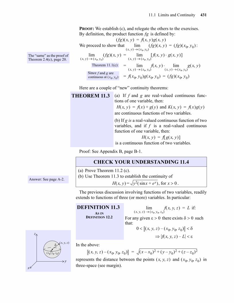
In the above:
represents the distance between the points and inthree-space (see margin).
The “same” as the proof ofTheorem 2.4(c), page 20.
THEOREM 11.3 (a) If f and g are real-valued continuous func-tions of one variable, then:
and are continuous functions of two variables.
(b) If g is a real-valued continuous function of twovariables, and if f is a real-valued continuousfunction of one variable, then:
is a continuous function of two variables.
fgfg x y f x y g x y =
fg x y x0 y0
lim x y fg x0 y0 =
fg x y x0 y0
lim x y f x y g x y x y x0 y0
lim=
f x y g x y x y x0 y0
limx y x0 y0
lim=
f x0 y0 g x0 y0 fg x0 y0 = =
Theorem 11.1(c):
Since f and g are continuous at x0 y0 :
H x y f x g y += K x y f x g y =
H x y f g x y =
Answer: See page A-2.
CHECK YOUR UNDERSTANDING 11.4
(a) Prove Theorem 11.2 (c).(b) Use Theorem 11.3 to establish the continuity of
, for .H x y y2 x ex+sin = x 0
x0 y0 z0
..
x y z
y
z
x
DEFINITION 11.3AS IN
DEFINITION 12.2
if:
For any given there exists suchthat:
f x y z x y z x0 y0 z0
lim L=
0 0
0 x y z x0 y0 z0 –
f x y z L–
x y z x0 y0 z0 – x x0– 2 y y0– 2 z z0– 2+ +=
x y z x0 y0 z0
gio
432 Chapter 11 Functions of Several Variables
We note that Theorems 11.1, 11.2, and 11.3 generalize to functions ofthree (or more) variables. In particular:
Definitions 11.2, 11.3, and 11.4, along with Theorems 12.2, 11.3, and11.4, assure us that polynomial functions of two or three variables arecontinuous everywhere, and that rational functions of two or three vari-ables are continuous throughout their domains (which exclude onlythose points where the polynomial in the denominator is zero).
DEFINITION 11.4AS IN
DEFINITION 11.3
The function is continuous at
if:
THEOREM 11.4AS IN
THEOREM 11.3
If f, g, and h are real-valued continuous func-tions of one variable, then the following are con-tinuous real-valued functions of three variables:
and
If f is a real-valued continuous function of onevariable, and if is a real-valued continuousfunction of three variables, then
is also a real-valuedcontinuous function of three variables.
f x y z x0 y0 z0
f x y z x y z x0 y0 z0
lim f x0 y0 z0 =
H x y z f x g y h z + +=K x y z f x g y h z =
g
H x y z f g x y z =
gio
11.1 Limits and Continuity 433
Exercises 1-4. Determine the domain of the given function.
Exercises 7-9. Use Definition 11.1 to verify that:
Exercises 10-20. Evaluate:
Exercises 21-28. Find the set of discontinuities of the given function.
29. Construct a function with domain which is discontinuous only at .
30. Construct a function with domain which is discontinuous only at and .
31. Construct a function with domain which is discontinuous only at .
EXERCISES
1. 2.3.
4. 5. 6.
7.8. 9.
10. 11. 12.
13. 14.15.
16. 17. 18.
19. 20.
21. 22. 23.
24. 25. 26.
27. 28.
f x y xy 100–x2 9+
--------------------= f x y x 100–x2 y2–
---------------------=f x y xytan=
f x y xyx ycos–sin
----------------------------= f x y z 1x y z+ +--------------------= f x y z 1
xyzsin----------------=
2x y+x y 1 1
lim 3=4y 3x–
x y 2 3 lim 6= x2 4xy– 4y2+
x 2y–-----------------------------------
x y 2 1 lim 0=
2x y+ 3
x y 0 1 lim y x xsin+
y2----------------------
x y 0 lim ex y+
1 xy–--------------
x y 0 0 lim
x4 y4–x2 y2–----------------
x y 2 2 lim
x4 y4–x2 y2+----------------
x y 2 2 lim
xy lnx y 1 e
lim
4x xy–4xy xy2–-----------------------
x y 0 4 lim x2 2xy y2 9–+ +
x y 3–+-----------------------------------------
x y 1 2 lim
x y+2y z–--------------
x y z 0 1 0 lim
zx zy–x y–
----------------x y z 1 1 1
lim xy z x–– x y z 1 1 1
lim
f x y x4 y4–x2 y2–----------------= f x y 4x xy–
4xy xy2–-----------------------= f x y x2exy
exln------------=
f x y y2
x2 y2+----------------= f x y z zx zy–
x y–----------------= f x y z x y+
2y z–--------------=
f x y x2 y2–x y–
---------------- if x y
x y+ if x y=
= f x y x2 y2–x y–
---------------- if x y
0 if x y=
=
f: 2 2 0 1
f: 2 2 0 1 1 0
f: 3 3 0 1 0
434 Chapter 11 Functions of Several Variables
32. Show that the function approaches 0 as along any line
. Does exist?
Exercises 33-41. Prove:
33. Theorem 11.1(b) 34. Theorem 11.1(c)
35. Theorem 11.2(a) 36. Theorem 11.2(b)
37. Theorem 11.2(d) 38. Theorem 11.2(e)
39. If , then .
40. If , then .
41. For any constant c,
f x y x2yx4 y2+----------------= x y 0 0
y mx= f x y x y 0 0
lim
f x y x= f x y x y x0 y0
lim x0=
f x y y= f x y x y x0 y0
lim y0=
cx y x0 y0
lim c=
gio
11.2 Graphing Functions of Two Variables 435
gio
11
Just as the graph of the function is a line, so thenis the graph of a plane in three-space. Andjust as a line is determined by two points, so then is a plane determinedby three points (that do not lie on a common line). Consider the follow-ing example.
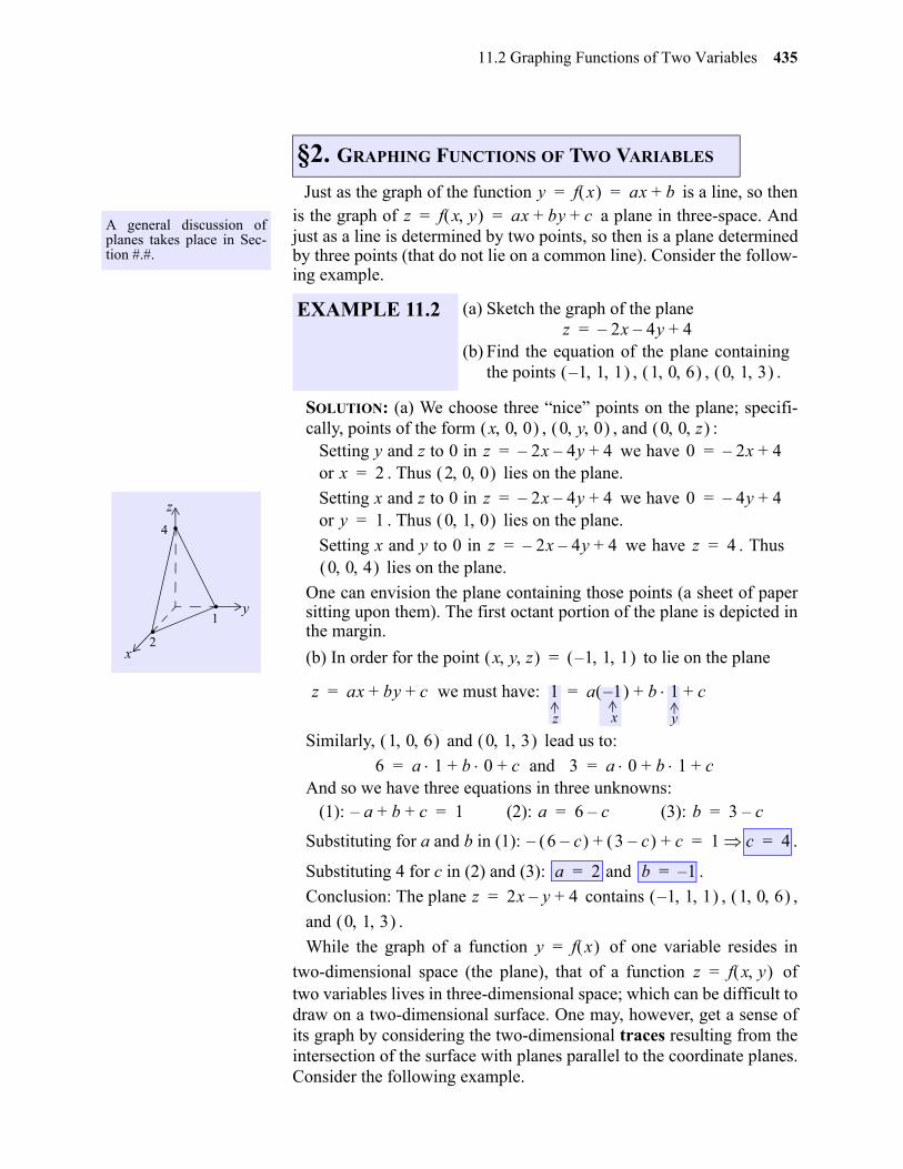
SOLUTION: (a) We choose three “nice” points on the plane; specifi-cally, points of the form , , and :
Setting y and z to 0 in we have or . Thus lies on the plane.
Setting x and z to 0 in we have or . Thus lies on the plane.
Setting x and y to 0 in we have . Thus lies on the plane.
One can envision the plane containing those points (a sheet of papersitting upon them). The first octant portion of the plane is depicted inthe margin.
(b) In order for the point to lie on the plane
Similarly, and lead us to:
And so we have three equations in three unknowns: (1): (2): (3):
Substituting for a and b in (1): .
Substituting 4 for c in (2) and (3): .
Conclusion: The plane contains , ,
and .
While the graph of a function of one variable resides in
two-dimensional space (the plane), that of a function oftwo variables lives in three-dimensional space; which can be difficult todraw on a two-dimensional surface. One may, however, get a sense ofits graph by considering the two-dimensional traces resulting from theintersection of the surface with planes parallel to the coordinate planes.Consider the following example.
A general discussion ofplanes takes place in Sec-tion #.#.
§2. GRAPHING FUNCTIONS OF TWO VARIABLES
EXAMPLE 11.2 (a) Sketch the graph of the plane
(b) Find the equation of the plane containingthe points , , .
y f x ax b+= =z f x y ax by c+ += =
z 2x– 4y– 4+=
1 1 1 – 1 0 6 0 1 3
x 0 0 0 y 0 0 0 z
..
.
x
y
z
2
1
4
z 2x– 4y– 4+= 0 2x– 4+=x 2= 2 0 0
z 2x– 4y– 4+= 0 4y– 4+=y 1= 0 1 0
z 2x– 4y– 4+= z 4=0 0 4
x y z 1 1 1 – =
z ax by c we must have: 1+ + a 1– b 1 c+ += =
z x y
1 0 6 0 1 3 6 a 1 b 0 c and 3+ + a 0 b 1 c+ += =
a– b c+ + 1= a 6 c–= b 3 c–=
6 c– – 3 c– c+ + 1 c 4= =
a 2 and b 1–= =
z 2x y– 4+= 1 1 1 – 1 0 6 0 1 3
y f x =
z f x y =
436 Chapter 11 Functions of Several Variables
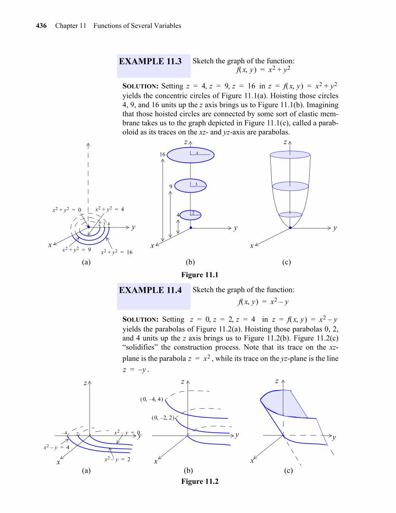
SOLUTION: Setting in yields the concentric circles of Figure 11.1(a). Hoisting those circles4, 9, and 16 units up the z axis brings us to Figure 11.1(b). Imaginingthat those hoisted circles are connected by some sort of elastic mem-brane takes us to the graph depicted in Figure 11.1(c), called a parab-oloid as its traces on the xz- and yz-axis are parabolas.
Figure 11.1
SOLUTION: Setting in yields the parabolas of Figure 11.2(a). Hoisting those parabolas 0, 2,and 4 units up the z axis brings us to Figure 11.2(b). Figure 11.2(c)“solidifies” the construction process. Note that its trace on the xz-
plane is the parabola , while its trace on the yz-plane is the line
.
Figure 11.2
EXAMPLE 11.3 Sketch the graph of the function:f x y x2 y2+=
z 4 z 9 z 16= = = z f x y x2 y2+= =
.x
y
z
3
416
9
.x
y
z
24.x
y
x2 y2+ 0= x2 y2+ 4=
x2 y2+ 9= x2 y2+ 16=
2 3 4
(a) (b) (c)(a) (b) (c)
EXAMPLE 11.4 Sketch the graph of the function:
f x y x2 y–=
z 0 z 2 z 4= = = z f x y x2 y–= =
z x2=
z y–=
x
y
z
y
x
z
x
y
z
x2 y– 4=
x2 y– 2=
x2 y– 0=4– 2–
0 2– 2
0 4– 4
(a) (b) (c)
11.2 Graphing Functions of Two Variables 437
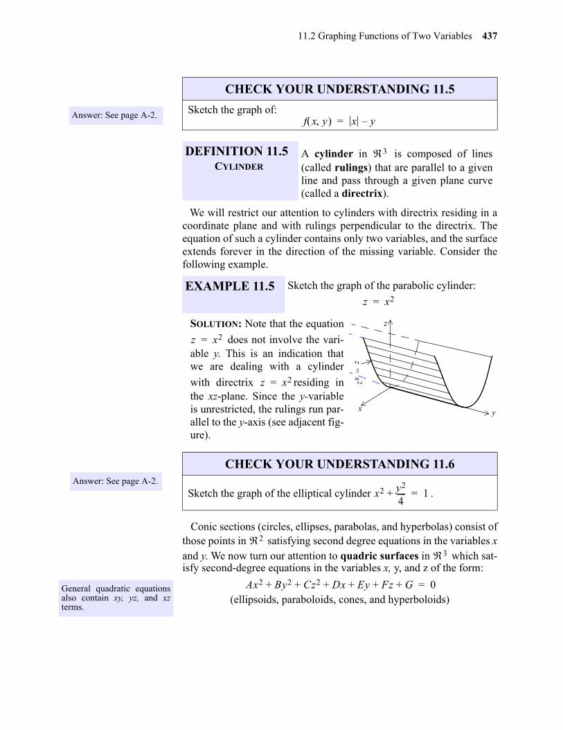
We will restrict our attention to cylinders with directrix residing in acoordinate plane and with rulings perpendicular to the directrix. Theequation of such a cylinder contains only two variables, and the surfaceextends forever in the direction of the missing variable. Consider thefollowing example.
SOLUTION: Note that the equation
does not involve the vari-able y. This is an indication thatwe are dealing with a cylinder
with directrix residing inthe xz-plane. Since the y-variableis unrestricted, the rulings run par-allel to the y-axis (see adjacent fig-ure).
Conic sections (circles, ellipses, parabolas, and hyperbolas) consist ofthose points in satisfying second degree equations in the variables xand y. We now turn our attention to quadric surfaces in which sat-isfy second-degree equations in the variables x, y, and z of the form:
(ellipsoids, paraboloids, cones, and hyperboloids)
Answer: See page A-2.
CHECK YOUR UNDERSTANDING 11.5
Sketch the graph of:
DEFINITION 11.5CYLINDER
A cylinder in is composed of lines(called rulings) that are parallel to a givenline and pass through a given plane curve(called a directrix).
f x y x y–=
3
Answer: See page A-2.
EXAMPLE 11.5 Sketch the graph of the parabolic cylinder:
CHECK YOUR UNDERSTANDING 11.6
Sketch the graph of the elliptical cylinder .
z x2=
x y
z
zx
2=
z x2=
z x2=
x2 y2
4-----+ 1=
General quadratic equationsalso contain xy, yz, and xzterms.
2
3
Ax2 By2 Cz2 Dx Ey Fz G+ + + + + + 0=
gio
438 Chapter 11 Functions of Several Variables
The quadric surface of Example 11.3 is said to be a
circular paraboloid [its trace on the planes (for ) are cir-
cles, while those with the planes and are parabolas]. It isa special case of an elliptic paraboloid — one of which is featuredbelow.
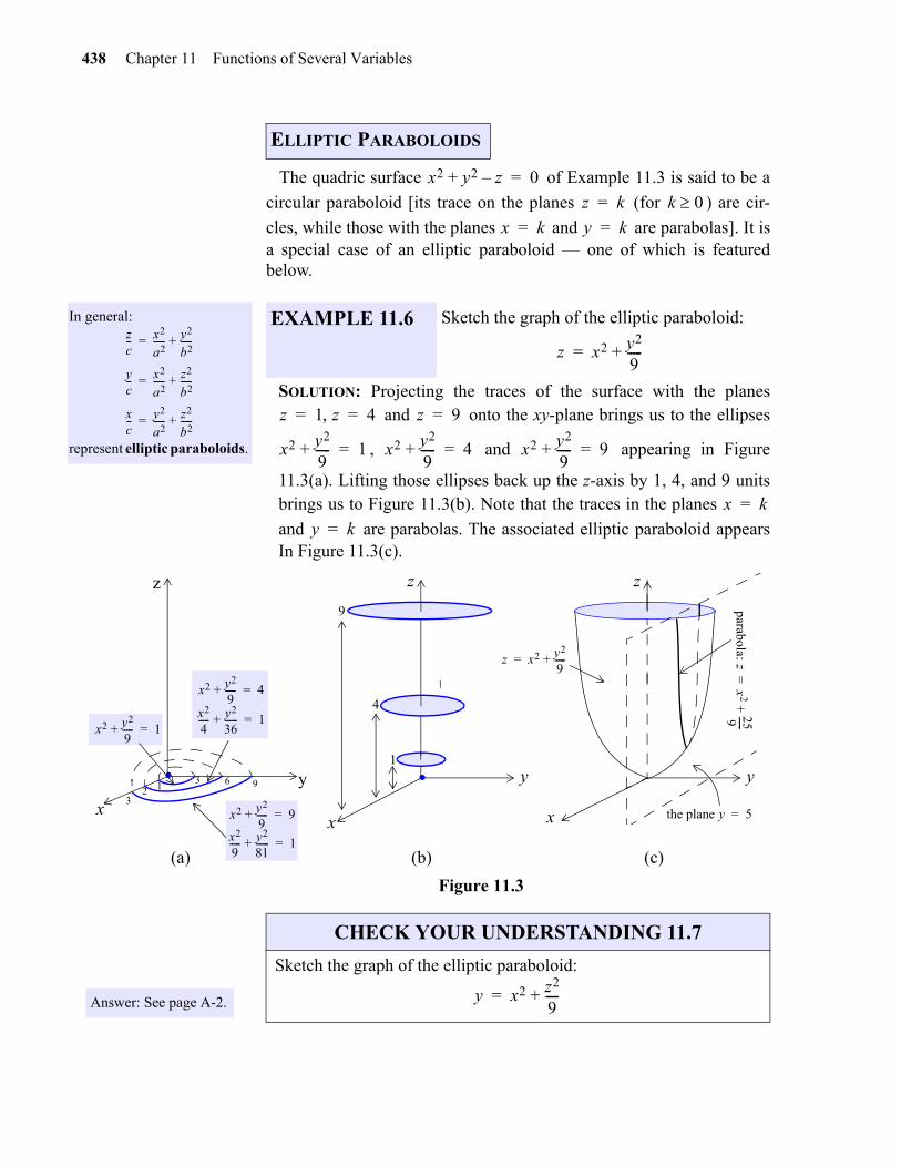
SOLUTION: Projecting the traces of the surface with the planes and onto the xy-plane brings us to the ellipses
, and appearing in Figure
11.3(a). Lifting those ellipses back up the z-axis by 1, 4, and 9 unitsbrings us to Figure 11.3(b). Note that the traces in the planes
and are parabolas. The associated elliptic paraboloid appearsIn Figure 11.3(c).
Figure 11.3
ELLIPTIC PARABOLOIDS
x2 y2 z–+ 0=
z k= k 0x k= y k=
In general:
represent elliptic paraboloids.
zc-- x2
a2----- y2
b2-----+=
yc-- x2
a2----- z2
b2-----+=
xc-- y2
a2----- z2
b2-----+=
EXAMPLE 11.6 Sketch the graph of the elliptic paraboloid:
z x2 y2
9-----+=
z 1 z 4= = z 9=
x2 y2
9-----+ 1= x2 y2
9-----+ 4= x2 y2
9-----+ 9=
x k=
y k=
.x
y
z
x
y
z
1.x
(a) (b) (c)
1
3
3
6
9
x2 y2
9-----+ 1=
x2 y2
9-----+ 4=
x2
4----- y2
36------+ 1=
x2 y2
9-----+ 9=
x2
9----- y2
81------+ 1=
4
9
z x2 y2
9-----+=
y
z
the plane y 5=
parabola: zx
2259 ------
+=
(a) (b) (c)
2
Answer: See page A-2.
CHECK YOUR UNDERSTANDING 11.7
Sketch the graph of the elliptic paraboloid:
y x2 z2
9----+=
11.2 Graphing Functions of Two Variables 439
Just as equations of the form represent ellipses centered
at the origin, so then do equations of the form repre-
sent ellipsoids centered at the origin. Consider the following example:
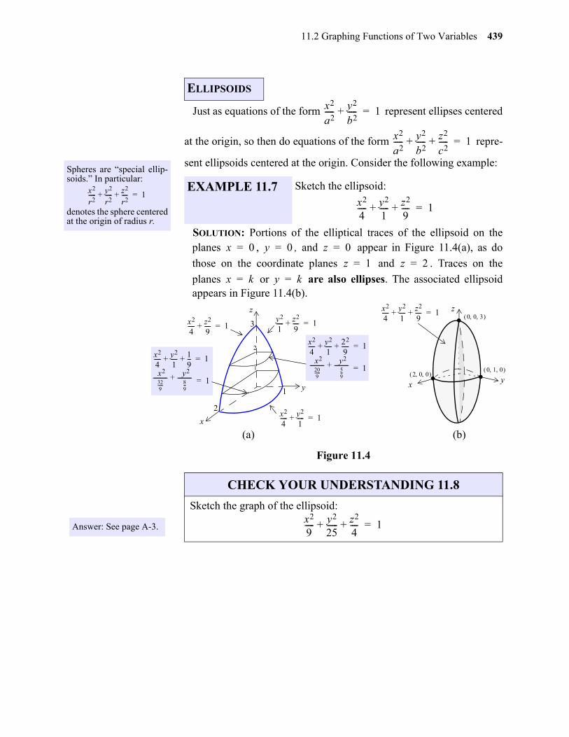
SOLUTION: Portions of the elliptical traces of the ellipsoid on theplanes , , and appear in Figure 11.4(a), as do
those on the coordinate planes and . Traces on the
planes or are also ellipses. The associated ellipsoidappears in Figure 11.4(b).
Figure 11.4
Spheres are “special ellip-soids.” In particular:
denotes the sphere centeredat the origin of radius r.
x2
r2----- y2
r2----- z2
r2----+ + 1=
ELLIPSOIDS
EXAMPLE 11.7 Sketch the ellipsoid:
x2
a2----- y2
b2-----+ 1=
x2
a2----- y2
b2----- z2
c2-----+ + 1=
x2
4----- y2
1----- z2
9----+ + 1=
x 0= y 0= z 0=
z 1= z 2=
x k= y k=
2
1
3
1
2
x2
4----- y2
1-----+ 1=
y2
1----- z2
9----+ 1=x2
4----- z2
9----+ 1=
x2
4----- y2
1----- 22
9-----+ + 1=
x2 209------
---------- y2 59---
----------+ 1=
x2
4----- y2
1----- 1
9---+ + 1=
x2 329------
---------- y2 89---
----------+ 1= xy
zx2
4----- y2
1----- z2
9----+ + 1=
x
y
z0 0 3
0 1 0 2 0 0
(a) (b)
.
. .
Answer: See page A-3.
CHECK YOUR UNDERSTANDING 11.8
Sketch the graph of the ellipsoid:x2
9----- y2
25------ z2
4----+ + 1=
gio
440 Chapter 11 Functions of Several Variables
2---
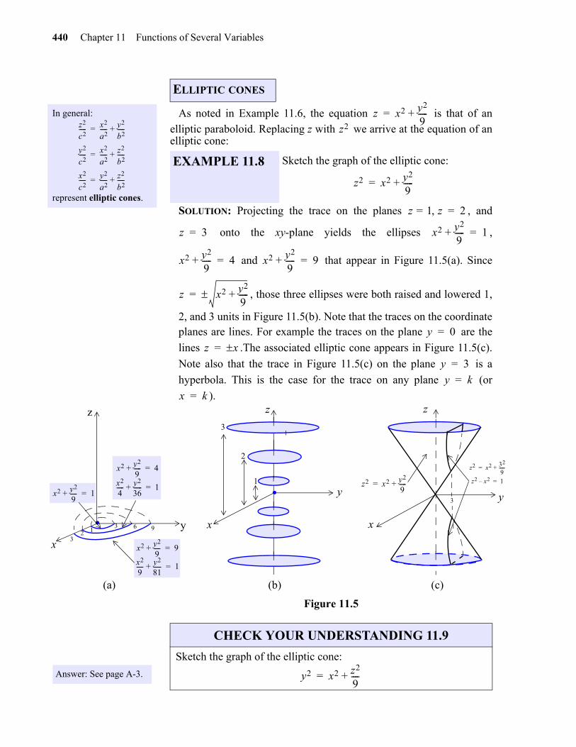
As noted in Example 11.6, the equation is that of an
elliptic paraboloid. Replacing z with we arrive at the equation of anelliptic cone:
SOLUTION: Projecting the trace on the planes , and
onto the xy-plane yields the ellipses ,
and that appear in Figure 11.5(a). Since
, those three ellipses were both raised and lowered 1,
2, and 3 units in Figure 11.5(b). Note that the traces on the coordinateplanes are lines. For example the traces on the plane are the
lines .The associated elliptic cone appears in Figure 11.5(c).
Note also that the trace in Figure 11.5(c) on the plane is a
hyperbola. This is the case for the trace on any plane (or
).
Figure 11.5
In general:
represent elliptic cones.
z2
c2----- x2
a2----- y2
b2-----+=
y2
c2----- x2
a2----- z2
b2-----+=
x2
c2----- y2
a2----- z2
b2-----+=
ELLIPTIC CONES
EXAMPLE 11.8 Sketch the graph of the elliptic cone:
z x2 y2
9-----+=
z2
z2 x2 y2
9-----+=
z 1= z 2=
z 3= x2 y2
9-----+ 1=
x2 y2
9-----+ 4= x2 y2
9-----+ 9=
z x2 y2
9-----+=
y 0=
z x=
y 3=
y k=
x k=
.x
y
z
1
(a) (b) (c)
2
3
x
y
z
(a) (b) (c)
z2 x2 39--+=
z2 x2– 1=
3
z2 x2 y2
9-----+=
.x
1
3
3
6
9
x2 y2
9-----+ 1=
x2 y2
9-----+ 4=
x2
4----- y2
36------+ 1=
x2 y2
9-----+ 9=
x2
9----- y2
81------+ 1=
y
z
2
Answer: See page A-3.
CHECK YOUR UNDERSTANDING 11.9
Sketch the graph of the elliptic cone:
y2 x2 z2
9----+=
11.2 Graphing Functions of Two Variables 441
gio
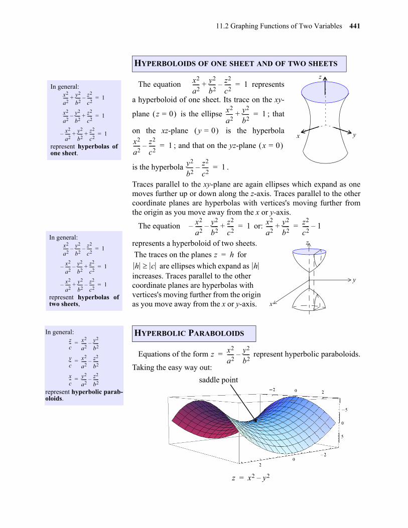
The equation represents
a hyperboloid of one sheet. Its trace on the xy-
plane is the ellipse ; that
on the xz-plane is the hyperbola
; and that on the yz-plane
is the hyperbola .
Traces parallel to the xy-plane are again ellipses which expand as onemoves further up or down along the z-axis. Traces parallel to the othercoordinate planes are hyperbolas with vertices's moving further fromthe origin as you move away from the x or y-axis.
The equation or:
represents a hyperboloid of two sheets.
The traces on the planes for
are ellipses which expand as increases. Traces parallel to the other coordinate planes are hyperbolas with vertices's moving further from the origin as you move away from the x or y-axis.
Equations of the form represent hyperbolic paraboloids.
Taking the easy way out:
In general:
represent hyperbolas ofone sheet.
x2
a2----- y2
b2----- z2
c2-----–+ 1=
x2
a2----- y2
b2-----– z2
c2-----+ 1=
x2
a2-----– y2
b2----- z2
c2-----+ + 1=
HYPERBOLOIDS OF ONE SHEET AND OF TWO SHEETS
x y
zx2
a2----- y2
b2----- z2
c2-----–+ 1=
z 0= x2
a2----- y2
b2-----+ 1=
y 0= x2
a2----- z2
c2-----– 1= x 0=
y2
b2----- z2
c2-----– 1=
In general:
represent hyperbolas oftwo sheets,
x2
a2----- y2
b2-----– z2
c2-----– 1=
x2
a2-----– y2
b2-----– z2
c2-----+ 1=
x2
a2-----– y2
b2----- z2
c2-----–+ 1=
x2
a2-----– y2
b2-----– z2
c2-----+ 1= x2
a2----- y2
b2-----+ z2
c2----- 1–=
x
y
z
z h=
h c h
In general:
represent hyperbolic parab-oloids.
zc-- x2
a2----- y2
b2-----–=
yc-- x2
a2----- z2
b2-----–=
xc-- y2
a2----- z2
b2-----–=
HYPERBOLIC PARABOLOIDS
z x2
a2----- y2
b2-----–=
z x2 y2–=
saddle point
442 Chapter 11 Functions of Several Variables
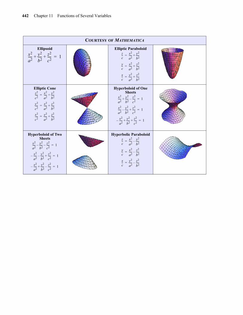
COURTESY OF MATHEMATICA
Ellipsoid
Elliptic Paraboloid
Elliptic Cone Hyperboloid of One Sheets
Hyperboloid of Two Sheets
Hyperbolic Paraboloid
x2
a2----- y2
b2----- z2
c2-----+ + 1=
zc-- x2
a2----- y2
b2-----+=
yc-- x2
a2----- z2
b2-----+=
xc-- y2
a2----- z2
b2-----+=
z2
c2----- x2
a2----- y2
b2-----+=
y2
c2----- x2
a2----- z2
b2-----+=
x2
c2----- y2
a2----- z2
b2-----+=
x2
a2----- y2
b2----- z2
c2-----–+ 1=
x2
a2----- y2
b2-----– z2
c2-----+ 1=
x2
a2-----– y2
b2----- z2
c2-----+ + 1=
x2
a2----- y2
b2-----– z2
c2-----– 1=
x2
a2-----– y2
b2-----– z2
c2-----+ 1=
x2
a2-----– y2
b2----- z2
c2-----–+ 1=
zc-- x2
a2----- y2
b2-----–=
yc-- x2
a2----- z2
b2-----–=
xc-- y2
a2----- z2
b2-----–=
11.2 Graphing Functions of Two Variables 443
Exercises 1-2. Sketch the graph of the given plane in the first octant.
Exercises 1-3. Find the equation of the plane containing the given points.
Exercises 5-10. Sketch the given cylinder in .
Exercises 11-26. Identify and sketch the given quadratic surface.
EXERCISES
1. 2.
3. , , 4. , ,
5. 6. 7.
8. 9. 10.
11. 12.
13. 14.
15. 16.
17. 18.
19. 20.
21. 22.
23. 24.
25. 26.
z 4x– 2y– 2+= z x– y– 1+=
0 0 0 1 0 2 0 2 5 1 1 1 – 1 0 0 0 1 2
3
x 2y+ 1= 4x2 z+ 4= y2 z+ 0=
25x2 9y2– 1– 0= x2 2y2– 1= x 2xy– 1=
z x2 y2+= x y2 4z2+=
36x2 9y2 4z2+ + 36= x y2– z2– 0=
x2 y2– z2+ 0= x2 2y z2+ + 0=
25x2 4y2– 25z2 100+ + 0= x2 4y z2+ + 0=
x2 4y z2–+ 0= 16x2 9y2– 9z2– 0=
x2 y2 4z2–+ 4= 9x2 36y2– 16z2 144+ + 0=
25x2 4y2– 25z2+ 100= z x 2+ 2 y 3– 2 9–+=
9x2 4y2– 36z= x2 y2– 9z– 0=
444 Chapter 11 Functions of Several Variables
11
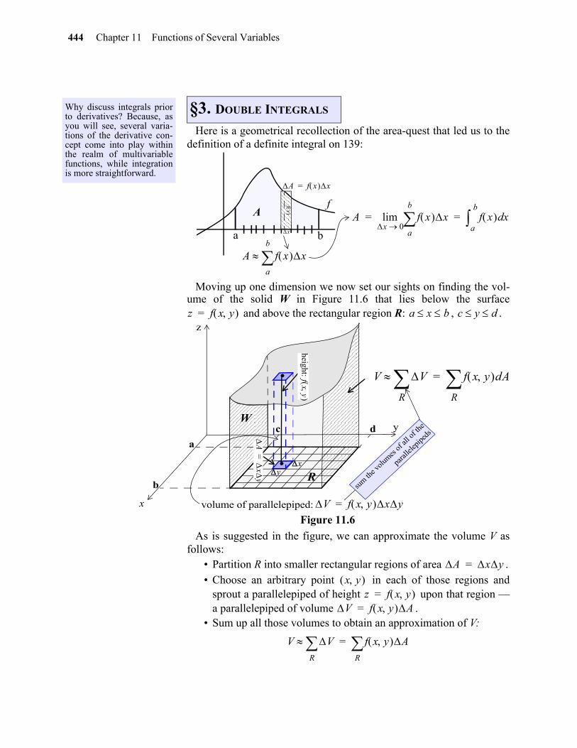
Here is a geometrical recollection of the area-quest that led us to thedefinition of a definite integral on 139:
Moving up one dimension we now set our sights on finding the vol-ume of the solid W in Figure 11.6 that lies below the surface
and above the rectangular region R: , .
Figure 11.6
As is suggested in the figure, we can approximate the volume V asfollows:
• Partition R into smaller rectangular regions of area .• Choose an arbitrary point in each of those regions and
sprout a parallelepiped of height upon that region —a parallelepiped of volume .
• Sum up all those volumes to obtain an approximation of V:
Why discuss integrals priorto derivatives? Because, asyou will see, several varia-tions of the derivative con-cept come into play withinthe realm of multivariablefunctions, while integrationis more straightforward.
§3. DOUBLE INTEGRALS
x
f
a b
fx
A f x x=
A f x xa
b
A A f x xa
b
x 0lim f x xd
a
b
= =
z f x y = a x b c y d
a
b
c d
yx
.
.
A
x
y=
height: fx
y
V f x y xy=volume of parallelepiped:
V V
R f x y dA
R=
sum th
e volu
mes of
all o
f the
paral
lelep
ipeds
x
y
z
R
W
A xy=x y
z f x y =V f x y A=
V VR f x y A
R=
gio
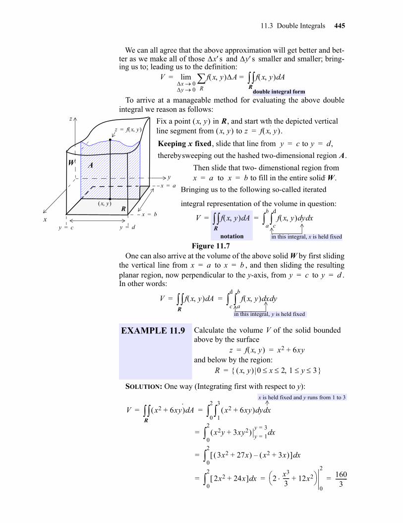
11.3 Double Integrals 445
We can all agree that the above approximation will get better and bet-ter as we make all of those and smaller and smaller; bring-ing us to; leading us to the definition:
To arrive at a manageable method for evaluating the above doubleintegral we reason as follows:
Figure 11.7One can also arrive at the volume of the above solid W by first sliding
the vertical line from to , and then sliding the resultingplanar region, now perpendicular to the y-axis, from to .In other words:
SOLUTION: One way (Integrating first with respect to y):
xs ys
V f x y ARx 0
y 0
lim f x y Ad= =R
double integral form
.
:
x
z f x y =
R
.
.
x y
Fix a point x y in R, and start wth the depicted verticalline segment from x y to z f x y .=
Keeping x fixed, slide that line from y c to y d,= =
therebysweeping out the hashed two-dimensional region A.
Then slide that two- dimenstional region from x a to x b to fill in the entire solid W.= =
y c= y d=
x a=
x b=
y
z
V f x y Ad f x y ydc
d
xda
b
= =
A
Bringing us to the following so-called iterated
R
W
integral representation of the volume in question:
in this integral, x is held fixednotation
EXAMPLE 11.9 Calculate the volume V of the solid boundedabove by the surface
and below by the region:
x a= x b=y c= y d=
V f x y Ad f x y xda
b
ydc
d
= =
in this integral, y is held fixedR
z f x y x2 6xy+= =
R x y 0 x 2 1 y 3 =
V x2 6xy+ Ad x2 6xy+ yd1
3
xd0
2
= =
x2y 3xy2+ y 1=
y 3=xd
0
2
=
3x2 27x+ x2 3x+ – xd0
2
=
2x2 24x+ xd0
2
2x3
3----- 12x2+
0
21603
---------= = =
x is held fixed and y runs from 1 to 3
R
.
446 Chapter 11 Functions of Several Variables
Another way (Integrating first with respect to x):
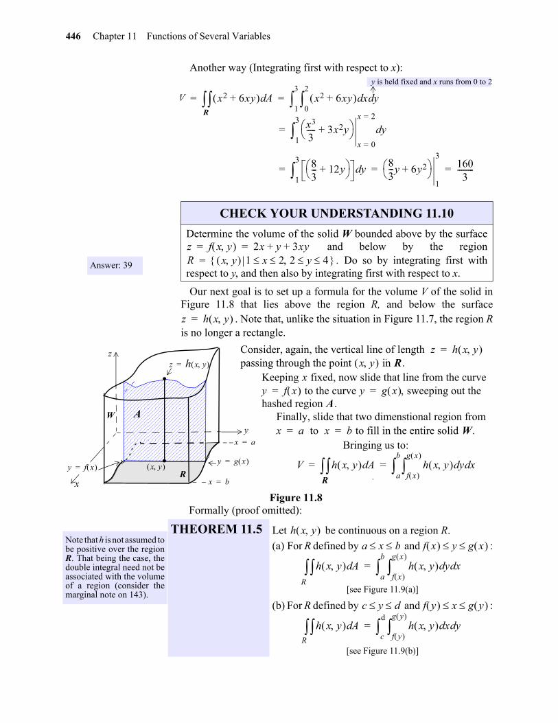
Our next goal is to set up a formula for the volume V of the solid inFigure 11.8 that lies above the region R, and below the surface
. Note that, unlike the situation in Figure 11.7, the region Ris no longer a rectangle.
Figure 11.8Formally (proof omitted):
V x2 6xy+ Ad x2 6xy+ xd0
2
yd1
3
= =
x3
3----- 3x2y+
x 0=
x 2=
yd1
3
=
83--- 12y+ yd
1
3
83---y 6y2+
1
31603
---------= = =
R
y is held fixed and x runs from 0 to 2
Answer: 39
CHECK YOUR UNDERSTANDING 11.10
Determine the volume of the solid W bounded above by the surface and below by the region
. Do so by integrating first withrespect to y, and then also by integrating first with respect to x.
z f x y 2x y 3xy+ += =R x y 1 x 2 2 y 4 =
z h x y =
.
.x
z h x y =
R
.
.
x y
Consider, again, the vertical line of length z h x y =passing through the point x y in R.
Keeping x fixed, now slide that line from the curvey f x to the curve y g x sweeping out the= =hashed region A.
Finally, slide that two dimenstional region from x a to x b to fill in the entire solid W.= =
x a=
x b=
y
z
A
y f x =y g x =
W
Bringing us to:
V h x y Ad h x y ydf x
g x
xda
b
= =R
Note that h is not assumed tobe positive over the regionR. That being the case, thedouble integral need not beassociated with the volumeof a region (consider themarginal note on 143).
THEOREM 11.5 Let be continuous on a region R.
(a) For R defined by and :
[see Figure 11.9(a)]
(b) For R defined by and :
[see Figure 11.9(b)]
h x y a x b f x y g x
h x y Ad h x y ydf x
g x
xda
b
=R
c y d f y x g y
h x y Ad h x y xdf y
g y
ydc
d
=R
gio
11.3 Double Integrals 447
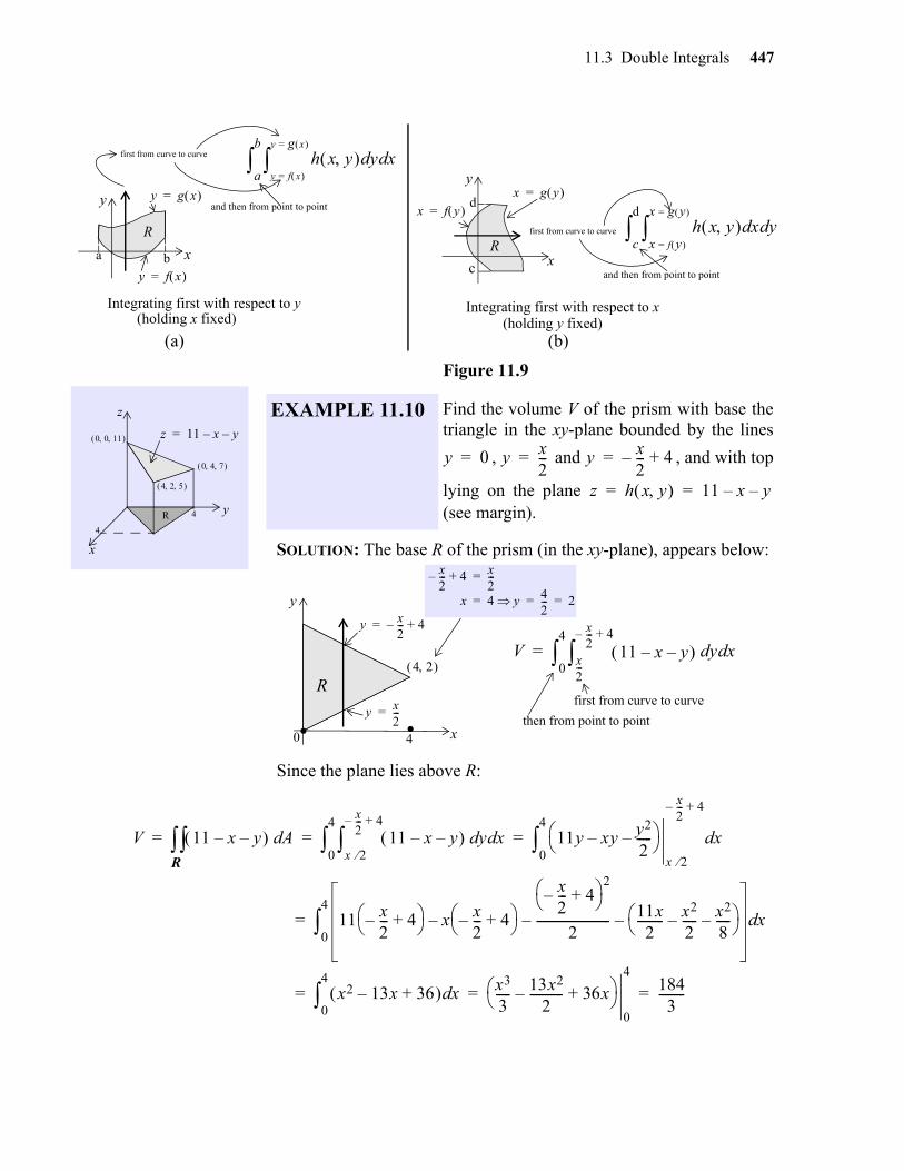
Figure 11.9
SOLUTION: The base R of the prism (in the xy-plane), appears below:
Since the plane lies above R:
a b x
y y g x =
y f x =
h x y ydy f x =
y g x =
xda
b
R
c x
yx g y =
x f y =
first from curve to curve
R
d
Integrating first with respect to y Integrating first with respect to x
(holding x fixed)
(holding y fixed)(a) (b)
and then from point to point
first from curve to curve
h x y xdx f y =
x g y =
ydc
d
and then from point to point
0 0 11
0 4 7
4 2 5
y
x
z
4
4
R
z 11 x– y–=
EXAMPLE 11.10 Find the volume V of the prism with base thetriangle in the xy-plane bounded by the lines
, and , and with top
lying on the plane (see margin).
y 0= y x2---= y x
2---– 4+=
z h x y 11 x– y–= =
V 11 x– y– ydx2---
x2---– 4+
xd0
4
=4 2
4
y x2---– 4+=
y x2---=
first from curve to curve
0
R
then from point to point. . x
y
x2---– 4+ x
2---=
x 4 y 42--- 2= = =
V 11 x– y– Ad 11 x– y– ydx 2
x2---– 4+
xd0
4
11y xy– y2
2-----–
x 2
x2---– 4+
xd0
4
= = =
11 x2---– 4+
x x2---– 4+
–
x2---– 4+
2
2-------------------------– 11x
2--------- x2
2-----– x2
8-----–
– xd0
4
=
x2 13x– 36+ xd0
4
x3
3----- 13x2
2-----------– 36x+
0
41843
---------= = =
R
448 Chapter 11 Functions of Several Variables
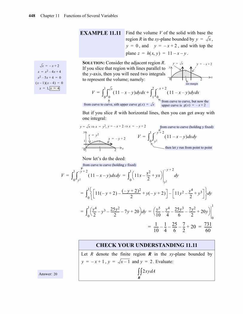
SOLUTION: Consider the adjacent region R.If you slice that region with lines parallel tothe y-axis, then you will need two integralsto represent the volume; namely:
But if you slice R with horizontal lines, then you can get away withone integral:
Now let’s do the deed:
x x– 2+=
x x2 4x– 4+=
x2 5x– 4+ 0=
x 1– x 4– 0=
x 1 x 4= =
EXAMPLE 11.11 Find the volume V of the solid with base theregion R in the xy-plane bounded by ,
, and , and with top the
plane .
y x=
y 0= y x– 2+=
z h x y 11 x– y–= =
1 20
y x= y x– 2+=
x
y
see margin
V 11 x– y– yd0
x
xd0
1
11 x– y– yd0
x– 2+
xd1
2
+=
from curve to curve, but now theupper curve is g x x– 2+=from curve to curve, sith upper curve g x x=
1 20
y x= x y2= y x– 2+= x y– 2+=
x
yx y2=
x y– 2+=1
V 11 x– y– xdy2
y– 2+
yd0
1
=
from curve to curve (holding y fixed)
then let y run from point to point
V 11 x– y– xdy2
y– 2+
yd0
1
11x x2
2-----– yx+
y2
y– 2+
yd0
1
= =
11 y– 2+ y– 2+ 2
2-----------------------– y y– 2+ + 11y2 y4
2-----– y3+–
yd0
1
=
y4
2----- y3– 25y2
2-----------– 7y– 20+
yd0
1
y5
10------ y4
4-----– 25y3
6-----------– 7y2
2--------– 20y+
0
1
= =
from curve to curve (holding y fixed)
110------ 1
4---– 25
6------– 7
2---– 20+ 731
60---------= =
Answer: 20
CHECK YOUR UNDERSTANDING 11.11
Let R denote the finite region R in the xy-plane bounded by
, and . Evaluate:y x– 1+= y x 1–= y 2=
2xy AdR
gio
11.3 Double Integrals 449
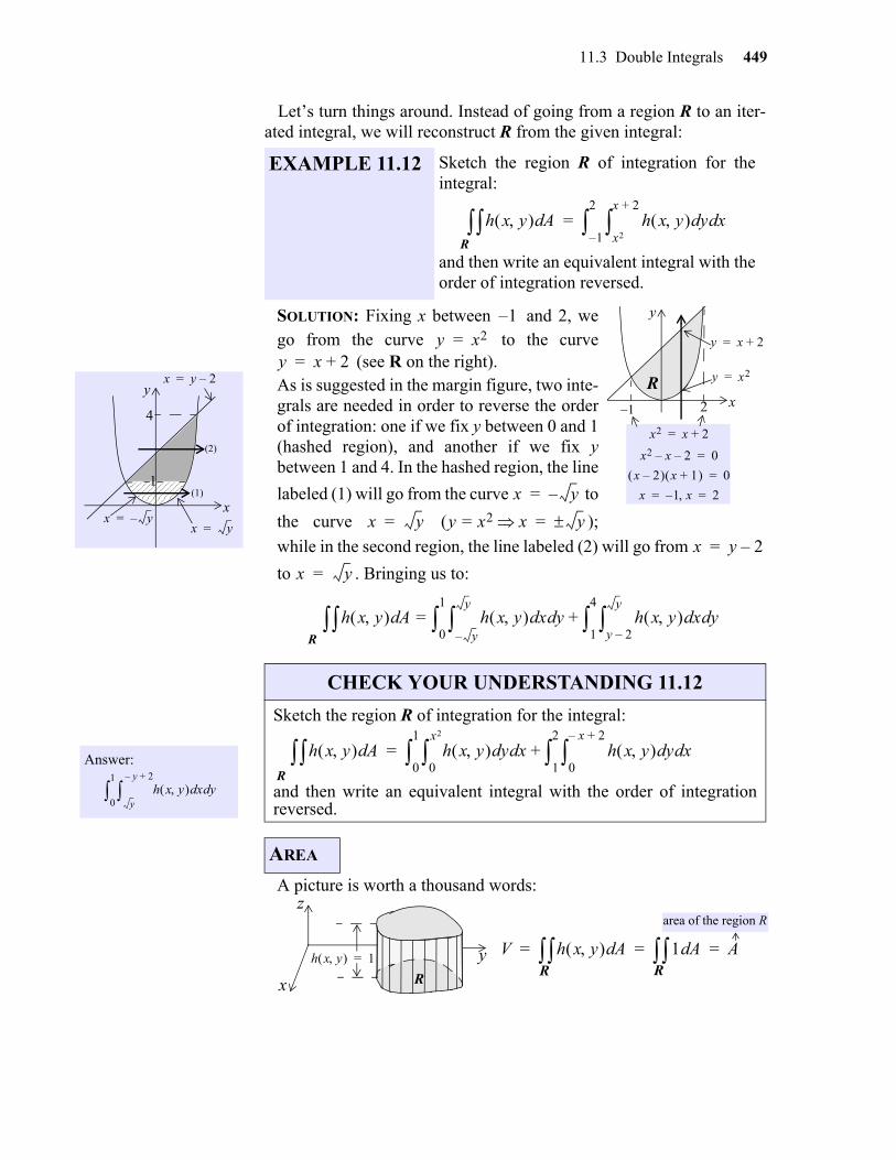
Let’s turn things around. Instead of going from a region R to an iter-ated integral, we will reconstruct R from the given integral:
SOLUTION: Fixing x between and 2, wego from the curve to the curve
(see R on the right).As is suggested in the margin figure, two inte-grals are needed in order to reverse the orderof integration: one if we fix y between 0 and 1(hashed region), and another if we fix ybetween 1 and 4. In the hashed region, the line
labeled (1) will go from the curve to
the curve ( );
while in the second region, the line labeled (2) will go from
to . Bringing us to:
A picture is worth a thousand words:
EXAMPLE 11.12 Sketch the region R of integration for theintegral:
and then write an equivalent integral with theorder of integration reversed.
h x y Ad h x y ydx2
x 2+
xd1–
2
=R
x
y
4
1(1)
(2)
x y 2–=
x y–=x y=
y x2=
y x 2+=
x
y
1– 2
R
x2 x 2+=
x2 x– 2– 0=
x 2– x 1+ 0=
x 1– x 2= =
1–y x2=
y x 2+=
x y–=
x y= y x2= x y=
x y 2–=
x y=
h x y Ad h x y xdy–
y
yd0
1
= h x y xdy 2–
y
yd1
4
+R
Answer:
h x y xdy
y– 2+
yd0
1
CHECK YOUR UNDERSTANDING 11.12
Sketch the region R of integration for the integral:
and then write an equivalent integral with the order of integrationreversed.
AREA
h x y Ad h x y yd0
x2
xd0
1
h x y yd0
x– 2+
xd1
2
+=R
R
h x y 1=V h x y Ad 1 Ad A= = =
R Ry
x
zarea of the region R
450 Chapter 11 Functions of Several Variables
gio
SOLUTION: (without words)
An idealized thin flat object is called a lamina. A homogeneous lam-ina is a lamina with uniform composition throughout. A lamina that isnot homogeneous is said to be inhomogeneous.
The density, , of a homogeneous lamina of mass M and area A isdefined to be its mass per unit Area:
.
The density function, , at a point in an inhomogeneouslamina R in the xy-plane is defined to be the limit of the masses of rect-angular regions containing divided by the area of those regions,as the dimensions of the rectangular regions tend to zero:
Bringing us to:
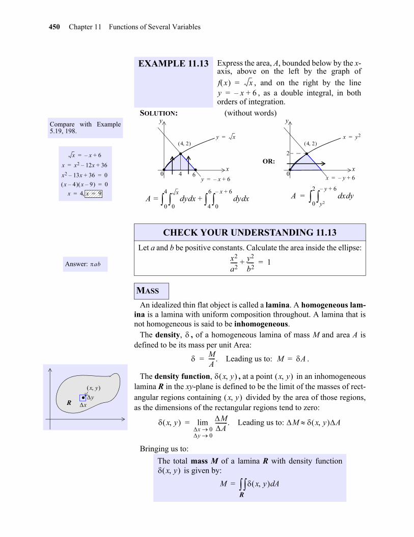
EXAMPLE 11.13 Express the area, A, bounded below by the x-axis, above on the left by the graph of
, and on the right by the line, as a double integral, in both
orders of integration.
f x x=y x– 6+=
Compare with Example5.19, 198.
x x– 6+=
x x2 12x– 36+=
x2 13x– 36+ 0=
x 4– x 9– 0=
x 4 x 9= =
OR:x
y
6
4 2 ...
0 4
y x=
y x– 6+=
A yd0
x
xd0
4
= yd0
x– 6+
xd4
6
+
x
y
4 2 ..0
x y2=
x y– 6+=
2
A xdy2
y– 6+
yd0
2
=
Answer: ab
CHECK YOUR UNDERSTANDING 11.13
Let a and b be positive constants. Calculate the area inside the ellipse:
MASS
x2
a2----- y2
b2-----+ 1=
. x y
yxR
The total mass M of a lamina R with density function is given by:
MA-----. Leading us to: M A= =
x y x y
x y
x y MA---------
x 0y 0
lim . Leading us to: M x y A=
x y
M x y Ad=R
11.3 Double Integrals 451
SOLUTION:
Roughly speaking, the center of mass, or center of gravity, of a laminaR is the point in R about which the lamina is “horizontally bal-anced”; which is to say: it will lie parallel to the ground when suspendedby a string attached to that point (see margin).
To be horizontally balanced at , R mustsurely be horizontally balanced when posi-tioned on the line parallel to the y-axis at .Partitioning the region into small rectangularregions of area , we conclude (see margin)
that the lamina R with density function will nearly balance about if:
It follows that R will balanced about if: .
A similar argument reveals that R will balance about the line par-
allel to the x-axis at : . Since and are con-
stant, we can express the above two double integral equations in theform:
y x2---– 4+=
y x2---=
R
4
y
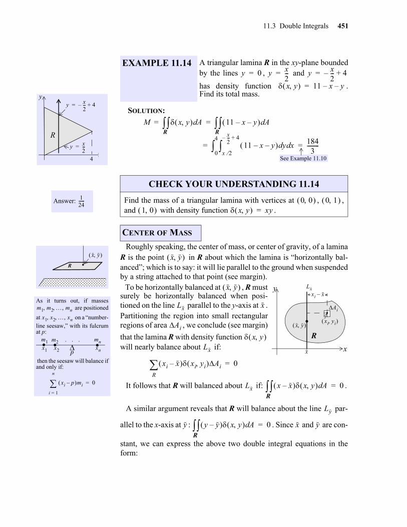
EXAMPLE 11.14 A triangular lamina R in the xy-plane boundedby the lines , and
has density function .Find its total mass.
y 0= y x2---= y x
2---– 4+=
x y 11 x– y–=
M x y Ad 11 x– y– Ad= =
11 x– y– ydx 2
x2---– 4+
xd0
4
1843
---------= =
See Example 11.10
R R
Answer: 124------
CHECK YOUR UNDERSTANDING 11.14
Find the mass of a triangular lamina with vertices at , ,and with density function .
0 0 0 1 1 0 x y xy=
As it turns out, if masses are positioned
at on a “number-
line seesaw,” with its fulcrumat p:
then the seesaw will balance ifand only if:
.R
x y
m1 m2 mn
x1 x2 xn
x2. . .x1 xn
m1 m2 mn. . .
p
xi p– mi
i 1=
n
0=
CENTER OF MASS
x y
A i
xi yi
.
x
xi x–
x
y
R .
x y
Lxx y
Lx x
A i
x y Lx
xi x– xi yi AiR 0=
Lx x x– x y Ad 0=R
Ly
y y y– x y Ad 0=R
x y
452 Chapter 11 Functions of Several Variables
The expression , denoted by , is said to be the
moment of R about the y-axis, while is the
moment of R about the x-axis.
To summarize:
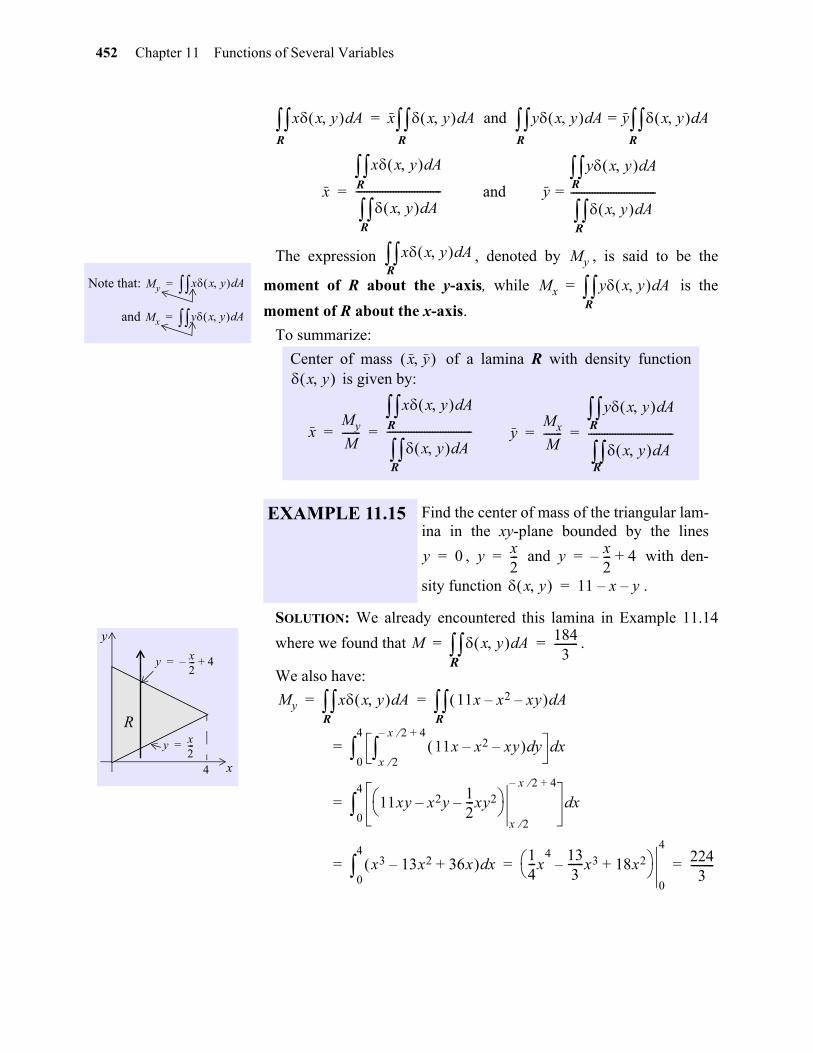
SOLUTION: We already encountered this lamina in Example 11.14
where we found that .
We also have:
Note that:
and
My x x y Ad=
Mx y x y Ad=
Center of mass of a lamina R with density function is given by:
EXAMPLE 11.15 Find the center of mass of the triangular lam-ina in the xy-plane bounded by the lines
, and with den-
sity function .
x x y Ad x x y A and y x y Ad y x y Ad=d=R R R R
x
x x y Ad
x y Ad-------------------------------- and y
y x y Ad
x y Ad--------------------------------==
R
R
R R
R
x x y AdR
My
Mx y x y Ad=R
x y x y
xMy
M-------
x x y Ad
x y Ad-------------------------------- = = y
Mx
M-------
y x y Ad
x y Ad--------------------------------= =R R
R R
y 0= y x2---= y x
2---– 4+=
x y 11 x– y–=
y x2---– 4+=
y x2---=
R
4 x
y M x y Ad 1843
---------= =R
11x x2– xy– ydx 2
x 2– 4+
xd0
4
=
11xy x2y–12---xy2–
x 2
x 2– 4+
xd0
4
=
x3 13x2– 36x+ xd0
4
14---x
4 133------x3– 18x2+
0
42243
---------= = =
R R
My x x y Ad 11x x2– xy– Ad= =
gio
11.3 Double Integrals 453
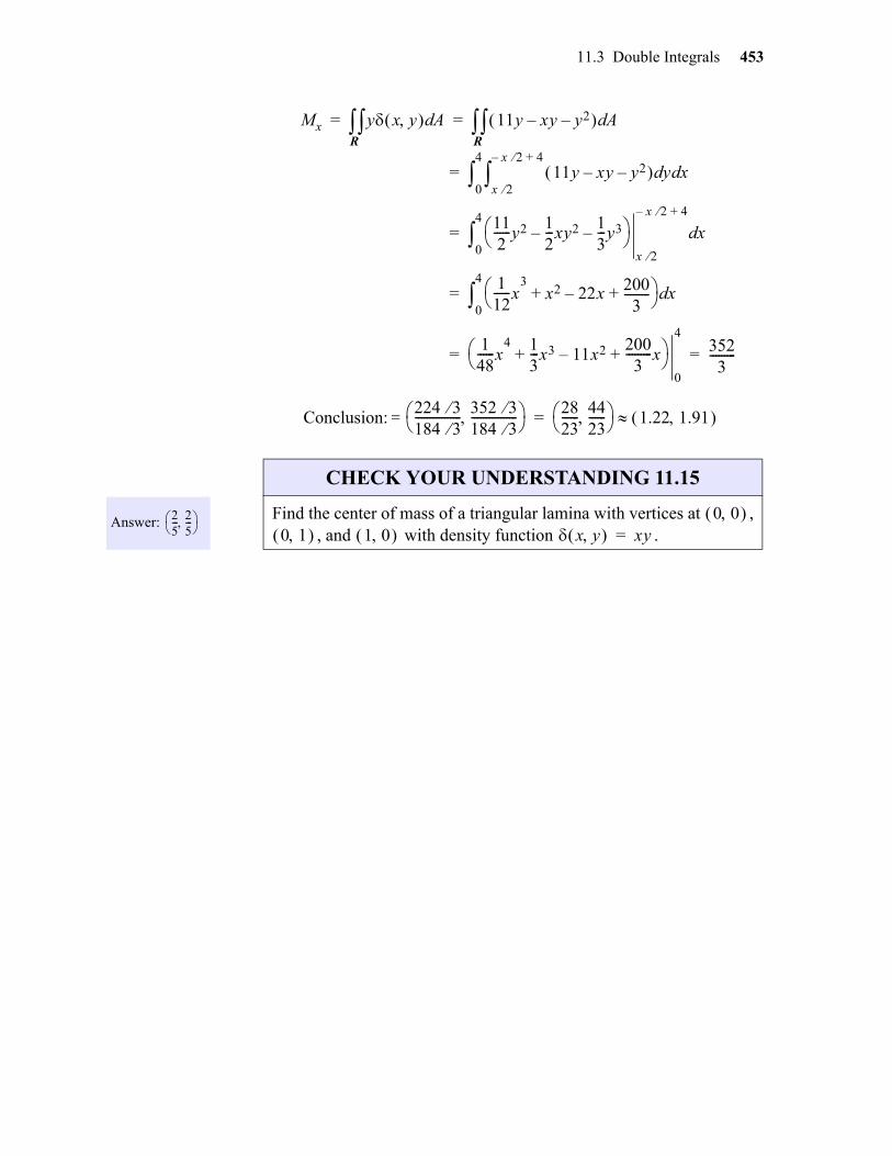
Conclusion:
11y xy– y2– ydx 2
x 2– 4+
xd0
4
=
112------y2 1
2---xy2–
13---y3–
x 2
x 2– 4+
xd0
4
=
112------x
3x2 22x– 200
3---------+ +
xd0
4
=
148------x
4 13---x3 11x2–
2003
---------x+ +
0
43523
---------= =
R R
Mx y x y Ad 11y xy– y2– Ad= =
224 3184 3---------------- 352 3
184 3----------------
=2823------ 44
23------
1.22 1.91 =
Answer: 25--- 2
5---
CHECK YOUR UNDERSTANDING 11.15
Find the center of mass of a triangular lamina with vertices at ,, and with density function .
0 0 0 1 1 0 x y xy=
454 Chapter 11 Multiple Integrals
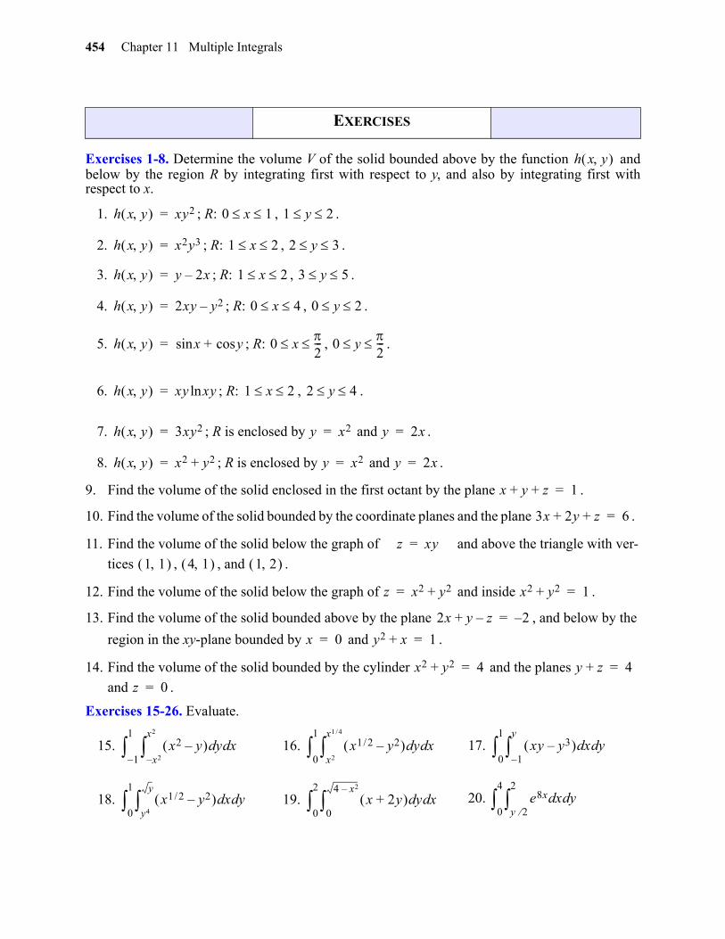
Exercises 1-8. Determine the volume V of the solid bounded above by the function andbelow by the region R by integrating first with respect to y, and also by integrating first withrespect to x.
9. Find the volume of the solid enclosed in the first octant by the plane .
10. Find the volume of the solid bounded by the coordinate planes and the plane .
11. Find the volume of the solid below the graph of and above the triangle with ver-
tices , , and .
12. Find the volume of the solid below the graph of and inside .
13. Find the volume of the solid bounded above by the plane , and below by the
region in the xy-plane bounded by and .
14. Find the volume of the solid bounded by the cylinder and the planes
and .
Exercises 15-26. Evaluate.
EXERCISES
1. ; R: , .
2. ; R: , .
3. ; R: , .
4. ; R: , .
5. ; R: , .
6. ; R: , .
7. ; R is enclosed by and .
8. ; R is enclosed by and .
15. 16. 17.
18. 19. 20.
h x y
h x y xy2= 0 x 1 1 y 2
h x y x2y3= 1 x 2 2 y 3
h x y y 2x–= 1 x 2 3 y 5
h x y 2xy y2–= 0 x 4 0 y 2
h x y x ycos+sin= 0 x2--- 0 y
2---
h x y xy xyln= 1 x 2 2 y 4
h x y 3xy2= y x2= y 2x=
h x y x2 y2+= y x2= y 2x=
x y z+ + 1=
3x 2y z+ + 6=
z xy=
1 1 4 1 1 2
z x2 y2+= x2 y2+ 1=
2x y z–+ 2–=
x 0= y2 x+ 1=
x2 y2+ 4= y z+ 4=
z 0=
x2 y– ydx2–
x2
xd1–
1
x1 2/ y2– ydx2
x1 4/
xd0
1
xy y3– xd1–
y
yd0
1
x1 2/ y2– xdy4
y
yd0
1
x 2y+ yd0
4 x2–
xd0
2
e8x xdy 2
2
yd0
4
11.3 Double Integrals 455
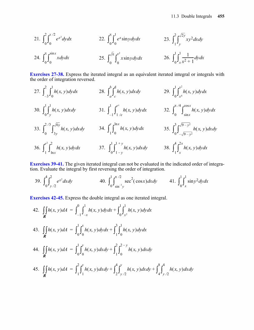
Exercises 27-38. Express the iterated integral as an equivalent iterated integral or integrals withthe order of integration reversed.
Exercises 39-41. The given iterated integral can not be evaluated in the indicated order of integra-tion. Evaluate the integral by first reversing the order of integration.
Exercises 42-45. Express the double integral as one iterated integral.
21. 22. 23.
24. 25. 26.
27. 28. 29.
30. 31. 32.
33. 34. 35.
36. 37. 38.
39. 40. 41.
42.
43.
44.
45.
ex2 yd0
x 2
xd0
2
ex y ydsin0
1
xd0
xy2 xdy
2y
yd1
2
x yd0
xsin
xd0
x y ydsin0
x2
xd0
1
x2 1+-------------- yd
x
1
xd0
1
h x y yd0
1
xd3–
2
h x y xdc
d
yda
b
h x y ydx4
x2
xd0
1
h x y xdy
1
yd0
1
h x y yd1 e
ex
xd1–
1
h x y ydxsin
xcos
xd0
4
h x y xd3y
6y
yd0
2 3
h x y yd0
xln
xd1
e
h x y xd9 y2––
9 y2–
yd0
3
h x y ydxln
2
xd1
e2
h x y xd1 y–
1 y+
yd0
1
h x y ydx
2x
xd1
4
ex2 xdy 2
2
yd0
4
sec2
xcos xdsin 1– y
2
yd0
1
y2sin ydx
1
xd0
1
h x y Ad h x y ydx–
1
xd1–
0
h x y ydx2
1
xd0
1
+=R
h x y Ad h x y yd0
x
xd0
1
h x y yd0
1
xd1
3
+=R
h x y Ad h x y xd0
y
yd0
1
h x y xd0
2 y–
yd1
2
+=R
h x y Ad h x y xd1
y
yd1
2
h x y xdy 2
y
yd2
4
h x y xdy 2
4
yd4
8
+ +=R
gio
456 Chapter 11 Multiple Integrals
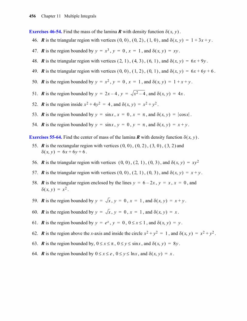
Exercises 46-54. Find the mass of the lamina R with density function .
Exercises 55-64. Find the center of mass of the lamina R with density function .
46. R is the triangular region with vertices , , , and .
47. R is the region bounded by , , , and .
48. R is the triangular region with vertices , , , and .
49. R is the triangular region with vertices , , , and .
50. R is the region bounded by , , , and .
51. R is the region bounded by , , and .
52. R is the region inside , and .
53. R is the region bounded by , , , and .
54. R is the region bounded by , , , and .
55. R is the rectangular region with vertices , , , and .
56. R is the triangular region with vertices , , , and
57. R is the triangular region with vertices , , , and .
58. R is the triangular region enclosed by the lines , , , and .
59. R is the region bounded by , , , and .
60. R is the region bounded by , , , and .
61. R is the region bounded by , , , and .
62. R is the region above the x-axis and inside the circle , and .
63. R is the region bounded by, , , and .
64. R is the region bounded by , , and .
x y
0 0 0 2 1 0 x y 1 3x y+ +=
y x3= y 0= x 1= x y xy=
2 1 4 3 6 1 x y 6x 9y+=
0 0 1 2 0 1 x y 6x 6y 6+ +=
y x2= y 0= x 1= x y 1 x y+ +=
y 2x 4–= y x2 4–= x y 4x=
x2 4y2+ 4= x y x2 y2+=
y xsin= x 0= x = x y xcos=
y xsin= y 0= y = x y x y+=
x y
0 0 0 2 3 0 3 2 x y 6x 6y 6+ +=
0 0 2 1 0 3 x y xy2=
0 0 2 1 0 3 x y x y+=
y 6 2x–= y x= x 0= x y x2=
y x= y 0= x 1= x y x y+=
y x= y 0= x 1= x y x=
y ex= y 0= 0 x 1 x y y=
x2 y2+ 1= x y x2 y2+=
0 x 0 y xsin x y 8y=
0 x e 0 y xln x y x=
11.4 Double Integrals in Polar Coordinates 457
gio
11
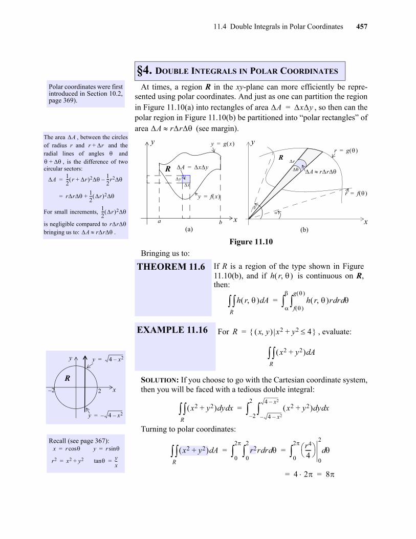
At times, a region R in the xy-plane can more efficiently be repre-sented using polar coordinates. And just as one can partition the regionin Figure 11.10(a) into rectangles of area , so then can thepolar region in Figure 11.10(b) be partitioned into “polar rectangles” ofarea (see margin).
Figure 11.10
Bringing us to:
SOLUTION: If you choose to go with the Cartesian coordinate system,then you will be faced with a tedious double integral:
Turning to polar coordinates:
Polar coordinates were firstintroduced in Section 10.2,page 369).
The area , between the circlesof radius r and and theradial lines of angles and
, is the difference of twocircular sectors:
For small increments,
is negligible compared to bringing us to: .
Ar r+
+
A12--- r r+ 2 1
2---r2–=
rr 12--- r 2+=
12--- r 2
rrA rr
§4. DOUBLE INTEGRALS IN POLAR COORDINATES
(a) (b)
A xy=
A rr
A xy=
xy
y g x =
y f x =
x
y
R
a b
r f =
r g =
y
x
r
R
A rr
x
y
2– 2
y 4 x2–=
y 4 x2––=
R
THEOREM 11.6 If R is a region of the type shown in Figure11.10(b), and if is continuous on R,then:
EXAMPLE 11.16 For , evaluate:
h r
h r AdR h r r rd d
f
g
=
R x y x2 y2+ 4 =
x2 y2+ AdR
x2 y2+ yd xdR x2 y2+ yd xd
4 x2––
4 x2–
2–
2
=
Recall (see page 367): x r ycos r sin= =
r2 x2 y2 tan+ yx--= =
x2 y2+ AdR r2r rd d
0
2
0
2
r4
4----
0
2
d0
2
= =
4 2 8= =
458 Chapter 11 Functions of Several Variables
As you know, if a positive function is defined on theregion R of Figure 11.10(a), then the volume of the surface boundedabove by h and below by the region R is given by:
(Theorem 11.5(a), page ###)
Similarly, if a positive function is defined on the regionR in Figure 11.10(b), then the volume V of the resulting solid can beapproximated by the Riemann sum:
Moreover, in a fashion analogous to that developed in the previoussection, we have:
SOLUTION: The approach of the previous section brings us to:
Not a nice integral! There is a better way:
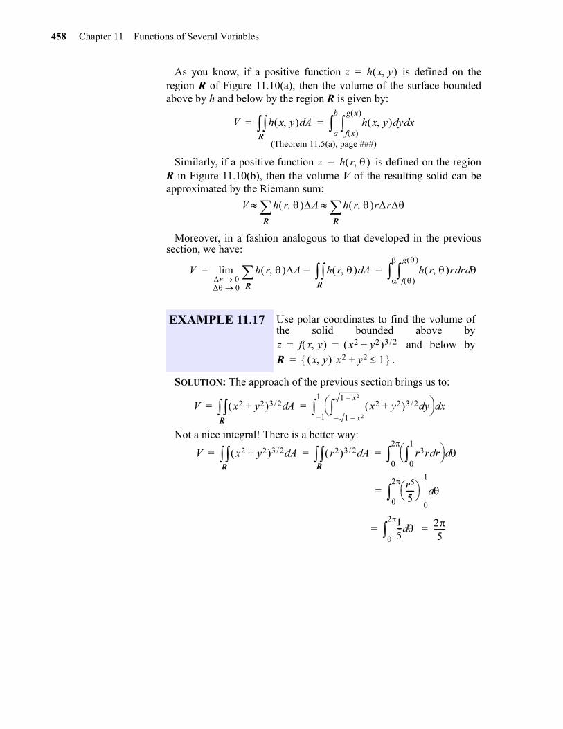
EXAMPLE 11.17 Use polar coordinates to find the volume ofthe solid bounded above by
and below by.
z h x y =
V h x y Ad h x y ydf x
g x
xda
b
= =R
z h r =
V h r AR h r rr
R
V h r ARr 0
0
lim h r Ad h r r rdf
g
d
= = =R
z f x y x2 y2+ 3 2/= =R x y x2 y2 1+ =
V x2 y2+ 3 2/ Ad x2 y2+ 3 2/ yd1 x2––
1 x2–
xd
1–
1
= =R
V x2 y2+ 3 2/ Ad r2 3 2/ Ad r3r rd0
1
d
0
2
= = =R R
r5
5----
0
1
d0
2
=
15--- d
0
2
25
------= =
11.4 Double Integrals in Polar Coordinates 459
SOLUTION:
(Compare with the solution of CYU 10.9, page A-65, Volume I.)
SOLUTION: Noting that the region and density are both symmetricalabout the x- and y-axis, we find the mass of the region by quadruplingits mass in the first quadrant [see Figure 10.8(a), page 372]:
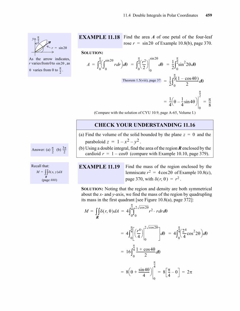
As the arrow indicates,r varies from 0 to , as
varies from 0 to .
y
r 2sin=
2---
2sin
2---
EXAMPLE 11.18 Find the area A of one petal of the four-leafrose of Example 10.8(b), page 370.r 2sin=
A r rd0
2sin
d
0
2---
r2
2----
0
2sin
d0
2---
12--- sin
22 d
0
2---
= = =
12--- 1 4cos–
2----------------------------- d
0
2---
=
14--- 1
4--- 4sin–
0
2---
8---= =
Theorem 1.5(viii), page 37:
Answer: (a) (b) 2--- 3
2------
CHECK YOUR UNDERSTANDING 11.16
(a) Find the volume of the solid bounded by the plane and the
paraboloid .(b) Using a double integral, find the area of the region R enclosed by the
cardioid (compare with Example 10.10, page 379).
z 0=
z 1 x2– y2–=
r 1 cos–=
Recall that:
(page ###)
M x y Ad=R
EXAMPLE 11.19 Find the mass of the region enclosed by thelemniscate of Example 10.8(c),page 370, with .
r2 4 2cos= r r2=
M r Ad 4 r2 r rd0
2 2cos
d0
4---
= =
4r4
4----
0
2 2cos
d0
4---
424
4-----cos
22
d0
4---
= =
16 1 4cos+2
------------------------ d0
4---
=
8 4sin4
--------------+
0
4---
8 4--- 0– 2= = =
R
gio
460 Chapter 11 Functions of Several Variables
SOLUTION: Determining the mass of R:
Finding and :
Conclusion:
Answer: 53
------
CHECK YOUR UNDERSTANDING 11.17
Find the mass of the region enclosed by the cardioid ofExample 10.9, page 373, with .
r 1 sin+= r r=
Recall that:
(page ###)
xMy
M-------
x x y Ad
R
x y Ad
R
---------------------------------= =
yMx
M-------
y x y Ad
R
x y Ad
R
---------------------------------= =
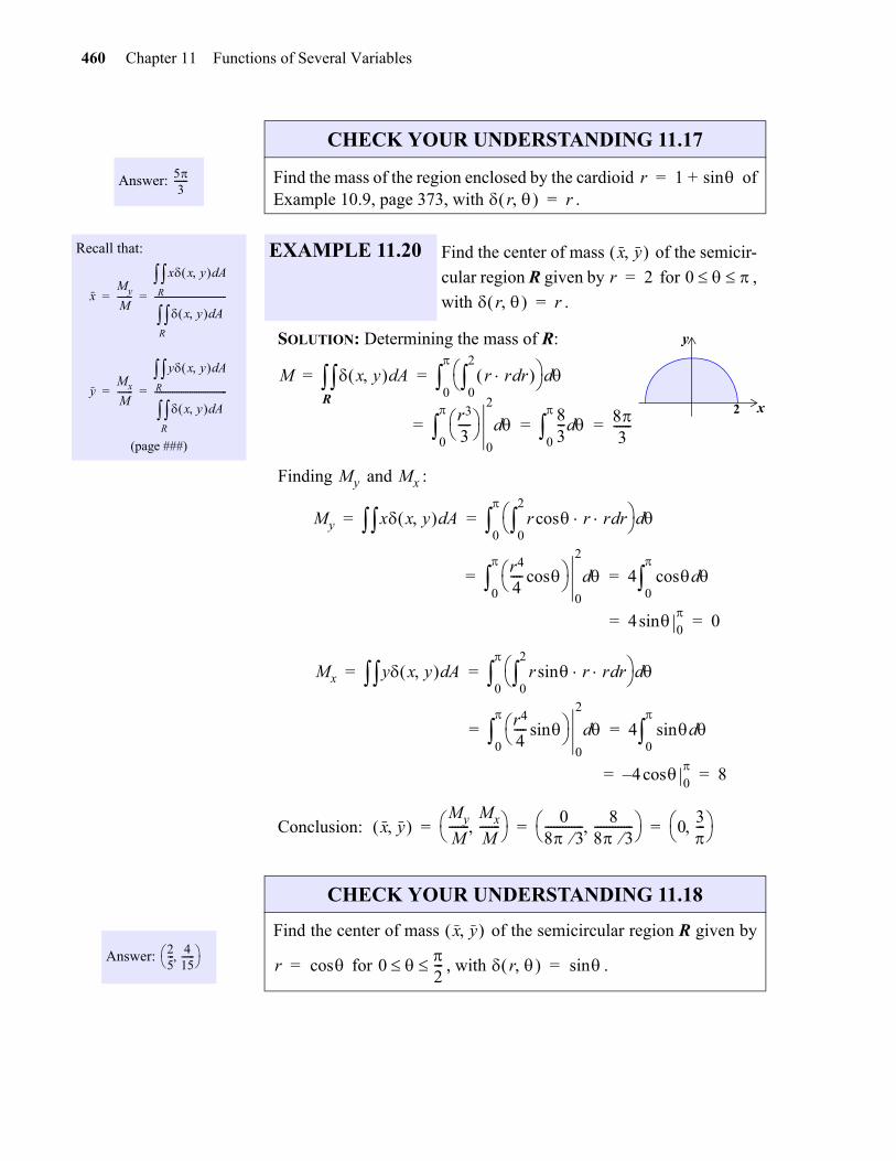
EXAMPLE 11.20 Find the center of mass of the semicir-
cular region R given by for ,
with .
x y r 2= 0
r r=
2 x
y
M x y Ad r r rd 0
2
d
0
= =
r3
3----
0
2
d0
83--- d
0
83
------= = =
R
My Mx
My x x y Ad r r r cos rd0
2
d
0
= =
r4
4---- cos
0
2
d0
4 dcos0
= =
4 0
sin 0= =
Mx y x y Ad r r r sin rd0
2
d
0
= =
r4
4---- sin
0
2
d0
4 sin d0
= =
4– 0
cos 8= =
x y My
M-------
Mx
M-------
08 3------------- 8
8 3-------------
03---
= = =
Answer: 25--- 4
15------
CHECK YOUR UNDERSTANDING 11.18
Find the center of mass of the semicircular region R given by
for , with .
x y
r cos= 0 2--- r sin=
11.4 Double Integrals in Polar Coordinates 461
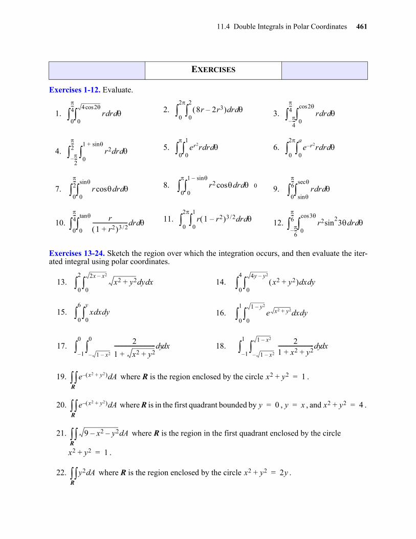
Exercises 1-12. Evaluate.
Exercises 13-24. Sketch the region over which the integration occurs, and then evaluate the iter-ated integral using polar coordinates.
EXERCISES
1. 2. 3.
4. 5. 6.
7. 8. 0 9.
10. 11. 12.
13. 14.
15. 16.
17. 18.
19. where R is the region enclosed by the circle .
20. where R is in the first quadrant bounded by , , and .
21. where R is the region in the first quadrant enclosed by the circle
.
22. where R is the region enclosed by the circle .
r rd0
4 2cos
d0
4---
8r 2r3– rd0
2
d0
2
r rd0
2cos
d4---–
4---
r2 rd0
1 sin+
d2---–
2---
er2r rd0
1
d0
e r2– r rd0
a
d0
2
r rdcos0
sin
d0
2---
r2 rdcos0
1 sin–
d0
r rdsin
sec
d0
6---
r1 r2+ 3 2/
-------------------------- rd0
tan
d0
4---
r 1 r2– 3 2/ rd0
1
d0
2
r2sin23 rd
0
3cos
d6---–
6---
x2 y2+ yd0
2x x2–
xd0
2
x2 y2+ xd0
4y y2–
yd0
4
x xd0
y
yd0
6
e x2 y2+ xd0
1 y2–
yd0
1
2
1 x2 y2++------------------------------ yd
1 x2––
0
xd1–
0
2
1 x2 y2+ +-------------------------- yd
1 x2––
1 x2–
xd1–
1
e x2 y2+ – AdR
x2 y2+ 1=
e x2 y2+ – AdR
y 0= y x= x2 y2+ 4=
9 x2– y2– AdR
x2 y2+ 1=
y2 AdR
x2 y2+ 2y=
462 Chapter 11 Functions of Several Variables
Exercises 25-34. Use polar coordinates and double integrals to determine the area of the givenregion.
Exercises 35-44. Use polar coordinates to find the volume of the given solid.
23. where R is the region enclosed by the circle .
24. where R is the region enclosed by .
25. The region lies inside the circle and to the right of the line (i.e. ).
26. The region lies inside the circle and above the line (i.e. ).
27. The region common to the circles and .
28. The region that lies outside the circle and inside the circle .
29. The region that lies inside the circle and outside the circle .
30. The region inside the cardioid .
31. The region inside the circle and outside the cardioid .
32. One leaf of the rose .
33. The region in the first quadrant that is inside the circle and outside the circle
.
34. The region common to the cardioids and .
35. A sphere of radius a.
36. The ellipsoid .
37. The solid that is under the cone and above the disk .
38. The solid that lies below by , above the xy-plane, and inside the cylinder
.
39. The solid that lies below the paraboloid , above the xy-plane, and inside the
cylinder .
y AdR
x2 y2+ y=
x2 y2+ AdR
r 3 cos+=
r 32---= x 3
4---= r cos 3
4---=
r 2= y 1= r sin 1=
r 2 cos= r 2 sin=
r 3 cos= r 32---=
r 3 cos= r 32---=
r 2 1 cos+ =
r 1= r 1 cos–=
r 3 4sin=
r 3 cos=
r sin=
r 2 1 cos+ = r 2 1 cos– =
x2
4----- y2
4----- z2
3----+ + 1=
z x2 y2+= x2 y2+ 4
z 1 x2– y2–=
x2 y2 x–+ 0=
z x2 y2+=
x2 y2+ 2x=
gio
11.4 Double Integrals in Polar Coordinates 463
Exercises 45-49. Find the mass of the region R.
Exercises 50-55. Find the center of mass of the region R.
40. The solid that is bounded by the paraboloids and .
41. The solid that is bounded below by the xy-plane, above by the spherical surface
, and on the sides by the cylinder .
42. The solid that is bounded above by the cone , and below by the region which
lies inside the circle .
43. The solid that is inside the cylinder and the ellipsoid .
44. The solid that is bounded above by the surface , below by the xy-plane, and
enclosed between the cylinders and .
45. R is the cardioid , and .
46. R is the region outside the circle , inside the circle , and .
47. R is the region outside the circle and inside the circle , and .
48. R is the region inside the circle , outside , and .
49. R is the region inside the circle , outside the circle , and
.
50. R is the washer between the circles , , if .
51. R is the cardioid , and .
52. R is the smaller region cut from the circle by the line if .
53. R is the region outside the circle , inside the circle , and .
54. R is the region bounded by , , and .
55. R is the region bounded by , , and .
z 3x2 3y2+= z 4 x2– y2–=
x2 y2 z2+ + 4= x2 y2+ 1=
z2 x2 y2+=
x2 y2+ 2a=
x2 y2+ 4= 4x2 4y2 z2+ + 64=
z 1
x2 y2+---------------------=
x2 y2+ 1= x2 y2+ 9=
r 1 sin+= x y r=
r 3= r 6 sin= x y r=
r 3= r 6 sin= x y 1r---=
r 3 cos= r 2 cos–= x y 1r---=
r a 0= r 2a sin=
x y 1r---=
r 2= r 4= r r2=
r 1 sin+= x y r=
r 6= r cos 3= r cos2=
r 3= r 6 sin= r 1r---=
r 2cos= 0 4--- r r=
r cos=4---
4--- – r r=
464 Chapter 11 Functions of Several Variables
11
In defining for , we had the luxury of being able
to represent the graph of f in the xy-plane (see page 139). Though con-
siderably more challenging, when defining , we were still
able to depict the function in three space (see page 445).But when it comes to the next task, that of defining the triple integral
over a three-dimensional region W, we must abandon
all hope of geometrically representing the function infour-dimensional space (we are, after all, three-dimensional creatures).
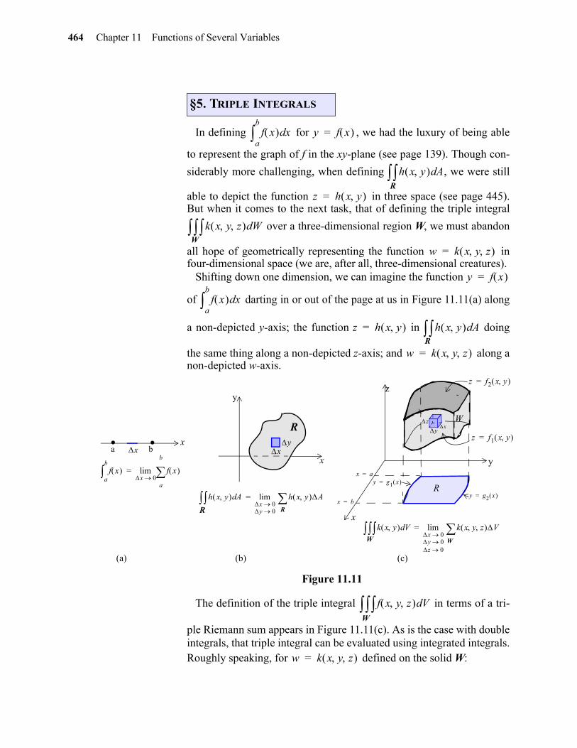
Shifting down one dimension, we can imagine the function
of darting in or out of the page at us in Figure 11.11(a) along
a non-depicted y-axis; the function in doing
the same thing along a non-depicted z-axis; and along anon-depicted w-axis.
Figure 11.11
The definition of the triple integral in terms of a tri-
ple Riemann sum appears in Figure 11.11(c). As is the case with doubleintegrals, that triple integral can be evaluated using integrated integrals.Roughly speaking, for defined on the solid W:
§5. TRIPLE INTEGRALS
f x xda
b
y f x =
h x y AdR
z h x y =
k x y z WdW
w k x y z =
y f x =
f x xda
b
z h x y = h x y Ad
R
w k x y z =
a b. . R
x xy
xy
z
f x a
b
f x
a
b
x 0lim=
h x y Ad h x y A
Rx 0
y 0
lim=
k x y Vd k x y z V
W
x 0y 0z 0
lim=
R
W
(a) (b) (c)
x
x
y
x
y
z
R
W
x a=
x b=
z f1 x y =
z f2 x y =
y g1 x =
y g2 x =
f x y z VdW
w k x y z =
gio
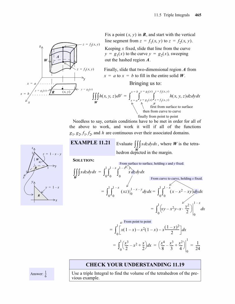
11.5 Triple Integrals 465
Needless to say, certain conditions have to be met in order for all ofthe above to work, and work it will if all of the functions
are continuous over their associated domains.
SOLUTION:
x
y
z
x b=y g1 x = y g2 x =
z f2 x y =
z f1 x y =
R
W
Keeping x fixed, slide that line from the curvey g1 x to the curve y g2 x sweeping= =out the hashed region A.
A
Finally, slide that two-dimensional region A fromx a to x b to fill in the entire solid W.= =
x y .
.
.
x a=
Fix a point x y in R, and start with the verticalline segment from z f1 x y to z f2 x y .= =
h x y z Vd h x y z zd yd xdz f1 x y =
z f2 x y =
y g1 x =
y g2 x =
x a=
x b=
=W
first from surface to surfacethen from curve to curve
finally from point to point
Bringing us to:
11
1 z 1 x– y–=
y
x
W
R
R
z
x
y
y 1 x–=
EXAMPLE 11.21 Evaluate , where W is the tetra-
hedron depicted in the margin.
g1 g2 f1 f2 and h
x zd yd xdW
x zd yd xd x zd yd xd0
1 x– y–
0
1 x–
0
1
=W
From surface to surface, holding x and y fixed.
xz 01 x– y–
yd xd0
1 x–
0
1
x x2– xy– yd xd0
1 x–
0
1
= =
From curve to curve, holding x fixed.
xy x2y xy2
2-----––
0
1 x–
xd0
1
=
x 1 x– x2 1 x– – x1 x– 2
2-------------------– xd
0
1
=
x3
2----- x2– x
2---+
xd0
1
x4
8----- x3
3-----– x2
4-----+
0
1124------= = =
From point to point
Answer: 16---
CHECK YOUR UNDERSTANDING 11.19
Use a triple Integral to find the volume of the tetrahedron of the pre-vious example.
466 Chapter 11 Functions of Several Variables
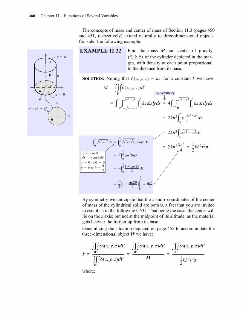
The concepts of mass and center of mass of Section 11.3 (pages 450and 451, respectively) extend naturally to three-dimensional objects.Consider the following example.
SOLUTION: Noting that for a constant k we have:
By symmetry we anticipate that the x and y coordinates of the centerof mass of the cylindrical solid are both 0, a fact that you are invitedto establish in the following CYU. That being the case, the center willlie on the z axis; but not at the midpoint of its altitude, as the materialgets heavier the further up from its base.
Generalizing the situation depicted on page 452 to accommodate thethree-dimensional object W we have:
where:
h
rR
z h=
z 0=
x2 y2+ r2=
R
W
EXAMPLE 11.22 Find the mass M and center of gravity of the cylinder depicted in the mar-
gin, with density at each point proportionalto the distance from its base.
x y z
x y z kz=
M x y z Vd=
kz zd yd xd0
h
r2 x2––
r2 x2–
r–
r
4 kz zd yd xd0
h
0
r2 x2–
0
r
= =
2kh2 y0
r2 x2–xd
0
r
=
2kh2 r2 x2– xd0
r
=
2kh2r2
4-------- 1
2---kh2r2= =
r2 x2–0
r
xd r2cos2r cos d
0
2---
=
r2 cos2 d
0
2---
=
r2 1 2cos+2
------------------------ d0
2---
=
r2
2---- 2sin
2--------------+
0
2---
r2
4--------= =
x r sin=dx r dcos=x 0 0= =
x r 2---= =
by symmetryV
z
z x y z Vd
x y z Vd----------------------------------------
z x y z VdM
----------------------------------------
z x y z Vd12---kh2r2
----------------------------------------= = = WWW
W
gio
11.5 Triple Integrals 467
And so:
Up to now we have systematically evaluated triple integrals by inte-grating first with respect to z, then y, and then x:
It may be advantageous to choose a different order. Consider the fol-
lowing example.
SOLUTION: Integrating first with respect to z would require two inte-grals (why?). On the other hand:
z x y z Vd z kz zd yd xd0
h
r2 x2––
r2 x2–
r–
r
=
4 z kz zd yd xd0
h
0
r2 x2–
0
r
=
4kh3
3----- yd xd
0
r2 x2–
0
r
=
4kh3
3----------- r2 x2– xd
0
r
4kh3
3----------- r2
4-------- 1
3---kh3r2= = =
by symmetry:
W
Answer: See page A-8.
CHECK YOUR UNDERSTANDING 11.20
Verify that in the previous example.
x y z 0 0
13---kh3r2
12---kh2r2---------------------
0 023---h
= =
independent of k
x y 0= =
There are six possibleorders of integration:
dzdydx dzdxdy dydzdx dydxdz dxdzdy dxdydz
k x yz Vd k x y z zd yd xdf1 x y
f2 x y
g1 x
g2 x
a
b
=
2
3
1
1 y
x
z
W
z 1 y–=z y
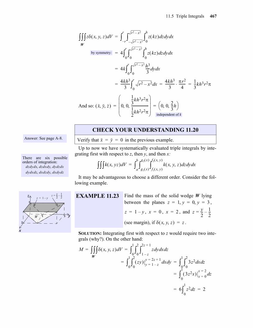
2---= 1
2---– EXAMPLE 11.23 Find the mass of the solid wedge W lying
between the planes ,
, , , and
(see margin), if .
z 1 y 0 y 3= = =
z 1 y–= x 0= x 2= z y2---= 1
2---–
x y z z=
M x y z Vd z yd xd zd1 z–
2z 1+
0
2
0
1
= =
zy y 1 z–=y 2z 1+=
xd yd0
2
0
1
3z2 xd zd0
2
0
1
= =
3z2x x 0=
x 2=zd
0
1
=
6 z2 zd0
1
2= =
W
468 Chapter 11 Functions of Several Variables
Answer: See page A-8.
CHECK YOUR UNDERSTANDING 11.21
The order of integration for M in the above example is .Express M in terms of the remaining five possible orders of integra-tion.
yd xd zd
gio
11.5 Triple Integrals 469
Exercises 1-10. Evaluate.
Exercises 11-18. Evaluate. Note the specified order of integration.
Exercises 19-26. Find the volume of the solid W,
EXERCISES
1. 2.
3. 4.
5. 6.
7. 8.
9. 10.
11. 12.
13. 14.
15. 16.
17. 18.
19. W is the solid in the first octant that lies between the planes and ,
20. W is the solid bounded above by the paraboloid and below by the plane .
21. W is the solid enclosed between the cylinder and the planes and .
zd yd xdx y+
x2 y2+
0
x2
0
1
x2 y2 z2+ + zd yd xd0
1
0
1
0
1
x zd yd xd0
x y+
0
2 3x–
0
1
x zd yd xd0
4 x2– y–
0
1 x2–
0
1
xyz2 zd yd xd0
1
1–
1
0
3
z zd yd xd0
2x y+
0
4 x–
0
1
4x 12z– zd yd xdy x–
y
x
2x
1
2
x2y y2x+ zd yd xd1
3
1–
1
2
4
xy2z3 zd yd xd0
xy3
0
x2
0
1
zy-- zdsin yd xd
0
xy
x
2---
0
2---
xd yd zd0
z2 y2+
0
z
0
1
x y+ zd xd yd0
x2y
0
y
0
1
y z xdsin yd zd0
0
0
1
1
xyz-------- xd yd zd
1
e
1
e
1
e
x3y2z zd yd xd0
x3y
0
x2
0
1
x3y4z2 zd yd xd0
x2y
0
x
0
1
ex y z+ + yd zd xdx– z–
x z+
x–
x
0
1
xyz x2 y2 z2+ + x yd zdd0
3 y2 z2+
0
3z
0
1
x y 2z+ + 2=2x 2y z+ + 4=
z 4 x2– y2–=z 4 2x–=
x2 y2+ 9= z 1=x z+ 5=
470 Chapter 11 Functions of Several Variables
Exercises 27-32. Find the mass of the object W with density function .
Exercises 33-40. Find the center of mass of the object W with density function .
22. W is the solid bounded by the cylinders , , and the planes and .
23. W is the tetrahedron bounded by the planes , , , and .
24. W is the solid enclosed by the cylinders and .
25. W is the solid enclosed by the paraboloids and .
26. W is the solid enclosed by the surface and the planes , and
.
27. W is the cube given by ; .
28. W is the solid bounded by the parabolic cylinder and the planes , ,and ; , for a constant k.
29. W is the solid bounded by the cylinder and the planes ;.
30. W is the cube given by ;
31. W is the solid bounded by the parabolic cylinder and the planes , , and; , for a constant k.
32. W is the solid bounded by the coordinate planes and the plane ;.
33. W is the solid bounded above by the paraboloid and below by the plane ; .
34. W is the solid enclosed by the surface , for , and the planes , , ; .
35. W is the solid bounded by the parabolic cylinder and the planes , , and ; , for a constant k.
36. W is the solid enclosed by the cylinder and the planes , , for ; ,
37. W is the cube given by ; .
z x2= z 4 x2–= y 0=z 2y+ 4=
z 0= x 0= x 2y= x 2y z+ + 2=
x2 y2+ 1= x2 z2+ 1=
z 5x2 5y2+= z 6 7x2– y2–=
z y1 x2+--------------= x 0 y 0 z 0= = =
x y+ 1=
x y z
0 x a 0 y a 0 z a x y z x2 y2 z2+ +=
z 1 y2–= x 0= z 0=x z+ 1= x y z k=
x2 y2+ 1= z 0 z 1= = x y z xyz=
0 x a 0 y a 0 z a x y z xyz=
x y2= z 0= x 1=x z= x y z k=
x y z+ + 1= x y z 1 x– y–=
x y z
z 4 x2– y2–=z 0= x y z a=
z 1 y2–= y 0 x 1–= x 1=z 0= x y z yz=
x y2= z 0= x 1=x z= x y z k=
x2 y2+ a2= z 0= z h=h 0 x y z h z–=
0 x a 0 y a 0 z a x y z x2 y2 z2+ +=
gio
11.5 Triple Integrals 471
Exercises 41-44. Express the integral in six different ways, where W is the solid
bounded by the given surfaces.
Exercises 45-48. Rewrite the given integral in five additional forms by changing the order of inte-gration.
38. ; .
39. , .
40. ; .
41. , , . 42. ,
43. 44.
45. 46.
47. 48.
W x y z 1– x 0 x y 1 x y+ z 2 = x y z x 3+=
W x y z 1 z 2 0 x z x y z = x y z y x–=
W x y z 9 z 4 x2 y2 4+ = x y z x2 y2 z2+ +=
k x y z VdW
y x2= y 2z– 4+= z 0= z 0 x 2 y 2= = = x y 2z–+ 2=
y 0 y 4 x2– 4z2–= = x 2 x– 2= = y2 z2+ 9=
k x y z zd xd yd0
y
y
1
0
1
k x y z zd yd xd0
1 y–
x2
1
1–
1
k x y z zd yd xd0
y2
1–
0
0
1
k x y z zd yd xd0
y
0
x2
0
1
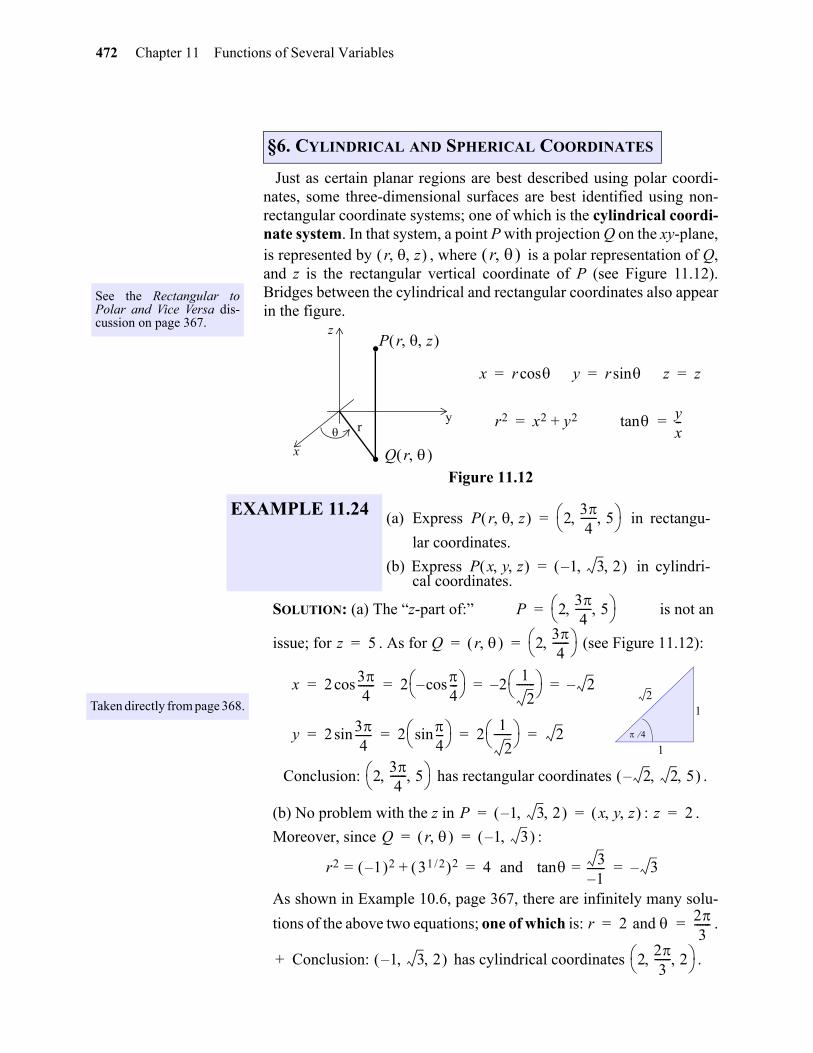
472 Chapter 11 Functions of Several Variables
gio
11
Just as certain planar regions are best described using polar coordi-nates, some three-dimensional surfaces are best identified using non-rectangular coordinate systems; one of which is the cylindrical coordi-nate system. In that system, a point P with projection Q on the xy-plane,is represented by , where is a polar representation of Q,and z is the rectangular vertical coordinate of P (see Figure 11.12).Bridges between the cylindrical and rectangular coordinates also appearin the figure.
Figure 11.12
SOLUTION: (a) The “z-part of:” is not an
issue; for . As for (see Figure 11.12):
Conclusion: has rectangular coordinates .
(b) No problem with the z in : .
Moreover, since :
As shown in Example 10.6, page 367, there are infinitely many solu-
tions of the above two equations; one of which is: and .
+ Conclusion: has cylindrical coordinates .
§6. CYLINDRICAL AND SPHERICAL COORDINATES
See the Rectangular toPolar and Vice Versa dis-cussion on page 367.
r z r
.
.
P r z
y
x
z
r
x r ycos r zsin z= = =
r2 x2 y2 tan+ yx--= =
Q r
EXAMPLE 11.24 (a) Express in rectangu-
lar coordinates.
(b) Express in cylindri-cal coordinates.
P r z 234
------ 5 =
P x y z 1 3– 2 =
Taken directly from page 368.
P 234
------ 5 =
z 5= Q r 234
------ = =
x 2 34
------cos 2 4---cos–
21
2------- – 2–= = = =
y 2 34
------sin 2 4---sin
21
2------- 2= = = = 4
1
1
2
234
------ 5 2– 2 5
P 1– 3 2 x y z = = z 2=
Q r 1– 3 = =
r2 1– 2 31 2/ 2+= 4 and tan 31–
-------= 3–= =
r 2= 23
------=
1 3– 2 223
------ 2
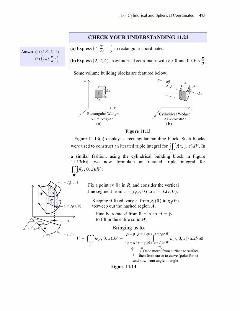
11.6 Cylindrical and Spherical Coordinates 473
Some volume building blocks are featured below:
Figure 11.13
Figure 11.13(a) displays a rectangular building block. Such blocks
were used to construct an iterated triple integral for . In
a similar fashion, using the cylindrical building block in Figure11.13(b)], we now formulate an iterated triple integral for
:
Figure 11.14
Answer: (a)
(b)
2 3 2 1–
2 24--- 4
CHECK YOUR UNDERSTANDING 11.22
(a) Express in rectangular coordinates.
(b) Express in cylindrical coordinates with and .
46--- 1–
2 2 4 r 0 0 2---
yx
z
rz
Rectangular Wedge: V xyz=
Cylindrical Wedge: V rrz
r
y
x
z
y
x
z
(a) (b)
f x y z VdW
f r z VdW
W
z f1 r =
z f2 r =
R
A
Fix a point r in R, and consider the verticalline segment from z f1 r to z f2 r .= =
Keeping fixed, vary r from g1 to g2 tosweep out the hashed region A.
Finally, rotate A from to = =to fill in the entire solid W.
V h r z VdW h r z r zd rd d
z f1 r =
z f2 r =
r g1 =
r g2 =
=
=
= =
r g1 =
r g2 =
.
.
.
=
=
Bringing us to:
Once more: from surface to surfacethen from curve to curve (polar form)
and now from angle to angle
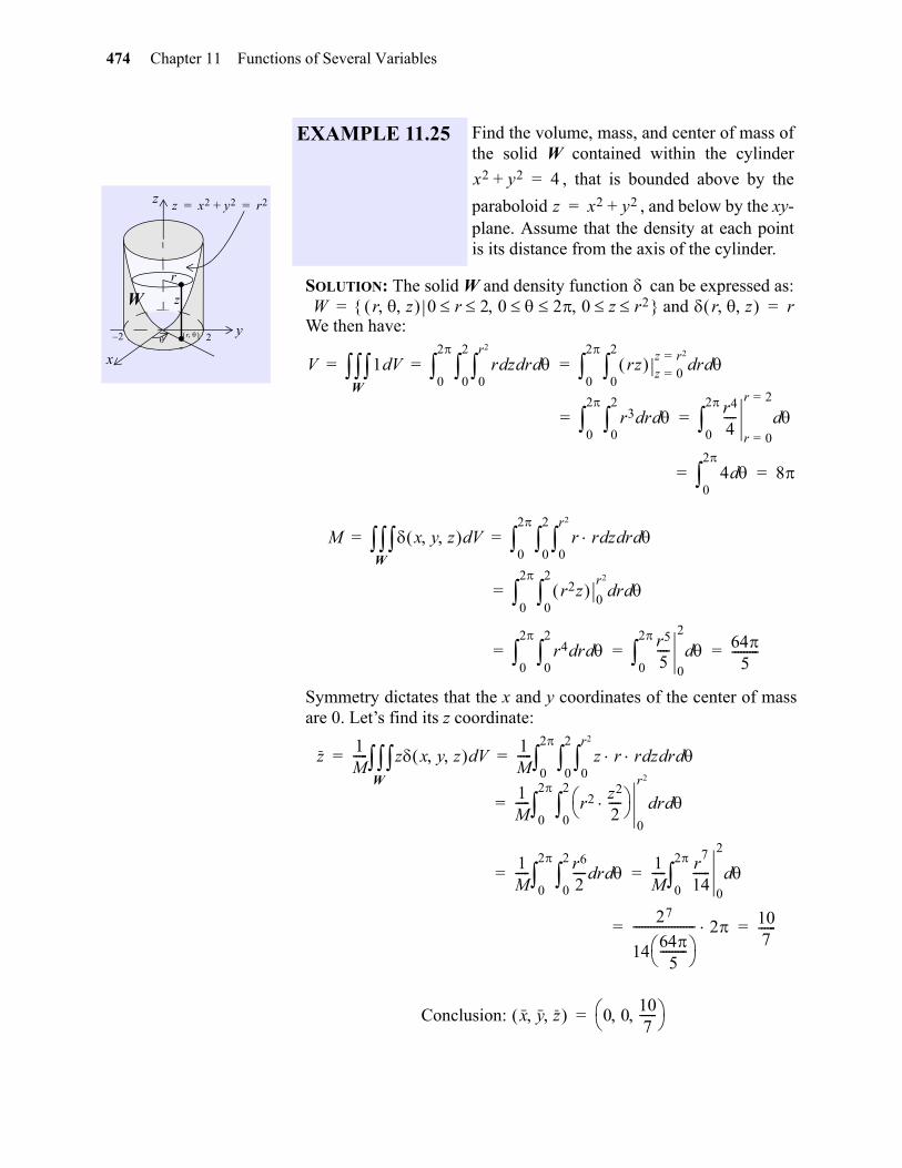
474 Chapter 11 Functions of Several Variables
SOLUTION: The solid W and density function can be expressed as:and
We then have:
Symmetry dictates that the x and y coordinates of the center of massare 0. Let’s find its z coordinate:
Conclusion:
y
x
z
r
z x2 y2+ r2= =
.
.z
r
W
22–
EXAMPLE 11.25 Find the volume, mass, and center of mass ofthe solid W contained within the cylinder
, that is bounded above by the
paraboloid , and below by the xy-plane. Assume that the density at each pointis its distance from the axis of the cylinder.
x2 y2+ 4=
z x2 y2+=
W r z 0 r 2 0 2 0 z r2 = r z r=
V 1 Vd r zd rd d0
r2
0
2
0
2
rz z 0=z r2=
rd d0
2
0
2
= = =
r3 rd d0
2
0
2
r4
4----
r 0=
r 2=
d0
2
= =
4 d0
2
8= =
W
M x y z Vd r r zd rd d0
r2
0
2
0
2
= =
r2z 0
r2
rd d0
2
0
2
=
r4 rd d0
2
0
2
r5
5----
0
2
d0
2
645
---------= = =
W
z1M----- z x y z Vd
1M----- z r r zd rd d
0
r2
0
2
0
2
= =
1M----- r2 z2
2----
0
r2
rd d0
2
0
2
=
1M----- r6
2---- rd d
0
2
0
2
1M----- r
7
14------
0
2
d0
2
= =
27
1464
5---------
--------------------- 2 107------= =
W
x y z 0 0107------
=
gio
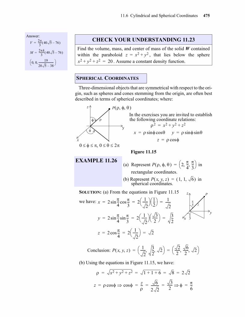
11.6 Cylindrical and Spherical Coordinates 475
Three-dimensional objects that are symmetrical with respect to the ori-gin, such as spheres and cones stemming from the origin, are often bestdescribed in terms of spherical coordinates; where:
Figure 11.15
SOLUTION: (a) From the equations in Figure 11.15
we have:
Conclusion:
(b) Using the equations in Figure 11.15, we have:
Answer:
V23
------ 40 5 76– =
M2k
3--------- 40 5 76– =
0 019
20 5 38–-------------------------
CHECK YOUR UNDERSTANDING 11.23
Find the volume, mass, and center of mass of the solid W containedwithin the paraboloid , that lies below the sphere
. Assume a constant density function.
SPHERICAL COORDINATES
EXAMPLE 11.26(a) Represent in
rectangular coordinates.
(b) Represent in spherical coordinates.
z x2 y2+=x2 y2 z2+ + 20=
P
y
x
z
2 x2 y2 z2+ +=
x ycossin sinsin= =
z cos=
In the exercises you are invited to establish
.the following coordinate relations:
0 0 2
P 24---
3---
=
P x y z 1 1 6 =
2
3---
4---
z
y
x
P.x 2
4---
3---cossin 2
1
2------- 1
2--- 1
2-------= = =
y 24---
3---sinsin 2
1
2------- 3
2------- 3
2---= = =
z 2 4---cos 2
1
2------- 2= = =
P x y z 1
2------- 3
2--- 2
22
------- 62
------- 2 = =
x2 y2 z2+ + 1 1 6+ + 8 2 2= = = =
z coscos z--- 6
2 2----------
32
------- 6---= = = = =
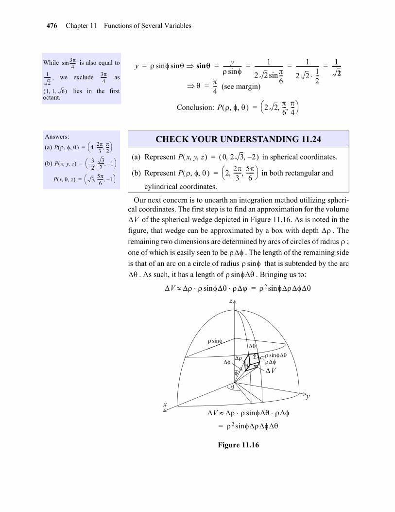
476 Chapter 11 Functions of Several Variables
Conclusion:
Our next concern is to unearth an integration method utilizing spheri-cal coordinates. The first step is to find an approximation for the volume
of the spherical wedge depicted in Figure 11.16. As is noted in the
figure, that wedge can be approximated by a box with depth . The
remaining two dimensions are determined by arcs of circles of radius ;
one of which is easily seen to be . The length of the remaining side
is that of an arc on a circle of radius that is subtended by the arc
. As such, it has a length of . Bringing us to:
Figure 11.16
While is also equal to
, we exclude as
lies in the firstoctant.
34
------sin
1
2------- 3
4------
1 1 6
y sinsinsin y sin-------------- 1
2 2 6---sin
---------------------- 1
2 212---
------------------ 1
2-------= = = = =
4---= (see margin)
P 2 26---
4---
=
Answers:
(a)
(b)
P 423
------ 2---
=
P x y z 32---–
32
------- 1– =
P r z 356
------ 1– =
CHECK YOUR UNDERSTANDING 11.24
(a) Represent in spherical coordinates.
(b) Represent in both rectangular and
cylindrical coordinates.
P x y z 0 2 3 2– =
P 223
------ 56
------ =
V
sin
sin
V sin 2 sin=
V sin
2 sin=
sin
yx
z
sin
V
gio
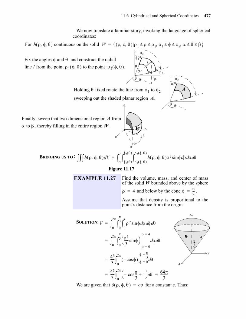
11.6 Cylindrical and Spherical Coordinates 477
We now translate a familiar story, invoking the language of sphericalcoordinates:
Figure 11.17
SOLUTION:
We are given that for a constant c. Thus:
For h continuous on the solid W 1 2 1 2 =
Fix the angles and and construct the radial
line l from the point 1 to the point 2 . l
1
2
1
2
2
1
Holding fixed rotate the line from 1 to 2
sweeping out the shaded planar region A.
W
Finally, sweep that two-dimensional region A from
to , thereby filling in the entire region W.
BRINGING US TO: h Vd h 2 sin d d d1
2
1
2
=
A
EXAMPLE 11.27 Find the volume, mass, and center of massof the solid W bounded above by the sphere
and below by the cone .
Assume that density is proportional to thepoint’s distance from the origin.
4= 3---=
y
x
z
3---
4W
V 2 sin d d d0
4
0
3---
0
2
=
3
3----- sin
0=
4=
d d0
3---
0
2
=
43
3----- cos– 0=
3---=
d0
2
=
43
3-----
3---cos– 1+
d0
2
643
---------= =
c=
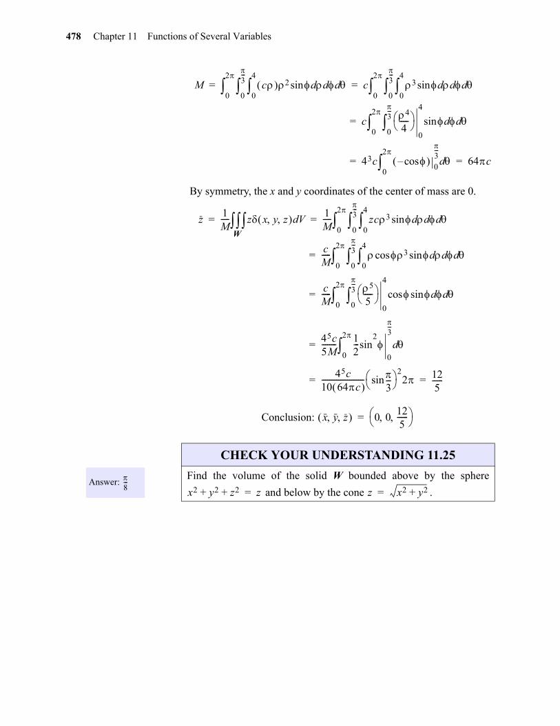
478 Chapter 11 Functions of Several Variables
By symmetry, the x and y coordinates of the center of mass are 0.
Conclusion:
M c 2 sin d d d0
4
0
3---
0
2
c 3 sin d d d0
4
0
3---
0
2
= =
c4
4-----
0
4
sin0
3---
d d0
2
=
43c cos– 0
3---
d0
2
64c= =
z1M----- z x y z Vd
1M----- zc3 sin d d d
0
4
0
3---
0
2
= =
cM----- cos 3 sin d d d
0
4
0
3---
0
2
=
cM----- 5
5-----
0
4
sincos d d0
3---
0
2
=
45c5M-------- 1
2---sin
2
0
3---
d0
2
=
45c10 64c -----------------------
3---sin
22 12
5------= =
W
x y z 0 0125------
=
Answer: 8---
CHECK YOUR UNDERSTANDING 11.25
Find the volume of the solid W bounded above by the sphere
and below by the cone .x2 y2 z2+ + z= z x2 y2+=
gio
11.6 Cylindrical and Spherical Coordinates 479
CYLINDRICAL COORDINATES
Exercises 1-4. The following points are given in cylindrical coordinates. Express them in rectan-gular coordinates.
Exercises 5-8. The following points are given in rectangular coordinates. Express them in cylin-drical coordinates.
Exercises 9-12. Write the equation in cylindrical coordinates.
Exercises 13-16. Evaluate.
Exercises 17-18. Evaluate using cylindrical coordinates.
Exercises 19-26. Use cylindrical coordinates to find the volume of the given solid.
EXERCISES
1. 2. 3. 4.
5. 6.
7. 8.
9. 10.
11. 12.
13. 14.
15. 16.
17. 18.
19. The solid bounded by the paraboloid and the plane .
20. The solid bounded by the paraboloid and the plane .
21. The solid lying outside the cone and inside the cylinder .
22. The solid lying above the cone and below the hemisphere
.
23. The solid enclosed by the cylinder and the planes and .
24. The solid bounded by the cone and the plane .
256
------ 3 3
23
------ 1 6
4--- 1
0 1–
4– 4 3– 8– 3 32
----------– 32---– 1–
0 2 2– 0 1–
z x2 y2+= 3x 2y z+ + 1=
x2 y2+ 2y= x2 y2+ 2x=
r zd rd d0
1 r2–
0
1
0
2
r zd rd dr2 3
18 r2–
0
3
0
2
r2cos2 z2+ r d rd zd
0
2
0
z
0
1
r zdsin rd d0
r2
0
cos
0
2
zd yd xd0
4 x2 y2+ –
0
1 x2–
0
1
z3 zd yd xdx2 y2+
1
0
1 x2–
1–
1
z x2 y2+= z 9=
z x2 y2+= z x=
z x2 y2+= x2 y2+ 4=
z x2 y2+=
z 1 1 x2 y2––+=
x2 y2+ 4= z 1–= x z+ 4=
zha---r= z h=
480 Chapter 11 Functions of Several Variables
Exercises 27-30. Find the mass of the given solid.
Exercises 31-36. Find the center of mass of the given solid.
25. The solid cut from the sphere by the cylinder .
26. The solid lying above the cone , below the plane , and bounded on the sides by the cylinder .
27. The ellipsoid lying above the xy-plane, with density function .
28. The circular cone of height h and circular base of radius a if the density at each point is proportional to its distance
(a) from the axis. (b) from the base.
29. The solid bounded by the paraboloid and if the density is pro-portional to
(a) its distance from the xy-plane. (b) the square of the distance from the origin.
30. The solid bounded by the paraboloid and if .
31. The solid is bounded by the paraboloid and the plane , for , and has constant density k.
32. The solid that lies within the cylinder , below the plane , and above the paraboloid , if .
33. The upper hemisphere of the unit sphere, and has constant density k.
34. The cone of constant density with height h and a base of radius b.
35. The solid is bounded by the paraboloids and and has constant density k.
x2 y2 z2+ + 4= r 2 sin=
z x2 y2+= z 0=x2 y2+ 3x=
4x2 4y2 z2+ + 16= x y z kz=
z 1 x2 y2+ –= z 0=
z x2 y2 4–+= z 0= x y z 1 x2 y2+ +=
z 4x2 4y2+= z a= a 0
x2 y2+ 1= z 4=z 1 x2– y2–= x y z z=
z x2 y2+= z 36 3x2– 3y2–=
gio
11.6 Cylindrical and Spherical Coordinates 481
SPHERICAL COORDINATES
36. Verify that if , then:
Exercises 37-40. The following points are given in spherical coordinates. Express them in rectan-gular coordinates.
Exercises 41-44. The following points are given in rectangular coordinates. Express them inspherical coordinates.
Exercises 45-48. Write the equation in spherical coordinates.
Exercises 49-52. Evaluate (note the order of integration).
Exercises 53-56. Evaluate using spherical coordinates.
Exercises 57-61. Use spherical coordinates to find the volume of the given solid.
37. 38. 39. 40.
41. 42. 43. 44.
45. 46.
47. 48.
49. 50.
51. 52.
53.
54.
55.
56.
57. A sphere of radius a.
58. A spherical shell whose outer radius is 2 and whose inner radius is 1.
59. The solid cut from the cone by the sphere .
60. The solid inside both of the spheres and
P P x y z =
2 x2 y2 z2+ +=
x ycossin sinsin= =
z cos=
43---
4---
2 2---–4---
72---
1256
------ 23
------
1 3 2 3 0 5– 0 0 1 1–– 1 1 1
z2 x2 y2+= x 2y 3z+ + 1=
x2 z2+ 9= x2 2x– y2 z2+ + 0=
3 dsin d d0
1
0
0
2
2 dcossin d d0
sin
0
2---
0
2---
2 dsin d d0
4---
0
sin
0
2---
d d d0
sin
0
2---
0
2---
x2 y2 z2+ + zd yd xd0
a2 x2 y2––
0
a2 x2–
0
a
x2 y2 z2+ + zd xd ydx2 y2+
18 x2– y2–
0
9 y2–
0
3
xy zd yd xdx2 y2+
2 x2 y2––
0
1 x2–
0
1
x2 y2 z2+ + zd yd xdx2 y2+
50 x2 y2––
0
25 x2–
0
5
4---= 2 acos=
1= 2 cos=
482 Chapter 11 Functions of Several Variables
Exercises 62-67. Find the mass of the given solid.
Exercises 68-72. Find the center of mass of the given solid.
61. The solid bounded below by the cone lying above the xy-plane and bounded above by the sphere .
62. A sphere or radius a if the density at a point is proportional to the square of its distance from the center.
63. A sphere of radius a if the density at a point is proportional to its distance from the center.
64. A hemisphere of radius a if the density at a point is proportional to its distance from the base.
65. The solid common to the sphere and the cone if
.
66. The solid enclosed between the spheres and if .
67. The solid ball of radius 1 if the density at each point d units from the center is .
68. A hemispherical solid if its density is proportional to the distance from its base.
69. A homogeneous cone of height h and base of radius a, positioned so that its vertex is at and the axis is the positive z-axis. 9
70. A homogeneous solid bounded above by the sphere and below by the cone
, where .
71. The homogeneous solid bounded below by the cone lying above the xy-plane and bounded above by the sphere .
72. The homogeneous solid that lies above the cone and below the hemisphere
.
z2 x2= y2+x2 y2 z2+ + 9=
x2 y2 z2+ + 1= z x2 y2+=
x y z x2 y2 z2+ +=
x2 y2 z2+ + 4= x2 y2 z2+ + 1= x y z x2 y2 z2+ + 1 2/–=
11 d2+--------------
0 0 0
a=
= 0 2---
z2 x2= y2+x2 y2 z2+ + 9=
z x2 y2+=
z 1 1 x2 y2+ –+=
gio
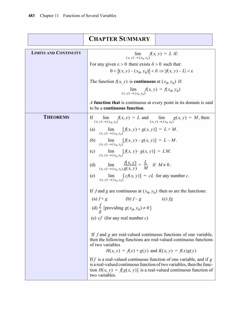
483 Chapter 11 Functions of Several Variables
gio
CHAPTER SUMMARY
LIMITS AND CONTINUITY if:
For any given there exists such that:
The function is continuous at if:
A function that is continuous at every point in its domain is saidto be a continuous function.
THEOREMS If and , then:
(a) .
(b) .
(c) .
(d) .
(e) for any number c.
If f and g are continuous at then so are the functions:
(a) (b) (c)
(d) [providing ]
(e) (for any real number c)
If f and g are real-valued continuous functions of one variable,then the following functions are real-valued continuous functionsof two variables
and
If f is a real-valued continuous function of one variable, and if is a real-valued continuous function of two variables, then the func-tion is a real-valued continuous function oftwo variables.
f x y x y x0 y0
lim L=
0 00 x y x0 y0 – f x y L–
f x y x0 y0
f x y x y x0 y0
lim f x0 y0 =
f x y x y x0 y0
lim L= g x y x y x0 y0
lim M=
f x y g x y + x y x0 y0
lim L M+=
f x y g x y – x y x0 y0
lim L M–=
f x y g x y x y x0 y0
lim LM=
f x y g x y ----------------
x y x0 y0 lim
LM----- if M 0=
cf x y x y x0 y0
lim cL=
x0 y0
f g+ f g– fgfg--- g x0 y0 0
cf
H x y f x g y += K x y f x g y =
g
H x y f g x y =
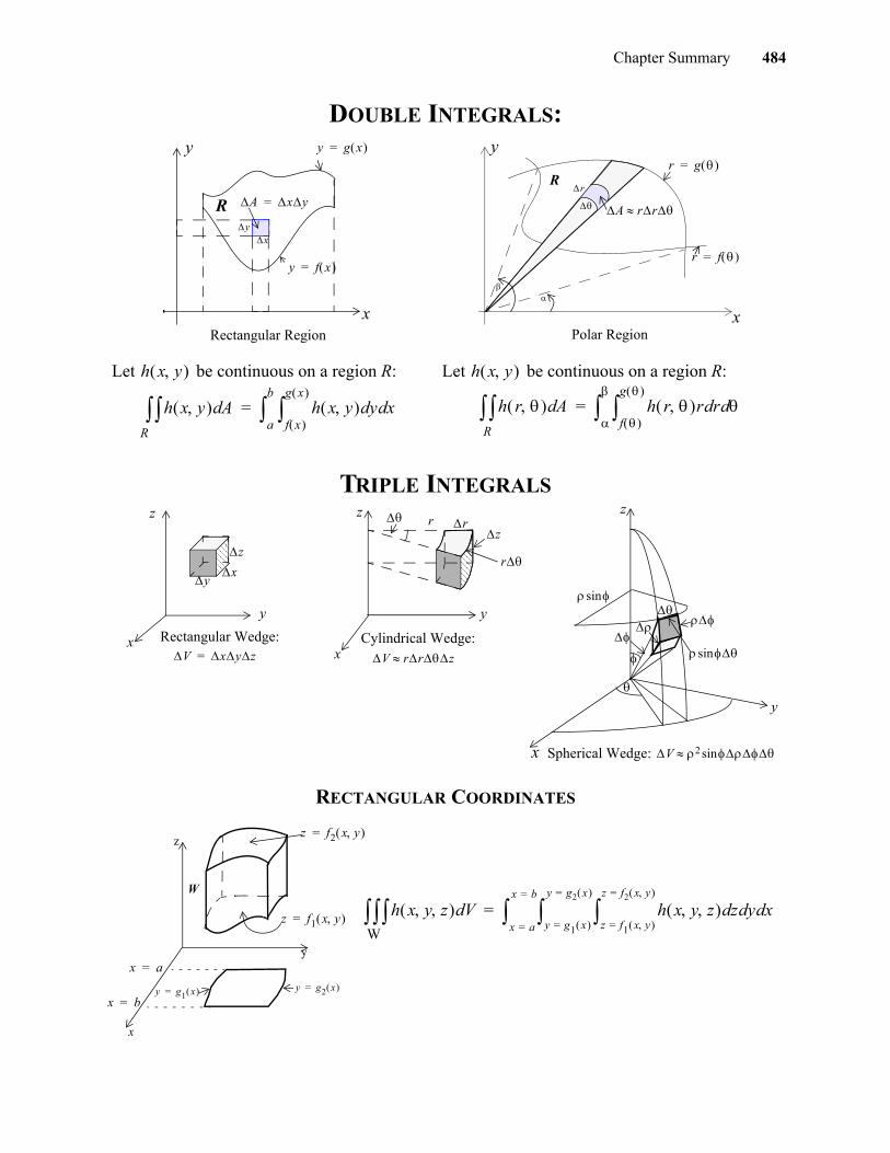
Chapter Summary 484
gio
DOUBLE INTEGRALS:
TRIPLE INTEGRALS
RECTANGULAR COORDINATES
Rectangular Region Polar Region
Let be continuous on a region R:
Let be continuous on a region R:
A xy=
xy
y f x =
y g x =
x
y
R
r f =
r g =
y
x
r
R
A rr
h x y
h x y Ad h x y ydf x
g x
xda
b
=R
h x y
h r AdR h r r rd d
f
g
=
yx
z
rz
Rectangular Wedge: V xyz=
Cylindrical Wedge: V rrz
r
Spherical Wedge:
sin
y
x
z
y
x
z
y
x
z
sin
V 2 sin
r
x
y
z
x b=y g1 x = y g2 x =
z f2 x y =
z f1 x y =
W
x a=
h x y z Vd h x y z zd yd xdz f1 x y =
z f2 x y =
y g1 x =
y g2 x =
x a=
x b=
=W
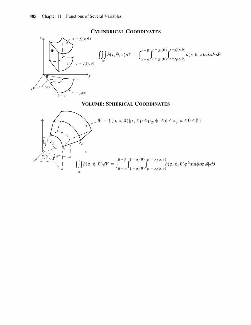
485 Chapter 11 Functions of Several Variables
CYLINDRICAL COORDINATES
VOLUME: SPHERICAL COORDINATES
W
z f1 r =
z f2 r =
r g1 =
r g2 = =
=
x
y
z
h r z VdW h r z r zd rd d
z f1 r =
z f2 r =
r g1 =
r g2 =
=
=
=
h Vd h 2 sin d d d 1 =
2 =
1 =
2 =
=
=
=
1 2
1
2
W 1 2 1 2 =
W
gio
Chapter Summary 486
gio
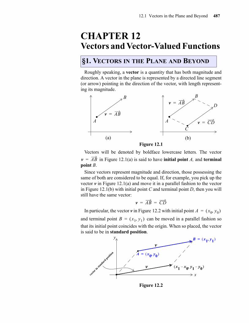
12.1 Vectors in the Plane and Beyond 487
12
CHAPTER 12Vectors and Vector-Valued Functions
Roughly speaking, a vector is a quantity that has both magnitude anddirection. A vector in the plane is represented by a directed line segment(or arrow) pointing in the direction of the vector, with length represent-ing its magnitude.
Figure 12.1
Vectors will be denoted by boldface lowercase letters. The vector
in Figure 12.1(a) is said to have initial point A, and terminalpoint B.
Since vectors represent magnitude and direction, those possessing thesame of both are considered to be equal. If, for example, you pick up thevector v in Figure 12.1(a) and move it in a parallel fashion to the vectorin Figure 12.1(b) with initial point C and terminal point D, then you willstill have the same vector:
In particular, the vector v in Figure 12.2 with initial point
and terminal point can be moved in a parallel fashion so
that its initial point coincides with the origin. When so placed, the vectoris said to be in standard position.
Figure 12.2
§1. VECTORS IN THE PLANE AND BEYOND
v AB=.A
B
(a)
v AB=
.A
B
.C
D
(b)
v CD=
v AB=
v AB CD= =
A x0 y0 =
B x1 y1 =
A x0 y0 =.
B x1 y1 =
x1 x0– y1 y0–
v
v
x
y
.vecto
r in st
andar
d pos
ition
gio
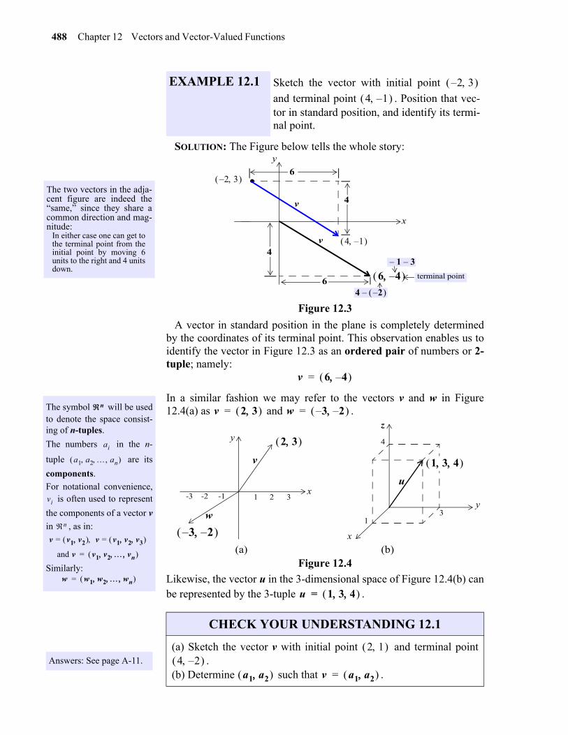
488 Chapter 12 Vectors and Vector-Valued Functions
SOLUTION: The Figure below tells the whole story:
Figure 12.3
A vector in standard position in the plane is completely determinedby the coordinates of its terminal point. This observation enables us toidentify the vector in Figure 12.3 as an ordered pair of numbers or 2-tuple; namely:
In a similar fashion we may refer to the vectors v and w in Figure12.4(a) as and .
Figure 12.4
Likewise, the vector u in the 3-dimensional space of Figure 12.4(b) canbe represented by the 3-tuple .
EXAMPLE 12.1 Sketch the vector with initial point
and terminal point . Position that vec-tor in standard position, and identify its termi-nal point.
2 3– 4 1–
The two vectors in the adja-cent figure are indeed the“same,” since they share acommon direction and mag-nitude:
In either case one can get tothe terminal point from theinitial point by moving 6units to the right and 4 unitsdown.
.y
2 3–
4 1–
6 4–
4 2– –
1– 3–
v
v
6
4
4
6terminal point
x
The symbol will be usedto denote the space consist-ing of n-tuples.
The numbers in the n-
tuple are its
components.
For notational convenience, is often used to represent
the components of a vector v
in , as in:
Similarly:
Answers: See page A-11.
n
ai
a1 a2 an
vi
n
v v1 v2 = v v1 v2 v3 =
and v v1 v2 vn =
w w1 w2 wn =
CHECK YOUR UNDERSTANDING 12.1
(a) Sketch the vector v with initial point and terminal point.
(b) Determine such that .
v 6 4– =
v 2 3 = w 3 2–– =
-3 -2 -1 1 2 3x
y
x
y
13
4
(a) (b)
v
w
u
2 3
3 2––
z
1 3 4
u 1 3 4 =
2 1 4 2–
a1 a2 v a1 a2 =
gio
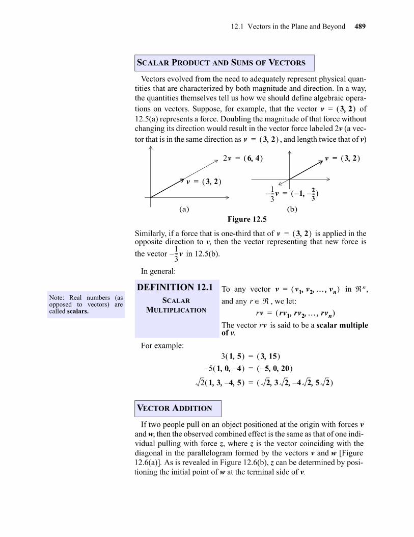
12.1 Vectors in the Plane and Beyond 489
Vectors evolved from the need to adequately represent physical quan-tities that are characterized by both magnitude and direction. In a way,the quantities themselves tell us how we should define algebraic opera-tions on vectors. Suppose, for example, that the vector of12.5(a) represents a force. Doubling the magnitude of that force withoutchanging its direction would result in the vector force labeled 2v (a vec-tor that is in the same direction as , and length twice that of v)
Figure 12.5
Similarly, if a force that is one-third that of is applied in theopposite direction to v, then the vector representing that new force is
the vector in 12.5(b).
In general:
For example:
If two people pull on an object positioned at the origin with forces vand w, then the observed combined effect is the same as that of one indi-vidual pulling with force z, where z is the vector coinciding with thediagonal in the parallelogram formed by the vectors v and w [Figure12.6(a)]. As is revealed in Figure 12.6(b), z can be determined by posi-tioning the initial point of w at the terminal side of v.
SCALAR PRODUCT AND SUMS OF VECTORS
v 3 2 =
v 3 2 =
v 3 2 =
2v 6 4 = v 3 2 =
13---– v 1– 2
3---– =
(a) (b)
v 3 2 =
13---v–
Note: Real numbers (asopposed to vectors) arecalled scalars.
DEFINITION 12.1SCALAR
MULTIPLICATION
To any vector in ,
and any , we let:
The vector is said to be a scalar multipleof v.
VECTOR ADDITION
v v1 v2 vn = n
r rv rv1 rv2 rvn =
rv
3 1 5 3 15 =
5 1 0 4– – 5 0 20 – =
2 1 3 4 5– 2 3 2 4 2 5 2– =
gio
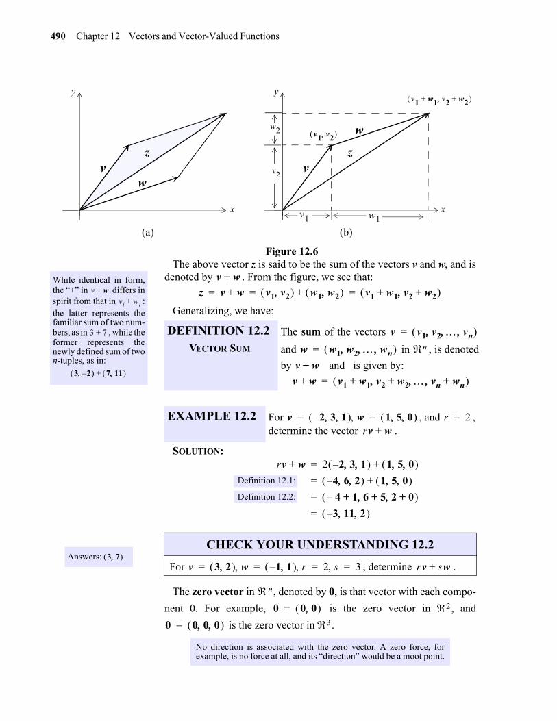
490 Chapter 12 Vectors and Vector-Valued Functions
Figure 12.6The above vector z is said to be the sum of the vectors v and w, and is
denoted by . From the figure, we see that:
Generalizing, we have:
SOLUTION:
The zero vector in , denoted by 0, is that vector with each compo-
nent 0. For example, is the zero vector in , and
is the zero vector in .
(a) (b)
vw
z
y
x
vz
y
x
v1 v2 w2
v2
w1
v1 w1+ v2 w2+
v1
w
While identical in form,the “+” in differs inspirit from that in :the latter represents thefamiliar sum of two num-bers, as in , while theformer represents thenewly defined sum of twon-tuples, as in:
v w+vi wi+
3 7+
3 2– 7 11 +
DEFINITION 12.2VECTOR SUM
The sum of the vectors
and in , is denoted
by and is given by:
EXAMPLE 12.2 For , and , determine the vector .
v w+
z v w+ v1 v2 w1 w2 + v1 w1+ v2 w2+ = = =
v v1 v2 vn =
w w1 w2 wn = n
v w+
v w+ v1 w1+ v2 w2 vn wn+ + =
v 2 3 1 – w 1 5 0 = = r 2=rv w+
Answers: 3 7 CHECK YOUR UNDERSTANDING 12.2
For , determine .
No direction is associated with the zero vector. A zero force, forexample, is no force at all, and its “direction” would be a moot point.
rv w+ 2 2 3 1 – 1 5 0 +=
4– 6 2 1 5 0 +=
4– 1 6 5 2 0+++ =
3– 11 2 =
Definition 12.1:
Definition 12.2:
v 3 2 w 1 1– r 2 s 3= = = = rv sw+
n
0 0 0 = 2
0 0 0 0 = 3
gio
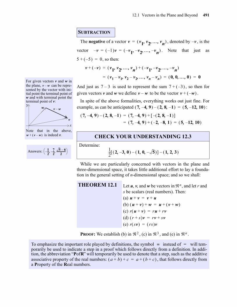
12.1 Vectors in the Plane and Beyond 491
The negative of a vector , denoted by , is the
vector . Note that just as
, so then:
And just as is used to represent the sum , so then for
given vectors v and w we define to be the vector .
In spite of the above formalities, everything works out just fine. Forexample, as can be anticipated :
While we are particularly concerned with vectors in the plane andthree-dimensional space, it takes little additional effort to lay a founda-tion in the general setting of n-dimensional space; and so we shall:
PROOF: We establish (b) in , (c) in , and (e) in .
SUBTRACTION
For given vectors v and w inthe plane, can be repre-sented by the vector with ini-tial point the terminal point ofw and with terminal point theterminal point of v:
Note that in the above, is indeed v.
Answers:
v w–
w
x
y
v
v w–
w v w– +
12---– 7
2---– 5 6–
2----------------
CHECK YOUR UNDERSTANDING 12.3
Determine:
THEOREM 12.1 Let u, v, and w be vectors in , and let r ands be scalars (real numbers). Then:(a)
(b)
(c)
(d)
(e)
v v1 v2 vn = v–
v– 1– v v– 1 v– 2 vn– = =
5 5– + 0=
v v– + v1 v2 vn v– 1 v– 2 vn– +=
v1 v1– v2 v2– vn vn– 0 0 0 0= = =
7 3– 7 3– +
v w– v w– +
7 4 9– 2 8 1– – 5 12– 10 =
7 4 9– 2 8 1– – 7 4 9– 2 8 1– – +=
7 4 9– 2– 8– 1 + 5 12– 10 = =
12--- 2 3– 0 1 0 5– – 1 2 3 –
n
u v+ v u+=
u v+ w+ u v w+ +=
r u v+ ru rv+=
r s+ v rv sv+=
r sv rs v=
2 3 n
To emphasize the important role played by definitions, the symbol instead of will tem-porarily be used to indicate a step in a proof which follows directly from a definition. In addi-tion, the abbreviation “PofR” will temporarily be used to denote that a step, such as the additiveassociative property of the real numbers: , that follows directly froma Property of the Real numbers.
=
a b+ c+ a b c+ +=
gio
492 Chapter 12 Vectors and Vector-Valued Functions
(b): (in ).
For :
(c): (in ).
For :
(e): (in ).
For :
The associative propertyeliminates the need forincluding parenthesis whensumming more than twovectors. In particular,
is perfectly well-defined.u v w+ +
u v+ w+ u v w+ += 2
u u1 u2 v v1 v2 and w w1 w2 = = =
Definition 12.2:
Definition 12.2:
Definition 12.2:
POFR:
u v+ w+ u1 u2 v1 v2 + w1 w2 +
u1 v1+ u2 v2+ w1 w2 +
u1 v1+ w1+ u2 v2+ w2+
u1 v 1+ w1 + u2 v2+ w2 + =
u1 u2 v1 v2 w1 w2 + +
u v w+ +
r u v+ ru rv+= 3
u u1 u2 u3 and v v1 v2 v3 = =
r u v+ r u1 u2 u3 v1 v2 v3 +
r u1 v1+ u2 v2 u3 v3++
r u1 v1+ r u2 v2+ r u3 v3+
ru1 rv1+ ru2 rv2+ ru3 rv3+ =
ru1 ru2 ru3 rv1 rv2 rv3 +
r u1 u2 u3 r v1 v2 v3 +
ru rv+
Definition 12.2:
Definition 12.1:
Defintion 12.2:
Definition 12.1:
PofR:
r sv rs v= Rn
Answer: See page A-12.
Throughout mathematics: DEFINITIONS RULE!
Just look at the above proof. It contains but one “logical step,”the step labeled PofR; all other steps hinge on DEFINITIONS.
CHECK YOUR UNDERSTANDING 12.4
Establish Theorem 12.1(a) in , and Theorem 12.1(d) in .
v v1 v2 vn =
r sv r s v1 v2 vn
r sv1 sv2 svn
r sv1 r sv2 r svn
rs v1 rs v2 rs vn =
rs v1 v2 vn
rs v
Definition 12.1:
Defintion 12.1:
Definition 12.1:
PofR:
3 n
gio
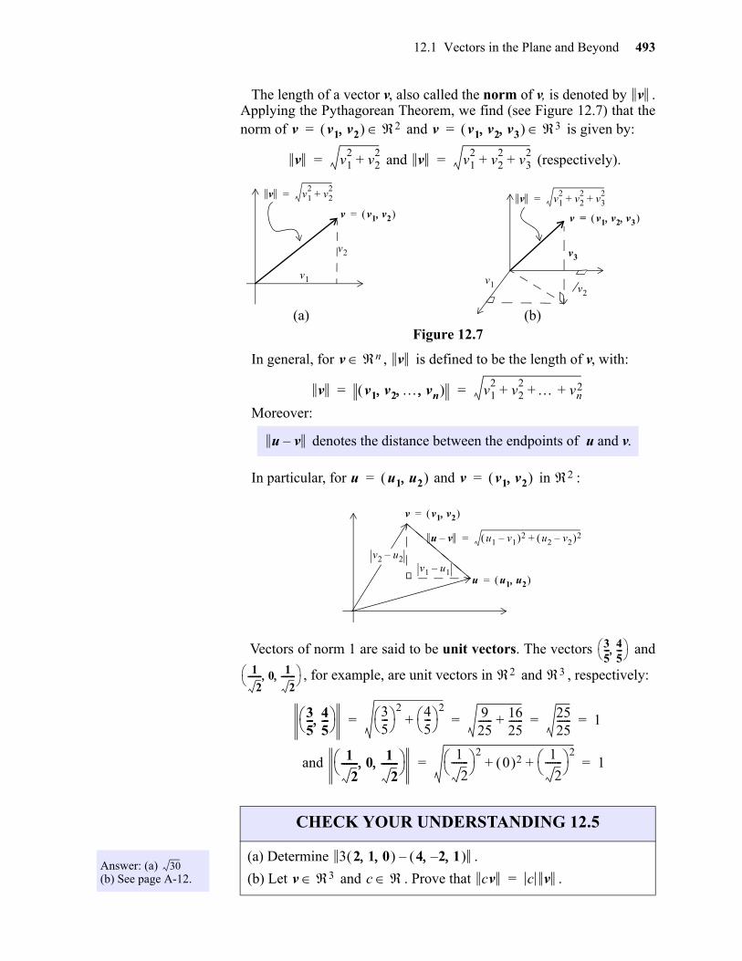
12.1 Vectors in the Plane and Beyond 493
gio
The length of a vector v, also called the norm of v, is denoted by .Applying the Pythagorean Theorem, we find (see Figure 12.7) that thenorm of and is given by:
and (respectively).
Figure 12.7
In general, for , is defined to be the length of v, with:
Moreover:
In particular, for and in :
Vectors of norm 1 are said to be unit vectors. The vectors and
, for example, are unit vectors in and , respectively:
and
denotes the distance between the endpoints of u and v.
v
v v1 v2 2= v v1 v2 v3 3=
v v12
v22
+= v v12
v22
v32
+ +=
v v12
v22
+=
v v1 v2 =
v2
v1
(a) (b)
v v1 v2 v3 =
v3
v2
v v12
v22
v32
+ +=
v1
v n v
v v1 v2 vn v12
v22 vn
2+ + += =
u v–
Answer: (a) (b) See page A-12.
30
CHECK YOUR UNDERSTANDING 12.5
(a) Determine .
(b) Let and . Prove that .
u u1 u2 = v v1 v2 = 2
v v1 v2 =
u u1 u2 =
v2 u2–v1 u1–
u v– u1 v1– 2 u2 v2– 2+=
35--- 4
5---
1
2------- 0 1
2-------
2 3
35--- 4
5---
35--- 2 4
5--- 2
+ 925------ 16
25------+ 25
25------ 1= = = =
1
2------- 0 1
2-------
1
2------- 2
0 2 1
2------- 2
+ + 1= =
3 2 1 0 4 2– 1 –
v 3 c cv c v=
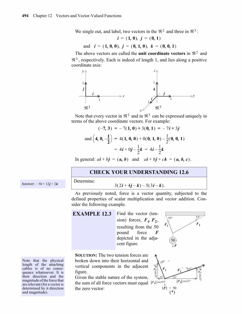
494 Chapter 12 Vectors and Vector-Valued Functions
gio
We single out, and label, two vectors in the and three in :
and
The above vectors are called the unit coordinate vectors in and, respectively. Each is indeed of length 1, and lies along a positive
coordinate axis:
Note that every vector in and in can be expressed uniquely interms of the above coordinate vectors. For example:
In general: .
As previously noted, force is a vector quantity, subjected to thedefined properties of scalar multiplication and vector addition. Con-sider the following example.
SOLUTION: The two tension forces arebroken down into their horizontal andvertical components in the adjacentfigure. Given the stable nature of the system,the sum of all force vectors must equalthe zero vector:
2 3
i 1 0 j 0 1 = =
i 1 0 0 j 0 1 0 k 0 0 1 = = =
2
3
ij
x
y
x
y
z
i
jk
2 3
1
1
1
1
1
2 3
7– 3 7 1 0 – 3 0 1 + 7i– 3j+= =
and 4 0 12---–
4 1 0 0 0 0 1 0 12--- 0 0 1 –+=
4i 0j12---k–+ 4i
12---k–= =
Answer: 9i– 12j 2k+ +
CHECK YOUR UNDERSTANDING 12.6
Determine: .
ai bj+ a b and ai bj ck+ + a b c = =
3 2i 4j k–+ 5 3i k– –
Note that the physicallength of the attachingcables is of no conse-quence whatsoever. It istheir direction and themagnitude of the force thatare relevant (for a vector isdetermined by it directionand magnitude).
EXAMPLE 12.3 Find the vector (ten-sion) forces, ,
resulting from the 50pound force Fdepicted in the adja-cent figure.
50
F1F2
55 23
F
F1 F2
F1 F2
55
23
23
55F2 23cos
F2
23sin
F1 55cos
F1
55sin
F 50=(*)
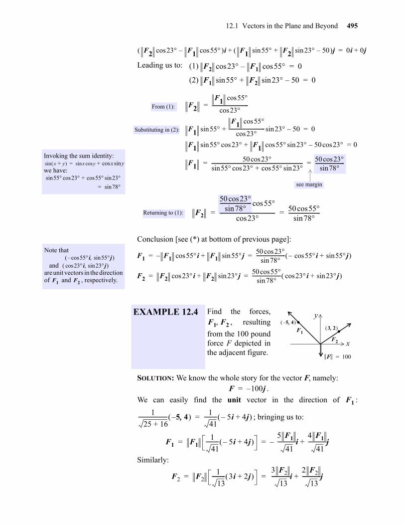
12.1 Vectors in the Plane and Beyond 495
j
gio
Leading us to:
Conclusion [see (*) at bottom of previous page]:
SOLUTION: We know the whole story for the vector F, namely: .
We can easily find the unit vector in the direction of :
; bringing us to:
Similarly:
Invoking the sum identity:
we have:x y+ sin x y x ysincos+cossin=
55 23 55 23sincos+cossin
78sin=
F2 23cos F1 55cos– i F1 55sin F2 23sin 50–+ j+ 0i 0+=
F2 23 F1 55cos–cos 0=
F1 55sin F2 23sin 50–+ 0=
(1)
(2)
F2
F1 55cos
23cos------------------------------=
F1 55sinF1 55cos
23cos------------------------------ 23sin 50–+ 0=
F1 55 23cossin F1 55 23 50 23cos–sincos+ 0=
F150 23cos
55 23 55cos 23sin+cossin--------------------------------------------------------------------------- 50 23cos
78sin------------------------= =
From (1):
Substituting in (2):
see margin
F2
50 23cos78sin
------------------------ 55cos
23cos------------------------------------------ 50 55cos
78sin------------------------= =Returning to (1):
Note that
and are unit vectors in the directionof and , respectively.
55i 55jsincos– 23i 23jsincos
F1 F2
EXAMPLE 12.4 Find the forces,, resulting
from the 100 poundforce F depicted inthe adjacent figure.
F1 F1 55i F1 55jsin+cos–50 23cos
78sin------------------------ 55icos– 55jsin+ = =
F2 F2 23i F2 23jsin+cos50 55cos
78sin------------------------ 23icos 23jsin+ = =
. .F1
F2
5– 4 3 2
x
y
F 100=
F1 F2
F 100j–=
F1
1
25 16+---------------------- 5– 4 1
41---------- 5i– 4j+ =
F1 F11
41---------- 5i– 4j+
5 F1
41--------------i–
4 F1
41--------------j+= =
F2 F21
13---------- 3i 2j+
3 F2
13--------------i
2 F2
13--------------j+= =
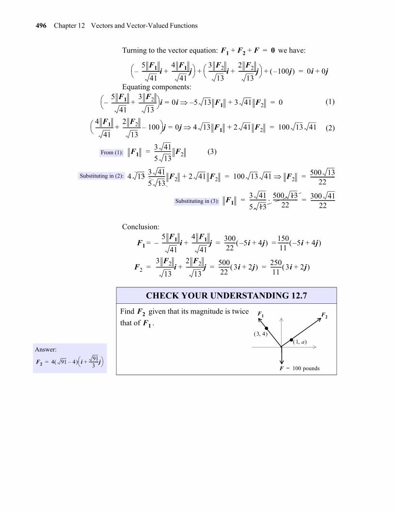
496 Chapter 12 Vectors and Vector-Valued Functions
Turning to the vector equation: we have:
Equating components:
Conclusion:
F1 F2 F+ + 0=
5 F1
41--------------i–
4 F1
41--------------j+
3 F2
13--------------i
2 F2
13--------------j+
100j– + + 0i 0j+=
5 F1
41--------------–
3 F2
13--------------+
i 0i= 5 13 F1 3 41 F2+– 0=
4 F1
41--------------
2 F2
13-------------- 100–+
j 0j= 4 13 F1 2 41 F2+ 100 13 41=
(1)
F13 41
5 13------------- F2=
4 13 3 41
5 13------------- F2 2 41 F2+ 100 13 41 F2 500 13
22-------------------= =
From (1):
Substituting in (2):
F13 41
5 13------------- 500 13
22------------------- 300 41
22-------------------= =
(3)
Substituting in (3):
(2)
Answer:
F2 4 91 4– i913
----------j+ =
CHECK YOUR UNDERSTANDING 12.7
Find given that its magnitude is twice
that of .
F1
5 F1
41--------------i–
4 F1
41--------------j+
30022--------- 5– i 4j+ 150
11--------- 5– i 4j+ = = =
F2
3 F2
13--------------i
2 F2
13--------------j+
50022--------- 3i 2j+ 250
11--------- 3i 2j+ = = =
.F1 F2
F 100 pounds=
.3 4 1 a
F2
F1
gio
12.1 Vectors in the Plane and Beyond 497
Exercises 1-6. Sketch the vector with given initial point A and terminal point B. Sketch the samevector in standard position in the plane and identify its terminal point.
Exercises 7-10. Express, as a 3-tuple, the vector with given initial point A and terminal point B.
Exercises 11-18. Perform the indicated vector operations.
Exercises 19-24. Find a unit vector in the direction of the given vector v, and then express v as aproduct of a scalar times that unit vector.
25. For , , and , find scalars r and s such that:
26. Find scalars r, s, and t, such that:
27. Find scalars r, s, and t, such that:
28. Show that there do not exist scalars r, s, and t, such that
EXERCISES
1. 2. 3.
4. 5. 6.
7. 8.
9. 10.
11. 12.
13. 14.
15. 16.
17. 18.
19. 20. 21.
22.23. 24.
(a) (b) (c)
A 2– 2– B 0 1 = = A 3 3 B 0 1– = = A 1 1 B 2– 3 = =
A 1 0 B 0 1– = = A 2– 1– B 1 1– = = A 2 2 B 1 2– = =
A 1 2 3 B 3 2 1 = = A 4 5 0 – B 2 5 1– = =
A 0 1 9– B 9 0 2 – = = A 3 5 3– – B 3 5 3– = =
5 3 2– 0 1 2 4–– + + 2 5 1 3 2 3– – + +
2 3 1 – 1 2 0– – + 1– 2 3 – – 3 2 2– +
4 2i 4j– i 3j+ – 4 2i 4j– i 3j+ –
2 3i 2k+ – 2j k– i j k+ + –+ 5 i 2j– 3k+ 2 2i k– i j k+ + + –
v 5 2 = v 4i 3j–= v 2i 4j– k+=
v 2 0 5 =v 2i
13---j–= v
12---i
23---j– 2k–=
u 1 3 = v 2 4 = w 6 2– =
ru sv+ w= r– u sw+ v= rv sw– + u=
r 1 3 0 s 2 1 6 t 1 4 6 + + 7 5 6 =
r– 1 3 0 s 2 1 6 t 1 4 6 – + + 7 5 6 =
r 2 3 5 s 3 2 5 t 1 2 3 + + 1 2 4 =
gio
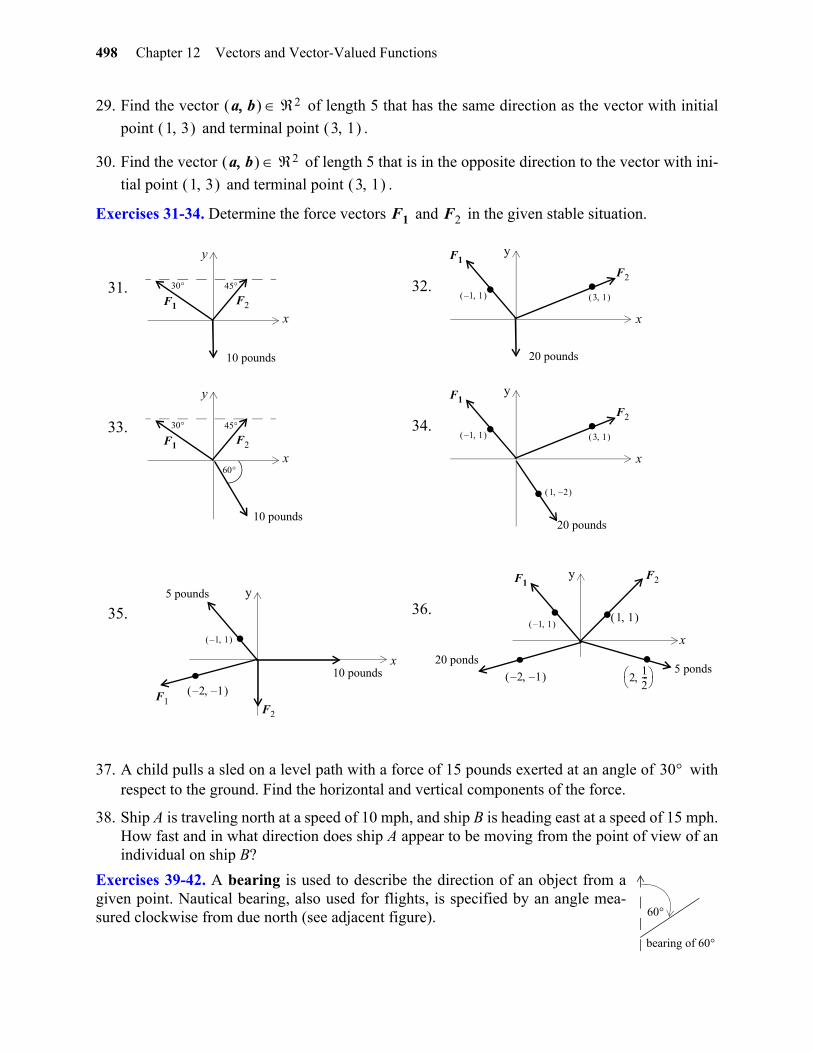
498 Chapter 12 Vectors and Vector-Valued Functions
29. Find the vector of length 5 that has the same direction as the vector with initial
point and terminal point .
30. Find the vector of length 5 that is in the opposite direction to the vector with ini-
tial point and terminal point .
Exercises 31-34. Determine the force vectors and in the given stable situation.
37. A child pulls a sled on a level path with a force of 15 pounds exerted at an angle of withrespect to the ground. Find the horizontal and vertical components of the force.
38. Ship A is traveling north at a speed of 10 mph, and ship B is heading east at a speed of 15 mph.How fast and in what direction does ship A appear to be moving from the point of view of anindividual on ship B?
Exercises 39-42. A bearing is used to describe the direction of an object from agiven point. Nautical bearing, also used for flights, is specified by an angle mea-sured clockwise from due north (see adjacent figure).
31. 32.
33. 34.
35. 36.
a b 21 3 3 1
a b 21 3 3 1
F1 F2
10 pounds
30 45
F1 F2
x
y
20 pounds
F1
F2.1– 1
.3 1
x
y
10 pounds
30 45
F1 F2
x
y
60
20 pounds
F1
F2.1– 1
.3 1
x
y
. 1 2–
10 pounds
F2
.1– 1
x
y
F1
.
5 pounds
2– 1–
F1 .1– 1
x
y F2
1 1
2– 1–
..20 ponds .
212---
5 ponds
30
60
bearing of 60
gio
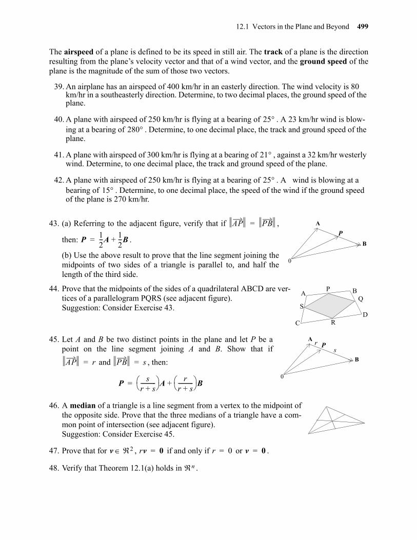
12.1 Vectors in the Plane and Beyond 499
The airspeed of a plane is defined to be its speed in still air. The track of a plane is the directionresulting from the plane’s velocity vector and that of a wind vector, and the ground speed of theplane is the magnitude of the sum of those two vectors.
43. (a) Referring to the adjacent figure, verify that if ,
then: .
(b) Use the above result to prove that the line segment joining themidpoints of two sides of a triangle is parallel to, and half thelength of the third side.
44. Prove that the midpoints of the sides of a quadrilateral ABCD are ver-tices of a parallelogram PQRS (see adjacent figure). Suggestion: Consider Exercise 43.
45. Let A and B be two distinct points in the plane and let P be apoint on the line segment joining A and B. Show that if
and , then:
46. A median of a triangle is a line segment from a vertex to the midpoint ofthe opposite side. Prove that the three medians of a triangle have a com-mon point of intersection (see adjacent figure). Suggestion: Consider Exercise 45.
47. Prove that for , if and only if or .
48. Verify that Theorem 12.1(a) holds in .
39. An airplane has an airspeed of 400 km/hr in an easterly direction. The wind velocity is 80 km/hr in a southeasterly direction. Determine, to two decimal places, the ground speed of the plane.
40. A plane with airspeed of 250 km/hr is flying at a bearing of . A 23 km/hr wind is blow-ing at a bearing of . Determine, to one decimal place, the track and ground speed of the plane.
41. A plane with airspeed of 300 km/hr is flying at a bearing of , against a 32 km/hr westerly wind. Determine, to one decimal place, the track and ground speed of the plane.
42. A plane with airspeed of 250 km/hr is flying at a bearing of . A wind is blowing at a bearing of . Determine, to one decimal place, the speed of the wind if the ground speed of the plane is 270 km/hr.
25280
21
2515
A
B
0
P
AP PB=
P12---A
12---B+=
A B
CD
P
Q
R
S
A
B
0
Prs
AP r= PB s=
Ps
r s+----------- A
rr s+----------- B+=
v 2 rv 0= r 0= v 0=
n
gio
500 Chapter 12 Vectors and Vector-Valued Functions
49. Verify that Theorem 12.1(b) holds in .
50. Verify that Theorem 12.1(c) holds in .
51. Verify that Theorem 12.1(d) holds in .
n
n
n
gio
12.2 Dot and Cross Products 501
gio
12
At this point, we can add vectors (Definition 12.2), and can multiplya vector by a scalar (Definition 12.1). In either of those cases, the endresult is again a vector. We now turn our attention to an operationwhich assigns a real number to each pair of vectors in :
For example:
and:
Here are four particularly important dot-product properties:
PROOF: We establish (c) and invite you to verify all other parts of thetheorem in the exercises:
As for the other part of (c):
§2. DOT AND CROSS PRODUCTS
Left to our own devices, wewould most likely define theproduct of two vectors in thismanner: As it turns out, however, theabove “natural definition”does not appear to be useful.The same, as you will see,cannot be said for the dotproduct concept.
2 1 3 2 5 3 4 5 9 =
DEFINITION 12.3DOT PRODUCT
The dot product of
and , denoted by ,is the real number:
THEOREM 12.2
For and any scalar r:
(a) , and only if
(b)
(c)
(d) and
n
u u1 u2 un =
v v1 v2 vn = u v
u v u1v1 u2v2 unvn+ + +=
2 4 3– 1 5 0 7 1– 2 5 4 0 3– 7 1 1– +++ 12–= =
2i 3j k–+ 5i 7j– 9k– 10 21– 9+ 2–= =
u v w n
v v 0 v v 0= v 0=
u v v u=
ru v r u v u rv= =
u v+ w u w v w+=
u v– w u w v w–=
Answer: See page A-13.
In 3:
r u1 u2 u3 v1 v2 v3
ru1 ru2 ru3 v1 v2 v3 =
ru1 v1 ru2 v2 ru3 v3+ +=
r u1v1 r u2v2 r u3v3 + +=
r u1v1 u2v2 u3v3+ + =
r u1 u2 u3 v1 v2 v3 =
CHECK YOUR UNDERSTANDING 12.8
Verify that for any and any scalar r:
ru v r u1 u2 un v1 v2 vn =
ru1 ru2 run v1 v2 vn =
ru1 v1 ru2 v2 run vn+ + +=
r u1v1 r u2v2 r unvn + + +=
r u1v1 u2v2 unvn+ + + =
r u v =
Defitition 12.1, page 489:
Definition 12.3:
Definition 12.3:
u v nu rv r u v =
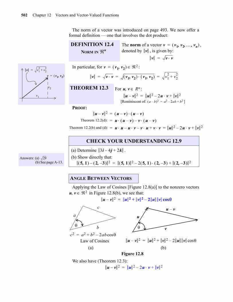
502 Chapter 12 Vectors and Vector-Valued Functions
gio
The norm of a vector was introduced on page 493. We now offer aformal definition — one that involves the dot product:
In particular, for :
PROOF:
Applying the Law of Cosines [Figure 12.8(a)] to the nonzero vectors in Figure 12.8(b), we see that:
Figure 12.8
We also have (Theorem 12.3):
v v12
v22
+=
v v1 v2 =
v2
v1
DEFINITION 12.4NORM IN
The norm of a vector ,denoted by , is given by:
THEOREM 12.3 For :
[Reminiscent of: ]
n
v v1 v2 vn =v
v v v=
v v1 v2 2=
v v v v1 v2 v1 v2 v12
v22
+= = =
u v Rnu v– 2 u 2 2u v v 2+–=
a b– 2 a2 2ab– b2+=
u v– 2 u v– u v– =
u u v– v u v– –=
u u u v– v u– v v+ u 2 2u v v 2+–= =
Theorem 12.2(d):
Theorem 12.2(b) and (d):
Answers: (a) (b) See page A-13.
29
CHECK YOUR UNDERSTANDING 12.9
(a) Determine .
(b) Show directly that:
ANGLE BETWEEN VECTORS
3i 4j– 2k+
5 1 2 3– – 2 5 1 2 2 5 1 2 3– 2 3– 2+–=
u v 2u v– 2 u 2 v 2 2 u v cos–+=
u
v
u v–
a
b
c
c2 a2 b2 2ab cos–+=Law of Cosines u v– 2 u 2 v 2 2 u v cos–+=
(a) (b)
u v– 2 u 2 2u v v 2+–=
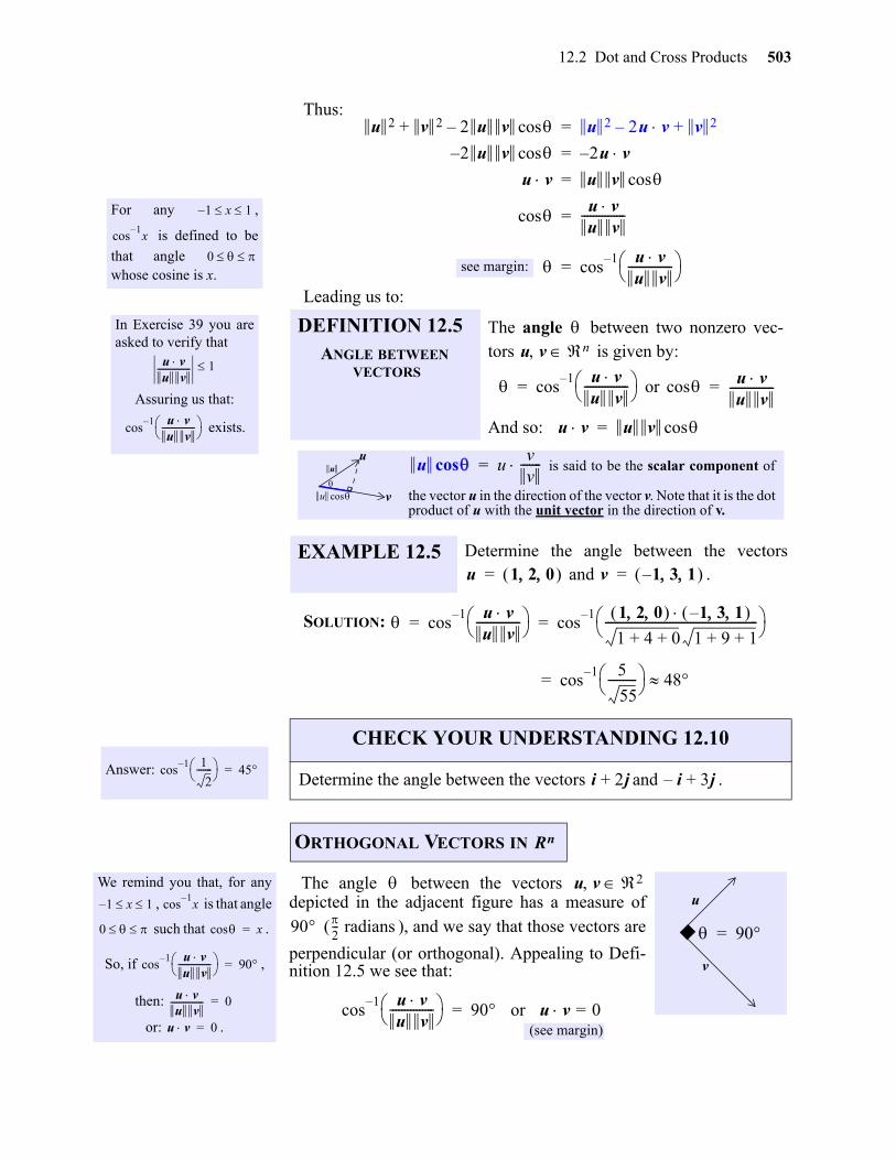
12.2 Dot and Cross Products 503
gio
Thus:
Leading us to:
SOLUTION:
For any ,
is defined to be
that angle whose cosine is x.
1 x 1 –
cos1–x
0
u 2 v 2 2 u v cos–+ u 2 2u v v 2+–=
2 u v cos– 2u v–=
u v u v cos=
cosu vu v
--------------- =
cos1– u v
u v--------------- =see margin:
In Exercise 39 you areasked to verify that
Assuring us that:
exists.
u vu v
--------------- 1
cos1– u v
u v---------------
DEFINITION 12.5ANGLE BETWEEN
VECTORS
The angle between two nonzero vec-tors is given by:
or
And so:
is said to be the scalar component of
the vector u in the direction of the vector v. Note that it is the dotproduct of u with the unit vector in the direction of v.
EXAMPLE 12.5 Determine the angle between the vectors and .
u v n
cos1– u v
u v--------------- = cos u v
u v---------------=
u v u v cos=
u
v
u
u cos
u cos uvv
-------=
u 1 2 0 = v 1– 3 1 =
cos1– u v
u v--------------- cos
1– 1 2 0 1– 3 1 1 4 0+ + 1 9 1+ +
---------------------------------------------------- = =
cos1– 5
55---------- 48=
Answer: cos1– 1
2------- 45=
CHECK YOUR UNDERSTANDING 12.10
Determine the angle between the vectors and .i 2j+ i– 3j+
We remind you that, for any
, is that angle
such that .
So, if ,
then:
or: .
1 x 1 – cos1–x
0 cos x=
cos1– u v
u v--------------- 90=
u vu v
--------------- 0=
u v 0=
ORTHOGONAL VECTORS IN
The angle between the vectors depicted in the adjacent figure has a measure of
( ), and we say that those vectors are
perpendicular (or orthogonal). Appealing to Defi-nition 12.5 we see that:
Rn
u v 2
90 2--- radians
cos1– u v
u v--------------- 90 or u v 0==
(see margin)
u
v
90=
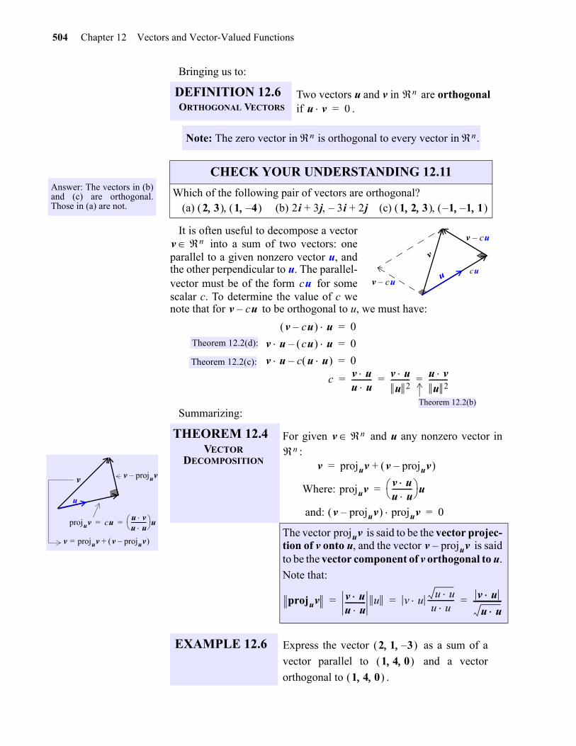
504 Chapter 12 Vectors and Vector-Valued Functions
Bringing us to:
It is often useful to decompose a vector into a sum of two vectors: one
parallel to a given nonzero vector u, andthe other perpendicular to u. The parallel-vector must be of the form for somescalar c. To determine the value of c wenote that for to be orthogonal to u, we must have:
Summarizing:
Answer: The vectors in (b)and (c) are orthogonal.Those in (a) are not.
DEFINITION 12.6ORTHOGONAL VECTORS
Two vectors u and v in are orthogonalif .
Note: The zero vector in is orthogonal to every vector in .
CHECK YOUR UNDERSTANDING 12.11
Which of the following pair of vectors are orthogonal? (a) (b) (c)
n
u v 0=
n n
2 3 1 4– 2i 3j 3i– 2j++ 1 2 3 1– 1– 1
u
v
v cu–
v cu–
cu
v n
cu
v cu–
Theorem 12.2(d):
Theorem 12.2(c):
v cu– u 0=
v u cu u– 0=
v u c u u – 0=
c v uu u----------- v u
u 2---------- u v
u 2----------= = =
Theorem 12.2(b)
projuv cuu vu u----------- u= =
v projuv–
u
v projuv= v projuv– +
v
THEOREM 12.4VECTOR
DECOMPOSITION
For given and u any nonzero vector in:
Where:
and:
The vector is said to be the vector projec-tion of v onto u, and the vector is saidto be the vector component of v orthogonal to u.
Note that:
EXAMPLE 12.6 Express the vector as a sum of a
vector parallel to and a vector
orthogonal to .
v nn
v projuv v projuv– +=
projuvv uu u----------- u=
v projuv– projuv 0=
projuvv projuv–
projuv v uu u----------- u v u u u
u u-------------- v u
u u---------------= = =
2 1 3– 1 4 0
1 4 0
gio
12.2 Dot and Cross Products 505
gio
SOLUTION: For and we have:
and
A two-by-two matrix of real numbers is an array consisting of tworows and two columns of numbers, as is the case with A and B below:
The determinant of , is the number: .
For example:
We now define the determinant of a three-by-three array with firstrow consisting of the unit coordinate vectors i, j, and k as follows:
v 2 1 3– = u 1 4 0 =
projuvu vu u----------- u
1 4 0 2 1 3– 1 4 0 1 4 0
----------------------------------------------- 1 4 0 617------ 1 4 0 = = =
Answer:
proj 0 2 v 0 1 =
v proj 0 2 v– 3 0 =
CHECK YOUR UNDERSTANDING 12.12
Express the vector as the sum of a vector parallel to and a vector orthogonal to u.
A DETERMINED PAUSE
v projuv– 2 1 3– 617------ 24
17------ 0
– 2817------ 7
17------– 3–
= =
2817------ 7
17------– 3–
617------ 24
17------ 0
+ 2 1 3– v= =
and 2817------ 7
17------– 3–
617------ 24
17------ 0
2817------ 6
17------ 7
17------–
2417------ + 0= =
Check:
v 3 1 =u 0 2 =
A 2 8
3– 5= B 0 5
9 7=
a b
c ddet a b
c dad bc–=
Answers: (a) 30 (b) 24 (c) 20–
CHECK YOUR UNDERSTANDING 12.13
Evaluate:
(a) (b) (c)
det 2 8
3– 52 5 8 3– – 34= =
det 5 3–
0 6det 2 3–
4 6det 2 5
4 0
det i j k
a b c
d e f
det b c
e fi det a c
d fj det a b
d ek+–=
i j k
a b c
d e f
i j k
a b c
d e f
i j k
a b c
d e fNote:
note negative sign
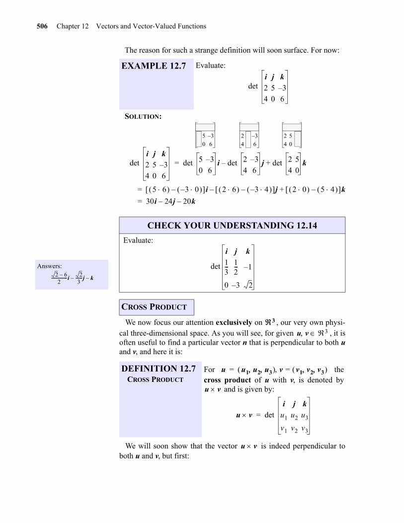
506 Chapter 12 Vectors and Vector-Valued Functions
The reason for such a strange definition will soon surface. For now:
SOLUTION:
We now focus our attention exclusively on , our very own physi-cal three-dimensional space. As you will see, for given , it isoften useful to find a particular vector n that is perpendicular to both uand v, and here it is:
We will soon show that the vector is indeed perpendicular toboth u and v, but first:
EXAMPLE 12.7 Evaluate:
det i j k
2 5 3–
4 0 6
Answers:
2 6–2
----------------i2
3-------j– k–
CHECK YOUR UNDERSTANDING 12.14
Evaluate:
CROSS PRODUCT
DEFINITION 12.7CROSS PRODUCT
For thecross product of u with v, is denoted by
and is given by:
det i j k
2 5 3–
4 0 6
det 5 3–
0 6i det 2 3–
4 6j det 2 5
4 0k+–=
5 6 3 0– – i 2 6 3 4– – j– 2 0 5 4 – k+=
30i 24j– 20k–=
i j k
2 5 3–
4 0 6
i j k
2 5 3–
4 0 6
i j k
2 5 3–
4 0 6
det
i j k
13--- 1
2--- 1–
0 3– 2
3
u v 3
u u1 u2 u3 v v1 v2 v3 ==
u v
u v det
i j k
u1 u2 u3
v1 v2 v3
=
u v
gio
12.2 Dot and Cross Products 507
gio
SOLUTION:
PROOF: Rolling up our sleeves, we simply show that ,and leave it for you to verify that is also zero:
As it turns out, the cross product is not a commutative operator. Inparticular:
Since the vectors i and j lie in the xy-plane (margin), and since the crossproduct of two vectors is orthogonal to both, it comes as no surprise thatboth of the above cross products must lie on the z-axis.
EXAMPLE 12.8 Evaluate:2i 5j 3k–+ 4i 6k+
2i 5j 3k–+ 4i 6k+ det i j k
2 5 3–
4 0 6
30i 24j– 20k–= =
Example 12.7
Answer: 10 16 7– –
CHECK YOUR UNDERSTANDING 12.15
Evaluate:2 3 4 3 1 2–
Answer: See page A-14.
THEOREM 12.5 For any , is orthogonal toboth u and v.
CHECK YOUR UNDERSTANDING 12.16
Verify, directly, that:
u v 3 u v
u v u 0=u v v
u v u det
i j k
u1 u2 u3
v1 v2 v3
u1 u2 u3 = =
u2v3 u3v2– i u1v3 u3v1– j– u1v2 u2v1– k+ u1 u2 u3
u2v3 u3v2– u1 u1v3 u3v1– u2– u1v2 u2v1– u3+=
u2v3u1 u3v2u1– u1v3u2 u3v1u2 u1v2u3 u2v1u3–+ +– 0= =
2 3 4 3 1 2– 3 1 2– 0=
x
y
z
ij
k i j det i j k
1 0 0
0 1 0
k while j i det i j k
0 1 0
1 0 0
k–= = = =
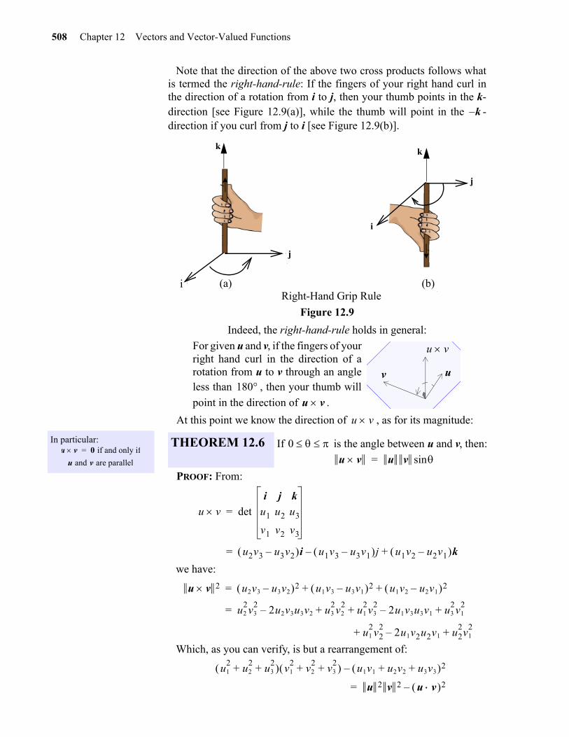
508 Chapter 12 Vectors and Vector-Valued Functions
gio
Note that the direction of the above two cross products follows whatis termed the right-hand-rule: If the fingers of your right hand curl inthe direction of a rotation from i to j, then your thumb points in the k-direction [see Figure 12.9(a)], while the thumb will point in the -direction if you curl from j to i [see Figure 12.9(b)].
Figure 12.9
Indeed, the right-hand-rule holds in general:
For given u and v, if the fingers of yourright hand curl in the direction of arotation from u to v through an angleless than , then your thumb will
point in the direction of .
At this point we know the direction of , as for its magnitude:
PROOF: From:
we have:
Which, as you can verify, is but a rearrangement of:
k–
(b)
i
j
i
kk
j
i (a) (b)Right-Hand Grip Rule
v u
u v
180u v
In particular:u v 0 if and only if=
u and v are parallel
THEOREM 12.6 If is the angle between u and v, then:
u v
0 u v u v sin=
u v det
i j k
u1 u2 u3
v1 v2 v3
=
u2v3 u3v2– i u1v3 u3v1– j– u1v2 u2v1– k+=
u v 2 u2v3 u3v2– 2 u1v3 u3v1– 2 u1v2 u2v1– 2+ +=
u22v3
22u2v3u3v2 u3
2v2
2u1
2v3
22u1v3u3v1 u3
2v1
2+–+ +–=
u12v2
22u1v2u2v1 u2
2v1
2+–+
u12
u22
u32
+ + v12
v22
v32
+ + u1v1 u2v2 u3v3+ + 2–
u 2 v 2 u v 2–=
12.2 Dot and Cross Products 509
At this point we have:
(*)We also know that (see Definition 12.5):
(**):
Substituting (**) in (*):
It follows that (see margin).
The above CYU shows that the cross product is neither a commuta-tive nor associative operator. It does, however, fall under the jurisdic-tion of some “familiar patterns:”
PROOF: We establish (a) and invite you to verify the rest in the exer-cises.
L
u v 2 u 2 v 2 u v 2–=
u v u v cos=
Since for :
Answers:
(a)
(b)
0sin 0
sin2 sin=
j k i k j i–= =
i k j k i– j= =
i i j j–=
i i j 0=
CHECK YOUR UNDERSTANDING 12.17
(a) Determine: .
(b) Determine: .
THEOREM 12.7 For and any scalar c:
(a)
(b)
(c)
(d)
u v 2 u 2 v 2 u v 2–=
u 2 v 2 u 2 v 2cos2–=
u 2 v 2 1 cos2– u 2 v 2sin
2= =
u v u v sin=
j k k j i k and k ii i j and i i j
u v w 3 u v w+ u v u w+=
u v+ w u w v w+=
cv w v cw c v w = =
v u u v –=
u v w+ u1 u2 u3 v1 w1+ v2 w2+ v3 w3+ det
i j k
u1 u2 u3
v1 w1 + v2 w2 + v3 w3+
= =
u2 v3 w3+ u3 v2 w2+ – i u1 v3 w3+ u3 v1 w1+ – j– u1 v2 w2+ u2 v1 w1+ – k+=
u2v3 u3v2– i u1v3 u3v1– j– u1v2 u2v1– k+ u2w3 u3w2– i u1w3 u3w1– j– u1w2 u2w1– k+ +=
det
i j k
u1 u2 u3
v1 v2 v3
det
i j k
u1 u2 u3
w1 w2 w3
+ u v u w+= =
Answers: See page A-15.
CHECK YOUR UNDERSTANDING 12.18
Let u and v be non-zero nonparallel vectors in
. Prove that is the area of the parallel-ogram with u and v as adjacent sides.
u
v0
3 u v
gio
510 Chapter 12 Vectors and Vector-Valued Functions
Exercises 1-6. Evaluate:
Exercises 7-18. Determine that angle between the given pair of vectors.
Exercises 19-22. Determine if the given pair of vectors are orthogonal, parallel, or neither.
Exercises 23-30. Express the vector v as the sum of a vector parallel to u and a vector orthogonalto u.
EXERCISES
1.2.
3. 4.
5. 6.
7. , 8. ,
9. 10.
11. 12.
13. 14.
15. 16.
17. 18.
19. 20.
21. 22. ,
23. 24.
25. 26.
27. 28.
29. 30.
2 5i 2j+ 3i– j+ 4 7– 3 5 1 5 2 4 +
3 2 1 4– 0 5 5 i 2j– 3k+ 2i 4j– k+
4 2i 4j– i 3j+ – i 2j– 3k+ 2 3 1 0 1 1 4 + 0 2 1 2 1 2– –
u i– 2j+= v 2i j+= u 4 1 = v 1 2 =
u 1 4 = v 3 2– = u 3i j–= v i 2j+=
u 2 1 1– = v 1 1 1– = u 2i 2j– 2k+= v i– j 5k+ +=
u i j+= v j k+= u 2 2 2– = v 1– 1 5 =
u 3 0 4 = v 0 7 5– = u 4i 2k+= v 2i j–=
u 3i j– 5k+= v 2i– 4j 3k+ += u 4 3 1– = v 2 0 1– =
u 2 1 1– = v 3 1 5– = u i12---j– 3k+= v 4i 2j– 12k+=
u 3i j– 5k+= v 2i– 4j 3k+ += u 0= v i 2j– 3k+=
v 2 1 = u 3 2– = v 4i 3j–= u i J+=
v 3j 4k u+ i j+= = v i j+= u 3j 4k+=
v 8 4 12– u 1 2 1– = = v 1 2 1– u 8 4 12– = =
v 12i 48k+ u 1
3-------i
1
3-------j
1
3-------k–+= = v 1
2--- 1 2– = u 2 1 1
2--- –
=
gio
12.2 Dot and Cross Products 511
Exercises 31-36. Evaluate:
37. Prove that , for:
(a) (b) (c)
38. Prove that , for:
(a) (b) (c)
39. (a) Prove, without using the law of cosines, that , for:
(a) (b) (c)
40. Prove: (a) Theorem 12.2 (a) (b) Theorem 12.2(b) (c) Theorem 12.2(d)
41. Prove: (a) Theorem 12.7 (b) (b) Theorem 12.7(c) (c) Theorem 12.7(d)
42. Prove that u and v are parallel if and only if , for:
(a) (b) (c)
43. Prove that a rectangle is a square if and only if its diagonals are perpendicular.
44. Prove that (a) for any .
(b) for any .
45. Establish the Jacoby Identity:
(for )
46. Establish the Lagrange Identity:
(for )
31. 32.
33. 34.
35. 36.
2 1 6– 3 4 1 – 3i 2j k–+ i k–
4– i j+ 2i j– 3k– 3i 2j– 3k– 3 1 0 – 2 1 3–– 3 2 3––
2 1 4– 7 2 3 1 1 2 – i k– 2i j k–+ i 3j+
u v– u v– u u v– v u v– –=
u v 2 u v R3 u v Rn
u u v– v u v– – u u u v– v u– v v+=
u v 2 u v R3 u v Rn
u vu v
--------------- 1
u v 2 u v R3 u v Rn
u v u v=
u v 2 u v R3 u v Rn
projcu v projuv = c
proju cv c projuv = c
u v w v w u w u v+ + 0= u v w 3
u v w z u w v z u z v w –= u v w z 3
gio
512 Chapter 12 Vectors and Vector-Valued Functions
Exercises 47-50. (Work) The work done when a constant force F isapplied along the line of motion of an object through a distance d, is givenby (see page 172). More generally, if a force F is applied in a
direction that makes an angle with the direction of motion, then thework done in moving the body from A to B is defined to be:
47. Find the work done by a force that moves an object along the line from the originto the point (1,1,1). Assume that the force is measured in pounds and the distance in feet.
48. Find the work done by a force that moves an object directly from the
point to the point . Assume that the force is measured in newtons and thedistance in meters.
49. How much work does it take to pull a 200 pound railroad car 100 feet along a track bymeans of a rope that makes a angle with the track?
50. Joe pushes on a lawnmower handle with a force of 30 pounds. Determine the angle the han-dle makes with the ground if 1125 foot-pounds of work is required to mow a line of 75 ft.
Exercises 51-53. (Torque) Let a vector force F be applied to apoint P in space and let O be another point is space. The momentof torque of the force F at the point P about the point O isdefined to be:
In particular, if we apply a force F to a wrench, then the resultingtorque acts along the axis of the bolt to drive the bolt forward (see adjacent figure).
51. Prove that .
52. An 8-inch wrench is used to drive a bolt at point O. A force F of magnitude 60 lb is appliedat the end of the handle (point P). Determine the magnitude of the torque produced if theangle of applications (see above figure) is:
(a) (b) (c)
53. A 9-inch wrench is used to drive a bolt at point O. A force F of magnitude 30 lb is appliedat the end of the handle (point P). Determine the magnitude of the torque produced if theangle of applications (see above figure) is:
(a) (b) (c)
d. .
A B
F
W Fd=
W F dcos F d= =the scalar component ofF in the direction of d
F 20k=
F 3i 2j 7k–+=
1 2 5 3 2 6
30
O
OP F=
P
F
OP F sin
OP F=
OP F sin=
30 90 135
30 90 135
gio
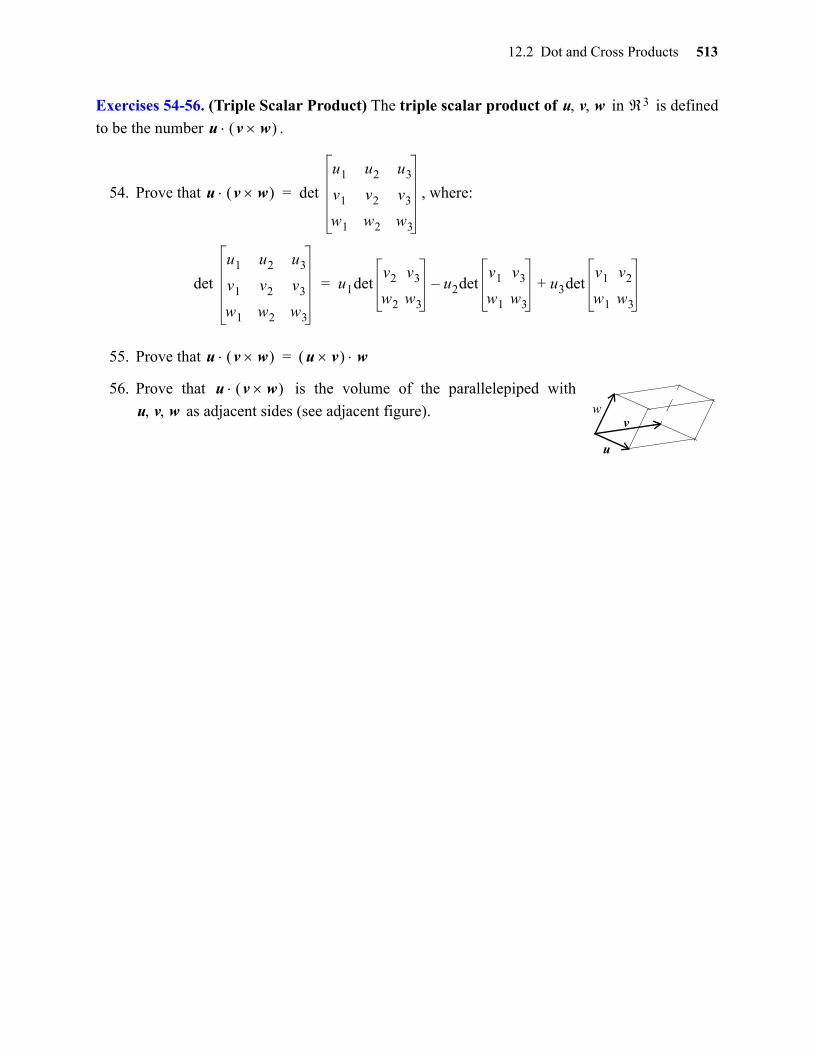
12.2 Dot and Cross Products 513
Exercises 54-56. (Triple Scalar Product) The triple scalar product of in is defined
to be the number .
54. Prove that , where:
55. Prove that
56. Prove that is the volume of the parallelepiped with
as adjacent sides (see adjacent figure).
u v w 3
u v w
u v w det
u1 u2 u3
v1 v2 v3
w1 w2 w3
=
det
u1 u2 u3
v1 v2 v3
w1 w2 w3
u1detv2 v3
w2 w3
u2detv1 v3
w1 w3
– u3detv1 v2
w1 w3
+=
u v w u v w=
u
vw
u v w u v w
gio
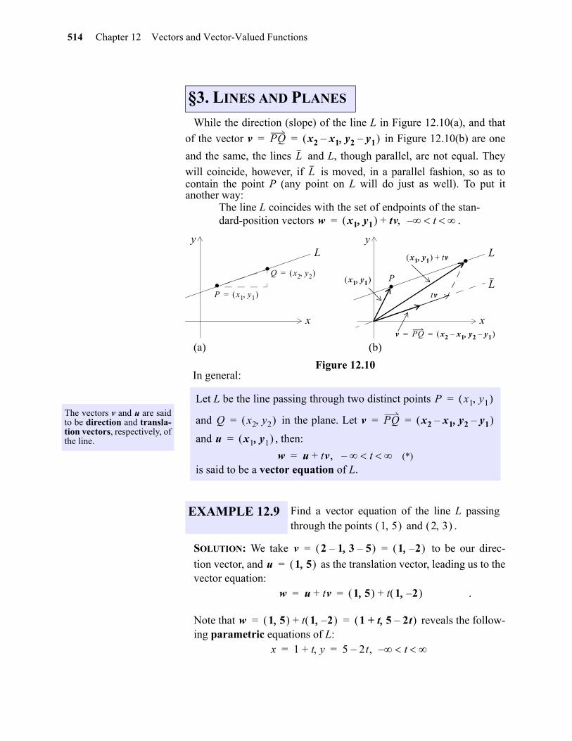
514 Chapter 12 Vectors and Vector-Valued Functions
12
While the direction (slope) of the line L in Figure 12.10(a), and that
of the vector in Figure 12.10(b) are one
and the same, the lines and L, though parallel, are not equal. They
will coincide, however, if is moved, in a parallel fashion, so as tocontain the point P (any point on L will do just as well). To put itanother way:
The line L coincides with the set of endpoints of the stan-dard-position vectors .
Figure 12.10In general:
SOLUTION: We take to be our direc-
tion vector, and as the translation vector, leading us to thevector equation:
.
Note that reveals the follow-ing parametric equations of L:
§3. LINES AND PLANES
v PQ x2 x1– y2 y1– = =
L
L
w x1 y1 tv t –+=
. .P x1 y1 =
Q x2 y2 =
x
y
(a) (b)
L
.x1 y1
x
yL
L
v PQ x2 x1– y2 y1– = =
P
x1 y1 tv+
tv
.
The vectors v and u are saidto be direction and transla-tion vectors, respectively, ofthe line.
Let L be the line passing through two distinct points
and in the plane. Let
and , then:
is said to be a vector equation of L.
EXAMPLE 12.9 Find a vector equation of the line L passingthrough the points and .
P x1 y1 =
Q x2 y2 = v PQ x2 x1– y2 y1– = =
u x1 y1 =
w u tv, t –+= (*)
1 5 2 3
v 2 1 3 5–– 1 2– = =
u 1 5 =
w u tv+ 1 5 t 1 2– += =
w 1 5 t 1 2– + 1 t+ 5 2t– = =
x 1 t y+ 5 2t, t ––= =
gio
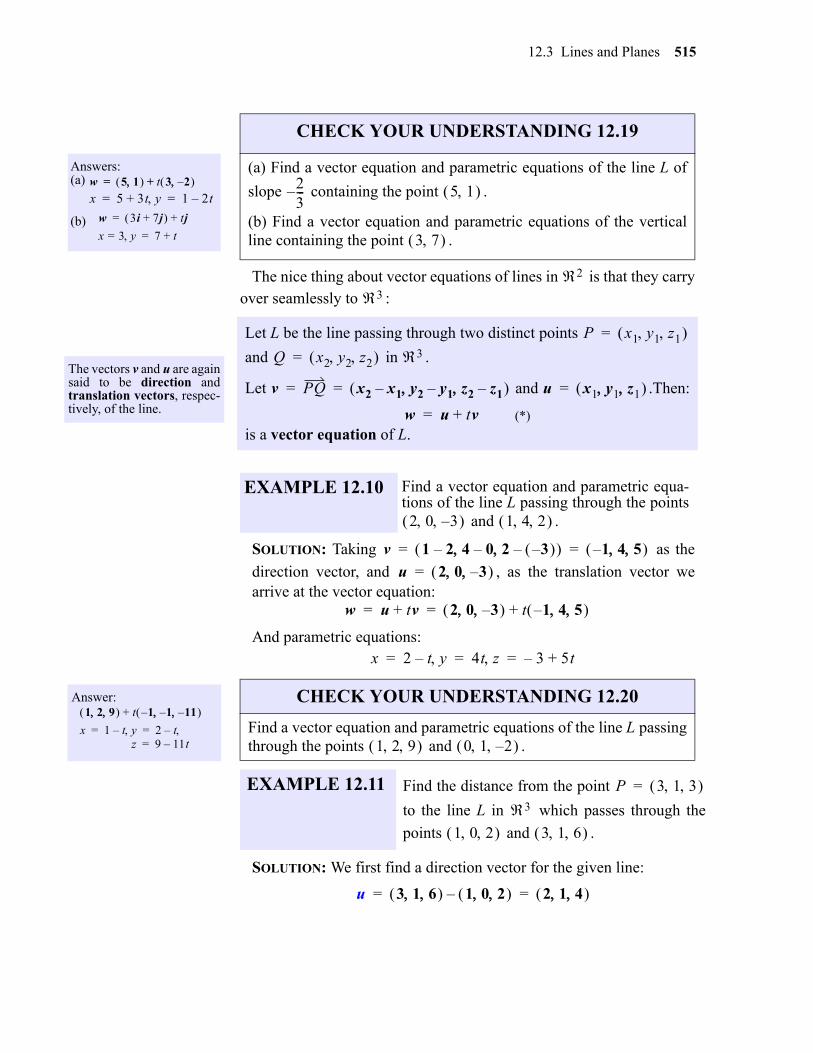
12.3 Lines and Planes 515
The nice thing about vector equations of lines in is that they carryover seamlessly to :
SOLUTION: Taking as the
direction vector, and , as the translation vector wearrive at the vector equation:
And parametric equations:
SOLUTION: We first find a direction vector for the given line:
Answers: (a)
(b)
The vectors v and u are againsaid to be direction andtranslation vectors, respec-tively, of the line.
x 5 3t y+ 1 2t–= =w 5 1 t 3 2– +=
w 3i 7j+ tj+=
x 3= y 7 t+=
CHECK YOUR UNDERSTANDING 12.19
(a) Find a vector equation and parametric equations of the line L of
slope containing the point .
(b) Find a vector equation and parametric equations of the verticalline containing the point .
Let L be the line passing through two distinct points
and in .
Let and .Then:
is a vector equation of L.
EXAMPLE 12.10 Find a vector equation and parametric equa-tions of the line L passing through the points
and .
23---– 5 1
3 7
2
3
P x1 y1 z1 =
Q x2 y2 z2 = 3
v PQ x2 x1 y2 y1–– z2 z1– = = u x1 y1 z1 =
w u tv+= (*)
2 0 3– 1 4 2
Answer: 1 2 9 t 1 1– 11– – +
x 1 t y– 2 t–= =z 9 11t–=
CHECK YOUR UNDERSTANDING 12.20
Find a vector equation and parametric equations of the line L passingthrough the points and .
EXAMPLE 12.11 Find the distance from the point
to the line L in which passes through the
points and .
v 1 2 4 0 2 3– ––– 1 4 5 – = =
u 2 0 3– =
w u tv+ 2 0 3– t 1 4 5 – += =
x 2 t y– 4t z 3– 5t+= = =
1 2 9 0 1 2–
P 3 1 3 =
3
1 0 2 3 1 6
u 3 1 6 1 0 2 – 2 1 4 = =
gio
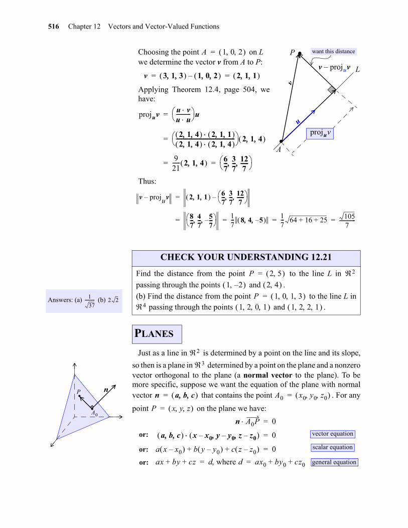
516 Chapter 12 Vectors and Vector-Valued Functions
Choosing the point on L we determine the vector v from A to P:
Applying Theorem 12.4, page 504, wehave:
Thus:
Just as a line in is determined by a point on the line and its slope,
so then is a plane in determined by a point on the plane and a nonzerovector orthogonal to the plane (a normal vector to the plane). To bemore specific, suppose we want the equation of the plane with normalvector that contains the point . For any
point on the plane we have:
u
v
.P
L
.A
want this distance
projuv
v projuv–
A 1 0 2 =
v 3 1 3 1 0 2 – 2 1 1 = =
projuvu vu u----------- u=
2 1 4 2 1 1 2 1 4 2 1 4
-------------------------------------------- 2 1 4 =
921------ 2 1 4 6
7--- 3
7--- 12
7------
= =
v projuv– 2 1 1 67--- 3
7--- 12
7------
–=
87--- 4
7--- 5
7---–
17--- 8 4 5– 1
7--- 64 16 25+ + 105
7-------------= = = =
Answers: (a) (b) 1
37---------- 2 2
CHECK YOUR UNDERSTANDING 12.21
Find the distance from the point to the line L in
passing through the points and .
(b) Find the distance from the point to the line L in passing through the points and .
PLANES
P 2 5 = 2
1 2– 2 4 P 1 0 1 3 =
4 1 2 0 1 1 2 2 1
..
A0
P n
2
3
n a b c = A0 x0 y0 z0 =
P x y z =
n A0P 0=
a b c x x0 y y0–– z z0– 0=
a x x0– b y y0– c z z0– + + 0=
or:
or:
ax by cz+ + d where d ax0 by0 cz0+ += =or:
vector equation
scalar equation
general equation
gio
12.3 Lines and Planes 517
gio
SOLUTION:
SOLUTION: Noting that the vectors
and are parallel to the plane, we employ Theorem 12.5, page 507, to find a normal to the plane:
Choosing the point on the plane, we proceed as in Example 12.12 to arrive at the general equation of the plane:
EXAMPLE 12.12 Find a vector, scalar, and general equation ofthe plane passing through the point
with normal vector .
Note that you can easily spot the normal tothe plane in any of the above equations.
1 3 2– n 4 1– 5 =
4 1– 5 x 1– y 3– z 2+ 0=
4 x 1– 1 y 3– – 5 z 2+ + 0=
4x y– 5z+ 9–=
vector:
scalar:general:
n 4 1– 5 =
Answer: See Page A-16.
CHECK YOUR UNDERSTANDING 12.22
Find a vector, scalar, and general equation of the plane passingthrough the point with normal parallel to the line contain-ing the points .
EXAMPLE 12.13 Find the general equation of the plane thatcontains the points ,
, .
1 3 2– 1 1 0 0 2 1
A 1 2 1– =
B 2 3 1 = C 3 1 2– =
AB 2 3 1 1 2 1– – 1 1 2 = =
AC 3 1 2– 1 2 1– – 2 3– 3 = =
n deti j k
1 1 2
2 3– 3
9i j 5k–+ 9 1 5– = = =
A 1 2 1– =
9 1 5– x 1– y 2– z 1+ 0=
9 x 1– y 2– 5 z 1+ –+ 0=
9x y 5z–+ 16=
Answer: 2x y z+ + 6=
CHECK YOUR UNDERSTANDING 12.23
Find the general equation of the plane that contains the points, , .A 3 2– 2 = B 2 5 3– = C 4 1 3– =
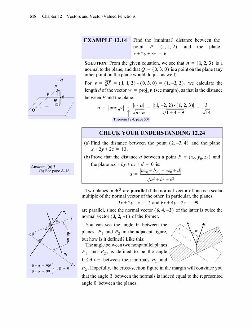
518 Chapter 12 Vectors and Vector-Valued Functions
SOLUTION: From the given equation, we see that is anormal to the plane, and that is a point on the plane (anyother point on the plane would do just as well).
For , we calculate the
length d of the vector (see margin), as that is the distance
between P and the plane:
Two planes in are parallel if the normal vector of one is a scalarmultiple of the normal vector of the other. In particular, the planes
and
are parallel, since the normal vector of the latter is twice thenormal vector of the former.
You can see the angle between the
planes and in the adjacent figure,
but how is it defined? Like this:The angle between two nonparallel planes
and , is defined to be the angle
between their normals and
. Hopefully, the cross-section figure in the margin will convince you
that the angle between the normals is indeed equal to the represented
angle between the planes.
EXAMPLE 12.14 Find the (minimal) distance between thepoint and the plane
.
P 1 1 2 =
x 2y 3z+ + 6=
Answers: (a) 3 (b) See page A-16.
Q
P
n
v }dw
CHECK YOUR UNDERSTANDING 12.24
(a) Find the distance between the point and the plane.
(b) Prove that the distance d between a point and
the plane is:
n 1 2 3 =Q 0 3 0 =
v QP 1 1 2 0 3 0 – 1 2 2– = = =
w projnv=
d projnv v nn n
--------------- 1 2 2– 1 2 3 1 4 9+ +
-------------------------------------------------- 3
14----------= = = =
Theorem 12.4, page 504
2 3 4– x 2y 2z+ + 13=
P x0 y0 z0 =
ax by cz d+ + + 0=
dax0 by0 cz0 d+ + +
a2 b2 c2+ +-------------------------------------------------=
+ 90=
+ 90=
=
planes
P1
P2
n1
n2
3
3x 2y z–+ 7= 6x 4y 2z–+ 99=
6 4 2– 3 2 1–
P1 P2
P1 P2
P1 P2
0 n1
n2
gio
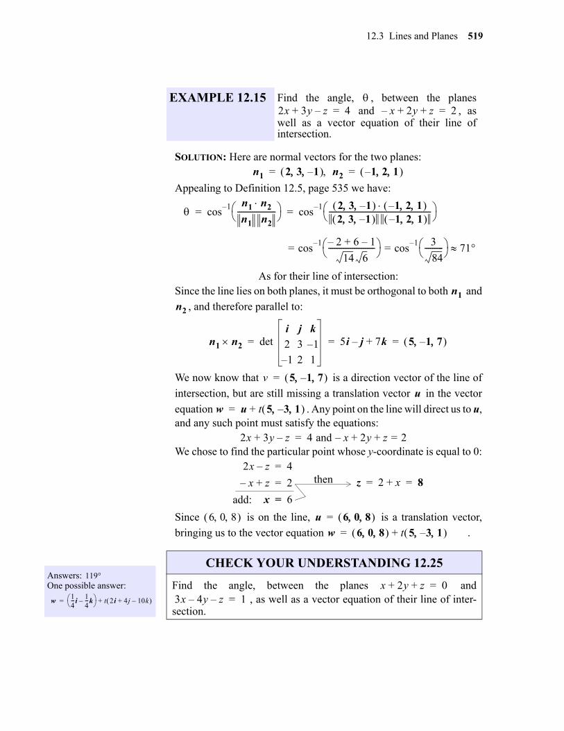
12.3 Lines and Planes 519
SOLUTION: Here are normal vectors for the two planes:
Appealing to Definition 12.5, page 535 we have:
As for their line of intersection:Since the line lies on both planes, it must be orthogonal to both and
, and therefore parallel to:
We now know that is a direction vector of the line of
intersection, but are still missing a translation vector in the vector
equation . Any point on the line will direct us to u,and any such point must satisfy the equations:
We chose to find the particular point whose y-coordinate is equal to 0:
Since is on the line, is a translation vector,
bringing us to the vector equation .
EXAMPLE 12.15 Find the angle, , between the planes and , as
well as a vector equation of their line ofintersection.
2x 3y z–+ 4= x– 2y z+ + 2=
n1 2 3 1– n2 1– 2 1 = =
cos1– n1 n2
n1 n2--------------------- cos
1– 2 3 1– 1– 2 1 2 3 1– 1– 2 1
------------------------------------------------------- = =
cos1– 2– 6 1–+
14 6------------------------- cos
1– 3
84---------- = = 71
n1
n2
n1 n2 det i j k
2 3 1–
1– 2 1
5i j– 7k+ 5 1– 7 = = =
v 5 1– 7 =
u
w u t 5 3– 1 +=
2x 3y z–+ 4 and x– 2y z+ + 2==
2x z– 4=
x– z+ 2=
x 6=
z 2 x+ 8= =
add:
then
Answers: One possible answer:
119
w14--- i
14---k–
t 2i 4j 10k–+ +=
CHECK YOUR UNDERSTANDING 12.25
Find the angle, between the planes and, as well as a vector equation of their line of inter-
section.
6 0 8 u 6 0 8 =
w 6 0 8 t 5 3– 1 +=
x 2y z+ + 0=3x 4y– z– 1=
gio
520 Chapter 12 Vectors and Vector-Valued Functions
Exercises 1-4. Find a vector equation and parametric equations of the given line L.
5. With respect to the line L in passing through the points , show that the twovector equations
and are one and the same by verifying that each vector in either representation is also a vector in theother.
6. With respect to the line L in passing through the points , show that thetwo vector equations
and are one and the same, by verifying that each vector in either representation is also a vector inthe other.
7. (a) Find the distance from the point to the line L in passing through the points
and .
(b) Find the distance from the point to the line L in passing through thepoints and .
(c) Find the distance from the point to the line L in passing through thepoints and .
8. (a) Find the distance from the point to the line L in passing through the points
and .
(b) Find the distance from the point to the line L in passing through thepoints and .
(c) Find the distance from the point to the line L in passing through thepoints and .
Exercises 9-12. Find a vector, scalar, and general equation of the plane with given normal vectorn that contains the given point Q.
EXERCISES
1. L in has slope 3 and contains the point .
2. L in passes through the points .
3. L in passes through the points .
4. L in passes through the points .
9. , 10. ,
11. , 12. ,
R2 1 3
R2 2 5– 1 0
R3 2 3 1 0 1 1–
R4 0 1 1 3 2– 0 1 2
R2 1 1 1 0
w 1 1 t 1 1 1 0 – += w 1 0 t 1 0 1 1 – +=
R3 1 1 1 1 2 0
w 1 1 1 t 1 1 1 1 2 0 – += w 1 2 0 t 1 1 1 1 2 0 – +=
P 1 5 = 2
2 3 0 4 P 2 0 3 = 3
1 2 2 2 0 4 P 1 0 1 0 = 4
2 2 1 1 1 0 2 1
P 5 3 = 2
2 2 1 4 P 1 1 1– = 3
3 0 1 2 1 3 P 1 3 1 1– = 4
0 2 0 1 1 3 1 1
n 1 4 2 = Q 2 0 3 = n 2i j 3k–+= Q 2 1 3– =
n 3i 2j k–+= Q 1 1 2 = n 2 2– 2 = Q 1 1– 5 =
gio
12.3 Lines and Planes 521
Exercises 13-16. Find the general equation of the plane containing the given points.
17. Find the distance between the point and the plane .
18. Find the distance between the point and the plane .
19. Find the distance between the origin and the plane with normal that contains
the point .
20. Find the distance between the point and the plane containing the points ,
, .
21. Find the distance between the point and the plane containing the point
that is parallel to the plane .
22. Find the values of x for which is 10 units from the plane .
23. Find the values of a for which the point is 1 unit from the plane .
24. Find an equation of the line that is common to the planes and
.
25. Find two planes that intersect in the line in the x, y-plane.
26. Find the angle between the planes and .
27. Find the angle between the planes and .
28. Find an equation of the plane consisting of all point that are equidistant from the points and .
29. Find an equation of the line containing the point that is parallel to the plane
and perpendicular to the line .
30. Verify that the plane contains the line .
31. Find an equation of the plane that contains the point and the line of intersection of
the planes and .
32. Find an equation of the plane containing the point that is perpendicular to the line
passing through the points and .
33. Find an equation of the plane that is perpendicular to each of the planes and
and contains the point .
13. , , 14. , ,
15. , , 16. , ,
1 2 0 2 1 2– 0 0 3 0 2 4– 1 1 1 2 0 0
1 1 0 0 2– 1 0 0 1 1 1 0 2 1 2 0 0 0
1 2 2 x y 2z+ + 4=
3 0 1 2x– 2z+ 3=
n 1 4 2 =
2 1 3
3 3 2– 1 1 0 0 2– 1 0 0 1
2 3 3– 1 2 2 3x 2y– 3z+ 1=
x 1 1 3x 2y– 3z+ 1=
3 0 1 ax 2y z+ + 3=
3x 2y– 3z+ 1=
ax 2y z–+ 3=
y 3x 2+=
2x 3y– 6z+ 5= 3x y 2z+ + 6=
x y z+ + 1= x y– z+ 1=
3 4 0 1 0 2–
0 1 2 x y z+ + 2= w 1 1 0 t 1 1 2– +=
5x 3y– z– 6– 0= w 1 1– 2 t 2 3 1 +=
2 1 3– 3x y z–+ 2= 2x y 4z+ + 1=
4 1 6– 1 6 2 – 8 10 2– –
2x y z–+ 2–=
x y– 3z+ 1= 1 3 2–
gio
522 Chapter 12 Vectors and Vector-Valued Functions
34. Show that the line is parallel to the plane
and find the distance between them.
35. Find the minimal distant between the line and the line
.
x 1– t y+ 3 2t z+ t–= = =
2– x 2y 2z+ + 3=
x 1 4t y+ 5 4t z– 1– 5t+= = =
x 2 8t y+ 4 3t z– 5 t+= = =
gio
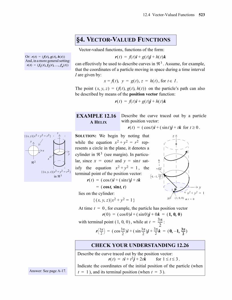
12.4 Vector-Valued Functions 523
12
Vector-valued functions, functions of the form:
can effectively be used to describe curves in . Assume, for example,that the coordinates of a particle moving in space during a time intervalI are given by:
, for .
The point on the particle’s path can alsobe described by means of the position vector function:
SOLUTION: We begin by noting that
while the equation rep-resents a circle in the plane, it denotes a
cylinder in (see margin). In particu-
lar, since and sat-
isfy the equation , theterminal point of the position vector:
lies on the cylinder:
At time , for example, the particle has position vector
with terminal point , while at :
§4. VECTOR-VALUED FUNCTIONS
Or: And, in a more general setting:
r t f t g t h t =
r t f1 t f2 t fn t =
x
y
x
y
z
x y z x2 y2+ r2=
x y x2 y2+ r2=
r
2
in 3
EXAMPLE 12.16A HELIX
Describe the curve traced out by a particlewith position vector:
for .
r t f t i g t j h t k+ +=
3
x f t = y g t , z h t = = t I
x y z f t g t h t =
r t f t i g t j h t k+ +=
r t tcos i tsin j tk+ += t 0
z
x
y..
1x2 y2+ 1=
0 132
------–
at t32 ------
=
1 0 0
x2 y2+ r2=
3
x tcos= y tsin=
x2 y2+ 1=
r t tcos i tsin j tk+ +=
t t tsincos =
x y z x2 y2+ 1=
t 0=r 0 0cos i 0sin j 0k+ + 1 0 0 = =
1 0 0 t 32
------=
r 32
------ 3
2------cos i 3
2------sin j 3
2------k+ + 0 1 3
2------– = =
Answer: See page A-17.
CHECK YOUR UNDERSTANDING 12.26
Describe the curve traced out by the position vector: for .
Indicate the coordinates of the initial position of the particle (when), and its terminal position (when ).
r t ti t2j 2tk+ += 1 t 3
t 1= t 3=
at t 0=
gio
524 Chapter 12 Vectors and Vector-Valued Functions
Some previously encountered concepts naturally extend to vector-valued functions:
In the exercises you are invited to show that if and exist, then:
(the limit of a sum is the sum of the limits)That being the case, by looking at as the
sum of the three vector-valued functions , , and , we seethat:
(providing the component-limits exist)
Moreover (see CYU 12.27 below):
(providing the component-derivatives exist)Also (see Exercise 31):
(providing the component-integrals exist)
Compare with Definition2.2, page 53.
Compare with Definitionon page 57.
Compare with Definition3.1, page 66.
Compare with Definition5.2, page 167.
DEFINITION 12.8
LIMIT
CONTINUOUS
DERIVATIVE
INDEFINITE INTEGRAL
For given andvector , we say that r haslimit L as t approaches and write:
if for any given there exists such that:
if then
is continuous at if:
The derivative of at is the vector
given by:
(providing the limit exists)
where and C represents anarbitrary constant vector.
So: You can arrive at the limit, or derivative, or integral ofa vector-valued functions by performing those opera-tions on the real-valued components of the function.
r t f t i g t j h t k+ +=L ai bj ck+ +=
t0
r t t t0lim L=
0 0
0 t t0– r t L–
r t t0
r t t t0lim r t0 =
r t t0
r t0
r t0 1h--- r t0 h+ r t0 –
h 0lim=
r t td R t C+=
R t r t =
r1 t t t0lim r2 t
t t0lim
r1 t r2 t + t t0lim r1 t
t t0lim r2 t
t t0lim+=
r t f t i g t j h t k+ +=f t i g t j h t k
r t t t0lim f t
t t0lim i g t
t t0lim j h t
t t0lim k+ +=
r t f t i g t j h t k+ +=
r t td f t td i g t td j h t td k C+ + +=
gio
12.4 Vector-Valued Functions 525
gio
SOLUTION:
(a)
(b)
(c)
Given that the derivative of vector-valued functions may be per-formed by differentiating their real-valued components, one mightexpect that the derivative formulas for such functions mimic those ofreal-valued functions, and so they do:
EXAMPLE 12.17 Let . Deter-mine:
(a) (b) (c)
r t t3 1+ i tsin j 9k+ +=
r t t 2lim r t r t td
r t t 2lim t3 1+ i tsin
t 2lim+
t 2lim j 9 k
t 2lim+=
9i 2sin j 9k+ +=
r t t3 1+ i tsin j 9 k+ + 3t2 i tcos j+= =
r t td t3 1+ td i t tdsin j 9 td k++=
t4
4---- t+ i tcos j– 9t k C+ +=
Answers: (i)
(ii)
(iii)
(b) See page A##. gio new
ei12---j 1 ksin+ +
et i t– 2 1+
t2 1+ 2--------------------- j tcos k+ +
eti12--- t2 1+ ln j+
tcos k– C+
CHECK YOUR UNDERSTANDING 12.27
(a) For , determine:
(i) (ii) (iii)
(b) Show that if the real-valued functions f, g, and h, are differentia-ble, them so is the function , and:
r t et i tt2 1+------------- j tsin k+ +=
r t t 1lim r t r t td
r t f t i g t j h t k+ +=
r t f t i g t j h t k+ +=
As it is with real-valuedfunctions, a vector-val-ued function is saidto be differentiable if
exists throughoutits domain.
Since in a scalar times a vec-tor expression such as , thescalar c appears to the left ofthe vector v, the chain rule isgenerally not expressed inwhat might be considered tobe the more reminiscent form: .
Why is there no quotient rule?
r t
r t
cv
u f t u f t f t =
THEOREM 12.8 For given differentiable vector-valued func-
tions in , and any scalar c, and
any real-valued function :
(a)
(b)
(c) (see margin)
(d)
(e)
(f)
(g)
Theorems (a) through (f)hold in any . Rn
u t v t R3
f t cu t cu t =
f t u t f t u t f t u t +=
u f t f t u f t =
u t v t + u t v t +=
u t v t – u t v t –=
u t v t u t v t u t v t +=
u t v t u v t u t v t +=
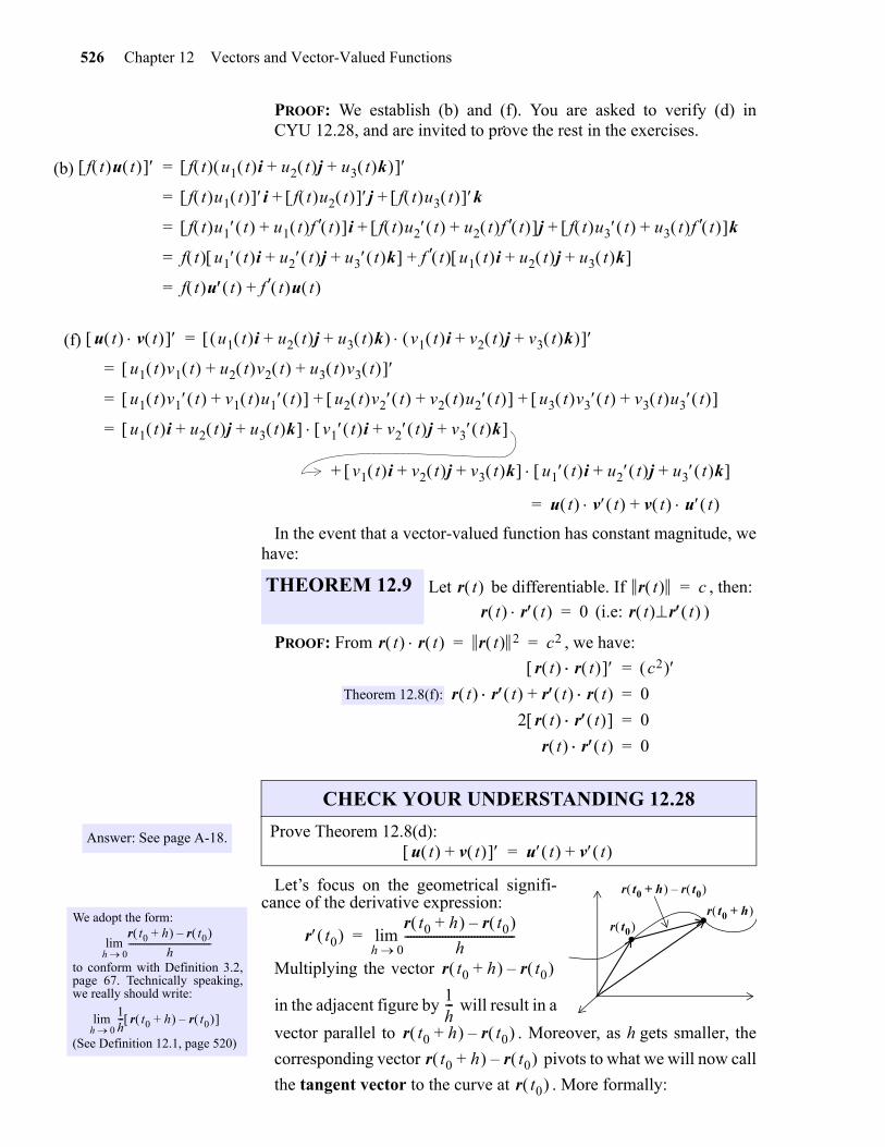
526 Chapter 12 Vectors and Vector-Valued Functions
(b
(
gio
PROOF: We establish (b) and (f). You are asked to verify (d) inCYU 12.28, and are invited to prove the rest in the exercises.
In the event that a vector-valued function has constant magnitude, wehave:
PROOF: From , we have:
Let’s focus on the geometrical signifi-cance of the derivative expression:
Multiplying the vector
in the adjacent figure by will result in a
vector parallel to . Moreover, as h gets smaller, the
corresponding vector pivots to what we will now call
the tangent vector to the curve at . More formally:
)
f)
f t u t f t u1 t i u2 t j u3 t k+ + =
f t u1 t i f t u2 t j f t u3 t k++=
f t u1 t u1 t f t + i f t u2 t u2 t f t + j f t u3 t u3 t f t + k+ +=
f t u1 t i u2 t j u3 t k+ + f t u1 t i u2 t j u3 t k+ + +=
f t u t f t u t +=
u t v t u1 t i u2 t j u3 t k+ + v1 t i v2 t j v3 t k+ + =
u1 t v1 t u2 t v2 t u3 t v3 t + + =
u1 t v1 t v1 t u1 t + u2 t v2 t v2 t u2 t + u3 t v3 t v3 t u3 t + + +=
u1 t i u2 t j u3 t k+ + v1 t i v2 t j v3 t k+ + =
v1 t i v2 t j v3 t k+ + u1 t i u2 t j u3 t k+ + +
u t v t v t u t +=
THEOREM 12.9 Let be differentiable. If , then:
(i.e: )
r t r t c=
r t r t 0= r t r t
r t r t r t 2 c2= =
r t r t c2 =
r t r t r t r t + 0=
2 r t r t 0=
r t r t 0=
Theorem 12.8(f):
Answer: See page A-18.
We adopt the form:
to conform with Definition 3.2,page 67. Technically speaking,we really should write:
(See Definition 12.1, page 520)
r t0 h+ r t0 –
h--------------------------------------
h 0lim
1h--- r t0 h+ r t0 –
h 0lim
CHECK YOUR UNDERSTANDING 12.28
Prove Theorem 12.8(d): u t v t + u t v t +=
. .r t0
r t0 h+
r t0 h+ r t0 –
r t0 r t0 h+ r t0 –
h--------------------------------------
h 0lim=
r t0 h+ r t0 –
1h---
r t0 h+ r t0 –
r t0 h+ r t0 –
r t0
:
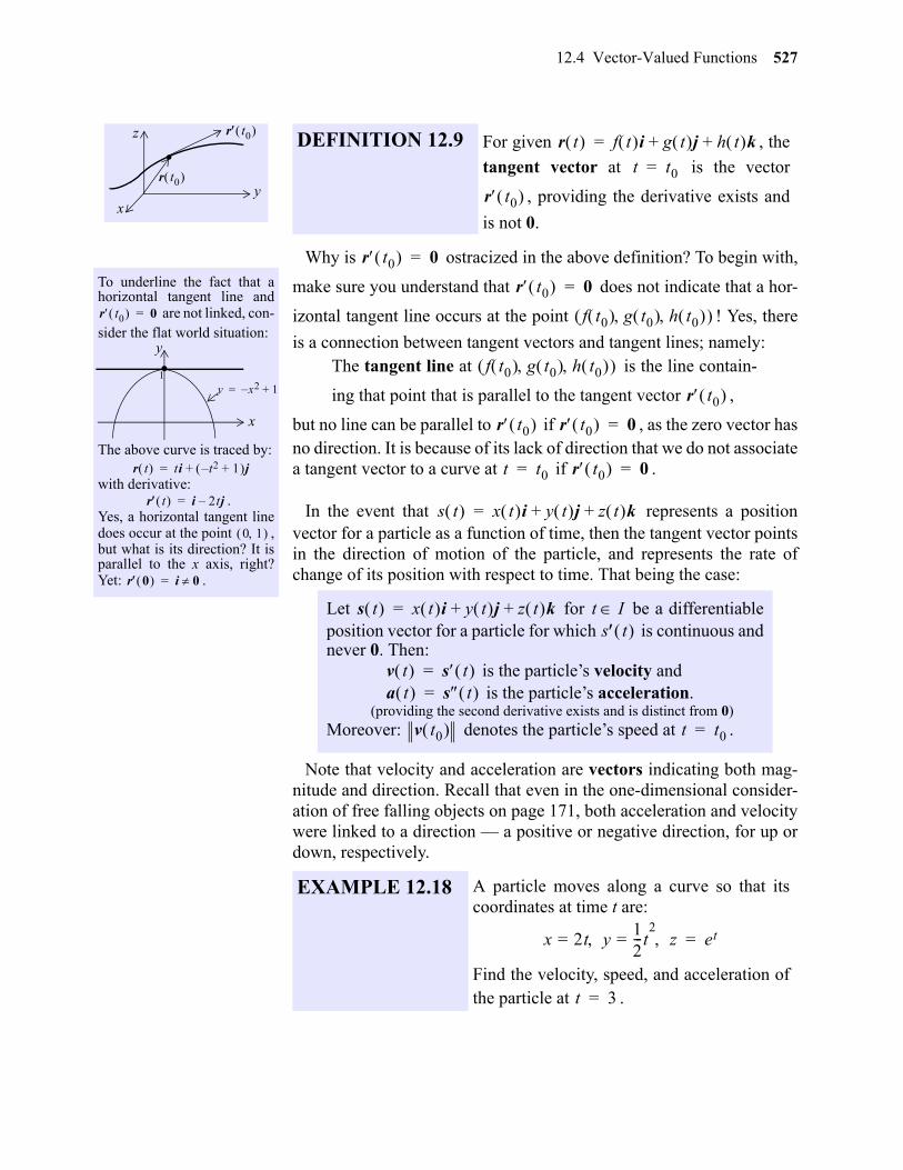
12.4 Vector-Valued Functions 527
Why is ostracized in the above definition? To begin with,
make sure you understand that does not indicate that a hor-
izontal tangent line occurs at the point ! Yes, there
is a connection between tangent vectors and tangent lines; namely:The tangent line at is the line contain-
ing that point that is parallel to the tangent vector ,
but no line can be parallel to if , as the zero vector hasno direction. It is because of its lack of direction that we do not associatea tangent vector to a curve at if .
In the event that represents a positionvector for a particle as a function of time, then the tangent vector pointsin the direction of motion of the particle, and represents the rate ofchange of its position with respect to time. That being the case:
Note that velocity and acceleration are vectors indicating both mag-nitude and direction. Recall that even in the one-dimensional consider-ation of free falling objects on page 171, both acceleration and velocitywere linked to a direction — a positive or negative direction, for up ordown, respectively.
.r t0
r t0
yx
z DEFINITION 12.9 For given , the
tangent vector at is the vector
, providing the derivative exists and
is not 0.
r t f t i g t j h t k+ +=
t t0=
r t0
To underline the fact that ahorizontal tangent line and
are not linked, con-sider the flat world situation:
The above curve is traced by:
with derivative: .
Yes, a horizontal tangent linedoes occur at the point ,but what is its direction? It isparallel to the x axis, right?Yet: .
r t0 0=
y x– 2 1+=
x
y.1
r t ti t– 2 1+ j+=
r t i 2tj–=
0 1
r 0 i 0=
Let for be a differentiableposition vector for a particle for which is continuous andnever 0. Then:
is the particle’s velocity and is the particle’s acceleration.
(providing the second derivative exists and is distinct from 0)Moreover: denotes the particle’s speed at .
EXAMPLE 12.18 A particle moves along a curve so that itscoordinates at time t are:
Find the velocity, speed, and acceleration ofthe particle at .
r t0 0=
r t0 0=
f t0 g t0 h t0
f t0 g t0 h t0
r t0
r t0 r t0 0=
t t0= r t0 0=
s t x t i y t j z t k+ +=
s t x t i y t j z t k+ += t Is t
v t s t =a t s t =
v t0 t t0=
x 2t y 12---t
2= = z et=
t 3=
gio
528 Chapter 12 Vectors and Vector-Valued Functions
SOLUTION: Focusing on the position vector:
we have:
and:
In particular, at :
And: .
SOLUTION: Since :
Since :
s t 2ti12---t
2j etk+ +=
v t r t 2i tj etk+ += =
a t v t j etk+= =
t 3=
v 3 2i 3j e3k and a 3 + + j e3k+= =
Speed at t 3: v 3 22 32 e3 2+ + 13 e6+= = =
Answer:v t tsin– i tcos j k+ +=
a t tcos – i tsin j–=
v t 2=
CHECK YOUR UNDERSTANDING 12.29
Find the velocity, acceleration, and speed of the particle movingalong the helix traced by .
EXAMPLE 12.19 Find and of a particle with initial
velocity and initial position
given that:
for .
s t tcos i tsin j tk+ +=
v t s t v 0 i 2j+=
s 0 i j k+ +=
a t 4ti 2tj 3t2k–+= t 0
Letting in we find that:
(as in Theorem 5.5, page 171)
At : .
t 0=
v t 2t2i t2j t3k– C+ +=
C v 0 v0= =
t 0= s 0 s0=
a t dvdt------=
v t a t td 4ti 2tj 3t2k–+ td 2t2i t2j t3k– C+ += = =
2t2i t2j t3k– v0+ +=
2t2i t2j t3k– i 2j+ + +=
2t2 1+ i t2 2+ j t3k–+=
see margin
v t drdt-----=
s t v t td 2t2 1+ i t2 2+ j t3k–+ td= =
2t3
3------- t+ i t3
3---- 2t+ j
t4
4----k– s0+ +=
2t3
3------- t+ i t3
3---- 2t+ j
t4
4----k– i j k+ + + +=
2t3
3------- t 1+ + i t3
3---- 2t 1+ + j t4
4---- 1– k–+=
see margin
gio
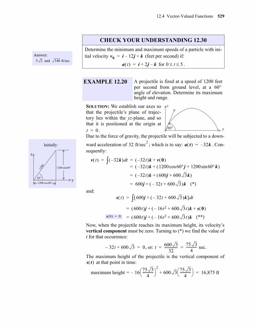
12.4 Vector-Valued Functions 529
gio
SOLUTION: We establish our axes sothat the projectile’s plane of trajec-tory lies within the yz-plane, and sothat it is positioned at the origin at
.Due to the force of gravity, the projectile will be subjected to a down-
ward acceleration of ; which is to say: . Con-sequently:
and:
Now, when the projectile reaches its maximum height, its velocity’svertical component must be zero. Turning to (*) we find the value oft for that occurrence:
The maximum height of the projectile is the vertical component of at that point in time:
Answer:5 2 and 146 ft/sec.
CHECK YOUR UNDERSTANDING 12.30
Determine the minimum and maximum speeds of a particle with ini-tial velocity (feet per second) if:
for .
EXAMPLE 12.20 A projectile is fired at a speed of 1200 feetper second from ground level, at a angle of elevation. Determine its maximumheight and range.
v0 i 12j– k+=
a t i 2j k–+= 0 t 5
60
z
y60t 0=
1200 1200 60sin
1200 60cos
60
Initially:
y
z
32 ft/sec2
a t 32k–=
v t 32k– td 32t– k v 0 += =32t– k 1200 60j 1200 60ksin+cos +=
32t– k 600j 600 3k+ +=
600j 32t– 600 3+ k+= (*)
s t 600j 32t– 600 3+ k+ td=
600t j 16t2– 600 3t+ k s 0 + +=
600t j 16t2– 600 3t+ k+=s 0 0:= (**)
32t– 600 3+ 0, or: t 600 332
----------------75 3
4------------- sec.= = =
s t
maximum height 1675 3
4-------------
2
– 600 3+=75 3
4------------- 16,875 ft=
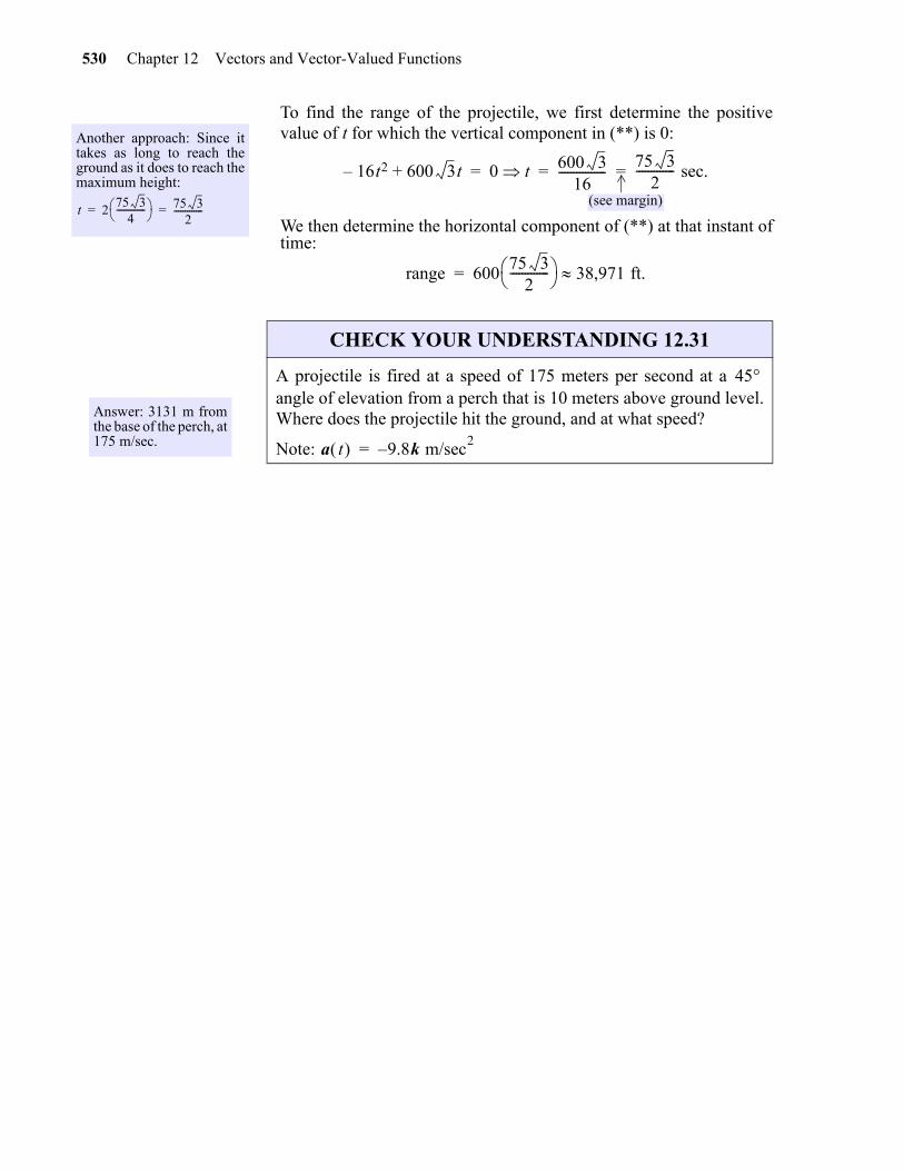
530 Chapter 12 Vectors and Vector-Valued Functions
To find the range of the projectile, we first determine the positivevalue of t for which the vertical component in (**) is 0:
We then determine the horizontal component of (**) at that instant oftime:
Another approach: Since ittakes as long to reach theground as it does to reach themaximum height:
t 275 3
4------------- 75 3
2-------------= =
16t2– 600 3t+ 0 t 600 316
----------------75 3
2------------- sec.= = =
(see margin)
range 60075 3
2------------- 38,971 ft.=
Answer: 3131 m fromthe base of the perch, at175 m/sec.
CHECK YOUR UNDERSTANDING 12.31
A projectile is fired at a speed of 175 meters per second at a angle of elevation from a perch that is 10 meters above ground level.Where does the projectile hit the ground, and at what speed?
Note:
45
a t 9.8k m/sec2
–=
gio
12.4 Vector-Valued Functions 531
Exercises 1-6. Sketch, in , the graph of the curve with given position vector.
Exercises 7-16. Determine , , and for the given vector function.
Exercises 17-20. Find parametric equations for the tangent line at the specified point on the curvewith given position vector.
Exercises 21-24. Find the velocity, acceleration, and speed of the particle moving along the givenpath at the indicated time.
25. Determine the minimum and maximum speed of a particle with initial velocity (feet per second) and , within the interval .
EXERCISES
1. , 2. ,
3. , 4.
5. 6.
7. 8.
9. 10.
11. 12.
13. 14.
15. 16.
17. , . 18. ,
19. , 20. ,
21. , 22. ,
23. , 24.
R3
r t ti= 0 t 1 r t ti 2tj+= 0 t 1
r t ti tj 4k+ += 1 t 2 r t tcos i tsin j– k 0 t2--- +=
r t 3i tj t2k 1– t 2 + += r t ti tj tsin k 0 t 2 + +=
r t t 1lim r t r t td
r t 2ti 5t2j+= r t 2ti 5t2j k+ +=
r t tsin i t2j–= r t tsin i t2j– etk+=
r t ti j k+ += r t et2 i 2t j t 1–t
----------k+sin–=
r t ti 3j–tln
t------- k+= r t t
t 1+-----------i
t 1+t3
-----------j k–+=
r t ti t2j– ttan k+= r t t t2sin i tj t tcos k–+=
r t 2ti 5t2j+= t 1= r t ti t2j t3k+ += t 0=
r t tsin i 2 tcos j– k+= t 0= r t tsin i t2j– etk+= t =
r t ti 2tj+= t 1= r t ti j t2k+ += t 0=
r t tsin i tj tcos k+ += t 0= r t ti tj– e2tk+= t 4=
v0 i 12j– k+= a t 2i j k–+= 0 t 6
gio
532 Chapter 12 Vectors and Vector Valued Functions
26. Determine the minimal and maximum speed of a particle with initial velocity (feet
per second) and , within the interval for .
Exercises 27-30. Prove:
30. Show that if and exist, then:
31. Show that for :
(providing the component-integrals exist)
32. Prove that any two antiderivatives of a vector-valued function can only differ by a con-stant vector C.
33. A projectile is fired at a speed of 500 meters per second at a angle of elevation, from apoint that is 30 meters above ground level. Find its speed when it hits the ground.
34. A projectile is fired at a speed of 800 feet per second from ground level, at a angle of ele-vation. Determine its maximum height, range, and speed when it hits the ground.
35. A projectile is fired from ground level with initial velocity feet per sec-ond. Determine its maximum height, range, and speed when it hits the ground.
36. Repeat Exercise 32 given a constant wind velocity of:
(a) feet per second. (b) feet per second.
37. A stone is thrown downward from the top of a 168 foot building, at an angle of depression of at a speed of 80 ft/sec. How far from the base of the building will the stone land?
38. A golf ball is hit at a speed of 90 feet per second at a angle of elevation. Will it clear thetop of a 35 foot tree that is 135 feet away?
39. Referring to Exercise 36, determine the minimum speed for which the ball will clear the tree(maintaining the angle of elevation).
40. Referring to Exercise 36, can the angle of elevation be adjusted so as to clear the tree (main-taining the 90 feet per second initial speed)?
41. At what speed must a stone be thrown horizontally from a point that is 25 feet above groundlevel if it is to hit a bottle sitting on a 4 foot pole 45 feet away?
42. At what speed must a stone be thrown at an angle of elevation of so as to achieve a max-imum height of 25 feet?
27. Theorem 12.8(a) and (e) 28. Theorem 12.8(g) 29. Theorem 12.8(c)
v0 i k–=
a t tsin i tcos j tk–+= 0 t2---
r1 t t t0lim r2 t
t t0lim
r1 t r2 t + t t0lim r1 t
t t0lim r2 t
t t0lim+=
r t f t i g t j h t k+ +=
r t td f t td i g t td j h t td k C+ + +=
r t
45
45
v 0 100j 100k+=
2j 2j k+
60
30
30
30
gio
12.4 Vector-Valued Functions 533
43. At what speed must a stone be thrown at an angle of elevation of so as to achieve a rangeof 50 feet?
44. Find two angles of elevation that will enable a projectile fired from ground level at a speed of800 feet per second to hit a ground-level target 10,000 feet away.
45. Show that in order to achieve maximum range, a projectile must be fired at a angle of ele-vation.
46. Show that a projectile fired at an angle , with , has the same range as one firedat the same speed at the angle .
47. Show that doubling a projectile’s initial speed while maintaining its launching angle will qua-druple its range.
48. Show that a projectile attains three-quarters of its maximum height in half the time it takes forit to reach its maximum height.
49. Prove that if the acceleration vector of a particle is always 0, then the path of the particle is aline.
50. Assume that you take true aim at a bottle that is sitting on a y foot pole that is x feet down theroad from you. Show that if the bottle starts to fall just as you pull the trigger, then the bottlewill be hit, regardless of the muzzle speed of the gun.
51. Prove that any non-vertical trajectory of a projectile subjected solely to the force of gravity isparabolic.
30
45
0 90 90 –
gio
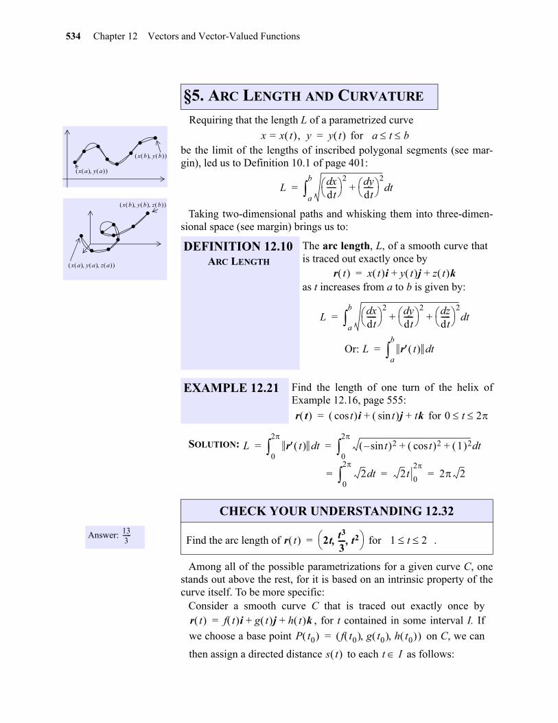
534 Chapter 12 Vectors and Vector-Valued Functions
12
Requiring that the length L of a parametrized curve
for be the limit of the lengths of inscribed polygonal segments (see mar-gin), led us to Definition 10.1 of page 401:
Taking two-dimensional paths and whisking them into three-dimen-sional space (see margin) brings us to:
SOLUTION:
Among all of the possible parametrizations for a given curve C, onestands out above the rest, for it is based on an intrinsic property of thecurve itself. To be more specific:
Consider a smooth curve C that is traced out exactly once by, for t contained in some interval I. If
we choose a base point on C, we can
then assign a directed distance to each as follows:
.. ... .. .x a y a
x b y b
.. .... .
..x b y b z b
x a y a z a
§5. ARC LENGTH AND CURVATURE
DEFINITION 12.10ARC LENGTH
The arc length, L, of a smooth curve thatis traced out exactly once by
as t increases from a to b is given by:
EXAMPLE 12.21 Find the length of one turn of the helix ofExample 12.16, page 555:
for
x x t = , y y t = a t b
Lxd
dt----- 2 yd
dt----- 2
+ tda
b
=
r t x t i y t j z t k+ +=
Lxd
dt----- 2 yd
dt----- 2 zd
dt----- 2
+ + tda
b
=
Or: L r t tda
b
=
r t tcos i tsin j tk+ += 0 t 2
L r t td0
2
tsin– 2 tcos 2 1 2+ + td0
2
= =
2 td0
2
2t0
22 2= = =
Answer: 133------
CHECK YOUR UNDERSTANDING 12.32
Find the arc length of for .r t 2t t3
3---- t2
= 1 t 2
r t f t i g t j h t k+ +=
P t0 f t0 g t0 h t0 =
s t t I
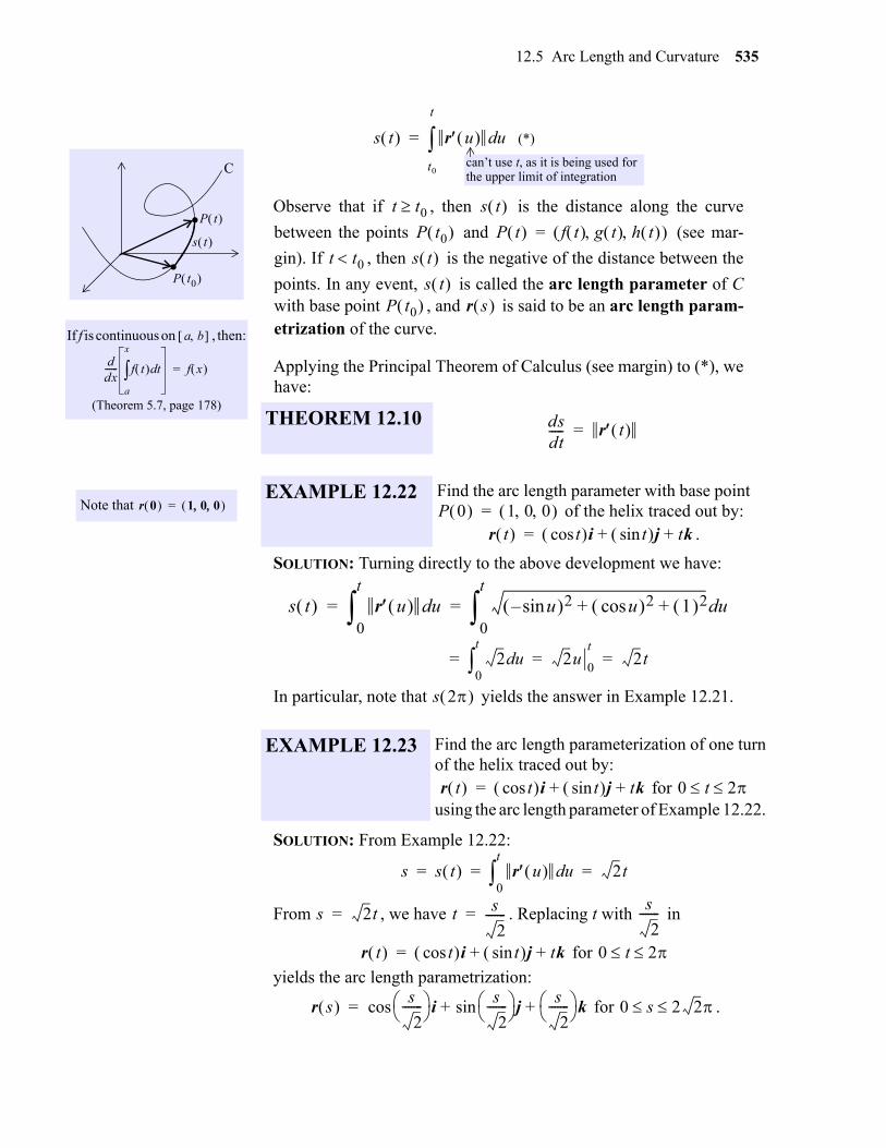
12.5 Arc Length and Curvature 535
Observe that if , then is the distance along the curve
between the points and (see mar-
gin). If , then is the negative of the distance between the
points. In any event, is called the arc length parameter of Cwith base point , and is said to be an arc length param-etrization of the curve. Applying the Principal Theorem of Calculus (see margin) to (*), wehave:
SOLUTION: Turning directly to the above development we have:
In particular, note that yields the answer in Example 12.21.
SOLUTION: From Example 12.22:
From , we have . Replacing t with in
for
yields the arc length parametrization:
for .
If f is continuous on , then:
.P t0
.P t
s t
C
a b
ddx------ f t td
a
x
f x =
(Theorem 5.7, page 178)THEOREM 12.10
s t r u ud
t0
t
=can’t use t, as it is being used for the upper limit of integration
(*)
t t0 s t P t0 P t f t g t h t =
t t0 s t s t
P t0 r s
dsdt----- r t =
Note that r 0 1 0 0 =EXAMPLE 12.22 Find the arc length parameter with base point
of the helix traced out by:.
EXAMPLE 12.23 Find the arc length parameterization of one turnof the helix traced out by: for using the arc length parameter of Example 12.22.
P 0 1 0 0 =r t tcos i tsin j tk+ +=
s t r u ud0
t
usin– 2 ucos 2 1 2+ + ud0
t
= =
2 ud0
t
2u0
t2t= = =
s 2
r t tcos i tsin j tk+ += 0 t 2
s s t r u ud0
t
2t= = =
s 2t= t s
2-------=
s
2-------
r t tcos i tsin j tk+ += 0 t 2
r s s
2------- i
s
2------- sin j
s
2------- k+ +cos= 0 s 2 2
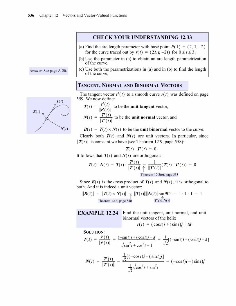
536 Chapter 12 Vectors and Vector-Valued Functions
The tangent vector to a smooth curve was defined on page559. We now define:
to be the unit tangent vector,
to be the unit normal vector, and
to be the unit binormal vector to the curve.
Clearly both and are unit vectors. In particular, since is constant we have (see Theorem 12.9, page 558):
It follows that and are orthogonal:
Since is the cross product of and , it is orthogonal toboth. And it is indeed a unit vector:
SOLUTION:
Answer: See page A-20.
CHECK YOUR UNDERSTANDING 12.33
(a) Find the arc length parameter with base point for the curve traced out by for .
(b) Use the parameter in (a) to obtain an arc length parametrizationof the curve.
(c) Use both the parametrizations in (a) and in (b) to find the lengthof the curve,
TANGENT, NORMAL AND BINORMAL VECTORS
P 1 2 1 2– =r t 2t t 2t– = 0 t 3
T t
N t
B t
EXAMPLE 12.24 Find the unit tangent, unit normal, and unitbinormal vectors of the helix
r t r t
T t r t r t
---------------=
N t T t T t
-----------------=
B t T t N t =
T t N t T t
T t T t 0=
T t N t
T t N t T t T t T t
----------------- 1T t
----------------- T t T t 0= = =
Theorem 12.2(c), page 533
B t T t N t
B t T t N t T t N t 90sin 1 1 1 1= = = =
Theorem 12.6, page 540 T t N t _
r t tcos i tsin j tk+ +=
T t r t r t
---------------- tsin– i tcos j k+ +
sin2t cos
2t 1+ +
-----------------------------------------------------1
2------- tsin– i tcos j k+ + = = =
N t T t T t
-----------------
1
2------- tcos– i tsin j–
1
2------- cos
2t sin
2t+
------------------------------------------------------ tcos– i tsin j–= = =
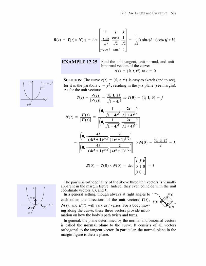
12.5 Arc Length and Curvature 537
SOLUTION: The curve is easy to sketch (and to see),for it is the parabola , residing in the y-z plane (see margin).As for the unit vectors:
The pairwise orthogonality of the above three unit vectors is visuallyapparent in the margin figure. Indeed, they even coincide with the unitcoordinate vectors i, j, and k.
In a general setting, though always at right angles toeach other, the directions of the unit vectors ,
, and will vary as t varies. For a body mov-ing along the curve, these three vectors provide infor-mation on how the body’s path twists and turns.
In general, the plane determined by the normal and binormal vectorsis called the normal plane to the curve. It consists of all vectorsorthogonal to the tangent vector. In particular, the normal plane in themargin figure is the x-z plane.
B t T t N t det
i j k
tsin
2---------–
tcos
2---------- 1
2------
tcos– tsin– 0
1
2------- tsin i tcos j– k+ = = =
EXAMPLE 12.25 Find the unit tangent, unit normal, and unitbinormal vectors of the curve:
at r t 0 t t2 = t 0=
x
y
z z y2=
x
y
z
T 0
N 0
B 0
r t 0 t t2 =z y2=
T t r t r t
----------------0 1 2t
1 4t2+----------------------- T 0 0 1 0 j= = = =
N t T t T t
-----------------
0 1
1 4t2+-------------------- 2t
1 4t2+--------------------
0 1
1 4t2+-------------------- 2t
1 4t2+--------------------
---------------------------------------------------------------= =
0 4t4t2 1+ 3 2/
----------------------------– 24t2 1+ 3 2/
----------------------------
0 4t4t2 1+ 3 2/
----------------------------– 24t2 1+ 3 2/
----------------------------
-------------------------------------------------------------------------------- N 0 0 0 2 2
------------------- k= = =
B 0 T 0 N 0 det i j k
0 1 0
0 0 1
i= = =
N t
T t
B t T t N t B t
538 Chapter 12 Vectors and Vector-Valued Functions
The plane determined by the normal and tangent vectors to a point ona curve is called the osculating plane, derived from the Latin osculum,for: “kiss.” It is a passionate kiss in that it contains more of the curve thanany other plane at that point. The osculating plane in the above marginfigure is the y-z plane which contains the entire curve.
You are invited to establish the following useful result in the exer-cises:
SOLUTION (Compare with solution of CYU 12.34):
Using the fact that (Exercise 30) we have:
Answer: See page A-20.
CHECK YOUR UNDERSTANDING 12.34
Find the unit tangent, unit normal, and unit binormal vectors of thecurve at , and then verify, directly that eachof the vectors is orthogonal to the remaining two.Determine the normal and osculating planes at .
THEOREM 12.11 If traces out asmooth curve, then the vector
has the same direction as the unit binormal
i.e:
EXAMPLE 12.26 Find the unit tangent, unit normal, and unitbinormal vectors of the curve
at
r t 2t t2 t– = t 1=
t 1=
r t f t i g t j h t k+ +=
B t det i j k
f t g t h t f t g t h t
=
B t B t B t B t
---------------=
r t 2t t2 t– = t 1=
T t 2t t2 t– 2t t2 t–
-------------------------------2 2t 1–
5 4t2+------------------------- T 1 1
3--- 2 2 1– == =
B 1 det i j k
f 1 g 1 h 1 f 1 g 1 h 1
det i j k
2 2 1–
0 2 0
2 0 4 = = = B 1 1
5------- 1 0 2 =
f t g t h t 2t t2 t– = f t g t h t 2 2t 1– f t g t h t 0 2 0 = =
N t B t T t =
N 1 B 1 T 1 det
i j k
1
5------- 0
2
5-------
23--- 2
3--- 1
3---–
= =1
3 5---------- 4– 5 2 =
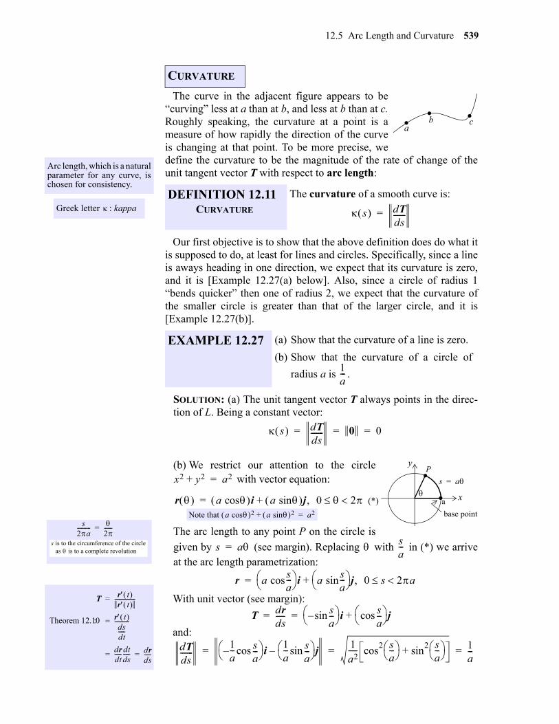
12.5 Arc Length and Curvature 539
The curve in the adjacent figure appears to be“curving” less at a than at b, and less at b than at c.Roughly speaking, the curvature at a point is ameasure of how rapidly the direction of the curveis changing at that point. To be more precise, wedefine the curvature to be the magnitude of the rate of change of theunit tangent vector T with respect to arc length:
Our first objective is to show that the above definition does do what itis supposed to do, at least for lines and circles. Specifically, since a lineis aways heading in one direction, we expect that its curvature is zero,and it is [Example 12.27(a) below]. Also, since a circle of radius 1“bends quicker” then one of radius 2, we expect that the curvature ofthe smaller circle is greater than that of the larger circle, and it is[Example 12.27(b)].
SOLUTION: (a) The unit tangent vector T always points in the direc-tion of L. Being a constant vector:
(b) We restrict our attention to the circle with vector equation:
The arc length to any point P on the circle is
given by (see margin). Replacing with in (*) we arriveat the arc length parametrization:
With unit vector (see margin):
and:
CURVATURE
Arc length, which is a naturalparameter for any curve, ischosen for consistency.
Greek letter : kappaDEFINITION 12.11
CURVATURE
The curvature of a smooth curve is:
EXAMPLE 12.27 (a) Show that the curvature of a line is zero.
(b) Show that the curvature of a circle of
radius a is .
. . .a
b c
s dTds-------=
1a---
s dTds------- 0 0= = =
s2a----------
2------=
s is to the circumference of the circle as is to a complete revolution
T r t r t
---------------=
r t dsdt-----
-----------=
drdt----- dt
ds----- dr
ds-----= =
Theorem 12.10:
x
y .P
.s a=
base point
a
x2 y2+ a2=
r a cos i a sin j, 0 2+=Note that a cos 2 a sin 2+ a2=
(*)
s a= sa---
r a cossa---
i a sinsa---
j, 0 s 2a+=
T drds----- s
a---sin–
i sa---cos
j+= =
dTds-------
1a--- s
a---cos–
i1a--- s
a---sin
j–1a2----- cos
2 sa--- sin
2 sa--- + 1
a---= = =
540 Chapter 12 Vectors and Vector-Valued Functions
The following curvature formula involves an arbitrary parameter t:
PROOF:
SOLUTION: Using the parametrization:
we have:
While more intimidating than the expression in Theorem 12.12, thefollowing representation for curvature is often the more practical to uti-lize:
PROOF: From we have:
Since the derivative of a vector-valued function is defined interms of the derivatives of itscomponents, the Chain RuleTheorem extends to vector-valued functions.
THEOREM 12.12 If traces out asmooth curve, then:
EXAMPLE 12.28 Use the above theorem to address Example12.27(b).
THEOREM 12.13 Let C be a smooth curve traced out by
The curvature at the point on C isgiven by:
r t f t i g t j h t k+ +=
T t r t
-----------------=
dTds-------
dTdt-------
dsdt------------
T t dsdt-----
----------------- T t r t
-----------------= = = =
Chain Rule Theorem 12.10
r t a cost i a sint j+=
T t r t
-----------------
r t r t
---------------
r t -------------------------------
a sint– i a cost j+
a sint– 2 a cost 2+---------------------------------------------------------
a sint– 2 a cost 2+-------------------------------------------------------------------------= = =
a sint– i a cost j+
a----------------------------------------------------
a--------------------------------------------------------------------=
sint– i cost j+
a
------------------------------------------------------------ cost– i sint j– a
------------------------------------------------------= =
tcos 2 tsin 2+a
--------------------------------------------- 1a---= =
r t f t i g t j h t k+ +=
r t
r t r t r t 3
----------------------------------=
(providing r t exists)
T rr
--------= r r Tdsdt-----T= =
Theorem 12.10
r dsdt-----T ds
dt-----T d 2s
dt2--------T+= =
Theorem 12.8(b), page 557
So:
12.5 Arc Length and Curvature 541
SOLUTION: For we have:
Thus:
u v u v sin=
T T T T 0sin 0= =
T T 0=
EXAMPLE 12.29 Find the curvature of the helix
r r dsdt-----T
dsdt-----T d 2s
dt2--------T+
=
dsdt----- 2 T T ds
dt----- d 2s
dt2-------- T T +=
dsdt----- 2 T T 0+=
Theorem 12.7(a) and (c), page 541:
Theorem 12.6, page 540 :(see margin)
Thus:
r r dsdt----- 2 T T=
dsdt----- 2 T T ds
dt----- 2 T= =
Consequently:
Theorem 12.6, page 541 :and Theorem 12.9, page 556
1
T r rdsdt----- 2
-------------------- r rr 2
--------------------= =Hence:
And finally: Tr
----------=
r rr 2
--------------------
r-------------------- r r
r 3--------------------= =
Theorem 12.12
r t tcos i tsin j tk+ +=
r t tcos i tsin j tk+ +=
r t tsin– i tcos j k+ +=
r t tcos– i tsin– j+=
r t r t deti j k
tsin– tcos 1
tcos– tsin– 0
tsin i tcos– j k+ += =
r t r t r t 3
---------------------------------- sin2t cos
2t 1+ +
sin2t cos
2t 1+ +
3--------------------------------------------------- 2
2 3-------------- 1
2---= = = =
Answer: and . 2 19143 2/------------- 2 181
1613 2/----------------
CHECK YOUR UNDERSTANDING 12.35
Find the curvature of the curve traced out by:
at the points and .r t ti t2j t3k+ +=
1 1 1 2 4 8
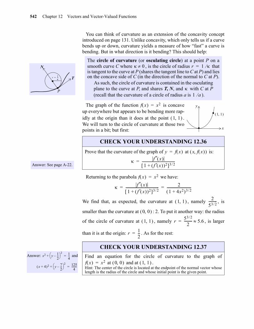
542 Chapter 12 Vectors and Vector-Valued Functions
You can think of curvature as an extension of the concavity conceptintroduced on page 131. Unlike concavity, which only tells us if a curvebends up or down, curvature yields a measure of how “fast” a curve isbending. But in what direction is it bending? This should help:
The graph of the function is concaveup everywhere but appears to be bending more rap-idly at the origin than it does at the point .We will turn to the circle of curvature at those twopoints in a bit; but first:
Returning to the parabola we have:
We find that, as expected, the curvature at , namely , is
smaller than the curvature at : 2. To put it another way: the radius
of the circle of curvature at , namely , is larger
than it is at the origin: . As for the rest:
.T
N
.r 1---=
P
The circle of curvature (or osculating circle) at a point P on asmooth curve C where , is the circle of radius thatis tangent to the curve at P (shares the tangent line to C at P) and lieson the concave side of C (in the direction of the normal to C at P).
As such, the circle of curvature is contained in the osculatingplane to the curve at P, and shares T, N, and with C at P(recall that the curvature of a circle of radius a is ).
0 r 1 =
1 a
Answer: See page A-22.
CHECK YOUR UNDERSTANDING 12.36
Prove that the curvature of the graph of at is:
.x
y
1 1
.
f x x2=
1 1
y f x = x f x
f x 1 f x 2+ 3 2/
----------------------------------------=
Answer: andx2 y 12---–
2+ 1
4---=
x 4+ 2 y 72---–
2+ 125
4---------=
CHECK YOUR UNDERSTANDING 12.37
Find an equation for the circle of curvature to the graph of at and at .
Hint: The center of the circle is located at the endpoint of the normal vector whoselength is the radius of the circle and whose initial point is the given point.
f x x2=
f x 1 f x 2+ 3 2/
---------------------------------------- 21 4x2+ 3 2/
-----------------------------= =
1 1 253 2/----------
0 0
1 1 r53 2/
2---------- 5.6=
r 12---=
f x x2= 0 0 1 1
12.5 Arc Length and Curvature 543
Exercises 1-8. Find the length of the given curve.
Exercises 9-14. Find parametric equations for the given curve using the arc length parameter withbase point at .
Exercises 15-19. Find the unit tangent, unit normal, unit binormal vectors and curvature of thegiven curve.
EXERCISES
1.
2.
3.
4.
5.
6.
7.
8.
9. 10.
11. 12.
13. 14.
15.16.
17. 18.
19. for
r t 2 tsin i 5tj 2 tcos k, 10– t 10 + +=
r t 2t t3
3---- t2
, 1 t 2 =
r t a 1 tsin– i a 1 tcos– j+ , 0 t 2 =
r t t2 i t2 j t2k, 0 t +cos–sin=
r t a tcos i a tsin j bt k, 0 t 2 + +=
r t 2 t 2 t t2sincos , 0 t 1 =
r t t tsec 3ln , 0 t4--- =
r t 2t i t2 2– j 1 t2– k, 0 t 2 + +=
t 0=
r t 3t 2– i 4t 3+ j+= r t 3 tcos+ 2 tsin+ =
r t 13---t3 1
2---t2
=r t et tcos i et tsin j+=
r t tsin i tcos j tk++= r t 2 tcos i 2 tsin j 2tk+ +=
r t 3 t 3 t 4tcossin =r t tsin i tcos j t2
2----k+ +=
r t et tcos i et tsin j 2k+ += r t 2 tsin i 5t j 2 tcos k + +=
r t t3
3---- t2
2---- 0
= t 0
gio
544 Chapter 12 Vectors and Vector-Valued Functions
Exercises 20-23. Determine the normal and osculating planes at the indicated point.
Exercises 24-25. Find the equation for the circle of curvature at the indicated point.
26. Prove that if the curvature of a curve is 0, then the curve is a line.
27. Show that the parabola achieves its maximum curvature at its vertex.
28. Find the point on the graph of the function at which the curvature is maximum.
29. Prove Theorem 12.11.
30. Show that for a smooth curve : and .
20.
21.
22.
23.
24. at 25. at
r t t t tsincos ; 1 0 0 =
r t 2 3tsin i tj 2 3tcos k; t+ + = =
r t ti t2j t3k; 1 1 1 + +=
r t t t tsincos ; 1
2------- 1
2-------
4---
=
r t 2 tsin 5t = 0 5 r t ti 2tsin j+=
4--- 1
y ax2=
y ex=
r t T t N t B t = N t B t T t =
gio
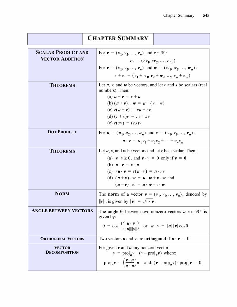
Chapter Summary 545
CHAPTER SUMMARY
SCALAR PRODUCT AND
VECTOR ADDITION
For and :
For and :
THEOREMS Let u, v, and w be vectors, and let r and s be scalars (realnumbers). Then:
(a)
(b)
(c)
(d)
(e)
DOT PRODUCT For and :
THEOREMS Let u, v, and w be vectors and let r be a scalar. Then:
(a) , and only if
(b)
(c)
(d) and
NORM The norm of a vector , denoted by
, is given by .
ANGLE BETWEEN VECTORS The angle between two nonzero vectors isgiven by:
or
ORTHOGONAL VECTORS Two vectors u and v are orthogonal if
VECTOR DECOMPOSITION
For given v and u any nonzero vector: where:
and:
v v1 v2 vn = r
rv rv1 rv2 rvn =
v v1 v2 vn = w w1 w2 wn =
v w+ v1 w1+ v2 w2 vn wn+ + =
u v+ v u+=
u v+ w+ u v w+ +=
r u v+ ru rv+=
r s+ v rv sv+=
r sv rs v=
u u1 u2 un = v v1 v2 vn =
u v u1v1 u2v2 unvn+ + +=
v v 0 v v 0= v 0=
u v v u=
ru v r u v u rv= =
u v+ w u w v w+=
u v– w u w v w–=
v v1 v2 vn =
v v v v=
u v n
cos1– u v
u v--------------- = u v u v cos=
u v 0=
v projuv v projuv– +=
projuvv uu u----------- u= v projuv– projuv 0=
gio
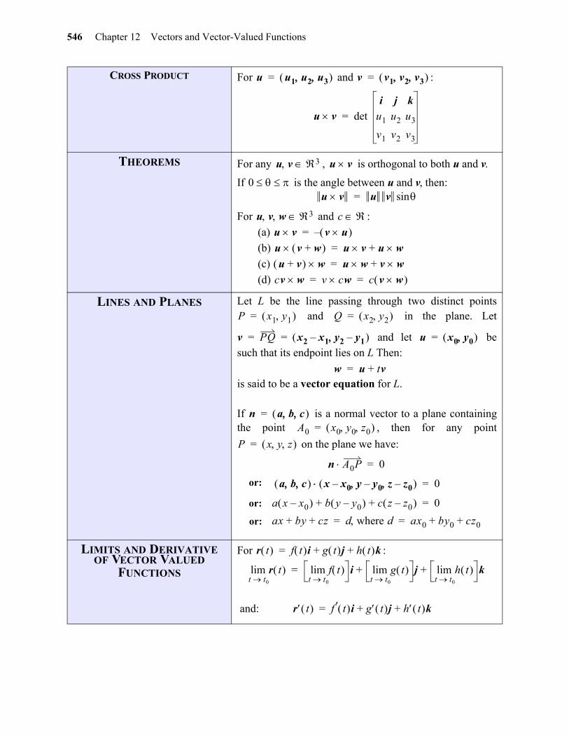
546 Chapter 12 Vectors and Vector-Valued Functions
CROSS PRODUCT For and :
THEOREMS For any , is orthogonal to both u and v.
If is the angle between u and v, then:
For and :
(a)
(b)
(c)
(d)
LINES AND PLANES Let L be the line passing through two distinct points and in the plane. Let
and let be
such that its endpoint lies on L Then:
is said to be a vector equation for L.
If is a normal vector to a plane containingthe point , then for any point
on the plane we have:
LIMITS AND DERIVATIVE OF VECTOR VALUED
FUNCTIONS
For :
and:
u u1 u2 u3 = v v1 v2 v3 =
u v det
i j k
u1 u2 u3
v1 v2 v3
=
u v 3 u v
0 u v u v sin=
u v w 3 c u v v u –=
u v w+ u v u w+=
u v+ w u w v w+=
cv w v cw c v w = =
P x1 y1 = Q x2 y2 =
v PQ x2 x1– y2 y1– = = u x0 y0 =
w u tv+=
n a b c =A0 x0 y0 z0 =
P x y z =
n A0P 0=
a b c x x0 y y0–– z z0– 0=
a x x0– b y y0– c z z0– + + 0=
or:
or:
ax by cz+ + d where d ax0 by0 cz0+ += =or:
r t f t i g t j h t k+ +=
r t t t0lim f t
t t0lim i g t
t t0lim j h t
t t0lim k+ +=
r t f t i g t j h t k+ +=
gio
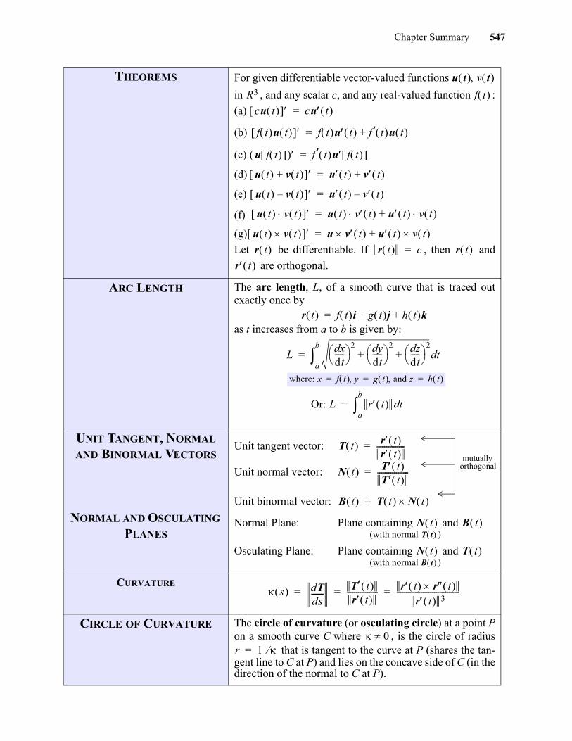
Chapter Summary 547
gio
THEOREMS For given differentiable vector-valued functions
in , and any scalar c, and any real-valued function :
(a)
(b)
(c)
(d)
(e)
(f)
(g)
Let be differentiable. If , then and
are orthogonal.
ARC LENGTH The arc length, L, of a smooth curve that is traced outexactly once by
as t increases from a to b is given by:
UNIT TANGENT, NORMAL AND BINORMAL VECTORS
NORMAL AND OSCULATING PLANES
Unit tangent vector:
Unit normal vector:
Unit binormal vector:
Normal Plane: Plane containing and (with normal )
Osculating Plane: Plane containing and (with normal )
CURVATURE
CIRCLE OF CURVATURE The circle of curvature (or osculating circle) at a point Pon a smooth curve C where , is the circle of radius
that is tangent to the curve at P (shares the tan-gent line to C at P) and lies on the concave side of C (in thedirection of the normal to C at P).
u t v t R3 f t
cu t cu t =
f t u t f t u t f t u t +=
u f t f t u f t =
u t v t + u t v t +=
u t v t – u t v t –=
u t v t u t v t u t v t +=
u t v t u v t u t v t +=
r t r t c= r t r t
r t f t i g t j h t k+ +=
Lxd
dt----- 2 yd
dt----- 2 zd
dt----- 2
+ + tda
b
=
where: x f t y g t and z h t = = =
Or: L r t tda
b
=
T t r t r t
---------------=
N t T t T t
-----------------=
B t T t N t =
N t B t T t
N t T t B t
s dTds-------
T t r t
----------------- r t r t r t 3
----------------------------------= = =
0r 1 =
mutuallyorthogonal
548 Chapter 12 Vectors and Vector-Valued Functions
gio
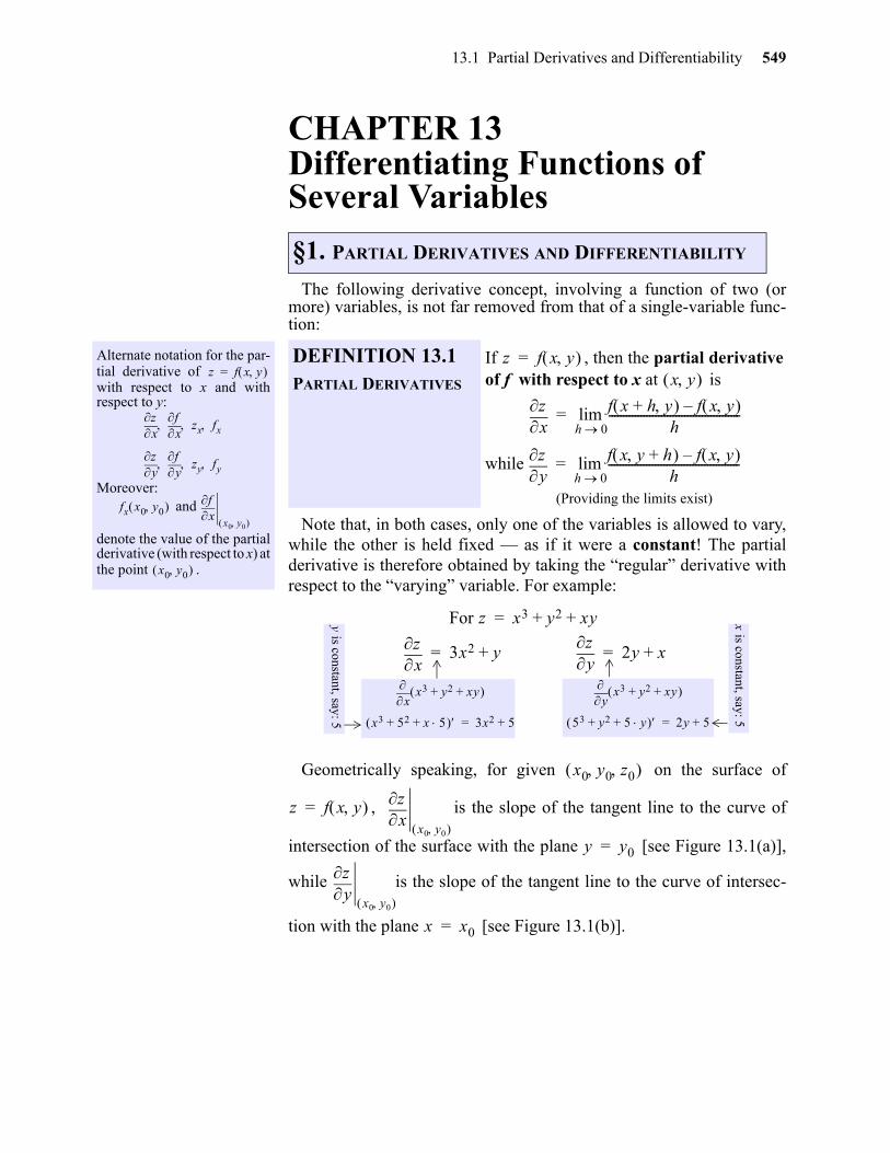
13.1 Partial Derivatives and Differentiability 549
13
CHAPTER 13Differentiating Functions of Several Variables
The following derivative concept, involving a function of two (ormore) variables, is not far removed from that of a single-variable func-tion:
Note that, in both cases, only one of the variables is allowed to vary,while the other is held fixed — as if it were a constant! The partialderivative is therefore obtained by taking the “regular” derivative withrespect to the “varying” variable. For example:
Geometrically speaking, for given on the surface of
, is the slope of the tangent line to the curve of
intersection of the surface with the plane [see Figure 13.1(a)],
while is the slope of the tangent line to the curve of intersec-
tion with the plane [see Figure 13.1(b)].
§1. PARTIAL DERIVATIVES AND DIFFERENTIABILITY
Alternate notation for the par-tial derivative of with respect to x and withrespect to y:
Moreover: and
denote the value of the partialderivative (with respect to x) atthe point .
z f x y =
xz
x
f zx fx
yz
y
f zy fy
fx x0 y0 x
f
x0 y0
x0 y0
DEFINITION 13.1PARTIAL DERIVATIVES
If , then the partial derivativeof f with respect to x at is
while
(Providing the limits exist)
z f x y =x y
xz f x h+ y f x y –
h---------------------------------------------
h 0lim=
yz f x y h+ f x y –
h---------------------------------------------
h 0lim=
xz 3x2 y
yz
+ 2y x+= =
y is constant, say: 5
x is constant, say: 5
x x3 y2 xy+ +
x3 52 x 5+ + 3x2 5+=
y x3 y2 xy+ +
53 y2 5 y+ + 2y 5+=
For z x3 y2+ xy+=
x0 y0 z0
z f x y =x
z
x0 y0 y y0=
yz
x0 y0
x x0=
gio
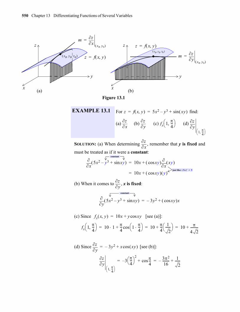
550 Chapter 13 Differentiating Functions of Several Variables
gio
Figure 13.1
SOLUTION: (a) When determining , remember that y is fixed and
must be treated as if it were a constant:
(b) When it comes to , x is fixed:
(c) Since [see (a)]:
(d) Since [see (b)]:
x
y
z .x0 y0 z0 z f x y =
mx
z
x0 y0
=
x
y
z .x0 y0 z0
z f x y =
my
z
x0 y0
=
(a) (b)
EXAMPLE 13.1 For find:
(a) (b) (c) (d)
z f x y 5x2 y3– xy sin+= =
xz
yz
fx 14---
y
z
14---
xz
x 5x2 y3– xysin+ 10x xycos
x xy +=
10x xycos y +=
constant
just like: 5x 5=
yz
y 5x2 y3– xysin+ 3y2– xycos x+=
constant
fx x y 10x y xycos+=
fx 14---
10 14--- 1
4---
cos+ 104--- 1
2------- + 10
4 2----------+= = =
yz 3y2– x xy cos+=
yz
14---
3–4--- 2
4---cos+ 32
16---------– 1
2-------+= =
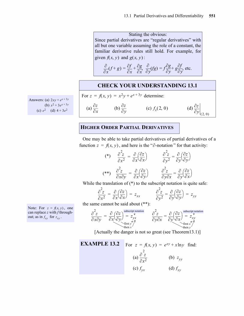
13.1 Partial Derivatives and Differentiability 551
One may be able to take partial derivatives of partial derivatives of afunction , and here is the “ ” for that activity:
While the translation of (*) to the subscript notation is quite safe:
the same cannot be said about (**):
[Actually the danger is not so great (see Theorem13.1)]
Answers: (a) (b) (c) (d)
2xy ex 3y++
x2 3ex 3y++
e2 4 3e2+
Stating the obvious:Since partial derivatives are “regular derivatives” withall but one variable assuming the role of a constant, thefamiliar derivative rules still hold. For example, forgiven and :
CHECK YOUR UNDERSTANDING 13.1
For determine:
(a) (b) (c) (d)
HIGHER ORDER PARTIAL DERIVATIVES
f x y g x y
x f g+
xf
xg+=
y
fg( ) fy
gg
yf
etc.+=
z f x y x2y ex 3y++= =
xz
yz
fx 2 0 y
z
2 0
z f x y = -notation
x2
2
z
x
xz
y2
2
z
y
yz ==
x y
2
z
x
yz
y x
2
z
y
xz ==
(*)
(**)
Note: For , onecan replace z with f through-out; as in for .
z f x y =
fxy zxy
EXAMPLE 13.2 For find:
(a) (b)
(c) (d)
x2
2
z
x
xz zxx
y2
2
z
y
yz = zyy= = =
x y
2
z
x
yz zyx
y x
2
z
y
xz = zxy= = =
subscript notation subscript notation
first ythen x
first xthen y
z f x y exy x yln+= =
x2
2
z
zyy
fyx fxy
gio
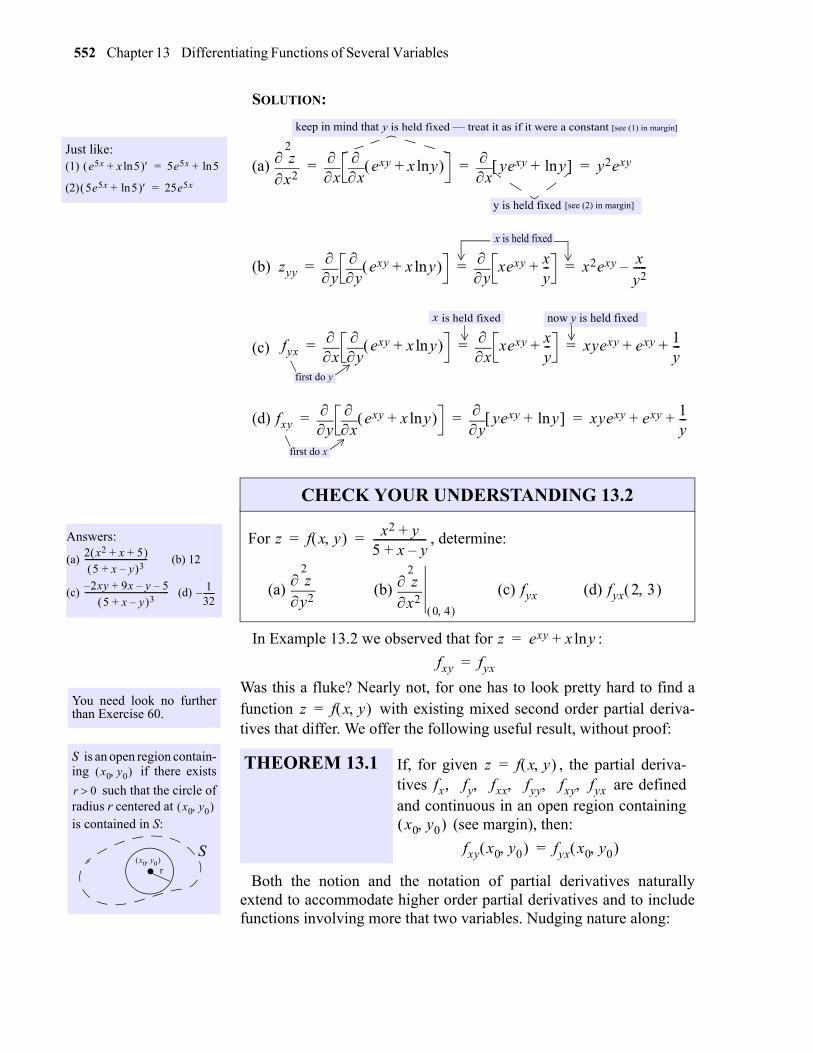
552 Chapter 13 Differentiating Functions of Several Variables
SOLUTION:
(a)
(b)
(c)
(d)
In Example 13.2 we observed that for :
Was this a fluke? Nearly not, for one has to look pretty hard to find afunction with existing mixed second order partial deriva-tives that differ. We offer the following useful result, without proof:
Both the notion and the notation of partial derivatives naturallyextend to accommodate higher order partial derivatives and to includefunctions involving more that two variables. Nudging nature along:
Just like:(1)
(2)
e5x x 5ln+ 5e5x 5ln+=
5e5x 5ln+ 25e5x=x2
2
z
x
x exy x yln+
x yexy yln+ y2exy= = =
y is held fixed [see (2) in margin]
keep in mind that y is held fixed — treat it as if it were a constant [see (1) in margin]
zyy y
y exy x yln+
y xexy x
y--+ x2exy x
y2-----–= = =
x is held fixed
fyx x
y exy x yln+
x xexy x
y--+ xyexy exy 1
y---+ += = =
x is held fixed now y is held fixed
first do y
fxy y
x exy x yln+
y yexy yln+ xyexy exy 1
y---+ += = =
first do x
Answers:
(a) (b) 12
(c) (d)
2 x2 x 5+ + 5 x y–+ 3
-------------------------------
2– xy 9x y– 5–+5 x y–+ 3
------------------------------------------ 132------–
CHECK YOUR UNDERSTANDING 13.2
For , determine:
(a) (b) (c) (d)
z f x y x2 y+5 x y–+--------------------= =
y2
2
z
x2
2
z
0 4
fyx fyx 2 3
You need look no furtherthan Exercise 60.
S is an open region contain-ing if there exists
such that the circle ofradius r centered at is contained in S:
x0 y0
r 0x0 y0
x0 y0 . r
S
THEOREM 13.1 If, for given , the partial deriva-tives are definedand continuous in an open region containing
(see margin), then:
z exy x yln+=
fxy fyx=
z f x y =
z f x y =fx fy fxx fyy fxy fyx
x0 y0 fxy x0 y0 fyx x0 y0 =
gio
13.1 Partial Derivatives and Differentiability 553
The derivative form of a single variable function :
does not readily extend to accommodate a function of twovariables:
And so we reformulate (*):
and observe that to say that:
is to say that the difference goes to zero as ;
or, equivalently, that:For
where as
Extending the above representation to accommodate a function of two variables we come to:
Answers: (a-1) (a-ii and a-iii) (b-i) (b-ii) (b-iii) (b-iv)
24xy3
36x2y2
y2 3x2yz– 2x
6– yz 3x2–
CHECK YOUR UNDERSTANDING 13.3
(a) For , determine:
(i) (ii) (iii)
(b) For , determine:
(i) (ii) (iii) (iv)
DIFFERENTIABILITY
z f x y x4y3= =
x3
3
z
zxyx zxxy
w f x y z xy2 z3y x3yz–+= =
xw
y2
2
w
wxxx wyzx
y f x =
f x0 f x0 x+ f x0 –
x------------------------------------------
x 0lim=
see Definition 3.1,page 66 with xreplacing h.
(*)
z f x y =
f x0 y0 f x0 x+ y0 y+ f x0 y0 –
?-----------------------------------------------------------------------
x 0y 0
lim=
but what goes here?
f x0 yx
------x 0lim , where y f x0 x+ f x0 –= =
Note that:
can be rewritten in the form:
yx
------ f x0 –=
y f x0 x= x+
f x0 yx
------x 0lim =
yx
------ f x0 –= x 0
y f x0 x+ f x0 –=
y f x0 x= x+ 0 x 0
DEFINITION 13.2DIFFERENTIABLE
A function is differentiable at
if can beexpressed in the form:
where , as .
A function f is said to be differentiable if it is differ-entiable at each point in its domain.
z f x y = x0 y0 z f x0 x+ y0 y+ f x0 y0 –=
z fx x0 y0 x= fy x0 y0 y 1x 2y+ + +
1 2 0 x y 0
gio
554 Chapter 13 Differentiating Functions of Several Variables
Built into the above definition is the requirement that both partialderivatives of f need to exist for f to be differentiable at a given point.That, as it turns out, is not quite enough. However:
PROOF: Appendix B, page B-2.
SOLUTION: Since both of the partial derivatives: and
are defined and continuous everywhere, is differentiable.
As it is with functions of one variable:
PROOF: We show that :
Since is differentiable at (Definition 13.2):
where:
and , as .
Letting and we have:
.
So:
THEOREM 13.2 If the partial derivatives and exist andare continuous in an open region about
, then f is differentiable at .
EXAMPLE 13.3 Verify that is a differ-entiable function.
fx fy
x0 y0 x0 y0
z f x y y2e3x= =
fx 3y2e3x=
fy 2ye3x= f x y y2e3x=
Answer: See page A-24.
CHECK YOUR UNDERSTANDING 13.4
Verify that is a differentiable function.f x y x2 ysin=
In the exercises you areinvited to show that thoughboth and exist for the function:
the function fails to be con-tinuous at , and is there-fore not differentiable at thatpoint.
fx 0 0 fy 0 0
f x y xy
x2 y2+------------------ if x y 0 0
0 if x y 0 0 =
=
0 0
THEOREM 13.3 If is differentiable at ,
then f is continuous at .
z f x y = x0 y0 x0 y0
f x y f x0 y0 – x y x0 y0
lim 0=
z f x y = x0 y0
z fx x0 y0 x= fy x0 y0 y 1x 2y+ + +
z f x0 x+ y0 y+ f x0 y0 –= 1 2 0 x y 0
x x x0–= y y y0–=
f x y f x0 y0 – f x0 x+ y0 y+ f x0 y0 – z= =
f x y f x0 y0 – x y x0 y0
lim zx y x0 y0
lim=
fx x0 y0 x fy x0 y0 y 1x 2y+ + +x y x0 y0
lim= 0=
gio
13.1 Partial Derivatives and Differentiability 555
gio
Here are some partial derivative variations of the single-variablechain rule of page 94 (see margin):
PROOF: (a)
(b) If is held fixed, then and become functions of u alone. Applying (a) with u in place of t, and if we use instead if d to indicate that the variable v is fixed, we obtain:
A similar argument can be used to establish the formula for :
SOLUTION: (a) Using the chain rule:
If and are differentiable func-tions, then the compositefunction isalso differentiable, and:
y f x = z g y =
z g f x =
dzdx------
dzdy------dy
dx------=
CHAIN RULE
THEOREM 13.4 (a) If is differentiable, and if and are differentiable
functions, then the single variable function is differentiable, and:
(b) If is differentiable, and if and are differentia-
ble functions, then the two variable function is differentiable, and:
EXAMPLE 13.4(a) Determine if:
(b) Determine if:
z f x y =x g t = y h t =
z f g t h t =
tddz
xz
tddx
yz
tddy
+=
z f x y =x g u v = y h u y =
z f g u v h u v =
uz
xz
ux
yz
uy
v
zx
zv
xy
zv
y+=+=
tddz z
t------
t 0lim x
zxy
zy 1x 2y+ + +
t---------------------------------------------------------------------
t 0lim= =
xz x
t------
t 0lim
yz y
t------
t 0lim 1
t 0lim x
t------
t 0lim 2
t 0lim y
t------
t 0lim+ + +=
xz
tddx
yz
tddy
+= as t 0: 1 0 and 2 0
v x g u v = y h u y =
uz
xz
ux
yz
uy
+=
vz
dzdt-----
z xy2 x t2 y t= = =
sz
z xy2= x s t2 y+ s tcos= =
tddz
xz
tddx
yz
tddy
+ y2 2t 2yx1
2t1 2/------------ += =
t 2 2t 2 t t2 12t1 2/------------ +=
2t2 t2+ 3t2= =
556 Chapter 13 Differentiating Functions of Several Variables
gio
Alternatively, we can express z explicitly as a function of t:
and then differentiate: .
(b) Let . Using the chain rule:
Without the chain rule:
And again we have:
We conclude this section by noting that both the notion and the nota-tion of partial derivatives extend to higher order partial derivatives, andcan also include functions involving more than two variables. Thatbeing the case (your turn):
z xy2 t2 t 2 t3= = =
tddz
tdd t3 3t2= =
z xy2= x s t2 y+ s tcos= =
sz
xz
sx
yz
sy
+ y2 1 2xy tcos += =
s2cos2t 2 s t2+ s tcos tcos +=
3s2cos2t 2st2cos
2t+=
z xy2 s t2+ s2cos2t s3cos
2t t2s2cos
2t+= = =
sz
s s3cos
2t t2s2cos
2t+ 3s2cos
2t 2st2cos
2t+= =
Answers:
(a)
(b)
Answers: (a-i) (a-ii)
(b-i) (b-ii) (b-iii)
(c) See page A-25
(d)
(e)
8 2 tsin et2
+ 3
tcos tet2+
ste s2t2 3st3+ 9t 2s+
y3exy
yexy xy 2+ y2 yz– 2x
1–
te3t sint 2 t 2t tcos+sin3t t sin+
rste t r2cossin 2 t r2 tcoscos+
CHECK YOUR UNDERSTANDING 13.5
(a) Let: . Use the chain rule to
find and check your result by expressing z explicitly as a
function of t and differentiating directly.(b) Let: . Use the chain rule to find
and check your result by expressing z explicitly as a function
of s and t and applying to that expression.
CHECK YOUR UNDERSTANDING 13.6
(a) For , find: (i) and (ii)
(b) For , find:
(i) (ii) (iii)
(c) Show that is a differentiable function.
(d) Use the chain rule to determine if:
(e) Use the chain rule to determine if:
z 2x ey + 4= x t ysin t2= =
tddz
z exy= x s 3t y+ st2= =
tz
t
z f x y exy x yln+= =x3
3
z
zxyx
w f x y z xy2 z3y xyz–+= =
xw
y2
2
w
wxyz
w f x y z zy2e3x= =dwdt-------
w xy2z3 x t2 y t zsin et= = = =
tw
w xeyz= x rst2 y t zsin r2cos= = =
13.1 Partial Derivatives and Differentiability 557
gio
Exercises 1-12. Find and .
Exercises 13-21. Find , and verify that .
Exercises 22-27. Find .
Exercise 28-36. Verify that the given function is differentiable.
EXERCISES
1. 2. 3.
4. 5. 6.
7. 8. 9.
10. 11. 12.
13. 14. 15.
16. 17. 18.
19. 20. 21.
22. 23. 24.
25. 26. 27.
28. 29. 30.
31. 32. 33.
34. 35. 36.
xz
yz
z x2 y2+= z 3x2 xy– y+= z xy 1– 2=
z x3 y2+= z 4ex2y3= z 1x y+-----------=
z x y+xy 1–--------------= z sin
2x 3y– = z ex ysin=
z x2 y2+ ln= z ex ycos xln= z x ycossin=
fxx fyy fxy and fyx fxy fyx=
f x y 6x2 8xy– 9y2+= f x y xy--ln= f x y e2x 3y+=
f x y sin2
x2 y– = f x y x2 y2+= f x y xx y+-----------=
f x y xsinycos
-----------= f x y yex ln= f x y xy y2– ln=
fxz fzx fyyy fzzy fzyz fxyz and fzyx
f x y z xyz= f x y z x3y2z= f x y z xy2 zsin=
f x y z exyz= f x y z x y z+ + ln= f x y z z2 y xcos+=
f x y x3y= f x y x2y 9–= f x y 3x2 y2+=
f x y e2x 3y+= f x y xsinycos
-----------= f x y xy y2– ln=
f x y y2
x-----= f x y z x3y2z4= f x y z e2z xycos=
558 Chapter 13 Differentiating Functions of Several Variables
Exercises 37-39. (Implicit Partial Differentiation) Find and .
Exercises 40-42. Find a function such that:
Exercises 43-44. (Cauchy-Riemann Equations) Show that the functions , satisfies
the following Cauchy-Riemann equations: :
45. Let . Show that .
46. Let . Show that .
47. Show that if , then .
48. Show that if , then .
49. Show that the function satisfies the partial differential equa-
tion .
50. Show that the function satisfies the partial differential equation
51. Show that the function satisfies the partial differential
equation .
52. Show that the function satisfies the partial differential equation
.
53. Show that the function satisfies the second order partial differ-ential equation .
54. Show that the function satisfies the second order partial differ-ential equation: .
37. 38. 39.
40. and 41. and 42. and
43. 44.
xz
yz
Note: x
xy2 x2z3+( ) y2 x2 3z2x
z2xz3+ +=
x2z 2y2z2 y+ + 0= exyz z2– xy= x3 y3 z3 6xyz+ + + 0=
f x y
fx x= fy y= fx y2= fy 2xy= fx ex ysin= fy ex ycos=
f x y g x y fx gy and fy gx–= =
f x y x2 y2–= g x y 2xy= f x y ex ycos= g x y ex ysin=
z tan1– xy--= zxx zyy+ 0=
f x y ecy cycos= fxx fyy+ 0=
f x y g x h y += fxy 0=
f x y z g x y h y z k z x + += fxyz 0=
z f x y x4 2x2y2 y4+ += =
xx
zy
yz
+ 4z=
z f x y x2y2
x y+-----------= =
xx
zy
yz
+ 3z=
w f x y z x2y y2z z2x+ += =
xw
yw
zw+ + x y z+ + 2=
w f x y z xz y2+yz
----------------= =
xx
wy
yw
zz
w+ + 0=
z x y+ cos x y– cos+=zxx zyy– 0=
z x y+ sin x y– ln+=zxx zyy– 0=
gio
13.1 Partial Derivatives and Differentiability 559
55. The pressure P of a gas confined in a container of volume V and temperature T is related by an equation of the form , where k is a positive constant. Verify that:
56. The kinetic energy of a body of mass m moving at a velocity v is given by . Verify
that .
57. When two resisters of resistance and ohms are connected in parallel, their combined
resistance R in ohms is given by . Verify that .
58. Find the slope of the tangent line to the curve of intersection of the curve and the plane if .
59. Find the slope of the tangent line to the curve of intersection of the sphere and the plane at .
60. Let . Verify that and .
Exercises 61-62. Find , both with and without using the chain rule.
Exercises 63-64. Find , both with and without using the chain rule.
Exercises 65-66. Find and , both with and without using the chain rule.
Exercises 67-68. Find and , both with and without using the chain rule.
61. , , 62. , ,
63. , , , 64. , , ,
65. 66.
67. 68.
PV kT=
VV
PP V
VP T
TP
+– 0 and T
V
PT
VP 1–= = =
K12---mv2=
mK
v2
2
K K=
R1 R2
RR1R2
R1 R2+------------------=
R12
2
R
R22
2
R 4R2
R1 R2+ 4--------------------------=
z x2 4y2+=x 1–= y 1=
x2 y2 z2+ + 9=x 2= 2 1 2
f x y x3y xy3–x2 y2+
---------------------- if x y 0 0
0 if x y 0 0 =
= fxy 0 0 1–= fyx 0 0 1=
tddz
z xy= x tcos= y tsin= z x3y exy+= x t2= y xsin=
tddw
w xy z+= x tcos= y tsin= z t= w z xy2 sin= x t2= y et= z xy=
tz
sz
z x ysin= x s 3t y+ t2= = z xexy= x st ysin st2= =
tw
sw
w x 2y 3z–+= x st y est z tsin= = = w xeyz= x st y est z t= = =
gio
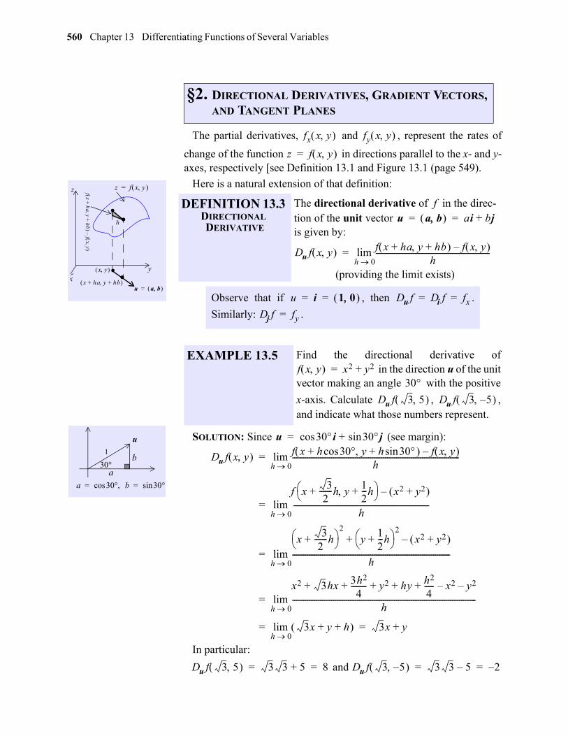
560 Chapter 13 Differentiating Functions of Several Variables
13484
The partial derivatives, and , represent the rates of
change of the function in directions parallel to the x- and y-axes, respectively [see Definition 13.1 and Figure 13.1 (page 549).
Here is a natural extension of that definition:
SOLUTION: Since (see margin):
In particular:
and
§2. DIRECTIONAL DERIVATIVES, GRADIENT VECTORS, AND TANGENT PLANES
y
z z f x y =
x y
x ha+ y hb+
.
u a b =
..
.
x
fx
ha
+y
hb
+
fx
y
–
h
DEFINITION 13.3DIRECTIONAL DERIVATIVE
The directional derivative of f in the direc-tion of the unit vector is given by:
(providing the limit exists)
Observe that if , then .
Similarly: .
fx x y fy x y
z f x y =
u a b ai bj+= =
Du f x y f x ha+ y hb+ f x y –h
-------------------------------------------------------------h 0lim=
u i 1 0 = = Du f Di f fx= =
Dj f fy=
b
a
1
u
30
a 30 bcos 30sin= =
EXAMPLE 13.5 Find the directional derivative of in the direction u of the unit
vector making an angle with the positive
x-axis. Calculate , ,and indicate what those numbers represent.
f x y x2 y2+=30
Du f 3 5 Du f 3 5–
u 30i 30jsin+cos=
Du f x y f x h 30cos+ y h 30sin+ f x y –h
------------------------------------------------------------------------------------------h 0lim=
f x3
2-------h+ y
12---h+
x2 y2+ –
h-------------------------------------------------------------------------
h 0lim=
x3
2-------h+
2
y12---h+
2x2 y2+ –+
h-------------------------------------------------------------------------------------
h 0lim=
x2 3hx 3h2
4-------- y2 hy h2
4----- x2– y2–+ + + + +
h---------------------------------------------------------------------------------------------------
h 0lim=
3x y h+ + h 0lim 3x y+= =
Du f 3 5 3 3 5+ 8= = Du f 3 5– 3 3 5– 2–= =
gio
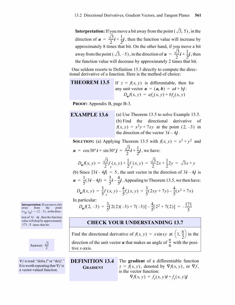
13.2 Directional Derivatives, Gradient Vectors, and Tangent Planes 561
gio
Interpretation: If you move a bit away from the point , in the
direction of , then the function value will increase by
approximately 8 times that bit. On the other hand, if you move a bit
away from the point , in the direction of , then
the function value will decrease by approximately 2 times that bit.
One seldom resorts to Definition 13.3 directly to compute the direc-tional derivative of a function. Here is the method of choice:
PROOF: Appendix B, page B-3.
SOLUTION: (a) Applying Theorem 13.5 with and
, we have:
(b) Since , the unit vector in the direction of is
. Appealing to Theorem 13.5, we then have:
In particular:
THEOREM 13.5 If is differentiable, then forany unit vector :
EXAMPLE 13.6 (a) Use Theorem 13.5 to solve Example 13.5.
(b) Find the directional derivative of at the point in
the direction of the vector .
3 5
u3
2-------i
12---j+=
3 5– u3
2-------i
12---j+=
z f x y =u a b ai bj+= =
Du f x y afx x y bfy x y +=
f x y x2y 7xy+= 2 3– 3i 4j–
f x y x2 y2+=
u 30cos i 30jsin+3
2-------i
12---j+= =
Du f x y 32
-------fx
x y 12---f
yx y +
32
-------2x12---2y+ 3x y+= = =
Interpretation: If you move a bitaway from the point
, in the direc-
tion of , then the functionvalue will drop by approximately
times that bit.
Answer:
x0 y0 2 3– =
3i 4j–
171 5
32
-------
CHECK YOUR UNDERSTANDING 13.7
Find the directional derivative of at in the
direction of the unit vector u that makes an angle of with the posi-tive x-axis.
3i 4j– 5= 3i 4j–
u15--- 3i 4j– 3
5---i
45---j–= =
Du f x y 35---f
xx y 4
5---fy x y –
35--- 2xy 7y+ 4
5--- x2 7x+ –= =
Du f 2 3– 35--- 2 2 3– 7 3– + 4
5--- 22 7 2 + – 171
5---------–= =
f x y x xysin= 12---
6---
is read: “delta f” or “del f.”It is worth repeating that isa vector-valued function.
ff
DEFINITION 13.4GRADIENT
The gradient of a differentiable function, denoted by , or ,
is the vector function:z f x y = f x y f
f x y fx x y i fy x y j+=
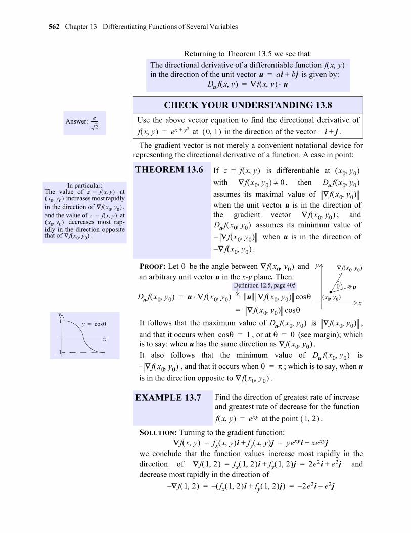
562 Chapter 13 Differentiating Functions of Several Variables
gio
Returning to Theorem 13.5 we see that:
The gradient vector is not merely a convenient notational device forrepresenting the directional derivative of a function. A case in point:
PROOF: Let be the angle between andan arbitrary unit vector u in the x-y plane. Then:
It follows that the maximum value of is ,
and that it occurs when , or at (see margin); whichis to say: when u has the same direction as .
It also follows that the minimum value of is
, and that it occurs when ; which is to say, when u
is in the direction opposite to .
SOLUTION: Turning to the gradient function:
we conclude that the function values increase most rapidly in thedirection of anddecrease most rapidly in the direction of
Answer: e
2-------
The directional derivative of a differentiable function in the direction of the unit vector is given by:
CHECK YOUR UNDERSTANDING 13.8
Use the above vector equation to find the directional derivative of
at in the direction of the vector .
f x y u ai bj+=
Du f x y f x y u=
f x y ex y2+= 0 1 i– j+
In particular:The value of at
increases most rapidlyin the direction of ,and the value of at
decreases most rap-idly in the direction oppositethat of .
z f x y =x0 y0
f x0 y0 z f x y =
x0 y0
f x0 y0
THEOREM 13.6 If is differentiable at
with , then
assumes its maximal value of when the unit vector u is in the direction ofthe gradient vector ; and
assumes its minimum value of
when u is in the direction of
.
z f x y = x0 y0 f x0 y0 0 Du f x0 y0
f x0 y0
f x0 y0 Du f x0 y0 f x0 y0 –
– f x0 y0
1
1–
y
y cos=
EXAMPLE 13.7 Find the direction of greatest rate of increaseand greatest rate of decrease for the function
at the point .
x0 y0 .
f x0 y0
u
x
y
f x0 y0
Du f x0 y0 u f x0 y0 u f x0 y0 cos= =
Definition 12.5, page 405
f x0 y0 cos=
Du f x0 y0 f x0 y0 cos 1= 0=
f x0 y0 Du f x0 y0
f x0 y0 – =
f x0 y0
f x y exy= 1 2
f x y fx x y i fy x y j+ yexyi xexyj+= =
f 1 2 fx 1 2 i fy 1 2 j+ 2e2i e2j+= =
– f 1 2 fx 1 2 i fy 1 2 j+ – 2– e2i e2j–= =
13.2 Directional Derivatives, Gradient Vectors, and Tangent Planes 563
The previous discussion extends to differentiable functions of three(or more) variables. In particular:
For and unit vector :
where:
SOLUTION: (a) From:
we have:
In particular: Since the unit vector in the direction of is
:
(b) By Theorem 13.6, the greatest value is:
and the smallest value is
Answer: 2 and .2–
CHECK YOUR UNDERSTANDING 13.9
Find the greatest value and smallest value of the directional deriva-tive for the function at the point .
FUNCTIONS OF THREE VARIABLES
EXAMPLE 13.8 (a) Determine the directional derivative of at in the
direction .
(b) Find the greatest value and smallestvalue of the directional derivative for
at .
f x y x ysin= 2 0
w f x y z = u ai bj ck+ +=
Du f x y z afx x y z bfy x y z cfz x y z + + u f x y z = =
f x y z fx x y z i fy x y z j fz x y z k+ +=
f x y z xeyz= 1 0 1 2i j k–+
f x y z xeyz= 1 0 1
fx x y z eyz= fy x y z xzeyz fz x y z xyeyz= =
f x y z eyzi xzeyzj xyeyzk+ +=
f 1 0 1 i j+=2i j k–+
u1
6------- 2i j k–+ =
Du f 1 0 1 f 1 0 1 1
6------- 2i j k–+ 2
6------- 1
6-------+ 3
6-------= = =
f 1 0 1 i j+ 2= =
f 1 0 1 – 2–=
Answer: and .63
------- 63
-------–
CHECK YOUR UNDERSTANDING 13.10
Find the greatest value and smallest value of the directional deriva-
tive for the function at .f x y z x2 y2 z2+ + ln= 1 1 2
gio
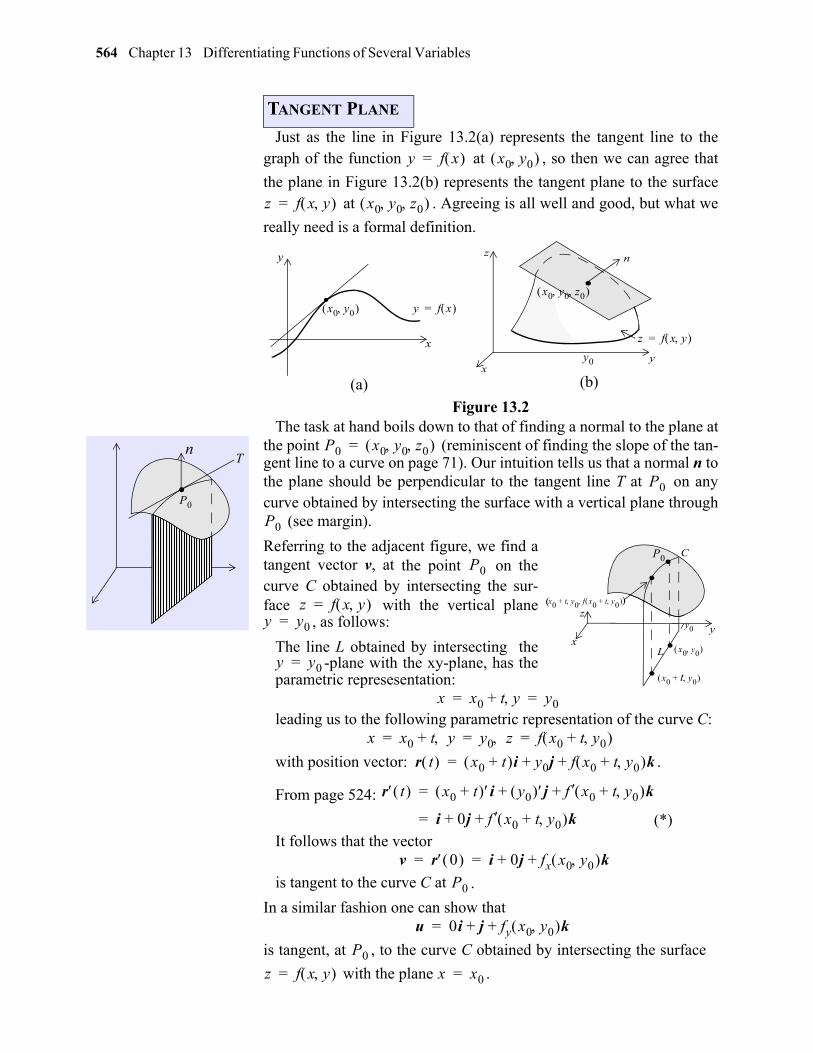
564 Chapter 13 Differentiating Functions of Several Variables
gio
Just as the line in Figure 13.2(a) represents the tangent line to thegraph of the function at , so then we can agree that
the plane in Figure 13.2(b) represents the tangent plane to the surface at . Agreeing is all well and good, but what we
really need is a formal definition.
Figure 13.2The task at hand boils down to that of finding a normal to the plane at
the point (reminiscent of finding the slope of the tan-gent line to a curve on page 71). Our intuition tells us that a normal n tothe plane should be perpendicular to the tangent line T at on anycurve obtained by intersecting the surface with a vertical plane through
(see margin).
Referring to the adjacent figure, we find atangent vector v, at the point on thecurve C obtained by intersecting the sur-face with the vertical plane
, as follows:
The line L obtained by intersecting the-plane with the xy-plane, has the
parametric represesentation:
leading us to the following parametric representation of the curve C:
with position vector: .
From page 524:
It follows that the vector
is tangent to the curve C at .
In a similar fashion one can show that
is tangent, at , to the curve C obtained by intersecting the surface
with the plane .
TANGENT PLANE
(a) (b)
y f x = x0 y0
z f x y = x0 y0 z0
x
y
.y f x =x0 y0
.x0 y0 z0
xy
z n
z f x y =
y0
.P0
nT
P0 x0 y0 z0 =
P0
P0
.
.
C
x0 y0 L.
.
x0 t+ y0
P0
x0 t+ y0 f x0 t+ y0
zy0
( )
yx
P0
z f x y =y y0=
y y0=
x x0 t y+ y0= =
x x0 t y+ y0 z f x0 t+ y0 = = =
r t x0 t+ i y0j f x0 t+ y0 k+ +=
r t x0 t+ i y0 j f x0 t+ y0 k+ +=
i 0j f x0 t+ y0 k+ += (*)
v r 0 i 0j fx x0 y0 k+ += =
P0
u 0i j fy x0 y0 k++=
P0
z f x y = x x0=
13.2 Directional Derivatives, Gradient Vectors, and Tangent Planes 565
Taking the cross product of u and v we arrive at a vector perpendic-ular to both u and v:
In the exercises you are invited to show that the above vector is, infact, perpendicular to the tangent line T at on any curve obtained byintersecting the surface with a vertical plane through . Bringing us to:
SOLUTION: From we have:
In particular:
Normal to the plane (Definition 13.5):
Consequently (see page 516):
DEFINITION 13.5TANGENT PLANE
Let be differentiable at
. The tangent plane to the graph of
f at is the plane passing
through that point with normal vector.
In particular, here is the scalar form equation of the plane (see page 418):
EXAMPLE 13.9 Find an equation of the tangent plane to the graphof at the point .
n u v det
i j k
0 1 fy x0 y0
1 0 fx x0 y0
fx x0 y0 i fy x0 y0 j k–+= = =
P0P0
z f x y =
x0 y0
x0 y0 f x0 y0
fx x0 y0 i fy x0 y0 j k–+
fx x0 y0 x x0– fy x0 y0 y y0– z z0– –+ 0=
f x y xyex y+= 1 2 2e3
f x y xyex y+=
fx x y y xex y+ ex y++ and fy x y x yex y+ ex y++ = =y is held fixed x is held fixed
fx 1 2 2 e3 e3+ 4e3 and fy 1 2 1 2e3 e3+ 3e3= = = =
n 4e3i 3e3j k–+=
4e3 3e3 1– x 1 y 2 z 2e3––– 0=
4e3 x 1– 3e3 y 2– 1 z 2e3– –+ 0=
4e3x 3e3y z–+ 8e3=
vector form
scalar form
general form
Answer: 7x 6y z+ + 5=
CHECK YOUR UNDERSTANDING 13.11
Find the general form equation of the tangent plane to the graph of
at the point . f x y 3y2 2x2– x+= 2 1 3––
gio
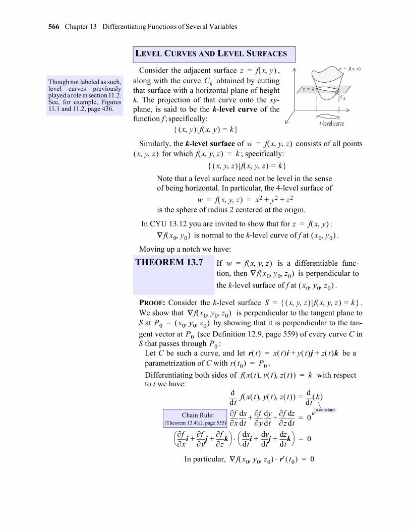
566 Chapter 13 Differentiating Functions of Several Variables
Consider the adjacent surface ,along with the curve obtained by cuttingthat surface with a horizontal plane of heightk. The projection of that curve onto the xy-plane, is said to be the k-level curve of thefunction f ; specifically:
Similarly, the k-level surface of consists of all points for which ; specifically:
Note that a level surface need not be level in the senseof being horizontal. In particular, the 4-level surface of
is the sphere of radius 2 centered at the origin.
In CYU 13.12 you are invited to show that for :
is normal to the k-level curve of f at .
Moving up a notch we have:
PROOF: Consider the k-level surface .We show that is perpendicular to the tangent plane toS at by showing that it is perpendicular to the tan-
gent vector at (see Definition 12.9, page 559) of every curve C inS that passes through :
Let C be such a curve, and let be aparametrization of C with .
Differentiating both sides of with respectto t we have:
In particular,
LEVEL CURVES AND LEVEL SURFACES
Though not labeled as such,level curves previouslyplayed a role in section 11.2.See, for example, Figures11.1 and 11.2, page 436.
THEOREM 13.7 If is a differentiable func-tion, then is perpendicular to
the k-level surface of f at .
z f x y =
z k=
Ck
k-level curve
z f x y =Ck
x y f x y k=
w f x y z =x y z f x y z k=
x y z f x y z k=
w f x y z x2 y2 z2+ += =
z f x y =
f x0 y0 x0 y0
w f x y z =f x0 y0 z0
x0 y0 z0
S x y z f x y z k= =f x0 y0 z0
P0 x0 y0 z0 =
P0P0
r t x t i y t j z t k+ +=r t0 P0=
f x t y t z t k=
tdd f x t y t z t
tdd= k
xf
tddx
yf
tddy
zf
tddz
+ + 0=
xf
iy
fj
zf
k+ +
tddx
itd
dyj
tddz
k+ + 0=
Chain Rule: (Theorem 13.4(a), page 555)
a constant
f x0 y0 z0 r t0 0=
gio
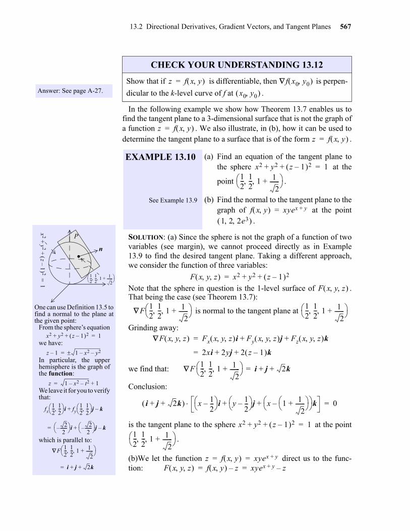
13.2 Directional Derivatives, Gradient Vectors, and Tangent Planes 567
gio
In the following example we show how Theorem 13.7 enables us tofind the tangent plane to a 3-dimensional surface that is not the graph ofa function . We also illustrate, in (b), how it can be used todetermine the tangent plane to a surface that is of the form .
SOLUTION: (a) Since the sphere is not the graph of a function of twovariables (see margin), we cannot proceed directly as in Example13.9 to find the desired tangent plane. Taking a different approach,we consider the function of three variables:
Note that the sphere in question is the 1-level surface of .That being the case (see Theorem 13.7):
is normal to the tangent plane at
Grinding away:
we find that:
Conclusion:
is the tangent plane to the sphere at the point
.
(b)We let the function direct us to the func-tion:
Answer: See page A-27.
CHECK YOUR UNDERSTANDING 13.12
Show that if is differentiable, then is perpen-
dicular to the k-level curve of f at .
z f x y = f x0 y0 x0 y0
One can use Definition 13.5 tofind a normal to the plane atthe given point:
From the sphere’s equation
we have:
In particular, the upperhemisphere is the graph ofthe function:
We leave it for you to verifythat:
which is parallel to:
.
x2
y2
z1
–
2+
+1
= 12--- 1
2--- 1 1
2-------+
P
n
x2 y2 z 1– 2+ + 1=
z 1– 1 x2– y2–=
z 1 x2– t2– 1+=
fx12--- 1
2---
i fy12--- 1
2---
j k–+
22
-------– i 2
2-------–
j k–+=
F12--- 1
2--- 1 1
2-------+
i j 2k+ +=
EXAMPLE 13.10
See Example 13.9
(a) Find an equation of the tangent plane tothe sphere at the
point .
(b) Find the normal to the tangent plane to thegraph of at the point
.
z f x y =z f x y =
x2 y2 z 1– 2+ + 1=12--- 1
2--- 1 1
2-------+
f x y xyex y+=1 2 2e3
F x y z x2 y2 z 1– 2+ +=
F x y z
F12--- 1
2--- 1 1
2-------+
12--- 1
2--- 1 1
2-------+
F x y z Fx x y z i Fy x y z j Fz x y z k+ +=
2xi 2yj 2 z 1– k+ +=
F12--- 1
2--- 1 1
2-------+
i j 2k+ +=
i j 2k+ + x 12---–
i y 12---–
j x 1 1
2-------+
– k+ + 0=
x2 y2 z 1– 2+ + 1=12--- 1
2--- 1 1
2-------+
z f x y xyex y+= =F x y z f x y z– xyex y+ z–= =
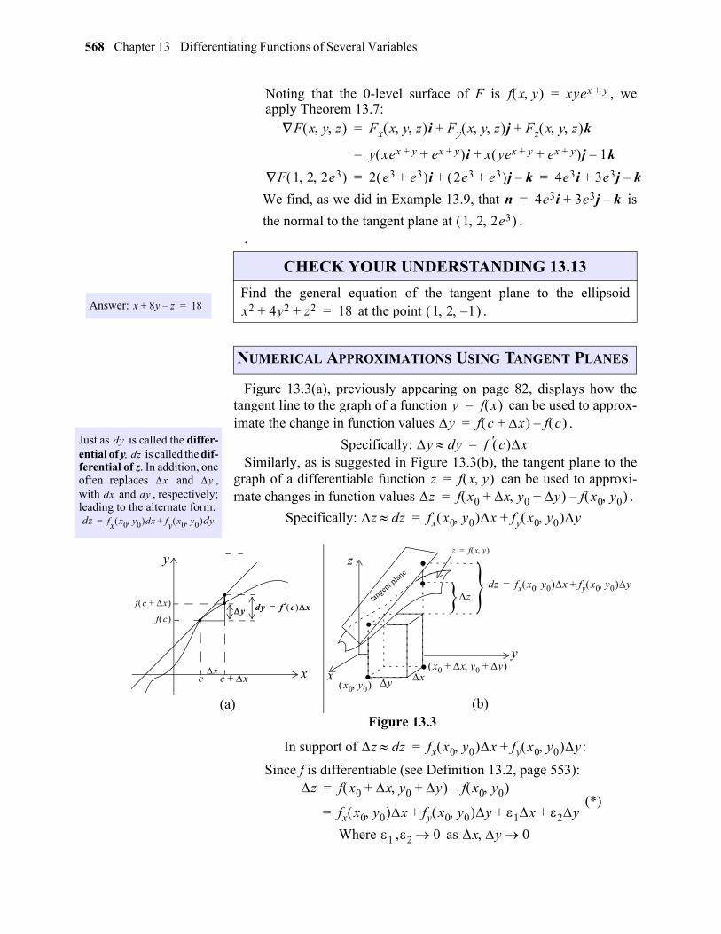
568 Chapter 13 Differentiating Functions of Several Variables
gio
Noting that the 0-level surface of F is , weapply Theorem 13.7:
We find, as we did in Example 13.9, that is
the normal to the tangent plane at ..
Figure 13.3(a), previously appearing on page 82, displays how thetangent line to the graph of a function can be used to approx-imate the change in function values .
Specifically: Similarly, as is suggested in Figure 13.3(b), the tangent plane to the
graph of a differentiable function can be used to approxi-mate changes in function values .
Specifically:
Figure 13.3
In support of :
Since f is differentiable (see Definition 13.2, page 553):
(*)
Where , as
f x y xyex y+=
F x y z Fx x y z i Fy x y z j Fz x y z k+ +=
y xex y+ ex y++ i x yex y+ ex y++ j 1k–+=
F 1 2 2e3 2 e3 e3+ i 2e3 e3+ j k–+ 4e3i 3e3j k–+= =
n 4e3i 3e3j k–+=
1 2 2e3
Answer: x 8y z–+ 18=
CHECK YOUR UNDERSTANDING 13.13
Find the general equation of the tangent plane to the ellipsoid at the point .
NUMERICAL APPROXIMATIONS USING TANGENT PLANES
x2 4y2 z2+ + 18= 1 2 1–
Just as is called the differ-ential of y, is called the dif-ferential of z. In addition, oneoften replaces and ,with and , respectively;leading to the alternate form:
dydz
x ydx dy
dz fx x0 y0 dx fy x0 y0 dy+=
y f x =y f c x+ f c –=
y dy f c x=
z f x y =z f x0 x+ y0 y+ f x0 y0 –=
z dz fx x0 y0 x fy x0 y0 y+=
(a) (b)
...
x
y dy f c x=
c x+c
f c
f c x+
x
y
x
y
zz f x y =
x0 y0
x0 x+ y0 y+ ..
.y x
..}z }tan
gent p
lane
dz fx x0 y0 x fy x0 y0 y+=
z dz fx x0 y0 x fy x0 y0 y+=
z f x0 x+ y0 y+ f x0 y0 –=
fx x0 y0 x fy x0 y0 y 1x 2y+ + +=
1 2 0 x y 0
13.2 Directional Derivatives, Gradient Vectors, and Tangent Planes 569
The tangent plane to the graph of passing through thepoint P is given by (see Definition 113.5):
Or:
When and , the tangent plane has height , and
when and it has height:
. So:
[see Figure 13.3(b)]
Returning to (*) we then have:
or that as and tend to 0.
SOLUTION: Turning to:
, , and
we have:
From , :
,
Thus:
z f x y =
fx x0 y0 x fy x0 y0 y z z0– –+ 0=
z z0 fx x0 y0 x fy x0 y0 y+ +=
x x0= y y0= z0
x x0 x+= y y0 y+=
z z0 fx x0 y0 x fy x0 y0 y+ +=
z z0– f x0 x+ y0 y+ f x0 y0 – dz= =
z dz 1x 2y+ +=
dz z x y
Admittedly, nowadays there isreally no need to approximateanything — just invoke a cal-culator. The main idea here,however, is to underline thefact that tangent planes can beused to approximate morecomplicated surfaces at pointsof interest, just as tangent linescan be used to approximatemore complicated functions ofa single variable.
EXAMPLE 13.11 Use a differential to approximate the change
in the volume of a cone result-
ing from a change in radius from 10 cm to10.01 cm, and a change in height from 20 cmto 19.97 cm.
V13---r2h=
V r h 13---r2h= r h 10 20 = r 0.01= h 0.03–=
V dv Vr 10 20 0.01 Vh 10 20 0.03– +=
Vr r 1
3---r2h
3--- 2rh = = Vh h
13---r2h
3---r2= =
Vr 10 20 3--- 2 10 20 400
3------------= = Vh 10 20
3---102 100
3------------= =
Answer: 0 0.1 –
CHECK YOUR UNDERSTANDING 13.14
Let . Use a differential to approximate thechange in z as varies form to .
V dv 4003
------------ 0.01 1003
------------ 0.03– 1.05 cm3+=
z f x y x2 y2+= =x y 3 4 3.01 3.98
gio
570 Chapter 13 Differentiating Functions of Several Variables
Exercises 1-2. Appeal directly to Definition 13.3 to verify that:
Exercises 3-25. Find the directional derivative of the given function at the indicated point anddirection.
EXERCISES
1. If and if u is the unit vector making an angle with the x-axis, then
.
2. If and if u is the unit vector making an angle with the x-axis, then
.
3. at in the direction of .
4. at in the direction of .
5. at in the direction of .
6. at in the direction of .
7. at in the direction of .
8. at in the direction of .
9. at in the direction of .
10. at in the direction of .
11. at in the direction of .
12. at in the direction of .
13. at in the direction of .
14. at in the direction from toward .
15. at in the direction from toward .
16. at in the direction of .
f x y x2 xy+= 45
Du f x y 3x y+
2---------------=
f x y y2 xy+= 60
Du f x y 3x 1 2 3+ y+2
--------------------------------------------=
f x y xy2 x2+= 1 2– 3---=
f x y 2xy y2–= 1 3– 23
------=
f x y xey yex+= 0 0 6---=
f x y ye x–= 0 4 23
------=
f x y xey yex–= 0 0 3i 4j+
f x y 4x3y2= 2 1 4i 3j–
f x y y2 xln= 1 4 3i– 3j+
f x y e4x 7y–= 0 2ln i
f x y 2x 3y+ 2= 2 2 j
f x y exye y–= 0 1– j–
f x y 1x2 y2+----------------= 2 2 j
f x y exy= 1 2 1 2 3 0
f x y x3 x2y– y2+= 1 1– 1 1– 4 3
f x y xy sinx y+
------------------= 1 1 1
2-------i
1
2-------j–
gio
13.2 Directional Derivatives, Gradient Vectors, and Tangent Planes 571
Exercises 26-39. Find the greatest value and smallest value of the directional derivative for thegiven function at the given point.
Exercises 40-43. Find the general form equation of the tangent plane to the graph of the givenfunction at the given point using: (a) Definition 13.5 (b) Theorem 13.7.
17. at in the direction of .
18. at in the direction of .
19. at in the direction of .
20. at in the direction from toward .
21. at the point in the direction of the vector .
22. at the point in the direction of the vector .
23. at the point in the direction of the vector .
24. at the point in the direction of the vector .
25. at the point in the direction of the vector .
26. at 27. at
28. at 29. at
30. at 31. at
32. at 33. at
34. at 35. at
36. at 37. at
38. at 39. at
40. at 41. at
42. at 43. at
f x y sin3
x y+ =3---
6---–
i–
f x y tan1– y
x-- = 1 2
4---=
f x y tan1– y
x-- = 2– 2 i– j–
f x y xy= a b a b 0 0
f x y z xy yz zx+ += 1 1– 2 3i 6j 2k–+
f x y z x y zsincos= 1 4---
2i j– 4k+
f x y z 3ex yz cos= 1 012---
i 2j 2k+ +
f x y z ztan1– y
x-- = 1 1 3 i j k–+
f x y z x y2 z3+ + 2= 1 2 1 i j+
f x y x2 xy+= 1 1– f x y x3y2 xy–= 2
12---
f x y y2
x-----= 2 4 f x y xey yex+= 0 0
f x y xex ye+= 1 1 f x y 3x y– cos=
6---
4---
f x y x yln= 5 1 f x y x y+ sinx y– cos
-------------------------=2---
4---
f x y 2x y– sin=4---
4---
f x y z xy-- yz–= 4 1 1
f x y z yyx----- yz–= 1 2 3 f x y z x2 y2 z2+ += 3 6 2–
f x y z ztan1– yx--= 1 1 3 f x y z xy yz xzln+ln+ln= 1 1 1
z 2x 3xy2+= 2 1 10– z xy y3– x2+= 1 4 59–
z 2x2 y+= 1 1 3 z 4x2 y2– 2y+= 1– 2 4
gio
572 Chapter 13 Differentiating Functions of Several Variables
Exercises 44-53. Find the general form equation of the tangent plane to the given surface at thegiven point.
54. Use a differential to approximate, to two decimal places, the value of .
55. Use a differential to approximate, to two decimal places, the value of .
56. Use differentials to estimate the change in from to .
57. Use differentials to approximate, to two decimal places, the change in from to .
58. Use differentials to approximate, to two decimal places, the increase in area of a triangle if its base in increased from 2 to 2.05 centimeters and its altitude is increased from 5 to 5.1 centi-meters.
59. Use differentials to approximate, to two decimal places, the increase in the area of a triangle if its base in increased from 2 to 2.05 cm, and its altitude is increased from 5 to 5.1 cm.
60. Use differentials to approximate, to two decimal places, the increase in the volume of a right circular cylinder if the height is increased from 2 to 2.1 cm, and the radius from0,5 to 0.51 cm.
61. Use differentials to approximate, to two decimal places, the change in from to .
62. Use differentials to approximate, to two decimal places, the change in from to .
63. The length, width, and height of a rectangular box are measured to be 3 cm, 4 cm, and 5 cm, respectively, each with a maximum error of 0.05 cm. Use differentials to approximate the maximum error in the calculated volume.
64. Use differentials to approximate the percentage error in if x, y, and z have errors of at most 1%, 2%2, and 3%, respectively.
65. Prove that if , then all directional derivatives of f at are 0.
66. Show that is the tangent plane to at .
67. Show that is the tangent plane to at .
44. at 45. at
46. at 47. at
48. at 49. at
50. at 51. at
52. at 53. at
z xe y–= 1 0 1 z y x y– cos= 2 2 2
z 2 x2 y2+ + ln= 1 2 7ln z e3y 3xsin=
6--- 0 1
x2 y2 z2+ + 49= 2 1 1– 2x2 3y2 z2–+ 10= 2 1 1–
x2 3/ y2 3/ z2 3/+ + 9= 1 8 8– yx z+----------- 2= 1 8 3
xyz cos 0= 4 18---
1 x y z+ + + ln 3=
e2 2 e3 e2 3––+
2.98 2 4.03 2+
1002 1992 2012+ +
z x2y 1–= 1 2 1.11 1.92
z ex= xyln1 2 0.9 2.1
f x y z 2xy2z3=1 1 2– 0.99 1.02 2.02–
f x y z x2 z y2 zsin–cos= 2 2 2 2.1 1.9 2.2
w xy2z3=
f x0 y0 0= x0 y0
xx0
a2--------
yy0
b2--------
zz0
c2-------+ + 1= x2
a2----- y2
b2----- z2
c2-----+ + 1= x0 y0 z0
xx0
a2--------
yy0
b2--------
zz0
c2-------–+ 1= x2
a2----- y2
b2----- z2
c2-----–+ 1= x0 y0 z0
gio
13.2 Directional Derivatives, Gradient Vectors, and Tangent Planes 573
68. The normal line at a point on a surface S is the line that is perpendicular to the tangent plane at that point. Two surfaces are said to be orthogonal at a point of intersection if their normal lines are perpendicular at that point. Prove that the surfaces and
are orthogonal at a point of intersection if and only if .
(Assume that and that .)
69. (Reminiscent of familiar derivative formulas) For and differentiable func-tions, and any number r, prove that:
(a) (b)
(c) (d)
70. Let be a point on a surface S with equation . Show that
is perpendicular to the tangent vector to any smooth curve
lying on S that passes through ; that is, for which
.
f x y z 0= g x y z 0=
x0 y0 z0 fxgx fygy fzgxz+ + 0=
f x0 y0 z0 0 g x0 y0 z0 0
f x y z g x y z
rf rf= f g f g=
fg fg gf+= fg--- gf fg–
g2-------------------------=
x0 y0 z0 z f x y =
fx x0 y0 i fy x0 y0 j k–+ r t0 r t x t i y t j z t k+ += x0 y0 z0 r t0 x0 y0 z0 =
gio
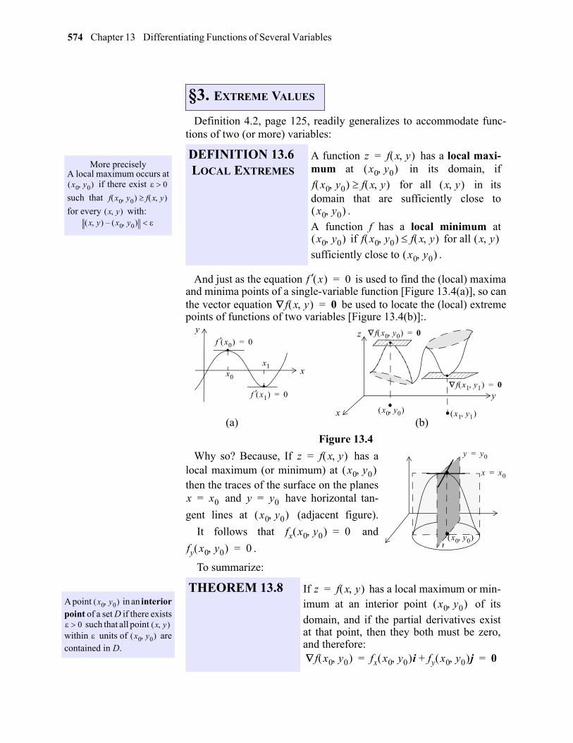
574 Chapter 13 Differentiating Functions of Several Variables
13
Definition 4.2, page 125, readily generalizes to accommodate func-tions of two (or more) variables:
And just as the equation is used to find the (local) maximaand minima points of a single-variable function [Figure 13.4(a)], so canthe vector equation be used to locate the (local) extremepoints of functions of two variables [Figure 13.4(b)]:.
Figure 13.4
Why so? Because, If has alocal maximum (or minimum) at then the traces of the surface on the planes
and have horizontal tan-
gent lines at (adjacent figure).
It follows that and
.
To summarize:
§3. EXTREME VALUES
More preciselyA local maximum occurs at
if there exist
such that
for every with:
x0 y0 0
f x0 y0 f x y
x y x y x0 y0 –
DEFINITION 13.6 LOCAL EXTREMES
A function has a local maxi-mum at in its domain, if
for all in itsdomain that are sufficiently close to
.
A function f has a local minimum at if for all
sufficiently close to .
z f x y =x0 y0
f x0 y0 f x y x y
x0 y0
x0 y0 f x0 y0 f x y x y x0 y0
f x 0=
f x y 0=
.
.
.
.y
z
x
yf x0 0=
f x1 0=
f x0 y0 0=
x0
x1
. .f x1 y1 0=
x0 y0 x1 y1 x (a) (b)
.
.
x0 y0
x x0=
y y0=z f x y =x0 y0
x x0= y y0=
x0 y0 fx x0 y0 0=
fy x0 y0 0=
A point in an interiorpoint of a set D if there exists
such that all point within units of arecontained in D.
x0 y0
0 x y x0 y0
THEOREM 13.8 If has a local maximum or min-imum at an interior point of its
domain, and if the partial derivatives existat that point, then they both must be zero,and therefore:
z f x y =x0 y0
f x0 y0 fx x0 y0 i fy x0 y0 j+ 0= =
gio
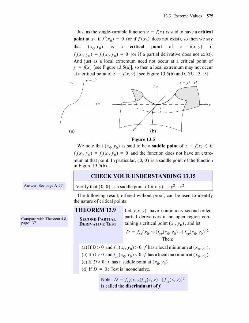
13.3 Extreme Values 575
Just as the single-variable function is said to have a critical
point at if (or if does not exist), so then we say
that is a critical point of if
(or if a partial derivative does not exist).
And just as a local extremum need not occur at a critical point of [see Figure 13.5(a)], so then a local extremum may not occur
at a critical point of [see Figure 13.5(b) and CYU 13.15]:
Figure 13.5We note that is said to be a saddle point of if
and the function does not have an extre-
mum at that point. In particular, is a saddle point of the functionin Figure 13.5(b).
The following result, offered without proof, can be used to identifythe nature of critical points:
y f x =
x0 f x0 0= f x0
x0 y0 z f x y =
fx x0 y0 fy x0 y0 0= =
y f x =z f x y =
x y
x
zy y x3=
z y2 x2–=
(a) (b)
Answer: See page A-27.
CHECK YOUR UNDERSTANDING 13.15
Verify that is a saddle point of .
x0 y0 z f x y =
fx x0 y0 fy x0 y0 0= =
0 0
0 0 f x y y2 x2–=
Compare with Theorem 4.8,page 137.
THEOREM 13.9
SECOND PARTIAL DERIVATIVE TEST
Let have continuous second-orderpartial derivatives in an open region con-taining a critical point , and let
Then:
(a) If and : f has a local minimum at .
(b) If and : f has a local maximum at .
(c) If : f has a saddle point at .
(d) If : Test is inconclusive.
Note: is called the discriminant of f.
f x y
x0 y0
D fxx x0 y0 fyy x0 y0 fxy x0 y0 2–=
D 0 fxx x0 y0 0 x0 y0 D 0 fxx x0 y0 0 x0 y0 D 0 x0 y0 D 0=
D fxx x y fyy x y fxy x y 2–=
gio
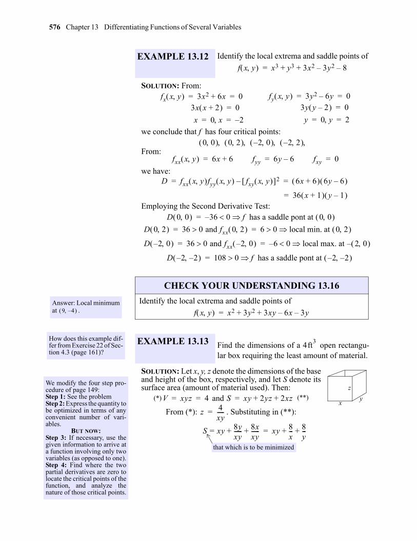
576 Chapter 13 Differentiating Functions of Several Variables
gio
SOLUTION: From:
we conclude that f has four critical points:
From:
we have:
Employing the Second Derivative Test:
SOLUTION: Let x, y, z denote the dimensions of the baseand height of the box, respectively, and let S denote itssurface area (amount of material used). Then:
and
From (*): . Substituting in (**):
EXAMPLE 13.12 Identify the local extrema and saddle points of
f x y x3 y3 3x2 3y2– 8–+ +=
fx x y 3x2 6x+ 0= =3x x 2+ 0=
x 0 x 2–= =
fy x y 3y2 6y– 0= =3y y 2– 0=
y 0 y 2= =
0 0 0 2 2– 0 2– 2
fxx x y 6x 6 fyy+ 6y 6 fxy– 0= = =
D fxx x y fyy x y fxy x y 2– 6x 6+ 6y 6– = =
36 x 1+ y 1– =
D 0 0 36 0 f has a saddle pont at 0 0 –=
D 0 2 36 0 and fxx 0 2 6 0 local min. at 0 2 = =
D 2– 0 36 0 and fxx 2– 0 6– 0 local max. at 2 0 –= =
D 2– 2– 108 0 f has a saddle pont at 2– 2– =
Answer: Local minimumat .9 4–
CHECK YOUR UNDERSTANDING 13.16
Identify the local extrema and saddle points of
f x y x2 3y2 3xy 6x– 3y–+ +=
How does this example dif-fer from Exercise 22 of Sec-tion 4.3 (page 161)?
EXAMPLE 13.13 Find the dimensions of a 4 open rectangu-lar box requiring the least amount of material.
ft3
We modify the four step pro-cedure of page 149:Step 1: See the problem Step 2: Express the quantity tobe optimized in terms of anyconvenient number of vari-ables.
BUT NOW:Step 3: If necessary, use thegiven information to arrive ata function involving only twovariables (as opposed to one).Step 4: Find where the twopartial derivatives are zero tolocate the critical points of thefunction, and analyze thenature of those critical points.
xy
z
V xyz 4= =(*) S xy 2yz 2xz++= (**)
z 4xy-----=
S xy 8yxy------+= 8x
xy------+ xy 8
x--- 8
y---+ +=
that which is to be minimized
13.3 Extreme Values 577
Locating the critical points (see Theorem12.12):
We now turn to Theorem 12.13 to make sure that a minimum occurs at
the (only) critical point . Since :
Conclusion: The box requiring the least material has a square base oflength 2 ft, and a height of 1 ft.
Let be defined on a region D. We say that f assumes its
absolute maximum at in D, if for every
. Similarly, f is said to assume its absolute minimum at
if for every . We already know
that if a differentiable function has a local maximum or
minimum at an interior point of D, then (Theorem
13.8). In order to locate the absolute extreme values of the function,however, we must also take into account the non-interior points of D.With this in mind, we direct your attention to the following particularlyimportant result:
Sx y 8x2-----– 0= =
Sy x 8y2-----– 0= =
yx2 8=
xy2 8=
yx2 xy2 yx2 xy2– 0==
xy x y– 0=x y=neither dimension x nor y can be zero:
y3 8=
x3 8=
x y 2= =So:
z 4xy----- 1= =
2 2 Sxx16x3------ Syy
16y3------== Sxy 1=
D Sxx 2 2 Syy 2 2 Sxy 2 2 2–168------ 16
8------ 12– 3 0= = =
and Sxx 2 2 2 0=
Answer: 13--- 1
3--- 1
3---
CHECK YOUR UNDERSTANDING 13.17
Find the three positive numbers whose sum is 1 and such that thesum of their squares is as small a possible.
ABSOLUTE MAXIMUM AND MINIMUM VALUES
Consider Exercises 33-38of Section 4.3 (page 146).
THEOREM 13.10 A real-valued continuous function f defined
on a bounded closed set K (in ) willachieve both its maximum value and itsminimum value at points in K.
z f x y =
x0 y0 f x0 y0 f x y
x y Dx0 y0 f x0 y0 f x y x y D
z f x y =
f x0 y0 0=
Rn
gio
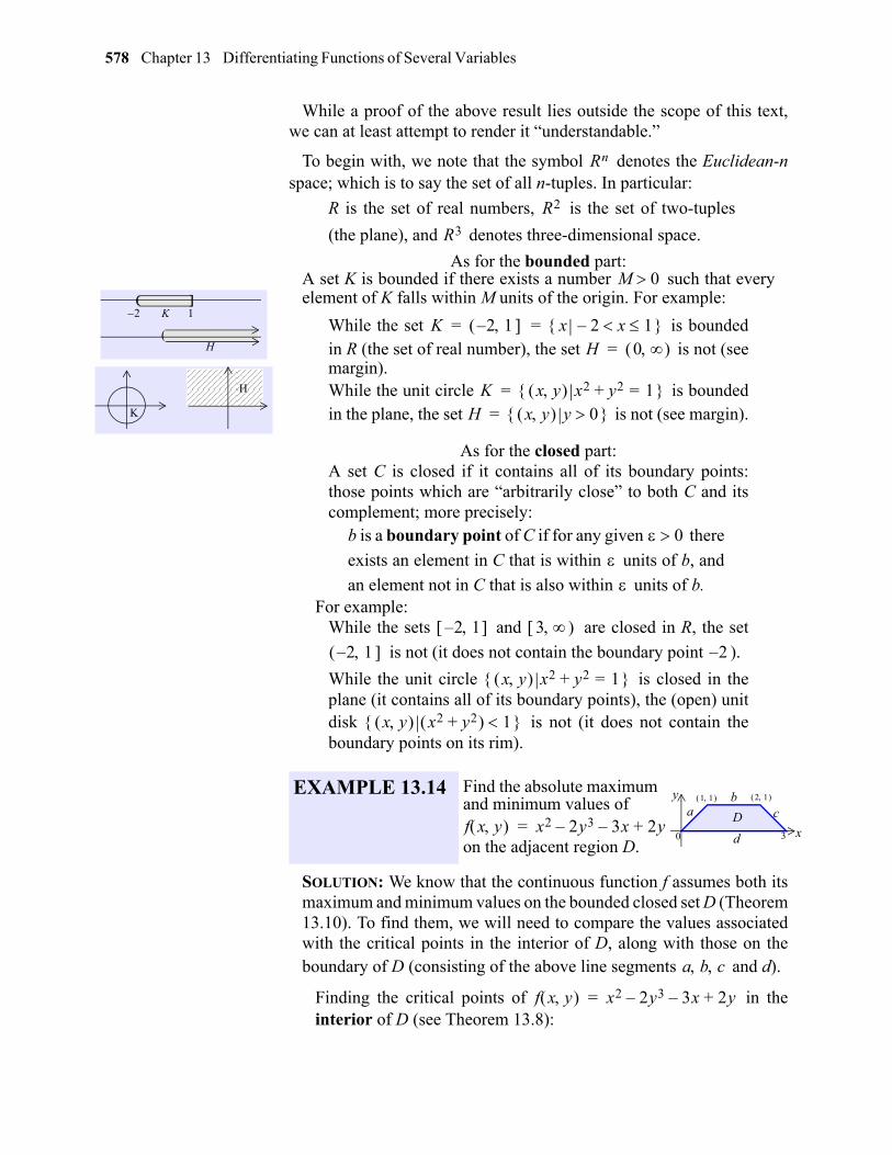
578 Chapter 13 Differentiating Functions of Several Variables
gio
While a proof of the above result lies outside the scope of this text,we can at least attempt to render it “understandable.”
To begin with, we note that the symbol denotes the Euclidean-nspace; which is to say the set of all n-tuples. In particular:
R is the set of real numbers, is the set of two-tuples
(the plane), and denotes three-dimensional space.
As for the bounded part: A set K is bounded if there exists a number such that everyelement of K falls within M units of the origin. For example:
While the set is boundedin R (the set of real number), the set is not (seemargin). While the unit circle is boundedin the plane, the set is not (see margin).
As for the closed part:A set C is closed if it contains all of its boundary points:those points which are “arbitrarily close” to both C and itscomplement; more precisely:
b is a boundary point of C if for any given there
exists an element in C that is within units of b, and
an element not in C that is also within units of b.For example:
While the sets and are closed in R, the set
is not (it does not contain the boundary point ).
While the unit circle is closed in theplane (it contains all of its boundary points), the (open) unitdisk is not (it does not contain theboundary points on its rim).
SOLUTION: We know that the continuous function f assumes both itsmaximum and minimum values on the bounded closed set D (Theorem13.10). To find them, we will need to compare the values associatedwith the critical points in the interior of D, along with those on theboundary of D (consisting of the above line segments and d).
Finding the critical points of in theinterior of D (see Theorem 13.8):
Rn
R2
R3
2– 1
K
(H
K
H
EXAMPLE 13.14 Find the absolute maximum and minimum values of
on the adjacent region D.
M 0
K 2– 1 x 2 x 1– = =H 0 =
K x y x2 y2+ 1= =H x y y 0 =
0
2 1– 3 2– 1 2–
x y x2 y2+ 1=
x y x2 y2+ 1
1 1 2 1
0 3 x
ya
bc
d
Df x y x2 2y3– 3x– 2y+=
a b c
f x y x2 2y3– 3x– 2y+=
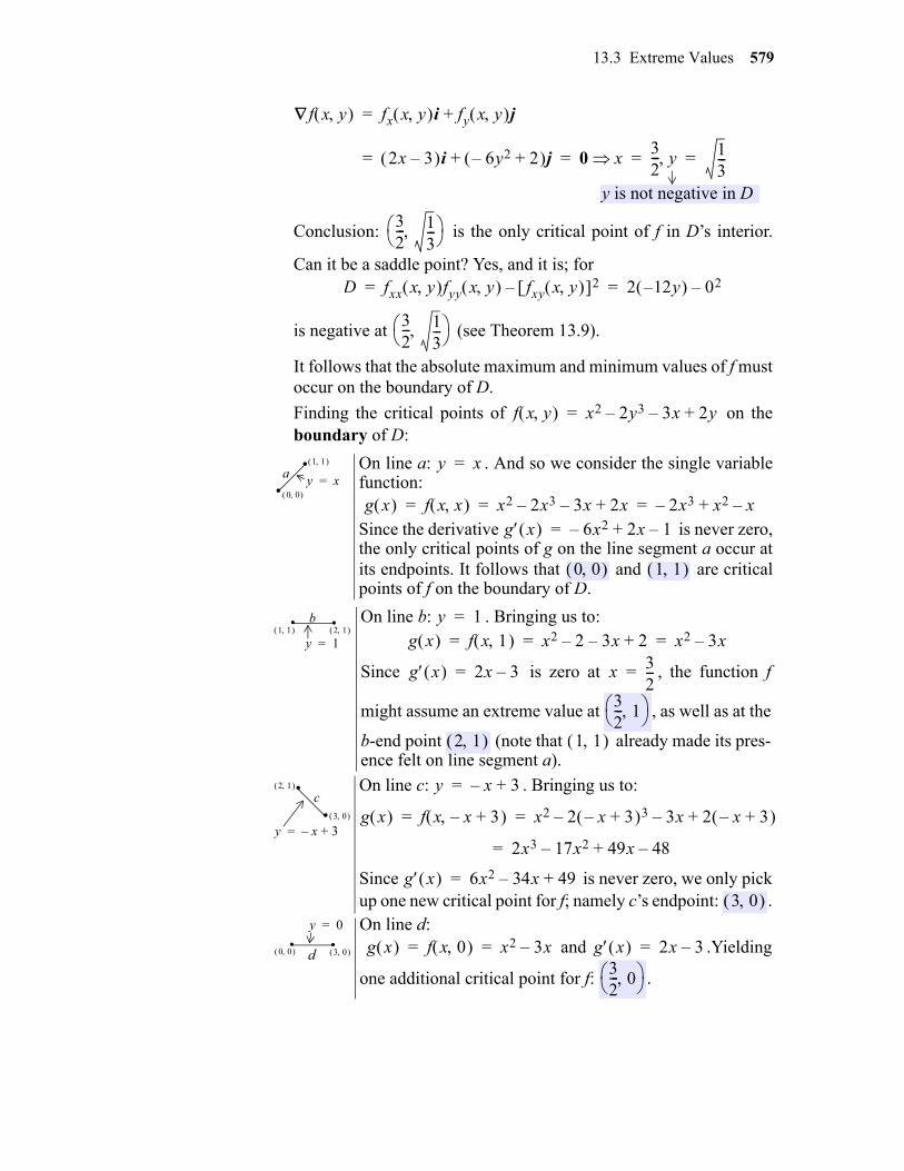
13.3 Extreme Values 579
Conclusion: is the only critical point of f in D’s interior.
Can it be a saddle point? Yes, and it is; for
is negative at (see Theorem 13.9).
It follows that the absolute maximum and minimum values of f mustoccur on the boundary of D.
Finding the critical points of on theboundary of D:
On line a: . And so we consider the single variablefunction: Since the derivative is never zero,the only critical points of g on the line segment a occur atits endpoints. It follows that and are criticalpoints of f on the boundary of D.
On line b: . Bringing us to:
Since is zero at , the function f
might assume an extreme value at , as well as at the
b-end point (note that already made its pres-ence felt on line segment a).
On line c: . Bringing us to:
Since is never zero, we only pickup one new critical point for f; namely c’s endpoint: .On line d: and .Yielding
one additional critical point for f: .
f x y fx x y i fy x y j+=
2x 3– i 6y2– 2+ j+ 0 x 32--- y 1
3---= = = =
y is not negative in D
32--- 1
3---
D fxx x y fyy x y fxy x y 2– 2 12y– 02–= =
32--- 1
3---
f x y x2 2y3– 3x– 2y+=
..
1 1
0 0
a y x=y x=
g x f x x x2 2x3– 3x– 2x+ 2x3– x2 x–+= = =g x 6x2– 2x 1–+=
0 0 1 1
y 1=
. .b1 1 2 1
y 1=g x f x 1 x2 2– 3x– 2+ x2 3x–= = =
g x 2x 3–= x 32---=
32--- 1
2 1 1 1
c.
.2 1
3 0
y x– 3+=
y x– 3+=
g x f x x– 3+ x2 2 x– 3+ 3– 3x– 2 x– 3+ += =
2x3 17x2– 49x 48–+=
g x 6x2 34x– 49+=3 0
. .0 0
y 0=
3 0 d g x f x 0 x2 3x–= = g x 2x 3–=32--- 0
gio
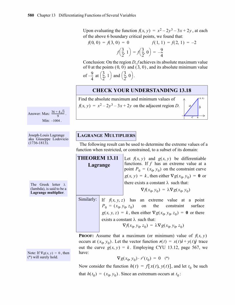
580 Chapter 13 Differentiating Functions of Several Variables
gio
Upon evaluating the function , at eachof the above 6 boundary critical points, we found that:
Conclusion: On the region D, f achieves its absolute maximum valueof 0 at the points and , and its absolute minimum value
of at and .
The following result can be used to determine the extreme values of afunction when restricted, or constrained, to a subset of its domain:
PROOF: Assume that a maximum (or minimum) value of occurs at . Let the vector function traceout the curve . Employing CYU 13.12, page 567, wehave:
Now consider the function , and let be such
that . Since an extremum occurs at :
f x y x2 2y3– 3x– 2y+=
f 0 0 f 3 0 0= = f 1 1 f 2 1 2–= =
f32--- 1 f
32--- 0 9
4---–= =
0 0 3 0 94---–
32--- 1 3
2--- 0
Answer: Max: .
Min: .
36 4 3+9
----------------------
1004–
CHECK YOUR UNDERSTANDING 13.18
Find the absolute maximum and minimum values of
on the adjacent region D.
4 8
4
a b
c
f x y x2 2y3– 3x– 2y+=
Joseph-Louis Lagrangeaka Giuseppe Lodovicio(1736-1813).
The Greek letter (lambda), is said to be aLagrange multiplier.
LAGRANGE MULTIPLIERS
THEOREM 13.11Lagrange
Let and be differentiablefunctions. If f has an extreme value at apoint on the constraint curve
, then either or
there exists a constant such that:
Similarly: If has an extreme value at a point on the constraint surface
, then either or there
exists a constant such that:
f x y g x y
P0 x0 y0 =
g x y k= g x0 y0 0=
f x0 y0 g x0 y0 =
f x y z P0 x0 y0 z0 =
g x y z k= g x0 y0 z0 0=
f x0 y0 z0 g x0 y0 z0 =
Note: If , then(*) will surely hold.
g x y 0=
f x y x0 y0 r t x t i y t j+=
g x y k=
g x0 y0 r t0 0= (*)
h t f x t y t = t0
h t0 x0 y0 = t0
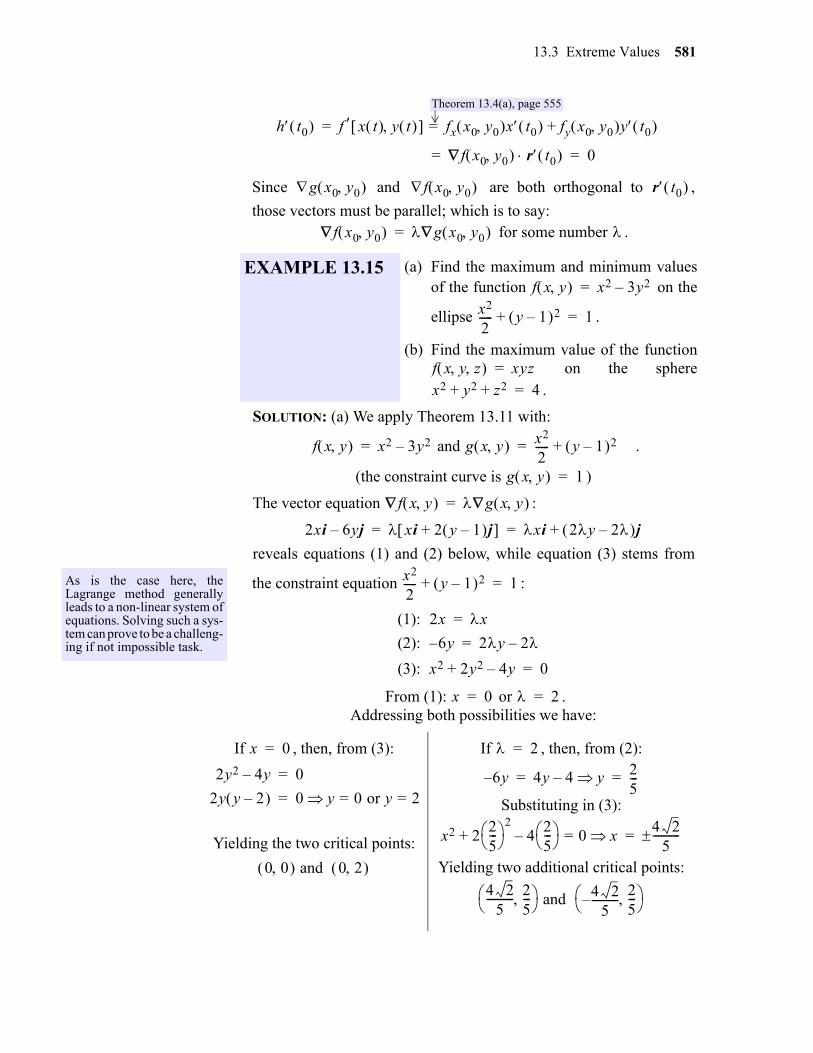
13.3 Extreme Values 581
Since and are both orthogonal to ,
those vectors must be parallel; which is to say: for some number .
SOLUTION: (a) We apply Theorem 13.11 with:
and .
(the constraint curve is )
The vector equation :
reveals equations (1) and (2) below, while equation (3) stems from
the constraint equation :
From (1): or . Addressing both possibilities we have:
EXAMPLE 13.15 (a) Find the maximum and minimum valuesof the function on the
ellipse .
(b) Find the maximum value of the function on the sphere.
h t0 f x t y t fx x0 y0 x t0 fy x0 y0 y t0 += =
f x0 y0 r t0 0= =
Theorem 13.4(a), page 555
g x0 y0 f x0 y0 r t0
f x0 y0 g x0 y0 =
f x y x2 3y2–=x2
2----- y 1– 2+ 1=
f x y z xyz=x2 y2 z2+ + 4=
As is the case here, theLagrange method generallyleads to a non-linear system ofequations. Solving such a sys-tem can prove to be a challeng-ing if not impossible task.
f x y x2 3y2–= g x y x2
2----- y 1– 2+=
g x y 1=
f x y g x y =
2xi 6yj– xi 2 y 1– j+ xi 2y 2– j+= =
x2
2----- y 1– 2+ 1=
(1): 2x x=
(2): 6y– 2y 2–=
(3): x2 2y2 4y–+ 0=
x 0= 2=
If , then, from (3):
Yielding the two critical points:
If , then, from (2):
Substituting in (3):
Yielding two additional critical points:
x 0=
2y2 4y– 0=
2y y 2– 0 y 0 or y 2= ==
0 0 and 0 2
2=
6y– 4y 4 y– 25---= =
x2 225--- 2
425--- –+ 0= x 4 2
5----------=
4 25
---------- 25---
and 4 25
----------–25---
gio
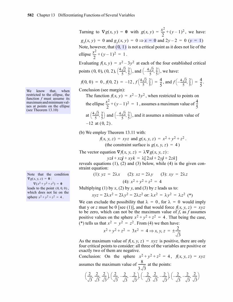
582 Chapter 13 Differentiating Functions of Several Variables
gio
Turning to with , we have:
Note, however, that is not a critical point as it does not lie of the
ellipse .
Evaluating at each of the four established critical
points , and , we have:
, , , and .
Conclusion (see margin):The function , when restricted to points on
the ellipse , assumes a maximum value of
at and , and it assumes a minimum value of
at .
(b) We employ Theorem 13.11 with: and .
(the constraint surface is )
The vector equation :
reveals equations (1), (2) and (3) below, while (4) is the given con-straint equation:
Multiplying (1) by x, (2) by y, and (3) by z leads us to:
We can exclude the possibility that , for would implythat y or z must be 0 [see (1)], and that would force to be zero, which can not be the maximum value of f, as f assumespositive values on the sphere . That being the case,(*) tells us that . From (4) we then have:
As the maximum value of is positive, there are onlyfour critical points to consider: all three of the variables are positive orexactly two of them are negative.Conclusion: On the sphere ,
assumes the maximum value of at the points:
g x y 0= g x y x2
2----- y 1– 2+=
gx x y 0 and gy x y 0 x 0 and 2y 2– 0 (y 1)= = = = =
0 1 x2
2----- y 1– 2+ 1=
We know that, whenrestricted to the ellipse, thefunction f must assume itsmaximum and minimum val-ues at points on the ellipse(see Theorem 13.10)
f x y x2 3y2–=
0 0 0 2 4 25
---------- 25---
4 25
----------– 25---
f 0 0 0= f 0 2 12–= f 4 25
---------- 25---
45---= f 4 2
5----------– 2
5---
45---=
f x y x2 3y2–=x2
2----- y 1– 2+ 1=
45---
4 25
---------- 25---
4 25
----------– 25---
12– 0 2
Note that the condition:
leads to the point ,which does not lie on thesphere .
g x y z 0=
x2 y2 z2+ + 0=0 0 0
x2 y2 z2+ + 4=
f x y z xyz= g x y z x2 y2 z2+ +=g x y z 4=
f x y z g x y z =yzi xzj xyk+ + 2xi 2yj 2zk+ + =
(1): yz 2x (2): xz 2y (3): xy= 2z= =
(4): x2 y2 z2+ + 4=
xyz 2x2 2y2 2z2= = = or: x2 y2 z2= = (*)
0= 0=f x y z xyz=
x2 y2 z2+ + 4=x2 y2 z2= =
x2 y2 z2+ + 3x2 4 x y z 2
3-------= = =
f x y z xyz=
x2 y2 z2+ + 4= f x y z xyz=8
3 3----------
2
3------- 2
3------- 2
3-------
2
3------- 2
3-------– 2
3-------–
2
3-------–
2
3------- 2
3-------–
2
3-------– 2
3-------–
2
3-------
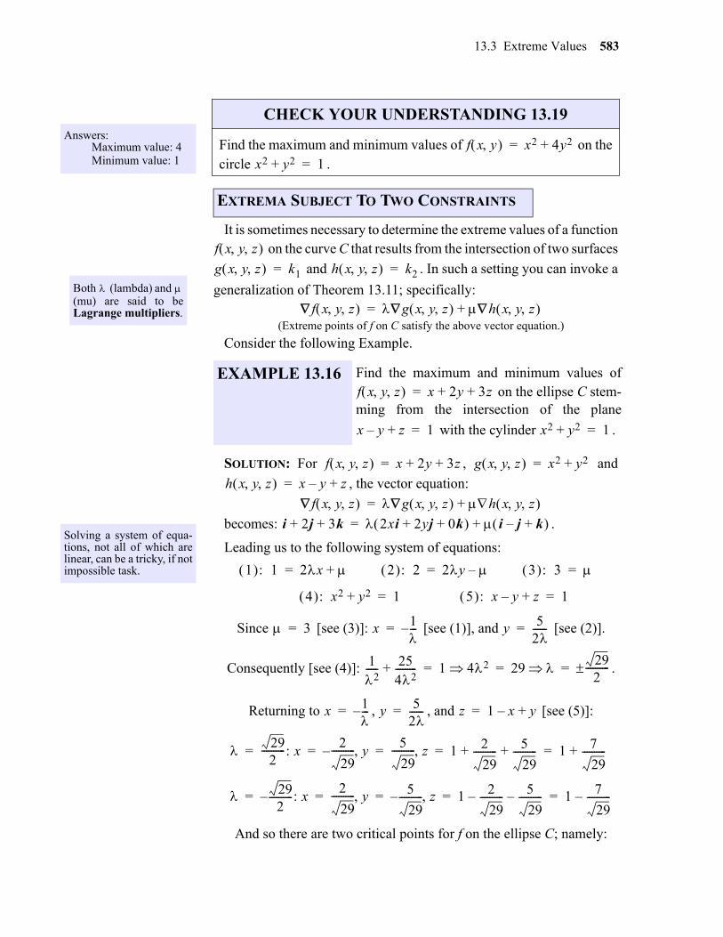
13.3 Extreme Values 583
It is sometimes necessary to determine the extreme values of a function on the curve C that results from the intersection of two surfaces
and . In such a setting you can invoke a
generalization of Theorem 13.11; specifically:
(Extreme points of f on C satisfy the above vector equation.)
Consider the following Example.
SOLUTION: For , and
, the vector equation:
becomes: .
Leading us to the following system of equations:
Since [see (3)]: [see (1)], and [see (2)].
Consequently [see (4)]: .
Returning to , , and [see (5)]:
And so there are two critical points for f on the ellipse C; namely:
Answers: Maximum value: 4
Minimum value: 1
CHECK YOUR UNDERSTANDING 13.19
Find the maximum and minimum values of on thecircle .
EXTREMA SUBJECT TO TWO CONSTRAINTS
f x y x2 4y2+=x2 y2+ 1=
Both (lambda) and (mu) are said to beLagrange multipliers.
EXAMPLE 13.16 Find the maximum and minimum values of on the ellipse C stem-
ming from the intersection of the plane
with the cylinder .
f x y z g x y z k1= h x y z k2=
f x y z g x y z h x y z +=
f x y z x 2y 3z+ +=
x y– z+ 1= x2 y2+ 1=
Solving a system of equa-tions, not all of which arelinear, can be a tricky, if notimpossible task.
f x y z x 2y 3z+ += g x y z x2 y2+=
h x y z x y– z+=
f x y z g x y z h x y z +=
i 2j 3k+ + 2xi 2yj 0k+ + i j– k+ +=
1 : 1 2x += 2 : 2 2y –= 3 : 3 =
4 : x2 y2+ 1= 5 : x y– z+ 1=
3= x 1---–= y 5
2------=
12----- 25
42---------+ 1 42 29 29
2----------= = =
x 1---–= y 5
2------= z 1 x– y+=
292
----------: x2
29---------- y–
5
29---------- z 1 2
29---------- 5
29----------+ + 1 7
29----------+= = = = =
292
----------– : x2
29---------- y 5
29----------– z 1 2
29----------– 5
29----------– 1 7
29----------–= = = = =
gio
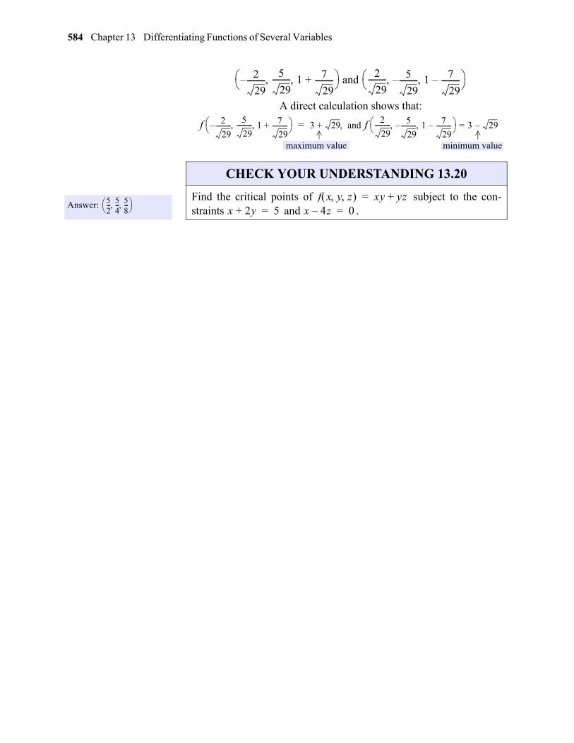
584 Chapter 13 Differentiating Functions of Several Variables
A direct calculation shows that:
2
29----------–
5
29---------- 1 7
29----------+
and 2
29---------- 5
29----------– 1 7
29----------–
f 2
29----------–
5
29---------- 1 7
29----------+
3 29 and f 2
29---------- 5
29----------– 1 7
29----------–
3 29–=+=
maximum value minimum value
Answer: 52--- 5
4--- 5
8---
CHECK YOUR UNDERSTANDING 13.20
Find the critical points of subject to the con-straints and .
f x y z xy yz+=x 2y+ 5= x 4z– 0=
gio
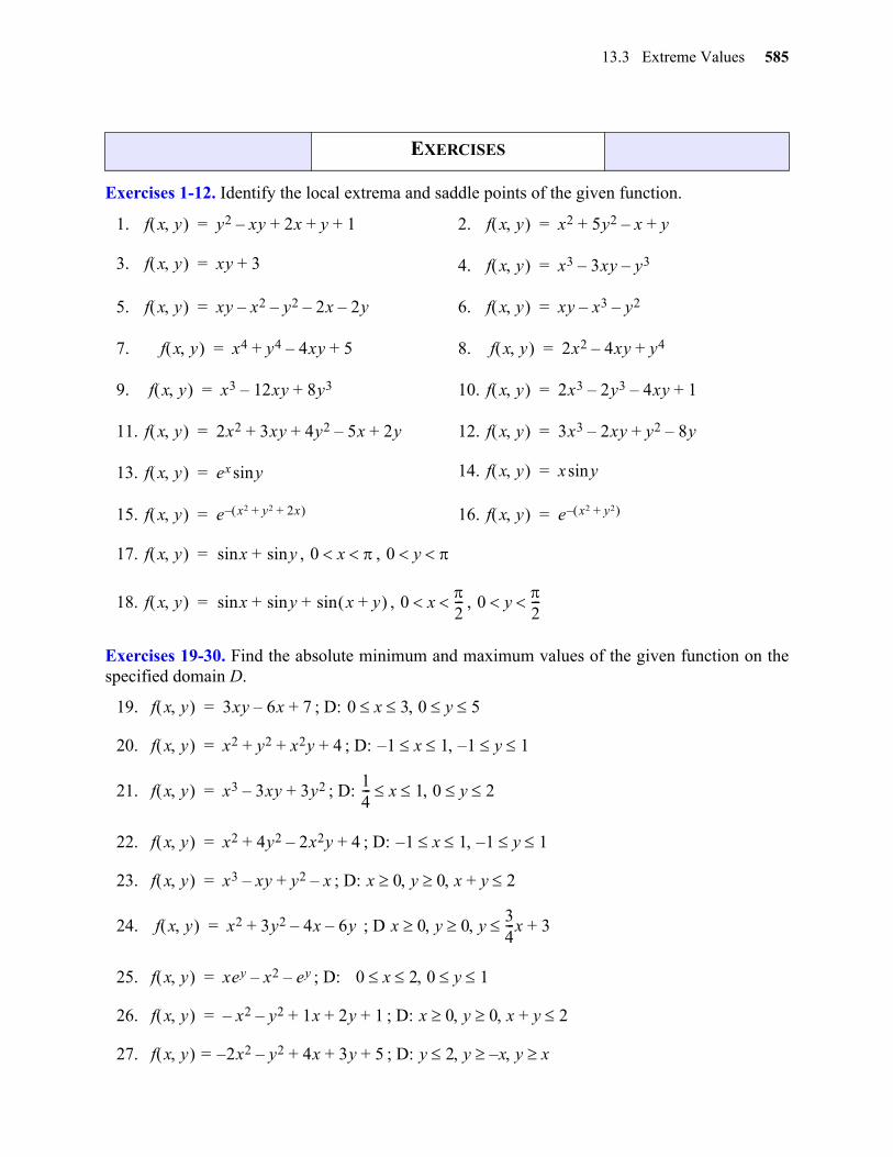
13.3 Extreme Values 585
gio
Exercises 1-12. Identify the local extrema and saddle points of the given function.
Exercises 19-30. Find the absolute minimum and maximum values of the given function on thespecified domain D.
EXERCISES
1. 2.
3. 4.
5. 6.
7. 8.
9. 10.
11. 12.
13. 14.
15. 16.
17. , ,
18. , ,
19. ; D:
20. ; D:
21. ; D:
22. ; D:
23. ; D:
24. ; D
25. ; D:
26. ; D:
27. ; D:
f x y y2 xy– 2x y 1+ + += f x y x2 5y2 x– y+ +=
f x y xy 3+= f x y x3 3xy– y3–=
f x y xy x2– y2– 2x– 2y–= f x y xy x3– y2–=
f x y x4 y4 4xy– 5+ += f x y 2x2 4xy– y4+=
f x y x3 12xy– 8y3+= f x y 2x3 2y3– 4xy– 1+=
f x y 2x2 3xy 4y2 5x– 2y+ + += f x y 3x3 2xy– y2 8y–+=
f x y ex ysin= f x y x ysin=
f x y e x2 y2 2x+ + –= f x y e x2 y2+ –=
f x y x ysin+sin= 0 x 0 y
f x y x y x y+ sin+sin+sin= 0 x2--- 0 y
2---
f x y 3xy 6x– 7+= 0 x 3 0 y 5
f x y x2 y2 x2y 4+ + += 1– x 1 1– y 1
f x y x3 3xy– 3y2+=14--- x 1 0 y 2
f x y x2 4y2 2x2y– 4+ += 1– x 1 1– y 1
f x y x3 xy– y2 x–+= x 0 y 0 x y 2+
f x y x2 3y2 4x– 6y–+= x 0 y 0 y34---x 3+
f x y xey x2– ey–= 0 x 2 0 y 1
f x y x2– y2– 1x 2y 1+ + += x 0 y 0 x y 2+
f x y 2– x2 y2– 4x 3y+ += 5+ y 2 y x y x–
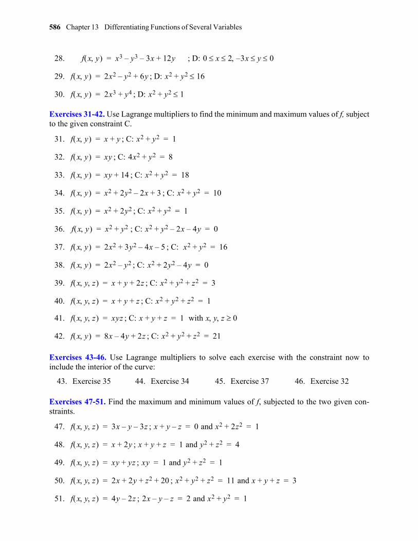
586 Chapter 13 Differentiating Functions of Several Variables
gio
Exercises 31-42. Use Lagrange multipliers to find the minimum and maximum values of f, subjectto the given constraint C.
Exercises 43-46. Use Lagrange multipliers to solve each exercise with the constraint now toinclude the interior of the curve:
Exercises 47-51. Find the maximum and minimum values of f, subjected to the two given con-straints.
28. ; D:
29. ; D:
30. ; D:
31. ; C:
32. ; C:
33. ; C:
34. ; C:
35. ; C:
36. ; C:
37. ; C:
38. ; C:
39. ; C:
40. ; C:
41. ; C:
42. ; C:
43. Exercise 35 44. Exercise 34 45. Exercise 37 46. Exercise 32
47. ;
48. ;
49. ;
50. ;
51. ;
f x y x3 y3– 3x– 12y+= 0 x 2 3x y 0 –
f x y 2x2 y2– 6y+= x2 y2 16+
f x y 2x3 y4+= x2 y2 1+
f x y x y+= x2 y2+ 1=
f x y xy= 4x2 y2+ 8=
f x y xy 14+= x2 y2+ 18=
f x y x2 2y2 2x– 3+ += x2 y2+ 10=
f x y x2 2y2+= x2 y2+ 1=
f x y x2 y2+= x2 y2 2x– 4y–+ 0=
f x y 2x2 3y2 4x– 5–+= x2 y2+ 16=
f x y 2x2 y2–= x2 2y2 4y–+ 0=
f x y z x y 2z+ += x2 y2 z2+ + 3=
f x y z x y z+ += x2 y2 z2+ + 1=
f x y z xyz= x y z+ + 1 with x y z 0 =
f x y 8x 4y– 2z+= x2 y2 z2+ + 21=
f x y z 3x y– 3z–= x y z–+ 0 and x2 2z2+ 1= =
f x y z x 2y+= x y z+ + 1 and y2 z2+ 4= =
f x y z xy yz+= xy 1 and y2 z2+ 1= =
f x y z 2x 2y z2 20+ + += x2 y2 z2+ + 11 and x y z+ + 3= =
f x y z 4y 2z–= 2x y– z– 2 and x2 y2+ 1= =
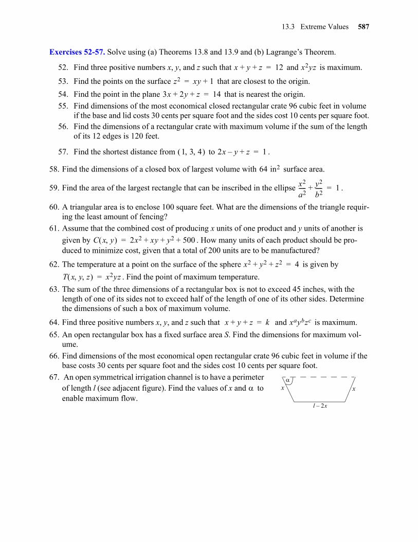
13.3 Extreme Values 587
Exercises 52-57. Solve using (a) Theorems 13.8 and 13.9 and (b) Lagrange’s Theorem.
52. Find three positive numbers x, y, and z such that and is maximum.
53. Find the points on the surface that are closest to the origin.
54. Find the point in the plane that is nearest the origin.
55. Find dimensions of the most economical closed rectangular crate 96 cubic feet in volume if the base and lid costs 30 cents per square foot and the sides cost 10 cents per square foot.
56. Find the dimensions of a rectangular crate with maximum volume if the sum of the length of its 12 edges is 120 feet.
57. Find the shortest distance from to .
58. Find the dimensions of a closed box of largest volume with surface area.
59. Find the area of the largest rectangle that can be inscribed in the ellipse .
60. A triangular area is to enclose 100 square feet. What are the dimensions of the triangle requir-ing the least amount of fencing?
61. Assume that the combined cost of producing x units of one product and y units of another is
given by . How many units of each product should be pro-duced to minimize cost, given that a total of 200 units are to be manufactured?
62. The temperature at a point on the surface of the sphere is given by
. Find the point of maximum temperature.
63. The sum of the three dimensions of a rectangular box is not to exceed 45 inches, with the length of one of its sides not to exceed half of the length of one of its other sides. Determine the dimensions of such a box of maximum volume.
64. Find three positive numbers x, y, and z such that and is maximum.
65. An open rectangular box has a fixed surface area S. Find the dimensions for maximum vol-ume.
66. Find dimensions of the most economical open rectangular crate 96 cubic feet in volume if the base costs 30 cents per square foot and the sides cost 10 cents per square foot.
67. An open symmetrical irrigation channel is to have a perimeter of length l (see adjacent figure). Find the values of x and to enable maximum flow.
x y z+ + 12= x2yz
z2 xy 1+=
3x 2y z+ + 14=
1 3 4 2x y– z+ 1=
64 in2
x2
a2----- y2
b2-----+ 1=
C x y 2x2 xy y2 500+ + +=
x2 y2 z2+ + 4=
T x y z x2yz=
x y z+ + k= xaybzc
x x
l 2x–
gio
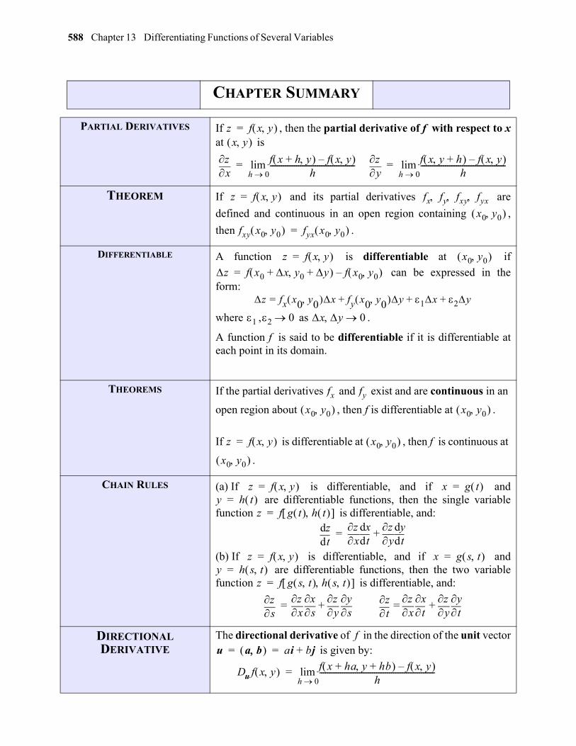
588 Chapter 13 Differentiating Functions of Several Variables
gio
CHAPTER SUMMARY
PARTIAL DERIVATIVES If , then the partial derivative of f with respect to xat is
THEOREM If and its partial derivatives are
defined and continuous in an open region containing ,
then .
DIFFERENTIABLE A function is differentiable at if
can be expressed in theform:
where , as .
A function f is said to be differentiable if it is differentiable ateach point in its domain.
THEOREMS If the partial derivatives and exist and are continuous in an
open region about , then f is differentiable at .
If is differentiable at , then f is continuous at
.
CHAIN RULES (a) If is differentiable, and if and are differentiable functions, then the single variable
function is differentiable, and:
(b) If is differentiable, and if and are differentiable functions, then the two variable
function is differentiable, and:
DIRECTIONALDERIVATIVE
The directional derivative of f in the direction of the unit vector is given by:
z f x y =x y
xz f x h+ y f x y –
h---------------------------------------------
h 0lim=
yz f x y h+ f x y –
h---------------------------------------------
h 0lim=
z f x y = fx fy fxy fyx x0 y0
fxy x0 y0 fyx x0 y0 =
z f x y = x0 y0 z f x0 x+ y0 y+ f x0 y0 –=
z fx x0 y0 x= fy x0 y0 y 1x 2y+ + +
1 2 0 x y 0
fx fy
x0 y0 x0 y0
z f x y = x0 y0
x0 y0
z f x y = x g t =y h t =
z f g t h t =
tddz
xz
tddx
yz
tddy
+=
z f x y = x g s t =y h s t =
z f g s t h s t =
sz
xz
sx
yz
sy
t
zx
zt
xy
zt
y+=+=
u a b ai bj+= =
Du f x y f x ha+ y hb+ f x y –h
-------------------------------------------------------------h 0lim=
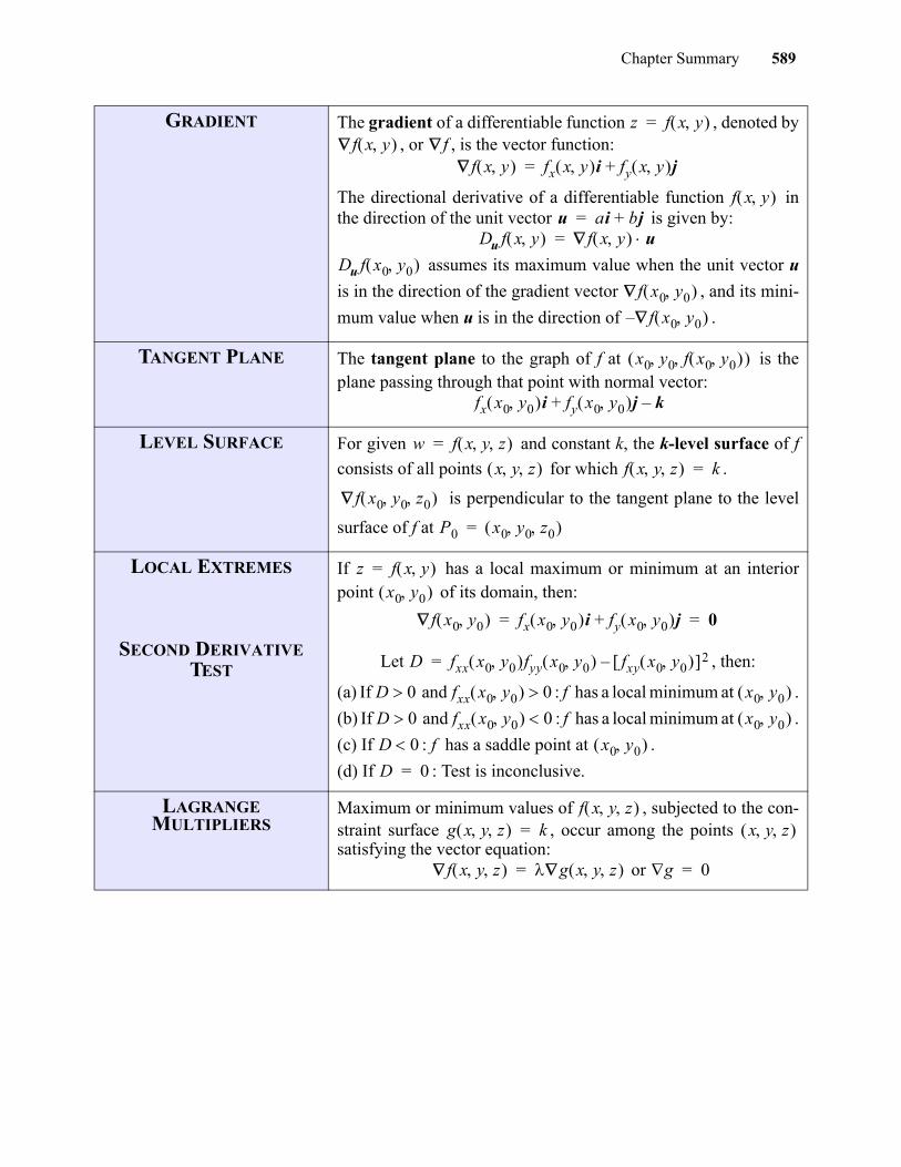
Chapter Summary 589
GRADIENT The gradient of a differentiable function , denoted by, or , is the vector function:
The directional derivative of a differentiable function inthe direction of the unit vector is given by:
assumes its maximum value when the unit vector u
is in the direction of the gradient vector , and its mini-
mum value when u is in the direction of .
TANGENT PLANE The tangent plane to the graph of f at is theplane passing through that point with normal vector:
LEVEL SURFACE For given and constant k, the k-level surface of f
consists of all points for which .
is perpendicular to the tangent plane to the level
surface of f at
LOCAL EXTREMES
SECOND DERIVATIVETEST
If has a local maximum or minimum at an interiorpoint of its domain, then:
Let , then:
(a) If and : f has a local minimum at .
(b) If and : f has a local minimum at .
(c) If : f has a saddle point at .
(d) If : Test is inconclusive.
LAGRANGEMULTIPLIERS
Maximum or minimum values of , subjected to the con-straint surface , occur among the points satisfying the vector equation:
or
z f x y =f x y f
f x y fx x y i fy x y j+=
f x y u ai bj+=
Du f x y f x y u=
Du f x0 y0 f x0 y0 – f x0 y0
x0 y0 f x0 y0
fx x0 y0 i fy x0 y0 j k–+
w f x y z =
x y z f x y z k=
f x0 y0 z0
P0 x0 y0 z0 =
z f x y =x0 y0
f x0 y0 fx x0 y0 i fy x0 y0 j+ 0= =
D fxx x0 y0 fyy x0 y0 fxy x0 y0 2–=
D 0 fxx x0 y0 0 x0 y0 D 0 fxx x0 y0 0 x0 y0 D 0 x0 y0 D 0=
f x y z g x y z k= x y z
f x y z g x y z = g 0=
gio
590 Chapter 13 Differentiating Functions of Several Variables
gio
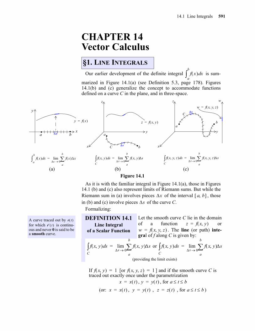
14.1 Line Integrals 591
gio
14
CHAPTER 14Vector Calculus
Our earlier development of the definite integral is sum-
marized in Figure 14.1(a) (see Definition 5.3, page 178). Figures14.1(b) and (c) generalize the concept to accommodate functionsdefined on a curve C in the plane, and in three-space.
Figure 14.1
As it is with the familiar integral in Figure 14.1(a), those in Figures14.1 (b) and (c) also represent limits of Riemann sums. But while theRiemann sum in (a) involves pieces of the interval , thosein (b) and (c) involve pieces of the curve C.
Formalizing:
If [or ] and if the smooth curve C istraced out exactly once under the parametrization
, , for
(or: , , , for )
§1. LINE INTEGRALS
f x xda
b
z f x y =y f x =
. .x .
.s
. .s
x
y
a b a
bC
y
x
z z
x
y
w f x y z =
w
f x xda
b
f x x
a
b
x 0lim= f x y sd
C f x y
a
b
s 0lim s= f x y z sd
C f x y z
a
b
s 0lim s=
(a) (b) (c)
ab
C
x a b s
A curve traced out by for which is continu-ous and never 0 is said to bea smooth curve.
r t r t
DEFINITION 14.1Line Integral
of a Scalar Function
Let the smooth curve C lie in the domainof a function or
. The line (or path) inte-gral of f along C is given by:
or
(providing the limit exists)
z f x y =w f x y z =
f x y sdC f x y
a
b
s 0lim s= f x y sd
C f x y
a
b
s 0lim s=
f x y 1= f x y z 1=
x x t = y y t = a t b
x x t = y y t = z z t = a t b
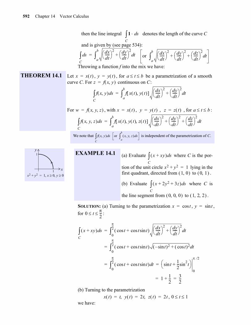
592 Chapter 14 Vector Calculus
gio
then the line integral denotes the length of the curve C
and is given by (see page 534):
Throwing a function f into the mix we have:
SOLUTION: (a) Turning to the parametrization , ,
for :
(b) Turning to the parametrization
, we have:
1 sdC
sdC
dxdt------ 2 dy
dt------ 2
+ tda
b
= or dxdt------ 2 dy
dt------ 2 dz
dt----- 2
+ + tda
b
THEOREM 14.1 Let , , for be a parametrization of a smoothcurve C. For continuous on C:
For , with , , , for :
x x t = y y t = a t b z f x y =
f x y sdC f x t y t dx
dt------ 2 dy
dt------ 2
+ tda
b
=
w f x y z = x x t = y y t = z z t = a t b
f x y z sdC f x t y t z t dx
dt------ 2 dy
dt------ 2 dz
dt----- 2
+ + tda
b
=
We note that is independent of the parametrization of C. f x y sd
C or x y z sd
a
b
x
y
x2 y2+ 1 x 0 y 0=1
1 EXAMPLE 14.1 (a) Evaluate where C is the por-
tion of the unit circle lying in thefirst quadrant, directed from to .
(b) Evaluate where C is
the line segment from to .
x xy+ sdC
x2 y2+ 1=1 0 0 1
x 2y2 3z+ + sdC
0 0 0 1 2 2
x tcos= y tsin=
0 t2---
x xy+ sdC tcos t tsincos+ dx
dt------ 2 dy
dt------ 2
+ td0
2---
=
tcos t tsincos+ tsin– 2 tcos 2+ td0
2---
=
tcos t tsincos+ td0
2---
tsin12---sin
2t+
0
2
= =
1 12---+ 3
2---= =
x t t y t 2t z t 2t= = = 0 t 1
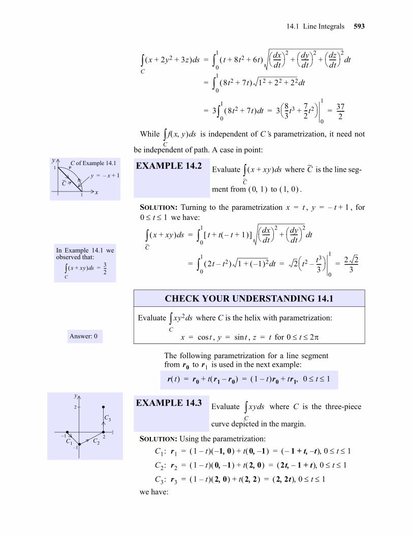
14.1 Line Integrals 593
gio
While is independent of C’s parametrization, it need not
be independent of path. A case in point:
SOLUTION: Turning to the parametrization , , for we have:
The following parametrization for a line segmentfrom to is used in the next example:
SOLUTION: Using the parametrization:
we have:
x 2y2 3z+ + sdC t 8t2 6t+ + dx
dt------ 2 dy
dt------ 2 dz
dt----- 2
+ + td0
1
=
8t2 7t+ 12 22 22+ + td0
1
=
3 8t2 7t+ td0
1
383---t3 7
2---t2+
0
1372------= = =
x
y C of Example 14.1
C
1
1
y x– 1+=
EXAMPLE 14.2 Evaluate where is the line seg-
ment from to .
f x y sdC
x xy+ sd
C
C
0 1 1 0
In Example 14.1 weobserved that:
x xy+ sd
C 3
2---=
x t= y t– 1+=0 t 1
x xy+ sd
C
t t t– 1+ + dxdt------ 2 dy
dt------ 2
+ td0
1
=
2t t2– 1 1– 2+ td0
1
2 t2 t3
3----–
0
12 2
3----------= = =
Answer: 0
CHECK YOUR UNDERSTANDING 14.1
Evaluate where C is the helix with parametrization:
, , for
xy2 sdC
x tcos= y tsin= z t= 0 t 2
. . ..
1–
1–
2
2_
y
C1 C2
C3
EXAMPLE 14.3 Evaluate where C is the three-piece
curve depicted in the margin.
r0 r1
r t r0 t r1 r0– + 1 t– r0 tr1 0 t 1 += =
xy sdC
C1: r1 1 t– 1– 0 t 0 1– + 1– t+ t– 0 t 1 = =
C2: r2 1 t– 0 1– t 2 0 + 2t 1– t+ 0 t 1 = =
C3: r3 1 t– 2 0 t 2 2 + 2 2t 0 t 1 = =
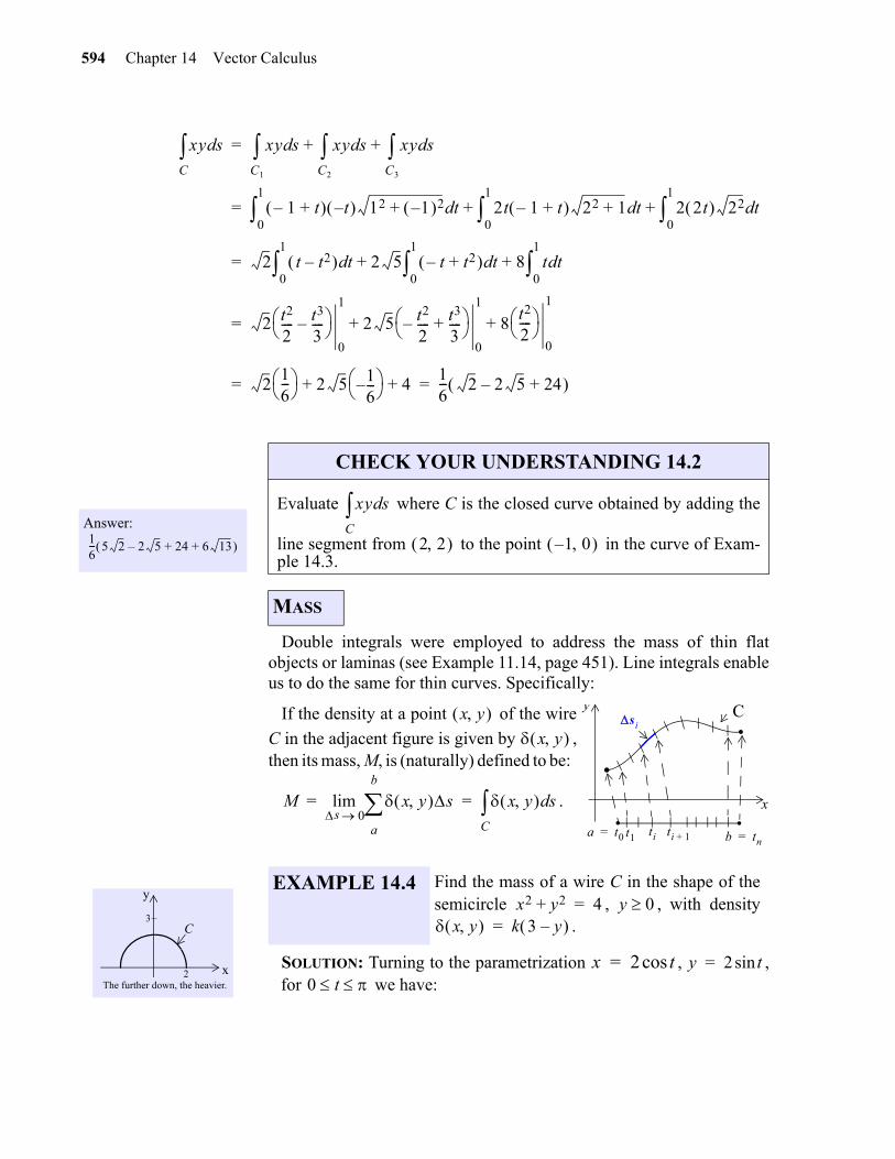
594 Chapter 14 Vector Calculus
Double integrals were employed to address the mass of thin flatobjects or laminas (see Example 11.14, page 451). Line integrals enableus to do the same for thin curves. Specifically:
If the density at a point of the wire
C in the adjacent figure is given by ,then its mass, M, is (naturally) defined to be:
.
SOLUTION: Turning to the parametrization , ,for we have:
xy sdC xy sd
C1
xy s xy sdC3
+dC2
+=
1– t+ t– 12 1– 2+ td0
1
2t 1– t+ 22 1+ td0
1
2 2t 22 td0
1
+ +=
2 t t2– td0
1
2 5 t– t2+ td0
1
8 t td0
1
+ +=
2 t2
2---- t3
3----–
0
1
2 5 t2
2----– t3
3----+
0
1
8t2
2----
0
1
+ +=
216--- 2 5 1
6---–
4+ +16--- 2 2 5– 24+ = =
Answer:
16--- 5 2 2 5– 24 6 13+ +
CHECK YOUR UNDERSTANDING 14.2
Evaluate where C is the closed curve obtained by adding the
line segment from to the point in the curve of Exam-ple 14.3.
MASS
xy sdC
2 2 1– 0
.. .
a t0= b tn=
si
t1 ti ti 1+
C
x
y
.x y x y
M x y
a
b
s 0lim s x y sd
C= =
3
2
The further down, the heavier.
_
x
y
C
EXAMPLE 14.4 Find the mass of a wire C in the shape of thesemicircle , , with density
.x2 y2+ 4= y 0
x y k 3 y– =
x 2 tcos= y 2 tsin=0 t
gio
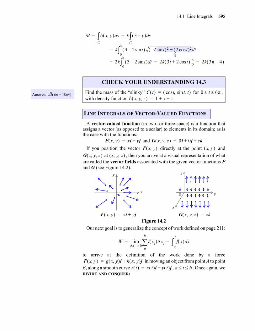
14.1 Line Integrals 595
A vector-valued function (in two- or three-space) is a function thatassigns a vector (as opposed to a scalar) to elements in its domain; as isthe case with the functions:
and
If you position the vector directly at the point and
at , then you arrive at a visual representation of whatare called the vector fields associated with the given vector functions Fand G (see Figure 14.2).
Figure 14.2
Our next goal is to generalize the concept of work defined on page 211:
to arrive at the definition of the work done by a force in moving an object from point A to point
B, along a smooth curve , . Once again, weDIVIDE AND CONQUER:
M x y sdC k 3 y– sd
C= =
2k 3 2 tsin– td0
2k 3t 2 tcos+ 0
2k 3 4– = = =
k 3 2 tsin– 2 tsin– 2 2 tcos 2+ td0
=1
Answer: 2 6 182+
CHECK YOUR UNDERSTANDING 14.3
Find the mass of the “slinky” for ,with density function
LINE INTEGRALS OF VECTOR-VALUED FUNCTIONS
C t t t tsincos = 0 t 6 x y z 1 x z+ +=
F x y xi yj+= G x y z 0i 0j zk+ +=
F x y x y G x y z x y z
... ...
....
..
x
y
x
y
z
... . . .. . . . . .. . . . . . ..
. . . . . . .
F x y xi yj+= G x y z zk=
W f xi xia
b
x 0lim f x xd
a
b
= =
F x y g x y i h x y j+=r t x t i y t j+= a t b
gio
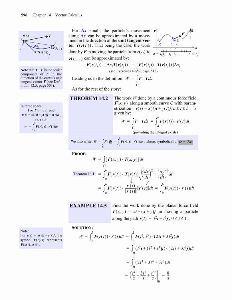
596 Chapter 14 Vector Calculus
gio
For small, the particle’s movementalong can be approximated by a move-ment in the direction of the unit tangent vec-tor . That being the case, the work
done by F in moving the particle from to
can be approximated by:
(see Exercises 49-52, page 512)
Leading us to the definition:
As for the rest of the story:
PROOF:
SOLUTION:
Note that is the scalarcomponent of F in thedirection of the curve’s unittangent vector T (see Defi-nition 12.5, page 503).
si
. .r ti
r ti 1+
F
T r ti
F T
..
a t0= b tn=t1 ti ti 1+
. .A
BF
s
x
yss
T r ti r ti
r ti 1+ F r ti siT r ti F r ti T r ti si=
W F T sdC=
In three space:For and
:
F x y z r t x t i= y t j z t k+ +
a t b
W F r t r t tda
b
=
THEOREM 14.2 The work W done by a continuous force field along a smooth curve C with param-
etrization isgiven by:
(providing the integral exists)
We also write: , where, symbolically:
F x y r t x t i= y t j a t b +
W F T sdC F r t r t td
a
b
= =
W F rdC F r t r t td
a
b
= = rd T sd=
W F x y T x y sdC=
F r t T r t dxdt------ 2 dy
dt------ 2
+ tda
b
=
F r t r t r t
--------------- r t tda
b
F r t r t tda
b
= =
Theorem 14.1:
Note:For , thesymbol represents
.
r t x t i y t j+=F r t
F x t y t
EXAMPLE 14.5 Find the work done by the planar force field in moving a particle
along the path , .
F x y xi x y+ j+=
r t t2i t3j+= 0 t 1
W F r t r t tda
b
F t2 t3 2ti 3t2j+ td0
1
= =
t2i t2 t3+ j+ 2ti 3t2j+ td0
1
=
2t3 3t4 3t5+ + td0
1
=
t4
2---- 3t5
5------- t6
2----+ +
0
185---= =
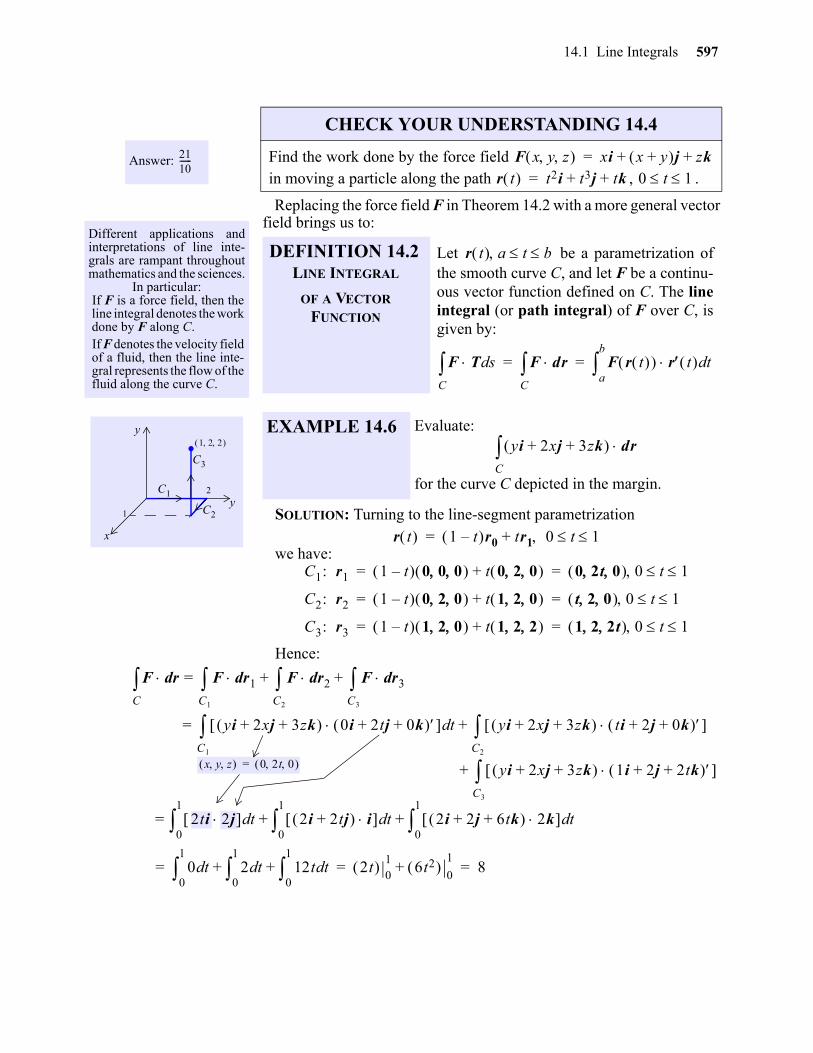
14.1 Line Integrals 597
Replacing the force field F in Theorem 14.2 with a more general vectorfield brings us to:
SOLUTION: Turning to the line-segment parametrization
we have:
Hence:
Answer: 2110------
CHECK YOUR UNDERSTANDING 14.4
Find the work done by the force field in moving a particle along the path , .
F x y z xi x y+ j zk+ +=r t t2i t3j tk+ += 0 t 1
Different applications andinterpretations of line inte-grals are rampant throughoutmathematics and the sciences.
In particular:If F is a force field, then theline integral denotes the workdone by F along C.If F denotes the velocity fieldof a fluid, then the line inte-gral represents the flow of thefluid along the curve C.
.1
2
1 2 2
y
x
y
C1
C2
C3
DEFINITION 14.2LINE INTEGRAL
OF A VECTOR FUNCTION
Let be a parametrization ofthe smooth curve C, and let F be a continu-ous vector function defined on C. The lineintegral (or path integral) of F over C, isgiven by:
EXAMPLE 14.6 Evaluate:
for the curve C depicted in the margin.
r t a t b
F T sdC F dr
C F r t r t td
a
b
= =
yi 2xj 3zk+ + drC
r t 1 t– r0 tr1 0 t 1 +=
C1: r1 1 t– 0 0 0 t 0 2 0 + 0 2t 0 0 t 1 = =
C2: r2 1 t– 0 2 0 t 1 2 0 + t 2 0 0 t 1 = =
C3: r3 1 t– 1 2 0 t 1 2 2 + 1 2 2t 0 t 1 = =
F rdC F r1d
C1
= F r2dC2
F r3dC3
+ +
yi 2xj 3zk+ + 0i 2tj 0k+ + tdC1
= yi 2xj 3zk+ + ti 2j 0k+ + C2
+
yi 2xj 3zk+ + 1i 2j 2tk+ + C3
+
2ti 2j td0
1
= 2i 2tj+ i t 2i 2j 6tk+ + 2k td0
1
+d0
1
+
0 t 2 td0
1
12t td0
1
+ +d0
1
2t 01
6t2 0
1+ 8= = =
x y z 0 2t 0 =
gio
598 Chapter 14 Vector Calculus
gio
If C is a curve with parametrization , then will denotethe curve with parametrization . Note that
traces out C, but in the opposite direction of :
starts at
and ends at .
PROOF:
Answer: 9
CHECK YOUR UNDERSTANDING 14.5
Evaluate for and C the line
segment from the origin to the point (compare with aboveexample).
F drC F x y z yi 2xj 3zk+ +=
1 2 2
Reminiscent of:
From the chain rule:
f x xda
b
f x xdb
a
–=
tdd r t
tdd r a b t–+ =
r a b t–+ a b t–+ =
r a b t–+ 1– =
THEOREM 14.3 If is a parametrization for thesmooth curve C and if F is a continuous vectorfunction defined on C, then:
r t a t b C–r t r a b t–+ a t b =
r t r t r t r a r a b a–+ r b = =
r b r a b b–+ r a = =
r t a t b
F drC F dr
C––=
u a b t–+=
du dt or dt– du–= =
t b= u a=
t a= u b=
F drC– F r t r t td
a
b
=
F r a b t–+ r a b t–+ tda
b
–=
F r a b t–+ r a b t–+ tdb
a
=
F r u r u uda
b
– F drC–= =
see margin
Answer: See page A-32.
CHECK YOUR UNDERSTANDING 14.6
Referring to the function F and curve C of Example 14.6, show,directly, that:
F drC F dr
C––=
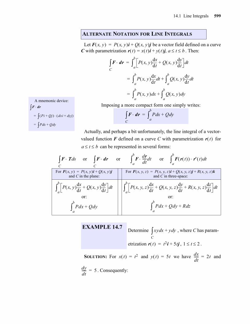
14.1 Line Integrals 599
Let be a vector field defined on a curveC with parametrization . Then:
Imposing a more compact form one simply writes:
Actually, and perhaps a bit unfortunately, the line integral of a vector-
valued function F defined on a curve C with parametrization for
can be represented in several forms:
SOLUTION: For and we have and
. Consequently:
ALTERNATE NOTATION FOR LINE INTEGRALS
A mnemonic device:
F drPi Qj+ dxi dyj+ =
P xd Q yd+=
F x y P x y i Q x y j+=r t x t i= y t j a t b +
F drC P x y
tddx
Q x y td
dy+ td
a
b
=
P x y td
dxtd
a
b
Q x y td
dytd
a
b
+=
P x y xda
b
Q x y yda
b
+=
F drC P xd Q yd+
a
b
=
r t
a t b
or or or
For and C in the plane:
For and C in three-space:
or: or:
F T sdC F dr
C F
drdt-----dt
a
b
F r t r t tda
b
F x y P x y i Q x y j+= F x y z P x y z i Q x y z j R x y z k+ +=
P x y td
dxQ x y
tddy
+ tda
b
Pdx Qdy+a
b
P x y z td
dxQ x y z
tddy
R x y z td
dz+ + td
a
b
Pdx Qdy R+ + zda
b
EXAMPLE 14.7Determine , where C has param-
etrization , .
xy xd y yd+C
r t t2i 5tj+= 1 t 2
x t t2= y t 5t= dxdt------ 2t=
dydt------ 5=
gio
600 Chapter 14 Vector Calculus
F rd
C 5t3i 5tj+ r t td
0
1
=
5t3i 5tj+ 2ti 5j+ td0
1
=
10t4 25 t+ td0
1
292------= =
Earlier notation:
Same
xy xd y yd+C t2 5t
tddx
5ttd
dy+ td
0
1
=
5t3 2t 5t 5 + td0
1
10t4 25t+ td0
1
= =
2t5 25t2
2----------+
0
1292------= =
notation for
Answer: 5352
---------
CHECK YOUR UNDERSTANDING 14.7
Determine , where C has parametrization
, .
xy xd y yd yz+ + zdC
r t t2i 5tj+= 2t2k– 1 t 2
gio
14.1 Line Integrals 601
gio
Exercises 1-11. Evaluate for the given function f and given path C.
Exercises 12-16. Evaluate for the given function f and given path C.
EXERCISES
1. , and C is the line segment from to .
2. and C is the line segment from to .
3. , and C is the upper half of the unit circle , traversed in a counterclockwise direction.
4. , and C is the lower half of the unit circle , traversed in a counterclockwise direction.
5. , and C is the right half of the unit circle , traversed in a counter-clockwise direction.
6. , and C is the right half of the ellipse , traversed in a counter-
clockwise direction.
7. , and C is the curve from to .
8. , and C is the curve from to .
9. , and C consists of the line segment from to followed by the line
segment from to .
10. , and C is given parametrically by for .
11. , and C consists of the line segment from to followed by
the graph of for , followed by the line segment from to .
12. , and C is the line segment from to .
13. , and C is the line segment from to .
14. , and C is consists of the line segment from to
followed by the line segment from to .
15. , and C is the helix given by , , for
.
16. , and C is given parametrically by , ,
for .
f x y sdC
f x y x2 y+= 0 0 1 1
f x y x y2+= 1 1 4 5
f x y 2 x2y+= x2 y2+ 1=
f x y 2 x2y+= x2 y2+ 1=
f x y xy4= x2 y2+ 4=
f x y 1 x2y+= x2
2----- y2+ 1=
f x y 3x= y x2= 0 0 3 9
f x y xy= x y2= 0 0 3 9
f x y xy= 0 0 1 1 1 1 1 2
f x y x1 y2+--------------= x 1 2t y+ t= = 0 t 1
f x y 4x3= 2 1–– 0 1– y x3 1–= 0 x 1 1 0 1 2
f x y z sdC
f x y z z y2+= 0 0 0 1 4 2
f x y z x 3y2– z+= 0 0 0 1 1 1
f x y z x 3y– z+= 0 0 0 1 1 1 1 1 1 1 1 3
f x y z xyz= x t tcos= y t tsin= z t 3t=
0 t 4
f x y z x2 z2+–= x t 0= y t a tcos=
z t a tsin= 0 t 2
602 Chapter 14 Vector Calculus
17. Find the mass of a wire in the shape of a semicircle , for, with density function .
18. Find the mass of a wire in the shape of the curve , , for
, with density function .
19. Find the mass of a wire in the shape of the helix , , for, with density the square of the distance from the origin.
Exercises 20-31. Evaluate for the given function F and curve C with given parametriza-
tion .
32. Find the work done by the force field in moving a particle along the path, .
33. Find the work done by the force field in moving a particle along the path, .
20. , for .
21. , for .
22. , for .
23. , for .
24. , for .
25. , for .
26. , for .
27. , for .
28. , for .
29. , for
.
30. , for .
31. , for .
x t 2 tcos= y t 2 tsin=0 t x y y 2+=
x t t= y t 2t= z t 2t3 2/
3------------=
0 t 1 3 5 t+=
x t 3 tcos= y t 3 tsin= z t 4t=0 t
F rdC
r t
F x y x 2y+ i 2x y+ j+= r t ti t2j+= 0 t 1
F x y xyi y2j+= r t ti tjsin+cos= 0 t3---
F x y xyi yjsin+= r t eti e t2– j+= 1 t 2
F x y ex y+ i xj+= r t ti t2j+= 0 t 1
F x y ex 1– i xyj+= r t t2i t3j+= 0 t 1
F x y x2i yj–= r t ti etj+= 0 t 2
F x y z xi yj zk–+= r t ti 3t2j 2t3k+ += 0 t 1
F x y z 8x2yzi 5zj 4xyk–+= r t ti t2j t3k+ += 0 t 1
F x y z x y+ i y z– j z2k–+= r t t2i t3j t2k+ += 0 t 1
F x y z 2xz y2+ i 2xyj x2 3z2+ k+ += r t t2i t 1+ j 2t 1– k+ +=
0 t 1
F x y z eyi xeyj z 1+ ezk–+= r t ti t2j t3k+ += 0 t 1
F x y z xisin yjcos xzk+ += r t t3i t2j tk+ += 0 t 1
F x y yi xj+=r t ti t2j+= 1 t 2
F x y xyi x3j+=r t t1 2/ i t1 4/ j+= 1 t 16
gio
14.1 Line Integrals 603
34. Find the work done by the force field in moving a particle along the
parabola from to .
35. Find the work done by the force field in moving a particle along thepath , .
36. Find the work done by the force field in moving aparticle along the line segment from to .
37. Find the work done by the force field in mov-ing a particle along the path , .
38. Find the work done by the force field in moving a particle along thepath , .
39. Find the work done by the force field in moving a particle alongthe path , .
40. Find the work done by the force field in moving a par-ticle along the path , .
F x y x yisin yj+=
y x2= 1– 1 2 4
F x y xi y 2+ j+=r t t tsin– i 1 tcos– j+= 0 t 2
F x y z y z+ i x z+ j x y+ k+ +=1 0 0 2 1 5
F x y z y x2– i z y2– j x z2– k+ +=r t ti t2j t3k+ += 0 t 1
F x y z zi xj yk+ +=r t tsin i tcos j tk+ += 0 t 2
F x y z x2i y2j z2k+ +=r t 1 t2+ i t2j 2 t sin+ k+ += 0 t 1
F x y z x y+ i x y– j 4zk+ +=r t 3t isin 3t jcos 3tk+ += 0 t 1
gio
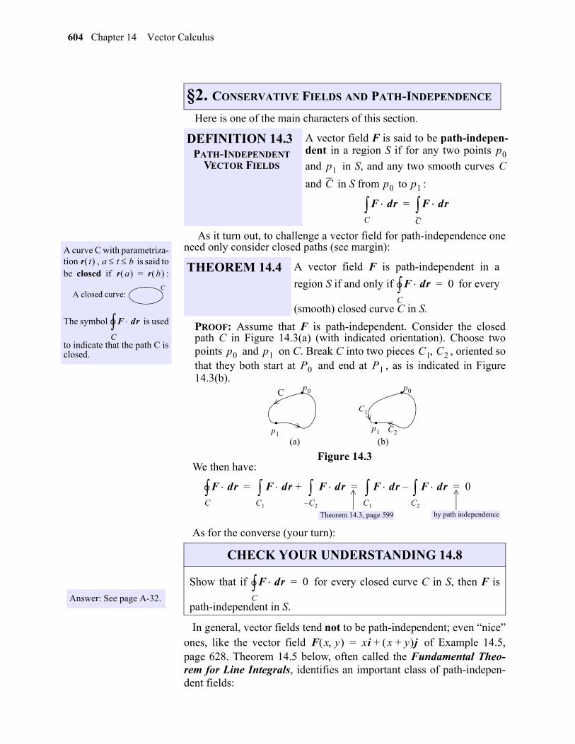
604 Chapter 14 Vector Calculus
14
Here is one of the main characters of this section.
As it turn out, to challenge a vector field for path-independence oneneed only consider closed paths (see margin):
PROOF: Assume that F is path-independent. Consider the closedpath C in Figure 14.3(a) (with indicated orientation). Choose twopoints and on C. Break C into two pieces , oriented sothat they both start at and end at , as is indicated in Figure14.3(b).
Figure 14.3We then have:
As for the converse (your turn):
In general, vector fields tend not to be path-independent; even “nice”ones, like the vector field of Example 14.5,page 628. Theorem 14.5 below, often called the Fundamental Theo-rem for Line Integrals, identifies an important class of path-indepen-dent fields:
§2. CONSERVATIVE FIELDS AND PATH-INDEPENDENCE
A curve C with parametriza-tion , is said tobe closed if :
The symbol is used
to indicate that the path C isclosed.
r t a t b r a r b =
CA closed curve:
F
C dr
DEFINITION 14.3PATH-INDEPENDENT
VECTOR FIELDS
A vector field F is said to be path-indepen-dent in a region S if for any two points
and in S, and any two smooth curves
and in S from to :
THEOREM 14.4 A vector field F is path-independent in a
region S if and only if for every
(smooth) closed curve C in S.
p0
p1 C
C p0 p1
F drC F dr
C
=
FC dr 0=
p0 p1 C1 C2P0 P1
..C
..p0p0
p1
C1
C2p1(a) (b)
F drC F dr
C1
F drC– 2
+ F drC1
F drC2
– 0= = =
Theorem 14.3, page 599 by path independence
Answer: See page A-32.
CHECK YOUR UNDERSTANDING 14.8
Show that if for every closed curve C in S, then F is
path-independent in S.
FC dr 0=
F x y xi x y+ j+=
gio
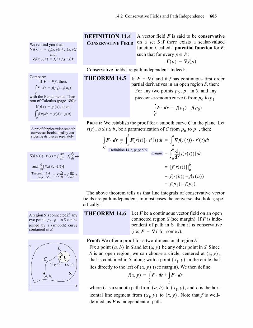
14.2 Conservative Fields and Path Independence 605
gio
Conservative fields are path independent. Indeed:
PROOF: We establish the proof for a smooth curve C in the plane. Let, , be a parametrization of C from to , then:
The above theorem tells us that line integrals of conservative vector
fields are path independent. In most cases the converse also holds; spe-cifically:
Proof: We offer a proof for a two-dimensional region S.Fix a point in S and let be any other point in S. SinceS is an open region, we can choose a circle, centered at ,that is contained in S, along with a point in the circle that
lies directly to the left of (see margin). We then define
where C is a smooth path from to , and L is the hor-
izontal line segment from to . Note that f is well-defined, as F is independent of path.
We remind you that:
and:
f x y fx x y i fy x y j+=
f x y z fxi fyj fzk+ +=
DEFINITION 14.4CONSERVATIVE FIELD
A vector field F is said to be conservativeon a set S if there exists a scalar-valuedfunction f, called a potential function for F,such that for every :
p SF p f p =
Compare:If , then:
with the Fundamental Theo-rem of Calculus (page 180):
If , then:
A proof for piecewise-smoothcurves can be obtained by con-sidering its pieces separately.
F f=
F drC f p1 f p0 –=
f x g x =
f x xda
b
g b g a –=
f r t r t fxdxdt------= fy
dydt------+
and: td
d f x t y t
fxdxdt------ fy
dydt------+=Theorem 13.4
page 555:
THEOREM 14.5 If and if f has continuous first orderpartial derivatives in an open region S, then:
For any two points , in S, and any
piecewise-smooth curve C from to :
F f=
p0 p1
p0 p1
F drC f p1 f p0 –=
r t a t b p0 p1
F drC F r t r t td
a
b
f r t r t tda
b
= =
tdd f r t td
a
b
=
f r t ab
=
f r b f r a –=
f p1 f p0 –=
Definition 14.2, page 597margin:
A region S is connected if anytwo points , in S can bejoined by a (smooth) curvecontained in S.
p0 p1
...
a b
x y x1 y
S
C
L
THEOREM 14.6 Let F be a continuous vector field on an openconnected region S (see margin). If F is inde-pendent of path in S, then it is conservative(i.e: for some f).F f=
a b x y x y
x1 y x y
f x y F rdC F rd
L+=
a b x1 y x1 y x y
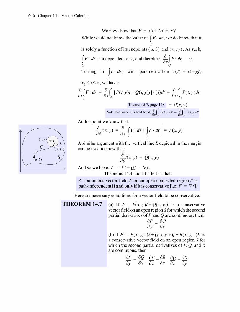
606 Chapter 14 Vector Calculus
We now show that :
While we do not know the value of , we do know that it
is solely a function of its endpoints and . As such,
is independent of x, and therefore: .
Turning to , with parametrization ,
, we have:
At this point we know that:
A similar argument with the vertical line L depicted in the margincan be used to show that:
And so we have: .Theorems 14.4 and 14.5 tell us that:
Here are necessary conditions for a vector field to be conservative:
F Pi Qj+ f= =
F rdCa b x1 y
F rdC x
F rdC 0=
F rdL r t ti yj+=
x1 t x
x F rd
L x
P t y i Q t y j+ i tdx1
x
x P t y td
x1
x
= =
P x y =Theorem 5.7, page 178:
Note that, since y is held fixed, x P t y td
x1
x
xdd P t y td
x1
x
=
...
a b
x y
x y1
S
CL
A continuous vector field F on an open connected region S ispath-independent if and only if it is conservative [i.e: ].
x f x y
x F rd
C F rd
L+ P x y = =
y f x y Q x y =
F Pi Qj+ f= =
F f=
THEOREM 14.7 (a) If is a conservativevector field on an open region S for which the secondpartial derivatives of P and Q are continuous, then:
(b) If isa conservative vector field on an open region S forwhich the second partial derivatives of P, Q, and Rare continuous, then:
F P x y i Q x y j+=
yP
xQ=
F P x y z i Q x y z j R x y z k+ +=
yP
xQ
z
Px
R
zQ
yR===
gio
14.2 Conservative Fields and Path Independence 607
PROOF: (a) If F is conservative with potential function f, then:
As for (b):
SOLUTION: (a) For :
and
Since the open region S must contain a point with , and
since for any such point, F is not conservative on S.
(b) For :
and .
It follows, from Theorem 14.7, that F is not conservative on S.
The converse of Theorem 14.7 need not hold:
F Pi Qj+ f x y fxi fy j+= = =
P fx and Q fy= =
yP fxy fyx x
Q= = =
Theorem 13.1, page 552
Answer: See page A-33.
CHECK YOUR UNDERSTANDING 14.9
Establish part (b) of Theorem 14.7.
As you might anticipate:S is an open region in three-space if for any point
in S there exists
such that the sphere ofradius r centered at is contained in S.
x0 y0 z0
r 0x0 y0 z0
EXAMPLE 14.8 (a) Show that is not con-servative on any open planar region S.
(b)Show that isnot conservative on any open spacial region S.
F x y xyi yxj+=
F x y z yi 2xj 3zk+ +=
F Pi Qj+ xyi yxj+= =
yP x=
xQ y=
We previously observed thatthis vector field F is notindependent of path (seeExample 14.6 and CYU14.5, pages 597and 598.
x y x y
yP
xQ
F Pi Qj Rk+ + yi 2xj 3zk+ += =
yP 1=
xQ 2=
Answer: See page A-33.
CHECK YOUR UNDERSTANDING 14.10
Show that the vector field is not conser-vative on any open spacial region S.
EXAMPLE 14.9 Show that the vector field
satisfies the condition but fails to
be conservative on the open region.
F x y z xi zj yzk+ +=
Fy
x2 y2+---------------- i
x–x2 y2+---------------- j+=
yP
xQ=
S x y x y 0 0 =
gio
608 Chapter 14 Vector Calculus
gio
SOLUTION: Note that F satisfies the given condition:
We now show that F is not conservative on S by demonstrating that itis not path independent in S (see Theorem 14.4):
Let C and be the curves from to with parame-trizations:
Then:
On the other hand:
We maintain that the culprit in the above example is not the vectorfield F, but is the region S, which contains a “hole”: it is missing thepoint . Indeed (proof omitted):
yx2 y2+----------------
y
x2 y2+ y 2y –x2 y2+ 2
---------------------------------------------- x2 y2–x2 y2+ 2
------------------------= =
and: x–
x2 y2+----------------
x
x2 y2+ 1– x– 2x –x2 y2+ 2
------------------------------------------------------------- x2 y2–x2 y2+ 2
------------------------= =
C 1 0 1 0–
r t tcos i tsin j 0 t +=
r t tcos i tsin j 0 t –=and , respectively
F drC F r t r t td
0
=
tsin i tcos– j+ tsin– i tcos j+ td0
=
sin2t– cos
2t– td
0
1 td0
– –= = =
note that x2 y2+ cos2t sin
2t+ 1= =
F drC
F r t r t td0
=
tsin– i tcos– j+ tsin– i tcos– j+ td0
=
sin2t cos
2t+ td
0
1 td0
= = =
Roughly speaking, S is simplyconnected if it has “no holes”in it. To put it another way: theinterior of every closed curvein S that does not intersectitself anywhere between itsendpoints is entirely containedin S. Visually speaking:
Not simply connected
S
THEOREM 14.8 Let be a continu-ously differentiable vector field on a simplyconnected open region S (see margin). If
in S, then there exists a function f
with continuous partial derivatives such that (i.e. F is conservative).
0 0
F P x y i Q x y j+=
yP
xQ=
F f=
14.2 Conservative Fields and Path Independence 609
Merging previous results we come to:
We now turn our attention to the task of finding potential functionsfor conservative vector fields:
SOLUTION: Theorem 14.9(iv) assures us that F is conservative:
To find f such that we consider:
Which brings us to:
Treating y as a constant in (1), we integrate with respect to x,realizing that the resulting constant of integration will be a function,
, of y:
They are equivalent inthat if any one holds, thenthe remaining three mustalso hold.
THEOREM 14.9 Let F be a continuous vector field on a simplyconnected open region S.
The following four properties are equivalent:
(i) for any smooth closed curve C in S.
(ii) F is a conservative vector field on S, i.e..
(iii) is path-independent on S with
for any smooth curve C from to .
(iv) For :
For :
EXAMPLE 14.10 Show that
is a conservative vector field, and find apotential function for F.
F drC 0=
F f=
F f=
F drC f p1 f p0 –=
p0 p1
F P x y i Q x y j+=
yP
xQ=
F P x y z i Q x y z j R x y z k+ +=
yP
xQ
z
Px
R
zQ
yR===
F x y x y2– i 2– xy ysin+ j+=
x y2– y 2y and 2xy– ysin+ x– 2y–= =
F f=
x y2– i 2– xy ysin+ j+ f x y fx x y i fy x y j+= =
(1): fx x y x y2 and (2): fy x y – 2– xy ysin+= =
x y2–
g y
(3): f x y x y2– xd x2
2----- xy2– g y += =
Note that, indeed: x2
2----- xy2– g y +
xx y2, since g y contains no x–=
gio
610 Chapter 14 Vector Calculus
Our next goal is to find . To do so, we take the partial derivativeof (3) with respect to y to arrive at:
Bringing (2) into the picture, we have:
So:
Letting we have an answer:
SOLUTION: Verifying (iv) of Theorem 14.9 (see margin):
At this point we know that for some f. To find such a poten-tial function we turn to:
Bringing us to:
Treating y and z as constants in (1), we integrate with respect tox, realizing that the resulting constant of integration will be a function
:
Our next goal is to find . To do so, we take the partial deriva-tive of (4) with respect to y to arrive at:
From (2):
So:
Returning to (4), we have: (5):
Taking the partial derivative with respect to z:
g y
fy x y 2– xy= g y y+ 2– xy g y +=g y contains no x
The appearance of the constantC tells us that the potentialfunction f in (3) is not unique.
2xy– ysin+ 2– xy g y g y ysin=+=
g y ysin yd y C+cos–= =
C 0=
F x y x y2– i 2– xy ysin+ j+ f x2
2----- xy2– ycos– = = =
For :P x y z i Q x y z j R x y z k+ +
Py Qx= Pz Rx= Qz Ry=
EXAMPLE 14.11 Show that
is a conservative vector field, and find a poten-tial function for F.
F x y z 2xz i 2yz– j x2 y2– k+ +=
Py 2xz = y 0 and Qx 2yz– x 0= = =
Pz 2xz z 2x and Rx x2 y2– x 2x= = = =
Qz 2yz– z 2y and Ry– x2 y2– y 2y–= = = =
F f=
2xz i 2yz– j x2 y2– k+ + fx x y z i fy x y z j fz x y z k+ +=
(1): fx x y z 2xz, (2): fy x y z 2yz, (3): fz x y z – x2 y2–= = =
2xz
g y z (4): f x y z 2xz xd x2z g y z += =
g y z
fy x y z g y z y=
2yz– g y z y=
g y z 2yz– yd y2z– h z += =
f x y z x2z y2z– h z +=
fz x y z x2 y2– h z +=
x2 y2– x2 y2– h z +=
h z 0 h z C= =
From (3):
gio
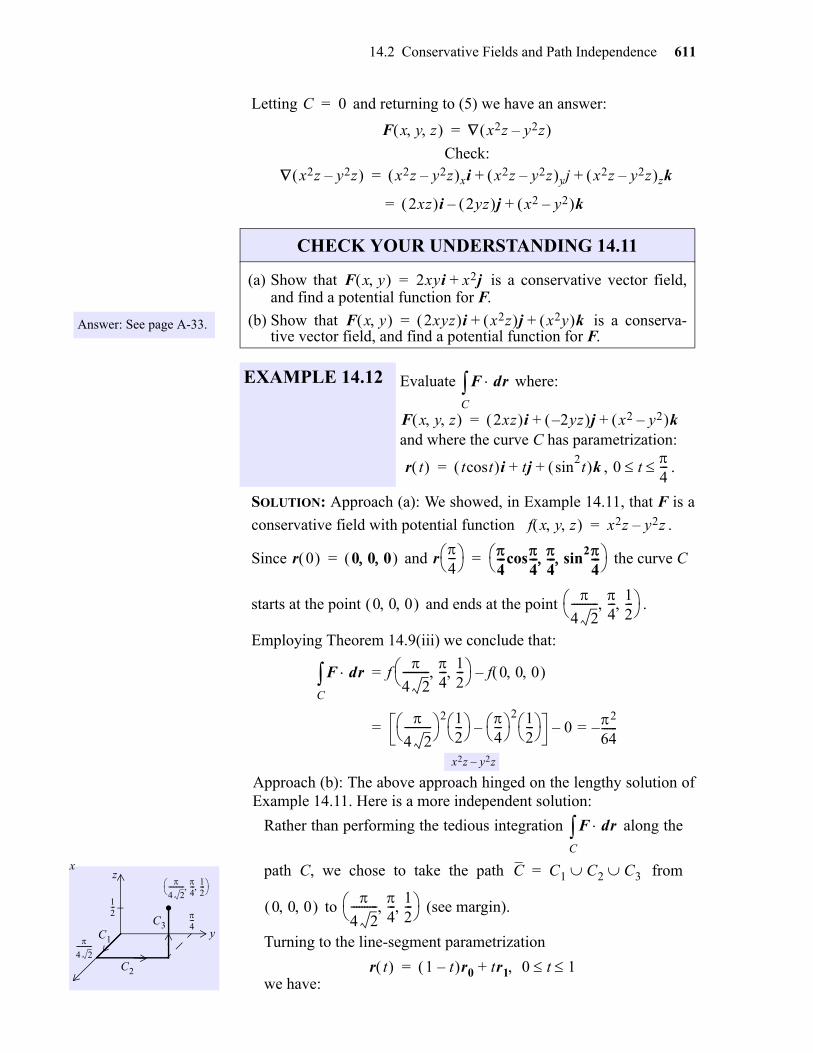
14.2 Conservative Fields and Path Independence 611
gio
Letting and returning to (5) we have an answer:
Check:
SOLUTION: Approach (a): We showed, in Example 14.11, that F is a
conservative field with potential function .
Since and the curve C
starts at the point and ends at the point .
Employing Theorem 14.9(iii) we conclude that:
Approach (b): The above approach hinged on the lengthy solution ofExample 14.11. Here is a more independent solution:
Rather than performing the tedious integration along the
path C, we chose to take the path from
to (see margin).
Turning to the line-segment parametrization
we have:
C 0=
F x y z x2z y2z– =
x2z y2z– x2z y2z– xi x2z y2z– yj x2z y2z– zk+ +=
2xz i 2yz j– x2 y2– k+=
Answer: See page A-33.
CHECK YOUR UNDERSTANDING 14.11
(a) Show that is a conservative vector field,and find a potential function for F.
(b) Show that is a conserva-tive vector field, and find a potential function for F.
EXAMPLE 14.12 Evaluate where:
and where the curve C has parametrization:
, .
F x y 2xyi x2j+=
F x y 2xyz i x2z j x2y k+ +=
F drC
F x y z 2xz i 2yz– j x2 y2– k+ +=
r t tcost i tj sin2t k+ += 0 t
4---
f x y z x2z y2z–=
r 0 0 0 0 = r4---
4---cos
4---
4--- sin
24---
=
0 0 0 4 2----------
4--- 1
2---
F drC f
4 2----------
4--- 1
2---
f 0 0 0 –=
4 2---------- 2 1
2---
4--- 2 1
2--- – 0– 2
64------–==
x2z y2z–
.4 2----------
4--- 1
2---
4 2----------
4---
12---
y
z
C1
C2
C3
F drC
C C1 C2 C3 =
0 0 0 4 2----------
4--- 1
2---
r t 1 t– r0 tr1 0 t 1 +=
x
612 Chapter 14 Vector Calculus
t
For we then have:
By now, the term conservative force field should be self-explana-tory. That being the case:
SOLUTION: We find a potential function f for F:
C1: r1 1 t– 0 0 0 t 4 2---------- 0 0 +
4 2----------t 0 0 0 t 1 = =
C2: r2 1 t– 4 2---------- 0 0 t
4 2----------
4--- 0
+ 4 2----------
4---t 0
0 t 1 = =
C3: r 1 t– 4 2----------
4--- 0
t 4 2----------
4--- 1
2---
+ 4 2----------
4--- t
2---
0 t 1 = =
F x y z 2xz i 2yz– j x2 y2– k+ +=
F drC
F dr1C1
F dr2C2
F dr3C3+ +=
4 2----------t 2
k
4 2---------- i
td0
1
4 2---------- 2
4---t –
2k
4--- j
td0
1
+=
2
4 2---------- t
2--- i 2
4--- t
2--- j–
4 2---------- 2
4--- 2
– + k
12--- k
d0
1
+
0 td0
1
0 td0
1
12--- 2
32------ 2
16------–
td0
1
+ + 2
64------– t
0
12
64------–= = =
Answer: 4
1024------------
CHECK YOUR UNDERSTANDING 14.12
Use both of the approaches of the previous example to evaluate
for and where the curve C has param-
etrization: for .
CONSERVATIVE FORCE FIELDS
F drC F x y 2xyi x2j+=
r t tcos2t i t2j+= 0 t
4---
Note that F is conservative:ey y xey x ey= =
EXAMPLE 14.13 Find the work done by a particle in movingfrom the origin to the point , while sub-
jected to the force field .
3 6 F x y eyi xeyj+=
eyi xeyj+ fx x y i fy x y j+=
gio
14.2 Conservative Fields and Path Independence 613
It follows that is a potential function for F. So:
integrating with respectto x, holding y fixed:
integrating with respectto y, holding x fixed:
fx x y ey=
f x y xey g y +=
fy x y xey=
f x y xey h x +=
f x y xey=
F drC f 3 6 f 0 0 – 3e6= =
Answer: See page A-34.
CHECK YOUR UNDERSTANDING 14.13
Show that the work done in moving a particle from the to when subjected solely to the force of gravity , is equal
to , independently of the chosen path taken from to
.
0 0 0 x0 y0 z0 mg–
mgz0– 0 0 0 x0 y0 z0
gio
614 Chapter 14 Vector Calculus
gio
Exercises 1-12. Determine if the vector field F is conservative on the region S. If it is, find a func-tion f such that .
Exercises 13-16. Verify that the vector field F is conservative. Evaluate using both
Approach (a) and Approach (b) of Example 14.12.
EXERCISES
1. , .
2. , .
3. , .
4. , .
5. , .
6. , .
7. , .
8. , .
9. , .
10. , .
11. , .
12. , .
13. and C with parametrization for .
14. and C with parametrization for .
15. where C is any smooth curve from the ori-
gin to the origin to the point .
16. and for .
F f=
F x y x y– i x 2– j+= S R2=
F x y 2xy2i 1 3x2y2+ j+= S R2=
F x y 2xy3i 1 3x2y2+ j+= S R2=
F x y 3 2xy+ i x2 3y2– j+= S R2=
F x y y x 2xey+cos i x xey+sin 4+ j+= S R2=
F x y y x 2xey+cos i x x2ey+sin 4+ j+= S R2=
F x y z yz2i 2xyz y– j xz2 z– k+ += S R3=
F x y z yz2i xz2 z– j 2xyz y– k+ += S R3=
F x y z ex ycos yz+ i xz ex ysin– j xy z+ k+ += S R3=
F x y z xz ex ysin– i ex ycos yz+ j xy z+ k+ += S R3=
F x y z y2i 2xy e3z+ j 3ye3zk+ += S R3=
F x y z y2i 2xy e3z+ j ye3zk+ += S R3=
F drC
F x y yi xj+= r t ti 2tj+sin=2--- t
F x y xy i x y– j+= r t t2i 2t3j+= 0 t 1
F x y z yz 1+ i xz 2+ j xy 3+ k+ +=
1 2 3
F x y z eyi xeyj z 1+ ezk+ += r t ti t2j t3k+ += 0 t 1
14.2 Conservative Fields and Path Independence 615
Exercises 17-25. Verify that the vector field F is conservative and then evaluate where C
has parametrization r.
Exercises 26-29. Determine a function for which the field F is conservative in .(no unique solutions)
Exercises 30-32. Determine functions and for which the field F is conserva-tive in .
33. Verify that is a conservative force field. Determine the work done if aparticle subjected to F moves around the circle for .
34. Verify that is a conservative force field. Determine the work done if aparticle subjected to F moves over the semicircle for .
17. , for .
18. , for .
19. , for .
20. , for .
21. , for .
22. , for .
23. , for .
24. , for .
25. , for .
26. 27.
28. 29.
30.
31.
32.
F drC
F x y 3 2xy+ i x2 3y2– j+= r t eti1
t2 2+-------------j+= 0 t 1
F x y 3 2xy+ i x2 3y2– j+= r t ti 2t3j+sin= 0 t 1
F x y xy2i x2yj+= r t t t2-----sin+
i t t2-----cos+
j+= 0 t 1
F x y x 2xy+ i x2 3y2– j+= r t 2ti t3j+sin= 0 t 1
F x y 3 2xy+ i x2 3y2– j+= r t et ti et tjcos+sin= 0 t
F x y z yz2i xz2 z– j 2xyz y– k+ += r t t2i t3j1
t2 1+-------------k+ += 0 t 1
F x y z yz2i xz2 z– j 2xyz y– k+ += r t 1t2 2+-------------i t2j k+ += 0 t 1
F x y z yz 1+ i xz 2+ j xy 3+ k+ += r t t2i t3j1
t2 1+-------------k+ += 0 t 1
F x y z yz 1+ i xz 2+ j xy 3+ k+ += r t eti t3j ett2k+ += 0 t 1
K x y S R2=
F x y x 2y+ i K x y j+= F x y 2xy2 i K x y j+=
F x y K x y i xy3j+= F x y K x y i x2ey j+=
M x y z N x y z S R3=
F x y z 2xy3i M x y z j N x y z k+ +=
F x y z M x y z i 2xy3j N x y z k+ +=
F x y z M x y z i N x y z j 2xy3k+ +=
F x y eyi xeyj+=r t ticos tjsin+= 0 t 2
F x y eyi xeyj+=r t ticos tjsin+= 0 t
gio
616 Chapter 14 Vector Calculus
35. Verify that is a conservative force field. Deter-mine the work done if a particle subjected to F moves over the helix
for .
36. Verify that is a conservative forcefield. Determine the work done if a particle subjected to F moves over the curve
for .
37. Prove that any two potential functions, and , for a conservative vector field can only differ by a constant.
F x y z x2 y+ i y2 x+ j zez k+ +=
r t ticos tjt
2------k+sin+= 0 t 2
F x y z eyzi xzeyz z ycos+ j xyeyz ysin+ k+ +=
r t ti t2j t3k++= 1– t 1
f x y h x y F x y P x y i Q x y j+=
gio
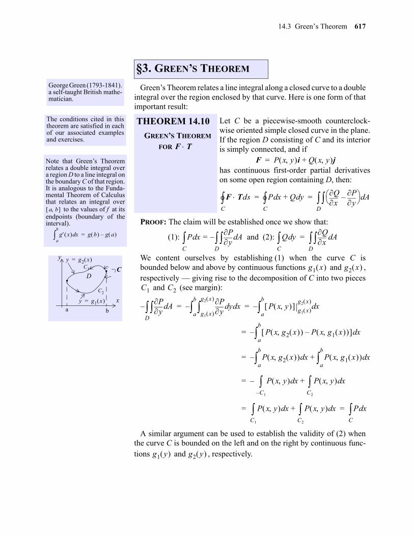
14.3 Green’s Theorem 617
14
Green’s Theorem relates a line integral along a closed curve to a doubleintegral over the region enclosed by that curve. Here is one form of thatimportant result:
PROOF: The claim will be established once we show that:
We content ourselves by establishing (1) when the curve C isbounded below and above by continuous functions and ,respectively — giving rise to the decomposition of C into two pieces
and (see margin):
A similar argument can be used to establish the validity of (2) whenthe curve C is bounded on the left and on the right by continuous func-tions and , respectively.
George Green (1793-1841).a self-taught British mathe-matician.
The conditions cited in thistheorem are satisfied in eachof our associated examplesand exercises.
Note that Green’s Theoremrelates a double integral overa region D to a line integral onthe boundary C of that region.It is analogous to the Funda-mental Theorem of Calculusthat relates an integral over
to the values of f at itsendpoints (boundary of theinterval).
a b
g x xda
b
g b g a –=
x
y
D..
a b
C1
C2
C
y g2 x =
y g1 x =
§3. GREEN’S THEOREM
THEOREM 14.10
GREEN’S THEOREM
FOR
Let C be a piecewise-smooth counterclock-wise oriented simple closed curve in the plane.If the region D consisting of C and its interioris simply connected, and if
has continuous first-order partial derivativeson some open region containing D, then:
F T
F P x y i Q x y j+=
F TdsC P xd Q+ yd
C x
Qy
P– Ad
D= =
(1): P xdC y
PA and (2): Q yd
Cd
D–=
xQ
AdD=
g1 x g2 x
C1 C2
yP
AdD–
yP
yd xdg1 x
g2 x
a
b
– P x y g1 x g2 x
xda
b
–= =
P x g2 x P x g1 x – xda
b
–=
P x g2 x x P x g1 x xda
b
+da
b
–=
P x y xdC– 1
– P x y xdC2
+=
P x y xdC1
P x y xdC2
+ P xdC= =
g1 y g2 y
gio
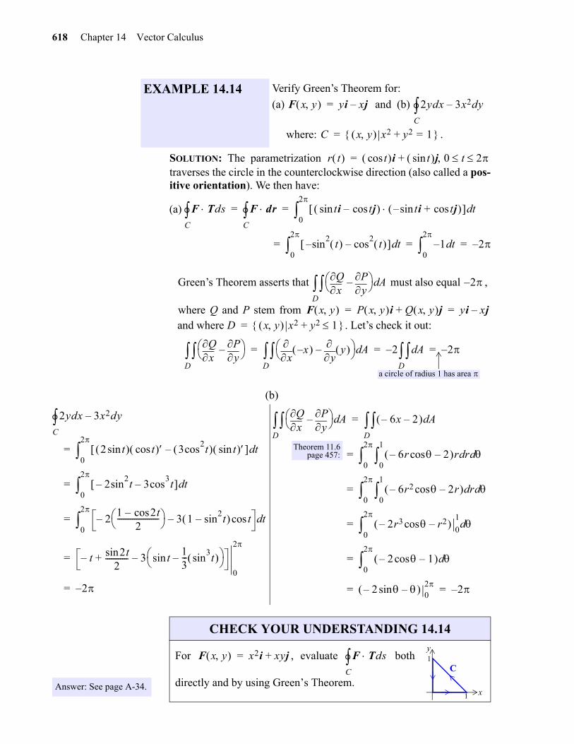
618 Chapter 14 Vector Calculus
gio
SOLUTION: The parametrization traverses the circle in the counterclockwise direction (also called a pos-itive orientation). We then have:
Green’s Theorem asserts that must also equal ,
where Q and P stem from and where . Let’s check it out:
(b)
EXAMPLE 14.14 Verify Green’s Theorem for:
(a) and (b)
where: .
F x y yi xj–= 2ydx 3x2dy–C
C x y x2 y2+ 1= =
r t tcos i tsin j 0 t 2 +=
F TdsC F dr
C tsin i tcos j– ti tjcos+sin– td
0
2
= =
sin–2
t cos2
t – td0
2
1– td0
2
2–= = =
(a)
xQ
yP–
AdD 2–
F x y P x y i Q x y j+ yi xj–= =D x y x2 y2+ 1 =
xQ
yP–
D x
x– y y –
AdD 2 Ad
D– 2–= = =
a circle of radius 1 has area
2ydx 3x2dy–C
2 tsin tcos 3cos2t tsin – td
0
2
=
2sin2t– 3cos
3t– td
0
2
=
21 2tcos–
2---------------------- – 3 1 sin
2t– tcos– td
0
2
=
t– 2tsin2
------------ 3 tsin13--- sin
3t –
–+0
2
=
2–=
xQ
yP–
AdD 6x– 2– Ad
D=
6r cos– 2– r rd d0
1
0
2
=
6r2 cos– 2r– rd d0
1
0
2
=
2r3 cos– r2– 0
1d
0
2
=
2 cos– 1– d0
2
=
2 sin– – 02
2–= =
Theorem 11.6page 457:
Answer: See page A-34.
CHECK YOUR UNDERSTANDING 14.14
For , evaluate both
directly and by using Green’s Theorem.1
1C
x
yF x y x2i xyj+= F Tds
C
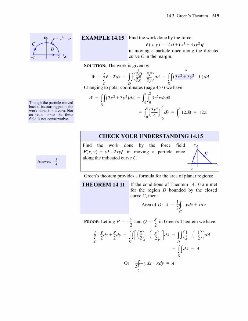
14.3 Green’s Theorem 619
SOLUTION: The work is given by:
Changing to polar coordinates (page 457) we have:
Green’s theorem provides a formula for the area of planar regions:
PROOF: Letting and in Green’s Theorem we have:
Or:
2 x
y
2–
y 4 x2–=
CD
EXAMPLE 14.15 Find the work done by the force:
in moving a particle once along the directedcurve C in the margin.
F x y 2xi x3 3xy2+ j+=
Though the particle movedback to its starting point, thework done is not zero. Notan issue, since the forcefield is not conservative.
W F TdsC x
Qy
P– Ad
D 3x2 3y2 0–+ Ad
D= = =
W 3x2 3y2+ AdD 3r2r rd d
0
2
0
= =
3r4
4--------
0
2
d0
12 d0
12= = =
Answer: 54---–
CHECK YOUR UNDERSTANDING 14.15
Find the work done by the force field in moving a particle once
along the indicated curve C.
THEOREM 14.11 If the conditions of Theorem 14.10 are metfor the region D bounded by the closedcurve C, then:
1
1C
12---–
x
y
F x y yi 2xyj–=
Area of D: A12--- ydx– xdy+
C=
P y2---–= Q x
2---=
y2---dx–
x2---dy+
C
x2---
x
y2---–
y
– AdD 1
2--- 1
2---–
– Ad
D= =
AdD A= =
12--- ydx– xdy+
C A=
gio
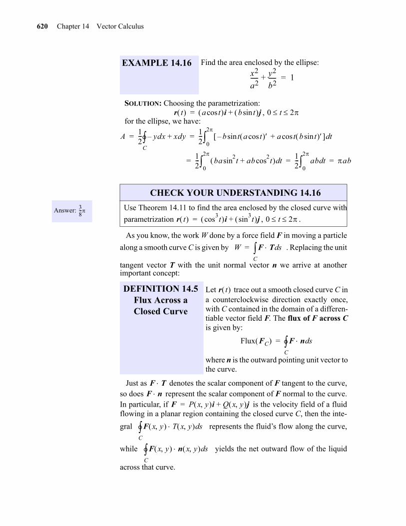
620 Chapter 14 Vector Calculus
SOLUTION: Choosing the parametrization: ,
for the ellipse, we have:
As you know, the work W done by a force field F in moving a particle
along a smooth curve C is given by . Replacing the unit
tangent vector T with the unit normal vector n we arrive at anotherimportant concept:
Just as denotes the scalar component of F tangent to the curve,so does represent the scalar component of F normal to the curve.In particular, if is the velocity field of a fluidflowing in a planar region containing the closed curve C, then the inte-
gral represents the fluid’s flow along the curve,
while yields the net outward flow of the liquid
across that curve.
EXAMPLE 14.16 Find the area enclosed by the ellipse:x2
a2----- y2
b2-----+ 1=
r t a tcos i b tsin j+= 0 t 2
A12--- ydx– xdy+
C
12--- b t a tcos sin– a t b tsin cos+ td
0
2
= =
12--- basin
2t abcos
2t+ td
0
2
12--- ab td
0
2
ab= = =
Answer: 38---
CHECK YOUR UNDERSTANDING 14.16
Use Theorem 14.11 to find the area enclosed by the closed curve with
parametrization , .
DEFINITION 14.5Flux Across a Closed Curve
Let trace out a smooth closed curve C ina counterclockwise direction exactly once,with C contained in the domain of a differen-tiable vector field F. The flux of F across Cis given by:
where n is the outward pointing unit vector tothe curve.
r t cos3t i sin
3t j+= 0 t 2
W F T sdC=
r t
Flux FC F n sdC=
F TF n
F P x y i Q x y j+=
F x y T x y sdC
F x y n x y sdC
gio
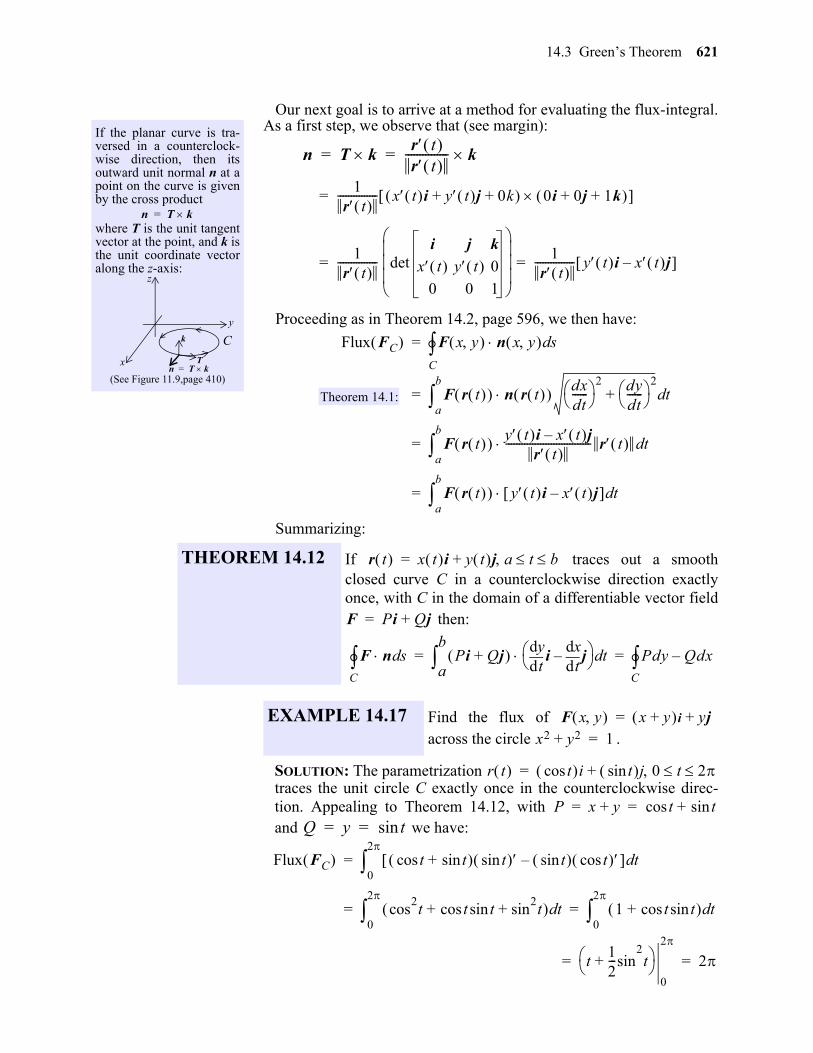
14.3 Green’s Theorem 621
gio
Our next goal is to arrive at a method for evaluating the flux-integral.As a first step, we observe that (see margin):
Proceeding as in Theorem 14.2, page 596, we then have:
Summarizing:
SOLUTION: The parametrization traces the unit circle C exactly once in the counterclockwise direc-tion. Appealing to Theorem 14.12, with and we have:
If the planar curve is tra-versed in a counterclock-wise direction, then itsoutward unit normal n at apoint on the curve is givenby the cross product
where T is the unit tangentvector at the point, and k isthe unit coordinate vectoralong the z-axis:
(See Figure 11.9,page 410)
n T k=
n T k=T
k
x
y
z
C
n T k r t r t
--------------- k= =
1r t
--------------- x t i y t j 0k+ + 0i 0j 1k+ + =
1r t
--------------- deti j k
x t y t 0
0 0 1
1r t
--------------- y t i x t j– = =
Flux FC F x y n x y sdC=
F r t n r t dxdt------ 2 dy
dt------ 2
+ tda
b
=
F r t y t i x t j–r t
-------------------------------- r t tda
b
=
F r t y t i x t j– tda
b
=
Theorem 14.1:
THEOREM 14.12 If traces out a smoothclosed curve C in a counterclockwise direction exactlyonce, with C in the domain of a differentiable vector field
then:
r t x t i y t j a t b +=
F Pi Qj+=
F n sdC Pi Qj+
tddy
itd
dxj–
tda
b Pdy Qdx–
C= =
EXAMPLE 14.17 Find the flux of across the circle .
F x y x y+ i yj+=x2 y2+ 1=
r t tcos i tsin j 0 t 2 +=
P x y+ t tsin+cos= =Q y tsin= =
Flux FC t tsin+cos tsin tsin tcos – td0
2
=
cos2t t t sin
2t+sincos+ td
0
2
1 t tsincos+ td0
2
= =
t12---sin
2t+
0
2
2= =
622 Chapter 14 Vector Calculus
Tweaking Theorem 14.12 a bit we arrive at another form of Green’sTheorem:
PROOF: Applying Theorem 14:10:
to the vector function we have:
SOLUTION: Turning to Theorem 14.13 with
we have:
Answer: 9–
CHECK YOUR UNDERSTANDING 14.17
Find the flux of across the trianglebounded by .
THEOREM 14.13
GREEN’S THEOREM
FOR
Let C be a piecewise-smooth counterclock-wise oriented simple closed curve in theplane. If the region D consisting of C and itsinterior is simply connected, and if
has continuous first-order partial derivatives on some open regioncontaining D, then:
F x y y2 x2– i x2 y2+ j+=y x x 3 and y 0= = =
F n
F P x y i Q x y j+=
F ndsC P yd Q– xd
C x
Py
Q+ Ad
D= =
P xd Q+ ydC x
Qy
P– Ad
D=
F2 Qi– Pj+=
Q– xd P+ ydC x
Py
Q– – Ad
D x
Py
Q+ Ad
D= =
Compare with Example 14.17,
EXAMPLE 14.18 Use Green’s Theorem to find the flux of across the circle
.F x y x y+ i yj+=x2 y2+ 1=
F x y P x y i Q x y j+ x y+ i yj+= =
F ndsC x
Py
Q+ Ad
D 1 1+ Ad
D 2= = =
Answer: 9–
CHECK YOUR UNDERSTANDING 14.18
Use Green’s Theorem to address CYU 14.17:
gio
14.3 Green’s Theorem 623
gio
Exercises 1-11.Verify both forms of Green’s Theorem (14.10).
Exercises 12-17.Use Green’s Theorem to evaluate the line integral along the given positively ori-ented curve C.
EXERCISES
1. , .
2. , D is the rectangular region with vertices , and
.
3. , D is the rectangular region with vertices ,
and .
4. ,
5. , D is the triangular region with vertices , and .
6. , D is the region bounded by the line segments from to
and from to , along with the parabola from to .
7. , D is the region bounded by the line segments to and
from to , along with the quarter-circle in the first quadrant.
8. and C is the triangle with vertices , and .
9. and C is the triangle with vertices , and .
10. , and C is the circle of radius 3 centered at the origin.
11. and C is the circle of radius 2 centered at the origin.
12. and C is the circle .
13. and C is the ellipse .
F x y x y– i xj+= D x y x2 y2 1+ =
F x y xy i x2j+= 0 0 2 0 2 3 0 3
F x y xy i x2 y2– j+= 0 0 0 1 1 0 1 1
F x y xy2– i xy2j+= D x y x2 y2 a2+ =
F x y x2i xy2j–= 0 0 0 1 1 1
F x y xi yj+= 0 0 0 1 0 0 1 0 y 1 x2–= 1 0 0 1
F x y y– i xj+= 0 0 0 1
0 0 1 0 y 1 x2–=
y2dx x2dy+C 0 0 1 0 0 1
xydxC x2y3dy+ 0 0 1 0 1 2
x2 y2– dx xdy+C
y3dx x3dy–C
y4dx 2xy3dy+C x2 y2+ 9=
y4dx 2xy3dy+C
x2
2----- y2+ 1=
624 Chapter 14 Vector Calculus
Exercises 18-22. Find the work done by the force F in moving a particle once along the givenpositively oriented curve C.
Exercises 23-27. Use Theorem 14.11 to find the area of the region D.
14. and C is the rectangle with vertices at , , , and
.
15. and C consists of the line segments joining to , joining to
, and the parabola from to .
16. and C is the circle of radius 3 centered at the origin.
17. and C is the boundary of the unit square in the first quadrant with a ver-
tex at the origin.
18. and C is the region in the first quadrant enclosed by the x-
axis, the line and the curve .
19. and C is the triangle with vertices , , and .
20. and C is the circle .
21. and C is bounded by the line segment from to
and the semicircle .
22. and C is the circle of radius 3 centered at the origin.
23. .
24.
25. D is the region between the curves and .
26. D is the curve , .
27. D is the region lying between the x-axis and one arch of the cycloid with parametric equa-tions and .
ydcos x x2 ydsin y+C 0 0 2 0 2 3
0 3
ydx xdy–C 0 0 0 1 0 0
1 0 y 1 x2–= 1 0 0 1
2y3dx– 2x3dy+C
y xdcos x x2dy+C
F x y 2xy3i 4x2y2j+=
x 1= y x3=
F x y x2 xy+ i xy2j+= 0 0 1 0 0 1
F x y 4x 2y– i 2x 4y– j+= x 2– 2 y 2– 2+ 4=
F x y 7xi x3 3xy2+ j+= 2 0– 2 0
y 4 x2–=
F x y 2y3– i 2x3j+=
D x y x2 y2 r2+ =
D x y x2 2y2 2+ =
y x2= y x3=
r t t2i t3
3---- t– j+= 3– t 3
x a t tsin– = y a 1 tcos– =
gio
14.3 Green’s Theorem 625
Exercises 28-31. Verify both forms of Green’s Theorem (Theorem 14.13). .
28. and C is the region in the first quadrant enclosed by the x-axis,
the line and the curve .
29. and .
30. and C is the triangular region with vertices , ,
and .
31. and C is the circle .
F x y 2xy3i 4x2y2j+=
x 1= y x3=
F x y x y– i xj+= C x y x2 y2+ 1= =
F x y x y+ i x2 y2+ j–= 1– 0 0 1 1 0
F x y 4x 2y– i 2x 4y– j+= x 2– 2 y 2– 2+ 4=
gio
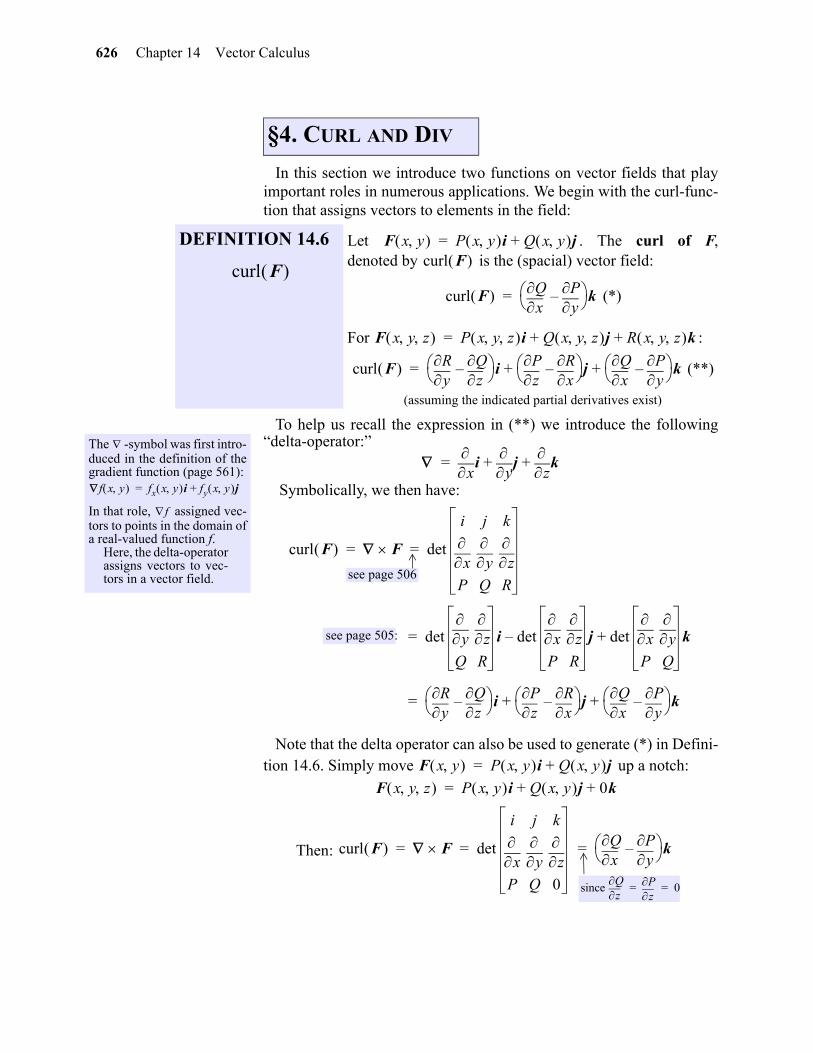
626 Chapter 14 Vector Calculus
14
In this section we introduce two functions on vector fields that playimportant roles in numerous applications. We begin with the curl-func-tion that assigns vectors to elements in the field:
To help us recall the expression in (**) we introduce the following“delta-operator:”
Symbolically, we then have:
Note that the delta operator can also be used to generate (*) in Defini-tion 14.6. Simply move up a notch:
Then:
§4. CURL AND DIV
DEFINITION 14.6
Let . The curl of F,denoted by is the (spacial) vector field:
(*)
For :
(**)
(assuming the indicated partial derivatives exist)
curl F
F x y P x y i Q x y j+=curl F
curl F x
Qy
P– k=
F x y z P x y z i Q x y z j R x y z k+ +=
curl F y
Rz
Q– i
zP
xR–
jx
Qy
P– k+ +=
The -symbol was first intro-duced in the definition of thegradient function (page 561):
In that role, assigned vec-tors to points in the domain ofa real-valued function f.
Here, the delta-operatorassigns vectors to vec-tors in a vector field.
f x y fx x y i fy x y j+=
f
x
iy
jz
k+ +=
curl F F det
i j k
x
y
z
P Q R
= =
det y
z
Q R
i det x
z
P R
j– det x
y
P Q
k+=
yR
zQ–
iz
Px
R– j
xQ
yP–
k+ +=
see page 506
see page 505:
F x y P x y i Q x y j+=
F x y z P x y i Q x y j 0k+ +=
curl F F det
i j k
x
y
z
P Q 0
xQ
yP–
k= = =
since z
Qz
P 0= =
gio
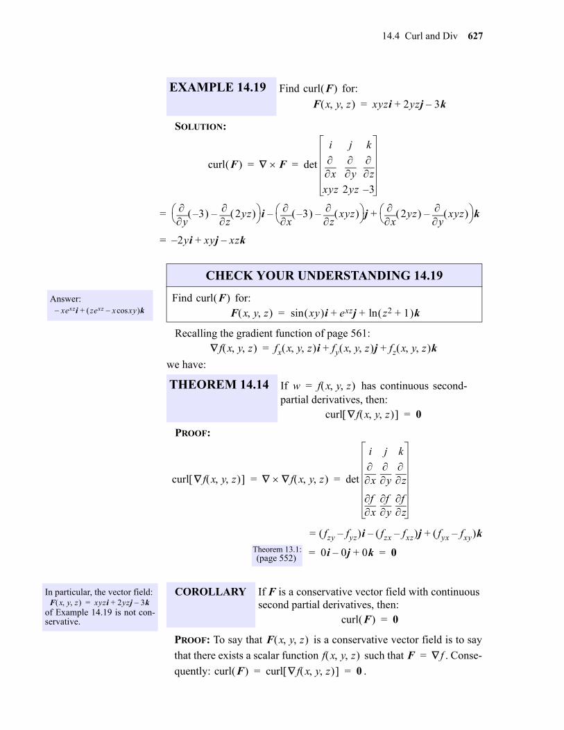
14.4 Curl and Div 627
SOLUTION:
Recalling the gradient function of page 561:
we have:
PROOF:
PROOF: To say that is a conservative vector field is to say
that there exists a scalar function such that . Conse-
quently: .
EXAMPLE 14.19 Find for:
curl F F x y z xyzi 2yzj 3k–+=
curl F F det
i j k
x
y
z
xyz 2yz 3–
= =
y 3–
z 2yz –
ix 3–
z xyz –
jx 2yz
y xyz –
k+–=
2yi xyj xzk–+–=
Answer:xexzi– zexz x xycos– k+
CHECK YOUR UNDERSTANDING 14.19
Find for:
THEOREM 14.14 If has continuous second-partial derivatives, then:
curl F F x y z xy isin exzj z2 1+ kln+ +=
f x y z fx x y z i fy x y z j fz x y z k+ +=
w f x y z =
curl f x y z 0=
curl f x y z f x y z det
i j k
x
y
z
xf
yf
zf
= =
fzy fyz– i fzx fxz– j–= fyx fxy– k+
0i 0j– 0k+ 0= =Theorem 13.1: (page 552)
In particular, the vector field:
of Example 14.19 is not con-servative.
F x y z xyzi 2yzj 3k–+=COROLLARY If F is a conservative vector field with continuous
second partial derivatives, then: curl F 0=
F x y z f x y z F f=
curl F curl f x y z 0= =
gio
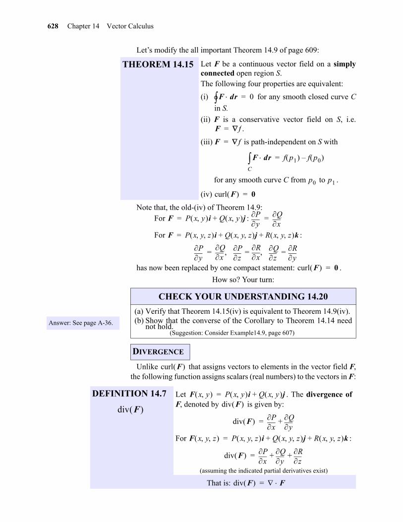
628 Chapter 14 Vector Calculus
gio
Let’s modify the all important Theorem 14.9 of page 609:
Note that, the old-(iv) of Theorem 14.9:For :
For :
has now been replaced by one compact statement: .
How so? Your turn:
Unlike that assigns vectors to elements in the vector field F,the following function assigns scalars (real numbers) to the vectors in F:
THEOREM 14.15 Let F be a continuous vector field on a simplyconnected open region S. The following four properties are equivalent:
(i) for any smooth closed curve C
in S.
(ii) F is a conservative vector field on S, i.e..
(iii) is path-independent on S with
for any smooth curve C from to .
(iv)
F dr 0=
F f=
F f=
F drC f p1 f p0 –=
p0 p1
curl F 0=
F P x y i Q x y j+=y
Px
Q=
F P x y z i Q x y z j R x y z k+ +=
yP
xQ
z
Px
R
zQ
yR===
Answer: See page A-36.
CHECK YOUR UNDERSTANDING 14.20
(a) Verify that Theorem 14.15(iv) is equivalent to Theorem 14.9(iv). (b) Show that the converse of the Corollary to Theorem 14.14 need
not hold. (Suggestion: Consider Example14.9, page 607)
DIVERGENCE
curl F 0=
curl F
DEFINITION 14.7
Let . The divergence ofF, denoted by is given by:
For :
(assuming the indicated partial derivatives exist)
That is:
div F
F x y P x y i Q x y j+=div F
div F x
Py
Q+=
F x y z P x y z i Q x y z j R x y z k+ +=
div F x
Py
Qz
R+ +=
div F F=
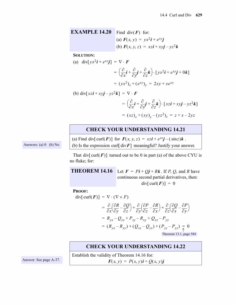
14.4 Curl and Div 629
SOLUTION:
(a)
(b)
That turned out to be 0 in part (a) of the above CYU isno fluke; for:
PROOF:
EXAMPLE 14.20 Find for:
(a)
(b)
div F F x y yx2i exyj+=
F x y z xzi xyj yz2k–+=
div yx2i exyj+ F=
x
iy
jz
k+ + yx2i exyj 0k+ + =
yx2 x exy y+ 2xy xexy+= =
div xzi xyj yz2k–+ F=
x
iy
jz
k+ + xzi xyj yz2k–+ =
xz x xy y yz2 z–+ z x 2yz–+= =
Answers: (a) 0 (b) No
CHECK YOUR UNDERSTANDING 14.21
(a) Find for .
(b) Is the expression meaningful? Justify your answer.
THEOREM 14.16 Let . If P, Q, and R havecontinuous second partial derivatives, then:
div curl F F x y z xzi exzj zsin k–+=
curl divF
div curl F
F Pi Qj Rk+ +=
div curl F 0=
div curl F F =
x
yR
zQ–
y
zP
xR–
z
xQ
yP–
+ +=
Ryx Qzx– Pzy Rxy– Qxz Pyz–+ +=
Ryx Rxy– Qxz Qzx– Pzy Pyz– + + 0= =
Theorem 13.1, page 584
Answer: See page A-37.
CHECK YOUR UNDERSTANDING 14.22
Establish the validity of Theorem 14.16 for: F x y P x y i Q x y j+=
gio
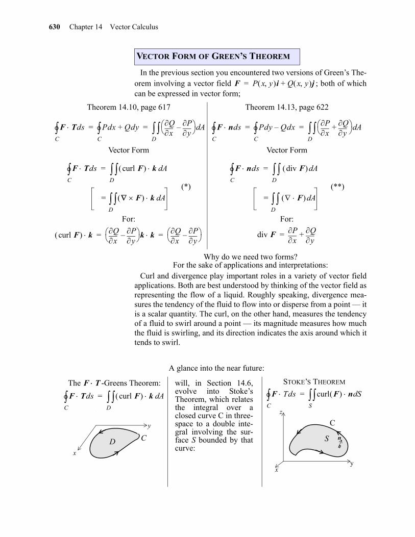
630 Chapter 14 Vector Calculus
In the previous section you encountered two versions of Green’s The-orem involving a vector field ; both of whichcan be expressed in vector form;
Why do we need two forms? For the sake of applications and interpretations:
Curl and divergence play important roles in a variety of vector fieldapplications. Both are best understood by thinking of the vector field asrepresenting the flow of a liquid. Roughly speaking, divergence mea-sures the tendency of the fluid to flow into or disperse from a point — itis a scalar quantity. The curl, on the other hand, measures the tendencyof a fluid to swirl around a point — its magnitude measures how muchthe fluid is swirling, and its direction indicates the axis around which ittends to swirl.
A glance into the near future:
VECTOR FORM OF GREEN’S THEOREM
F P x y i Q x y j+=
Theorem 14.10, page 617 Theorem 14.13, page 622
Vector Form Vector Form
(*)
For:
(**)
For:
F TdsC Pdx Qdy+
C x
Qy
P– Ad
D= = F nds
C Pdy Qdx–
C x
Py
Q+ Ad
D= =
F TdsC curl F k Ad
D=
F k AdD=
curl F kx
Qy
P– k k
xQ
yP–
= =
F ndsC div F Ad
D=
F AdD=
div Fx
Py
Q+=
The -Greens Theorem: will, in Section 14.6,evolve into Stoke’sTheorem, which relatesthe integral over aclosed curve C in three-space to a double inte-gral involving the sur-face S bounded by thatcurve:
STOKE’S THEOREMF T
F TdsC curl F k Ad
D=
y
x
CD
F TdsC curl F n Sd
S=
S
C
yx
z
n
gio
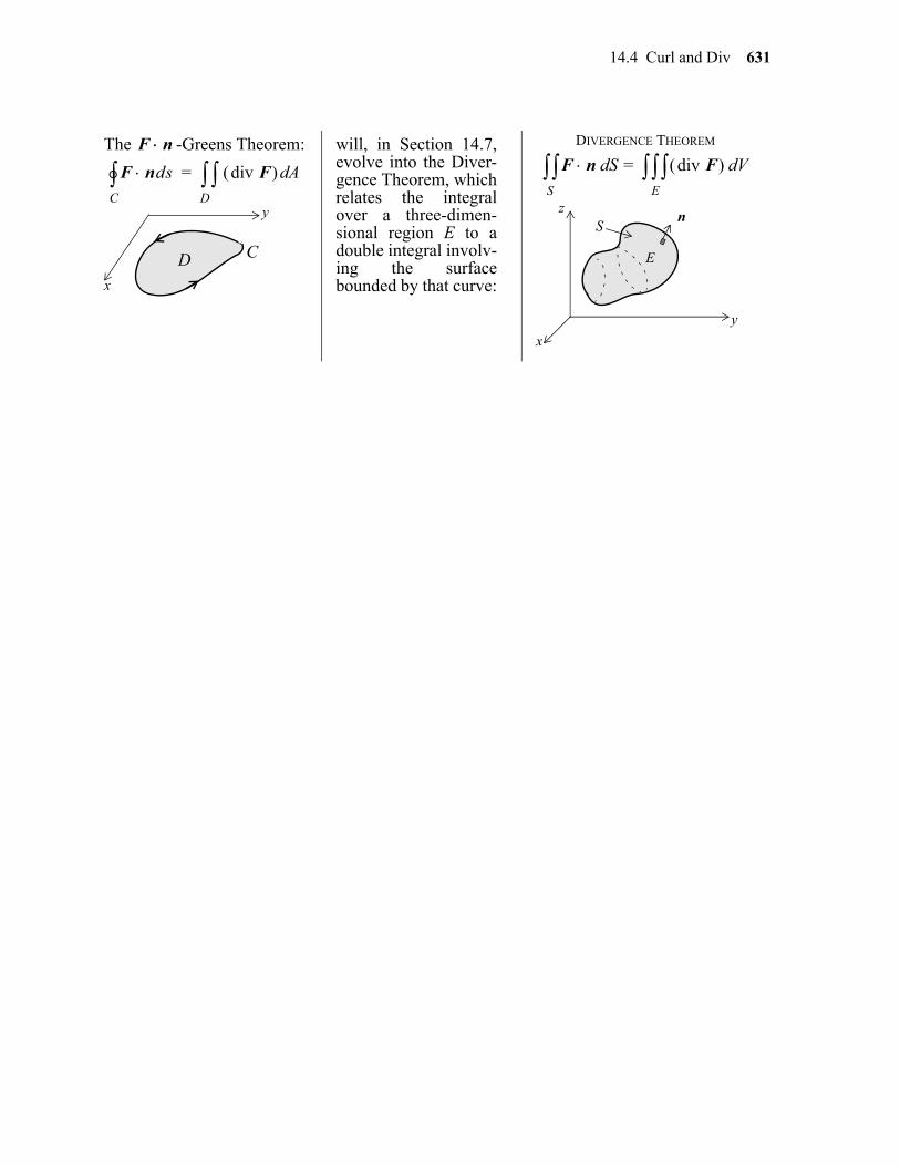
14.4 Curl and Div 631
The -Greens Theorem: will, in Section 14.7,evolve into the Diver-gence Theorem, whichrelates the integralover a three-dimen-sional region E to adouble integral involv-ing the surfacebounded by that curve:
DIVERGENCE THEOREMF n
F ndsC div F Ad
D=
y
x
CD
F n SdS div F Vd
E=
S
E
n
x
y
z
gio
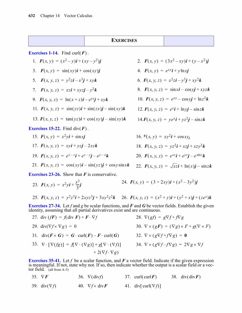
632 Chapter 14 Vector Calculus
gio
Exercises 1-14. Find .
Exercises 15-22. Find .
Exercises 23-26. Show that F is conservative.
Exercises 27-34. Let f and g be scalar functions, and F and G be vector fields. Establish the givenidentity, assuming that all partial derivatives exist and are continuous.
Exercises 35-41. Let f be a scalar function, and F a vector field. Indicate if the given expressionis meaningful. If not, state why not. If so, then indicate whether the output is a scalar field or a vec-tor field. (all from A-3)
EXERCISES
1. 2.
3. 4.
5. 6.
7. 8.
9. 10.
11. 12.
13. 14.
15. 16.
17. 18.
19. 20.
21. 22.
23.24.
25. 26.
27. 28.
29. 30.
31. 32.
33. 34.
35. 36. 37. 38.
39. 40. 41.
curl F
F x y x2 y– i xy y2– j+= F x y 3x2 xy– i y x2– j+=
F x y xy sin i xy cos j+= F x y exyi y xjln+=
F x y z y2zi x3j– xyk+= F x y z x2zi y3j– xy2k+=
F x y z xzi xyzj y2k–+= F x y z xisin yjcos– xyzk+=
F x y z x z+ iln eyzj– xyk+= F x y z exy yjcos– z2kln+=
F x y z yz isin zx jsin xy ksin–+= F x y z exi yjln zksin–+=
F x y z yz tan i xy cos j xy ksin–+= F x y z yexi yz2j zksin–+=
div F
F x y x2yi xjsin+= F x y xy2i xycos j+=
F x y z xyi yzj 2xzk–+= F x y z yz2i xzj xzy2k+ +=
F x y z ex z– i ez y– j ey x– k–+= F x y z exzi eyzj e zsin k–+=
F x y z xy cos i yz jsin– y xksincos+= F x y z xzi x jln zksin–+=
F x y x2yix3
3-----j+=
F x y 3 2xy+ i x2 3y2– j+=
F x y z y2z3i 2xyz3j 3xy2z2k+ += F x y z x2 y+ i y2 x+ j zez k+ +=
div fF f div F F f+= gf gf fg+=
div(f g 0= gF g F g F +=
div(F G G curl F F curl G –= gf fg+ 0=
fg f g g f +=
2 f g +
gf fg– 2g f=
F divf curl curlF div divF
div f f divF div curl f
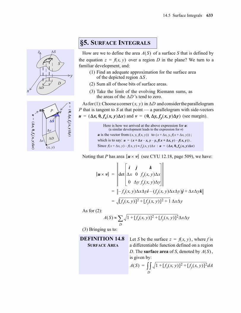
14.5 Surface Integrals 633
14+
How are we to define the area of a surface S that is defined by
the equation over a region D in the plane? We turn to afamiliar development, and:
(1) Find an adequate approximation for the surface areaof the depicted region .
(2) Sum all of those bits of surface areas.
(3) Take the limit of the evolving Riemann sums, asthe areas of the ’s tend to zero.
As for (1): Choose a corner in and consider the parallelogramP that is tangent to S at that point — a parallelogram with side-vectors
and (see margin).
Noting that P has area (see CYU 12.18, page 509), we have:
As for (2):
(3) Bringing us to:
D
S
S
D
y
x
z
D
P
S
u v
.x y
x
y
u
x0
fxx
y
x
=
v0
yfy
xy
y
=
§5. SURFACE INTEGRALS
Here is how we arrived at the above expression for u: (a similar development leads to the expression for v)
u is the vector from: to ;
which is to say: .
Since :
DEFINITION 14.8SURFACE AREA
Let S be the surface , where f isa differentiable function defined on a regionD. The surface area of S, denoted by ,is given by:
A S z f x y =
S
D
x y D
u x 0 fx x y x = v 0 y fy x y y =
x y f x y x x+ y f x x+ y
u x x x y y f x x+ y f x y –––+ =
f x x+ y f x y – fx x y x u x 0 fx x y x =
u v
u v det
i j k
x 0 fx x y x
0 y fy x y y
=
fx x y xyi– fy x y xy j– xyk+=
fx x y 2 fy x y 2 1+ + xy=
A S 1 fx x y 2 fy x y 2+ + xyD
z f x y =
A S
A S 1 fx x y 2 fy x y 2+ +D dA=
gio
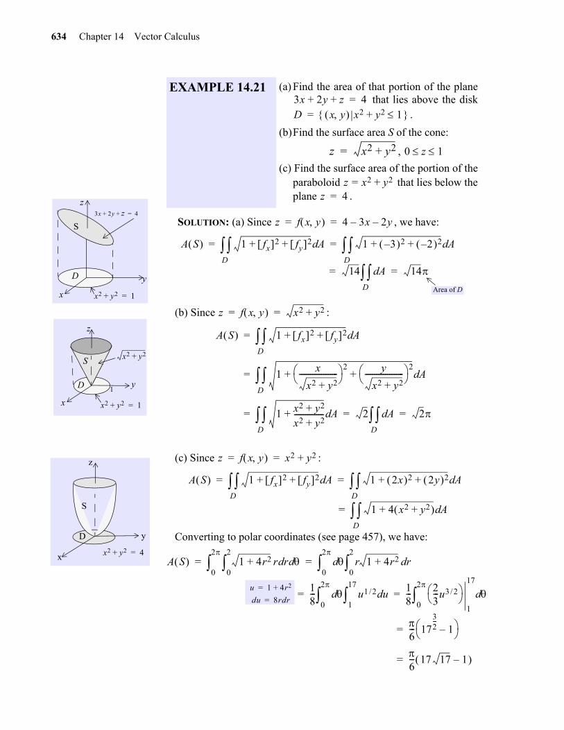
634 Chapter 14 Vector Calculus
gio
SOLUTION: (a) Since , we have:
(b) Since :
(c) Since :
Converting to polar coordinates (see page 457), we have:
y
z
x
3x 2y z+ + 4=
x2 y2+ 1=
S
D
EXAMPLE 14.21 (a) Find the area of that portion of the plane that lies above the disk
.
(b)Find the surface area S of the cone:
,
(c) Find the surface area of the portion of theparaboloid that lies below theplane .
3x 2y z+ + 4=D x y x2 y2 1+ =
z x2 y2+= 0 z 1
z x2= y2+z 4=
z f x y 4 3x– 2y–= =
A S 1 fx 2 fy 2+ + AdD 1 3– 2 2– 2+ + Ad
D= =
14 AdD 14= =
Area of D
S
D 1
x
y
z
x2 y2+ 1=
x2 y2+S
z f x y x2 y2+= =
A S 1 fx 2 fy 2+ + AdD=
1x
x2 y2+--------------------- 2 y
x2 y2+--------------------- 2
+ + AdD=
1 x2 y2+x2 y2+----------------+ Ad
D 2 Ad
D 2= = =
y
x
z
S
D
x2 y2+ 4=
z f x y x2 y2+= =
A S 1 fx 2 fy 2+ + AdD 1 2x 2 2y 2+ + Ad
D= =
1 4 x2 y2+ + AdD=
A S 1 4r2+ r rd d0
2
0
2
r 1 4r2+ rd0
2
d0
2
= =
u 1 4r2+=
du 8rdr=
18--- u1 2/ ud
1
17
d0
2
18--- 2
3---u3 2/
1
17
d0
2
= =
6--- 17
32---
1– =
6--- 17 17 1– =
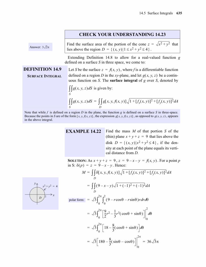
14.5 Surface Integrals 635
gio
Extending Definition 14.8 to allow for a real-valued function gdefined on a surface S in three space, we come to:
SOLUTION: As , . For a point pin S: . Hence:
Answer: 3 2
CHECK YOUR UNDERSTANDING 14.23
Find the surface area of the portion of the cone thatlies above the region .
z x2 y2+=D x y 1 x2 y2 4+ =
DEFINITION 14.9
SURFACE INTEGRAL
Let S be the surface , where f is a differentiable function
defined on a region D in the xy-plane, and let be a contin-uous function on S. The surface integral of g over S, denoted by
is given by:
Note that while f is defined on a region D in the plane, the function g is defined on a surface S in three-space.Because the points in S are of the form , the expression , as opposed to , appearsin the above integral.
z f x y =
g x y z
g x y z SdS
g x y z SdS g x y f x y 1 fx x y 2 fy x y 2+ + Ad
D=
x y f x y g x y f x y g x y z
EXAMPLE 14.22 Find the mass M of that portion S of the(thin) plane that lies above the
disk , if the den-sity at each point of the plane equals its verti-cal distance from D.
x y z+ + 9=
D x y x2 y2 4+ =
x
yx2 y2+ 4=
2D
x y z+ + 9= z 9 x– y– f x y = = p z 9 x– y–= =
M x y f x y 1 fx x y 2 fy x y 2+ + AdD=
9 x– y– D 1 1– 2 1– 2+ + Ad=
3 9 r r sin–cos– r rd d0
2
0
2
=
392---r2 1
3---r3 sin+cos –
0
2
d0
2
=
3 1883--- cos sin+ – d
0
2
=
3 18 83--- cos–sin –
0
2
36 3= =
polar form:
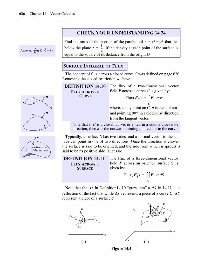
636 Chapter 14 Vector Calculus
gio
The concept of flux across a closed curve C was defined on page 620.Removing the closed-restriction we have:
Typically, a surface S has two sides, and a normal vector to the sur-face can point in one of two directions. Once the direction is chosen,the surface is said to be oriented, and the side from which n sprouts issaid to be its positive side. That said:
Note that the in Definition14.10 “grew into” a in 14.11 — areflection of the fact that while represents a piece of a curve C, represent a piece of a surface S:
Figure 14.4
Answer: 560--------- 13 2 8+
CHECK YOUR UNDERSTANDING 14.24
Find the mass of the portion of the paraboloid that lies
below the plane , if the density at each point of the surface is
equal to the square of its distance from the origin D.
SURFACE INTEGRAL OF FLUX
z x2= y2+
z 14---=
.. nC
C
n
n
Spositive sideof the surface
DEFINITION 14.10FLUX ACROSS A
CURVE
The flux of a two-dimensional vectorfield F across a curve C is given by:
where, at any point on C, n is the unit nor-mal pointing in a clockwise directionfrom the tangent vector.
Note that if C is a closed curve, oriented in a counterclockwisedirection, then n is the outward pointing unit vector to the curve.
DEFINITION 14.11FLUX ACROSS A
SURFACE
The flux of a three-dimensional vectorfield F across an oriented surface S isgiven by:
Flux FC F n sdC=
90
Flux FS F n SdS=
ds dSs S
s
n
C S
n
S
x
y
x
y
zF
F
(a) (b)
A
V
14.5 Surface Integrals 637
gio
As for the rest of the story assume that, in both instances, F rep-resents the velocity field of a fluid. If so, then the area in Figure
14.4(a) is an approximation of the amount of fluid crossing in a unit
of time: ; while the volume in Figure 14.4(b) is an
approximation of the amount of fluid crossing in a unit of time:
. The “.n” comes into play since, in each situation, the
height of the shaded region is not perpendicular to its base [the base
in (a), and the base in (b)].
To compute a unit normal to a surface S of the form wefirst rewrite the equation as , which is a level surface forthe function:
Theorem13.7, page 566, tells us that:
is a normal to the surface, with corresponding unit normal:
Since k is positive, it is the upward unit normal to the surface. Thatbeing the case, the downward unit normal is given by:
The next theorem addresses the flux issue across a surface S of theform .
PROOF: Assume that S is oriented by upward normals. Turning toTheorem 14.1, page 592, we have:
THEOREM 14.17 Let the surface S be defined by a differentia-ble function defined on a regionD in the xy-plane.
If S is oriented by upward normals:
If S is oriented by downward normals:
A
s
A F n s V
S
V F n Ss
S
z f x y =z f x y – 0=
g x y z z f x y –=
g f– x x y i fy x y j– k+=
nf– xi fyj– k+
fx 2 fy 2 1+ +------------------------------------------=
n–fxi fyj k–+
fx 2 fy 2 1+ +------------------------------------------=
z f x y =
z f x y =
F n SdS F fxi– fyj– k+ Ad
D=
F n SdS F fxi fyj k–+ Ad
D=
F n SdS F
f– xi fyj– k+
fx 2 fy 2 1+ +------------------------------------------ 1 fx 2 fy 2+ + Ad
D F f– xi fyj– k+ Ad
D= =
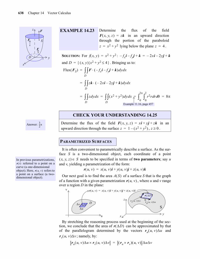
638 Chapter 14 Vector Calculus
gio
SOLUTION: For :
and . Bringing us to:
It is often convenient to parametrically describe a surface. As the sur-face S is a two-dimensional object, each coordinate of a point
needs to be specified in terms of two parameters; say uand v, yielding a parametrization of the form:
Our next goal is to find the area of a surface S that is the graphof a function with a given parametrization , where u and v rangeover a region D in the plane:
By stretching the reasoning process used at the beginning of the sec-tion, we conclude that the area of can be approximated by thatof the parallelogram determined by the vectors and
; namely, by:
x
z
2 y
..
.
F
F
F
S
D
EXAMPLE 14.23 Determine the flux of the field in an upward direction
through the portion of the paraboloid
lying below the plane .
F x y z zk=
z x2 y2+= z 4=
f x y x2 y2+= fxi– fyj– k+ 2xi– 2yj– k+=
D x y x2 y2 4+ =
Flux FS F fxi– fyj– k+ dydxD=
zk 2xi– 2yj– k+ dydxD=
zdydxD x2 y2+ dydx
D r2r rd d
0
2
0
2
8= = = =
Example 11.16, page 457
Answer: 32---
CHECK YOUR UNDERSTANDING 14.25
Determine the flux of the field in anupward direction through the surface , .
F x y z xi yj zk+ +=z 1 x2 y2+ –= z 0
In previous parametrizations, referred to a point on a
curve (a one-dimensionalobject). Here, refers toa point on a surface (a two-dimensional object).
r t
r u v
PARAMETRIZED SURFACES
x y z S
r u v x u v i y u v j z u v k+ +=
A S r u v
DS
r u v x u v i y u v j z u v k+ +=
.x
y
z
u
v
Du
v
r D
ru u v urv u v v
r D ru u v u
rv u v v
ru u v u rv u v v ru rv u v uv=
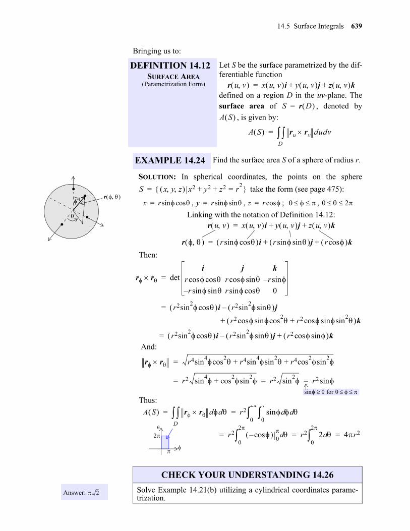
14.5 Surface Integrals 639
gio
Bringing us to:
SOLUTION: In spherical coordinates, the points on the sphere
take the form (see page 475):
, , ; ,
Linking with the notation of Definition 14.12:
Then:
And:
Thus:
DEFINITION 14.12SURFACE AREA
(Parametrization Form)
Let S be the surface parametrized by the dif-ferentiable function
defined on a region D in the uv-plane. Thesurface area of , denoted by
, is given by:
EXAMPLE 14.24 Find the surface area S of a sphere of radius r.
r u v x u v i y u v j z u v k+ +=
S r D =
A S
A S ru rvD dudv=
..
. . r
S x y z x2 y2 z2+ + r2
= =
x r cossin= y r sin sin= z r cos= 0 0 2
r u v x u v i y u v j z u v k+ +=
r r cossin i r sin sin j r cos k+ +=
r r deti j k
r coscos r sincos r sin–
r sinsin– r cossin 0
=
r2sin2 cos i r2sin
2 sin j–=
r2 cos2sincos r2 sin
2sincos+ k+
r2sin2 cos i r2sin
2 sin j– r2 sincos k+=
r r r4sin4cos
2 r4sin4sin
2+ r4cos2+ sin
2=
r2 sin4 cos
2sin2+ r2 sin
2 r2 sin= = = 0 for 0 sin
A S r rD dd r2 dsin d
0
0
2
= =
r2 cos– 0 d
0
2
r2 2 d0
2
4r2= = =
2
Answer: 2
CHECK YOUR UNDERSTANDING 14.26
Solve Example 14.21(b) utilizing a cylindrical coordinates parame-trization.
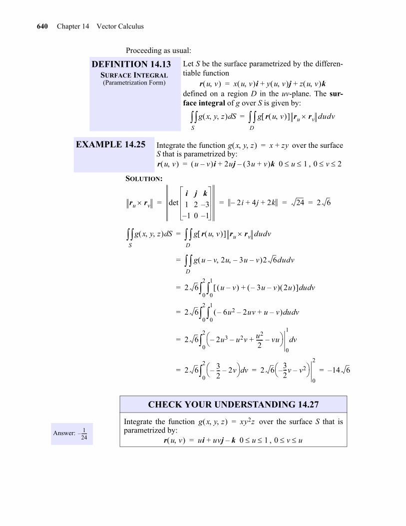
640 Chapter 14 Vector Calculus
gio
Proceeding as usual:
SOLUTION:
DEFINITION 14.13SURFACE INTEGRAL(Parametrization Form)
Let S be the surface parametrized by the differen-tiable function
defined on a region D in the uv-plane. The sur-face integral of g over S is given by:
EXAMPLE 14.25 Integrate the function over the surfaceS that is parametrized by:
,
r u v x u v i y u v j z u v k+ +=
g x y z SdS g r u v ru rv
D dudv=
g x y z x zy+=
r u v u v– i 2uj 3u v+ k–+= 0 u 1 0 v 2
ru rv deti j k
1 2 3–
1– 0 1–
2i– 4j 2k+ + 24 2 6= = = =
g x y z SdS g r u v ru rv
D dudv=
g u v– 2u 3u– v– D 2 6dudv=
2 6 u v– 3u– v– 2u + ud vd0
1
0
2
=
2 6 6u2– 2uv– u v–+ ud vd0
1
0
2
=
2 6 2u3– u2v– u2
2----- vu–+
0
1
vd0
2
=
2 6 32---– 2v–
vd0
2
2 632---v v2––
0
2
14 6–= = =
Answer: 124------–
CHECK YOUR UNDERSTANDING 14.27
Integrate the function over the surface S that isparametrized by:
,
g x y z xy2z=
r u v ui uvj k–+= 0 u 1 0 v u
14.5 Surface Integrals 641
Exercises 1-10. Find the area of the given surface.
Exercises 11-18. Evaluate.
EXERCISES
1. That part of the surface that lies inside the cylinder .
2. That part of the plane that lies within the cylinder .
3. That part of the surface that lies above .
4. That part of the parabolic cylinder that lies above the triangle with vertices , ,.
5. That part of the hyperbolic paraboloid that lies between the cylinders and .
6. That part of the hyperbolic paraboloid that lies inside the cylinder .
7. That part of the hemisphere that lies above the disk .
8. That portion of the sphere that lies above the plane .
9. That part of the surface that lies above .
10. That part of the surface that lies above
11. where S is the part of the surface that lies above the trian-
gle with vertices .
12. where S is the part of the paraboloid between the planes and
.
13. where S is the surface above .
14. where S is the parabolic cylinder above .
z x2 y2+= x2 y2+ 4=
x 2y 3z 4+ + + 0= x2 y2+ a2=
z x23---y3 2/+= D x y 1 x 4 2 y 7 =
z y2= 0 0 0 1 1 1
z y2 x2–= x2 y2+ 1=x2 y2+ 4=
z xy= x2 y2+ a2=
z 25 x2– y2–= x2 y2 9+
x2 y2 z2+ + 9= z 2=
z23--- x3 2/ y3 2/+ = D x y 2 x 4 1 y 4 =
z e y– 7x+= D x y 0 x e 2y– 0 y 3 =
z 3y x2–+ SdS z 2 3y– x2+=
0 0 2 0 2 4–
32z SdS z 2x2 2y2+= z 0=
z 4=
y SdS z x y2+= D x y 0 x 1 0 y 2 =
3y SdS z
12---y2= D x y 0 x 1 0 y 1 =
gio
642 Chapter 14 Vector Calculus
Exercises 19-22. Find the mass of the (thin) surface S with density .
Exercises 23-26. Integrate the function g over the surface S with given parametrization .
Exercises 27-30. Calculate the flux of the vector field F in the upward direction through the sur-face S.
15. where S is the part of the circular cylinder , in the first octant
between the planes and .
16. where S is that part of the plane that lies in the first octant.
17. over the surface of the cone which lies between and .
18. where S is the surface of the parabolic cylinder cut by the planes
, and .
19. S is the portion of the parabolic cylinder between the planes, and , and .
20. S is the portion of the cone between the planes and , and.
21. S is the triangle , and .
22. S is the surface that lies above , and
.
23. , with , .
24. , with , .
25. , with , .
26. , with ,
27. , and S is the rectangular plate with corners at ,.
28. , and S is the paraboloid , for .
x z+ SdS y2 z2+ 9=
x 0= x 4=
xz SdS x y z+ + 1= 3
24-------
x2y2z2 SdS x2 y2+ z2= z 0= z 1=
x 4 y2 Sd+S y2 4z+ 16=
x 0 x 1= = z 0=
y2 9 z–=x 0 x 3 y 0= = = y 3= x y z y=
z x2 y2+= z 1= z 4= x y z x2z=
a 0 0 0 a 0 0 0 a x y z kx2=
z 112--- x2 y2+ –= D x y 0 x 1 0 y 1 =
x y z xy=
r u v
g x y z xyz= r u v u v+ i vj u v– k+ += 0 u 1 0 v 2
g x y z x2 yz+= r u v u v+ i uj vk+ += 0 u 1 0 v 2
g x y z 1 x2 y2+ += r u v u vcos i u vjsin vk+ += 0 u 1 0 v
g x y z zy xy–= r u v vi uj u v+ k+ += 3 u 5 2 v 3
F x y z zk= 0 0 0 1 0 0 0 1 3 1 1 3
F x y z xi yj zk+ += z x2 y2 1–+= 1 z 0 –
gio
14.5 Surface Integrals 643
29. , and S is the surface that lies above the xy-plane.
30. , and S is the parabolic cylinder that lies above
F x y z yi xj zk+ += z 16 x2– y2–=
F x y z yzi xj y2k–+= z x2=D x y 0 x 1 0 y 4 =
gio
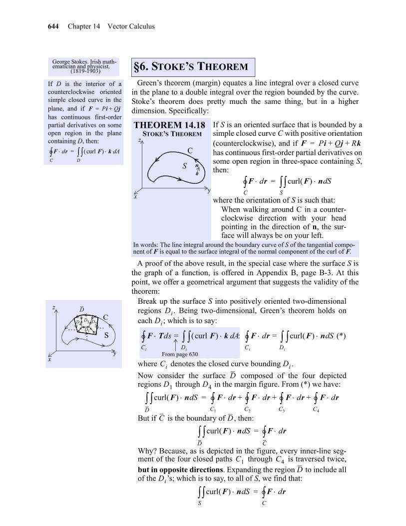
644 Chapter 14 Vector Calculus
gio
14
Green’s theorem (margin) equates a line integral over a closed curvein the plane to a double integral over the region bounded by the curve.Stoke’s theorem does pretty much the same thing, but in a higherdimension. Specifically:
A proof of the above result, in the special case where the surface S isthe graph of a function, is offered in Appendix B, page B-3. At thispoint, we offer a geometrical argument that suggests the validity of thetheorem:
Break up the surface S into positively oriented two-dimensionalregions . Being two-dimensional, Green’s theorem holds oneach ; which is to say:
(*)
where denotes the closed curve bounding .
Now consider the surface composed of the four depictedregions through in the margin figure. From (*) we have:
But if is the boundary of , then:
Why? Because, as is depicted in the figure, every inner-line seg-ment of the four closed paths through is traversed twice,but in opposite directions. Expanding the region to include allof the ’s; which is to say, to all of S, we find that:
George Stokes. Irish math-ematician and physicist.
(1819-1903)
If D is the interior of acounterclockwise orientedsimple closed curve in theplane, and if has continuous first-orderpartial derivatives on someopen region in the planecontaining D, then:
F Pi Qj+=
F drC curl F k Ad
D=
§6. STOKE’S THEOREM
THEOREM 14.18STOKE’S THEOREM
If S is an oriented surface that is bounded by asimple closed curve C with positive orientation(counterclockwise), and if has continuous first-order partial derivatives onsome open region in three-space containing S,then:
where the orientation of S is such that:When walking around C in a counter-clockwise direction with your headpointing in the direction of n, the sur-face will always be on your left.
In words: The line integral around the boundary curve of S of the tangential compo-nent of F is equal to the surface integral of the normal component of the curl of F.
S
C
yx
z
n
F Pi Qj Rk+ +=
F drC curl F n Sd
S=
C
yx
z
D1
D2D4
S
D3
D DiDi
F TdsCi
curl F k AdDi
= : F drCi
curl F n SdDi
=
From page 630
Ci Di
DD1 D4
curl F n SdD
F drC1
F drC2
F drC3
F drC4
+ + +=
C D
curl F n SdD
F drC
=
C1 C4
DDi
curl F n SdS F dr
C=
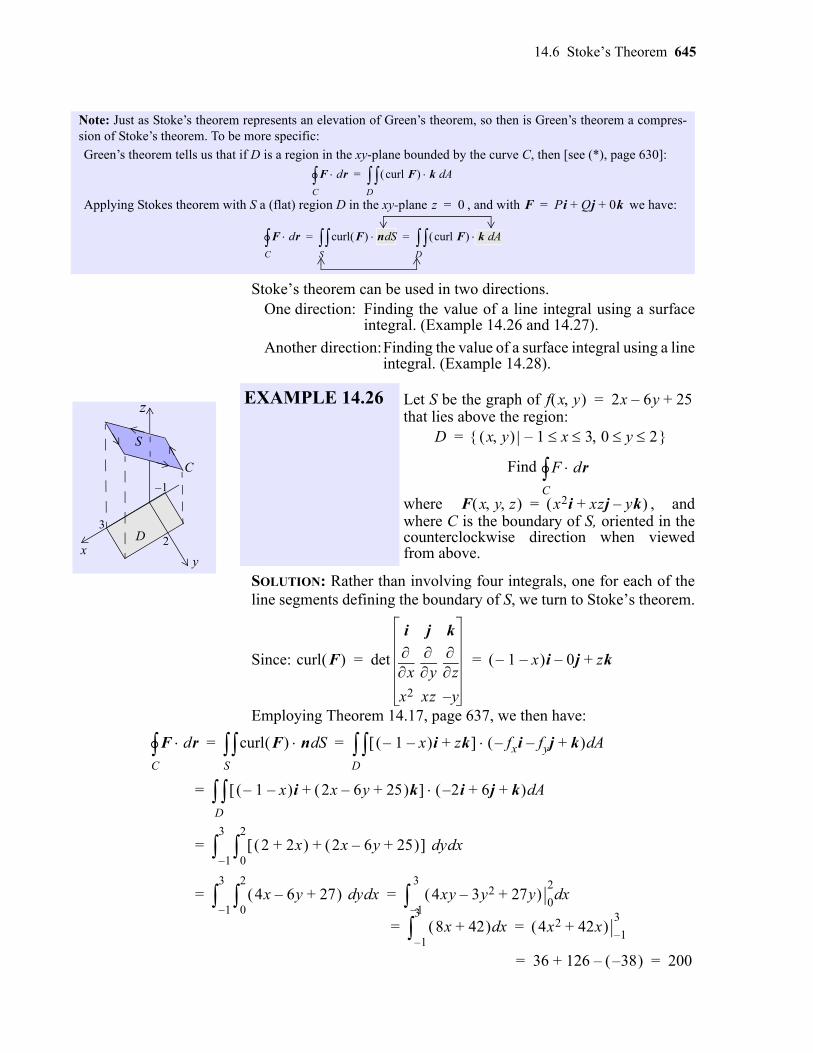
14.6 Stoke’s Theorem 645
gio
Stoke’s theorem can be used in two directions.One direction: Finding the value of a line integral using a surface
integral. (Example 14.26 and 14.27).
Another direction:Finding the value of a surface integral using a lineintegral. (Example 14.28).
SOLUTION: Rather than involving four integrals, one for each of theline segments defining the boundary of S, we turn to Stoke’s theorem.
Since:
Employing Theorem 14.17, page 637, we then have:
Note: Just as Stoke’s theorem represents an elevation of Green’s theorem, so then is Green’s theorem a compres-sion of Stoke’s theorem. To be more specific:
Green’s theorem tells us that if D is a region in the xy-plane bounded by the curve C, then [see (*), page 630]:
Applying Stokes theorem with S a (flat) region D in the xy-plane , and with we have:
F drC curl F k Ad
D=
z 0= F Pi Qj 0k+ +=
F drC curl F n Sd
S curl F k Ad
D= =
y
z
x
S
D3
2
1–
C
EXAMPLE 14.26 Let S be the graph of that lies above the region:
Find
where , andwhere C is the boundary of S, oriented in thecounterclockwise direction when viewedfrom above.
f x y 2x 6y– 25+=
D x y 1 x 3 0 y 2 – =
F drC
F x y z x2i xzj yk–+ =
curl F det
i j k
x
y
z
x2 xz y–
1– x– i 0j– zk+= =
F drC curl F n Sd
S 1– x– i zk+ fxi– fyj– k+ Ad
D= =
1– x– i 2x 6y– 25+ k+ 2– i 6j k+ + AdD=
2 2x+ 2x 6y– 25+ + yd xd0
2
1–
3
=
4x 6y– 27+ yd xd0
2
1–
3
4xy 3y2– 27y+ 0
2xd
1–
3
= =
8x 42+ xd1–
3
4x2 42x+ 1–
3= =
36 126 38– –+ 200= =
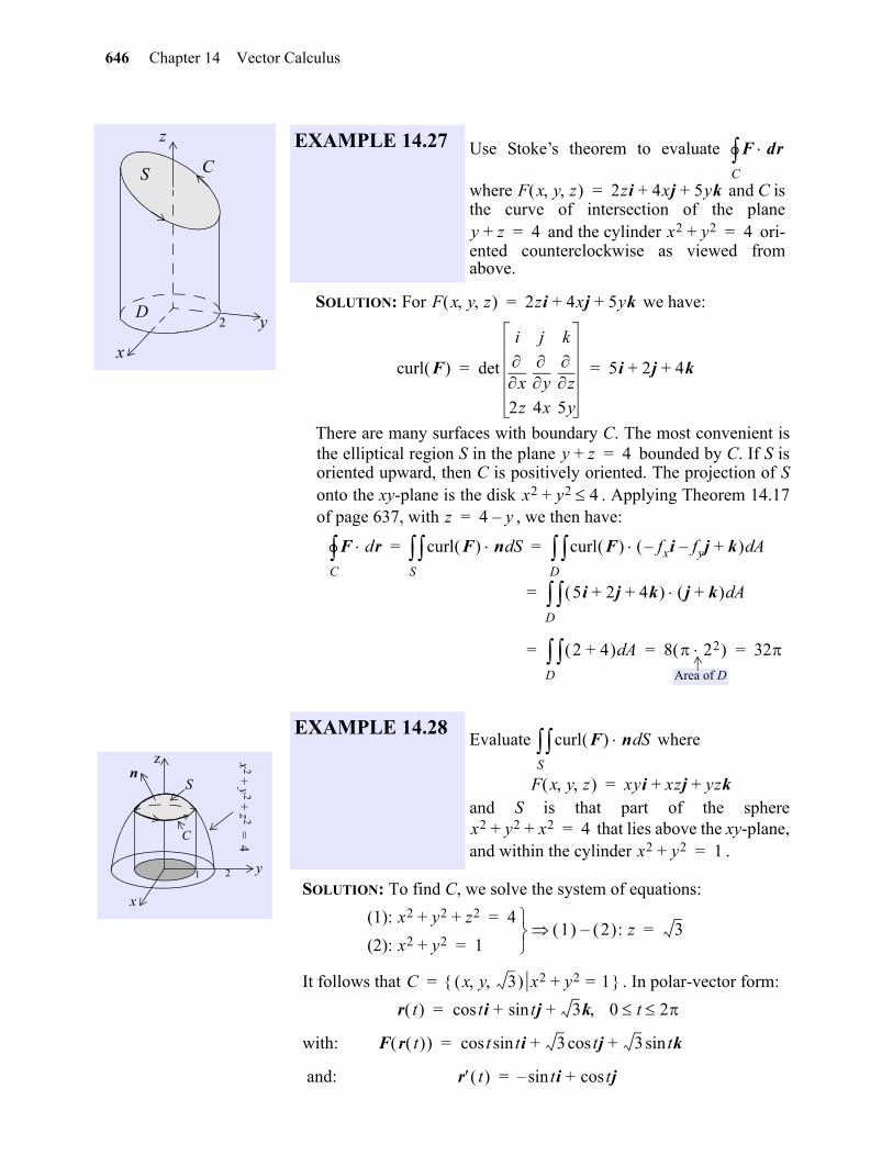
646 Chapter 14 Vector Calculus
gio
SOLUTION: For we have:
There are many surfaces with boundary C. The most convenient isthe elliptical region S in the plane bounded by C. If S isoriented upward, then C is positively oriented. The projection of Sonto the xy-plane is the disk . Applying Theorem 14.17of page 637, with , we then have:
SOLUTION: To find C, we solve the system of equations:
It follows that . In polar-vector form:
with:
and:
S
D
C
z
x
y2
EXAMPLE 14.27 Use Stoke’s theorem to evaluate
where and C isthe curve of intersection of the plane
and the cylinder ori-ented counterclockwise as viewed fromabove.
F drC
F x y z 2zi 4xj 5yk+ +=
y z+ 4= x2 y2+ 4=
F x y z 2zi 4xj 5yk+ +=
curl F det
i j k
x
y
z
2z 4x 5y
5i 2j 4k+ += =
y z+ 4=
x2 y2+ 4z 4 y–=
F drC curl F n Sd
S curl F fxi– fyj– k+ Ad
D= =
5i 2j 4k+ + j k+ AdD=
2 4+ AdD 8 22 32= = =
Area of D
y
x
x2
y2
z2
++
4=
1 2
z
C
nS
EXAMPLE 14.28Evaluate where
and S is that part of the sphere
that lies above the xy-plane,and within the cylinder .
curl F n SdS
F x y z xyi xzj yzk+ +=
x2 y2 x2+ + 4=x2 y2+ 1=
(1): x2 y2 z2+ + 4=
(2): x2 y2+ 1=
1 2 : z– 3=
C x y 3 x2 y2+ 1= =
r t tcos i tsin j 3k 0 t 2 + +=
F r t t tsincos i 3 tcos j 3 tsin k+ +=
r t tsin– i tcos j+=
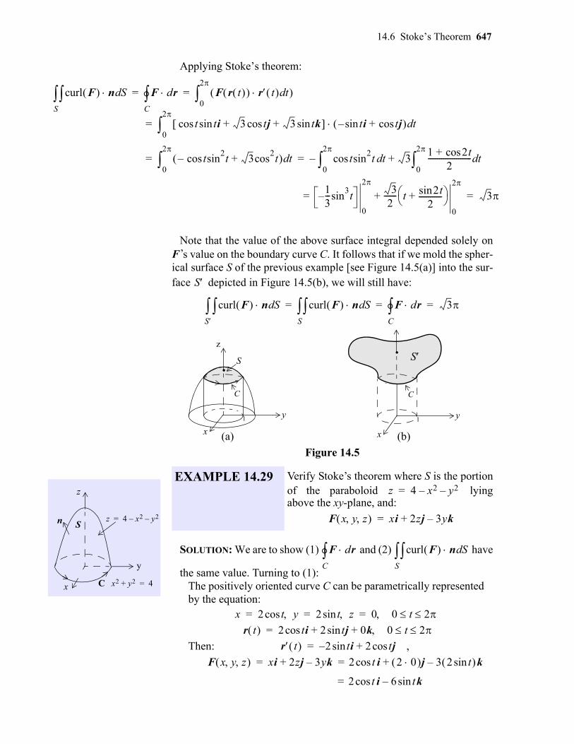
14.6 Stoke’s Theorem 647
gio
Applying Stoke’s theorem:
Note that the value of the above surface integral depended solely onF’s value on the boundary curve C. It follows that if we mold the spher-ical surface S of the previous example [see Figure 14.5(a)] into the sur-face depicted in Figure 14.5(b), we will still have:
Figure 14.5
SOLUTION: We are to show (1) and (2) have
the same value. Turning to (1):The positively oriented curve C can be parametrically representedby the equation:
Then: ,
curl F n SdS F dr
C F r t r t td
0
2
= =
t tsincos i 3 tcos j 3 tsin k+ + tsin– i tcos j+ td0
2
=
tsin2tcos– 3cos
2t+ td
0
2
tsin2tcos td
0
2
– 31 2tcos+
2----------------------- td
0
2
+= =
13---sin
3t–
0
2
=3
2------- t 2tsin
2------------+
0
2
+ 3=
S
curl F n SdS curl F n Sd
S F dr
C 3= = =
y
x
1
z
C
S
y
x
1
C
..
S
(a) (b)
y
x
z
Sz 4 x2– y2–=n
x2 y2+ 4=C
EXAMPLE 14.29 Verify Stoke’s theorem where S is the portionof the paraboloid lyingabove the xy-plane, and:
z 4 x2– y2–=
F x y z xi 2zj 3yk–+=
F drC curl F n Sd
S
x 2 t ycos 2 t zsin 0 0 t 2 = = =
r t 2 tcos i 2 tsin j 0k+ 0 t 2 +=
r t 2– tsin i 2 tcos j+=
F x y z xi 2zj 3yk–+ 2 tcos i 2 0 j 3 2 tsin k–+= =
2 tcos i 6 tsin k–=
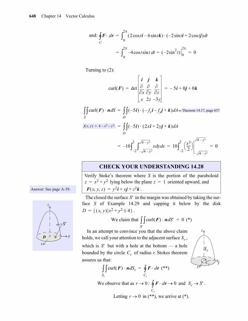
648 Chapter 14 Vector Calculus
gio
and:
Turning to (2):
The closed the surface in the margin was obtained by taking the sur-face S of Example 14.29 and capping it below by the disk
.
We claim that (*)
In an attempt to convince you that the above claimholds, we call your attention to the adjacent surface ,
which is but with a hole at the bottom — a hole
bounded by the circle of radius r. Stokes theorem
assures us that:
(**)
We observe that as : and .
Letting in (**), we arrive at (*).
F drC 2 tcos i 6 tsin k– 2– tsin i 2 tcos j+ td
0
2
=
4 t tsincos– td0
2
2sin2t–
0
20= = =
curl F det
i j k
x
y
z
x 2z 3y–
5i– 0j 0k+ += =
curl F n SdS 5i– fxi– fyj– k+ Ad
D=
5i– 2xi 2yj k+ + AdD=
10 x yd xd4 y2––
4 y2–
2–
2
– 10x2
2-----
4 y2––
4 y2–
2–
2
0= = =
f x y 4 x2– y2:–=
Theorem 14.17, page 637
Answer: See page A-39.
CHECK YOUR UNDERSTANDING 14.28
Verify Stoke’s theorem where S is the portion of the paraboloid lying below the plane oriented upward, and
.
z x2 y2+= z 1=
F x y z y2i xj z2k+ +=
y
x
z
D
S
S
D x y x2 y2+ 4 =
curl F n SdS 0=
x
z
Cr
Sr
y
Sr
SCr
curl F n SrdSr
F drCr
=
r 0 F drCr
0 Sr S
r 0
14.6 Stoke’s Theorem 649
In general: if has continuous first-order partialderivatives on some open region in three-space containingthe closed surface S, then:
Answer: See page A-40.
CHECK YOUR UNDERSTANDING 14.29
Use Stoke’s theorem to prove that if in a region S, thenF is path independent in S.
F Pi Qj Rk+ +=
curl F n SdS 0=
curl F 0=
gio
650 Chapter 14 Vector Calculus
Exercises 1-9. Use Stoke’s Theorem to evaluate .
Exercises 10-17. Use Stoke’s Theorem to evaluate .
EXERCISES
1. , S is the graph of that lies above theregion: , and C is the boundary of S, oriented in thecounterclockwise direction when viewed from above.
2. and C is the triangle with vertices and ,oriented in the counterclockwise direction when viewed from above.
3. and C is the circle , , oriented in the coun-terclockwise direction when viewed from above.
4. and C is the curve of intersection of the cone and the plane , oriented in the counterclockwise direction when viewed from above.
5. and C is the intersection of the cylinder and the plane oriented in the counterclockwise direction when viewed from above.
6. and C is the intersection of the sphere andthe plane oriented in the counterclockwise direction when viewed from above.
7. and C is the circle defined by the parametric equations
.
8. and C is the boundary of the part of the plane in the first octant, oriented in the counterclockwise direction when viewed from
above.
9. and C is the boundary of the portion of the plane in the first octant, oriented in the counterclockwise direction when viewed from above.
10. and S is that part of the sphere that lies abovethe xy-plane, and within the cylinder .
11. , and S is the part of that lies above the plane. Assume that S is oriented upwards.
12. , and S is the surface oriented upwards.
F drC
F x y z 3zi– x y+ j yk+ += f x y 4x 8y– 5+=D x y x 1– 2 9 y 3– 2 36+ =
F x y z z2i y2j xk+ += 1 0 0 0 1 0 0 0 1
F x y z yi xz3j zy3k–+= x2 y2+ 4= z 3–=
F x y z x2 y– i 4zj x2k+ += z x2 y2+=z 2=
F x y z y3– i x3j z3k–+= x2 y2+ 1=x y z+ + 1=
F x y z x2yzi yz2j z3exyk+ += x2 y2 z2+ + 5=x 1=
F x y z x2e5zi x yj 3yk+cos+=
x 0 y 2 2 tcos+= = z 2 2 t 0 t 2 sin+=
F x y z x2 y2– i y2 z2– j z2 x2– k+ +=x y z+ + 2=
F x y z xzi xyj 3xzk+ += 2x y z+ + 2=
curl F n SdS
F x y z xzi yzj xyk+ += x2 y2 z2+ + 4=x2 y2+ 1=
F x y z z2i 3xyj– x3y3k+= z 5 x2– y2–=z 1=
F x y z exy zi x2zj xyk+ +cos= x 1 y2– z2–=
gio
14.6 Stoke’s Theorem 651
Exercises 18-27. Verify Stoke’s Theorem:
13. , and S is the square .
14. and S is the part of the paraboloid that lies
inside the cylinder , oriented upward.
15. and S is the part of the hemisphere above the plane , oriented upward.
16. and S is the part of the cone betweenthe planes and , oriented upward.
17. and S is the part of the plane inside the cylinder, oriented upward.
18. and S is that part of the paraboloid for which, oriented upward.
19. and S is that part of the paraboloid for which ,oriented upward.
20. and S is that graph of the function
where , , oriented upward.
21. and S is the upper half of the sphere , orientedupward.
22. and S is the paraboloid , , orientedupward.
23. and S is the upper half of the sphere , ori-ented upward.
24. and S is the triangle , , , orientedupward.
25. and S is the triangle , , traversed counterclockwise.
26. and S is the part of the plane that lies in the firstoctant, oriented upward.
27. and S is the part of the paraboloid that lies above the plane , oriented upward.
F x y z z2i 5xj+= 0 x 1 0 y 1 z 1=
F x y z x2z2i y2z2j xyzk+ += z x2 y2+=
x2 y2+ 4=
F x y z 2y zicos ex zjsin xeyk+ += x2 y2 z2+ + 9=z 0=
F x y z x2yz3i xyzj xyz ksin+ += z2 x2 y2+=z 0= z 3=
F x y z y2– i xj z2k++= y z+ 2=x2 y2+ 1=
F drC curl F n Sd
S=
F x y z 2zi 3xj 5yk+ += z 4 x2– y2–=z 0
F x y z yi zj xk+ += z 1 x2– y2–= z 0
F x y z 3xi x 2x3
3-------- 2xy2+ +
j zk+ +=
z 1 2 x2 y2+ –= 0 x2 y2 12---+ z 0
F x y z z2i 2xj– y3k+= x2 y2 z2+ + 1=
F x y z 3yi 4zj 6xk–+= z 16 x2– y2–= z 0
F x y z 6xzi x2j– 3y2k–= x2 y2 z2+ + 1=
F x y z x4i xyj z4k+ += 2 0 0 0 2 0 0 0 2
F x y z x2 y2+ i y2j x2 z2+ k+ += 2 0 0 0 2 0 0 0 2
F x y z xi yj xyzk+ += 2x y z+ + 2=
F x y z z y– i z x+ j x y+ k–+=z 1 x2– y2–= z 0=
gio
652 Chapter 14 Vector Calculus
28. A particle moves along the line segments from the origin to the points , ,, and back to the origin under the influence of the force field
. Determine the work done.Suggestion: See Theorem 14.2, page 628, and apply Stoke’s theorem to the plane S containing the three points.
29. Let C be a simple closed smooth curve that lies in the plane . Show that
depends only on the area of the region enclosed by C and not on the
shape of C or its location on the plane.
1 0 0 1 2 1 0 2 1
F x y z z2i 2xyj 4y2k+ +=
x y z+ + 1=
zdx 2xdy– 3ydz+C
gio
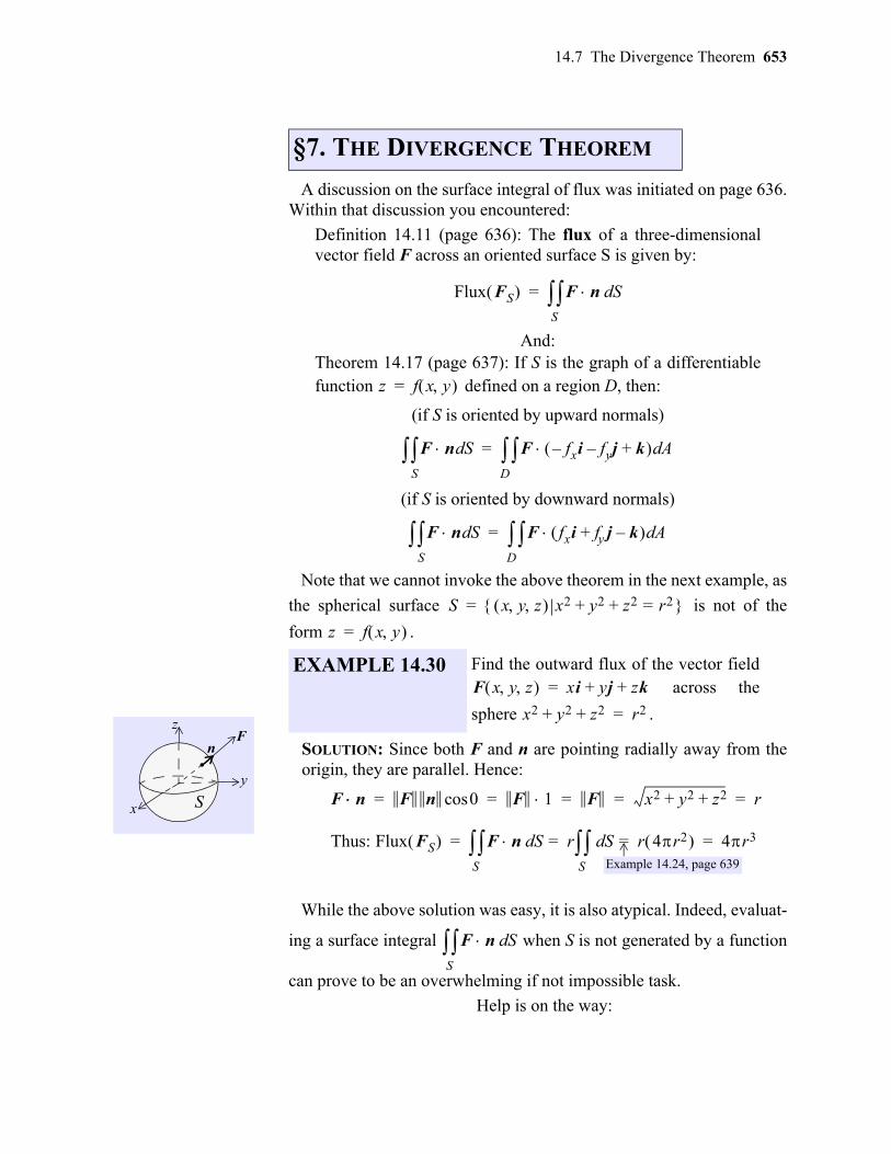
14.7 The Divergence Theorem 653
14
A discussion on the surface integral of flux was initiated on page 636.Within that discussion you encountered:
Definition 14.11 (page 636): The flux of a three-dimensionalvector field F across an oriented surface S is given by:
And:Theorem 14.17 (page 637): If S is the graph of a differentiablefunction defined on a region D, then:
(if S is oriented by upward normals)
(if S is oriented by downward normals)
Note that we cannot invoke the above theorem in the next example, as
the spherical surface is not of the
form .
SOLUTION: Since both F and n are pointing radially away from theorigin, they are parallel. Hence:
Thus:
While the above solution was easy, it is also atypical. Indeed, evaluat-
ing a surface integral when S is not generated by a function
can prove to be an overwhelming if not impossible task.
Help is on the way:
§7. THE DIVERGENCE THEOREM
Flux FS F n SdS=
z f x y =
F n SdS F fxi– fyj– k+ Ad
D=
F n SdS F fxi fy j k–+ Ad
D=
.F
n
x
y
z
S
EXAMPLE 14.30 Find the outward flux of the vector field across the
sphere .
S x y z x2 y2 z2+ + r2= =
z f x y =
F x y z xi yj zk+ +=
x2 y2 z2+ + r2=
F n F n 0cos F 1 F x2 y2 z2+ + r= = = = =
Flux FS F n SdS r Sd
S r 4r2 4r3= = = =
Example 14.24, page 639
F n SdS
gio
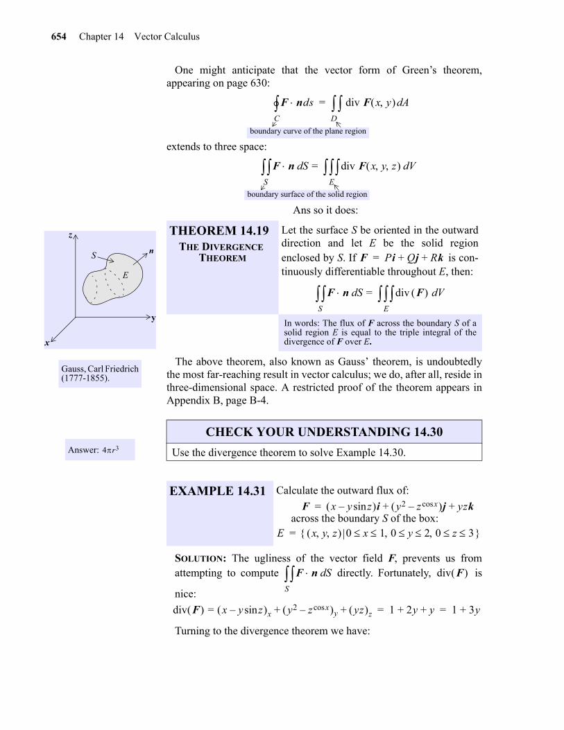
654 Chapter 14 Vector Calculus
One might anticipate that the vector form of Green’s theorem,appearing on page 630:
extends to three space:
Ans so it does:
The above theorem, also known as Gauss’ theorem, is undoubtedlythe most far-reaching result in vector calculus; we do, after all, reside inthree-dimensional space. A restricted proof of the theorem appears inAppendix B, page B-4.
SOLUTION: The ugliness of the vector field F, prevents us fromattempting to compute directly. Fortunately, is
nice:
Turning to the divergence theorem we have:
F ndsC div F x y Ad
D=
boundary curve of the plane region
F n SdS div F x y z Vd
E=
boundary surface of the solid region
Gauss, Carl Friedrich(1777-1855).
S n
y
z
x
E
THEOREM 14.19THE DIVERGENCE
THEOREM
Let the surface S be oriented in the outwarddirection and let E be the solid regionenclosed by S. If is con-tinuously differentiable throughout E, then:
In words: The flux of F across the boundary S of asolid region E is equal to the triple integral of thedivergence of F over E.
F Pi Qj Rk+ +=
F n SdS div F Vd
E=
Answer: 4r3
CHECK YOUR UNDERSTANDING 14.30
Use the divergence theorem to solve Example 14.30.
EXAMPLE 14.31 Calculate the outward flux of:
across the boundary S of the box:F x y zsin– i y2 z xcos– j yzk+ +=
E x y z 0 x 1 0 y 2 0 z 3 =
F n SdS div F
div F x y zsin– x= y2 z xcos– y yz z+ + 1 2y y+ + 1 3y+= =
gio
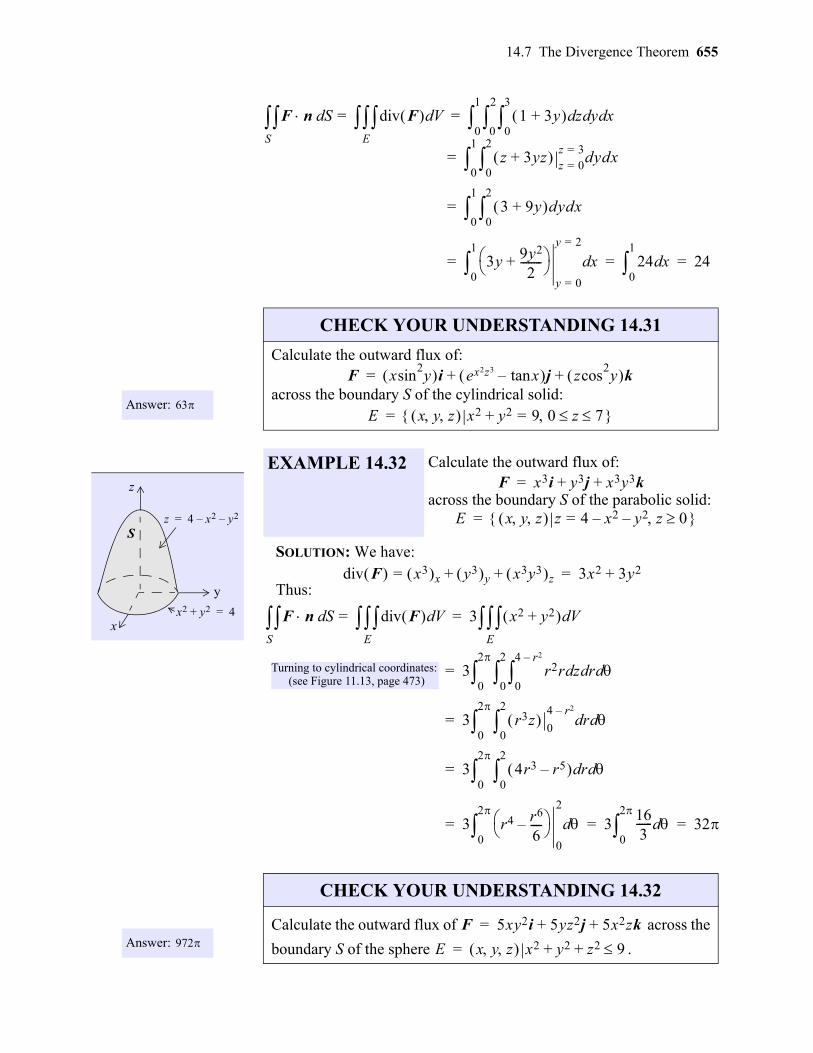
14.7 The Divergence Theorem 655
gio
SOLUTION: We have:
Thus:
F n SdS div F Vd
E 1 3y+ zd yd xd
0
3
0
2
0
1
= =
z 3yz+ z 0=z 3=
0
2
0
1
dydx=
3 9y+ 0
2
0
1
dydx=
3y 9y2
2--------+
y 0=
y 2=
xd0
1
24 xd0
1
24= = =
Answer: 63
CHECK YOUR UNDERSTANDING 14.31
Calculate the outward flux of:
across the boundary S of the cylindrical solid:F xsin
2y i ex2z3 xtan– j zcos
2y k+ +=
E x y z x2 y2+ 9 0 z 7 = =
y
x
z
Sz 4 x2– y2–=
x2 y2+ 4=
EXAMPLE 14.32 Calculate the outward flux of:
across the boundary S of the parabolic solid:F x3i y3j x3y3k+ +=
E x y z z 4 x2– y2 z 0–= =
div F x3 x= y3 y x3y3 z+ + 3x2 3y2+=
F n SdS div F Vd
E 3 x2 y2+ Vd
E= =
3 r2r zd rd d0
4 r2–
0
2
0
2
=
3 r3z 0
4 r2–rd d
0
2
0
2
=
3 4r3 r5– 0
2
rd d0
2
=
3 r4 r6
6----–
0
2
d0
2
3163------ d
0
2
32= = =
Turning to cylindrical coordinates:(see Figure 11.13, page 473)
Answer: 972
CHECK YOUR UNDERSTANDING 14.32
Calculate the outward flux of across the
boundary S of the sphere .
F 5xy2i 5yz2j 5x2zk+ +=
E x y z x2 y2 z2 9+ +=
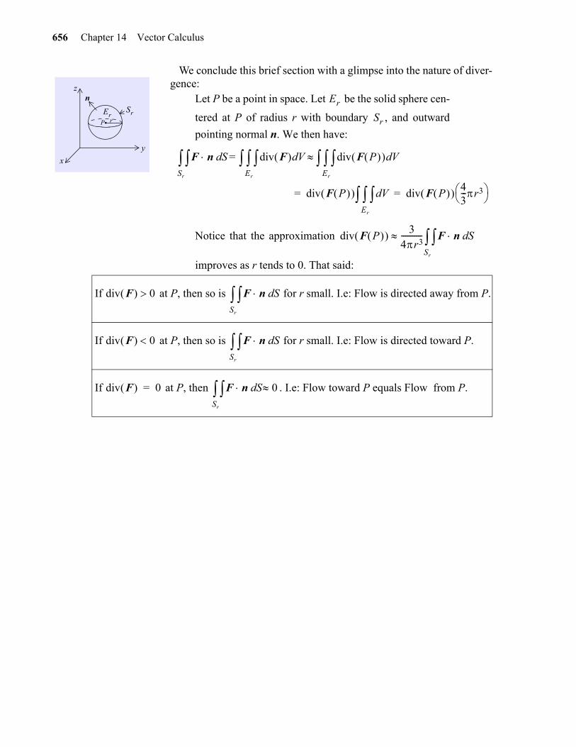
656 Chapter 14 Vector Calculus
We conclude this brief section with a glimpse into the nature of diver-gence:
Let P be a point in space. Let be the solid sphere cen-
tered at P of radius r with boundary , and outward
pointing normal n. We then have:
Notice that the approximation
improves as r tends to 0. That said:
.P rEr
Sr
y
z
x
n Er
Sr
F n SdSr
div F VdEr
= div F P VdEr
div F P VdEr
div F P 43---r3 = =
div F P 34r3----------- F n Sd
Sr
If at P, then so is for r small. I.e: Flow is directed away from P.
If at P, then so is for r small. I.e: Flow is directed toward P.
If at P, then . I.e: Flow toward P equals Flow from P.
div F 0 F n SdSr
div F 0 F n SdSr
div F 0= F n SdSr
0
gio
14.7 The Divergence Theorem 657
Exercises 1-12. Use the divergence theorem to evaluate .
EXERCISES
1. and S is the sphere .
2. and S is the sphere .
3. and S is the surface of the solid hemisphere:
(with outward normal).
4. and S is the surface of the solid:
(with outward normal).
5. and S the surface of the solid:
(with outward normal).
6. and S is the surface of the solid cylinder:
(with outward normal).
7. and S is the surface of the solid cylinder:
(with outward normal).
8. and S is the surface of the solid unit cube:
(with outward normal).
9. and S is the surface of the solid:
(with outward normal).
10. and S is the surface of the solid:
(with outward normal).
11. and S is the surface of the solid bounded by the par-abolic cylinder and the planes , and (with outward normal).
12. and S is the surface, with outward normal, of the wedge cut fromthe first octant by the plane and the elliptical cylinder .
F n SdS
F x y z x3i y3j z3k+ += x2 y2 z2++ a2=
F x y z x3 y+ i y3 z+ j z3 x+ k+ += x2 y2 z2++ 1=
F x y z x y+ i z2j x2k+ +=
E x y z x2 y2 z2 1 z 0+ + =
F x y z xyi yzj xzk+ +=
E x y z 0 x 1 0 x 1 0 z 1 x– y– =
F x y z yez2i y2j exyk+ +=
E x y z x2 y2 9 0 z y 3– + =
F x y z 3xy2i xezj z3k+ +=
E x y z y2 z2 1 1– x 2 + =
F x y z y2i xz3j z 1– 2k+ +=
E x y z x2 y2 16 1 z 5 + =
F x y z 2xyi 3yezj x z ksin+ +=
E x y z 0 x 1 0 y 1 0 z 1 =
F x y z xz yz x3+sin i yz jcos 3zy2 ex2 y2+– k+ +=
E x y z 0 z 4 x2– y2– =
F x y z xyiy2
2-----j– zk+=
E x y z z 4 x2– y2 1 z 4 – x y z x2 y2 1 0 z 1 + =
F x y z xyi y2 exz2+ j xy ksin+ +=z 1 x2–= z 0 y 0= = y 2 z–=
F x y z 2xzi xyj– z2k–=z 4 y–= 4x2 y2+ 16=
gio
658 Chapter 14 Vector Calculus
13. Verify the divergence theorem for the vector field and S is the surface of the solid unit cube .
Note: You will need to compute six surface integrals to evaluate directly.
14. Verify the divergence theorem for the vector field and S is the surface of the solid .
15. Verify the divergence theorem for the vector field and S is the sphere .
16. Show that for and for S the surface of any solid E satisfying the conditions of the divergence theorem:
17. Show that the outward flux of a constant vector field across any closed surface satisfy-ing the conditions of the divergence theorem is zero.
18. Verify that if the conditions of the divergence theorem are satisfied, then:
F x2i y2j z2k+ +=E x y z 0 x 1 0 y 1 0 z 1 =
F n SdS
F xi yj zk+ +=E x y z 0 z 16 x2– y2– =
F x2i xzj 3zk+ +=x2 y2 z2+ + 4=
F xi yj zk+ +=
Volume of E13--- F n Sd
S=
F c=
curl F n SdS 0=
gio
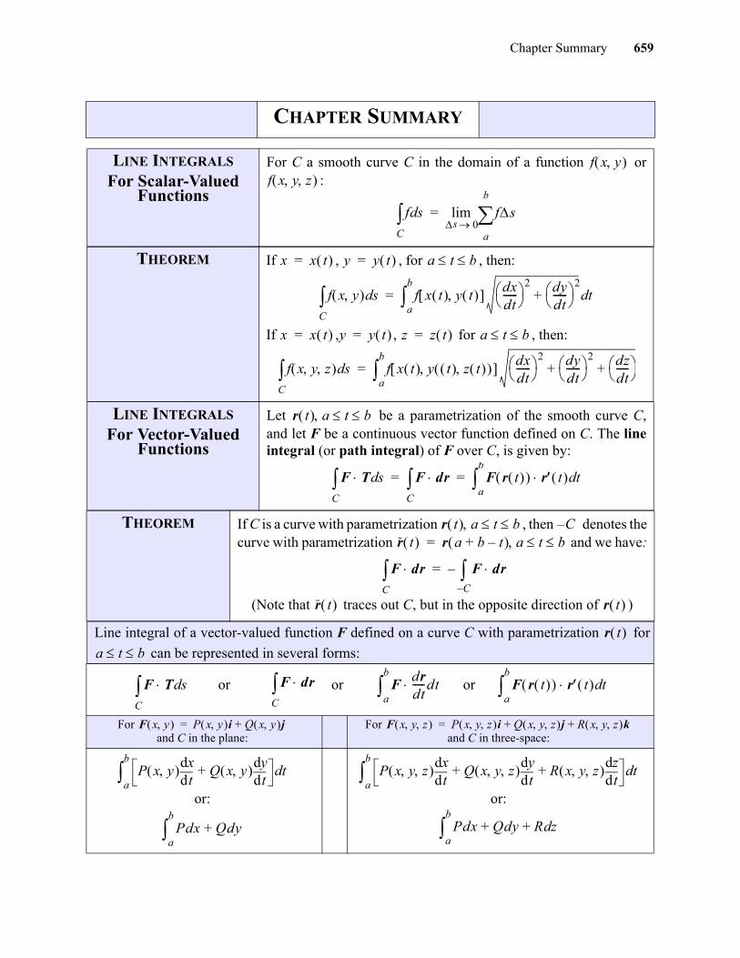
Chapter Summary 659
gio
CHAPTER SUMMARY
LINE INTEGRALS
For Scalar-ValuedFunctions
For C a smooth curve C in the domain of a function or:
THEOREM If , , for , then:
If , , for , then:
LINE INTEGRALS
For Vector-Valued Functions
Let be a parametrization of the smooth curve C,and let F be a continuous vector function defined on C. The lineintegral (or path integral) of F over C, is given by:
THEOREM If C is a curve with parametrization , then denotes thecurve with parametrization and we have:
(Note that traces out C, but in the opposite direction of )
Line integral of a vector-valued function F defined on a curve C with parametrization for
can be represented in several forms:
or or or
For and C in the plane:
For and C in three-space:
or: or:
f x y f x y z
f sdC f
a
b
s 0lim s=
x x t = y y t = a t b
f x y sdC f x t y t dx
dt------ 2 dy
dt------ 2
+ tda
b
=
x x t = y y t = z z t = a t b
f x y z sdC f x t y t z t dx
dt------ 2 dy
dt------ 2 dz
dt----- + +
a
b
=
r t a t b
F T sdC F dr
C F r t r t td
a
b
= =
r t a t b C–r t r a b t–+ a t b =
F drC F dr
C––=
r t r t
r t a t b
F T sdC F dr
C F
drdt-----dt
a
b
F r t r t tda
b
F x y P x y i Q x y j+= F x y z P x y z i Q x y z j R x y z k+ +=
P x y td
dxQ x y
tddy
+ tda
b
Pdx Qdy+a
b
P x y z td
dxQ x y z
tddy
R x y z td
dz+ + td
a
b
Pdx Qdy R+ + zda
b
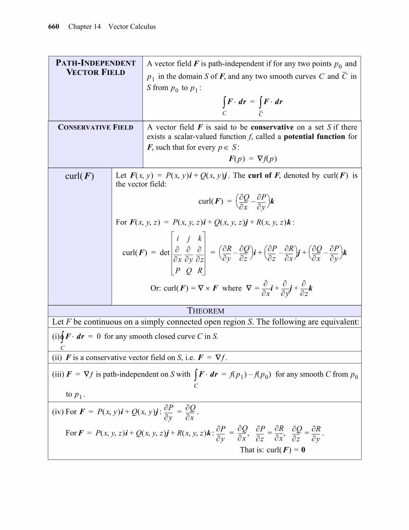
660 Chapter 14 Vector Calculus
PATH-INDEPENDENT VECTOR FIELD
A vector field F is path-independent if for any two points and
in the domain S of F, and any two smooth curves and in
S from to :
CONSERVATIVE FIELD A vector field F is said to be conservative on a set S if thereexists a scalar-valued function f, called a potential function forF, such that for every :
Let . The curl of F, denoted by isthe vector field:
For :
THEOREM
Let F be continuous on a simply connected open region S. The following are equivalent:
(i) for any smooth closed curve C in S.
(ii) F is a conservative vector field on S, i.e. .
(iii) is path-independent on S with for any smooth C from
to .
(iv) For : .
For : .
p0
p1 C C
p0 p1
F drC F dr
C
=
p SF p f p =
curl F F x y P x y i Q x y j+= curl F
curl F x
Qy
P– k=
F x y z P x y z i Q x y z j R x y z k+ +=
curl F det
i j k
x
y
z
P Q R
yR
zQ–
iz
Px
R– j
xQ
yP–
k+ += =
Or: curl F F where x
iy
jz
k+ +==
F drC 0=
F f=
F f= F drC f p1 f p0 –= p0
p1
F P x y i Q x y j+=y
Px
Q=
F P x y z i Q x y z j R x y z k+ +=y
Px
Q
zP
xR
z
Qy
R===
That is: curl F 0=
gio
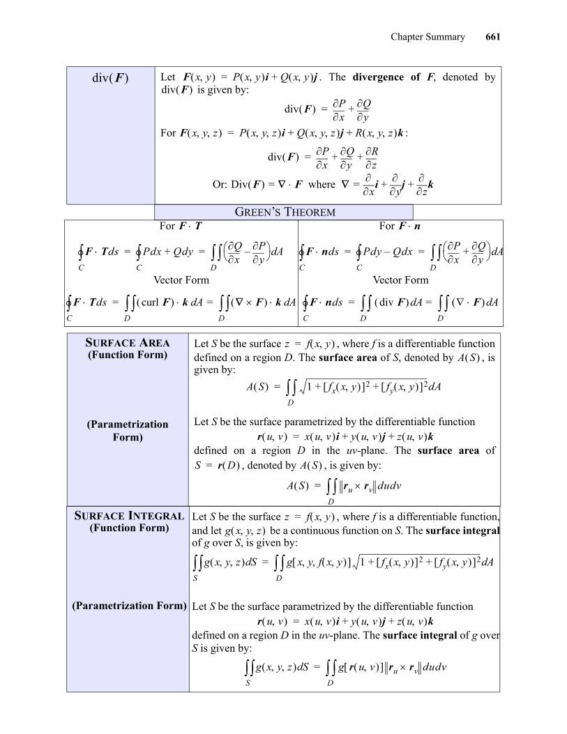
Chapter Summary 661
gio
Let . The divergence of F, denoted by is given by:
For :
GREEN’S THEOREMFor For
Vector Form Vector Form
SURFACE AREA(Function Form)
(Parametrization Form)
Let S be the surface , where f is a differentiable functiondefined on a region D. The surface area of S, denoted by , isgiven by:
Let S be the surface parametrized by the differentiable function
defined on a region D in the uv-plane. The surface area of, denoted by , is given by:
SURFACE INTEGRAL(Function Form)
(Parametrization Form)
Let S be the surface , where f is a differentiable function,and let be a continuous function on S. The surface integralof g over S, is given by:
Let S be the surface parametrized by the differentiable function
defined on a region D in the uv-plane. The surface integral of g overS is given by:
div F F x y P x y i Q x y j+=div F
div F x
Py
Q+=
F x y z P x y z i Q x y z j R x y z k+ +=
div F x
Py
Qz
R+ +=
Or: Div F F where x
iy
jz
k+ +==
F T F n
F TdsC Pdx Qdy+
C x
Qy
P– Ad
D= = F nds
C Pdy Qdx–
C x
Py
Q+ Ad
D= =
F TdsC curl F k Ad
D F k Ad
D= = F nds
C div F Ad
D F Ad
D= =
z f x y =A S
A S 1 fx x y 2 fy x y 2+ +D dA=
r u v x u v i y u v j z u v k+ +=
S r D = A S
A S ru rvD dudv=
z f x y =g x y z
g x y z SdS g x y f x y 1 fx x y 2 fy x y 2+ + Ad
D=
r u v x u v i y u v j z u v k+ +=
g x y z SdS g r u v ru rv
D dudv=
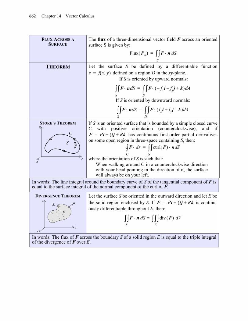
662 Chapter 14 Vector Calculus
FLUX ACROSS A SURFACE
The flux of a three-dimensional vector field F across an orientedsurface S is given by:
THEOREM Let the surface S be defined by a differentiable function defined on a region D in the xy-plane.
If S is oriented by upward normals:
If S is oriented by downward normals:
STOKE’S THEOREM If S is an oriented surface that is bounded by a simple closed curveC with positive orientation (counterclockwise), and if
has continuous first-order partial derivativeson some open region in three-space containing S, then:
where the orientation of S is such that:When walking around C in a counterclockwise directionwith your head pointing in the direction of n, the surfacewill always be on your left.
In words: The line integral around the boundary curve of S of the tangential component of F isequal to the surface integral of the normal component of the curl of F.
DIVERGENCE THEOREM Let the surface S be oriented in the outward direction and let E bethe solid region enclosed by S. If is continu-ously differentiable throughout E, then:
In words: The flux of F across the boundary S of a solid region E is equal to the triple integralof the divergence of F over E.
Flux FS F n SdS=
z f x y =
F n SdS F fxi– fyj– k+ Ad
D=
F n SdS F fxi fyj k–+ Ad
D=
S
C
yx
z
n
F Pi Qj Rk+ +=
F drC curl F n Sd
S=
S n
y
z
x
E
F Pi Qj Rk+ +=
F n SdS div F Vd
E=
gio
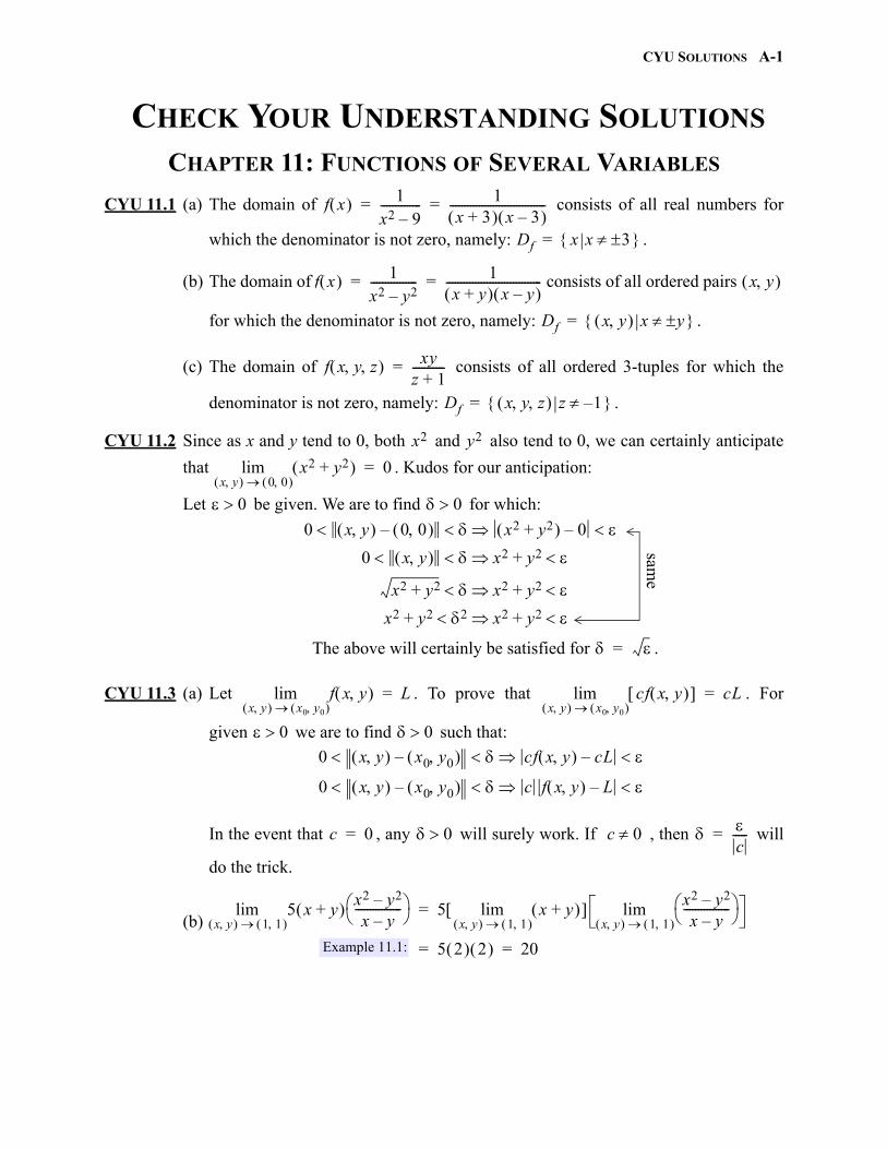
CYU SOLUTIONS A-1
CHECK YOUR UNDERSTANDING SOLUTIONS
CHAPTER 11: FUNCTIONS OF SEVERAL VARIABLES
CYU 11.1 (a) The domain of consists of all real numbers for
which the denominator is not zero, namely: .
(b) The domain of consists of all ordered pairs
for which the denominator is not zero, namely: .
(c) The domain of consists of all ordered 3-tuples for which the
denominator is not zero, namely: .
CYU 11.2 Since as x and y tend to 0, both and also tend to 0, we can certainly anticipate
that . Kudos for our anticipation:
Let be given. We are to find for which:
The above will certainly be satisfied for .
CYU 11.3 (a) Let . To prove that . For
given we are to find such that:
In the event that , any will surely work. If , then will
do the trick.
(b)
f x 1x2 9–-------------- 1
x 3+ x 3– ---------------------------------= =
Df x x 3 =
f x 1x2 y2–---------------- 1
x y+ x y– ---------------------------------= = x y
Df x y x y =
f x y z xyz 1+-----------=
Df x y z z 1– =
x2 y2
x2 y2+ x y 0 0
lim 0=
0 00 x y 0 0 – x2 y2+ 0–
0 x y x2 y2 +
x2 y2+ x2 y2 +
x2 y2+ 2 x2 y2 +
same
=
f x y x y x0 y0
lim L= cf x y x y x0 y0
lim cL=
0 00 x y x0 y0 – cf x y cL–
0 x y x0 y0 – c f x y L–
c 0= 0 c 0 c-----=
5 x y+ x2 y2–x y–
----------------
x y 1 1 lim 5 x y+
x y 1 1 lim x2 y2–
x y–----------------
x y 1 1 lim=
5 2 2 20= =Example 11.1:
gio
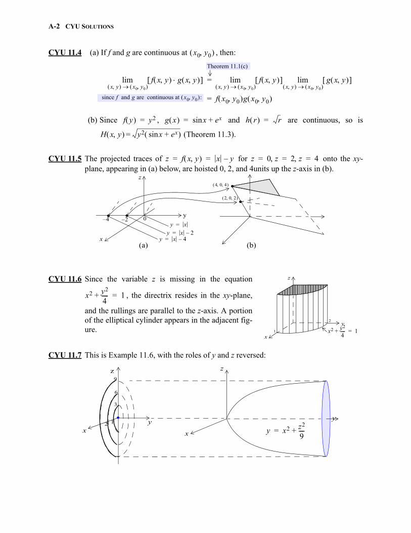
A-2 CYU SOLUTIONS
CYU 11.4 (a) If f and g are continuous at , then:
(b) Since , and are continuous, so is
(Theorem 11.3).
CYU 11.5 The projected traces of for onto the xy-plane, appearing in (a) below, are hoisted 0, 2, and 4units up the z-axis in (b).
CYU 11.6 Since the variable z is missing in the equation
, the directrix resides in the xy-plane,
and the rullings are parallel to the z-axis. A portionof the elliptical cylinder appears in the adjacent fig-ure.
CYU 11.7 This is Example 11.6, with the roles of y and z reversed:
x0 y0
f x y g x y x y x0 y0
lim f x y g x y x y x0 y0
limx y x0 y0
lim=
f x0 y0 g x0 y0 =
Theorem 11.1(c)
since f and g are continuous at x0 y0 :
f y y2= g x x ex+sin= h r r=
H x y y2 x ex+sin =
z f x y x y–= = z 0 z 2 z 4= = =
.. .
.
y x=y x 2–=
y x 4–=
4 0 4
2 0 2
(a) (b)
4– 2–y
x
z
0
x
y
z
x2 y2
4-----+ 1=1
2
x2 y2
4-----+ 1=
x
y
z
.x
y
z
y x2 z2
9----+=
12
3
6
9
gio
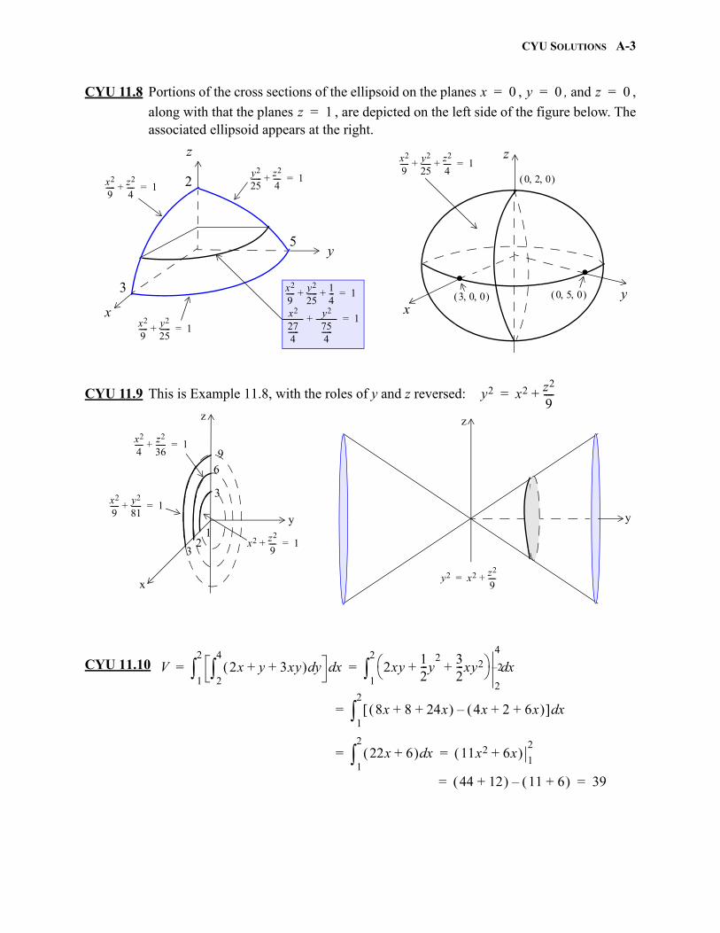
CYU SOLUTIONS A-3
gio
CYU 11.8 Portions of the cross sections of the ellipsoid on the planes , , and ,
along with that the planes , are depicted on the left side of the figure below. Theassociated ellipsoid appears at the right.
CYU 11.9 This is Example 11.8, with the roles of y and z reversed:
CYU 11.10
x 0= y 0= z 0=
z 1=
3
2
5
x2
9----- y2
25------ 1
4---+ + 1=
x2 274------
------------ y2 754------
------------+ 1=x
y
z
x2
9----- z2
4----+ 1=
y2
25------ z2
4----+ 1=
x2
9----- y2
25------+ 1=
x2
9----- y2
25------ z2
4----+ + 1=
x
z
y
..3 0 0 0 5 0
0 2 0
y2 x2 z2
9----+=
y
z
x
y
z
y2 x2 z2
9----+=
3 2
1
96
3
x2 z2
9----+ 1=
x2
4----- z2
36------+ 1=
x2
9----- y2
81------+ 1=
V 2x y 3xy+ + yd2
4
xd1
2
2xy12---y
2 32---xy2+ +
2
4
xd1
2
= =
8x 8 24x+ + 4x 2 6x+ + – xd1
2
=
22x 6+ xd1
2
11x2 6x+ 1
2= =
44 12+ 11 6+ – 39= =
2–
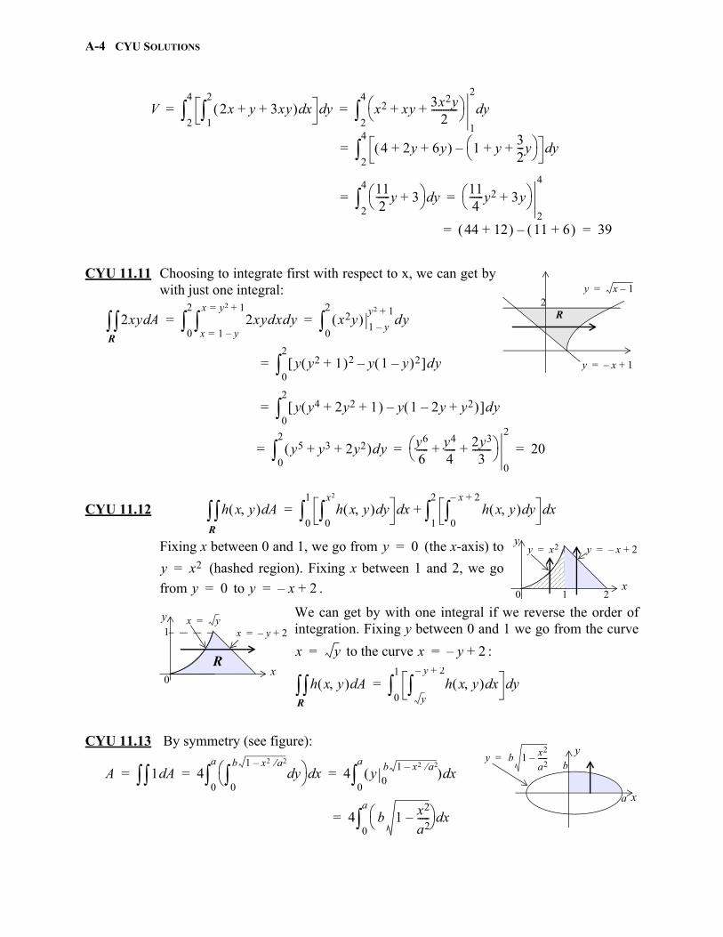
A-4 CYU SOLUTIONS
gio
CYU 11.11 Choosing to integrate first with respect to x, we can get bywith just one integral:
CYU 11.12
Fixing x between 0 and 1, we go from (the x-axis) to
(hashed region). Fixing x between 1 and 2, we go
from to .
We can get by with one integral if we reverse the order ofintegration. Fixing y between 0 and 1 we go from the curve
to the curve :
CYU 11.13 By symmetry (see figure):
V 2x y 3xy+ + xd1
2
yd2
4
x2 xy 3x2y2
-----------+ +
1
2
yd2
4
= =
4 2y 6y+ + 1 y32---y+ +
– yd2
4
=
112------y 3+ yd
2
4
114------y2 3y+
2
4
= =
44 12+ 11 6+ – 39= =
2y x 1–=
y x– 1+=
R2xy Ad 2xyx 1 y–=
x y2 1+=
0
2
dxdy x2y 1 y–
y2 1+
0
2
dy= =
y y2 1+ 2 y 1 y– 2– 0
2
dy=
y y4 2y2 1+ + y 1 2y– y2+ – 0
2
dy=
R
y5 y3 2y2+ + 0
2
dy y6
6----- y4
4----- 2y3
3--------+ +
0
2
20= = =
h x y Ad h x y yd0
x2
xd0
1
h x y yd0
x– 2+
xd1
2
+=R
y x2= y x– 2+=
x
y
0 1 2
y 0=
y x2=
y 0= y x– 2+=
x y=x y– 2+=
x
y
0
R
1
x y= x y– 2+=
h x y Ad h x y xdy
y– 2+
yd0
1
=R
y b 1 x2
a2-----–=
x
yb
a
A 1 Ad 4 yd0
b 1 x2 a2–
xd
0
a
4 y0b 1 x2 a2– xd
0
a
= = =
4 b 1 x2
a2-----–
xd0
a
=
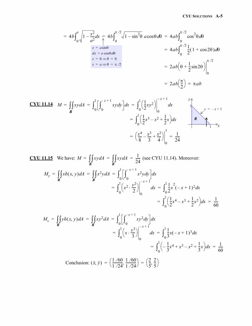
CYU SOLUTIONS A-5
CYU 11.14
CYU 11.15 We have: (see CYU 11.14). Moreover:
Conclusion:
4b 1 x2
a2-----– xd
0
a
4b 1 sin2– a cos d
0
2
4ab cos2 d
0
2
= = =
x a sin=
dx a dcos=
x 0 0= =
x a 2= =
4ab12--- 1 2cos+ d
0
2
=
2ab 12--- 2sin+
0
2
=
2ab2--- ab= =
x
y
1
1
y x– 1+=
R
M xy Ad xy yd0
x– 1+
xd0
1
12---xy2
0
x– 1+
xd0
1
= = =
12---x3 x2–
12---x+
xd0
1
=
x4
8----- x3
3-----– x2
4-----+
0
1124------= =
R
M xy Ad xy Ad 124------= = =
R R
My x x y Ad x2y Ad x2y yd0
x– 1+
xd0
1
= = =
x2 y2
2-----
0
x– 1+
xd0
1
12---x
2x– 1+ 2 xd
0
1
= =
12---x4 x3–
12---x2+
xd0
1
160------= =
R R
Mx y x y Ad xy2 Ad xy2 yd0
x– 1+
xd0
1
= = =
xy3
3-----
0
x– 1+
xd0
1
13---x x– 1+ 3 xd
0
1
= =
13---x4– x3 x2–
13---x+ +
xd0
1
160------= =
R R
x y 1 601 24------------- 1 60
1 24-------------
25--- 2
5---
= =
gio
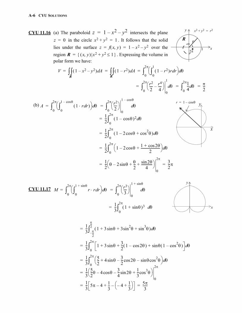
A-6 CYU SOLUTIONS
gio
CYU 11.16 (a) The paraboloid intersects the plane
in the circle . It follows that the solid
lies under the surface over the
region . Expressing the volume inpolar form we have:
(b)
CYU 11.17
x
y
R
2
r
x2 y2+ r2=
1
z 1 x2– y2–=z 0= x2 y2+ 1=
z f x y 1 x2– y2–= =
R x y x2 y2 1+ =
V 1 x2– y2– Ad 1 r2– Ad 1 r2– r rd0
1
d
0
2
= = =R R
r2
2---- r4
4----–
0
1
d0
2
14--- d
0
2
2---= = =
x
yr 1 cos–=A 1 r rd
0
1 cos–
d
0
2
r2
2----
0
1 cos–
d0
2
= =
12--- 1 cos– 2 d
0
2
=
12--- 1 2 cos– cos
2+ d0
2
=
12--- 1 2 cos– 1 2cos+
2------------------------+
d0
2
=
12--- 2 sin–
2--- 2sin
4--------------+ +
0
232---= =
x
y
M r r rd0
1 sin+
d
0
2
r3
3----
0
1 sin+
d0
2
= =
13--- 1 sin+ 3 d
0
2
=
13--- 1 3 3sin
2 sin3+ +sin+ d
2---–
2---
=
13--- 1 3 sin
32--- 1 2cos– 1 cos
2– sin+ + + d0
2
=
13--- 5
2--- 4 3
2--- 2 cos
2sin–cos–sin+ d
0
2
=
13--- 5
2--- 4 3
4--- 2sin–cos–
13---cos
3+
0
2
=
13--- 5 4– 1
3--- 4– 1
3---+
–+ 53
------= =
CYU SOLUTIONS A-7
CYU 11.18
Conclusion:
CYU 11.19 Just as the area of a two-dimensional region R equals the volume of the solid of base
R and height 1, which is to say: ; so does the volume of a three-dimensional
region W equal . That being the case, we simply evaluate the integral of
Example 11.12 with “1” replacing the “x”:
M x y Ad sin r rd0
cos
d
0
2---
= =R
r2
2---- sin
0
cos
d0
2---
12--- cos
2 dsin0
2---
12--- 1
3---cos
3–
0
2---
16---= = = =
My x x y Ad r sin r cos rd0
cos
d
0
2---
= =
r3
3---- sincos
0
cos
d0
2---
13--- cos
3 dsincos0
2---
= =
13--- cos
4 sin d0
2---
13--- 1
5---cos
5–
0
2---
= =
R
Mx y x y Ad r sin r sin rd0
cos
d
0
2---
= =
r3
3----sin
2
0
cos
d0
2---
13--- cos 3sin
2 d0
2---
= =
13--- cos 1 sin
2– sin2 d
0
2---
=
13--- sin
4– cos sin2 cos+ d
0
2---
=
13--- 1
5---sin
5–13---sin
3+
0
2---
245------= =
x y My
M-------
Mx
M-------
1 151 6------------- 2 45
1 6-------------
615------ 12
45------
25--- 4
15------
= = = =
1 yd xdR
1 zd yd xdW
gio
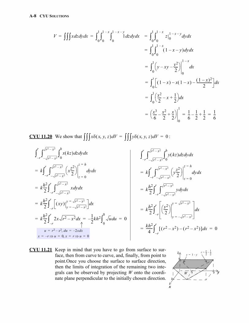
A-8 CYU SOLUTIONS
CYU 11.20 We show that :
CYU 11.21 Keep in mind that you have to go from surface to sur-face, then from curve to curve, and, finally, from point topoint.Once you choose the surface to surface direction,then the limits of integration of the remaining two inte-grals can be observed by projecting W onto the coordi-nate plane perpendicular to the initially chosen direction.
V x zd yd xd 1 zd yd xd0
1 x– y–
0
1 x–
0
1
z01 x– y–
yd xd0
1 x–
0
1
= = =
1 x– y– yd xd0
1 x–
0
1
=
y xy– y2
2-----–
0
1 x–
xd0
1
=
1 x– x 1 x– – 1 x– 2
2-------------------– xd
0
1
=
x2
2----- x– 1
2---+
xd0
1
=
x3
6----- x2
2-----– x
2---+
0
116--- 1
2---– 1
2---+ 1
6---= = =
x x y z Vd y x y z Vd 0= =
x kz zd yd xd0
h
r2 x2––
r2 x2–
r–
r
k xz2
2----
z 0=
z h=
yd xdr2 x2––
r2 x2–
r–
r
=
kh2
2----- x yd xd
r2 x2––
r2 x2–
r–
r
=
kh2
2----- xy
y r2 x2––=
y r2 x2–=xd
r–
r
=
kh2
2----- 2x r2 x2– xd
r–
r
12---k– h2 u ud
0
0
0= = =
u r2 x2 du– 2xdx–= =
x r u– 0 x r u 0= = = =
y kz zd yd xd0
h
r2 x2––
r2 x2–
r–
r
k yz2
2----
z 0=
z h=
yd xdr2 x2––
r2 x2–
r–
r
=
kh2
2----- y yd xd
r2 x2––
r2 x2–
r–
r
=
kh2
2----- y2
2-----
y r2 x2––=
y r2 x2–=
xdr–
r
=
kh2
4-------- r2 x2– r2 x2– – xd
r–
r
0= =
2
3
1
1 y
x
z
W
z 1 y–=z y
2---= 1
2---–
gio
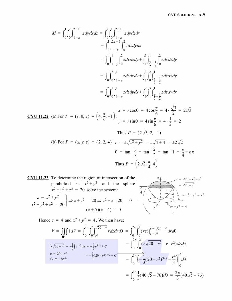
CYU SOLUTIONS A-9
gio
CYU 11.22 (a) For :
Thus .
(b) For :
Thus
CYU 11.23 To determine the region of intersection of theparaboloid and the sphere
solve the system:
Hence and . We then have:
M z yd xd zd1 z–
2z 1+
0
2
0
1
z yd zd xd1 z–
2z 1+
0
1
0
2
= =
z xd yd zd0
2
1 z–
2z 1+
0
1
=
z xd zd yd0
2
1 y–
1
0
1
z xd zd yd0
2
y2--- 1
2---–
1
1
3
+=
z zd xd yd1 y–
1
0
2
0
1
z zd xd ydy2--- 1
2---–
1
0
2
1
3
+=
z zd yd xd1 y–
1
0
1
0
2
z zd yd xdy2--- 1
2---–
1
1
3
0
2
+=
P r z 46--- 1–
= =x r cos 4
6---cos 4
32
------- 2 3= = = =
y r sin 4 6---sin 4
12--- 2= = = =
P 2 3 2 1– =
P x y z 2 2 4 = = r x2 y2+ 4 4+ 2 2= = =
tan1– yx-- tan
1– 22--- tan
1–1
4--- n+= = = =
P 2 24--- 4
=
z x2 y2+ r2= =
. z 20 x2– y2–=
20 r2–=T
x2 y2+ 4=
y
z
x
.
.
2
4
z x2 y2+=x2 y2 z2+ + 20=
z x2 y2+=
x2 y2 z2+ + 20=
z z2+ 20 z2 z 20–+ 0= =
z 5+ z 4– 0=
z 4= x2 y2+ 4=
V 1 Vd r zd rd dr2
20 r2–
0
2
0
2
rz z r2=z 20 r2–=
rd d0
2
0
2
= = =
r 20 r2– r r2– rd d0
2
0
2
=
13--- 20 r2– 3 2/– r4
4----–
0
2
d0
2
=
13--- 40 5 76– d
0
2
23
------ 40 5 76– = =
W
r 20 r2– 12---– u1 2/ ud
13---u3 2/– C+= =
u 20 r2–=
du 2rdr–=
13--- 20 r2– 3 2/– C+=
A-10 CYU SOLUTIONS
Also, for :
By symmetry, the x and y coordinates of the center of mass are 0. As for :
CYU 11.24 (a) For :
From we have: ; as , .
From we have: ; as , .
Thus: .
(b) For (see Figure 13.9):
Thus:
As for the cylindrical coordinates, , we have ; and, from above: .
As for r: . Thus: .
x y z k= M x y z Vd k Vd2k
3--------- 40 5 76– = = =
W W
z
z1M----- z x y z Vd
1M----- zkr zd rd d
r2
20 r2–
0
2
0
2
= =
kM----- z2
2----
r2
20 r2–
rd d0
2
0
2
=
k2M-------- 20r r3– r5– rd d
0
2
0
2
k
2M-------- 10r2 r4
4----– r6
6----–
0
2
d0
2
= =
k2M-------- 76
3------
0
2
d0
2
76k3M
------------= =
38
40 5 76–------------------------- 1.4=M
23
------k 40 5 76– :=
W
P x y z 0 2 3 2– = 0 12 4+ + 4= =
z cos= 2– 4 coscos 12---–= = 0 2
3------=
x cossin= 0 423
------ coscossin 0= = y 0 2---=
P 423
------ 2---
=
P 223
------ 56
------ =
x cossin 223
------ 56
------cossin 23
2------- 3
2-------–
32---–= = = =
y sinsin 223
------ 56
------sinsin 23
2------- 1
2--- 3
2-------= = = =
z cos 2 23
------cos 2 12---–
1–= = = =
P x y z 32---–
32
------- 1– =
P r z 56
------= z 1–=
r x2 y2+ 32---–
2 32
-------
2
+ 3= = = P r z 356
------ 1– =
gio
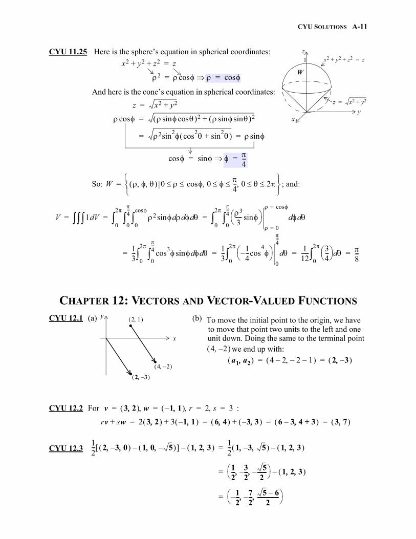
CYU SOLUTIONS A-11
gio
CYU 11.25 Here is the sphere’s equation in spherical coordinates:
And here is the cone’s equation in spherical coordinates:
So: ; and:
CHAPTER 12: VECTORS AND VECTOR-VALUED FUNCTIONS
CYU 12.1 (a) (b)
CYU 12.2 For :
CYU 12.3
1 x2 y2 z2+ + z=
z x2 y2+=
y
z
x
Wx2 y2 z2+ + z=
2 cos cos= =
z x2 y2+=
cos cossin 2 sinsin 2+=
2sin2 cos
2 sin2+ sin= =
cos sin 4---= =
W 0 cos 0 4--- 0 2
=
V 1 Vd 2 sin d d d0
cos
0
4---
0
2
3
3----- sin
0=
cos=
d d0
4---
0
2
= = =
13--- cos
3 dsin d0
4---
0
2
13--- 1
4---cos–
4
0
4---
d0
2
112------ 3
4--- d
0
2
8---= = = =
y
x
.
.
2 1
4 2–
2 3– .
To move the initial point to the origin, we have to move that point two units to the left and one unit down. Doing the same to the terminal point
we end up with: 4 2– a1 a2 4 2– 2– 1– 2 3– = =
v 3 2 w 1 1– r 2 s 3= = = =
rv sw+ 2 3 2 3 1 1– + 6 4 3– 3 + 6 3– 4 3+ 3 7 = = = =
12--- 2 3– 0 1 0 5– – 1 2 3 –
12--- 1 3– 5 1 2 3 –=
12--- 3
2---– 5
2-------–
1 2 3 –=
12---– 7
2---– 5 6–
2----------------
=
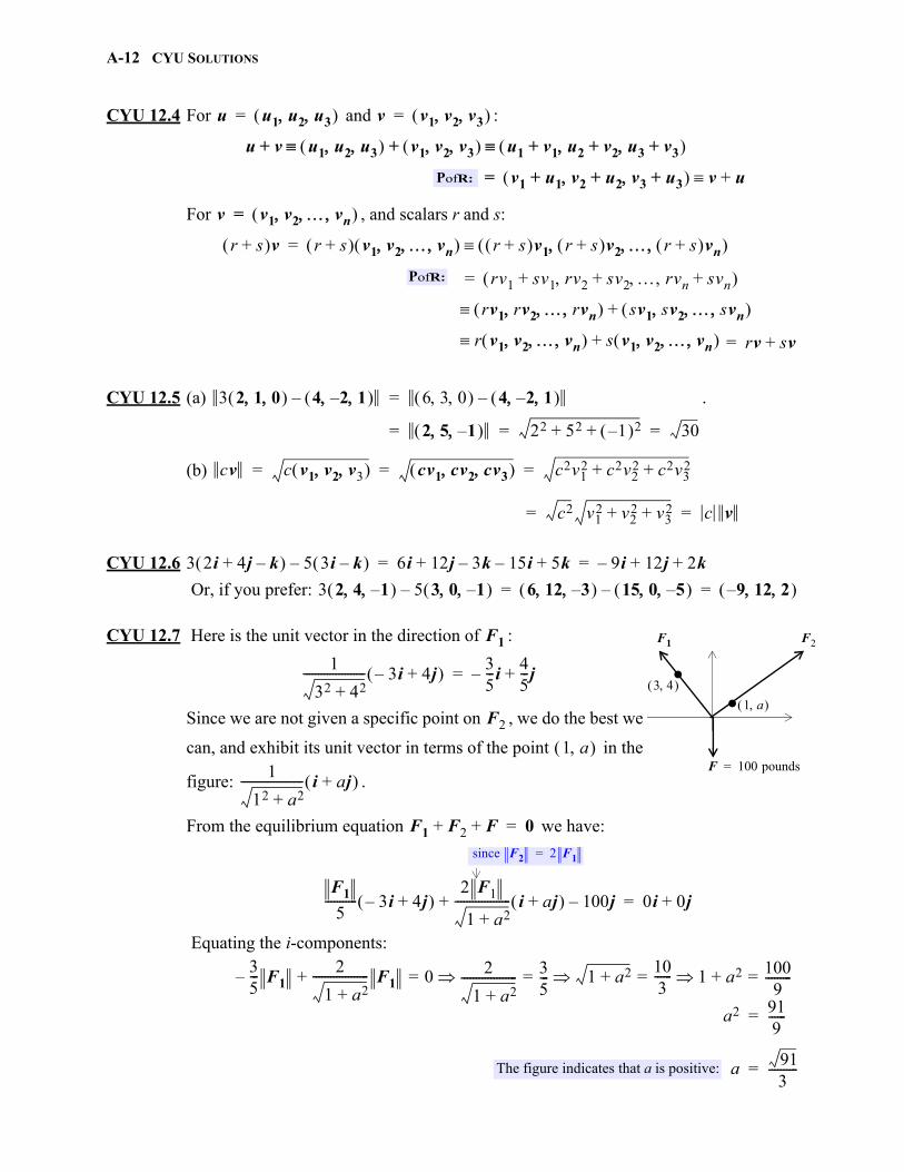
A-12 CYU SOLUTIONS
gio
CYU 12.4 For and :
For , and scalars r and s:
CYU 12.5 (a) .
(b)
CYU 12.6
Or, if you prefer:
CYU 12.7 Here is the unit vector in the direction of :
Since we are not given a specific point on , we do the best we
can, and exhibit its unit vector in terms of the point in the
figure: .
From the equilibrium equation we have:
Equating the i-components:
u u1 u2 u3 = v v1 v2 v3 =
u v+ u1 u2 u3 v1 v2 v3 u1 v1+ u2 v2+ u3 v3+ +
v1 u1+ v2 u2+ v3 u3+ v u+=PofR:
v v1 v2 vn =
r s+ v r s+ v1 v2 vn r s+ v1 r s+ v2 r s+ vn =
rv1 sv1 rv2 sv2++ rvn svn+ =
rv1 rv2 rvn sv1 sv2 svn +
r v1 v2 vn s v1 v2 vn + rv sv+=
PofR:
3 2 1 0 4 2– 1 – 6 3 0 4 2– 1 –=
2 5 1– 22 52 1– 2+ + 30= = =
cv c v1 v2 v3 cv1 cv2 cv3 c2v12 c2v2
2 c2v32+ += = =
c2 v12 v2
2 v32+ + c v= =
3 2i 4j k–+ 5 3i k– – 6i 12j 3k– 15i– 5k+ + 9i– 12j 2k+ += =
3 2 4 1– 5 3 0 1– – 6 12 3– 15 0 5– – 9 12 2 – = =
.F1 F2
F 100 pounds=
3 4 .1 a
F1
1
32 42+--------------------- 3i– 4j+ 3
5---i–
45---j+=
F2
1 a 1
12 a2+--------------------- i aj+
F1 F2 F+ + 0=
since F2 2 F1=
F1
5----------- 3i– 4j+
2 F1
1 a2+------------------- i aj+ 100j–+ 0i 0j+=
35--- F1–
2
1 a2+------------------- F1+ 0 2
1 a2+------------------- 3
5---== 1 a2+
103------ 1 a2+ 100
9---------==
a2 919------=
a 913
----------=The figure indicates that a is positive:
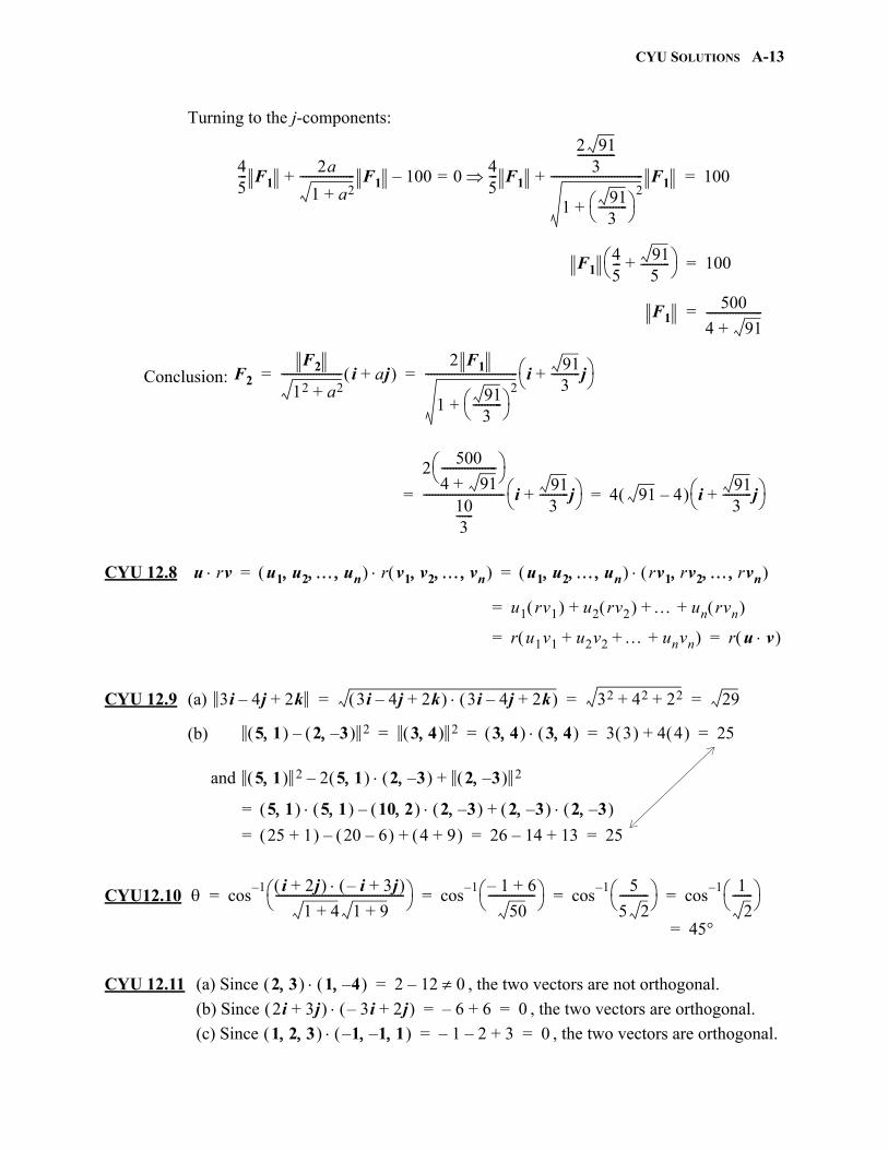
CYU SOLUTIONS A-13
gio
Turning to the j-components:
Conclusion:
CYU 12.8
CYU 12.9 (a)
(b)
CYU12.10
CYU 12.11 (a) Since , the two vectors are not orthogonal.
(b) Since , the two vectors are orthogonal.
(c) Since , the two vectors are orthogonal.
45--- F1
2a
1 a2+------------------- F1 100–+ 0=
45--- F1
2 913
-------------
1913
----------
2
+
-------------------------------- F1+ 100=
F145--- 91
5----------+
100=
F1500
4 91+-------------------=
F2
F2
12 a2+--------------------- i aj+
2 F1
1913
----------
2
+
-------------------------------- i913
----------j+ = =
2500
4 91+-------------------
103------
---------------------------- i913
----------j+ 4 91 4– i
913
----------j+ = =
u rv u1 u2 un r v1 v2 vn u1 u2 un rv1 rv2 rvn = =
u1 rv1 u2 rv2 un rvn + + +=
r u1v1 u2v2 unvn+ + + r u v = =
3i 4j– 2k+ 3i 4j– 2k+ 3i 4j– 2k+ 32 42 22+ + 29= = =
5 1 2 3– – 2 3 4 2 3 4 3 4 3 3 4 4 + 25= = = =
5 1 5 1 10 2 2 3– 2 3– 2 3– +–=
25 1+ 20 6– – 4 9+ + 26 14– 13+ 25= = =
and 5 1 2 2 5 1 2 3– 2 3– 2+–
cos1– i 2j+ i– 3j+
1 4+ 1 9+-------------------------------------------- cos
1– 1– 6+
50---------------- cos
1– 5
5 2---------- cos
1– 1
2------- = = = =
45=
2 3 1 4– 2 12 0–=
2i 3j+ 3i– 2j+ 6– 6+ 0= =
1 2 3 1– 1– 1 1– 2– 3+ 0= =
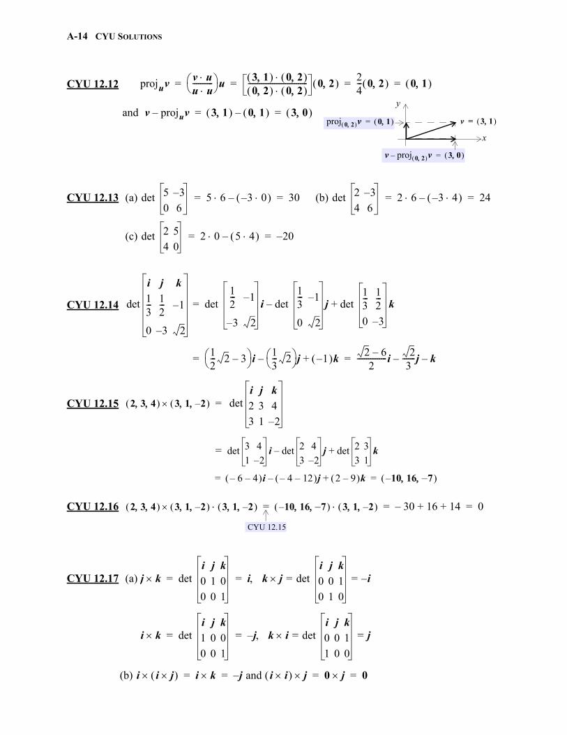
A-14 CYU SOLUTIONS
gio
CYU 12.12
CYU 12.13 (a) (b)
(c)
CYU 12.14
CYU 12.15
CYU 12.16
CYU 12.17 (a)
(b)
projuvv uu u----------- u
3 1 0 2 0 2 0 2
-------------------------------- 0 2 24--- 0 2 0 1 = = = =
and v projuv– 3 1 0 1 – 3 0 = =
x
y
v 3 1 =proj 0 2 v 0 1 =
v proj 0 2 v– 3 0 =
det 5 3–
0 65 6 3 0– – 30= = det 2 3–
4 62 6 3 4– – 24= =
det 2 5
4 02 0 5 4 – 20–= =
det
i j k
13--- 1
2--- 1–
0 3– 2
det 12--- 1–
3– 2
i det 13--- 1–
0 2
j– det 13--- 1
2---
0 3–
k+=
12--- 2 3– i
13--- 2 j– 1– k+
2 6–2
----------------i2
3-------j– k–= =
2 3 4 3 1 2– deti j k
2 3 4
3 1 2–
=
det 3 4
1 2–i det 2 4
3 2–j det 2 3
3 1k+–=
6– 4– i 4– 12– j– 2 9– k+ 10 16 7– – = =
2 3 4 3 1 2– 3 1 2– 10 16 7– – 3 1 2– 30– 16 14+ + 0= = =
CYU 12.15
j k det i j k
0 1 0
0 0 1
i k j det i j k
0 0 1
0 1 0
i–= == =
i k det i j k
1 0 0
0 0 1
j– k i det i j k
0 0 1
1 0 0
j= == =
i i j i k j and i i j– 0 j 0= = = =
CYU SOLUTIONS A-15
gio
CYU 12.18 The area of triangle OAB is one half its basetimes it height:
Flipping that triangle about and line segmentjoining A to B yields the depicted parallelogram. It follows that the parallelogramhas area .
CYU 12.19 (a) The given slope of (over 3, down 2) gives us the direction vector:
, and the given point gives us the translation vector: .
Vector equation: . Parametric equations:
(b) A direction vector for any vertical line is j. Taking as our trans-
lation vector we have: , and: .
CYU 12.20 Taking as the direction vector, and
, as the translation vector we arrive at the vector equation:
Which brings us to the parametric equations:
CYU 12.21 (a) A direction vector for the line L passing through and :
The vector from the point on L to :
Applying Theorem 12.4:
Hence: .
(b) . .
Hence: .
Note: If you chose as the direction vector and as the translation vector you will end up with the vector equation:
, which certainly looks differ-ent than (*) above. But appearance can be deceiving, for if you replace t in (**)with you will arrive at (*), and as t takes on all real numbers, so does .
u
vO
A
B
h
12--- v h
12--- v u sin
12--- u v= =
Theorem 12.6
u v
23---–
u 3 2– = 5 1 u 5 1 =
w 5 1 t 3 2– +=
x 5 3t y+ 1 2t–= =
3 7 3i 7j+=
w 3i 7j+ tj+= x 3= y 7 t+=
v 0 1 2– 1 2 9 – 1 1– 11– – = =
u 1 2 9 =
w 1 2 9 t 1 1– 11– – + 1 t– 2 t– 9 11t– = = (*)
x 1 t y– 2 t z– 9 11t–= = =
v 1 2 9 0 1 2– –= 0 1 2–
w 0 1 2– t 1 1 11 + t 1 t+ 2– 11t+ = = (**)
1 t– 1 t–
1 2– 2 4 u 2 4 1 2– – 1 6 = =
1 2– P 2 5 =
v 2 5 1 2– – 1 7 = =
projuvu vu u----------- u
1 6 1 7 1 6 1 6
-------------------------------- 1 6 43
37------ 1 6 = = =
v projuv– 1 7 4337------ 258
37---------
– 637------– 1
37------
62 12+37
--------------------- 1
37----------= = = =
u 1 2 2 1 1 2 0 1 – 0 0 2 0 = = v 1 0 1 3 1 2 0 1 – 0 2– 1 2 = =
projuvu vu u----------- u
0 0 2 0 0 2– 1 2 0 0 2 0 0 0 2 0
----------------------------------------------------------- 0 0 2 0 1
2--- 0 0 2 0 0 0 1 0 = = = =
v projuv– 0 2– 1 2 0 0 1 0 – 0 2– 0 2 8 2 2= = = =
A-16 CYU SOLUTIONS
CYU 12.22 A normal to the desired plane will have the same direction as that of the line passingthrough the two given points; namely: .
Vector equation: .
Scalar equation:
General equation:
CYU 12.23
and .
Here is a normal to the plane: .
Here is a “nicer” normal: .
Choosing the point on the plane, we arrive at the vector and general equation of the plane: .
CYU 12.24 (a) From the given equation , we see that is a nor-
mal to the plane, and that is a point on the plane.
For , we calculate the length d
of the vector , as that is the distance between P and the plane:
(b) We know that is a normal to the plane .
Let be any point on the plane, and let:
Following the procedure of (a) above we calculate the distance d between and the plane:
n 0 2 1 1 1 0 – 1– 1 1 = =
1– 1 1 x 1– y 3– z 2+ 0=
x 1– – y 3– z 2+ + + 0=
x– y z+ + 0=
AB 2 5 3– 3 2– 2 – 1– 7 5– = = AC 4 1 3– 3 2– 2 – 1 3 5– = =
n deti j k
1– 7 5–
1 3 5–
20i– 10j– 10k– 20 10–– 10– = = =
n110------ 20 10–– 10– – 2 1 1 = =
A 3 2– 2 =2 1 1 x 3– y 2+ z 2– 0 and 2x y z+ + 6= =
x 2y 2z+ + 13= n 1 2 2 =
Q 13 0 0 =
v QP 2 3– 4 13 0 0 – 11– 3 4– = = =
w projnv=
d projnv v nn n
--------------- 11– 3 4– 1 2 2 1 2 2 1 2 2
-------------------------------------------------------- 93--- 3= = = = =
n a b c = ax by cz d+ + + 0=
Q x1 y1 z1 =
v QP x0 y0 z0 x1 y1 z1 – x0 x1– y0 y1– z0 z1– = = =
P x0 y0 z0 =
d v nn n
---------------a x0 x1– b y0 y1– c z0 z1– + +
a2 b2 c2+ +----------------------------------------------------------------------------------------= =
ax0 by0 cz0 ax1– by1– cz1– + + +
a2 b2 c2+ +---------------------------------------------------------------------------------------------
ax0 by0 cz0 d+ + +
a2 b2 c2+ +-------------------------------------------------= =
since ax1 by1 cz1 d+ + + 0=
gio
CYU SOLUTIONS A-17
gio
CYU 12.25 are normal vectors for the planes
and , respectively. Consequently:
The line of intersection is parallel to the vector:
Setting in the two given equations and , and
solving for x and z we find that the line contains the point .
Consequently: is a vector equation of the line of
intersection. [As is ]
CYU 12.26 While represents a
parabola in the plane, in it representsthe parabolic cylinder with vector equa-tion:
.
At time the particle has position
vector , and occupies the point
. At time it is at the point
. As time progresses from 1 to 3,the path remains on the parabolic cylinderas is suggested in the adjacent figure.
CYU 12.27 (a) For :
(i)
(ii)
n1 i 2j k+ + and n2 3i 4j– k–= =
x 2y z+ + 0= 3x 4y– z– 1=
cos1– i 2j k+ + 3i 4j– k–
i 2j k+ + 3i 4j– k– -------------------------------------------------------------- cos
1– 3 8– 1–
6 26--------------------- = =
cos1– 6–
156------------- = 119
n1 n2 det i j k
1 2 1
3 4– 1–
2i 4j 10k–+= =
y 0= x 2y z+ + 0= 3x 4y– z– 1=14--- 0 1
4---–
w 14---i 1
4---k– t 2i 4j 10k–+ +=
w 14---i 1
4---k– t i 2j 5k–+ +=
.
. 3 9 6
1 1 2 path
y x2=x
z
y
y x2=
3
r t ti t2j 2tk+ + t t2 2t = =
t 1=
1 1 2 1 1 2 t 3=
3 9 6
r t et i tt2 1+------------- j tsin k+ +=
r t t 1lim et i t
t2 1+-------------
t 1lim+
t 1lim j tsin k
t 1lim+ ei
12---j 1sin k+ += =
r t et i tt2 1+------------- j tsin k+ +=
et i t2 1+ t 2t –t2 1+ 2
------------------------------------j tcos k+ + et i t– 2 1+t2 1+ 2
---------------------j tcos k+ += =
A-18 CYU SOLUTIONS
(iii)
(b)
CYU 12.28
CYU 12.29 For :
CYU 12.30 Since :
Leading us to the speed function:
Differentiating the above real-valued function we have:
r t td et td i tt2 1+------------- td
j tsin td k+ +=
eti12--- ud
u------
j tkcos–+ eti12--- uln j tcos k– C+ += =
u t2 1+=
du 2tdt=eti
12--- t2 1+ ln j tcos k– C+ +=
r t 1h---
h 0lim r t h+ r t – =
1h--- f t h+ i g t h+ j h t h+ k+ +
h 0lim f t i g t j h t k+ + –=
1h--- f t h+ f t – i 1
h--- g t h+ g t – j 1
h--- h t h+ h t – k+ +
h 0lim=
1h---
h 0lim f t h+ f t – i 1
h---
h 0lim g t h+ g t – j 1
h---
h 0lim h t h+ h t – k+ +=
f t i g t j h t k+ +=
u t v t + u1 t i u2 t j u3 t k+ + v1 t i v2 t j v3 t k+ + + =
u1 t v1 t + i u2 t v2 t + j u3 t v3 t + k++ =
u1 t v1 t + i u2 t v2 t + j u3 t v3 t + k++=
u1 t v1 t + i u2 t v2 t + j u3 t v3 t + k++=
u1 t i u2 t j u3 t k+ + v1 t i v2 t j v3 t k+ + +=
u t v t +=
s t tcos i tsin j tk+ +=
v t r t tsin– i tcos j k v t + + sin2t cos
2t 12+ + 2= = = =
a t v t tcos– i tsin j–= =
a t i 2j k–+=
v t i 2j k–+ td ti 2tj tk– i 12j– k+ + + t 1+ i 2t 12– j t– 1+ k+ += = =initial velocity
v t t 1+ 2 2t 12– 2 t– 1+ 2+ + 6t2 48t– 146+= =
v t 12--- 6t2 48t– 146+ 1 2/– 6t2 48t– 146+ =
12t 48–
2 6t2 48t– 146+-------------------------------------------- 6t 24–
6t2 48t– 146+-----------------------------------------= = SIGN:
4.c_ +
0 5
gio
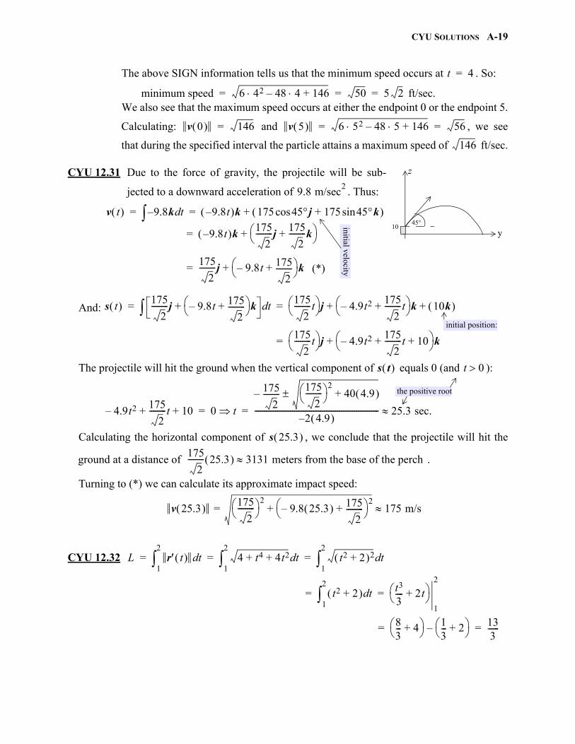
CYU SOLUTIONS A-19
gio
The above SIGN information tells us that the minimum speed occurs at . So:
ft/sec.We also see that the maximum speed occurs at either the endpoint 0 or the endpoint 5.
Calculating: and , we see
that during the specified interval the particle attains a maximum speed of ft/sec.
CYU 12.31 Due to the force of gravity, the projectile will be sub-
jected to a downward acceleration of . Thus:
And:
The projectile will hit the ground when the vertical component of equals 0 (and ):
Calculating the horizontal component of , we conclude that the projectile will hit the
ground at a distance of .
Turning to (*) we can calculate its approximate impact speed:
CYU 12.32
t 4=
minimum speed 6 42 48 4– 146+ 50 5 2= = =
v 0 146= v 5 6 52 48 5– 146+ 56= =
146
z
45
y10
9.8 m/sec2
v t 9.8k– td 9.8t– k 175 45j 175 45ksin+cos += =
9.8t– k 175
2---------j
175
2---------k+
+=
175
2---------j 9.8t– 175
2---------+
k+=
initial velocity(*)
s t 175
2---------j 9.8t– 175
2---------+
k+ td175
2---------t j 4.9t2–
175
2---------t+
k 10k + += =
175
2---------t j 4.9t2–
175
2---------t 10+ +
k+=
initial position:
s t t 0
4.9t2–175
2---------t 10+ + 0 t
175
2---------–
175
2--------- 2
40 4.9 +
2 4.9 –------------------------------------------------------------------ 25.3 sec.= =
the positive root
s 25.3 175
2--------- 25.3 3131 meters from the base of the perch
v 25.3 175
2--------- 2
9.8 25.3 – 175
2---------+
2+= 175 m/s
L r t td1
2
4 t4 4t2+ + td1
2
t2 2+ 2 td1
2
= = =
t2 2+ td1
2
t3
3---- 2t+
1
2
= =
83--- 4+ 1
3--- 2+ – 13
3------= =
A-20 CYU SOLUTIONS
CYU 12.33 (a) Noting that , we start at :
(b) From , we have . Replacing t with in
for we have:
for .
(c) Arc Length using for :
Arc Length using for :
CYU 12.34 The solution is a tad tedious. The main thing is to understand the process:
and:
and:
Then:
P 1 2 1 2– = t 1=
s s t r u ud1
t
4 1 4+ + ud1
t
3u1t
3t 3–= = = = =
s 3t 3–= t s3--- 1+= s
3--- 1+
r 2ti tj 2tk–+= 1 t 3
r 2 s3--- 1+ i s
3--- 1+ j 2 s
3--- 1+ k–+= 0 s 6
r t 2ti tj 2tk–+= 1 t 3
L r t td1
3
4 1 4+ + td1
3
3t13
9 3– 6= = = = =
r s 2s3----- 2+ i s
3--- 1+ j 2s
3----- 2+ k–+= 0 s 6
L r s sd0
6
23--- 2 1
3--- 2 2
3--- 2
+ + td0
6
6= = =
T t 2t t2 t– 2t t2 t–
------------------------------- 2 2t 1–
5 4t2+-------------------------= = T 1 1
3--- 2 2 1– =
N t T t T t
-----------------
2
5 4t2+-------------------- 2t
5 4t2+-------------------- 1–
5 4t2+--------------------
2
5 4t2+-------------------- 2t
5 4t2+-------------------- 1–
5 4t2+--------------------
---------------------------------------------------------------------------------= =
8t–5 4t2+ 3 2/
---------------------------- 105 4t2+ 3 2/
---------------------------- 4t5 4t2+ 3 2/
----------------------------
8t–5 4t2+ 3 2/
---------------------------- 105 4t2+ 3 2/
---------------------------- 4t5 4t2+ 3 2/
----------------------------
-------------------------------------------------------------------------------------------------------=
N 1
827------– 10
27------ 4
27------
827------–
2 1027------ 2 4
27------ 2
+ +
---------------------------------------------------------------
127------ 8 10 4 –
2 59
----------
--------------------------------5
15------- 4 5 2 – = = =
B 1 T 1 N 1 545-------det
i j k
2 2 1–
4– 5 2
545------- 9 0 18 5
5------- 1 0 2 = = = =
Theorem 12.7(c), page 509
gio
CYU SOLUTIONS A-21
As for orthogonality:
Since is a normal to the normal plane, so then is , and since
, the point lies on the plane. Thus:
Since is a normal to the osculating plane, so then is . Thus:
CYU 12.35 For we have:
Thus:
Note that and are the terminal points of and , respec-tively. Hence:
Curvature at and
Curvature at
Roughly speaking: The curve is bending about 17 times faster at than it is at .
T 1 N 1 13--- 2 2 1– 5
15------- 4 5 2 – 5
45------- 2 4– 2 5 1 2–+ 0= = =
T 1 B 1 13--- 2 2 1– 5
5------- 1 0 2 5
15------- 2 1 2 0 1 2–+ 0= = =
N 1 B 1 515------- 4 5 2 – 5
5------- 1 0 2 1
15------ 4 1 5 0+– 2 2+ 0= = =
T 1 13--- 2 2 1– = 2 2 1–
r 1 2t t2 t– = 2 1 1– Normal Plane: 2 2 1– x 2– y 1– z 1+ 0 or: 2x 2y z–+= 7=
(consider Example 12.12, page 517)
B 1 55
------- 1 0 2 = 1 0 2
Osculating Plane: 1 0 2 x 2– y 1– z 1+ 0 or: x 2z+= 0=
r t ti t2j t3k+ +=
r t i 2tj 3t2k+ +=
r t 2j 6tk+=
r t r t deti j k
1 2t 3t2
0 2 6t
6t2i 6tj– 2k+= =
t r t r t r t 3
---------------------------------- 36t4 36t2 4+ +
1 4t2 9t4+ + 3------------------------------------------ 2 9t4 9t2 1+ +
1 4t2 9t4+ + 3------------------------------------------= = =
1 1 1 2 4 8 r 1 r 2
1 1 1 1 2 19143 2/------------- 0.17= =
2 4 8 2 2 1811613 2/---------------- 0.01= =
1 1 1 2 4 8
gio
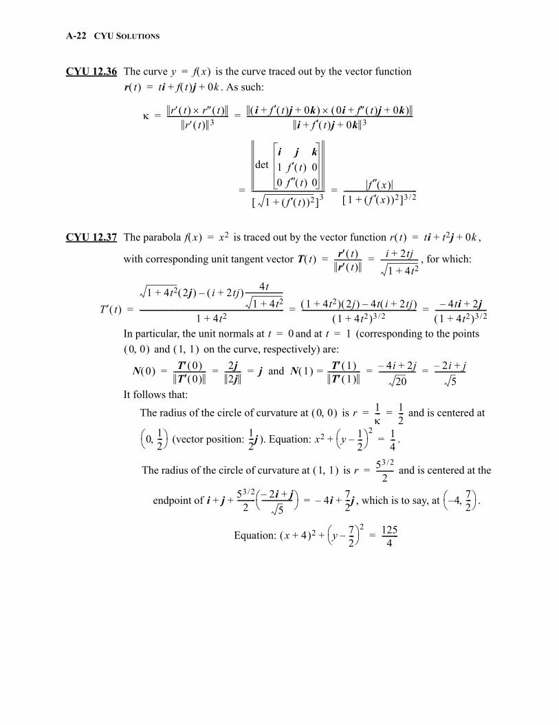
A-22 CYU SOLUTIONS
gio
CYU 12.36 The curve is the curve traced out by the vector function
. As such:
CYU 12.37 The parabola is traced out by the vector function ,
with corresponding unit tangent vector , for which:
In particular, the unit normals at and at (corresponding to the points
and on the curve, respectively) are:
It follows that:
The radius of the circle of curvature at is and is centered at
(vector position: ). Equation: .
The radius of the circle of curvature at is and is centered at the
endpoint of , which is to say, at .
Equation:
y f x =
r t ti f t j 0k+ +=
r t r t r t 3
---------------------------------- i f t j 0k+ + 0i f t j 0k+ + i f t j 0k+ + 3
-------------------------------------------------------------------------------------------= =
det i j k
1 f t 0
0 f t 0
1 f t 2+ 3---------------------------------------- f x
1 f x 2+ 3 2/----------------------------------------= =
f x x2= r t ti t2j 0k+ +=
T t r t r t
--------------- i 2tj+
1 4t2+---------------------= =
T t 1 4t2+ 2j i 2tj+ 4t
1 4t2+---------------------–
1 4t2+------------------------------------------------------------------------------- 1 4t2+ 2j 4t i 2tj+ –
1 4t2+ 3 2/--------------------------------------------------------------- 4ti– 2j+
1 4t2+ 3 2/----------------------------= = =
t 0= t 1=
0 0 1 1
N 0 T 0 T 0
------------------ 2j2j
--------- j and N 1 T 1 T 1
------------------= 4i– 2j+
20-------------------- 2i– j+
5-----------------= = = = =
0 0 r 1--- 1
2---= =
012---
12---j x2 y 1
2---–
2+ 1
4---=
1 1 r 53 2/
2----------=
i j53 2/
2---------- 2i– j+
5----------------- + + 4i–
72---j+= 4–
72---
x 4+ 2 y 72---–
2+ 125
4---------=
CYU SOLUTIONS A-23
CHAPTER 13: DIFFERENTIATING FUNCTIONS OF SEVERAL VARIABLES
CYU 13.1 (a)
(b)
(c) Since [see (a)]: .
(d) Since [see (b)]: .
CYU 13.2 (a)
(b)
In particular:
x x2y ex 3y++ y
x x2 ex 3y+
x x 3y+ +=
y 2x ex 3y+ 1 + 2xy ex 3y++= =
constant
y x2y ex 3y++ x2
yy
ex 3y+y x 3y+ +=
x2 1 ex 3y+ 3 + x2 3ex 3y++= =
fx x y 2xy ex 3y++= fx 2 0 e2=
yz x2 3ex 3y++=
yz
2 0
4 3e2+=
y2
2
z
y
y x2 y+
5 x y–+--------------------
y
5 x y–+ x2 y+ 1– –5 x y–+ 2
--------------------------------------------------------------= =
y
x2 x 5+ +5 x y–+ 2
----------------------------=
0 x2 x 5+ + 2 5 x y–+ 1– –5 x y–+ 4
------------------------------------------------------------------------------ 2 x2 x 5+ + 5 x y–+ 3
-------------------------------= =3
x2
2
z
x
x x2 y+
5 x y–+--------------------
x
5 x y–+ 2x x2 y+ –5 x y–+ 2
---------------------------------------------------------= =
x
x2 2xy– 10x y–+5 x y–+ 2
--------------------------------------------=
5 x y–+ 2 2x 2y– 10+ x2 2xy– 10x y–+ 2 5 x y–+ –5 x y–+ 4
----------------------------------------------------------------------------------------------------------------------------------------------------=
2 5 x y–+ x2– 8x– y– 2xy 10+ + 5 x y–+ 4
--------------------------------------------------------------------------------------------=
x2
2
z
0 4
2 02– 8 0 – 4– 2 0 4 10+ + 5 0 4–+ 3
--------------------------------------------------------------------------------- 12= =
gio
A-24 CYU SOLUTIONS
gio
(c)
(d)
CYU 13.3 (a) For :
(i)
(ii)
(iii)
(b) For
(i)
(ii)
(iii)
(iv)
CYU 13.4 For :
Theorem 11.3 assures us that both partial derivatives are continuous. It follows that fis differentiable (Theorem 13.2).
CYU 13.5 (a) For :
fyxx2 y+
5 x y–+--------------------
y x
5 x y–+ x2 y+ 1– –5 x y–+ 2
--------------------------------------------------------------x
= =
x2 x 5+ +5 x y–+ 2
----------------------------x
=
5 x y–+ 2 2x 1+ x2 x 5+ + 2 5 x y–+ –5 x y–+ 4
--------------------------------------------------------------------------------------------------------------------=
2– xy 9x y– 5–+5 x y–+ 3
------------------------------------------=
3
fyx 2 3 2– 2 3 9 2 3– 5–+ 5 2 3–+ 3
-------------------------------------------------------- 2–43------ 1–
32------= = =
z f x y x4y3= =
x3
3
z
x2
2
x x4y3
x2
2
4x3y3 x
x
4x3y3 = = =
x 12x2y3 24xy3= =
zxyx x4y3 x yx 4x3y3 yx 4x3y3 y x 12x3y2 x 36x2y2= = = = =
zyxx x4y3 y xx 3x4y2 xx 12x3y2 x 36x2y2= = = =
w f x y z xy2 z3y x3yz–+= =
xw
x xy2 z3y x3yz–+ y2 3x2yz–= =
y2
2
w
y
y
xy2 z3y x3yz–+ y 2xy z3 x3z–+ 2x= = =
wxxx xy2 z3y x3yz–+ x xx y2 3x2yz– x x 6xyz– x 6yz–= = = =
wyzx xy2 z3y x3yz–+ y zx 2xy z3 x3z–+ z x 3z2
x3– x 3x2–= = = =
f x y x2 ysin=fx x y 2x y and fy xy sin x2 ycos= =
z 2x ey + 4= x t ysin t2= =
tddz
xz
tddx
yz
tddy
+ 4 2x ey + 3 2 t 4 2x ey + 3ey 2t+cos = =
8 2x ey+ 3 t tey+cos =
8 2 tsin et2+ 3 tcos tet2+ =
CYU SOLUTIONS A-25
Alternatively:
(b) For :
Alternatively:
CYU 13.6 (a) For :
(i)
(ii)
(b) For :
(i)
(ii)
(iii)
(c) Let . Since the partial derivatives ,
and are defined and continuous everywhere, f is differentiable.
(d) For :
z 2x ey + 4 2 tsin et2+ 4= =
tddz 4 2 tsin et2+ 3
tdd 2 tsin et2+ =
4 2 tsin et2+ 3 2 tcos 2tet2+ 8 2 tsin et2+ 3 tcos tet2+ = =
z exy= x s 3t y+ st2= =
tz
xz
tx
yz
ty
+ yexy 3 xexy 2st+ 3st2e s 3t+ st2 s 3t+ e s 3t+ st2 2st+= = =
ste s2t2 3st3+ 3t 2s 6t+ + =
ste s2t2 3st3+ 9t 2s+ =
z exy e s 3t+ st2 es2t2 3st3+= = =
and: t es2t2 3st3+ es2t2 3st3+
t s2t2 3st3+ =
es2t2 3st3+ 2ts2 9st2+ ste s2t2 3st3+ 9t 2s+ = =
z f x y exy x yln+= =
x3
3
z exy x yln+ x xx yexy yln+ x x y2exy x y3exy= = = =
zxyx exy x yln+ x yx yexy yln+ y x yxexy exy 1y---+ +
x
= = =
xy2exy yexy yexy+ + yexy xy 2+ = =
w f x y z xy2 z3y xyz–+= =
xw y2 yz–=
y2
2
w
y
y xy2 z3y xyz–+
y 2xy z3 xz–+ 2x= = =
wxyz xy2 z3y xyz–+ x yz y2 yz– y z 2y z– z 1–= = = =
w f x y z zy2e3x= = fx 3zy2e3x= fy 2zye3x=
fz y2e3x=
w xy2z3 x t2 y t zsin et= = = =
dwdt-------
xw
tddx
yw
tddy
zw
tddz
+ + y2z3 2t 2xz3y t 3xy2z2et+cos+= =
2te3tsin2t 2t2e3t t t 3t2e3tsin
2t+cossin+=
te3t tsin 2 t 2t t 3t tsin+cos+sin =
gio
A-26 CYU SOLUTIONS
(e) For :
CYU 13.7 If is a unit vector making an angle with the posi-tive x-axis then and .
In particular, for : .
Bringing us to:
Since :
Thus: .
CYU 13.8 Unit vector in the direction of : .
Gradient vector:
In particular, , and therefore:
CYU 13.9 Gradient of at :
In particular: .
By Theorem 13.6, the greatest value of the directional derivative at (2,0) is, and the smallest value is .
CYU 13.10 Gradient of at :
In particular: .
By Theorem 13.6, the greatest value of the directional derivative at (1,1,2) is
, and the smallest value is .
w xeyz= x rst2 y t zsin r2cos= = =
tw
xw
tx
yw
ty
zw
tz
+ + eyz 2rst xzeyz tcos xyeyz 0+ += =
2rste t r2cossin rst2 r2e t r2cossin tcoscos+=
rste t r2cossin 2 t r2 tcoscos+ =
a
b1
u ai bj+=u ai bj+= a cos= b sin=
6---= u
6--- icos
6---sin
j+3
2-------i
12---j+= =
Du f 12---
32
-------fx 12---
12---fy 1
2---
+=
fx x x xysin xy xy xy fysin+cos
y x xysin x2 xycos= = = =
fx 12---
1 and fy 12---
0= =
Du f 12---
32
-------=
i– j+ u1
2------- i– j+ =
f x y fx x y i fy x y j+ ex y2+ i 2yex y2+ j+= =
f 0 1 ei 2ej+=
Du f 0 1 f 0 1 u ei 2ej+ 1
2------- i– j+ e
2-------– 2e
2-------+ e
2-------= = = =
f x y x ysin= x y f x y fx x y i fy x y j+ yisin x yjcos+= =
f 2 0 fx 2 0 i fy 2 0 j+ 0sin i 2 0cos j+ 2j= = =
f 2 0 2j 2= = f 2 0 – 2–=
f x y z x2 y2 z2+ + ln= 1 1 2
f x y z 2xx2 y2 z2+ +----------------------------i
2yx2 y2 z2+ +----------------------------j
2zx2 y2 z2+ +----------------------------k+ +=
f 1 1 2 26---i
26---j
46---k+ +
13---i
13---j
23---k+ += =
f 1 1 2 19--- 1
9--- 4
9---+ + 6
3-------= = f 1 1 2 – 6
3-------–=
gio
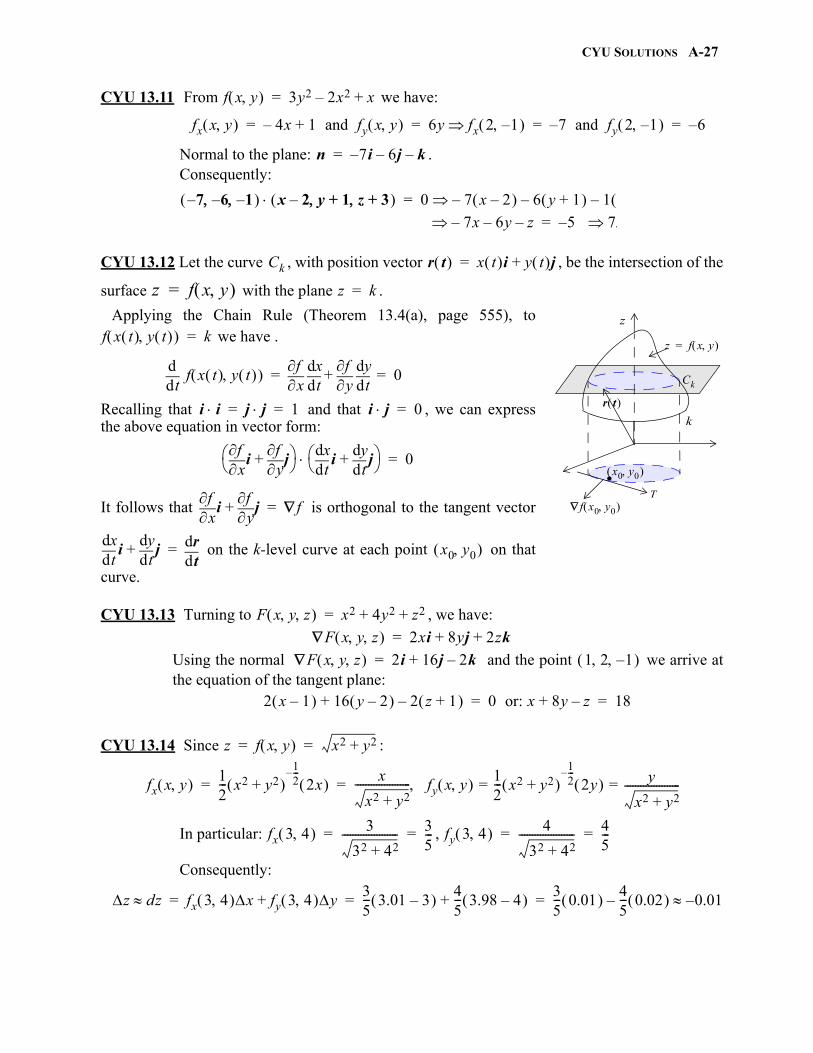
CYU SOLUTIONS A-27
CYU 13.11 From we have:
Normal to the plane: .Consequently:
CYU 13.12 Let the curve , with position vector , be the intersection of the
surface with the plane .
Applying the Chain Rule (Theorem 13.4(a), page 555), to we have .
Recalling that and that , we can expressthe above equation in vector form:
It follows that is orthogonal to the tangent vector
on the k-level curve at each point on that
curve.
CYU 13.13 Turning to , we have:
Using the normal and the point we arrive atthe equation of the tangent plane:
CYU 13.14 Since :
In particular: ,
Consequently:
f x y 3y2 2x2– x+=
fx x y 4x– 1 and fy x y + 6y fx 2 1– 7 and fy 2 1– – 6–= = = =
n 7– i 6j– k–=
7– 6– 1– x 2 y 1+– z 3+ 0 7 x 2– – 6 y 1+ – 1–=
7x– 6y– z– 5 7x–=
Ck r t x t i y t j+=
z f x y = z k=
z
z f x y =
r t
Ck
.f x0 y0
T
k
x0 y0
f x t y t k=
tdd
f x t y t x
ftd
dxy
ftd
dy+ 0= =
i i j j 1= = i j 0=
xf
iy
fj+
td
dxi
tddy
j+ 0=
xf
iy
fj+ f=
tddx
itd
dyj+
tddr= x0 y0
F x y z x2 4y2 z2+ +=
F x y z 2xi 8yj 2zk+ +=
F x y z 2i 16j 2k–+= 1 2 1–
2 x 1– 16 y 2– 2 z 1+ –+ 0 or: x 8y z–+ 18= =
z f x y x2 y2+= =
fx x y 12--- x2 y2+
12---–
2x x
x2 y2+--------------------- fy x y 1
2--- x2 y2+
12---–
2y y
x2 y2+---------------------= == =
fx 3 4 3
32 42+--------------------- 3
5---= = fy 3 4 4
32 42+--------------------- 4
5---= =
z dz fx 3 4 x fy 3 4 y+35--- 3.01 3– 4
5--- 3.98 4– +
35--- 0.01 4
5--- 0.02 0.01––= = =
gio
A-28 CYU SOLUTIONS
CYU 13.15 For , and .
Since , is a critical point of f.
Since there are both positive and negative function values in any open region con-taining :
for all , and for any
neither a maximum nor minimum occurs at .
CYU 13.16 For :
and , and both exist for all x,y.
Finding f ’s critical points:
Substituting in , we can now say that the only critical point
occurs at . To determine the nature of that critical point we turn to Theorem13.9:
From , , and , we have:
and
Conclusion: A (local) minimum occurs at .
CYU 13.17 For x, y, and z positive, we are to minimize:
given (*)
From (*): . Hence:
Employing Theorem 13.8:
Repeating the above argument, but now with the substitution leads tothe conclusion that . Consequently: . Returning to (*), we have:
We leave it to you to verify, via Theorem 13.9, that S achieves its minimum value at
the point .
f x y y2 x2–= fx x y 2x–= fy x y 2y=
fx 0 0 fy 0 0 0= = 0 0
0 0 f 0 y y2 0= y 0 f x 0 x2– 0= x 0
0 0
f x y x2 3y2 3xy 6x– 3y–+ +=
fx x y 2x 3y 6–+= fy x y 6y 3x 3–+=
2x 3y 6–+ 0=
6y 3x 3–+ 0= 2x 3y+ 6=
3x 6y+ 3= 4x 6y+ 12=
3x 6y+ 3=
x 9 and= y 3– 9 3+6
----------------------- 4–= =subtract:
y 4–= 2x 3y+ 6=
9 4–
fxx x y 2= fyy x y 6= fxy x y 3=
D fxx 9 4– fyy 9 4– fxy 9 4– 2– 2 6 32– 3 0= = = fxx 9 4– 2 0=
9 4–
S x2 y2 z2+ += x y z+ + 1=
z 1 x– y–=
S x2 y2 1 x– y– 2+ + 2x2 2y2 2xy 2x– 2y– 1+ + += =
Sx 4x 2y 2–+ 0 and Sy 4y 2x 2–+ 0= = = =
4x 2y 2–+ 4y 2x 2–+=
2x 2y=
x y=y 1 x– z–=
x z= x y z= =
x y z 13---= = =
13--- 1
3--- 1
3---
gio
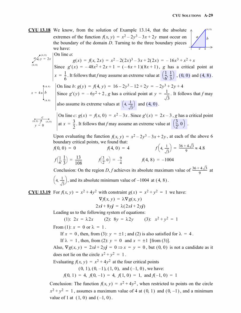
CYU SOLUTIONS A-29
gio
CYU 13.18 We know, from the solution of Example 13.14, that the absolute
extremes of the function must occur onthe boundary of the domain D. Turning to the three boundary pieceswe have:
Upon evaluating the function , at each of the above 6boundary critical points, we found that:
Conclusion: On the region D, f achieves its absolute maximum value of at
, and its absolute minimum value of at .
CYU 13.19 For with constraint we have:
Leading us to the following system of equations:
From (1): .
If , then, from (3): ; and (2) is also satisfied for .
If , then, from (2): and [from (3)].
Also, , but is not a candidate as it
does not lie on the circle .
Evaluating at the four critical points
, we have:
Conclusion: The function , when restricted to points on the circle
, assumes a maximum value of 4 at and , and a minimum
value of 1 at and .
On line a:
Since , g has a critical point at
. It follows that f may assume an extreme value at , and .
On line b:
Since , g has a critical point at . It follows that f may
also assume its extreme values at and .
On line c: . Since , g has a critical point
at . It follows that f may assume an extreme value at .
4 8
4
a b
c
f x y x2 2y3– 3x– 2y+=
..a y 2x=
0 0
4 8
g x f x 2x x2 2 2x 3– 3x– 2 2x + 16x3– x2 x+ += = =g x 48x2– 2x 1+ + 6x– 1+ 8x 1+ = =
x 16---=
16--- 1
3---
0 0 4 8
4 8
4 0
.
.x 4= b
g y f 4 y 16 2y3– 12– 2y+ 2y3– 2y 4+ += = =
g y 6y2– 2+= y 1
3-------=
41
3-------
4 0
0 0 4 0 . .y 0=
c g x f x 0 x2 3x–= = g x 2x 3–=
x 32---=
32--- 0
f x y x2 2y3– 3x– 2y+=
f 0 0 0= f 4 0 4= f 41
3-------
36 4 3+9
---------------------- 4.8=
f 16---
13---
13108---------= f 3
2--- 0 9
4---–= f 4 8 1004–=
36 4 3+9
----------------------
41
3-------
1004– 4 8
f x y x2 4y2+= g x x2 y2+ 1= =
f x y g x y =
2xi 8yj+ 2xi 2yj+ =
(1): 2x 2x (2): 8y 2y (3): x2 y2+ 1= = =
x 0 or 1= =
x 0= y 1= 4=
1= y 0= x 1=
g x y 2xi 2yj+ 0 x y 0= = = = 0 0 x2 y2+ 1=
f x y x2 4y2+=
0 1 0 1– 1 0 and 1 0– f 0 1 4 f 0 1– 4 f 1 0 1 and f 1 0– 1= = = =
f x y x2 4y2+=
x2 y2+ 1= 0 1 0 1– 1 0 1 0–
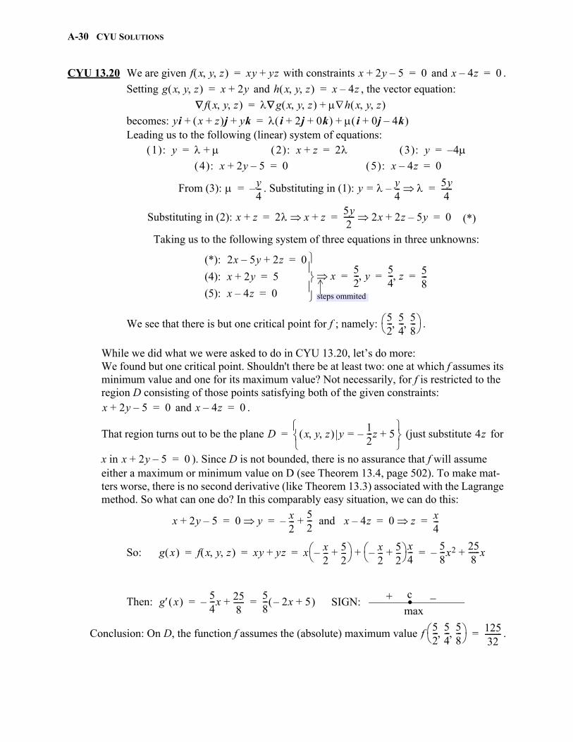
A-30 CYU SOLUTIONS
CYU 13.20 We are given with constraints and .
Setting and , the vector equation:
becomes: Leading us to the following (linear) system of equations:
From (3): . Substituting in (1):
Substituting in (2):
Taking us to the following system of three equations in three unknowns:
We see that there is but one critical point for f ; namely: .
While we did what we were asked to do in CYU 13.20, let’s do more:We found but one critical point. Shouldn't there be at least two: one at which f assumes its minimum value and one for its maximum value? Not necessarily, for f is restricted to the region D consisting of those points satisfying both of the given constraints:
and .
That region turns out to be the plane (just substitute for
x in ). Since D is not bounded, there is no assurance that f will assume either a maximum or minimum value on D (see Theorem 13.4, page 502). To make mat-ters worse, there is no second derivative (like Theorem 13.3) associated with the Lagrange method. So what can one do? In this comparably easy situation, we can do this:
So:
Then:
Conclusion: On D, the function f assumes the (absolute) maximum value .
f x y z xy yz+= x 2y 5–+ 0= x 4z– 0=
g x y z x 2y+= h x y z x 4z–=
f x y z g x y z h x y z +=
yi x z+ j yk+ + i 2j 0k+ + i 0j 4k–+ +=
1 : y += 2 : x z+ 2= 3 : y 4–=
4 : x 2y 5–+ 0= 5 : x 4z– 0=
y4---–= y y
4---–= 5y
4------=
x z+ 2 x z+ 5y2------ 2x 2z 5y–+ 0= = = (*)
(*): 2x 5y– 2z+ 0=
(4): x 2y+ 5=
(5): x 4z– 0=
x 52--- y 5
4--- z 5
8---= = =
steps ommited
52--- 5
4--- 5
8---
x 2y 5–+ 0= x 4z– 0=
D x y z y12---z– 5+=
= 4z
x 2y 5–+ 0=
x 2y 5–+ 0 y x2---–
52--- and x 4z–+ 0 z x
4---= = = =
g x f x y z xy yz+ x x2---– 5
2---+
x2---– 5
2---+
x4---+
58---x2–
258------x+= = = =
g x 54---x– 25
8------+
58--- 2x– 5+ = = SIGN: .c+ _
max
f52--- 5
4--- 5
8---
12532---------=
gio
CYU SOLUTIONS A-31
gio
CHAPTER 14: VECTOR CALCULUS
CYU 14.1
CYU 14.2 Using the parametrization:
:
We then have:
CYU 14.3
CYU 14.4
CYU 14.5 For and we have:
xy2 sdC t sin
2t
dxdt------ 2 dy
dt------ 2 dz
dt----- 2
+ + tdcos0
2
=
t sin2t tsin– 2 tcos 2 1 2+ + tdcos
0
2
2 t sin2t tdcos
0
2
= =1=
213--- sin
3t
0
2
0= =
. . ..
1–
1–
2
2_
x
y
C1 C2
C3
C4C4: r4 1 t– 2 2 t 1– 0 + 2 3t– 2 2t– 0 t 1 = =
xy sdC4
2 3t– 2 2t– 3– 2 2– 2+ td0
1
=
13 4 10t– 6t2+ td0
1
13 4t 5t2– 2t3+ 0
113= = =
xy sdC xy sd
C1
xy s xy sdC3
+dC2
xy sdC4
+ +16--- 2 2 5– 24+ 13+= =
Example 14.3
M x y sdC 1 x z+ + sd
C 1 tcos t+ + tsin– 2 tcos 2 1+ + td
0
6
= = =
2 1 tcos t+ + td0
6
=
2 t t t2
2----+sin+
0
6
2 6 182+ = =
W F r t r t tda
b
F t2 t3 t 2ti 3t2j k+ + td0
1
= =
t2i t2 t3+ j tk+ + 2ti 3t2j k+ + td0
1
=
2t3 3t4 3t5 t+ + + td0
1
t4
2---- 3t5
5------- t6
2---- t2
2----+ + +
0
12110------= = = =
.1
2
1 2 2
y
x
y
C
F x y z yi 2xj 3zk+ += r t t 2t 2t 0 t 1 =
F rdC F r t r t td
0
1
2ti 2tj 6tk+ + i 2j 2k+ + td0
1
= =
2 4 12+ + t td0
1
18t td0
1
9t2 0
19= = = =
A-32 CYU SOLUTIONS
CYU 14.6 We know that (Example 14.6), and now show
that , where .
As noted above Theorem 14.3:For a given parametrization of a curve C, the parame-trization , denoted by , traverses C in the opposite direction.
Firstly, and throughout . So:
Thus:
CYU 14.7 For , , and , , we have: , ,
and Consequently:
CYU 14.8 If and are two paths in S from to , then
is a closed path in S. As such .
Since ,
.1
2
1 2 2
y
x
y
C–
F rd
C 8=
F rdC– 8–= F x y z yi 2xj 3zk+ +=
r t a t b r t r a b t–+ a t b = C–
a 0= b 1= a b t–+ 1 t–=
r1 t 0 2t 0 r1 t r1 1 t– = 0 2 1 t– 0 0 2 2t 0– for 0 t 1 = = =
r2 t t 2 0 r2 t r2 1 t– = 1 t– 2 0 for 0 t 1 = =
r3 t 1 2 2t r3 t r3 1 t– = 1 2 2 1 t– 1 2 2 2t– for 0 t 1 = = =
F rdC– F r1 t r1 t td
0
1
= F r2 t r2 t td0
1
F r3 t r3 t td0
1
+ +
2 2t– i 2j– td0
1
= 2i 2 1 t– j+ i– t 2i 2j 3 2 2t– k+ + 2k– td0
1
+d0
1
+
0 2– td0
1
6 2 2t– td0
1
–+ 2t– 01
6 2t t2– 0
1– 8– F rd
C–= = = =
x t t2= y t 5t= z t 2t2–= 1 t 2 dxdt------ 2t= dy
dt------ 5=
dzdt----- 4t–=
xy xd y y yz+d+ zdC t2 5t
tddx
5ttd
dyt2 2t2–
tddz
+ + td1
2
=
5t3 2t 5t 5 4t4 4t– –+ td1
2
10t4 25t 16t5+ + td1
2
= =
2t5 25t2
2---------- 8t6
3-------+ +
1
25352
---------= =
.
.
P1C1
C2
P2
C1 C2 P1 P2 C C1 C2– =
F drC 0=
F drC F dr
C1
F drC2
–=
Theorem 14.3
F drC1
F drC2
=
gio
CYU SOLUTIONS A-33
CYU 14.9 If F is conservative with potential function f, then:
CYU 14.10 If, for given , any one of the equations
fails to hold in S, then F is not conservative in S.
While the first two of those equations do hold for , the third
does not: while .
CYU 14.11 (a) Theorem 14.9(iv) holds for : .
For f such that , we have:
Bringing us to: .
Treating y as a constant in (1), we have: .
Taking the partial derivative of (3) with respect to y: .
Replacing with [see (2)]: .
Letting we have an answer: .(b) Theorem 14.9(iv) holds for :
For f such that we have:
Bringing us to:
Treating y and z as constants in (1), we have: .
Taking the partial derivative of (4) with respect to y: .
Replacing with [see (2)]:
.
Returning to (4), we have: (5) . Taking the partial derivative with respect to z: .
From (3):
Letting and returning to (5) we have an answer: .
F Pi Qj Rk+ + f x y z fxi fy j fzk+ += = =
P fx Q fy R fz= = =
yP fxy fyx x
Q
zP fxz fzx x
R
zQ fyz= fzy y
R= = = = = = = =
Theorem 13.1, page 552
F P x y z i Q x y z j R x y z k+ +=
yP
xQ
z
Px
R
zQ
yR===
F x y z xi zj yzk+ +=
zQ
zz 1= =
yR z=
F x y 2xyi x2j+= 2xy y x2 x 2x= =
F f= 2xy i x2 j+ f x y fx x y i fy x y j+= =
(1): fx x y 2xy and (2): fy x y x2= =
(3): f x y 2xy xd x2y g y += =
fy x y x2= g y +
fy x y x2 x2 x2= g y g y + 0 g y C= =
C 0= F x y 2xyi x2j+ f x2y = = =F x y z 2xyz i x2z j x2y k+ +=
2xyz y x2z x 2xz= = 2xyz z x2y x 2xy x2z z x2y y x2= = = =
F f=2xyz i x2z j x2y k+ + f fx x y z i fy x y z j fz x y z k+ += =
(1): fx x y z 2xyz, (2): fy x y z x2z, (3): fz x y z x2y= = =
(4): f x y z 2xyz xd x2yz g y z += =
fy x y z x2z= g y z y+
fy x y z x2z
x2z x2z g y z y g y z y+ 0 g y z h z = = =
f x y z x2yz h z +=fz x y z x2y h z +=
x2y x2y h z h z + C= =
C 0= F x y z x2yz =
gio
A-34 CYU SOLUTIONS
gio
CYU 14.12 One approach: is a conservative field with potential function
(see CYU 14.11). Since and the
curve C starts at the point and ends at the point . Hence:
Another approach: Choosing to integrate along the path with
parametrizations:
for and
we have:
CYU 14.13 The force field is conservative:
, with .It follows that for any path C from to :
[Negative work indicates that the force field impedes movement along the curve (see page 594)]
CYU 14.14 Using the parametrization of a line segment from to :
We have:
Thus:
F x y 2xyi x2j+=
f x y x2y= r 0 0 0 = r4---
4---cos
24--- 2
16------
=
0 0 8--- 2
16------
F drC f
8--- 2
16------
f 0 0 –8--- 2 2
16------ 0– 4
1024------------= = =
x2y
8---
2
16------
x
y
C1
C2
.C C1 C2=
r1 t ti 0 t8--- = C1 r2 t
8---i tj+ 0 t
2
16------ =
F drC F dr
C
F dr1C1
F dr2C2
+= =
2xyi x2j+ i td 2xyi x2j+ j tdC2
+C1
=
2xy td x2 tdC2
+C1
08--- 2
td0
2
16------
+2
64------t
0
2
16------
4
1024------------= = = =
F x y z 0i 0j mg– k+ +=
F x y z f x y z = f x y z mgz–=0 0 0 x0 y0 z0
W F rdC f x0 y0 z0 f 0 0 0 – mgz0–= = =
r0 r1
r t r0 t r1 r0– + 1 t– r0 tr1 0 t 1 += =
C1: r 1 t– 0 0 t 1 0 + t 0 0 t 1 = =
C2: r 1 t– 1 0 t 0 1 + 1 t– t 0 t 1 = =
C3: r 1 t– 0 1 t 0 0 + 0 1 t– 0 t 1 = =1
1
x
y
C2
C1
C3
F TdsC x2i xyj+ dr
C x2i xyj+ dr
C1
x2i xyj+ drC2
x2i xyj+ drC3
+ += =
t2i i td0
1
1 t– 2i t 1 t– j+ i– j+ t 0 td0
1
+d0
1
+=
t2 1 t– 2– t 1 t– + td0
1
t2– 3t 1–+ td0
1
13---– t3 3
2---t2 t–+
0
116---= = = =
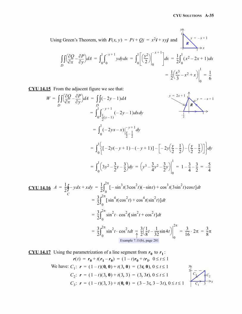
CYU SOLUTIONS A-35
gio
Using Green’s Theorem, with and
CYU 14.15 From the adjacent figure we see that:
CYU 14.16
CYU 14.17 Using the parametrization of a line segment from to :
We have:
F x y Pi Qj+ x2i xyj+= =
1
1
R
y x– 1+=
x
y
xQ
yP–
AdD y yd xd
0
x– 1+
0
1
y2
2-----
0
x– 1+
xd0
1
12--- x2 2x– 1+ xd
0
1
= = =
12--- x3
3----- x2– x+
0
116---= =
1
1
R
12---–
y x– 1+=y 2x 1+=
Wx
Qy
P– Ad
D 2y– 1– Ad
D= =
2y– 1– xd yd12--- y 1–
y– 1+
0
1
=
2yx– x– y2--- 1
2---–
y– 1+yd
0
1
=
2y y– 1+ – y– 1+ – 2y y2--- 1
2---–
– y2--- 1
2---–
––
yd0
1
=
3y2 32---y– 3
2---–
yd0
1
y3 34---y2–
32---y–
0
1
1 34---– 3
2---– 5
4---–= = = =
A12--- ydx– xdy+
C
12--- sin
3t 3cos
2t tsin– – cos
3t 3sin
2t tcos+ td
0
2
= =
32--- sin
4t cos
2t cos
4t sin
2t + td
0
2
=
32--- sin
2t cos
2t sin
2t cos
2t+ td
0
2
=
32--- sin
2t cos
2t td
0
2
32--- 1
8---t
132------ 4tsin–
0
2316------ 2 3
8---= = = =
Example 7.11(b), page 281
r0 r1
r t r0 t r1 r0– + 1 t– r0 tr1 0 t 1 += =
C1: r 1 t– 0 0 t 3 0 + 3t 0 0 t 1 = =
C2: r 1 t– 3 0 t 3 3 + 3 3t 0 t 1 = =
C3: r 1 t– 3 3 t 0 0 + 3 3t– 3 3t– 0 t 1 = = x
y
3
3
C1
C2C3
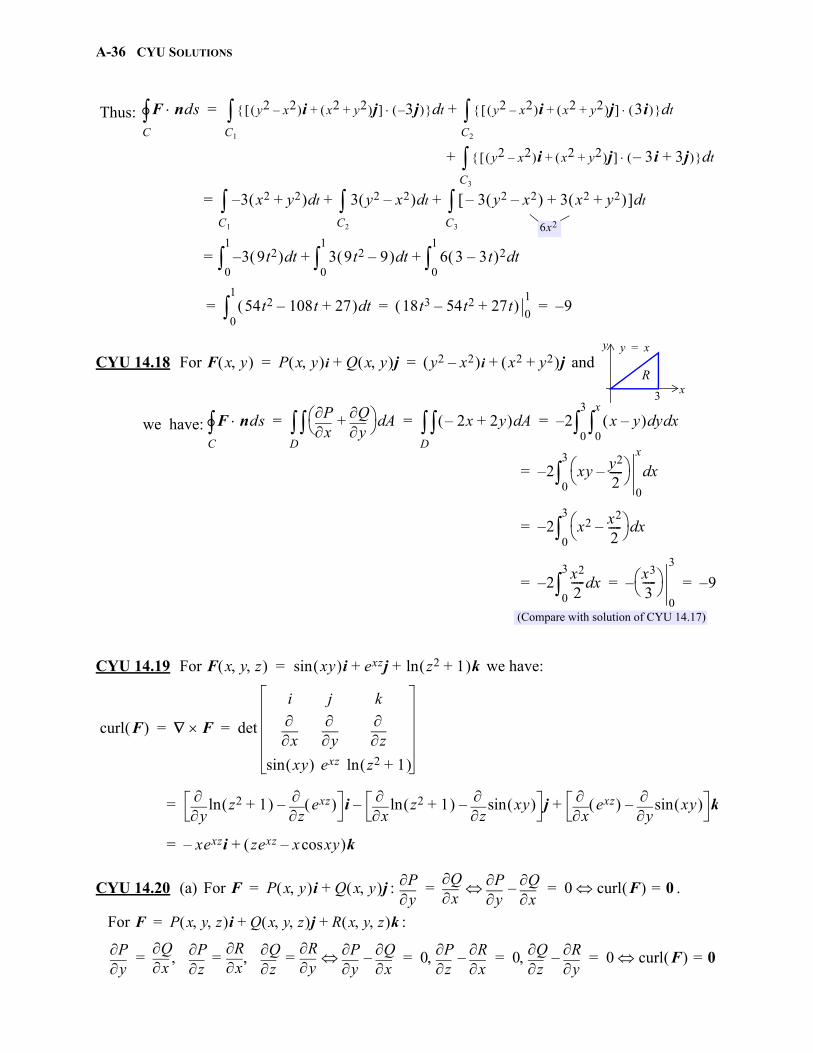
A-36 CYU SOLUTIONS
gio
Thus:
CYU 14.18 For and
we have:
CYU 14.19 For we have:
CYU 14.20 (a) For : .
For :
F ndsC y2 x2– i x2 y2+ j+ 3j– td
C1
y2 x2– i x2 y2+ j+ 3i tdC2
+=
y2 x2– i x2 y2+ j+ 3i– 3j+ tdC3
+
3 x2 y2+ – tdC1
= 3 y2 x2– tdC2
3 y2 x2– – 3 x2 y2+ + tdC3
+ +
3 9t2 td–0
1
3 9t2 9– td0
1
+= 6 3 3t– 2 td0
1
+
54t2 108t– 27+ td0
1
18t3 54t2– 27t+ 0
19–= = =
6x2
F x y P x y i Q x y j+ y2 x2– i x2 y2+ j+= =
x
y
3
y x=
R
F ndsC x
Py
Q+ Ad
D 2x– 2y+ Ad
D 2 x y– yd xd
0
x
0
3
–= = =
2 xy y2
2-----–
0
x
xd0
3
–=
2 x2 x2
2-----–
xd0
3
–=
2x2
2----- xd
0
3
–x3
3-----
0
3
– 9–= = =
(Compare with solution of CYU 14.17)
F x y z xy isin exzj z2 1+ kln+ +=
curl F F det
i j k
x
y
z
xy sin exz z2 1+ ln
= =
y z2 1+ ln
z exz – i
x z2 1+ ln
z xy sin– j
x exz
y xy sin– k+–=
xexzi– zexz x xycos– k+=
F P x y i Q x y j+=y
Px
Qy
Px
Q– 0 curl F 0== =
F P x y z i Q x y z j R x y z k+ +=
yP
xQ
z
Px
R
zQ
yR
yP
xQ–== 0
zP
xR– 0
zQ
yR– 0 curl F 0== = = =
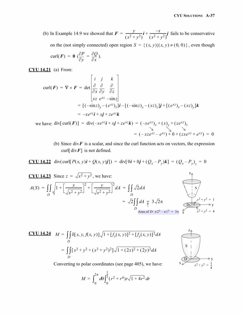
CYU SOLUTIONS A-37
gio
(b) In Example 14.9 we showed that fails to be conservative
on the (not simply connected) open region , even though
( ).
CYU 14.21 (a) From:
we have:
(b) Since is a scalar, and since the curl function acts on vectors, the expression
is not defined.
CYU 14.22
CYU 14.23 Since , we have:
CYU 14.24
Converting to polar coordinates (see page 405), we have:
Fy
x2 y2+ ---------------------i
x–x2 y2+
---------------------j+=
S x y x y 0 0 =
curl F 0=y
Px
Q=
curl F F det
i j k
x
y
z
xz exz zsin–
= =
zsin– y exz z– i zsin– x xz z– – j exz x xz y– k+=
xexz– i xj zexzk+ +=
div curl F div xexz– i xj zexzk+ + xexz– x x y zexz z+ += =
xzexz– exz– 0 zxexz exz+ + + 0= =
divF
curl divF
div curl P x y i Q x y j+ div 0i 0j Qx Py– k+ + Qx Py– z 0= = =
y
x
z
x2 y2+ 4=
D
S
x2 y2+ 1=
z x2 y2+=
A S 1x
x2 y2+---------------------
2 y
x2 y2+---------------------
2+ +
D dA 2
D dA= =
2 AdD 3 2= =
Area of D: 22 12– 3=
yx
z
S
D
x2 y2+ 14---=
M x y f x y 1 fx x y 2 fy x y 2+ + AdD=
x2 y2 x2 y2+ 2+ + D 1 2x 2 2y 2+ + Ad=
M r2 r4+ r 1 4r2+ rd0
12---
d0
2
=
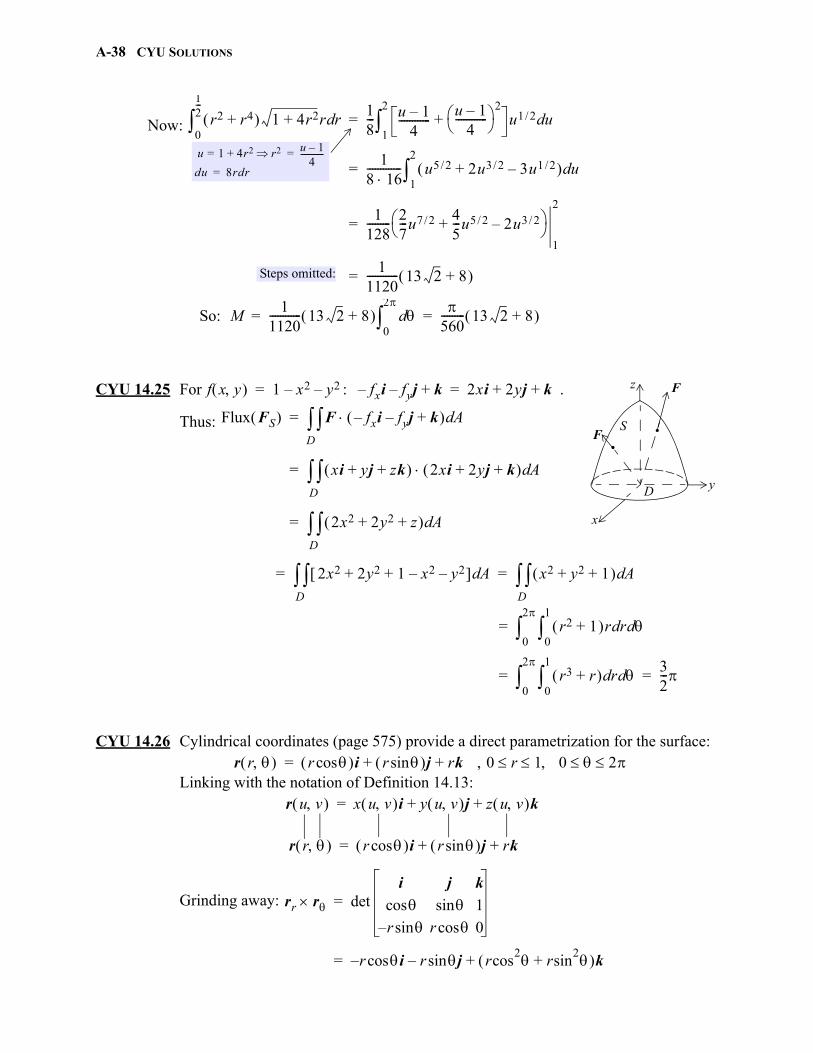
A-38 CYU SOLUTIONS
gio
Now:
So:
CYU 14.25 For : .
Thus:
CYU 14.26 Cylindrical coordinates (page 575) provide a direct parametrization for the surface: ,
Linking with the notation of Definition 14.13:
Grinding away:
r2 r4+ 1 4r2+ r rd0
12---
18--- u 1–
4------------
u 1–4
------------ 2
+ u1 2/ ud1
2
=
18 16------------- u5 2/ 2u3 2/ 3u1 2/–+ ud
1
2
=
1128--------- 2
7---u7 2/ 4
5---u5 2/ 2u3 2/–+
1
2
=
11120------------ 13 2 8+ =
u 1 4r2+= r2 u 1–4
------------=
du 8rdr=
Steps omitted:
M1
1120------------ 13 2 8+ d
0
2
560--------- 13 2 8+ = =
x
y
z
D
S
. .F
F
f x y 1 x2– y2–= fxi– fyj– k+ 2xi 2yj k+ +=
Flux FS F fxi– fyj– k+ AdD=
xi yj zk+ + 2xi 2yj k+ + AdD=
2x2 2y2 z+ + AdD=
2x2 2y2 1 x2– y2–+ + AdD x2 y2 1+ + Ad
D= =
r2 1+ r rd d0
1
0
2
=
r3 r+ rd d0
1
0
2
32---= =
r r r cos i r sin j rk+ += 0 r 1 0 2
r u v x u v i y u v j z u v k+ +=
r r r cos i r sin j rk+ +=
rr r deti j k
cos sin 1
r sin– r cos 0
=
r cos– i r j rcos2 rsin
2+ k+sin–=
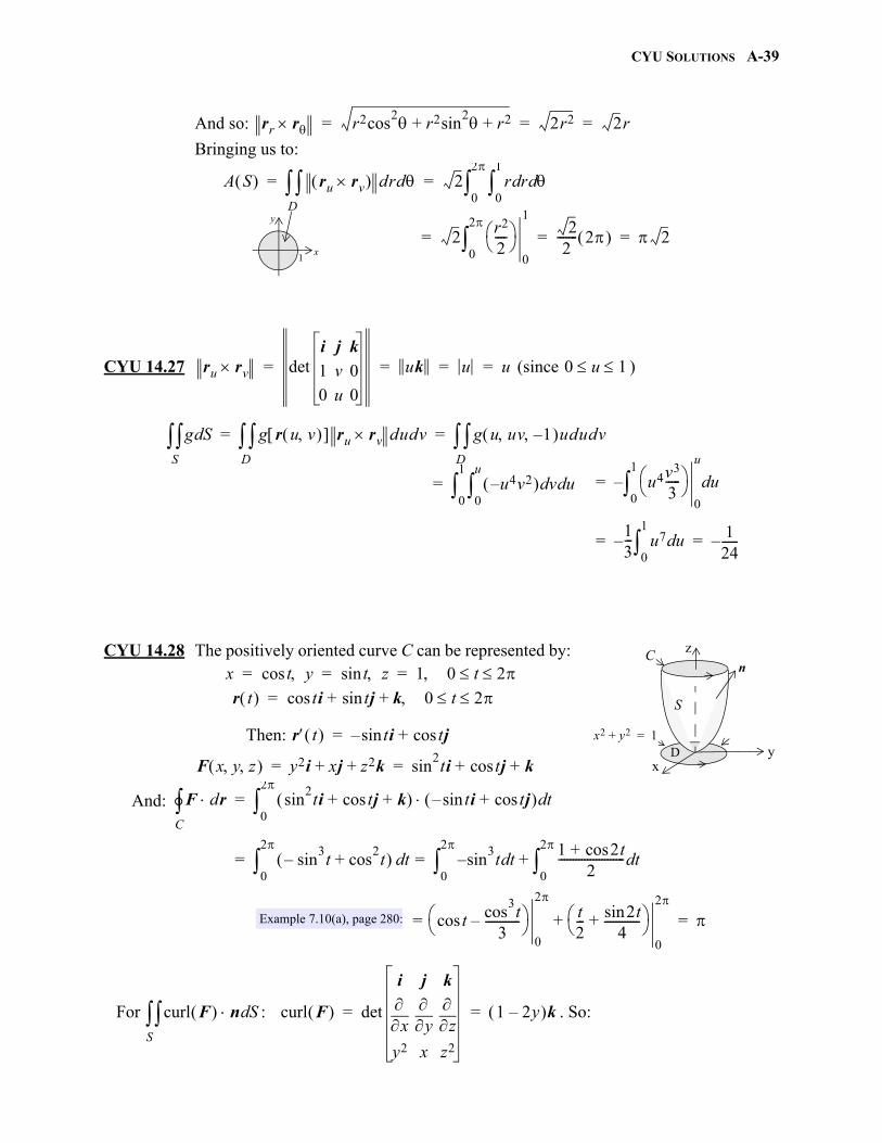
CYU SOLUTIONS A-39
gio
And so:
Bringing us to:
CYU 14.27 (since )
CYU 14.28 The positively oriented curve C can be represented by:
Then:
For : . So:
rr r r2cos2 r2sin
2 r2++ 2r2 2r= = =
A S ru rv D drd 2 r rd d
0
1
0
2
= =
2r2
2----
0
1
0
2
2
2------- 2 2= = =
1x
y
ru rv deti j k
1 v 0
0 u 0
uk u u= = = = 0 u 1
g SdS g r u v ru rv
D dudv g u uv 1–
D ududv= =
u4v2– vd ud0
u
0
1
= u4v3
3-----
0
u
ud0
1
–=
13--- u7 ud
0
1
– 124------–= =
yx
z
S
Dx2 y2+ 1=
nC
x t ycos t zsin 1 0 t 2 = = =
r t tcos i tsin j k+ 0 t 2 +=
r t tsin– i tcos j+=
F x y z y2i xj z2k+ + sin2ti tjcos k+ += =
F drC sin
2ti tjcos k+ + tsin– i tcos j+ td
0
2
=
sin3t– cos
2t+ td
0
2
sin–3t td
0
2
1 2tcos+
2----------------------- td
0
2
+= =
tcos cos3t
3------------–
0
2
= t2--- 2tsin
4------------+
0
2
+ =Example 7.10(a), page 280:
And:
curl F n SdS curl F det
i j k
x
y
z
y2 x z2
1 2y– k= =
A-40 CYU SOLUTIONS
CYU 14.29 If , then for every closed path in S. It
then follows, from Theorem 14.4 (page 636), that F is path independent.
CYU 14.30 Since: :
CYU 14.31 Since: :
curl F n SdS 1 2y– k fxi– fyj– k+ Ad
D 1 2y– k 2x– i 2yj– k+ Ad
D= =
1 2y– Ad1 x2––
1 x2–
1–
1
=
1 2 sin– r rd d0
1
0
2
=
r2
2---- r2 sin–
0
1
d0
1
0
2
=
12--- sin– d
0
2
=
2--- cos+
0
2
= =
using polar coordinates:
curl F 0= F drC curl F n Sd
S 0= =
div F x x= y y z z+ + 1 1 1+ + 3= =
Flux FS F n SdS div F Vd
E 3 Vd
E 3
43---r3 4 r3 = = = = =
volume of the sphere E of radius r (Exercise 37, page 206)
div F xsin2y x= ex2z3 xtan– y zcos
2y z+ + sin
2y cos
2y+ 1= =
Flux FS F n SdS div F Vd
E Vd
E 32 7 63= = = = =
volume of the cylinder E of radius 3 and height 7
gio
CYU SOLUTIONS A-41
CYU 14.32 Since: :div F 5xy2 xi 5yz2 y j 5x2z zk+ += 5 y2 z2 x2+ + =
Flux FS F n SdS div F Vd
E 5 x2 y2 z2+ + Vd
E= = =
Turning to spherical coordinates:(see Figure 13.12, page 580)
522 sin d d d0
3
0
0
2
=
5 sin 0
3
0
0
2
d d 35 sin0
0
2
d= =
35 cos– 0
0
2
=
35 2 d0
2
97= =
gio

A-42 CYU SOLUTIONS
gio
Additional Theoretical Development B-1
APPENDIX BADDITIONAL THEORETICAL DEVELOPMENT
PROOF: (a) Let be in the domain of H.
and:
(b) (Compare with the proof of Theorem 2.5, page 58). Let be in the domain of ,
and let be given. Since f is continuous at , we can find a such that
. Now, think of as being an “ -challenge” for the
function g. By the continuity of g we can find a such that:
. Putting this together, we have:
THEOREM 12.6 (a) If f and g are real-valued continuous functions of one variable,then:
(i) and (ii) are continuous functions of two variables.
(b) If g is a real-valued continuous function of two variables, and if fis a real-valued continuous function of one variable, then:
is a continuous function of two variables.
THEOREM 11.3, PAGE 431
H x y f x g y += K x y f x g y =
H x y f g x y =
x0 y0 H x y
x y x0 y0 lim f x g y +
x y x0 y0 lim f x g y
x y x0 y0 lim+
x y x0 y0 lim= =
f x g y y y0lim+
x x0lim=
f x0 g y0 + H x0 y0 = =
K x y x y x0 y0
lim f x g y x y x0 y0
lim f x g x x y x0 y0
limx y x0 y0
lim= =
f x g y y y0lim
x x0lim=
f x0 g y0 K x0 y0 = =
x0 y0 H gf=
0 g x0 y0
y g x0 y0 – f y f g x0 y0 –
x y x0 y0 – g x y g x0 y0 –
x y x0 y0 – g x y g x0 y0 –
f g x y f g x0 y0 – H x y H x0 y0 – =
gio
B-2 Additional Theoretical Development
PROOF: We show that can be expressed in the form
where , as .
Adjoining a clever zero to , we have:
Applying the Mean Value Theorem to the single-variable function: (**)
on the interval , we have:
, for some c between and
. Returning to (**) we have:
.
Returning to (*) we then have: .
In a similar fashion, by applying the Mean Value Theorem to the single-valued function on the interval we can arrive at:
, for some
Adding two more cleaver zeros we have:
Or: , where:
Finally, the continuity of and assures us that , as .
THEOREM 13.2 If the partial derivatives and exist and are continuous in an open
region about , then f is differentiable at .
THEOREM 13.2, PAGE 554
fx fy
x0 y0 x0 y0
z f x0 x+ y0 y+ f x0 y0 –=
z fx x0 y0 x= fy x0 y0 y 1x 2y+ + + 1 2 0 x y 0
z
z f x0 x+ y0 y+ f x0 y0 y+ – f x0 y0 y+ f x0 y0 – += (*)
g x f x y0 y+ =
x0 x0 x+
g c g x0 x+ g x0 –
x--------------------------------------------- or: g c x g x0 x+ g x0 –= = x0
x0 x+
fx c y0 y+ x f x0 x+ y0 y+ f x0 y0 y+ –=
z fx c y0 y+ x f x0 y0 y+ f x0 y0 – +=
h y f x0 y = y0 y0 x+
z fx c y0 y+ x fy x0 d y+= y0 d y0 y+
z fx x0 y0 x fx c y0 y+ fx x0 y0 – x fy x0 y0 y fy x0 d fy x0 y0 – y+ + +=
z fx x0 y0 x= fy x0 y0 y 1x 2y+ + +
1 fx c y0 y+ fx x0 y0 and 2– fy x0 d fy x0 y0 –= =
fx fy 1 2 0 x y 0
gio
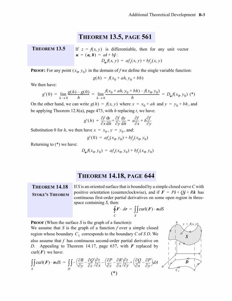
Additional Theoretical Development B-3
PROOF: For any point in the domain of f we define the single variable function:
We then have:
(*)
On the other hand, we can write where and , and
be applying Theorem 12.8(a), page 473, with h replacing t, we have:
Substitution 0 for h, we then have , , and:
Returning to (*) we have:
PROOF (When the surface S is the graph of a function): We assume that S is the graph of a function f over a simple closedregion whose boundary corresponds to the boundary C of S D. We
also assume that f has continuous second-order partial derivative onD. Appealing to Theorem 14.17, page 637, with F replaced by
we have:
THEOREM 13.5 If is differentiable, then for any unit vector:
THEOREM 14.18
STOKE’S THEOREM
If S is an oriented surface that is bounded by a simple closed curve C withpositive orientation (counterclockwise), and if hascontinuous first-order partial derivatives on some open region in three-space containing S, then:
THEOREM 13.5, PAGE 561
z f x y =u a b ai bj+= =
Du f x y afx x y bfy x y +=
x0 y0
g h f x0 ah+ y0 bh+ =
g 0 g h g 0 –h
----------------------------h 0lim
f x0 ah+ y0 bh+ f x0 y0 –
h-----------------------------------------------------------------------
h 0lim Du f x0 y0 = = =
g h f x y = x x0 ah+= y y0 bh+=
g h x
fhd
dxy
fhd
dy+ a
xf
by
f+= =
x x0= y y0=
g 0 afx x0 y0 bfy x0 y0 +=
Du f x0 y0 afx x0 y0 bfy x0 y0 +=
THEOREM 14.18, PAGE 644
F Pi Qj Rk+ +=
F drC curl F n Sd
S=
S
D
z f x y =
C
C1
curl F
curl F n SdS y
Rz
Q–
xz
–z
Px
R–
yz
–x
Qy
P– + Ad
D=
(*)C1
gio
B-4 Additional Theoretical Development
If , , , is a parametrization of , then
, , , is a parametrization of C. We then have:
Four of the terms in the above double integral cancel, and the remaining six terms can be rear-ranged to coincide with the double integral (*) at the bottom of the previous page.
PROOF: Restricted to the case where E lies between the graphs of two continuous functions of xand y, two continuous functions of y and z, and two continuous functions of x and z:
Let . Then , and:
Moreover:
THEOREM 14.19
THE DIVERGENCE
THEOREM
Let the surface S be oriented in the outward direction and let E be thesolid region enclosed by S. If is continuously dif-ferentiable throughout E, then:
x x t = y y t = a t b C1
x x t = y y t = z f x t y t = a t b
F drC P
tddx
Qtd
dyR
tddz
+ + td
a
b
=
Ptd
dxQ
tddy
Rx
ztd
dxy
ztd
dy+
+ + tda
b
=
P Rx
z+
td
dxQ R
yz
+
tddy
+ tda
b
=
P Rx
z+
x Q Ry
z+
+d ydC=
x
Q Ry
z+
y
P Rx
z+– Ad
D=
xQ
zQ
xz
xR
yz
zR
xz
yz
Rx y
2
z
+ + + +
yP
zP
yz
yR
xz
zR
yz
xz
Ry x
2
z
+ + + +
– AdD=
Chain Rule, page 555:
Chain Rule, page 555:
Green’s Theorempage 617:
THEOREM 14.19, PAGE 654
F Pi Qj Rk+ +=
F n SdS div F Vd
E=
E x y z x y Dz z1 x y z z2 x y =
x y z y z Dx x1 y z x x2 y z =
x y z x z Dy y1 x z y y2 x z =
F Pi Qj Rk+ += div F Px Qy Rz+ +=
div F VdE Px Vd
E Qy Vd
E Rz Vd
E+ +=
gio
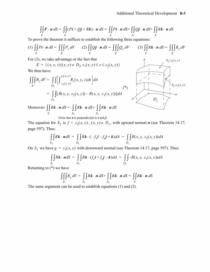
Additional Theoretical Development B-5
To prove the theorem it suffices to establish the following three equations:
(1) (2) (3)
For (3), we take advantage or the fact that
We then have:
(*)
Moreover:
The equation for is , , with upward normal n (see Theorem 14.17,
page 597). Thus:
On we have with downward normal (see Theorem 14.17, page 597). Thus:
Returning to (*) we have
The same argument can be used to establish equations (1) and (2).
F n SdS Pi Qj Rk+ + n Sd
S Pi n Sd
S Qj n Sd
S Rk n Sd
S+ += =
Pi n SdS Px Vd
E= Qj n Sd
S Qy Vd
E= Rk n Sd
S Rz Vd
E=
Dz
S2:z2 x y
S2:z1 x y
E x y z x y Dz z1 x y z z2 x y =
Rz VdE Rz x y z zd
z1 x y
z2 x y
AdDz
=
R x y z2 x y R x y z1 x y – AdDz
=
Rk n SdS Rk n Sd
S1
Rk n SdS2
+=
(Note that n is perpendicular to i and j)
S2 f z2 x y = x y Dz
Rk n SdS2
Rk fxi– fyj– k+ AdDz
R x y z2 x y AdDz
= =
S1 g z1 x y =
Rk n SdS1
Rk fxi fyj k–+ AdDz
R x y z1 x y – AdDz
= =
Rz VdE Rk n Sd
S1
Rk n SdS2
+ Rk n SdS= =
gio
B-6 Additional Theoretical Development
gio
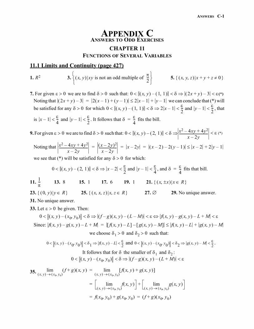
ANSWERS C-1
APPENDIX CANSWERS TO ODD EXERCISES
CHAPTER 11FUNCTIONS OF SEVERAL VARIABLES
11.1 Limits and Continuity (page 427)
1. 3. 5.
7. For given we are to find such that:
Noting that we can conclude that (*) will
be satisfied for any for which , that
is and . It follows that fits the bill.
9. For given we are to find such that:
Noting that
we see that (*) will be satisfied for any for which:
, and fits that bill.
11. 13. 8 15. 1 17. 6 19. 1 21.
23. 25. 27. 29. No unique answer.
31. No unique answer.
33. Let be given. Then:
Since:
we choose and such that:
and .
It follows that for the smaller of and :
35.
R2 x y xy is not an odd multiple of 2---
x y z x y z 0+ +
0 0 0 x y 1 1 – 2x y+ 3– (*)
2x y+ 3– 2 x 1– y 1– + 2 x 1– y 1–+=
0 0 x y 1 1 – 2 x 1–2--- and y 1–
2---
x 1–4--- y 1–
2---
4---=
0 0 0 x y 2 1 – x2 4xy– 4y2+x 2y–
----------------------------------- (*)
x2 4xy– 4y2+x 2y–
----------------------------------- x 2y– 2
x 2y–---------------------- x 2y– x 2– 2 y 1– – x 2– 2 y 1–+= = =
0
0 x y 2 1 – x 2–2--- and y 1–
4---
4---=
1--- x x x R
0 y y R x x z x z R
0
0 x y x0 y0 – f g– x y L M– – f x y g x y – L– M+
f x y g x y – L– M+ f x y L– g x y M– – f x y L– g x y M–+=
1 0 2 0
0 x y x0 y0 – 1 f x y L–2--- 0 x y x0 y0 – 2 g x y M–
2---
1 20 x y x0 y0 – f g– x y L M+ –
f g+ x y x y x0 y0
lim f x y g x y + x y x0 y0
lim=
f x y x y x0 y0
lim g x y x y x0 y0
lim+=
f x0 y0 g x0 y0 + f g+ x0 y0 = =
gio
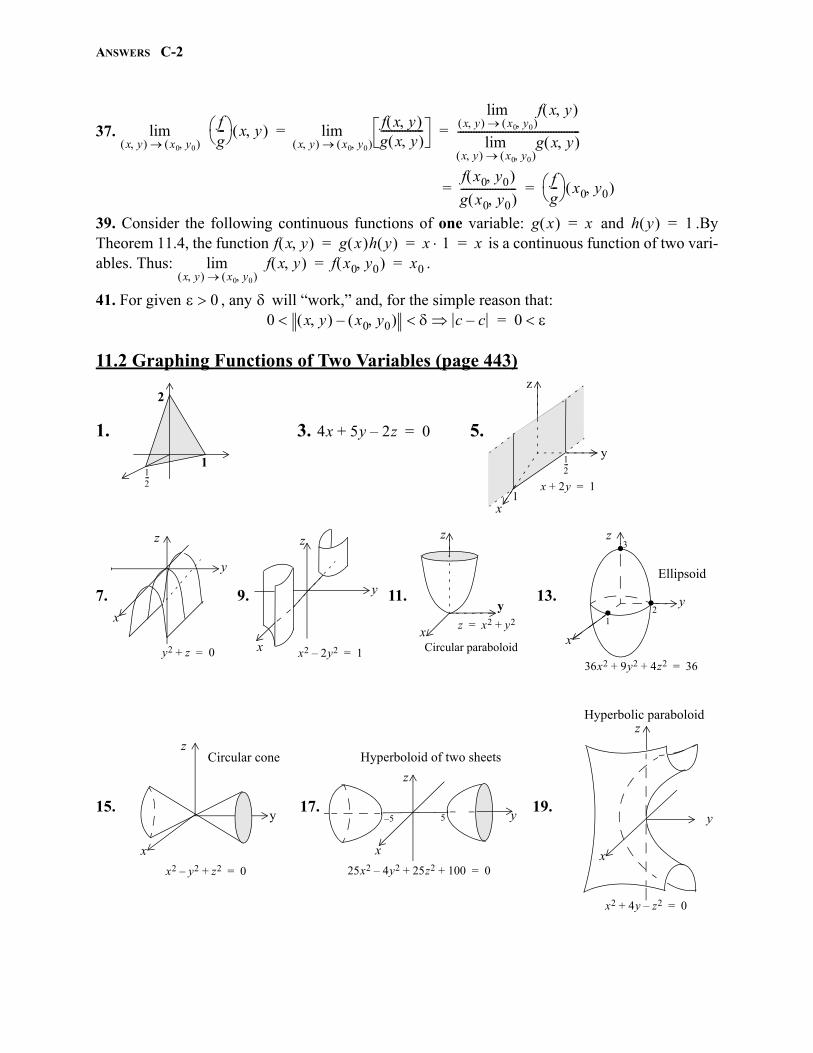
ANSWERS C-2
37.
39. Consider the following continuous functions of one variable: and .ByTheorem 11.4, the function is a continuous function of two vari-ables. Thus: .
41. For given , any will “work,” and, for the simple reason that:
11.2 Graphing Functions of Two Variables (page 443)
1. 3. 5.
7. 9. 11. 13.
15. 17. 19.
fg--- x y
x y x0 y0 lim
f x y g x y ----------------
x y x0 y0 lim
f x y x y x0 y0
lim
g x y x y x0 y0
lim----------------------------------------------= =
f x0 y0 g x0 y0 ---------------------
fg--- x0 y0 = =
g x x= h y 1=f x y g x h y x 1 x= = =
f x y x y x0 y0
lim f x0 y0 x0= =
0 0 x y x0 y0 – c c– 0 =
2
112---
4x 5y 2z–+ 0=
x 2y+ 1=
y
z
x1
12---
y
z
x
y2 z+ 0= x
y
z
x2 2y2– 1= Circular paraboloid
z x2 y2+=x
z
y
x
y
z
Ellipsoid
36x2 9y2 4z2+ + 36=
. .
.
12
3
x
z
x2 y2– z2+ 0=
Circular cone
y y
x
z
5– 5
25x2 4y2– 25z2 100+ + 0=
Hyperboloid of two sheets
Hyperbolic paraboloid
x2 4y z2–+ 0=
y
z
x
gio
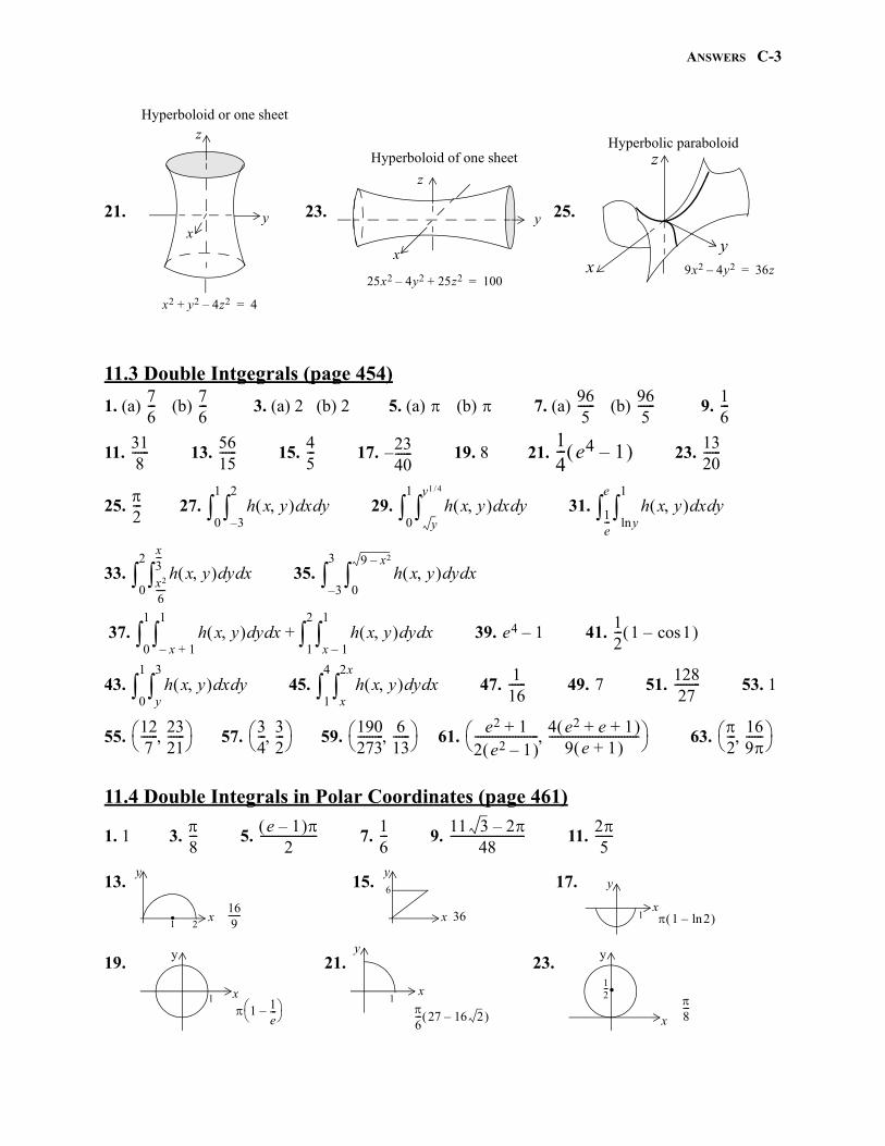
ANSWERS C-3
21. 23. 25.
11.3 Double Intgegrals (page 454)
1. (a) (b) 3. (a) 2 (b) 2 5. (a) (b) 7. (a) (b) 9.
11. 13. 15. 17. 19. 8 21. 23.
25. 27. 29. 31.
33. 35.
37. 39. 41.
43. 45. 47. 49. 51. 53. 1
55. 57. 59. 61. 63.
11.4 Double Integrals in Polar Coordinates (page 461)
1. 1 3. 5. 7. 9. 11.
13. 15. 17.
19. 21. 23.
y
z
x2 y2 4z2–+ 4=
Hyperboloid or one sheet
xy
x
z
25x2 4y2– 25z2+ 100=
Hyperboloid of one sheet
9x2 4y2– 36z=
Hyperbolic paraboloidz
yx
76--- 7
6--- 96
5------ 96
5------ 1
6---
318------ 56
15------ 4
5--- 23
40------–
14--- e4 1– 13
20------
2--- h x y
3–
2
xd yd0
1
h x y y
y1 4/
xd yd0
1
h x y yln
1
xd yd1e---
e
h x y x2
6----
x3---
yd xd0
2
h x y 0
9 x2–
yd xd3–
3
h x y x– 1+
1
yd xd0
1
h x y x 1–
1
yd xd1
2
+ e4 1–12--- 1 1cos–
h x y y
3
xd yd0
1
h x y x
2x
yd xd1
4
116------ 7
12827---------
127------ 23
21------
34--- 3
2---
190273--------- 6
13------
e2 1+2 e2 1– ---------------------- 4 e2 e 1+ +
9 e 1+ -------------------------------
2--- 16
9------
8--- e 1–
2-------------------- 1
6--- 11 3 2–
48-------------------------- 2
5------
2x
y
.1
169
------ x
y
36
6
x
y
1 2ln– 1
1 1 1
e---–
y
x 16--- 27 16 2–
x
y
8---
y
x
.12---
gio
ANSWERS C-4
25. 27. 29. 31. 33.
35. 37. 39. 41. 43. 45.
47. 49. 51. 53. 55.
11.5 Triple Integrals (page 469)
1. 3. 5. 0 7. 9. 11. 13.
15. 17. 19. 2 21. 23. 25. 27.
29. 31. 33. 35. 37. 39.
41. , ,
, ,
43. ,
,
,
45. , ,
,
47. , ,
,
34
------ 9 316
----------– 2--- 1–
38--- 2 3 3+ 2
4---–
6--- 3
4-------+
43---a3 16
3--------- 3
2------ 2
3------ 8 3 3– 64
3--------- 8 3 3– 5
3------
2 – 3 3+ 2a 23
------ 3 2–+ 02120------
09 3
6 3 2–-----------------------
129200--------- 0
43420---------–
124------ 30–
12160------------ 1
3--- 3
2----- 1 1cos–
1200--------- 1
8--- e4 13– 36 1
3--- 3
2------- a5
14--- 4k
5------ 0 0
43---
57--- 0
514------
7a12------ 7a
12------ 7a
12------
3175------ 31
25------ 124
75---------
k x y z zd xd yd0
212---y–
y–
y
0
4
k x y z zd yd xd0
212---y–
x2
4
2–
2
k x y z xd yd zdy–
y
0
2z– 4+
0
2
k x y z xd zd ydy–
y
0
212---y–
0
4
k x y z yd xd zdx2
2z– 4+
4 2z––
4 2z–
0
2
k x y z yd zd xdx2
2z– 4+
0
212---x2–
2–
2
k x y z zd xd yd12--- 4 x2– y––
12--- 4 x2– y–
4 y––
4 y–
0
4
k x y z zd yd xd12--- 4 x2– y––
12--- 4 x2– y–
0
4 x2–
2–
2
k x y z xd yd zd4 4z2– y––
4 4z2– y–
0
4 4z2–
1–
1
k x y z xd zd yd4 4z2– y––
4 4z2– y–
12--- 4 y––
12--- 4 y–
0
4
k x y z yd xd zd0
4 x2– 4z2–
4 4z2––
4 4z2–
1–
1
k x y z yd zd xd0
4 x2– 4z2–
12--- 4 x2––
12--- 4 x2–
2–
2
k x y z zd yd xd0
y
0
x
0
1
k x y z xd yd zdy
1
z
1
0
1
k x y z xd zd ydy
1
0
y
0
1
k x y z yd xd zd
z
x
z
1
0
1
k x y z yd zd xdz
x
0
x
0
1
k x y z zd xd yd0
y2
0
1
1–
0
k x y z xd yd zd0
1
1–
z–
0
1
k x y z xd zd yd0
1
0
y2
1–
0
k x y z yd xd zd1–
z–
0
1
0
1
k x y z yd zd xd1–
z–
0
1
0
1
gio
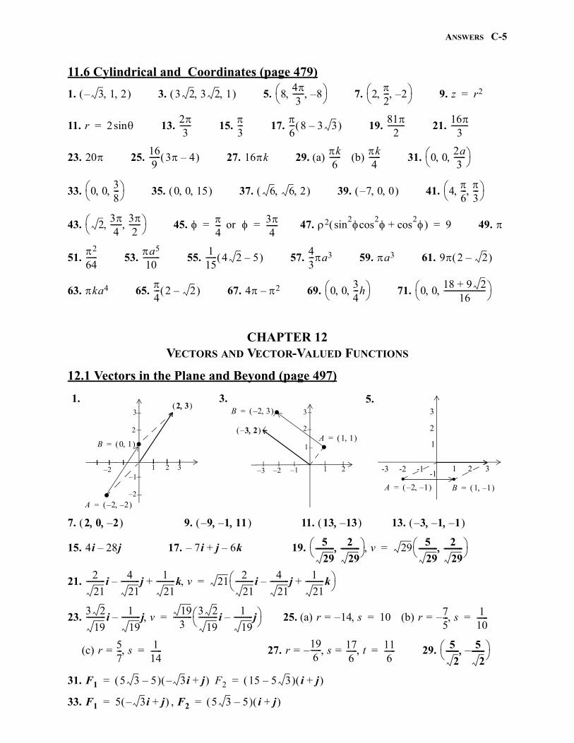
ANSWERS C-5
gio
11.6 Cylindrical and Coordinates (page 479)
1. 3. 5. 7. 9.
11. 13. 15. 17. 19. 21.
23. 25. 27. 29. (a) (b) 31.
33. 35. 37. 39. 41.
43. 45. or 47. 49.
51. 53. 55. 57. 59. 61.
63. 65. 67. 69. 71.
CHAPTER 12VECTORS AND VECTOR-VALUED FUNCTIONS
12.1 Vectors in the Plane and Beyond (page 497)
7. 9. 11. 13.
15. 17. 19.
21.
23. 25. (a) (b)
(c) 27. 29.
31.
33. ,
1. 3. 5.
3– 1 2 3 2 3 2 1 843
------ 8– 2
2--- 2–
z r2=
r 2 sin=23
------ 3---
6--- 8 3 3– 81
2--------- 16
3---------
20 169------ 3 4– 16k
k6
------ k4
------ 0 02a3
------
0 038---
0 0 15 6 6 2 7– 0 0 46---
3---
234
------ 32
------
4---= 3
4------= 2 sin
2cos2 cos
2+ 9=
2
64------ a5
10--------- 1
15------ 4 2 5– 4
3---a3 a3 9 2 2–
ka4 4--- 2 2– 4 2– 0 0
34---h
0 018 9 2+
16----------------------
1 2 3
2
3
..B 0 1 =
2 3
2–
_
_
_
_
1–
2–
A 2– 2– =
1 2
1
2
3
..
1–2–
_
_
_
3–
A 1 1 =
B 2– 3 =
3 2–
1 2 3
1
2
3
-3 -2 -1-1. .
A 2– 1– = B 1 1– =
2 0 2– 9 1 11–– 13 13– 3 1 1–––
4i 28j– 7i– j 6k–+ 5
29---------- 2
29----------
v 29 5
29---------- 2
29----------
=
2
21----------i
4
21----------j–
1
21----------k+ v 21
2
21----------i
4
21----------j–
1
21----------k+
=
3 2
19----------i
1
19----------j– v 19
3---------- 3 2
19----------i
1
19----------j–
= r 14–= s 10= r 75---–= s 1
10------=
r 57---= s 1
14------= r
196------ s– 17
6------= = t 11
6------= 5
2------- 5
2-------–
F1 5 3 5– 3– i j+ = F2 15 5 3– i j+ =
F1 5 3– i j+ = F2 5 3 5– i j+ =
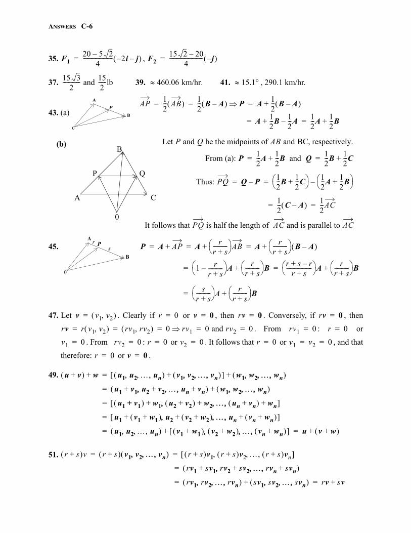
ANSWERS C-6
35. ,
37. 39. 41. , 290.1 km/hr.
43. (a)
(b)
45.
47. Let . Clearly if or , then . Conversely, if , then
. From : or
. From : or . It follows that or , and that
therefore: or .
49.
51.
F120 5 2–
4---------------------- 2– i j– = F2
15 2 20–4
------------------------- j– =
15 32
------------- and 152------lb 460.06 km/hr. 15.1
A
B
0
PAP
12--- AB 1
2--- B A– P A
12--- B A– += = =
A12---B
12---A–+
12---A
12---B+= =
Let P and Q be the midpoints of AB and BC, respectively.
From (a): P12---A
12---B and Q+
12---B
12---C+= =
Thus: PQ Q P–12---B
12---C+
12---A
12---B+
–= =
12--- C A– 1
2---AC= =
It follows that PQ is half the length of AC and is parallel to AC
A C
B
0
P Q
A
B
0
Prs P A AP+ A
rr s+----------- AB+ A
rr s+----------- B A– += = =
1 rr s+-----------–
Ar
r s+----------- B+
r s r–+r s+
------------------- A
rr s+----------- B+= =
sr s+----------- A
rr s+----------- B+=
v v1 v2 = r 0= v 0= rv 0= rv 0=
rv r v1 v2 rv1 rv2 0 rv1 0 and rv2 0= = = = = rv1 0= r 0=
v1 0= rv2 0= r 0= v2 0= r 0= v1 v2 0= =
r 0= v 0=
u v+ w+ u1 u2 un v1 v2 vn + w1 w2 wn +=
u1 v1+ u2 v2+ un vn+ w1 w2 wn +=
u1 v1+ w1+ u2 v2+ w2+ un vn+ wn+ =
u1 v1 w1+ + u2 v2 w2+ + un vn wn+ + =
u1 u2 un v1 w1+ v2 w2+ vn wn+ + u v w+ += =
r s+ v r s+ v1 v2 vn r s+ v1 r s+ v2 r s+ vn = =
rv1 sv1+ rv2 sv2+ rvn svn+ =
rv1 rv2 rvn sv1 sv2 svn + rv sv+= =
gio
ANSWERS C-7
12.2 Dot and Cross Products (Page 510)
1. 3. 5. 7. 9. 11.
13. 15. 17. 19. orthogonal 21. neither
23. 25.
27. 29.
31. 33. 35.
37. (a) Expand both and
and observe that each is equal to .
(b) Expand both
and directly and observe that each is equal to:
(c) Expand both and
directly and observe that each is equal to:
39. (a)
(b) Omitted here. A solution appears in the Student Solutions Manual.
41. (a) First:
26– 7– 60 90 cos1– 5–
17 13-------------------- 110 90
60 135 cos1– 5
1015---------------- 81
2 1 1213------ 8
13------–
1413------ 21
13------+
+= 3j 4k+32---i
32---j+
32---i–
32---j 4k+ +
+=
143------ 28
3------ 14
3------–
103------ 16
3------– 22
3------–
+ 2
3-------– i 2
3-------– j
2
3-------k+
8
3-------i
2
3-------j
10
3-------k+ +
+
25 20 5–– 40i 3j– 42k+ 55
u v– u v– u1 v1– u2 v2– u1 v1– u2 v2– =
u u v– v u v– – u12 2u1v1– v1
2 u22 2u2v2 v2
2+–+ +
u v– u v– u1 v1– u2 v2– u3 v3– u1 v1– u2 v2– u3 v3– =
u u v– v u v– –
u12 2u1v1– v1
2 u22 2u2v2 v2
2+– u32 2u3v3 v3
2+–+ + +
u v– u v– u1 v1– u2 v2– u n vn– u1 v1– u2 v2– u n vn– =
u u v– v u v– –
u12 2u1v1– v1
2 u22 2u2v2 v2
2 un2 2unvn vn
2+–+ + +–+ +
u vu v
---------------u1v1 u2v2+
u12 u2
2+ v12 v2
2+------------------------------------------- 1 u1v1 u2v2+ u1
2 u22+ v1
2 v22+=
u1v1 u2v2+ 2 u12 u2
2+ v12 v2
2+
u12v1
2 2u1v1u2v2 u22v2
2 u12v1
2 u12v2
2 u22v1
2 u22v2
2+ + +++
u12v2
2 2u1v1u2v2 u22v1
2 0+–
True, since u12v2
2 2u1v1u2v2 u22v1
2+– u1v2 u2v1+ 2=
u v+ w u1 v1+ u2 v2+ u3 v3+ w1 w2 w3 =
det
i j k
u1 v1+ u2 v2+ u3 v3+
w1 w2 w3
=
u2w3 v2w3 u3w2– v3w2–+ i u1w3 v1w3 u3w1– v3w1–+ j–=
u1w2 v1w2 u2w1– v2w1–+ + k(*)
gio
ANSWERS C-8
Then show that equals
(b) Expand , , and , and observe that each can
be expressed in the form
(c)
43.
45. Omitted here. A solution appears in the Student Solutions Manual.
47. 20 foot-pounds 49. 10,000 foot-pounds
51.
53. (a) 11.25 foot-pounds (b) 22.5 foot-pounds (c) foot-pounds
55. Show, directly, that both and can be expressed in the form:
u w v w+ det
i j k
u1 u2 u3
w1 w2 w3
det
i j k
v1 v2 v3
w1 w2 w3
+= *
cv w det
i j k
cv1 cv2 cv3
w1 w2 w3
= v cw c v w
c v2w3 v3w2– i v1w3 v3w1– j– v1w2 v2w1– k+
u v det
i j k
u1 u2 u3
v1 v2 v3
detu2 u3
v2 v3
i detu1 u3
v1 v3
j detu1 u2
v1 v2
k+–= =
det–v2 v3
u2 u3
i detv1 v3
u1 u3
j detv1 v2
u1 u2
k–+ det
i j k
v1 v2 v3
u1 u2 u3
– v u –= = =
det a b
c dad bc– bc ad– – det c d
a b–= = =
ab
ai bj+
ai bj–
x
y Diagonals are orhogonal ai bj+ ai bj– 0=
a2 b2– 0=
a b (since both a and b are positive)=
3
OP F= OP F OP F (Theorem 12.6)sin= =45
2 2---------- 15.9
u v w u v wu1v2w3 u1v3w2– u2v1w3– u2v3w1 u3v1w2 u3v2w1–+ +
gio
ANSWERS C-9
12.3 Lines and Planes (Page 520)1. ;
3. ;
5. First, we show that for any given t there is a such that
From the above we also see that for any given there is a t for which (*) is satisfied; namely:
.
7. (a) (b) (c)
9.
11.
13. 15. 17. 19. 21. 23.
25. No unique answers. 27. 29.
31. 33. 35.
12.4 Vector-Valued Functions (Page 531)
1. 3. 5.
7. 9.
11. 13.
15. 17.
19. 21.
23. 25.
27. (a) Proof of Theorem 12.8(a):
w 1 3 t 1 3 += x 1 t y+ 3 3t+= =
w 0 1 1– t 1 1 1 += x t y 1 t z+ 1– t+= = =
t
1 1 t 1 1 1 0 – + 1 0 t 1 0 1 1 – +=
i.e. 1 1 0 t + 1 0 0 t– i.e. 1 1 t+ + 1 t– t 1 t+ –= = =
(*)
tt 1 t+ –=
3 55
---------- 53
------- 666
----------
1 4 2 x 2– y z 3– 0 x 2– 4y 2 z 3– + + 0 x 4y 2z+ + 8= = =
3 2 1– x 1 y 1 z 2––– 0 3 x 1– 2 y 1– z 2– –+ 0 3x 2y z–+ 3= = =
7x y 3z+ + 9= x z+ 1=6
2------- 4 21
7------------- 8 22
11------------- a 3 11
4-------------------=
cos1– 1
3--- 70.5 w 0 1 2 t 3 1 2–– +=
5x 2y 3z+ + 3= 2x 7y– 3z– 13–=95
1817----------------
1x
y
z4
x
y
z
2
2
1 1 4 2 2 4
x
y
z . 3 2 4
.3 1 1–
2i 5j+ 2i 10tj t2i53---t3j C+ ++ sin 1 i j tcos i 2tj tcos– i t3
3----j– C+––
i j k i t2
2----i tj tk C+ + + + + i 3j i
1 tln–t2
----------------k t2
2----i 3tj–
tln 2
2--------------k C+ ++–
i j– 1tan k i 2tj– sec2t k t2
2----i
t3
3----j– tsecln k C+ +++ x 2 2t y+ 5 10t+= =
x t y 2 z– 1= = = v 1 i 2j a 1 + 0 v 1 5= = =
v 0 i j a 0 + k– v 0 2= = = 7556
--------- (at t116------), 230 (at t 6 = =
cu t c u1 t i u2 t j u3 t k+ + cu1 t i cu2 t j cu3 t k+ + = =
cu1 t i cu2 t j cu3 t k+ + cu1 t i cu2 t j cu3 t k+ += =
c u1 t i u2 t j u3 t k+ + cu t = =
gio
ANSWERS C-10
(b) Proof of Theorem 12.8(e):
29.
31. Since :
33. 35.
37. 39. 41. 43.
45. Let be the angle at which a projectile is fired at a speed of ft/sec from the origin, so .
Then:
And:
Maximum range occurs when the vertical component of is zero, so:
The range at that time is the horizontal component of :
Maximum value of the range occurs when .
47. The range, d, when a a projectile is fired at an angle at an initials peed ft/sec is
. Doubling the initial speed results in the range .
u t v t – u1 t i u2 t j u3 t k+ + v1 t i v2 t j v3 t k+ + –=
u1 t v1 t – i u2 t v2 t – j u3 t v3 t – k+ +=
u t v t – u1 t v1 t – i u2 t v2 t – j u3 t v3 t – k+ +=
u1 t i u2 t j u3 t k+ + v1 t i v2 t j v3 t k+ + – u t v t –= =
u f t u1 f t i u2 f t j u3 f t k+ + =
u1 f t i u2 f t j u3 f t k+ +=
u1 f t f t i u2 f t f t j u3 f t f t k+ +=
f t u1 f t i u2 f t j u3 f t k+ + f t u f t = =
tdd f t td i g t td j h t td k+ +
tdd f t td i
tdd g t td j
tdd h t td k++=
f t i g t j h t k+ + r t = =
r t td f t td i g t td j h t td k C+ + +=
500.6 m/sec. Max height: 625/4 ft, Range: 625 ft, Impact speed: 100 2 ft/sec
40 3 ft 95 ft/sec 4 45 21
-------------- 39 ft/sec 3200
3------------ 43 ft/sec
v0 r0 0=
v t 32k– td 32k– v0 cos j v0 sin k+ + v0 cos j 32t– v0 sin+ k+= = =initial velocity
r t v t td v0 cos t j 16t2– v0 sin t+ k (as r0 0 =+= =
r t
16t2– v0 sin t+ 0= 16t v0 tsinv0 sin
16-----------------= =
r t
v0 cos v0 sin
16----------------- v0
2 cossin
16------------------------------
v02
2 cossin32
-------------------------------------v0
22sin
32--------------------= = =
2sin 1 2 90 45= = =
v0
dv0
22sin
32--------------------=
2v0 2 2sin
32------------------------------- 4d=
gio
ANSWERS C-11
gio
49. Since acceleration is zero, the velocity must be constant; say
. It follows that:
(vector equation of a line).
51. Letting g denote the force of gravity we have: . Integrating twice we have:
and:
Letting we have:
.
12.5 Arc Length and Curvature (Page 543)
1. 3. 5. 7. 9.
11. 13.
15.
17. ,
19.
21. 23.
25.
r t v t r t =
r t bj ck+=
r t r t td btj ctk r0+ + r0 t bj ck+ += = =
a t r t gk–= =
v t gtk– v0+ gtk– aj bk+ += =
r t gt2–2
----------k atj btk+ r0+ +gt2–2
----------k atj btk+ cj dk+ + += =
at c+ j gt2–2
---------- bt d+ + k+=
r t xj yk+=
x at c t+x c–
a----------- (note that since the trajectory is non-vertical, a 0 = =
y gt2–2
---------- bt d+ += y12---g
x c–a
----------- 2
bx c–
a----------- d+ +–=
since y is a quadratic function of x,the graph is a parabola.
20 29 2 a 2 a2 b2+ 1 2+ ln x35---s 2 y–
45---s 3+= =
x13--- 3s 1+ 2 3/ 1– 3 2/ y
12--- 3s 1+ 2 3/ 1– == x
s
2------- ysin
s
2------- zcos s
2-------= = =
T t 35--- t 3
5--- tsin–cos 4
5---
= N t tsin– t 0cos– = B t 45--- t 4
5--- tsin–cos 3
5---–
325------= =
T t 1
2------- t tsin–cos i 1
2------- t tsin+cos j+=
N t 1
2------- t tsin–cos– i 1
2------- tsin– tcos+ j, B t + k 1
et 2-----------= = =
T t t
t2 1+------------------ 1
t2 1+------------------ 0
N t 1
t2 1+------------------ t
t2 1+------------------ 0–
B t 0 0 1– 1
t t2 1+ 3 2/------------------------------= = = =
6x– y+ = x 6y+ 6= x
2-------– y
2------- z+ +
4--- x
2------- y
2-------– z+
4---==
x 4---–
2y 3
4---–
2+ 1
16------=
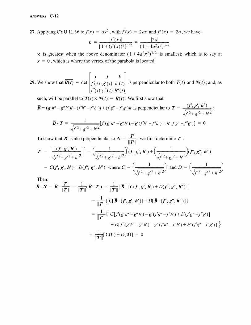
ANSWERS C-12
27. Applying CYU 11.36 to , with and , we have:
is greatest when the above denominator is smallest; which is to say at
, which is where the vertex of the parabola is located.
29. We show that is perpendicular to both and ; and, as
such, will be parallel to . We first show that
is perpendicular to :
To show that is also perpendicular to , we first determine :
Then:
f x ax2= f x 2ax= f x 2a=
f x 1 f x 2+ 3 2/
---------------------------------------- 2a1 4a2x2+ 3 2/
-----------------------------------= =
1 4a2x2+ 3 2/
x 0=
B t det i j k
f t g t h t f t g t h t
= T t N t
T t N t B t =
B gh gh– i= f h f h– j– f g f g– k+ T f g h
f 2 g 2 h 2+ +-----------------------------------=
B T 1
f 2 g 2 h 2+ +----------------------------------- f gh gh– g f h f h– – h f g f g– + 0= =
B N TT
----------= T
T f g h
f 2 g 2 h 2+ +----------------------------------- 1
f 2 g 2 h 2+ +----------------------------------- f g h 1
f 2 g 2 h 2+ +----------------------------------- f g h += =
C f g h D f g h where C+1
f2 g2 h2+ +----------------------------------- and D
1
f 2 g 2 h 2+ +----------------------------------- = = =
B N BTT
---------- 1T
---------- B T 1T
---------- B C f g h D f g h + = = =
1T
---------- C B f g h D B f g h + =
1T
---------- C f gh gh– g f h f h– – h f g f g– + =
D f gh gh– g f h f h– – h f g f g– + +
1T
---------- C 0 D 0 + 0= =
gio
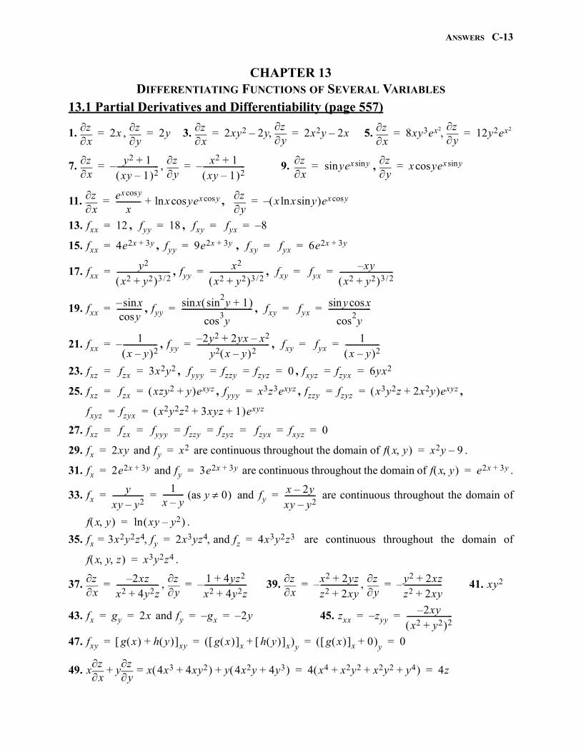
ANSWERS C-13
CHAPTER 13DIFFERENTIATING FUNCTIONS OF SEVERAL VARIABLES
13.1 Partial Derivatives and Differentiability (page 557)
1. , 3. 5.
7. , 9. ,
11. ,
13. , ,
15. , ,
17. , ,
19. , ,
21. , ,
23. , ,
25. , , ,
27.
29. and are continuous throughout the domain of .
31. and are continuous throughout the domain of .
33. and are continuous throughout the domain of
.
35. are continuous throughout the domain of
.
37. , 39. , 41.
43. and 45.
47.
49.
xz 2x=
yz 2y=
xz 2xy2 2y
yz– 2x2y 2x–= =
xz 8xy3ex2
yz 12y2ex2= =
xz y2 1+
xy 1– 2----------------------–=
yz x2 1+
xy 1– 2----------------------–=
xz yex ysinsin=
yz x ycos ex ysin=
xz ex ycos
x------------- x yex ycoscosln+=
yz x x ysinln ex ycos–=
fxx 12= fyy 18= fxy fyx 8–= =
fxx 4e2x 3y+= fyy 9e2x 3y+= fxy fyx 6e2x 3y+= =
fxxy2
x2 y2+ 3 2/----------------------------= fyy
x2
x2 y2+ 3 2/----------------------------= fxy fyx
xy–x2 y2+ 3 2/
----------------------------= =
fxxxsin–ycos
-------------= fyyx sin
2y 1+ sin
cos3y
-------------------------------------= fxy fyxy xcossin
cos2y
----------------------= =
fxx1
x y– 2------------------–= fyy
2– y2 2yx x2–+y2 x y– 2
--------------------------------------= fxy fyx1
x y– 2------------------= =
fxz fzx 3x2y2= = fyyy fzzy fzyz 0= = = fxyz fzyx 6yx2= =
fxz fzx xzy2 y+ exyz= = fyyy x3z3exyz= fzzy fzyz x3y2z 2x2y+ exyz= =
fxyz fzyx x2y2z2 3xyz 1+ + exyz= =
fxz fzx fyyy fzzy fzyz fzyx fxyz 0= = = = = = =
fx 2xy= fy x2= f x y x2y 9–=
fx 2e2x 3y+= fy 3e2x 3y+= f x y e2x 3y+=
fxy
xy y2–----------------
1x y–----------- (as y 0)= = fy
x 2y–xy y2–----------------=
f x y xy y2– ln=
fx 3x2y2z4= fy 2x3yz4 and fz 4x3y2z3= =
f x y z x3y2z4=
xz 2xz–
x2 4y2+ z----------------------=
yz 1 4yz2+
x2 4y2z+----------------------–=
xz x2 2yz+
z2 2xy+--------------------–=
yz y2 2xz+
z2 2xy+--------------------–= xy2
fx gy 2x= = fy gx– 2y–= = zxx z– yy2– xy
x2 y2+ 2------------------------= =
fxy g x h y + xy g x x h y x+ y g x x 0+ y 0= = = =
xx
zy
yz
+ x 4x3 4xy2+ = y 4x2y 4y3+ + 4 x4 x2y2 x2y2 y4+ + + 4z= =
gio
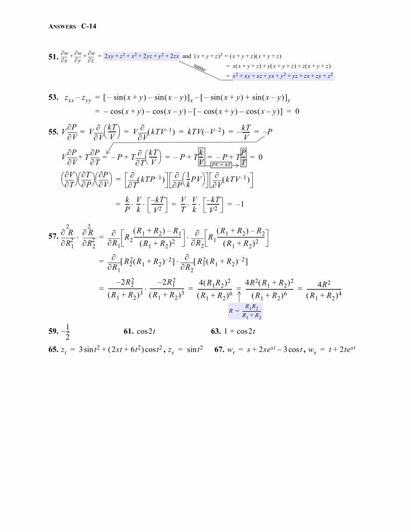
ANSWERS C-14
51.
53.
55.
57.
59. 61. 63.
65. , 67. ,
xw
yw
zw+ + 2xy z2 x2 2yz y2 2zx and x y z+ + 2 x y z+ + x y z+ + =+ + + + +=
x x y z+ + y x y z+ + z x y z+ + + +=
x2 xy xz yx y2 yz zx zy z2+ + + + + + + +=
same
zxx zyy– x y+ sin– x y– sin– x x y+ sin– x y– sin+ y–=
x y+ cos– x y– x y+ cos– x y– cos– –cos– 0= =
VV
PV
V kT
V------ V
V kTV 1– kTV V 2–– kT
V------– P–= = = = =
VV
PT
TP
+ P– TT kT
V------ + P– T
kV---+ P– T
PT---+ 0= = = =
PV kT=
TV
PT
VP
T kTP 1–
P 1
k---PV
V kTV 1– =
kP--- V
k--- kT–
V2--------- V
T--- V
k--- k– T
V2--------- 1–= = =
R12
2
R
R22
2
R
R1 R2
R1 R2+ R1–
R1 R2+ 2-----------------------------------
R2 R1
R1 R2+ R2–
R1 R2+ 2-----------------------------------=
R1 R2
2 R1 R2+ 2– R2 R1
2 R1 R2+ 2– =
2R22–
R1 R2+ 3--------------------------
2R12–
R1 R2+ 3--------------------------
4 R1R2 2
R1 R2+ 6--------------------------
4R2 R1 R2+ 2
R1 R2+ 6------------------------------------ 4R2
R1 R2+ 4--------------------------= = = =
RR1R2
R1 R2+------------------=
12---– 2tcos 1 2tcos+
zt 3 t2 2st 6t2+ t2cos+sin= zs t2sin= wt s 2sest 3 tcos–+= ws t 2test+=
gio
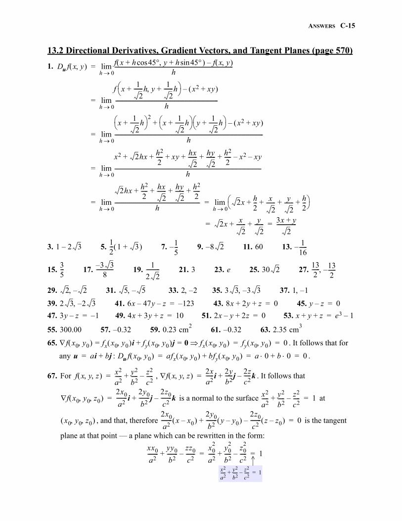
ANSWERS C-15
13.2 Directional Derivatives, Gradient Vectors, and Tangent Planes (page 570)
1.
3. 5. 7. 9. 11. 13.
15. 17. 19. 21. 23. 25. 27.
29. 31. 33. 35. 37.
39. 41. 43. 45.
47. 49. 51. 53.
55. 57. 59. 61. 63.
65. . It follows that for
any : .
67. For , . It follows that
is a normal to the surface at
, and that, therefore is the tangent
plane at that point — a plane which can be rewritten in the form:
Du f x y f x h 45cos+ y h 45sin+ f x y –h
------------------------------------------------------------------------------------------h 0lim=
f x1
2-------h+ y
1
2-------h+
x2 xy+ –
h------------------------------------------------------------------------------
h 0lim=
x1
2-------h+
2x
1
2-------h+
y1
2-------h+
x2 xy+ –+
h-----------------------------------------------------------------------------------------------------------------
h 0lim=
x2 2hx h2
2----- xy hx
2------- hy
2------- h2
2----- x2 xy––+ + + + + +
h----------------------------------------------------------------------------------------------------------------
h 0lim=
2hx h2
2----- hx
2------- hy
2------- h2
2-----+ + + +
h-----------------------------------------------------------------
h 0lim 2x h
2--- x
2------- y
2------- h
2---+ + + +
h 0lim= =
2x x
2------- y
2-------+ + 3x y+
2---------------= =
1 2 3–12--- 1 3+ 1
5---– 8 2– 60 1
16------–
35--- 3 3–
8------------- 1
2 2---------- 3 e 30 2
132------ 13
2------–
2 2– 5 5– 2 2– 3 3 3 3– 1 1–
2 3 2 3– 6x 47y– z– 123–= 8x 2y z+ + 0= y z– 0=
3y z– 1–= 4x 3y z+ + 10= 2x y– 2z+ 0= x y z+ + e3 1–=
300.00 0.32– 0.23 cm2
0.32– 2.35 cm3
f x0 y0 fx x0 y0 i fy x0 y0 j+ 0= = fx x0 y0 fy x0 y0 0= =
u ai bj+= Du f x0 y0 afx x0 y0 bfy x0 y0 + a 0 b 0+ 0= = =
f x y z x2
a2----- y2
b2----- z2
c2-----–+= f x y z 2x
a2------i
2yb2------j
2zc2-----k–+=
f x0 y0 z0 2x0
a2--------i
2y0
b2--------j
2z0
c2--------k–+= x2
a2----- y2
b2----- z2
c2-----–+ 1=
x0 y0 z0 2x0
a2-------- x x0–
2y0
b2-------- y y0–
2z0
c2-------- z z0– –+ 0=
xx0
a2--------
yy0
b2--------
zz0
c2-------–+
x02
a2-----
y02
b2-----
z02
c2-----–+ 1= =
x2
a2----- y2
b2----- z2
c2-----–+ 1=
gio
ANSWERS C-16
69. (a)
(b)
(c)
(d)
13.3 Extreme Values (page 585)1. Saddle point at . 3. Saddle point at . 5. Local maximum at . 7. Local minimum at and at , saddle point at .9. Local minimum at , saddle point at . 11. Local minimum at .
13. None. 15. Local maximum at . 17. Local maximum at .
19. Absolute minimum: ; absolute maximum: .
21. Absolute minimum: ; absolute maximum: .
23. Absolute minimum: ; absolute maximum: .
25. Absolute minimum: ; absolute maximum: .
27. Absolute minimum: ; absolute maximum: .
29. Absolute minimum: ; absolute maximum: .
31. Minimum: ; maximum: .
33. Minimum: ; maximum: .
35. Minimum: ; maximum: .
37. Minimum: ; maximum: .
39. Minimum: ; maximum: .
41. Minimum: ; maximum: .
43. Minimum: ; maximum: .
rf rf xi rf y j rf zk+ + rfxi rfy j rfzk+ + r fxi fy j fzk+ + rf= = = =
f g f g xi f g y j f g zk+ + fx gx i fy gy j fz gz k+ += =
fxi fy j fzk+ + gxi gy j gzk+ + f g= =
fg fg xi fg y j fg zk+ + fgx gfx+ i fgy gfy+ j fgz gfz+ k+ += =
f gxi gy j gzk+ + g fxi fy j gzk+ + + fg gf+= =
fg--- f
g---
xi
fg---
yj
fg---
zk+ +
gfx fgx–
g2--------------------i
gfy fgy–
g2-------------------- j
gfz fgz–
g2--------------------k+ += =
g fxi fy j fzk+ + f gxi gy j gyk+ + –
g2---------------------------------------------------------------------------------------- gf fg–
g2-------------------------= =
5 2 0 0 2– 2– 1 1 1 1–– 0 0 2 1 0 0 2 1–
1 0– 2---
2---
f 3 0 11–= f 3 5 34=
f12--- 1
4---
116------–= f
14--- 2 673
64---------=
f23--- 1
3---
1327------–= f 2 0 6=
f 2 0 3–= f12--- 0 3
4---–=
f 2– 2 9–= f 132---
374------=
f 0 4– 40–= f 15 1 35=
f 1
2-------–
1
2-------
2–= f1
2------- 1
2-------
2=
f 3– 3 f 3 3– 5= = f 3 3 f 3– 3– 23= =
f 1 0 1= f 0 1 2=
f 4 0 11= f 2– 2 3 47=
f 1
2-------– 1
2-------– 2–
3 2–= f1
2------- 1
2------- 2
3 2=
f 0 0 1 f 0 1 0 f 1 0 0 0= = = f13--- 1
3--- 1
3---
127------=
f 0 0 0= f 0 1 2=
gio
ANSWERS C-17
45. Minimum: ; maximum: .
47. Minimum: ; maximum: .
49. Min: ; max: .
51. Min: ; max: .
53. 55. Square base of side ft. and height of ft. 57.
59. 61. 63. 10 in. by 20 in. by 15 in.
65. Base: by ; height 67.
CHAPTER 14VECTOR CALCULUS
14.1 Line Interals (page 601)
1. 3. 5. 7. 9. 11.
13. 0 15. 17. 19. 21. 0 23. 25.
27. 1 29. 7 31. 33. 35. 37. 39.
14.2 Conservative Fields and Path Independence (page 614)1. Not conservative 3. 5. Not conservative 7. Not conservative
9. 11. 13. 15. 20
17. 19. 2 21. 23. 25. 27.
29. 31. 33. 0 35. 1
37. Since and are both potential functions of the same conservative vector field, , which means that (1): and (2): .
Let . From (1): . From (2):
. It follows that .
14.3 Green’s Theorem (page 623)
1. 3. 5. 7. 9. 11. 13. 0 15. 17.
19. 21. 23. 25. 27. 29. 31. 0
f 1 0 7–= f 2– 2 3 47=
f 2
6-------–
3
6------- 1
6-------
2 6–= f2
6------- 3
6-------– 1
6-------–
2 6=
f 2– 1
2-------–
1
2-------
f 21
2------- 1
2-------–
12---= = f 2– 1
2-------– 1
2-------–
f 21
2------- 1
2-------
32---= =
f2
13---------- 3
13----------– 2– 7
13----------+
4 2 13–= f 2
13----------–
3
13---------- 2– 7
13----------–
4 2 13+=
0 0 1 2 41 3/ 6 41 3/ 63
-------
2ab x 50 y 150= =
S3--- S
3---
12--- S
3--- x l
3---= 60=
5 26
---------- 2 23---+
1285
--------- 14--- 37 37 1– 2 2 9+
6------------------- 20 10 218–
27-------------------------------
3 10– 4 8+ 45 803------3+ e 19
6------ e4
2-----–
65--- 1 1sin+cos–
106935
------------ 22 2960------ 8
3---
f x y x2y3 y+=
f x y z ex ycos xyz12---z2+ += f x y z xy2 ye3z+= –
3e13---e2 737
216---------–+ e3 1+ 2
3---– e2 4e 1+ + 2x2y
2xey 12---y4i 2xy3j zk+ +
f x y h x y f h= fx x y hx x y = fy x y hy x y =
k x y f x y h x y –= kx x y 0 k x y k y = =
k y 0 k y C= = f x y h x y – C=
2 12--- 1
4---–
2--- 2
3--- 24– 4
3---– 1 1sin–
112------– 12 r2 1
12------ 3a2
gio
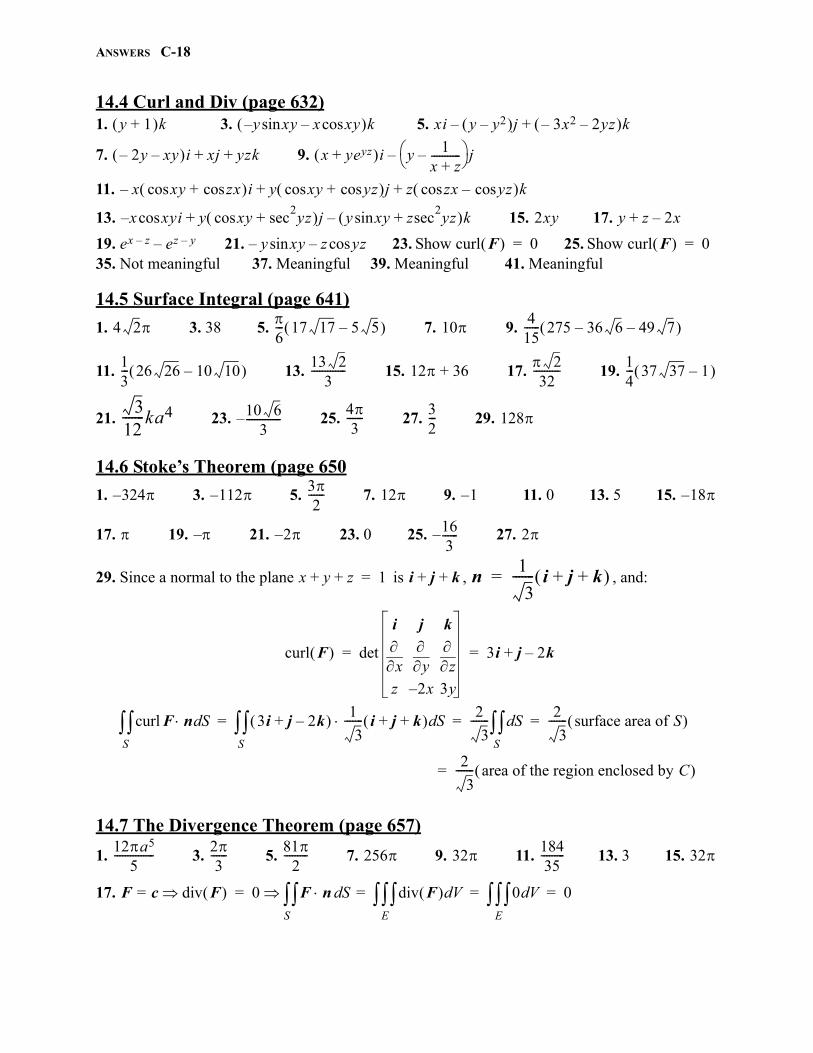
ANSWERS C-18
14.4 Curl and Div (page 632)1. 3. 5.
7. 9.
11.
13. 15. 17.
19. 21. 23. Show 25. Show 35. Not meaningful 37. Meaningful 39. Meaningful 41. Meaningful
14.5 Surface Integral (page 641)
1. 3. 38 5. 7. 9.
11. 13. 15. 17. 19.
21. 23. 25. 27. 29.
14.6 Stoke’s Theorem (page 650
1. 3. 5. 7. 9. 11. 0 13. 5 15.
17. 19. 21. 23. 0 25. 27.
29. Since a normal to the plane is , , and:
14.7 The Divergence Theorem (page 657)
1. 3. 5. 7. 9. 11. 13. 3 15.
17.
y 1+ k y xy x xycos–sin– k xi y y2– j– 3x2– 2yz– k+
2y– xy– i xj yzk+ + x yeyz+ i y 1x z+-----------–
j–
x xy zxcos+cos i– y xcos y yzcos+ j z zx yzcos–cos k+ +
x xyi y xy sec2yz+cos j y xy z+sin sec
2yz k–+cos– 2xy y z 2x–+
ex z– ez y–– y xsin y– z yzcos– curl F 0= curl F 0=
4 2 6--- 17 17 5 5– 10 4
15------ 275 36 6– 49 7–
13--- 26 26 10 10– 13 2
3------------- 12 36+
232
---------- 14--- 37 37 1–
312-------ka4 10 6
3-------------–
43
------ 32--- 128
324– 112–32
------ 12 1– 18–
– 2– 163------– 2
x y z+ + 1= i j k+ + n1
3------- i j k+ + =
curl F det
i j k
x
y
z
z 2x– 3y
3i j 2k–+= =
curl F n SdS 3i j 2k–+ 1
3------- i j k+ + Sd
S
2
3------- Sd
S
2
3------- surface area of S = = =
2
3------- area of the region enclosed by C =
12a5
5--------------- 2
3------ 81
2--------- 256 32 184
35--------- 32
F c= div F 0 F n SdS div F Vd
E 0 Vd
E 0= = = =
gio
INDEX I - 1
AAbsolute Convergence, 356Absolute Value, 1, 577Acceleration, 171, 527Alternating Series, 337
Test, 337Angle Between Vectors, 503Antiderivative, 167Arc Length, 208, 309, 534Area, 177, 449
Between Curves, 158Polar, 378Surface, 633
AsymptoteHorizontal, 138Oblique, 138
Vertical, 139
BBinomial Series, 380Binormal Vector, 536Bounded Sequence, 327Boundary Point, 578
CCenter of Mass, 216, 451Chain Rule, 94, 555Circle of Curvature, 542Composition, 7Comparison Test, 347Concavity, 131Conditional Convergence, 356Conservative Field, 605, 612Continuity, 57, 430, 432Continuous Function, 50, 57, 430Cross Product, 506Critical Point, 125, 575Curl(F), 626Curvature, 539Cylinder, 437Cylindrical Coordinates, 472
DDecomposition of Vectors, 504Decreasing Function, 123Decreasing Sequence, 327Definite Integral, 177Density, 450
DerivativeAt a Point, 66Directional, 560Geometrical Insight, 71Higher Order, 85Of Functions, 29
In Polar Form, 373Partial, 467
Higher Order, 551Determinant, 505Differentiability, 553Differential, 82Differential Equation, 172Discontinuity 48 Jump, 49
Removable, 49Directional Derivative, 560Distance, 5, 14Div(F), 628, 656Divergence Test, 332Divergence Theorem, 654Domain, 3Dot Product, 501Double Integral 440
In Polar Coordinates 457
EElliptic Cone 440Elliptic Paraboloid, 438Ellipsoid, 439Endpoint Extremes, 137Exponential Function
General, 242Natural, 231
Exponential Growth and Decay, 235Extreme Values
Absolute 577Local 574Subject to a constraint, 580Subject to two constraints, 583
FFlux, 652
Across a Curve, 636Across a Closed Curve, 620Across a Surface, 536
Force Field, 612Free Falling Object, 171, 529Function, 2
Absolute Value, 35Composition, 7
gio
I - 2 Index
Continuous, 50, 57, 430Decreasing, 123Domain, 3Graphing, 131Increasing, 123Inverse, 13One-to-One, 11Piece-Wise Defined, 4Range, 3Vector Valued, 523
Fundamental Theorem of Calculus, 180, 605
GGeneralized Power Rule, 95Geometric Series, 334Gradient , 561Graphing Functions, 131
Polynomial, 132Radical, 143Rational, 138
Graphing functions of Two Variables, 435Green’s Theorem, 617, 622, 630
HHelix, 523Higher Order Derivatives, 85Hyperbolic Paraboloid, 441Hyperboloid, 441Horizontal Asymptote, 138
IImplicit Differentiation, 103Improper Integral, 310
Discontinuous, 313Infinite Region, 310, 272, 275
Increasing Sequence, 377Increasing Function, 123Indefinite Integral, 167Induction, 83Inflection Point, 131Instantaneous Rate of Change, 70Integral
Definite, 178Double, 444 In Polar Coordinates, 449Improper, 310, 316Indefinite, 167Triple, 464
Integral Test, 345Integration by Parts, 261Interior Point, 125
Intermediate Value Theorem, 126Inverse Function, 13
Graph, 14 Inverse Trigonometric Functions, 250
JJump Discontinuity, 11
LLagrange Theorem and Multipliers, 580Lagrange Remainder Theorem, 339L’Hopitals’ Rule, 301
“0/0” Type, 301“ ” Type, 304Other Forms, 205
Level Curve, 566Level Surface, 566Limit, 55
Definition, 55, 427, 431Geometrical Interpretation, 47Intuitive, 43One-Sided, 46Uniqueness, 53
Limit Comparison Test, 348Line, 514
Parametric Equation,514Vector Equation, 514
Line Integrals, 591Of Scalar Valued Functions, 591Of Vector Valued Functions, 597 Alternate Notation, 599
Linearization, 82Local Extremes, 121, 574Logarithmic Function,223 Common, 2441 General, 233 Natural, 223
MMaclaurin Series, 375Mass, 450, 594
Center, 451Mathematical Induction, 83Maximum/Minimum Theorem, 127, 574Mean Value Theorem, 121Monotone Sequence, 327
NNatural Exponential Function, 231Natural Logarithmic Function, 223
f
gio
INDEX I - 3
Net Change, 184Norm, 502Normal Vector, 536
OOblique Asymptote, 138One-to-one function, 11Optimization, 149, 574
Using a Graphing Utility, 157Orthogonal Vectors, 503Osculating Circle, 542Osculating Plane, 538
PParallel Planes, 518Parametrization of Curves, 392
Arc Length, 400, 401Parameter, 393
Parametrization of Surfaces, 638Partial Derivatives, 549Partial Fractions, 272Partial Sums, 332Path Independent, 604Pinching Theorem, 89, 324Plane, 516
Normal, 565Tangent, 565Equations
General, 516Scalar, 516Vector, 516
Point of Inflection, 131Polar Coordinates, 405Polar Curves, 407
Area, 416Length, 420
Power Series, 364Functions, 367Interval of Convergence, 365Radius of Convergence, 365
Principal Theorem of Calculus, 161P-Series, 347Pythagorean Theorem, 14
QQuadrant Angle, 31Quadratic Formula, 19Quadratic Surfaces, 437
RRange, 1Rate of Change, 70
Average, 70Instantaneous, 70
Ratio Test, 350, 358Related Rates, 110Removable Discontinuity, 49Rolle’s Theorem, 121Root Test, 351
SSecond Derivative Test, 137Second Partial Derivative Test, 575Sequences, 321
Bounded, 327Convergent, 321Decreasing, 327Divergent, 321Increasing, 327Monotone, 327Subsequence, 328The Algebra of, 323
Set, 1Intersection, 2Union, 2
SeriesAbsolute Convergence, 356Alternating, 327 Error Estimate, 340 Test,337Binomial, 380Conditional Convergence, 356
Rearranging Terms, 360Convergent, 2332Divergent, 232Divergent Test, 332Geometric, 334Maclaurin, 375Of Positive Terms, 347
Comparison Test, 347Integral Test, 307Limit Comparison Test, 348Ratio Test, 350, 358Root Test, 352
P-Series, 347Partial Sums, 232Power Series, 364
Interval of Convergence, 365Radius of Convergence, 365
Taylor, 373Polynomial, 376
gio
I - 4 Index
Smooth Curve, 591Spherical Coordinates, 475Stoke’s Theorem, 644Subsequence, 328Substitutuion Method, 189, 192Surface Area, 633, 639Surface Integral, 635, 640
TTangent Line, 65Tangent Plane, 565Tangent Vector, 527, 536Taylor Convergence Theorem, 378Taylor Inequality, 377Taylor Polynomial, 376Taylor Series, 373Techniques of Integrations, 261
By Part, 261Completing the Square, 270Partial Fractions, 272Trigonometric substitution, 280
Trigonometric Identities, 37Triple Integrals, 454
UUnit Vector, 493
VVector, 487
Addition, 490Component, 504Angle Between Vectors, 503Cross Product, 506
Right-Hand-Rule, 508Decomposition, 504Dot Product, 501Initial Point and Terminal Point, 487Norm, 493Orthogonal Vectors, 504Projection, 504Scalar Product, 489Standard Position, 487Subtraction, 491Tangent, 527Unit, 493Unit Binormal, 536Unit Normal, 536Unit Tangent, 536
Vector-Valued Functions, 523
Continuous,523Derivative, 523Integral, 523Limit, 523
Vector Field, 604Conservative, 605Path-Independent, 604
Velocity, 171, 527Vertical Asymptote, 139Volume of Solids of Revolution, 195
Disk Method, 199Shell Method, 202
Volume (Slicing), 203
WWork, 210, 595
ZZeros and Factors of a Polynomial, 19
gio