Embed Size (px)
Citation preview
Measurement Guide
Cable and Antenna Analyzerfor Anritsu RF and Microwave Handheld Instruments
Site Master™ Cell Master™ PIM Master™ MW82119B
NoteNot all instrument models offer every option or every measurement within a given option. Please refer to the Technical Data Sheet of your instrument for available options and measurements.
Anritsu Company490 Jarvis DriveMorgan Hill, CA 95037-2809USAhttp://www.anritsu.com
Part Number: 10580-00241Revision: C
Published: November 2017Copyright 2017 Anritsu Company
TRADEMARK ACKNOWLEDGMENTSWindows and Windows XP are registered trademarks of Microsoft Corporation.Site Master, Cell Master, and PIM Master are trademarks of Anritsu Company.
NOTICEAnritsu Company has prepared this manual for use by Anritsu Company personnel and customers as aguide for the proper installation, operation and maintenance of Anritsu Company equipment andcomputer programs. The drawings, specifications, and information contained herein are the property ofAnritsu Company, and any unauthorized use or disclosure of these drawings, specifications, andinformation is prohibited; they shall not be reproduced, copied, or used in whole or in part as the basisfor manufacture or sale of the equipment or software programs without the prior written consent ofAnritsu Company.Read the Handheld Instruments Product Information, Compliance, and Safety Guide (PN: 10100-00065)for important safety, legal, and regulatory notices before operating the equipment.
UPDATESUpdates, if any, can be downloaded from the Documents area of the Anritsu web site at:http://www.anritsu.com
Cable & Antenna Analyzer MG PN: 10580-00241 Rev. C Contents-1
Table of Contents
Chapter 1—General Information
1-3 General Measurement Setups . . . . . . . . . . . . . . . . . . . . . . . . . . . . . . . . . . 1-2
Chapter 2—Cable and Antenna Analyzer
2-2 Cable and Antenna Measurement Setup . . . . . . . . . . . . . . . . . . . . . . . . . . 2-1
Calibration . . . . . . . . . . . . . . . . . . . . . . . . . . . . . . . . . . . . . . . . . . . . . . . 2-1
Frequency/Distance. . . . . . . . . . . . . . . . . . . . . . . . . . . . . . . . . . . . . . . . 2-2
2-3 Markers. . . . . . . . . . . . . . . . . . . . . . . . . . . . . . . . . . . . . . . . . . . . . . . . . . . . 2-9
2-4 Trace . . . . . . . . . . . . . . . . . . . . . . . . . . . . . . . . . . . . . . . . . . . . . . . . . . . . 2-12
2-5 Cable and Antenna Measurements Overview . . . . . . . . . . . . . . . . . . . . . 2-14
Line Sweep Fundamentals . . . . . . . . . . . . . . . . . . . . . . . . . . . . . . . . . 2-14
Line Sweep Measurement Types . . . . . . . . . . . . . . . . . . . . . . . . . . . . 2-15
2-6 Line Sweep Measurements . . . . . . . . . . . . . . . . . . . . . . . . . . . . . . . . . . . 2-16
Return Loss Measurement . . . . . . . . . . . . . . . . . . . . . . . . . . . . . . . . . 2-16
2-7 1-Port Measurements . . . . . . . . . . . . . . . . . . . . . . . . . . . . . . . . . . . . . . . . 2-23
Phase Measurements . . . . . . . . . . . . . . . . . . . . . . . . . . . . . . . . . . . . . 2-23
Smith Chart . . . . . . . . . . . . . . . . . . . . . . . . . . . . . . . . . . . . . . . . . . . . . 2-23
2-8 Cable and Antenna Analyzer Menus . . . . . . . . . . . . . . . . . . . . . . . . . . . . 2-25
2-9 Freq Menu . . . . . . . . . . . . . . . . . . . . . . . . . . . . . . . . . . . . . . . . . . . . . . . . 2-27
2-10 Freq/Dist Menu . . . . . . . . . . . . . . . . . . . . . . . . . . . . . . . . . . . . . . . . . . . . . 2-29
2-11 Amplitude Menu . . . . . . . . . . . . . . . . . . . . . . . . . . . . . . . . . . . . . . . . . . . . 2-30
2-12 Sweep/Setup Menu . . . . . . . . . . . . . . . . . . . . . . . . . . . . . . . . . . . . . . . . . 2-31
2-13 Measurement Menu . . . . . . . . . . . . . . . . . . . . . . . . . . . . . . . . . . . . . . . . . 2-32
2-14 Marker Menu. . . . . . . . . . . . . . . . . . . . . . . . . . . . . . . . . . . . . . . . . . . . . . . 2-34
2-15 Sweep Menu. . . . . . . . . . . . . . . . . . . . . . . . . . . . . . . . . . . . . . . . . . . . . . . 2-35
2-17 Trace Menu. . . . . . . . . . . . . . . . . . . . . . . . . . . . . . . . . . . . . . . . . . . . . . . . 2-35
2-18 Limit Menu . . . . . . . . . . . . . . . . . . . . . . . . . . . . . . . . . . . . . . . . . . . . . . . . 2-36
2-19 Other Menus. . . . . . . . . . . . . . . . . . . . . . . . . . . . . . . . . . . . . . . . . . . . . . . 2-38
Chapter 3—Calibration
3-2 Chapter Overview. . . . . . . . . . . . . . . . . . . . . . . . . . . . . . . . . . . . . . . . . . . . 3-1
3-3 Calibration Methods . . . . . . . . . . . . . . . . . . . . . . . . . . . . . . . . . . . . . . . . . . 3-1
3-4 Calibration Verification . . . . . . . . . . . . . . . . . . . . . . . . . . . . . . . . . . . . . . . . 3-2
Trace Characteristics in Return Loss Mode . . . . . . . . . . . . . . . . . . . . . 3-2
Contents-2 PN: 10580-00241 Rev. C Cable & Antenna Analyzer MG
Table of Contents (Continued)
3-5 Calibration Procedures . . . . . . . . . . . . . . . . . . . . . . . . . . . . . . . . . . . . . . . . 3-3
OSL Calibration Procedure (Standard and FlexCal) . . . . . . . . . . . . . . . 3-3
InstaCal Module Calibration Procedures (Standard and FlexCal) . . . . . 3-4
3-6 InstaCal Module Verification . . . . . . . . . . . . . . . . . . . . . . . . . . . . . . . . . . . . 3-5
3-7 Calibrate Menu . . . . . . . . . . . . . . . . . . . . . . . . . . . . . . . . . . . . . . . . . . . . . . 3-5
Appendix A—Windowing
Index
Cable & Antenna Analyzer MG PN: 10580-00241 Rev. C 1-1
Chapter 1 — General Information
1-1 IntroductionThe Site Master, Cell Master, and PIM Master (MW82119B with Option 331) offer a wide range of cable and antenna measurements: Return Loss, VSWR, Cable Loss, Distance-To-Fault RL, Distance-To-Fault VSWR, 1-Port Phase, and Smith Chart. This manual provides setup and measurement procedures for each measurement. It also includes a line sweep fundamentals overview section.
1-2 Contacting Anritsu To contact Anritsu, visit the following URL and select the services in your region:http://www.anritsu.com/contact-us.
Updated product information can be found on the Anritsu web site:
http://www.anritsu.com/
Search for the product model number. The latest documentation is on the product page under the Library tab.
Read the Handheld Instruments Product Information, Compliance, and Safety Guide (PN: 10100-00065) for important safety, legal, and regulatory notices before operating the equipment.
1-2 PN: 10580-00241 Rev. C Cable & Antenna Analyzer MG
1-3 General Measurement Setups The User Guide for your instrument provides a general overview of file management, system settings, and GPS. Chapter 2 of this guide provides specific setup, measurement, and menu information for cable and antenna measurements.
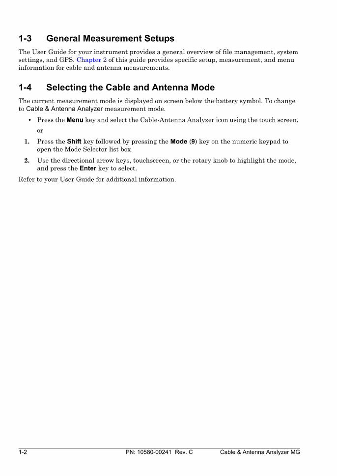
1-4 Selecting the Cable and Antenna ModeThe current measurement mode is displayed on screen below the battery symbol. To change to Cable & Antenna Analyzer measurement mode.
• Press the Menu key and select the Cable-Antenna Analyzer icon using the touch screen.
or
1. Press the Shift key followed by pressing the Mode (9) key on the numeric keypad to open the Mode Selector list box.
2. Use the directional arrow keys, touchscreen, or the rotary knob to highlight the mode, and press the Enter key to select.
Refer to your User Guide for additional information.
Cable & Antenna Analyzer MG PN: 10580-00241 Rev. C 2-1
Chapter 2 — Cable and Antenna Analyzer
2-1 OverviewThis chapter shows how to setup the instrument and perform basic line sweep measurements.
2-2 Cable and Antenna Measurement SetupThis section covers the following measurement setups functions:
• “Select Measurement Type” on page 2-1
• “Calibration” on page 2-1
• “Frequency” on page 2-2
• “Amplitude” on page 2-3
• “Sweep/Setup” on page 2-3
• “Display Setup” on page 2-6
• “Limit Lines” on page 2-7
Select Measurement Type
Press the Measurement main menu key and select the appropriate measurement. The setup instructions below apply to all cable and antenna measurements. For specific instructions on how to setup Distance-To-Fault, refer to “Distance-To-Fault (DTF)” on page 2-18.
Calibration
For accurate results, the instrument must be calibrated before making any measurements.
The instrument must be re-calibrated whenever the temperature exceeds the calibration temperature range or when the test port extension cable is removed or replaced. Unless the calibration type is Flexcal, the instrument must also be re-calibrated every time the setup frequency changes. See Chapter 3, “Calibration” for details on how to perform a calibration.
NoteConfirm that the instrument is in Cable and Antenna Analyzer mode. Refer to “Selecting the Cable and Antenna Mode” on page 1-2.
2-2 Cable and Antenna Measurement Setup Cable and Antenna Analyzer
2-2 PN: 10580-00241 Rev. C Cable & Antenna Analyzer MG
Frequency
(for VSWR, Return Loss, Cable Loss, Smith Chart, 1-Port Phase measurements)
Setting up the Measurement Frequency using Start and Stop Frequencies
1. Press the Freq/Dist main menu key.
2. Press the Start Freq submenu key and use the keypad to enter the start frequency. When entering a frequency using the keypad, the soft key labels change to GHz, MHz, kHz, and Hz. Press the appropriate unit key to complete the entry.
3. Press Stop Freq and use the keypad to enter the stop frequency. Press the appropriate unit key to complete the entry.
Setting up the Measurement Frequency by Selecting a Signal Standard
1. Press the Freq/Dist main menu key.
2. Press the Signal Standard submenu key.
3. Select uplink, downlink, or uplink plus downlink.
4. Press the Select Standard key.
5. Use the rotary knob or the Up/Down arrow keys and scroll to the appropriate signal standard and press Enter to select.
Frequency/Distance
(Distance-To-Fault Return Loss, Distance-To-Fault VSWR)
1. Press the Freq/Dist main menu key.
2. Press the Start Dist submenu key and use the keypad to enter the start distance.When entering a distance using the keypad, the key label changes to m or ft. Press the unit key or Enter to complete the entry.
3. Press Stop Dist and use the keypad to enter the stop distance. Press the unit key or Enter to complete the entry.
4. To set the frequency, press DTF Aid. For more details about DTF Aid, refer to “DTF Setup” on page 2-19.
Refer to “Freq Menu” on page 2-27 for additional information.
NoteThe Signal Standard menu can be customized. If a particular standard is missing, Master Software Tools (MST) can be used to edit the signal standard list. Please see the MST manual for more details.

Cable and Antenna Analyzer 2-2 Cable and Antenna Measurement Setup
Cable & Antenna Analyzer MG PN: 10580-00241 Rev. C 2-3
Amplitude
(For Amplitude in Smith Chart measurements, see “Smith Chart” on page 2-23)
Setting the Amplitude using Top and Bottom Keys
1. Press the Amplitude main menu key.
2. Press the Top submenu key and use the keypad, rotary knob, or the Up/Down arrow key to edit the top scale value. Press Enter to set.
3. Press the Bottom key and use the keypad, rotary knob, or the Up/Down arrow key to edit the bottom scale value. Press Enter to set.
Setting the Amplitude using Autoscale
The instrument will automatically set the top and bottom scales to the minimum and maximum values of the measurement with some margin on the y-axis of the display.
1. Press the Amplitude main menu key
2. Press the Autoscale submenu key
Setting the Amplitude using Fullscale
To automatically set the scale to the default setting (0 dB to 60 dB for Return Loss and 1 to 65.535 for VSWR), press the Fullscale key. The instrument will automatically set the top and bottom scales to the default values.
1. Press the Amplitude main menu key.
2. Press the Fullscale submenu key.
Refer to “Amplitude Menu” on page 2-30 for additional information.
Sweep/Setup
The sweep/setup menus include keys to set Run/Hold, Sweep Type, RF Immunity, Data Points, Average / Smoothing, and Output power.
Run/Hold
When in the Hold mode, this key starts the instrument sweeping and provides a Single Sweep Mode trigger; when in the Run mode, it pauses the sweep.
1. Press the Sweep/Setup main menu key.
2. Toggle the Run/Hold key.
Sweep Type Single and Continuous
This toggles the sweep between single sweep and continuous sweep. In single sweep mode, each sweep must be activated by the Run/Hold key.
1. Press the Sweep/Setup main menu key.
2. Toggle the Single/Continuous key.
2-2 Cable and Antenna Measurement Setup Cable and Antenna Analyzer
2-4 PN: 10580-00241 Rev. C Cable & Antenna Analyzer MG
RF Immunity High / Low
The instrument defaults to RF Immunity High. This setting protects the instrument from stray signals from nearby or co-located transmitters that can affect frequency and DTF measurements. The algorithm used to improve instrument’s ability to reject unwanted signals slows down the sweep speed. If the instrument is used in an environment where immunity is not as issue, the RF Immunity key can be set to Low to optimize sweep speed. Use this feature with caution, as the introduction of an interfering signal might be mistaken for a problem with the antenna or cable run. If Immunity is set to Low during a normal RL or VSWR measurement, the instrument will be more susceptible to interfering signals. Interfering signals can make the measurement look better or worse than it really is.
1. Press the Sweep/Setup main menu key.
2. Toggle the RF Immunity High/Low key.
Data Points
The number of data points can be set to 137, 275, 551, 1102, and 2204 data points. This can be changed before or after calibration regardless of the display setting. The default setting is 275. This is recommended for most measurements. More data points slow down the sweep speed. More data points are helpful in DTF as this enables better coverage for the same fault resolution.
1. Press the Sweep/Setup main menu key.
2. Select 137, 275, 551, 1102, or 2204 data points.
Refer to “Sweep/Setup Menu” on page 2-31 for additional information about the Sweep/Setup main menu and submenus.
Averaging
Averaging helps to average out the trace and minimize the effect of outliers. Trace averaging takes the running average of the number of traces indicated in the Averaging Factor. The Average Count in the status window turns on if Averaging is turned on. When the Average Count reaches the entered average count, a running average of the last set of sweeps is performed. Averaging Factor can be set between 1 and 65535.
1. Press the Sweep/Setup main menu key.
2. Press the Averaging/Smoothing submenu key.
3. Press Averaging Factor and enter the number of running averages using the keypad, then press the Enter key.
4. Press the Averaging On/Off key and toggle Averaging to On.
5. Use the Restart key to start the averaging sequence from the beginning.
Cable and Antenna Analyzer 2-2 Cable and Antenna Measurement Setup
Cable & Antenna Analyzer MG PN: 10580-00241 Rev. C 2-5
Smoothing %
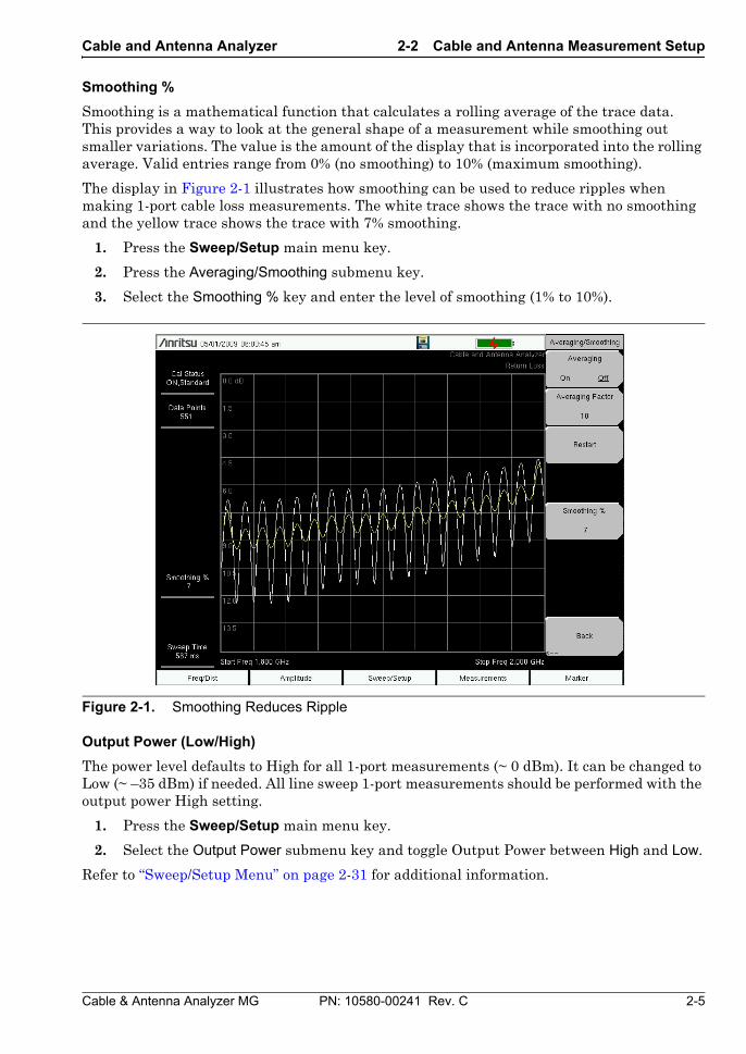
Smoothing is a mathematical function that calculates a rolling average of the trace data. This provides a way to look at the general shape of a measurement while smoothing out smaller variations. The value is the amount of the display that is incorporated into the rolling average. Valid entries range from 0% (no smoothing) to 10% (maximum smoothing).
The display in Figure 2-1 illustrates how smoothing can be used to reduce ripples when making 1-port cable loss measurements. The white trace shows the trace with no smoothing and the yellow trace shows the trace with 7% smoothing.
1. Press the Sweep/Setup main menu key.
2. Press the Averaging/Smoothing submenu key.
3. Select the Smoothing % key and enter the level of smoothing (1% to 10%).
Output Power (Low/High)
The power level defaults to High for all 1-port measurements (~ 0 dBm). It can be changed to Low (~ –35 dBm) if needed. All line sweep 1-port measurements should be performed with the output power High setting.
1. Press the Sweep/Setup main menu key.
2. Select the Output Power submenu key and toggle Output Power between High and Low.
Refer to “Sweep/Setup Menu” on page 2-31 for additional information.
Figure 2-1. Smoothing Reduces Ripple
2-2 Cable and Antenna Measurement Setup Cable and Antenna Analyzer
2-6 PN: 10580-00241 Rev. C Cable & Antenna Analyzer MG
Display Setup
Single and Dual Display
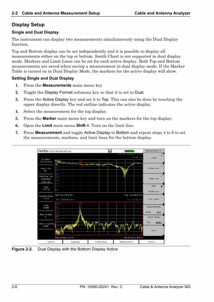
The instrument can display two measurements simultaneously using the Dual Display function.
Top and Bottom display can be set independently and it is possible to display all measurements either on the top or bottom. Smith Chart is not supported in dual display mode. Markers and Limit Lines can be set for each active display. Both Top and Bottom measurements are saved when saving a measurement in dual display mode. If the Marker Table is turned on in Dual Display Mode, the markers for the active display will show.
Setting Single and Dual Display
1. Press the Measurements main menu key
2. Toggle the Display Format submenu key so that it is set to Dual.
3. Press the Active Display key and set it to Top. This can also be done by touching the upper display directly. The red outline indicates the active display.
4. Select the measurement for the top display.
5. Press the Marker main menu key and turn on the markers for the top display.
6. Open the Limit main menu Shift-6. Turn on the limit line.
7. Press Measurement and toggle Active Display to Bottom and repeat steps 4 to 6 to set the measurements, markers, and limit lines for the bottom display.
Figure 2-2. Dual Display with the Bottom Display Active
Cable and Antenna Analyzer 2-2 Cable and Antenna Measurement Setup
Cable & Antenna Analyzer MG PN: 10580-00241 Rev. C 2-7
Limit Lines
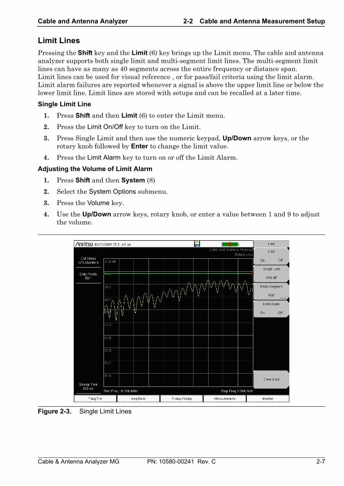
Pressing the Shift key and the Limit (6) key brings up the Limit menu. The cable and antenna analyzer supports both single limit and multi-segment limit lines. The multi-segment limit lines can have as many as 40 segments across the entire frequency or distance span. Limit lines can be used for visual reference , or for pass/fail criteria using the limit alarm. Limit alarm failures are reported whenever a signal is above the upper limit line or below the lower limit line. Limit lines are stored with setups and can be recalled at a later time.
Single Limit Line
1. Press Shift and then Limit (6) to enter the Limit menu.
2. Press the Limit On/Off key to turn on the Limit.
3. Press Single Limit and then use the numeric keypad, Up/Down arrow keys, or the rotary knob followed by Enter to change the limit value.
4. Press the Limit Alarm key to turn on or off the Limit Alarm.
Adjusting the Volume of Limit Alarm
1. Press Shift and then System (8)
2. Select the System Options submenu.
3. Press the Volume key.
4. Use the Up/Down arrow keys, rotary knob, or enter a value between 1 and 9 to adjust the volume.
Figure 2-3. Single Limit Lines
2-2 Cable and Antenna Measurement Setup Cable and Antenna Analyzer
2-8 PN: 10580-00241 Rev. C Cable & Antenna Analyzer MG
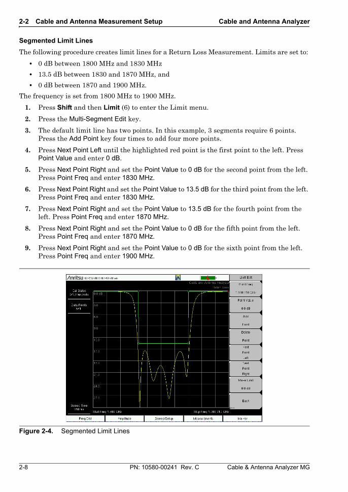
Segmented Limit Lines
The following procedure creates limit lines for a Return Loss Measurement. Limits are set to:
• 0 dB between 1800 MHz and 1830 MHz
• 13.5 dB between 1830 and 1870 MHz, and
• 0 dB between 1870 and 1900 MHz.
The frequency is set from 1800 MHz to 1900 MHz.
1. Press Shift and then Limit (6) to enter the Limit menu.
2. Press the Multi-Segment Edit key.
3. The default limit line has two points. In this example, 3 segments require 6 points. Press the Add Point key four times to add four more points.
4. Press Next Point Left until the highlighted red point is the first point to the left. Press Point Value and enter 0 dB.
5. Press Next Point Right and set the Point Value to 0 dB for the second point from the left. Press Point Freq and enter 1830 MHz.
6. Press Next Point Right and set the Point Value to 13.5 dB for the third point from the left. Press Point Freq and enter 1830 MHz.
7. Press Next Point Right and set the Point Value to 13.5 dB for the fourth point from the left. Press Point Freq and enter 1870 MHz.
8. Press Next Point Right and set the Point Value to 0 dB for the fifth point from the left. Press Point Freq and enter 1870 MHz.
9. Press Next Point Right and set the Point Value to 0 dB for the sixth point from the left. Press Point Freq and enter 1900 MHz.
Figure 2-4. Segmented Limit Lines
Cable and Antenna Analyzer 2-3 Markers
Cable & Antenna Analyzer MG PN: 10580-00241 Rev. C 2-9
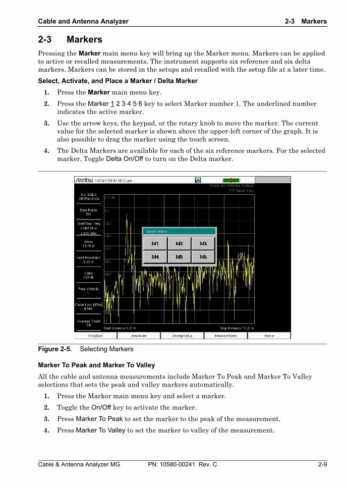
2-3 Markers Pressing the Marker main menu key will bring up the Marker menu. Markers can be applied to active or recalled measurements. The instrument supports six reference and six delta markers. Markers can be stored in the setups and recalled with the setup file at a later time.
Select, Activate, and Place a Marker / Delta Marker
1. Press the Marker main menu key.
2. Press the Marker 1 2 3 4 5 6 key to select Marker number 1. The underlined number indicates the active marker.
3. Use the arrow keys, the keypad, or the rotary knob to move the marker. The current value for the selected marker is shown above the upper-left corner of the graph. It is also possible to drag the marker using the touch screen.
4. The Delta Markers are available for each of the six reference markers. For the selected marker, Toggle Delta On/Off to turn on the Delta marker.
Marker To Peak and Marker To Valley
All the cable and antenna measurements include Marker To Peak and Marker To Valley selections that sets the peak and valley markers automatically.
1. Press the Marker main menu key and select a marker.
2. Toggle the On/Off key to activate the marker.
3. Press Marker To Peak to set the marker to the peak of the measurement.
4. Press Marker To Valley to set the marker to valley of the measurement.
Figure 2-5. Selecting Markers
2-3 Markers Cable and Antenna Analyzer
2-10 PN: 10580-00241 Rev. C Cable & Antenna Analyzer MG
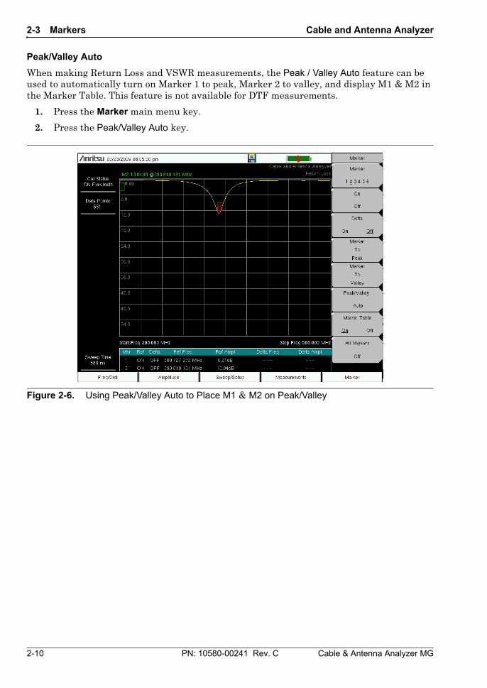
Peak/Valley Auto
When making Return Loss and VSWR measurements, the Peak / Valley Auto feature can be used to automatically turn on Marker 1 to peak, Marker 2 to valley, and display M1 & M2 in the Marker Table. This feature is not available for DTF measurements.
1. Press the Marker main menu key.
2. Press the Peak/Valley Auto key.
Figure 2-6. Using Peak/Valley Auto to Place M1 & M2 on Peak/Valley
Cable and Antenna Analyzer 2-3 Markers
Cable & Antenna Analyzer MG PN: 10580-00241 Rev. C 2-11
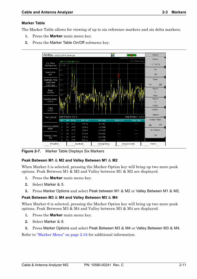
Marker Table
The Marker Table allows for viewing of up to six reference markers and six delta markers.
1. Press the Marker main menu key.
2. Press the Marker Table On/Off submenu key.
Peak Between M1 & M2 and Valley Between M1 & M2
When Marker 5 is selected, pressing the Marker Option key will bring up two more peak options. Peak Between M1 & M2 and Valley between M1 & M2 are displayed.
1. Press the Marker main menu key.
2. Select Marker & 5.
3. Press Marker Options and select Peak between M1 & M2 or Valley Between M1 & M2.
Peak Between M3 & M4 and Valley Between M3 & M4
When Marker 6 is selected, pressing the Marker Option key will bring up two more peak options. Peak Between M3 & M4 and Valley between M3 & M4 are displayed.
1. Press the Marker main menu key.
2. Select Marker & 6.
3. Press Marker Options and select Peak Between M3 & M4 or Valley Between M3 & M4.
Refer to “Marker Menu” on page 2-34 for additional information.
Figure 2-7. Marker Table Displays Six Markers
2-4 Trace Cable and Antenna Analyzer
2-12 PN: 10580-00241 Rev. C Cable & Antenna Analyzer MG
2-4 Trace Pressing the Shift key and the Trace (5) key brings up the Trace main menu. The trace math menu inside the cable and antenna analyzer supports Trace Overlay features to allow viewing a two traces at the same time. This is useful when comparing a stored trace to a live trace. Trace Math operations include Trace – Memory and Trace + Memory. It is possible to copy a trace to display memory directly from the trace math menu. Traces can also be downloaded from Master Software Tools into the instrument and compared with live traces.
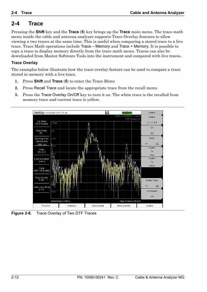
Trace Overlay
The examples below illustrate how the trace overlay feature can be used to compare a trace stored in memory with a live trace.
1. Press Shift and Trace (5) to enter the Trace Menu
2. Press Recall Trace and locate the appropriate trace from the recall menu.
3. Press the Trace Overlay On/Off key to turn it on. The white trace is the recalled from memory trace and current trace is yellow.
Figure 2-8. Trace Overlay of Two DTF Traces
Cable and Antenna Analyzer 2-4 Trace
Cable & Antenna Analyzer MG PN: 10580-00241 Rev. C 2-13
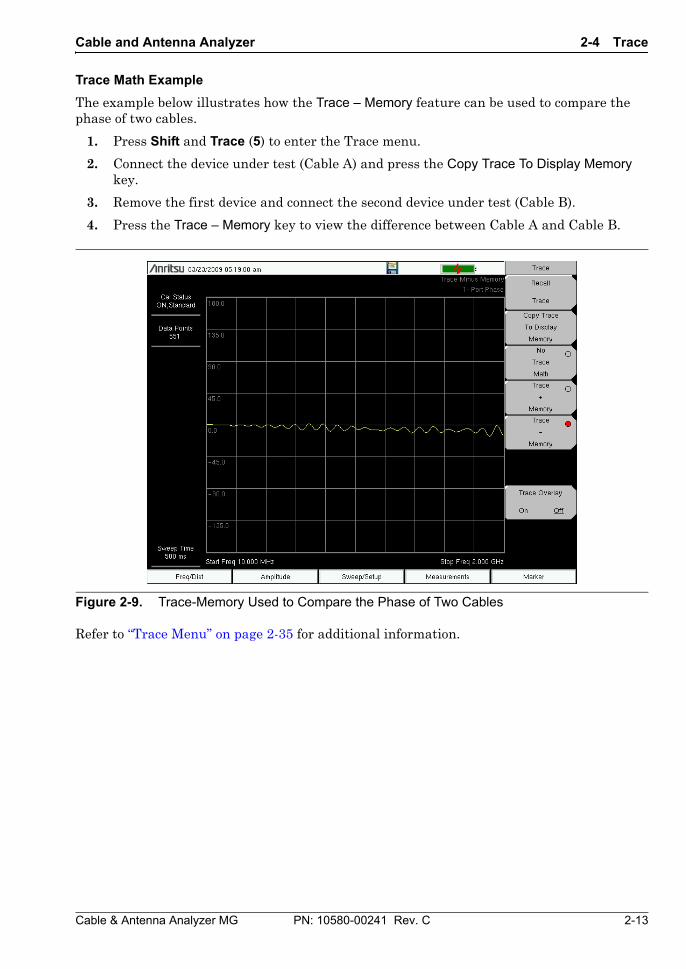
Trace Math Example
The example below illustrates how the Trace – Memory feature can be used to compare the phase of two cables.
1. Press Shift and Trace (5) to enter the Trace menu.
2. Connect the device under test (Cable A) and press the Copy Trace To Display Memory key.
3. Remove the first device and connect the second device under test (Cable B).
4. Press the Trace – Memory key to view the difference between Cable A and Cable B.
Refer to “Trace Menu” on page 2-35 for additional information.
Figure 2-9. Trace-Memory Used to Compare the Phase of Two Cables
2-5 Cable and Antenna Measurements Overview Cable and Antenna Analyzer
2-14 PN: 10580-00241 Rev. C Cable & Antenna Analyzer MG
2-5 Cable and Antenna Measurements Overview
Line Sweep Fundamentals
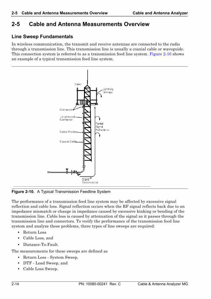
In wireless communication, the transmit and receive antennas are connected to the radio through a transmission line. This transmission line is usually a coaxial cable or waveguide. This connection system is referred to as a transmission feed line system. Figure 2-10 shows an example of a typical transmission feed line system.
The performance of a transmission feed line system may be affected by excessive signal reflection and cable loss. Signal reflection occurs when the RF signal reflects back due to an impedance mismatch or change in impedance caused by excessive kinking or bending of the transmission line. Cable loss is caused by attenuation of the signal as it passes through the transmission line and connectors. To verify the performance of the transmission feed line system and analyze these problems, three types of line sweeps are required:
• Return Loss• Cable Loss, and
• Distance-To-Fault.
The measurements for these sweeps are defined as
• Return Loss - System Sweep, • DTF - Load Sweep, and • Cable Loss Sweep.
Figure 2-10. A Typical Transmission Feedline System
Cable and Antenna Analyzer 2-5 Cable and Antenna Measurements Overview
Cable & Antenna Analyzer MG PN: 10580-00241 Rev. C 2-15
Line Sweep Types
Return Loss / VSWR Measurement
Return Loss measures the reflected power of the system in decibels (dB). This measurement can also be taken in the Standing Wave Ratio (SWR) mode, which is the ratio of the transmitted power to the reflected power.
Cable Loss Measurement
Measures the energy absorbed, or lost, by the transmission line in dB/meter or dB/ft. Different transmission lines have different losses, and the loss is frequency and distance specific. The higher the frequency or longer the distance, the greater the loss.
Distance-To-Fault (DTF) Measurement
Reveals the precise fault location of components in the transmission line system. This test helps to identify specific problems in the system, such as connector transitions, jumpers, kinks in the cable or moisture intrusion.
Line Sweep Measurement Types
Return Loss – System Sweep
A measurement made when the antenna is connected at the end of the transmission line. This measurement provides an analysis of how the various components of the system are interacting and provides an aggregate return loss of the entire system.
Distance To Fault – Load Sweep
A measurement is made with the antenna disconnected and replaced with a 50Ω precision load at the end of the transmission line. This measurement allows analysis of the various components of the transmission feed line system in the DTF mode.
Cable Loss Sweep
A measurement made when a short is connected at the end of the transmission line. This condition allows analysis of the signal loss through the transmission line and identifies the problems in the system. High insertion loss in the feed line or jumpers can contribute to poor system performance and loss of coverage.
This whole process of measurements and testing the transmission line system is called Line Sweeping.
2-6 Line Sweep Measurements Cable and Antenna Analyzer
2-16 PN: 10580-00241 Rev. C Cable & Antenna Analyzer MG
2-6 Line Sweep Measurements This section provides typical line sweep measurements used to analyze the performance of a transmission feed line system including Return Loss, Cable Loss, and DTF.
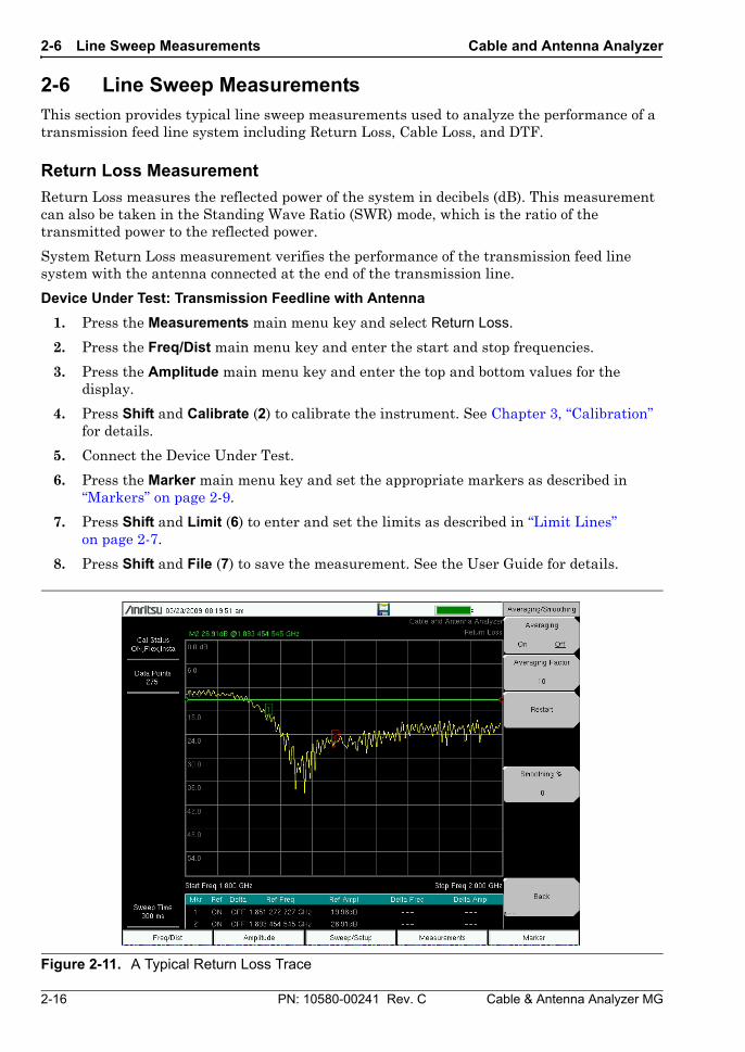
Return Loss Measurement
Return Loss measures the reflected power of the system in decibels (dB). This measurement can also be taken in the Standing Wave Ratio (SWR) mode, which is the ratio of the transmitted power to the reflected power.
System Return Loss measurement verifies the performance of the transmission feed line system with the antenna connected at the end of the transmission line.
Device Under Test: Transmission Feedline with Antenna
1. Press the Measurements main menu key and select Return Loss.
2. Press the Freq/Dist main menu key and enter the start and stop frequencies.
3. Press the Amplitude main menu key and enter the top and bottom values for the display.
4. Press Shift and Calibrate (2) to calibrate the instrument. See Chapter 3, “Calibration” for details.
5. Connect the Device Under Test.
6. Press the Marker main menu key and set the appropriate markers as described in “Markers” on page 2-9.
7. Press Shift and Limit (6) to enter and set the limits as described in “Limit Lines” on page 2-7.
8. Press Shift and File (7) to save the measurement. See the User Guide for details.
Figure 2-11. A Typical Return Loss Trace
Cable and Antenna Analyzer 2-6 Line Sweep Measurements
Cable & Antenna Analyzer MG PN: 10580-00241 Rev. C 2-17
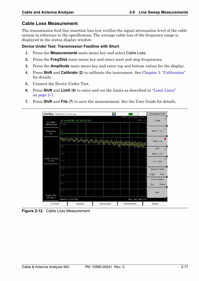
Cable Loss Measurement
The transmission feed line insertion loss test verifies the signal attenuation level of the cable system in reference to the specification. The average cable loss of the frequency range is displayed in the status display window.
Device Under Test: Transmission Feedline with Short
1. Press the Measurements main menu key and select Cable Loss.
2. Press the Freq/Dist main menu key and enter start and stop frequencies.
3. Press the Amplitude main menu key and enter top and bottom values for the display.
4. Press Shift and Calibrate (2) to calibrate the instrument. See Chapter 3, “Calibration” for details.
5. Connect the Device Under Test.
6. Press Shift and Limit (6) to enter and set the limits as described in “Limit Lines” on page 2-7.
7. Press Shift and File (7) to save the measurement. See the User Guide for details.
Figure 2-12. Cable Loss Measurement
2-6 Line Sweep Measurements Cable and Antenna Analyzer
2-18 PN: 10580-00241 Rev. C Cable & Antenna Analyzer MG
Distance-To-Fault (DTF)
DTF reveals the precise fault location of components in the transmission line system. This test helps to identify specific problems in the system, such as connector transitions, jumpers, kinks in the cable or moisture intrusion.
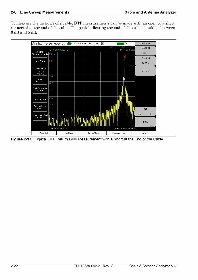
To measure the distance of a cable, DTF measurements can be made with an open or a short connected at the end of the cable. The peak indicating the end of the cable should be between 0 dB and 5 dB. An open or short should not be used when DTF is used for troubleshooting because the open/short will reflect everything and the true value of a connector might be misinterpreted and a good connector could look like a failing connector.
A 50 Ω load is the best termination for troubleshooting DTF problems because it will be 50 Ω over the entire frequency range. The antenna can also be used as a terminating device but the impedance of the antenna will change over different frequencies because the antenna is only designed to have 15 dB or better return loss in the passband of the antenna.
DTF measurement is a frequency domain measurement and the data is transformed to the time domain using mathematics. The distance information is obtained by analyzing how much the phase is changing when the system is swept in the frequency domain. Frequency selective devices such as TMAs (Tower Mounted Amplifiers), duplexers, filters, and quarter wave lightning arrestors change the phase information (distance information) if they are not swept over the correct frequencies. Care needs to be taken when setting up the frequency range whenever a TMA is present in the path.
Because of the nature of the measurement, maximum distance range and fault resolution is dependent upon the frequency range and number of data points. DTF Aid shows how the parameters are related. If the cable is longer than DMax, the only way to improve the horizontal range is to reduce the frequency span or to increase the number of data points. Similarly, the fault resolution is inversely proportional to the frequency range and the only way to improve the fault resolution is to widen the frequency span.
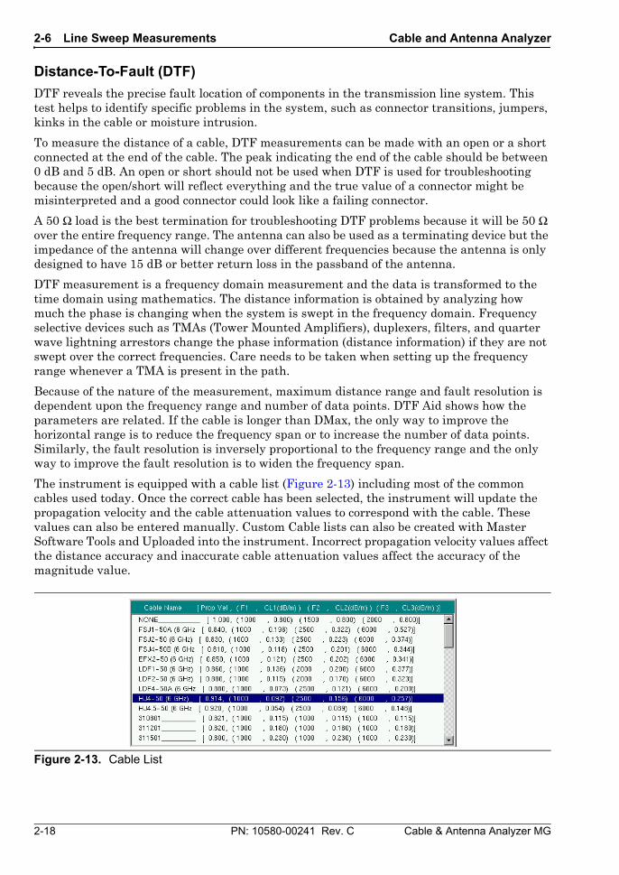
The instrument is equipped with a cable list (Figure 2-13) including most of the common cables used today. Once the correct cable has been selected, the instrument will update the propagation velocity and the cable attenuation values to correspond with the cable. These values can also be entered manually. Custom Cable lists can also be created with Master Software Tools and Uploaded into the instrument. Incorrect propagation velocity values affect the distance accuracy and inaccurate cable attenuation values affect the accuracy of the magnitude value.
Figure 2-13. Cable List
Cable and Antenna Analyzer 2-6 Line Sweep Measurements
Cable & Antenna Analyzer MG PN: 10580-00241 Rev. C 2-19
Fault Resolution
Fault resolution is the system's ability to separate two closely spaced discontinuities. If the fault resolution is 10 feet and there are two faults 5 feet apart, the instrument will not be able to show both faults unless Fault Resolution is improved by widening the frequency span.
Fault Resolution (m) = 1.5 x 10⁸ x vp / ΔF
where vp is the propagation velocity of the transmission cable as discussed in the previous section.
DMax
DMax is the maximum horizontal distance that can be analyzed. The Stop Distance can not exceed Dmax. If the cable is longer than Dmax, Dmax needs to be improved by increasing the number of data points or lowering the frequency span (ΔF). Note that the data points can be set to 137, 275, 551, 1102, or 2204
Dmax = (Datapoints – 1) x Fault Resolution
DTF Setup
1. Press the Measurements main menu key and select DTF Return Loss or DTF VSWR.
2. Press the Freq/Dist main menu key.
3. Press the Units submenu key and select m to display distance in meters or ft to display distance in feet.
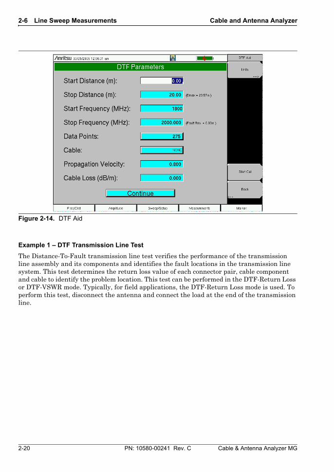
4. Press DTF Aid and use the touch screen, or arrow keys to navigate through all the DTF parameters.
a. Set Start Distance and Stop Distance. Stop Distance needs to be smaller than Dmax.
b. Enter the Start and Stop frequencies.
c. Press Cable and select the appropriate cable from the cable list (Figure 2-13).
d. Press Continue.
5. Press Shift and Calibrate (2) to calibrate the instrument. See Chapter 3, “Calibration” for details.
6. Press the Marker main menu key and set the appropriate markers as described in “Markers” on page 2-9.
7. Press Shift and Limit (6) to enter and set the limits as described in “Limit Lines” on page 2-7.
8. Press Shift and File (7) to save the measurement. See the User Guide for details.
Note If Stop Distance is greater than DMax, increase the number of data points.
2-6 Line Sweep Measurements Cable and Antenna Analyzer
2-20 PN: 10580-00241 Rev. C Cable & Antenna Analyzer MG
Example 1 – DTF Transmission Line Test
The Distance-To-Fault transmission line test verifies the performance of the transmission line assembly and its components and identifies the fault locations in the transmission line system. This test determines the return loss value of each connector pair, cable component and cable to identify the problem location. This test can be performed in the DTF-Return Loss or DTF-VSWR mode. Typically, for field applications, the DTF-Return Loss mode is used. To perform this test, disconnect the antenna and connect the load at the end of the transmission line.
Figure 2-14. DTF Aid
Cable and Antenna Analyzer 2-6 Line Sweep Measurements
Cable & Antenna Analyzer MG PN: 10580-00241 Rev. C 2-21
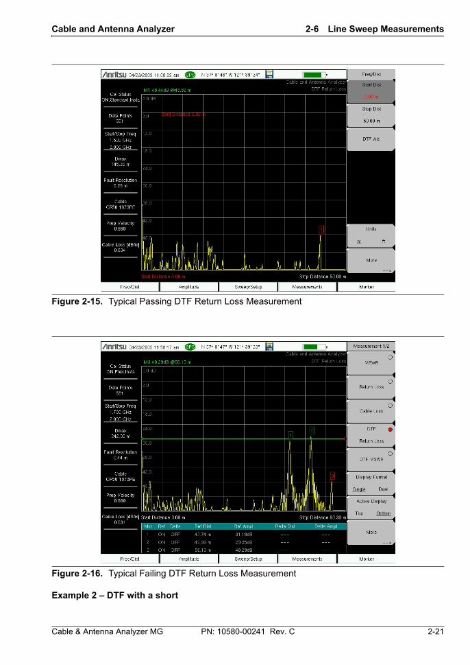
Example 2 – DTF with a short
Figure 2-15. Typical Passing DTF Return Loss Measurement
Figure 2-16. Typical Failing DTF Return Loss Measurement
2-6 Line Sweep Measurements Cable and Antenna Analyzer
2-22 PN: 10580-00241 Rev. C Cable & Antenna Analyzer MG
To measure the distance of a cable, DTF measurements can be made with an open or a short connected at the end of the cable. The peak indicating the end of the cable should be between 0 dB and 5 dB.
Figure 2-17. Typical DTF Return Loss Measurement with a Short at the End of the Cable
Cable and Antenna Analyzer 2-7 1-Port Measurements
Cable & Antenna Analyzer MG PN: 10580-00241 Rev. C 2-23
2-7 1-Port Measurements
Phase Measurements
The instrument can display 1-port phase measurements. The following example compares the phase of two cables using a 1-port phase measurement.
1. Press the Measurements main menu key
2. Press the More submenu key.
3. Press the 1-Port Phase key.
4. Press the Freq/Dist main menu key and set the start frequency and stop frequency.
5. Press Shift and Calibrate (2) to calibrate the instrument. See Chapter 3, “Calibration” for details.
6. Connect device under test (Cable A) and press Copy Trace To Display Memory.
7. Remove the first device under test and connect the second device under test (Cable B).
8. Press the Trace – Memory key to view the difference between Cable A and Cable B.
Smith Chart
The instrument can display 1-port measurements in a standard Normalized 50 ohm Smith Chart. When markers are used, the real and imaginary components of the Smith Chart value are displayed.
Anritsu Master Software Tools includes additional options and a calculator that can easily show what the return loss, VSWR, or reflection coefficient values of a specific Smith Chart value are.
It is possible to change the zoom size in the Amplitude menu. Expand 10 dB zooms in the Smith Chart so that the reflection coefficient is between 0 and 0.3162. Expand 20 dB expands the Smith Chart to show rho between 0 and 0.1 and Expand 30 dB expands to show rho between 0 and 0.0316.
Smith Chart Measurement
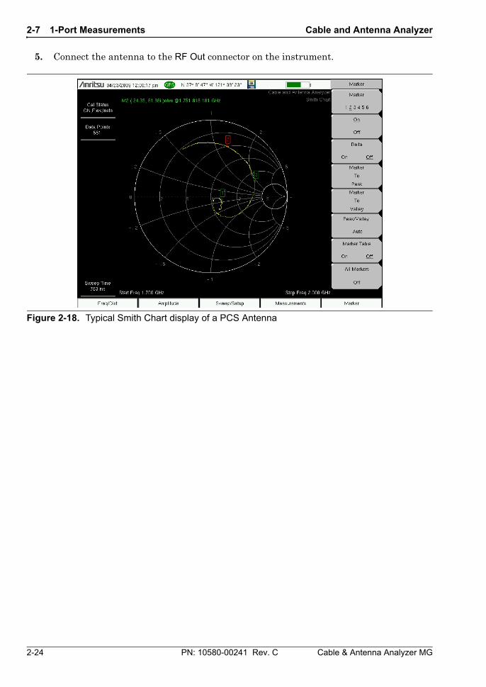
The following example shows how a Smith Chart can be used to measure the match of an antenna.
1. Press the Measurements main menu key.
2. Press the More submenu key and select Smith Chart.
3. Press the Freq/Dist main menu key and set the start frequency and stop frequency.
4. Press Shift and Calibrate (2) to calibrate the instrument. See Chapter 3, “Calibration” for details.
2-7 1-Port Measurements Cable and Antenna Analyzer
2-24 PN: 10580-00241 Rev. C Cable & Antenna Analyzer MG
5. Connect the antenna to the RF Out connector on the instrument.
Figure 2-18. Typical Smith Chart display of a PCS Antenna
Cable and Antenna Analyzer 2-8 Cable and Antenna Analyzer Menus
Cable & Antenna Analyzer MG PN: 10580-00241 Rev. C 2-25
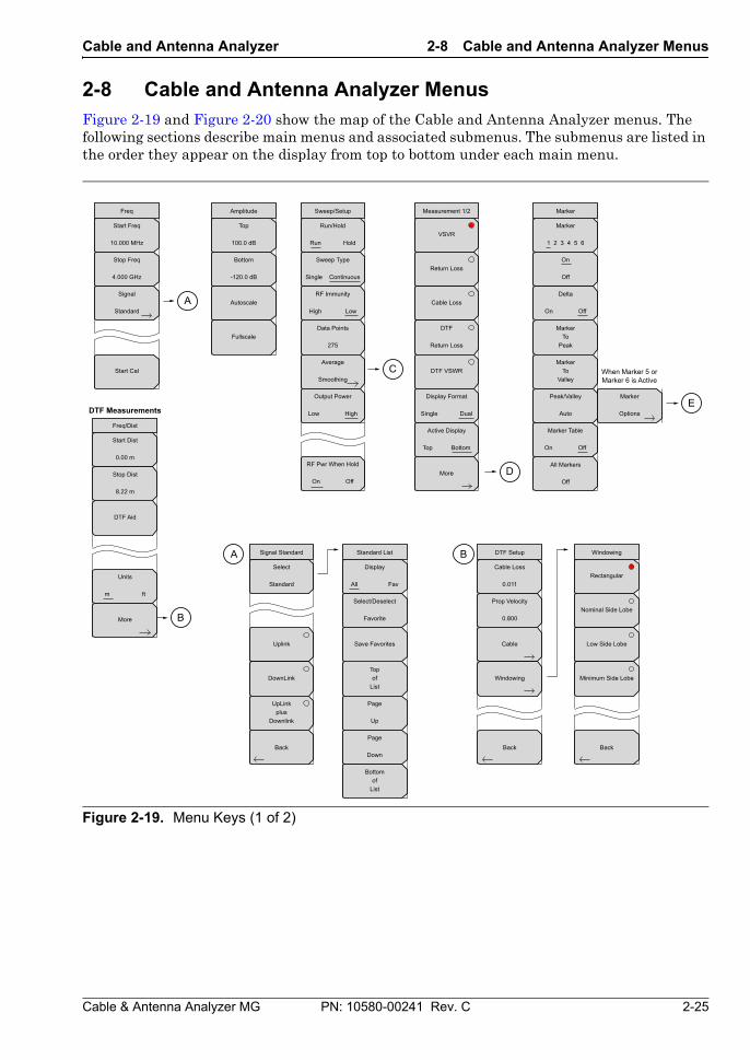
2-8 Cable and Antenna Analyzer MenusFigure 2-19 and Figure 2-20 show the map of the Cable and Antenna Analyzer menus. The following sections describe main menus and associated submenus. The submenus are listed in the order they appear on the display from top to bottom under each main menu.
Figure 2-19. Menu Keys (1 of 2)
Amplitude Measurement 1/2
Bottom
-120.0 dB
Top
100.0 dB
B
C
D
E
More
Cable
Windowing
More
Marker
Options
Autoscale
Data Points
275Fullscale
Freq
Start Freq
10.000 MHz
Stop Freq
4.000 GHzReturn Loss
Cable Loss
DTF
Return Loss
Uplink
DownLink
UpLinkplus
Downlink
DTF VSWR
VSVR
Windowing
Nominal Side Lobe
Low Side Lobe
Minimum Side Lobe
Rectangular
Marker
On
Off
MarkerTo
Peak
MarkerTo
ValleyWhen Marker 5 orMarker 6 is Active
Peak/Valley
Auto
All Markers
Off
Start Cal
Marker
1 2 3 4 5 6
Delta
On Off
Marker Table
On Off
Select
Standard
A Signal Standard B DTF Setup
Back BackBack
Signal
Standard
DTF Aid
Freq/Dist
Start Dist
0.00 m
DTF Measurements
Stop Dist
8.22 m
Average
Smoothing
Sweep Type
Single Continuous
Sweep/Setup
Run/Hold
Run Hold
RF Immunity
High Low
Output Power
Low High
RF Pwr When Hold
On Off
Display Format
Single Dual
Active Display
Top Bottom
Topof
List
Page
Up
Page
Down
Bottomof
List
Standard List
A
Prop Velocity
0.800
Cable Loss
0.011Units
m ft
Save Favorites
Display
All Fav
Select/Deselect
Favorite
2-8 Cable and Antenna Analyzer Menus Cable and Antenna Analyzer
2-26 PN: 10580-00241 Rev. C Cable & Antenna Analyzer MG
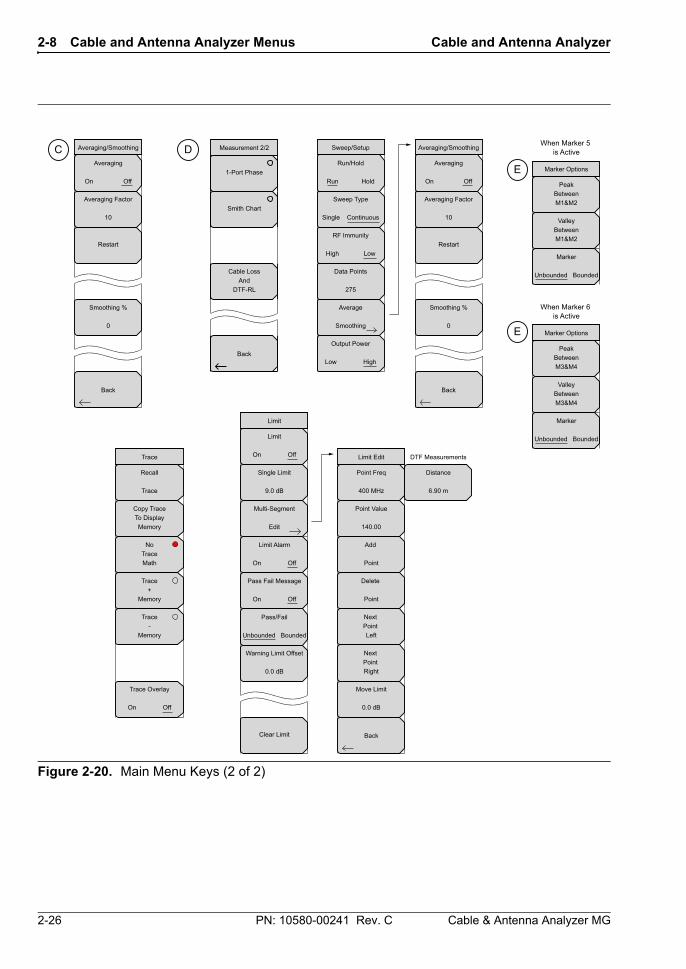
Figure 2-20. Main Menu Keys (2 of 2)
Limit Edit
Point Freq
400 MHz
Distance
6.90 m
DTF Measurements
Point Value
140.00
Add
Point
Delete
Point
Next Point Left
Next Point Right
Move Limit
0.0 dB
Trace
Copy TraceTo DisplayMemory
NoTraceMath
Trace+
Memory
Trace-
Memory
Recall
Trace
Trace Overlay
On Off
D
Back
Smoothing %
0
Restart
Averaging Factor
10
C Averaging/Smoothing
Back
Averaging
On OffE
E
Data Points
275
Average
Smoothing
Sweep Type
Single Continuous
Sweep/Setup
Run/Hold
Run Hold
RF Immunity
High Low
Output Power
Low High
Smoothing %
0
Restart
Averaging Factor
10
Averaging/Smoothing
Back
Averaging
On Off
Cable LossAnd
DTF-RL
Measurement 2/2
Smith Chart
1-Port Phase
Back
Multi-Segment
Edit
Limit
Clear Limit
Limit
On Off
Single Limit
9.0 dB
Limit Alarm
On Off
Pass Fail Message
On Off
Pass/Fail
Unbounded Bounded
Warning Limit Offset
0.0 dB
ValleyBetweenM1&M2
PeakBetweenM1&M2
Marker Options
When Marker 5 is Active
ValleyBetweenM3&M4
PeakBetweenM3&M4
Marker Options
When Marker 6 is Active
Marker
Unbounded Bounded
Marker
Unbounded Bounded
Cable and Antenna Analyzer 2-9 Freq Menu
Cable & Antenna Analyzer MG PN: 10580-00241 Rev. C 2-27
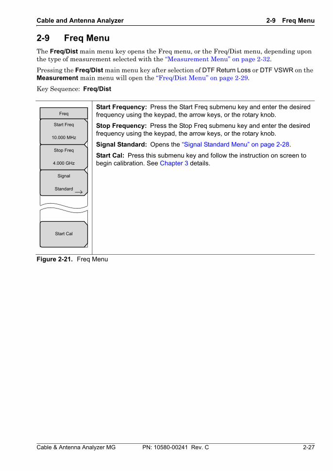
2-9 Freq Menu The Freq/Dist main menu key opens the Freq menu, or the Freq/Dist menu, depending upon the type of measurement selected with the “Measurement Menu” on page 2-32.
Pressing the Freq/Dist main menu key after selection of DTF Return Loss or DTF VSWR on the Measurement main menu will open the “Freq/Dist Menu” on page 2-29.
Key Sequence: Freq/Dist
Start Frequency: Press the Start Freq submenu key and enter the desired frequency using the keypad, the arrow keys, or the rotary knob.
Stop Frequency: Press the Stop Freq submenu key and enter the desired frequency using the keypad, the arrow keys, or the rotary knob.
Signal Standard: Opens the “Signal Standard Menu” on page 2-28.
Start Cal: Press this submenu key and follow the instruction on screen to begin calibration. See Chapter 3 details.
Figure 2-21. Freq Menu
Freq
Start Freq
10.000 MHz
Stop Freq
4.000 GHz
Start Cal
Signal
Standard
2-9 Freq Menu Cable and Antenna Analyzer
2-28 PN: 10580-00241 Rev. C Cable & Antenna Analyzer MG
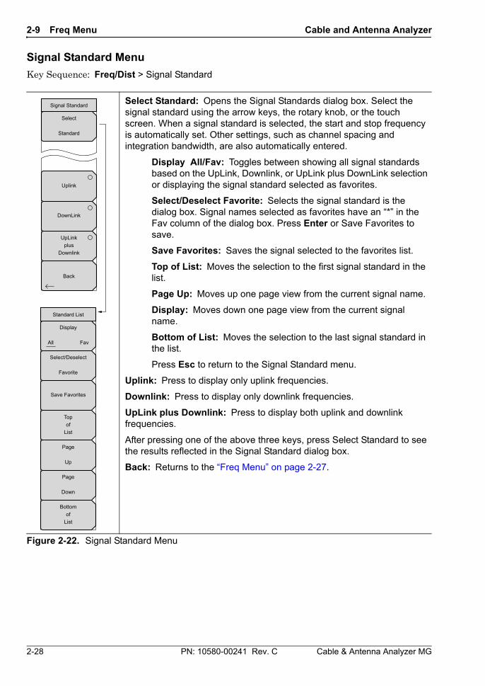
Signal Standard Menu
Key Sequence: Freq/Dist > Signal Standard
Select Standard: Opens the Signal Standards dialog box. Select the signal standard using the arrow keys, the rotary knob, or the touch screen. When a signal standard is selected, the start and stop frequency is automatically set. Other settings, such as channel spacing and integration bandwidth, are also automatically entered.
Display All/Fav: Toggles between showing all signal standards based on the UpLink, Downlink, or UpLink plus DownLink selection or displaying the signal standard selected as favorites.
Select/Deselect Favorite: Selects the signal standard is the dialog box. Signal names selected as favorites have an “*” in the Fav column of the dialog box. Press Enter or Save Favorites to save.
Save Favorites: Saves the signal selected to the favorites list.
Top of List: Moves the selection to the first signal standard in the list.
Page Up: Moves up one page view from the current signal name.
Display: Moves down one page view from the current signal name.
Bottom of List: Moves the selection to the last signal standard in the list.
Press Esc to return to the Signal Standard menu.
Uplink: Press to display only uplink frequencies.
Downlink: Press to display only downlink frequencies.
UpLink plus Downlink: Press to display both uplink and downlink frequencies.
After pressing one of the above three keys, press Select Standard to see the results reflected in the Signal Standard dialog box.
Back: Returns to the “Freq Menu” on page 2-27.
Figure 2-22. Signal Standard Menu
Uplink
DownLink
UpLinkplus
Downlink
Select
Standard
Signal Standard
Back
Topof
List
Save Favorites
Display
All Fav
Select/Deselect
Favorite
Page
Up
Page
Down
Bottomof
List
Standard List

Cable and Antenna Analyzer 2-10 Freq/Dist Menu
Cable & Antenna Analyzer MG PN: 10580-00241 Rev. C 2-29
2-10 Freq/Dist Menu The Freq/Dist main menu key opens the Freq menu, or the Freq/Dist menu, depending upon the type of measurement selected with the “Measurement Menu” on page 2-32.
Pressing the Freq/Dist main menu key after selection of VSWR, Return Loss, or Cable Loss on the Measurement main menu will open the “Freq Menu” on page 2-27.
Key Sequence: Freq/Dist
Start Dist: Press the Start Dist submenu key and enter the desired start distance using the keypad, the arrow keys, or the rotary knob.
Stop Dist: Press the Stop Dist submenu key and enter the desired stop distance using the keypad, the arrow keys, or the rotary knob.
DTF Aid: Opens the DTF Aid dialog box (Figure 2-14) for entering parameters.
Units: Toggles between meters and feet.
More: Opens the “DTF Setup Menu” on page 2-30.
Figure 2-23. Freq/Dist Menu
More
Units
m ft
DTF Aid
Freq/Dist
Start Dist
0.00 m
Stop Dist
8.22 m
2-11 Amplitude Menu Cable and Antenna Analyzer
2-30 PN: 10580-00241 Rev. C Cable & Antenna Analyzer MG
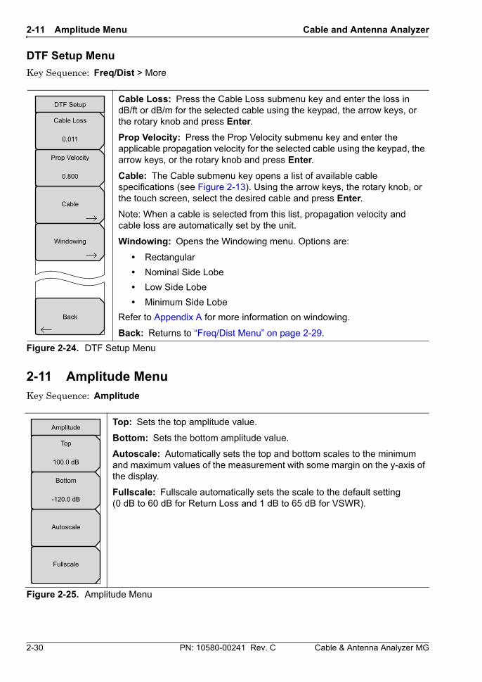
DTF Setup Menu
Key Sequence: Freq/Dist > More
2-11 Amplitude Menu Key Sequence: Amplitude
Cable Loss: Press the Cable Loss submenu key and enter the loss in dB/ft or dB/m for the selected cable using the keypad, the arrow keys, or the rotary knob and press Enter.
Prop Velocity: Press the Prop Velocity submenu key and enter the applicable propagation velocity for the selected cable using the keypad, the arrow keys, or the rotary knob and press Enter.
Cable: The Cable submenu key opens a list of available cable specifications (see Figure 2-13). Using the arrow keys, the rotary knob, or the touch screen, select the desired cable and press Enter.
Note: When a cable is selected from this list, propagation velocity and cable loss are automatically set by the unit.
Windowing: Opens the Windowing menu. Options are:
• Rectangular
• Nominal Side Lobe
• Low Side Lobe
• Minimum Side Lobe
Refer to Appendix A for more information on windowing.
Back: Returns to “Freq/Dist Menu” on page 2-29.
Figure 2-24. DTF Setup Menu
Top: Sets the top amplitude value.
Bottom: Sets the bottom amplitude value.
Autoscale: Automatically sets the top and bottom scales to the minimum and maximum values of the measurement with some margin on the y-axis of the display.
Fullscale: Fullscale automatically sets the scale to the default setting (0 dB to 60 dB for Return Loss and 1 dB to 65 dB for VSWR).
Figure 2-25. Amplitude Menu
Cable
Windowing
Prop Velocity
0.800
DTF Setup
Back
Cable Loss
0.011
Amplitude
Bottom
-120.0 dB
Top
100.0 dB
Autoscale
Fullscale
Cable and Antenna Analyzer 2-12 Sweep/Setup Menu
Cable & Antenna Analyzer MG PN: 10580-00241 Rev. C 2-31
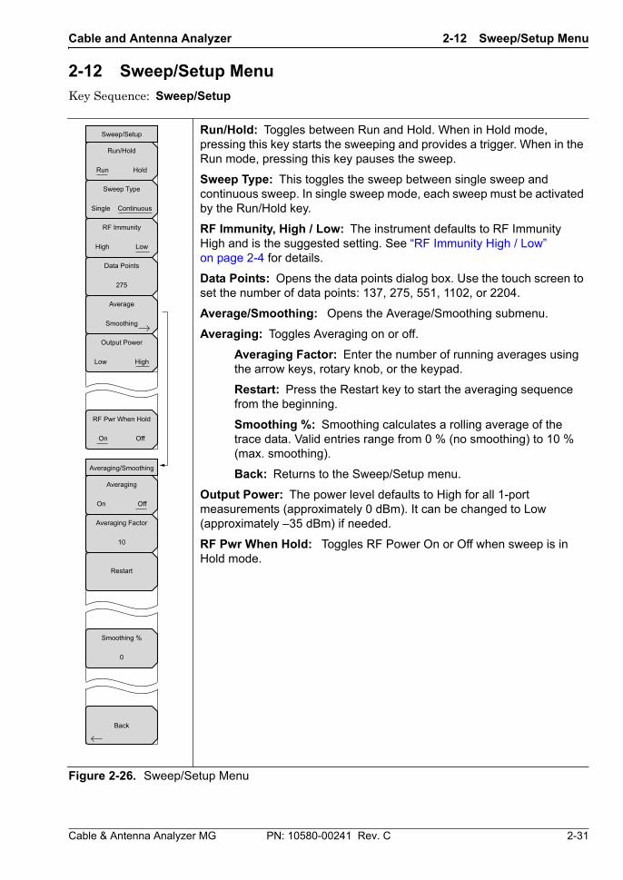
2-12 Sweep/Setup Menu Key Sequence: Sweep/Setup
Run/Hold: Toggles between Run and Hold. When in Hold mode, pressing this key starts the sweeping and provides a trigger. When in the Run mode, pressing this key pauses the sweep.
Sweep Type: This toggles the sweep between single sweep and continuous sweep. In single sweep mode, each sweep must be activated by the Run/Hold key.
RF Immunity, High / Low: The instrument defaults to RF Immunity High and is the suggested setting. See “RF Immunity High / Low” on page 2-4 for details.
Data Points: Opens the data points dialog box. Use the touch screen to set the number of data points: 137, 275, 551, 1102, or 2204.
Average/Smoothing: Opens the Average/Smoothing submenu.
Averaging: Toggles Averaging on or off.
Averaging Factor: Enter the number of running averages using the arrow keys, rotary knob, or the keypad.
Restart: Press the Restart key to start the averaging sequence from the beginning.
Smoothing %: Smoothing calculates a rolling average of the trace data. Valid entries range from 0 % (no smoothing) to 10 % (max. smoothing).
Back: Returns to the Sweep/Setup menu.
Output Power: The power level defaults to High for all 1-port measurements (approximately 0 dBm). It can be changed to Low (approximately –35 dBm) if needed.
RF Pwr When Hold: Toggles RF Power On or Off when sweep is in Hold mode.
Figure 2-26. Sweep/Setup Menu
Data Points
275
Average
Smoothing
Sweep Type
Single Continuous
Sweep/Setup
Run/Hold
Run Hold
RF Immunity
High Low
Output Power
Low High
RF Pwr When Hold
On Off
Smoothing %
0
Restart
Averaging Factor
10
Averaging/Smoothing
Back
Averaging
On Off
2-13 Measurement Menu Cable and Antenna Analyzer
2-32 PN: 10580-00241 Rev. C Cable & Antenna Analyzer MG
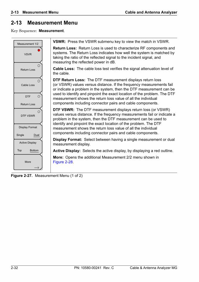
2-13 Measurement MenuKey Sequence: Measurement.
VSWR: Press the VSWR submenu key to view the match in VSWR.
Return Loss: Return Loss is used to characterize RF components and systems. The Return Loss indicates how well the system is matched by taking the ratio of the reflected signal to the incident signal, and measuring the reflected power in dB.
Cable Loss: The cable loss test verifies the signal attenuation level of the cable.
DTF Return Loss: The DTF measurement displays return loss (or VSWR) values versus distance. If the frequency measurements fail or indicate a problem in the system, then the DTF measurement can be used to identify and pinpoint the exact location of the problem. The DTF measurement shows the return loss value of all the individual components including connector pairs and cable components.
DTF VSWR: The DTF measurement displays return loss (or VSWR) values versus distance. If the frequency measurements fail or indicate a problem in the system, then the DTF measurement can be used to identify and pinpoint the exact location of the problem. The DTF measurement shows the return loss value of all the individual components including connector pairs and cable components.
Display Format: Select between having a single measurement or dual measurement display.
Active Display: Selects the active display, by displaying a red outline.
More: Opens the additional Measurement 2/2 menu shown in Figure 2-28.
Figure 2-27. Measurement Menu (1 of 2)
Measurement 1/2
More
Return Loss
Cable Loss
DTF
Return Loss
DTF VSWR
VSVR
Display Format
Single Dual
Active Display
Top Bottom
Cable and Antenna Analyzer 2-13 Measurement Menu
Cable & Antenna Analyzer MG PN: 10580-00241 Rev. C 2-33
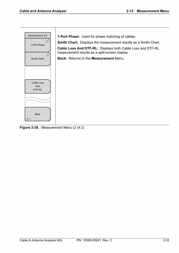
1-Port Phase: Used for phase matching of cables.
Smith Chart: Displays the measurement results as a Smith Chart.
Cable Loss And DTF-RL: Displays both Cable Loss and DTF-RL measurement results as a split-screen display.
Back: Returns to the Measurement Menu.
Figure 2-28. Measurement Menu (2 of 2)
Cable LossAnd
DTF-RL
Measurement 2/2
Smith Chart
1-Port Phase
Back
2-14 Marker Menu Cable and Antenna Analyzer
2-34 PN: 10580-00241 Rev. C Cable & Antenna Analyzer MG
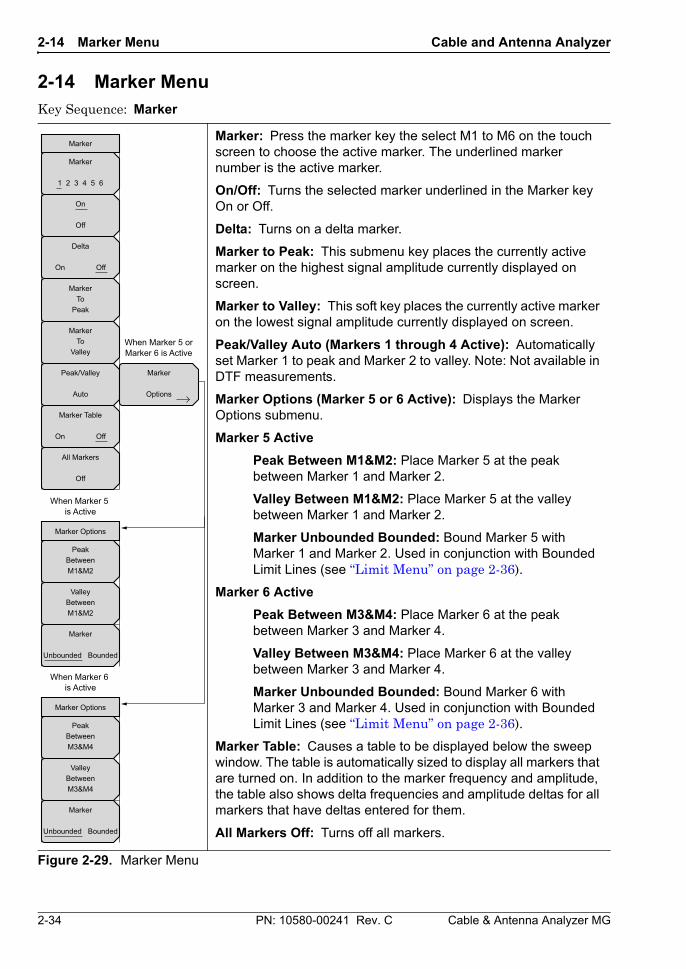
2-14 Marker MenuKey Sequence: Marker
Marker: Press the marker key the select M1 to M6 on the touch screen to choose the active marker. The underlined marker number is the active marker.
On/Off: Turns the selected marker underlined in the Marker key On or Off.
Delta: Turns on a delta marker.
Marker to Peak: This submenu key places the currently active marker on the highest signal amplitude currently displayed on screen.
Marker to Valley: This soft key places the currently active marker on the lowest signal amplitude currently displayed on screen.
Peak/Valley Auto (Markers 1 through 4 Active): Automatically set Marker 1 to peak and Marker 2 to valley. Note: Not available in DTF measurements.
Marker Options (Marker 5 or 6 Active): Displays the Marker Options submenu.
Marker 5 Active
Peak Between M1&M2: Place Marker 5 at the peak between Marker 1 and Marker 2.
Valley Between M1&M2: Place Marker 5 at the valley between Marker 1 and Marker 2.
Marker Unbounded Bounded: Bound Marker 5 with Marker 1 and Marker 2. Used in conjunction with Bounded Limit Lines (see “Limit Menu” on page 2-36).
Marker 6 Active
Peak Between M3&M4: Place Marker 6 at the peak between Marker 3 and Marker 4.
Valley Between M3&M4: Place Marker 6 at the valley between Marker 3 and Marker 4.
Marker Unbounded Bounded: Bound Marker 6 with Marker 3 and Marker 4. Used in conjunction with Bounded Limit Lines (see “Limit Menu” on page 2-36).
Marker Table: Causes a table to be displayed below the sweep window. The table is automatically sized to display all markers that are turned on. In addition to the marker frequency and amplitude, the table also shows delta frequencies and amplitude deltas for all markers that have deltas entered for them.
All Markers Off: Turns off all markers.
Figure 2-29. Marker Menu
Marker Table
On Off
Marker
On
Off
MarkerTo
Peak
MarkerTo
Valley
Peak/Valley
Auto
Marker
1 2 3 4 5 6
Delta
On Off
All Markers
Off
Marker
Options
When Marker 5 orMarker 6 is Active
ValleyBetweenM1&M2
PeakBetweenM1&M2
Marker Options
When Marker 5 is Active
ValleyBetweenM3&M4
PeakBetweenM3&M4
Marker Options
When Marker 6 is Active
Marker
Unbounded Bounded
Marker
Unbounded Bounded
Cable and Antenna Analyzer 2-15 Sweep Menu
Cable & Antenna Analyzer MG PN: 10580-00241 Rev. C 2-35
2-15 Sweep MenuThis menu open the “Sweep/Setup Menu” on page 2-31.
2-16 Measure MenuThis menu open the “Measurement Menu” on page 2-32.
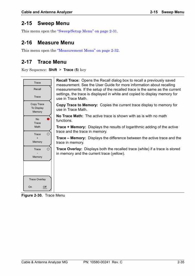
2-17 Trace MenuKey Sequence: Shift > Trace (5) key
Recall Trace: Opens the Recall dialog box to recall a previously saved measurement. See the User Guide for more information about recalling measurements. If the setup of the recalled trace is the same as the current settings, the trace is displayed in white and copied to display memory for use in Trace Math.
Copy Trace to Memory: Copies the current trace display to memory for use in Trace Math.
No Trace Math: The active trace is shown with as is with no math functions.
Trace + Memory: Displays the results of logarithmic adding of the active trace and the trace in memory.
Trace – Memory: Displays the difference between the active trace and the trace in memory.
Trace Overlay: Displays both the recalled trace (white) if a trace is stored in memory and the current trace (yellow).
Figure 2-30. Trace Menu
Trace
Copy TraceTo DisplayMemory
NoTraceMath
Trace+
Memory
Trace-
Memory
Recall
Trace
Trace Overlay
On Off
2-18 Limit Menu Cable and Antenna Analyzer
2-36 PN: 10580-00241 Rev. C Cable & Antenna Analyzer MG
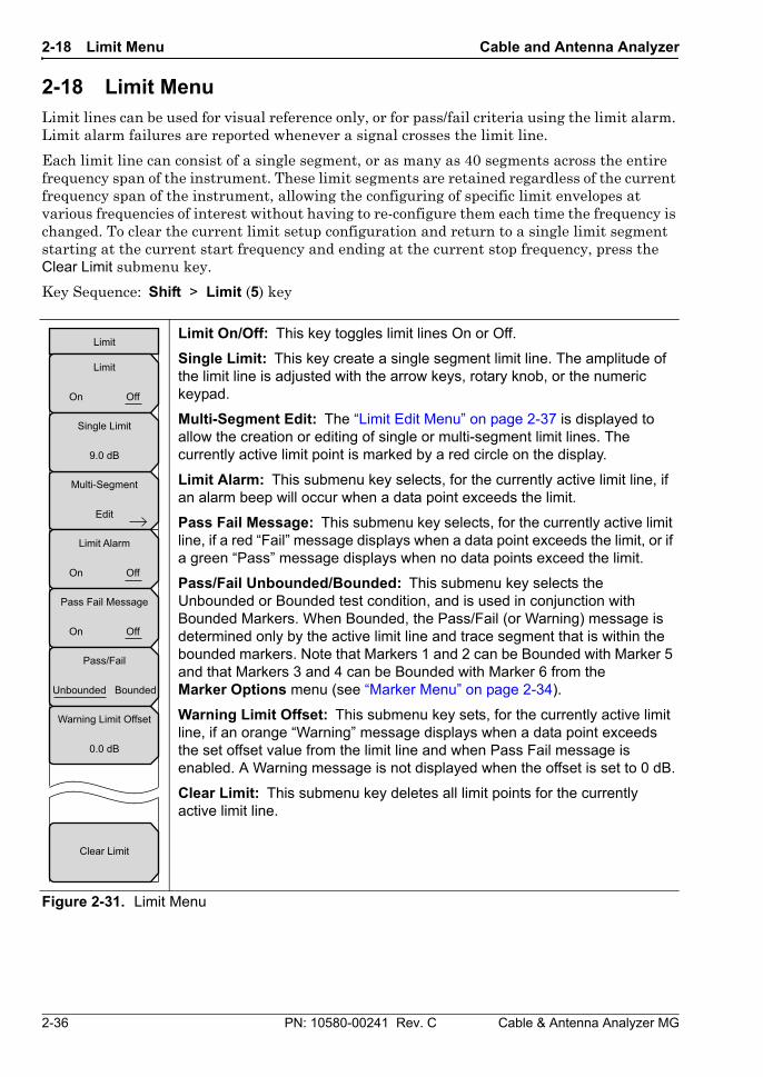
2-18 Limit Menu Limit lines can be used for visual reference only, or for pass/fail criteria using the limit alarm. Limit alarm failures are reported whenever a signal crosses the limit line.
Each limit line can consist of a single segment, or as many as 40 segments across the entire frequency span of the instrument. These limit segments are retained regardless of the current frequency span of the instrument, allowing the configuring of specific limit envelopes at various frequencies of interest without having to re-configure them each time the frequency is changed. To clear the current limit setup configuration and return to a single limit segment starting at the current start frequency and ending at the current stop frequency, press the Clear Limit submenu key.
Key Sequence: Shift > Limit (5) key
Limit On/Off: This key toggles limit lines On or Off.
Single Limit: This key create a single segment limit line. The amplitude of the limit line is adjusted with the arrow keys, rotary knob, or the numeric keypad.
Multi-Segment Edit: The “Limit Edit Menu” on page 2-37 is displayed to allow the creation or editing of single or multi-segment limit lines. The currently active limit point is marked by a red circle on the display.
Limit Alarm: This submenu key selects, for the currently active limit line, if an alarm beep will occur when a data point exceeds the limit.
Pass Fail Message: This submenu key selects, for the currently active limit line, if a red “Fail” message displays when a data point exceeds the limit, or if a green “Pass” message displays when no data points exceed the limit.
Pass/Fail Unbounded/Bounded: This submenu key selects the Unbounded or Bounded test condition, and is used in conjunction with Bounded Markers. When Bounded, the Pass/Fail (or Warning) message is determined only by the active limit line and trace segment that is within the bounded markers. Note that Markers 1 and 2 can be Bounded with Marker 5 and that Markers 3 and 4 can be Bounded with Marker 6 from the Marker Options menu (see “Marker Menu” on page 2-34).
Warning Limit Offset: This submenu key sets, for the currently active limit line, if an orange “Warning” message displays when a data point exceeds the set offset value from the limit line and when Pass Fail message is enabled. A Warning message is not displayed when the offset is set to 0 dB.
Clear Limit: This submenu key deletes all limit points for the currently active limit line.
Figure 2-31. Limit Menu
Multi-Segment
Edit
Limit
Clear Limit
Limit
On Off
Single Limit
9.0 dB
Limit Alarm
On Off
Pass Fail Message
On Off
Pass/Fail
Unbounded Bounded
Warning Limit Offset
0.0 dB
Cable and Antenna Analyzer 2-18 Limit Menu
Cable & Antenna Analyzer MG PN: 10580-00241 Rev. C 2-37
Limit Edit Menu
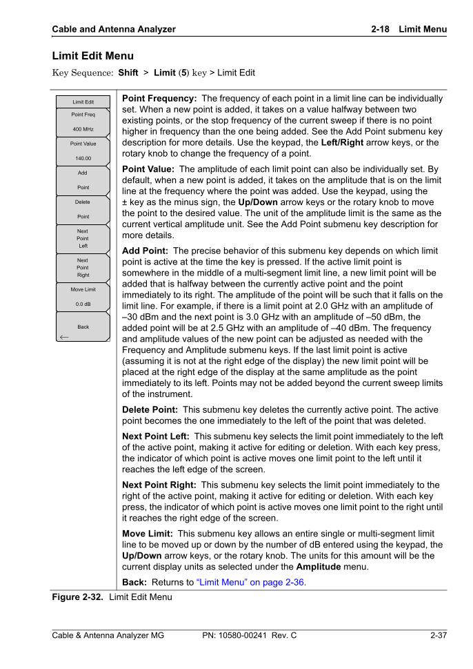
Key Sequence: Shift > Limit (5) key > Limit Edit
Point Frequency: The frequency of each point in a limit line can be individually set. When a new point is added, it takes on a value halfway between two existing points, or the stop frequency of the current sweep if there is no point higher in frequency than the one being added. See the Add Point submenu key description for more details. Use the keypad, the Left/Right arrow keys, or the rotary knob to change the frequency of a point.
Point Value: The amplitude of each limit point can also be individually set. By default, when a new point is added, it takes on the amplitude that is on the limit line at the frequency where the point was added. Use the keypad, using the ± key as the minus sign, the Up/Down arrow keys or the rotary knob to move the point to the desired value. The unit of the amplitude limit is the same as the current vertical amplitude unit. See the Add Point submenu key description for more details.
Add Point: The precise behavior of this submenu key depends on which limit point is active at the time the key is pressed. If the active limit point is somewhere in the middle of a multi-segment limit line, a new limit point will be added that is halfway between the currently active point and the point immediately to its right. The amplitude of the point will be such that it falls on the limit line. For example, if there is a limit point at 2.0 GHz with an amplitude of –30 dBm and the next point is 3.0 GHz with an amplitude of –50 dBm, the added point will be at 2.5 GHz with an amplitude of –40 dBm. The frequency and amplitude values of the new point can be adjusted as needed with the Frequency and Amplitude submenu keys. If the last limit point is active (assuming it is not at the right edge of the display) the new limit point will be placed at the right edge of the display at the same amplitude as the point immediately to its left. Points may not be added beyond the current sweep limits of the instrument.
Delete Point: This submenu key deletes the currently active point. The active point becomes the one immediately to the left of the point that was deleted.
Next Point Left: This submenu key selects the limit point immediately to the left of the active point, making it active for editing or deletion. With each key press, the indicator of which point is active moves one limit point to the left until it reaches the left edge of the screen.
Next Point Right: This submenu key selects the limit point immediately to the right of the active point, making it active for editing or deletion. With each key press, the indicator of which point is active moves one limit point to the right until it reaches the right edge of the screen.
Move Limit: This submenu key allows an entire single or multi-segment limit line to be moved up or down by the number of dB entered using the keypad, the Up/Down arrow keys, or the rotary knob. The units for this amount will be the current display units as selected under the Amplitude menu.
Back: Returns to “Limit Menu” on page 2-36.
Figure 2-32. Limit Edit Menu
Limit Edit
Point Freq
400 MHz
Point Value
140.00
Add
Point
Delete
Point
Next Point Left
Next Point Right
Move Limit
0.0 dB
Back
2-19 Other Menus Cable and Antenna Analyzer
2-38 PN: 10580-00241 Rev. C Cable & Antenna Analyzer MG
2-19 Other MenusPreset, File, Mode and System are described in the User Guide. Calibrate is described in Chapter 3.
Cable & Antenna Analyzer MG PN: 10580-00241 Rev. C 3-1
Chapter 3 — Calibration
3-1 IntroductionThis chapter provides details and procedures about the following calibration methods: InstaCal, Open-Short-Load, Standard Cal, Flexcal
3-2 Chapter Overview• Section 3-3 “Calibration Methods” on page 3-1
• Section 3-4 “Calibration Verification” on page 3-2
• Section 3-5 “Calibration Procedures” on page 3-3
• Section 3-6 “InstaCal Module Verification” on page 3-5
3-3 Calibration MethodsFor accurate results, the instrument must be calibrated before making any measurements.
The instrument must be re-calibrated whenever the temperature exceeds the calibration temperature range or when the test port extension cable is removed or replaced. Unless the calibration type is Flexcal, the instrument must also be re-calibrated every time the setup frequency changes.
The instrument can be manually calibrated with a precision OSL (Open-Short-Load) calibration tee / discrete components or with the InstaCal module. The benefit of the InstaCal module is that it is much faster, requires no connection changes, and eliminates the need to use three different terminations (open, short, load) for calibration. The trade-off is that the specified corrected directivity is 38 dB instead of 42 dB.
While InstaCal or OSL Cal tee provides two alternatives for the tools needed to perform the calibration, Standard Cal or FlexCal determines how often calibration will need to be performed. A standard calibration is an Open, Short and Load calibration for a selected frequency range, and is no longer valid if the frequency is changed. The default calibration mode is standard.
FlexCal is a broadband frequency calibration that remains valid if the frequency is changed.
Flexcal calibrates the instrument over the entire frequency range and interpolates datapoints if the frequency range is changed. This method saves time as it does not require the user to re-calibrate the system for frequency changes. The trade-off is that the accuracy is not the same as it would be with the standard calibration. It is recommended for troubleshooting purposes. Table 3-1 has a summary of calibration methods and tools.
3-4 Calibration Verification Calibration
3-2 PN: 10580-00241 Rev. C Cable & Antenna Analyzer MG
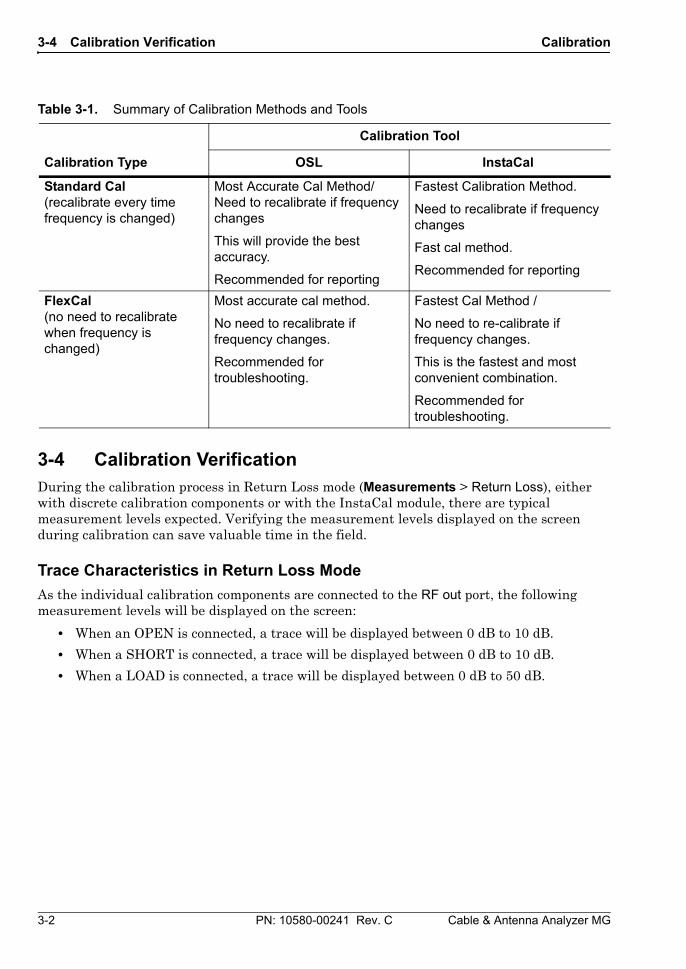
3-4 Calibration VerificationDuring the calibration process in Return Loss mode (Measurements > Return Loss), either with discrete calibration components or with the InstaCal module, there are typical measurement levels expected. Verifying the measurement levels displayed on the screen during calibration can save valuable time in the field.
Trace Characteristics in Return Loss Mode
As the individual calibration components are connected to the RF out port, the following measurement levels will be displayed on the screen:
• When an OPEN is connected, a trace will be displayed between 0 dB to 10 dB.
• When a SHORT is connected, a trace will be displayed between 0 dB to 10 dB.
• When a LOAD is connected, a trace will be displayed between 0 dB to 50 dB.
Table 3-1. Summary of Calibration Methods and Tools
Calibration Type
Calibration Tool
OSL InstaCal
Standard Cal (recalibrate every time frequency is changed)
Most Accurate Cal Method/ Need to recalibrate if frequency changes
This will provide the best accuracy.
Recommended for reporting
Fastest Calibration Method.
Need to recalibrate if frequency changes
Fast cal method.
Recommended for reporting
FlexCal (no need to recalibrate when frequency is changed)
Most accurate cal method.
No need to recalibrate if frequency changes.
Recommended for troubleshooting.
Fastest Cal Method /
No need to re-calibrate if frequency changes.
This is the fastest and most convenient combination.
Recommended for troubleshooting.
Calibration 3-5 Calibration Procedures
Cable & Antenna Analyzer MG PN: 10580-00241 Rev. C 3-3
3-5 Calibration ProceduresIn Cable and Antenna Analyzer Mode, calibration is required when the “Not Calibrated” message is displayed or when the test port cable has been changed. The following sections detail how to perform OSL and InstaCal calibration.
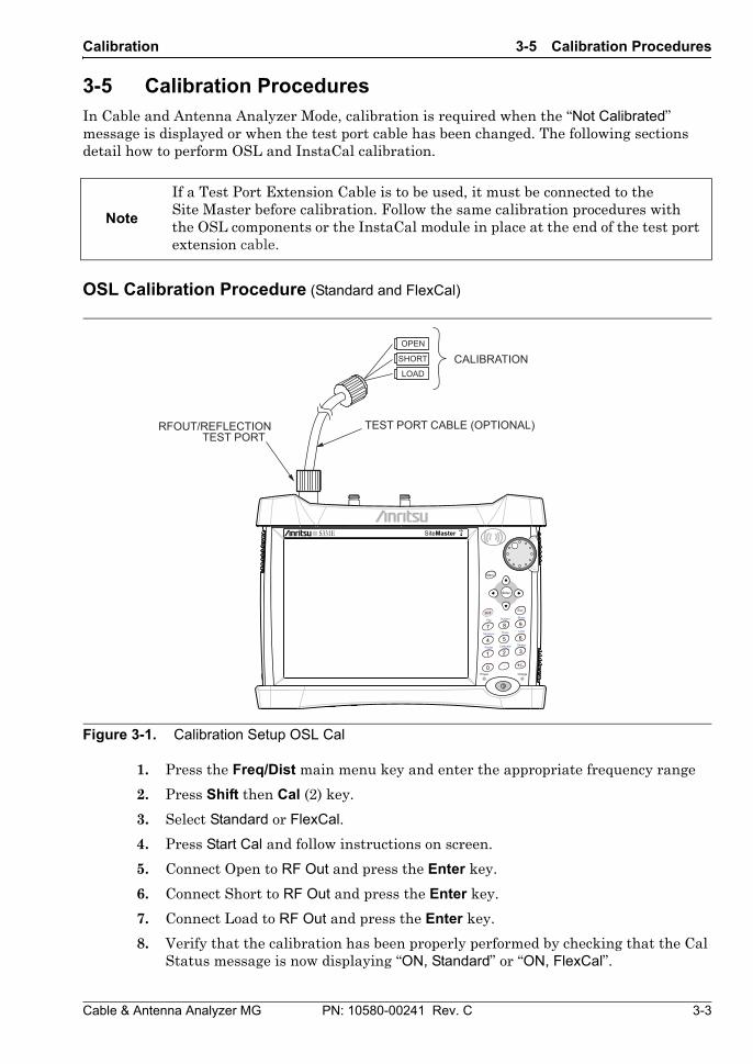
OSL Calibration Procedure (Standard and FlexCal)
1. Press the Freq/Dist main menu key and enter the appropriate frequency range
2. Press Shift then Cal (2) key.
3. Select Standard or FlexCal.
4. Press Start Cal and follow instructions on screen.
5. Connect Open to RF Out and press the Enter key.
6. Connect Short to RF Out and press the Enter key.
7. Connect Load to RF Out and press the Enter key.
8. Verify that the calibration has been properly performed by checking that the Cal Status message is now displaying “ON, Standard” or “ON, FlexCal”.
Note
If a Test Port Extension Cable is to be used, it must be connected to the Site Master before calibration. Follow the same calibration procedures with the OSL components or the InstaCal module in place at the end of the test port extension cable.
Figure 3-1. Calibration Setup OSL Cal
Power Charge
+/-.0
3Sweep
2Calibrate
1Preset
6Limit
5Trace
4Measure
9Mode
8System
7File
ShiftEsc
Enter
Menu
SiteMasterS331E
OPEN
LOAD
SHORT CALIBRATION
RFOUT/REFLECTION TEST PORT
TEST PORT CABLE (OPTIONAL)
3-5 Calibration Procedures Calibration
3-4 PN: 10580-00241 Rev. C Cable & Antenna Analyzer MG
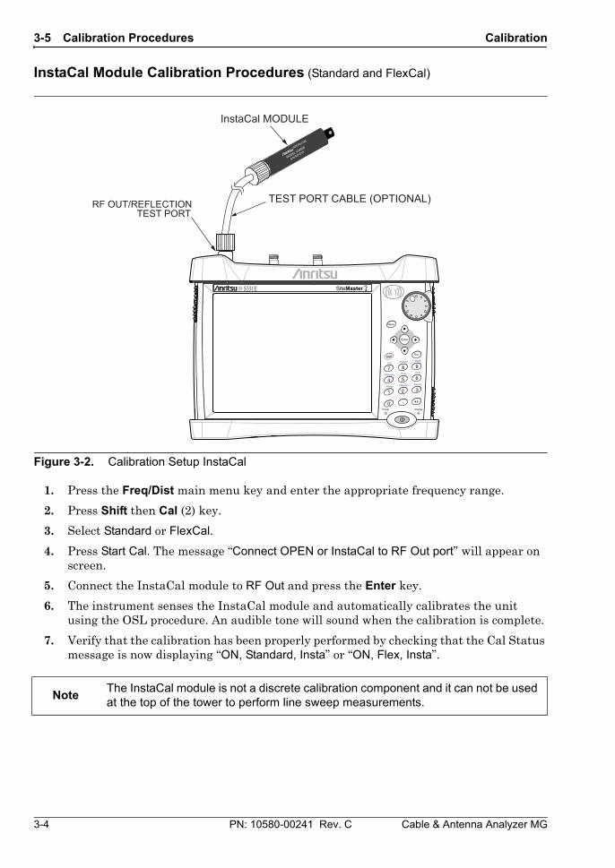
InstaCal Module Calibration Procedures (Standard and FlexCal)
1. Press the Freq/Dist main menu key and enter the appropriate frequency range.
2. Press Shift then Cal (2) key.
3. Select Standard or FlexCal.
4. Press Start Cal. The message “Connect OPEN or InstaCal to RF Out port” will appear on screen.
5. Connect the InstaCal module to RF Out and press the Enter key.
6. The instrument senses the InstaCal module and automatically calibrates the unit using the OSL procedure. An audible tone will sound when the calibration is complete.
7. Verify that the calibration has been properly performed by checking that the Cal Status message is now displaying “ON, Standard, Insta” or “ON, Flex, Insta”.
Figure 3-2. Calibration Setup InstaCal
NoteThe InstaCal module is not a discrete calibration component and it can not be used at the top of the tower to perform line sweep measurements.
Power Charge
+/-.0
3Sweep
2Calibrate
1Preset
6Limit
5Trace
4Measure
9Mode
8System
7File
ShiftEsc
Enter
Menu
RF OUT/REFLECTION TEST PORT
SiteMasterS331E
InstaCal MODULE
INSTALCAL
MODEL ICN508
S/N 601010
TEST PORT CABLE (OPTIONAL)
Calibration 3-6 InstaCal Module Verification
Cable & Antenna Analyzer MG PN: 10580-00241 Rev. C 3-5
3-6 InstaCal Module VerificationVerifying the InstaCal module before any line sweeping measurements is critical to the measured data. InstaCal module verification identifies any failures in the module due to circuitry damage or failure of the control circuitry. This test does not attempt to characterize the InstaCal module, which is performed at the factory or the service center.
The performance of the InstaCal module can be verified by the Termination method which is similar to testing a bad load against a known good load.
Termination Method
The Termination method compares a precision load against the InstaCal module and provides a baseline for other field measurements. A precision load provides better than 42 dB directivity.
1. Set the instrument frequency for the device under test.
2. Press the Measurements main menu key and select Return Loss.
3. Connect the InstaCal module to the instrument’s RF Out port and calibrate the Site Master using the InstaCal module requiring verification.
4. Remove the InstaCal module from the RF Out port and connect the precision load to the RF Out port.
5. Measure the return loss of the precision load. The level should be less than 35 dB across the calibrated frequency range.
6. Press the Marker main menu key and set Marker1 to Marker To Peak. The M1 value should be less than 35 dB return loss.
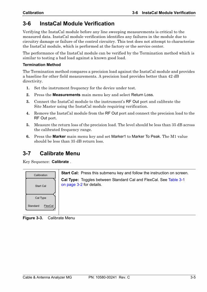
3-7 Calibrate MenuKey Sequence: Calibrate .
Start Cal: Press this submenu key and follow the instruction on screen.
Cal Type: Toggles between Standard Cal and FlexCal. See Table 3-1 on page 3-2 for details.
Figure 3-3. Calibrate Menu
Cal Type
Standard FlexCal
Calibration
Start Cal

3-6 PN: 10580-00241 Rev. C Cable & Antenna Analyzer MG
Cable & Antenna Analyzer MG PN: 10580-00241 Rev. C A-1
Appendix A — Windowing
A-1 Introduction The theoretical requirement for inverse FFT is for the data to extend from zero frequency to infinity. Side lobes appear around a discontinuity because the spectrum is cut off at a finite frequency. Windowing reduces the side lobes by smoothing out the sharp transitions at the beginning and the end of the frequency sweep. As the side lobes are reduced, the main lobe widens, thereby reducing the resolution.
In situations where a small discontinuity may be close to a large one, side lobe reduction windowing helps to reveal the discrete discontinuities. If distance resolution is critical, then reduce the windowing for greater signal resolution.
If strong interfering frequency components are present, but are distant from the frequency of interest, then use a windowing format with higher side lobes, such as Rectangular Windowing or Nominal Side Lobe Windowing.
If strong interfering signals are present and are near the frequency of interest, then use a windowing format with lower side lobes, such as Low Side Lobe Windowing or Minimum Side Lobe Windowing.
If two or more signals are very near to each other, then spectral resolution is important. In this case, use Rectangular Windowing for the sharpest main lobe (the best resolution).
If the amplitude accuracy of a single frequency component is more important than the exact location of the component in a given frequency bin, then choose a windowing format with a wide main lobe.
When examining a single frequency, if the amplitude accuracy is more important than the exact frequency, then use Low Side Lobe Windowing or Minimum Side Lobe Windowing.
A-2 PN: 10580-00241 Rev. C Cable & Antenna Analyzer MG
Rectangular Windowing
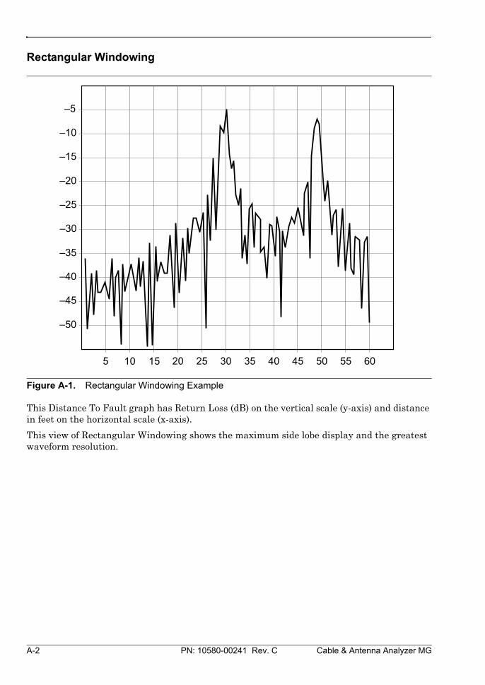
This Distance To Fault graph has Return Loss (dB) on the vertical scale (y-axis) and distance in feet on the horizontal scale (x-axis).
This view of Rectangular Windowing shows the maximum side lobe display and the greatest waveform resolution.
Figure A-1. Rectangular Windowing Example
–5
–10
–15
–20
–25
–30
–35
–40
–45
–50
5 10 15 20 25 30 35 40 45 50 55 60
Cable & Antenna Analyzer MG PN: 10580-00241 Rev. C A-3
Nominal Side Lobe Windowing
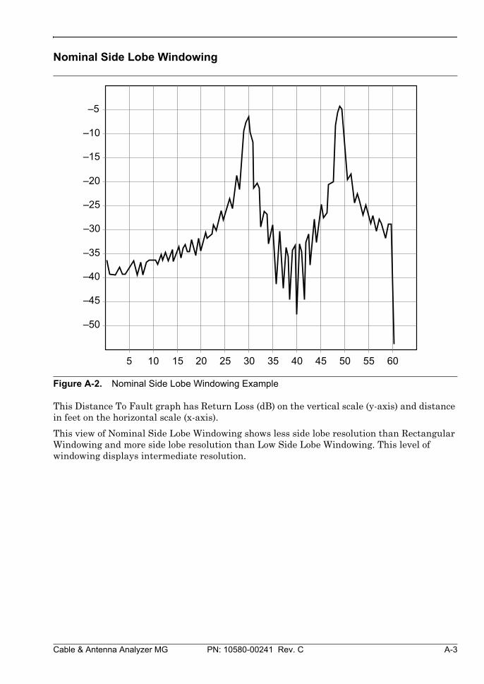
This Distance To Fault graph has Return Loss (dB) on the vertical scale (y-axis) and distance in feet on the horizontal scale (x-axis).
This view of Nominal Side Lobe Windowing shows less side lobe resolution than Rectangular Windowing and more side lobe resolution than Low Side Lobe Windowing. This level of windowing displays intermediate resolution.
Figure A-2. Nominal Side Lobe Windowing Example
–5
–10
–15
–20
–25
–30
–35
–40
–45
–50
5 10 15 20 25 30 35 40 45 50 55 60

A-4 PN: 10580-00241 Rev. C Cable & Antenna Analyzer MG
Low Side Lobe Windowing
This Distance To Fault graph has Return Loss (dB) on the vertical scale (y-axis) and distance in feet on the horizontal scale (x-axis).
This view of Low Side Lobe Windowing shows less side lobe resolution than Nominal Side Lobe Windowing and more side lobe resolution than Minimum Side Lobe Windowing. This level of windowing displays intermediate resolution.
Figure A-3. Low Side Lobe Windowing Example
–5
–10
–15
–20
–25
–30
–35
–40
–45
–50
5 10 15 20 25 30 35 40 45 50 55 60

Cable & Antenna Analyzer MG PN: 10580-00241 Rev. C A-5
Minimum Side Lobe Windowing
This Distance To Fault graph has Return Loss (dB) on the vertical scale (y-axis) and distance in feet on the horizontal scale (x-axis).
This view of Minimum Side Lobe Windowing shows less side lobe resolution than Low Side Lobe Windowing and displays the lowest side lobe and waveform resolution.
Figure A-4. Minimum Side Lobe Windowing Example
–5
–10
–15
–20
–25
–30
–35
–40
–45
–50
5 10 15 20 25 30 35 40 45 50 55 60

A-6 PN: 10580-00241 Rev. C Cable & Antenna Analyzer MG
Numerics to W
Cable & Antenna Analyzer MG PN: 10580-00241 Rev. C Index-1
IndexNumerics
1-port phase . . . . . . . . . . . . . . . .2-23, 2-33
Aamplitude menu . . . . . . . . . . . . . . . . . 2-30Anritsu, contact . . . . . . . . . . . . . . . . . . 1-1autoscale . . . . . . . . . . . . . . . . . . . . . . . 2-30averaging . . . . . . . . . . . . . . . . . . . . 2-4, 2-31
Ccable . . . . . . . . . . . . . . . . . . . . . . . . . . . 2-30cable and antenna analyzer menus . . 2-25cable and antenna mode . . . . . . . . . . . . 1-2cable loss . . . . . . . . . . . . . . . . . . .2-17, 2-32calibrate menu . . . . . . . . . . . . . . . . . . . 3-5calibration . . . . . . . . . . . . . . . . . . . . . . . 2-1calibration of instrument . . . . . . . . . . . 3-1contacting Anritsu . . . . . . . . . . . . . . . . 1-1
Ddata point . . . . . . . . . . . . . . . . . . . . . . . 2-4delta marker . . . . . . . . . . . . . . . . . . . . . 2-9distance
resolution, windowing . . . . . . . . . . A-1distance to fault . . . . . . . . . . . . .2-18, 2-32DTF aid . . . . . . . . . . . . . . . . . . . . . . . . 2-19DTF setup menu . . . . . . . . . . . . . . . . . 2-30
FFlexCal . . . . . . . . . . . . . . . . . . . . . . . . . 3-1freq menu . . . . . . . . . . . . . . . . . . . . . . 2-27freq/dist menu . . . . . . . . . . . . . . . . . . . 2-29frequency setup . . . . . . . . . . . . . . . . . . . 2-2fullscale . . . . . . . . . . . . . . . . . . . . . . . . 2-30
Hhttp, contacting Anritsu . . . . . . . . . . . . 1-1
IInstaCal . . . . . . . . . . . . . . . . . . . . . . . . . 3-1
Llimit edit menu . . . . . . . . . . . . . . . . . . 2-37limit lines setup . . . . . . . . . . . . . . . . . . 2-7limit menu . . . . . . . . . . . . . . . . . . . . . . 2-36line sweep basics . . . . . . . . . . . . . . . . . 2-14
linkscontacting Anritsu . . . . . . . . . . . . . 1-1
Mmarker menu . . . . . . . . . . . . . . . 2-34, 2-35marker table . . . . . . . . . . . . . . . . 2-11, 2-34markers setup . . . . . . . . . . . . . . . . . . . . 2-9measurement menu . . . . . . . . . . . . . . 2-32measurement mode . . . . . . . . . . . . . . . 1-2menu
calibrate . . . . . . . . . . . . . . . . . . . . . 3-5menu map . . . . . . . . . . . . . . . . . . . . . . 2-25
OOSL calibration . . . . . . . . . . . . . . . . . . . 3-1output power . . . . . . . . . . . . . . . . . 2-5, 2-31
Pprop velocity . . . . . . . . . . . . . . . . . . . . 2-30
Rresolution, windowing . . . . . . . . . . . . . A-1return loss . . . . . . . . . . . . . . . . . . 2-16, 2-32RF immunity . . . . . . . . . . . . . . . . . . . . . 2-4
Ssignal standards . . . . . . . . . . . . . . 2-2, 2-27single or dual display . . . . . . . . . . . . . . 2-6smith chart . . . . . . . . . . . . . . . . . 2-23, 2-33smoothing . . . . . . . . . . . . . . . . . . . . . . . 2-5Standard Cal . . . . . . . . . . . . . . . . . . . . . 3-1sweep/setup menu . . . . . . . . . . . . . . . 2-31
Ttrace math . . . . . . . . . . . . . . . . . . 2-12, 2-35trace menu . . . . . . . . . . . . . . . . . . . . . 2-35trace overlay . . . . . . . . . . . . . . . . . . . . 2-35
UURL contacting Anritsu . . . . . . . . . . . . 1-1
Vverification . . . . . . . . . . . . . . . . . . . . . . 3-2VSWR . . . . . . . . . . . . . . . . . . . . . . . . . 2-32
Wwebsite, contacting Anritsu . . . . . . . . . 1-1windowing . . . . . . . . . . . . . . . . . . 2-30, A-1

Index-2 PN: 10580-00241 Rev. C Cable & Antenna Analyzer MG


Anritsu Company490 Jarvis Drive
Morgan Hill, CA 95037-2809USA
http://www.anritsu.com
Anritsu utilizes recycled paper and environmentally conscious inks and toner.


![Understanding Cable and Antenna Analysis[1]](https://img.pdfslide.us/doc/110x75/577d26d81a28ab4e1ea25639/understanding-cable-and-antenna-analysis1.jpg)