Embed Size (px)
Citation preview

c©Copyright 2019
Alaina Green
Heteronuclear Feshbach Resonances in Ultracold Mixtures of
Ytterbium and Lithium
Alaina Green
A dissertationsubmitted in partial fulfillment of the
requirements for the degree of
Doctor of Philosophy
University of Washington
2019
Reading Committee:
Subhadeep Gupta, Chair
Kai-Mei Fu
Boris Blinov
Program Authorized to Offer Degree:Physics
University of Washington
Abstract
Heteronuclear Feshbach Resonances in Ultracold Mixtures of Ytterbium and Lithium
Alaina Green
Chair of the Supervisory Committee:Professor Subhadeep Gupta
Physics
This thesis reports on experimental observation of heteronuclear Feshbach resonances be-
tween ultracold alkaline-earth-like Yb and alkali Li atoms, revealing methods for experimen-
tal control of heteronuclear scattering properties and strategies for coherent production of
YbLi molecules. Optical Feshbach resonances are observed between 174Yb and 6Li through
photoassociation (PA) spectroscopy. Two-photon PA spectroscopy of a series of the least-
bound vibrational states in the YbLi electronic ground state provides an accurate description
of the long-range interatomic potential and an accurate value of the s-wave scattering lengths
between Yb and Li. A dark atom-molecule superposition state is created by optically dress-
ing pairs of colliding atoms within an optically trapped bulk mixture and the feasibility of
using such a state for coherent molecule production through stimulated Raman adiabatic
passage is discussed. Magnetic Feshbach resonances (MFRs) between 173Yb and 6Li are ob-
served. In the combination of closed-shell Yb and open-shell Li, MFRs are shown to stem
from short-ranged hyperfine coupling between the unpaired Li electron spin and the 173Yb
nuclear spin, as demonstrated by analysis of Feshbach spectroscopy on ultracold mixtures
in which both species are fully spin polarized. This work identifies two pathways for the
coherent production of paramagnetic, polar molecules from a mixture of trapped Yb and Li:
manipulation of either an optical or magnetic Feshbach resonance.
TABLE OF CONTENTS
Page
List of Figures . . . . . . . . . . . . . . . . . . . . . . . . . . . . . . . . . . . . . . . iii
List of Tables . . . . . . . . . . . . . . . . . . . . . . . . . . . . . . . . . . . . . . . . vi
Chapter 1: Introduction . . . . . . . . . . . . . . . . . . . . . . . . . . . . . . . . 1
Chapter 2: Ultracold Molecules: Why You Want Them and How to Make Them . 4
2.1 Motivation: Cool Science with Ultracold Molecules . . . . . . . . . . . . . . 4
2.2 Two Methods for Producing Ultracold Molecules . . . . . . . . . . . . . . . . 9
2.3 Properties of Yb . . . . . . . . . . . . . . . . . . . . . . . . . . . . . . . . . 12
2.4 Properties of Li . . . . . . . . . . . . . . . . . . . . . . . . . . . . . . . . . . 15
2.5 Motivation: Properties of YbLi . . . . . . . . . . . . . . . . . . . . . . . . . 17
2.6 An Overview of the Experimental Apparatus . . . . . . . . . . . . . . . . . . 20
Chapter 3: Molecular Potentials of YbLi . . . . . . . . . . . . . . . . . . . . . . . 24
3.1 Anatomy of a Dimer . . . . . . . . . . . . . . . . . . . . . . . . . . . . . . . 24
3.2 Ab-initio Analysis of Dimers . . . . . . . . . . . . . . . . . . . . . . . . . . . 28
3.3 Methods of Probing Molecular Potentials . . . . . . . . . . . . . . . . . . . . 29
3.4 One-photon PA Experimental Setup . . . . . . . . . . . . . . . . . . . . . . . 33
3.5 Excited Bound States . . . . . . . . . . . . . . . . . . . . . . . . . . . . . . . 42
3.6 Two-photon PA Experimental Setup . . . . . . . . . . . . . . . . . . . . . . 56
3.7 Ground Bound States . . . . . . . . . . . . . . . . . . . . . . . . . . . . . . . 61
3.8 Correction to Interspecies Scattering Length . . . . . . . . . . . . . . . . . . 64
Chapter 4: Atom-Molelcule Coherence in 174Yb6Li . . . . . . . . . . . . . . . . . . 69
4.1 Producing Molecules with PA Transitions . . . . . . . . . . . . . . . . . . . . 69
4.2 Three-state Lambda Systems . . . . . . . . . . . . . . . . . . . . . . . . . . 72
i
4.3 Atom-molecule Coherence in Yb+Li . . . . . . . . . . . . . . . . . . . . . . . 76
4.4 Adiabaticity and Quantifying ΩFB and ΩBB . . . . . . . . . . . . . . . . . . . 79
4.5 Two Regimes for the Three-state System . . . . . . . . . . . . . . . . . . . . 81
4.6 StiRAP Attempts in ODT . . . . . . . . . . . . . . . . . . . . . . . . . . . . 85
4.7 Numerical Model for Three-state System . . . . . . . . . . . . . . . . . . . . 88
4.8 Isotope Shift Measurements . . . . . . . . . . . . . . . . . . . . . . . . . . . 91
Chapter 5: Magnetic Feshbach Resonances in 173Yb6Li . . . . . . . . . . . . . . . 94
5.1 Scattering Resonances . . . . . . . . . . . . . . . . . . . . . . . . . . . . . . 94
5.2 Applications of MFRs to Cold Atom Physics . . . . . . . . . . . . . . . . . . 101
5.3 Prototypical MFR: Interactions in the Bialkali Dimer . . . . . . . . . . . . . 103
5.4 Exotic MFRs . . . . . . . . . . . . . . . . . . . . . . . . . . . . . . . . . . . 105
5.5 Interactions in the 1S + 2S System . . . . . . . . . . . . . . . . . . . . . . . 107
5.6 Controlling the Li Spin Polarization . . . . . . . . . . . . . . . . . . . . . . . 109
5.7 Controlling the Yb Spin Polarization . . . . . . . . . . . . . . . . . . . . . . 112
5.8 First Observation of MFR in Yb+Li . . . . . . . . . . . . . . . . . . . . . . 123
5.9 Magnetic Field Calibration . . . . . . . . . . . . . . . . . . . . . . . . . . . . 131
5.10 Temperature Dependence and MFR-induced Loss Model . . . . . . . . . . . 140
Chapter 6: Outlook . . . . . . . . . . . . . . . . . . . . . . . . . . . . . . . . . . . 142
Bibliography . . . . . . . . . . . . . . . . . . . . . . . . . . . . . . . . . . . . . . . . 146
Appendix A: Additional Experimental Detail for Chapter 5 . . . . . . . . . . . . . . 164
A.1 Trapping 173Yb . . . . . . . . . . . . . . . . . . . . . . . . . . . . . . . . . . 164
A.2 OSG Beam Alignment and Vertical Imaging Setup . . . . . . . . . . . . . . . 165
A.3 Alternative Pumping Scheme: “Blue Pumping” . . . . . . . . . . . . . . . . 167
A.4 Magnetic Field Control Electronics . . . . . . . . . . . . . . . . . . . . . . . 171
ii
LIST OF FIGURES
Figure Number Page
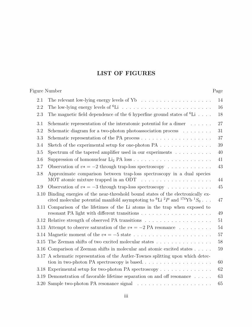
2.1 The relevant low-lying energy levels of Yb . . . . . . . . . . . . . . . . . . . 14
2.2 The low-lying energy levels of 6Li . . . . . . . . . . . . . . . . . . . . . . . . 16
2.3 The magnetic field dependence of the 6 hyperfine ground states of 6Li . . . . 18
3.1 Schematic representation of the interatomic potential for a dimer . . . . . . 27
3.2 Schematic diagram for a two-photon photoassociation process . . . . . . . . 31
3.3 Schematic representation of the PA process . . . . . . . . . . . . . . . . . . . 37
3.4 Sketch of the experimental setup for one-photon PA . . . . . . . . . . . . . . 39
3.5 Spectrum of the tapered amplifier used in our experiments . . . . . . . . . . 40
3.6 Suppression of homonuclear Li2 PA loss . . . . . . . . . . . . . . . . . . . . . 41
3.7 Observation of v∗ = −2 through trap-loss spectroscopy . . . . . . . . . . . . 43
3.8 Approximate comparison between trap-loss spectroscopy in a dual speciesMOT atomic mixture trapped in an ODT . . . . . . . . . . . . . . . . . . . 44
3.9 Observation of v∗ = −3 through trap-loss spectroscopy . . . . . . . . . . . . 45
3.10 Binding energies of the near-threshold bound states of the electronically ex-cited molecular potential manifold asymptoting to 6Li 2P and 174Yb 1S0 . . . 47
3.11 Comparison of the lifetimes of the Li atoms in the trap when exposed toresonant PA light with different transitions . . . . . . . . . . . . . . . . . . . 49
3.12 Relative strength of observed PA transitions . . . . . . . . . . . . . . . . . . 51
3.13 Attempt to observe saturation of the v∗ = −2 PA resonance . . . . . . . . . 54
3.14 Magnetic moment of the v∗ = −5 state . . . . . . . . . . . . . . . . . . . . . 57
3.15 The Zeeman shifts of two excited molecular states . . . . . . . . . . . . . . . 58
3.16 Comparison of Zeeman shifts in molecular and atomic excited states . . . . . 59
3.17 A schematic representation of the Autler-Townes splitting upon which detec-tion in two-photon PA spectroscopy is based. . . . . . . . . . . . . . . . . . . 60
3.18 Experimental setup for two-photon PA spectroscopy . . . . . . . . . . . . . . 62
3.19 Demonstration of favorable lifetime separation on and off resonance . . . . . 63
3.20 Sample two-photon PA resonance signal . . . . . . . . . . . . . . . . . . . . 65
iii
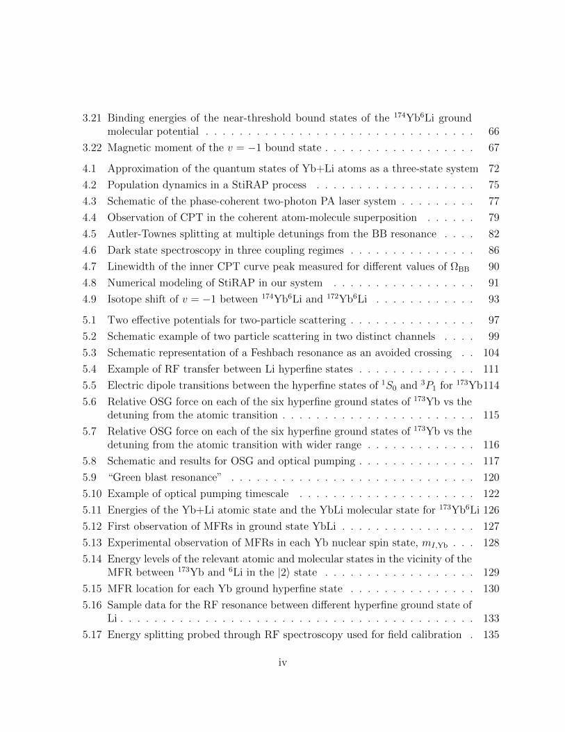
3.21 Binding energies of the near-threshold bound states of the 174Yb6Li groundmolecular potential . . . . . . . . . . . . . . . . . . . . . . . . . . . . . . . . 66
3.22 Magnetic moment of the v = −1 bound state . . . . . . . . . . . . . . . . . . 67
4.1 Approximation of the quantum states of Yb+Li atoms as a three-state system 72
4.2 Population dynamics in a StiRAP process . . . . . . . . . . . . . . . . . . . 75
4.3 Schematic of the phase-coherent two-photon PA laser system . . . . . . . . . 77
4.4 Observation of CPT in the coherent atom-molecule superposition . . . . . . 79
4.5 Autler-Townes splitting at multiple detunings from the BB resonance . . . . 82
4.6 Dark state spectroscopy in three coupling regimes . . . . . . . . . . . . . . . 86
4.7 Linewidth of the inner CPT curve peak measured for different values of ΩBB 90
4.8 Numerical modeling of StiRAP in our system . . . . . . . . . . . . . . . . . 91
4.9 Isotope shift of v = −1 between 174Yb6Li and 172Yb6Li . . . . . . . . . . . . 93
5.1 Two effective potentials for two-particle scattering . . . . . . . . . . . . . . . 97
5.2 Schematic example of two particle scattering in two distinct channels . . . . 99
5.3 Schematic representation of a Feshbach resonance as an avoided crossing . . 104
5.4 Example of RF transfer between Li hyperfine states . . . . . . . . . . . . . . 111
5.5 Electric dipole transitions between the hyperfine states of 1S0 and 3P1 for 173Yb114
5.6 Relative OSG force on each of the six hyperfine ground states of 173Yb vs thedetuning from the atomic transition . . . . . . . . . . . . . . . . . . . . . . . 115
5.7 Relative OSG force on each of the six hyperfine ground states of 173Yb vs thedetuning from the atomic transition with wider range . . . . . . . . . . . . . 116
5.8 Schematic and results for OSG and optical pumping . . . . . . . . . . . . . . 117
5.9 “Green blast resonance” . . . . . . . . . . . . . . . . . . . . . . . . . . . . . 120
5.10 Example of optical pumping timescale . . . . . . . . . . . . . . . . . . . . . 122
5.11 Energies of the Yb+Li atomic state and the YbLi molecular state for 173Yb6Li 126
5.12 First observation of MFRs in ground state YbLi . . . . . . . . . . . . . . . . 127
5.13 Experimental observation of MFRs in each Yb nuclear spin state, mI,Yb . . . 128
5.14 Energy levels of the relevant atomic and molecular states in the vicinity of theMFR between 173Yb and 6Li in the |2〉 state . . . . . . . . . . . . . . . . . . 129
5.15 MFR location for each Yb ground hyperfine state . . . . . . . . . . . . . . . 130
5.16 Sample data for the RF resonance between different hyperfine ground state ofLi . . . . . . . . . . . . . . . . . . . . . . . . . . . . . . . . . . . . . . . . . . 133
5.17 Energy splitting probed through RF spectroscopy used for field calibration . 135
iv
5.18 Observation of MFRs in Li2 via trap-loss spectroscopy . . . . . . . . . . . . 136
5.19 Spectroscopy of the Yb 3P1 state for field calibration . . . . . . . . . . . . . 137
5.20 Magnetic field calibration data and fit results . . . . . . . . . . . . . . . . . 139
5.21 Temperature dependence of YbLi MFR with calculation of three-body evenrate . . . . . . . . . . . . . . . . . . . . . . . . . . . . . . . . . . . . . . . . 141
6.1 Atom-molecule coupling strength at a magnetic Feshbach resonance. . . . . . 143
A.1 Optical paths added to the existing apparatus in order to perform OSG . . . 168
A.2 Schematic of optical pumping on the 1S0 → 1P1 transition of 173Yb . . . . . 169
A.3 Schematic of the control electronics used for the bias “Feshbach” coils . . . . 172
v
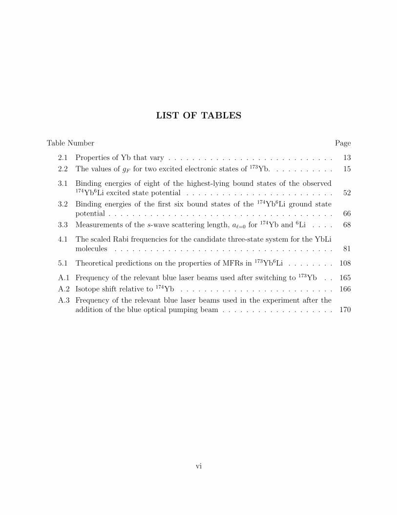
LIST OF TABLES
Table Number Page
2.1 Properties of Yb that vary . . . . . . . . . . . . . . . . . . . . . . . . . . . . 13
2.2 The values of gF for two excited electronic states of 173Yb. . . . . . . . . . . 15
3.1 Binding energies of eight of the highest-lying bound states of the observed174Yb6Li excited state potential . . . . . . . . . . . . . . . . . . . . . . . . . 52
3.2 Binding energies of the first six bound states of the 174Yb6Li ground statepotential . . . . . . . . . . . . . . . . . . . . . . . . . . . . . . . . . . . . . . 66
3.3 Measurements of the s-wave scattering length, a`=0 for 174Yb and 6Li . . . . 68
4.1 The scaled Rabi frequencies for the candidate three-state system for the YbLimolecules . . . . . . . . . . . . . . . . . . . . . . . . . . . . . . . . . . . . . 81
5.1 Theoretical predictions on the properties of MFRs in 173Yb6Li . . . . . . . . 108
A.1 Frequency of the relevant blue laser beams used after switching to 173Yb . . 165
A.2 Isotope shift relative to 174Yb . . . . . . . . . . . . . . . . . . . . . . . . . . 166
A.3 Frequency of the relevant blue laser beams used in the experiment after theaddition of the blue optical pumping beam . . . . . . . . . . . . . . . . . . . 170
vi
ACKNOWLEDGMENTS
Six years is a long time to get used to the idea that you work in a real research lab. Yet
somehow I never did. I never lost sight of how lucky I was to work in the Gupta Lab. For
this amazing experience I will always be grateful to my advisor Deep. In innumerable ways,
Deep’s unflagging support has helped me make the best of the opportunity, always finding
the time to provide insightful feedback and to dispense advice and encouragement. He sets
an example not only of perspicacity but also of dedication, kindness and good humor.
I would also like to thank the other members of my supervisory committee for supporting
my work: Anton Andreev, Boris Blinov, Kai-Mei Fu, Bob Holzworth and Arka Majumdar.
I thank Boris in particular for serving on my reading committee and for his insightful career
advice and friendly encouragement. Kai-Mei also took great pains to help improve my thesis
while serving on my reading committee for which I am grateful. From Kai-Mei’s example I
have worked to develop a fundamental and important skill which I had not fully appreciated:
doing what is important! It sounds easy but it is not and after graduation I will continue to
ask myself how I would use my time if I were Kai-Mei.
I am also grateful for the opportunity to have worked with Svetlana Kotochigova, Eite
Tiesinga, Ming Li and Hui Li, all of whom worked patiently to bring together our rather
different perspectives.
Over the years I have come to think of my basement lab - with its half-dead panels
of garish fluorescent lights, concrete floor and cacophonous orchestra of instruments - as a
cozily appointed fortress from which I rule the world. Like any space so transformed from
it’s fundamentals, this feeling of being at home is built on memories: small triumphs and
acute devastation; hard-fought campaigns and wild goose chases; good jokes and also puns.
vii
Good or bad, all were made better by the people I shared them with.
Ricky Roy was a patient and insightful teacher who taught me everything about the
lab and served as an inspiring role model. In later years I worked closely with Jun Hui
See Toh who became an integral part of the lab through his ability to quickly synthesize
information, dedication to getting things right and willingness to work hard. As unflappable
as he is competent, I could not have imagined a better labmate. Xinxin Tang has brought an
unprecedented cheerfulness to the lab and I am inspired by his curiosity about wide-ranging
subjects. I have also benefited greatly from the eclectic insights of Yifei Bai.
I am grateful for two postdocs who I have had the privilege to work with in the lab:
Ryan Bowler and Katie McCormick. From Ryan I learned several valuable technical skills
and received much needed encouragement when I felt like I was flailing. In the short time I
have known Katie McC I have marveled at her extreme competence and acumen.
Although the time I actually worked with them was very short, I am grateful to Anders
Hansen, Alex Khramov, Alan Jamison, and Will Dowd, who as the first graduate students
in the lab set a congenial tone and a high bar.
Working next door in the interferometry lab, Ben Plotkin-Swing, Katie McAlpine, and
Dan Gochnauer were a reliable resource of information and advice. With the recent addition
of Tahiyat Rahman and Anna Wirth, the combined Gupta group has become a more vibrant
community. Combined with the Blinovians working even farther down the hall, I have found
joy putting our heads together to decipher the more inscrutable bits of the interesting articles
we read for journal club.
I want to thank all the members of PIE who attended socials, book clubs and lunch
meetings. For me these interludes were a powerful antidote against self-reproach that can
haunt us all in stressed isolation.
I would like to thank many dear friends without whom I would never have made it to
the point of writing a thesis. My life in graduate school was made immeasurably better by
viii
a group of awesome housemates who were also among my closest friends: Rachel Osofsky,
Tong Wan and Sarah Carter. I am so grateful to Alex Ditter for chill times with culinary
experiments and jigsaw puzzles that I will even forgive him for consistently losing critical edge
pieces. I thank Katie Brennan and Ali Ashtari Esfahani for enlightening lunch engagements
that always brightened my day. On Stephen French and Tyson Price I could always rely for
wide-ranging and many-stranded conversations that could end only when we had broken out
the Mathematica model or lit something on fire. I thank Gary and Laurie Ness for helping
a recent college graduate start a new life in a new city. It has been my honor to call Katie
McAlpine a labmate, a gym partner and a friend. Being the most insightful person I know,
I have benefited greatly from having her in many parts of my life.
Getting my PhD was an exciting adventure I never would have started without support
from the faculty at Lewis & Clark College. First among them is the late Shannon O’Leary,
unicorn warrior physicist. Under Shannon’s guidance I found both the fun in physics research
and the belief that I could do it. In the years that I was so lucky to have known her, she taught
me the value of taking every opportunity to succeed while making every opportunity to help
others do the same. In this same tradition I have found invaluable support and mentorship
from Anne Bentley. I would also like to thank Aojie Zheng for being an unwavering partner
to my many infamous lab crimes.
Lastly I thank my family. First, I want to express my gratitude to both my parents and
grandparents for humanely raising me as a 100% free-range child. I consider my pursuit of
physics to be a mere extension of my childhood whiled away in exploration and discovery,
full of love and care but light on structure and rigidity. The well-beyond-perturbative forces
of my three brothers have made me scrappier and more determined. I thank them all for
making me the person I am today.
ix
1
Chapter 1
INTRODUCTION
Quantum gases are deceptively simple systems. Absent the confusing tumult of temper-
ature, particles in quantum gases dramatically manifest their indistinguishability and are
governed by quantum statistics. In ultracold quantum gases, we can “see” the inherent
quantumness of the particles using well-developed tools of atomic physics, not only to ac-
cess observables, but also to change the particles’ energy landscape. Indeed it was clever
manipulation of atomic properties with lasers that enabled the first creation of a gaseous
Bose-Einstein condensate (BEC) in 1995, followed a few years later by the first degenerate
Fermi gas of atoms.
Since first leveraging the precise control afforded by lasers to engineer an entirely new
phase of matter in the form of BEC, ultracold-atoms researchers have continued to expand
the range of this control by cooling and trapping an increasingly diverse set of atoms and
molecules, each with unique properties such as electronic transitions or different interactions.
In turn, these properties can make certain species of ultracold atoms or molecules a powerful
tool for studies of specific aspects of quantum simulation, precision measurement or quantum
information processing.
That the cooling and trapping of a large set of atomic and molecular species would be
integral to the rapidly expanding field of quantum gases was recognized at its foundation.
In 1998, when the population of quantum degenerate atomic species numbered only three,
the creators of the first BEC boldly proclaimed that “the number of different atomic and
molecular species that could eventually be cooled to the BEC transition may be in the
hundreds” [1]. Two decades later, we are still trying to prove them right. While the number of
ultracold species at or near degeneracy has indeed increased, the interest in further diversity
2
has persisted. This thesis aims particularly at the frontier of ultracold paramagnetic, polar
molecules by investigating the possibility of synthesizing YbLi from an ultracold atomic
mixture by manipulating scattering resonances.
This thesis contains four principal chapters. Chapter 2 describes the broader scientific
benefit of studying neutral ultracold molecules, discussing both proposed impacts and active
research projects. This chapter also discusses the particular properties of Yb and Li which are
important not only to understand the peculiar challenges to making YbLi molecules, but also
to outline its particularly interesting qualities. In Chapter 3, we present experimental results
on spectroscopy of the YbLi molecule in one of the lowest excited electronic states and the
sole electronic ground state. These results constitute the first study of Feshbach resonances
in YbLi - the optical Feshbach resonance (OFR). More practically, these spectroscopies made
possible the work in subsequent chapters that investigate in more detail coherent control of
these scattering resonances for the purposes of molecule formation. In Chapter 4, we discuss
the molecular states probed in the previous chapter in the context of coherent addressing of
a three-level system. Such addressing may allow for efficient transfer of the atomic mixture
into a molecular state even under the condition that the coupling between states is not the
fastest timescale in the system. As our first efforts to create molecules in this way failed, we
present our experimental analysis of the timescales involved, and through numerical modeling
confirm that we are limited by two different oft-ignored mechanisms of decoherence, noting
the ways in which the relevant timescales would change if these attempts are repeated with
the atomic mixture in a deep optical lattice. Chapter 5 reports on a different and more
widely studied type of Feshbach resonance - magnetic Feshbach resonances which rely on
control of the spin degree(s) of freedom rather than the orbital degree of freedom. Because
magnetic Feshbach resonances were long thought not to exist between YbLi, this chapter
begins with an explanation of the origin of MFRs both in a more typical system and in a
system such as YbLi. The latter parts of this chapter concern the experimental techniques
used and first observation of such resonances in the mixture of ground state Yb and Li. The
thesis closes with a discussion of the required steps to synthesize molecules in Chapter 6.
3
Here we discuss the feasibility of using our experimental control of the external magnetic
field to convert atomic mixtures into molecules, exploiting the existence of the MFR and
sketch the technical upgrades necessary to do so. Finally, we outline an exciting experiment
to immediately pursue upon the successful creation of YbLi molecules.
4
Chapter 2
ULTRACOLD MOLECULES: WHY YOU WANT THEM ANDHOW TO MAKE THEM
This chapter discusses the motivation behind this thesis. A general description of the
broader scientific goals of the study of ultracold molecules is presented first. Then we discuss
the current capabilities of researchers studying ultracold molecules which follow two distinct
and complementary strategies. Before introducing the properties of the YbLi molecule that
make it uniquely interesting among the cast of ultracold molecules, we briefly describe the
properties of the Yb and Li atoms. This serves not only to explain the properties of the YbLi
molecule but also to provide relevant background information to experimental techniques
presented later in the thesis. Finally, a brief and somewhat generalized description of the
experimental apparatus used in this work is presented for the uninitiated.
2.1 Motivation: Cool Science with Ultracold Molecules
The study of ultracold molecules is largely motivated by the same scientific promise as
ultracold atoms which constitute a well-isolated, easily probed quantum system to which
various interesting complications can be added such as tailored potentials and controlled
interactions. The defining difference between atoms and molecules is the diversity of quantum
states in which they can be prepared. While ultracold molecules are also characterized by
electronic and nuclear spin states, they are further distinguished by the quantized motion
of the nuclei relative to each other in the form of vibration and rotation. The additional
degrees of freedom available in molecules makes their study an interdisciplinary field requiring
collaboration, not only between different subfields of physics, but also between physicists
and chemists. In what follows, we sketch four categories of research enabled by the study
5
of ultracold molecules: quantum chemistry, quantum simulation, quantum information and
precision measurement.
2.1.1 Quantum Chemistry
Trapped ultracold molecules allow for a bottom-up approach to quantum chemistry in which
the participating reactants can be prepared in a single quantum state with their spins and
dipole moments well-defined by the confinement of the trap [2]. By preparing samples of
ultracold molecules and/or atoms in a single quantum state, the number of possible product
states is limited, confining the reaction to a few or even just one pathway [3, 4]. This
extraordinary simplification teases the possibility of fully understanding the transformation
from reactants to products in a level of detail that cannot be accomplished even in cold
molecular beams.
Fully-state controlled chemical reactants were first studied in samples of optically trapped
KRb molecules at around 100 nK when unexpected losses from the ultracold sample were
attributed to the bimolecular reaction KRb + KRb→K2+Rb2 [5]. In this work, researchers
used control over the molecule’s hyperfine state to “turn down” the rate of chemical reac-
tions by preparing a spin-polarized fermionic sample in which intermolecular collisions are
suppressed by the necessity of tunneling through the angular momentum barrier.
While the ability to precisely prepare the state of an ultracold molecular sample gives a
degree of control to the experimenters, a complete understanding of the chemical reaction
would require the ability to probe and/or control also the product states as well as the
intermediate complexes made up of all the involved atoms that form during the reaction.
More recently, researchers have developed methods to probe the products and the four-body
intermediate complex in the same KRb + KRb→K2+Rb2 reaction [6]. The technique which
relies on ionization of the particles participating in the reaction is itself dependent on the
ability to precisely prepare the reactants in their lowest energy ro-vibrational state for which
the reaction proceeds slowly enough to be probed.
Other proposals for studying the products of a chemical reaction involve trapping them.
6
This situation doesn’t arise “naturally” as the energy released in most exothermic chemical
reactions greatly exceeds the depths of the traps that are designed to capture laser-cooled
atoms. However, in [7, 8] the authors proposed to observe reactions involving ultracold
dimers that release a smaller than typical amount of energy in their reaction: ‘isotope ex-
change reactions’ in which two dimers containing different isotopes of the same element react
to form two dimers each containing only one isotope. Further, the authors of [7, 8] have
proposed that the amount of energy released could be tuned over a wide range using laser
fields. Still others prospose to study the process of chemical reaction, not by capturing the
products, but through probes of the short-lived intermediate states with external field con-
trol being used to detect resonant behavior, and therefore learn about the complex’s spin
structure [9, 10].
As of this writing, studies of fully-state controlled chemistry have been limited to a
small number of ultracold heteronuclear dimers. Despite their small number, the study of
these ultracold heteronuclear dimers continue to produce surprising results such as the rapid
collisional loss of chemically stable ultracold molecules [11, 4, 12]. The cause of this rapid
loss is currently the focus of much debate [13, 14, 15] and calls for further study of ultracold
molecules with a variety of different properties. While the collisions of ultracold molecules
is of integral importance to the study of quantum chemistry, it is also imperative that they
be understood and perhaps prevented, as the production of a stable molecular sample is a
precondition for a wide variety of proposed studies, discussed in the following subsections.
2.1.2 Quantum Simulation
Ultracold molecules are sought not only for their internal properties but also for their distinct
interactions. Owing to the uneven distribution of the electron density around the various
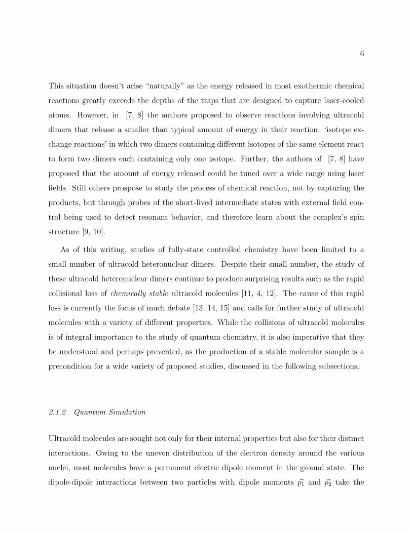
nuclei, most molecules have a permanent electric dipole moment in the ground state. The
dipole-dipole interactions between two particles with dipole moments ~p1 and ~p2 take the
7
following form.
Vd−d =1
4πε
~p1 · ~p2 − 3 (~p1 · r) (~p2 · r)r3
where ε is the permittivity, r is the interparticle separation unit vector and r is the interparti-
cle separation magnitude. This interaction, which is characteristic not only of polar molecules
but also of highly magnetic atoms [16, 17] and Rydberg atoms [18], are distinguished from
more typical atom-atom interactions in two distinct ways.
First, since Vd−d ∝ r−3, it is longer range than van der Waals interactions which are
typically the longest range interaction between neutral ground state particles and are given
by Vvdw ∝ r−6. Intuitively, this means that each particle will“see” more of the other particles
in the sample. More specifically, the r−3 dependence of the dipole-dipole interaction potential
makes the scattering properties between two such particles distinctly different from that of
the r−6 potential by overcoming the effects of the angular momentum barrier as will be
briefly discussed in Chapter 5 [19].
Second, the dipole-dipole interaction is distinguished from van der Waals interactions in
that it is anisotropic, with an angular dependence from the relative orientation of ~p1 and
~p2. This further complicates the rules of inter-particle scattering by allowing for coupling
between different scattering partial waves as will also be briefly mentioned in Chapter 5 [19].
Combined with the ability to precisely probe and control the quantum state of ultracold
atoms/molecules, the above properties are proposed as the basis for quantum simulation of
quantum magnetism [20], novel types of superfluidity [21, 22] or the observation of topological
phases [23]. As we shall see in the next section, these properties also provide the foundation
for proposed quantum information processing with ultracold molecules.
2.1.3 Quantum Information
Ultracold molecules feature multiple properties that are crucial for a quantum information
platform: seconds-long coherence times and strong long-range interactions for fast gates [24,
25, 26]. In contrast to ions, the interactions native to such molecules can be generally “turned
8
off” by transferring the molecule to the ground rotational state where the expectation value
of the dipole moment is zero [27, 28]. The ability to turn these interactions off at will can
decouple them from environmental noise. This feature, combined with their seconds long
trap and radiative lifetimes make ultracold molecules a particularly promising candidate to
serve as storage qubits in a hybrid quantum information platform [29, 30].
Ultracold molecules also offer a high degree of scalability; with current capabilities one
can easily imagine trapping and preparing in a target quantum state ∼ 104 or more ultra-
cold dimers in an optical lattice, with individual addressing available, either through field
gradients or precisely aligned, narrow-focus laser beams [24, 27]. In such endeavors, ultracold-
molecule trappers could greatly reduce motional decoherence effects by duplicating strategies
for complete motional control in optical tweezers developed in atoms [31, 32, 33].
Since the first proposal for using polar molecules for quantum information [24], several
proposals have considered in more detail the energy structure of particular molecules and the
experimental simplifications they enable [25, 34, 35]. In light of these proposals, the seemingly
infinite diversity of molecular species, combined with rapid expansion of our ability to cool
and trap them, motivates further investigation of specific ultracold molecule candidates for
quantum information.
2.1.4 Precision Measurement
Ultracold molecules are well-suited to extend our understanding of fundamental physics
through tabletop spectroscopy experiments, much like spectroscopic measurements of atoms
and molecules have done in the past [36]. Already, cold molecules (∼ 1 K) have been used
to put increasingly tight limits on CP violation, significantly constraining certain theories
beyond the standard model through measurements of the electron electric dipole moment in
paramagnetic ThO [37].
While the low temperatures and state preparation control are a general advantage of pre-
cision measurement with ultracold particles, a particular advantage of molecules lies in their
myriad internal states which are not only greater in number but are also of different “types.”
9
The interleaving of rotational and hyperfine spectra, for example, sets up the possibility that
two states of different character (e.g. opposite parity) happen to be nearly degenerate [38].
Probes of such energy separations have been proposed for sensitive tests of temporal vari-
ations of unitless physical constants such as the electron-to-proton mass ratio [39, 40, 41].
With implications for proposed theories for unification of the four fundamental forces [38],
these measurements are being actively pursued in the KRb molecule, and although the re-
sults are not yet competitive with previous measurements made using atomic clocks, rapid
improvement seems likely [42].
Additional proposals for probes of fundamental physics through precision spectroscopy
of molecules include time variation of the fine structure constant α [43], detection of non-
Newtonian gravity [44], and measurements of nuclear-spin-dependent parity violation to
better constrain electroweak coupling parameters [45, 46].
2.2 Two Methods for Producing Ultracold Molecules
The creation of ultracold molecules is typically accomplished using two different strategies,
both of which are pursued with seemingly equal intensity as each has its own advantages.
Below, we describe the general methods used and progress made with both strategies.
2.2.1 Direct Cooling
The direct cooling method is most analogous to the means of preparing ultracold atoms but
has some key differences. The generation of ultracold atomic gases almost always begins
with a hot atomic vapor that is slowed and cooled through precisely controlled spontaneous
emission of photons [47]. Because the momentum imparted by a photon onto an atom is
small compared to the momentum associated with its temperature, the atom must scatter
photons repeatedly, meaning that the atom must spontaneously decay to the same state
from which it was originally excited. The existence of such ‘closed cooling cycles’ is what
generally limits the diversity in the population of ultracold atomic gases. In contrast to
atoms however, the much larger number of internal states characterizing molecules typically
10
precludes their having a closed cooling cycle. Nevertheless, there exist a subset of molecules
for which these closed cycles can be approximately realized through the use of just a few
repumping laser beams that plug the leaks in the cycle [48, 49].
Through judicious choice of molecular species, several groups have adapted the technique
of laser cooling to form magneto-optic traps (MOT) of ultracold molecules and subsequently
loaded the cooled samples into conservative traps including quadrupole magnetic traps and
optical tweezers [50, 51, 32] and as of this writing, there are multiple other molecular species
being experimentally investigated for application of these strategies [52, 53, 54, 55, 56, 57,
58, 59]. By combining the traditional method of MOT cooling and trapping with pre-cooling
and slowing stages [60, 61, 62, 49], these groups have rapidly demonstrated the ability to
recreate temperatures similar to a typical first stage cooling process for atoms, reaching
∼ 10µK with sub-Doppler laser cooling techniques. However, the relatively low particle
density of these molecular samples means that the maximum phase space densities achieved
∼ 10−8 [63] remain a few orders of magnitude lower than a typical laser cooling stage for
atoms, posing a significant challenge to the creation of quantum degenerate samples.
Having made huge strides in the development of laser cooling techniques, the next chal-
lenge for direct cooling of molecules will be to develop or adapt existing techniques for cooling
in conservative potentials as is necessary to approach quantum degeneracy. Following a laser
cooling stage, atomic coolers will perform a variety of different techniques to further increase
the phase-space density of their gases including: evaporative cooling [64, 65], sympathetic
cooling [66] and degenerate Raman sideband cooling (dRSC) [67]. While evaporative cool-
ing of molecules has been demonstrated in one case [58] it is thought to be hampered both
by the high rate of inelastic collisions expected for molecules and also the relatively low
starting phase space densities. Sympathetic cooling is also expected to suffer from the high
rate of inelastic collisions although it has been demonstrated in ro-vibrational ground state
molecules [68] and theoretical work hints at its feasibility in cases where spin-changing col-
lisions can be suppressed [69, 70]. However, the recently accomplished feat of capturing
laser-cooled molecules in optical traps holds promise for application of dRSC to molecular
11
samples [63, 32].
2.2.2 Indirect Cooling
An alternate method to producing large samples of ultracold molecules is to form them from
ultracold atoms which are already trapped, a method sometimes referred to as the “indirect
approach”. If the process of converting atoms to molecules is coherent, the sample will have
nearly the same phase-space density as the atomic mixture from which it was created [71].
Although this strategy has only been used to create a limited selection of dimers, it remains
the best strategy for attaining very high phase space densities and has even been used to
create the first quantum degenerate gas of molecules [72].
This process is usually accomplished through a process known as magneto-association:
an adiabatic sweep across an avoided crossing between an atomic scattering state and a
bound molecular state [71]. While this process results in molecules that remain translation-
ally ultracold and in a single ro-vibrational state, they are usually prepared by necessity in
the highest energy vibrational state of the molecule. In this state they are not only less
scientifically interesting than molecules in the ro-vibrational ground state, but are also diffi-
cult to hold onto as they are collisionally unstable. For this reason, the magneto-association
will typically be followed by one or more coherent processes that transfers the molecules to
the ro-vibrational ground state, such as Stimulated Raman Adiabatic Passage (StiRAP) in
which a two-photon laser field is used to dynamically manipulate a coherent superposition
of the initial and final molecular states via a third electronically excited state [73].
Many research groups have used the coherent association+StiRAP technique to form
ultracold molecules in their ro-vibrational ground state [74, 75, 76, 11, 77, 78, 79]. At the
time of this writing there were several additional groups actively working to develop coherent
association techniques in novel systems [80, 81, 82, 83, 84, 85]. As will be explained in
Chapter 5, the roster of ultracold dimers made via this indirect approach is made up almost
entirely of molecules containing two alkali atoms, owing to two general facts: there are
widespread, easily implemented methods for cooling alkali atoms and pairs of alkali atoms
12
often exhibit broad magnetic Feshbach resonances which are necessary for the magneto-
association process. The notable exception is Sr2 which is a bi-alkaline earth molecule [80].
In this case, molecules are formed from pairs of atoms using only laser fields in a StiRAP
process that addresses not a superposition of two molecular states but rather a superposition
of one free atom scattering state and one molecular state. As we shall see in Chapter 4, the
replication of this technique in our group is of great experimental interest.
2.3 Properties of Yb
Before discussing the properties of the YbLi molecule which motivate our effort to make
these ultracold molecules, it is instructive to consider the properties of its constituent atoms.
This discussion will also include details important to the experimental methods throughout
this thesis.
Yb (element 70) is a lanthanide atom with electronic structure similar to the alkaline-
earth (group II) elements. In the context of ultracold atoms, Yb is generally attractive for
several reasons.
• Yb has a 1S0 (singlet) ground state which distinguishes it from the more typical 2S1/2
(doublet) ground state characteristic of alkali atoms.
• Yb has multiple electronic transitions in the visible range with varying linewidths
spanning several order of magnitude.
• Yb has several abundant isotopes, both bosonic and fermionic.
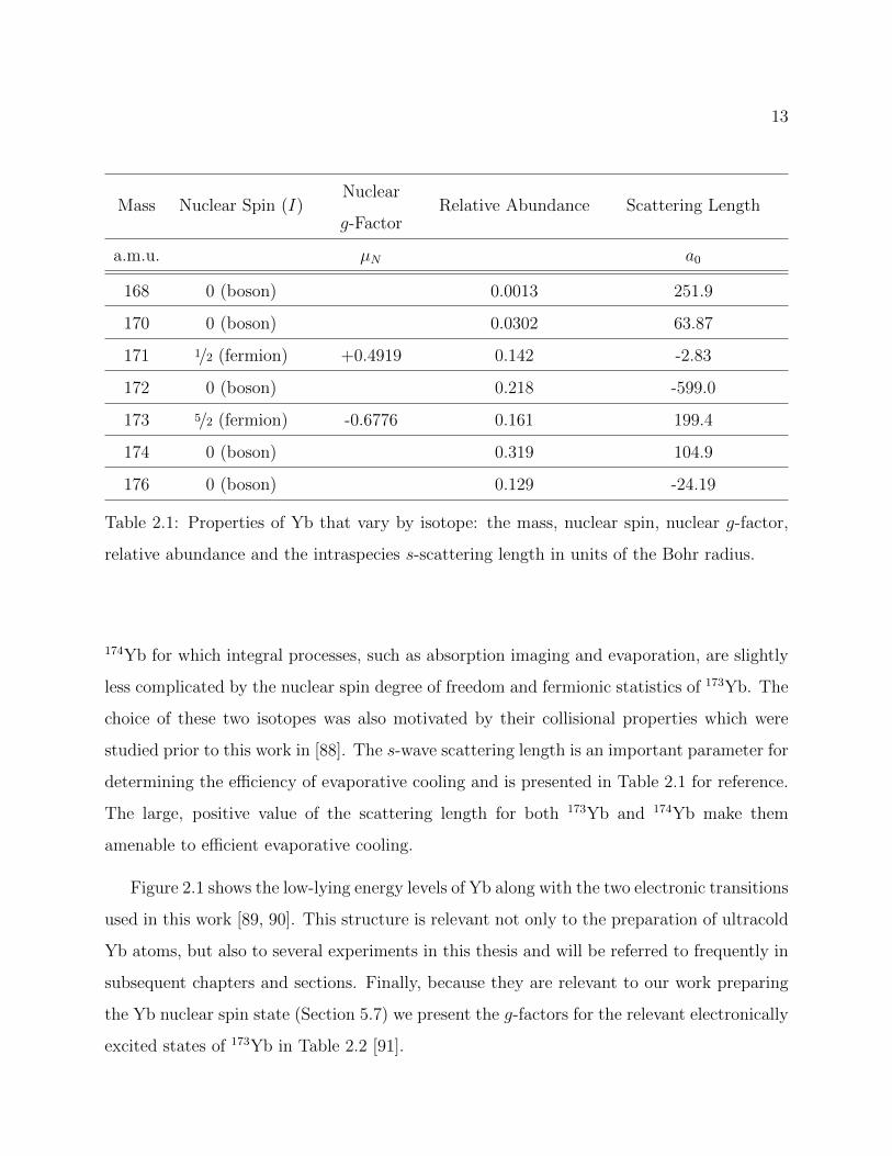
In one way or another, the work in this thesis is made possible because of these properties.
We have used samples of 173Yb and 174Yb. Both isotopes have rather high natural abundance
as seen in Table 2.1 [86]. The choice of these isotopes had several motivations. Critical to
our experiments presented in Chapter 5, the fermionic isotope 173Yb has a nonzero nuclear
spin with a nuclear g-factor of -0.6776 [87]. Other experiments used in this thesis utilized
13
Mass Nuclear Spin (I)Nuclear
g-FactorRelative Abundance Scattering Length
a.m.u. µN a0
168 0 (boson) 0.0013 251.9
170 0 (boson) 0.0302 63.87
171 1/2 (fermion) +0.4919 0.142 -2.83
172 0 (boson) 0.218 -599.0
173 5/2 (fermion) -0.6776 0.161 199.4
174 0 (boson) 0.319 104.9
176 0 (boson) 0.129 -24.19
Table 2.1: Properties of Yb that vary by isotope: the mass, nuclear spin, nuclear g-factor,
relative abundance and the intraspecies s-scattering length in units of the Bohr radius.
174Yb for which integral processes, such as absorption imaging and evaporation, are slightly
less complicated by the nuclear spin degree of freedom and fermionic statistics of 173Yb. The
choice of these two isotopes was also motivated by their collisional properties which were
studied prior to this work in [88]. The s-wave scattering length is an important parameter for
determining the efficiency of evaporative cooling and is presented in Table 2.1 for reference.
The large, positive value of the scattering length for both 173Yb and 174Yb make them
amenable to efficient evaporative cooling.
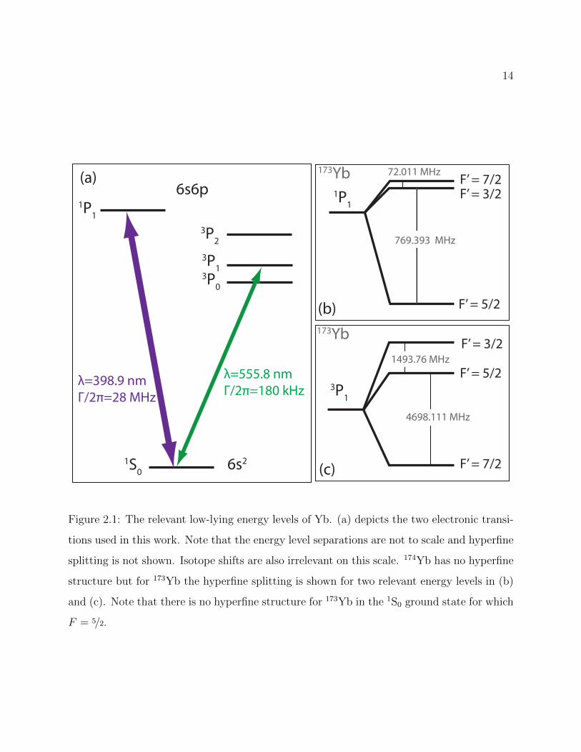
Figure 2.1 shows the low-lying energy levels of Yb along with the two electronic transitions
used in this work [89, 90]. This structure is relevant not only to the preparation of ultracold
Yb atoms, but also to several experiments in this thesis and will be referred to frequently in
subsequent chapters and sections. Finally, because they are relevant to our work preparing
the Yb nuclear spin state (Section 5.7) we present the g-factors for the relevant electronically
excited states of 173Yb in Table 2.2 [91].
14
1S0
3P2
3P13P0
1P1
3P1
1P1
F’ = 5/2
F’ = 5/2
F’ = 3/2
F’ = 3/2F’ = 7/2
F’ = 7/2
λ=555.8 nmΓ/2π=180 kHz
λ=398.9 nmΓ/2π=28 MHz
72.011 MHz
769.393 MHz
1493.76 MHz
4698.111 MHz
(a)
(b)
(c)
6s6p
6s2
173Yb
173Yb
Figure 2.1: The relevant low-lying energy levels of Yb. (a) depicts the two electronic transi-
tions used in this work. Note that the energy level separations are not to scale and hyperfine
splitting is not shown. Isotope shifts are also irrelevant on this scale. 174Yb has no hyperfine
structure but for 173Yb the hyperfine splitting is shown for two relevant energy levels in (b)
and (c). Note that there is no hyperfine structure for 173Yb in the 1S0 ground state for which
F = 5/2.
15
F ′ 1P13P1
3/2 -0.400 -0.600
5/2 0.114 0.171
7/2 0.286 0.429
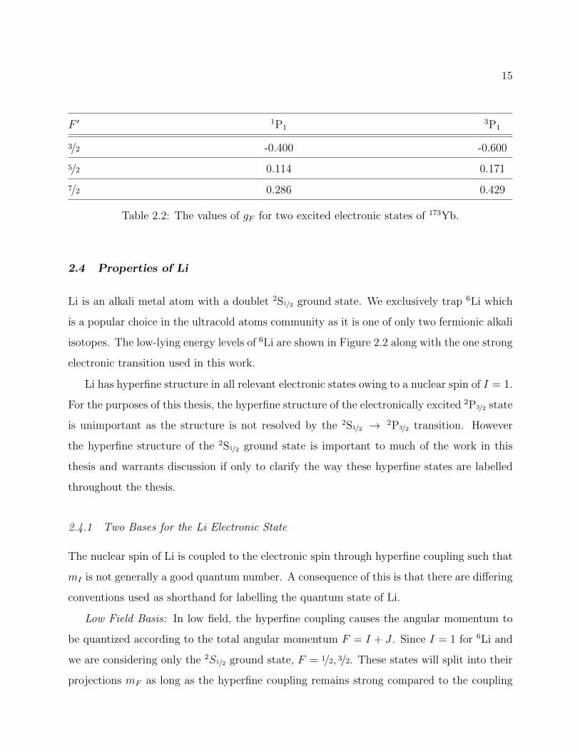
Table 2.2: The values of gF for two excited electronic states of 173Yb.
2.4 Properties of Li
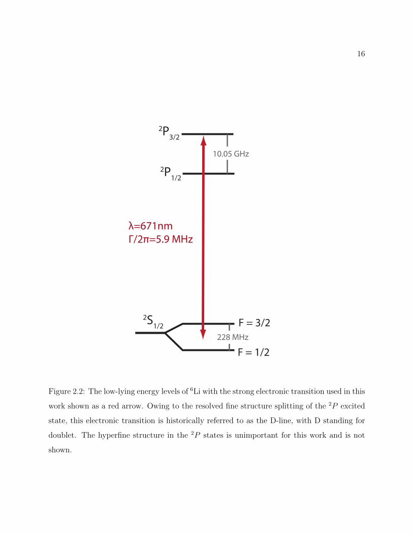
Li is an alkali metal atom with a doublet 2S1/2 ground state. We exclusively trap 6Li which
is a popular choice in the ultracold atoms community as it is one of only two fermionic alkali
isotopes. The low-lying energy levels of 6Li are shown in Figure 2.2 along with the one strong
electronic transition used in this work.
Li has hyperfine structure in all relevant electronic states owing to a nuclear spin of I = 1.
For the purposes of this thesis, the hyperfine structure of the electronically excited 2P3/2 state
is unimportant as the structure is not resolved by the 2S1/2 → 2P3/2 transition. However
the hyperfine structure of the 2S1/2 ground state is important to much of the work in this
thesis and warrants discussion if only to clarify the way these hyperfine states are labelled
throughout the thesis.
2.4.1 Two Bases for the Li Electronic State
The nuclear spin of Li is coupled to the electronic spin through hyperfine coupling such that
mI is not generally a good quantum number. A consequence of this is that there are differing
conventions used as shorthand for labelling the quantum state of Li.
Low Field Basis: In low field, the hyperfine coupling causes the angular momentum to
be quantized according to the total angular momentum F = I + J . Since I = 1 for 6Li and
we are considering only the 2S1/2 ground state, F = 1/2, 3/2. These states will split into their
projections mF as long as the hyperfine coupling remains strong compared to the coupling
16
2S1/2
2P1/2
2P3/2
λ=671nmΓ/2π=5.9 MHz
10.05 GHz
228 MHz
F = 1/2
F = 3/2
Figure 2.2: The low-lying energy levels of 6Li with the strong electronic transition used in this
work shown as a red arrow. Owing to the resolved fine structure splitting of the 2P excited
state, this electronic transition is historically referred to as the D-line, with D standing for
doublet. The hyperfine structure in the 2P states is unimportant for this work and is not
shown.
17
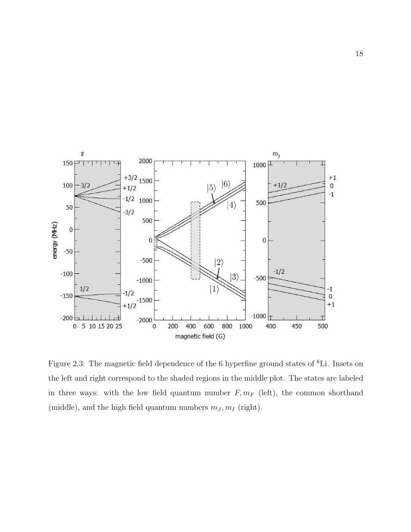
of the individual spins to the external field, evolving as EZeeman = gFµBmFB where gF
is the hyperfine g-factor, µB is the Bohr magneton and B is the external field. As shown
in Figure 2.3 the relatively small hyperfine coupling of Li and the strong coupling of the
electronic spin to the external field means that the shift from the magnetic field deviates
from this prescription even at ≈ 20 G.
High Field Basis: When the Zeeman coupling to the external field exceeds the hyperfine
coupling between the electron and nuclear spins, the projections mI and mJ become good
quantum numbers, making the state |IJmImJ〉 a good approximation of the true eigenstate
of the system.
The Common Convention: The connection between states |IJFmF 〉 in low field and
|IJmImJ〉 in high field is generally well understood by researchers working with ground
state Li atoms. For this reason, it is common to label the six hyperfine ground states simply
as |1〉 through |6〉 in order of ascending energy at finite field (see Figure 2.3). In this thesis
we will usually use the common convention. However, we will sometimes use |IJFmF 〉 even
to refer to eigenstates at high field, assuming the correspondence between high and low field
states is understood.
2.5 Motivation: Properties of YbLi
The primary interest in making ultracold YbLi molecules from Yb and Li stems from the
atoms’ different electronic properties. The combination of the 2S1/2 ground state of Li with
the 1S0 ground state of Yb means that the molecule itself has an unpaired electron. In an
analogy to the typical atomic term symbol, molecules of this type are given the label 2Σ.
This doublet electronic structure distinguishes the YbLi molecule from the bi-alkali molecular
species that make up the majority of the molecules created through direct cooling. With
the sole exception of NaLi which is prepared in a triplet state (3Σ), all the molecules formed
near quantum degeneracy using the indirect method are in a spin-singlet state (1Σ).
The ground state magnetic moment of YbLi affords an additional means with which to
control them. In the most general sense, the YbLi molecule (and those like it such as CsYb
18
Figure 2.3: The magnetic field dependence of the 6 hyperfine ground states of 6Li. Insets on
the left and right correspond to the shaded regions in the middle plot. The states are labeled
in three ways: with the low field quantum number F,mF (left), the common shorthand
(middle), and the high field quantum numbers mJ ,mI (right).
19
and RbSr) is the alkali atom of the molecule world and therefore ripe for examination by the
same methods which have been developed and refined over multiple decades of research into
ultracold alkalis. Most fundamentally, the YbLi molecule can be magnetically trapped. This
could be of critical importance for the study of ultracold molecules as trapping molecules
in optical traps may be associated with higher loss rates than for atoms [15]. As we shall
see in Chapter 5, the ability to magnetically control interactions in ultracold atoms has
been pivotal to studying them in the more general and highly diverse contexts of few- and
many-body physics. Unlike the spin-singlet molecules, it’s possible that magnetically tunable
interactions exist between spin-doublet molecules.
The YbLi molecule, being a heteronuclear dimer also has a permanent electric dipole
moment arising from the uneven distribution of the electrons around the two different nuclei.
Ground state molecules with both an electric and magnetic dipole moment are the subject
of wide-ranging theoretical discourse. Much of this interest hinges on coupling between
the electron spin and the molecular rotation. With control over the rotational degree of
freedom being the “switch” used to access long-range interactions between dipolar molecules,
this spin-rotation coupling allows for controllable effective spin-spin interactions which are
the essential ingredient for a variety of lattice spin models, central to condensed matter
studies [92]. This coupling also allows for unique implementation of quantum information
processing with ultracold molecules which is distinguished from other proposed schemes
that typically require fine control over external electric fields in order to achieve individual
qubit addressability [93]. Additionally, this coupling allows for the implementation of field-
controlled chemical reactions [94].
Unfortunately, the magnitude of the YbLi ground state electric dipole moment is pre-
dicted to be too small for dipole-dipole interactions to be productively wielded in experiments
as they are designed today [95], though it’s possible that larger dipole moments could be
coherently accessed by mixing the ground state with an excited state via a narrow electronic
transition within the molecule [96].
20
2.6 An Overview of the Experimental Apparatus
The purpose of this section is to briefly explain the common elements and methods of ul-
tracold atom experiments to a reader unfamiliar with these techniques, as an understanding
of these will be assumed throughout. For specific details on our apparatus, the reader is
referred to the theses of Anders Hansen [97] and Alex Khramov [98].
Vacuum System In the course of our experiments, ultracold atoms are held for several
seconds in traps with a depth corresonding to a temperature∼ 1µK. Consequently, a collision
between a trapped atom and an air molecule will necessarily cause loss from the trap and the
lifetime of atoms in the trap will ultimately be limited by the pressure they are exposed to.
For this reason, our experiments take place in a chamber under ultra-high vacuum. A typical
pressure inside our main vacuum chamber where the atoms are trapped is ∼ 10−11 Torr. We
measure typical trap lifetimes of about 4 seconds for Yb and longer than 20 seconds for Li.
Atomic Source Both Yb and Li are metallic solids at room temperature (even under
vacuum) and must be heated to produce a vapor that can be laser cooled. Our apparatus
includes two separate ovens - one for each element - which are heated to about 400 degrees
Celsius. Each oven is connected to the main vacuum chamber by a long tube through which
a beam of atomic vapor travels to the main chamber after being roughly collimated by a
nozzle at the output of the oven. The RMS speed of the vapor is ∼ 100 m/s, too fast to be
captured in our traps. The vapor is slowed using the Zeeman slower approach which utilizes
the radiation pressure from a resonant laser beam propagating in the opposite direction
of the vapor [99]. As the atoms are slowed, the change in the Doppler shift significantly
detunes the slowing laser beam from resonance. This shift is counteracted by a spatially
varying magnetic field that cancels the Doppler shift using a Zeeman shift. In our apparatus
the magnetic field is generated by electromagnets wound in a tapered solenoid configuration
along the whole length of the slowing tube. By the time the vapor reaches the main vacuum
chamber, the RMS speed is reduced to ∼ 10 m/s.
Magneto-optic Trap The magneto-optic trap (MOT) performs the first stage of cooling in
21
all dimensions and also traps the atoms [47]. Cooling in the magneto-optic trap is based on
laser cooling through which the momentum of many photons is used to reduce the momentum
of an atom. This process relies on repeated spontaneous emission of photons after electronic
excitation. In order for the momentum of the atoms to be reduced, the laser beams must
be near but at a slightly lower energy than the electronic transition within the atom such
that an atom moving antiparallel to the laser beam propagation will scatter more strongly
than one moving parallel to it owing to different Doppler shifts. These red-detuned beams
are oriented along three orthogonal directions in counterpropagating pairs in order to cool
in all directions. Under these conditions - known as optical molasses - cold atoms can still
randomly walk out of the molasses because the restoring force in each direction is uncoupled
to that of the other directions. To avoid loss from the molasses, a magnetic field gradient
is used to impose a spatial dependence on the scattering rate of photons and each pair of
counterpropagating beams is given opposite circular polarization beams such that selection
rules effect an overall restoring force to the center of the trap. After the MOT has captured
and cooled a large sample of atoms, we compress the MOT such that the sample can be more
readily trapped by the optical dipole trap where they will undergo further cooling. This
compression is done by simultaneously increasing the magnetic field gradient and reducing
both the detuning and intensity of the MOT beams which has the total effect of reducing
the temperature and increasing the density of the sample. By the end of the compressed
MOT stage, the atoms are at ∼ 10−100µK, cold enough to be trapped in our optical dipole
trap and number ∼ 108 and density ∼ 1011 cm−3. For Li, the MOT beams are formed of
light detuned from the 2S1/2 → 2P3/2 transition. Because hyperfine structure of 2P3/2 is not
resolved, atoms fall into both hyperfine ground states of 2S1/2, which are resolved. For this
reason, the Li MOT beams contains two frequencies known as the “MOT beam” (tuned to
the 3/2 ground state) and the “repumping beam” (tuned to the 1/2 ground state). For Yb
the 1S0 → 3P1 transition is used.
Optical Dipole Trap Unlike the MOT, the optical dipole trap (ODT) is a conservative
potential utilizing laser light that is far detuned from any strong electronic transitions of
22
either Yb or Li: 1064 nm. As a collection of charges, atoms can be polarized in an AC
electric field and depending on the sign of the polarizability can be attracted or repelled from
areas of higher field. The use of light that is red detuned from strong electronic transitions
will ensure that this force is attractive. Hence, a trap can be formed at the focus of such a
red-detuned laser beam [91]. Important experimental detail on the use of such traps for cold
atoms can be found in [100]. In practice, we are typically able to transfer from the MOTs
∼ 107 Yb atoms and ∼ 105 Li atoms into our ODT at densities ∼ 1014 cm−3 and ∼ 1013 cm−3
respectively. The second stage of cooling for Yb and Li occurs in the ODT through forced
evaporative cooling [65]. By reducing the power of the trapping laser the trapping potential
is lowered, releasing the hottest atoms from the trap. Subsequent rethermalization through
elastic collisions means the final temperature is lower. By continuously dropping the depth of
the trap, the temperature is reduced at the expense of the number of atoms trapped but with
a net effect of increasing the phase-space density. In our case, this process preferentially spills
out Yb owing to it’s lower polarizability at 1064 nm. However, the process of reducing the
trap depth also cools the Li atoms through interspecies elastic collisions, a method referred to
as sympathetic cooling [66, 101]. Our group has used this method to achieve simultaneous
quantum degeneracy of Yb and Li [102], although this is not a requirement for the work
in this thesis. In addition to controlling the intensity of the ODT light, we also change
the effective size of the ODT beam through rapid modulation of the beam’s position. This
process is termed ‘painting’ and details can be found in [103].
Absorption Imaging Atoms in the ODT scatter very few photons and thus cannot be seen.
We utilize the most typical technique to probe the trapped atoms: absorption imaging. A
resonant laser beam is collimated and impinges on the atoms. The preferential absorption
of the imaging beam in areas of higher atomic density imprints a “shadow” on the laser
beam. This shadow is collected and focused onto a CCD camera for processing which gives
an average spatial distribution of the atoms in the trap. More commonly, we perform ab-
sorption imaging after the ODT light has been shut off and the atoms have expanded in the
vacuum. By imaging atoms after this time-of-flight, we gain information on their momentum

23
distribution in the trap.
24
Chapter 3
MOLECULAR POTENTIALS OF YBLI
This chapter concerns spectroscopic studies of YbLi. A description of the general prop-
erties of two-atom molecules - dimers - is presented first. Following this is a discussion of
the theoretical and experimental methods for understanding the energy spectra of dimers.
Then we discuss the experimental methods used and results obtained in our study of an
electronically excited state and the electronic ground state of the YbLi molecules. Finally
we revise the 174Yb6Li scattering length based on these measurements.
3.1 Anatomy of a Dimer
A large portion of the scientific interest in ultracold molecules is due to the fact that they have
a richer internal structure than atoms. However, all the ultracold molecules formed through
the indirect method are dimers: merely two atoms. Is a bound state of two atoms really
all that different from one atom? In this first subsection, we will discuss the surprisingly
complex landscape of dimer quantum states and the approximations required to understand
them even on a rudimentary level.
We start by considering the Hamiltonian for a heteronuclear dimer with N electrons.
H = − ~2
2m
N∑i=1
~∇i
2− ~2
2M1
~∇1
2− ~2
2M2
~∇2
2+ V
(~ri, ~R1, ~R2
)(3.1)
V(~ri, ~R1, ~R2
)=
e2
4πε0
Z1Z2∣∣∣ ~R1 − ~R2
∣∣∣ −N∑i=1
Z1∣∣∣~ri − ~R1
∣∣∣ −N∑i=1
Z2∣∣∣~ri − ~R2
∣∣∣ +N∑i=1
i∑j=1
1
|~ri − ~rj|
(3.2)
25
where ~ri, ~R1 and ~R2 are the coordinates of the ith electron, the first nucleus and the second
nucleus respectively and m, M1, and M2 are their respective masses. In the above, only
electrostatic interactions have been considered as spin-spin interactions will only constitute
perturbative corrections. Assuming relativistic effects are also small, we could utilize this
Hamiltonian to attempt to solve the Schrodinger equation. However, even for the simplest
case of one electron, it cannot be solved analytically. Nevertheless, it is possible to arrive
at approximate solutions based on a physically justified assumption. To get a sense of these
approximate solutions, we will consider the case with just one electron.
The pivotal assumption is that owing to their much lighter mass, the electrons can adjust
to any motion of the nuclei instantaneously. In other words, the nuclear motion is adiabatic
according to the electrons and so at any point in time there is a well defined electronic
wavefunction that depends on the coordinates ~R1 and ~R2 but only as parameters. This wave
function obeys the partial equation shown below, assuming the electronic energy is much
larger than the kinetic energy of the nuclei [104].
[− ~2
2m~∇2 + V
(~r, ~R1, ~R2
)]φn = E0
nφn (3.3)
In the above, n is used to label the electronic state which as we will see in Section 3.5 can
itself be challenging to define. We have designated the energy as E0n to indicate that this
is the zeroth order energy and we will add the effect of the kinetic energy of the nuclei
perturbatively. The assumption that the electrons adiabatically follow the motion of the
nuclei is known as the adiabatic approximation or Born-Oppenheimer equation and justifies
the separation of the total wave function into the product below [104].
Ψ =∑m
χmφm (3.4)
where φ = φ(~r, ~R1, ~R2
)but χ
(~R1, ~R2
)is only a function of ~R1 and ~R2 and can be considered
the nuclear part of the total wavefunction. Note that we have chosen to consider only
the simplest case of having one electron. Putting this form for Ψ into the Schrodinger
26
equation using the full Hamiltonian that includes the kinetic term for the nuclei, we obtain
the following [104].
(E0n −
~2
2M1
~∇1
2− ~2
2M2
~∇2
2)χn = Eχn (3.5)
where E is the total energy of the molecule. It is important to stress that E0n is not the total
energy of the molecule but rather the contribution of the potential energy V(~r, ~R1, ~R2
)and
the electronic kinetic energy both averaged over the rapid motion of the electrons. As we will
see in the next section, this potential is not itself easy to understand but we have succeeded
in decoupling the nuclear and electronic wavefunctions themselves, effectively reducing the
problem of quantum mechanically understanding a dimer to the problem of understanding
this potential. For this reason E0n will throughout the remainder of this thesis be referred
to as the Born-Oppenheimer potential or the interatomic potential and assigned the symbol
V (R). Despite this relabeling, the fact that there may be multiple different potentials indexed
by n should not be overlooked.
The study of this potential will be discussed in the following section. For now we take
this as a fact: the heteronuclear dimer’s nuclei are approximately an anharmonic oscillator.
As such the wavefunctions can be labeled according to the number of vibrational quanta.
In a standard harmonic oscillator, states are labeled in order of increasing energy from
the ground state. Because the spectroscopy of heteronuclear dimers in ultracold atoms
is typically focused on high-lying states, we choose to count in negative quanta with the
absolute value increasing as the binding energy increases. Thus, the highest-lying or least-
bound vibrational state is called v = −1, as shown in Figure 3.1. In this way the vibrational
number doesn’t indicate the number of vibrational quanta unless the number of bound states
supported by the potential is known, in which case it can be inferred through subtraction.
Thus far we have concerned ourselves with solving the radial Schrodinger equation for the
nuclear part of the molecular wavefunction and have determined the basis for the molecule’s
vibrational states. However, the molecule can also rotate. Additionally, we have neglected
the two nuclear spins. The existence of these degrees of freedom is noted here only for
27
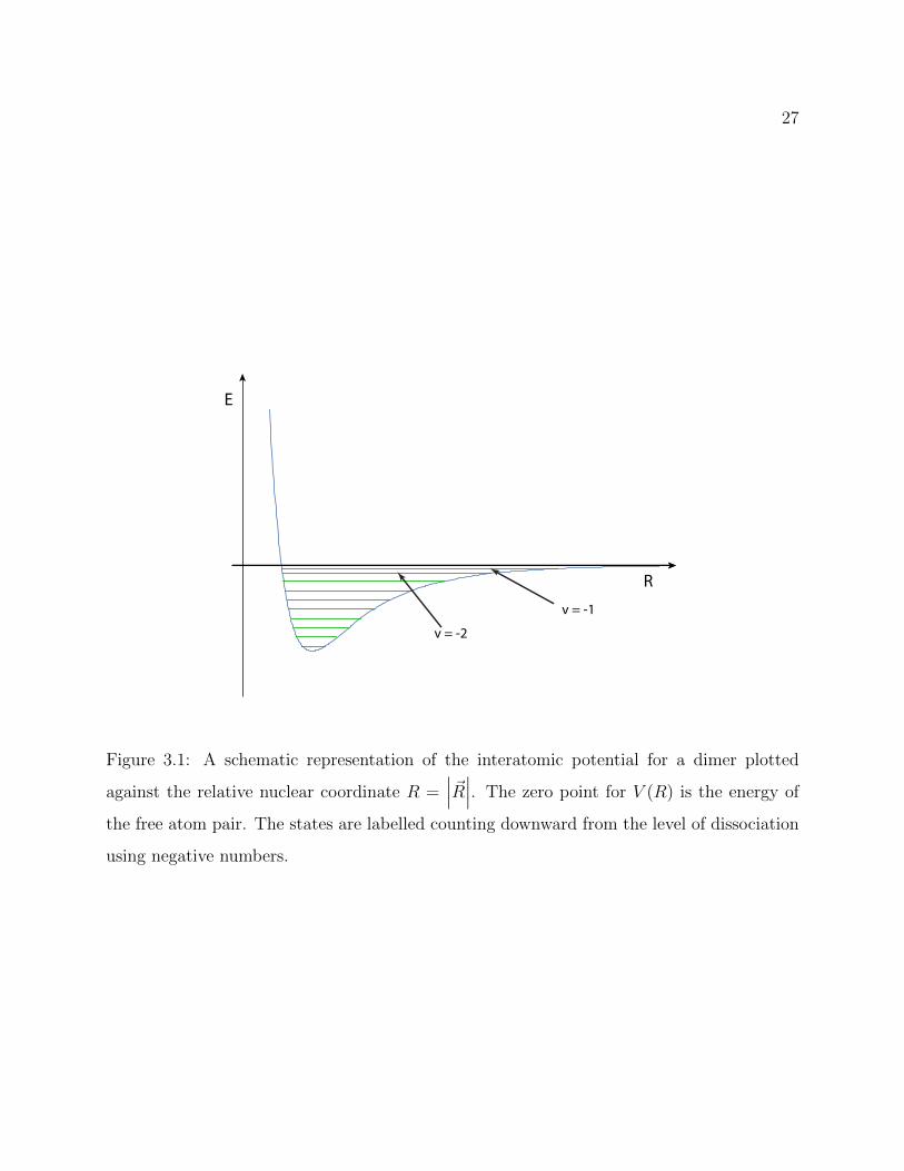
R
E
v = -1
v = -2
Figure 3.1: A schematic representation of the interatomic potential for a dimer plotted
against the relative nuclear coordinate R =∣∣∣~R∣∣∣. The zero point for V (R) is the energy of
the free atom pair. The states are labelled counting downward from the level of dissociation
using negative numbers.
28
completeness as the experimental work in this thesis is confined to the study of vibrational
spectra in the YbLi molecule.
3.2 Ab-initio Analysis of Dimers
As mentioned in the previous section, the principal problem of understanding a dimer’s
quantum states lies in determining the interatomic potential. For dimers in particular,
this problem is easier to visualize as the potential depends explicitly on only two nuclear
coordinates ~R1 and ~R2. Therefore, what would ordinarily be a potential surface, is reduced
to a function of one variable R =∣∣∣ ~R1 − ~R2
∣∣∣. However, the potential still includes the
interaction of many electrons with each other as well as with the nuclei making this an
extremely complex problem under the purview of quantum chemistry.
Even as the field of quantum chemistry moves towards more refined methods to fully
construct the molecular wavefunction from first principles, other approximation methods
remain useful in the collaborations between quantum chemists and cold atom physicists. In
particular, it has been fruitful to model the interatomic potential with the effective potential
below.
V = VSR + VD (3.6)
In the above, VSR is the potential at short range that is dominated by Coulomb repulsion
between the nuclei. At long range the potential is dominated by VD, the dispersion potential
arising from interactions between instantaneous dipoles (or other multipoles) formed within
each constituent atom. VD has the following form.
VD =∑n
CnRn
(3.7)
As we shall see in later sections, understanding the Cn coefficients provides a powerful advan-
tage for experimental probes in ultracold gases, where the least-bound molecules are most
easily observed experimentally. For this purpose, ab-initio calculations on the YbLi system
29
in particular have been used to determine the relevant values of Cn with impressive accu-
racy. This was made possible by advances in quantum chemical calculations that begin with
the Hartree approximation of molecular orbitals whereby electron-electron interactions are
considered on average to affect a shielding of the Coulombic potential of the nuclei but the
electrons are otherwise independent. To this average shielding potential, electron correlations
are incorporated nonperturbatively in “clusters” of 1 to N electron interactions. Calcula-
tions may then be performed up to some truncation of the series of clusters (usually 1 or 2).
Sometimes, an additional term beyond the truncation is added perturbatively [105, 106].
Using these methods, quantum chemical calculations have been used to predict not only
the relevant Cn values but various properties of the dimers that could be formed in various
ultracold atoms laboratories working on molecule formation in atomic mixtures such as the
permanent electric dipole moment for heteronuclear dimers. Multiple theoretical research
groups have shown interest in the YbLi molecule in particular [107, 95, 108, 109].
While the collaboration between theoretical quantum chemists and experimental cold
atom physicists has provided both high resolution spectroscopic data for benchmarking the-
oretical models for the chemists and some powerful predictive elements for the physicists,
there are other important molecular properties that can only be determined with the required
accuracy through spectroscopy. In particular, the difficulty of constructing the form of VSR
makes accurate ab-initio predictions of the vibrational spectra impossible. For this reason,
experimental efforts to create ultracold molecules by forming a coherent connection between
free atoms and a known molecular bound state will begin with some form of spectroscopy
into the foreseeable future.
3.3 Methods of Probing Molecular Potentials
With their electronic, vibrational and rotational states, molecules have a daunting number
of internal states, separated by energies that combinatorially span huge swathes of the elec-
tromagnetic spectrum. For this reason, comprehensive studies of molecular spectroscopy in
thermal sources cannot be used to positively identify certain spectral features as belonging
30
to a particular pair of quantum states, as is possible with ultracold atoms. Luckily, in the
context of ultracold molecules, it isn’t necessary to understand the spectrum in its entirety.
The scattering properties of the ultracold atoms depend strongly only on the character of
the interatomic potential at large internuclear separation, so probing the highest lying states
is of particular importance. Additionally, in the context of searching for magnetic Feshbach
resonances in YbLi, only the very least-bound state supported by the potential is of practical
importance.
Photoassociation (PA) spectroscopy allows us to use optical photons to probe near-
threshold bound states of an electronically excited potential. In the PA process, two atoms
absorb a photon to create an electronically excited molecule, and this formation can be de-
tected through heating in the trap from subsequent dissociation or through photoionization
of the molecules [110]. In the limit of zero kinetic energy, this association occurs with some
finite probability as long as the photon energy plus the binding energy of the molecule is
equal to that of the the electronic excitation in the single atom. However, as we will ex-
plain in a later section, the probability of association is typically significant only for the
near-threshold states.
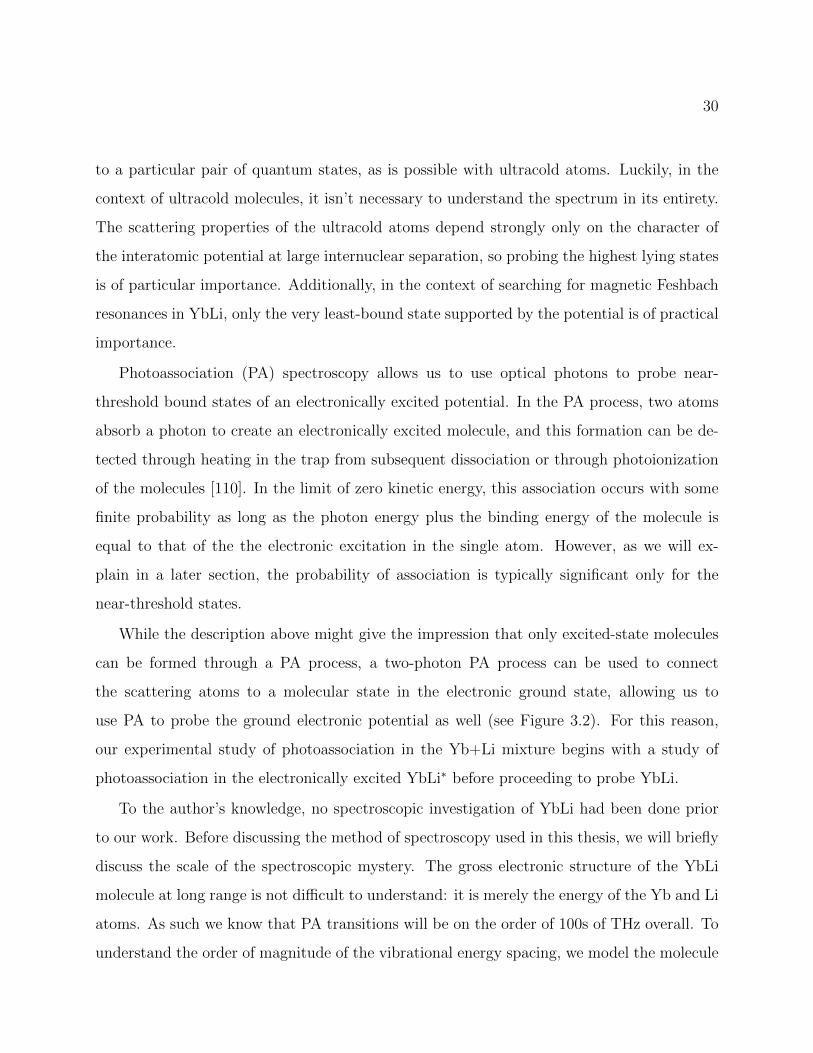
While the description above might give the impression that only excited-state molecules
can be formed through a PA process, a two-photon PA process can be used to connect
the scattering atoms to a molecular state in the electronic ground state, allowing us to
use PA to probe the ground electronic potential as well (see Figure 3.2). For this reason,
our experimental study of photoassociation in the Yb+Li mixture begins with a study of
photoassociation in the electronically excited YbLi∗ before proceeding to probe YbLi.
To the author’s knowledge, no spectroscopic investigation of YbLi had been done prior
to our work. Before discussing the method of spectroscopy used in this thesis, we will briefly
discuss the scale of the spectroscopic mystery. The gross electronic structure of the YbLi
molecule at long range is not difficult to understand: it is merely the energy of the Yb and Li
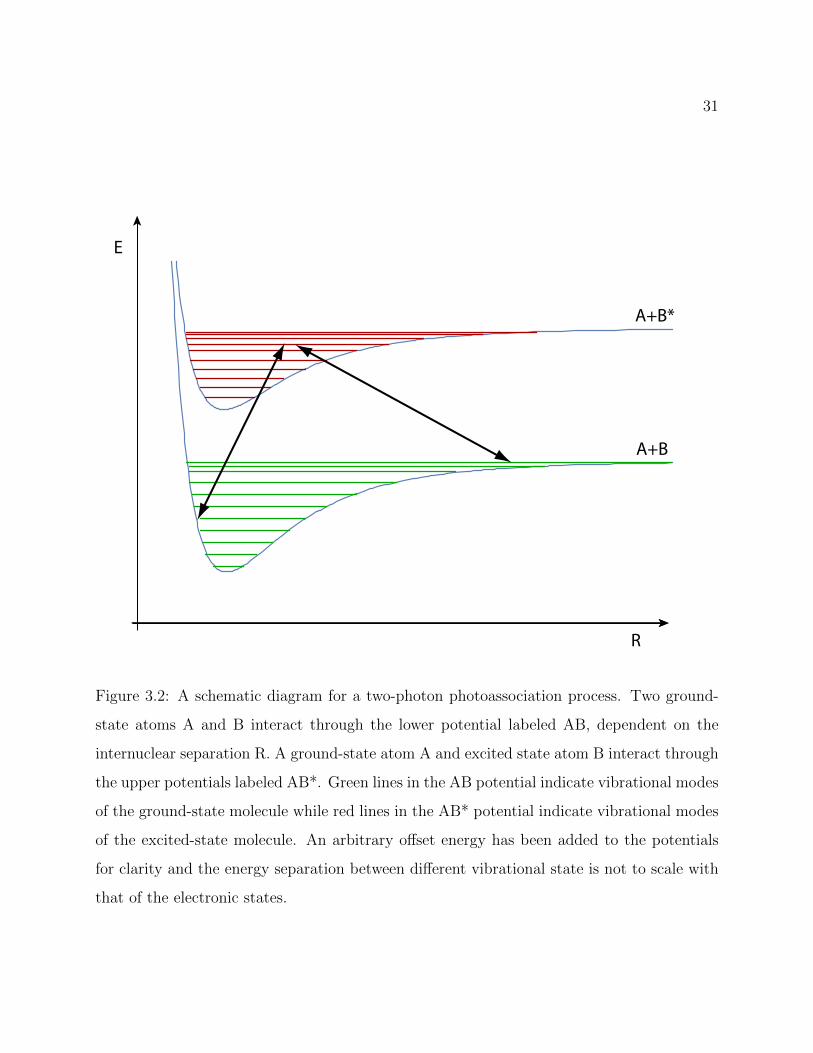
atoms. As such we know that PA transitions will be on the order of 100s of THz overall. To
understand the order of magnitude of the vibrational energy spacing, we model the molecule
31
A+B*
A+B
R
E
Figure 3.2: A schematic diagram for a two-photon photoassociation process. Two ground-
state atoms A and B interact through the lower potential labeled AB, dependent on the
internuclear separation R. A ground-state atom A and excited state atom B interact through
the upper potentials labeled AB*. Green lines in the AB potential indicate vibrational modes
of the ground-state molecule while red lines in the AB* potential indicate vibrational modes
of the excited-state molecule. An arbitrary offset energy has been added to the potentials
for clarity and the energy separation between different vibrational state is not to scale with
that of the electronic states.
32
as a harmonic oscillator: two nuclei of mass M ∼ mp with mp being the mass of the proton.
In order for the molecule to be stable, the restoring force of the oscillator must balance
the Coulomb repulsion at the equilibrium distance R0 [111].
V (R) ∼ k(R−R0)2
Near R = 0, the valence electrons overlap significantly, resulting in a potential energy on the
same order as typical electronic energies such that
kR20 ∼
e2
R0
Here e is the elementary charge. Since the nuclei will be separated by R0 ∼ a0, we make the
following approximation of k.
k ∼ e2
R3∼ m3e8
~6
wherem is mass of the electron. Hence, we can calculate the energy of the harmonic oscillator.
Evib = ~
√k
mp
∼√
m
mp
√m2e8
~4=
√m
mp
ERydberg
Thus the approximate ratio of the vibrational and electronic energies of a diatomic molecule
are
Evib ∼√me
mp
Eelectronic
From this approximation, we believe that the vibrational state separation of the molecules
should be about 2 orders of magnitude smaller than electronic states. Namely, ∼ 1 THz.
Though owing to the anharmonicity near-threshold, the spacing will be narrower than this
estimate for the most weakly bound states.
With these approximations in hand, we know approximately what a complete vibrational
spectrum would look like but not the energy of each vibrational state. As mentioned in the
previous section, it is not currently possible to precisely predict the vibrational spectrum of a
molecule from first principles. However, for a long-range potential of the form in Equation 3.7,
the spectrum of the near-threshold bound states can be approximately determined by the
Leroy-Bernstein Formula, given below [112].
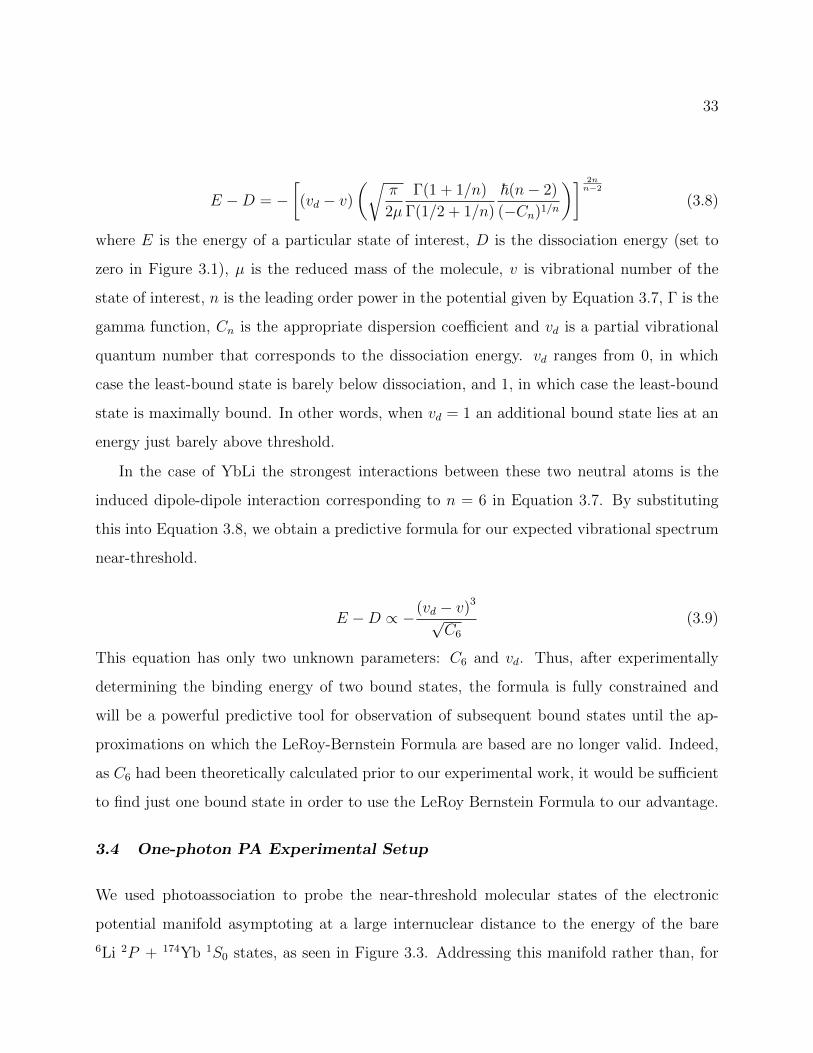
33
E −D = −[(vd − v)
(√π
2µ
Γ(1 + 1/n)
Γ(1/2 + 1/n)
~(n− 2)
(−Cn)1/n
)] 2nn−2
(3.8)
where E is the energy of a particular state of interest, D is the dissociation energy (set to
zero in Figure 3.1), µ is the reduced mass of the molecule, v is vibrational number of the
state of interest, n is the leading order power in the potential given by Equation 3.7, Γ is the
gamma function, Cn is the appropriate dispersion coefficient and vd is a partial vibrational
quantum number that corresponds to the dissociation energy. vd ranges from 0, in which
case the least-bound state is barely below dissociation, and 1, in which case the least-bound
state is maximally bound. In other words, when vd = 1 an additional bound state lies at an
energy just barely above threshold.
In the case of YbLi the strongest interactions between these two neutral atoms is the
induced dipole-dipole interaction corresponding to n = 6 in Equation 3.7. By substituting
this into Equation 3.8, we obtain a predictive formula for our expected vibrational spectrum
near-threshold.
E −D ∝ −(vd − v)3
√C6
(3.9)
This equation has only two unknown parameters: C6 and vd. Thus, after experimentally
determining the binding energy of two bound states, the formula is fully constrained and
will be a powerful predictive tool for observation of subsequent bound states until the ap-
proximations on which the LeRoy-Bernstein Formula are based are no longer valid. Indeed,
as C6 had been theoretically calculated prior to our experimental work, it would be sufficient
to find just one bound state in order to use the LeRoy Bernstein Formula to our advantage.
3.4 One-photon PA Experimental Setup
We used photoassociation to probe the near-threshold molecular states of the electronic
potential manifold asymptoting at a large internuclear distance to the energy of the bare
6Li 2P + 174Yb 1S0 states, as seen in Figure 3.3. Addressing this manifold rather than, for
34
example, those asymptoting 6Li 1S + 174Yb 3P1 states, has a few advantages, enumerated
below.
• The fundamental limit on the PA linewidth is the same as the atomic electronic tran-
sition it is associated with and the fairly large linewidth for the Li 2S1/2 → 2P1/2,3/2
transition (Γ = 2π × 5.9MHz) would relax the requirements on the step size in our
search for the first resonances.
• The ≈ 671 nm laser light required was relatively easy to obtain even at high powers
and arbitrary detunings
• Spectroscopy of this manifold, being the lowest excited state manifold in the system,
will not be complicated by predissociation effects
We observed PA resonances through trap-loss spectroscopy, in which a collection of
trapped atoms is exposed to PA light of various frequencies until a particular frequency
is seen to deplete the number of atoms in the trap. This is an indication of molecule forma-
tion because the molecules rapidly dissociate back to atoms, releasing the binding energy as
kinetic energy which is orders of magnitude higher than our trap depth. Even if PA processes
happen to populate radiatively stable molecular states, they are usually not collisionally sta-
ble and thus will also be lost from the trap. Most often these trap-loss spectroscopies are
carried out in a MOT. This has been done not only for homonuclear molecules where PA
rates are quite strong but also for heteronuclear molecules for which PA rates are relatively
weak. In 2015 our lab performed trap-loss spectroscopy on a two-species MOT of 174Yb and
6Li [113]. In that work we were able to observe one vibration state, which we identified as
v∗ = −2 but no others.
To pursue a more extensive study of the electronically excited molecular states, we began
new trap-loss spectroscopy experiments in late 2016, this time trapping the atoms in the
ODT. This had the disadvantage of taking a lot longer than MOT-based spectroscopies in
35
which atoms can be continuously reloaded into the trap while the PA laser frequency is
scanned or stepped through different frequencies. In the ODT-based experiments, we would
have to prepare the atoms in the ODT, expose the atoms to the PA light of some frequency,
perform absorption imaging on the remaining atoms and then reload the ODT again and
repeat the process for a different frequency of PA light. Collecting one data point in such
an experiment takes about 15 seconds, with the preparation of the ultracold atom sample
taking the majority if the time. Exposure of the PA light lasts typically 1 to 100 ms while
the complete absorption imaging process takes a few 100 ms.
Despite the low data collection rate, performing these experiments in the ODT had two
key advantages, both of which help us satisfy the condition of visibility of a PA resonance
through trap-loss spectroscopy: that the rate of loss from the trap induced by photoassocia-
tion must be on the same order as any other loss process from the trap. The first advantage
of the ODT is allowing for an increase in the PA rate. The PA rate is given by:
d
dtnLi,Yb = −KPAnLinYb (3.10)
where nYb(Li) is the density of Yb(Li) and KPA is the two body event rate constant that is
independent of density. KPA is determined by two parameters: the coupling matrix element
of the electronic transition and the wave function overlap between the incoming scattering
state and the bound state. Critically for this work, typical densities achievable in a MOT
are about 1010 cm−3, whereas in the ODT densities ∼ 1013 cm−3 can be achieved.
In addition to increasing the PA rate by moving to the ODT, we were also able to limit
one of the strongest competing loss processes that obscures the PA signal we are looking
for: other kinds of PA. Necessarily, the PA light with which we searched for YbLi PA
resonances can also drive Li2 resonances. This is a particularly acute problem because the
Li2 PA resonances connect to an excited state molecular potential VD ∼ −C3/R3 owing to the
resonant dipole-dipole interaction available in homonuclear systems between an s state and
a p state. Examining the LeRoy Bernstein formula and comparing it to the VD ∼ −C6/R6
potential for YbLi* shows that the Li2 resonances will be more numerous. Further, the longer
36
range of the homonuclear interaction means that the coefficients KPA will typically be much
larger for Li2 than for YbLi. In this way, homonuclear PA represents a strong background
that must be curtailed in order to observe the heteronuclear resonances. Suppressing PA
rates can be done simply by suppressing collisions between two Li atoms generally. Because
we are working at temperatures well below the p-wave threshold for Li, we may limit collisions
between two Li atoms simply by keeping the sample spin polarized so the sample in our trap
is composed of identical fermions. Unlike in the MOT, we can readily prepare the Li cloud
in the ODT in a spin polarized state. Beyond preparing the cloud in a single spin state,
we also mitigate affects that would disturb the polarization. Specifically, we prepare the Li
atoms in a stretched ground spin state (|3〉 = |ms,mi〉 = |−1/2,−1〉), which means that only
returning to the original state is allowed by dipole selection rules. This prevents the PA laser
beam from transferring atoms to other ground spin states by off-resonant scattering.
Having previously observed the v∗ = −2 resonance in our earlier PA experiments and
believing that v∗ = −1 could not be observed due to large trap loss from spontaneous
scatter of the atomic transition, we sought to observe the v∗ = −3 resonance with the
new experiment. Each experimental run began with the creation of an ultracold mixture of
atoms loaded into the ODT. For our initial experiments, we performed a modest amount of
evaporative cooling and then held the trap depth constant for 1 second for thermalization.
At this point, a typical starting Li(Yb) atom number was 2.0× 10⁵(1.5× 10⁶) and they were
at a temperature of 35µK. The trap frequencies for Li were ω = 2π485, 330, 195 Hz, with
the highest trap frequency corresponding to the axis parallel to that of gravity. Subsequent
changes to these initial parameters are noted along with the data presented in the remainder
of this chapter. After preparation the sample was exposed to PA light of various intensities
and pulse lengths, which we varied in order to achieve optimal signal.
The PA light laser system is principally composed of: an external cavity diode laser
(ECDL) (DL-100 with an EYP-RWA-0670 diode), a lab-built tapered amplifier system (EYP-
TPA-0670 TA chip), a Li vapor cell and a single pass acousto-optic modulator (AOM). The
Li vapor cell was necessitated by the broadband spectrum of the tapered amplifier chip.
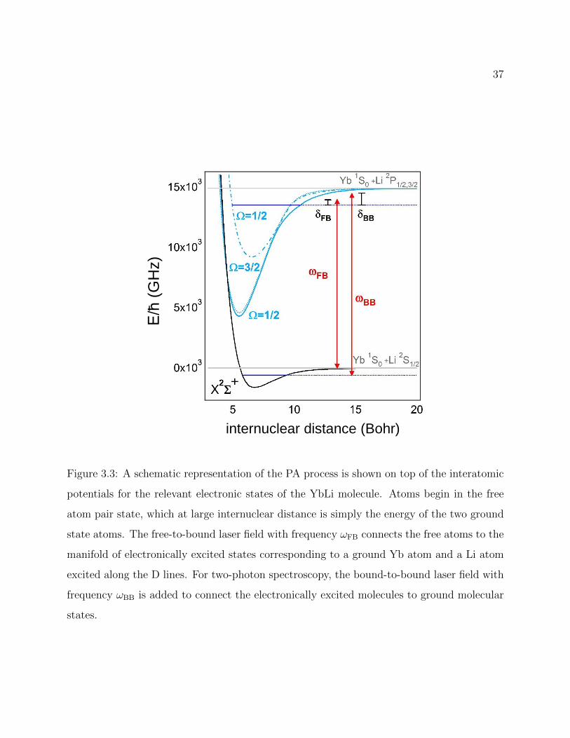
37
E/ħ
(G
Hz)
internuclear distance (Bohr)
Figure 3.3: A schematic representation of the PA process is shown on top of the interatomic
potentials for the relevant electronic states of the YbLi molecule. Atoms begin in the free
atom pair state, which at large internuclear distance is simply the energy of the two ground
state atoms. The free-to-bound laser field with frequency ωFB connects the free atoms to the
manifold of electronically excited states corresponding to a ground Yb atom and a Li atom
excited along the D lines. For two-photon spectroscopy, the bound-to-bound laser field with
frequency ωBB is added to connect the electronically excited molecules to ground molecular
states.
38
Although most of the TA spectrum is dominated by the frequency of the seed beam supplied
by the ECDL, the TA acts as a light-emitting diode itself, causing output of amplified
spontaneous emission (ASE). Figure 3.5 provided an example of the free-running (unseeded)
and injected (seeded) TA similar to that used in this work for the PA light. The spread of the
residual ASE in the spectrum was much larger than the detuning of the PA light from the
atomic resonance, meaning that atoms would be exposed to resonant light if unfiltered. We
found that the vapor cell needed to be heated to about 400 degrees and the PA beam sent
as close to the source of the vapor as possible (skimming the bottom of the cell viewports)
in order to remove the resonant component of the light. We confirmed that the resonant
component was removed by noting that the lifetime of the Li atoms exposed to PA light in
the trap increased quadratically with the detuning from the atomic resonance. Before the
successful filtering the lifetime was linear in the detuning.
After passing through the vapor cell, the PA light was sent through a single pass AOM
operating at 230 MHz and the -1 order was coupled into a polarization-maintaining (PM)
fiber, allowing for fast switching or intensity feedback on the PA beam, whichever is more
important (a shutter is also used for slow switching and blocking of leaked light during the
preparation stages of the sequence). The output of the fiber was placed on the vertically
oriented breadboard above the vacuum chamber. A single 100 mm lens placed just above the
upper viewport of the vacuum chamber focused the PA beam near the ODT. We estimated
the waist of the PA beam to be about 75µm using a beam profiler with a mock setup of this
simple beam path off the main optics table. A flipper mirror was used in the vertical MOT
path to allow the PA beam to propagate from the top of the vacuum chamber towards the
ODT.
The frequency of the PA laser was stabilized by using the reading of a wavemeter (High
Finesse WS-7) to feedback to the ECDL grating angle. Though the wavemeter is quoted
to a precision of 10 MHz, we determined through high field imaging resonances of Li atoms
that the laser linewidth was less than 5 MHz when locked.
Because our typical preparation of ultracold atoms ends with Li atoms polarized in |2〉
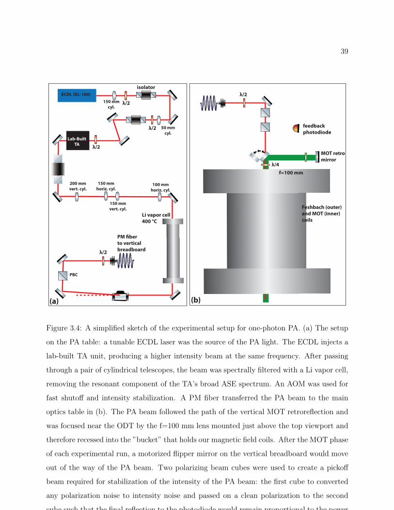
39
ECDL (DL-100)
Lab-Built TA
λ/2
λ/2
λ/2
λ/2
PM berto vertical breadboard
150 mmcyl.
50 mmcyl.
200 mmvert. cyl.
150 mmhoriz. cyl.
150 mmvert. cyl.
100 mmhoriz. cyl.
PBC
feedback photodiode
MOT retro mirror
f=100 mm
λ/2
λ/4
Feshbach (outer) and MOT (inner) coils
(a) (b)
isolator
Li vapor cell400 °C
Figure 3.4: A simplified sketch of the experimental setup for one-photon PA. (a) The setup
on the PA table: a tunable ECDL laser was the source of the PA light. The ECDL injects a
lab-built TA unit, producing a higher intensity beam at the same frequency. After passing
through a pair of cylindrical telescopes, the beam was spectrally filtered with a Li vapor cell,
removing the resonant component of the TA’s broad ASE spectrum. An AOM was used for
fast shutoff and intensity stabilization. A PM fiber transferred the PA beam to the main
optics table in (b). The PA beam followed the path of the vertical MOT retroreflection and
was focused near the ODT by the f=100 mm lens mounted just above the top viewport and
therefore recessed into the ”bucket” that holds our magnetic field coils. After the MOT phase
of each experimental run, a motorized flipper mirror on the vertical breadboard would move
out of the way of the PA beam. Two polarizing beam cubes were used to create a pickoff
beam required for stabilization of the intensity of the PA beam: the first cube to converted
any polarization noise to intensity noise and passed on a clean polarization to the second
cube such that the final reflection to the photodiode would remain proportional to the power
in the beam at the atoms even if the polarization going into the first cube changed.
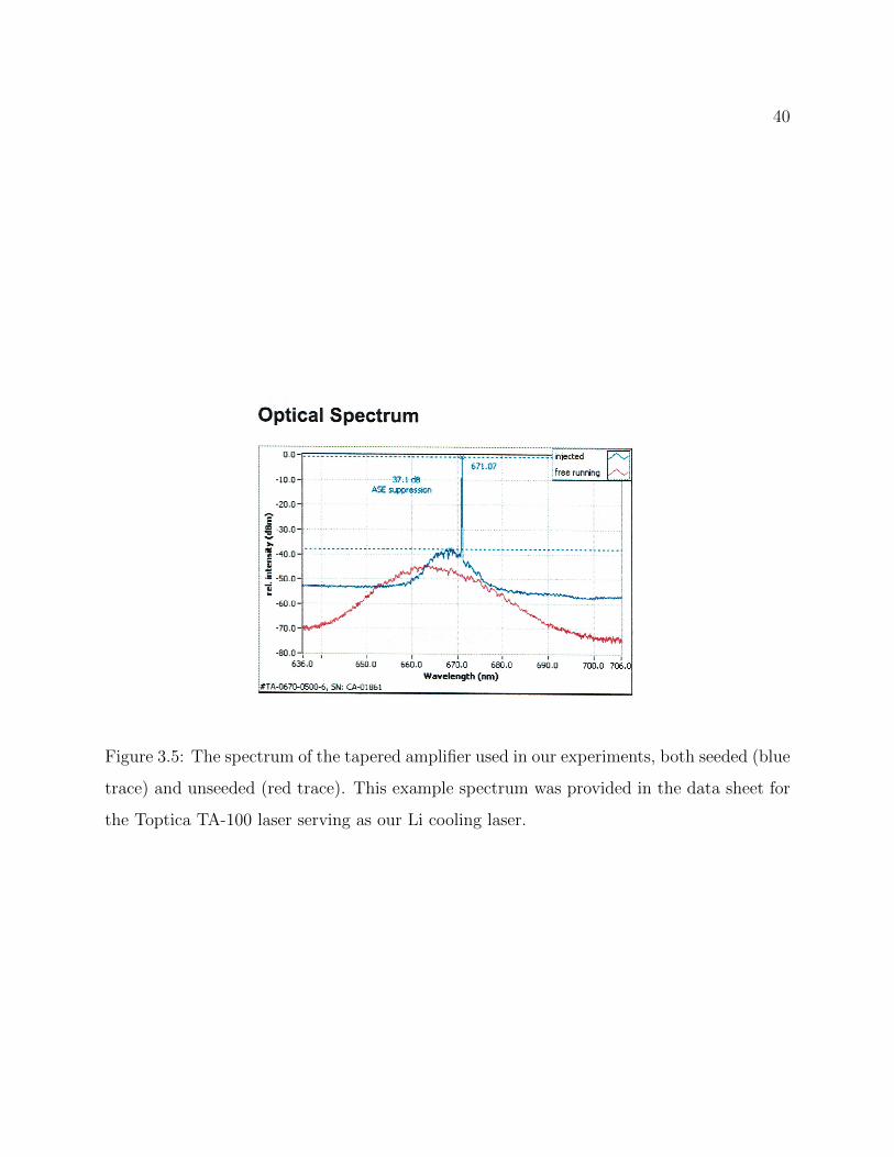
40
Figure 3.5: The spectrum of the tapered amplifier used in our experiments, both seeded (blue
trace) and unseeded (red trace). This example spectrum was provided in the data sheet for
the Toptica TA-100 laser serving as our Li cooling laser.
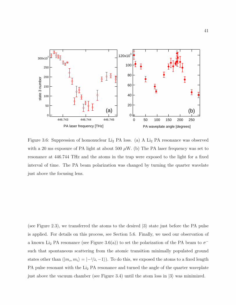
41
300x103
250
200
150
100
50
0
sta
te 3
num
ber
446.745446.744446.743
PA laser frequency [THz]
120x103
100
80
60
40
20
0250200150100500
PA waveplate angle [degrees]
(a) (b)
Figure 3.6: Suppression of homonuclear Li2 PA loss. (a) A Li2 PA resonance was observed
with a 20 ms exposure of PA light at about 500 µW. (b) The PA laser frequency was set to
resonance at 446.744 THz and the atoms in the trap were exposed to the light for a fixed
interval of time. The PA beam polarization was changed by turning the quarter wavelate
just above the focusing lens.
(see Figure 2.3), we transferred the atoms to the desired |3〉 state just before the PA pulse
is applied. For details on this process, see Section 5.6. Finally, we used our observation of
a known Li2 PA resonance (see Figure 3.6(a)) to set the polarization of the PA beam to σ−
such that spontaneous scattering from the atomic transition minimally populated ground
states other than (|ms,mi〉 = |−1/2,−1〉). To do this, we exposed the atoms to a fixed length
PA pulse resonant with the Li2 PA resonance and turned the angle of the quarter waveplate
just above the vacuum chamber (see Figure 3.4) until the atom loss in |3〉 was minimized.
42
3.5 Excited Bound States
3.5.1 Loss Resonances
Figure 3.7 shows the first strong observation of heteronuclear PA in the ODT, corresponding
to resonance with v∗ = −2. We distinguished the heteronuclear PA resonance from nearby
homonuclear resonances by repeating the spectroscopy in the absence of Yb. To perform
the experiment without Yb we removed it from the trap with a resonant light blast on the
1S0 → 1P1 transition prior to the PA light pulse. We note here that despite knowing exactly
where to look for this resonance because we had observed it in our previous MOT-based
experiments, the first observation of this heteronuclear resonance was quite faint. It was
then that we realized that the heteronuclear PA rate was quite sensitive to the alignment
of the second beam of our crossed ODT. In this sense, heteronuclear PA is a method for
determining the extent of the actual spatial overlap of the two clouds in the trap.
The proximity to multiple homonuclear PA lines highlights the advantage of working in
the ODT rather than the MOT. As an approximate comparison of the two methods we have
plotted the trap-loss signal from both the ODT and the MOT in this range of frequencies
in Figure 3.8. The colder temperature of the ODT alone (factor of 10 for Yb and 100 for
Li) allows the YbLi resonance to be resolved against the background of multiple nearby Li2
resonances. However, as is indicated by the gaps in the red trace, we were unable to scan
the full frequency range in this area due to residual atom loss from homonuclear PA.
Our initial attempts to observe additional resonances began with a comprehensive scan
which was uninformed by the best values to use for the PA power and exposure time and was
also susceptible to low signal due to poor interspecies overlap. However, under the following
conditions we scanned the range of 120 GHz to 450 GHz below the Li D2 resonance at
446.80014 THz: 0.5 mW with 1 second of exposure with a triangle wave frequency sweep
amplitude of 460 MHz. After observing the v∗ = −2, we were able to use that signal to
optimize the overlap and chose to revisit a narrower scan range for v∗ = −3, which was
motivated by the input of the theoretically predicted value of C6 into the LeRoy Bernstein
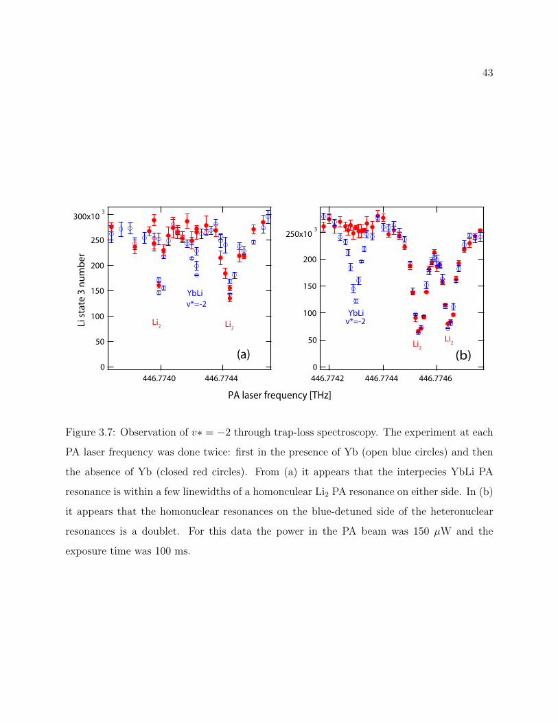
43
300x103
250
200
150
100
50
0
Li s
tate
3 n
umbe
r
446.7744446.7740
250x103
200
150
100
50
0446.7746446.7744446.7742
PA laser frequency [THz]
(a) (b)
YbLi
Li2Li2
YbLi
Li2
Li2
v*=-2
v*=-2
Figure 3.7: Observation of v∗ = −2 through trap-loss spectroscopy. The experiment at each
PA laser frequency was done twice: first in the presence of Yb (open blue circles) and then
the absence of Yb (closed red circles). From (a) it appears that the interpecies YbLi PA
resonance is within a few linewidths of a homonculear Li2 PA resonance on either side. In (b)
it appears that the homonuclear resonances on the blue-detuned side of the heteronuclear
resonances is a doublet. For this data the power in the PA beam was 150 µW and the
exposure time was 100 ms.
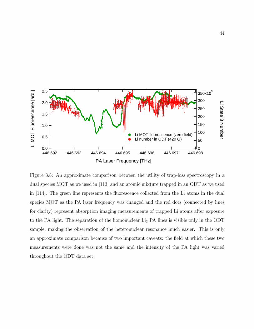
44
2.5
2.0
1.5
1.0
0.5
0.0 Li M
OT
Flu
ores
cens
e [a
rb.]
446.698446.697446.696446.695446.694446.693446.692
PA Laser Frequency [THz]
350x103
300
250
200
150
100
50
0
Li State 3 N
umber Li MOT fluorescence (zero field) Li number in ODT (420 G)
Figure 3.8: An approximate comparison between the utility of trap-loss spectroscopy in a
dual species MOT as we used in [113] and an atomic mixture trapped in an ODT as we used
in [114]. The green line represents the fluorescence collected from the Li atoms in the dual
species MOT as the PA laser frequency was changed and the red dots (connected by lines
for clarity) represent absorption imaging measurements of trapped Li atoms after exposure
to the PA light. The separation of the homonuclear Li2 PA lines is visible only in the ODT
sample, making the observation of the heteronuclear resonance much easier. This is only
an approximate comparison because of two important caveats: the field at which these two
measurements were done was not the same and the intensity of the PA light was varied
throughout the ODT data set.
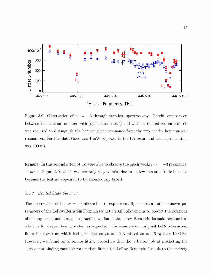
45
400x103
300
200
100
0Li s
tate
3 n
umbe
r
446.6950446.6945446.6940446.6935446.6930
PA Laser Frequency [THz]
Li2
Li2
YbLiv*=-3
Figure 3.9: Observation of v∗ = −3 through trap-loss spectroscopy. Careful comparison
between the Li atom number with (open blue circles) and without (closed red circles) Yb
was required to distinguish the heteronuclear resonance from the two nearby homonuclear
resonances. For this data there was 4 mW of power in the PA beam and the exposure time
was 100 ms.
formula. In this second attempt we were able to observe the much weaker v∗ = −3 resonance,
shown in Figure 3.9, which was not only easy to miss due to its low loss amplitude but also
because the feature appeared to be anomalously broad.
3.5.2 Excited State Spectrum
The observation of the v∗ = −3 allowed us to experimentally constrain both unknown pa-
rameters of the LeRoy-Bernstein Formula (equation 3.9), allowing us to predict the locations
of subsequent bound states. In practice, we found the Leroy-Bernstein formula became less
effective for deeper bound states, as expected. For example our original LeRoy-Bernstein
fit to the spectrum which included data on v∗ = −2, 3 missed v∗ = −6 by over 10 GHz.
However, we found an alternate fitting procedure that did a better job at predicting the
subsequent binding energies; rather than fitting the LeRoy-Bernstein formula to the entirety
46
of the spectrum we had hitherto observed, we fit it to only the deepest few bound states
(or those states just above the state we were wanting to predict for). In this way, we were
able to observe all the bound states ranging to v∗ = −9 as shown in Figure 3.10. States
deeper than v∗ = −9 could not be observed as the PA frequencies for these states lay outside
the bandwidth of our PA laser. The binding energies of the eight states observed in this
vibrational series are presented in Table 3.1.
It should be stressed that this method of search left gigantic swaths of the PA spectrum
for YbLi unobserved. Based on the agreement with the LeRoy Bernstein formula, we know
that this is a vibrational series corresponding to a single electronic state. We never observed
a rotational spectrum associated with one of the vibrational states either because rotational
states other than those we observed lay outside of our search range (which was limited
because of the low data collection rate of this method) or more likely due to some sort of
effective selection rule in this spectroscopy. Nor did we observe any PA lines outside of this
vibrational series, corresponding to different electronic states, as we did in the MOT PA
experiment, although we did not focus on detecting these states.
3.5.3 Free-to-Bound Transition Strengths
To quantify the relative strength of the PA resonances, we performed lifetime measurements
on the atoms in the trap when exposed to PA light. We compared these lifetimes against
the losses in the absence of PA-driven trap loss by also performing lifetime measurements
without Yb. Figure 3.11 shows the rate of PA and non-PA loss or “background loss” for both
the v∗ = −2 and v∗ = −3 resonances. Because the resonant PA light addressing v∗ = −3
is much further detuned from that of v∗ = −2 the lifetime under the same conditions is
much longer. But despite this it is clear that the separation between the PA lifetime and the
background lifetime is greater for v∗ = −2 because the PA rate is significantly higher. This
is expected based on the Franck-Condon Principle: transitions between vibrational states of
a molecule will be more likely to happen if the wavefunction overlap between the two states is
higher. In the case of free-to-bound PA, the transition is actually between a scattering state
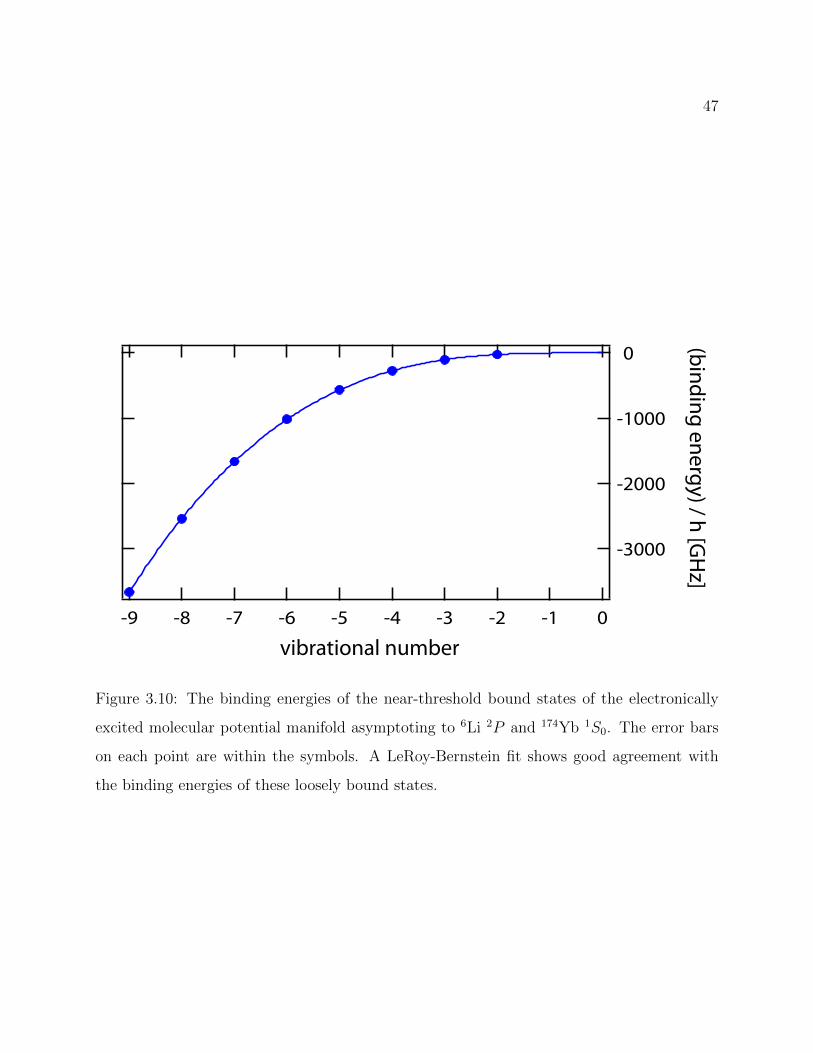
47
-3000
-2000
-1000
0
-9 -8 -7 -6 -5 -4 -3 -2 -1 0
(binding energy) / h [GH
z]
vibrational number
Figure 3.10: The binding energies of the near-threshold bound states of the electronically
excited molecular potential manifold asymptoting to 6Li 2P and 174Yb 1S0. The error bars
on each point are within the symbols. A LeRoy-Bernstein fit shows good agreement with
the binding energies of these loosely bound states.
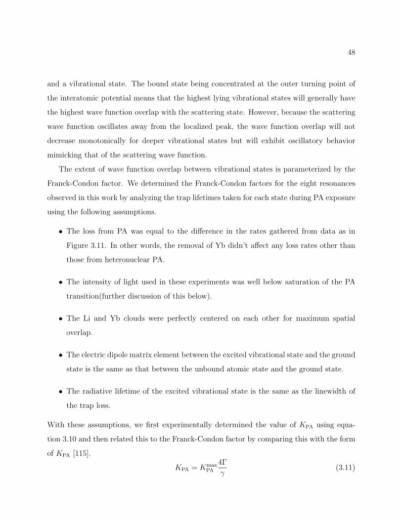
48
and a vibrational state. The bound state being concentrated at the outer turning point of
the interatomic potential means that the highest lying vibrational states will generally have
the highest wave function overlap with the scattering state. However, because the scattering
wave function oscillates away from the localized peak, the wave function overlap will not
decrease monotonically for deeper vibrational states but will exhibit oscillatory behavior
mimicking that of the scattering wave function.
The extent of wave function overlap between vibrational states is parameterized by the
Franck-Condon factor. We determined the Franck-Condon factors for the eight resonances
observed in this work by analyzing the trap lifetimes taken for each state during PA exposure
using the following assumptions.
• The loss from PA was equal to the difference in the rates gathered from data as in
Figure 3.11. In other words, the removal of Yb didn’t affect any loss rates other than
those from heteronuclear PA.
• The intensity of light used in these experiments was well below saturation of the PA
transition(further discussion of this below).
• The Li and Yb clouds were perfectly centered on each other for maximum spatial
overlap.
• The electric dipole matrix element between the excited vibrational state and the ground
state is the same as that between the unbound atomic state and the ground state.
• The radiative lifetime of the excited vibrational state is the same as the linewidth of
the trap loss.
With these assumptions, we first experimentally determined the value of KPA using equa-
tion 3.10 and then related this to the Franck-Condon factor by comparing this with the form
of KPA [115].
KPA = KmaxPA
4Γ
γ(3.11)
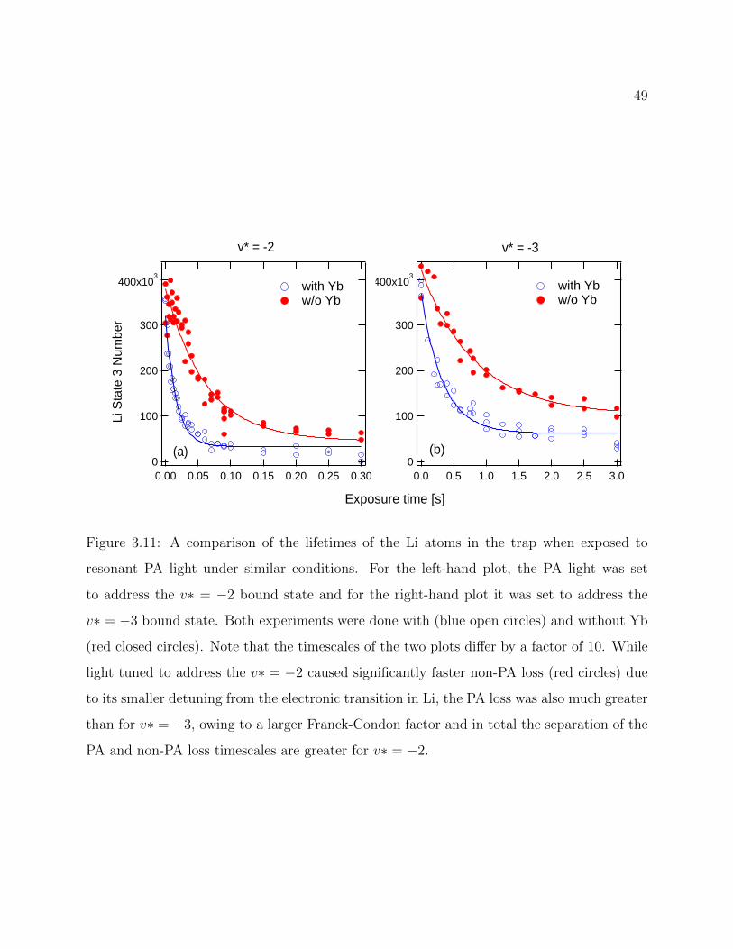
49
400x103
300
200
100
03.02.52.01.51.00.50.0
with Yb w/o Yb
400x103
300
200
100
00.300.250.200.150.100.050.00
with Yb w/o Yb
Exposure time [s]
Li S
tate
3 N
umbe
r
v* = -2 v* = -3
(a) (b)
Figure 3.11: A comparison of the lifetimes of the Li atoms in the trap when exposed to
resonant PA light under similar conditions. For the left-hand plot, the PA light was set
to address the v∗ = −2 bound state and for the right-hand plot it was set to address the
v∗ = −3 bound state. Both experiments were done with (blue open circles) and without Yb
(red closed circles). Note that the timescales of the two plots differ by a factor of 10. While
light tuned to address the v∗ = −2 caused significantly faster non-PA loss (red circles) due
to its smaller detuning from the electronic transition in Li, the PA loss was also much greater
than for v∗ = −3, owing to a larger Franck-Condon factor and in total the separation of the
PA and non-PA loss timescales are greater for v∗ = −2.
50
Here, Γ is the atom-molecule coupling, γ is the linewidth of the excited vibrational state,
and KmaxPA is the unitarity-limited rate for any two-body collision given by
KmaxPA =
~2
µ3/2
√2π
kBT(3.12)
with µ as the reduced mass of the molecule. Γ is the value of interest as it depends on the
Franck-Condon factors (fFC):
Γ = 2π~Ω2fFC (3.13)
where Ω is the Rabi frequency of the electronic transition to the excited state.
Figure 3.12 shows the results of these measurements. As expected, the Franck-Condon
factors drop off sharply as the states become more deeply bound but they do not do so
monotonically. Figure 3.12 also displays the experimentally observed widths for the trap-
loss measurements. The apparent anti-correlation between the Franck-Condon factor and the
width is striking given that the calculations of the Franck-Condon factor explicitly included
the dependence on the observed width. The cause of this anti-correlation is not currently
known.
The magnitude of the observed PA resonance widths is also something of a mystery as it
is theoretically expected that the radiative linewidths of these near-threshold states would
be about the same as that of the electronic transition, Γ = 2π × 5.9 MHz [116]. There
are of course several factors other than the radiative linewidth that can contribute to the
width. Above saturation the linewidth can be power broadened. We have attempted to
power broaden the v∗ = −2 and v∗ = −7 lines but were not able to observe any significant
dependence of the experimentally observed linewidth on the intensity within the range of
intensities we could use (see Figure 3.13). In addition to trap loss being driven by excited
state molecules which are radiatively transferred back to atomic states (either stimulated
or spontaneous), excited molecules could de-excite to different molecular states, broadening
the total linewidth. In particular, the 1064 nm light used to create the ODT has the correct
order of magnitude energy to drive molecules between different vibrational states (though it
is not known if 1064 nm is near resonance for the YbLi molecule in particular). To eliminate
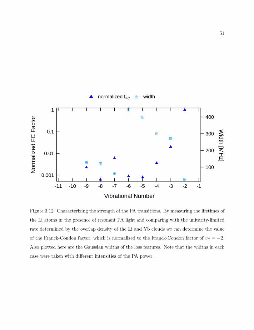
51
0.001
0.01
0.1
1
Nor
mal
ized
FC
Fac
tor
-11 -10 -9 -8 -7 -6 -5 -4 -3 -2 -1
Vibrational Number
400
300
200
100
Width [M
Hz]
normalized fFC width
Figure 3.12: Characterizing the strength of the PA transitions. By measuring the lifetimes of
the Li atoms in the presence of resonant PA light and comparing with the unitarity-limited
rate determined by the overlap density of the Li and Yb clouds we can determine the value
of the Franck-Condon factor, which is normalized to the Franck-Condon factor of v∗ = −2.
Also plotted here are the Gaussian widths of the loss features. Note that the widths in each
case were taken with different intensities of the PA power.
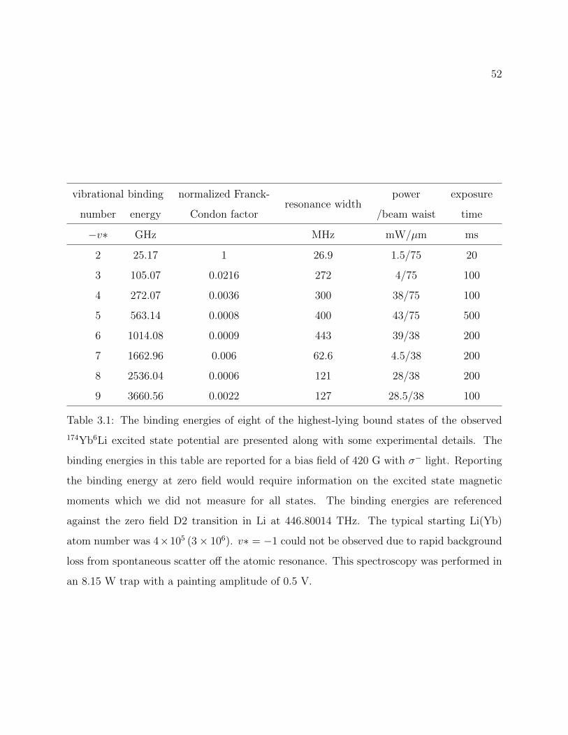
52
vibrational
number
binding
energy
normalized Franck-
Condon factorresonance width
power
/beam waist
exposure
time
−v∗ GHz MHz mW/µm ms
2 25.17 1 26.9 1.5/75 20
3 105.07 0.0216 272 4/75 100
4 272.07 0.0036 300 38/75 100
5 563.14 0.0008 400 43/75 500
6 1014.08 0.0009 443 39/38 200
7 1662.96 0.006 62.6 4.5/38 200
8 2536.04 0.0006 121 28/38 200
9 3660.56 0.0022 127 28.5/38 100
Table 3.1: The binding energies of eight of the highest-lying bound states of the observed
174Yb6Li excited state potential are presented along with some experimental details. The
binding energies in this table are reported for a bias field of 420 G with σ− light. Reporting
the binding energy at zero field would require information on the excited state magnetic
moments which we did not measure for all states. The binding energies are referenced
against the zero field D2 transition in Li at 446.80014 THz. The typical starting Li(Yb)
atom number was 4×10⁵ (3× 10⁶). v∗ = −1 could not be observed due to rapid background
loss from spontaneous scatter off the atomic resonance. This spectroscopy was performed in
an 8.15 W trap with a painting amplitude of 0.5 V.
53
this possibility, we repeated the trap-loss spectroscopy technique while eliminating the effect
of the ODT light. We pulsed the ODT light out of phase with PA light such that the atoms
never experienced both optical fields at once but remained localized at the location of the
trap. Under these conditions, we still observed loss from the atom cloud, presumably driven
by atoms that achieve too much kinetic energy through dissociation during the PA phase to
be recaptured by the ODT light. Indeed, the linewidth of the trap loss in the modulated
case was the same as that in the unmodulated case, even when the time averaged trap depth
and the time averaged PA intensity was the same in both cases.
Since a connection to other molecular states due to the trap light is not the reason for our
anomalously broad PA resonances, one theory is spontaneous decay not to free atoms but
to ground state molecules, an indication of unusually large Frank-Condon factors between
high-lying vibrationally excited states and molecular ground states. To some extent this is
an expected feature of heteronuclear dimers for which, in contrast to homonuclear dimers,
the short range potential in the ground and excited states are quite similar as the excited
state is not distorted by the relatively long range VD ≈ C3
R3 potential between the S and P
states of homonuclear atom pairs.
3.5.4 Excited State Magnetic Moments
For the vibrational series observed in this work, we do not know much about the electronic
state other than it converges to that of Yb 1S0 + Li 2P for large internuclear distance. In
the spherically symmetric potential of a nucleus within an atom, an electron’s state can be
characterized simply by its principal quantum number n, the orbital and electronic angular
momentum ` and s as well as their respective projections, m` and ms. This formulation
cannot be exactly applied to the electrons in dimers (though in some cases it can be approx-
imately used) for multiple reasons. First, the involvement of two nuclei breaks the spherical
symmetry of the field seen by the electrons and the resulting torque will cause the electron
angular momentum to precess about the internuclear axis. How that precession happens
depends on the strength of the spin-orbit coupling within the constituent atoms. In the
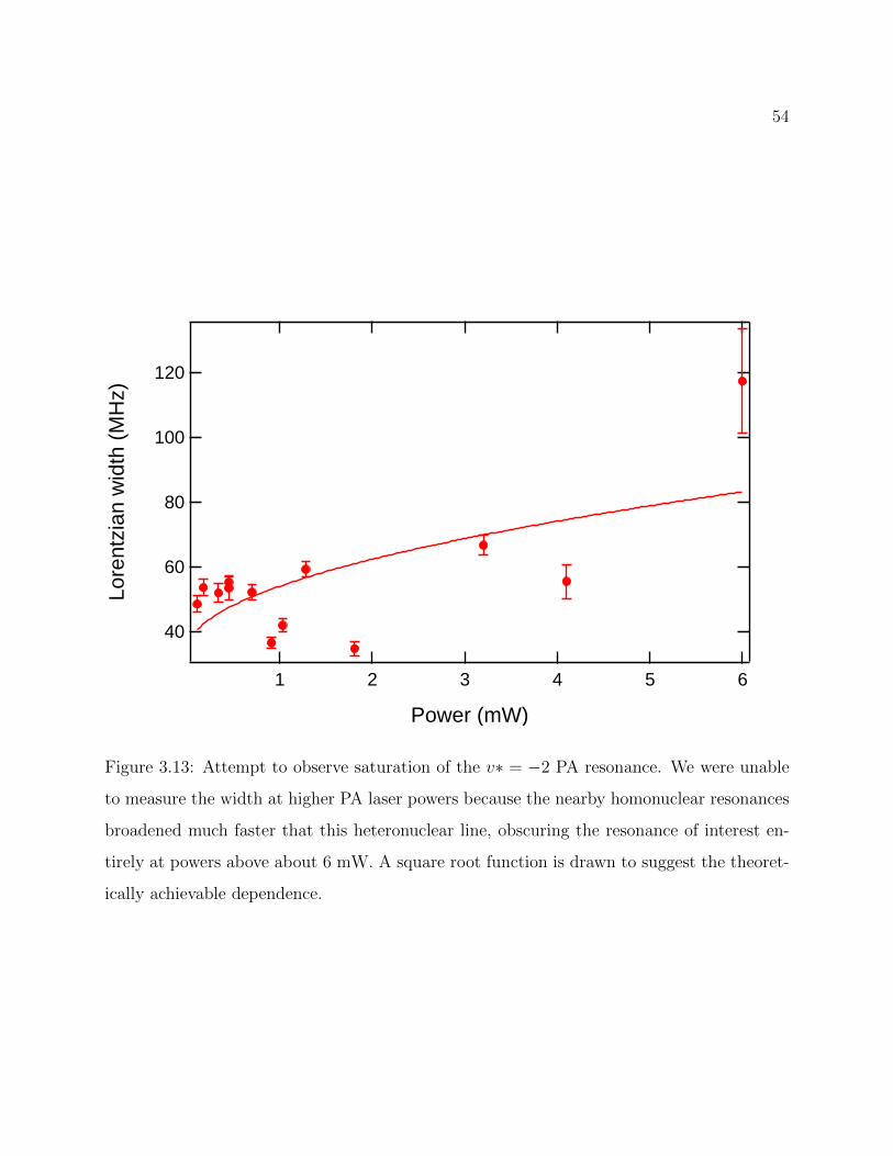
54
120
100
80
60
40
Lore
ntzi
an w
idth
(M
Hz)
654321
Power (mW)
Figure 3.13: Attempt to observe saturation of the v∗ = −2 PA resonance. We were unable
to measure the width at higher PA laser powers because the nearby homonuclear resonances
broadened much faster that this heteronuclear line, obscuring the resonance of interest en-
tirely at powers above about 6 mW. A square root function is drawn to suggest the theoret-
ically achievable dependence.
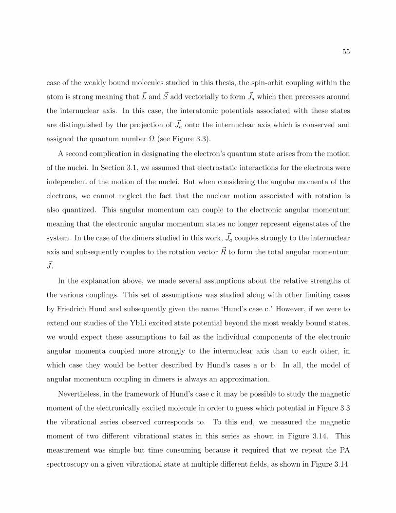
55
case of the weakly bound molecules studied in this thesis, the spin-orbit coupling within the
atom is strong meaning that ~L and ~S add vectorially to form ~Ja which then precesses around
the internuclear axis. In this case, the interatomic potentials associated with these states
are distinguished by the projection of ~Ja onto the internuclear axis which is conserved and
assigned the quantum number Ω (see Figure 3.3).
A second complication in designating the electron’s quantum state arises from the motion
of the nuclei. In Section 3.1, we assumed that electrostatic interactions for the electrons were
independent of the motion of the nuclei. But when considering the angular momenta of the
electrons, we cannot neglect the fact that the nuclear motion associated with rotation is
also quantized. This angular momentum can couple to the electronic angular momentum
meaning that the electronic angular momentum states no longer represent eigenstates of the
system. In the case of the dimers studied in this work, ~Ja couples strongly to the internuclear
axis and subsequently couples to the rotation vector ~R to form the total angular momentum
~J .
In the explanation above, we made several assumptions about the relative strengths of
the various couplings. This set of assumptions was studied along with other limiting cases
by Friedrich Hund and subsequently given the name ‘Hund’s case c.’ However, if we were to
extend our studies of the YbLi excited state potential beyond the most weakly bound states,
we would expect these assumptions to fail as the individual components of the electronic
angular momenta coupled more strongly to the internuclear axis than to each other, in
which case they would be better described by Hund’s cases a or b. In all, the model of
angular momentum coupling in dimers is always an approximation.
Nevertheless, in the framework of Hund’s case c it may be possible to study the magnetic
moment of the electronically excited molecule in order to guess which potential in Figure 3.3
the vibrational series observed corresponds to. To this end, we measured the magnetic
moment of two different vibrational states in this series as shown in Figure 3.14. This
measurement was simple but time consuming because it required that we repeat the PA
spectroscopy on a given vibrational state at multiple different fields, as shown in Figure 3.14.
56
After noting the apparent binding energy of the molecule relative to the zero field atomic
energy, we subtracted the shift of the Zeeman shift of the ground states atoms to find the
Zeeman shift of that particular vibrational state as shown in Figure 3.15. Since there are no
unpaired electrons in Yb it is interesting to compare these magnetic moments to those of Li
in the 2P states, which are given by gµBmJB for large fields with g being the g-factor for the
appropriate fine structure state 2P1/2 or 2P1/2, µB is the Bohr magneton, mJ the projection of
the total electronic angular momentum of the atom and B the magnitude of the external field.
The comparison of the free atom magnetic moment with those measured for v∗ = −5,−7
are shown in Figure 3.16. The deviation from the atomic limit is tantalizing proof of the
complexity of the molecular energies’ dependence on the contributions from various different
angular momenta. However, because we were principally interested in molecule formation
rather than a study of molecular structure, we chose not to pursue this line of research any
further.
3.6 Two-photon PA Experimental Setup
Utilizing our knowledge of the excited state PA spectroscopy, we probed the YbLi molecular
ground state through two-photon PA. To understand the basis of this technique, refer to
Figure 3.3. For this technique, we replicated the conditions of one-photon PA, referring
to the laser field which drives atoms into the excited molecular state as the free-to-bound
laser. If the free-to-bound (FB) laser is tuned to a one-photon PA resonance, a fixed amount
of atom loss will occur in fixed time. The second laser field in this two-photon scheme
is referred to as the bound-to-bound (BB) laser. When the BB laser energy is the same
as the energy splitting between a bound state in the electronic ground state and one in
the electronic excited state, the excited state will experience Autler-Townes (AT) splitting,
a manifestation of the AC stark shift from the bound-to-bound laser mixing the ground
molecular and excited molecular states. As can be seen in Figure 3.17, this effectively makes
the FB laser non-resonant, suppressing the PA atom loss. This suppression forms the signal
with which to probe the bound states ground electronic potential.
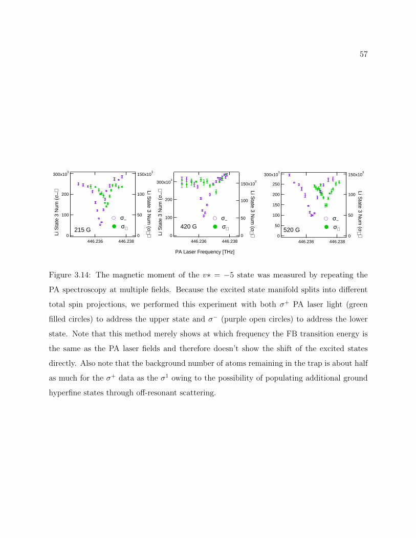
57
300x103
200
100
0Li S
tate
3 N
um (
σ −)
446.238446.236
150x103
100
50
0
Li State 3 N
um (σ+ )
σ−σ+ 215 G
150x103
100
50
0
Li State 3 N
um (σ+ )
446.238446.236
300x103
250
200
150
100
50
0
σ−σ+ 520 G
300x103
200
100
0Li S
tate
3 N
um (
σ −)
446.238446.236
150x103
100
50
0
Li State 3 N
um (σ+ )
σ−σ+420 G
PA Laser Frequency [THz]
Figure 3.14: The magnetic moment of the v∗ = −5 state was measured by repeating the
PA spectroscopy at multiple fields. Because the excited state manifold splits into different
total spin projections, we performed this experiment with both σ+ PA laser light (green
filled circles) to address the upper state and σ− (purple open circles) to address the lower
state. Note that this method merely shows at which frequency the FB transition energy is
the same as the PA laser fields and therefore doesn’t show the shift of the excited states
directly. Also note that the background number of atoms remaining in the trap is about half
as much for the σ+ data as the σ1 owing to the possibility of populating additional ground
hyperfine states through off-resonant scattering.
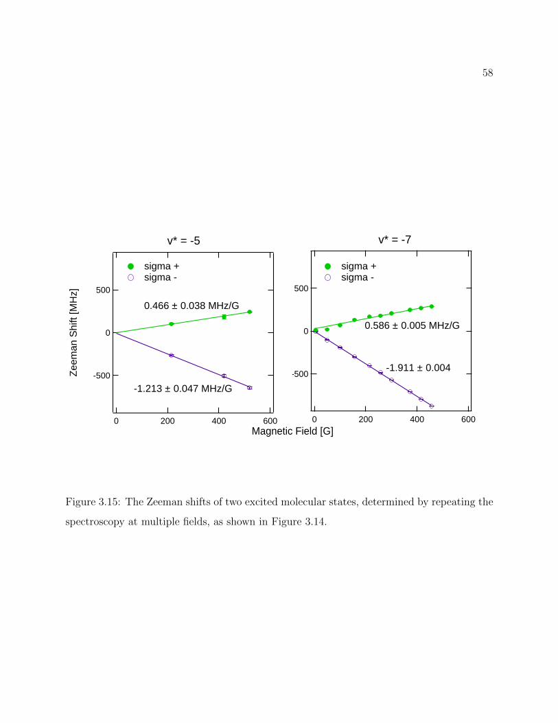
58
-500
0
500
6004002000
-1.911 ± 0.004
0.586 ± 0.005 MHz/G
sigma + sigma -
-500
0
500
Zee
man
Shi
ft [M
Hz]
6004002000
sigma + sigma -
0.466 ± 0.038 MHz/G
-1.213 ± 0.047 MHz/G
Magnetic Field [G]
v* = -7v* = -5
Figure 3.15: The Zeeman shifts of two excited molecular states, determined by repeating the
spectroscopy at multiple fields, as shown in Figure 3.14.
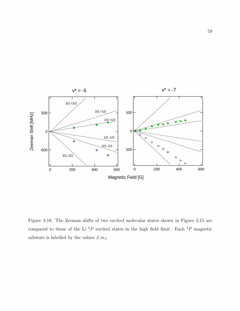
59
-500
0
500
6004002000
-500
0
500
Zee
man
Shi
ft [M
Hz]
6004002000
3/2,-3/2
3/2,-1/2
3/2,+3/2
1/2,-1/2
3/2,+1/2
1/2,+1/2
Magnetic Field [G]
v* = -7v* = -5
Figure 3.16: The Zeeman shifts of two excited molecular states shown in Figure 3.15 are
compared to those of the Li 2P excited states in the high field limit. Each 2P magnetic
substate is labelled by the values J,mJ .
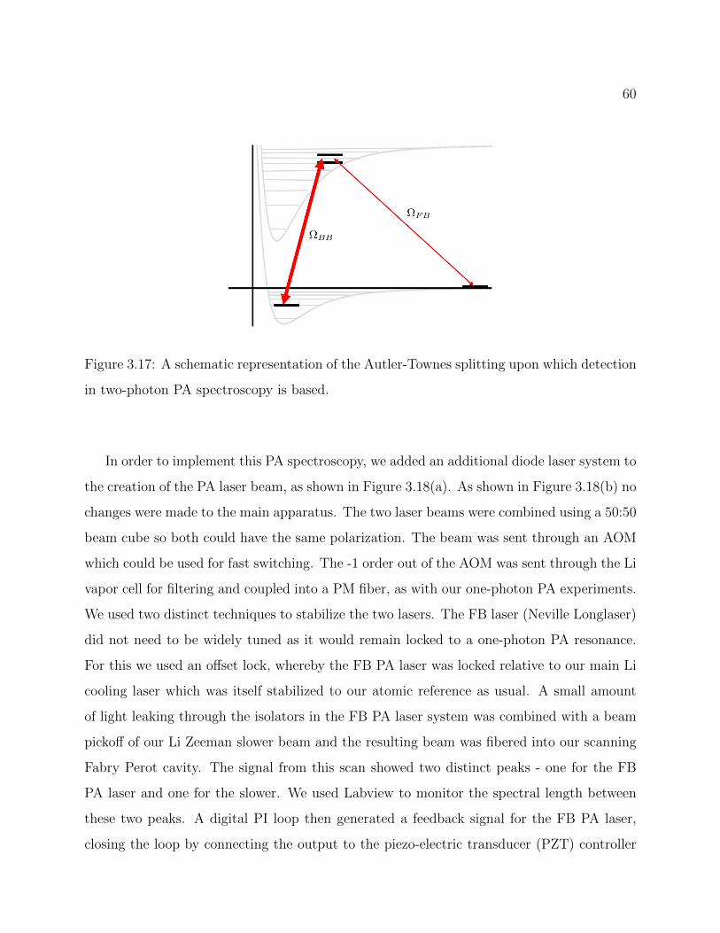
60
Figure 3.17: A schematic representation of the Autler-Townes splitting upon which detection
in two-photon PA spectroscopy is based.
In order to implement this PA spectroscopy, we added an additional diode laser system to
the creation of the PA laser beam, as shown in Figure 3.18(a). As shown in Figure 3.18(b) no
changes were made to the main apparatus. The two laser beams were combined using a 50:50
beam cube so both could have the same polarization. The beam was sent through an AOM
which could be used for fast switching. The -1 order out of the AOM was sent through the Li
vapor cell for filtering and coupled into a PM fiber, as with our one-photon PA experiments.
We used two distinct techniques to stabilize the two lasers. The FB laser (Neville Longlaser)
did not need to be widely tuned as it would remain locked to a one-photon PA resonance.
For this we used an offset lock, whereby the FB PA laser was locked relative to our main Li
cooling laser which was itself stabilized to our atomic reference as usual. A small amount
of light leaking through the isolators in the FB PA laser system was combined with a beam
pickoff of our Li Zeeman slower beam and the resulting beam was fibered into our scanning
Fabry Perot cavity. The signal from this scan showed two distinct peaks - one for the FB
PA laser and one for the slower. We used Labview to monitor the spectral length between
these two peaks. A digital PI loop then generated a feedback signal for the FB PA laser,
closing the loop by connecting the output to the piezo-electric transducer (PZT) controller
61
for the FB PA laser. The BB PA laser (Toptica DL-100), which needed to be widely tunable,
was frequency stabilized using the High Finesse WS-7 wavemeter, as in our one-photon PA
spectroscopies.
Detecting a bound-to-bound resonance using the AT splitting as shown in Figure 3.17 is
simple in principle, but experimental success requires a careful balance of parameters. There
are two considerations which are at odds. First, in order to see suppression of the one-photon
PA loss, the AT splitting must be at least on the order of the one-photon PA linewidth. In
order to guarantee this, one could add more power to the BB laser as the AT splitting will
increase as ∆ ∼√IBB (details in the following chapter). However, increasing the BB laser
intensity also increases the rate of background loss from spontaneous scatter from the atomic
resonance. If the background loss becomes larger than the PA loss, the one-photon signal is
entirely lost, precluding the observation of a two-photon resonance. In that sense, there is
a limit to the amount of BB intensity that can be used to create the AT splitting. Before
proceeding with our spectroscopic search, we determined the maximum amount of BB power
we could use before the background losses exceed the PA losses. Figure 3.19 shows the result
of such a test. Achieving sufficient separation between the on and off resonant lifetimes in
the presence of the BB laser beam restricted us to the use of relatively strong one-photon
PA resonances. For that reason, all the two-photon spectroscopy work was done with the
FB laser locked to either the v∗ = −2 or v∗ = −7 resonances.
3.7 Ground Bound States
Figure 3.20 shows a representative two-photon PA resonance. As with the one-photon spec-
troscopy, we used the LeRoy-Bernstein formula to predict the locations of the subsequent
bound states. In this way we were able to observe the first six bound states in the electronic
ground potential (see Figure 3.21). We were unable to observe v = −7, presumably because
of a combination of two factors. While we did much of our two-photon PA spectroscopy with
v∗ = −7 as the one-photon “intermediate” resonance required to induce the PA loss, we were
unable to use this intermediate state because the expected location of v = −7 would put the
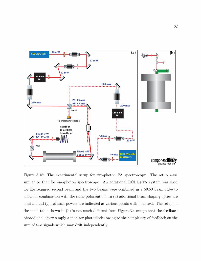
62
ECDL (DL-100)
Lab-Built TA
PM berto vertical breadboard
PBC
(a) (b)
Lab-Built TA
ECDL (”Neville Longlaser”)
50:50
monitor photodiode
49 mW
42 mW
20 mW
220 mW
170 mW
36 mW
27 mW
17 mW
250 mWFB: 79 mWBB: 65 mW
FB: 65 mWBB: 50 mW
FB: 35 mWBB: 27 mW
Figure 3.18: The experimental setup for two-photon PA spectroscopy. The setup wasa
similar to that for one-photon spectroscopy. An additional ECDL+TA system was used
for the required second beam and the two beams were combined in a 50:50 beam cube to
allow for combination with the same polarization. In (a) additional beam shaping optics are
omitted and typical laser powers are indicated at various points with blue text. The setup on
the main table shown in (b) is not much different from Figure 3.4 except that the feedback
photodiode is now simply a monitor photodiode, owing to the complexity of feedback on the
sum of two signals which may drift independently.
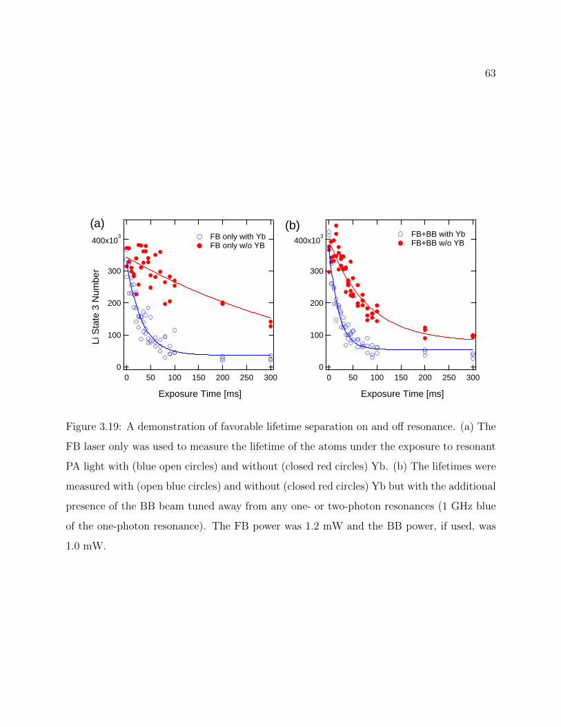
63
400x103
300
200
100
0300250200150100500
Exposure Time [ms]
FB+BB with Yb FB+BB w/o YB400x10
3
300
200
100
0
Li S
tate
3 N
umbe
r
300250200150100500
Exposure Time [ms]
FB only with Yb FB only w/o YB
(a) (b)
Figure 3.19: A demonstration of favorable lifetime separation on and off resonance. (a) The
FB laser only was used to measure the lifetime of the atoms under the exposure to resonant
PA light with (blue open circles) and without (closed red circles) Yb. (b) The lifetimes were
measured with (open blue circles) and without (closed red circles) Yb but with the additional
presence of the BB beam tuned away from any one- or two-photon resonances (1 GHz blue
of the one-photon resonance). The FB power was 1.2 mW and the BB power, if used, was
1.0 mW.
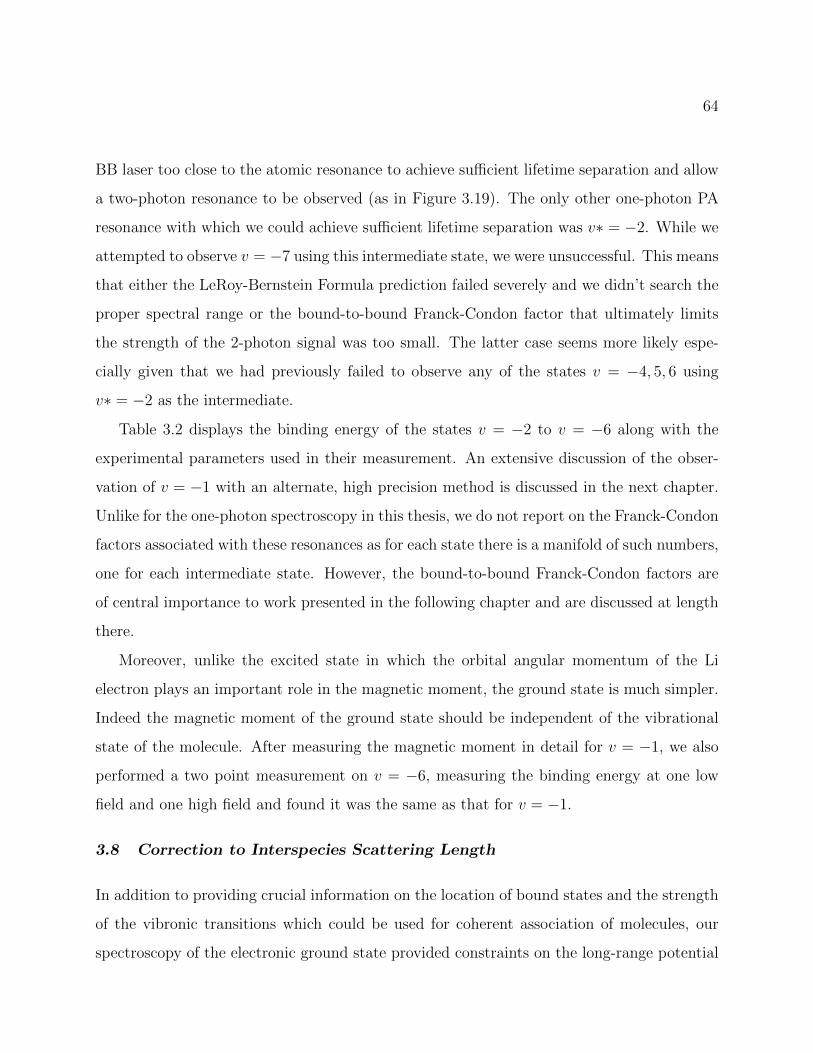
64
BB laser too close to the atomic resonance to achieve sufficient lifetime separation and allow
a two-photon resonance to be observed (as in Figure 3.19). The only other one-photon PA
resonance with which we could achieve sufficient lifetime separation was v∗ = −2. While we
attempted to observe v = −7 using this intermediate state, we were unsuccessful. This means
that either the LeRoy-Bernstein Formula prediction failed severely and we didn’t search the
proper spectral range or the bound-to-bound Franck-Condon factor that ultimately limits
the strength of the 2-photon signal was too small. The latter case seems more likely espe-
cially given that we had previously failed to observe any of the states v = −4, 5, 6 using
v∗ = −2 as the intermediate.
Table 3.2 displays the binding energy of the states v = −2 to v = −6 along with the
experimental parameters used in their measurement. An extensive discussion of the obser-
vation of v = −1 with an alternate, high precision method is discussed in the next chapter.
Unlike for the one-photon spectroscopy in this thesis, we do not report on the Franck-Condon
factors associated with these resonances as for each state there is a manifold of such numbers,
one for each intermediate state. However, the bound-to-bound Franck-Condon factors are
of central importance to work presented in the following chapter and are discussed at length
there.
Moreover, unlike the excited state in which the orbital angular momentum of the Li
electron plays an important role in the magnetic moment, the ground state is much simpler.
Indeed the magnetic moment of the ground state should be independent of the vibrational
state of the molecule. After measuring the magnetic moment in detail for v = −1, we also
performed a two point measurement on v = −6, measuring the binding energy at one low
field and one high field and found it was the same as that for v = −1.
3.8 Correction to Interspecies Scattering Length
In addition to providing crucial information on the location of bound states and the strength
of the vibronic transitions which could be used for coherent association of molecules, our
spectroscopy of the electronic ground state provided constraints on the long-range potential
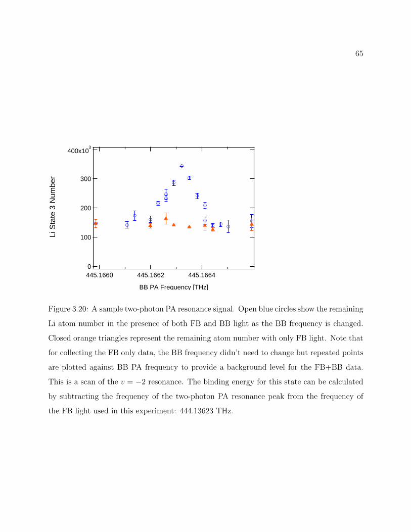
65
400x103
300
200
100
0
Li S
tate
3 N
umbe
r
445.1664445.1662445.1660
BB PA Frequency [THz]
Figure 3.20: A sample two-photon PA resonance signal. Open blue circles show the remaining
Li atom number in the presence of both FB and BB light as the BB frequency is changed.
Closed orange triangles represent the remaining atom number with only FB light. Note that
for collecting the FB only data, the BB frequency didn’t need to change but repeated points
are plotted against BB PA frequency to provide a background level for the FB+BB data.
This is a scan of the v = −2 resonance. The binding energy for this state can be calculated
by subtracting the frequency of the two-photon PA resonance peak from the frequency of
the FB light used in this experiment: 444.13623 THz.
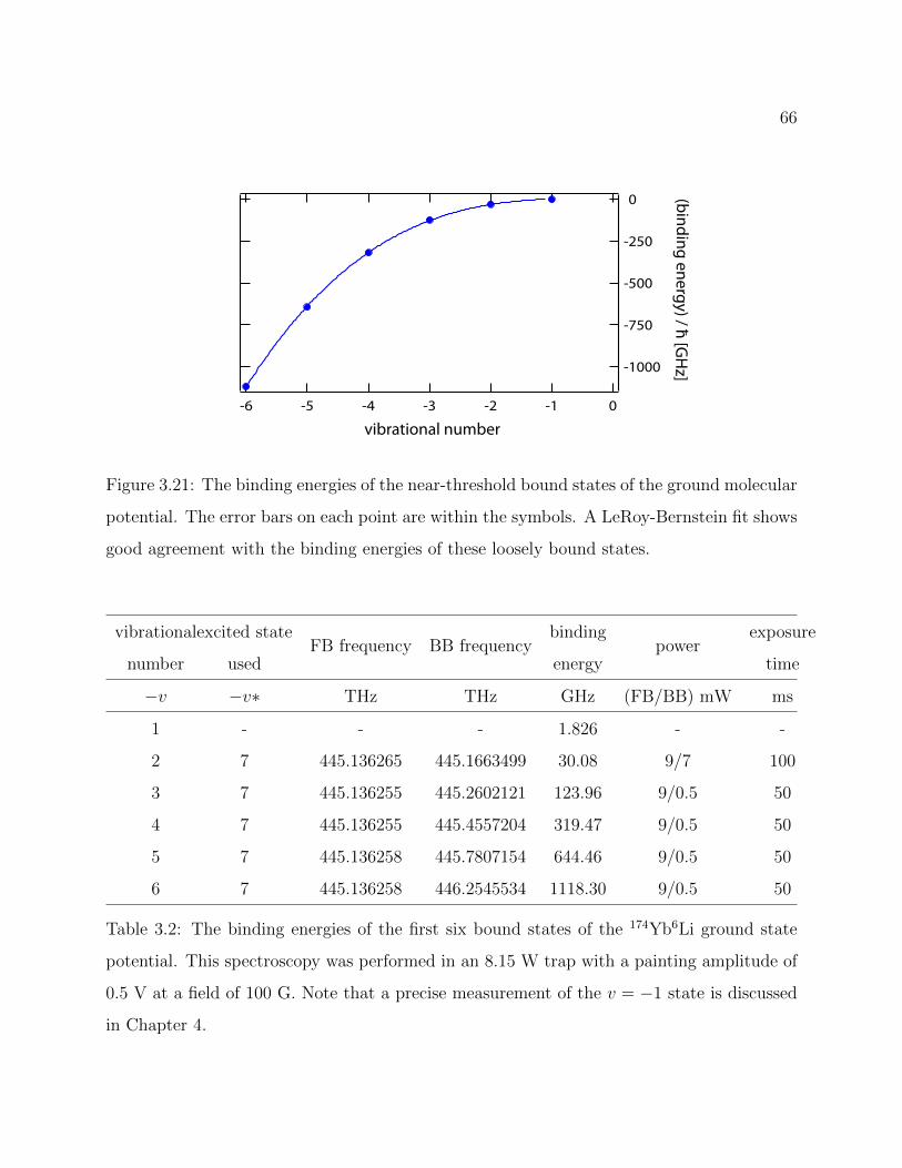
66
-1000
-750
-500
-250
0
-6 -5 -4 -3 -2 -1 0
(binding energy) / ħ [GH
z]
vibrational number
Figure 3.21: The binding energies of the near-threshold bound states of the ground molecular
potential. The error bars on each point are within the symbols. A LeRoy-Bernstein fit shows
good agreement with the binding energies of these loosely bound states.
vibrational
number
excited state
usedFB frequency BB frequency
binding
energypower
exposure
time
−v −v∗ THz THz GHz (FB/BB) mW ms
1 - - - 1.826 - -
2 7 445.136265 445.1663499 30.08 9/7 100
3 7 445.136255 445.2602121 123.96 9/0.5 50
4 7 445.136255 445.4557204 319.47 9/0.5 50
5 7 445.136258 445.7807154 644.46 9/0.5 50
6 7 445.136258 446.2545534 1118.30 9/0.5 50
Table 3.2: The binding energies of the first six bound states of the 174Yb6Li ground state
potential. This spectroscopy was performed in an 8.15 W trap with a painting amplitude of
0.5 V at a field of 100 G. Note that a precise measurement of the v = −1 state is discussed
in Chapter 4.
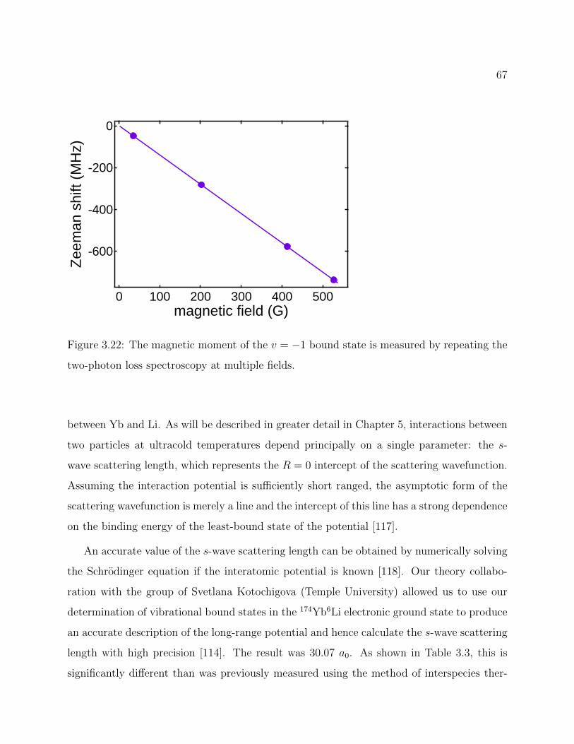
67
-600
-400
-200
0
Zee
man
shi
ft (M
Hz)
5004003002001000magnetic field (G)
Figure 3.22: The magnetic moment of the v = −1 bound state is measured by repeating the
two-photon loss spectroscopy at multiple fields.
between Yb and Li. As will be described in greater detail in Chapter 5, interactions between
two particles at ultracold temperatures depend principally on a single parameter: the s-
wave scattering length, which represents the R = 0 intercept of the scattering wavefunction.
Assuming the interaction potential is sufficiently short ranged, the asymptotic form of the
scattering wavefunction is merely a line and the intercept of this line has a strong dependence
on the binding energy of the least-bound state of the potential [117].
An accurate value of the s-wave scattering length can be obtained by numerically solving
the Schrodinger equation if the interatomic potential is known [118]. Our theory collabo-
ration with the group of Svetlana Kotochigova (Temple University) allowed us to use our
determination of vibrational bound states in the 174Yb6Li electronic ground state to produce
an accurate description of the long-range potential and hence calculate the s-wave scattering
length with high precision [114]. The result was 30.07 a0. As shown in Table 3.3, this is
significantly different than was previously measured using the method of interspecies ther-
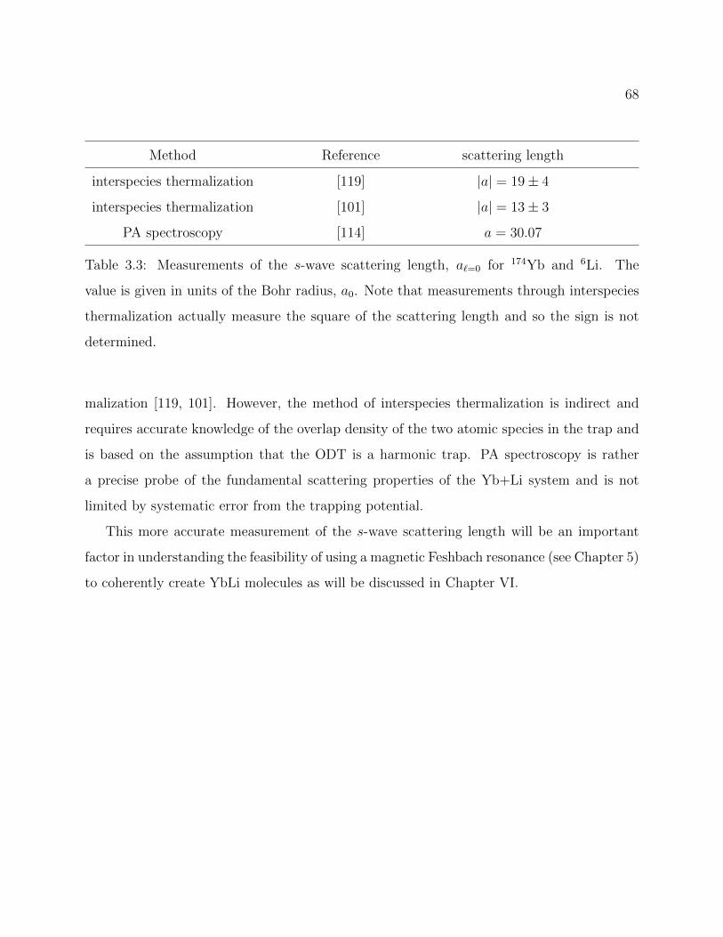
68
Method Reference scattering length
interspecies thermalization [119] |a| = 19± 4
interspecies thermalization [101] |a| = 13± 3
PA spectroscopy [114] a = 30.07
Table 3.3: Measurements of the s-wave scattering length, a`=0 for 174Yb and 6Li. The
value is given in units of the Bohr radius, a0. Note that measurements through interspecies
thermalization actually measure the square of the scattering length and so the sign is not
determined.
malization [119, 101]. However, the method of interspecies thermalization is indirect and
requires accurate knowledge of the overlap density of the two atomic species in the trap and
is based on the assumption that the ODT is a harmonic trap. PA spectroscopy is rather
a precise probe of the fundamental scattering properties of the Yb+Li system and is not
limited by systematic error from the trapping potential.
This more accurate measurement of the s-wave scattering length will be an important
factor in understanding the feasibility of using a magnetic Feshbach resonance (see Chapter 5)
to coherently create YbLi molecules as will be discussed in Chapter VI.
69
Chapter 4
ATOM-MOLELCULE COHERENCE IN 174YB6LI
This chapter concerns the creation of a coherent superposition state between an atomic
pair state and a bound molecule. We first discuss the reasons that using PA transitions to
pump atoms into a molecular state is not a feasible route to molecule production. Then we
introduce the eigenstates of the atom-molecule three-state system which exhibits a ‘dark’
superposition state that can be manipulated to transfer atomic populations to molecular
populations using two phase-coherent laser beams. We describe the method by which we
observed the formation of this dark state. After describing our failed attempts to perform
coherent transfer to the molecular state, we extract from our spectroscopic measurements the
timescales relevant to the efficiency of the transfer process and conclude that the apparatus
we used for these experiments was not suitable for association. We outline the necessary
improvements under which better results can be expected.
4.1 Producing Molecules with PA Transitions
In the previous chapter we discussed photoassociation as a technique to probe the interatomic
potential. This discussion overlooked the fact that photoassociation is also a technique with
which to create molecules by using the ro-vibronic transitions studied in PA to transfer
atoms into bound molecular states. Indeed PA as a means for molecule creation has been
intensively studied both theoretically and experimentally. However, the method as described
in the previous chapter generally lacks two essential properties of a useful association scheme
that we now state explicitly.
• Stability: molecules must have a sufficiently long lifetime in the trap to be useful for
70
subsequent experimentation.
• Low ro-vibrational temperature: molecules should ideally be created in just one vibra-
tional state as many proposed studies based on ultracold molecules are premised on
preparation into a single internal quantum state.
Molecules created in the excited state by one-photon PA are radiatively unstable with life-
times similar to those of the bare atomic transition to which they correspond and are thus
not suitable for subsequent experimentation. However, molecules can be formed in stable
electronic states through an initial one-photon PA excitation followed by transfer to a bound
state in the electronic ground state. The simplest such scheme would involve spontaneous
emission into a ground bound state. However, this scheme usually fails to meet the second
criterion listed above; there is no selection rule constraining the ro-vibrational states to which
the molecule can decay and the result would be a mixture distributed according to the values
of the various Franck-Condon factors rather than a single state. Recent theoretical work pro-
poses to control this decay by performing one-photon PA in an optical cavity [120]. However,
it should be noted that a combination of favorable Franck-Condon factors and the use of
narrow electronic transitions allows for the efficient creation of a vibrationally cold sample
of 88Sr2 molecules [121] which have since been used to probe quantum chemistry [122]. This
method of relying on favorable Franck-Condon factors has been studied extensively in het-
eronuclear systems, in particular where BB Frank-Condon factors are generally expected to
be larger than for homonuclear molecules even for deeply bound, and hence more collisionally
stable states [123, 124].
4.1.1 Coherent Association of Molecules with Light Fields
Preparation of a sample of ultracold atoms into a chosen quantum state can be achieved
instead through coherent control of ro-vibronic transitions. The simplest imaginable coherent
scheme would be a pair of π pulses: one which transfers the population into an excited
molecular state, followed by a second that transfers the population down to a bound state
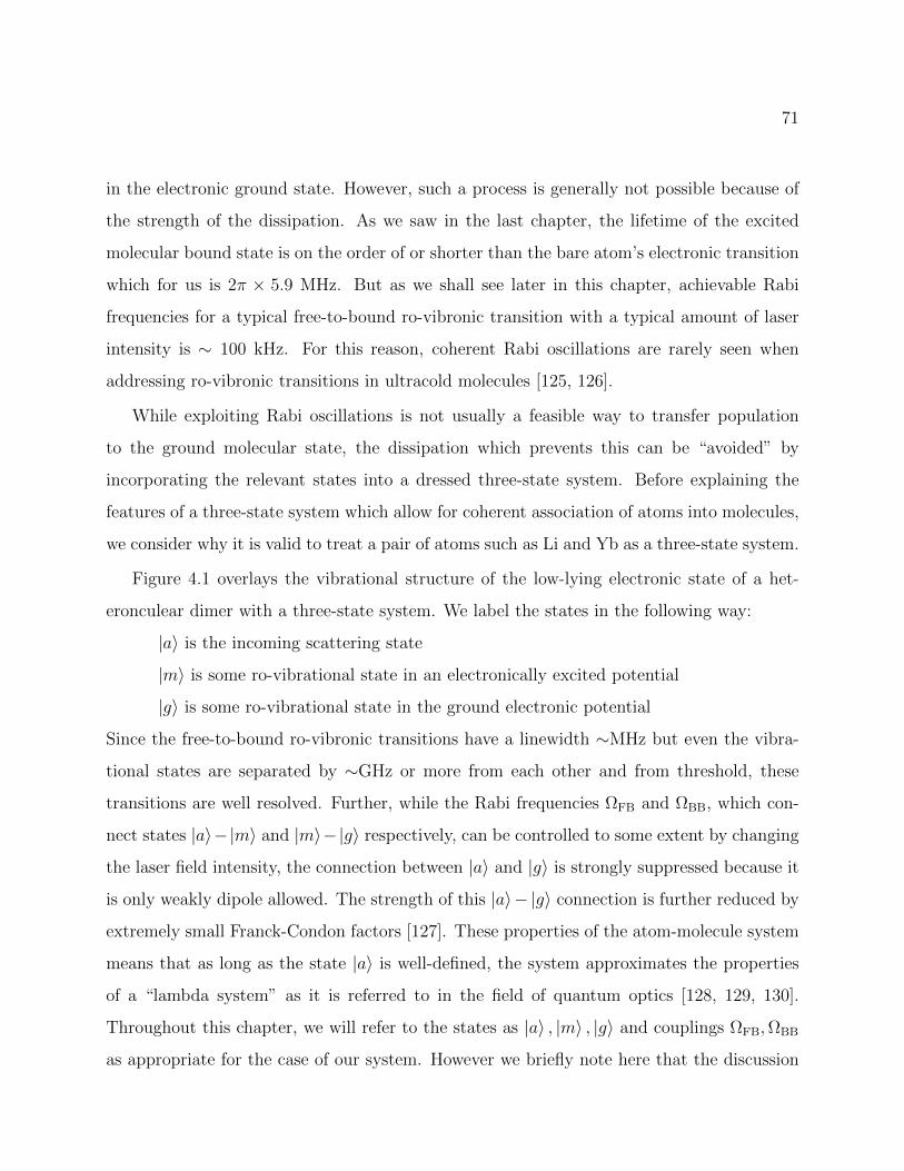
71
in the electronic ground state. However, such a process is generally not possible because of
the strength of the dissipation. As we saw in the last chapter, the lifetime of the excited
molecular bound state is on the order of or shorter than the bare atom’s electronic transition
which for us is 2π × 5.9 MHz. But as we shall see later in this chapter, achievable Rabi
frequencies for a typical free-to-bound ro-vibronic transition with a typical amount of laser
intensity is ∼ 100 kHz. For this reason, coherent Rabi oscillations are rarely seen when
addressing ro-vibronic transitions in ultracold molecules [125, 126].
While exploiting Rabi oscillations is not usually a feasible way to transfer population
to the ground molecular state, the dissipation which prevents this can be “avoided” by
incorporating the relevant states into a dressed three-state system. Before explaining the
features of a three-state system which allow for coherent association of atoms into molecules,
we consider why it is valid to treat a pair of atoms such as Li and Yb as a three-state system.
Figure 4.1 overlays the vibrational structure of the low-lying electronic state of a het-
eronculear dimer with a three-state system. We label the states in the following way:
|a〉 is the incoming scattering state
|m〉 is some ro-vibrational state in an electronically excited potential
|g〉 is some ro-vibrational state in the ground electronic potential
Since the free-to-bound ro-vibronic transitions have a linewidth ∼MHz but even the vibra-
tional states are separated by ∼GHz or more from each other and from threshold, these
transitions are well resolved. Further, while the Rabi frequencies ΩFB and ΩBB, which con-
nect states |a〉−|m〉 and |m〉−|g〉 respectively, can be controlled to some extent by changing
the laser field intensity, the connection between |a〉 and |g〉 is strongly suppressed because it
is only weakly dipole allowed. The strength of this |a〉− |g〉 connection is further reduced by
extremely small Franck-Condon factors [127]. These properties of the atom-molecule system
means that as long as the state |a〉 is well-defined, the system approximates the properties
of a “lambda system” as it is referred to in the field of quantum optics [128, 129, 130].
Throughout this chapter, we will refer to the states as |a〉 , |m〉 , |g〉 and couplings ΩFB,ΩBB
as appropriate for the case of our system. However we briefly note here that the discussion
72
Figure 4.1: (left) The approximation of the quantum states of Yb+Li atoms as a three-state
system. The scattering state and a bound state in the electronic ground state are both
coupled to a bound excited state. (right) The labeling conventions used for treatment of
the three-state system in this state. ΩFB and ΩBB are the Rabi frequencies for the free-to-
bound and bound-to-bound ro-vibronic transitions respectively. δFB and δBB are the one-
photon detunings of the light field from the free-to-bound and bound-to-bound PA resonances
respectively (note that they are drawn with negative values in this schematic).
in the following two sections applies equally well to other three-state systems for which this
labelling scheme would make little sense.
4.2 Three-state Lambda Systems
Under the rotating wave approximation, the Hamiltonian for such a system is given by the
following [130].
HRWA = ~
0 ΩFB/2 0
ΩFB/2 δFB ΩBB/2
0 ΩBB/2 δFB − δBB
(4.1)
73
Where ΩFB and ΩBB are the Rabi frequencies for the free-to-bound and bound-to-bound
ro-vibronic transitions respectively, and δFB and δBB are the one-photon detunings of the
light field from the free-to-bound and bound-to-bound PA resonances respectively. Under
the conditions δBB = δFB = 0 the eigenstates of this system are given by the expressions
below.
|+〉 =sin θ√
2|a〉+
1√2|m〉+
cos θ√2|g〉 (4.2a)
|−〉 =sin θ√
2|a〉 − 1√
2|m〉+
cos θ√2|g〉 (4.2b)
|0〉 = cos θ |a〉 − sin θ |g〉 (4.2c)
θ = arctanΩFB
ΩBB
(4.2d)
The state designated by |0〉 is referred to as the “dark state” because it contains no pro-
jection onto |m〉, the only strongly radiative state in the system. Unlike what one might
refer to as “typical” quantum interference, in which a differential phase accumulation can
lead to destructive interference of probability amplitudes, a three-state system can exhibit
destructive interference in the coherences, which leads to the decoupling of |m〉 from the
light field.
The creation of this dark state has been studied in a variety of different physical systems
such as atomic gases, quantum dots, and optical cavities [131, 132, 133, 134] where the
typical experimental signature is sometimes called electromagnetically induced transparency
(EIT) because for ΩBB ΩFB the absorption of the FB field is strongly suppressed over a
narrow range of δFB, leading to transparency. Without such strict limits, the creation of the
dark state may instead be interpreted as coherent population trapping (CPT) because the
formation of the dark state allows for transfer into the dark state. For the purpose of this
thesis, we will refer generally to the creation of the dark state as CPT.
74
4.2.1 Adiabatic Manipulation of the Lambda System: Stimulated Raman Adiabatic Passage
The dark state |0〉 is the key to performing population transfer from |a〉 to |g〉 while meeting
the criteria outlined at the beginning of this chapter. By considering the possible values for
θ in Equation 4.2, we arrive at the following two equations.
|0〉θ=0 = |a〉 (4.3a)
|0〉θ=π2
= − |g〉 (4.3b)
We see that by changing the value of θ from 0 toπ
2, we change the state from the atomic
state to the ground molecular state, provided that the change of θ is slow enough for |0〉 to
remain an eigenstate of the system. This process is given the general name of stimulated
Raman adiabatic passage (StiRAP) [130]. Its application for molecule formation is referred
to as free-to-bound StiRAP.
To effect the desired change in θ, the values of ΩBB and ΩFB may be manipulated by
changing the intensities of the driving laser fields in time. For whatever temporal shape
the FB and BB pulses take, in order to effect θ = 0 → π
2, the ΩBB must be applied
first followed by a partially time-overlapping pulse of ΩFB. Since this is the reverse order
compared to a pair of π pulses designed for the same objective, it is sometimes referred to
as the “counterintuitive” pulse sequence.
Figures 4.2(a) and (b) show a possible StiRAP pulse sequence and the corresponding evo-
lution of θ. In Figure 4.2(c) the population of each three-states is shown through numerically
solving the Liouville equation, using H as in Equation 4.1 with the addition of a dissipation
term. As an easy example, we consider the case for which γa = 10 max(ΩFB) = 10 max(ΩBB)
(a case for which using π pulses is impossible). As seen in Figure 4.2, even under the condi-
tion that γa > ΩFB,ΩBB, the transfer of the population from |a〉 to |g〉 is almost 100% owing
to the fact that |m〉 is barely populated through the pulse sequence.
Although this model is too crude to exactly capture the dynamics for molecule formation,
the scheme has been successfully demonstrated. Free-to-bound StiRAP was used for coherent
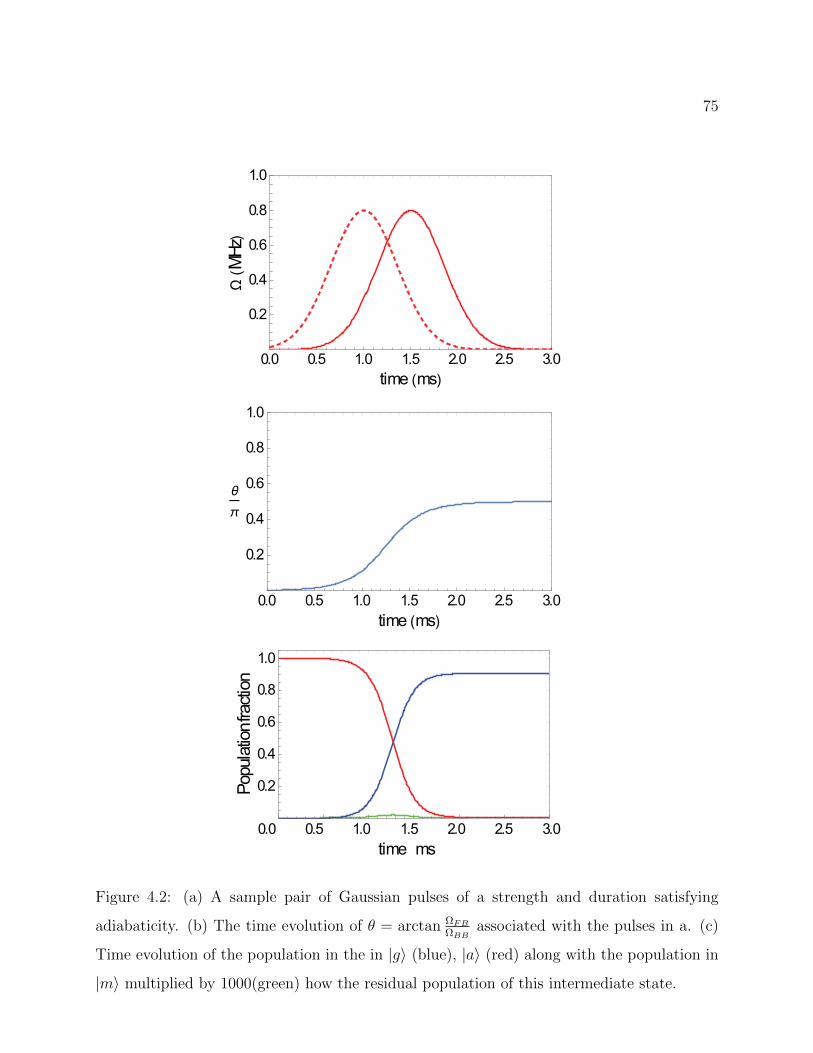
75
0.0 0.5 1.0 1.5 2.0 2.5 3.0
0.2
0.4
0.6
0.8
1.0
time ms
MHz
0.0 0.5 1.0 1.5 2.0 2.5 3.0
0.2
0.4
0.6
0.8
1.0
time ms
0.2
0.4
0.6
0.8
1.0
Popu
latio
nfra
ction
0.0 0.5 1.0 1.5 2.0 2.5 3.0time ms
Figure 4.2: (a) A sample pair of Gaussian pulses of a strength and duration satisfying
adiabaticity. (b) The time evolution of θ = arctan ΩFBΩBB
associated with the pulses in a. (c)
Time evolution of the population in the in |g〉 (blue), |a〉 (red) along with the population in
|m〉 multiplied by 1000(green) how the residual population of this intermediate state.
76
creation of Sr2 molecules in a 3D optical lattice with formation efficiencies over 80% [80, 135].
However, to the author’s best knowledge there are at this time no published accounts of
successful creation of heteronuclear molecules using free-to-bound StiRAP.
4.3 Atom-molecule Coherence in Yb+Li
As a basis for molecule formation via StiRAP, we sought a coherence between |a〉 and |g〉
by addressing a pair of free-to-bound and bound-to-bound ro-vibronic transitions, connected
through the same state |m〉. Although we had identified in our spectroscopy several vibra-
tional levels of the YbLi ground state, we chose to target the v = −1 state for experimental
simplicity. The light-driven coherence requires dressing by two laser beams which are phase
coherent and separated in frequency by the binding energy of the target state in the ground
potential. Since the binding energy of v = −1 is only 1.8 GHz, this could easily be achieved
using AOMs to shift the bifurcated output of a single master laser.
Figure 4.3 shows the experimental setup for our initial studies of the atom-molecule
coherence. A single ECDL was frequency locked to the wavemeter as in Chapter 3. The
output of the ECDL was amplified with a lab-built tapered amplifier and split into two
components. The ratio of this splitting was adjusted in order to control the ratioΩFB
ΩBB
,
though a typical ratio is indicated in Figure 4.3. Each path was sent through an AOM four
times using a method detailed in [136], resulting in a total frequency between the two beams
of eight times the AOM frequency. The AOMs (center frequency 200 MHz) were driven by a
single DDS-based frequency source (ADD9910) which was built in the lab. By independently
shifting the laser frequency with the wavemeter lock and the RF frequency with the DDS
source, we were able vary the values of both δFB and δBB and thereby probe the coherence.
The two shifted beams were combined on a 50:50 beam cube and sent through a Li vapor
cell for spectral filtering. Finally, the beam was coupled into a PM fiber. The output of the
PM fiber was focused onto the atoms in the same way as discussed in Chapter 3.
We observed the formation of the “dark” coherent superposition state |0〉 through trap-
loss spectroscopy [137]. A mixture of 174Yb and 6Li atoms were laser cooled and sequentially
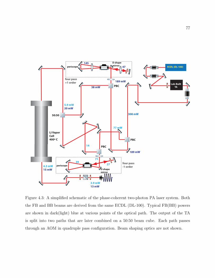
77
Li Vapor Cell400º C
ECDL (DL-100)
Lab-Built TA
D shape mirror
D shape mirror
periscope
periscopefour pass -1 order
four pass +1 order
50:50
PBC
PBC
PBC
308 mW
189 mW
77 mW
71
5.9 mW20 mW
3927
14
4.3 mW15 mW
3.9 mW13 mW
189 mW
14547
38 mW
Figure 4.3: A simplified schematic of the phase-coherent two-photon PA laser system. Both
the FB and BB beams are derived from the same ECDL (DL-100). Typical FB(BB) powers
are shown in dark(light) blue at various points of the optical path. The output of the TA
is split into two paths that are later combined on a 50:50 beam cube. Each path passes
through an AOM in quadruple pass configuration. Beam shaping optics are not shown.
78
loaded into the ODT. After forced evaporative cooling the Li was prepared in state |3〉
through RF sweeps as described in Chapter 5. Typical starting conditions for this spec-
troscopy are detailed below.
Yb(Li) Number: 2.1× 10⁶ (3.1× 10⁵)
Yb(Li) Temperature: 4.8(6.1) µK
Yb Trap Frequency: ω = 2π × 481, 220, 135 Hz
ODT Trap Parameters: P = 3 W, painting amplitude = 0.5 V
To perform spectroscopy we applied a simultaneous square pulse on both the FB and
BB laser beams. The pulse length and the intensity of the FB beam were chosen such that
absent the BB laser beam 50− 80% of the Li atoms were lost from the trap, mostly due to
loss through decay of the molecular excited state. After we exposed the atomic sample to
these pulses, we measured the remaining atoms in the trap through absorption imaging. We
repeated this process at different values of δFB, keeping δBB constant.
Figure 4.4 is a sample spectrum obtained through trap-loss spectroscopy. The number
of atoms remaining in the trap has a loss dip in a range of detunings spanning about 25
MHz as would be expected from the strong coupling of |a〉 to the lossy state |m〉 through
photoassociation. However, within a narrow range of about 2.7 MHz the trap loss is strongly
suppressed. This response relative to detuning takes the same form as the transmission
through a medium characterized by a dressed three-state system and is likewise an indication
of CPT. The creation of a spectral feature narrower than the natural linewidth of the atomic
electronic transition of Γ = 2π × 5.9 MHz indicates that the excited state linewidth is no
longer the strongest source of decoherence in the system.
To assess the feasibility of manipulating this atom-molecule coherence for the efficient cre-
ation of molecules, we must first consider whether we can fulfill the adiabaticity requirements
for StiRAP.
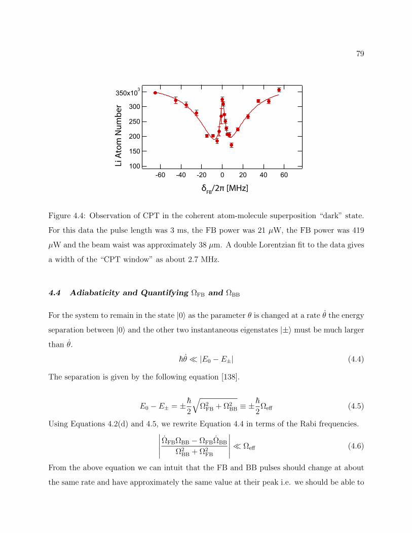
79
350x103
300
250
200
150
100-60 -40 -20 0 20 40 60
δFB/2π [MHz]
Li A
tom
Num
ber
Figure 4.4: Observation of CPT in the coherent atom-molecule superposition “dark” state.
For this data the pulse length was 3 ms, the FB power was 21 µW, the FB power was 419
µW and the beam waist was approximately 38 µm. A double Lorentzian fit to the data gives
a width of the “CPT window” as about 2.7 MHz.
4.4 Adiabaticity and Quantifying ΩFB and ΩBB
For the system to remain in the state |0〉 as the parameter θ is changed at a rate θ the energy
separation between |0〉 and the other two instantaneous eigenstates |±〉 must be much larger
than θ.
~θ |E0 − E±| (4.4)
The separation is given by the following equation [138].
E0 − E± = ±~2
√Ω2
FB + Ω2BB ≡ ±
~2
Ωeff (4.5)
Using Equations 4.2(d) and 4.5, we rewrite Equation 4.4 in terms of the Rabi frequencies.∣∣∣∣∣ΩFBΩBB − ΩFBΩBB
Ω2BB + Ω2
FB
∣∣∣∣∣ Ωeff (4.6)
From the above equation we can intuit that the FB and BB pulses should change at about
the same rate and have approximately the same value at their peak i.e. we should be able to
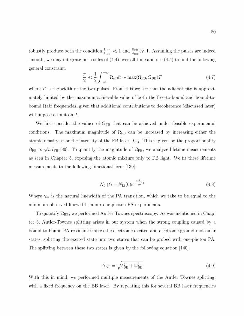
80
robustly produce both the condition ΩFB
ΩBB 1 and ΩFB
ΩBB 1. Assuming the pulses are indeed
smooth, we may integrate both sides of (4.4) over all time and use (4.5) to find the following
general constraint.π
2 1
2
∫ +∞
−∞Ωeffdt ∼ max(ΩFB,ΩBB)T (4.7)
where T is the width of the two pulses. From this we see that the adiabaticity is approxi-
mately limited by the maximum achievable value of both the free-to-bound and bound-to-
bound Rabi frequencies, given that additional contributions to decoherence (discussed later)
will impose a limit on T .
We first consider the values of ΩFB that can be achieved under feasible experimental
conditions. The maximum magnitude of ΩFB can be increased by increasing either the
atomic density, n or the intensity of the FB laser, IFB. This is given by the proportionality
ΩFB ∝√n IFB [80]. To quantify the magnitude of ΩFB, we analyze lifetime measurements
as seen in Chapter 3, exposing the atomic mixture only to FB light. We fit these lifetime
measurements to the following functional form [139].
NLi(t) = NLi(0)e−Ω2
FBγm
t (4.8)
Where γm is the natural linewidth of the PA transition, which we take to be equal to the
minimum observed linewidth in our one-photon PA experiments.
To quantify ΩBB, we performed Autler-Townes spectroscopy. As was mentioned in Chap-
ter 3, Autler-Townes splitting arises in our system when the strong coupling caused by a
bound-to-bound PA resonance mixes the electronic excited and electronic ground molecular
states, splitting the excited state into two states that can be probed with one-photon PA.
The splitting between these two states is given by the following equation [140].
∆AT =√δ2
BB + Ω2BB (4.9)
With this in mind, we performed multiple measurements of the Autler Townes splitting,
with a fixed frequency on the BB laser. By repeating this for several BB laser frequencies
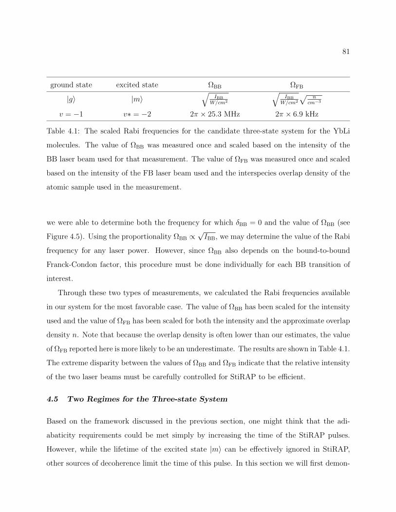
81
ground state excited state ΩBB ΩFB
|g〉 |m〉√
IBB
W/cm2
√IBB
W/cm2
√n
cm−3
v = −1 v∗ = −2 2π × 25.3 MHz 2π × 6.9 kHz
Table 4.1: The scaled Rabi frequencies for the candidate three-state system for the YbLi
molecules. The value of ΩBB was measured once and scaled based on the intensity of the
BB laser beam used for that measurement. The value of ΩFB was measured once and scaled
based on the intensity of the FB laser beam used and the interspecies overlap density of the
atomic sample used in the measurement.
we were able to determine both the frequency for which δBB = 0 and the value of ΩBB (see
Figure 4.5). Using the proportionality ΩBB ∝√IBB, we may determine the value of the Rabi
frequency for any laser power. However, since ΩBB also depends on the bound-to-bound
Franck-Condon factor, this procedure must be done individually for each BB transition of
interest.
Through these two types of measurements, we calculated the Rabi frequencies available
in our system for the most favorable case. The value of ΩBB has been scaled for the intensity
used and the value of ΩFB has been scaled for both the intensity and the approximate overlap
density n. Note that because the overlap density is often lower than our estimates, the value
of ΩFB reported here is more likely to be an underestimate. The results are shown in Table 4.1.
The extreme disparity between the values of ΩBB and ΩFB indicate that the relative intensity
of the two laser beams must be carefully controlled for StiRAP to be efficient.
4.5 Two Regimes for the Three-state System
Based on the framework discussed in the previous section, one might think that the adi-
abaticity requirements could be met simply by increasing the time of the StiRAP pulses.
However, while the lifetime of the excited state |m〉 can be effectively ignored in StiRAP,
other sources of decoherence limit the time of this pulse. In this section we will first demon-
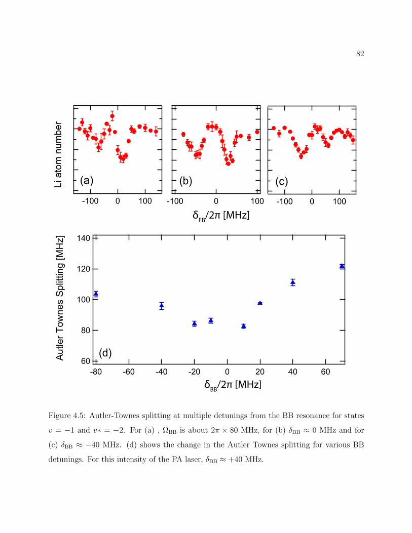
82
-100 0 100-100 0 100 -100 0 100
Li a
tom
num
ber
(a) (b) (c)
140
120
100
80
60 Aut
ler T
owne
s S
plitt
ing
[MH
z]
-80 -60 -40 -20 0 20 40 60
(d)
δFB/2π [MHz]
δBB/2π [MHz]
Figure 4.5: Autler-Townes splitting at multiple detunings from the BB resonance for states
v = −1 and v∗ = −2. For (a) , ΩBB is about 2π × 80 MHz, for (b) δBB ≈ 0 MHz and for
(c) δBB ≈ −40 MHz. (d) shows the change in the Autler Townes splitting for various BB
detunings. For this intensity of the PA laser, δBB ≈ +40 MHz.
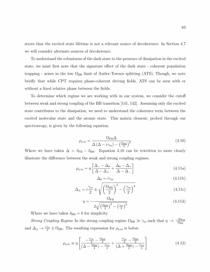
83
strate that the excited state lifetime is not a relevant source of decoherence. In Section 4.7
we will consider alternate sources of decoherence.
To understand the robustness of the dark state to the presence of dissipation in the excited
state, we must first note that the signature effect of the dark state - coherent population
trapping - arises in the low ΩBB limit of Autler-Townes splitting (ATS). Though, we note
briefly that while CPT requires phase-coherent driving fields, ATS can be seen with or
without a fixed relative phase between the fields.
To determine which regime we are working with in our system, we consider the cutoff
between weak and strong coupling of the BB transition [141, 142]. Assuming only the excited
state contributes to the dissipation, we need to understand the coherence term between the
excited molecular state and the atomic state. This matrix element, probed through our
spectroscopy, is given by the following equation.
ρa,m =ΩFB∆
∆ (∆− iγm)−(
ΩBB
2
)2 (4.10)
Where we have taken ∆ = δFB − δBB. Equation 4.10 can be rewritten to more clearly
illustrate the difference between the weak and strong coupling regimes.
ρa,m = η
[∆− −∆0
∆−∆+
+∆0 −∆+
∆−∆−
](4.11a)
∆0 = iγm (4.11b)
∆± = iγm2±
√(ΩBB
2
)2
−(γm
2
)2
(4.11c)
η = − ΩFB
2
√(ΩBB
2
)2 −(γm2
)2(4.11d)
Where we have taken δBB = 0 for simplicity.
Strong Coupling Regime In the strong coupling regime ΩBB γm such that η → −2ΩFB
ΩBB
and ∆± → iγm2± ΩBB. The resulting expression for ρa,m is below.
ρa,m ∝ η
[− iγm
2− ΩBB
2
(∆− ΩBB
2)− iγm
2
+iγm
2− ΩBB
2
(∆ + ΩBB
2)− iγm
2
](4.12)
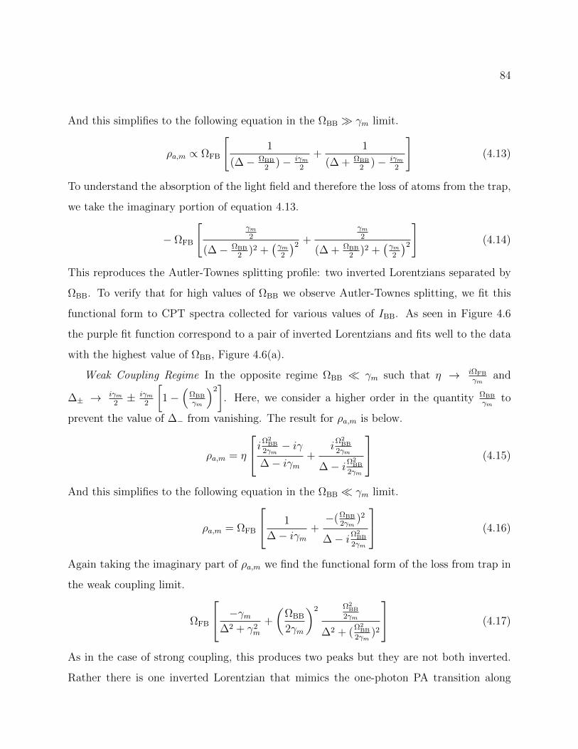
84
And this simplifies to the following equation in the ΩBB γm limit.
ρa,m ∝ ΩFB
[1
(∆− ΩBB
2)− iγm
2
+1
(∆ + ΩBB
2)− iγm
2
](4.13)
To understand the absorption of the light field and therefore the loss of atoms from the trap,
we take the imaginary portion of equation 4.13.
− ΩFB
[γm2
(∆− ΩBB
2)2 +
(γm2
)2 +γm2
(∆ + ΩBB
2)2 +
(γm2
)2
](4.14)
This reproduces the Autler-Townes splitting profile: two inverted Lorentzians separated by
ΩBB. To verify that for high values of ΩBB we observe Autler-Townes splitting, we fit this
functional form to CPT spectra collected for various values of IBB. As seen in Figure 4.6
the purple fit function correspond to a pair of inverted Lorentzians and fits well to the data
with the highest value of ΩBB, Figure 4.6(a).
Weak Coupling Regime In the opposite regime ΩBB γm such that η → iΩFB
γmand
∆± → iγm2± iγm
2
[1−
(ΩBB
γm
)2]. Here, we consider a higher order in the quantity ΩBB
γmto
prevent the value of ∆− from vanishing. The result for ρa,m is below.
ρa,m = η
iΩ2BB
2γm− iγ
∆− iγm+
iΩ2
BB
2γm
∆− iΩ2BB
2γm
(4.15)
And this simplifies to the following equation in the ΩBB γm limit.
ρa,m = ΩFB
1
∆− iγm+−(ΩBB
2γm)2
∆− iΩ2BB
2γm
(4.16)
Again taking the imaginary part of ρa,m we find the functional form of the loss from trap in
the weak coupling limit.
ΩFB
−γm∆2 + γ2
m
+
(ΩBB
2γm
)2 Ω2BB
2γm
∆2 + (Ω2
BB
2γm)2
(4.17)
As in the case of strong coupling, this produces two peaks but they are not both inverted.
Rather there is one inverted Lorentzian that mimics the one-photon PA transition along
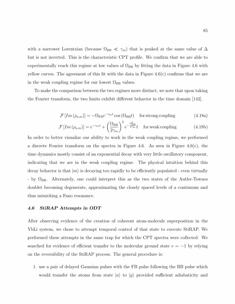
85
with a narrower Lorentzian (because ΩBB γm) that is peaked at the same value of ∆
but is not inverted. This is the characteristic CPT profile. We confirm that we are able to
experimentally reach this regime at low values of ΩBB by fitting the data in Figure 4.6 with
yellow curves. The agreement of this fit with the data in Figure 4.6(c) confirms that we are
in the weak coupling regime for our lowest ΩBB values.
To make the comparison between the two regimes more distinct, we note that upon taking
the Fourier transform, the two limits exhibit different behavior in the time domain [142].
F [Im (ρa,m)] = −ΩFBe−γmt cos (ΩBBt) for strong coupling (4.18a)
F [Im (ρa,m)] = e−γmt +
(ΩBB
2γm
)2
e−Ω2
BB2γm t for weak coupling (4.18b)
In order to better visualize our ability to work in the weak coupling regime, we performed
a discrete Fourier transform on the spectra in Figure 4.6. As seen in Figure 4.6(c), the
time dynamics mostly consist of an exponential decay with very little oscillatory component,
indicating that we are in the weak coupling regime. The physical intuition behind this
decay behavior is that |m〉 is decaying too rapidly to be efficiently populated - even virtually
- by ΩBB. Alternately, one could interpret this as the two states of the Autler-Townes
doublet becoming degenerate, approximating the closely spaced levels of a continuum and
thus mimicking a Fano resonance.
4.6 StiRAP Attempts in ODT
After observing evidence of the creation of coherent atom-molecule superposition in the
YbLi system, we chose to attempt temporal control of that state to execute StiRAP. We
performed these attempts in the same trap for which the CPT spectra were collected. We
searched for evidence of efficient transfer to the molecular ground state v = −1 by relying
on the reversibility of the StiRAP process. The general procedure is:
1. use a pair of delayed Gaussian pulses with the FB pulse following the BB pulse which
would transfer the atoms from state |a〉 to |g〉 provided sufficient adiabaticity and
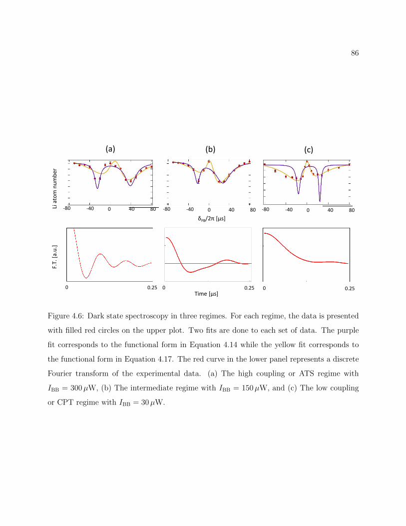
86F.
T. [a
.u.]
0.250 0.250 0.250
400 80-40-80 400 80-40-80 400 80-40-80
rebmun
mota iL
Time [μs]
δFB/2π [μs]
(a) (b) (c)
Figure 4.6: Dark state spectroscopy in three regimes. For each regime, the data is presented
with filled red circles on the upper plot. Two fits are done to each set of data. The purple
fit corresponds to the functional form in Equation 4.14 while the yellow fit corresponds to
the functional form in Equation 4.17. The red curve in the lower panel represents a discrete
Fourier transform of the experimental data. (a) The high coupling or ATS regime with
IBB = 300µW, (b) The intermediate regime with IBB = 150µW, and (c) The low coupling
or CPT regime with IBB = 30µW.
87
coherence
2. remove all unassociated atoms from the trap using a laser pulse resonant with the
atomic transitions 2S1/2 → 2P3/2 for Li and 1S0 → 1P1 for Yb
3. use a pair of Gaussian pulses with the BB pulse following the FB pulse to transfer any
molecules in state |g〉 back to |a〉
4. count the atoms remaining through absorption imaging
Knowing that we would be limited by the low values of ΩFB in the existing coherent two-
photon spectroscopy setup, we made a relatively simple upgrade to the setup shown in
Figure 4.3 in order to boost the power in the FB laser beam. After passing through the
4-pass AOM used to shift the FB laser beam, the beam was not coupled through a fiber
to the atoms but rather coupled into a free-running diode laser mount for injection locking.
The output of this beam was sent to a lab-built tapered amplifier to produce the FB laser
beam, still phase coherent with the BB beam. In this way we were able to produce about
20 mW of FB light and 5 mW of BB light as measured just before the beam was focused on
the atoms. Before attempting StiRAP we also sought to increase ΩFB by narrowing the PA
beam waist to 38 µm.
We also sought to make the removal of unassociated atoms as fast as possible such that
any population of molecules formed during the initial StiRAP did not fully decay before
they could be transferred back to |a〉 for detection. Since the same beam used for absorption
imaging was used to remove unassociated atoms, we began controlling the intensity in each
of these beams through the RF power to the AOMs used to produce these beams. This
control boosted the imaging power during the removal pulse such that a pulse of 5µs would
remove all the atoms.
We repeated the attempts to confirm successful StiRAP using the procedure above, always
using the maximum amount of FB power available. We varied the BB power over several
orders of magnitude and tried a variety of different pulse times. We also varied the time
88
between pulses. Additionally, we tried using both v∗ = −2 and v∗ = −7 as the intermediate
state. This could have been a critical decision as the maximum amount of FB power which we
could use for v∗ = −2 was limited by the proximity of the Li2 PA lines (see Chapter 3) which
would power broaden and merge with the YbLi resonance, making the v∗ = −2 resonance
unusable for StiRAP. However, the FB Franck-Condon factor for v∗ = −7 being so much
smaller than v∗ = −2 meant that even if we used more power, the achievable Rabi frequency
in either case was about the same: ΩFB ≈ 2π × 200 kHz. Despite our various attempts we
were unable to observe any formation of molecules via a free-to-bound StiRAP process.
4.7 Numerical Model for Three-state System
To understand the possible reasons for our failure to transfer atoms into molecules via Sti-
RAP, we performed numerical modeling of an ideal three-state system under the condition
that all three-states |a〉 , |m〉 , |g〉 could decay and be lost from the system at rates γa, γb, γg.
We add this dissipation to Equation 4.1 to get the following Hamiltonian.
H = ~
−iγa ΩFB/2 0
ΩFB/2 −iγm + δFB − δBBΩBB/2
0 ΩBB/2 −iγg + δFB
(4.19)
In the following three subsections we will discuss how we determined appropriate values to
input into this model by analyzing dark state spectroscopy measurements.
4.7.1 Determining ΩFB and ΩBB
ΩFB and ΩBB were chosen according to the values in Table 4.1, although in practice we
assumed that ΩBB could be set to essentially any relevant value. Since we set both beams
to resonance, δFB and δFB are assumed to be zero as IFB, IBB → 0. Though a Stark shift
on each state is added according to experimental measurements of the dark state shift with
increasing intensity. Since under typical conditions IFB IBB, we only consider shifts from
the FB laser.
89
4.7.2 Determining γa
We assume that γa is given by the loss of atoms from the trap from spontaneous scatter off
the atomic transition, which we measure through off-resonant lifetimes. Critically, γa will
increase with intensity, limiting the beneficial effects of using more intensity to increase ΩFB.
4.7.3 Determining γg
As was demonstrated experimentally in [137], the linewidth of the CPT curve is limited by
the decay of the ground molecular state, γg, in the limit of vanishing ΩBB according to the
equation below.
∆CPT =Ω2
BB
γm+ γg (4.20)
To quantify γg we performed several measurements of the CPT linewidth for different
values of ΩBB, shown in Figure 4.7. We extrapolated these results to ΩBB = 0 to find a
value of γg under the three-state model. We obtained a value of γg ≈ 2π × 300 kHz. The
physical cause of γg is unknown however it is expected that these highly vibrationally excited
molecules exhibit significant inelastic loss both with each other as well as with atoms in the
trap which are not associated into molecules. If this is the case, we could expect a sharp
reduction of γg if the Yb and Li atoms are loaded pairwise into individual sites of a deep
optical lattice.
4.7.4 Results of Numerical Modeling
Under the condition that all the atoms begin in the atomic state |a〉 we numerically solved
the Liouville equation for Gaussian pulses [143].
ρ = − i~
[H, ρ] (4.21)
where H is given by Equation 4.19. The results of this calculation are shown in Figure 4.8(a).
Consistent with our experimental observation, no population is transferred to the ground
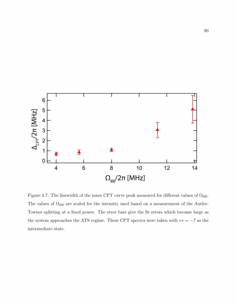
90
6
5
4
3
2
1
0141210864
ΩBB/2π [MHz]
∆ CPT/2
π [M
Hz]
Figure 4.7: The linewidth of the inner CPT curve peak measured for different values of ΩBB.
The values of ΩBB are scaled for the intensity used based on a measurement of the Autler-
Townes splitting at a fixed power. The error bars give the fit errors which become large as
the system approaches the ATS regime. These CPT spectra were taken with v∗ = −7 as the
intermediate state.
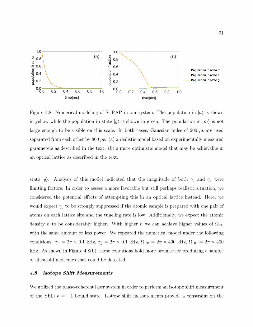
91
(a) (b)
Figure 4.8: Numerical modeling of StiRAP in our system. The population in |a〉 is shown
in yellow while the population in state |g〉 is shown in green. The population in |m〉 is not
large enough to be visible on this scale. In both cases, Gaussian pulse of 200 µs are used
separated from each other by 800 µs. (a) a realistic model based on experimentally measured
parameters as described in the text. (b) a more optimistic model that may be achievable in
an optical lattice as described in the text.
state |g〉. Analysis of this model indicated that the magnitude of both γa and γg were
limiting factors. In order to assess a more favorable but still perhaps realistic situation, we
considered the potential effects of attempting this in an optical lattice instead. Here, we
would expect γg to be strongly suppressed if the atomic sample is prepared with one pair of
atoms on each lattice site and the tuneling rate is low. Additionally, we expect the atomic
density n to be considerably higher. With higher n we can achieve higher values of ΩFB
with the same amount or less power. We repeated the numerical model under the following
conditions: γa = 2π × 0.1 kHz, γg = 2π × 0.1 kHz, ΩFB = 2π × 400 kHz, ΩBB = 2π × 400
kHz. As shown in Figure 4.8(b), these conditions hold more promise for producing a sample
of ultracold molecules that could be detected.
4.8 Isotope Shift Measurements
We utilized the phase-coherent laser system in order to perform an isotope shift measurement
of the YbLi v = −1 bound state. Isotope shift measurements provide a constraint on the
92
short range portion of the interatomic potential. A sufficiently precise measurement would
allow us to determine the number of bound states supported by the potential, predicting the
full spectrum. Such a measurement was relatively easy to perform by switching the isotope
of Yb which, unlike the Li isotope, can be changed without a major overhaul of the laser
system. However, owing to the extreme mass imbalance between Li and Yb, changing the Yb
isotope only changes the reduced mass by ∼ 0.1%, making the spectroscopic shifts too small
to discern using regular two-photon PA. In contrast, the precision afforded by the relatively
narrow linewidth of the CPT curve is sufficiently high [144].
An example isotope shift measurement is shown in Figure 4.9 where we perform dark
state spectroscopy of YbLi v = −1 bound state in a sample containing either 172Yb or 174Yb.
By performing Gaussian fits to the CPT window we determine the binding energy of each
isotope. We measured the isotope shift between 172Yb6Li and 176Yb6Li to be 80.6 MHz
with a statistical uncertainty of 0.3 MHz. However, we observed systematic shifts of about
0.5 MHz in repeated measurements, which ultimately prevented us from using the isotope
shift measurements to constrain the number of bound states supported by the interatomic
potential. We speculated that these systematic errors may be Stark shifts from fluctuations
in the beam intensity, particular from physical drifts of the beam alignment optics.
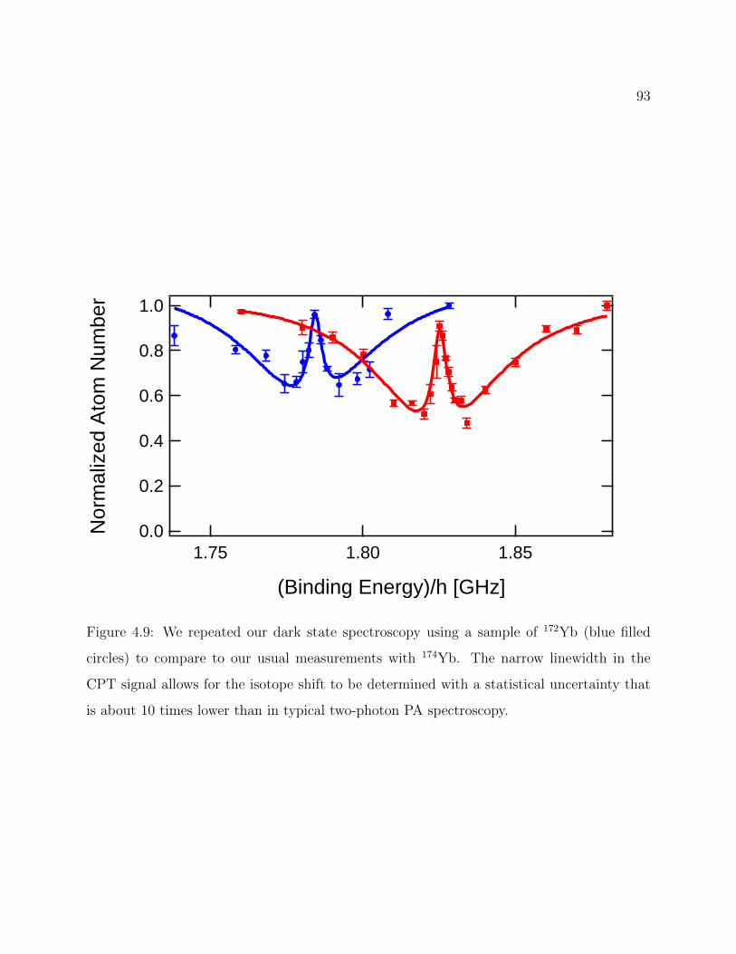
93
1.0
0.8
0.6
0.4
0.2
0.0Nor
mal
ized
Ato
m N
umbe
r
1.851.801.75
(Binding Energy)/h [GHz]
Figure 4.9: We repeated our dark state spectroscopy using a sample of 172Yb (blue filled
circles) to compare to our usual measurements with 174Yb. The narrow linewidth in the
CPT signal allows for the isotope shift to be determined with a statistical uncertainty that
is about 10 times lower than in typical two-photon PA spectroscopy.
94
Chapter 5
MAGNETIC FESHBACH RESONANCES IN 173YB6LI
This chapter concerns the first observation of magnetic Feshbach resonances (MFR) in
YbLi. In the previous chapter we discussed StiRAP as the first of two possible methods for
coherent formation of YbLi molecules. Magnetic Feshbach resonances represent the second
possible method. As we shall see, the observation of MFRs in YbLi was made possible by
our knowledge of the YbLi molecule’s vibrational spectrum, obtained in Chapter 3. The first
section of this chapter explains the origin of scattering resonances such as MFRs. Because
MFRs are considerably different than the resonances discussed in previous chapters, we will
also contextualize the importance of MFRs by discussing the ways in which these resonances
have enabled the study of ultracold gases to gain insight into key elements of few- and many-
body physics. Next, we discuss the unique challenges and benefits for observing MFRs in
YbLi. Finally, we present and analyze our observation of MFRs in YbLi after a description
of the experimental technique.
5.1 Scattering Resonances
Ultracold atoms provide a unique setting in which to study quantum scattering (i.e. scatter-
ing for which semiclassical approximations will fail) [145]. This is a consequence of multiple
properties of these gases:
• Their low densities mean that scattering is dominated by two-body events.
• For neutral atoms, their interaction is usually short ranged and isotropic, allowing for
a central potential model for the interaction between two atoms.
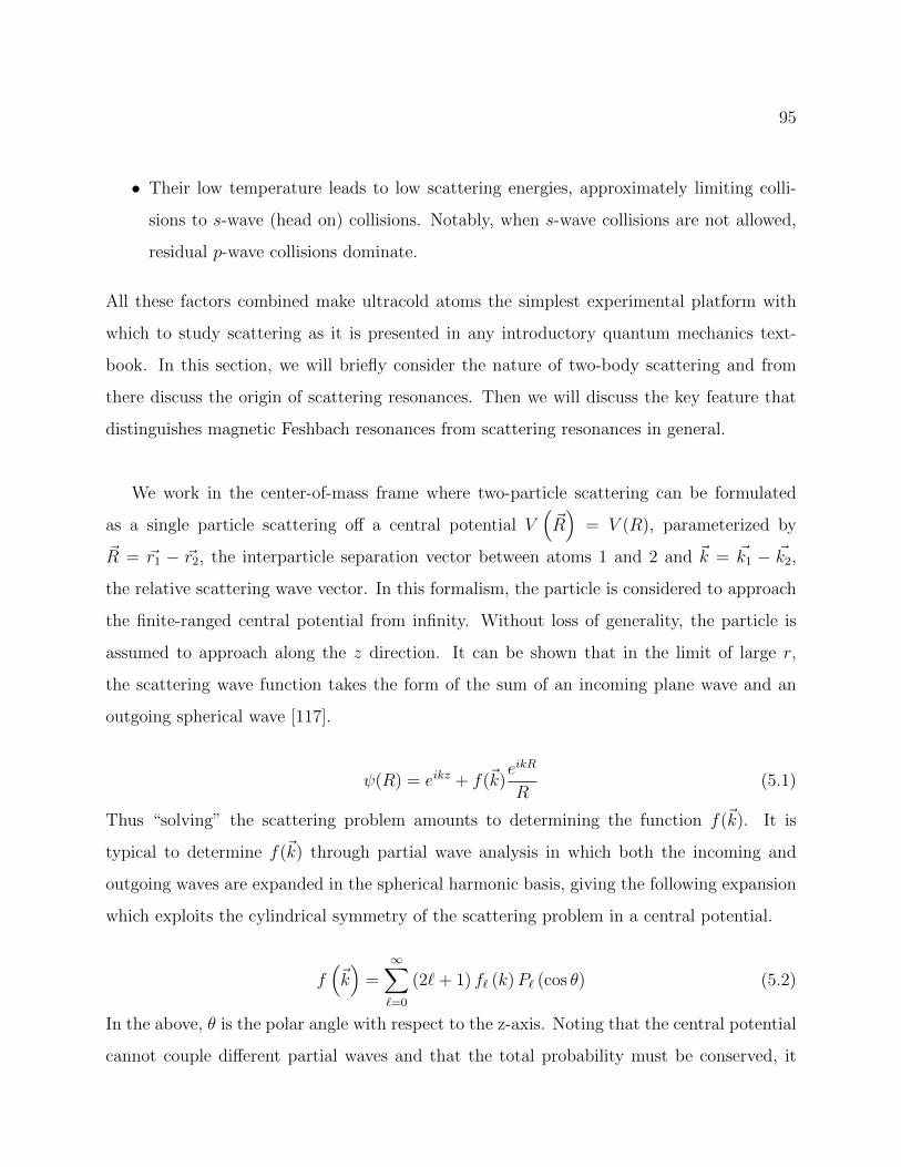
95
• Their low temperature leads to low scattering energies, approximately limiting colli-
sions to s-wave (head on) collisions. Notably, when s-wave collisions are not allowed,
residual p-wave collisions dominate.
All these factors combined make ultracold atoms the simplest experimental platform with
which to study scattering as it is presented in any introductory quantum mechanics text-
book. In this section, we will briefly consider the nature of two-body scattering and from
there discuss the origin of scattering resonances. Then we will discuss the key feature that
distinguishes magnetic Feshbach resonances from scattering resonances in general.
We work in the center-of-mass frame where two-particle scattering can be formulated
as a single particle scattering off a central potential V(~R)
= V (R), parameterized by
~R = ~r1 − ~r2, the interparticle separation vector between atoms 1 and 2 and ~k = ~k1 − ~k2,
the relative scattering wave vector. In this formalism, the particle is considered to approach
the finite-ranged central potential from infinity. Without loss of generality, the particle is
assumed to approach along the z direction. It can be shown that in the limit of large r,
the scattering wave function takes the form of the sum of an incoming plane wave and an
outgoing spherical wave [117].
ψ(R) = eikz + f(~k)eikR
R(5.1)
Thus “solving” the scattering problem amounts to determining the function f(~k). It is
typical to determine f(~k) through partial wave analysis in which both the incoming and
outgoing waves are expanded in the spherical harmonic basis, giving the following expansion
which exploits the cylindrical symmetry of the scattering problem in a central potential.
f(~k)
=∞∑`=0
(2`+ 1) f` (k)P` (cos θ) (5.2)
In the above, θ is the polar angle with respect to the z-axis. Noting that the central potential
cannot couple different partial waves and that the total probability must be conserved, it
96
can be shown that each partial wave scattering amplitude f` hinges on its particular phase
shift δ` according to the following:
f`
(~k)
=1
k
1
tan δ` − i(5.3)
In samples of ultracold atoms, it is often more important to consider the effective potential
that includes both the real potential and the centrifugal barrier.
Veff(R) = V (R) +~2`(`+ 1)
2µR2(5.4)
In the above, µ is the reduced mass. Figure 5.1(b) schematically represents the further
simplification of the scattering problem in ultracold neutral atoms: the angular momentum
barrier classically forbids accessing the short-ranged central potential. In reality this only
means that scattering from the higher order partial waves is strongly suppressed. Absent
symmetry considerations for identical particles, only s-wave scattering need be considered.
Under certain conditions, the potential at long range may be neglected entirely. This is
justified in the limit that kR0 1 with R0 being the effective range of the potential V (R).
For a typical Van der Waals interaction between neutral atoms R0 =
(1µC6
~2
)1/4
∼ 10 a0
whereas atoms that have been through even just the typical first stage of laser cooling can
have a relative wave vector1
k∼ 1000 a0. It may be shown that for power law potentials
V ∝ R−s with s > 2`+3 the condition kR0 1 enforces an asymptotic power law dependence
on the scattering phase shifts, giving the following result for the s-wave phase shift [146, 117].
a`=0 ≡ a = − limk→0
tan δ0
k(5.5)
It is through this single parameter that the scattering properties of ultracold gases are typ-
ically analyzed (a notable exception being for identical fermions, which do not collide via
s-wave for symmetry reasons). Beyond this point the s-wave scattering length will be re-
ferred to simply as the scattering length. As was briefly discussed in Chapter 3, the scattering
length depends critically on the energy of the nearest threshold bound states supported by
97
R
l = 0
R
ener
gy
l = 1
(a) (b)
Figure 5.1: Two effective potentials for two-particle scattering. (a) is the effective potential
for a p-wave collision that includes an angular momentum barrier. The scattering energy,
E = (~k)2
2µ(dashed red) is drawn below the centrifugal barrier in order to suggest the minimal
effect of the short-ranged central potential. (b) is the effective potential for particles in a
s-wave collision in the same potential.
98
the interatomic potential. Further, the value and sign of a for certain combinations of ultra-
cold gases have practical implications for cooling the gases.
Beyond determining the scattering length in general, the presence of bound states can
cause resonant behavior, inducing a large change in the scattering length over a relatively
narrow region of an experimentally tunable parameter space. In particular, a Feshbach
resonance can arise when there are two or more distinct potentials through which the particles
can scatter, as sketched in Figure 5.2(a). These different potentials are distinguished by
different internal states of the scattering atoms in the large R limit and may be coupled to
each other. The atoms will approach each other in an“open channel” where the scattering
energy is above the asymptotic limit of the potential. However, under the condition that
a second “closed channel,” with asymptotic energy above the scattering energy, becomes
nearly degenerate with the open-channel scattering state, the coupling strongly modifies the
outgoing scattering wave.
It can be shown that the nature of this modification results in a resonant part of the
scattering phase called δres0 . This additional phase is added to the uncoupled scattering
phase that exists far from resonance in the open channel which we refer to as the background
scattering phase, δbg0 [147]. Thus the total scattering phase is
δ0 = δbg0 + δres
0 (5.6)
Since we already know that the value of δbg0 is largely determined by the energies of the
nearest threshold bound states, it remains to consider the form of δres0 and what effect it has
on the scattering length. δres0 takes the Breit-Wigner form as shown below [147].
δres0 = − arctan
(Γ/2
E − Eres − δE
)(5.7)
Here Γ describes the lifetime of the transiently occupied bound state in the closed channel,
Eres is the energy at which the resonance occurs and δE is a shift of the resonance location
from the energy of the closed-channel bound state. Although not explicitly formulated in
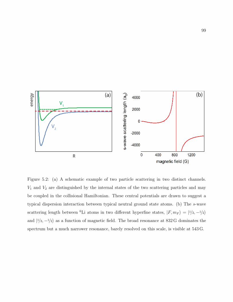
99
V1
V2
energy
R
(a) (b)
Figure 5.2: (a) A schematic example of two particle scattering in two distinct channels.
V1 and V2 are distinguished by the internal states of the two scattering particles and may
be coupled in the collisional Hamiltonian. These central potentials are drawn to suggest a
typical dispersion interaction between typical neutral ground state atoms. (b) The s-wave
scattering length between 6Li atoms in two different hyperfine states, |F,mF 〉 = |1/2,−1/2〉
and |1/2,−1/2〉 as a function of magnetic field. The broad resonance at 832 G dominates the
spectrum but a much narrower resonance, barely resolved on this scale, is visible at 543 G.
100
the above, δE and Γ are k dependent.
To determine the effect of this resonant scattering phase on the scattering length, we
plug into Equation 5.5 the new value of δ0.
a = − limk→0
δbg0
k− lim
k→0
1
karctan
(Γ/2
E − Eres − δE
)(5.8)
We note that the first term is simply the usual scattering length which we now label abg and
apply the two threshold laws that govern the behavior of these resonances at low values of
k: Γ/2→ kabgΓ0 and Eres + δE → E0 with Γ0 being a k-independent constant that depends
on the coupling between the open and closed channels.
a = abg − limk→0
1
karctan
(kabgΓ0
E − E0
)(5.9)
a = abg −abgΓ0
E − E0
= abg
(1− Γ0
E − E0
)(5.10)
Now that we understand the effect of the resonant portion of the scattering phase shift on
the scattering length, we focus in particular on the possibility that the quantity E −E0 can
be experimentally changed. This will be possible via the Zeeman effect if the bound state in
the closed scattering channel (green dashed line in Figure 5.2) and the scattering state of the
open channel (red dashed line in Figure 5.2) have different magnetic moments. By calling
the difference in their magnetic moments δµ we find that the scattering length is a function
of magnetic field.
a = abg
(1− Γ0/δµ
(E − E0)/δµ
)= abg
(1− ∆
B −B0
)(5.11)
A resonance which arises through Zeeman tuning is called a “magnetic Feshbach resonance”
and is by far the most common scattering resonance exploited in ultracold atoms. From
Equation 5.11 we conclude that if a Feshbach resonance exists at B = B0, the scattering
length will experience a pole with a width ∆ = Γ0/δµ, as seen in the example of 6Li, shown in
Figure 5.2(b). Thus the scattering length is tunable not only in magnitude but also in sign,
101
allowing an experimenter to both control the strength of the contact interactions between
ultracold atoms but also to change their character from attractive to repulsive - all by simply
changing the magnetic field. In the following section, we will see the many ways in which
this has expanded the scientific reach of ultracold atoms.
5.2 Applications of MFRs to Cold Atom Physics
MFRs are critical ingredients in a large subset of cutting edge ultracold atoms experiments
and have long been considered a standard “tool” on the experimenter’s metaphorical work-
bench. The most powerful aspect of the MFR is the ability to control the s-wave scattering
length as is demonstrated in Figure 5.2(b) [148]. This ability to tune the interactions be-
tween particles using a magnetic field is of fundamental importance to cold atom studies of
many- and few-body physics.
Outside of the observation of MFRs themselves, using MFRs to modify the interactions
between ultracold atoms has made them a fruitful platform for studies of few-body physics
through their ability to study “universal properties” which are exhibited in different physical
systems with different interactions [149, 150, 151]. This universal scattering regime can
be engineered within an ultracold sample by eliminating the importance of the interatomic
spacing and the interaction range. Although this spacing remains large in these dilute gases
(∼ 105a0), near an MFR the s-wave scattering length can be made arbitrarily large such that
both the interparticle spacing and interaction range are irrelevant.
By using the tunability of the scattering length near an MFR, ultracold atoms were the
first platform to allow the direct observation of a particular aspect of this universal behavior:
the formation of Efimov states [152], families of three-body bound states that exist even when
the constituent two-body interactions are too weak to support a bound state themselves [153].
While Efimov physics has been studied in a number of unique ultracold systems, including
mixtures of different species, the interplay between resonant interactions and symmetrization
requirements is a vast area of theoretical study and motivates experimental input through
the extension of Efimov studies in ultracold gases to new atomic mixtures [154].
102
Ultracold atoms are presently the leading platform for quantum simulation, a broad field
of study that leverages the controllability of an experimenter’s quantum system to model
phenomena in other systems of interest which both defy explication by an analytical or
numerical model and are experimentally less amenable to manipulation or observation [155,
156]. Using an MFR to change the interactions of a model system is fundamental to exploring
its phase space. A prominent example of quantum simulation with ultracold atoms is the
precise study of the BEC-BCS crossover using ultracold fermions, the theory of which is
thought to be intimately connected to that of high temperature superconductivity [157].
Feshbach resonances have also been used to observe quantum phase transitions such as the
Mott insulator-superfluid transition [158], the BEC-supersolid transition [159, 160, 161] and
the Berezinskii–Kosterlitz–Thouless transition [162].
It is common to see the use of MFRs in the simulation of condensed matter systems in
which ultracold atoms are loaded into an optical lattice which simulates the ionic structure
of solids, but quantum simulation with ultracold atoms can also be applicable to many other
fields of physics. For example, ultracold atoms can be used to simulate cosmic inflation [163,
164], lattice gauge theories [165], and neutron stars [166].
While one might say that the studies described above used MFRs as a tool to achieve
their result, the interactions were themselves part of the physics being studied. In contrast,
MFRs have been utilized as a tool simply to create novel forms of ultracold gases. The use of
MFRs is critical to the observation of superfluidity in Fermi gases [167]. As a more practical
example, the ability to control the scattering length was a critical step in the formation of
BECs in 85Rb and 133Cs for which the effective use of evaporative cooling to create a BEC
is impossible without the use of MFRs [168, 169].
But in terms of using MFRs as a tool to create more exotic quantum gases, the most
prominent example is the efficient creation of ultracold dimers via association of ultracold
atoms. In the most naive interpretation, one can think of using an MFR to essentially trap
the molecules which transiently formed as a bound state in the closed channel by raising
the scattering energy, or alternately, lowering the energy of the bound state relative to the
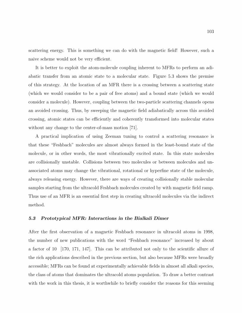
103
scattering energy. This is something we can do with the magnetic field! However, such a
naive scheme would not be very efficient.
It is better to exploit the atom-molecule coupling inherent to MFRs to perform an adi-
abatic transfer from an atomic state to a molecular state. Figure 5.3 shows the premise
of this strategy. At the location of an MFR there is a crossing between a scattering state
(which we would consider to be a pair of free atoms) and a bound state (which we would
consider a molecule). However, coupling between the two-particle scattering channels opens
an avoided crossing. Thus, by sweeping the magnetic field adiabatically across this avoided
crossing, atomic states can be efficiently and coherently transformed into molecular states
without any change to the center-of-mass motion [71].
A practical implication of using Zeeman tuning to control a scattering resonance is
that these “Feshbach” molecules are almost always formed in the least-bound state of the
molecule, or in other words, the most vibrationally excited state. In this state molecules
are collisionally unstable. Collisions between two molecules or between molecules and un-
associated atoms may change the vibrational, rotational or hyperfine state of the molecule,
always releasing energy. However, there are ways of creating collisionally stable molecular
samples starting from the ultracold Feshbach molecules created by with magnetic field ramp.
Thus use of an MFR is an essential first step in creating ultracold molecules via the indirect
method.
5.3 Prototypical MFR: Interactions in the Bialkali Dimer
After the first observation of a magnetic Feshbach resonance in ultracold atoms in 1998,
the number of new publications with the word “Feshbach resonance” increased by about
a factor of 10 [170, 171, 147]. This can be attributed not only to the scientific allure of
the rich applications described in the previous section, but also because MFRs were broadly
accessible; MFRs can be found at experimentally achievable fields in almost all alkali species,
the class of atoms that dominates the ultracold atoms population. To draw a better contrast
with the work in this thesis, it is worthwhile to briefly consider the reasons for this seeming
104
magnec field
ygrenE
bare molecule
twobare atoms
Figure 5.3: A schematic representation of a Feshbach resonance as an avoided crossing
between atomic (scattering) and molecular (bound) states. The differential magnetic moment
gives rise to a crossing between the scattering (blue) and bound state (green) which is avoided
if there is a coupling between the two. The dashed lines represent the adiabatic eigenstates
of the atom-molecule system.
105
abundance of MFRs.
As mentioned in Section 5.1, Feshbach resonances can arise only when there is a coupling
between two different scattering channels. Alkali+alkali combinations, when colliding in the
electronic ground state, represent a combination of 2S and 2S electronic states. Thus there
are two distinct scattering channels depending on the relative orientation of the valence
electron with s1 = s2 = 1/2: the singlet and triplet channels. These channels will be coupled
to each other due to the combined effect of the hyperfine coupling present in each constituent
atom. To examine this in more detail, consider the Hamiltonian of a pair of alkali atoms [172]:
H =−~2
2µ∇2 + VD + [µ1 ~s1 + µ2 ~s2] · ~B︸ ︷︷ ︸
Zeeman shifts
+ [a1 ~s1 · ~i1 + a2 ~s2 · ~i2]︸ ︷︷ ︸hyperfine interactions
(5.12)
In the above, VD captures the electrostatic interaction between atoms 1 and 2, and µ is
the reduced mass in the relative kinetic energy term. Not included for simplicity here are
the relatively small nuclear Zeeman shifts and direct interactions between ~s1 and ~s2. The
coupling that is responsible for most MFRs exhibited in alkali+alkali combinations is due to
the fact that the combined hyperfine interactions are not diagonal in the total spin ~S = ~s1+~s2
as can be seen through a suggestive rewriting of the sum of the hyperfine interaction terms:
[a1 ~s1 · ~i1 + a2 ~s2 · ~i2] = ~S ·(a1
2~i1 +
a2
2~i2
)+a1
2(~s1 − ~s2) · ~i1 +
a2
2(~s2 − ~s1) · ~i2 (5.13)
The last two terms in Equation 5.13 are not diagonal in the~S = 0, 1
basis. This provides
the coupling between the singlet and triplet states that is at the heart of the majority (though
not all) MFRs among pairs of alkali atoms.
5.4 Exotic MFRs
In the previous section we saw that a relative spin degree of freedom was responsible for
distinguishing two coupled scattering channels. However, MFRs can arise from scattering
channels distinguished by other degrees of freedom, such as the orbital angular momentum.
106
Indeed the photoassociation processes studied in the previous chapter constitute Feshbach
resonances hinging on the orbital angular momentum, though the scattering resonances in
photoassociation are typically referred to as optical Feshbach resonances because they are
not tuned with the Zeeman effect [173, 174].
Another opportunity to utilize the orbital angular momentum degree of freedom to control
interactions - without the use of a laser field - is found in the electronic structure of alkaline-
earth (e.g. Sr) and alkaline-earth-like (e.g. Yb) atoms which exhibit metastable excited
states with lifetimes in excess of 10 or even 100 seconds [175, 176]. Thus, it is possible to
prepare a long-lived mixture of ground and excited state atoms which may exhibit Feshbach
resonances due to novel couplings. For example it was predicted and later observed that
inter-orbital spin exchange interactions between the 1S0 and 3P0 states of 173Yb causes an
MFR [177, 178].
MFRs have also been observed in the 1S0 and 3P2 combination in both 170Yb and 174Yb,
arising not from a relative spin degree of freedom but from anisotropic contributions to the
electrostatic interaction VD [179]. Interactions of this character were also predicted to exist
in heteronuclear combinations and were observed by our group between ground state 6Li
and 174Yb in the 3P2 excited state [180, 181, 182, 183]. Indeed interactions of this kind have
proven to be rather widespread, leading to MFRs that have been observed in the lanthanides
dysprosium [184, 185, 186, 187] and erbium [188, 187]. More recently, an anisotropy-induced
MFR was observed between ground state dysprosium and potassium [189]. Feshbach res-
onances have also been observed in an ultracold gas containing atomic potassium and the
dimer NaK [190].
Finally, the first observation of MFRs between closed- and open-shell atoms was made
in RbSr [83] which will be explained in the following section. In the next section, we will
discuss the origin of the exotic MFRs observed in this thesis: those between 2S (open shell)
and 1S (closed-shell) atoms such as ground state Li and Yb.
107
5.5 Interactions in the 1S + 2S System
First consider the Hamiltonian for a pair of such atoms which we will label using the sub-
scripts Li and Yb for concreteness.
H =−~2
2µ∇2 + VD +Hasym
Li +HasymYb + Uint (5.14a)
HasymYb = gYbµN ~iYb · ~B (5.14b)
HasymLi = gLiµN ~iLi · ~B + geµB ~iLi · ~B + aLi ~sLi · ~iLi (5.14c)
Here ge is the electronic g-factor for the Li 2S1/2 ground state, gLi and gYb are the appropriate
nuclear g-factors, µB is the Bohr magneton, µN is the nuclear magneton, and aLi is the
hyperfine constant for Li (often labeled as ζLi in the literature).
The existence of MFRs arising from this Hamiltonian depends on the nature of Uint.
In the efforts to predict the locations of feasible MFRs (that is to say resonances at fields
low enough to be reached in a cold atoms lab and wide enough to be used for magneto-
association) in the 1S +2 S system, many different interactions have been considered for
Uint [191, 192, 193, 83]. We will discuss only those interactions presently considered to be
the strongest: those arising from a change to the electron spin density at one nucleus in
response to the proximity of the other nucleus, which are given below.
Uint = ∆aLi~iLi · ~sLi︸ ︷︷ ︸
coupling mechanism I
+ ∆aYb~iYb · ~sLi︸ ︷︷ ︸
coupling mechanism II
(5.15)
Here the modification to the hyperfine constants ∆aLi and ∆aYb are dependent on the
internuclear distance R and are nonzero only at short range (R . 10 a0). The name “coupling
mechanisms I and II” are used as shorthand in the literature.
Before our experimental study of MFRs in the YbLi system, the nature of the MFRs aris-
ing from these two coupling mechanisms had been investigated theoretically by two groups.
Although accurate predictions for the locations of these resonances required the input of
experimental data, the widths were theoretically predicted and the relevant selection rules
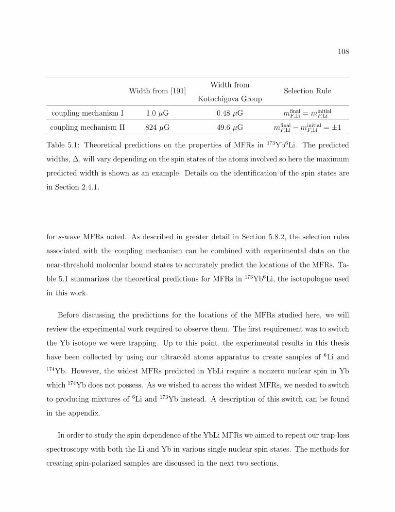
108
Width from [191]Width from
Kotochigova GroupSelection Rule
coupling mechanism I 1.0 µG 0.48 µG mfinalF,Li = minitial
F,Li
coupling mechanism II 824 µG 49.6 µG mfinalF,Li −minitial
F,Li = ±1
Table 5.1: Theoretical predictions on the properties of MFRs in 173Yb6Li. The predicted
widths, ∆, will vary depending on the spin states of the atoms involved so here the maximum
predicted width is shown as an example. Details on the identification of the spin states are
in Section 2.4.1.
for s-wave MFRs noted. As described in greater detail in Section 5.8.2, the selection rules
associated with the coupling mechanism can be combined with experimental data on the
near-threshold molecular bound states to accurately predict the locations of the MFRs. Ta-
ble 5.1 summarizes the theoretical predictions for MFRs in 173Yb6Li, the isotopologue used
in this work.
Before discussing the predictions for the locations of the MFRs studied here, we will
review the experimental work required to observe them. The first requirement was to switch
the Yb isotope we were trapping. Up to this point, the experimental results in this thesis
have been collected by using our ultracold atoms apparatus to create samples of 6Li and
174Yb. However, the widest MFRs predicted in YbLi require a nonzero nuclear spin in Yb
which 174Yb does not possess. As we wished to access the widest MFRs, we needed to switch
to producing mixtures of 6Li and 173Yb instead. A description of this switch can be found
in the appendix.
In order to study the spin dependence of the YbLi MFRs we aimed to repeat our trap-loss
spectroscopy with both the Li and Yb in various single nuclear spin states. The methods for
creating spin-polarized samples are discussed in the next two sections.
109
5.6 Controlling the Li Spin Polarization
Throughout this discussion the Li spin state will be described as in Section 2.4.1.
5.6.1 Determining the spin composition of the ultracold Li sample
In the course of completing this thesis we have worked exclusively with Li in the states |1〉,
|2〉, and |3〉 as the final product of our cooling and trapping stages. We determine the spin
composition of our ultracold Li sample by performing state dependent absorption imaging
on these states. Although all correspond to mJ = −12, these states are split by ∼ 100 MHz
at fields exceeding ∼ 100 G as shown in Figure 2.3. This splitting is much larger than the
natural linewidth (Γ/2π = 5.9 MHz) of the electronic transition connecting the 2S1/2 ground
state to the 2P3/2 excited state which we use for absorption imaging. By simply performing
absorption imaging three times - each time using a frequency resonant with the state of
interest - we can determine how many of the total number of atoms are in each state.
In reality, our experimental setup used to control the frequency of the imaging beam
(composed principally of a double passed AOM operating at 200 MHz) cannot easily span
the full range of frequencies required to be resonant with all three states at the same field.
Therefore it is our general practice to shift the field at which imaging takes place by 20 -
50 G to bring the resonance of interest near the imaging AOM’s center frequency and use our
control of the AOM frequency to finely adjust the laser frequency to match the resonance
at that field. We note here that preparation of the Li in a single spin state is such a routine
procedure that for most experiments we do not bother imaging the sample all three times,
each time resonant with a different state.
5.6.2 Preparing the Li spin
We control the Li spin state through a combination of optical pumping, removal by resonant
scattering, and Landau-Zener sweeps across RF resonances. For a typical experimental run
on our apparatus, the Li is prepared in |2〉 for the evaporation stage in the following way.
110
After the MOT compression stage, atoms in the ODT are in all six hyperfine ground states.
We then extinguish the repump beam such that only light addressing the 2S1/2 (F = 3/2) →2P3/2 (F ′) transition is applied to the atoms, pumping them into the F = 1/2 state. While
holding this mixture of |1〉 and |2〉 in the trap, we ramp the magnetic field to ≈ 500 G. At
this field, the hyperfine ground states are resolved (see Figure 2.3) with respect to the probe
electronic transition and we apply a laser pulse resonant only with |1〉 to remove those atoms
from the trap.
More recently, we accidentally discovered that maintaining the various DC fields used to
compress the MOT during the optical pumping pulse allowed us to prepare the sample of
atoms entirely in |2〉. We have speculated that the field is splitting the excited hyperfine
states to such a degree that the optical pumping pulse is more strongly populating those
excited m′F states that connect to |2〉 though this could only explain a slight imbalance in
favor of |2〉, not an entire transfer into |2〉 that we observe.
After the atoms are prepared in |2〉, we typically perform evaporative cooling on Yb
before preparing the Li spin state as desired. If not wanting to perform experiments with
|2〉 we perform Landau-Zener (LZ) sweeps across the RF resonance |2〉 ↔ |3〉 or |2〉 ↔ |1〉.
To perform these sweeps, we first identify the resonant frequency at the field chosen for
the transfer using the same method as described in Section 5.9.2. Then, we must find
a suitable frequency ramp across this resonance. We typically choose a frequency range
spanning 80 kHz. We then empirically determine the sweep time that will make the process
adiabatic and thus an efficient transfer scheme. Figure 5.4 gives an example of a transfer
from |2〉 to |1〉 by plotting the atom number in each of the two states as the total time for
the sweep is changed, changing the rate of the LZ sweep. For a typical 2 W of RF power,
the time needed for efficient transfer is ≈ 100 ms. Although we typically use this method to
completely transfer into a single state, we can also use this method to create superpositions
of two adjacent states by choosing a nonadiabatic ramp speed. Such a superposition will
subsequently decohere into a spin mixture, which is important for observing interactions
between different Li spin states.
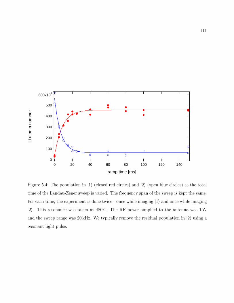
111
600x103
500
400
300
200
100
0
Li a
tom
n nu
mbe
r
140120100806040200
ramp time [ms]
Figure 5.4: The population in |1〉 (closed red circles) and |2〉 (open blue circles) as the total
time of the Landau-Zener sweep is varied. The frequency span of the sweep is kept the same.
For each time, the experiment is done twice - once while imaging |1〉 and once while imaging
|2〉. This resonance was taken at 480 G. The RF power supplied to the antenna was 1 W
and the sweep range was 20 kHz. We typically remove the residual population in |2〉 using a
resonant light pulse.
112
5.7 Controlling the Yb Spin Polarization
The central feature of Yb in the context of making YbLi molecules is its closed-shell elec-
tronic structure. However, this feature complicates the necessity of preparing the 173Yb in
a particular nuclear state. Unlike Li there is no hyperfine coupling in the ground state that
splits different nuclear states by a significant amount. Because S = 0, different mI states in
173Yb split at a rate of EZeeman = gNµNmIB. Thus, the six different nuclear states split at
a rate ∼ 1 kHz/G. This splitting is too small to allow for each of the nuclear states in the
ground state to be individually addressed as in Section 5.6, assuming the we would use the
strong 1S0 → 1P1 transition. Instead we used distinct techniques for both diagnosing and
controlling the spin population of the Yb sample.
5.7.1 State Labeling
In the case of 173Yb in the 1S0 ground state, there is only a single hyperfine ground state
at zero field, which is the sum of S = 0 and I = 5/2, namely F = 5/2. Consequently, mF is
equivalent to mI . When discussing the magnetic substates of 1S0 in this thesis, we will use
these labels interchangeably.
5.7.2 Optical Stern-Gerlach
To determine the spin composition of the Yb sample, we perform a Stern-Gerlach test,
spatially separating the spin states before taking an absorption image that allows us to
count the number of atoms in each cloud. A typical Stern-Gerlach experiment would use a
DC magnetic field gradient to provide a spin dependent force on the sample. But the weak
magnetic moment of Yb atoms means that the magnetic field gradient required to separate
the different spin states before each cloud disperses into the vacuum is infeasibly high. To
be more specific, the rate of separation of the different spin states must exceed the rate of
expansion as the cloud is released from the trap. The rate of expansion goes as√
kBTm
where
kB is the Boltzmann constant, T is the temperature of the gas and m is the mass of the
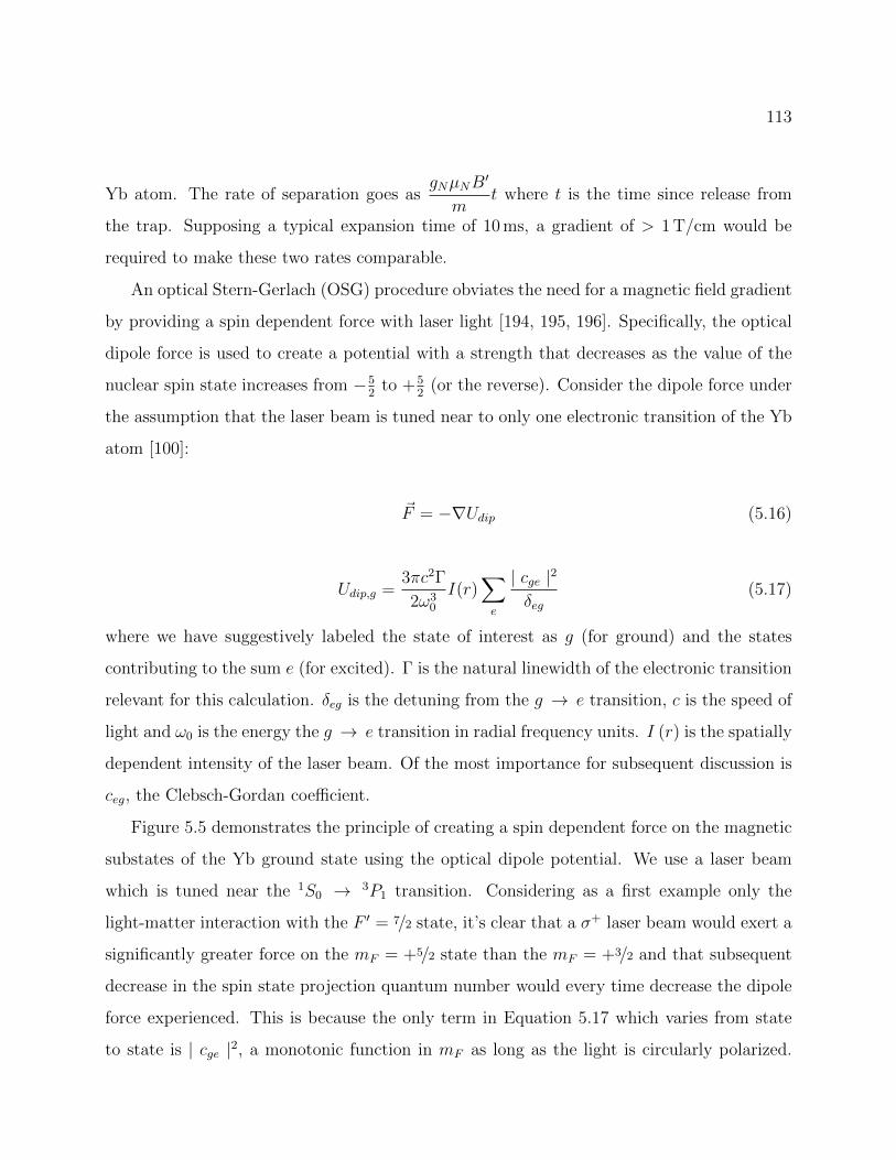
113
Yb atom. The rate of separation goes asgNµNB
′
mt where t is the time since release from
the trap. Supposing a typical expansion time of 10 ms, a gradient of > 1 T/cm would be
required to make these two rates comparable.
An optical Stern-Gerlach (OSG) procedure obviates the need for a magnetic field gradient
by providing a spin dependent force with laser light [194, 195, 196]. Specifically, the optical
dipole force is used to create a potential with a strength that decreases as the value of the
nuclear spin state increases from −52
to +52
(or the reverse). Consider the dipole force under
the assumption that the laser beam is tuned near to only one electronic transition of the Yb
atom [100]:
~F = −∇Udip (5.16)
Udip,g =3πc2Γ
2ω30
I(r)∑e
| cge |2
δeg(5.17)
where we have suggestively labeled the state of interest as g (for ground) and the states
contributing to the sum e (for excited). Γ is the natural linewidth of the electronic transition
relevant for this calculation. δeg is the detuning from the g → e transition, c is the speed of
light and ω0 is the energy the g → e transition in radial frequency units. I (r) is the spatially
dependent intensity of the laser beam. Of the most importance for subsequent discussion is
ceg, the Clebsch-Gordan coefficient.
Figure 5.5 demonstrates the principle of creating a spin dependent force on the magnetic
substates of the Yb ground state using the optical dipole potential. We use a laser beam
which is tuned near the 1S0 → 3P1 transition. Considering as a first example only the
light-matter interaction with the F ′ = 7/2 state, it’s clear that a σ+ laser beam would exert a
significantly greater force on the mF = +5/2 state than the mF = +3/2 and that subsequent
decrease in the spin state projection quantum number would every time decrease the dipole
force experienced. This is because the only term in Equation 5.17 which varies from state
to state is | cge |2, a monotonic function in mF as long as the light is circularly polarized.
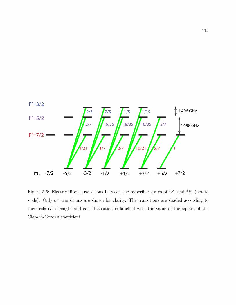
114
mF -5/2-7/2 -3/2 -1/2 +1/2 +3/2 +5/2 +7/2
F’=7/2
F’=5/2
F’=3/2
2/7 2/716/35 18/35 16/35
1/152/3 2/5 1/5
15/710/212/71/71/21
1.496 GHz
4.698 GHz
Figure 5.5: Electric dipole transitions between the hyperfine states of 1S0 and 3P1 (not to
scale). Only σ+ transitions are shown for clarity. The transitions are shaded according to
their relative strength and each transition is labelled with the value of the square of the
Clebsch-Gordan coefficient.
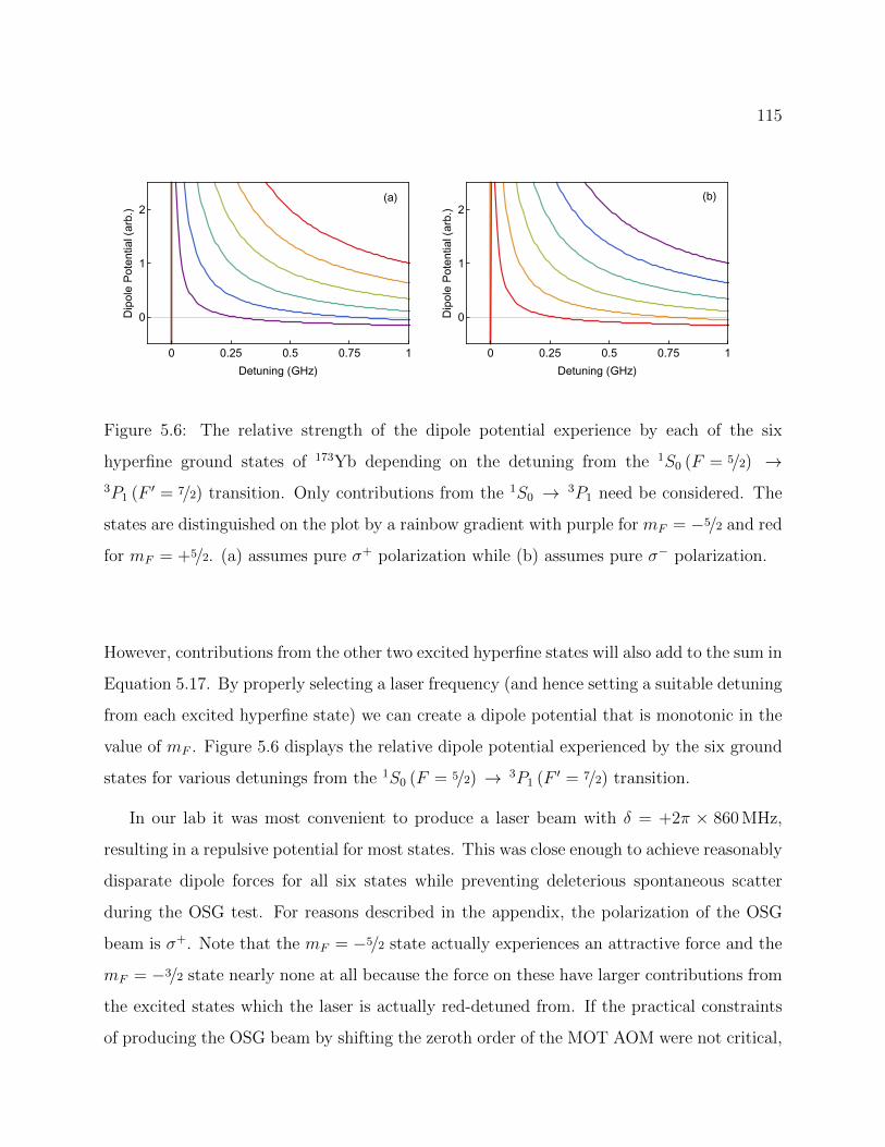
115
0 0.25 0.5 0.75 1
0
1
2
Detuning (GHz)
DipolePotential(arb.)
0 0.25 0.5 0.75 1
0
1
2
Detuning (GHz)
DipolePotential(arb.)
(a) (b)
Figure 5.6: The relative strength of the dipole potential experience by each of the six
hyperfine ground states of 173Yb depending on the detuning from the 1S0 (F = 5/2) →3P1 (F ′ = 7/2) transition. Only contributions from the 1S0 → 3P1 need be considered. The
states are distinguished on the plot by a rainbow gradient with purple for mF = −5/2 and red
for mF = +5/2. (a) assumes pure σ+ polarization while (b) assumes pure σ− polarization.
However, contributions from the other two excited hyperfine states will also add to the sum in
Equation 5.17. By properly selecting a laser frequency (and hence setting a suitable detuning
from each excited hyperfine state) we can create a dipole potential that is monotonic in the
value of mF . Figure 5.6 displays the relative dipole potential experienced by the six ground
states for various detunings from the 1S0 (F = 5/2) → 3P1 (F ′ = 7/2) transition.
In our lab it was most convenient to produce a laser beam with δ = +2π × 860 MHz,
resulting in a repulsive potential for most states. This was close enough to achieve reasonably
disparate dipole forces for all six states while preventing deleterious spontaneous scatter
during the OSG test. For reasons described in the appendix, the polarization of the OSG
beam is σ+. Note that the mF = −5/2 state actually experiences an attractive force and the
mF = −3/2 state nearly none at all because the force on these have larger contributions from
the excited states which the laser is actually red-detuned from. If the practical constraints
of producing the OSG beam by shifting the zeroth order of the MOT AOM were not critical,
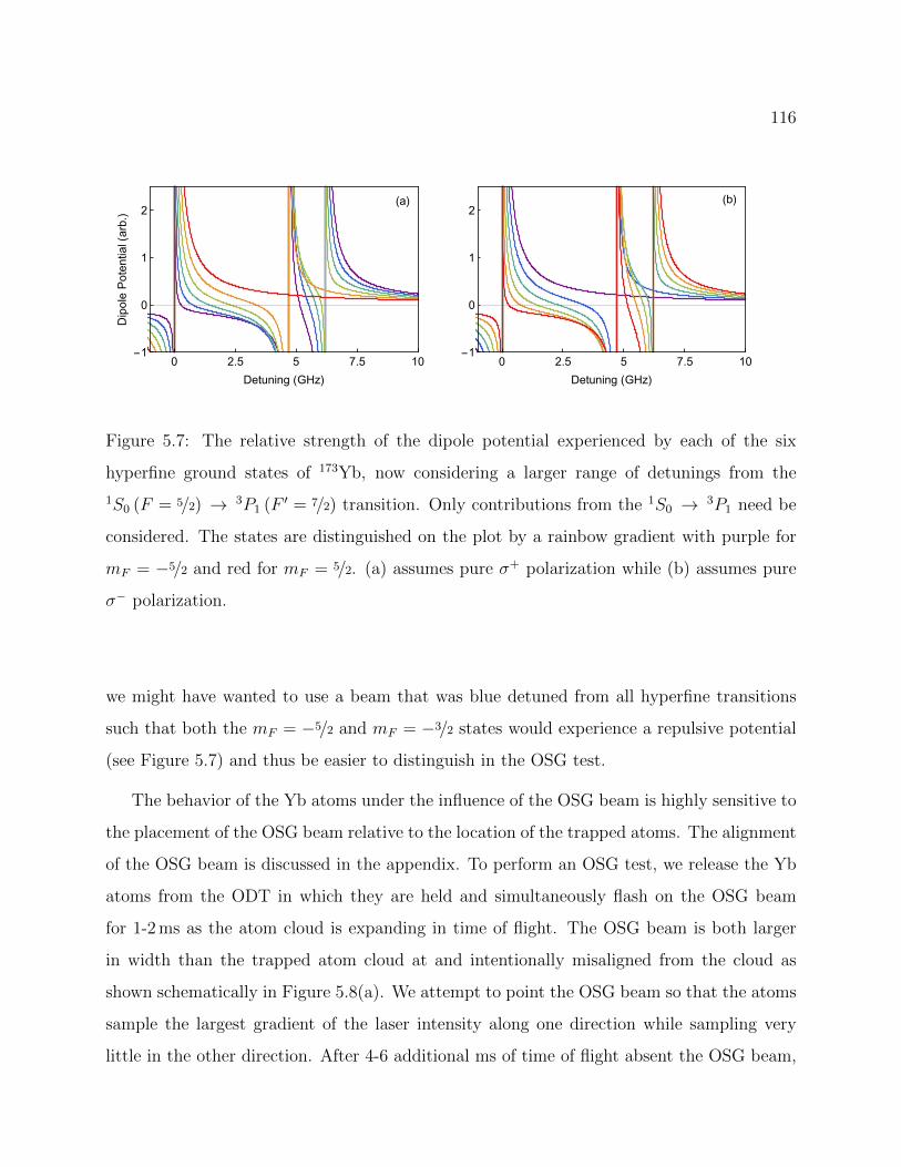
116
0 2.5 5 7.5 10-1
0
1
2
Detuning (GHz)
DipolePotential(arb.)
0 2.5 5 7.5 10-1
0
1
2
Detuning (GHz)
(a) (b)
Figure 5.7: The relative strength of the dipole potential experienced by each of the six
hyperfine ground states of 173Yb, now considering a larger range of detunings from the
1S0 (F = 5/2) → 3P1 (F ′ = 7/2) transition. Only contributions from the 1S0 → 3P1 need be
considered. The states are distinguished on the plot by a rainbow gradient with purple for
mF = −5/2 and red for mF = 5/2. (a) assumes pure σ+ polarization while (b) assumes pure
σ− polarization.
we might have wanted to use a beam that was blue detuned from all hyperfine transitions
such that both the mF = −5/2 and mF = −3/2 states would experience a repulsive potential
(see Figure 5.7) and thus be easier to distinguish in the OSG test.
The behavior of the Yb atoms under the influence of the OSG beam is highly sensitive to
the placement of the OSG beam relative to the location of the trapped atoms. The alignment
of the OSG beam is discussed in the appendix. To perform an OSG test, we release the Yb
atoms from the ODT in which they are held and simultaneously flash on the OSG beam
for 1-2 ms as the atom cloud is expanding in time of flight. The OSG beam is both larger
in width than the trapped atom cloud at and intentionally misaligned from the cloud as
shown schematically in Figure 5.8(a). We attempt to point the OSG beam so that the atoms
sample the largest gradient of the laser intensity along one direction while sampling very
little in the other direction. After 4-6 additional ms of time of flight absent the OSG beam,
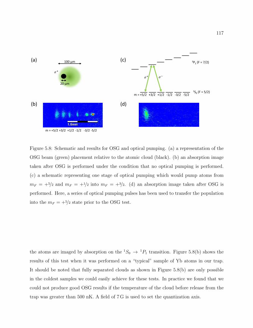
117
m = -5/2 -3/2 -1/2 +1/2 +3/2 +5/2
100 µm
20 µm
3P1 (F = 7/2)
1S0 (F = 5/2)
(a)
(d)
(c)
(b)
m = -5/2 -3/2 -1/2 +1/2 +3/2 +5/2
Figure 5.8: Schematic and results for OSG and optical pumping. (a) a representation of the
OSG beam (green) placement relative to the atomic cloud (black). (b) an absorption image
taken after OSG is performed under the condition that no optical pumping is performed.
(c) a schematic representing one stage of optical pumping which would pump atoms from
mF = +5/2 and mF = +1/2 into mF = +3/2. (d) an absorption image taken after OSG is
performed. Here, a series of optical pumping pulses has been used to transfer the population
into the mF = +5/2 state prior to the OSG test.
the atoms are imaged by absorption on the 1S0 → 1P1 transition. Figure 5.8(b) shows the
results of this test when it was performed on a “typical” sample of Yb atoms in our trap.
It should be noted that fully separated clouds as shown in Figure 5.8(b) are only possible
in the coldest samples we could easily achieve for these tests. In practice we found that we
could not produce good OSG results if the temperature of the cloud before release from the
trap was greater than 500 nK. A field of 7 G is used to set the quantization axis.
118
5.7.3 Optical Pumping
We saw in Section 5.6 that the residual effects of the hyperfine coupling within the Li
atom allowed us to manipulate the spin polarization of our sample at high field because
the different ground hyperfine states are resolved. We could either address these ground
hyperfine states individually through removal by resonant scattering or by rapid adiabatic
passage with RF transitions between adjacent ground magnetic substates. As alluded to at
the beginning of this section, the lack of hyperfine coupling in the Yb ground state precludes
the first option. The second option is impossible because the RF resonances between different
hyperfine ground state are necessarily degenerate because they are split from each other only
by Zeeman energy of the nuclear spin states (no hyperfine coupling).
Instead we utilize the relatively narrow 1S0 → 3P1 transition to perform optical pumping,
targeting different ground magnetic substates through proper choice of the polarization and
dependence on selection rules rather than frequency selectivity between the ground substates.
In contrast to the ground state, the 3P1 excited state has a sizable magnetic moment ∼ µB.
Given that for this transition Γ/2π = 180 kHz, a field of only a few G is required to split
the states by many times the linewidth of this transition. In reality we are limited by the
∼ 1 MHz linewidth of the 556 nm laser used to address these transitions, so in order to
selectively address the different magnetic substates of 3P1, we usually apply a magnetic field
of 50 G, splitting adjacent states by 21.4 MHz.
Figure 5.8(c) shows how addressing resolved magnetic substates in the 3P1 state allows
us to manipulate the spin polarization of the ground state population. In this example, laser
light is resonant with 1S0 (m) → 3P1 (m′ = +3/2). Atoms in the m′F = +3/2 state can decay
back to mF = +5/2,+3/2,+1/2 but only mF = +3/2 is dark to the optical pumping light so
population will be pumped from mF = +5/2,+1/2 into mF = +3/2. By applying multiple
pulses in sequence, each targeting a different m′F state, the Yb sample can be prepared in a
single ground magnetic substate, as demonstrated in Figure 5.8(d).
Conveniently, the apparatus needed very little modification for implementing optical
119
pumping of this kind as laser beams tuned near the 1S0 (F = 5/2) → 3P1 (F ′ = 7/2) transition
already entered the vacuum chamber from several directions in the form of the MOT beams.
For this reason, the beams that achieve the optical pumping will simply be referred to as
the MOT beams. To achieve the proper polarizations for the optical pumping, we used a
motorized flipper mount to block the two horizontal MOT beam pairs. The vertical MOT
beam pair runs parallel to both our two principal electromagnets - the anti-Helmholtz coils
for the MOT gradient and the Helmholtz coils for the bias field. Thus, the vertical MOT
beam pair has a polarization designed to address both σ+ and σ− transitions in the presence
of the bias field used to split the excited magnetic substates.
To selectively address different m′F states, we changed the frequency of the MOT beams
by controlling the RF tone applied to the MOT AOM. To determine the frequency to apply
to the AOM in order to address each individual state, we first calculated the g-factor of
the 3P1 (F ′ = 7/2) state to be 0.58. We used this calculation to predict the shift of each
state from the zero field 1S0 → 3P1 resonance at 50 G. With this initial guess we performed
spectroscopy to determine the shift more accurately. For simplicity this took the form of a
“blast resonance” in which we apply the MOT beams to the atoms held into ODT for a fixed
amount of time and measure the remaining atom number. Resonant light scattering removes
atoms from the trap leading to dips in the atom number on resonance (See Figure 5.9). Note
that for this purpose, we use all six MOT beams, rather than the vertical pair alone, to
prevent optical pumping from stopping the loss from the trap.
Once the proper frequency for each resonance is known, we took care to prevent MOT
light from reaching the atoms unless we were performing intentional optical pumping. This
was challenging as a small amount of light can diffract through the AOM and reach the
atoms even when we have set the RF power to the AOM to be zero with our control system.
For this reason, a typical optical pumping scheme would follow this sequence: set the MOT
AOM frequency to the first target m′F state, open the MOT shutter and pulse on the MOT
AOM, turn off the MOT AOM and close the MOT shutter, change the MOT AOM frequency
to the second target m′F , etc.
120
6x10⁶
5
4
3
2
1
0
Yb
atom
num
ber
rem
aini
ng
-50 0 50
shift from zero field resonance (MHz)
Figure 5.9: “Green blast resonance”. All six MOT beams are used to blast atoms from the
trap when on resonance. Here are six peaks corresponding to the states m′F = −5/2, ..., 5/2.
States ±7/2 could also be addressed but were not reachable by the bandwidth of our AOM
at the chosen 50 G field.
121
After performing the proper sequence of optical pumping pulses to transfer the population
to the desired ground mF state, we perform OSG and absorption imaging to test the result of
the optical pumping. As mentioned in Section 5.7.2, the OSG requires that we evaporatively
cool the atoms to less than about 300 nK. However, in such a low trap the recoil from the
optical pumping can rapidly deplete atoms from the trap. For this reason we perform most
of the optical pumping sequence at a higher trap depth. While we do pump population
from four of the non-target states into the target state at this higher trap, we retain one
state with its population unchanged by any optical pumping. The purpose of retaining this
“sacrificial” state is to provide non-identical particles with which the target state can collide,
enabling evaporative cooling in the sample of fermionic Yb even after some pumping has
taken place. After evaporation to the trap depth at which we reach the ≈ 500 nK level, we
blast the atoms in the sacrificial state using a resonant blast with all six MOT beams. At
last we check the result of the optical pumping sequence by performing OSG and absorption
imaging. The timescales required to accomplish one stage of the optical pumping are shown
in Figure 5.10.
5.7.4 Alternative Polarization Test: Green Blast Resonances
For much of the experiments in the following section, we preferred to use our typical side
imaging system to probe the atoms. But doing so would prevent us from being able to
consistently check the efficacy of the optical pumping steps used to prepare the sample in
the proper spin state because the OSG signal can only be viewed with vertical imaging.
For this reason we sometimes relied on an alternative method as a quick check on the spin
polarization. This method basically involved performing a quick blast resonance like that in
Figure 5.9. The fraction of the total atoms lost when the blasting light is resonant with each
of the eight excited state transitions can be analyzed to approximate the spin distribution
as follows: when the blasting light is resonant with the m′F = +7/2 state, only atoms in the
mF = +5/2 state will be removed from the trap. From this number we determine the number
of atoms in mF = +5/2. Whereas when the blasting light is resonant with the m′F = +5/2
122
40x103
30
20
10
0
Yb
atom
num
ber
300250200150100500
OP time (ms)
Figure 5.10: The typical timescale for optical pumping. In this plot we have determined as
an example the number of atoms in states mF = −5/2 (blue squares) and mF = −3/2 (red
circles) after optical pumping is applied with σ− and σ+ beams tuned to resonance with
the m′F = −3/2 state. The number in each state is determined through selective analysis
of the absorption image after OSG: we determine by eye a region of interest that contains
atoms which appear to belong to one single state and count the atoms in it with our usual
integration method. For this data, the intensity in a single MOT beam was approximately
74 µW/cm2, corresponding to a saturation parameter s ≈ 0.5.
123
state, only atoms in mF = +5/2,+3/2 states will be removed. Thus, the amount removed in
the second case minus the amount removed in the first case constitutes the number of atoms
in mF = +3/2. Repeating the blast resonance for all eight excited states can then give you
the population of each ground state through iterative subtraction.
5.8 First Observation of MFR in Yb+Li
5.8.1 Trap-Loss Spectroscopy Method
The capstone result of this thesis is the observation of magnetic Feshbach resonances between
Yb and Li. In this work, the signature of heteronuclear Feshbach resonances is the observation
of rapid loss from the trap through inelastic, exothermic collisions which are enhanced in the
vicinity of an MFR [171, 197, 198].
The procedure for observation of MFRs through trap-loss spectroscopy can be roughly
divided into two phases: the preparation phase followed by the spectroscopy phase. Since the
spectroscopy phase is necessarily destructive to the ultracold atomic mixture, a new sample
must be prepared for every variation in the magnetic field, which is our independent variable.
A brief description of the preparation step follows: laser-cooled 173Yb atoms are captured
in a crossed ODT composed of two focused laser beams at 1064 nm, remaining in an approx-
imately even spin mixture of all six ground states. Laser-cooled 6Li are subsequently loaded
into the trap and allowed to thermalize with the colder 173Yb at about 20µK. Just after
loading, the Li atoms are optically pumped into |F 〉 = |12〉. A large magnetic field is applied
which allows us to remove the |ms,mI〉 = |−12,+1〉 atoms through a frequency resolved reso-
nant light pulse, leaving the Li sample entirely in the |ms,mI〉 = |−12, 0〉. Forced evaporative
cooling of Yb is performed by lowering the intensity of the ODT laser and Li is cooled sym-
pathetically. When the temperature of both species has reached about 10µK, the reduction
in intensity is paused and the Yb spin population is manipulated via optical pumping on
the 1S0 → 3P1 transition in a 50 G bias field, individually addressing the resolved excited
states with a mixture of σ+ and σ− polarizations. Typically, a “target state” is chosen for
124
the majority of the population to be transferred to by pumping, while a small amount of
the population remains in the “sacrificial state.” The sacrificial state is retained to serve as
a scattering partner for the “target state” during a second stage of evaporation. In most
of this work, the atoms are cooled to a temperature of about 1µK by further reducing the
intensity of the trap. In the final stage of the preparation, the sacrificial state is removed
from the trap through a resolved resonant light pulse.
After preparation the Li atoms are in |ms,mI〉 = |−12, 0〉 and the Yb atoms are in a single
nuclear spin state with at least 90% purity at around 1µK. The spectroscopy phase begins
when the field is ramped to a fixed magnetic field and held for 4 seconds. The field is then
reduced to about 500 G and absorption imaging is performed on Li, principally recording the
number of atoms remaining in the trap. This method suffices to roughly locate the resonance
location, but it is susceptible to a slight asymmetry arising from the finite time needed to
reach the target magnetic field. The mechanism of this asymmetry and the methods we have
used to mitigate it are described in Section 5.9.2. We iterate the combination of preparation
and spectroscopy, changing the holding field each time.
5.8.2 Observation at Predicted Locations
After discussing the experimental strategy for observing MFRs with our apparatus, the final
consideration is the field at which these resonances are expected. The single ground electronic
state in the YbLi system (2Σ) makes the location of these resonances easy to understand
in theory. Loosely bound vibrational states in the (2Σ) electronic potential will exhibit the
same splitting in the magnetic field as the Yb+Li atom pair because any coupling of the
constituent spins to the nuclear motion is typically very weak for loosely bound states. Thus,
as seen in Figure 5.11(a), the MFRs in this system can occur when the high field seeking
atomic states intersect the low field seeking molecular states. These states shift relative to
each other at a rate of 2µB. Therefore, to determine the rough location of the MFRs, it
is sufficient to know the energy separation of the atomic and molecular states at zero field.
The energies of these states was determined by our theory collaborators at Temple University
125
by using the potential from our work in [114] to find the bound states of 173Yb6Li. Finer
prediction of the field required only the additional consideration of the splitting between
the Li hyperfine states and the selection rules determined by the coupling mechanisms. In
Figure 5.11(a) we mark the location of three MFRs corresponding to coupling mechanism
II, one for each Li hyperfine state in the high field seeking manifold.
We use the method of trap-loss spectroscopy to observe each MFR indicated by triangles
in Figure 5.11(a). The spectrum is shown in one plot in Figure 5.12, with colored symbols
matching those in Figure 5.11(a), though it should be noted that the sample preparation
step was changed for each data set such that the sample was prepared in the appropriate Li
hyperfine state for each experiment.
We also performed a search for the resonances in this area which were predicted to arise
from coupling mechanism I, however we found that these resonances were too weak to be
observed with our current experimental setup. Further improvements to the apparatus such
as the loading of the atomic mixture into a deep optical lattice or a reduction of our magnetic
field noise may make their observation possible, though as they are much narrower than the
coupling mechanism II resonances, they may not be of much experimental interest.
We also investigated the dependence of these interspecies MFRs on the spin state of
173Yb. We repeated our trap-loss spectroscopy measurements this time always preparing
Li in |2〉 but changing the state in which we prepare the Yb. The results are shown in
Figure 5.13. Five of the six ground states exhibit a resonant loss feature, indicating that
these five states have a magnetic field-controlled scattering resonance with 6Li in the |2〉 =
|F = 1/2,mF = −1/2〉 state. This is an expected consequence of the selection rule associated
with coupling mechanism II:
mfinalF,Li −minitial
F,Li = ±1 and mfinalI,Yb −minitial
I,Yb = ∓1
Since the only available crossings are characterized by mfinalF,Li−minitial
F,Li = +1 only mI,Yb = −5/2
exhibits no resonance.
Of the five Yb nuclear spin states that exhibit an MFR, each is shifted relative to the
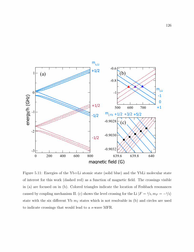
126
0 200 400 600 800
magnetic field (G)
-3
-2
-1
0
1
ener
gy/h
(G
Hz)
500 600 700
-1
-0.8
-0.6
639.6 639.8 640
-0.9032
-0.9030
-0.9028
ms,Li
+1/2
-1/2mi,Yb
(a)
mi,Li
-1
0+1
+5/2+3/2+1/2
(b)
(c)
+1/2
+1/2
-1/2
-1/2
Figure 5.11: Energies of the Yb+Li atomic state (solid blue) and the YbLi molecular state
of interest for this work (dashed red) as a function of magnetic field. The crossings visible
in (a) are focused on in (b). Colored triangles indicate the location of Feshbach resonances
caused by coupling mechanism II. (c) shows the level crossing for the Li |F = 1/2,mF = −1/2〉
state with the six different Yb mI states which is not resolvable in (b) and circles are used
to indicate crossings that would lead to a s-wave MFR.
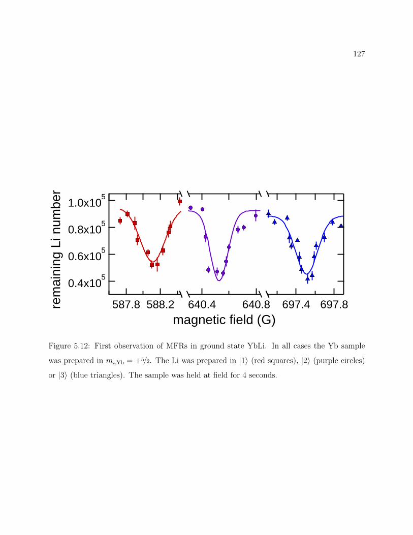
127
1.0x10⁵
0.8x10⁵
0.6x10⁵
0.4x10⁵
rem
aini
ng L
i num
ber
588.2587.8 697.8697.4640.8640.4magnetic field (G)
Figure 5.12: First observation of MFRs in ground state YbLi. In all cases the Yb sample
was prepared in mi,Yb = +5/2. The Li was prepared in |1〉 (red squares), |2〉 (purple circles)
or |3〉 (blue triangles). The sample was held at field for 4 seconds.
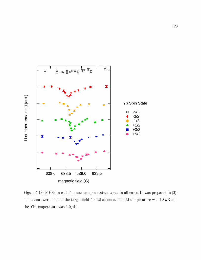
128Li
num
ber
rem
aini
ng (
arb.
)
639.5639.0638.5638.0
magnetic field (G)
Yb Spin State
-5/2 -3/2 -1/2 +1/2 +3/2 +5/2
Figure 5.13: MFRs in each Yb nuclear spin state, mI,Yb. In all cases, Li was prepared in |2〉.
The atoms were held at the target field for 1.5 seconds. The Li temperature was 1.8µK and
the Yb temperature was 1.0µK.
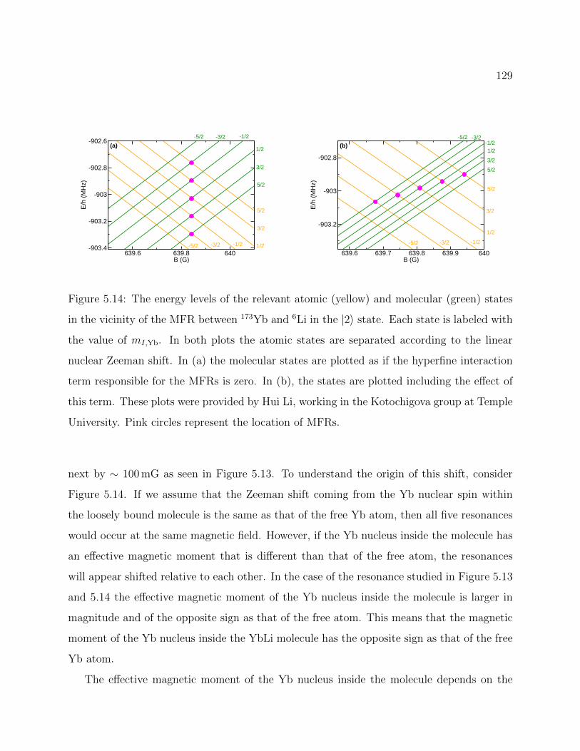
129
639.6 639.8 640B (G)
-903.4
-903.2
-903
-902.8
-902.6
E/h
(MH
z)
-5/2 -3/2 -1/2 1/2
3/2
5/2
5/2
3/2
1/2
-1/2-3/2-5/2(a)
639.6 639.7 639.8 639.9 640B (G)
-903.2
-903
-902.8
E/h
(MH
z)
-5/2 -3/2 -1/2
1/2
3/2
5/2
5/23/21/2
-1/2-3/2-5/2
(b)
Figure 5.14: The energy levels of the relevant atomic (yellow) and molecular (green) states
in the vicinity of the MFR between 173Yb and 6Li in the |2〉 state. Each state is labeled with
the value of mI,Yb. In both plots the atomic states are separated according to the linear
nuclear Zeeman shift. In (a) the molecular states are plotted as if the hyperfine interaction
term responsible for the MFRs is zero. In (b), the states are plotted including the effect of
this term. These plots were provided by Hui Li, working in the Kotochigova group at Temple
University. Pink circles represent the location of MFRs.
next by ∼ 100 mG as seen in Figure 5.13. To understand the origin of this shift, consider
Figure 5.14. If we assume that the Zeeman shift coming from the Yb nuclear spin within
the loosely bound molecule is the same as that of the free Yb atom, then all five resonances
would occur at the same magnetic field. However, if the Yb nucleus inside the molecule has
an effective magnetic moment that is different than that of the free atom, the resonances
will appear shifted relative to each other. In the case of the resonance studied in Figure 5.13
and 5.14 the effective magnetic moment of the Yb nucleus inside the molecule is larger in
magnitude and of the opposite sign as that of the free atom. This means that the magnetic
moment of the Yb nucleus inside the YbLi molecule has the opposite sign as that of the free
Yb atom.
The effective magnetic moment of the Yb nucleus inside the molecule depends on the
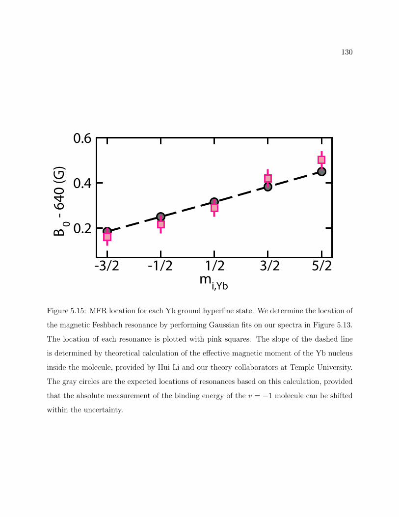
130
-3/2 -1/2 1/2 3/2 5/2mi,Yb
0.2
0.4
0.6
B0 -
640
(G)
Figure 5.15: MFR location for each Yb ground hyperfine state. We determine the location of
the magnetic Feshbach resonance by performing Gaussian fits on our spectra in Figure 5.13.
The location of each resonance is plotted with pink squares. The slope of the dashed line
is determined by theoretical calculation of the effective magnetic moment of the Yb nucleus
inside the molecule, provided by Hui Li and our theory collaborators at Temple University.
The gray circles are the expected locations of resonances based on this calculation, provided
that the absolute measurement of the binding energy of the v = −1 molecule can be shifted
within the uncertainty.
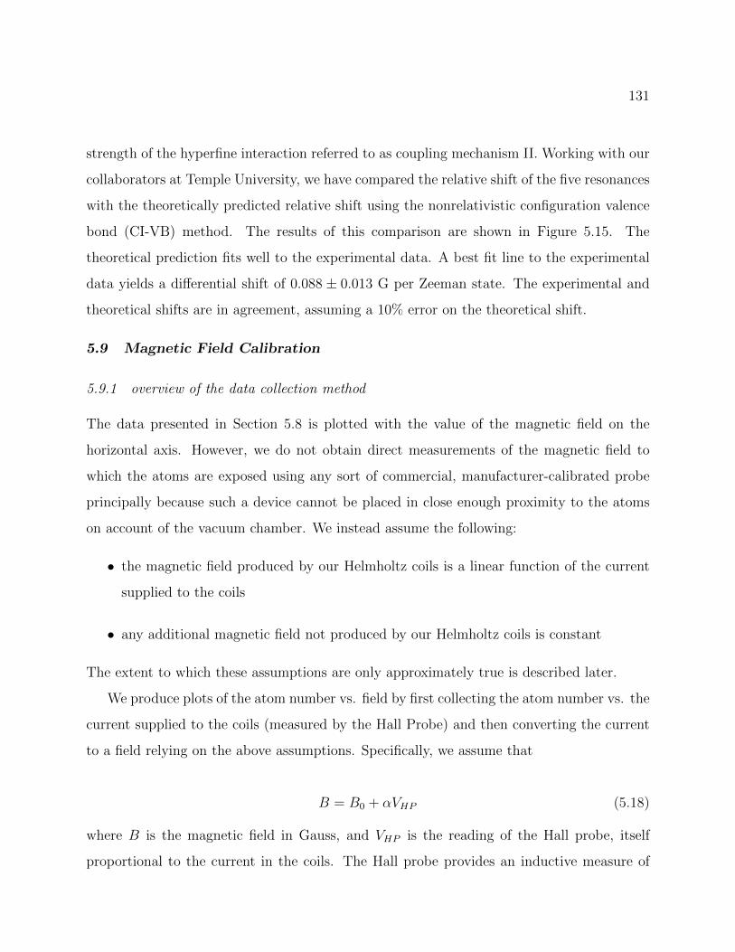
131
strength of the hyperfine interaction referred to as coupling mechanism II. Working with our
collaborators at Temple University, we have compared the relative shift of the five resonances
with the theoretically predicted relative shift using the nonrelativistic configuration valence
bond (CI-VB) method. The results of this comparison are shown in Figure 5.15. The
theoretical prediction fits well to the experimental data. A best fit line to the experimental
data yields a differential shift of 0.088 ± 0.013 G per Zeeman state. The experimental and
theoretical shifts are in agreement, assuming a 10% error on the theoretical shift.
5.9 Magnetic Field Calibration
5.9.1 overview of the data collection method
The data presented in Section 5.8 is plotted with the value of the magnetic field on the
horizontal axis. However, we do not obtain direct measurements of the magnetic field to
which the atoms are exposed using any sort of commercial, manufacturer-calibrated probe
principally because such a device cannot be placed in close enough proximity to the atoms
on account of the vacuum chamber. We instead assume the following:
• the magnetic field produced by our Helmholtz coils is a linear function of the current
supplied to the coils
• any additional magnetic field not produced by our Helmholtz coils is constant
The extent to which these assumptions are only approximately true is described later.
We produce plots of the atom number vs. field by first collecting the atom number vs. the
current supplied to the coils (measured by the Hall Probe) and then converting the current
to a field relying on the above assumptions. Specifically, we assume that
B = B0 + αVHP (5.18)
where B is the magnetic field in Gauss, and VHP is the reading of the Hall probe, itself
proportional to the current in the coils. The Hall probe provides an inductive measure of
132
the current and is placed around the 000 gauge wire connecting the power supply to the
Helmholtz coils at the return side. B0 and α are determined through calibration, with B0
depending on the sum of all fields at the atoms which are not produced by the Helmoltz coils
(we assume that to a good approximation this background field points in the same direction
of the Helmholtz coils). α is dependent on the conversion factor of the Hall probe and the
size and number of windings of the coils, in addition to their distance from the atoms.
By reading VHP for all data collected, we need only determine values for α and B0 to
determine the field at each data point.
5.9.2 methods of calibration
To determine the values of α and B0 we perform various field-dependent spectroscopies on
the atoms in our trap. These spectroscopies either have a precisely known relation to the
magnetic field through calculation from fundamental constants or have simply been repeated
by multiple research groups, providing a precise average against which our results can be
normalized. Below is a description of the methods we have used, along with some sample
calibration data.
RF resonances. A reliable and commonly used method is to perform RF spectroscopy
to probe the energy difference between states within the hyperfine ground manifold of Li.
Within the F = 1/2 state in particular, the frequency of an observed resonance is a reliable
probe because the Breit-Rabi formula provides an exact analytical solution to the energy
splitting and all relevant constants are known to high accuracy.
We perform these RF measurements using the RF antenna installed at the base of our
vacuum chamber, connected to our RF source via a BNC feedthrough (see [199]). When
searching for such RF resonances we perform a coarse search followed by a fine search. Both
searches begin with Li atoms in the optical trap at a temperature of about 15µK. Yb is also
present in the trap. We program the magnetic field control electronics to hold at a fixed
field for the duration of the pulse and use any previous calibration to roughly predict the RF
resonance frequency. For the coarse search we apply an RF pulse of 50 ms in length which
133
200x103
150
100
50
0
Li a
tom
num
ber
53.2453.2053.16
RF frequency (MHz)
250x103
200
150
100
50
018.2418.2018.16
RF frequency (MHz)
(a) (b)
Figure 5.16: Sample data for the RF resonance between states 1 and 2. (a) taken at 77.52 G
and (b) taken at 19.98 G.
sweeps the field in a single sawtooth over a frequency range of 50 or 100 kHz, centered on
the predicted value. The resulting number of atoms in the trap is measured using a typical
high-field absorption imaging process. We repeat this with different values of the frequency
sweep center until we observe a loss from |2〉, the state in which we always begin. Within this
loss feature, we perform the same procedure with a narrower frequency sweep: 5 to 10 kHz.
Finally, we perform a fine scan by using a pure RF tone and apply a pulse of 25 ms, stepping
the pulse through different values and recording the number remaining each time. A typical
RF power for this final step is 200 mW. See Figure 5.16 for a representative sample of fine
RF resonance scans.
This method is limited to use at low fields because the energy splitting between the two
F = 1/2 states becomes a weak function of field as the electronic and nuclear spins decouple
from each other. This is quantified in Figure 5.17(b). Further evidence for the limitation at
high field can be seen in Figure 5.16 where instability in the magnetic field is imprinted onto
the RF resonance to a greater magnitude at lower fields in the form of a larger RF resonance
width. In some cases the amount of data we collect in low field is not sufficient to average
134
out long term drifts in the field resulting in RF resonances that have a flattened bottom in
the average. In practice we find that at fields larger than about 100 G we need a level of
accuracy on those resonance measurements which is not easily achieved on our apparatus.
Beyond the issue of accuracy, this method is only useful up to about 150 G at which point
a typical error on the RF resonance measurement of ∼ 1 kHz translates to a magnetic field
precision beyond the precision at which we can presently measure the corresponding current
(20 mG).
In the future it would be beneficial to extend the RF resonance calibration to higher
fields by performing spectroscopy between the F = 1/2 and F = 3/2 states, such as between
|2〉 and |5〉. This will require a change to the RF source typically used for this spectroscopy
for which there are plans underway at the writing of this thesis.
comparison with known magnetic Feshbach resonances. There are three narrow Feshbach
resonances (< 150 mG width) between different combinations of the Li ground hyperfine
states |1〉 and |2〉 which have been reported in multiple articles with high precision [200, 201].
We observed these three resonances using a trap-loss spectroscopy technique similar to that
in Section 5.8 and used the reported values to calibrate our field against the literature. The
only material difference between our method of trap-loss spectroscopy in the Li2 calibration
measurements and the YbLi MFR observations in Section 5.8 is the ordering of the magnetic
field ramps used to reach the field targeted for each point in the spectroscopy. Because the
Li2 MFRs are much stronger than the YbLi MFRs, even crossing the resonant field in the
course of a rapid ramp up to the target field can result in appreciable atom loss, resulting
in asymmetric loss lineshapes. To solve this problem, we added extraneous ramps to offset
fields about 20 G away from the target field and arranged these extraneous ramps such that
the whole series of magnetic field ramps went over the resonant field exactly three times no
matter if the target field was higher or lower than the resonant field. This depressed the
apparent off-resonant atom number but did so uniformly.
“green blast resonances”: spectroscopy of the Yb 3P1 state. We perform spectroscopy
on the relatively narrow 1S0 → 3P1 transition in Yb. We probe this transition through
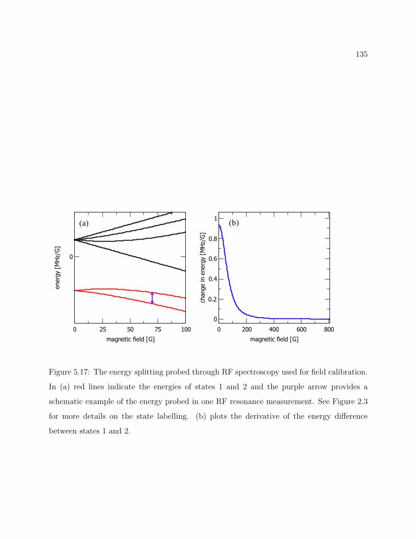
135
0 25 50 75 100
magnetic field [G]
0
ener
gy [
MH
z/G
]
0 200 400 600 800
magnetic field [G]
0
0.2
0.4
0.6
0.8
1
chan
ge in
ene
rgy
[MH
z/G
]
(a) (b)
Figure 5.17: The energy splitting probed through RF spectroscopy used for field calibration.
In (a) red lines indicate the energies of states 1 and 2 and the purple arrow provides a
schematic example of the energy probed in one RF resonance measurement. See Figure 2.3
for more details on the state labelling. (b) plots the derivative of the energy difference
between states 1 and 2.
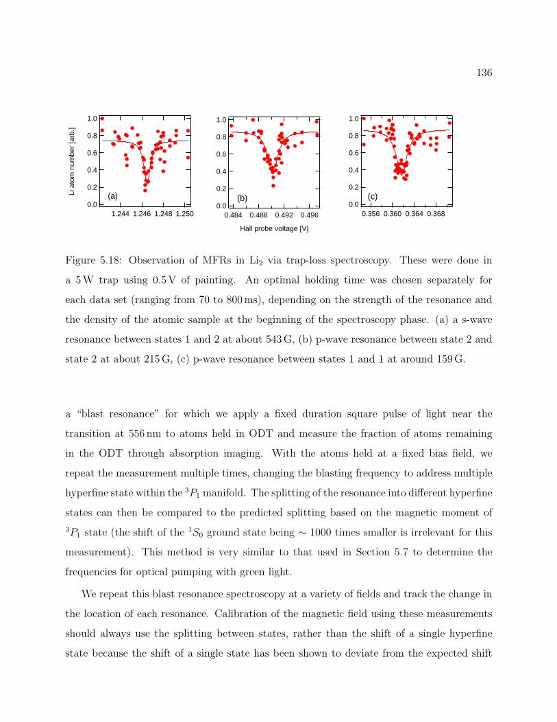
136
1.0
0.8
0.6
0.4
0.2
0.0
Li a
tom
num
ber
[arb
.]
1.2501.2481.2461.244
1.0
0.8
0.6
0.4
0.2
0.00.4960.4920.4880.484
Hall probe voltage [V]
1.0
0.8
0.6
0.4
0.2
0.00.3680.3640.3600.356
(a) (b) (c)
Figure 5.18: Observation of MFRs in Li2 via trap-loss spectroscopy. These were done in
a 5 W trap using 0.5 V of painting. An optimal holding time was chosen separately for
each data set (ranging from 70 to 800 ms), depending on the strength of the resonance and
the density of the atomic sample at the beginning of the spectroscopy phase. (a) a s-wave
resonance between states 1 and 2 at about 543 G, (b) p-wave resonance between state 2 and
state 2 at about 215 G, (c) p-wave resonance between states 1 and 1 at around 159 G.
a “blast resonance” for which we apply a fixed duration square pulse of light near the
transition at 556 nm to atoms held in ODT and measure the fraction of atoms remaining
in the ODT through absorption imaging. With the atoms held at a fixed bias field, we
repeat the measurement multiple times, changing the blasting frequency to address multiple
hyperfine state within the 3P1 manifold. The splitting of the resonance into different hyperfine
states can then be compared to the predicted splitting based on the magnetic moment of
3P1 state (the shift of the 1S0 ground state being ∼ 1000 times smaller is irrelevant for this
measurement). This method is very similar to that used in Section 5.7 to determine the
frequencies for optical pumping with green light.
We repeat this blast resonance spectroscopy at a variety of fields and track the change in
the location of each resonance. Calibration of the magnetic field using these measurements
should always use the splitting between states, rather than the shift of a single hyperfine
state because the shift of a single state has been shown to deviate from the expected shift
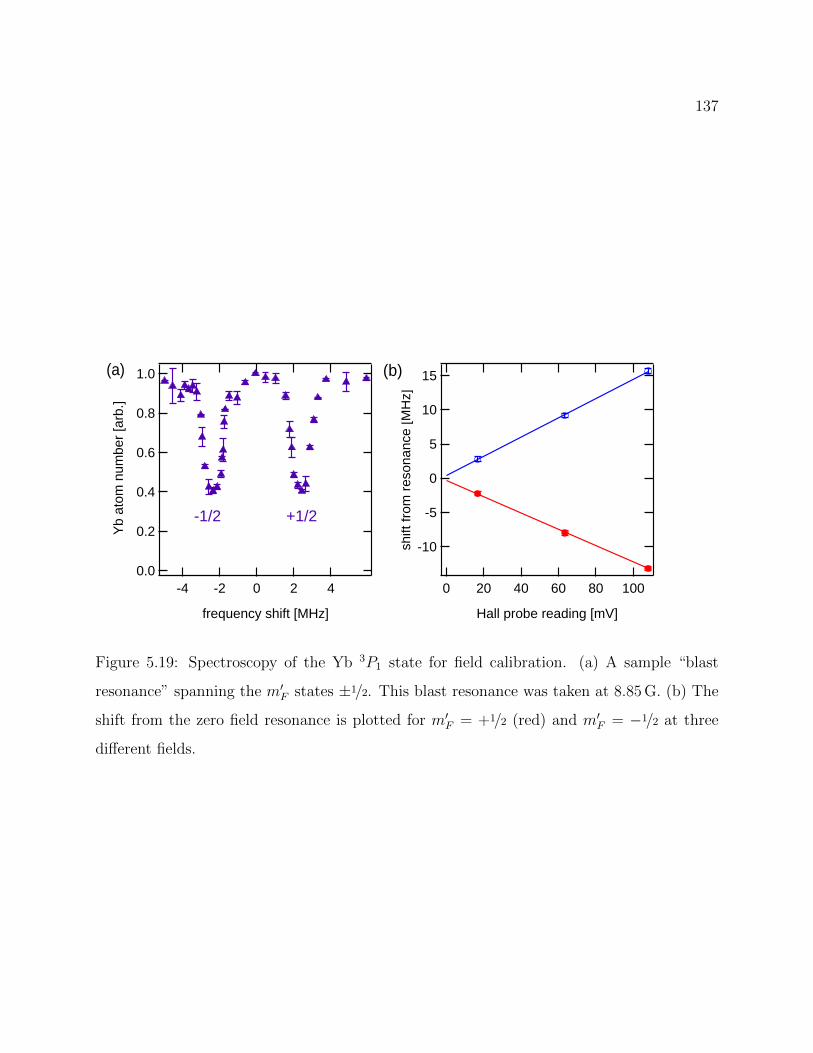
137
15
10
5
0
-5
-10shift
from
res
onan
ce [M
Hz]
100806040200
Hall probe reading [mV]
1.0
0.8
0.6
0.4
0.2
0.0
Yb
atom
num
ber
[arb
.]
420-2-4
frequency shift [MHz]
+1/2-1/2
(a) (b)
Figure 5.19: Spectroscopy of the Yb 3P1 state for field calibration. (a) A sample “blast
resonance” spanning the m′F states ±1/2. This blast resonance was taken at 8.85 G. (b) The
shift from the zero field resonance is plotted for m′F = +1/2 (red) and m′F = −1/2 at three
different fields.
138
based on calculation of the Zeeman shift from the nuclear g-factor [90]. If using only the
mF = ±1/2 states for this spectroscopy, this method works up to 50 G, limited by the tuning
range of the MOT AOM used to control the blast frequency. The method could be extended
to higher fields through the installation of additional AOMs or other methods to reach greater
detunings from the zero field resonance at which the MOT beams are typically tuned.
5.9.3 quantifying error on calibration
We use our calibration data from |1〉 − |2〉 RF resonances and Li2 MFRs to find best fit
values for α and δB0. We attribute the error in α principally to the limited precision of the
Hall probe used in the calibration (and in our data collection for the YbLi MFR study). We
attribute the error in B0 principally to variations in the ambient magnetic field over time.
The general consequences of our calibration model are
• all measurements carry an uncertainty of at least δB0, the error on B0 (20 mG in our
current calibration)
• higher fields are associated with higher uncertainty, accumulated from the error in α
(relative error of 2.3× 10⁻⁴ in our current calibration).
• at high fields, the error on relative shifts between closely spaced resonances are still
roughly equal to δB0
The results of the calibration model are presented in Section 5.9.4. From the above conse-
quences and the calibration results, we say that the absolute uncertainty on the field in the
vicinity of each resonances is 149 mG for |1〉, 161 mG for |2〉, and 174 mG for |3〉. However,
when determining the spacing between adjacent mi,Yb states for a given Li state we consider
the uncertainty to be 20 mG.
Finally, it should be noted that all of our calibration methods are sensitive only to the
scalar field. Our assumption that B = B0+αVHP is only valid if stray fields point in the same
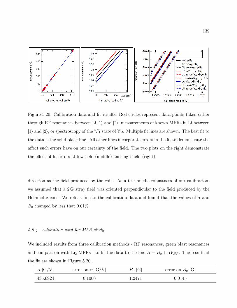
139
Figure 5.20: Calibration data and fit results. Red circles represent data points taken either
through RF resonances between Li |1〉 and |2〉, measurements of known MFRs in Li between
|1〉 and |2〉, or spectroscopy of the 3P1 state of Yb. Multiple fit lines are shown. The best fit to
the data is the solid black line. All other lines incorporate errors in the fit to demonstrate the
affect such errors have on our certainty of the field. The two plots on the right demonstrate
the effect of fit errors at low field (middle) and high field (right).
direction as the field produced by the coils. As a test on the robustness of our calibration,
we assumed that a 2 G stray field was oriented perpendicular to the field produced by the
Helmholtz coils. We refit a line to the calibration data and found that the values of α and
B0 changed by less that 0.01%.
5.9.4 calibration used for MFR study
We included results from three calibration methods - RF resonances, green blast resonances
and comparison with Li2 MFRs - to fit the data to the line B = B0 + αVHP . The results of
the fit are shown in Figure 5.20.
α [G/V] error on α [G/V] B0 [G] error on B0 [G]
435.6924 0.1000 1.2471 0.0145
140
5.10 Temperature Dependence and MFR-induced Loss Model
The observations of MFRs in Section 5.8.2 relied on the enhancement of three-body loss
from the trap near an MFR. In our work, both species are fermionic and spin polarized,
meaning that two of the three scattering partners in such a process are identical fermions.
Because the MFRs observed in this work are narrow compared to the residual kinetic energy
at ultracold temperatures, we had a unique opportunity to study the effect of Fermi statistics
on the temperature dependence of the three-body event rate coefficient K(B, T ). To study
this, we collected trap-loss spectra for one MFR at a variety of different temperatures. The
MFR chosen for this study was between Yb in the mI,Yb = +5/2 state and Li in the |2〉 state.
To change the temperature of the atomic mixture, we controlled the final intensity of the
ODT laser. In all cases, we performed forced evaporation on the mixture until it reached a
temperature of 5.8µK. To reach lower temperature, we continued the forced evaporation by
lowering the ODT laser power further. To reach higher temperatures we “recompressed” the
ODT by increasing the power, which reduced the volume of the gas and hence increased its
temperature. As the temperature increased, the spectra became noticeably more asymmetric
as seen in Figures 5.21(a)-(d). Though more subtle, the magnetic field at which the trap-loss
is maximum also shifts to higher fields for higher temperatures.
Our theory collaborators constructed a model for the temperature dependence of K(B, T )
and used it as a fit to the trap-loss spectroscopy data in Figures 5.21(a)-(d) [202]. The
agreement between the model and the data, combined with the model’s explicit dependence
on the particles’ quantum statistics, confirms the expected p-wave threshold behavior near
the resonance. A notable consequence of this model is that the maximum value of K(B, T )
is actually independent of temperature. This is in contrast to the Bose-Bose case for which
the maximum value of K(B, T ) either decreases or increases with temperature depending on
whether the threshold is s-wave or d-wave [186].
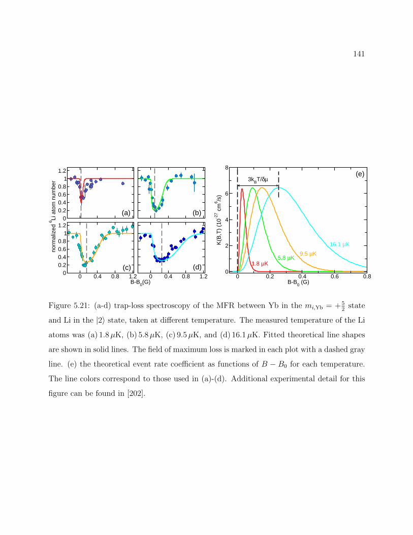
141
00.20.40.60.8
11.2
0 0.4 0.8 1.2B-B0(G)
00.20.40.60.8
11.2
norm
aliz
ed 6 Li
ato
m n
umbe
r
0 0.4 0.8 1.2
(a) (b)
(c) (d)0 0.2 0.4 0.6 0.8
B-B0 (G)
0
2
4
6
8
K(B,
T) (1
0-27 c
m6 /s
)
3kBT/δµ(e)
1.8 µK5.8 µK
9.5 µK16.1 µK
Figure 5.21: (a-d) trap-loss spectroscopy of the MFR between Yb in the mi,Yb = +52
state
and Li in the |2〉 state, taken at different temperature. The measured temperature of the Li
atoms was (a) 1.8µK, (b) 5.8µK, (c) 9.5µK, and (d) 16.1µK. Fitted theoretical line shapes
are shown in solid lines. The field of maximum loss is marked in each plot with a dashed gray
line. (e) the theoretical event rate coefficient as functions of B − B0 for each temperature.
The line colors correspond to those used in (a)-(d). Additional experimental detail for this
figure can be found in [202].
142
Chapter 6
OUTLOOK
The work in this thesis has outlined in detail two possible paths for the coherent cre-
ation of YbLi molecules. While the two paths have respective advantages, both will require
dynamical dressing that is adiabatic. We have determined that for YbLi, the adiabaticity re-
quirements demand that the atoms be loaded pairwise into a 3D optical lattice. For molecule
association with either strategy, the lattice serves two purposes. First, loading the atomic
mixture into an optical lattice makes it easier to achieve adiabaticity by significantly reduc-
ing constraints on the dynamical timescale set by inelastic losses between molecules that are
forming and un-associated atoms. Second, the boost in overlap density increases the cou-
pling between atom and molecule, making the other technical constraints less demanding.
Construction of the 3D optical lattice is underway at the time of this writing.
Pursuit of the StiRAP course has the advantage of being general: we could use it to make
molecules composed of 6Li plus any other easily cooled and trapped isotope of Yb, which
would allow us to make fermionic molecules (174Yb6Li) or bosonic molecules (173Yb6Li) with
the same method and equipment. In contrast, magneto-association requires the use of a
fermionic isotope of Yb as only the fermionic isotopes have a nuclear spin and therefore
strong MFR. For this reason, if we wish to make fermionic molecules, the isotope of Li will
need to be changed to 7Li, which requires time-consuming changes to the apparatus.
The lab is well prepared to attempt StiRAP again once loading atoms pairwise into the
lattice is accomplished as we have already demonstrated the ability to create phase coherent
pulses and to perform the necessary cleaning pulses between an associative StiRAP pulse
and its dissociative reversal for the purposes of detection. Loading the atoms into a lattice
where the density is much higher than in the ODT will allow us to achieve larger values
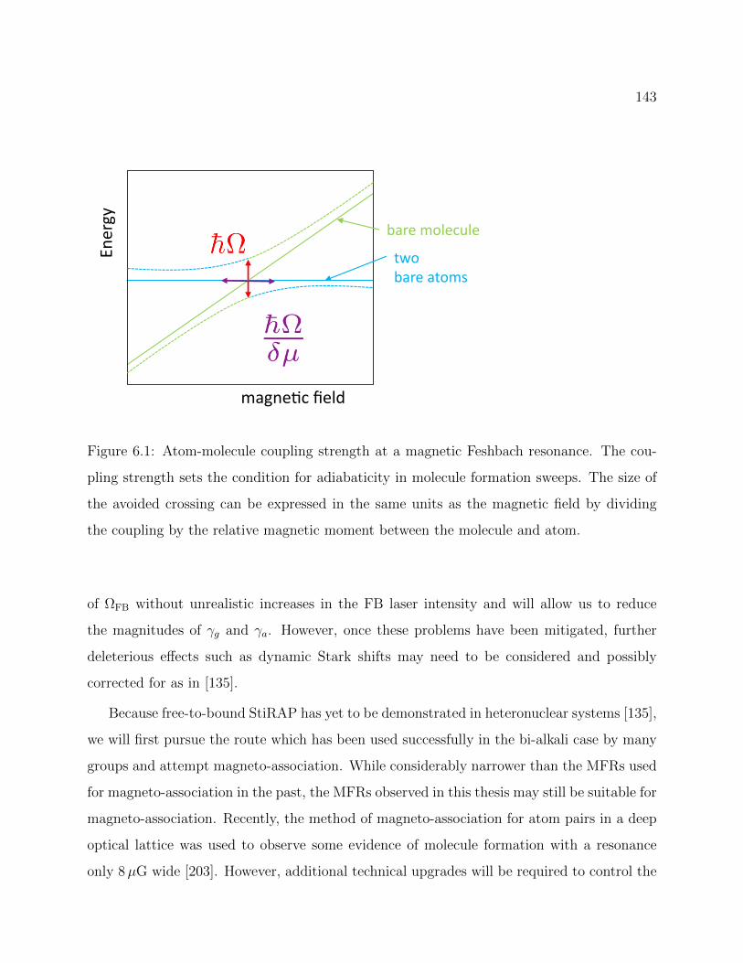
143
magnec field
ygrenE
bare molecule
twobare atoms
Figure 6.1: Atom-molecule coupling strength at a magnetic Feshbach resonance. The cou-
pling strength sets the condition for adiabaticity in molecule formation sweeps. The size of
the avoided crossing can be expressed in the same units as the magnetic field by dividing
the coupling by the relative magnetic moment between the molecule and atom.
of ΩFB without unrealistic increases in the FB laser intensity and will allow us to reduce
the magnitudes of γg and γa. However, once these problems have been mitigated, further
deleterious effects such as dynamic Stark shifts may need to be considered and possibly
corrected for as in [135].
Because free-to-bound StiRAP has yet to be demonstrated in heteronuclear systems [135],
we will first pursue the route which has been used successfully in the bi-alkali case by many
groups and attempt magneto-association. While considerably narrower than the MFRs used
for magneto-association in the past, the MFRs observed in this thesis may still be suitable for
magneto-association. Recently, the method of magneto-association for atom pairs in a deep
optical lattice was used to observe some evidence of molecule formation with a resonance
only 8µG wide [203]. However, additional technical upgrades will be required to control the
144
magnetic field used to sweep across the MFR for magneto-association.
To understand the magnetic field stability that will be required to achieve efficient
magneto-association, we quantify the atom-molecule coupling Ω (see Figure 6.1) in the fol-
lowing way [71, 204].
~Ω =
√EF
3/2E
1/20
3π2(6.1a)
EF =6π2n
2/3~2
m(6.1b)
E0 =(δµ∆)2
~2ma2
bg (6.1c)
where EF is the effective Fermi energy (applicable for both bosons and fermions) and E0 is
the energetic width of the MFR. δµ is the differential magnetic moment between the atomic
and molecular states, m is the reduced mass, ∆ is the bare resonance width, n is the atomic
density and abg is the background s-wave scattering length.
In the case of YbLi, we have no experimental knowledge of ∆ as the measurements made
in this thesis were limited predominantly by thermal broadening but also by magnetic field
instability. To perform these calculations, we rely on the theoretical width of the MFRs,
∆ ≈ 50µG. For abg, we take the value measured in [114] and calculate the change from
174Yb6Li to 173Yb6Li to get abg = 30.36 a0 and we know that δµ = 2µB and m ≈ 6 a.m.u.
This gives the following for the energetic resonance width.
E0
h≈ 30µHz (6.2)
To calculate the effective Fermi energy, we calculate the on-site density for Yb in a lattice
at 1070 nm noting from [204] that a good approximation of the coupling can be achieved
using the more dense species for this calculation. We assume a typical lattice depth for Yb
of 100Er where Er is the recoil energy Er =~2k2
2mwith k being the wave vector of the lattice.
We make the harmonic approximation to find the density: n =
√6
2π2a−3
HO with aHO =s−1/4
k
145
and s =U
Er, the lattice depth in units of the photon-recoil energy. This gives the following
for the effective Fermi energy.
EFh≈ 8.6 MHz (6.3)
Putting the results for E0 and EF into Equation 6.1a and using the appropriate value of δµ
to convert this to magnetic field width we find the following.
~Ω
δµ= 1.3 mG (6.4)
Thus, in order to perform magneto-association of YbLi in a lattice, we will need to
stabilize our magnetic field to the 1.3 mG level. To make this job easier, we will plan on
using the MFR at the lowest field ≈ 600 G. This represents a stability of about 2 ppm.
While this is challenging, it is not impossible as demonstrated in [205]. Development of the
magnetic field stabilization electronics is also presently underway.
This thesis has explored two methods by which YbLi molecules could be coherently
associated from atomic mixtures. The results presented here suggest good chances for the
creation of these molecules after overcoming the challenges of pairwise lattice loading and
magnetic field stabilization. Within striking distance of this goal, it is worth considering:
what do we do if we succeed?
As mentioned in Section 2.1.1 collisions between trapped ultracold dimers remain poorly
understood. Studies of YbLi are particularly well-suited to studying such collisions because
unlike the other ultracold dimers studied in this context, its ground state magnetic mo-
ment may allow for control of these collisions through an intermolecular magnetic Feshbach
resonance.
146
BIBLIOGRAPHY
[1] Cornell, E. A., Ensher, J. R. and Wieman, C. E. “Experiments in dilute atomic Bose-Einstein condensation.” Proceedings of the International School of Physics EnricoFermi, 140, 15 (1998).
[2] Quemener, G. and Julienne, P. S. “Ultracold Molecules under Control!” ChemicalReviews, 112, 4949 (2012).
[3] Wolf, J., Deiß, M., Krukow, A., Tiemann, E., Ruzic, B. P., Wang, Y., D’Incao, J. P.,Julienne, P. S. and Denschlag, J. H. “State-to-state chemistry for three-body recom-bination in an ultracold rubidium gas.” Science, 358, 6365, 921 (2017).
[4] Ye, X., Guo, M., Gonzalez-Martınez, M. L., Quemener, G. and Wang, D. “Collisions ofultracold 23Na87Rb molecules with controlled chemical reactivities.” Science Advances,4, 1 (2018).
[5] Ospelkaus, S., Ni, K.-K., Wang, D., de Miranda, M. H. G., Neyenhuis, B., Quemener,G., Julienne, P. S., Bohn, J. L., Jin, D. S. and Ye, J. “Quantum-State ControlledChemical Reactions of Ultracold Potassium-Rubidium Molecules.” Science, 327, 5967,853 (2010).
[6] Hu, M.-G., Liu, Y., Grimes, D. D., Lin, Y.-W., Gheorghe, A. H., Vexiau, R., Boulufa-Maafa, N., Dulieu, O. and Ni, K.-K. “Direct Observation of Ultracold BimolecularReactions.” arXiv, 1907.13628 (2019).
[7] Tomza, M. “Energetics and Control of Ultracold Isotope-Exchange Reactions betweenHeteronuclear Dimers in External Fields.” Physical Review Letters, 115, 063201 (2015).
[8] Kosicki, M. B., Zuchowski, P. S., Gonzalez-Martınez, M. L. and Dulieu, O. “Product-state distribution after isotopic substitution in ultracold atom-molecule collisions.”arXiv, 1910.04263 (2019).
[9] Krems, R. “Cold controlled chemistry.” Physical Chemistry Chemical Physics, 10,4079 (2008).
[10] Bohn, J. L., Rey, A. M. and Ye, J. “Cold molecules: Progress in quantum engineeringof chemistry and quantum matter.” Science, 357, 6355, 1002 (2017).
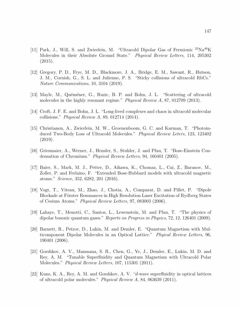
147
[11] Park, J., Will, S. and Zwierlein, M. “Ultracold Dipolar Gas of Fermionic 23Na40KMolecules in their Absolute Ground State.” Physical Review Letters, 114, 205302(2015).
[12] Gregory, P. D., Frye, M. D., Blackmore, J. A., Bridge, E. M., Sawant, R., Hutson,J. M., Cornish, G., S. L. and Julienne, P. S. “Sticky collisions of ultracold RbCs.”Nature Communications, 10, 3104 (2019).
[13] Mayle, M., Quemener, G., Ruzic, B. P. and Bohn, J. L. “Scattering of ultracoldmolecules in the highly resonant regime.” Physical Review A, 87, 012709 (2013).
[14] Croft, J. F. E. and Bohn, J. L. “Long-lived complexes and chaos in ultracold molecularcollisions.” Physical Review A, 89, 012714 (2014).
[15] Christianen, A., Zwierlein, M. W., Groenenboom, G. C. and Karman, T. “Photoin-duced Two-Body Loss of Ultracold Molecules.” Physical Review Leters, 123, 123402(2019).
[16] Griesmaier, A., Werner, J., Hensler, S., Stuhler, J. and Pfau, T. “Bose-Einstein Con-densation of Chromium.” Physical Review Letters, 94, 160401 (2005).
[17] Baier, S., Mark, M. J., Petter, D., Aikawa, K., Chomaz, L., Cai, Z., Baranov, M.,Zoller, P. and Ferlaino, F. “Extended Bose-Hubbard models with ultracold magneticatoms.” Science, 352, 6282, 201 (2016).
[18] Vogt, T., Viteau, M., Zhao, J., Chotia, A., Comparat, D. and Pillet, P. “DipoleBlockade at Forster Resonances in High Resolution Laser Excitation of Rydberg Statesof Cesium Atoms.” Physical Review Letters, 97, 083003 (2006).
[19] Lahaye, T., Menotti, C., Santos, L., Lewenstein, M. and Pfau, T. “The physics ofdipolar bosonic quantum gases.” Reports on Progress in Physics, 72, 12, 126401 (2009).
[20] Barnett, R., Petrov, D., Lukin, M. and Demler, E. “Quantum Magnetism with Mul-ticomponent Dipolar Molecules in an Optical Lattice.” Phyical Review Letters, 96,190401 (2006).
[21] Gorshkov, A. V., Manmana, S. R., Chen, G., Ye, J., Demler, E., Lukin, M. D. andRey, A. M. “Tunable Superfluidity and Quantum Magnetism with Ultracold PolarMolecules.” Physical Review Letters, 107, 115301 (2011).
[22] Kuns, K. A., Rey, A. M. and Gorshkov, A. V. “d-wave superfluidity in optical latticesof ultracold polar molecules.” Physical Review A, 84, 063639 (2011).
148
[23] Yao, N. Y., Gorshkov, A. V., Laumann, C. R., Lauchli, A. M., Ye, J. and Lukin, M. D.“Realizing Fractional Chern Insulators in Dipolar Spin Systems.” Physical ReviewLetters, 110, 185302 (2013).
[24] DeMille, D. “Quantum Computation with Trapped Polar Molecules.” Physical ReviewLetters, 88, 067901 (2002).
[25] Soderberg, K.-A. B., Gemelke, N. and Chin, C. “Ultracold molecules: vehicles toscalable quantum information processing.” New Journal of Physics, 11, 5, 055022(2009).
[26] Park, J. W., Yan, Z. Z., Loh, H., Will, S. A. and Zwierlein, M. W. “Second-scalenuclear spin coherence time of ultracold 23Na40K molecules.” Science, 357, 6349, 372(2017).
[27] Kotochigova, S. and Tiesinga, E. “Controlling polar molecules in optical lattices.”Physical Review A, 73, 041405 (2006).
[28] Yelin, S. F., Kirby, K. and Cote, R. “Schemes for robust quantum computation withpolar molecules.” Physical Review A, 74, 050301 (2006).
[29] Rabl, P., DeMille, D., Doyle, J. M., Lukin, M. D., Schoelkopf, R. J. and Zoller, P.“Hybrid Quantum Processors: Molecular Ensembles as Quantum Memory for SolidState Circuits.” Physical Review Letters, 97, 033003 (2006).
[30] Andre, A., DeMille, D., Doyle, J., Lukin, M. D., Maxwell, S. E., Rabl, P., Schoelopf,R. J. and Zoller, P. “A coherent all-elecrical interface between molecules and mesoscopicsuperconducting resonators.” Nature Physics, 2, 636 (2006).
[31] Kaufman, A. M., Lester, B. J. and Regal, C. A. “Cooling a Single Atom in an OpticalTweezer to Its Quantum Ground State.” Physical Review X, 2, 041014 (2012).
[32] Anderegg, L., Cheuk, L. W., Bao, Y., Burchesky, S., Ketterle, W., Ni, K.-K. andDoyle, J. M. “An optical tweezer array of ultracold molecules.” Science, 365, 6458,1156 (2019).
[33] Norcia, M. A., Young, A. W. and Kaufman, A. M. “Microscopic Control and Detectionof Ultracold Strontium in Optical-Tweezer Arrays.” Physical Review X, 8, 041054(2018).
[34] Ni, K.-K., Rosenband, T. and Grimes, D. D. “Dipolar exchange quantum logic gatewith polar molecules.” Chemical Science, 9, 6830 (2018).
149
[35] Yu, P., Cheuk, L. W., Kozyryev, I. and Doyle, J. M. “A scalable quantum computingplatform using symmetric-top molecules.” New Journal of Physics, 21, 9, 093049(2019).
[36] Safronova, M. S., Budker, D., DeMille, D., Kimball, D. F. J., Derevianko, A. andClark, C. W. “Search for new physics with atoms and molecules.” Review of ModernPhysics, 90, 025008 (2018).
[37] Andreev, V., Ang, D. G., Doyle, J. M., Gabrielse, G., Haefner, J., Hutzler, N. R.,Lasner, Z., Meisenhelder, C., O’Leary, B. R., Panda, C. D., West, A. D., West, E. P.and Wu, X. “Improved limit on the electric dipole moment of the electron.” Nature,562, 355 (2018).
[38] Chin, C., Flambaum, V. V. and Kozlov, M. G. “Ultracold molecules: new probes onthe variation of fundamental constants.” New Journal of Physics, 11, 5, 055048 (2009).
[39] DeMille, D., Sainis, S., Sage, J., Bergeman, T., Kotochigova, S. and Tiesinga, E.“Enhanced Sensitivity to Variation of me/mp in Molecular Spectra.” Physical ReviewLetters, 100, 043202 (2008).
[40] Zelevinsky, T., Kotochigova, S. and Ye, J. “Precision Test of Mass-Ratio Variationswith Lattice-Confined Ultracold Molecules.” Physical Review Letters, 100, 043201(2008).
[41] Kotochigova, S., Zelevinsky, T. and Ye, J. “Prospects for application of ultracold Sr2
molecules in precision measurements.” Physical Review A, 79, 012504 (2009).
[42] Kobayashi, J., Ogino, A. and Inouye, S. “Measurement of the variation of the electron-to-proton mass ration using ultracold molecules produced from laser-cooled atoms.”Nature Communications, 10, 3771 (2019).
[43] Flambaum, V. V., Stadnik, Y. V., Kozlov, M. G. and Petrov, A. N. “Enhanced effectsof temporal variation of the fundamental constants in 2Π1/2-term diatomic molecules:207Pb19F.” Physical Review A, 88, 052124 (2013).
[44] Salumbides, E. J., Koelemeij, J. C. J., Komasa, J., Pachucki, K., Eikema, K. S. E.and Ubachs, W. “Bounds on fifth forces from precision measurements on molecules.”Physical Review D, 87, 112008 (2013).
[45] Altuntas, E., Ammon, J., Cahn, S. B. and DeMille, D. “Demonstration of a Sensi-tive Method to Measure Nuclear-Spin-Dependent Parity Violation.” Physical ReviewLetters, 120, 142501 (2018).
150
[46] Norrgard, E. B., Barker, D. S., Eckel, S., Fedchak, J. A., Klimov, N. N. and Scher-schligt, J. “Nuclear-spin dependent parity violation in optically trapped polyatomicmolecules.” Communications Physics, 2, 77 (2019).
[47] Metcalf, H. J. and van der Straten, P. Laser Cooling and Trapping. Springer-VerlagNew York (1999).
[48] Di Rosa, M. D. “Laser-cooling molecules.” The European Physical Journal D - Atomic,Molecular, Optical and Plasma Physics, 31, 2, 395 (2004).
[49] McCarron, D. “Laser cooling and trapping molecules.” Journal of Physics B: Atomic,Molecular and Optical Physics, 51, 21, 212001 (2018).
[50] McCarron, D. J., Steinecker, M. H., Zhu, Y. and DeMille, D. “Magnetic Trapping ofan Ultracold Gas of Polar Molecules.” Physical Review Letters, 121, 013202 (2018).
[51] Williams, H. J., Caldwell, L., Fitch, N. J., Truppe, S., Rodewald, J., Hinds, E. A.,Sauer, B. E. and Tarbutt, M. R. “Magnetic Trapping and Coherent Control of Laser-Cooled Molecules.” Physical Review Letters, 120, 163201 (2018).
[52] Collopy, A. L., Ding, S., Wu, Y., Finneran, I. A., Anderegg, L., Augenbraun, B. L.,Doyle, J. M. and Ye, J. “3D Magneto-Optical Trap of Yttrium Monoxide.” PhysicalReview Letters, 121, 213201 (2018).
[53] Collopy, A. L., Hummon, M. T., Yeo, M., Yan, B. and Ye, J. “Prospects for a narrowline MOT in YO.” New Journal of Physics, 17, 5, 055008 (2015).
[54] Railing, L., Shaw, J. and McCarron, D. “Progress towards laser-cooled CH molecules.”(2019). APS Division of Atomic, Molecular and Optical Physics APS Meeting.
[55] Kozyryev, I., Baum, L., Matsuda, K., Augenbraun, B. L., Anderegg, L., Sedlack, A. P.and Doyle, J. M. “Sisyphus Laser Cooling of a Polyatomic Molecule.” Physical ReviewLetters, 118, 173201 (2017).
[56] Kozyryev, I., Steimle, T. C., Yu, P., Nguyen, D.-T. and Doyle, J. M. “Determination ofCaOH and CaOCH3 vibrational branching ratios for direct laser cooling and trapping.”New Journal of Physics, 21, 5, 052002 (2019).
[57] Moore, K., Lane, I. C., McNally, R. L. and Zelevinsky, T. “Assignment of excited-statebond lengths using branching-ratio measurements: The B2Σ+ state of BaH molecules.”Physical Review A, 100, 022506 (2019).
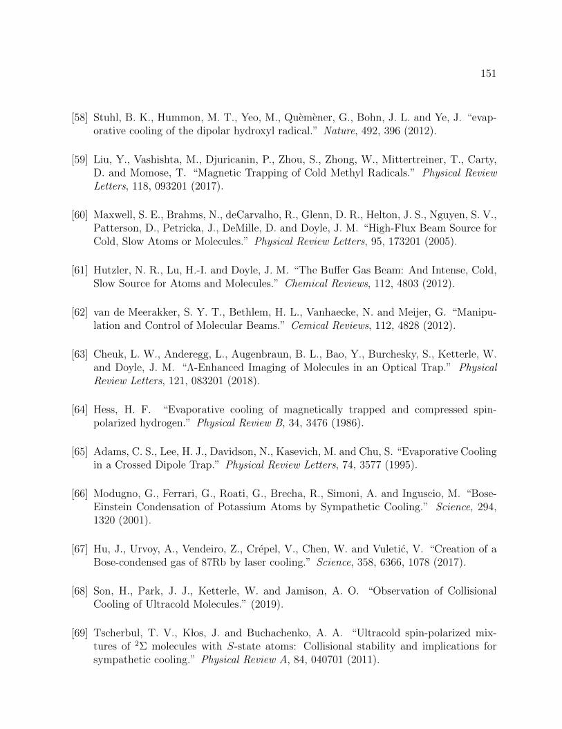
151
[58] Stuhl, B. K., Hummon, M. T., Yeo, M., Quemener, G., Bohn, J. L. and Ye, J. “evap-orative cooling of the dipolar hydroxyl radical.” Nature, 492, 396 (2012).
[59] Liu, Y., Vashishta, M., Djuricanin, P., Zhou, S., Zhong, W., Mittertreiner, T., Carty,D. and Momose, T. “Magnetic Trapping of Cold Methyl Radicals.” Physical ReviewLetters, 118, 093201 (2017).
[60] Maxwell, S. E., Brahms, N., deCarvalho, R., Glenn, D. R., Helton, J. S., Nguyen, S. V.,Patterson, D., Petricka, J., DeMille, D. and Doyle, J. M. “High-Flux Beam Source forCold, Slow Atoms or Molecules.” Physical Review Letters, 95, 173201 (2005).
[61] Hutzler, N. R., Lu, H.-I. and Doyle, J. M. “The Buffer Gas Beam: And Intense, Cold,Slow Source for Atoms and Molecules.” Chemical Reviews, 112, 4803 (2012).
[62] van de Meerakker, S. Y. T., Bethlem, H. L., Vanhaecke, N. and Meijer, G. “Manipu-lation and Control of Molecular Beams.” Cemical Reviews, 112, 4828 (2012).
[63] Cheuk, L. W., Anderegg, L., Augenbraun, B. L., Bao, Y., Burchesky, S., Ketterle, W.and Doyle, J. M. “Λ-Enhanced Imaging of Molecules in an Optical Trap.” PhysicalReview Letters, 121, 083201 (2018).
[64] Hess, H. F. “Evaporative cooling of magnetically trapped and compressed spin-polarized hydrogen.” Physical Review B, 34, 3476 (1986).
[65] Adams, C. S., Lee, H. J., Davidson, N., Kasevich, M. and Chu, S. “Evaporative Coolingin a Crossed Dipole Trap.” Physical Review Letters, 74, 3577 (1995).
[66] Modugno, G., Ferrari, G., Roati, G., Brecha, R., Simoni, A. and Inguscio, M. “Bose-Einstein Condensation of Potassium Atoms by Sympathetic Cooling.” Science, 294,1320 (2001).
[67] Hu, J., Urvoy, A., Vendeiro, Z., Crepel, V., Chen, W. and Vuletic, V. “Creation of aBose-condensed gas of 87Rb by laser cooling.” Science, 358, 6366, 1078 (2017).
[68] Son, H., Park, J. J., Ketterle, W. and Jamison, A. O. “Observation of CollisionalCooling of Ultracold Molecules.” (2019).
[69] Tscherbul, T. V., K los, J. and Buchachenko, A. A. “Ultracold spin-polarized mix-tures of 2Σ molecules with S-state atoms: Collisional stability and implications forsympathetic cooling.” Physical Review A, 84, 040701 (2011).
152
[70] Lim, J., Frye, M. D., Hutson, J. M. and Tarbutt, M. R. “Modeling sympathetic coolingof molecules by ultracold atoms.” Physical Review A, 92, 053419 (2015).
[71] Kohler, T., Goral, K. and Julienne, P. S. “Production of cold molecules via magneti-cally tunable Feshbach resonances.” Review of Modern Physics, 78, 1311 (2006).
[72] De Marco, L., Valtolina, G., Matsuda, K., Tobias, W. G., Covey, J. P. and Ye, J. “Adegenerate Fermi gas of polar molecules.” Science, 363, 6429, 853 (2019).
[73] Ospelkaus, S., Pe’er, A., Ni, K.-K., Zirbel, J. J., Neyenhuis, B., Kotochigova, S.,Julienne, P. S., Ye, J. and Jin, D. S. “Efficient state transfer in an ultracold dense gasof heteronuclear molecules.” Nature Physics, 4, 622 (2008).
[74] Ni, K.-K., Ospelkaus, S., de Miranda, M. H. G., Peer, A., Neyenhuis, B., Zirbel, J. J.,Kotochigova, S., Julienne, P. S., Jin, D. S. and Ye, J. “A High Phase-Space-DensityGas of Polar Molecules.” Science, 322, 231 (2008).
[75] Takekoshi, T., Reichsollner, L., Schindewolf, A., Hutson, J., Le Sueur, C., Dulieu, O.,Ferlaino, F., Grimm, R. and Nagerl, H.-C. “Ultracold dense samples of dipolar RbCsmolecules in the rovibrational and hyperfine ground state.” Physical Review Letters,113, 205301 (2014).
[76] Molony, P., Gregory, P., Ji, Z., Lu, B., Koppinger, M., Le Sueur, C., Blackley, C.,Hutson, J. and Cornish, S. “Creation of Ultracold 87Rb133Cs Molecules in the Rovi-brational Ground State.” Physical Review Letters, 113, 255301 (2014).
[77] Guo, M., Zhu, B., Lu, B., Ye, X., Wang, F., Vexiau, R., Bouloufa-Maafa, N., Quemener,G., Dulieu, O. and Wang, D. “Creation of an Ultracold Gas of Ground-State Dipolar23Na87Rb Molecules.” Physical Review Letters, 116, 205303 (2016).
[78] Rvachov, T. M., Son, H., Sommer, A. T., Ebadi, S., Park, J. J., Zwierlein, M. W.,Ketterle, W. and Jamison, A. O. “Long-Lived Ultracold Molecules with Electric andMagnetic Dipole Moments.” Physical Review Letters, 119, 143001 (2017).
[79] Seeßelberg, F., Buchheim, N., Lu, Z.-K., Schneider, T., Luo, X.-Y., Tiemann, E.,Bloch, I. and Gohle, C. “Modeling the adiabatic creation of ultracold polar 23Na40Kmolecules.” Physical Review A, 97, 013405 (2018).
[80] Stellmer, S., Pasquiou, B., Grimm, R. and Schreck, F. “Creation of Ultracold Sr2
Molecules in the Electronic Ground State.” Physical Review Letters, 109, 115302(2012).
153
[81] Voges, K. K., Gersema, P., Hartmann, T., Schulze, T. A., Zenesini, A. and Ospelkaus,S. “A pathway to ultracold bosonic 23Na39K ground state molecules.” (2019).
[82] Liu, L. R., Hood, J. D., Yu, Y., Zhang, J. T., Hutzler, N. R., Rosenband, T. and Ni,K.-K. “Building one molecule from a reservoir of two atoms.” Science, 360, 6391, 900(2018).
[83] Barbe, V., Ciamei, A., Pasquiou, B., Reichsollner, L., Schreck, F., Zuchowski, P. andHutson, J. M. “Observation of Feshbach resonances between alkali and closed-shellatoms.” Nature Physics, 14, 881 (2018).
[84] Guttridge, A., Frye, M. D., Yang, B. C., Hutson, J. M. and Cornish, S. L. “Two-photon photoassociation spectroscopy of CsYb: Ground-state interaction potentialand interspecies scattering lengths.” Physical Review A, 98, 022707 (2018).
[85] Deiglmayr, J., Grochola, A., Repp, M., Dulieu, O., Wester, R. and Weidemuller, M.“Permanent dipole moment of LiCs in the ground state.” Physical Review A, 82,032503 (2010).
[86] “Commission on Isotopic Abundances and Atomic Weights: Ytterbium.” (2017).
[87] Sansonetti, J. E. and Martin, W. C. “Handbook of Basic Atomic Spectroscopic Data.”Journal of Physical and Chemical Reference Data, 34, 4, 1559 (2005).
[88] Kitagawa, M., Enomoto, K., Kasa, K., Takahashi, Y., Ciury lo, R., Naidon, P. andJulienne, P. S. “Two-color photoassociation spectroscopy of ytterbium atoms and theprecise determinations of s-wave scattering lengths.” Physical Review A, 77, 012719(2008).
[89] Das, D., Barthwal, S., Banerjee, A. and Natarajan, V. “Absolute frequency measure-ments in Yb with 0.08 ppb uncertainty: Isotope shifts and hyperfine structure in the399− nm 1S0 →1 P1 line.” Physical Review A, 72, 032506 (2005).
[90] Pandey, K., Singh, A. K., Kumar, P. V. K., Suryanarayana, M. V. and Natarajan,V. “Isotope shifts and hyperfine structure in the 555.8-nm 1S0 → 3P 1 line of Yb.”Physical Review A, 80, 022518 (2009).
[91] Foot, C. J. Atomic Physics. Oxford University Press (2005).
[92] Micheli, A., Brennen, G. K. and Zoller, P. “A Toolbox for Lattice-Spin Models withPolar Molecules.” Nature Physics, 2, 341 (2006).
154
[93] Herrera, F., Cao, Y., Kais, S. and Whaley, K. B. “Infrared-dressed entanglement ofcold open-shell polar molecules for universal matchgate quantum computing.” NewJournal of Physics, 16, 7, 075001 (2014).
[94] Abrahamsson, E., Tscherbul, T. V. and Krems, R. V. “Inelastic collisions of coldpolar molecules in nonparallel electric and magnetic fields.” The Journal of ChemicalPhysics, 127, 4, 044302 (2007).
[95] Kotochigova, S., Petrov, A., Linnik, M., Klos, J. and Julienne, P. S. “Ab initio proper-ties of Li-group-II molecules for ultracold matter studies.” Journal of Chemical Physics,135, 164108 (2011).
[96] Kotochigova, S. “private communication.” Temple University.
[97] Hansen, A. H. “Interacting Quantum Gases of Lithium and Ytterbium.” PhD Thesis- University of Washington (2011).
[98] Khramov, A. “Experiments in the Ultracold Lithium-Ytterbium.” PhD Thesis - Uni-versity of Washington (2013).
[99] Phillips, W. D. and Metcalf, H. “Laser Deceleration of an Atomic Beam.” PhysicalReview Letters, 48, 596 (1982).
[100] Grimm, R., Weidemuller, M. and Ovchinnikov, Y. B. “Optical Dipole Traps for NeutralAtoms.” volume 42 of Advances In Atomic, Molecular, and Optical Physics, 95 – 170.Academic Press (2000).
[101] Ivanov, V. V., Khramov, A., Hansen, A. H., Dowd, W. H., Munchow, F., Jamison,A. O. and Gupta, S. “Sympathetic Cooling in an Optically Trapped Mixture of Alkaliand Spin-Singlet Atoms.” Physical Review Letters, 106, 153201 (2011).
[102] Hansen, A. H., Khramov, A., Dowd, W. H., Jamison, A. O., Ivanov, V. V. and Gupta,S. “Quantum Degenerate Mixture of Ytterbium and Lithium Atoms.” Physical ReviewA, 84, 011606(R) (2011).
[103] Roy, R., Green, A., Bowler, R. and Gupta, S. “Rapid cooling to quantum degeneracyin dynamically shaped atom traps.” Physical Review A, 93, 043403 (2016).
[104] Demtroder, W. Molecular Physics. Wiley-VCH (2005).
[105] Sinanoglu, O. Many-Electron Theory of Atoms, Molecules and Their Interactions.John Wiley & Sons, Ltd (2007).
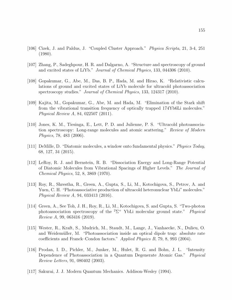
155
[106] Cizek, J. and Paldus, J. “Coupled Cluster Approach.” Physica Scripta, 21, 3-4, 251(1980).
[107] Zhang, P., Sadeghpour, H. R. and Dalgarno, A. “Structure and spectroscopy of groundand excited states of LiYb.” Journal of Chemical Physics, 133, 044306 (2010).
[108] Gopakumar, G., Abe, M., Das, B. P., Hada, M. and Hirao, K. “Relativistic calcu-lations of ground and excited states of LiYb molecule for ultracold photoassociationspectroscopy studies.” Journal of Chemical Physics, 133, 124317 (2010).
[109] Kajita, M., Gopakumar, G., Abe, M. and Hada, M. “Elimination of the Stark shiftfrom the vibrational transition frequency of optically trapped 174Yb6Li molecules.”Physical Review A, 84, 022507 (2011).
[110] Jones, K. M., Tiesinga, E., Lett, P. D. and Julienne, P. S. “Ultracold photoassocia-tion spectroscopy: Long-range molecules and atomic scattering.” Review of ModernPhysics, 78, 483 (2006).
[111] DeMille, D. “Diatomic molecules, a window onto fundamental physics.” Physics Today,68, 127, 34 (2015).
[112] LeRoy, R. J. and Bernstein, R. B. “Dissociation Energy and Long-Range Potentialof Diatomic Molecules from Vibrational Spacings of Higher Levels.” The Journal ofChemical Physics, 52, 8, 3869 (1970).
[113] Roy, R., Shrestha, R., Green, A., Gupta, S., Li, M., Kotochigova, S., Petrov, A. andYuen, C. H. “Photoassociative production of ultracold heteronuclear YbLi∗ molecules.”Physical Review A, 94, 033413 (2016).
[114] Green, A., See Toh, J. H., Roy, R., Li, M., Kotochigova, S. and Gupta, S. “Two-photonphotoassociation spectroscopy of the 2Σ+ YbLi molecular ground state.” PhysicalReview A, 99, 063416 (2019).
[115] Wester, R., Kraft, S., Mudrich, M., Staudt, M., Lange, J., Vanhaecke, N., Dulieu, O.and Weidemuller, M. “Photoassociation inside an optical dipole trap: absolute ratecoefficients and Franck–Condon factors.” Applied Physics B, 79, 8, 993 (2004).
[116] Prodan, I. D., Pichler, M., Junker, M., Hulet, R. G. and Bohn, J. L. “IntensityDependence of Photoassociation in a Quantum Degenerate Atomic Gas.” PhysicalReview Letters, 91, 080402 (2003).
[117] Sakurai, J. J. Modern Quantum Mechanics. Addison-Wesley (1994).
156
[118] Gordon, R. G. “New Method for Constructing Wavefunctions for Bound States andScattering.” The Journal of Chemical Physics, 51, 1, 14 (1969).
[119] Hara, H., Takasu, Y., Yamaoka, Y., Doyle, J. and Y., T. “Quantum DegenerateMixtures of Alkali and Alkaline-Earth-Like Atoms.” Physical Review Letters, 106,205304 (2011).
[120] Kampschulte, T. and Denschlag, J. H. “Cavity-controlled formation of ultracoldmolecules.” New Journal of Physics, 20, 12, 123015 (2018).
[121] Reinaudi, G., Osborn, C. B., McDonald, M., Kotochigova, S. and Zelevinsky, T. “Op-tical Production of Stable Ultracold 88Sr2 Molecules.” Physical Review Letters, 109,115303 (2012).
[122] McDonald, M., McGuyer, B., Apfelbeck, F., Lee, C.-H., Majewska, I., Moszynski, R.and Zelevinsky, T. “Photodissociation of ultracold diatomic strontium molecules withquantum state control.” Nature, 535, 122 (2016).
[123] Zabawa, P., Wakim, A., Haruza, M. and Bigelow, N. P. “Formation of ultracoldX 1Σ+(v′ = 0) NaCs molecules via coupled photoassociation channels.” Physical Re-view A, 84, 061401 (2011).
[124] Banerjee, J., Rahmlow, D., Carollo, R., Bellos, M., Eyler, E. E., Gould, P. L. andStwalley, W. C. “Direct photoassociative formation of ultracold KRb molecules in thelowest vibrational levels of the electronic ground state.” Physical Review A, 86, 053428(2012).
[125] Yan, M., DeSalvo, B. J., Huang, Y., Naidon, P. and Killian, T. C. “Rabi Oscilla-tions between Atomic and Molecular Condensates Driven with Coherent One-ColorPhotoassociation.” Physical Review Letters, 111, 150402 (2013).
[126] McGuyer, B. H., McDonald, M., Iwata, G. Z., Tarallo, M. G., Grier, A. T., Apfelbeck,F. and Zelevinsky, T. “High-precision spectroscopy of ultracold molecules in an opticallattice.” New Journal of Physics, 17, 5, 055004 (2015).
[127] Kotochigova, S. “Prospects for Making Polar Molecules with Microwave Fields.” Phys-ical Review Letters, 99, 073003 (2007).
[128] Fox, M. Quantum Optics: An Introduction. Oxford University Press (2006).
[129] Bergmann, K., Theuer, H. and Shore, B. W. “Coherent population transfer amongquantum states of atoms and molecules.” Review of Modern Physics, 70, 1003 (1998).
157
[130] Vitanov, N. V., Rangelov, A. A., Shore, B. W. and Bergmann, K. “Stimulated Ramanadiabatic passage in physics, chemistry, and beyond.” Review of Modern Physics, 89,015006 (2017).
[131] Boller, K.-J., Imamoglu, A. and Harris, S. E. “Observation of electromagneticallyinduced transparency.” Physical Review Letters, 66, 2593 (1991).
[132] Hau, L. V., Harris, S. E., Dutton, Z. and Behroozi, C. H. “Light speed reduction to17 metres per second in an ultracold atomic gas.” Nature, 397, 594 (1999).
[133] Peng, D., Ozdemir, S. K., Chen, W., Nori, F. and Yang, L. “What is and what is notelectromagnetically induced transparency in whispering-gallery microcavities.” NatureCommunications, 5, 5082 (2014).
[134] Donarini, A., Niklas, M., Schafberger, M., Paradiso, N., Strunk, C. and Grifoni, M.“Coherent population trapping by dark state formation in a carbon nanotube quantumdot.” Nature Communications, 10 (2019).
[135] Ciamei, A., Bayerle, A., Chen, C., Pasquiou, B. and Schreck, F. “Efficient productionof long-lived ultracold Sr2 molecules.” Physical Review A, 96, 013406 (2017).
[136] Lu, B. and Wang, D. “Note: A four-pass acousto-optic modulator system for lasercooling of sodium atoms.” Rev. Sci. Instr., 88, 076105 (2017).
[137] Winkler, K., Thalhammer, G., Theis, M., Ritsch, H., Grimm, R. and Hecker Denschlag,J. “Atom-Molecule Dark States in a Bose-Einstein Condensate.” Physical ReviewLetters, 95, 063202 (2005).
[138] Kuklinski, J. R., Gaubatz, U., Hioe, F. T. and Bergmann, K. “Adiabatic populationtransfer in a three-level system driven by delayed laser pulses.” Physical Review A, 40,6741 (1989).
[139] Danzl, J. G., Mark, M. J., Haller, E., Gustavsson, M., Bouloufa, N., Dulieu, O.,Ritsch, H., Hart, R. and Nagerl, H.-C. “Precision molecular spectroscopy for groundstate transfer of molecular quantum gases.” Faraday Discuss., 142, 283 (2009).
[140] Cohen-Tannoudji, C. and Reynaud, S. “Simultaneous saturation of two atomic transi-tions sharing a common level.” Journal of Physics B: Atomic and Molecular Physics,10, 12, 2311 (1977).
[141] Abi-Salloum, T. Y. “Electromagnetically induced transparency and Autler-Townessplitting: Two similar but distinct phenomena in two categories of three-level atomicsystems.” Physical Review A, 81, 053836 (2010).
158
[142] Lu, X., Miao, X., Bai, J., Pei, L., Wang, M., Gao, Y., Wu, L.-A., Fu, P., Wang, R.and Zuo, Z. “Transition from Autler–Townes splitting to electromagnetically inducedtransparency based on the dynamics of decaying dressed states.” Journal of PhysicsB: Atomic, Molecular and Optical Physics, 48, 5, 055003 (2015).
[143] Meystre, P. and Sargent, M. Elements of Quantum Optics. Springer (2007).
[144] Li, M. “private communication.” (2019). Temple University.
[145] Weiner, J., Bagnato, V. S., Zilio, S. and Julienne, P. S. “Experiments and theory incold and ultracold collisions.” Review of Modern Physics, 71, 1 (1999).
[146] Mott, N. F. The Theory of Atomic Collisions. Oxford Clarendon Press (1965).
[147] Chin, C., Grimm, R., Julienne, P. and Tiesinga, E. “Feshbach resonances in ultracoldgases.” Review of Modern Physics, 82, 1225 (2010).
[148] Tiesinga, E., Verhaar, B. J. and Stoof, H. T. C. “Threshold and resonance phenomenain ultracold ground-state collisions.” Physical Review A, 47, 4114 (1993).
[149] Berninger, M., Zenesini, A., Huang, B., Harm, W., Nagerl, H.-C., Ferlaino, F., Grimm,R., Julienne, P. S. and Hutson, J. M. “Universality of the Three-Body Parameter forEfimov States in Ultracold Cesium.” Physical Review Letters, 107, 120401 (2011).
[150] Gross, N., Shotan, Z., Kokkelmans, S. and Khaykovich, L. “Observation of Universalityin Ultracold 7Li Three-Body Recombination.” Physical Review Letters, 103, 163202(2009).
[151] Pollack, S. E., Dries, D. and Hulet, R. G. “Universality in Three- and Four-BodyBound States of Ultracold Atoms.” Science, 326, 5960, 1683 (2009).
[152] Kraemer, T., Mark, M., Waldburger, P., Danzl, J. G., Chin, C., Engeser, B., Lange,A., Pilch, K., Jaakkola, A., Nagerl, H. and Grimm, R. “Evidence for Efimov quantumstates in an ultracold gas of caesium atoms.” Nature (London), 440, 315 (2006).
[153] D’Incao, J. P. “Few-body physics in resonantly interacting ultracold quantum gases.”Journal of Physics B: Atomic, Molecular and Optical Physics, 51, 043001 (2018).
[154] Naidon, P. and Endo, S. “Efimov physics: a review.” Reports on Progress in Physics,80, 056001 (2017).
159
[155] Cirac, J. and Zoller, P. “Goals and opportunities in quantum simulation.” NaturePhysics, 8, 264 (2012).
[156] Bloch, I., Dalibard, J. and Nascimbne, S. “Quantum simulations with ultracold quan-tum gases.” Nature Physics, 8, 267 (2012).
[157] Chen, Q., Stajic, J., Tan, S. and Levin, K. “BCS-BEC crossover: From high temper-ature superconductors to ultracold fermi superfluids.” Physics Reports, 412.
[158] Greiner, M., Mandel, O., Esslinger, T., T., H. and Bloch, I. “Quantum phase transitionfrom a superfluid to a Mott insulator in a gas of ultracold atoms.” Nature, 415, 39(2002).
[159] Tanzi, L., Roccuzzo, S. M., Lucioni, E., Fama, F., Fioretti, A., Gabbanini, C., Mod-ugno, G., Recati, A. and Stringari, S. “Supersolid symmetry breaking from compres-sional oscillations in a dipolar quantum gas.” Nature, 573, 7773 (2019).
[160] Bottcher, F., Schmidt, J.-N., Wenzel, M., Hertkorn, J., Guo, M., Langen, T. andPfau, T. “Transient Supersolid Properties in an Array of Dipolar Quantum Droplets.”Physical Review X, 9, 011051 (2019).
[161] Chomaz, L., Petter, D., Ilzhofer, P., Natale, G., Trautmann, A., Politi, C., Durastante,G., van Bijnen, R. M. W., Patscheider, A., Sohmen, M., Mark, M. J. and Ferlaino, F.“Long-Lived and Transient Supersolid Behaviors in Dipolar Quantum Gases.” PhysicalReview X, 9, 021012 (2019).
[162] Murthy, P. A., Boettcher, I., Bayha, L., Holzmann, M., Kedar, D., Neidig, M., Ries,M. G., Wenz, A. N., Zurn, G. and Jochim, S. “Observation of the Berezinskii-Kosterlitz-Thouless Phase Transition in an Ultracold Fermi Gas.” Physical ReviewLetters, 115, 010401 (2015).
[163] Fischer, U. R. and Schutzhold, R. “Quantum simulation of cosmic inflation in two-component Bose-Einstein condensates.” Physical Review A, 70, 063615 (2004).
[164] Eckel, S., Kumar, A., Jacobson, T., Spielman, I. B. and Campbell, G. K. “A RapidlyExpanding Bose-Einstein Condensate: An Expanding Universe in the Lab.” PhysicalReview X, 8, 021021 (2018).
[165] Tewari, S., Scarola, V. W., Senthil, T. and Sarma, S. D. “Emergence of ArtificialPhotons in an Optical Lattice.” Physical Review Letters, 97, 200401 (2006).
160
[166] Gandolfi, S., Gezerlis, A. and Carlson, J. “Neutron Matter from Low to High Density.”Annual Review of Nuclear and Particle Science, 65, 1, 303 (2015).
[167] Zwierlein, M. W., Abo-Shaeer, J. R., Schirotzek, A., Schunck, C. H. and Ketterle, W.“Vortices and superfluidity in a strongly interacting Fermi gas.” Nature, 435, 7045,1047 (2005).
[168] Cornish, S. L., Claussen, N. R., Roberts, J. L., Cornell, E. A. and Wieman, C. E.“Stable 85Rb Bose-Einstein Condensates with Widely Tunable Interactions.” PhysicalReview Letters, 85, 1795 (2000).
[169] Weber, T., Herbig, J., Mark, M., Nagerl, H.-C. and Grimm, R. “Three-Body Recom-bination at Large Scattering Lengths in an Ultracold Atomic Gas.” Physical ReviewLetters, 91, 123201 (2003).
[170] Courteille, P., Freeland, R. S., Heinzen, D. J., van Abeelen, F. A. and Verhaar, B. J.“Observation of a Feshbach Resonance in Cold Atom Scattering.” Physical ReviewLetters, 41, 1532 (1978).
[171] Inouye, S., Andrews, M. R., Stenger, J., Miesner, H.-J., Stamper-Kurn, D. M. andKetterle, W. “Observation of Feshbach resonances in a Bose-Einstein condensate.”Nature, 392, 151 (1998).
[172] Moerdijk, A. J., Verhaar, B. J. and Axelsson, A. “Resonances in ultracold collisionsof 6Li, 7Li, and 23Na.” Physical Review A, 51, 4852 (1995).
[173] Fatemi, F. K., Jones, K. M. and Lett, P. D. “Observation of Optically Induced FeshbachResonances in Collisions of Cold Atoms.” Physical Review Letters, 85, 4462 (2000).
[174] Theis, M., Thalhammer, G., Winkler, K., Hellwig, M., Ruff, G., Grimm, R. and Den-schlag, J. H. “Tuning the Scattering Length with an Optically Induced FeshbachResonance.” Physical Review Letters, 93, 123001 (2004).
[175] Reschovsky, B. “Studies of Ultracold Strontium Gases.” PhD Thesis - University ofMaryland (2017).
[176] Dzuba, V. A., Flambaum, V. V. and Schiller, S. “Testing physics beyond the standardmodel through additional clock transitions in neutral ytterbium.” Physical Review A,98, 022501 (2018).
[177] Zhang, R., Cheng, Y., Zhai, H. and Zhang, P. “Orbital Feshbach Resonance in Alkali-Earth Atoms.” Physical Review Letters, 115, 135301 (2015).
161
[178] Hofer, M., Riegger, L., Scazza, F., Hofrichter, C., Fernandes, D. R., Parish, M. M.,Levinsen, J., Bloch, I. and Folling, S. “Observation of an Orbital Interaction-InducedFeshbach Resonance in 173Yb.” Physical Review Letters, 115, 265302 (2015).
[179] Kato, S., Sugawa, S., Shibata, K., Yamamoto, R. and Takahashi, Y. “Control ofResonant Interaction between Electronic Ground and Excited States.” Physical ReviewLetters, 110, 173201 (2013).
[180] Gonzalez-Martınez, M. L. and Hutson, J. M. “Magnetically tunable Feshbach reso-nances in Li + Yb(3PJ).” Physical Review A, 88, 020701 (2013).
[181] Petrov, A., Makrides, C. and Kotochigova, S. “Magnetic control of ultra-cold 6Li and174Yb(3P2) atom mixtures with Feshbach resonances.” New Journal of Physics, 17,045010 (2015).
[182] Dowd, W., Roy, R., Shrestha, R., Petrov, A., Makrides, C., Kotochigova, S. and Gupta,S. “Magnetic field dependent interactions in an ultracold Li-Yb(3P 2) mixture.” NewJournal of Physics, 17, 055007 (2015).
[183] Chen, T., Zhang, C., Li, X., Qian, J. and Wang, Y. “Anisotropy induced Feshbachresonances in mixtures of 6Li(2S)+171Yb(3P2.” New Journal of Physics, 17, 103036(2015).
[184] Petrov, A., Tiesinga, E. and Kotochigova, S. “Anisotropy-Induced Feshbach Res-onances in a Quantum Dipolar Gas of Highly Magnetic Atoms.” Physical ReviewLetters, 109, 103002 (2012).
[185] Baumann, K., Burdick, N. Q., Lu, M. and Lev, B. L. “Observation of low-field Fano-Feshbach resonances in ultracold gases of dysprosium.” Physical Review A, 89, 020701(2014).
[186] Maier, T., Ferrier-Barbut, I., Kadau, H., Schmitt, M., Wenzel, M., Wink, C., Pfau,T., Jachymski, K. and Julienne, P. S. “Broad universal Feshbach resonances in thechaotic spectrum of dysprosium atoms.” Physical Review A, 92, 060702 (2015).
[187] Maier, T., Kadau, H., Schmitt, M., Wenzel, M., Ferrier-Barbut, I., Pfau, T., Frisch,A., Baier, S., Aikawa, K., Chomaz, L. et al. “Emergence of Chaotic Scattering inUltracold Er and Dy.” Physical Review X, 5, 041029 (2015).
[188] Frisch, A., Mark, M., Aikawa, K., Ferlaino, F., Bohn, J. L., Makrides, C., Petrov,A. and Kotochigova, S. “Quantum chaos in ultracold collisions of gas-phase erbiumatoms.” Nature, 507, 475 (2014).
162
[189] Ravensbergen, C., Soave, E., Corre, V., Kreyer, M., Huang, B., Kirilov, E. and Grimm,R. “Strongly Interacting Fermi-Fermi Mixture of 161Dy and 40K.” arXiv:1909.03424[cond-mat.quant-gas] (2019).
[190] Yang, H., Zhang, D.-C., Liu, L., Liu, Y.-X., Nan, J., Zhao, B. and Pan, J.-W. “Ob-servation of magnetically tunable Feshbach resonances in ultracold 23Na40K + 40Kcollisions.” Science, 363, 6424, 261 (2019).
[191] Brue, D. A. and Hutson, J. M. “Magnetically Tunable Feshbach Resonances in Ultra-cold Li-Yb Mixtures.” Physical Review Letters, 108, 043201 (2012).
[192] Brue, D. A. and Hutson, J. M. “Prospects of forming ultracold molecules in 2Σ statesby magnetoassociation of alkali-metal atoms with Yb.” Physical Review A, 87, 052709(2013).
[193] Yang, B. C., Frye, M. D., Guttridge, A., Aldegunde, J., Zuchowski, P. S., Cornish,S. L. and Hutson, J. M. “Magnetic Feshbach resonances in ultracold collisions betweenCs and Yb atoms.” Physical Review A, 100, 022704 (2019).
[194] Sleator, T., Pfau, T., Balykin, V., Carnal, O. and Mlynek, J. “Experimental demon-stration of the optical Stern-Gerlach effect.” Physical Review Letters, 68, 1996 (1992).
[195] Taie, S., Takasu, Y., Sugawa, S., Yamazaki, R., Tsujimoto, T., Murakami, R. andTakahashi, Y. “Realization of a SU(2)× SU(6) System of Fermions in a Cold AtomicGas.” Physical Review Letters, 105, 190401 (2010).
[196] Stellmer, S., Grimm, R. and Schreck, F. “Detection and manipulation of nuclear spinstates in fermionic strontium.” Physical Review A, 84, 043611 (2011).
[197] Roberts, J. L., Claussen, N. R., Cornish, S. L. and Wieman, C. E. “Magnetic FieldDependence of Ultracold Inelastic Collisions near a Feshbach Resonance.” PhysicalReview Letters, 85, 728 (2000).
[198] Chin, C., Vuletic, V., Kerman, A. J., Chu, S., Tiesinga, E., Leo, P. J. and Williams,C. J. “Precision Feshbach spectroscopy of ultracold Cs2.” Physical Review A, 70,032701 (2004).
[199] Dowd, W. H. “Interactions in the Ultracold Lithium - Ytterbium 3P2 System.” PhDThesis - University of Washington (2014).
[200] Zhang, J., van Kempen, E. G. M., Bourdel, T., Khaykovich, L., Cubizolles, J., Chevy,F., Teichmann, M., Tarruell, L., Kokkelmans, S. J. J. M. F. and Salomon, C. “P -waveFeshbach resonances of ultracold 6Li.” Physical Review A, 70, 030702 (2004).
163
[201] Schunck, C. H., Zwierlein, M. W., Stan, C. A., Raupach, S. M. F., Ketterle, W.,Simoni, A., Tiesinga, E., Williams, C. J. and Julienne, P. S. “Feshbach resonances infermionic 6Li.” Physical Review A, 71, 045601 (2005).
[202] Green, A., Li, H., See Toh, J. H., Tang, X., McCormick, K., Li, M., Ko-tochigova, S. and Gupta, S. “Feshbach resonances in p-wave three-body recombi-nation within Fermi-Fermi mixtures of open-shell 6Li and closed-shell 173Yb atoms.”arXiv:1912.04874[physics.atom-ph] (2019).
[203] Mark, M., Meinert, F., Lauber, K. and Nagerl, H. “Mott-Insulator-Aided Detection ofUltra-Narrow Feshbach Resonances.” SciPost Phys., 5, 055 (2018).
[204] Heo, M.-S., Wang, T. T., Christensen, C. A., Rvachov, T. M., Cotta, D. A., Choi,J.-H., Lee, Y.-R. and Ketterle, W. “Formation of ultracold fermionic NaLi Feshbachmolecules.” Phys. Rev. A, 86, 021602 (2012).
[205] Merkel, B., Thirumalai, K., Tarlton, J. E., Schafer, V. M., Ballance, C. J., Harty, T. P.and Lucas, D. M. “Magnetic field stabilization system for atomic physics experiments.”Review of Scientific Instruments, 90, 4, 044702 (2019).
[206] Hansen, A. H., Khramov, A., Dowd, W. H., Jamison, A. O., Plotkin-Swing, B., Roy,R. J. and Gupta, S. “Production of quantum degenerate mixtures of ytterbium andlithium with controllable interspecies overlap.” Physical Review A, 87, 013615 (2013).
164
Appendix A
ADDITIONAL EXPERIMENTAL DETAIL FOR CHAPTER 5
A.1 Trapping 173Yb
Although our lab has created quantum degenerate samples of 173Yb [206] in the past, at
the time of our attempt to observe YbLi MFRs we had not used that ability for about five
years. For this reason we will briefly summarize the changes made to the apparatus to create
ultracold 173Yb atoms.
Since the oven that supplies the atomic beam to our main vacuum chamber contains an
un-enriched sample of Yb for which the abundance of 173Yb is quite high, we did not have to
load any additional Yb into the oven. The only change that needed be made to successfully
capture 173Yb atoms in the MOT was to shift the frequency of the slowing and MOT beams
to address the electronic transitions in 173Yb instead of 174Yb. Additionally, the imaging
beam frequency needed to be shifted to be resonant with 173Yb. For the green laser system
this was simple because the spectroscopy and MOT AOMs are arranged such that if we lock
the laser using the error signal derived from a particular isotope’s signal in our saturated
absorption spectroscopy setup, the MOT light will be near the proper detuning.
Locking the “blue” laser properly is somewhat more complicated because we utilize the
spectroscopy signal from a different isotope which is shifted by a convenient span of energy to
achieve the large detuning from resonance required for the Zeeman slower beam. Specifically,
when trapping 174Yb we lock the laser to the error signal derived from the 176Yb spectroscopy
peak. The imaging and spectroscopy AOMs are then used to bring the imaging light into
resonance with 174Yb. A description of how this is done is shown in Table A.1. When
switching to 173Yb we decided to lock the laser to 174Yb as this would require relatively
small changes to the imaging and spectroscopy AOMs to achieve resonance with the 173Yb
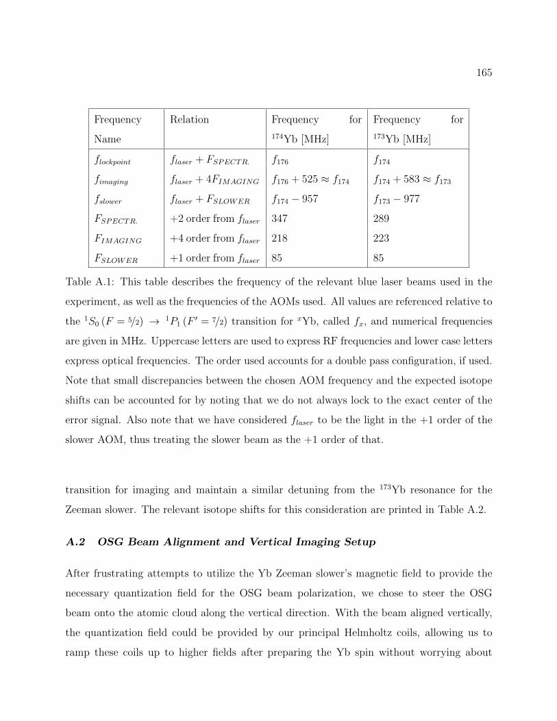
165
Frequency
Name
Relation Frequency for
174Yb [MHz]
Frequency for
173Yb [MHz]
flockpoint flaser + FSPECTR. f176 f174
fimaging flaser + 4FIMAGING f176 + 525 ≈ f174 f174 + 583 ≈ f173
fslower flaser + FSLOWER f174 − 957 f173 − 977
FSPECTR. +2 order from flaser 347 289
FIMAGING +4 order from flaser 218 223
FSLOWER +1 order from flaser 85 85
Table A.1: This table describes the frequency of the relevant blue laser beams used in the
experiment, as well as the frequencies of the AOMs used. All values are referenced relative to
the 1S0 (F = 5/2) → 1P1 (F ′ = 7/2) transition for xYb, called fx, and numerical frequencies
are given in MHz. Uppercase letters are used to express RF frequencies and lower case letters
express optical frequencies. The order used accounts for a double pass configuration, if used.
Note that small discrepancies between the chosen AOM frequency and the expected isotope
shifts can be accounted for by noting that we do not always lock to the exact center of the
error signal. Also note that we have considered flaser to be the light in the +1 order of the
slower AOM, thus treating the slower beam as the +1 order of that.
transition for imaging and maintain a similar detuning from the 173Yb resonance for the
Zeeman slower. The relevant isotope shifts for this consideration are printed in Table A.2.
A.2 OSG Beam Alignment and Vertical Imaging Setup
After frustrating attempts to utilize the Yb Zeeman slower’s magnetic field to provide the
necessary quantization field for the OSG beam polarization, we chose to steer the OSG
beam onto the atomic cloud along the vertical direction. With the beam aligned vertically,
the quantization field could be provided by our principal Helmholtz coils, allowing us to
ramp these coils up to higher fields after preparing the Yb spin without worrying about
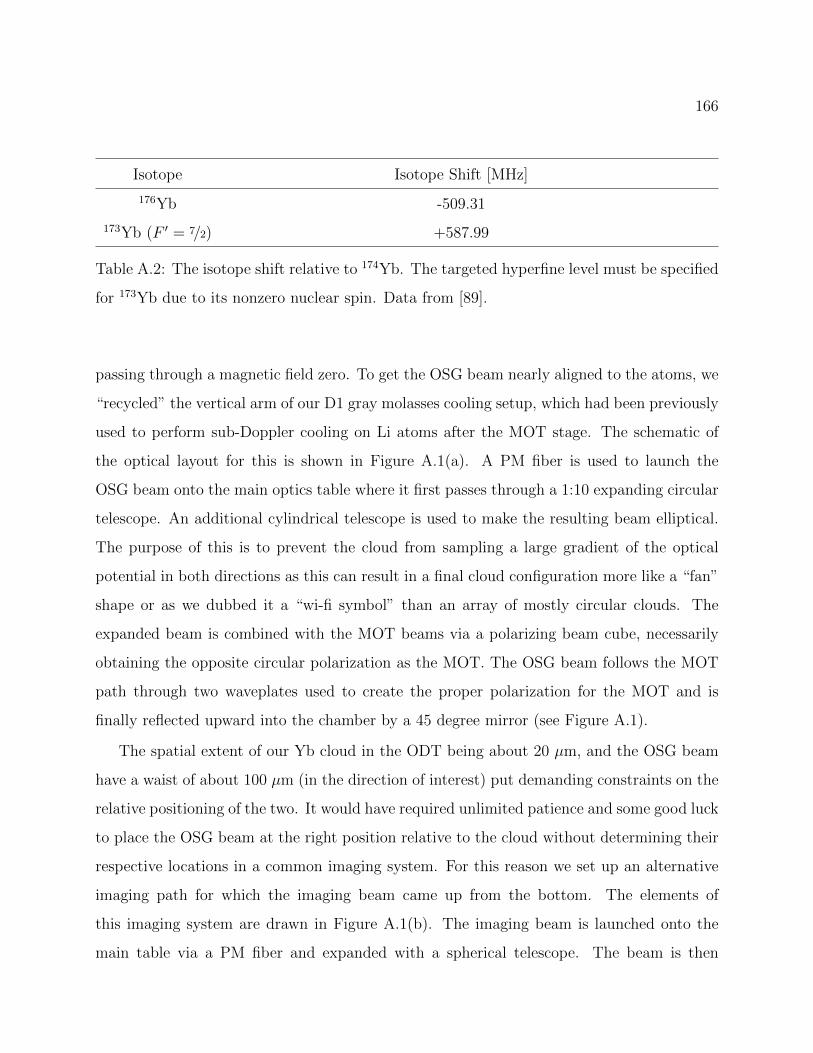
166
Isotope Isotope Shift [MHz]
176Yb -509.31
173Yb (F ′ = 7/2) +587.99
Table A.2: The isotope shift relative to 174Yb. The targeted hyperfine level must be specified
for 173Yb due to its nonzero nuclear spin. Data from [89].
passing through a magnetic field zero. To get the OSG beam nearly aligned to the atoms, we
“recycled” the vertical arm of our D1 gray molasses cooling setup, which had been previously
used to perform sub-Doppler cooling on Li atoms after the MOT stage. The schematic of
the optical layout for this is shown in Figure A.1(a). A PM fiber is used to launch the
OSG beam onto the main optics table where it first passes through a 1:10 expanding circular
telescope. An additional cylindrical telescope is used to make the resulting beam elliptical.
The purpose of this is to prevent the cloud from sampling a large gradient of the optical
potential in both directions as this can result in a final cloud configuration more like a “fan”
shape or as we dubbed it a “wi-fi symbol” than an array of mostly circular clouds. The
expanded beam is combined with the MOT beams via a polarizing beam cube, necessarily
obtaining the opposite circular polarization as the MOT. The OSG beam follows the MOT
path through two waveplates used to create the proper polarization for the MOT and is
finally reflected upward into the chamber by a 45 degree mirror (see Figure A.1).
The spatial extent of our Yb cloud in the ODT being about 20 µm, and the OSG beam
have a waist of about 100 µm (in the direction of interest) put demanding constraints on the
relative positioning of the two. It would have required unlimited patience and some good luck
to place the OSG beam at the right position relative to the cloud without determining their
respective locations in a common imaging system. For this reason we set up an alternative
imaging path for which the imaging beam came up from the bottom. The elements of
this imaging system are drawn in Figure A.1(b). The imaging beam is launched onto the
main table via a PM fiber and expanded with a spherical telescope. The beam is then
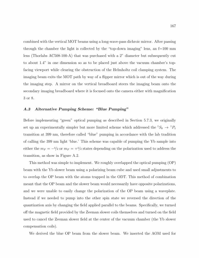
167
combined with the vertical MOT beams using a long-wave-pass dichroic mirror. After passing
through the chamber the light is collected by the “top-down imaging” lens, an f=100 mm
lens (Thorlabs AC508-100-A) that was purchased with a 2” diameter but subsequently cut
to about 1.4” in one dimension so as to be placed just above the vacuum chamber’s top-
facing viewport while clearing the obstruction of the Helmholtz coil clamping system. The
imaging beam exits the MOT path by way of a flipper mirror which is out of the way during
the imaging step. A mirror on the vertical breadboard steers the imaging beam onto the
secondary imaging breadboard where it is focused onto the camera either with magnification
3 or 8.
A.3 Alternative Pumping Scheme: “Blue Pumping”
Before implementing “green” optical pumping as described in Section 5.7.3, we originally
set up an experimentally simpler but more limited scheme which addressed the 1S0 → 1P1
transition at 399 nm, therefore called “blue” pumping in accordance with the lab tradition
of calling the 399 nm light ‘blue.’ This scheme was capable of pumping the Yb sample into
either the mF = −5/2 or mF = +5/2 states depending on the polarization used to address the
transition, as show in Figure A.2.
This method was simple to implement. We roughly overlapped the optical pumping (OP)
beam with the Yb slower beam using a polarizing beam cube and used small adjustments to
to overlap the OP beam with the atoms trapped in the ODT. This method of combination
meant that the OP beam and the slower beam would necessarily have opposite polarizations,
and we were unable to easily change the polarization of the OP beam using a waveplate.
Instead if we needed to pump into the other spin state we reversed the direction of the
quantization axis by changing the field applied parallel to the beams. Specifically, we turned
off the magnetic field provided by the Zeeman slower coils themselves and turned on the field
used to cancel the Zeeman slower field at the center of the vacuum chamber (the Yb slower
compensation coils).
We derived the blue OP beam from the slower beam. We inserted the AOM used for
168
Figure A.1: A schematic representation of the optical paths added to the existing apparatus
in order to perform OSG. (a) shows the combination of the OSG beam with the MOT beam,
as seen looking down onto the optics table and (b) shows the three principal parts of the
vertical imaging system: lower right - imaging beam launch into chamber (top-down view).
Lower left - imaging beam after passing through chamber (side view). Upper - focusing and
magnification optics (top-down view).
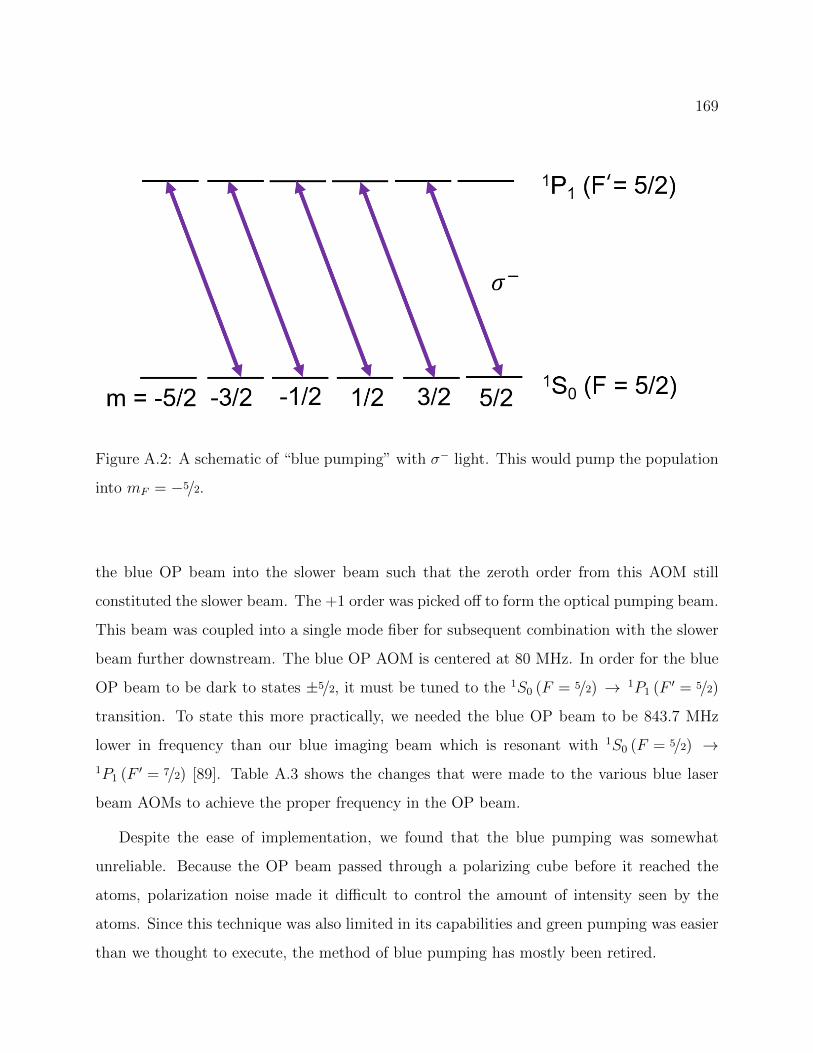
169
‘
Figure A.2: A schematic of “blue pumping” with σ− light. This would pump the population
into mF = −5/2.
the blue OP beam into the slower beam such that the zeroth order from this AOM still
constituted the slower beam. The +1 order was picked off to form the optical pumping beam.
This beam was coupled into a single mode fiber for subsequent combination with the slower
beam further downstream. The blue OP AOM is centered at 80 MHz. In order for the blue
OP beam to be dark to states ±5/2, it must be tuned to the 1S0 (F = 5/2) → 1P1 (F ′ = 5/2)
transition. To state this more practically, we needed the blue OP beam to be 843.7 MHz
lower in frequency than our blue imaging beam which is resonant with 1S0 (F = 5/2) →1P1 (F ′ = 7/2) [89]. Table A.3 shows the changes that were made to the various blue laser
beam AOMs to achieve the proper frequency in the OP beam.
Despite the ease of implementation, we found that the blue pumping was somewhat
unreliable. Because the OP beam passed through a polarizing cube before it reached the
atoms, polarization noise made it difficult to control the amount of intensity seen by the
atoms. Since this technique was also limited in its capabilities and green pumping was easier
than we thought to execute, the method of blue pumping has mostly been retired.
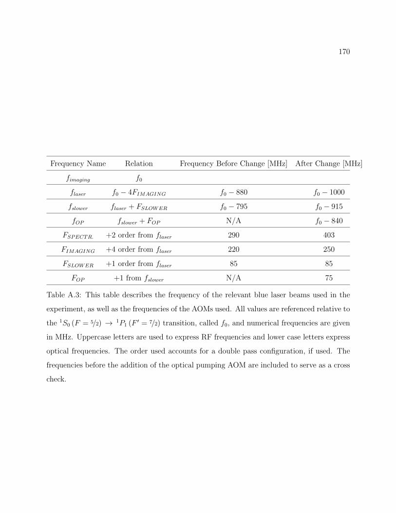
170
Frequency Name Relation Frequency Before Change [MHz] After Change [MHz]
fimaging f0
flaser f0 − 4FIMAGING f0 − 880 f0 − 1000
fslower flaser + FSLOWER f0 − 795 f0 − 915
fOP fslower + FOP N/A f0 − 840
FSPECTR. +2 order from flaser 290 403
FIMAGING +4 order from flaser 220 250
FSLOWER +1 order from flaser 85 85
FOP +1 from fslower N/A 75
Table A.3: This table describes the frequency of the relevant blue laser beams used in the
experiment, as well as the frequencies of the AOMs used. All values are referenced relative to
the 1S0 (F = 5/2) → 1P1 (F ′ = 7/2) transition, called f0, and numerical frequencies are given
in MHz. Uppercase letters are used to express RF frequencies and lower case letters express
optical frequencies. The order used accounts for a double pass configuration, if used. The
frequencies before the addition of the optical pumping AOM are included to serve as a cross
check.
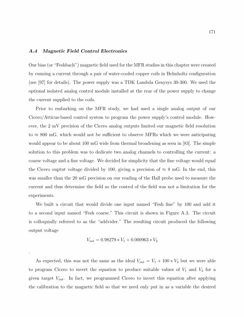
171
A.4 Magnetic Field Control Electronics
Our bias (or “Feshbach”) magnetic field used for the MFR studies in this chapter were created
by running a current through a pair of water-cooled copper coils in Helmholtz configuration
(see [97] for details). The power supply was a TDK Lambda Genysys 30-300. We used the
optional isolated analog control module installed at the rear of the power supply to change
the current supplied to the coils.
Prior to embarking on the MFR study, we had used a single analog output of our
Cicero/Atticus-based control system to program the power supply’s control module. How-
ever, the 2 mV precision of the Cicero analog outputs limited our magnetic field resolution
to ≈ 800 mG, which would not be sufficient to observe MFRs which we were anticipating
would appear to be about 100 mG wide from thermal broadening as seen in [83]. The simple
solution to this problem was to dedicate two analog channels to controlling the current: a
coarse voltage and a fine voltage. We decided for simplicity that the fine voltage would equal
the Cicero ouptut voltage divided by 100, giving a precision of ≈ 8 mG. In the end, this
was smaller than the 20 mG precision on our reading of the Hall probe used to measure the
current and thus determine the field so the control of the field was not a limitation for the
experiments.
We built a circuit that would divide one input named “Fesh fine” by 100 and add it
to a second input named “Fesh coarse.” This circuit is shown in Figure A.3. The circuit
is colloquially referred to as the “addvider.” The resulting circuit produced the following
output voltage
Vout = 0.98279 ∗ V1 + 0.000963 ∗ V2
.
As expected, this was not the same as the ideal Vout = V1 + 100 ∗ V2 but we were able
to program Cicero to invert the equation to produce suitable values of V1 and V2 for a
given target Vout. In fact, we programmed Cicero to invert this equation after applying
the calibration to the magnetic field so that we need only put in as a variable the desired
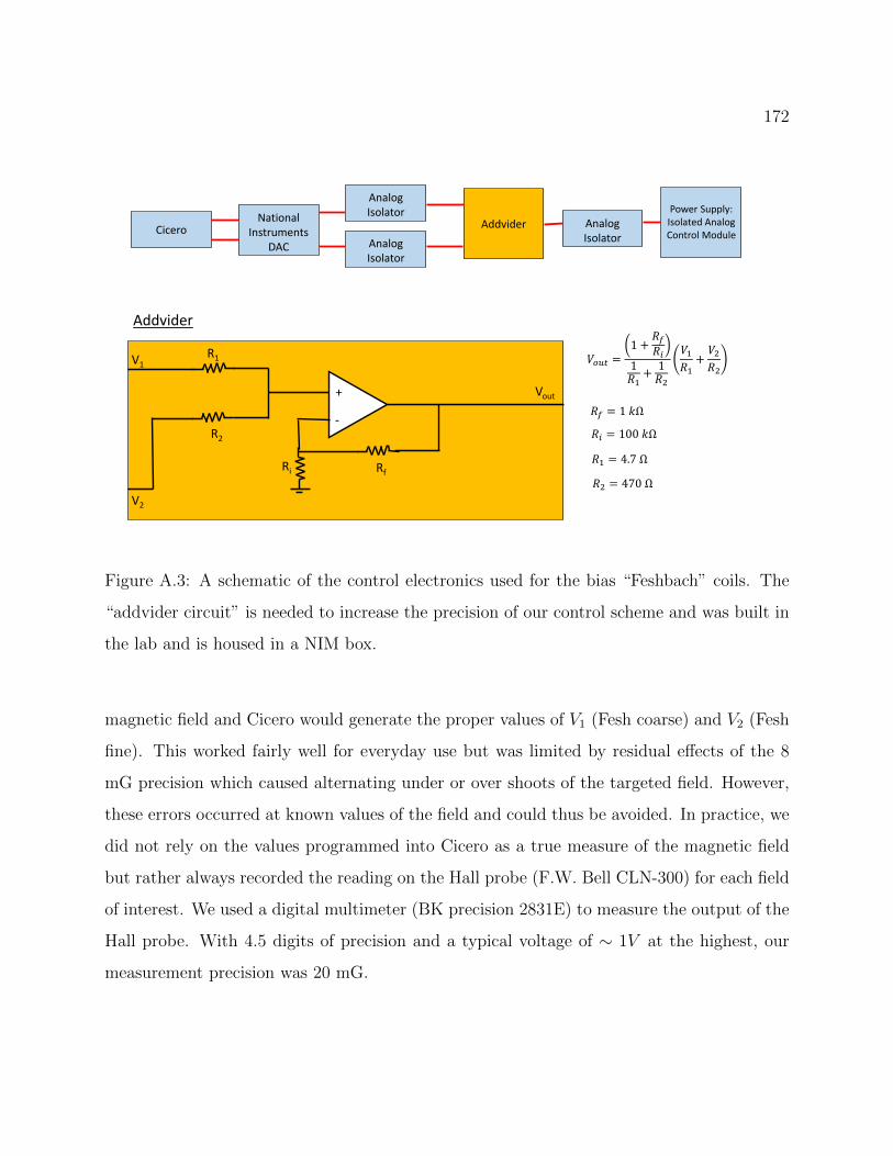
172
AddviderNational
Instruments DAC
Analog Isolator
Analog Isolator
CiceroAnalog Isolator
Power Supply:Isolated Analog Control Module
Addvider
V1
V2
Vout
R1
R2
Ri Rf
+
-
𝑉𝑜𝑢𝑡 =1 +
𝑅𝑓𝑅𝑖
1𝑅1
+1𝑅2
𝑉1𝑅1
+𝑉2𝑅2
𝑅𝑓 = 1 𝑘Ω
𝑅𝑖 = 100 𝑘Ω
𝑅1 = 4.7 Ω
𝑅2 = 470 Ω
Figure A.3: A schematic of the control electronics used for the bias “Feshbach” coils. The
“addvider circuit” is needed to increase the precision of our control scheme and was built in
the lab and is housed in a NIM box.
magnetic field and Cicero would generate the proper values of V1 (Fesh coarse) and V2 (Fesh
fine). This worked fairly well for everyday use but was limited by residual effects of the 8
mG precision which caused alternating under or over shoots of the targeted field. However,
these errors occurred at known values of the field and could thus be avoided. In practice, we
did not rely on the values programmed into Cicero as a true measure of the magnetic field
but rather always recorded the reading on the Hall probe (F.W. Bell CLN-300) for each field
of interest. We used a digital multimeter (BK precision 2831E) to measure the output of the
Hall probe. With 4.5 digits of precision and a typical voltage of ∼ 1V at the highest, our
measurement precision was 20 mG.