c© 2013 by Esteban Meneses Rojas. All rights reserved.

SCALABLE MESSAGE-LOGGING TECHNIQUES FOREFFECTIVE FAULT TOLERANCE IN

HPC APPLICATIONS

BY

ESTEBAN MENESES ROJAS

DISSERTATION

Submitted in partial fulfillment of the requirementsfor the degree of Doctor of Philosophy in Computer Science

in the Graduate College of theUniversity of Illinois at Urbana-Champaign, 2013

Urbana, Illinois

Doctoral Committee:

Professor Laxmikant V. Kale, ChairProfessor Franck CappelloProfessor Michael T. HeathProfessor Nitin H. VaidyaDoctor Greg Bronevetsky, Lawrence Livermore National Laboratory

Abstract

An important set of challenges emerge as the High Performance Computing (HPC) com-

munity aims to reach extreme scale. Resilience and energy consumption are two of those

challenges. Extreme-scale machines are expected to have a high failure frequency. This is

an inevitable consequence of the mismatch between two trends. The number of components

assembled in supercomputers grows exponentially. However, the improvement on the reli-

ability of each individual component is much slower. At the same time, the vast number

of components in a single machine will consume a non-trivial amount of energy. To keep

a supercomputer within operational margins, HPC systems have to be both reliable and

energy-aware. For an application to be able to run and make progress in spite of constant

interruptions, it has to incorporate some fashion of fault tolerance. Rollback-recovery tech-

niques provide a framework to overcome crashes in the system by periodically saving the

state of the application and rolling back to checkpoints in case of failures. Two well-known

rollback-recovery techniques are checkpoint/restart and message-logging. The former is eas-

ier to implement and has become the de facto standard to make applications fault tolerant.

It has, however, a high performance and energy cost during recovery. Message-logging, on

the other hand, makes it possible to recover faster from a failure and to consume less energy.

The downside of message-logging is the overhead it exhibits in the failure-free scenario. Mem-

ory and performance overheads may offset its advantages. This thesis focuses on techniques

to alleviate the downsides of message-logging. It presents a mechanism based on high-level

programming language constructs to decrease the performance overhead of message-logging.

It also introduces two strategies to reduce the memory overhead created by the message

log. Additionally, it addresses important architectural constraints of modern supercomput-

ers. Based on large-scale experimental results and projections from an analytical model, we

conclude message-logging is a promising strategy to provide fault tolerance at a low energy

cost for extreme-scale machines.

ii

To Abuelita Balbina.

For teaching me what resilience means in real life.

iii

Acknowledgments

First and foremost, I want to thank Veronica and Emma for their love, and for the sacrifices

they made when my time and energy were devoted to finishing this thesis. They are my

family, two dimensions of the same love, en la calle, codo a codo, somos mucho mas que dos.

The PhD was the most challenging of all the academic degrees I have worked toward. My

parents were essential in keeping me on the right track all the time. Thanks to Mami, Roger,

Benjo, and Lili for sending me good vibes during my time as a graduate student. Thanks

Mami for letting me walk alone to primary school since I was 7. This is how far I got.

Thanks to Sanjay Kale for being a generous and exemplary advisor. He taught me how

important teamwork is in producing groundbreaking ideas. The philosophy of the PPL,

application-oriented, computer-science centric, is something I will embrace in my academic

career.

My mentors, Celso Mendes and Greg Bronevetsky, played a key role in teaching me fun-

damental things about academia. Celso introduced me to the wonderful world of resilience

in HPC. Greg provided me with constant guidance during my time as a PhD student.

Terry Jones diligently led the Colony II project, which funded a big part of my academic

program. Thanks to that project I was able to spend time working on topics I find extremely

exciting.

My labmates deserve a special mention. I spent many hours with them, shared many

ideas, and discussed many issues. They taught me as many things as the courses did. Xiang

and Osman were great colleagues with whom I worked on developing really exciting ideas.

Nikhil and Jonathan are out-of-this-world ingenious. Phil probably proofread all of my

papers (thanks for embracing such a painful task). I will miss seeing Akhil at 8:00 am in

the morning or seeing Yanhua on Saturdays. Pritish and Lukasz helped me during my first

years as a PPLer. Thanks Ehsan for inviting me to join Persian lunches and the Persian

soccer team, Teraktor power! Abhishek and Harshitha were gentle colleagues with whom I

iv

had numerous conversations about family life. The new generation of PPLers, Ronak, Mike,

and Bilge remind me of my early years in the group. I hope they do not make the same

mistakes I made. Eric and Ram were a good source of feedback.

During my time in grad school, I learned that group studying can be effective if the right

team is assembled. I passed my Qual thanks, in part, to the group of smart guys that

accompanied me in that process. Thank you, Albert and Siva, for such a lesson.

The small latino community in the department was always a constant suport for me. They

were there in difficult times. I was also there to see the big turns life can make sometimes.

Juan and Thyago, thanks for sharing with me this important time in your lives.

My tico friends in town, Roy, Adriana, and Jaffet made the winters warmer, the nights

more tropical and the distant home closer. Thanks guys for always carrying a piece of Costa

Rica with you.

Last but not least, I would like to thank all the people I ran into during my stay in

Urbana-Champaign. I may not remember their names, but they made a difference in one of

the most exciting adventures of my life.

v

Grants

This work was partially supported by the following sources:

• HPC Colony II. This project is funded by the US Department of Energy under grant

DOE DE-SC0001845. The Principal Investigator of this project is Terry Jones.

• XSEDE Allocation. The Parallel Programming Laboratory at the University of Illi-

nois was granted an allocation on XSEDE through award ASC050039N. The Principal

Investigator of this project is Celso Mendes.

• ALCF Allocation. This research used resources of the Argonne Leadership Com-

puting Facility at Argonne National Laboratory, which is supported by the Office of

Science of the U.S. Department of Energy under contract DE-AC02-06CH11357.

vi

Table of Contents

List of Figures . . . . . . . . . . . . . . . . . . . . . . . . . . . . . . . . . . . . . . . ix

List of Tables . . . . . . . . . . . . . . . . . . . . . . . . . . . . . . . . . . . . . . . . xi

List of Algorithms . . . . . . . . . . . . . . . . . . . . . . . . . . . . . . . . . . . . . xii

CHAPTER 1 Introduction . . . . . . . . . . . . . . . . . . . . . . . . . . . . . . . . 11.1 Justification . . . . . . . . . . . . . . . . . . . . . . . . . . . . . . . . . . . . 21.2 Research Challenges . . . . . . . . . . . . . . . . . . . . . . . . . . . . . . . 51.3 Thesis Organization . . . . . . . . . . . . . . . . . . . . . . . . . . . . . . . . 6

CHAPTER 2 Background . . . . . . . . . . . . . . . . . . . . . . . . . . . . . . . . 72.1 Fault Tolerance Goals . . . . . . . . . . . . . . . . . . . . . . . . . . . . . . 92.2 System Model . . . . . . . . . . . . . . . . . . . . . . . . . . . . . . . . . . . 112.3 Checkpoint/Restart . . . . . . . . . . . . . . . . . . . . . . . . . . . . . . . . 122.4 Message-Logging . . . . . . . . . . . . . . . . . . . . . . . . . . . . . . . . . 162.5 Parallel Recovery . . . . . . . . . . . . . . . . . . . . . . . . . . . . . . . . . 212.6 Simple Causal Message-Logging . . . . . . . . . . . . . . . . . . . . . . . . . 232.7 Experimental Results . . . . . . . . . . . . . . . . . . . . . . . . . . . . . . . 282.8 Discussion . . . . . . . . . . . . . . . . . . . . . . . . . . . . . . . . . . . . . 342.9 Related Work . . . . . . . . . . . . . . . . . . . . . . . . . . . . . . . . . . . 34

CHAPTER 3 Fast Message-Logging . . . . . . . . . . . . . . . . . . . . . . . . . . . 383.1 Removing Determinants in Parallel Programs . . . . . . . . . . . . . . . . . 413.2 Fast Message-Logging Protocol . . . . . . . . . . . . . . . . . . . . . . . . . 463.3 Experimental Results . . . . . . . . . . . . . . . . . . . . . . . . . . . . . . . 503.4 Discussion . . . . . . . . . . . . . . . . . . . . . . . . . . . . . . . . . . . . . 533.5 Related Work . . . . . . . . . . . . . . . . . . . . . . . . . . . . . . . . . . . 54

CHAPTER 4 Performance and Energy Models . . . . . . . . . . . . . . . . . . . . . 564.1 Parameters . . . . . . . . . . . . . . . . . . . . . . . . . . . . . . . . . . . . 584.2 Performance Model . . . . . . . . . . . . . . . . . . . . . . . . . . . . . . . . 604.3 Energy Model . . . . . . . . . . . . . . . . . . . . . . . . . . . . . . . . . . . 62

vii

4.4 Large-Scale Projections . . . . . . . . . . . . . . . . . . . . . . . . . . . . . . 644.5 Simulation . . . . . . . . . . . . . . . . . . . . . . . . . . . . . . . . . . . . . 684.6 Discussion . . . . . . . . . . . . . . . . . . . . . . . . . . . . . . . . . . . . . 714.7 Related Work . . . . . . . . . . . . . . . . . . . . . . . . . . . . . . . . . . . 73

CHAPTER 5 Team-based Message-Logging . . . . . . . . . . . . . . . . . . . . . . 745.1 Mining for Communication Clusters . . . . . . . . . . . . . . . . . . . . . . . 775.2 Message-Logging Protocol . . . . . . . . . . . . . . . . . . . . . . . . . . . . 805.3 Team-based Load Balancing . . . . . . . . . . . . . . . . . . . . . . . . . . . 855.4 Experimental Results . . . . . . . . . . . . . . . . . . . . . . . . . . . . . . . 875.5 Discussion . . . . . . . . . . . . . . . . . . . . . . . . . . . . . . . . . . . . . 895.6 Related Work . . . . . . . . . . . . . . . . . . . . . . . . . . . . . . . . . . . 90

CHAPTER 6 Collective-Aware Message-Logging . . . . . . . . . . . . . . . . . . . . 946.1 Message-Logging Protocol . . . . . . . . . . . . . . . . . . . . . . . . . . . . 976.2 Design and Implementation . . . . . . . . . . . . . . . . . . . . . . . . . . . 1056.3 Experimental Results . . . . . . . . . . . . . . . . . . . . . . . . . . . . . . . 1066.4 Discussion . . . . . . . . . . . . . . . . . . . . . . . . . . . . . . . . . . . . . 1086.5 Related Work . . . . . . . . . . . . . . . . . . . . . . . . . . . . . . . . . . . 109

CHAPTER 7 Multicore-Node Message-Logging . . . . . . . . . . . . . . . . . . . . 1117.1 Unit of Failure . . . . . . . . . . . . . . . . . . . . . . . . . . . . . . . . . . 1137.2 Message-Logging Protocol . . . . . . . . . . . . . . . . . . . . . . . . . . . . 1177.3 Analysis of Survivability . . . . . . . . . . . . . . . . . . . . . . . . . . . . . 1207.4 Experimental Results . . . . . . . . . . . . . . . . . . . . . . . . . . . . . . . 1237.5 Discussion . . . . . . . . . . . . . . . . . . . . . . . . . . . . . . . . . . . . . 1257.6 Related Work . . . . . . . . . . . . . . . . . . . . . . . . . . . . . . . . . . . 127

CHAPTER 8 Concluding Remarks . . . . . . . . . . . . . . . . . . . . . . . . . . . 1298.1 Conclusions . . . . . . . . . . . . . . . . . . . . . . . . . . . . . . . . . . . . 1298.2 Contributions . . . . . . . . . . . . . . . . . . . . . . . . . . . . . . . . . . . 1318.3 Future Work . . . . . . . . . . . . . . . . . . . . . . . . . . . . . . . . . . . . 132

APPENDIX A Further Opportunities for Message-Logging . . . . . . . . . . . . . . 135A.1 Application-level Message-Logging . . . . . . . . . . . . . . . . . . . . . . . . 135A.2 Asymmetric-Communication Applications . . . . . . . . . . . . . . . . . . . 138

APPENDIX B Supercomputer Descriptions . . . . . . . . . . . . . . . . . . . . . . 141

APPENDIX C Benchmark Descriptions . . . . . . . . . . . . . . . . . . . . . . . . . 144

REFERENCES . . . . . . . . . . . . . . . . . . . . . . . . . . . . . . . . . . . . . . . 148

viii

List of Figures

1.1 The trend in the size of supercomputers and their associated MTTI . . . . . 21.2 Progress diagram . . . . . . . . . . . . . . . . . . . . . . . . . . . . . . . . . 4

2.1 System model . . . . . . . . . . . . . . . . . . . . . . . . . . . . . . . . . . . 122.2 Coordinated Checkpoint/Restart . . . . . . . . . . . . . . . . . . . . . . . . 152.3 Message-logging with coordinated checkpoint . . . . . . . . . . . . . . . . . . 172.4 Message-logging protocols . . . . . . . . . . . . . . . . . . . . . . . . . . . . 182.5 Latency overhead scenarios in pessimistic message-logging. . . . . . . . . . . 202.6 Parallel recovery in message-logging . . . . . . . . . . . . . . . . . . . . . . . 232.7 Performance overhead of message-logging protocols . . . . . . . . . . . . . . 292.8 Performance overhead of simple causal message-logging . . . . . . . . . . . . 302.9 Overhead in scaling causal message-logging . . . . . . . . . . . . . . . . . . . 312.10 Evaluation of parallel recovery . . . . . . . . . . . . . . . . . . . . . . . . . . 322.11 Power levels with checkpoint/restart . . . . . . . . . . . . . . . . . . . . . . 322.12 Energy profile of different fault-tolerance methods . . . . . . . . . . . . . . . 33

3.1 Performance cost of determinants in LULESH . . . . . . . . . . . . . . . . . 403.2 Program structure of a two-dimensional stencil code . . . . . . . . . . . . . . 433.3 High-level script for program in Figure 3.2 . . . . . . . . . . . . . . . . . . . 453.4 Fast message-logging protocol . . . . . . . . . . . . . . . . . . . . . . . . . . 473.5 Effect of virtualization ratio on performance . . . . . . . . . . . . . . . . . . 513.6 Performance overhead of fast message-logging . . . . . . . . . . . . . . . . . 513.7 Parallel recovery in fast message-logging . . . . . . . . . . . . . . . . . . . . 523.8 Large strong-scale experiment with LULESH . . . . . . . . . . . . . . . . . . 53

4.1 Hierarchical organization of protocols . . . . . . . . . . . . . . . . . . . . . . 574.2 Execution model example. . . . . . . . . . . . . . . . . . . . . . . . . . . . . 604.3 Comparison of performance of fault-tolerance methods at large scale. . . . . 664.4 Comparison of energy consumption of fault-tolerance methods . . . . . . . . 674.5 Comparison of the checkpoint period of different protocols . . . . . . . . . . 684.6 Exploration of the analytical model . . . . . . . . . . . . . . . . . . . . . . . 694.7 Simulation of fault tolerance methods . . . . . . . . . . . . . . . . . . . . . . 704.8 Simulation results of fault tolerance protocols . . . . . . . . . . . . . . . . . 71

ix

5.1 Characteristics of NPB-CG benchmark class B on 64 PEs . . . . . . . . . . . 755.2 Communication graphs of several parallel programs . . . . . . . . . . . . . . 785.3 Team-based message-logging protocol . . . . . . . . . . . . . . . . . . . . . . 805.4 Multilevel load-balancing framework for team formation . . . . . . . . . . . . 865.5 Evaluation of TeamLB with NPB-BT multizone . . . . . . . . . . . . . . . . 885.6 Scale tests for TeamLB . . . . . . . . . . . . . . . . . . . . . . . . . . . . . . 895.7 Performance evaluation of TeamLB . . . . . . . . . . . . . . . . . . . . . . . 90

6.1 Communication volume captured by collective communication operations . . 956.2 Minimizing memory overhead in collective communication operations. . . . . 966.3 Spanning tree for multicast and reduction operations . . . . . . . . . . . . . 986.4 Different failure scenarios for a multicast operation . . . . . . . . . . . . . . 1006.5 Different failure scenarios for a reduction operation . . . . . . . . . . . . . . 1016.6 Implementation of collective-aware message-logging . . . . . . . . . . . . . . 1066.7 Memory overhead reduction in LeanMD with CAML . . . . . . . . . . . . . 1076.8 Memory overhead reduction in OpenAtom with CAML . . . . . . . . . . . . 108

7.1 Adoption of multicore nodes by major supercomputer vendors . . . . . . . . 1127.2 Distribution of failures according to the number of nodes affected . . . . . . 1157.3 Best-fit curves for distributions in Figure 7.1(b) . . . . . . . . . . . . . . . . 1167.4 A multicore-node system and its implications on the design of a message-

logging protocol . . . . . . . . . . . . . . . . . . . . . . . . . . . . . . . . . . 1187.5 Sample execution of an application using the message-logging protocol for

multicore-node systems . . . . . . . . . . . . . . . . . . . . . . . . . . . . . . 1207.6 Different mappings for storing checkpoints and determinants . . . . . . . . . 1217.7 Survival probability to multiple-node crashes for different fault tolerance

protocols . . . . . . . . . . . . . . . . . . . . . . . . . . . . . . . . . . . . . . 1227.8 Performance indicators of message-logging on multicore-node systems . . . . 1257.9 Node-failure correlation in multicore-node systems . . . . . . . . . . . . . . . 127

A.1 Simplified diagram of objects in ChaNGa . . . . . . . . . . . . . . . . . . . . 136A.2 Distributions of average number of requests per iteration on ChaNGa . . . . 137A.3 Different message-logging objects. . . . . . . . . . . . . . . . . . . . . . . . . 139

x

List of Tables

3.1 Number of determinants in different programs. . . . . . . . . . . . . . . . . . 53

4.1 Parameters of performance and energy consumption models . . . . . . . . . 594.2 Baseline values of parameters in the model. . . . . . . . . . . . . . . . . . . . 65

5.1 Edge cut or fraction of total communication that crosses team boundaries . . 795.2 Memory overhead of team-based message-logging . . . . . . . . . . . . . . . 87

7.1 List of supercomputers for which failure information is available . . . . . . . 1147.2 Best-fit functions and errors for distributions of Figure 7.2 . . . . . . . . . . 1167.3 Survivability of different fault tolerance protocols . . . . . . . . . . . . . . . 1247.4 Determinants and messages . . . . . . . . . . . . . . . . . . . . . . . . . . . 1247.5 Relative memory overhead in message-logging . . . . . . . . . . . . . . . . . 1257.6 Lock contention costs . . . . . . . . . . . . . . . . . . . . . . . . . . . . . . . 126

A.1 Average number of requests per iteration in ChaNGa . . . . . . . . . . . . . 138

B.1 Summary of features of supercomputers used in this thesis . . . . . . . . . . 141

C.1 Summary of features of benchmarks used in this thesis . . . . . . . . . . . . 144

xi

List of Algorithms

1 Message send in simple causal message-logging . . . . . . . . . . . . . . . . . 25

2 Message receive in simple causal message-logging . . . . . . . . . . . . . . . 26

3 Acknowledge of determinants in simple causal message-logging . . . . . . . . 26

4 Checkpoint method in simple causal message-logging . . . . . . . . . . . . . 26

5 Restart method in simple causal message-logging . . . . . . . . . . . . . . . 27

6 Message send in fast message-logging . . . . . . . . . . . . . . . . . . . . . . 48

7 Message receive in fast message-logging . . . . . . . . . . . . . . . . . . . . . 48

8 Checkpoint method in fast message-logging . . . . . . . . . . . . . . . . . . . 49

9 Restart method in fast message-logging . . . . . . . . . . . . . . . . . . . . . 49

10 Parallel recovery fast message-logging . . . . . . . . . . . . . . . . . . . . . . 49

11 Message send in team-based message-logging . . . . . . . . . . . . . . . . . . 82

12 Message receive in team-based message-logging . . . . . . . . . . . . . . . . . 83

13 Ackowledge of determinants in team-based message-logging . . . . . . . . . . 83

14 Checkpoint method in team-based message-logging . . . . . . . . . . . . . . 83

15 Restart method in team-based message-logging . . . . . . . . . . . . . . . . . 83

16 Multicast send in collective-aware message-logging . . . . . . . . . . . . . . . 102

17 Multicast receive in collective-aware message-logging . . . . . . . . . . . . . 103

18 Reduction send in collective-aware message-logging . . . . . . . . . . . . . . 103

19 Reduction receive in collective-aware message-logging . . . . . . . . . . . . . 104

20 Restart method in collective-aware message-logging . . . . . . . . . . . . . . 104

21 Garbage collection method in collective-aware message-logging . . . . . . . . 104

22 Accumulating determinants in multicore message-logging . . . . . . . . . . . 119

23 Piggybacking determinants in multicore message-logging . . . . . . . . . . . 119

24 Acknowledging determinants in multicore message-logging . . . . . . . . . . 119

xii

CHAPTER 1Introduction

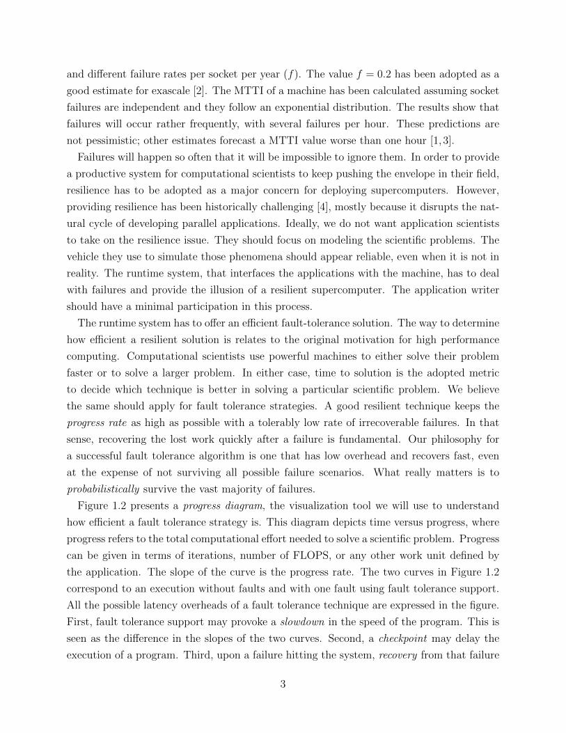
Self-healing materials are among the most amazing engineering inventions. These bio-

inspired polymers have the ability to recover from a crack, or snap back after a puncture,

reestablishing the original structural properties of the material. It is not a surprise that space

agencies are very interested in materials with self-healing properties. Building a spacecraft

with such materials will make missions to outer space safer. Otherwise, fast-moving debris

may hit the spaceship and jeopardize the goals of the mission. With such a resilient cover,

the astronauts can be safe and free to focus on the fundamental goal of the trip: explore the

unknown portions of the Universe.

The same way astronauts use a spaceship to get to previously hidden places outside our

planet, many computational scientists rely on supercomputers to extend the body of knowl-

edge in their research area. A supercomputer is sometimes their vehicle to find groundbreak-

ing facts about Nature. It used to be the case that supercomputers were highly resilient.

They had low failure rates and crashes were considered a rarity. However, as we approach

exascale and the size of the machines increases substantially, the tenet of reliable supercom-

puters will fall and what is currently the former rarity will most likely become the standard.

A machine at exascale will face frequent failures. The high performance computing (HPC)

community, and particularly the system builders, must provide computational scientists with

the illusion of a self-healing supercomputer. The same way smart materials let astronauts

concentrate on their work by providing a safe spaceship, resilience protocols in supercomput-

ers should allow computational scientists to concentrate on extending the frontiers of what

we know and keep enjoying the wonderful journey of Science.

1

1.1 Justification

Computational scientists are among the main users of high performance parallel computing.

They usually run codes to simulate a physical process. Their programs use models that can

be accurate enough to avoid running an experiment in real life. Running an experiment in

real life may sometimes be too costly. Additionally, models can predict what will happen in

different scenarios that may be infeasible to replicate in reality. In applications that range

from molecular dynamics to weather forecasting, computational scientists are always ready

to consume as many FLOPS as a machine can provide.

In order to satisfy the demand for faster supercomputers, the architects of these machines

relied on three major factors during the last decades: Moore’s Law, increase in the clock

frequency and an increment in the number of sockets per machine. As Moore’s Law comes

to an end, and the clock speed has stagnated, the main source to boost the performance in

a supercomputer is the number of sockets.

1000

10000

100000

1e+06

1994 1998 2002 2006 2010 2014 2018 2022

Num

ber

of

Sockets

Year

Exascale

(a) Historical view of the number of sockets in thetop 10 largest systems. An exascale machine is ex-pected to have more than 200,000 sockets and to beavailable between 2018-2022.

3

5

13

26

52

131

262

200K 500K 1M

Machin

e M

TT

I (m

inute

s)

Number of Sockets

f=0.01f=0.02f=0.05f=0.10f=0.20

(b) MTTI of a machine for various failure rates (f)per socket. An exascale machine is expected to faceseveral failures per hour.

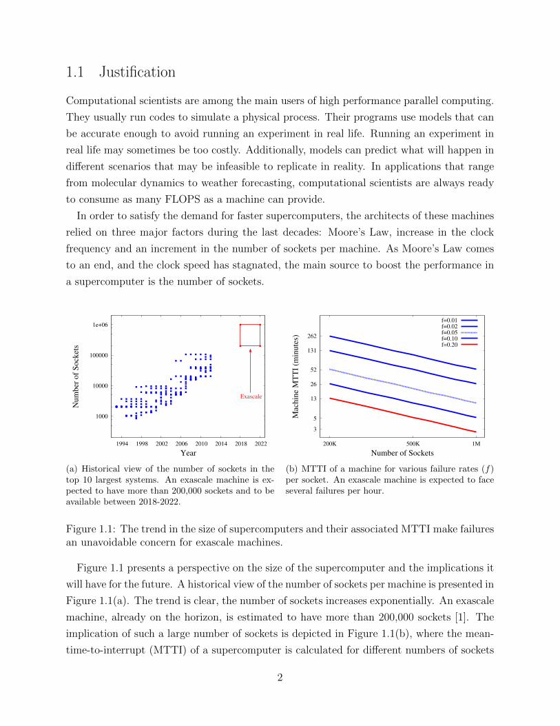
Figure 1.1: The trend in the size of supercomputers and their associated MTTI make failuresan unavoidable concern for exascale machines.

Figure 1.1 presents a perspective on the size of the supercomputer and the implications it

will have for the future. A historical view of the number of sockets per machine is presented in

Figure 1.1(a). The trend is clear, the number of sockets increases exponentially. An exascale

machine, already on the horizon, is estimated to have more than 200,000 sockets [1]. The

implication of such a large number of sockets is depicted in Figure 1.1(b), where the mean-

time-to-interrupt (MTTI) of a supercomputer is calculated for different numbers of sockets

2

and different failure rates per socket per year (f). The value f = 0.2 has been adopted as a

good estimate for exascale [2]. The MTTI of a machine has been calculated assuming socket

failures are independent and they follow an exponential distribution. The results show that

failures will occur rather frequently, with several failures per hour. These predictions are

not pessimistic; other estimates forecast a MTTI value worse than one hour [1, 3].

Failures will happen so often that it will be impossible to ignore them. In order to provide

a productive system for computational scientists to keep pushing the envelope in their field,

resilience has to be adopted as a major concern for deploying supercomputers. However,

providing resilience has been historically challenging [4], mostly because it disrupts the nat-

ural cycle of developing parallel applications. Ideally, we do not want application scientists

to take on the resilience issue. They should focus on modeling the scientific problems. The

vehicle they use to simulate those phenomena should appear reliable, even when it is not in

reality. The runtime system, that interfaces the applications with the machine, has to deal

with failures and provide the illusion of a resilient supercomputer. The application writer

should have a minimal participation in this process.

The runtime system has to offer an efficient fault-tolerance solution. The way to determine

how efficient a resilient solution is relates to the original motivation for high performance

computing. Computational scientists use powerful machines to either solve their problem

faster or to solve a larger problem. In either case, time to solution is the adopted metric

to decide which technique is better in solving a particular scientific problem. We believe

the same should apply for fault tolerance strategies. A good resilient technique keeps the

progress rate as high as possible with a tolerably low rate of irrecoverable failures. In that

sense, recovering the lost work quickly after a failure is fundamental. Our philosophy for

a successful fault tolerance algorithm is one that has low overhead and recovers fast, even

at the expense of not surviving all possible failure scenarios. What really matters is to

probabilistically survive the vast majority of failures.

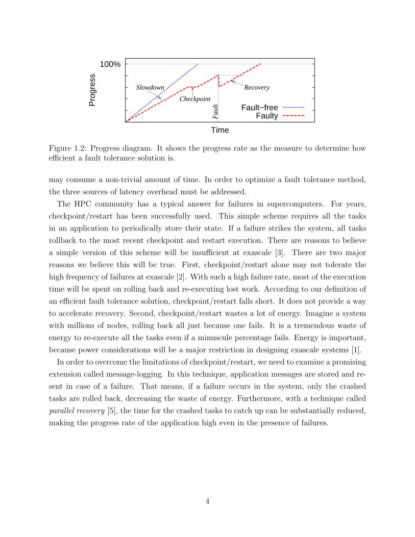
Figure 1.2 presents a progress diagram, the visualization tool we will use to understand

how efficient a fault tolerance strategy is. This diagram depicts time versus progress, where

progress refers to the total computational effort needed to solve a scientific problem. Progress

can be given in terms of iterations, number of FLOPS, or any other work unit defined by

the application. The slope of the curve is the progress rate. The two curves in Figure 1.2

correspond to an execution without faults and with one fault using fault tolerance support.

All the possible latency overheads of a fault tolerance technique are expressed in the figure.

First, fault tolerance support may provoke a slowdown in the speed of the program. This is

seen as the difference in the slopes of the two curves. Second, a checkpoint may delay the

execution of a program. Third, upon a failure hitting the system, recovery from that failure

3

100%

Pro

gres

s

Time

Slowdown

Checkpoint

Recovery

Fau

lt Fault−freeFaulty

Figure 1.2: Progress diagram. It shows the progress rate as the measure to determine howefficient a fault tolerance solution is.

may consume a non-trivial amount of time. In order to optimize a fault tolerance method,

the three sources of latency overhead must be addressed.

The HPC community has a typical answer for failures in supercomputers. For years,

checkpoint/restart has been successfully used. This simple scheme requires all the tasks

in an application to periodically store their state. If a failure strikes the system, all tasks

rollback to the most recent checkpoint and restart execution. There are reasons to believe

a simple version of this scheme will be insufficient at exascale [3]. There are two major

reasons we believe this will be true. First, checkpoint/restart alone may not tolerate the

high frequency of failures at exascale [2]. With such a high failure rate, most of the execution

time will be spent on rolling back and re-executing lost work. According to our definition of

an efficient fault tolerance solution, checkpoint/restart falls short. It does not provide a way

to accelerate recovery. Second, checkpoint/restart wastes a lot of energy. Imagine a system

with millions of nodes, rolling back all just because one fails. It is a tremendous waste of

energy to re-execute all the tasks even if a minuscule percentage fails. Energy is important,

because power considerations will be a major restriction in designing exascale systems [1].

In order to overcome the limitations of checkpoint/restart, we need to examine a promising

extension called message-logging. In this technique, application messages are stored and re-

sent in case of a failure. That means, if a failure occurs in the system, only the crashed

tasks are rolled back, decreasing the waste of energy. Furthermore, with a technique called

parallel recovery [5], the time for the crashed tasks to catch up can be substantially reduced,

making the progress rate of the application high even in the presence of failures.

4

1.2 Research Challenges

Message-logging can potentially overcome the two major limitations of checkpoint/restart.

If failures are frequent, it can substantially reduce the total energy spent in the computation.

Additionally, it can recover faster from a failure, reducing the execution time. There are,

however, several limitations and challenges before this technique can be widely adopted.

The first problem to solve is the latency overhead. Message-logging requires handling

meta-data about messages to guarantee a correct recovery from a failure. Depending on

the characteristics of the application, the amount of meta-data and the required time to

process it may be onerous. Furthermore, popular parallel programming constructions, such

as collectives, aggravate this problem [6]. The main challenge is to find a way to reduce

the amount of meta-data required for a consistent recovery. That way, the latency overhead

can be reduced or even overlapped with communication delays. Also, it is important to

understand how the overhead behaves to avoid those cases where it peaks. Control flow in

an application should be considered in order to minimize the amount of meta-data needed.

A major criticism to message-logging is its obvious drawback: memory overhead. If mes-

sages have to be stored to be re-sent in case of a failure, then those messages can potentially

consume a great deal of memory. A trade-off must be found to alleviate memory pressure in

message-logging. Is it possible to design a protocol that stores only a subset of the messages?

Not storing some messages may result in a higher cost at recovery. For instance, more tasks

may need to get rolled back. However, if properly done, it could dramatically reduce memory

consumption at a relatively small cost. It is necessary to explore the communication graph of

an application and use that information to create that trade-off. Also, parallel programming

constructs must be analyzed in order to decrease memory requirements.

As multicore nodes are becoming the building blocks of parallel machines, it is important

to understand how this architecture affects the design of message-logging protocols. A

fundamental challenge is to determine the granularity at which machines fail. Finding an

appropriate failure unit will determine how the protocols are built and what guarantees

are provided. A multicore node has shared memory among the constituting cores and that

resource has to be used to improve the resiliency and performance of the message-logging

protocol.

A way to predict the performance of message-logging for different scenarios is instrumental

in understanding the impact of the different optimizations. A performance model that

incorporates all the different sources of overhead and speedup can shed some light on the

potential of message-logging for exascale. At the same time, it may categorize applications

according to how suitable message-logging is for them.

5

1.3 Thesis Organization

This thesis is organized in three major parts. Part one contains chapters 2, 3 and 4. This

part introduces all the necessary theoretical background and justifies why message-logging

is a promising technique to provide fault tolerance at scale. Chapter 2 presents a survey of

the background work for this thesis. It focuses on the migratable-objects model for parallel

programming and how various resilience methods have been implemented. Experimental

results on the various approaches are presented, including execution time and energy mea-

surements. Chapter 3 shows how message-logging can be implemented efficiently and how

it can be scaled. Next, Chapter 4 offers both a performance and energy model for check-

point/restart, message-logging and parallel recovery.

Part two of the thesis contains chapters 5, 6 and 7. It presents a series of optimizations that

make message-logging a more usable approach. Chapter 5 introduces the first protocol of a

set of strategies to decrease memory pressure in message-logging. It starts with a technique

that trades off memory consumption for recovery cost. It does it by creating teams of nodes

and treating each team as a recovery unit. The next strategy is presented in Chapter 6.

It shows a protocol for collective communication operations and how memory overhead is

reduced in that case. The new features of multicore systems are addressed in Chapter 7 and

a new protocol is shown. That chapter also contains a discussion on the appropriate unit of

failure and a reliability analysis for real-world data.

The last part of the thesis contains Chapter 8 and Appendix A. In Chapter 8 we present

the conclusions of the work on the thesis as well as a list of promising future work. A

couple of opportunities to further explore the potential of message-logging are presented in

Appendix A. The first idea relates to performing message-logging at the application level.

The second idea deals with certain types of applications where communication is asymmetric

and a different trade-off can be made.

6

CHAPTER 2Background

Fault tolerance has been a constant concern in computer systems. From the very beginning

of the field, the processing of information on a faulty infrastructure was a common concern.

A good example of this is the way Shannon’s theorem was incorporated in many areas

of computer science, ranging from communications to data storage. Shannon’s theorem

determines the maximum rate at which data can be transmitted over a channel that has a

given degree of noise and data corruption. It is a fundamental concept in Information Theory

because it provides a key insight on what type of techniques should be used to effectively

communicate over a faulty medium.

The memory hierarchy provides a couple additional examples that illustrate the integration

of fault tolerance into the design of computer systems. The redundant array of independent

disks (RAID) offers a fault-tolerant method for secondary storage. RAID consists in assem-

bling different disk drives into a single logical storage unit [7]. RAID has different levels,

depending on the degree of reliability. Naturally, each increase in reliability comes at the

expense of decreased efficiency in space or a decrease in performance. As for main memory,

error correcting codes (ECC) have been found to be successful in alleviating the impact of

soft errors. These errors appear when electrical or magnetic interference cause a bit in main

memory to flip, creating a potential error in the data of the application. An ECC memory

works by adding redundant bits to detect and, in some cases, correct soft errors in memory.

More recently, the deployment of large-scale services over distributed systems has brought

resilience into the picture. A remarkable example can be found in peer-to-peer platforms

that implement distributed hash tables [8, 9]. These data structures are a cornerstone in

building file sharing services. One salient feature of peer-to-peer systems is the dynamical

nature in the membership of its components. Computers participating in the system may

connect intermittently. Thus, peer-to-peer systems must handle a high churn in its members.

7

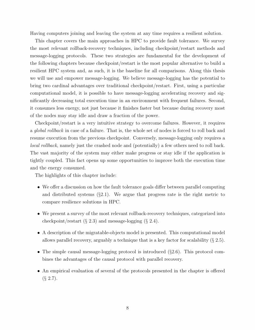
Having computers joining and leaving the system at any time requires a resilient solution.

This chapter covers the main approaches in HPC to provide fault tolerance. We survey

the most relevant rollback-recovery techniques, including checkpoint/restart methods and

message-logging protocols. These two strategies are fundamental for the development of

the following chapters because checkpoint/restart is the most popular alternative to build a

resilient HPC system and, as such, it is the baseline for all comparisons. Along this thesis

we will use and empower message-logging. We believe message-logging has the potential to

bring two cardinal advantages over traditional checkpoint/restart. First, using a particular

computational model, it is possible to have message-logging accelerating recovery and sig-

nificantly decreasing total execution time in an environment with frequent failures. Second,

it consumes less energy, not just because it finishes faster but because during recovery most

of the nodes may stay idle and draw a fraction of the power.

Checkpoint/restart is a very intuitive strategy to overcome failures. However, it requires

a global rollback in case of a failure. That is, the whole set of nodes is forced to roll back and

resume execution from the previous checkpoint. Conversely, message-logging only requires a

local rollback, namely just the crashed node and (potentially) a few others need to roll back.

The vast majority of the system may either make progress or stay idle if the application is

tightly coupled. This fact opens up some opportunities to improve both the execution time

and the energy consumed.

The highlights of this chapter include:

• We offer a discussion on how the fault tolerance goals differ between parallel computing

and distributed systems (§2.1). We argue that progress rate is the right metric to

compare resilience solutions in HPC.

• We present a survey of the most relevant rollback-recovery techniques, categorized into

checkpoint/restart (§ 2.3) and message-logging (§ 2.4).

• A description of the migratable-objects model is presented. This computational model

allows parallel recovery, arguably a technique that is a key factor for scalability (§ 2.5).

• The simple causal message-logging protocol is introduced (§2.6). This protocol com-

bines the advantages of the causal protocol with parallel recovery.

• An empirical evaluation of several of the protocols presented in the chapter is offered

(§ 2.7).

8

2.1 Fault Tolerance Goals

One of the most popular terms related to fault tolerance is RAS [10]. It stands for reliability,

availability and serviceability and it was initially introduced by IBM to describe a robust

mainframe computer. RAS provides a scale in which high levels of RAS represent a highly

assured system, guaranteeing data integrity and the possibility of access the system for long

and uninterrupted periods of time.

To better understand the RAS guarantees, let us define the three pillar terms:

Reliability is a function that expresses the probability of the system to survive during a

particular time period [11]. To increase the reliability of a system, different techniques

aim at avoiding, detecting and repairing component failures. A reliable system must

always provide an error free operations. Thus, if the system detects an error, it will

try to fix the error by retrying the set of operations that went wrong. If it cannot fix

the error, it will halt and declare a fatal error has occurred. At that point, manual

intervention will be required to bring the system back up. This definition represents

reliability as a function of time, therefore a typical measure used is mean-time-to-failure

(MTTF).

Availability is the fraction of the time the system is up for use. In real systems, after a fatal

error occurs, the system is inspected and some components are replaced or repaired.

Eventually, the system is brought up again and continues providing the service. Thus,

if the system is not operational, it will reduce the availability. Sometimes, the system

may continue its operation without the failed component, but at a reduced capacity.

This will increase availability at the cost of efficiency.

Serviceability is the easiness with which a system can be repaired. Serviceability is also

known as maintainability. Among the methods to reduce the repair time, there are

early detection and fast diagnosing mechanisms. These methods aim at decreasing

the down time of the system and lower the cost of manual intervention to repair the

components.

The RAS principles have been applied to a wide range of areas in computer systems, from

databases to processors. RAS represents a common ground to understand how robust a

system is.

In distributed systems, the reliability goals adopt a slightly different form [12]. The

first concern is recoverability or the ability of the system to automatically restart after a

failure. The second concern is continuous availability or the ability of the system to continue

9

providing correct results despite the failure of a limited number of components. The rest

of operational components guarantee a consistent behavior and avoid a down time of the

system. This last objective sets the research direction of reliability in distributed systems.

The major goal is to avoid a fatal crash of the system by tolerating the failure of up to t

components. The larger t, the more reliable the system is, because there are fewer cases that

bring down the system into a catastrophic crash.

We believe that the same set of goals should not be applied to evaluate the reliability

solutions in high performance computing. The major goal of a supercomputer is not so

much to provide a highly available service, but to speed up the computational programs of

the users. Most of the jobs on a supercomputer are run offline, which means sacrificing a

little of response time is not going to have a huge impact on the satisfaction of the users.

In fact, users of HPC installations usually have a limited amount of computational units to

use. This allocation time must be carefully budgeted to make the best use of precious time

on the supercomputer. Therefore, accelerating their code is still the main goal in HPC.

In a faulty HPC environment the goal should remain the same, i.e., to finish the execution

as soon as possible despite frequent component failures. Therefore, we propose progress

rate as the metric to compare and evaluate fault tolerance solutions in HPC. Average time to

completion and not reliability should be the main focus when designing new fault tolerance

solutions. Since there is a tradeoff between making a system more robust to different failures

taking down up to t components and running the application fast, speedup should be the

fundamental consideration. This approach does not mean that reliability should be ignored

altogether. Rather, fault tolerance techniques should provide a level of reliability above a

reasonable threshold. Therefore, the probability of an unrecoverable failure must be small.

Additionally, with extreme scale systems on the horizon, energy consumption and power

management considerations become more prevalent. Our philosophy is that a successful fault

tolerance mechanism in HPC should decrease the average execution time of an application

subject to the power limitations.

The distributed systems community has worked on reliability for several decades. In

that time frame, they have built a significant body of knowledge on the topic, including

many implementations, models and studies. It is natural to port that knowledge into high

performance computing, which has not dealt with reliability as much time. However, there

is a risk in blindly adopting the same reliability techniques, because the goals of the two

areas are different and so must be the kind of tools.

10

2.2 System Model

We assume a parallel application is divided into a set Γ of G tasks. There is no global

shared memory in the application. Each task has its own private memory to store part of

the application’s data. The only way to share information between tasks is through message

exchange. We assume the underlying machine is composed of a set Σ of S nodes. The nodes

are connected through a network that delivers messages in-order between any pair of nodes.

The network is reliable, but latency is unbounded.

The tasks are distributed among the nodes with potentially more than one task per node.

This is G ≥ S. When a nodes crashes, all the tasks residing on that node are lost and

their state must be recovered from another entity in the system, either other node or the

storage system. Although there are several components that can fail in the system, we will

only consider node crashes. A node failure is defined as a behavior that deviates from that

required by the specifications [11]. If a node can not provide the service it is supposed to,

the system can detect that failure. A failure is typically the manifestation of an error. An

error is a deviation from correctness or accuracy in the state of a component. It is usually

caused by a fault. Faults are usually physical defects or flaws in hardware or software.

A failure in the system will render one or more nodes unusable. In other words, we follow

the fail-stop model, where the failed component ceases to work and never comes back. We

assume the underlying machine has a pool of spare nodes that will replace the failed ones.

That way, a failed task can be relaunched in one fresh node. We will call forward path any

portion of the execution that does not include a failure. This concept will be important,

given that different fault tolerance strategies present a tradeoff between overhead in the

forward path and a slowdown during recovery.

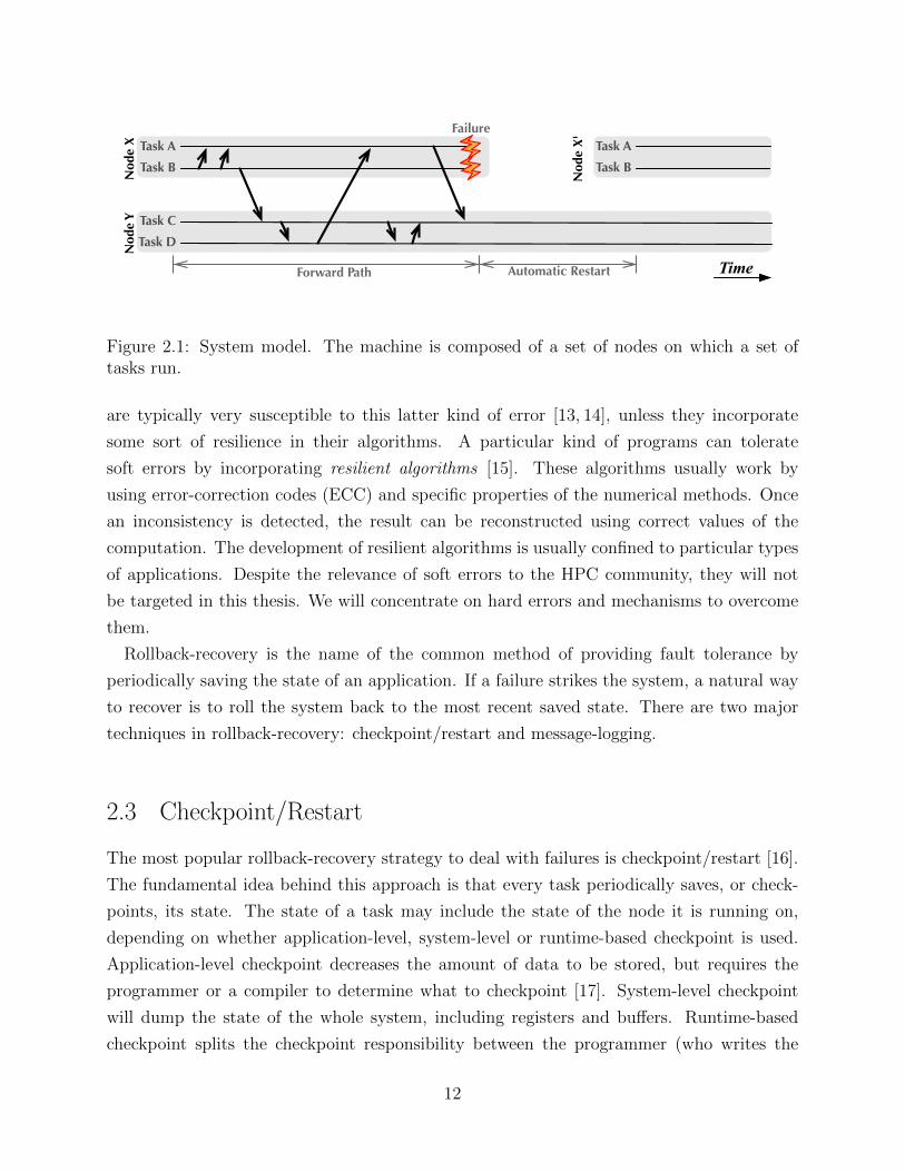
Figure 2.1 presents an example of the system model where a machine has 2 nodes (X and

Y ) and a set of 4 tasks (A, B, C and D). Tasks A and B execute on node X, while tasks C

and D on Y . The arrows in the figure represent messages exchanged between the tasks. The

forward path corresponds to the time period between the start of the execution until the

first failure. Once node X crashes, the runtime system will automatically find a replacement

for X. In this case, node X ′ takes over all the responsibility of X, including tasks A and B.

The fail-stop model is a good representation of hard errors, which implies a component

breaks and suffers a permanent physical change. The system can not continue with the

execution of the application until the component is replaced. A different type of failures,

called soft errors occur when there is an fault in the system, but the system may still be

completely functional and able to finish execution. An example of a soft failure is a bit-

flip in a memory region. Cosmic rays may cause this type of phenomenon. Applications

11

Time

Task A

Task B

Task C

Task D

Automatic RestartForward Path

Task A

Task B

FailureN

ode

XN

ode

Y

Node

X'

Figure 2.1: System model. The machine is composed of a set of nodes on which a set oftasks run.

are typically very susceptible to this latter kind of error [13, 14], unless they incorporate

some sort of resilience in their algorithms. A particular kind of programs can tolerate

soft errors by incorporating resilient algorithms [15]. These algorithms usually work by

using error-correction codes (ECC) and specific properties of the numerical methods. Once

an inconsistency is detected, the result can be reconstructed using correct values of the

computation. The development of resilient algorithms is usually confined to particular types

of applications. Despite the relevance of soft errors to the HPC community, they will not

be targeted in this thesis. We will concentrate on hard errors and mechanisms to overcome

them.

Rollback-recovery is the name of the common method of providing fault tolerance by

periodically saving the state of an application. If a failure strikes the system, a natural way

to recover is to roll the system back to the most recent saved state. There are two major

techniques in rollback-recovery: checkpoint/restart and message-logging.

2.3 Checkpoint/Restart

The most popular rollback-recovery strategy to deal with failures is checkpoint/restart [16].

The fundamental idea behind this approach is that every task periodically saves, or check-

points, its state. The state of a task may include the state of the node it is running on,

depending on whether application-level, system-level or runtime-based checkpoint is used.

Application-level checkpoint decreases the amount of data to be stored, but requires the

programmer or a compiler to determine what to checkpoint [17]. System-level checkpoint

will dump the state of the whole system, including registers and buffers. Runtime-based

checkpoint splits the checkpoint responsibility between the programmer (who writes the

12

checkpoint method for the tasks) and the runtime system (which checkpoint all the internal

data structures).

If the system experiences a failure, all the tasks roll back to the most recent checkpoint

and restart from there. There are two major issues that should be addressed. First, there

is a question of how often to checkpoint. The optimum checkpoint period depends, among

other things, on the MTTF of the machine and the time to checkpoint. The specifics of how

to compute the best checkpoint interval can be found elsewhere [18, 19]. The second point

is how to guarantee a consistent state when checkpointing. There are two options on this

regard, the checkpoint can be either uncoordinated or coordinated.

In uncoordinated checkpoint, each task checkpoints at its own frequency, without synchro-

nizing with the rest of the system. However, a failure may require the rollback of multiple

checkpoint periods. Imagine that a task A sends message m to task B. If A sends the

message before it checkpoints and B receives the message after it checkpoints, the message

is called in-flight. If both tasks roll back to the previous checkpoint, it will make the system

inconsistent, since B would wait for a message that will never come. In that case, to get A to

resend the message will require forcing it to rollback to an older checkpoint. This reasoning

can lead to a cascading rollback until a consistent state is obtained. There is no bound in

the number of checkpoint periods that must be rolled back and it exists the possibility that

a single error may roll back the whole application to the very start of the execution.

Coordinated checkpoint, instead, guarantees that no cascading rollback will occur in any

failure. In order to achieve this, it avoids in-flight messages and other types of inconsistencies.

All tasks have to checkpoint a global but consistent state. There are two major approaches

for this: blocking and non-blocking. The former case implies that all tasks must come to a

halt and wait until all outgoing messages have been received. At that point, the state of the

tasks is safely stored. The non-blocking case is based on an algorithm that does not interrupt

the execution of the application, but instead uses markers to initiate a global snapshot of

the system [20]. Those markers are propagated across the entire system and the algorithm

guarantees that the set of states is globally consistent. A comparison of these two versions

of coordinated checkpoint can be found in other sources [21].

A coordinated checkpoint can be achieved through looking at some properties of the

application. For instance, barrier operations require all tasks to reach a point without

letting any task continue execution before every other task has reached the barrier. Barriers

and other synchronization operations are commonly used in HPC applications. If those

synchronization points are used to trigger checkpoint, then a synchronized checkpoint is

obtained.

Usually, each task will store its checkpoint in stable storage. However, saving the state

13

to disk (particularly if NFS is used) may congest the file servers and delay the checkpoint.

A way to reduce the jitter to the file system is by aggregating writes at a node level and

submitting one single write operation [22]. Another approach to reduce the checkpoint

bandwidth is to have tasks performing incremental checkpoint [23]. Under this approach,

after a task saves its full checkpoint, it may submit a differential checkpoint with only the

portions of the data that have changed since the last checkpoint. Using all those incremental

changes, the system may reconstruct the latest state of a task. It is possible to build a hybrid

scheme, combining full and incremental checkpoints. Such a scheme has been applied to HPC

applications [24]. In the hybrid scheme, a task will occasionally perform a full checkpoint.

Between full checkpoints, it will just do an incremental checkpoint. A combination of both

types of checkpoints reduces bandwidth consumption and storage requirements.

Another possibility to alleviate the problem of making disks a bottleneck is to use dou-

ble in-memory checkpointing [25]. The fundamental assumption is that system memory

is enough to hold the application’s data and the checkpoint. Recent studies suggest that

HPC applications do not exhaust the physical memory [26]. Under this approach, each task

checkpoints its state into the memory of two nodes. One is the local node on which it is

running. The other is the checkpoint buddy of the local node. Then, if a node fails, the

system will relaunch the tasks of the failed node on a replacement node. After that, the

runtime system will get the checkpoint from the buddy node. All other tasks in the system

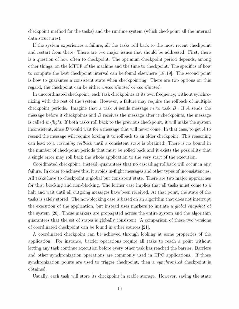
retrieve their checkpoint from the local node. Figure 2.2 shows an example of how double

in-memory checkpoint/restart works. There are four tasks in this case and they checkpoint

in coordination. The collection of all those checkpoints is called a recovery line. Imagine the

application sends some messages between tasks before a failure hits node X. At that point,

the runtime system detects the failure and proceeds to react to that failure. We call restart

interval the time lapse between the failure detection and the point where all tasks are ready

to resume execution. That time includes relaunching the tasks on another physical node

and retrieving the checkpoints. Since we assume spare computational nodes, tasks A and B

are relaunched on a free physical node and they get their checkpoints from the checkpoint

buddy (node Y in this example). Once all tasks are ready to continue with execution, then

recovery starts and this phase lasts until all the work lost due to the failure is redone. Note

that figure 2.2 shows that messages m1 and m2 are received in different order during recovery

and before the failure. This is possible and legitimate, since message reception is in general

non-deterministic.

Double in-memory requires 2MG space in memory for a system with G tasks and each

task having M bytes of application’s data. Essentially, every task multiplies its memory

footprint by 3. It is possible to reduce that overhead by using redundancy codes [27]. That

14

TimeTask A

Task B

Task C

Task D

Recovery Line

RecoveryRestart

m1

m2

m1

m2

Task A

Task BNode

XN

ode

Y

Failure

Node

X'

Checkpoint

Checkpoint

Figure 2.2: Coordinated Checkpoint/Restart. All tasks in the system checkpoint in a coordi-nated fashion. Often times the programmer triggers the checkpoint at global synchronizationpoints in the application.

means, instead of each task storing M bytes for its own checkpoint and M bytes for its

buddy, it may store only 2kM/G bytes for its buddy, where k is the number of concurrent

failures to be tolerated. A simple way to achieve this is to apply a xor operator to the data

of a set of G tasks. The xor of M bytes from each of the G tasks will result in M bytes for

the redundancy code. This M bytes have to be divided among the G tasks. This method

increases the checkpoint time, but reduces the memory requirements. An extension of this

protocol has shown how it is possible to tolerate the concurrent failure of a high number of

nodes in the system [28].

A version of checkpoint/restart that does not rely on coordinated checkpoint is named

communication induced checkpoint (CIC). The spirit of CIC is to allow each task to check-

point at any time and enforce some additional checkpoints at message reception. Thus, if a

task receives a message from another task that has taken more checkpoints than the receiver,

the system forces the receiver to take a checkpoint before delivering the message. Although

CIC has an elegant theory to prove certain properties of the global checkpoint, in practice

it has been shown to have a high overhead due to the additional checkpoints it induces [29].

Checkpoint/restart continues to be the preferred method for providing fault tolerance in

HPC with multiple implementations. A popular library is Berkeley Lab Checkpoint Restart

(BLCR) that provides system-level checkpoint for Linux clusters [30]. The Scalable Check-

point Restart (SCR) library offers a model with multiple levels for storing the checkpoint,

from main memory, flash memory, local disks and network file system [31].

The fundamental drawback of checkpoint/restart is that it suffers from a high cost during

recovery. If a single node fails on a large scale system with hundreds of thousands of nodes,

then all tasks have to roll back and redo the work just because few tasks failed. This

15

scheme will not scale if failure rates are high, because the system will spend most of the

time recovering from failures and making no progress in the execution. We have addressed

this problem by accelerating the recovery using an alternative method that will be discussed

below. Other authors have pointed out that checkpoint/restart also requires coordinated

checkpoint and that may saturate the network file system if state is stored in stable storage

[32].

2.4 Message-Logging

In order to avoid all tasks in the system having to roll back in case of a failure, an additional

mechanism to checkpoint/restart should be employed to keep track of the communication

among the tasks. Each task will keep a copy of every message it sends. After a node fails,

only that node is rolled back and starts recovering. The messages sent to tasks on the failed

node must be resent and messages should be delivered in the same order to guarantee that

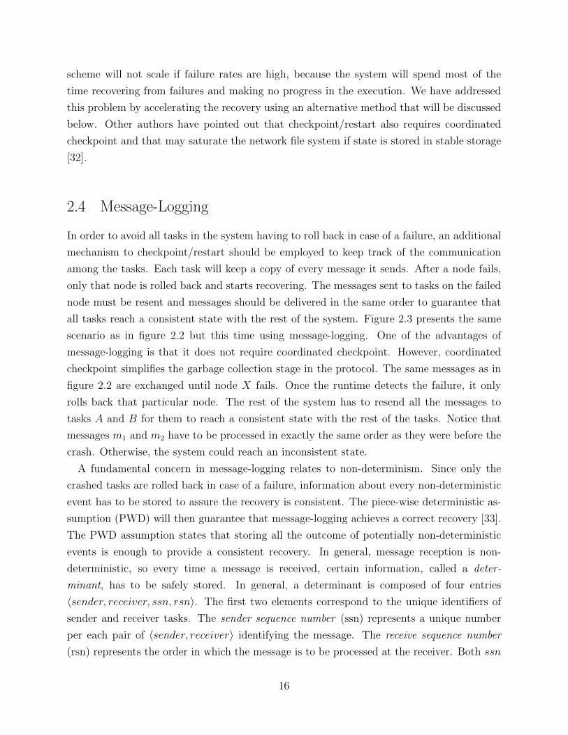
all tasks reach a consistent state with the rest of the system. Figure 2.3 presents the same

scenario as in figure 2.2 but this time using message-logging. One of the advantages of

message-logging is that it does not require coordinated checkpoint. However, coordinated

checkpoint simplifies the garbage collection stage in the protocol. The same messages as in

figure 2.2 are exchanged until node X fails. Once the runtime detects the failure, it only

rolls back that particular node. The rest of the system has to resend all the messages to

tasks A and B for them to reach a consistent state with the rest of the tasks. Notice that

messages m1 and m2 have to be processed in exactly the same order as they were before the

crash. Otherwise, the system could reach an inconsistent state.

A fundamental concern in message-logging relates to non-determinism. Since only the

crashed tasks are rolled back in case of a failure, information about every non-deterministic

event has to be stored to assure the recovery is consistent. The piece-wise deterministic as-

sumption (PWD) will then guarantee that message-logging achieves a correct recovery [33].

The PWD assumption states that storing all the outcome of potentially non-deterministic

events is enough to provide a consistent recovery. In general, message reception is non-

deterministic, so every time a message is received, certain information, called a deter-

minant, has to be safely stored. In general, a determinant is composed of four entries

〈sender, receiver, ssn, rsn〉. The first two elements correspond to the unique identifiers of

sender and receiver tasks. The sender sequence number (ssn) represents a unique number

per each pair of 〈sender, receiver〉 identifying the message. The receive sequence number

(rsn) represents the order in which the message is to be processed at the receiver. Both ssn

16

and rsn are used during recovery to reach a consistent state.

TimeTask A

Task B

Task C

Task D

Recovery Line

RecoveryRestart

m1

m2

m1

m2

Task A

Task BNode

XN

ode

Y

Failure

Node

X'

Checkpoint

Checkpoint

m3

m4 m4

Figure 2.3: Message-Logging with coordinated checkpoint. The same example as in Fig-ure 2.2 is presented, but this time using message-logging. Only tasks in node X are forcedto roll back. Messages are re-sent by other nodes and determinants help to ensure receptionorder is the same as before the crash.

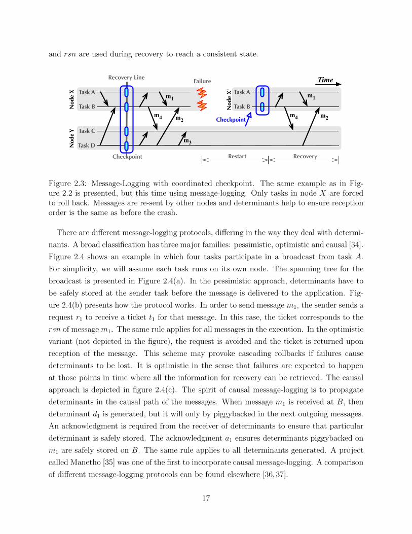
There are different message-logging protocols, differing in the way they deal with determi-

nants. A broad classification has three major families: pessimistic, optimistic and causal [34].

Figure 2.4 shows an example in which four tasks participate in a broadcast from task A.

For simplicity, we will assume each task runs on its own node. The spanning tree for the

broadcast is presented in Figure 2.4(a). In the pessimistic approach, determinants have to

be safely stored at the sender task before the message is delivered to the application. Fig-

ure 2.4(b) presents how the protocol works. In order to send message m1, the sender sends a

request r1 to receive a ticket t1 for that message. In this case, the ticket corresponds to the

rsn of message m1. The same rule applies for all messages in the execution. In the optimistic

variant (not depicted in the figure), the request is avoided and the ticket is returned upon

reception of the message. This scheme may provoke cascading rollbacks if failures cause

determinants to be lost. It is optimistic in the sense that failures are expected to happen

at those points in time where all the information for recovery can be retrieved. The causal

approach is depicted in figure 2.4(c). The spirit of causal message-logging is to propagate

determinants in the causal path of the messages. When message m1 is received at B, then

determinant d1 is generated, but it will only by piggybacked in the next outgoing messages.

An acknowledgment is required from the receiver of determinants to ensure that particular

determinant is safely stored. The acknowledgment a1 ensures determinants piggybacked on

m1 are safely stored on B. The same rule applies to all determinants generated. A project

called Manetho [35] was one of the first to incorporate causal message-logging. A comparison

of different message-logging protocols can be found elsewhere [36,37].

17

A

B

C D

m1

m2 m3

(a) Scenario.

Time

Task A

Task B

Task C

Task D

m1r1 t1r2 r3

t3

m3 t2m2

(b) Pessimistic approach.

Time

m1 a1

a3

m3!d1 a2m2!d1

Task A

Task B

Task C

Task D

(c) Causal approach.

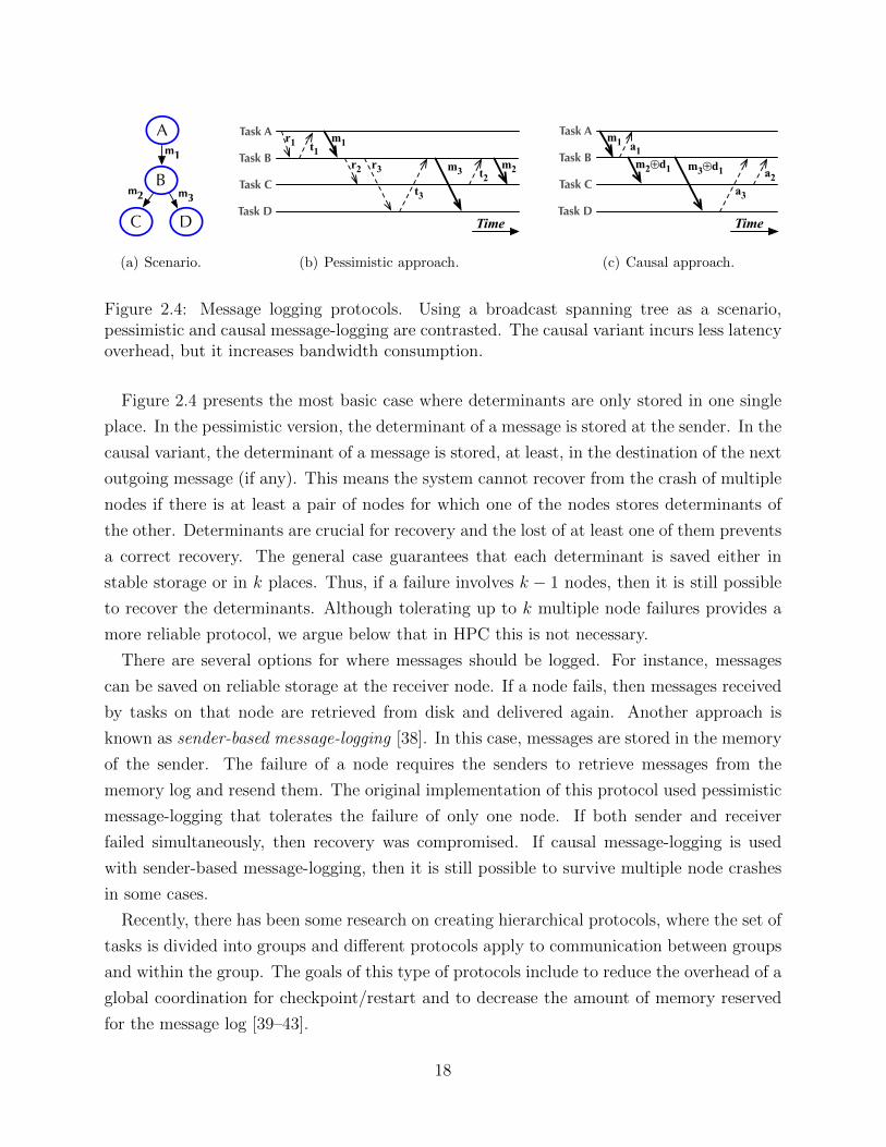
Figure 2.4: Message logging protocols. Using a broadcast spanning tree as a scenario,pessimistic and causal message-logging are contrasted. The causal variant incurs less latencyoverhead, but it increases bandwidth consumption.

Figure 2.4 presents the most basic case where determinants are only stored in one single

place. In the pessimistic version, the determinant of a message is stored at the sender. In the

causal variant, the determinant of a message is stored, at least, in the destination of the next

outgoing message (if any). This means the system cannot recover from the crash of multiple

nodes if there is at least a pair of nodes for which one of the nodes stores determinants of

the other. Determinants are crucial for recovery and the lost of at least one of them prevents

a correct recovery. The general case guarantees that each determinant is saved either in

stable storage or in k places. Thus, if a failure involves k − 1 nodes, then it is still possible

to recover the determinants. Although tolerating up to k multiple node failures provides a

more reliable protocol, we argue below that in HPC this is not necessary.

There are several options for where messages should be logged. For instance, messages

can be saved on reliable storage at the receiver node. If a node fails, then messages received

by tasks on that node are retrieved from disk and delivered again. Another approach is

known as sender-based message-logging [38]. In this case, messages are stored in the memory

of the sender. The failure of a node requires the senders to retrieve messages from the

memory log and resend them. The original implementation of this protocol used pessimistic

message-logging that tolerates the failure of only one node. If both sender and receiver

failed simultaneously, then recovery was compromised. If causal message-logging is used

with sender-based message-logging, then it is still possible to survive multiple node crashes

in some cases.

Recently, there has been some research on creating hierarchical protocols, where the set of

tasks is divided into groups and different protocols apply to communication between groups

and within the group. The goals of this type of protocols include to reduce the overhead of a

global coordination for checkpoint/restart and to decrease the amount of memory reserved

for the message log [39–43].

18

Although MPI does not include a standard mechanism to handle failures, there have

been various libraries implementing message-logging for MPI applications. The MPICH-V

project [44] provided various protocols for fault tolerance [32, 45], including pessimistic [46]

and causal variants [47]. The FT-MPI project [48] incorporates a version of pessimistic

message-logging.

An interesting observation about HPC applications is that a high percentage of them show

a deterministic behavior in their communication [49]. Programs in HPC follow, most of the

time, a regular pattern to compute and to exchange data. A send-deterministic application

is one that always sends the same sequence of messages in any valid execution. In other

words, regardless of the reception order of messages, tasks necessarily send out exactly

the same messages. Send-deterministic applications, also called linear order programs in

other contexts [50], are appealing for simulation, since they impose less restrictions for the

execution of the basic blocks that make the application. An even more restrictive property

for an application is to be deterministic in which case, both send and receive sequences are

always the same.

Communication determinism can be used to develop new message-logging protocols. One

of them was implemented in MPICH2 [51], a popular implementation of MPI. The key

observation of this algorithm is that it is possible to avoid storing most of the determinants.

A protocol based on this property [51] uses uncoordinated checkpoint and a few extra

concepts, necessary for the correctness of the approach. Each task will checkpoint in an

uncoordinated fashion, but it will keep track of the checkpoint interval, called an epoch

in this method. For every message sent, a response is always expected from the receiver.

That response will notify the sender whether or not the sender has to log the message. The

protocol only logs messages that cross epochs from an earlier epoch to a later one. Messages

in the same epoch are not logged, since they will be recreated in case of a failure.

2.4.1 Comparison of Pessimistic and Causal Message-Logging

Message-logging protocols require determinants to provide a consistent recovery. The dif-

ferent flavors of message-logging differ in the way determinants are saved. However, the

particular mechanisms to ensure that determinants survive a crash may have markedly dif-

ferent performance penalizations.

The most popular implementation of messages-logging is the pessimistic approach de-

scribed above [52]. There are a few implementations of this protocol in HPC libraries

[46,53,54]. The pessimistic variant of message-logging has the advantage that it is relatively

19

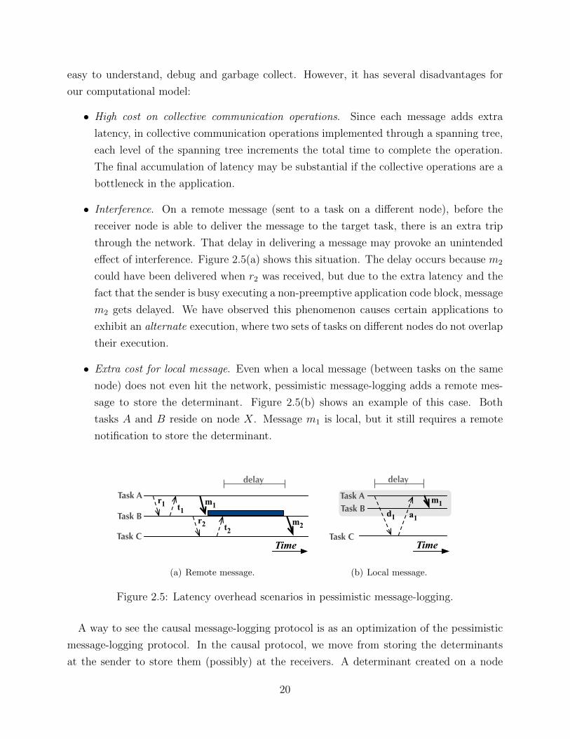
easy to understand, debug and garbage collect. However, it has several disadvantages for

our computational model:

• High cost on collective communication operations. Since each message adds extra

latency, in collective communication operations implemented through a spanning tree,

each level of the spanning tree increments the total time to complete the operation.

The final accumulation of latency may be substantial if the collective operations are a

bottleneck in the application.

• Interference. On a remote message (sent to a task on a different node), before the

receiver node is able to deliver the message to the target task, there is an extra trip

through the network. That delay in delivering a message may provoke an unintended

effect of interference. Figure 2.5(a) shows this situation. The delay occurs because m2

could have been delivered when r2 was received, but due to the extra latency and the

fact that the sender is busy executing a non-preemptive application code block, message

m2 gets delayed. We have observed this phenomenon causes certain applications to

exhibit an alternate execution, where two sets of tasks on different nodes do not overlap

their execution.

• Extra cost for local message. Even when a local message (between tasks on the same

node) does not even hit the network, pessimistic message-logging adds a remote mes-

sage to store the determinant. Figure 2.5(b) shows an example of this case. Both

tasks A and B reside on node X. Message m1 is local, but it still requires a remote

notification to store the determinant.

Time

Task A

Task B

Task C

m1r1 t1r2 t2

m2

delay

(a) Remote message.

Time

Task A

Task C

m1d1 a1

delay

Task B

(b) Local message.

Figure 2.5: Latency overhead scenarios in pessimistic message-logging.

A way to see the causal message-logging protocol is as an optimization of the pessimistic

message-logging protocol. In the causal protocol, we move from storing the determinants

at the sender to store them (possibly) at the receivers. A determinant created on a node

20

might not be replicated, because that depends on whether the node sends a message after

it is created. As an optimization, causal message-logging gets rid of the extra network

roundtrip per message. That way, collectives perform better and there is no risk of inducing

interference in the application since message sends are not delayed. Finally, local messages

do not require a remote acknowledgment, since determinants are accumulated at the node

level. In conclusion, causal message-logging does not have any of the limitations of the

pessimistic approach listed above.

The disadvantage of the causal approach comes in two different places. One is during

garbage collection, i.e., the removal of unneeded messages from the log. If an object has

stored the effect of a message m into a checkpoint, then message m is not required any

more. Garbage collecting is rather straightforward with pessimistic message-logging, but

becomes more burdensome with causal message-logging. In the pessimistic case, after an

object checkpoints, it sends the largest ticket number processed so far to all other objects

that have sent messages to it. Each sender will remove from its message log all messages

having a smaller ticket number. In the case of causal message-logging, all determinants

must be sent to the senders. However, since garbage collection runs asynchronously with the

application, it does not have a major impact on performance. One possible optimization of

causal message-logging protocols is to use coordinated checkpoint. Even though checkpoint

may be either coordinated or not in message-logging, the coordinated variant makes it easier

to garbage collect, since at every checkpoint all data structures and the message log are

flushed.

The second drawback of causal message-logging is that during recovery messages and

determinants come from different places and the recovering object has to sort them out.

The performance penalty for this is not significant but it adds more complexity to the

protocol.

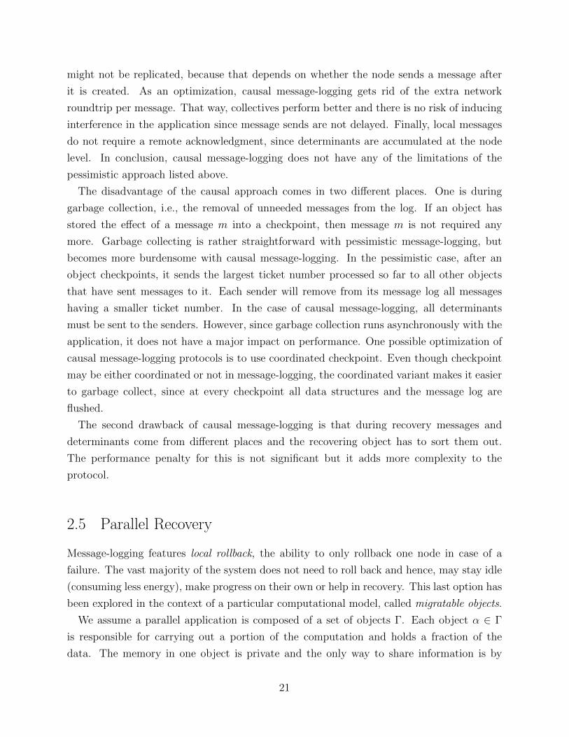
2.5 Parallel Recovery

Message-logging features local rollback, the ability to only rollback one node in case of a

failure. The vast majority of the system does not need to roll back and hence, may stay idle

(consuming less energy), make progress on their own or help in recovery. This last option has

been explored in the context of a particular computational model, called migratable objects.

We assume a parallel application is composed of a set of objects Γ. Each object α ∈ Γ

is responsible for carrying out a portion of the computation and holds a fraction of the

data. The memory in one object is private and the only way to share information is by

21

asynchronous method invocation. This means, an object α can call a remote method on

another object β. The asynchrony arises from the fact that calling a remote method is in

general a non-blocking operation.

The architecture on which the application runs is formed by a set of processing elements

(PEs), denoted by Σ. In modern architectures a PE may correspond to a core. The set of PEs

is connected through a reliable network that does not guarantee FIFO order in its channels.

There is a runtime system that orchestrates the execution of an application by assigning

objects to PEs, schedules what method has to execute on a particular PE and moves objects

around to dynamically adapt to the runtime conditions. To serialize an object, the runtime

system relies on the programmer to write a marshaling method for each object. This permits

the runtime system to save the state of any object at certain points in the execution where

the programmer agreed the object could be moved or checkpointed.

There are several advantages in having user-level checkpoint. First, the programmer may

determine at what points in the execution the state of the object is minimum (or small

enough) to be saved. Second, it is portable across different architectures. Third, user-level

checkpoint allows the program to be run on a different number of PEs than the initial number

of PEs used.

This model has been implemented by the Charm++ runtime system [55]. The programmer

of a Charm++ application decomposes the computation into chares or objects that will

react to method invocations by other chares. The number of objects does not need to match

the number of physical cores, but usually there are many more objects than cores for the

runtime system to have room to overlap computation with communication and to adapt to

load imbalances in the system. Thus, we say the programmer in Charm++ overdecomposes

the application. The ratio between the number of objects and the number of PEs is called

the virtualization ratio.

The Message Passing Interface (MPI) also fits our model. Each rank in MPI can be con-

ceived as an object that reacts to the reception of messages. However, MPI makes the model

more rigid, since it has blocking operations and requires channels to be FIFO. An extension

to Charm++, called Adaptive MPI (AMPI) [56] permits MPI applications to run on top of

the Charm++ runtime and get the benefits of migratable objects (overlap of communica-

tion and computation, load balance, fault tolerance, and more). We use Charm++ as the

substrate for the fault-tolerance research described in this dissertation.

The main advantage of using message-logging in the migratabale-objects model comes

from the ability to implement parallel recovery, a mechanism the accelerates the recovery

of the failed PE, reducing to a fraction the time required to redo the work lost due to a

failure [5]. Figure 2.10 presents the main characteristics of parallel recovery. The figure

22

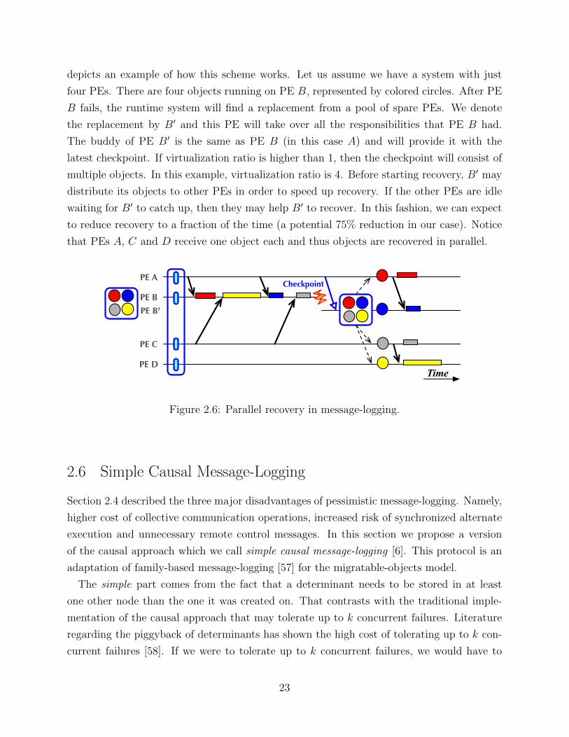
depicts an example of how this scheme works. Let us assume we have a system with just

four PEs. There are four objects running on PE B, represented by colored circles. After PE

B fails, the runtime system will find a replacement from a pool of spare PEs. We denote

the replacement by B′ and this PE will take over all the responsibilities that PE B had.

The buddy of PE B′ is the same as PE B (in this case A) and will provide it with the

latest checkpoint. If virtualization ratio is higher than 1, then the checkpoint will consist of

multiple objects. In this example, virtualization ratio is 4. Before starting recovery, B′ may

distribute its objects to other PEs in order to speed up recovery. If the other PEs are idle

waiting for B′ to catch up, then they may help B′ to recover. In this fashion, we can expect

to reduce recovery to a fraction of the time (a potential 75% reduction in our case). Notice

that PEs A, C and D receive one object each and thus objects are recovered in parallel.

Time

PE A

PE B'

PE C

PE D

PE B

Checkpoint

Figure 2.6: Parallel recovery in message-logging.

2.6 Simple Causal Message-Logging

Section 2.4 described the three major disadvantages of pessimistic message-logging. Namely,

higher cost of collective communication operations, increased risk of synchronized alternate

execution and unnecessary remote control messages. In this section we propose a version

of the causal approach which we call simple causal message-logging [6]. This protocol is an

adaptation of family-based message-logging [57] for the migratable-objects model.

The simple part comes from the fact that a determinant needs to be stored in at least

one other node than the one it was created on. That contrasts with the traditional imple-

mentation of the causal approach that may tolerate up to k concurrent failures. Literature

regarding the piggyback of determinants has shown the high cost of tolerating up to k con-

current failures [58]. If we were to tolerate up to k concurrent failures, we would have to

23

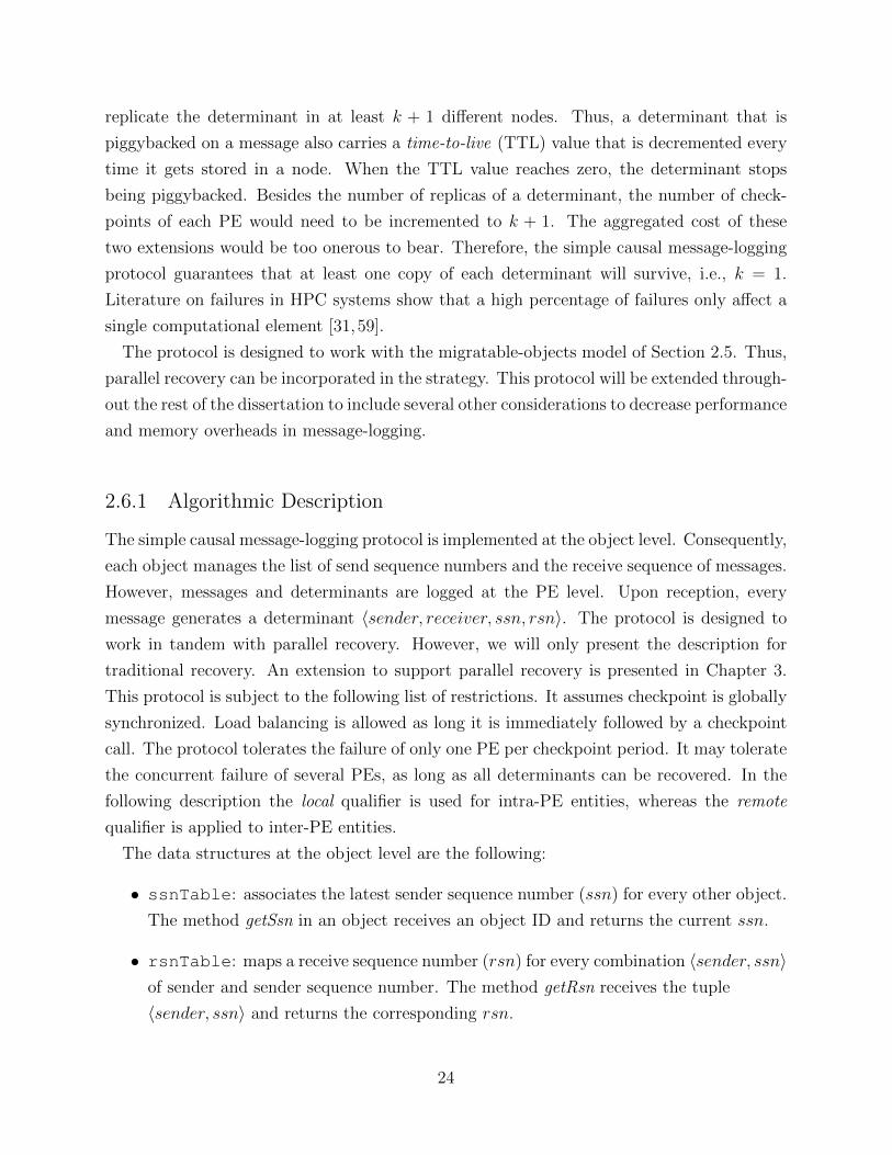
replicate the determinant in at least k + 1 different nodes. Thus, a determinant that is

piggybacked on a message also carries a time-to-live (TTL) value that is decremented every

time it gets stored in a node. When the TTL value reaches zero, the determinant stops

being piggybacked. Besides the number of replicas of a determinant, the number of check-

points of each PE would need to be incremented to k + 1. The aggregated cost of these

two extensions would be too onerous to bear. Therefore, the simple causal message-logging

protocol guarantees that at least one copy of each determinant will survive, i.e., k = 1.

Literature on failures in HPC systems show that a high percentage of failures only affect a

single computational element [31,59].

The protocol is designed to work with the migratable-objects model of Section 2.5. Thus,

parallel recovery can be incorporated in the strategy. This protocol will be extended through-

out the rest of the dissertation to include several other considerations to decrease performance

and memory overheads in message-logging.

2.6.1 Algorithmic Description

The simple causal message-logging protocol is implemented at the object level. Consequently,

each object manages the list of send sequence numbers and the receive sequence of messages.

However, messages and determinants are logged at the PE level. Upon reception, every

message generates a determinant 〈sender, receiver, ssn, rsn〉. The protocol is designed to

work in tandem with parallel recovery. However, we will only present the description for

traditional recovery. An extension to support parallel recovery is presented in Chapter 3.

This protocol is subject to the following list of restrictions. It assumes checkpoint is globally

synchronized. Load balancing is allowed as long it is immediately followed by a checkpoint

call. The protocol tolerates the failure of only one PE per checkpoint period. It may tolerate

the concurrent failure of several PEs, as long as all determinants can be recovered. In the

following description the local qualifier is used for intra-PE entities, whereas the remote

qualifier is applied to inter-PE entities.

The data structures at the object level are the following:

• ssnTable: associates the latest sender sequence number (ssn) for every other object.

The method getSsn in an object receives an object ID and returns the current ssn.

• rsnTable: maps a receive sequence number (rsn) for every combination 〈sender, ssn〉of sender and sender sequence number. The method getRsn receives the tuple

〈sender, ssn〉 and returns the corresponding rsn.

24

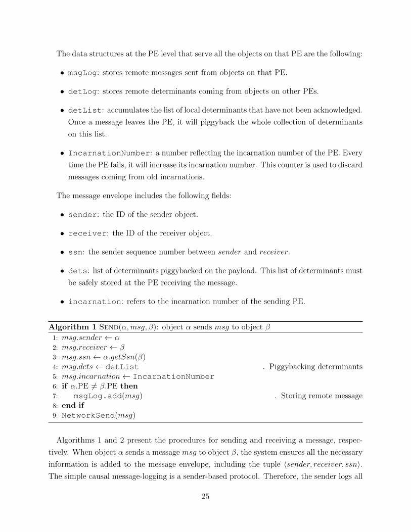
The data structures at the PE level that serve all the objects on that PE are the following:

• msgLog: stores remote messages sent from objects on that PE.

• detLog: stores remote determinants coming from objects on other PEs.

• detList: accumulates the list of local determinants that have not been acknowledged.

Once a message leaves the PE, it will piggyback the whole collection of determinants

on this list.

• IncarnationNumber: a number reflecting the incarnation number of the PE. Every

time the PE fails, it will increase its incarnation number. This counter is used to discard

messages coming from old incarnations.

The message envelope includes the following fields:

• sender: the ID of the sender object.

• receiver: the ID of the receiver object.

• ssn: the sender sequence number between sender and receiver.

• dets: list of determinants piggybacked on the payload. This list of determinants must

be safely stored at the PE receiving the message.

• incarnation: refers to the incarnation number of the sending PE.

Algorithm 1 Send(α,msg, β): object α sends msg to object β

1: msg.sender ← α2: msg.receiver ← β3: msg.ssn← α.getSsn(β)4: msg.dets← detList . Piggybacking determinants5: msg.incarnation← IncarnationNumber6: if α.PE 6= β.PE then7: msgLog.add(msg) . Storing remote message8: end if9: NetworkSend(msg)

Algorithms 1 and 2 present the procedures for sending and receiving a message, respec-

tively. When object α sends a message msg to object β, the system ensures all the necessary

information is added to the message envelope, including the tuple 〈sender, receiver, ssn〉.The simple causal message-logging is a sender-based protocol. Therefore, the sender logs all

25

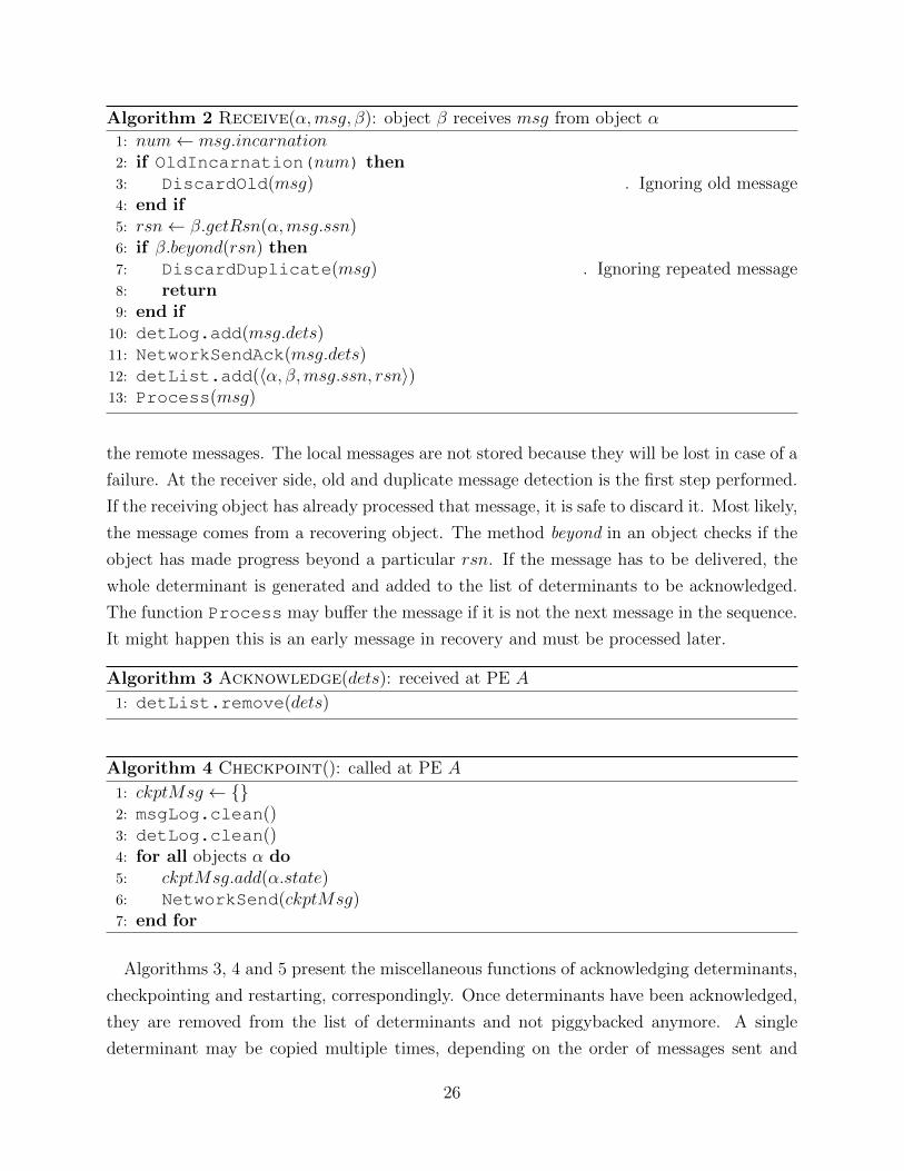
Algorithm 2 Receive(α,msg, β): object β receives msg from object α

1: num← msg.incarnation2: if OldIncarnation(num) then3: DiscardOld(msg) . Ignoring old message4: end if5: rsn← β.getRsn(α,msg.ssn)6: if β.beyond(rsn) then7: DiscardDuplicate(msg) . Ignoring repeated message8: return9: end if

10: detLog.add(msg.dets)11: NetworkSendAck(msg.dets)12: detList.add(〈α, β,msg.ssn, rsn〉)13: Process(msg)

the remote messages. The local messages are not stored because they will be lost in case of a

failure. At the receiver side, old and duplicate message detection is the first step performed.

If the receiving object has already processed that message, it is safe to discard it. Most likely,

the message comes from a recovering object. The method beyond in an object checks if the

object has made progress beyond a particular rsn. If the message has to be delivered, the

whole determinant is generated and added to the list of determinants to be acknowledged.

The function Process may buffer the message if it is not the next message in the sequence.

It might happen this is an early message in recovery and must be processed later.

Algorithm 3 Acknowledge(dets): received at PE A

1: detList.remove(dets)

Algorithm 4 Checkpoint(): called at PE A

1: ckptMsg ← 2: msgLog.clean()3: detLog.clean()4: for all objects α do5: ckptMsg.add(α.state)6: NetworkSend(ckptMsg)7: end for

Algorithms 3, 4 and 5 present the miscellaneous functions of acknowledging determinants,

checkpointing and restarting, correspondingly. Once determinants have been acknowledged,

they are removed from the list of determinants and not piggybacked anymore. A single

determinant may be copied multiple times, depending on the order of messages sent and

26

Algorithm 5 Restart(A): received at every PE except A

1: for all objects α in A do2: Send all determinants of α in detLog3: Send all messages bound to α in msgLog4: end for

acknowledge messages received at the sender. The checkpoint mechanism is supposed to

be globally coordinated, thus both message and determinant logs can be cleaned at that

point. Finally, the restart method is called on every PE other than the one failed, A. The

fundamental task for every PE is to forward all the messages and determinants logged for

PE A.

2.6.2 Formal Proof of Correctness

Lemma 2.1. All required determinants are successfully retrieved during recovery.

Proof Sketch. If a particular object α generated a determinant d at PE A and that deter-

minant was piggybacked and received at some other PE B, then it will be provided by B to

A for recovery. It is possible (and valid) to lose some determinants if they did not affect the

rest of the system. For instance, if determinant d is piggybacked on message m from A to B

and m arrives after the failure notification on B, then m is going to be discarded, because

its incarnation number would not match the incarnation number for A at B. In that case, it

is possible to lose determinant d because it never affected the rest of the system. This may

provoke messages to be received in a different order during the recovery of A, but it would

still be a correct execution of the program.

Lemma 2.2. All required messages are successfully replayed during recovery.

Proof Sketch. Note that all remote messages are logged at the sender. Thus, if PE A crashes,

all messages bound to A will be replayed again by the senders. If the messages are local,

then they will be regenerated by the PWD assumption on the program.

Lemma 2.3. There are no orphan objects.

Proof Sketch. By contradiction. Imagine object β at PE B received a message m from object

α in PE A. During the recovery of PE A and all its objects, including α, all determinants and

messages are available. Given the PWD assumption and the application of all the available

determinants, α will again send message m to β. This is a contradiction, therefore there are

no orphan objects.

27

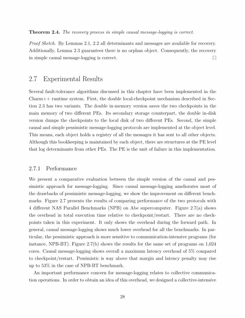
Theorem 2.4. The recovery process in simple causal message-logging is correct.

Proof Sketch. By Lemmas 2.1, 2.2 all determinants and messages are available for recovery.

Additionally, Lemma 2.3 guarantees there is no orphan object. Consequently, the recovery

in simple causal message-logging is correct.

2.7 Experimental Results

Several fault-tolerance algorithms discussed in this chapter have been implemented in the

Charm++ runtime system. First, the double local-checkpoint mechanism described in Sec-

tion 2.3 has two variants. The double in-memory version saves the two checkpoints in the

main memory of two different PEs. Its secondary storage counterpart, the double in-disk

version dumps the checkpoints to the local disk of two different PEs. Second, the simple

causal and simple pessimistic message-logging protocols are implemented at the object level.

This means, each object holds a registry of all the messages it has sent to all other objects.

Although this bookkeeping is maintained by each object, there are structures at the PE level

that log determinants from other PEs. The PE is the unit of failure in this implementation.

2.7.1 Performance

We present a comparative evaluation between the simple version of the causal and pes-

simistic approach for message-logging. Since causal message-logging ameliorates most of

the drawbacks of pessimistic message-logging, we show the improvement on different bench-

marks. Figure 2.7 presents the results of comparing performance of the two protocols with

4 different NAS Parallel Benchmarks (NPB) on Abe supercomputer. Figure 2.7(a) shows

the overhead in total execution time relative to checkpoint/restart. There are no check-

points taken in this experiment. It only shows the overhead during the forward path. In

general, causal message-logging shows much lower overhead for all the benchmarks. In par-

ticular, the pessimistic approach is more sensitive to communication-intensive programs (for

instance, NPB-BT). Figure 2.7(b) shows the results for the same set of programs on 1,024

cores. Causal message-logging shows overall a maximum latency overhead of 5% compared

to checkpoint/restart. Pessimistic is way above that margin and latency penalty may rise

up to 53% in the case of NPB-BT benchmark.

An important performance concern for message-logging relates to collective communica-

tion operations. In order to obtain an idea of this overhead, we designed a collective-intensive

28

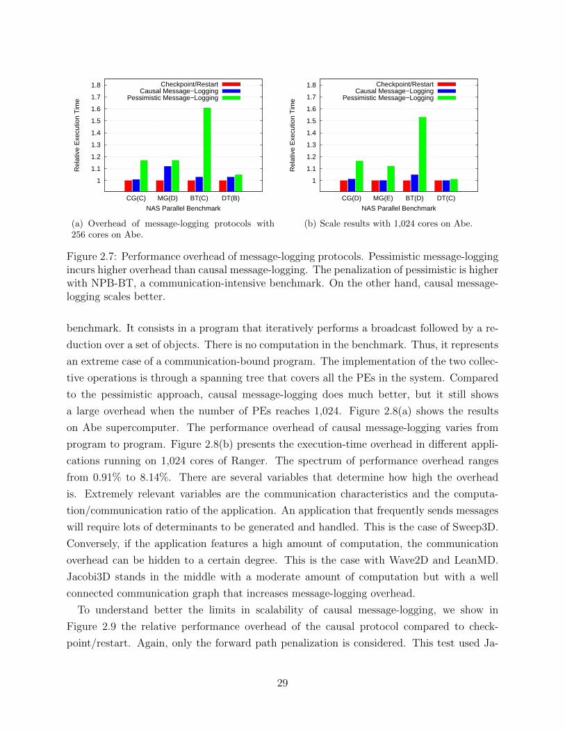
1

1.1

1.2

1.3

1.4

1.5

1.6

1.7

1.8

CG(C) MG(D) BT(C) DT(B)

Rel

ativ

e E

xecu

tion

Tim

e

NAS Parallel Benchmark

Checkpoint/RestartCausal Message−Logging

Pessimistic Message−Logging

(a) Overhead of message-logging protocols with256 cores on Abe.

1

1.1

1.2

1.3

1.4

1.5

1.6

1.7

1.8

CG(D) MG(E) BT(D) DT(C)

Rel

ativ

e E

xecu

tion

Tim

e

NAS Parallel Benchmark

Checkpoint/RestartCausal Message−Logging

Pessimistic Message−Logging

(b) Scale results with 1,024 cores on Abe.

Figure 2.7: Performance overhead of message-logging protocols. Pessimistic message-loggingincurs higher overhead than causal message-logging. The penalization of pessimistic is higherwith NPB-BT, a communication-intensive benchmark. On the other hand, causal message-logging scales better.

benchmark. It consists in a program that iteratively performs a broadcast followed by a re-

duction over a set of objects. There is no computation in the benchmark. Thus, it represents

an extreme case of a communication-bound program. The implementation of the two collec-

tive operations is through a spanning tree that covers all the PEs in the system. Compared

to the pessimistic approach, causal message-logging does much better, but it still shows

a large overhead when the number of PEs reaches 1,024. Figure 2.8(a) shows the results

on Abe supercomputer. The performance overhead of causal message-logging varies from

program to program. Figure 2.8(b) presents the execution-time overhead in different appli-

cations running on 1,024 cores of Ranger. The spectrum of performance overhead ranges

from 0.91% to 8.14%. There are several variables that determine how high the overhead

is. Extremely relevant variables are the communication characteristics and the computa-

tion/communication ratio of the application. An application that frequently sends messages

will require lots of determinants to be generated and handled. This is the case of Sweep3D.

Conversely, if the application features a high amount of computation, the communication

overhead can be hidden to a certain degree. This is the case with Wave2D and LeanMD.

Jacobi3D stands in the middle with a moderate amount of computation but with a well

connected communication graph that increases message-logging overhead.

To understand better the limits in scalability of causal message-logging, we show in

Figure 2.9 the relative performance overhead of the causal protocol compared to check-

point/restart. Again, only the forward path penalization is considered. This test used Ja-

29

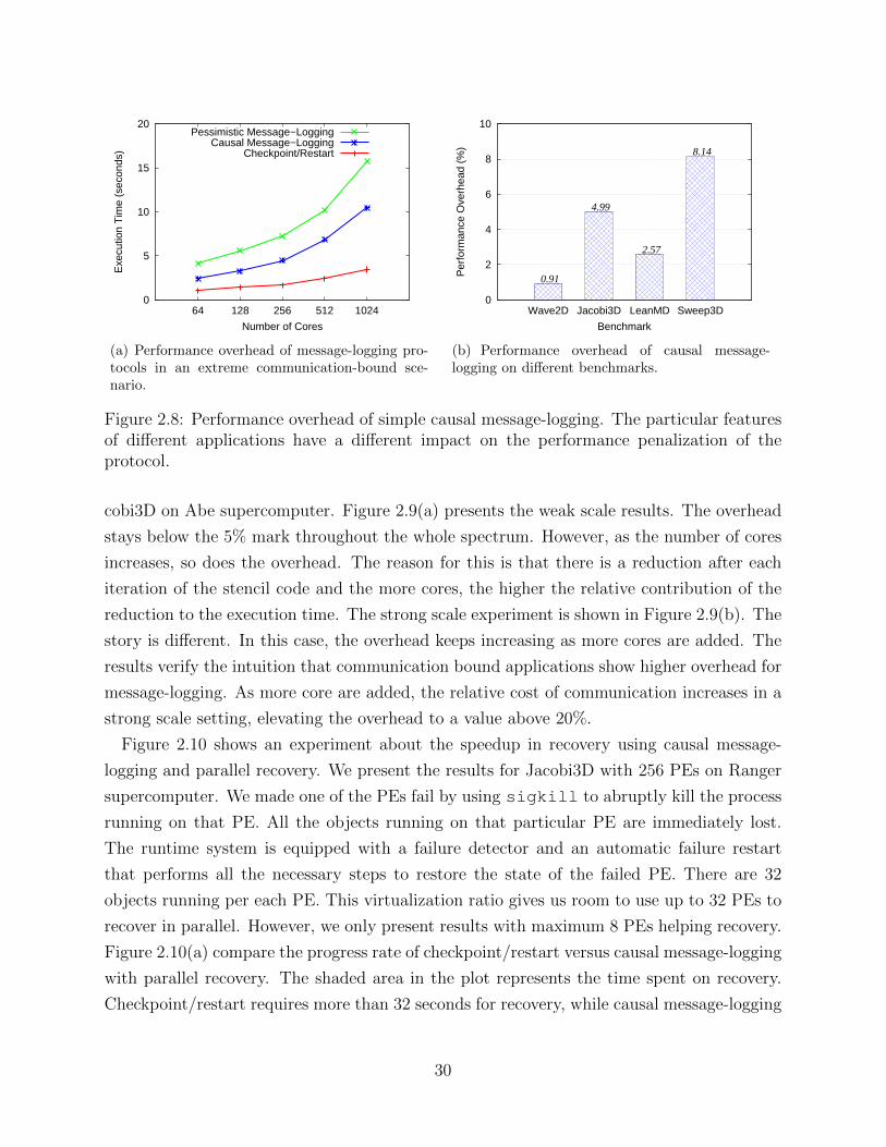
0

5

10

15

20

64 128 256 512 1024

Exe

cutio

n T

ime

(sec

onds

)

Number of Cores

Pessimistic Message−LoggingCausal Message−Logging

Checkpoint/Restart

(a) Performance overhead of message-logging pro-tocols in an extreme communication-bound sce-nario.

0

2

4

6

8

10

Wave2D Jacobi3D LeanMD Sweep3D

Per

form

ance

Ove

rhea

d (%

)

Benchmark

0.91

4.99

2.57

8.14

(b) Performance overhead of causal message-logging on different benchmarks.

Figure 2.8: Performance overhead of simple causal message-logging. The particular featuresof different applications have a different impact on the performance penalization of theprotocol.

cobi3D on Abe supercomputer. Figure 2.9(a) presents the weak scale results. The overhead

stays below the 5% mark throughout the whole spectrum. However, as the number of cores

increases, so does the overhead. The reason for this is that there is a reduction after each

iteration of the stencil code and the more cores, the higher the relative contribution of the

reduction to the execution time. The strong scale experiment is shown in Figure 2.9(b). The

story is different. In this case, the overhead keeps increasing as more cores are added. The

results verify the intuition that communication bound applications show higher overhead for

message-logging. As more core are added, the relative cost of communication increases in a

strong scale setting, elevating the overhead to a value above 20%.

Figure 2.10 shows an experiment about the speedup in recovery using causal message-

logging and parallel recovery. We present the results for Jacobi3D with 256 PEs on Ranger

supercomputer. We made one of the PEs fail by using sigkill to abruptly kill the process

running on that PE. All the objects running on that particular PE are immediately lost.

The runtime system is equipped with a failure detector and an automatic failure restart

that performs all the necessary steps to restore the state of the failed PE. There are 32

objects running per each PE. This virtualization ratio gives us room to use up to 32 PEs to

recover in parallel. However, we only present results with maximum 8 PEs helping recovery.

Figure 2.10(a) compare the progress rate of checkpoint/restart versus causal message-logging

with parallel recovery. The shaded area in the plot represents the time spent on recovery.

Checkpoint/restart requires more than 32 seconds for recovery, while causal message-logging

30

1

1.05

1.1

1.15

1.2

1.25

64 128 256 512 1024

Rel

ativ

e E

xecu

tion

Tim

e

Number of Cores

Checkpoint/RestartCausal Message−Logging

(a) Weak-scale experiment.

1

1.05

1.1

1.15

1.2

1.25

64 128 256 512 1024

Rel

ativ

e E

xecu

tion

Tim

e

Number of Cores

Checkpoint/RestartCausal Message−Logging

(b) Strong-scale experiment.

Figure 2.9: Overhead in scaling causal message-logging. The weak scale experiment showscausal message-logging scales well. However, the strong scale experiment suggest the com-munication overhead starts dominating at the right extreme of the scale.

less than 4 seconds. The plot in Figure 2.10 presents different levels of parallelism during

recovery. It shows the speedup in recovery compared to the progress rate during the forward

path. It may seem surprising to have superlinear speedup in Figure 2.10 when using just 1

PE to recover. The reason for that behavior is due to the fact that with message-logging

there is no delay in receiving most of the messages. A normal execution of the application

(what occurs during recovery with checkpoint/restart) will sometimes make objects wait for

a message before they can start computation. With message-logging, those messages are

already available during recovery and there is no wait. Adding more PEs to the recovery

increases speedup. There are, however, diminishing returns when many PEs are added,

because then communication among those PEs has to be considered.

2.7.2 Energy Consumption

One of the advantages of message-logging lies precisely on its ability to perform a local

rollback. Avoiding a global rollback should translate in potentially a huge reduction in energy

consumption during recovery. We examine this advantage of message-logging combined

with parallel recovery. In fact, for our experiments with the Energy Cluster, we consider

checkpoint/restart, message-logging and parallel recovery as levels in a hierarchy of protocols.

The base is coordinated checkpoint/restart that is extended by message-logging, which in

turns is augmented with parallel recovery.

Figure 2.11 shows the different energy levels that appears during the execution of Jacobi3D

31

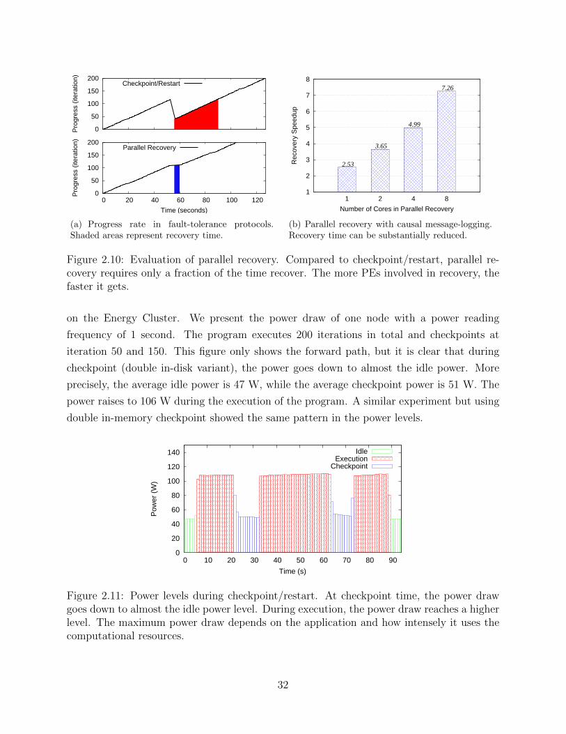
0

50

100

150

200

0 20 40 60 80 100 120

Pro

gres

s (it

erat

ion)

Time (seconds)

Parallel Recovery

0

50

100

150

200P

rogr

ess

(iter

atio

n)Checkpoint/Restart

(a) Progress rate in fault-tolerance protocols.Shaded areas represent recovery time.

1

2

3

4

5

6

7

8

1 2 4 8

Rec

over

y S

peed

up

Number of Cores in Parallel Recovery

2.53

3.65

4.99

7.26

(b) Parallel recovery with causal message-logging.Recovery time can be substantially reduced.

Figure 2.10: Evaluation of parallel recovery. Compared to checkpoint/restart, parallel re-covery requires only a fraction of the time recover. The more PEs involved in recovery, thefaster it gets.

on the Energy Cluster. We present the power draw of one node with a power reading

frequency of 1 second. The program executes 200 iterations in total and checkpoints at

iteration 50 and 150. This figure only shows the forward path, but it is clear that during

checkpoint (double in-disk variant), the power goes down to almost the idle power. More

precisely, the average idle power is 47 W, while the average checkpoint power is 51 W. The

power raises to 106 W during the execution of the program. A similar experiment but using

double in-memory checkpoint showed the same pattern in the power levels.

0

20

40

60

80

100

120

140

0 10 20 30 40 50 60 70 80 90

Pow

er (

W)

Time (s)

IdleExecution

Checkpoint

Figure 2.11: Power levels during checkpoint/restart. At checkpoint time, the power drawgoes down to almost the idle power level. During execution, the power draw reaches a higherlevel. The maximum power draw depends on the application and how intensely it uses thecomputational resources.

32

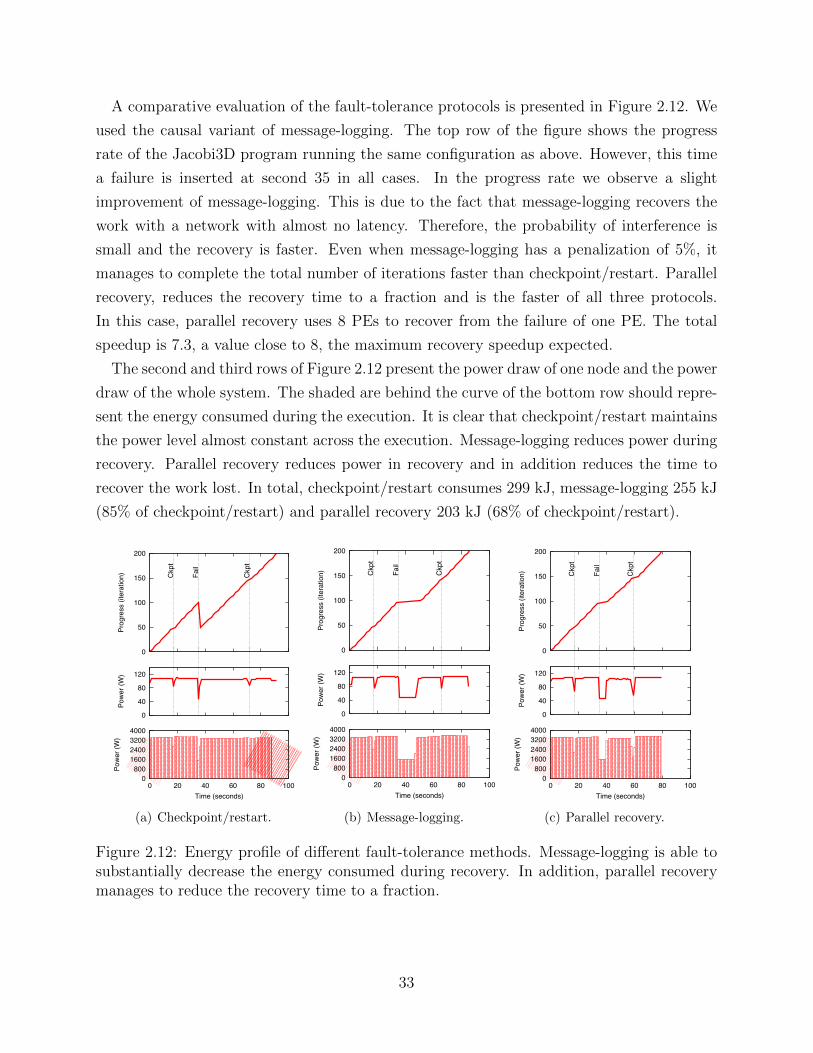
A comparative evaluation of the fault-tolerance protocols is presented in Figure 2.12. We

used the causal variant of message-logging. The top row of the figure shows the progress

rate of the Jacobi3D program running the same configuration as above. However, this time

a failure is inserted at second 35 in all cases. In the progress rate we observe a slight

improvement of message-logging. This is due to the fact that message-logging recovers the

work with a network with almost no latency. Therefore, the probability of interference is

small and the recovery is faster. Even when message-logging has a penalization of 5%, it

manages to complete the total number of iterations faster than checkpoint/restart. Parallel

recovery, reduces the recovery time to a fraction and is the faster of all three protocols.

In this case, parallel recovery uses 8 PEs to recover from the failure of one PE. The total

speedup is 7.3, a value close to 8, the maximum recovery speedup expected.

The second and third rows of Figure 2.12 present the power draw of one node and the power

draw of the whole system. The shaded are behind the curve of the bottom row should repre-

sent the energy consumed during the execution. It is clear that checkpoint/restart maintains

the power level almost constant across the execution. Message-logging reduces power during

recovery. Parallel recovery reduces power in recovery and in addition reduces the time to

recover the work lost. In total, checkpoint/restart consumes 299 kJ, message-logging 255 kJ

(85% of checkpoint/restart) and parallel recovery 203 kJ (68% of checkpoint/restart).

0 800

1600 2400 3200 4000

0 20 40 60 80 100

Pow

er (W

)

Time (seconds)

0

40

80

120

Pow

er (W

)

0

50

100

150

200

Prog

ress

(ite

ratio

n) Fail

Ckp

t

Ckp

t

(a) Checkpoint/restart.

0 800

1600 2400 3200 4000

0 20 40 60 80 100

Pow

er (W

)

Time (seconds)

0

40

80

120

Pow

er (W

)

0

50

100

150

200

Prog

ress

(ite

ratio

n) Fail

Ckp

t

Ckp

t

(b) Message-logging.

0 800

1600 2400 3200 4000

0 20 40 60 80 100

Pow

er (W

)

Time (seconds)

0

40

80

120

Pow

er (W

)

0

50

100

150

200

Prog

ress

(ite

ratio

n) Fail

Ckp

t

Ckp

t

(c) Parallel recovery.

Figure 2.12: Energy profile of different fault-tolerance methods. Message-logging is able tosubstantially decrease the energy consumed during recovery. In addition, parallel recoverymanages to reduce the recovery time to a fraction.

33

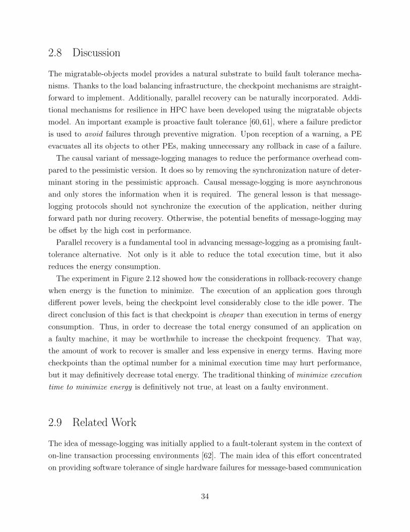
2.8 Discussion

The migratable-objects model provides a natural substrate to build fault tolerance mecha-

nisms. Thanks to the load balancing infrastructure, the checkpoint mechanisms are straight-

forward to implement. Additionally, parallel recovery can be naturally incorporated. Addi-

tional mechanisms for resilience in HPC have been developed using the migratable objects

model. An important example is proactive fault tolerance [60,61], where a failure predictor

is used to avoid failures through preventive migration. Upon reception of a warning, a PE

evacuates all its objects to other PEs, making unnecessary any rollback in case of a failure.

The causal variant of message-logging manages to reduce the performance overhead com-

pared to the pessimistic version. It does so by removing the synchronization nature of deter-

minant storing in the pessimistic approach. Causal message-logging is more asynchronous

and only stores the information when it is required. The general lesson is that message-

logging protocols should not synchronize the execution of the application, neither during

forward path nor during recovery. Otherwise, the potential benefits of message-logging may

be offset by the high cost in performance.

Parallel recovery is a fundamental tool in advancing message-logging as a promising fault-

tolerance alternative. Not only is it able to reduce the total execution time, but it also

reduces the energy consumption.

The experiment in Figure 2.12 showed how the considerations in rollback-recovery change

when energy is the function to minimize. The execution of an application goes through

different power levels, being the checkpoint level considerably close to the idle power. The

direct conclusion of this fact is that checkpoint is cheaper than execution in terms of energy

consumption. Thus, in order to decrease the total energy consumed of an application on

a faulty machine, it may be worthwhile to increase the checkpoint frequency. That way,

the amount of work to recover is smaller and less expensive in energy terms. Having more

checkpoints than the optimal number for a minimal execution time may hurt performance,

but it may definitively decrease total energy. The traditional thinking of minimize execution

time to minimize energy is definitively not true, at least on a faulty environment.

2.9 Related Work

The idea of message-logging was initially applied to a fault-tolerant system in the context of

on-line transaction processing environments [62]. The main idea of this effort concentrated

on providing software tolerance of single hardware failures for message-based communication

34

systems. Each primary process would have one or more backup processes that were capable

of continuing execution if the primary process failed. Global synchronization points would

serve as checkpoints for the processes in the system. Therefore, messages sent since the last

synchronization point had to be stored in order to be replayed to the backup process after

a crash. The backup process was supposed to read the messages in the exact same order as

the primary had read them. To this effect the system used a replication mechanism where

each primary process would be mirrored by a backup process. A message sent to a primary

process has to be sent to the backup too. The backup process would receive the messages

but not process them. That way, in case of a crash, the backup process would take over the

position of the primary and would replay the messages in its own log to catch up with the

rest of the system. Atomicity in the delivery of the messages was ensured by the hardware.

Also, counters would be used to suppress duplicate messages.

Fundamentally, migrating a task and checkpointing a task are very similar. Both func-

tionalities require the serialization of the tasks. This parallel between task migration and

task checkpointing was drawn in the MPI model with a tool called CoCheck [63]. Within the

same framework, CoCheck provides disk checkpoint and dynamic migration of MPI ranks.

CoCheck implements an algorithm that finds global consistent states [20]. A global state of

a system is formed by the state of each task plus all messages that were in transit when the

snapshot of the system was taken. In a consistent global state, if a receive of a message is

part of the global state, then the send of such a message is part of the state. Conversely,

if the send of a message is part of the state, but the receive is not, then the message must

be stored as part of the checkpoint. CoCheck maintains a mapping of MPI ranks to IP

addresses in a network and that mapping changes when a migration is enforced. The task

migration in CoCheck is synchronous with the execution of the system. This means before

CoCheck can migrate an MPI rank, it has to ensure that all the communicating ranks hold

back all messages. Once the rank has been successfully migrated to its new location, the

communication with that rank resumes. Migration time is usually measured in a handful of

seconds. CoCheck relies on system-level checkpoint.

Process-level live migration has also been applied to MPI applications [64]. The idea

in these projects is to combine health monitoring of nodes with live migration to form a

proactive fault tolerance mechanism. A migration of an MPI rank is live because it occurs

concurrent with the execution of the application. Upon the reception of a warning about

an impending failure, the system starts migrating a process by shipping the whole memory

footprint of the process to the destination. Given that the MPI rank may execute during

migration, the set of dirty memory pages have to be sent before the migration process is

complete. Once this is done, the system enforces a consistent state in which all in-flight

35

messages are stored and all processes stop while the migrating task completes the migration.

After the MPI rank is finally settled on the new location, the communication channels are

reestablished and the computation can continue. This scheme is based on BLCR [30] and it

performs system-level checkpoint. The migration time obtained was in the order of seconds.

A comparative study of checkpoint versus migration [26] introduced an analytical model to

understand which factors affect performance. This study provides several future scenarios

with plausible values for the parameters of the model. It argues that migration is more

beneficial in the short term and will eventually be as powerful as checkpoint as we move

toward larger systems. This model assumes a perfect failure predictor. A different model that

incorporates both proactive migration and checkpoint is FT-Pro [65]. It uses a stochastic

model to adaptively schedule checkpoints and migrate processors when impending failures

are detected.

Perhaps the most intuitive way to deal with failures is to provide redundancy in the

computation. Imagine each task t has a copy t′ performing exactly the same computation.

If the node on which t is running fails, then its copy t′ may take over its place and continue

with the execution. The advantage of this method is that there is no need to store any

checkpoint and to roll back to any previous state, since a task and its copy have the same

state at any point in time. An implementation of this idea in Message Passing Interface

(MPI) has shown the benefits of the approach if failure rates are extremely high [66, 67].

Double modular redundancy makes it possible to recover from hard errors and detect soft

errors. Triple modular redundancy could detect and correct soft errors.

The drawback of this method is that it incurs a high cost. In the best case, the resources

have to be duplicated, exhausting any allocation on a machine twice as fast. Moreover,

in order to keep a task consistent with its copy, additional verification is necessary. For

example, before delivering a message to a task the runtime system should verify that both

the task and the copy have received the message. This will add certain overhead to the

forward path.

We believe that full replication of all the tasks in the system may become impractical

in exascale. In fact, using replication will bound the efficiency of the system to 50%, even

for an application that scales perfectly all the way to millions of nodes. It is to be seen if

partial replication of the system, where only a subset of the tasks are replicated, is promising

for some scenarios. At any rate, we will not consider replication as a major contender to

provide fault tolerance to HPC applications. The rest of this document will be devoted to

rollback-recovery mechanisms.

Parallel recovery achieves acceleration during recovery by spreading out the objects on

the failed PE to multiple other PEs. The same effect can be obtained with other parallel

36

programming models. For instance, task parallelism naturally allows the tasks to migrate

from one processor to another. Work stealing computations guarantee that tasks will migrate

during computation. A data-driven fault-tolerance approach for this type of computations

allows recovery in parallel [68]. The authors propose the use of a marker-based mechanism

that enforces idempotent data structures. A structure is said idempotent if the execution of

the same operation does not alter the final result. An example of this occurs with the put

operation on a memory region. However, non-idempotent operations must be handled in a

special way. Therefore, a marker exists per each task and each data region. This marker

identifies update operations from the execution of a task. If the task fails in the middle

of a computation, the recreated tasks will attempt to perform the same set of operations.

Markers help to prevent multiple inconsistent updates. In some sense, the markers play the

role of determinants, avoiding duplicate operations. The parallelism during recovery comes

once a crash is detected and the task subtree is recreated. Since during recovery, many

processors may be idle, they will be able to help in executing the recovering tasks.

37

CHAPTER 3Fast Message-Logging

Programming languages are a fundamental tool to help humans communicate with com-

puters. It is not surprising to find a plethora of programming languages. After all, they

all are a natural extension of our human need of developing languages and interact with

our environment. There are more than 6, 000 natural languages known and more than 600

notable programming languages. These artificial languages to program machines come in

many different flavors, ranging from a wide scope of expressiveness and some with highly so-

phisticated properties. There is usually a tradeoff between the freedom with which programs

can be written and the safety of a particular programming language.

One example of this compromise appears in type systems. Languages in the Lisp family

have usually used dynamic typing, which is less strict than many statically types languages.

Hence, symbols in programs written in Lisp get dynamically a type according to the value

they hold at certain point in the computation. A symbol that represents a string at the

beginning of the program may transition to a number in the middle of the computation

and end up as a list. This flexibility permits the user to write code without the burden of

declaring the types of each symbol. It also helps in reusing symbols for different parts of

the computation where they may have the same meaning but different type. On the other

hand, programming languages from the C tradition have relied on a strong type system

that requires programmers to make the type of each variable explicit. Although it is more

cumbersome to write programs in this fashion, it avoids hard-to-track bugs that may appear

as a result of a liberal type mechanism. The discipline of declaring types also helps the

memory allocator to efficiently pack data and optimize data transmission.

Not only is type systems a difference between programs written in Lisp and C, but also

the two different paradigms these two languages come from. In the functional programming

paradigm, which has Lisp as an archetypical example, the programmer focuses on what data

38

is required and what transformations are needed to perform a computation. The usual con-

trol flow mechanism is recursion and the primary manipulation unit is a function. There is

little focus on the state of the system. Conversely, in the imperative programming paradigm

represented by C, the programmer focuses on how the computation should be carried out.

The flow control mechanisms include loops, conditionals and particularly variable assign-

ments. In this paradigm, the state of the program is fundamental. A computation is seen

as a transition of states from start to end. Although the functional paradigm enjoys cleaner

expressions of the programs, it has struggled to provide the same performance as its im-

perative counterpart. By making more explicit how computation should be performed, the

programmer can give a key insight on how to decrease execution time.

This is the main reason the HPC community has mostly used imperative languages. Fur-

thermore, highly scalable codes in HPC usually follow a method that makes additional

information explicit. Two big paradigms for parallel codes are shared memory and message-

passing. The former provides the notion of a common set of variables all tasks have access

to. The runtime system is in charge on finding the actual location of a variable and han-

dling the concurrent accesses to those variables. The latter paradigm forces the programmer

to specify where the variables will reside. Each task has its own private memory and the

only way to update values and share information is through messages. The message-passing

paradigm dominates scalability.

In this chapter we explore a scripting language that makes the control flow explicit. This

is a language extension to Charm++ that provides certain structures and tame the relative

flexibility in which messages can be processed at their destination in the migratable-objects

model. These extra constructs in the language are referred as SDAG or structured dagger.

Using programs written in SDAG, we aim to reduce the number of determinants generated

in the program and reduce the total execution-time overhead of message-logging.

Determinants play a major role in the performance penalization of message-logging. Fig-

ure 3.1(a) presents the results of an experiment that reported the different components of the

slowdown imposed by message-logging. Using 1, 024 cores on Stampede and the LULESH

benchmark, we examine the four sources of performance loss for the causal message-logging

protocol. i) Bookkeeping refers to the mechanism that assigns sender and receiver sequence

numbers to the different messages. It also checks for duplicate messages upon reception of

every message. Its relative contribution to the total slowdown is little over 2%. ii) Logging

represents the cost of storing the messages in main memory and all the indirect effects of

this. The cost of logging messages is about 4%. iii) Piggybacking overhead is derived from

increasing the envelope size of each message to piggyback the sequence numbers, sender,

and receiver of a message. The cost of this overhead goes up to 10%. iv) Determinants

39

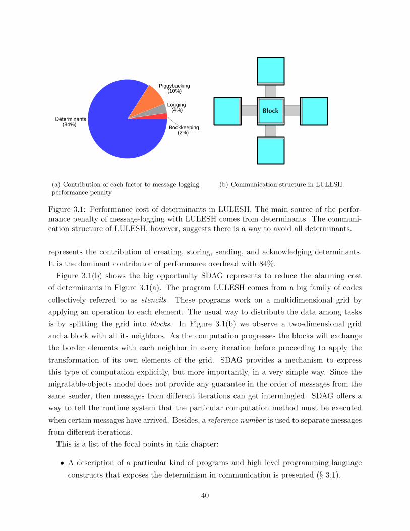
Determinants (84%)

Piggybacking (10%)

Logging (4%)

Bookkeeping (2%)

(a) Contribution of each factor to message-loggingperformance penalty.

Block

(b) Communication structure in LULESH.

Figure 3.1: Performance cost of determinants in LULESH. The main source of the perfor-mance penalty of message-logging with LULESH comes from determinants. The communi-cation structure of LULESH, however, suggests there is a way to avoid all determinants.

represents the contribution of creating, storing, sending, and acknowledging determinants.

It is the dominant contributor of performance overhead with 84%.

Figure 3.1(b) shows the big opportunity SDAG represents to reduce the alarming cost

of determinants in Figure 3.1(a). The program LULESH comes from a big family of codes

collectively referred to as stencils. These programs work on a multidimensional grid by

applying an operation to each element. The usual way to distribute the data among tasks

is by splitting the grid into blocks. In Figure 3.1(b) we observe a two-dimensional grid

and a block with all its neighbors. As the computation progresses the blocks will exchange

the border elements with each neighbor in every iteration before proceeding to apply the

transformation of its own elements of the grid. SDAG provides a mechanism to express

this type of computation explicitly, but more importantly, in a very simple way. Since the

migratable-objects model does not provide any guarantee in the order of messages from the

same sender, then messages from different iterations can get intermingled. SDAG offers a

way to tell the runtime system that the particular computation method must be executed

when certain messages have arrived. Besides, a reference number is used to separate messages

from different iterations.

This is a list of the focal points in this chapter:

• A description of a particular kind of programs and high level programming language

constructs that exposes the determinism in communication is presented (§ 3.1).

40

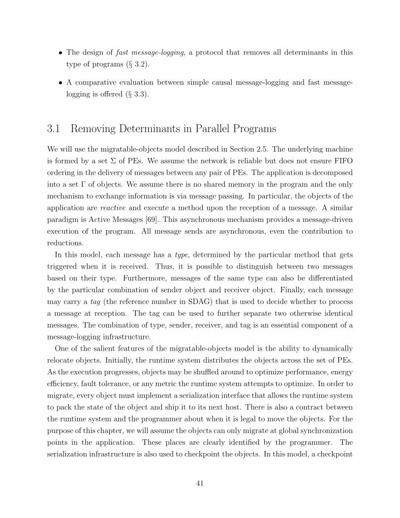
• The design of fast message-logging, a protocol that removes all determinants in this

type of programs (§ 3.2).

• A comparative evaluation between simple causal message-logging and fast message-

logging is offered (§ 3.3).

3.1 Removing Determinants in Parallel Programs

We will use the migratable-objects model described in Section 2.5. The underlying machine

is formed by a set Σ of PEs. We assume the network is reliable but does not ensure FIFO

ordering in the delivery of messages between any pair of PEs. The application is decomposed

into a set Γ of objects. We assume there is no shared memory in the program and the only

mechanism to exchange information is via message passing. In particular, the objects of the

application are reactive and execute a method upon the reception of a message. A similar

paradigm is Active Messages [69]. This asynchronous mechanism provides a message-driven

execution of the program. All message sends are asynchronous, even the contribution to

reductions.

In this model, each message has a type, determined by the particular method that gets

triggered when it is received. Thus, it is possible to distinguish between two messages

based on their type. Furthermore, messages of the same type can also be differentiated

by the particular combination of sender object and receiver object. Finally, each message

may carry a tag (the reference number in SDAG) that is used to decide whether to process

a message at reception. The tag can be used to further separate two otherwise identical

messages. The combination of type, sender, receiver, and tag is an essential component of a

message-logging infrastructure.

One of the salient features of the migratable-objects model is the ability to dynamically

relocate objects. Initially, the runtime system distributes the objects across the set of PEs.

As the execution progresses, objects may be shuffled around to optimize performance, energy

efficiency, fault tolerance, or any metric the runtime system attempts to optimize. In order to

migrate, every object must implement a serialization interface that allows the runtime system

to pack the state of the object and ship it to its next host. There is also a contract between

the runtime system and the programmer about when it is legal to move the objects. For the

purpose of this chapter, we will assume the objects can only migrate at global synchronization

points in the application. These places are clearly identified by the programmer. The

serialization infrastructure is also used to checkpoint the objects. In this model, a checkpoint

41

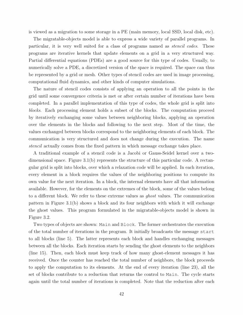
is viewed as a migration to some storage in a PE (main memory, local SSD, local disk, etc).

The migratable-objects model is able to express a wide variety of parallel programs. In

particular, it is very well suited for a class of programs named as stencil codes. These

programs are iterative kernels that update elements on a grid in a very structured way.

Partial differential equations (PDEs) are a good source for this type of codes. Usually, to

numerically solve a PDE, a discretized version of the space is required. The space can thus

be represented by a grid or mesh. Other types of stencil codes are used in image processing,

computational fluid dynamics, and other kinds of computer simulations.

The nature of stencil codes consists of applying an operation to all the points in the

grid until some convergence criteria is met or after certain number of iterations have been

completed. In a parallel implementation of this type of codes, the whole grid is split into

blocks. Each processing element holds a subset of the blocks. The computation proceed

by iteratively exchanging some values between neighboring blocks, applying an operation

over the elements in the blocks and following to the next step. Most of the time, the

values exchanged between blocks correspond to the neighboring elements of each block. The

communication is very structured and does not change during the execution. The name

stencil actually comes from the fixed pattern in which message exchange takes place.

A traditional example of a stencil code is a Jacobi or Gauss-Seidel kernel over a two-

dimensional space. Figure 3.1(b) represents the structure of this particular code. A rectan-

gular grid is split into blocks, over which a relaxation code will be applied. In each iteration,

every element in a block requires the values of the neighboring positions to compute its

own value for the next iteration. In a block, the internal elements have all that information

available. However, for the elements on the extremes of the block, some of the values belong

to a different block. We refer to these extreme values as ghost values. The communication

pattern in Figure 3.1(b) shows a block and its four neighbors with which it will exchange

the ghost values. This program formulated in the migratable-objects model is shown in

Figure 3.2.

Two types of objects are shown: Main and Block. The former orchestrates the execution

of the total number of iterations in the program. It initially broadcasts the message start

to all blocks (line 5). The latter represents each block and handles exchanging messages

between all the blocks. Each iteration starts by sending the ghost elements to the neighbors

(line 15). Then, each block must keep track of how many ghost-element messages it has

received. Once the counter has reached the total number of neighbors, the block proceeds

to apply the computation to its elements. At the end of every iteration (line 23), all the

set of blocks contribute to a reduction that returns the control to Main. The cycle starts

again until the total number of iterations is completed. Note that the reduction after each

42

1 class Main2 Collection<Block> blocks;3 method main()4 iteration = 0;5 blocks.start();6 7 method reduction()8 iteration++;9 if(iteration <= TOTAL_ITERATIONS)

10 blocks.start();11 12 13 class Block14 method start()15 sendGhostElems();16 17 method ghostElems(msg)18 copyElems(msg);19 counter++;20 if(counter == neighbors)21 counter = 0;22 compute();23 contribute(Main::reduction);24 25 26

Figure 3.2: Program structure of a two-dimensional stencil code. Each block exchanges theghost elements with its neighbors in each step. There is an asynchronous barrier after eachiteration.

iteration is inevitable in this model. Since the channels are not FIFO in delivering the

messages, then it is possible for a couple of messages between neighboring blocks to go out-

of-order. Therefore, a synchronization must be used to avoid such scenario. The reduction

effectively separates messages from consecutive iterations.

The very nature of the migratable-objects model offers a lot of flexibility in the way

the parallel program executes. It does, however, introduce concerns regarding the order in

which messages are going to be received. The counter in Figure 3.2 reflects the palliative

effort in the program to allow concurrency but avoid erroneous receptions. The same effect

can be achieved through a high-level script language that expresses the control dependencies

between certain types of events. Additionally, this script language must retain the advantages

of the reactive characteristic of objects in the program. To illustrate the way a high-level

description would work with the same example as in Figure 3.2, we show the new version of

the code in Figure 3.3.

The high-level script in Figure 3.3 features various grammatical constructs that alleviate

43

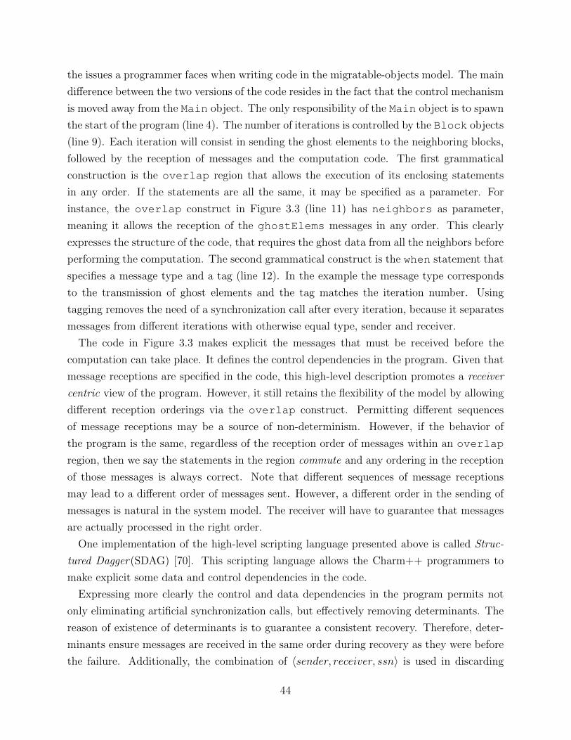
the issues a programmer faces when writing code in the migratable-objects model. The main

difference between the two versions of the code resides in the fact that the control mechanism

is moved away from the Main object. The only responsibility of the Main object is to spawn

the start of the program (line 4). The number of iterations is controlled by the Block objects

(line 9). Each iteration will consist in sending the ghost elements to the neighboring blocks,

followed by the reception of messages and the computation code. The first grammatical

construction is the overlap region that allows the execution of its enclosing statements

in any order. If the statements are all the same, it may be specified as a parameter. For

instance, the overlap construct in Figure 3.3 (line 11) has neighbors as parameter,

meaning it allows the reception of the ghostElems messages in any order. This clearly

expresses the structure of the code, that requires the ghost data from all the neighbors before

performing the computation. The second grammatical construct is the when statement that

specifies a message type and a tag (line 12). In the example the message type corresponds

to the transmission of ghost elements and the tag matches the iteration number. Using

tagging removes the need of a synchronization call after every iteration, because it separates

messages from different iterations with otherwise equal type, sender and receiver.

The code in Figure 3.3 makes explicit the messages that must be received before the

computation can take place. It defines the control dependencies in the program. Given that

message receptions are specified in the code, this high-level description promotes a receiver

centric view of the program. However, it still retains the flexibility of the model by allowing

different reception orderings via the overlap construct. Permitting different sequences

of message receptions may be a source of non-determinism. However, if the behavior of

the program is the same, regardless of the reception order of messages within an overlap

region, then we say the statements in the region commute and any ordering in the reception

of those messages is always correct. Note that different sequences of message receptions

may lead to a different order of messages sent. However, a different order in the sending of

messages is natural in the system model. The receiver will have to guarantee that messages

are actually processed in the right order.

One implementation of the high-level scripting language presented above is called Struc-

tured Dagger(SDAG) [70]. This scripting language allows the Charm++ programmers to

make explicit some data and control dependencies in the code.

Expressing more clearly the control and data dependencies in the program permits not

only eliminating artificial synchronization calls, but effectively removing determinants. The

reason of existence of determinants is to guarantee a consistent recovery. Therefore, deter-

minants ensure messages are received in the same order during recovery as they were before

the failure. Additionally, the combination of 〈sender, receiver, ssn〉 is used in discarding

44

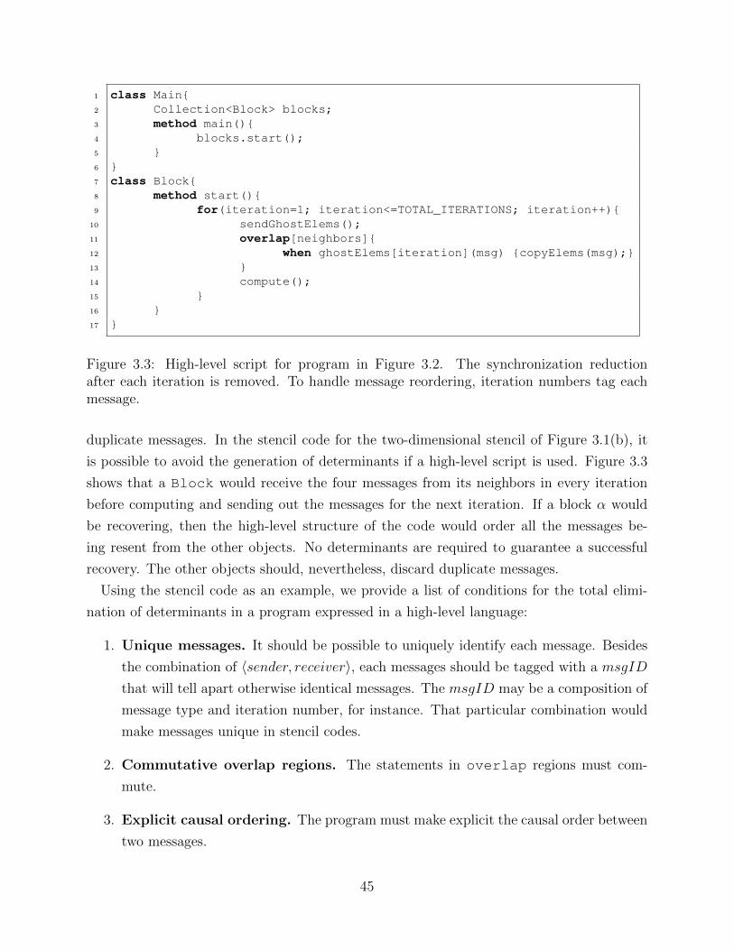
1 class Main2 Collection<Block> blocks;3 method main()4 blocks.start();5 6 7 class Block8 method start()9 for(iteration=1; iteration<=TOTAL_ITERATIONS; iteration++)

10 sendGhostElems();11 overlap[neighbors]12 when ghostElems[iteration](msg) copyElems(msg);13 14 compute();15 16 17

Figure 3.3: High-level script for program in Figure 3.2. The synchronization reductionafter each iteration is removed. To handle message reordering, iteration numbers tag eachmessage.

duplicate messages. In the stencil code for the two-dimensional stencil of Figure 3.1(b), it

is possible to avoid the generation of determinants if a high-level script is used. Figure 3.3

shows that a Block would receive the four messages from its neighbors in every iteration

before computing and sending out the messages for the next iteration. If a block α would

be recovering, then the high-level structure of the code would order all the messages be-

ing resent from the other objects. No determinants are required to guarantee a successful

recovery. The other objects should, nevertheless, discard duplicate messages.

Using the stencil code as an example, we provide a list of conditions for the total elimi-

nation of determinants in a program expressed in a high-level language:

1. Unique messages. It should be possible to uniquely identify each message. Besides

the combination of 〈sender, receiver〉, each messages should be tagged with a msgID

that will tell apart otherwise identical messages. The msgID may be a composition of

message type and iteration number, for instance. That particular combination would

make messages unique in stencil codes.

2. Commutative overlap regions. The statements in overlap regions must com-

mute.

3. Explicit causal ordering. The program must make explicit the causal order between

two messages.

45

In addition, if determinants disappear from the message-logging layer, it must be guaran-

teed that all internal structures in the runtime system are still correct. This includes all the

data structures for load balancing, checkpointing, collective communication operations, etc.

3.2 Fast Message-Logging Protocol

Using the insight from the previous section and the background work of Chapter 2, we

present a new breed of message-logging protocols. We name it fast message-logging because

it focuses on accelerating the three sources of overhead in a resilience solution presented in

Figure 1.2. This is brief justification about why it is fast message-logging:

Fast forward-path By removing determinants from an execution, it reduces the slowdown

of message-logging. According to Figure 3.1(a) determinants are the main source of

overhead, so eliminating them should bring the performance overhead to a minimum.

Fast checkpoint It uses local checkpoint to avoid checkpoint-time congestion in the file

system. This reduces the robustness of the system, but just by a tiny margin, given

that most failure in HPC systems only involve a single node [59].

Fast recovery It uses parallel recovery to accelerate the recovery of the failed components.

The fast message-logging only generates message identifiers and does not create determi-

nants. At send time, each message is labeled with 〈sender, receiver,msgID〉. This informa-

tion will be used to eventually ignore messages if they are repeated. It relies on the high-level

scripting infrastructure to buffer early messages and to deliver them in a correct order for

the program. This way, there is a clear separation of concerns with respect to the functions

that must be executed during recovery. Figure 3.4(a) show the way this protocol achieves a

separation of concerns between the layers in the software stack. The bottom layer stands for

the message-logging protocol that is in charge of reacting to a failure. This mainly represents

performing two tasks. The first is to replay the messages to the failed objects. The second

task is to suppress duplicates during recovery based on the tuple 〈sender, receiver,msgID〉.The top layer is the high-level language infrastructure that guarantees the consistency in the

state of the failed objects by delivering the messages in the correct order.

We call the type of programs that comply with all the conditions to remove all the de-

terminants is called receive deterministic. Even when receives and sends may not be de-

terministic, the state of the objects will nevertheless be the same. Figure 3.4(b) shows a

Venn diagram with the relationships between piece-wise deterministic, send-deterministic

and receive-deterministic programs.

46

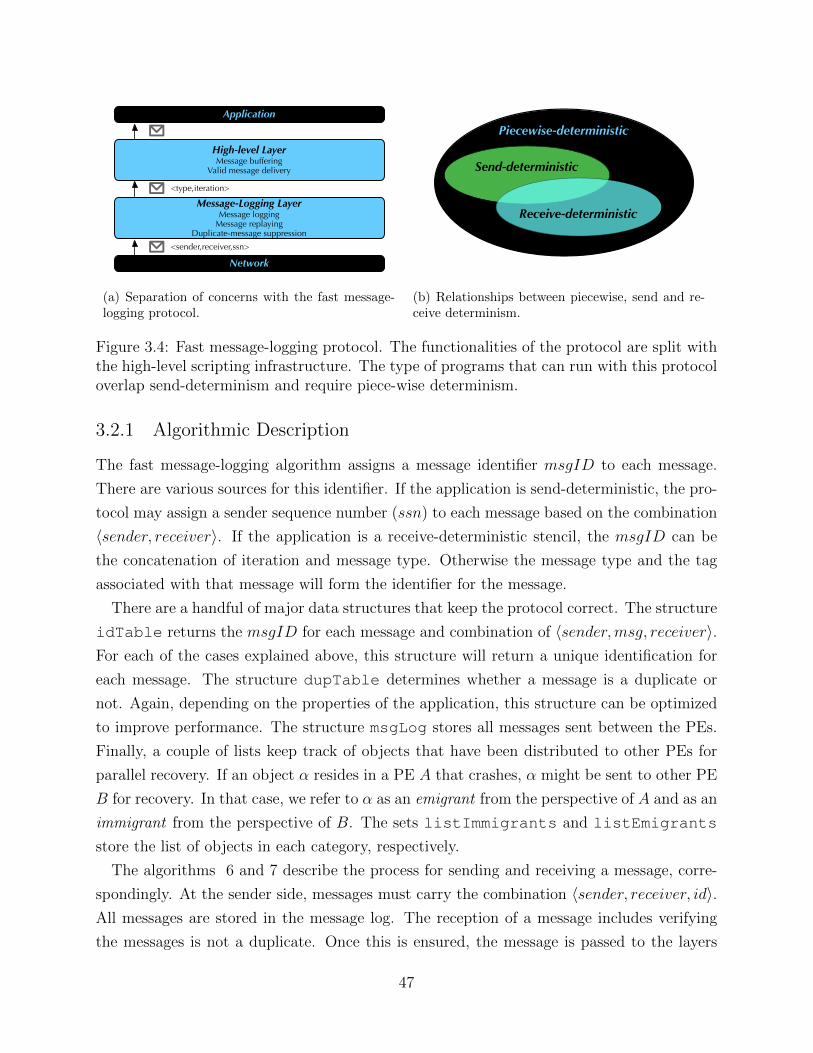
Network

Message-Logging LayerMessage logging

Message replayingDuplicate-message suppression

High-level LayerMessage buffering

Valid message delivery

Application

<sender,receiver,ssn>

<type,iteration>

(a) Separation of concerns with the fast message-logging protocol.

Piecewise-deterministic

Send-deterministic

Receive-deterministic

(b) Relationships between piecewise, send and re-ceive determinism.

Figure 3.4: Fast message-logging protocol. The functionalities of the protocol are split withthe high-level scripting infrastructure. The type of programs that can run with this protocoloverlap send-determinism and require piece-wise determinism.

3.2.1 Algorithmic Description

The fast message-logging algorithm assigns a message identifier msgID to each message.

There are various sources for this identifier. If the application is send-deterministic, the pro-

tocol may assign a sender sequence number (ssn) to each message based on the combination

〈sender, receiver〉. If the application is a receive-deterministic stencil, the msgID can be

the concatenation of iteration and message type. Otherwise the message type and the tag

associated with that message will form the identifier for the message.

There are a handful of major data structures that keep the protocol correct. The structure

idTable returns the msgID for each message and combination of 〈sender,msg, receiver〉.For each of the cases explained above, this structure will return a unique identification for

each message. The structure dupTable determines whether a message is a duplicate or

not. Again, depending on the properties of the application, this structure can be optimized

to improve performance. The structure msgLog stores all messages sent between the PEs.

Finally, a couple of lists keep track of objects that have been distributed to other PEs for

parallel recovery. If an object α resides in a PE A that crashes, α might be sent to other PE

B for recovery. In that case, we refer to α as an emigrant from the perspective of A and as an

immigrant from the perspective of B. The sets listImmigrants and listEmigrants

store the list of objects in each category, respectively.

The algorithms 6 and 7 describe the process for sending and receiving a message, corre-

spondingly. At the sender side, messages must carry the combination 〈sender, receiver, id〉.All messages are stored in the message log. The reception of a message includes verifying

the messages is not a duplicate. Once this is ensured, the message is passed to the layers

47

above to be correctly processed. This may include buffering the message, forwarding the

message to other PE or delivering the message to the application.

Algorithm 6 Send(α,msg, β): object α sends msg to object β

1: id← idTable.getID(α,msg, β)2: msg.id← id3: msg.sender ← α4: msg.receiver ← β5: msg.incarnation← IncarnationNumber6: if α.PE 6= β.PE then7: msgLog.add(msg) . Storing remote message8: end if9: NetworkSend(msg)

Algorithm 7 Receive(α,msg, β): object β receives msg from object α

1: num← msg.incarnation2: if OldIncarnation(num) then3: DiscardOld(msg) . Ignoring old message4: end if5: flag ← dupTable.getFlag(α, β,msg.id)6: if flag then7: DiscardDuplicate(msg) . Ignoring repeated message8: return9: end if

10: Process(msg) . Forward to high-level layer

Fast message-logging relies on globally coordinated synchronized checkpoint. The pro-

grammer uses global synchronization points in the application to trigger the checkpoint

calls. Algorithm 8 presents the steps included in the checkpoint process. First, all immi-

grant objects are send back to their original PEs. These objects may have been migrated to

a PE for parallel recovery purposes. Next, a PE waits for all its emigrant objects to arrive.

The message log is cleaned up then and a new checkpoint message is built with the state of

all the objects.

Once a failure has been detected, the runtime system notifies the rest of the PEs about

the crash of one PE. Let us assume PE A fails, thus Algorithm 9 shows the steps after each

PE receives the failure notification. It merely consists in replaying the messages in msgLog

bound to objects in PE A. At the same time, PE A follows the recovery procedure, that

includes Algorithm 10 to distribute all its objects to as many PEs are involved in parallel

recovery. The set A1, A2, ..., AP stands for the set of other P PEs helping the recovery of

A.

48

Algorithm 8 Checkpoint(): called at PE A

1: Send all objects α in listImmigrants2: Wait for all objects α in listEmigrants3: ckptMsg ← 4: msgLog.clean()5: for all objects α do6: ckptMsg.add(α.state)7: NetworkSend(ckptMsg)8: end for

Algorithm 9 Restart(A): received at every PE except for A

1: for all objects α in A do2: Send all messages bound to α in msgLog3: end for

Algorithm 10 Recovery(): called at PE A

1: for all objects α in A do2: Distribute α to a PE in A1, A2, ..., AP3: Add α to listEmigrants4: end for

3.2.2 Formal Proof of Correctness

Lemma 3.1. All necessary messages for recovery are available.

Proof Sketch. Let us assume PE A crashes. All remote messages sent to objects in A have

to be available at their sender PE. During restart, those messages will be replayed form the

message logs. Since we assume PWD applications, all the local messages will be regenerated

after the causally dependent messages are received and the necessary computation takes

place. Note that in the case of parallel recovery, an object that was distributed to a different

PE will get its messages thanks to the forwarding mechanism in the high-level layer.

Lemma 3.2. All replayed messages are received in the same order as before the failure or

in an equivalent order.

Proof Sketch. During the recovery of PE A, all necessary messages will be resent again.

Duplicate messages are discarded by the message-logging layer using the dupTable data

structure and the combination 〈sender, receiver, id〉. Since messages can be uniquely iden-

tified, then the high-level layer will deliver them in the same order as before the crash or in

an order that is consistent with the state of the rest of the application.

Lemma 3.3. There are no orphan objects.

49

Proof Sketch. By contradiction. Let us assume object β is an orphan. It other words, its

state depends on a message m that does not get resend during recovery. The original sender

of message m was object α, which used to live on the failed PE A. Given that object α

recieves all the messages it received before the crash and those messages are delivered in the

same order (or an equivalent one), α will necessarily send the same messages because of the

PWD assumption. Albeit not in the same order, message m must eventually arrive at β.

Theorem 3.4. The recovery process in fast message-logging is correct.

Proof Sketch. After lemmas 3.1,3.2 and 3.3, all messages are sent again, they are processed

in the same order or in an equivalent consistent order and there are no orphan objects.

Therefore, the recovery of a PE is correct.

3.3 Experimental Results

In order to understand the performance penalization imposed by the fast message-logging

protocol, we examined three stencil codes: Wave2D, Jacobi3D and LULESH. These programs

were implemented in SDAG to decrease execution time (since barriers between iterations are

not needed anymore) and allow the possibility of removing determinants.

We first examine the effect of virtualization ratio on each program. Recall from Chapter 2

that virtualization ratio stands for the average number of objects per PE. For this experi-

ment, each PE is a core. Figure 3.5 presents the results on 1, 024 cores of Intrepid. Each data

point reflects the average of 5 repetitions of the same experiment. Wave2D in Figure 3.5(a)

seems to manifest that Wave2D benefits from virtualization. In fact, the performance of the

program stays within a 5% difference up to 32 objects per core. A similar behavior occurs in

Jacobi3D in Figure 3.5(b), except in this case the program is always slightly slowed down by

virtualization. Again, the average iteration time stays within a 10% margin up to 32 objects

per core. Finally, Figure 3.5(c) accepts a higher virtualization ratio without a significant

performance degradation. Even 128 objects per core stays within a 3% margin. Having a

high virtualization ratio is beneficial for applications in view of the eminent thermal vari-

ation of future systems. With more objects per core, it is possible to obtain a better load

balance in case some of the PEs have to be slowed down to reduce their temperature.

Using a virtualization ratio of 32 for Wave2D and Jacobi3D and 128 for LULESH, we ran

5 times each program and compared the results between fast message-logging and causal

message-logging. The results are presented in Figure 3.6 and offer the relative performance

overhead when compared with the base Charm++. The figure shows a weak-scale experiment

50

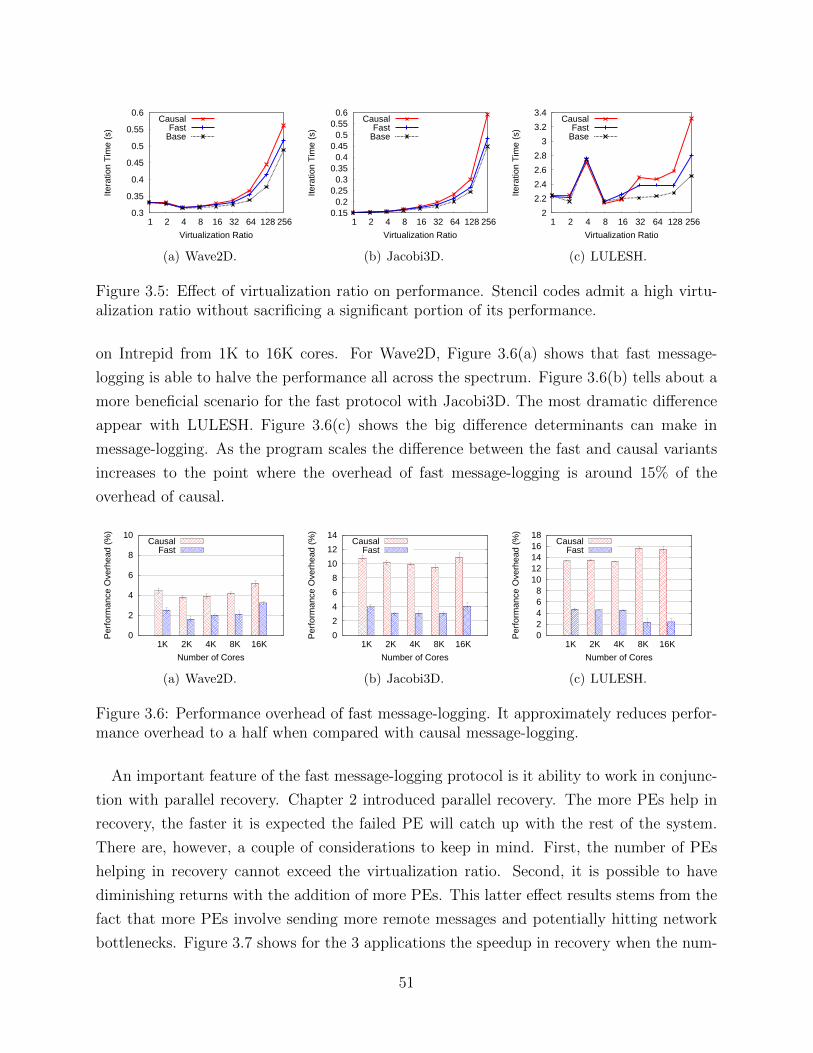
0.3

0.35

0.4

0.45

0.5

0.55

0.6

1 2 4 8 16 32 64 128 256

Itera

tion

Tim

e (s

)

Virtualization Ratio

CausalFast

Base

(a) Wave2D.

0.15 0.2

0.25 0.3

0.35 0.4

0.45 0.5

0.55 0.6

1 2 4 8 16 32 64 128 256

Itera

tion

Tim

e (s

)

Virtualization Ratio

CausalFast

Base

(b) Jacobi3D.

2

2.2

2.4

2.6

2.8

3

3.2

3.4

1 2 4 8 16 32 64 128 256

Itera

tion

Tim

e (s

)

Virtualization Ratio

CausalFast

Base

(c) LULESH.

Figure 3.5: Effect of virtualization ratio on performance. Stencil codes admit a high virtu-alization ratio without sacrificing a significant portion of its performance.

on Intrepid from 1K to 16K cores. For Wave2D, Figure 3.6(a) shows that fast message-

logging is able to halve the performance all across the spectrum. Figure 3.6(b) tells about a

more beneficial scenario for the fast protocol with Jacobi3D. The most dramatic difference

appear with LULESH. Figure 3.6(c) shows the big difference determinants can make in

message-logging. As the program scales the difference between the fast and causal variants

increases to the point where the overhead of fast message-logging is around 15% of the

overhead of causal.

0

2

4

6

8

10

1K 2K 4K 8K 16K

Per

form

ance

Ove

rhea

d (%

)

Number of Cores

CausalFast

(a) Wave2D.

0

2

4

6

8

10

12

14

1K 2K 4K 8K 16K

Per

form

ance

Ove

rhea

d (%

)

Number of Cores

CausalFast

(b) Jacobi3D.

0 2 4 6 8

10 12 14 16 18

1K 2K 4K 8K 16K

Per

form

ance

Ove

rhea

d (%

)

Number of Cores

CausalFast

(c) LULESH.

Figure 3.6: Performance overhead of fast message-logging. It approximately reduces perfor-mance overhead to a half when compared with causal message-logging.

An important feature of the fast message-logging protocol is it ability to work in conjunc-

tion with parallel recovery. Chapter 2 introduced parallel recovery. The more PEs help in

recovery, the faster it is expected the failed PE will catch up with the rest of the system.

There are, however, a couple of considerations to keep in mind. First, the number of PEs

helping in recovery cannot exceed the virtualization ratio. Second, it is possible to have

diminishing returns with the addition of more PEs. This latter effect results stems from the

fact that more PEs involve sending more remote messages and potentially hitting network

bottlenecks. Figure 3.7 shows for the 3 applications the speedup in recovery when the num-

51

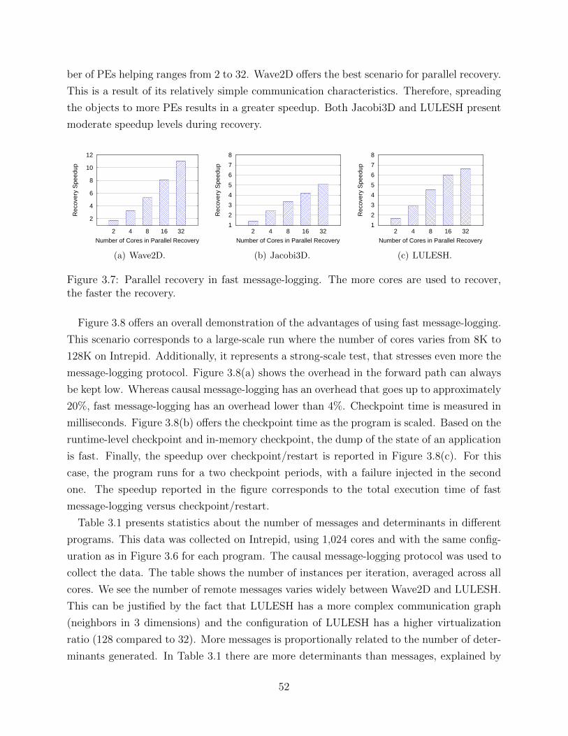
ber of PEs helping ranges from 2 to 32. Wave2D offers the best scenario for parallel recovery.

This is a result of its relatively simple communication characteristics. Therefore, spreading

the objects to more PEs results in a greater speedup. Both Jacobi3D and LULESH present

moderate speedup levels during recovery.

2

4

6

8

10

12

2 4 8 16 32

Rec

over

y S

peed

up

Number of Cores in Parallel Recovery

(a) Wave2D.

1

2

3

4

5

6

7

8

2 4 8 16 32

Rec

over

y S

peed

up

Number of Cores in Parallel Recovery

(b) Jacobi3D.

1

2

3

4

5

6

7

8

2 4 8 16 32

Rec

over

y S

peed

up

Number of Cores in Parallel Recovery

(c) LULESH.

Figure 3.7: Parallel recovery in fast message-logging. The more cores are used to recover,the faster the recovery.

Figure 3.8 offers an overall demonstration of the advantages of using fast message-logging.

This scenario corresponds to a large-scale run where the number of cores varies from 8K to

128K on Intrepid. Additionally, it represents a strong-scale test, that stresses even more the

message-logging protocol. Figure 3.8(a) shows the overhead in the forward path can always

be kept low. Whereas causal message-logging has an overhead that goes up to approximately

20%, fast message-logging has an overhead lower than 4%. Checkpoint time is measured in

milliseconds. Figure 3.8(b) offers the checkpoint time as the program is scaled. Based on the

runtime-level checkpoint and in-memory checkpoint, the dump of the state of an application

is fast. Finally, the speedup over checkpoint/restart is reported in Figure 3.8(c). For this

case, the program runs for a two checkpoint periods, with a failure injected in the second

one. The speedup reported in the figure corresponds to the total execution time of fast

message-logging versus checkpoint/restart.

Table 3.1 presents statistics about the number of messages and determinants in different

programs. This data was collected on Intrepid, using 1,024 cores and with the same config-

uration as in Figure 3.6 for each program. The causal message-logging protocol was used to

collect the data. The table shows the number of instances per iteration, averaged across all

cores. We see the number of remote messages varies widely between Wave2D and LULESH.

This can be justified by the fact that LULESH has a more complex communication graph

(neighbors in 3 dimensions) and the configuration of LULESH has a higher virtualization

ratio (128 compared to 32). More messages is proportionally related to the number of deter-

minants generated. In Table 3.1 there are more determinants than messages, explained by

52

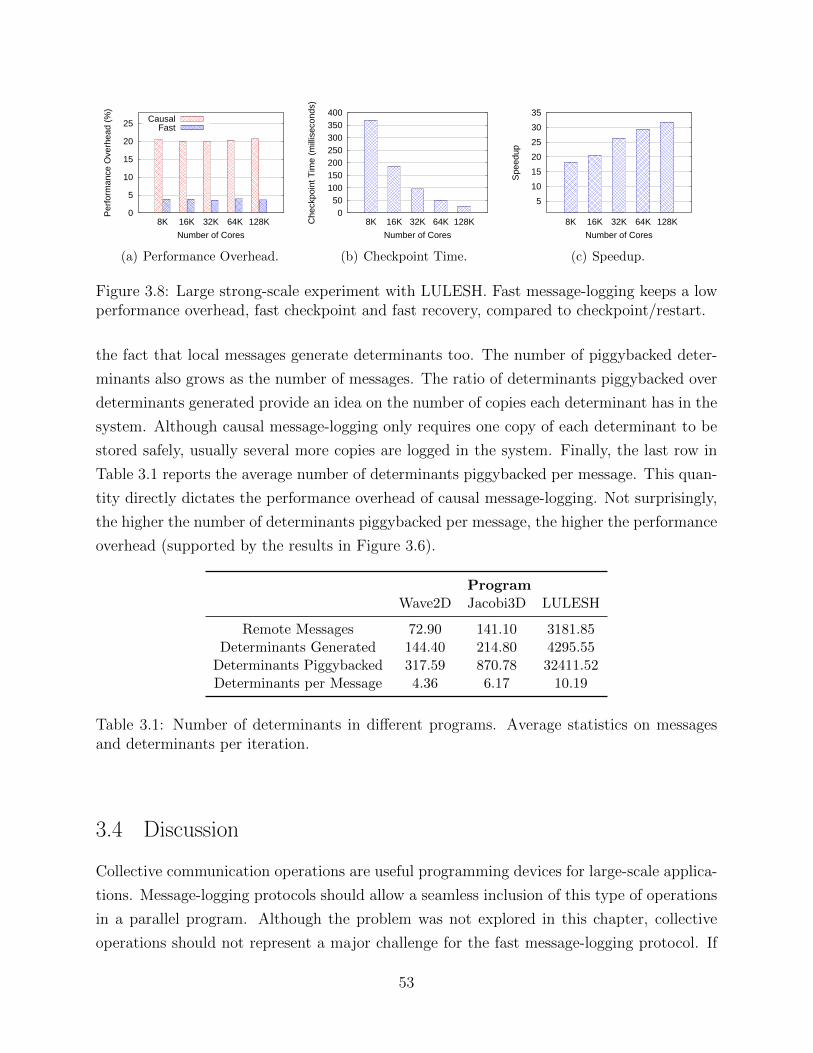
0

5

10

15

20

25

8K 16K 32K 64K 128K

Per

form

ance

Ove

rhea

d (%

)

Number of Cores

CausalFast

(a) Performance Overhead.

0 50

100 150 200 250 300 350 400

8K 16K 32K 64K 128KChe

ckpo

int T

ime

(mill

isec

onds

)

Number of Cores

(b) Checkpoint Time.

5

10

15

20

25

30

35

8K 16K 32K 64K 128K

Spe

edup

Number of Cores

(c) Speedup.

Figure 3.8: Large strong-scale experiment with LULESH. Fast message-logging keeps a lowperformance overhead, fast checkpoint and fast recovery, compared to checkpoint/restart.

the fact that local messages generate determinants too. The number of piggybacked deter-

minants also grows as the number of messages. The ratio of determinants piggybacked over

determinants generated provide an idea on the number of copies each determinant has in the

system. Although causal message-logging only requires one copy of each determinant to be

stored safely, usually several more copies are logged in the system. Finally, the last row in

Table 3.1 reports the average number of determinants piggybacked per message. This quan-

tity directly dictates the performance overhead of causal message-logging. Not surprisingly,

the higher the number of determinants piggybacked per message, the higher the performance

overhead (supported by the results in Figure 3.6).

ProgramWave2D Jacobi3D LULESH

Remote Messages 72.90 141.10 3181.85Determinants Generated 144.40 214.80 4295.55

Determinants Piggybacked 317.59 870.78 32411.52Determinants per Message 4.36 6.17 10.19

Table 3.1: Number of determinants in different programs. Average statistics on messagesand determinants per iteration.

3.4 Discussion

Collective communication operations are useful programming devices for large-scale applica-

tions. Message-logging protocols should allow a seamless inclusion of this type of operations

in a parallel program. Although the problem was not explored in this chapter, collective

operations should not represent a major challenge for the fast message-logging protocol. If

53

the collective operation is synchronous, it will enforce an ordering of the reception order,

guaranteeing that recovery will respect that order. If the collective is asynchronous, it will

require an identification number. Using this unique number, the system can differentiate be-

tween contributing messages for particular collective operations. This means that collective

calls can be uniquely identified in any case.

A further issue related to collective operations lies in the way the contribution from the

different tasks is accumulated. More specifically, floating-point arithmetic is not associative.

Therefore, in principle, the same set of operations should be repeated to produce the same

contribution message. Note however that the contribution messages for a reduction, for

instance, will nevertheless be ignored by the receiver. Thus, the way results are accumulated

in a collective call is irrelevant. All that matters is the state of the different tasks and the

fact they need to be kept consistent.

Despite the fact that most failure bring down one single node at a time [31, 59], toler-

ating multiple concurrent node failures is a positive feature. It increases the robustness of

the system and it may be adopted in environments where this type of failures occur more

frequently. The fast message-logging protocol is able to tolerate any arbitrary number of

concurrent node failures. Given that it does not require determinants and the high level lan-

guage enforces the reception order, any number of nodes can simultaneously fail (provided

they are still able to recover their checkpoint) and resume execution.

3.5 Related Work

The seminal work on send determinism [49, 51, 71] provided a clear insight on the futility

of creating determinants for all message receptions. The protocol presented in the send-

determinism literature depends on FIFO channels for it to properly work. We remove that

assumption to use the asynchronous execution model of Charm++. However, to tame the

excessive flexibility in the order of message reception, we relied on high level programming

language constructs. Additionally, a major difference in the send-determinism protocol and

fast message-logging appears during recovery. The send-determinism protocol requires to

replay the causally-dependent messages in a synchronized fashion. In other words, the

senders of messages can not send the whole set of messages to the recovering node as soon as

they are notified about the restart. They must wait to receive the causally related messages

to emit the next message. This hampers the ability of message-logging to achieve a faster

recovery. By using a reception control mechanism, fast message-logging is able to receive all

messages at once and completely sort them in a valid program order. Thus, during recovery

54

it is possible to achieve near-zero latency. The evaluation of send-determinism used up to

256 processors.

A new design of the message-logging layer for Open MPI [53] revealed that vast amount of

determinants that are not necessary to guarantee a safe recovery. By interposing a message-

logging substrate between the application and the network layer, this new design is able

to create matchings of events posted by the application and arrival events coming from the

network. Matchings may be deterministic if the expected sender and the actual sender of the

message are the same. Use of wildcards will create non-deterministic matches. By logging

only non-deterministic matches, this design is able to dramatically reduce the number of

determinants.

The large scale simulator BigSim [50] used parallel discrete event simulation (PDES) to

make predictions on the performance of scientific codes for supercomputers. Since BigSim is

based on POSE (a framework for PDES), it would allow speculative simulation of different

threads of events. In that regard, programs that allow only one possible execution sequence

would find a very efficient simulation. In BigSim, linear order parallel programs are a special

kind of codes for which messages are processed in exactly one order.

55

CHAPTER 4Performance and Energy Models

Essentially, all models are wrong, but

some are useful

George E.P. Box

Understanding the laws that govern the universe has been a constant quest in science. The

result of that quest has brought several theories of how things came to be. The Victorians,

for instance, believed the whole universe was filled with ether. This medium was able to carry

light and objects moving through ether would generate ether wind. Later on, experimental

evidence denied the existence of ether and the special theory of relativity defined spacetime,

a single entity that represents the flexibility of time and space. In that theory, there was

a cosmological constant that would provide the illusion of a static and eternal universe.

However, more recent empirical evidence and theoretical breakthroughs have given rise to

the big bang theory, which states the universe had a beginning and it is dynamic. All these

theories of the universe are models to facilitate the comprehension of our physical reality.

A model is a conceptual device that represents reality in a way that makes different

phenomena easier to understand. From that definition, a good model has to be realistic

and simple. The first characteristic is fundamental for the model to have any applicability.

The second characteristic is what makes a model convenient. If a model were as complex

as reality, it would not make a particular phenomenon easier to study. The real power of

a model comes from the ability to abstract the unimportant details of reality and consider

those fundamental variables that contribute the most to the effect under study. Simplicity

does not necessarily means dullness. A simple model can be powerful if it is able to provide

two additional features. It ought to be insightful if it can reveal the hidden connections of

the different components and what can be expected from the interplay of those components.

56

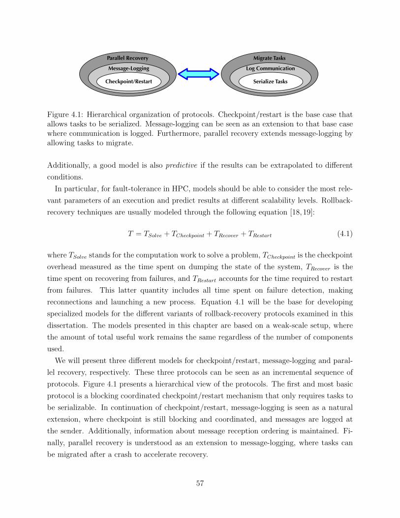
Parallel Recovery

Message-Logging

Checkpoint/Restart

Migrate Tasks

Log Communication

Serialize Tasks

Figure 4.1: Hierarchical organization of protocols. Checkpoint/restart is the base case thatallows tasks to be serialized. Message-logging can be seen as an extension to that base casewhere communication is logged. Furthermore, parallel recovery extends message-logging byallowing tasks to migrate.

Additionally, a good model is also predictive if the results can be extrapolated to different

conditions.

In particular, for fault-tolerance in HPC, models should be able to consider the most rele-

vant parameters of an execution and predict results at different scalability levels. Rollback-

recovery techniques are usually modeled through the following equation [18,19]:

T = TSolve + TCheckpoint + TRecover + TRestart (4.1)

where TSolve stands for the computation work to solve a problem, TCheckpoint is the checkpoint

overhead measured as the time spent on dumping the state of the system, TRecover is the

time spent on recovering from failures, and TRestart accounts for the time required to restart

from failures. This latter quantity includes all time spent on failure detection, making

reconnections and launching a new process. Equation 4.1 will be the base for developing

specialized models for the different variants of rollback-recovery protocols examined in this

dissertation. The models presented in this chapter are based on a weak-scale setup, where

the amount of total useful work remains the same regardless of the number of components

used.

We will present three different models for checkpoint/restart, message-logging and paral-

lel recovery, respectively. These three protocols can be seen as an incremental sequence of

protocols. Figure 4.1 presents a hierarchical view of the protocols. The first and most basic

protocol is a blocking coordinated checkpoint/restart mechanism that only requires tasks to

be serializable. In continuation of checkpoint/restart, message-logging is seen as a natural

extension, where checkpoint is still blocking and coordinated, and messages are logged at

the sender. Additionally, information about message reception ordering is maintained. Fi-

nally, parallel recovery is understood as an extension to message-logging, where tasks can

be migrated after a crash to accelerate recovery.

57

In this model, failures are assumed to be exponentially distributed. This means, the

interarrival time between failures is modeled through a random variable with exponential

distribution. Although, other distributions have been found to model better interarrival fail-

ures in supercomputers [72], the exponential distribution significantly simplifies the model.

This chapter highlights the following contributions:

• An analytical model to predict the performance for message-logging protocols and

parallel recovery at large scale (§4.2).

• An analytical model to predict the energy consumption for rollback-recovery protocols

at large scale (§4.3).

• Large-scale projections on the benefits of message-logging and parallel recovery for

both performance and energy consumption (§4.4).

• A simulation-based set of projections of message-logging protocols at very high failure

rates. The results show that parallel recovery is able to have a checkpoint period longer

than the mean-time-between-failures (§4.5).

4.1 Parameters

In order to capture the most relevant phenomena of rollback-recovery protocols in the per-

formance and energy-consumption models, we use the parameters listed in Table 4.1. They

can be divided in roughly 4 categories (seen as segments in the table). The first category

corresponds to system-specific data. The second category stands for application-specific

data. The third accounts for application-specific data regarding message-logging. Finally,

the last category collects system-specific data about energy consumption. Let us examine

these parameters closely.

Parameters M and S are interrelated. The size of the machine will define how reliable the

whole system is. In general, the higher the value of S, the lower the value of M . In fact,

these two values are related through the mean-time-between-failures of a socket, MS. The

actual equation relating M and S is M = MS

S. Each application will have an optimal value

of V . In fact, this value may change according to the scale of the run. The other values

for rollback-recovery come from the original formulation of the performance model [19]. It

is assumed the application has to perform W time units of work without any interruption.

The application takes δ time units to checkpoint and restarts in R. The performance model

computes the optimum value of τ that minimizes total execution time T . It is clear that the

58

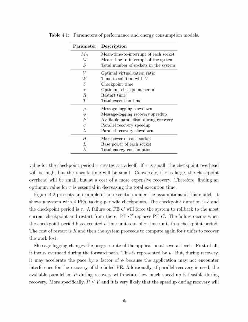
Table 4.1: Parameters of performance and energy consumption models.

Parameter Description

MS Mean-time-to-interrupt of each socketM Mean-time-to-interrupt of the systemS Total number of sockets in the system

V Optimal virtualization ratioW Time to solution with Vδ Checkpoint timeτ Optimum checkpoint periodR Restart timeT Total execution time

µ Message-logging slowdownφ Message-logging recovery speedupP Available parallelism during recoveryσ Parallel recovery speedupλ Parallel recovery slowdown

H Max power of each socketL Base power of each socketE Total energy consumption

value for the checkpoint period τ creates a tradeoff. If τ is small, the checkpoint overhead

will be high, but the rework time will be small. Conversely, if τ is large, the checkpoint

overhead will be small, but at a cost of a more expensive recovery. Therefore, finding an

optimum value for τ is essential in decreasing the total execution time.

Figure 4.2 presents an example of an execution under the assumptions of this model. It

shows a system with 4 PEs, taking periodic checkpoints. The checkpoint duration is δ and

the checkpoint period is τ . A failure on PE C will force the system to rollback to the most

current checkpoint and restart from there. PE C ′ replaces PE C. The failure occurs when

the checkpoint period has executed t time units out of τ time units in a checkpoint period.

The cost of restart is R and then the system proceeds to compute again for t units to recover

the work lost.

Message-logging changes the progress rate of the application at several levels. First of all,

it incurs overhead during the forward path. This is represented by µ. But, during recovery,

it may accelerate the pace by a factor of φ because the application may not encounter

interference for the recovery of the failed PE. Additionally, if parallel recovery is used, the

available parallelism P during recovery will dictate how much speed up is feasible during

recovery. More specifically, P ≤ V and it is very likely that the speedup during recovery will

59

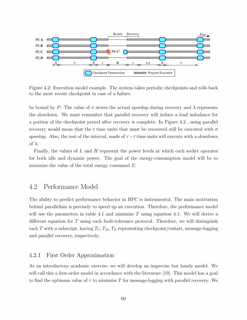
PE A

PE B

PE C PE C'

PE D! " ! t R

Time

t "-t

Restart Recovery

Checkpoint Transmission Program Execution

! "

Figure 4.2: Execution model example. The system takes periodic checkpoints and rolls backto the most recent checkpoint in case of a failure.

be bound by P . The value of σ stores the actual speedup during recovery and λ represents

the slowdown. We must remember that parallel recovery will induce a load imbalance for

a portion of the checkpoint period after recovery is complete. In Figure 4.2 , using parallel

recovery would mean that the t time units that must be recovered will be executed with σ

speedup. Also, the rest of the interval, made of τ−t time units will execute with a slowdown

of λ.

Finally, the values of L and H represent the power levels at which each socket operates

for both idle and dynamic power. The goal of the energy-consumption model will be to

minimize the value of the total energy consumed E.

4.2 Performance Model

The ability to predict performance behavior in HPC is instrumental. The main motivation

behind parallelism is precisely to speed up an execution. Therefore, the performance model

will use the parameters in table 4.1 and minimize T using equation 4.1. We will derive a

different equation for T using each fault-tolerance protocol. Therefore, we will distinguish

each T with a subscript, having TC , TM , TP representing checkpoint/restart, message-logging

and parallel recovery, respectively.

4.2.1 First Order Approximation

As an introductory academic exercise, we will develop an imprecise but handy model. We

will call this a first-order model in accordance with the literature [19]. This model has a goal

to find the optimum value of τ to minimize T for message-logging with parallel recovery. We

60

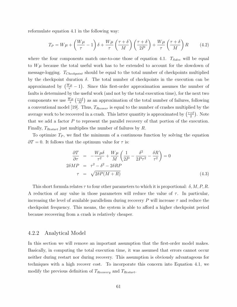
reformulate equation 4.1 in the following way:

TP = Wµ+

(Wµ

τ− 1

)δ +

Wµ

τ

(τ + δ

M

)(τ + δ

2P

)+Wµ

τ

(τ + δ

M

)R (4.2)

where the four components match one-to-one those of equation 4.1. TSolve will be equal

to Wµ because the total useful work has to be extended to account for the slowdown of

message-logging. TCheckpoint should be equal to the total number of checkpoints multiplied

by the checkpoint duration δ. The total number of checkpoints in the execution can be

approximated by(Wµτ− 1). Since this first-order approximation assumes the number of

faults is determined by the useful work (and not by the total execution time), for the next two

components we use Wµτ

(τ+δM

)as an approximation of the total number of failures, following

a conventional model [19]. Thus, TRecover is equal to the number of crashes multiplied by the

average work to be recovered in a crash. This latter quantity is approximated by(τ+δ2

). Note

that we add a factor P to represent the parallel recovery of that portion of the execution.

Finally, TRestart just multiplies the number of failures by R.

To optimize TP , we find the minimum of a continuous function by solving the equation

∂T = 0. It follows that the optimum value for τ is:

∂T

∂τ= −Wµδ

τ 2+Wµ

M

(1

2P− δ2

2Pτ 2− δR

τ 2

)= 0

2δMP = τ 2 − δ2 − 2δRP

τ =√

2δP (M +R) (4.3)

This short formula relates τ to four other parameters to which it is proportional: δ,M, P,R.

A reduction of any value in those parameters will reduce the value of τ . In particular,

increasing the level of available parallelism during recovery P will increase τ and reduce the

checkpoint frequency. This means, the system is able to afford a higher checkpoint period

because recovering from a crash is relatively cheaper.

4.2.2 Analytical Model

In this section we will remove an important assumption that the first-order model makes.

Basically, in computing the total execution time, it was assumed that errors cannot occur

neither during restart nor during recovery. This assumption is obviously advantageous for

techniques with a high recover cost. To incorporate this concern into Equation 4.1, we

modify the previous definition of TRecovery and TRestart.

61

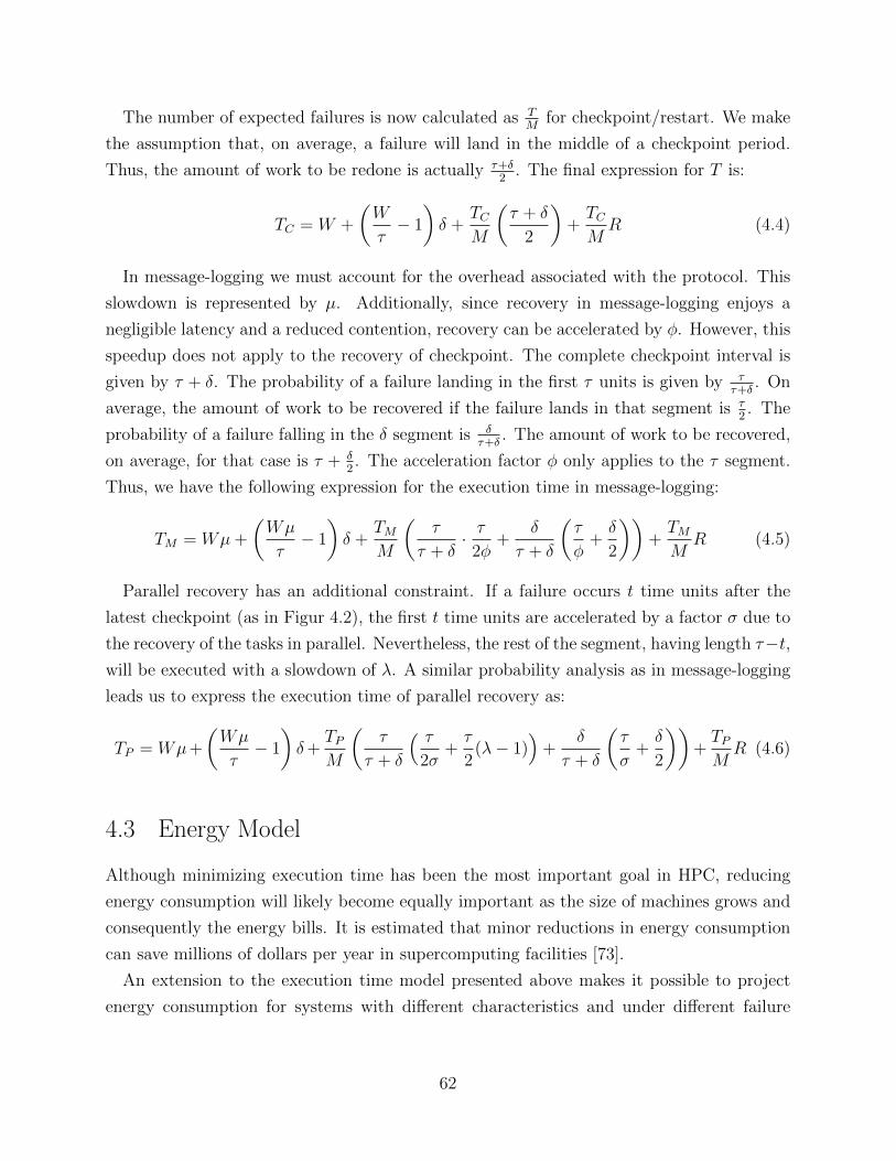
The number of expected failures is now calculated as TM

for checkpoint/restart. We make

the assumption that, on average, a failure will land in the middle of a checkpoint period.

Thus, the amount of work to be redone is actually τ+δ2

. The final expression for T is:

TC = W +

(W

τ− 1

)δ +

TCM

(τ + δ

2

)+TCMR (4.4)

In message-logging we must account for the overhead associated with the protocol. This

slowdown is represented by µ. Additionally, since recovery in message-logging enjoys a

negligible latency and a reduced contention, recovery can be accelerated by φ. However, this

speedup does not apply to the recovery of checkpoint. The complete checkpoint interval is

given by τ + δ. The probability of a failure landing in the first τ units is given by ττ+δ

. On

average, the amount of work to be recovered if the failure lands in that segment is τ2. The

probability of a failure falling in the δ segment is δτ+δ

. The amount of work to be recovered,

on average, for that case is τ + δ2. The acceleration factor φ only applies to the τ segment.

Thus, we have the following expression for the execution time in message-logging:

TM = Wµ+

(Wµ

τ− 1

)δ +

TMM

(τ

τ + δ· τ

2φ+

δ

τ + δ

(τ

φ+δ

2

))+TMM

R (4.5)

Parallel recovery has an additional constraint. If a failure occurs t time units after the

latest checkpoint (as in Figur 4.2), the first t time units are accelerated by a factor σ due to

the recovery of the tasks in parallel. Nevertheless, the rest of the segment, having length τ−t,will be executed with a slowdown of λ. A similar probability analysis as in message-logging

leads us to express the execution time of parallel recovery as:

TP = Wµ+

(Wµ

τ− 1

)δ+

TPM

(τ

τ + δ

( τ2σ

+τ

2(λ− 1)

)+

δ

τ + δ

(τ

σ+δ

2

))+TPMR (4.6)

4.3 Energy Model

Although minimizing execution time has been the most important goal in HPC, reducing

energy consumption will likely become equally important as the size of machines grows and

consequently the energy bills. It is estimated that minor reductions in energy consumption

can save millions of dollars per year in supercomputing facilities [73].

An extension to the execution time model presented above makes it possible to project

energy consumption for systems with different characteristics and under different failure

62

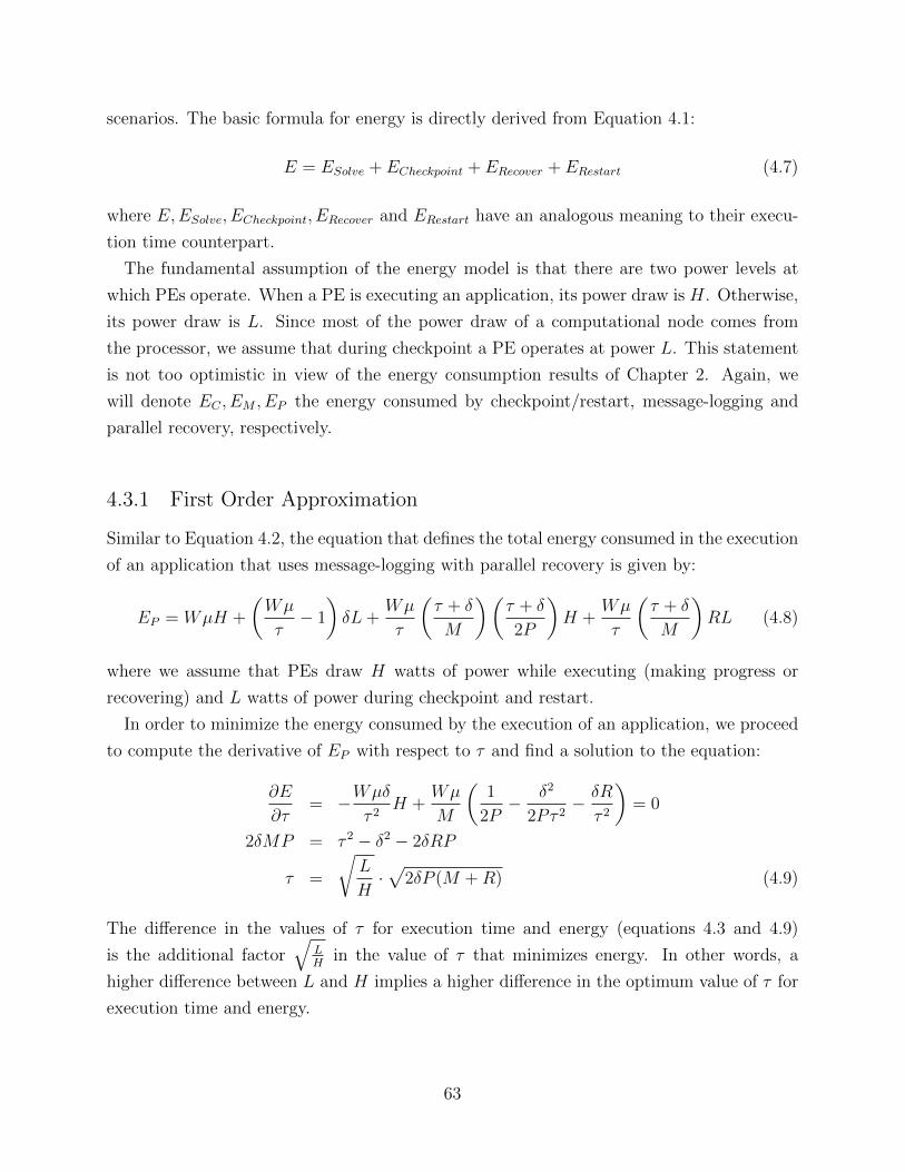
scenarios. The basic formula for energy is directly derived from Equation 4.1:

E = ESolve + ECheckpoint + ERecover + ERestart (4.7)

where E,ESolve, ECheckpoint, ERecover and ERestart have an analogous meaning to their execu-

tion time counterpart.

The fundamental assumption of the energy model is that there are two power levels at

which PEs operate. When a PE is executing an application, its power draw is H. Otherwise,

its power draw is L. Since most of the power draw of a computational node comes from

the processor, we assume that during checkpoint a PE operates at power L. This statement

is not too optimistic in view of the energy consumption results of Chapter 2. Again, we

will denote EC , EM , EP the energy consumed by checkpoint/restart, message-logging and

parallel recovery, respectively.

4.3.1 First Order Approximation

Similar to Equation 4.2, the equation that defines the total energy consumed in the execution

of an application that uses message-logging with parallel recovery is given by:

EP = WµH +

(Wµ

τ− 1

)δL+

Wµ

τ

(τ + δ

M

)(τ + δ

2P

)H +

Wµ

τ

(τ + δ

M

)RL (4.8)

where we assume that PEs draw H watts of power while executing (making progress or

recovering) and L watts of power during checkpoint and restart.

In order to minimize the energy consumed by the execution of an application, we proceed

to compute the derivative of EP with respect to τ and find a solution to the equation:

∂E

∂τ= −Wµδ

τ 2H +

Wµ

M

(1

2P− δ2

2Pτ 2− δR

τ 2

)= 0

2δMP = τ 2 − δ2 − 2δRP

τ =

√L

H·√

2δP (M +R) (4.9)

The difference in the values of τ for execution time and energy (equations 4.3 and 4.9)

is the additional factor√

LH

in the value of τ that minimizes energy. In other words, a

higher difference between L and H implies a higher difference in the optimum value of τ for

execution time and energy.

63

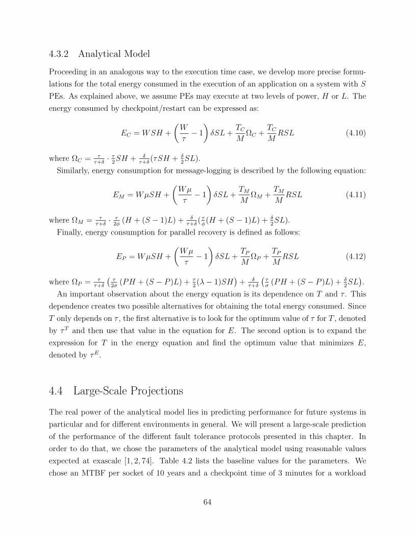
4.3.2 Analytical Model

Proceeding in an analogous way to the execution time case, we develop more precise formu-

lations for the total energy consumed in the execution of an application on a system with S

PEs. As explained above, we assume PEs may execute at two levels of power, H or L. The

energy consumed by checkpoint/restart can be expressed as:

EC = WSH +

(W

τ− 1

)δSL+

TCM

ΩC +TCMRSL (4.10)

where ΩC = ττ+δ· τ2SH + δ

τ+δ(τSH + δ

2SL).

Similarly, energy consumption for message-logging is described by the following equation:

EM = WµSH +

(Wµ

τ− 1

)δSL+

TMM

ΩM +TMM

RSL (4.11)

where ΩM = ττ+δ· τ2φ

(H + (S − 1)L) + δτ+δ

( τφ(H + (S − 1)L) + δ

2SL).

Finally, energy consumption for parallel recovery is defined as follows:

EP = WµSH +

(Wµ

τ− 1

)δSL+

TPM

ΩP +TPMRSL (4.12)

where ΩP = ττ+δ

(τ2σ

(PH + (S − P )L) + τ2(λ− 1)SH

)+ δ

τ+δ

(τσ

(PH + (S − P )L) + δ2SL).

An important observation about the energy equation is its dependence on T and τ . This

dependence creates two possible alternatives for obtaining the total energy consumed. Since

T only depends on τ , the first alternative is to look for the optimum value of τ for T , denoted

by τT and then use that value in the equation for E. The second option is to expand the

expression for T in the energy equation and find the optimum value that minimizes E,

denoted by τE.

4.4 Large-Scale Projections

The real power of the analytical model lies in predicting performance for future systems in

particular and for different environments in general. We will present a large-scale prediction

of the performance of the different fault tolerance protocols presented in this chapter. In

order to do that, we chose the parameters of the analytical model using reasonable values

expected at exascale [1, 2, 74]. Table 4.2 lists the baseline values for the parameters. We

chose an MTBF per socket of 10 years and a checkpoint time of 3 minutes for a workload

64

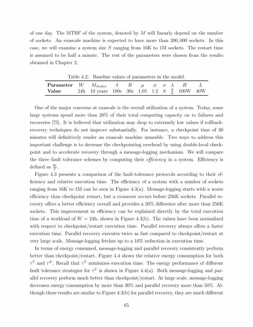
of one day. The MTBF of the system, denoted by M will linearly depend on the number

of sockets. An exascale machine is expected to have more than 200, 000 sockets. In this

case, we will examine a system size S ranging from 16K to 1M sockets. The restart time

is assumed to be half a minute. The rest of the parameters were chosen from the results

obtained in Chapter 2.

Table 4.2: Baseline values of parameters in the model.

Parameter W MSocket δ R µ φ σ λ H LValue 24h 10 years 180s 30s 1.05 1.2 8 9

8100W 40W

One of the major concerns at exascale is the overall utilization of a system. Today, some

large systems spend more than 20% of their total computing capacity on to failures and

recoveries [75]. It is believed that utilization may drop to extremely low values if rollback-

recovery techniques do not improve substantially. For instance, a checkpoint time of 30

minutes will definitively render an exascale machine unusable. Two ways to address this

important challenge is to decrease the checkpointing overhead by using double-local check-

point and to accelerate recovery through a message-logging mechanism. We will compare

the three fault tolerance schemes by computing their efficiency in a system. Efficiency is

defined as WT

.

Figure 4.3 presents a comparison of the fault-tolerance protocols according to their ef-

ficiency and relative execution time. The efficiency of a system with a number of sockets

ranging from 16K to 1M can be seen in Figure 4.3(a). Message-logging starts with a worse

efficiency than checkpoint restart, but a crossover occurs before 256K sockets. Parallel re-

covery offers a better efficiency overall and provides a 20% difference after more than 256K

sockets. This improvement in efficiency can be explained directly by the total execution

time of a workload of W = 24h, shown in Figure 4.3(b). The values have been normalized

with respect to checkpoint/restart execution time. Parallel recovery always offers a faster

execution time. Parallel recovery executes twice as fast compared to checkpoint/restart at

very large scale. Message-logging fetches up to a 10% reduction in execution time.

In terms of energy consumed, message-logging and parallel recovery consistently perform

better than checkpoint/restart. Figure 4.4 shows the relative energy consumption for both

τT and τE. Recall that τT minimizes execution time. The energy performance of different

fault tolerance strategies for τT is shown in Figure 4.4(a). Both message-logging and par-

allel recovery perform much better than checkpoint/restart. At large scale, message-logging

decreases energy consumption by more than 30% and parallel recovery more than 50%. Al-

though these results are similar to Figure 4.3(b) for parallel recovery, they are much different

65

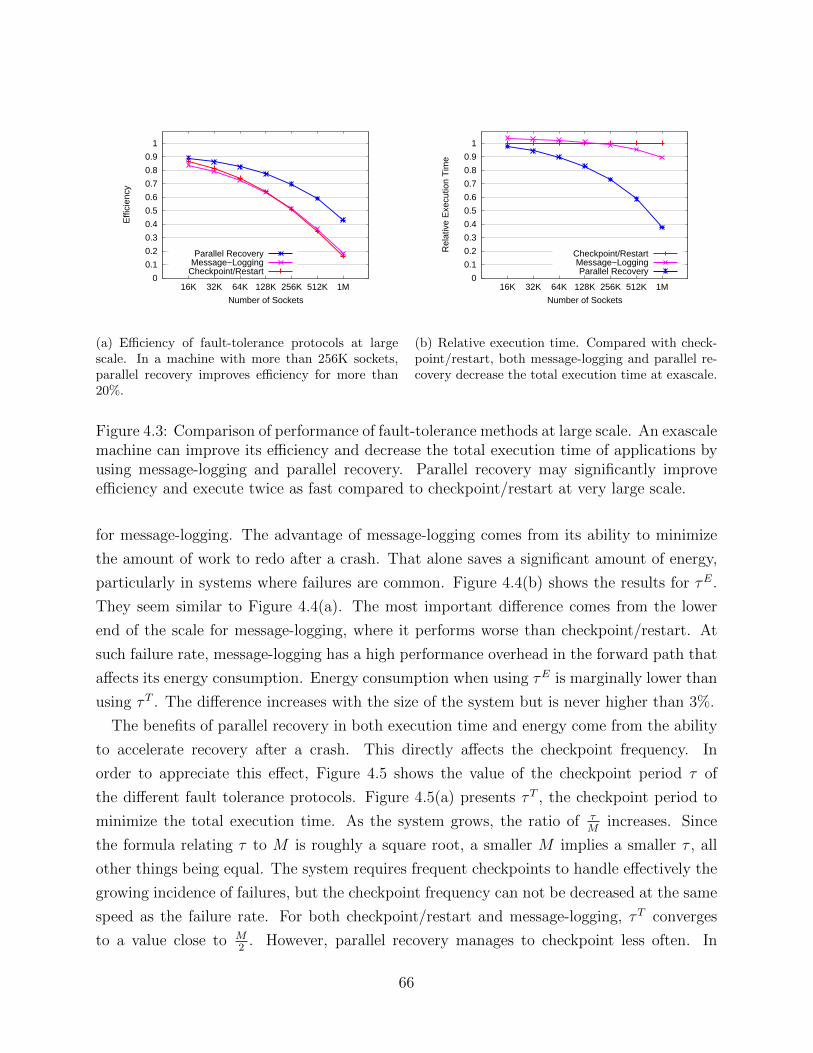
0

0.1

0.2

0.3

0.4

0.5

0.6

0.7

0.8

0.9

1

16K 32K 64K 128K 256K 512K 1M

Effi

cien

cy

Number of Sockets

Parallel RecoveryMessage−Logging

Checkpoint/Restart

(a) Efficiency of fault-tolerance protocols at largescale. In a machine with more than 256K sockets,parallel recovery improves efficiency for more than20%.

0

0.1

0.2

0.3

0.4

0.5

0.6

0.7

0.8

0.9

1

16K 32K 64K 128K 256K 512K 1M

Rel

ativ

e E

xecu

tion

Tim

e

Number of Sockets

Checkpoint/RestartMessage−LoggingParallel Recovery

(b) Relative execution time. Compared with check-point/restart, both message-logging and parallel re-covery decrease the total execution time at exascale.

Figure 4.3: Comparison of performance of fault-tolerance methods at large scale. An exascalemachine can improve its efficiency and decrease the total execution time of applications byusing message-logging and parallel recovery. Parallel recovery may significantly improveefficiency and execute twice as fast compared to checkpoint/restart at very large scale.

for message-logging. The advantage of message-logging comes from its ability to minimize

the amount of work to redo after a crash. That alone saves a significant amount of energy,

particularly in systems where failures are common. Figure 4.4(b) shows the results for τE.

They seem similar to Figure 4.4(a). The most important difference comes from the lower

end of the scale for message-logging, where it performs worse than checkpoint/restart. At

such failure rate, message-logging has a high performance overhead in the forward path that

affects its energy consumption. Energy consumption when using τE is marginally lower than

using τT . The difference increases with the size of the system but is never higher than 3%.

The benefits of parallel recovery in both execution time and energy come from the ability

to accelerate recovery after a crash. This directly affects the checkpoint frequency. In

order to appreciate this effect, Figure 4.5 shows the value of the checkpoint period τ of

the different fault tolerance protocols. Figure 4.5(a) presents τT , the checkpoint period to

minimize the total execution time. As the system grows, the ratio of τM

increases. Since

the formula relating τ to M is roughly a square root, a smaller M implies a smaller τ , all

other things being equal. The system requires frequent checkpoints to handle effectively the

growing incidence of failures, but the checkpoint frequency can not be decreased at the same

speed as the failure rate. For both checkpoint/restart and message-logging, τT converges

to a value close to M2

. However, parallel recovery manages to checkpoint less often. In

66

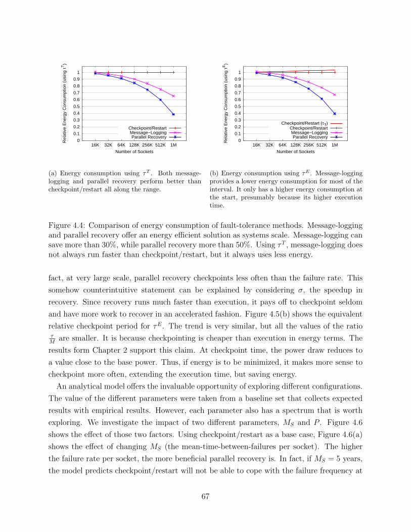
0

0.1

0.2

0.3

0.4

0.5

0.6

0.7

0.8

0.9

1

16K 32K 64K 128K 256K 512K 1M

Rel

ativ

e E

nerg

y C

onsu

mpt

ion

(usi

ng τ

T)

Number of Sockets

Checkpoint/RestartMessage−LoggingParallel Recovery

(a) Energy consumption using τT . Both message-logging and parallel recovery perform better thancheckpoint/restart all along the range.

0

0.1

0.2

0.3

0.4

0.5

0.6

0.7

0.8

0.9

1

16K 32K 64K 128K 256K 512K 1M

Rel

ativ

e E

nerg

y C

onsu

mpt

ion

(usi

ng τ

E)

Number of Sockets

Checkpoint/Restart (τT)Checkpoint/RestartMessage−LoggingParallel Recovery

(b) Energy consumption using τE . Message-loggingprovides a lower energy consumption for most of theinterval. It only has a higher energy consumption atthe start, presumably because its higher executiontime.

Figure 4.4: Comparison of energy consumption of fault-tolerance methods. Message-loggingand parallel recovery offer an energy efficient solution as systems scale. Message-logging cansave more than 30%, while parallel recovery more than 50%. Using τT , message-logging doesnot always run faster than checkpoint/restart, but it always uses less energy.

fact, at very large scale, parallel recovery checkpoints less often than the failure rate. This

somehow counterintuitive statement can be explained by considering σ, the speedup in

recovery. Since recovery runs much faster than execution, it pays off to checkpoint seldom

and have more work to recover in an accelerated fashion. Figure 4.5(b) shows the equivalent

relative checkpoint period for τE. The trend is very similar, but all the values of the ratioτM

are smaller. It is because checkpointing is cheaper than execution in energy terms. The

results form Chapter 2 support this claim. At checkpoint time, the power draw reduces to

a value close to the base power. Thus, if energy is to be minimized, it makes more sense to

checkpoint more often, extending the execution time, but saving energy.

An analytical model offers the invaluable opportunity of exploring different configurations.

The value of the different parameters were taken from a baseline set that collects expected

results with empirical results. However, each parameter also has a spectrum that is worth

exploring. We investigate the impact of two different parameters, MS and P . Figure 4.6

shows the effect of those two factors. Using checkpoint/restart as a base case, Figure 4.6(a)

shows the effect of changing MS (the mean-time-between-failures per socket). The higher

the failure rate per socket, the more beneficial parallel recovery is. In fact, if MS = 5 years,

the model predicts checkpoint/restart will not be able to cope with the failure frequency at

67

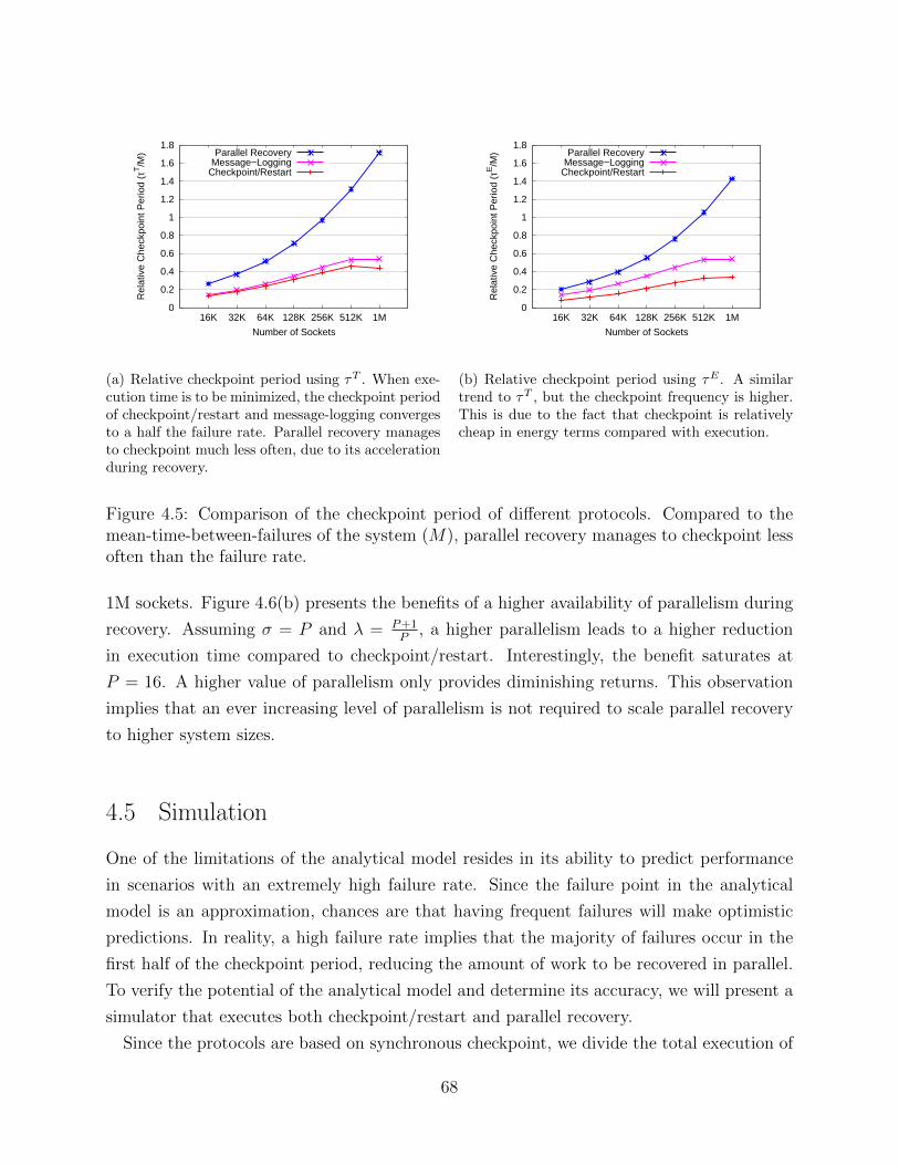
0

0.2

0.4

0.6

0.8

1

1.2

1.4

1.6

1.8

16K 32K 64K 128K 256K 512K 1M

Rel

ativ

e C

heck

poin

t Per

iod

(τT/M

)

Number of Sockets

Parallel RecoveryMessage−Logging

Checkpoint/Restart

(a) Relative checkpoint period using τT . When exe-cution time is to be minimized, the checkpoint periodof checkpoint/restart and message-logging convergesto a half the failure rate. Parallel recovery managesto checkpoint much less often, due to its accelerationduring recovery.

0

0.2

0.4

0.6

0.8

1

1.2

1.4

1.6

1.8

16K 32K 64K 128K 256K 512K 1M

Rel

ativ

e C

heck

poin

t Per

iod

(τE/M

)

Number of Sockets

Parallel RecoveryMessage−Logging

Checkpoint/Restart

(b) Relative checkpoint period using τE . A similartrend to τT , but the checkpoint frequency is higher.This is due to the fact that checkpoint is relativelycheap in energy terms compared with execution.

Figure 4.5: Comparison of the checkpoint period of different protocols. Compared to themean-time-between-failures of the system (M), parallel recovery manages to checkpoint lessoften than the failure rate.

1M sockets. Figure 4.6(b) presents the benefits of a higher availability of parallelism during

recovery. Assuming σ = P and λ = P+1P

, a higher parallelism leads to a higher reduction

in execution time compared to checkpoint/restart. Interestingly, the benefit saturates at

P = 16. A higher value of parallelism only provides diminishing returns. This observation

implies that an ever increasing level of parallelism is not required to scale parallel recovery

to higher system sizes.

4.5 Simulation

One of the limitations of the analytical model resides in its ability to predict performance

in scenarios with an extremely high failure rate. Since the failure point in the analytical

model is an approximation, chances are that having frequent failures will make optimistic

predictions. In reality, a high failure rate implies that the majority of failures occur in the

first half of the checkpoint period, reducing the amount of work to be recovered in parallel.

To verify the potential of the analytical model and determine its accuracy, we will present a

simulator that executes both checkpoint/restart and parallel recovery.

Since the protocols are based on synchronous checkpoint, we divide the total execution of

68

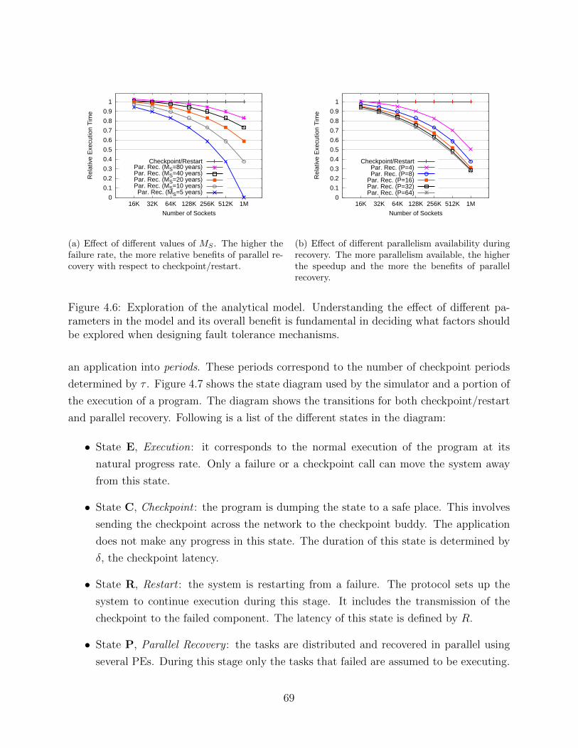
0

0.1

0.2

0.3

0.4

0.5

0.6

0.7

0.8

0.9

1

16K 32K 64K 128K 256K 512K 1M

Rel

ativ

e E

xecu

tion

Tim

e

Number of Sockets

Checkpoint/RestartPar. Rec. (MS=80 years)Par. Rec. (MS=40 years)Par. Rec. (MS=20 years)Par. Rec. (MS=10 years)Par. Rec. (MS=5 years)

(a) Effect of different values of MS . The higher thefailure rate, the more relative benefits of parallel re-covery with respect to checkpoint/restart.

0

0.1

0.2

0.3

0.4

0.5

0.6

0.7

0.8

0.9

1

16K 32K 64K 128K 256K 512K 1M

Rel

ativ

e E

xecu

tion

Tim

e

Number of Sockets

Checkpoint/RestartPar. Rec. (P=4)Par. Rec. (P=8)

Par. Rec. (P=16)Par. Rec. (P=32)Par. Rec. (P=64)

(b) Effect of different parallelism availability duringrecovery. The more parallelism available, the higherthe speedup and the more the benefits of parallelrecovery.

Figure 4.6: Exploration of the analytical model. Understanding the effect of different pa-rameters in the model and its overall benefit is fundamental in deciding what factors shouldbe explored when designing fault tolerance mechanisms.

an application into periods. These periods correspond to the number of checkpoint periods

determined by τ . Figure 4.7 shows the state diagram used by the simulator and a portion of

the execution of a program. The diagram shows the transitions for both checkpoint/restart

and parallel recovery. Following is a list of the different states in the diagram:

• State E, Execution: it corresponds to the normal execution of the program at its

natural progress rate. Only a failure or a checkpoint call can move the system away

from this state.

• State C, Checkpoint : the program is dumping the state to a safe place. This involves

sending the checkpoint across the network to the checkpoint buddy. The application

does not make any progress in this state. The duration of this state is determined by

δ, the checkpoint latency.

• State R, Restart : the system is restarting from a failure. The protocol sets up the

system to continue execution during this stage. It includes the transmission of the

checkpoint to the failed component. The latency of this state is defined by R.

• State P, Parallel Recovery : the tasks are distributed and recovered in parallel using

several PEs. During this stage only the tasks that failed are assumed to be executing.

69

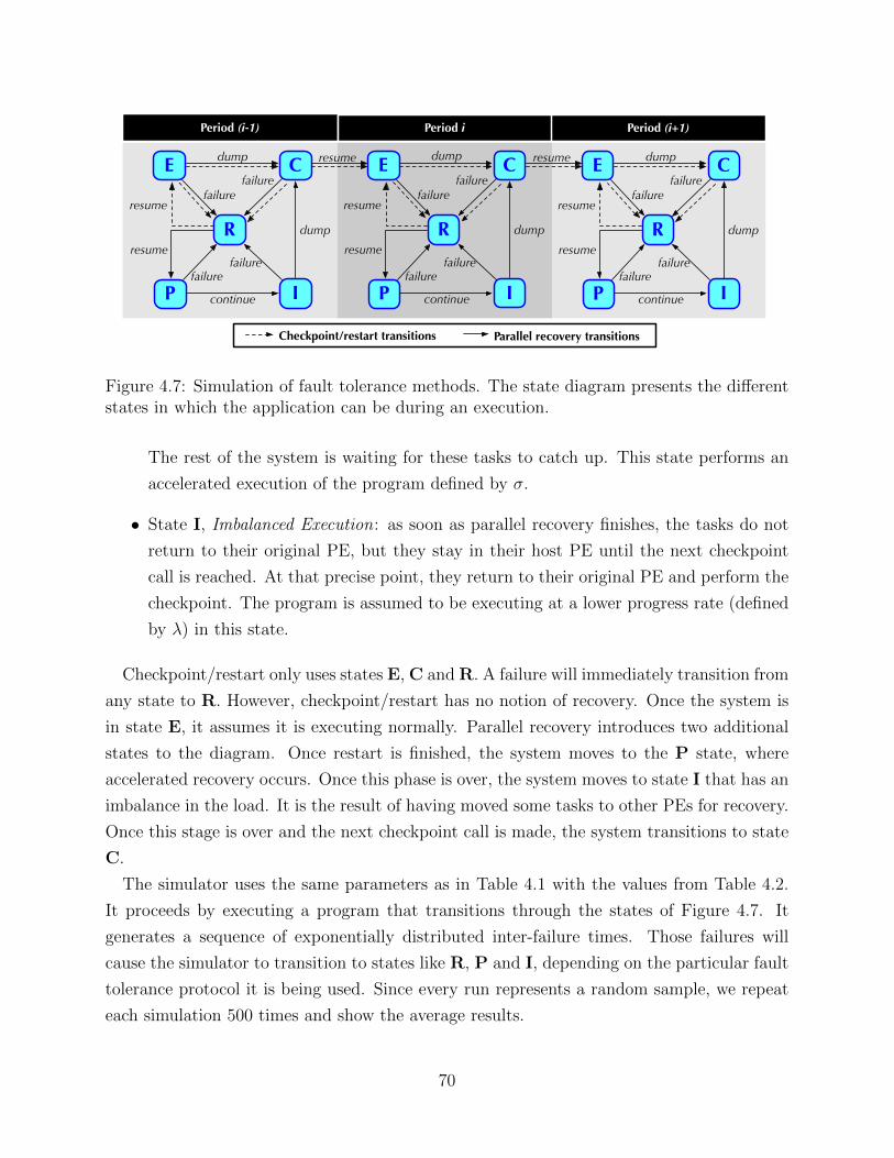
Checkpoint/restart transitions Parallel recovery transitions

IP

E C

R

dump resume

failurefailure

resume

failurefailure

resume

continue

dump

IP

E C

R

dump

failurefailure

resume

failurefailure

resume

continue

dump

IP

E C

R

dump

failurefailure

resume

failurefailure

resume

continue

dump

resume

Period (i-1) Period i Period (i+1)

Figure 4.7: Simulation of fault tolerance methods. The state diagram presents the differentstates in which the application can be during an execution.

The rest of the system is waiting for these tasks to catch up. This state performs an

accelerated execution of the program defined by σ.

• State I, Imbalanced Execution: as soon as parallel recovery finishes, the tasks do not

return to their original PE, but they stay in their host PE until the next checkpoint

call is reached. At that precise point, they return to their original PE and perform the

checkpoint. The program is assumed to be executing at a lower progress rate (defined

by λ) in this state.

Checkpoint/restart only uses states E, C and R. A failure will immediately transition from

any state to R. However, checkpoint/restart has no notion of recovery. Once the system is

in state E, it assumes it is executing normally. Parallel recovery introduces two additional

states to the diagram. Once restart is finished, the system moves to the P state, where

accelerated recovery occurs. Once this phase is over, the system moves to state I that has an

imbalance in the load. It is the result of having moved some tasks to other PEs for recovery.

Once this stage is over and the next checkpoint call is made, the system transitions to state

C.

The simulator uses the same parameters as in Table 4.1 with the values from Table 4.2.

It proceeds by executing a program that transitions through the states of Figure 4.7. It

generates a sequence of exponentially distributed inter-failure times. Those failures will

cause the simulator to transition to states like R, P and I, depending on the particular fault

tolerance protocol it is being used. Since every run represents a random sample, we repeat

each simulation 500 times and show the average results.

70

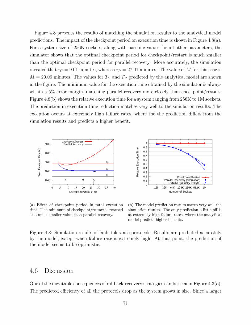
Figure 4.8 presents the results of matching the simulation results to the analytical model

predictions. The impact of the checkpoint period on execution time is shown in Figure 4.8(a).

For a system size of 256K sockets, along with baseline values for all other parameters, the

simulator shows that the optimal checkpoint period for checkpoint/restart is much smaller

than the optimal checkpoint period for parallel recovery. More accurately, the simulation

revealed that τC = 9.01 minutes, whereas τP = 27.01 minutes. The value of M for this case is

M = 20.06 minutes. The values for TC and TP predicted by the analytical model are shown

in the figure. The minimum value for the execution time obtained by the simulator is always

within a 5% error margin, matching parallel recovery more closely than checkpoint/restart.

Figure 4.8(b) shows the relative execution time for a system ranging from 256K to 1M sockets.

The prediction in execution time reduction matches very well to the simulation results. The

exception occurs at extremely high failure rates, where the the prediction differs from the

simulation results and predicts a higher benefit.

1000

2000

3000

4000

5000

0 5 10 15 20 25 30 35 40

To

tal

Ex

ecu

tio

n T

ime

(m)

Checkpoint Period, τ (m)

W

TC

TP

τC M τP

Checkpoint/RestartParallel Recovery

(a) Effect of checkpoint period in total executiontime. The minimum of checkpoint/restart is reachedat a much smaller value than parallel recovery.

0

0.1

0.2

0.3

0.4

0.5

0.6

0.7

0.8

0.9

1

16K 32K 64K 128K 256K 512K 1M

Rel

ativ

e E

xecu

tion

Tim

e

Number of Sockets

Checkpoint/RestartParallel Recovery (simulation)

Parallel Recovery (model)

(b) The model prediction results match very well thesimulation results. The only prediction a little off isat extremely high failure rates, where the analyticalmodel predicts higher benefits.

Figure 4.8: Simulation results of fault tolerance protocols. Results are predicted accuratelyby the model, except when failure rate is extremely high. At that point, the prediction ofthe model seems to be optimistic.

4.6 Discussion

One of the inevitable consequences of rollback-recovery strategies can be seen in Figure 4.3(a).

The predicted efficiency of all the protocols drop as the system grows in size. Since a larger

71

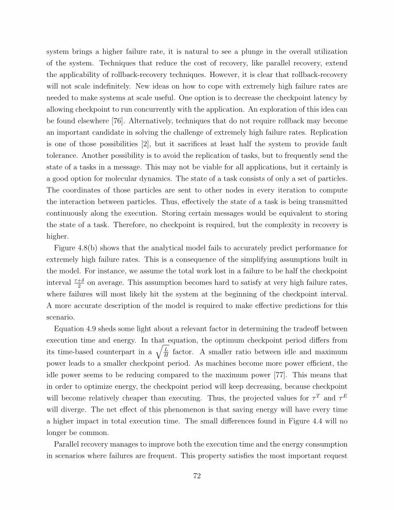
system brings a higher failure rate, it is natural to see a plunge in the overall utilization

of the system. Techniques that reduce the cost of recovery, like parallel recovery, extend

the applicability of rollback-recovery techniques. However, it is clear that rollback-recovery

will not scale indefinitely. New ideas on how to cope with extremely high failure rates are

needed to make systems at scale useful. One option is to decrease the checkpoint latency by

allowing checkpoint to run concurrently with the application. An exploration of this idea can

be found elsewhere [76]. Alternatively, techniques that do not require rollback may become

an important candidate in solving the challenge of extremely high failure rates. Replication

is one of those possibilities [2], but it sacrifices at least half the system to provide fault

tolerance. Another possibility is to avoid the replication of tasks, but to frequently send the

state of a tasks in a message. This may not be viable for all applications, but it certainly is

a good option for molecular dynamics. The state of a task consists of only a set of particles.

The coordinates of those particles are sent to other nodes in every iteration to compute

the interaction between particles. Thus, effectively the state of a task is being transmitted

continuously along the execution. Storing certain messages would be equivalent to storing

the state of a task. Therefore, no checkpoint is required, but the complexity in recovery is

higher.

Figure 4.8(b) shows that the analytical model fails to accurately predict performance for

extremely high failure rates. This is a consequence of the simplifying assumptions built in

the model. For instance, we assume the total work lost in a failure to be half the checkpoint

interval τ+δ2

on average. This assumption becomes hard to satisfy at very high failure rates,

where failures will most likely hit the system at the beginning of the checkpoint interval.

A more accurate description of the model is required to make effective predictions for this

scenario.

Equation 4.9 sheds some light about a relevant factor in determining the tradeoff between

execution time and energy. In that equation, the optimum checkpoint period differs from

its time-based counterpart in a√

LH

factor. A smaller ratio between idle and maximum

power leads to a smaller checkpoint period. As machines become more power efficient, the

idle power seems to be reducing compared to the maximum power [77]. This means that

in order to optimize energy, the checkpoint period will keep decreasing, because checkpoint

will become relatively cheaper than executing. Thus, the projected values for τT and τE

will diverge. The net effect of this phenomenon is that saving energy will have every time

a higher impact in total execution time. The small differences found in Figure 4.4 will no

longer be common.

Parallel recovery manages to improve both the execution time and the energy consumption

in scenarios where failures are frequent. This property satisfies the most important request

72

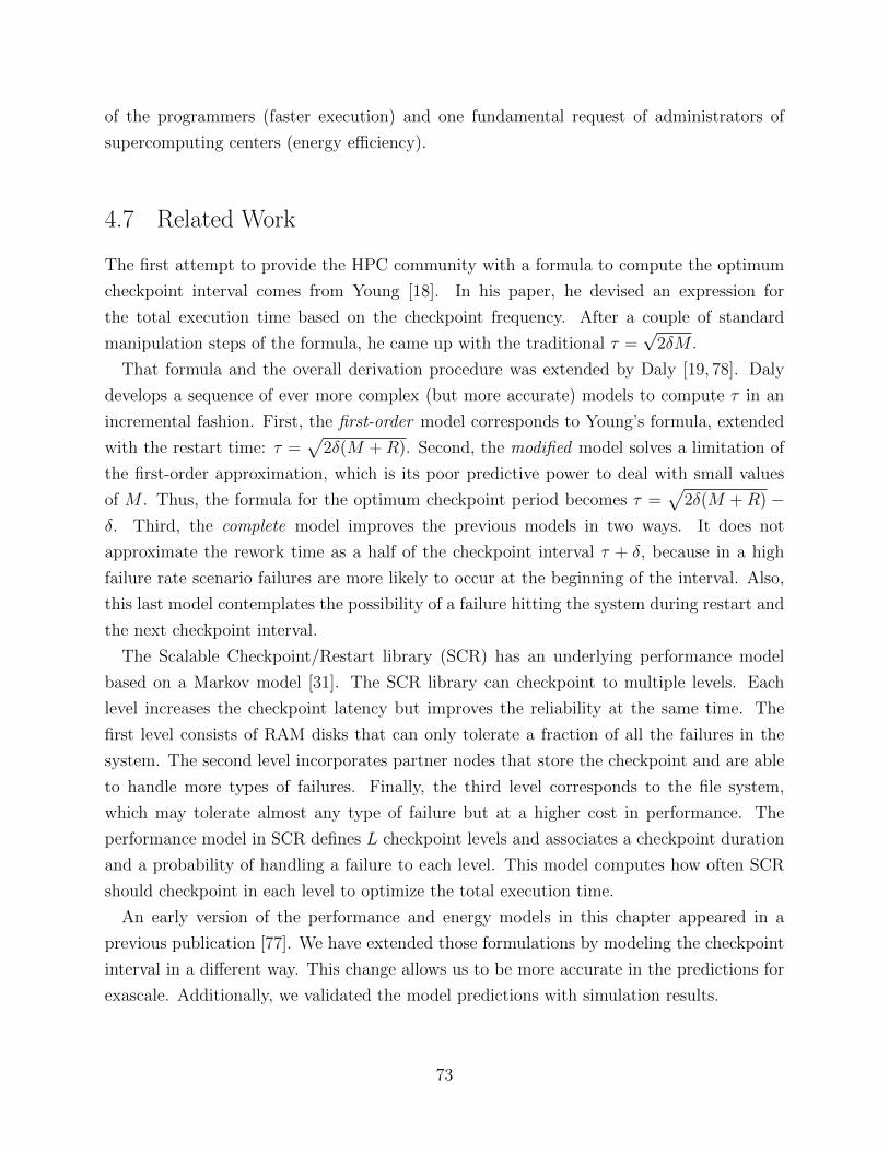
of the programmers (faster execution) and one fundamental request of administrators of

supercomputing centers (energy efficiency).

4.7 Related Work

The first attempt to provide the HPC community with a formula to compute the optimum

checkpoint interval comes from Young [18]. In his paper, he devised an expression for

the total execution time based on the checkpoint frequency. After a couple of standard

manipulation steps of the formula, he came up with the traditional τ =√

2δM .

That formula and the overall derivation procedure was extended by Daly [19, 78]. Daly

develops a sequence of ever more complex (but more accurate) models to compute τ in an

incremental fashion. First, the first-order model corresponds to Young’s formula, extended

with the restart time: τ =√

2δ(M +R). Second, the modified model solves a limitation of

the first-order approximation, which is its poor predictive power to deal with small values

of M . Thus, the formula for the optimum checkpoint period becomes τ =√

2δ(M +R) −δ. Third, the complete model improves the previous models in two ways. It does not

approximate the rework time as a half of the checkpoint interval τ + δ, because in a high

failure rate scenario failures are more likely to occur at the beginning of the interval. Also,

this last model contemplates the possibility of a failure hitting the system during restart and

the next checkpoint interval.

The Scalable Checkpoint/Restart library (SCR) has an underlying performance model

based on a Markov model [31]. The SCR library can checkpoint to multiple levels. Each

level increases the checkpoint latency but improves the reliability at the same time. The

first level consists of RAM disks that can only tolerate a fraction of all the failures in the

system. The second level incorporates partner nodes that store the checkpoint and are able

to handle more types of failures. Finally, the third level corresponds to the file system,

which may tolerate almost any type of failure but at a higher cost in performance. The

performance model in SCR defines L checkpoint levels and associates a checkpoint duration

and a probability of handling a failure to each level. This model computes how often SCR

should checkpoint in each level to optimize the total execution time.

An early version of the performance and energy models in this chapter appeared in a

previous publication [77]. We have extended those formulations by modeling the checkpoint

interval in a different way. This change allows us to be more accurate in the predictions for

exascale. Additionally, we validated the model predictions with simulation results.

73

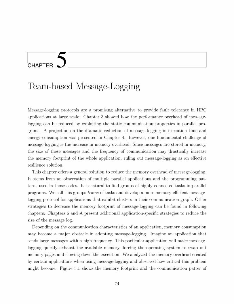
CHAPTER 5Team-based Message-Logging

Message-logging protocols are a promising alternative to provide fault tolerance in HPC

applications at large scale. Chapter 3 showed how the performance overhead of message-

logging can be reduced by exploiting the static communication properties in parallel pro-

grams. A projection on the dramatic reduction of message-logging in execution time and

energy consumption was presented in Chapter 4. However, one fundamental challenge of

message-logging is the increase in memory overhead. Since messages are stored in memory,

the size of these messages and the frequency of communication may drastically increase

the memory footprint of the whole application, ruling out message-logging as an effective

resilience solution.

This chapter offers a general solution to reduce the memory overhead of message-logging.

It stems from an observation of multiple parallel applications and the programming pat-

terns used in those codes. It is natural to find groups of highly connected tasks in parallel

programs. We call this groups teams of tasks and develop a more memory-efficient message-

logging protocol for applications that exhibit clusters in their communication graph. Other

strategies to decrease the memory footprint of message-logging can be found in following

chapters. Chapters 6 and A present additional application-specific strategies to reduce the

size of the message log.

Depending on the communication characteristics of an application, memory consumption

may become a major obstacle in adopting message-logging. Imagine an application that

sends large messages with a high frequency. This particular application will make message-

logging quickly exhaust the available memory, forcing the operating system to swap out

memory pages and slowing down the execution. We analyzed the memory overhead created

by certain applications when using message-logging and observed how critical this problem

might become. Figure 5.1 shows the memory footprint and the communication patter of

74

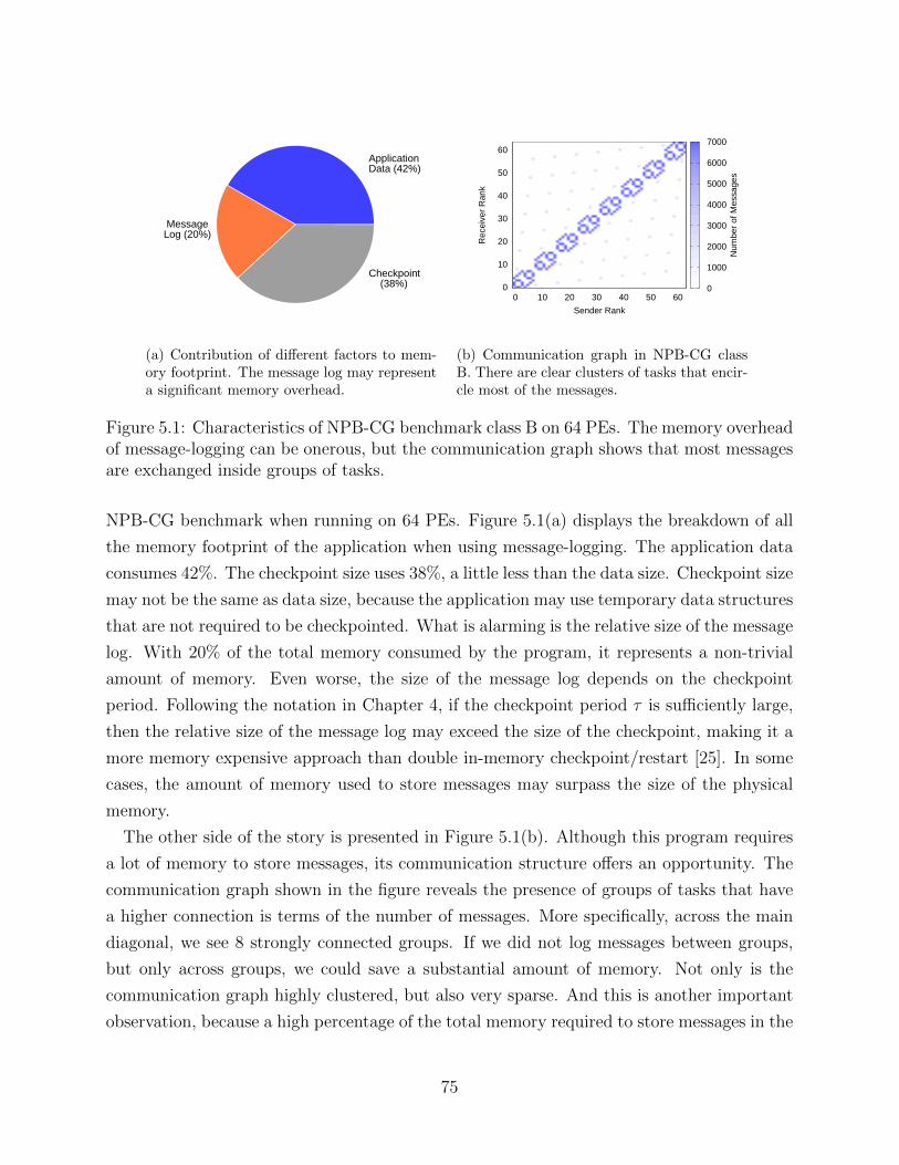
ApplicationData (42%)

MessageLog (20%)

Checkpoint (38%)

(a) Contribution of different factors to mem-ory footprint. The message log may representa significant memory overhead.

0

10

20

30

40

50

60

0 10 20 30 40 50 60

Rec

eive

r R

ank

Sender Rank

0

1000

2000

3000

4000

5000

6000

7000

Num

ber

of M

essa

ges

(b) Communication graph in NPB-CG classB. There are clear clusters of tasks that encir-cle most of the messages.

Figure 5.1: Characteristics of NPB-CG benchmark class B on 64 PEs. The memory overheadof message-logging can be onerous, but the communication graph shows that most messagesare exchanged inside groups of tasks.

NPB-CG benchmark when running on 64 PEs. Figure 5.1(a) displays the breakdown of all

the memory footprint of the application when using message-logging. The application data

consumes 42%. The checkpoint size uses 38%, a little less than the data size. Checkpoint size

may not be the same as data size, because the application may use temporary data structures

that are not required to be checkpointed. What is alarming is the relative size of the message

log. With 20% of the total memory consumed by the program, it represents a non-trivial

amount of memory. Even worse, the size of the message log depends on the checkpoint

period. Following the notation in Chapter 4, if the checkpoint period τ is sufficiently large,

then the relative size of the message log may exceed the size of the checkpoint, making it a

more memory expensive approach than double in-memory checkpoint/restart [25]. In some

cases, the amount of memory used to store messages may surpass the size of the physical

memory.

The other side of the story is presented in Figure 5.1(b). Although this program requires

a lot of memory to store messages, its communication structure offers an opportunity. The

communication graph shown in the figure reveals the presence of groups of tasks that have

a higher connection is terms of the number of messages. More specifically, across the main

diagonal, we see 8 strongly connected groups. If we did not log messages between groups,

but only across groups, we could save a substantial amount of memory. Not only is the

communication graph highly clustered, but also very sparse. And this is another important

observation, because a high percentage of the total memory required to store messages in the

75

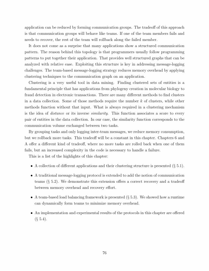
application can be reduced by forming communication groups. The tradeoff of this approach

is that communication groups will behave like teams. If one of the team members fails and

needs to recover, the rest of the team will rollback along the failed member.

It does not come as a surprise that many applications show a structured communication

pattern. The reason behind this topology is that programmers usually follow programming

patterns to put together their application. That provides well structured graphs that can be

analyzed with relative ease. Exploiting this structure is key in addressing message-logging

challenges. The team-based message-logging strategy reduces memory overhead by applying

clustering techniques to the communication graph on an application.

Clustering is a very useful tool in data mining. Finding clustered sets of entities is a

fundamental principle that has applications from phylogeny creation in molecular biology to

fraud detection in electronic transactions. There are many different methods to find clusters

in a data collection. Some of those methods require the number k of clusters, while other

methods function without that input. What is always required in a clustering mechanism

is the idea of distance or its inverse similarity. This function associates a score to every

pair of entities in the data collection. In our case, the similarity function corresponds to the

communication volume exchanged between two tasks.

By grouping tasks and only logging inter-team messages, we reduce memory consumption,

but we rollback more tasks. This tradeoff will be a constant in this chapter. Chapters 6 and

A offer a different kind of tradeoff, where no more tasks are rolled back when one of them

fails, but an increased complexity in the code is necessary to handle a failure.

This is a list of the highlights of this chapter:

• A collection of different applications and their clustering structure is presented (§ 5.1).

• A traditional message-logging protocol is extended to add the notion of communication

teams (§ 5.2). We demonstrate this extension offers a correct recovery and a tradeoff

between memory overhead and recovery effort.

• A team-based load balancing framework is presented (§ 5.3). We showed how a runtime

can dynamically form teams to minimize memory overhead.

• An implementation and experimental results of the protocols in this chapter are offered

(§ 5.4).

76

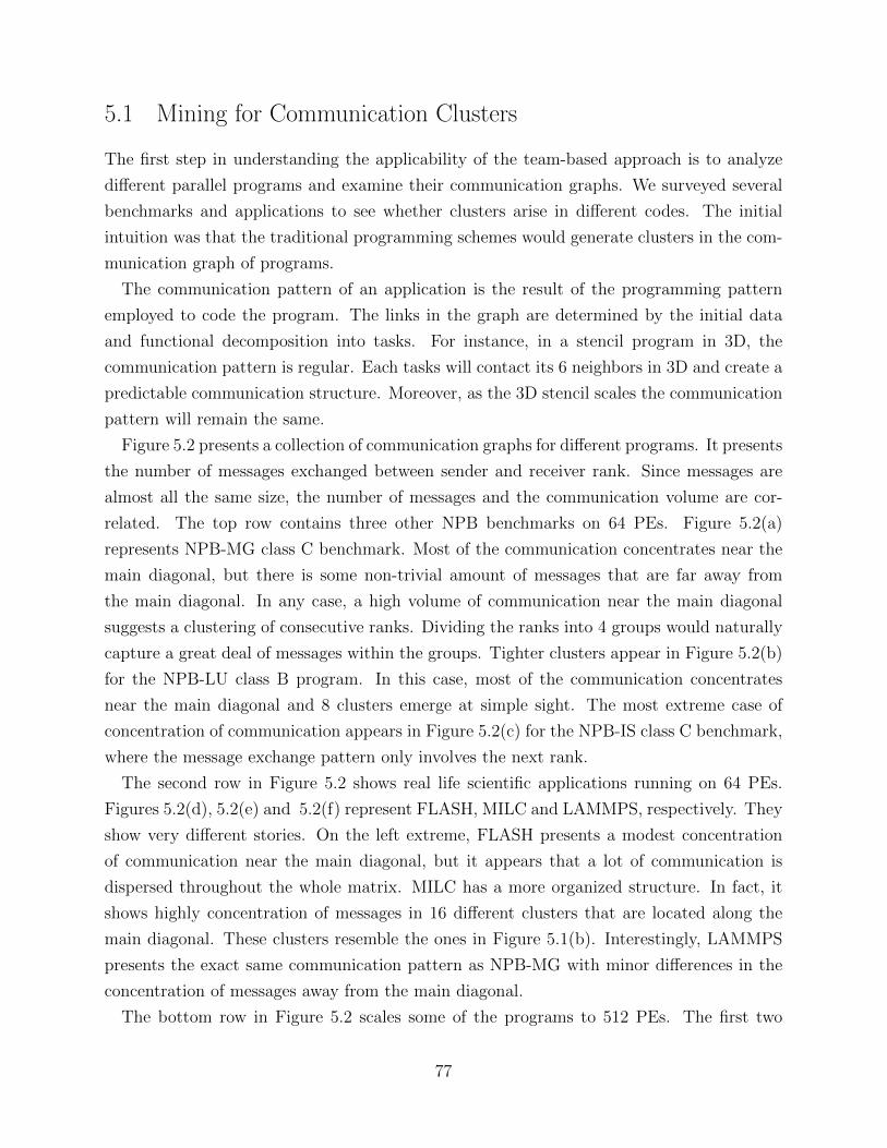
5.1 Mining for Communication Clusters

The first step in understanding the applicability of the team-based approach is to analyze

different parallel programs and examine their communication graphs. We surveyed several

benchmarks and applications to see whether clusters arise in different codes. The initial

intuition was that the traditional programming schemes would generate clusters in the com-

munication graph of programs.

The communication pattern of an application is the result of the programming pattern

employed to code the program. The links in the graph are determined by the initial data

and functional decomposition into tasks. For instance, in a stencil program in 3D, the

communication pattern is regular. Each tasks will contact its 6 neighbors in 3D and create a

predictable communication structure. Moreover, as the 3D stencil scales the communication

pattern will remain the same.

Figure 5.2 presents a collection of communication graphs for different programs. It presents

the number of messages exchanged between sender and receiver rank. Since messages are

almost all the same size, the number of messages and the communication volume are cor-

related. The top row contains three other NPB benchmarks on 64 PEs. Figure 5.2(a)

represents NPB-MG class C benchmark. Most of the communication concentrates near the

main diagonal, but there is some non-trivial amount of messages that are far away from

the main diagonal. In any case, a high volume of communication near the main diagonal

suggests a clustering of consecutive ranks. Dividing the ranks into 4 groups would naturally

capture a great deal of messages within the groups. Tighter clusters appear in Figure 5.2(b)

for the NPB-LU class B program. In this case, most of the communication concentrates

near the main diagonal and 8 clusters emerge at simple sight. The most extreme case of

concentration of communication appears in Figure 5.2(c) for the NPB-IS class C benchmark,

where the message exchange pattern only involves the next rank.

The second row in Figure 5.2 shows real life scientific applications running on 64 PEs.

Figures 5.2(d), 5.2(e) and 5.2(f) represent FLASH, MILC and LAMMPS, respectively. They

show very different stories. On the left extreme, FLASH presents a modest concentration

of communication near the main diagonal, but it appears that a lot of communication is

dispersed throughout the whole matrix. MILC has a more organized structure. In fact, it

shows highly concentration of messages in 16 different clusters that are located along the

main diagonal. These clusters resemble the ones in Figure 5.1(b). Interestingly, LAMMPS

presents the exact same communication pattern as NPB-MG with minor differences in the

concentration of messages away from the main diagonal.

The bottom row in Figure 5.2 scales some of the programs to 512 PEs. The first two

77

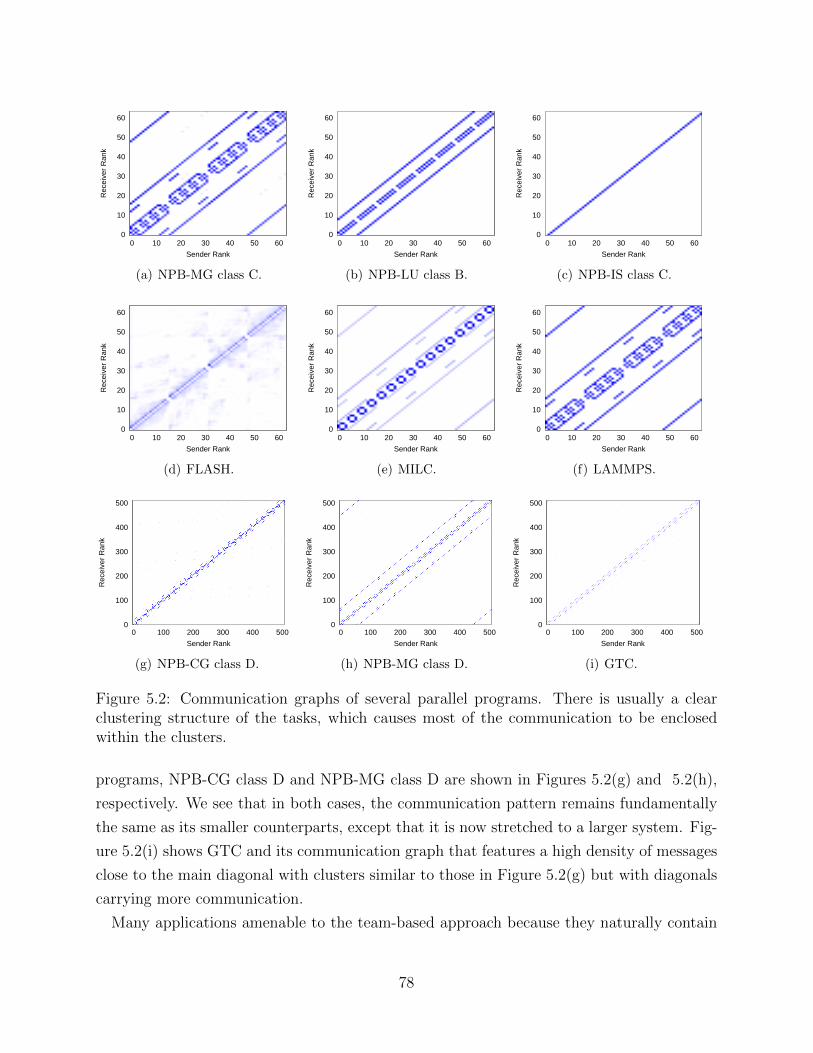
0

10

20

30

40

50

60

0 10 20 30 40 50 60

Rec

eive

r R

ank

Sender Rank

(a) NPB-MG class C.

0

10

20

30

40

50

60

0 10 20 30 40 50 60

Rec

eive

r R

ank

Sender Rank

(b) NPB-LU class B.

0

10

20

30

40

50

60

0 10 20 30 40 50 60

Rec

eive

r R

ank

Sender Rank

(c) NPB-IS class C.

0

10

20

30

40

50

60

0 10 20 30 40 50 60

Rec

eive

r R

ank

Sender Rank

(d) FLASH.

0

10

20

30

40

50

60

0 10 20 30 40 50 60

Rec

eive

r R

ank

Sender Rank

(e) MILC.

0

10

20

30

40

50

60

0 10 20 30 40 50 60

Rec

eive

r R

ank

Sender Rank

(f) LAMMPS.

0

100

200

300

400

500

0 100 200 300 400 500

Rec

eive

r R

ank

Sender Rank

(g) NPB-CG class D.

0

100

200

300

400

500

0 100 200 300 400 500

Rec

eive

r R

ank

Sender Rank

(h) NPB-MG class D.

0

100

200

300

400

500

0 100 200 300 400 500

Rec

eive

r R

ank

Sender Rank

(i) GTC.

Figure 5.2: Communication graphs of several parallel programs. There is usually a clearclustering structure of the tasks, which causes most of the communication to be enclosedwithin the clusters.

programs, NPB-CG class D and NPB-MG class D are shown in Figures 5.2(g) and 5.2(h),

respectively. We see that in both cases, the communication pattern remains fundamentally

the same as its smaller counterparts, except that it is now stretched to a larger system. Fig-

ure 5.2(i) shows GTC and its communication graph that features a high density of messages

close to the main diagonal with clusters similar to those in Figure 5.2(g) but with diagonals

carrying more communication.

Many applications amenable to the team-based approach because they naturally contain

78

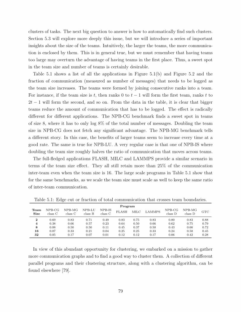
clusters of tasks. The next big question to answer is how to automatically find such clusters.

Section 5.3 will explore more deeply this issue, but we will introduce a series of important

insights about the size of the teams. Intuitively, the larger the teams, the more communica-

tion is enclosed by them. This is in general true, but we must remember that having teams

too large may overturn the advantage of having teams in the first place. Thus, a sweet spot

in the team size and number of teams is certainly desirable.

Table 5.1 shows a list of all the applications in Figure 5.1(b) and Figure 5.2 and the

fraction of communication (measured as number of messages) that needs to be logged as

the team size increases. The teams were formed by joining consecutive ranks into a team.

For instance, if the team size is t, then ranks 0 to t− 1 will form the first team, ranks t to

2t − 1 will form the second, and so on. From the data in the table, it is clear that bigger

teams reduce the amount of communication that has to be logged. The effect is radically

different for different applications. The NPB-CG benchmark finds a sweet spot in teams

of size 8, where it has to only log 8% of the total number of messages. Doubling the team

size in NPB-CG does not fetch any significant advantage. The NPB-MG benchmark tells

a different story. In this case, the benefits of larger teams seem to increase every time at a

good rate. The same is true for NPB-LU. A very regular case is that one of NPB-IS where

doubling the team size roughly halves the ratio of communication that moves across teams.

The full-fledged applications FLASH, MILC and LAMMPS provide a similar scenario in

terms of the team size effect. They all still retain more than 25% of the communication

inter-team even when the team size is 16. The large scale programs in Table 5.1 show that

for the same benchmarks, as we scale the team size must scale as well to keep the same ratio

of inter-team communication.

Table 5.1: Edge cut or fraction of total communication that crosses team boundaries.

ProgramTeam NPB-CG NPB-MG NPB-LU NPB-IS

FLASH MILC LAMMPSNPB-CG NPB-MG

GTCSize class C class C class B class C class D class D

2 0.69 0.83 0.71 0.49 0.83 0.75 0.83 0.80 0.83 0.884 0.38 0.66 0.57 0.23 0.64 0.50 0.66 0.62 0.75 0.798 0.08 0.50 0.50 0.11 0.45 0.37 0.50 0.43 0.66 0.7216 0.07 0.33 0.21 0.04 0.25 0.25 0.33 0.24 0.50 0.4532 0.05 0.17 0.07 0.01 0.12 0.12 0.17 0.06 0.42 0.28

In view of this abundant opportunity for clustering, we embarked on a mission to gather

more communication graphs and to find a good way to cluster them. A collection of different

parallel programs and their clustering structure, along with a clustering algorithm, can be

found elsewhere [79].

79

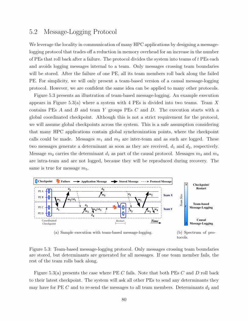
5.2 Message-Logging Protocol

We leverage the locality in communication of many HPC applications by designing a message-

logging protocol that trades off a reduction in memory overhead for an increase in the number

of PEs that roll back after a failure. The protocol divides the system into teams of t PEs each

and avoids logging messages internal to a team. Only messages crossing team boundaries

will be stored. After the failure of one PE, all its team members roll back along the failed

PE. For simplicity, we will only present a team-based version of a causal message-logging

protocol. However, we are confident the same idea can be applied to many other protocols.

Figure 5.3 presents an illustration of team-based message-logging. An example execution

appears in Figure 5.3(a) where a system with 4 PEs is divided into two teams. Team X

contains PEs A and B and team Y groups PEs C and D. The execution starts with a

global coordinated checkpoint. Although this is not a strict requirement for the protocol,

we will assume global checkpoints across the system. This is a safe assumption considering

that many HPC applications contain global synchronization points, where the checkpoint

calls could be made. Messages m1 and m2 are inter-team and as such are logged. These

two messages generate a determinant as soon as they are received, d1 and d2, respectively.

Message m2 carries the determinant d1 as part of the causal protocol. Messages m3 and m4

are intra-team and are not logged, because they will be reproduced during recovery. The

same is true for message m5.

PE A

PE B

PE C

PE D

CoordinatedCheckpoint

Restart

m1

m3

Team X

Team Y

Checkpoint Failure Application Message Protocol Message

d1

d3

m2!d1

m5m1

d2

Time

m2

Stored Message

d2

m4!d3

d4

d5

d3 m3m4

(a) Sample execution with team-based message-logging.

Checkpoint/Restart

CausalMessage-Logging

Team-basedMessage-Logging

Team

Siz

eN

1

t

(b) Spectrum of pro-tocols.

Figure 5.3: Team-based message-logging protocol. Only messages crossing team boundariesare stored, but determinants are generated for all messages. If one team member fails, therest of the team rolls back along.

Figure 5.3(a) presents the case where PE C fails. Note that both PEs C and D roll back

to their latest checkpoint. The system will ask all other PEs to send any determinants they

may have for PE C and to re-send the messages to all team members. Determinants d2 and

80

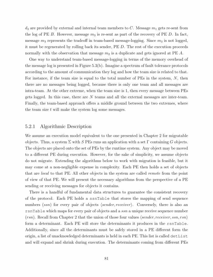
d3 are provided by external and internal team members to C. Message m1 gets re-sent from

the log of PE B. However, message m3 is re-sent as part of the recovery of PE D. In fact,

message m3 represents the tradeoff in team-based message-logging. Since m3 is not logged,

it must be regenerated by rolling back its sender, PE D. The rest of the execution proceeds

normally with the observation that message m2 is a duplicate and gets ignored at PE A.

One way to understand team-based message-logging in terms of the memory overhead of

the message log is presented in Figure 5.3(b). Imagine a spectrum of fault tolerance protocols

according to the amount of communication they log and how the team size is related to that.

For instance, if the team size is equal to the total number of PEs in the system, N , then

there are no messages being logged, because there is only one team and all messages are

intra-team. At the other extreme, when the team size is 1, then every message between PEs

gets logged. In this case, there are N teams and all the external messages are inter-team.

Finally, the team-based approach offers a middle ground between the two extremes, where

the team size t will make the system log some messages.

5.2.1 Algorithmic Description

We assume an execution model equivalent to the one presented in Chapter 2 for migratable

objects. Thus, a system Σ with S PEs runs an application with a set Γ containing G objects.

The objects are placed onto the set of PEs by the runtime system. Any object may be moved

to a different PE during execution. However, for the sake of simplicity, we assume objects

do not migrate. Extending the algorithms below to work with migration is feasible, but it

may come at a non-negligible expense in complexity. Each PE then holds a set of objects

that are local to that PE. All other objects in the system are called remote from the point

of view of that PE. We will present the necessary algorithms from the perspective of a PE

sending or receiving messages for objects it contains.

There is a handful of fundamental data structures to guarantee the consistent recovery

of the protocol. Each PE holds a ssnTable that stores the mapping of send sequence

numbers (ssn) for every pair of objects 〈sender, receiver〉. Conversely, there is also an

rsnTable which maps for every pair of objects and a ssn a unique receive sequence number

(rsn). Recall from Chapter 2 that the union of those four values 〈sender, receiver, ssn, rsn〉form a determinant. Each PE will store the determinants it produces in the rsnTable.

Additionally, since all the determinants must be safely stored in a PE different form the

origin, a list of unacknowledged determinants is held in each PE. This list is called detList

and will expand and shrink during execution. The determinants coming from different PEs

81

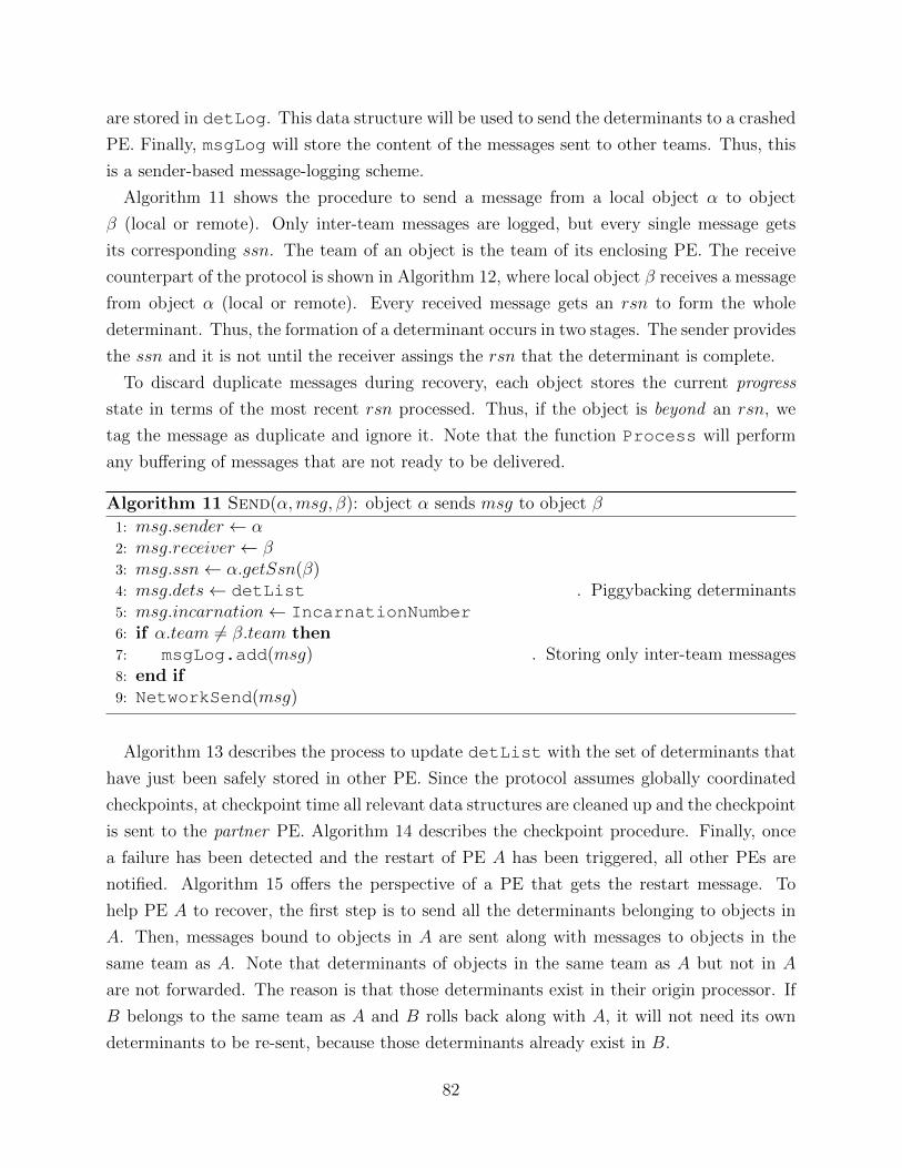
are stored in detLog. This data structure will be used to send the determinants to a crashed

PE. Finally, msgLog will store the content of the messages sent to other teams. Thus, this

is a sender-based message-logging scheme.

Algorithm 11 shows the procedure to send a message from a local object α to object

β (local or remote). Only inter-team messages are logged, but every single message gets

its corresponding ssn. The team of an object is the team of its enclosing PE. The receive

counterpart of the protocol is shown in Algorithm 12, where local object β receives a message

from object α (local or remote). Every received message gets an rsn to form the whole

determinant. Thus, the formation of a determinant occurs in two stages. The sender provides

the ssn and it is not until the receiver assings the rsn that the determinant is complete.

To discard duplicate messages during recovery, each object stores the current progress

state in terms of the most recent rsn processed. Thus, if the object is beyond an rsn, we

tag the message as duplicate and ignore it. Note that the function Process will perform

any buffering of messages that are not ready to be delivered.

Algorithm 11 Send(α,msg, β): object α sends msg to object β

1: msg.sender ← α2: msg.receiver ← β3: msg.ssn← α.getSsn(β)4: msg.dets← detList . Piggybacking determinants5: msg.incarnation← IncarnationNumber6: if α.team 6= β.team then7: msgLog.add(msg) . Storing only inter-team messages8: end if9: NetworkSend(msg)

Algorithm 13 describes the process to update detList with the set of determinants that

have just been safely stored in other PE. Since the protocol assumes globally coordinated

checkpoints, at checkpoint time all relevant data structures are cleaned up and the checkpoint

is sent to the partner PE. Algorithm 14 describes the checkpoint procedure. Finally, once

a failure has been detected and the restart of PE A has been triggered, all other PEs are

notified. Algorithm 15 offers the perspective of a PE that gets the restart message. To

help PE A to recover, the first step is to send all the determinants belonging to objects in

A. Then, messages bound to objects in A are sent along with messages to objects in the

same team as A. Note that determinants of objects in the same team as A but not in A

are not forwarded. The reason is that those determinants exist in their origin processor. If

B belongs to the same team as A and B rolls back along with A, it will not need its own

determinants to be re-sent, because those determinants already exist in B.

82

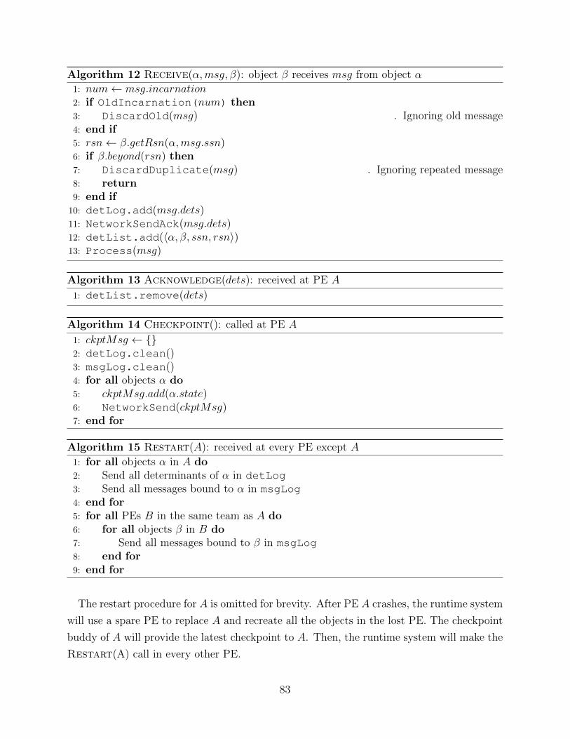
Algorithm 12 Receive(α,msg, β): object β receives msg from object α

1: num← msg.incarnation2: if OldIncarnation(num) then3: DiscardOld(msg) . Ignoring old message4: end if5: rsn← β.getRsn(α,msg.ssn)6: if β.beyond(rsn) then7: DiscardDuplicate(msg) . Ignoring repeated message8: return9: end if

10: detLog.add(msg.dets)11: NetworkSendAck(msg.dets)12: detList.add(〈α, β, ssn, rsn〉)13: Process(msg)

Algorithm 13 Acknowledge(dets): received at PE A

1: detList.remove(dets)

Algorithm 14 Checkpoint(): called at PE A

1: ckptMsg ← 2: detLog.clean()3: msgLog.clean()4: for all objects α do5: ckptMsg.add(α.state)6: NetworkSend(ckptMsg)7: end for

Algorithm 15 Restart(A): received at every PE except A

1: for all objects α in A do2: Send all determinants of α in detLog3: Send all messages bound to α in msgLog4: end for5: for all PEs B in the same team as A do6: for all objects β in B do7: Send all messages bound to β in msgLog8: end for9: end for

The restart procedure for A is omitted for brevity. After PE A crashes, the runtime system

will use a spare PE to replace A and recreate all the objects in the lost PE. The checkpoint

buddy of A will provide the latest checkpoint to A. Then, the runtime system will make the

Restart(A) call in every other PE.

83

5.2.2 Formal Proof of Correctness

We will prove that the team-based message-logging protocol recovers correctly from the

failure of one PE. We will constructively prove that the protocol retrieves all necessary

determinants and all necessary messages during recovery. Additionally, there are no orphan

objects and a global consistent state is reached.

Lemma 5.1. All required determinants are successfully retrieved during recovery.

Proof Sketch. Let us suppose PE A fails and during recovery object α in A collects all its

determinants. Since the process to generate, piggyback and collect determinants remains

the same as in the regular causal message-logging protocol, then all determinants for α are

successfully collected. If a determinant was generated by α but was never piggybacked in

any outbound message from A, then it is impossible to retrieve. However, that determinant

is not necessary for a consistent recovery, because it never affected the rest of the system.

An object β in PE B belonging to the same team as A will successfully retrieve all its

determinants because B clearly has them all, as B never failed and its data structures still

persist.

Lemma 5.2. All required messages are successfully replayed during recovery.

Proof Sketch. Let us assume object α is recovering in PE A. If message m was sent to α

before the crash, it will be sent again during recovery. There are 3 possible cases. First,

message m may have been an inter-team message in which case it will be stored in the

message log of some PE and replayed after restart. Second, it may have been an intra-team

message. Thus, message m was never logged and can not be replayed. However, the sender

of message m must be recovering along with α and given the PWD assumption, it will

eventually send m. Third, message m may have been a local message. If this is the case,

then m will be generated by the same token as the previous case.

Lemma 5.3. There are no orphan objects.

Proof Sketch. By contradiction. Let us assume there is an orphan object γ. This object

must have received at least one message that was not re-sent during recovery. Let us call m

one of those messages. The sender of m did not send m during recovery, but it received all

necessary determinants and messages according to Lemmas 5.1 and 5.2. Thus, according to

the PWD assumption, all the causally related events before message m must have occurred

and m must have been sent. This is a contradiction, then there can not be neither such a

message m nor such an orphan object γ.

84

Theorem 5.4. The recovery process in team-based message-logging is correct.

Proof Sketch. By Lemmas 5.1 and 5.2 all determinants and messages are retrieved during

recovery. That guarantees all the necessary information for a recovery is available. Finally,

the recovery is consistent by Lemma 5.3.

5.3 Team-based Load Balancing

The team-based message-logging protocol provides a promising method to decrease the mem-

ory overhead of the message log. The number of teams k provides a tradeoff between the

memory overhead reduction and the additional recovery cost. Given a user-defined value for

k, there are at least two important classifications for the type of teams to be formed. First,

the teams can be either random or structured if the communication graph of the application

is taken into consideration when forming the teams. Second, the groups can be either static

or dynamic if they are allowed to change during execution.

Random team formation provides nevertheless a moderate benefit. If messages were sent

to random targets, using k teams, we should expect having a reduction of 1/k in the total

memory used. This is because there is a chance of 1/k that a particular message is sent to a

target in the same team and does not require logging. However, as figure 5.1(b) illustrates,

many HPC applications have a well defined communication structure that can be exploited

to aggressively reduce the memory overhead. Thus, we will prefer structured teams to further

improve the impact of the team-based philosophy.

Static structured teams are able to leverage the divide-and-conquer approach of teams for

message-logging. However, dynamic structured teams provide at least two major advantages.

In the first place, dynamic teams are automatic. As such, there is no need to profile the

application to get the structure of the teams. This provides a great advantage when the same

application is used at a different scale or with a different problem size. Second, dynamic

teams may capture the communication changes of an application during execution. Imagine

a weather modeling application that is simulating a storm over a small geographical region.

As the storm makes its way through the region, the communication volume between the

different objects that represent subregions in the space will change. To better capture that

pattern, dynamic teams will adapt accordingly.

In order to obtain dynamic structured teams to use as the basis for the team-based ap-

proach, we build upon the notion of a load balancing framework. The fundamental reason to

use the load balancer is that a change in communication will probably be correlated with a

change in the load of the different PEs in the system. Thus, the two aspects, teams and load,

85

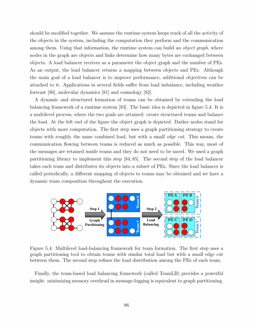
should be modified together. We assume the runtime system keeps track of all the activity of

the objects in the system, including the computation they perform and the communication

among them. Using that information, the runtime system can build an object graph, where

nodes in the graph are objects and links determine how many bytes are exchanged between

objects. A load balancer receives as a parameter the object graph and the number of PEs.

As an output, the load balancer returns a mapping between objects and PEs. Although

the main goal of a load balancer is to improve performance, additional objectives can be

attached to it. Applications in several fields suffer from load imbalance, including weather

forecast [80], molecular dynamics [81] and cosmology [82].

A dynamic and structured formation of teams can be obtained by extending the load

balancing framework of a runtime system [83]. The basic idea is depicted in figure 5.4. It is

a multilevel process, where the two goals are attained: create structured teams and balance

the load. At the left end of the figure the object graph is depicted. Darker nodes stand for

objects with more computation. The first step uses a graph partitioning strategy to create

teams with roughly the same combined load, but with a small edge cut. This means, the

communication flowing between teams is reduced as much as possible. This way, most of

the messages are retained inside teams and they do not need to be saved. We used a graph

partitioning library to implement this step [84, 85]. The second step of the load balancer

takes each team and distributes its objects into a subset of PEs. Since the load balancer is

called periodically, a different mapping of objects to teams may be obtained and we have a

dynamic team composition throughout the execution.

Tea

m X

Tea

m Y

PE A PE B

Step 1 Tea

m X

PE C PE D

Tea

m YGraph

Partitioning

Step 2

LoadBalancing

Figure 5.4: Multilevel load-balancing framework for team formation. The first step uses agraph partitioning tool to obtain teams with similar total load but with a small edge cutbetween them. The second step refines the load distribution among the PEs of each team.

Finally, the team-based load balancing framework (called TeamLB) provides a powerful

insight: minimizing memory overhead in message-logging is equivalent to graph partitioning.

86

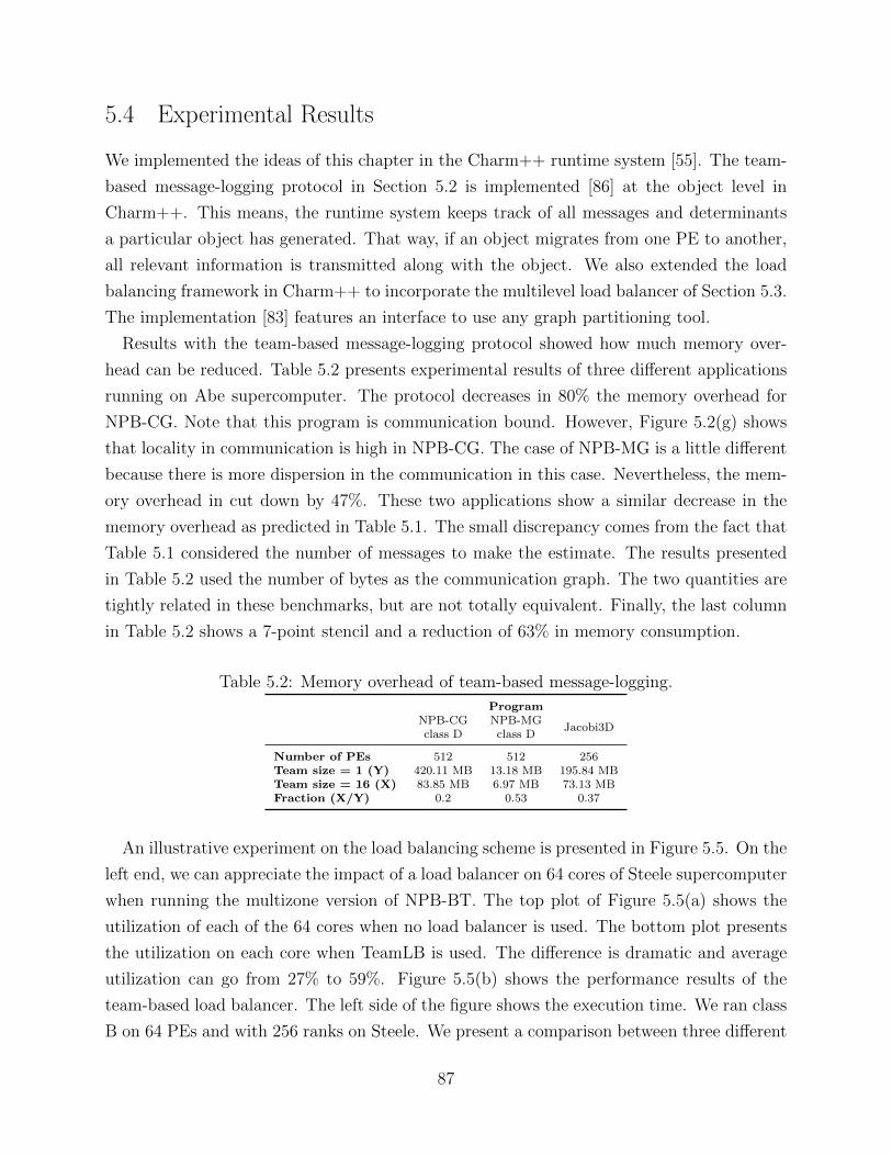
5.4 Experimental Results

We implemented the ideas of this chapter in the Charm++ runtime system [55]. The team-

based message-logging protocol in Section 5.2 is implemented [86] at the object level in

Charm++. This means, the runtime system keeps track of all messages and determinants

a particular object has generated. That way, if an object migrates from one PE to another,

all relevant information is transmitted along with the object. We also extended the load

balancing framework in Charm++ to incorporate the multilevel load balancer of Section 5.3.

The implementation [83] features an interface to use any graph partitioning tool.

Results with the team-based message-logging protocol showed how much memory over-

head can be reduced. Table 5.2 presents experimental results of three different applications

running on Abe supercomputer. The protocol decreases in 80% the memory overhead for

NPB-CG. Note that this program is communication bound. However, Figure 5.2(g) shows

that locality in communication is high in NPB-CG. The case of NPB-MG is a little different

because there is more dispersion in the communication in this case. Nevertheless, the mem-

ory overhead in cut down by 47%. These two applications show a similar decrease in the

memory overhead as predicted in Table 5.1. The small discrepancy comes from the fact that

Table 5.1 considered the number of messages to make the estimate. The results presented

in Table 5.2 used the number of bytes as the communication graph. The two quantities are

tightly related in these benchmarks, but are not totally equivalent. Finally, the last column

in Table 5.2 shows a 7-point stencil and a reduction of 63% in memory consumption.

Table 5.2: Memory overhead of team-based message-logging.

ProgramNPB-CG NPB-MG

Jacobi3Dclass D class D

Number of PEs 512 512 256Team size = 1 (Y) 420.11 MB 13.18 MB 195.84 MBTeam size = 16 (X) 83.85 MB 6.97 MB 73.13 MBFraction (X/Y) 0.2 0.53 0.37

An illustrative experiment on the load balancing scheme is presented in Figure 5.5. On the

left end, we can appreciate the impact of a load balancer on 64 cores of Steele supercomputer

when running the multizone version of NPB-BT. The top plot of Figure 5.5(a) shows the

utilization of each of the 64 cores when no load balancer is used. The bottom plot presents

the utilization on each core when TeamLB is used. The difference is dramatic and average

utilization can go from 27% to 59%. Figure 5.5(b) shows the performance results of the

team-based load balancer. The left side of the figure shows the execution time. We ran class

B on 64 PEs and with 256 ranks on Steele. We present a comparison between three different

87

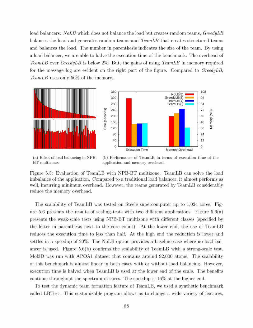
load balancers: NoLB which does not balance the load but creates random teams, GreedyLB

balances the load and generates random teams and TeamLB that creates structured teams

and balances the load. The number in parenthesis indicates the size of the team. By using

a load balancer, we are able to halve the execution time of the benchmark. The overhead of

TeamLB over GreedyLB is below 2%. But, the gains of using TeamLB in memory required

for the message log are evident on the right part of the figure. Compared to GreedyLB,

TeamLB uses only 56% of the memory.

(a) Effect of load balancing in NPB-BT multizone.

0

40

80

120

160

200

240

280

320

360

Execution Time Memory Overhead 0

12

24

36

48

60

72

84

96

108

Tim

e (s

econ

ds)

Mem

ory

(MB

)

NoLB(8)GreedyLB(8)

TeamLB(1)TeamLB(8)

(b) Performance of TeamLB in terms of execution time of theapplication and memory overhead.

Figure 5.5: Evaluation of TeamLB with NPB-BT multizone. TeamLB can solve the loadimbalance of the application. Compared to a traditional load balancer, it almost performs aswell, incurring minimum overhead. However, the teams generated by TeamLB considerablyreduce the memory overhead.

The scalability of TeamLB was tested on Steele supercomputer up to 1,024 cores. Fig-

ure 5.6 presents the results of scaling tests with two different applications. Figure 5.6(a)

presents the weak-scale tests using NPB-BT multizone with different classes (specified by

the letter in parenthesis next to the core count). At the lower end, the use of TeamLB

reduces the execution time to less than half. At the high end the reduction is lower and

settles in a speedup of 20%. The NoLB option provides a baseline case where no load bal-

ancer is used. Figure 5.6(b) confirms the scalability of TeamLB with a strong-scale test.

Mol3D was run with APOA1 dataset that contains around 92,000 atoms. The scalability

of this benchmark is almost linear in both cases with or without load balancing. However,

execution time is halved when TeamLB is used at the lower end of the scale. The benefits

continue throughout the spectrum of cores. The speedup is 16% at the higher end.

To test the dynamic team formation feature of TeamLB, we used a synthetic benchmark

called LBTest. This customizable program allows us to change a wide variety of features,

88

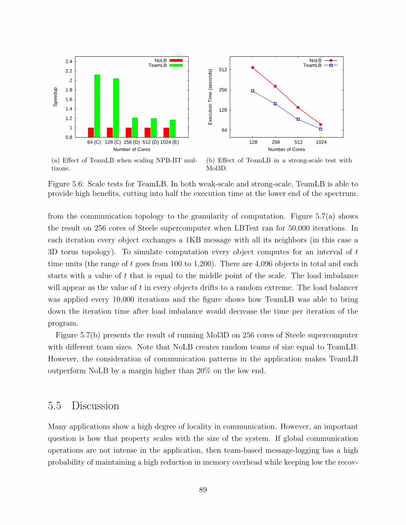
0.8

1

1.2

1.4

1.6

1.8

2

2.2

2.4

64 (C) 128 (C) 256 (D) 512 (D) 1024 (E)

Spe

edup

Number of Cores

NoLBTeamLB

(a) Effect of TeamLB when scaling NPB-BT mul-tizone.

64

128

256

512

128 256 512 1024

Exe

cutio

n T

ime

(sec

onds

)

Number of Cores

NoLBTeamLB

(b) Effect of TeamLB in a strong-scale test withMol3D.

Figure 5.6: Scale tests for TeamLB. In both weak-scale and strong-scale, TeamLB is able toprovide high benefits, cutting into half the execution time at the lower end of the spectrum.

from the communication topology to the granularity of computation. Figure 5.7(a) shows

the result on 256 cores of Steele supercomputer when LBTest ran for 50,000 iterations. In

each iteration every object exchanges a 1KB message with all its neighbors (in this case a

3D torus topology). To simulate computation every object computes for an interval of t

time units (the range of t goes from 100 to 1,200). There are 4,096 objects in total and each

starts with a value of t that is equal to the middle point of the scale. The load imbalance

will appear as the value of t in every objects drifts to a random extreme. The load balancer

was applied every 10,000 iterations and the figure shows how TeamLB was able to bring

down the iteration time after load imbalance would decrease the time per iteration of the

program.

Figure 5.7(b) presents the result of running Mol3D on 256 cores of Steele supercomputer

with different team sizes. Note that NoLB creates random teams of size equal to TeamLB.

However, the consideration of communication patterns in the application makes TeamLB

outperform NoLB by a margin higher than 20% on the low end.

5.5 Discussion

Many applications show a high degree of locality in communication. However, an important

question is how that property scales with the size of the system. If global communication

operations are not intense in the application, then team-based message-logging has a high

probability of maintaining a high reduction in memory overhead while keeping low the recov-

89

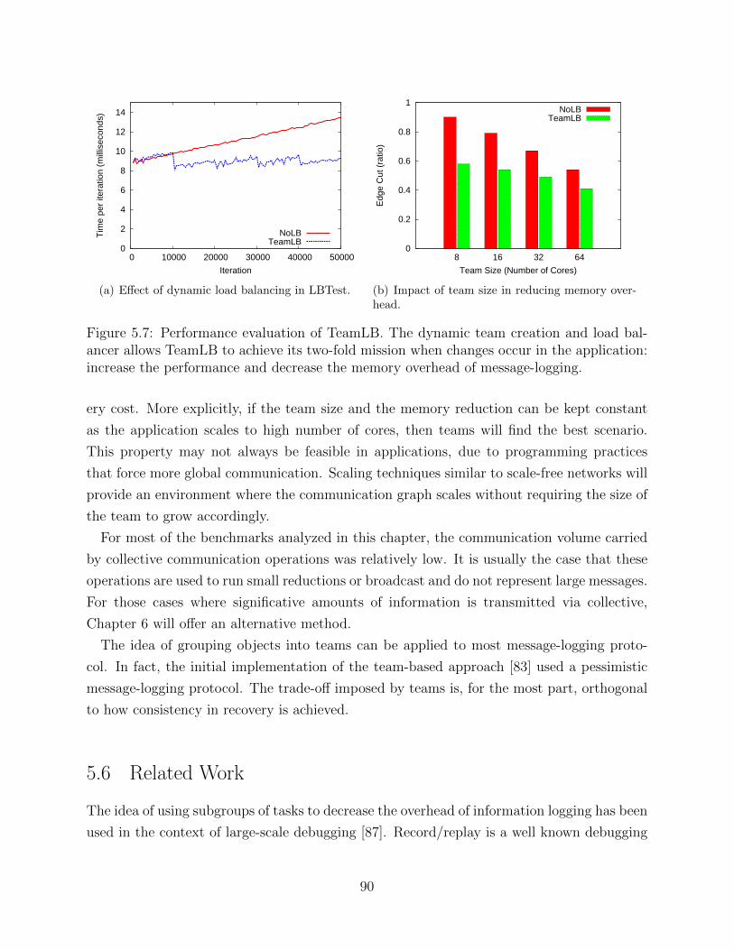
0

2

4

6

8

10

12

14

0 10000 20000 30000 40000 50000

Tim

e pe

r ite

ratio

n (m

illis

econ

ds)

Iteration

NoLBTeamLB

(a) Effect of dynamic load balancing in LBTest.

0

0.2

0.4

0.6

0.8

1

8 16 32 64

Edg

e C

ut (

ratio

)

Team Size (Number of Cores)

NoLBTeamLB

(b) Impact of team size in reducing memory over-head.

Figure 5.7: Performance evaluation of TeamLB. The dynamic team creation and load bal-ancer allows TeamLB to achieve its two-fold mission when changes occur in the application:increase the performance and decrease the memory overhead of message-logging.

ery cost. More explicitly, if the team size and the memory reduction can be kept constant

as the application scales to high number of cores, then teams will find the best scenario.

This property may not always be feasible in applications, due to programming practices

that force more global communication. Scaling techniques similar to scale-free networks will

provide an environment where the communication graph scales without requiring the size of

the team to grow accordingly.

For most of the benchmarks analyzed in this chapter, the communication volume carried

by collective communication operations was relatively low. It is usually the case that these

operations are used to run small reductions or broadcast and do not represent large messages.

For those cases where significative amounts of information is transmitted via collective,

Chapter 6 will offer an alternative method.

The idea of grouping objects into teams can be applied to most message-logging proto-

col. In fact, the initial implementation of the team-based approach [83] used a pessimistic

message-logging protocol. The trade-off imposed by teams is, for the most part, orthogonal

to how consistency in recovery is achieved.

5.6 Related Work

The idea of using subgroups of tasks to decrease the overhead of information logging has been

used in the context of large-scale debugging [87]. Record/replay is a well known debugging

90

technique that offers a framework where a particular faulty execution can be deterministically

reproduced. Such reproducibility of results and conditions helps in determining more easily

the causes of problems and limitations in the programs. There are two kinds of record/replay

mechanisms. Data replay consists in storing all incoming messages to each of the tasks in an

execution and replaying them during debugging. Although there is a high memory consump-

tion with this technique, during replay the user can choose which tasks in particular will be

replayed. Alternatively, order replay strategies only store the outcome of non-deterministic

events in the execution. To generate the messages during replay, all the tasks are forced to

execute. Memory consumption is minimum, but the cost of replay may be too high. This

is particularly problematic in a large-scale environment. MPIWIZ is a record/replay tool

that offers a middle ground between the two types of mechanisms previously described. It

introduces a subgroup reproducible replay (SRR) that balances the benefits of both data

replay and order replay. Each SRR is a disjoint group of tasks. MPIWIZ only records the

messages crossing group boundaries. For intra-group messages, it records the ordering but

not the messages themselves. In the replay phase, each group will be replayed as a unit,

but it will not require the replay of additional groups, since inter-group messages are always

recorded. A key value in MPIWIZ is the size of each group. To find an appropriate value

for the group size, MPIWIZ uses the strong communication locality present in many HPC

applications [88].

In distributed computing settings, like grid or cloud infrastructures, the cost of coordinated

checkpoint may be prohibitive. In those environments interconnection technologies are still

dominated by Ethernet. That means bandwidth may not be an issue, but latency will hurt

performance of tightly coupled applications. In particular, coordinating a global checkpoint

of a large number of machines may result in a significant delay in the progress rate of an

execution. Message-logging does not require coordinated checkpoint and as such represent a

clear opportunity to provide fault tolerance in this type of scenarios. However, the memory

overhead of the message log could offset the benefit of message-logging. One of the first

approaches to explore a trade-off between coordinated checkpoint and message-logging is

called coarse-grained pessimistic message-logging [41, 89]. The system of N processes is

divided into g groups. Each group checkpoints in a coordinated fashion following a time-

based coordinated checkpoint scheme. A causal message-logging protocol is used inside each

cluster, but a pessimistic message-logging is used across clusters. Hence, the granularity

of the pessimistic protocol is increased from a process level to a cluster level. Messages

that are exchanged between members of the same cluster are not logged. The experimental

evaluation of this approach did not go beyond 16 processes.

The notion of distributed recovery units (DRUs) offers the same tradeoff between size of

91

message log and overhead of recovery [90]. A DRU is a collection of processes that may

reside on different processors. The whole distributed system is seen as a collection of DRUs.

Similar to teams, a DRU can be formed by only one process in the extreme case. However,

processes are dynamically assigned to DRUs according to the needs of the application. The

particular partition of processes into DRUs may have different goals. For instance, processes

may be assigned to the same DRU if there is a high frequency of messages between them.

Alternatively, processes may belong to the same DRU if they reside on a predetermined set

of processors. Recovery in DRUs follows a simple scheme [91]. Each DRU recovers using a

local recovery scheme, whereas the system as a whole relies on a global recovery system. The

difference between the implementation of DRUs and teams resides in the fact that DRUs

use receiver-based optimistic message-logging. The DRU approach dumps the messages to

the storage system as opposed to main memory.

A similar argument was followed to create a group-based checkpoint/restart technique [42].

The authors of the paper justify the approach by showing that coordinated checkpoint may

take several seconds in a system with less than 100 processes. To reduce the coordination

cost, the authors resort to groups of processes that checkpoint in a coordinated way. Each

group will checkpoint at its own pace, but to guarantee a successful recovery, message-logging

is used to store messages across groups. There is no notion of determinants in the message-

logging mechanism, making this scheme only effective for fully deterministic applications.

The paper introduces a greedy algorithm to create the groups dynamically, based on the

communication graph of the program. The only parameter of the clustering algorithm is

the maximum size of a cluster. The algorithm proceeds in a similar manner to other greedy

clustering methods, like hierarchical agglomerative clustering (HAC). The evaluation of this

approach used up to 144 processes.

The programming pattern of the application can be used in determining the proper fault

tolerance mechanism for a particular application [92]. In particular, that paper presents

a master-worker pattern and how the set of workers can be divided into communication

subgroups. Each subgroup shows a highly concentration of the communication in the ap-

plication. If those subgroups are sparsely connected, then a failure in one group should

affect only the members of its same group. This assumes message-logging occurs between

the groups. A color mechanism is employed to form checkpoints inside each group. Each

checkpoint will have a particular color and members of a group will be colored according to

which is the latest successful checkpoint. The colors also help to keep track of the causal

dependencies between checkpoints in the groups. The paper presents no evaluation and its

applicability is limited to master-worker programs.

A different approach to generate groups of highly connected processes uses a string match-

92

ing algorithm [43]. The paper is motivated by the need to co-migrate processes in case of load

imbalance in a grid setting. If a node becomes overloaded, a group of processes running on

that node can be checkpointed and migrated away and overall utilization can be increased.

In order to do that, groups of processes that exchange a high communication volume must

be detected. The analogy used in the paper is that an MPI process sequence of messages can

be seen as a string. A function maps every pair of MPI processes to a unique symbol. Using

these strings, an algorithm can dynamically identify similar strings that will correspond to

MPI processes that exchange a significant amount of messages among them. These groups

of similar sequences will determine the group of MPI processes that will migrate together.

The evaluation used only 8 processes.

In a specialization of a message-logging based on send-deterministic programs [71], groups

of ranks are formed to provide failure containment. Thus, the failure of one rank will not

propagate beyond its enclosing group.

93

CHAPTER 6Collective-Aware Message-Logging

Collective communication operations offer a convenient way to coordinate the work of the

objects involved in a parallel computation. This type of operations are commonly found

in most HPC programs. They play an important role in efficiently scaling parallel codes.

In fact, improving the implementation of collectives may bring a substantial performance

benefit [93]. The research question we will answer in this chapter is how message-logging

can be tailored for this type of operations. The design of a collective-aware message-logging

protocol has two major goals: a reduction in memory overhead and a reduction in the number

of determinants generated as part of a collective operation.

The use of collective communication operations can be substantial in some codes. For

instance, a typical implementation of Fast Fourier Transform (FFT) involves exchange of

data between groups of tasks in an all-to-all fashion. There is little computation in FFT

relative to the use of collectives. In other applications, computation may be substantial but

collective operations represent the main mechanism to transport data. Figure 6.1 presents

a couple of applications with that profile.

The molecular dynamics benchmark LeanMD (see Appendix C) carries most of the data

through two collective operations: multicast and reduction, as shown in Figure 6.1(a). This

is justified by the program structure in LeanMD, where a three-dimensional space is divided

into cells and each cell contains a subset of the total collection of particles. In each iteration,

the cells exchange the positions of their particles with the neighboring cells. The number of

neighbors changes according to the parameters in the program. To make the code scalable,

LeanMD employs the same strategy as NAMD [94]. A set of objects, called computes perform

the interaction computation between particles of cells. Each compute is associated with two

cells, but a cell is associated with potentially many computes. In some cases, depending

on the range of the interaction, a cell many interact with dozens of computes. When a cell

94

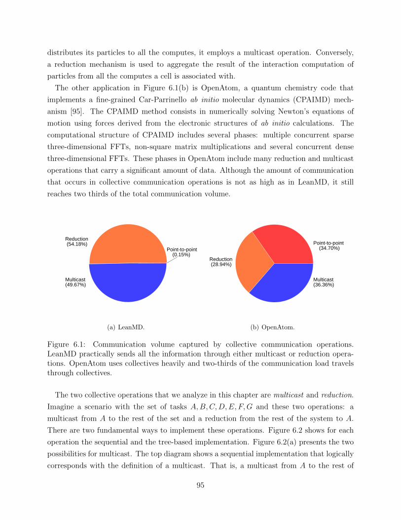
distributes its particles to all the computes, it employs a multicast operation. Conversely,

a reduction mechanism is used to aggregate the result of the interaction computation of

particles from all the computes a cell is associated with.

The other application in Figure 6.1(b) is OpenAtom, a quantum chemistry code that

implements a fine-grained Car-Parrinello ab initio molecular dynamics (CPAIMD) mech-

anism [95]. The CPAIMD method consists in numerically solving Newton’s equations of

motion using forces derived from the electronic structures of ab initio calculations. The

computational structure of CPAIMD includes several phases: multiple concurrent sparse

three-dimensional FFTs, non-square matrix multiplications and several concurrent dense

three-dimensional FFTs. These phases in OpenAtom include many reduction and multicast

operations that carry a significant amount of data. Although the amount of communication

that occurs in collective communication operations is not as high as in LeanMD, it still

reaches two thirds of the total communication volume.

Reduction (54.18%)

Multicast(49.67%)

Point-to-point (0.15%)

(a) LeanMD.

Reduction (28.94%)

Multicast(36.36%)

Point-to-point (34.70%)

(b) OpenAtom.

Figure 6.1: Communication volume captured by collective communication operations.LeanMD practically sends all the information through either multicast or reduction opera-tions. OpenAtom uses collectives heavily and two-thirds of the communication load travelsthrough collectives.

The two collective operations that we analyze in this chapter are multicast and reduction.

Imagine a scenario with the set of tasks A,B,C,D,E, F,G and these two operations: a

multicast from A to the rest of the set and a reduction from the rest of the system to A.

There are two fundamental ways to implement these operations. Figure 6.2 shows for each

operation the sequential and the tree-based implementation. Figure 6.2(a) presents the two

possibilities for multicast. The top diagram shows a sequential implementation that logically

corresponds with the definition of a multicast. That is, a multicast from A to the rest of

95

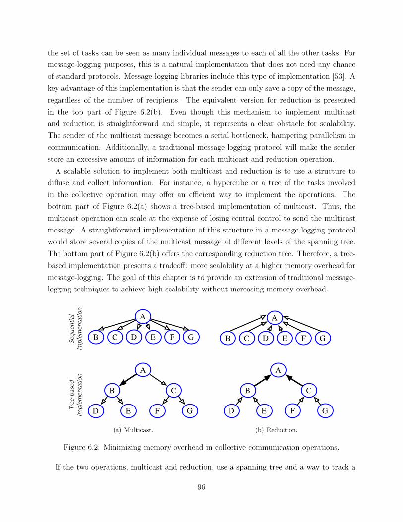
the set of tasks can be seen as many individual messages to each of all the other tasks. For

message-logging purposes, this is a natural implementation that does not need any chance

of standard protocols. Message-logging libraries include this type of implementation [53]. A

key advantage of this implementation is that the sender can only save a copy of the message,

regardless of the number of recipients. The equivalent version for reduction is presented

in the top part of Figure 6.2(b). Even though this mechanism to implement multicast

and reduction is straightforward and simple, it represents a clear obstacle for scalability.

The sender of the multicast message becomes a serial bottleneck, hampering parallelism in

communication. Additionally, a traditional message-logging protocol will make the sender

store an excessive amount of information for each multicast and reduction operation.

A scalable solution to implement both multicast and reduction is to use a structure to

diffuse and collect information. For instance, a hypercube or a tree of the tasks involved

in the collective operation may offer an efficient way to implement the operations. The

bottom part of Figure 6.2(a) shows a tree-based implementation of multicast. Thus, the

multicast operation can scale at the expense of losing central control to send the multicast

message. A straightforward implementation of this structure in a message-logging protocol

would store several copies of the multicast message at different levels of the spanning tree.

The bottom part of Figure 6.2(b) offers the corresponding reduction tree. Therefore, a tree-

based implementation presents a tradeoff: more scalability at a higher memory overhead for

message-logging. The goal of this chapter is to provide an extension of traditional message-

logging techniques to achieve high scalability without increasing memory overhead.

A

B D EC F G

A

B

D E

C

F G

Sequen

tial

implemen

tation

Tree-based

implemen

tation

(a) Multicast.

A

B

D E

C

F G

A

B D EC F G

(b) Reduction.

Figure 6.2: Minimizing memory overhead in collective communication operations.

If the two operations, multicast and reduction, use a spanning tree and a way to track a

96

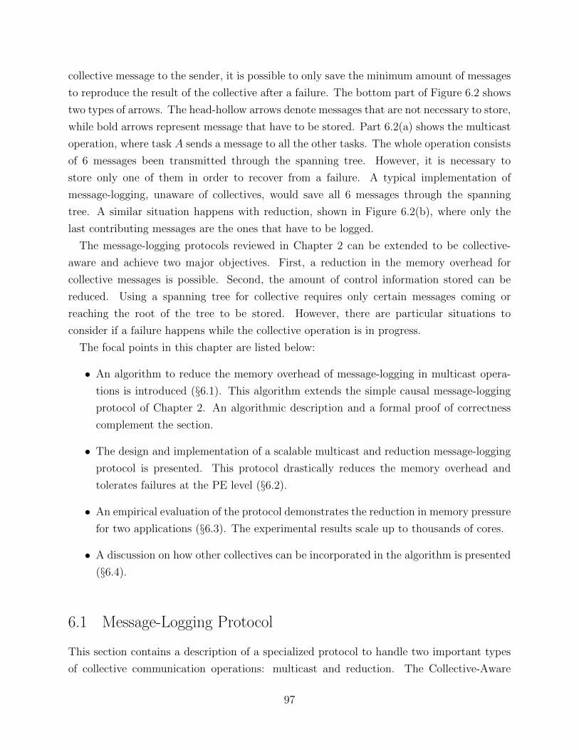
collective message to the sender, it is possible to only save the minimum amount of messages

to reproduce the result of the collective after a failure. The bottom part of Figure 6.2 shows

two types of arrows. The head-hollow arrows denote messages that are not necessary to store,

while bold arrows represent message that have to be stored. Part 6.2(a) shows the multicast

operation, where task A sends a message to all the other tasks. The whole operation consists

of 6 messages been transmitted through the spanning tree. However, it is necessary to

store only one of them in order to recover from a failure. A typical implementation of

message-logging, unaware of collectives, would save all 6 messages through the spanning

tree. A similar situation happens with reduction, shown in Figure 6.2(b), where only the

last contributing messages are the ones that have to be logged.

The message-logging protocols reviewed in Chapter 2 can be extended to be collective-

aware and achieve two major objectives. First, a reduction in the memory overhead for

collective messages is possible. Second, the amount of control information stored can be

reduced. Using a spanning tree for collective requires only certain messages coming or

reaching the root of the tree to be stored. However, there are particular situations to

consider if a failure happens while the collective operation is in progress.

The focal points in this chapter are listed below:

• An algorithm to reduce the memory overhead of message-logging in multicast opera-

tions is introduced (§6.1). This algorithm extends the simple causal message-logging

protocol of Chapter 2. An algorithmic description and a formal proof of correctness

complement the section.

• The design and implementation of a scalable multicast and reduction message-logging

protocol is presented. This protocol drastically reduces the memory overhead and

tolerates failures at the PE level (§6.2).

• An empirical evaluation of the protocol demonstrates the reduction in memory pressure

for two applications (§6.3). The experimental results scale up to thousands of cores.

• A discussion on how other collectives can be incorporated in the algorithm is presented

(§6.4).

6.1 Message-Logging Protocol

This section contains a description of a specialized protocol to handle two important types

of collective communication operations: multicast and reduction. The Collective-Aware

97

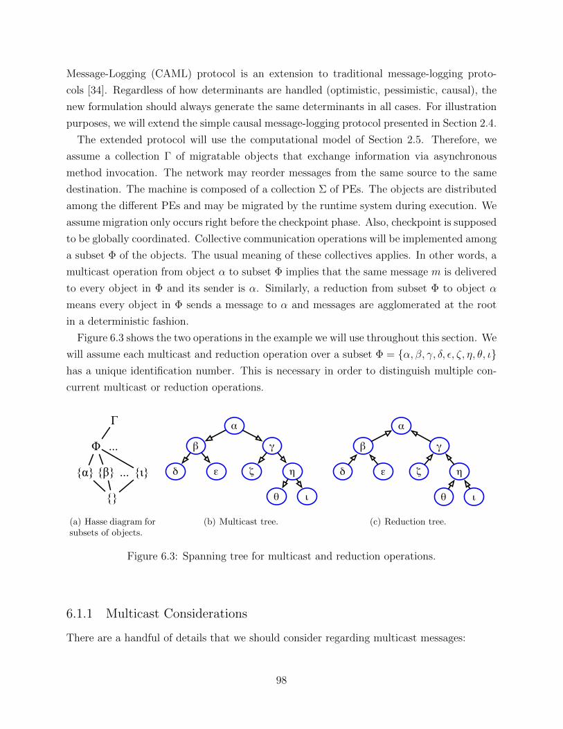
Message-Logging (CAML) protocol is an extension to traditional message-logging proto-

cols [34]. Regardless of how determinants are handled (optimistic, pessimistic, causal), the

new formulation should always generate the same determinants in all cases. For illustration

purposes, we will extend the simple causal message-logging protocol presented in Section 2.4.

The extended protocol will use the computational model of Section 2.5. Therefore, we

assume a collection Γ of migratable objects that exchange information via asynchronous

method invocation. The network may reorder messages from the same source to the same

destination. The machine is composed of a collection Σ of PEs. The objects are distributed

among the different PEs and may be migrated by the runtime system during execution. We

assume migration only occurs right before the checkpoint phase. Also, checkpoint is supposed

to be globally coordinated. Collective communication operations will be implemented among

a subset Φ of the objects. The usual meaning of these collectives applies. In other words, a

multicast operation from object α to subset Φ implies that the same message m is delivered

to every object in Φ and its sender is α. Similarly, a reduction from subset Φ to object α

means every object in Φ sends a message to α and messages are agglomerated at the root

in a deterministic fashion.

Figure 6.3 shows the two operations in the example we will use throughout this section. We

will assume each multicast and reduction operation over a subset Φ = α, β, γ, δ, ε, ζ, η, θ, ιhas a unique identification number. This is necessary in order to distinguish multiple con-

current multicast or reduction operations.

!

"

#$ %

...

...

(a) Hasse diagram forsubsets of objects.

!

"

# $

%

& '

( )

(b) Multicast tree.

!

"

# $

%

& '

( )

(c) Reduction tree.

Figure 6.3: Spanning tree for multicast and reduction operations.

6.1.1 Multicast Considerations

There are a handful of details that we should consider regarding multicast messages:

98

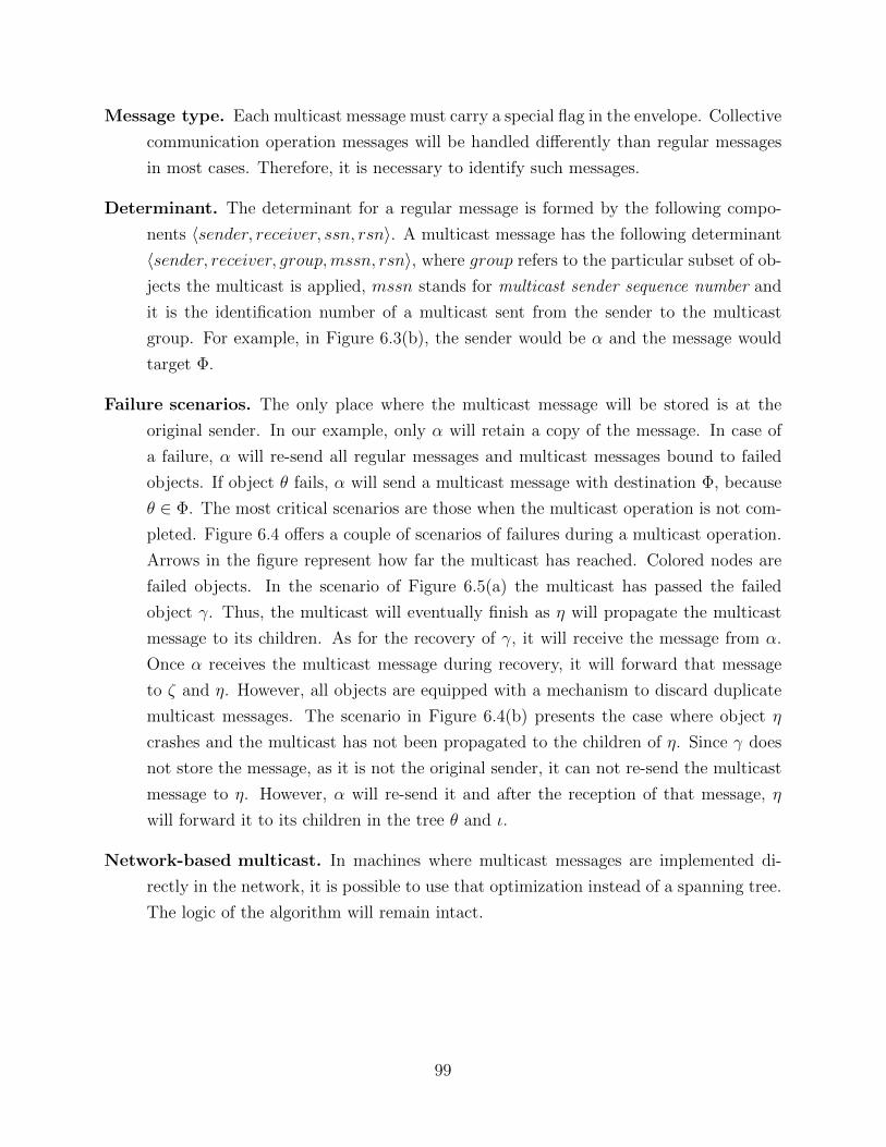
Message type. Each multicast message must carry a special flag in the envelope. Collective

communication operation messages will be handled differently than regular messages

in most cases. Therefore, it is necessary to identify such messages.

Determinant. The determinant for a regular message is formed by the following compo-

nents 〈sender, receiver, ssn, rsn〉. A multicast message has the following determinant

〈sender, receiver, group,mssn, rsn〉, where group refers to the particular subset of ob-

jects the multicast is applied, mssn stands for multicast sender sequence number and

it is the identification number of a multicast sent from the sender to the multicast

group. For example, in Figure 6.3(b), the sender would be α and the message would

target Φ.

Failure scenarios. The only place where the multicast message will be stored is at the

original sender. In our example, only α will retain a copy of the message. In case of

a failure, α will re-send all regular messages and multicast messages bound to failed

objects. If object θ fails, α will send a multicast message with destination Φ, because

θ ∈ Φ. The most critical scenarios are those when the multicast operation is not com-

pleted. Figure 6.4 offers a couple of scenarios of failures during a multicast operation.

Arrows in the figure represent how far the multicast has reached. Colored nodes are

failed objects. In the scenario of Figure 6.5(a) the multicast has passed the failed

object γ. Thus, the multicast will eventually finish as η will propagate the multicast

message to its children. As for the recovery of γ, it will receive the message from α.

Once α receives the multicast message during recovery, it will forward that message

to ζ and η. However, all objects are equipped with a mechanism to discard duplicate

multicast messages. The scenario in Figure 6.4(b) presents the case where object η

crashes and the multicast has not been propagated to the children of η. Since γ does

not store the message, as it is not the original sender, it can not re-send the multicast

message to η. However, α will re-send it and after the reception of that message, η

will forward it to its children in the tree θ and ι.

Network-based multicast. In machines where multicast messages are implemented di-

rectly in the network, it is possible to use that optimization instead of a spanning tree.

The logic of the algorithm will remain intact.

99

!

"

# $

%

& '

( )

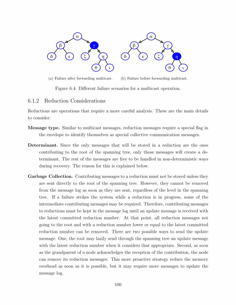
(a) Failure after forwarding multicast.

!

"

# $

%

& '

( )

(b) Failure before forwarding multicast.

Figure 6.4: Different failure scenarios for a multicast operation.

6.1.2 Reduction Considerations

Reductions are operations that require a more careful analysis. These are the main details

to consider:

Message type. Similar to multicast messages, reduction messages require a special flag in

the envelope to identify themselves as special collective communication messages.

Determinant. Since the only messages that will be stored in a reduction are the ones

contributing to the root of the spanning tree, only those messages will create a de-

terminant. The rest of the messages are free to be handled in non-deterministic ways

during recovery. The reason for this is explained below.

Garbage Collection. Contributing messages to a reduction must not be stored unless they

are sent directly to the root of the spanning tree. However, they cannot be removed

from the message log as soon as they are sent, regardless of the level in the spanning

tree. If a failure strikes the system while a reduction is in progress, some of the

intermediate contributing messages may be required. Therefore, contributing messages

to reductions must be kept in the message log until an update message is received with

the latest committed reduction number. At that point, all reduction messages not

going to the root and with a reduction number lower or equal to the latest committed

reduction number can be removed. There are two possible ways to send the update

message. One, the root may lazily send through the spanning tree an update message

with the latest reduction number when it considers that appropriate. Second, as soon

as the grandparent of a node acknowledges the reception of the contribution, the node

can remove its reduction messages. This more proactive strategy reduce the memory

overhead as soon as it is possible, but it may require more messages to update the

message log.

100

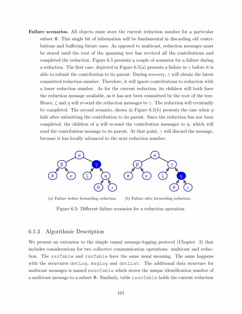
Failure scenarios. All objects must store the current reduction number for a particular

subset Φ. This single bit of information will be fundamental in discarding old contri-

butions and buffering future ones. As opposed to multicast, reduction messages must

be stored until the root of the spanning tree has received all the contributions and

completed the reduction. Figure 6.5 presents a couple of scenarios for a failure during

a reduction. The first case, depicted in Figure 6.5(a) presents a failure in γ before it is

able to submit the contribution to its parent. During recovery, γ will obtain the latest

committed reduction number. Therefore, it will ignore contributions to reduction with

a lower reduction number. As for the current reduction, its children will both have

the reduction message available, as it has not been committed by the root of the tree.

Hence, ζ and η will re-send the reduction messages to γ. The reduction will eventually

be completed. The second scenario, shown in Figure 6.5(b) presents the case when η

fails after submitting the contribution to its parent. Since the reduction has not been

completed, the children of η will re-send the contribution messages to η, which will

send the contribution message to its parent. At that point, γ will discard the message,

because it has locally advanced to the next reduction number.

!

"

# $

%

& '

( )

(a) Failure before forwarding reduction.

!

"

# $

%

& '

( )

(b) Failure after forwarding reduction.

Figure 6.5: Different failure scenarios for a reduction operation.

6.1.3 Algorithmic Description

We present an extension to the simple causal message-logging protocol (Chapter 2) that

includes considerations for two collective communication operations: multicast and reduc-

tion. The ssnTable and rsnTable have the same usual meaning. The same happens

with the structures detLog, msgLog and detList. The additional data structure for

multicast messages is named mssnTable which stores the unique identification number of

a multicast message to a subset Φ. Similarly, table rssnTable holds the current reduction

101

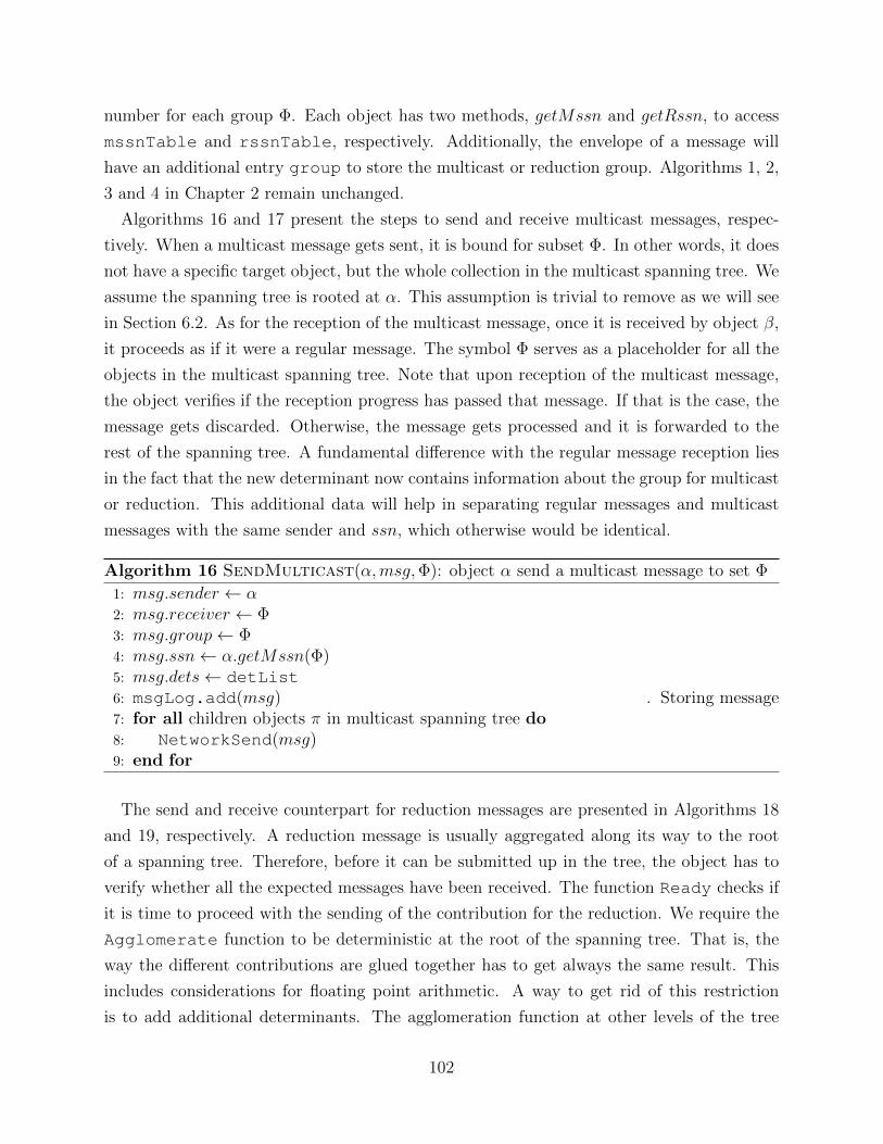
number for each group Φ. Each object has two methods, getMssn and getRssn, to access

mssnTable and rssnTable, respectively. Additionally, the envelope of a message will

have an additional entry group to store the multicast or reduction group. Algorithms 1, 2,

3 and 4 in Chapter 2 remain unchanged.

Algorithms 16 and 17 present the steps to send and receive multicast messages, respec-

tively. When a multicast message gets sent, it is bound for subset Φ. In other words, it does

not have a specific target object, but the whole collection in the multicast spanning tree. We

assume the spanning tree is rooted at α. This assumption is trivial to remove as we will see

in Section 6.2. As for the reception of the multicast message, once it is received by object β,

it proceeds as if it were a regular message. The symbol Φ serves as a placeholder for all the

objects in the multicast spanning tree. Note that upon reception of the multicast message,

the object verifies if the reception progress has passed that message. If that is the case, the

message gets discarded. Otherwise, the message gets processed and it is forwarded to the

rest of the spanning tree. A fundamental difference with the regular message reception lies

in the fact that the new determinant now contains information about the group for multicast

or reduction. This additional data will help in separating regular messages and multicast

messages with the same sender and ssn, which otherwise would be identical.

Algorithm 16 SendMulticast(α,msg,Φ): object α send a multicast message to set Φ

1: msg.sender ← α2: msg.receiver ← Φ3: msg.group← Φ4: msg.ssn← α.getMssn(Φ)5: msg.dets← detList6: msgLog.add(msg) . Storing message7: for all children objects π in multicast spanning tree do8: NetworkSend(msg)9: end for

The send and receive counterpart for reduction messages are presented in Algorithms 18

and 19, respectively. A reduction message is usually aggregated along its way to the root

of a spanning tree. Therefore, before it can be submitted up in the tree, the object has to

verify whether all the expected messages have been received. The function Ready checks if

it is time to proceed with the sending of the contribution for the reduction. We require the

Agglomerate function to be deterministic at the root of the spanning tree. That is, the

way the different contributions are glued together has to get always the same result. This

includes considerations for floating point arithmetic. A way to get rid of this restriction

is to add additional determinants. The agglomeration function at other levels of the tree

102

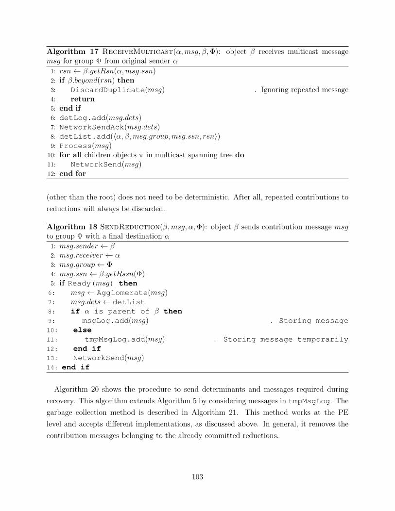
Algorithm 17 ReceiveMulticast(α,msg, β,Φ): object β receives multicast messagemsg for group Φ from original sender α

1: rsn← β.getRsn(α,msg.ssn)2: if β.beyond(rsn) then3: DiscardDuplicate(msg) . Ignoring repeated message4: return5: end if6: detLog.add(msg.dets)7: NetworkSendAck(msg.dets)8: detList.add(〈α, β,msg.group,msg.ssn, rsn〉)9: Process(msg)

10: for all children objects π in multicast spanning tree do11: NetworkSend(msg)12: end for

(other than the root) does not need to be deterministic. After all, repeated contributions to

reductions will always be discarded.

Algorithm 18 SendReduction(β,msg, α,Φ): object β sends contribution message msgto group Φ with a final destination α

1: msg.sender ← β2: msg.receiver ← α3: msg.group← Φ4: msg.ssn← β.getRssn(Φ)5: if Ready(msg) then6: msg ← Agglomerate(msg)7: msg.dets← detList8: if α is parent of β then9: msgLog.add(msg) . Storing message10: else11: tmpMsgLog.add(msg) . Storing message temporarily12: end if13: NetworkSend(msg)14: end if

Algorithm 20 shows the procedure to send determinants and messages required during

recovery. This algorithm extends Algorithm 5 by considering messages in tmpMsgLog. The

garbage collection method is described in Algorithm 21. This method works at the PE

level and accepts different implementations, as discussed above. In general, it removes the

contribution messages belonging to the already committed reductions.

103

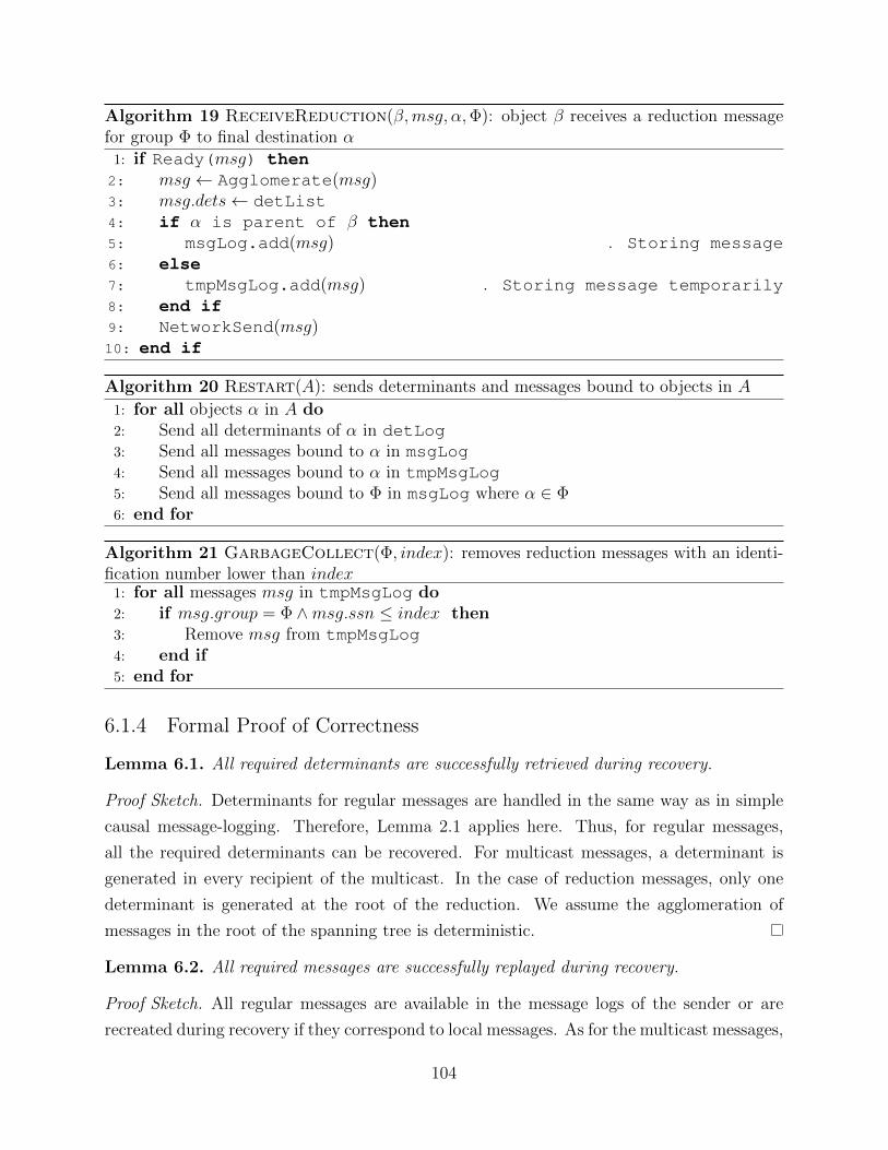
Algorithm 19 ReceiveReduction(β,msg, α,Φ): object β receives a reduction messagefor group Φ to final destination α

1: if Ready(msg) then2: msg ← Agglomerate(msg)3: msg.dets← detList4: if α is parent of β then5: msgLog.add(msg) . Storing message6: else7: tmpMsgLog.add(msg) . Storing message temporarily8: end if9: NetworkSend(msg)10: end if

Algorithm 20 Restart(A): sends determinants and messages bound to objects in A

1: for all objects α in A do2: Send all determinants of α in detLog3: Send all messages bound to α in msgLog4: Send all messages bound to α in tmpMsgLog5: Send all messages bound to Φ in msgLog where α ∈ Φ6: end for

Algorithm 21 GarbageCollect(Φ, index): removes reduction messages with an identi-fication number lower than index

1: for all messages msg in tmpMsgLog do2: if msg.group = Φ ∧msg.ssn ≤ index then3: Remove msg from tmpMsgLog4: end if5: end for

6.1.4 Formal Proof of Correctness

Lemma 6.1. All required determinants are successfully retrieved during recovery.

Proof Sketch. Determinants for regular messages are handled in the same way as in simple

causal message-logging. Therefore, Lemma 2.1 applies here. Thus, for regular messages,

all the required determinants can be recovered. For multicast messages, a determinant is

generated in every recipient of the multicast. In the case of reduction messages, only one

determinant is generated at the root of the reduction. We assume the agglomeration of

messages in the root of the spanning tree is deterministic.

Lemma 6.2. All required messages are successfully replayed during recovery.

Proof Sketch. All regular messages are available in the message logs of the sender or are

recreated during recovery if they correspond to local messages. As for the multicast messages,

104

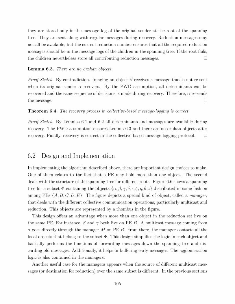
they are stored only in the message log of the original sender at the root of the spanning

tree. They are sent along with regular messages during recovery. Reduction messages may

not all be available, but the current reduction number ensures that all the required reduction

messages should be in the message logs of the children in the spanning tree. If the root fails,

the children nevertheless store all contributing reduction messages.

Lemma 6.3. There are no orphan objects.

Proof Sketch. By contradiction. Imaging an object β receives a message that is not re-sent

when its original sender α recovers. By the PWD assumption, all determinants can be

recovered and the same sequence of decisions is made during recovery. Therefore, α re-sends

the message.

Theorem 6.4. The recovery process in collective-based message-logging is correct.

Proof Sketch. By Lemmas 6.1 and 6.2 all determinants and messages are available during

recovery. The PWD assumption ensures Lemma 6.3 and there are no orphan objects after

recovery. Finally, recovery is correct in the collective-based message-logging protocol.

6.2 Design and Implementation

In implementing the algorithm described above, there are important design choices to make.

One of them relates to the fact that a PE may hold more than one object. The second

deals with the structure of the spanning tree for different roots. Figure 6.6 shows a spanning

tree for a subset Φ containing the objects α, β, γ, δ, ε, ζ, η, θ, ι distributed in some fashion

among PEs A,B,C,D,E. The figure depicts a special kind of object, called a manager,

that deals with the different collective communication operations, particularly multicast and

reduction. This objects are represented by a rhombus in the figure.

This design offers an advantage when more than one object in the reduction set live on

the same PE. For instance, β and γ both live on PE B. A multicast message coming from

α goes directly through the manager M on PE B. From there, the manager contacts all the

local objects that belong to the subset Φ. This design simplifies the logic in each object and

basically performs the functions of forwarding messages down the spanning tree and dis-

carding old messages. Additionally, it helps in buffering early messages. The agglomeration

logic is also contained in the managers.

Another useful case for the managers appears when the source of different multicast mes-

sages (or destination for reduction) over the same subset is different. In the previous sections

105

!

" # $% &

' ( )

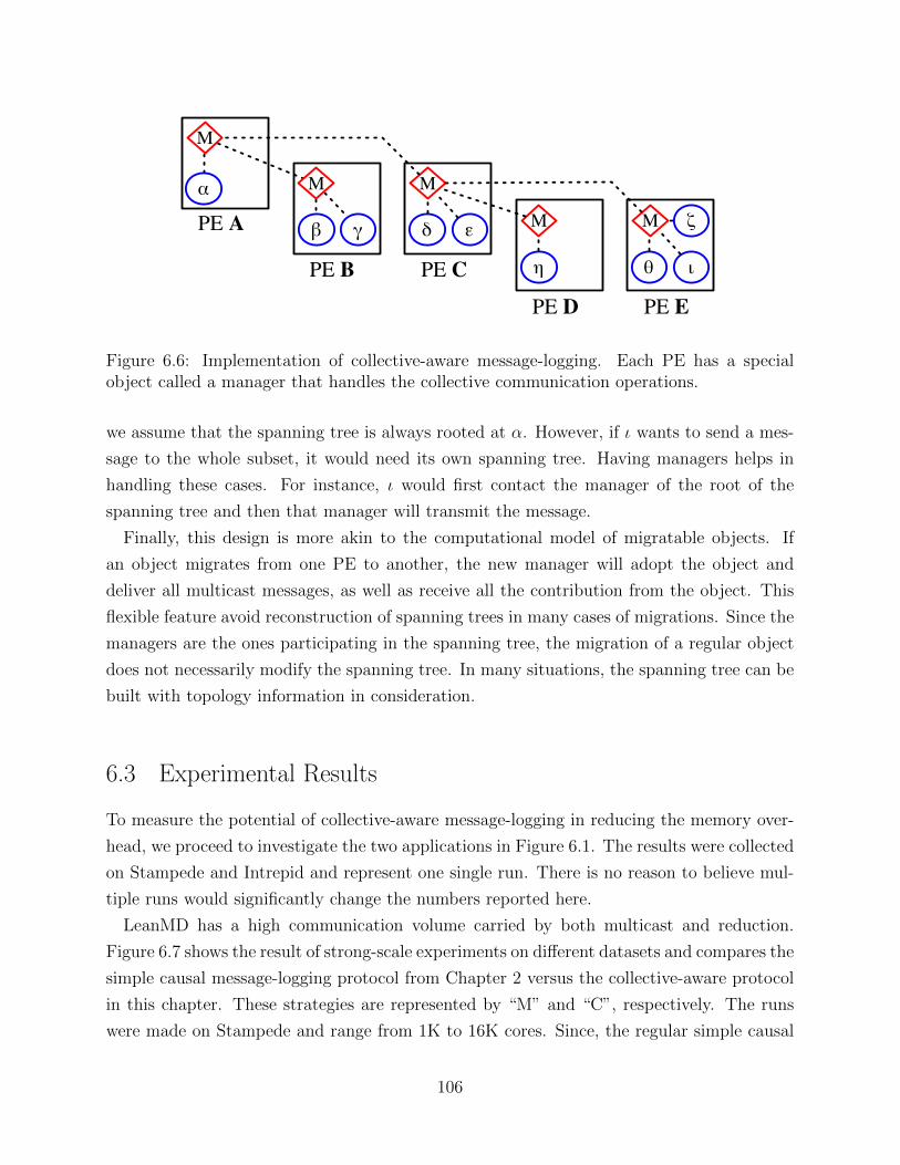
M

M M

M MPE A

PE B PE C

PE D PE E

Figure 6.6: Implementation of collective-aware message-logging. Each PE has a specialobject called a manager that handles the collective communication operations.

we assume that the spanning tree is always rooted at α. However, if ι wants to send a mes-

sage to the whole subset, it would need its own spanning tree. Having managers helps in

handling these cases. For instance, ι would first contact the manager of the root of the

spanning tree and then that manager will transmit the message.

Finally, this design is more akin to the computational model of migratable objects. If

an object migrates from one PE to another, the new manager will adopt the object and

deliver all multicast messages, as well as receive all the contribution from the object. This

flexible feature avoid reconstruction of spanning trees in many cases of migrations. Since the

managers are the ones participating in the spanning tree, the migration of a regular object

does not necessarily modify the spanning tree. In many situations, the spanning tree can be

built with topology information in consideration.

6.3 Experimental Results

To measure the potential of collective-aware message-logging in reducing the memory over-

head, we proceed to investigate the two applications in Figure 6.1. The results were collected

on Stampede and Intrepid and represent one single run. There is no reason to believe mul-

tiple runs would significantly change the numbers reported here.

LeanMD has a high communication volume carried by both multicast and reduction.

Figure 6.7 shows the result of strong-scale experiments on different datasets and compares the

simple causal message-logging protocol from Chapter 2 versus the collective-aware protocol

in this chapter. These strategies are represented by “M” and “C”, respectively. The runs

were made on Stampede and range from 1K to 16K cores. Since, the regular simple causal

106

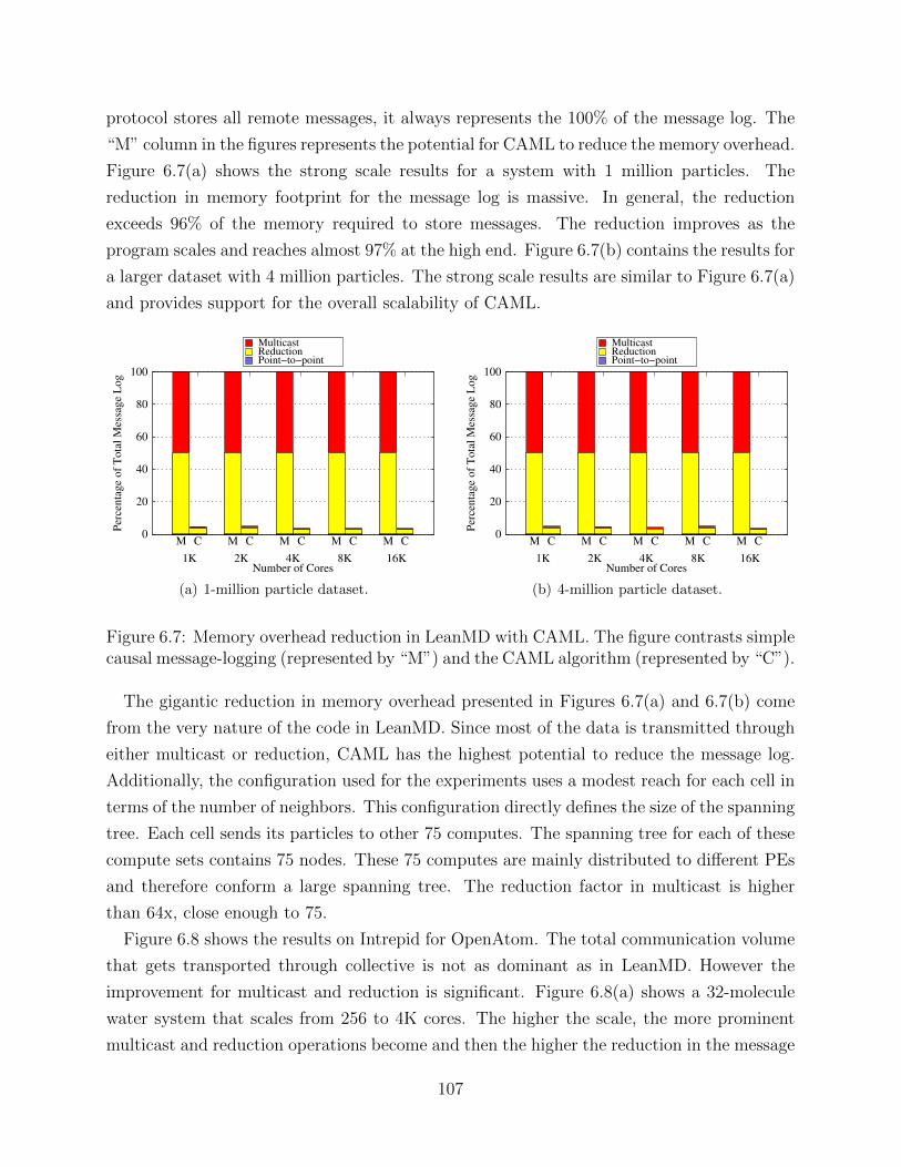
protocol stores all remote messages, it always represents the 100% of the message log. The

“M” column in the figures represents the potential for CAML to reduce the memory overhead.

Figure 6.7(a) shows the strong scale results for a system with 1 million particles. The

reduction in memory footprint for the message log is massive. In general, the reduction

exceeds 96% of the memory required to store messages. The reduction improves as the

program scales and reaches almost 97% at the high end. Figure 6.7(b) contains the results for

a larger dataset with 4 million particles. The strong scale results are similar to Figure 6.7(a)

and provides support for the overall scalability of CAML.

Number of Cores1K 2K 4K 8K 16K

MulticastReductionPoint−to−point

0

20

40

60

80

100

M C M C M C M C M C

Per

cen

tag

e o

f T

ota

l M

essa

ge

Lo

g

(a) 1-million particle dataset.

Number of Cores1K 2K 4K 8K 16K

MulticastReductionPoint−to−point

0

20

40

60

80

100

M C M C M C M C M C

Per

cen

tag

e o

f T

ota

l M

essa

ge

Lo

g

(b) 4-million particle dataset.

Figure 6.7: Memory overhead reduction in LeanMD with CAML. The figure contrasts simplecausal message-logging (represented by “M”) and the CAML algorithm (represented by “C”).

The gigantic reduction in memory overhead presented in Figures 6.7(a) and 6.7(b) come

from the very nature of the code in LeanMD. Since most of the data is transmitted through

either multicast or reduction, CAML has the highest potential to reduce the message log.

Additionally, the configuration used for the experiments uses a modest reach for each cell in

terms of the number of neighbors. This configuration directly defines the size of the spanning

tree. Each cell sends its particles to other 75 computes. The spanning tree for each of these

compute sets contains 75 nodes. These 75 computes are mainly distributed to different PEs

and therefore conform a large spanning tree. The reduction factor in multicast is higher

than 64x, close enough to 75.

Figure 6.8 shows the results on Intrepid for OpenAtom. The total communication volume

that gets transported through collective is not as dominant as in LeanMD. However the

improvement for multicast and reduction is significant. Figure 6.8(a) shows a 32-molecule

water system that scales from 256 to 4K cores. The higher the scale, the more prominent

multicast and reduction operations become and then the higher the reduction in the message

107

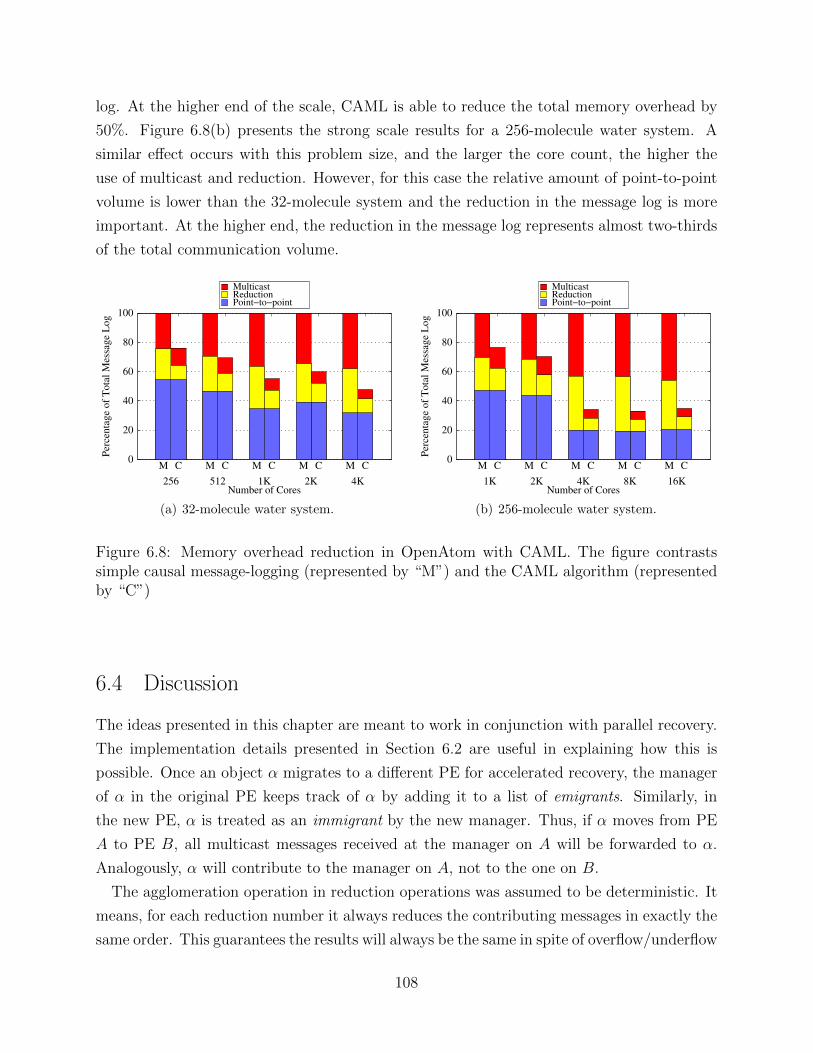
log. At the higher end of the scale, CAML is able to reduce the total memory overhead by

50%. Figure 6.8(b) presents the strong scale results for a 256-molecule water system. A

similar effect occurs with this problem size, and the larger the core count, the higher the

use of multicast and reduction. However, for this case the relative amount of point-to-point

volume is lower than the 32-molecule system and the reduction in the message log is more

important. At the higher end, the reduction in the message log represents almost two-thirds

of the total communication volume.

Number of Cores256 512 1K 2K 4K

MulticastReductionPoint−to−point

0

20

40

60

80

100

M C M C M C M C M C

Per

cen

tag

e o

f T

ota

l M

essa

ge

Lo

g

(a) 32-molecule water system.

Number of Cores1K 2K 4K 8K 16K

MulticastReductionPoint−to−point

0

20

40

60

80

100

M C M C M C M C M C

Per

cen

tag

e o

f T

ota

l M

essa

ge

Lo

g

(b) 256-molecule water system.

Figure 6.8: Memory overhead reduction in OpenAtom with CAML. The figure contrastssimple causal message-logging (represented by “M”) and the CAML algorithm (representedby “C”)

6.4 Discussion

The ideas presented in this chapter are meant to work in conjunction with parallel recovery.

The implementation details presented in Section 6.2 are useful in explaining how this is

possible. Once an object α migrates to a different PE for accelerated recovery, the manager

of α in the original PE keeps track of α by adding it to a list of emigrants. Similarly, in

the new PE, α is treated as an immigrant by the new manager. Thus, if α moves from PE

A to PE B, all multicast messages received at the manager on A will be forwarded to α.

Analogously, α will contribute to the manager on A, not to the one on B.

The agglomeration operation in reduction operations was assumed to be deterministic. It

means, for each reduction number it always reduces the contributing messages in exactly the

same order. This guarantees the results will always be the same in spite of overflow/underflow

108

floating-point arithmetic operations. It is well-known that floating point arithmetic is not

associative. Round-off errors can cause the same parameters in the same operation to give

different results. A way to remove this assumption is to add determinants in the reception

of the contributing messages at the root of the reduction spanning tree. Thus, each message

coming from a child will get a determinant that will keep agglomeration deterministic during

recovery. Note that intermediate levels in the spanning tree do not require determinants.

Since the contribution of all those intermediate levels (except for the children of the root)

will be discarded, there is no need in ensuring determinism.

More collective communication operations can be added to the algorithms described in this

chapter. Some of them can be directly implemented using the multicast and reduction. For

instance, the all-reduce operation may be interpreted as a reduction immediately followed

by a broadcast. Also, an all-to-all operation is a broadcast executed in every element of

the collection. A scan operation is similar to a set of reduction operations. Hence, it can

be handled by CAML. The gather and scatter operations present a different scenario. The

former may be treated as a reduction that agglomerates the individual results through a

spanning tree. The latter can not be optimized by CAML, because it inherently involves a

different message for every task. Other operations may require a deeper analysis, but the

principles should remain the same. Fundamentally, intermediate nodes should not play other

role than mere forwarding of collective messages. Roots of the spanning tree carry most of

the burden at sending and receiving messages.

Figure 6.3(a) shows the partial order of subsets in the collection of objects. There is a

parallel between the lattice of partial order sets and a hierarchical distribution of objects.

As the multicast message travels down the tree, the set of targets become more and more

concrete. If the system is hierarchically divided, then it is possible to associate a level in the

spanning tree with a subgroup of nodes that behave as a recovery unit. Similar to the team-

based message-logging protocol in Chapter 5, if a multicast message enters a new domain

on its way throughout the spanning tree, then it may be necessary to store that message to

satisfy the restrictions of a hierarchical method.

6.5 Related Work

A proposal on building fault-tolerant collective communication operations on MPI showed

an efficient mechanism to achieve low overhead [96]. The main goal behind this idea is

to promote algorithm-based fault tolerance (ABFT) based on a resilient implementation of

MPI collectives. That way, the programmer of the algorithm can incorporate the optimized

109

implementation of resilient collectives. A recent proposal in the MPI Forum addressed the

need for resilient MPI calls and, among other operations, defined MPI Comm validate all

that helps a rank to recognize all failures in a communicator. That way, the application is

aware of the failure in different ranks. The authors of the paper review three different de-

signs for tree-based collectives. First, a rerouting approach would check for a failed process

before interacting with it and route around crashed processes in a recursive fashion. Second,

the lookup-avoiding design would remove the check for failures and calculate the relation-

ships parent/child at the end of MPI Comm validate all. Third, a rebalancing method

will remove the check for failures and balance the tree for the collective call at the end of

MPI Comm validate all. This last design provides the best performance and a negligible

overhead compared to the fault-unaware implementation. The results in their paper scale

up to 256 processes.

A protocol for application-level coordinated checkpoint that targetted applications without

global synchronization points had an extension for collective communication operations [97].

Their checkpoint infrastructure was based on an algorithm that would create a coordinated

checkpoint similar to Chandy-Lamport algorithm [20]. Therefore, an initiator would start

the checkpoint process and coordinate the rest of the procedure. Since this protocol assumes

the checkpoint calls are not made in global synchronization points, there are special measures

to log messages and non-deterministic events during checkpoint. That way, recovery can

work properly by replaying the necessary messages and reproducing all non-deterministic

events. The algorithm creates two important distributed cuts. The first is composed by the

collection of local checkpoints of the processes. This cut will form a recovery line to which

all processes will roll back. The second cut is composed by the points at which processes

stop recording messages and non-deterministic events. The algorithm makes strong claims

about the consistency of both cuts. In particular, there must not be any data flow from

collectives crossing the stop-recording cut.

110

CHAPTER 7Multicore-Node Message-Logging

For a long time, the HPC world used the continuous increase in processor speed as a mech-

anism to make supercomputers more powerful. While Moore’s Law held, smaller and faster

processors provided the needed additional FLOPS to move from megascale to terascale.

However, as the new millennium dawned, the fundamental tenet of an ever increasingly

faster processor came to an end. It was unfeasible to increase the clock rate of processors

without melting the chip. But, a few tricks fetched additional time to keep miniaturizing the

transistors and have more transistors per chip. Those additional transistors would provide

the real state in the chip to have multiple cores. Thus, processor speeds converged to a few

gigahertz and the multicore era was born. It is likely this same technology will take us to

exascale, but not beyond [73].

In the last decade, the rising availability of parallelism at the chip level has changed the

nature of supercomputers. A quick view at the most recent machines shows how this trend

has impacted the architecture of parallel computers. Figure 7.1 presents a selected set of

machines installed in the last decade. Using the four major vendors of supercomputers

(Appro, Cray, HP, and IBM), Figure 7.1(a) presents a historical picture of the ratio cores

versus nodes in different machines. The trend is to exponentially increase this ratio. Also

presented in the figure is the relative speed at which each vendor adopts the newest level of

chip parallelism. From the particular dataset presented here, it seems Appro is the earliest

adopter, while IBM is the latest. The name of the systems, along with their introduction

date is presented in Table 7.1(b). Although this dataset only includes few systems, the entire

Top 500 list follows a similar pattern [98].

Thus, the nature of processors in current supercomputers is multicore. Each machine is

composed of a set of multicore nodes assembled in a hierarchical fashion. Nodes are grouped

into blades, several blades form a rack, and so on. This particular organization must have

111

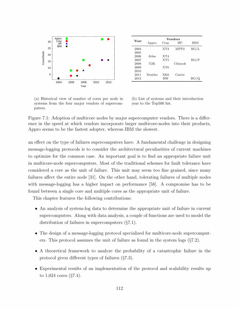
5

10

15

20

25

30

2004 2006 2008 2010 2012

Cor

es/N

ode

Year

ApproCray

HPIBM

(a) Historical view of number of cores per node insystems from the four major vendors of supercom-puters.

YearVendors

Appro Cray HP IBM

2004 XT3 MPP2 BG/L20052006 Atlas XT42007 XT5 BG/P2008 T2K Chinook2009 XT620102011 Trestles XK6 Carter2012 BW BG/Q

(b) List of systems and their introductionyear to the Top500 list.

Figure 7.1: Adoption of multicore nodes by major supercomputer vendors. There is a differ-ence in the speed at which vendors incorporate larger multicore-nodes into their products,Appro seems to be the fastest adopter, whereas IBM the slowest.

an effect on the type of failures supercomputers have. A fundamental challenge in designing

message-logging protocols is to consider the architectural peculiarities of current machines

to optimize for the common case. An important goal is to find an appropriate failure unit

in multicore-node supercomputers. Most of the traditional schemes for fault tolerance have

considered a core as the unit of failure. This unit may seem too fine grained, since many

failures affect the entire node [31]. On the other hand, tolerating failures of multiple nodes

with message-logging has a higher impact on performance [58]. A compromise has to be

found between a single core and multiple cores as the appropriate unit of failure.

This chapter features the following contributions:

• An analysis of system-log data to determine the appropriate unit of failure in current

supercomputers. Along with data analysis, a couple of functions are used to model the

distribution of failures in supercomputers (§7.1).

• The design of a message-logging protocol specialized for multicore-node supercomput-

ers. This protocol assumes the unit of failure as found in the system logs (§7.2).

• A theoretical framework to analyze the probability of a catastrophic failure in the

protocol given different types of failures (§7.3).

• Experimental results of an implementation of the protocol and scalability results up

to 1,024 cores (§7.4).

112

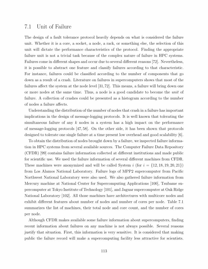
7.1 Unit of Failure

The design of a fault tolerance protocol heavily depends on what is considered the failure

unit. Whether it is a core, a socket, a node, a rack, or something else, the selection of this

unit will dictate the performance characteristics of the protocol. Finding the appropriate

failure unit is not a trivial task because of the complex nature of failure in HPC systems.

Failures come in different shapes and occur due to several different reasons [72]. Nevertheless,

it is possible to abstract one feature and classify failures according to that characteristic.

For instance, failures could be classified according to the number of components that go

down as a result of a crash. Literature on failures in supercomputers shows that most of the

failures affect the system at the node level [31,72]. This means, a failure will bring down one

or more nodes at the same time. Thus, a node is a good candidate to become the unit of

failure. A collection of crashes could be presented as a histogram according to the number

of nodes a failure affects.

Understanding the distribution of the number of nodes that crash in a failure has important

implications in the design of message-logging protocols. It is well known that tolerating the

simultaneous failure of any k nodes in a system has a high impact on the performance

of message-logging protocols [47, 58]. On the other side, it has been shown that protocols

designed to tolerate one single failure at a time present low overhead and good scalability [6].

To obtain the distribution of nodes brought down by a failure, we inspected failure informa-

tion in HPC systems from several available sources. The Computer Failure Data Repository

(CFDR) [99] contains failure information collected at different institutions and made public

for scientific use. We used the failure information of several different machines from CFDR.

These machines were anonymized and will be called System i (for i = 12, 18, 19, 20, 21)from Los Alamos National Laboratory. Failure logs of MPP2 supercomputer from Pacific

Northwest National Laboratory were also used. We also gathered failure information from

Mercury machine at National Center for Supercomputing Applications [100], Tsubame su-

percomputer at Tokyo Institute of Technology [101], and Jaguar supercomputer at Oak Ridge

National Laboratory [102]. All those machines have architectures with multicore nodes and

exhibit different features about number of nodes and number of cores per node. Table 7.1

summarizes the list of machines, their total node and core count, and the number of cores

per node.

Although CFDR makes available some failure information about supercomputers, finding

recent information about failures on any machine is not always possible. Several reasons

justify that situation. First, this information is very sensitive. It is considered that making

public the failure record will make a supercomputing facility less attractive for scientists.

113

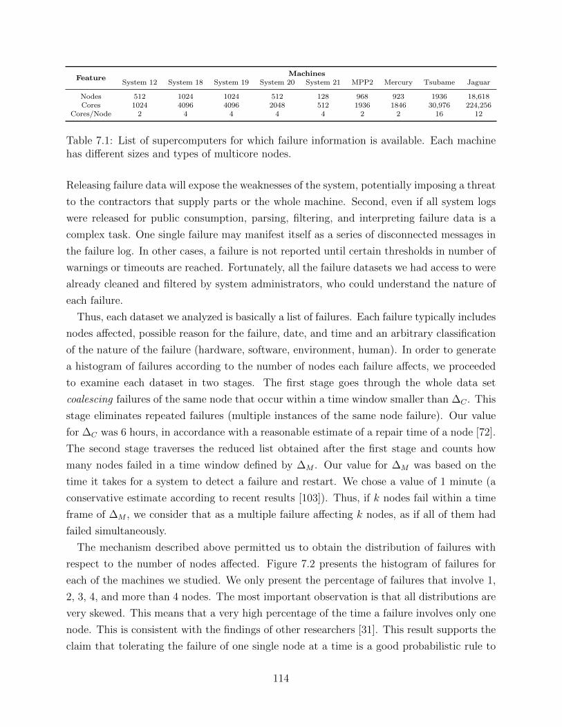
FeatureMachines

System 12 System 18 System 19 System 20 System 21 MPP2 Mercury Tsubame Jaguar

Nodes 512 1024 1024 512 128 968 923 1936 18,618Cores 1024 4096 4096 2048 512 1936 1846 30,976 224,256

Cores/Node 2 4 4 4 4 2 2 16 12

Table 7.1: List of supercomputers for which failure information is available. Each machinehas different sizes and types of multicore nodes.

Releasing failure data will expose the weaknesses of the system, potentially imposing a threat

to the contractors that supply parts or the whole machine. Second, even if all system logs

were released for public consumption, parsing, filtering, and interpreting failure data is a

complex task. One single failure may manifest itself as a series of disconnected messages in

the failure log. In other cases, a failure is not reported until certain thresholds in number of

warnings or timeouts are reached. Fortunately, all the failure datasets we had access to were

already cleaned and filtered by system administrators, who could understand the nature of

each failure.

Thus, each dataset we analyzed is basically a list of failures. Each failure typically includes

nodes affected, possible reason for the failure, date, and time and an arbitrary classification

of the nature of the failure (hardware, software, environment, human). In order to generate

a histogram of failures according to the number of nodes each failure affects, we proceeded

to examine each dataset in two stages. The first stage goes through the whole data set

coalescing failures of the same node that occur within a time window smaller than ∆C . This

stage eliminates repeated failures (multiple instances of the same node failure). Our value

for ∆C was 6 hours, in accordance with a reasonable estimate of a repair time of a node [72].

The second stage traverses the reduced list obtained after the first stage and counts how

many nodes failed in a time window defined by ∆M . Our value for ∆M was based on the

time it takes for a system to detect a failure and restart. We chose a value of 1 minute (a

conservative estimate according to recent results [103]). Thus, if k nodes fail within a time

frame of ∆M , we consider that as a multiple failure affecting k nodes, as if all of them had

failed simultaneously.

The mechanism described above permitted us to obtain the distribution of failures with

respect to the number of nodes affected. Figure 7.2 presents the histogram of failures for

each of the machines we studied. We only present the percentage of failures that involve 1,

2, 3, 4, and more than 4 nodes. The most important observation is that all distributions are

very skewed. This means that a very high percentage of the time a failure involves only one

node. This is consistent with the findings of other researchers [31]. This result supports the

claim that tolerating the failure of one single node at a time is a good probabilistic rule to

114

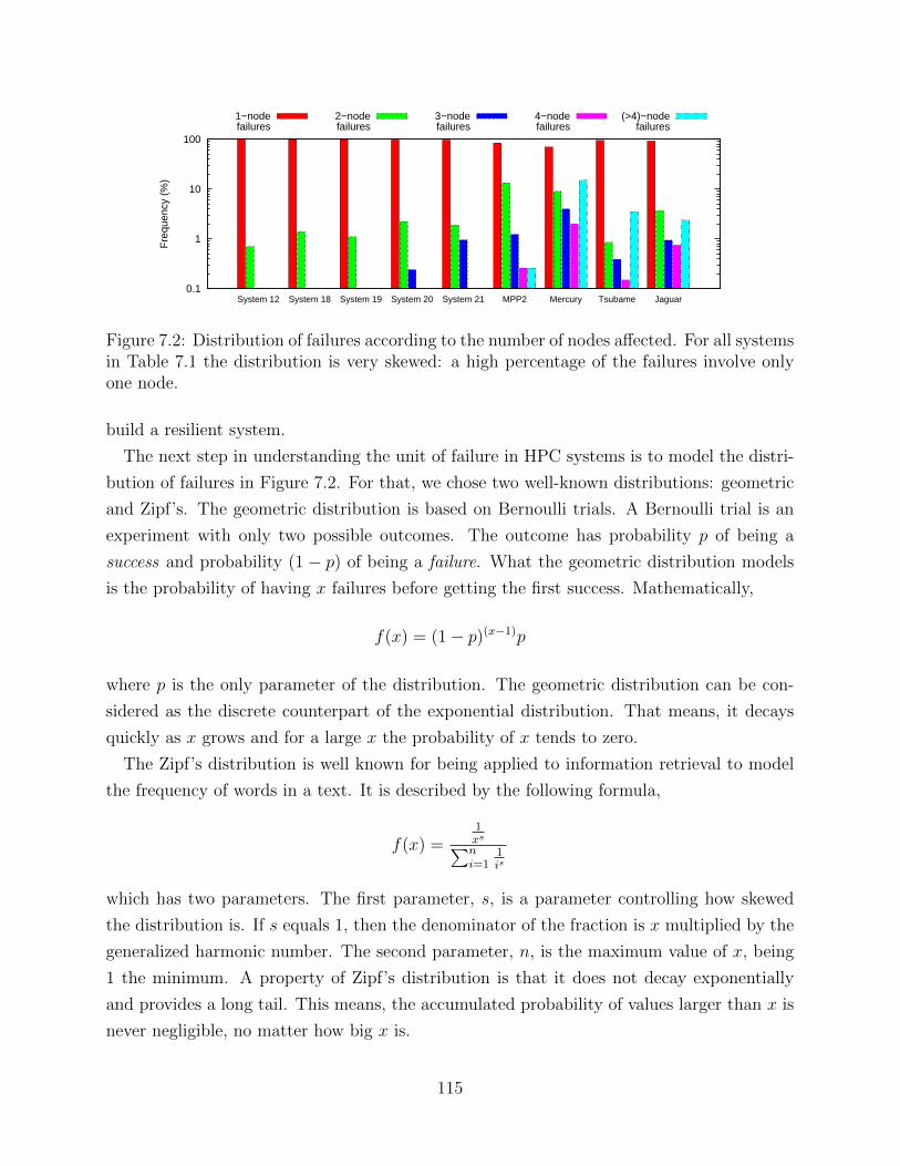
0.1

1

10

100

System 12 System 18 System 19 System 20 System 21 MPP2 Mercury Tsubame Jaguar

Fre

quen

cy (

%)

1−nodefailures

2−nodefailures

3−nodefailures

4−nodefailures

(>4)−nodefailures

Figure 7.2: Distribution of failures according to the number of nodes affected. For all systemsin Table 7.1 the distribution is very skewed: a high percentage of the failures involve onlyone node.

build a resilient system.

The next step in understanding the unit of failure in HPC systems is to model the distri-

bution of failures in Figure 7.2. For that, we chose two well-known distributions: geometric

and Zipf’s. The geometric distribution is based on Bernoulli trials. A Bernoulli trial is an

experiment with only two possible outcomes. The outcome has probability p of being a

success and probability (1 − p) of being a failure. What the geometric distribution models

is the probability of having x failures before getting the first success. Mathematically,

f(x) = (1− p)(x−1)p

where p is the only parameter of the distribution. The geometric distribution can be con-

sidered as the discrete counterpart of the exponential distribution. That means, it decays

quickly as x grows and for a large x the probability of x tends to zero.

The Zipf’s distribution is well known for being applied to information retrieval to model

the frequency of words in a text. It is described by the following formula,

f(x) =1xs∑ni=1

1is

which has two parameters. The first parameter, s, is a parameter controlling how skewed

the distribution is. If s equals 1, then the denominator of the fraction is x multiplied by the

generalized harmonic number. The second parameter, n, is the maximum value of x, being

1 the minimum. A property of Zipf’s distribution is that it does not decay exponentially

and provides a long tail. This means, the accumulated probability of values larger than x is

never negligible, no matter how big x is.

115

0.1

1

10

100

System 12 System 18 System 19 System 20 System 21 MPP2 Mercury Tsubame Jaguar

Fre

quen

cy (

%)

1-nodefailures

2-nodefailures

3-nodefailures

4-nodefailures

(>4)-nodefailures

Figure 7.3: Best-fit curves for distributions in Figure 7.1(b) obtained using the Newton-Raphson method to minimize the least-squares distance. System 12 and MPP2 are modeledthrough a geometric distribution. The rest of the systems are modeled via a Zipf’s distribu-tion.

Using these two functions, we chose proper parameters to model the distributions in figure

7.2. The results are shown in figure 7.3 and the results of a Newton-Raphson best-fit analysis

are presented in Table 7.2. The error was represented by the least-square distance. A value

of n equals to 1024 was used for the Zipf’s distributions. Table 7.2 shows that System 12 and

MPP2 were better matched by a geometric distribution. The rest of the systems are better

modeled by a Zipf’s distribution. There are systems that are markedly well represented by

the model function (low least-squares error). However, the failure distribution of Mercury

is hard to match for any model distribution. Part of the reason is the long tail the original

distribution has.

Best FitMachines

System 12 System 18 System 19 System 20 System 21 MPP2 Mercury Tsubame Jaguar

Geometricp 0.9924 0.9848 0.9878 0.9755 0.9755 0.8473 0.7498 0.9699 0.9395

Error 3.66E-7 2.20E-6 2.54E-6 7.37E-6 1.20E-4 7.72E-5 1.21E-2 8.08E-4 7.76E-4

Zipf’ss 7.0410 6.0875 6.4146 5.4300 5.3970 2.9451 2.2190 5.0671 4.1365

Error 4.89E-7 2.81E-7 5.62E-7 9.63E-8 7.04E-5 1.19E-3 7.35E-3 6.67E-4 4.16E-4

Table 7.2: Best-fit functions and errors for distributions of Figure 7.2. A low error pointsto a distribution easily represented by one of the model functions. Other cases, such asMercury failure distribution, are hard to match and the error is relatively high.

To decide what function matches the data better and perform statistical hypothesis testing,

a chi-square goodness-of-fit test can be used. This test applies to data coming from discrete

distributions. It also works for binned data. Giving a series of observations oi and expected

116

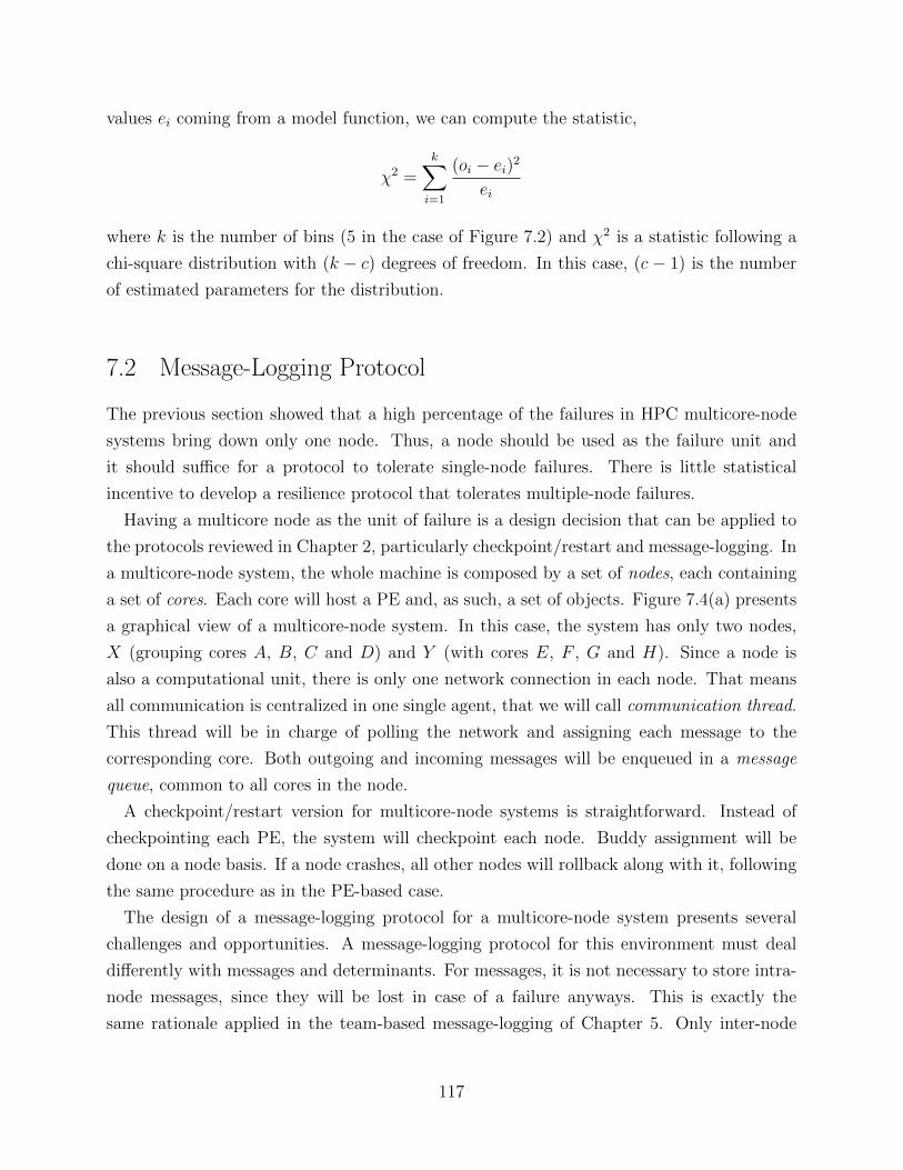
values ei coming from a model function, we can compute the statistic,

χ2 =k∑i=1

(oi − ei)2

ei

where k is the number of bins (5 in the case of Figure 7.2) and χ2 is a statistic following a

chi-square distribution with (k − c) degrees of freedom. In this case, (c − 1) is the number

of estimated parameters for the distribution.

7.2 Message-Logging Protocol

The previous section showed that a high percentage of the failures in HPC multicore-node

systems bring down only one node. Thus, a node should be used as the failure unit and

it should suffice for a protocol to tolerate single-node failures. There is little statistical

incentive to develop a resilience protocol that tolerates multiple-node failures.

Having a multicore node as the unit of failure is a design decision that can be applied to

the protocols reviewed in Chapter 2, particularly checkpoint/restart and message-logging. In

a multicore-node system, the whole machine is composed by a set of nodes, each containing

a set of cores. Each core will host a PE and, as such, a set of objects. Figure 7.4(a) presents

a graphical view of a multicore-node system. In this case, the system has only two nodes,

X (grouping cores A, B, C and D) and Y (with cores E, F , G and H). Since a node is

also a computational unit, there is only one network connection in each node. That means

all communication is centralized in one single agent, that we will call communication thread.

This thread will be in charge of polling the network and assigning each message to the

corresponding core. Both outgoing and incoming messages will be enqueued in a message

queue, common to all cores in the node.

A checkpoint/restart version for multicore-node systems is straightforward. Instead of

checkpointing each PE, the system will checkpoint each node. Buddy assignment will be

done on a node basis. If a node crashes, all other nodes will rollback along with it, following

the same procedure as in the PE-based case.

The design of a message-logging protocol for a multicore-node system presents several

challenges and opportunities. A message-logging protocol for this environment must deal

differently with messages and determinants. For messages, it is not necessary to store intra-

node messages, since they will be lost in case of a failure anyways. This is exactly the

same rationale applied in the team-based message-logging of Chapter 5. Only inter-node

117

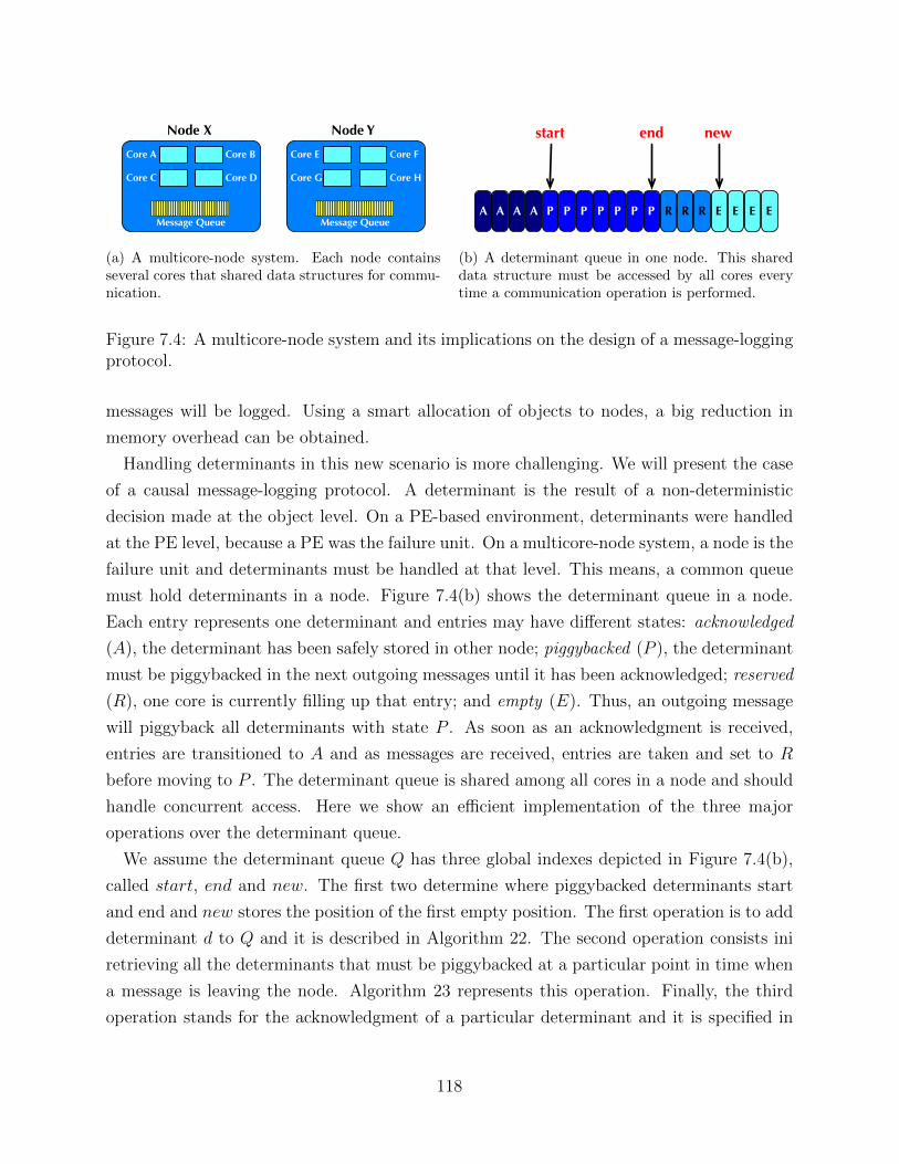
Core A

Node X

Core B

Core C Core D

Message Queue

Core E

Node Y

Core F

Core G Core H

Message Queue

(a) A multicore-node system. Each node containsseveral cores that shared data structures for commu-nication.

A A A A P P P P P P P R R R E E E E

start end new

(b) A determinant queue in one node. This shareddata structure must be accessed by all cores everytime a communication operation is performed.

Figure 7.4: A multicore-node system and its implications on the design of a message-loggingprotocol.

messages will be logged. Using a smart allocation of objects to nodes, a big reduction in

memory overhead can be obtained.

Handling determinants in this new scenario is more challenging. We will present the case

of a causal message-logging protocol. A determinant is the result of a non-deterministic

decision made at the object level. On a PE-based environment, determinants were handled

at the PE level, because a PE was the failure unit. On a multicore-node system, a node is the

failure unit and determinants must be handled at that level. This means, a common queue

must hold determinants in a node. Figure 7.4(b) shows the determinant queue in a node.

Each entry represents one determinant and entries may have different states: acknowledged

(A), the determinant has been safely stored in other node; piggybacked (P ), the determinant

must be piggybacked in the next outgoing messages until it has been acknowledged; reserved

(R), one core is currently filling up that entry; and empty (E). Thus, an outgoing message

will piggyback all determinants with state P . As soon as an acknowledgment is received,

entries are transitioned to A and as messages are received, entries are taken and set to R

before moving to P . The determinant queue is shared among all cores in a node and should

handle concurrent access. Here we show an efficient implementation of the three major

operations over the determinant queue.

We assume the determinant queue Q has three global indexes depicted in Figure 7.4(b),

called start, end and new. The first two determine where piggybacked determinants start

and end and new stores the position of the first empty position. The first operation is to add

determinant d to Q and it is described in Algorithm 22. The second operation consists ini

retrieving all the determinants that must be piggybacked at a particular point in time when

a message is leaving the node. Algorithm 23 represents this operation. Finally, the third

operation stands for the acknowledgment of a particular determinant and it is specified in

118

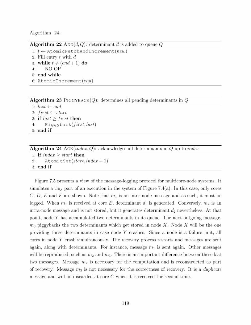
Algorithm 24.

Algorithm 22 Add(d,Q): determinant d is added to queue Q

1: t← AtomicFetchAndIncrement(new)2: Fill entry t with d3: while t 6= (end+ 1) do4: NO OP5: end while6: AtomicIncrement(end)

Algorithm 23 Piggyback(Q): determines all pending determinants in Q

1: last← end2: first← start3: if last ≥ first then4: Piggyback(first, last)5: end if

Algorithm 24 Ack(index,Q): acknowledges all determinants in Q up to index

1: if index ≥ start then2: AtomicSet(start, index+ 1)3: end if

Figure 7.5 presents a view of the message-logging protocol for multicore-node systems. It

simulates a tiny part of an execution in the system of Figure 7.4(a). In this case, only cores

C, D, E and F are shown. Note that m1 is an inter-node message and as such, it must be

logged. When m1 is received at core E, determinant d1 is generated. Conversely, m2 is an

intra-node message and is not stored, but it generates determinant d2 nevertheless. At that

point, node Y has accumulated two determinants in its queue. The next outgoing message,

m3 piggybacks the two determinants which get stored in node X. Node X will be the one

providing those determinants in case node Y crashes. Since a node is a failure unit, all

cores in node Y crash simultaneously. The recovery process restarts and messages are sent

again, along with determinants. For instance, message m1 is sent again. Other messages

will be reproduced, such as m2 and m3. There is an important difference between these last

two messages. Message m2 is necessary for the computation and is reconstructed as part

of recovery. Message m3 is not necessary for the correctness of recovery. It is a duplicate

message and will be discarded at core C when it is received the second time.

119

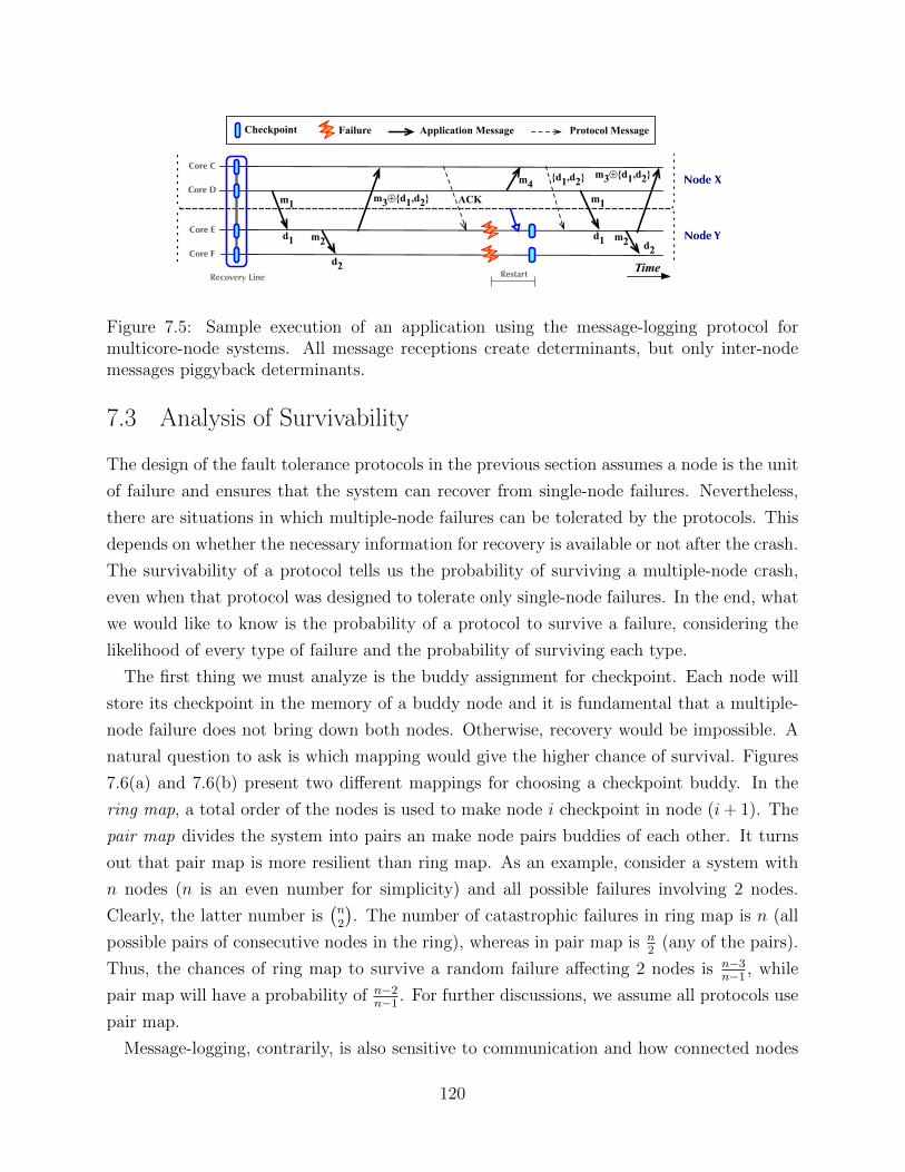
Core C

Core D

Core E

Core F

Recovery Line Restart

m1

m2

Node X

Node Y

Checkpoint Failure Application Message Protocol Message

d1

d2

m3!d1,d2 ACK

m4m1

d1,d2

d1

Time

m2

m3!d1,d2

d2

Figure 7.5: Sample execution of an application using the message-logging protocol formulticore-node systems. All message receptions create determinants, but only inter-nodemessages piggyback determinants.

7.3 Analysis of Survivability

The design of the fault tolerance protocols in the previous section assumes a node is the unit

of failure and ensures that the system can recover from single-node failures. Nevertheless,

there are situations in which multiple-node failures can be tolerated by the protocols. This

depends on whether the necessary information for recovery is available or not after the crash.

The survivability of a protocol tells us the probability of surviving a multiple-node crash,

even when that protocol was designed to tolerate only single-node failures. In the end, what

we would like to know is the probability of a protocol to survive a failure, considering the

likelihood of every type of failure and the probability of surviving each type.

The first thing we must analyze is the buddy assignment for checkpoint. Each node will

store its checkpoint in the memory of a buddy node and it is fundamental that a multiple-

node failure does not bring down both nodes. Otherwise, recovery would be impossible. A

natural question to ask is which mapping would give the higher chance of survival. Figures

7.6(a) and 7.6(b) present two different mappings for choosing a checkpoint buddy. In the

ring map, a total order of the nodes is used to make node i checkpoint in node (i+ 1). The

pair map divides the system into pairs an make node pairs buddies of each other. It turns

out that pair map is more resilient than ring map. As an example, consider a system with

n nodes (n is an even number for simplicity) and all possible failures involving 2 nodes.

Clearly, the latter number is(n2

). The number of catastrophic failures in ring map is n (all

possible pairs of consecutive nodes in the ring), whereas in pair map is n2

(any of the pairs).

Thus, the chances of ring map to survive a random failure affecting 2 nodes is n−3n−1 , while

pair map will have a probability of n−2n−1 . For further discussions, we assume all protocols use

pair map.

Message-logging, contrarily, is also sensitive to communication and how connected nodes

120

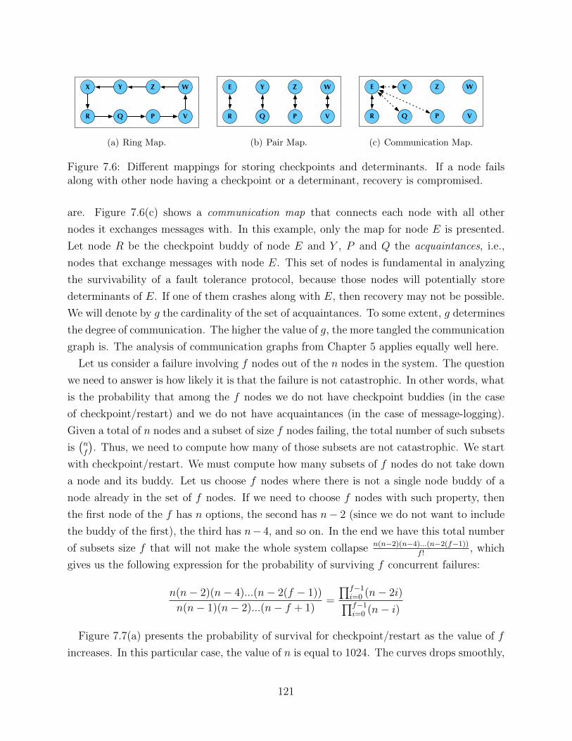
X Y Z W

R Q P V

(a) Ring Map.

E Y Z W

R Q P V

(b) Pair Map.

E Y Z W

R Q P V

(c) Communication Map.

Figure 7.6: Different mappings for storing checkpoints and determinants. If a node failsalong with other node having a checkpoint or a determinant, recovery is compromised.

are. Figure 7.6(c) shows a communication map that connects each node with all other

nodes it exchanges messages with. In this example, only the map for node E is presented.

Let node R be the checkpoint buddy of node E and Y , P and Q the acquaintances, i.e.,

nodes that exchange messages with node E. This set of nodes is fundamental in analyzing

the survivability of a fault tolerance protocol, because those nodes will potentially store

determinants of E. If one of them crashes along with E, then recovery may not be possible.

We will denote by g the cardinality of the set of acquaintances. To some extent, g determines

the degree of communication. The higher the value of g, the more tangled the communication

graph is. The analysis of communication graphs from Chapter 5 applies equally well here.

Let us consider a failure involving f nodes out of the n nodes in the system. The question

we need to answer is how likely it is that the failure is not catastrophic. In other words, what

is the probability that among the f nodes we do not have checkpoint buddies (in the case

of checkpoint/restart) and we do not have acquaintances (in the case of message-logging).

Given a total of n nodes and a subset of size f nodes failing, the total number of such subsets

is(nf

). Thus, we need to compute how many of those subsets are not catastrophic. We start

with checkpoint/restart. We must compute how many subsets of f nodes do not take down

a node and its buddy. Let us choose f nodes where there is not a single node buddy of a

node already in the set of f nodes. If we need to choose f nodes with such property, then

the first node of the f has n options, the second has n− 2 (since we do not want to include

the buddy of the first), the third has n− 4, and so on. In the end we have this total number

of subsets size f that will not make the whole system collapse n(n−2)(n−4)...(n−2(f−1))f !

, which

gives us the following expression for the probability of surviving f concurrent failures:

n(n− 2)(n− 4)...(n− 2(f − 1))

n(n− 1)(n− 2)...(n− f + 1)=

∏f−1i=0 (n− 2i)∏f−1i=0 (n− i)

Figure 7.7(a) presents the probability of survival for checkpoint/restart as the value of f

increases. In this particular case, the value of n is equal to 1024. The curves drops smoothly,

121

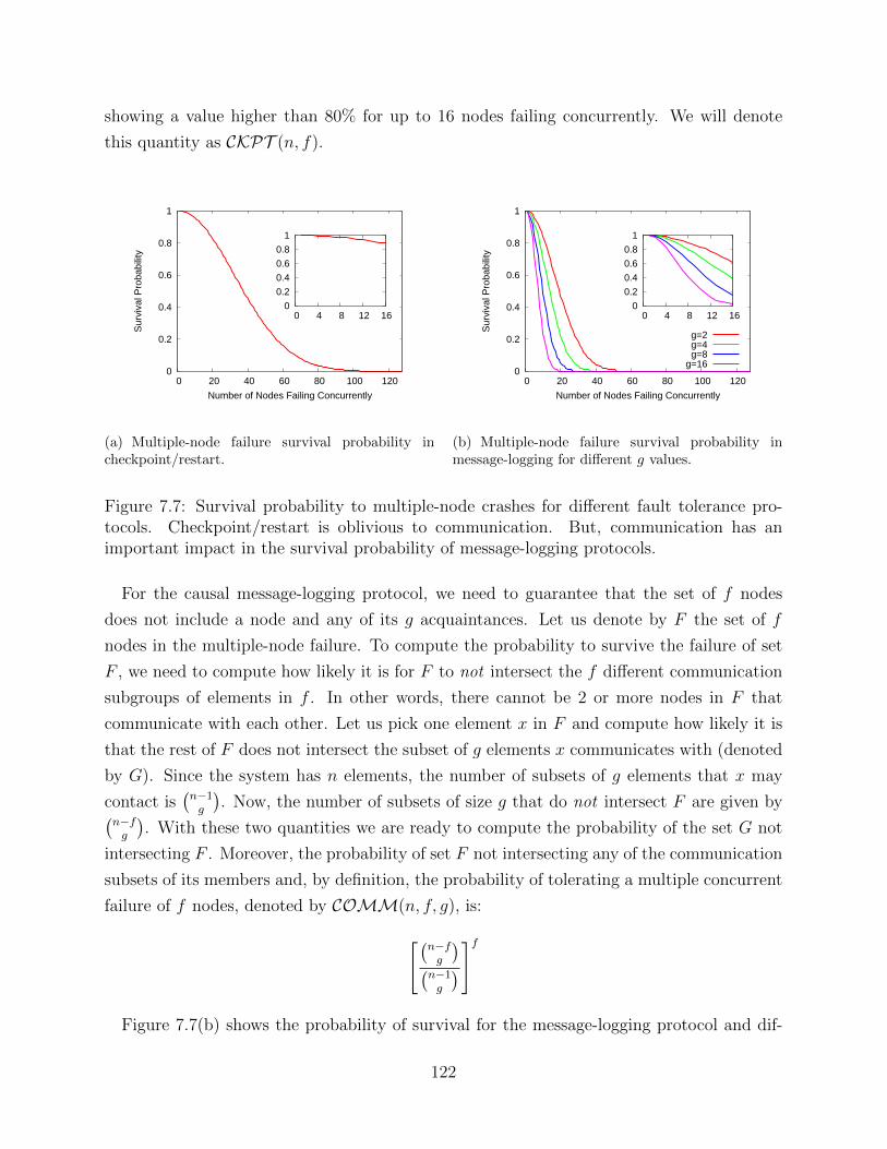
showing a value higher than 80% for up to 16 nodes failing concurrently. We will denote

this quantity as CKPT (n, f).

0

0.2

0.4

0.6

0.8

1

0 20 40 60 80 100 120

Sur

viva

l Pro

babi

lity

Number of Nodes Failing Concurrently

0

0.2

0.4

0.6

0.8

1

0 4 8 12 16

(a) Multiple-node failure survival probability incheckpoint/restart.

0

0.2

0.4

0.6

0.8

1

0 20 40 60 80 100 120

Sur

viva

l Pro

babi

lity

Number of Nodes Failing Concurrently

g=2g=4g=8

g=16

0

0.2

0.4

0.6

0.8

1

0 4 8 12 16

(b) Multiple-node failure survival probability inmessage-logging for different g values.

Figure 7.7: Survival probability to multiple-node crashes for different fault tolerance pro-tocols. Checkpoint/restart is oblivious to communication. But, communication has animportant impact in the survival probability of message-logging protocols.

For the causal message-logging protocol, we need to guarantee that the set of f nodes

does not include a node and any of its g acquaintances. Let us denote by F the set of f

nodes in the multiple-node failure. To compute the probability to survive the failure of set

F , we need to compute how likely it is for F to not intersect the f different communication

subgroups of elements in f . In other words, there cannot be 2 or more nodes in F that

communicate with each other. Let us pick one element x in F and compute how likely it is

that the rest of F does not intersect the subset of g elements x communicates with (denoted

by G). Since the system has n elements, the number of subsets of g elements that x may

contact is(n−1g

). Now, the number of subsets of size g that do not intersect F are given by(

n−fg

). With these two quantities we are ready to compute the probability of the set G not

intersecting F . Moreover, the probability of set F not intersecting any of the communication

subsets of its members and, by definition, the probability of tolerating a multiple concurrent

failure of f nodes, denoted by COMM(n, f, g), is:[(n−fg

)(n−1g

)]f

Figure 7.7(b) shows the probability of survival for the message-logging protocol and dif-

122

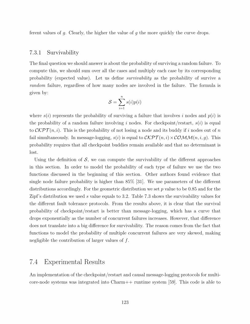
ferent values of g. Clearly, the higher the value of g the more quickly the curve drops.

7.3.1 Survivability

The final question we should answer is about the probability of surviving a random failure. To

compute this, we should sum over all the cases and multiply each case by its corresponding

probability (expected value). Let us define survivability as the probability of survive a

random failure, regardless of how many nodes are involved in the failure. The formula is

given by:

S =n∑i=1

s(i)p(i)

where s(i) represents the probability of surviving a failure that involves i nodes and p(i) is

the probability of a random failure involving i nodes. For checkpoint/restart, s(i) is equal

to CKPT (n, i). This is the probability of not losing a node and its buddy if i nodes out of n

fail simultaneously. In message-logging, s(i) is equal to CKPT (n, i)×COMM(n, i, g). This

probability requires that all checkpoint buddies remain available and that no determinant is

lost.

Using the definition of S, we can compute the survivability of the different approaches

in this section. In order to model the probability of each type of failure we use the two

functions discussed in the beginning of this section. Other authors found evidence that

single node failure probability is higher than 85% [31]. We use parameters of the different

distributions accordingly. For the geometric distribution we set p value to be 0.85 and for the

Zipf’s distribution we used s value equals to 3.2. Table 7.3 shows the survivability values for

the different fault tolerance protocols. From the results above, it is clear that the survival

probability of checkpoint/restart is better than message-logging, which has a curve that

drops exponentially as the number of concurrent failures increases. However, that difference

does not translate into a big difference for survivability. The reason comes from the fact that

functions to model the probability of multiple concurrent failures are very skewed, making

negligible the contribution of larger values of f .

7.4 Experimental Results

An implementation of the checkpoint/restart and causal message-logging protocols for multi-

core-node systems was integrated into Charm++ runtime system [59]. This code is able to

123

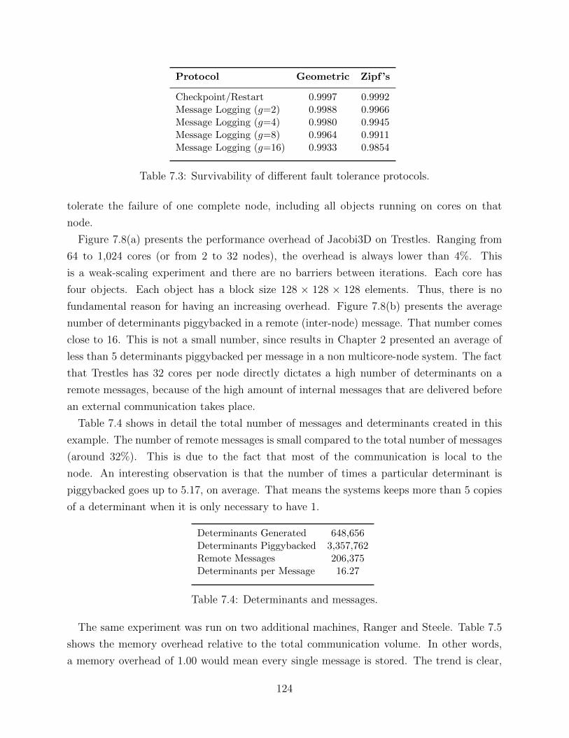
Protocol Geometric Zipf’s

Checkpoint/Restart 0.9997 0.9992Message Logging (g=2) 0.9988 0.9966Message Logging (g=4) 0.9980 0.9945Message Logging (g=8) 0.9964 0.9911Message Logging (g=16) 0.9933 0.9854

Table 7.3: Survivability of different fault tolerance protocols.

tolerate the failure of one complete node, including all objects running on cores on that

node.

Figure 7.8(a) presents the performance overhead of Jacobi3D on Trestles. Ranging from

64 to 1,024 cores (or from 2 to 32 nodes), the overhead is always lower than 4%. This

is a weak-scaling experiment and there are no barriers between iterations. Each core has

four objects. Each object has a block size 128 × 128 × 128 elements. Thus, there is no

fundamental reason for having an increasing overhead. Figure 7.8(b) presents the average

number of determinants piggybacked in a remote (inter-node) message. That number comes

close to 16. This is not a small number, since results in Chapter 2 presented an average of

less than 5 determinants piggybacked per message in a non multicore-node system. The fact

that Trestles has 32 cores per node directly dictates a high number of determinants on a

remote messages, because of the high amount of internal messages that are delivered before

an external communication takes place.

Table 7.4 shows in detail the total number of messages and determinants created in this

example. The number of remote messages is small compared to the total number of messages

(around 32%). This is due to the fact that most of the communication is local to the

node. An interesting observation is that the number of times a particular determinant is

piggybacked goes up to 5.17, on average. That means the systems keeps more than 5 copies

of a determinant when it is only necessary to have 1.

Determinants Generated 648,656Determinants Piggybacked 3,357,762Remote Messages 206,375Determinants per Message 16.27

Table 7.4: Determinants and messages.

The same experiment was run on two additional machines, Ranger and Steele. Table 7.5

shows the memory overhead relative to the total communication volume. In other words,

a memory overhead of 1.00 would mean every single message is stored. The trend is clear,

124

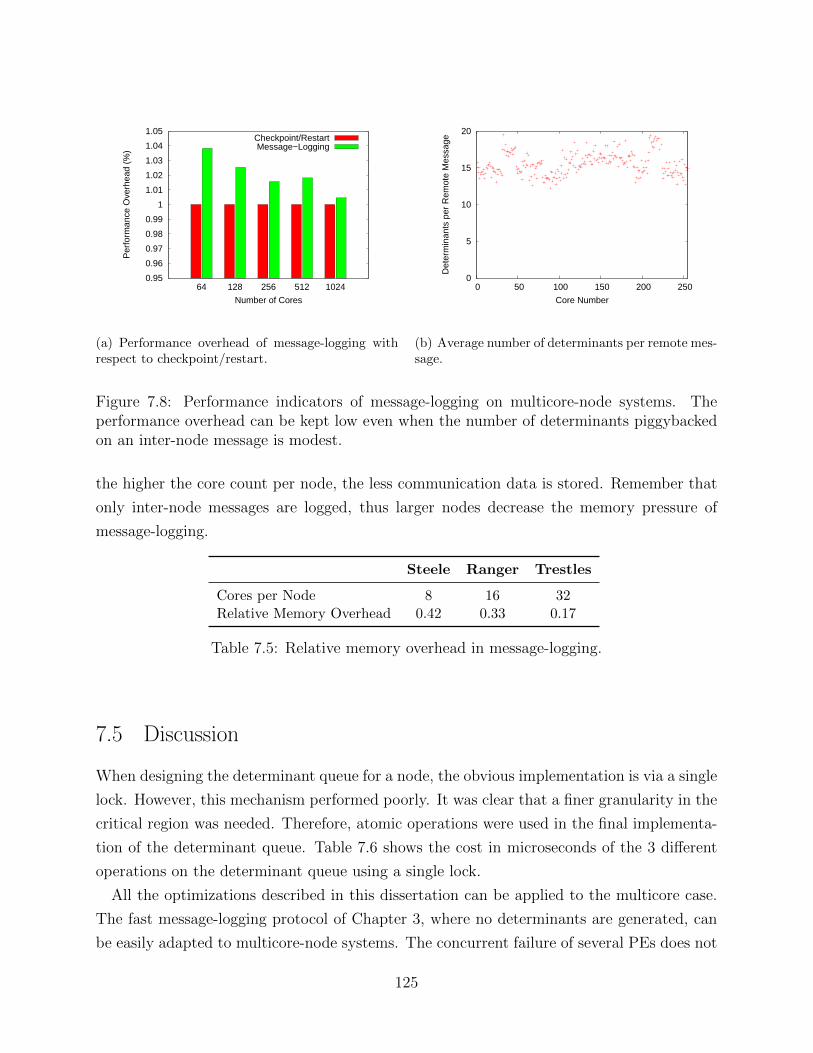
0.95

0.96

0.97

0.98

0.99

1

1.01

1.02

1.03

1.04

1.05

64 128 256 512 1024

Per

form

ance

Ove

rhea

d (%

)

Number of Cores

Checkpoint/RestartMessage−Logging

(a) Performance overhead of message-logging withrespect to checkpoint/restart.

0

5

10

15

20

0 50 100 150 200 250

Det

erm

inan

ts p

er R

emot

e M

essa

ge

Core Number

(b) Average number of determinants per remote mes-sage.

Figure 7.8: Performance indicators of message-logging on multicore-node systems. Theperformance overhead can be kept low even when the number of determinants piggybackedon an inter-node message is modest.

the higher the core count per node, the less communication data is stored. Remember that

only inter-node messages are logged, thus larger nodes decrease the memory pressure of

message-logging.

Steele Ranger Trestles

Cores per Node 8 16 32Relative Memory Overhead 0.42 0.33 0.17

Table 7.5: Relative memory overhead in message-logging.

7.5 Discussion

When designing the determinant queue for a node, the obvious implementation is via a single

lock. However, this mechanism performed poorly. It was clear that a finer granularity in the

critical region was needed. Therefore, atomic operations were used in the final implementa-

tion of the determinant queue. Table 7.6 shows the cost in microseconds of the 3 different

operations on the determinant queue using a single lock.

All the optimizations described in this dissertation can be applied to the multicore case.

The fast message-logging protocol of Chapter 3, where no determinants are generated, can

be easily adapted to multicore-node systems. The concurrent failure of several PEs does not

125

Add Piggyback Acknowledge

41µs 60 µs 79µs

Table 7.6: Lock contention costs.

affect the correctness of the protocol. Parallel recovery, reviewed in Chapter 2, is equally

applicable to the multicore-node case. It this case, once a node crashes, the objects on that

node can be distributed to other nodes for parallel recovery. The team-based message-logging

protocol of Chapter 5 is also useful in multicore-node machines, with the property that now

teams contain nodes instead of PEs. This would bring a further decrease in the memory

overhead, because even some inter-node messages may not be logged (those traveling within

team boundaries).

It is impossible not to connect this chapter with the MPI+X programming model, where

MPI is used to transmit messages from one node to another and a different programming

model is used within the node. The MPI+X model would precisely render unnecessary

the work in this chapter. The reason is that having only one communication agent per

node would be equivalent to have a PE-based system. There is no need for the additional

shared-memory data structures.

It has been noted that node failures may co-occur in supercomputers [72]. This phe-

nomenon is specially relevant during the first stage of the lifetime of a machine. Since there

is a period of instability where the system administrators are still tuning up the components,

several nodes may crash due to a common reason.

It is possible to collect evidence for this type of failures from the open repositories of

failures in supercomputers. Using that information it will be useful to understand what

reach the failure correlation has. In other words, how many nodes a failure may bring down

simultaneously. If nodes X and Y appear to crash altogether in a high percent of the cases,

we may adjust the runtime system to deal with this type of failure. There are at least

a couple of alternatives: i) using the load balancer to distribute objects in a way that a

simultaneous failure does not make the system lose any determinants, and ii) strengthen the

causal message-logging protocol to piggyback determinants along with messages until they

are safely stored.

Before describing both alternatives in more detail, we need to define a couple of terms.

Failure data analysis can provide a node-failure correlation graph of the system. This graph

has nodes as vertices and there is an edge between two nodes if they happen to fail concur-

rently. Each edge may be labeled with the probability of the two nodes failing altogether.

Using this graph, we can form failure domains by applying a partitioning algorithm. Nodes

126

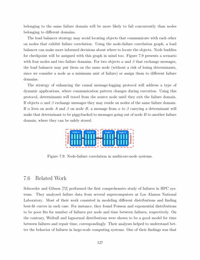
belonging to the same failure domain will be more likely to fail concurrently than nodes

belonging to different domains.

The load balancer strategy may avoid locating objects that communicate with each other

on nodes that exhibit failure correlation. Using the node-failure correlation graph, a load

balancer can make more informed decisions about where to locate the objects. Node buddies

for checkpoint will be assigned with this graph in mind too. Figure 7.9 presents a scenario

with four nodes and two failure domains. For two objects α and β that exchange messages,

the load balancer may put them on the same node (without a risk of losing determinants,

since we consider a node as a minimum unit of failure) or assign them to different failure

domains.

The strategy of enhancing the causal message-logging protocol will address a type of

dynamic applications, where communication pattern changes during execution. Using this

protocol, determinants will travel from the source node until they exit the failure domain.

If objects α and β exchange messages they may reside on nodes of the same failure domain.

If α lives on node A and β on node B, a message from α to β carrying a determinant will

make that determinant to be piggybacked to messages going out of node B to another failure

domain, where they can be safely stored.

Node A Node B Node C Node D

Dom

ain X

Dom

ain Y

Figure 7.9: Node-failure correlation in multicore-node systems.

7.6 Related Work

Schroeder and Gibson [72] performed the first comprehensive study of failures in HPC sys-

tems. They analyzed failure data from several supercomputers at Los Alamos National

Laboratory. Most of their work consisted in modeling different distributions and finding

best-fit curves in each case. For instance, they found Poisson and exponential distributions

to be poor fits for number of failures per node and time between failures, respectively. On

the contrary, Weibull and lognormal distributions were shown to be a good model for time

between failures and repair time, correspondingly. Their analyses helped to understand bet-

ter the behavior of failures in large-scale computing systems. One of their findings was that

127

failure rates do not grow significantly faster than linearly with system size. Based on that

fact, we can assume failure frequency will scale as supercomputers grow within the same

architecture type.

Traditionally, fault tolerance message-logging protocols have had a core, not a node, as the

unit of failure. Whereas some of the protocols only tolerate the failure of one single core [5,6],

others tolerate the failure of multiple cores but only at the cost of a high overhead [34].

Recently, protocols based on properties of HPC applications have been shown to tolerate

multiple simultaneous crashes [51], but they may have a high cost on recovery. Moody et

al [31] mention that 85% of the failures disable at most one compute node on the clusters

at Lawrence Livermore National Laboratory where the Scalable Checkpoint/Restart (SCR)

library is run.

Previous work on checkpoint/restart for multicore machines has focused on reducing the

jitter at the time of checkpoint by merging multiple requests to the file system into coarser

writes. Ouyang et al have identified the benefits of write aggregation and interleaving in

this scenario [22].

Ropars and Morin [104] developed a distributed event logger to store the non-deterministic

events in an active optimistic message-logging protocol for MPI applications. Each node

holds a certain portion of the total number of determinants and there is some redundancy

among the event loggers in the different nodes. In this dissertation, determinants are al-

ways stored at the receivers of the messages according to a causal message-logging protocol.

Therefore, we do not handle the notion of event logger. Alternatively, we always use a

distributed logging of determinants.

Bouteiller et al [105] explored the failure correlation of cores in the same node. They

propose a technique to enhance message-logging and deal with correlated failures. In their

approach, a group of cores that have correlation according to their failure pattern checkpoint

coordinately and rollback as a unit in case of failure.

128

CHAPTER 8Concluding Remarks

This thesis provides theoretical and empirical support for a scalable message-logging ap-

proach to improve fault tolerance in HPC applications. It contains a set of strategies to

ameliorate the overheads introduced by traditional message-logging protocols. Such over-

heads come in the form of performance penalization and increased memory footprint. The

simple causal and the fast message-logging protocols decrease the former, while team-based

and collective-aware message-logging strategies alleviate the latter.

Our philosophy for providing an effective fault-tolerance solution in HPC applications is to

maintain the progress rate of the application as high as possible even in the case of a faulty

hardware. Additionally, energy consumption is an important concern. Thus, strategies that

provide a high progress rate and reduce energy consumption should be preferred. Message-

logging is one of those promising strategies, particularly when combined with the migratable-

objects model.

8.1 Conclusions

This thesis concludes the following:

• Message-logging is faster than traditional checkpoint/restart in a faulty environment.

Chapters 2 and 3 contain experimental results that confirm such a claim. With fast

message-logging it is possible to maintain the scheme efficient and alleviate the three

major sources of overhead of fault-tolerance mechanisms. The forward-path overhead

can be kept below a small margin. Checkpoint can be performed on local storage

to keep it fast. Recovery can be accelerated with migratable objects that recover in

parallel.

129

• Message-logging is a green alternative for resilient HPC applications. Since it relies

on local recovery, the vast majority of the system does not draw peak power during

recovery, as shown in Chapter 2. Instead, the power drawn by most nodes goes down

to almost the idle power level until the crashed node catches up.

• The popular belief that minimize time is sufficient to minimize energy is false. A clear

demonstration of this appears in Chapter 4 where message-logging may sometimes

increase total execution time over checkpoint/restart, but it always consumes less

energy.

• The future of message-logging on supercomputers looks bright as the failure rate in-

creases. The analytical model of Chapter 4 predicts message-logging with parallel

recovery can halve the execution time and energy consumption of parallel programs at

large scale.

• Determinants play a major role in the performance penalization of message-logging

protocols. However, high-level description of the program may help in removing the

need for determinants. The fast message-logging protocol of Chapter 3 shows the

benefits in both weak and strong-scale settings.

• The most important limitation of message-logging lies on its increased memory foot-

print. To address this critical issue, it is possible to trade off memory consumption for

recovery cost.

• The team-based message-logging protocol reduces the memory overhead of the message

log by grouping nodes into groups and avoiding the internal communication to be

logged. The groups, however, recover as a unit: if one of the team members fails,

the entire team has to roll back. Applications that naturally exhibit communication

locality are good candidates for this protocol.

• Programs with a heavy use of collective communication operations can substantially

decrease the memory pressure of message-logging by using the protocol explained in

Chapter 6.

• Multicore nodes are commonplace in current machines. The trend of adding more cores

per node seems to hold in the foreseeable future. Resilient solutions that address this

type of architectures will definitively be easier to deploy in modern supercomputers.

Furthermore, a multicore node can be taken as the unit of failure.

130

• Application-level message-logging can help in reducing the performance penalization of

building the same message multiple times during a single step of iterative applications.

Chapter A introduces an example where logging messages at the application level may

dramatically reduce the size of a message log and speed up the execution.

• Asymmetry in communication represents a formidable opportunity to reduce memory

consumption in the message log in exchange for a small cost during recovery. Chapter A

presents a protocol that takes advantage of such scenarios.

• An overall observation from the results in this dissertation is that standard message-

logging should not be blindly used as an infallible resilient mechanism for all types of

applications. Chapter 5 shows how a communication-bound application can quickly

saturate the available memory. Therefore, specific message-logging techniques should

target particular kinds of applications.

8.2 Contributions

This thesis makes the following contributions:

• The design, implementation and evaluation of simple causal message-logging. This

protocol is presented in Chapter 2. It has several advantages in performance over

the more popular pessimistic approach. Those advantages play a major role in the

migratable-objects model.

• An evaluation of the energy profile of different fault-tolerance methods. Chapter 2

contains a comparative study between three strategies and some insights on how the

different methods can reduce energy consumption.

• The fast message-logging protocol, which removes an important part of the perfor-

mance overhead by eliminating determinants, is introduced in Chapter 3. This proto-

col uses information from a high-level description of the program that contains clues

on reception determinism. Therefore, determinants can be safely removed. We demon-

strated the scalability of this approach using up to 131, 072 cores.

• A performance and energy model for message-logging protocols that may use parallel

recovery. This analytical formulation, explained in Chapter 4, allows us to make

predictions at extreme scale and evaluate the potential of different optimizations.

131

• The team-based message-logging protocol that trades off a reduction in memory over-

head for an increase in recovery cost. It manages to reduce the size of the message log

by grouping highly-connected tasks and only logging messages across groups. Chap-

ter 5 presents a load balancing framework that permits the dynamic formation of teams

and also achieves a competitive load balance.

• A message-logging protocol that stores the minimum number of messages necessary

for recovery when collective communication operations are used intensely. It assumes

the implementation of this type of operations is scalable and uses a tree structure.

Chapter 6 offers experimental results where the memory overhead reduction can be

dramatic.

• The adaptation of a well-known message-logging protocol to fit the architectural con-

straints of multicore-node systems. Chapter 7 shows the details of the protocol along

with an experimental evaluation.

8.3 Future Work

This is an incomplete list of promising ideas derived from the contributions in this thesis:

One-sided message-logging. It is well known that message copying has a significant im-

pact on the performance of applications. One-sided communication operations were

introduced to alleviate the synchronization cost of data exchange and to eliminate the

need of copying the same message several times before delivering it. At the same time,

this type of operations leverage the architecture of many network designs that allow

remote memory access. The semantics of one-sided communication operations is very

particular to each programming language. In fact, the MPI-2 standard [106] defines

three possible mechanisms to use this type of operations. In most cases, languages

may define a region in the code where data transmission with one-sided operations

will occur. In these regions the order of completion is unimportant, as long as all

the operations are completed by the end of the region. This assumption opens up an

opportunity for an optimized message-logging protocol that manages determinants in

a way similar to the overlap regions of Chapter 3.

Partial determinism. The fast message-logging protocol in Chapter 3 showed that an

explicit control flow description of the program can eliminate the need of determinants

for a particular kind of programs. The next logical step consists in examining scenarios

132

where some determinants can be eliminated and some not. This situation will lead to

partial ordering of events in a program. As opposed to a traditional message-logging

protocol that imposes a strict linear order in the non-deterministic events, a partially

deterministic program would allow commutative events to happen in any order but it

would require a strict order for other events.

Application-level message-logging. Keeping a copy of sent messages may bring an ad-

ditional benefit in performance if the same message is generated multiple times in a

short period of time. An example of such type of applications appears in Appendix A.

Section A.1 describes ChaNGa, a cosmology simulation program that splits a group

of particles into a set of objects. On average, each object receives dozens of requests

per iteration. Each request will return the same message consisting in the set of par-

ticles of that object. Therefore, the application may cache that response and save

time. Additionally, the stored messages could be kept across iterations to be used by

a message-logging protocol. A similar pattern may be found in other applications,

making application-level message-logging an alternative to increase performance and

resilience.

Message-logging protocol for asymmetric communication applications. The tradi-

tional message-logging techniques are sender-based. In other words, the sender stores

the messages it sends in main memory. To alleviate the potentially high memory foot-

print, asymmetries in the communication volume of different tasks can be exploited.

For instance, if the distribution of bytes sent is highly skewed, with few tasks sending

most of the data, then these tasks may become non-loggers. They do not store mes-

sages, albeit they still generate and handle determinants. If a tasks fails, and it needs

a message from a non-logger, it will request the non-logger to roll back along with

it. This mechanism is transitive until all needed messages come from sender-loggers.

A different kind of asymmetry may force some tasks to be receiver-based instead of

sender-based. Appendix A describes the different types of loggers that may be possible

in this new ecosystem and some of the additional considerations for a message-logging

protocol.

Node-correlated failures. Chapter 7 presents a protocol for multicore-node systems, where

multiple PEs need to share some data structures in order to effectively achieve recovery.

A single node was assumed to be the unit of failure. However, different scenarios may

bring a higher frequency of node-correlated failures. As some nodes may share power

source, network link or cooling equipment, they may present a high chance of corre-

133

lated failures. Developing message-logging techniques for such scenarios is required to

further improve the reliability of the protocol.

Immediate recovery. This thesis reviews, in Chapter 2, the most relevant techniques to

provide fault tolerance in HPC. It presents rollback-recovery as the most popular mech-

anism. Parallel recovery relies on rollback to a previous checkpoint, but accelerates

recovery via object migration. That same chapter presents replication as a way to offer

fault tolerance without having to rollback. Every computational unit gets replicated.

If a node fails, its replica will take over its role and execution can continue. The main

disadvantage of replication is that it requires an investment of at least half the ma-

chine to run the redundant nodes. A strategy that avoids rollback without sacrificing

additional resources could have an enormous impact in faulty scenarios. We envision

this strategy for particle interaction applications. In this type of programs, a node is

constantly sending the positions of its particles to other nodes. This data is basically

the state of the node. The insight consists in using the messages from a node as its

checkpoint. Therefore, the recipients of the messages from a node will store those

messages and provide the latest one in case of a failure. We foresee message-logging

techniques playing a vital role in keeping the whole recovery consistent. At the same

time we believe the recovery will be immediate because the “checkpoint” of a node will

have the state of the node in the previous iteration.

134

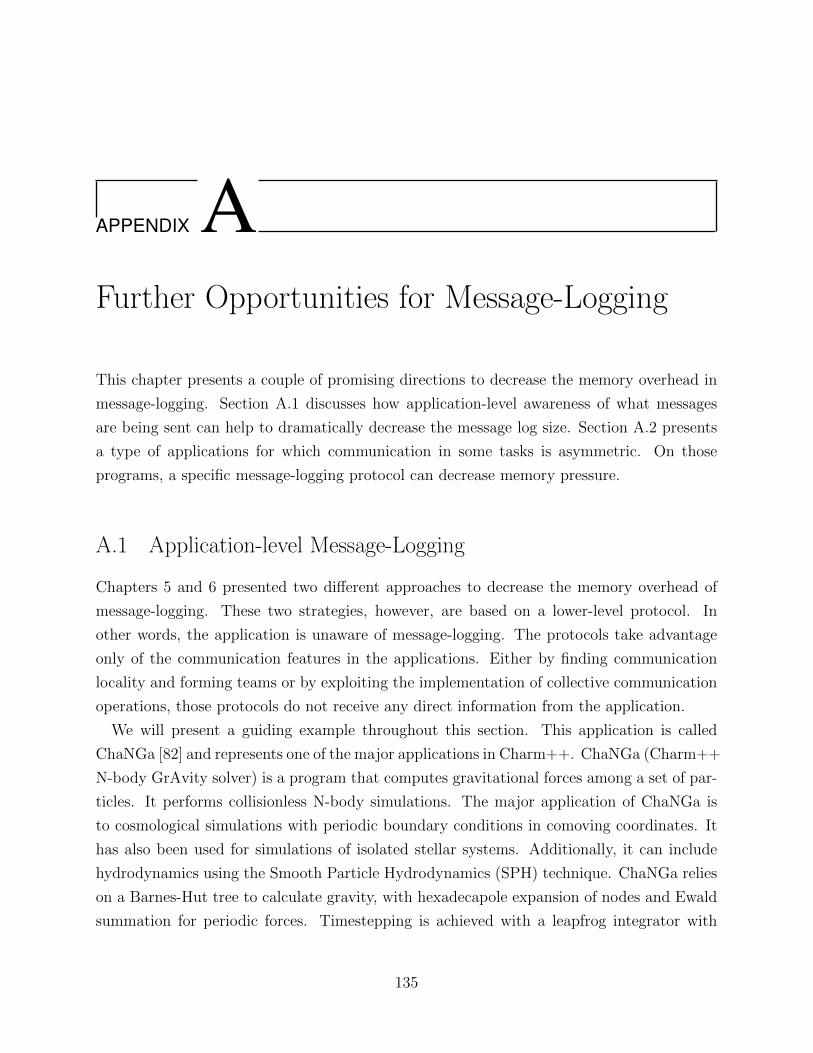
APPENDIX AFurther Opportunities for Message-Logging

This chapter presents a couple of promising directions to decrease the memory overhead in

message-logging. Section A.1 discusses how application-level awareness of what messages

are being sent can help to dramatically decrease the message log size. Section A.2 presents

a type of applications for which communication in some tasks is asymmetric. On those

programs, a specific message-logging protocol can decrease memory pressure.

A.1 Application-level Message-Logging

Chapters 5 and 6 presented two different approaches to decrease the memory overhead of

message-logging. These two strategies, however, are based on a lower-level protocol. In

other words, the application is unaware of message-logging. The protocols take advantage

only of the communication features in the applications. Either by finding communication

locality and forming teams or by exploiting the implementation of collective communication

operations, those protocols do not receive any direct information from the application.

We will present a guiding example throughout this section. This application is called

ChaNGa [82] and represents one of the major applications in Charm++. ChaNGa (Charm++

N-body GrAvity solver) is a program that computes gravitational forces among a set of par-

ticles. It performs collisionless N-body simulations. The major application of ChaNGa is

to cosmological simulations with periodic boundary conditions in comoving coordinates. It

has also been used for simulations of isolated stellar systems. Additionally, it can include

hydrodynamics using the Smooth Particle Hydrodynamics (SPH) technique. ChaNGa relies

on a Barnes-Hut tree to calculate gravity, with hexadecapole expansion of nodes and Ewald

summation for periodic forces. Timestepping is achieved with a leapfrog integrator with

135

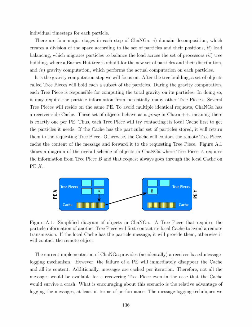
individual timesteps for each particle.

There are four major stages in each step of ChaNGa: i) domain decomposition, which

creates a division of the space according to the set of particles and their positions, ii) load

balancing, which migrates particles to balance the load across the set of processors iii) tree

building, where a Barnes-Hut tree is rebuilt for the new set of particles and their distribution,

and iv) gravity computation, which performs the actual computation on each particles.

It is the gravity computation step we will focus on. After the tree building, a set of objects

called Tree Pieces will hold each a subset of the particles. During the gravity computation,

each Tree Piece is responsible for computing the total gravity on its particles. In doing so,

it may require the particle information from potentially many other Tree Pieces. Several

Tree Pieces will reside on the same PE. To avoid multiple identical requests, ChaNGa has

a receiver-side Cache. These set of objects behave as a group in Charm++, meaning there

is exactly one per PE. Thus, each Tree Piece will try contacting its local Cache first to get

the particles it needs. If the Cache has the particular set of particles stored, it will return

them to the requesting Tree Piece. Otherwise, the Cache will contact the remote Tree Piece,

cache the content of the message and forward it to the requesting Tree Piece. Figure A.1

shows a diagram of the overall scheme of objects in ChaNGa where Tree Piece A requires

the information from Tree Piece B and that request always goes through the local Cache on

PE X.

Tree Pieces

PE X A

Cache Cache

Tree PiecesB

PE Y

Figure A.1: Simplified diagram of objects in ChaNGa. A Tree Piece that requires theparticle information of another Tree Piece will first contact its local Cache to avoid a remotetransmission. If the local Cache has the particle message, it will provide them, otherwise itwill contact the remote object.

The current implementation of ChaNGa provides (accidentally) a receiver-based message-

logging mechanism. However, the failure of a PE will immediately disappear the Cache

and all its content. Additionally, messages are cached per iteration. Therefore, not all the

messages would be available for a recovering Tree Piece even in the case that the Cache

would survive a crash. What is encouraging about this scenario is the relative advantage of

logging the messages, at least in terms of performance. The message-logging techniques we

136

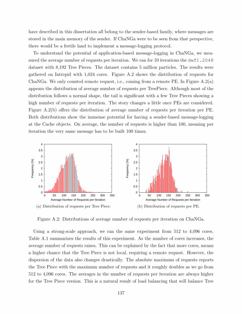
have described in this dissertation all belong to the sender-based family, where messages are

stored in the main memory of the sender. If ChaNGa were to be seen from that perspective,

there would be a fertile land to implement a message-logging protocol.

To understand the potential of application-based message-logging in ChaNGa, we mea-

sured the average number of requests per iteration. We ran for 10 iterations the dwf1.2048

dataset with 8,192 Tree Pieces. The dataset contains 5 million particles. The results were

gathered on Intrepid with 1,024 cores. Figure A.2 shows the distribution of requests for

ChaNGa. We only counted remote request, i.e., coming from a remote PE. In Figure A.2(a)

appears the distribution of average number of requests per TreePiece. Although most of the

distribution follows a normal shape, the tail is significant with a few Tree Pieces showing a

high number of requests per iteration. The story changes a little once PEs are considered.

Figure A.2(b) offers the distribution of average number of requests per iteration per PE.

Both distributions show the immense potential for having a sender-based message-logging

at the Cache objects. On average, the number of requests is higher than 100, meaning per

iteration the very same message has to be built 100 times.

0

0.5

1

1.5

2

2.5

3

3.5

4

0 50 100 150 200 250 300 350

Fre

quen

cy (

%)

Average Number of Requests per Iteration

(a) Distribution of requests per Tree Piece.

0

0.5

1

1.5

2

2.5

3

3.5

4

0 50 100 150 200 250 300 350

Fre

quen

cy (

%)

Average Number of Requests per Iteration

(b) Distribution of requests per PE.

Figure A.2: Distributions of average number of requests per iteration on ChaNGa.

Using a strong-scale approach, we ran the same experiment from 512 to 4,096 cores.

Table A.1 summarizes the results of this experiment. As the number of cores increases, the

average number of requests raises. This can be explained by the fact that more cores, means

a higher chance that the Tree Piece is not local, requiring a remote request. However, the

dispersion of the data also changes drastically. The absolute maximum of requests reports

the Tree Piece with the maximum number of requests and it roughly doubles as we go from

512 to 4,096 cores. The averages in the number of requests per iteration are always higher

for the Tree Piece version. This is a natural result of load balancing that will balance Tree

137

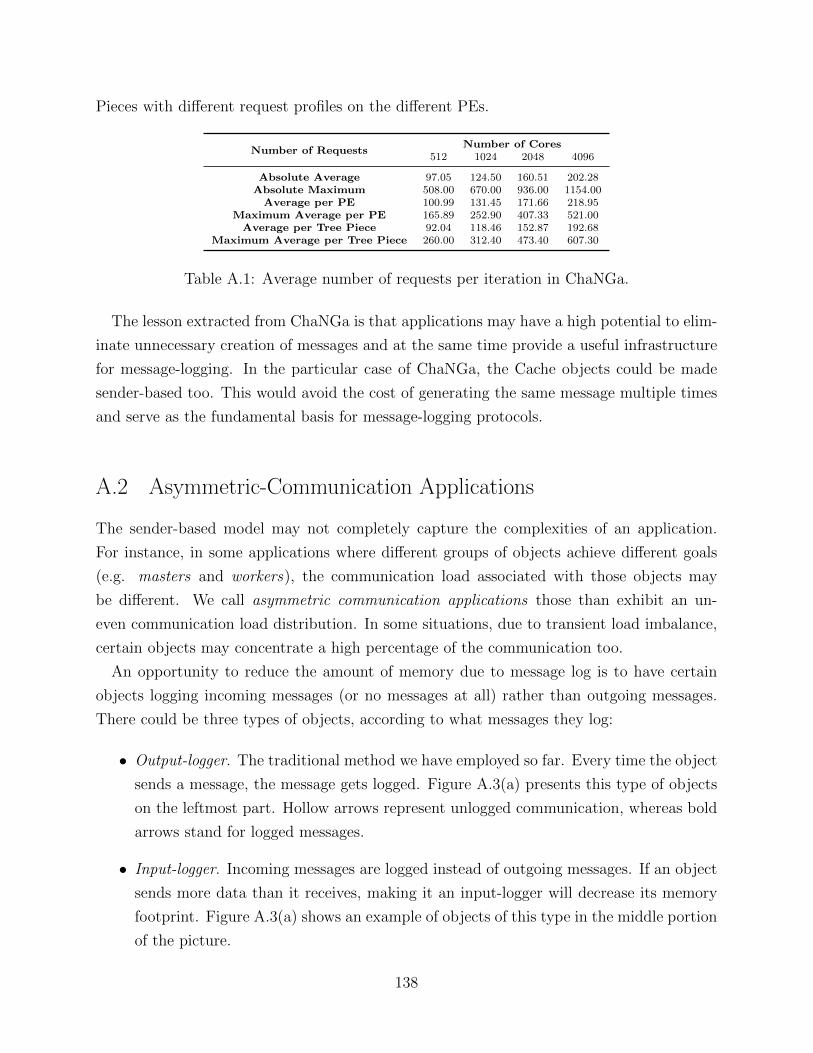
Pieces with different request profiles on the different PEs.

Number of RequestsNumber of Cores

512 1024 2048 4096

Absolute Average 97.05 124.50 160.51 202.28Absolute Maximum 508.00 670.00 936.00 1154.00Average per PE 100.99 131.45 171.66 218.95

Maximum Average per PE 165.89 252.90 407.33 521.00Average per Tree Piece 92.04 118.46 152.87 192.68

Maximum Average per Tree Piece 260.00 312.40 473.40 607.30

Table A.1: Average number of requests per iteration in ChaNGa.

The lesson extracted from ChaNGa is that applications may have a high potential to elim-

inate unnecessary creation of messages and at the same time provide a useful infrastructure

for message-logging. In the particular case of ChaNGa, the Cache objects could be made

sender-based too. This would avoid the cost of generating the same message multiple times

and serve as the fundamental basis for message-logging protocols.

A.2 Asymmetric-Communication Applications

The sender-based model may not completely capture the complexities of an application.

For instance, in some applications where different groups of objects achieve different goals

(e.g. masters and workers), the communication load associated with those objects may

be different. We call asymmetric communication applications those than exhibit an un-

even communication load distribution. In some situations, due to transient load imbalance,

certain objects may concentrate a high percentage of the communication too.

An opportunity to reduce the amount of memory due to message log is to have certain

objects logging incoming messages (or no messages at all) rather than outgoing messages.

There could be three types of objects, according to what messages they log:

• Output-logger. The traditional method we have employed so far. Every time the object

sends a message, the message gets logged. Figure A.3(a) presents this type of objects

on the leftmost part. Hollow arrows represent unlogged communication, whereas bold

arrows stand for logged messages.

• Input-logger. Incoming messages are logged instead of outgoing messages. If an object

sends more data than it receives, making it an input-logger will decrease its memory

footprint. Figure A.3(a) shows an example of objects of this type in the middle portion

of the picture.

138

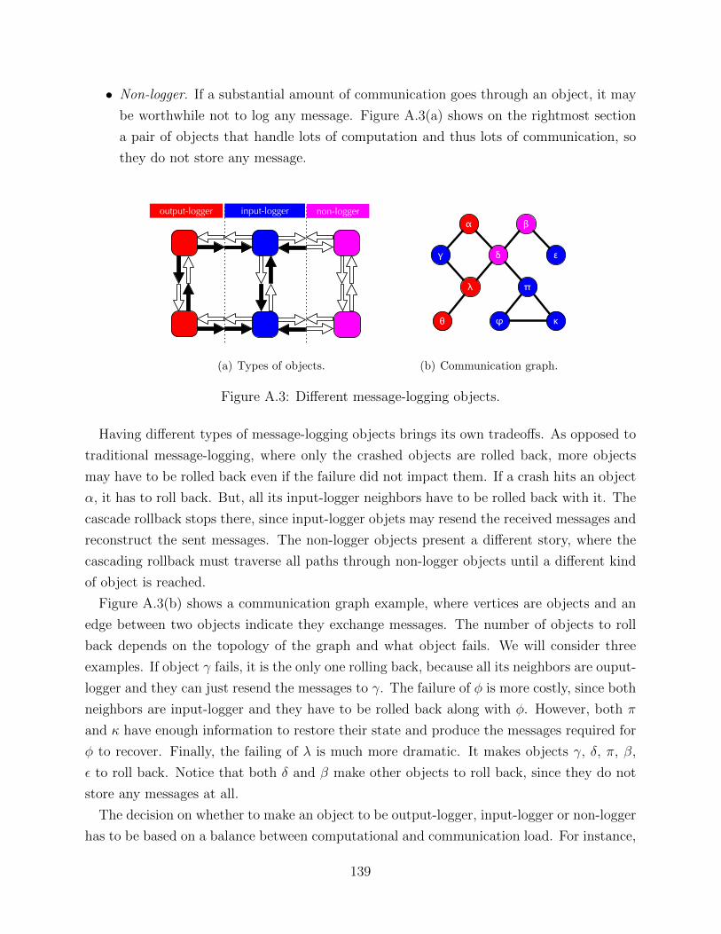
• Non-logger. If a substantial amount of communication goes through an object, it may

be worthwhile not to log any message. Figure A.3(a) shows on the rightmost section

a pair of objects that handle lots of computation and thus lots of communication, so

they do not store any message.

input-loggeroutput-logger non-logger

(a) Types of objects.

α

γ δ

λ π

β

ε

φθ κ

(b) Communication graph.

Figure A.3: Different message-logging objects.

Having different types of message-logging objects brings its own tradeoffs. As opposed to

traditional message-logging, where only the crashed objects are rolled back, more objects

may have to be rolled back even if the failure did not impact them. If a crash hits an object

α, it has to roll back. But, all its input-logger neighbors have to be rolled back with it. The

cascade rollback stops there, since input-logger objets may resend the received messages and

reconstruct the sent messages. The non-logger objects present a different story, where the

cascading rollback must traverse all paths through non-logger objects until a different kind

of object is reached.

Figure A.3(b) shows a communication graph example, where vertices are objects and an

edge between two objects indicate they exchange messages. The number of objects to roll

back depends on the topology of the graph and what object fails. We will consider three

examples. If object γ fails, it is the only one rolling back, because all its neighbors are ouput-

logger and they can just resend the messages to γ. The failure of φ is more costly, since both

neighbors are input-logger and they have to be rolled back along with φ. However, both π

and κ have enough information to restore their state and produce the messages required for

φ to recover. Finally, the failing of λ is much more dramatic. It makes objects γ, δ, π, β,

ε to roll back. Notice that both δ and β make other objects to roll back, since they do not

store any messages at all.

The decision on whether to make an object to be output-logger, input-logger or non-logger

has to be based on a balance between computational and communication load. For instance,

139

an object sending a disproportionate amount of data but receiving little data and performing

low computation is a good candidate to be a input-logger, since rolling it back as a result of

the crash of another object would not imply a high cost on recovery.

140

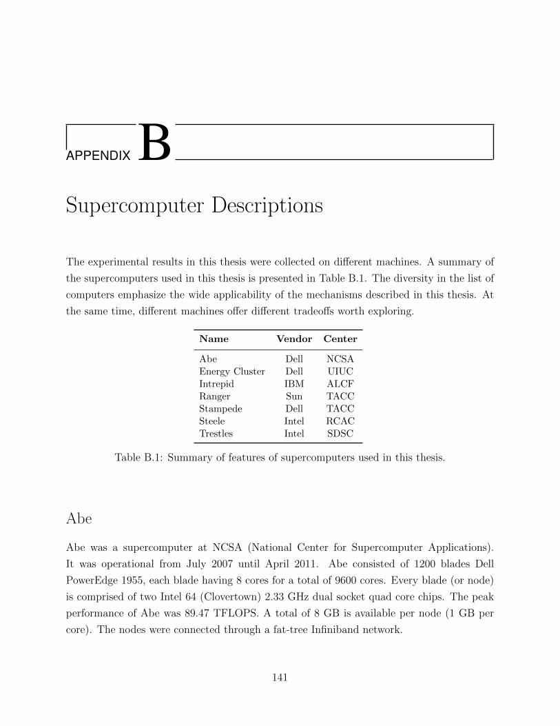
APPENDIX BSupercomputer Descriptions

The experimental results in this thesis were collected on different machines. A summary of

the supercomputers used in this thesis is presented in Table B.1. The diversity in the list of

computers emphasize the wide applicability of the mechanisms described in this thesis. At

the same time, different machines offer different tradeoffs worth exploring.

Name Vendor Center

Abe Dell NCSAEnergy Cluster Dell UIUCIntrepid IBM ALCFRanger Sun TACCStampede Dell TACCSteele Intel RCACTrestles Intel SDSC

Table B.1: Summary of features of supercomputers used in this thesis.

Abe

Abe was a supercomputer at NCSA (National Center for Supercomputer Applications).

It was operational from July 2007 until April 2011. Abe consisted of 1200 blades Dell

PowerEdge 1955, each blade having 8 cores for a total of 9600 cores. Every blade (or node)

is comprised of two Intel 64 (Clovertown) 2.33 GHz dual socket quad core chips. The peak

performance of Abe was 89.47 TFLOPS. A total of 8 GB is available per node (1 GB per

core). The nodes were connected through a fat-tree Infiniband network.

141

Energy Cluster

It is a cluster of 32 nodes (128 cores) installed in the Department of Computer Science of

the University of Illinois at Urbana-Champaign. Each node has a single socket with a four-

core Intel Xeon X3430 processor chip running CentOS 5.7. The cluster nodes are connected

by a 48-port gigabit Ethernet switch. It contains a Liebert power distribution unit (PDU)

installed on the rack containing the cluster to measure the machine power after at 1-second

intervals on a per-node basis.

Intrepid

Intrepid is an IBM Blue Gene/P machines with 40,960 nodes at the Argonne Leadership

Computing Facility (ALCF) in Argonne National Laboratory (ANL). Each node in Intrepid

consists of one quad-core 850MHz PowerPC 450 processor and 2GB DDR2 memory. With

a total of 163,840 cores, 80 terabytes of RAM, Intrepid has a peak performance of 557

TFLOPS.

Ranger

Ranger was a machine installed at Texas Advanced Computing Center (TACC). Retired in

April 2013, it was comprised of 3,936 16-way SMP compute nodes with a peak performance

of 579-TFLOPS. Each node contained 32 GB of memory. Ranger had in total 15,744 AMD

Opteron processors, which translates into 62,976 compute cores. The interconnect topology

was a 7-stage, full-CLOS fat tree, which provides a 1GB/sec point-to-point bandwidth.

Stampede

Stampede is machine at Texas Advanced Computing Center (TACC). It is a 10-PFLOPS

machine with more than 96,000 cores divided into 6,400 nodes. Each node contains 2 Intel

Xeon processors (16 cores total) and 32GB of memory. The interconnect uses Mellanox FDR

Infiniband technology in a 2-level fat-tree topology.

142

Steele

Steele is a supercomputer at the Rosen Center for Advanced Computing (RCAC) in Perdue

University. Steele has 893 nodes, each with 16GB of memory and two Intel E5410 Harper-

town 2.33 Ghz quad core processors. The nodes are connected through Infiniband for a total

peak performance of 60 TFLOPS.

Trestles

Trestles supercomputer is installed at San Diego Supercomputer Center (SDSC). Trestles is

a 100-TFLOPS machine with 324 nodes, each having 32 cores. There are 4 sockets in a node,

each having an 8-core 2.4 GHz AMD Magny-Cours core. A fat tree Infiniband interconnect

links all the nodes.

143

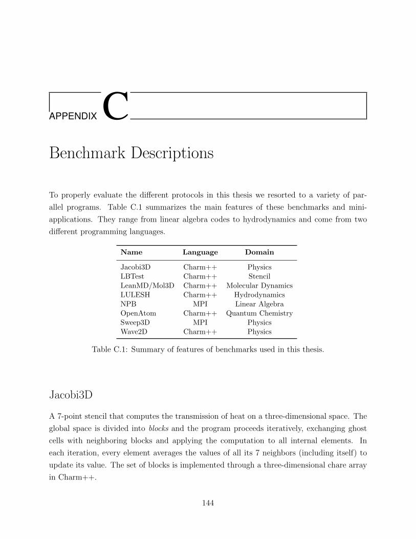
APPENDIX CBenchmark Descriptions

To properly evaluate the different protocols in this thesis we resorted to a variety of par-

allel programs. Table C.1 summarizes the main features of these benchmarks and mini-

applications. They range from linear algebra codes to hydrodynamics and come from two

different programming languages.

Name Language Domain

Jacobi3D Charm++ PhysicsLBTest Charm++ StencilLeanMD/Mol3D Charm++ Molecular DynamicsLULESH Charm++ HydrodynamicsNPB MPI Linear AlgebraOpenAtom Charm++ Quantum ChemistrySweep3D MPI PhysicsWave2D Charm++ Physics

Table C.1: Summary of features of benchmarks used in this thesis.

Jacobi3D

A 7-point stencil that computes the transmission of heat on a three-dimensional space. The

global space is divided into blocks and the program proceeds iteratively, exchanging ghost

cells with neighboring blocks and applying the computation to all internal elements. In

each iteration, every element averages the values of all its 7 neighbors (including itself) to

update its value. The set of blocks is implemented through a three-dimensional chare array

in Charm++.

144

LeanMD/Mol3D

A mini-application that emulates the communication pattern in NAMD [94]. It computes

the interaction forces between particles in a three-dimensional space. This computation is

based on the Lennard-Jones potential. It does not include long-range force computation.

The object decomposition follows the same pattern as in NAMD. A three-dimensional space

is divided into orthotopes or hyperrectangles. Each of these boxes, called cells or patches

in NAMD’s nomenclature, contain a subset of the particles. To compute the interaction

of the particles between each pair of cells, a specific object called a compute is connected

to the two cells and receives the particles from both to perform the computation. In each

iteration of LeanMD, each cell sends its particles to all the computes attached to it and

receives the udpates from those computes. The groups of cells and the groups of computes

are implemented each as a chare array in Charm++.

LBTest

It is a synthetic benchmark in Charm++ for load balancing experimentation. It creates

a collection of objects with different customizable properties. Its parameters include the

communication topology among the objects, a range for the load of objects, frequency of

load balancing and whether the load in each object is static or dynamic (progressively changes

across the execution). This program enables the analysis of the effect of one single parameter

at a time and measure how susceptible the load balancer is to different scenarios.

LULESH

The Livermore Unstructured Lagrangian Explicit Shock Hydrodynamics (LULESH) is code

for modeling hydrodynamics. This types of codes describe the motion of materials relative

to each other when subject to forces. LULESH is a typical hydrocode and represents a

proxy mini-application for more complex codes. LULESH approximates the hydrodynamics

equations discretely by partitioning the spatial problem domain into a set of volumetric

elements defined by a mesh. Each node on the mesh is a point where mesh lines intersect.

The program proceeds iteratively, exchanging ghost elements with neighboring elements.

The set of elements is implemented through a three-dimensional chare array in Charm++.

145

NAS Parallel Benchmarks (NPB)

The NAS Parallel Benchmarks suite (NPB) was adapted to AMPI to have migratable MPI

threads. The NPB is a collection of linear algebra numerical methods [107]. We focused

our experiments in some of the benchmarks from NPB: block-tridiagonal (BT), conjugate

gradient (CG), data traffic (DT), multi-grid (MG) and scalar pentadiagonal (SP). The multi-

zone version of the NAS Parallel Benchmarks (NPB-MZ) compute discrete solutions in three

spatial dimensions for the unsteady and compressible Navier-Stokes equations. There are

three different benchmarks in this version of NPB, lower-upper symmetric Gauss-Seidel (LU),

scalar pentadiagonal (SP) and block tridiagonal (BT). In our experiments we only use BT

since it presents the highest load imbalance among the three programs. BT solver operates

on a logical cube that is seen as a structured discretization mesh. To describe a complex

domain, BT uses multiple meshes (called zones) to cover it.

OpenAtom

It is a highly scalable and portable parallel application for molecular dynamics simulations

based on fundamental quantum mechanics principles. Car-Parrinello ab initio molecular

dynamics (CPAIMD) is a well-known approach that has proven to be relatively efficient

and useful in this type of simulations. The parallelization of this approach beyond a few

thousand processors is challenging, due to the complex dependencies among various sub-

computations. This may lead to complex communication optimization and load balancing

problems. OpenAtom is a mechanism to parallelize CPAIMD using the migratable-objects

model in Charm++.

Sweep3D

A benchmark representing the core of a real Accelerated Strategic Computing Initiative

(ASCI) application. It solves a 1-group time-independent neutron transport problem on

discrete ordinates 3D cartesian geometry. The three-dimensional geometry is represented by

a logically rectangular grid of blocks. The angular dependence in Sweep3D is handled by

discrete angles with a spherical harmonics treatment for the scattering source. The solution

process involves two steps: i) the streaming operator is solved by sweeps for each angle, and

ii) the scattering operator is solved iteratively.

146

Wave2D

A benchmark that runs a finite difference method to compute pressure information on a

two-dimensional grid. The global space is divided into rectangles or blocks that will contain

a portion of the grids. In each iteration, each block exchanges its ghost cells with its

four neighboring blocks. The computation updates all the elements in the grid using the

two previous values of the neighboring cells. The set of blocks is implemented as a two-

dimensional chare array in Charm++.

147

REFERENCES

[1] P. Kogge, K. Bergman, S. Borkar, D. Campbell, W. Carlson, W. Dally, M. Denneau,P. Franzon, W. Harrod, J. Hiller, S. Karp, S. Keckler, D. Klein, R. Lucas, M. Richards,A. Scarpelli, S. Scott, A. Snavely, T. Sterling, R. S. Williams, and K. Yelick, “Exascalecomputing study: Technology challenges in achieving exascale systems,” 2008.

[2] K. Ferreira, J. Stearley, J. H. Laros, III, R. Oldfield, K. Pedretti, R. Brightwell,R. Riesen, P. G. Bridges, and D. Arnold, “Evaluating the viability of process replicationreliability for exascale systems,” in Proceedings of 2011 International Conference forHigh Performance Computing, Networking, Storage and Analysis. New York, NY,USA: ACM, 2011. [Online]. Available: http://doi.acm.org/10.1145/2063384.2063443pp. 44:1–44:12.

[3] F. Cappello, A. Geist, B. Gropp, L. Kale, B. Kramer, and M. Snir, “Toward exascaleresilience,” Int. J. High Perform. Comput. Appl., vol. 23, no. 4, pp. 374–388, Nov.2009. [Online]. Available: http://dx.doi.org/10.1177/1094342009347767

[4] F. Cappello, “Fault tolerance in petascale/ exascale systems: Current knowledge, chal-lenges and research opportunities,” IJHPCA, vol. 23, no. 3, pp. 212–226, 2009.

[5] S. Chakravorty and L. V. Kale, “A fault tolerance protocol with fast fault recovery,” inProceedings of the 21st IEEE International Parallel and Distributed Processing Sym-posium. IEEE Press, 2007.

[6] E. Meneses, G. Bronevetsky, and L. V. Kale, “Evaluation of simple causal message log-ging for large-scale fault tolerant hpc systems,” in 16th IEEE Workshop on DependableParallel, Distributed and Network-Centric Systems in 25th IEEE International Paralleland Distributed Processing Symposium (IPDPS 2011)., May 2011.

[7] D. A. Patterson, G. Gibson, and R. H. Katz, “A case for redundant arrays of inexpen-sive disks (raid),” in Proceedings of the 1988 ACM SIGMOD international conferenceon Management of data, ser. SIGMOD ’88. New York, NY, USA: ACM, 1988, pp.109–116.

[8] I. Stoica, R. Morris, D. Karger, M. F. Kaashoek, and H. Balakrishnan, “Chord: Ascalable peer-to-peer lookup service for internet applications,” in Proceedings of the2001 conference on Applications, technologies, architectures, and protocols for com-puter communications, ser. SIGCOMM ’01. New York, NY, USA: ACM, 2001, pp.149–160.

148

[9] S. Ratnasamy, P. Francis, M. Handley, R. Karp, and S. Shenker, “A scalable content-addressable network,” in IN PROC. ACM SIGCOMM 2001, 2001, pp. 161–172.

[10] D. P. Siewiorek and R. S. Swarz, Reliable computer systems (3rd ed.): design andevaluation. Natick, MA, USA: A. K. Peters, Ltd., 1998.

[11] P. Jalote, Fault tolerance in distributed systems. Prentice Hall, 1994.

[12] K. P. Birman, Guide to Reliable Distributed Systems - Building High-Assurance Ap-plications and Cloud-Hosted Services, ser. Texts in computer science. Springer, 2012.

[13] C. da Lu and D. A. Reed, “Assessing fault sensitivity in mpi applications,” in SC,2004, p. 37.

[14] G. Bronevetsky and B. R. de Supinski, “Soft error vulnerability of iterative linearalgebra methods,” in ICS, 2008, pp. 155–164.

[15] G. Bosilca, R. Delmas, J. Dongarra, and J. Langou, “Algorithm-based fault toleranceapplied to high performance computing,” J. Parallel Distrib. Comput., vol. 69, no. 4,pp. 410–416, 2009.

[16] M. Schulz, “Checkpointing,” in Encyclopedia of Parallel Computing, 2011, pp. 264–273.

[17] G. Bronevetsky, D. Marques, K. Pingali, and P. Stodghill, “Automated application-level checkpointing of MPI programs,” in ACM SIGPLAN Symposium on Principlesand Practice of Parallel Programming (PPoPP), 2003.

[18] J. W. Young, “A first order approximation to the optimal checkpoint interval,” Com-mun. ACM, vol. 17, no. 9, pp. 530–531, 1974.

[19] J. T. Daly, “A higher order estimate of the optimum checkpoint interval for restartdumps,” Future Generation Comp. Syst., vol. 22, no. 3, pp. 303–312, 2006.

[20] K. M. Chandy and L. Lamport, “Distributed snapshots : Determining global states ofdistributed systems,” ACM Transactions on Computer Systems, Feb. 1985.

[21] D. Buntinas, C. Coti, T. Herault, P. Lemarinier, L. Pilard, A. Rezmerita, E. Rodriguez,and F. Cappello, “Blocking vs. non-blocking coordinated checkpointing for large-scalefault tolerant mpi protocols,” Future Generation Comp. Syst., vol. 24, no. 1, pp. 73–84,2008.

[22] X. Ouyang, K. Gopalakrishnan, T. Gangadharappa, and D. K. Panda, “Fast check-pointing by write aggregation with dynamic buffer and interleaving on multicore ar-chitecture,” in HiPC, 2009, pp. 99–108.

[23] J. S. Plank, J. Xu, and R. H. B. Netzer, “Compressed differences: An algorithmfor fast incremental checkpointing,” University of Tennessee, Tech. Rep. CS-95-302,August 1995.

149

[24] C. Wang, F. Mueller, C. Engelmann, and S. L. Scott, “Hybrid checkpointing for mpijobs in hpc environments,” in ICPADS, 2010, pp. 524–533.

[25] G. Zheng, L. Shi, and L. V. Kale, “FTC-Charm++: An In-Memory Checkpoint-Based Fault Tolerant Runtime for Charm++ and MPI,” in 2004 IEEE InternationalConference on Cluster Computing, San Diego, CA, September 2004, pp. 93–103.

[26] F. Cappello, H. Casanova, and Y. Robert, “Preventive migration vs. preventive check-pointing for extreme scale supercomputers,” Parallel Processing Letters, vol. 21, no. 2,pp. 111–132, 2011.

[27] Z. Chen and J. Dongarra, “A scalable checkpoint encoding algorithm for diskless check-pointing,” in HASE, 2008, pp. 71–79.

[28] L. Bautista-Gomez, D. Komatitsch, N. Maruyama, S. Tsuboi, F. Cappello, and S. Mat-suoka, “FTI: High performance fault tolerance interface for hybrid systems,” in 2011International Conference for High Performance Computing, Networking, Storage andAnalysis (SC), Nov. 2011, pp. 1 –12.

[29] L. Alvisi, E. N. Elnozahy, S. Rao, S. A. Husain, and A. D. Mel, “An analysis ofcommunication induced checkpointing,” in FTCS, 1999, pp. 242–249.

[30] P. H. Hargrove and J. C. Duell, “Berkeley lab checkpoint/restart (blcr) for linux clus-ters,” in SciDAC, 2006.

[31] A. Moody, G. Bronevetsky, K. Mohror, and B. R. de Supinski, “Design, modeling, andevaluation of a scalable multi-level checkpointing system,” in SC, 2010, pp. 1–11.

[32] P. Lemarinier, A. Bouteiller, T. Herault, G. Krawezik, and F. Cappello, “Improvedmessage logging versus improved coordinated checkpointing for fault tolerant MPI,”Cluster Computing, IEEE International Conference on, vol. 0, pp. 115–124, 2004.

[33] R. Strom and S. Yemini, “Optimistic recovery in distributed systems,” ACM Trans.Comput. Syst., vol. 3, no. 3, pp. 204–226, 1985.

[34] L. Alvisi and K. Marzullo, “Message logging: pessimistic, optimistic, and causal,”Distributed Computing Systems, International Conference on, vol. 0, p. 0229, 1995.

[35] E. N. Elnozahy, “Manetho: Fault-tolerance in distributed systems using rollback-recovery and process replication,” Ph.D. dissertation, Rice University, October 1993.

[36] S. Rao, L. Alvisi, and H. M. Vin, “The cost of recovery in message logging protocols,”IEEE Trans. Knowl. Data Eng., vol. 12, no. 2, pp. 160–173, 2000.

[37] A. Bouteiller, T. Ropars, G. Bosilca, C. Morin, and J. Dongarra, “Reasons for a pes-simistic or optimistic message logging protocol in mpi uncoordinated failure, recovery,”in CLUSTER, 2009, pp. 1–9.

150

[38] D. B. Johnson and W. Zwaenepoel, “Sender-based message logging,” in In Digest ofPapers: 17 Annual International Symposium on Fault-Tolerant Computing. IEEEComputer Society, 1987, pp. 14–19.

[39] S. Monnet, “Hybrid checkpointing for parallel applications in cluster federations,” inProc. 4 th IEEE/ACM International Symposium on Cluster Computing and the Grid,2004, pp. 773–782.

[40] Z. Wei, H. F. Li, and D. Goswami, “A locality-driven atomic group checkpoint proto-col,” in PDCAT, 2006, pp. 558–564.

[41] J.-M. Yang, K. F. Li, D.-F. Zhang, and J. Cheng, “A coarse-grained pessimistic mes-sage logging scheme for improving rollback recovery efficiency,” in Proceedings of theThird IEEE International Symposium on Dependable, Autonomic and Secure Comput-ing. Washington, DC, USA: IEEE Computer Society, 2007, pp. 29–36.

[42] J. C. Y. Ho, C.-L. Wang, and F. C. M. Lau, “Scalable group-based checkpoint/restartfor large-scale message-passing systems,” in IPDPS, 2008, pp. 1–12.

[43] R. Singh and P. Graham, “Grouping mpi processes for partial checkpoint and co-migration,” in Euro-Par, 2009, pp. 69–80.

[44] G. Bosilca, A. Bouteiller, F. Cappello, S. Djilali, G. Fedak, C. Germain, T. Herault,P. Lemarinier, O. Lodygensky, F. Magniette, V. Neri, and A. Selikhov, “Toward ascalable fault tolerant MPI for volatile nodes,” in Proceedings of SC 2002. IEEE,2002.

[45] A. Bouteiller, P. Lemarinier, G. Krawezik, and F. Cappello, “Coordinated checkpointversus message log for fault tolerant MPI,” Cluster Computing, IEEE InternationalConference on, vol. 0, p. 242, 2003.

[46] A. Bouteiller, F. Cappello, T. Herault, G. Krawezik, P. Lemarinier, and F. Magniette,“MPICH-V2: A fault tolerant MPI for volatile nodes based on the pessimistic senderbased message logging programming via processor virtualization,” in Proceedings ofSC’03, November 2003.

[47] A. Bouteiller, B. Collin, T. Herault, P. Lemarinier, and F. Cappello, “Impact of eventlogger on causal message logging protocols for fault tolerant MPI,” in IPDPS’05, 2005,p. 97.

[48] G. Fagg and J. Dongarra, “FT-MPI: Fault Tolerant MPI, Supporting Dynamic Ap-plications in Dynamic World,” in Euro PVM/MPI User’s Group Meeting, S. Verlag,Ed., Berlin, Germany, 2000, pp. 346–353.

[49] F. Cappello, A. Guermouche, and M. Snir, “On communication determinism in parallelhpc applications,” in ICCCN, 2010, pp. 1–8.

151

[50] G. Zheng, G. Kakulapati, and L. V. Kale, “Bigsim: A parallel simulator for perfor-mance prediction of extremely large parallel machines,” in 18th International Paralleland Distributed Processing Symposium (IPDPS), Santa Fe, New Mexico, April 2004,p. 78.

[51] A. Guermouche, T. Ropars, E. Brunet, M. Snir, and F. Cappello, “Uncoordinatedcheckpointing without domino effect for send-deterministic mpi applications,” inIPDPS, 2011, pp. 989–1000.

[52] E. N. Elnozahy, L. Alvisi, Y.-M. Wang, and D. B. Johnson, “A survey of rollback-recovery protocols in message-passing systems,” ACM Comput. Surv., vol. 34, no. 3,pp. 375–408, 2002.

[53] A. Bouteiller, G. Bosilca, and J. Dongarra, “Redesigning the message logging model forhigh performance,” Concurrency and Computation: Practice and Experience, vol. 22,no. 16, pp. 2196–2211, 2010.

[54] S. Chakravorty and L. V. Kale, “A fault tolerant protocol for massively parallel ma-chines,” in FTPDS Workshop for IPDPS 2004. IEEE Press, 2004.

[55] L. Kale and S. Krishnan, “CHARM++: A Portable Concurrent Object Oriented Sys-tem Based on C++,” in Proceedings of OOPSLA’93, A. Paepcke, Ed. ACM Press,September 1993, pp. 91–108.

[56] C. Huang, O. Lawlor, and L. V. Kale, “Adaptive MPI,” in Proceedings of the 16thInternational Workshop on Languages and Compilers for Parallel Computing (LCPC2003), LNCS 2958, College Station, Texas, October 2003, pp. 306–322.

[57] L. Alvisi, B. Hoppe, and K. Marzullo, “Nonblocking and orphan-free message loggingprotocols,” in FTCS, 1993, pp. 145–154.

[58] K. Bhatia, K. Marzullo, and L. Alvisi, “The relative overhead of piggybacking incausal message logging protocols,” in SRDS ’98: Proceedings of the The 17th IEEESymposium on Reliable Distributed Systems. Washington, DC, USA: IEEE ComputerSociety, 1998, p. 348.

[59] E. Meneses, X. Ni, and L. V. Kale, “A Message-Logging Protocol for Multicore Sys-tems,” in Proceedings of the 2nd Workshop on Fault-Tolerance for HPC at ExtremeScale (FTXS), Boston, USA, June 2012.

[60] Sayantan Chakravorty, Celso Mendes and L. V. Kale, “Proactive fault tolerance inlarge systems,” in HPCRI Workshop in conjunction with HPCA 2005, 2005.

[61] S. Chakravorty, C. L. Mendes, and L. V. Kale, “Proactive fault tolerance in mpiapplications via task migration.” in HiPC, ser. Lecture Notes in Computer Science,vol. 4297. Springer, 2006, pp. 485–496.

152

[62] A. Borg, J. Baumbach, and S. Glazer, “A message system supporting fault tolerance,”in Proceedings of the ninth ACM symposium on Operating systems principles, ser.SOSP ’83, 1983, pp. 90–99.

[63] G. Stellner, “CoCheck: Checkpointing and Process Migration for MPI,” in Proceedingsof the 10th International Parallel Processing Symposium (IPPS ’96), Honolulu, Hawaii,1996.

[64] C. Wang, F. Mueller, C. Engelmann, and S. L. Scott, “Proactive process-level livemigration in hpc environments,” in SC, 2008, p. 43.

[65] Z. Lan and Y. Li, “Adaptive fault management of parallel applications for high-performance computing,” IEEE Trans. Computers, vol. 57, no. 12, pp. 1647–1660,2008.

[66] R. Riesen, K. Ferreira, and J. Stearley, “See applications run and throughput jump:The case for redundant computing in HPC,” in 1st International Workshop on Fault-Tolerance for HPC at Extreme Scale (FTXS 2010) in conjunction with The 40th An-nual IEEE/IFIP International Conference on Dependable Systems and Networks (DSN2010), Chicago, IL, USA, June 2010.

[67] R. Brightwell, K. Ferreira, and R. Riesen, “Transparent redundant computing withMPI,” in Recent Advances in the Message Passing Interface: 17th European MPIUsers’ Group Meeting, EuroMPI 2010, Stuttgart, Germany, September 2010. Proceed-ings, ser. Lecture Notes in Computer Science, R. Keller, E. Gabriel, M. Resch, andJ. Dongarra, Eds., vol. 6305. Springer Verlag, 2010, pp. 208–218.

[68] W. Ma and S. Krishnamoorthy, “Data-driven fault tolerance for work stealing compu-tations,” in Proceedings of the 26th ACM international conference on Supercomputing,ser. ICS ’12. New York, NY, USA: ACM, 2012, pp. 79–90.

[69] T. von Eicken, D. Culler, S. Goldstein, and K. Schauser, “Active Messages: a Mech-anism for Integrated Communication and Computation,” in Proceedings of the 19thInternational Symposium on Computer Architecture, Gold Coast, Australia, May 1992.

[70] L. V. Kale and M. Bhandarkar, “Structured Dagger: A Coordination Language forMessage-Driven Programming,” in Proceedings of Second International Euro-Par Con-ference, ser. Lecture Notes in Computer Science, vol. 1123-1124, September 1996, pp.646–653.

[71] A. Guermouche, T. Ropars, M. Snir, and F. Cappello, “Hydee: Failure containmentwithout event logging for large scale send-deterministic mpi applications,” in IPDPS,2012, pp. 1216–1227.

[72] B. Schroeder and G. Gibson, “A large scale study of failures in high-performance-computing systems,” in International Symposium on Dependable Systems and Net-works (DSN), 2006.

153

[73] M. Snir, W. Gropp, and P. Kogge, “Exascale Research: Preparing for thePost Moore Era,” https://www.ideals.illinois.edu/bitstream/handle/2142/25468/Exascale%20Research.pdf, 2011.

[74] B. Schroeder and G. A. Gibson, “Understanding failures in petascale computers,”Journal of Physics: Conference Series: SciDAC, vol. 78, 2007.

[75] E. N. Elnozahy, R. Bianchini, T. El-Ghazawi, A. Fox, F. Godfrey, A. Hoisie, K. McKin-ley, R. Melhem, J. S. Plank, P. Ranganathan and J. Simons, “System resilience atextreme scale,” Defense Advanced Research Project Agency (DARPA), Tech. Rep.,2008.

[76] X. Ni, E. Meneses, and L. V. Kale, “Hiding checkpoint overhead in hpc applicationswith a semi-blocking algorithm,” in IEEE Cluster 12, Beijing, China, September 2012.

[77] E. Meneses, O. Sarood, and L. V. Kale, “Assessing Energy Efficiency of Fault Toler-ance Protocols for HPC Systems,” in Proceedings of the 2012 IEEE 24th InternationalSymposium on Computer Architecture and High Performance Computing (SBAC-PAD2012), New York, USA, October 2012.

[78] J. Daly, “A model for predicting the optimum checkpoint interval for restart dumps,”in Proceedings of the 2003 international conference on Computational science, ser.ICCS’03, 2003, pp. 3–12.

[79] T. Ropars, A. Guermouche, B. Ucar, E. Meneses, L. V. Kale, and F. Cappello, “Onthe use of cluster-based partial message logging to improve fault tolerance for mpi hpcapplications,” in Euro-Par (1), 2011, pp. 567–578.

[80] E. R. Rodrigues, P. O. A. Navaux, J. Panetta, A. Fazenda, C. L. Mendes, and L. V.Kale, “A Comparative Analysis of Load Balancing Algorithms Applied to a WeatherForecast Model,” in Proceedings of 22nd International Symposium on Computer Ar-chitecture and High Performance Computing (SBAC-PAD), Itaipava, Brazil, 2010.

[81] J. C. Phillips, R. Braun, W. Wang, J. Gumbart, E. Tajkhorshid, E. Villa, C. Chipot,R. D. Skeel, L. Kale, and K. Schulten, “Scalable molecular dynamics with NAMD,”Journal of Computational Chemistry, vol. 26, no. 16, pp. 1781–1802, 2005.

[82] F. Gioachin, A. Sharma, S. Chakravorty, C. Mendes, L. V. Kale, and T. R. Quinn,“Scalable cosmology simulations on parallel machines,” in VECPAR 2006, LNCS 4395,pp. 476-489, 2007.

[83] E. Meneses, G. Bronevetsky, and L. V. Kale, “Dynamic load balance for optimizedmessage logging in fault tolerant hpc applications,” in IEEE International Conferenceon Cluster Computing (Cluster) 2011, September 2011.

[84] F. Pellegrini and J. Roman, “Scotch: A software package for static mapping by dualrecursive bipartitioning of process and architecture graphs,” in HPCN Europe, 1996,pp. 493–498.

154

[85] George Karypis and Vipin Kumar, “Multilevel k-way Partitioning Scheme forIrregular Graphs,” Journal of Parallel and Distributed Computing, vol. 48, pp. 96–129, 1998. [Online]. Available: http://www-users.cs.umn.edu/∼karypis/publications/Papers/PDF/mlevel kparallel.pdf

[86] E. Meneses, C. L. Mendes, and L. V. Kale, “Team-based message logging: Preliminaryresults,” in 3rd Workshop on Resiliency in High Performance Computing (Resilience)in Clusters, Clouds, and Grids (CCGRID 2010)., May 2010.

[87] R. Xue, X. Liu, M. Wu, Z. Guo, W. Chen, W. Zheng, Z. Zhang, and G. M. Voelker,“MPIWiz: Subgroup reproducible replay of MPI applications,” in In PPoPP, 2009.

[88] A. Faraj and X. Yuan, “Communication Characteristics in the NAS Parallel Bench-marks,” in Parallel and Distributed Computing Systems, 2002, pp. 724–729.

[89] J.-M. Yang, K. F. Li, W.-W. Li, and D.-F. Zhang, “Trading off logging overheadand coordinating overhead to achieve efficient rollback recovery,” Concurrency andComputation: Practice and Experience, vol. 21, no. 6, pp. 819–853, 2009.

[90] N. Vaidya, “Distributed recovery units: An approach for hybrid and adaptive dis-tributed recovery,” Texas A&M University, Tech. Rep., 1993.

[91] A. P. Sistla and J. L. Welch, “Efficient distributed recovery using message logging,”in Proceedings of the eighth annual ACM Symposium on Principles of distributed com-puting, ser. PODC ’89. New York, NY, USA: ACM, 1989, pp. 223–238.

[92] G. Jakadeesan and D. Goswami, “A classification-based approach to fault-tolerancesupport in parallel programs,” in Parallel and Distributed Computing, Applicationsand Technologies, 2009 International Conference on, 2009, pp. 255–262.

[93] R. Thakur, R. Rabenseifner, and W. Gropp, “Optimization of collective communi-cation operations in mpich,” International Journal of High Performance ComputingApplications, vol. 19, no. 1, pp. 49–66, Spring 2005.

[94] J. C. Phillips, G. Zheng, S. Kumar, and L. V. Kale, “NAMD: Biomolecular simulationon thousands of processors,” in Proceedings of the 2002 ACM/IEEE conference onSupercomputing, Baltimore, MD, September 2002, pp. 1–18.

[95] E. Bohm, A. Bhatele, L. V. Kale, M. E. Tuckerman, S. Kumar, J. A. Gunnels, and G. J.Martyna, “Fine Grained Parallelization of the Car-Parrinello ab initio MD Method onBlue Gene/L,” IBM Journal of Research and Development: Applications of MassivelyParallel Systems, vol. 52, no. 1/2, pp. 159–174, 2008.

[96] J. Hursey and R. L. Graham, “Preserving collective performance across process failurefor a fault tolerant mpi,” in Proceedings of the 2011 IEEE International Symposiumon Parallel and Distributed Processing Workshops and PhD Forum, ser. IPDPSW ’11.Washington, DC, USA: IEEE Computer Society, 2011, pp. 1208–1215.

155

[97] G. Bronevetsky, D. Marques, K. Pingali, and P. Stodghill, “Collective operations inapplication-level fault-tolerant mpi,” in Proceedings of the 17th annual internationalconference on Supercomputing, ser. ICS ’03. New York, NY, USA: ACM, 2003, pp.234–243.

[98] “Top500 supercomputing sites,” http://top500.org.

[99] CFDR, “Computer failure data repository,” May 2011. [Online]. Available:http://cfdr.usenix.org/

[100] A. Gainaru, “Mercury failure data,” personal communication, 2011.

[101] L. A. B. Gomez, “Tsubame failure data,” personal communication, 2011.

[102] T. Jones, “Jaguar failure data,” personal communication, 2010.

[103] G. Zheng, X. Ni, and L. V. Kale, “A Scalable Double In-memory Checkpoint andRestart Scheme towards Exascale,” in Proceedings of the 2nd Workshop on Fault-Tolerance for HPC at Extreme Scale (FTXS), Boston, USA, June 2012.

[104] T. Ropars and C. Morin, “Improving message logging protocols scalability throughdistributed event logging,” in Euro-Par (1), 2010, pp. 511–522.

[105] A. Bouteiller, T. Herault, G. Bosilca, and J. J. Dongarra, “Correlated set coordinationin fault tolerant message logging protocols,” in Euro-Par (2), 2011, pp. 51–64.

[106] Draft Document for the MPI-2 Standard, Message Passing Interface Forum, October1995.

[107] D. Bailey, E. Barszcz, J. Barton, D. Browning, R. Carter, L. Dagum, R. Fatoohi,S. Fineberg, P. Frederickson, T. Lasinski, R. Schreiber, H. Simon, V. Venkatakrishnan,and S. Weeratunga, “The NAS parallel benchmarks,” NASA Ames Research Center,Tech. Rep. RNR-04-077, 1994.

156