Embed Size (px)
Citation preview
DRAFT
DYNAMIC NETWORK
ANALYSIS
BY
KATHLEEN M. CARLEY
Draft
Center for Computational Analysisof Social and Organizational Systems
Carnegie Mellon University, Pittsburgh, USA

DRAFT
2
Many people were involved in the development of this book. Different chaptersof the book were created with the support of Matt deReno, Jamie Olson,Terrill Frantz, Jana Diesner, Brian Hirshman, George Davis, Peter Landwehr,Jeff Reminga, Ju-Sung Lee, and Hope Armstrong.
DRAFT
Preface
Everything is connected! From small groups to economic markets to globalsocieties – interactions among people, organizations, technology, and policieslead to complex systems. These connected systems cannot be described withsimple equations–they need to be articulated as networks. Social NetworkAnalysis (SNA) offers a wide variety of tools to analyze complex connectedsystems. The ability to store and work with network data in a digital en-vironment has enabled a multiplicity of new analytic methods for networks.Layout algorithms help analysts create attractive and compelling renderingsof data. More sophisticated techniques for detecting significant groups andagents can be applied to larger networks than ever before. These develop-ments and others have changed our way of perceiving and analyzing networksin the world, and they are the ground layer for future understanding of hownetworks function.
Dynamic Network Analysis (DNA) brings network reasoning to a new levelby going beyond the social connections. By adding organizations, knowledge,tasks, locations, beliefs, etc. to the network data and analyzing all theseinformation together as well as the change over time offers new insights intocomplex socio-cultural systems. This is a teaching book for learning DNA. Itis intended for students in all majors as well as for non-academia people whowant to analyze networks. The book is targeted to an audience that has littleor no experience with network analysis. For the advanced reader, the bookserves as a reference book, as it offers an extensive glossary and a collection ofanalytical network algorithms. Readers who are familiar with SNA can learnhow to extend the scope of analysis beyond people to multi-modal networksof people, organizations, task, resources, knowledge, events, and locations.
This book is not a manual for a specific software program, but rather anintroduction to DNA. Nevertheless, every researcher and every analyst needssoftware to perform her or his research. We use ORA. ORA is a powerfulsoftware tool to handle and analyze dynamic networks and is developed by
3
DRAFT
4
the Center for Computational Analysis of Social and Organizational Systems(CASOS) at Carnegie Mellon University. To get the most out of learningdynamic network analysis with this book, we recommend using ORA, too.
The book is organized as follows. The first three chapters are introductionsto DNA. We suggest reading those chapters first. Chapter 1 is a general intro-duction and it also gives a plot overview of The Tragedy of Julius Caesar, aplay by William Shakespeare which is primarily used in this book to introducedifferent aspects of network analysis. Chapter 2 introduces the topic of SNA.Chapter 3 expands people networks to meta-networks by including other en-tity classes and covers the different methods that can be followed when usingnetworks consisting of two or more entity classes. Chapter 4 shows you howto analyze groups in networks. Space (chapter 5) and time (chapter 6) arecovered in the following chapters. Chapter 7 discusses simulation of networkdata and chapter 8 presents various aspects of network text analysis. Finally,chapter 9 discusses future directions of DNA. The last part of the book coversa structured collection of many methods and algorithms for DNA. We do notdiscuss the algorithms of these measures in detail during the course of thechapters, but they are defined at the end of the book.
At the end of every chapter you will find problem sets. You can use themto test your knowledge about the topics that are presented in each chapter.We do not offer solutions to these problem sets because often the answer isnot trivially ”yes” or ”no,” but you will be able to find all the informationyou need to solve the questions in the book itself.
DRAFT
Contents
1 The Essence of Network Analysis 15
1.1 Network analysis beyond the social graph . . . . . . . . . . . . 16
1.1.1 Communication as a function of distance . . . . . . . . 17
1.1.2 Co-word analysis of invisible colleges . . . . . . . . . . . 18
1.1.3 An acquaintance process . . . . . . . . . . . . . . . . . . 19
1.2 Dynamic Network Analysis as answer . . . . . . . . . . . . . . 19
1.2.1 Who can use DNA? . . . . . . . . . . . . . . . . . . . . 22
1.2.2 More than “who you know” . . . . . . . . . . . . . . . . 23
1.3 Caesar, Brutus, and co. . . . . . . . . . . . . . . . . . . . . . . 26
1.3.1 The plot of the tragedy . . . . . . . . . . . . . . . . . . 27
1.3.2 Saving Julius Caesar? . . . . . . . . . . . . . . . . . . . 31
1.4 Problem set . . . . . . . . . . . . . . . . . . . . . . . . . . . . . 32
2 Analyzing Social Networks 35
2.1 Units of interest . . . . . . . . . . . . . . . . . . . . . . . . . . 35
2.1.1 Entities: Friends, romans, and countrymen . . . . . . . 35
2.1.2 Relations: To love and to hate . . . . . . . . . . . . . . 37
2.2 More definitions . . . . . . . . . . . . . . . . . . . . . . . . . . 39
2.3 The structure of human connections . . . . . . . . . . . . . . . 41
2.3.1 Networks on personal level . . . . . . . . . . . . . . . . 41
2.3.2 Networks on group and society level . . . . . . . . . . . 43
2.4 Analyzing social networks . . . . . . . . . . . . . . . . . . . . . 47
2.4.1 Visualizing networks . . . . . . . . . . . . . . . . . . . . 47
5
DRAFT
6 CONTENTS
2.4.2 Networks over time . . . . . . . . . . . . . . . . . . . . . 48
2.4.3 Identifying important agents . . . . . . . . . . . . . . . 50
2.5 Problem set . . . . . . . . . . . . . . . . . . . . . . . . . . . . . 54
3 Meta-Networks 57
3.1 More than who: Additional entity classes . . . . . . . . . . . . 59
3.1.1 Skills in the roman empire . . . . . . . . . . . . . . . . . 62
3.1.2 Tasks that drive the tragedy . . . . . . . . . . . . . . . 63
3.1.3 Where everything takes place . . . . . . . . . . . . . . . 64
3.1.4 Events as corner posts of the story . . . . . . . . . . . . 66
3.1.5 Some comments on node classes . . . . . . . . . . . . . 67
3.2 Adding it all together – the meta-network . . . . . . . . . . . . 69
3.3 Concepts for two entity classes . . . . . . . . . . . . . . . . . . 70
3.3.1 Quantity . . . . . . . . . . . . . . . . . . . . . . . . . . 70
3.3.2 Variance . . . . . . . . . . . . . . . . . . . . . . . . . . . 74
3.3.3 Correlation . . . . . . . . . . . . . . . . . . . . . . . . . 75
3.3.4 Specialization . . . . . . . . . . . . . . . . . . . . . . . . 77
3.4 Concepts for three and more entity classes . . . . . . . . . . . . 79
3.4.1 Quantity . . . . . . . . . . . . . . . . . . . . . . . . . . 81
3.4.2 Coherence . . . . . . . . . . . . . . . . . . . . . . . . . . 81
3.4.3 Substitution . . . . . . . . . . . . . . . . . . . . . . . . . 82
3.4.4 Control . . . . . . . . . . . . . . . . . . . . . . . . . . . 82
3.5 Problem set . . . . . . . . . . . . . . . . . . . . . . . . . . . . . 84
4 Finding Groups 87
4.1 Interesting patterns . . . . . . . . . . . . . . . . . . . . . . . . . 90
4.2 Grouping Methods . . . . . . . . . . . . . . . . . . . . . . . . . 91
4.2.1 Newman grouping . . . . . . . . . . . . . . . . . . . . . 91
4.2.2 CONCOR grouping . . . . . . . . . . . . . . . . . . . . 92
4.2.3 Johnson grouping . . . . . . . . . . . . . . . . . . . . . . 93
4.2.4 Fuzzy Grouping . . . . . . . . . . . . . . . . . . . . . . . 93
4.2.5 Block-Modeling . . . . . . . . . . . . . . . . . . . . . . . 93
4.2.6 Other approaches . . . . . . . . . . . . . . . . . . . . . . 94
DRAFT
CONTENTS 7
4.3 Groups in meta-networks . . . . . . . . . . . . . . . . . . . . . 94
4.4 Problem set . . . . . . . . . . . . . . . . . . . . . . . . . . . . . 94
5 Spatially Embedded Networks 97
5.1 Propinquity – Those close by form a tie . . . . . . . . . . . . . 98
5.2 GIS, shape-files, and Co. . . . . . . . . . . . . . . . . . . . . . . 98
5.3 Spatial visualizations . . . . . . . . . . . . . . . . . . . . . . . . 98
5.4 Spatial centralities . . . . . . . . . . . . . . . . . . . . . . . . . 98
6 Temporal Networks 99
6.1 Networks over time . . . . . . . . . . . . . . . . . . . . . . . . . 99
6.1.1 Creating networks over time . . . . . . . . . . . . . . . . 99
6.1.2 Levels of aggregation . . . . . . . . . . . . . . . . . . . . 100
6.2 Trails . . . . . . . . . . . . . . . . . . . . . . . . . . . . . . . . 102
6.3 Measuring change . . . . . . . . . . . . . . . . . . . . . . . . . . 104
6.3.1 Levels of comparison . . . . . . . . . . . . . . . . . . . . 104
6.3.2 Network distances . . . . . . . . . . . . . . . . . . . . . 105
6.3.3 Correlation of networks and its problems . . . . . . . . 107
6.3.4 QAP/MRQAP . . . . . . . . . . . . . . . . . . . . . . . 108
6.3.5 Exponential Random Graph (p∗) Models . . . . . . . . 110
6.4 Detecting change . . . . . . . . . . . . . . . . . . . . . . . . . . 111
6.4.1 Shewhart’s Chart . . . . . . . . . . . . . . . . . . . . . . 112
6.4.2 Cumulative Sum (CUSUM) . . . . . . . . . . . . . . . . 115
6.5 Periodicities . . . . . . . . . . . . . . . . . . . . . . . . . . . . . 116
6.6 Problem set . . . . . . . . . . . . . . . . . . . . . . . . . . . . . 117
7 Network Evolution and Diffusion 121
7.1 Diffusion of apples, ideas and beliefs . . . . . . . . . . . . . . . 121
7.1.1 Random networks and stylized networks . . . . . . . . . 121
7.1.2 Diffusion of innovation . . . . . . . . . . . . . . . . . . . 121
7.1.3 Epidemic concepts . . . . . . . . . . . . . . . . . . . . . 121
7.2 Agent-based dynamic-network computer simulations . . . . . . 121
7.2.1 Models . . . . . . . . . . . . . . . . . . . . . . . . . . . 121
DRAFT
8 CONTENTS
7.2.2 Models for diffusion processes . . . . . . . . . . . . . . . 121
7.3 Evolution of networks . . . . . . . . . . . . . . . . . . . . . . . 121
8 Extracting Networks from Texts 123
8.1 Analyzing texts . . . . . . . . . . . . . . . . . . . . . . . . . . . 124
8.1.1 Content analysis . . . . . . . . . . . . . . . . . . . . . . 124
8.1.2 tf*idf . . . . . . . . . . . . . . . . . . . . . . . . . . . . 124
8.2 Text processing . . . . . . . . . . . . . . . . . . . . . . . . . . . 124
8.2.1 Deletion . . . . . . . . . . . . . . . . . . . . . . . . . . . 124
8.2.2 Thesauri . . . . . . . . . . . . . . . . . . . . . . . . . . . 124
8.2.3 Concept lists . . . . . . . . . . . . . . . . . . . . . . . . 124
8.2.4 Bi-grams . . . . . . . . . . . . . . . . . . . . . . . . . . 124
8.2.5 Stemming . . . . . . . . . . . . . . . . . . . . . . . . . . 124
8.3 From texts to networks . . . . . . . . . . . . . . . . . . . . . . . 124
8.3.1 Keyword in context . . . . . . . . . . . . . . . . . . . . 124
8.3.2 Windowing . . . . . . . . . . . . . . . . . . . . . . . . . 124
8.3.3 Extracting meta-networks from texts . . . . . . . . . . . 124
9 The Future of Dynamic Network Analysis 125
Appendix A SNA Measures Glossary 127
A.1 Notations . . . . . . . . . . . . . . . . . . . . . . . . . . . . . . 128
A.1.1 Node Classes . . . . . . . . . . . . . . . . . . . . . . . . 128
A.1.2 Matrices . . . . . . . . . . . . . . . . . . . . . . . . . . . 128
A.2 Standard network measures . . . . . . . . . . . . . . . . . . . . 128
A.2.1 Degree Centrality . . . . . . . . . . . . . . . . . . . . . . 128
A.2.2 Closeness Centrality . . . . . . . . . . . . . . . . . . . . 128
A.2.3 Betweenness Centrality . . . . . . . . . . . . . . . . . . 129
A.2.4 Eigenvector Centrality . . . . . . . . . . . . . . . . . . . 130
A.2.5 Clustering Coefficient . . . . . . . . . . . . . . . . . . . 130
A.3 Grouping algorithms . . . . . . . . . . . . . . . . . . . . . . . . 131
A.4 Change measures . . . . . . . . . . . . . . . . . . . . . . . . . . 131
A.5 Network text algorithms . . . . . . . . . . . . . . . . . . . . . . 131
DRAFT
CONTENTS 9
Appendix B Two-Mode Network Measures 133
B.1 Quantity . . . . . . . . . . . . . . . . . . . . . . . . . . . . . . . 133
B.1.1 Degree . . . . . . . . . . . . . . . . . . . . . . . . . . . . 133
B.1.2 Load . . . . . . . . . . . . . . . . . . . . . . . . . . . . . 133
B.2 Variance . . . . . . . . . . . . . . . . . . . . . . . . . . . . . . . 134
B.2.1 Centralization . . . . . . . . . . . . . . . . . . . . . . . . 134
B.2.2 Diversity . . . . . . . . . . . . . . . . . . . . . . . . . . 134
B.3 Correlation . . . . . . . . . . . . . . . . . . . . . . . . . . . . . 135
B.3.1 Similarity . . . . . . . . . . . . . . . . . . . . . . . . . . 135
B.3.2 Distinctiveness . . . . . . . . . . . . . . . . . . . . . . . 136
B.3.3 Resemblance . . . . . . . . . . . . . . . . . . . . . . . . 136
B.3.4 Expertise . . . . . . . . . . . . . . . . . . . . . . . . . . 136
B.4 Specialization . . . . . . . . . . . . . . . . . . . . . . . . . . . . 137
B.4.1 Exclusivity . . . . . . . . . . . . . . . . . . . . . . . . . 137
B.4.2 Redundancy . . . . . . . . . . . . . . . . . . . . . . . . . 137
B.4.3 Access . . . . . . . . . . . . . . . . . . . . . . . . . . . . 138
Appendix C Multi-Mode Network Measures 139
C.1 Quantity . . . . . . . . . . . . . . . . . . . . . . . . . . . . . . . 139
C.1.1 Degree . . . . . . . . . . . . . . . . . . . . . . . . . . . . 139
C.1.2 Load . . . . . . . . . . . . . . . . . . . . . . . . . . . . . 139
C.2 Coherence . . . . . . . . . . . . . . . . . . . . . . . . . . . . . . 140
C.2.1 Congruence . . . . . . . . . . . . . . . . . . . . . . . . . 140
C.2.2 Needs . . . . . . . . . . . . . . . . . . . . . . . . . . . . 141
C.2.3 Waste . . . . . . . . . . . . . . . . . . . . . . . . . . . . 142
C.2.4 Performance . . . . . . . . . . . . . . . . . . . . . . . . 143
C.2.5 Workload . . . . . . . . . . . . . . . . . . . . . . . . . . 143
C.2.6 Negotiation . . . . . . . . . . . . . . . . . . . . . . . . . 144
C.3 Substitution . . . . . . . . . . . . . . . . . . . . . . . . . . . . . 144
C.3.1 Availability . . . . . . . . . . . . . . . . . . . . . . . . . 144
C.3.2 Reuse . . . . . . . . . . . . . . . . . . . . . . . . . . . . 145
C.4 Control . . . . . . . . . . . . . . . . . . . . . . . . . . . . . . . 145

DRAFT
10 CONTENTS
C.4.1 Demand . . . . . . . . . . . . . . . . . . . . . . . . . . . 145
C.4.2 Awareness . . . . . . . . . . . . . . . . . . . . . . . . . . 147
Appendix D Julius Caesar Data 149
D.1 Interactions of Agents . . . . . . . . . . . . . . . . . . . . . . . 149
D.2 Agents and Their Connections . . . . . . . . . . . . . . . . . . 149
D.3 Other Networks . . . . . . . . . . . . . . . . . . . . . . . . . . . 149
DRAFT
List of Figures
1.1 Distance and communication . . . . . . . . . . . . . . . . . . . 17
1.2 The genealogical tree of dynamic network analysis . . . . . . . 24
2.1 Triads of Heider’s balance theory . . . . . . . . . . . . . . . . . 43
2.2 Hierarchical organization of nodes in a personal network . . . . 45
2.3 Network visualization of the first act of Julius Caesar . . . . . . 48
2.4 Networks of five acts of Julius Caesar . . . . . . . . . . . . . . 49
2.5 A simple network to illustrate different aspects of centrality . . 51
2.6 Degree centrality of six agents over the course of the tragedy . 52
2.7 Change of betweenness centrality over time . . . . . . . . . . . 53
3.1 Agent and Location network . . . . . . . . . . . . . . . . . . . . 65
3.2 Event x Event network of Events following each other . . . . . 67
3.3 Conceptual connections between the four main node classes . . 80
4.1 Network visualization of the first act of Julius Caesar . . . . . . 89
4.2 Example for line betweenness centrality . . . . . . . . . . . . . 92
6.1 Aggregation of temporal data . . . . . . . . . . . . . . . . . . . 101
6.2 Aggregation of temporal network data . . . . . . . . . . . . . . 102
6.3 Hamming distance of two networks . . . . . . . . . . . . . . . . 106
6.4 Quadratic Assignment Procedure . . . . . . . . . . . . . . . . . 109
6.5 Shewhart chart for degree centralization of e-mail data . . . . . 114
6.6 Cumulative sum chart . . . . . . . . . . . . . . . . . . . . . . . 116
11

DRAFT
12 LIST OF FIGURES
D.1 Agent by Knowledge link matrix . . . . . . . . . . . . . . . . . 150
D.2 Agent by Location link matrix . . . . . . . . . . . . . . . . . . 150

DRAFT
List of Tables
2.1 Entities (cast) of characters in Julius Caesar (whos) . . . . . . 36
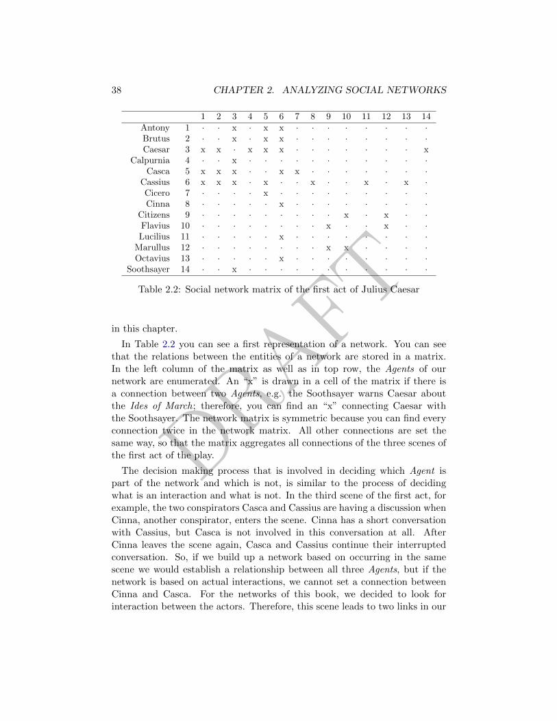
2.2 Social network matrix of the first act of Julius Caesar . . . . . 38
3.1 Knowledge list in Julius Caesar . . . . . . . . . . . . . . . . . . 63
3.2 Task list in Julius Caesar . . . . . . . . . . . . . . . . . . . . . 64
3.3 Locations where the tragedy takes place . . . . . . . . . . . . . 64
3.4 Events of the tragedy . . . . . . . . . . . . . . . . . . . . . . . 66
3.5 Meta-network matrix with all possible 55 networks . . . . . . . 71
3.6 Measure concepts for two entity classes . . . . . . . . . . . . . . 72
3.7 Load and Density of different networks . . . . . . . . . . . . . . 73
3.8 Centralization and Diversity of Degree Centrality . . . . . . . . 75
3.9 Correlation measures of Agents in Caesar’s empire . . . . . . . 77
3.10 Measure concepts for three and more entity classes . . . . . . . 79
4.1 Block modeling the social network matrix of the first act ofJulius Caesar . . . . . . . . . . . . . . . . . . . . . . . . . . . . 94
A.1 Node Classes . . . . . . . . . . . . . . . . . . . . . . . . . . . . 128
A.2 Matrix notations . . . . . . . . . . . . . . . . . . . . . . . . . . 129
13

DRAFT
14 LIST OF TABLES
DRAFT
Chapter 1
The Essence of NetworkAnalysis
Traditionally, network analysis has focused on the social network–who inter-acts with whom. Most classic measures were developed from research on suchnetworks and were meant to be interpreted in a social context. For example,a researcher might survey fraternity members about who they consider to betheir friends (Newcomb, 1961). The most popular individual would show upas the Agent with the most in-links.
Unlike a conventional social network, a dynamic network bundles togethera variety of networks between different types of entities into a meta-network.These different networks include the social network mentioned above, as wellas the membership networks. The membership networks are the relation-ships of the students to their different fraternities, and the inter-organizationalnetwork—and the relationships of the fraternities to each other. Humans arenot simply situated within one social network but rather a vast sea of overlap-ping networks of different types. An analyst working with a dynamic networkattempts to choose a particular set from this ocean of relationships that ismost relevant to their work, bundles them together, and then tries to incorpo-rate and layer them into their analysis. The analyst needs to understand thecontext in which a social network operates. Thus, rather than asking just whodo you know, dynamic network analysis supports asking additional contextquestions such as: How does who you know impact what you know? Whatyou do? Where you do it? And of course, networks change over time. In otherwords, networks of interaction are now embedded in complex meta-networksthat link who, what, how, and why through time and space. Dynamic Net-
15
DRAFT
16 CHAPTER 1. THE ESSENCE OF NETWORK ANALYSIS
work Analysis (DNA) is the study of these complex networks, generally froma quantitative perspective. Agent-based simulation is often used to forecastchange and explore variations in the networks over time. In this book, we willmove from the basics of Social Network Analysis (SNA) to the more detailedDNA.
DNA can be applied in a wide number of settings. Gaining an understand-ing of the structure of Al-Qaeda is critical in fighting the war on terror andcould help prevent future events such as another September 11 attack. Pos-sessing a true ecological map of a food chain will help keep environmentsstable (Johnson et al., 2001). Because of limited resources, understanding thevaried shipping lanes merchant marine vessels traverse as they conduct inter-national trade is vital to protecting ports of call (Davis and Carley, 2007).Understanding how a network of satellites is connected to various locationsaround the world is critical for a global company’s bottom line. A financialnetwork, such as those that enabled the fraud at Enron to destroy the entirecompany and make a lifetime’s retirement fund disappear in a day, is alsofertile territory for DNA.
Networks surround us and pervade our interactions. Your co-workers, yourfood supply, and even your own body can be construed as networks. You can-not go through life without belonging to a network of some sort. You can evenbelong to vastly different multitudes of networks which are all interconnectedto other sorts of networks that you may or may not have a clue as to theirvery existence. Even if you are not associated with one particular network,you can still be defined by your isolation from it.
So how can we use an understanding of the relations among who, what,where, how, why and when to analyze how complex systems such as foodchains plotted to blow up a U.S. Embassy in Tanzania, the plot to murderJulius Caesar, the performance of public health organizations, the mergerof companies, and so on? The answer lies in the science of DNA, a robustapproach to network analysis.
1.1 Network analysis beyond the social graph
It is not all about who knows whom. A lot of other factors are importantwhen it comes to analyzing networks. And even if we are interested in whoknows whom, looking at where the Agents are located, having a closer lookat not just who talks to whom but also what the people are talking about, oranalyzing the interaction patterns over time, may help us to gain more andbetter insights into network dynamics. To give you a better impression of

DRAFT
1.1. NETWORK ANALYSIS BEYOND THE SOCIAL GRAPH 17
Figure 1.1: Distance and communication in a research laboratory (Allen andFustfeld, 1975).
what we are talking about, you can find three examples of studies, in whichresearchers analyzed networks beyond the single social graph.
1.1.1 Communication as a function of distance
Allen and Fustfeld (1975) surveyed people in seven research laboratories.Based on a list of all colleagues, the interviewee where asked with whomthey communicate “about technical or scientific matters” (Allen and Fustfeld,1975, p. 154) at least once a week. In addition, the physical distances betweenthe desks of all employees were measured. For every scientist a radial distancenetwork was created with the person of interest as the focal node in the middleand a circle for every 3 meters (10 feet) forming distance groups (see Figure1.1). Furthermore, the proportion of communication partners was calculatedfor every distance group.
In their analysis, Allen and Fusfeld were able to show that the probabilityof communication follows an exponential decay1 as a function of distance.This was not a very surprising result for the authors. More astonishing wasthe rate of the decay. Allen and Fusfeld figured out that the probability ofweekly communication is almost zero for any distance between two scientistshaving their desks more than 25–30 meters. Even more, they show the resultsof intervention experiments in which the communication between groups ofpeople could be increased significantly just by moving their offices closer toeach other. Allen and Fustfeld (1975) were able to show strong evidence that
1The authors fit the decay with a hyperbola curve.
DRAFT
18 CHAPTER 1. THE ESSENCE OF NETWORK ANALYSIS
“communication is influenced by the physical, architectural arrangement” ofthe working environment. Similar results were shown in subsequent studies inthe following years. A recent study including a review on spatial dimensionsof social networks is provided by Sailer and McCulloh (2012). All studiesabout social networks and geographical proximity or distance have one resultin common: Space matters! We will talk more about geo-spatial networks inchapter 5.
1.1.2 Co-word analysis of invisible colleges
Networks of scientists in a particular field who collaborate for publications andgrant proposals—independently from their institutional affiliation—are calledInvisible colleges (Crane, 1972). Lievrouw et al. (1987) were interested in pos-sible invisible colleges in a special sub-field of biomedical science. Lievrouwand her colleagues asked the scientists in the field about their collaborationpartners. They looked for the intellectual structure of the field by analyz-ing co-citation as well as common use of content in scientific articles. Thecontent analysis was accomplished by making use of index terms that werepre-assigned by a team of professional indexers at the NIH. These indexershad used a thesaurus of 13,000 words and had assigned on average 15 termsto every grant. Lievrouw et al. (1987) showed in their work that
“. . . there is indeed a distinction between the communication struc-ture, or social network, among scientists, and the actual contentof the work in which they engage.” (Lievrouw et al., 1987, p. 245)
The authors were able to reject the assumption that “social structures in sci-ence somehow reflect or represent the intellectual structure of the researchspecialty” (Lievrouw et al., 1987, p. 245). Even most scientists in the ana-lyzed field knew each other and had many collaboration overlap, the contentanalysis of their work showed different groups of specialization. From theperspective of raising money for grants, these groups were competitors in afight for constraint research Resources. In a nutshell, Lievrouw et al. (1987)showed in their research that analyzing the content of written text can resultin broader insights into the connections between people than just looking attheir social interaction ties. Networks that are created from large amounts oftext data are a very important aspect of DNA since an enormous amount oftext is created every day by journalists describing incidents around the worldand by billions of Internet and in particular Social Media users. We discussthe different aspects of network text analysis in chapter 8.
DRAFT
1.2. DYNAMIC NETWORK ANALYSIS AS ANSWER 19
1.1.3 An acquaintance process
Analyzing change in networks over time is another very essential task in DNA.In chapter 6 of this book, you will learn a lot about networks over time andhow to measure and detect change in these dynamic networks. At this point,we tell you about the most famous analysis of networks over time in SocialNetwork literature. Theodore Newcomb (1961) was interested in the dynamicsthat drive the formation of friendship ties—consequently, the resulting bookis titles The Acquaintance Process. To gather the data that was required forhis research, Newcomb recruited 17 students from the University of Michiganin fall 1956 to live for 16 weeks in an off-campus fraternity housing. None ofthe students had known anyone of the other students before the start of theexperiment. After every week, every student had to rank all other students ofthe observed group from 1 (= best friend) to 16. Newcomb himself analyzedhis data primarily with statistical methods showing that physical proximity,reciprocity, similarity, and complementarity were the main reasons to formfriendship. The first three of these points became generally accepted theoriesfor tie formation in the subsequent decades and we will describe their meaningin chapter 2.
Many scientists analyzed the networks that were created in Newcomb’s(1961) study. They were particularly interested in the forming of the networkstructure (e.g. sub-groups). Most of the studies that re-analyzed Newcomb’sfraternity data, came to the conclusion that the acquaintance forming processwas more or less finished after four or five weeks and that not so much changedafter this point. Nevertheless, the dynamic analysis of the networks and inparticular the original study of Newcomb (1961) describing the underlyingimpulses of the acquaintance process were not possible without analyzing notjust a single social network but a collection of networks over time.
1.2 Dynamic Network Analysis as answer
DNA is concerned with who is connected to whom (as in traditional SNA)and the strength, direction, and type of connection. In addition, DNA movesbeyond the social to simultaneously examine who is in what groups, has whatcapabilities or expertise, is engaged in what activities, and holds what beliefs.DNA simultaneously puts these networks in a geo-temporal context that de-fines who was where and when. These diverse entities define a meta-network ofconnections that link who, what, where, when, how, and why (Carley, 2004a).In this book, we introduce the exciting field of DNA to the uninitiated and
DRAFT
20 CHAPTER 1. THE ESSENCE OF NETWORK ANALYSIS
provide additional information on current research to the initiated. It is ourbroad and lofty hope that you will soon find yourself immersed in DNA andthus able to reap the powerful, insightful and critical analysis that only DNAmakes possible.
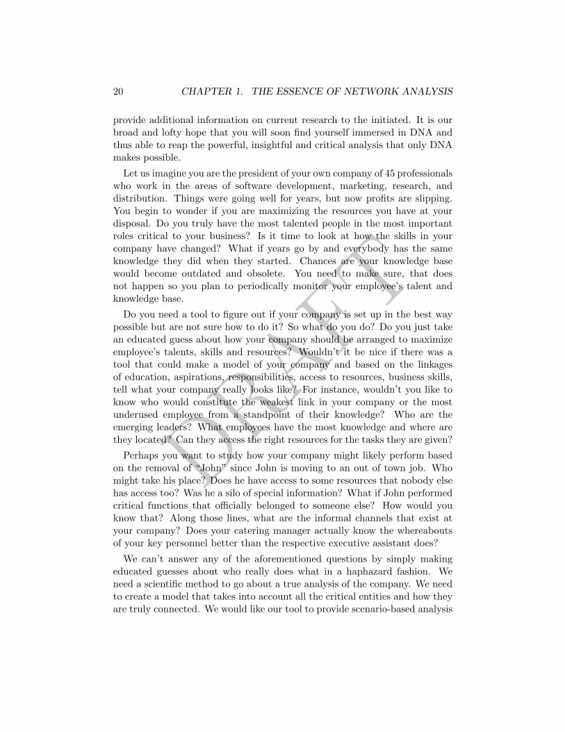
Let us imagine you are the president of your own company of 45 professionalswho work in the areas of software development, marketing, research, anddistribution. Things were going well for years, but now profits are slipping.You begin to wonder if you are maximizing the resources you have at yourdisposal. Do you truly have the most talented people in the most importantroles critical to your business? Is it time to look at how the skills in yourcompany have changed? What if years go by and everybody has the sameknowledge they did when they started. Chances are your knowledge basewould become outdated and obsolete. You need to make sure, that doesnot happen so you plan to periodically monitor your employee’s talent andknowledge base.
Do you need a tool to figure out if your company is set up in the best waypossible but are not sure how to do it? So what do you do? Do you just takean educated guess about how your company should be arranged to maximizeemployee’s talents, skills and resources? Wouldn’t it be nice if there was atool that could make a model of your company and based on the linkagesof education, aspirations, responsibilities, access to resources, business skills,tell what your company really looks like? For instance, wouldn’t you like toknow who would constitute the weakest link in your company or the mostunderused employee from a standpoint of their knowledge? Who are theemerging leaders? What employees have the most knowledge and where arethey located? Can they access the right resources for the tasks they are given?
Perhaps you want to study how your company might likely perform basedon the removal of “John” since John is moving to an out of town job. Whomight take his place? Does he have access to some resources that nobody elsehas access too? Was he a silo of special information? What if John performedcritical functions that officially belonged to someone else? How would youknow that? Along those lines, what are the informal channels that exist atyour company? Does your catering manager actually know the whereaboutsof your key personnel better than the respective executive assistant does?
We can’t answer any of the aforementioned questions by simply makingeducated guesses about who really does what in a haphazard fashion. Weneed a scientific method to go about a true analysis of the company. We needto create a model that takes into account all the critical entities and how theyare truly connected. We would like our tool to provide scenario-based analysis
DRAFT
1.2. DYNAMIC NETWORK ANALYSIS AS ANSWER 21
as well. Moreover, we need it to consider incomplete or outdated information.Could such a tool allow us to even predict how your company might growin the near future given the removal or addition of any key employee? Theanswer is DNA.
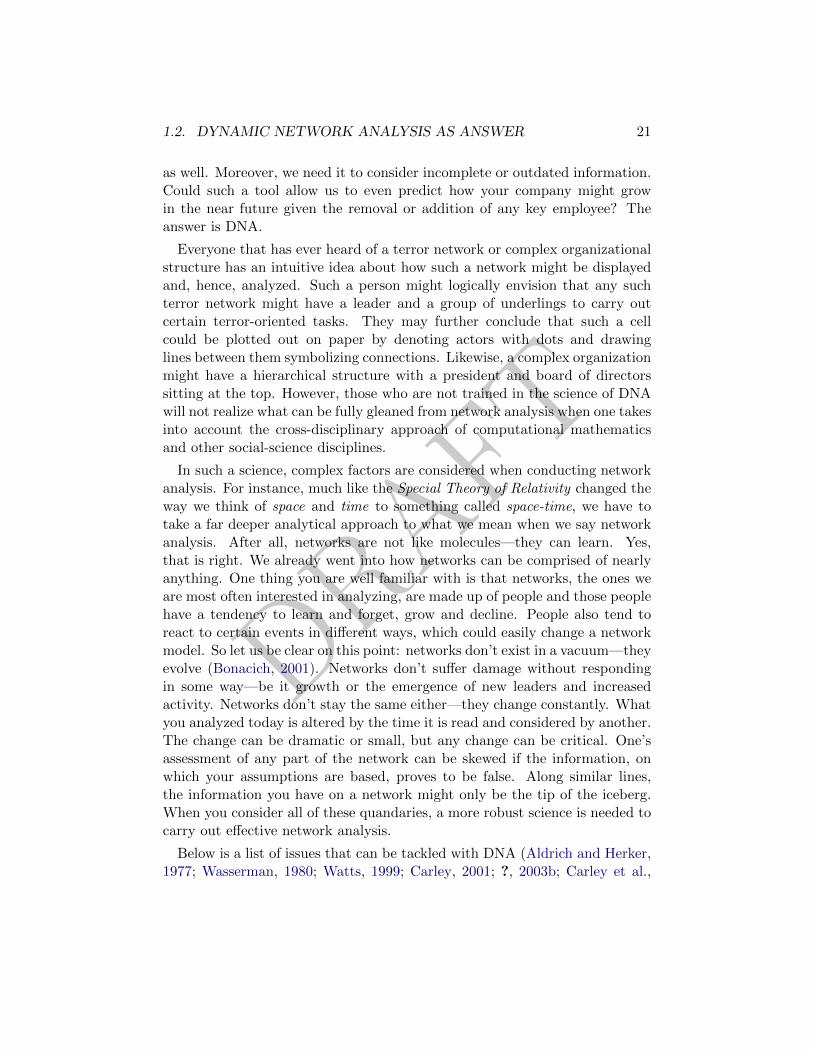
Everyone that has ever heard of a terror network or complex organizationalstructure has an intuitive idea about how such a network might be displayedand, hence, analyzed. Such a person might logically envision that any suchterror network might have a leader and a group of underlings to carry outcertain terror-oriented tasks. They may further conclude that such a cellcould be plotted out on paper by denoting actors with dots and drawinglines between them symbolizing connections. Likewise, a complex organizationmight have a hierarchical structure with a president and board of directorssitting at the top. However, those who are not trained in the science of DNAwill not realize what can be fully gleaned from network analysis when one takesinto account the cross-disciplinary approach of computational mathematicsand other social-science disciplines.
In such a science, complex factors are considered when conducting networkanalysis. For instance, much like the Special Theory of Relativity changed theway we think of space and time to something called space-time, we have totake a far deeper analytical approach to what we mean when we say networkanalysis. After all, networks are not like molecules—they can learn. Yes,that is right. We already went into how networks can be comprised of nearlyanything. One thing you are well familiar with is that networks, the ones weare most often interested in analyzing, are made up of people and those peoplehave a tendency to learn and forget, grow and decline. People also tend toreact to certain events in different ways, which could easily change a networkmodel. So let us be clear on this point: networks don’t exist in a vacuum—theyevolve (Bonacich, 2001). Networks don’t suffer damage without respondingin some way—be it growth or the emergence of new leaders and increasedactivity. Networks don’t stay the same either—they change constantly. Whatyou analyzed today is altered by the time it is read and considered by another.The change can be dramatic or small, but any change can be critical. One’sassessment of any part of the network can be skewed if the information, onwhich your assumptions are based, proves to be false. Along similar lines,the information you have on a network might only be the tip of the iceberg.When you consider all of these quandaries, a more robust science is needed tocarry out effective network analysis.
Below is a list of issues that can be tackled with DNA (Aldrich and Herker,1977; Wasserman, 1980; Watts, 1999; Carley, 2001; ?, 2003b; Carley et al.,
DRAFT
22 CHAPTER 1. THE ESSENCE OF NETWORK ANALYSIS
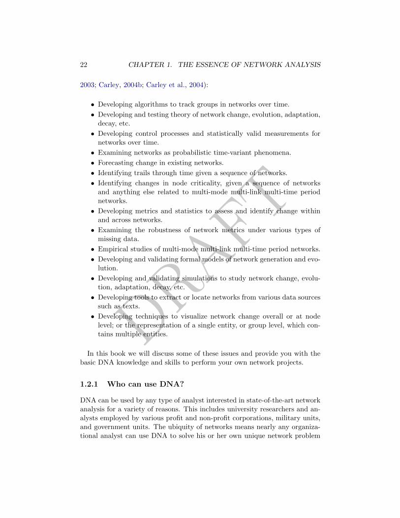
2003; Carley, 2004b; Carley et al., 2004):
• Developing algorithms to track groups in networks over time.
• Developing and testing theory of network change, evolution, adaptation,decay, etc.
• Developing control processes and statistically valid measurements fornetworks over time.
• Examining networks as probabilistic time-variant phenomena.
• Forecasting change in existing networks.
• Identifying trails through time given a sequence of networks.
• Identifying changes in node criticality, given a sequence of networksand anything else related to multi-mode multi-link multi-time periodnetworks.
• Developing metrics and statistics to assess and identify change withinand across networks.
• Examining the robustness of network metrics under various types ofmissing data.
• Empirical studies of multi-mode multi-link multi-time period networks.
• Developing and validating formal models of network generation and evo-lution.
• Developing and validating simulations to study network change, evolu-tion, adaptation, decay, etc.
• Developing tools to extract or locate networks from various data sourcessuch as texts.
• Developing techniques to visualize network change overall or at nodelevel; or the representation of a single entity, or group level, which con-tains multiple entities.
In this book we will discuss some of these issues and provide you with thebasic DNA knowledge and skills to perform your own network projects.
1.2.1 Who can use DNA?
DNA can be used by any type of analyst interested in state-of-the-art networkanalysis for a variety of reasons. This includes university researchers and an-alysts employed by various profit and non-profit corporations, military units,and government units. The ubiquity of networks means nearly any organiza-tional analyst can use DNA to solve his or her own unique network problem
DRAFT
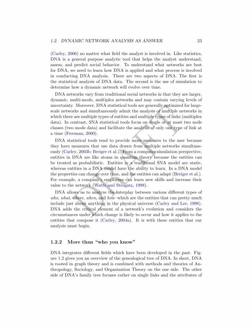
1.2. DYNAMIC NETWORK ANALYSIS AS ANSWER 23
(Carley, 2006) no matter what field the analyst is involved in. Like statistics,DNA is a general purpose analytic tool that helps the analyst understand,assess, and predict social behavior. To understand what networks are bestfor DNA, we need to learn how DNA is applied and what process is involvedin conducting DNA analysis. There are two aspects of DNA. The first isthe statistical analysis of DNA data. The second is the use of simulation todetermine how a dynamic network will evolve over time.
DNA networks vary from traditional social networks in that they are larger,dynamic, multi-mode, multiplex networks and may contain varying levels ofuncertainty. Moreover, DNA statistical tools are generally optimized for large-scale networks and simultaneously admit the analysis of multiple networks inwhich there are multiple types of entities and multiple types of links (multiplexdata). In contrast, SNA statistical tools focus on single or at most two nodeclasses (two mode data) and facilitate the analysis of only one type of link ata time (Freeman, 2000).
DNA statistical tools tend to provide more measures to the user becausethey have measures that use data drawn from multiple networks simultane-ously (Carley, 2003b; Breiger et al.). From a computer simulation perspective,entities in DNA are like atoms in quantum theory because the entities canbe treated as probabilistic. Entities in a traditional SNA model are static,whereas entities in a DNA model have the ability to learn. In a DNA modelthe properties can change over time, and the entities can adapt (Breiger et al.).For example, a company’s employees can learn new skills and increase theirvalue to the network (Watts and Strogatz, 1998).
DNA allows us to analyze the interplay between various different types ofwho, what, where, when, and how–which are the entities that can pretty muchinclude just about anything in the physical universe (Carley and Lee, 1998).DNA adds the critical element of a network’s evolution and considers thecircumstances under which change is likely to occur and how it applies to theentities that compose it (Carley, 2004a). It is with these entities that ouranalysis must begin.
1.2.2 More than “who you know”
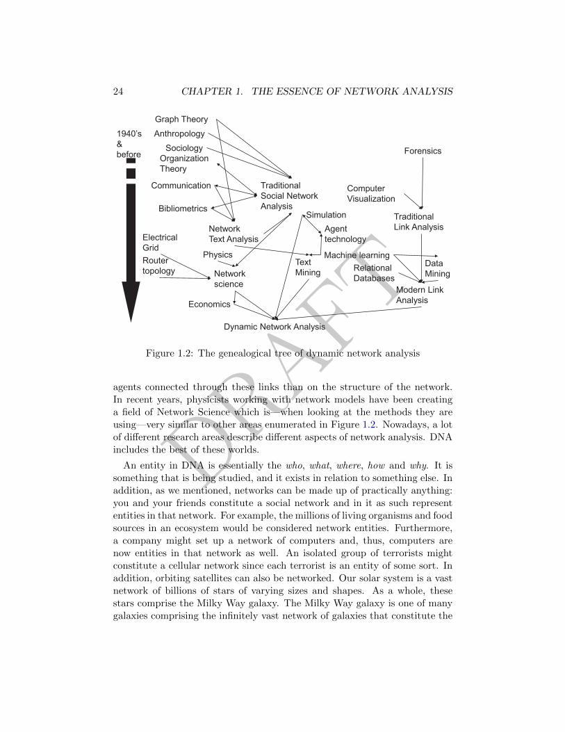
DNA integrates different fields which have been developed in the past. Fig-ure 1.2 gives you an overview of the genealogical tree of DNA. In short, DNAis rooted in graph theory and is combined with methods and theories of An-thropology, Sociology, and Organization Theory on the one side. The otherside of DNA’s family tree focuses rather on single links and the attributes of
DRAFT
24 CHAPTER 1. THE ESSENCE OF NETWORK ANALYSIS
Anthropology
SociologyOrganization Theory
Traditional Social Network Analysis
Physics
Forensics
Computer Visualization
Traditional Link Analysis
Machine learningRelational Databases
Modern Link Analysis
Agent technology
Simulation
Dynamic Network Analysis
Network science
Graph Theory
Economics
Communication
Bibliometrics
NetworkText Analysis
Text Mining
Data Mining
Router topology
Electrical Grid
1940’s &before
Figure 1.2: The genealogical tree of dynamic network analysis
agents connected through these links than on the structure of the network.In recent years, physicists working with network models have been creatinga field of Network Science which is—when looking at the methods they areusing—very similar to other areas enumerated in Figure 1.2. Nowadays, a lotof different research areas describe different aspects of network analysis. DNAincludes the best of these worlds.
An entity in DNA is essentially the who, what, where, how and why. It issomething that is being studied, and it exists in relation to something else. Inaddition, as we mentioned, networks can be made up of practically anything:you and your friends constitute a social network and in it as such represententities in that network. For example, the millions of living organisms and foodsources in an ecosystem would be considered network entities. Furthermore,a company might set up a network of computers and, thus, computers arenow entities in that network as well. An isolated group of terrorists mightconstitute a cellular network since each terrorist is an entity of some sort. Inaddition, orbiting satellites can also be networked. Our solar system is a vastnetwork of billions of stars of varying sizes and shapes. As a whole, thesestars comprise the Milky Way galaxy. The Milky Way galaxy is one of manygalaxies comprising the infinitely vast network of galaxies that constitute the
DRAFT
1.2. DYNAMIC NETWORK ANALYSIS AS ANSWER 25
Universe. Are you beginning to notice a pattern? Have we made it clearthat just about anything you think of can be considered a network on someabstract level and, as such, anything that makes up a network is an entity ofsome kind which interacts with other entities?
We will get into more details about the sorts of entities a DNA scientisttypically deals with soon enough. For now, we want to consider anotherelement that is very integral to an entity. This element is time. Time doesnot stand still and over any given period, things, that are entities, are likely tochange. This is similar to how Albert Einstein made the connection betweenspace and time. It is clear that networks occupy space, and it would onlymake sense to see that time is integral to the space in which the networkexists. A network that exists this year can be dramatically different than thesame network represented next year. DNA takes this change into account.Actually, the analysis of change is the main challenge of DNA.
Entities and their relations are always changing, and this makes networksdynamic. DNA is plowing the path for the study of this dynamic activitywhich was previously inaccessible in the traditional disciplines of link analysiswhere change was not likely to be a key factor. DNA looks at networks notmerely as a bunch of people connected to other people, but people that existin time and can be different, and often are, from one time period to the next.Some people, after all, learn new knowledge and forgot knowledge just thesame. We are looking at networks in terms of their interconnectedness toother entity networks and how change occurs as time marches on (Carley,2001). This is where DNA proves its mettle. With DNA we can take asnapshot of a network in time and with some skill in analysis, stay one stepahead of the curve.
Let us now consider DNA on a more practical level, in a manner thatmight help explain situations you have probably encountered many times.The importance of networking is something we have all encountered beforein one form or another–be it in our personal or professional lives. In sucheveryday experiences, we might say that networking is the art of makingmeaningful connections. We have all heard the expression: It is not what youknow but who you know. Let us consider this common morsel of wisdom fromthe perspective of DNA.
Countless variations of the phrase It is not what you know but who youknow ring true across many boundaries from the cynically hardened skepticsto the most incorrigible optimists. Moreover, such a turn of phrase is oftenascribed as the key to both personal and professional success. However, whatis this phrase really hinting at? We know it describes a network but what
DRAFT
26 CHAPTER 1. THE ESSENCE OF NETWORK ANALYSIS
exactly about the network? The laws of sociological nature? The laws ofsocial dynamics? How to get ahead? The art of networking? A certain part,or aspect, of what it means to be an important component of a network? Allof the above? None of the above? Some of the above?
The truth is that the simple phrase, It is not what you know, but whoyou know describes merely one single facet of any social network, and thedynamic network analyst would find this turn of phrase incredibly simplistic.In fact, have you ever considered it might totally be wrong? Can you think ofexamples where the opposite might be true? How about a network model ofa Ph.D. program where an advanced degree is conferred by accumulating andpresenting research than defending such research until the thesis is accepted?In this network, could it not be argued that what you know is more importantthan whom you know? Perhaps. Nevertheless, back to that hackneyed phrase:It is not what you know, but who you know. What is to be made of it fromthe stand point of DNA?
1.3 Caesar, Brutus, and co.
To understand DNA more fully, we will apply the tool to The Tragedy of JuliusCaesar as crafted by William Shakespeare. Why Julius Caesar? In short, wehave chosen The Tragedy of Julius Caesar because chances are it is a literarywork many of us have encountered at one time or another in our educationalbackgrounds, whether it be from high school or at the post-secondary level.Moreover, it is about a simple usurpation of power, an assassination, andbetrayal. Meanwhile there are conflicting values, a plot, and a network ofpeople who made decisions. There is a lot of network complexity in thatplay. Therefore, in our opinion, The Tragedy of Julius Caesar is a highlyuseful network from that standpoint: neither too big nor small. It is justright to show the power of DNA properly with a model that you may likelyknow already. It is especially useful because it is made up of a fairly complexarrangement of characters, allegiances, and resources. With the use of DNAand a time machine, we might even be able to suggest to Julius Caesar howhe could have prevented his own demise.
You need not re-read the play to understand the examples we will go throughin our application of DNA. However, a familiarity with The Tragedy of JuliusCaesar might help you get more out of this book. We suggest Sparknotes.comfor a short but concise summary of the characters, events and plot (simplysearch “Julius Caesar” on the SparkNote’s site search function). You can alsoget a copy of Cliff’s Notes from your local bookstore. Better yet, purchase a

DRAFT
1.3. CAESAR, BRUTUS, AND CO. 27
copy of the play, dust off the old one in your book collection, and do somethingnovel, like read the play over again. It shouldn’t take you more than a couplehours. You might even enjoy it.
It is our hope that when presented with the proper DNA model, even Bru-tus would have seen that the fault surely did not “lie in the stars” as Cassiusreminded him in course of events. Rather, the fault lies in the failure to ana-lyze a complex multi-modal network of Roman politicians, plebeians, militaryleaders, poets, family member, citizens, soothsayers, battles, skills, allegiances,knowledge, rhetoric and what have you–that is where true fault resides.
So we begin a journey, in hindsight nonetheless, to analyze The Tragedyof Julius Caesar by William Shakespeare, and offer our own analytical rec-ommendations and insights surrounding Caesar’s assassination by putting thepower of DNA to work on the network of Julius Caesar as extrapolated fromthe legendary play The Tragedy of Julius Caesar.
1.3.1 The plot of the tragedy
Let us begin to consider DNA in the context of our specially created examplesolely for the illustrative purposes of this book. The Tragedy of Julius Caesarby William Shakespeare represents the assassination against the Roman dic-tator Julius Caesar, including the aftermath. It is based on true events fromRoman history. Although the title of the play is The Tragedy of Julius Caesar,Julius Caesar is not the central character in the plot, as you will soon learn. Infact, Julius Caesar only appears in three scenes and he dies at the beginningof the third act. The protagonist of the play is actually Marcus Brutus. Theplot focuses on his internal struggle with the conflicting demands of honor,loyalty, and companionship.
The play begins with two tribunes named Flavius and Marullus who discovera large crowd of Roman citizens roving the streets. The pedestrians are cele-brating Julius Caesar’s victory over the Roman general Pompey, his archrival,during a battle. The tribunes scold the citizenry for abandoning their dutiesand instruct them to remove the decorations from Caesar’s statues. Caesarenters with his associates, including the military and political figures Brutus,Cassius, and Antony. Famously, a Soothsayer calls out “beware the Ides ofMarch,” but Caesar ignores him and continues with his victory celebration.
Later, Cassius and Brutus, who are friends of Caesar and each other, beginto confer. Cassius tells Brutus that he seemed withdrawn recently. Brutusresponds by saying that he is full of self-doubt. Cassius replies by voicing hiswishes that Brutus could see himself as others see him. Cassius goes on to
DRAFT
28 CHAPTER 1. THE ESSENCE OF NETWORK ANALYSIS
explain that if Brutus had more confidence in himself he would realize howhonored and respected he is. Therefore, in turn, he would feel more securein his rightful place. Brutus states that he worries the people want Caesarto become king, which would overturn the republic and convert it into anauthoritative regime. Cassius agrees with Brutus, and they point out thatCaesar is already considered to be a god-like figure that people idolize. In aneffort to empower Caesar, Cassius reminds Brutus that Caesar is only a man,and he is not superior to Brutus or Cassius. To back up his claims, Cassiusrecounts incidents of Caesar’s physical weakness and expresses his shock thatthis fallible man has become so powerful. He blames his and Brutus’s lackof conviction for allowing Caesar’s rise to power. Brutus considers Cassius’scommentary as Caesar returns. Upon seeing Cassius, Caesar lets Antony knowabout his suspicion and distrust for Cassius.
After Caesar departs, a politician named Casca tells Brutus and Cassiusthat, during the celebration, Antony offered the crown to Caesar three times.Each time the crown was offered the people cheered, but Caesar refused itevery time. Casca reports that right afterwards, Caesar fell to the ground andhad some kind of seizure in front of the crowd. While some would consider thisto be a sign of weakness the plebeians were unaffected by it, and continued toshow their devotion to him. Later, Brutus considers Casca’s observations thatsuggest Caesar’s poor qualifications to rule. Meanwhile, Cassius brainstormsa plan to involve Brutus in a conspiracy against Caesar.
That evening, Rome experiences destructive weather and a variety of badomens and forewarnings. Brutus finds letters in his house that are suppos-edly written by Roman citizens who are worried that Caesar has become toodominant and controlling. In actuality, the letters have been fabricated andplanted by Cassius. Cassius does this because he wants Brutus to believethat the public is dissatisfied with Caesar. He knows that Brutus is deeplyaffected by the republic’s reaction, and, therefore, after reading the letters heknows that he will likely become more supportive of Cassius’s plot to removeCaesar from power. Brutus fears that the populace would lose its voice ina dictator-led empire. When Cassius arrives at Brutus’s home with his con-spirators, Brutus is already influenced by the letters, and he takes control ofthe meeting. The men unanimously agree to lure Caesar from his house andmurder him. In addition, Cassius wants to kill Antony too. His logic is thatAntony will ruin their plans. Brutus refuses to murder Antony since he fearsthat too many deaths in their plan will appear too bloody and dishonorable.After they all agree to spare Antony, the conspirators depart. Brutus’s wife,Portia observes that Brutus appears distracted and ill at ease. She begs himto confide in her, but he ignores her.
DRAFT
1.3. CAESAR, BRUTUS, AND CO. 29
As Caesar continues to prepare to go to the Senate, his wife, Calpurnia,begs him not to go as well. In an effort to persuade him, she describes recentnightmares she has had. In the nightmares she envisions a statue of Caesarcovered with blood and smiling men bathing their hands in the blood. Caesarrefuses to react to fear and insists on going about his normal routine. Eventu-ally, Calpurnia convinces him to stay home. He agrees to stay home only as afavor to her, and is careful to point out that his decision is not based on fear.However, soon his plans change when Decius, one of the conspirators, arrives.He assures Caesar that Calpurnia has misinterpreted her dreams, as well asthe recent omens. Caesar heads toward the Senate with the conspirators. AsCaesar proceeds through the streets toward the Senate, the Soothsayer onceagain tries to warn him. However, his attempt to get his attention is unsuc-cessful. In another attempt to warn Caesar, Artemidorus, a citizen, handshim a letter to advise him about the conspirators, but Caesar refuses to readit. While at the Senate, the conspirators speak to Caesar. As they are hud-dled around him, they take turns stabbing him to death. When Caesar seeshis close friend Brutus among his murderers, he stops resisting the attack anddies.
Calpurnia’s prediction comes true when the murderers bathe their handsand swords in Caesar’s blood. Antony returns, after having been led away ona false pretext, and vows his allegiance to Brutus. Later, however, he weepsover Caesar’s body. He shakes hands with the conspirators, thus making themall appear guilty while trying to make a gesture of conciliation. When Antonyasks for an explanation as to why they killed Caesar, Brutus replies that hewill explain their reason at the funeral. Antony asks to be allowed to speakat the funeral, and Brutus grants his permission. Cassius, however, remainsleery of Antony. After the conspirators depart, and Antony is alone, he assertsthat Caesar’s death must be avenged.
Later, Brutus and Cassius go to speak at a public forum. Cassius exits tospeak to another section of the crowd. Brutus explains to the crowd that al-though he admired Caesar, his ambition put Roman liberty at risk. The speechpacifies the crowd. Brutus turns the pulpit over to Antony when Antony ap-pears with Caesar’s body. Antony’s speech begins with praise for Brutus, butthen becomes increasingly sarcastic. He questions the statements that Brutusmade in his speech that Caesar acted only out of ambition. Antony calls at-tention to the wealth and glory that Caesar brought to Rome. However, withall the success that Caesar had, he rejected the crown three times. Antonypoints out that Caesar was clearly not solely interested in the power to rule.Antony takes out Caesar’s will with the intention of reading it, but then hestops himself from reading it since he decides that it will cause unnecessary
DRAFT
30 CHAPTER 1. THE ESSENCE OF NETWORK ANALYSIS
distress to the people. Nevertheless, the crowd pleads for him to read the will.He leaves the pulpit to stand next to Caesar’s body. He describes Caesar’sabhorrent death and presents Caesar’s wounded body to the crowd. After-wards he reads Caesar’s will, which states that a sum of money will be givento every citizen and orders that his private gardens shall be made open to thepublic. The fact that such a generous man was horribly murdered enrages thecrowd, and the crowd begins to call Brutus and Cassius traitors. The massesbegin their plan to eject them from the city.
In the meantime, Caesar’s adopted son and appointed successor, Octavius,arrives in Rome and forms a pact with Antony and Lepidus. They prepareto fight Cassius and Brutus, who have been driven into exile and are raisingarmies outside of the city. Brutus and Cassius have a heated argument regard-ing money and honor, but they ultimately decide to settle their disagreements.Brutus reveals that he is grieving the death of Portia, who committed suicide.The two continue to prepare for battle with Antony and Octavius. The Ghostof Caesar appears to Brutus that night. It announces that Brutus will meethim again on the battlefield.
As Octavius and Antony march their army toward Brutus and Cassius,Antony instructs Octavius where to attack, but Octavius stubbornly repliesthat he will make his own orders. He is eager to assert his authority as theheir of Caesar and the next ruler of Rome. The rivaling generals meet on thebattlefield and exchange harsh words to each other before beginning to fight.
Cassius begins to notice that his own men are retreating and he hears thatBrutus’s men also are not performing effectively. Cassius sends one of hismen, Pindarus, to check on the situation. From afar, Pindarus sees one oftheir leaders, Cassius’s best friend, Titinius, being surrounded by applaudingtroops and infers that he has been seized. Cassius becomes distraught andorders Pindarus to kill him with his own sword. He dies after proclaiming thatCaesar is avenged. Soon after, Titinius arrives, and it is revealed that the menwho were encircling him were actually on his team, and they were celebratingthe victory over the opponents. When Titinius sees Cassius’s corpse he beginsto mourn the death of his friend. He is so distraught that he kills himself.
When Brutus learns of the deaths of Cassius and Titinius he is also upset,and he prepares to take on the Romans once again. When his army loses thebattle, Brutus asks one of his comrades to hold his sword while he impaleshimself on it. As he is dying, he proclaims that Caesar can rest satisfied.When Antony speaks over Brutus’s body, he calls him the noblest Roman ofall. He points out that while the other conspirators acted out of envy andambition, Brutus genuinely believed that he acted for the benefit of Rome.
DRAFT
1.3. CAESAR, BRUTUS, AND CO. 31
Octavius orders that Brutus be buried in an honorable way. Afterwards, themen leave to celebrate their victory.
This was the story of the Tragedy of Julius Caesar by William Shakespeare.Now that we got that out of the way, it is time to get down to some DNA.After all, now that we know the story, now we need to know the nodes (thewhos) that will make up our meta-network. And, without further adieu, weare ready to talk about the basic building blocks of network analysis.
1.3.2 Saving Julius Caesar?
Nearly everything is a network. The universe is expanding. Your knowledgeis growing or languishing. People move on to different roles. One day you’re ason, the next day you are a parent. Like string theory and quantum mechanics,everything in our vast interconnected universe is, on some level, constantly onthe move and this is what you will come to see in Julius Caesar. The timeelement makes depicting network models especially tricky because no soonerthan you construct a network, it has changed. Since this applies to JuliusCaesar, we will explore several techniques that will help you properly accountfor time in your own network model.
Using DNA, our aim is to discover what Julius Caesar could not discernfor himself; how he was vulnerable in his own empire by failing to understandthe complex multi-modal evolving network around him. In doing so, we willintroduce and explore the power of DNA. We aim to show how this is donebased on our knowledge of the Julius Caesar network as presented by Shake-speare. A DNA analyst could have made certain recommendations, based onrock-solid mathematical computations, to Caesar, which might have seen himcarrying on his rule as emperor of Rome and conquering the rest of knownworld, as he probably would have liked to have done.
Although a skeptic might conjecture that he too would have ignored ourinsights, much as he did the dire warnings of the Soothsayer, the nightmaresof his wife Calpurnia, and the advice of Artemidorus shortly before his ill-fatedtrip to the Roman Senate. But, that only underscores a human volatility thatcan in part affect the impact of a well put together network model: is theperson who is looking at the model shrewd enough to see what it really is?
We know one thing: if we presented Julius Caesar our findings, based onthe authority of the cutting-edge computational mathematics of DNA, Deciuswould have had a much harder time convincing Julius Caesar that his wife’sdream was merely misinterpreted and that he should attend the Senate meet-ing that day, where he would promptly be stabbed by his closest friends. Our
DRAFT
32 CHAPTER 1. THE ESSENCE OF NETWORK ANALYSIS
findings would have given him much pause. Still, Caesar would have to actupon them by making some kind of policy decision. He seemed to “go at italone,” and it cost him his life.
Nonetheless, rooted in the knowledge of DNA, a better policy for JuliusCaesar could have been crafted to avert his impending doom. We can takesolace in our lesson, however, that grounded with the results of better analyt-ical methods we might construct policies that would prevent a network fromdoing the same again be it for nefarious purposes or altruistic. Along thoselines, we should add that our purpose is not necessarily to show how DNAcan buttress the continuation of a tyrant, as Cassius might have argued, butjust demonstrate how useful it can be when applied with foresight and skill.Brutus could have also used his own DNA model, perhaps, to see the likelyoutcome of killing Caesar. He might not have needed an ill dream to tell himthat Rome would be divided in two. He might have only needed his DNAmodel.
Therefore, before we begin to build our network model of the Julius Caesarworld, we first need to explain to Caesar what a network is, what its com-ponents are, what the best ways of analyzing them are, and what challengesare faced in analyzing complex multi-modal networks over periods. We beginwith the basics for those Roman citizens of network analysis lacking in therudiments as we are sure Caesar would have been in the same class as thesoothsayers and cobblers in that regards.
1.4 Problem set
1. Remember the study by Allen and Fustfeld described in this chapter—why is the desk-to-desk distance in a company important for collabora-tion?
2. What is the main difference between social network analysis and dy-namic network analysis regarding to the entities of the analysis?
3. Imagine the network consisting of all employees in your company or allstudents of your university as well as their connections based on sendingand receiving e-mails. What are the questions which you want to haveanswered with such network data?
4. Thinking of accomplishing tasks, why do you think is it important toknow which person in an organization has which knowledge?
DRAFT
1.4. PROBLEM SET 33
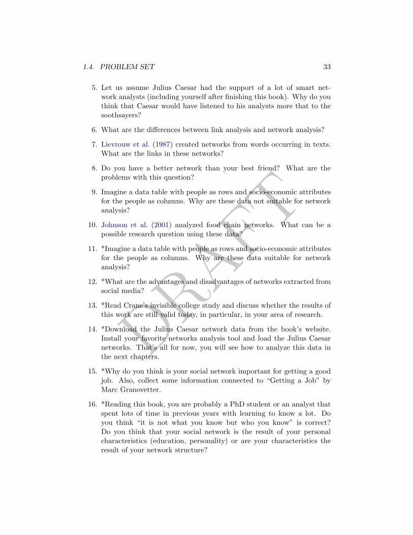
5. Let us assume Julius Caesar had the support of a lot of smart net-work analysts (including yourself after finishing this book). Why do youthink that Caesar would have listened to his analysts more that to thesoothsayers?
6. What are the differences between link analysis and network analysis?
7. Lievrouw et al. (1987) created networks from words occurring in texts.What are the links in these networks?
8. Do you have a better network than your best friend? What are theproblems with this question?
9. Imagine a data table with people as rows and socio-economic attributesfor the people as columns. Why are these data not suitable for networkanalysis?
10. Johnson et al. (2001) analyzed food chain networks. What can be apossible research question using these data?
11. *Imagine a data table with people as rows and socio-economic attributesfor the people as columns. Why are these data suitable for networkanalysis?
12. *What are the advantages and disadvantages of networks extracted fromsocial media?
13. *Read Crane’s invisible college study and discuss whether the results ofthis work are still valid today, in particular, in your area of research.
14. *Download the Julius Caesar network data from the book’s website.Install your favorite networks analysis tool and load the Julius Caesarnetworks. That’s all for now, you will see how to analyze this data inthe next chapters.
15. *Why do you think is your social network important for getting a goodjob. Also, collect some information connected to “Getting a Job” byMarc Granovetter.
16. *Reading this book, you are probably a PhD student or an analyst thatspent lots of time in previous years with learning to know a lot. Doyou think “it is not what you know but who you know” is correct?Do you think that your social network is the result of your personalcharacteristics (education, personality) or are your characteristics theresult of your network structure?
DRAFT
34 CHAPTER 1. THE ESSENCE OF NETWORK ANALYSIS
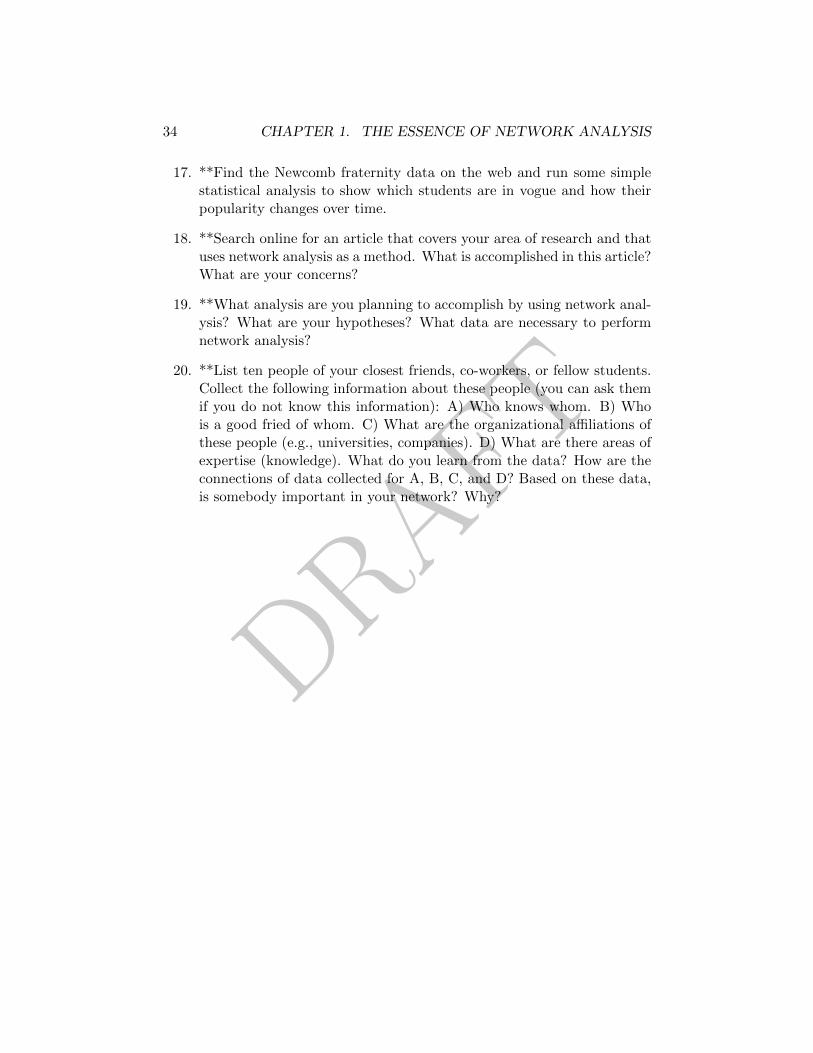
17. **Find the Newcomb fraternity data on the web and run some simplestatistical analysis to show which students are in vogue and how theirpopularity changes over time.
18. **Search online for an article that covers your area of research and thatuses network analysis as a method. What is accomplished in this article?What are your concerns?
19. **What analysis are you planning to accomplish by using network anal-ysis? What are your hypotheses? What data are necessary to performnetwork analysis?
20. **List ten people of your closest friends, co-workers, or fellow students.Collect the following information about these people (you can ask themif you do not know this information): A) Who knows whom. B) Whois a good fried of whom. C) What are the organizational affiliations ofthese people (e.g., universities, companies). D) What are there areas ofexpertise (knowledge). What do you learn from the data? How are theconnections of data collected for A, B, C, and D? Based on these data,is somebody important in your network? Why?
DRAFT
Chapter 2
Analyzing Social Networks
Social networks are networks consisting of human beings. The people in thesenetworks are often called Agents, nodes, or actors. These terms are usedinterchangeably. Connections between these Agents are called edges (or links).These two sets, nodes and edges, are sufficient to describe the essence of socialnetworks. Therefore, before we can start to collect and analyze the networkof Julius Caesar, we have to answer the two fundamental questions of socialnetwork analysis: What are the entities of our networks? And how are theseentities connected with each other?
2.1 Units of interest
2.1.1 Entities: Friends, romans, and countrymen
In the following list, we have the characters that make up our Julius Cae-sar Network, which is based on William Shakespeares The Tragedy of JuliusCaesar. All of the characters on this list constitute an entity, which for thepurposes of DNA we say is a who. After all, they are people, even though itis in a fictional sense. Other entity classes, which you will see later in thisbook, allow us to put certain entities into other different containers, which,perhaps you have guessed by now, correspond to the who, what, when, whereand why model. There are even more components as well, but we will explorethose more deeply when we learn about entity classes. For now, let us visitour whos as they relate to the Julius Caesar Network we are going to build inthe next chapter. Here are the whos!
By reading the names of characters in Table 2.1 you can imagine that the
35
DRAFT
36 CHAPTER 2. ANALYZING SOCIAL NETWORKS
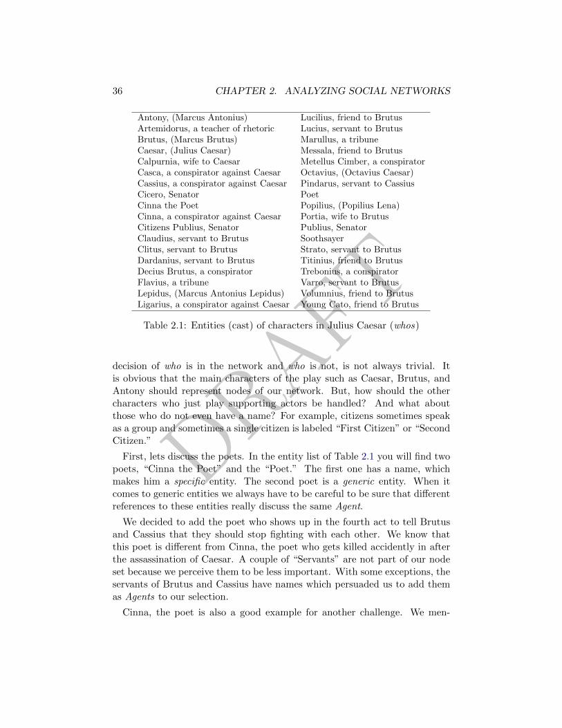
Antony, (Marcus Antonius) Lucilius, friend to BrutusArtemidorus, a teacher of rhetoric Lucius, servant to BrutusBrutus, (Marcus Brutus) Marullus, a tribuneCaesar, (Julius Caesar) Messala, friend to BrutusCalpurnia, wife to Caesar Metellus Cimber, a conspiratorCasca, a conspirator against Caesar Octavius, (Octavius Caesar)Cassius, a conspirator against Caesar Pindarus, servant to CassiusCicero, Senator PoetCinna the Poet Popilius, (Popilius Lena)Cinna, a conspirator against Caesar Portia, wife to BrutusCitizens Publius, Senator Publius, SenatorClaudius, servant to Brutus SoothsayerClitus, servant to Brutus Strato, servant to BrutusDardanius, servant to Brutus Titinius, friend to BrutusDecius Brutus, a conspirator Trebonius, a conspiratorFlavius, a tribune Varro, servant to BrutusLepidus, (Marcus Antonius Lepidus) Volumnius, friend to BrutusLigarius, a conspirator against Caesar Young Cato, friend to Brutus
Table 2.1: Entities (cast) of characters in Julius Caesar (whos)
decision of who is in the network and who is not, is not always trivial. Itis obvious that the main characters of the play such as Caesar, Brutus, andAntony should represent nodes of our network. But, how should the othercharacters who just play supporting actors be handled? And what aboutthose who do not even have a name? For example, citizens sometimes speakas a group and sometimes a single citizen is labeled “First Citizen” or “SecondCitizen.”
First, lets discuss the poets. In the entity list of Table 2.1 you will find twopoets, “Cinna the Poet” and the “Poet.” The first one has a name, whichmakes him a specific entity. The second poet is a generic entity. When itcomes to generic entities we always have to be careful to be sure that differentreferences to these entities really discuss the same Agent.
We decided to add the poet who shows up in the fourth act to tell Brutusand Cassius that they should stop fighting with each other. We know thatthis poet is different from Cinna, the poet who gets killed accidently in afterthe assassination of Caesar. A couple of “Servants” are not part of our nodeset because we perceive them to be less important. With some exceptions, theservants of Brutus and Cassius have names which persuaded us to add themas Agents to our selection.
Cinna, the poet is also a good example for another challenge. We men-
DRAFT
2.1. UNITS OF INTEREST 37
tioned earlier that he got killed by the citizens because they confounded himwith another guy called Cinna who was one of the conspirators against Cae-sar. What happened to the citizens of Rome can also happen to us when weare collecting data for our Social Network Analysis (SNA). Unifying differentpeople to one entity of our analysis can easily create interesting artifacts—or,in other words, it can destroy your whole analysis!
Finally, the most critical of our decision is certainly the node “Citizens,”which is a group node that represents a couple of anonymous people. We canuse the same arguments discussed for generic nodes to ignore these nodes inour networks. For your own networks you should not mix up individuals andgroups in one node class unless you have a really good argument for that.In our case, we think we have a good reason to lump them together. TheCitizens are of key importance when it comes to the succession of Caesar and,less gloriously, they kill Cinna the Poet. In addition, we also want to refer tothese incidents in the networks. But, we must be aware of the implicationsfor calculating measures for our networks. We will discuss these implicationsin the later chapters of this book.
2.1.2 Relations: To love and to hate
Now that we have the nodes, the next fundamental decision is to determinehow to connect the nodes with each other. In creating our social networkof The Tragedy of Julius Caesar, we can say that the characters in the playconstitute a social network based on their interactions. It will be a who bywho network. Since the elements of our network are people, this is often calleda social network. A social network should be something familiar to anyone.Whomever you regularly talk with can be a social network. It can be yourfriends, family, the people you work with, or any combination of them. Thissocial network will be our first network, and it will tell us who is connectedto whom. In the case of The Tragedy of Julius Caesar the who elements arethe persons of the play as we described in the previous sub-section.
Now that we have all of the characters recorded, we need to figure out whois connected to whom. The question to answer is what do we consider as beingconnected? In our case, we are going to consider that they are connected witheach other if they appear in the same scene and interact with each other. Letus start coding our network. Actually, we need to create five networks insteadof just one network—every act in the play of Julius Caesar gets a separatenetwork. The multiple networks will allow us to examine change over timelater on. But, let us start with the first act and discuss over time issues later
DRAFT
38 CHAPTER 2. ANALYZING SOCIAL NETWORKS
1 2 3 4 5 6 7 8 9 10 11 12 13 14Antony 1 · · x · x x · · · · · · · ·Brutus 2 · · x · x x · · · · · · · ·Caesar 3 x x · x x x · · · · · · · x
Calpurnia 4 · · x · · · · · · · · · · ·Casca 5 x x x · · x x · · · · · · ·
Cassius 6 x x x · x · · x · · x · x ·Cicero 7 · · · · x · · · · · · · · ·Cinna 8 · · · · · x · · · · · · · ·
Citizens 9 · · · · · · · · · x · x · ·Flavius 10 · · · · · · · · x · · x · ·Lucilius 11 · · · · · x · · · · · · · ·
Marullus 12 · · · · · · · · x x · · · ·Octavius 13 · · · · · x · · · · · · · ·
Soothsayer 14 · · x · · · · · · · · · · ·
Table 2.2: Social network matrix of the first act of Julius Caesar
in this chapter.
In Table 2.2 you can see a first representation of a network. You can seethat the relations between the entities of a network are stored in a matrix.In the left column of the matrix as well as in top row, the Agents of ournetwork are enumerated. An “x” is drawn in a cell of the matrix if there isa connection between two Agents, e.g. the Soothsayer warns Caesar aboutthe Ides of March; therefore, you can find an “x” connecting Caesar withthe Soothsayer. The network matrix is symmetric because you can find everyconnection twice in the network matrix. All other connections are set thesame way, so that the matrix aggregates all connections of the three scenes ofthe first act of the play.
The decision making process that is involved in deciding which Agent ispart of the network and which is not, is similar to the process of decidingwhat is an interaction and what is not. In the third scene of the first act, forexample, the two conspirators Casca and Cassius are having a discussion whenCinna, another conspirator, enters the scene. Cinna has a short conversationwith Cassius, but Casca is not involved in this conversation at all. AfterCinna leaves the scene again, Casca and Cassius continue their interruptedconversation. So, if we build up a network based on occurring in the samescene we would establish a relationship between all three Agents, but if thenetwork is based on actual interactions, we cannot set a connection betweenCinna and Casca. For the networks of this book, we decided to look forinteraction between the actors. Therefore, this scene leads to two links in our
DRAFT
2.2. MORE DEFINITIONS 39
network, one between Casca and Cassius and a second between Cassius andCinna.
This little example should show you that the decision whether a link is ina specific network or not can be tricky. In general, the definition of a linkhas to be made in every DNA project. When it comes to your own networkprojects, this is an important question to ask even if you are working withdata collected by other people. In the next chapters, you will learn a lotabout different measures to identify interesting nodes or groups of nodes orother patterns. These measures very much rely on your data. The networksof the same organization or other group of people, or even the networks of aplay by Shakespeare, can look very different based on the definition of who isin the network and who is not, as well as the decision about which kind ofconnections to observe and which not to observe.
2.2 More definitions
This book is an introduction of network analysis, and it is targeted to studentsin all majors as well as non-academia people. Therefore, we avoid complicateddefinitions and equations in larger parts of the book, and we have put all of themathematical details in the glossary part at the end of the book. Nevertheless,some basic definitions are necessary to be sure that we are all talking aboutthe same things. First of all, when reading the first pages of this book, youhave already seen that a network is defined by a set of nodes (e.g. Agents)and links connecting these nodes. A link which connects a node with itself iscalled a self-loop. Two nodes are neighbors if there is a link connecting thispair of nodes directly with each other. Two nodes are indirectly connected ifthere is a path through the network connecting a node with another node byintermediate nodes. For example, if a is connected to b, b is connected to c,and c is connected to d, then a and d are indirectly connected. The shortestindirect connection (using the smallest number if intermediate nodes) is calledshortest path. The longest shortest path in a network is the diameter of thenetwork. A group of nodes connected by direct or indirect connections iscalled a component. If you look at Figure 2.4 you can see that in act 1 and4 our network consists of 2 components while in the acts 2, 3 and 5 all nodesare part of one single component.
The edges can be of different types. In our five Julius Caesar networks theedges are unweighted. This means that the importance of every edge is thesame. Each has an “x” in the matrix and they all have lines with the samewidth in the network visualization. If it would not be the case that all the
DRAFT
40 CHAPTER 2. ANALYZING SOCIAL NETWORKS
edges in our networks are treated identically, the network would be weighted.We could, for example, say that the relation between Caesar and his wifeCalpurnia is much more important than the relation between Caesar and theSoothsayer and, consequently, we are interested in coding this fact into thenetwork model. We can do so, by putting different numbers into the networkmatrix, e.g. “5” into the matrix cells connecting Caesar and Calpurnia and“1” to his connection with the Soothsayer. If we write different edge weightsinto the network matrix, we call it a weighted network. To also representthe different line weights in the network visualization, we draw the lines withdifferent widths.
In the context of edges we can introduce another definition. A network iscalled undirected if case A is connected to B and B is connected to A. It isdirected if the connection is just in one direction. Why is this important? TheJulius Caesar networks we constructed earlier in this chapter are undirectedbecause our definition of a single connection is an observation while readingthe book. If we had the ability to jump back in time and ask Caesar andhis contemporaries with whom they interact with, our network data wouldlook different. Why? Imagine an ancient scientist surveying Caesar about hissocial interactions. Probably this would turn out to be a long lasting interviewbecause Caesar interacts with a lot of different people. There is, however, apretty good chance that Caesar misses some people in answering this question;maybe he would not remember that he ever talked with the Soothsayer. Onthe other hand, a lot of people in ancient Rome who had contact with Caesarwould recall him as one of the first names in their enumeration of connectedpeople. To handle this asymmetric information about a single relation, we usedirected edges. So, we are able to add a connection from the Soothsayer toCaesar but not vice versa.
We use the term simple networks to refer to networks which just consistof undirected and unweighted links, which have no self-loop, and which in-clude all nodes in a single component. When considering the question aboutweighted or directed networks, you will realize that in social life almost no con-nection between people is undirected; even the most fundamental emotionalconnections, like love and hate, are somehow directed information. And ofcourse, adding weights can help to describe these relations more in detail, e.g.how often do the people communicate, how close do they feel, or how long dothey know each other. Nevertheless, in real world scientific and business SNAprojects, the most networks are unweighted and undirected. These networksare easier to collect and to handle. A lot of measures ignore the direction orthe weight of edges at all. In this book, you will find both variation; some-times we will use networks with more characteristics. For the first measures
DRAFT
2.3. THE STRUCTURE OF HUMAN CONNECTIONS 41
we are going to introduce later in this chapter, just simple networks are used.
2.3 The structure of human connections
Before we start to analyze social networks, we want to give some attentionto the question why people interact with each other at all and which networkstructures emerge as a result of social relations.
2.3.1 Networks on personal level
Think about the people that you met today or that you send emails to beforeyou started to read these pages, why did you interact with them? Or why doFlavius and Marullus as well as Brutus and Cassius communicate with eachother rather than all of the four as a group? During the last couple of decadesscientists figured out that a vast part of the dynamics that drive the formationof social connections can be described with a few theories.
Reciprocity. The simplest answer to the question, “why does A communi-cate with B” is: “Maybe, B communicated with A the day before”. Networkanalysts call the tendency of these bi-directional relations reciprocity (Katzand Powell, 1955). Following this theory, people interact with each other be-cause there is communication history. There is a good chance that you sendan e-mail to John because John had sent you an e-mail before, asking you aquestion or telling you some news. Cassius confides his doubts with Caesarto Brutus because he trusts him, probably because they have discussed otherserious matters before. Consequently, when you observe networks over time,reciprocal connections will be a phenomenon that you will find very often.“Reciprocal service” is also one of the characteristics that describe strong ties(Granovetter, 1973) – we discuss weak and strong ties in some paragraphsmore in detail. In opposite, very asymmetric relations, i.e. A sends a lot ofinformation to B but B does not answer very often or maybe never, are a goodindicator for hierarchies (e.g. A is an employee of B and has to report himabout his project progress) or possession of valuable Knowledge or Resources(Wellman, 1988, p. 45).
Homophily. The second big theory of social connections is homophily.Homophily that people tend to connect with other people that are similarto themselves. Similar based on age, gender, education, or any other socio-demographic characteristic as well as similar behavior, goals, political posi-tions, and religious Beliefs. Homophily is, therefore, what people mean whenthey use the saying “birds of a feather flock together”. In their review arti-
DRAFT
42 CHAPTER 2. ANALYZING SOCIAL NETWORKS
cle about homophily McPherson et al. (2001) emphasized the importance forsocial connections when they stated:
“Homophily limits peoples social worlds in a way that has powerfulimplications for the information they receive, the attitudes theyform, and the interactions they experience.”
The fact that people create connections based on homophily has very impor-tant implications for the formation of groups – we will discuss this topic in thenext section. For now, we can answer the initial question of this section aboutthe relations in the Tragedy of Julius Caesar simply with “perhaps Flaviusand Marullus as well as Brutus and Cassius interact because they are verysimilar to each other”.
Propinquity. A special form of homophily is similarity based on physicalLocations. Festinger et al. (1950) figured out in their Westgate West Studythat the friendship of students within a dorm is a function of the closeness oftheir rooms. Physical (geographical) closeness is very important impetus toforming relations – in other words: “Those close by, form a tie”. This is notjust true for students but also for co-workers or neighbors in suburbs.
Transitivity. So far, we have just discussed the direct interactions betweentwo people. The next theory about why people form relations with each otherinvolves a third person. Transitivity describes the tendency that people formnew relationships with friends of existing friends. In other words, if Jane andBetty are friends for many years and Jane also is good fried with Joe, thanthere is a good chance that Betty and Joe also form a positive relation witheach other. The dynamics in these triadic relationships where introduced byHeider (1946) in his Balance Theory that describes the interaction of twopeople and their relationship to a third person (Cartwright and Harary, 1956)or any other form of entity (e.g. Event, idea, etc.). Look at Figure 2.1,triad number 1 shows a balanced triad, i.e. A and B like each other andthey both like C. In opposite, triad 2 is unbalanced since A likes C but Bdoesnt. Why is this unbalanced? Imagine once again the two friends Bettyand Jane and a slightly changed situation in which Betty likes Joe but Janedoesnt. What do you think happens in such a situation? Right, Betty andJane start to argue about whether Joe is a nice guy or not. This results inan unbalanced triad. And the dynamics of this arguing between Betty andJane are also quite predictable. Actually, there are two very likely outcomes.First, Betty convinces Jane that Joe is a nice guy. In this case the balancedtriad number 1 would be the result. Second, Jane convinces Betty that Joeis not a nice guy. The result is triad number 3—which is again a balance
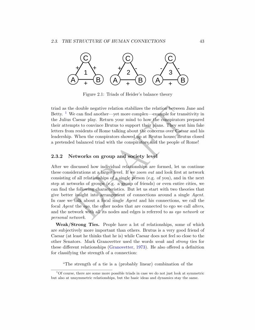
DRAFT
2.3. THE STRUCTURE OF HUMAN CONNECTIONS 43
C
A B
+ +
+
C
A B
- +
+
C
A B
- -
+
1 2 3
Figure 2.1: Triads of Heider’s balance theory
triad as the double negative relation stabilizes the relation between Jane andBetty. 1 We can find another—yet more complex—example for transitivity inthe Julius Caesar play. Return your mind to how the conspirators preparedtheir attempts to convince Brutus to support their plans. They sent him fakeletters from residents of Rome talking about the concerns over Caesar and hisleadership. When the conspirators showed up at Brutus house, Brutus closeda pretended balanced triad with the conspirators and the people of Rome!
2.3.2 Networks on group and society level
After we discussed how individual relationships are formed, let us continuethese considerations at a larger level. If we zoom out and look first at networkconsisting of all relationships of a single person (e.g. of you), and in the nextstep at networks of groups (e.g. a group of friends) or even entire cities, wecan find the following characteristics. But let us start with two theories thatgive better insight into arrangement of connections around a single Agent.In case we talk about a focal single Agent and his connections, we call thefocal Agent the ego, the other nodes that are connected to ego we call alters,and the network with all its nodes and edges is referred to as ego network orpersonal network.
Weak/Strong Ties. People have a lot of relationships, some of whichare subjectively more important than others. Brutus is a very good friend ofCaesar (at least he thinks that he is) while Caesar does not feel so close to theother Senators. Mark Granovetter used the words weak and strong ties forthese different relationships (Granovetter, 1973). He also offered a definitionfor classifying the strength of a connection:
“The strength of a tie is a (probably linear) combination of the
1Of course, there are some more possible triads in case we do not just look at symmetricbut also at unsymmetric relationships, but the basic ideas and dynamics stay the same.
DRAFT
44 CHAPTER 2. ANALYZING SOCIAL NETWORKS
amount of time, the emotional intensity, the intimacy (mutualconfiding), and the reciprocal services which characterize the tie.”(Granovetter, 1973, p. 1361)
Based on this definition, every person has a small number of strong ties anda more or less large number of weak ties (see next paragraph). Strong tiesare our best friends and parts of our core family. These connections are veryimportant for our everyday life as well as for support in important situations.But, Granovetter’s article (1973) was titled “The Strength of Weak Ties”.He wanted to emphasize in particular these connections in the context of thediffusion of information. To give you an example why weak ties can be im-portant, we refer to another study by Granovetter in which he surveyed ablue-collar worker in a suburb of Boston (Granovetter, 1974). Granovetteranalyzed how people get their jobs and he found out that not just friendsand family were the providers of information about a vacant job, but alsoacquaintance and loose connections. Even more, Granovetter concluded thatthe more a job is ranked superior the more information about this job oppor-tunity is communicated via weak ties. This is the case because strong tiesare often homogeneous ties (see homophily) while weak ties are connectionsto different people with different information, Knowledge, and Resources.
Dunbar’s number. Robin Ian McDonald Dunbar leveraged the SocialBrain Hypothesis (Dunbar, 1998), based on which the social group size of pri-mates and humans is a result of the size of their brains. Dunbar analyzed thesize of the neocortex (part of the brain that is responsible for higher func-tions, e.g. senses, spatial–temporal reasoning, and language) from differentprimates as well as their average group size and predicted a mean group sizefor humans (based on the size of our neocortex) of approximately 150. Thisnumber has since then been called Dunbars’s number and was reconfirmedin empirical studies (Hill and Dunbar, 2003). Even some people have muchmore connections and others have less, on average this turned out to be agood estimation of social network sizes for humans.
Hierarchical organization of personal networks. In the previous para-graphs we talked about a) weak and strong ties and b) Dunbar’s number.Consequently, the question arises how these 150 people are organized in dif-ferent groups of tie strength. Zhou et al. (2005) answered this question withfour hierarchical layers surrounding every human being (see Figure 2.2), withevery group being roughly three times larger than the previous one. Thesegroups are defined as follows:
1. Support clique. The strongest ties of a person including the core family
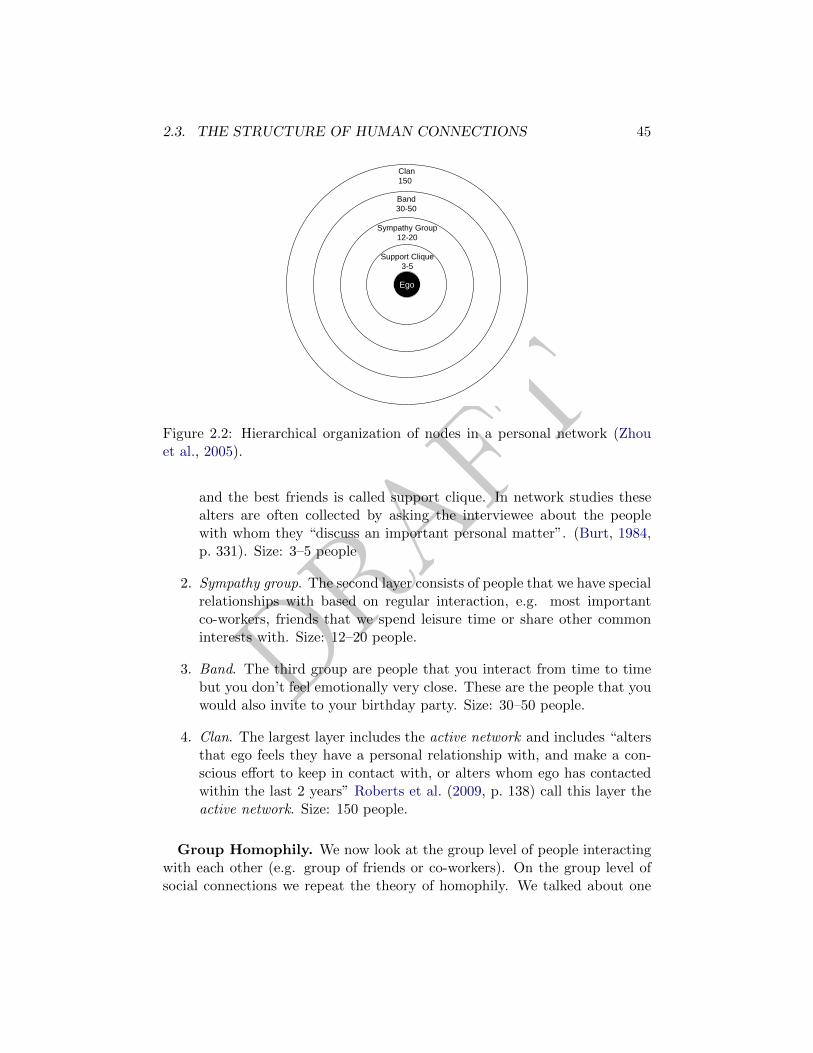
DRAFT
2.3. THE STRUCTURE OF HUMAN CONNECTIONS 45
Ego
Support Clique
3-5
Sympathy Group
12-20
Band
30-50
Clan
150
Figure 2.2: Hierarchical organization of nodes in a personal network (Zhouet al., 2005).
and the best friends is called support clique. In network studies thesealters are often collected by asking the interviewee about the peoplewith whom they “discuss an important personal matter”. (Burt, 1984,p. 331). Size: 3–5 people
2. Sympathy group. The second layer consists of people that we have specialrelationships with based on regular interaction, e.g. most importantco-workers, friends that we spend leisure time or share other commoninterests with. Size: 12–20 people.
3. Band. The third group are people that you interact from time to timebut you don’t feel emotionally very close. These are the people that youwould also invite to your birthday party. Size: 30–50 people.
4. Clan. The largest layer includes the active network and includes “altersthat ego feels they have a personal relationship with, and make a con-scious effort to keep in contact with, or alters whom ego has contactedwithin the last 2 years” Roberts et al. (2009, p. 138) call this layer theactive network. Size: 150 people.
Group Homophily. We now look at the group level of people interactingwith each other (e.g. group of friends or co-workers). On the group level ofsocial connections we repeat the theory of homophily. We talked about one
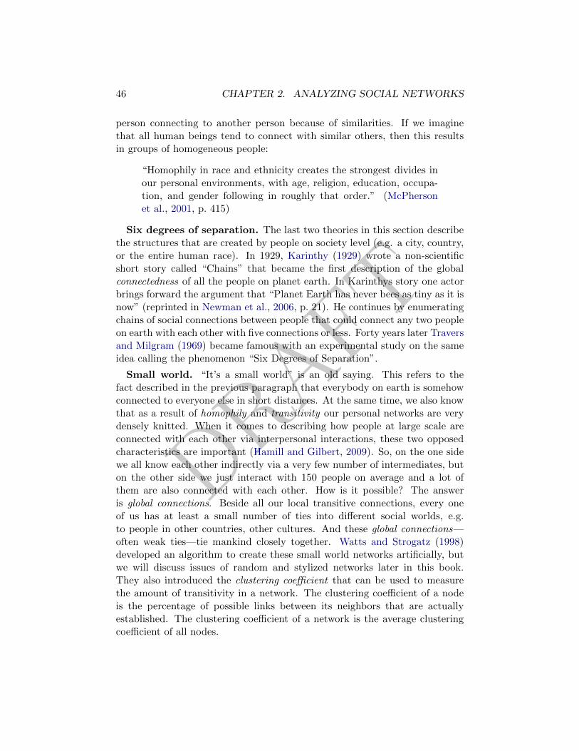
DRAFT
46 CHAPTER 2. ANALYZING SOCIAL NETWORKS
person connecting to another person because of similarities. If we imaginethat all human beings tend to connect with similar others, then this resultsin groups of homogeneous people:
“Homophily in race and ethnicity creates the strongest divides inour personal environments, with age, religion, education, occupa-tion, and gender following in roughly that order.” (McPhersonet al., 2001, p. 415)
Six degrees of separation. The last two theories in this section describethe structures that are created by people on society level (e.g. a city, country,or the entire human race). In 1929, Karinthy (1929) wrote a non-scientificshort story called “Chains” that became the first description of the globalconnectedness of all the people on planet earth. In Karinthys story one actorbrings forward the argument that “Planet Earth has never bees as tiny as it isnow” (reprinted in Newman et al., 2006, p. 21). He continues by enumeratingchains of social connections between people that could connect any two peopleon earth with each other with five connections or less. Forty years later Traversand Milgram (1969) became famous with an experimental study on the sameidea calling the phenomenon “Six Degrees of Separation”.
Small world. “It’s a small world” is an old saying. This refers to thefact described in the previous paragraph that everybody on earth is somehowconnected to everyone else in short distances. At the same time, we also knowthat as a result of homophily and transitivity our personal networks are verydensely knitted. When it comes to describing how people at large scale areconnected with each other via interpersonal interactions, these two opposedcharacteristics are important (Hamill and Gilbert, 2009). So, on the one sidewe all know each other indirectly via a very few number of intermediates, buton the other side we just interact with 150 people on average and a lot ofthem are also connected with each other. How is it possible? The answeris global connections. Beside all our local transitive connections, every oneof us has at least a small number of ties into different social worlds, e.g.to people in other countries, other cultures. And these global connections—often weak ties—tie mankind closely together. Watts and Strogatz (1998)developed an algorithm to create these small world networks artificially, butwe will discuss issues of random and stylized networks later in this book.They also introduced the clustering coefficient that can be used to measurethe amount of transitivity in a network. The clustering coefficient of a nodeis the percentage of possible links between its neighbors that are actuallyestablished. The clustering coefficient of a network is the average clusteringcoefficient of all nodes.

DRAFT
2.4. ANALYZING SOCIAL NETWORKS 47
2.4 Analyzing social networks
Now that we know what drives the creation of links between Agents and whichkind of network structures are formed by these dynamics, we will start toactually analyze networks. First, we visualize the connections of our networkto get an impression of the underlying structure. Second, we are interested inidentifying important actors in our networks. For accomplishing these points,use social networks created from the Tragedy of Julius Caesar. We discusssome details of creating these networks in this chapter and you can find thenetwork matrices for all five acts in the appendix of this book. So, let’s havea look at the Julius Caesar networks.
2.4.1 Visualizing networks
We spent a lot of time discussing different aspects of networks in the lastcouple of pages. Now it is time to actually see how networks look like when wevisualize them. The matrix in Table 2.2 is easy to read but hard to interpret,e.g. it is not easy to identify groups of interacting people or the structure ofthis network. To overcome these drawbacks of the matrix representation, thesociogram representation is used. Sociogram pictures, which were developedin the 1930s by Jacob Levy Moreno (1953) are also called “stick-and-ball”diagrams. Looking at Figure 4.1 helps to explain why. Every Agent in ournetwork is represented by a circle while every connection creates a line betweentwo circles. The “x” in the matrix between the Soothsayer and Caesar issymbolized with a line between those two Agents.
This network visualization makes it easier to see the structure of the un-derlying network. We can see that the two tribunes Flavius and Murellus areinteracting with citizens, that Caesar and the four senators Brutus, Cassius,Casca, and Antony form the core of this network, and that other individualsof the story are connected by a single line with this network core.
A network picture can help us to see an overview of the network structure,but it is just the first step of analysis. The decision of deciding which nodeof the network to put in a certain place in order to show a good network is,fortunately, not your decision. Special algorithms—so called layout algorithms(Torgerson, 1952; Fruchterman and Reingold, 1991)—are included in networkanalysis software to optimize the positioning of the nodes based on the networkstructure. We do not discuss further details of these algorithms in this book,but their purpose is simple. Connected nodes are positioned closely together,while unconnected nodes are kept apart. By doing so, the underlying structure
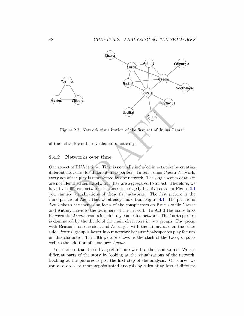
DRAFT
48 CHAPTER 2. ANALYZING SOCIAL NETWORKS
Figure 2.3: Network visualization of the first act of Julius Caesar
of the network can be revealed automatically.
2.4.2 Networks over time
One aspect of DNA is time. Time is normally included in networks by creatingdifferent networks for different time periods. In our Julius Caesar Network,every act of the play is represented by one network. The single scenes of an actare not identified separately, but they are aggregated to an act. Therefore, wehave five different networks because the tragedy has five acts. In Figure 2.4you can see visualizations of these five networks. The first picture is thesame picture of Act 1 that we already know from Figure 4.1. The picture inAct 2 shows the increasing focus of the conspirators on Brutus while Caesarand Antony move to the periphery of the network. In Act 3 the many linksbetween the Agents results in a densely connected network. The fourth pictureis dominated by the divide of the main characters in two groups. The groupwith Brutus is on one side, and Antony is with the triumvirate on the otherside. Brutus’ group is larger in our network because Shakespeares play focuseson this character. The fifth picture shows us the clash of the two groups aswell as the addition of some new Agents.
You can see that these five pictures are worth a thousand words. We seedifferent parts of the story by looking at the visualizations of the network.Looking at the pictures is just the first step of the analysis. Of course, wecan also do a lot more sophisticated analysis by calculating lots of different
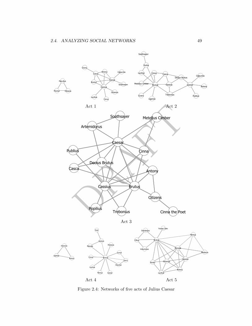
DRAFT
2.4. ANALYZING SOCIAL NETWORKS 49
Act 1 Act 2
Act 3
Act 4 Act 5
Figure 2.4: Networks of five acts of Julius Caesar
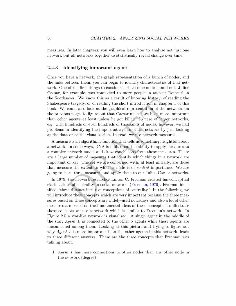
DRAFT
50 CHAPTER 2. ANALYZING SOCIAL NETWORKS
measures. In later chapters, you will even learn how to analyze not just onenetwork but all networks together to statistically reveal change over time.
2.4.3 Identifying important agents
Once you have a network, the graph representation of a bunch of nodes, andthe links between them, you can begin to identify characteristics of that net-work. One of the first things to consider is that some nodes stand out. JuliusCaesar, for example, was connected to more people in ancient Rome thanthe Soothsayer. We know this as a result of knowing history, of reading theShakespeare tragedy, or of reading the short introduction in chapter 1 of thisbook. We could also look at the graphical representation of the networks onthe previous pages to figure out that Caesar must have been more importantthan other agents–at least unless he got killed. In case of larger networks,e.g. with hundreds or even hundreds of thousands of nodes, however, we hadproblems in identifying the important agents of the network by just lookingat the data or at the visualization. Instead, we use network measures.
A measure is an algorithmic function that tells us something insightful abouta network. In some ways, DNA is built upon the ability to apply measures toa complex network model and draw conclusions from those measures. Thereare a large number of measures that identify which things in a network areimportant or key. The set we are concerned with, at least initially, are thosethat measure the extent to which a node is of central importance. We aregoing to learn three measures and apply them to our Julius Caesar networks.
In 1979, the network researcher Linton C. Freeman created his conceptualclarifications of centrality in social networks (Freeman, 1979). Freeman iden-tified “three distinct intuitive conceptions of centrality.” In the following, wewill introduce these concepts which are very important because the three mea-sures based on these concepts are widely-used nowadays and also a lot of othermeasures are based on the fundamental ideas of these concepts. To illustratethese concepts we use a network which is similar to Freeman’s network. InFigure 2.5 a star-like network is visualized. A single agent in the middle ofthe star, Agent 1, is connected to the other 5 agents while these agents areunconnected among them. Looking at this picture and trying to figure outwhy Agent 1 is more important than the other agents in this network, leadsto three different answers. These are the three concepts that Freeman wastalking about:
1. Agent 1 has more connections to other nodes than any other node inthe network (degree)
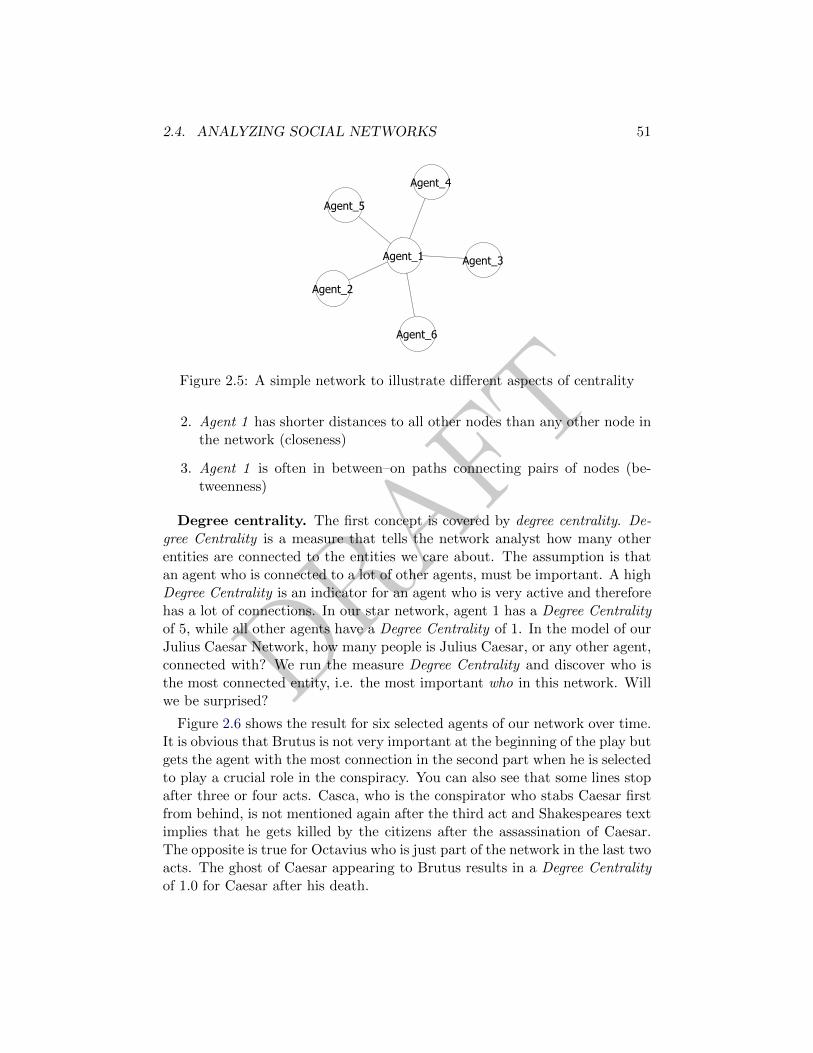
DRAFT
2.4. ANALYZING SOCIAL NETWORKS 51
Figure 2.5: A simple network to illustrate different aspects of centrality
2. Agent 1 has shorter distances to all other nodes than any other node inthe network (closeness)
3. Agent 1 is often in between–on paths connecting pairs of nodes (be-tweenness)
Degree centrality. The first concept is covered by degree centrality. De-gree Centrality is a measure that tells the network analyst how many otherentities are connected to the entities we care about. The assumption is thatan agent who is connected to a lot of other agents, must be important. A highDegree Centrality is an indicator for an agent who is very active and thereforehas a lot of connections. In our star network, agent 1 has a Degree Centralityof 5, while all other agents have a Degree Centrality of 1. In the model of ourJulius Caesar Network, how many people is Julius Caesar, or any other agent,connected with? We run the measure Degree Centrality and discover who isthe most connected entity, i.e. the most important who in this network. Willwe be surprised?
Figure 2.6 shows the result for six selected agents of our network over time.It is obvious that Brutus is not very important at the beginning of the play butgets the agent with the most connection in the second part when he is selectedto play a crucial role in the conspiracy. You can also see that some lines stopafter three or four acts. Casca, who is the conspirator who stabs Caesar firstfrom behind, is not mentioned again after the third act and Shakespeares textimplies that he gets killed by the citizens after the assassination of Caesar.The opposite is true for Octavius who is just part of the network in the last twoacts. The ghost of Caesar appearing to Brutus results in a Degree Centralityof 1.0 for Caesar after his death.
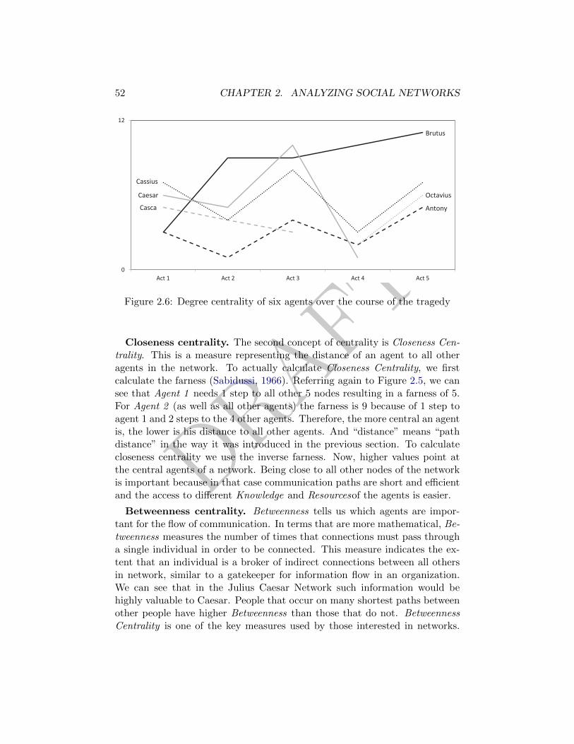
DRAFT
52 CHAPTER 2. ANALYZING SOCIAL NETWORKS
0
12
Act 1 Act 2 Act 3 Act 4 Act 5
Brutus
Cassius
Caesar
Casca Antony
Octavius
Figure 2.6: Degree centrality of six agents over the course of the tragedy
Closeness centrality. The second concept of centrality is Closeness Cen-trality. This is a measure representing the distance of an agent to all otheragents in the network. To actually calculate Closeness Centrality, we firstcalculate the farness (Sabidussi, 1966). Referring again to Figure 2.5, we cansee that Agent 1 needs 1 step to all other 5 nodes resulting in a farness of 5.For Agent 2 (as well as all other agents) the farness is 9 because of 1 step toagent 1 and 2 steps to the 4 other agents. Therefore, the more central an agentis, the lower is his distance to all other agents. And “distance” means “pathdistance” in the way it was introduced in the previous section. To calculatecloseness centrality we use the inverse farness. Now, higher values point atthe central agents of a network. Being close to all other nodes of the networkis important because in that case communication paths are short and efficientand the access to different Knowledge and Resourcesof the agents is easier.
Betweenness centrality. Betweenness tells us which agents are impor-tant for the flow of communication. In terms that are more mathematical, Be-tweenness measures the number of times that connections must pass througha single individual in order to be connected. This measure indicates the ex-tent that an individual is a broker of indirect connections between all othersin network, similar to a gatekeeper for information flow in an organization.We can see that in the Julius Caesar Network such information would behighly valuable to Caesar. People that occur on many shortest paths betweenother people have higher Betweenness than those that do not. BetweennessCentrality is one of the key measures used by those interested in networks.
DRAFT
2.4. ANALYZING SOCIAL NETWORKS 53
0
70
Act 1 Act 2 Act 3 Act 4 Act 5
Brutus
Cassius
Caesar
Casca
Antony
Figure 2.7: Change of betweenness centrality over time
In Figure 2.7 Betweenness Centrality is calculated for some agents. The mostastonishing result is the big change of the score of Brutus over time. In act1, Brutus is very unimportant for the information flow; he is just connectedto agents that are also connected with each other and he lies on no singleshortest path between two other nodes. This situation changes completelyin act 2 when Brutus acts as an intermediate in many connections. Whensearching the shortest paths between all pairs of other agents, Brutus lies onthese paths in almost 70 cases.
For all three measures which were introduced in the previous paragraphsyou need to know one additional point. Look at the y-axes in Figure 2.6 andFigure 2.7. The values for Degree Centrality are in the range from 0 to 11and even higher for Betweenness Centrality. These values are pretty muchdepending on the number of agents in the network. For example, in act 2our network consists of 16 agents. If we want to know how often Brutus ison shortest paths between two other agents, we would look at 15 agents eachof which connected to all other 14 agents resulting in 105 different pairs ofagents. If we add just two nodes, this number goes up to 136. And the chanceis quite high that Brutus, because of his central position in the network,would be on the shortest path of a large number of these pairs of agents. Toprevent this artifact, we scale network measures with the maximal possiblescore. We do not discuss the scaling in detail at this point in the book . Theinterested reader can look in the glossary. For now, we state that the resultof scaling centrality measures is that all scores are in the range of 0 and 1 for
DRAFT
54 CHAPTER 2. ANALYZING SOCIAL NETWORKS
all networks.
2.5 Problem set
1. Think of your three best friends, and now of the three people you havebeen interacting with the most during the last 10 days. Do you see howsimple definitions of your network can change your whole network data?
2. Why would you not add “Citizens” to your own network?
3. Describe reciprocity and transitivity. What is the main difference be-tween these two concepts?
4. Why does homophily constraint the information that you get from yourpersonal network?
5. Why is the world small after all regards to social distances?
6. What do the lines in the network visualizations represent?
7. Why does it make sense to analyze networks over time?
8. What is the highest possible degree one agent can have in a networkwith 50 agents?
9. What is meant by sympathy group and how big is your personal sympathygroup?
10. Find one agent in act 3 with a betweenness centrality score of 0.
11. *Find five agents in act 3 with a betweenness centrality score of 0.
12. *Calculate the farness of the Soothsayer in act 2.
13. *Find a pretty network visualization online. Why do you like the pic-ture? Is the network graph a good approach to visualize the underlyinginformation? What is bad/confusing in your visualization?
14. *Cinna the Poet is getting killed by being confounded with Cinna theconspirator. Think of the centrality measures, what happens when youunify two actors to one node of your network?
15. *Explore the Julius Caesar networks from the book’s website. Createnetwork visualizations that are similar to the figures in this chapter.

DRAFT
2.5. PROBLEM SET 55
16. *Calculate different centrality measures and discuss the results.
17. **Read the centrality article by Freeman (1979). Freeman discusses histhree measures exclusively for connected, undirected, and unweightednetworks. Discuss implications for the measure calculation in the contextof unconnected, directed, and weighted networks.
18. **Find out what about the average number of connections and the clus-tering coefficient of the Facebook friendship network. Imagine two ran-dom people A and B that are friends on Facebook. What is the expectednumber of shared friends of A and B?
19. **Gather the data for a connected and directed network with at least15 nodes. You are now interested in who is connected to all other nodeson short paths. Which metrics X of the three Freeman metrics will youuse? Why is X not trivial for your directed network? Based on theconcepts of this metrics, create two new metrics Xin and Xout that areapplicable for directed networks. Calculate the results of these metricsfor your network and discuss the differences of the results.
20. **Perform a literature review to answer these questions: What are cri-teria for “good” network visualizations. Discuss the network pictures ofthis chapter with these criteria. Create a visualization of the third actthat is better than our visualization. Why is it better?

DRAFT
56 CHAPTER 2. ANALYZING SOCIAL NETWORKS
DRAFT
Chapter 3
Meta-Networks
Based on the techniques Julius Caesar has learned in the previous chapterof this book, he can now complete a thorough network annual analysis ofhow all of his senators, generals and administrators connect to each other sohe can figure out if there are any within his own imperial ranks that are invery central network positions and can become maybe a threat for himself—information that would be valuable to any dictator right? Julius Caesar isinterested in a local rumored plot operating in the Roman imperial Senate.Caesar has identified several social networks containing a number of ”personsof interest” who communicate with each other regularly by letter, chattingat parades, conversing in whispers, meeting in secrecy. Based on carefullyobtained surveillance Caesar constructs a network model of who is talking towhom and come up with an elaborate map detailing these relationships. Hecarefully analyzes this data and draws conclusions about how best to disruptthis network. Once again, it is the hope of the network analyst inside Caesarthat the data obtained reveals vulnerabilities within the network structure.
To get better insights into his empire, Caesar conducts a survey (let usassume for now that all the important people in the empire participate in thissurvey and answer honestly). Caesar can soon discover from the data who istalking to whom inside his empire but he can’t quite determine if by nature ofthese connections any of these pairs of communicators are a threat. After all,his model tells him very little about what they are talking about. His modeltells him very little about what Tasks those that are talking share. His modeltells him very little about what Events those who are talking share in common.Moreover, it would be nice if Caesar had a model of how the Knowledge ofthose who are assigned for specific Tasks actually fits the Knowledge needs to
57

DRAFT
58 CHAPTER 3. META-NETWORKS
successfully accomplish these Tasks. Such a complex picture might indeed bewhat is needed to save Caesar from the Senatorial daggers.
In addition, Caesar is maybe interested in which armories are accessible bywhich generals within his empire. He studies in close detail an inventory ofthe all the armories as well as the servers they are networked to and how theycommunicate with each other. He wants to take this information and drawcertain conclusions about the way the network is structured so he can drawconclusions about how to make his military stronger. Will his current networkmodel of how the armories are connected help him get the job done?
In all these examples we can get network data about people and other enti-ties are connected with each other, be they workers conspiring senators in theRoman imperial senate, administrators and his trusted generals in the upperechelons of his government or how his armories are all interconnected. Clearlythe complex information described above would prove extremely useful in pro-viding an in-depth analysis of the dynamics relevant to Caesar’s dictatorship.Meta-networks are the models to describe this complexity in a network model.
The set of networks for two or more of these entity classes is called themeta-network. The entire field of Dynamic Network Analysis (DNA) is basedon the concept of the meta-network. Therefore, we need to ask what is ameta-network, and how does it relate to our Julius Caesar dataset? In thischapter, you will learn about the different node classes beyond Agents andhow they can be used and combined to create various networks. We will usethese new node classes to collect even more data from the Tragedy of JuliusCaesar. And you will learn about different concepts and measures which makeuse of all these networks.
To begin with, what is an entity? In the previous chapter we defined net-work entities as human beings. In this chapter we are going to extend thisperspective. An entity is essentially the building block of all networks. Ingeneral, an entity is a node in a network. It is what we are networking. It iswhat we are looking at and it can literally be anything that you can possiblythink of in terms of what you can possibly imagine. You name it–it is anentity! We can’t build a network without entities. In DNA, an entity is oftenbest described as a who, what, where, when, how or why. These descriptionsare the hallmark of any good news story and are convenient ways to describeany complex system or story. Networks tell stories and vice versa. We canalmost extrapolate any network from a story and a network model may indeedtell a story, but we are getting ahead of ourselves.
If you take a few moments to ponder this, most anything you can think ofcan fit into one of these categories. So, think of entities in terms of who, what,
DRAFT
3.1. MORE THAN WHO: ADDITIONAL ENTITY CLASSES 59
where, when, and why :
• A who such as Julius Caesar, Cassius, Brutus, CEOs, famous historicalpeople, imaginary people, myths, your friends, family members, terror-ists, people that owe you money, scientists, celebrities, athletes, religiousfigures, etc.
• A where such as The Roman Senate, The streets of Rome, Brutus’House, cities, stores, swimming pools, lakes, rivers, oceans, countries,roads, Planets, galaxies, etc.
• A what such as a dagger, computers, satellites, cars, cell phones, food,money, molecules, etc.
• A why Julius Caesar is becoming too powerful and so should be killed,other beliefs and attitudes.
So now that we met the whos in Julius Caesar, remember that an entitycan be literally anything. But for a moment, think of all the connectionsthat would compose a network of a company or a country. You couldn’tdescribe these networks with one type of entity called ”nodes”. If indeed itwere possible at all, it is plainly obvious that we would need to interconnectall sorts of different types of entities. We would need a model beyond a merenetwork of same type entities. We would need a better model, one that wouldincorporate different entity classes and allow us to perform an analysis on themodel that way. Such a model is called a meta-network.
Before we talk about meta-networks, we to need get a firm understandingof what an entity is and how entities are the building blocks of networks. Inthis chapter, we want to create a meta-network of Julius Caesar, which willattempt to capture and present to us a model of all the entities that make upthe plot of Shakespeare’s classic play. Even though it may seem small, withonly 36 whos, just watch and see what happens when we start factoring inLocations, Knowledge bases, Events–every entity-types that can meaningfullydescribe a who, what, when, where and why of the Julius Caesar Networkmodel. Indeed, things can get complex fast as you will also come to see. Andof course, real world meta-networks can have tens of thousands of nodes.
3.1 More than who: Additional entity classes
It is useful to classify certain type of entities into categories or classes. A groupof entities of the same type is referred to as an entity class. The relation of

DRAFT
60 CHAPTER 3. META-NETWORKS
entity class to entities is sort of like genus to species in the Linnaeus systemof classification. Toward those ends, there are ten entity classes that socialscientist have determined to be of the most value in network analysis: Agents,Resources, Knowledge, and Tasks are the main node classes for which mostof the meta-network measures have been developed (see in the next sectionsof this chapter). The other node classes are Organizations, Locations, Events,Actions, Beliefs, and Roles. These are the genus categories of which we canfit most species–entities. Are they beginning to sound familiar now? Can yousee the parallel between these types and the who, what, when, where, why andhow model?
These classifications are what drive many of the advanced mathematicalalgorithms that can make a highly complex meta-network comprehensible toan analyst. The good news is that nearly anything that can be an entity canneatly fall into one of these entity classes and you will see that as we buildthe Julius Caesar model, we will place our entities into such containers as theentity class types described above. In detail, the ten entity classes can bedefined as follows:
1. Agents are individual decision makers. The most common type of de-cision makers are people. However, this category could also be usedfor other types of actors such as robots or monkeys. A single Agentrepresents any person: a family member, a Roman soldier, Soothsayer,Calpurnia, Cicero, any historical figure, a terrorist, or a teacher.
2. Resources are products, materials, or goods that are necessary to per-form Tasks, Events, and Actions. A Resource could literally be a dagger,a cloak, a crown, a short sword, a computer, money, bombs, tools, orbooks.
3. Knowledge describes cognitive capabilities and skills. Knowledge couldbe Trigonometry, History, English, Economics, the science of DNA, orthe Knowledge about how to perform a surgery or to build bombs.
4. Tasks are well defined procedures or goals. A Task could be any processin a company, e.g. product development or administration, but also theplan to kill Caesar.
5. Organizations are collectives of people that try to reach a common goal.An Organization could be a specific company, the United Nations, orthe government of a country.

DRAFT
3.1. MORE THAN WHO: ADDITIONAL ENTITY CLASSES 61
6. Locations are geographical positions at any aggregation level that de-scribe places or areas. A Location could be 1600 Pennsylvania Avenuein Washington, London, Florida, The Middle East, Earth, or Mars.
7. Events are occurrences or phenomena that happen. An Event could be9-11, the JFK Assignation, the Super Bowl, a wedding, a funeral, or aninauguration. Specific Events are one time occurrences with a specificdate.
8. Actions are specific activities done by Agents. An Action could be buy-ing a car, writing a letter of recommendation, or flying to Africa.
9. Beliefs are any form of religion or other persuasion. A Belief could beto believe that there is a god, or that there are many gods, or that thatEarth is flat. Some Beliefs are signaled by sentiment such as ”war isbad.”
10. Roles describe functions of individual decision makers abstracted fromspecific Agents. A Role could be leader of a group, driver of a car, ormother of an Agent.
In addition to these 10 node classes we use an 11th node class that is differ-ent. Groups also referred to as meta-nodes, are any categorization of nodesinto a cluster. Groups are defined by one or more of the grouping algorithms(see next chapter).
To repeat the function of these node classes and to show their differencesas well as give a first impression about how these node classes are connectedwith each other, we summarize the Julius Caesar plot very briefly. Brutus(Agent) and other senators (Roles) agree that Rome (Location) would bea better place without Caesar (Belief ). To kill Caesar (Task) they form agroup of assassins (Organization). To accomplish their Task they need toknow about Caesar’s daily routine (Knowledge) and how to get their knives(Resources) into the senate. Finally, the assassination (Event) takes placebecause somebody actually stabs Caesar (Action).
So when building a network the DNA scientist needs to be aware of how tocategorize the entities he or she wishes to study, that is a decision has to bemade as to what entity classes are needed and where it makes sense to putthe entity in. To a certain extent one can make up their own entity classessole and separate from the ones aforementioned. However, it probably is notwise to do so; by fitting your entities into a traditional, if not obvious, entityclasses, we can then run powerful measures on them. What is a measure? Wewill get to that shortly.
DRAFT
62 CHAPTER 3. META-NETWORKS
The networks in chapter 2 were all just constructed by using nodes from onesingle node class—Agents. You have just learned that there are ten differentnode classes. When combining them with each other, we can create a lotof networks. Most of these new network data are different from the Agent xAgent networks of chapter 2. For instance, a matrix describing the connectionsbetween Agents and Knowledge, i.e. a skills network, is not squared butrectangular as the x-axis (Agents) and the y-axis (Knowledge) have differententities. If you are having a hard time to imagining these rectangular matrices,don’t worry, you will see a lot of them at the following pages.
But before we can come to the point of coding the meta-network of theTragedy of Julius Caesar, we first have to make the decision which entityclass we will need. Naturally, we need to think up of a least two differentnetworks. But, to really hammer the point home, let us come up with three,maybe five different networks relating to Julius Caesar and add them togetherto see what we get. Again, before we truly get into DNA, our goal is to createmultiple networks to create our multi-modal ”meta-network.” So, let’s nowcreate another network by repeating the process for building our who by whonetwork and then another until we are satisfied that we have captured enoughpertinent and interesting data that could be of use to us if presented as ameta-network. For purposes of our Julius Caesar model, we are going tocapture about as many useful networks as possible, graphing the relationshipsof who, what, where, how. The when is covered by the temporal aspect of thefive acts which have been introduced in the previous chapter. To cover theother aspects, we will create the node classes Knowledge, Tasks, Locations,and Events.
3.1.1 Skills in the roman empire
To build our first network with nodes other than agents, we are going to graphwho x what. The what in this case represents Knowledge (K). So, our who bywhat network constitutes an Agent (A) by Knowledge (K) network. Let usbegin by determining a list of what Knowledge bases would seem applicableto our network. We defined Knowledge as skills. Based on our understandingof the play, we have identified the following Knowledge sets to be of relevanceto the network analysis. Table 3.1 enumerates the six Knowledge nodes thatwe have identified in the Tragedy.
We just selected the—from our perspective—most important skills. Ofcourse, you could come up with a totally different list. In networks that arederived from real world Organizations, the list of Knowledge entities can be
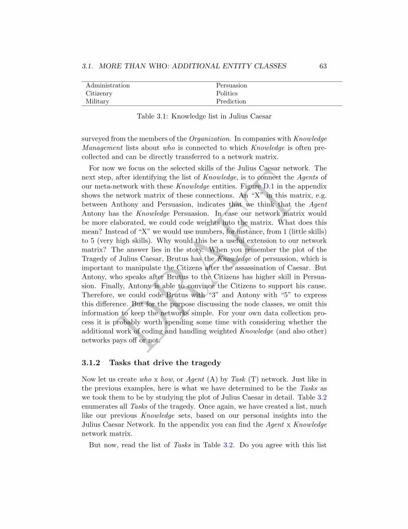
DRAFT
3.1. MORE THAN WHO: ADDITIONAL ENTITY CLASSES 63
Administration PersuasionCitizenry PoliticsMilitary Prediction
Table 3.1: Knowledge list in Julius Caesar
surveyed from the members of the Organization. In companies with KnowledgeManagement lists about who is connected to which Knowledge is often pre-collected and can be directly transferred to a network matrix.
For now we focus on the selected skills of the Julius Caesar network. Thenext step, after identifying the list of Knowledge, is to connect the Agents ofour meta-network with these Knowledge entities. Figure D.1 in the appendixshows the network matrix of these connections. An “X” in this matrix, e.g.between Anthony and Persuasion, indicates that we think that the AgentAntony has the Knowledge Persuasion. In case our network matrix wouldbe more elaborated, we could code weights into the matrix. What does thismean? Instead of “X” we would use numbers, for instance, from 1 (little skills)to 5 (very high skills). Why would this be a useful extension to our networkmatrix? The answer lies in the story. When you remember the plot of theTragedy of Julius Caesar, Brutus has the Knowledge of persuasion, which isimportant to manipulate the Citizens after the assassination of Caesar. ButAntony, who speaks after Brutus to the Citizens has higher skill in Persua-sion. Finally, Antony is able to convince the Citizens to support his cause.Therefore, we could code Brutus with “3” and Antony with “5” to expressthis difference. But for the purpose discussing the node classes, we omit thisinformation to keep the networks simple. For your own data collection pro-cess it is probably worth spending some time with considering whether theadditional work of coding and handling weighted Knowledge (and also other)networks pays off or not.
3.1.2 Tasks that drive the tragedy
Now let us create who x how, or Agent (A) by Task (T) network. Just like inthe previous examples, here is what we have determined to be the Tasks aswe took them to be by studying the plot of Julius Caesar in detail. Table 3.2enumerates all Tasks of the tragedy. Once again, we have created a list, muchlike our previous Knowledge sets, based on our personal insights into theJulius Caesar Network. In the appendix you can find the Agent x Knowledgenetwork matrix.
But now, read the list of Tasks in Table 3.2. Do you agree with this list
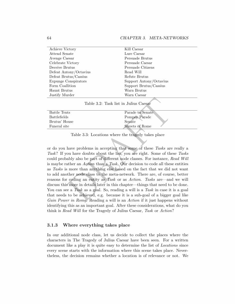
DRAFT
64 CHAPTER 3. META-NETWORKS
Achieve Victory Kill CaesarAttend Senate Lure CaesarAvenge Caesar Persuade BrutusCelebrate Victory Persuade CaesarDeceive Brutus Persuade CitizensDefeat Antony/Octavius Read WillDefeat Brutus/Cassius Refute BrutusExpunge Conspirators Support Antony/OctaviusForm Coallition Support Brutus/CassiusHaunt Brutus Warn BrutusJustify Murder Warn Caesar
Table 3.2: Task list in Julius Caesar
Battle Tents Parade to SenateBattlefields Pompey ParadeBrutus’ House SenateFuneral site Streets of Rome
Table 3.3: Locations where the tragedy takes place
or do you have problems in accepting that some of these Tasks are really aTask? If you have doubts about the list, you are right. Some of these Taskscould probably also be part of different node classes. For instance, Read Willis maybe rather an Action than a Task. Our decision to code all these entitiesas Tasks is more than anything else based on the fact that we did not wantto add another node class to the meta-network. There are, of course, betterreasons for coding an entity as Task or as Action. Tasks are—and we willdiscuss this more in details later in this chapter—things that need to be done.You can see a Task as a goal. So, reading a will is a Task in case it is a goalthat needs to be achieved, e.g. because it is a sub-goal of a bigger goal likeGain Power in Rome. Reading a will is an Action if it just happens withoutidentifying this as an important goal. After these considerations, what do youthink is Read Will for the Tragedy of Julius Caesar, Task or Action?
3.1.3 Where everything takes place
In our additional node class, let us decide to collect the places where thecharacters in The Tragedy of Julius Caesar have been seen. For a writtendocument like a play it is quite easy to determine the list of Locations sinceevery scene starts with the information where this scene takes place. Never-theless, the decision remains whether a location is of relevance or not. We
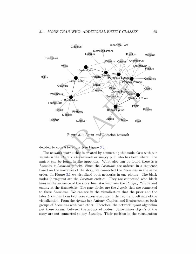
DRAFT
3.1. MORE THAN WHO: ADDITIONAL ENTITY CLASSES 65
Antony
Brutus
Caesar
Calpurnia
CascaCassius CiceroCinna
Citizens
Flavius
Lucilius
Marullus
Octavius
Soothsayer
Decius Brutus
LigariusMetellus Cimber
PortiaPublius
Trebonius
Artemidorus
Cinna the Poet
Popilius
Claudius
Lepidus LuciusMessala
Pindarus
Poet
Titinius
Varro
Clitus
Dardanius
Strato
Volumnius
Young Cato
Battle Tents
Battlefields
Brutus' House
Funeral site
Parade to SenatePompey Parade
Senate
Streets of Rome
Figure 3.1: Agent and Location network
decided to code 8 locations (see Figure 3.3).
The network matrix that is created by connecting this node class with ourAgents is the where x who network or simply put: who has been where. Thematrix can be found in the appendix. What also can be found there is aLocation x Location matrix. Since the Locations are ordered in a sequencebased on the narrative of the story, we connected the Locations in the sameorder. In Figure 3.1 we visualized both networks in one picture. The blacknodes (hexagons) are the Location entities. They are connected with blacklines in the sequence of the story line, starting from the Pompey Parade andending at the Battlefields. The gray circles are the Agents that are connectedto these Locations. We can see in the visualization that the prior and thelater Locations form two more cohesive groups in the right and left side of thevisualization. From the Agents just Antony, Cassius, and Brutus connect bothgroups of Locations with each other. Therefore, the network layout algorithmput these Agents between the groups of nodes. Some minor Agents of thestory are not connected to any Location. Their position in the visualization
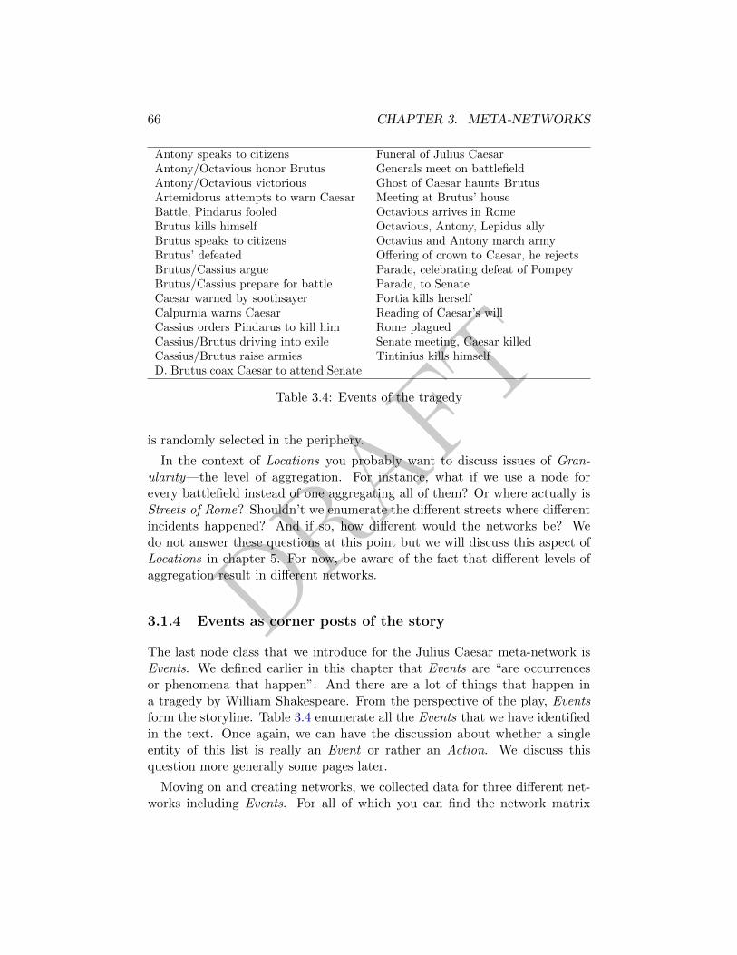
DRAFT
66 CHAPTER 3. META-NETWORKS
Antony speaks to citizens Funeral of Julius CaesarAntony/Octavious honor Brutus Generals meet on battlefieldAntony/Octavious victorious Ghost of Caesar haunts BrutusArtemidorus attempts to warn Caesar Meeting at Brutus’ houseBattle, Pindarus fooled Octavious arrives in RomeBrutus kills himself Octavious, Antony, Lepidus allyBrutus speaks to citizens Octavius and Antony march armyBrutus’ defeated Offering of crown to Caesar, he rejectsBrutus/Cassius argue Parade, celebrating defeat of PompeyBrutus/Cassius prepare for battle Parade, to SenateCaesar warned by soothsayer Portia kills herselfCalpurnia warns Caesar Reading of Caesar’s willCassius orders Pindarus to kill him Rome plaguedCassius/Brutus driving into exile Senate meeting, Caesar killedCassius/Brutus raise armies Tintinius kills himselfD. Brutus coax Caesar to attend Senate
Table 3.4: Events of the tragedy
is randomly selected in the periphery.
In the context of Locations you probably want to discuss issues of Gran-ularity—the level of aggregation. For instance, what if we use a node forevery battlefield instead of one aggregating all of them? Or where actually isStreets of Rome? Shouldn’t we enumerate the different streets where differentincidents happened? And if so, how different would the networks be? Wedo not answer these questions at this point but we will discuss this aspect ofLocations in chapter 5. For now, be aware of the fact that different levels ofaggregation result in different networks.
3.1.4 Events as corner posts of the story
The last node class that we introduce for the Julius Caesar meta-network isEvents. We defined earlier in this chapter that Events are “are occurrencesor phenomena that happen”. And there are a lot of things that happen ina tragedy by William Shakespeare. From the perspective of the play, Eventsform the storyline. Table 3.4 enumerate all the Events that we have identifiedin the text. Once again, we can have the discussion about whether a singleentity of this list is really an Event or rather an Action. We discuss thisquestion more generally some pages later.
Moving on and creating networks, we collected data for three different net-works including Events. For all of which you can find the network matrix
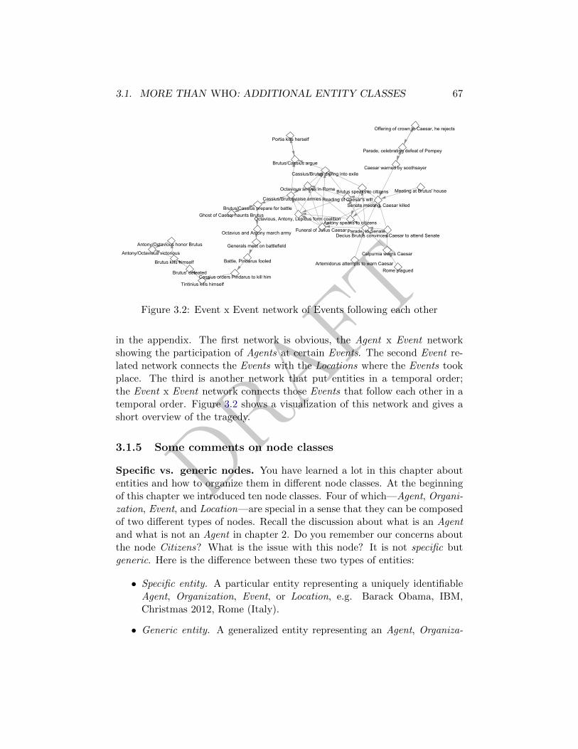
DRAFT
3.1. MORE THAN WHO: ADDITIONAL ENTITY CLASSES 67
Antony speaks to citizens
Antony/Octavious honor Brutus
Antony/Octavious victorious
Artemidorus attempts to warn CaesarBattle, Pindarus fooledBrutus kills himself
Brutus speaks to citizens
Brutus' defeated
Brutus/Cassius argue
Brutus/Cassius prepare for battle
Caesar warned by soothsayer
Calpurnia warns Caesar
Cassius orders Pindarus to kill him
Cassius/Brutus driving into exile
Cassius/Brutus raise armies
Decius Brutus convinces Caesar to attend SenateFuneral of Julius Caesar
Generals meet on battlefield
Ghost of Caesar haunts Brutus
Meeting at Brutus' houseOctavious arrives in Rome
Octavious, Antony, Lepidus form coalition
Octavius and Antony march army
Offering of crown to Caesar, he rejects
Parade, celebrating defeat of Pompey
Parade, to Senate
Portia kills herself
Reading of Caesar's will
Rome plagued
Senate meeting, Caesar killed
Tintinius kills himself
Figure 3.2: Event x Event network of Events following each other
in the appendix. The first network is obvious, the Agent x Event networkshowing the participation of Agents at certain Events. The second Event re-lated network connects the Events with the Locations where the Events tookplace. The third is another network that put entities in a temporal order;the Event x Event network connects those Events that follow each other in atemporal order. Figure 3.2 shows a visualization of this network and gives ashort overview of the tragedy.
3.1.5 Some comments on node classes
Specific vs. generic nodes. You have learned a lot in this chapter aboutentities and how to organize them in different node classes. At the beginningof this chapter we introduced ten node classes. Four of which—Agent, Organi-zation, Event, and Location—are special in a sense that they can be composedof two different types of nodes. Recall the discussion about what is an Agentand what is not an Agent in chapter 2. Do you remember our concerns aboutthe node Citizens? What is the issue with this node? It is not specific butgeneric. Here is the difference between these two types of entities:
• Specific entity. A particular entity representing a uniquely identifiableAgent, Organization, Event, or Location, e.g. Barack Obama, IBM,Christmas 2012, Rome (Italy).
• Generic entity. A generalized entity representing an Agent, Organiza-
DRAFT
68 CHAPTER 3. META-NETWORKS
tion, Event, or Location, e.g. citizen, committee, Christmas, house.
It is importance to differentiate between generic and specific entities. Thisis particularly important when it comes to measure calculation with networkdata. We talk more about measures later in this chapter, but we can imaginea simple example: Let us assume that some police officers in Rome wantedto analyze the background stories behind the assassination of Julius Caesarsome days after his death. For this purpose, police officers fan out to differentLocations and try to figure out who participated in different Events that tookplace in these Locations. The result of this data gathering process could besimilar to our Agent x Location network in Figure ??. After analyzing thisnetwork, guess what, beside Brutus and Antony, the Agent “Citizens” is veryimportant in this network. So, while the fact that citizens are connected tosome incidents or to some Agents was an interesting information for visual-izing the data and understanding the story, this becomes problematic in thecontext of measures because one and the same generic node can representdifferent specific entities. Therefore, a generic node can—dependent from themeasure—create artifacts in the results.
Knowledge vs. Resources. Note that there is one entity set that we arenot employing in our Julius Caesar dataset even this node class sounds quiteimportant based on the definition at the beginning of this chapter, and that isResources. Why have we opted not to use Resources? Primarily because themain characters in the tragedy did not use important Resources during thecourse of the play. In addition, it seemed that Knowledge was every bit as aResource and they were in a sense interchangeable in our network. It is notalways easy to decide whether to put an entity into a Knowledge node class ora Resource node class. For instance, having a Bachelor’s degree in computerscience is connected to a lot of Knowledge. That Bachelor’s degree can surelybe also a Resource for an IT department of a company.
The good news for you: Later in this chapter you will learn about differentmeasures for meta-networks. When you read about these measures as well astheir underlying concepts, you will figure out that Knowledge and Resourcesare most of the time treaded interchangeable by the network measures. There-fore, it is actually not very important whether you decide for Knowledge orResources, as long as you stay consistent within your project.
Task vs. Action vs. Event. We also had some difficulties in the previousparagraphs to decide whether an entity is a Task, and Event, or an Action.For clarification, Tasks are scheduled or planned activities, for instance, fromthe perspective of the conspirators in William Shakespeare’s tragedy, killingCaesar is a Task. The assassination of Caesar is an Event—even more a
DRAFT
3.2. ADDING IT ALL TOGETHER – THE META-NETWORK 69
specific Event. Focusing more closely to the Event, we could have the need todescribe a bit more in detail what is going on. For this reason we also havethe node class Action. So, the actual killing—the stabbing of Caesar—can becoded as Action.
In general, you are very much interesting in Tasks as Tasks describe theregular patters of activity in a meta-network. In addition, you will see thatTasks are heavily involved in multi-mode measures which is also an argumentfor coding entities that are hard to decide rather as Tasks than as Event orAction.
3.2 Adding it all together – the meta-network
As you should be seeing by now, real networks are not one dimensional. Peoplehave Knowledge, they have access to Resources, Events happen and changenetworks and certain nodal points will contain varying attributes distinguish-ing them from the others. In fact, real networks for that matter are rarelyone dimensional except, perhaps, on the most abstract levels. For the JuliusCaesar network we have coded the following ten networks:
1. Agent x Agent (who knows who)
2. Agent x Event (who goes to what)
3. Agent x Knowledge (who knows what)
4. Agent x Location (who is where)
5. Agent x Task (who does what)
6. Event x Event (when by when)
7. Knowledge x Task (what is needed to do what)
8. Location x Location (where by where)
9. Task x Event (what by when)
10. Task x Task (what by what)
When looking at this list and recalling the ten node classes that we haveintroduced in the beginning of this chapter, it is easy to imagine that there aremany more possible networks that we can create with these 10 node classes.Table 3.5 shows all networks based on all possible combinations of node classes.As you can see, there are 55 different networks for one single meta-network.Of course, in most of your network projects you will not use them all at thesame time, but be aware of them because every additional network can giveyou deeper insights into your real-world system that you are going to describe.
DRAFT
70 CHAPTER 3. META-NETWORKS
Now you may be saying to yourself–just what kind of model are we now leftwith? This complex meta-network could be said to resemble a ball of yarn.What are we to make of it? Well, your reaction is to be expected because meta-network analysis is beyond first intuitions and the resultant meta-networkcan be hard for an analyst to comprehend. However, this is where powerfulcomputational methods come into play in the form of measures and we canbegin to break down the meta-network and glean some powerful insight intothe network’s architecture.
3.3 Concepts for two entity classes
It is time to revisit measures once again. We learned in previous chapters thata measure tells us something unique about a network using computationalmethods. More specifically, a measure is an algorithm specially formulated totell us meaningful information about network data that we apply our algo-rithm to. In chapter 2, you have learned about centrality measures that canidentify important nodes in networks.
So far as the dynamic network analyst is concerned, measures can spantwo or even more entity classes. Such measures are carefully constructed andarrived at by research and scientific method.
Measures and algorithm are created to answer questions by analyzing net-work data. These questions can be grouped based on the underlying ideas.We call these groups of measures and questions concepts. In the followingwe describe these concepts and introduce some measures that can be derivedfrom the concepts. In this chapter we focus on discussing the measures. Wewill also use the measures to analyze the Julius Caesar network. We will notdiscuss the algorithmic details of the measures. This will be accomplished inthe appendix. The interested reader can explore all the mathematical detailsof the measures that we are using at the end of this book.
3.3.1 Quantity
Let’s start with the easiest and most intuitive concept of two-mode measures—quantity. Quantity measures simply count or summarize information. Re-member Degree Centrality (Freeman, 1979), a measures that we used in chap-ter 2 to identify the most active Agents in our network. This centrality was cal-culated in the one-mode network describing the interactions between Agents.We use the same idea to describe activity in two-mode networks. We con-structed the Agent x Task network earlier in this chapter. We can now use

DRAFT
3.3. CONCEPTS FOR TWO ENTITY CLASSES 71
Agen
tsKnowledge
Resources
Tasks
Organization
Even
tActions
Loca
tions
Beliefs
Roles
Agen
tInteraction
Network
Knowledge
Network
AR
Network
Assignmen
tNetwork
Employmen
tNetwork
AE
Network
AA
Network
AL
Network
AB
Network
AX
Network
Knowledge
Inform
ation
Network
KR
Network
Req
uirem
ents
Network
Compe-tency
Network
KE
Network
KA
Network
KL
Network
KB
Network
KX
Network
Resources
RR
Network
Preceden
ceNetwork
Industrial
Network
RE
Network
RA
Network
RL
Network
RB
Network
RX
Network
Tasks
Interorganizational
Network
TE
Network
TA
Network
TL
Network
TB
Network
TX
Network
Organization
OE
Network
OA
Network
OL
Network
OB
Network
OX
Network
Even
tEE
Network
EA
Network
EL
Network
EB
Network
EX
Network
Actions
AA
Network
AL
Network
AB
Network
AX
Network
Loca
tions
LL
Network
LB
Network
LX
Network
Beliefs
BB
Network
BX
Network
Roles
RX
Network
Tab
le3.
5:M
eta-
net
wor
km
atri
xw
ith
all
pos
sib
le55
net
wor
ks
bas
edon
10
nod
ecl
ass
es
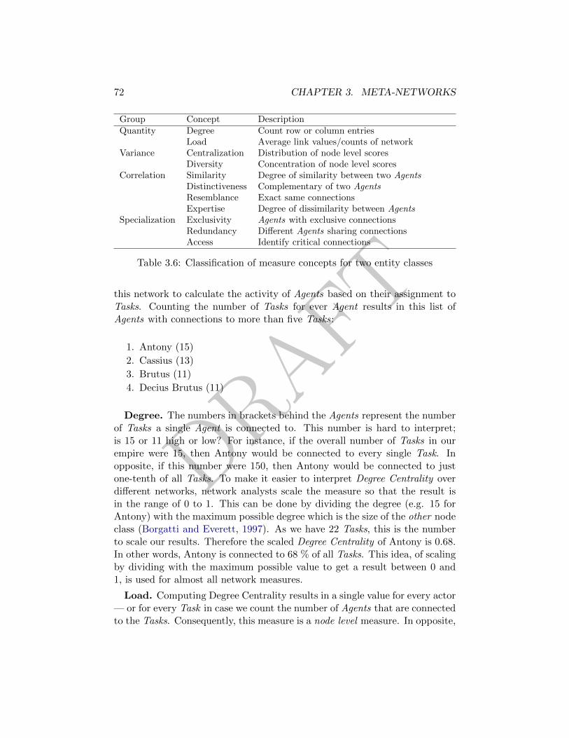
DRAFT
72 CHAPTER 3. META-NETWORKS
Group Concept DescriptionQuantity Degree Count row or column entries
Load Average link values/counts of networkVariance Centralization Distribution of node level scores
Diversity Concentration of node level scoresCorrelation Similarity Degree of similarity between two Agents
Distinctiveness Complementary of two AgentsResemblance Exact same connectionsExpertise Degree of dissimilarity between Agents
Specialization Exclusivity Agents with exclusive connectionsRedundancy Different Agents sharing connectionsAccess Identify critical connections
Table 3.6: Classification of measure concepts for two entity classes
this network to calculate the activity of Agents based on their assignment toTasks. Counting the number of Tasks for ever Agent results in this list ofAgents with connections to more than five Tasks:
1. Antony (15)
2. Cassius (13)
3. Brutus (11)
4. Decius Brutus (11)
Degree. The numbers in brackets behind the Agents represent the numberof Tasks a single Agent is connected to. This number is hard to interpret;is 15 or 11 high or low? For instance, if the overall number of Tasks in ourempire were 15, then Antony would be connected to every single Task. Inopposite, if this number were 150, then Antony would be connected to justone-tenth of all Tasks. To make it easier to interpret Degree Centrality overdifferent networks, network analysts scale the measure so that the result isin the range of 0 to 1. This can be done by dividing the degree (e.g. 15 forAntony) with the maximum possible degree which is the size of the other nodeclass (Borgatti and Everett, 1997). As we have 22 Tasks, this is the numberto scale our results. Therefore the scaled Degree Centrality of Antony is 0.68.In other words, Antony is connected to 68 % of all Tasks. This idea, of scalingby dividing with the maximum possible value to get a result between 0 and1, is used for almost all network measures.
Load. Computing Degree Centrality results in a single value for every actor— or for every Task in case we count the number of Agents that are connectedto the Tasks. Consequently, this measure is a node level measure. In opposite,
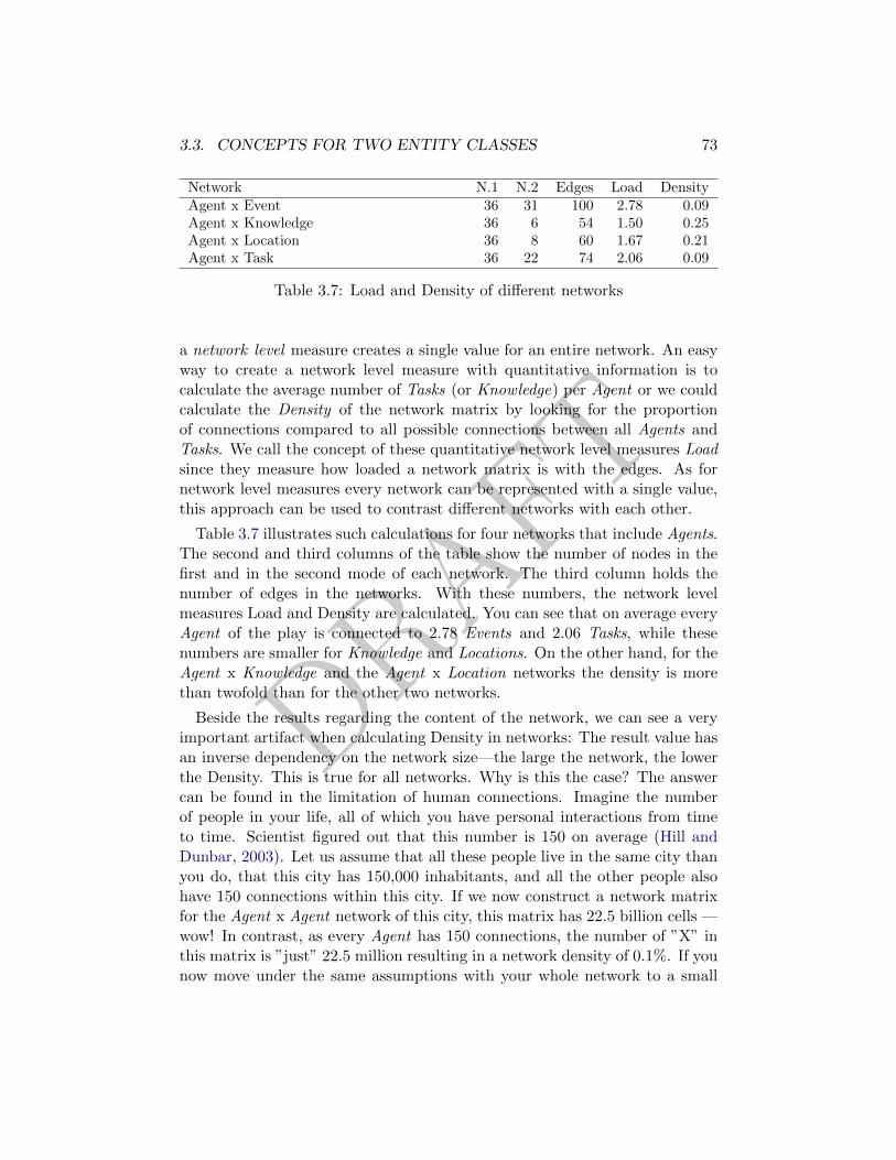
DRAFT
3.3. CONCEPTS FOR TWO ENTITY CLASSES 73
Network N.1 N.2 Edges Load DensityAgent x Event 36 31 100 2.78 0.09Agent x Knowledge 36 6 54 1.50 0.25Agent x Location 36 8 60 1.67 0.21Agent x Task 36 22 74 2.06 0.09
Table 3.7: Load and Density of different networks
a network level measure creates a single value for an entire network. An easyway to create a network level measure with quantitative information is tocalculate the average number of Tasks (or Knowledge) per Agent or we couldcalculate the Density of the network matrix by looking for the proportionof connections compared to all possible connections between all Agents andTasks. We call the concept of these quantitative network level measures Loadsince they measure how loaded a network matrix is with the edges. As fornetwork level measures every network can be represented with a single value,this approach can be used to contrast different networks with each other.
Table 3.7 illustrates such calculations for four networks that include Agents.The second and third columns of the table show the number of nodes in thefirst and in the second mode of each network. The third column holds thenumber of edges in the networks. With these numbers, the network levelmeasures Load and Density are calculated. You can see that on average everyAgent of the play is connected to 2.78 Events and 2.06 Tasks, while thesenumbers are smaller for Knowledge and Locations. On the other hand, for theAgent x Knowledge and the Agent x Location networks the density is morethan twofold than for the other two networks.
Beside the results regarding the content of the network, we can see a veryimportant artifact when calculating Density in networks: The result value hasan inverse dependency on the network size—the large the network, the lowerthe Density. This is true for all networks. Why is this the case? The answercan be found in the limitation of human connections. Imagine the numberof people in your life, all of which you have personal interactions from timeto time. Scientist figured out that this number is 150 on average (Hill andDunbar, 2003). Let us assume that all these people live in the same city thanyou do, that this city has 150,000 inhabitants, and all the other people alsohave 150 connections within this city. If we now construct a network matrixfor the Agent x Agent network of this city, this matrix has 22.5 billion cells —wow! In contrast, as every Agent has 150 connections, the number of ”X” inthis matrix is ”just” 22.5 million resulting in a network density of 0.1%. If younow move under the same assumptions with your whole network to a small
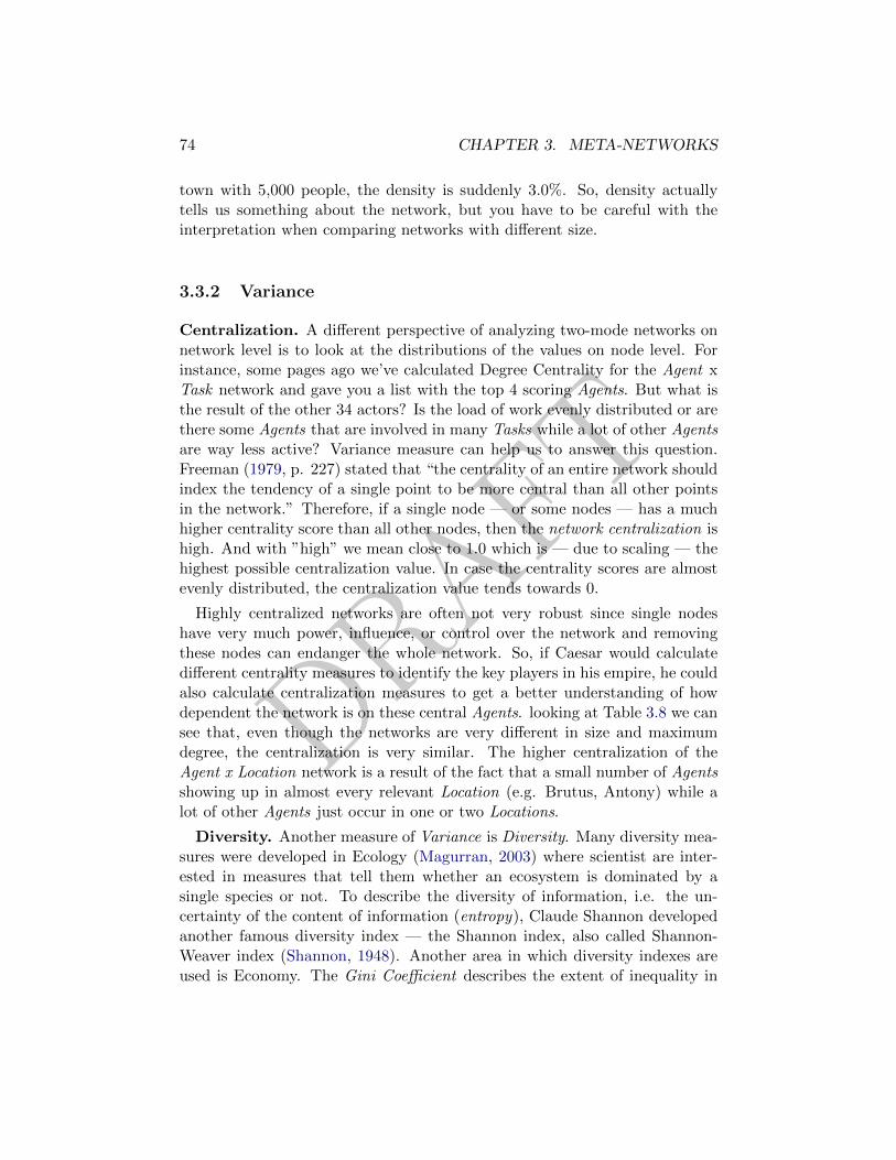
DRAFT
74 CHAPTER 3. META-NETWORKS
town with 5,000 people, the density is suddenly 3.0%. So, density actuallytells us something about the network, but you have to be careful with theinterpretation when comparing networks with different size.
3.3.2 Variance
Centralization. A different perspective of analyzing two-mode networks onnetwork level is to look at the distributions of the values on node level. Forinstance, some pages ago we’ve calculated Degree Centrality for the Agent xTask network and gave you a list with the top 4 scoring Agents. But what isthe result of the other 34 actors? Is the load of work evenly distributed or arethere some Agents that are involved in many Tasks while a lot of other Agentsare way less active? Variance measure can help us to answer this question.Freeman (1979, p. 227) stated that “the centrality of an entire network shouldindex the tendency of a single point to be more central than all other pointsin the network.” Therefore, if a single node — or some nodes — has a muchhigher centrality score than all other nodes, then the network centralization ishigh. And with ”high” we mean close to 1.0 which is — due to scaling — thehighest possible centralization value. In case the centrality scores are almostevenly distributed, the centralization value tends towards 0.
Highly centralized networks are often not very robust since single nodeshave very much power, influence, or control over the network and removingthese nodes can endanger the whole network. So, if Caesar would calculatedifferent centrality measures to identify the key players in his empire, he couldalso calculate centralization measures to get a better understanding of howdependent the network is on these central Agents. looking at Table 3.8 we cansee that, even though the networks are very different in size and maximumdegree, the centralization is very similar. The higher centralization of theAgent x Location network is a result of the fact that a small number of Agentsshowing up in almost every relevant Location (e.g. Brutus, Antony) while alot of other Agents just occur in one or two Locations.
Diversity. Another measure of Variance is Diversity. Many diversity mea-sures were developed in Ecology (Magurran, 2003) where scientist are inter-ested in measures that tell them whether an ecosystem is dominated by asingle species or not. To describe the diversity of information, i.e. the un-certainty of the content of information (entropy), Claude Shannon developedanother famous diversity index — the Shannon index, also called Shannon-Weaver index (Shannon, 1948). Another area in which diversity indexes areused is Economy. The Gini Coefficient describes the extent of inequality in
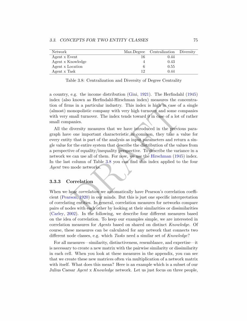
DRAFT
3.3. CONCEPTS FOR TWO ENTITY CLASSES 75
Network Max.Degree Centralization DiversityAgent x Event 16 0.44Agent x Knowledge 4 0.43Agent x Location 6 0.55Agent x Task 12 0.44
Table 3.8: Centralization and Diversity of Degree Centrality
a country, e.g. the income distribution (Gini, 1921). The Herfindahl (1945)index (also known as Herfindahl-Hirschman index) measures the concentra-tion of firms in a particular industry. This index is high in case of a single(almost) monopolistic company with very high turnover and some companieswith very small turnover. The index tends toward 0 in case of a lot of rathersmall companies.
All the diversity measures that we have introduced in the previous para-graph have one important characteristic in common, they take a value forevery entity that is part of the analysis as input parameters and return a sin-gle value for the entire system that describe the distribution of the values froma perspective of equality/inequality perspective. To describe the variance in anetwork we can use all of them. For now, we use the Hirschman (1945) index.In the last column of Table 3.8 you can find this index applied to the fourAgent two mode networks.
3.3.3 Correlation
When we hear correlation we automatically have Pearson’s correlation coeffi-cient (Pearson, 1920) in our minds. But this is just one specific interpretationof correlating entities. In general, correlation measures for networks comparepairs of nodes with each other by looking at their similarities or dissimilarities(Carley, 2002). In the following, we describe four different measures basedon the idea of correlation. To keep our examples simple, we are interested incorrelation measures for Agents based on shared on distinct Knowledge. Ofcourse, these measures can be calculated for any network that connects twodifferent node classes, e.g. which Tasks need a similar set of Knowledge?
For all measures—similarity, distinctiveness, resemblance, and expertise—itis necessary to create a new matrix with the pairwise similarity or dissimilarityin each cell. When you look at these measures in the appendix, you can seethat we create these new matrices often via multiplication of a network matrixwith itself. What does this mean? Here is an example which is a subset of ourJulius Caesar Agent x Knowledge network. Let us just focus on three people,
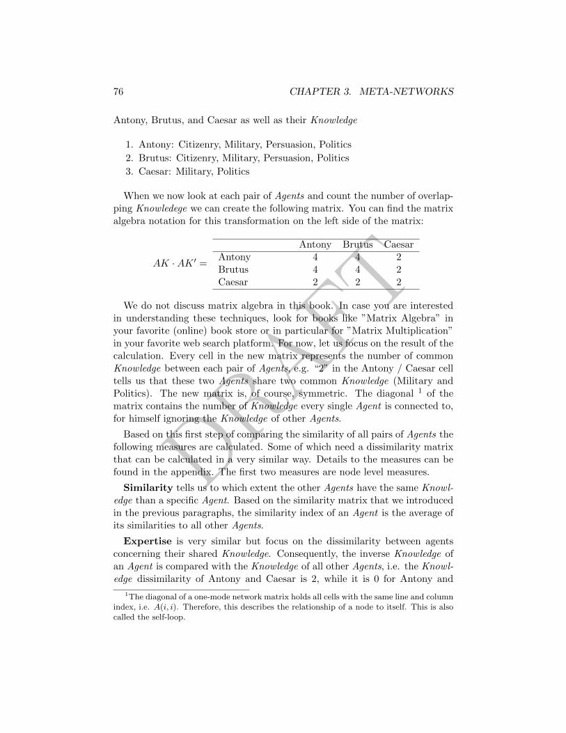
DRAFT
76 CHAPTER 3. META-NETWORKS
Antony, Brutus, and Caesar as well as their Knowledge
1. Antony: Citizenry, Military, Persuasion, Politics
2. Brutus: Citizenry, Military, Persuasion, Politics
3. Caesar: Military, Politics
When we now look at each pair of Agents and count the number of overlap-ping Knowledege we can create the following matrix. You can find the matrixalgebra notation for this transformation on the left side of the matrix:
AK ·AK ′ =
Antony Brutus CaesarAntony 4 4 2Brutus 4 4 2Caesar 2 2 2
We do not discuss matrix algebra in this book. In case you are interestedin understanding these techniques, look for books like ”Matrix Algebra” inyour favorite (online) book store or in particular for ”Matrix Multiplication”in your favorite web search platform. For now, let us focus on the result of thecalculation. Every cell in the new matrix represents the number of commonKnowledge between each pair of Agents, e.g. “2” in the Antony / Caesar celltells us that these two Agents share two common Knowledge (Military andPolitics). The new matrix is, of course, symmetric. The diagonal 1 of thematrix contains the number of Knowledge every single Agent is connected to,for himself ignoring the Knowledge of other Agents.
Based on this first step of comparing the similarity of all pairs of Agents thefollowing measures are calculated. Some of which need a dissimilarity matrixthat can be calculated in a very similar way. Details to the measures can befound in the appendix. The first two measures are node level measures.
Similarity tells us to which extent the other Agents have the same Knowl-edge than a specific Agent. Based on the similarity matrix that we introducedin the previous paragraphs, the similarity index of an Agent is the average ofits similarities to all other Agents.
Expertise is very similar but focus on the dissimilarity between agentsconcerning their shared Knowledge. Consequently, the inverse Knowledge ofan Agent is compared with the Knowledge of all other Agents, i.e. the Knowl-edge dissimilarity of Antony and Caesar is 2, while it is 0 for Antony and
1The diagonal of a one-mode network matrix holds all cells with the same line and columnindex, i.e. A(i, i). Therefore, this describes the relationship of a node to itself. This is alsocalled the self-loop.
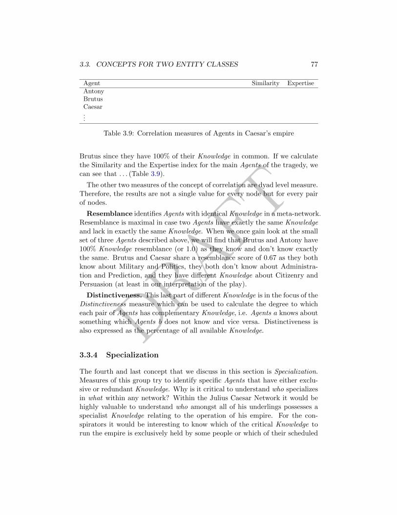
DRAFT
3.3. CONCEPTS FOR TWO ENTITY CLASSES 77
Agent Similarity ExpertiseAntonyBrutusCaesar...
Table 3.9: Correlation measures of Agents in Caesar’s empire
Brutus since they have 100% of their Knowledge in common. If we calculatethe Similarity and the Expertise index for the main Agents of the tragedy, wecan see that . . . (Table 3.9).
The other two measures of the concept of correlation are dyad level measure.Therefore, the results are not a single value for every node but for every pairof nodes.
Resemblance identifies Agents with identical Knowledge in a meta-network.Resemblance is maximal in case two Agents have exactly the same Knowledgeand lack in exactly the same Knowledge. When we once gain look at the smallset of three Agents described above, we will find that Brutus and Antony have100% Knowledge resemblance (or 1.0) as they know and don’t know exactlythe same. Brutus and Caesar share a resemblance score of 0.67 as they bothknow about Military and Politics, they both don’t know about Administra-tion and Prediction, and they have different Knowledge about Citizenry andPersuasion (at least in our interpretation of the play).
Distinctiveness. This last part of different Knowledge is in the focus of theDistinctiveness measure which can be used to calculate the degree to whicheach pair of Agents has complementary Knowledge, i.e. Agents a knows aboutsomething which Agents b does not know and vice versa. Distinctiveness isalso expressed as the percentage of all available Knowledge.
3.3.4 Specialization
The fourth and last concept that we discuss in this section is Specialization.Measures of this group try to identify specific Agents that have either exclu-sive or redundant Knowledge. Why is it critical to understand who specializesin what within any network? Within the Julius Caesar Network it would behighly valuable to understand who amongst all of his underlings possesses aspecialist Knowledge relating to the operation of his empire. For the con-spirators it would be interesting to know which of the critical Knowledge torun the empire is exclusively held by some people or which of their scheduled
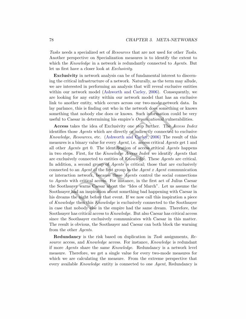
DRAFT
78 CHAPTER 3. META-NETWORKS
Tasks needs a specialized set of Resources that are not used for other Tasks.Another perspective on Specialization measures is to identify the extent towhich the Knowledge in a network is redundantly connected to Agents. Butlet us first have a closer look at Exclusivity.
Exclusivity in network analysis can be of fundamental interest to discern-ing the critical infrastructure of a network. Naturally, as the term may allude,we are interested in performing an analysis that will reveal exclusive entitieswithin our network model (Ashworth and Carley, 2006). Consequently, weare looking for any entity within our network model that has an exclusivelink to another entity, which occurs across our two-mode network data. Inlay parlance, this is finding out who in the network does something or knowssomething that nobody else does or knows. Such information could be veryuseful to Caesar in determining his empire’s Organizational vulnerabilities.
Access takes the idea of Exclusivity one step further. The Access Indexidentifies those Agents which are directly or indirectly connected to exclusiveKnowledge, Resources, etc. (Ashworth and Carley, 2006) The result of thismeasures is a binary value for every Agent, i.e. access critical Agents get 1 andall other Agents get 0. The identification of access critical Agents happensin two steps. First, for the Knowledge Access Index we identify Agents thatare exclusively connected to entities of Knowledge. These Agents are critical.In addition, a second group of Agents is critical; those that are exclusivelyconnected to an Agent of the first group in the Agent x Agent communicationor interaction network, because these Agents control the social connectionsto Agents with critical access. For instance, in the first act of Julius Caesarthe Soothsayer warns Caesar about the “Ides of March”. Let us assume theSoothsayer had an inspiration about something bad happening with Caesar inhis dreams the night before that event. If we now call this inspiration a pieceof Knowledge then this Knowledge is exclusively connected to the Soothsayerin case that nobody else in the empire had the same dream. Therefore, theSoothsayer has critical access to Knowledge. But also Caesar has critical accesssince the Soothsayer exclusively communicates with Caesar in this matter.The result is obvious, the Soothsayer and Caesar can both block the warningfrom the other Agents.
Redundancy is the risk based on duplication in Task assignments, Re-source access, and Knowledge access. For instance, Knowledge is redundantif more Agents share the same Knowledge. Redundancy is a network levelmeasure. Therefore, we get a single value for every two-mode measures forwhich we are calculating the measure. From the extreme perspective thatevery available Knowledge entity is connected to one Agent, Redundancy is
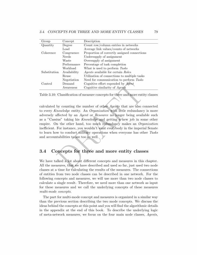
DRAFT
3.4. CONCEPTS FOR THREE AND MORE ENTITY CLASSES 79
Group Concept DescriptionQuantity Degree Count row/column entries in networks
Load Average link values/counts of networksCoherence Congruence Proportion of correctly assigned connections
Needs Undersupply of assignmentWaste Oversupply of assignmentPerformance Percentage of task completionWorkload What is used to perform Tasks
Substitution Availability Agents available for certain RolesReuse Utilization of connections to multiple tasksNegotiation Need for communication to perform Tasks
Control Demand Cognitive effort expended by AgentAwareness Cognitive similarity of Agents
Table 3.10: Classification of measure concepts for three and more entity classes
calculated by counting the number of other Agents that are also connectedto every Knowledge entity. An Organization with little redundancy is moreadversely affected by an Agent or Resource no longer being available suchas a ”Cassius” taking his Knowledge and getting a new job in some otherempire. On the other hand, too much redundancy makes an Organizationinefficient. For instance, you wouldn’t want everybody in the imperial Senateto learn how to conduct military operations when everyone has other Tasksand accountabilities to see too as well.
3.4 Concepts for three and more entity classes
We have talked a lot about different concepts and measures in this chapter.All the measures, that we have described and used so far, just used two nodeclasses at a time for calculating the results of the measures. The connectionsof entities from two node classes can be described in one network. For thefollowing concepts and measures, we will use more than two node classes tocalculate a single result. Therefore, we need more than one network as inputfor these measures and we call the underlying concepts of these measuresmulti-mode concepts.
The part for multi-mode concept and measures is organized in a similar waythan the previous section describing the two mode concepts. We discuss theideas behind the concepts at this point and you will find the algorithmic detailsin the appendix at the end of this book. To describe the underlying logicof meta-network measures, we focus on the four main node classes, Agents,
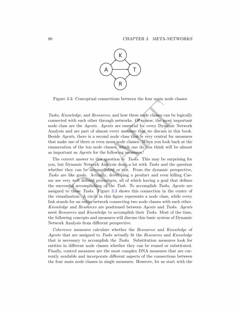
DRAFT
80 CHAPTER 3. META-NETWORKS
A T
K
R
Figure 3.3: Conceptual connections between the four main node classes
Tasks, Knowledge, and Resources, and how these node classes can be logicallyconnected with each other through networks. Of course, the most importantnode class are the Agents. Agents are essential for every Dynamic NetworkAnalysis and are part of almost every measure that we discuss in this book.Beside Agents, there is a second node class that is very central for measuresthat make use of three or even more node classes. When you look back at theenumeration of the ten node classes, which one do you think will be almostas important as Agents for the following measures?
The correct answer to this question is: Tasks. This may be surprising foryou, but Dynamic Network Analysis deals a lot with Tasks and the questionwhether they can be accomplished or not. From the dynamic perspective,Tasks are like goals. Actually, developing a product and even killing Cae-sar are very well defined procedures, all of which having a goal that definesthe successful accomplishing of the Task. To accomplish Tasks, Agents areassigned to these Tasks. Figure 3.3 shows this connection in the center ofthe visualization. A circle in this figure represents a node class, while everylink stands for an entire network connecting two node classes with each other.Knowledge and Resources are positioned between Agents and Tasks. Agentsneed Resources and Knowledge to accomplish their Tasks. Most of the time,the following concepts and measures will discuss this basic system of DynamicNetwork Analysis from different perspective.
Coherence measures calculate whether the Resources and Knowledge ofAgents that are assigned to Tasks actually fit the Resources and Knowledgethat is necessary to accomplish the Tasks. Substitution measures look forentities in different node classes whether they can be reused or substituted.Finally, control measures are the most complex DNA measures that are cur-rently available and incorporate different aspects of the connections betweenthe four main node classes in single measures. However, let us start with the
DRAFT
3.4. CONCEPTS FOR THREE AND MORE ENTITY CLASSES 81
easiest group of measures grouped under the concept of Quantity.
3.4.1 Quantity
Quantity measures—similar than for two-mode measures—just count cells inthe network matrices.
Degree. A multi-mode degree measure is Personal Costs. It counts thenumber of labor-intensive connections of an Agent in the entire meta-network,i.e. the number of people reporting to the Agent (in-degree) plus the numberof connections to Knowledge, Resources, Tasks, etc (Ashworth and Carley,2003)
Load measures are similar to the idea of density. We call these measureconcept Load in meta-networks because they tell us how loaded a network is.(Wasserman and Faust, 1994)
3.4.2 Coherence
The biggest group of measures for multi-mode networks is created throughthe concept of coherence. These measures cover the connections of the mainnode classes as visualized in Figure 3.3. The line in the middle of the picturerepresents the assignment of Agents to Tasks. In a nutshell, coherence mea-sures use the networks represented by the other lines of this figure to checkwhether the Agents have the right Knowledge and Resources to perform theirassigned Tasks or not. Just as in the previous sections, we focus on Knowledgeto describe the following measures.
Congruence is a network level measure that calculates the extent to whichthe Knowledge of Agents which are assigned to Tasks actually fits the Knowl-edge that is actually needed to accomplish the Tasks (Carley, 2002). Maximalcongruence (1.0) is just achieved in case Agents have exactly the Knowledgethey need for their Task—nothing less and nothing more.
Needs is similar to Knowledge Congruence, but quantifies only the undersupply of Knowledge to Tasks (Lee and Carley, 2004). Task Knowledge Needscompares the Knowledge requirements of each Task with the Knowledge avail-able to the Task via Agents assigned to it. Needs is a node level measure forTasks. Therefore a value is calculated for every Task describing the amountof missing Knowledge to accomplish this Task.
Waste measures the opposite of Needs and is also a node level measurefor the Task node class (Lee and Carley, 2004). Agent Knowledge Waste
DRAFT
82 CHAPTER 3. META-NETWORKS
compares the Knowledge of the Agent with the Knowledge it actually needsto do its Tasks. Any unused Knowledge is considered wasted.
Performance also calculates a Task related measure but results in a net-work level result. On particular performance measure is Knowledge BasedTask Completion (Carley, 2002). For this measure the percentage of Tasks isdetermined that cannot be completed because the Agents assigned to theseTasks lack in needed Knowledge.
Negotiation is a network level measures that is based on identifying theproportion of Tasks that need negotiation of the Agents (Carley, 2002). Ne-gotiation is necessary in case the Agents assigned to Tasks do not have all theKnowledge and Resources that are necessary to accomplish the Tasks. Basedon the congruence of the main node classes Agents, Tasks, Resources, andKnowledge the Tasks that need negotiation are identified.
3.4.3 Substitution
Availability is a Role based measure of Substitution. The idea behind Avail-ability is that to accomplishing a specific task it often does not need a partic-ular Agent but rather an Agent fulfilling a certain Role (Behrman).
Reuse The Reuse measures (Carley et al., 2000) looks for utilization ofKnowledge or Resources. The question here is whether Knowledge that isneeded for a Task is already available in an Organization/Company becausethe particular piece of Knowledge or Resource is already used for other Tasks.Reuse measures are often referred to Omega measures.
3.4.4 Control
Control measures express the extent to which agents are in control about theentire meta-network or about the situation of the other Agents of the network.Both measures of this concept can be referred to as Cognitive measures.
Cognitive Demand is a node level measures that incorporates ten differentaspects of Agents being cognitively engaged in a meta-network (Carley, 2002).Some of these aspects can just be calculated in case you have Knowledge andResources in your data. In case your meta-network includes just one of thesenode classes as well as Agents and Tasks, you can still compute CognitiveDemand by just calculating the feasible aspects. The ten aspects covered byCognitive Demand are the following:
1. The number of other Agents that a single Agent is connected to.
DRAFT
3.4. CONCEPTS FOR THREE AND MORE ENTITY CLASSES 83
2. The number of Tasks an Agent is assigned to.
3. The amount of Knowledge an Agent has.
4. The amount of Resources an Agent is connected to.
5. The number of Agents that are assigned to the same Tasks than theAgent.
6. The amount of Knowledge that is necessary to accomplish the Tasksthat an Agent is assigned to.
7. The amount of Resources that is necessary to accomplish the Tasks thatan Agent is assigned to.
8. The amount of negotiation on Resources with other Agents that is nec-essary to accomplish the assigned Tasks.
9. The amount of negotiation on Knowledge with other Agents that isnecessary to accomplish the assigned Tasks.
10. The number of Agents that an Agent depends on or that depend on anAgent to handle his Task.
This enumeration of different aspects that are incorporated in CognitiveDemand makes it clear that people that score high in this measure are veryimportant in a network. We call these people “Emergent Leaders”. Emergentleaders are identified in terms of the amount of cognitive effort that is inferredto be expended based on the individual’s position in the meta-network. Indi-viduals who are strong emergent leaders are likely to be not just connected tomany people, organizations, tasks, events, areas of expertise, and resources;but also, are engaged in complex tasks where they may not have all the neededresources or knowledge and so have to coordinate with others, or have otherreasons why they need to coordinate or share data or resources. The drawbackfor Emergent Leaders is that they are so busy with keeping the company (orthe empire) running, that there is a good chance that they never become aformal leader.
Awareness is another control measure that creates dyadic results (Grahamet al., 2004). The measure tells us to which extent two Agents are similar froma meta-network perspective. Shared Situation Awareness is a mixture of fourdifferent aspects:
1. The interaction between the two Agents.
DRAFT
84 CHAPTER 3. META-NETWORKS
2. The power of the two Agents calculated by their Eigenvector Centrality.
3. The Agents physical proximity approximated through their shared Lo-cations or Events.
4. The Agents socio-demographic similarity approximated through theirshared Knowledge and Resources.
This enumeration covers different aspects of having shared awareness aboutthe networked system.
3.5 Problem set
1. What are the main four nodes classes of dynamic network analysis?
2. Which two node classes occur in almost every measure that uses threeor more node classes?
3. What is the difference between the quantity concept of two-mode mea-sures and the quantity concept of multi-mode measures?
4. Describe the underlying idea of coherence measures.
5. Why are people critical in a network that score high in Exclusivity?
6. Which situations create the need for Negotiation in a company?
7. Draw a small network consisting of Agents and Resources that describesthe Access measure.
8. What do you think, is it likely that the person in an Organization thatscores highest in Cognitive Demand will become the next leader of thisOrganization?
9. In Figure ?? you can find the conceptual linkage between Agents, Tasks,Knowledge, and Resources. Find another combination of four nodeclasses that can be used for any coherence measure.
10. What is the main difference between Congruence, on the one hand, andNeeds and Waste, on the other hand?
11. *Imagine that you are the head of a company and you measure highRedundancy in one department. Why could this be a problem? Andwhy could this be important?

DRAFT
3.5. PROBLEM SET 85
12. *Imagine that you had to calculate betweenness centrality in the networkthat is an aggregated representation of all five acts. Why is the genericnode Citizens problematic for the centrality score of ALL nodes of thenetwork?
13. *What is the 11th node class and why could analysis involving this nodeclass make sense?
14. *Calculate the Coherence measures for the Julius Caesar meta-networkand give an interpretation of the results.
15. *Download the company network from the book’s website. Identify thecognitive leader of the company.
16. *The Event x Event network in Figure 3.2 consists of long chains ofevents. Why is this the case? Is this typical for real world Event net-works?
17. **Take a sheet of paper. Copy the Agent x Knowledge network matrixand perform a matrix multiplication by hand so that the result is aKnowledge x Knowledge matrix. What is the meaning of the resultingmatrix?
18. **Calculate by hand the network level measure “negotiation”. Describethe different steps of the calculation.
19. **Take your favorite movie and code as many node classes as possible.What nodes classes are tricky to code? Visualize and analyze this meta-network. Can you describe the narrative as well as the highlights ofthe movie with network visualizations and metrics? There is no need tocreate more than one meta-network for the entire movie.
20. **Take all two-mode and multi-mode measure concepts and find a newclassification system that does not use the number of entity classes asfirst separator.

DRAFT
86 CHAPTER 3. META-NETWORKS
DRAFT
Chapter 4
Finding Groups
Imagine, Julius Caesar is going through some major organizational restructur-ing. The soldiers are naturally worried, but the whole idea is for the empire torealign strategically to allow the groups within the empire the most efficientuse of Resources. It is the theory of Julius Caesar that the empire can thenbecome more profitable and hence more stable. Therefore, ultimately, it isabout reassuring the soldiers of the empire that Julius Caesar will continueto remain strong long into the near future. Now, that should make some resteasier but perhaps it makes politicians, especially Cassius, a little uneasy. Af-ter all, they have given themselves a daunting task: they want to know aboutthe groups that exist inside their organizational structure. They believe, quitecorrectly, that knowing the make-up of how groups and teams function acrossthe empire will therein provide clues as to where Julius Caesars empire canreallocate Resources to make Julius Caesars empire more efficient and hencemore enduring. The problem is how do they go about discovering the groupsthat exist within their empire?
Inside Julius Caesars empire, we have Cassius, who interacts with Brutusand Calpurnia. Everyone interacts within his or her group. We will say thatthey are part of distinct organizational group called Roman Countrymen butcould there be other groups they interact with outside of their core group?Of course there could. There could be countless amounts of other groupswhich they interact with on a regular basis. Cassius could hang out with theaccounting group while on lunch. He may have privy to Knowledge that isgenerally available only to those in the friends group. Likewise, Brutus mighttake Roman baths on the weekends and belong to the same club that manyof the senior leaders belong too. He may therefore have the inside scoop on a
87
DRAFT
88 CHAPTER 4. FINDING GROUPS
lot of high-level strategy that generally would be unavailable to anyone withinthe customer service group. He may even serve as a source of information tothe senior executives as to what really works in the custumer service group.
Groups are a natural part of our human experience. Individuals are indeedsocial actors who tend to migrate into membership into a group, or severalgroups, for a variety of reasons. In prehistory ages, the human species seemedto have figured out that the family group is the starting social structure forour very core survival and that being part of an even larger group providesus with increased access to critical resources, such as food, water, potentialmates, etc. Moreover, being part of a group afforded the individual betterprotection from our enemies, both the difficulties of nature and the brutalitiesof other humans. Today, this drive for affiliation continues; we each are amember of numerous groups, from personal-contact groups, to cyber-spacevirtual world groups.
From a DNA perspective, groups also encapsulate objects and ideas, such ascomputer networks, music genres, and job categories. Whether by the force ofa natural law, or the limited capacity of humans, objects and ideas are placedinto groups. Groups of all types, forms and made up of various complementsand, even, subgroups are everywhere.
So it follows, that a network analysis will typically investigate a networkdata from the perspective of the network as a group or a set of groups. Thisperspective accomplishes two things: (1) it reduces the number of entities toanalyze, and (2) the natural tendency for things (including people) to grav-itate into groups, suggests that understanding the sub-groups in a networkmay provide hidden clues to that network. So, people are interested in groupsis, because when you look at groups in a network, it is a very easy way tosummarize information in a network. Rather than saying something aboutany particular node, we are trying to aggregate information to higher rep-resentations groups. This is especially helpful when the network is large.When we think of groups we automatically think of communities that shareknowledge, information, or norms or have similar experiences. So, you couldinteract with them in similar ways and you can expect similar reactions frommembers of the same group.
In this chapter we will first introduce some interesting patters in networkswhich can be considered as groups, e.g. disconnected components or sub-setsof nodes in which every node is connected to every other node. In the secondpart of this chapter we will discuss more complicated group structures—thosewhich need algorithms to be identified. Finally, we will have a closer look atour Julius Caesar network to discuss grouping issues in meta-networks or in

DRAFT
89
Figure 4.1: Network visualization of the first act of Julius Caesar
networks over time.
In general, groups are a set of nodes that meet certain criteria. This soundseasy but creates a major implication: There are no natural groups in networks;you create groups based on your definition. Therefore, there is no one-fits-all method to identify groups. This is the reason why many new groupingalgorithms are being developed every year and grouping is a big topic inDNA. When working with groups in the network setting, there is not yetagreement on a precise definition (Seidman & Foster 1978; Alba & Moore1978; Mokken 1979; Burt 1980; Freeman 1984; Freeman 1992; Sailer & Gaulin1984). Exactly what constitutes a group is a matter of ones perspective, thedata, and analytic question. For our purposes here: cohesive sub-groups, orjust groups, are collections of nodes that share some specific characteristic(s)or property(ies); most often a nodes membership is bounded by being in onlyone sub-group, but some grouping processes allow for multiple memberships.We seek to identify and characterize these groups because often the analystcan locate, often hidden, sets of actors that have something (loosely defined)in common that can be useful information in explaining, understanding andforecasting, either the group itself or the larger network. As mentioned earlier,these often-hidden groups are sometimes (self-) organized for some collectiveaction of sorts.
Let’s have a look at Act 1 of the Julius Caesar play again (Figure 4.1. WhatAgents form a group? Well, as you would probably know by now, this dependson the selected criteria.
DRAFT
90 CHAPTER 4. FINDING GROUPS
The first criteria that we look at is not directly connected to networks.Agents share different attributes and form groups based on that. For instance,age, gender, occupation, or sympathy to Caesar can be used to group theAgents of reffig:act1. Sharing specific attributes can lead to nominal groups,e.g. nurses, teachers, or senators. Even though attributes include no networkinformation at first sight, we know from chapter 2 that similarity in attributes(homophily) is number one drive for network formation. Conspirators tendto hang out with other conspirators and new Agents are more likely of beingaccepted by the group when they share this attribute.
4.1 Interesting patterns
A second set of grouping criteria are based on graph theoretic definition. Whenwe look at the structure of the network, the most obvious groups in thisnetwork are the two unconnected parts, Marullus and Flavius together withthe Citizens of the left side and all other nodes on the right side. We call theseunconnected parts of a network components. Are these different scenes of theplay? No, components are created when there is no path between (at least)two groups on nodes. For the play this means, when there are two Agentsfrom different scene that do not co-occur with any Agent that can create achain of links between them.
Another interesting structural pattern is created by Antony, Cascar, Brutus,Cassius, and Caesar. When there is a group of nodes with each of whichis connected to every other node, then we call it a clique. Cliques are thestrongest pattern of structural pattern but you need to be careful using cliques,when your network data is created by folding two-mode data to one-modedata, as we did for the network in reffig:act1. Every node of the second modeforms a clique in the folded one-mode network. This can create confusingartifacts of large cliques in case of, let us say Events, with many participants.
Cliques are very intriguing, however, not often used in real-world networks.There are two reasons for why this group criteria is not so great after all. First,in real-world groups that exist of a certain number of Agents, some links areoften missing even in the strongest group of friends or co-workers. Secondly,cliques are very time consuming to calculate for larger networks.
Some other concepts for group identification are similar to cliques but aremore realistic and very fast to calculate. k-Cores ?? are groups of nodes thatare all connected to at least k other nodes of the groups. Therefore, we canuse this approach to identify clique-like groups. k-Plex ?? is a similar concept.Here, a group is defined as a set of nodes that ... ??. It is worthwhile knowing
DRAFT
4.2. GROUPING METHODS 91
that k-cores and k-plexes as well as cliques can and often do overlap—onenode can be part of more than one group.
Equivalence i Equivalence Structurally indistinguishable Same degree, cen-trality, belong to same number of cliques, etc. Only the label on the nodecan distinguish it from those equivalent to it. Perfectly substitutable: samecontacts, resources
Face the same social environment Similar forces affecting them same influ-encers On average, hear things equally early, influenced similarly, have similarthings to cope with
Role equivalent
4.2 Grouping Methods
When groups are extracted from networks with grouping algorithms, they areoften called communities. A community consists of a subset of nodes withinwhich the node-node
4.2.1 Newman grouping
connections are dense, and the edges to nodes in other communities are lessdense. Be aware that this is just another criteria definition for groups—although one that is highly relevant for networks consisting of people. Thegrouping algorithm by ? is very often used to identify communities becauseit is a very intuitive approach. Remember betweenness centrality (Freeman,1977). We discussed in chapter 2 that a node scores high in this measurein case this node links parts of the network that were not connected as wellwithout this node. It is clear that the nodes 1, 2, and 3 in the networkvisualized in 4.2 fulfill this criteria while peripheral nodes have a betweennesscentrality score of 0.0. Now the same idea is used for links of the network.The link with the highest betweenness centrality is considered to connectingdifferent groups that were not connected as well without this link. In Figure4.2 the line width are drawn based on line betweenness centrality. You cansee that the connecting line between node 1 and 2 scores highest. The smartalgorithmic move now is, to remove this link. By doing so, the examplenetwork breaks in two components. Of course, in real networks network partsare not connected by just one link. Therefore, we recalculate line betweennesscentrality again, delete the line that scores highest, etc. Recalculating themetrics again after removing a link is necessary as the the results may change
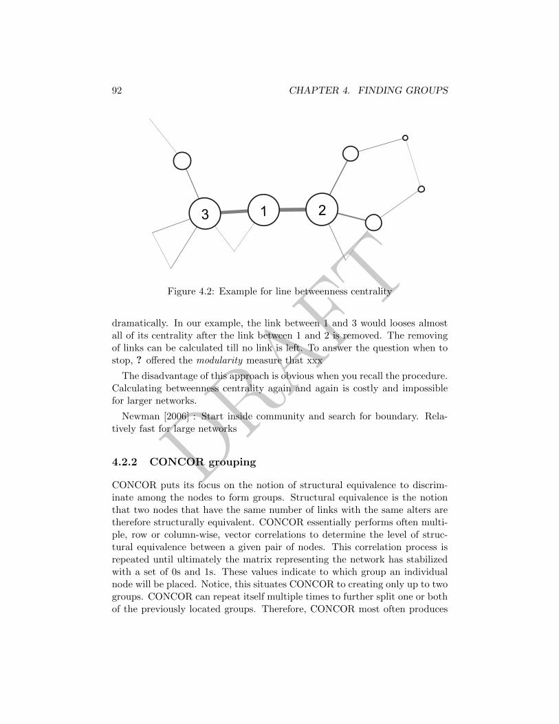
DRAFT
92 CHAPTER 4. FINDING GROUPS
13 2
Figure 4.2: Example for line betweenness centrality
dramatically. In our example, the link between 1 and 3 would looses almostall of its centrality after the link between 1 and 2 is removed. The removingof links can be calculated till no link is left. To answer the question when tostop, ? offered the modularity measure that xxx
The disadvantage of this approach is obvious when you recall the procedure.Calculating betweenness centrality again and again is costly and impossiblefor larger networks.
Newman [2006] : Start inside community and search for boundary. Rela-tively fast for large networks
4.2.2 CONCOR grouping
CONCOR puts its focus on the notion of structural equivalence to discrim-inate among the nodes to form groups. Structural equivalence is the notionthat two nodes that have the same number of links with the same alters aretherefore structurally equivalent. CONCOR essentially performs often multi-ple, row or column-wise, vector correlations to determine the level of struc-tural equivalence between a given pair of nodes. This correlation process isrepeated until ultimately the matrix representing the network has stabilizedwith a set of 0s and 1s. These values indicate to which group an individualnode will be placed. Notice, this situates CONCOR to creating only up to twogroups. CONCOR can repeat itself multiple times to further split one or bothof the previously located groups. Therefore, CONCOR most often produces
DRAFT
4.2. GROUPING METHODS 93
a number of groups that are a power of two. The number of groups identi-fied by CONCOR is a user-parameter (often times the number of “splits” isthe expected input). PRO: Only commonly used algorithm detecting relaxedstructural equivalence. CON: Top down splitting of nodes imposes structureCON: Requires user to choose a power of 2 for the number of groups.
4.2.3 Johnson grouping
The Johnson procedure uses a distance metric to discriminate groups. Itcreates groups according to a network that is constructed with links thatindicate the distance between dyads. Johnson will segregate groups accordingto these weights by separating those who are most distant from others in thesame group from the original group and off to a group of nodes that are closerin this distance value.
4.2.4 Fuzzy Grouping
The FOG / K-FOG are powerful approaches that recognize that nodes canoften be members of more than one group at a time (fuzzy groups), which canbe a major weakness of the aforementioned techniques. FOG begins with acollection of nodes and uses a maximum likelihood perspective to determinethe probability that a link exists among the various dyads in the group. Itcompares the probability with the actual data and as a result, a node canindeed be assigned membership in the group, or not. By taking this approach,FOG can assign a node to multiple groups.
4.2.5 Block-Modeling
Block-Modeling ?? is a grouping approach that optimizes the matrix repre-sentation of a network. A block model is a reduced form representation suchthat nodes are divided into a set of mutually exclusive groups. The resultinggroups can then be analyzed as a network such thatThe groups connection to itself is the density of the connections among mem-bersFor each pair of groups, the inter-group connection is the density of the con-nections of group 1 (row) to group 2 (column)The resulting block matrix can be turned into a binary matrix by simplycomparing the level of connections in the block to the overall density of theoriginal matrix such that there if the value of the cell is ¿= to the overalldensity then we replace it with a 1, else 0
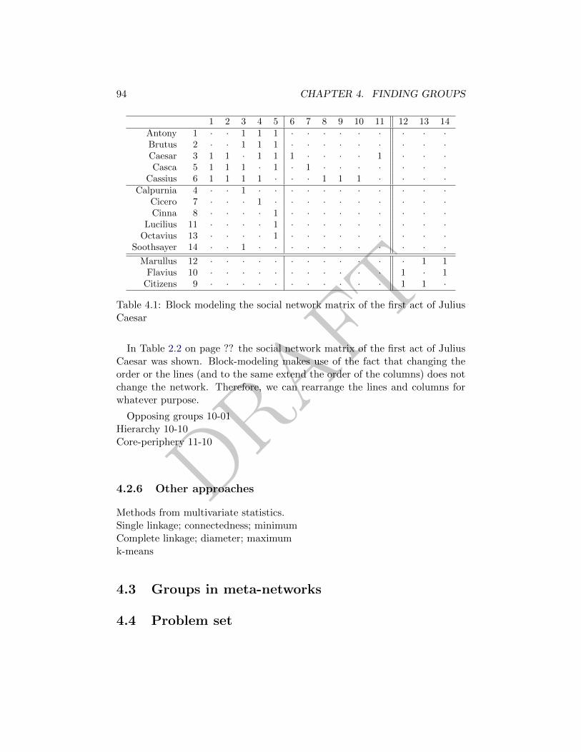
DRAFT
94 CHAPTER 4. FINDING GROUPS
1 2 3 4 5 6 7 8 9 10 11 12 13 14Antony 1 · · 1 1 1 · · · · · · · · ·Brutus 2 · · 1 1 1 · · · · · · · · ·Caesar 3 1 1 · 1 1 1 · · · · 1 · · ·Casca 5 1 1 1 · 1 · 1 · · · · · · ·
Cassius 6 1 1 1 1 · · · 1 1 1 · · · ·Calpurnia 4 · · 1 · · · · · · · · · · ·
Cicero 7 · · · 1 · · · · · · · · · ·Cinna 8 · · · · 1 · · · · · · · · ·
Lucilius 11 · · · · 1 · · · · · · · · ·Octavius 13 · · · · 1 · · · · · · · · ·
Soothsayer 14 · · 1 · · · · · · · · · · ·Marullus 12 · · · · · · · · · · · · 1 1
Flavius 10 · · · · · · · · · · · 1 · 1Citizens 9 · · · · · · · · · · · 1 1 ·
Table 4.1: Block modeling the social network matrix of the first act of JuliusCaesar
In Table 2.2 on page ?? the social network matrix of the first act of JuliusCaesar was shown. Block-modeling makes use of the fact that changing theorder or the lines (and to the same extend the order of the columns) does notchange the network. Therefore, we can rearrange the lines and columns forwhatever purpose.
Opposing groups 10-01Hierarchy 10-10Core-periphery 11-10
4.2.6 Other approaches
Methods from multivariate statistics.Single linkage; connectedness; minimumComplete linkage; diameter; maximumk-means
4.3 Groups in meta-networks
4.4 Problem set

DRAFT
4.4. PROBLEM SET 95
1.
2.
3.
4.
5.
6.
7.
8.
9.
10.
11. *
12. *
13. *
14. *
15. *
16. *
17. **
18. **
19. **
20. **

DRAFT
96 CHAPTER 4. FINDING GROUPS
DRAFT
Chapter 5
Spatially EmbeddedNetworks
In exploring the various influences and roles in human relationships we willnow consider one of the most important features for understanding social in-teractions: space. Clearly, space is important, and as such, we intend to equipthe reader with appropriate methods for analyzing networks where locationalinformation is available. Physical proximity has long been known to play amajor role in shaping human interpersonal relationships. In general, peopleare more likely to interact with others who are nearby. This effect, calledpropinquity, has been documented time and time again for a wide variety ofnetworks (Butts, 2002; Faust, 2000; Festinger, 1950; Latane, 1995). It haseven been proven theoretically that for large social networks, the locations inspace of individuals can explain almost all of the information in the network(Butts, 2002).
This chapter should provide an overview of the core issues in analyzingspatially embedded networks. After discussing different aspects of networksand space—including the importance of aggregation, clustering, informationloss and smoothing—we introduce technical artifacts that are needed to han-dle geographical information. Section 3 continues with spatial visualizationsand the final section discusses centrality measures that make use of spacialinformation.
97

DRAFT
98 CHAPTER 5. SPATIALLY EMBEDDED NETWORKS
5.1 Propinquity – Those close by form a tie
5.2 GIS, shape-files, and Co.
5.3 Spatial visualizations
5.4 Spatial centralities
DRAFT
Chapter 6
Temporal Networks
We should know by now that networks evolve and change over time and itis the key role of dynamic network analysis to identify and describe thosechanges. Furthermore, by analyzing change in networks, we are maybe capableof predicting how networks evolve in the future and how the underlying real-world system will change. In fact, it is this time consideration that marks thetrue difference between Dynamic Network Analysis (DNA) and traditionallink analysis.
In this chapter we discuss different aspects of temporal networks. Afterintroducing some definitions and discussing aggregation issues, we try to de-scribe and measure change in networks. You will learn in this chapter thatthe statistical analysis of correlating different networks to identify similaritiesof multiple networks is possible, but not trivial. The final part of this chapterintroduces different ways to detect change and periodicities in networks overtime. Some of the measures that we discuss in this chapter are mathematicallychallenging. We try our best to describe the underlying ideas of the methodsin an understandable way here and we want to refer the advanced reader tothe algorithms in the appendix or the cited literature.
6.1 Networks over time
6.1.1 Creating networks over time
When network analysts talk about temporal networks, they normally talkabout networks that are created through data aggregation for a specific timeperiod (e.g. by day, week, month, year). For instance, if you think about e-
99
DRAFT
100 CHAPTER 6. TEMPORAL NETWORKS
mail communication in a company, then all e-mail that are sent at one day canbe grouped together to form the communication network for this particularday. Another example is our Julius Caesar data. When coding the socialinteraction of this network (see chapter 2), we decided to aggregate on actlevel. This was a deliberate decision. Both aggregation levels—for the JuliusCaesar as well as for the e-mail network— also can be selected at a differentlevel. We talk more about aggregation on network data later in this chapter.
In general, there are two different ways of describing change in meta-networks:
1. Keyframes. A meta-network over time is collected as a set of networks,e.g. one meta-network per day, month, year.
2. Deltas. A meta-network as a set of single “change events” in time.These change events can be: add/remove a node, add/remove a link,and modify an attribute.
As we discussed above, keyframes are the common way of describing changein networks. But keyframes and deltas are highly connected with each other.Remember the Julius Caesar social network from chapter 2. The act-by-actnetworks are not just an aggregation by scene, actually theses networks arethe result of aggregating every single interaction in every scene, e.g. Calpurnia(the wife of Caesar) tries to convince Caesar not to go to the Senate and Deciusdoes the opposite; both interactions (deltas) are coded in the second act of ournetwork as one edge. Imagine that we have coded every single interaction asdelta, we could create the act-by-act keyframes easily by aggregating severaldeltas within the specified period of of the play. However, we will discusstemporal networks in this chapter from the perspective of keyframes.
6.1.2 Levels of aggregation
We already used the term aggregation in this chapter. Aggregating over timedata means creating keyframes. To illustrate this process and to discuss issuesof aggregation, we look at a dataset of e-mail communication. The datasetincludes approximately 200,000 e-mails over the course of 81 days. Theselarge amount of e-mails were sent from 2,427 people to 2,563 recipients. Letus just look at one week of this dataset including 16,277 e-mails. If we start tothink about how to analyze this data with statistical methods, a very intuitiveapproach is to count the number of e-mails by day or by hour. Figure 6.1 showsthe result of this statistical approach. Figure 6.1(a) reveals very little activityon Saturday (day 7) and Sunday (day 1) and rather stable activity during
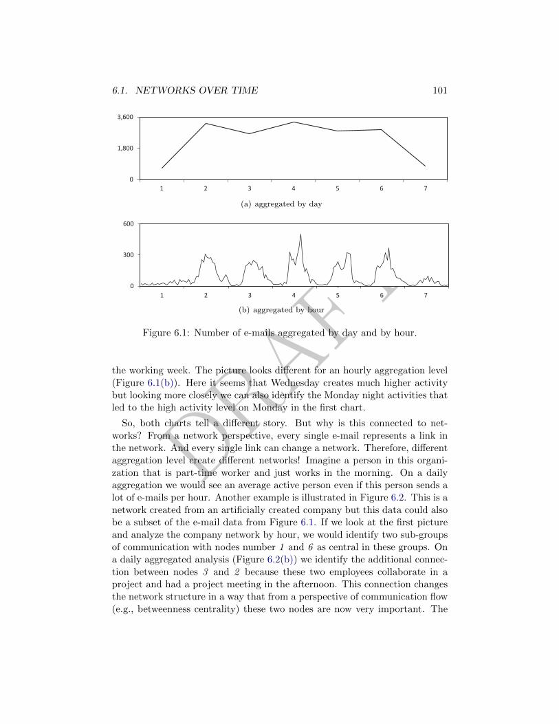
DRAFT
6.1. NETWORKS OVER TIME 101
0
1,800
3,600
1 2 3 4 5 6 7
(a) aggregated by day
0
300
600
1 2 3 4 5 6 7
(b) aggregated by hour
Figure 6.1: Number of e-mails aggregated by day and by hour.
the working week. The picture looks different for an hourly aggregation level(Figure 6.1(b)). Here it seems that Wednesday creates much higher activitybut looking more closely we can also identify the Monday night activities thatled to the high activity level on Monday in the first chart.
So, both charts tell a different story. But why is this connected to net-works? From a network perspective, every single e-mail represents a link inthe network. And every single link can change a network. Therefore, differentaggregation level create different networks! Imagine a person in this organi-zation that is part-time worker and just works in the morning. On a dailyaggregation we would see an average active person even if this person sends alot of e-mails per hour. Another example is illustrated in Figure 6.2. This is anetwork created from an artificially created company but this data could alsobe a subset of the e-mail data from Figure 6.1. If we look at the first pictureand analyze the company network by hour, we would identify two sub-groupsof communication with nodes number 1 and 6 as central in these groups. Ona daily aggregated analysis (Figure 6.2(b)) we identify the additional connec-tion between nodes 3 and 2 because these two employees collaborate in aproject and had a project meeting in the afternoon. This connection changesthe network structure in a way that from a perspective of communication flow(e.g., betweenness centrality) these two nodes are now very important. The

DRAFT
102 CHAPTER 6. TEMPORAL NETWORKS
1
2
3
4
5
6
7
89
(a) aggregation by hour
1
2
3
4
5
6
7
89
(b) aggregation by day
1
2
3
4
5
6
7
89
(c) aggregation by week
Figure 6.2: Networks created based on three different aggregation level.
weekly observation, again, looks different because now we identify that thereis—for some reason—a lot of communication in this company between almostall people and especially node number 4 seems to communicate with all othernodes. So, what is the the right aggregation level? It depends on your re-search question and your data. If it is possible, try different aggregation levelsanalyze (and interpret) the differences. If your aggregation level is selectedwrong, these are possible implications:
• Aggregation level too high. The network gets dense and is harderto analyze. Interesting structures are masked by more or less randominteractions. It is also possible that two or more interesting patternsuperimpose each other.
• Aggregation level too low. Miss of important structural patterns.Overemphasize of links having high communication. Very sparse net-works result in highly fluctuating measures as a single link can changethe global structure of the network.
6.2 Trails
In the last chapter we discussed ways of analyzing network data when it isconnected to geo-spatial Locations. Now, let us add the perspective of timeto this data. For instance, Julius Caesar has seen his empire and bureaucracyever expanding. He analyzed who the important Agents in his empire are andhe already accomplished some spatial analysis regarding his empire. In aneffort to better analyze the structure of his empire, Caesar decides that hewants to know exactly how his military command travels the known world.
DRAFT
6.2. TRAILS 103
Could the emerging travel patterns lead Caesar and his staff to draw newconclusions about where the business is located or where it should open newLocations to better serve the geographic needs of the empire? And whatabout all the Locations that are shared in common by Caesar’s military andadministration stuff, such as cities they passed through, houses they stayed atin various cities, routes they took, stops they made, on their way to formingthe enemy army? In other words, how can we analyze network data in spaceand time?
When observed over time, spatially embedded networks exhibit a specifickind of dynamism deserving of its own forms of analysis. Agents occupy onlyone Location at a time, but progress from Location to Location longitudinally,creating a temporally embedded sequence of relationships we call a ”trail”.Trails are paths that whos move through within a network. Naturally, trailsinvolve both a who and where and even a when. When you can link thoseentities together over period you have a trail.
Trails are just one perspective on one part of the larger dynamic network,but thinking about relationships in sequence makes certain kinds of analysismuch more intuitive. Using trails, we can begin to analyze questions like,”Where do people at Location X tend to go next?”, ”Which other Agents doesAgent A frequently cross paths with?”, or ”What kind of seasonal patternsgovern movements in my networks?”
Stepping back from the spatial context, we can see that sequential relation-ships, and the type of question we ask about them above, are not limited totracking movement. We might also consider changes in Agent affiliation, suchas an Agent x Employer relationship, or changes of power, such as a Country xPolitical Party relationship. The formal, generalized definition of ”trail” is (1)a subject node (such as an Agent) and (2) a time-labeled sequence of targetnodes from the same class (such as Locations). Any dynamic relation can beused as a trail set, so long as it has the property that at any given time—itis many-to-one (an Agent can occupy only one Location but a Location mayhost many Agents).
Having established that general view, we will return to discussing trails intheir most intuitive context, as a description of spatial transitions. Since trailsand networks are closely related and defined in this way, trails are actuallya type of network. Although analyzing the trail as a network may not seeminteresting, trails can be used to create useful networks. For example, trailscan be used to create co-Location or co-affiliation networks, showing who wasat the same place or Organization at the same time. Trails can also be usedto create transition networks showing how people in aggregate tend to move
DRAFT
104 CHAPTER 6. TEMPORAL NETWORKS
from place to place or from Organization to Organization (2008b). Trails canalso be generated from networks. Although networks do not have sufficientinformation to reproduce trails, networks can be used to create prototypicaltrails that might be expected given e.g. a transition network (Davis, 2008).
So, when we look for trails in networks over time, we look for interestingpatterns and shared similar behaviors.
ToDo: example of trails, e.g. Davis, 2008. Focus: What can be analyzed?
6.3 Measuring change
Questions for Comparison: Are two networks similar? What is the differenceof two networks? How to compare more than two networks? How to com-pare predicted networks to the actual future observed networks? Can we usestandard statistics (e.g. correlations)?
6.3.1 Levels of comparison
We distinguish between four levels of comparison based on what is calculatedfor every network:
Node measures. Measures are calculated on node level (e.g. centralitymeasures) and the results are compared with each other, e.g. comparison ofthe set to top 10 key entities, the ranks of the entities, or the centrality scoresof the entities. We did this in chapter 2 with the Agents in the five acts ofthe Julius Caesar network.
Network measures. Network level indices are calculated (distributionof node measure values, network centralization, density, etc.) and then com-pared between different networks. This approach is similar to comparing nodemeasures.
Network structure. The network matrices are compared with each other,e.g. Hamming distance, Euclidean distances, correlation of networks, regres-sion models with networks. The remaining sections of this chapter will pri-marily deal with these topics.
Motifs. Local patterns in networks are analyzed and compared betweennetworks to describe the dynamics of change, e.g. transitivity, reciprocity. Oneapproach to compare motifs is the triad census from Holland and Leinhardt

DRAFT
6.3. MEASURING CHANGE 105
(1976). A more comprehensive method is called Exponential Random Graphmodeling and is presented later in this chapter.
6.3.2 Network distances
One straightforward approach to compare networks with each other to identifythe amount of change over time is to calculate the difference between networks.So exactly, how does the network scientist measure the differences between twonetworks? Well, one the short answer is that they dynamic network analyst isinterested in learning about the distance between the network. To do so, is toconsider the network matrix as list of numbers. The most common means fordoing so is to calculate the Hamming distance between two networks. Anothermethod is to use Euclidean geometry to ascertain differences. Of course, thereare other methods, each of which is done differently and warrants its ownrespective considered by the analysts.
Hamming distance. Hamming distance considers network matrices asstrings of binary information. Therefore, every cell of the string is either 1or 0. In Figure 6.3 we illustrate the process of comparing two networks bycalculating the hamming distance. You can see visualization and matrix of twodifferent networks, each consisting of 5 nodes and directed links connectingthe nodes. On the lower left part of the Figure, the two network matrices aretransformed into a string by concatenating the lines of the matrices. If wenow compare these two strings bit-by-bit (column-by-column), we can countthe number of disparity—in our example 5 elements are different resulting ina proportion of 20 % difference. Consequently the Hamming distance betweenour two example networks is 0.2.
Let us look again to the Tragedy of Julius Caesar. When we look at thesocial networks that we have introduced in the first chapter and we want tocalculate the hamming distance between the first and the second network,the second and the thirds network, and so on, we are facing a problem—thenetworks are of different size and when we concatenate the lines of the matricesthe resulting strings are also of different size which makes it impossible tocompare them. In addition, we can find Agents in the second network that arenot part of the first and vice versa. And this is not the exemption but ratherthe rule because in real world—and in written tragedies—different networksbarely ever have the exact same Agents. To overcome this constraint thatwe have two options adjust networks so that they have the same size beforecalculating Hamming distance. Both methods result in different results andyou have to be aware of what you are interested in:
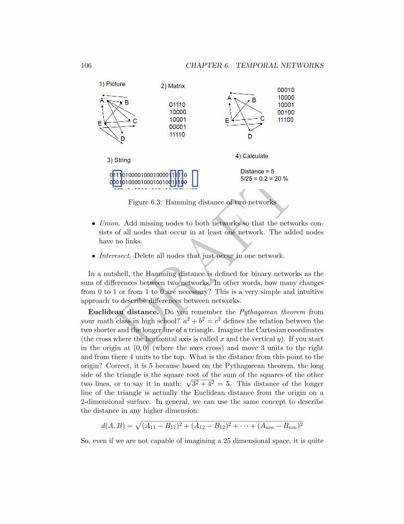
DRAFT
106 CHAPTER 6. TEMPORAL NETWORKS
0111010000100010000111110 0001010000100010010011100
Distance = 5 5/25 = 0.2 = 20 %
Figure 6.3: Hamming distance of two networks
• Union. Add missing nodes to both networks so that the networks con-sists of all nodes that occur in at least one network. The added nodeshave no links.
• Interesect. Delete all nodes that just occur in one network.
In a nutshell, the Hamming distance is defined for binary networks as thesum of differences between two networks. In other words, how many changesfrom 0 to 1 or from 1 to 0 are necessary? This is a very simple and intuitiveapproach to describe differences between networks.
Euclidean distance. Do you remember the Pythagorean theorem fromyour math class in high school? a2 + b2 = c2 defines the relation between thetwo shorter and the longer line of a triangle. Imagine the Cartesian coordinates(the cross where the horizontal axis is called x and the vertical y). If you startin the origin at (0, 0) (where the axes cross) and move 3 units to the rightand from there 4 units to the top. What is the distance from this point to theorigin? Correct, it is 5 because based on the Pythagorean theorem, the longside of the triangle is the square root of the sum of the squares of the othertwo lines, or to say it in math:
√32 + 42 = 5. This distance of the longer
line of the triangle is actually the Euclidean distance from the origin on a2-dimensional surface. In general, we can use the same concept to describethe distance in any higher dimension:
d(A,B) =√
(A11 −B11)2 + (A12 −B12)2 + · · ·+ (Anm −Bnm)2
So, even if we are not capable of imagining a 25 dimensional space, it is quite
DRAFT
6.3. MEASURING CHANGE 107
easy to take 25 times each with two numbers, calculate the difference, squarethe difference, 1. sum up all sub results and calculate the square root from thesum. If you do so and calculate the Euclidean distance for the example of 6.3you will probably figure out that the result is the square root of the absoluteHamming distance. This is the case because our network is binary and thesquare of 1 (or -1) is also 1. However, Euclidean distance has a very importantadvantage compared to Hamming distance, it takes link weights into account.Therefore, if your network is weighted and you are interested in distancesbetween networks, than Euclidean distance is probably your preferred choice.
6.3.3 Correlation of networks and its problems
Another approach to compare networks is to correlate its network matrices.Person correlation (Pearson, 1920) compares any list of numbers and tells ushow similar these numbers are. People run their statistical tools and calculatecorrelations because they are interested in comparing different variables witheach other. For instance, managers are interested in whether employees withhigher income have higher productivity, teacher want to know whether middleschool students that perform better in math do also better in physics, andCaesar could be interested in whether the happiness of his subjects is higher inparts of his empire in which more gladiator fights are happening or in which thetaxes are lower. All these examples have in common that different attributesof set of people are compared with each other. When we compare networks weare interested in correlations of relations. To modify the previous examples torelational questions, managers are interested in whether employees that sharemore common projects interact more often which each other, teachers can beinterested in whether students use their friendship ties when they ask eachother for advice, and Caesar could be interested in whether private relations(e.g. marriages between families) or business relations between the senatorsresult in a common voting behavior in the Senate. The naıve approach tothese network correlation questions is almost right.
If we transform the network matrices into lists of numbers (like for calcu-lating distances), we can correlate these lists. For the two networks used inthe distance examples, the Pearson correlation coefficient is 0.53 if we ignorethe diagonal elements. At first glance, to Calculate the correlation betweenthe edge values in two networks, seems to be a straightforward–and also quiteintuitive— approach to compare network matrices. But after careful con-
1Squaring the differences has the big advantage that the ordering of the two numbers isnot relevant for the results. In case the difference is negative, the square is also positive
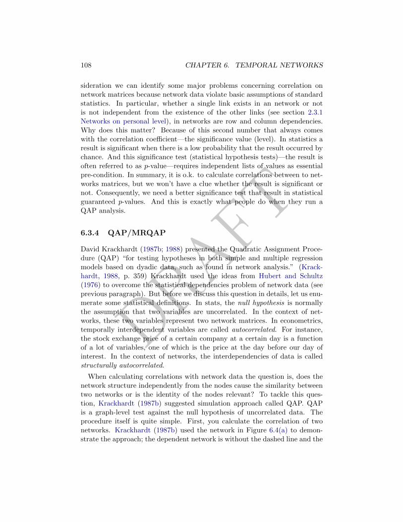
DRAFT
108 CHAPTER 6. TEMPORAL NETWORKS
sideration we can identify some major problems concerning correlation onnetwork matrices because network data violate basic assumptions of standardstatistics. In particular, whether a single link exists in an network or notis not independent from the existence of the other links (see section 2.3.1Networks on personal level), in networks are row and column dependencies.Why does this matter? Because of this second number that always comeswith the correlation coefficient—the significance value (level). In statistics aresult is significant when there is a low probability that the result occurred bychance. And this significance test (statistical hypothesis tests)—the result isoften referred to as p-value—requires independent lists of values as essentialpre-condition. In summary, it is o.k. to calculate correlations between to net-works matrices, but we won’t have a clue whether the result is significant ornot. Consequently, we need a better significance test that result in statisticalguaranteed p-values. And this is exactly what people do when they run aQAP analysis.
6.3.4 QAP/MRQAP
David Krackhardt (1987b; 1988) presented the Quadratic Assignment Proce-dure (QAP) “for testing hypotheses in both simple and multiple regressionmodels based on dyadic data, such as found in network analysis.” (Krack-hardt, 1988, p. 359) Krackhardt used the ideas from Hubert and Schultz(1976) to overcome the statistical dependencies problem of network data (seeprevious paragraph). But before we discuss this question in details, let us enu-merate some statistical definitions. In stats, the null hypothesis is normallythe assumption that two variables are uncorrelated. In the context of net-works, these two variables represent two network matrices. In econometrics,temporally interdependent variables are called autocorrelated. For instance,the stock exchange price of a certain company at a certain day is a functionof a lot of variables, one of which is the price at the day before our day ofinterest. In the context of networks, the interdependencies of data is calledstructurally autocorrelated.
When calculating correlations with network data the question is, does thenetwork structure independently from the nodes cause the similarity betweentwo networks or is the identity of the nodes relevant? To tackle this ques-tion, Krackhardt (1987b) suggested simulation approach called QAP. QAPis a graph-level test against the null hypothesis of uncorrelated data. Theprocedure itself is quite simple. First, you calculate the correlation of twonetworks. Krackhardt (1987b) used the network in Figure 6.4(a) to demon-strate the approach; the dependent network is without the dashed line and the
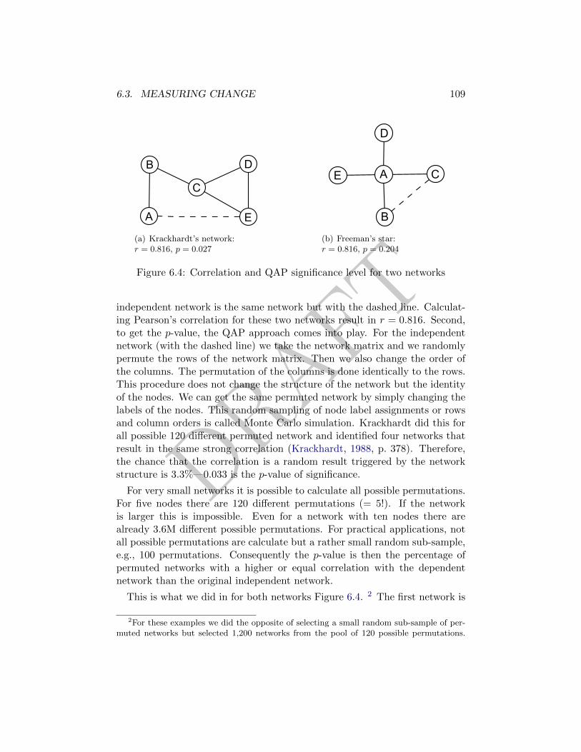
DRAFT
6.3. MEASURING CHANGE 109
A
B
C
D
E
(a) Krackhardt’s network:r = 0.816, p = 0.027
A
B
C
D
E
(b) Freeman’s star:r = 0.816, p = 0.204
Figure 6.4: Correlation and QAP significance level for two networks
independent network is the same network but with the dashed line. Calculat-ing Pearson’s correlation for these two networks result in r = 0.816. Second,to get the p-value, the QAP approach comes into play. For the independentnetwork (with the dashed line) we take the network matrix and we randomlypermute the rows of the network matrix. Then we also change the order ofthe columns. The permutation of the columns is done identically to the rows.This procedure does not change the structure of the network but the identityof the nodes. We can get the same permuted network by simply changing thelabels of the nodes. This random sampling of node label assignments or rowsand column orders is called Monte Carlo simulation. Krackhardt did this forall possible 120 different permuted network and identified four networks thatresult in the same strong correlation (Krackhardt, 1988, p. 378). Therefore,the chance that the correlation is a random result triggered by the networkstructure is 3.3%—0.033 is the p-value of significance.
For very small networks it is possible to calculate all possible permutations.For five nodes there are 120 different permutations (= 5!). If the networkis larger this is impossible. Even for a network with ten nodes there arealready 3.6M different possible permutations. For practical applications, notall possible permutations are calculate but a rather small random sub-sample,e.g., 100 permutations. Consequently the p-value is then the percentage ofpermuted networks with a higher or equal correlation with the dependentnetwork than the original independent network.
This is what we did in for both networks Figure 6.4. 2 The first network is
2For these examples we did the opposite of selecting a small random sub-sample of per-muted networks but selected 1,200 networks from the pool of 120 possible permutations.
DRAFT
110 CHAPTER 6. TEMPORAL NETWORKS
the network that we have discussed in the previous paragraphs. The right net-work is the star structured network that Freeman (1979) used to describe thecentrality measures. Both networks have five nodes and to both networks justone link is added to create the second network for comparison. The correlationcoefficient is identical for both networks but the p-values are very different.The reason for the very bad (high) p-value for the second correlation is thestructural dominance over the individual nodes—the structural autocorrela-tion. More than 20% of random permutations result in networks with equalor better correlation coefficient that the original independent network. Evenr = 0.816, the result is not significant.
Multiple regression quadratic assignment procedure (MRQAP) is the ap-proach for running regression analysis with more than two networks. Like re-gression analysis for regular statistical data, MRQAP describes the dependentnetwork with a set of independent networks. The approach is very similar toQAP. We do not discuss details of MRQAP in this book; the interested readerwill find more information about this topic at (Krackhardt, 1988) and (Dekkeret al., 2007).
6.3.5 Exponential Random Graph (p∗) Models
Exponential Random Graph Models, also known as (p∗) models, are a familyof statistical models that help analyze the structure and properties of socialand other networks. There are other well known techniques to describe thestructural properties of a network such as centrality, density etc. As opposedto these techniques which describe only the network for which they are mea-sured, ERGMs try to describe all possible networks with the same statisticalproperties as the current one. The other alternative networks may or may nothave the same structure, but the underlying statistical model that generatesthem is the same as the observed network. The networks that are being stud-ied today are substantially larger in structure for example, the World WideWeb, Internet, communication networks, food web networks, etc which havemillions and even billions of nodes. It is very hard to visualize the shape andstructure of such networks, even with modern advances in computing tech-nology. In absence of reliable visualization techniques, statistical modelingtechniques can provide an answer by quantifying large networks. Networkswith similar properties will have similar statistical models. This change inscale also makes traditional questions like, which nodes removal will affect theconnectivity in the network the most, largely irrelevant. For large scale net-
This approach makes the resulting p-values very stable when re-running the analysis.

DRAFT
6.4. DETECTING CHANGE 111
works a question which makes more sense is what percentage of nodes whenremoved would significantly affect network connectivity? Newman (2003).Statistical modeling of networks will allow us to answer this question.
Exponential random graph models have the following form:
Pθ(X = x) =exp(θts(x))
c(θ)
Where X is a random graph consisting on n nodes and x is the observedgraph. The assumption of this model is that the structure of the observedgraph x can be derived from a known vector of graph statistics, s(x) and theassociated vector of model parameters θ. The parameter c(θ), is a normalizingconstant where
c(θ) =∑
all possible graphs x
exp(θts(x))
All exponential random graph models are of the form of the first equation,which describes a general probability distribution of graphs with n nodes. Theparticular probability for observing the graph x is dependent on its statisticss(x) and on θt for all configurations in the model. Configurations includeties, triads and are these dependence assumptions are important because theypick different configurations as relevant to the model and also because theyconstrain the possible configurations possible in the model ?. The simplestdependence assumption is the Bernoulli random graph distributions where theedges are assumed to be independent whereas more complex ERGMs incor-porate node level effects (actor attributes) in the configurations. This flexibil-ity in dependence assumptions allows for greater variability in the statisticalmodeling depending on the requirements and needs of the end user using theERGM technique.
6.4 Detecting change
In the previous sections we learned how to compare specific networks witheach other. For the last two sections of this chapter our focus shifts to an-alyzing many keyframes of a network over time. The initial example of thischapter in which we had thousands of emails for a time period of 81 days fitsthis criteria. Other examples of data are, the interaction of users in SocialMedia or co-publishing of scientific articles over decades, etc. In particular
DRAFT
112 CHAPTER 6. TEMPORAL NETWORKS
when you think on data from Social Media, you can create keyframes aggre-gating data on a daily level, or even for every hour. This results in a largenumber of keyframes, i.e. networks. Having all these networks, we are inter-ested in quickly determine that (change detection) and when (change pointidentification) a change occurred in the network.
One approach to identify whether something interesting happened in thesenetworks at some point in time make use of Statistical Process Control(McCullohand Carley, 2011). Statistical Process Control (SPC) approaches are used inindustrial production processes. Imagine a big machine producing lids fortubes of toothpaste. At the end of the production circle, right before the lidsgot packaged into boxes to be shipped to the toothpaste company, there areelectrical sensors that take different measurements from every lid, e.g., weight,size, color. Each of this measure has an expected value that is pre-defined bythe product engineers. As the instrument that collect these measures arevery precise, it is almost impossible that the exact expected values are met.Therefore, a tolerance area of satisfactory is defined, i.e., a deviation from theexpected value. We now use this idea of SPC for DNA.
6.4.1 Shewhart’s Chart
The first SPC approach to detect change is Shewhart’s chart (Shewhart, 1927).Recall the lid example from the previous paragraph. What do we need to an-alyze whether the lids have the correct size and color? We need to know whatwe are measuring (statistic) and when the measure is outside the expectedarea (signal). The first question is easy to answer. Various measures on nodelevel or on network level that have been described in this and other books canbe used to create statistics of interest, e.g., centrality measures. To create thestatistic over time, we simply calculate the measure(s) of a network for eachkeyframe. The underlying assumption of change detection is that a change inan appropriate network measure is the result of a change in the underlyingreal-world network.
To illustrate Shewhart’s approach for network data, we calculate total de-gree centralization Freeman (1979) over time for the e-mail network. TheCurve in Figure 6.5 shows the result for every keyframe—please ignore they-axes and the horizontal lines in the chart for now. For interpretation ofthis chart we need to know that day 1 of our data is a Thursday. With thisknowledge we can identify a peak in centralization on the first weekend aswell as on the third weekend and the consecutive days. In the second partof the data, the peaks get higher and the last 20 days of observation show a
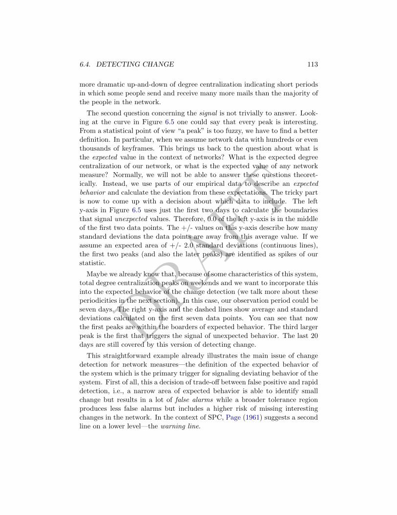
DRAFT
6.4. DETECTING CHANGE 113
more dramatic up-and-down of degree centralization indicating short periodsin which some people send and receive many more mails than the majority ofthe people in the network.
The second question concerning the signal is not trivially to answer. Look-ing at the curve in Figure 6.5 one could say that every peak is interesting.From a statistical point of view “a peak” is too fuzzy, we have to find a betterdefinition. In particular, when we assume network data with hundreds or eventhousands of keyframes. This brings us back to the question about what isthe expected value in the context of networks? What is the expected degreecentralization of our network, or what is the expected value of any networkmeasure? Normally, we will not be able to answer these questions theoret-ically. Instead, we use parts of our empirical data to describe an expectedbehavior and calculate the deviation from these expectations. The tricky partis now to come up with a decision about which data to include. The lefty-axis in Figure 6.5 uses just the first two days to calculate the boundariesthat signal unexpected values. Therefore, 0.0 of the left y-axis is in the middleof the first two data points. The +/- values on this y-axis describe how manystandard deviations the data points are away from this average value. If weassume an expected area of +/- 2.0 standard deviations (continuous lines),the first two peaks (and also the later peaks) are identified as spikes of ourstatistic.
Maybe we already know that, because of some characteristics of this system,total degree centralization peaks on weekends and we want to incorporate thisinto the expected behavior of the change detection (we talk more about theseperiodicities in the next section). In this case, our observation period could beseven days. The right y-axis and the dashed lines show average and standarddeviations calculated on the first seven data points. You can see that nowthe first peaks are within the boarders of expected behavior. The third largerpeak is the first that triggers the signal of unexpected behavior. The last 20days are still covered by this version of detecting change.
This straightforward example already illustrates the main issue of changedetection for network measures—the definition of the expected behavior ofthe system which is the primary trigger for signaling deviating behavior of thesystem. First of all, this a decision of trade-off between false positive and rapiddetection, i.e., a narrow area of expected behavior is able to identify smallchange but results in a lot of false alarms while a broader tolerance regionproduces less false alarms but includes a higher risk of missing interestingchanges in the network. In the context of SPC, Page (1961) suggests a secondline on a lower level—the warning line.
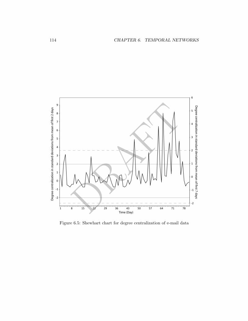
DRAFT
114 CHAPTER 6. TEMPORAL NETWORKS
1 8 15 22 29 36 43 50 57 64 71 78
9
8
7
0
1
2
3
4
6
-2
-1
5
5
-2
-1
0
1
2
3
4
6
Deg
ree
cent
raliz
atio
n in
sta
ndar
d de
viat
ions
from
mea
n of
�rs
t 2 d
ays
Degree centralization in standard deviations from
mean of �rst 7 days
Time (Day)
Figure 6.5: Shewhart chart for degree centralization of e-mail data
DRAFT
6.4. DETECTING CHANGE 115
6.4.2 Cumulative Sum (CUSUM)
Shewhart’s control chart Shewhart (1927), that was introduced in the lastsection, focuses on the identification of single outliers in the data. The cu-mulative sum (CUSUM) approach is good for detecting smaller but constantchange. A simple version of CUSUM is the following. Imagine a control chartlike in Figure 6.5. Instead of one action line that signals a deviation of thesystem, we could draw two or more lines, some of which even closer to theexpected average value. Passing the first control line results in 1 point, pass-ing the second line results in 2 points, and so forth. A data value withinthe expected area results in, e.g., -2 points. If we now setup the system in away that reaching 3 (or more) points triggers the deviation signal than thisthreshold can be reached with one or two big deviations or a larger numberof smaller deviations.
A more generalized version of CUSUM was introduced by (Page, 1961). TheCUSUM chart consists of two lines. Let us first focus on the first line thatcontrols for positive deviations, i.e., the observed data points xi are biggerthan the expected value k. For instance, the first data points of our observedmeasures are above k. CUSUM accumulates now the deviation from k bycalculating S2 = (x1− k) + (x2− k). It is clear that this line is going upwardsas long as the data points are larger than the expected value. In case the datapoints are smaller than k, the CUSUM value gets smaller but the accumulateddeviation is still positive. If this line hits now, e.g., as a result of many smallpositive deviations, a pre-defined threshold, the change signal is triggered. Incase the threshold is not reached but instead the CUSUM gets smaller andsmaller and finally undershoots zero, the positive lines is set to zero and thenegative CUSUM line starts to accumulate negative deviations.
In Figure 6.6 we used the same email data that was used previously in thischapter. As we have seen before that the weekends are very different in ourdata, we deleted the Saturday and Sunday networks from our Dynamic MetaNetwork. For the CUSUM analysis we looked at the number of Agents inthe network. The number of nodes that are involved in email conversation(send and/or receive) is visualized with the gray line in Figure 6.6. The y-axesmarks the amount of standard deviations from the mean based on the firstfive observations. If you look at the gray curve in of the statistic you maythink that values go up and down around the zero line marking the average.Looking at the cumulative sums reveals a very different picture. Even theone day peak at day 20 is followed by a rather stable period of 20 days, thevalues of this period are almost completely above the average—the constantlyraising increase lines indicates this artifact of our statistic. Moreover, when
DRAFT
116 CHAPTER 6. TEMPORAL NETWORKS
1 5 7 9 13 15 19 21 23 27 29 33 35 37 41 43 47 49 51 55 57 61 63 65 69 71 75 77 792 6 8 12 1614 20 22 26 28 30 34 36 40 42 44 48 50 54 56 58 62 64 68 70 72 76 78
Time (Day)
5
Stan
dard
dev
iatio
ns fr
om m
ean
of �
rst 5
dat
a po
ints
-10
-5
0
10
15
(value-avg)/stdev
increase/stdevdecrease/stdev
Figure 6.6: Cumulative sum chart
we look at the point at which the increase line leaves the zero line we canidentify the change point of the statistic (day 12). CUSUM The very highvalues of the last 20 days of the data burst the bonds of the chart. Therefore,we stop drawing the increase CUSUM at this point.
Shewhart’s control chart and Page’s CUSUM are straightforward approachesthat are easy to understand and to calculate. The decision about which ap-proach to use is based on the question of whether you are more interested indetecting all spikes of deviation or you are looking for constant (and probablysmaller) changes. Another advantage of CUSUM is the built-in change pointdetection. If you are interested in statistically more elaborated approachesto Statistical Process Control we want to point your attention to McCulloh(2009) for an introduction to this topic in the context of network analysis.
6.5 Periodicities
Many real world network data over time, in particular data based on commu-nication like the e-mail data that we have used in the previous sections, showperiodic patters, i.e., a very similar up-and-down over time. For instance,it makes perfects sense that e-mail data has a weekly periodicity as people
DRAFT
6.6. PROBLEM SET 117
work less on the weekends. In addition a monthly periodicity could indicatereporting a reporting structure that create more communication at the end ofthe month independently from the weekday. This changing behavior createssimilar networks on a periodic intervals that probably result in similar net-work statistics on network or node level. In real-world data the weekly andthe monthly periodicity overlay each other. Actually, additional periodicitiesbased on project cycles can make it even harder to identify the underlyingperiodicities. Nevertheless, identifying the periodic behavior of ones data canbe a very interesting step of analysis.
A very powerful but all but trivial approach to describe periodicities auto-matically is Fourier analysis. Fourier analysis decomposes a signal into a sumof sine waves. What does this mean? A sine wave is function a · sin(t/b).
Figure xx with 3 or four difference sine waves: 2 · sin(t/π)
Figure xx shows how different sine waves can be used to describe morecomplex periodicities. The third sine wave is the product of the first two sinewaves. Adding more sine waves can create any possible curve—theoreticallywe could even create the rectangular signal utut with an infinite number ofsine waves.
figure: sum of 2 sine waves (from AHFE workshop)—write sin(xx) to thefigure.
Spectral analysis.
Use Sine waves to describe periodicityDetect temporal regularities and cyclesPower spectral density (PSD): How much power/energy lays in which period-icity?frequency domain Dominant Frequencies: Shows just frequencies that aregreater than two standard deviations from the mean frequencyPeriod Plot: applying an inverse Fourier transform to the dominant frequen-cies
6.6 Problem set
1. What are the two ways of describing change in network and which oneis used normally in network analysis?
2. What two-mode network can be used to show the trail of Julius Caesarin the tragedy?
DRAFT
118 CHAPTER 6. TEMPORAL NETWORKS
3. What data is used when network distances are calculated?
4. If you assume two networks that have 80% of the nodes overlapping.Does the union or the intersect of the networks have more nodes? Why?
5. When we want to compare the centrality of an actor over time. Whatdata do we use to create the line diagram of importance over time? Howdo we get this data?
6. What is false positive and false negative?
7. What is the advantage of CUSUM compared to Shewhart’s chart?
8. What is the basic idea of fast Fourier transformation?
9. How is it possible that we can calculate Pearson correlation for twonetwork matrices?
10. Look at the overtime calculations in chapter 2 that show the importanceof Agents in the tragedy of Julius Caesar. What network level metricscould we use to analyze change in this network?
11. *If your want to calculate Hamming distance from the network of anorganization over time with fluctuating members; what is the problem?How can you overcome this problem?
12. *Aggregate (union) all five acts of the Julius Caesar Agent x Agentnetwork. Calculate degree, closeness, and betweenness centrality for theaggregated as well as for the per-act networks. Discuss the differencesof the calculations. What are the advantages and disadvantages of bothmethods?
13. *What is the problem with network correlation and how can we overcomethis problem?
14. *We used Freeman’s star network in this chapter to show a bad examplefor the QAP procedure. Find another network consisting of five nodesfor which adding a single link results in bad QAP significance level.
15. *Find a scenario that satisfies these conditions: The node level metricis completely different and the network level metric is identical.
16. *Visualize the overlapping trails of three main Agents of the Julius Cae-sar network.

DRAFT
6.6. PROBLEM SET 119
17. **Enumerate the four levels of comparison and describe how change oneach of these levels can be calculated. Find a network with at least twokeyframes and calculate a change metrics for every level. Discuss theyour results in the context of your network data.
18. **Figure out why correlation of two binary network matrices is prob-lematic. You can discuss this question with a statistician.
19. **Find and example for exponential random graph models in the liter-ature and understand what was accomplished in this work.
20. **Find a network online or create a network that has at least tenkeyframes. Calculate degree centralization for every keyframe and cal-culate the Shewhart’s chart. Experiment with different numbers of net-works that are in control. Can you find useful results?

DRAFT
120 CHAPTER 6. TEMPORAL NETWORKS
DRAFT
Chapter 7
Network Evolution andDiffusion
7.1 Diffusion of apples, ideas and beliefs
7.1.1 Random networks and stylized networks
7.1.2 Diffusion of innovation
7.1.3 Epidemic concepts
7.2 Agent-based dynamic-network computer simu-lations
7.2.1 Models
7.2.2 Models for diffusion processes
7.3 Evolution of networks
121

DRAFT
122 CHAPTER 7. NETWORK EVOLUTION AND DIFFUSION
DRAFT
Chapter 8
Extracting Networks fromTexts
It has become fast, cheap, and easy to collect and store large amounts ofnatural language text data. New text data is created every second on theinternet as hundreds of million of user interact on social media platformswith each other. But also traditional media is more and more available sincearchival text data such as newspapers and books are being converted to digitalforms daily. The increasing availability of these data has exacerbated the needfor techniques, measures and tools for automated knowledge discovery andreasoning about text. The family of methods developed to address this issueis collectively known as Relational Text Analysis (RTA). Or, in the contextof networks it is often referred to as Network Text Analysis ( Carley, 1997;Danowski, 1993; van Cuilenburg, Kleinnijenhuis and Ridder, 1986). Whiletext data does not automatically entail a network analysis, text is a readysource of new information about relationships between entities and additionalattributes for single entities.
The goal of this chapter is to introduce you to the applicability and usage oftext analysis in the domain of network analysis. You will learn how to extractrelevant information and structured data from text data in an efficient andsystematic fashion, how to perform appropriate analysis on the extracted data,and how to interpret and evaluate your results. The secondary goals are tounderstand how the different choices that you make throughout this processimpact your results. We will describe the basics for how to distill relevantinformation as well as one-mode and multi-mode network data from texts.We will also discuss what metrics you would use in analyzing the extracted
123
DRAFT
124 CHAPTER 8. EXTRACTING NETWORKS FROM TEXTS
information and network data.
8.1 Analyzing texts
8.1.1 Content analysis
8.1.2 tf*idf
8.2 Text processing
8.2.1 Deletion
8.2.2 Thesauri
8.2.3 Concept lists
8.2.4 Bi-grams
8.2.5 Stemming
8.3 From texts to networks
8.3.1 Keyword in context
8.3.2 Windowing
8.3.3 Extracting meta-networks from texts
DRAFT
Chapter 9
The Future of DynamicNetwork Analysis
125

DRAFT
126 CHAPTER 9. THE FUTURE OF DYNAMIC NETWORK ANALYSIS
DRAFT
Appendix A
SNA Measures Glossary
Dynamic network analysis uses a lot of different measures to gain better in-sights into network structure and dynamic. In the chapters of this book wediscussed various measures to identify important nodes, find group structures,detect change, etc. We have not defined these measures mathematically oralgorithmically so far. This is what you can find in this chapter. At the fol-lowing pages you will find a lot of measures including a short description, thereference of the paper where the measure was originally presented, as well asthe equation or algorithm describing the actual calculation of the measures.
Scaling a measures means to transform the results of a certain calculationinto the range of 0 to 1, with 0 being the smallest possible value and 1 indi-cating nodes having the maximum possible value. This is important to makeresults of different networks comparable. The basic idea of scaling networkmeasures is to find the maximum possible value and divide by this number,e.g. in a network with N nodes a single node can have N − 1 maximum pos-sible neighbors. Degree centrality, therefore, counts the number of nodes, asingle not is connected to and divides this number by N − 1. In the followingequations you will find an apostrophe to indicate scaled measures, e.g. C ′Dstands for scaled degree centrality. Consequently, C is unscaled degree cen-trality, which is the number of neighbors of a node. For some measures weoffer the unscaled version and the maximum possible value. In this case, toget the scaled measure you have to divide the unscaled with the maximumvalue:
C ′ =C
Cmax
127
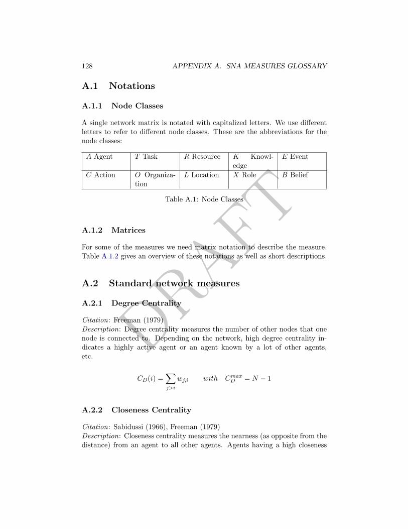
DRAFT
128 APPENDIX A. SNA MEASURES GLOSSARY
A.1 Notations
A.1.1 Node Classes
A single network matrix is notated with capitalized letters. We use differentletters to refer to different node classes. These are the abbreviations for thenode classes:
A Agent T Task R Resource K Knowl-edge
E Event
C Action O Organiza-tion
L Location X Role B Belief
Table A.1: Node Classes
A.1.2 Matrices
For some of the measures we need matrix notation to describe the measure.Table A.1.2 gives an overview of these notations as well as short descriptions.
A.2 Standard network measures
A.2.1 Degree Centrality
Citation: Freeman (1979)Description: Degree centrality measures the number of other nodes that onenode is connected to. Depending on the network, high degree centrality in-dicates a highly active agent or an agent known by a lot of other agents,etc.
CD(i) =∑j>i
wj,i with CmaxD = N − 1
A.2.2 Closeness Centrality
Citation: Sabidussi (1966), Freeman (1979)Description: Closeness centrality measures the nearness (as opposite from thedistance) from an agent to all other agents. Agents having a high closeness
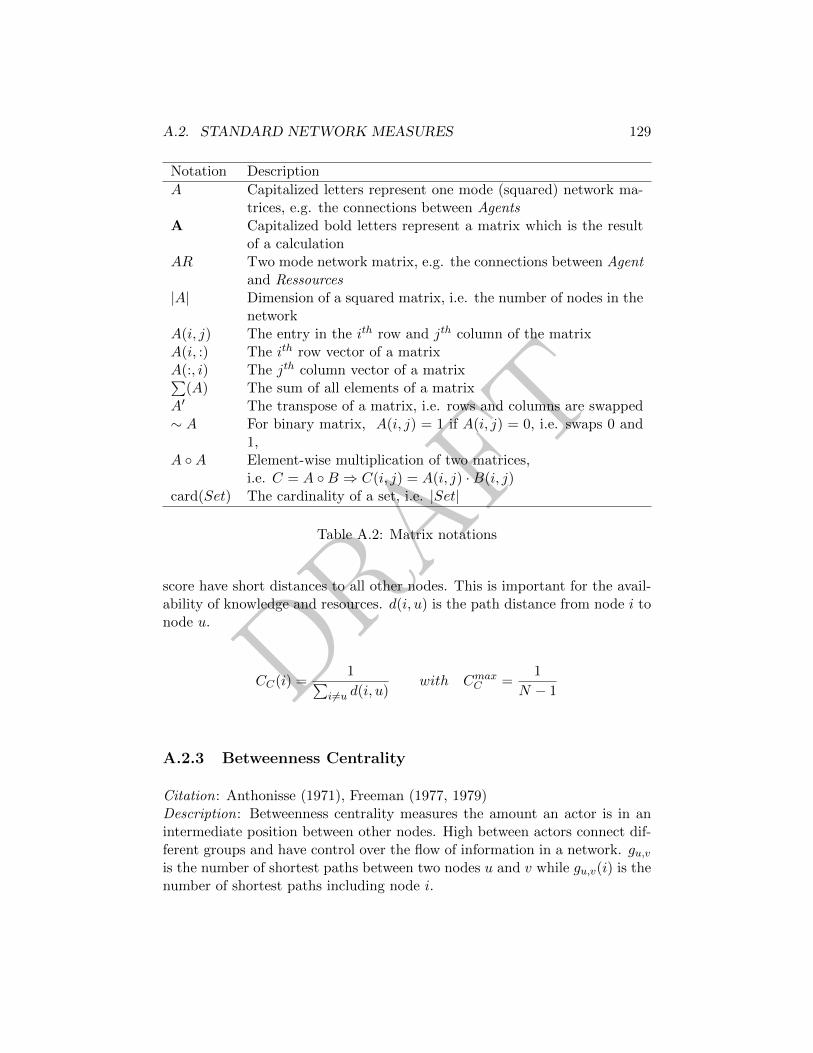
DRAFT
A.2. STANDARD NETWORK MEASURES 129
Notation Description
A Capitalized letters represent one mode (squared) network ma-trices, e.g. the connections between Agents
A Capitalized bold letters represent a matrix which is the resultof a calculation
AR Two mode network matrix, e.g. the connections between Agentand Ressources
|A| Dimension of a squared matrix, i.e. the number of nodes in thenetwork
A(i, j) The entry in the ith row and jth column of the matrixA(i, :) The ith row vector of a matrixA(:, i) The jth column vector of a matrix∑
(A) The sum of all elements of a matrixA′ The transpose of a matrix, i.e. rows and columns are swapped∼ A For binary matrix, A(i, j) = 1 if A(i, j) = 0, i.e. swaps 0 and
1,A ◦A Element-wise multiplication of two matrices,
i.e. C = A ◦B ⇒ C(i, j) = A(i, j) ·B(i, j)card(Set) The cardinality of a set, i.e. |Set|
Table A.2: Matrix notations
score have short distances to all other nodes. This is important for the avail-ability of knowledge and resources. d(i, u) is the path distance from node i tonode u.
CC(i) =1∑
i 6=u d(i, u)with CmaxC =
1
N − 1
A.2.3 Betweenness Centrality
Citation: Anthonisse (1971), Freeman (1977, 1979)Description: Betweenness centrality measures the amount an actor is in anintermediate position between other nodes. High between actors connect dif-ferent groups and have control over the flow of information in a network. gu,vis the number of shortest paths between two nodes u and v while gu,v(i) is thenumber of shortest paths including node i.
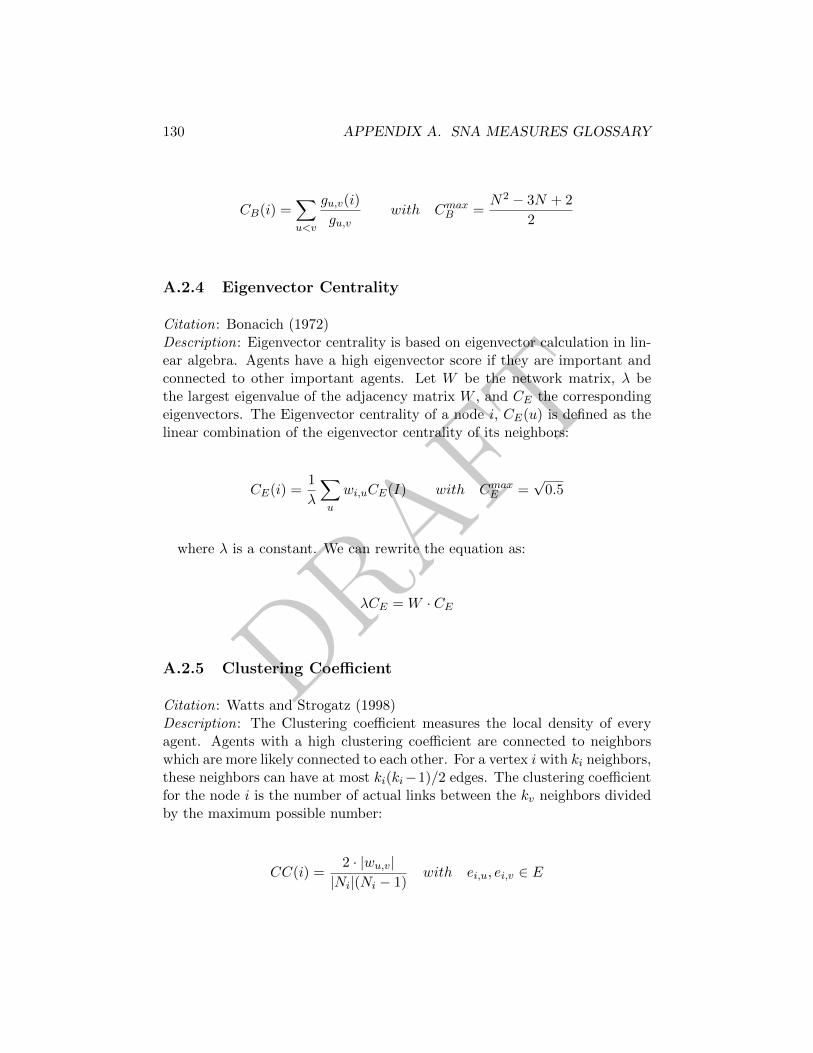
DRAFT
130 APPENDIX A. SNA MEASURES GLOSSARY
CB(i) =∑u<v
gu,v(i)
gu,vwith CmaxB =
N2 − 3N + 2
2
A.2.4 Eigenvector Centrality
Citation: Bonacich (1972)Description: Eigenvector centrality is based on eigenvector calculation in lin-ear algebra. Agents have a high eigenvector score if they are important andconnected to other important agents. Let W be the network matrix, λ bethe largest eigenvalue of the adjacency matrix W , and CE the correspondingeigenvectors. The Eigenvector centrality of a node i, CE(u) is defined as thelinear combination of the eigenvector centrality of its neighbors:
CE(i) =1
λ
∑u
wi,uCE(I) with CmaxE =√
0.5
where λ is a constant. We can rewrite the equation as:
λCE = W · CE
A.2.5 Clustering Coefficient
Citation: Watts and Strogatz (1998)Description: The Clustering coefficient measures the local density of everyagent. Agents with a high clustering coefficient are connected to neighborswhich are more likely connected to each other. For a vertex i with ki neighbors,these neighbors can have at most ki(ki−1)/2 edges. The clustering coefficientfor the node i is the number of actual links between the kv neighbors dividedby the maximum possible number:
CC(i) =2 · |wu,v||Ni|(Ni − 1)
with ei,u, ei,v ∈ E

DRAFT
A.3. GROUPING ALGORITHMS 131
A.3 Grouping algorithms
A.4 Change measures
A.5 Network text algorithms

DRAFT
132 APPENDIX A. SNA MEASURES GLOSSARY
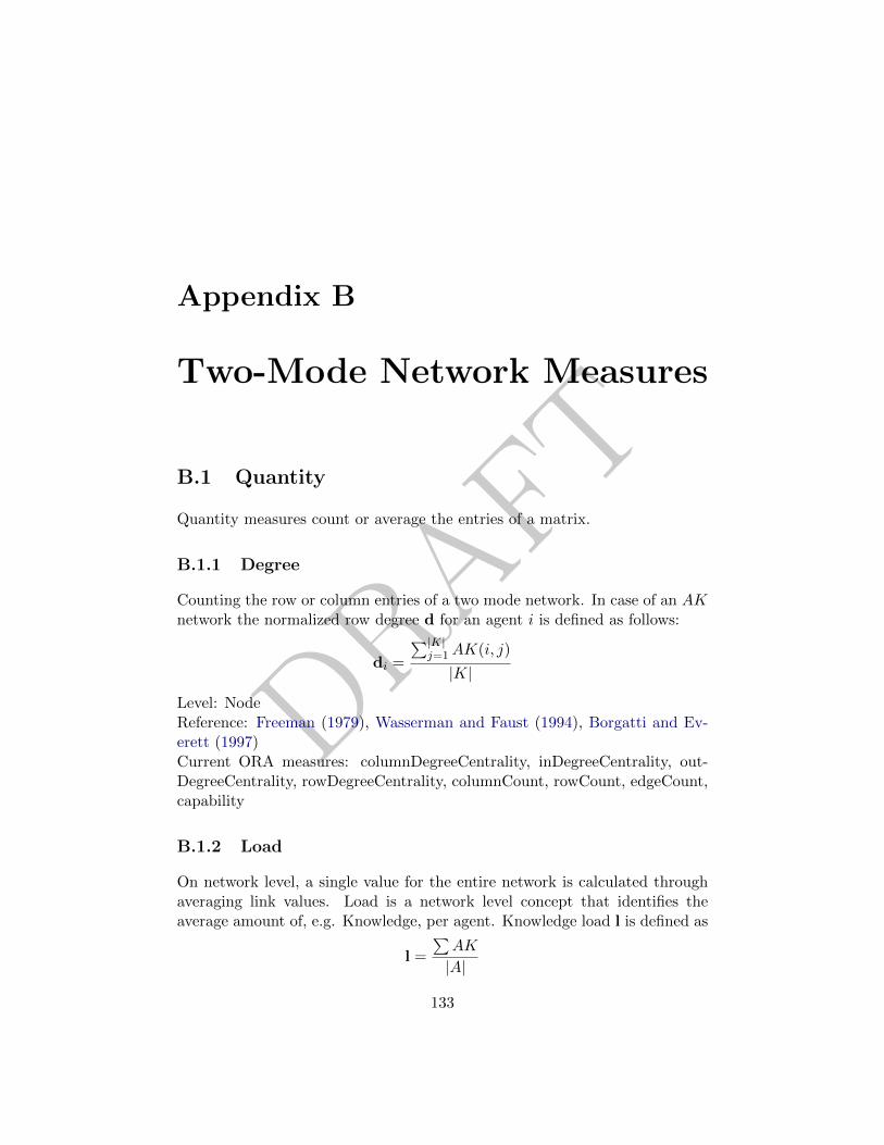
DRAFT
Appendix B
Two-Mode Network Measures
B.1 Quantity
Quantity measures count or average the entries of a matrix.
B.1.1 Degree
Counting the row or column entries of a two mode network. In case of an AKnetwork the normalized row degree d for an agent i is defined as follows:
di =
∑|K|j=1AK(i, j)
|K|
Level: NodeReference: Freeman (1979), Wasserman and Faust (1994), Borgatti and Ev-erett (1997)Current ORA measures: columnDegreeCentrality, inDegreeCentrality, out-DegreeCentrality, rowDegreeCentrality, columnCount, rowCount, edgeCount,capability
B.1.2 Load
On network level, a single value for the entire network is calculated throughaveraging link values. Load is a network level concept that identifies theaverage amount of, e.g. Knowledge, per agent. Knowledge load l is defined as
l =
∑AK
|A|
133
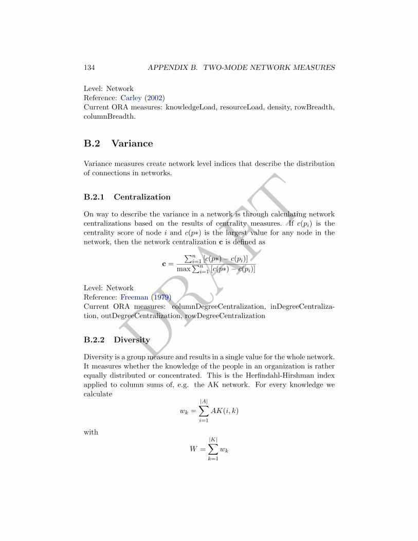
DRAFT
134 APPENDIX B. TWO-MODE NETWORK MEASURES
Level: NetworkReference: Carley (2002)Current ORA measures: knowledgeLoad, resourceLoad, density, rowBreadth,columnBreadth.
B.2 Variance
Variance measures create network level indices that describe the distributionof connections in networks.
B.2.1 Centralization
On way to describe the variance in a network is through calculating networkcentralizations based on the results of centrality measures. If c(pi) is thecentrality score of node i and c(p∗) is the largest value for any node in thenetwork, then the network centralization c is defined as
c =
∑ni=1 [c(p∗)− c(pi)]
max∑n
i=1 [c(p∗)− c(pi)]
Level: NetworkReference: Freeman (1979)Current ORA measures: columnDegreeCentralization, inDegreeCentraliza-tion, outDegreeCentralization, rowDegreeCentralization
B.2.2 Diversity
Diversity is a group measure and results in a single value for the whole network.It measures whether the knowledge of the people in an organization is ratherequally distributed or concentrated. This is the Herfindahl-Hirshman indexapplied to column sums of, e.g. the AK network. For every knowledge wecalculate
wk =
|A|∑i=1
AK(i, k)
with
W =
|K|∑k=1
wk
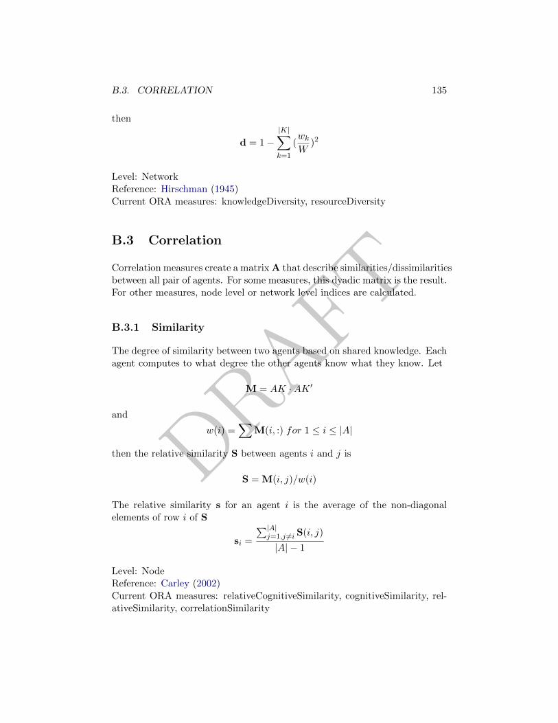
DRAFT
B.3. CORRELATION 135
then
d = 1−|K|∑k=1
(wkW
)2
Level: NetworkReference: Hirschman (1945)Current ORA measures: knowledgeDiversity, resourceDiversity
B.3 Correlation
Correlation measures create a matrix A that describe similarities/dissimilaritiesbetween all pair of agents. For some measures, this dyadic matrix is the result.For other measures, node level or network level indices are calculated.
B.3.1 Similarity
The degree of similarity between two agents based on shared knowledge. Eachagent computes to what degree the other agents know what they know. Let
M = AK ·AK ′
and
w(i) =∑
M(i, :) for 1 ≤ i ≤ |A|
then the relative similarity S between agents i and j is
S = M(i, j)/w(i)
The relative similarity s for an agent i is the average of the non-diagonalelements of row i of S
si =
∑|A|j=1,j 6=i S(i, j)
|A| − 1
Level: NodeReference: Carley (2002)Current ORA measures: relativeCognitiveSimilarity, cognitiveSimilarity, rel-ativeSimilarity, correlationSimilarity
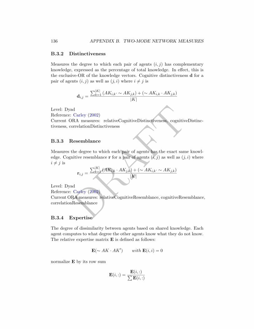
DRAFT
136 APPENDIX B. TWO-MODE NETWORK MEASURES
B.3.2 Distinctiveness
Measures the degree to which each pair of agents (i, j) has complementaryknowledge, expressed as the percentage of total knowledge. In effect, this isthe exclusive-OR of the knowledge vectors. Cognitive distinctiveness d for apair of agents (i, j) as well as (j, i) where i 6= j is
di,j =
∑|K|k=1 (AKi,k· ∼ AKj,k) + (∼ AKi,k ·AKj,k)
|K|
Level: DyadReference: Carley (2002)Current ORA measures: relativeCognitiveDistinctiveness, cognitiveDistinc-tiveness, correlationDistinctiveness
B.3.3 Resemblance
Measures the degree to which each pair of agents has the exact same knowl-edge. Cognitive resemblance r for a pair of agents (i, j) as well as (j, i) wherei 6= j is
ri,j =
∑|K|k=1 (AKi,k ·AKj,k) + (∼ AKi,k· ∼ AKj,k)
|K|
Level: DyadReference: Carley (2002)Current ORA measures: relativeCognitiveResemblance, cognitiveResemblance,correlationResemblance
B.3.4 Expertise
The degree of dissimilarity between agents based on shared knowledge. Eachagent computes to what degree the other agents know what they do not know.The relative expertise matrix E is defined as follows:
E(∼ AK ·AK ′) with E(i, i) = 0
normalize E by its row sum
E(i, :) =E(i, :)∑E(i, :)
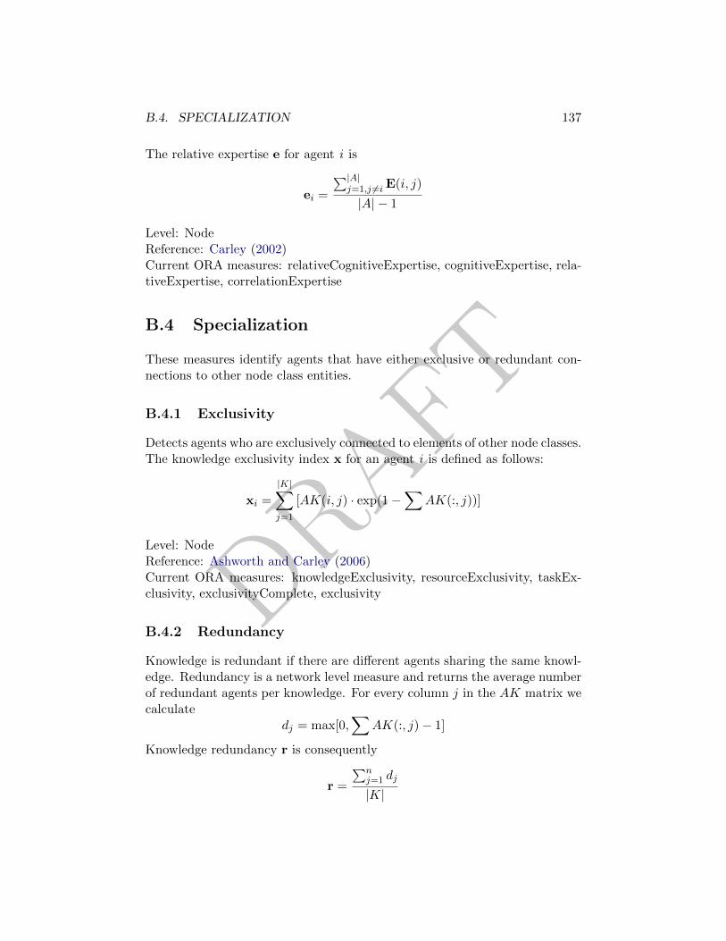
DRAFT
B.4. SPECIALIZATION 137
The relative expertise e for agent i is
ei =
∑|A|j=1,j 6=i E(i, j)
|A| − 1
Level: NodeReference: Carley (2002)Current ORA measures: relativeCognitiveExpertise, cognitiveExpertise, rela-tiveExpertise, correlationExpertise
B.4 Specialization
These measures identify agents that have either exclusive or redundant con-nections to other node class entities.
B.4.1 Exclusivity
Detects agents who are exclusively connected to elements of other node classes.The knowledge exclusivity index x for an agent i is defined as follows:
xi =
|K|∑j=1
[AK(i, j) · exp(1−∑
AK(:, j))]
Level: NodeReference: Ashworth and Carley (2006)Current ORA measures: knowledgeExclusivity, resourceExclusivity, taskEx-clusivity, exclusivityComplete, exclusivity
B.4.2 Redundancy
Knowledge is redundant if there are different agents sharing the same knowl-edge. Redundancy is a network level measure and returns the average numberof redundant agents per knowledge. For every column j in the AK matrix wecalculate
dj = max[0,∑
AK(:, j)− 1]
Knowledge redundancy r is consequently
r =
∑nj=1 dj
|K|
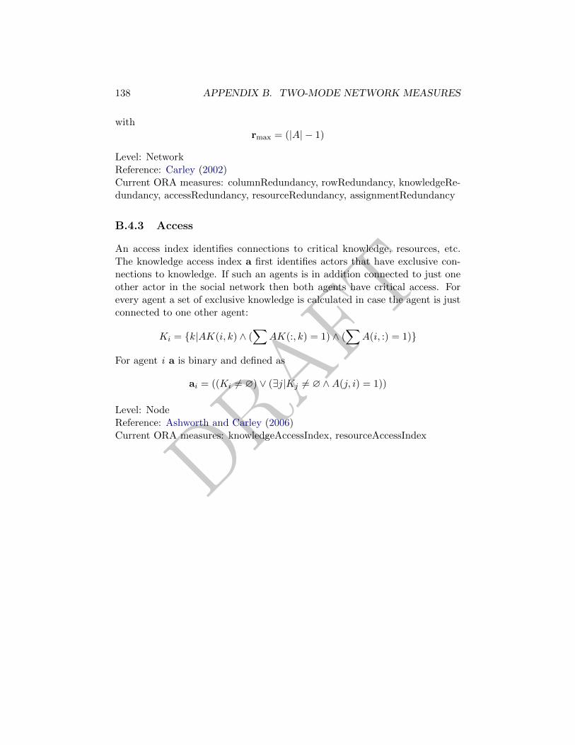
DRAFT
138 APPENDIX B. TWO-MODE NETWORK MEASURES
withrmax = (|A| − 1)
Level: NetworkReference: Carley (2002)Current ORA measures: columnRedundancy, rowRedundancy, knowledgeRe-dundancy, accessRedundancy, resourceRedundancy, assignmentRedundancy
B.4.3 Access
An access index identifies connections to critical knowledge, resources, etc.The knowledge access index a first identifies actors that have exclusive con-nections to knowledge. If such an agents is in addition connected to just oneother actor in the social network then both agents have critical access. Forevery agent a set of exclusive knowledge is calculated in case the agent is justconnected to one other agent:
Ki = {k|AK(i, k) ∧ (∑
AK(:, k) = 1) ∧ (∑
A(i, :) = 1)}
For agent i a is binary and defined as
ai = ((Ki 6= ∅) ∨ (∃j|Kj 6= ∅ ∧A(j, i) = 1))
Level: NodeReference: Ashworth and Carley (2006)Current ORA measures: knowledgeAccessIndex, resourceAccessIndex
DRAFT
Appendix C
Multi-Mode NetworkMeasures
C.1 Quantity
C.1.1 Degree
Total number of people reporting to an agent, plus its total knowledge, re-sources, and tasks can be considered as Personnel Costs:
ci =
∑|A|j=1,j 6=iAA(j, i) +
∑AK(i, :) +
∑AR(i, :) +
∑AT (i, :)
(|A| − 1) + |K|+ |R|+ |T |
A very similar measure is Socio Economic Power that measures the power ofAgents based on access to knowledge, resources, and tasks. It is defined likePersonnel Costs but without the Agents parts of the equation.
Level: NodeReference: Ashworth and Carley (2003), Carley (2004)Current ORA measures: personnelCost, agentSocioEconomicPower
C.1.2 Load
Complexity is a meta-network measures of load. It calculates the density ofthe meta-matrix that results from concatenating all available networks:
139

DRAFT
140 APPENDIX C. MULTI-MODE NETWORK MEASURES
c =card{∀i, j ∈ A|i 6= j ∧AA(i, j) > 0}+ card{∀i ∈ A ∧ ∀t ∈ T |AT (i, t) > 0}+ · · ·
|A|(|A| − 1) + |AT |+ · · ·
Level: NetworkReference: Wasserman and Faust (1994)Current ORA measures: complexity
C.2 Coherence
Coherence measures analyze to what extent requirements are accomplishedby the actual allocation of agents to tasks. The three different concepts ofthis group describe coherence from different perspectives. Congruence mea-sures the level of conformance, need algorithms focus on missing Knowledgeor Resources, and waste algorithms identify surplus Knowledge or Resourcescompared to the actual needed ones for completing tasks. Performance looksat Tasks which can be completed.
C.2.1 Congruence
Measures the similarity between what Knowledge is assigned to tasks viaagents, and what Knowledge is required to do Tasks. Perfect congruenceoccurs when Agents have Knowledge when and only when it is needful tocomplete their Tasks. Let KT be the matrix representing the Knowledgeassigned to Tasks via Agents
KT = AK ′ ·AT
then then Knowledge Congruence is the proportion of correctly assigned Knowl-edge
c =card{(i, j)|[(KT(i, j) > 0) = (KT (i, j) > 0)]}
|K| · |T |
Another more elaborated measures is Communication Congruence that mea-sures to what extent Agents communicate when and only when it is needfulto complete Tasks. We assume that Agents i and j must reciprocally commu-nicate if at least one of the following is true. a) if i is assigned to a Task sand j is assigned to a Task t and s directly precedes Task t (handoff). b) if

DRAFT
C.2. COHERENCE 141
i is assigned to a Task s and j is also assigned to s (co-assignment). c) if i isassigned to a Task s and j is not, and there is a Resource r to which Agentsassigned to s have no access but j does (negotiation to get needed Resource).These three cases are computed as follows:
a) H = AT · T ·AT ′b) C = AT ·AT ′
c) N = AT · Z ·AR′ with Z(t, r) =
{1 if [AT ′ ·AR−RT ′](t, r) < 00 otherwise
Let Q be the reciprocal communication matrix that is required
Q(t, r) =
{1 if [(H + C + N) + (H + C + N)′](i, j) > 00 otherwise
then Communication Congruence is, similar to Knowledge Congruence, thedegree to which actual communication differs from that which is needed to dotasks
c =card{(i, j)|[(A(i, j) > 0) = (Q(i, j) > 0)]}
|A| · (|A| − 1)
Level: NetworkReference: Carley (2002)Current ORA measures: communicationCongruence, knowledgeCongruence,resourceCongruence, socialTechnicalCongruence (2 mode)
C.2.2 Needs
Task Knowledge Needs compares the Knowledge requirements of each Taskwith the Knowledge available to the Task via Agents assigned to it. It issimilar to Knowledge Congruence, but quantifies only the under supply ofKnowledge to Tasks. Let S be the Knowledge supplied to Tasks via assignedAgents.
S = AT ′ ·AK
then Task Knowledge Needs for t is defined as
nt =
∑|K|k=1KT
′(t, k) · (S(t, k) = 0)∑|K|k=1KT
′(t, k)
DRAFT
142 APPENDIX C. MULTI-MODE NETWORK MEASURES
Organization Needs measures are the corresponding network level measures,e.g. the Knowledge that Agents lack to do their assigned Task expressed as apercentage of the total Knowledge needed by all Agents:
n =
∑|T |t=1
∑|K|k=1KT
′(t, k) · (S(t, k) = 0)∑KT
Level: Node, NetworkReference:Lee and Carley (2004)
Current ORA measures: communicativeNeeds (communication), congruenceAgen-tKnowledgeNeeds, congruenceOrgAgentKnowledgeNeeds, congruenceOrgTaskKnowl-edgeNeeds, congruenceTaskKnowledgeNeeds, congruenceAgentResourceNeeds,congruenceOrgAgentResourceNeeds, congruenceOrgTaskResourceNeeds, con-gruenceTaskResourceNeeds, knowledgeUnderSupply, resourceUnderSupply
C.2.3 Waste
Waste measures focus on the oversupply part of congruence. Task KnowledgeWaste counts the number of skills supplied to a Task via Agents that are notrequired by it expressed as a percentage of the total skills required for theTask. This measure results in a value for every Task. Let, again, S be theKnowledge supplied to Tasks via assigned Agents.
S = AT ′ ·AK
then Task Knowledge Waste for t is defined as
wt =
∑|K|k=1 S(t, k) · (∼ KT ′(t, k))∑|K|
k=1 S(t, k)
Organizational Waste measures are the corresponding network level measures,e.g. the Knowledge supplied to Tasks via Agents that are not required bythem, expressed as a percentage of the total skills needed by all Tasks:
w =
∑|T |t=1
∑|K|k=1 S(t, k) · (∼ KT ′(t, k))∑
S
Level: Node, NetworkReference: Lee and Carley (2004)
DRAFT
C.2. COHERENCE 143
Current ORA measures: congruenceAgentKnowledgeWaste, congruenceOr-gAgentKnowledgeWaste, congruenceOrgTaskKnowledgeWaste, congruenceTaskKnowl-edgeWaste, congruenceAgentResourceWaste, congruenceOrgAgentResource-Waste, congruenceOrgTaskResourceWaste, congruenceTaskResourceWaste
C.2.4 Performance
Knowledge Based Task Completion calculated the percentage of tasks thatcan be completed by the agents assigned to them, based solely on whetherthe agents have the requisite Knowledge to do the Tasks. First, we find theTasks that cannot be completed because the Agents assigned to the Taskslack necessary Knowledge:
N = (AT ′ ·AK)−KT ′
Then we calculate the set of Tasks which cannot be completed:
S = {t|t ∈ T ∧ ∃k : N(t, k) < 0}
Knowledge Based Task Completion is then the percentage of tasks that couldbe completed:
c =|T | − |S||T |
Level: NetworkReference: Carley (2002)Current ORA measures: resourceTaskCompletion, overallTaskCompletion,knowledgeTaskCompletion, performanceAsAccuracy
C.2.5 Workload
Workload measures look for the Knowledge or Resource an Agent uses toperform Tasks to which it is assigned. The Potential Knowledge Workload isdefined as
wi =
∑(AK ·KT )(i, :)∑
KT
while the Actual Knowlede Workload also takes the actual AT network intoaccount:
wi =
∑(AK ·KT ·AT ′)(i, i)∑
KT
Level: NodeReference: Carley (2002)
DRAFT
144 APPENDIX C. MULTI-MODE NETWORK MEASURES
Current ORA measures: knowledgeActualWorkload, resourceActualWorkload,actualWorkload, knowledgePotentialWorkload, resourcePotentialWorkload, po-tentialWorkload
C.2.6 Negotiation
The extent to which Agents need to negotiate with each other because theylack the Knowledge to complete their assigned Tasks. The Negotiation mea-sure computes the percentage of tasks that lack at least one Knowledge. First,a TK congruence matrix is calculated with
C = (AT ′ ·AK)−KT ′
to get proportion of unassigned Tasks:
n =card{t|t ∈ T ∧ ∃k : C(t, k) < 0}
|T |
Level: NetworkReference: Carley (2002)Current ORA measures: knowledgeNegotiation, resourceNegotiation
C.3 Substitution
This group is rather diverse and include concepts and measures describingto which extent Agents can be substituted base on identical Roles or Agentsneed to negotiate with each other as well as Knowledge and Resources that isused or reused to perform Tasks.
C.3.1 Availability
Availability measures use the node class Roles. Role Based Knowledge Avail-ability computes the number of roles that an agent is qualified to have based onknowledge requirements. Overall Role Based Availability computes the degreeto which agents are available to do tasks based on their access to knowledgeand resources and roles that are needed to do the tasks. The later is definedas . . .
a =?AK??AR??AX?
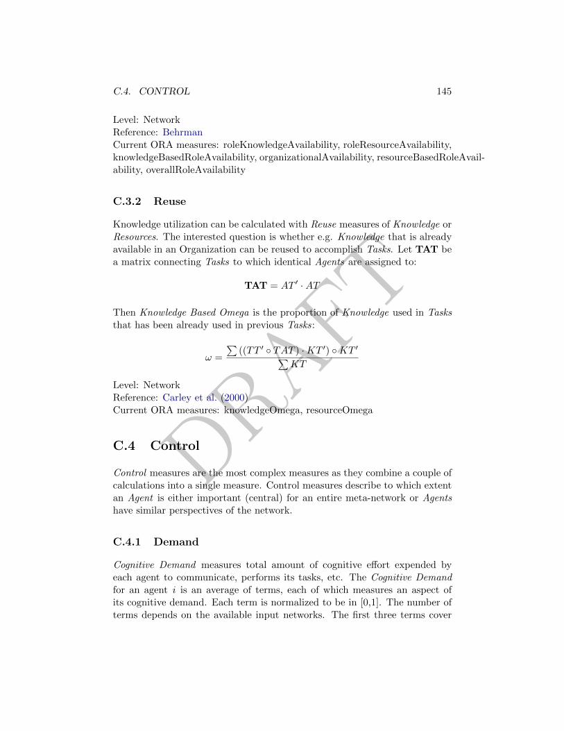
DRAFT
C.4. CONTROL 145
Level: NetworkReference: BehrmanCurrent ORA measures: roleKnowledgeAvailability, roleResourceAvailability,knowledgeBasedRoleAvailability, organizationalAvailability, resourceBasedRoleAvail-ability, overallRoleAvailability
C.3.2 Reuse
Knowledge utilization can be calculated with Reuse measures of Knowledge orResources. The interested question is whether e.g. Knowledge that is alreadyavailable in an Organization can be reused to accomplish Tasks. Let TAT bea matrix connecting Tasks to which identical Agents are assigned to:
TAT = AT ′ ·AT
Then Knowledge Based Omega is the proportion of Knowledge used in Tasksthat has been already used in previous Tasks:
ω =
∑((TT ′ ◦ TAT ) ·KT ′) ◦KT ′∑
KT
Level: NetworkReference: Carley et al. (2000)Current ORA measures: knowledgeOmega, resourceOmega
C.4 Control
Control measures are the most complex measures as they combine a couple ofcalculations into a single measure. Control measures describe to which extentan Agent is either important (central) for an entire meta-network or Agentshave similar perspectives of the network.
C.4.1 Demand
Cognitive Demand measures total amount of cognitive effort expended byeach agent to communicate, performs its tasks, etc. The Cognitive Demandfor an agent i is an average of terms, each of which measures an aspect ofits cognitive demand. Each term is normalized to be in [0,1]. The number ofterms depends on the available input networks. The first three terms cover
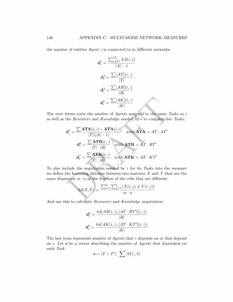
DRAFT
146 APPENDIX C. MULTI-MODE NETWORK MEASURES
the number of entities Agent i is connected to in different networks:
d1i =
∑|A|j,j 6=iAA(i, j)
|A| − 1
d2i =
∑[AT ](i, :)
|T |
d3i =
∑[AR](i, :)
|R|
d4i =
∑[AK](i, :)
|K|
The next terms cover the number of Agents assigned to the same Tasks as ias well as the Resources and Knowledge needed by i to complete her Tasks:
d5i =
∑ATA(i, :)−ATA(i, i)
|T |(|A| − 1)with ATA = AT ·AT ′
d6i =
∑ATR(i, :)
|T | · |R|with ATR = AT ·RT ′
d7i =
∑ATK(i, :)
|T | · |K|with ATK = AT ·KT ′
To also include the negotiation needed by i for its Tasks into the measurewe define the hamming distance between two matrices X and Y that are thesame dimension m · n as the fraction of the cells that are different:
hd(X,Y ) =
∑mi=1
∑nj=1 (X(i, j) 6= Y (i, j))
m · n
And use this to calculate Resourece and Knowledge negotiation:
d8i =
hd(AR(i, :), [AT ·RT ′](i, :))|R|
d9i =
hd(AK(i, :), [AT ·KT ′](i, :))|K|
The last term represents number of Agents that i depends on or that dependon i. Let s be a vector describing the number of Agents that dependent oneach Task
s = (T + T ′) ·∑
AT (:, t)
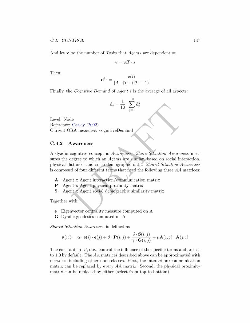
DRAFT
C.4. CONTROL 147
And let v be the number of Tasks that Agents are dependent on
v = AT · s
Then
d10 =v(i)
|A| · |T | · (|T | − 1)
Finally, the Cognitive Demand of Agent i is the average of all aspects:
di =1
10·
10∑j=1
dji
Level: NodeReference: Carley (2002)Current ORA measures: cognitiveDemand
C.4.2 Awareness
A dyadic cognitive concept is Awareness. Share Situation Awareness mea-sures the degree to which an Agents are similar, based on social interaction,physical distance, and socio-demographic data. Shared Situation Awarenessis composed of four different terms that need the following three AA matrices:
A Agent x Agent interaction/communication matrixP Agent x Agent physical proximity matrixS Agent x Agent social demographic similarity matrix
Together with
e Eigenvector centrality measure computed on AG Dyadic geodesics computed on A
Shared Situation Awareness is defined as
a(ij) = α · e(i) · e(j) + β ·P(i, j) +δ · S(i, j)
γ ·G(i, j)+ µA(i, j) ·A(j, i)
The constants α, β, etc., control the influence of the specific terms and are setto 1.0 by default. The AA matrices described above can be approximated withnetworks including other node classes. First, the interaction/communicationmatrix can be replaced by every AA matrix. Second, the physical proximitymatrix can be replaced by either (select from top to bottom)

DRAFT
148 APPENDIX C. MULTI-MODE NETWORK MEASURES
AL ·AL′ in case AL exists, orSimilarity of [ATAE] in case AT and/or AE exist.
Otherwise ignore any physical proximity calculation. Third, the social demo-graphic similarity matrix can be replaced with
Similarity of [AKAR] in case AK and/or AR exist.
Otherwise ignore the social demographic similarity calculation.
Level: Graham et al. (2004)Reference: Node, DyadCurrent ORA measures: sharedSituationAwareness
DRAFT
Appendix D
Julius Caesar Data
D.1 Interactions of Agents
Agent x Agent - Act 1
Agent x Agent - Act 2
Agent x Agent - Act 3
Agent x Agent - Act 4
Agent x Agent - Act 5
D.2 Agents and Their Connections
Agent x Knowledge
Agent x Location
Agent x Event
Agent x Task
D.3 Other Networks
Event x Event
Knowledge x Task
149
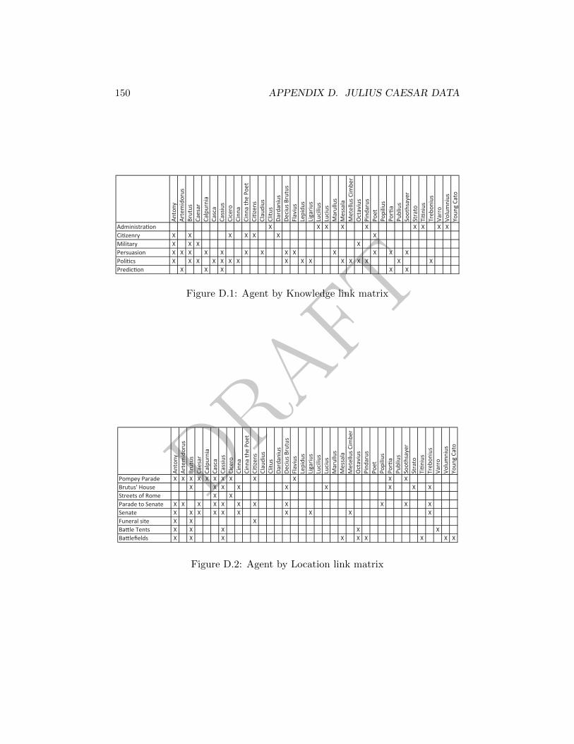
DRAFT
150 APPENDIX D. JULIUS CAESAR DATA
Anto
nyAr
tem
idor
usBr
utus
Caes
arCa
lpur
nia
Casc
aCa
ssiu
sCi
cero
Cinn
aCi
nna
the
Poet
Citiz
ens
Clau
dius
Clitu
sDa
rdan
ius
Deci
us B
rutu
sFl
aviu
sLe
pidu
sLi
gariu
sLu
ciliu
sLu
cius
Mar
ullu
sM
essa
laM
etel
lus C
imbe
rO
ctav
ius
Pind
arus
Poet
Popi
lius
Porti
aPu
bliu
sSo
oths
ayer
Stra
toTitin
ius
Treb
oniu
sVa
rro
Volu
mni
usYo
ung
Cato
Administration X X X X X X X X XCitizenry X X X X X X XMilitary X X X XPersuasion X X X X X X X X X X X X XPolitics X X X X X X X X X X X X X X X XPrediction X X X X X
Figure D.1: Agent by Knowledge link matrix
Anto
nyAr
tem
idor
usBr
utus
Caes
arCa
lpur
nia
Casc
aCa
ssiu
sCi
cero
Cinn
aCi
nna
the
Poet
Citiz
ens
Clau
dius
Clitu
sDa
rdan
ius
Deci
us B
rutu
sFl
aviu
sLe
pidu
sLi
gariu
sLu
ciliu
sLu
cius
Mar
ullu
sM
essa
laM
etel
lus C
imbe
rO
ctav
ius
Pind
arus
Poet
Popi
lius
Porti
aPu
bliu
sSo
oths
ayer
Stra
toTitin
ius
Treb
oniu
sVa
rro
Volu
mni
usYo
ung
Cato
Pompey Parade X X X X X X X X X X X XBrutus' House X X X X X X X X XStreets of Rome X XParade to Senate X X X X X X X X X X XSenate X X X X X X X X X XFuneral site X X XBattle Tents X X X X XBattlefields X X X X X X X X X
Figure D.2: Agent by Location link matrix

DRAFT
D.3. OTHER NETWORKS 151
Location x Location
Task x Event
Task x Task

DRAFT
152 APPENDIX D. JULIUS CAESAR DATA

DRAFT
Bibliography
Adar, E. and Adamic, L. (2005). Tracking information epidemics in blogspace.In Proceedings of the 2005 IEEE/WIC/ACM International Conference onWeb Intelligence, volume Compiegne, France.
Alderson, D. (2008). Catching the ”network science” bug: insight and oppor-tunity for the operations researcher. Operations Research, 56:1047–1065.
Aldrich, H. E. and Herker, D. (1977). Boundary spanning roles and organiza-tion structure. Academy of Management Review, 2(2):217–230.
Allen, T. J. and Fustfeld, A. R. (1975). Research laboratory architecture andthe structuring of communications. R&D Management, 5(2):153–164.
Anthonisse, J. M. (1971). The rush in a directed graph. Technical Report BN9/71, Stichting Mathematisch Centrum, Amsterdam.
Ashworth, M. and Carley, K. M. (2003). Critical human capital. UnpublishedDocument: Carnegie Mellon University.
Ashworth, M. and Carley, K. M. (2006). Who you know vs. what you know:The impact of social position and knowledge on team performance. Journalof Mathematical Sociology, 30(1):43–75.
Axelrod, R. M. (1997a). The Complexity of Cooperation: Agent-Based Modelsof Competition and Collaboration. Princeton University Press, Princeton,NJ.
Axelrod, R. M. (1997b). The Complexity of Cooperation: Agent-Based Modelsof Competition and Collaboration. Princeton University Press.
Barabasi, A.-L. (1999). Emergence of scaling in random networks. Science,286:509–512.
153
DRAFT
154 BIBLIOGRAPHY
Barabasi, A.-L. and Albert, R. (1999). Emergence of scaling in random net-works. Science, 286:509–512.
Barnes, J. A. (1954a). Class and committees in a Norwegian island parish.Human Relations, 7:39–58.
Barnes, J. A. (1954b). Class and committees in a Norwegian island parish.Human Relations, 7:39–58.
Barnlund, D. C. and Harland, C. (1963). Propinquity and prestige as deter-minants of communication networks. Sociometry, 26(4):467–479.
Behrman, R. Network analysis of the structure and capacity of brigade levelmilitary organizations. Unpublished Document: Carnegie Mellon Univer-sity.
Berelson, B. (1952). Content analysis in communication research. Hafner,New York, NY.
Bernard, H. R. and Ryan, G. W. (1998). Text analysis: Qualitative andquantitative methods. In Bernard, H. R., editor, Handbook of Methods inCultural Anthropology, pages 595–642. AltaMira, Walnut Creek, CA.
Berners-Lee, T., Hendler, J., and Lassila, O. (2001). The sematic web. Sci-entific American, 284(5):34–43.
Bonacich, P. (1972). Factoring and weighting approaches to status scores andclique identification. Journal of Mathematical Sociology, 2:113–120.
Bonacich, P. (2001). The evolution of exchange networks: A simulation study.Journal of Social Structure, 2(5).
Borgatti, S. and Everett, M. (1997). Network analysis of 2-mode data. SocialNetworks, 19(3):243–269.
Borgatti, S. P. (2009a). 2-mode concepts in social network analysis. In Meyers,R. A., editor, Encyclopedia of Complexity and System Science, pages 8279–8291. Springer-Verlag, New York, NY.
Borgatti, S. P. (2009b). 2-mode concepts in social network analysis. In Meyers,R. A., editor, Encyclopedia of Complexity and System Science, pages 8279–8291. Springer-Verlag, New York.
Brandes, U. (2001). A faster algorithm for betweenness centrality. Journal ofMathematical Sociology, 25(2):163–177.
DRAFT
BIBLIOGRAPHY 155
Brandes, U. and Pich, C. (2007a). Eigensolver methods for progressive mul-tidimensional scaling of large data. Proceedings of the 14th InternationalSymposium on Graph Drawing (GD’06), pages 42–53.
Brandes, U. and Pich, C. (2007b). Eigensolver methods for progressive mul-tidimensional scaling of large data. Proceedings of the 14th InternationalSymposium on Graph Drawing (GD’06), pages 42–53.
Breiger, R., Carley, K. M., and Pattison, P., editors. Dynamic Social NetworkModeling and Analysis: Worskshop Summary and Papers.
Breiger, R. L. (1974a). The duality of persons and groups. Social Forces,53:181–90.
Breiger, R. L. (1974b). The duality of persons and groups. Social Forces,53:181–90.
Burt, R. S. (1984). Network items and the general social survey. SocialNetworks, 6:293–340.
Burt, R. S. (1992a). Structural Holes. Cambridge University Press, Cam-bridge, MA.
Burt, R. S. (1992b). Structural Holes. Cambridge University Press.
Butts, C. and Carley, K. M. (2000). Spatial models of large-scale interpersonalnetworks.
Carley, K. M. (1988). Formalizing the social expert’s knowledge. SociologicalMethods and Research, 17(2):165–232.
Carley, K. M. (1990). Content analysis. In Asher, R.E., e. a., editor, The En-cyclopedia of Language and Linguistics, volume 2, pages 725–730. PergamonPress, Edinburgh, UK.
Carley, K. M. (1991). A theory of group stability. American SociologicalReview, 56(3):331–354.
Carley, K. M. (1994). Extracting culture through textual analysis. Poetics,22(4):291–312.
Carley, K. M. (1995). Communication technologies and their effect on cul-tural homegeneity, consensus, and the diffusion of new ideas. SociologicalPerspectives, 38(4):547–571.
DRAFT
156 BIBLIOGRAPHY
Carley, K. M. (1997). Network text analysis: The network position of concepts.In Roberts, C., editor, Text Analysis for the Social Sciences: Methods forDrawing Statistical Inferences from Texts and Transcripts, chapter 4, pages79–100. Lawrence Erlbaum Associates, Inc., Mahwah, NJ.
Carley, K. M. (1999). On the evolution of social and organizational networks.Research on the Sociology of Organizations, 16:1–30.
Carley, K. M. (2001). Computational approaches to sociological theorizing.In Turner, J., editor, Handbook of Sociological Theory, pages 69–84. KluwerAcademic/Plenum Publishers, New York, NY.
Carley, K. M. (2002). Smart agents and organizations of the future. InLievrouw, L. and Livingstone, S., editors, The Handbook of New Media:Social Shaping and Consequences of ICTs, pages 206–220. Sage, ThousandOaks, CA.
Carley, K. M. (2003a). Computational organizational science and organiza-tional engineering. Simulation Modeling Practice and Theory, 10(5–7):253–269.
Carley, K. M. (2003b). Dynamic network analysis. In Breiger, R., Car-ley, K. M., and Pattison, P., editors, Dynamic Social Network Modelingand Analysis: Workshop Summary and Papers, Committee on Human Fac-tors, National Research Council, pages 133–145. National Research Council,Washington, DC.
Carley, K. M. (2004a). Dynamic social network modeling and analysis. InBreiger, R. L., Carley, K. M., and Pattison, P., editors, 2002 WorkshopSummary and Papers, pages 133–45. National Academies Press, Washing-ton, DC.
Carley, K. M. (2004b). Estimating vulnerabilities in large covert networksusing multi-level data. In Proceedings of the NAACSOS 2004 Conference,Pittsburgh, PA.
Carley, K. M. (2006). Destabilization of covert networks. Computational andMathematical Organization Theory, 12(1):51–66.
Carley, K. M., Dekker, D., and Krackhardt, D. (2000). How do social net-works affect organizational knowledge utilitization? Unpublished Docu-ment: Carnegie Mellon University.
DRAFT
BIBLIOGRAPHY 157
Carley, K. M., Diesner, J., Reminga, J., and Tsvetovat, M. (2007). Towardan interoperable dynamic network analyssi toolkit, dss special issue on cy-berinfrastructure for homeland security: Advances in information sharing,data mining, and collaboration systems. 43(4):1324–1347.
Carley, K. M., Fridsma, D., Casman, E., Yahja, A., Altman, N., Chen, L.-C.,Kaminsky, B., and Nave, D. (2004). Biowar: Scalable agent-based model ofbioattacks. IEEE Transactions on Systems, Man and Cybernetics-Part A,36(2):252–265.
Carley, K. M. and Lee, J.-S. (1998). Dynamic organizations: Organizationaladaptation in a changing environment. In Baum, J., editor, Advanced inStrategic Management, Roots of Strategic Management Research, volume 15,pages 269–297. JAI Press, Greenwich, CT.
Carley, K. M., Martin, M., and Hirshman, B. R. (2009a). The etiology ofsocial change. Topics in Cognitive Science, 1(4):621–650.
Carley, K. M. and Palmquist, M. (1992). Extracting, representing and ana-lyzing mental models. Social Forces, 70(3):601–636.
Carley, K. M., Pfeffer, J., Reminga, J., Storrick, J., and Columbus, D. (2012).ORA user’s guide 2012. Technical Report CMU-ISR-12-105, Carnegie Mel-lon University, School of Computer Science, Institute for Software Research.
Carley, K. M., Reminga, J., and Borgatti, S. (2003). Destabilizing dynamicnetworks under conditions of uncertainty. In IEEE KIMAS, Boston, MA.
Carley, K. M., Reminga, J., Storrick, J., and De Reno, M. (2009b). Orauser’s guide 2009. Technical Report CMU-ISR-09-115, Carnegie MellonUniversity, School of Computer Science, Institute for Software Research.
Carley, K. M. and Ren, Y. (2001). Tradeoffs between performance and adapt-ability for c3i architectures. Proceedings of the 2001 Command and ControlResearch and Technology Symposium.
Cartwright, D. and Harary, F. (1956). Structural balance: A generalizationof Heider’s theory. Psychological Review, 63:277–93.
Collins, A. and Quillian, M. (1969). Retrieval time from semantic memory.Journal of Verbal Learning and Verbal Behavior, 8(2):240–248.
Corman, S. R., Kuhn, T., McPhee, R. D., and Dooley, K. (2002). Studyingcomplex discursive systems: Centering resonance analysis of organizationalcommunication. Human Communication Research, 28(2):157–206.
DRAFT
158 BIBLIOGRAPHY
Crane, D. (1972). Invisible colleges. Diffusion of knowledge in scientific com-munities. The University of Chicago Press, Chicago, IL.
Danowski, J. A. (1993). Network analysis of message content. In Richards,W. D. and Barnett, G. A., editors, Progress in Communication Sciences,volume 12. Norwood, NJ.
Davis, A., Gardner, B. B., and Gardner, M. R. (1941a). Deep South: A SocialAnthropological Study of Caste and Class. University of Chicago Press,Chicago, IL.
Davis, A., Gardner, B. B., and Gardner, M. R. (1941b). Deep South: A SocialAnthropological Study of Caste and Class. University of Chicago Press,Chicago.
Davis, G. and Carley, K. M. (2007). Computational analysis of merchant ma-rine global positioning data. Technical Report CMU-ISR-07-109, CarnegieMellon University, School of Computer Science, Institute for Software Re-search.
Davis, G. and Carley, K. M. (2008). Clearing the fog: Fuzzy, overlappinggroups for social networks. Social Networks, 30(3):201–212.
Deerwester, S., Dumais, S., Furnas, G., Landauer, T., and Harshman, R.(1990). Indexing by latent semantic analysis. Journal of the Americansociety for information science, 41(6):391–407.
Dekker, D., Krackhardt, D., and Snijders, T. A. B. (2007). Sensitivity ofMRQAP tests to collinearity and autocorrelation conditions. Psychome-trika, 72(4):563–581.
Diesner, J. and Carley, K. M. (2004). Automap 1.2 : extract, analyze, repre-sent, and compare mental models from texts. Technical Report CMU-ISRI-04-100, Carnegie Mellon University, School of Computer Science, Institutefor Software Research International.
Diesner, J. and Carley, K. M. (2005). Revealing social structure from texts:Meta-matrix text analysis as a novel method for network text analysis. InNarayanan, V. and Armstrong, D., editors, Causal Mapping for InformationSystems and Technology Research: Approaches, Advances, and Illustrations,chapter 4, pages 81–108. Idea Group Publishing, Harrisburg, PA.
Diesner, J. and Carley, K. M. (2008). Conditional random fields for entity ex-traction and ontological text coding. Journal of Computational and Math-ematical Organization Theory, 14:248–262.

DRAFT
BIBLIOGRAPHY 159
Doerfel, M. (1998). What constitutes semantic network analysis? a compari-son of research and methodologies. Connections, 21(2):16–26.
Dunbar, R. I. M. (1998). The social brain hypothesis. Evol. Anthropol, 6:178–190.
Epstein, J. and Axtell, R. (1996). Growing Artificial Societies. MIT Press,Boston, MA.
Faust, K. Centrality in affiliation networks. Social Networks, 19(3 , year =).
Faust, K. Centrality in affiliation networks. Social Networks, 19(3 , year =).
Festinger, L., Schachter, S., and Back, K. (1950). The spatial ecology of groupformation. In Festinger, L., Schachter, S., and Back, K., editors, SocialPressure in Informal Groups, page Chapter 4. MIT Press, Cambridge, MA.
Freeman, L. C. (1977). A set of measures of centrality based on betweenness.Sociometry, 40:35–41.
Freeman, L. C. (1979). Centrality in social networks: Conceptual clarification.Social Networks, 1(3):215–239.
Freeman, L. C. (2000). Visualizing social networks. Journal of Social Struc-ture, 1(1).
Fruchterman, T. M. J. and Reingold, E. M. (1991). Graph drawing by force-directed placement. Software: Practice and Experience, 21(11):1129–1164.
Gerner, D., Schrodt, P., Francisco, R., and Weddle, J. (1994). Machine codingof event data using regional and international sources. International StudiesQuarterly, 38(1):91–119.
Gini, C. (1921). Measurement of inequality of incomes. The Economic Journal,31:124–126.
Giuffre, K. (2001). Mental maps: Social netowrks and the language of criticalreviews. Sociological Inquiry, 71(3):381–393.
Gladwell, M. (2000). The Tipping point: how little things can make a bigdifference. Little Brown, Inc, New York, NY.
Glaser, B. and Strauss, A. (1967). The Discovery of Grounded Theory: Strate-gies for Qualitative Research. Aldine de Gruyter, Hawthorne, NY.
DRAFT
160 BIBLIOGRAPHY
Graham, J. M., Schneider, M., and Gonzalez, C. (2004). Report social networkanalysis of unit of action battle laboratory simulations. Technical ReportCMU-SDS-DDML-04-01, Carnegie Mellon University, Social and DecisionSciences.
Granovetter, M. S. (1973). The strength of weak ties. American Journal ofSociology, 78(6):1360–1680.
Granovetter, M. S. (1974). Getting a job. University of Chicago Press,Chicago, IL.
Hamill, L. and Gilbert, N. (2009). Social circles: A simple structure foragent-based social network models. Journal of Artificial Societies and SocialSimulation, 12.
Harrison, D., Price, K., and Bell, M. (1998). Beyond relational demogra-phy: Time and the effects of surface-and deep-level diversity on work groupcohesion. Academy of Management Journal.
Heider, F. (1946). Attitudes and cognitive organizations. Journal of Psychol-ogy, 21:107–112.
Hill, R. A. and Dunbar, R. I. M. (2003). Social network size in humans. Hum.Nature, 14:53–72.
Hirschman, A. O. (1945). National Power and the Structure of Foreign Trade.University of California Press, Berkeley, CA.
Hirshman, B. R., Martin, M. K., and Carley, K. M. (2008). Modeling infor-mation access in construct. Technical Report CMU-CS-08-115, CarnegieMellon University.
Hirshman, B. R. and St. Charles, J. (2009). Simulating emergent multi-tierdsocial ties. In Proceedings of the 2009 Human Behavior and ComputationalIntelligence Modeling Conference, volume Oak Ridge National Laboratory,TN.
Holland, P. W. and Leinhardt, S. (1976). The statistical analysis of local struc-ture in social networks. In Heise, D. R., editor, Sociological Methodology,pages 1–45. Jossey-Bass, San Francisco, CA.
Hubert, L. J. and Schultz, J. (1976). Quadratic assignment as a general dataanalysis strategy. British Journal of Mathematical and Statistical Psychol-ogy, 29:190–241.
DRAFT
BIBLIOGRAPHY 161
Janas, J. and Schwind, C. (1979). Extensional semantic networks. In Findler,N., editor, Associative Networks. Representation and Use of Knowledge byComputers, pages 267–302. Academic Press, New York, NY.
Johnson, J., Borgatti, S., Luczkovich, J., and Everett, M. (2001). Network roleanalysis in the study of food webs: An application of regular role coloration.The Journal of Social Structure, 2(3):1–15.
Kamada, T. and Kawai, S. (1989). An algorithm for drawing general undi-rected graphs. Information Processing Letters, 31:7–15.
Kamp, H. (1981). A theory of truth and semantic representation formal meth-ods in the study of language. In Groenendijk, J., Janssen, T. M. V., andStokhof, M. B. J., editors, Formal Meithods in the Study of Language, pages277–322. Mathematical Centre Tracts 135, Amsterdam, Netherlands.
Kapferer, B. (1972). Strategy and Transaction in an African Factory: AfricanWorkers and Indian Management in a Zambian Town. University of Manch-ester Press, Manchester, England.
Karinthy, F. (1929). Chains. In Karinthy, F., editor, Everything is Different,page Chapter 4. Atheneum. Press, Budapest, Hungaria.
Katz, L. and Powell, J. H. (1955). Measurement of the tendency towardreciprocation of choice. Sociometry, 18(4):403–409.
King, G. and Lowe, W. (2003). An automated information extraction tool forinternational conflict data with performance as good as human coders: Arare events evaluation design. International Organization, 57(3):617–642.
Klimoski, R. and Mohammed, S. (1994). Team mental model: Construct ormetaphor? Journal of Management, 20(2):403–437.
Krackhardt, D. (1987a). AQP partialling as a test of spuriousness. SocialNetworks, 9:171–186.
Krackhardt, D. (1987b). QAP partialling as a test of spuriousness. SocialNetworks, 9:171–186.
Krackhardt, D. (1988). Predicting with networks: Nonparametric multipleregression analysis of dynamic data. Social Networks, 10:359–381.
Krackhardt, D. and Carley, K. M. (1998). A pcans model of structure inorganization. In Proceedings of the International Symposium on Commandand Control Research and Technology, volume Monterray, CA, pages 113–119.
DRAFT
162 BIBLIOGRAPHY
Lee, J.-S. and Carley, K. M. (2004). Orgahead: A computational model oforganizational learning and decision making. Technical Report CMU-ISRI-04-117, Carnegie Mellon University, Social and Decision Sciences.
Lewis, E., Carley, K. M., and Diesner, J. (2003). Concept networks in orga-nizational language: Consensus or creativity? In Proceedings of the XXIIISunbelt Social Network Conference, volume Cancun, Mexico.
Lievrouw, L. A., Rogers, E. M., Lowe, C. U., and Nadel, E. (1987). Tri-angulation as a research strategy for identifying invisible colleges amongbiomedical scientists. Social Networks, 9(3):217–248.
Lin, N. (2001a). Social Capital: A Theory of Social Structure and Action.Cambridge University Press, Cambridge, MA.
Lin, N. (2001b). Social Capital: A Theory of Social Structure and Action.Cambridge University Press, Cambridge.
Magurran, A. E. (2003). Measuring Biological Diversity. Wiley-Blackwell,Malden, MA.
McCulloh, I. (2009). Detecting Changes in a Dynamic Social Network. PhDthesis, Carnegie Mellon University, School of Computer Science, Institutefor Software Research.
McCulloh, I. and Carley, K. M. (2011). Detecting change in longitudinal socialnetworks. Journal of Social Structure, 3:1–37.
McPherson, M., Smith-Lovin, L., and Cook, J. (2001). Birds of a feather:Homophily in social networks. Annual Review of Sociology, 27(1):415–444.
Milgram, S. (1967a). The small world problem. Psychology Today, 5:60–67.
Milgram, S. (1967b). The small world problem. Psychology Today, 5:60–67.
Milroy, J. and Milroy, L. (1985). Linguistic change, social network and speakerinnovation. Journal of Linguistics, 21(2):339–384.
Mohr, J. (1998). Measuring meaning structures. Annual Reviews in Sociology,24(1):345–370.
Monge, P. R. and Contractor, N. (2003). Theories of Communication Net-works. Oxford University Press, New York, NY.
DRAFT
BIBLIOGRAPHY 163
Moon, I. and Carley, K. M. (2006). Estimating the near-term changes of anorganization with simulations. In AAMAS, volume Honolulu, HI, pages111–118.
Moreno, J. L. (1953). Who Shall Survive? Foundations of Sociometry, GroupPsychotherapy and Sociodrama. Beacon House, New York, NY.
Newcomb, T. (1961). The Acquaintance Process. Holt, Rinehart, and Winston,New York, NY.
Newman, M. (2003). The structure and function of complex networks. SIAMReview, 45(2):167–256.
Newman, M., Barabsi, A.-L., and Watts, D. J. (2006). The Structure andDynamics of Networks. Princeton University Press, Princeton, NJ.
Page, E. (1961). Cumulative sum control charts. Technometrics, 3:1–9.
Pearl, J. (1988). Probabilistic reasoning in intelligent systems: networks ofplausible inference. Morgan Kaufmann, San Francisco, CA, 1st edition edi-tion.
Pearson, K. (1920). Notes on the history of correlations. Biometrika, 13:25–45.
Roberts, S. G. B., Dunbar, R. I. M., Pollet, T. V., and Kuppens, T. (2009).Exploring variation in active network size: Constraints and ego character-istics. Social Networks, 31:138–146.
Robins, G., Pattison, P. E., Kalish, Y., and Lusher, D. (2007a). An introduc-tion to exponential random graph (p∗) models for social networks. SocialNetworks, 29(2):173–191.
Robins, G., Pattison, P. E., Kalish, Y., and Lusher, D. (2007b). An introduc-tion to exponential random graph (p∗) models for social networks. SocialNetworks, 29(2):173–191.
Rogers, E. M. (2003a). Diffusion of Innovations. Free Press, New York, NY,5th edition.
Rogers, E. M. (2003b). Diffusion of Innovations. Free Press, New York, 5thedition.
Rouse, W. and Morris, N. (1986). On looking into the black box; prospects andlimits in the search for mental models. Psychological Bulletin, 100:349–363.
DRAFT
164 BIBLIOGRAPHY
Ryan, G. W. and Bernard, H. R. (2000). Data management and analysismethods. In Denzin, N. K. and Lincoln, Y. S., editors, Handbook of Quali-tative Research, pages 769–802. Sage Publications, Thousand Oaks, CA, 2edition.
Sabidussi, G. (1966). The centrality index of a graph. Psychometrika,31(4):581–603.
Sailer, K. and McCulloh, I. (2012). Social networks and spatial configuration—how office layouts drive social interaction. Social Networks, 34(1):47–58.
Sampson, S. F. (1969a). Crisis in a cloister. PhD thesis, Cornell University.
Sampson, S. F. (1969b). Crisis in a cloister. PhD thesis, Cornell University.
Schrodt, P., Yilmaz, O., Gerner, D. J., and Hermick, D. (2008). Coding sub-state actors using the cameo (conflict and mediation event observations)actor coding framework. In Annual Meeting of the International StudiesAssociation, volume San Francisco, CA.
Shannon, C. E. (1948). A mathematical theory of communication. The BellSystem Technical Journal, 27:379–423 and 623–656.
Shapiro, S. (1971). A net structure for semantic information storage, de-duction and retrieval. In Proceedings of the Second International JointConference on Artificial Intelligence, pages 512–523. Barcelona, Spain.
Shewhart, W. (1927). Quality control. Bell Systems Technical Journal,6(4):722–735.
Simon, H. (1957). A behavioral model of rational choice. In Models of Man:Mathematical Essays on Rational Human Behavior in a Social Setting,pages 241–60. John Wiley and Sons, ltd, London, England.
Sowa, J. (1992). Semantic networks. In Shapiro, S., editor, Encyclopedia ofArtificial Intelligence, pages 1493–1511. Wiley and Sons, New York, NY,2nd edition.
Sowa, J. F. (1984). Conceptual Structures: Information Processing in Mindand Machine. The Systems Programming Series. Addison-Wesley Publish-ing Company, Inc, Reading, MA.
Steglich, C., Snijders, T. A. B., and West, P. (2006). Applying sienna: anillustrative analysis of the co-evolution of adolescents’ friendship networks,taste in music, and alcohol consumption. Methodology, 2(1):48–56.
DRAFT
BIBLIOGRAPHY 165
Torgerson, W. S. (1952). Multidimensional scaling. Psychometrika, 17:401–419.
Travers, J. and Milgram, S. (1969). An experimental study of the small worldproblem. Sociometry, 32(4):425–443.
Van Atteveldt, W. (2008). Semantic Network Analysis: Techniques for Ex-tracting, Representing, and Querying Media Content. BookSurge Publish-ing, Charleston, SC.
van Cuilenburg, J., Kleinnijenhuis, J., and de Ridder, J. (1986). A theory ofevaluative discourse: Towards a graph theory of journalistic texts. EuropeanJournal of Communication, 1(1):65–96.
Wasserman, S. (1980). Analyzing social networks as stochastic processes.Journal of American Statistical Association, 75:280–294.
Wasserman, S. and Faust, K. (1994). Social Network Analysis: Methods andApplications. Cambridge University Press, Cambridge, MA.
Watts, D. J. (1999). Networks, dynamics, and the small world phenomenon.American Journal of Sociology, 105:493–527.
Watts, D. J. and Strogatz, S. H. (1998). Collective dynamics of ’small-world’networks. Nature, 393:440–442.
Wegner, D. (1986). Transactive memory: A contemporary analysis of thegroup mind. In Mullen, B. and Goethals, G. R., editors, Theories of groupbehavior, pages 185–208. Springer-Verlag, New York, NY.
Wellman, B. (1988). Structural analysis: From method and metaphor totheory and substance. In Wellman, B. and Berkowitz, S. D., editors, SocialStructure, pages 19–61. Cambridge University Press, Cambridge, MA.
Woods, W. (1975). What’s in a link: Foundations for semantic networks. InCollins, D. B. and A., editors, Representationi and Understanding: Studiesin Cognitive Science, pages 35–82. Academic Press, New York, NY.
Zhou, W. X., Sornette, D., Hill, R. A., and Dunbar, R. I. M. (2005). Discretehierarchical organization of social group sizes. Proceedings of the RoyalSociety Biological Sciences, 272(1561):439–444.