Embed Size (px)
Citation preview
Detailed Analysis of Factors Affecting Team Success and Failure in the America's Army Game*
CASOS Technical Report
CMU-ISRI-05-120
Kathleen Carley, Il-Chul Moon, Mike Schneider, Oleg Shigiltchoff
Carnegie Mellon University School of Computer Science
ISRI - Institute for Software Research International CASOS - Center for Computational Analysis of Social and Organizational Systems
Abstract We analyzed an extensive data trace of the on-line multi-player first-person-shooter game America’s Army to understand the traits of the social and dynamic networks present in the game. Analyses were performed at the player level, team level, and clan level. Statistical analysis methods are used to examine the data at those three levels. In addition, the dynamic social networks of the teams are examined using a variety of social network analysis methods. Particular focus is given to discovering and explaining winning strategies employed by game players. From the analyses, some ways to win the game are revealed: top America’s Army players’ distinct behaviors, the optimum size of an America’s Army team, the importance of fire volume toward opponent, the recommendable communication structure and content, and the contribution of the unity among the team members. Also, the analyses are compared to squad-level military research, and some similarities and differences are found.
* This work was supported in part by DARPA and the Office of Naval Research for research on massively parallel on-line games. Additional support was provided by CASOS - the center for Computational Analysis of Social and Organizational Systems at Carnegie Mellon University. The views and conclusions contained in this document are those of the author and should not be interpreted as representing the official policies, either expressed or implied, of Darpa, the Office of Naval Research or the U.S. government.

CMU SCS ISRI CASOS Report -ii-
Keywords: Organization theory, computational organization theory, dynamic social network, computer simulation, computer game, America’s Army
CMU SCS ISRI CASOS Report -iii-
Table of contents
I. Index of Tables.................................................................................................................................... iv II. Index of Figures ................................................................................................................................... v 1. Motivation ............................................................................................................................................ 7 2. Raw data and initial processing............................................................................................................ 7 3. Research process .................................................................................................................................. 8 4. Database processing ........................................................................................................................... 10 5. Data Analysis ..................................................................................................................................... 11
5.1. Definition of a performance measure and methodology to construct communication network for data analyses ..................................................................................................................................... 11
5.1.1. Anomalies in the original score of America’s Army and a new performance measure ........... 11 5.1.2. Communication Network Analysis .......................................................................................... 13
5.2. Player level data analysis .......................................................................................................... 14 5.2.1 Top 100 players, middle 100 players, and bottom 100 players................................................. 14 5.2.2 Outlier analysis among top 100 players .................................................................................... 19
5.2.2.1 Medic specialized top players ............................................................................................ 19 5.2.2.2 Frequent Report-In top players .......................................................................................... 20
5.3. Team level data analysis.................................................................................................................. 24 5.3.1 Overall team level statistics and interpretation ......................................................................... 24 5.3.2 Weapon usage analysis.............................................................................................................. 31 5.3.3 Damage results analysis ............................................................................................................ 39 5.3.4 Communication network analysis using ORA .......................................................................... 44
5.3.4.1 Correlation analysis between team performance measures and team organizational measures......................................................................................................................................... 44 5.3.4.2 Regression analyses between organizational measures and amount of damage received and inflicted ................................................................................................................................... 45
5.3.5 Analysis of top 1000 teams and finding alternative strategies to win ....................................... 47 5.3.5.1 Principal Component Analyses on entire measures ........................................................... 48 5.3.5.2 Correspondence Analysis on entire measures and ORA network measures...................... 50
5.4 Clan level data analysis .................................................................................................................... 54 5.4.1 Overall clan level statistics and interpretation .......................................................................... 54 5.4.2 Clanishness-strong statistics and interpretation ........................................................................ 55 5.4.3 Clanishness-weak statistics and interpretation .......................................................................... 57
6. Guidelines to win the America’s Army game .................................................................................... 60 7. Comparison of America’s Army game to Real-world Military Research.......................................... 61
7.1. Structures of America’s Army team and squad unit........................................................................ 61 7.2. Communication Patterns of America’s Army teams and Army Squads.......................................... 61 7.3. Training inexperienced soldiers by using America’s Army game .................................................. 62 7.4. Comparison between C2 dataset and America’s Army dataset ....................................................... 62
8. Conclusion.......................................................................................................................................... 64 Appendix A – Format of DynetML file used in America’s Army.............................................................. 66 Appendix B – List of Measures used in the America’s Army project ........................................................ 67 Appendix C – Correlation analysis results between team performance measures and team organizational measures...................................................................................................................................................... 71 Appendix D – Beta Coefficient resulted from the regression analysis ....................................................... 85 Appendix E – Summary of Principal Component Analysis........................................................................ 86 References................................................................................................................................................... 88
CMU SCS ISRI CASOS Report -iv-
I. Index of Tables Table 1 Meta-Matrix showing networks of America's Army ........................................................................................8 Table 2 Brief summary of America's Army dataset.....................................................................................................11 Table 3 Coefficient values to calculate new performance measure .............................................................................12 Table 4 The selected players to represent the three player categories: 100 top players, 100 middle players, and 100
bottom players. The count of distinct players who played more than 10 games is 53725. The index for ordering is the average total score for each. .......................................................................................................14
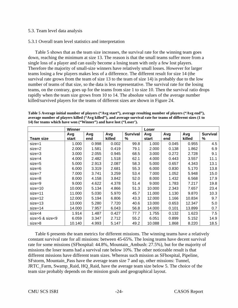
Table 5 Average initial number of players (“Avg start”), average resulting number of players (“Avg end”), average number of players killed (“Avg killed”), and average survival rate for teams of different sizes (1 to 14) for teams which have won (“Winner”) and have lost (“Loser’). .............................................................................24
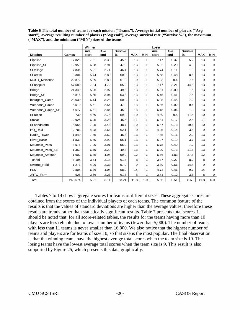
Table 6 The total number of teams for each mission (“Teams”). Average initial number of players (“Avg start”), average resulting number of players (“Avg end”), average survival rate (“Survive %”), the maximum (“MAX”), and the minimum (“MIN”) sizes of the teams ..................................................................................26
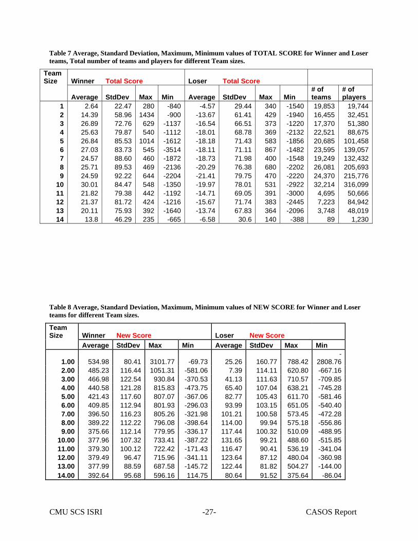
Table 7 Average, Standard Deviation, Maximum, Minimum values of TOTAL SCORE for Winner and Loser teams, Total number of teams and players for different Team sizes. ............................................................................27
Table 8 Average, Standard Deviation, Maximum, Minimum values of NEW SCORE for Winner and Loser teams for different Team sizes. ....................................................................................................................................27
Table 9 Average, Standard Deviation, Maximum, Minimum values of LEADER SCORE for Winner and Loser teams for different Team sizes. ..........................................................................................................................28
Table 10 Average, Standard Deviation, Maximum, Minimum values of WINS SCORE for Winner and Loser teams for different Team sizes. ....................................................................................................................................28
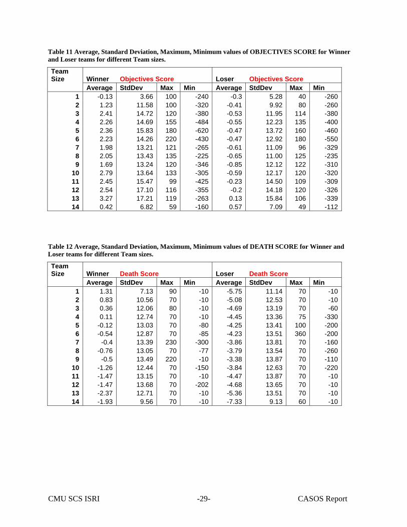
Table 11 Average, Standard Deviation, Maximum, Minimum values of OBJECTIVES SCORE for Winner and Loser teams for different Team sizes. ................................................................................................................29
Table 12 Average, Standard Deviation, Maximum, Minimum values of DEATH SCORE for Winner and Loser teams for different Team sizes. ..........................................................................................................................29
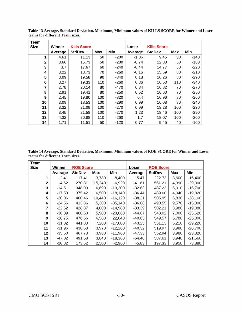
Table 13 Average, Standard Deviation, Maximum, Minimum values of KILLS SCORE for Winner and Loser teams for different Team sizes. ....................................................................................................................................30
Table 14 Average, Standard Deviation, Maximum, Minimum values of ROE SCORE for Winner and Loser teams for different Team sizes. ....................................................................................................................................30
Table 15 Number of times each type of weapon has been used for Winner and Loser teams for large (more than 8), medium (between 4 and 9), and small (less than 5) size teams..........................................................................34
Table 16 The ratios of how many times each type of weapon has been used for Winner and Loser teams for large (more than 8), medium (between 4 and 9), and small (less than 5) size teams ..................................................35
Table 17 The ratios of how many times “per player” a weapon has been used for Winner and Loser teams for large (more than 8), medium (between 4 and 9), and small (less than 5) size teams for different missions. ..............37
Table 18 The damage caused by the players from winning and losing teams for large (more than 8), medium (between 4 and 9), and small (less than 5) size teams for different missions.....................................................39
Table 19 The number of times a communication message has been used for winning and losing teams for large (more than 8), medium (between 4 and 9), and small (less than 5) size teams for different missions. ..............40
Table 20 The ratios of how many times per player a communication message has been used for winning and losing teams for large (more than 8), medium (between 4 and 9), and small (less than 5) size teams for different missions..............................................................................................................................................................41
Table 21 Average frequency of the Report-In Communication for the first period, the second period, the third period, and the entire game ............................................................................................................................................42
Table 22 Adjusted R-square from regression analysis between ORA network level measures and team received/inflicted damage ..................................................................................................................................46
Table 23 Regression analysis result summary, ORA network level measures vs team received damage ...................47 Table 24 Regression analysis result summary, ORA network level measures vs team inflicted damage ...................47 Table 25 Clusters determined by kmeans analysis on top 1000 teams ........................................................................48 Table 26 Dividing sample teams into three groups according to the clannishness-strong: 1 >= high clannishness-
strong >= 0.66, 0.66 > middle clannishness-strong >=0.33, 0.33 > low clannishness-strong >= 0 ..................56 Table 27 Dividing sample teams into three groups according to the clannishness-weak: 1 >= high clannishness-
weak >= 0.66, 0.66 > middle clannishness-weak >=0.33, 0.33 > low clannishness-weak >= 0 .......................58
CMU SCS ISRI CASOS Report -v-
II. Index of Figures Figure 1 America's Army Research Process Diagram...................................................................................................9 Figure 2 America's Army Raw Log Database Design ER-Diagram............................................................................10 Figure 3 Bar graph showing frequency of weapon usage, damage caused, and communication frequency with 1606
teams having top average total scores ................................................................................................................12 Figure 4 Bar graph illustrating decomposed scores from total score with top 1000 players .......................................13 Figure 5 Bar graph displaying percentage of winning and survival for teams sorted with new performance measure
...........................................................................................................................................................................13 Figure 6 Example of the Who-talks-after-whom Heuristic .........................................................................................14 Figure 7 Top 100 players' weapon selection................................................................................................................15 Figure 8 Middle 100 players' weapon selection...........................................................................................................16 Figure 9 Bottom 100 players' weapon selection. .........................................................................................................16 Figure 10 Scatter Plot for 100 Top Players(Avg. Normal Comm. vs Avg. Report-In) ...............................................17 Figure 11 Scatter Plot for 100 Middle Players(Avg. Normal Comm. vs Avg. Report-In) ..........................................17 Figure 12 Scatter Plot for 100 Bottom Players(Avg. Normal Comm. vs Avg. Report-In) ..........................................17 Figure 13 Scatter Plot for 100 Top Players(Avg. Received Damage vs Avg. Inflicted Damage) ..............................18 Figure 14 Scatter Plot for 100 Middle Players(Avg. Received Damage vs Avg. Inflicted Damage) ..........................18 Figure 15 Scatter Plot for 100 Bottom Players(Avg. Received Damage vs Avg. Inflicted Damage)..........................18 Figure 16 Histogram for ratio of choosing medic as role ............................................................................................18 Figure 17 The average player number of becoming a medic in the game (among 100 top players) ...........................19 Figure 18 Comparison between typical top players and medic specialized top players ..............................................20 Figure 19 the average number of transmitting the given number of Report-In communication (amoung 100 top
players)...............................................................................................................................................................21 Figure 20 Comparison between typical top players and frequent Report-In top players.............................................21 Figure 21 observing the frequent Report-In top player's play (1) (The outlying player is the player in the red box.).22 Figure 22 observing the frequent Report-In top player's play (2) (The outlying player is the player in the red box.)23 Figure 23 observing the frequent Report-In top player's play (3) (The outlying player is the player in red box.) .....23 Figure 24 Average number of killed/survived players for Winner/Loser teams..........................................................25 Figure 25 Average Total score for Winner/Loser teams of different size ...................................................................32 Figure 26 New score for Winner/Loser teams of different size...................................................................................33 Figure 27 Weapon Usage ratio (Winner/Loser) vs. Team Size for different WEAPON, Weapon choice affects
SMALL SIZE teams ..........................................................................................................................................36 Figure 28 Weapon Usage ratio (Winner/Loser) vs. Team Size for different WEAPON , Weapon choice affects
LARGE SIZE teams...........................................................................................................................................36 Figure 29 Weapon Usage ratio (Winner/Loser) vs. Team Size for different MISSIONS, Weapon choice affects
SMALL SIZE teams ..........................................................................................................................................38 Figure 30 Weapon Usage ratio (Winner/Loser) vs. Team Size for different MISSIONS, Weapon choice affects
LARGE SIZE teams...........................................................................................................................................38 Figure 31 Communication Usage ratio (Winning/Losing) vs. Team Size for different MISSIONS, Weapon choice
affects LARGE SIZE teams ...............................................................................................................................42 Figure 32 Different Report-In Communication Usages between Winners and Losers through the Entire Game .......43 Figure 33 Different Report-In Communication Usages according to the Team Size and the Periods of the Games...43 Figure 34 Predicted value X Actual value scatter plot generated by regression analysis between ORA network level
measures and team received damage .................................................................................................................46 Figure 35 Predicted value X Actual value scatter plot generated by regression analysis between ORA network level
measures and team inflicted damage..................................................................................................................47 Figure 36 Formula for labeling measures into groups .................................................................................................48 Figure 37 Scatter plot with 3 most important principal components explaining 67.5% of variance ..........................49 Figure 38 Decision tree showing how clusters can be divided by using principal components ..................................49 Figure 39 Frequency percentage of labeled measures with top 5 information gain (Selected cluster is cluster 4, and
the other clusters are the rest of the clusters.) ....................................................................................................50 Figure 40 Graph from correspondence analysis, with 439 measures and 10 clusters..................................................51 Figure 41 Graph from correspondence analysis, with 31 ORA measures and 10 clusters, narrow scoped with
focusing the distribution of clusters and with some usage of jittering function .................................................52 Figure 42 Graph from correspondence analysis, with 31 ORA measures and 10 clusters ..........................................53
CMU SCS ISRI CASOS Report -vi-
Figure 43 The number of clan members in the teams..................................................................................................54 Figure 44 the number of teams according to the clannishness-strong .........................................................................55 Figure 45 Winning rates and losing rates across the three groups in the clannishness-strong.....................................56 Figure 46 Average player survival ratio across the three groups in the clannishness-strong.......................................57 Figure 47 Communication styles across the three groups in the clannishness-strong ( Normal Communication vs
Report-In )..........................................................................................................................................................57 Figure 48 The number of teams according to the clannishness-weak .........................................................................58 Figure 49 Winning rates and losing rates across the three groups in the clannishness-weak ......................................59 Figure 50 Average player survival ratio across the three groups in the clannishness-weak ........................................59 Figure 51 Communication styles across the three groups in the clannishness-weak ( Normal Communication vs
Report-In )..........................................................................................................................................................59
CMU SCS ISRI CASOS Report -7-
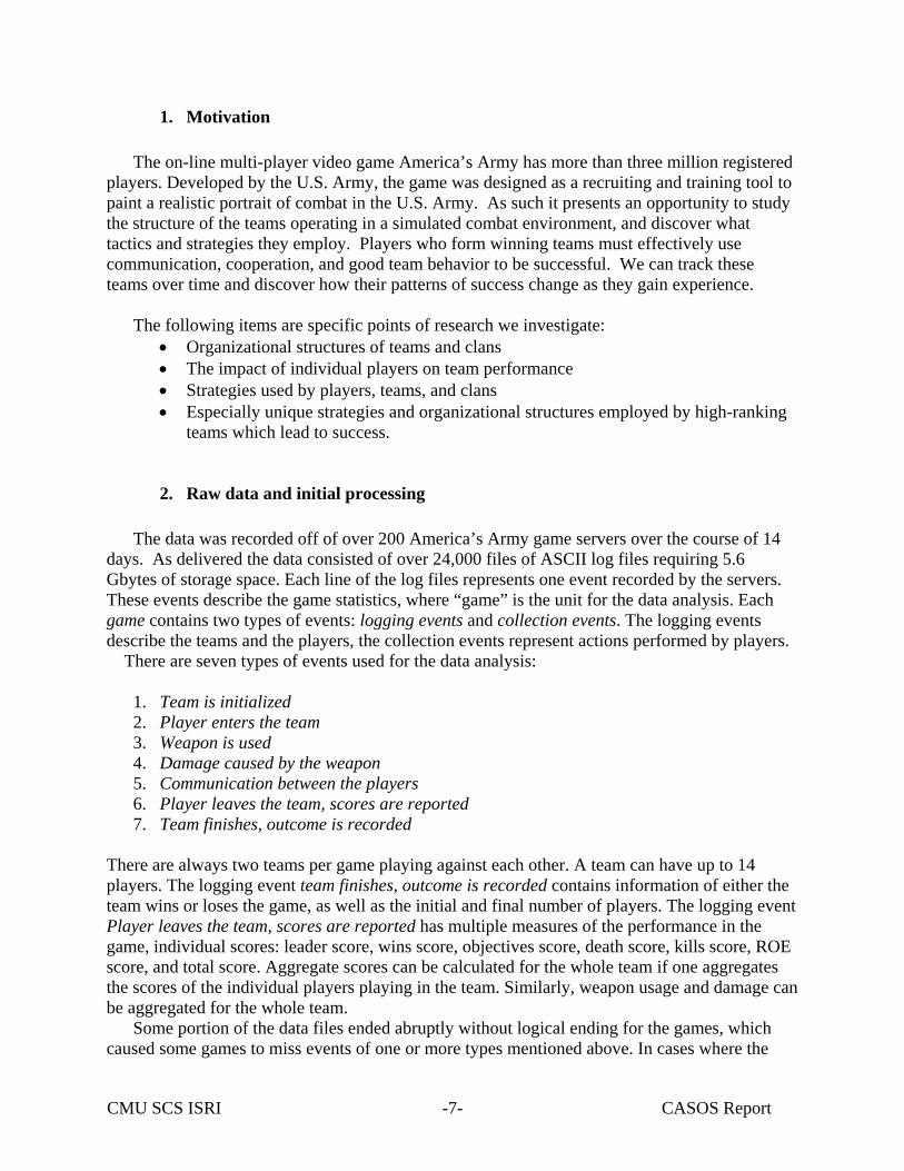
1. Motivation The on-line multi-player video game America’s Army has more than three million registered
players. Developed by the U.S. Army, the game was designed as a recruiting and training tool to paint a realistic portrait of combat in the U.S. Army. As such it presents an opportunity to study the structure of the teams operating in a simulated combat environment, and discover what tactics and strategies they employ. Players who form winning teams must effectively use communication, cooperation, and good team behavior to be successful. We can track these teams over time and discover how their patterns of success change as they gain experience.
The following items are specific points of research we investigate:
• Organizational structures of teams and clans • The impact of individual players on team performance • Strategies used by players, teams, and clans • Especially unique strategies and organizational structures employed by high-ranking
teams which lead to success.
2. Raw data and initial processing
The data was recorded off of over 200 America’s Army game servers over the course of 14 days. As delivered the data consisted of over 24,000 files of ASCII log files requiring 5.6 Gbytes of storage space. Each line of the log files represents one event recorded by the servers. These events describe the game statistics, where “game” is the unit for the data analysis. Each game contains two types of events: logging events and collection events. The logging events describe the teams and the players, the collection events represent actions performed by players. There are seven types of events used for the data analysis:
1. Team is initialized 2. Player enters the team 3. Weapon is used 4. Damage caused by the weapon 5. Communication between the players 6. Player leaves the team, scores are reported 7. Team finishes, outcome is recorded
There are always two teams per game playing against each other. A team can have up to 14 players. The logging event team finishes, outcome is recorded contains information of either the team wins or loses the game, as well as the initial and final number of players. The logging event Player leaves the team, scores are reported has multiple measures of the performance in the game, individual scores: leader score, wins score, objectives score, death score, kills score, ROE score, and total score. Aggregate scores can be calculated for the whole team if one aggregates the scores of the individual players playing in the team. Similarly, weapon usage and damage can be aggregated for the whole team.
Some portion of the data files ended abruptly without logical ending for the games, which caused some games to miss events of one or more types mentioned above. In cases where the
CMU SCS ISRI CASOS Report -8-
event Team finishes, outcome is recorded is missing, the game was considered to be incomplete and excluded from analysis. In cases where the event Player leaves the team, scores are reported is missing for particular players, the information about those players is not recorded. In rare occasions, some games have teams which either both have won or both have lost. We discard games where both teams won as having no reasonable explanation. If both teams lost, it means neither team satisfied the conditions to win the game, so such behavior is considered reasonable and the data was included for analysis.
Each game takes place in one of about 30 scenarios, called missions. Each mission has a unique 3-d environment and selection of weapons available to the players, and a unique objective each team is trying to achieve.
3. Research process
The fundamental data of the America’s army project is an ASCII formatted raw log file. This
file required transformation to appropriate formats for the analyses we conducted. Thus, one of the major parts in the research was storing the data in a relational database and converting the data into the DynetML format for ORA analysis. We constructed a custom parsing program to read the log files and insert the data into a database.
The social network analyses of the data were done using the ORA tool (the Organizational
Risk Analyzer) [1]. The raw log files were translated to DynetML [2] format (an xml format for storing social network information) for use with ORA. The following networks were extracted and stored for analysis. The accumulated size of the DynetML files was over 15GB. The format of DynetML file used in America’s Army can be found in Appendix A.
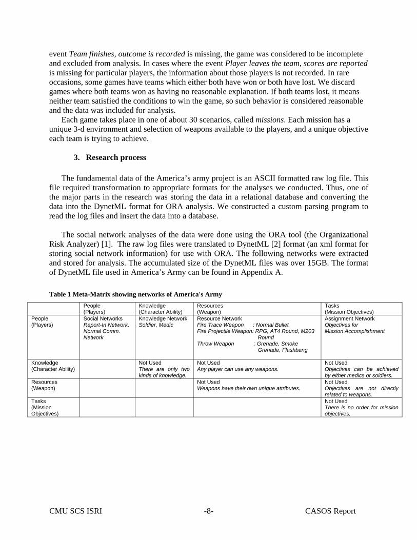
Table 1 Meta-Matrix showing networks of America's Army
People (Players)
Knowledge (Character Ability)
Resources (Weapon)
Tasks (Mission Objectives)
People (Players)
Social Networks Report-In Network, Normal Comm. Network
Knowledge Network Soldier, Medic
Resource Network Fire Trace Weapon : Normal Bullet Fire Projectile Weapon: RPG, AT4 Round, M203 Round Throw Weapon : Grenade, Smoke Grenade, Flashbang
Assignment Network Objectives for Mission Accomplishment
Knowledge (Character Ability)
Not Used There are only two kinds of knowledge.
Not Used Any player can use any weapons.
Not Used Objectives can be achieved by either medics or soldiers.
Resources (Weapon)
Not Used Weapons have their own unique attributes.
Not Used Objectives are not directly related to weapons.
Tasks (Mission Objectives)
Not Used There is no order for mission objectives.
CMU SCS ISRI CASOS Report -9-
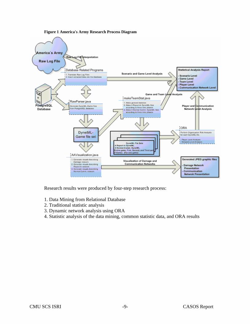
Figure 1 America's Army Research Process Diagram
Research results were produced by four-step research process: 1. Data Mining from Relational Database 2. Traditional statistic analysis 3. Dynamic network analysis using ORA 4. Statistic analysis of the data mining, common statistic data, and ORA results
CMU SCS ISRI CASOS Report -10-
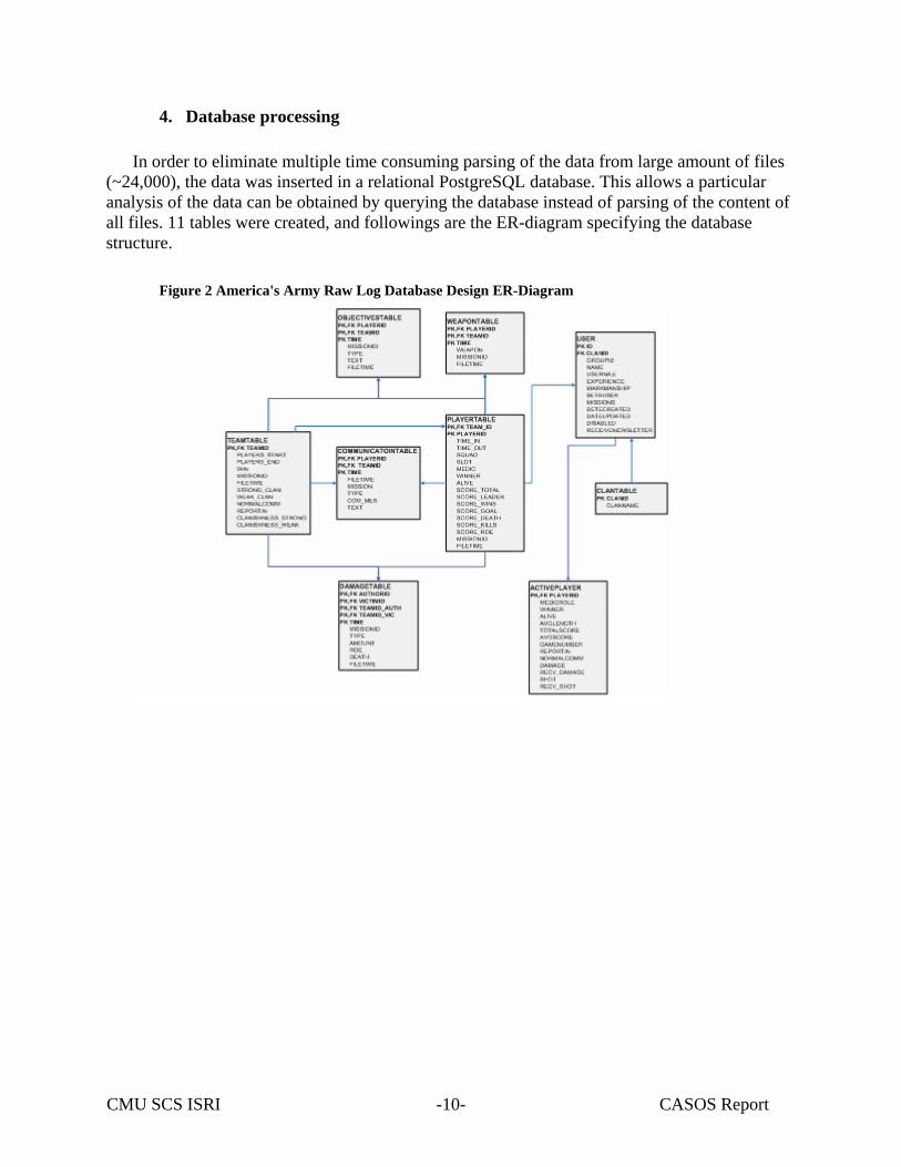
4. Database processing In order to eliminate multiple time consuming parsing of the data from large amount of files
(~24,000), the data was inserted in a relational PostgreSQL database. This allows a particular analysis of the data can be obtained by querying the database instead of parsing of the content of all files. 11 tables were created, and followings are the ER-diagram specifying the database structure.
Figure 2 America's Army Raw Log Database Design ER-Diagram
CMU SCS ISRI CASOS Report -11-
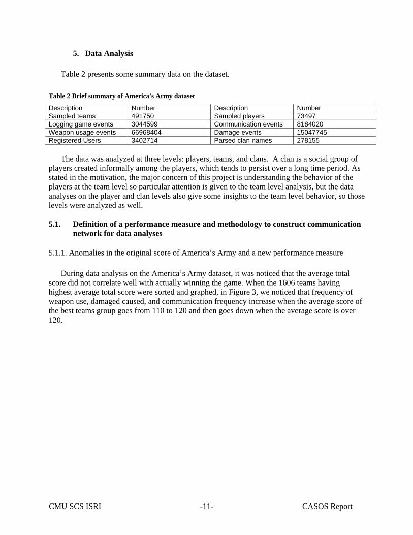
5. Data Analysis
Table 2 presents some summary data on the dataset. Table 2 Brief summary of America's Army dataset
Description Number Description Number Sampled teams 491750 Sampled players 73497 Logging game events 3044599 Communication events 8184020 Weapon usage events 66968404 Damage events 15047745 Registered Users 3402714 Parsed clan names 278155
The data was analyzed at three levels: players, teams, and clans. A clan is a social group of players created informally among the players, which tends to persist over a long time period. As stated in the motivation, the major concern of this project is understanding the behavior of the players at the team level so particular attention is given to the team level analysis, but the data analyses on the player and clan levels also give some insights to the team level behavior, so those levels were analyzed as well.
5.1. Definition of a performance measure and methodology to construct communication
network for data analyses
5.1.1. Anomalies in the original score of America’s Army and a new performance measure During data analysis on the America’s Army dataset, it was noticed that the average total
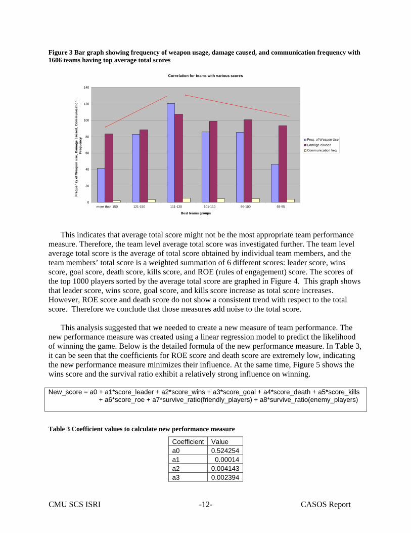
score did not correlate well with actually winning the game. When the 1606 teams having highest average total score were sorted and graphed, in Figure 3, we noticed that frequency of weapon use, damaged caused, and communication frequency increase when the average score of the best teams group goes from 110 to 120 and then goes down when the average score is over 120.
CMU SCS ISRI CASOS Report -12-
Figure 3 Bar graph showing frequency of weapon usage, damage caused, and communication frequency with 1606 teams having top average total scores
Correlation for teams with various scores
0
20
40
60
80
100
120
140
1 2 3 4 5 6
Best teams groups
Freq
uens
y of
Wea
pon
use,
Dam
age
caus
ed, C
omm
unic
atio
n Fr
eque
ncy Freq. of Weapon Use
Damage causedCommunication freq.
more than 150 121-150 111-120 101-110 96-100 93-95
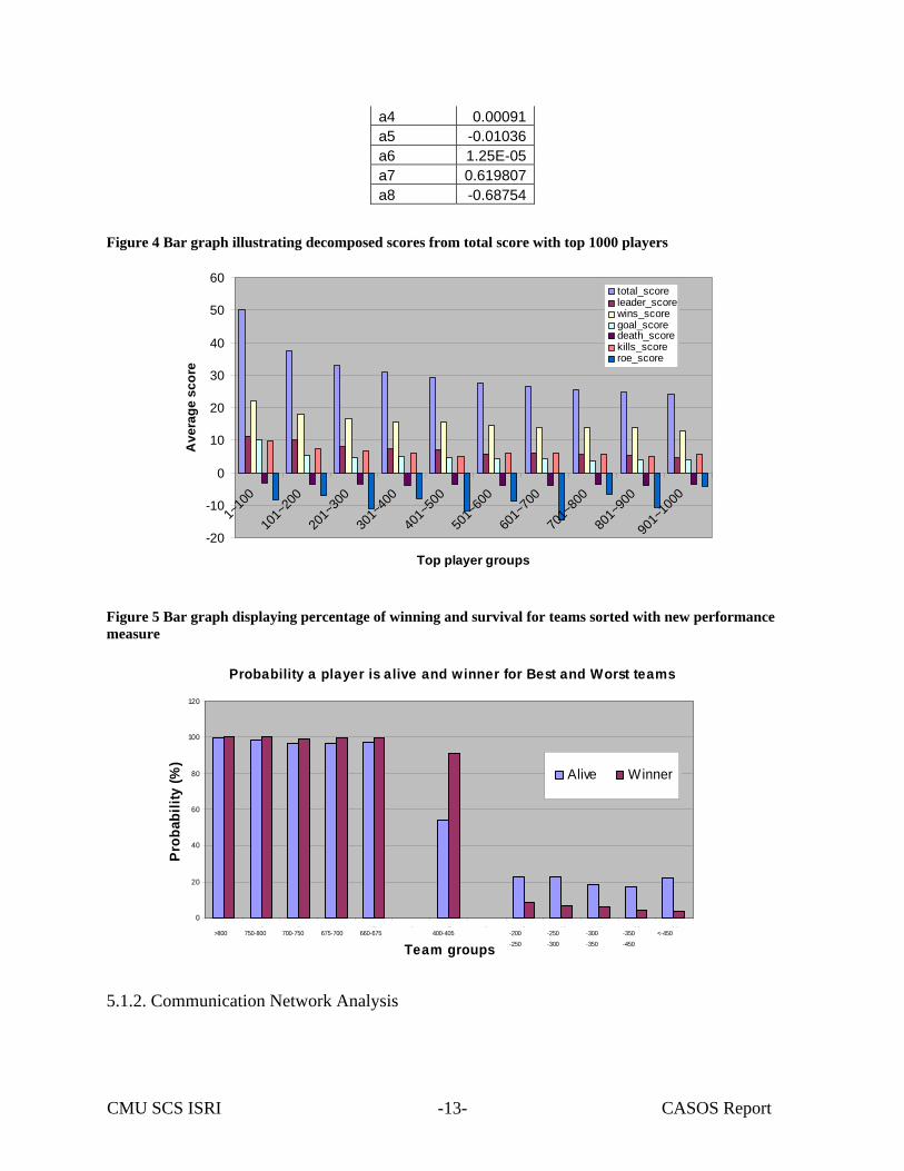
This indicates that average total score might not be the most appropriate team performance measure. Therefore, the team level average total score was investigated further. The team level average total score is the average of total score obtained by individual team members, and the team members’ total score is a weighted summation of 6 different scores: leader score, wins score, goal score, death score, kills score, and ROE (rules of engagement) score. The scores of the top 1000 players sorted by the average total score are graphed in Figure 4. This graph shows that leader score, wins score, goal score, and kills score increase as total score increases. However, ROE score and death score do not show a consistent trend with respect to the total score. Therefore we conclude that those measures add noise to the total score.
This analysis suggested that we needed to create a new measure of team performance. The
new performance measure was created using a linear regression model to predict the likelihood of winning the game. Below is the detailed formula of the new performance measure. In Table 3, it can be seen that the coefficients for ROE score and death score are extremely low, indicating the new performance measure minimizes their influence. At the same time, Figure 5 shows the wins score and the survival ratio exhibit a relatively strong influence on winning.
New_score = a0 + a1*score_leader + a2*score_wins + a3*score_goal + a4*score_death + a5*score_kills + a6*score_roe + a7*survive_ratio(friendly_players) + a8*survive_ratio(enemy_players) Table 3 Coefficient values to calculate new performance measure
Coefficient Value a0 0.524254a1 0.00014a2 0.004143a3 0.002394
CMU SCS ISRI CASOS Report -13-
a4 0.00091a5 -0.01036a6 1.25E-05a7 0.619807a8 -0.68754
Figure 4 Bar graph illustrating decomposed scores from total score with top 1000 players
-20
-10
0
10
20
30
40
50
60
1~10
0
101~
200
201~
300
301~
400
401~
500
501~
600
601~
700
701~
800
801~
900
901~
1000
Top player groups
Ave
rage
sco
re
total_scoreleader_scorewins_scoregoal_scoredeath_scorekills_scoreroe_score
Figure 5 Bar graph displaying percentage of winning and survival for teams sorted with new performance measure
Probability a player is alive and winner for Best and Worst teams
0
20
40
60
80
100
120
1 2 3 4 5 6 7 8 9 10 11 12 13
Team groups
Pro
babi
lity
(%)
Alive Winner
>800 400-405660-675675-700700-750750-800 -200
-250
<-450-350
-450
-300
-350
-250
-300
5.1.2. Communication Network Analysis
CMU SCS ISRI CASOS Report -14-
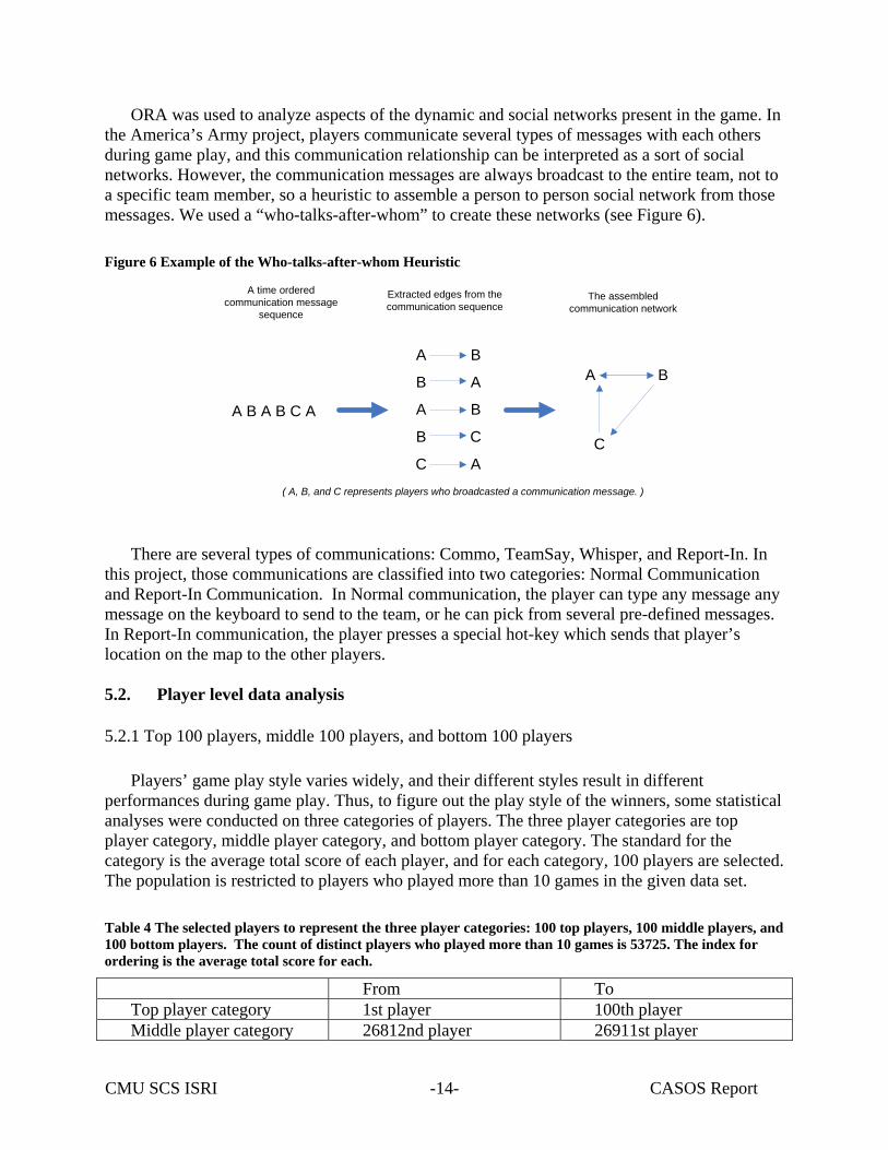
ORA was used to analyze aspects of the dynamic and social networks present in the game. In the America’s Army project, players communicate several types of messages with each others during game play, and this communication relationship can be interpreted as a sort of social networks. However, the communication messages are always broadcast to the entire team, not to a specific team member, so a heuristic to assemble a person to person social network from those messages. We used a “who-talks-after-whom” to create these networks (see Figure 6).
Figure 6 Example of the Who-talks-after-whom Heuristic
A B A B C A
B A
A B
B C
A B
C A
A B
C
A time ordered communication message
sequence
Extracted edges from the communication sequence
The assembled communication network
( A, B, and C represents players who broadcasted a communication message. )
There are several types of communications: Commo, TeamSay, Whisper, and Report-In. In
this project, those communications are classified into two categories: Normal Communication and Report-In Communication. In Normal communication, the player can type any message any message on the keyboard to send to the team, or he can pick from several pre-defined messages. In Report-In communication, the player presses a special hot-key which sends that player’s location on the map to the other players. 5.2. Player level data analysis
5.2.1 Top 100 players, middle 100 players, and bottom 100 players Players’ game play style varies widely, and their different styles result in different
performances during game play. Thus, to figure out the play style of the winners, some statistical analyses were conducted on three categories of players. The three player categories are top player category, middle player category, and bottom player category. The standard for the category is the average total score of each player, and for each category, 100 players are selected. The population is restricted to players who played more than 10 games in the given data set.
Table 4 The selected players to represent the three player categories: 100 top players, 100 middle players, and 100 bottom players. The count of distinct players who played more than 10 games is 53725. The index for ordering is the average total score for each.
From To Top player category 1st player 100th player Middle player category 26812nd player 26911st player
CMU SCS ISRI CASOS Report -15-
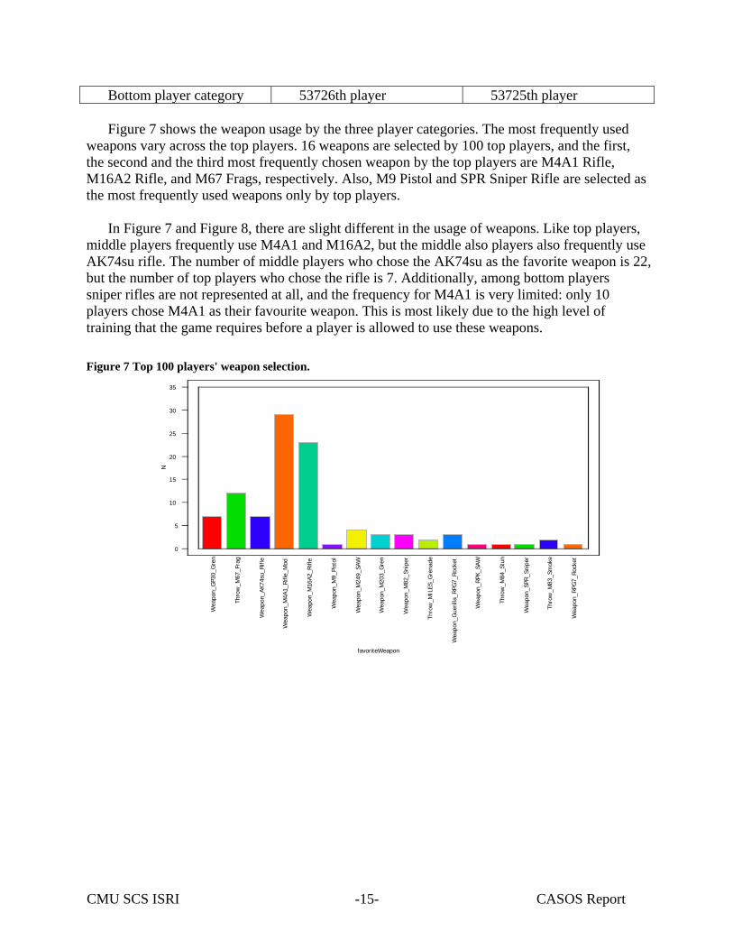
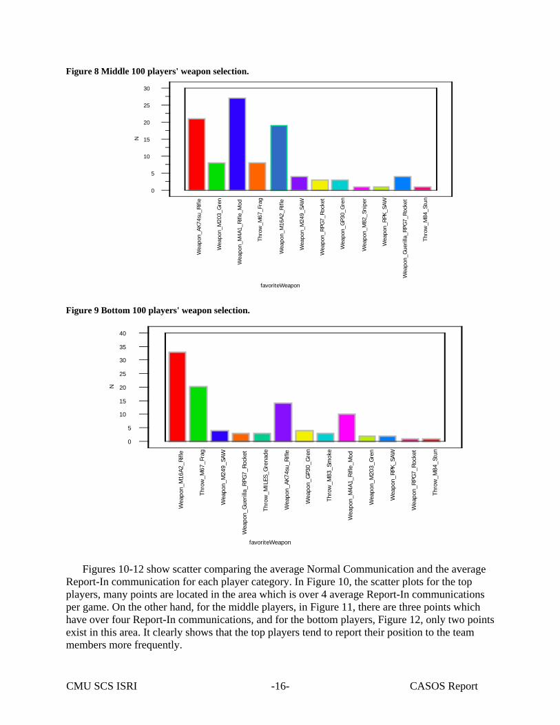
Bottom player category 53726th player 53725th player Figure 7 shows the weapon usage by the three player categories. The most frequently used
weapons vary across the top players. 16 weapons are selected by 100 top players, and the first, the second and the third most frequently chosen weapon by the top players are M4A1 Rifle, M16A2 Rifle, and M67 Frags, respectively. Also, M9 Pistol and SPR Sniper Rifle are selected as the most frequently used weapons only by top players.
In Figure 7 and Figure 8, there are slight different in the usage of weapons. Like top players,
middle players frequently use M4A1 and M16A2, but the middle also players also frequently use AK74su rifle. The number of middle players who chose the AK74su as the favorite weapon is 22, but the number of top players who chose the rifle is 7. Additionally, among bottom players sniper rifles are not represented at all, and the frequency for M4A1 is very limited: only 10 players chose M4A1 as their favourite weapon. This is most likely due to the high level of training that the game requires before a player is allowed to use these weapons.
Figure 7 Top 100 players' weapon selection.
0
5
10
15
20
25
30
35
N
Wea
pon_
GP3
0_G
ren
Thro
w_M
67_F
rag
Wea
pon_
AK74
su_R
ifle
Wea
pon_
M4A
1_Rifl
e_M
od
Wea
pon_
M16
A2_R
ifle
Wea
pon_
M9_
Pist
ol
Wea
pon_
M24
9_SA
W
Wea
pon_
M20
3_G
ren
Wea
pon_
M82
_Sni
per
Thro
w_M
ILES
_Gre
nade
Wea
pon_
Gue
rilla
_RPG
7_Ro
cket
Wea
pon_
RPK
_SAW
Thro
w_M
84_S
tun
Wea
pon_
SPR_
Snip
er
Thro
w_M
83_S
mok
e
Wea
pon_
RPG
7_Ro
cket
favoriteWeapon
CMU SCS ISRI CASOS Report -16-
Figure 8 Middle 100 players' weapon selection.
0
5
10
15
20
25
30
N
Wea
pon_
AK74
su_R
ifle
Wea
pon_
M20
3_G
ren
Wea
pon_
M4A
1_Ri
fle_M
od
Thro
w_M
67_F
rag
Wea
pon_
M16
A2_R
ifle
Wea
pon_
M24
9_SA
W
Wea
pon_
RPG
7_Ro
cket
Wea
pon_
GP3
0_G
ren
Wea
pon_
M82
_Sni
per
Wea
pon_
RPK_
SAW
Wea
pon_
Gue
rilla
_RPG
7_Ro
cket
Thro
w_M
84_S
tun
favoriteWeapon
Figure 9 Bottom 100 players' weapon selection.
0
5
10
15
20
25
30
35
40
N
Wea
pon_
M16
A2_R
ifle
Thro
w_M
67_F
rag
Wea
pon_
M24
9_SA
W
Wea
pon_
Gue
rilla
_RPG
7_Roc
ket
Thro
w_M
ILES
_Gre
nade
Wea
pon_
AK74
su_R
ifle
Wea
pon_
GP3
0_G
ren
Thro
w_M
83_S
mok
e
Wea
pon_
M4A
1_Rifl
e_M
od
Wea
pon_
M20
3_G
ren
Wea
pon_
RPK
_SAW
Wea
pon_
RPG
7_Roc
ket
Thro
w_M
84_S
tun
favoriteWeapon
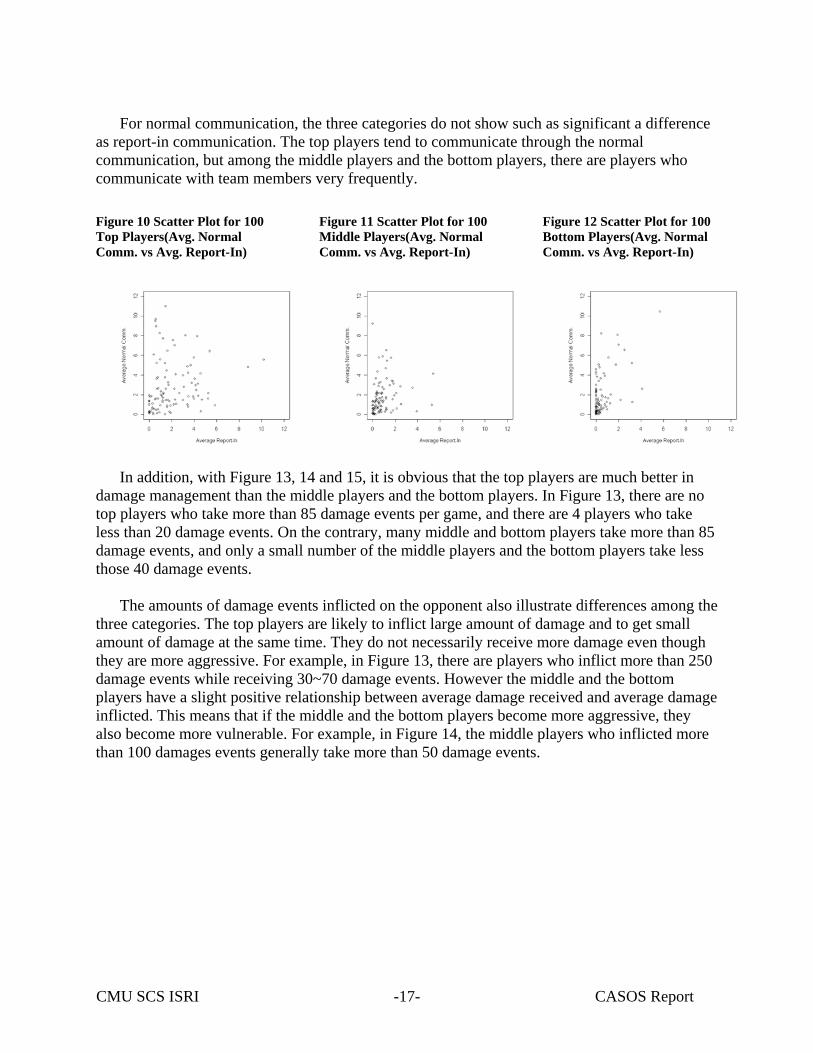
Figures 10-12 show scatter comparing the average Normal Communication and the average Report-In communication for each player category. In Figure 10, the scatter plots for the top players, many points are located in the area which is over 4 average Report-In communications per game. On the other hand, for the middle players, in Figure 11, there are three points which have over four Report-In communications, and for the bottom players, Figure 12, only two points exist in this area. It clearly shows that the top players tend to report their position to the team members more frequently.
CMU SCS ISRI CASOS Report -17-
For normal communication, the three categories do not show such as significant a difference
as report-in communication. The top players tend to communicate through the normal communication, but among the middle players and the bottom players, there are players who communicate with team members very frequently.
Figure 10 Scatter Plot for 100 Top Players(Avg. Normal Comm. vs Avg. Report-In)
Figure 11 Scatter Plot for 100 Middle Players(Avg. Normal Comm. vs Avg. Report-In)
Figure 12 Scatter Plot for 100 Bottom Players(Avg. Normal Comm. vs Avg. Report-In)
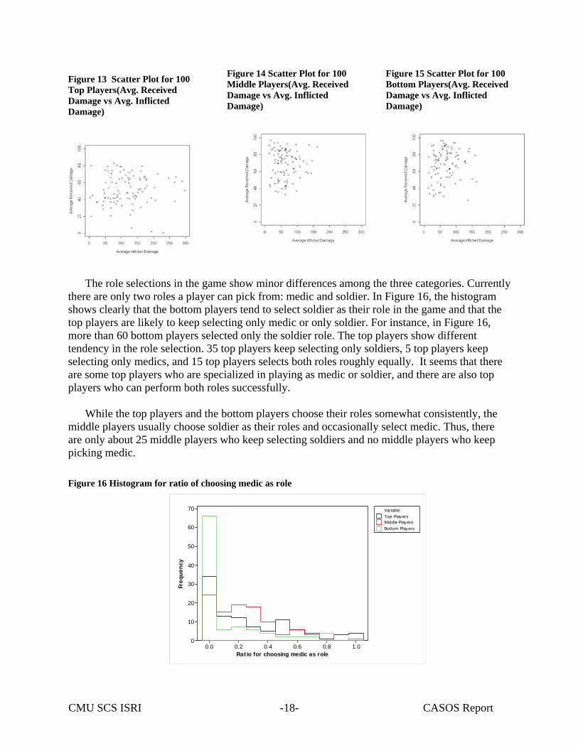
In addition, with Figure 13, 14 and 15, it is obvious that the top players are much better in damage management than the middle players and the bottom players. In Figure 13, there are no top players who take more than 85 damage events per game, and there are 4 players who take less than 20 damage events. On the contrary, many middle and bottom players take more than 85 damage events, and only a small number of the middle players and the bottom players take less those 40 damage events.
The amounts of damage events inflicted on the opponent also illustrate differences among the
three categories. The top players are likely to inflict large amount of damage and to get small amount of damage at the same time. They do not necessarily receive more damage even though they are more aggressive. For example, in Figure 13, there are players who inflict more than 250 damage events while receiving 30~70 damage events. However the middle and the bottom players have a slight positive relationship between average damage received and average damage inflicted. This means that if the middle and the bottom players become more aggressive, they also become more vulnerable. For example, in Figure 14, the middle players who inflicted more than 100 damages events generally take more than 50 damage events.
CMU SCS ISRI CASOS Report -18-
Figure 13 Scatter Plot for 100 Top Players(Avg. Received Damage vs Avg. Inflicted Damage)
Figure 14 Scatter Plot for 100 Middle Players(Avg. Received Damage vs Avg. Inflicted Damage)
Figure 15 Scatter Plot for 100 Bottom Players(Avg. Received Damage vs Avg. Inflicted Damage)
The role selections in the game show minor differences among the three categories. Currently there are only two roles a player can pick from: medic and soldier. In Figure 16, the histogram shows clearly that the bottom players tend to select soldier as their role in the game and that the top players are likely to keep selecting only medic or only soldier. For instance, in Figure 16, more than 60 bottom players selected only the soldier role. The top players show different tendency in the role selection. 35 top players keep selecting only soldiers, 5 top players keep selecting only medics, and 15 top players selects both roles roughly equally. It seems that there are some top players who are specialized in playing as medic or soldier, and there are also top players who can perform both roles successfully.
While the top players and the bottom players choose their roles somewhat consistently, the
middle players usually choose soldier as their roles and occasionally select medic. Thus, there are only about 25 middle players who keep selecting soldiers and no middle players who keep picking medic.
Figure 16 Histogram for ratio of choosing medic as role
Ratio for choosing medic as role
Freq
uenc
y
1.00.80.60.40.20.0
70
60
50
40
30
20
10
0
VariableTop PlayersMiddle PlayersBottom Players
CMU SCS ISRI CASOS Report -19-
5.2.2 Outlier analysis among top 100 players We have identified statistical outliers among top players along various axes that we have
analyzed. These outlying players are dissimilar to the other top players, even though they are all doing excellent in the game. Thus, the investigation of the outliers is a good first step to identify different ways for players to succeed in the game.
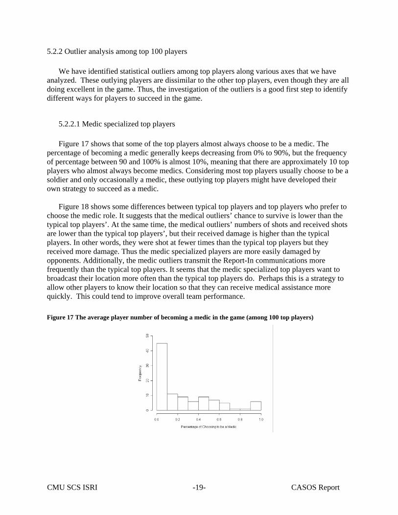
5.2.2.1 Medic specialized top players Figure 17 shows that some of the top players almost always choose to be a medic. The
percentage of becoming a medic generally keeps decreasing from 0% to 90%, but the frequency of percentage between 90 and 100% is almost 10%, meaning that there are approximately 10 top players who almost always become medics. Considering most top players usually choose to be a soldier and only occasionally a medic, these outlying top players might have developed their own strategy to succeed as a medic.
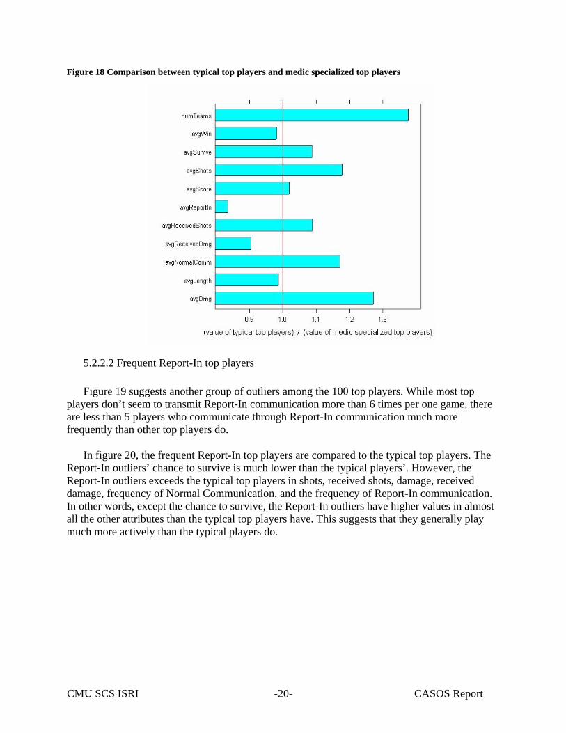
Figure 18 shows some differences between typical top players and top players who prefer to
choose the medic role. It suggests that the medical outliers’ chance to survive is lower than the typical top players’. At the same time, the medical outliers’ numbers of shots and received shots are lower than the typical top players’, but their received damage is higher than the typical players. In other words, they were shot at fewer times than the typical top players but they received more damage. Thus the medic specialized players are more easily damaged by opponents. Additionally, the medic outliers transmit the Report-In communications more frequently than the typical top players. It seems that the medic specialized top players want to broadcast their location more often than the typical top players do. Perhaps this is a strategy to allow other players to know their location so that they can receive medical assistance more quickly. This could tend to improve overall team performance.
Figure 17 The average player number of becoming a medic in the game (among 100 top players)
CMU SCS ISRI CASOS Report -20-
Figure 18 Comparison between typical top players and medic specialized top players
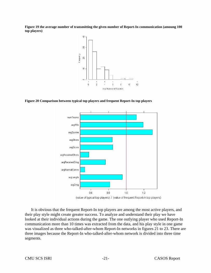
5.2.2.2 Frequent Report-In top players Figure 19 suggests another group of outliers among the 100 top players. While most top
players don’t seem to transmit Report-In communication more than 6 times per one game, there are less than 5 players who communicate through Report-In communication much more frequently than other top players do.
In figure 20, the frequent Report-In top players are compared to the typical top players. The
Report-In outliers’ chance to survive is much lower than the typical players’. However, the Report-In outliers exceeds the typical top players in shots, received shots, damage, received damage, frequency of Normal Communication, and the frequency of Report-In communication. In other words, except the chance to survive, the Report-In outliers have higher values in almost all the other attributes than the typical top players have. This suggests that they generally play much more actively than the typical players do.
CMU SCS ISRI CASOS Report -21-
Figure 19 the average number of transmitting the given number of Report-In communication (amoung 100 top players)
Figure 20 Comparison between typical top players and frequent Report-In top players
It is obvious that the frequent Report-In top players are among the most active players, and
their play style might create greater success. To analyze and understand their play we have looked at their individual actions during the game. The one outlying player who used Report-In communication more than 10 times was extracted from the data, and his play style in one game was visualized as three who-talked-after-whom Report-In networks in figures 21 to 23. There are three images because the Report-In who-talked-after-whom network is divided into three time segments.
CMU SCS ISRI CASOS Report -22-
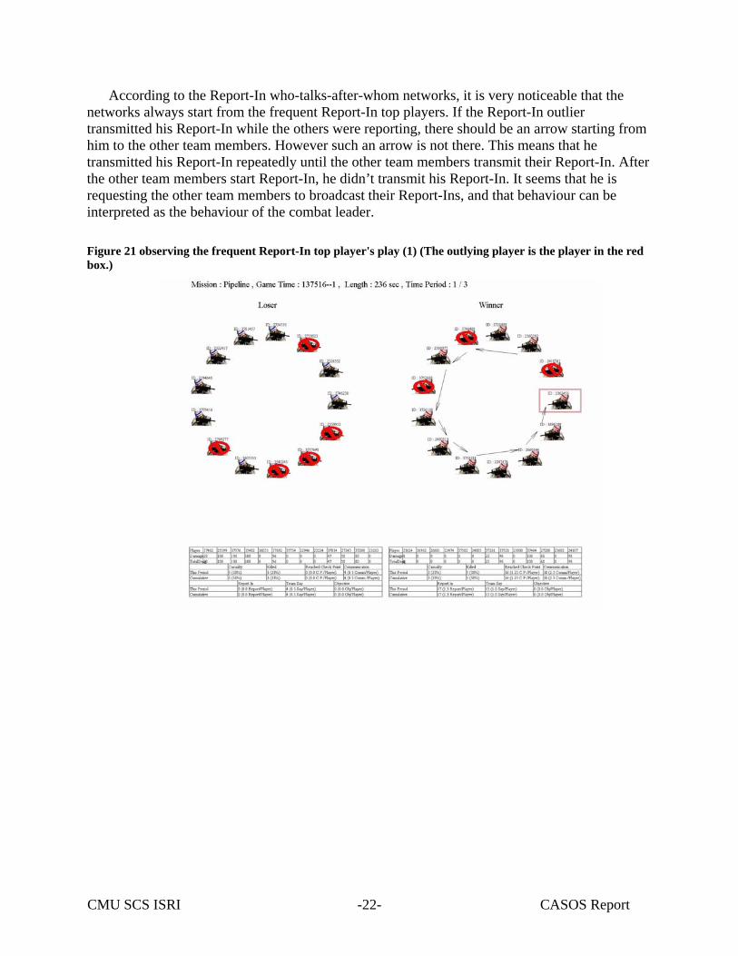
According to the Report-In who-talks-after-whom networks, it is very noticeable that the networks always start from the frequent Report-In top players. If the Report-In outlier transmitted his Report-In while the others were reporting, there should be an arrow starting from him to the other team members. However such an arrow is not there. This means that he transmitted his Report-In repeatedly until the other team members transmit their Report-In. After the other team members start Report-In, he didn’t transmit his Report-In. It seems that he is requesting the other team members to broadcast their Report-Ins, and that behaviour can be interpreted as the behaviour of the combat leader.
Figure 21 observing the frequent Report-In top player's play (1) (The outlying player is the player in the red box.)
CMU SCS ISRI CASOS Report -23-
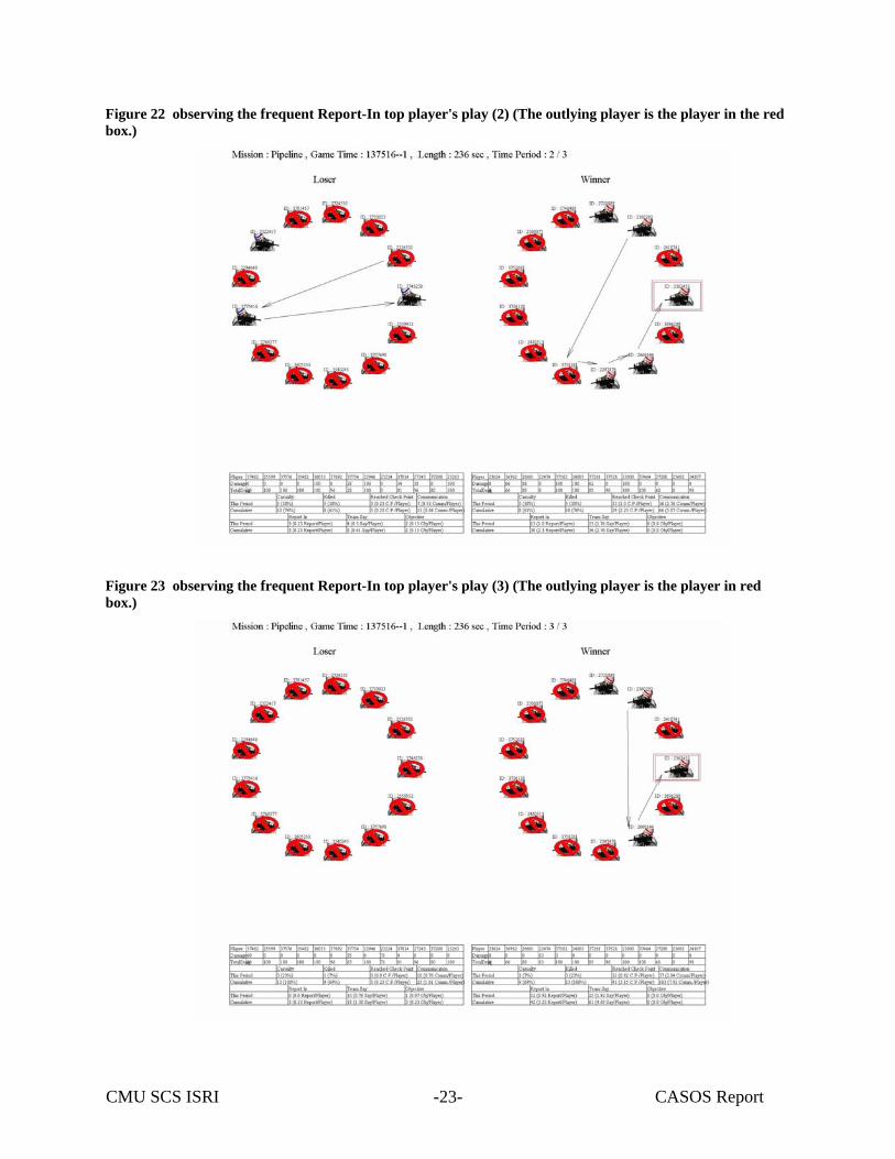
Figure 22 observing the frequent Report-In top player's play (2) (The outlying player is the player in the red box.)
Figure 23 observing the frequent Report-In top player's play (3) (The outlying player is the player in red box.)
CMU SCS ISRI CASOS Report -24-
5.3. Team level data analysis 5.3.1 Overall team level statistics and interpretation
Table 5 shows that as the team size increases, the survival rate for the winning team goes
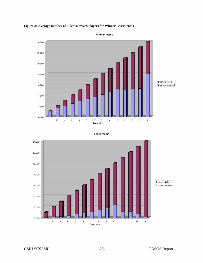
down, reaching the minimum at size 13. The reason is that the small teams suffer more from a single loss of a player and can easily become a losing team with only a few lost players. Therefore the majority of small-size winners have relatively small losses. However for larger teams losing a few players makes less of a difference. The different result for size 14 (the survival rate grows from the team of size 13 to the team of size 14) is probably due to the low number of teams of that size, so the data is less representative. The survival rate for the losing teams, on the contrary, goes up for the teams from size 1 to size 10. Then the survival ratio drops rapidly when the team size grows from 10 to 14. The absolute values of the average number killed/survived players for the teams of different sizes are shown in Figure 24. Table 5 Average initial number of players (“Avg start”), average resulting number of players (“Avg end”), average number of players killed (“Avg killed”), and average survival rate for teams of different sizes (1 to 14) for teams which have won (“Winner”) and have lost (“Loser’).
Winner Loser
Team size Avg start
Avg end
Avg killed
Survival %
Avg start
Avg end
Avg killed
Survival %
size=1 1.000 0.998 0.002 99.8 1.000 0.045 0.955 4.5size=2 2.000 1.581 0.419 79.1 2.000 0.138 1.862 6.9size=3 3.000 2.055 0.945 68.5 3.000 0.272 2.728 9.1size=4 4.000 2.482 1.518 62.1 4.000 0.443 3.557 11.1size=5 5.000 2.913 2.087 58.3 5.000 0.657 4.343 13.1size=6 6.000 3.319 2.681 55.3 6.000 0.830 5.170 13.8size=7 7.000 3.741 3.259 53.4 7.000 1.052 5.948 15.0size=8 8.000 4.158 3.842 52.0 8.000 1.432 6.568 17.9size=9 9.000 4.622 4.378 51.4 9.000 1.783 7.217 19.8size=10 10.000 5.134 4.866 51.3 10.000 2.343 7.657 23.4size=11 11.000 5.030 5.970 45.7 11.000 1.130 9.870 10.3size=12 12.000 5.194 6.806 43.3 12.000 1.166 10.834 9.7size=13 13.000 5.280 7.720 40.6 13.000 0.653 12.347 5.0size=14 14.000 7.957 6.043 56.8 14.000 0.101 13.899 0.7size<4 1.914 1.487 0.427 77.7 1.755 0.132 1.623 7.5size>5 & size<9 6.059 3.347 2.712 55.2 6.051 0.899 5.152 14.9size>8 10.140 4.993 5.147 49.2 10.088 1.868 8.220 18.5
Table 6 presents the team metrics for different missions. The winning teams have a relatively
constant survival rate for all missions: between 45-65%. The losing teams have decent survival rate for some missions (SFhospital: 44.8%, Mountain_Ambush: 27.5%), but for the majority of missions the loser teams had a survival rate below 10%. The other noticeable result is that different missions have different team sizes. Whereas such mission as SFhospital, Pipeline, SFstorm, Mountain_Pass have the average team size 7 and up, other missions: Tunnel, JRTC_Farm, Swamp_Raid, HQ_Raid, have the average team size below 5. The choice of the team size probably depends on the mission goals and geographical layout.
CMU SCS ISRI CASOS Report -25-
Figure 24 Average number of killed/survived players for Winner/Loser teams
0.000
2.000
4.000
6.000
8.000
10.000
12.000
14.000
1 2 3 4 5 6 7 8 9 10 11 12 13 14Team size
Winner teams
players killedplayers survived
0.000
2.000
4.000
6.000
8.000
10.000
12.000
14.000
1 2 3 4 5 6 7 8 9 10 11 12 13 14Team size
Loser teams
players killedplayers survived
CMU SCS ISRI CASOS Report -26-
Table 6 The total number of teams for each mission (“Teams”). Average initial number of players (“Avg start”), average resulting number of players (“Avg end”), average survival rate (“Survive %”), the maximum (“MAX”), and the minimum (“MIN”) sizes of the teams
Winner Loser
Mission Games Ave start
Ave end
Survive % MAX MIN
Ave start
Ave end
Survive % MAX MIN
Pipeline 17,828 7.31 3.33 45.6 13 1 7.17 0.37 5.2 13 0 Pipeline_SF 12,959 6.08 2.91 47.9 13 1 5.92 0.29 4.9 13 0 SFvillage 7,836 5.91 2.74 46.4 13 1 5.74 0.11 1.9 13 0 SFarctic 8,301 5.74 2.89 50.3 13 1 5.58 0.48 8.6 13 0 MOUT_McKenna 22,872 5.39 2.80 51.9 9 1 5.23 0.4 7.6 9 0 SFhospital 57,580 7.24 4.72 65.2 13 1 7.17 3.21 44.8 13 0 Bridge 21,349 5.96 2.97 49.8 13 1 5.81 0.09 1.5 13 0 Bridge_SE 5,816 5.65 3.04 53.8 13 1 5.45 0.41 7.5 13 0 Insurgent_Camp 23,030 6.44 3.28 50.9 13 1 6.25 0.45 7.2 13 0 Weapons_Cache 16,510 5.51 2.64 47.9 13 1 5.36 0.02 0.4 13 0 Weapons_Cache_SE 4,677 6.31 2.84 45.0 13 1 6.18 0.06 1.0 13 0 SFrecon 730 4.59 2.75 59.9 10 1 4.39 0.5 11.4 10 0 Sfcsar 12,924 6.95 3.23 46.5 11 1 6.81 0.17 2.5 11 0 SFsandstorm 8,058 7.05 3.43 48.7 10 1 6.87 0.73 10.6 10 0 HQ_Raid 2,783 4.28 2.66 62.1 9 1 4.05 0.14 3.5 9 0 Radio_Tower 1,849 7.55 3.52 46.6 13 1 7.35 0.16 2.2 13 0 River_Basin 1,839 5.30 2.92 55.1 13 1 5.07 0.19 3.7 13 0 Mountain_Pass 3,576 7.00 3.91 55.9 13 1 6.78 0.49 7.2 13 0 Mountain_Pass_SE 1,359 6.49 3.20 49.3 13 1 6.29 0.73 11.6 13 0 Mountain_Ambush 1,902 6.85 4.04 59.0 12 1 6.66 1.83 27.5 12 0 Tunnel 5,194 3.54 2.18 61.6 8 1 3.37 0.27 8.0 8 0 Swamp_Raid 1,273 4.09 2.33 57.0 9 1 3.89 0.56 14.4 9 0 FLS 2,804 6.86 4.04 58.9 14 1 4.73 0.46 9.7 14 0 JRTC_Farm 625 3.66 2.26 61.7 8 1 3.44 0.12 3.5 8 0
Total 243,674 5.91 3.11 53.21 11.8 1.0 5.65 0.51 8.60 11.8 0.0
Tables 7 to 14 show aggregate scores for teams of different sizes. These aggregate scores are
obtained from the scores of the individual players of each teams. The common feature of the results is that the values of standard deviations are higher than the average values; therefore these results are trends rather than statistically significant results. Table 7 presents total scores. It should be noted that, for all score-related tables, the results for the teams having more than 10 players are less reliable due to lower number of teams (fewer than 5,000). The number of teams with less than 11 teams is never smaller than 16,000. We also notice that the highest number of teams and players are for teams of size 10, so that size is the most popular. The final observation is that the winning teams have the highest average total scores when the team size is 10. The losing teams have the lowest average total scores when the team size is 9. This result is also supported by Figure 25, which presents this data graphically.
CMU SCS ISRI CASOS Report -27-
Table 7 Average, Standard Deviation, Maximum, Minimum values of TOTAL SCORE for Winner and Loser teams, Total number of teams and players for different Team sizes.
Team Size Winner Total Score Loser Total Score
Average StdDev Max Min Average StdDev Max Min # of teams
# of players
1 2.64 22.47 280 -840 -4.57 29.44 340 -1540 19,853 19,7442 14.39 58.96 1434 -900 -13.67 61.41 429 -1940 16,455 32,4513 26.89 72.76 629 -1137 -16.54 66.51 373 -1220 17,370 51,3804 25.63 79.87 540 -1112 -18.01 68.78 369 -2132 22,521 88,6755 26.84 85.53 1014 -1612 -18.18 71.43 583 -1856 20,685 101,4586 27.03 83.73 545 -3514 -18.11 71.11 867 -1482 23,595 139,0577 24.57 88.60 460 -1872 -18.73 71.98 400 -1548 19,249 132,4328 25.71 89.53 469 -2136 -20.29 76.38 680 -2202 26,081 205,6939 24.59 92.22 644 -2204 -21.41 79.75 470 -2220 24,370 215,776
10 30.01 84.47 548 -1350 -19.97 78.01 531 -2922 32,214 316,09911 21.82 79.38 442 -1192 -14.71 69.05 391 -3000 4,695 50,66612 21.37 81.72 424 -1216 -15.67 71.74 383 -2445 7,223 84,94213 20.11 75.93 392 -1640 -13.74 67.83 364 -2096 3,748 48,01914 13.8 46.29 235 -665 -6.58 30.6 140 -388 89 1,230
Table 8 Average, Standard Deviation, Maximum, Minimum values of NEW SCORE for Winner and Loser teams for different Team sizes.
Team Size Winner New Score Loser New Score Average StdDev Max Min Average StdDev Max Min
1.00 534.98 80.41 3101.77 -69.73 25.26 160.77 788.42 -
2808.762.00 485.23 116.44 1051.31 -581.06 7.39 114.11 620.80 -667.163.00 466.98 122.54 930.84 -370.53 41.13 111.63 710.57 -709.854.00 440.58 121.28 815.83 -473.75 65.40 107.04 638.21 -745.285.00 421.43 117.60 807.07 -367.06 82.77 105.43 611.70 -581.466.00 409.85 112.94 801.93 -296.03 93.99 103.15 651.05 -540.407.00 396.50 116.23 805.26 -321.98 101.21 100.58 573.45 -472.288.00 389.22 112.22 796.08 -398.64 114.00 99.94 575.18 -556.869.00 375.66 112.14 779.95 -336.17 117.44 100.32 510.09 -488.95
10.00 377.96 107.32 733.41 -387.22 131.65 99.21 488.60 -515.8511.00 379.30 100.12 722.42 -171.43 116.47 90.41 536.19 -341.0412.00 379.49 96.47 715.96 -341.11 123.64 87.12 480.04 -360.9813.00 377.99 88.59 687.58 -145.72 122.44 81.82 504.27 -144.0014.00 392.64 95.68 596.16 114.75 80.64 91.52 375.64 -86.04
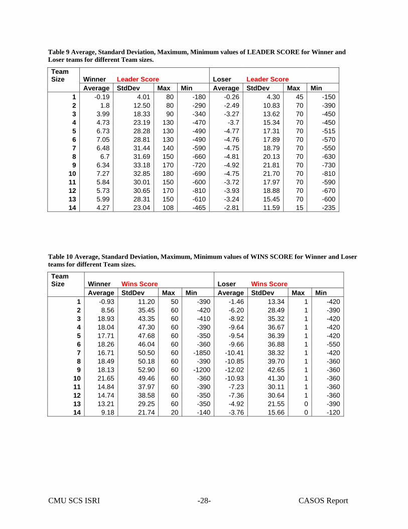
CMU SCS ISRI CASOS Report -28-
Table 9 Average, Standard Deviation, Maximum, Minimum values of LEADER SCORE for Winner and Loser teams for different Team sizes.
Team Size Winner Leader Score Loser Leader Score Average StdDev Max Min Average StdDev Max Min
1 -0.19 4.01 80 -180 -0.26 4.30 45 -1502 1.8 12.50 80 -290 -2.49 10.83 70 -3903 3.99 18.33 90 -340 -3.27 13.62 70 -4504 4.73 23.19 130 -470 -3.7 15.34 70 -4505 6.73 28.28 130 -490 -4.77 17.31 70 -5156 7.05 28.81 130 -490 -4.76 17.89 70 -5707 6.48 31.44 140 -590 -4.75 18.79 70 -5508 6.7 31.69 150 -660 -4.81 20.13 70 -6309 6.34 33.18 170 -720 -4.92 21.81 70 -730
10 7.27 32.85 180 -690 -4.75 21.70 70 -81011 5.84 30.01 150 -600 -3.72 17.97 70 -59012 5.73 30.65 170 -810 -3.93 18.88 70 -67013 5.99 28.31 150 -610 -3.24 15.45 70 -60014 4.27 23.04 108 -465 -2.81 11.59 15 -235
Table 10 Average, Standard Deviation, Maximum, Minimum values of WINS SCORE for Winner and Loser teams for different Team sizes.
Team Size Winner Wins Score Loser Wins Score Average StdDev Max Min Average StdDev Max Min
1 -0.93 11.20 50 -390 -1.46 13.34 1 -4202 8.56 35.45 60 -420 -6.20 28.49 1 -3903 18.93 43.35 60 -410 -8.92 35.32 1 -4204 18.04 47.30 60 -390 -9.64 36.67 1 -4205 17.71 47.68 60 -350 -9.54 36.39 1 -4206 18.26 46.04 60 -360 -9.66 36.88 1 -5507 16.71 50.50 60 -1850 -10.41 38.32 1 -4208 18.49 50.18 60 -390 -10.85 39.70 1 -3609 18.13 52.90 60 -1200 -12.02 42.65 1 -360
10 21.65 49.46 60 -360 -10.93 41.30 1 -36011 14.84 37.97 60 -390 -7.23 30.11 1 -36012 14.74 38.58 60 -350 -7.36 30.64 1 -36013 13.21 29.25 60 -350 -4.92 21.55 0 -39014 9.18 21.74 20 -140 -3.76 15.66 0 -120
CMU SCS ISRI CASOS Report -29-
Table 11 Average, Standard Deviation, Maximum, Minimum values of OBJECTIVES SCORE for Winner and Loser teams for different Team sizes.
Team Size Winner Objectives Score Loser Objectives Score Average StdDev Max Min Average StdDev Max Min
1 -0.13 3.66 100 -240 -0.3 5.28 40 -2602 1.23 11.58 100 -320 -0.41 9.92 80 -2603 2.41 14.72 120 -380 -0.53 11.95 114 -3804 2.26 14.69 155 -484 -0.55 12.23 135 -4005 2.36 15.83 180 -620 -0.47 13.72 160 -4606 2.23 14.26 220 -430 -0.47 12.92 180 -5507 1.98 13.21 121 -265 -0.61 11.09 96 -3298 2.05 13.43 135 -225 -0.65 11.00 125 -2359 1.69 13.24 120 -346 -0.85 12.12 122 -310
10 2.79 13.64 133 -305 -0.59 12.17 120 -32011 2.45 15.47 99 -425 -0.23 14.50 109 -30912 2.54 17.10 116 -355 -0.2 14.18 120 -32613 3.27 17.21 119 -263 0.13 15.84 106 -33914 0.42 6.82 59 -160 0.57 7.09 49 -112
Table 12 Average, Standard Deviation, Maximum, Minimum values of DEATH SCORE for Winner and Loser teams for different Team sizes.
Team Size Winner Death Score Loser Death Score Average StdDev Max Min Average StdDev Max Min
1 1.31 7.13 90 -10 -5.75 11.14 70 -102 0.83 10.56 70 -10 -5.08 12.53 70 -103 0.36 12.06 80 -10 -4.69 13.19 70 -604 0.11 12.74 70 -10 -4.45 13.36 75 -3305 -0.12 13.03 70 -80 -4.25 13.41 100 -2006 -0.54 12.87 70 -85 -4.23 13.51 360 -2007 -0.4 13.39 230 -300 -3.86 13.81 70 -1608 -0.76 13.05 70 -77 -3.79 13.54 70 -2609 -0.5 13.49 220 -10 -3.38 13.87 70 -110
10 -1.26 12.44 70 -150 -3.84 12.63 70 -22011 -1.47 13.15 70 -10 -4.47 13.87 70 -1012 -1.47 13.68 70 -202 -4.68 13.65 70 -1013 -2.37 12.71 70 -10 -5.36 13.51 70 -1014 -1.93 9.56 70 -10 -7.33 9.13 60 -10
CMU SCS ISRI CASOS Report -30-
Table 13 Average, Standard Deviation, Maximum, Minimum values of KILLS SCORE for Winner and Loser teams for different Team sizes.
Team Size Winner Kills Score Loser Kills Score Average StdDev Max Min Average StdDev Max Min
1 4.61 11.13 50 -200 -1.06 9.45 30 -1402 3.66 15.73 50 -200 -0.74 12.83 50 -1803 3.7 17.67 60 -240 -0.44 14.77 50 -2204 3.22 18.73 70 -260 -0.16 15.59 80 -2105 3.09 19.58 90 -340 0.18 16.26 80 -2906 3.27 19.33 110 -260 0.36 16.50 110 -3407 2.78 20.14 80 -470 0.34 16.82 70 -2708 2.91 19.41 80 -250 0.52 16.60 70 -2509 2.45 19.80 100 -320 0.4 16.96 80 -260
10 3.09 18.53 100 -290 0.99 16.08 80 -24011 3.32 21.09 100 -270 0.99 18.28 100 -23012 3.45 21.58 100 -270 1.23 18.46 100 -29013 4.32 20.88 110 -260 1.7 18.07 100 -26014 1.71 11.51 50 -120 0.77 9.45 40 -160
Table 14 Average, Standard Deviation, Maximum, Minimum values of ROE SCORE for Winner and Loser teams for different Team sizes.
Team Size Winner ROE Score Loser ROE Score Average StdDev Max Min Average StdDev Max Min
1 -2.41 117.41 3,780 -8,400 -5.47 222.72 3,600 -15,4002 -4.62 270.31 15,240 -6,920 -41.61 561.21 4,390 -29,0003 -14.51 348.00 6,690 -19,200 -32.63 487.23 5,010 -15,7004 -17.53 375.42 6,500 -18,140 -36.44 489.60 4,040 -19,8205 -20.06 400.46 10,440 -16,120 -38.21 505.95 6,830 -28,1606 -24.56 413.86 5,300 -35,140 -36.08 490.55 9,570 -15,8007 -22.62 428.87 4,000 -14,980 -33.39 502.21 3,980 -19,0808 -30.89 460.60 5,900 -23,060 -44.67 548.02 7,000 -25,6209 -28.75 476.66 6,580 22,040 -40.63 549.57 5,780 -25,800
10 -31.32 441.83 7,200 -17,000 -43.25 531.13 5,210 -29,22011 -31.96 438.68 3,970 -12,260 -40.32 519.97 3,980 -28,70012 -35.60 467.73 3,980 -11,960 -47.33 552.94 3,980 -23,32013 -47.02 491.58 3,840 -18,360 -64.40 587.61 3,940 -21,56014 -10.82 173.62 2,500 -2,960 -5.83 197.33 3,950 -3,880
CMU SCS ISRI CASOS Report -31-
5.3.2 Weapon usage analysis
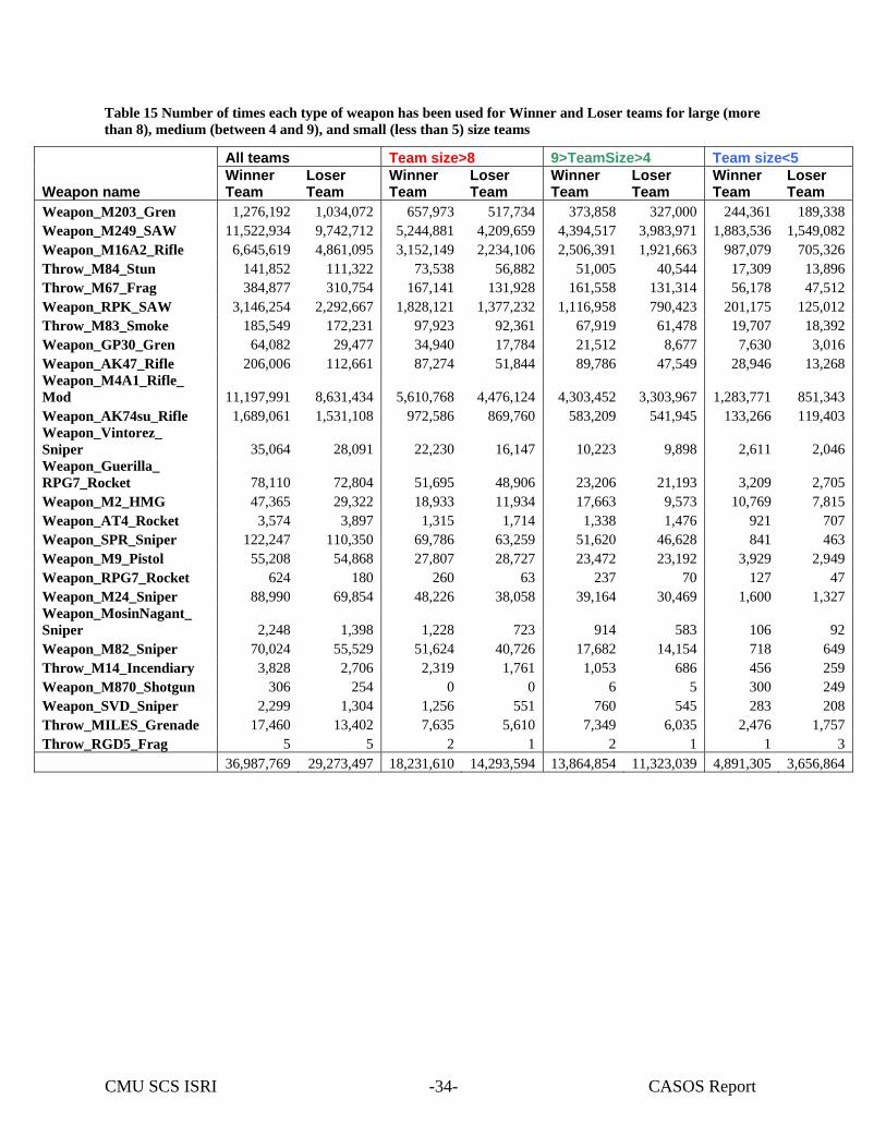
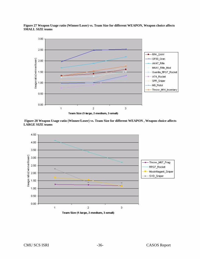
Each mission has a particular set of weapons available to the players. In this section we look at how this weapon usage (type and frequency) affects the game outcome for particular missions. To answer this question, the weapon usage was analyzed for different weapon types. Table 15 shows how many times each weapon was used by winning and losing teams. There is a noticeable difference between weapon usage for winning and losing teams. Averaging over all types of weapons, the winners use any weapon 1.22-1.34 times more often than the opponents. This suggests that in general more frequent weapon usage contributes to the success in the game.
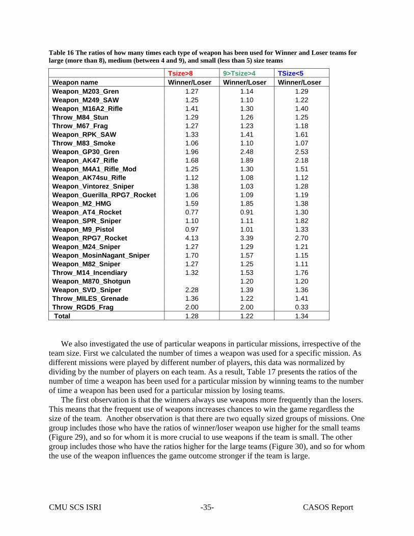
The choice of the weapon types also affects the game outcome. For example, the usage of RPG7_Rocket (624 by winners against 180 by losers) affects the game outcome significantly stronger than M9_Pistol (55,208 by winner against 54,868 by losers). To show these distinctions between different weapon types quantitatively, the data from table 15 are presented in table 16, which shows the winner/loser ratios of the weapon usage. There are three groups of weapon types with respect to the team size. One group consists of the weapon types, in which the winner/loser ratios of the weapon usage are higher if the team size is small. This means that a weapon of this type has higher impact if the team is small than if the team is large. The data for this group is presented on figure 27. A smaller group consists of the weapon types in which the winner/loser ratios of the weapon usage are higher if the team is large. This data is presented in figure 28. The rest of the weapon types do not show any dependence on the team size.
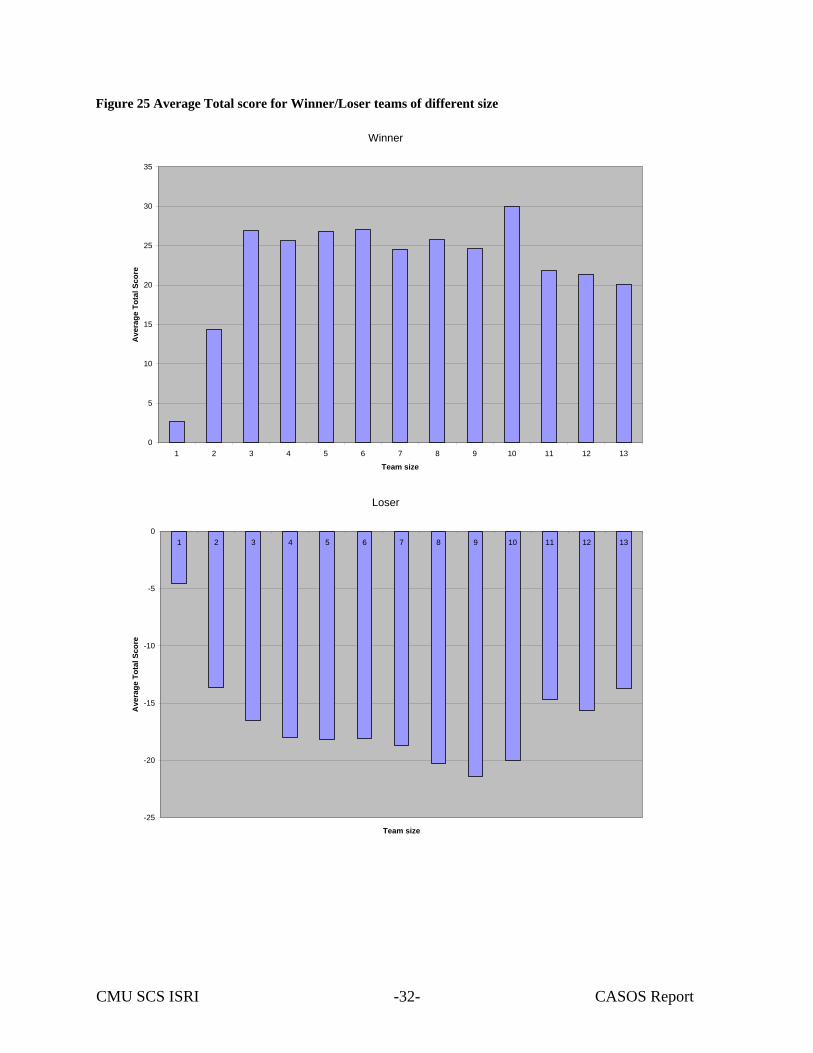
CMU SCS ISRI CASOS Report -32-
Figure 25 Average Total score for Winner/Loser teams of different size
Winner
0
5
10
15
20
25
30
35
1 2 3 4 5 6 7 8 9 10 11 12 13
Team size
Ave
rage
Tot
al S
core
Loser
-25
-20
-15
-10
-5
01 2 3 4 5 6 7 8 9 10 11 12 13
Team size
Ave
rage
Tot
al S
core
CMU SCS ISRI CASOS Report -33-
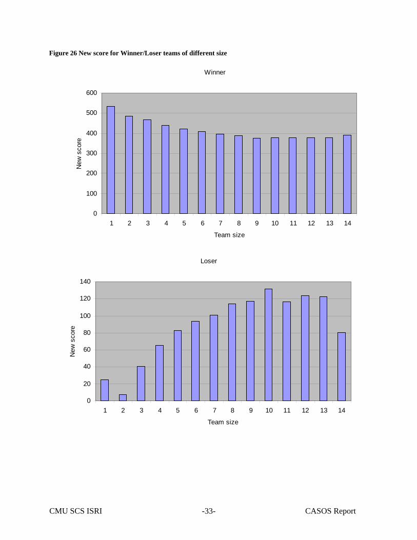
Figure 26 New score for Winner/Loser teams of different size
Winner
0
100
200
300
400
500
600
1 2 3 4 5 6 7 8 9 10 11 12 13 14
Team size
New
sco
re
Loser
0
20
40
60
80
100
120
140
1 2 3 4 5 6 7 8 9 10 11 12 13 14
Team size
New
sco
re
CMU SCS ISRI CASOS Report -34-
Table 15 Number of times each type of weapon has been used for Winner and Loser teams for large (more than 8), medium (between 4 and 9), and small (less than 5) size teams
All teams Team size>8 9>TeamSize>4 Team size<5
Weapon name Winner Team
Loser Team
Winner Team
Loser Team
Winner Team
Loser Team
Winner Team
Loser Team
Weapon_M203_Gren 1,276,192 1,034,072 657,973 517,734 373,858 327,000 244,361 189,338 Weapon_M249_SAW 11,522,934 9,742,712 5,244,881 4,209,659 4,394,517 3,983,971 1,883,536 1,549,082 Weapon_M16A2_Rifle 6,645,619 4,861,095 3,152,149 2,234,106 2,506,391 1,921,663 987,079 705,326 Throw_M84_Stun 141,852 111,322 73,538 56,882 51,005 40,544 17,309 13,896 Throw_M67_Frag 384,877 310,754 167,141 131,928 161,558 131,314 56,178 47,512 Weapon_RPK_SAW 3,146,254 2,292,667 1,828,121 1,377,232 1,116,958 790,423 201,175 125,012 Throw_M83_Smoke 185,549 172,231 97,923 92,361 67,919 61,478 19,707 18,392 Weapon_GP30_Gren 64,082 29,477 34,940 17,784 21,512 8,677 7,630 3,016 Weapon_AK47_Rifle 206,006 112,661 87,274 51,844 89,786 47,549 28,946 13,268 Weapon_M4A1_Rifle_ Mod 11,197,991 8,631,434 5,610,768 4,476,124 4,303,452 3,303,967 1,283,771 851,343 Weapon_AK74su_Rifle 1,689,061 1,531,108 972,586 869,760 583,209 541,945 133,266 119,403 Weapon_Vintorez_ Sniper 35,064 28,091 22,230 16,147 10,223 9,898 2,611 2,046 Weapon_Guerilla_ RPG7_Rocket 78,110 72,804 51,695 48,906 23,206 21,193 3,209 2,705 Weapon_M2_HMG 47,365 29,322 18,933 11,934 17,663 9,573 10,769 7,815 Weapon_AT4_Rocket 3,574 3,897 1,315 1,714 1,338 1,476 921 707 Weapon_SPR_Sniper 122,247 110,350 69,786 63,259 51,620 46,628 841 463 Weapon_M9_Pistol 55,208 54,868 27,807 28,727 23,472 23,192 3,929 2,949 Weapon_RPG7_Rocket 624 180 260 63 237 70 127 47 Weapon_M24_Sniper 88,990 69,854 48,226 38,058 39,164 30,469 1,600 1,327 Weapon_MosinNagant_ Sniper 2,248 1,398 1,228 723 914 583 106 92 Weapon_M82_Sniper 70,024 55,529 51,624 40,726 17,682 14,154 718 649 Throw_M14_Incendiary 3,828 2,706 2,319 1,761 1,053 686 456 259 Weapon_M870_Shotgun 306 254 0 0 6 5 300 249 Weapon_SVD_Sniper 2,299 1,304 1,256 551 760 545 283 208 Throw_MILES_Grenade 17,460 13,402 7,635 5,610 7,349 6,035 2,476 1,757 Throw_RGD5_Frag 5 5 2 1 2 1 1 3 36,987,769 29,273,497 18,231,610 14,293,594 13,864,854 11,323,039 4,891,305 3,656,864
CMU SCS ISRI CASOS Report -35-
Table 16 The ratios of how many times each type of weapon has been used for Winner and Loser teams for large (more than 8), medium (between 4 and 9), and small (less than 5) size teams
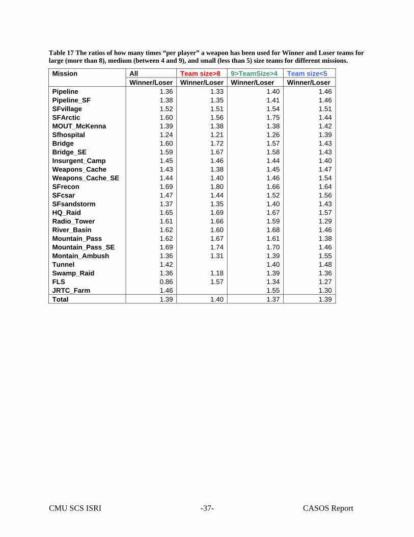
We also investigated the use of particular weapons in particular missions, irrespective of the
team size. First we calculated the number of times a weapon was used for a specific mission. As different missions were played by different number of players, this data was normalized by dividing by the number of players on each team. As a result, Table 17 presents the ratios of the number of time a weapon has been used for a particular mission by winning teams to the number of time a weapon has been used for a particular mission by losing teams.
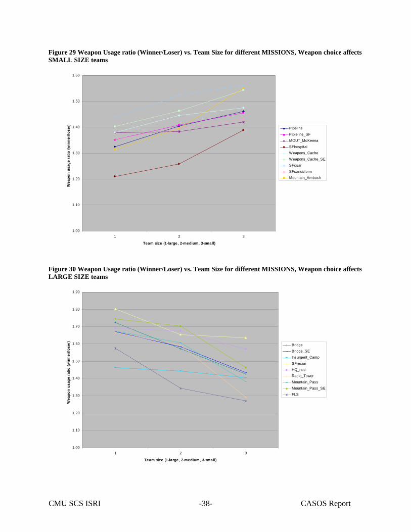
The first observation is that the winners always use weapons more frequently than the losers. This means that the frequent use of weapons increases chances to win the game regardless the size of the team. Another observation is that there are two equally sized groups of missions. One group includes those who have the ratios of winner/loser weapon use higher for the small teams (Figure 29), and so for whom it is more crucial to use weapons if the team is small. The other group includes those who have the ratios higher for the large teams (Figure 30), and so for whom the use of the weapon influences the game outcome stronger if the team is large.
Tsize>8 9>Tsize>4 TSize<5 Weapon name Winner/Loser Winner/Loser Winner/Loser Weapon_M203_Gren 1.27 1.14 1.29 Weapon_M249_SAW 1.25 1.10 1.22 Weapon_M16A2_Rifle 1.41 1.30 1.40 Throw_M84_Stun 1.29 1.26 1.25 Throw_M67_Frag 1.27 1.23 1.18 Weapon_RPK_SAW 1.33 1.41 1.61 Throw_M83_Smoke 1.06 1.10 1.07 Weapon_GP30_Gren 1.96 2.48 2.53 Weapon_AK47_Rifle 1.68 1.89 2.18 Weapon_M4A1_Rifle_Mod 1.25 1.30 1.51 Weapon_AK74su_Rifle 1.12 1.08 1.12 Weapon_Vintorez_Sniper 1.38 1.03 1.28 Weapon_Guerilla_RPG7_Rocket 1.06 1.09 1.19 Weapon_M2_HMG 1.59 1.85 1.38 Weapon_AT4_Rocket 0.77 0.91 1.30 Weapon_SPR_Sniper 1.10 1.11 1.82 Weapon_M9_Pistol 0.97 1.01 1.33 Weapon_RPG7_Rocket 4.13 3.39 2.70 Weapon_M24_Sniper 1.27 1.29 1.21 Weapon_MosinNagant_Sniper 1.70 1.57 1.15 Weapon_M82_Sniper 1.27 1.25 1.11 Throw_M14_Incendiary 1.32 1.53 1.76 Weapon_M870_Shotgun 1.20 1.20 Weapon_SVD_Sniper 2.28 1.39 1.36 Throw_MILES_Grenade 1.36 1.22 1.41 Throw_RGD5_Frag 2.00 2.00 0.33 Total 1.28 1.22 1.34
CMU SCS ISRI CASOS Report -36-
Figure 27 Weapon Usage ratio (Winner/Loser) vs. Team Size for different WEAPON, Weapon choice affects SMALL SIZE teams
Figure 28 Weapon Usage ratio (Winner/Loser) vs. Team Size for different WEAPON , Weapon choice affects LARGE SIZE teams
CMU SCS ISRI CASOS Report -37-
Table 17 The ratios of how many times “per player” a weapon has been used for Winner and Loser teams for large (more than 8), medium (between 4 and 9), and small (less than 5) size teams for different missions.
Mission All Team size>8 9>TeamSize>4 Team size<5 Winner/Loser Winner/Loser Winner/Loser Winner/Loser Pipeline 1.36 1.33 1.40 1.46 Pipeline_SF 1.38 1.35 1.41 1.46 SFvillage 1.52 1.51 1.54 1.51 SFArctic 1.60 1.56 1.75 1.44 MOUT_McKenna 1.39 1.38 1.38 1.42 Sfhospital 1.24 1.21 1.26 1.39 Bridge 1.60 1.72 1.57 1.43 Bridge_SE 1.59 1.67 1.58 1.43 Insurgent_Camp 1.45 1.46 1.44 1.40 Weapons_Cache 1.43 1.38 1.45 1.47 Weapons_Cache_SE 1.44 1.40 1.46 1.54 SFrecon 1.69 1.80 1.66 1.64 SFcsar 1.47 1.44 1.52 1.56 SFsandstorm 1.37 1.35 1.40 1.43 HQ_Raid 1.65 1.69 1.67 1.57 Radio_Tower 1.61 1.66 1.59 1.29 River_Basin 1.62 1.60 1.68 1.46 Mountain_Pass 1.62 1.67 1.61 1.38 Mountain_Pass_SE 1.69 1.74 1.70 1.46 Montain_Ambush 1.36 1.31 1.39 1.55 Tunnel 1.42 1.40 1.48 Swamp_Raid 1.36 1.18 1.39 1.36 FLS 0.86 1.57 1.34 1.27 JRTC_Farm 1.46 1.55 1.30 Total 1.39 1.40 1.37 1.39
CMU SCS ISRI CASOS Report -38-
Figure 29 Weapon Usage ratio (Winner/Loser) vs. Team Size for different MISSIONS, Weapon choice affects SMALL SIZE teams
1.00
1.10
1.20
1.30
1.40
1.50
1.60
1 2 3
Team size (1-large, 2-medium, 3-small)
Wea
pon
usag
e ra
tio (w
inne
r/los
er)
PipelinePipleline_SFMOUT_McKennaSFhospitalWeapons_CacheWeapons_Cache_SESFcsarSFsandstormMountain_Ambush
Figure 30 Weapon Usage ratio (Winner/Loser) vs. Team Size for different MISSIONS, Weapon choice affects LARGE SIZE teams
1.00
1.10
1.20
1.30
1.40
1.50
1.60
1.70
1.80
1.90
1 2 3
Team size (1-large, 2-medium, 3-small)
Wea
pon
usag
e ra
tio (w
inne
r/los
er)
BridgeBridge_SEInsurgent_CampSFreconHQ_raidRadio_TowerMountain_PassMountain_Pass_SEFLS
CMU SCS ISRI CASOS Report -39-
Table 18 The damage caused by the players from winning and losing teams for large (more than 8), medium (between 4 and 9), and small (less than 5) size teams for different missions.
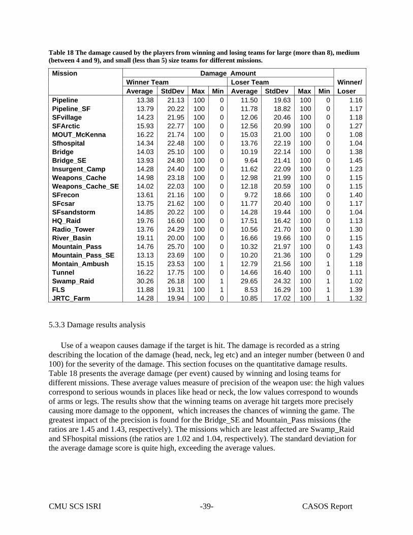
5.3.3 Damage results analysis Use of a weapon causes damage if the target is hit. The damage is recorded as a string
describing the location of the damage (head, neck, leg etc) and an integer number (between 0 and 100) for the severity of the damage. This section focuses on the quantitative damage results. Table 18 presents the average damage (per event) caused by winning and losing teams for different missions. These average values measure of precision of the weapon use: the high values correspond to serious wounds in places like head or neck, the low values correspond to wounds of arms or legs. The results show that the winning teams on average hit targets more precisely causing more damage to the opponent, which increases the chances of winning the game. The greatest impact of the precision is found for the Bridge_SE and Mountain_Pass missions (the ratios are 1.45 and 1.43, respectively). The missions which are least affected are Swamp_Raid and SFhospital missions (the ratios are 1.02 and 1.04, respectively). The standard deviation for the average damage score is quite high, exceeding the average values.
Mission Damage Amount Winner Team Loser Team Winner/ Average StdDev Max Min Average StdDev Max Min Loser Pipeline 13.38 21.13 100 0 11.50 19.63 100 0 1.16Pipeline_SF 13.79 20.22 100 0 11.78 18.82 100 0 1.17SFvillage 14.23 21.95 100 0 12.06 20.46 100 0 1.18SFArctic 15.93 22.77 100 0 12.56 20.99 100 0 1.27MOUT_McKenna 16.22 21.74 100 0 15.03 21.00 100 0 1.08Sfhospital 14.34 22.48 100 0 13.76 22.19 100 0 1.04Bridge 14.03 25.10 100 0 10.19 22.14 100 0 1.38Bridge_SE 13.93 24.80 100 0 9.64 21.41 100 0 1.45Insurgent_Camp 14.28 24.40 100 0 11.62 22.09 100 0 1.23Weapons_Cache 14.98 23.18 100 0 12.98 21.99 100 0 1.15Weapons_Cache_SE 14.02 22.03 100 0 12.18 20.59 100 0 1.15SFrecon 13.61 21.16 100 0 9.72 18.66 100 0 1.40SFcsar 13.75 21.62 100 0 11.77 20.40 100 0 1.17SFsandstorm 14.85 20.22 100 0 14.28 19.44 100 0 1.04HQ_Raid 19.76 16.60 100 0 17.51 16.42 100 0 1.13Radio_Tower 13.76 24.29 100 0 10.56 21.70 100 0 1.30River_Basin 19.11 20.00 100 0 16.66 19.66 100 0 1.15Mountain_Pass 14.76 25.70 100 0 10.32 21.97 100 0 1.43Mountain_Pass_SE 13.13 23.69 100 0 10.20 21.36 100 0 1.29Montain_Ambush 15.15 23.53 100 1 12.79 21.56 100 1 1.18Tunnel 16.22 17.75 100 0 14.66 16.40 100 0 1.11Swamp_Raid 30.26 26.18 100 1 29.65 24.32 100 1 1.02FLS 11.88 19.31 100 1 8.53 16.29 100 1 1.39JRTC_Farm 14.28 19.94 100 0 10.85 17.02 100 1 1.32
CMU SCS ISRI CASOS Report -40-
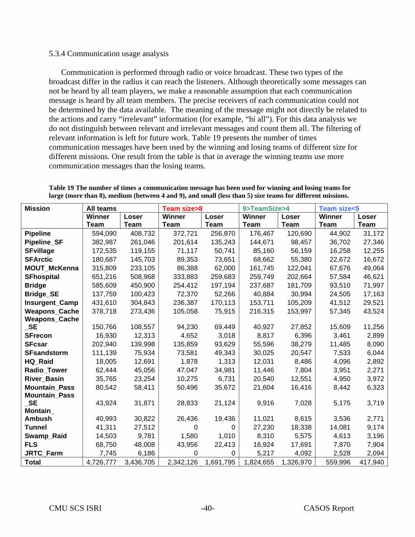
5.3.4 Communication usage analysis Communication is performed through radio or voice broadcast. These two types of the
broadcast differ in the radius it can reach the listeners. Although theoretically some messages can not be heard by all team players, we make a reasonable assumption that each communication message is heard by all team members. The precise receivers of each communication could not be determined by the data available. The meaning of the message might not directly be related to the actions and carry “irrelevant” information (for example, “hi all”). For this data analysis we do not distinguish between relevant and irrelevant messages and count them all. The filtering of relevant information is left for future work. Table 19 presents the number of times communication messages have been used by the winning and losing teams of different size for different missions. One result from the table is that in average the winning teams use more communication messages than the losing teams.
Table 19 The number of times a communication message has been used for winning and losing teams for large (more than 8), medium (between 4 and 9), and small (less than 5) size teams for different missions.
Mission All teams Team size>8 9>TeamSize>4 Team size<5
Winner Team
Loser Team
Winner Team
Loser Team
Winner Team
Loser Team
Winner Team
Loser Team
Pipeline 594,090 408,732 372,721 256,870 176,467 120,690 44,902 31,172Pipeline_SF 382,987 261,046 201,614 135,243 144,671 98,457 36,702 27,346SFvillage 172,535 119,155 71,117 50,741 85,160 56,159 16,258 12,255SFArctic 180,687 145,703 89,353 73,651 68,662 55,380 22,672 16,672MOUT_McKenna 315,809 233,105 86,388 62,000 161,745 122,041 67,676 49,064SFhospital 651,216 508,968 333,883 259,683 259,749 202,664 57,584 46,621Bridge 585,609 450,900 254,412 197,194 237,687 181,709 93,510 71,997Bridge_SE 137,759 100,423 72,370 52,266 40,884 30,994 24,505 17,163Insurgent_Camp 431,610 304,843 236,387 170,113 153,711 105,209 41,512 29,521Weapons_Cache 378,718 273,436 105,058 75,915 216,315 153,997 57,345 43,524Weapons_Cache _SE 150,766 108,557 94,230 69,449 40,927 27,852 15,609 11,256SFrecon 16,930 12,313 4,652 3,018 8,817 6,396 3,461 2,899SFcsar 202,940 139,998 135,859 93,629 55,596 38,279 11,485 8,090SFsandstorm 111,139 75,934 73,581 49,343 30,025 20,547 7,533 6,044HQ_Raid 18,005 12,691 1,878 1,313 12,031 8,486 4,096 2,892Radio_Tower 62,444 45,056 47,047 34,981 11,446 7,804 3,951 2,271River_Basin 35,765 23,254 10,275 6,731 20,540 12,551 4,950 3,972Mountain_Pass 80,542 58,411 50,496 35,672 21,604 16,416 8,442 6,323Mountain_Pass _SE 43,924 31,871 28,833 21,124 9,916 7,028 5,175 3,719Montain_ Ambush 40,993 30,822 26,436 19,436 11,021 8,615 3,536 2,771Tunnel 41,311 27,512 0 0 27,230 18,338 14,081 9,174Swamp_Raid 14,503 9,781 1,580 1,010 8,310 5,575 4,613 3,196FLS 68,750 48,008 43,956 22,413 16,924 17,691 7,870 7,904JRTC_Farm 7,745 6,186 0 0 5,217 4,092 2,528 2,094Total 4,726,777 3,436,705 2,342,126 1,691,795 1,824,655 1,326,970 559,996 417,940
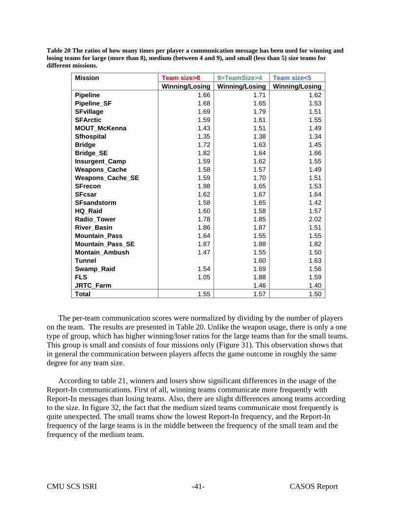
CMU SCS ISRI CASOS Report -41-
Table 20 The ratios of how many times per player a communication message has been used for winning and losing teams for large (more than 8), medium (between 4 and 9), and small (less than 5) size teams for different missions.
The per-team communication scores were normalized by dividing by the number of players on the team. The results are presented in Table 20. Unlike the weapon usage, there is only a one type of group, which has higher winning/loser ratios for the large teams than for the small teams. This group is small and consists of four missions only (Figure 31). This observation shows that in general the communication between players affects the game outcome in roughly the same degree for any team size.
According to table 21, winners and losers show significant differences in the usage of the
Report-In communications. First of all, winning teams communicate more frequently with Report-In messages than losing teams. Also, there are slight differences among teams according to the size. In figure 32, the fact that the medium sized teams communicate most frequently is quite unexpected. The small teams show the lowest Report-In frequency, and the Report-In frequency of the large teams is in the middle between the frequency of the small team and the frequency of the medium team.
Mission Team size>8 9>TeamSize>4 Team size<5 Winning/Losing Winning/Losing Winning/LosingPipeline 1.66 1.71 1.62Pipeline_SF 1.68 1.65 1.53SFvillage 1.69 1.79 1.51SFArctic 1.59 1.61 1.55MOUT_McKenna 1.43 1.51 1.49Sfhospital 1.35 1.38 1.34Bridge 1.72 1.63 1.45Bridge_SE 1.82 1.64 1.66Insurgent_Camp 1.59 1.62 1.55Weapons_Cache 1.58 1.57 1.49Weapons_Cache_SE 1.59 1.70 1.51SFrecon 1.98 1.65 1.53SFcsar 1.62 1.67 1.64SFsandstorm 1.58 1.65 1.42HQ_Raid 1.60 1.58 1.57Radio_Tower 1.78 1.85 2.02River_Basin 1.86 1.87 1.51Mountain_Pass 1.64 1.55 1.55Mountain_Pass_SE 1.87 1.88 1.82Montain_Ambush 1.47 1.55 1.50Tunnel 1.60 1.63Swamp_Raid 1.54 1.69 1.56FLS 1.05 1.88 1.59JRTC_Farm 1.46 1.40Total 1.55 1.57 1.50
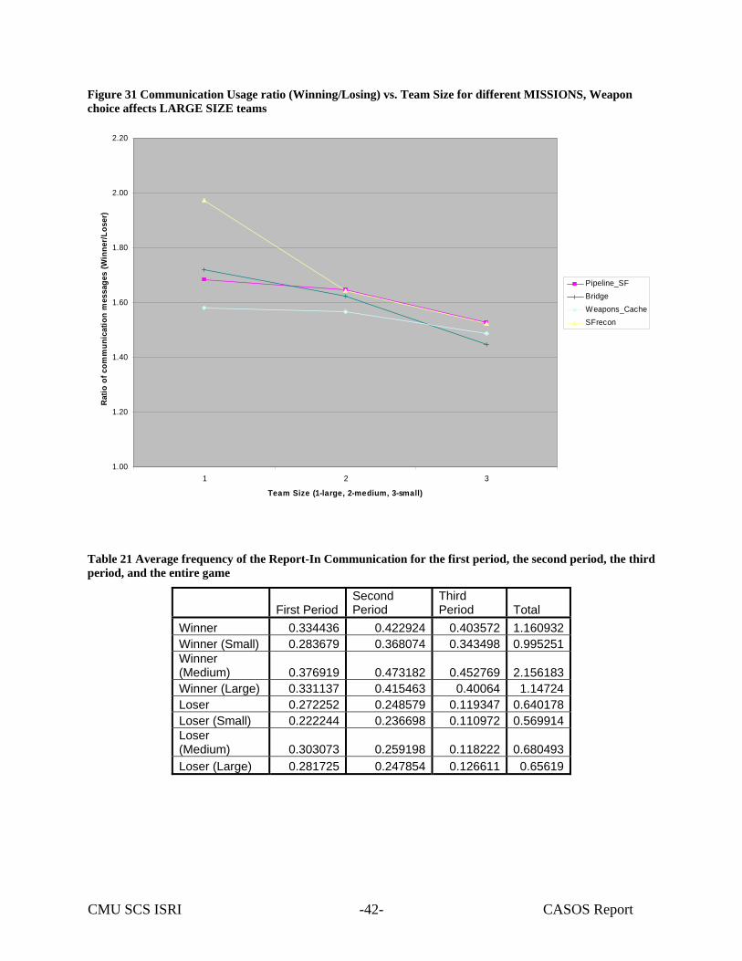
CMU SCS ISRI CASOS Report -42-
Figure 31 Communication Usage ratio (Winning/Losing) vs. Team Size for different MISSIONS, Weapon choice affects LARGE SIZE teams
1.00
1.20
1.40
1.60
1.80
2.00
2.20
1 2 3
Team Size (1-large, 2-medium, 3-small)
Ratio
of c
omm
unic
atio
n m
essa
ges
(Win
ner/L
oser
)
Pipeline_SFBridgeWeapons_CacheSFrecon
Table 21 Average frequency of the Report-In Communication for the first period, the second period, the third period, and the entire game
First Period Second Period
Third Period Total
Winner 0.334436 0.422924 0.403572 1.160932 Winner (Small) 0.283679 0.368074 0.343498 0.995251 Winner (Medium) 0.376919 0.473182 0.452769 2.156183 Winner (Large) 0.331137 0.415463 0.40064 1.14724 Loser 0.272252 0.248579 0.119347 0.640178 Loser (Small) 0.222244 0.236698 0.110972 0.569914 Loser (Medium) 0.303073 0.259198 0.118222 0.680493 Loser (Large) 0.281725 0.247854 0.126611 0.65619
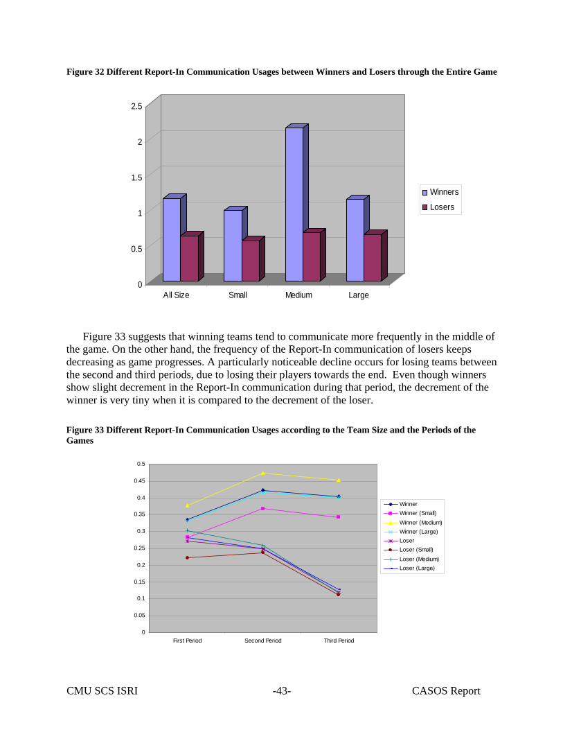
CMU SCS ISRI CASOS Report -43-
Figure 32 Different Report-In Communication Usages between Winners and Losers through the Entire Game
0
0.5
1
1.5
2
2.5
All Size Small Medium Large
Winners
Losers
Figure 33 suggests that winning teams tend to communicate more frequently in the middle of the game. On the other hand, the frequency of the Report-In communication of losers keeps decreasing as game progresses. A particularly noticeable decline occurs for losing teams between the second and third periods, due to losing their players towards the end. Even though winners show slight decrement in the Report-In communication during that period, the decrement of the winner is very tiny when it is compared to the decrement of the loser.
Figure 33 Different Report-In Communication Usages according to the Team Size and the Periods of the Games
0
0.05
0.1
0.15
0.2
0.25
0.3
0.35
0.4
0.45
0.5
First Period Second Period Third Period
WinnerWinner (Small)Winner (Medium)Winner (Large)LoserLoser (Small)Loser (Medium)Loser (Large)
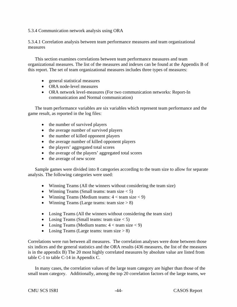
CMU SCS ISRI CASOS Report -44-
5.3.4 Communication network analysis using ORA
5.3.4.1 Correlation analysis between team performance measures and team organizational measures
This section examines correlations between team performance measures and team
organizational measures. The list of the measures and indexes can be found at the Appendix B of this report. The set of team organizational measures includes three types of measures:
• general statistical measures • ORA node-level measures • ORA network level-measures (For two communication networks: Report-In
communication and Normal communication) The team performance variables are six variables which represent team performance and the
game result, as reported in the log files:
• the number of survived players • the average number of survived players • the number of killed opponent players • the average number of killed opponent players • the players’ aggregated total scores • the average of the players’ aggregated total scores • the average of new score
Sample games were divided into 8 categories according to the team size to allow for separate
analysis. The following categories were used:
• Winning Teams (All the winners without considering the team size) • Winning Teams (Small teams: team size < 5) • Winning Teams (Medium teams: 4 < team size < 9) • Winning Teams (Large teams: team size > 8)
• Losing Teams (All the winners without considering the team size) • Losing Teams (Small teams: team size < 5) • Losing Teams (Medium teams: 4 < team size < 9) • Losing Teams (Large teams: team size > 8)
Correlations were run between all measures. The correlation analyses were done between those six indices and the general statistics and the ORA results (436 measures, the list of the measures is in the appendix B) The 20 most highly correlated measures by absolute value are listed from table C-1 to table C-14 in Appendix C.
In many cases, the correlation values of the large team category are higher than those of the
small team category. Additionally, among the top 20 correlation factors of the large teams, we
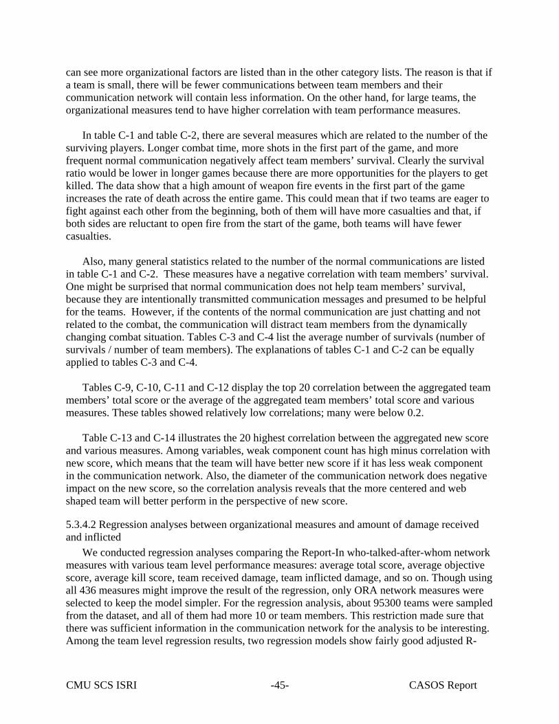
CMU SCS ISRI CASOS Report -45-
can see more organizational factors are listed than in the other category lists. The reason is that if a team is small, there will be fewer communications between team members and their communication network will contain less information. On the other hand, for large teams, the organizational measures tend to have higher correlation with team performance measures.
In table C-1 and table C-2, there are several measures which are related to the number of the surviving players. Longer combat time, more shots in the first part of the game, and more frequent normal communication negatively affect team members’ survival. Clearly the survival ratio would be lower in longer games because there are more opportunities for the players to get killed. The data show that a high amount of weapon fire events in the first part of the game increases the rate of death across the entire game. This could mean that if two teams are eager to fight against each other from the beginning, both of them will have more casualties and that, if both sides are reluctant to open fire from the start of the game, both teams will have fewer casualties.
Also, many general statistics related to the number of the normal communications are listed
in table C-1 and C-2. These measures have a negative correlation with team members’ survival. One might be surprised that normal communication does not help team members’ survival, because they are intentionally transmitted communication messages and presumed to be helpful for the teams. However, if the contents of the normal communication are just chatting and not related to the combat, the communication will distract team members from the dynamically changing combat situation. Tables C-3 and C-4 list the average number of survivals (number of survivals / number of team members). The explanations of tables C-1 and C-2 can be equally applied to tables C-3 and C-4.
Tables C-9, C-10, C-11 and C-12 display the top 20 correlation between the aggregated team
members’ total score or the average of the aggregated team members’ total score and various measures. These tables showed relatively low correlations; many were below 0.2.
Table C-13 and C-14 illustrates the 20 highest correlation between the aggregated new score
and various measures. Among variables, weak component count has high minus correlation with new score, which means that the team will have better new score if it has less weak component in the communication network. Also, the diameter of the communication network does negative impact on the new score, so the correlation analysis reveals that the more centered and web shaped team will better perform in the perspective of new score.
5.3.4.2 Regression analyses between organizational measures and amount of damage received and inflicted
We conducted regression analyses comparing the Report-In who-talked-after-whom network measures with various team level performance measures: average total score, average objective score, average kill score, team received damage, team inflicted damage, and so on. Though using all 436 measures might improve the result of the regression, only ORA network measures were selected to keep the model simpler. For the regression analysis, about 95300 teams were sampled from the dataset, and all of them had more 10 or team members. This restriction made sure that there was sufficient information in the communication network for the analysis to be interesting. Among the team level regression results, two regression models show fairly good adjusted R-
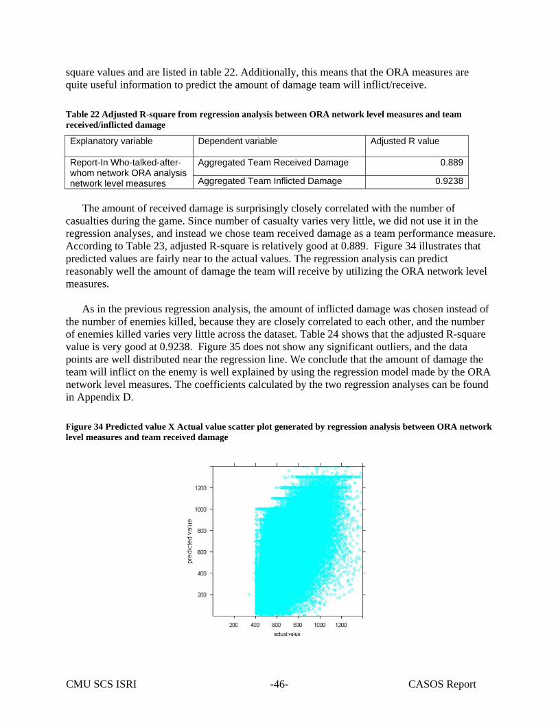
CMU SCS ISRI CASOS Report -46-
square values and are listed in table 22. Additionally, this means that the ORA measures are quite useful information to predict the amount of damage team will inflict/receive. Table 22 Adjusted R-square from regression analysis between ORA network level measures and team received/inflicted damage
Explanatory variable Dependent variable Adjusted R value
Aggregated Team Received Damage 0.889Report-In Who-talked-after-whom network ORA analysis network level measures Aggregated Team Inflicted Damage 0.9238
The amount of received damage is surprisingly closely correlated with the number of
casualties during the game. Since number of casualty varies very little, we did not use it in the regression analyses, and instead we chose team received damage as a team performance measure. According to Table 23, adjusted R-square is relatively good at 0.889. Figure 34 illustrates that predicted values are fairly near to the actual values. The regression analysis can predict reasonably well the amount of damage the team will receive by utilizing the ORA network level measures.
As in the previous regression analysis, the amount of inflicted damage was chosen instead of
the number of enemies killed, because they are closely correlated to each other, and the number of enemies killed varies very little across the dataset. Table 24 shows that the adjusted R-square value is very good at 0.9238. Figure 35 does not show any significant outliers, and the data points are well distributed near the regression line. We conclude that the amount of damage the team will inflict on the enemy is well explained by using the regression model made by the ORA network level measures. The coefficients calculated by the two regression analyses can be found in Appendix D.
Figure 34 Predicted value X Actual value scatter plot generated by regression analysis between ORA network level measures and team received damage
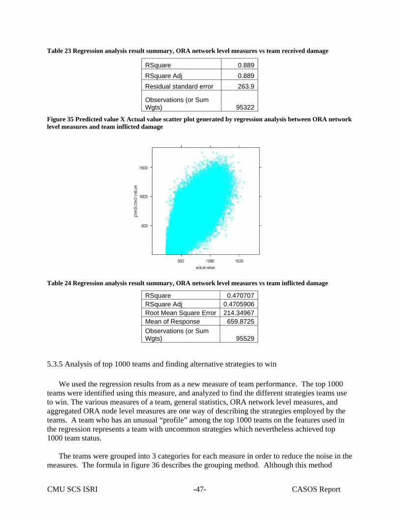
CMU SCS ISRI CASOS Report -47-
Table 23 Regression analysis result summary, ORA network level measures vs team received damage
RSquare 0.889RSquare Adj 0.889Residual standard error 263.9
Observations (or Sum Wgts) 95322
Figure 35 Predicted value X Actual value scatter plot generated by regression analysis between ORA network level measures and team inflicted damage
Table 24 Regression analysis result summary, ORA network level measures vs team inflicted damage
RSquare 0.470707RSquare Adj 0.4705906Root Mean Square Error 214.34967Mean of Response 659.8725Observations (or Sum Wgts) 95529
5.3.5 Analysis of top 1000 teams and finding alternative strategies to win
We used the regression results from as a new measure of team performance. The top 1000 teams were identified using this measure, and analyzed to find the different strategies teams use to win. The various measures of a team, general statistics, ORA network level measures, and aggregated ORA node level measures are one way of describing the strategies employed by the teams. A team who has an unusual “profile” among the top 1000 teams on the features used in the regression represents a team with uncommon strategies which nevertheless achieved top 1000 team status.
The teams were grouped into 3 categories for each measure in order to reduce the noise in the measures. The formula in figure 36 describes the grouping method. Although this method
CMU SCS ISRI CASOS Report -48-
reduces the variance of the data, it makes understanding and interpreting the following analyses easier.
Figure 36 Formula for labeling measures into groups
⎜⎜⎜⎜⎜⎜⎜
⎝
⎛
−<
+<≤−
+≥
=
==
d
dd
d
21ma when ,'1'
21ma
21m when ,'2'
21ma when ,'3'
a)for data labeled (the
a, is data actual Ifd A) ofdeviation (standard m, A) of (average
let A, measureFor
5.3.5.1 Principal Component Analyses on entire measures
A principal component analysis was done to convert the measures into the smaller number of variables, to make it simpler to recognize the variance among the top 1000 teams. We also used k-means clustering to group the 1000 teams into 10 clusters. Table 25 shows 10 clusters determined by using k-means analysis on top 1000 teams Table 25 Clusters determined by kmeans analysis on top 1000 teams
Cluster Cluster1 Cluster2 Cluster3 Cluster4 Cluster5 Cluster6 Cluster7 Cluster8 Cluster9 Cluster10
# of Teams 173 41 97 108 215 58 41 6 65 196
The top 36 principal components captured over 95% of the variance, and 67.5% variance was
captured using only 3 principal components. The summary of the principal component analysis can be found in Appendix E.
Figure 37 shows a scatter-plot of the top 3 principal components of the regression, grouped by color into 10 groups. The orange cluster, number 4, is noticeably separate from the other groups. The pink, cyan, and magenta, number 9, number 8, number 7 respectively, together form another outlying group.
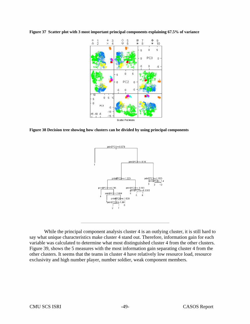
CMU SCS ISRI CASOS Report -49-
Figure 37 Scatter plot with 3 most important principal components explaining 67.5% of variance
Figure 38 Decision tree showing how clusters can be divided by using principal components
While the principal component analysis cluster 4 is an outlying cluster, it is still hard to say what unique characteristics make cluster 4 stand out. Therefore, information gain for each variable was calculated to determine what most distinguished cluster 4 from the other clusters. Figure 39, shows the 5 measures with the most information gain separating cluster 4 from the other clusters. It seems that the teams in cluster 4 have relatively low resource load, resource exclusivity and high number player, number soldier, weak component members.
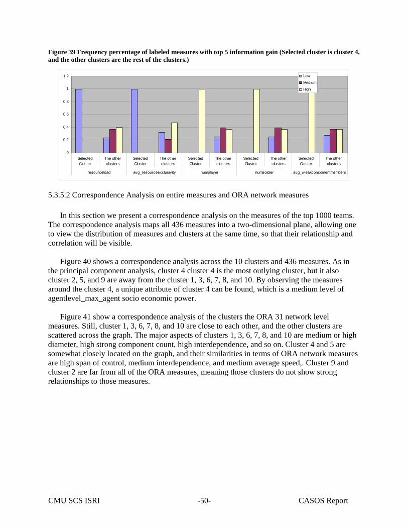
CMU SCS ISRI CASOS Report -50-
Figure 39 Frequency percentage of labeled measures with top 5 information gain (Selected cluster is cluster 4, and the other clusters are the rest of the clusters.)
0
0.2
0.4
0.6
0.8
1
1.2
SelectedCluster
The otherclusters
SelectedCluster
The otherclusters
SelectedCluster
The otherclusters
SelectedCluster
The otherclusters
SelectedCluster
The otherclusters
resourceload avg_resourceexclusivity numplayer numsoldier avg_w eakcomponentmembers
Low
Medium
High
5.3.5.2 Correspondence Analysis on entire measures and ORA network measures
In this section we present a correspondence analysis on the measures of the top 1000 teams. The correspondence analysis maps all 436 measures into a two-dimensional plane, allowing one to view the distribution of measures and clusters at the same time, so that their relationship and correlation will be visible.
Figure 40 shows a correspondence analysis across the 10 clusters and 436 measures. As in the principal component analysis, cluster 4 cluster 4 is the most outlying cluster, but it also cluster 2, 5, and 9 are away from the cluster 1, 3, 6, 7, 8, and 10. By observing the measures around the cluster 4, a unique attribute of cluster 4 can be found, which is a medium level of agentlevel_max_agent socio economic power.
Figure 41 show a correspondence analysis of the clusters the ORA 31 network level
measures. Still, cluster 1, 3, 6, 7, 8, and 10 are close to each other, and the other clusters are scattered across the graph. The major aspects of clusters 1, 3, 6, 7, 8, and 10 are medium or high diameter, high strong component count, high interdependence, and so on. Cluster 4 and 5 are somewhat closely located on the graph, and their similarities in terms of ORA network measures are high span of control, medium interdependence, and medium average speed,. Cluster 9 and cluster 2 are far from all of the ORA measures, meaning those clusters do not show strong relationships to those measures.
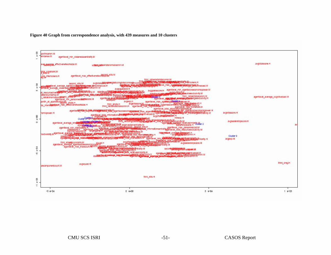
CMU SCS ISRI CASOS Report -51-
Figure 40 Graph from correspondence analysis, with 439 measures and 10 clusters
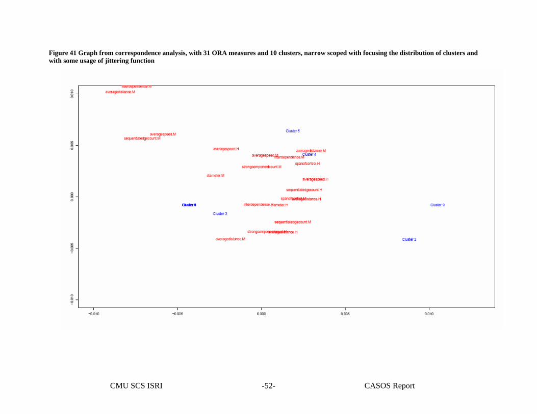
CMU SCS ISRI CASOS Report -52-
Figure 41 Graph from correspondence analysis, with 31 ORA measures and 10 clusters, narrow scoped with focusing the distribution of clusters and with some usage of jittering function
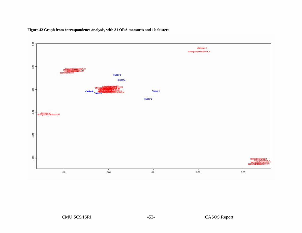
CMU SCS ISRI CASOS Report -53-
Figure 42 Graph from correspondence analysis, with 31 ORA measures and 10 clusters
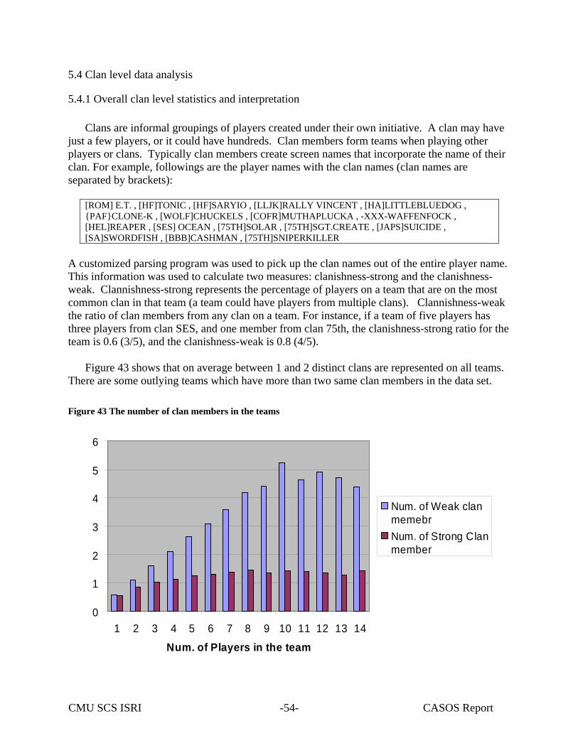
CMU SCS ISRI CASOS Report -54-
5.4 Clan level data analysis
5.4.1 Overall clan level statistics and interpretation
Clans are informal groupings of players created under their own initiative. A clan may have just a few players, or it could have hundreds. Clan members form teams when playing other players or clans. Typically clan members create screen names that incorporate the name of their clan. For example, followings are the player names with the clan names (clan names are separated by brackets):
[ROM] E.T. , [HF]TONIC , [HF]SARYIO , [LLJK]RALLY VINCENT , [HA]LITTLEBLUEDOG , {PAF}CLONE-K , [WOLF]CHUCKELS , [COFR]MUTHAPLUCKA , -XXX-WAFFENFOCK , [HEL]REAPER , [SES] OCEAN , [75TH]SOLAR , [75TH]SGT.CREATE , [JAPS]SUICIDE , [SA]SWORDFISH , [BBB]CASHMAN , [75TH]SNIPERKILLER
A customized parsing program was used to pick up the clan names out of the entire player name. This information was used to calculate two measures: clanishness-strong and the clanishness-weak. Clannishness-strong represents the percentage of players on a team that are on the most common clan in that team (a team could have players from multiple clans). Clannishness-weak the ratio of clan members from any clan on a team. For instance, if a team of five players has three players from clan SES, and one member from clan 75th, the clanishness-strong ratio for the team is 0.6 (3/5), and the clanishness-weak is 0.8 (4/5).
Figure 43 shows that on average between 1 and 2 distinct clans are represented on all teams.
There are some outlying teams which have more than two same clan members in the data set.
Figure 43 The number of clan members in the teams
0
1
2
3
4
5
6
1 2 3 4 5 6 7 8 9 10 11 12 13 14
Num. of Players in the team
Num. of Weak clanmemebrNum. of S trong C lanmember
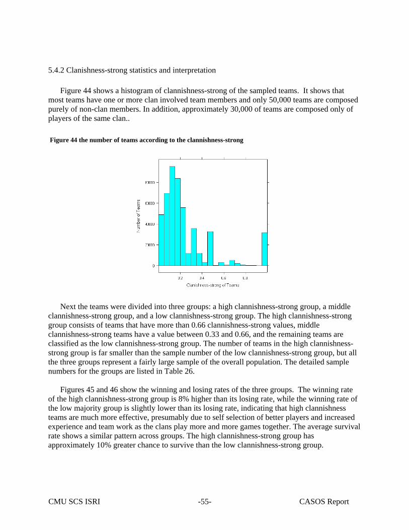
CMU SCS ISRI CASOS Report -55-
5.4.2 Clanishness-strong statistics and interpretation
Figure 44 shows a histogram of clannishness-strong of the sampled teams. It shows that most teams have one or more clan involved team members and only 50,000 teams are composed purely of non-clan members. In addition, approximately 30,000 of teams are composed only of players of the same clan..
Figure 44 the number of teams according to the clannishness-strong
Next the teams were divided into three groups: a high clannishness-strong group, a middle clannishness-strong group, and a low clannishness-strong group. The high clannishness-strong group consists of teams that have more than 0.66 clannishness-strong values, middle clannishness-strong teams have a value between 0.33 and 0.66, and the remaining teams are classified as the low clannishness-strong group. The number of teams in the high clannishness-strong group is far smaller than the sample number of the low clannishness-strong group, but all the three groups represent a fairly large sample of the overall population. The detailed sample numbers for the groups are listed in Table 26.
Figures 45 and 46 show the winning and losing rates of the three groups. The winning rate of the high clannishness-strong group is 8% higher than its losing rate, while the winning rate of the low majority group is slightly lower than its losing rate, indicating that high clannishness teams are much more effective, presumably due to self selection of better players and increased experience and team work as the clans play more and more games together. The average survival rate shows a similar pattern across groups. The high clannishness-strong group has approximately 10% greater chance to survive than the low clannishness-strong group.
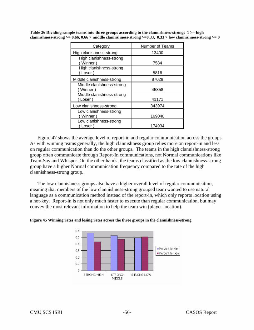
CMU SCS ISRI CASOS Report -56-
Table 26 Dividing sample teams into three groups according to the clannishness-strong: 1 >= high clannishness-strong >= 0.66, 0.66 > middle clannishness-strong >=0.33, 0.33 > low clannishness-strong >= 0
Category Number of Teams High clanishness-strong 13400 High clanishness-strong ( Winner ) 7584 High clanishness-strong ( Loser ) 5816 Middle clanishness-strong 87029 Middle clanishness-strong ( Winner ) 45858 Middle clanishness-strong ( Loser ) 41171 Low clanishness-strong 343974 Low clanishness-strong ( Winner ) 169040 Low clanishness-strong ( Loser ) 174934
Figure 47 shows the average level of report-in and regular communication across the groups.
As with winning teams generally, the high clannishness group relies more on report-in and less on regular communication than do the other groups. The teams in the high clannishness-strong group often communicate through Report-In communications, not Normal communications like Team-Say and Whisper. On the other hands, the teams classified as the low clannishness-strong group have a higher Normal communication frequency compared to the rate of the high clannishness-strong group.
The low clannishness groups also have a higher overall level of regular communication,
meaning that members of the low clannishness-strong grouped team wanted to use natural language as a communication method instead of the report-in, which only reports location using a hot-key. Report-in is not only much faster to execute than regular communication, but may convey the most relevant information to help the team win (player location).
Figure 45 Winning rates and losing rates across the three groups in the clannishness-strong
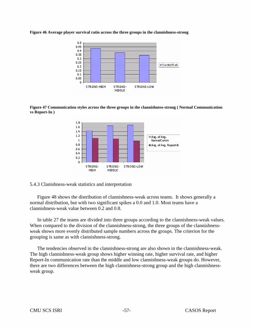
CMU SCS ISRI CASOS Report -57-
Figure 46 Average player survival ratio across the three groups in the clannishness-strong
Figure 47 Communication styles across the three groups in the clannishness-strong ( Normal Communication vs Report-In )
5.4.3 Clanishness-weak statistics and interpretation
Figure 48 shows the distribution of clannishness-weak across teams. It shows generally a normal distribution, but with two significant spikes a 0.0 and 1.0. Most teams have a clannishness-weak value between 0.2 and 0.8.
In table 27 the teams are divided into three groups according to the clannishness-weak values.
When compared to the division of the clannishness-strong, the three groups of the clannishness-weak shows more evenly distributed sample numbers across the groups. The criterion for the grouping is same as with clannishness-strong.
The tendencies observed in the clannishness-strong are also shown in the clannishness-weak.
The high clannishness-weak group shows higher winning rate, higher survival rate, and higher Report-In communication rate than the middle and low clannishness-weak groups do. However, there are two differences between the high clannishness-strong group and the high clannishness-weak group.
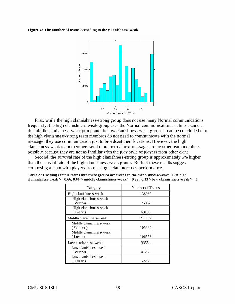
CMU SCS ISRI CASOS Report -58-
Figure 48 The number of teams according to the clannishness-weak
First, while the high clannishness-strong group does not use many Normal communications
frequently, the high clanishness-weak group uses the Normal communication as almost same as the middle clanishness-weak group and the low clanishness-weak group. It can be concluded that the high clanishness-strong team members do not need to communicate with the normal message: they use communication just to broadcast their locations. However, the high clanishness-weak team members send more normal text messages to the other team members, possibly because they are not as familiar with the play style of players from other clans.
Second, the survival rate of the high clanishness-strong group is approximately 5% higher than the survial rate of the high clanishness-weak group. Both of these results suggest composing a team with players from a single clan increases performance. Table 27 Dividing sample teams into three groups according to the clannishness-weak: 1 >= high clannishness-weak >= 0.66, 0.66 > middle clannishness-weak >=0.33, 0.33 > low clannishness-weak >= 0
Category Number of Teams High clanishness-weak 138960 High clanishness-weak ( Winner ) 75857 High clanishness-weak ( Loser ) 63103 Middle clanishness-weak 211889 Middle clanishness-weak ( Winner ) 105336 Middle clanishness-weak ( Loser ) 106553 Low clanishness-weak 93554 Low clanishness-weak ( Winner ) 41289 Low clanishness-weak ( Loser ) 52265
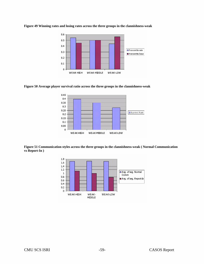
CMU SCS ISRI CASOS Report -59-
Figure 49 Winning rates and losing rates across the three groups in the clannishness-weak
Figure 50 Average player survival ratio across the three groups in the clannishness-weak
Figure 51 Communication styles across the three groups in the clannishness-weak ( Normal Communication vs Report-In )
CMU SCS ISRI CASOS Report -60-
6. Guidelines to win the America’s Army game
There is not an absolute way to win the America’s Army game, but we could discover some
conspicuous tendencies of winners and losers from the data analysis. If we could assume these tendencies are the very strategies of winners or losers, a player or a team can be a winner by adopting winner’s tendencies. Because the analysis was conducted at player level, team level, and clan level, the findings can be categorized similarly.
6.1. Strategies for players
Among top players in America’s Army game, there are same traits from the viewpoint of weapon usage, communication style, damage control, and role selection. According to the analysis, top players should be able to
Handle various weapons: from M4 and M16 rifles to M9 pistol and SPR sniper rifle Transmit Report-In communications as many times as possible Do seeking covers and firing weapons to enemy at the same time Keep selecting the medic role if you want to be a medic
6.2. Strategies for teams
Because we could detect some outlier winning teams, we cannot say there are explicit shapes
of organization structure of winning teams, but we could reveal several important distinctions between winning teams and losing teams. Winning teams are usually able to
Be consisted of 10 players to maximize the survival rate Fire weapons more frequently and use heavy weapons like RPG7 a lot Transmit communications very often: especially Report-In communication
6.3. Strategies for clans
Clans are not organized by America’s Army game system, but we could see some players
form a clan and play together very often. With considering the existence of the clans, there are some methods to improve the performance of a team.
Organize a team with same clan member Organize a team with players who are in clans if it is impossible to make a team with
your clan member. Try to reduce the Normal Communications by becoming familiar with your clan
member’s play style and try to focus on sending the Report-In Communications Use both Normal Communications and Report-In Communications frequently if there
are team players who are not in your clan
CMU SCS ISRI CASOS Report -61-
7. Comparison of America’s Army game to Real-world Military Research
This section compares the America’s Army analysis with existing research on squad-level interaction among soldiers. This may provide some insights to future research on squad-level team organization. The similarities and the new findings can be categorized into two issues: team structure and communication protocol.
7.1. Structures of America’s Army team and squad unit
America’s Army team size varies from one to fourteen which is similar to the size of a typical army squad unit, so the squad is an appropriate level for comparison. A great deal of research has been conducted in this area since the end of the World War II. The first modern study was done during the 1946 Infantry Conference, and the recommended squad structure was 9 men consisting of 1 squad leader, 1 assistant squad leader, 1 automatic rifle man, 1 assistant gunner, and 5 rifle men. This squad structure was reformed after the Korean War: from a 9-man squad structure without a sub-teams to a 9-man squad with 2 fire teams as sub-units of the squad. Each fire team consisted of 1 team leader, 1 automatic rifle man, and 2 rifle men. The major reason of this change was the discovery of the importance of heavy weapons such as the automatic rifle, flamethrower, and bazooka. The soldiers with heavier weapons were more effective in combat, [3] so adding one more automatic rifle to the squad structure was considered the effective way to increase fire volume. This tendency, emphasizing the importance of the heavy weapons, could be observed in the America’s Army game. Table 16 clearly shows the importance of the heavy weapons: the M2 heavy machine gun, RPK SAW, and RPG7 rocket were all used more frequently by the winning team than the losing team.
Also, the optimal America’s Army team size is similar to the recommended army squad unit
size. In real world, to determine the army squad size, many factors were considered such as how many soldiers are controlled by one squad leader, how large a size is sustainable and maneuverable with casualties or a pinned down squad leader, and how many soldiers can be carried by an infantry fighting vehicle. The recommended army squad unit sizes is usually between 9 and 13. Table 5 indicates that the most favorable team size of an America’s Army team is 10. Table 5 also shows that the 10-man America’s Army teams have a relatively high survival ratio even when they are losing and better survival ratio that others when they are winning.
7.2. Communication Patterns of America’s Army teams and Army Squads
To date infantryman-level radio usage has not been well researched. Possible reasons for this
include the difficulty of collecting well-organized intra-squad radio usage datasets in real-word conditions, and research concentration on the team size and the team equipment rather than intra-squad radio communication. However, we could see the importance of structure, content, and frequency of the intra-squad communication through the data analysis result of America’s Army, and there is an increasing demand for the research of the optimal communication protocol in an army squad unit.
CMU SCS ISRI CASOS Report -62-
Christ and Evans [4] present one field experiment about using intra-squad radio communication. The research identified 5 tactics, techniques, and procedures concerning the rules for radio discipline (who is permitted to talk at what time), and 13 communication content categories that explain 13 types of message contents. Compared to the America’s Army data analysis, we can interpret that the America’s Army communication style is equal to the TTP 5, (Free Talk), and Report-In communication in America’s Army data analysis is same as the Provide Information (Friend) communication.
As we can see in Figure 32, it is very clear that the frequent Report-In communication is a
key to wining the game, and the research from ARI states that the Provide Information (friend) communication was the one of the most frequent communications in squads. At the same time, squad leaders broadcast the Provide Information (friend) communication more frequently than squad members does, and this tendency is also observed and analyzed in the chapter 5.2.2.2. Frequent Report-In top players. Among 100 top players, there were some players who used the Report-In communication very often, and we conjecture that they are taking the role of combat leader.
Though some similarities could be found, the America’s Army data analysis chose different
approach from ARI research about the communication protocol and structure. ARI research used strict five types of TTP for experiment, and the experiment displays that the TTP 1, “Don’t Talk”, results the highest situation awareness result. On the other hand, in America’s Army, every team follows TTP 5, and the communication network structures of top 1000 teams are investigated. According to the regression analysis, low average distance, high network level, and high sequential edge count can result reduced team received damage. Similarly, low average speed, low closeness centralization, high minimum speed, and high total degree centralization generates increased team inflicted damage. Because the ARI research didn’t conducted any rigorous analysis on the communication dynamics or structure, the data analysis of America’s Army cannot be compared directly on this matter, but it should be noted that the data analysis of America’s Army suggests more detailed squad communication structure shape than the ARI research did.
7.3. Training inexperienced soldiers by using America’s Army game
America’s Army game is one of the well-known shooting games, and it is freely distributed
through on-line game web sites and Army recruiting officers, which makes the game ideal to use a method to introduce and train young adults and inexperienced soldiers. From the above comparisons, we could identify that the game situation is quite similar to the real-world situation. Moreover, the game play style of top players in the America’s Army game and the combat style of trained soldiers in real-world are quite similar to each other. For example, there are some top players who send out the Report-In Communication very frequently, and ARI research could reveal squad leaders transmit the Provide Information (Friend) Communication very often. Also, top players are able to seek the covers and to fire the weapons at the same time, which Army wants to make inexperienced soldiers do so. Therefore, it would be a good way to use the America’s Army game as a method to train the inexperienced soldiers.
7.4. Comparison between C2 dataset and America’s Army dataset
CMU SCS ISRI CASOS Report -63-
Command and control (C2) dataset is collected from Fort Lee, Fort Leavenworth, and Fort Knox. This dataset is modeling the brigade level staff officer social network. Even though America’s Army dataset is about the squad level army unit, both dataset are analyzed in the perspective of the social network, so it was worth enough to compare each other. From the C2 dataset, it is concluded that physical and social distance, and background similarity, can predict how well people can estimate information about others. In the America’s Army dataset, the ORA measures of social network could predict the damage team will receive/inflict. Also, the high clannishness representing the common background among team members was the one of the traits of winning teams. With these similarities, we conjecture that the social network and the background setting are the performance predictors which can be applied to organizations beyond the limitation of size and problem domain.
CMU SCS ISRI CASOS Report -64-
8. Conclusion
America’s Army dataset is researched at player level, team level, and clan level. Particularly, many statistical methods are applied to discover traits of dynamic social networks of winning teams in America’s Army. From the research, several commonalities among top teams were found, and some outlying teams were adopting unusual ways to win.
The player level analyses could reveal that there are several distinguishing characteristics of
top players. The characteristics are the variety of weapon selection, dodging bullets and being aggressive at the same time, and transmitting Report-In communication frequently. To be a top player in America’s Army game, a player should be able to deal with various weapons, which means they should be equipped with various weapons (obtain high powered weapons from the enemy during the game), and be experienced in using them. Top players are capable of using rifle, sniper rifle, and grenades when they are needed. Not only weapon usage, but also communication style distinguishes the top players: usually top player are very apt to send out their position through the Report-In communication, which means there is more possibility that he can get supports or covering fires from other team members. When it comes to the top players’ attack and defense behavior, it is very clear that the top players can inflict good amount of damage toward the opponent without having much damage themselves. We cannot say that how they behave to dodge the bullets and to fire the weapons, but it is quite certain that they are not just attacking without seeking covers or just running away from the combat without attacking the enemies: the top players should be able to fire weapons and to seek the covers at the same time.
The team level analyses have shown that there are some factors which distinguish winning
teams from losing teams and which makes the team more efficient and safer. The most favorable size of teams is 10 players, and the 10-men teams are very similar to the size of the squad unit which is specified by the recommendation of Reorganization of the Army Division when it compared to Army squad. The 10-men team has the relatively higher survival ratio than the other sizes of teams have, in both cases, losing and winning. It has been found that some parameters, frequent usage of the weapon, precision of the weapon use, and frequency of communication, can be the distinctions between winning teams and losing teams. High weapon usage is one of the best indicators of winning teams in America’s Army game, and this corresponds to the argument that the high volume of weapon fire leads success of the real world squad, which is the common belief of the army officers. Also, the high frequency of Report-In communication is the essential factor to win the games, and this result are very similar to the ARI research which claims that the Provide Information (friend) communications, similar to the Report-In communication, are frequently transmitted by trained soldiers when they can use intra-squad radio communication. By using the Report-In communication, the team will have more chance to have unified situation awareness: where the team members are and how team members can support the other team members. This can lead more effective covering fires, avoiding friendly fires, and medical supports to wounded soldiers.
Additionally, the correlation and regression analyses of the general statistical data and the ORA analysis results suggest some insights in the combat result. For example, the longer the game and more weapon fires in the first part of game lower the entire number of survivals. The regression analyses, between ORA network level measures and team received/inflicted damage,
CMU SCS ISRI CASOS Report -65-
suggest that observing Report-In who-talked-after-whom network can be a good way to collect explanatory variables which can predict the amount of team received/inflicted damage. For example, communication structure having high sequential edge count and high network level will reduce team received damage. The shape of that kind of structure will be a long chain of communication line. Also, to enhance the team inflict damage, the long chain shaped communication structure would be good because the team inflicted damage will be increased with a communication structure with high average speed and high closeness centralization.
To identify the alternative ways to win, principal component analysis and correspondence
analysis are done. To do the analyses, top 1000 teams are sampled from the dataset, and they are categorized into 10 clusters by using K-means analysis. After the categorization, principal component analysis and correspondence analysis could identify that 6 clusters are very closely located, and the other 4 clusters are remotely located from the other clusters. The 4 clusters can be the outlying teams having unusual aspects in the perspective of team measures, and the unusual aspects of the 4 clusters might be interpreted as the alternative ways to win. For instance, teams in one of the outlying clusters have a communication network with the high reciprocal edge count, high clustering coefficient, and high connectedness: this means that they are using not a chain shaped communication network, but more web shaped communication network.
The clan level analyses strongly suggest that making a team with same clan members is the
most effective way to win the. Inherently, there is no functionality to identify players’ clan participation in America’s Army game. However, in America’s Army community, players usually decorate their ID with identical prefix with same clan members. Thus, we develop a parser for players’ ID and extract the clan names and participants by identifying the prefix of the players’ ID. Being in a same clan, players play together very often, and it results that each player becomes very familiar with the other players’ play style. Thus, when they organize an America’s Army team and start a game, they just transmit the Report-In communications to the other team members without using the other communication messages to organize their tactical plans, and this makes the team very efficient. In other words, the teams consisted of the same clan members can maximize the frequency of the Report-In communications and gain the benefit of the Report-In communication maximally. The data analysis clearly demonstrates that the teams with same clan members have less casualties and high possibility to win the game. When this is not an option, forming a team with players who are participating in clans is the alternative way to win. When someone is a clan member, it means that he played enough to get involved with certain clans and he certainly have a good knowledge about playing the game. Then, it is quite obvious that the team will win if a team is organized with experienced members. However, in this case, the frequency of Normal communication, communication in natural language, increases to communicate with unfamiliar team members because of the necessity to coordinate their game play plan. These observations displays the importance to organize the squad team with the soldiers who are familiar to each other, so they don’t spend valuable time in communicating each other in lengthy words.
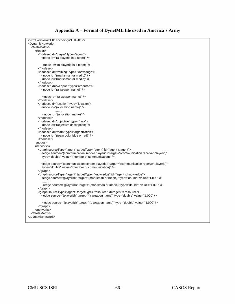
CMU SCS ISRI CASOS Report -66-
Appendix A – Format of DynetML file used in America’s Army
<?xml version="1.0" encoding="UTF-8" ?> <DynamicNetwork> <MetaMatrix> <nodes> <nodeset id="player" type="agent"> <node id="(a playerid in a team)" /> ........ <node id="(a playerid in a team)" /> </nodeset> <nodeset id="training" type="knowledge"> <node id="(marksman or medic)" /> <node id="(marksman or medic)" /> </nodeset> <nodeset id="weapon" type="resource"> <node id="(a weapon name)" /> ........ <node id="(a weapon name)" /> </nodeset> <nodeset id="location" type="location"> <node id="(a location name)" /> ........ <node id="(a location name)" /> </nodeset> <nodeset id="objective" type="task"> <node id="(objective description)" /> </nodeset> <nodeset id="team" type="organization"> <node id="(team color:blue or red)" /> </nodeset> </nodes> <networks> <graph sourceType="agent" targetType="agent" id="agent x agent"> <edge source="(communication sender playerid)" target="(communication receiver playerid)" type="double" value="(number of communication)" /> ........ <edge source="(communication sender playerid)" target="(communication receiver playerid)" type="double" value="(number of communication)" /> </graph> <graph sourceType="agent" targetType="knowledge" id="agent x knowledge"> <edge source="(playerid)" target="(marksman or medic)" type="double" value="1.000" /> ........ <edge source="(playerid)" target="(marksman or medic)" type="double" value="1.000" /> </graph> <graph sourceType="agent" targetType="resource" id="agent x resource"> <edge source="(playerid)" target="(a weapon name)" type="double" value="1.000" /> ........ <edge source="(playerid)" target="(a weapon name)" type="double" value="1.000" /> </graph> </networks> </MetaMatrix> </DynamicNetwork>
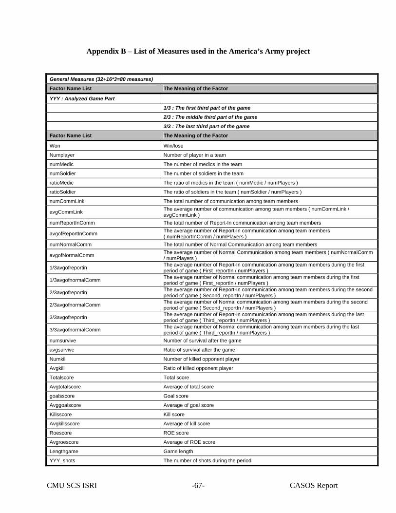
CMU SCS ISRI CASOS Report -67-
Appendix B – List of Measures used in the America’s Army project
General Measures (32+16*3=80 measures)
Factor Name List The Meaning of the Factor
YYY : Analyzed Game Part
1/3 : The first third part of the game
2/3 : The middle third part of the game
3/3 : The last third part of the game
Factor Name List The Meaning of the Factor
Won Win/lose
Numplayer Number of player in a team
numMedic The number of medics in the team
numSoldier The number of soldiers in the team
ratioMedic The ratio of medics in the team ( numMedic / numPlayers )
ratioSoldier The ratio of soldiers in the team ( numSoldier / numPlayers )
numCommLink The total number of communication among team members
avgCommLink The average number of communication among team members ( numCommLink / avgCommLink )
numReportInComm The total number of Report-In communication among team members
avgofReportInComm The average number of Report-In communication among team members ( numReportInComm / numPlayers )
numNormalComm The total number of Normal Communication among team members
avgofNormalComm The average number of Normal Communication among team members ( numNormalComm / numPlayers )
1/3avgofreportin The average number of Report-In communication among team members during the first period of game ( First_reportIn / numPlayers )
1/3avgofnormalComm The average number of Normal communication among team members during the first period of game ( First_reportIn / numPlayers )
2/3avgofreportin The average number of Report-In communication among team members during the second period of game ( Second_reportIn / numPlayers )
2/3avgofnormalComm The average number of Normal communication among team members during the second period of game ( Second_reportIn / numPlayers )
3/3avgofreportin The average number of Report-In communication among team members during the last period of game ( Third_reportIn / numPlayers )
3/3avgofnormalComm The average number of Normal communication among team members during the last period of game ( Third_reportIn / numPlayers )
numsurvive Number of survival after the game
avgsurvive Ratio of survival after the game
Numkill Number of killed opponent player
Avgkill Ratio of killed opponent player
Totalscore Total score
Avgtotalscore Average of total score
goalsscore Goal score
Avggoalscore Average of goal score
Killsscore Kill score
Avgkillsscore Average of kill score
Roescore ROE score
Avgroescore Average of ROE score
Lengthgame Game length
YYY_shots The number of shots during the period
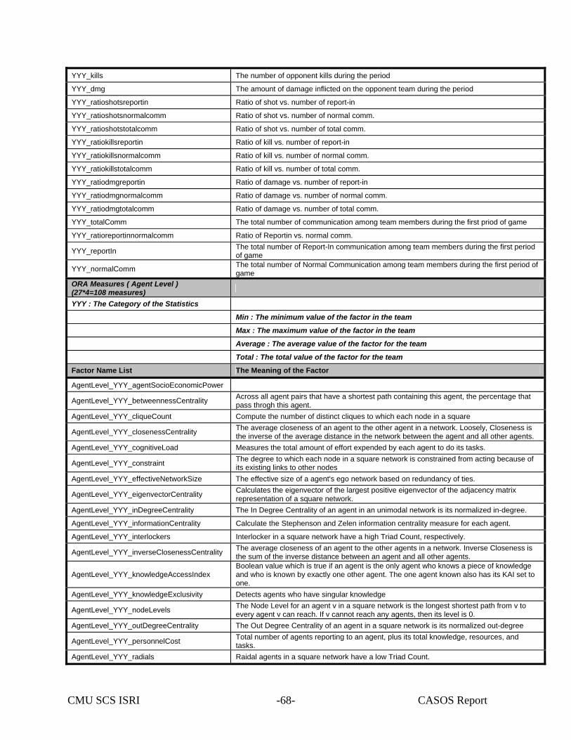
CMU SCS ISRI CASOS Report -68-
YYY_kills The number of opponent kills during the period
YYY_dmg The amount of damage inflicted on the opponent team during the period
YYY_ratioshotsreportin Ratio of shot vs. number of report-in
YYY_ratioshotsnormalcomm Ratio of shot vs. number of normal comm.
YYY_ratioshotstotalcomm Ratio of shot vs. number of total comm.
YYY_ratiokillsreportin Ratio of kill vs. number of report-in
YYY_ratiokillsnormalcomm Ratio of kill vs. number of normal comm.
YYY_ratiokillstotalcomm Ratio of kill vs. number of total comm.
YYY_ratiodmgreportin Ratio of damage vs. number of report-in
YYY_ratiodmgnormalcomm Ratio of damage vs. number of normal comm.
YYY_ratiodmgtotalcomm Ratio of damage vs. number of total comm.
YYY_totalComm The total number of communication among team members during the first priod of game
YYY_ratioreportinnormalcomm Ratio of Reportin vs. normal comm.
YYY_reportIn The total number of Report-In communication among team members during the first period of game
YYY_normalComm The total number of Normal Communication among team members during the first period of game
ORA Measures ( Agent Level ) (27*4=108 measures)
YYY : The Category of the Statistics
Min : The minimum value of the factor in the team
Max : The maximum value of the factor in the team
Average : The average value of the factor for the team
Total : The total value of the factor for the team
Factor Name List The Meaning of the Factor
AgentLevel_YYY_agentSocioEconomicPower
AgentLevel_YYY_betweennessCentrality Across all agent pairs that have a shortest path containing this agent, the percentage that pass throgh this agent.
AgentLevel_YYY_cliqueCount Compute the number of distinct cliques to which each node in a square
AgentLevel_YYY_closenessCentrality The average closeness of an agent to the other agent in a network. Loosely, Closeness is the inverse of the average distance in the network between the agent and all other agents.
AgentLevel_YYY_cognitiveLoad Measures the total amount of effort expended by each agent to do its tasks.
AgentLevel_YYY_constraint The degree to which each node in a square network is constrained from acting because of its existing links to other nodes
AgentLevel_YYY_effectiveNetworkSize The effective size of a agent's ego network based on redundancy of ties.
AgentLevel_YYY_eigenvectorCentrality Calculates the eigenvector of the largest positive eigenvector of the adjacency matrix representation of a square network.
AgentLevel_YYY_inDegreeCentrality The In Degree Centrality of an agent in an unimodal network is its normalized in-degree.
AgentLevel_YYY_informationCentrality Calculate the Stephenson and Zelen information centrality measure for each agent.
AgentLevel_YYY_interlockers Interlocker in a square network have a high Triad Count, respectively.
AgentLevel_YYY_inverseClosenessCentrality The average closeness of an agent to the other agents in a network. Inverse Closeness is the sum of the inverse distance between an agent and all other agents.
AgentLevel_YYY_knowledgeAccessIndex Boolean value which is true if an agent is the only agent who knows a piece of knowledge and who is known by exactly one other agent. The one agent known also has its KAI set to one.
AgentLevel_YYY_knowledgeExclusivity Detects agents who have singular knowledge
AgentLevel_YYY_nodeLevels The Node Level for an agent v in a square network is the longest shortest path from v to every agent v can reach. If v cannot reach any agents, then its level is 0.
AgentLevel_YYY_outDegreeCentrality The Out Degree Centrality of an agent in a square network is its normalized out-degree
AgentLevel_YYY_personnelCost Total number of agents reporting to an agent, plus its total knowledge, resources, and tasks.
AgentLevel_YYY_radials Raidal agents in a square network have a low Triad Count.
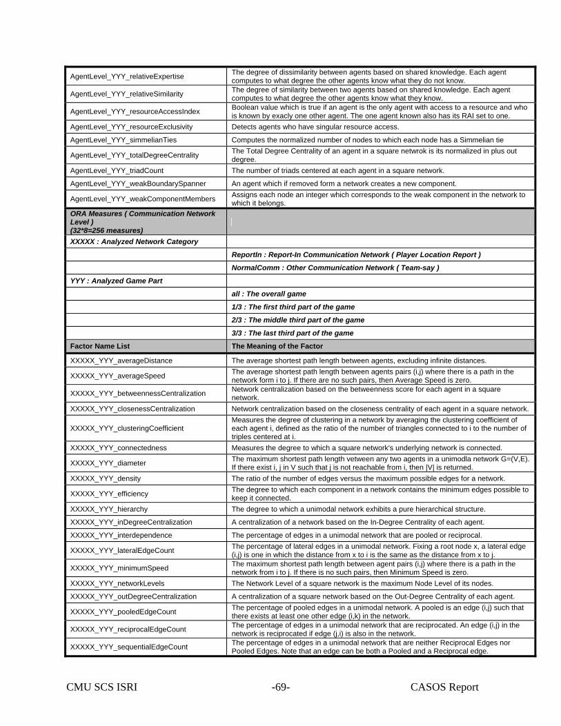
CMU SCS ISRI CASOS Report -69-
AgentLevel_YYY_relativeExpertise The degree of dissimilarity between agents based on shared knowledge. Each agent computes to what degree the other agents know what they do not know.
AgentLevel_YYY_relativeSimilarity The degree of similarity between two agents based on shared knowledge. Each agent computes to what degree the other agents know what they know.
AgentLevel_YYY_resourceAccessIndex Boolean value which is true if an agent is the only agent with access to a resource and who is known by exacly one other agent. The one agent known also has its RAI set to one.
AgentLevel_YYY_resourceExclusivity Detects agents who have singular resource access.
AgentLevel_YYY_simmelianTies Computes the normalized number of nodes to which each node has a Simmelian tie
AgentLevel_YYY_totalDegreeCentrality The Total Degree Centrality of an agent in a square netwrok is its normalized in plus out degree.
AgentLevel_YYY_triadCount The number of triads centered at each agent in a square network.
AgentLevel_YYY_weakBoundarySpanner An agent which if removed form a network creates a new component.
AgentLevel_YYY_weakComponentMembers Assigns each node an integer which corresponds to the weak component in the network to which it belongs.
ORA Measures ( Communication Network Level ) (32*8=256 measures)
XXXXX : Analyzed Network Category
ReportIn : Report-In Communication Network ( Player Location Report )
NormalComm : Other Communication Network ( Team-say )
YYY : Analyzed Game Part
all : The overall game
1/3 : The first third part of the game
2/3 : The middle third part of the game
3/3 : The last third part of the game
Factor Name List The Meaning of the Factor
XXXXX_YYY_averageDistance The average shortest path length between agents, excluding infinite distances.
XXXXX_YYY_averageSpeed The average shortest path length between agents pairs (i,j) where there is a path in the network form i to j. If there are no such pairs, then Average Speed is zero.
XXXXX_YYY_betweennessCentralization Network centralization based on the betweenness score for each agent in a square network.
XXXXX_YYY_closenessCentralization Network centralization based on the closeness centrality of each agent in a square network.
XXXXX_YYY_clusteringCoefficient Measures the degree of clustering in a network by averaging the clustering coefficient of each agent i, defined as the ratio of the number of triangles connected to i to the number of triples centered at i.
XXXXX_YYY_connectedness Measures the degree to which a square network's underlying network is connected.
XXXXX_YYY_diameter The maximum shortest path length vetween any two agents in a unimodla network G=(V,E). If there exist i, j in V such that j is not reachable from i, then |V| is returned.
XXXXX_YYY_density The ratio of the number of edges versus the maximum possible edges for a network.
XXXXX_YYY_efficiency The degree to which each component in a network contains the minimum edges possible to keep it connected.
XXXXX_YYY_hierarchy The degree to which a unimodal network exhibits a pure hierarchical structure.
XXXXX_YYY_inDegreeCentralization A centralization of a network based on the In-Degree Centrality of each agent.
XXXXX_YYY_interdependence The percentage of edges in a unimodal network that are pooled or reciprocal.
XXXXX_YYY_lateralEdgeCount The percentage of lateral edges in a unimodal network. Fixing a root node x, a lateral edge (i,j) is one in which the distance from x to i is the same as the distance from x to j.
XXXXX_YYY_minimumSpeed The maximum shortest path length between agent pairs (i,j) where there is a path in the network from i to j. If there is no such pairs, then Minimum Speed is zero.
XXXXX_YYY_networkLevels The Network Level of a square network is the maximum Node Level of its nodes.
XXXXX_YYY_outDegreeCentralization A centralization of a square network based on the Out-Degree Centrality of each agent.
XXXXX_YYY_pooledEdgeCount The percentage of pooled edges in a unimodal network. A pooled is an edge (i,j) such that there exists at least one other edge (i,k) in the network.
XXXXX_YYY_reciprocalEdgeCount The percentage of edges in a unimodal network that are reciprocated. An edge (i,j) in the network is reciprocated if edge (j,i) is also in the network.
XXXXX_YYY_sequentialEdgeCount The percentage of edges in a unimodal network that are neither Reciprocal Edges nor Pooled Edges. Note that an edge can be both a Pooled and a Reciprocal edge.
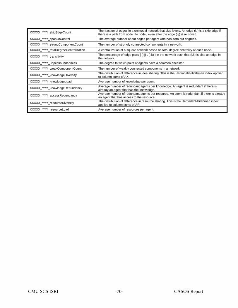
CMU SCS ISRI CASOS Report -70-
XXXXX_YYY_skipEdgeCount The fraction of edges in a unimodal network that skip levels. An edge (i,j) is a skip edge if there is a path from node i to node j even after the edge (i,j) is removed.
XXXXX_YYY_spanOfControl The average number of out edges per agent with non-zero out degrees.
XXXXX_YYY_strongComponentCount The number of strongly connected components in a network.
XXXXX_YYY_totalDegreeCentralization A centralization of a square network based on total degree centrality of each node.
XXXXX_YYY_transitivity The percentage of edge pairs { (i,j) , (j,k) } in the network such that (i,k) is also an edge in the network.
XXXXX_YYY_upperBoundedness The degree to which pairs of agents have a common ancestor.
XXXXX_YYY_weakComponentCount The number of weakly connected components in a network.
XXXXX_YYY_knowledgeDiversity The distribution of difference in idea sharing. This is the Herfindahl-Hirshman index applied to column sums of AK.
XXXXX_YYY_knowledgeLoad Average number of knowledge per agent.
XXXXX_YYY_knowledgeRedundancy Average number of redundant agents per knowledge. An agent is redundant if there is already an agent that has the knowledge.
XXXXX_YYY_accessRedundancy Average number of redundant agents per resource. An agent is redundant if there is already an agent that has access to the resource.
XXXXX_YYY_resourceDiversity The distribution of difference in resource sharing. This is the Herfindahl-Hirshman index applied to column sums of AR
XXXXX_YYY_resourceLoad Average number of resources per agent.
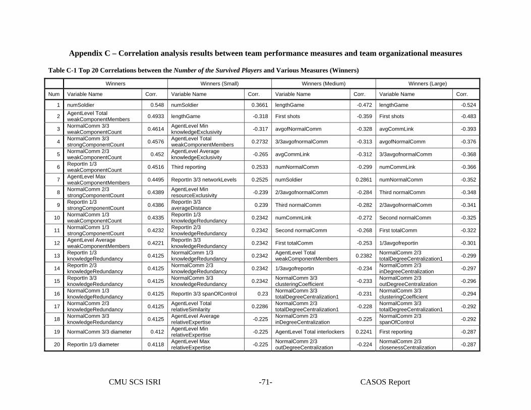
CMU SCS ISRI CASOS Report -71-
Appendix C – Correlation analysis results between team performance measures and team organizational measures
Table C-1 Top 20 Correlations between the Number of the Survived Players and Various Measures (Winners)
Winners Winners (Small) Winners (Medium) Winners (Large)
Num Variable Name Corr. Variable Name Corr. Variable Name Corr. Variable Name Corr.
1 numSoldier 0.548 numSoldier 0.3661 lengthGame -0.472 lengthGame -0.524
2 AgentLevel Total weakComponentMembers 0.4933 lengthGame -0.318 First shots -0.359 First shots -0.483
3 NormalComm 3/3 weakComponentCount 0.4614 AgentLevel Min
knowledgeExclusivity -0.317 avgofNormalComm -0.328 avgCommLink -0.393
4 NormalComm 3/3 strongComponentCount 0.4576 AgentLevel Total
weakComponentMembers 0.2732 3/3avgofnormalComm -0.313 avgofNormalComm -0.376
5 NormalComm 2/3 weakComponentCount 0.452 AgentLevel Average
knowledgeExclusivity -0.265 avgCommLink -0.312 3/3avgofnormalComm -0.368
6 ReportIn 1/3 weakComponentCount 0.4516 Third reporting 0.2533 numNormalComm -0.299 numCommLink -0.366
7 AgentLevel Max weakComponentMembers 0.4495 ReportIn 3/3 networkLevels 0.2525 numSoldier 0.2861 numNormalComm -0.352
8 NormalComm 2/3 strongComponentCount 0.4389 AgentLevel Min
resourceExclusivity -0.239 2/3avgofnormalComm -0.284 Third normalComm -0.348
9 ReportIn 1/3 strongComponentCount 0.4386 ReportIn 3/3
averageDistance 0.239 Third normalComm -0.282 2/3avgofnormalComm -0.341
10 NormalComm 1/3 weakComponentCount 0.4335 ReportIn 1/3
knowledgeRedundancy 0.2342 numCommLink -0.272 Second normalComm -0.325
11 NormalComm 1/3 strongComponentCount 0.4232 ReportIn 2/3
knowledgeRedundancy 0.2342 Second normalComm -0.268 First totalComm -0.322
12 AgentLevel Average weakComponentMembers 0.4221 ReportIn 3/3
knowledgeRedundancy 0.2342 First totalComm -0.253 1/3avgofreportin -0.301
13 ReportIn 1/3 knowledgeRedundancy 0.4125 NormalComm 1/3
knowledgeRedundancy 0.2342 AgentLevel Total weakComponentMembers 0.2382 NormalComm 2/3
totalDegreeCentralization1 -0.299
14 ReportIn 2/3 knowledgeRedundancy 0.4125 NormalComm 2/3
knowledgeRedundancy 0.2342 1/3avgofreportin -0.234 NormalComm 2/3 inDegreeCentralization -0.297
15 ReportIn 3/3 knowledgeRedundancy 0.4125 NormalComm 3/3
knowledgeRedundancy 0.2342 NormalComm 3/3 clusteringCoefficient -0.233 NormalComm 2/3
outDegreeCentralization -0.296
16 NormalComm 1/3 knowledgeRedundancy 0.4125 ReportIn 3/3 spanOfControl 0.23 NormalComm 3/3
totalDegreeCentralization1 -0.231 NormalComm 3/3 clusteringCoefficient -0.294
17 NormalComm 2/3 knowledgeRedundancy 0.4125 AgentLevel Total
relativeSimilarity 0.2286 NormalComm 2/3 totalDegreeCentralization1 -0.228 NormalComm 3/3
totalDegreeCentralization1 -0.292
18 NormalComm 3/3 knowledgeRedundancy 0.4125 AgentLevel Average
relativeExpertise -0.225 NormalComm 2/3 inDegreeCentralization -0.225 NormalComm 2/3
spanOfControl -0.292
19 NormalComm 3/3 diameter 0.412 AgentLevel Min relativeExpertise -0.225 AgentLevel Total interlockers 0.2241 First reporting -0.287
20 ReportIn 1/3 diameter 0.4118 AgentLevel Max relativeExpertise -0.225 NormalComm 2/3
outDegreeCentralization -0.224 NormalComm 2/3 closenessCentralization -0.287
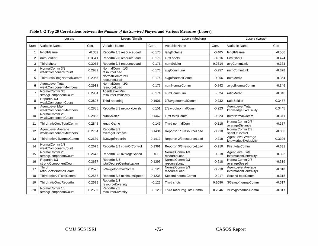
CMU SCS ISRI CASOS Report -72-
Table C-2 Top 20 Correlations between the Number of the Survived Players and Various Measures (Losers)
Losers Losers (Small) Losers (Medium) Losers (Large)
Num Variable Name Corr. Variable Name Corr. Variable Name Corr. Variable Name Corr.
1 lengthGame -0.362 ReportIn 1/3 resourceLoad -0.176 lengthGame -0.405 lengthGame -0.536
2 numSoldier 0.3541 ReportIn 2/3 resourceLoad -0.176 First shots -0.316 First shots -0.474
3 Third shots 0.3055 ReportIn 3/3 resourceLoad -0.176 numSoldier 0.2614 avgCommLink -0.383
4 NormalComm 3/3 weakComponentCount 0.2982 NormalComm 1/3
resourceLoad -0.176 avgCommLink -0.257 numCommLink -0.378
5 Third ratioDmgNormalComm! 0.2955 NormalComm 2/3 resourceLoad -0.176 avgofNormalComm -0.256 numMedic -0.354
6 AgentLevel Total weakComponentMembers 0.2918 NormalComm 3/3
resourceLoad -0.176 numNormalComm -0.243 avgofNormalComm -0.346
7 NormalComm 3/3 strongComponentCount 0.2904 AgentLevel Min
resourceExclusivity -0.174 numCommLink -0.24 ratioMedic -0.346
8 ReportIn 1/3 weakComponentCount 0.2898 Third reporting 0.1601 3/3avgofnormalComm -0.232 ratioSoldier 0.3457
9 AgentLevel Max weakComponentMembers 0.2885 ReportIn 3/3 networkLevels 0.151 2/3avgofnormalComm -0.223 AgentLevel Total
knowledgeExclusivity 0.3445
10 NormalComm 2/3 weakComponentCount 0.2868 numSoldier 0.1462 First totalComm -0.223 numNormalComm -0.341
11 Third ratioDmgTotalComm 0.2848 lengthGame -0.145 Third normalComm -0.218 NormalComm 2/3 averageDistance -0.337
12 AgentLevel Average weakComponentMembers 0.2764 ReportIn 3/3
averageDistance 0.1434 ReportIn 1/3 resourceLoad -0.218 NormalComm 2/3 spanOfControl -0.336
13 Third ratioKillNormalComm 0.2689 3/3avgofreportin 0.1413 ReportIn 2/3 resourceLoad -0.218 AgentLevel Average knowledgeExclusivity 0.3326
14 NormalComm 1/3 weakComponentCount 0.2675 ReportIn 3/3 spanOfControl 0.1391 ReportIn 3/3 resourceLoad -0.218 First totalComm -0.331
15 NormalComm 2/3 strongComponentCount 0.2643 ReportIn 3/3 averageSpeed 0.13 NormalComm 1/3
resourceLoad -0.218 AgentLevel Total informationCentrality -0.322
16 ReportIn 1/3 strongComponentCount 0.2637 ReportIn 3/3
totalDegreeCentralization 0.1293 NormalComm 2/3 resourceLoad -0.218 NormalComm 2/3
averageSpeed -0.319
17 Third ratioShotsNormalComm 0.2576 3/3avgofnormalComm -0.125 NormalComm 3/3
resourceLoad -0.218 AgentLevel Average informationCentrality1 -0.318
18 Third ratioKillTotalComm! 0.2567 ReportIn 3/3 minimumSpeed 0.1235 Second normalComm -0.217 Second totalComm -0.318
19 Third ratioDmgReportIn 0.2528 ReportIn 1/3 resourceDiversity -0.123 Third shots 0.2086 3/3avgofnormalComm -0.317
20 NormalComm 1/3 strongComponentCount 0.2509 ReportIn 2/3
resourceDiversity -0.123 Third ratioDmgTotalComm 0.2046 2/3avgofnormalComm -0.317
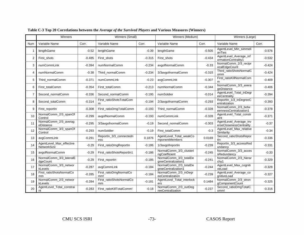
CMU SCS ISRI CASOS Report -73-
Table C-3 Top 20 Correlations between the Average of the Survived Players and Various Measures (Winners)
Winners Winners (Small) Winners (Medium) Winners (Large)
Num Variable Name Corr. Variable Name Corr. Variable Name Corr. Variable Name Corr.
1 lengthGame -0.52 lengthGame -0.39 lengthGame -0.505 AgentLevel_Min_simmelianTies -0.576
2 First_shots -0.485 First_shots -0.315 First_shots -0.434 AgentLevel_Average_informationCentrality1 -0.532
3 numCommLink -0.394 numNormalComm -0.234 avgofNormalComm -0.33 NormalComm_2/3_reciprocalEdgeCount -0.424
4 numNormalComm -0.38 Third_normalComm -0.234 3/3avgofnormalComm -0.315 Third_ratioShotsNormalComm -0.424
5 Third_normalComm -0.371 numCommLink -0.23 avgCommLink -0.307 First_ratioKillNormalComm -0.409
6 First_totalComm -0.354 First_totalComm -0.213 numNormalComm -0.344 NormalComm_3/3_averageDistance -0.406
7 Second_normalComm -0.336 Second_normalComm -0.195 numSoldier -0.014 AgentLevel_Total_inDegreeCentrality -0.394
8 Second_totalComm -0.314 First_ratioShotsTotalComm -0.194 2/3avgofnormalComm -0.293 ReportIn_1/3_inDegreeC
entralization -0.393
9 First_reportIn -0.308 First_ratioDmgTotalComm -0.193 Third_normalComm -0.328 NormalComm_2/3_betweennessCentralization1 -0.378
10 NormalComm_2/3_spanOfControl -0.299 avgofNormalComm -0.193 numCommLink -0.328 AgentLevel_Total_constr
aint -0.371
11 NormalComm_2/3_averageDistance -0.295 3/3avgofnormalComm -0.19 Second_normalComm -0.303 AgentLevel_Average_inv
erseClosenessCentrality -0.37
12 NormalComm_3/3_spanOfControl -0.293 numSoldier -0.19 First_totalComm -0.3 AgentLevel_Max_relative
Similarity -0.34
13 avgCommLink -0.291 ReportIn_3/3_connectedness 0.1876 AgentLevel_Total_weakCo
mponentMembers 0.0169 Second_ratioShotsReportIn -0.336
14 AgentLevel_Max_effectiveNetworkSize -0.29 First_ratioDmgReportIn -0.186 1/3avgofreportin -0.239 ReportIn_3/3_accessRed
undancy -0.331
15 avgofNormalComm -0.29 First_ratioShotsReportIn1 -0.186 NormalComm_3/3_clusteringCoefficient -0.245 NormalComm_3/3_acces
sRedundancy -0.33
16 NormalComm_3/3_lateralEdgeCount -0.29 First_reportIn -0.185 NormalComm_3/3_totalDe
greeCentralization1 -0.241 NormalComm_2/3_hierarchy1 -0.329
17 NormalComm_3/3_networkLevels -0.287 avgCommLink -0.184 NormalComm_2/3_totalDe
greeCentralization1 -0.244 AgentLevel_Max_cognitiveLoad -0.328
18 First_ratioShotsNormalComm -0.285 First_ratioDmgNormalCo
mm! -0.184 NormalComm_2/3_inDegreeCentralization -0.239 AgentLevel_Average_co
gnitiveLoad -0.327
19 NormalComm_2/3_networkLevels -0.284 First_ratioShotsNormalCo
mm -0.181 AgentLevel_Total_interlockers 0.1484 NormalComm_2/3_stron
gComponentCount -0.325
20 AgentLevel_Total_constraint -0.283 First_ratioKillTotalComm! -0.18 NormalComm_2/3_outDeg
reeCentralization -0.237 Second_ratioDmgTotalComm! -0.316
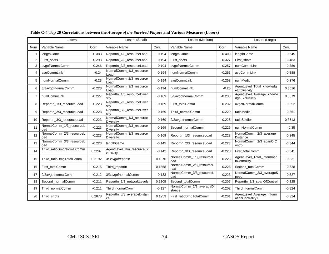
CMU SCS ISRI CASOS Report -74-
Table C-4 Top 20 Correlations between the Average of the Survived Players and Various Measures (Losers)
Losers Losers (Small) Losers (Medium) Losers (Large)
Num Variable Name Corr. Variable Name Corr. Variable Name Corr. Variable Name Corr.
1 lengthGame -0.383 ReportIn_1/3_resourceLoad -0.194 lengthGame -0.409 lengthGame -0.545
2 First_shots -0.298 ReportIn_2/3_resourceLoad -0.194 First_shots -0.327 First_shots -0.483
3 avgofNormalComm -0.246 ReportIn_3/3_resourceLoad -0.194 avgofNormalComm -0.257 numCommLink -0.389
4 avgCommLink -0.24 NormalComm_1/3_resourceLoad -0.194 numNormalComm -0.253 avgCommLink -0.388
5 numNormalComm -0.23 NormalComm_2/3_resourceLoad -0.194 avgCommLink -0.253 numMedic -0.376
6 3/3avgofnormalComm -0.228 NormalComm_3/3_resourceLoad -0.194 numCommLink -0.25 AgentLevel_Total_knowledg
eExclusivity 0.3616
7 numCommLink -0.227 ReportIn_1/3_resourceDiversity -0.169 3/3avgofnormalComm -0.233 AgentLevel_Average_knowle
dgeExclusivity 0.3579
8 ReportIn_1/3_resourceLoad -0.223 ReportIn_2/3_resourceDiversity -0.169 First_totalComm -0.232 avgofNormalComm -0.352
9 ReportIn_2/3_resourceLoad -0.223 ReportIn_3/3_resourceDiversity -0.169 Third_normalComm -0.229 ratioMedic -0.351
10 ReportIn_3/3_resourceLoad -0.223 NormalComm_1/3_resourceDiversity -0.169 2/3avgofnormalComm -0.225 ratioSoldier 0.3513
11 NormalComm_1/3_resourceLoad -0.223 NormalComm_2/3_resource
Diversity -0.169 Second_normalComm -0.225 numNormalComm -0.35
12 NormalComm_2/3_resourceLoad -0.223 NormalComm_3/3_resource
Diversity -0.169 ReportIn_1/3_resourceLoad -0.223 NormalComm_2/3_averageDistance -0.345
13 NormalComm_3/3_resourceLoad -0.223 lengthGame -0.145 ReportIn_2/3_resourceLoad -0.223 NormalComm_2/3_spanOfC
ontrol -0.344
14 Third_ratioDmgNormalComm! 0.2207 AgentLevel_Min_resourceEx
clusivity -0.142 ReportIn_3/3_resourceLoad -0.223 First_totalComm -0.341
15 Third_ratioDmgTotalComm 0.2192 3/3avgofreportin 0.1376 NormalComm_1/3_resourceLoad -0.223 AgentLevel_Total_informatio
nCentrality -0.331
16 First_totalComm -0.215 Third_reportIn 0.1358 NormalComm_2/3_resourceLoad -0.223 Second_totalComm -0.328
17 2/3avgofnormalComm -0.212 3/3avgofnormalComm -0.133 NormalComm_3/3_resourceLoad -0.223 NormalComm_2/3_averageS
peed -0.327
18 Second_normalComm -0.211 ReportIn_3/3_networkLevels 0.1305 Second_totalComm -0.207 ReportIn_1/3_spanOfControl -0.325
19 Third_normalComm -0.211 Third_normalComm -0.127 NormalComm_2/3_averageDistance -0.202 Third_normalComm -0.324
20 Third_shots 0.2078 ReportIn_3/3_averageDistance 0.1253 First_ratioDmgTotalComm -0.201 AgentLevel_Average_inform
ationCentrality1 -0.324
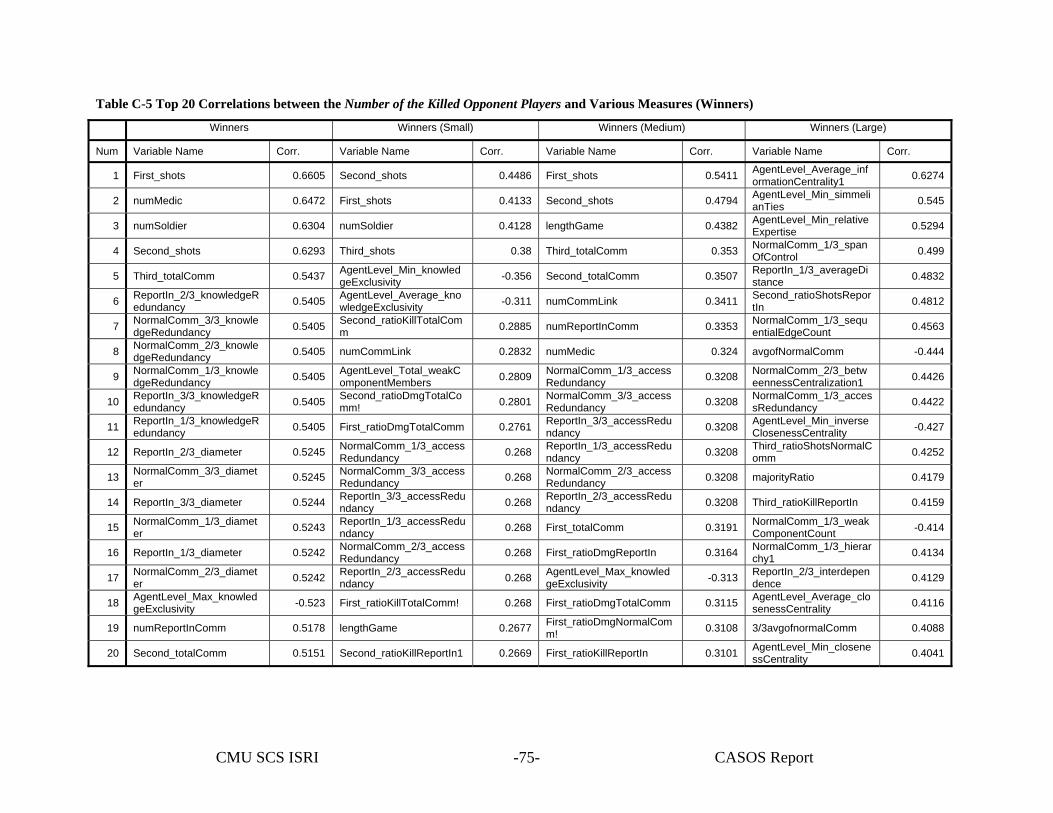
CMU SCS ISRI CASOS Report -75-
Table C-5 Top 20 Correlations between the Number of the Killed Opponent Players and Various Measures (Winners)
Winners Winners (Small) Winners (Medium) Winners (Large)
Num Variable Name Corr. Variable Name Corr. Variable Name Corr. Variable Name Corr.
1 First_shots 0.6605 Second_shots 0.4486 First_shots 0.5411 AgentLevel_Average_informationCentrality1 0.6274
2 numMedic 0.6472 First_shots 0.4133 Second_shots 0.4794 AgentLevel_Min_simmelianTies 0.545
3 numSoldier 0.6304 numSoldier 0.4128 lengthGame 0.4382 AgentLevel_Min_relativeExpertise 0.5294
4 Second_shots 0.6293 Third_shots 0.38 Third_totalComm 0.353 NormalComm_1/3_spanOfControl 0.499
5 Third_totalComm 0.5437 AgentLevel_Min_knowledgeExclusivity -0.356 Second_totalComm 0.3507 ReportIn_1/3_averageDi
stance 0.4832
6 ReportIn_2/3_knowledgeRedundancy 0.5405 AgentLevel_Average_kno
wledgeExclusivity -0.311 numCommLink 0.3411 Second_ratioShotsReportIn 0.4812
7 NormalComm_3/3_knowledgeRedundancy 0.5405 Second_ratioKillTotalCom
m 0.2885 numReportInComm 0.3353 NormalComm_1/3_sequentialEdgeCount 0.4563
8 NormalComm_2/3_knowledgeRedundancy 0.5405 numCommLink 0.2832 numMedic 0.324 avgofNormalComm -0.444
9 NormalComm_1/3_knowledgeRedundancy 0.5405 AgentLevel_Total_weakC
omponentMembers 0.2809 NormalComm_1/3_accessRedundancy 0.3208 NormalComm_2/3_betw
eennessCentralization1 0.4426
10 ReportIn_3/3_knowledgeRedundancy 0.5405 Second_ratioDmgTotalCo
mm! 0.2801 NormalComm_3/3_accessRedundancy 0.3208 NormalComm_1/3_acces
sRedundancy 0.4422
11 ReportIn_1/3_knowledgeRedundancy 0.5405 First_ratioDmgTotalComm 0.2761 ReportIn_3/3_accessRedu
ndancy 0.3208 AgentLevel_Min_inverseClosenessCentrality -0.427
12 ReportIn_2/3_diameter 0.5245 NormalComm_1/3_accessRedundancy 0.268 ReportIn_1/3_accessRedu
ndancy 0.3208 Third_ratioShotsNormalComm 0.4252
13 NormalComm_3/3_diameter 0.5245 NormalComm_3/3_access
Redundancy 0.268 NormalComm_2/3_accessRedundancy 0.3208 majorityRatio 0.4179
14 ReportIn_3/3_diameter 0.5244 ReportIn_3/3_accessRedundancy 0.268 ReportIn_2/3_accessRedu
ndancy 0.3208 Third_ratioKillReportIn 0.4159
15 NormalComm_1/3_diameter 0.5243 ReportIn_1/3_accessRedu
ndancy 0.268 First_totalComm 0.3191 NormalComm_1/3_weakComponentCount -0.414
16 ReportIn_1/3_diameter 0.5242 NormalComm_2/3_accessRedundancy 0.268 First_ratioDmgReportIn 0.3164 NormalComm_1/3_hierar
chy1 0.4134
17 NormalComm_2/3_diameter 0.5242 ReportIn_2/3_accessRedu
ndancy 0.268 AgentLevel_Max_knowledgeExclusivity -0.313 ReportIn_2/3_interdepen
dence 0.4129
18 AgentLevel_Max_knowledgeExclusivity -0.523 First_ratioKillTotalComm! 0.268 First_ratioDmgTotalComm 0.3115 AgentLevel_Average_clo
senessCentrality 0.4116
19 numReportInComm 0.5178 lengthGame 0.2677 First_ratioDmgNormalComm! 0.3108 3/3avgofnormalComm 0.4088
20 Second_totalComm 0.5151 Second_ratioKillReportIn1 0.2669 First_ratioKillReportIn 0.3101 AgentLevel_Min_closenessCentrality 0.4041
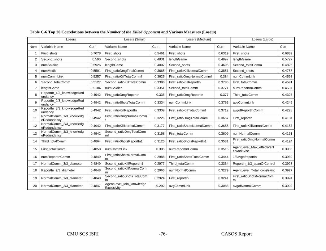
CMU SCS ISRI CASOS Report -76-
Table C-6 Top 20 Correlations between the Number of the Killed Opponent and Various Measures (Losers)
Losers Losers (Small) Losers (Medium) Losers (Large)
Num Variable Name Corr. Variable Name Corr. Variable Name Corr. Variable Name Corr.
1 First_shots 0.7078 First_shots 0.5461 First_shots 0.6319 First_shots 0.6889
2 Second_shots 0.596 Second_shots 0.4831 lengthGame 0.4997 lengthGame 0.5727
3 numSoldier 0.5926 lengthGame 0.4007 Second_shots 0.4695 Second_totalComm 0.4825
4 numMedic 0.5501 First_ratioDmgTotalComm 0.3665 First_ratioKillNormalComm 0.3851 Second_shots 0.4758
5 numCommLink 0.5257 First_ratioKillTotalComm! 0.3625 First_ratioDmgNormalComm! 0.384 numCommLink 0.4593
6 Second_totalComm 0.5127 Second_ratioKillTotalComm 0.3396 First_ratioKillReportIn 0.3785 First_totalComm 0.4591
7 lengthGame 0.5104 numSoldier 0.3351 Second_totalComm 0.3771 numReportInComm 0.4537
8 ReportIn_1/3_knowledgeRedundancy 0.4942 First_ratioDmgReportIn 0.335 First_ratioDmgReportIn 0.377 Third_totalComm 0.4327
9 ReportIn_2/3_knowledgeRedundancy 0.4942 First_ratioShotsTotalComm 0.3334 numCommLink 0.3763 avgCommLink 0.4246
10 ReportIn_3/3_knowledgeRedundancy 0.4942 First_ratioKillReportIn 0.3309 First_ratioKillTotalComm! 0.3712 avgofReportInComm 0.4228
11 NormalComm_1/3_knowledgeRedundancy 0.4942 First_ratioDmgNormalComm
! 0.3226 First_ratioDmgTotalComm 0.3657 First_reportIn 0.4184
12 NormalComm_2/3_knowledgeRedundancy 0.4942 First_ratioKillNormalComm 0.3177 First_ratioShotsNormalComm 0.3655 First_ratioKillNormalComm 0.4157
13 NormalComm_3/3_knowledgeRedundancy 0.4942 Second_ratioDmgTotalCom
m! 0.3158 First_totalComm 0.3609 numNormalComm 0.4151
14 Third_totalComm 0.4864 First_ratioShotsReportIn1 0.3125 First_ratioShotsReportIn1 0.3581 First_ratioDmgNormalComm! 0.4124
15 First_totalComm 0.4858 numCommLink 0.305 numReportInComm 0.3515 AgentLevel_Max_effectiveNetworkSize 0.3986
16 numReportInComm 0.4849 First_ratioShotsNormalComm 0.2988 First_ratioShotsTotalComm 0.3444 1/3avgofreportin 0.3939
17 NormalComm_3/3_diameter 0.4849 Second_ratioKillReportIn1 0.2977 Third_totalComm 0.3334 ReportIn_1/3_spanOfControl 0.3928
18 ReportIn_2/3_diameter 0.4848 Second_ratioKillNormalComm 0.2965 numNormalComm 0.3279 AgentLevel_Total_constraint 0.3927
19 NormalComm_1/3_diameter 0.4848 Second_ratioShotsTotalComm 0.2924 First_reportIn 0.3241 First_ratioShotsNormalCom
m 0.3924
20 NormalComm_2/3_diameter 0.4847 AgentLevel_Min_knowledgeExclusivity -0.292 avgCommLink 0.3088 avgofNormalComm 0.3902
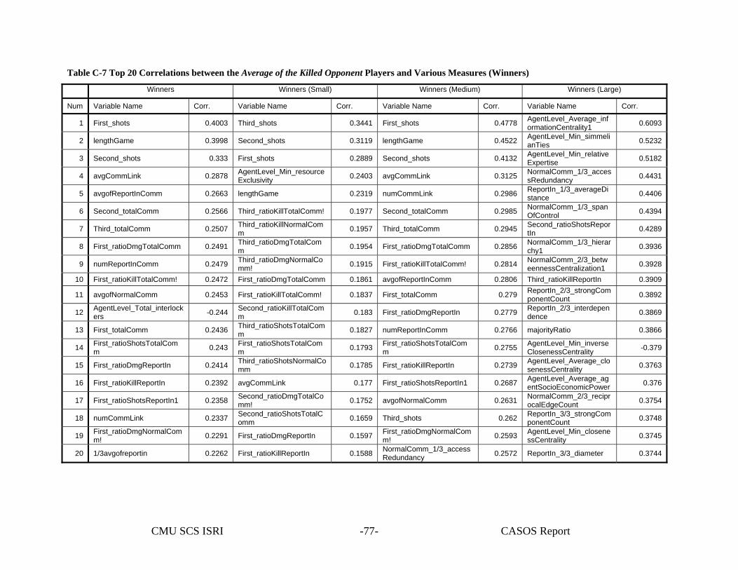
CMU SCS ISRI CASOS Report -77-
Table C-7 Top 20 Correlations between the Average of the Killed Opponent Players and Various Measures (Winners)
Winners Winners (Small) Winners (Medium) Winners (Large)
Num Variable Name Corr. Variable Name Corr. Variable Name Corr. Variable Name Corr.
1 First_shots 0.4003 Third_shots 0.3441 First_shots 0.4778 AgentLevel_Average_informationCentrality1 0.6093
2 lengthGame 0.3998 Second_shots 0.3119 lengthGame 0.4522 AgentLevel_Min_simmelianTies 0.5232
3 Second_shots 0.333 First_shots 0.2889 Second_shots 0.4132 AgentLevel_Min_relativeExpertise 0.5182
4 avgCommLink 0.2878 AgentLevel_Min_resourceExclusivity 0.2403 avgCommLink 0.3125 NormalComm_1/3_acces
sRedundancy 0.4431
5 avgofReportInComm 0.2663 lengthGame 0.2319 numCommLink 0.2986 ReportIn_1/3_averageDistance 0.4406
6 Second_totalComm 0.2566 Third_ratioKillTotalComm! 0.1977 Second_totalComm 0.2985 NormalComm_1/3_spanOfControl 0.4394
7 Third_totalComm 0.2507 Third_ratioKillNormalComm 0.1957 Third_totalComm 0.2945 Second_ratioShotsRepor
tIn 0.4289
8 First_ratioDmgTotalComm 0.2491 Third_ratioDmgTotalComm 0.1954 First_ratioDmgTotalComm 0.2856 NormalComm_1/3_hierar
chy1 0.3936
9 numReportInComm 0.2479 Third_ratioDmgNormalComm! 0.1915 First_ratioKillTotalComm! 0.2814 NormalComm_2/3_betw
eennessCentralization1 0.3928
10 First_ratioKillTotalComm! 0.2472 First_ratioDmgTotalComm 0.1861 avgofReportInComm 0.2806 Third_ratioKillReportIn 0.3909
11 avgofNormalComm 0.2453 First_ratioKillTotalComm! 0.1837 First_totalComm 0.279 ReportIn_2/3_strongComponentCount 0.3892
12 AgentLevel_Total_interlockers -0.244 Second_ratioKillTotalCom
m 0.183 First_ratioDmgReportIn 0.2779 ReportIn_2/3_interdependence 0.3869
13 First_totalComm 0.2436 Third_ratioShotsTotalComm 0.1827 numReportInComm 0.2766 majorityRatio 0.3866
14 First_ratioShotsTotalComm 0.243 First_ratioShotsTotalCom
m 0.1793 First_ratioShotsTotalComm 0.2755 AgentLevel_Min_inverse
ClosenessCentrality -0.379
15 First_ratioDmgReportIn 0.2414 Third_ratioShotsNormalComm 0.1785 First_ratioKillReportIn 0.2739 AgentLevel_Average_clo
senessCentrality 0.3763
16 First_ratioKillReportIn 0.2392 avgCommLink 0.177 First_ratioShotsReportIn1 0.2687 AgentLevel_Average_agentSocioEconomicPower 0.376
17 First_ratioShotsReportIn1 0.2358 Second_ratioDmgTotalComm! 0.1752 avgofNormalComm 0.2631 NormalComm_2/3_recipr
ocalEdgeCount 0.3754
18 numCommLink 0.2337 Second_ratioShotsTotalComm 0.1659 Third_shots 0.262 ReportIn_3/3_strongCom
ponentCount 0.3748
19 First_ratioDmgNormalComm! 0.2291 First_ratioDmgReportIn 0.1597 First_ratioDmgNormalCom
m! 0.2593 AgentLevel_Min_closenessCentrality 0.3745
20 1/3avgofreportin 0.2262 First_ratioKillReportIn 0.1588 NormalComm_1/3_accessRedundancy 0.2572 ReportIn_3/3_diameter 0.3744
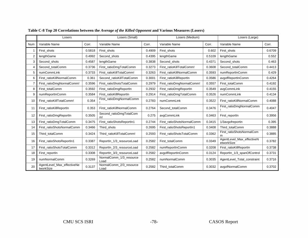
CMU SCS ISRI CASOS Report -78-
Table C-8 Top 20 Correlations between the Average of the Killed Opponent and Various Measures (Losers)
Losers Losers (Small) Losers (Medium) Losers (Large)
Num Variable Name Corr. Variable Name Corr. Variable Name Corr. Variable Name Corr.
1 First_shots 0.5818 First_shots 0.4909 First_shots 0.602 First_shots 0.6709
2 lengthGame 0.4992 Second_shots 0.4395 lengthGame 0.5109 lengthGame 0.552
3 Second_shots 0.4587 lengthGame 0.3838 Second_shots 0.4371 Second_shots 0.463
4 Second_totalComm 0.3736 First_ratioDmgTotalComm 0.3273 First_ratioKillTotalComm! 0.3608 Second_totalComm 0.4413
5 numCommLink 0.3733 First_ratioKillTotalComm! 0.3263 First_ratioKillNormalComm 0.3593 numReportInComm 0.429
6 First_ratioKillNormalComm 0.361 Second_ratioKillTotalComm 0.3001 First_ratioKillReportIn 0.3586 avgofReportInComm 0.4264
7 First_ratioDmgNormalComm! 0.3596 First_ratioShotsTotalComm 0.2979 First_ratioDmgNormalComm! 0.3557 First_totalComm 0.4192
8 First_totalComm 0.3592 First_ratioDmgReportIn 0.2932 First_ratioDmgReportIn 0.3549 avgCommLink 0.4155
9 numReportInComm 0.3584 First_ratioKillReportIn 0.2914 First_ratioDmgTotalComm 0.3526 numCommLink 0.4134
10 First_ratioKillTotalComm! 0.354 First_ratioDmgNormalComm! 0.2783 numCommLink 0.3522 First_ratioKillNormalComm 0.4088
11 First_ratioKillReportIn 0.353 First_ratioKillNormalComm 0.2764 Second_totalComm 0.3476 First_ratioDmgNormalComm! 0.4047
12 First_ratioDmgReportIn 0.3505 Second_ratioDmgTotalComm! 0.275 avgCommLink 0.3463 First_reportIn 0.3956
13 First_ratioDmgTotalComm 0.3475 First_ratioShotsReportIn1 0.2744 First_ratioShotsNormalComm 0.3415 1/3avgofreportin 0.395
14 First_ratioShotsNormalComm 0.3466 Third_shots 0.2695 First_ratioShotsReportIn1 0.3408 Third_totalComm 0.3888
15 Third_totalComm 0.3424 Third_ratioKillTotalComm! 0.2593 First_ratioShotsTotalComm 0.3362 First_ratioShotsNormalComm 0.3885
16 First_ratioShotsReportIn1 0.3387 ReportIn_1/3_resourceLoad 0.2582 First_totalComm 0.3349 AgentLevel_Max_effectiveNetworkSize 0.3782
17 First_ratioShotsTotalComm 0.3312 ReportIn_2/3_resourceLoad 0.2582 numReportInComm 0.3208 First_ratioKillReportIn 0.3738
18 First_reportIn 0.3308 ReportIn_3/3_resourceLoad 0.2582 avgofReportInComm 0.3124 ReportIn_1/3_spanOfControl 0.3731
19 numNormalComm 0.3269 NormalComm_1/3_resourceLoad 0.2582 numNormalComm 0.3035 AgentLevel_Total_constraint 0.3716
20 AgentLevel_Max_effectiveNetworkSize 0.3137 NormalComm_2/3_resource
Load 0.2582 Third_totalComm 0.3032 avgofNormalComm 0.3702
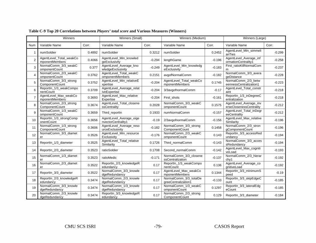
CMU SCS ISRI CASOS Report -79-
Table C-9 Top 20 Correlations between Players’ total score and Various Measures (Winners)
Winners Winners (Small) Winners (Medium) Winners (Large)
Num Variable Name Corr. Variable Name Corr. Variable Name Corr. Variable Name Corr.
1 numSoldier 0.4892 numSoldier 0.3212 numSoldier 0.2452 AgentLevel_Min_simmelianTies -0.299
2 AgentLevel_Total_weakComponentMembers 0.4066 AgentLevel_Min_knowled
geExclusivity -0.294 lengthGame -0.196 AgentLevel_Average_informationCentrality1 -0.258
3 NormalComm_3/3_weakComponentCount 0.377 AgentLevel_Average_kno
wledgeExclusivity -0.249 AgentLevel_Min_knowledgeExclusivity -0.183 First_ratioKillNormalCom
m -0.237
4 NormalComm_2/3_weakComponentCount 0.3762 AgentLevel_Total_weakC
omponentMembers 0.2151 avgofNormalComm -0.182 NormalComm_3/3_averageDistance -0.228
5 NormalComm_3/3_strongComponentCount 0.3752 AgentLevel_Min_relativeE
xpertise -0.204 AgentLevel_Total_weakComponentMembers 0.1745 NormalComm_2/3_betw
eennessCentralization1 -0.223
6 ReportIn_1/3_weakComponentCount 0.3709 AgentLevel_Average_relat
iveExpertise -0.204 3/3avgofnormalComm -0.17 AgentLevel_Total_constraint -0.218
7 AgentLevel_Max_weakComponentMembers 0.3693 AgentLevel_Max_relative
Expertise -0.204 First_shots -0.161 ReportIn_1/3_inDegreeCentralization -0.218
8 NormalComm_2/3_strongComponentCount 0.3674 AgentLevel_Total_closene
ssCentrality 0.2028 NormalComm_3/3_weakComponentCount 0.1575 AgentLevel_Average_inv
erseClosenessCentrality -0.212
9 NormalComm_1/3_weakComponentCount 0.3659 Third_reportIn 0.1933 numNormalComm -0.157 AgentLevel_Total_inDegr
eeCentrality -0.212
10 ReportIn_1/3_strongComponentCount 0.3656 AgentLevel_Average_eige
nvectorCentrality1 -0.19 2/3avgofnormalComm -0.156 AgentLevel_Max_relativeSimilarity -0.196
11 NormalComm_1/3_strongComponentCount 0.3606 AgentLevel_Average_reso
urceExclusivity -0.182 NormalComm_3/3_strongComponentCount 0.1458 NormalComm_2/3_stron
gComponentCount -0.196
12 NormalComm_3/3_diameter 0.3526 AgentLevel_Min_resource
Exclusivity -0.176 NormalComm_2/3_weakComponentCount 0.143 ReportIn_3/3_accessRed
undancy -0.194
13 ReportIn_1/3_diameter 0.3525 AgentLevel_Total_relativeSimilarity 0.1726 Third_normalComm -0.143 NormalComm_3/3_acces
sRedundancy -0.194
14 ReportIn_2/3_diameter 0.3523 ratioSoldier 0.1708 Second_normalComm -0.142 AgentLevel_Max_cognitiveLoad -0.193
15 NormalComm_1/3_diameter 0.3523 ratioMedic -0.171 NormalComm_3/3_closene
ssCentralization -0.137 NormalComm_2/3_hierarchy1 -0.192
16 NormalComm_2/3_diameter 0.3522 ReportIn_2/3_knowledgeR
edundancy 0.17 ReportIn_1/3_weakComponentCount 0.136 AgentLevel_Average_co
gnitiveLoad -0.192
17 ReportIn_3/3_diameter 0.3522 NormalComm_3/3_knowledgeRedundancy 0.17 AgentLevel_Max_weakCo
mponentMembers 0.1344 ReportIn_3/3_minimumSpeed -0.19
18 ReportIn_2/3_knowledgeRedundancy 0.3474 NormalComm_2/3_knowle
dgeRedundancy 0.17 NormalComm_3/3_totalDegreeCentralization1 -0.133 ReportIn_3/3_skipEdgeC
ount -0.185
19 NormalComm_3/3_knowledgeRedundancy 0.3474 NormalComm_1/3_knowle
dgeRedundancy 0.17 NormalComm_1/3_weakComponentCount 0.1297 ReportIn_3/3_lateralEdg
eCount -0.185
20 NormalComm_2/3_knowledgeRedundancy 0.3474 ReportIn_3/3_knowledgeR
edundancy 0.17 NormalComm_2/3_strongComponentCount 0.129 ReportIn_3/3_diameter -0.184
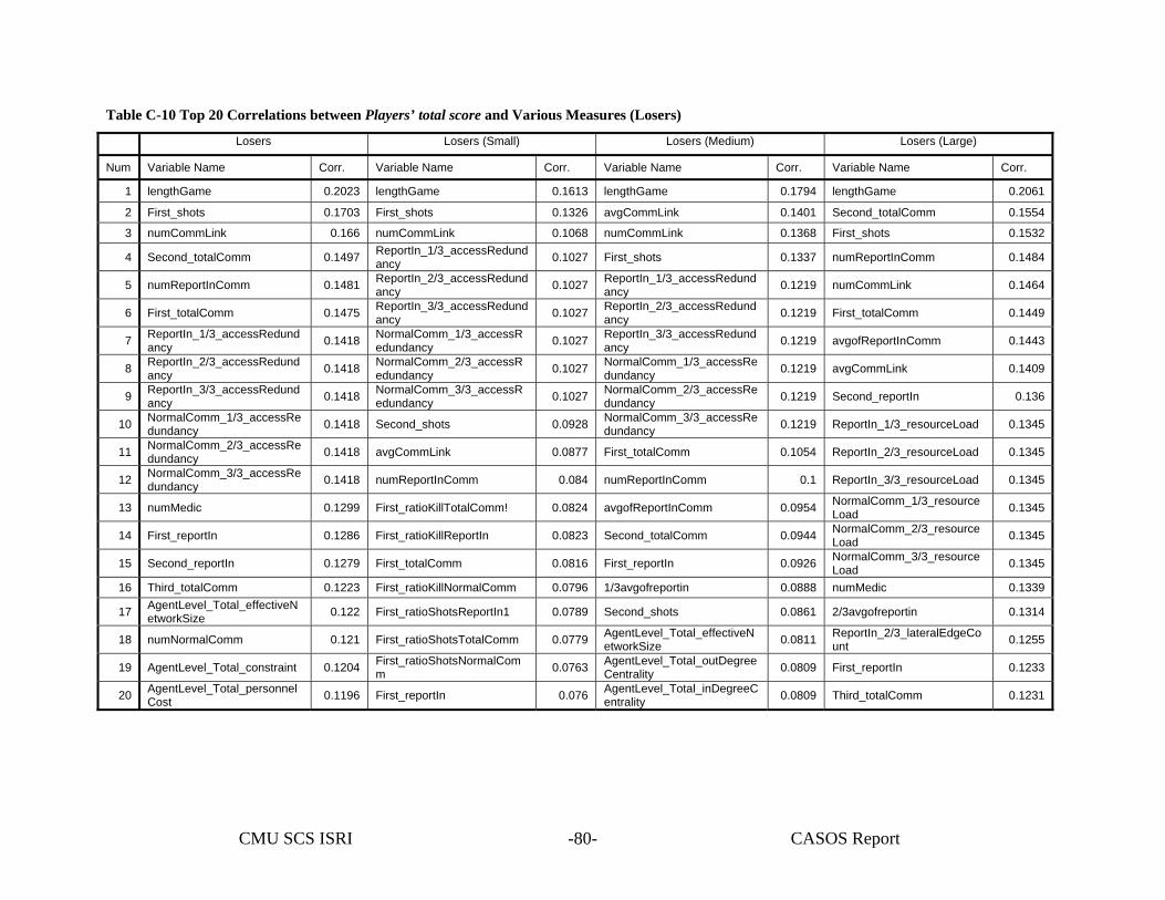
CMU SCS ISRI CASOS Report -80-
Table C-10 Top 20 Correlations between Players’ total score and Various Measures (Losers)
Losers Losers (Small) Losers (Medium) Losers (Large)
Num Variable Name Corr. Variable Name Corr. Variable Name Corr. Variable Name Corr.
1 lengthGame 0.2023 lengthGame 0.1613 lengthGame 0.1794 lengthGame 0.2061
2 First_shots 0.1703 First_shots 0.1326 avgCommLink 0.1401 Second_totalComm 0.1554
3 numCommLink 0.166 numCommLink 0.1068 numCommLink 0.1368 First_shots 0.1532
4 Second_totalComm 0.1497 ReportIn_1/3_accessRedundancy 0.1027 First_shots 0.1337 numReportInComm 0.1484
5 numReportInComm 0.1481 ReportIn_2/3_accessRedundancy 0.1027 ReportIn_1/3_accessRedund
ancy 0.1219 numCommLink 0.1464
6 First_totalComm 0.1475 ReportIn_3/3_accessRedundancy 0.1027 ReportIn_2/3_accessRedund
ancy 0.1219 First_totalComm 0.1449
7 ReportIn_1/3_accessRedundancy 0.1418 NormalComm_1/3_accessR
edundancy 0.1027 ReportIn_3/3_accessRedundancy 0.1219 avgofReportInComm 0.1443
8 ReportIn_2/3_accessRedundancy 0.1418 NormalComm_2/3_accessR
edundancy 0.1027 NormalComm_1/3_accessRedundancy 0.1219 avgCommLink 0.1409
9 ReportIn_3/3_accessRedundancy 0.1418 NormalComm_3/3_accessR
edundancy 0.1027 NormalComm_2/3_accessRedundancy 0.1219 Second_reportIn 0.136
10 NormalComm_1/3_accessRedundancy 0.1418 Second_shots 0.0928 NormalComm_3/3_accessRe
dundancy 0.1219 ReportIn_1/3_resourceLoad 0.1345
11 NormalComm_2/3_accessRedundancy 0.1418 avgCommLink 0.0877 First_totalComm 0.1054 ReportIn_2/3_resourceLoad 0.1345
12 NormalComm_3/3_accessRedundancy 0.1418 numReportInComm 0.084 numReportInComm 0.1 ReportIn_3/3_resourceLoad 0.1345
13 numMedic 0.1299 First_ratioKillTotalComm! 0.0824 avgofReportInComm 0.0954 NormalComm_1/3_resourceLoad 0.1345
14 First_reportIn 0.1286 First_ratioKillReportIn 0.0823 Second_totalComm 0.0944 NormalComm_2/3_resourceLoad 0.1345
15 Second_reportIn 0.1279 First_totalComm 0.0816 First_reportIn 0.0926 NormalComm_3/3_resourceLoad 0.1345
16 Third_totalComm 0.1223 First_ratioKillNormalComm 0.0796 1/3avgofreportin 0.0888 numMedic 0.1339
17 AgentLevel_Total_effectiveNetworkSize 0.122 First_ratioShotsReportIn1 0.0789 Second_shots 0.0861 2/3avgofreportin 0.1314
18 numNormalComm 0.121 First_ratioShotsTotalComm 0.0779 AgentLevel_Total_effectiveNetworkSize 0.0811 ReportIn_2/3_lateralEdgeCo
unt 0.1255
19 AgentLevel_Total_constraint 0.1204 First_ratioShotsNormalComm 0.0763 AgentLevel_Total_outDegree
Centrality 0.0809 First_reportIn 0.1233
20 AgentLevel_Total_personnelCost 0.1196 First_reportIn 0.076 AgentLevel_Total_inDegreeC
entrality 0.0809 Third_totalComm 0.1231
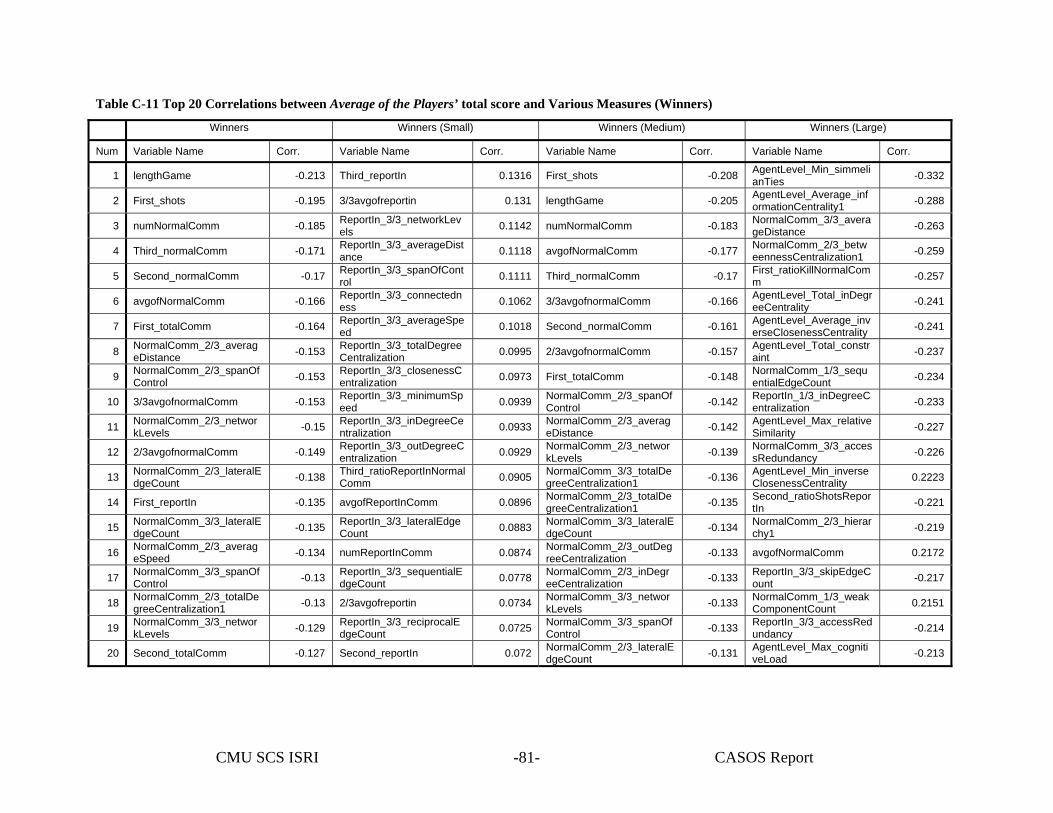
CMU SCS ISRI CASOS Report -81-
Table C-11 Top 20 Correlations between Average of the Players’ total score and Various Measures (Winners)
Winners Winners (Small) Winners (Medium) Winners (Large)
Num Variable Name Corr. Variable Name Corr. Variable Name Corr. Variable Name Corr.
1 lengthGame -0.213 Third_reportIn 0.1316 First_shots -0.208 AgentLevel_Min_simmelianTies -0.332
2 First_shots -0.195 3/3avgofreportin 0.131 lengthGame -0.205 AgentLevel_Average_informationCentrality1 -0.288
3 numNormalComm -0.185 ReportIn_3/3_networkLevels 0.1142 numNormalComm -0.183 NormalComm_3/3_avera
geDistance -0.263
4 Third_normalComm -0.171 ReportIn_3/3_averageDistance 0.1118 avgofNormalComm -0.177 NormalComm_2/3_betw
eennessCentralization1 -0.259
5 Second_normalComm -0.17 ReportIn_3/3_spanOfControl 0.1111 Third_normalComm -0.17 First_ratioKillNormalCom
m -0.257
6 avgofNormalComm -0.166 ReportIn_3/3_connectedness 0.1062 3/3avgofnormalComm -0.166 AgentLevel_Total_inDegr
eeCentrality -0.241
7 First_totalComm -0.164 ReportIn_3/3_averageSpeed 0.1018 Second_normalComm -0.161 AgentLevel_Average_inv
erseClosenessCentrality -0.241
8 NormalComm_2/3_averageDistance -0.153 ReportIn_3/3_totalDegree
Centralization 0.0995 2/3avgofnormalComm -0.157 AgentLevel_Total_constraint -0.237
9 NormalComm_2/3_spanOfControl -0.153 ReportIn_3/3_closenessC
entralization 0.0973 First_totalComm -0.148 NormalComm_1/3_sequentialEdgeCount -0.234
10 3/3avgofnormalComm -0.153 ReportIn_3/3_minimumSpeed 0.0939 NormalComm_2/3_spanOf
Control -0.142 ReportIn_1/3_inDegreeCentralization -0.233
11 NormalComm_2/3_networkLevels -0.15 ReportIn_3/3_inDegreeCe
ntralization 0.0933 NormalComm_2/3_averageDistance -0.142 AgentLevel_Max_relative
Similarity -0.227
12 2/3avgofnormalComm -0.149 ReportIn_3/3_outDegreeCentralization 0.0929 NormalComm_2/3_networ
kLevels -0.139 NormalComm_3/3_accessRedundancy -0.226
13 NormalComm_2/3_lateralEdgeCount -0.138 Third_ratioReportInNormal
Comm 0.0905 NormalComm_3/3_totalDegreeCentralization1 -0.136 AgentLevel_Min_inverse
ClosenessCentrality 0.2223
14 First_reportIn -0.135 avgofReportInComm 0.0896 NormalComm_2/3_totalDegreeCentralization1 -0.135 Second_ratioShotsRepor
tIn -0.221
15 NormalComm_3/3_lateralEdgeCount -0.135 ReportIn_3/3_lateralEdge
Count 0.0883 NormalComm_3/3_lateralEdgeCount -0.134 NormalComm_2/3_hierar
chy1 -0.219
16 NormalComm_2/3_averageSpeed -0.134 numReportInComm 0.0874 NormalComm_2/3_outDeg
reeCentralization -0.133 avgofNormalComm 0.2172
17 NormalComm_3/3_spanOfControl -0.13 ReportIn_3/3_sequentialE
dgeCount 0.0778 NormalComm_2/3_inDegreeCentralization -0.133 ReportIn_3/3_skipEdgeC
ount -0.217
18 NormalComm_2/3_totalDegreeCentralization1 -0.13 2/3avgofreportin 0.0734 NormalComm_3/3_networ
kLevels -0.133 NormalComm_1/3_weakComponentCount 0.2151
19 NormalComm_3/3_networkLevels -0.129 ReportIn_3/3_reciprocalE
dgeCount 0.0725 NormalComm_3/3_spanOfControl -0.133 ReportIn_3/3_accessRed
undancy -0.214
20 Second_totalComm -0.127 Second_reportIn 0.072 NormalComm_2/3_lateralEdgeCount -0.131 AgentLevel_Max_cogniti
veLoad -0.213
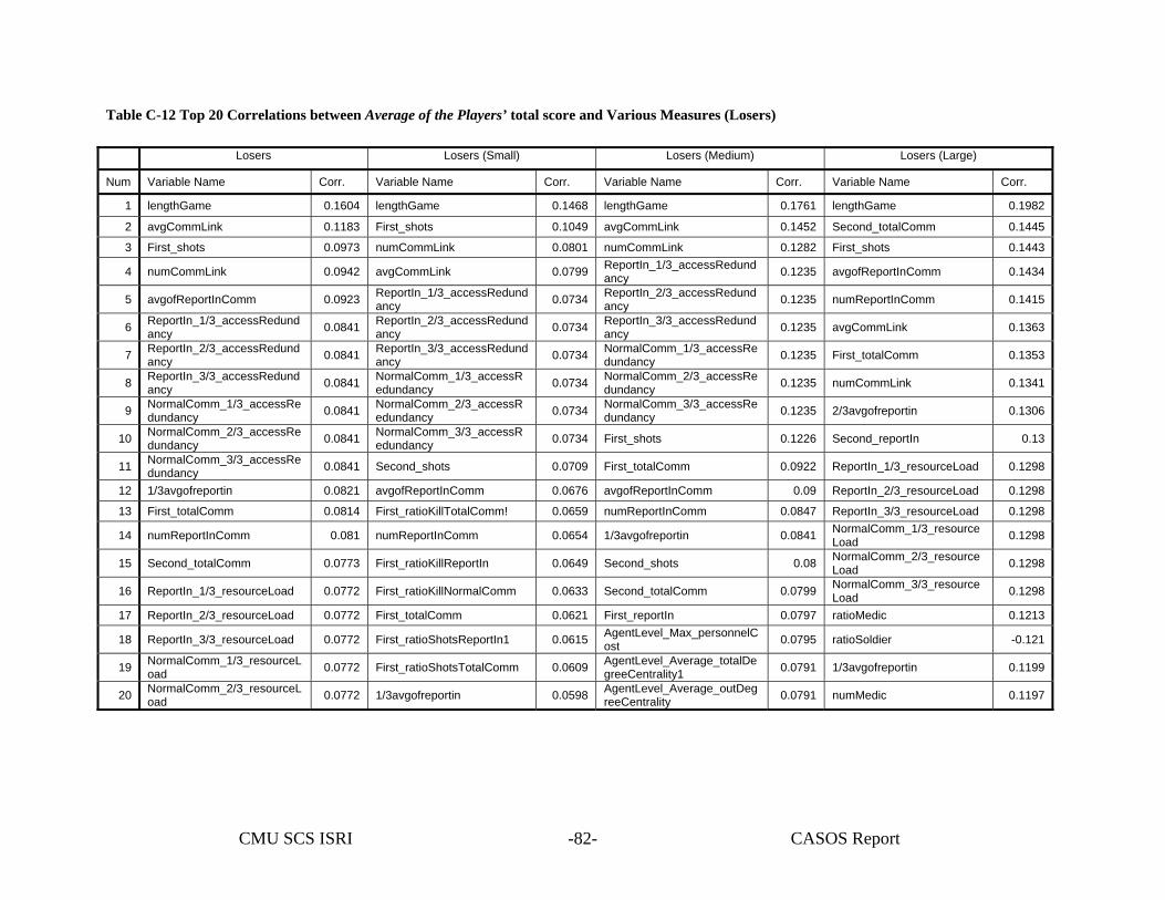
CMU SCS ISRI CASOS Report -82-
Table C-12 Top 20 Correlations between Average of the Players’ total score and Various Measures (Losers)
Losers Losers (Small) Losers (Medium) Losers (Large)
Num Variable Name Corr. Variable Name Corr. Variable Name Corr. Variable Name Corr.
1 lengthGame 0.1604 lengthGame 0.1468 lengthGame 0.1761 lengthGame 0.1982
2 avgCommLink 0.1183 First_shots 0.1049 avgCommLink 0.1452 Second_totalComm 0.1445
3 First_shots 0.0973 numCommLink 0.0801 numCommLink 0.1282 First_shots 0.1443
4 numCommLink 0.0942 avgCommLink 0.0799 ReportIn_1/3_accessRedundancy 0.1235 avgofReportInComm 0.1434
5 avgofReportInComm 0.0923 ReportIn_1/3_accessRedundancy 0.0734 ReportIn_2/3_accessRedund
ancy 0.1235 numReportInComm 0.1415
6 ReportIn_1/3_accessRedundancy 0.0841 ReportIn_2/3_accessRedund
ancy 0.0734 ReportIn_3/3_accessRedundancy 0.1235 avgCommLink 0.1363
7 ReportIn_2/3_accessRedundancy 0.0841 ReportIn_3/3_accessRedund
ancy 0.0734 NormalComm_1/3_accessRedundancy 0.1235 First_totalComm 0.1353
8 ReportIn_3/3_accessRedundancy 0.0841 NormalComm_1/3_accessR
edundancy 0.0734 NormalComm_2/3_accessRedundancy 0.1235 numCommLink 0.1341
9 NormalComm_1/3_accessRedundancy 0.0841 NormalComm_2/3_accessR
edundancy 0.0734 NormalComm_3/3_accessRedundancy 0.1235 2/3avgofreportin 0.1306
10 NormalComm_2/3_accessRedundancy 0.0841 NormalComm_3/3_accessR
edundancy 0.0734 First_shots 0.1226 Second_reportIn 0.13
11 NormalComm_3/3_accessRedundancy 0.0841 Second_shots 0.0709 First_totalComm 0.0922 ReportIn_1/3_resourceLoad 0.1298
12 1/3avgofreportin 0.0821 avgofReportInComm 0.0676 avgofReportInComm 0.09 ReportIn_2/3_resourceLoad 0.1298
13 First_totalComm 0.0814 First_ratioKillTotalComm! 0.0659 numReportInComm 0.0847 ReportIn_3/3_resourceLoad 0.1298
14 numReportInComm 0.081 numReportInComm 0.0654 1/3avgofreportin 0.0841 NormalComm_1/3_resourceLoad 0.1298
15 Second_totalComm 0.0773 First_ratioKillReportIn 0.0649 Second_shots 0.08 NormalComm_2/3_resourceLoad 0.1298
16 ReportIn_1/3_resourceLoad 0.0772 First_ratioKillNormalComm 0.0633 Second_totalComm 0.0799 NormalComm_3/3_resourceLoad 0.1298
17 ReportIn_2/3_resourceLoad 0.0772 First_totalComm 0.0621 First_reportIn 0.0797 ratioMedic 0.1213
18 ReportIn_3/3_resourceLoad 0.0772 First_ratioShotsReportIn1 0.0615 AgentLevel_Max_personnelCost 0.0795 ratioSoldier -0.121
19 NormalComm_1/3_resourceLoad 0.0772 First_ratioShotsTotalComm 0.0609 AgentLevel_Average_totalDe
greeCentrality1 0.0791 1/3avgofreportin 0.1199
20 NormalComm_2/3_resourceLoad 0.0772 1/3avgofreportin 0.0598 AgentLevel_Average_outDeg
reeCentrality 0.0791 numMedic 0.1197
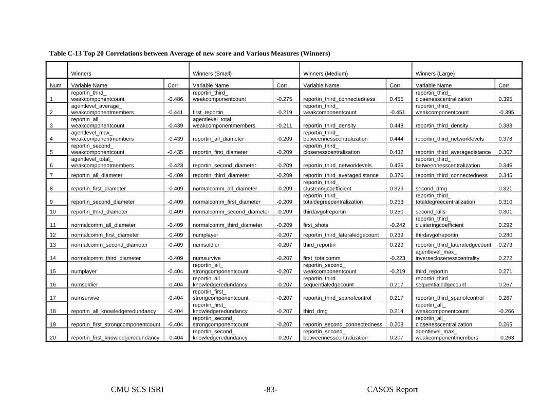
CMU SCS ISRI CASOS Report -83-
Table C-13 Top 20 Correlations between Average of new score and Various Measures (Winners)
Winners Winners (Small) Winners (Medium) Winners (Large)
Num Variable Name Corr. Variable Name Corr. Variable Name Corr. Variable Name Corr.
1 reportin_third_ weakcomponentcount -0.486
reportin_third_ weakcomponentcount -0.275 reportin_third_connectedness 0.455
reportin_third_ closenesscentralization 0.395
2 agentlevel_average_ weakcomponentmembers -0.441 first_reportin -0.219
reportin_third_ weakcomponentcount -0.451
reportin_third_ weakcomponentcount -0.395
3 reportin_all_ weakcomponentcount -0.439
agentlevel_total_ weakcomponentmembers -0.211 reportin_third_density 0.448 reportin_third_density 0.388
4 agentlevel_max_ weakcomponentmembers -0.439 reportin_all_diameter -0.209
reportin_third_ betweennesscentralization 0.444 reportin_third_networklevels 0.378
5 reportin_second_ weakcomponentcount -0.435 reportin_first_diameter -0.209
reportin_third_ closenesscentralization 0.432 reportin_third_averagedistance 0.367
6 agentlevel_total_ weakcomponentmembers -0.423 reportin_second_diameter -0.209 reportin_third_networklevels 0.426
reportin_third_ betweennesscentralization 0.346
7 reportin_all_diameter -0.409 reportin_third_diameter -0.209 reportin_third_averagedistance 0.376 reportin_third_connectedness 0.345
8 reportin_first_diameter -0.409 normalcomm_all_diameter -0.209 reportin_third_ clusteringcoefficient 0.329 second_dmg 0.321
9 reportin_second_diameter -0.409 normalcomm_first_diameter -0.209 reportin_third_ totaldegreecentralization 0.253
reportin_third_ totaldegreecentralization 0.310
10 reportin_third_diameter -0.409 normalcomm_second_diameter -0.209 thirdavgofreportin 0.250 second_kills 0.301
11 normalcomm_all_diameter -0.409 normalcomm_third_diameter -0.209 first_shots -0.242 reportin_third_ clusteringcoefficient 0.292
12 normalcomm_first_diameter -0.409 numplayer -0.207 reportin_third_lateraledgecount 0.239 thirdavgofreportin 0.280
13 normalcomm_second_diameter -0.409 numsoldier -0.207 third_reportin 0.229 reportin_third_lateraledgecount 0.273
14 normalcomm_third_diameter -0.409 numsurvive -0.207 first_totalcomm -0.223 agentlevel_max_ inverseclosenesscentrality 0.272
15 numplayer -0.404 reportin_all_ strongcomponentcount -0.207
reportin_second_ weakcomponentcount -0.219 third_reportin 0.271
16 numsoldier -0.404 reportin_all_ knowledgeredundancy -0.207
reportin_third_ sequentialedgecount 0.217
reportin_third_ sequentialedgecount 0.267
17 numsurvive -0.404 reportin_first_ strongcomponentcount -0.207 reportin_third_spanofcontrol 0.217 reportin_third_spanofcontrol 0.267
18 reportin_all_knowledgeredundancy -0.404 reportin_first_ knowledgeredundancy -0.207 third_dmg 0.214
reportin_all_ weakcomponentcount -0.266
19 reportin_first_strongcomponentcount -0.404 reportin_second_ strongcomponentcount -0.207 reportin_second_connectedness 0.208
reportin_all_ closenesscentralization 0.265
20 reportin_first_knowledgeredundancy -0.404 reportin_second_ knowledgeredundancy -0.207
reportin_second_ betweennesscentralization 0.207
agentlevel_max_ weakcomponentmembers -0.263
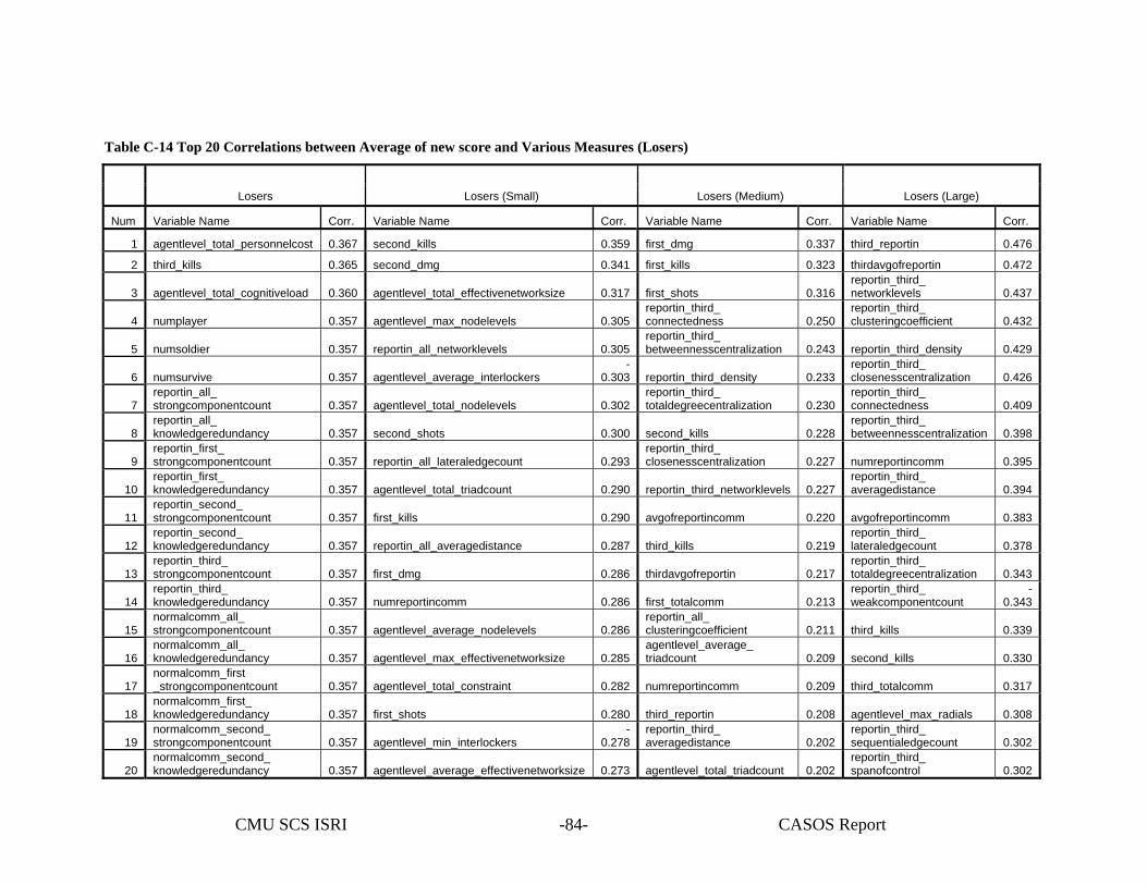
CMU SCS ISRI CASOS Report -84-
Table C-14 Top 20 Correlations between Average of new score and Various Measures (Losers)
Losers Losers (Small) Losers (Medium) Losers (Large)
Num Variable Name Corr. Variable Name Corr. Variable Name Corr. Variable Name Corr.
1 agentlevel_total_personnelcost 0.367 second_kills 0.359 first_dmg 0.337 third_reportin 0.476
2 third_kills 0.365 second_dmg 0.341 first_kills 0.323 thirdavgofreportin 0.472
3 agentlevel_total_cognitiveload 0.360 agentlevel_total_effectivenetworksize 0.317 first_shots 0.316 reportin_third_ networklevels 0.437
4 numplayer 0.357 agentlevel_max_nodelevels 0.305 reportin_third_ connectedness 0.250
reportin_third_ clusteringcoefficient 0.432
5 numsoldier 0.357 reportin_all_networklevels 0.305 reportin_third_ betweennesscentralization 0.243 reportin_third_density 0.429
6 numsurvive 0.357 agentlevel_average_interlockers -
0.303 reportin_third_density 0.233 reportin_third_ closenesscentralization 0.426
7 reportin_all_ strongcomponentcount 0.357 agentlevel_total_nodelevels 0.302
reportin_third_ totaldegreecentralization 0.230
reportin_third_ connectedness 0.409
8 reportin_all_ knowledgeredundancy 0.357 second_shots 0.300 second_kills 0.228
reportin_third_ betweennesscentralization 0.398
9 reportin_first_ strongcomponentcount 0.357 reportin_all_lateraledgecount 0.293
reportin_third_ closenesscentralization 0.227 numreportincomm 0.395
10 reportin_first_ knowledgeredundancy 0.357 agentlevel_total_triadcount 0.290 reportin_third_networklevels 0.227
reportin_third_ averagedistance 0.394
11 reportin_second_ strongcomponentcount 0.357 first_kills 0.290 avgofreportincomm 0.220 avgofreportincomm 0.383
12 reportin_second_ knowledgeredundancy 0.357 reportin_all_averagedistance 0.287 third_kills 0.219
reportin_third_ lateraledgecount 0.378
13 reportin_third_ strongcomponentcount 0.357 first_dmg 0.286 thirdavgofreportin 0.217
reportin_third_ totaldegreecentralization 0.343
14 reportin_third_ knowledgeredundancy 0.357 numreportincomm 0.286 first_totalcomm 0.213
reportin_third_ weakcomponentcount
-0.343
15 normalcomm_all_ strongcomponentcount 0.357 agentlevel_average_nodelevels 0.286
reportin_all_ clusteringcoefficient 0.211 third_kills 0.339
16 normalcomm_all_ knowledgeredundancy 0.357 agentlevel_max_effectivenetworksize 0.285
agentlevel_average_ triadcount 0.209 second_kills 0.330
17 normalcomm_first _strongcomponentcount 0.357 agentlevel_total_constraint 0.282 numreportincomm 0.209 third_totalcomm 0.317
18 normalcomm_first_ knowledgeredundancy 0.357 first_shots 0.280 third_reportin 0.208 agentlevel_max_radials 0.308
19 normalcomm_second_ strongcomponentcount 0.357 agentlevel_min_interlockers
-0.278
reportin_third_ averagedistance 0.202
reportin_third_ sequentialedgecount 0.302
20 normalcomm_second_ knowledgeredundancy 0.357 agentlevel_average_effectivenetworksize 0.273 agentlevel_total_triadcount 0.202
reportin_third_ spanofcontrol 0.302
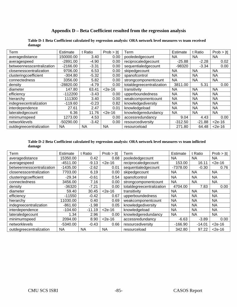
CMU SCS ISRI CASOS Report -85-
Appendix D – Beta Coefficient resulted from the regression analysis
Table D-1 Beta Coefficient calculated by regression analysis: ORA network level measures vs team received damage
Term Estimate t Ratio Prob > |t| Term Estimate t Ratio Prob > |t| averagedistance 150000.00 3.40 0.00 poolededgecount NA NA NA averagespeed -2891.00 -4.90 0.00 reciprocaledgecount -25.88 -2.28 0.02betweennesscentralization -2166.00 -3.31 0.00 sequentialedgecount -98320 -3.34 0.00closenesscentralization 9706.00 6.53 0.00 skipedgecount NA NA NA clusteringcoefficient -304.80 -5.32 0.00 spanofcontrol NA NA NA connectedness 3356.00 5.82 0.00 strongcomponentcount NA NA NA density -28820.00 -4.79 0.00 totaldegreecentralization 3811.00 5.31 0.00diameter 147.80 63.41 <2e-16 transitivity NA NA NA efficiency -112200 -3.43 0.00 upperboundedness NA NA NA hierarchy 111300 3.40 0.00 weakcomponentcount NA NA NA indegreecentralization -119.60 -0.23 0.82 knowledgediversity NA NA NA interdependence 27.61 2.47 0.01 knowledgeload NA NA NA lateraledgecount 6.36 11.76 <2e-16 knowledgeredundancy NA NA NA minimumspeed 1273.00 4.53 0.00 accessredundancy 9.04 4.43 0.00networklevels -50290.00 -3.42 0.00 resourcediversity -312.50 -21.88 <2e-16 outdegreecentralization NA NA NA resourceload 271.80 64.48 <2e-16
Table D-2 Beta Coefficient calculated by regression analysis: ORA network level measures vs team inflicted damage
Term Estimate t Ratio Prob > |t| Term Estimate t Ratio Prob > |t| averagedistance 15350.00 0.42 0.68 poolededgecount NA NA NA averagespeed -4511.00 -9.13 <2e-16 reciprocaledgecount 153.00 16.11 <2e-16 betweennesscentralization -1435.00 -2.62 0.01 sequentialedgecount -7378.00 -0.30 0.76closenesscentralization 7703.00 6.19 0.00 skipedgecount NA NA NA clusteringcoefficient -29.34 -0.61 0.54 spanofcontrol NA NA NA connectedness 3456.00 7.16 0.00 strongcomponentcount NA NA NA density -36320 -7.21 0.00 totaldegreecentralization 4704.00 7.83 0.00diameter 59.40 30.45 <2e-16 transitivity NA NA NA efficiency -11550 -0.42 0.67 upperboundedness NA NA NA hierarchy 11030.00 0.40 0.69 weakcomponentcount NA NA NA indegreecentralization -861.60 -1.98 0.05 knowledgediversity NA NA NA interdependence -104.60 -11.19 <2e-16 knowledgeload NA NA NA lateraledgecount 1.34 2.96 0.00 knowledgeredundancy NA NA NA minimumspeed 2094.00 8.90 <2e-16 accessredundancy -6.63 -3.89 0.00networklevels -5340.00 -0.43 0.66 resourcediversity -166.90 -14.01 <2e-16 outdegreecentralization NA NA NA resourceload 342.80 97.22 <2e-16
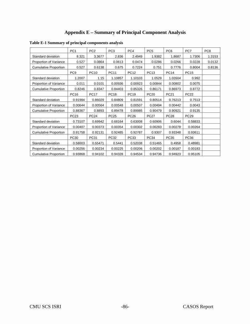
CMU SCS ISRI CASOS Report -86-
Appendix E – Summary of Principal Component Analysis
Table E-1 Summary of principal components analysis
PC1 PC2 PC3 PC4 PC5 PC6 PC7 PC8 Standard deviation 8.321 3.3677 2.836 2.4949 1.9382 1.8687 1.7306 1.3153 Proportion of Variance 0.527 0.0864 0.0613 0.0474 0.0286 0.0266 0.0228 0.0132 Cumulative Proportion 0.527 0.6138 0.675 0.7224 0.751 0.7776 0.8004 0.8136 PC9 PC10 PC11 PC12 PC13 PC14 PC15 Standard deviation 1.2007 1.15 1.10857 1.10103 1.0529 1.02604 0.992 Proportion of Variance 0.011 0.0101 0.00936 0.00923 0.00844 0.00802 0.0075 Cumulative Proportion 0.8246 0.8347 0.84403 0.85326 0.86171 0.86973 0.8772 PC16 PC17 PC18 PC19 PC20 PC21 PC22 Standard deviation 0.91984 0.86029 0.84809 0.81591 0.80514 0.76213 0.7513 Proportion of Variance 0.00644 0.00564 0.00548 0.00507 0.00494 0.00442 0.0043 Cumulative Proportion 0.88367 0.8893 0.89478 0.89985 0.90479 0.90921 0.9135 PC23 PC24 PC25 PC26 PC27 PC28 PC29 Standard deviation 0.73107 0.69942 0.68164 0.63008 0.60906 0.6044 0.58833 Proportion of Variance 0.00407 0.00373 0.00354 0.00302 0.00283 0.00278 0.00264 Cumulative Proportion 0.91758 0.92131 0.92485 0.92787 0.9307 0.93348 0.93611 PC30 PC31 PC32 PC33 PC34 PC35 PC36 Standard deviation 0.58003 0.55471 0.5441 0.52038 0.51465 0.4958 0.48981 Proportion of Variance 0.00256 0.00234 0.00225 0.00206 0.00202 0.00187 0.00183 Cumulative Proportion 0.93868 0.94102 0.94328 0.94534 0.94736 0.94923 0.95105
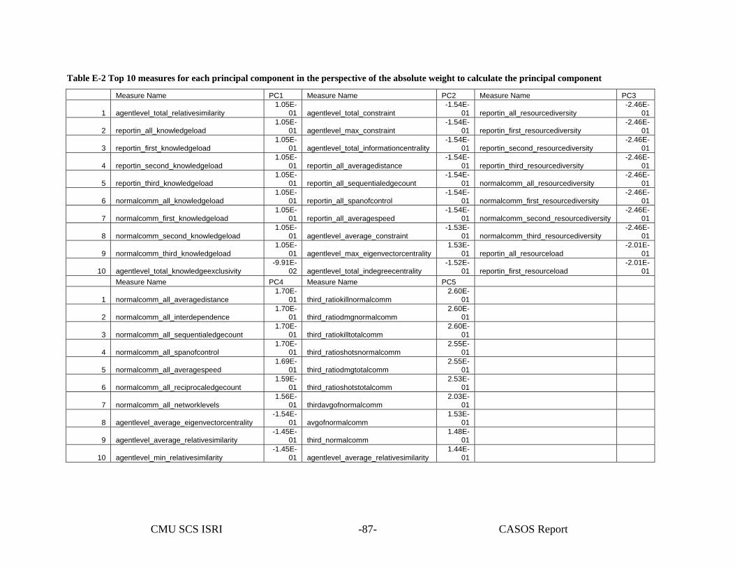
CMU SCS ISRI CASOS Report -87-
Table E-2 Top 10 measures for each principal component in the perspective of the absolute weight to calculate the principal component
Measure Name PC1 Measure Name PC2 Measure Name PC3
1 agentlevel_total_relativesimilarity 1.05E-
01 agentlevel_total_constraint -1.54E-
01 reportin_all_resourcediversity -2.46E-
01
2 reportin_all_knowledgeload 1.05E-
01 agentlevel_max_constraint -1.54E-
01 reportin_first_resourcediversity -2.46E-
01
3 reportin_first_knowledgeload 1.05E-
01 agentlevel_total_informationcentrality -1.54E-
01 reportin_second_resourcediversity -2.46E-
01
4 reportin_second_knowledgeload 1.05E-
01 reportin_all_averagedistance -1.54E-
01 reportin_third_resourcediversity -2.46E-
01
5 reportin_third_knowledgeload 1.05E-
01 reportin_all_sequentialedgecount -1.54E-
01 normalcomm_all_resourcediversity -2.46E-
01
6 normalcomm_all_knowledgeload 1.05E-
01 reportin_all_spanofcontrol -1.54E-
01 normalcomm_first_resourcediversity -2.46E-
01
7 normalcomm_first_knowledgeload 1.05E-
01 reportin_all_averagespeed -1.54E-
01 normalcomm_second_resourcediversity -2.46E-
01
8 normalcomm_second_knowledgeload 1.05E-
01 agentlevel_average_constraint -1.53E-
01 normalcomm_third_resourcediversity -2.46E-
01
9 normalcomm_third_knowledgeload 1.05E-
01 agentlevel_max_eigenvectorcentrality 1.53E-
01 reportin_all_resourceload -2.01E-
01
10 agentlevel_total_knowledgeexclusivity -9.91E-
02 agentlevel_total_indegreecentrality -1.52E-
01 reportin_first_resourceload -2.01E-
01 Measure Name PC4 Measure Name PC5
1 normalcomm_all_averagedistance 1.70E-
01 third_ratiokillnormalcomm 2.60E-
01
2 normalcomm_all_interdependence 1.70E-
01 third_ratiodmgnormalcomm 2.60E-
01
3 normalcomm_all_sequentialedgecount 1.70E-
01 third_ratiokilltotalcomm 2.60E-
01
4 normalcomm_all_spanofcontrol 1.70E-
01 third_ratioshotsnormalcomm 2.55E-
01
5 normalcomm_all_averagespeed 1.69E-
01 third_ratiodmgtotalcomm 2.55E-
01
6 normalcomm_all_reciprocaledgecount 1.59E-
01 third_ratioshotstotalcomm 2.53E-
01
7 normalcomm_all_networklevels 1.56E-
01 thirdavgofnormalcomm 2.03E-
01
8 agentlevel_average_eigenvectorcentrality -1.54E-
01 avgofnormalcomm 1.53E-
01
9 agentlevel_average_relativesimilarity -1.45E-
01 third_normalcomm 1.48E-
01
10 agentlevel_min_relativesimilarity -1.45E-
01 agentlevel_average_relativesimilarity 1.44E-
01
CMU SCS ISRI CASOS Report -88-
References [1] Reminga, J. and K. M. Carley (2004), ORA:Organization Risk Analyzer, Tech Report, CMU-ISRI-04-106, CASOS, Carnegie Mellon, Pittsburgh PA. [2] Tsvetovat, M. , Reminga, J., and K. M. Carley (2004), DyNetML:Interchange Format for Rich Social Network Data, Tech Report, CMU-ISRI-04-105, CASOS, Carnegie Mellon, Pittsburgh PA. [3] Timothy M. Karcher, MAJ (2002), Enhancing combat effectiveness, the evolution of the United States Army infantry rifle squad since the end of World War II, Fort Leavenworth, Kansas [4] Richard E. Christ and Kenneth L. Evans (2002), Radio Communications and Situation Awareness of Infantry Squads during Urban Operations, U.S. Army Research Institute [5] Elizabeth S. Redden and Cynthia L. Blackwell (2001), Situation Awareness and Communication Experiment for Military Operations in Urban Terrain: Experiment I, U.S. Army Research Laboratory