Embed Size (px)
Citation preview
7/18/2019 Precalculus Tradler Carley
http://slidepdf.com/reader/full/precalculus-tradler-carley 1/424
7/18/2019 Precalculus Tradler Carley
http://slidepdf.com/reader/full/precalculus-tradler-carley 2/424
ii
Copyright c2012 Thomas Tradler and Holly Carley
This work is licensed under a Creative Commons Attribution-NonCommercial-NoDerivs 3.0 United States License. (CC BY-NC-ND 3.0)
To view a copy of the license, visit:
http://creativecommons.org/licenses/by-nc-nd/3.0/us/
Under this license, you are free:
• to Share: to copy, distribute and transmit the work
Under the following conditions:
• Attribution: You must attribute the work in the manner specified by the authoror licensor (but not in any way that suggests that they endorse you or youruse of the work).
• Noncommercial: You may not use this work for commercial purposes.
• No Derivative Works: You may not alter, transform, or build upon this work.
With the understanding that:
• Waiver: Any of the above conditions can be waived if you get permission fromthe copyright holder.
• Public Domain: Where the work or any of its elements is in the public domain
under applicable law, that status is in no way affected by the license.• Other Rights: In no way are any of the following rights affected by the license:
– Your fair dealing or fair use rights, or other applicable copyright excep-tions and limitations;
– The author’s moral rights;
– Rights other persons may have either in the work itself or in how thework is used, such as publicity or privacy rights.
• Notice: For any reuse or distribution, you must make clear to others thelicense terms of this work. The best way to do this is with a link to the above
web page.
This document was created with LATEX. The TI-84 images were createdwith the TI-SmartView software.
7/18/2019 Precalculus Tradler Carley
http://slidepdf.com/reader/full/precalculus-tradler-carley 3/424
Preface
These are notes for a course in precalculus, as it is taught at New York CityCollege of Technology - CUNY (where it is offered under the course number
MAT 1375). Our approach is calculator based. For this, we will use thecurrently standard TI-84 calculator, and in particular, many of the exampleswill be explained and solved with it. However, we want to point out thatthere are also many other calculators that are suitable for the purpose of this course and many of these alternatives have similar functionalities as thecalculator that we have chosen to use. An introduction to the TI-84 calculatortogether with the most common applications needed for this course is providedin appendix A. In the future we may expand on this by providing introductionsto other calculators or computer algebra systems.
This course in precalculus has the overarching theme of “functions.” Thismeans that many of the often more algebraic topics studied in the previouscourses are revisited under this new function theoretic point of view. However,in order to keep this text as self contained as possible we always recall allresults that are necessary to follow the core of the course even if we assumethat the student has familiarity with the formula or topic at hand. After a firstintroduction to the abstract notion of a function, we study polynomials, ratio-nal functions, exponential functions, logarithmic functions, and trigonometricfunctions with the function viewpoint. Throughout, we will always place par-ticular importance to the corresponding graph of the discussed function whichwill be analyzed with the help of the TI-84 calculator as mentioned above.These are in fact the topics of the first four (of the five) parts of this precalculus
course.In the fifth and last part of the book, we deviate from the above theme
and collect more algebraically oriented topics that will be needed in calculusor other advanced mathematics courses or even other science courses. Thispart includes a discussion of the algebra of complex numbers (in particular
iii
7/18/2019 Precalculus Tradler Carley
http://slidepdf.com/reader/full/precalculus-tradler-carley 4/424
iv
complex numbers in polar form), the 2-dimensional real vector space R2, se-
quences and series with focus on the arithmetic and geometric series (whichare again examples of functions, though this is not emphasized), and finallythe generalized binomial theorem.
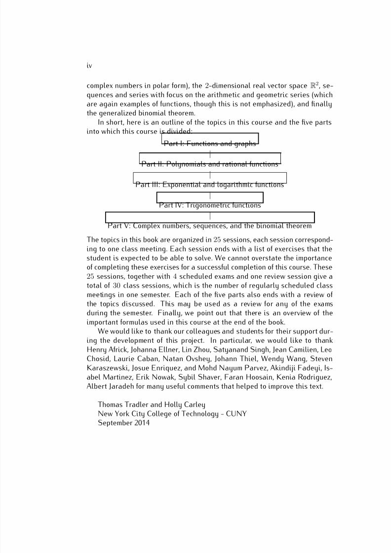
In short, here is an outline of the topics in this course and the five partsinto which this course is divided:
Part I: Functions and graphs
|Part II: Polynomials and rational functions
|Part III: Exponential and logarithmic functions
|Part IV: Trigonometric functions
|Part V: Complex numbers, sequences, and the binomial theorem
The topics in this book are organized in 25 sessions, each session correspond-ing to one class meeting. Each session ends with a list of exercises that thestudent is expected to be able to solve. We cannot overstate the importanceof completing these exercises for a successful completion of this course. These25 sessions, together with 4 scheduled exams and one review session give atotal of 30 class sessions, which is the number of regularly scheduled classmeetings in one semester. Each of the five parts also ends with a review of the topics discussed. This may be used as a review for any of the examsduring the semester. Finally, we point out that there is an overview of theimportant formulas used in this course at the end of the book.
We would like to thank our colleagues and students for their support dur-ing the development of this project. In particular, we would like to thankHenry Africk, Johanna Ellner, Lin Zhou, Satyanand Singh, Jean Camilien, LeoChosid, Laurie Caban, Natan Ovshey, Johann Thiel, Wendy Wang, StevenKaraszewski, Josue Enriquez, and Mohd Nayum Parvez, Akindiji Fadeyi, Is-abel Martinez, Erik Nowak, Sybil Shaver, Faran Hoosain, Kenia Rodriguez,
Albert Jaradeh for many useful comments that helped to improve this text.
Thomas Tradler and Holly CarleyNew York City College of Technology - CUNYSeptember 2014
7/18/2019 Precalculus Tradler Carley
http://slidepdf.com/reader/full/precalculus-tradler-carley 5/424
Contents
Preface iii
Table of contents v
I Functions and graphs 1
1 The absolute value 2
1.1 Background regarding numbers . . . . . . . . . . . . . . . . . . . 21.2 The absolute value . . . . . . . . . . . . . . . . . . . . . . . . . . 31.3 Inequalities and intervals . . . . . . . . . . . . . . . . . . . . . . 41.4 Absolute value inequalities . . . . . . . . . . . . . . . . . . . . . 6
1.5 Exercises . . . . . . . . . . . . . . . . . . . . . . . . . . . . . . . . 11
2 Lines and functions 13
2.1 Lines, slope and intercepts . . . . . . . . . . . . . . . . . . . . . 132.2 Introduction to functions . . . . . . . . . . . . . . . . . . . . . . . 222.3 Exercises . . . . . . . . . . . . . . . . . . . . . . . . . . . . . . . . 28
3 Functions by formulas and graphs 32
3.1 Functions given by formulas . . . . . . . . . . . . . . . . . . . . 323.2 Functions given by graphs . . . . . . . . . . . . . . . . . . . . . 373.3 Exercises . . . . . . . . . . . . . . . . . . . . . . . . . . . . . . . . 44
4 Introduction to the TI-84 49
4.1 Graphing with the TI-84 . . . . . . . . . . . . . . . . . . . . . . . 494.2 Finding zeros, maxima, and minima . . . . . . . . . . . . . . . . 534.3 Exercises . . . . . . . . . . . . . . . . . . . . . . . . . . . . . . . . 61
v
7/18/2019 Precalculus Tradler Carley
http://slidepdf.com/reader/full/precalculus-tradler-carley 6/424
vi CONTENTS
5 Basic functions and transformations 63
5.1 Graphing basic functions . . . . . . . . . . . . . . . . . . . . . . 635.2 Transformation of graphs . . . . . . . . . . . . . . . . . . . . . . 65
5.3 Exercises . . . . . . . . . . . . . . . . . . . . . . . . . . . . . . . . 73
6 Operations on functions 76
6.1 Operations on functions given by formulas . . . . . . . . . . . . 76
6.2 Operations on functions given by tables . . . . . . . . . . . . . 81
6.3 Exercises . . . . . . . . . . . . . . . . . . . . . . . . . . . . . . . . 83
7 The inverse of a function 86
7.1 One-to-one functions . . . . . . . . . . . . . . . . . . . . . . . . . 867.2 Inverse function . . . . . . . . . . . . . . . . . . . . . . . . . . . . 88
7.3 Exercises . . . . . . . . . . . . . . . . . . . . . . . . . . . . . . . . 95
Review of functions and graphs 98
II Polynomials and rational functions 100
8 Dividing polynomials 101
8.1 Long division . . . . . . . . . . . . . . . . . . . . . . . . . . . . . 1028.2 Dividing by (x − c) . . . . . . . . . . . . . . . . . . . . . . . . . . 106
8.3 Optional section: Synthetic division . . . . . . . . . . . . . . . . 109
8.4 Exercises . . . . . . . . . . . . . . . . . . . . . . . . . . . . . . . . 111
9 Graphing polynomials 113
9.1 Graphs of polynomials . . . . . . . . . . . . . . . . . . . . . . . . 113
9.2 Finding roots of a polynomial with the TI-84 . . . . . . . . . . . 121
9.3 Optional section: Graphing polynomials by hand . . . . . . . . 124
9.4 Exercises . . . . . . . . . . . . . . . . . . . . . . . . . . . . . . . . 127
10 Roots of polynomials 130
10.1 Optional section: The rational root theorem . . . . . . . . . . . 130
10.2 The fundamental theorem of algebra . . . . . . . . . . . . . . . . 134
10.3 Exercises . . . . . . . . . . . . . . . . . . . . . . . . . . . . . . . . 144
7/18/2019 Precalculus Tradler Carley
http://slidepdf.com/reader/full/precalculus-tradler-carley 7/424
CONTENTS vii
11 Rational functions 147
11.1 Graphs of rational functions . . . . . . . . . . . . . . . . . . . . . 14711.2 Optional section: Rational functions by hand . . . . . . . . . . 159
11.3 Exercises . . . . . . . . . . . . . . . . . . . . . . . . . . . . . . . . 168
12 Polynomial and rational inequalities 169
12.1 Polynomial inequalities . . . . . . . . . . . . . . . . . . . . . . . 169
12.2 Rational inequalities and absolute value inequalities . . . . . . 176
12.3 Exercises . . . . . . . . . . . . . . . . . . . . . . . . . . . . . . . . 179
Review of polynomials and rational functions 181
III Exponential and logarithmic functions 183
13 Exponential and logarithmic functions 184
13.1 Exponential functions and their graphs . . . . . . . . . . . . . . 184
13.2 Logarithmic functions and their graphs . . . . . . . . . . . . . . 190
13.3 Exercises . . . . . . . . . . . . . . . . . . . . . . . . . . . . . . . . 197
14 Properties of exp and log 199
14.1 Algebraic properties of exp and log . . . . . . . . . . . . . . . . 199
14.2 Solving exponential and logarithmic equations . . . . . . . . . . 202
14.3 Exercises . . . . . . . . . . . . . . . . . . . . . . . . . . . . . . . . 206
15 Applications of exp and log 208
15.1 Applications of exponential functions . . . . . . . . . . . . . . . 208
15.2 Exercises . . . . . . . . . . . . . . . . . . . . . . . . . . . . . . . . 214
16 Half-life and compound interest 216
16.1 Half-life . . . . . . . . . . . . . . . . . . . . . . . . . . . . . . . . 21616.2 Compound interest . . . . . . . . . . . . . . . . . . . . . . . . . . 220
16.3 Exercises . . . . . . . . . . . . . . . . . . . . . . . . . . . . . . . . 226
Review of exponential and logarithmic functions 229
7/18/2019 Precalculus Tradler Carley
http://slidepdf.com/reader/full/precalculus-tradler-carley 8/424
viii CONTENTS
IV Trigonometric functions 231
17 Trigonometric functions 232
17.1 Basic trigonometric definitions and facts . . . . . . . . . . . . . 232
17.2 sin, cos, and tan as functions . . . . . . . . . . . . . . . . . . . . 239
17.3 Exercises . . . . . . . . . . . . . . . . . . . . . . . . . . . . . . . . 249
18 Addition of angles and multiple angles 252
18.1 Addition and subtraction of angles . . . . . . . . . . . . . . . . . 252
18.2 Double and half angles . . . . . . . . . . . . . . . . . . . . . . . 256
18.3 Exercises . . . . . . . . . . . . . . . . . . . . . . . . . . . . . . . . 261
19 Inverse trigonometric functions 262
19.1 The functions sin−1, cos−1, and tan−1 . . . . . . . . . . . . . . . 262
19.2 Exercises . . . . . . . . . . . . . . . . . . . . . . . . . . . . . . . . 269
20 Trigonometric equations 270
20.1 Basic trigonometric equations . . . . . . . . . . . . . . . . . . . 270
20.2 Equations involving trigonometric functions . . . . . . . . . . . . 278
20.3 Exercises . . . . . . . . . . . . . . . . . . . . . . . . . . . . . . . . 283
Review of trigonometric functions 284
V Complex numbers, sequences, and the binomial theorem286
21 Complex numbers 287
21.1 Polar form of complex numbers . . . . . . . . . . . . . . . . . . . 287
21.2 Multiplication and division of complex numbers . . . . . . . . . 294
21.3 Exercises . . . . . . . . . . . . . . . . . . . . . . . . . . . . . . . . 297
22 Vectors in the plane 299
22.1 Introduction to vectors . . . . . . . . . . . . . . . . . . . . . . . . 299
22.2 Operations on vectors . . . . . . . . . . . . . . . . . . . . . . . . 303
22.3 Exercises . . . . . . . . . . . . . . . . . . . . . . . . . . . . . . . . 309
7/18/2019 Precalculus Tradler Carley
http://slidepdf.com/reader/full/precalculus-tradler-carley 9/424
CONTENTS ix
23 Sequences and series 311
23.1 Introduction to sequences and series . . . . . . . . . . . . . . . 31123.2 The arithmetic sequence . . . . . . . . . . . . . . . . . . . . . . . 31823.3 Exercises . . . . . . . . . . . . . . . . . . . . . . . . . . . . . . . . 323
24 The geometric series 325
24.1 Finite geometric series . . . . . . . . . . . . . . . . . . . . . . . . 32524.2 Infinite geometric series . . . . . . . . . . . . . . . . . . . . . . . 33024.3 Exercises . . . . . . . . . . . . . . . . . . . . . . . . . . . . . . . . 334
25 The binomial theorem 337
25.1 The binomial theorem . . . . . . . . . . . . . . . . . . . . . . . . 337
25.2 Binomial expansion . . . . . . . . . . . . . . . . . . . . . . . . . . 34225.3 Exercises . . . . . . . . . . . . . . . . . . . . . . . . . . . . . . . . 345
Review of complex numbers, sequences, and the binomial theorem 347
A Introduction to the TI-84 349
A.1 Basic calculator functions . . . . . . . . . . . . . . . . . . . . . . 349A.2 Graphing a function . . . . . . . . . . . . . . . . . . . . . . . . . 353
A.2.1 Rescaling the graphing window . . . . . . . . . . . . . . 354A.3 Graphing more than one function . . . . . . . . . . . . . . . . . . 357A.4 Graphing a piecewise defined function . . . . . . . . . . . . . . 359A.5 Using the table . . . . . . . . . . . . . . . . . . . . . . . . . . . . 361A.6 Solving an equation using the solver . . . . . . . . . . . . . . . 362A.7 Special functions (absolute value, n-th root, etc.) . . . . . . . . 363A.8 Programming the calculator . . . . . . . . . . . . . . . . . . . . . 366A.9 Common errors . . . . . . . . . . . . . . . . . . . . . . . . . . . . 370A.10 Resetting the calculator to factory settings . . . . . . . . . . . . 373
Answers to exercises 374
Session 1 . . . . . . . . . . . . . . . . . . . . . . . . . . . . . . . . . . . 374Session 2 . . . . . . . . . . . . . . . . . . . . . . . . . . . . . . . . . . . 375
Session 3 . . . . . . . . . . . . . . . . . . . . . . . . . . . . . . . . . . . 375Session 4 . . . . . . . . . . . . . . . . . . . . . . . . . . . . . . . . . . . 377Session 5 . . . . . . . . . . . . . . . . . . . . . . . . . . . . . . . . . . . 379Session 6 . . . . . . . . . . . . . . . . . . . . . . . . . . . . . . . . . . . 380Session 7 . . . . . . . . . . . . . . . . . . . . . . . . . . . . . . . . . . . 381
7/18/2019 Precalculus Tradler Carley
http://slidepdf.com/reader/full/precalculus-tradler-carley 10/424
x CONTENTS
Review part I . . . . . . . . . . . . . . . . . . . . . . . . . . . . . . . . 383
Session 8 . . . . . . . . . . . . . . . . . . . . . . . . . . . . . . . . . . . 383Session 9 . . . . . . . . . . . . . . . . . . . . . . . . . . . . . . . . . . . 384Session 10 . . . . . . . . . . . . . . . . . . . . . . . . . . . . . . . . . . 385Session 11 . . . . . . . . . . . . . . . . . . . . . . . . . . . . . . . . . . 386Session 12 . . . . . . . . . . . . . . . . . . . . . . . . . . . . . . . . . . 388Review part II . . . . . . . . . . . . . . . . . . . . . . . . . . . . . . . . 389Session 13 . . . . . . . . . . . . . . . . . . . . . . . . . . . . . . . . . . 389Session 14 . . . . . . . . . . . . . . . . . . . . . . . . . . . . . . . . . . 392Session 15 . . . . . . . . . . . . . . . . . . . . . . . . . . . . . . . . . . 393Session 16 . . . . . . . . . . . . . . . . . . . . . . . . . . . . . . . . . . 393Review part III . . . . . . . . . . . . . . . . . . . . . . . . . . . . . . . . 393
Session 17 . . . . . . . . . . . . . . . . . . . . . . . . . . . . . . . . . . 393Session 18 . . . . . . . . . . . . . . . . . . . . . . . . . . . . . . . . . . 396Session 19 . . . . . . . . . . . . . . . . . . . . . . . . . . . . . . . . . . 396Session 20 . . . . . . . . . . . . . . . . . . . . . . . . . . . . . . . . . . 397Review part IV . . . . . . . . . . . . . . . . . . . . . . . . . . . . . . . . 398Session 21 . . . . . . . . . . . . . . . . . . . . . . . . . . . . . . . . . . 398Session 22 . . . . . . . . . . . . . . . . . . . . . . . . . . . . . . . . . . 399Session 23 . . . . . . . . . . . . . . . . . . . . . . . . . . . . . . . . . . 400Session 24 . . . . . . . . . . . . . . . . . . . . . . . . . . . . . . . . . . 400Session 25 . . . . . . . . . . . . . . . . . . . . . . . . . . . . . . . . . . 401
Review part V . . . . . . . . . . . . . . . . . . . . . . . . . . . . . . . . 401
References 402
Important formulas used in precalculus 403
Index 411

7/18/2019 Precalculus Tradler Carley
http://slidepdf.com/reader/full/precalculus-tradler-carley 11/424
Part I
Functions and graphs
1
7/18/2019 Precalculus Tradler Carley
http://slidepdf.com/reader/full/precalculus-tradler-carley 12/424
Session 1
Absolute value equations and
inequalities
1.1 Background regarding numbers
The natural numbers (denoted by N) are the numbers
1, 2, 3, 4, 5, . . .
The integers (denoted by Z) are the numbers
. . . , −4, −3, −2, −1, 0, 1, 2, 3, 4, 5, . . .
The rational numbers (denoted by Q) are the fractions ab
of integers a and bwith b = 0. Here are some examples of rational numbers:
3
5, −2
6, 17, 0,
3
−8
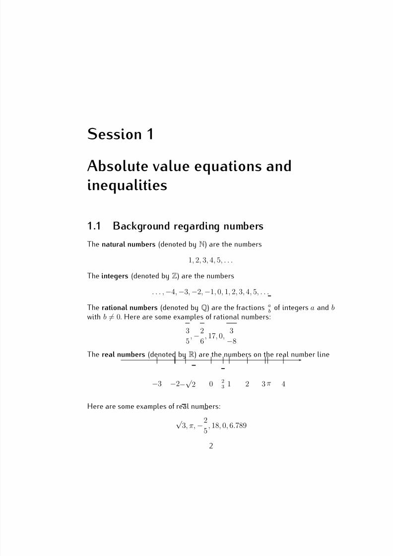
The real numbers (denoted by R) are the numbers on the real number line
0 23 1
−√
2 2 3 4−
2−
3 π
Here are some examples of real numbers:
√ 3, π, −2
5, 18, 0, 6.789
2
7/18/2019 Precalculus Tradler Carley
http://slidepdf.com/reader/full/precalculus-tradler-carley 13/424
1.2. THE ABSOLUTE VALUE 3
A real number that is not a rational number is called an irrational number.
Here are some examples of irrational numbers:
π,√
2, 523 , e
1.2 The absolute value
The absolute value of a real number c, denoted by |c| the non-negative numberwhich is equal in magnitude (or size) to c, i.e., is the number resulting fromdisregarding the sign:
|c| = c, if c is positive or zero−c, if c is negative
Example 1.1. | − 4| = 4
Example 1.2. |12| = 12
Example 1.3. | − 3.523| = 3.523
Example 1.4. For which real numbers x do you have |x| = 3?
Solution. Since
|3
| = 3 and
| −3
| = 3, we see that there are two solutions,
x = 3 or x = −3. The solution set is S = {−3, 3}.
Example 1.5. Solve for x: |x| = 5
Solution. x = 5 or x = −5. The solution set is S = {−5, 5}.
Example 1.6. Solve for x: |x| = −7.
Solution. Note that | − 7| = 7 and |7| = 7 so that these cannot give anysolutions. Indeed, there are no solutions, since the absolute value is alwaysnon-negative. The solution set is the empty set S = {}.
Example 1.7. Solve for x: |x| = 0.
Solution. Since −0 = 0, there is only one solution, x = 0. Thus, S = {0}.
Example 1.8. Solve for x: |x + 2| = 6.
7/18/2019 Precalculus Tradler Carley
http://slidepdf.com/reader/full/precalculus-tradler-carley 14/424
4 SESSION 1. THE ABSOLUTE VALUE
Solution. Since the absolute value of x + 2 is 6, we see that x + 2 has to be
either 6 or −6. We evaluate each case,
either x + 2 = 6, or x + 2 = −6,=⇒ x = 6 − 2, =⇒ x = −6 − 2,=⇒ x = 4; =⇒ x = −8.
The solution set is S = {−8, 4}.
Example 1.9. Solve for x: |3x − 4| = 5
Solution.Either 3x
−4 = 5 or 3x
−4 =
−5
=⇒ 3x = 9 =⇒ 3x = −1=⇒ x = 3 =⇒ x = −1
3
The solution set is S = {−13 , 3}.
Example 1.10. Solve for x: −2 · |12 + 3x| = −18
Solution. Dividing both sides by −2 gives |12 + 3x| = 9. With this, we havethe two cases
Either 12 + 3x = 9 or 12 + 3x = −9=⇒
3x =−
3 =⇒
3x =−
21=⇒ x = −1 =⇒ x = −7
The solution set is S = {−7, −1}.
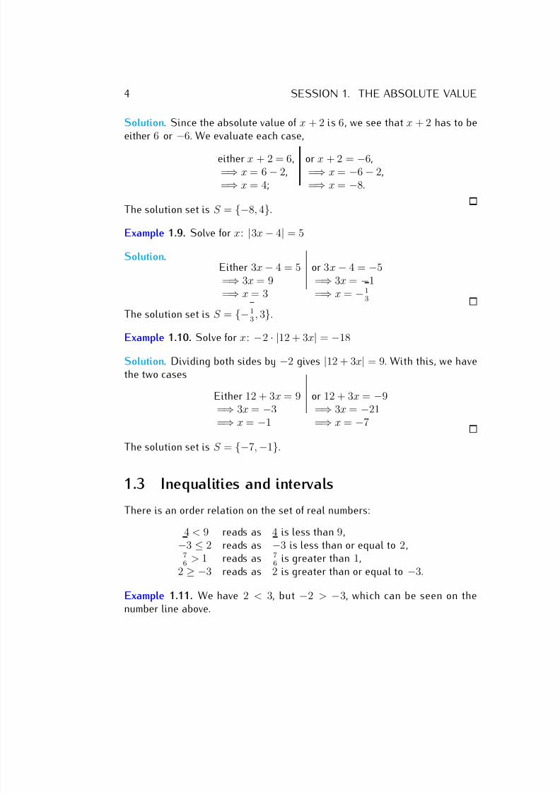
1.3 Inequalities and intervals
There is an order relation on the set of real numbers:
4 < 9 reads as 4 is less than 9,
−3
≤2 reads as
−3 is less than or equal to 2,
76 > 1 reads as 7
6 is greater than 1,2 ≥ −3 reads as 2 is greater than or equal to −3.
Example 1.11. We have 2 < 3, but −2 > −3, which can be seen on thenumber line above.
7/18/2019 Precalculus Tradler Carley
http://slidepdf.com/reader/full/precalculus-tradler-carley 15/424
1.3. INEQUALITIES AND INTERVALS 5
Example 1.12. We have 5 ≤ 5 and 5 ≥ 5. However the same is not true when
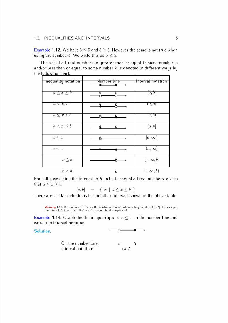
using the symbol <. We write this as 5 ≮ 5.The set of all real numbers x greater than or equal to some number a
and/or less than or equal to some number b is denoted in different ways bythe following chart:
Inequality notation Number line Interval notation
a ≤ x ≤ b a b [a, b]
a < x < b a b (a, b)
a ≤ x < b a b [a, b)
a < x ≤ b a b (a, b]
a ≤ x a [a, ∞)
a < x a (a, ∞)
x ≤ b b (−∞, b]
x < b b (−∞, b)
Formally, we define the interval [a, b] to be the set of all real numbers x suchthat a ≤ x ≤ b:
[a, b] = { x | a ≤ x ≤ b }There are similar definitions for the other intervals shown in the above table.
Warning 1.13. Be sure to write the smaller number a < b first when writing an interval [a, b]. For example,the interval [5, 3] = { x | 5 ≤ x ≤ 3 } would be the empty set!
Example 1.14. Graph the the inequality π < x ≤ 5 on the number line andwrite it in interval notation.
Solution.
On the number line: π 5Interval notation: (π, 5]
7/18/2019 Precalculus Tradler Carley
http://slidepdf.com/reader/full/precalculus-tradler-carley 16/424
6 SESSION 1. THE ABSOLUTE VALUE
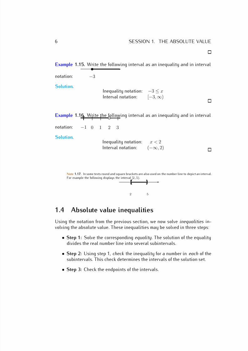
Example 1.15. Write the following interval as an inequality and in interval
notation: −3
Solution.Inequality notation: −3 ≤ xInterval notation: [−3, ∞)
Example 1.16. Write the following interval as an inequality and in interval
notation: −1 0 1 2 3
Solution.Inequality notation: x < 2Interval notation: (−∞, 2)
Note 1.17. In some texts round and square brackets are also used on the number line to depict an interval.For example the following displays the interval [2, 5).
2 5
1.4 Absolute value inequalities
Using the notation from the previous section, we now solve inequalities in-volving the absolute value. These inequalities may be solved in three steps:
• Step 1: Solve the corresponding equality. The solution of the equality
divides the real number line into several subintervals.• Step 2: Using step 1, check the inequality for a number in each of the
subintervals. This check determines the intervals of the solution set.
• Step 3: Check the endpoints of the intervals.
7/18/2019 Precalculus Tradler Carley
http://slidepdf.com/reader/full/precalculus-tradler-carley 17/424
1.4. ABSOLUTE VALUE INEQUALITIES 7
Here are some examples for the above solution method.
Example 1.18. Solve for x:
a) |x + 7| < 2 b) |3x − 5| ≥ 11 c) |12 − 5x| ≤ 1
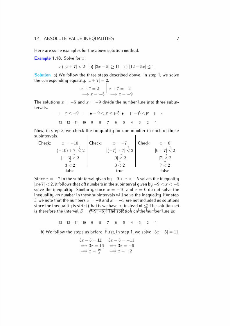
Solution. a) We follow the three steps described above. In step 1, we solvethe corresponding equality, |x + 7| = 2.
x + 7 = 2 x + 7 = −2=⇒ x = −5 =⇒ x = −9
The solutions x = −5 and x = −9 divide the number line into three subin-tervals:
x < −9 − 9 < x < −5 − 5 < x
-13 -12 -11 -10 -9 -8 -7 -6 -5 -4 -3 -2 -1
Now, in step 2, we check the inequality for one number in each of thesesubintervals.
Check: x = −10 Check: x = −7 Check: x = 0
|(−10) + 7| ?< 2 |(−7) + 7| ?
< 2 |0 + 7| ?< 2
| − 3| ?< 2 |0| ?
< 2 |7| ?< 2
3 ?< 2 0
?< 2 7
?< 2
false true falseSince x = −7 in the subinterval given by −9 < x < −5 solves the inequality|x+7| < 2, it follows that all numbers in the subinterval given by −9 < x < −5solve the inequality. Similarly, since x = −10 and x = 0 do not solve theinequality, no number in these subintervals will solve the inequality. For step3, we note that the numbers x = −9 and x = −5 are not included as solutionssince the inequality is strict (that is we have < instead of ≤).The solution setis therefore the interval S = (−9, −5). The solution on the number line is:
-13 -12 -11 -10 -9 -8 -7 -6 -5 -4 -3 -2 -1
b) We follow the steps as before. First, in step 1, we solve |3x − 5| = 11.
3x − 5 = 11 3x − 5 = −11=⇒ 3x = 16 =⇒ 3x = −6=⇒ x = 16
3 =⇒ x = −2
7/18/2019 Precalculus Tradler Carley
http://slidepdf.com/reader/full/precalculus-tradler-carley 18/424
8 SESSION 1. THE ABSOLUTE VALUE
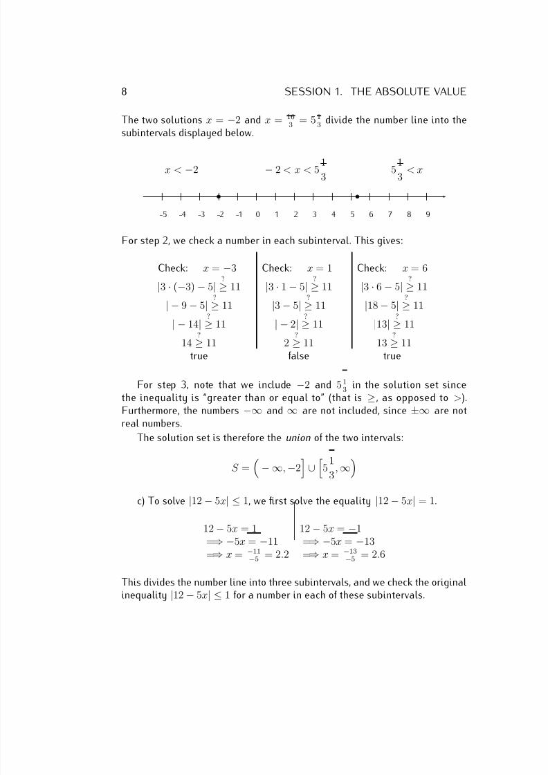
The two solutions x = −2 and x = 163
= 5 13
divide the number line into the
subintervals displayed below.
x < −2 − 2 < x < 51
3 5
1
3 < x
-5 -4 -3 -2 -1 0 1 2 3 4 5 6 7 8 9
For step 2, we check a number in each subinterval. This gives:
Check: x = −3 Check: x = 1 Check: x = 6|3 · (−3) − 5| ?≥ 11 |3 · 1 − 5| ?≥ 11 |3 · 6 − 5| ?≥ 11
| − 9 − 5| ?≥ 11 |3 − 5| ?≥ 11 |18 − 5| ?≥ 11
| − 14| ?≥ 11 | − 2| ?≥ 11 |13| ?≥ 11
14?≥ 11 2
?≥ 11 13?≥ 11
true false true
For step 3, note that we include −2 and 5 13
in the solution set sincethe inequality is “greater than or equal to” (that is
≥, as opposed to >).
Furthermore, the numbers −∞ and ∞ are not included, since ±∞ are notreal numbers.
The solution set is therefore the union of the two intervals:
S =
− ∞, −2
∪
51
3, ∞
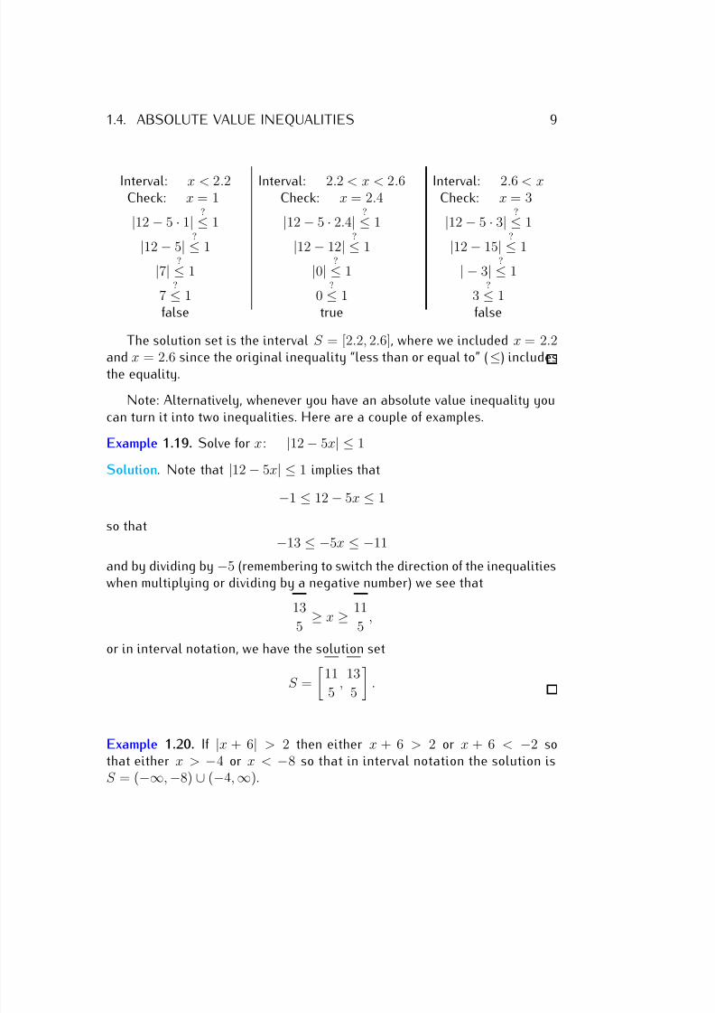
c) To solve |12 − 5x| ≤ 1, we first solve the equality |12 − 5x| = 1.
12 − 5x = 1 12 − 5x = −1
=⇒ −5x = −11 =⇒ −5x = −13=⇒ x = −11
−5 = 2.2 =⇒ x = −13−5 = 2.6
This divides the number line into three subintervals, and we check the originalinequality |12 − 5x| ≤ 1 for a number in each of these subintervals.
7/18/2019 Precalculus Tradler Carley
http://slidepdf.com/reader/full/precalculus-tradler-carley 19/424
1.4. ABSOLUTE VALUE INEQUALITIES 9
Interval: x < 2.2 Interval: 2.2 < x < 2.6 Interval: 2.6 < xCheck: x = 1 Check: x = 2.4 Check: x = 3
|12 − 5 · 1| ?≤ 1 |12 − 5 · 2.4| ?≤ 1 |12 − 5 · 3| ?≤ 1
|12 − 5| ?≤ 1 |12 − 12| ?≤ 1 |12 − 15| ?≤ 1
|7| ?≤ 1 |0| ?≤ 1 | − 3| ?≤ 1
7?≤ 1 0
?≤ 1 3?≤ 1
false true false
The solution set is the interval S = [2.2, 2.6], where we included x = 2.2
and x = 2.6 since the original inequality “less than or equal to” (≤) includesthe equality.
Note: Alternatively, whenever you have an absolute value inequality youcan turn it into two inequalities. Here are a couple of examples.
Example 1.19. Solve for x: |12 − 5x| ≤ 1
Solution. Note that |12 − 5x| ≤ 1 implies that
−1 ≤ 12 − 5x ≤ 1
so that −13 ≤ −5x ≤ −11
and by dividing by −5 (remembering to switch the direction of the inequalitieswhen multiplying or dividing by a negative number) we see that
13
5 ≥ x ≥ 11
5 ,
or in interval notation, we have the solution set
S =
11
5 ,
13
5
.
Example 1.20. If |x + 6| > 2 then either x + 6 > 2 or x + 6 < −2 sothat either x > −4 or x < −8 so that in interval notation the solution isS = (−∞, −8) ∪ (−4, ∞).
7/18/2019 Precalculus Tradler Carley
http://slidepdf.com/reader/full/precalculus-tradler-carley 20/424
10 SESSION 1. THE ABSOLUTE VALUE
Observation 1.21. There is a geometric interpretation of the absolute value
on the number line as the distance between two numbers:
distance between a and b is |b − a| which is also equal to |a − b|
a b
This interpretation can also be used to solve absolute value equations andinequalities.
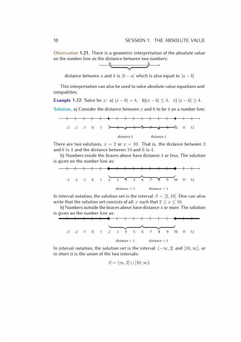
Example 1.22. Solve for x: a) |x − 6| = 4, b)|x − 6| ≤ 4, c) |x − 6| ≥ 4.
Solution. a) Consider the distance between x and 6 to be 4 on a number line:
-3 -2 -1 0 1 2 3 4 5 6 7 8 9 10 11 12
distance 4 distance 4
There are two solutions, x = 2 or x = 10. That is, the distance between 2and 6 is 4 and the distance between 10 and 6 is 4.
b) Numbers inside the braces above have distance 4 or less. The solutionis given on the number line as:
-3 -2 -1 0 1 2 3 4 5 6 7 8 9 10 11 12
distance ≤ 4 distance ≤ 4
In interval notation, the solution set is the interval S = [2, 10]. One can alsowrite that the solution set consists of all x such that 2 ≤ x ≤ 10.
b) Numbers outside the braces above have distance 4 or more. The solutionis given on the number line as:
-3 -2 -1 0 1 2 3 4 5 6 7 8 9 10 11 12
distance < 4 distance < 4
In interval notation, the solution set is the interval (−∞, 2] and [10, ∞), orin short it is the union of the two intervals:
S = (∞, 2] ∪ [10, ∞).
7/18/2019 Precalculus Tradler Carley
http://slidepdf.com/reader/full/precalculus-tradler-carley 21/424
1.5. EXERCISES 11
One can also write that the solution set consists of all x such that x ≤ 2 or
x ≥ 10.
1.5 Exercises
Exercise 1.1. Give examples of numbers that are
a) natural numbers b) integers c) integers but not natural numbersd) rational numbers e) real numbers f ) rational numbers but not integers
Exercise 1.2. Which of the following numbers are natural numbers, integers,rational numbers, or real numbers? Which of these numbers are irrational?
a) 73
b) −5 c) 0 d) 17, 000 e) 124
f )√
7 g)√
25
Exercise 1.3. Evaluate the following absolute value expressions:
a) | − 8|, b) |10|, c) | − 99|, d) −|3|,e) −| − 2|, f ) | − √ 6|, g) |3 + 4|, h) |2 − 9|,i) | − 5.4|, j)
−23
, k) 5−2
, l) −−−6
−3
.Exercise 1.4. Solve for x:
a) |x| = 8 b) |x| = 0 c) |x| = −3d) |x + 3| = 10 e) |2x + 5| = 9 f ) |2 − 5x| = 22g) |4x| = −8 h) | − 7x − 3| = 0 i) |4 − 4x| = 44
j) −2 · |2 − 3x| = −12 k) 5 + |2x + 7| = 14 l) −| − 8 − 2x| = −12
Exercise 1.5. Solve for x using the geometric interpretation of the absolutevalue:
a) |x| = 8 b) |x| = 0 c) |x| = −3d) |x − 4| = 2 e) |x + 5| = 9 f ) |2 − x| = 5
7/18/2019 Precalculus Tradler Carley
http://slidepdf.com/reader/full/precalculus-tradler-carley 22/424
12 SESSION 1. THE ABSOLUTE VALUE
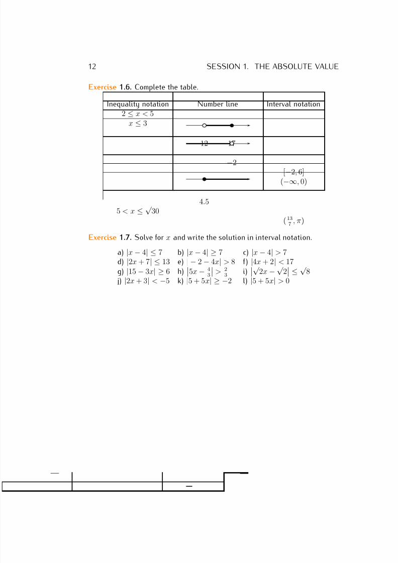
Exercise 1.6. Complete the table.
Inequality notation Number line Interval notation2 ≤ x < 5
x ≤ 3
12 17
−2[−2, 6]
(−∞, 0)
4.55 < x ≤ √
30( 13
7 , π)
Exercise 1.7. Solve for x and write the solution in interval notation.
a) |x − 4| ≤ 7 b) |x − 4| ≥ 7 c) |x − 4| > 7d) |2x + 7| ≤ 13 e) | − 2 − 4x| > 8 f ) |4x + 2| < 17g) |15 − 3x| ≥ 6 h)
5x − 43
> 23
i)√
2x − √ 2 ≤ √
8 j) |2x + 3| < −5 k) |5 + 5x| ≥ −2 l) |5 + 5x| > 0
7/18/2019 Precalculus Tradler Carley
http://slidepdf.com/reader/full/precalculus-tradler-carley 23/424
Session 2
Lines and functions
2.1 Lines, slope and intercepts
In this chapter we will introduce the notion of a function. Before we givethe general definition, we recall one special kind of function which is alreadyfamiliar to the student. More precisely, we start by recalling functions thatare given by straight lines.
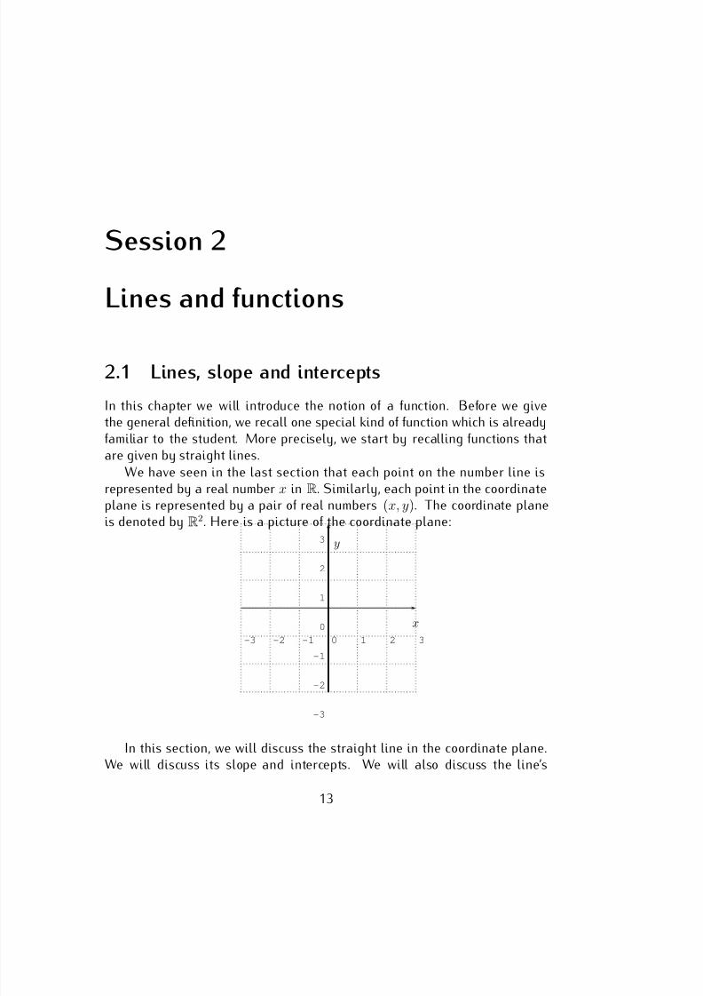
We have seen in the last section that each point on the number line isrepresented by a real number x in R. Similarly, each point in the coordinateplane is represented by a pair of real numbers (x, y). The coordinate plane
is denoted by R2
. Here is a picture of the coordinate plane:
-3 -2 -1 0 1 2 3
-3
-2
-1
0
1
2
3
x
y
In this section, we will discuss the straight line in the coordinate plane.We will discuss its slope and intercepts. We will also discuss the line’s
13
7/18/2019 Precalculus Tradler Carley
http://slidepdf.com/reader/full/precalculus-tradler-carley 24/424
14 SESSION 2. LINES AND FUNCTIONS
corresponding algebraic forms: the point-slope form and the slope-intercept
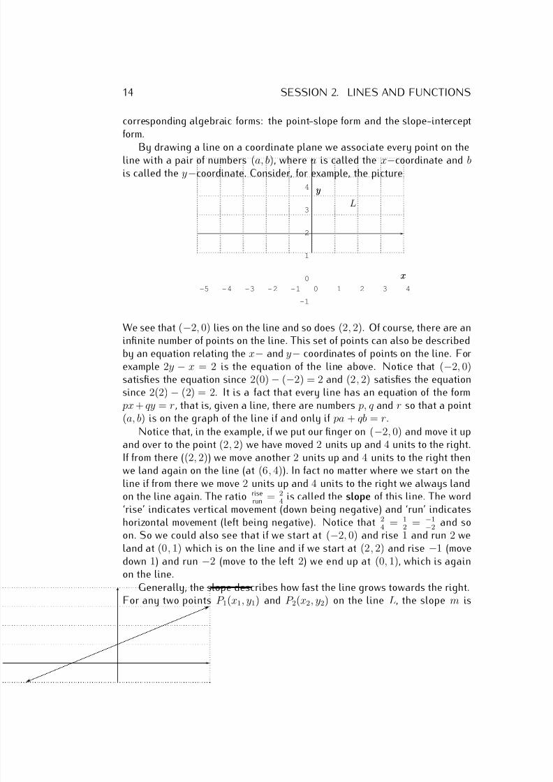
form.By drawing a line on a coordinate plane we associate every point on the
line with a pair of numbers (a, b), where a is called the x−coordinate and bis called the y−coordinate. Consider, for example, the picture
-5 -4 -3 -2 -1 0 1 2 3 4
-1
0
1
2
3
4
x
y
x
y
L
We see that (−2, 0) lies on the line and so does (2, 2). Of course, there are aninfinite number of points on the line. This set of points can also be describedby an equation relating the x− and y− coordinates of points on the line. Forexample 2y − x = 2 is the equation of the line above. Notice that (−2, 0)satisfies the equation since 2(0) − (−2) = 2 and (2, 2) satisfies the equationsince 2(2) − (2) = 2. It is a fact that every line has an equation of the form
px + qy = r, that is, given a line, there are numbers p, q and r so that a point(a, b) is on the graph of the line if and only if pa + qb = r.Notice that, in the example, if we put our finger on (−2, 0) and move it up
and over to the point (2, 2) we have moved 2 units up and 4 units to the right.If from there ((2, 2)) we move another 2 units up and 4 units to the right thenwe land again on the line (at (6, 4)). In fact no matter where we start on theline if from there we move 2 units up and 4 units to the right we always landon the line again. The ratio rise
run = 24 is called the slope of this line. The word
‘rise’ indicates vertical movement (down being negative) and ‘run’ indicateshorizontal movement (left being negative). Notice that 2
4 = 12 = −1
−2 and soon. So we could also see that if we start at (
−2, 0) and rise 1 and run 2 we
land at (0, 1) which is on the line and if we start at (2, 2) and rise −1 (movedown 1) and run −2 (move to the left 2) we end up at (0, 1), which is againon the line.
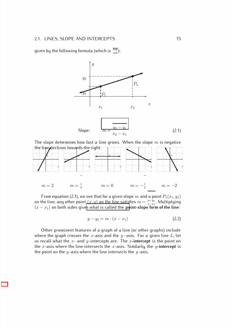
Generally, the slope describes how fast the line grows towards the right.For any two points P 1(x1, y1) and P 2(x2, y2) on the line L, the slope m is
7/18/2019 Precalculus Tradler Carley
http://slidepdf.com/reader/full/precalculus-tradler-carley 25/424
2.1. LINES, SLOPE AND INTERCEPTS 15
given by the following formula (which is riserun
):
x
y
P 2
P 1
x1 x2
y1
y2
Slope: m = y2 − y1
x2 − x1(2.1)
The slope determines how fast a line grows. When the slope m is negativethe line declines towards the right.
x
y
x
y
x
y
x
y
x
y
m = 2 m = 12
m = 0 m = −12
m = −2
From equation (2.1), we see that for a given slope m and a point P 1(x1, y1)on the line, any other point (x, y) on the line satisfies m = y−y1
x−x1. Multiplying
(x − x1) on both sides gives what is called the point-slope form of the line:
y − y1 = m · (x − x1) (2.2)
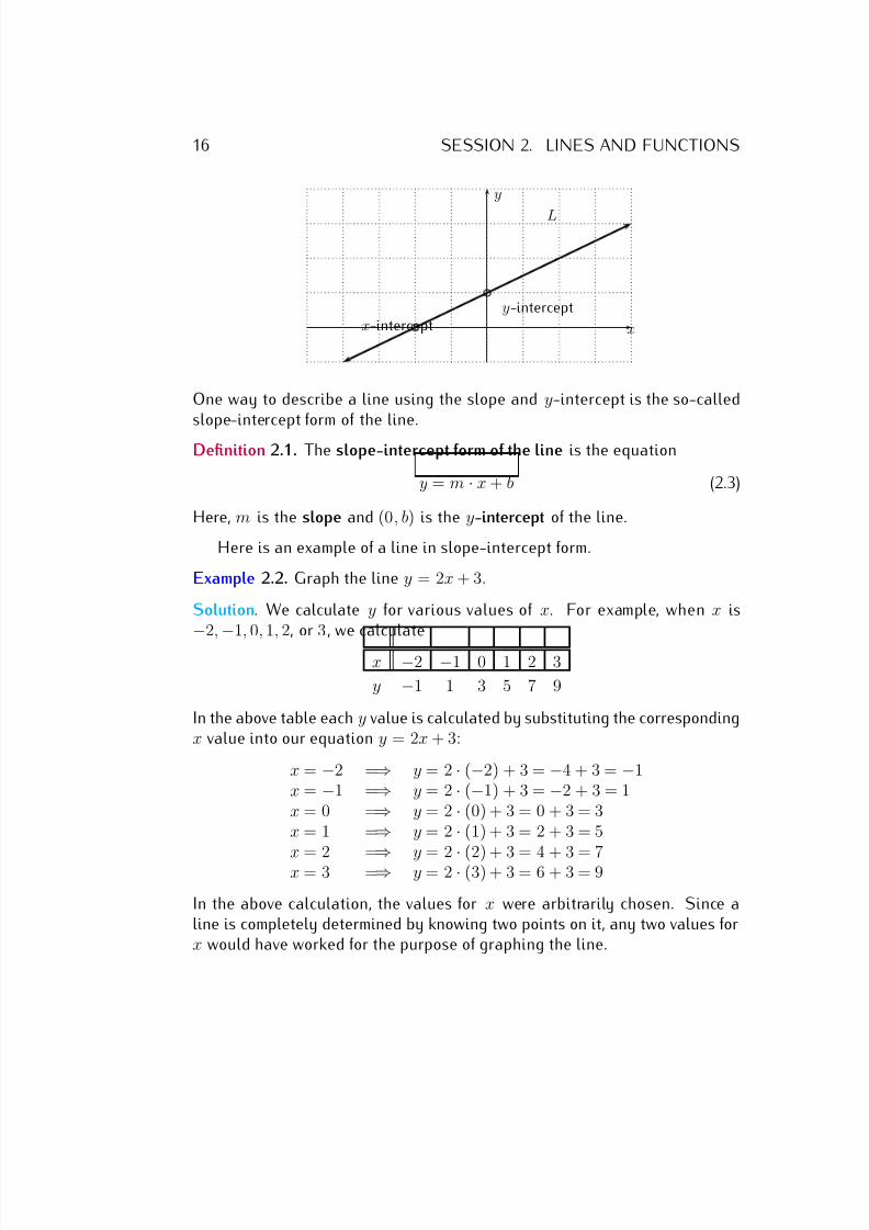
Other prominent features of a graph of a line (or other graphs) includewhere the graph crosses the x-axis and the y−axis. For a given line L, letus recall what the x- and y-intercepts are. The x-intercept is the point onthe x-axis where the line intersects the x-axis. Similarly, the y-intercept isthe point on the y-axis where the line intersects the y-axis.
7/18/2019 Precalculus Tradler Carley
http://slidepdf.com/reader/full/precalculus-tradler-carley 26/424
16 SESSION 2. LINES AND FUNCTIONS
x
y
L
y-interceptx-intercept
One way to describe a line using the slope and y-intercept is the so-calledslope-intercept form of the line.
Definition 2.1. The slope-intercept form of the line is the equation
y = m · x + b (2.3)
Here, m is the slope and (0, b) is the y-intercept of the line.
Here is an example of a line in slope-intercept form.
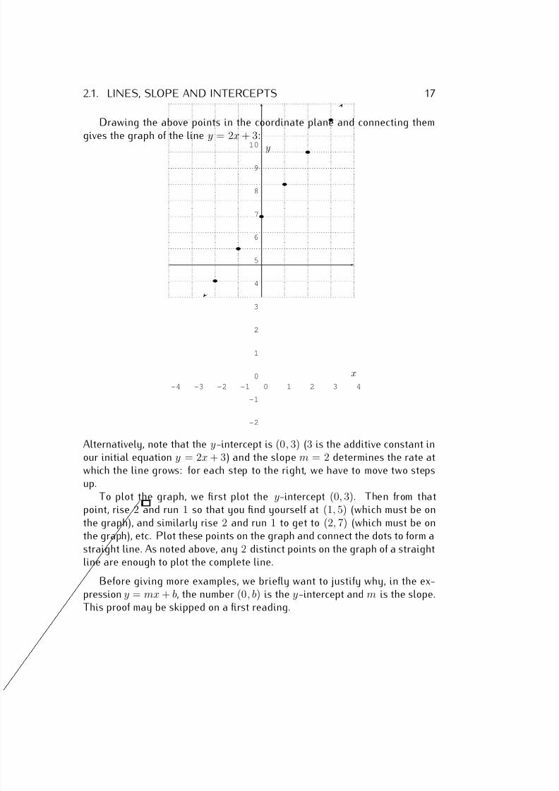
Example 2.2. Graph the line y = 2x + 3.
Solution. We calculate y for various values of x. For example, when x is
−2,
−1, 0, 1, 2, or 3, we calculate
x −2 −1 0 1 2 3
y −1 1 3 5 7 9
In the above table each y value is calculated by substituting the correspondingx value into our equation y = 2x + 3:
x = −2 =⇒ y = 2 · (−2) + 3 = −4 + 3 = −1x = −1 =⇒ y = 2 · (−1) + 3 = −2 + 3 = 1x = 0 =⇒ y = 2 · (0) + 3 = 0 + 3 = 3x = 1 =⇒ y = 2 · (1) + 3 = 2 + 3 = 5x = 2 =
⇒ y = 2
·(2) + 3 = 4 + 3 = 7
x = 3 =⇒ y = 2 · (3) + 3 = 6 + 3 = 9
In the above calculation, the values for x were arbitrarily chosen. Since aline is completely determined by knowing two points on it, any two values forx would have worked for the purpose of graphing the line.
7/18/2019 Precalculus Tradler Carley
http://slidepdf.com/reader/full/precalculus-tradler-carley 27/424
2.1. LINES, SLOPE AND INTERCEPTS 17
Drawing the above points in the coordinate plane and connecting them
gives the graph of the line y = 2x + 3:
-4 -3 -2 -1 0 1 2 3 4
-2
-1
0
1
2
3
4
5
6
7
8
9
10
x
y
Alternatively, note that the y-intercept is (0, 3) (3 is the additive constant inour initial equation y = 2x + 3) and the slope m = 2 determines the rate atwhich the line grows: for each step to the right, we have to move two stepsup.
To plot the graph, we first plot the y-intercept (0, 3). Then from thatpoint, rise 2 and run 1 so that you find yourself at (1, 5) (which must be onthe graph), and similarly rise 2 and run 1 to get to (2, 7) (which must be onthe graph), etc. Plot these points on the graph and connect the dots to form a
straight line. As noted above, any 2 distinct points on the graph of a straightline are enough to plot the complete line.
Before giving more examples, we briefly want to justify why, in the ex-pression y = mx + b, the number (0, b) is the y-intercept and m is the slope.This proof may be skipped on a first reading.
7/18/2019 Precalculus Tradler Carley
http://slidepdf.com/reader/full/precalculus-tradler-carley 28/424
18 SESSION 2. LINES AND FUNCTIONS
Proof that (0, b) is the y-intercept, and m is the slope.
Given the line y = mx + b, we want to calculate its y-intercept and itsslope. The y-intercept is the value of y where x = 0. Therefore, we have thatthe y−coordinate of the y-intercept is
y = m · 0 + b = b.
This shows the first claim.Next, to see why m is the slope, note that P 1(x1, y1) lies on the line
exactly when y1 = mx1 + b. Similarly, P 2(x2, y2) lies on the line exactly wheny2 = mx2 + b. Subtracting y1 = mx1 + b from y2 = mx2 + b, we obtain:
y2
−y1 = (mx2 + b)
−(mx1 + b) = mx2 + b
−mx1
−b = m
·(x2
−x1).
Dividing by (x2 − x1) gives
y2 − y1
(x2 − x1) =
m · (x2 − x1)
(x2 − x1) =
m
1 = m.
By Equation (2.1) the fraction y2−y1
x2−x1is the slope, establishing that our m is
indeed the slope, as we claimed.
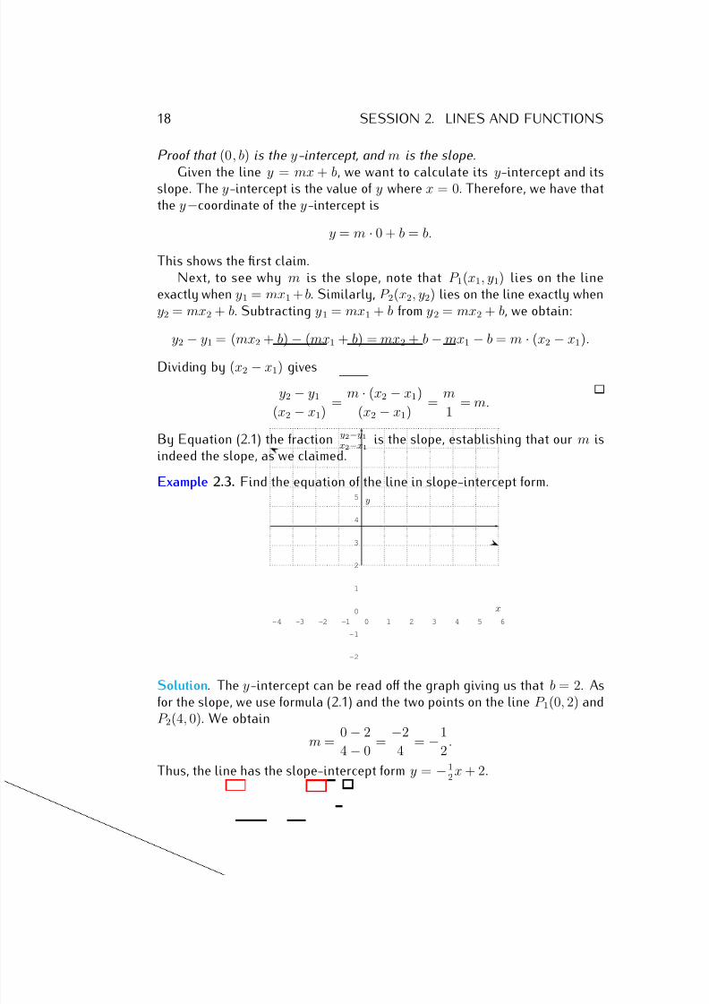
Example 2.3. Find the equation of the line in slope-intercept form.
-4 -3 -2 -1 0 1 2 3 4 5 6
-2
-1
0
1
2
3
4
5
x
y
Solution. The y-intercept can be read off the graph giving us that b = 2. As
for the slope, we use formula (2.1) and the two points on the line P 1(0, 2) andP 2(4, 0). We obtain
m = 0 − 2
4 − 0 =
−2
4 = −1
2.
Thus, the line has the slope-intercept form y = −12
x + 2.
7/18/2019 Precalculus Tradler Carley
http://slidepdf.com/reader/full/precalculus-tradler-carley 29/424
2.1. LINES, SLOPE AND INTERCEPTS 19
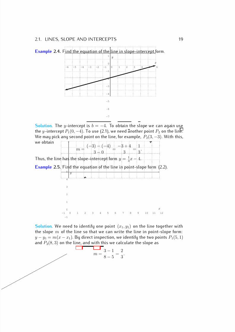
Example 2.4. Find the equation of the line in slope-intercept form.
-6 -5 -4 -3 -2 -1 0 1 2 3 4 5 6
-7
-6
-5
-4
-3
-2
-1
0
1
xy
Solution. The y-intercept is b = −4. To obtain the slope we can again usethe y-intercept P 1(0, −4). To use (2.1), we need another point P 2 on the line.We may pick any second point on the line, for example, P 2(3, −3). With this,we obtain
m = (−3) − (−4)
3 − 0 =
−3 + 4
3 =
1
3.
Thus, the line has the slope-intercept form y = 13
x − 4.
Example 2.5. Find the equation of the line in point-slope form (2.2).
-1 0 1 2 3 4 5 6 7 8 9 10 11 12
-1
0
1
2
3
4
5
x
y
Solution. We need to identify one point (x1, y1) on the line together with
the slope m of the line so that we can write the line in point-slope form:y − y1 = m(x − x1). By direct inspection, we identify the two points P 1(5, 1)and P 2(8, 3) on the line, and with this we calculate the slope as
m = 3 − 1
8 − 5 =
2
3.
7/18/2019 Precalculus Tradler Carley
http://slidepdf.com/reader/full/precalculus-tradler-carley 30/424
20 SESSION 2. LINES AND FUNCTIONS
Using the point (5, 1) we write the line in point-slope form as follows:
y − 1 = 2
3(x − 5)
Note that our answer depends on the chosen point (5, 1) on the line. Indeed,if we choose a different point on the line, such as (8, 3), we obtain a differentequation, (which nevertheless represents the same line):
y − 3 = 2
3(x − 8)
Note, that we do not need to solve this for y, since we are looking for ananswer in point-slope form.
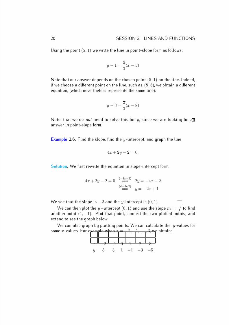
Example 2.6. Find the slope, find the y-intercept, and graph the line
4x + 2y − 2 = 0.
Solution. We first rewrite the equation in slope-intercept form.
4x + 2y − 2 = 0 (−4x+2)
=⇒ 2y = −4x + 2(divide 2)
=⇒ y = −2x + 1
We see that the slope is −2 and the y-intercept is (0, 1).
We can then plot the y−intercept (0, 1) and use the slope m = −21
to findanother point (1, −1). Plot that point, connect the two plotted points, andextend to see the graph below.
We can also graph by plotting points. We can calculate the y-values forsome x-values. For example when x = −2, −1, . . . , 3, we obtain:
x −2 −1 0 1 2 3
y 5 3 1 −1 −3 −5
7/18/2019 Precalculus Tradler Carley
http://slidepdf.com/reader/full/precalculus-tradler-carley 31/424
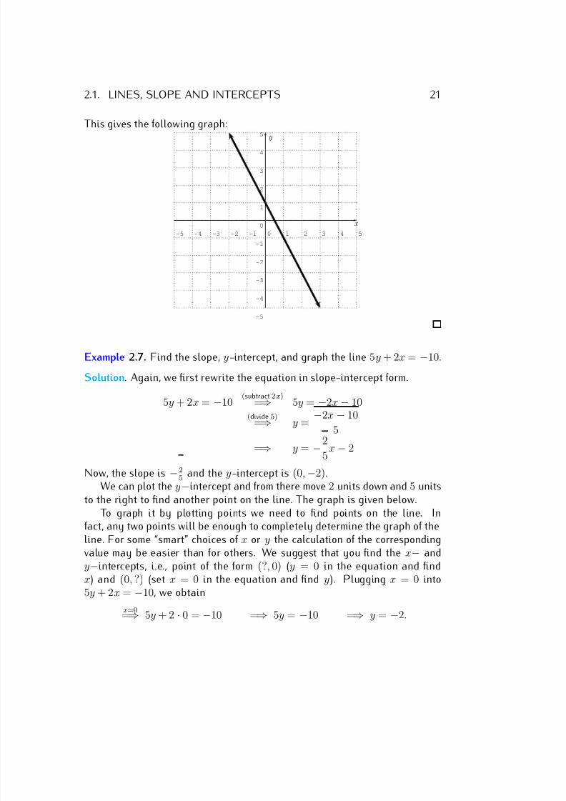
2.1. LINES, SLOPE AND INTERCEPTS 21
This gives the following graph:
-5 -4 -3 -2 -1 0 1 2 3 4 5
-5
-4
-3
-2
-1
0
1
2
3
4
5
x
y
Example 2.7. Find the slope, y-intercept, and graph the line 5y + 2x = −10.
Solution. Again, we first rewrite the equation in slope-intercept form.
5y + 2x = −10 (subtract 2x)
=⇒ 5y = −2x − 10(divide 5)
=⇒ y = −2x − 105
=⇒ y = −2
5x − 2
Now, the slope is −25 and the y-intercept is (0, −2).
We can plot the y−intercept and from there move 2 units down and 5 unitsto the right to find another point on the line. The graph is given below.
To graph it by plotting points we need to find points on the line. Infact, any two points will be enough to completely determine the graph of theline. For some “smart” choices of x or y the calculation of the correspondingvalue may be easier than for others. We suggest that you find the x
− and
y−intercepts, i.e., point of the form (?, 0) (y = 0 in the equation and findx) and (0, ?) (set x = 0 in the equation and find y). Plugging x = 0 into5y + 2x = −10, we obtain
x=0=⇒ 5y + 2 · 0 = −10 =⇒ 5y = −10 =⇒ y = −2.
7/18/2019 Precalculus Tradler Carley
http://slidepdf.com/reader/full/precalculus-tradler-carley 32/424
22 SESSION 2. LINES AND FUNCTIONS
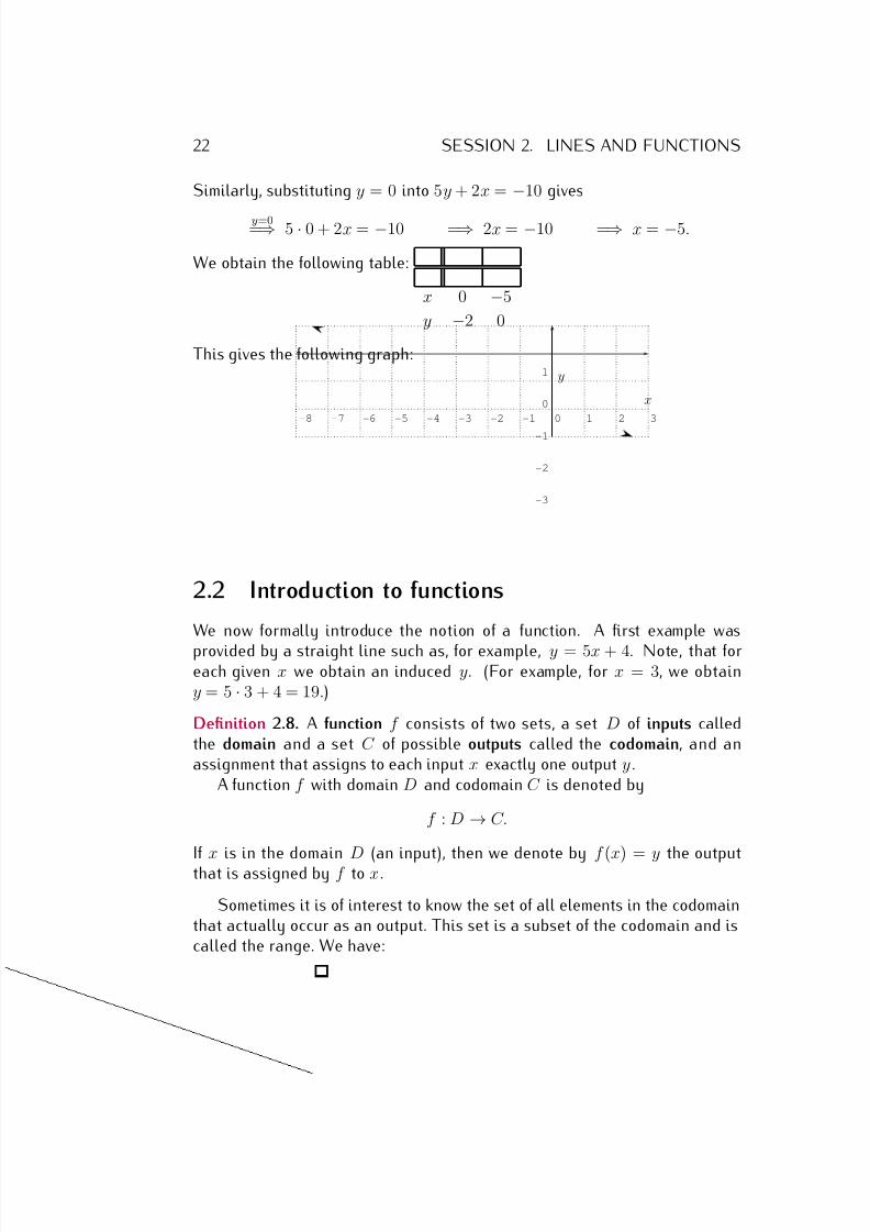
Similarly, substituting y = 0 into 5y + 2x = −10 gives
y=0=⇒ 5 · 0 + 2x = −10 =⇒ 2x = −10 =⇒ x = −5.
We obtain the following table:
x 0 −5
y −2 0
This gives the following graph:
-8 -7 -6 -5 -4 -3 -2 -1 0 1 2 3
-3
-2
-1
0
1
x
y
2.2 Introduction to functions
We now formally introduce the notion of a function. A first example was
provided by a straight line such as, for example, y = 5x + 4. Note, that foreach given x we obtain an induced y. (For example, for x = 3, we obtainy = 5 · 3 + 4 = 19.)
Definition 2.8. A function f consists of two sets, a set D of inputs calledthe domain and a set C of possible outputs called the codomain, and anassignment that assigns to each input x exactly one output y .
A function f with domain D and codomain C is denoted by
f : D → C.
If x is in the domain D (an input), then we denote by f (x) = y the outputthat is assigned by f to x.
Sometimes it is of interest to know the set of all elements in the codomainthat actually occur as an output. This set is a subset of the codomain and iscalled the range. We have:
7/18/2019 Precalculus Tradler Carley
http://slidepdf.com/reader/full/precalculus-tradler-carley 33/424
2.2. INTRODUCTION TO FUNCTIONS 23
Definition 2.9. The range R of a function f is a subset of the codomain given
by R = {f (x) | x in the domain of f }. That is, the range is the set of alloutputs.
Warning 2.10. Some authors use a slightly different convention by calling the range what we called thecodomain above.
Since we will be dealing with many functions it is convenient to name vari-ous functions (usually with letters f, g, h, etc). Often we will implicitly assumethat a domain and codomain are given without specifying these explicitly. If the range can be determined and the codomain is not given explicitly, then we
take the codomain to be the range. If the range can not easily be determinedand the codomain is not explicitly given, then the codomain should be takento be a ‘simple’ set which clearly contains the range.
There are several ways to represent a particular function (all of whichmay not apply to a specific function): via a table of values (listing the input-output pairs), via a formula (with the domain and range explicitly or implicitlygiven), via a graph (representing input-output pairs on a coordinate plane),or in words, just to name a few. We have seen examples of the first three of these in previous sections. Our discussion in this section goes into greaterdetail.
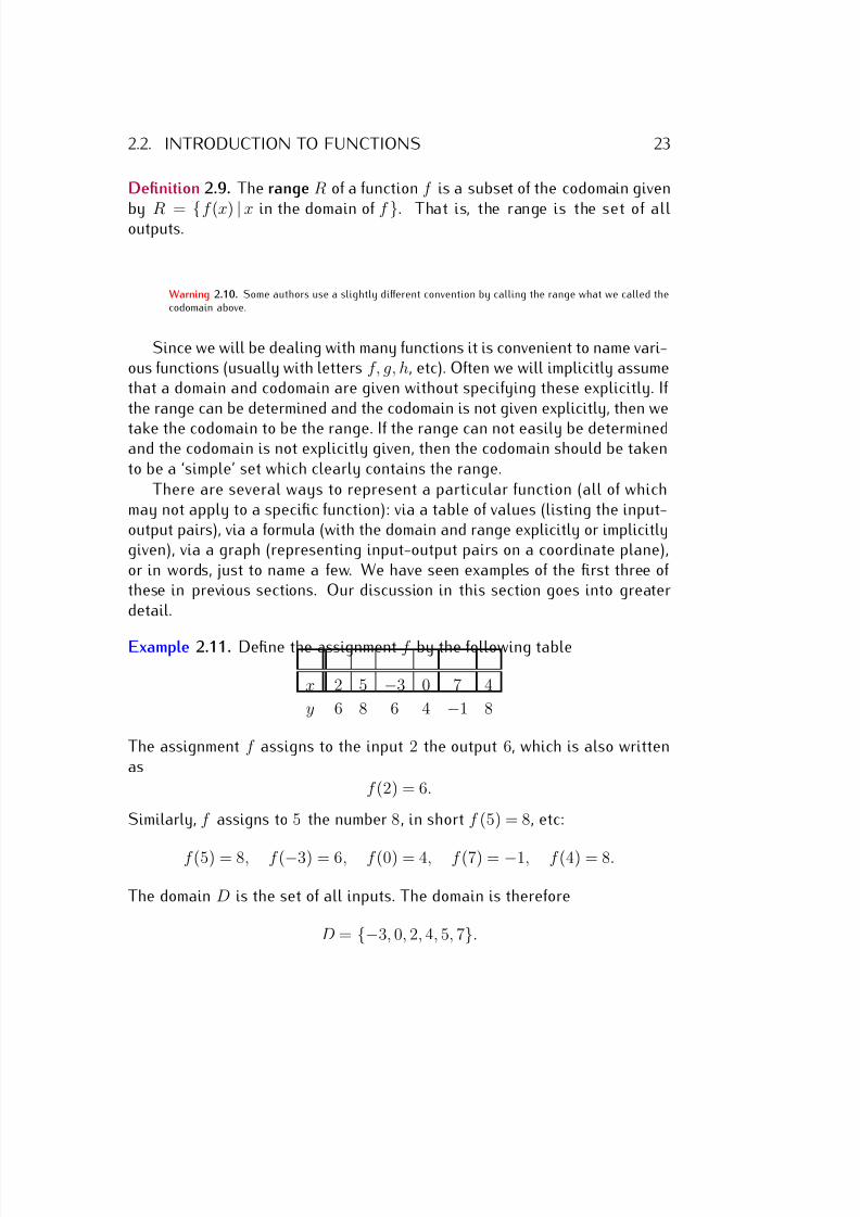
Example 2.11. Define the assignment f by the following table
x 2 5 −3 0 7 4
y 6 8 6 4 −1 8
The assignment f assigns to the input 2 the output 6, which is also writtenas
f (2) = 6.
Similarly, f assigns to 5 the number 8, in short f (5) = 8, etc:
f (5) = 8, f (−3) = 6, f (0) = 4, f (7) = −1, f (4) = 8.
The domain D is the set of all inputs. The domain is therefore
D = {−3, 0, 2, 4, 5, 7}.
7/18/2019 Precalculus Tradler Carley
http://slidepdf.com/reader/full/precalculus-tradler-carley 34/424
24 SESSION 2. LINES AND FUNCTIONS
The range R is the set of all outputs. The range is therefore
R = {−1, 4, 6, 8}.
The assignment f is indeed a function since each element of the domain getsassigned exactly one element in the range. Note that for an input numberthat is not in the domain, f does not assign an output to it. For example,
f (1) = undefined.
Note also that f (5) = 8 and f (4) = 8, so that f assigns to the inputs 5and 4 the same output 8. Similarly, f also assigns the same output to theinputs 2 and
−3. Therefore we see that:
• A function may assign the same output to two different inputs!
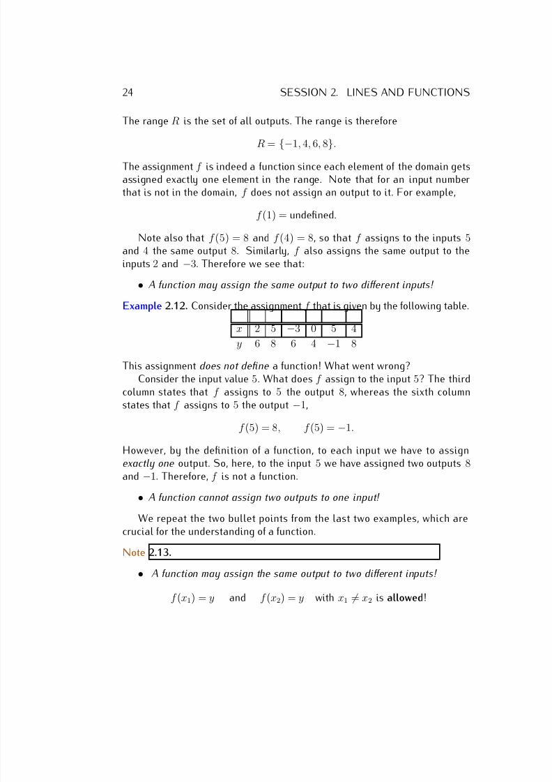
Example 2.12. Consider the assignment f that is given by the following table.
x 2 5 −3 0 5 4
y 6 8 6 4 −1 8
This assignment does not define a function! What went wrong?Consider the input value 5. What does f assign to the input 5? The third
column states that f assigns to 5 the output 8, whereas the sixth columnstates that f assigns to 5 the output
−1,
f (5) = 8, f (5) = −1.
However, by the definition of a function, to each input we have to assignexactly one output. So, here, to the input 5 we have assigned two outputs 8and −1. Therefore, f is not a function.
• A function cannot assign two outputs to one input!
We repeat the two bullet points from the last two examples, which arecrucial for the understanding of a function.
Note 2.13.
• A function may assign the same output to two different inputs!
f (x1) = y and f (x2) = y with x1 = x2 is allowed!
7/18/2019 Precalculus Tradler Carley
http://slidepdf.com/reader/full/precalculus-tradler-carley 35/424
2.2. INTRODUCTION TO FUNCTIONS 25
• A function cannot assign two outputs to one input!
f (x) = y1 and f (x) = y2 with y1 = y2 is not allowed!
Example 2.14. A university creates a mentoring program, which matches eachfreshman student with a senior student as his or her mentor. Within this pro-gram it is guaranteed that each freshman gets precisely one mentor, howevertwo freshmen may receive the same mentor. Does the assignment of freshmento mentor, or mentor to freshmen describe a function? If so, what is its domain,what is its range?
Solution. Since a senior may mentor several freshman, we cannot take amentor as an “input,” as he or she would be assigned to several “output”freshmen students. So freshman is not a function of mentor.
On the other hand, we can assign each freshmen to exactly one mentor,which therefore describes a function. The domain (the set of all inputs) isgiven by the set of all freshmen students. The range (the set of all outputs) isgiven by the set of all senior students that are mentors. The function assignseach “input” freshmen student to his or her unique “output” mentor.
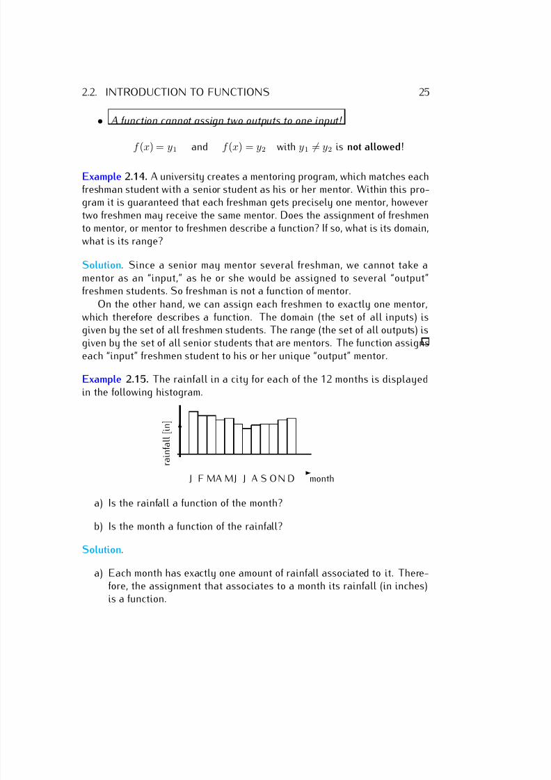
Example 2.15. The rainfall in a city for each of the 12 months is displayedin the following histogram.
r a i n f a l l
[ i n ]
J F MA MJ J A S ON D month
a) Is the rainfall a function of the month?
b) Is the month a function of the rainfall?
Solution.
a) Each month has exactly one amount of rainfall associated to it. There-fore, the assignment that associates to a month its rainfall (in inches)is a function.
7/18/2019 Precalculus Tradler Carley
http://slidepdf.com/reader/full/precalculus-tradler-carley 36/424
26 SESSION 2. LINES AND FUNCTIONS
b) If we take a certain rainfall amount as our input data, can we associate
a unique month to it? For example, February and March have the sameamount of rainfall. Therefore, to one input amount of rainfall we cannotassign a unique month. The month is not a function of the rainfall.
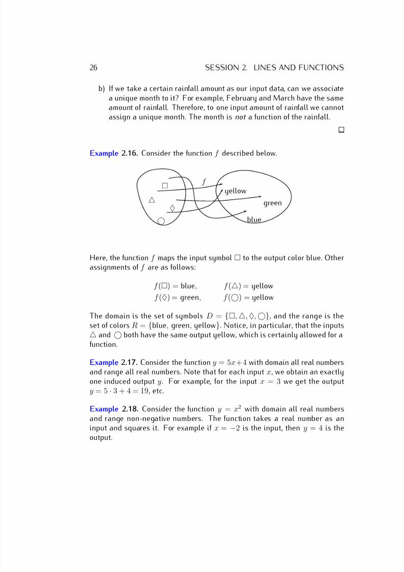
Example 2.16. Consider the function f described below.
△♦
yellow
green
blue
f
Here, the function f maps the input symbol to the output color blue. Otherassignments of f are as follows:
f () = blue, f (△) = yellow
f (♦) = green, f () = yellow
The domain is the set of symbols D = {, △,♦, }, and the range is theset of colors R = {blue, green, yellow}. Notice, in particular, that the inputs△ and both have the same output yellow, which is certainly allowed for afunction.
Example 2.17. Consider the function y = 5x+4 with domain all real numbersand range all real numbers. Note that for each input x, we obtain an exactlyone induced output y. For example, for the input x = 3 we get the outputy = 5 · 3 + 4 = 19, etc.
Example 2.18. Consider the function y = x2 with domain all real numbersand range non-negative numbers. The function takes a real number as aninput and squares it. For example if x = −2 is the input, then y = 4 is theoutput.
7/18/2019 Precalculus Tradler Carley
http://slidepdf.com/reader/full/precalculus-tradler-carley 37/424
2.2. INTRODUCTION TO FUNCTIONS 27
Example 2.19. For each real number x, denote by ⌊x⌋ the greatest integer
that is less or equal to x. We call ⌊x⌋ the floor of x. For example, to calculate⌊4.37⌋, note that all integers 4, 3, 2, . . . are less or equal to 4.37:
. . . , −3, −2, −1, 0, 1, 2, 3, 4 ≤ 4.37
The greatest of these integers is 4, so that ⌊4.37⌋ = 4. We define the floorfunction as f (x) = ⌊x⌋. Here are more examples of function values of thefloor function.
⌊7.3⌋ = 7, ⌊π⌋ = 3, ⌊−4.65⌋ = −5,
⌊12⌋ = 12, −26
3 = ⌊−8.667⌋ = −9
The domain of the floor function is the set of all real numbers, that is D = R.The range is the set of all integers, R = Z.
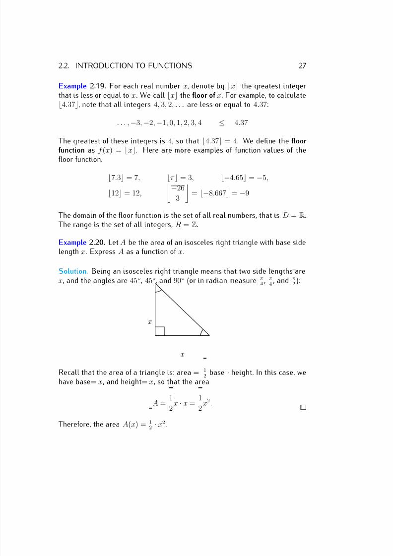
Example 2.20. Let A be the area of an isosceles right triangle with base sidelength x. Express A as a function of x.
Solution. Being an isosceles right triangle means that two side lengths arex, and the angles are 45◦, 45◦, and 90◦ (or in radian measure π
4 , π4 , and π
2 ):
x
x
Recall that the area of a triangle is: area = 12
base · height. In this case, wehave base= x, and height= x, so that the area
A = 1
2x · x =
1
2x2.
Therefore, the area A(x) = 12 · x2.
7/18/2019 Precalculus Tradler Carley
http://slidepdf.com/reader/full/precalculus-tradler-carley 38/424
28 SESSION 2. LINES AND FUNCTIONS
Example 2.21. Consider the equation y = x2 + 3. This equation associates
to each input number a exactly one output number b = a2
+ 3. Therefore, theequation defines a function. For example:
To the input 5 we assign the output 52 + 3 = 25 + 3 = 28.
The domain D is all real numbers, D = R. Since x2 is always ≥ 0, wesee that x2 + 3 ≥ 3, and vice versa every number y ≥ 3 can be written asy = x2 + 3. (To see this, note that the input x =
√ y − 3 for y ≥ 3 gives
the output x2 − 3 = (√
y − 3)2 + 3 = y − 3 + 3 = y .) Therefore, the range isR = [3, ∞).
Example 2.22. Consider the equation x2 +y2 = 25. Does this equation definey as a function of x? That is, does this equation assign to each input x exactlyone output y?
An input number x gets assigned to y with x2 + y2 = 25. Solving this fory, we obtain
y2 = 25 − x2 =⇒ y = ±√
25 − x2.
Therefore, there are two possible outputs associated to the input x(= 5):
either y = +√
25
−x2 or y =
−
√ 25
−x2.
For example, the input x = 0 has two outputs y = 5 and y = −5. However,a function cannot assign two outputs to one input x! The conclusion is thatx2 + y2 = 25 does not determine y as a function!
Note 2.23. Note that if y = f (x) then x is called the independent variable
and y is called the dependent variable (since it depends on x). If x = g(y)then y is the independent variable and x is the dependent variable (since itdepends on y ).
2.3 Exercises
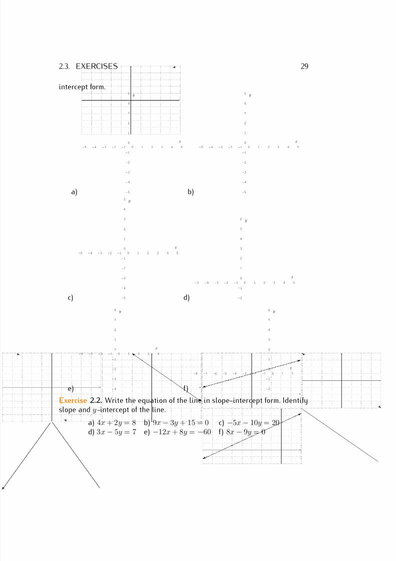
Exercise 2.1. Find the slope and y-intercept of the line with the given data.Using the slope and y-intercept, write the equation of the line in slope-
7/18/2019 Precalculus Tradler Carley
http://slidepdf.com/reader/full/precalculus-tradler-carley 39/424
2.3. EXERCISES 29
intercept form.
a)
-5 -4 -3 -2 -1 0 1 2 3 4 5
-5
-4
-3
-2
-1
0
1
2
3
4
5
x
y
b)
-5 -4 -3 -2 -1 0 1 2 3 4 5
-5
-4
-3
-2
-1
0
1
2
3
4
5
x
y
c)
-5 -4 -3 -2 -1 0 1 2 3 4 5
-5
-4
-3
-2
-1
0
1
2
3
4
5
x
y
d)
-5 -4 -3 -2 -1 0 1 2 3 4 5
-2
-1
0
1
2
3
4
5
6
x
y
e)
-4 -3 -2 -1 0 1 2 3 4
-4
-3
-2
-1
0
1
2
3
4
x
y
f )
-8 -7 -6 -5 -4 -3 -2 -1 0 1 2
-2
-1
0
1
2
3
4
5
6
x
y
Exercise 2.2. Write the equation of the line in slope-intercept form. Identifyslope and y-intercept of the line.
a) 4x + 2y = 8 b) 9x − 3y + 15 = 0 c) −5x − 10y = 20d) 3x − 5y = 7 e) −12x + 8y = −60 f ) 8x − 9y = 0
7/18/2019 Precalculus Tradler Carley
http://slidepdf.com/reader/full/precalculus-tradler-carley 40/424
30 SESSION 2. LINES AND FUNCTIONS
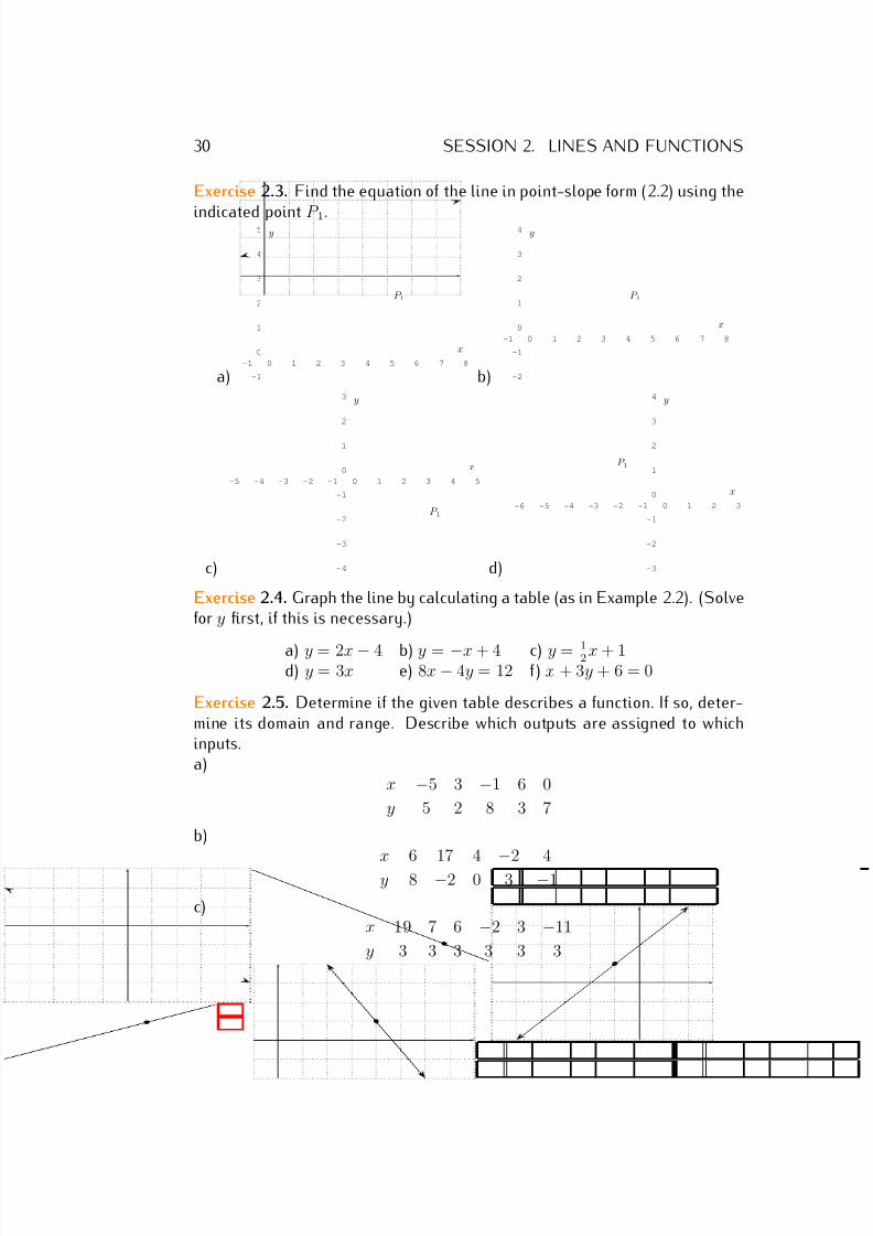
Exercise 2.3. Find the equation of the line in point-slope form (2.2) using the
indicated point P 1.
a)-1 0 1 2 3 4 5 6 7 8
-1
0
1
2
3
4
5
x
y
P 1
b)
-1 0 1 2 3 4 5 6 7 8
-2
-1
0
1
2
3
4
x
y
P 1
c)
-5 -4 -3 -2 -1 0 1 2 3 4 5
-4
-3
-2
-1
0
1
2
3
x
y
P 1
d)
-6 -5 -4 -3 -2 -1 0 1 2 3
-3
-2
-1
0
1
2
3
4
x
y
P 1
Exercise 2.4. Graph the line by calculating a table (as in Example 2.2). (Solvefor y first, if this is necessary.)
a) y = 2x − 4 b) y = −x + 4 c) y = 12 x + 1d) y = 3x e) 8x − 4y = 12 f ) x + 3y + 6 = 0
Exercise 2.5. Determine if the given table describes a function. If so, deter-mine its domain and range. Describe which outputs are assigned to whichinputs.a)
x −5 3 −1 6 0
y 5 2 8 3 7
b)x 6 17 4
−2 4
y 8 −2 0 3 −1
c)x 19 7 6 −2 3 −11
y 3 3 3 3 3 3
7/18/2019 Precalculus Tradler Carley
http://slidepdf.com/reader/full/precalculus-tradler-carley 41/424
2.3. EXERCISES 31
d)
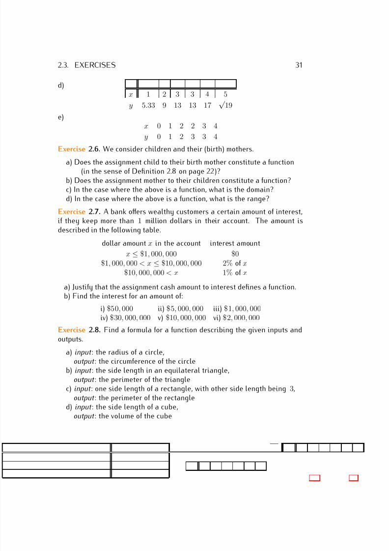
x 1 2 3 3 4 5y 5.33 9 13 13 17
√ 19
e)x 0 1 2 2 3 4
y 0 1 2 3 3 4
Exercise 2.6. We consider children and their (birth) mothers.
a) Does the assignment child to their birth mother constitute a function(in the sense of Definition 2.8 on page 22)?
b) Does the assignment mother to their children constitute a function?
c) In the case where the above is a function, what is the domain?d) In the case where the above is a function, what is the range?
Exercise 2.7. A bank offers wealthy customers a certain amount of interest,if they keep more than 1 million dollars in their account. The amount isdescribed in the following table.
dollar amount x in the account interest amount
x ≤ $1, 000, 000 $0$1, 000, 000 < x ≤ $10, 000, 000 2% of x
$10, 000, 000 < x 1% of x
a) Justify that the assignment cash amount to interest defines a function.b) Find the interest for an amount of:
i) $50, 000 ii) $5, 000, 000 iii) $1, 000, 000iv) $30, 000, 000 v) $10, 000, 000 vi) $2, 000, 000
Exercise 2.8. Find a formula for a function describing the given inputs andoutputs.
a) input : the radius of a circle,output : the circumference of the circle
b) input : the side length in an equilateral triangle,output : the perimeter of the triangle
c) input : one side length of a rectangle, with other side length being 3,output : the perimeter of the rectangle
d) input : the side length of a cube,output : the volume of the cube
7/18/2019 Precalculus Tradler Carley
http://slidepdf.com/reader/full/precalculus-tradler-carley 42/424
Session 3
Functions by formulas and graphs
3.1 Functions given by formulas
Most of the time we will discuss functions that take some real numbers asinputs, and give real numbers as outputs. These functions are commonlydescribed with a formula.
Example 3.1. For the given function f , calculate the outputs f (2), f (−3), andf (−1).
a) f (x) = 3x + 4, b) f (x) = √ x2
− 3,c) f (x) =
5x − 6 , for −1 ≤ x ≤ 1
x3 + 2x , for 1 < x ≤ 5 d) f (x) = x+2
x+3 .
Solution. We substitute the input values into the function and simplify.
a) f (2) = 3 · 2 + 4 = 6 + 4 = 10,
f (−3) = 3 · (−3) + 4 = −9 + 4 = −5,
f (−1) = 3 · (−1) + 4 = −3 + 4 = 1.
b) Similarly, we calculate
f (2) =√
22 − 3 =√
4 − 3 =√
1 = 1,
f (−3) =
(−3)2 − 3 =√
9 − 3 =√
6,
f (−1) =
(−1)2 − 3 =√
1 − 3 =√ −2 = undefined.
32
7/18/2019 Precalculus Tradler Carley
http://slidepdf.com/reader/full/precalculus-tradler-carley 43/424
3.1. FUNCTIONS GIVEN BY FORMULAS 33
For the last step, we are assuming that we only deal with real numbers. Of
course, as we will see later on, √ −2 can be defined as a complex number.But for now, we will only allow real solutions outputs.
c) The function f (x) =
5x − 6 , for −1 ≤ x ≤ 1
x3 + 2x , for 1 < x ≤ 5 is given as a piece-
wise defined function. We have to substitute the values into the correctbranch:
f (2) = 23 + 2 · 2 = 8 + 4 = 12, since 1 < 2 ≤ 5,
f (−3) = undefined, since −3 is not in any of the two branches,
f (−1) = 5 · (−1) − 7 = −5 − 6 = −11, since − 1 ≤ −1 ≤ 1.
d) Finally for f (x) = x+2
x+3, we have:
f (2) = 2 + 2
2 + 3 =
4
5,
f (−3) = −3 + 2
−3 + 3 =
−1
0 = undefined,
f (−1) = −1 + 2
−1 + 3 =
1
2.
Example 3.2. Let f be the function given by f (x) = x2 + 2x − 3. Find thefollowing function values.
a) f (5) b) f (2) c) f (−2) d) f (0)
e) f (√
5) f ) f (√
3 + 1) g) f (a) h) f (a) + 5
i) f (x + h) j) f (x + h) − f (x) k) f (x+h)−f (x)h l) f (x)−f (a)
x−a
Solution. The first four function values ((a)-(d)) can be calculated directly:
f (5) = 52 + 2 · 5 − 3 = 25 + 10 − 3 = 32,
f (2) = 22 + 2 · 2 − 3 = 4 + 4 − 3 = 5,
f (−2) = (−2)2 + 2 · (−2) − 3 = 4 + −4 − 3 = −3,
f (0) = 02 + 2 · 0 − 3 = 0 + 0 − 3 = −3.
The next two values ((e) and (f)) are similar, but the arithmetic is a bitmore involved.
f (√
5) =√
52
+ 2 ·√
5 − 3 = 5 + 2 ·√
5 − 3 = 2 + 2 ·√
5,
7/18/2019 Precalculus Tradler Carley
http://slidepdf.com/reader/full/precalculus-tradler-carley 44/424
34 SESSION 3. FUNCTIONS BY FORMULAS AND GRAPHS
f (√
3 + 1) = (√
3 + 1)2 + 2 · (√
3 + 1) − 3
= (√ 3 + 1) · (√ 3 + 1) + 2 · (√ 3 + 1) − 3=
√ 3 ·
√ 3 + 2 ·
√ 3 + 1 · 1 + 2 ·
√ 3 + 2 − 3
= 3 + 2 ·√
3 + 1 + 2 ·√
3 + 2 − 3
= 3 + 4 ·√
3.
The last five values ((g)-(l)) are purely algebraic:
f (a) = a2 + 2 · a − 3,
f (a) + 5 = a2 + 2 · a − 3 + 5 = a2 + 2 · a + 2,
f (x + h) = (x + h)2 + 2 · (x + h) − 3
= x2
+ 2xh + h2
+ 2x + 2h − 3,f (x + h) − f (x) = (x2 + 2xh + h2 + 2x + 2h − 3) − (x2 + 2x − 3)
= x2 + 2xh + h2 + 2x + 2h − 3 − x2 − 2x + 3
= 2xh + h2 + 2h,
f (x + h) − f (x)
h =
2xh + h2 + 2h
h
= h · (2x + h + 2)
h = 2x + h + 2,
and
f (x) − f (a)x − a
= (x2 + 2x − 3) − (a2 + 2a − 3)x − a
= x2 + 2x − 3 − a2 − 2a + 3
x − a =
x2 − a2 + 2x − 2a
x − a
= (x + a)(x − a) + 2(x − a)
x − a =
(x − a)(x + a + 2)
(x − a) = x + a + 2.
The quotients f (x+h)−f (x)h
and f (x)−f (a)x−a
as in the last two examples 3.2(k)and (l) will become particularly important in calculus. They are called differ-
ence quotients. We now calculate some more examples of difference quotients.Example 3.3. Calculate the difference quotient f (x+h)−f (x)
h for
a) f (x) = x3 + 2, b) f (x) = 1
x.
7/18/2019 Precalculus Tradler Carley
http://slidepdf.com/reader/full/precalculus-tradler-carley 45/424
3.1. FUNCTIONS GIVEN BY FORMULAS 35
Solution. We calculate first the difference quotient step by step.
a) f (x + h) = (x + h)3 + 2 = (x + h) · (x + h) · (x + h) + 2
= (x2 + 2xh + h2) · (x + h) + 2
= x3 + 2x2h + xh2 + x2h + 2xh2 + h3 + 2,
= x3 + 3x2h + 3xh2 + h3 + 2.
Subtracting f (x) from f (x + h) gives
f (x + h) − f (x) = (x3 + 3x2h + 3xh2 + h3 + 2) − (x3 + 2)
= x3 + 3x2h + 3xh2 + h3 + 2 − x3 − 2
= 3x
2
h + 3xh
2
+ h
3
.
With this we obtain:
f (x + h) − f (x)
h =
3x2h + 3xh2 + h3
h
= h · (3x2 + 3xh + h2)
h = 3x2 + 3xh + h2.
We handle part (b) similarly.
b) f (x + h) = 1
x + h
,
so that
f (x + h) − f (x) = 1
x + h − 1
x.
We obtain the solution after simplifying the double fraction:
f (x + h) − f (x)
h =
1x+h − 1
x
h =
x−(x+h)(x+h)·x
h =
x−x−h(x+h)·x
h =
−h(x+h)·x
h
= −h
(x + h) · x · 1
h =
−1
(x + h) · x.
So far, we have not mentioned the domain and range of the functionsdefined above. Indeed, we will often not describe the domain explicitly butuse the following convention:
7/18/2019 Precalculus Tradler Carley
http://slidepdf.com/reader/full/precalculus-tradler-carley 46/424
36 SESSION 3. FUNCTIONS BY FORMULAS AND GRAPHS
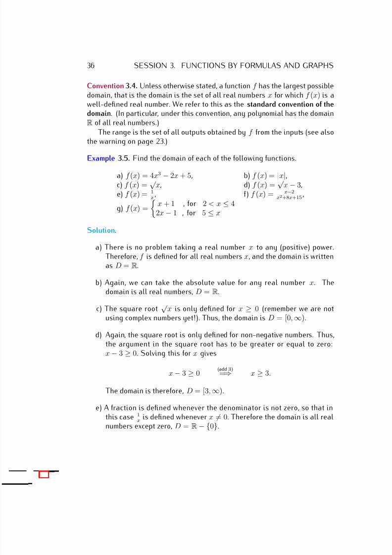
Convention 3.4. Unless otherwise stated, a function f has the largest possible
domain, that is the domain is the set of all real numbers x for which f (x) is awell-defined real number. We refer to this as the standard convention of thedomain. (In particular, under this convention, any polynomial has the domainR of all real numbers.)
The range is the set of all outputs obtained by f from the inputs (see alsothe warning on page 23.)
Example 3.5. Find the domain of each of the following functions.
a) f (x) = 4x3 − 2x + 5, b) f (x) = |x|,c) f (x) =
√ x, d) f (x) =
√ x
−3,
e) f (x) = 1x , f ) f (x) = x−2x2+8x+15 ,
g) f (x) =
x + 1 , for 2 < x ≤ 42x − 1 , for 5 ≤ x
Solution.
a) There is no problem taking a real number x to any (positive) power.Therefore, f is defined for all real numbers x, and the domain is writtenas D = R.
b) Again, we can take the absolute value for any real number x. The
domain is all real numbers, D = R.
c) The square root √
x is only defined for x ≥ 0 (remember we are notusing complex numbers yet!). Thus, the domain is D = [0, ∞).
d) Again, the square root is only defined for non-negative numbers. Thus,the argument in the square root has to be greater or equal to zero:x − 3 ≥ 0. Solving this for x gives
x − 3 ≥ 0 (add 3)
=⇒ x ≥ 3.
The domain is therefore, D = [3, ∞).
e) A fraction is defined whenever the denominator is not zero, so that inthis case 1
x is defined whenever x = 0. Therefore the domain is all realnumbers except zero, D = R− {0}.
7/18/2019 Precalculus Tradler Carley
http://slidepdf.com/reader/full/precalculus-tradler-carley 47/424
3.2. FUNCTIONS GIVEN BY GRAPHS 37
f) Again, we need to make sure that the denominator does not become
zero; however we do not care about the numerator. The denominator iszero exactly when x2 + 8x + 15 = 0. Solving this for x gives:
x2 + 8x + 15 = 0 =⇒ (x + 3) · (x + 5) = 0
=⇒ x + 3 = 0 or x + 5 = 0
=⇒ x = −3 or x = −5.
The domain is all real numbers except for −3 and −5, that is D =R− {−5, −3}.
g) The function is explicitly defined for all 2 < x ≤ 4 and 5 ≤ x. Therefore,the domain is D = (2, 4] ∪ [5, ∞).
3.2 Functions given by graphs
In many situations, a function is represented by its graph. The graph of a function f is the set of all points (on the coordinate plane) of the form(x, f (x)), where x is in the domain of f . We have already seen an exampleof graphing a function when we discussed lines and their graphs. Here isanother example that shows how the formulaic definition relates to the graphof the function.
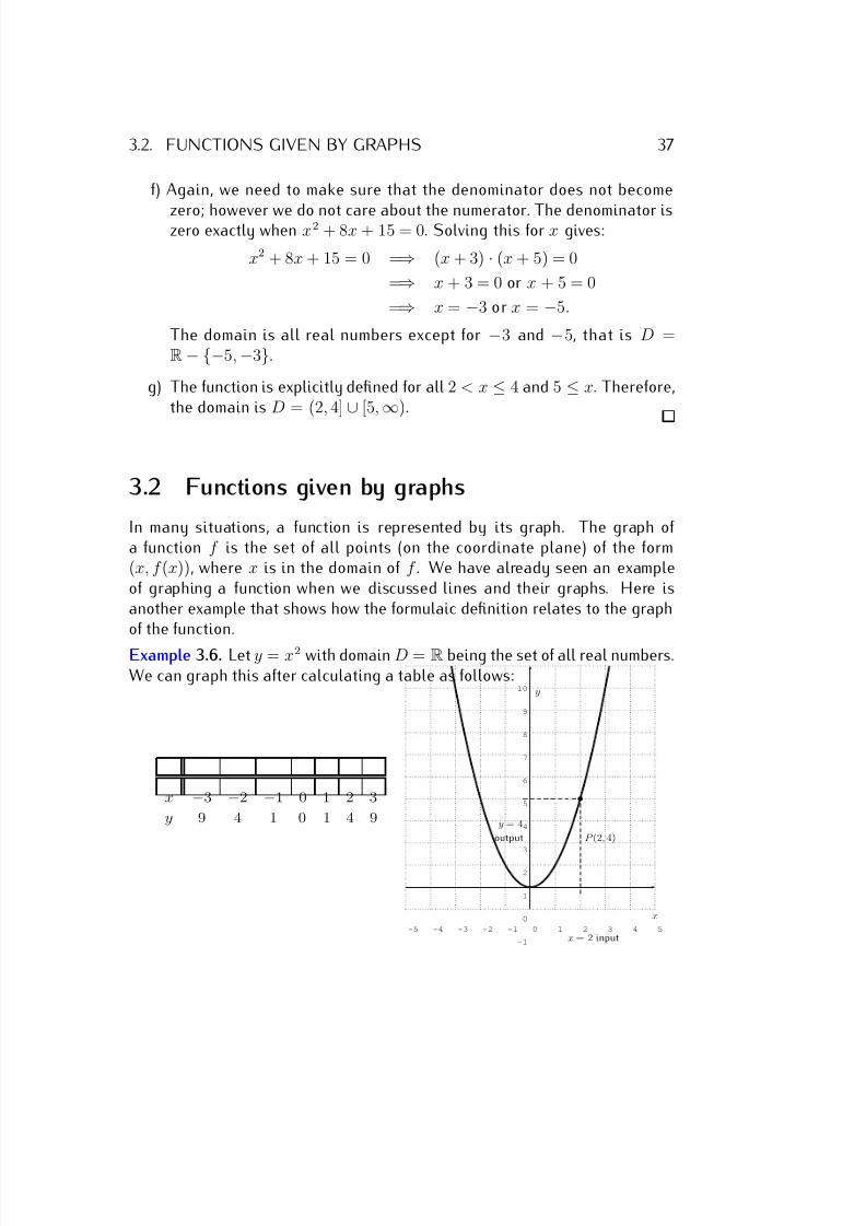
Example 3.6. Let y = x2 with domain D = R being the set of all real numbers.We can graph this after calculating a table as follows:
x −3 −2 −1 0 1 2 3
y 9 4 1 0 1 4 9
-5 -4 -3 -2 -1 0 1 2 3 4 5
-1
0
1
2
3
4
5
6
7
8
9
10
x
y
P (2, 4)
x = 2 input
y = 4
output
7/18/2019 Precalculus Tradler Carley
http://slidepdf.com/reader/full/precalculus-tradler-carley 48/424
38 SESSION 3. FUNCTIONS BY FORMULAS AND GRAPHS
Many function values can be read from this graph. For example, for the input
x = 2, we obtain the output y = 4. This corresponds to the point P (2, 4) onthe graph as depicted above.
In general, an input (placed on the x-axis) gets assigned to an output(placed on the y-axis) according to where the vertical line at x intersectswith the given graph. This is used in the next example.
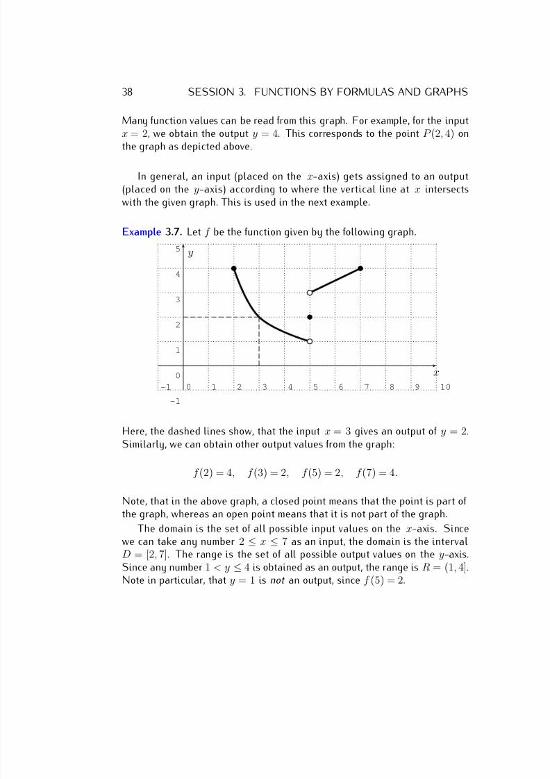
Example 3.7. Let f be the function given by the following graph.
-1 0 1 2 3 4 5 6 7 8 9 10
-1
0
1
2
3
4
5
x
y
Here, the dashed lines show, that the input x = 3 gives an output of y = 2.Similarly, we can obtain other output values from the graph:
f (2) = 4, f (3) = 2, f (5) = 2, f (7) = 4.
Note, that in the above graph, a closed point means that the point is part of the graph, whereas an open point means that it is not part of the graph.
The domain is the set of all possible input values on the x-axis. Since
we can take any number 2 ≤ x ≤ 7 as an input, the domain is the intervalD = [2, 7]. The range is the set of all possible output values on the y-axis.Since any number 1 < y ≤ 4 is obtained as an output, the range is R = (1, 4].Note in particular, that y = 1 is not an output, since f (5) = 2.
7/18/2019 Precalculus Tradler Carley
http://slidepdf.com/reader/full/precalculus-tradler-carley 49/424
3.2. FUNCTIONS GIVEN BY GRAPHS 39
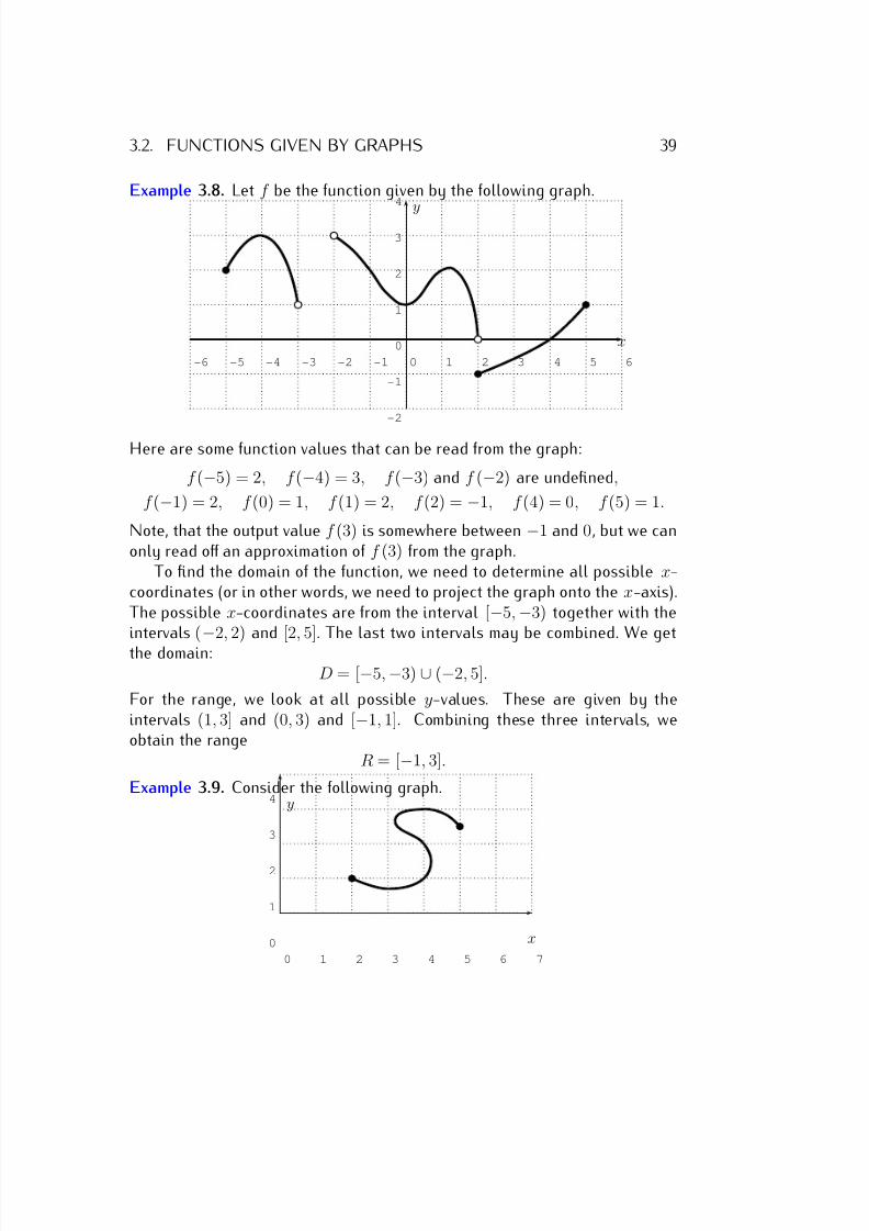
Example 3.8. Let f be the function given by the following graph.
-6 -5 -4 -3 -2 -1 0 1 2 3 4 5 6
-2
-1
0
1
2
3
4
x
y
Here are some function values that can be read from the graph:
f (−5) = 2, f (−4) = 3, f (−3) and f (−2) are undefined,
f (−1) = 2, f (0) = 1, f (1) = 2, f (2) = −1, f (4) = 0, f (5) = 1.
Note, that the output value f (3) is somewhere between −1 and 0, but we canonly read off an approximation of f (3) from the graph.
To find the domain of the function, we need to determine all possible x-coordinates (or in other words, we need to project the graph onto the x-axis).The possible x-coordinates are from the interval [−5, −3) together with theintervals (
−2, 2) and [2, 5]. The last two intervals may be combined. We get
the domain:D = [−5, −3) ∪ (−2, 5].
For the range, we look at all possible y-values. These are given by theintervals (1, 3] and (0, 3) and [−1, 1]. Combining these three intervals, weobtain the range
R = [−1, 3].
Example 3.9. Consider the following graph.
0 1 2 3 4 5 6 7
0
1
2
3
4
x
y
7/18/2019 Precalculus Tradler Carley
http://slidepdf.com/reader/full/precalculus-tradler-carley 50/424
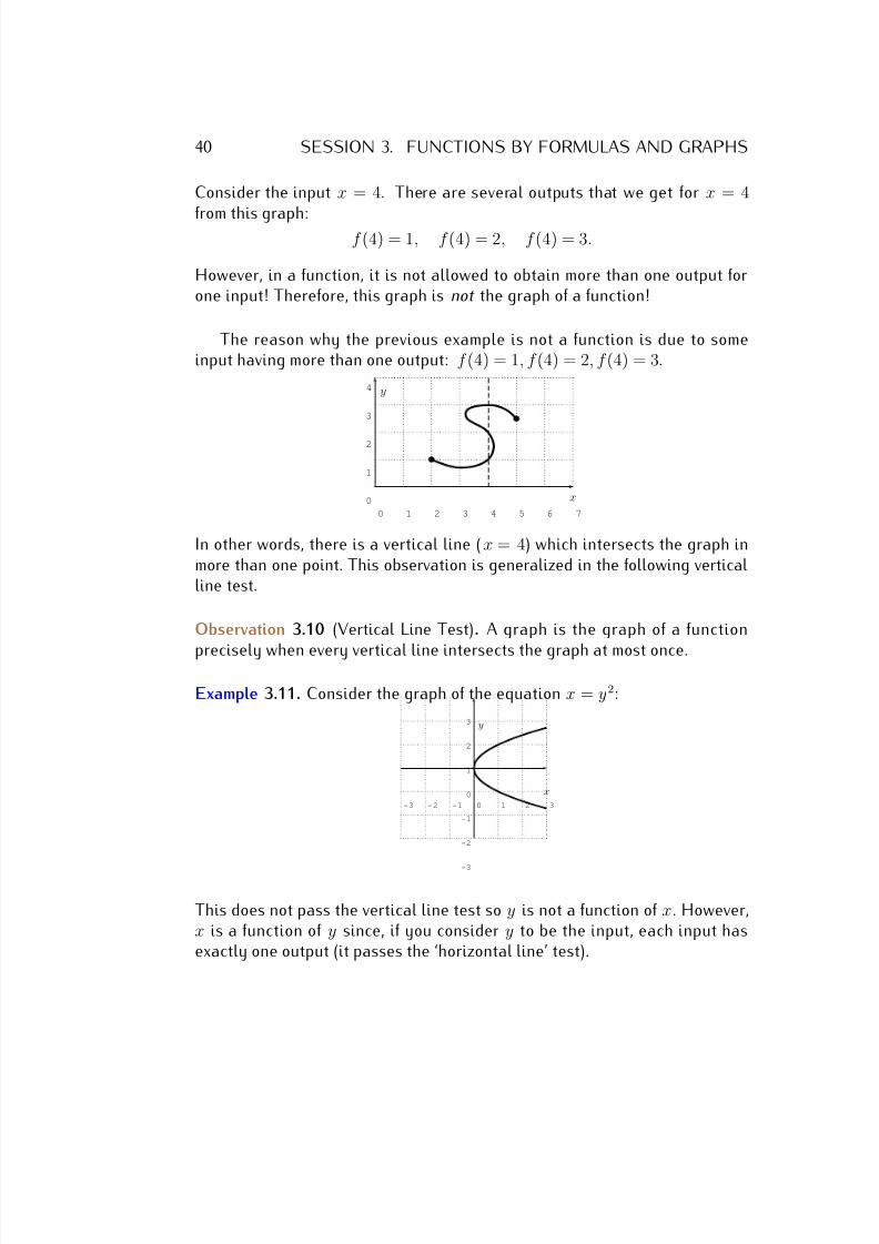
40 SESSION 3. FUNCTIONS BY FORMULAS AND GRAPHS
Consider the input x = 4. There are several outputs that we get for x = 4
from this graph:f (4) = 1, f (4) = 2, f (4) = 3.
However, in a function, it is not allowed to obtain more than one output forone input! Therefore, this graph is not the graph of a function!
The reason why the previous example is not a function is due to someinput having more than one output: f (4) = 1, f (4) = 2, f (4) = 3.
0 1 2 3 4 5 6 7
0
1
2
3
4
x
y
In other words, there is a vertical line (x = 4) which intersects the graph inmore than one point. This observation is generalized in the following verticalline test.
Observation 3.10 (Vertical Line Test). A graph is the graph of a function
precisely when every vertical line intersects the graph at most once.
Example 3.11. Consider the graph of the equation x = y2:
-3 -2 -1 0 1 2 3
-3
-2
-1
0
1
2
3
x
y
This does not pass the vertical line test so y is not a function of x. However,x is a function of y since, if you consider y to be the input, each input hasexactly one output (it passes the ‘horizontal line’ test).
7/18/2019 Precalculus Tradler Carley
http://slidepdf.com/reader/full/precalculus-tradler-carley 51/424
3.2. FUNCTIONS GIVEN BY GRAPHS 41
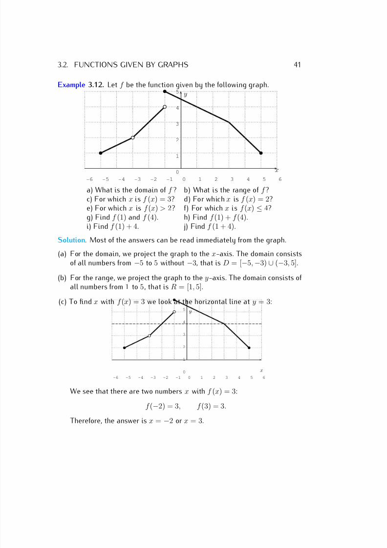
Example 3.12. Let f be the function given by the following graph.
-6 -5 -4 -3 -2 -1 0 1 2 3 4 5 6
0
1
2
3
4
5
x
y
a) What is the domain of f ? b) What is the range of f ?c) For which x is f (x) = 3? d) For which x is f (x) = 2?e) For which x is f (x) > 2? f) For which x is f (x) ≤ 4?g) Find f (1) and f (4). h) Find f (1) + f (4).i) Find f (1) + 4. j) Find f (1 + 4).
Solution. Most of the answers can be read immediately from the graph.
(a) For the domain, we project the graph to the x-axis. The domain consistsof all numbers from −5 to 5 without −3, that is D = [−5, −3) ∪ (−3, 5].
(b) For the range, we project the graph to the y-axis. The domain consists of
all numbers from 1 to 5, that is R = [1, 5].
(c) To find x with f (x) = 3 we look at the horizontal line at y = 3:
-6 -5 -4 -3 -2 -1 0 1 2 3 4 5 6
0
1
2
3
4
5
x
y
We see that there are two numbers x with f (x) = 3:
f (−2) = 3, f (3) = 3.
Therefore, the answer is x = −2 or x = 3.
7/18/2019 Precalculus Tradler Carley
http://slidepdf.com/reader/full/precalculus-tradler-carley 52/424
42 SESSION 3. FUNCTIONS BY FORMULAS AND GRAPHS
(d) Looking at the horizontal line y = 2, we see that there is only one x
with f (x) = 2; namely f (4) = 2. Note, that x = −3 does not solve theproblem, since f (−3) is undefined. The answer is x = 4.
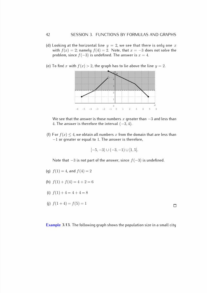
(e) To find x with f (x) > 2, the graph has to lie above the line y = 2.
-6 -5 -4 -3 -2 -1 0 1 2 3 4 5 6
0
1
2
3
4
5
x
y
We see that the answer is those numbers x greater than −3 and less than4. The answer is therefore the interval (−3, 4).
(f) For f (x) ≤ 4, we obtain all numbers x from the domain that are less than−1 or greater or equal to 1. The answer is therefore,
[
−5,
−3)
∪(
−3,
−1)
∪[1, 5].
Note that −3 is not part of the answer, since f (−3) is undefined.
(g) f (1) = 4, and f (4) = 2
(h) f (1) + f (4) = 4 + 2 = 6
(i) f (1) + 4 = 4 + 4 = 8
(j) f (1 + 4) = f (5) = 1
Example 3.13. The following graph shows the population size in a small city
7/18/2019 Precalculus Tradler Carley
http://slidepdf.com/reader/full/precalculus-tradler-carley 53/424
3.2. FUNCTIONS GIVEN BY GRAPHS 43
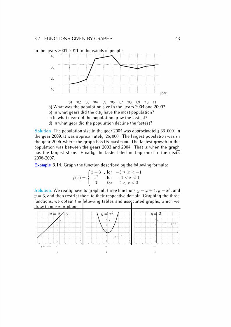
in the years 2001-2011 in thousands of people.
’01 ’02 ’03 ’04 ’05 ’06 ’07 ’08 ’09 ’10 ’11
10
20
30
40
year
a) What was the population size in the years 2004 and 2009?
b) In what years did the city have the most population?c) In what year did the population grow the fastest?d) In what year did the population decline the fastest?
Solution. The population size in the year 2004 was approximately 36, 000. Inthe year 2009, it was approximately 26, 000. The largest population was inthe year 2006, where the graph has its maximum. The fastest growth in thepopulation was between the years 2003 and 2004. That is when the graphhas the largest slope. Finally, the fastest decline happened in the years2006-2007.
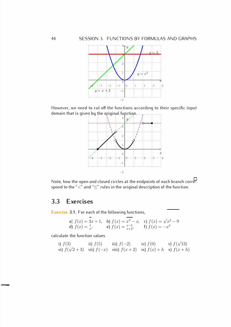
Example 3.14. Graph the function described by the following formula:
f (x) =x + 3 , for −3 ≤ x < −1
x2 , for −1 < x < 13 , for 2 < x ≤ 3
Solution. We really have to graph all three functions y = x + 4, y = x2, andy = 3, and then restrict them to their respective domain. Graphing the threefunctions, we obtain the following tables and associated graphs, which wedraw in one x-y-plane:
y = x + 3 y = x2 y = 3
-4 -3 -2 -1 0 1 2 3 4
-2
-1
0
1
2
3
4
x
y
y = x + 3
-4 -3 -2 -1 0 1 2 3 4
-2
-1
0
1
2
3
4
x
y
y = x2
-4 -3 -2 -1 0 1 2 3 4
-2
-1
0
1
2
3
4
x
y
y = 3
7/18/2019 Precalculus Tradler Carley
http://slidepdf.com/reader/full/precalculus-tradler-carley 54/424
44 SESSION 3. FUNCTIONS BY FORMULAS AND GRAPHS
-4 -3 -2 -1 0 1 2 3 4
-2
-1
0
1
2
3
4
x
y
y = 3
y = x2
y = x + 3
However, we need to cut off the functions according to their specific input
domain that is given by the original function.
-4 -3 -2 -1 0 1 2 3 4
-2
-1
0
1
2
3
4
x
y
Note, how the open and closed circles at the endpoints of each branch corre-spond to the “<” and “≤” rules in the original description of the function.
3.3 Exercises
Exercise 3.1. For each of the following functions,
a) f (x) = 3x + 1, b) f (x) = x2 − x, c) f (x) =√
x2 − 9d) f (x) = 1
x, e) f (x) = x−5
x+2, f ) f (x) =
−x3
calculate the function values
i) f (3) ii) f (5) iii) f (−2) iv) f (0) v) f (√
13)
vi) f (√
2 + 3) vii) f (−x) viii) f (x + 2) ix) f (x) + h x) f (x + h)
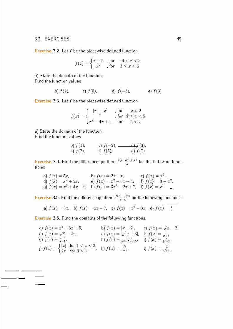
7/18/2019 Precalculus Tradler Carley
http://slidepdf.com/reader/full/precalculus-tradler-carley 55/424
3.3. EXERCISES 45
Exercise 3.2. Let f be the piecewise defined function
f (x) =
x − 5 , for −4 < x < 3x2 , for 3 ≤ x ≤ 6
a) State the domain of the function.Find the function values
b) f (2), c) f (5), d) f (−3), e) f (3)
Exercise 3.3. Let f be the piecewise defined function
f (x) = |x
| −x2 , for x < 2
7 , for 2 ≤ x < 5x2 − 4x + 1 , for 5 < x
a) State the domain of the function.Find the function values
b) f (1), c) f (−2), d) f (3),e) f (2), f ) f (5), g) f (7).
Exercise 3.4. Find the difference quotient f (x+h)−f (x)h
for the following func-tions:
a) f (x) = 5x, b) f (x) = 2x − 6, c) f (x) = x2,d) f (x) = x2 + 5x, e) f (x) = x2 + 3x + 4, f ) f (x) = 3 − x2,g) f (x) = x2 + 4x − 9, h) f (x) = 3x2 − 2x + 7, i) f (x) = x3
Exercise 3.5. Find the difference quotient f (x)−f (a)x−a
for the following functions:
a) f (x) = 3x, b) f (x) = 4x − 7, c) f (x) = x2 − 3x d) f (x) = 1x
Exercise 3.6. Find the domains of the following functions.
a) f (x) = x2 + 3x + 5, b) f (x) =|x
−2|, c) f (x) =
√ x
−2
d) f (x) = √ 8 − 2x, e) f (x) = |x + 3|, f ) f (x) = 1
x+6
g) f (x) = x−5x−7 , h) f (x) = x+1
x2−7x+10 , i) f (x) = x|x−2|
j) f (x) =
|x| for 1 < x < 22x for 3 ≤ x
, k) f (x) =√
xx−9
, l) f (x) = 5√ x+4
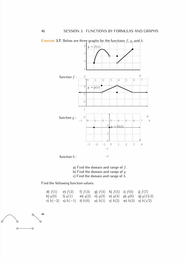
7/18/2019 Precalculus Tradler Carley
http://slidepdf.com/reader/full/precalculus-tradler-carley 56/424
46 SESSION 3. FUNCTIONS BY FORMULAS AND GRAPHS
Exercise 3.7. Below are three graphs for the functions f , g , and h.
function f :0 1 2 3 4 5 6 7
0
1
2
3
4
x
y = f (x)
function g :-1 0 1 2 3 4 5 6 7 8
0
1
2
3
4
x
y = g(x)
function h :
-3 -2 -1 0 1 2 3 4
-2
-1
0
1
2
x
y = h(x)
a) Find the domain and range of f .b) Find the domain and range of g .c) Find the domain and range of h.
Find the following function values:
d) f (1) e) f (2) f) f (3) g) f (4) h) f (5) i) f (6) j) f (7)k) g(0) l) g (1) m) g(2) n) g(3) o) g(4) p) g(6) q) g(13.2)
r) h(−2) s) h(−1) t) h(0) u) h(1) v) h(2) w) h(3) x) h(√
2)
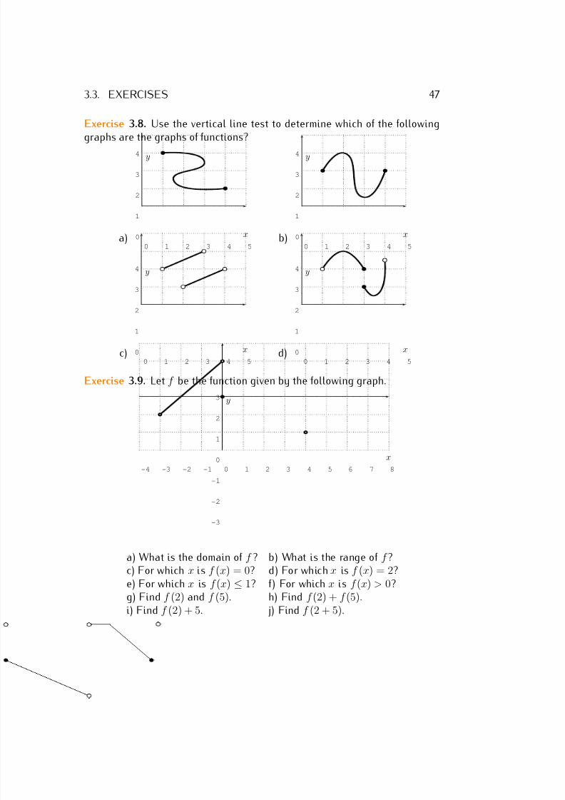
7/18/2019 Precalculus Tradler Carley
http://slidepdf.com/reader/full/precalculus-tradler-carley 57/424
3.3. EXERCISES 47
Exercise 3.8. Use the vertical line test to determine which of the following
graphs are the graphs of functions?
a)0 1 2 3 4 5
0
1
2
3
4
x
y
b)0 1 2 3 4 5
0
1
2
3
4
x
y
c)0 1 2 3 4 5
0
1
2
3
4
x
y
d)0 1 2 3 4 5
0
1
2
3
4
x
y
Exercise 3.9. Let f be the function given by the following graph.
-4 -3 -2 -1 0 1 2 3 4 5 6 7 8
-3
-2
-1
0
1
2
3
x
y
a) What is the domain of f ? b) What is the range of f ?c) For which x is f (x) = 0? d) For which x is f (x) = 2?e) For which x is f (x) ≤ 1? f) For which x is f (x) > 0?g) Find f (2) and f (5). h) Find f (2) + f (5).i) Find f (2) + 5. j) Find f (2 + 5).
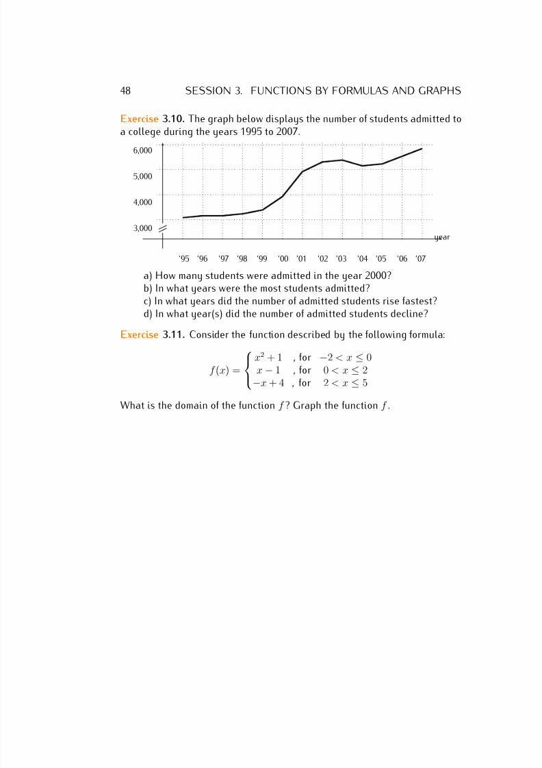
7/18/2019 Precalculus Tradler Carley
http://slidepdf.com/reader/full/precalculus-tradler-carley 58/424
48 SESSION 3. FUNCTIONS BY FORMULAS AND GRAPHS
Exercise 3.10. The graph below displays the number of students admitted to
a college during the years 1995 to 2007.
’95 ’96 ’97 ’98 ’99 ’00 ’01 ’02 ’03 ’04 ’05 ’06 ’07
3,000
4,000
5,000
6,000
year
a) How many students were admitted in the year 2000?b) In what years were the most students admitted?c) In what years did the number of admitted students rise fastest?d) In what year(s) did the number of admitted students decline?
Exercise 3.11. Consider the function described by the following formula:
f (x) =
x2 + 1 , for −2 < x ≤ 0x − 1 , for 0 < x ≤ 2
−x + 4 , for 2 < x ≤ 5
What is the domain of the function f ? Graph the function f .
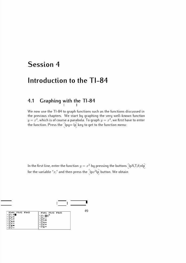
7/18/2019 Precalculus Tradler Carley
http://slidepdf.com/reader/full/precalculus-tradler-carley 59/424
Session 4
Introduction to the TI-84
4.1 Graphing with the TI-84
We now use the TI-84 to graph functions such as the functions discussed inthe previous chapters. We start by graphing the very well-known functiony = x2, which is of course a parabola. To graph y = x2, we first have to enter
the function. Press the
lpy= lp key to get to the function menu:
In the first line, enter the function y = x2 by pressing the buttons
lpX,T,θ,nlp
for the variable “x,” and then press the
lpx2lp button. We obtain
49
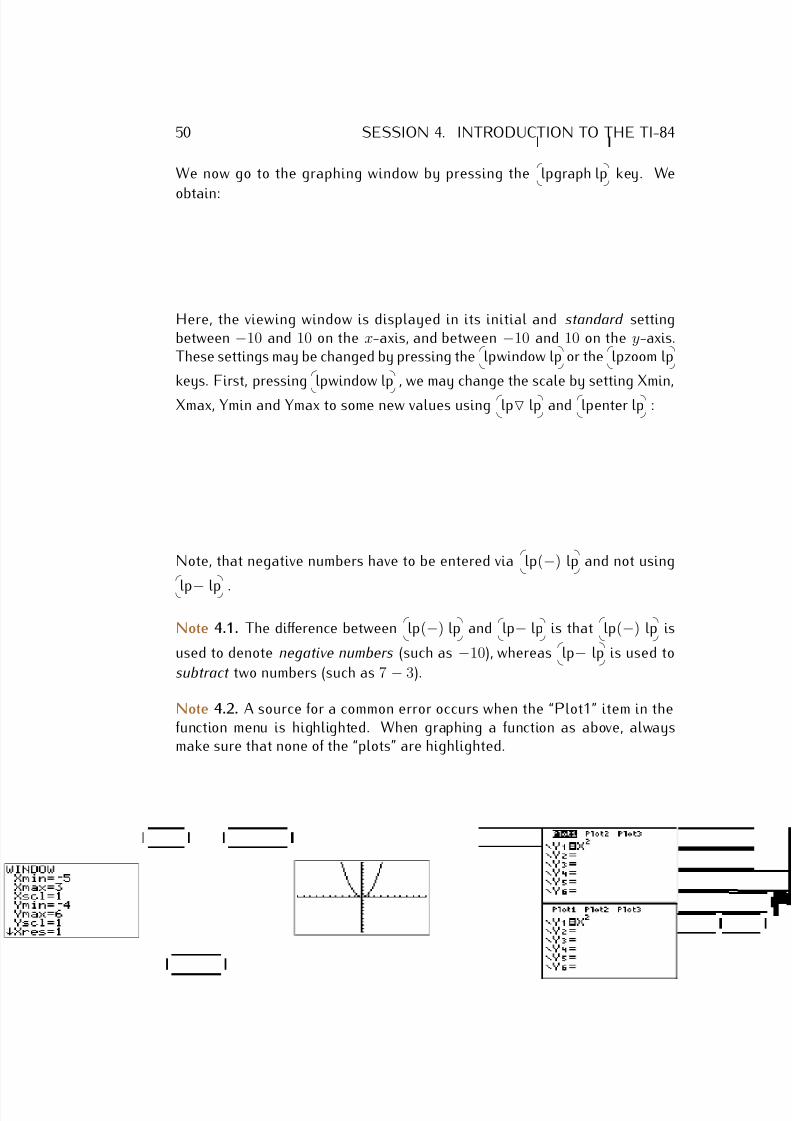
7/18/2019 Precalculus Tradler Carley
http://slidepdf.com/reader/full/precalculus-tradler-carley 60/424
50 SESSION 4. INTRODUCTION TO THE TI-84
We now go to the graphing window by pressing the
lpgraph lp key. We
obtain:
Here, the viewing window is displayed in its initial and standard settingbetween −10 and 10 on the x-axis, and between −10 and 10 on the y-axis.These settings may be changed by pressing the
lpwindow lp or the
lpzoom lp
keys. First, pressing
lpwindow lp , we may change the scale by setting Xmin,
Xmax, Ymin and Ymax to some new values using
lp▽ lp and
lpenter lp :
Note, that negative numbers have to be entered via
lp(−) lp and not using
lp− lp .
Note 4.1. The difference between
lp(−) lp and
lp− lp is that
lp(−) lp is
used to denote negative numbers (such as −10), whereas
lp− lp is used to
subtract two numbers (such as 7 − 3).
Note 4.2. A source for a common error occurs when the “Plot1” item in thefunction menu is highlighted. When graphing a function as above, alwaysmake sure that none of the “plots” are highlighted.
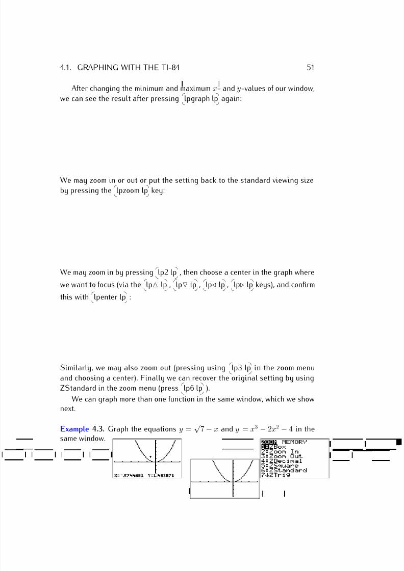
7/18/2019 Precalculus Tradler Carley
http://slidepdf.com/reader/full/precalculus-tradler-carley 61/424
4.1. GRAPHING WITH THE TI-84 51
After changing the minimum and maximum x- and y-values of our window,
we can see the result after pressing
lpgraph lp again:
We may zoom in or out or put the setting back to the standard viewing size
by pressing the
lpzoom lp key:
We may zoom in by pressing
lp2 lp , then choose a center in the graph where
we want to focus (via the
lp△ lp ,
lp▽ lp ,
lp⊳ lp ,
lp⊲ lp keys), and confirm
this with
lpenter lp :
Similarly, we may also zoom out (pressing using
lp3 lp in the zoom menu
and choosing a center). Finally we can recover the original setting by using
ZStandard in the zoom menu (press
lp6 lp ).
We can graph more than one function in the same window, which we shownext.
Example 4.3. Graph the equations y =√
7 − x and y = x3 − 2x2 − 4 in thesame window.
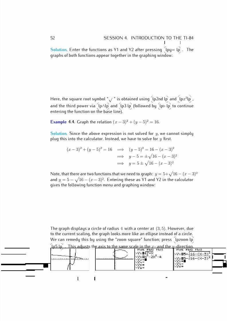
7/18/2019 Precalculus Tradler Carley
http://slidepdf.com/reader/full/precalculus-tradler-carley 62/424
52 SESSION 4. INTRODUCTION TO THE TI-84
Solution. Enter the functions as Y1 and Y2 after pressing
lpy= lp . The
graphs of both functions appear together in the graphing window:
Here, the square root symbol “√
” is obtained using
lp2nd lp and
lpx2lp ,
and the third power via
lp∧lp and
lp3 lp (followed by
lp⊲ lp to continue
entering the function on the base line).
Example 4.4. Graph the relation (x − 3)2 + (y − 5)2 = 16.
Solution. Since the above expression is not solved for y, we cannot simplyplug this into the calculator. Instead, we have to solve for y first.
(x − 3)2 + (y − 5)2 = 16 =⇒ (y − 5)2 = 16 − (x − 3)2
=⇒ y − 5 = ±
16 − (x − 3)2
=
⇒ y = 5
± 16
−(x
−3)2
Note, that there are two functions that we need to graph: y = 5+
16 − (x − 3)2
and y = 5 −
16 − (x − 3)2. Entering these as Y1 and Y2 in the calculatorgives the following function menu and graphing window:
The graph displays a circle of radius 4 with a center at (3, 5). However, dueto the current scaling, the graph looks more like an ellipse instead of a circle.
We can remedy this by using the “zoom square” function; press
lpzoom lp
lp5 lp . This adjusts the axis to the same scale in the x- and the y-direction.
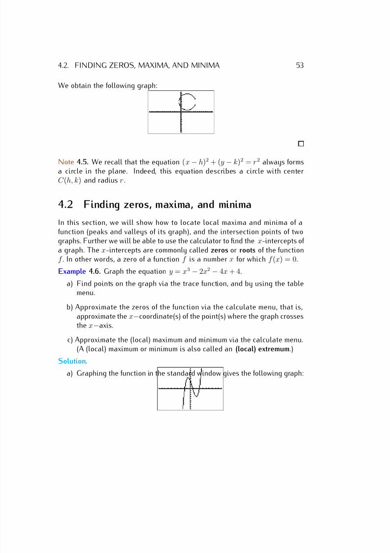
7/18/2019 Precalculus Tradler Carley
http://slidepdf.com/reader/full/precalculus-tradler-carley 63/424
4.2. FINDING ZEROS, MAXIMA, AND MINIMA 53
We obtain the following graph:
Note 4.5. We recall that the equation (x − h)2 + (y − k)2 = r2 always formsa circle in the plane. Indeed, this equation describes a circle with centerC (h, k) and radius r .
4.2 Finding zeros, maxima, and minima
In this section, we will show how to locate local maxima and minima of afunction (peaks and valleys of its graph), and the intersection points of twographs. Further we will be able to use the calculator to find the x-intercepts of a graph. The x-intercepts are commonly called zeros or roots of the functionf . In other words, a zero of a function f is a number x for which f (x) = 0.
Example 4.6. Graph the equation y = x3 − 2x2 − 4x + 4.
a) Find points on the graph via the trace function, and by using the table
menu.
b) Approximate the zeros of the function via the calculate menu, that is,approximate the x−coordinate(s) of the point(s) where the graph crossesthe x−axis.
c) Approximate the (local) maximum and minimum via the calculate menu.(A (local) maximum or minimum is also called an (local) extremum.)
Solution.
a) Graphing the function in the standard window gives the following graph:
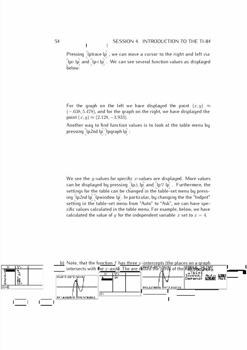
7/18/2019 Precalculus Tradler Carley
http://slidepdf.com/reader/full/precalculus-tradler-carley 64/424
54 SESSION 4. INTRODUCTION TO THE TI-84
Pressing
lptrace lp , we can move a cursor to the right and left via
lp⊲ lp and
lp⊳ lp . We can see several function values as displayedbelow:
For the graph on the left we have displayed the point (x, y) ≈(−.638, 5.478), and for the graph on the right, we have displayed thepoint (x, y)
≈(2.128,
−3.933).
Another way to find function values is to look at the table menu by
pressing
lp2nd lp
lpgraph lp :
We see the y-values for specific x-values are displayed. More values
can be displayed by pressing
lp△ lp and
lp▽ lp . Furthermore, thesettings for the table can be changed in the table-set menu by press-
ing
lp2nd lp
lpwindow lp . In particular, by changing the the “Indpnt”
setting in the table-set menu from “Auto” to “Ask”, we can have spe-cific values calculated in the table menu. For example, below, we havecalculated the value of y for the independent variable x set to x = 4.
b) Note, that the function f has three x-intercepts (the places on a graphintersects with the x-axis). The are called the zeros of the function and
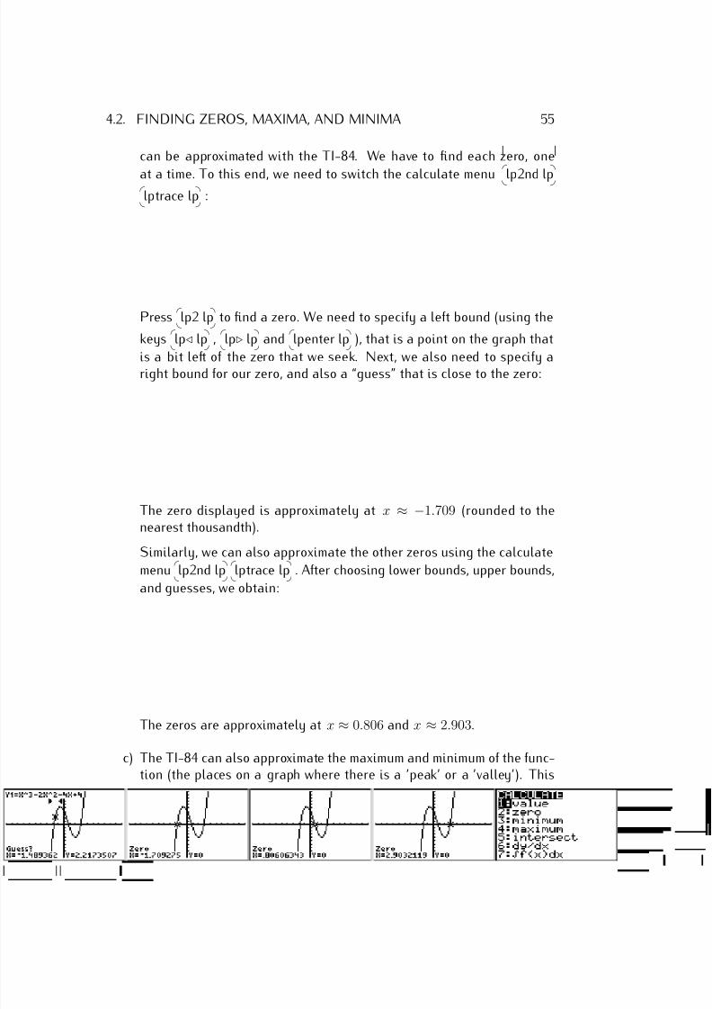
7/18/2019 Precalculus Tradler Carley
http://slidepdf.com/reader/full/precalculus-tradler-carley 65/424
4.2. FINDING ZEROS, MAXIMA, AND MINIMA 55
can be approximated with the TI-84. We have to find each zero, one
at a time. To this end, we need to switch the calculate menu
lp2nd lp
lptrace lp :
Press
lp2 lp to find a zero. We need to specify a left bound (using the
keys
lp⊳ lp ,
lp⊲ lp and
lpenter lp ), that is a point on the graph that
is a bit left of the zero that we seek. Next, we also need to specify aright bound for our zero, and also a “guess” that is close to the zero:
The zero displayed is approximately at x ≈ −1.709 (rounded to the
nearest thousandth).Similarly, we can also approximate the other zeros using the calculate
menu
lp2nd lp
lptrace lp . After choosing lower bounds, upper bounds,
and guesses, we obtain:
The zeros are approximately at x ≈ 0.806 and x ≈ 2.903.
c) The TI-84 can also approximate the maximum and minimum of the func-tion (the places on a graph where there is a ’peak’ or a ’valley’). This
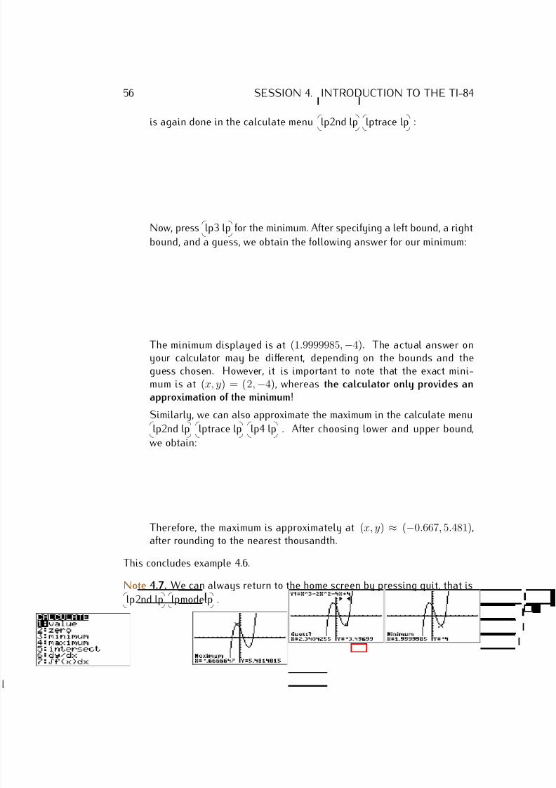
7/18/2019 Precalculus Tradler Carley
http://slidepdf.com/reader/full/precalculus-tradler-carley 66/424
56 SESSION 4. INTRODUCTION TO THE TI-84
is again done in the calculate menu
lp2nd lp
lptrace lp :
Now, press
lp3 lp for the minimum. After specifying a left bound, a right
bound, and a guess, we obtain the following answer for our minimum:
The minimum displayed is at (1.9999985, −4). The actual answer onyour calculator may be different, depending on the bounds and theguess chosen. However, it is important to note that the exact mini-mum is at (x, y) = (2, −4), whereas the calculator only provides anapproximation of the minimum!
Similarly, we can also approximate the maximum in the calculate menu
lp2nd lp
lptrace lp
lp4 lp . After choosing lower and upper bound,
we obtain:
Therefore, the maximum is approximately at (x, y) ≈ (−0.667, 5.481),after rounding to the nearest thousandth.
This concludes example 4.6.
Note 4.7. We can always return to the home screen by pressing quit, that is
lp2nd lp
lpmodelp .
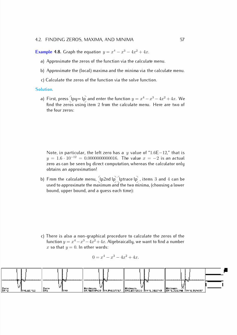
7/18/2019 Precalculus Tradler Carley
http://slidepdf.com/reader/full/precalculus-tradler-carley 67/424
4.2. FINDING ZEROS, MAXIMA, AND MINIMA 57
Example 4.8. Graph the equation y = x4 − x3 − 4x2 + 4x.
a) Approximate the zeros of the function via the calculate menu.
b) Approximate the (local) maxima and the minima via the calculate menu.
c) Calculate the zeros of the function via the solve function.
Solution.
a) First, press
lpy= lp and enter the function y = x4 − x3 − 4x2 + 4x. We
find the zeros using item 2 from the calculate menu. Here are two of the four zeros:
Note, in particular, the left zero has a y value of “1.6E−12,” that isy = 1.6 · 10−12 = 0.0000000000016. The value x = −2 is an actualzero as can be seen by direct computation, whereas the calculator onlyobtains an approximation!
b) From the calculate menu,
lp2nd lp
lptrace lp , items 3 and 4 can be
used to approximate the maximum and the two minima, (choosing a lowerbound, upper bound, and a guess each time):
c) There is also a non-graphical procedure to calculate the zeros of thefunction y = x4 −x3 −4x2 + 4x. Algebraically, we want to find a numberx so that y = 0. In other words:
0 = x4 − x3 − 4x2 + 4x.
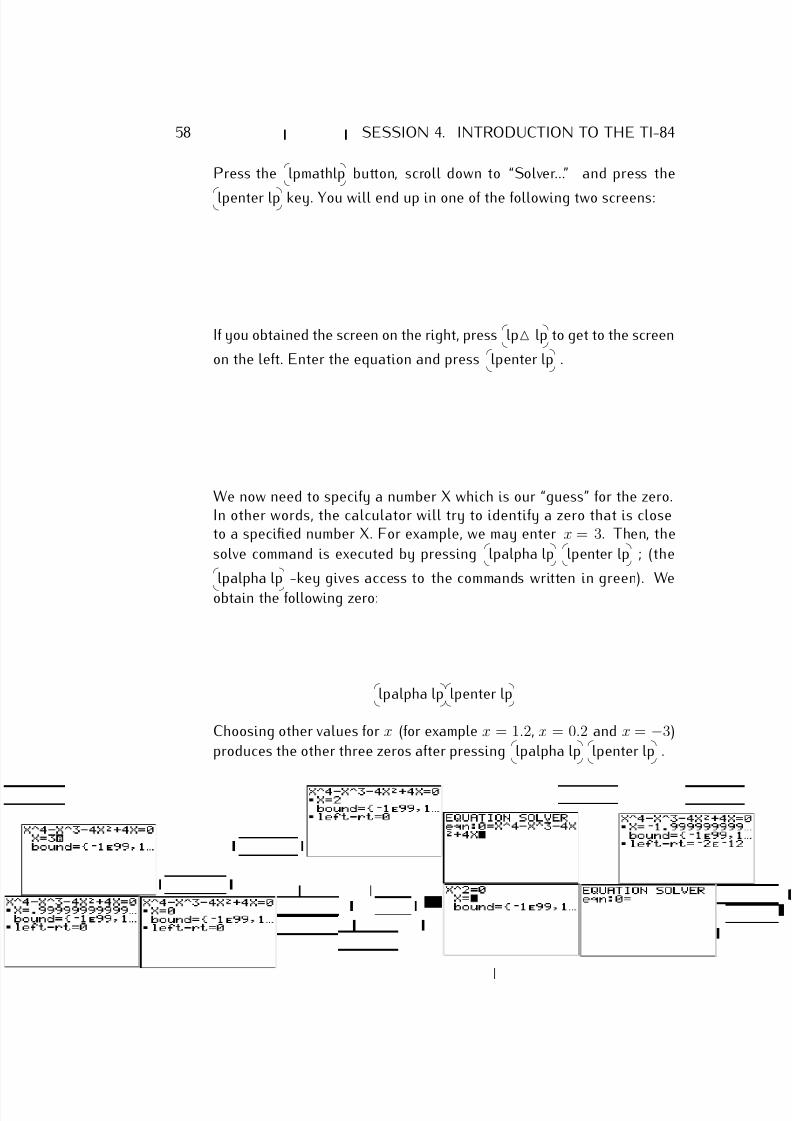
7/18/2019 Precalculus Tradler Carley
http://slidepdf.com/reader/full/precalculus-tradler-carley 68/424
58 SESSION 4. INTRODUCTION TO THE TI-84
Press the
lpmathlp button, scroll down to “Solver...” and press the
lpenter lp key. You will end up in one of the following two screens:
If you obtained the screen on the right, press
lp△ lp to get to the screen
on the left. Enter the equation and press
lpenter lp .
We now need to specify a number X which is our “guess” for the zero.In other words, the calculator will try to identify a zero that is closeto a specified number X. For example, we may enter x = 3. Then, the
solve command is executed by pressing
lpalpha lp
lpenter lp ; (the
lpalpha lp -key gives access to the commands written in green). We
obtain the following zero:
lpalpha lp
lpenter lp
Choosing other values for x (for example x = 1.2, x = 0.2 and x = −3)
produces the other three zeros after pressing
lpalpha lp
lpenter lp .
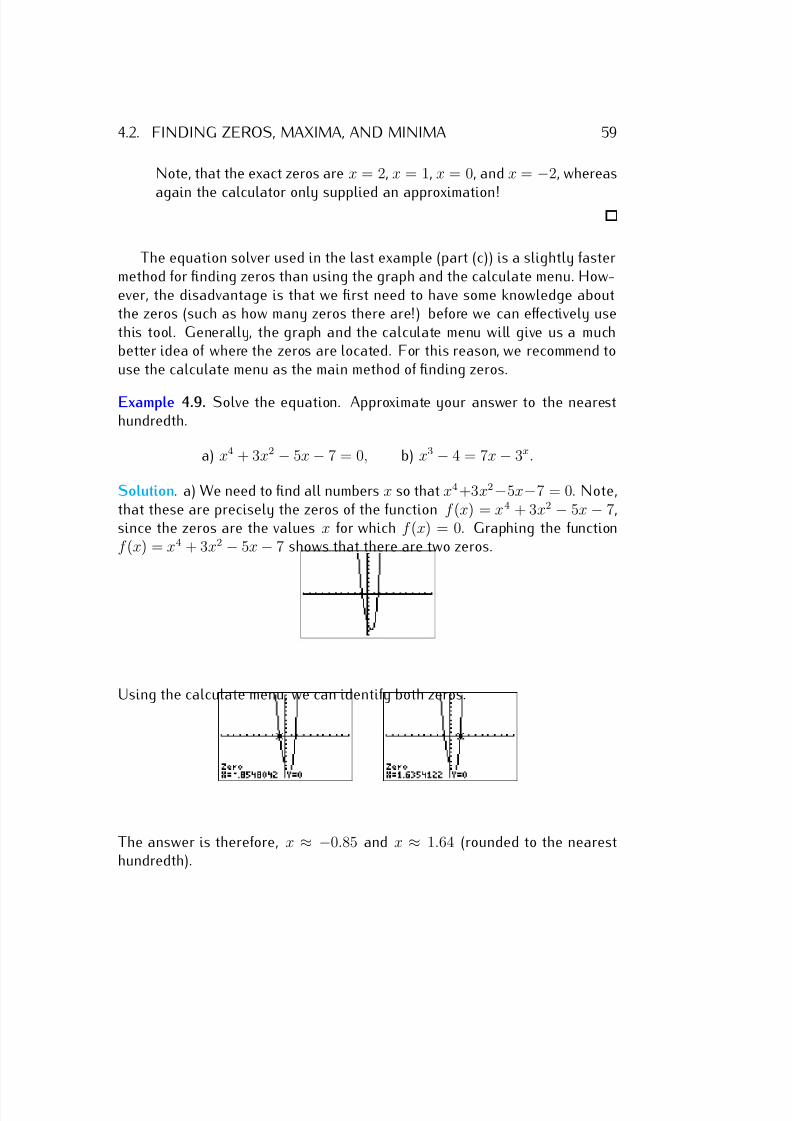
7/18/2019 Precalculus Tradler Carley
http://slidepdf.com/reader/full/precalculus-tradler-carley 69/424
4.2. FINDING ZEROS, MAXIMA, AND MINIMA 59
Note, that the exact zeros are x = 2, x = 1, x = 0, and x = −2, whereas
again the calculator only supplied an approximation!
The equation solver used in the last example (part (c)) is a slightly fastermethod for finding zeros than using the graph and the calculate menu. How-ever, the disadvantage is that we first need to have some knowledge aboutthe zeros (such as how many zeros there are!) before we can effectively usethis tool. Generally, the graph and the calculate menu will give us a muchbetter idea of where the zeros are located. For this reason, we recommend touse the calculate menu as the main method of finding zeros.
Example 4.9. Solve the equation. Approximate your answer to the nearesthundredth.
a) x4 + 3x2 − 5x − 7 = 0, b) x3 − 4 = 7x − 3x.
Solution. a) We need to find all numbers x so that x4 +3x2−5x−7 = 0. Note,that these are precisely the zeros of the function f (x) = x4 + 3x2 − 5x − 7,since the zeros are the values x for which f (x) = 0. Graphing the functionf (x) = x4 + 3x2 − 5x − 7 shows that there are two zeros.
Using the calculate menu, we can identify both zeros.
The answer is therefore, x ≈ −0.85 and x ≈ 1.64 (rounded to the nearesthundredth).
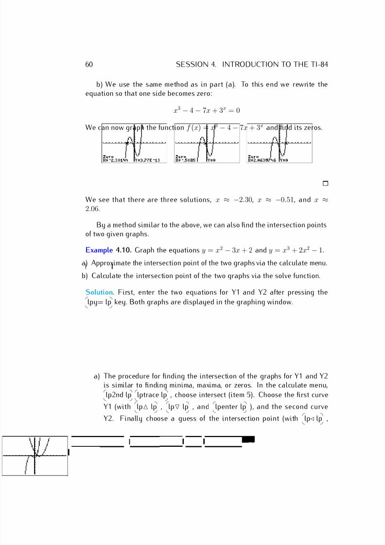
7/18/2019 Precalculus Tradler Carley
http://slidepdf.com/reader/full/precalculus-tradler-carley 70/424
60 SESSION 4. INTRODUCTION TO THE TI-84
b) We use the same method as in part (a). To this end we rewrite the
equation so that one side becomes zero:
x3 − 4 − 7x + 3x = 0
We can now graph the function f (x) = x3 − 4 − 7x + 3x and find its zeros.
We see that there are three solutions, x ≈ −2.30, x ≈ −0.51, and x ≈2.06.
By a method similar to the above, we can also find the intersection pointsof two given graphs.
Example 4.10. Graph the equations y = x2 − 3x + 2 and y = x3 + 2x2 − 1.
a) Approximate the intersection point of the two graphs via the calculate menu.
b) Calculate the intersection point of the two graphs via the solve function.
Solution. First, enter the two equations for Y1 and Y2 after pressing the
lpy= lp key. Both graphs are displayed in the graphing window.
a) The procedure for finding the intersection of the graphs for Y1 and Y2is similar to finding minima, maxima, or zeros. In the calculate menu,
lp2nd lp
lptrace lp , choose intersect (item 5). Choose the first curve
Y1 (with
lp△ lp ,
lp▽ lp , and
lpenter lp ), and the second curve
Y2. Finally choose a guess of the intersection point (with
lp⊳ lp ,
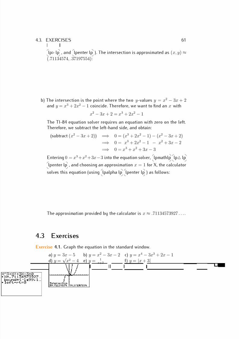
7/18/2019 Precalculus Tradler Carley
http://slidepdf.com/reader/full/precalculus-tradler-carley 71/424
4.3. EXERCISES 61
lp⊲ lp , and
lpenter lp ). The intersection is approximated as (x, y) ≈
(.71134574, .37197554):
b) The intersection is the point where the two y-values y = x2 − 3x + 2and y = x3 + 2x2 − 1 coincide. Therefore, we want to find an x with
x2
−3x + 2 = x3 + 2x2
−1
The TI-84 equation solver requires an equation with zero on the left.Therefore, we subtract the left-hand side, and obtain:
(subtract (x2 − 3x + 2)) =⇒ 0 = (x3 + 2x2 − 1) − (x2 − 3x + 2)
=⇒ 0 = x3 + 2x2 − 1 − x2 + 3x − 2
=⇒ 0 = x3 + x2 + 3x − 3
Entering 0 = x3 +x2 +3x−3 into the equation solver,
lpmathlp
lp△ lp
lpenter lp , and choosing an approximation x = 1 for X, the calculator
solves this equation (using
lpalpha lp
lpenter lp ) as follows:
The approximation provided by the calculator is x ≈ .71134573927 . . . .
4.3 ExercisesExercise 4.1. Graph the equation in the standard window.
a) y = 3x − 5 b) y = x2 − 3x − 2 c) y = x4 − 3x3 + 2x − 1d) y =
√ x2 − 4 e) y = 1
x+2 f ) y = |x + 3|
7/18/2019 Precalculus Tradler Carley
http://slidepdf.com/reader/full/precalculus-tradler-carley 72/424
62 SESSION 4. INTRODUCTION TO THE TI-84
For the last exercise, the absolute value is obtained by pressing
lpmathlp
lp⊲ lp
lpenter lp .
Exercise 4.2. Solve the equation for y and graph all branches in the samewindow.
a) x2 + y2 = 4 b) (x + 5)2 + y2 = 15 c) (x − 1)2 + (y − 2)2 = 9d) y 2 + x2 − 8x − 14 = 0 e) y2 = x2 + 3 f ) y2 = −x2 + 77
Exercise 4.3. Find all zeros of the given function. Round your answer to thenearest hundredth.
a) f (x) = x2 + 3x + 1 b) f (x) = x4 − 3x2 + 2
c) f (x) = x3
+ 2x − 6 d) f (x) = x5
− 11x4
+ 20x3
+ 88x2
− 224x + 1e) f (x) = x3 − 5x2 + 2x + 3 f ) f (x) = √ 2x − 3 − 2x + 3
g) 0 = 0.04x3 − 0.02x2 − 0.5174x + 0.81h) 0 = 0.04x3 − 0.02x2 − 0.5175x + 0.81i) 0 = 0.04x3 − 0.02x2 − 0.5176x + 0.81
Exercise 4.4. Find all solutions of the equation. Round your answer to thenearest thousandth.
a) x3 + 3 = x5 + 7 b) 4x3 + 6x2 − 3x − 2 = 0
c) 2xx
−3
= x2+2x+1
d) 53x+1 = x5 + 6
e) x3 + x2 = x4 − x2 + x f ) 3x2 = x3 − x2 + 3x
Exercise 4.5. Graph the equation. Determine how many maxima and minimathe graph has. To this end, resize the graphing window (via the zoom-in,zoom-out, and zoom-box functions of the calculator) to zoom into the maximaor minima of the graph.
a) y = x2 − 4x + 13 b) y = −x2 + x − 20c) y = 2x3 − 5x2 + 3x d) y = x4 − 5x3 + 8x2 − 5x + 1
Exercise 4.6. Approximate the (local) maxima and minima of the graph. Roundyour answer to the nearest tenth.
a) y = x3 + 2x2 − x + 1 b) y = x3 − 5x2 + 8x − 3c) y = −x4 + 3x3 + x2 + 2 d) y = x4 − x3 − 4x2 + 6x + 2e) y = x4 − x3 − 4x2 + 8x + 2 f ) y = x4 − x3 − 4x2 + 7x + 2
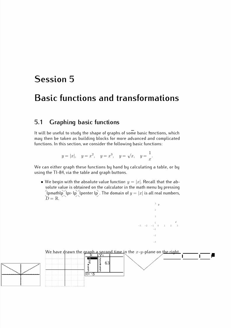
7/18/2019 Precalculus Tradler Carley
http://slidepdf.com/reader/full/precalculus-tradler-carley 73/424
Session 5
Basic functions and transformations
5.1 Graphing basic functions
It will be useful to study the shape of graphs of some basic functions, whichmay then be taken as building blocks for more advanced and complicatedfunctions. In this section, we consider the following basic functions:
y = |x|, y = x2, y = x3, y =√
x, y = 1
x.
We can either graph these functions by hand by calculating a table, or by
using the TI-84, via the table and graph buttons.
• We begin with the absolute value function y = |x|. Recall that the ab-solute value is obtained on the calculator in the math menu by pressing
lpmathlp
lp⊲ lp
lpenter lp . The domain of y = |x| is all real numbers,
D = R.
-3 -2 -1 0 1 2 3
-3
-2
-1
0
1
2
3
x
y
We have drawn the graph a second time in the x-y-plane on the right.
63
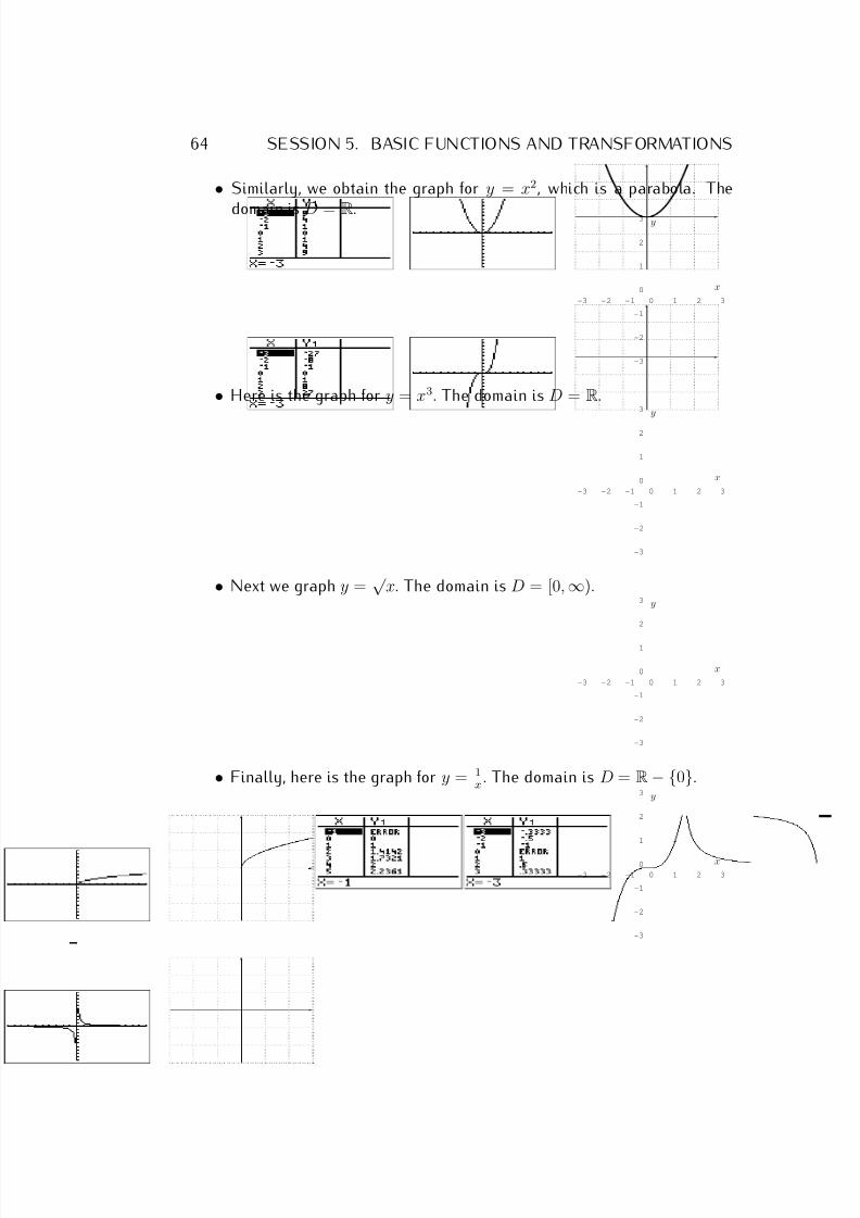
7/18/2019 Precalculus Tradler Carley
http://slidepdf.com/reader/full/precalculus-tradler-carley 74/424
64 SESSION 5. BASIC FUNCTIONS AND TRANSFORMATIONS
• Similarly, we obtain the graph for y = x2, which is a parabola. The
domain is D = R.
-3 -2 -1 0 1 2 3
-3
-2
-1
0
1
2
3
x
y
• Here is the graph for y = x3. The domain is D = R.
-3 -2 -1 0 1 2 3
-3
-2
-1
0
1
2
3
x
y
• Next we graph y =√
x. The domain is D = [0, ∞).
-3 -2 -1 0 1 2 3
-3
-2
-1
0
1
2
3
x
y
• Finally, here is the graph for y = 1x . The domain is D = R− {0}.
-3 -2 -1 0 1 2 3
-3
-2
-1
0
1
2
3
x
y
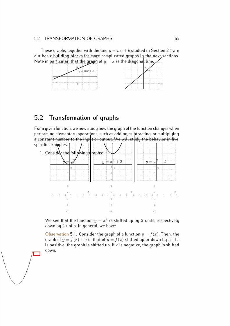
7/18/2019 Precalculus Tradler Carley
http://slidepdf.com/reader/full/precalculus-tradler-carley 75/424
5.2. TRANSFORMATION OF GRAPHS 65
These graphs together with the line y = mx + b studied in Section 2.1 are
our basic building blocks for more complicated graphs in the next sections.Note in particular, that the graph of y = x is the diagonal line.
x
yy = mx + c
c x
yy = x
5.2 Transformation of graphs
For a given function, we now study how the graph of the function changes whenperforming elementary operations, such as adding, subtracting, or multiplyinga constant number to the input or output. We will study the behavior in fivespecific examples.
1. Consider the following graphs:
y = x2 y = x2 + 2 y = x2 − 2
-3 -2 -1 0 1 2 3
-3
-2
-1
0
1
2
3
4
x
y
-3 -2 -1 0 1 2 3
-3
-2
-1
0
1
2
3
4
x
y
-3 -2 -1 0 1 2 3
-3
-2
-1
0
1
2
3
4
x
y
We see that the function y = x2 is shifted up by 2 units, respectivelydown by 2 units. In general, we have:
Observation 5.1. Consider the graph of a function y = f (x). Then, thegraph of y = f (x) + c is that of y = f (x) shifted up or down by c. If cis positive, the graph is shifted up, if c is negative, the graph is shifteddown.
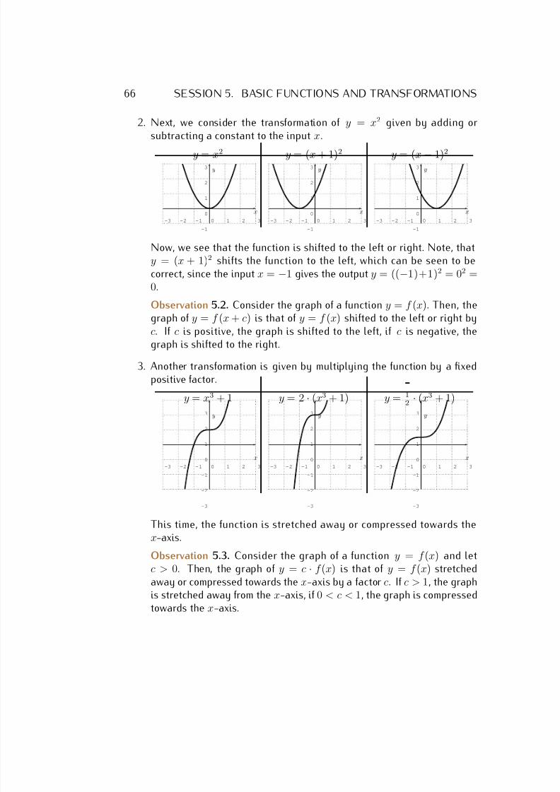
7/18/2019 Precalculus Tradler Carley
http://slidepdf.com/reader/full/precalculus-tradler-carley 76/424
66 SESSION 5. BASIC FUNCTIONS AND TRANSFORMATIONS
2. Next, we consider the transformation of y = x2 given by adding or
subtracting a constant to the input x.y = x2 y = (x + 1)2 y = (x − 1)2
-3 -2 -1 0 1 2 3
-1
0
1
2
3
x
y
-3 -2 -1 0 1 2 3
-1
0
1
2
3
x
y
-3 -2 -1 0 1 2 3
-1
0
1
2
3
x
y
Now, we see that the function is shifted to the left or right. Note, thaty = (x + 1)2 shifts the function to the left, which can be seen to be
correct, since the input x = −1 gives the output y = ((−1)+1)2
= 02
=0.
Observation 5.2. Consider the graph of a function y = f (x). Then, thegraph of y = f (x + c) is that of y = f (x) shifted to the left or right byc. If c is positive, the graph is shifted to the left, if c is negative, thegraph is shifted to the right.
3. Another transformation is given by multiplying the function by a fixedpositive factor.
y = x3 + 1 y = 2 · (x3 + 1) y = 12 · (x3 + 1)
-3 -2 -1 0 1 2 3
-3
-2
-1
0
1
2
3
x
y
-3 -2 -1 0 1 2 3
-3
-2
-1
0
1
2
3
x
y
-3 -2 -1 0 1 2 3
-3
-2
-1
0
1
2
3
x
y
This time, the function is stretched away or compressed towards thex-axis.
Observation 5.3. Consider the graph of a function y = f (x) and letc > 0. Then, the graph of y = c · f (x) is that of y = f (x) stretchedaway or compressed towards the x-axis by a factor c. If c > 1, the graphis stretched away from the x-axis, if 0 < c < 1, the graph is compressedtowards the x-axis.
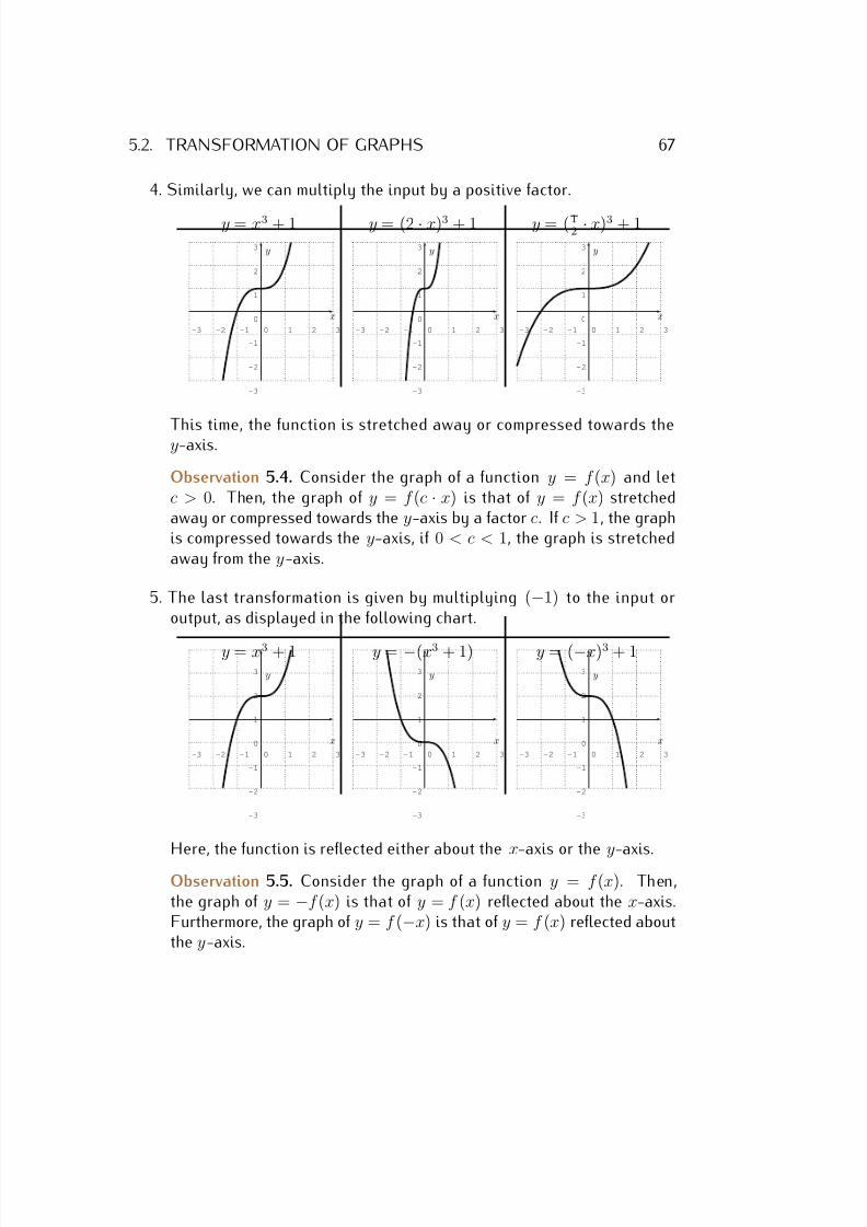
7/18/2019 Precalculus Tradler Carley
http://slidepdf.com/reader/full/precalculus-tradler-carley 77/424
5.2. TRANSFORMATION OF GRAPHS 67
4. Similarly, we can multiply the input by a positive factor.
y = x3 + 1 y = (2 · x)3 + 1 y = ( 12 · x)3 + 1
-3 -2 -1 0 1 2 3
-3
-2
-1
0
1
2
3
x
y
-3 -2 -1 0 1 2 3
-3
-2
-1
0
1
2
3
x
y
-3 -2 -1 0 1 2 3
-3
-2
-1
0
1
2
3
x
y
This time, the function is stretched away or compressed towards they-axis.
Observation 5.4. Consider the graph of a function y = f (x) and letc > 0. Then, the graph of y = f (c · x) is that of y = f (x) stretchedaway or compressed towards the y-axis by a factor c. If c > 1, the graphis compressed towards the y-axis, if 0 < c < 1, the graph is stretchedaway from the y-axis.
5. The last transformation is given by multiplying (−1) to the input oroutput, as displayed in the following chart.
y = x3 + 1 y = −(x3 + 1) y = (−x)3 + 1
-3 -2 -1 0 1 2 3
-3
-2
-1
0
1
2
3
x
y
-3 -2 -1 0 1 2 3
-3
-2
-1
0
1
2
3
x
y
-3 -2 -1 0 1 2 3
-3
-2
-1
0
1
2
3
x
y
Here, the function is reflected either about the x-axis or the y-axis.
Observation 5.5. Consider the graph of a function y = f (x). Then,the graph of y = −f (x) is that of y = f (x) reflected about the x-axis.Furthermore, the graph of y = f (−x) is that of y = f (x) reflected aboutthe y-axis.
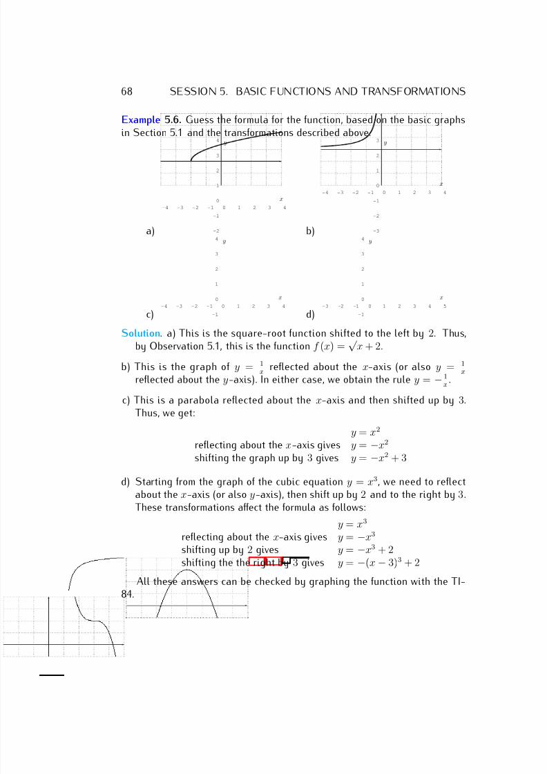
7/18/2019 Precalculus Tradler Carley
http://slidepdf.com/reader/full/precalculus-tradler-carley 78/424
68 SESSION 5. BASIC FUNCTIONS AND TRANSFORMATIONS
Example 5.6. Guess the formula for the function, based on the basic graphs
in Section 5.1 and the transformations described above.
a)
-4 -3 -2 -1 0 1 2 3 4
-2
-1
0
1
2
3
4
x
y
b)
-4 -3 -2 -1 0 1 2 3 4
-3
-2
-1
0
1
2
3
x
y
c)-4 -3 -2 -1 0 1 2 3 4
-1
0
1
2
3
4
x
y
d)-3 -2 -1 0 1 2 3 4 5
-1
0
1
2
3
4
x
y
Solution. a) This is the square-root function shifted to the left by 2. Thus,by Observation 5.1, this is the function f (x) =
√ x + 2.
b) This is the graph of y = 1x reflected about the x-axis (or also y = 1
x
reflected about the y-axis). In either case, we obtain the rule y = − 1x
.
c) This is a parabola reflected about the x-axis and then shifted up by 3.Thus, we get:
y = x2
reflecting about the x-axis gives y = −x2
shifting the graph up by 3 gives y = −x2 + 3
d) Starting from the graph of the cubic equation y = x3, we need to reflectabout the x-axis (or also y-axis), then shift up by 2 and to the right by 3.These transformations affect the formula as follows:
y = x3
reflecting about the x-axis gives y = −x
3
shifting up by 2 gives y = −x3 + 2shifting the the right by 3 gives y = −(x − 3)3 + 2
All these answers can be checked by graphing the function with the TI-84.
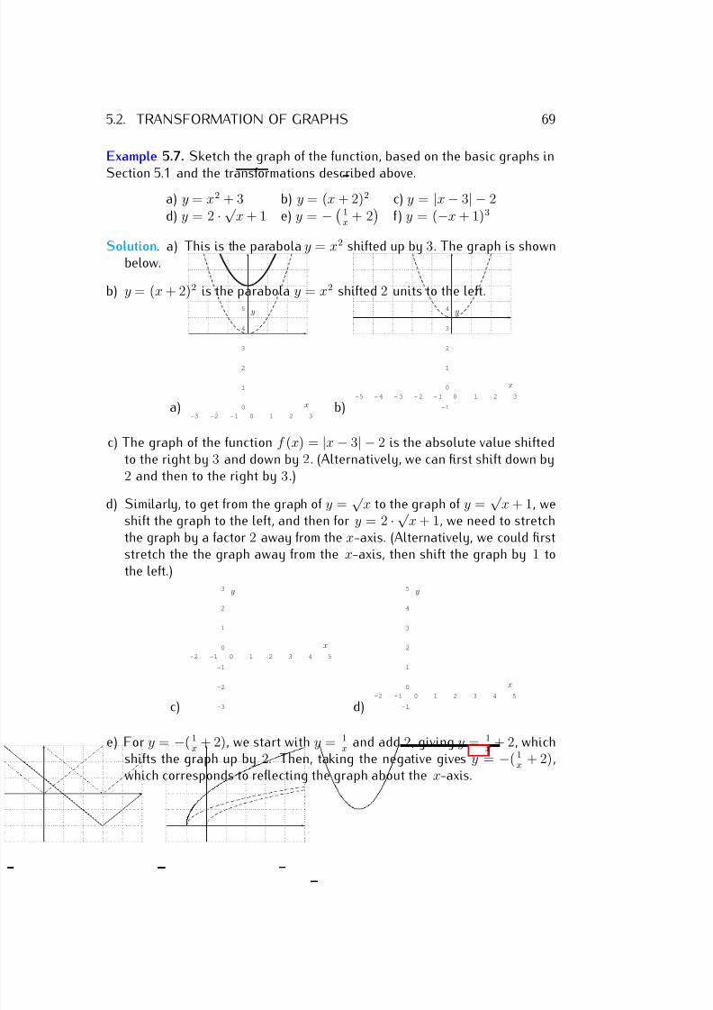
7/18/2019 Precalculus Tradler Carley
http://slidepdf.com/reader/full/precalculus-tradler-carley 79/424
5.2. TRANSFORMATION OF GRAPHS 69
Example 5.7. Sketch the graph of the function, based on the basic graphs in
Section 5.1 and the transformations described above.a) y = x2 + 3 b) y = (x + 2)2 c) y = |x − 3| − 2d) y = 2 · √
x + 1 e) y = − 1x + 2
f ) y = (−x + 1)3
Solution. a) This is the parabola y = x2 shifted up by 3. The graph is shownbelow.
b) y = (x + 2)2 is the parabola y = x2 shifted 2 units to the left.
a)-3 -2 -1 0 1 2 3
0
1
2
3
4
5
x
y
b)-5 - 4 - 3 - 2 - 1 0 1 2 3
-1
0
1
2
3
4
x
y
c) The graph of the function f (x) = |x − 3| − 2 is the absolute value shiftedto the right by 3 and down by 2. (Alternatively, we can first shift down by2 and then to the right by 3.)
d) Similarly, to get from the graph of y =√
x to the graph of y =√
x + 1, weshift the graph to the left, and then for y = 2
·√
x + 1, we need to stretchthe graph by a factor 2 away from the x-axis. (Alternatively, we could firststretch the the graph away from the x-axis, then shift the graph by 1 tothe left.)
c)
-2 -1 0 1 2 3 4 5
-3
-2
-1
0
1
2
3
x
y
d)
-2 -1 0 1 2 3 4 5
-1
0
1
2
3
4
5
x
y
e) For y = −( 1x + 2), we start with y = 1
x and add 2, giving y = 1x + 2, which
shifts the graph up by 2. Then, taking the negative gives y = −( 1x + 2),
which corresponds to reflecting the graph about the x-axis.
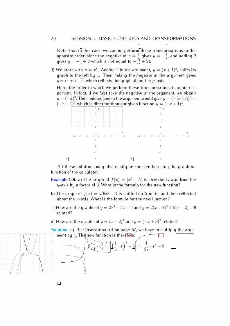
7/18/2019 Precalculus Tradler Carley
http://slidepdf.com/reader/full/precalculus-tradler-carley 80/424
70 SESSION 5. BASIC FUNCTIONS AND TRANSFORMATIONS
Note, that in this case, we cannot perform these transformations in the
opposite order, since the negative of y = 1
x gives y = −1
x , and adding 2gives y = − 1x + 2 which is not equal to −( 1
x + 2).
f) We start with y = x3. Adding 1 in the argument, y = (x + 1)3, shifts itsgraph to the left by 1. Then, taking the negative in the argument givesy = (−x + 1)3, which reflects the graph about the y-axis.
Here, the order in which we perform these transformations is again im-portant. In fact, if we first take the negative in the argument, we obtainy = (−x)3. Then, adding one in the argument would give y = (−(x+1))3 =(−x − 1)3 which is different than our given function y = (−x + 1)3.
e)
-4 -3 -2 -1 0 1 2 3 4
-4
-3
-2
-1
0
1
2
3
4
x
y
f )
-4 -3 -2 -1 0 1 2 3 4
-4
-3
-2
-1
0
1
2
3
4
x
y
All these solutions may also easily be checked by using the graphing
function of the calculator.
Example 5.8. a) The graph of f (x) = |x3 − 5| is stretched away from they-axis by a factor of 3. What is the formula for the new function?
b) The graph of f (x) =√
6x2 + 3 is shifted up 5 units, and then reflectedabout the x-axis. What is the formula for the new function?
c) How are the graphs of y = 2x3 + 5x − 9 and y = 2(x − 2)3 + 5(x − 2) − 9related?
d) How are the graphs of y = (x − 2)2 and y = (−x + 3)2 related?
Solution. a) By Observation 5.4 on page 67, we have to multiply the argu-ment by 1
3 . The new function is therefore:
f 1
3 · x
=
1
3 · x
3
− 5
=
1
27 · x3 − 5
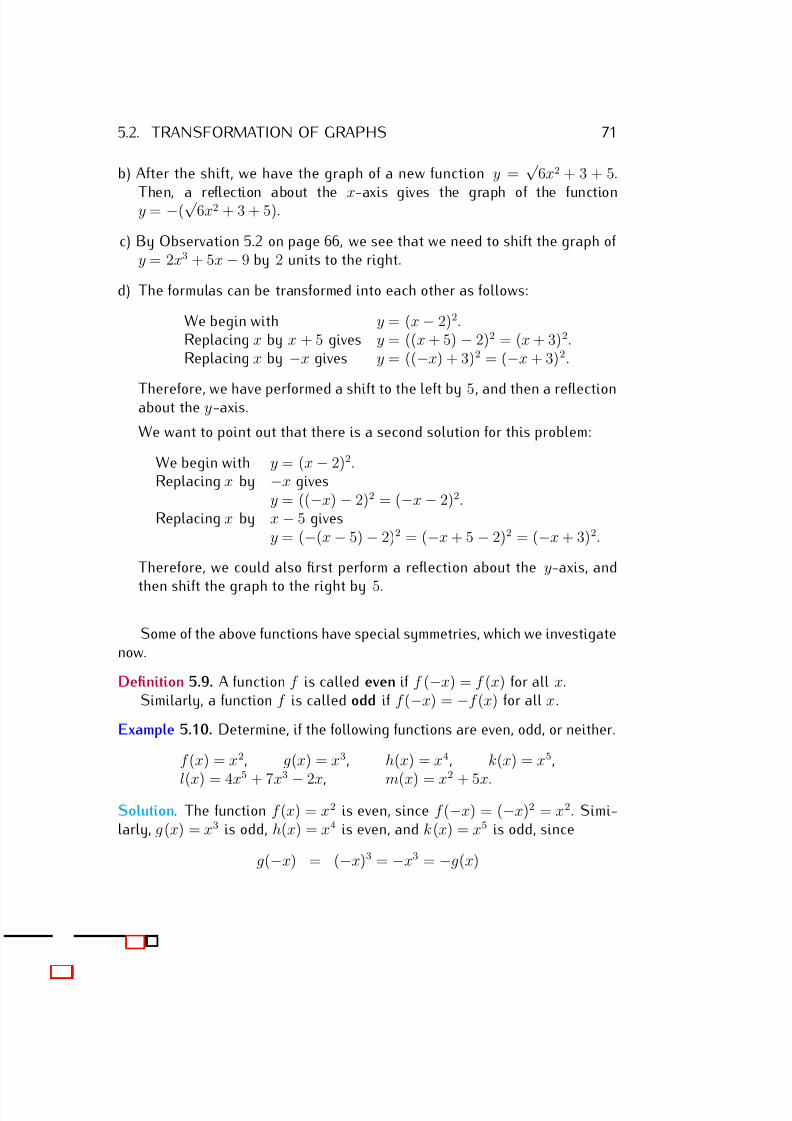
7/18/2019 Precalculus Tradler Carley
http://slidepdf.com/reader/full/precalculus-tradler-carley 81/424
5.2. TRANSFORMATION OF GRAPHS 71
b) After the shift, we have the graph of a new function y =√
6x2 + 3 + 5.
Then, a reflection about the x-axis gives the graph of the functiony = −(√ 6x2 + 3 + 5).
c) By Observation 5.2 on page 66, we see that we need to shift the graph of y = 2x3 + 5x − 9 by 2 units to the right.
d) The formulas can be transformed into each other as follows:
We begin with y = (x − 2)2.Replacing x by x + 5 gives y = ((x + 5) − 2)2 = (x + 3)2.Replacing x by −x gives y = ((−x) + 3)2 = (−x + 3)2.
Therefore, we have performed a shift to the left by 5, and then a reflectionabout the y-axis.
We want to point out that there is a second solution for this problem:
We begin with y = (x − 2)2.Replacing x by −x gives
y = ((−x) − 2)2 = (−x − 2)2.Replacing x by x − 5 gives
y = (−(x − 5) − 2)2 = (−x + 5 − 2)2 = (−x + 3)2.
Therefore, we could also first perform a reflection about the y-axis, and
then shift the graph to the right by 5.
Some of the above functions have special symmetries, which we investigatenow.
Definition 5.9. A function f is called even if f (−x) = f (x) for all x.Similarly, a function f is called odd if f (−x) = −f (x) for all x.
Example 5.10. Determine, if the following functions are even, odd, or neither.
f (x) = x2, g(x) = x3, h(x) = x4, k(x) = x5,
l(x) = 4x
5
+ 7x
3
− 2x, m(x) = x
2
+ 5x.Solution. The function f (x) = x2 is even, since f (−x) = (−x)2 = x2. Simi-larly, g(x) = x3 is odd, h(x) = x4 is even, and k(x) = x5 is odd, since
g(−x) = (−x)3 = −x3 = −g(x)
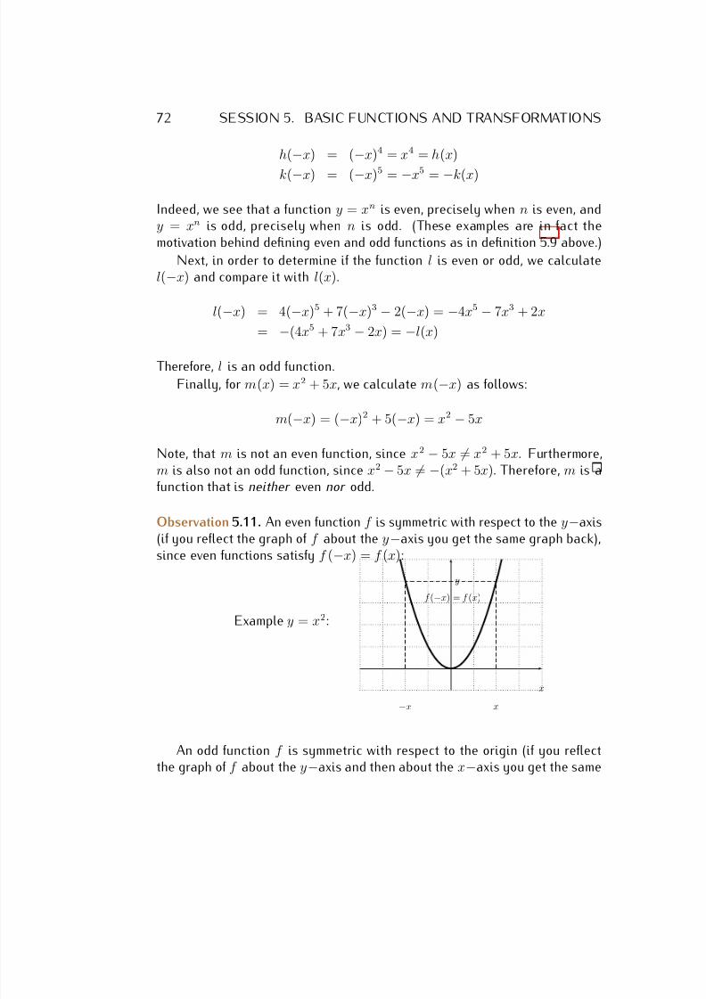
7/18/2019 Precalculus Tradler Carley
http://slidepdf.com/reader/full/precalculus-tradler-carley 82/424
72 SESSION 5. BASIC FUNCTIONS AND TRANSFORMATIONS
h(−x) = (−x)4 = x4 = h(x)
k(−x) = (−x)5 = −x5 = −k(x)
Indeed, we see that a function y = xn is even, precisely when n is even, andy = xn is odd, precisely when n is odd. (These examples are in fact themotivation behind defining even and odd functions as in definition 5.9 above.)
Next, in order to determine if the function l is even or odd, we calculatel(−x) and compare it with l(x).
l(−x) = 4(−x)5 + 7(−x)3 − 2(−x) = −4x5 − 7x3 + 2x
= −(4x5 + 7x3 − 2x) = −l(x)
Therefore, l is an odd function.
Finally, for m(x) = x2 + 5x, we calculate m(−x) as follows:
m(−x) = (−x)2 + 5(−x) = x2 − 5x
Note, that m is not an even function, since x2 − 5x = x2 + 5x. Furthermore,m is also not an odd function, since x2 − 5x = −(x2 + 5x). Therefore, m is afunction that is neither even nor odd.
Observation 5.11. An even function f is symmetric with respect to the y−axis(if you reflect the graph of f about the y−axis you get the same graph back),since even functions satisfy f (−x) = f (x):
Example y = x2:
x
y
x−x
f (−x) = f (x)
An odd function f is symmetric with respect to the origin (if you reflectthe graph of f about the y−axis and then about the x−axis you get the same
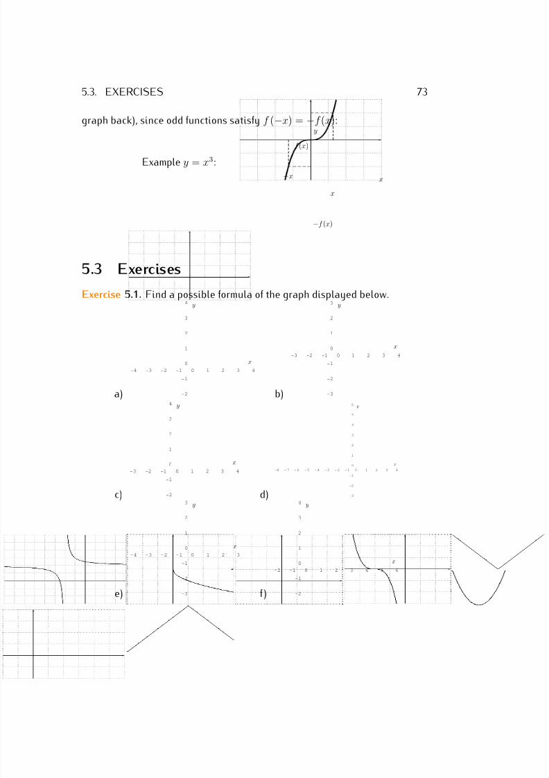
7/18/2019 Precalculus Tradler Carley
http://slidepdf.com/reader/full/precalculus-tradler-carley 83/424
5.3. EXERCISES 73
graph back), since odd functions satisfy f (−x) = −f (x):
Example y = x3:
x
y
x
−x
f (x)
−f (x)
5.3 ExercisesExercise 5.1. Find a possible formula of the graph displayed below.
a)
-4 -3 -2 -1 0 1 2 3 4
-2
-1
0
1
2
3
4
x
y
b)
-3 -2 -1 0 1 2 3 4
-3
-2
-1
0
1
2
3
x
y
c)
-3 -2 -1 0 1 2 3 4
-2
-1
0
1
2
3
4
x
y
d)
-8 - 7 - 6 - 5 - 4 - 3 - 2 - 1 0 1 2 3 4
-3
-2
-1
0
1
2
3
4
5
6
x
y
e)
-4 - 3 - 2 - 1 0 1 2 3
-3
-2
-1
0
1
2
3
x
y
f )
-2 -1 0 1 2 3 4 5 6
-2
-1
0
1
2
3
4
x
y
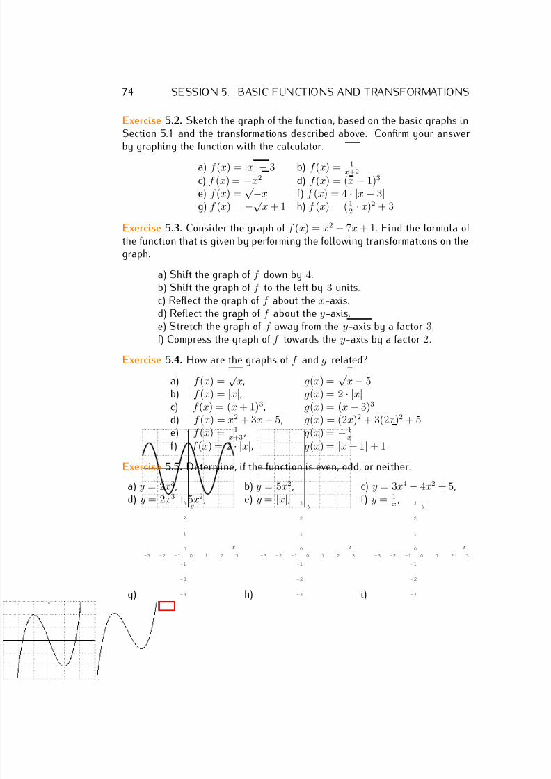
7/18/2019 Precalculus Tradler Carley
http://slidepdf.com/reader/full/precalculus-tradler-carley 84/424
74 SESSION 5. BASIC FUNCTIONS AND TRANSFORMATIONS
Exercise 5.2. Sketch the graph of the function, based on the basic graphs in
Section 5.1 and the transformations described above. Confirm your answerby graphing the function with the calculator.
a) f (x) = |x| − 3 b) f (x) = 1x+2
c) f (x) = −x2 d) f (x) = (x − 1)3
e) f (x) =√ −x f ) f (x) = 4 · |x − 3|
g) f (x) = −√ x + 1 h) f (x) = ( 1
2 · x)2 + 3
Exercise 5.3. Consider the graph of f (x) = x2 − 7x + 1. Find the formula of the function that is given by performing the following transformations on thegraph.
a) Shift the graph of f down by 4.b) Shift the graph of f to the left by 3 units.c) Reflect the graph of f about the x-axis.d) Reflect the graph of f about the y-axis.e) Stretch the graph of f away from the y-axis by a factor 3.f) Compress the graph of f towards the y-axis by a factor 2.
Exercise 5.4. How are the graphs of f and g related?
a) f (x) =√
x, g(x) =√
x − 5b) f (x) = |x|, g(x) = 2 · |x|c) f (x) = (x + 1)
3
, g(x) = (x − 3)3
d) f (x) = x2 + 3x + 5, g(x) = (2x)2 + 3(2x)2 + 5e) f (x) = 1
x+3, g(x) = − 1
x
f ) f (x) = 2 · |x|, g(x) = |x + 1| + 1
Exercise 5.5. Determine, if the function is even, odd, or neither.
a) y = 2x3, b) y = 5x2, c) y = 3x4 − 4x2 + 5,d) y = 2x3 + 5x2, e) y = |x|, f ) y = 1
x ,
g)
-3 -2 -1 0 1 2 3
-3
-2
-1
0
1
2
3
x
y
h)
-3 -2 -1 0 1 2 3
-3
-2
-1
0
1
2
3
x
y
i)
-3 -2 -1 0 1 2 3
-3
-2
-1
0
1
2
3
x
y
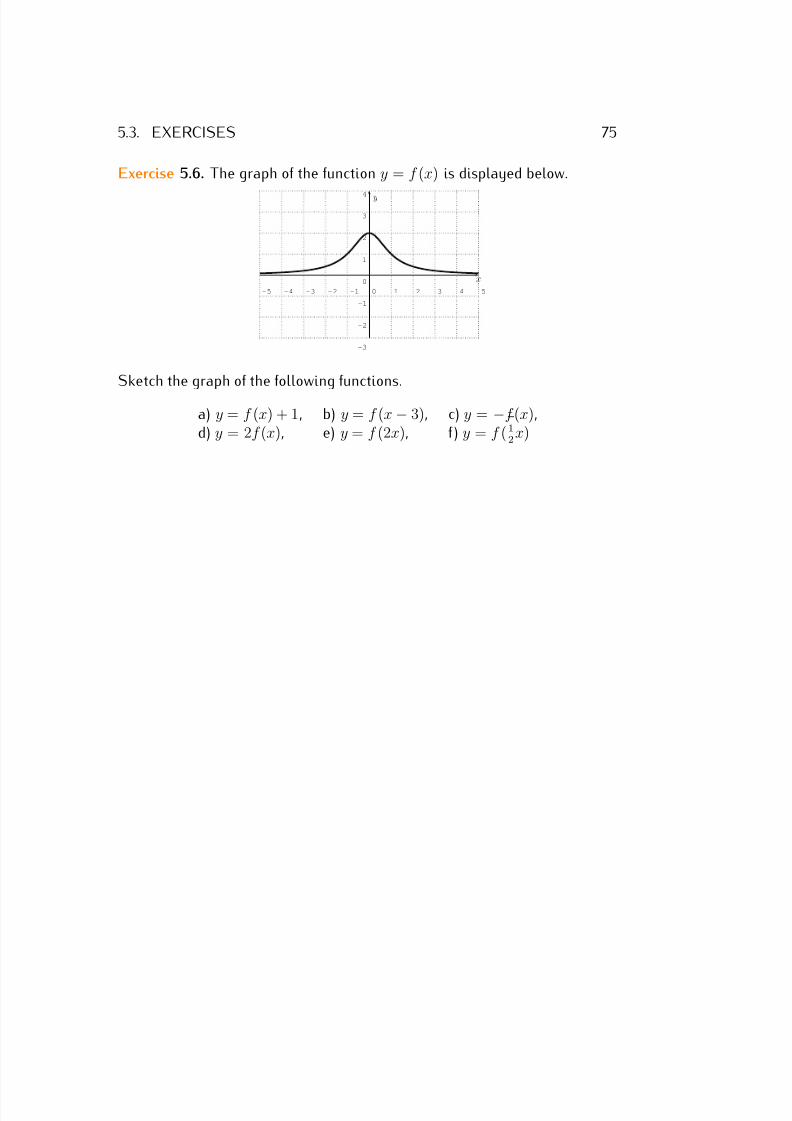
7/18/2019 Precalculus Tradler Carley
http://slidepdf.com/reader/full/precalculus-tradler-carley 85/424
5.3. EXERCISES 75
Exercise 5.6. The graph of the function y = f (x) is displayed below.
-5 -4 -3 -2 -1 0 1 2 3 4 5
-3
-2
-1
0
1
2
3
4
x
y
Sketch the graph of the following functions.
a) y = f (x) + 1, b) y = f (x − 3), c) y = −f (x),d) y = 2f (x), e) y = f (2x), f ) y = f ( 1
2 x)
7/18/2019 Precalculus Tradler Carley
http://slidepdf.com/reader/full/precalculus-tradler-carley 86/424
Session 6
Operations on functions
6.1 Operations on functions given by formulas
We can combine functions in many different ways. First, note that we canadd, subtract, multiply, and divide functions.
Example 6.1. Let f (x) = x2 + 5x and g(x) = 7x − 3. Find the followingfunctions, and state their domain.
(f + g)(x), (f − g)(x), (f · g)(x), and f
g (x).
Solution. The functions are calculated by adding the functions (or subtract-ing, multiplying, dividing).
(f + g)(x) = (x2 + 5x) + (7x − 3) = x2 + 12x − 3,
(f − g)(x) = (x2 + 5x) − (7x − 3)
= x2 + 5x − 7x + 3 = x2 − 2x + 3,
(f · g)(x) = (x2 + 5x) · (7x − 3)
= 7x3 − 3x2 + 35x2 − 15x = 7x3 + 32x2 − 15x,
f
g (x) =
x2 + 5x
7x − 3 .
The calculation of these functions was straightforward. To state their domainis also straightforward, except for the domain of the quotient f
g . Note, thatf + g , f − g , and f · g are all polynomials. By the standard convention
76
7/18/2019 Precalculus Tradler Carley
http://slidepdf.com/reader/full/precalculus-tradler-carley 87/424
6.1. OPERATIONS ON FUNCTIONS GIVEN BY FORMULAS 77
(Convention 3.4 on page 36) all these functions have the domain R, that is
their domain is all real numbers.Now, for the domain of f g , we have to be a bit more careful, since the
denominator of a fraction cannot be zero. The denominator of f g
(x) = x2+5x7x−3
is zero, exactly when
7x − 3 = 0 =⇒ 7x = 3 =⇒ x = 3
7.
We have to exclude 37 from the domain. The domain of the quotient f
g is
therefore R− {37}.
We can formally state the observation we made in the previous example.
Observation 6.2. Let f be a function with domain Df , and g be a functionwith domain Dg . A value x can be used as an input of f + g, f − g, and f · gexactly when x is an input of both f and g. Therefore, the domains of thecombined functions are the intersection of the domains Df and Dg:
Df +g = Df ∩ Dg = {x | x ∈ Df and x ∈ Dg},
Df −g = Df ∩ Dg,
Df ·g = Df ∩ Dg.
For the quotient f g , we also have to make sure that the denominator g(x) is
not zero.Df
g= {x | x ∈ Df , x ∈ Dg, and g(x) = 0}.
Example 6.3. Let f (x) =√
x + 2, and let g(x) = x2 − 5x + 4. Find thefunctions f
g and gf and state their domains.
Solution. First, the domain of f consists of those numbers x for which thesquare root is defined. In other words, we need x + 2 ≥ 0, that is x ≥ −2, sothat the domain of f is Df = [−2, ∞). On the other hand, the domain of g isall real numbers, Dg = R. Now, we have the quotients
f
g (x) =
√ x + 2
x2 − 5x + 4
, and g
f (x) = x2 − 5x + 4
√ x + 2
.
For the domain of f g , we need to exclude those numbers x for which x2 −
5x + 4 = 0. Thus,
x2 − 5x + 4 = 0 =⇒ (x − 1)(x − 4) = 0
7/18/2019 Precalculus Tradler Carley
http://slidepdf.com/reader/full/precalculus-tradler-carley 88/424
78 SESSION 6. OPERATIONS ON FUNCTIONS
=⇒ x = 1, or x = 4.
We obtain the domain for f g
as the combined domain for f and g , and exclude
1 and 4. Therefore, D f g
= [−2, ∞) − {1, 4}.
Now, for gf
(x) = x2−5x+4√ x+2
, the denominator becomes zero exactly when
x + 2 = 0, =⇒ x = −2.
Therefore, we need to exclude −2 from the domain, that is
D gf
= [−2, ∞) − {−2} = (−2, ∞).
Example 6.4. To form the quotient f g
(x) where f (x) = x2 −1 and g(x) = x +1
we write f g (x) = x2−1
x+1 = (x+1)(x−1)x+1 = x − 1. One might be tempted to say
that the domain is all real numbers. But it is not! The domain is all realnumbers except −1, and the last step of the simplification performed above isonly valid for x = −1.
Another operation we can perform is the composition of two functions.
Definition 6.5. Let f and g be functions, and assume that g(x) is in thedomain of f . Then define the composition of f and g at x to be
(f ◦ g)(x) := f (g(x)).
We can take any x as an input of f ◦ g which is an input of g and for whichg(x) is an input of f . Therefore, if Df is the domain of f and Dg is the domainof g , the domain of Df ◦g is
Df ◦g = { x | x ∈ Dg, g(x) ∈ Df }.
Example 6.6. Let f (x) = 2x2 + 5x and g(x) = 2 − x. Find the followingcompositions
a) f (g(3)), b) g(f (3)), c) f (f (1)), d) f (2 · g(5)), e) g(g(4) + 5).
Solution. We evaluate the expressions, one at a time, as follows:
a) f (g(3)) = f (2 − 3) = f (−1) = 2 · (−1)2 + 5 · (−1)
7/18/2019 Precalculus Tradler Carley
http://slidepdf.com/reader/full/precalculus-tradler-carley 89/424
6.1. OPERATIONS ON FUNCTIONS GIVEN BY FORMULAS 79
= 2 − 5 = −3,
b) g(f (3)) = g(2 · 32 + 5 · 3) = g(18 + 15) = g(33)= 2 − 33 = −31,
c) f (f (1)) = f (2 · 12 + 5 · 1) = f (2 + 5) = f (7)
= 2 · 72 + 5 · 7 = 98 + 35 = 133,
d) f (2 · g(5)) = f (2 · (2 − 5)) = f (2 · (−3)) = f (−6)
= 2 · (−6)2 + 5 · (−6) = 72 − 30 = 42,
e) g(g(4) + 5) = g((2 − 4) + 5) = g((−2) + 5) = g(3) = 2 − 3 = −1.
We can also calculate composite functions for arbitrary x in the domain.
Example 6.7. Let f (x) = x2 + 1 and g(x) = x + 3. Find the followingcompositions
a) (f ◦ g)(x), b) (g ◦ f )(x), c) (f ◦ f )(x), d) (g ◦ g)(x).
Solution. a) There are essentially two ways to evaluate (f ◦ g)(x) = f (g(x)).We can either first use the explicit formula for f (x) and then the one for g(x),or vice versa. We will evaluate f (g(x)) by substituting g(x) into the formulafor f (x):
(f ◦ g)(x) = f (g(x)) = (g(x))2 + 1 = (x + 3)2 + 1
= x2 + 6x + 9 + 1 = x2 + 6x + 10.
Similarly, we evaluate the other expressions (b)-(d):
b) (g ◦ f )(x) = g(f (x)) = f (x) + 3 = x2 + 1 + 3 = x2 + 4,
c) (f ◦ f )(x) = f (f (x)) = (f (x))2 + 1 = (x2 + 1)2 + 1
= x4 + 2x2 + 1 + 1 = x4 + 2x2 + 2,
d) (g ◦ g)(x) = g(g(x)) = g(x) + 3 = x + 3 + 3 = x + 6.
Example 6.8. Find (f ◦ g)(x) and (g ◦ f )(x) for the following functions, and
state their domains.a) f (x) = 3
x+2, and g(x) = x2 − 3x,
b) f (x) = |3x − 2| − 6x + 4, and g(x) = 5x + 1,
c) f (x) =
12 · (x − 4), and g(x) = 2x2 + 4.
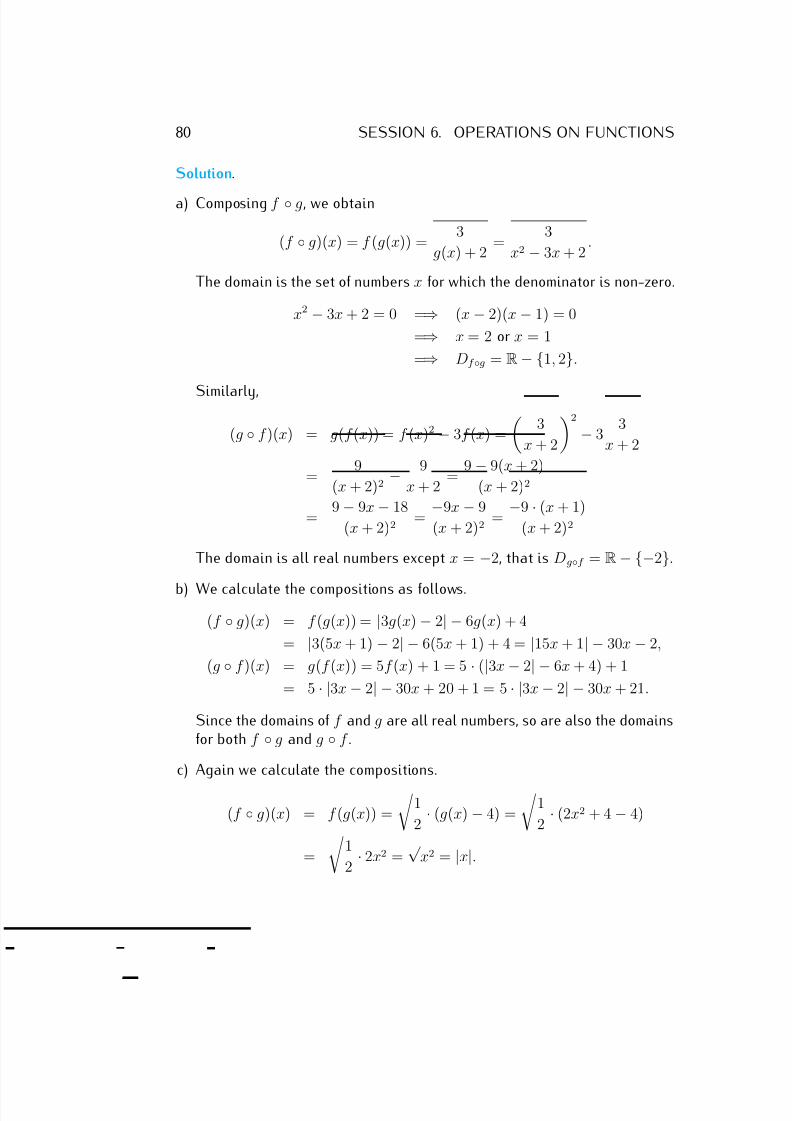
7/18/2019 Precalculus Tradler Carley
http://slidepdf.com/reader/full/precalculus-tradler-carley 90/424
80 SESSION 6. OPERATIONS ON FUNCTIONS
Solution.
a) Composing f ◦ g, we obtain
(f ◦ g)(x) = f (g(x)) = 3
g(x) + 2 =
3
x2 − 3x + 2.
The domain is the set of numbers x for which the denominator is non-zero.
x2 − 3x + 2 = 0 =⇒ (x − 2)(x − 1) = 0
=⇒ x = 2 or x = 1
=⇒ Df ◦g = R− {1, 2}.
Similarly,
(g ◦ f )(x) = g(f (x)) = f (x)2 − 3f (x) =
3
x + 2
2
− 3 3
x + 2
= 9
(x + 2)2 − 9
x + 2 =
9 − 9(x + 2)
(x + 2)2
= 9 − 9x − 18
(x + 2)2 =
−9x − 9
(x + 2)2 =
−9 · (x + 1)
(x + 2)2
The domain is all real numbers except x = −2, that is Dg◦f = R− {−2}.
b) We calculate the compositions as follows.
(f ◦ g)(x) = f (g(x)) = |3g(x) − 2| − 6g(x) + 4
= |3(5x + 1) − 2| − 6(5x + 1) + 4 = |15x + 1| − 30x − 2,
(g ◦ f )(x) = g(f (x)) = 5f (x) + 1 = 5 · (|3x − 2| − 6x + 4) + 1
= 5 · |3x − 2| − 30x + 20 + 1 = 5 · |3x − 2| − 30x + 21.
Since the domains of f and g are all real numbers, so are also the domainsfor both f ◦ g and g ◦ f .
c) Again we calculate the compositions.
(f ◦ g)(x) = f (g(x)) =
1
2 · (g(x) − 4) =
1
2 · (2x2 + 4 − 4)
=
1
2 · 2x2 =
√ x2 = |x|.
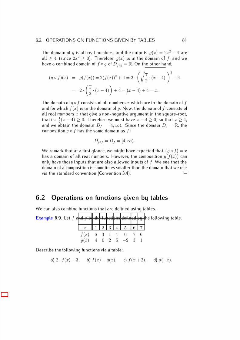
7/18/2019 Precalculus Tradler Carley
http://slidepdf.com/reader/full/precalculus-tradler-carley 91/424
6.2. OPERATIONS ON FUNCTIONS GIVEN BY TABLES 81
The domain of g is all real numbers, and the outputs g(x) = 2x2 + 4 are
all ≥ 4, (since 2x2
≥ 0). Therefore, g(x) is in the domain of f , and wehave a combined domain of f ◦ g of Df ◦g = R. On the other hand,
(g ◦ f )(x) = g(f (x)) = 2(f (x))2 + 4 = 2 ·
1
2 · (x − 4)
2
+ 4
= 2 ·
1
2 · (x − 4)
+ 4 = (x − 4) + 4 = x.
The domain of g ◦ f consists of all numbers x which are in the domain of f and for which f (x) is in the domain of g . Now, the domain of f consists of all real numbers x that give a non-negative argument in the square-root,
that is: 12 (x − 4) ≥ 0. Therefore we must have x − 4 ≥ 0, so that x ≥ 4,and we obtain the domain Df = [4, ∞). Since the domain Dg = R, thecomposition g ◦ f has the same domain as f :
Dg◦f = Df = [4, ∞).
We remark that at a first glance, we might have expected that (g ◦ f ) = xhas a domain of all real numbers. However, the composition g(f (x)) canonly have those inputs that are also allowed inputs of f . We see that thedomain of a composition is sometimes smaller than the domain that we usevia the standard convention (Convention 3.4).
6.2 Operations on functions given by tables
We can also combine functions that are defined using tables.
Example 6.9. Let f and g be the functions defined by the following table.
x 1 2 3 4 5 6 7
f (x) 6 3 1 4 0 7 6
g(x) 4 0 2 5 −2 3 1
Describe the following functions via a table:
a) 2 · f (x) + 3, b) f (x) − g(x), c) f (x + 2), d) g(−x).
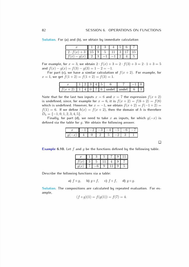
7/18/2019 Precalculus Tradler Carley
http://slidepdf.com/reader/full/precalculus-tradler-carley 92/424
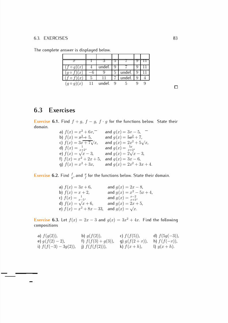
7/18/2019 Precalculus Tradler Carley
http://slidepdf.com/reader/full/precalculus-tradler-carley 93/424
6.3. EXERCISES 83
The complete answer is displayed below.
x 1 3 5 7 9 11
(f ◦ g)(x) 4 undef. 9 7 9 11(g ◦ f )(x) −6 9 5 undef. 9 11(f ◦ f )(x) 5 11 7 undef. 9 4(g ◦ g)(x) 11 undef. 9 5 9 9
6.3 ExercisesExercise 6.1. Find f + g , f − g, f · g for the functions below. State theirdomain.
a) f (x) = x2 + 6x, and g (x) = 3x − 5,b) f (x) = x3 + 5, and g (x) = 5x2 + 7,c) f (x) = 3x + 7
√ x, and g (x) = 2x2 + 5
√ x,
d) f (x) = 1x+2 , and g (x) = 5x
x+2 ,
e) f (x) =√
x − 3, and g (x) = 2√
x − 3,f ) f (x) = x2 + 2x + 5, and g (x) = 3x − 6,g) f (x) = x2 + 3x, and g (x) = 2x2 + 3x + 4.
Exercise 6.2. Find f g , and g
f for the functions below. State their domain.
a) f (x) = 3x + 6, and g(x) = 2x − 8,b) f (x) = x + 2, and g(x) = x2 − 5x + 4,c) f (x) = 1
x−5 , and g(x) = x−2x+3 ,
d) f (x) =√
x + 6, and g(x) = 2x + 5,e) f (x) = x2 + 8x − 33, and g(x) =
√ x.
Exercise 6.3. Let f (x) = 2x − 3 and g(x) = 3x2 + 4x. Find the following
compositions
a) f (g(2)), b) g(f (2)), c) f (f (5)), d) f (5g(−3)),e) g(f (2) − 2), f ) f (f (3) + g(3)), g) g(f (2 + x)), h) f (f (−x)),i) f (f (−3) − 3g(2)), j) f (f (f (2))), k) f (x + h), l) g(x + h).
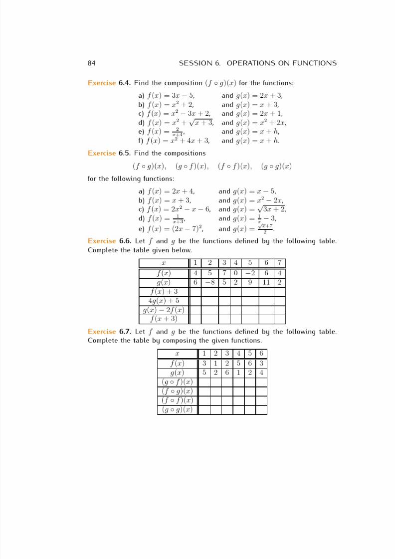
7/18/2019 Precalculus Tradler Carley
http://slidepdf.com/reader/full/precalculus-tradler-carley 94/424

7/18/2019 Precalculus Tradler Carley
http://slidepdf.com/reader/full/precalculus-tradler-carley 95/424
6.3. EXERCISES 85
Exercise 6.8. Let f and g be the functions defined by the following table.
Complete the table by composing the given functions.
x 0 2 4 6 8 10 12
f (x) 4 8 5 6 12 −1 10g(x) 10 2 0 −6 7 2 8
(g ◦ f )(x)(f ◦ g)(x)(f ◦ f )(x)(g ◦ g)(x)
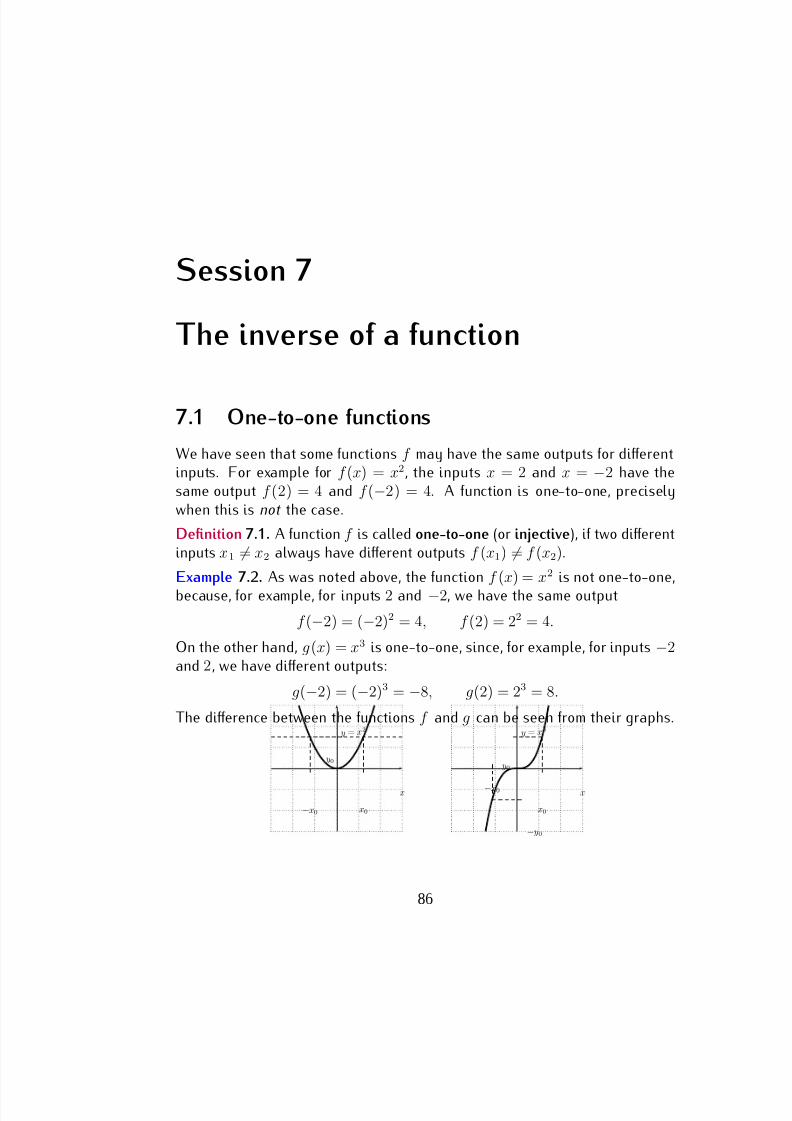
7/18/2019 Precalculus Tradler Carley
http://slidepdf.com/reader/full/precalculus-tradler-carley 96/424
Session 7
The inverse of a function
7.1 One-to-one functions
We have seen that some functions f may have the same outputs for differentinputs. For example for f (x) = x2, the inputs x = 2 and x = −2 have thesame output f (2) = 4 and f (−2) = 4. A function is one-to-one, preciselywhen this is not the case.
Definition 7.1. A function f is called one-to-one (or injective), if two differentinputs x1 = x2 always have different outputs f (x1) = f (x2).
Example 7.2. As was noted above, the function f (x) = x2 is not one-to-one,because, for example, for inputs 2 and −2, we have the same output
f (−2) = (−2)2 = 4, f (2) = 22 = 4.
On the other hand, g(x) = x3 is one-to-one, since, for example, for inputs −2and 2, we have different outputs:
g(−2) = (−2)3 = −8, g(2) = 23 = 8.
The difference between the functions f and g can be seen from their graphs.
x
y
y0
x0−x0
= x2
x
y
y0
x0
−y0
−x0
= x3
86
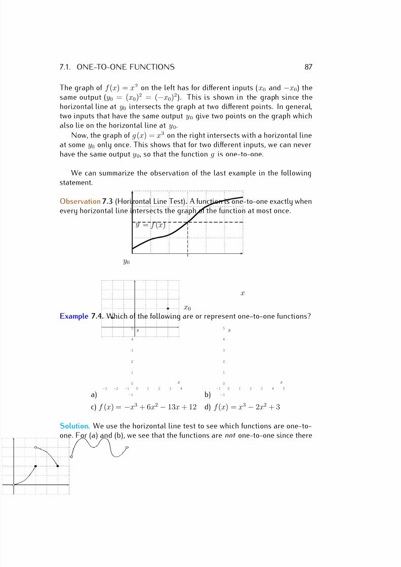
7/18/2019 Precalculus Tradler Carley
http://slidepdf.com/reader/full/precalculus-tradler-carley 97/424
7.1. ONE-TO-ONE FUNCTIONS 87
The graph of f (x) = x2 on the left has for different inputs (x0 and −x0) the
same output (y0 = (x0)2
= (−x0)2
). This is shown in the graph since thehorizontal line at y0 intersects the graph at two different points. In general,two inputs that have the same output y0 give two points on the graph whichalso lie on the horizontal line at y0.
Now, the graph of g(x) = x3 on the right intersects with a horizontal lineat some y0 only once. This shows that for two different inputs, we can neverhave the same output y0, so that the function g is one-to-one.
We can summarize the observation of the last example in the followingstatement.
Observation 7.3 (Horizontal Line Test). A function is one-to-one exactly whenevery horizontal line intersects the graph of the function at most once.
x
y
y0
x0
= f (x)
Example 7.4. Which of the following are or represent one-to-one functions?
a)
-3 -2 -1 0 1 2 3 4
-1
0
1
2
3
4
5
x
y
b)
-1 0 1 2 3 4 5
-1
0
1
2
3
4
5
x
y
c) f (x) = −x3 + 6x2 − 13x + 12 d) f (x) = x3 − 2x2 + 3
Solution. We use the horizontal line test to see which functions are one-to-one. For (a) and (b), we see that the functions are not one-to-one since there
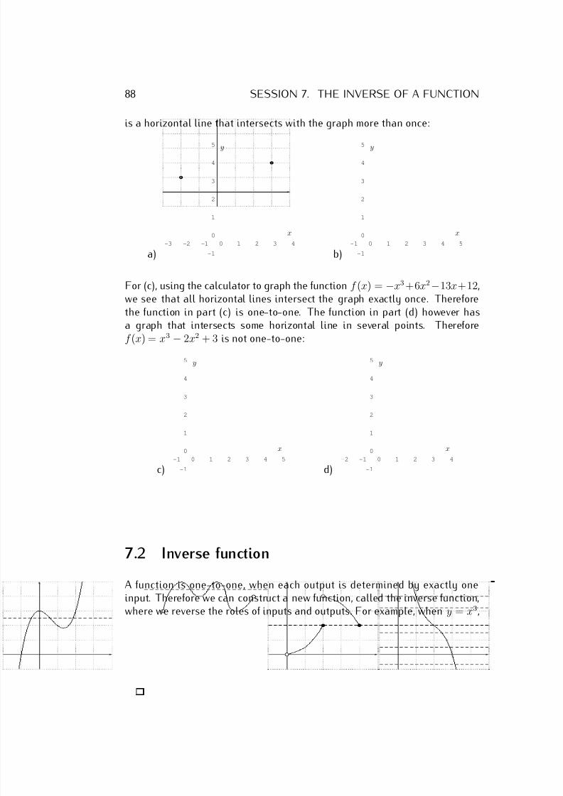
7/18/2019 Precalculus Tradler Carley
http://slidepdf.com/reader/full/precalculus-tradler-carley 98/424
88 SESSION 7. THE INVERSE OF A FUNCTION
is a horizontal line that intersects with the graph more than once:
a)-3 -2 -1 0 1 2 3 4
-1
0
1
2
3
4
5
x
y
b)-1 0 1 2 3 4 5
-1
0
1
2
3
4
5
x
y
For (c), using the calculator to graph the function f (x) = −x3 +6x2−13x+12,we see that all horizontal lines intersect the graph exactly once. Thereforethe function in part (c) is one-to-one. The function in part (d) however hasa graph that intersects some horizontal line in several points. Thereforef (x) = x3 − 2x2 + 3 is not one-to-one:
c)-1 0 1 2 3 4 5
-1
0
1
2
3
4
5
x
y
d)-2 -1 0 1 2 3 4
-1
0
1
2
3
4
5
x
y
7.2 Inverse function
A function is one-to-one, when each output is determined by exactly oneinput. Therefore we can construct a new function, called the inverse function,where we reverse the roles of inputs and outputs. For example, when y = x3,
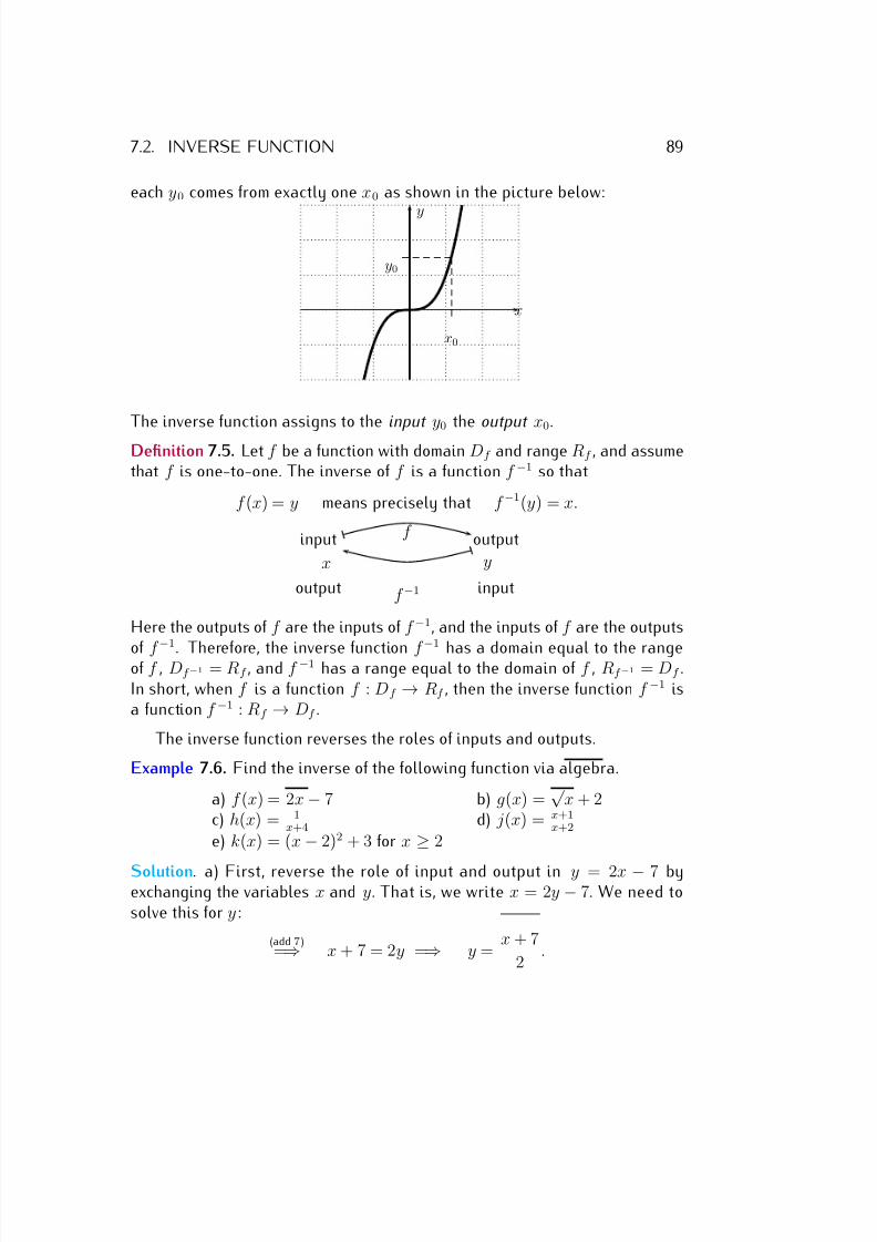
7/18/2019 Precalculus Tradler Carley
http://slidepdf.com/reader/full/precalculus-tradler-carley 99/424
7.2. INVERSE FUNCTION 89
each y0 comes from exactly one x0 as shown in the picture below:
x
y
y0
x0
The inverse function assigns to the input y0 the output x0.
Definition 7.5. Let f be a function with domain Df and range Rf , and assumethat f is one-to-one. The inverse of f is a function f −1 so that
f (x) = y means precisely that f −1(y) = x.
x
input
output
y
output
input
f
f −1
Here the outputs of f are the inputs of f −1, and the inputs of f are the outputs
of f −1
. Therefore, the inverse function f −1
has a domain equal to the rangeof f , Df −1 = Rf , and f −1 has a range equal to the domain of f , Rf −1 = Df .In short, when f is a function f : Df → Rf , then the inverse function f −1 isa function f −1 : Rf → Df .
The inverse function reverses the roles of inputs and outputs.
Example 7.6. Find the inverse of the following function via algebra.
a) f (x) = 2x − 7 b) g(x) =√
x + 2c) h(x) = 1
x+4 d) j(x) = x+1
x+2
e) k(x) = (x − 2)2 + 3 for x ≥ 2
Solution. a) First, reverse the role of input and output in y = 2x − 7 byexchanging the variables x and y. That is, we write x = 2y − 7. We need tosolve this for y :
(add 7)=⇒ x + 7 = 2y =⇒ y =
x + 7
2 .
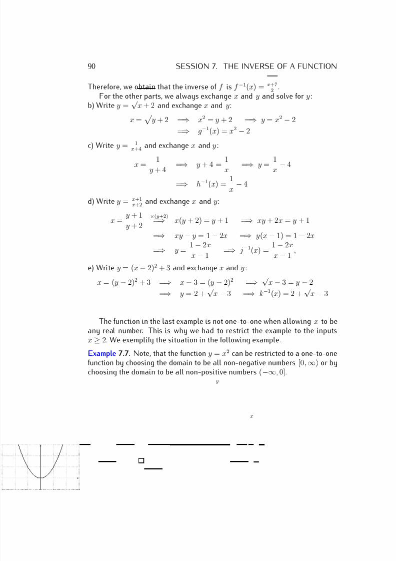
7/18/2019 Precalculus Tradler Carley
http://slidepdf.com/reader/full/precalculus-tradler-carley 100/424
90 SESSION 7. THE INVERSE OF A FUNCTION
Therefore, we obtain that the inverse of f is f −1(x) = x+72
.
For the other parts, we always exchange x and y and solve for y :b) Write y = √ x + 2 and exchange x and y:
x =
y + 2 =⇒ x2 = y + 2 =⇒ y = x2 − 2
=⇒ g−1(x) = x2 − 2
c) Write y = 1x+4 and exchange x and y :
x = 1
y + 4 =⇒ y + 4 =
1
x =⇒ y =
1
x − 4
=⇒ h−1(x) = 1
x − 4
d) Write y = x+1x+2 and exchange x and y:
x = y + 1
y + 2
×(y+2)=⇒ x(y + 2) = y + 1 =⇒ xy + 2x = y + 1
=⇒ xy − y = 1 − 2x =⇒ y(x − 1) = 1 − 2x
=⇒ y = 1 − 2x
x − 1 =⇒ j−1(x) =
1 − 2x
x − 1 ,
e) Write y = (x − 2)2 + 3 and exchange x and y :
x = (y − 2)2 + 3 =⇒ x − 3 = (y − 2)2 =⇒ √ x − 3 = y − 2
=⇒ y = 2 + √ x − 3 =⇒ k−1
(x) = 2 + √ x − 3
The function in the last example is not one-to-one when allowing x to beany real number. This is why we had to restrict the example to the inputsx ≥ 2. We exemplify the situation in the following example.
Example 7.7. Note, that the function y = x2 can be restricted to a one-to-onefunction by choosing the domain to be all non-negative numbers [0, ∞) or bychoosing the domain to be all non-positive numbers (−∞, 0].
x
y
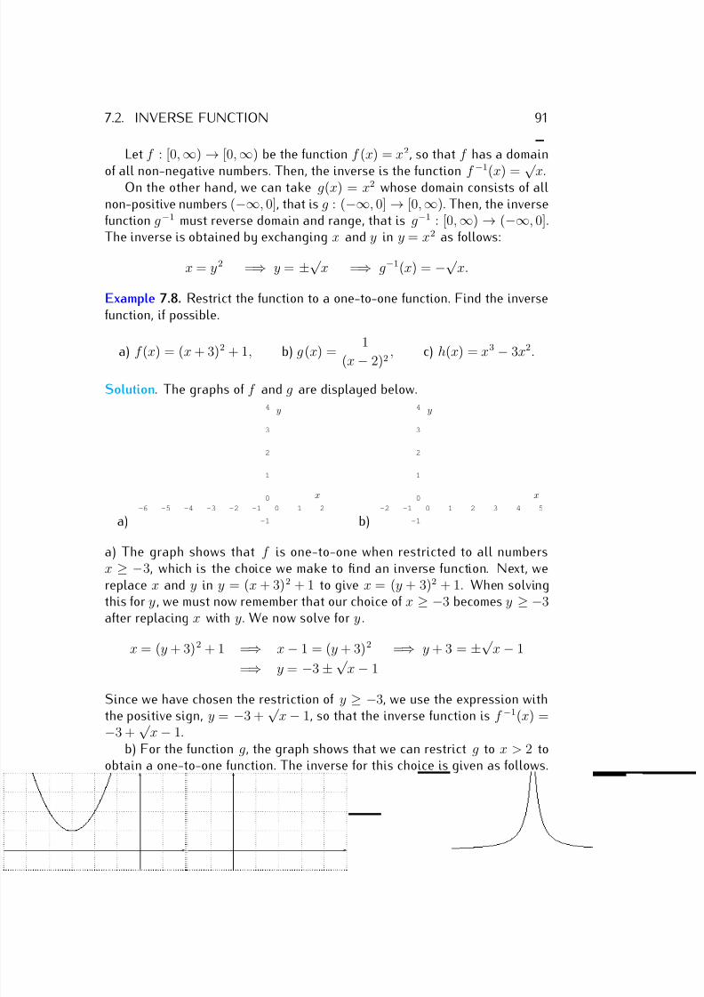
7/18/2019 Precalculus Tradler Carley
http://slidepdf.com/reader/full/precalculus-tradler-carley 101/424
7.2. INVERSE FUNCTION 91
Let f : [0, ∞) → [0, ∞) be the function f (x) = x2, so that f has a domain
of all non-negative numbers. Then, the inverse is the function f −1
(x) = √ x.On the other hand, we can take g(x) = x2 whose domain consists of allnon-positive numbers (−∞, 0], that is g : (−∞, 0] → [0, ∞). Then, the inversefunction g−1 must reverse domain and range, that is g−1 : [0, ∞) → (−∞, 0].The inverse is obtained by exchanging x and y in y = x2 as follows:
x = y2 =⇒ y = ±√ x =⇒ g−1(x) = −√
x.
Example 7.8. Restrict the function to a one-to-one function. Find the inversefunction, if possible.
a) f (x) = (x + 3)2 + 1, b) g(x) = 1(x − 2)2 , c) h(x) = x3 − 3x2.
Solution. The graphs of f and g are displayed below.
a)
-6 -5 -4 -3 -2 -1 0 1 2
-1
0
1
2
3
4
x
y
b)
-2 -1 0 1 2 3 4 5
-1
0
1
2
3
4
x
y
a) The graph shows that f is one-to-one when restricted to all numbersx ≥ −3, which is the choice we make to find an inverse function. Next, wereplace x and y in y = (x + 3)2 + 1 to give x = (y + 3)2 + 1. When solvingthis for y , we must now remember that our choice of x ≥ −3 becomes y ≥ −3after replacing x with y. We now solve for y .
x = (y + 3)2 + 1 =⇒ x − 1 = (y + 3)2 =⇒ y + 3 = ±√ x − 1
=⇒ y = −3 ± √ x − 1
Since we have chosen the restriction of y ≥ −3, we use the expression withthe positive sign, y = −3 +
√ x − 1, so that the inverse function is f −1(x) =
−3 +√
x − 1.b) For the function g, the graph shows that we can restrict g to x > 2 to
obtain a one-to-one function. The inverse for this choice is given as follows.
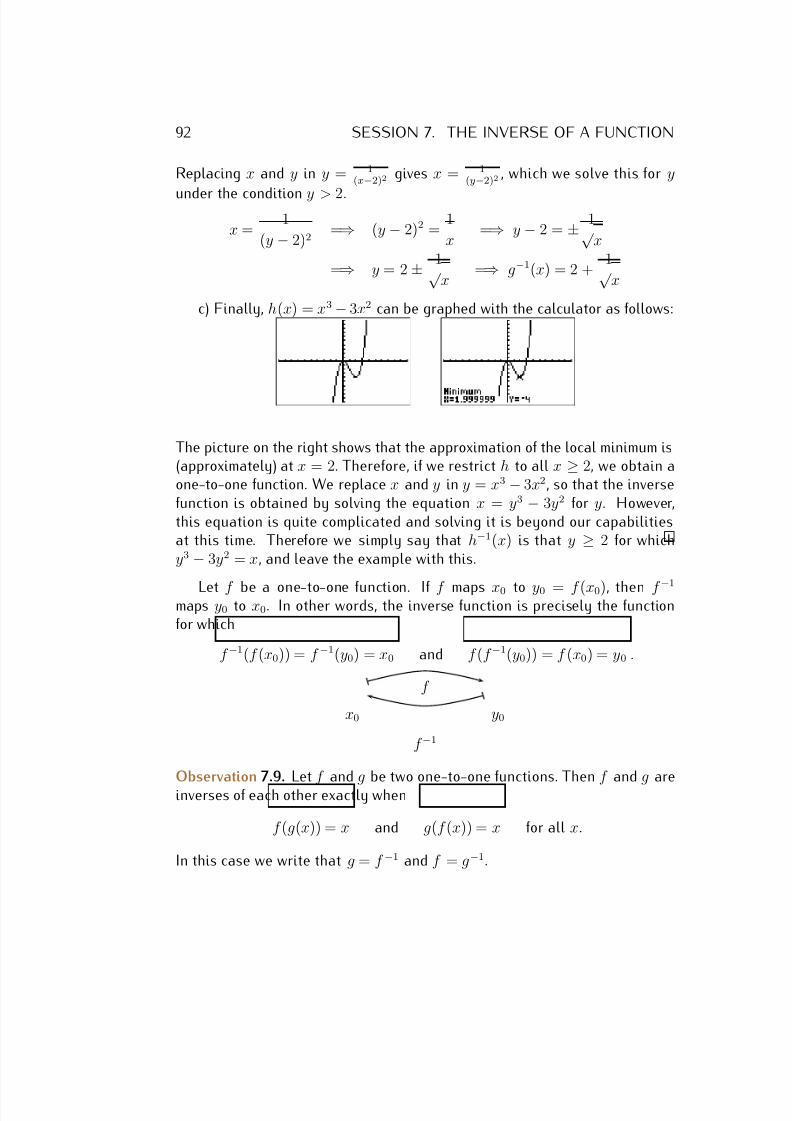
7/18/2019 Precalculus Tradler Carley
http://slidepdf.com/reader/full/precalculus-tradler-carley 102/424
92 SESSION 7. THE INVERSE OF A FUNCTION
Replacing x and y in y = 1(x−2)2 gives x = 1
(y−2)2 , which we solve this for y
under the condition y > 2.
x = 1
(y − 2)2 =⇒ (y − 2)2 =
1
x =⇒ y − 2 = ± 1√
x
=⇒ y = 2 ± 1√ x
=⇒ g−1(x) = 2 + 1√
x
c) Finally, h(x) = x3 − 3x2 can be graphed with the calculator as follows:
The picture on the right shows that the approximation of the local minimum is(approximately) at x = 2. Therefore, if we restrict h to all x ≥ 2, we obtain aone-to-one function. We replace x and y in y = x3 − 3x2, so that the inversefunction is obtained by solving the equation x = y3 − 3y2 for y. However,this equation is quite complicated and solving it is beyond our capabilitiesat this time. Therefore we simply say that h−1(x) is that y ≥ 2 for whichy3 − 3y2 = x, and leave the example with this.
Let f be a one-to-one function. If f maps x0 to y0 = f (x0), then f −1
maps y0 to x0. In other words, the inverse function is precisely the functionfor which
f −1(f (x0)) = f −1(y0) = x0 and f (f −1(y0)) = f (x0) = y0 .
x0 y0
f
f −1
Observation 7.9. Let f and g be two one-to-one functions. Then f and g areinverses of each other exactly when
f (g(x)) = x and g(f (x)) = x for all x.
In this case we write that g = f −1 and f = g−1.
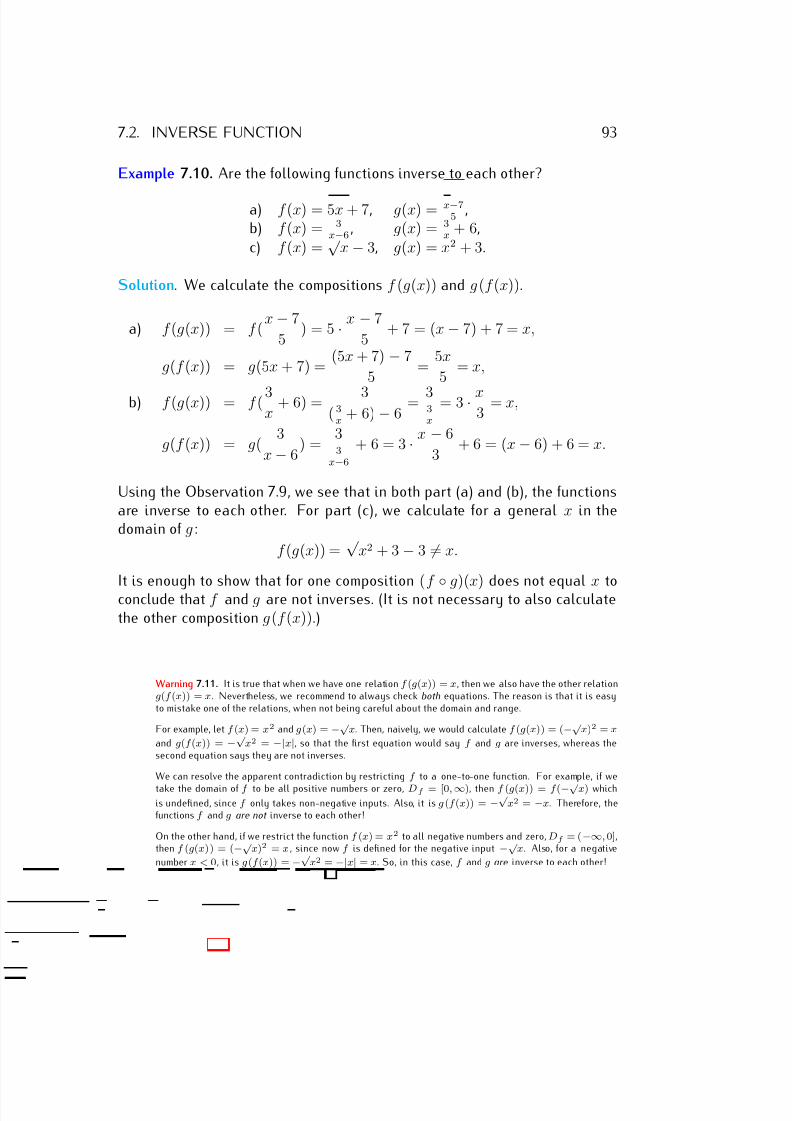
7/18/2019 Precalculus Tradler Carley
http://slidepdf.com/reader/full/precalculus-tradler-carley 103/424
7.2. INVERSE FUNCTION 93
Example 7.10. Are the following functions inverse to each other?
a) f (x) = 5x + 7, g(x) = x−75
,b) f (x) = 3
x−6 , g(x) = 3x + 6,
c) f (x) =√
x − 3, g(x) = x2 + 3.
Solution. We calculate the compositions f (g(x)) and g(f (x)).
a) f (g(x)) = f (x − 7
5 ) = 5 · x − 7
5 + 7 = (x − 7) + 7 = x,
g(f (x)) = g(5x + 7) = (5x + 7) − 7
5 =
5x
5 = x,
b) f (g(x)) = f ( 3x
+ 6) = 3( 3
x + 6) − 6
= 33x
= 3 · x3
= x,
g(f (x)) = g( 3
x − 6) =
33
x−6
+ 6 = 3 · x − 6
3 + 6 = (x − 6) + 6 = x.
Using the Observation 7.9, we see that in both part (a) and (b), the functionsare inverse to each other. For part (c), we calculate for a general x in thedomain of g :
f (g(x)) =√
x2 + 3 − 3 = x.
It is enough to show that for one composition (f ◦ g)(x) does not equal x toconclude that f and g are not inverses. (It is not necessary to also calculatethe other composition g(f (x)).)
Warning 7.11. It is true that when we have one relation f (g(x)) = x, then we also have the other relationg(f (x)) = x. Nevertheless, we recommend to always check both equations. The reason is that it is easyto mistake one of the relations, when not being careful about the domain and range.
For example, let f (x) = x2 and g(x) = −√ x. Then, naively, we would calculate f (g(x)) = (−√ x)2 = x
and g(f (x)) = −√
x2 = −|x|, so that the first equation would say f and g are inverses, whereas thesecond equation says they are not inverses.
We can resolve the apparent contradiction by restricting f to a one-to-one function. For example, if we
take the domain of f to be all positive numbers or zero, Df = [0,∞), then f (g(x)) = f (−√ x) which
is undefined, since f only takes non-negative inputs. Also, it is g (f (x)) = −√
x2 = −x. Therefore, thefunctions f and g are not inverse to each other!
On the other hand, if we restrict the function f (x) = x2 to all negative numbers and zero, Df = (−∞, 0],then f (g(x)) = (−√ x)2 = x , since now f is defined for the negative input −√ x. Also, for a negative
number x < 0, it is g(f (x)) = −√
x2 = −|x| = x. So, in this case, f and g are inverse to each other!
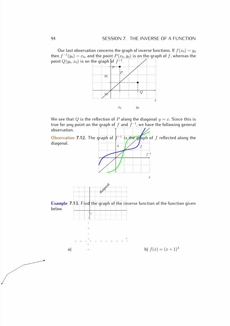
7/18/2019 Precalculus Tradler Carley
http://slidepdf.com/reader/full/precalculus-tradler-carley 104/424
94 SESSION 7. THE INVERSE OF A FUNCTION
Our last observation concerns the graph of inverse functions. If f (x0) = y0
then f −1
(y0) = x0, and the point P (x0, y0) is on the graph of f , whereas thepoint Q(y0, x0) is on the graph of f −1.
x
y
y0
x0
P
y0
x0Q
We see that Q is the reflection of P along the diagonal y = x. Since this istrue for any point on the graph of f and f −1, we have the following generalobservation.
Observation 7.12. The graph of f −1 is the graph of f reflected along thediagonal.
x
y
d i a g
o n a l
f
f −1
Example 7.13. Find the graph of the inverse function of the function givenbelow.
a)
-3 -2 -1 0 1 2 3 4 5 6 7
-2
-1
0
1
2
3
4
5
x
y
b) f (x) = (x + 1)3
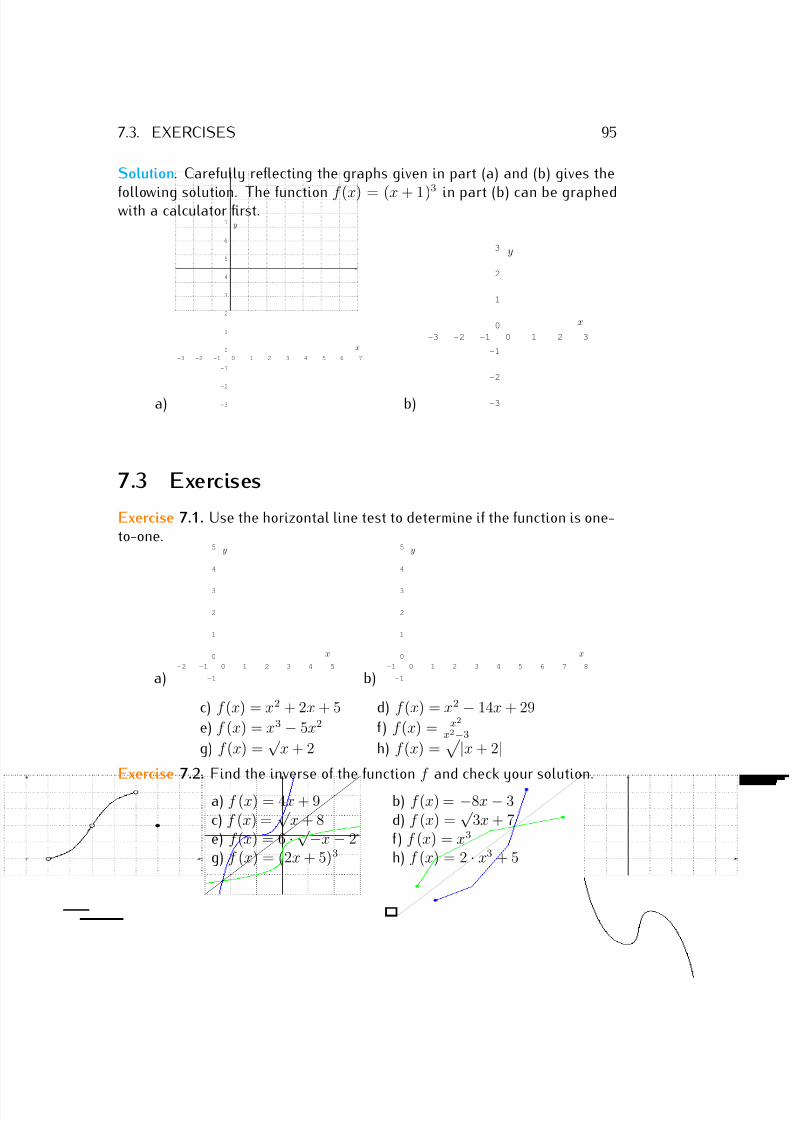
7/18/2019 Precalculus Tradler Carley
http://slidepdf.com/reader/full/precalculus-tradler-carley 105/424
7.3. EXERCISES 95
Solution. Carefully reflecting the graphs given in part (a) and (b) gives the
following solution. The function f (x) = (x + 1)3
in part (b) can be graphedwith a calculator first.
a)
-3 -2 -1 0 1 2 3 4 5 6 7
-3
-2
-1
0
1
2
3
4
5
6
7
x
y
b)
-3 -2 -1 0 1 2 3
-3
-2
-1
0
1
2
3
x
y
7.3 Exercises
Exercise 7.1. Use the horizontal line test to determine if the function is one-to-one.
a)-2 -1 0 1 2 3 4 5
-1
0
1
2
3
4
5
x
y
b)-1 0 1 2 3 4 5 6 7 8
-1
0
1
2
3
4
5
x
y
c) f (x) = x2 + 2x + 5 d) f (x) = x2 − 14x + 29
e) f (x) = x3 − 5x2 f ) f (x) = x2
x2−3
g) f (x) =√
x + 2 h) f (x) =
|x + 2|Exercise 7.2. Find the inverse of the function f and check your solution.
a) f (x) = 4x + 9 b) f (x) = −8x − 3c) f (x) =
√ x + 8 d) f (x) =
√ 3x + 7
e) f (x) = 6 · √ −x − 2 f ) f (x) = x3
g) f (x) = (2x + 5)3 h) f (x) = 2 · x3 + 5
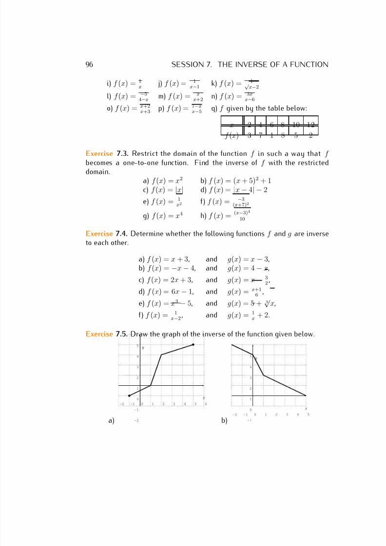
7/18/2019 Precalculus Tradler Carley
http://slidepdf.com/reader/full/precalculus-tradler-carley 106/424
96 SESSION 7. THE INVERSE OF A FUNCTION
i) f (x) = 1x
j) f (x) = 1x−1
k) f (x) = 1√ x−2
l) f (x) = −54−x m) f (x) = xx+2 n) f (x) = 3xx−6
o) f (x) = x+2x+3 p) f (x) = 7−x
x−5 q) f given by the table below:
x 2 4 6 8 10 12
f (x) 3 7 1 8 5 2
Exercise 7.3. Restrict the domain of the function f in such a way that f becomes a one-to-one function. Find the inverse of f with the restricteddomain.
a) f (x) = x2 b) f (x) = (x + 5)2 + 1
c) f (x) = |x| d) f (x) = |x − 4| − 2e) f (x) = 1
x2 f ) f (x) = −3(x+7)2
g) f (x) = x4 h) f (x) = (x−3)4
10
Exercise 7.4. Determine whether the following functions f and g are inverseto each other.
a) f (x) = x + 3, and g(x) = x − 3,b) f (x) = −x − 4, and g(x) = 4 − x,
c) f (x) = 2x + 3, and g(x) = x
− 32 ,
d) f (x) = 6x − 1, and g(x) = x+16 ,
e) f (x) = x3 − 5, and g(x) = 5 + 3√
x,
f ) f (x) = 1x−2 , and g(x) = 1
x + 2.
Exercise 7.5. Draw the graph of the inverse of the function given below.
a)
-2 -1 0 1 2 3 4 5 6
-2
-1
0
1
2
3
4
5
x
y
b)-2 -1 0 1 2 3 4 5
-1
0
1
2
3
4
5
x
y
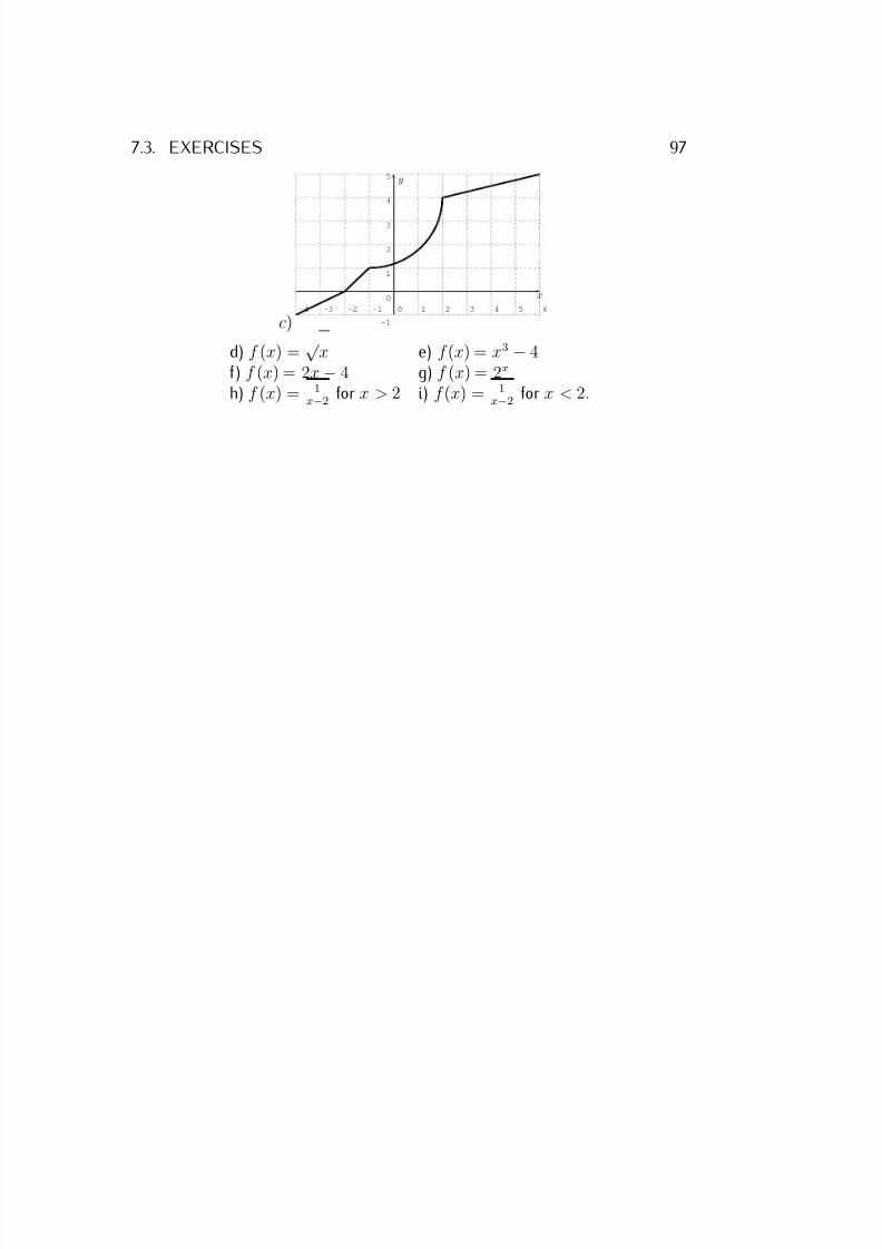
7/18/2019 Precalculus Tradler Carley
http://slidepdf.com/reader/full/precalculus-tradler-carley 107/424
7.3. EXERCISES 97
c)-4 -3 -2 -1 0 1 2 3 4 5 6
-1
0
1
2
3
4
5
x
y
d) f (x) =√
x e) f (x) = x3 − 4f ) f (x) = 2x − 4 g) f (x) = 2x
h) f (x) = 1x−2
for x > 2 i) f (x) = 1x−2
for x < 2.
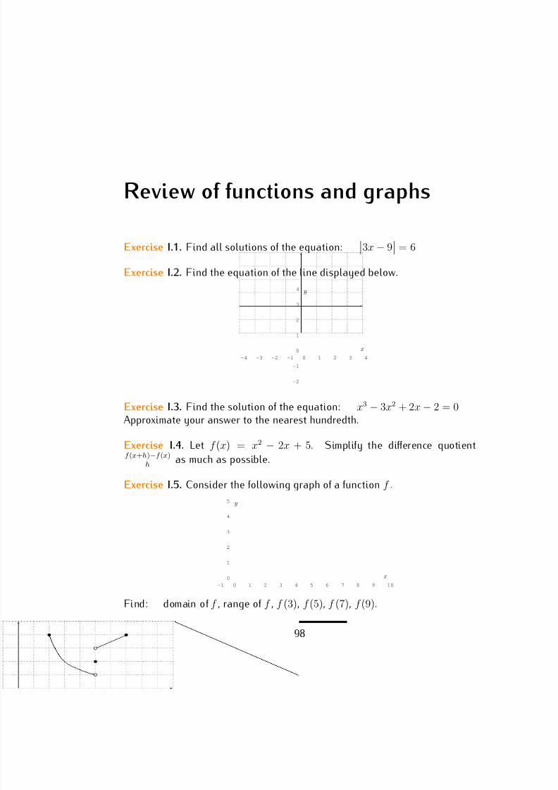
7/18/2019 Precalculus Tradler Carley
http://slidepdf.com/reader/full/precalculus-tradler-carley 108/424
Review of functions and graphs
Exercise I.1. Find all solutions of the equation:3x − 9
= 6
Exercise I.2. Find the equation of the line displayed below.
-4 -3 -2 -1 0 1 2 3 4
-2
-1
0
1
2
3
4
x
y
Exercise I.3. Find the solution of the equation: x3
−3x2 + 2x
−2 = 0
Approximate your answer to the nearest hundredth.
Exercise I.4. Let f (x) = x2 − 2x + 5. Simplify the difference quotientf (x+h)−f (x)
h as much as possible.
Exercise I.5. Consider the following graph of a function f .
-1 0 1 2 3 4 5 6 7 8 9 10
0
1
2
3
4
5
x
y
Find: domain of f , range of f , f (3), f (5), f (7), f (9).
98
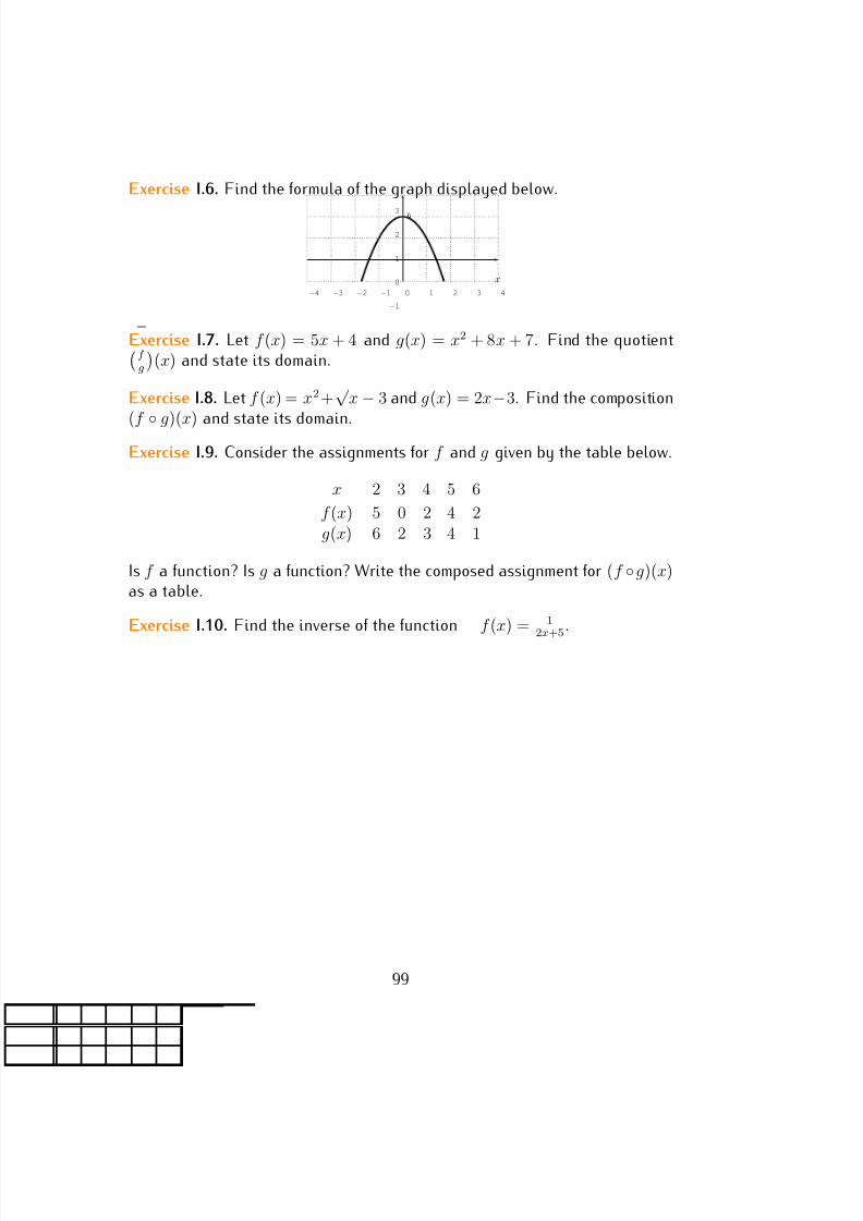
7/18/2019 Precalculus Tradler Carley
http://slidepdf.com/reader/full/precalculus-tradler-carley 109/424
Exercise I.6. Find the formula of the graph displayed below.
-4 -3 -2 -1 0 1 2 3 4
-1
0
1
2
3
x
y
Exercise I.7. Let f (x) = 5x + 4 and g(x) = x2 + 8x + 7. Find the quotientf g
(x) and state its domain.
Exercise I.8. Let f (x) = x2 +√
x − 3 and g(x) = 2x−3. Find the composition(f
◦g)(x) and state its domain.
Exercise I.9. Consider the assignments for f and g given by the table below.
x 2 3 4 5 6
f (x) 5 0 2 4 2g(x) 6 2 3 4 1
Is f a function? Is g a function? Write the composed assignment for (f ◦g)(x)as a table.
Exercise I.10. Find the inverse of the function f (x) = 12x+5 .
99
7/18/2019 Precalculus Tradler Carley
http://slidepdf.com/reader/full/precalculus-tradler-carley 110/424
Part II
Polynomials and rational functions
100
7/18/2019 Precalculus Tradler Carley
http://slidepdf.com/reader/full/precalculus-tradler-carley 111/424
Session 8
Dividing polynomials
We now start our discussion of specific classes of examples of functions. Thefirst class of functions that we discuss are polynomials and rational functions.Let us first recall the definition of polynomials and rational functions.
Definition 8.1. A monomial is a number, a variable, or a product of numbersand variables. A polynomial is a sum (or difference) of monomials.
Example 8.2. The following are examples of monomials:
5, x, 7x2y, −12x3y2z 4,√
2 · a3n2xy
The following are examples of polynomials:
x2 + 3x − 7, 4x2y3 + 2x + z 3 + 4mn2, −5x3 − x2 − 4x − 9, 5x2y4
In particular, every monomial is also a polynomial.
We are mainly interested in polynomials in one variable x, and considerthese as functions. For example, f (x) = x2 + 3x − 7 is such a function.
Definition 8.3. A polynomial is a function f of the form
f (x) = anxn + an−1xn−1 + · · · + a2x2 + a1x + a0,
for some real (or complex) numbers a0, a1, . . . , an. The domain of a polynomialf is all real numbers (see our standard convention 3.4).
The numbers a0, a1, . . . , an are called coefficients. For each k , the numberak is the coefficient of xk. The number an is called the leading coefficient
and n is the degree of the polynomial.The zeros of a polynomial are usually referred to as roots. Therefore x is
a root of a polynomial f precisely when f (x) = 0.
101
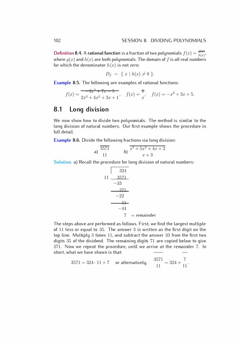
7/18/2019 Precalculus Tradler Carley
http://slidepdf.com/reader/full/precalculus-tradler-carley 112/424
102 SESSION 8. DIVIDING POLYNOMIALS
Definition 8.4. A rational function is a fraction of two polynomials f (x) = g(x)h(x)
,
where g(x) and h(x) are both polynomials. The domain of f is all real numbersfor which the denominator h(x) is not zero:
Df = { x | h(x) = 0 }.
Example 8.5. The following are examples of rational functions:
f (x) = −3x2 + 7x − 5
2x3 + 4x2 + 3x + 1, f (x) =
1
x, f (x) = −x2 + 3x + 5.
8.1 Long division
We now show how to divide two polynomials. The method is similar to thelong division of natural numbers. Our first example shows the procedure infull detail.
Example 8.6. Divide the following fractions via long division:
a) 3571
11 b)
x3 + 5x2 + 4x + 2
x + 3
Solution. a) Recall the procedure for long division of natural numbers:
324
11 3571−33
271−22
51−44
7 = remainder
The steps above are performed as follows. First, we find the largest multipleof 11 less or equal to 35. The answer 3 is written as the first digit on thetop line. Multiply 3 times 11, and subtract the answer 33 from the first two
digits 35 of the dividend. The remaining digits 71 are copied below to give271. Now we repeat the procedure, until we arrive at the remainder 7. Inshort, what we have shown is that:
3571 = 324 · 11 + 7 or alternatively, 3571
11 = 324 +
7
11.
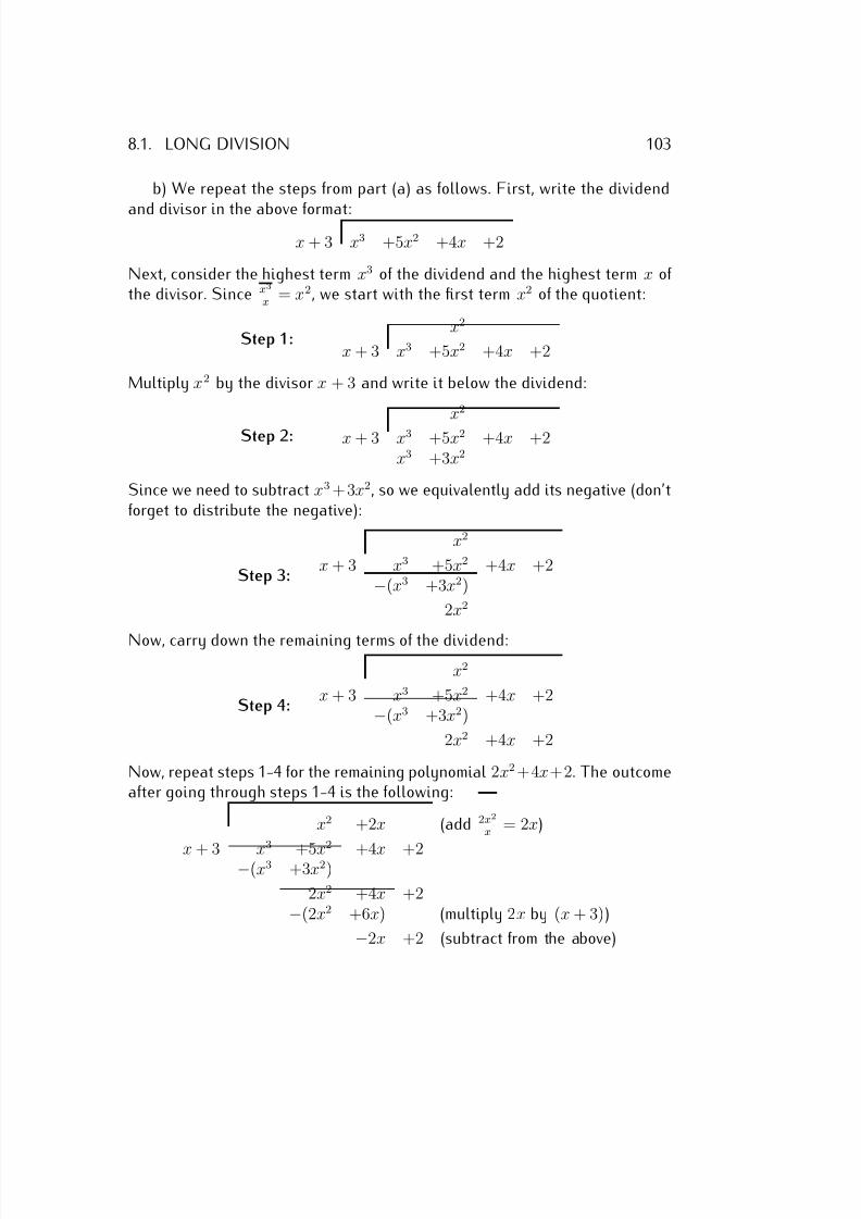
7/18/2019 Precalculus Tradler Carley
http://slidepdf.com/reader/full/precalculus-tradler-carley 113/424
8.1. LONG DIVISION 103
b) We repeat the steps from part (a) as follows. First, write the dividend
and divisor in the above format:
x + 3 x3 +5x2 +4x +2
Next, consider the highest term x3 of the dividend and the highest term x of the divisor. Since x3
x = x2, we start with the first term x2 of the quotient:
Step 1:x2
x + 3 x3 +5x2 +4x +2
Multiply x2 by the divisor x + 3 and write it below the dividend:
Step 2:
x2
x + 3 x3 +5x2 +4x +2x3 +3x2
Since we need to subtract x3 + 3x2, so we equivalently add its negative (don’tforget to distribute the negative):
Step 3:
x2
x + 3 x3 +5x2 +4x +2−(x3 +3x2)
2x2
Now, carry down the remaining terms of the dividend:
Step 4:
x2
x + 3 x3 +5x2 +4x +2−(x3 +3x2)
2x2 +4x +2
Now, repeat steps 1-4 for the remaining polynomial 2x2 +4x+2. The outcomeafter going through steps 1-4 is the following:
x2 +2x (add 2x2
x = 2x)
x + 3 x3
+5x2
+4x +2−(x3 +3x2)
2x2 +4x +2−(2x2 +6x) (multiply 2x by (x + 3))
−2x +2 (subtract from the above)
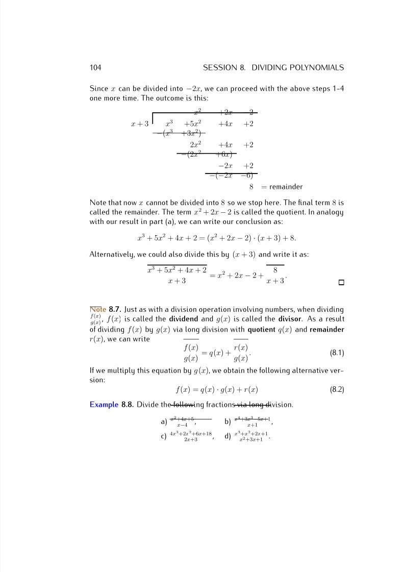
7/18/2019 Precalculus Tradler Carley
http://slidepdf.com/reader/full/precalculus-tradler-carley 114/424
104 SESSION 8. DIVIDING POLYNOMIALS
Since x can be divided into −2x, we can proceed with the above steps 1-4
one more time. The outcome is this:x2 +2x −2
x + 3 x3 +5x2 +4x +2−(x3 +3x2)
2x2 +4x +2−(2x2 +6x)
−2x +2−(−2x −6)
8 = remainder
Note that now x cannot be divided into 8 so we stop here. The final term 8 iscalled the remainder. The term x2 + 2x − 2 is called the quotient. In analogywith our result in part (a), we can write our conclusion as:
x3 + 5x2 + 4x + 2 = (x2 + 2x − 2) · (x + 3) + 8.
Alternatively, we could also divide this by (x + 3) and write it as:
x3 + 5x2 + 4x + 2
x + 3 = x2 + 2x − 2 +
8
x + 3.
Note 8.7. Just as with a division operation involving numbers, when dividingf (x)g(x)
, f (x) is called the dividend and g(x) is called the divisor. As a result
of dividing f (x) by g(x) via long division with quotient q (x) and remainder
r(x), we can writef (x)
g(x) = q (x) +
r(x)
g(x). (8.1)
If we multiply this equation by g (x), we obtain the following alternative ver-sion:
f (x) = q (x) · g(x) + r(x) (8.2)
Example 8.8. Divide the following fractions via long division.
a) x2+4x+5x−4 , b) x4+3x3−5x+1
x+1 ,
c) 4x3+2x2+6x+182x+3 , d) x3+x2+2x+1
x2+3x+1 .
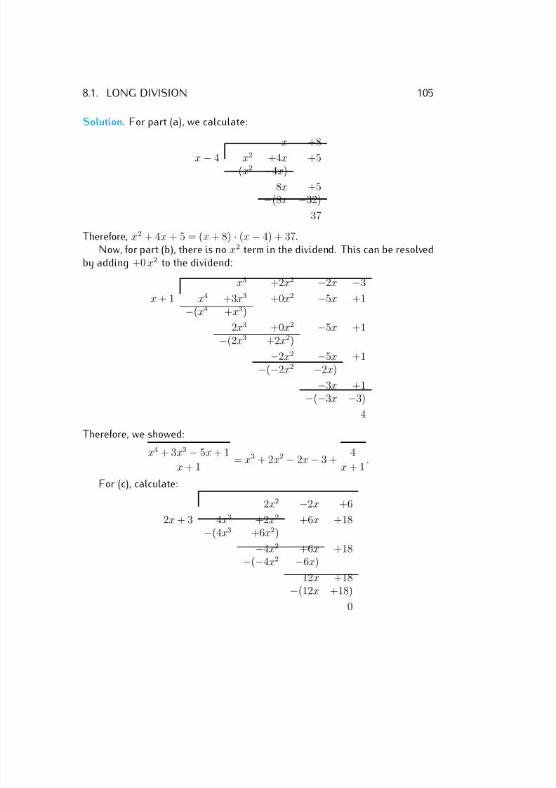
7/18/2019 Precalculus Tradler Carley
http://slidepdf.com/reader/full/precalculus-tradler-carley 115/424
8.1. LONG DIVISION 105
Solution. For part (a), we calculate:
x +8
x − 4 x2 +4x +5−(x2 −4x)
8x +5−(8x −32)
37
Therefore, x2 + 4x + 5 = (x + 8) · (x − 4) + 37.Now, for part (b), there is no x2 term in the dividend. This can be resolved
by adding +0 x2 to the dividend:
x3 +2x2 −2x −3
x + 1 x4 +3x3 +0x2 −5x +1−(x4 +x3)
2x3 +0x2 −5x +1−(2x3 +2x2)
−2x2 −5x +1−(−2x2 −2x)
−3x +1−(−3x −3)
4
Therefore, we showed:
x4 + 3x3 − 5x + 1
x + 1 = x3 + 2x2 − 2x − 3 +
4
x + 1.
For (c), calculate:
2x2 −2x +6
2x + 3 4x3 +2x2 +6x +18−(4x3 +6x2)
−4x2
+6x +18−(−4x2 −6x)
12x +18−(12x +18)
0
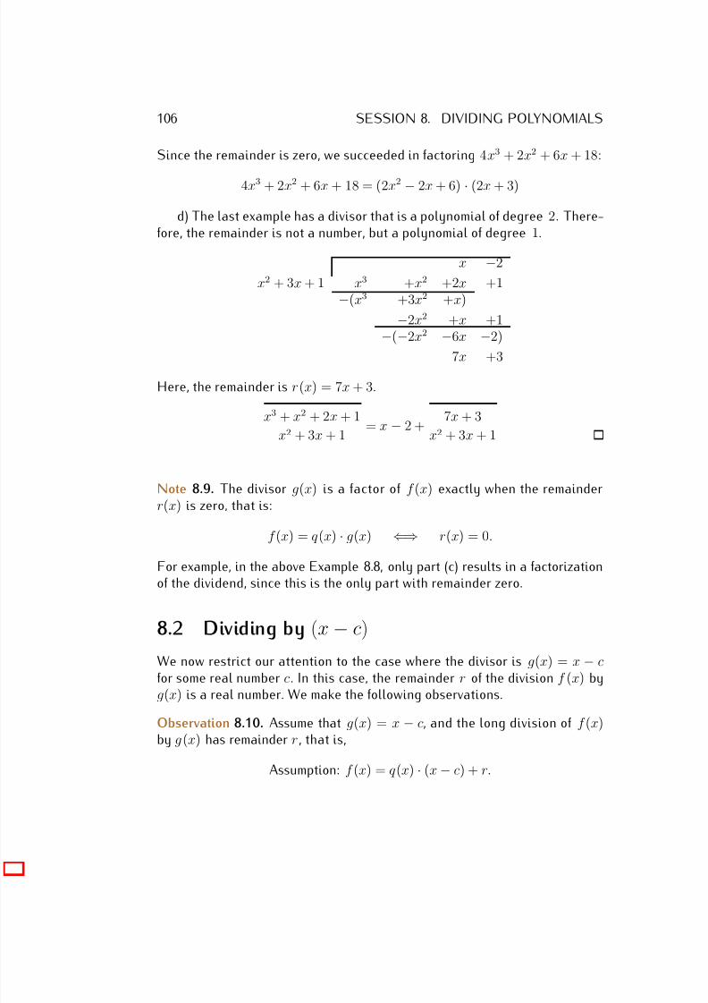
7/18/2019 Precalculus Tradler Carley
http://slidepdf.com/reader/full/precalculus-tradler-carley 116/424
106 SESSION 8. DIVIDING POLYNOMIALS
Since the remainder is zero, we succeeded in factoring 4x3 + 2x2 + 6x + 18:
4x3 + 2x2 + 6x + 18 = (2x2 − 2x + 6) · (2x + 3)
d) The last example has a divisor that is a polynomial of degree 2. There-fore, the remainder is not a number, but a polynomial of degree 1.
x −2
x2 + 3x + 1 x3 +x2 +2x +1−(x3 +3x2 +x)
−2x2 +x +1
−(
−2x2
−6x
−2)
7x +3
Here, the remainder is r(x) = 7x + 3.
x3 + x2 + 2x + 1
x2 + 3x + 1 = x − 2 +
7x + 3
x2 + 3x + 1
Note 8.9. The divisor g(x) is a factor of f (x) exactly when the remainderr(x) is zero, that is:
f (x) = q (x) · g(x) ⇐⇒ r(x) = 0.
For example, in the above Example 8.8, only part (c) results in a factorizationof the dividend, since this is the only part with remainder zero.
8.2 Dividing by (x − c)
We now restrict our attention to the case where the divisor is g(x) = x − cfor some real number c. In this case, the remainder r of the division f (x) byg(x) is a real number. We make the following observations.
Observation 8.10. Assume that g(x) = x − c, and the long division of f (x)by g(x) has remainder r , that is,
Assumption: f (x) = q (x) · (x − c) + r.
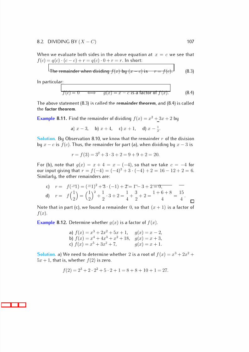
7/18/2019 Precalculus Tradler Carley
http://slidepdf.com/reader/full/precalculus-tradler-carley 117/424
8.2. DIVIDING BY (X − C ) 107
When we evaluate both sides in the above equation at x = c we see that
f (c) = q (c) · (c − c) + r = q (c) · 0 + r = r . In short:
The remainder when dividing f (x) by (x − c) is r = f (c). (8.3)
In particular:
f (c) = 0 ⇐⇒ g(x) = x − c is a factor of f (x). (8.4)
The above statement (8.3) is called the remainder theorem, and (8.4) is calledthe factor theorem.
Example 8.11. Find the remainder of dividing f (x) = x2 + 3x + 2 by
a) x − 3, b) x + 4, c) x + 1, d) x − 12 .
Solution. By Observation 8.10, we know that the remainder r of the divisionby x − c is f (c). Thus, the remainder for part (a), when dividing by x − 3 is
r = f (3) = 32 + 3 · 3 + 2 = 9 + 9 + 2 = 20.
For (b), note that g(x) = x + 4 = x − (−4), so that we take c = −4 forour input giving that r = f (−4) = (−4)2 + 3 · (−4) + 2 = 16 − 12 + 2 = 6.Similarly, the other remainders are:
c) r = f (−1) = (−1)2 + 3 · (−1) + 2 = 1 − 3 + 2 = 0,
d) r = f 1
2
=1
2
2
+ 1
2 · 3 + 2 =
1
4 +
3
2 + 2 =
1 + 6 + 8
4 =
15
4 .
Note that in part (c), we found a remainder 0, so that (x + 1) is a factor of f (x).
Example 8.12. Determine whether g (x) is a factor of f (x).
a) f (x) = x3 + 2x2 + 5x + 1, g(x) = x − 2,b) f (x) = x4 + 4x3 + x2 + 18, g(x) = x + 3,
c) f (x) = x
5
+ 3x
2
+ 7, g(x) = x + 1.Solution. a) We need to determine whether 2 is a root of f (x) = x3 + 2x2 +5x + 1, that is, whether f (2) is zero.
f (2) = 23 + 2 · 22 + 5 · 2 + 1 = 8 + 8 + 10 + 1 = 27.
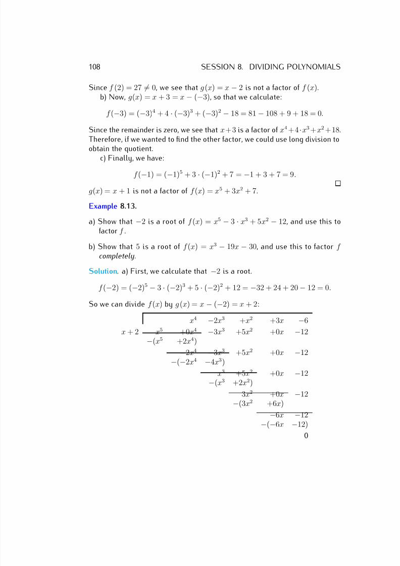
7/18/2019 Precalculus Tradler Carley
http://slidepdf.com/reader/full/precalculus-tradler-carley 118/424
108 SESSION 8. DIVIDING POLYNOMIALS
Since f (2) = 27 = 0, we see that g(x) = x − 2 is not a factor of f (x).
b) Now, g(x) = x + 3 = x − (−3), so that we calculate:
f (−3) = (−3)4 + 4 · (−3)3 + (−3)2 − 18 = 81 − 108 + 9 + 18 = 0.
Since the remainder is zero, we see that x+3 is a factor of x4 +4 ·x3 +x2 +18.Therefore, if we wanted to find the other factor, we could use long division toobtain the quotient.
c) Finally, we have:
f (−1) = (−1)5 + 3 · (−1)2 + 7 = −1 + 3 + 7 = 9.
g(x) = x + 1 is not a factor of f (x) = x5 + 3x2 + 7.
Example 8.13.
a) Show that −2 is a root of f (x) = x5 − 3 · x3 + 5x2 − 12, and use this tofactor f .
b) Show that 5 is a root of f (x) = x3 − 19x − 30, and use this to factor f completely.
Solution. a) First, we calculate that −2 is a root.
f (
−2) = (
−2)5
−3
·(
−2)3 + 5
·(
−2)2 + 12 =
−32 + 24 + 20
−12 = 0.
So we can divide f (x) by g(x) = x − (−2) = x + 2:
x4 −2x3 +x2 +3x −6
x + 2 x5 +0x4 −3x3 +5x2 +0x −12−(x5 +2x4)
−2x4 −3x3 +5x2 +0x −12−(−2x4 −4x3)
x3 +5x2 +0x −12−(x3 +2x2)
3x2
+0x −12−(3x2 +6x)
−6x −12−(−6x −12)
0
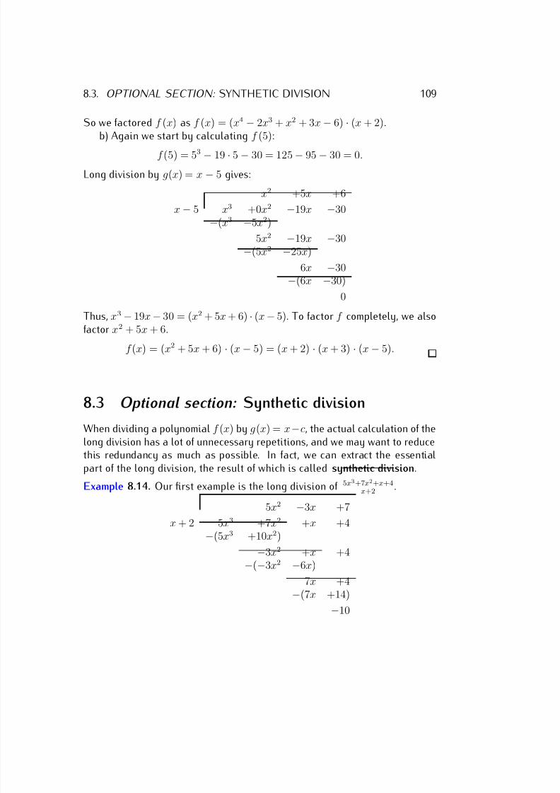
7/18/2019 Precalculus Tradler Carley
http://slidepdf.com/reader/full/precalculus-tradler-carley 119/424
8.3. OPTIONAL SECTION: SYNTHETIC DIVISION 109
So we factored f (x) as f (x) = (x4 − 2x3 + x2 + 3x − 6) · (x + 2).
b) Again we start by calculating f (5):f (5) = 53 − 19 · 5 − 30 = 125 − 95 − 30 = 0.
Long division by g(x) = x − 5 gives:
x2 +5x +6
x − 5 x3 +0x2 −19x −30−(x3 −5x2)
5x2 −19x −30−(5x2 −25x)
6x
−30
−(6x −30)
0
Thus, x3 − 19x − 30 = (x2 + 5x + 6) · (x − 5). To factor f completely, we alsofactor x2 + 5x + 6.
f (x) = (x2 + 5x + 6) · (x − 5) = (x + 2) · (x + 3) · (x − 5).
8.3 Optional section: Synthetic division
When dividing a polynomial f (x) by g(x) = x−c, the actual calculation of thelong division has a lot of unnecessary repetitions, and we may want to reducethis redundancy as much as possible. In fact, we can extract the essentialpart of the long division, the result of which is called synthetic division.
Example 8.14. Our first example is the long division of 5x3+7x2+x+4x+2 .
5x2 −3x +7
x + 2 5x3 +7x2 +x +4−(5x3 +10x2)
−3x2
+x +4−(−3x2 −6x)
7x +4−(7x +14)
−10
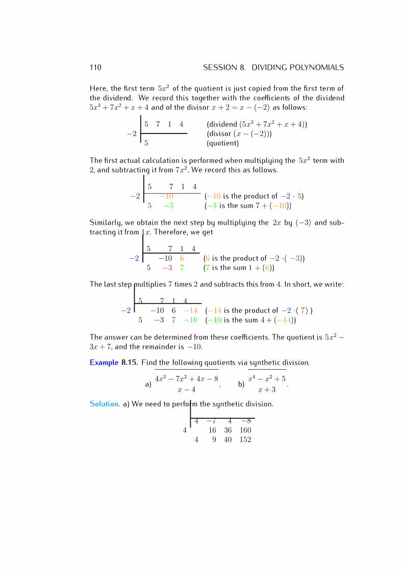
7/18/2019 Precalculus Tradler Carley
http://slidepdf.com/reader/full/precalculus-tradler-carley 120/424
110 SESSION 8. DIVIDING POLYNOMIALS
Here, the first term 5x2 of the quotient is just copied from the first term of
the dividend. We record this together with the coefficients of the dividend5x3 + 7x2 + x + 4 and of the divisor x + 2 = x − (−2) as follows:
5 7 1 4 (dividend (5x3 + 7x2 + x + 4))−2 (divisor (x − (−2)))
5 (quotient)
The first actual calculation is performed when multiplying the 5x2 term with2, and subtracting it from 7x2. We record this as follows.
5 7 1 4
−2 −10 (−10 is the product of −2 · 5)5 −3 (−3 is the sum 7 + (−10))
Similarly, we obtain the next step by multiplying the 2x by (−3) and sub-tracting it from 1x. Therefore, we get
5 7 1 4−2 −10 6 (6 is the product of −2 ·( −3))
5 −3 7 (7 is the sum 1 + (6))
The last step multiplies 7 times 2 and subtracts this from 4. In short, we write:
5 7 1 4−2 −10 6 −14 (−14 is the product of −2 ·( 7) )5 −3 7 −10 (−10 is the sum 4 + (−14))
The answer can be determined from these coefficients. The quotient is 5x2 −3x + 7, and the remainder is −10.
Example 8.15. Find the following quotients via synthetic division.
a) 4x3 − 7x2 + 4x − 8
x − 4 , b)
x4 − x2 + 5
x + 3 .
Solution. a) We need to perform the synthetic division.
4 −7 4 −84 16 36 160
4 9 40 152
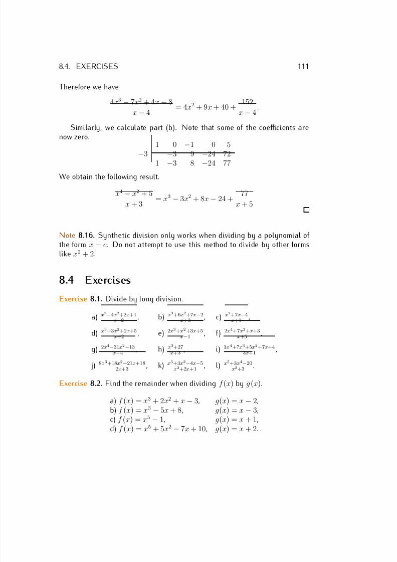
7/18/2019 Precalculus Tradler Carley
http://slidepdf.com/reader/full/precalculus-tradler-carley 121/424
8.4. EXERCISES 111
Therefore we have
4x3 − 7x2 + 4x − 8
x − 4 = 4x2 + 9x + 40 +
152
x − 4.
Similarly, we calculate part (b). Note that some of the coefficients arenow zero.
1 0 −1 0 5−3 −3 9 −24 72
1 −3 8 −24 77
We obtain the following result.
x4
− x2
+ 5x + 3 = x3 − 3x2 + 8x − 24 + 77x + 5
Note 8.16. Synthetic division only works when dividing by a polynomial of the form x − c. Do not attempt to use this method to divide by other formslike x2 + 2.
8.4 Exercises
Exercise 8.1. Divide by long division.
a) x3−4x2+2x+1x−2 , b) x3+6x2+7x−2
x+3 , c) x2+7x−4x+1 ,
d) x3+3x2+2x+5x+2 , e) 2x3+x2+3x+5
x−1 , f ) 2x4+7x3+x+3x+5 ,
g) 2x4−31x2−13x−4
, h) x3+27x+3
, i) 3x4+7x3+5x2+7x+43x+1
,
j) 8x3+18x2+21x+182x+3
, k) x3+3x2−4x−5x2+2x+1
, l) x5+3x4−20x2+3
.
Exercise 8.2. Find the remainder when dividing f (x) by g(x).
a) f (x) = x3 + 2x2 + x − 3, g(x) = x − 2,b) f (x) = x3 − 5x + 8, g(x) = x − 3,c) f (x) = x5 − 1, g(x) = x + 1,d) f (x) = x5 + 5x2 − 7x + 10, g(x) = x + 2.
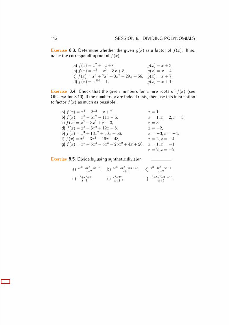
7/18/2019 Precalculus Tradler Carley
http://slidepdf.com/reader/full/precalculus-tradler-carley 122/424
112 SESSION 8. DIVIDING POLYNOMIALS
Exercise 8.3. Determine whether the given g(x) is a factor of f (x). If so,
name the corresponding root of f (x).
a) f (x) = x2 + 5x + 6, g(x) = x + 3,b) f (x) = x3 − x2 − 3x + 8, g(x) = x − 4,c) f (x) = x4 + 7x3 + 3x2 + 29x + 56, g(x) = x + 7,d) f (x) = x999 + 1, g(x) = x + 1.
Exercise 8.4. Check that the given numbers for x are roots of f (x) (seeObservation 8.10). If the numbers x are indeed roots, then use this informationto factor f (x) as much as possible.
a) f (x) = x
3
− 2x
2
− x + 2, x = 1,b) f (x) = x3 − 6x2 + 11x − 6, x = 1, x = 2, x = 3,c) f (x) = x3 − 3x2 + x − 3, x = 3,d) f (x) = x3 + 6x2 + 12x + 8, x = −2,e) f (x) = x3 + 13x2 + 50x + 56, x = −3, x = −4,f) f (x) = x3 + 3x2 − 16x − 48, x = 2, x = −4,g) f (x) = x5 + 5x4 − 5x3 − 25x2 + 4x + 20, x = 1, x = −1,
x = 2, x = −2.
Exercise 8.5. Divide by using synthetic division.
a) 2x3+3x2
−5x+7
x−2 , b) 4x3+3x2
−15x+18
x+3 , c) x3+4x2
−3x+1
x+2 ,
d) x4+x3+1x−1 , e) x5+32
x+2 , f ) x3+5x2−3x−10x+5 .
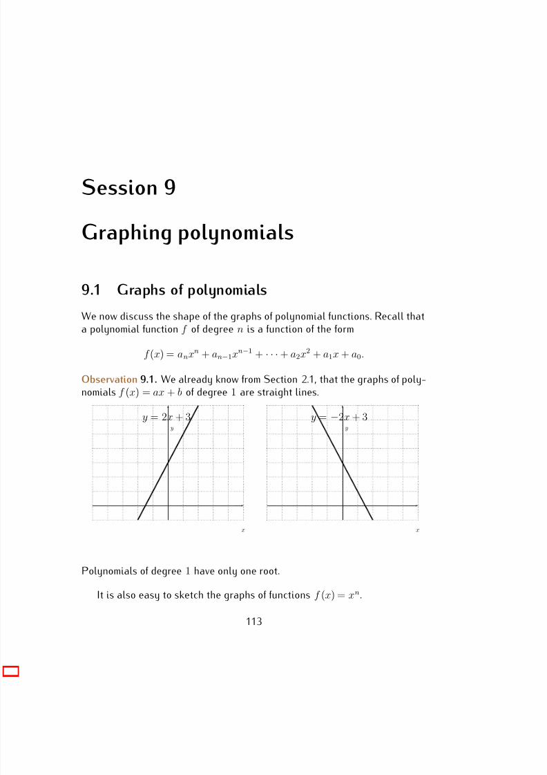
7/18/2019 Precalculus Tradler Carley
http://slidepdf.com/reader/full/precalculus-tradler-carley 123/424
Session 9
Graphing polynomials
9.1 Graphs of polynomials
We now discuss the shape of the graphs of polynomial functions. Recall thata polynomial function f of degree n is a function of the form
f (x) = anxn + an−1xn−1 + · · · + a2x2 + a1x + a0.
Observation 9.1. We already know from Section 2.1, that the graphs of poly-nomials f (x) = ax + b of degree 1 are straight lines.
y = 2x + 3 y = −2x + 3
x
y
x
y
Polynomials of degree 1 have only one root.
It is also easy to sketch the graphs of functions f (x) = xn.
113
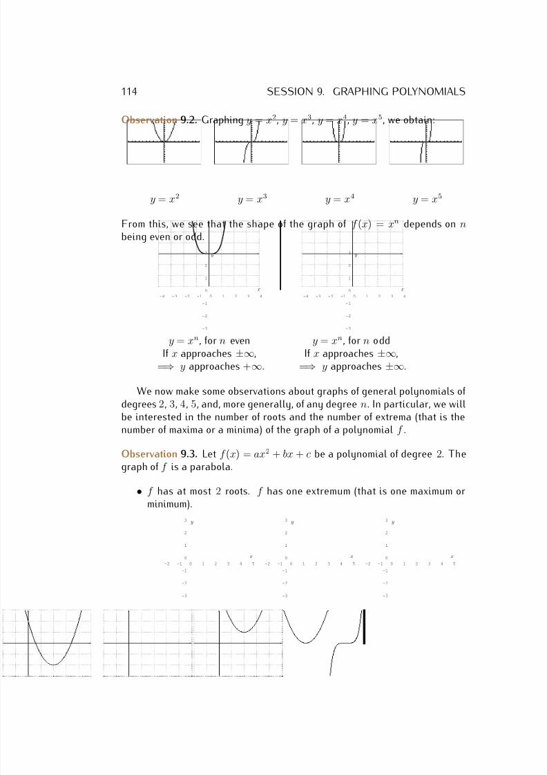
7/18/2019 Precalculus Tradler Carley
http://slidepdf.com/reader/full/precalculus-tradler-carley 124/424
114 SESSION 9. GRAPHING POLYNOMIALS
Observation 9.2. Graphing y = x2, y = x3, y = x4, y = x5, we obtain:
y = x2 y = x3 y = x4 y = x5
From this, we see that the shape of the graph of f (x) = xn depends on nbeing even or odd.
-4 -3 -2 -1 0 1 2 3 4
-3
-2
-1
0
1
2
3
x
y
-4 -3 -2 -1 0 1 2 3 4
-3
-2
-1
0
1
2
3
x
y
y = xn, for n even y = xn, for n oddIf x approaches ±∞, If x approaches ±∞,
=⇒ y approaches +∞. =⇒ y approaches ±∞.
We now make some observations about graphs of general polynomials of
degrees 2, 3, 4, 5, and, more generally, of any degree n. In particular, we willbe interested in the number of roots and the number of extrema (that is thenumber of maxima or a minima) of the graph of a polynomial f .
Observation 9.3. Let f (x) = ax2 + bx + c be a polynomial of degree 2. Thegraph of f is a parabola.
• f has at most 2 roots. f has one extremum (that is one maximum orminimum).
-2 -1 0 1 2 3 4 5
-3
-2
-1
0
1
2
3
x
y
-2 -1 0 1 2 3 4 5
-3
-2
-1
0
1
2
3
x
y
-2 -1 0 1 2 3 4 5
-3
-2
-1
0
1
2
3
x
y
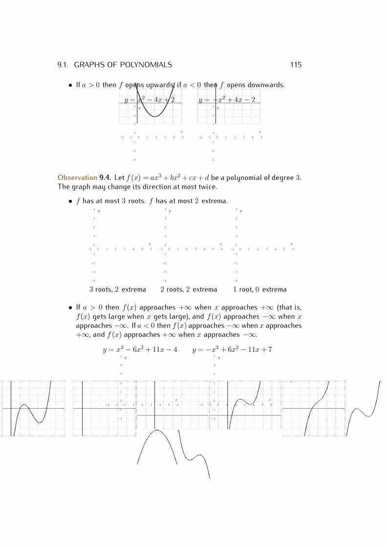
7/18/2019 Precalculus Tradler Carley
http://slidepdf.com/reader/full/precalculus-tradler-carley 125/424
9.1. GRAPHS OF POLYNOMIALS 115
• If a > 0 then f opens upwards, if a < 0 then f opens downwards.
y = x2 − 4x + 2 y = −x2 + 4x − 2
-2 -1 0 1 2 3 4 5
-3
-2
-1
0
1
2
3
x
y
-2 -1 0 1 2 3 4 5
-3
-2
-1
0
1
2
3
x
y
Observation 9.4. Let f (x) = ax3 + bx2 + cx + d be a polynomial of degree 3.The graph may change its direction at most twice.
• f has at most 3 roots. f has at most 2 extrema.
-1 0 1 2 3 4 5 6
-4
-3
-2
-1
0
1
2
3
4
x
y
-1 0 1 2 3 4 5 6
-4
-3
-2
-1
0
1
2
3
4
x
y
-1 0 1 2 3 4 5 6
-4
-3
-2
-1
0
1
2
3
4
x
y
3 roots, 2 extrema 2 roots, 2 extrema 1 root, 0 extrema
• If a > 0 then f (x) approaches +∞ when x approaches +∞ (that is,f (x) gets large when x gets large), and f (x) approaches −∞ when xapproaches −∞. If a < 0 then f (x) approaches −∞ when x approaches+∞, and f (x) approaches +∞ when x approaches −∞.
y = x3 − 6x2 + 11x − 4 y = −x3 + 6x2 − 11x + 7
-2 -1 0 1 2 3 4 5 6
-2
-1
0
1
2
3
4
5
x
y
-2 -1 0 1 2 3 4 5 6
-2
-1
0
1
2
3
4
5
x
y
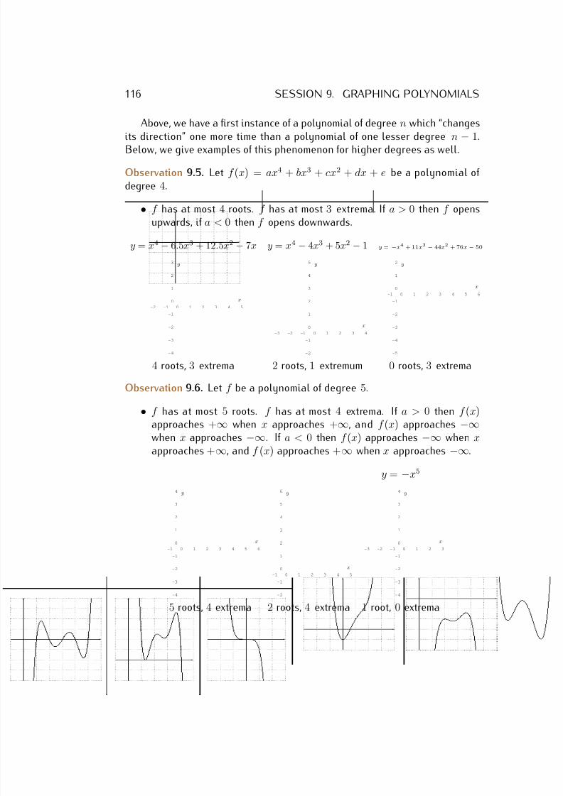
7/18/2019 Precalculus Tradler Carley
http://slidepdf.com/reader/full/precalculus-tradler-carley 126/424
116 SESSION 9. GRAPHING POLYNOMIALS
Above, we have a first instance of a polynomial of degree n which “changes
its direction” one more time than a polynomial of one lesser degree n − 1.Below, we give examples of this phenomenon for higher degrees as well.
Observation 9.5. Let f (x) = ax4 + bx3 + cx2 + dx + e be a polynomial of degree 4.
• f has at most 4 roots. f has at most 3 extrema. If a > 0 then f opensupwards, if a < 0 then f opens downwards.
y = x4 − 6.5x3 + 12.5x2 − 7x y = x4 − 4x3 + 5x2 − 1 y = −x4 + 11x3 − 44x2 + 76x− 50
-2 -1 0 1 2 3 4 5
-4
-3
-2
-1
0
1
2
3
x
y
-3 -2 -1 0 1 2 3 4
-2
-1
0
1
2
3
4
5
x
y
-1 0 1 2 3 4 5 6
-5
-4
-3
-2
-1
0
1
2
x
y
4 roots, 3 extrema 2 roots, 1 extremum 0 roots, 3 extrema
Observation 9.6. Let f be a polynomial of degree 5.
• f has at most 5 roots. f has at most 4 extrema. If a > 0 then f (x)approaches +∞ when x approaches +∞, and f (x) approaches −∞when x approaches −∞. If a < 0 then f (x) approaches −∞ when xapproaches +∞, and f (x) approaches +∞ when x approaches −∞.
y = −x5
-1 0 1 2 3 4 5 6
-4
-3
-2
-1
0
1
2
3
4
x
y
-1 0 1 2 3 4 5
-2
-1
0
1
2
3
4
5
6
x
y
-3 -2 -1 0 1 2 3
-4
-3
-2
-1
0
1
2
3
4
x
y
5 roots, 4 extrema 2 roots, 4 extrema 1 root, 0 extrema
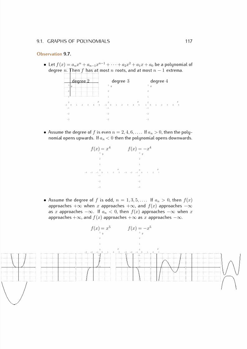
7/18/2019 Precalculus Tradler Carley
http://slidepdf.com/reader/full/precalculus-tradler-carley 127/424
9.1. GRAPHS OF POLYNOMIALS 117
Observation 9.7.
• Let f (x) = anxn + an−1xn−1 + · · · + a2x2 + a1x + a0 be a polynomial of degree n. Then f has at most n roots, and at most n − 1 extrema.
degree 2 degree 3 degree 4
-1 0 1 2 3 4 5
-3
-2
-1
0
1
2
3
x
y
-1 0 1 2 3 4 5
-3
-2
-1
0
1
2
3
x
y
-1 0 1 2 3 4 5
-3
-2
-1
0
1
2
3
x
y
• Assume the degree of f is even n = 2, 4, 6, . . . . If an > 0, then the poly-nomial opens upwards. If an < 0 then the polynomial opens downwards.
f (x) = x4 f (x) = −x4
-3 -2 -1 0 1 2 3
-3
-2
-1
0
1
2
3
x
y
-3 -2 -1 0 1 2 3
-3
-2
-1
0
1
2
3
x
y
• Assume the degree of f is odd, n = 1, 3, 5, . . . . If an > 0, then f (x)approaches +∞ when x approaches +∞, and f (x) approaches −∞as x approaches −∞. If an < 0, then f (x) approaches −∞ when xapproaches +∞, and f (x) approaches +∞ as x approaches −∞.
f (x) = x5 f (x) = −x5
-3 -2 -1 0 1 2 3
-3
-2
-1
0
1
2
3
x
y
-3 -2 -1 0 1 2 3
-3
-2
-1
0
1
2
3
x
y

7/18/2019 Precalculus Tradler Carley
http://slidepdf.com/reader/full/precalculus-tradler-carley 128/424
118 SESSION 9. GRAPHING POLYNOMIALS
• The domain of a polynomial f is all real numbers, and f is continuous
for all real numbers (there are no jumps in the graph). The graph of f has no horizontal or vertical asymptotes, no discontinuities ( jumps inthe graph), and no corners. Furthermore, f (x) approaches ±∞ when xapproaches ±∞. Therefore, the following graphs cannot be graphs of polynomials.
-1 0 1 2 3 4 5
-1
0
1
2
3
4
5
x
y
-1 0 1 2 3 4 5
-1
0
1
2
3
4
5
x
y
-1 0 1 2 3 4 5
-1
0
1
2
3
4
5
x
y
-1 0 1 2 3 4 5
-1
0
1
2
3
4
5
x
y
vertical discontinuity corner horizontalasymptote / pole asymptote
Example 9.8. Which of the following graphs could be the graphs of a poly-nomial? If the graph could indeed be a graph of a polynomial then determinea possible degree of the polynomial.
a)
-3 -2 -1 0 1 2 3 4
-3
-2
-1
0
1
2
3
4
x
y
b)-1 0 1 2 3 4 5
-1
0
1
2
3
4
5
6
x
y
c)
0 1 2 3 4 5 6
-2
-1
0
1
2
3
4
5
x
y
d)-4 -3 -2 -1 0 1 2 3 4 5 6
0
1
2
3
4
5
x
y
e)-5 -4 -3 -2 -1 0 1 2 3 4 5
-1
0
1
2
3
4
x
y
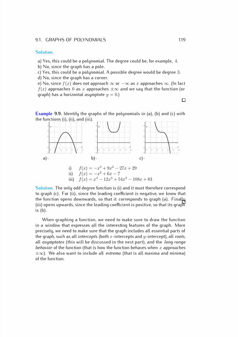
7/18/2019 Precalculus Tradler Carley
http://slidepdf.com/reader/full/precalculus-tradler-carley 129/424
9.1. GRAPHS OF POLYNOMIALS 119
Solution.
a) Yes, this could be a polynomial. The degree could be, for example, 4.b) No, since the graph has a pole.c) Yes, this could be a polynomial. A possible degree would be degree 3.d) No, since the graph has a corner.e) No, since f (x) does not approach ∞ or −∞ as x approaches ∞. (In factf (x) approaches 0 as x approaches ±∞ and we say that the function (orgraph) has a horizontal asymptote y = 0.)
Example 9.9. Identify the graphs of the polynomials in (a), (b) and (c) with
the functions (i), (ii), and (iii).
a)
0 1 2 3 4 5 6
-2
-1
0
1
2
3
4
x
y
b)
0 1 2 3 4 5 6
-2
-1
0
1
2
3
4
x
y
c)
0 1 2 3 4 5 6
-2
-1
0
1
2
3
4
x
y
i) f (x) = −x3 + 9x2 − 27x + 29ii) f (x) =
−x2 + 6x
−7
iii) f (x) = x4 − 12x3 + 54x2 − 108x + 83
Solution. The only odd degree function is (i) and it must therefore correspondto graph (c). For (ii), since the leading coefficient is negative, we know thatthe function opens downwards, so that it corresponds to graph (a). Finally(iii) opens upwards, since the leading coefficient is positive, so that its graphis (b).
When graphing a function, we need to make sure to draw the functionin a window that expresses all the interesting features of the graph. Moreprecisely, we need to make sure that the graph includes all essential parts of
the graph, such as all intercepts (both x-intercepts and y-intercept), all roots,all asymptotes (this will be discussed in the next part), and the long range
behavior of the function (that is how the function behaves when x approaches±∞). We also want to include all extrema (that is all maxima and minima)of the function.
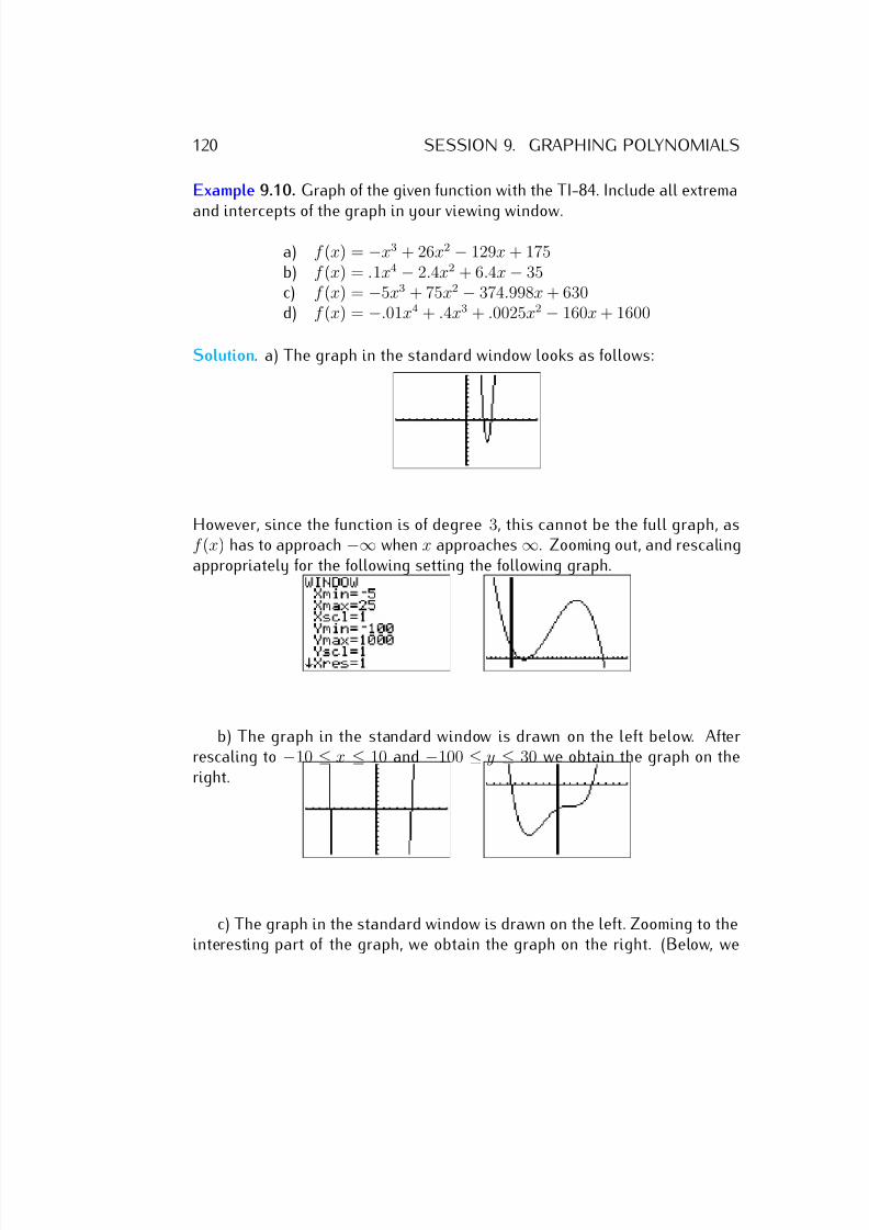
7/18/2019 Precalculus Tradler Carley
http://slidepdf.com/reader/full/precalculus-tradler-carley 130/424
120 SESSION 9. GRAPHING POLYNOMIALS
Example 9.10. Graph of the given function with the TI-84. Include all extrema
and intercepts of the graph in your viewing window.
a) f (x) = −x3 + 26x2 − 129x + 175b) f (x) = .1x4 − 2.4x2 + 6.4x − 35c) f (x) = −5x3 + 75x2 − 374.998x + 630d) f (x) = −.01x4 + .4x3 + .0025x2 − 160x + 1600
Solution. a) The graph in the standard window looks as follows:
However, since the function is of degree 3, this cannot be the full graph, asf (x) has to approach −∞ when x approaches ∞. Zooming out, and rescalingappropriately for the following setting the following graph.
b) The graph in the standard window is drawn on the left below. Afterrescaling to −10 ≤ x ≤ 10 and −100 ≤ y ≤ 30 we obtain the graph on theright.
c) The graph in the standard window is drawn on the left. Zooming to theinteresting part of the graph, we obtain the graph on the right. (Below, we
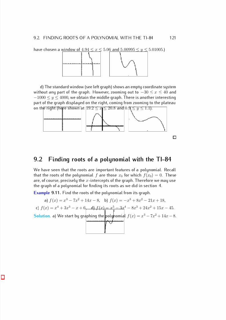
7/18/2019 Precalculus Tradler Carley
http://slidepdf.com/reader/full/precalculus-tradler-carley 131/424
9.2. FINDING ROOTS OF A POLYNOMIAL WITH THE TI-84 121
have chosen a window of 4.94 ≤ x ≤ 5.06 and 5.00995 ≤ y ≤ 5.01005.)
d) The standard window (see left graph) shows an empty coordinate systemwithout any part of the graph. However, zooming out to −30 ≤ x ≤ 40 and−1000 ≤ y ≤ 4000, we obtain the middle graph. There is another interestingpart of the graph displayed on the right, coming from zooming to the plateauon the right (here shown at 19.2
≤x
≤20.8 and 0.9
≤y
≤1.1).
9.2 Finding roots of a polynomial with the TI-84
We have seen that the roots are important features of a polynomial. Recallthat the roots of the polynomial f are those x0 for which f (x0) = 0. Theseare, of course, precisely the x-intercepts of the graph. Therefore we may usethe graph of a polynomial for finding its roots as we did in section 4.
Example 9.11. Find the roots of the polynomial from its graph.
a) f (x) = x3 − 7x2 + 14x − 8, b) f (x) = −x3 + 8x2 − 21x + 18,
c) f (x) = x4 + 3x3 − x + 6, d) f (x) = x5 − 3x4 − 8x3 + 24x2 + 15x − 45.
Solution. a) We start by graphing the polynomial f (x) = x3 − 7x2 + 14x − 8.
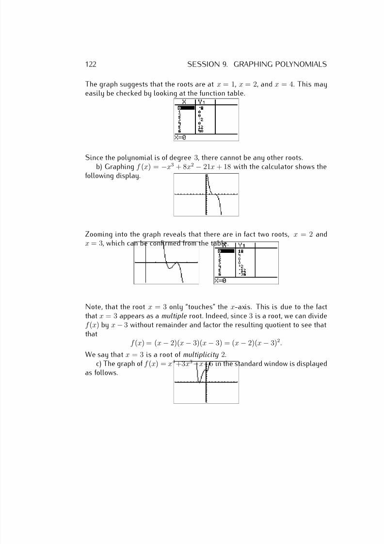
7/18/2019 Precalculus Tradler Carley
http://slidepdf.com/reader/full/precalculus-tradler-carley 132/424
122 SESSION 9. GRAPHING POLYNOMIALS
The graph suggests that the roots are at x = 1, x = 2, and x = 4. This may
easily be checked by looking at the function table.
Since the polynomial is of degree 3, there cannot be any other roots.b) Graphing f (x) = −x3 + 8x2 − 21x + 18 with the calculator shows the
following display.
Zooming into the graph reveals that there are in fact two roots, x = 2 andx = 3, which can be confirmed from the table.
Note, that the root x = 3 only “touches” the x-axis. This is due to the factthat x = 3 appears as a multiple root. Indeed, since 3 is a root, we can dividef (x) by x − 3 without remainder and factor the resulting quotient to see thatthat
f (x) = (x − 2)(x − 3)(x − 3) = (x − 2)(x − 3)2.
We say that x = 3 is a root of multiplicity 2.c) The graph of f (x) = x4 +3x3−x+6 in the standard window is displayed
as follows.
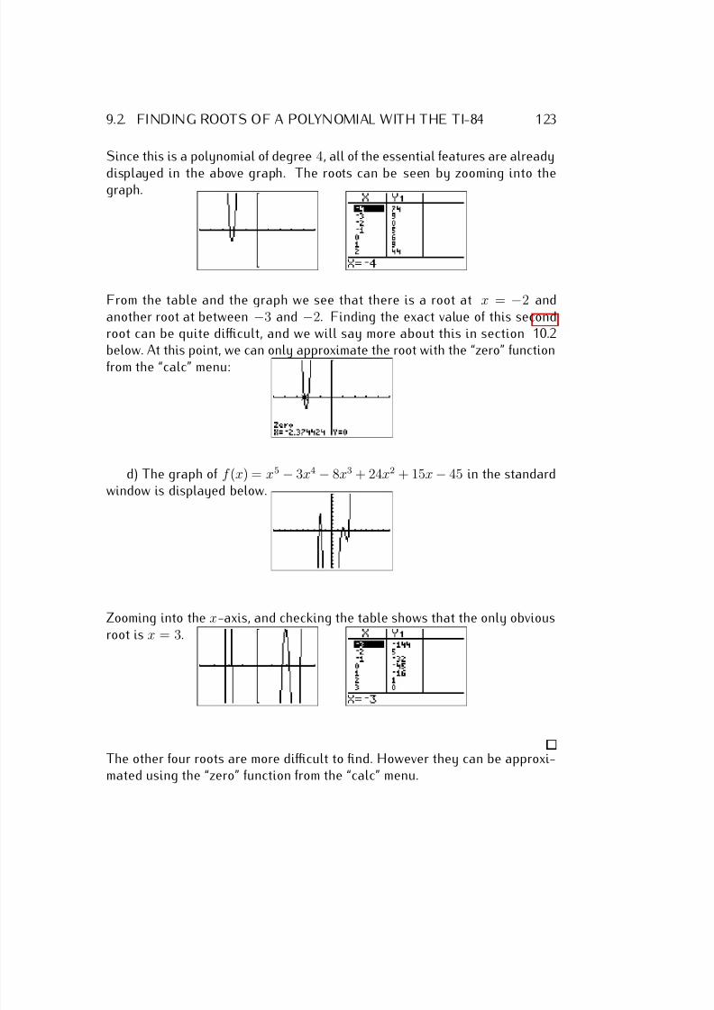
7/18/2019 Precalculus Tradler Carley
http://slidepdf.com/reader/full/precalculus-tradler-carley 133/424
9.2. FINDING ROOTS OF A POLYNOMIAL WITH THE TI-84 123
Since this is a polynomial of degree 4, all of the essential features are already
displayed in the above graph. The roots can be seen by zooming into thegraph.
From the table and the graph we see that there is a root at x = −2 andanother root at between −3 and −2. Finding the exact value of this secondroot can be quite difficult, and we will say more about this in section 10.2
below. At this point, we can only approximate the root with the “zero” functionfrom the “calc” menu:
d) The graph of f (x) = x5 − 3x4 − 8x3 + 24x2 + 15x − 45 in the standardwindow is displayed below.
Zooming into the x-axis, and checking the table shows that the only obviousroot is x = 3.
The other four roots are more difficult to find. However they can be approxi-mated using the “zero” function from the “calc” menu.
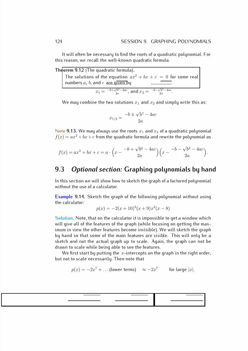
7/18/2019 Precalculus Tradler Carley
http://slidepdf.com/reader/full/precalculus-tradler-carley 134/424
124 SESSION 9. GRAPHING POLYNOMIALS
It will often be necessary to find the roots of a quadratic polynomial. For
this reason, we recall the well-known quadratic formula.
Theorem 9.12 (The quadratic formula).
The solutions of the equation ax2 + bx + c = 0 for some realnumbers a, b, and c are given by
x1 = −b+√
b2−4ac2a , and x2 = −b−√ b2−4ac
2a .
We may combine the two solutions x1 and x2 and simply write this as:
x1/2 = −b ± √
b2 − 4ac
2aNote 9.13. We may always use the roots x1 and x2 of a quadratic polynomialf (x) = ax2 + bx + c from the quadratic formula and rewrite the polynomial as
f (x) = ax2 + bx + c = a ·
x − −b +√
b2 − 4ac
2a
x − −b − √
b2 − 4ac
2a
.
9.3 Optional section: Graphing polynomials by hand
In this section we will show how to sketch the graph of a factored polynomialwithout the use of a calculator.
Example 9.14. Sketch the graph of the following polynomial without usingthe calculator:
p(x) = −2(x + 10)3(x + 9)x2(x − 8)
Solution. Note, that on the calculator it is impossible to get a window whichwill give all of the features of the graph (while focusing on getting the max-imum in view the other features become invisible). We will sketch the graphby hand so that some of the main features are visible. This will only be asketch and not the actual graph up to scale. Again, the graph can not be
drawn to scale while being able to see the features.We first start by putting the x-intercepts on the graph in the right order,
but not to scale necessarily. Then note that
p(x) = −2x7 + . . . (lower terms) ≈ −2x7 for large |x|.
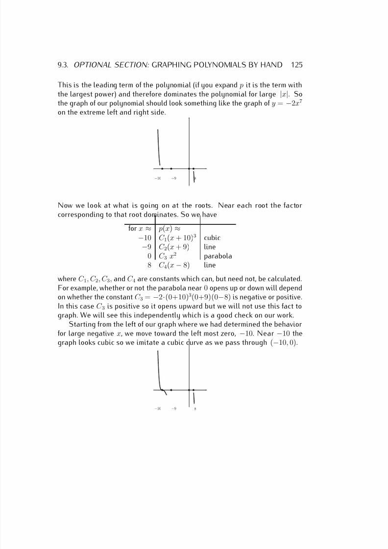
7/18/2019 Precalculus Tradler Carley
http://slidepdf.com/reader/full/precalculus-tradler-carley 135/424
9.3. OPTIONAL SECTION: GRAPHING POLYNOMIALS BY HAND 125
This is the leading term of the polynomial (if you expand p it is the term with
the largest power) and therefore dominates the polynomial for large |x|. Sothe graph of our polynomial should look something like the graph of y = −2x7
on the extreme left and right side.
−10 −9 8
Now we look at what is going on at the roots. Near each root the factorcorresponding to that root dominates. So we have
for x ≈ p(x) ≈−10 C 1(x + 10)3 cubic−9 C 2(x + 9) line
0 C 3 x2 parabola8 C 4(x − 8) line
where C 1, C 2, C 3, and C 4 are constants which can, but need not, be calculated.
For example, whether or not the parabola near 0 opens up or down will dependon whether the constant C 3 = −2·(0+10)3(0+9)(0−8) is negative or positive.In this case C 3 is positive so it opens upward but we will not use this fact tograph. We will see this independently which is a good check on our work.
Starting from the left of our graph where we had determined the behaviorfor large negative x, we move toward the left most zero, −10. Near −10 thegraph looks cubic so we imitate a cubic curve as we pass through (−10, 0).
−10 −9 8
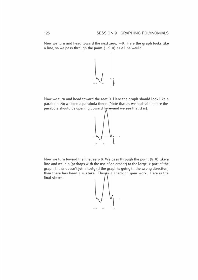
7/18/2019 Precalculus Tradler Carley
http://slidepdf.com/reader/full/precalculus-tradler-carley 136/424
126 SESSION 9. GRAPHING POLYNOMIALS
Now we turn and head toward the next zero, −9. Here the graph looks like
a line, so we pass through the point (−9, 0) as a line would.
−10 −9 8
Now we turn and head toward the root 0. Here the graph should look like aparabola. So we form a parabola there. (Note that as we had said before theparabola should be opening upward here–and we see that it is).
−10 −9 8
Now we turn toward the final zero 8. We pass through the point (8, 0) like aline and we join (perhaps with the use of an eraser) to the large x part of thegraph. If this doesn’t join nicely (if the graph is going in the wrong direction)then there has been a mistake. This is a check on your work. Here is thefinal sketch.
−10 −9 8
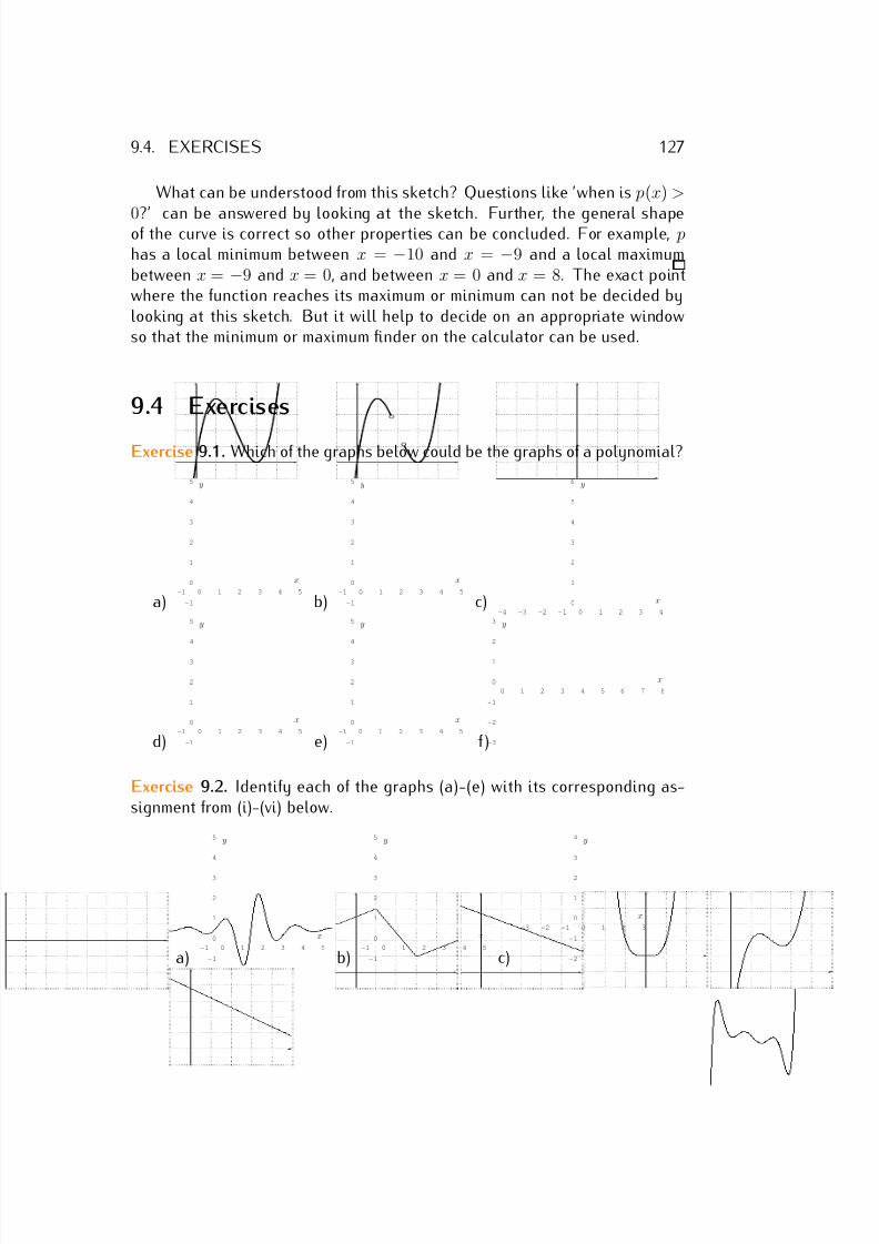
7/18/2019 Precalculus Tradler Carley
http://slidepdf.com/reader/full/precalculus-tradler-carley 137/424
9.4. EXERCISES 127
What can be understood from this sketch? Questions like ’when is p(x) >
0?’ can be answered by looking at the sketch. Further, the general shapeof the curve is correct so other properties can be concluded. For example, phas a local minimum between x = −10 and x = −9 and a local maximumbetween x = −9 and x = 0, and between x = 0 and x = 8. The exact pointwhere the function reaches its maximum or minimum can not be decided bylooking at this sketch. But it will help to decide on an appropriate windowso that the minimum or maximum finder on the calculator can be used.
9.4 Exercises
Exercise 9.1. Which of the graphs below could be the graphs of a polynomial?
a)-1 0 1 2 3 4 5
-1
0
1
2
3
4
5
x
y
b)-1 0 1 2 3 4 5
-1
0
1
2
3
4
5
x
y
c)-4 -3 -2 -1 0 1 2 3 4
0
1
2
3
4
5
6
x
y
d)-1 0 1 2 3 4 5
-1
0
1
2
3
4
5
x
y
e)-1 0 1 2 3 4 5
-1
0
1
2
3
4
5
x
y
f )
0 1 2 3 4 5 6 7 8
-3
-2
-1
0
1
2
3
x
y
Exercise 9.2. Identify each of the graphs (a)-(e) with its corresponding as-signment from (i)-(vi) below.
a)-1 0 1 2 3 4 5
-1
0
1
2
3
4
5
x
y
b)-1 0 1 2 3 4 5
-1
0
1
2
3
4
5
x
y
c)
-3 -2 -1 0 1 2 3
-2
-1
0
1
2
3
4
x
y
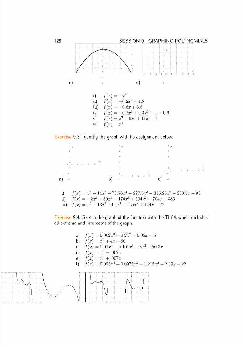
7/18/2019 Precalculus Tradler Carley
http://slidepdf.com/reader/full/precalculus-tradler-carley 138/424
128 SESSION 9. GRAPHING POLYNOMIALS
d)
-5 -4 -3 -2 -1 0 1 2 3 4 5
-3
-2
-1
0
1
2
3
x
y
e)
-4 -3 -2 -1 0 1 2 3 4 5
-2
-1
0
1
2
3
4
x
y
i) f (x) = −x2
ii) f (x) = −0.2x2 + 1.8iii) f (x) = −0.6x + 3.8iv) f (x) = −0.2x3 + 0.4x2 + x − 0.6v) f (x) = x3
−6x2 + 11x
−4
vi) f (x) = x4
Exercise 9.3. Identify the graph with its assignment below.
a)
-1 0 1 2 3 4 5
-3
-2
-1
0
1
2
3
x
y
b)-1 0 1 2 3 4 5
-1
0
1
2
3
4
5
x
y
c)
-1 0 1 2 3 4 5 6
-2
-1
0
1
2
3
4
x
y
i) f (x) = x6 − 14x5 + 78.76x4 − 227.5x3 + 355.25x2 − 283.5x + 93ii) f (x) = −2x5 + 30x4 − 176x3 + 504x2 − 704x + 386iii) f (x) = x5 − 13x4 + 65x3 − 155x2 + 174x − 72
Exercise 9.4. Sketch the graph of the function with the TI-84, which includesall extrema and intercepts of the graph.
a) f (x) = 0.002x3 + 0.2x2 − 0.05x − 5
b) f (x) = x3
+ 4x + 50c) f (x) = 0.01x4 − 0.101x3 − 3x2 + 50.3xd) f (x) = x3 − .007xe) f (x) = x3 + .007xf ) f (x) = 0.025x4 + 0.0975x3 − 1.215x2 + 2.89x − 22
7/18/2019 Precalculus Tradler Carley
http://slidepdf.com/reader/full/precalculus-tradler-carley 139/424
9.4. EXERCISES 129
Exercise 9.5. Find the exact value of at least one root of the given polynomial.
a) f (x) = x3 − 10x2 + 31x − 30,b) f (x) = −x3 − x2 + 8x + 8,c) f (x) = x3 − 11x2 − 3x + 33,d) f (x) = x4 + 9x3 − 6x2 − 136x − 192,e) f (x) = x2 + 6x + 3,f ) f (x) = x4 − 6x3 + 3x2 + 5x.
Exercise 9.6. Graph the following polynomials without using the calculator.
a) f (x) = (x + 4)2(x − 5),
b) f (x) = −3(x + 2)
3
x
2
(x − 4)
5
,c) f (x) = 2(x − 3)2(x − 5)3(x − 7),d) f (x) = −(x + 4)(x + 3)(x + 2)2(x + 1)(x − 2)2.
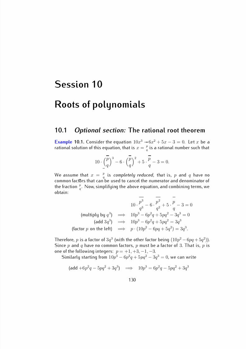
7/18/2019 Precalculus Tradler Carley
http://slidepdf.com/reader/full/precalculus-tradler-carley 140/424
Session 10
Roots of polynomials
10.1 Optional section: The rational root theorem
Example 10.1. Consider the equation 10x3 − 6x2 + 5x − 3 = 0. Let x be arational solution of this equation, that is x = p
q is a rational number such that
10 · p
q
3
− 6 · p
q
2
+ 5 · p
q − 3 = 0.
We assume that x = pq is completely reduced , that is, p and q have no
common factors that can be used to cancel the numerator and denominator of the fraction p
q . Now, simplifying the above equation, and combining terms, weobtain:
10 · p3
q 3 − 6 · p2
q 2 + 5 · p
q − 3 = 0
(multiply by q 3) =⇒ 10 p3 − 6 p2q + 5 pq 2 − 3q 3 = 0
(add 3q 3) =⇒ 10 p3 − 6 p2q + 5 pq 2 = 3q 3
(factor p on the left) =⇒ p · (10 p2 − 6 pq + 5q 2) = 3q 3.
Therefore, p is a factor of 3q 3 (with the other factor being (10 p2
−6 pq + 5q 2)).
Since p and q have no common factors, p must be a factor of 3. That is, p isone of the following integers: p = +1, +3, −1, −3.
Similarly starting from 10 p3 − 6 p2q + 5 pq 2 − 3q 3 = 0, we can write
(add +6 p2q − 5 pq 2 + 3q 3) =⇒ 10 p3 = 6 p2q − 5 pq 2 + 3q 3
130
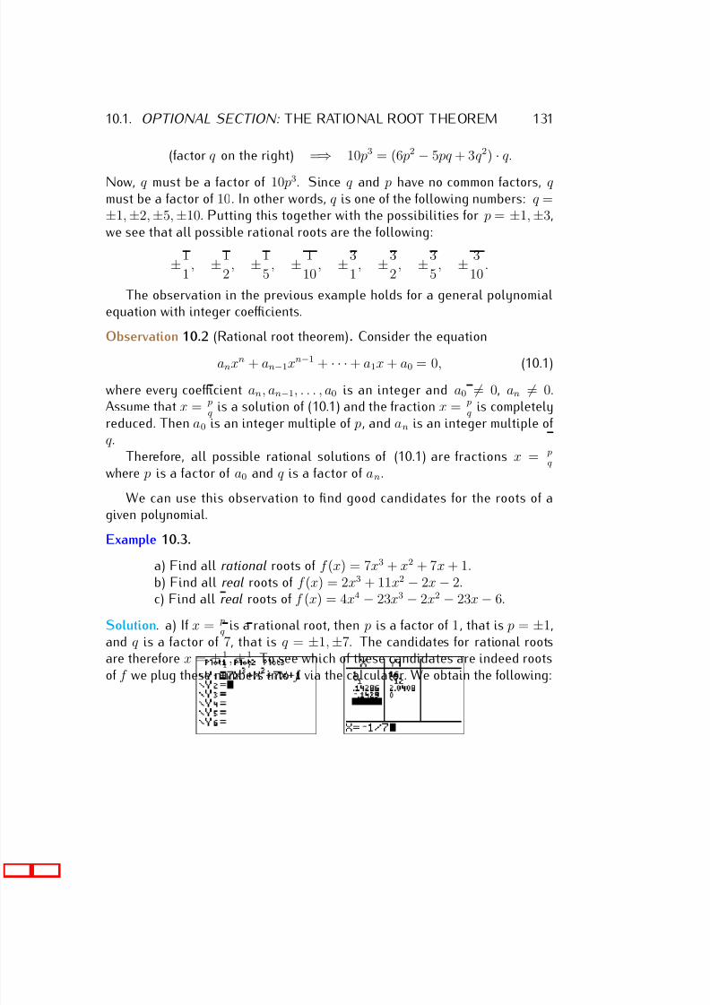
7/18/2019 Precalculus Tradler Carley
http://slidepdf.com/reader/full/precalculus-tradler-carley 141/424
10.1. OPTIONAL SECTION: THE RATIONAL ROOT THEOREM 131
(factor q on the right) =⇒ 10 p3 = (6 p2 − 5 pq + 3q 2) · q.
Now, q must be a factor of 10 p3. Since q and p have no common factors, q must be a factor of 10. In other words, q is one of the following numbers: q =±1, ±2, ±5, ±10. Putting this together with the possibilities for p = ±1, ±3,we see that all possible rational roots are the following:
±1
1, ±1
2, ±1
5, ± 1
10, ±3
1, ±3
2, ±3
5, ± 3
10.
The observation in the previous example holds for a general polynomialequation with integer coefficients.
Observation 10.2 (Rational root theorem). Consider the equation
anxn + an−1xn−1 + · · · + a1x + a0 = 0, (10.1)
where every coefficient an, an−1, . . . , a0 is an integer and a0 = 0, an = 0.Assume that x = p
q is a solution of (10.1) and the fraction x = p
q is completely
reduced. Then a0 is an integer multiple of p, and an is an integer multiple of q .
Therefore, all possible rational solutions of (10.1) are fractions x = pq
where p is a factor of a0 and q is a factor of an.
We can use this observation to find good candidates for the roots of agiven polynomial.
Example 10.3.
a) Find all rational roots of f (x) = 7x3 + x2 + 7x + 1.b) Find all real roots of f (x) = 2x3 + 11x2 − 2x − 2.c) Find all real roots of f (x) = 4x4 − 23x3 − 2x2 − 23x − 6.
Solution. a) If x = pq is a rational root, then p is a factor of 1, that is p = ±1,
and q is a factor of 7, that is q = ±1, ±7. The candidates for rational rootsare therefore x = ±1
1, ±1
7. To see which of these candidates are indeed roots
of f we plug these numbers into f via the calculator. We obtain the following:
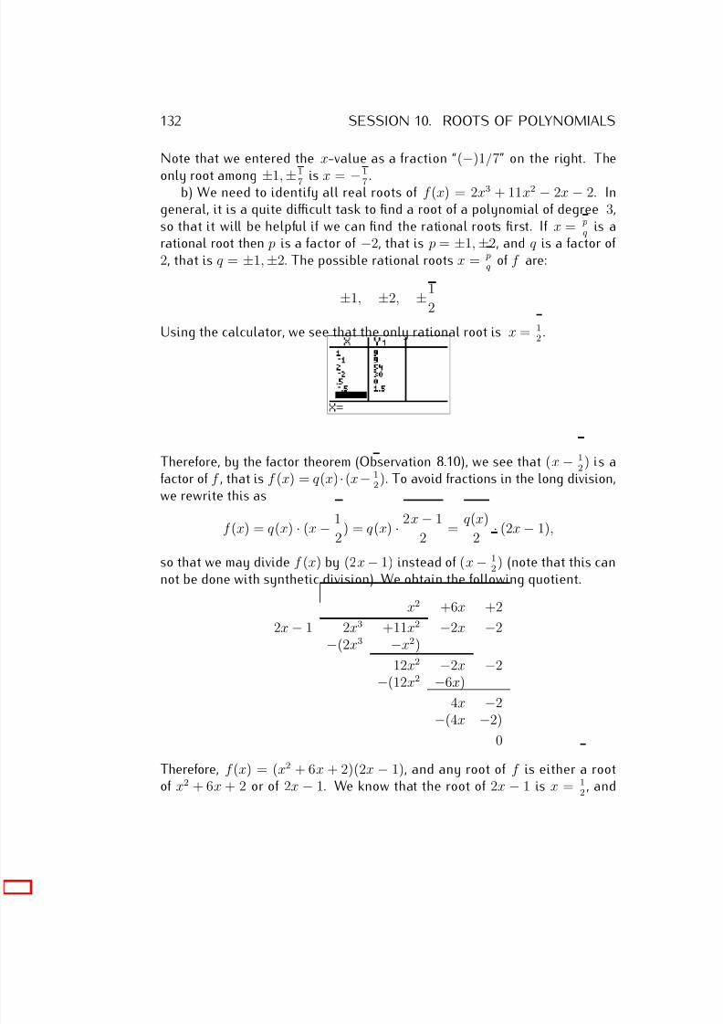
7/18/2019 Precalculus Tradler Carley
http://slidepdf.com/reader/full/precalculus-tradler-carley 142/424
132 SESSION 10. ROOTS OF POLYNOMIALS
Note that we entered the x-value as a fraction “(−)1/7” on the right. The
only root among ±1, ±1
7 is x = −1
7 .b) We need to identify all real roots of f (x) = 2x3 + 11x2 − 2x − 2. Ingeneral, it is a quite difficult task to find a root of a polynomial of degree 3,so that it will be helpful if we can find the rational roots first. If x = p
q is arational root then p is a factor of −2, that is p = ±1, ±2, and q is a factor of 2, that is q = ±1, ±2. The possible rational roots x = p
q of f are:
±1, ±2, ±1
2
Using the calculator, we see that the only rational root is x = 12 .
Therefore, by the factor theorem (Observation 8.10), we see that (x − 12 ) is a
factor of f , that is f (x) = q (x) ·(x− 12
). To avoid fractions in the long division,we rewrite this as
f (x) = q (x)·
(x−
1
2) = q (x)
· 2x − 1
2 =
q (x)
2 ·(2x
−1),
so that we may divide f (x) by (2x − 1) instead of (x − 12
) (note that this cannot be done with synthetic division). We obtain the following quotient.
x2 +6x +2
2x − 1 2x3 +11x2 −2x −2−(2x3 −x2)
12x2 −2x −2−(12x2 −6x)
4x
−2
−(4x −2)0
Therefore, f (x) = (x2 + 6x + 2)(2x − 1), and any root of f is either a rootof x2 + 6x + 2 or of 2x − 1. We know that the root of 2x − 1 is x = 1
2, and
7/18/2019 Precalculus Tradler Carley
http://slidepdf.com/reader/full/precalculus-tradler-carley 143/424
10.1. OPTIONAL SECTION: THE RATIONAL ROOT THEOREM 133
that x2 + 6x + 2 has no other rational roots. Nevertheless, we can identify all
other real roots of x2
+ 6x + 2 via the quadratic formula, (see Theorem 9.12below).
x2 + 6x + 2 = 0 =⇒ x1/2 = −6 ± √
62 − 4 · 1 · 2
2
= −6 ± √
36 − 8
2 =
−6 ± √ 28
2
= −6 ± √
4 · 7
2 =
−6 ± 2√
7
2
=
−3
±
√ 7
Therefore, the roots of f are precisely the following
x1 = −3 +√
7, x2 = −3 −√
7, x3 = 1
2.
c) First we find the rational roots x = pq of f (x) = 4x4−23x3−2x2−23x−6.
Since p is a factor of −6 it must be p = ±1, ±2, ±3, ±6, and since q is a factorof 4 it must be q = ±1, ±2, ±4. All candidates for rational roots x = p
q arethe following (where we excluded repeated ways of writing x):
±1, ±2, ±3, ±6, ±1
2, ±3
2, ±1
4, ±3
4
Checking all these candidates with the calculator produces exactly two ra-tional roots: x = 6 and x = − 1
4 . Therefore, we may divide f (x) by both(x − 6) and by (x + 1
4) without remainder. To avoid fractions, we use the
term 4 · (x + 14 ) = (4x + 1) instead of (x + 1
4 ) for our factor of f . Therefore,f (x) = q (x) · (x− 6) · (4x + 1). The quotient q (x) is determined by performinga long division by (x − 6) and then another long division by (4x + 1), oralternatively by only one long division by
(x − 6) · (4x + 1) = 4x2 + x − 24x − 6 = 4x2 − 23x − 6.
Dividing f (x) = 4x4 − 23x3 − 2x2 − 23x − 6 by 4x2 − 23x − 6 produces the
7/18/2019 Precalculus Tradler Carley
http://slidepdf.com/reader/full/precalculus-tradler-carley 144/424
134 SESSION 10. ROOTS OF POLYNOMIALS
quotient q (x):
x2 +1
4x2 − 23x − 6 4x4 −23x2 −2x2 −23x −6−(4x4 −23x3 −6x2)
4x2 −23x −6−(4x2 −23x −6)
0
We obtain the factored expression for f (x) as f (x) = (x2 +1)(4x +1)(x − 6).The only remaining real roots we need to find are those of x2 + 1. However,
x2 + 1 = 0 =⇒ x2 = −1
has no real solution. In other words there are only complex solutions of x2 = −1, which are x = i and x = −i (we will discuss complex solutions inmore detail in the next section). Since the problem requires us to find the realroots of f , our answer is that the only real roots are x1 = 6 and x2 = −1
4.
In the above example, we used the quadratic formula 9.12 from page 124.
10.2 The fundamental theorem of algebraWe have seen in Observation 8.10 on page 106 that every root c of a poly-nomial f (x) gives a factor (x − c) of f (x). There is a theorem which sayssomething about the existence of roots and factors but we will need to discusscomplex numbers briefly before stating that theorem.
As stated above, we know that there is no real number that satisfiesx2 = −1. So we define i to be a solution to this equation. This i is not a realnumber but a new kind of number called a complex number. We can think of i as
√ −1. We can now consider numbers of the form a + ib where a and b arereal numbers. Numbers of this form constitutes the set of complex numbers,
denoted by C. a is called the real part and b is called the imaginary part of the complex number a + ib. We can add two complex numbers by adding theirreal and imaginary parts to form the real and imaginary parts of the sum. Wecan multiply two complex numbers by ordinary distribution (FOIL) then usethe property that i2 = −1.
7/18/2019 Precalculus Tradler Carley
http://slidepdf.com/reader/full/precalculus-tradler-carley 145/424
10.2. THE FUNDAMENTAL THEOREM OF ALGEBRA 135
Example 10.4. We have
(2 − 3i) − (4 + 3i) = (2 − 4) + (−3 − 3)i = −2 − 6i
and
(2 − 3i)(4 + 3i) = 8 + 6i − 12i − 9i2 = 8 − 6i − 9(−1) = 17 − 6i.
We can see by writing, for example,√ −6 = i
√ 6, that these numbers
arise naturally as roots of quadratic equations. But there is more! Thefollowing fundamental theorem of algebra guarantees the existence of rootsof any polynomial.
Theorem 10.5 (Fundamental theorem of algebra).
Let f (x) = anxn + an−1xn−1 + · · · + a1x + a0 be a non-constantpolynomial. Then there exists a complex number c which is a rootof f .
Let us make two remarks about the fundamental theorem of algebra toclarify the statement of the theorem.
Note 10.6.
• In the above Theorem 10.5 we did not specify what kind of coefficientsa0, . . . an are allowed for the theorem to hold. In fact, to be precise, thefundamental theorem of algebra states that for any complex numbers
a0, . . . an, the polynomial f (x) = anxn + an−1xn−1 + · · · + a1x + a0 hasa root.
• In general there may not exist a real root c of a given polynomial,but the root c may only be a complex number. For example, considerf (x) = x2 + 1, and consider the roots c of f , that is c2 + 1 = 0. Then,for any real number c, we have always c2 ≥ 0, so that f (c) = c2 + 1 ≥ 1,so that there cannot be a real root c of f . However, if we multiply
(x − i)(x + i) = x2 + xi − xi − i2 = x2 + 1,
we see that f has complex roots c = i and c =−
i.
Now, while the fundamental theorem of algebra guarantees a root c of apolynomial f , we can use the remainder theorem from Observation 8.10 tocheck possible candidates c for the roots, and the factor theorem to factorf (x) = q (x) · (x − c).
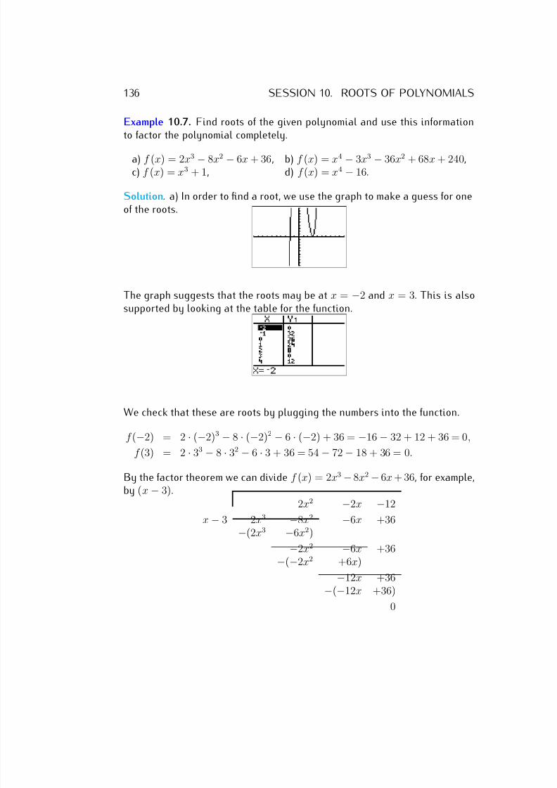
7/18/2019 Precalculus Tradler Carley
http://slidepdf.com/reader/full/precalculus-tradler-carley 146/424
136 SESSION 10. ROOTS OF POLYNOMIALS
Example 10.7. Find roots of the given polynomial and use this information
to factor the polynomial completely.
a) f (x) = 2x3 − 8x2 − 6x + 36, b) f (x) = x4 − 3x3 − 36x2 + 68x + 240,c) f (x) = x3 + 1, d) f (x) = x4 − 16.
Solution. a) In order to find a root, we use the graph to make a guess for oneof the roots.
The graph suggests that the roots may be at x = −2 and x = 3. This is alsosupported by looking at the table for the function.
We check that these are roots by plugging the numbers into the function.
f (−2) = 2 · (−2)3 − 8 · (−2)2 − 6 · (−2) + 36 = −16 − 32 + 12 + 36 = 0,
f (3) = 2 · 33 − 8 · 32 − 6 · 3 + 36 = 54 − 72 − 18 + 36 = 0.
By the factor theorem we can divide f (x) = 2x3 − 8x2 − 6x + 36, for example,by (x − 3).
2x2 −2x −12
x − 3 2x3 −8x2 −6x +36−(2x3 −6x2)
−2x2
−6x +36−(−2x2 +6x)
−12x +36−(−12x +36)
0
7/18/2019 Precalculus Tradler Carley
http://slidepdf.com/reader/full/precalculus-tradler-carley 147/424
10.2. THE FUNDAMENTAL THEOREM OF ALGEBRA 137
Therefore, f (x) = (2x2 − 2x − 12)(x − 3). To factor f completely, we still
need to factor the first polynomial 2x2
− 2x − 12:
f (x) = (2x2 − 2x − 12)(x − 3) = 2 · (x2 − x − 6) · (x − 3)
= 2 · (x − 3) · (x + 2) · (x − 3) = 2 · (x + 2) · (x − 3)2.
b) The graph of f (x) = x4 −3x3 −36x2 +68x+240 in the standard windowis the following:
We suspect that x = −5, x = −2, x = 4, and x = 6 are the roots of thefunction. This is confirmed by checking the table on the calculator, and alsoby direct computation.
f (−5) = (−5)4 − 3(−5)3 − 36(−5)2 + 68(−5) + 240 = 0,
f (−2) = (−2)4 − 3(−2)3 − 36(−2)2 + 68(−2) + 240 = 0,
f (4) = 44 − 3 · 43 − 36 · 42 + 68 · 4 + 240 = 0,
f (6) = 64 − 3 · 63 − 36 · 62 + 68 · 6 + 240 = 0.
Therefore, each (x+5), (x+2), (x−4), and (x−6) is a factor of f (x), and thentheir product is also a factor of f (x). The product (x+5)(x+2)(x−4)(x−6) iscalculated as follows. Since (x+5)(x+2) = x2 +7x+10 and (x−4)(x−6) =x2
−10x + 24, we obtain
(x + 5)(x + 2)(x − 4)(x − 6) = (x2 + 7x + 10)(x2 − 10x + 24)
= x4 − 10x3 + 24x2+7x3 − 70x2 + 168x+10x2 − 100x + 240
= x4 − 3x3 − 36x2 + 68x + 240 = f (x).
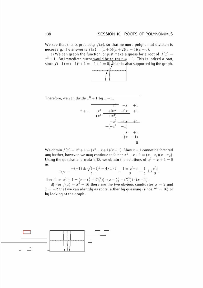
7/18/2019 Precalculus Tradler Carley
http://slidepdf.com/reader/full/precalculus-tradler-carley 148/424
138 SESSION 10. ROOTS OF POLYNOMIALS
We see that this is precisely f (x), so that no more polynomial division is
necessary. The answer is f (x) = (x + 5)(x + 2)(x − 4)(x − 6).c) We can graph the function, or just make a guess for a root of f (x) =x3 + 1. An immediate guess would be to try x = −1. This is indeed a root,since f (−1) = (−1)3 + 1 = −1+ 1 = 0, which is also supported by the graph.
Therefore, we can divide x3 + 1 by x + 1.
x2 −x +1
x + 1 x3 +0x2 +0x +1−(x3 +x2)
−x2 +0x +1−(−x2 −x)
x +1−(x +1)
0
We obtain f (x) = x3
+ 1 = (x2
− x +1)(x + 1). Now x + 1 cannot be factoredany further, however, we may continue to factor x2 − x + 1 = (x − x1)(x − x2).Using the quadratic formula 9.12, we obtain the solutions of x2 − x + 1 = 0as
x1/2 = −(−1) ±
(−1)2 − 4 · 1 · 1
2 · 1 =
1 ± √ −3
2 =
1
2 ± i
√ 3
2 .
Therefore, x3 + 1 = (x − ( 12
+ i√
32
)) · (x − ( 12 − i
√ 3
2 )) · (x + 1).
d) For f (x) = x4 − 16 there are the two obvious candidates x = 2 andx = −2 that we can identify as roots, either by guessing (since 24 = 16) orby looking at the graph.
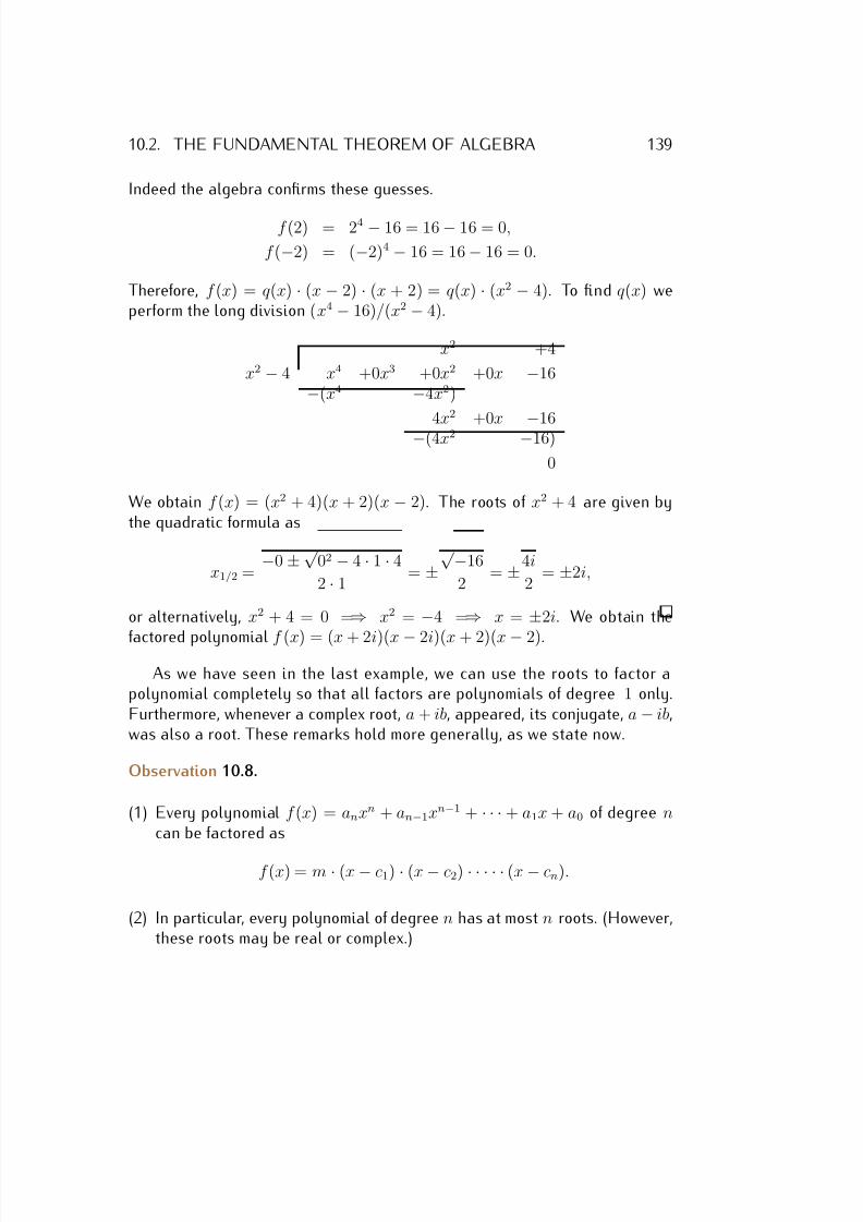
7/18/2019 Precalculus Tradler Carley
http://slidepdf.com/reader/full/precalculus-tradler-carley 149/424
10.2. THE FUNDAMENTAL THEOREM OF ALGEBRA 139
Indeed the algebra confirms these guesses.
f (2) = 24 − 16 = 16 − 16 = 0,
f (−2) = (−2)4 − 16 = 16 − 16 = 0.
Therefore, f (x) = q (x) · (x − 2) · (x + 2) = q (x) · (x2 − 4). To find q (x) weperform the long division (x4 − 16)/(x2 − 4).
x2 +4
x2 − 4 x4 +0x3 +0x2 +0x −16−(x4 −4x2)
4x2 +0x −
16−(4x2 −16)
0
We obtain f (x) = (x2 + 4)(x + 2)(x − 2). The roots of x2 + 4 are given bythe quadratic formula as
x1/2 = −0 ± √
02 − 4 · 1 · 4
2 · 1 = ±
√ −16
2 = ±4i
2 = ±2i,
or alternatively, x2 + 4 = 0 =⇒ x2 = −4 =⇒ x = ±2i. We obtain the
factored polynomial f (x) = (x + 2i)(x − 2i)(x + 2)(x − 2).
As we have seen in the last example, we can use the roots to factor apolynomial completely so that all factors are polynomials of degree 1 only.Furthermore, whenever a complex root, a + ib, appeared, its conjugate, a − ib,was also a root. These remarks hold more generally, as we state now.
Observation 10.8.
(1) Every polynomial f (x) = anxn + an−1xn−1 + · · · + a1x + a0 of degree ncan be factored as
f (x) = m · (x − c1) · (x − c2) · · · · · (x − cn).
(2) In particular, every polynomial of degree n has at most n roots. (However,these roots may be real or complex.)
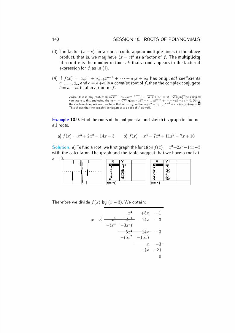
7/18/2019 Precalculus Tradler Carley
http://slidepdf.com/reader/full/precalculus-tradler-carley 150/424
140 SESSION 10. ROOTS OF POLYNOMIALS
(3) The factor (x − c) for a root c could appear multiple times in the above
product, that is, we may have (x − c)k
as a factor of f . The multiplicityof a root c is the number of times k that a root appears in the factoredexpression for f as in (1).
(4) If f (x) = anxn + an−1xn−1 + · · · + a1x + a0 has only real coefficientsa0, . . . , an, and c = a+bi is a complex root of f , then the complex conjugatec = a − bi is also a root of f .
Proof. If x is any root, then anxn + an−1xn−1 + · · · + a1x + a0 = 0. Applying the complexconjugate to this and using that u · v = u · v gives anxn + an−1xn−1 + · · ·+ a1x + a0 = 0. Sincethe coefficients aj are real, we have that aj = aj , so that anxn + an−1xn−1 + · · ·+ a1x + a0 = 0.This shows that the complex conjugate x is a root of f as well.
Example 10.9. Find the roots of the polynomial and sketch its graph includingall roots.
a) f (x) = x3 + 2x2 − 14x − 3 b) f (x) = x4 − 7x3 + 11x2 − 7x + 10
Solution. a) To find a root, we first graph the function f (x) = x3+2x2−14x−3with the calculator. The graph and the table suggest that we have a root atx = 3.
Therefore we divide f (x) by (x − 3). We obtain:
x2 +5x +1
x − 3 x3 +2x2 −14x −3−(x3 −3x2)
5x2
−14x −3−(5x2 −15x)
x −3−(x −3)
0
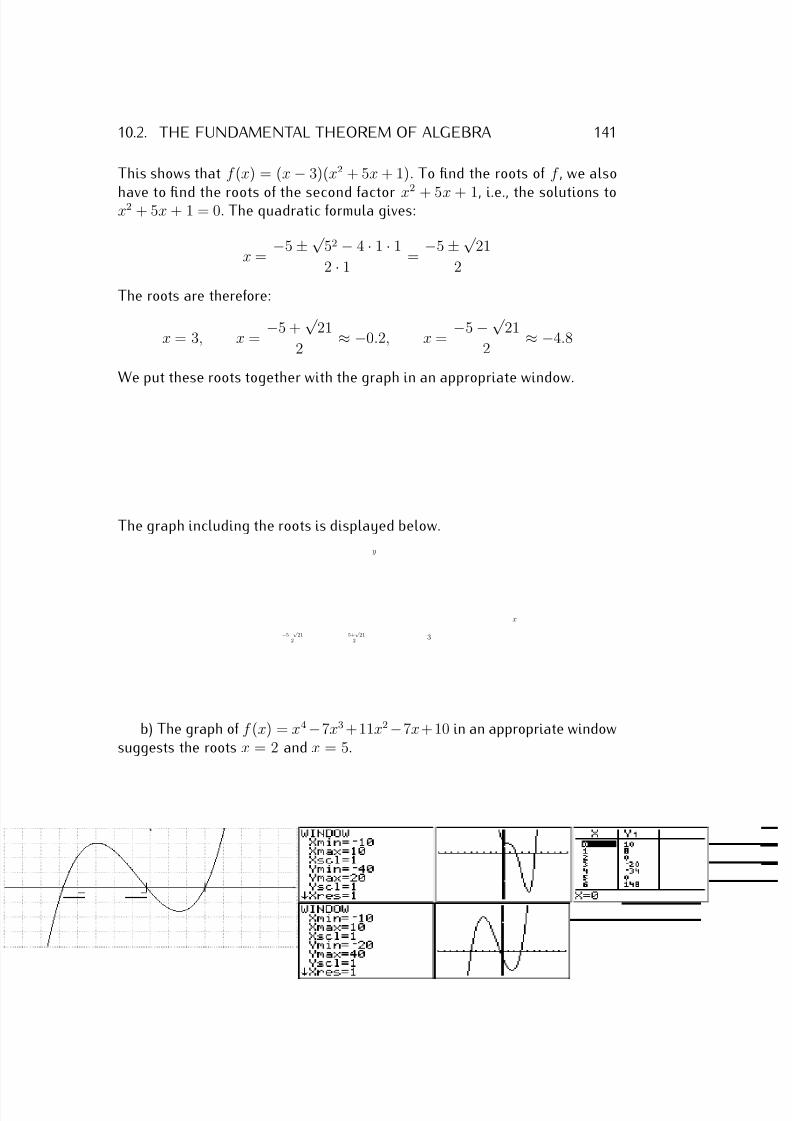
7/18/2019 Precalculus Tradler Carley
http://slidepdf.com/reader/full/precalculus-tradler-carley 151/424
10.2. THE FUNDAMENTAL THEOREM OF ALGEBRA 141
This shows that f (x) = (x − 3)(x2 + 5x + 1). To find the roots of f , we also
have to find the roots of the second factor x2
+ 5x + 1, i.e., the solutions tox2 + 5x + 1 = 0. The quadratic formula gives:
x = −5 ± √
52 − 4 · 1 · 1
2 · 1 =
−5 ± √ 21
2
The roots are therefore:
x = 3, x = −5 +
√ 21
2 ≈ −0.2, x =
−5 − √ 21
2 ≈ −4.8
We put these roots together with the graph in an appropriate window.
The graph including the roots is displayed below.
x
y
−5+√
212
−5−√ 212 3
b) The graph of f (x) = x4 −7x3 +11x2 −7x+ 10 in an appropriate windowsuggests the roots x = 2 and x = 5.
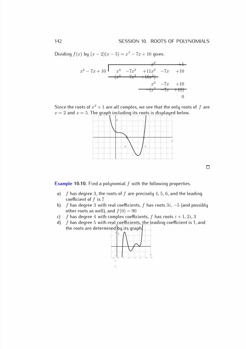
7/18/2019 Precalculus Tradler Carley
http://slidepdf.com/reader/full/precalculus-tradler-carley 152/424
142 SESSION 10. ROOTS OF POLYNOMIALS
Dividing f (x) by (x − 2)(x − 5) = x2 − 7x + 10 gives:
x2 +1
x2 − 7x + 10 x4 −7x3 +11x2 −7x +10−(x4 −7x3 +10x2)
x2 −7x +10−(x2 −7x +10)
0
Since the roots of x2 + 1 are all complex, we see that the only roots of f arex = 2 and x = 5. The graph including its roots is displayed below.
x
y
2 5
Example 10.10. Find a polynomial f with the following properties.
a) f has degree 3, the roots of f are precisely 4, 5, 6, and the leadingcoefficient of f is 7
b) f has degree 3 with real coefficients, f has roots 3i, −5 (and possiblyother roots as well), and f (0) = 90
c) f has degree 4 with complex coefficients, f has roots i + 1, 2i, 3d) f has degree 5 with real coefficients, the leading coefficient is 1, and
the roots are determined by its graph:
-1 0 1 2 3 4 5 6
-2
-1
0
1
2
3
4
x
y
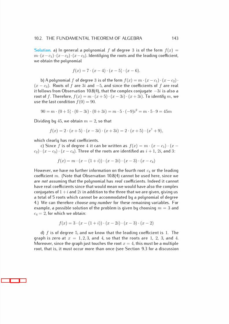
7/18/2019 Precalculus Tradler Carley
http://slidepdf.com/reader/full/precalculus-tradler-carley 153/424
10.2. THE FUNDAMENTAL THEOREM OF ALGEBRA 143
Solution. a) In general a polynomial f of degree 3 is of the form f (x) =
m ·(x−c1) ·(x−c2) ·(x−c3). Identifying the roots and the leading coefficient,we obtain the polynomial
f (x) = 7 · (x − 4) · (x − 5) · (x − 6).
b) A polynomial f of degree 3 is of the form f (x) = m · (x − c1) · (x − c2) ·(x − c3). Roots of f are 3i and −5, and since the coefficients of f are realit follows from Observation 10.8(4), that the complex conjugate −3i is also aroot of f . Therefore, f (x) = m · (x + 5) · (x − 3i) · (x + 3i). To identify m, weuse the last condition f (0) = 90.
90 = m · (0 + 5) · (0 − 3i) · (0 + 3i) = m · 5 · (−9)i
2
= m · 5 · 9 = 45mDividing by 45, we obtain m = 2, so that
f (x) = 2 · (x + 5) · (x − 3i) · (x + 3i) = 2 · (x + 5) · (x2 + 9),
which clearly has real coefficients.c) Since f is of degree 4 it can be written as f (x) = m · (x − c1) · (x −
c2) · (x − c3) · (x − c4). Three of the roots are identified as i + 1, 2i, and 3:
f (x) = m · (x − (1 + i)) · (x − 2i) · (x − 3) · (x − c4)
However, we have no further information on the fourth root c4 or the leadingcoefficient m. (Note that Observation 10.8(4) cannot be used here, since weare not assuming that the polynomial has real coefficients. Indeed it cannothave real coefficients since that would mean we would have also the complexconjugates of 1 + i and 2i in addition to the three that we are given, giving usa total of 5 roots which cannot be accommodated by a polynomial of degree4.) We can therefore choose any number for these remaining variables. Forexample, a possible solution of the problem is given by choosing m = 3 andc4 = 2, for which we obtain:
f (x) = 3
·(x
−(1 + i))
·(x
−2i)
·(x
−3)
·(x
−2)
d) f is of degree 5, and we know that the leading coefficient is 1. Thegraph is zero at x = 1, 2, 3, and 4, so that the roots are 1, 2, 3, and 4.Moreover, since the graph just touches the root x = 4, this must be a multipleroot, that is, it must occur more than once (see Section 9.3 for a discussion
7/18/2019 Precalculus Tradler Carley
http://slidepdf.com/reader/full/precalculus-tradler-carley 154/424
144 SESSION 10. ROOTS OF POLYNOMIALS
of multiple roots and their graphical consequences). We obtain the following
solution:f (x) = (x − 1)(x − 2)(x − 3)(x − 4)2.
Note that the root x = 4 is a root of multiplicity 2.
Note that to see that a polynomial has real coefficients, it may be neces-sary to multiply factors like (x − (2 + 3i))(x − (2 − 3i)). We suggest a wayof doing this for which we use the fact that a2 − b2 = (a + b)(a − b). We have
(x − (2 + 3i))(x − (2 − 3i)) = ((x − 2) − 3i)((x − 2) + 3i) = (x − 2)2 + 9,
which clearly has real coefficients.
10.3 Exercises
Exercise 10.1.
a) Find all rational roots of f (x) = 2x3 − 3x2 − 3x + 2.b) Find all rational roots of f (x) = 3x3 − x2 + 15x − 5.c) Find all rational roots of f (x) = 6x3 + 7x2 − 11x − 12.d) Find all real roots of f (x) = 6x4 + 25x3 + 8x2 − 7x − 2.e) Find all real roots of f (x) = 4x3 + 9x2 + 26x + 6.
Exercise 10.2. Find a root of the polynomial by guessing possible candidatesof the root.
a) f (x) = x5 − 1 b) f (x) = x4 − 1 c) f (x) = x3 − 27d) f (x) = x3 + 1000 e) f (x) = x4 − 81 f ) f (x) = x3 − 125g) f (x) = x5 + 32 h) f (x) = x777 − 1 i) f (x) = x2 + 64
Exercise 10.3. Find the roots of the polynomial and use it to factor thepolynomial completely.
a) f (x) = x3
− 7x + 6, b) f (x) = x3
− x2
− 16x − 20,c) f (x) = x4 − 5x2 + 4, d) f (x) = x3 + x2 − 5x − 2,e) f (x) = 2x3 + x2 − 7x − 6, f ) f (x) = 12x3 + 49x2 − 2x − 24,g) f (x) = x4 − 1, h) f (x) = x5 − 6x4 + 8x3 + 6x2 − 9x,i) f (x) = x3 − 27, j) f (x) = x4 + 2x2 − 15.
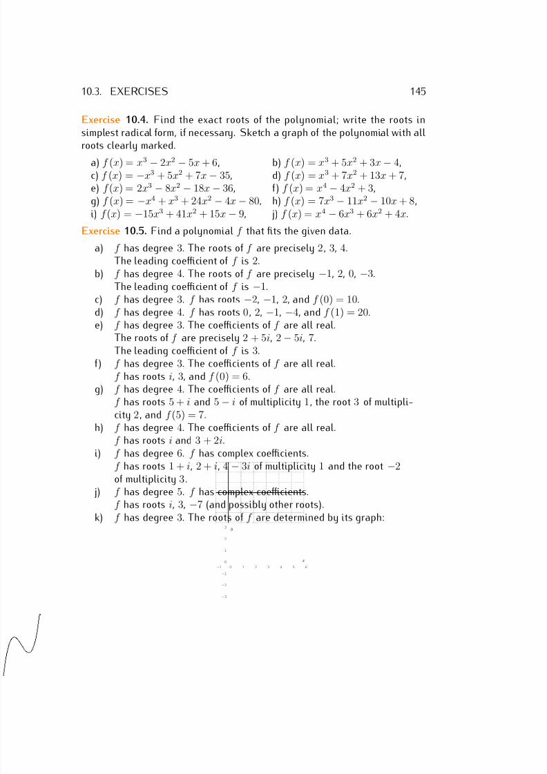
7/18/2019 Precalculus Tradler Carley
http://slidepdf.com/reader/full/precalculus-tradler-carley 155/424
10.3. EXERCISES 145
Exercise 10.4. Find the exact roots of the polynomial; write the roots in
simplest radical form, if necessary. Sketch a graph of the polynomial with allroots clearly marked.
a) f (x) = x3 − 2x2 − 5x + 6, b) f (x) = x3 + 5x2 + 3x − 4,c) f (x) = −x3 + 5x2 + 7x − 35, d) f (x) = x3 + 7x2 + 13x + 7,e) f (x) = 2x3 − 8x2 − 18x − 36, f ) f (x) = x4 − 4x2 + 3,g) f (x) = −x4 + x3 + 24x2 − 4x − 80, h) f (x) = 7x3 − 11x2 − 10x + 8,i) f (x) = −15x3 + 41x2 + 15x − 9, j) f (x) = x4 − 6x3 + 6x2 + 4x.
Exercise 10.5. Find a polynomial f that fits the given data.
a) f has degree 3. The roots of f are precisely 2, 3, 4.The leading coefficient of f is 2.
b) f has degree 4. The roots of f are precisely −1, 2, 0, −3.The leading coefficient of f is −1.
c) f has degree 3. f has roots −2, −1, 2, and f (0) = 10.d) f has degree 4. f has roots 0, 2, −1, −4, and f (1) = 20.e) f has degree 3. The coefficients of f are all real.
The roots of f are precisely 2 + 5i, 2 − 5i, 7.The leading coefficient of f is 3.
f ) f has degree 3. The coefficients of f are all real.f has roots i, 3, and f (0) = 6.
g) f has degree 4. The coefficients of f are all real.
f has roots 5 + i and 5 − i of multiplicity 1, the root 3 of multipli-city 2, and f (5) = 7.h) f has degree 4. The coefficients of f are all real.
f has roots i and 3 + 2i.i) f has degree 6. f has complex coefficients.
f has roots 1 + i, 2 + i, 4 − 3i of multiplicity 1 and the root −2of multiplicity 3.
j) f has degree 5. f has complex coefficients.f has roots i, 3, −7 (and possibly other roots).
k) f has degree 3. The roots of f are determined by its graph:
-1 0 1 2 3 4 5 6
-3
-2
-1
0
1
2
3
x
y
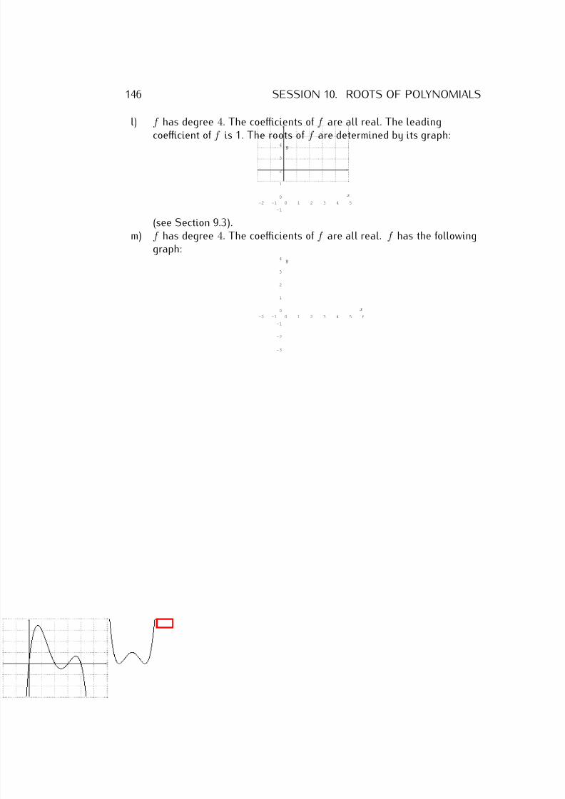
7/18/2019 Precalculus Tradler Carley
http://slidepdf.com/reader/full/precalculus-tradler-carley 156/424
146 SESSION 10. ROOTS OF POLYNOMIALS
l) f has degree 4. The coefficients of f are all real. The leading
coefficient of f is 1. The roots of f are determined by its graph:
-2 -1 0 1 2 3 4 5
-1
0
1
2
3
4
x
y
(see Section 9.3).m) f has degree 4. The coefficients of f are all real. f has the following
graph:
-2 -1 0 1 2 3 4 5 6
-3
-2
-1
0
1
2
3
4
x
y
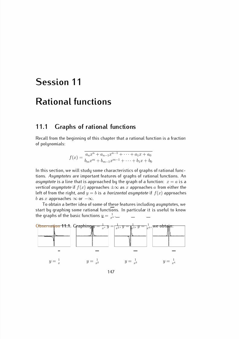
7/18/2019 Precalculus Tradler Carley
http://slidepdf.com/reader/full/precalculus-tradler-carley 157/424
Session 11
Rational functions
11.1 Graphs of rational functions
Recall from the beginning of this chapter that a rational function is a fractionof polynomials:
f (x) = anxn + an−1xn−1 + · · · + a1x + a0
bmxm + bm−1xm−1 + · · · + b1x + b0
In this section, we will study some characteristics of graphs of rational func-
tions. Asymptotes are important features of graphs of rational functions. Anasymptote is a line that is approached by the graph of a function: x = a is avertical asymptote if f (x) approaches ±∞ as x approaches a from either theleft of from the right, and y = b is a horizontal asymptote if f (x) approachesb as x approaches ∞ or −∞.
To obtain a better idea of some of these features including asymptotes, westart by graphing some rational functions. In particular it is useful to knowthe graphs of the basic functions y = 1
xn .
Observation 11.1. Graphing y = 1x
, y = 1x2 , y = 1
x3 , y = 1x4 , we obtain:
y = 1x y = 1
x2 y = 1x3 y = 1
x4
147
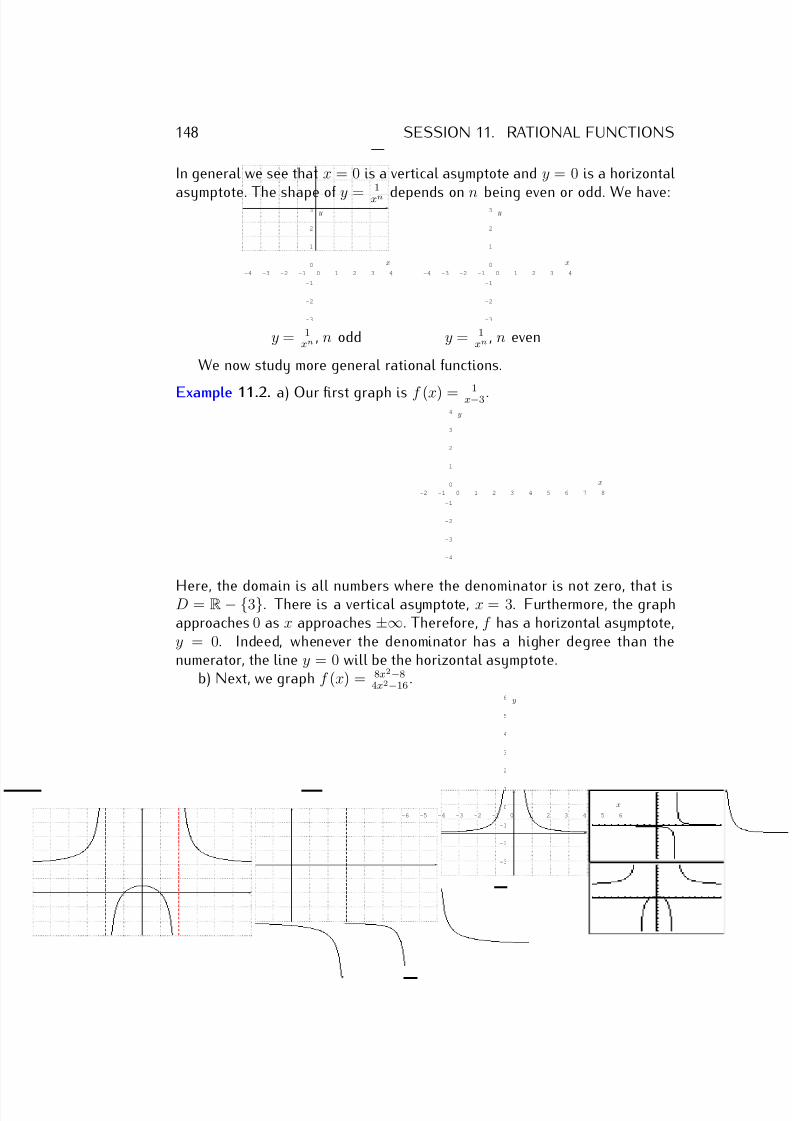
7/18/2019 Precalculus Tradler Carley
http://slidepdf.com/reader/full/precalculus-tradler-carley 158/424
148 SESSION 11. RATIONAL FUNCTIONS
In general we see that x = 0 is a vertical asymptote and y = 0 is a horizontal
asymptote. The shape of y = 1
xn depends on n being even or odd. We have:
-4 -3 -2 -1 0 1 2 3 4
-3
-2
-1
0
1
2
3
x
y
-4 -3 -2 -1 0 1 2 3 4
-3
-2
-1
0
1
2
3
x
y
y = 1xn , n odd y = 1
xn , n even
We now study more general rational functions.
Example 11.2. a) Our first graph is f (x) = 1x−3 .
-2 -1 0 1 2 3 4 5 6 7 8
-4
-3
-2
-1
0
1
2
3
4
x
y
Here, the domain is all numbers where the denominator is not zero, that isD = R − {3}. There is a vertical asymptote, x = 3. Furthermore, the graphapproaches 0 as x approaches ±∞. Therefore, f has a horizontal asymptote,y = 0. Indeed, whenever the denominator has a higher degree than thenumerator, the line y = 0 will be the horizontal asymptote.
b) Next, we graph f (x) = 8x2−84x2−16
.
-6 -5 -4 -3 -2 -1 0 1 2 3 4 5 6
-3
-2
-1
0
1
2
3
4
5
6
x
y
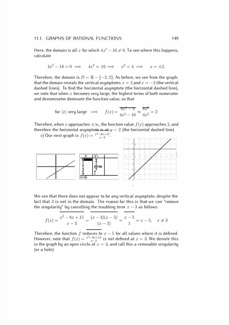
7/18/2019 Precalculus Tradler Carley
http://slidepdf.com/reader/full/precalculus-tradler-carley 159/424
11.1. GRAPHS OF RATIONAL FUNCTIONS 149
Here, the domain is all x for which 4x2 − 16 = 0. To see where this happens,
calculate
4x2 − 16 = 0 =⇒ 4x2 = 16 =⇒ x2 = 4 =⇒ x = ±2.
Therefore, the domain is D = R− {−2, 2}. As before, we see from the graph,that the domain reveals the vertical asymptotes x = 2 and x = −2 (the verticaldashed lines). To find the horizontal asymptote (the horizontal dashed line),we note that when x becomes very large, the highest terms of both numeratorand denominator dominate the function value, so that
for |x| very large =⇒ f (x) =
8x2
−8
4x2 − 16 ≈ 8x2
4x2 = 2
Therefore, when x approaches ±∞, the function value f (x) approaches 2, andtherefore the horizontal asymptote is at y = 2 (the horizontal dashed line).
c) Our next graph is f (x) = x2−8x+15x−3 .
-2 -1 0 1 2 3 4 5 6 7 8
-6
-5
-4
-3
-2
-1
0
1
2
x
y
We see that there does not appear to be any vertical asymptote, despite thefact that 3 is not in the domain. The reason for this is that we can “removethe singularity” by cancelling the troubling term x − 3 as follows:
f (x) = x2 − 8x + 15
x
−3
= (x − 3)(x − 5)
(x
−3)
= x − 5
1 = x − 5, x = 3
Therefore, the function f reduces to x − 5 for all values where it is defined.However, note that f (x) = x2−8x+15
x−3 is not defined at x = 3. We denote thisin the graph by an open circle at x = 3, and call this a removable singularity(or a hole).
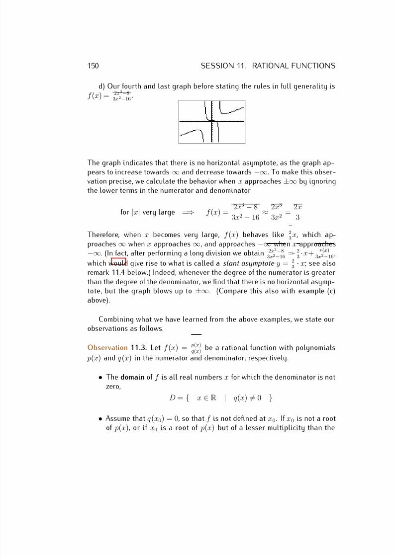
7/18/2019 Precalculus Tradler Carley
http://slidepdf.com/reader/full/precalculus-tradler-carley 160/424
150 SESSION 11. RATIONAL FUNCTIONS
d) Our fourth and last graph before stating the rules in full generality is
f (x) = 2x3
−8
3x2−16 .
The graph indicates that there is no horizontal asymptote, as the graph ap-pears to increase towards ∞ and decrease towards −∞. To make this obser-vation precise, we calculate the behavior when x approaches ±∞ by ignoringthe lower terms in the numerator and denominator
for |x| very large =⇒ f (x) = 2x3 − 8
3x2 − 16 ≈ 2x3
3x2 =
2x
3
Therefore, when x becomes very large, f (x) behaves like 23
x, which ap-proaches ∞ when x approaches ∞, and approaches −∞ when x approaches−∞. (In fact, after performing a long division we obtain 2x3−8
3x2−16 = 2
3·x+ r(x)
3x2−16,
which would give rise to what is called a slant asymptote y = 23· x; see also
remark 11.4 below.) Indeed, whenever the degree of the numerator is greaterthan the degree of the denominator, we find that there is no horizontal asymp-
tote, but the graph blows up to ±∞. (Compare this also with example (c)above).
Combining what we have learned from the above examples, we state ourobservations as follows.
Observation 11.3. Let f (x) = p(x)q(x)
be a rational function with polynomials
p(x) and q (x) in the numerator and denominator, respectively.
• The domain of f is all real numbers x for which the denominator is not
zero,D = { x ∈ R | q (x) = 0 }
• Assume that q (x0) = 0, so that f is not defined at x0. If x0 is not a rootof p(x), or if x0 is a root of p(x) but of a lesser multiplicity than the
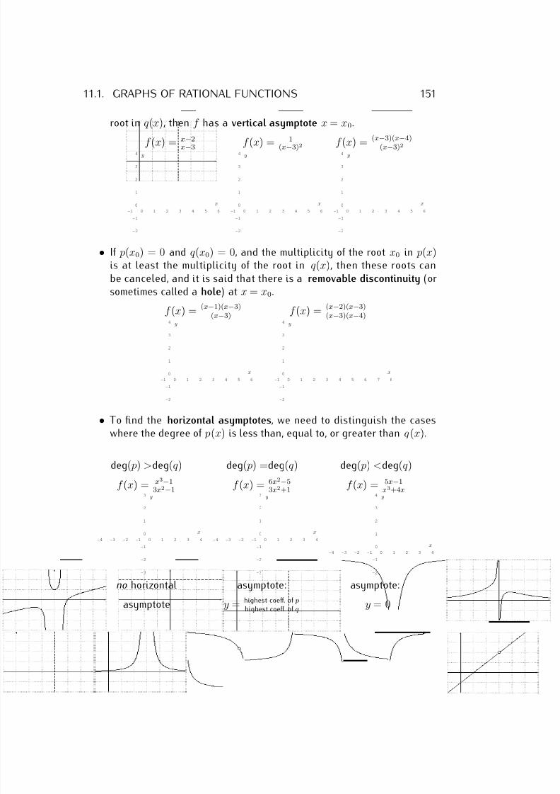
7/18/2019 Precalculus Tradler Carley
http://slidepdf.com/reader/full/precalculus-tradler-carley 161/424
11.1. GRAPHS OF RATIONAL FUNCTIONS 151
root in q (x), then f has a vertical asymptote x = x0.
f (x) = x−2x−3 f (x) = 1
(x−3)2 f (x) = (x−3)(x−4)(x−3)2
-1 0 1 2 3 4 5 6
-2
-1
0
1
2
3
4
x
y
-1 0 1 2 3 4 5 6
-2
-1
0
1
2
3
4
x
y
-1 0 1 2 3 4 5 6
-2
-1
0
1
2
3
4
x
y
• If p(x0) = 0 and q (x0) = 0, and the multiplicity of the root x0 in p(x)is at least the multiplicity of the root in q (x), then these roots can
be canceled, and it is said that there is a removable discontinuity (orsometimes called a hole) at x = x0.
f (x) = (x−1)(x−3)(x−3) f (x) = (x−2)(x−3)
(x−3)(x−4)
-1 0 1 2 3 4 5 6
-2
-1
0
1
2
3
4
x
y
-1 0 1 2 3 4 5 6 7 8
-2
-1
0
1
2
3
4
x
y
• To find the horizontal asymptotes, we need to distinguish the caseswhere the degree of p(x) is less than, equal to, or greater than q (x).
deg( p) >deg(q ) deg( p) =deg(q ) deg( p) <deg(q )
f (x) = x3−13x2−1
f (x) = 6x2−53x2+1
f (x) = 5x−1x3+4x
-4 -3 -2 -1 0 1 2 3 4
-3
-2
-1
0
1
2
3
x
y
-4 -3 -2 -1 0 1 2 3 4
-3
-2
-1
0
1
2
3
x
y
-4 -3 -2 -1 0 1 2 3 4
-2
-1
0
1
2
3
4
x
y
no horizontal asymptote: asymptote:
asymptote y = highest coeff. of phighest coeff. of q y = 0
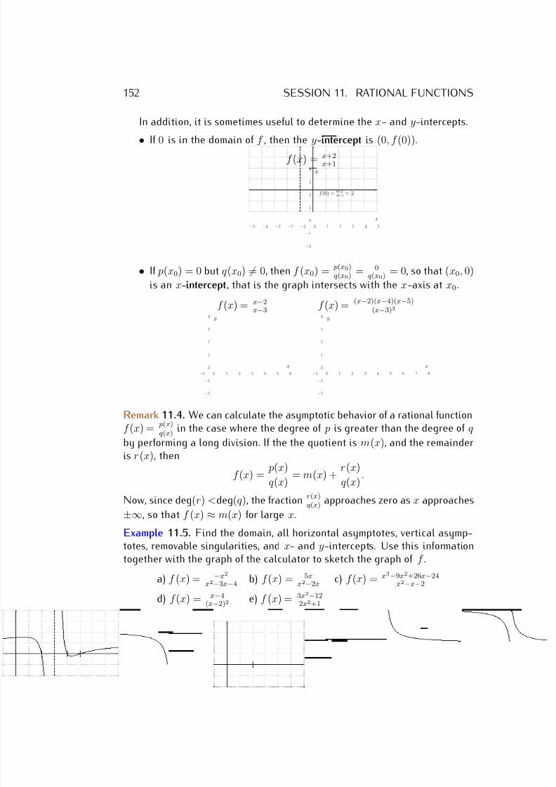
7/18/2019 Precalculus Tradler Carley
http://slidepdf.com/reader/full/precalculus-tradler-carley 162/424
152 SESSION 11. RATIONAL FUNCTIONS
In addition, it is sometimes useful to determine the x- and y-intercepts.
• If 0 is in the domain of f , then the y-intercept is (0, f (0)).
f (x) = x+2x+1
-5 -4 -3 -2 -1 0 1 2 3 4 5
-2
-1
0
1
2
3
4
x
y
f (0) = 0+20+1 = 2
• If p(x0) = 0 but q (x0) = 0, then f (x0) =
p(x0)
q(x0) =
0
q(x0) = 0, so that (x0, 0)is an x-intercept, that is the graph intersects with the x-axis at x0.
f (x) = x−2x−3 f (x) = (x−2)(x−4)(x−5)
(x−3)3
-1 0 1 2 3 4 5 6
-2
-1
0
1
2
3
4
x
y
-1 0 1 2 3 4 5 6 7 8
-2
-1
0
1
2
3
4
x
y
Remark 11.4. We can calculate the asymptotic behavior of a rational functionf (x) = p(x)
q(x) in the case where the degree of p is greater than the degree of q
by performing a long division. If the the quotient is m(x), and the remainderis r(x), then
f (x) = p(x)
q (x) = m(x) +
r(x)
q (x).
Now, since deg(r) <deg(q ), the fraction r(x)q(x) approaches zero as x approaches
±∞, so that f (x) ≈ m(x) for large x.
Example 11.5. Find the domain, all horizontal asymptotes, vertical asymp-
totes, removable singularities, and x- and y-intercepts. Use this informationtogether with the graph of the calculator to sketch the graph of f .
a) f (x) = −x2
x2−3x−4 b) f (x) = 5x
x2−2x c) f (x) = x3−9x2+26x−24
x2−x−2
d) f (x) = x−4(x−2)2 e) f (x) = 3x2−12
2x2+1
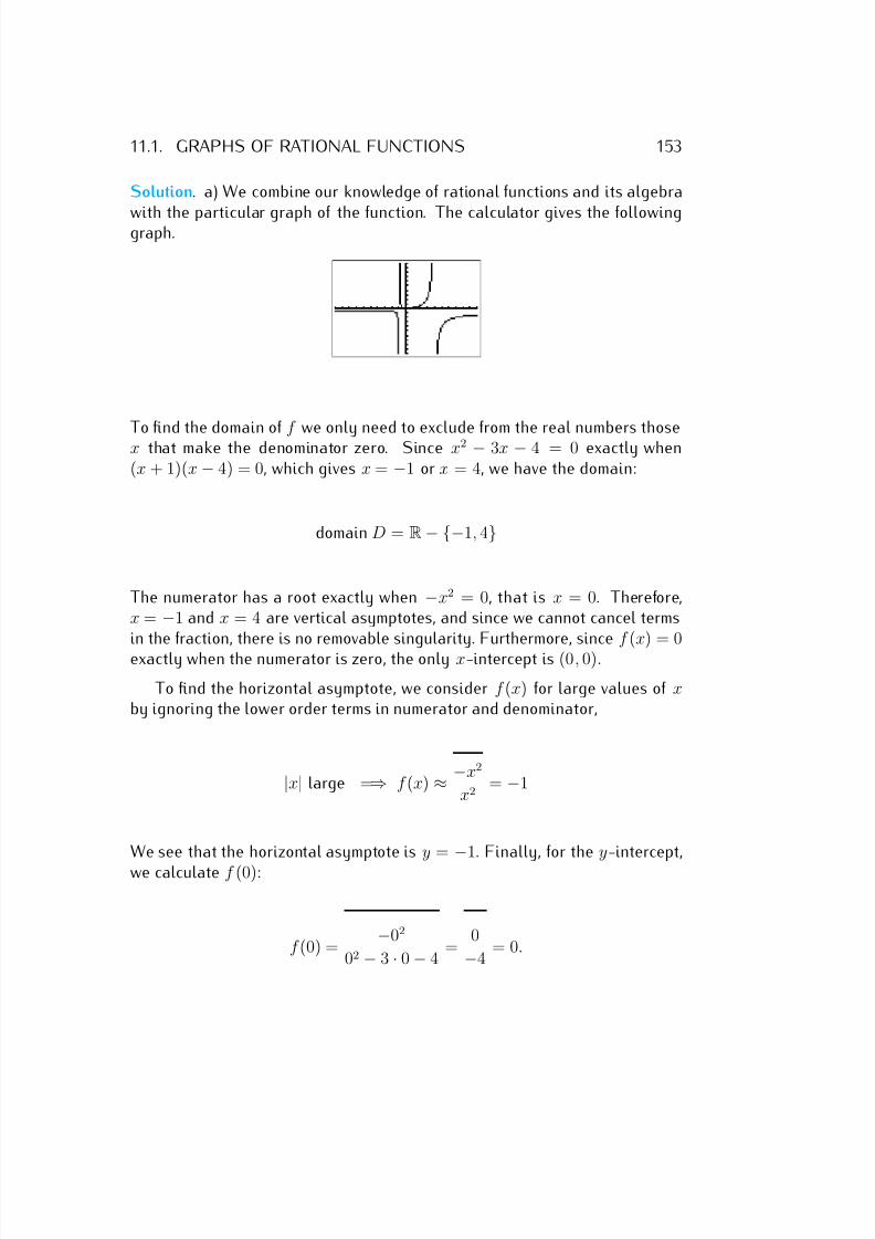
7/18/2019 Precalculus Tradler Carley
http://slidepdf.com/reader/full/precalculus-tradler-carley 163/424
11.1. GRAPHS OF RATIONAL FUNCTIONS 153
Solution. a) We combine our knowledge of rational functions and its algebra
with the particular graph of the function. The calculator gives the followinggraph.
To find the domain of f we only need to exclude from the real numbers thosex that make the denominator zero. Since x2 − 3x − 4 = 0 exactly when(x + 1)(x − 4) = 0, which gives x = −1 or x = 4, we have the domain:
domain D = R− {−1, 4}
The numerator has a root exactly when −x2 = 0, that is x = 0. Therefore,x = −1 and x = 4 are vertical asymptotes, and since we cannot cancel termsin the fraction, there is no removable singularity. Furthermore, since f (x) = 0exactly when the numerator is zero, the only x-intercept is (0, 0).
To find the horizontal asymptote, we consider f (x) for large values of xby ignoring the lower order terms in numerator and denominator,
|x| large =⇒ f (x) ≈ −x2
x2 = −1
We see that the horizontal asymptote is y =
−1. Finally, for the y-intercept,
we calculate f (0):
f (0) = −02
02 − 3 · 0 − 4 =
0
−4 = 0.
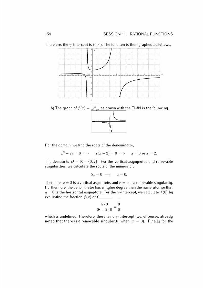
7/18/2019 Precalculus Tradler Carley
http://slidepdf.com/reader/full/precalculus-tradler-carley 164/424
154 SESSION 11. RATIONAL FUNCTIONS
Therefore, the y-intercept is (0, 0). The function is then graphed as follows.
-6 -5 -4 -3 -2 -1 0 1 2 3 4 5 6 7 8 9 10 11 12
-5
-4
-3
-2
-1
0
1
2
3
4
x
y
b) The graph of f (x) = 5xx2−2x
as drawn with the TI-84 is the following.
For the domain, we find the roots of the denominator,
x2 − 2x = 0 =⇒ x(x − 2) = 0 =⇒ x = 0 or x = 2.
The domain is D = R − {0, 2}. For the vertical asymptotes and removablesingularities, we calculate the roots of the numerator,
5x = 0 =⇒ x = 0.
Therefore, x = 2 is a vertical asymptote, and x = 0 is a removable singularity.Furthermore, the denominator has a higher degree than the numerator, so thaty = 0 is the horizontal asymptote. For the y-intercept, we calculate f (0) byevaluating the fraction f (x) at 0
5 · 0
02 − 2 · 0 =
0
0,
which is undefined. Therefore, there is no y-intercept (we, of course, alreadynoted that there is a removable singularity when x = 0). Finally for the
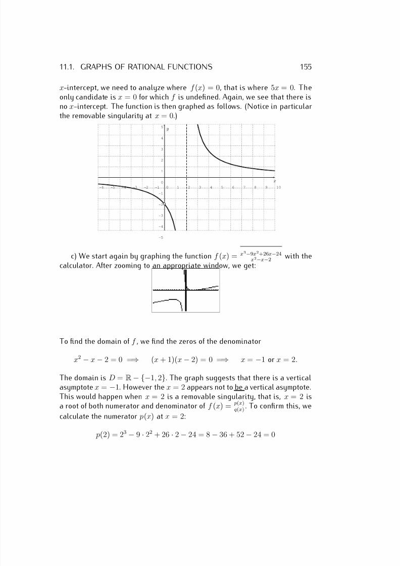
7/18/2019 Precalculus Tradler Carley
http://slidepdf.com/reader/full/precalculus-tradler-carley 165/424
11.1. GRAPHS OF RATIONAL FUNCTIONS 155
x-intercept, we need to analyze where f (x) = 0, that is where 5x = 0. The
only candidate is x = 0 for which f is undefined. Again, we see that there isno x-intercept. The function is then graphed as follows. (Notice in particularthe removable singularity at x = 0.)
-6 -5 -4 -3 -2 -1 0 1 2 3 4 5 6 7 8 9 10
-5
-4
-3
-2
-1
0
1
2
3
4
5
x
y
c) We start again by graphing the function f (x) = x3−9x2+26x−24x2−x−2
with thecalculator. After zooming to an appropriate window, we get:
To find the domain of f , we find the zeros of the denominator
x2 − x − 2 = 0 =⇒ (x + 1)(x − 2) = 0 =⇒ x = −1 or x = 2.
The domain is D = R− {−1, 2}. The graph suggests that there is a verticalasymptote x =
−1. However the x = 2 appears not to be a vertical asymptote.
This would happen when x = 2 is a removable singularity, that is, x = 2 isa root of both numerator and denominator of f (x) = p(x)
q(x). To confirm this, we
calculate the numerator p(x) at x = 2:
p(2) = 23 − 9 · 22 + 26 · 2 − 24 = 8 − 36 + 52 − 24 = 0
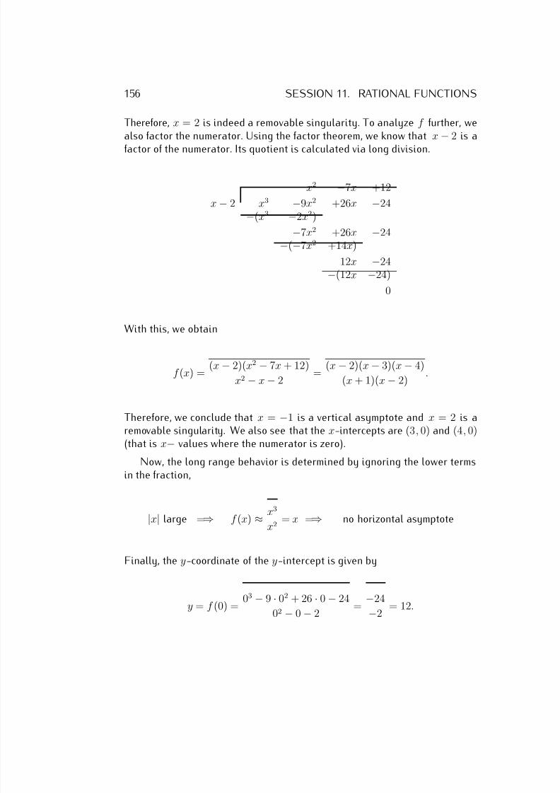
7/18/2019 Precalculus Tradler Carley
http://slidepdf.com/reader/full/precalculus-tradler-carley 166/424
156 SESSION 11. RATIONAL FUNCTIONS
Therefore, x = 2 is indeed a removable singularity. To analyze f further, we
also factor the numerator. Using the factor theorem, we know that x − 2 is afactor of the numerator. Its quotient is calculated via long division.
x2 −7x +12
x − 2 x3 −9x2 +26x −24−(x3 −2x2)
−7x2 +26x −24−(−7x2 +14x)
12x −24
−(12x −24)0
With this, we obtain
f (x) = (x − 2)(x2 − 7x + 12)
x2 − x − 2 =
(x − 2)(x − 3)(x − 4)
(x + 1)(x − 2) .
Therefore, we conclude that x = −1 is a vertical asymptote and x = 2 is aremovable singularity. We also see that the x-intercepts are (3, 0) and (4, 0)(that is x− values where the numerator is zero).
Now, the long range behavior is determined by ignoring the lower termsin the fraction,
|x| large =⇒ f (x) ≈ x3
x2 = x =⇒ no horizontal asymptote
Finally, the y-coordinate of the y-intercept is given by
y = f (0) = 03 − 9 · 02 + 26 · 0 − 24
02 − 0 − 2 =
−24
−2 = 12.
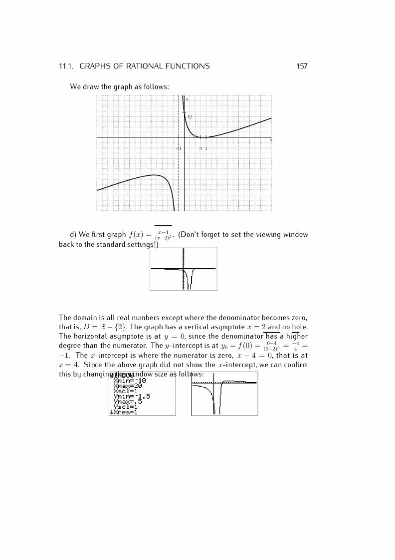
7/18/2019 Precalculus Tradler Carley
http://slidepdf.com/reader/full/precalculus-tradler-carley 167/424
11.1. GRAPHS OF RATIONAL FUNCTIONS 157
We draw the graph as follows:
x
y
3 4−1
12
d) We first graph f (x) = x−4(x−2)2 . (Don’t forget to set the viewing window
back to the standard settings!)
The domain is all real numbers except where the denominator becomes zero,that is, D = R− {2}. The graph has a vertical asymptote x = 2 and no hole.The horizontal asymptote is at y = 0, since the denominator has a higherdegree than the numerator. The y-intercept is at y0 = f (0) = 0−4
(0−2)2 = −44 =
−1. The x-intercept is where the numerator is zero, x − 4 = 0, that is atx = 4. Since the above graph did not show the x-intercept, we can confirmthis by changing the window size as follows:
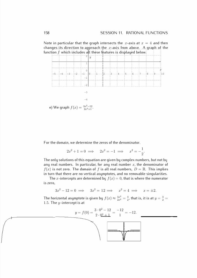
7/18/2019 Precalculus Tradler Carley
http://slidepdf.com/reader/full/precalculus-tradler-carley 168/424
158 SESSION 11. RATIONAL FUNCTIONS
Note in particular that the graph intersects the x-axis at x = 4 and then
changes its direction to approach the x-axis from above. A graph of thefunction f which includes all these features is displayed below.
-5 -4 -3 -2 -1 0 1 2 3 4 5 6 7 8 9 10
-4
-3
-2
-1
0
1
2
x
y
e) We graph f (x) = 3x2−122x2+1 .
For the domain, we determine the zeros of the denominator.
2x2 + 1 = 0 =⇒ 2x2 = −1 =⇒ x2 = −1
2.
The only solutions of this equation are given by complex numbers, but not byany real numbers. In particular, for any real number x, the denominator of f (x) is not zero. The domain of f is all real numbers, D = R. This impliesin turn that there are no vertical asymptotes, and no removable singularities.
The x-intercepts are determined by f (x) = 0, that is where the numeratoris zero,
3x2
−12 = 0 =
⇒ 3x2 = 12 =
⇒ x2 = 4 =
⇒ x =
±2.
The horizontal asymptote is given by f (x) ≈ 3x2
2x2 = 32 , that is, it is at y = 3
2 =1.5. The y-intercept is at
y = f (0) = 3 · 02 − 12
2 · 02 + 1 =
−12
1 = −12.
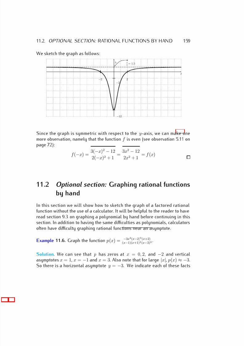
7/18/2019 Precalculus Tradler Carley
http://slidepdf.com/reader/full/precalculus-tradler-carley 169/424
11.2. OPTIONAL SECTION: RATIONAL FUNCTIONS BY HAND 159
We sketch the graph as follows:
x
y
−2 2
−12
−2
32
= 1.5
Since the graph is symmetric with respect to the y-axis, we can make onemore observation, namely that the function f is even (see observation 5.11 onpage 72):
f (−x) = 3(−x)2 − 12
2(−x)2 + 1 =
3x2 − 12
2x2 + 1 = f (x)
11.2 Optional section: Graphing rational functions
by hand
In this section we will show how to sketch the graph of a factored rationalfunction without the use of a calculator. It will be helpful to the reader to haveread section 9.3 on graphing a polynomial by hand before continuing in thissection. In addition to having the same difficulties as polynomials, calculatorsoften have difficulty graphing rational functions near an asymptote.
Example 11.6. Graph the function p(x) = −3x2(x
−2)3(x+2)
(x−1)(x+1)2 (x−3)3 .
Solution. We can see that p has zeros at x = 0, 2, and −2 and verticalasymptotes x = 1, x = −1 and x = 3. Also note that for large |x|, p(x) ≈ −3.So there is a horizontal asymptote y = −3. We indicate each of these facts
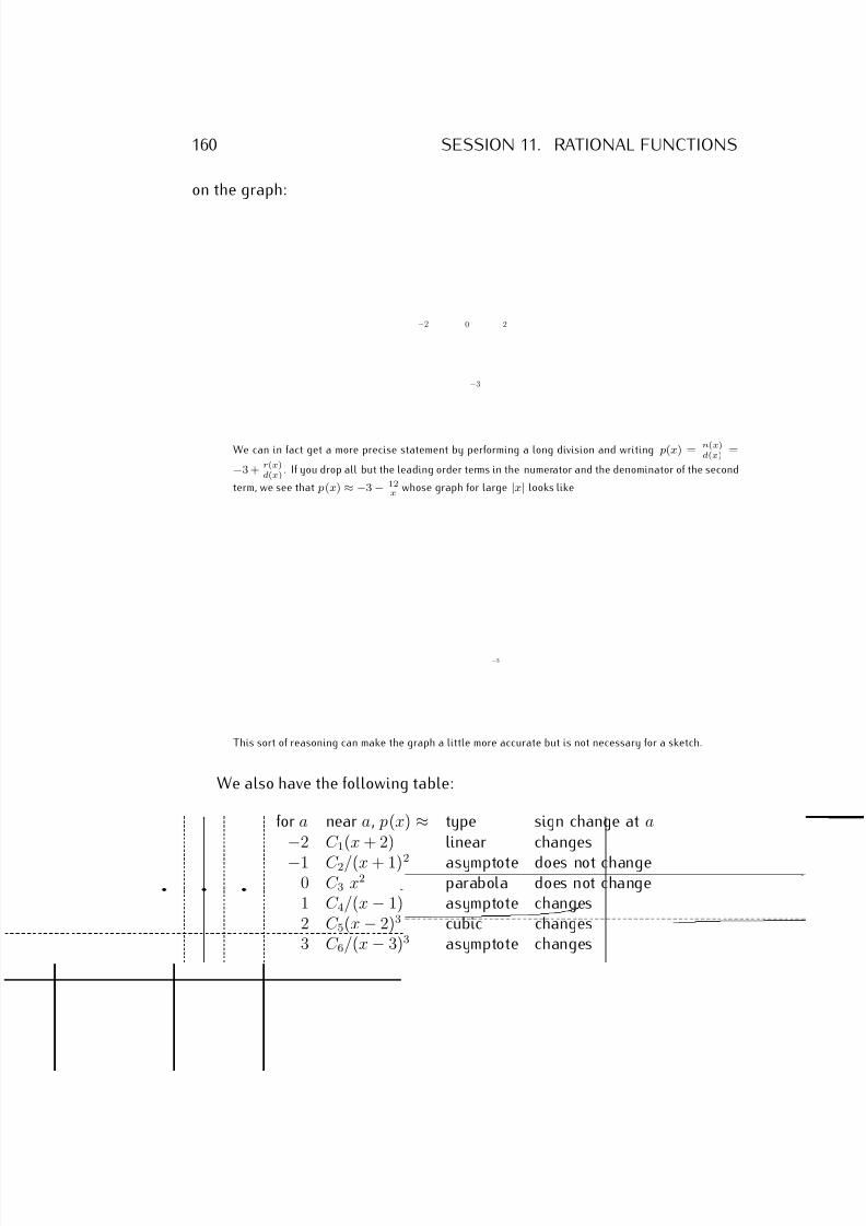
7/18/2019 Precalculus Tradler Carley
http://slidepdf.com/reader/full/precalculus-tradler-carley 170/424
160 SESSION 11. RATIONAL FUNCTIONS
on the graph:
−2 0 2
−3
We can in fact get a more precise statement by performing a long division and writing p(x) = n(x)d(x)
=
−3 + r(x)d(x)
. If you drop all but the leading order terms in the numerator and the denominator of the second
term, we see that p(x) ≈ −3 − 12x
whose graph for large |x| looks like
−3
This sort of reasoning can make the graph a little more accurate but is not necessary for a sketch.
We also have the following table:
for a near a, p(x) ≈ type sign change at a
−2 C 1(x + 2) linear changes
−1 C 2/(x + 1)2 asymptote does not change0 C 3 x2 parabola does not change1 C 4/(x − 1) asymptote changes2 C 5(x − 2)3 cubic changes3 C 6/(x − 3)3 asymptote changes

7/18/2019 Precalculus Tradler Carley
http://slidepdf.com/reader/full/precalculus-tradler-carley 171/424
11.2. OPTIONAL SECTION: RATIONAL FUNCTIONS BY HAND 161
Note that if the power appearing in the second column is even then the
function does not change from one side of a to the other. If the power is odd,the sign changes (either from positive to negative or from negative to positive).Now we move from large negative x values toward the right, taking into
account the above table. For large negative x, we start our sketch as follows:
−2 0 2
−3
And noting that near x = −2 the function p(x) is approximately linear, wehave
−2 0 2
−3
Then noting that we have an asymptote (noting that we can not cross the
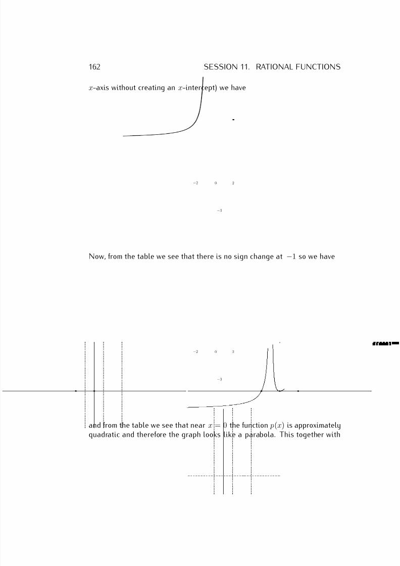
7/18/2019 Precalculus Tradler Carley
http://slidepdf.com/reader/full/precalculus-tradler-carley 172/424
162 SESSION 11. RATIONAL FUNCTIONS
x-axis without creating an x-intercept) we have
−2 0 2
−3
Now, from the table we see that there is no sign change at −1 so we have
−2 0 2
−3
and from the table we see that near x = 0 the function p(x) is approximatelyquadratic and therefore the graph looks like a parabola. This together with
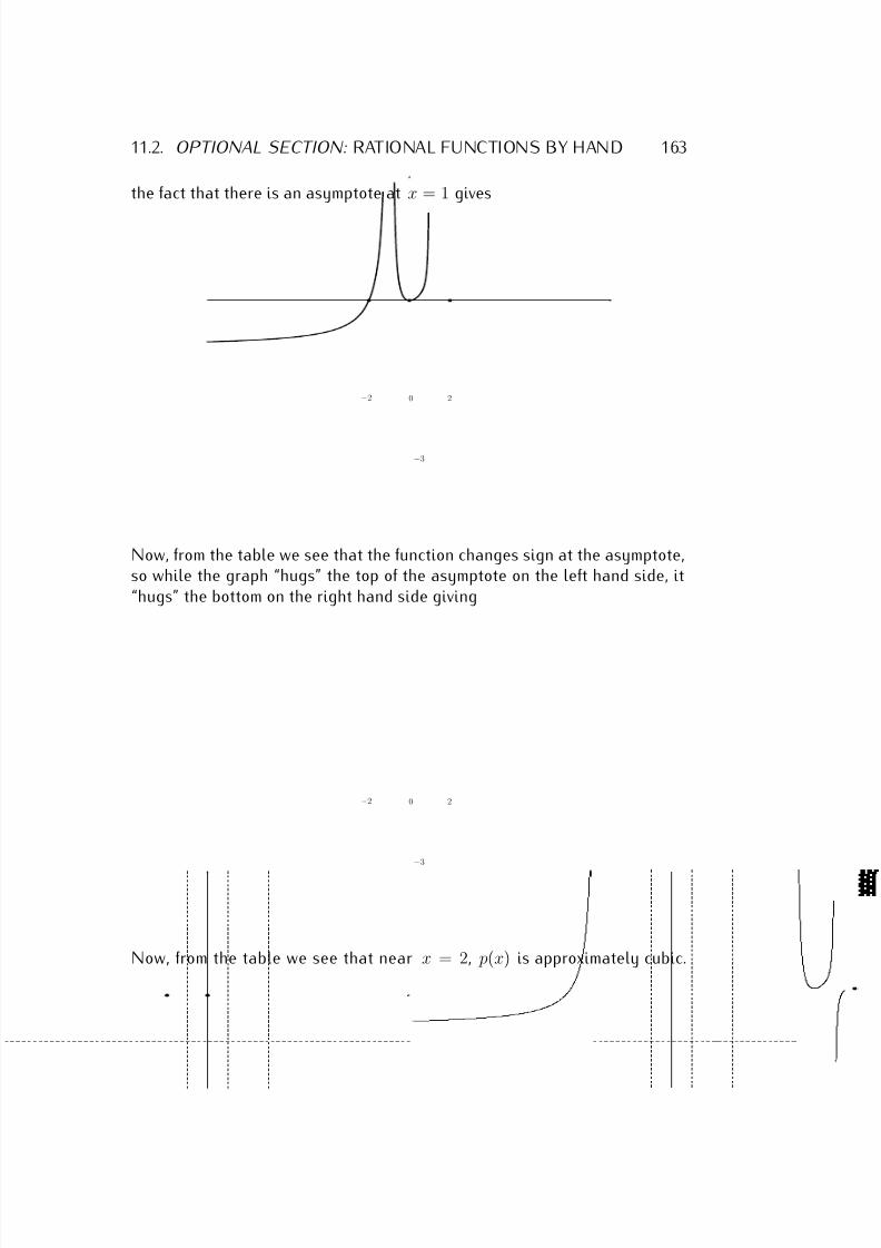
7/18/2019 Precalculus Tradler Carley
http://slidepdf.com/reader/full/precalculus-tradler-carley 173/424
11.2. OPTIONAL SECTION: RATIONAL FUNCTIONS BY HAND 163
the fact that there is an asymptote at x = 1 gives
−2 0 2
−3
Now, from the table we see that the function changes sign at the asymptote,so while the graph “hugs” the top of the asymptote on the left hand side, it“hugs” the bottom on the right hand side giving
−2 0 2
−3
Now, from the table we see that near x = 2, p(x) is approximately cubic.
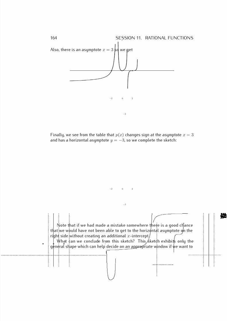
7/18/2019 Precalculus Tradler Carley
http://slidepdf.com/reader/full/precalculus-tradler-carley 174/424
164 SESSION 11. RATIONAL FUNCTIONS
Also, there is an asymptote x = 3 so we get
−2 0 2
−3
Finally, we see from the table that p(x) changes sign at the asymptote x = 3and has a horizontal asymptote y = −3, so we complete the sketch:
−2 0 2
−3
Note that if we had made a mistake somewhere there is a good chancethat we would have not been able to get to the horizontal asymptote on theright side without creating an additional x-intercept.
What can we conclude from this sketch? This sketch exhibits only thegeneral shape which can help decide on an appropriate window if we want to
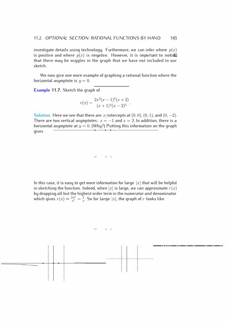
7/18/2019 Precalculus Tradler Carley
http://slidepdf.com/reader/full/precalculus-tradler-carley 175/424
11.2. OPTIONAL SECTION: RATIONAL FUNCTIONS BY HAND 165
investigate details using technology. Furthermore, we can infer where p(x)
is positive and where p(x) is negative. However, it is important to notice,that there may be wiggles in the graph that we have not included in oursketch.
We now give one more example of graphing a rational function where thehorizontal asymptote is y = 0.
Example 11.7. Sketch the graph of
r(x) = 2x2(x − 1)3(x + 2)
(x + 1)4(x − 2)3 .
Solution. Here we see that there are x-intercepts at (0, 0), (0, 1), and (0, −2).There are two vertical asymptotes: x = −1 and x = 2. In addition, there is ahorizontal asymptote at y = 0. (Why?) Putting this information on the graphgives
10−2
In this case, it is easy to get more information for large |x| that will be helpfulin sketching the function. Indeed, when |x| is large, we can approximate r(x)by dropping all but the highest order term in the numerator and denominatorwhich gives r(x) ≈ 2x6
x7 = 2x
. So for large |x|, the graph of r looks like
10−2
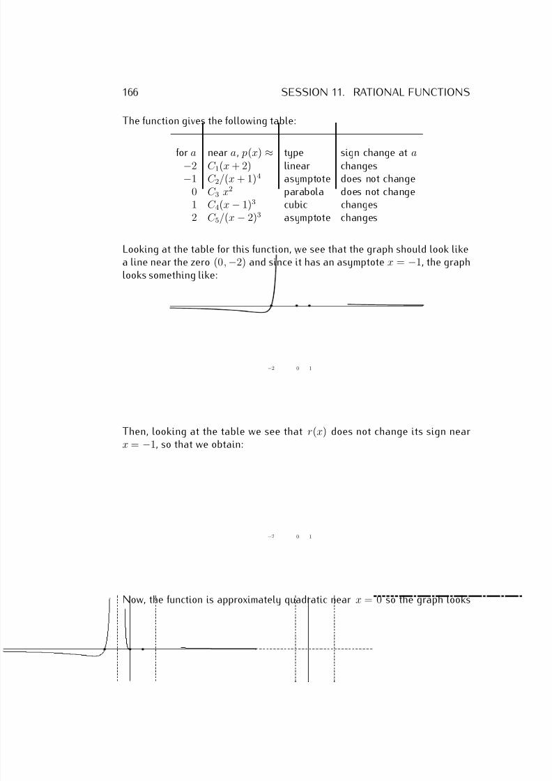
7/18/2019 Precalculus Tradler Carley
http://slidepdf.com/reader/full/precalculus-tradler-carley 176/424
166 SESSION 11. RATIONAL FUNCTIONS
The function gives the following table:
for a near a, p(x) ≈ type sign change at a−2 C 1(x + 2) linear changes−1 C 2/(x + 1)4 asymptote does not change
0 C 3 x2 parabola does not change1 C 4(x − 1)3 cubic changes2 C 5/(x − 2)3 asymptote changes
Looking at the table for this function, we see that the graph should look likea line near the zero (0,
−2) and since it has an asymptote x =
−1, the graph
looks something like:
10−2
Then, looking at the table we see that r(x) does not change its sign nearx = −1, so that we obtain:
10−2
Now, the function is approximately quadratic near x = 0 so the graph looks
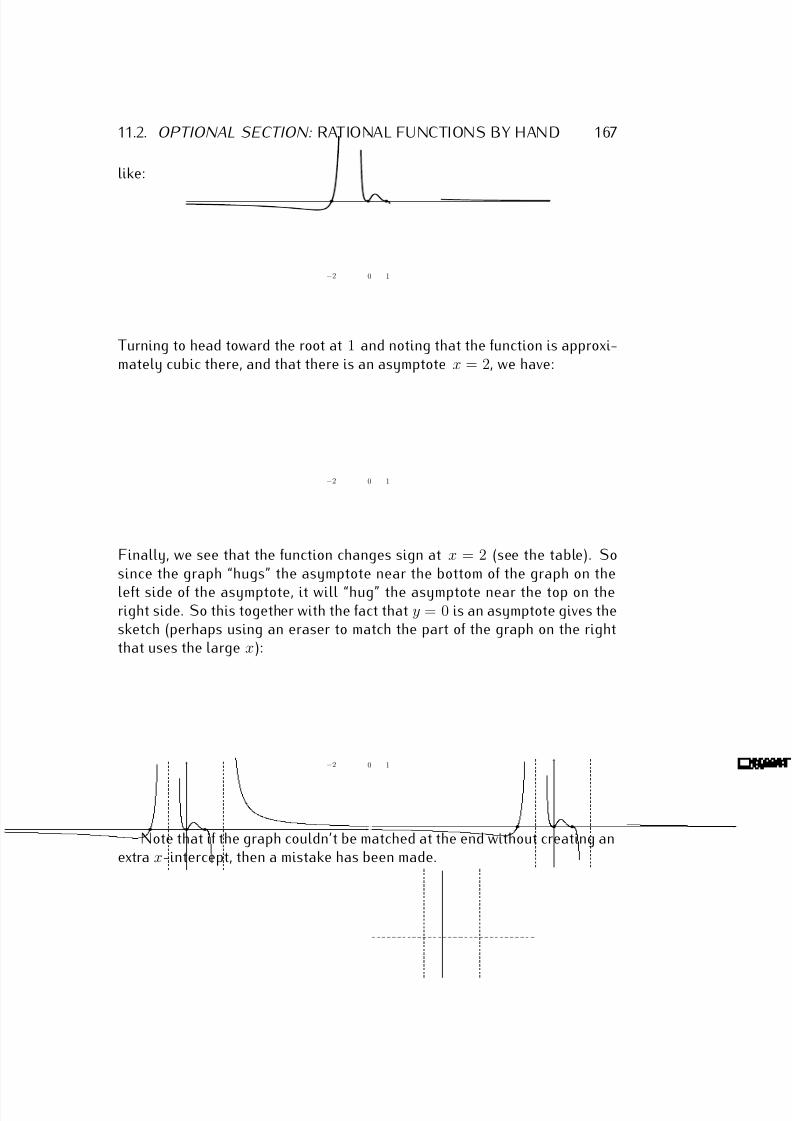
7/18/2019 Precalculus Tradler Carley
http://slidepdf.com/reader/full/precalculus-tradler-carley 177/424
11.2. OPTIONAL SECTION: RATIONAL FUNCTIONS BY HAND 167
like:
10−2
Turning to head toward the root at 1 and noting that the function is approxi-mately cubic there, and that there is an asymptote x = 2, we have:
10−2
Finally, we see that the function changes sign at x = 2 (see the table). Sosince the graph “hugs” the asymptote near the bottom of the graph on the
left side of the asymptote, it will “hug” the asymptote near the top on theright side. So this together with the fact that y = 0 is an asymptote gives thesketch (perhaps using an eraser to match the part of the graph on the rightthat uses the large x):
10−2
Note that if the graph couldn’t be matched at the end without creating anextra x-intercept, then a mistake has been made.
7/18/2019 Precalculus Tradler Carley
http://slidepdf.com/reader/full/precalculus-tradler-carley 178/424
168 SESSION 11. RATIONAL FUNCTIONS
11.3 Exercises
Exercise 11.1. Find the domain, the vertical asymptotes and removable dis-continuities of the functions.
a) f (x) = 2x−2 b) f (x) = x2+2
x2−6x+8
c) f (x) = 3x+6x3−4x
d) f (x) = (x−2)(x+3)(x+4)(x−2)2(x+3)(x−5)
e) f (x) = x−1x3−1 f ) f (x) = 2
x3−2x2−x+2
Exercise 11.2. Find the horizontal asymptotes of the functions.
a) f (x) = 8x2+2x+1
2x2
+3x−2 b) f (x) = 1
(x−3)2
c) f (x) = x2+3x+2x−1
d) f (x) = 12x3−4x+2−3x3+2x2+1
Exercise 11.3. Find the x- and y-intercepts of the functions.
a) f (x) = x−3x−1 b) f (x) = x3−4x
x2−8x+15
c) f (x) = (x−3)(x−1)(x+4)(x−2)(x−5) d) f (x) = x2+5x+6
x2+2x
Exercise 11.4. Sketch the graph of the function f by using the domain of f , the horizontal and vertical asymptotes, the removable singularities, the x-
and y-intercepts of the function, together with a sketch of the graph obtainedfrom the calculator.
a) f (x) = 6x−22x+4 b) f (x) = x−3
x3−3x2−6x+8
c) f (x) = x4−10x2+9x2−3x+2 d) f (x) = x3−3x2−x+3
x3−2x2
Exercise 11.5. Find a rational function f that satisfies all the given properties.
a) vertical asymptote at x = 4 and horizontal asymptote y = 0b) vertical asymptotes at x = 2 and x = 3 and horizontal asymptote y = 5c) removable singularity at x = 1 and no horizontal asymptote
7/18/2019 Precalculus Tradler Carley
http://slidepdf.com/reader/full/precalculus-tradler-carley 179/424
Session 12
Polynomial and rational
inequalities
12.1 Polynomial inequalities
We now consider inequalities. Solving inequalities is quite similar to solvingequalities. There is one extra consideration, that multiplying or dividing by anegative number on both sides of an inequality changes the direction of theinequality sign.
−2x ≤ −6 =⇒ x≥3
but 2x ≤ 6 =⇒ x ≤ 3
Example 12.1. Solve for x.
a) −3x + 7 > 19, b) 2x + 5 ≥ 4x − 11c) 3 < −6x − 4 ≤ 13, d) −2x − 1 ≤ 3x + 4 < 4x − 20
Solution. The first three calculations are straightforward.
a) −3x + 7 > 19 (−7)
=⇒ −3x > 12 (÷(−3))
=⇒ x < −4
b) 2x + 5 ≥ 4x − 11 (−4x−5)
=⇒ −2x ≥ −16 (÷(−2))
=⇒ x ≤ 8
c) 3 < −6x − 4 ≤ 13 (+4)=⇒ 7 < −6x ≤ 17 (÷(−6))=⇒ 7−6 > x ≥ 17−6
=⇒ −176 ≤ x < −7
6,
The last implication was obtained by switching the right and left terms of theinequality. The solution set is the interval [−17
6 , −7
6).
169
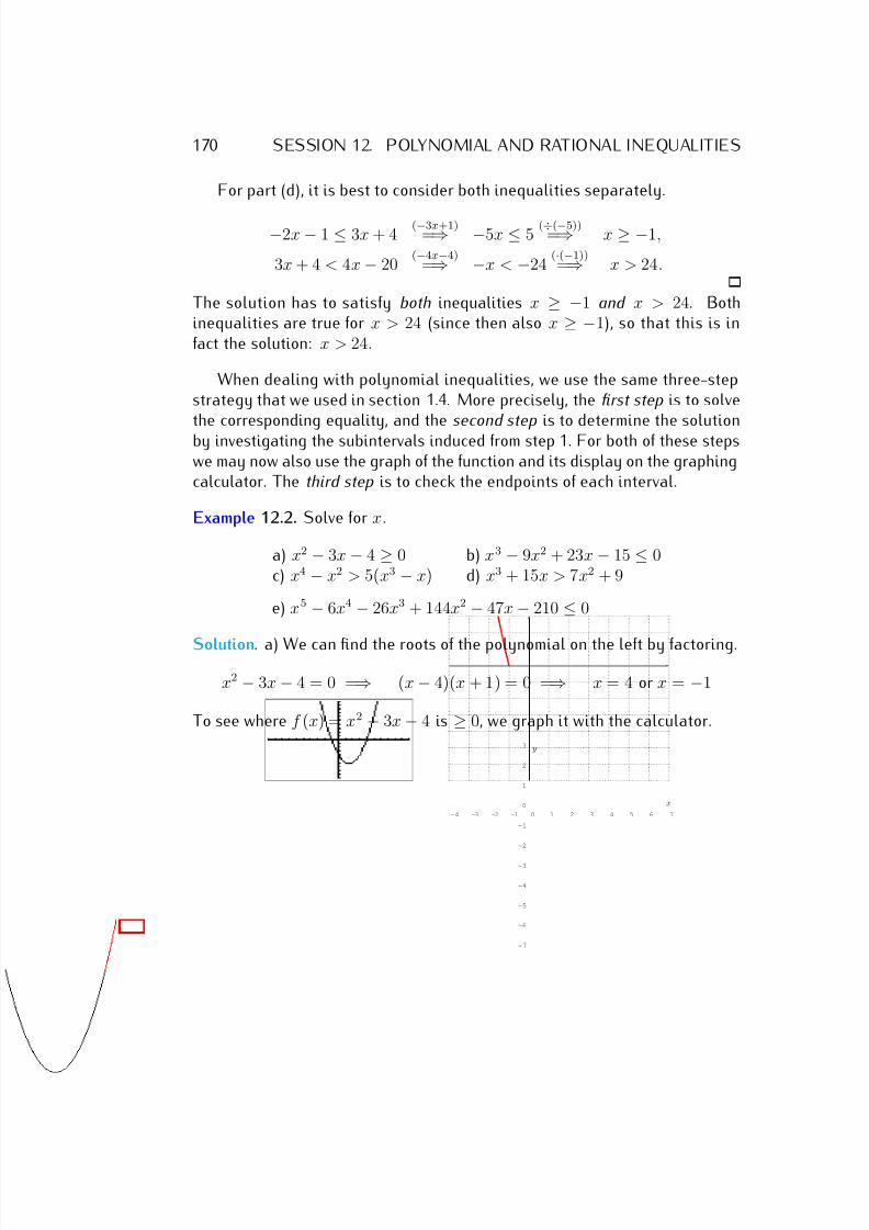
7/18/2019 Precalculus Tradler Carley
http://slidepdf.com/reader/full/precalculus-tradler-carley 180/424
170 SESSION 12. POLYNOMIAL AND RATIONAL INEQUALITIES
For part (d), it is best to consider both inequalities separately.
−2x − 1 ≤ 3x + 4 (−3x+1)
=⇒ −5x ≤ 5 (÷(−5))
=⇒ x ≥ −1,
3x + 4 < 4x − 20 (−4x−4)
=⇒ −x < −24 (·(−1))
=⇒ x > 24.
The solution has to satisfy both inequalities x ≥ −1 and x > 24. Bothinequalities are true for x > 24 (since then also x ≥ −1), so that this is infact the solution: x > 24.
When dealing with polynomial inequalities, we use the same three-stepstrategy that we used in section 1.4. More precisely, the first step is to solvethe corresponding equality, and the second step is to determine the solutionby investigating the subintervals induced from step 1. For both of these stepswe may now also use the graph of the function and its display on the graphingcalculator. The third step is to check the endpoints of each interval.
Example 12.2. Solve for x.
a) x2 − 3x − 4 ≥ 0 b) x3 − 9x2 + 23x − 15 ≤ 0c) x4 − x2 > 5(x3 − x) d) x3 + 15x > 7x2 + 9
e) x5 − 6x4 − 26x3 + 144x2 − 47x − 210 ≤ 0
Solution. a) We can find the roots of the polynomial on the left by factoring.
x2 − 3x − 4 = 0 =⇒ (x − 4)(x + 1) = 0 =⇒ x = 4 or x = −1
To see where f (x) = x2 − 3x − 4 is ≥ 0, we graph it with the calculator.
-4 -3 -2 -1 0 1 2 3 4 5 6 7
-7
-6
-5
-4
-3
-2
-1
0
1
2
3
x
y
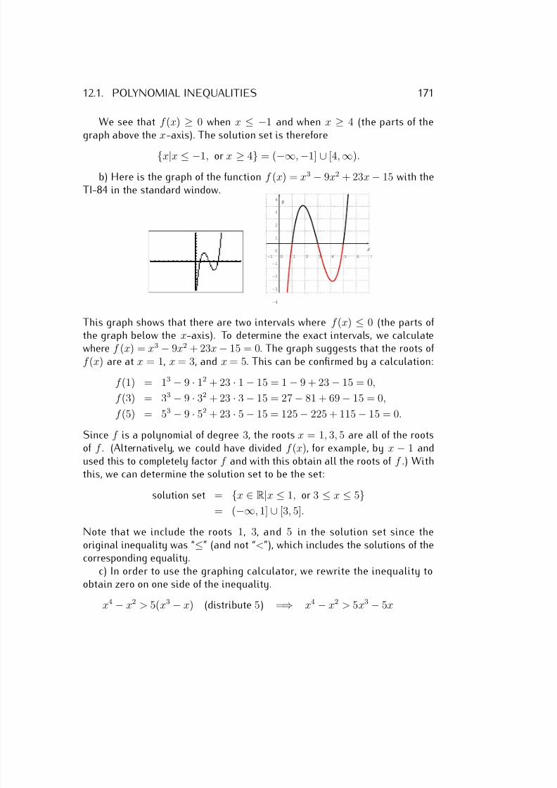
7/18/2019 Precalculus Tradler Carley
http://slidepdf.com/reader/full/precalculus-tradler-carley 181/424
12.1. POLYNOMIAL INEQUALITIES 171
We see that f (x) ≥ 0 when x ≤ −1 and when x ≥ 4 (the parts of the
graph above the x-axis). The solution set is therefore{x|x ≤ −1, or x ≥ 4} = (−∞, −1] ∪ [4, ∞).
b) Here is the graph of the function f (x) = x3 − 9x2 + 23x − 15 with theTI-84 in the standard window.
-1 0 1 2 3 4 5 6 7
-4
-3
-2
-1
0
1
2
3
4
x
y
This graph shows that there are two intervals where f (x) ≤ 0 (the parts of the graph below the x-axis). To determine the exact intervals, we calculatewhere f (x) = x3 − 9x2 + 23x − 15 = 0. The graph suggests that the roots of f (x) are at x = 1, x = 3, and x = 5. This can be confirmed by a calculation:
f (1) = 13 − 9 · 12 + 23 · 1 − 15 = 1 − 9 + 23 − 15 = 0,
f (3) = 33 − 9 · 32 + 23 · 3 − 15 = 27 − 81 + 69 − 15 = 0,
f (5) = 53 − 9 · 52 + 23 · 5 − 15 = 125 − 225 + 115 − 15 = 0.
Since f is a polynomial of degree 3, the roots x = 1, 3, 5 are all of the rootsof f . (Alternatively, we could have divided f (x), for example, by x − 1 andused this to completely factor f and with this obtain all the roots of f .) Withthis, we can determine the solution set to be the set:
solution set = {x ∈ R|x ≤ 1, or 3 ≤ x ≤ 5}= (−∞, 1] ∪ [3, 5].
Note that we include the roots 1, 3, and 5 in the solution set since theoriginal inequality was “
≤” (and not “<”), which includes the solutions of the
corresponding equality.c) In order to use the graphing calculator, we rewrite the inequality to
obtain zero on one side of the inequality.
x4 − x2 > 5(x3 − x) (distribute 5) =⇒ x4 − x2 > 5x3 − 5x
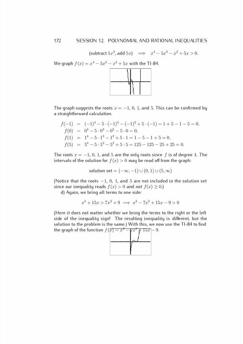
7/18/2019 Precalculus Tradler Carley
http://slidepdf.com/reader/full/precalculus-tradler-carley 182/424
172 SESSION 12. POLYNOMIAL AND RATIONAL INEQUALITIES
(subtract 5x3, add 5x) =⇒ x4 − 5x3 − x2 + 5x > 0.
We graph f (x) = x4 − 5x3 − x2 + 5x with the TI-84.
The graph suggests the roots x = −1, 0, 1, and 5. This can be confirmed bya straightforward calculation.
f (−1) = (−1)4 − 5 · (−1)3 − (−1)2 + 5 · (−1) = 1 + 5 − 1 − 5 = 0,
f (0) = 04 − 5 · 03 − 02 − 5 · 0 = 0,
f (1) = 14 − 5 · 13 − 12 + 5 · 1 = 1 − 5 − 1 + 5 = 0,
f (5) = 54 − 5 · 53 − 52 + 5 · 5 = 125 − 125 − 25 + 25 = 0.
The roots x = −1, 0, 1, and 5 are the only roots since f is of degree 4. Theintervals of the solution for f (x) > 0 may be read off from the graph:
solution set = (−∞, −1) ∪ (0, 1) ∪ (5, ∞)
(Notice that the roots −1, 0, 1, and 5 are not included in the solution setsince our inequality reads f (x) > 0 and not f (x) ≥ 0.)
d) Again, we bring all terms to one side:
x3 + 15x > 7x2 + 9 =⇒ x3 − 7x2 + 15x − 9 > 0
(Here it does not matter whether we bring the terms to the right or the leftside of the inequality sign! The resulting inequality is different, but thesolution to the problem is the same.) With this, we now use the TI-84 to findthe graph of the function f (x) = x3 − 7x2 + 15x − 9.
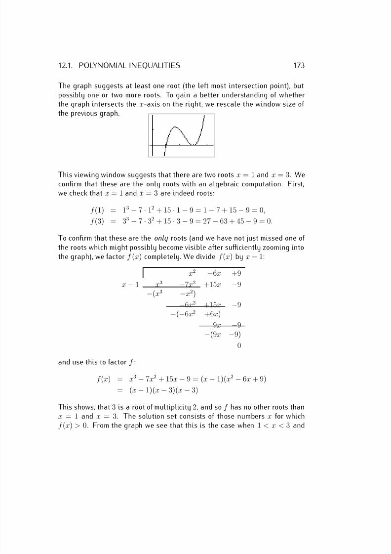
7/18/2019 Precalculus Tradler Carley
http://slidepdf.com/reader/full/precalculus-tradler-carley 183/424
12.1. POLYNOMIAL INEQUALITIES 173
The graph suggests at least one root (the left most intersection point), but
possibly one or two more roots. To gain a better understanding of whetherthe graph intersects the x-axis on the right, we rescale the window size of the previous graph.
This viewing window suggests that there are two roots x = 1 and x = 3. Weconfirm that these are the only roots with an algebraic computation. First,
we check that x = 1 and x = 3 are indeed roots:
f (1) = 13 − 7 · 12 + 15 · 1 − 9 = 1 − 7 + 15 − 9 = 0,
f (3) = 33 − 7 · 32 + 15 · 3 − 9 = 27 − 63 + 45 − 9 = 0.
To confirm that these are the only roots (and we have not just missed one of the roots which might possibly become visible after sufficiently zooming intothe graph), we factor f (x) completely. We divide f (x) by x − 1:
x2 −6x +9
x
−1 x3
−7x2 +15x
−9
−(x3 −x2)
−6x2 +15x −9−(−6x2 +6x)
9x −9−(9x −9)
0
and use this to factor f :
f (x) = x3
−7x2 + 15x
−9 = (x
−1)(x2
−6x + 9)
= (x − 1)(x − 3)(x − 3)
This shows, that 3 is a root of multiplicity 2, and so f has no other roots thanx = 1 and x = 3. The solution set consists of those numbers x for whichf (x) > 0. From the graph we see that this is the case when 1 < x < 3 and
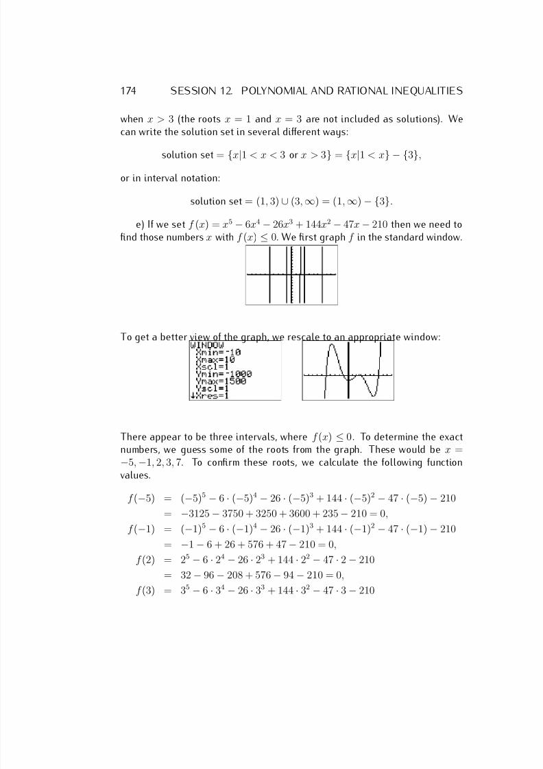
7/18/2019 Precalculus Tradler Carley
http://slidepdf.com/reader/full/precalculus-tradler-carley 184/424
174 SESSION 12. POLYNOMIAL AND RATIONAL INEQUALITIES
when x > 3 (the roots x = 1 and x = 3 are not included as solutions). We
can write the solution set in several different ways:
solution set = {x|1 < x < 3 or x > 3} = {x|1 < x} − {3},
or in interval notation:
solution set = (1, 3) ∪ (3, ∞) = (1, ∞) − {3}.
e) If we set f (x) = x5 − 6x4 − 26x3 + 144x2 − 47x − 210 then we need tofind those numbers x with f (x) ≤ 0. We first graph f in the standard window.
To get a better view of the graph, we rescale to an appropriate window:
There appear to be three intervals, where f (x) ≤ 0. To determine the exactnumbers, we guess some of the roots from the graph. These would be x =−5, −1, 2, 3, 7. To confirm these roots, we calculate the following functionvalues.
f (−5) = (−5)5 − 6 · (−5)4 − 26 · (−5)3 + 144 · (−5)2 − 47 · (−5) − 210
= −3125 − 3750 + 3250 + 3600 + 235 − 210 = 0,
f (
−1) = (
−1)5
−6
·(
−1)4
−26
·(
−1)3 + 144
·(
−1)2
−47
·(
−1)
−210
= −1 − 6 + 26 + 576 + 47 − 210 = 0,
f (2) = 25 − 6 · 24 − 26 · 23 + 144 · 22 − 47 · 2 − 210
= 32 − 96 − 208 + 576 − 94 − 210 = 0,
f (3) = 35 − 6 · 34 − 26 · 33 + 144 · 32 − 47 · 3 − 210
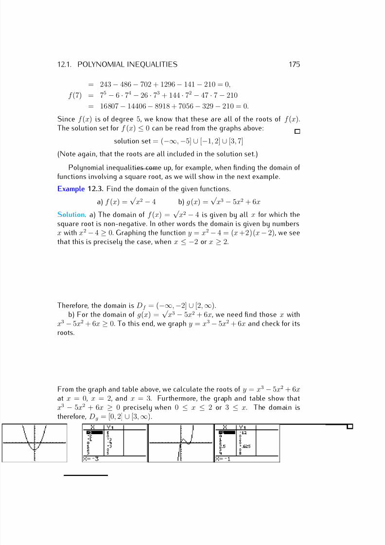
7/18/2019 Precalculus Tradler Carley
http://slidepdf.com/reader/full/precalculus-tradler-carley 185/424
12.1. POLYNOMIAL INEQUALITIES 175
= 243 − 486 − 702 + 1296 − 141 − 210 = 0,
f (7) = 75 − 6 · 74 − 26 · 73 + 144 · 72 − 47 · 7 − 210= 16807 − 14406 − 8918 + 7056 − 329 − 210 = 0.
Since f (x) is of degree 5, we know that these are all of the roots of f (x).The solution set for f (x) ≤ 0 can be read from the graphs above:
solution set = (−∞, −5] ∪ [−1, 2] ∪ [3, 7]
(Note again, that the roots are all included in the solution set.)
Polynomial inequalities come up, for example, when finding the domain of functions involving a square root, as we will show in the next example.
Example 12.3. Find the domain of the given functions.a) f (x) =
√ x2 − 4 b) g(x) =
√ x3 − 5x2 + 6x
Solution. a) The domain of f (x) =√
x2 − 4 is given by all x for which thesquare root is non-negative. In other words the domain is given by numbersx with x2 − 4 ≥ 0. Graphing the function y = x2 − 4 = (x +2)(x − 2), we seethat this is precisely the case, when x ≤ −2 or x ≥ 2.
Therefore, the domain is Df = (−∞, −2] ∪ [2, ∞).b) For the domain of g(x) =
√ x3 − 5x2 + 6x, we need find those x with
x3 − 5x2 + 6x ≥ 0. To this end, we graph y = x3 − 5x2 + 6x and check for itsroots.
From the graph and table above, we calculate the roots of y = x3 − 5x2 + 6xat x = 0, x = 2, and x = 3. Furthermore, the graph and table show thatx3 − 5x2 + 6x ≥ 0 precisely when 0 ≤ x ≤ 2 or 3 ≤ x. The domain istherefore, Dg = [0, 2] ∪ [3, ∞).
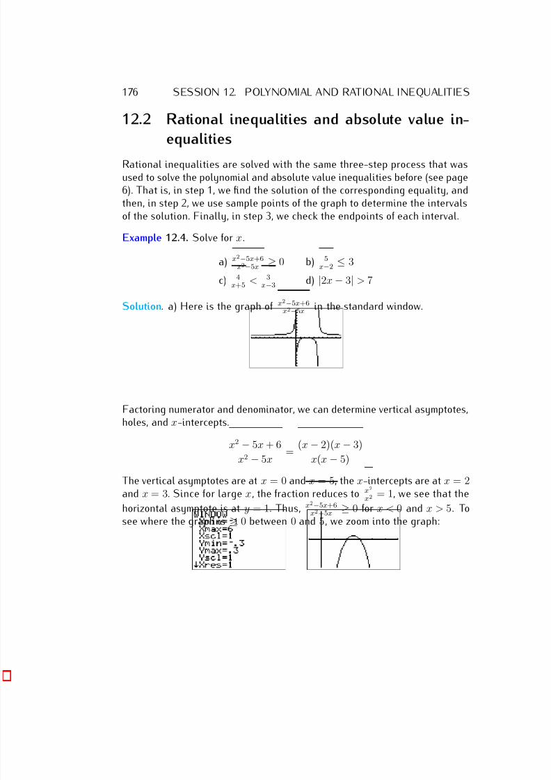
7/18/2019 Precalculus Tradler Carley
http://slidepdf.com/reader/full/precalculus-tradler-carley 186/424
176 SESSION 12. POLYNOMIAL AND RATIONAL INEQUALITIES
12.2 Rational inequalities and absolute value in-
equalities
Rational inequalities are solved with the same three-step process that wasused to solve the polynomial and absolute value inequalities before (see page6). That is, in step 1, we find the solution of the corresponding equality, andthen, in step 2, we use sample points of the graph to determine the intervalsof the solution. Finally, in step 3, we check the endpoints of each interval.
Example 12.4. Solve for x.
a) x2−5x+6x2
−5x
≥0 b) 5
x
−2
≤3
c) 4x+5 < 3
x−3 d) |2x − 3| > 7
Solution. a) Here is the graph of x2−5x+6x2−5x in the standard window.
Factoring numerator and denominator, we can determine vertical asymptotes,holes, and x-intercepts.
x2 − 5x + 6
x2 − 5x =
(x − 2)(x − 3)
x(x − 5)
The vertical asymptotes are at x = 0 and x = 5, the x-intercepts are at x = 2and x = 3. Since for large x, the fraction reduces to x2
x2 = 1, we see that the
horizontal asymptote is at y = 1. Thus, x2−5x+6x2−5x
≥ 0 for x < 0 and x > 5. Tosee where the graph is ≥ 0 between 0 and 5, we zoom into the graph:
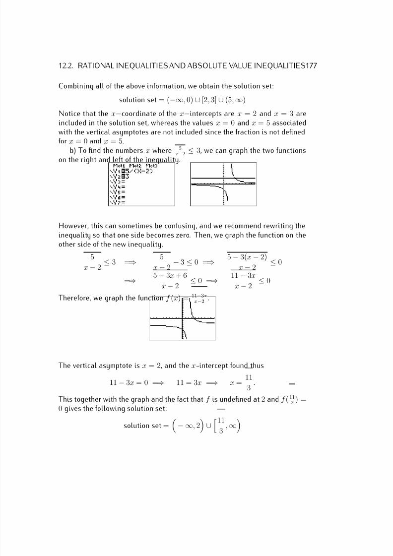
7/18/2019 Precalculus Tradler Carley
http://slidepdf.com/reader/full/precalculus-tradler-carley 187/424
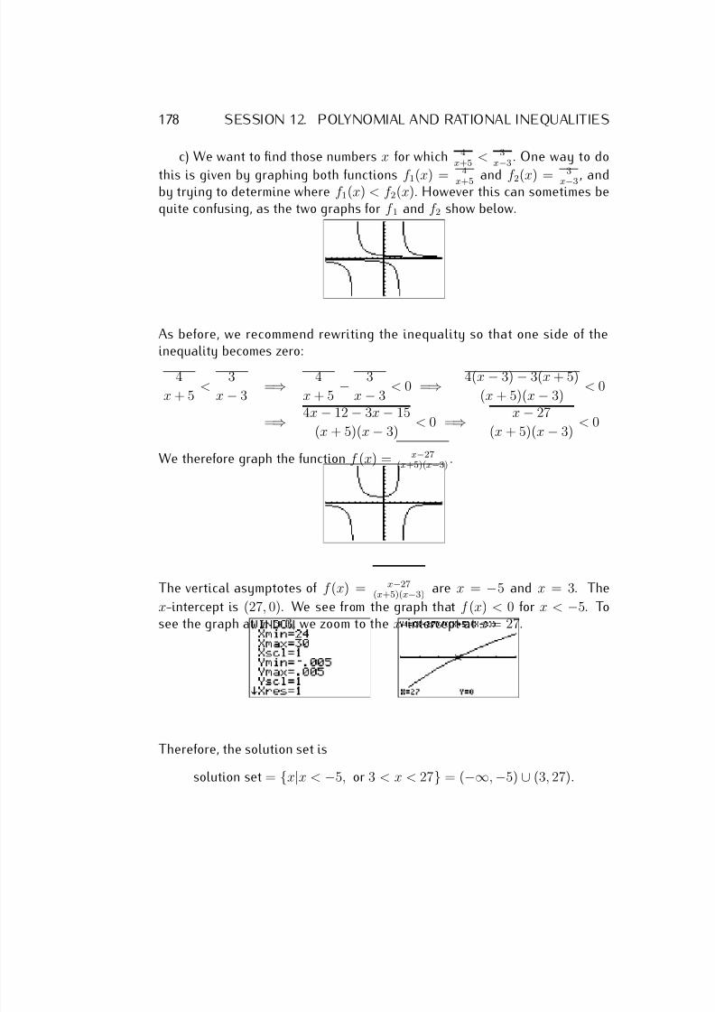
7/18/2019 Precalculus Tradler Carley
http://slidepdf.com/reader/full/precalculus-tradler-carley 188/424
178 SESSION 12. POLYNOMIAL AND RATIONAL INEQUALITIES
c) We want to find those numbers x for which 4x+5
< 3x−3
. One way to do
this is given by graphing both functions f 1(x) = 4x+5 and f 2(x) =
3x−3 , and
by trying to determine where f 1(x) < f 2(x). However this can sometimes bequite confusing, as the two graphs for f 1 and f 2 show below.
As before, we recommend rewriting the inequality so that one side of the
inequality becomes zero:4
x + 5 <
3
x − 3 =⇒ 4
x + 5 − 3
x − 3 < 0 =⇒ 4(x − 3) − 3(x + 5)
(x + 5)(x − 3) < 0
=⇒ 4x − 12 − 3x − 15
(x + 5)(x − 3) < 0 =⇒ x − 27
(x + 5)(x − 3) < 0
We therefore graph the function f (x) = x−27(x+5)(x−3) .
The vertical asymptotes of f (x) = x−27(x+5)(x−3)
are x = −5 and x = 3. The
x-intercept is (27, 0). We see from the graph that f (x) < 0 for x < −5. Tosee the graph at x > 3, we zoom to the x-intercept at x = 27.
Therefore, the solution set is
solution set = {x|x < −5, or 3 < x < 27} = (−∞, −5) ∪ (3, 27).
7/18/2019 Precalculus Tradler Carley
http://slidepdf.com/reader/full/precalculus-tradler-carley 189/424
12.3. EXERCISES 179
(The x-intercept x = 27 is not included in the solution set since the original
equation had a “<” and not “≤” sign.)d) To analyze |2x − 3| > 7, we graph the function f (x) = |2x − 3| − 7.
To see where f (x) > 0, we find the zeros of f (x).
|2x
−3| −
7 = 0 =⇒ |
2x−
3|
= 7 =⇒
2x−
3 =±
7
=⇒ 2x − 3 = 7 =⇒ 2x − 3 = −7(add 3) =⇒ 2x = 10 (add 3) =⇒ 2x = −4
(divide by 2) =⇒ x = 5 (divide by 2) =⇒ x = −2
Thus, we read off the solution set for f (x) > 0 from the graph.
solution set = (−∞, −2) ∪ (5, ∞)
12.3 ExercisesExercise 12.1. Solve for x.
a) 5x + 6 ≤ 21, b) 3 + 4x > 10xc) 2x + 8 ≥ 6x + 24, d) 9 − 3x < 2x − 13e) −5 ≤ 2x + 5 ≤ 19, f ) 15 > 7 − 2x ≥ 1g) 3x + 4 ≤ 6x − 2 ≤ 8x + 5, h) 5x + 2 < 4x − 18 ≤ 7x + 11
Exercise 12.2. Solve for x.
a) x2 − 5x − 14 > 0, b) x2 − 2x ≥ 35
c) x2 − 4 ≤ 0, d) x2 + 3x − 3 < 0e) 2x2 + 2x ≤ 12, f ) 3x2 < 2x + 1g) x2 − 4x + 4 > 0, h) x3 − 2x2 − 5x + 6 ≥ 0i) x3 + 4x2 + 3x + 12 < 0, j) −x3 − 4x < −4x2
k) x4 − 10x2 + 9 ≤ 0, l) x4 − 5x3 + 5x2 + 5x < 6m) x4 − 5x3 + 6x2 > 0, n) x5 − 6x4 + x3 + 24x2 − 20x ≤ 0
7/18/2019 Precalculus Tradler Carley
http://slidepdf.com/reader/full/precalculus-tradler-carley 190/424
180 SESSION 12. POLYNOMIAL AND RATIONAL INEQUALITIES
o) x5 − 15x4 + 85x3 − 225x2 + 274x − 120 ≥ 0,
p) x11
− x10
+ x − 1 ≤ 0Exercise 12.3. Find the domain of the functions below.
a) f (x) =√
x2 − 8x + 15 b) f (x) =√
9x − x3
c) f (x) =
(x − 1)(4 − x) d) f (x) =
(x − 2)(x − 5)(x − 6)
e) f (x) = 5√ 6−2x
f ) f (x) = 1√ x2−6x−7
Exercise 12.4. Solve for x.
a) x−52−x
> 0 b) 4x−4x2−4
≥ 0 c) x−2x2−4x−5
< 0 d) x2−9x2−4
≥ 0
e) x−3x+3 ≤ 4 f) 1
x+10 > 5 g) 2x−2 ≤ 5
x+1 h) x2x+4 ≤ x
Exercise 12.5. Solve for x.
a) |2x + 7| > 9 b) |6x + 2| < 3
c) |5 − 3x| ≥ 4 d) | − x − 7| ≤ 5
e) |1 − 8x| ≥ 3 f ) 1 >2 + x
5
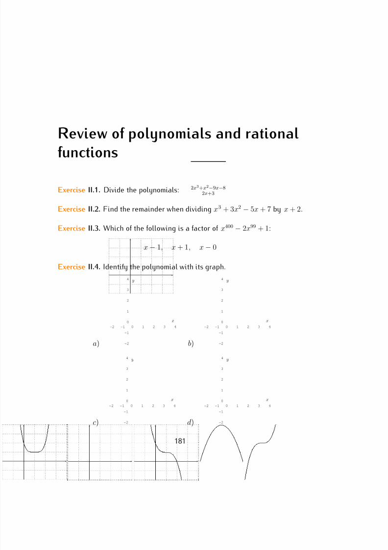
7/18/2019 Precalculus Tradler Carley
http://slidepdf.com/reader/full/precalculus-tradler-carley 191/424
Review of polynomials and rational
functions
Exercise II.1. Divide the polynomials: 2x3+x2
−9x
−8
2x+3
Exercise II.2. Find the remainder when dividing x3 + 3x2 − 5x + 7 by x + 2.
Exercise II.3. Which of the following is a factor of x400 − 2x99 + 1:
x − 1, x + 1, x − 0
Exercise II.4. Identify the polynomial with its graph.
a)
-2 -1 0 1 2 3 4
-2
-1
0
1
2
3
4
x
y
b)
-2 -1 0 1 2 3 4
-2
-1
0
1
2
3
4
x
y
c)
-2 -1 0 1 2 3 4
-2
-1
0
1
2
3
4
x
y
d)
-2 -1 0 1 2 3 4
-2
-1
0
1
2
3
4
x
y
181
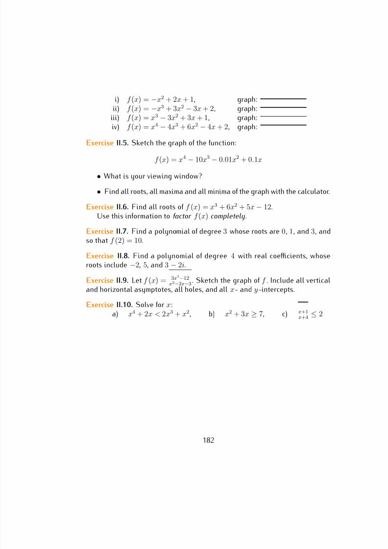
7/18/2019 Precalculus Tradler Carley
http://slidepdf.com/reader/full/precalculus-tradler-carley 192/424
i) f (x) = −x2 + 2x + 1, graph:ii) f (x) = −x3 + 3x2 − 3x + 2, graph:
iii) f (x) = x3 − 3x2 + 3x + 1, graph:iv) f (x) = x4 − 4x3 + 6x2 − 4x + 2, graph:
Exercise II.5. Sketch the graph of the function:
f (x) = x4 − 10x3 − 0.01x2 + 0.1x
• What is your viewing window?
• Find all roots, all maxima and all minima of the graph with the calculator.
Exercise II.6. Find all roots of f (x) = x3 + 6x2 + 5x − 12.Use this information to factor f (x) completely.
Exercise II.7. Find a polynomial of degree 3 whose roots are 0, 1, and 3, andso that f (2) = 10.
Exercise II.8. Find a polynomial of degree 4 with real coefficients, whoseroots include −2, 5, and 3 − 2i.
Exercise II.9. Let f (x) = 3x2−12x2
−2x
−3 . Sketch the graph of f . Include all vertical
and horizontal asymptotes, all holes, and all x- and y-intercepts.
Exercise II.10. Solve for x:a) x4 + 2x < 2x3 + x2, b) x2 + 3x ≥ 7, c) x+1
x+4 ≤ 2
182
7/18/2019 Precalculus Tradler Carley
http://slidepdf.com/reader/full/precalculus-tradler-carley 193/424
Part III
Exponential and logarithmic
functions
183
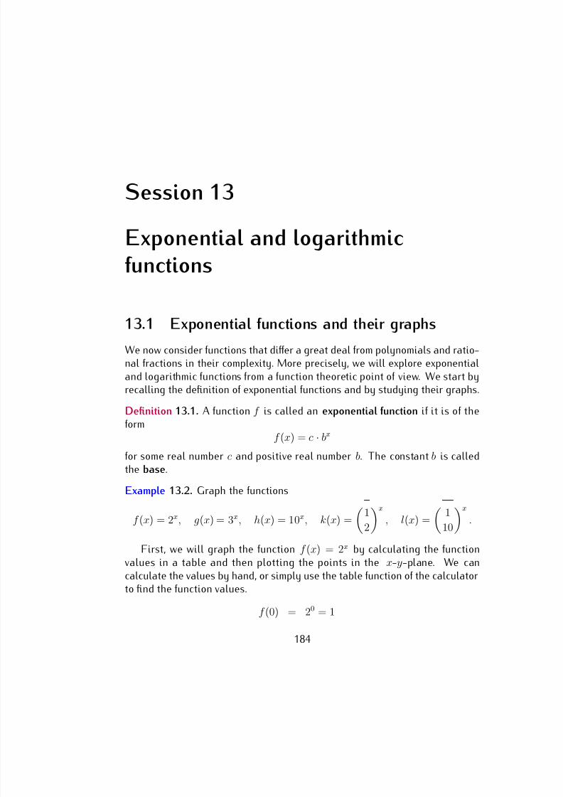
7/18/2019 Precalculus Tradler Carley
http://slidepdf.com/reader/full/precalculus-tradler-carley 194/424
Session 13
Exponential and logarithmic
functions
13.1 Exponential functions and their graphs
We now consider functions that differ a great deal from polynomials and ratio-nal fractions in their complexity. More precisely, we will explore exponentialand logarithmic functions from a function theoretic point of view. We start byrecalling the definition of exponential functions and by studying their graphs.
Definition 13.1. A function f is called an exponential function if it is of theform
f (x) = c · bx
for some real number c and positive real number b. The constant b is calledthe base.
Example 13.2. Graph the functions
f (x) = 2x, g(x) = 3x, h(x) = 10x, k(x) =
1
2
x
, l(x) =
1
10
x
.
First, we will graph the function f (x) = 2x by calculating the function
values in a table and then plotting the points in the x-y-plane. We cancalculate the values by hand, or simply use the table function of the calculatorto find the function values.
f (0) = 20 = 1
184
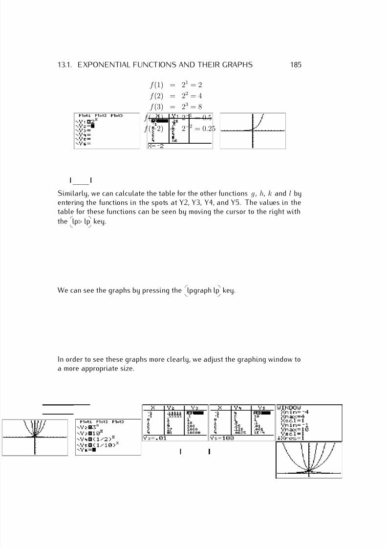
7/18/2019 Precalculus Tradler Carley
http://slidepdf.com/reader/full/precalculus-tradler-carley 195/424
13.1. EXPONENTIAL FUNCTIONS AND THEIR GRAPHS 185
f (1) = 21 = 2
f (2) = 22 = 4f (3) = 23 = 8
f (−1) = 2−1 = 0.5
f (−2) = 2−2 = 0.25
Similarly, we can calculate the table for the other functions g , h, k and l byentering the functions in the spots at Y2, Y3, Y4, and Y5. The values in thetable for these functions can be seen by moving the cursor to the right with
the
lp⊲ lp key.
We can see the graphs by pressing the
lpgraph lp key.
In order to see these graphs more clearly, we adjust the graphing window toa more appropriate size.
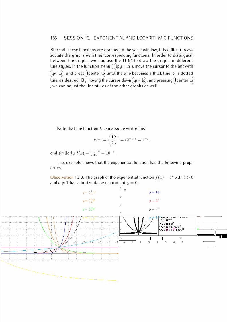
7/18/2019 Precalculus Tradler Carley
http://slidepdf.com/reader/full/precalculus-tradler-carley 196/424
186 SESSION 13. EXPONENTIAL AND LOGARITHMIC FUNCTIONS
Since all these functions are graphed in the same window, it is difficult to as-
sociate the graphs with their corresponding functions. In order to distinguishbetween the graphs, we may use the TI-84 to draw the graphs in different
line styles. In the function menu (
lpy= lp ), move the cursor to the left with
lp⊳ lp , and press
lpenter lp until the line becomes a thick line, or a dotted
line, as desired. By moving the cursor down
lp▽ lp , and pressing
lpenter lp
, we can adjust the line styles of the other graphs as well.
Note that the function k can also be written as
k(x) =
1
2
x
= (2−1)x = 2−x,
and similarly, l(x) =
110
x= 10−x.
This example shows that the exponential function has the following prop-
erties.
Observation 13.3. The graph of the exponential function f (x) = bx with b > 0and b = 1 has a horizontal asymptote at y = 0.
-7 -6 -5 -4 -3 -2 -1 0 1 2 3 4 5 6 7
-1
0
1
2
3
4
5
6
x
yy = 10x
y = 3x
y = 2x
y = 1x
y = 1.2x
y = ( 110
)x
y = ( 13
)x
y = ( 12
)x
y = ( 11.2
)x
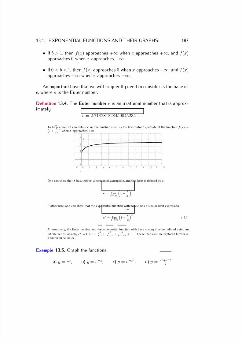
7/18/2019 Precalculus Tradler Carley
http://slidepdf.com/reader/full/precalculus-tradler-carley 197/424
13.1. EXPONENTIAL FUNCTIONS AND THEIR GRAPHS 187
• If b > 1, then f (x) approaches +∞ when x approaches +∞, and f (x)
approaches 0 when x approaches −∞.
• If 0 < b < 1, then f (x) approaches 0 when x approaches +∞, and f (x)approaches +∞ when x approaches −∞.
An important base that we will frequently need to consider is the base of e, where e is the Euler number.
Definition 13.4. The Euler number e is an irrational number that is approx-imately
e = 2.718281828459045235 . . .
To be precise, we can define e as the number which is the horizontal asymptote of the function f (x) =1 + 1
x
xwhen x approaches +∞.
-1 0 1 2 3 4 5 6 7 8 9 10 11 12
-1
0
1
2
3
4
x
y
e
One can show that f has, indeed, a horizontal asymptote, and this limit is defined as e .
e := limx→∞
1 +
1
x
x
Furthermore, one can show that the exponential function with base e has a similar limit expression.
er = limx→∞
1 +
r
x
x(13.1)
Alternatively, the Euler number and the exponential function with base e may also be defined using an
infinite series, namely, er = 1 + r + r2
1·2 + r3
1·2·3 + r4
1·2·3·4 + . . . . These ideas will be explored further ina course in calculus.
Example 13.5. Graph the functions.
a) y = ex, b) y = e−x, c) y = e−x2, d) y = ex+e−x
2
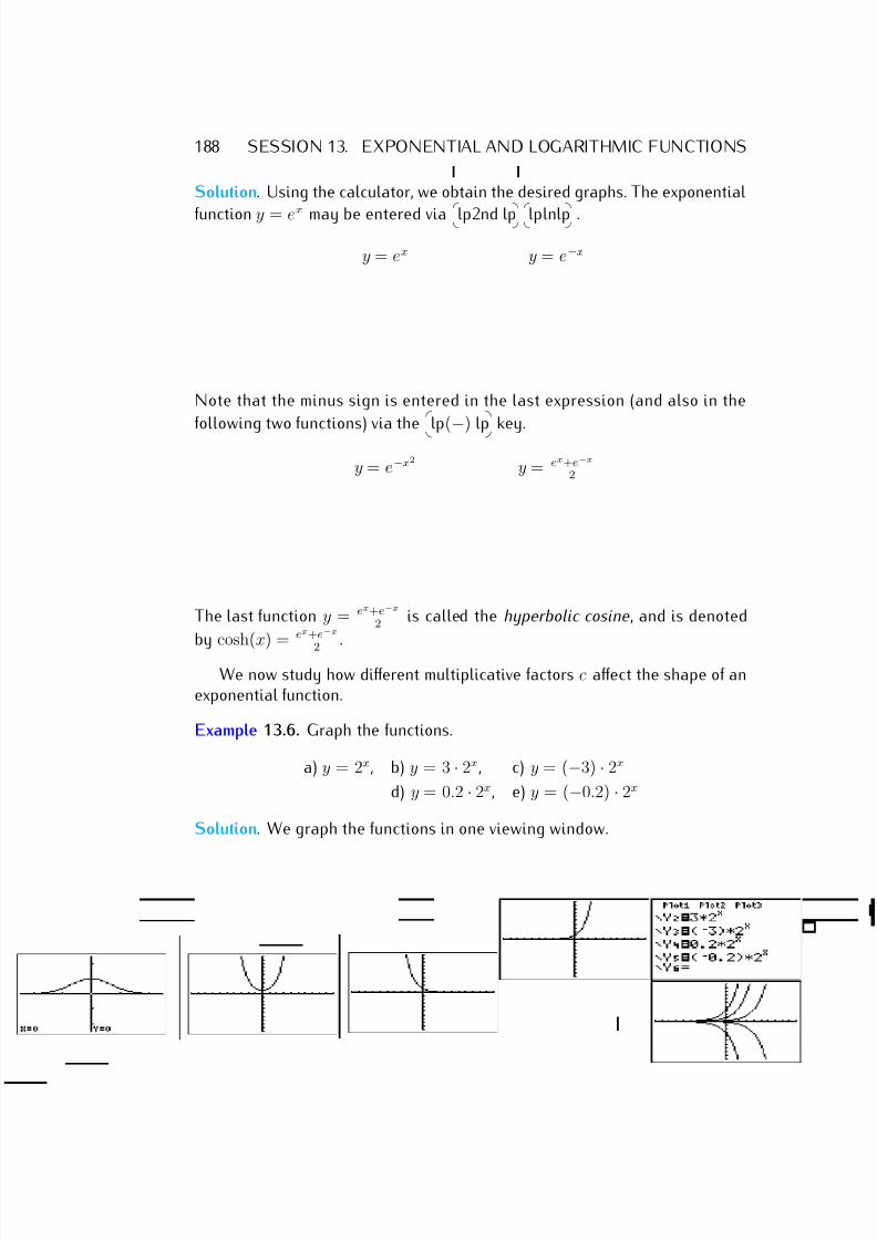
7/18/2019 Precalculus Tradler Carley
http://slidepdf.com/reader/full/precalculus-tradler-carley 198/424
188 SESSION 13. EXPONENTIAL AND LOGARITHMIC FUNCTIONS
Solution. Using the calculator, we obtain the desired graphs. The exponential
function y = ex
may be entered via
lp2nd lp
lplnlp .
y = ex y = e−x
Note that the minus sign is entered in the last expression (and also in the
following two functions) via the
lp(
−) lp key.
y = e−x2y = ex+e−x
2
The last function y = ex+e−x2 is called the hyperbolic cosine, and is denoted
by cosh(x) = ex+e−x
2
.
We now study how different multiplicative factors c affect the shape of anexponential function.
Example 13.6. Graph the functions.
a) y = 2x, b) y = 3 · 2x, c) y = (−3) · 2x
d) y = 0.2 · 2x, e) y = (−0.2) · 2x
Solution. We graph the functions in one viewing window.
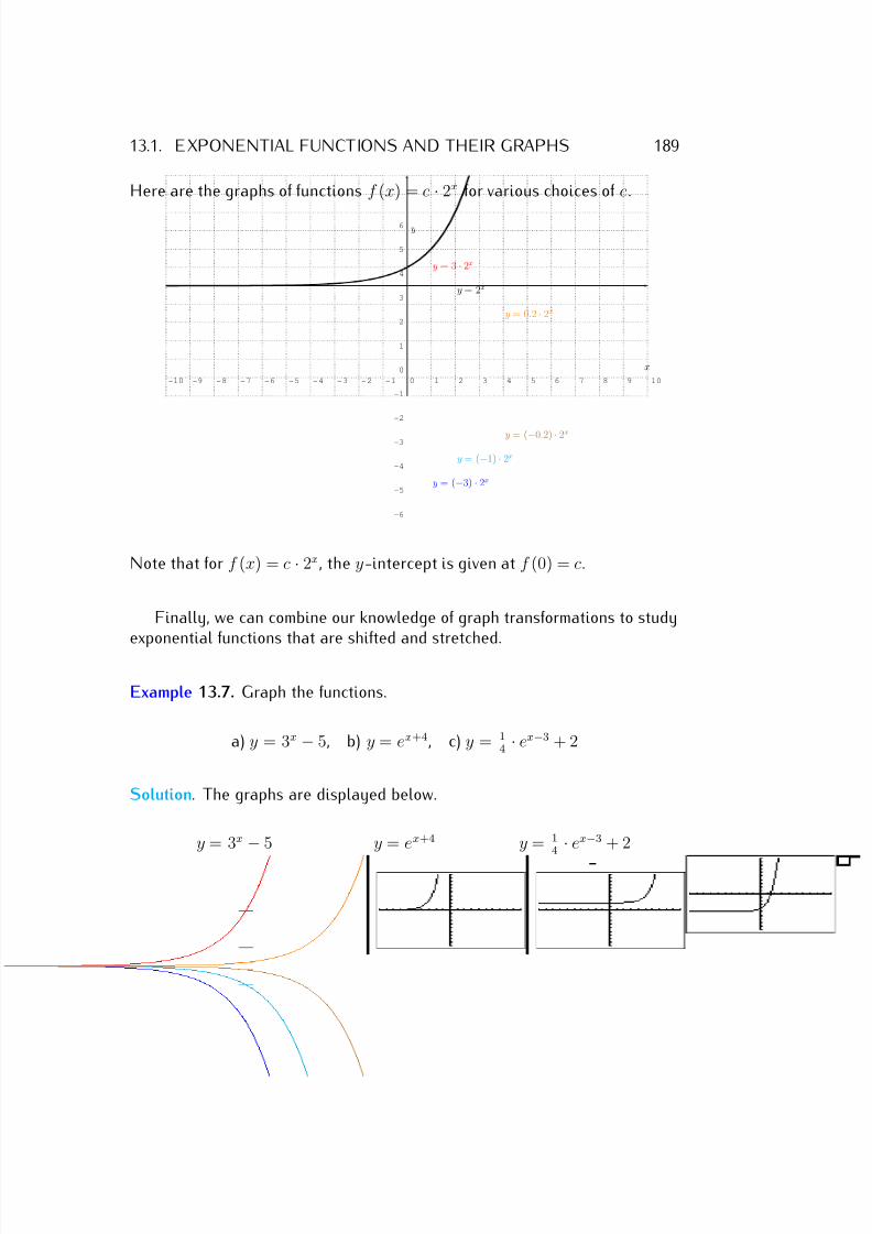
7/18/2019 Precalculus Tradler Carley
http://slidepdf.com/reader/full/precalculus-tradler-carley 199/424
13.1. EXPONENTIAL FUNCTIONS AND THEIR GRAPHS 189
Here are the graphs of functions f (x) = c · 2x for various choices of c.
-10 -9 - 8 - 7 - 6 - 5 - 4 - 3 - 2 - 1 0 1 2 3 4 5 6 7 8 9 10
-6
-5
-4
-3
-2
-1
0
1
2
3
4
5
6
x
y
y = 3 · 2x
y = 2x
y = 0.2 · 2x
y = (−0.2) · 2x
y = (−1) · 2x
y = (−3) · 2x
Note that for f (x) = c · 2x, the y-intercept is given at f (0) = c.
Finally, we can combine our knowledge of graph transformations to studyexponential functions that are shifted and stretched.
Example 13.7. Graph the functions.
a) y = 3x − 5, b) y = ex+4, c) y = 14 · ex−3 + 2
Solution. The graphs are displayed below.
y = 3x − 5 y = ex+4 y = 14 · ex−3 + 2
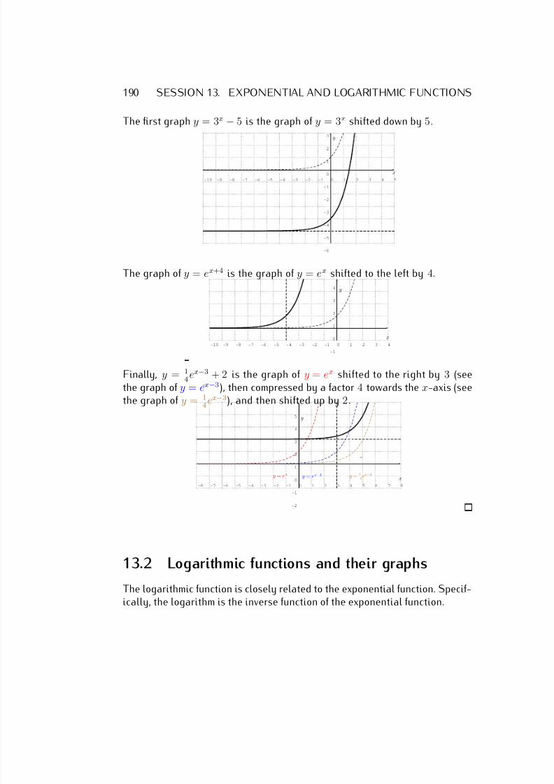
7/18/2019 Precalculus Tradler Carley
http://slidepdf.com/reader/full/precalculus-tradler-carley 200/424
190 SESSION 13. EXPONENTIAL AND LOGARITHMIC FUNCTIONS
The first graph y = 3x − 5 is the graph of y = 3x shifted down by 5.
-10 -9 -8 -7 -6 -5 -4 -3 -2 -1 0 1 2 3 4 5
-6
-5
-4
-3
-2
-1
0
1
2
3
x
y
The graph of y = ex+4
is the graph of y = ex
shifted to the left by 4.
-10 -9 -8 -7 -6 -5 -4 -3 -2 -1 0 1 2 3 4
-1
0
1
2
3
4
x
y
Finally, y = 14
ex−3 + 2 is the graph of y = ex shifted to the right by 3 (seethe graph of y = ex−3), then compressed by a factor 4 towards the x-axis (seethe graph of y = 1
4ex−3), and then shifted up by 2.
-8 -7 -6 -5 -4 -3 -2 -1 0 1 2 3 4 5 6 7 8
-2
-1
0
1
2
3
4
5
x
y
y = ex y = ex−3 y = 14 ex−4
13.2 Logarithmic functions and their graphs
The logarithmic function is closely related to the exponential function. Specif-ically, the logarithm is the inverse function of the exponential function.
7/18/2019 Precalculus Tradler Carley
http://slidepdf.com/reader/full/precalculus-tradler-carley 201/424
13.2. LOGARITHMIC FUNCTIONS AND THEIR GRAPHS 191
Definition 13.8. Let 0 < b = 1 be a positive real number that is not equal to
1. For x > 0, the logarithm of x with base b is defined by the equivalence
y = logb(x) ⇔ by = x (13.2)
For the particular base b = 10 we use the short form
log(x) := log10(x)
For the particular base b = e, where e ≈ 2.71828 is the Euler number, we callthe logarithm with base e the natural logarithm, and write
ln(x) := loge(x)
The logarithmic function is the function y = logb(x) with domain D ={x ∈ R|x > 0} of all positive real numbers, and range R = R of all realnumbers. It is the inverse of the exponential function y = bx with base b.
Example 13.9. Rewrite the equation as a logarithmic equation.
a) 34 = 81, b) 103 = 1000,c) ex = 17, d) 27·a = 53.
Solution. We can immediately apply equation (13.2). For part (a), we have
b = 3, y = 4, and x = 81. Therefore we have:
34 = 81 ⇔ log3(81) = 4
Similarly, we obtain the solutions for (b), (c), and (d).
b) 103 = 1000 ⇔ log(1000) = 3c) ex = 17 ⇔ ln(17) = xd) 27a = 53 ⇔ log2(53) = 7a
Example 13.10. Evaluate the expression by rewriting it as an exponentialexpression.
a) log2(16), b) log5(125), c) log13(1), d) log4(4)e) log(10, 000), f ) log(0.001), g) ln(e7), h) logb(bx)
7/18/2019 Precalculus Tradler Carley
http://slidepdf.com/reader/full/precalculus-tradler-carley 202/424
192 SESSION 13. EXPONENTIAL AND LOGARITHMIC FUNCTIONS
Solution. a) If we set y = log2(16), then this is equivalent to 2y = 16. Since,
clearly, 24
= 16, we see that y = 4. Therefore, we have log2(16) = 4.
b) log5(125) = y ⇔ 5y = 125(since 53=125)
=⇒ 3 = y = log5(125)
c) log13(1) = y ⇔ 13y = 1(since 130=1)
=⇒ 0 = y = log13(1)
d) log4(4) = y ⇔ 4y = 4(since 41=4)
=⇒ 1 = y = log4(4)
e) log(100, 000) = y ⇔
10y = 100, 000(since 105=100,000)
=⇒ 5 = y = log(100, 000)
f ) log(0.001) = y ⇔ 10y = 0.001(since 10−3=0.001)
=⇒ −3 = y = log(0.001)
g) ln(e7) = y ⇔ ey = e7 =⇒ 7 = y = ln(e7)
h) logb(bx) = y ⇔ by = bx =⇒ x = y = logb(bx)
In fact, the last example, in which we obtained logb(bx) = x, combines all of the previous examples.
In the previous example (in parts (c), (d), and (h)), we were able to findcertain elementary logarithms. We record these in the next observation.
Observation 13.11. We have the elementary logarithms:
logb(bx) = x logb(b) = 1 logb(1) = 0 (13.3)
In general, when the argument is not a power of the base, we can use thecalculator to approximate the values of a logarithm via the formulas:
logb(x) =
log(x)
log(b) or logb(x) =
ln(x)
ln(b) (13.4)
The last two formulas will be proved in proposition 14.1 below. For now,we want to show how they can be used to calculate any logarithmic expressionwith the calculator.
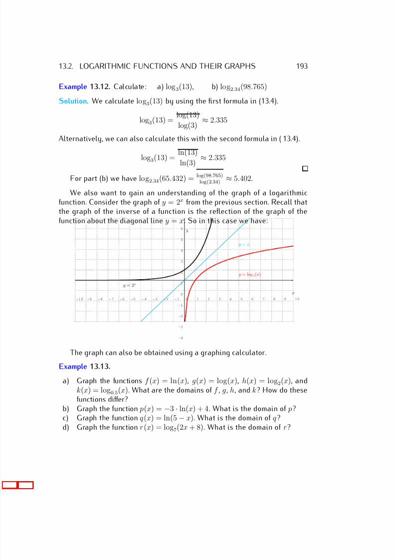
7/18/2019 Precalculus Tradler Carley
http://slidepdf.com/reader/full/precalculus-tradler-carley 203/424
13.2. LOGARITHMIC FUNCTIONS AND THEIR GRAPHS 193
Example 13.12. Calculate: a) log3(13), b) log2.34(98.765)
Solution. We calculate log3(13) by using the first formula in (13.4).
log3(13) = log(13)
log(3) ≈ 2.335
Alternatively, we can also calculate this with the second formula in (13.4).
log3(13) = ln(13)
ln(3) ≈ 2.335
For part (b) we have log2.34(65.432) = log(98.765)log(2.34)
≈ 5.402.
We also want to gain an understanding of the graph of a logarithmicfunction. Consider the graph of y = 2x from the previous section. Recall thatthe graph of the inverse of a function is the reflection of the graph of thefunction about the diagonal line y = x. So in this case we have:
-10 -9 - 8 - 7 - 6 - 5 - 4 - 3 - 2 - 1 0 1 2 3 4 5 6 7 8 9 10
-4
-3
-2
-1
0
1
2
3
4
5
6
x
y
y = 2x
y = x
y = log2(x)
The graph can also be obtained using a graphing calculator.
Example 13.13.
a) Graph the functions f (x) = ln(x), g(x) = log(x), h(x) = log2(x), and
k(x) = log0.5(x). What are the domains of f , g , h, and k? How do thesefunctions differ?b) Graph the function p(x) = −3 · ln(x) + 4. What is the domain of p?c) Graph the function q (x) = ln(5 − x). What is the domain of q ?d) Graph the function r(x) = log7(2x + 8). What is the domain of r?
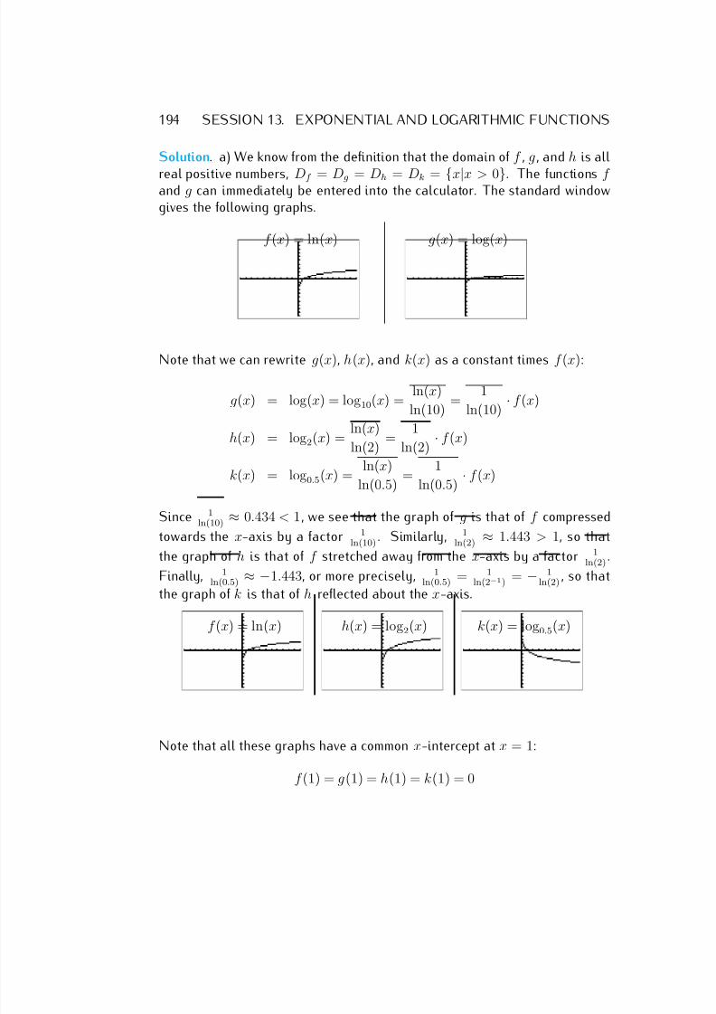
7/18/2019 Precalculus Tradler Carley
http://slidepdf.com/reader/full/precalculus-tradler-carley 204/424
194 SESSION 13. EXPONENTIAL AND LOGARITHMIC FUNCTIONS
Solution. a) We know from the definition that the domain of f , g , and h is all
real positive numbers, Df = Dg = Dh = Dk = {x|x > 0}. The functions f and g can immediately be entered into the calculator. The standard windowgives the following graphs.
f (x) = ln(x) g(x) = log(x)
Note that we can rewrite g(x), h(x), and k(x) as a constant times f (x):
g(x) = log(x) = log10(x) = ln(x)
ln(10) =
1
ln(10) · f (x)
h(x) = log2(x) = ln(x)
ln(2) =
1
ln(2) · f (x)
k(x) = log0.5(x) = ln(x)
ln(0.5) =
1
ln(0.5) · f (x)
Since 1ln(10)
≈0.434 < 1, we see that the graph of g is that of f compressed
towards the x-axis by a factor 1ln(10) . Similarly, 1
ln(2) ≈ 1.443 > 1, so thatthe graph of h is that of f stretched away from the x-axis by a factor 1
ln(2).
Finally, 1ln(0.5) ≈ −1.443, or more precisely, 1
ln(0.5) = 1ln(2−1) = − 1
ln(2) , so that
the graph of k is that of h reflected about the x-axis.
f (x) = ln(x) h(x) = log2(x) k(x) = log0.5(x)
Note that all these graphs have a common x-intercept at x = 1:
f (1) = g(1) = h(1) = k(1) = 0
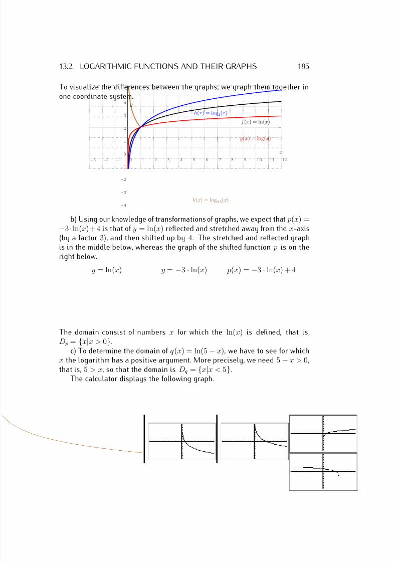
7/18/2019 Precalculus Tradler Carley
http://slidepdf.com/reader/full/precalculus-tradler-carley 205/424
13.2. LOGARITHMIC FUNCTIONS AND THEIR GRAPHS 195
To visualize the differences between the graphs, we graph them together in
one coordinate system.
-3 -2 -1 0 1 2 3 4 5 6 7 8 9 10 11 12
-4
-3
-2
-1
0
1
2
3
4
x
y
f (x) = ln(x)
g(x) = log(x)
h(x) = log2(x)
k(x) = log0.5(x)
b) Using our knowledge of transformations of graphs, we expect that p(x) =−3 · ln(x) + 4 is that of y = ln(x) reflected and stretched away from the x-axis(by a factor 3), and then shifted up by 4. The stretched and reflected graphis in the middle below, whereas the graph of the shifted function p is on theright below.
y = ln(x) y = −3 · ln(x) p(x) = −3 · ln(x) + 4
The domain consist of numbers x for which the ln(x) is defined, that is,D p = {x|x > 0}.
c) To determine the domain of q (x) = ln(5 − x), we have to see for whichx the logarithm has a positive argument. More precisely, we need 5 − x > 0,that is, 5 > x, so that the domain is Dq = {x|x < 5}.
The calculator displays the following graph.
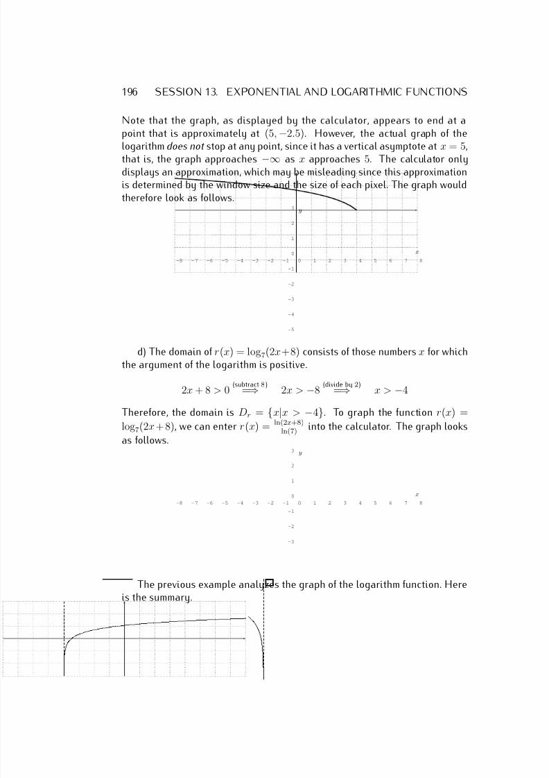
7/18/2019 Precalculus Tradler Carley
http://slidepdf.com/reader/full/precalculus-tradler-carley 206/424
196 SESSION 13. EXPONENTIAL AND LOGARITHMIC FUNCTIONS
Note that the graph, as displayed by the calculator, appears to end at a
point that is approximately at (5, −2.5). However, the actual graph of thelogarithm does not stop at any point, since it has a vertical asymptote at x = 5,that is, the graph approaches −∞ as x approaches 5. The calculator onlydisplays an approximation, which may be misleading since this approximationis determined by the window size and the size of each pixel. The graph wouldtherefore look as follows.
-8 -7 -6 -5 -4 -3 -2 -1 0 1 2 3 4 5 6 7 8
-5
-4
-3
-2
-1
0
1
2
3
x
y
d) The domain of r(x) = log7(2x+8) consists of those numbers x for whichthe argument of the logarithm is positive.
2x + 8 > 0 (subtract 8)
=⇒ 2x > −8 (divide by 2)
=⇒ x > −4
Therefore, the domain is Dr = {x|x > −4}. To graph the function r(x) =log7(2x + 8), we can enter r(x) = ln(2x+8)
ln(7) into the calculator. The graph looks
as follows.
-8 -7 -6 -5 -4 -3 -2 -1 0 1 2 3 4 5 6 7 8
-3
-2
-1
0
1
2
3
x
y
The previous example analyzes the graph of the logarithm function. Hereis the summary.
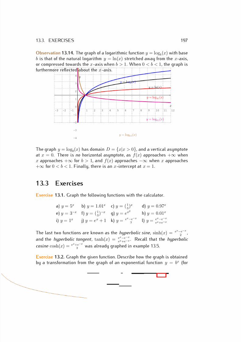
7/18/2019 Precalculus Tradler Carley
http://slidepdf.com/reader/full/precalculus-tradler-carley 207/424
13.3. EXERCISES 197
Observation 13.14. The graph of a logarithmic function y = logb(x) with base
b is that of the natural logarithm y = ln(x) stretched away from the x-axis,or compressed towards the x-axis when b > 1. When 0 < b < 1, the graph isfurthermore reflected about the x-axis.
-3 -2 -1 0 1 2 3 4 5 6 7 8 9 10 11 12
-4
-3
-2
-1
0
1
2
3
4
x
y
y = ln(x)
y = log10(x)
y = log0.1(x)
y = log2(x)
y = log0.5(x)
The graph y = logb(x) has domain D = {x|x > 0}, and a vertical asymptoteat x = 0. There is no horizontal asymptote, as f (x) approaches +∞ whenx approaches +∞ for b > 1, and f (x) approaches −∞ when x approaches+∞ for 0 < b < 1. Finally, there is an x-intercept at x = 1.
13.3 Exercises
Exercise 13.1. Graph the following functions with the calculator.
a) y = 5x b) y = 1.01x c) y = ( 13
)x d) y = 0.97x
e) y = 3−x f ) y = ( 13 )−x g) y = ex2
h) y = 0.01x
i) y = 1x j) y = ex + 1 k) y = ex−e−x2 l) y = ex−e−x
ex+e−x
The last two functions are known as the hyperbolic sine, sinh(x) = ex−e−x2
,
and the hyperbolic tangent , tanh(x) = ex
−e−x
ex+e−x . Recall that the hyperbolic cosine cosh(x) = ex+e−x
2 was already graphed in example 13.5.
Exercise 13.2. Graph the given function. Describe how the graph is obtainedby a transformation from the graph of an exponential function y = bx (for
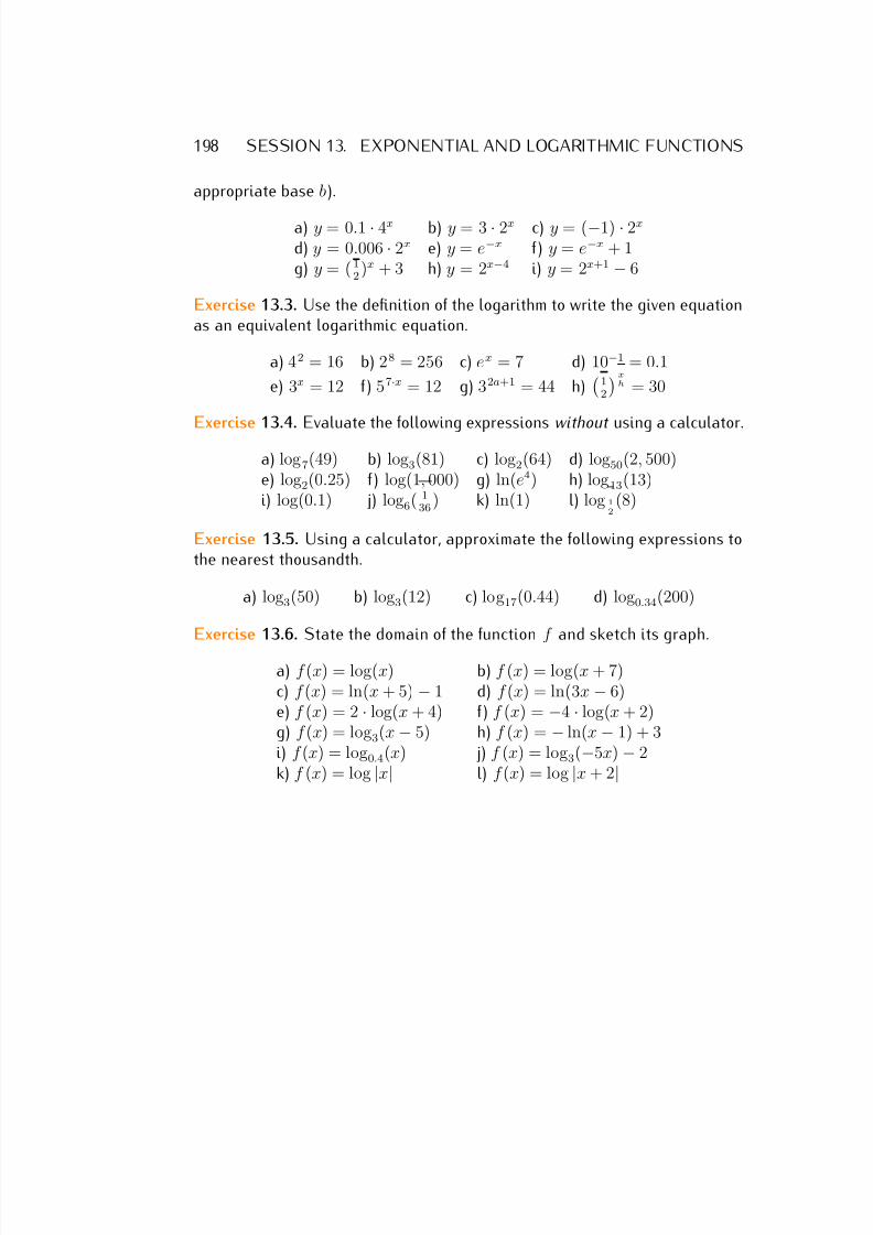
7/18/2019 Precalculus Tradler Carley
http://slidepdf.com/reader/full/precalculus-tradler-carley 208/424
198 SESSION 13. EXPONENTIAL AND LOGARITHMIC FUNCTIONS
appropriate base b).
a) y = 0.1 · 4x b) y = 3 · 2x c) y = (−1) · 2x
d) y = 0.006 · 2x e) y = e−x f ) y = e−x + 1g) y = ( 1
2 )x + 3 h) y = 2x−4 i) y = 2x+1 − 6
Exercise 13.3. Use the definition of the logarithm to write the given equationas an equivalent logarithmic equation.
a) 42 = 16 b) 28 = 256 c) ex = 7 d) 10−1 = 0.1
e) 3x = 12 f ) 57·x = 12 g) 32a+1 = 44 h)
12
xh = 30
Exercise 13.4. Evaluate the following expressions without using a calculator.
a) log7(49) b) log3(81) c) log2(64) d) log50(2, 500)e) log2(0.25) f ) log(1, 000) g) ln(e4) h) log13(13)i) log(0.1) j) log6( 1
36) k) ln(1) l) log 1
2(8)
Exercise 13.5. Using a calculator, approximate the following expressions tothe nearest thousandth.
a) log3(50) b) log3(12) c) log17(0.44) d) log0.34(200)
Exercise 13.6. State the domain of the function f and sketch its graph.
a) f (x) = log(x) b) f (x) = log(x + 7)c) f (x) = ln(x + 5) − 1 d) f (x) = ln(3x − 6)e) f (x) = 2 · log(x + 4) f ) f (x) = −4 · log(x + 2)g) f (x) = log3(x − 5) h) f (x) = − ln(x − 1) + 3i) f (x) = log0.4(x) j) f (x) = log3(−5x) − 2k) f (x) = log |x| l) f (x) = log |x + 2|
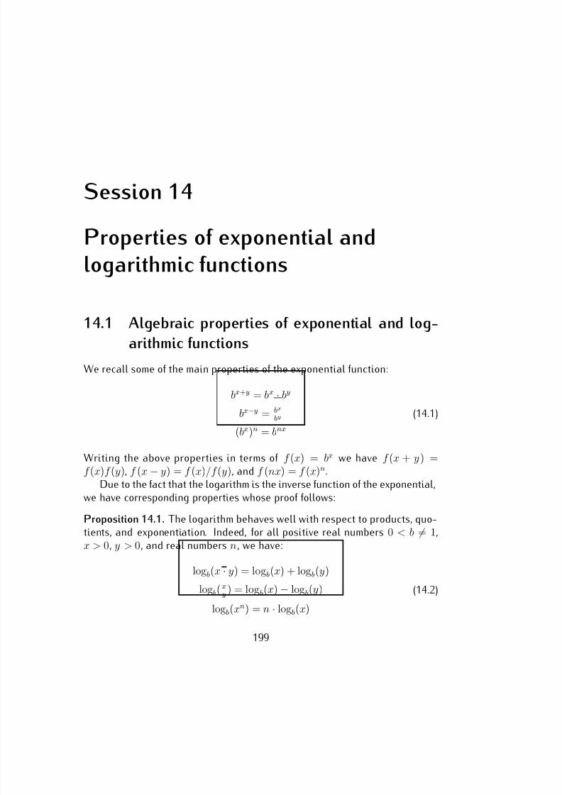
7/18/2019 Precalculus Tradler Carley
http://slidepdf.com/reader/full/precalculus-tradler-carley 209/424
Session 14
Properties of exponential and
logarithmic functions
14.1 Algebraic properties of exponential and log-
arithmic functions
We recall some of the main properties of the exponential function:
bx+y = bx · by
bx
−y
= bx
by
(bx)n = bnx(14.1)
Writing the above properties in terms of f (x) = bx we have f (x + y) =f (x)f (y), f (x − y) = f (x)/f (y), and f (nx) = f (x)n.
Due to the fact that the logarithm is the inverse function of the exponential,we have corresponding properties whose proof follows:
Proposition 14.1. The logarithm behaves well with respect to products, quo-tients, and exponentiation. Indeed, for all positive real numbers 0 < b = 1,x > 0, y > 0, and real numbers n, we have:
logb(x · y) = logb(x) + logb(y)
logb( xy ) = logb(x) − logb(y)
logb(xn) = n · logb(x)
(14.2)
199
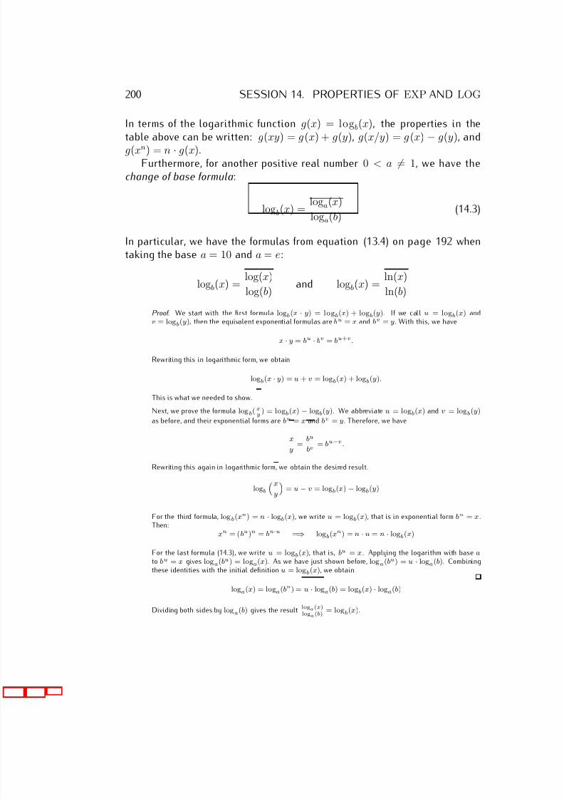
7/18/2019 Precalculus Tradler Carley
http://slidepdf.com/reader/full/precalculus-tradler-carley 210/424
200 SESSION 14. PROPERTIES OF EXP AND LOG
In terms of the logarithmic function g(x) = logb(x), the properties in the
table above can be written: g(xy) = g(x) + g(y), g(x/y) = g(x) − g(y), andg(xn) = n · g(x).Furthermore, for another positive real number 0 < a = 1, we have the
change of base formula:
logb(x) = loga(x)
loga(b) (14.3)
In particular, we have the formulas from equation (13.4) on page 192 whentaking the base a = 10 and a = e:
logb(x) = log(x)log(b)
and logb(x) = ln(x)ln(b)
Proof. We start with the first formula logb(x · y) = logb(x) + logb(y). If we call u = logb(x) andv = logb(y), then the equivalent exponential formulas are bu = x and bv = y . With this, we have
x · y = bu · bv = bu+v.
Rewriting this in logarithmic form, we obtain
logb(x · y) = u + v = logb(x) + logb(y).
This is what we needed to show.
Next, we prove the formula logb(xy
) = logb(x)
−logb(y). We abbreviate u = logb(x) and v = logb(y)
as before, and their exponential forms are bu = x and bv = y . Therefore, we have
x
y=
bu
bv = bu−v.
Rewriting this again in logarithmic form, we obtain the desired result.
logb
x
y
= u − v = logb(x) − logb(y)
For the third formula, logb(xn) = n · logb(x), we write u = logb(x), that is in exponential form bu = x .Then:
xn = (bu)n = bn·u =⇒ logb(xn) = n · u = n · logb(x)
For the last formula (14.3), we write u = logb(x), that is, bu = x . Applying the logarithm with base a
to bu = x gives loga(bu) = loga(x). As we have just shown before, loga(bu) = u · loga(b). Combiningthese identities with the initial definition u = logb(x), we obtain
loga(x) = loga(bu) = u · loga(b) = logb(x) · loga(b)
Dividing both sides by loga(b) gives the result loga(x)loga(b)
= logb(x).
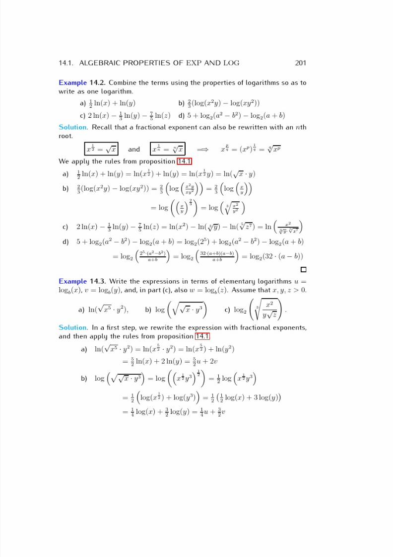
7/18/2019 Precalculus Tradler Carley
http://slidepdf.com/reader/full/precalculus-tradler-carley 211/424
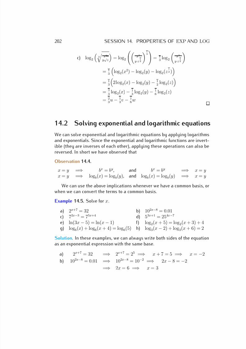
7/18/2019 Precalculus Tradler Carley
http://slidepdf.com/reader/full/precalculus-tradler-carley 212/424
202 SESSION 14. PROPERTIES OF EXP AND LOG
c) log2 3 x2
y√ z = log2 x2
y·z1
2 13
= 1
3
log2 x2
y·z1
2 = 1
3
log2(x2) − log2(y) − log2(z
12 )
= 13
2log2(x) − log2(y) − 1
2 log2(z )
= 23 log2(x) − 1
3 log2(y) − 1
6 log2(z )
= 23 u − 1
3 v − 16 w
14.2 Solving exponential and logarithmic equations
We can solve exponential and logarithmic equations by applying logarithmsand exponentials. Since the exponential and logarithmic functions are invert-ible (they are inverses of each other), applying these operations can also bereversed. In short we have observed that
Observation 14.4.
x = y =⇒ bx = by , and bx = by =⇒ x = yx = y =⇒ logb(x) = logb(y), and logb(x) = logb(y) =⇒ x = y
We can use the above implications whenever we have a common basis, orwhen we can convert the terms to a common basis.
Example 14.5. Solve for x.
a) 2x+7 = 32 b) 102x−8 = 0.01c) 72x−3 = 75x+4 d) 53x+1 = 254x−7
e) ln(3x − 5) = ln(x − 1) f) log2(x + 5) = log2(x + 3) + 4g) log6(x) + log6(x + 4) = log6(5) h) log3(x − 2) + log3(x + 6) = 2
Solution. In these examples, we can always write both sides of the equation
as an exponential expression with the same base.
a) 2x+7 = 32 =⇒ 2x+7 = 25 =⇒ x + 7 = 5 =⇒ x = −2
b) 102x−8 = 0.01 =⇒ 102x−8 = 10−2 =⇒ 2x − 8 = −2
=⇒ 2x = 6 =⇒ x = 3

7/18/2019 Precalculus Tradler Carley
http://slidepdf.com/reader/full/precalculus-tradler-carley 213/424
14.2. SOLVING EXPONENTIAL AND LOGARITHMIC EQUATIONS 203
Here it is useful to recall the powers of 10, which were also used to solve the
equation above.
103 = 1, 000102 = 100101 = 10100 = 1
10−1 = 0.110−2 = 0.0110−3 = 0.001
In general (n ≥ 1) :
10n = 100 · · · 00 n zeros
10−n = 0.0 · · · 00 n zeros
1
c) 72x−3 = 75x+4 =⇒ 2x − 3 = 5x + 4 (−5x+3)
=⇒ −3x = 7
=⇒ x = −7
3d) 53x+1 = 254x−7 =⇒ 53x+1 = 52·(4x−7) =⇒ 3x + 1 = 2 · (4x − 7)
=⇒ 3x + 1 = 8x − 14 (−8x−1)
=⇒ −5x = −15
=⇒ x = 3
By a similar reasoning we can solve equations involving logarithms wheneverthe bases coincide.
e) ln(3x − 5) = ln(x − 1) =⇒ 3x − 5 = x − 1 (−x+5)
=⇒ 2x = 4
=⇒ x = 2
For part (f), we have to solve log2(x+5) = log2(x+3)+4. To combine the right-hand side, recall that 4 can be written as a logarithm, 4 = log2(24) = log2 16.With this remark we can now solve the equation for x.
log2(x + 5) = log2(x + 3) + 4 =⇒ log2(x + 5) = log2(x + 3) + log2(16)
=⇒ log2(x + 5) = log2(16 · (x + 3)) =⇒ x + 5 = 16(x + 3)
=⇒ x + 5 = 16x + 48 (
−16x
−5)
=⇒ −15x = 43 =⇒ x = −4315
Next, in part (g), we start by combining the logarithms.
log6(x) + log6(x + 4) = log6(5) =⇒ log6(x(x + 4)) = log6(5)
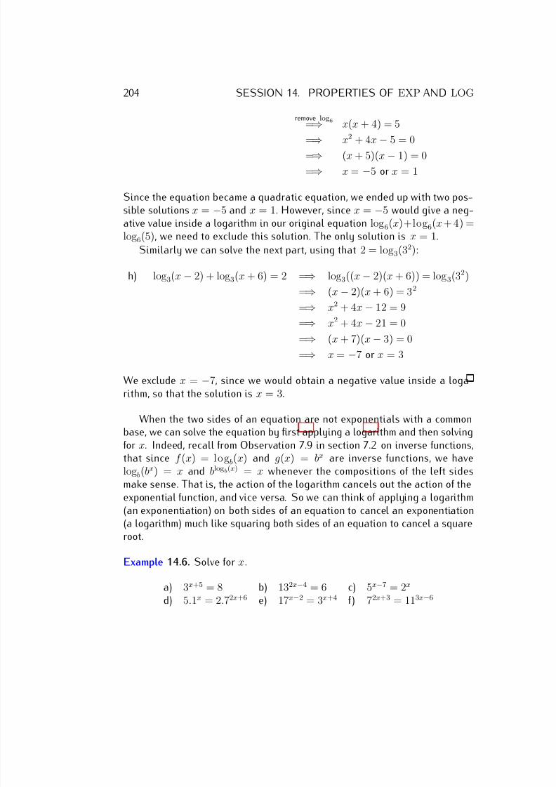
7/18/2019 Precalculus Tradler Carley
http://slidepdf.com/reader/full/precalculus-tradler-carley 214/424
204 SESSION 14. PROPERTIES OF EXP AND LOG
remove log6=⇒ x(x + 4) = 5
=⇒ x2 + 4x − 5 = 0=⇒ (x + 5)(x − 1) = 0
=⇒ x = −5 or x = 1
Since the equation became a quadratic equation, we ended up with two pos-sible solutions x = −5 and x = 1. However, since x = −5 would give a neg-ative value inside a logarithm in our original equation log6(x)+log6(x + 4) =log6(5), we need to exclude this solution. The only solution is x = 1.
Similarly we can solve the next part, using that 2 = log3(32):
h) log3(x − 2) + log3(x + 6) = 2 =⇒ log3((x − 2)(x + 6)) = log3(32)=⇒ (x − 2)(x + 6) = 32
=⇒ x2 + 4x − 12 = 9
=⇒ x2 + 4x − 21 = 0
=⇒ (x + 7)(x − 3) = 0
=⇒ x = −7 or x = 3
We exclude x = −7, since we would obtain a negative value inside a loga-rithm, so that the solution is x = 3.
When the two sides of an equation are not exponentials with a commonbase, we can solve the equation by first applying a logarithm and then solvingfor x. Indeed, recall from Observation 7.9 in section 7.2 on inverse functions,that since f (x) = logb(x) and g(x) = bx are inverse functions, we havelogb(bx) = x and blogb(x) = x whenever the compositions of the left sidesmake sense. That is, the action of the logarithm cancels out the action of theexponential function, and vice versa. So we can think of applying a logarithm(an exponentiation) on both sides of an equation to cancel an exponentiation(a logarithm) much like squaring both sides of an equation to cancel a squareroot.
Example 14.6. Solve for x.
a) 3x+5 = 8 b) 132x−4 = 6 c) 5x−7 = 2x
d) 5.1x = 2.72x+6 e) 17x−2 = 3x+4 f ) 72x+3 = 113x−6
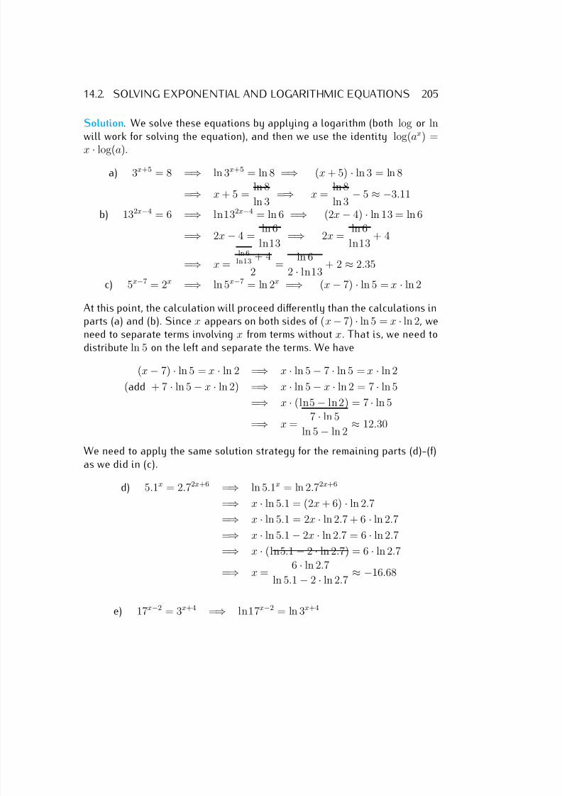
7/18/2019 Precalculus Tradler Carley
http://slidepdf.com/reader/full/precalculus-tradler-carley 215/424
14.2. SOLVING EXPONENTIAL AND LOGARITHMIC EQUATIONS 205
Solution. We solve these equations by applying a logarithm (both log or ln
will work for solving the equation), and then we use the identity log(ax
) =x · log(a).
a) 3x+5 = 8 =⇒ ln 3x+5 = ln 8 =⇒ (x + 5) · ln 3 = ln 8
=⇒ x + 5 = ln 8
ln 3 =⇒ x =
ln 8
ln 3 − 5 ≈ −3.11
b) 132x−4 = 6 =⇒ ln132x−4 = ln 6 =⇒ (2x − 4) · ln 13 = ln 6
=⇒ 2x − 4 = ln 6
ln13 =⇒ 2x =
ln 6
ln13 + 4
=⇒ x =ln 6
ln13 + 4
2 =
ln 6
2·
ln13 + 2 ≈ 2.35
c) 5x−7 = 2x =⇒ ln 5x−7 = ln 2x =⇒ (x − 7) · ln 5 = x · ln 2
At this point, the calculation will proceed differently than the calculations inparts (a) and (b). Since x appears on both sides of (x − 7) · ln 5 = x · ln 2, weneed to separate terms involving x from terms without x. That is, we need todistribute ln 5 on the left and separate the terms. We have
(x − 7) · ln 5 = x · ln 2 =⇒ x · ln 5 − 7 · ln 5 = x · ln 2
(add + 7 · ln 5 − x · ln 2) =⇒ x · ln 5 − x · ln 2 = 7 · ln 5
=⇒ x · (ln5 − ln 2) = 7 · ln 5
=⇒ x = 7 · ln 5ln 5 − ln 2
≈ 12.30
We need to apply the same solution strategy for the remaining parts (d)-(f)as we did in (c).
d) 5.1x = 2.72x+6 =⇒ ln 5.1x = ln 2.72x+6
=⇒ x · ln 5.1 = (2x + 6) · ln 2.7
=⇒ x · ln 5.1 = 2x · ln 2.7 + 6 · ln 2.7
=⇒ x · ln 5.1 − 2x · ln 2.7 = 6 · ln 2.7
=⇒
x·
(ln5.1−
2·
ln 2.7) = 6·
ln 2.7
=⇒ x = 6 · ln 2.7
ln 5.1 − 2 · ln 2.7 ≈ −16.68
e) 17x−2 = 3x+4 =⇒ ln17x−2 = ln 3x+4
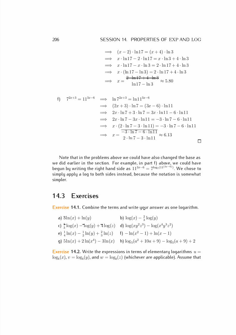
7/18/2019 Precalculus Tradler Carley
http://slidepdf.com/reader/full/precalculus-tradler-carley 216/424
206 SESSION 14. PROPERTIES OF EXP AND LOG
=⇒ (x − 2) · ln17 = (x + 4) · ln 3
=⇒ x · ln17 − 2 · ln17 = x · ln 3 + 4 · ln 3=⇒ x · ln17 − x · ln 3 = 2 · ln 17 + 4 · ln 3
=⇒ x · (ln 17 − ln 3) = 2 · ln 17 + 4 · ln 3
=⇒ x = 2 · ln 17 + 4 · ln 3
ln17 − ln 3 ≈ 5.80
f ) 72x+3 = 113x−6 =⇒ ln 72x+3 = ln113x−6
=⇒ (2x + 3) · ln 7 = (3x − 6) · ln11
=
⇒ 2x
·ln 7 + 3
·ln 7 = 3x
·ln11
−6
·ln11
=⇒ 2x · ln 7 − 3x · ln11 = −3 · ln 7 − 6 · ln11
=⇒ x · (2 · ln 7 − 3 · ln 11) = −3 · ln 7 − 6 · ln11
=⇒ x = −3 · ln 7 − 6 · ln11
2 · ln 7 − 3 · ln11 ≈ 6.13
Note that in the problems above we could have also changed the base aswe did earlier in the section. For example, in part f ) above, we could havebegun by writing the right hand side as 113x−6 = 7log7(11(3x−6)). We chose to
simply apply a log to both sides instead, because the notation is somewhatsimpler.
14.3 Exercises
Exercise 14.1. Combine the terms and write your answer as one logarithm.
a) 3ln(x) + ln(y) b) log(x) − 23 log(y)
c) 13 log(x) − log(y) + 4 log(z ) d) log(xy2z 3) − log(x4y3z 2)
e) 1
4 ln(x) − 1
2 ln(y) + 2
3 ln(z ) f ) − ln(x2
− 1) + ln(x − 1)g) 5ln(x) + 2 ln(x4) − 3ln(x) h) log5(a2 + 10a + 9) − log5(a + 9) + 2
Exercise 14.2. Write the expressions in terms of elementary logarithms u =logb(x), v = logb(y), and w = logb(z ) (whichever are applicable). Assume that
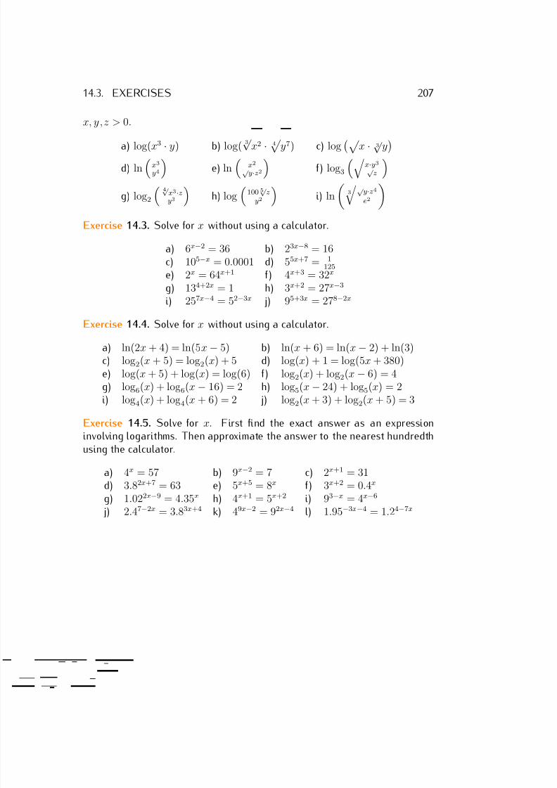
7/18/2019 Precalculus Tradler Carley
http://slidepdf.com/reader/full/precalculus-tradler-carley 217/424
14.3. EXERCISES 207
x, y,z > 0.
a) log(x3 · y) b) log( 3√ x2 · 4
y7) c) log
x · 3√ y
d) ln
x3
y4
e) ln
x2√
y·z2
f ) log3
x·y3√
z
g) log2
4√
x3·zy3
h) log
100 5
√ z
y2
i) ln
3
√ y·z4
e2
Exercise 14.3. Solve for x without using a calculator.
a) 6x−2 = 36 b) 23x−8 = 16c) 105−x = 0.0001 d) 55x+7 = 1
125
e) 2x = 64x+1 f ) 4x+3 = 32x
g) 134+2x = 1 h) 3x+2 = 27x−3
i) 257x−4 = 52−3x j) 95+3x = 278−2x
Exercise 14.4. Solve for x without using a calculator.
a) ln(2x + 4) = ln(5x − 5) b) ln(x + 6) = ln(x − 2) + ln(3)c) log2(x + 5) = log2(x) + 5 d) log(x) + 1 = log(5x + 380)e) log(x + 5) + log(x) = log(6) f ) log2(x) + log2(x − 6) = 4g) log6(x) + log6(x − 16) = 2 h) log5(x − 24) + log5(x) = 2i) log4(x) + log4(x + 6) = 2 j) log2(x + 3) + log2(x + 5) = 3
Exercise 14.5. Solve for x. First find the exact answer as an expressioninvolving logarithms. Then approximate the answer to the nearest hundredthusing the calculator.
a) 4x = 57 b) 9x−2 = 7 c) 2x+1 = 31d) 3.82x+7 = 63 e) 5x+5 = 8x f ) 3x+2 = 0.4x
g) 1.022x−9 = 4.35x h) 4x+1 = 5x+2 i) 93−x = 4x−6
j) 2.47−2x = 3.83x+4 k) 49x−2 = 92x−4 l) 1.95−3x−4 = 1.24−7x
7/18/2019 Precalculus Tradler Carley
http://slidepdf.com/reader/full/precalculus-tradler-carley 218/424
Session 15
Applications of the exponential and
the logarithm
15.1 Applications of exponential functions
Before giving specific applications, we note that the exponential function y =c · bx is uniquely determined by providing any two of its function values.
Example 15.1. Let f (x) = c · bx. Determine the constant c and base b underthe given conditions.
a) f (0) = 5, f (1) = 20 b) f (0) = 3, f (4) = 48c) f (2) = 160, f (7) = 5 d) f (−2) = 55, f (1) = 7
Solution. a) Applying f (0) = 5 to f (x) = c · bx, we get
5 = f (0) = c · b0 = c · 1 = c
Indeed, in general, we always have f (0) = c for any exponential function. Thebase b is then determined by substituting the second equation f (1) = 20.
20 = f (1) = c · b1 = 5 · b (÷5)
=⇒ b = 4
Therefore, f (x) = 5 · 4x. Note that in the last implication, we used that thebase must be positive.
b) As before, we get 3 = f (0) = c · b0 = c, and
48 = f (4) = c · b4 = 3 · b4 (÷3)=⇒ 16 = b4 (exponentiate by 1
4)
=⇒ b = 1614 = 2
208
7/18/2019 Precalculus Tradler Carley
http://slidepdf.com/reader/full/precalculus-tradler-carley 219/424
15.1. APPLICATIONS OF EXPONENTIAL FUNCTIONS 209
Therefore, f (x) = 3 · 2x.
c) When f (0) is not given, it is easiest to solve for b first. We can see thisas follows. Since 160 = f (2) = c · b2 and 5 = f (7) = c · b7, the quotient of these equations eliminates c.
160
5 =
c · b2
c · b7 =
1
b5 =⇒ 32 = b−5
(exponentiate by (− 15
))=⇒ b = 32−
15 =
1
3215
= 1
2
Then c is determined by any of the original equations.
160 = f (2) = c · b2 = c · 122
= c · 14 =⇒ c = 4 · 160 = 640
Therefore, f (x) = 640 ·
12
x
.
d) This solution is similar to part (c).
55
7 =
f (−2)
f (1) =
c · b−2
c · b1 =
1
b3 =⇒ b3 =
7
55
=⇒ b = 7
55
13 ≈ 0.503
55 = f (−2) = c · b−2 = c · 7
55
13−2
= c · 7
55
−23
=⇒ c = 55
755
−23
= 55 · 7
23
5523
= 55
13 · 7
23 =
3√
55 · 72 = 3√
2695 ≈ 13.916
therefore, f (x) = 3√
2695 ·
3
755
x
.
Many situations are modeled by exponential functions.
Example 15.2. The mass of a bacteria sample is 2 · 1.02t grams after t hours.
a) What is the mass of the bacteria sample after 4 hours?b) When will the mass reach 10 grams?
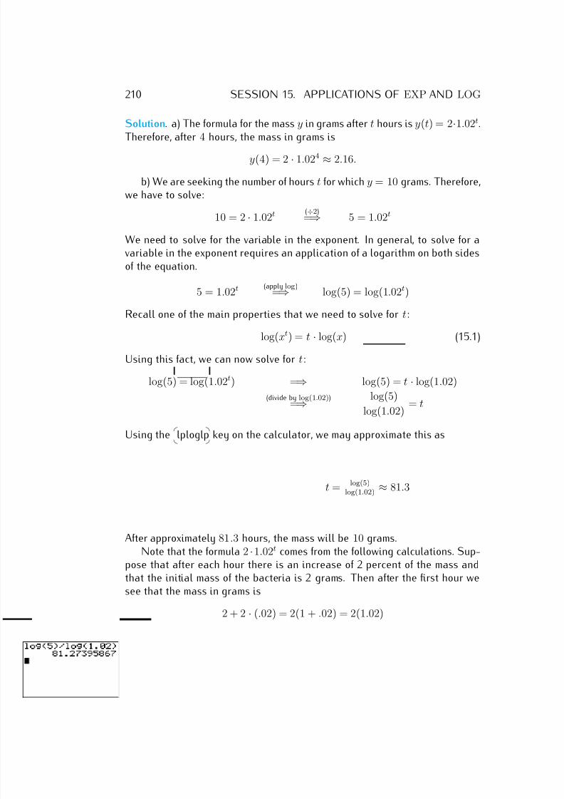
7/18/2019 Precalculus Tradler Carley
http://slidepdf.com/reader/full/precalculus-tradler-carley 220/424
210 SESSION 15. APPLICATIONS OF EXP AND LOG
Solution. a) The formula for the mass y in grams after t hours is y(t) = 2·1.02t.
Therefore, after 4 hours, the mass in grams is
y(4) = 2 · 1.024 ≈ 2.16.
b) We are seeking the number of hours t for which y = 10 grams. Therefore,we have to solve:
10 = 2 · 1.02t (÷2)=⇒ 5 = 1.02t
We need to solve for the variable in the exponent. In general, to solve for avariable in the exponent requires an application of a logarithm on both sidesof the equation.
5 = 1.02t (apply log )=⇒ log(5) = log(1.02t)
Recall one of the main properties that we need to solve for t:
log(xt) = t · log(x) (15.1)
Using this fact, we can now solve for t:
log(5) = log(1.02t) =⇒ log(5) = t · log(1.02)
(divide by log(1.02))=⇒ log(5)
log(1.02) = t
Using the
lploglp key on the calculator, we may approximate this as
t = log(5)log(1.02)
≈ 81.3
After approximately 81.3 hours, the mass will be 10 grams.Note that the formula 2
·1.02t comes from the following calculations. Sup-
pose that after each hour there is an increase of 2 percent of the mass andthat the initial mass of the bacteria is 2 grams. Then after the first hour wesee that the mass in grams is
2 + 2 · (.02) = 2(1 + .02) = 2(1.02)
7/18/2019 Precalculus Tradler Carley
http://slidepdf.com/reader/full/precalculus-tradler-carley 221/424
15.1. APPLICATIONS OF EXPONENTIAL FUNCTIONS 211
and that after the second hour the mass is
2(1.02) + 2(1.02)(.02) = 2(1.02)(1 + .02) = 2(1.02)2
and that after three hours the mass is
2(1.02)2 + 2(1.02)2(.02) = 2(1.02)2(1 + .02) = 2(1.02)3.
Continuing in this manner we can see that, at least for whole numbers of hours t, the weight is given by
2 · 1.02t.
The same sort of idea can be used in all of the following applications.
Example 15.3. The population size of a country was 12.7 million in the year2000, and 14.3 million in the year 2010.
a) Assuming an exponential growth for the population size, find the formulafor the population depending on the year t.
b) What will the population size be in the year 2015, assuming the formulaholds until then?
c) When will the population reach 18 million?
Solution. a) The growth is assumed to be exponential, so that y(t) = c · bt
describes the population size depending on the year t, where we set t = 0
corresponding to the year 2000. Then the example describes y(0) = c asc = 12.7, which we assume in units of millions. To find the base b, wesubstitute the data of t = 10 and y(t) = 14.3 into y(t) = c · bt.
14.3 = 12.7 · b10 =⇒ 14.3
12.7 = b10 =⇒
14.3
12.7
110
= (b10) 110 = b
=⇒ b =14.3
12.7
110 ≈ 1.012
The formula for the population size is y(t) ≈ 12.7 · 1.012t.b) We calculate the population size in the year 2015 by setting t = 15:
y(15) = 12.7 · 1.01215 ≈ 15.2
c) We seek t so that y(t) = 18. We solve for t using the logarithm.
18 = 12.7 · 1.012t =⇒ 18
12.7 = 1.012t =⇒ log
18
12.7
= log(1.012t)
7/18/2019 Precalculus Tradler Carley
http://slidepdf.com/reader/full/precalculus-tradler-carley 222/424
212 SESSION 15. APPLICATIONS OF EXP AND LOG
=
⇒ log
18
12.7 = t
·log(1.012)
=⇒ t =log
1812.7
log(1.012)
≈ 29.2
The population will reach 18 million in the year 2029.
In many instances the exponential function f (x) = c · bx is given via a rateof growth r.
Definition 15.4. An exponential function with a rate of growth r is a functionf (x) = c · bx with base
b = 1 + r .
For an example of why this is a reasonable definition see the note followingExample 15.2.
Note 15.5. We want to point out that some authors use a different convention than the one given indefinition 15.4. Indeed, sometimes a function with rate of growth r is defined as an exponential function
with base b = er , whereas for us it has base b = 1+ r. Since er can be expanded as er = 1 +r + r2
2 + . . . ,
we see that the two versions only differ by an error of order 2.
Example 15.6. The number of PCs that are sold in the U.S. in the year 2011is approximately 350 million with a rate of growth of 3.6% per year. Assumingthe rate stays constant over the next years, how many PCs will be sold in theyear 2015?
Solution. Since the rate of growth is r = 3.6% = 0.036, we obtain a base of b = 1 + r = 1.036, giving the number of PCs to be modeled by c(1.036)t. If we set t = 0 for the year 2011, we find that c = 350, so the number of salesis given by y(t) = 350 · 1.036t. Since the year 2015 corresponds to t = 4, wecan calculate the number of sales in the year 2015 as
y(4) = 350 · 1.0364 ≈ 403.
Approximately 403 million PCs will be sold in the year 2015.
Example 15.7. The size of an ant colony is decreasing at a rate of 1% permonth. How long will it take until the colony has reached 80% of its originalsize?
7/18/2019 Precalculus Tradler Carley
http://slidepdf.com/reader/full/precalculus-tradler-carley 223/424
15.1. APPLICATIONS OF EXPONENTIAL FUNCTIONS 213
Solution. Since r = −1% = −0.01, we obtain the base b = 1+r = 1−0.01 =
0.99. We have a colony size of y(t) = c · 0.99t
after t months, where c is theoriginal size. We need to find t so that the size is at 80% of its original sizec, that is, y(t) = 80% · c = 0.8 · c.
0.8 · c = c · 0.99t (÷c)=⇒ 0.8 = 0.99t =⇒ log(0.8) = log(0.99t)
=⇒ log(0.8) = t · log(0.99)
=⇒ t = log(0.8)
log(0.99) ≈ 22.2
After approximately 22.2 months, the ant colony has decreased to 80% of itsoriginal size.
Example 15.8. a) The population size of a country is increasing at a rateof 4% per year. How long does it take until the country has doubledits population size?
b) The number of new flu cases is decreasing at a rate of 5% per week.After how much time will the number of new flu cases reach a quarterof its current level?
Solution. a) The rate of change is r = 4% = 0.04, so that population size is anexponential function with base b = 1+0.04 = 1.04. Therefore, f (x) = c ·1.04x
denotes the population size, with c being the initial population in the yearcorresponding to x = 0. In order for the population size to double, f (x) hasto reach twice its initial size, that is:
f (x) = 2c =⇒ c · 1.04x = 2c (÷c)
=⇒ 1.04x = 2
=⇒ log(1.04x) = log(2) =⇒ x log(1.04) = log(2)
=⇒ x = log(2)
log(1.04) ≈ 17.7
It will take about 17.7 years until the population size has doubled.b) Since the number of new flu cases is decreasing, the rate of growth
is negative, r = −5% = −0.05 per week, so that we have an exponentialfunction with base b = 1 + r = 1 + (−0.05) = 0.95. To reach a quarter of itsinitial number of flu cases, we set f (x) = c · 0.95x equal to 1
4c.
c · 0.95x = 1
4c
(÷c)=⇒ 0.95x =
1
4 =⇒ x log(0.95) = log(
1
4)
7/18/2019 Precalculus Tradler Carley
http://slidepdf.com/reader/full/precalculus-tradler-carley 224/424
214 SESSION 15. APPLICATIONS OF EXP AND LOG
=
⇒ x =
log( 14 )
log(0.95) ≈27.0
It will therefore take about 27 weeks until the number of new flu cases hasdecreased to a quarter of its current level.
15.2 Exercises
Exercise 15.1. Assuming that f (x) = c · bx is an exponential function, findthe constants c and b from the given conditions.
a) f (0) = 4, f (1) = 12 b) f (0) = 5, f (3) = 40c) f (0) = 3, 200, f (6) = 0.0032 d) f (3) = 12, f (5) = 48e) f (−1) = 4, f (2) = 500 f ) f (2) = 3, f (4) = 15
Exercise 15.2. The number of downloads of a certain software applicationwas 8.4 million in the year 2005 and 13.6 million in the year 2010.
a) Assuming an exponential growth for the number of downloads, find theformula for the downloads depending on the year t.
b) Assuming the number of downloads will follow the formula from part (a),what will the number of downloads be in the year 2015?
c) In which year will the number of downloaded applications reach the 20million barrier?
Exercise 15.3. The population size of a city was 79, 000 in the year 1990and 136, 000 in the year 2005. Assume that the population size follows anexponential function.
a) Find the formula for the population size.b) What is the population size in the year 2010?c) What is the population size in the year 2015?d) When will the city reach its expected maximum capacity of 1, 000, 000
residents?
Exercise 15.4. The population of a city decreases at a rate of 2.3% per year.After how many years will the population be at 90% of its current size? Roundyour answer to the nearest tenth.
7/18/2019 Precalculus Tradler Carley
http://slidepdf.com/reader/full/precalculus-tradler-carley 225/424
15.2. EXERCISES 215
Exercise 15.5. A big company plans to expand its franchise and, with this,
its number of employees. For tax reasons it is most beneficial to expand thenumber of employees at a rate of 5% per year. If the company currently has4, 730 employees, how many years will it take until the company has 6, 000employees? Round your answer to the nearest hundredth.
Exercise 15.6. An ant colony has a population size of 4, 000 ants and isincreasing at a rate of 3% per week. How long will it take until the antpopulation has doubled? Round your answer to the nearest tenth.
Exercise 15.7. The size of a beehive is decreasing at a rate of 15% per month.How long will it take for the beehive to be at half of its current size? Round
your answer to the nearest hundredth.Exercise 15.8. If the population size of the world is increasing at a rate of 0.5% per year, how long does it take until the world population doubles insize? Round your answer to the nearest tenth.
7/18/2019 Precalculus Tradler Carley
http://slidepdf.com/reader/full/precalculus-tradler-carley 226/424
Session 16
More applications: Half-life and
compound interest
We have already encountered applications of the logarithm in solving equa-tions in section 15.1. In this chapter we solve more equations related toapplications by using the logarithm.
16.1 Half-life
Recall from definition 15.4 on page 212 that a function with rate of growth r
is an exponential function f (x) = c · bx with base b = 1 + r. There is alsoanother important way of determining the base of an exponential function,which is given by the notion of half-life. We start with a motivating example.
Example 16.1. Consider the function f (x) = 200 · 12
x7 . We calculate the
function values f (x), for x = 0, 7, 14, 21, and 28.
f (0) = 200 ·
1
2
07
= 200 · 1 = 200
f (7) = 200 ·
1
277
= 200 · 1
2 = 100
f (14) = 200 ·
1
2
147
= 200 · 1
4 = 50
f (21) = 200 ·
1
2
217
= 200 · 1
8 = 25
216
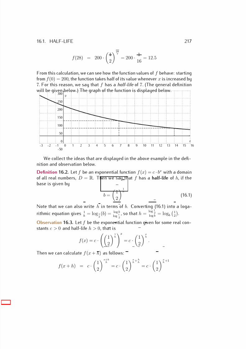
7/18/2019 Precalculus Tradler Carley
http://slidepdf.com/reader/full/precalculus-tradler-carley 227/424
16.1. HALF-LIFE 217
f (28) = 200·
1
2287
= 200·
1
16 = 12.5
From this calculation, we can see how the function values of f behave: startingfrom f (0) = 200, the function takes half of its value whenever x is increased by7. For this reason, we say that f has a half-life of 7. (The general definitionwill be given below.) The graph of the function is displayed below.
x
y
-3 -2 -1 0 1 2 3 4 5 6 7 8 9 10 11 12 13 14 15 160
50
100
150
200
250
300
-50
We collect the ideas that are displayed in the above example in the defi-nition and observation below.
Definition 16.2. Let f be an exponential function f (x) = c · bx with a domainof all real numbers, D = R. Then we say that f has a half-life of h, if the
base is given by
b =
1
2
1h
(16.1)
Note that we can also write h in terms of b. Converting (16.1) into a loga-
rithmic equation gives 1h
= log 12
(b) = log b
log 12
, so that h = log 1
2
log b = logb
12
.
Observation 16.3. Let f be the exponential function given for some real con-stants c > 0 and half-life h > 0, that is
f (x) = c
·1
21h
x
= c
· 1
2xh
.
Then we can calculate f (x + h) as follows:
f (x + h) = c ·
1
2
x+hh
= c ·
1
2
xh
+hh
= c ·
1
2
xh
+1
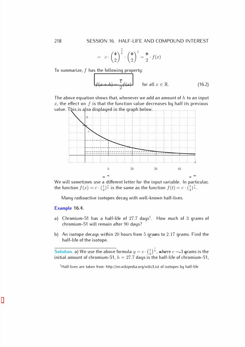
7/18/2019 Precalculus Tradler Carley
http://slidepdf.com/reader/full/precalculus-tradler-carley 228/424
218 SESSION 16. HALF-LIFE AND COMPOUND INTEREST
= c·
1
2xh
· 1
21
= 1
2 ·f (x)
To summarize, f has the following property:
f (x + h) = 1
2f (x) for all x ∈ R. (16.2)
The above equation shows that, whenever we add an amount of h to an inputx, the effect on f is that the function value decreases by half its previousvalue. This is also displayed in the graph below.
x
y
c
h 2h 3h 4h
We will sometimes use a different letter for the input variable. In particular,the function f (x) = c · ( 1
2)xh is the same as the function f (t) = c · ( 1
2)th .
Many radioactive isotopes decay with well-known half-lives.
Example 16.4.
a) Chromium-51 has a half-life of 27.7 days1. How much of 3 grams of chromium-51 will remain after 90 days?
b) An isotope decays within 20 hours from 5 grams to 2.17 grams. Find thehalf-life of the isotope.
Solution. a) We use the above formula y = c · 12
th , where c = 3 grams is the
initial amount of chromium-51, h = 27.7 days is the half-life of chromium-51,
1Half-lives are taken from: http://en.wikipedia.org/wiki/List of isotopes by half-life
7/18/2019 Precalculus Tradler Carley
http://slidepdf.com/reader/full/precalculus-tradler-carley 229/424
16.1. HALF-LIFE 219
and t = 90 days is time that the isotope decayed. Substituting these numbers
into the formula for y , we obtain:
y = 3 ·
1
2
9027.7
≈ 0.316
Therefore, after 90 days, 0.316 grams of the chromium-51 is remaining.b) We have an initial amount of c = 5 grams and a remaining amount of
y = 2.17 grams after t = 20 hours. The half-life can be obtained as follows.
2.17 = 5 ·
1
2
20h (÷5)
=⇒ 0.434 =
1
2
20h
(apply ln)
=⇒ ln(0.434) = ln 0.520h
=⇒ ln(0.434) = 20
h · ln(0.5)
(× hln(0.434)
)
=⇒ h = 20 · ln(0.5)
ln(0.434)=⇒ t ≈ 16.6
Therefore, the half-life of the isotope is approximately 16.6 hours.
Note 16.5. An important isotope is the radioisotope carbon-14. It decayswith a half-life of 5730 years with an accuracy of
±40 years. For definiteness
we will take 5730 years as the half-life of carbon-14.
The half-life of carbon-14 is 5730 years.
One can use the knowledge of the half-life of carbon-14 in dating organicmaterials via the so called carbon dating method. Carbon-14 is produced bya plant during the process of photosynthesis at a fixed level until the plantdies. Therefore by measuring the remaining amount of carbon-14 in a deadplant one can determine the date when the plant died. Furthermore, sincehumans and animals consume plants, the same argument can be applied todetermine their (approximate) dates of death.
Example 16.6.
a) A dead tree trunk has 86% of its original carbon-14. (Approximately) howmany years ago did the tree die?
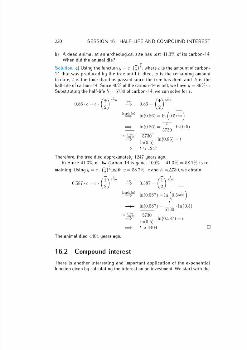
7/18/2019 Precalculus Tradler Carley
http://slidepdf.com/reader/full/precalculus-tradler-carley 230/424
220 SESSION 16. HALF-LIFE AND COMPOUND INTEREST
b) A dead animal at an archeological site has lost 41.3% of its carbon-14.
When did the animal die?Solution. a) Using the function y = c ·1
2
th , where c is the amount of carbon-
14 that was produced by the tree until it died, y is the remaining amountto date, t is the time that has passed since the tree has died, and h is thehalf-life of carbon-14. Since 86% of the carbon-14 is left, we have y = 86% ·c.Substituting the half-life h = 5730 of carbon-14, we can solve for t.
0.86 · c = c ·
1
2
t5730 (÷c)
=⇒ 0.86 =
1
2
t5730
(apply ln)=⇒ ln(0.86) = ln0.5
t5730
=⇒ ln(0.86) = t5730
· ln(0.5)
(× 5730ln(0.5)
)
=⇒ 5730
ln(0.5) · ln(0.86) = t
=⇒ t ≈ 1247
Therefore, the tree died approximately 1247 years ago.b) Since 41.3% of the carbon-14 is gone, 100% − 41.3% = 58.7% is re-
maining. Using y = c · 12
th with y = 58.7% · c and h = 5730, we obtain
0.587 · c = c · 1
2 t
5730 (
÷c)
=⇒ 0.587 = 1
2 t
5730
(apply ln)=⇒ ln(0.587) = ln
0.5
t5730
=⇒ ln(0.587) =
t
5730 · ln(0.5)
(× 5730ln(0.5)
)
=⇒ 5730
ln(0.5) · ln(0.587) = t
=⇒ t ≈ 4404
The animal died 4404 years ago.
16.2 Compound interest
There is another interesting and important application of the exponentialfunction given by calculating the interest on an investment. We start with the
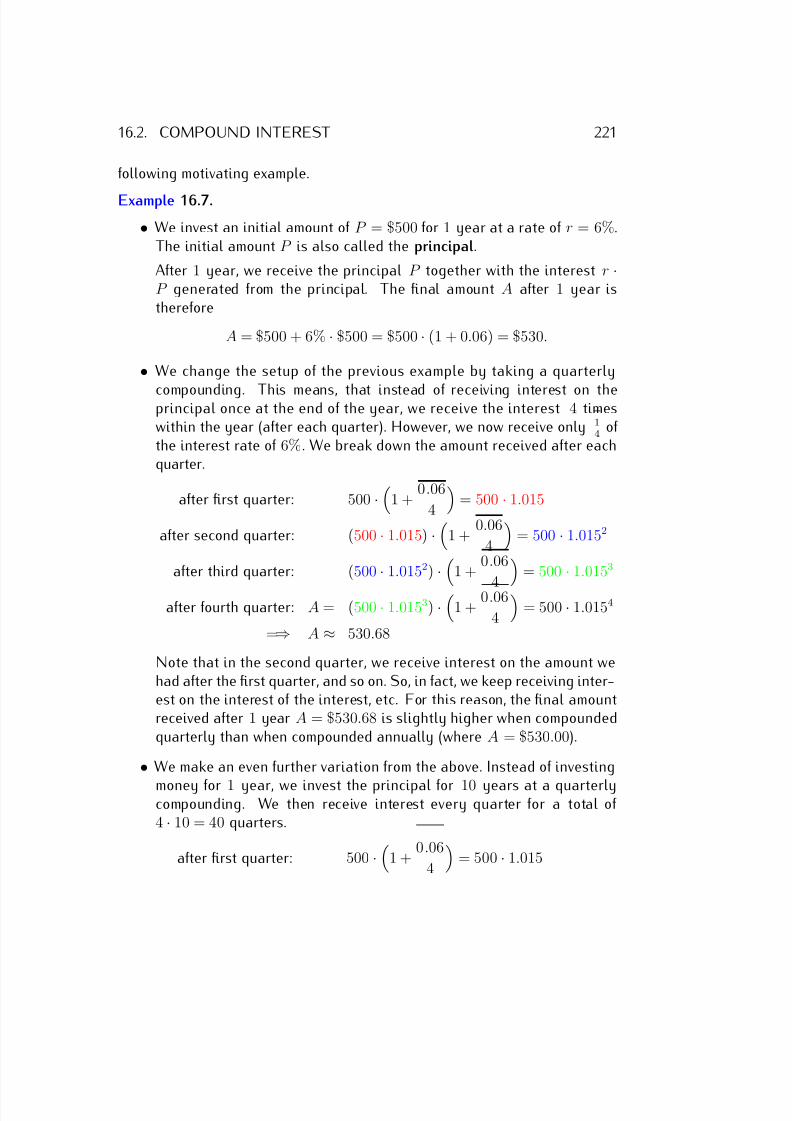
7/18/2019 Precalculus Tradler Carley
http://slidepdf.com/reader/full/precalculus-tradler-carley 231/424
16.2. COMPOUND INTEREST 221
following motivating example.
Example 16.7.
• We invest an initial amount of P = $500 for 1 year at a rate of r = 6%.The initial amount P is also called the principal.
After 1 year, we receive the principal P together with the interest r ·P generated from the principal. The final amount A after 1 year istherefore
A = $500 + 6% · $500 = $500 · (1 + 0.06) = $530.
• We change the setup of the previous example by taking a quarterly
compounding. This means, that instead of receiving interest on theprincipal once at the end of the year, we receive the interest 4 timeswithin the year (after each quarter). However, we now receive only 1
4 of
the interest rate of 6%. We break down the amount received after eachquarter.
after first quarter: 500 ·
1 + 0.06
4
= 500 · 1.015
after second quarter: (500 · 1.015) ·
1 + 0.06
4
= 500 · 1.0152
after third quarter: (500
·1.0152)
· 1 + 0.06
4 = 500
·1.0153
after fourth quarter: A = (500 · 1.0153) ·
1 + 0.06
4
= 500 · 1.0154
=⇒ A ≈ 530.68
Note that in the second quarter, we receive interest on the amount wehad after the first quarter, and so on. So, in fact, we keep receiving inter-est on the interest of the interest, etc. For this reason, the final amountreceived after 1 year A = $530.68 is slightly higher when compoundedquarterly than when compounded annually (where A = $530.00).
• We make an even further variation from the above. Instead of investing
money for 1 year, we invest the principal for 10 years at a quarterlycompounding. We then receive interest every quarter for a total of 4 · 10 = 40 quarters.
after first quarter: 500 ·
1 + 0.06
4
= 500 · 1.015
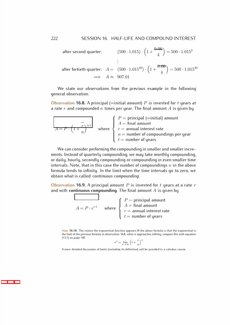
7/18/2019 Precalculus Tradler Carley
http://slidepdf.com/reader/full/precalculus-tradler-carley 232/424
222 SESSION 16. HALF-LIFE AND COMPOUND INTEREST
after second quarter: (500
·1.015)
· 1 + 0.06
4 = 500
·1.0152
...
after fortieth quarter: A = (500 · 1.01539) ·
1 + 0.06
4
= 500 · 1.01540
=⇒ A ≈ 907.01
We state our observations from the previous example in the followinggeneral observation.
Observation 16.8. A principal (=initial amount) P is invested for t years ata rate r and compounded n times per year. The final amount A is given by
A = P ·
1 + r
n
n·twhere
P = principal (=initial) amountA = final amountr = annual interest raten = number of compoundings per yeart = number of years
We can consider performing the compounding in smaller and smaller incre-ments. Instead of quarterly compounding, we may take monthly compounding,or daily, hourly, secondly compounding or compounding in even smaller timeintervals. Note, that in this case the number of compoundings n in the above
formula tends to infinity. In the limit when the time intervals go to zero, weobtain what is called continuous compounding.
Observation 16.9. A principal amount P is invested for t years at a rate rand with continuous compounding. The final amount A is given by
A = P · er·t where
P = principal amountA = final amountr = annual interest ratet = number of years
Note 16.10. The reason the exponential function appears in the above formula is that the exponential isthe limit of the previous formula in observation 16.8, when n approaches infinity; compare this with equation(13.1) on page 187.
er = limn→∞
1 +
r
n
n
A more detailed discussion of limits (including its definition) will be provided in a calculus course.
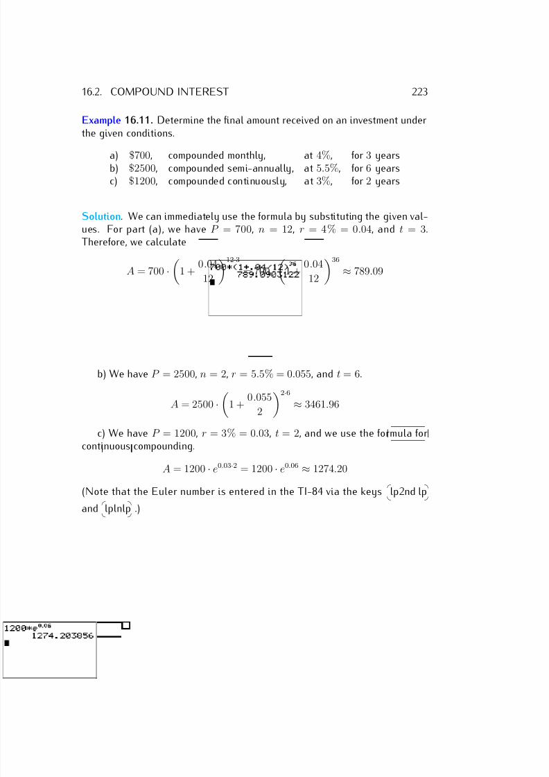
7/18/2019 Precalculus Tradler Carley
http://slidepdf.com/reader/full/precalculus-tradler-carley 233/424
16.2. COMPOUND INTEREST 223
Example 16.11. Determine the final amount received on an investment under
the given conditions.
a) $700, compounded monthly, at 4%, for 3 yearsb) $2500, compounded semi-annually, at 5.5%, for 6 yearsc) $1200, compounded continuously, at 3%, for 2 years
Solution. We can immediately use the formula by substituting the given val-ues. For part (a), we have P = 700, n = 12, r = 4% = 0.04, and t = 3.Therefore, we calculate
A = 700 · 1 + 0.04
1212·3
= 700 · 1 + 0.04
1236
≈ 789.09
b) We have P = 2500, n = 2, r = 5.5% = 0.055, and t = 6.
A = 2500 ·1 +
0.055
2 2·6
≈ 3461.96
c) We have P = 1200, r = 3% = 0.03, t = 2, and we use the formula forcontinuous compounding.
A = 1200 · e0.03·2 = 1200 · e0.06 ≈ 1274.20
(Note that the Euler number is entered in the TI-84 via the keys
lp2nd lp
and
lplnlp .)
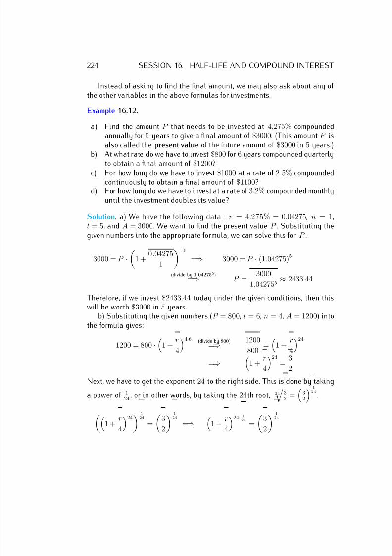
7/18/2019 Precalculus Tradler Carley
http://slidepdf.com/reader/full/precalculus-tradler-carley 234/424
224 SESSION 16. HALF-LIFE AND COMPOUND INTEREST
Instead of asking to find the final amount, we may also ask about any of
the other variables in the above formulas for investments.
Example 16.12.
a) Find the amount P that needs to be invested at 4.275% compoundedannually for 5 years to give a final amount of $3000. (This amount P isalso called the present value of the future amount of $3000 in 5 years.)
b) At what rate do we have to invest $800 for 6 years compounded quarterlyto obtain a final amount of $1200?
c) For how long do we have to invest $1000 at a rate of 2.5% compoundedcontinuously to obtain a final amount of $1100?
d) For how long do we have to invest at a rate of 3.2% compounded monthlyuntil the investment doubles its value?
Solution. a) We have the following data: r = 4.275% = 0.04275, n = 1,t = 5, and A = 3000. We want to find the present value P . Substituting thegiven numbers into the appropriate formula, we can solve this for P .
3000 = P ·
1 + 0.04275
1
1·5=⇒ 3000 = P · (1.04275)5
(divide by 1.042755)=⇒ P =
3000
1.042755 ≈ 2433.44
Therefore, if we invest $2433.44 today under the given conditions, then thiswill be worth $3000 in 5 years.
b) Substituting the given numbers (P = 800, t = 6, n = 4, A = 1200) intothe formula gives:
1200 = 800 ·
1 + r
4
4·6 (divide by 800)=⇒ 1200
800 =
1 +
r
4
24
=⇒
1 + r
4
24
= 3
2
Next, we have to get the exponent 24 to the right side. This is done by taking
a power of 124
, or in other words, by taking the 24th root, 24 3
2 =
32
124
.
1 +
r
4
24 1
24
=
3
2
124
=⇒
1 + r
4
24· 124
=
3
2
124
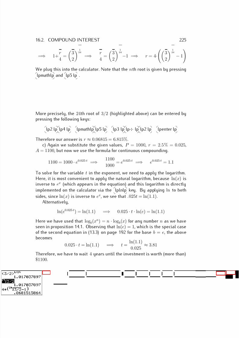
7/18/2019 Precalculus Tradler Carley
http://slidepdf.com/reader/full/precalculus-tradler-carley 235/424
16.2. COMPOUND INTEREST 225
=⇒
1+r
4 = 3
2 124
=⇒
r
4 = 3
2 124
−1 =
⇒ r = 4
·3
2 124
−1
We plug this into the calculator. Note that the nth root is given by pressing
lpmathlp and
lp5 lp .
More precisely, the 24th root of 3/2 (highlighted above) can be entered by
pressing the following keys:
lp2 lp
lp4 lp
lpmathlp
lp5 lp
lp3 lp
lp÷ lp
lp2 lp
lpenter lp
Therefore our answer is r ≈ 0.06815 = 6.815%.c) Again we substitute the given values, P = 1000, r = 2.5% = 0.025,
A = 1100, but now we use the formula for continuous compounding.
1100 = 1000 · e0.025·t =⇒ 1100
1000 = e0.025·t =⇒ e0.025·t = 1.1
To solve for the variable t in the exponent, we need to apply the logarithm.
Here, it is most convenient to apply the natural logarithm, because ln(x) isinverse to ex (which appears in the equation) and this logarithm is directly
implemented on the calculator via the
lplnlp key. By applying ln to both
sides, since ln(x) is inverse to ex, we see that .025t = ln(1.1).Alternatively,
ln(e0.025·t) = ln(1.1) =⇒ 0.025 · t · ln(e) = ln(1.1)
Here we have used that logb(xn) = n · logb(x) for any number n as we haveseen in proposition 14.1. Observing that ln(e) = 1, which is the special caseof the second equation in (13.3) on page 192 for the base b = e, the above
becomes
0.025 · t = ln(1.1) =⇒ t = ln(1.1)
0.025 ≈ 3.81
Therefore, we have to wait 4 years until the investment is worth (more than)$1100.
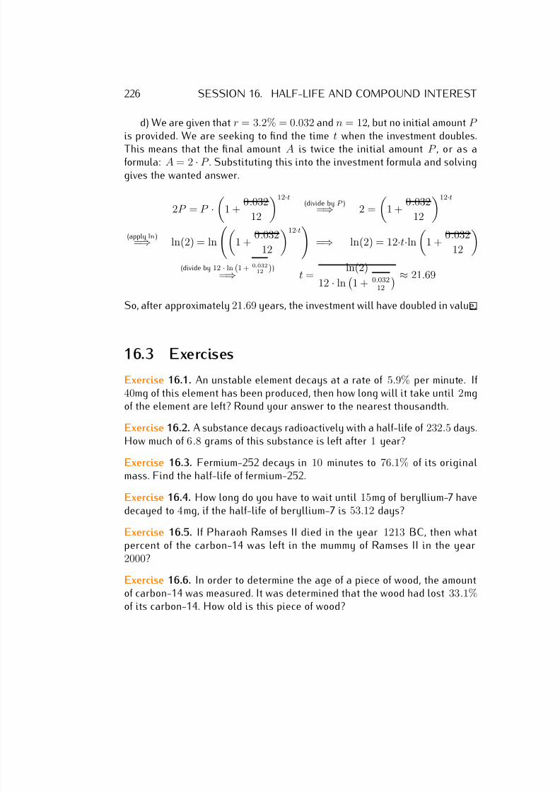
7/18/2019 Precalculus Tradler Carley
http://slidepdf.com/reader/full/precalculus-tradler-carley 236/424
226 SESSION 16. HALF-LIFE AND COMPOUND INTEREST
d) We are given that r = 3.2% = 0.032 and n = 12, but no initial amount P
is provided. We are seeking to find the time t when the investment doubles.This means that the final amount A is twice the initial amount P , or as aformula: A = 2 · P . Substituting this into the investment formula and solvinggives the wanted answer.
2P = P ·
1 + 0.032
12
12·t(divide by P )
=⇒ 2 =
1 +
0.032
12
12·t
(apply ln)=⇒ ln(2) = ln
1 +
0.032
12
12·t =⇒ ln(2) = 12·t·ln
1 +
0.032
12
(divide by 12 · ln 1 + 0.032
12 )
=⇒ t =
ln(2)
12 · ln 1 + 0.03212 ≈ 21.69
So, after approximately 21.69 years, the investment will have doubled in value.
16.3 Exercises
Exercise 16.1. An unstable element decays at a rate of 5.9% per minute. If 40mg of this element has been produced, then how long will it take until 2mgof the element are left? Round your answer to the nearest thousandth.
Exercise 16.2. A substance decays radioactively with a half-life of 232.5 days.How much of 6.8 grams of this substance is left after 1 year?
Exercise 16.3. Fermium-252 decays in 10 minutes to 76.1% of its originalmass. Find the half-life of fermium-252.
Exercise 16.4. How long do you have to wait until 15mg of beryllium-7 havedecayed to 4mg, if the half-life of beryllium-7 is 53.12 days?
Exercise 16.5. If Pharaoh Ramses II died in the year 1213 BC, then whatpercent of the carbon-14 was left in the mummy of Ramses II in the year
2000?
Exercise 16.6. In order to determine the age of a piece of wood, the amountof carbon-14 was measured. It was determined that the wood had lost 33.1%of its carbon-14. How old is this piece of wood?

7/18/2019 Precalculus Tradler Carley
http://slidepdf.com/reader/full/precalculus-tradler-carley 237/424
16.3. EXERCISES 227
Exercise 16.7. Archaeologists uncovered a bone at an ancient resting ground.
It was determined that 62% of the carbon-14 was left in the bone. How oldis the bone?
Exercise 16.8. An investment of $5, 000 was locked in for 30 years. Accordingto the agreed conditions, the investment will be worth $5, 000 · 1.08t after tyears.
a) How much is the investment worth after 5 years?b) After how many years will the investment be worth $20, 000?
Exercise 16.9. Determine the final amount in a savings account under thegiven conditions.
a) $700, compounded quarterly, at 3%, for 7 yearsb) $1400, compounded annually, at 2.25%, for 5 yearsc) $1400, compounded continuously, at 2.25%, for 5 yearsd) $500, compounded monthly, at 3.99%, for 2 yearse) $5000, compounded continuously, at 7.4%, for 3 yearsf) $1600, compounded daily, at 3.333%, for 1 yearg) $750, compounded semi-annually, at 4.9%, for 4 years
Exercise 16.10.
a) Find the amount P that needs to be invested at a rate of 5% compoundedquarterly for 6 years to give a final amount of $2000.
b) Find the present value P of a future amount of A = $3500 invested at6% compounded annually for 3 years.
c) Find the present value P of a future amount of $1000 invested at a rateof 4.9% compounded continuously for 7 years.
d) At what rate do we have to invest $1900 for 4 years compounded monthlyto obtain a final amount of $2250?
e) At what rate do we have to invest $1300 for 10 years compounded con-
tinuously to obtain a final amount of $2000?f) For how long do we have to invest $3400 at a rate of 5.125% compounded
annually to obtain a final amount of $3700?g) For how long do we have to invest $1000 at a rate of 2.5% compounded
continuously to obtain a final amount of $1100?

7/18/2019 Precalculus Tradler Carley
http://slidepdf.com/reader/full/precalculus-tradler-carley 238/424
228 SESSION 16. HALF-LIFE AND COMPOUND INTEREST
h) How long do you have to invest a principal at a rate of 6.75% com-
pounded daily until the investment doubles its value?i) An certain amount of money has tripled its value while being in a savingsaccount that has an interest rate of 8% compounded continuously. Forhow long was the money in the savings account?
7/18/2019 Precalculus Tradler Carley
http://slidepdf.com/reader/full/precalculus-tradler-carley 239/424
Review of exponential and
logarithmic functions
Exercise III.1. The population of a country grows exponentially at a rate of 1% per year. If the population was 35.7 million in the year 2010, then what
is the population size of this country in the year 2015?
Exercise III.2. A radioactive substance decays exponentially at a rate of 7%per hour. How long do you have to wait until the substance has decayed to14 of its original size?
Exercise III.3. Combine to an expression with only one logarithm.
a) 2
3 ln(x) + 4 ln(y), b)
1
2 log2(x) − 3
4 log2(y) + 3 log2(z )
Exercise III.4. Assuming that x , y > 0, write the following expressions interms of u = log(x) and v = log(y):
a) log
3√
x4
y2
, b) log
x
y5
, c) log
5
xy4
Exercise III.5. Solve without using the calculator: log3(x)+log3(x−8) = 2
Exercise III.6.
a) Find the exact solution of the equation: 6x+2 = 7x
b) Use the calculator to approximate your solution from part (a).Exercise III.7. 45mg of fluorine-18 decay in 3 hours to 14.4mg. Find thehalf-life of fluorine-18.
Exercise III.8. A bone has lost 35% of its carbon-14. How old is the bone?
229

7/18/2019 Precalculus Tradler Carley
http://slidepdf.com/reader/full/precalculus-tradler-carley 240/424
Exercise III.9. How much do you have to invest today at 3% compounded
quarterly to obtain $2, 000 in return in 3 years?
Exercise III.10. $500 is invested with continuous compounding. If $692.01 isreturned after 5 years, what is the interest rate?
230

7/18/2019 Precalculus Tradler Carley
http://slidepdf.com/reader/full/precalculus-tradler-carley 241/424
Part IV
Trigonometric functions
231
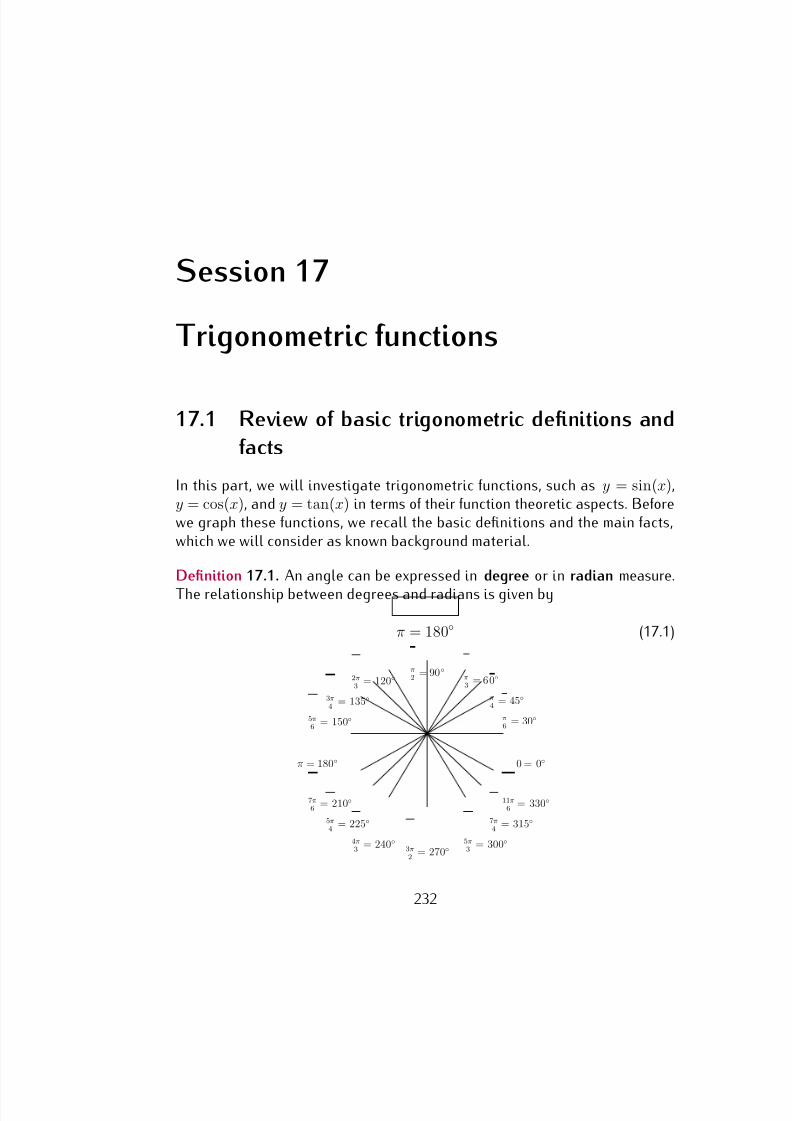
7/18/2019 Precalculus Tradler Carley
http://slidepdf.com/reader/full/precalculus-tradler-carley 242/424
Session 17
Trigonometric functions
17.1 Review of basic trigonometric definitions and
facts
In this part, we will investigate trigonometric functions, such as y = sin(x),y = cos(x), and y = tan(x) in terms of their function theoretic aspects. Beforewe graph these functions, we recall the basic definitions and the main facts,which we will consider as known background material.
Definition 17.1. An angle can be expressed in degree or in radian measure.
The relationship between degrees and radians is given by
π = 180◦ (17.1)
0 = 0◦π = 180◦
π2
= 90◦
3π2
= 270◦
π4
= 45◦
5π4
= 225◦
π3
= 60◦
4π3
= 240◦
π6
= 30◦
7π6
= 210◦
3π4
= 135◦
7π4
= 315◦
11π6
= 330◦
5π6
= 150◦
5π3
= 300◦
2π3
= 120◦
232
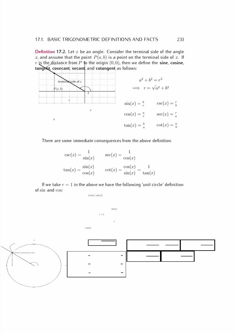
7/18/2019 Precalculus Tradler Carley
http://slidepdf.com/reader/full/precalculus-tradler-carley 243/424
17.1. BASIC TRIGONOMETRIC DEFINITIONS AND FACTS 233
Definition 17.2. Let x be an angle. Consider the terminal side of the angle
x, and assume that the point P (a, b) is a point on the terminal side of x. If r is the distance from P to the origin (0, 0), then we define the sine, cosine,tangent, cosecant, secant, and cotangent as follows:
P (a, b)
x
a
b
r
terminal side of x a2 + b2 = r2
=⇒ r =√
a2 + b2
sin(x) = br
csc(x) = rb
cos(x) = a
r
sec(x) = r
a
tan(x) = ba
cot(x) = ab
There are some immediate consequences from the above definition.
csc(x) = 1
sin(x) sec(x) =
1
cos(x)
tan(x) = sin(x)
cos(x) cot(x) =
cos(x)
sin(x) =
1
tan(x)
If we take r = 1 in the above we have the following ‘unit circle’ definitionof sin and cos:
x
(cos(x), sin(x))
cos(x)
sin(x)
r = 1
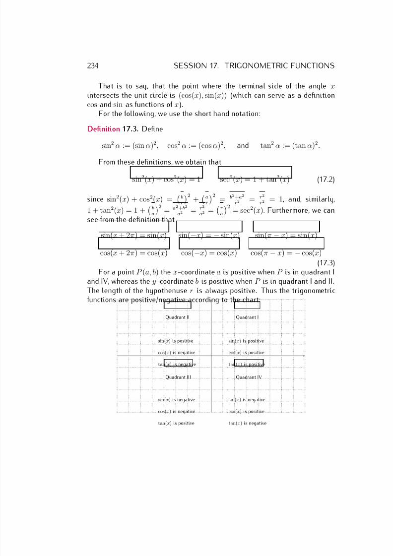
7/18/2019 Precalculus Tradler Carley
http://slidepdf.com/reader/full/precalculus-tradler-carley 244/424
234 SESSION 17. TRIGONOMETRIC FUNCTIONS
That is to say, that the point where the terminal side of the angle x
intersects the unit circle is (cos(x), sin(x)) (which can serve as a definitioncos and sin as functions of x).For the following, we use the short hand notation:
Definition 17.3. Define
sin2 α := (sin α)2, cos2 α := (cos α)2, and tan2 α := (tan α)2.
From these definitions, we obtain that
sin2(x) + cos2(x) = 1 sec2(x) = 1 + tan2(x) (17.2)
since sin2(x) + cos2(x) = b
r
2 +a
r
2 = b2+a2
r2 = r2
r2 = 1, and, similarly,
1 + tan2(x) = 1 +
ba
2= a2+b2
a2 = r2
a2 =
ra
2= sec2(x). Furthermore, we can
see from the definition that
sin(x + 2π) = sin(x) sin(−x) = − sin(x) sin(π − x) = sin(x)
cos(x + 2π) = cos(x) cos(−x) = cos(x) cos(π − x) = − cos(x)
(17.3)For a point P (a, b) the x-coordinate a is positive when P is in quadrant I
and IV, whereas the y-coordinate b is positive when P is in quadrant I and II.
The length of the hypothenuse r is always positive. Thus the trigonometricfunctions are positive/negative according to the chart:
Quadrant I
sin(x) is positive
cos(x) is positive
tan(x) is positive
Quadrant II
sin(x) is positive
cos(x) is negative
tan(x) is negative
Quadrant III
sin(x) is negative
cos(x) is negative
tan(x) is positive
Quadrant IV
sin(x) is negative
cos(x) is positive
tan(x) is negative
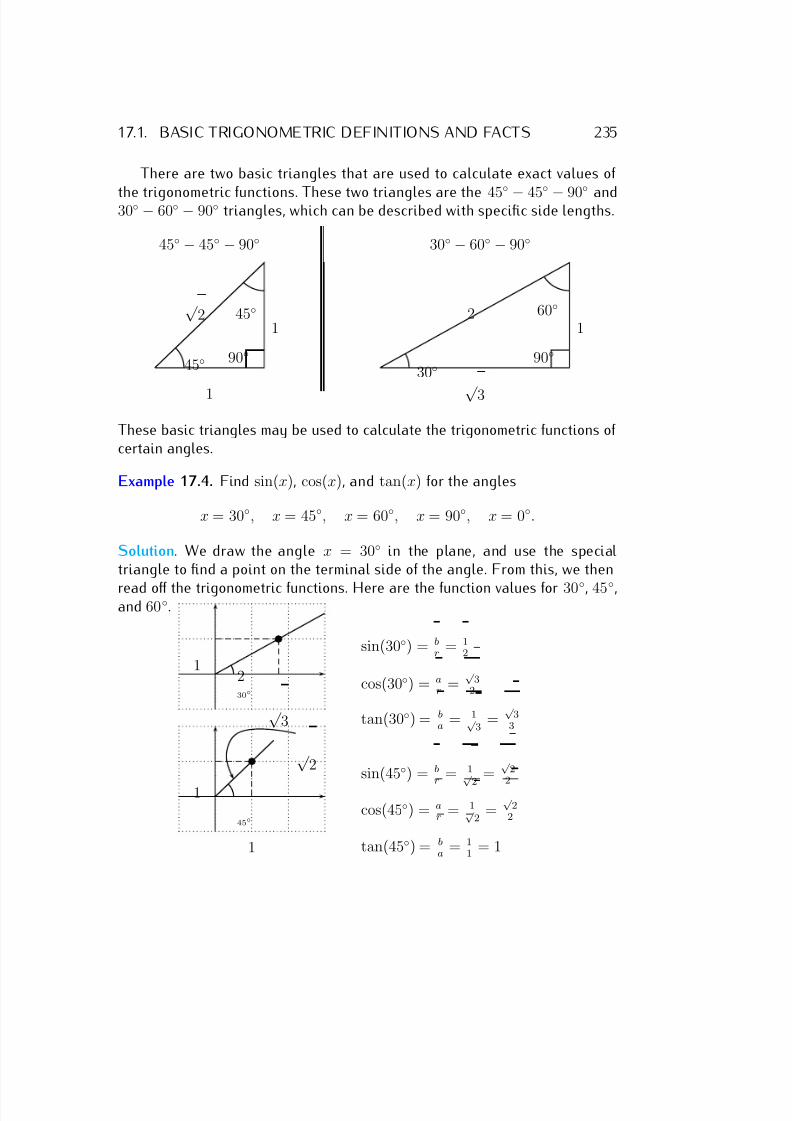
7/18/2019 Precalculus Tradler Carley
http://slidepdf.com/reader/full/precalculus-tradler-carley 245/424
17.1. BASIC TRIGONOMETRIC DEFINITIONS AND FACTS 235
There are two basic triangles that are used to calculate exact values of
the trigonometric functions. These two triangles are the 45◦ − 45◦ − 90◦ and30◦ − 60◦ − 90◦ triangles, which can be described with specific side lengths.
45◦ − 45◦ − 90◦ 30◦ − 60◦ − 90◦
45◦
145◦
1
90◦
√ 2
30◦
160◦
√ 3
90◦
2
These basic triangles may be used to calculate the trigonometric functions of certain angles.
Example 17.4. Find sin(x), cos(x), and tan(x) for the angles
x = 30◦, x = 45◦, x = 60◦, x = 90◦, x = 0◦.
Solution. We draw the angle x = 30◦ in the plane, and use the specialtriangle to find a point on the terminal side of the angle. From this, we then
read off the trigonometric functions. Here are the function values for 30◦, 45◦,and 60◦.
30◦
√ 3
12
sin(30◦) = br
= 12
cos(30◦) = ar =
√ 3
2
tan(30◦) = ba = 1√
3 =
√ 3
3
45◦
1
1
√ 2
sin(45◦) = b
r
= 1
√ 2 =
√ 2
2
cos(45◦) = ar = 1√
2 =
√ 2
2
tan(45◦) = ba = 1
1 = 1
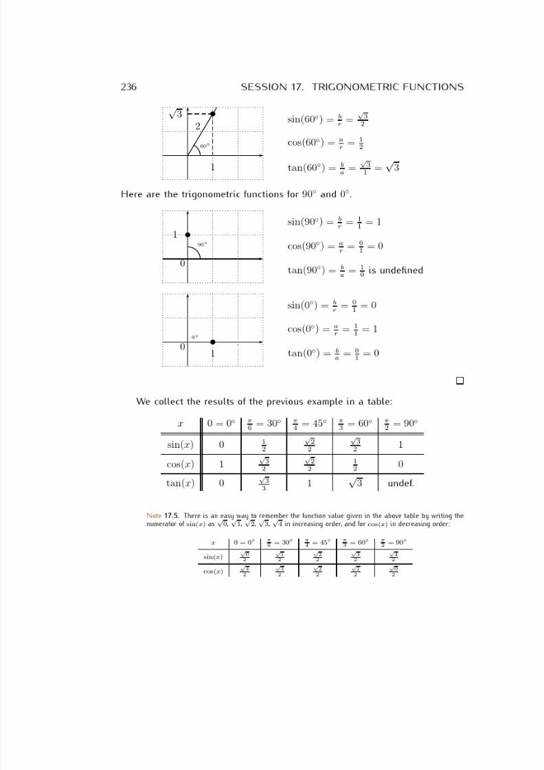
7/18/2019 Precalculus Tradler Carley
http://slidepdf.com/reader/full/precalculus-tradler-carley 246/424
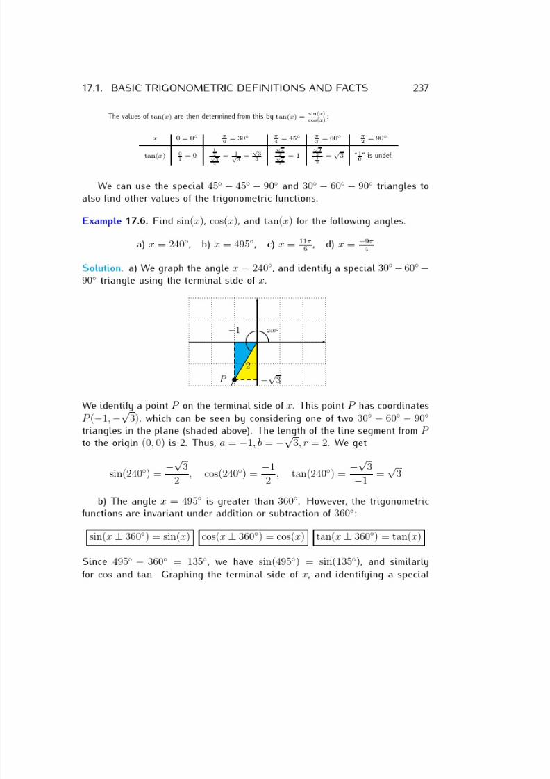
7/18/2019 Precalculus Tradler Carley
http://slidepdf.com/reader/full/precalculus-tradler-carley 247/424
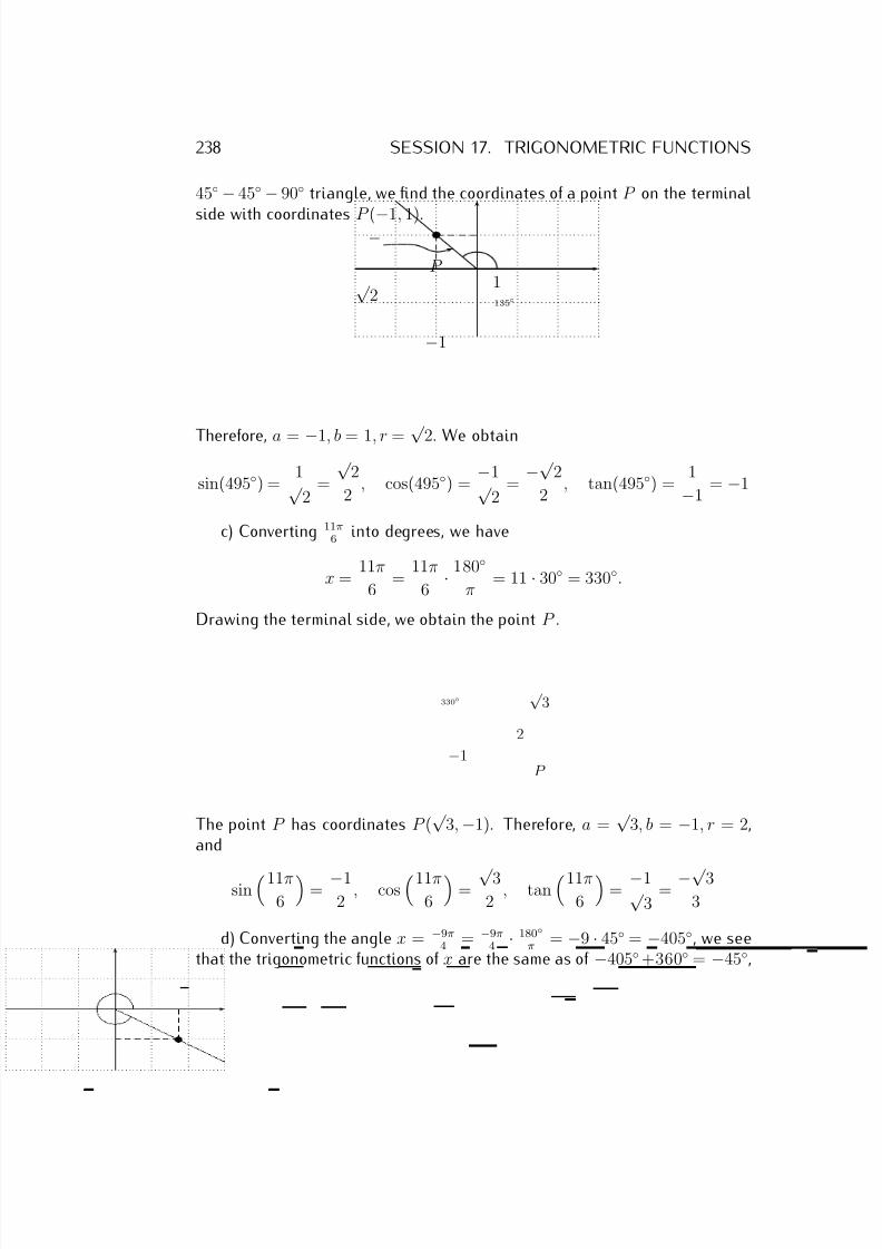
7/18/2019 Precalculus Tradler Carley
http://slidepdf.com/reader/full/precalculus-tradler-carley 248/424
238 SESSION 17. TRIGONOMETRIC FUNCTIONS
45◦ − 45◦ − 90◦ triangle, we find the coordinates of a point P on the terminal
side with coordinates P (−1, 1).
135◦
1
−1
P √
2
Therefore, a = −1, b = 1, r = √ 2. We obtain
sin(495◦) = 1√
2=
√ 2
2 , cos(495◦) =
−1√ 2
= −√
2
2 , tan(495◦) =
1
−1 = −1
c) Converting 11π6 into degrees, we have
x = 11π
6 =
11π
6 · 180◦
π = 11 · 30◦ = 330◦.
Drawing the terminal side, we obtain the point P .
330◦√
3
−1
2
P
The point P has coordinates P (√
3, −1). Therefore, a =√
3, b = −1, r = 2,and
sin11π
6
= −1
2 , cos
11π6
= √ 3
2 , tan
11π6
= −1√
3= −√ 3
3
d) Converting the angle x = −9π4 = −9π
4 · 180◦π = −9 · 45◦ = −405◦, we see
that the trigonometric functions of x are the same as of −405◦+360◦ = −45◦,
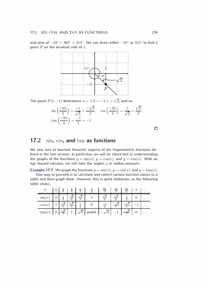
7/18/2019 Precalculus Tradler Carley
http://slidepdf.com/reader/full/precalculus-tradler-carley 249/424
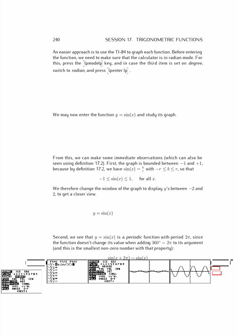
7/18/2019 Precalculus Tradler Carley
http://slidepdf.com/reader/full/precalculus-tradler-carley 250/424
240 SESSION 17. TRIGONOMETRIC FUNCTIONS
An easier approach is to use the TI-84 to graph each function. Before entering
the function, we need to make sure that the calculator is in radian mode. Forthis, press the
lpmodelp key, and in case the third item is set on degree,
switch to radian, and press
lpenter lp .
We may now enter the function y = sin(x) and study its graph.
From this, we can make some immediate observations (which can also beseen using definition 17.2). First, the graph is bounded between −1 and +1,because by definition 17.2, we have sin(x) = b
r with −r ≤ b ≤ r, so that
−1 ≤ sin(x) ≤ 1, for all x.
We therefore change the window of the graph to display y ’s between −2 and2, to get a closer view.
y = sin(x)
Second, we see that y = sin(x) is a periodic function with period 2π, sincethe function doesn’t change its value when adding 360◦ = 2π to its argument(and this is the smallest non-zero number with that property):
sin(x + 2π) = sin(x)
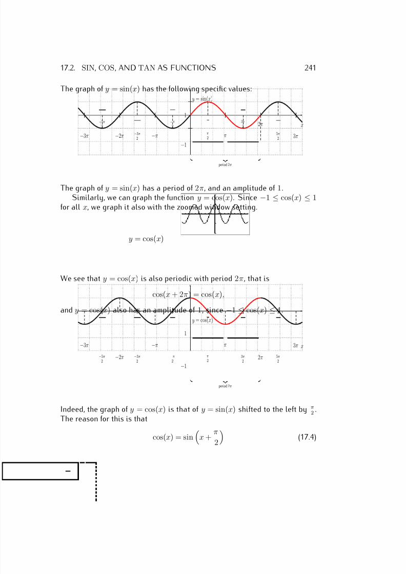
7/18/2019 Precalculus Tradler Carley
http://slidepdf.com/reader/full/precalculus-tradler-carley 251/424
17.2. SIN, COS, AND TAN AS FUNCTIONS 241
The graph of y = sin(x) has the following specific values:
x
y = sin(x)
π
2
−π
2
π−π
3π
2
−3π
2
2π
−2π 5π
2
−5π
2
3π−3π
period 2π
1
−1
The graph of y = sin(x) has a period of 2π, and an amplitude of 1.
Similarly, we can graph the function y = cos(x). Since −1 ≤ cos(x) ≤ 1for all x, we graph it also with the zoomed window setting.
y = cos(x)
We see that y = cos(x) is also periodic with period 2π, that is
cos(x + 2π) = cos(x),
and y = cos(x) also has an amplitude of 1, since −1 ≤ cos(x) ≤ 1.
x
y = cos(x)
π
2
−π
2
π−π
3π
2
−3π
22π−2π 5π
2
−5π
2
3π−3π
period 2π
1
−1
Indeed, the graph of y = cos(x) is that of y = sin(x) shifted to the left by π2 .
The reason for this is that
cos(x) = sin
x + π
2
(17.4)
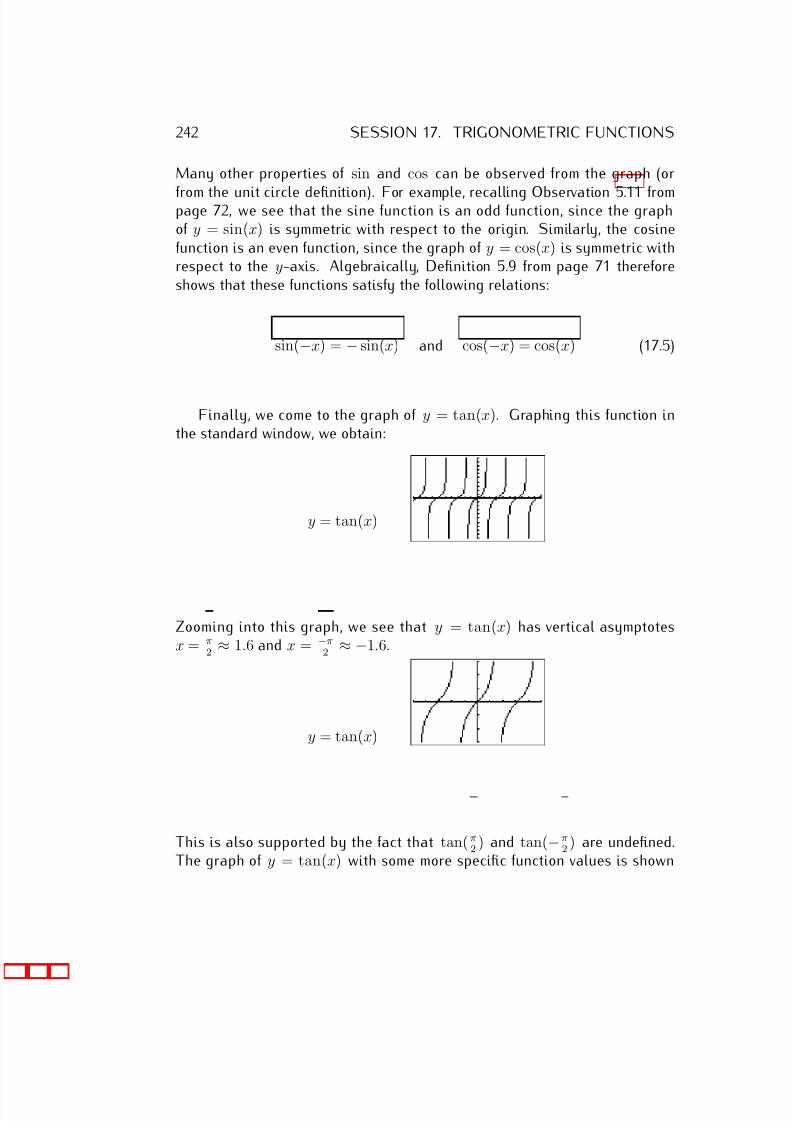
7/18/2019 Precalculus Tradler Carley
http://slidepdf.com/reader/full/precalculus-tradler-carley 252/424
242 SESSION 17. TRIGONOMETRIC FUNCTIONS
Many other properties of sin and cos can be observed from the graph (or
from the unit circle definition). For example, recalling Observation 5.11 frompage 72, we see that the sine function is an odd function, since the graphof y = sin(x) is symmetric with respect to the origin. Similarly, the cosinefunction is an even function, since the graph of y = cos(x) is symmetric withrespect to the y-axis. Algebraically, Definition 5.9 from page 71 thereforeshows that these functions satisfy the following relations:
sin(−x) = − sin(x) and cos(−x) = cos(x) (17.5)
Finally, we come to the graph of y = tan(x). Graphing this function inthe standard window, we obtain:
y = tan(x)
Zooming into this graph, we see that y = tan(x) has vertical asymptotesx = π
2 ≈ 1.6 and x = −π
2 ≈ −1.6.
y = tan(x)
This is also supported by the fact that tan( π2 ) and tan(−π
2 ) are undefined.The graph of y = tan(x) with some more specific function values is shown
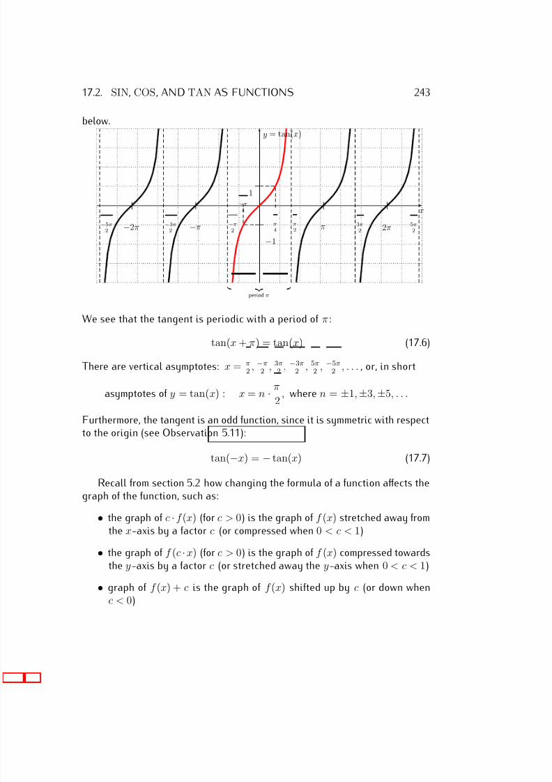
7/18/2019 Precalculus Tradler Carley
http://slidepdf.com/reader/full/precalculus-tradler-carley 253/424
17.2. SIN, COS, AND TAN AS FUNCTIONS 243
below.
x
y = tan(x)
π4
−π4
π2
−π2
π−π 3π2
−3π2 2π−2π 5π
2−5π
2
period π
1
−1
We see that the tangent is periodic with a period of π :
tan(x + π) = tan(x) (17.6)
There are vertical asymptotes: x = π2 , −π
2 , 3π2 , −3π
2 , 5π2 , −5π
2 , . . . , or, in short
asymptotes of y = tan(x) : x = n · π
2, where n = ±1, ±3, ±5, . . .
Furthermore, the tangent is an odd function, since it is symmetric with respectto the origin (see Observation 5.11):
tan(−x) = − tan(x) (17.7)
Recall from section 5.2 how changing the formula of a function affects thegraph of the function, such as:
• the graph of c · f (x) (for c > 0) is the graph of f (x) stretched away fromthe x-axis by a factor c (or compressed when 0 < c < 1)
• the graph of f (c · x) (for c > 0) is the graph of f (x) compressed towardsthe y-axis by a factor c (or stretched away the y-axis when 0 < c < 1)
• graph of f (x) + c is the graph of f (x) shifted up by c (or down whenc < 0)
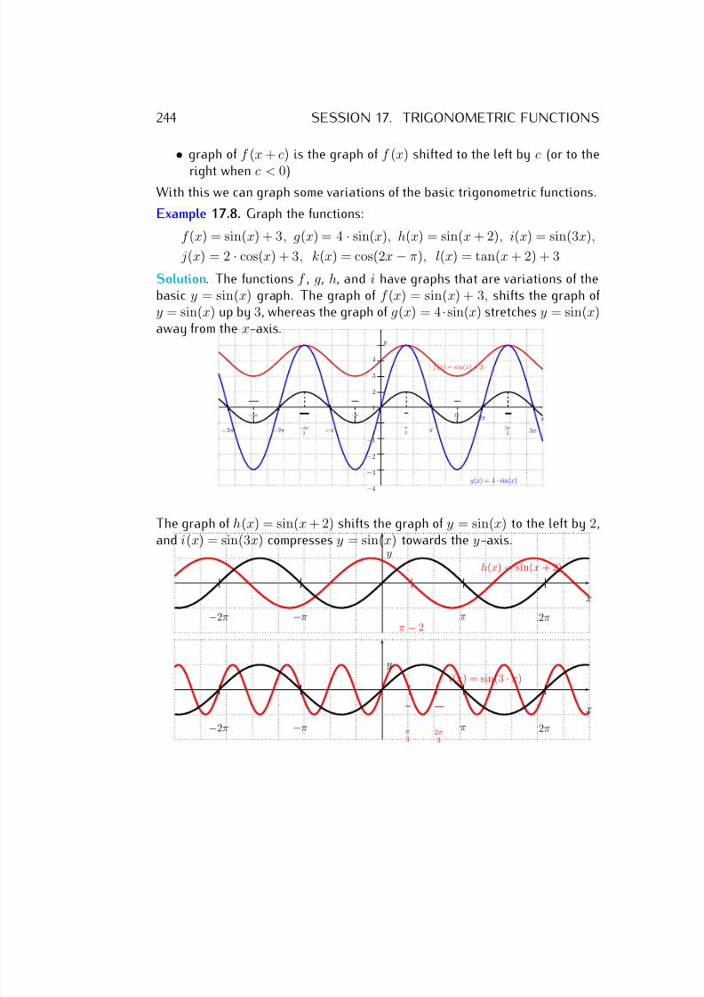
7/18/2019 Precalculus Tradler Carley
http://slidepdf.com/reader/full/precalculus-tradler-carley 254/424
244 SESSION 17. TRIGONOMETRIC FUNCTIONS
• graph of f (x + c) is the graph of f (x) shifted to the left by c (or to the
right when c < 0)With this we can graph some variations of the basic trigonometric functions.
Example 17.8. Graph the functions:
f (x) = sin(x) + 3, g(x) = 4 · sin(x), h(x) = sin(x + 2), i(x) = sin(3x),
j(x) = 2 · cos(x) + 3, k(x) = cos(2x − π), l(x) = tan(x + 2) + 3
Solution. The functions f , g, h, and i have graphs that are variations of thebasic y = sin(x) graph. The graph of f (x) = sin(x) + 3, shifts the graph of y = sin(x) up by 3, whereas the graph of g(x) = 4 ·sin(x) stretches y = sin(x)away from the x-axis.
x
y
π2
−π2
π−π
3π2
−3π2
2π
−2π 5π2
−5π2
3π−3π
1
−1
2
3
−2
−3
4
−4
f (x) = sin(x) + 3
g(x) = 4 · sin(x)
The graph of h(x) = sin(x + 2) shifts the graph of y = sin(x) to the left by 2,and i(x) = sin(3x) compresses y = sin(x) towards the y-axis.
x
y
π−π 2π−2π
h(x) = sin(x + 2)
π − 2
x
y
π−π 2π−2π
i(x) = sin(3 · x)
π3
2π3
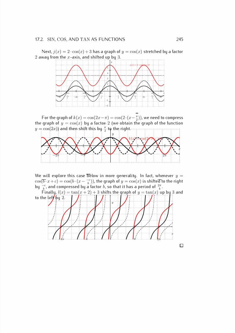
7/18/2019 Precalculus Tradler Carley
http://slidepdf.com/reader/full/precalculus-tradler-carley 255/424
17.2. SIN, COS, AND TAN AS FUNCTIONS 245
Next, j(x) = 2 · cos(x) + 3 has a graph of y = cos(x) stretched by a factor
2 away from the x-axis, and shifted up by 3.
x
y
π2
−π2
π−π 3π2
−3π2 2π−2π 5π
2−5π
2 3π−3π
1
−1
2
3
−2
4
5 j(x) = 2 · cos(x) + 3
For the graph of k(x) = cos(2x−π) = cos(2·(x− π2 )), we need to compress
the graph of y = cos(x) by a factor 2 (we obtain the graph of the functiony = cos(2x)) and then shift this by π
2 to the right.
x
y
π−π 2π−2π
k(x) = cos(2 · x − π)
We will explore this case below in more generality. In fact, whenever y =cos(b · x + c) = cos(b · (x − −c
b )), the graph of y = cos(x) is shifted to the rightby −c
b , and compressed by a factor b, so that it has a period of 2π
b .
Finally, l(x) = tan(x + 2) + 3 shifts the graph of y = tan(x) up by 3 andto the left by 2.
x
y
π−π 2π−2π
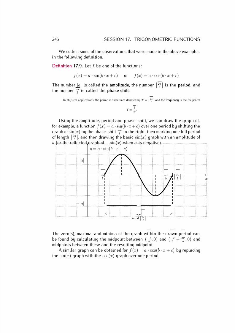
7/18/2019 Precalculus Tradler Carley
http://slidepdf.com/reader/full/precalculus-tradler-carley 256/424
246 SESSION 17. TRIGONOMETRIC FUNCTIONS
We collect some of the observations that were made in the above examples
in the following definition.Definition 17.9. Let f be one of the functions:
f (x) = a · sin(b · x + c) or f (x) = a · cos(b · x + c)
The number |a| is called the amplitude, the number2π
b
is the period, andthe number −c
b is called the phase shift.
In physical applications, the period is sometimes denoted by T = 2πb
and the frequency is the reciprocal
f = 1
T .
Using the amplitude, period and phase-shift, we can draw the graph of,for example, a function f (x) = a · sin(b · x + c) over one period by shifting thegraph of sin(x) by the phase-shift −c
b to the right, then marking one full periodof length
2πb
, and then drawing the basic sin(x) graph with an amplitude of a (or the reflected graph of − sin(x) when a is negative).
x
y = a · sin(b · x + c)
−cb
−cb + 2π
b
period | 2π
b |
|a|
−|a|
The zero(s), maxima, and minima of the graph within the drawn period canbe found by calculating the midpoint between (−c
b , 0) and (−c
b + 2π
b , 0) and
midpoints between these and the resulting midpoint.A similar graph can be obtained for f (x) = a · cos(b · x + c) by replacing
the sin(x) graph with the cos(x) graph over one period.
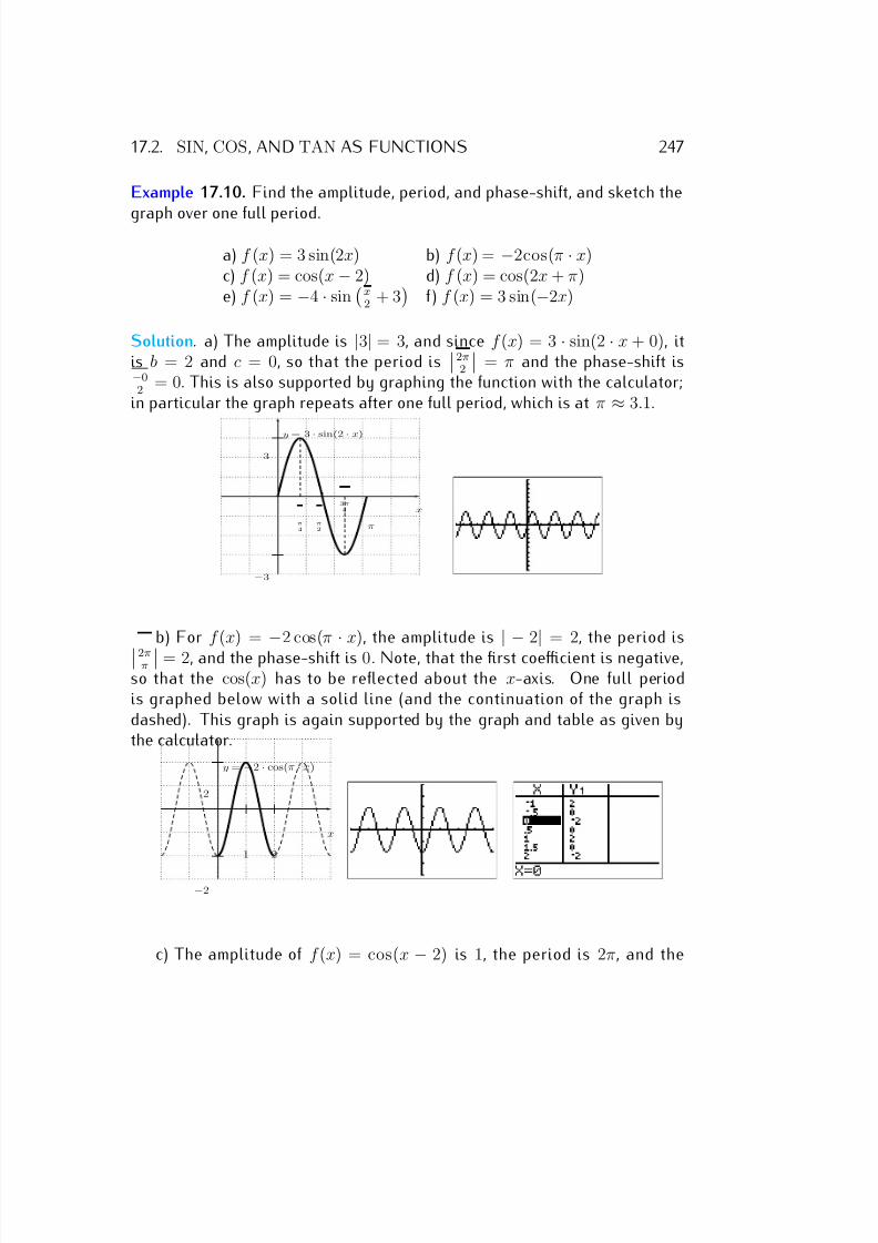
7/18/2019 Precalculus Tradler Carley
http://slidepdf.com/reader/full/precalculus-tradler-carley 257/424
17.2. SIN, COS, AND TAN AS FUNCTIONS 247
Example 17.10. Find the amplitude, period, and phase-shift, and sketch the
graph over one full period.
a) f (x) = 3 sin(2x) b) f (x) = −2cos(π · x)c) f (x) = cos(x − 2) d) f (x) = cos(2x + π)e) f (x) = −4 · sin
x2 + 3
f ) f (x) = 3 sin(−2x)
Solution. a) The amplitude is |3| = 3, and since f (x) = 3 · sin(2 · x + 0), itis b = 2 and c = 0, so that the period is
2π2
= π and the phase-shift is−0
2 = 0. This is also supported by graphing the function with the calculator;
in particular the graph repeats after one full period, which is at π ≈ 3.1.
x
y = 3 ·
sin(2 ·
x)
π
2 π
π
4
3π
4
3
−3
b) For f (x) =
−2 cos(π
·x), the amplitude is
| −2
| = 2, the period is2π
π = 2, and the phase-shift is 0. Note, that the first coefficient is negative,
so that the cos(x) has to be reflected about the x-axis. One full periodis graphed below with a solid line (and the continuation of the graph isdashed). This graph is again supported by the graph and table as given bythe calculator.
x
y = −2 · cos(π · x)
1 2
2
−2
c) The amplitude of f (x) = cos(x − 2) is 1, the period is 2π, and the
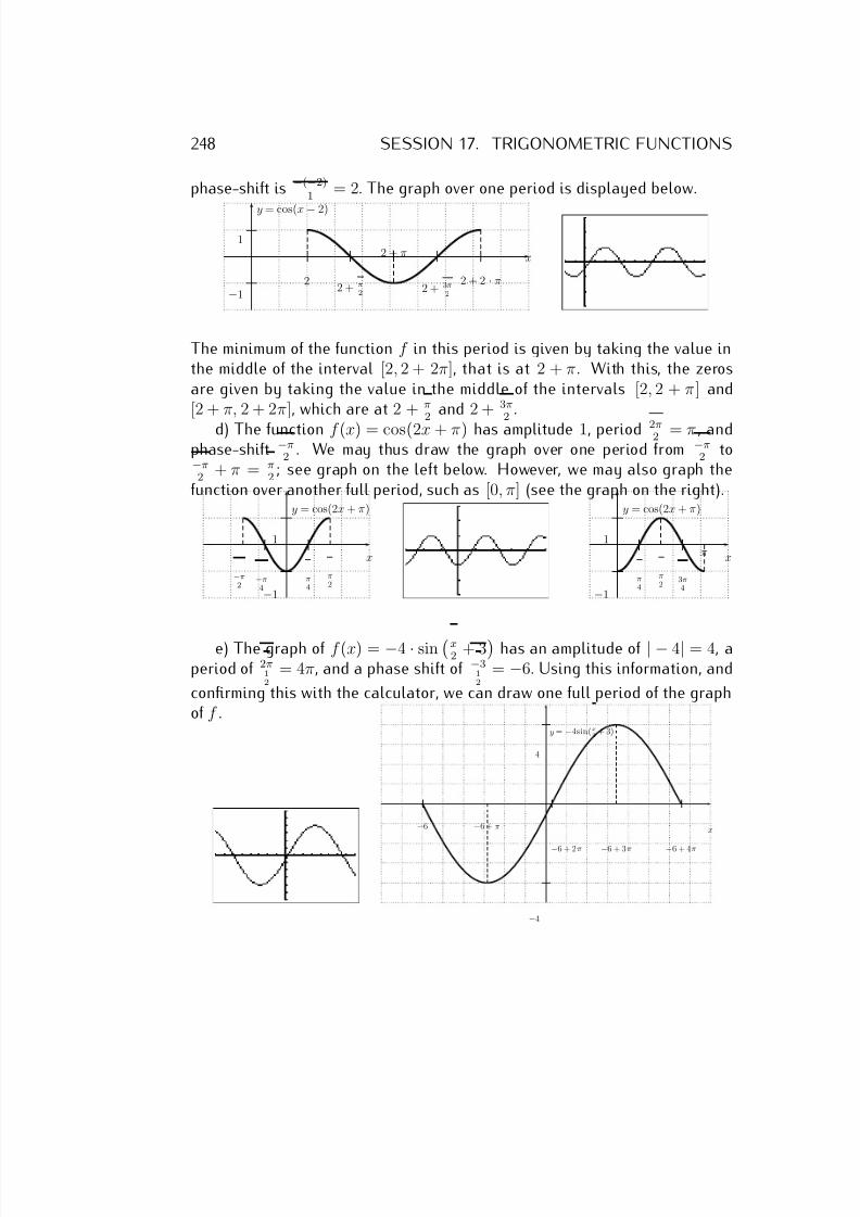
7/18/2019 Precalculus Tradler Carley
http://slidepdf.com/reader/full/precalculus-tradler-carley 258/424
248 SESSION 17. TRIGONOMETRIC FUNCTIONS
phase-shift is −(−2)1
= 2. The graph over one period is displayed below.
x
y = cos(x − 2)
2 + 2 · π2
2 + π
2 + π2 2 + 3π
2
1
−1
The minimum of the function f in this period is given by taking the value inthe middle of the interval [2, 2 + 2π], that is at 2 + π. With this, the zerosare given by taking the value in the middle of the intervals [2, 2 + π] and[2 + π, 2 + 2π], which are at 2 + π
2 and 2 + 3π
2 .
d) The function f (x) = cos(2x + π) has amplitude 1, period 2π2 = π , andphase-shift −π
2 . We may thus draw the graph over one period from −π2 to
−π2
+ π = π2
; see graph on the left below. However, we may also graph thefunction over another full period, such as [0, π] (see the graph on the right).
x
y = cos(2x + π)
−π2
π2
−π4
π4
1
−1
x
y = cos(2x + π)
π
π2
3π4
π4
1
−1
e) The graph of f (x) = −4 · sin x2 + 3 has an amplitude of | − 4| = 4, a
period of 2π12
= 4π, and a phase shift of −312
= −6. Using this information, and
confirming this with the calculator, we can draw one full period of the graphof f .
x
y = −4sin( x2
+ 3)
−6 −6 + π
−6 + 2π −6 + 3π −6 + 4π
4
−4
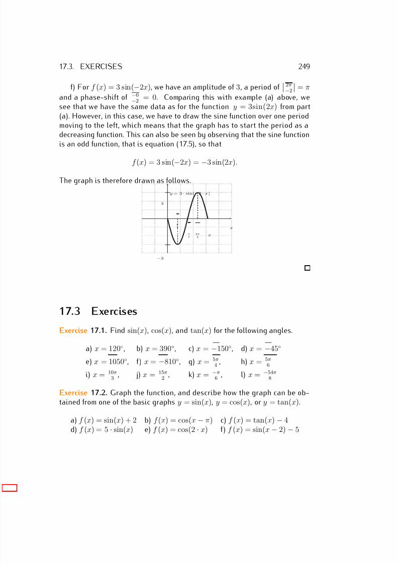
7/18/2019 Precalculus Tradler Carley
http://slidepdf.com/reader/full/precalculus-tradler-carley 259/424
17.3. EXERCISES 249
f) For f (x) = 3 sin(−2x), we have an amplitude of 3, a period of 2π−2 = π
and a phase-shift of −0
−2 = 0. Comparing this with example (a) above, wesee that we have the same data as for the function y = 3sin(2x) from part(a). However, in this case, we have to draw the sine function over one periodmoving to the left, which means that the graph has to start the period as adecreasing function. This can also be seen by observing that the sine functionis an odd function, that is equation (17.5), so that
f (x) = 3 sin(−2x) = −3 sin(2x).
The graph is therefore drawn as follows.
x
y = 3 · sin(−2 · x)
π
2 π
π
4
3π
4
3
−3
17.3 Exercises
Exercise 17.1. Find sin(x), cos(x), and tan(x) for the following angles.
a) x = 120◦, b) x = 390◦, c) x = −150◦, d) x = −45◦
e) x = 1050◦, f ) x = −810◦, g) x = 5π4 , h) x = 5π
6
i) x = 10π3
, j) x = 15π2
, k) x = −π6
, l) x = −54π8
Exercise 17.2. Graph the function, and describe how the graph can be ob-tained from one of the basic graphs y = sin(x), y = cos(x), or y = tan(x).
a) f (x) = sin(x) + 2 b) f (x) = cos(x − π) c) f (x) = tan(x) − 4d) f (x) = 5 · sin(x) e) f (x) = cos(2 · x) f ) f (x) = sin(x − 2) − 5
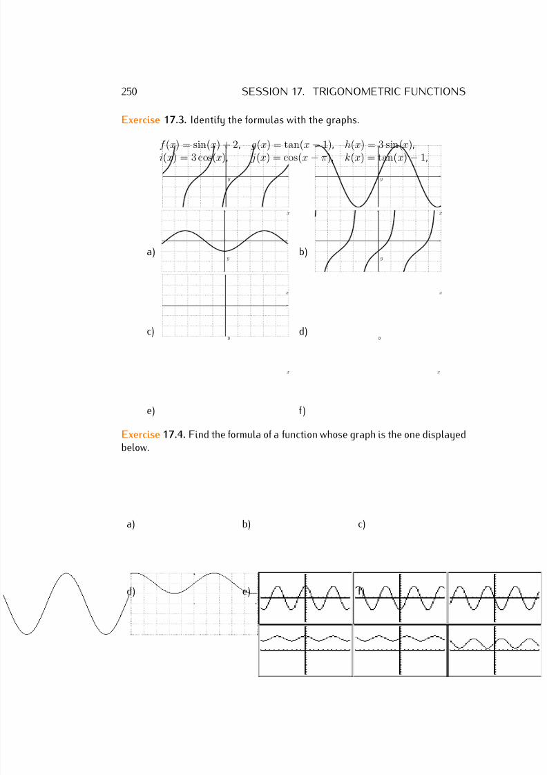
7/18/2019 Precalculus Tradler Carley
http://slidepdf.com/reader/full/precalculus-tradler-carley 260/424
250 SESSION 17. TRIGONOMETRIC FUNCTIONS
Exercise 17.3. Identify the formulas with the graphs.
f (x) = sin(x) + 2, g(x) = tan(x − 1), h(x) = 3 sin(x),i(x) = 3 cos(x), j(x) = cos(x − π), k(x) = tan(x) − 1,
a)
x
y
b)
x
y
c)
x
y
d)
x
y
e)
x
y
f )
x
y
Exercise 17.4. Find the formula of a function whose graph is the one displayedbelow.
a) b) c)
d) e) f )
7/18/2019 Precalculus Tradler Carley
http://slidepdf.com/reader/full/precalculus-tradler-carley 261/424
17.3. EXERCISES 251
Exercise 17.5. Find the amplitude, period, and phase-shift of the function.
a) f (x) = 5 sin(2x + 3) b) f (x) = sin(πx − 5) c) f (x) = 6 sin(4x)d) f (x) = −2cos(x + π
4 ) e) f (x) = 8 cos(2x − 6) f ) f (x) = 3 sin(x4 )
g) f (x) = − cos(x + 2) h) f (x) = 7 sin(2π5 x − 6π
5 ) i) f (x) = cos(−2x)
Exercise 17.6. Find the amplitude, period, and phase-shift of the function.Use this information to graph the function over a full period. Label all maxima,minima, and zeros of the function.
a) y = 5 cos(2x) b) y = 4 sin(πx) c) y = 2 sin(2π3
x)
d) y = cos(2x − π) e) y = cos(πx − π) f ) y = −6 cos(−x4 )
g) y = − cos(4x + π) h) y = 7 sin x + π4 i) y = 5 cos(x +
3π2 )
j) y = 4 sin(5x − π) k) y = −3 cos(2πx − 4) l) y = 7 sin
14 x + π
4
m) y = cos(3x − 4π) n) y = 2 sin
15 x − π
10
o) y = 1
3 cos
145 x − 6π
5
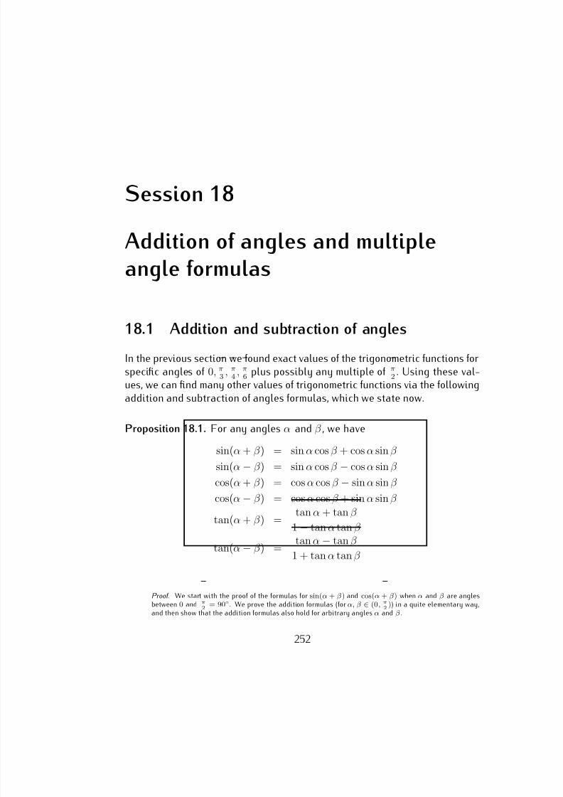
7/18/2019 Precalculus Tradler Carley
http://slidepdf.com/reader/full/precalculus-tradler-carley 262/424
Session 18
Addition of angles and multiple
angle formulas
18.1 Addition and subtraction of angles
In the previous section we found exact values of the trigonometric functions forspecific angles of 0, π
3 , π4 , π
6 plus possibly any multiple of π2 . Using these val-
ues, we can find many other values of trigonometric functions via the followingaddition and subtraction of angles formulas, which we state now.
Proposition 18.1. For any angles α and β , we have
sin(α + β ) = sin α cos β + cos α sin β
sin(α − β ) = sin α cos β − cos α sin β
cos(α + β ) = cos α cos β − sin α sin β
cos(α − β ) = cos α cos β + sin α sin β
tan(α + β ) = tan α + tan β
1 − tan α tan β
tan(α
−β ) =
tan α − tan β
1 + tan α tan β
Proof. We start with the proof of the formulas for sin(α + β) and cos(α + β) when α and β are anglesbetween 0 and π
2 = 90◦ . We prove the addition formulas (for α, β ∈ (0, π
2)) in a quite elementary way,
and then show that the addition formulas also hold for arbitrary angles α and β .
252
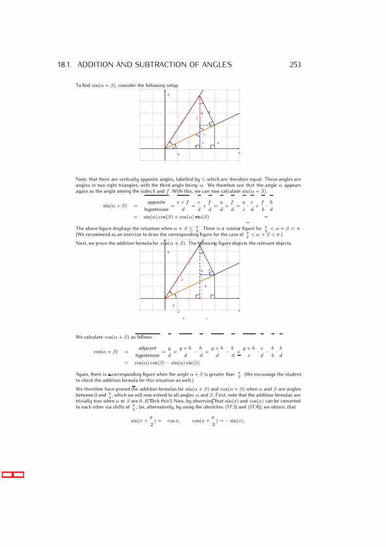
7/18/2019 Precalculus Tradler Carley
http://slidepdf.com/reader/full/precalculus-tradler-carley 263/424
18.1. ADDITION AND SUBTRACTION OF ANGLES 253
To find sin(α + β), consider the following setup.
x
y
α
β γ
γ
α
a
b
d
c
f
e
Note, that there are vertically opposite angles, labelled by γ , which are therefore equal. These angles areangles in two right triangles, with the third angle being α. We therefore see that the angle α appears
again as the angle among the sides b and f . With this, we can now calculate sin(α + β).
sin(α + β) = opposite
hypotenuse =
e + f
d =
e
d +
f
d =
a
d +
f
d =
a
c · c
d +
f
b · b
d
= sin(α) cos(β) + cos(α) sin(β)
The above figure displays the situation when α + β ≤ π2
. There is a similar figure for π2
< α + β < π.(We recommend as an exercise to draw the corresponding figure for the case of π
2 < α + β < π .)
Next, we prove the addition formula for cos(α + β). The following figure depicts the relevant objects.
x
y
α
β
α b
d
c
g h
k
We calculate cos(α + β) as follows.
cos(α + β) = adjacent
hypotenuse=
g
d=
g + h
d− h
d=
g + h
d− k
d=
g + h
c· c
d− k
b· b
d
= cos(α) cos(β) − sin(α) sin(β)
Again, there is a corresponding figure when the angle α + β is greater than π2
. (We encourage the studentto check the addition formula for this situation as well.)
We therefore have proved the addition formulas for sin(α + β) and cos(α + β) when α and β are anglesbetween 0 and π
2 , which we will now extend to all angles α and β . First, note that the addition formulas are
trivially true when α or β are 0. (Check this!) Now, by observing that sin(x) and cos(x) can be convertedto each other via shifts of π
2 , (or, alternatively, by using the identities (17.3) and (17.4)), we obtain, that
sin(x + π
2) = cos x, cos(x +
π
2) = − sin(x),
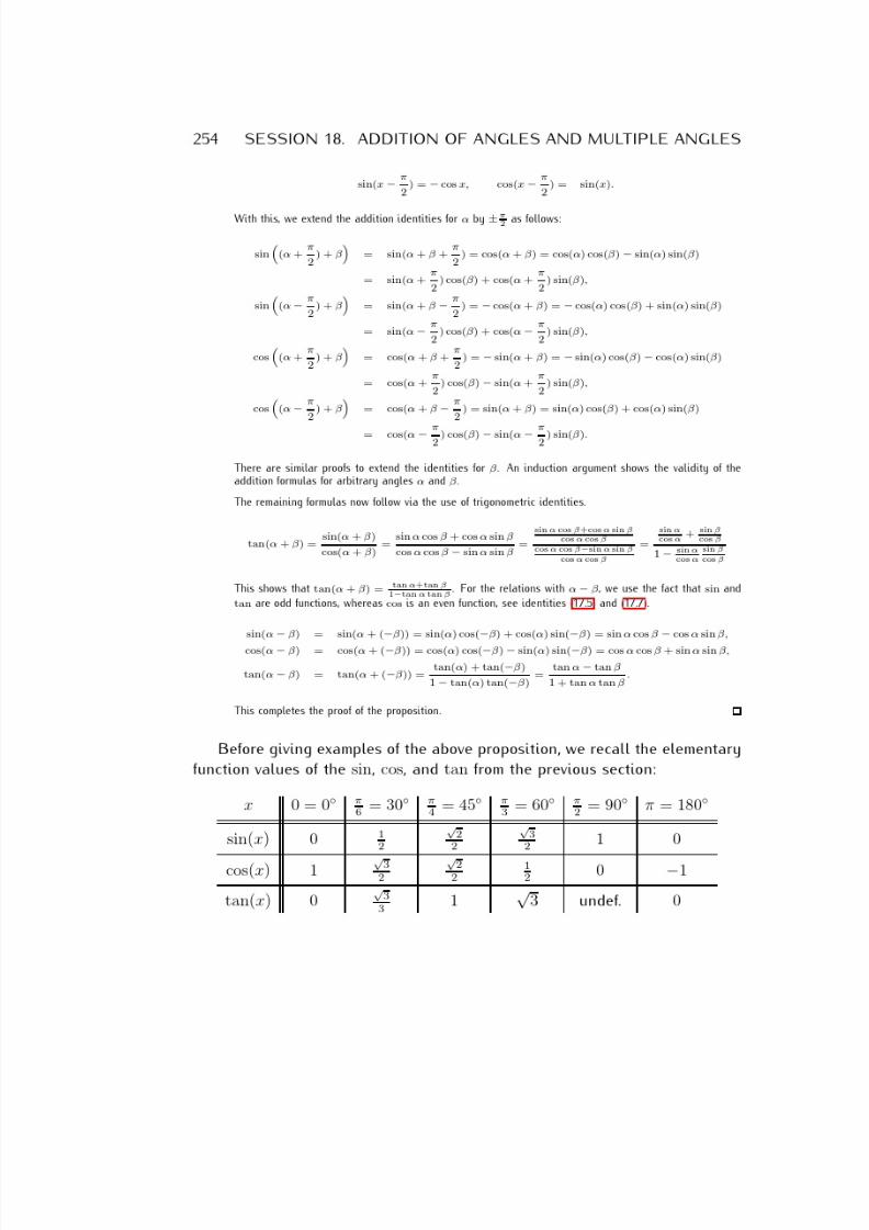
7/18/2019 Precalculus Tradler Carley
http://slidepdf.com/reader/full/precalculus-tradler-carley 264/424
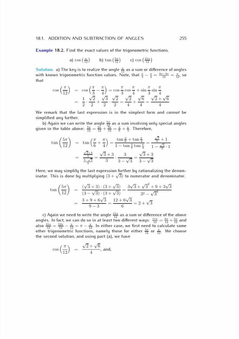
7/18/2019 Precalculus Tradler Carley
http://slidepdf.com/reader/full/precalculus-tradler-carley 265/424
7/18/2019 Precalculus Tradler Carley
http://slidepdf.com/reader/full/precalculus-tradler-carley 266/424
7/18/2019 Precalculus Tradler Carley
http://slidepdf.com/reader/full/precalculus-tradler-carley 267/424
18.2. DOUBLE AND HALF ANGLES 257
Proposition 18.5. Let α be an angle. Then we have the half-angle formulas:
sin α
2 = ±
1 − cos α
2
cos α
2 = ±
1 + cos α
2
tan α
2 =
1 − cos α
sin α =
sin α
1 + cos α = ±
1 − cos α
1 + cos α
Here, the signs “±” are determined by the quadrant in which the angle α2
lies. (For more on the signs, see also page 234.)
Furthermore, we have the double angle formulas:
sin(2α) = 2 sin α cos α
cos(2α) = cos2 α − sin2 α = 1 − 2sin2 α = 2cos2 α − 1
tan(2α) = 2tan α
1 − tan2 α
Proof. We start with the double angle formulas, which we prove using Proposition 18.1.
sin(2α) = sin(α + α) = sin α cos α + cos α sin α = 2sin α cos α
cos(2α) = cos(α + α) = cos α cos α
−sin α sin α = cos2 α
−sin2 α
tan(2α) = tan(α + α) = tan α + tan α
1 − tan α tan α=
2tan α
1− tan2 α
Notice that cos(2α) = cos2 α − sin2 α can be rewritten using sin2 α + cos2 α = 1 as follows:
cos2 α − sin2 α = (1 − sin2 α) − sin2 α = 1 − 2sin2 α
and cos2 α − sin2 α = cos2 α − (1 − cos2 α) = 2 cos2 α − 1
This shows the double angle formulas. These formulas can now be used to prove the half-angle formulas.
cos(2α) = 1 − 2sin2 α =⇒ 2sin2 α = 1 − cos(2α) =⇒ sin2 α = 1 − cos(2α)
2
=⇒ sin α = ±
1 − cos(2α)
2
replace α by α2=⇒ sin
α
2= ±
1 − cos α
2
cos(2α) = 2 cos2 α − 1 =⇒ 2cos2 α = 1 + cos(2α) =⇒ cos2 α = 1 + cos(2α)
2
=⇒ cos α = ±
1 + cos(2α)
2
replace α by α2=⇒ cos
α
2= ±
1 + cos α
2
in particular: tan α
2=
sin(α2
)
cos(α2
)=±
1−cosα2
±
1+cos α2
= ±
1 − cos α
1 + cos α
7/18/2019 Precalculus Tradler Carley
http://slidepdf.com/reader/full/precalculus-tradler-carley 268/424
7/18/2019 Precalculus Tradler Carley
http://slidepdf.com/reader/full/precalculus-tradler-carley 269/424
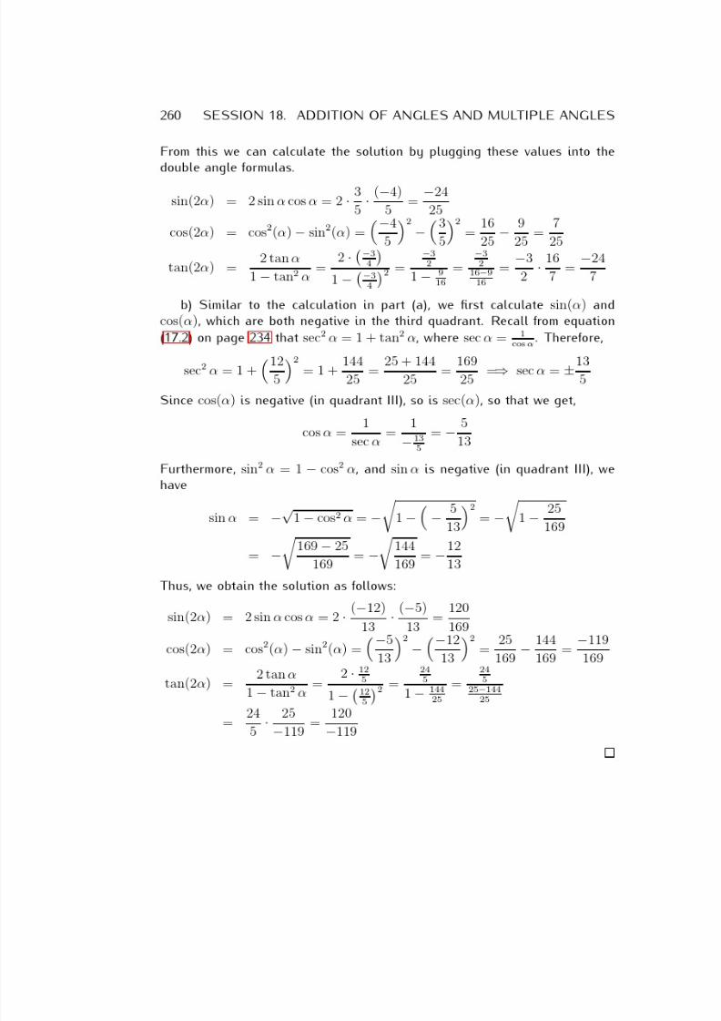
7/18/2019 Precalculus Tradler Carley
http://slidepdf.com/reader/full/precalculus-tradler-carley 270/424
7/18/2019 Precalculus Tradler Carley
http://slidepdf.com/reader/full/precalculus-tradler-carley 271/424
18.3. EXERCISES 261
18.3 Exercises
Exercise 18.1. Find the trigonometric function values.
a) sin
5π12
b) cos
5π12
c) tan
π
12
d) sin
7π12
e) cos
11π12
f ) sin
2π3
g) sin
5π6
h) cos
3π4
i) tan
13π12
j) cos
− π12
k) sin
11π12
l) sin
29π12
Exercise 18.2. Simplify the function f using the addition and subtractionformulas.
a) f (x) = sin x + π2 b) f (x) = cos x
− π
4 c) f (x) = tan (π
−x)
d) f (x) = sinπ
6 − x
e) f (x) = cos
x + 11π
12
f) f (x) = cos
2π3 − x
Exercise 18.3. Find the exact values of the trigonometric functions appliedto the given angles by using the half-angle formulas.
a) cos
π12
b) tan
π8
c) sin
π24
d) cos
π24
e) sin
9π8
f ) tan
3π8
g) sin
−π8
h) sin
13π24
Exercise 18.4. Find the exact values of the trigonometric functions of α
2 andof 2α by using the half-angle and double angle formulas.
a) sin(α) = 45 , and α in quadrant I
b) cos(α) = 713
, and α in quadrant IV
c) sin(α) = −35 , and α in quadrant III
d) tan(α) = 43 , and α in quadrant III
e) tan(α) = −512
, and α in quadrant II
f ) cos(α) = −23
, and α in quadrant II
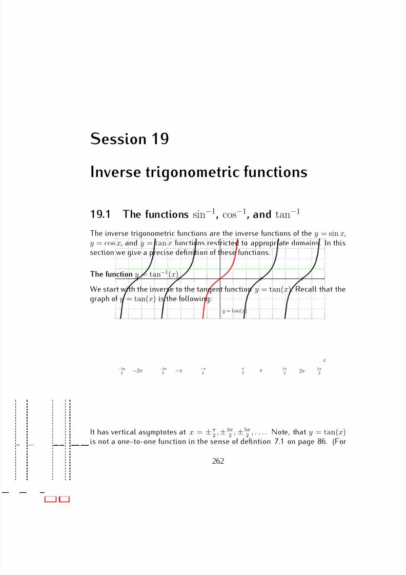
7/18/2019 Precalculus Tradler Carley
http://slidepdf.com/reader/full/precalculus-tradler-carley 272/424
Session 19
Inverse trigonometric functions
19.1 The functions sin−1, cos−1, and tan−1
The inverse trigonometric functions are the inverse functions of the y = sin x,y = cos x, and y = tan x functions restricted to appropriate domains. In thissection we give a precise definition of these functions.
The function y = tan−1(x)
We start with the inverse to the tangent function y = tan(x). Recall that the
graph of y = tan(x) is the following:
x
y = tan(x)
π2
−π2
π−π 3π2
−3π2 2π−2π 5π
2−5π
2
It has vertical asymptotes at x = ± π2 , ±3π
2 , ±5π2 , . . . . Note, that y = tan(x)
is not a one-to-one function in the sense of defintion 7.1 on page 86. (For
262
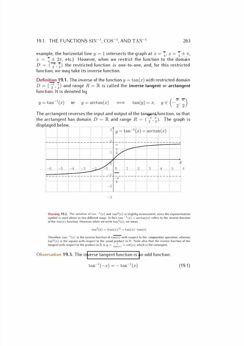
7/18/2019 Precalculus Tradler Carley
http://slidepdf.com/reader/full/precalculus-tradler-carley 273/424
19.1. THE FUNCTIONS SIN−1, COS−1, AND TAN−1 263
example, the horizontal line y = 1 intersects the graph at x = π4
, x = π4 ± π,
x = π
4 ± 2π, etc.) However, when we restrict the function to the domainD = (−π2 , π
2 ) the restricted function is one-to-one, and, for this restrictedfunction, we may take its inverse function.
Definition 19.1. The inverse of the function y = tan(x) with restricted domainD = (−π
2 , π
2) and range R = R is called the inverse tangent or arctangent
function. It is denoted by
y = tan−1(x) or y = arctan(x) ⇐⇒ tan(y) = x, y ∈−π
2, π
2
The arctangent reverses the input and output of the tangent function, so that
the arctangent has domain D = R and range R = (−π
2 , π
2 ). The graph isdisplayed below.
-6 -5 -4 -3 -2 -1 0 1 2 3 4 5 6
-3
-2
-1
0
1
2
3
x
y
π2
−π
2
= tan−1(x) = arctan(x)
Warning 19.2. The notation of tan−1(x) and tan2(x) is slightly inconsistent, since the exponentiationsymbol is used above in two different ways. In fact, tan−1(x) = arctan(x) refers to the inverse functionof the tan(x) function. However, when we write tan2(x), we mean
tan2(x) = (tan(x))2 = tan(x) · tan(x)
Therefore, tan−1(x) is the inverse function of tan(x) with respect to the composition operation, whereas
tan2
(x) is the square with respect to the usual product in R . Note also that the inverse function of thetangent with respect to the product in R is y = 1tan(x)
= cot(x), which is the cotangent.
Observation 19.3. The inverse tangent function is an odd function:
tan−1(−x) = − tan−1(x) (19.1)
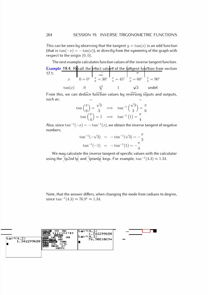
7/18/2019 Precalculus Tradler Carley
http://slidepdf.com/reader/full/precalculus-tradler-carley 274/424
264 SESSION 19. INVERSE TRIGONOMETRIC FUNCTIONS
This can be seen by observing that the tangent y = tan(x) is an odd function
(that is tan(−x) = − tan(x)), or directly from the symmetry of the graph withrespect to the origin (0, 0).
The next example calculates function values of the inverse tangent function.
Example 19.4. Recall the exact values of the tangent function from section17.1:
x 0 = 0◦ π6
= 30◦ π4
= 45◦ π3
= 60◦ π2
= 90◦
tan(x) 0√
33
1√
3 undef.
From this, we can deduce function values by reversing inputs and outputs,such as:
tanπ
6
=
√ 33
=⇒ tan−1√ 3
3
=
π
6
tanπ
4
= 1 =⇒ tan−1
1
= π
4
Also, since tan−1(−x) = − tan−1(x), we obtain the inverse tangent of negativenumbers.
tan−1(−√
3) = − tan−1(√
3) = −π
3
tan−1(−1) = − tan−1(1) = −π
4
We may calculate the inverse tangent of specific values with the calculatorusing the
lp2nd lp and
lptanlp keys. For example, tan−1(4.3) ≈ 1.34.
Note, that the answer differs, when changing the mode from radians to degree,since tan−1(4.3) ≈ 76.9◦ ≈ 1.34.
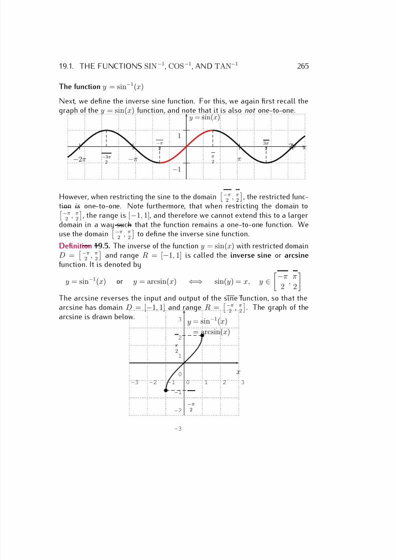
7/18/2019 Precalculus Tradler Carley
http://slidepdf.com/reader/full/precalculus-tradler-carley 275/424
19.1. THE FUNCTIONS SIN−1, COS−1, AND TAN−1 265
The function y = sin−1(x)
Next, we define the inverse sine function. For this, we again first recall thegraph of the y = sin(x) function, and note that it is also not one-to-one.
x
y = sin(x)
π2
−π2
π−π
3π2
−3π2
2π
−2π
1
−1
However, when restricting the sine to the domain −π2 , π2, the restricted func-
tion is one-to-one. Note furthermore, that when restricting the domain to−π2
, π2
, the range is [−1, 1], and therefore we cannot extend this to a larger
domain in a way such that the function remains a one-to-one function. Weuse the domain
−π2
, π2
to define the inverse sine function.
Definition 19.5. The inverse of the function y = sin(x) with restricted domainD =
−π2 , π
2
and range R = [−1, 1] is called the inverse sine or arcsine
function. It is denoted by
y = sin−1(x) or y = arcsin(x) ⇐⇒ sin(y) = x, y ∈−π
2 ,
π
2The arcsine reverses the input and output of the sine function, so that thearcsine has domain D = [−1, 1] and range R =
−π2
, π2
. The graph of the
arcsine is drawn below.
-3 -2 -1 0 1 2 3
-3
-2
-1
0
1
2
3
x
y = sin−1(x)
= arcsin(x)
π2
−π2
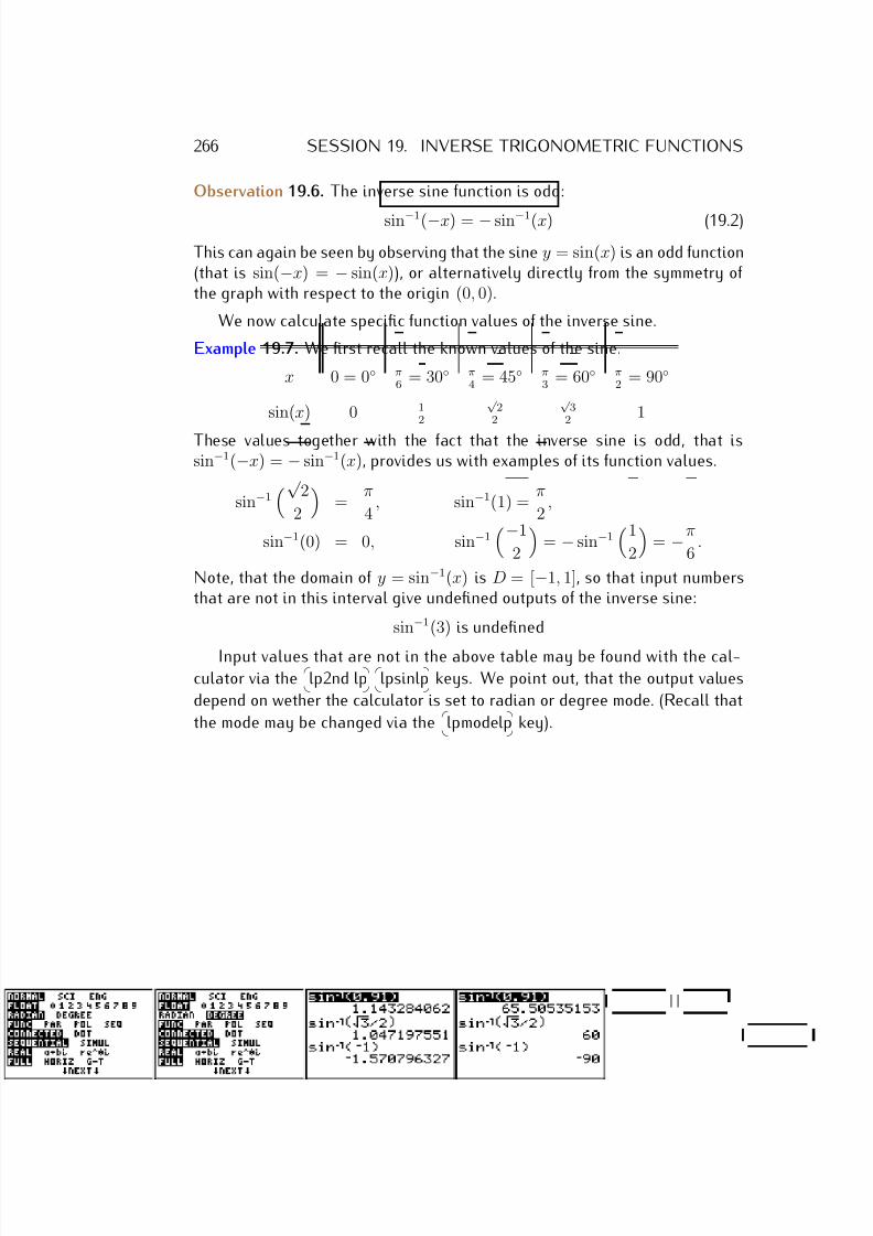
7/18/2019 Precalculus Tradler Carley
http://slidepdf.com/reader/full/precalculus-tradler-carley 276/424
266 SESSION 19. INVERSE TRIGONOMETRIC FUNCTIONS
Observation 19.6. The inverse sine function is odd:
sin−1(−x) = − sin−1(x) (19.2)
This can again be seen by observing that the sine y = sin(x) is an odd function(that is sin(−x) = − sin(x)), or alternatively directly from the symmetry of the graph with respect to the origin (0, 0).
We now calculate specific function values of the inverse sine.
Example 19.7. We first recall the known values of the sine.
x 0 = 0◦ π6
= 30◦ π4
= 45◦ π3
= 60◦ π2
= 90◦
sin(x) 0 12
√ 2
2
√ 3
2 1
These values together with the fact that the inverse sine is odd, that issin−1(−x) = − sin−1(x), provides us with examples of its function values.
sin−1√
2
2
=
π
4, sin−1(1) =
π
2,
sin−1(0) = 0, sin−1−1
2
= − sin−1
1
2
= −π
6.
Note, that the domain of y = sin−1(x) is D = [−1, 1], so that input numbersthat are not in this interval give undefined outputs of the inverse sine:
sin−1(3) is undefined
Input values that are not in the above table may be found with the cal-culator via the
lp2nd lp
lpsinlp keys. We point out, that the output values
depend on wether the calculator is set to radian or degree mode. (Recall that
the mode may be changed via the
lpmodelp key).
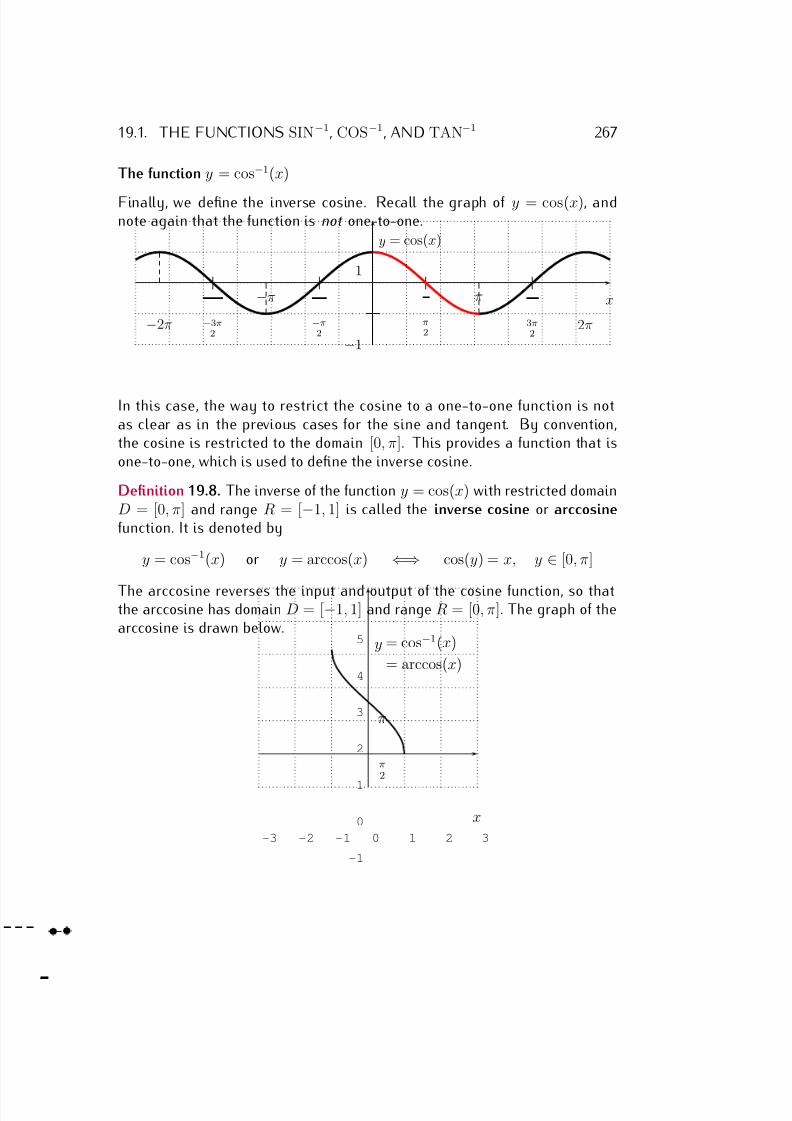
7/18/2019 Precalculus Tradler Carley
http://slidepdf.com/reader/full/precalculus-tradler-carley 277/424
19.1. THE FUNCTIONS SIN−1, COS−1, AND TAN−1 267
The function y = cos−1(x)
Finally, we define the inverse cosine. Recall the graph of y = cos(x), andnote again that the function is not one-to-one.
x
y = cos(x)
π2
−π2
π−π
3π2
−3π2
2π−2π
1
−1
In this case, the way to restrict the cosine to a one-to-one function is notas clear as in the previous cases for the sine and tangent. By convention,the cosine is restricted to the domain [0, π]. This provides a function that isone-to-one, which is used to define the inverse cosine.
Definition 19.8. The inverse of the function y = cos(x) with restricted domainD = [0, π] and range R = [−1, 1] is called the inverse cosine or arccosinefunction. It is denoted by
y = cos−1(x) or y = arccos(x) ⇐⇒ cos(y) = x, y ∈ [0, π]
The arccosine reverses the input and output of the cosine function, so thatthe arccosine has domain D = [−1, 1] and range R = [0, π]. The graph of thearccosine is drawn below.
-3 -2 -1 0 1 2 3
-1
0
1
2
3
4
5
x
y = cos−1(x)
= arccos(x)
π2
π
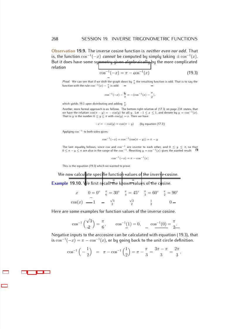
7/18/2019 Precalculus Tradler Carley
http://slidepdf.com/reader/full/precalculus-tradler-carley 278/424
268 SESSION 19. INVERSE TRIGONOMETRIC FUNCTIONS
Observation 19.9. The inverse cosine function is neither even nor odd . That
is, the function cos−1
(−x) cannot be computed by simply taking ± cos−1
(x).But it does have some symmetry given algebraically by the more complicatedrelation
cos−1(−x) = π − cos−1(x) (19.3)
Proof. We can see that if we shift the graph down by π2
the resulting function is odd. That is to say the
function with the rule cos−1(x) − π2
is odd:
cos−1(−x) − π
2 = −(cos−1(x) − π
2),
which yields 19.3 upon distributing and adding π2
.
Another, more formal approach is as follows. The bottom right relation of (17.3) on page 234 states, thatwe have the relation cos(π
−y) =
−cos(y) for all y . Let
−1
≤ x
≤ 1 , and denote by y = cos−1(x).
That is y is the number 0 ≤ y ≤ π with cos(y) = x. Then we have
−x = − cos(y) = cos(π − y) (by equation (17.3))
Applying cos−1 to both sides gives:
cos−1(−x) = cos−1(cos(π − y)) = π − y
The last equality follows, since cos and cos−1 are inverse to each other, and 0 ≤ y ≤ π, so that0 ≤ π − y ≤ π are also in the range of the cos−1. Rewriting y = cos−1(x) gives the wanted result:
cos−1(−x) = π − cos−1(x)
This is the equation (19.3) which we wanted to prove.
We now calculate specific function values of the inverse cosine.
Example 19.10. We first recall the known values of the cosine.
x 0 = 0◦ π6 = 30◦ π
4 = 45◦ π3 = 60◦ π
2 = 90◦
cos(x) 1√
32
√ 2
212 0
Here are some examples for function values of the inverse cosine.
cos−1
√
3
2 = π
6, cos−1(1) = 0, cos−1(0) =
π
2.
Negative inputs to the arccosine can be calculated with equation (19.3), thatis cos−1(−x) = π − cos−1(x), or by going back to the unit circle definition.
cos−1
− 1
2
= π − cos−1
1
2
= π − π
3 =
3π − π
3 =
2π
3 ,
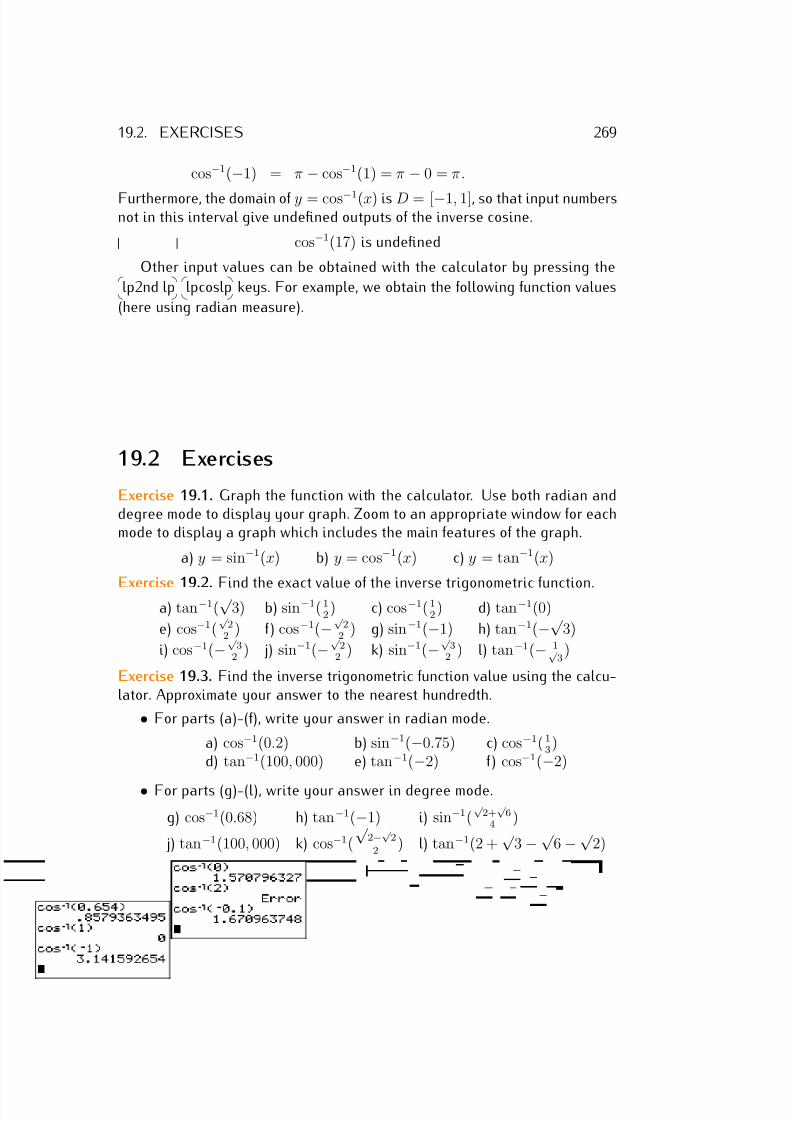
7/18/2019 Precalculus Tradler Carley
http://slidepdf.com/reader/full/precalculus-tradler-carley 279/424
19.2. EXERCISES 269
cos−1(−1) = π − cos−1(1) = π − 0 = π.
Furthermore, the domain of y = cos−1(x) is D = [−1, 1], so that input numbersnot in this interval give undefined outputs of the inverse cosine.
cos−1(17) is undefined
Other input values can be obtained with the calculator by pressing the
lp2nd lp
lpcoslp keys. For example, we obtain the following function values
(here using radian measure).
19.2 Exercises
Exercise 19.1. Graph the function with the calculator. Use both radian anddegree mode to display your graph. Zoom to an appropriate window for eachmode to display a graph which includes the main features of the graph.
a) y = sin−1(x) b) y = cos−1(x) c) y = tan−1(x)
Exercise 19.2. Find the exact value of the inverse trigonometric function.a) tan−1(
√ 3) b) sin−1( 1
2) c) cos−1( 1
2) d) tan−1(0)
e) cos−1(√
22 ) f ) cos−1(−
√ 2
2 ) g) sin−1(−1) h) tan−1(−√ 3)
i) cos−1(−√
32
) j) sin−1(−√
22
) k) sin−1(−√
32
) l) tan−1(− 1√ 3
)
Exercise 19.3. Find the inverse trigonometric function value using the calcu-lator. Approximate your answer to the nearest hundredth.
• For parts (a)-(f), write your answer in radian mode.
a) cos−1(0.2) b) sin−1(−0.75) c) cos−1( 13 )
d) tan−1(100, 000) e) tan−1(−2) f) cos−1(−2)
• For parts (g)-(l), write your answer in degree mode.
g) cos−1(0.68) h) tan−1(−1) i) sin−1(√
2+√
64 )
j) tan−1(100, 000) k) cos−1(
√ 2−√ 2
2 ) l) tan−1(2 +
√ 3 − √
6 − √ 2)
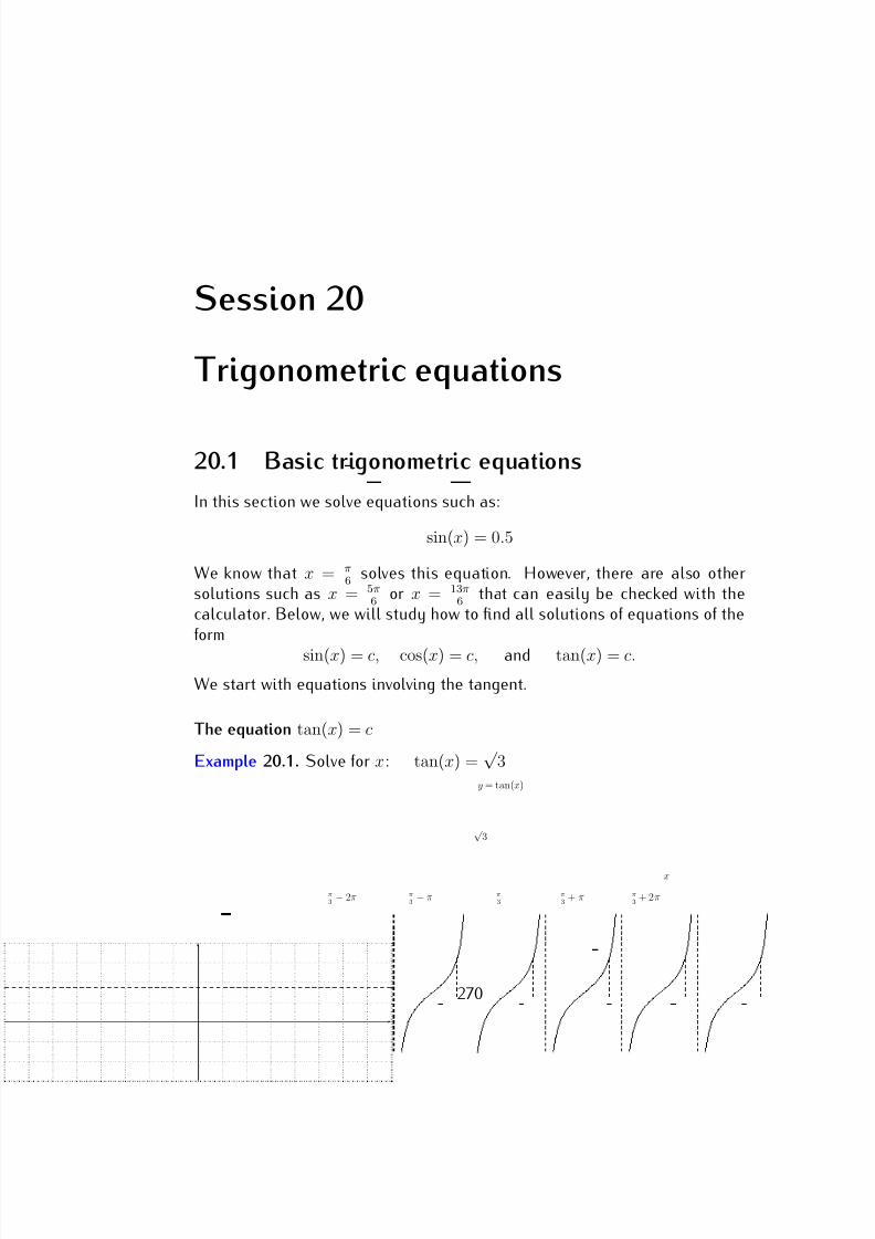
7/18/2019 Precalculus Tradler Carley
http://slidepdf.com/reader/full/precalculus-tradler-carley 280/424
Session 20
Trigonometric equations
20.1 Basic trigonometric equations
In this section we solve equations such as:
sin(x) = 0.5
We know that x = π6 solves this equation. However, there are also other
solutions such as x = 5π6 or x = 13π
6 that can easily be checked with thecalculator. Below, we will study how to find all solutions of equations of theform
sin(x) = c, cos(x) = c, and tan(x) = c.
We start with equations involving the tangent.
The equation tan(x) = c
Example 20.1. Solve for x: tan(x) =√
3
x
y = tan(x)
√ 3
π3
π3
+ π π3
+ 2ππ3 − ππ
3 − 2π
270
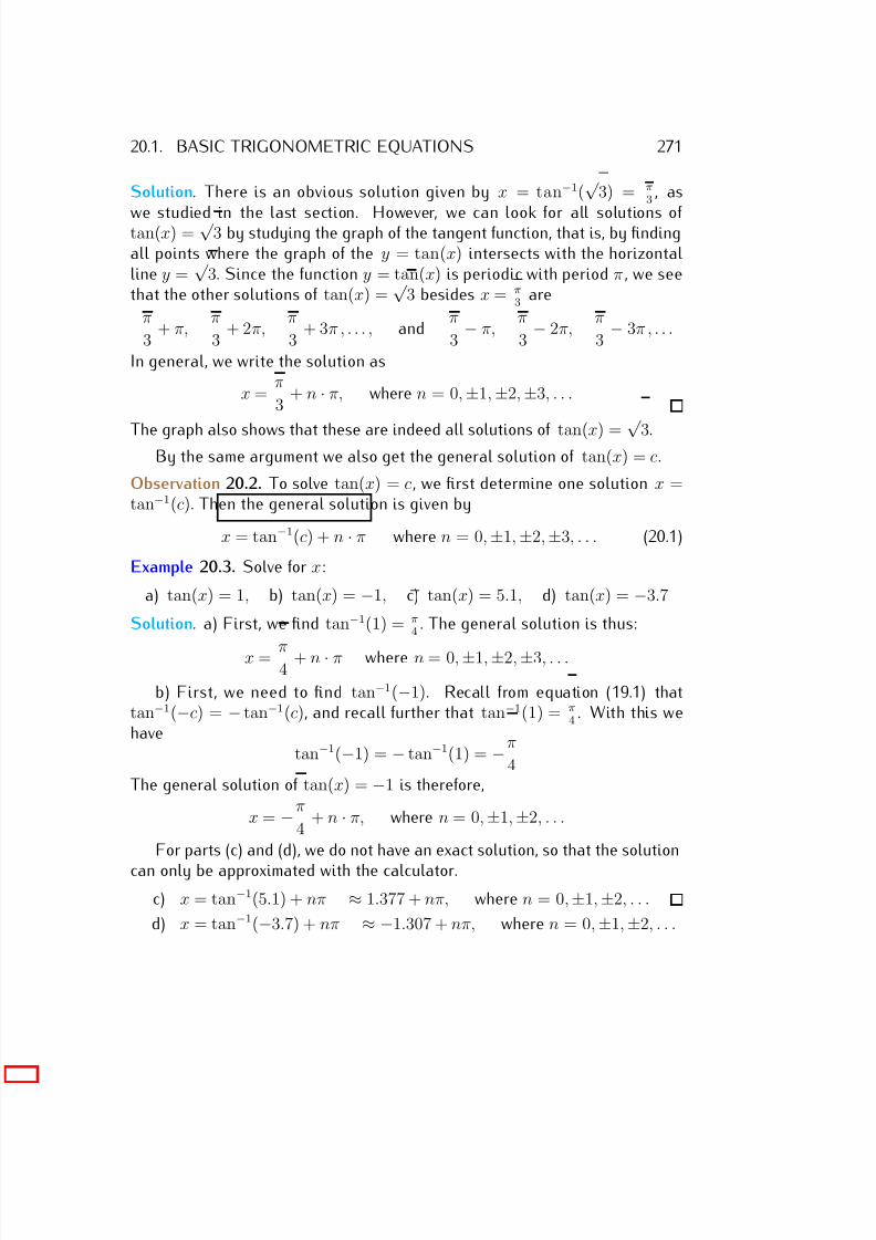
7/18/2019 Precalculus Tradler Carley
http://slidepdf.com/reader/full/precalculus-tradler-carley 281/424
20.1. BASIC TRIGONOMETRIC EQUATIONS 271
Solution. There is an obvious solution given by x = tan−1(√
3) = π3
, as
we studied in the last section. However, we can look for all solutions of tan(x) = √ 3 by studying the graph of the tangent function, that is, by findingall points where the graph of the y = tan(x) intersects with the horizontalline y =
√ 3. Since the function y = tan(x) is periodic with period π , we see
that the other solutions of tan(x) =√
3 besides x = π3
are
π
3 + π,
π
3 + 2π,
π
3 + 3π , . . . , and
π
3 − π,
π
3 − 2π,
π
3 − 3π , . . .
In general, we write the solution as
x = π
3 + n · π, where n = 0, ±1, ±2, ±3, . . .
The graph also shows that these are indeed all solutions of tan(x) = √ 3.By the same argument we also get the general solution of tan(x) = c.
Observation 20.2. To solve tan(x) = c, we first determine one solution x =tan−1(c). Then the general solution is given by
x = tan−1(c) + n · π where n = 0, ±1, ±2, ±3, . . . (20.1)
Example 20.3. Solve for x:
a) tan(x) = 1, b) tan(x) = −1, c) tan(x) = 5.1, d) tan(x) = −3.7
Solution. a) First, we find tan−1(1) = π4
. The general solution is thus:
x = π4
+ n · π where n = 0, ±1, ±2, ±3, . . .
b) First, we need to find tan−1(−1). Recall from equation (19.1) thattan−1(−c) = − tan−1(c), and recall further that tan−1(1) = π
4 . With this wehave
tan−1(−1) = − tan−1(1) = −π
4The general solution of tan(x) = −1 is therefore,
x = −π
4 + n · π, where n = 0, ±1, ±2, . . .
For parts (c) and (d), we do not have an exact solution, so that the solution
can only be approximated with the calculator.
c) x = tan−1(5.1) + nπ ≈ 1.377 + nπ, where n = 0, ±1, ±2, . . .
d) x = tan−1(−3.7) + nπ ≈ −1.307 + nπ, where n = 0, ±1, ±2, . . .
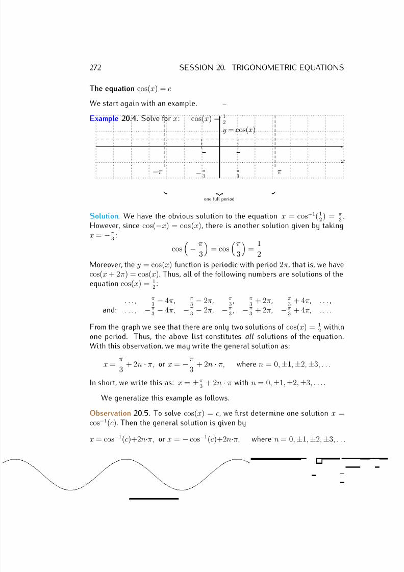
7/18/2019 Precalculus Tradler Carley
http://slidepdf.com/reader/full/precalculus-tradler-carley 282/424
272 SESSION 20. TRIGONOMETRIC EQUATIONS
The equation cos(x) = c
We start again with an example.
Example 20.4. Solve for x: cos(x) = 12
x
y = cos(x)
π3
−π3
π−π
one full period
Solution. We have the obvious solution to the equation x = cos−1( 12 ) = π
3 .However, since cos(−x) = cos(x), there is another solution given by takingx = −π
3 :
cos
− π
3
= cos
π
3
=
1
2
Moreover, the y = cos(x) function is periodic with period 2π, that is, we havecos(x + 2π) = cos(x). Thus, all of the following numbers are solutions of theequation cos(x) = 1
2:
. . . , π3 − 4π, π3 − 2π, π3 , π3 + 2π, π3 + 4π, . . . ,and: . . . , −π
3 − 4π, −π3 − 2π, −π
3 , −π3 + 2π, −π
3 + 4π, . . . .
From the graph we see that there are only two solutions of cos(x) = 12
withinone period. Thus, the above list constitutes all solutions of the equation.With this observation, we may write the general solution as:
x = π
3 + 2n · π, or x = −π
3 + 2n · π, where n = 0, ±1, ±2, ±3, . . .
In short, we write this as: x = ±π3
+ 2n · π with n = 0, ±1, ±2, ±3, . . . .
We generalize this example as follows.Observation 20.5. To solve cos(x) = c, we first determine one solution x =cos−1(c). Then the general solution is given by
x = cos−1(c)+2n·π, or x = − cos−1(c)+2n·π, where n = 0, ±1, ±2, ±3, . . .
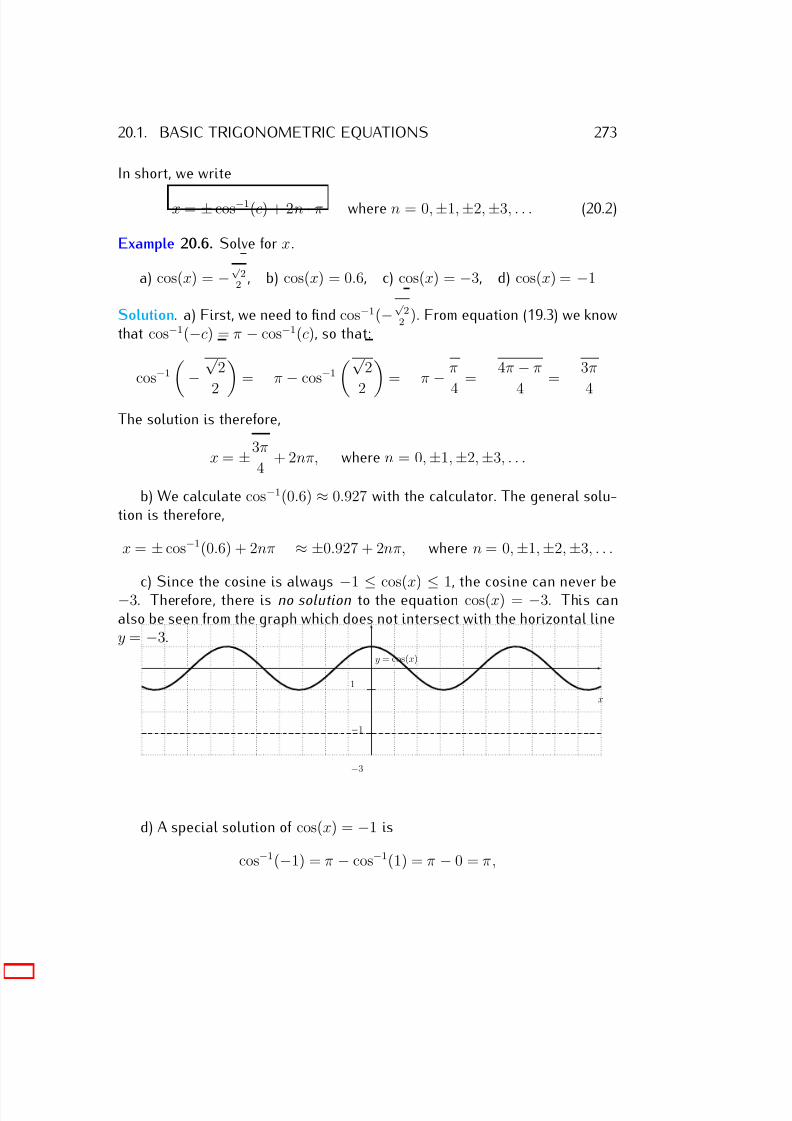
7/18/2019 Precalculus Tradler Carley
http://slidepdf.com/reader/full/precalculus-tradler-carley 283/424
20.1. BASIC TRIGONOMETRIC EQUATIONS 273
In short, we write
x = ± cos−1(c) + 2n · π where n = 0, ±1, ±2, ±3, . . . (20.2)
Example 20.6. Solve for x.
a) cos(x) = −√
22 , b) cos(x) = 0.6, c) cos(x) = −3, d) cos(x) = −1
Solution. a) First, we need to find cos−1(−√
22
). From equation (19.3) we knowthat cos−1(−c) = π − cos−1(c), so that:
cos−1 −
√ 2
2 = π
−cos−1
√ 2
2 = π
− π
4
= 4π − π
4
= 3π
4
The solution is therefore,
x = ±3π
4 + 2nπ, where n = 0, ±1, ±2, ±3, . . .
b) We calculate cos−1(0.6) ≈ 0.927 with the calculator. The general solu-tion is therefore,
x = ± cos−1(0.6) + 2nπ ≈ ±0.927 + 2nπ, where n = 0, ±1, ±2, ±3, . . .
c) Since the cosine is always −1 ≤ cos(x) ≤ 1, the cosine can never be−3. Therefore, there is no solution to the equation cos(x) = −3. This canalso be seen from the graph which does not intersect with the horizontal liney = −3.
x
y = cos(x)
−3
1
−1
d) A special solution of cos(x) = −1 is
cos−1(−1) = π − cos−1(1) = π − 0 = π,
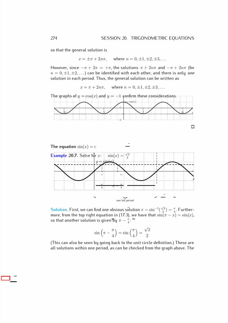
7/18/2019 Precalculus Tradler Carley
http://slidepdf.com/reader/full/precalculus-tradler-carley 284/424
274 SESSION 20. TRIGONOMETRIC EQUATIONS
so that the general solution is
x = ±π + 2nπ, where n = 0, ±1, ±2, ±3, . . .
However, since −π + 2π = +π, the solutions π + 2nπ and −π + 2nπ (forn = 0, ±1, ±2, . . . ) can be identified with each other, and there is only one
solution in each period. Thus, the general solution can be written as
x = π + 2nπ, where n = 0, ±1, ±2, ±3, . . .
The graphs of y = cos(x) and y = −1 confirm these considerations.
x
y = cos(x)
1
−1
π 3π−π−3π
The equation sin(x) = c
Example 20.7. Solve for x: sin(x) =√
22
x
y = sin(x)
π4 π − π
4
one full period
Solution. First, we can find one obvious solution x = sin−1(√
22 ) = π
4 . Further-more, from the top right equation in (17.3), we have that sin(π − x) = sin(x),so that another solution is given by π − π
4:
sin
π − π
4
= sin
π
4
=
√ 22
(This can also be seen by going back to the unit circle definition.) These areall solutions within one period, as can be checked from the graph above. The
7/18/2019 Precalculus Tradler Carley
http://slidepdf.com/reader/full/precalculus-tradler-carley 285/424
20.1. BASIC TRIGONOMETRIC EQUATIONS 275
function y = sin(x) is periodic with period 2π, so that adding 2n · π for any
n = 0, ±1, ±2, . . . gives all solutions of sin(x) =
√ 2
2 . This means that thegeneral solution is:
x = π
4 + 2n · π, or x = (π − π
4) + 2n · π, for n = 0, ±1, ±2, ±3, . . .
We rewrite these solutions to obtain one single formula for the solutions.Note, that π − π
4 + 2n · π = −π
4 + (2n + 1) · π. Therefore, all solutions are of
the form
x = ±π
4 + k · π
where, for even k = 2n, the sign in front of π
4
is “+,” and, for odd k = 2n + 1,the sign in front of π
4 is “−.” This can be summarized as:
x = (−1)k · π
4 + k · π
Renaming the indexing variable k to the usual n, we obtain the final version
for the solutions of sin(x) =√
22 .
x = (−1)n · π
4 + n · π, where n = 0, ±1, ±2, ±3, . . .
We have the following general statement.
Observation 20.8. To solve sin(x) = c, we first determine one solution x =sin−1(c). Then the general solution is given by
x = (−1)n · sin−1(c) + n · π where n = 0, ±1, ±2, ±3, . . . (20.3)
Example 20.9. Solve for x.
a) sin(x) = 1
2 b) sin(x) = −1
2 c) sin(x) = −5
7 d) sin(x) = 1
Solution. a) First, we calculate sin−1( 12
) = π6
. The general solution is there-fore,
x = (−1)n · π
6 + n · π, where n = 0, ±1, ±2, ±3, . . .
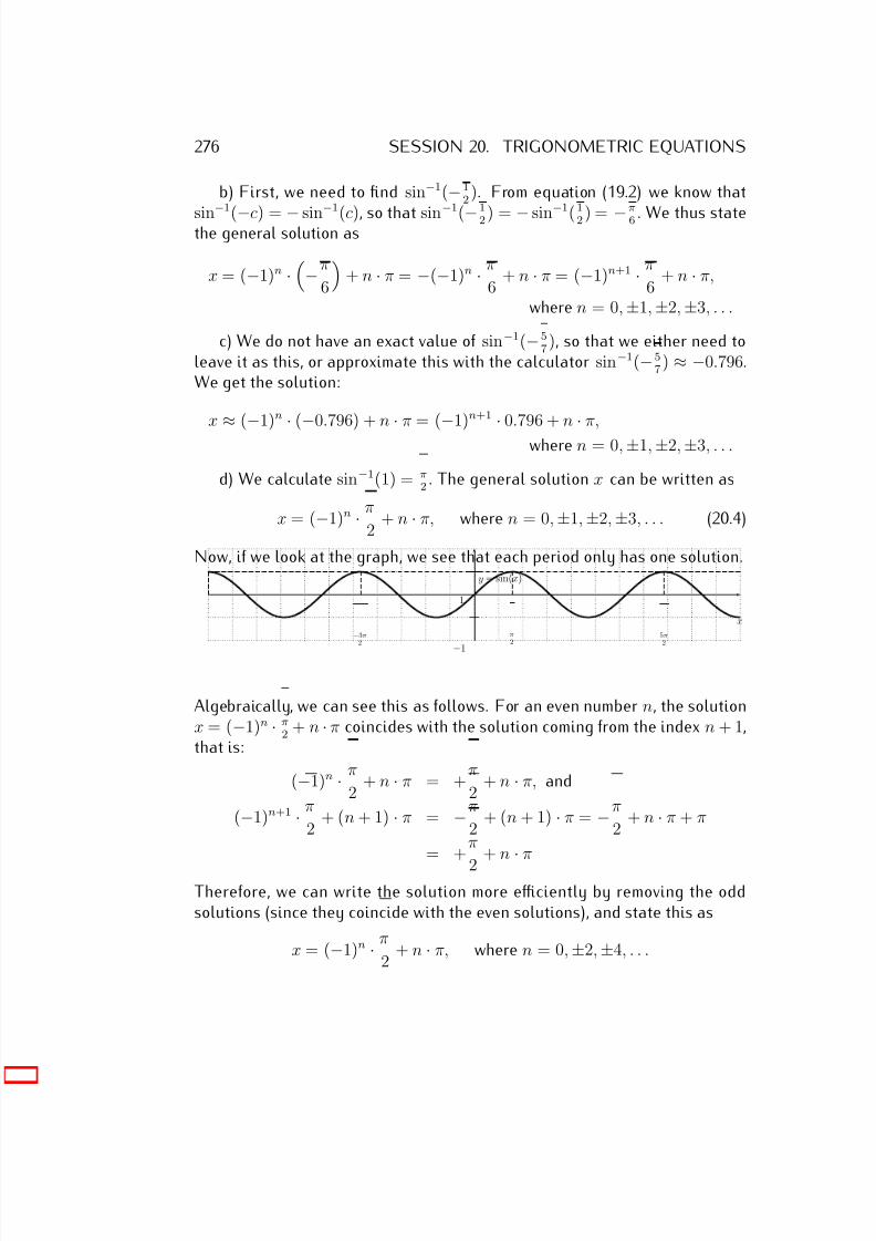
7/18/2019 Precalculus Tradler Carley
http://slidepdf.com/reader/full/precalculus-tradler-carley 286/424
276 SESSION 20. TRIGONOMETRIC EQUATIONS
b) First, we need to find sin−1(−12
). From equation (19.2) we know that
sin−1
(−c) = − sin−1
(c), so that sin−1
(−1
2 ) = − sin−1
(1
2 ) = −π
6 . We thus statethe general solution as
x = (−1)n ·−π
6
+ n · π = −(−1)n · π
6 + n · π = (−1)n+1 · π
6 + n · π,
where n = 0, ±1, ±2, ±3, . . .
c) We do not have an exact value of sin−1(−57
), so that we either need toleave it as this, or approximate this with the calculator sin−1(−5
7 ) ≈ −0.796.We get the solution:
x
≈(
−1)n
·(
−0.796) + n
·π = (
−1)n+1
·0.796 + n
·π,
where n = 0, ±1, ±2, ±3, . . .
d) We calculate sin−1(1) = π2 . The general solution x can be written as
x = (−1)n · π
2 + n · π, where n = 0, ±1, ±2, ±3, . . . (20.4)
Now, if we look at the graph, we see that each period only has one solution.
x
y = sin(x)
1
−1
π2
5π2
−3π2
Algebraically, we can see this as follows. For an even number n, the solutionx = (−1)n · π
2 + n · π coincides with the solution coming from the index n + 1,that is:
(−1)n · π
2 + n · π = +
π
2 + n · π, and
(−1)n+1 · π
2 + (n + 1) · π = −π
2 + (n + 1) · π = −π
2 + n · π + π
= +π
2
+ n
·π
Therefore, we can write the solution more efficiently by removing the oddsolutions (since they coincide with the even solutions), and state this as
x = (−1)n · π
2 + n · π, where n = 0, ±2, ±4, . . .
7/18/2019 Precalculus Tradler Carley
http://slidepdf.com/reader/full/precalculus-tradler-carley 287/424
20.1. BASIC TRIGONOMETRIC EQUATIONS 277
Since (−1)n = +1 for even n, we can just write this as
x = π2
+ 2n · π, where n = 0, ±1, ±2, ±3, . . . (20.5)
Writing the solutions as x = π2 + 2n · π as in (20.5) instead of the original
x = (−1)n · π2
+ n · π from (20.4) for n = 0, ±1, ±2, . . . certainly does notchange the overall solution set. However, writing the solutions as in (20.5) ismore efficient, since it does not repeat any of the solutions, and is thereforea simplified and preferred way of presenting the solutions.
Summary
We summarize the different formulas we used to solve the basic trigonometricequations in the following table.
Solve: sin(x) = c Solve: cos(x) = c Solve: tan(x) = c
First, find one solution, First, find one solution, First, find one solution,that is: sin−1(c). Use: that is: cos−1(c). Use: that is: tan−1(c). Use:
sin−1(−c) = − sin−1(c) cos−1(−c) = π − cos−1(c) tan−1(−c) = − tan−1(c)
The general solution is: The general solution is: The general solution is:
x = (−
1)n sin−1(c) + nπ x =±
cos−1(c) + 2nπ x = tan−1(c) + nπ
where n = 0, ±1, ±2, . . . where n = 0, ±1, ±2, . . . where n = 0, ±1, ±2, . . .
Example 20.10. Find the general solution of the equation, and state at least5 distinct solutions.
a) sin(x) = −12 b) cos(x) = −
√ 3
2
Solution. a) We already calculated the general solution in example 20.9 (b).It is
x = (−1)n+1 · π
6 + n · π, where n = 0, ±1, ±2, ±3, . . .
We simplify the solutions for n = 0, 1, −1, 2, −2.
n = 0 : x = (−1)0+1 · π6
+ 0 · π = −π
6
n = 1 : x = (−1)1+1 · π6
+ 1 · π = π
6 + π =
π + 6π
6 =
7π
6
7/18/2019 Precalculus Tradler Carley
http://slidepdf.com/reader/full/precalculus-tradler-carley 288/424
278 SESSION 20. TRIGONOMETRIC EQUATIONS
n =
−1 : x = (
−1)−1+1
·
π
6
+ (
−1)
·π =
π
6 −π =
π − 6π
6
= −5π
6n = 2 : x = (−1)2+1 · π
6 + 2 · π = −π
6 + 2π =
−π + 12π
6 =
11π
6
n = −2 : x = (−1)−2+1 · π
6 + (−2) · π = −π
6 − 2π =
−π − 12π
6 =
−13π
6
b) It is cos−1(−√
32 ) = π − cos−1(
√ 3
2 ) = π − π6 = 6π−π
6 = 5π6 . The solutions
of cos(x) = −√
32 are:
x = ±5π
6 + 2nπ, where n = 0, ±1, ±2, ±3, . . .
We write the 6 solutions with n = 0, +1,−
1, and for each use the two distinctfirst terms + 5π
6 and −5π6 .
n = 0 : x = +5π
6 + 2 · 0 · π =
5π
6
n = 0 : x = −5π
6 + 2 · 0 · π = −5π
6
n = 1 : x = +5π
6 + 2 · 1 · π =
5π
6 + 2π =
5π + 12π
6 =
17π
6
n = 1 : x = −5π
6 + 2 · 1 · π = −5π
6 + 2π =
−5π + 12π
6 =
7π
6
n = −1 : x = +
5π
6 + 2 · (−1) · π =
5π
6 − 2π =
5π
−12π
6 = −7π
6
n = −1 : x = −5π
6 + 2 · (−1) · π = −5π
6 − 2π =
−5π − 12π
6 =
−17π
6
Further solutions can be found by taking values n = +2, −2, +3, −3, . . . .
20.2 Equations involving trigonometric functions
The previous section showed how to solve the basic trigonometric equations
sin(x) = c, cos(x) = c, and tan(x) = c.
The next examples can be reduced to these basic equations.
Example 20.11. Solve for x.
a) 2 sin(x) − 1 = 0 b) sec(x) = −√ 2 c) 7 cot(x) + 3 = 0
7/18/2019 Precalculus Tradler Carley
http://slidepdf.com/reader/full/precalculus-tradler-carley 289/424
20.2. EQUATIONS INVOLVING TRIGONOMETRIC FUNCTIONS 279
Solution. a) Solving for sin(x), we get
2sin(x) − 1 = 0 (+1)=⇒ 2sin(x) = 1
(÷2)=⇒ sin(x) =
1
2
One solution of sin(x) = 12 is sin−1( 1
2 ) = π6 . The general solution is
x = (−1)n · π
6 + nπ, where n = 0, ±1, ±2, . . .
b) Recall that sec(x) = 1cos(x) . Therefore,
sec(x) =
−
√ 2 =
⇒
1
cos(x)
=
−
√ 2
(reciprocal)=
⇒ cos(x) =
−
1
√ 2=
−
√ 2
2
A special solution of cos(x) = −√
22
is
cos−1(−√
2
2 ) = π − cos−1(
√ 2
2 ) = π − π
4 =
4π − π
4 =
3π
4 .
The general solution is
x = ±3π
4 + 2nπ, where n = 0, ±1, ±2, . . .
c) Recall that cot(x) = 1
tan(x)
. So
7 cot(x) + 3 = 0 (−3)
=⇒ 7cot(x) = −3 (÷7)=⇒ cot(x) = −3
7
=⇒ 1
tan(x) = −3
7
(reciprocal)=⇒ tan(x) = −7
3
The solution is
x = tan−1
−7
3
+ nπ ≈ −1.166 + nπ, where n = 0, ±1, ±2, . . .
For some of the more advanced problems it can be helpful to substituteu for a trigonometric expression first, then solve for u, and finally apply therules from the previous section to solve for the wanted variable. This methodis used in the next example.
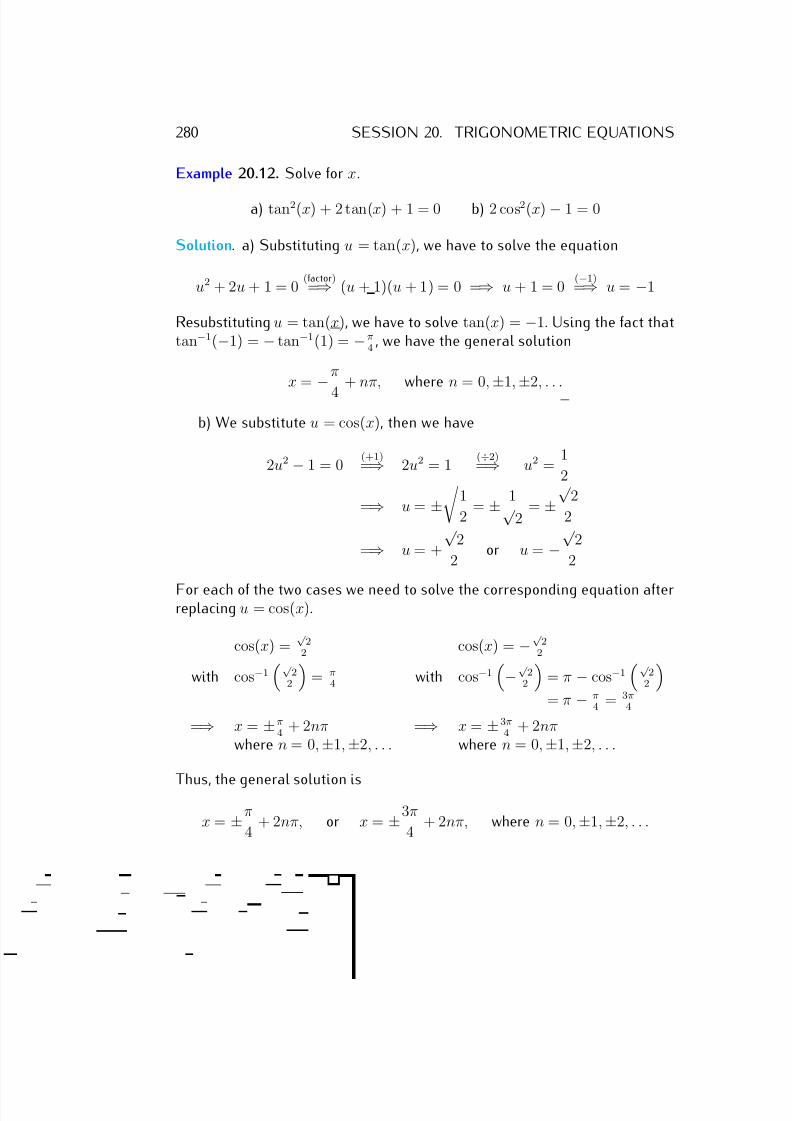
7/18/2019 Precalculus Tradler Carley
http://slidepdf.com/reader/full/precalculus-tradler-carley 290/424
280 SESSION 20. TRIGONOMETRIC EQUATIONS
Example 20.12. Solve for x.
a) tan2(x) + 2 tan(x) + 1 = 0 b) 2 cos2(x) − 1 = 0
Solution. a) Substituting u = tan(x), we have to solve the equation
u2 + 2u + 1 = 0 (factor)
=⇒ (u + 1)(u + 1) = 0 =⇒ u + 1 = 0 (−1)=⇒ u = −1
Resubstituting u = tan(x), we have to solve tan(x) = −1. Using the fact thattan−1(−1) = − tan−1(1) = −π
4 , we have the general solution
x =−
π
4 + nπ, where n = 0,
±1,
±2, . . .
b) We substitute u = cos(x), then we have
2u2 − 1 = 0 (+1)
=⇒ 2u2 = 1 (÷2)
=⇒ u2 = 1
2
=⇒ u = ±
1
2 = ± 1√
2= ±
√ 2
2
=⇒ u = +
√ 2
2 or u = −
√ 2
2
For each of the two cases we need to solve the corresponding equation afterreplacing u = cos(x).
cos(x) =√
22
cos(x) = −√
22
with cos−1√
22
= π
4 with cos−1−√
22
= π − cos−1
√ 2
2
= π − π
4 = 3π4
=⇒ x = ±π4
+ 2nπ =⇒ x = ±3π4
+ 2nπwhere n = 0, ±1, ±2, . . . where n = 0, ±1, ±2, . . .
Thus, the general solution is
x = ±π
4 + 2nπ, or x = ±3π
4 + 2nπ, where n = 0, ±1, ±2, . . .
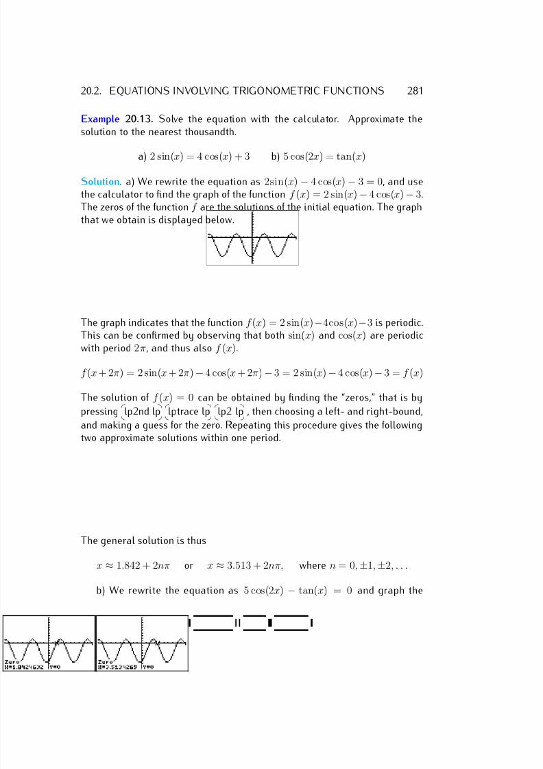
7/18/2019 Precalculus Tradler Carley
http://slidepdf.com/reader/full/precalculus-tradler-carley 291/424
20.2. EQUATIONS INVOLVING TRIGONOMETRIC FUNCTIONS 281
Example 20.13. Solve the equation with the calculator. Approximate the
solution to the nearest thousandth.
a) 2 sin(x) = 4 cos(x) + 3 b) 5 cos(2x) = tan(x)
Solution. a) We rewrite the equation as 2sin(x) − 4 cos(x) − 3 = 0, and usethe calculator to find the graph of the function f (x) = 2 sin(x) − 4 cos(x) − 3.The zeros of the function f are the solutions of the initial equation. The graphthat we obtain is displayed below.
The graph indicates that the function f (x) = 2 sin(x)−4cos(x)−3 is periodic.This can be confirmed by observing that both sin(x) and cos(x) are periodicwith period 2π, and thus also f (x).
f (x + 2π) = 2 sin(x + 2π) − 4 cos(x + 2π) − 3 = 2 sin(x) − 4 cos(x) − 3 = f (x)
The solution of f (x) = 0 can be obtained by finding the “zeros,” that is by
pressing
lp2nd lp
lptrace lp
lp2 lp , then choosing a left- and right-bound,
and making a guess for the zero. Repeating this procedure gives the followingtwo approximate solutions within one period.
The general solution is thus
x ≈ 1.842 + 2nπ or x ≈ 3.513 + 2nπ, where n = 0, ±1, ±2, . . .
b) We rewrite the equation as 5 cos(2x) − tan(x) = 0 and graph the
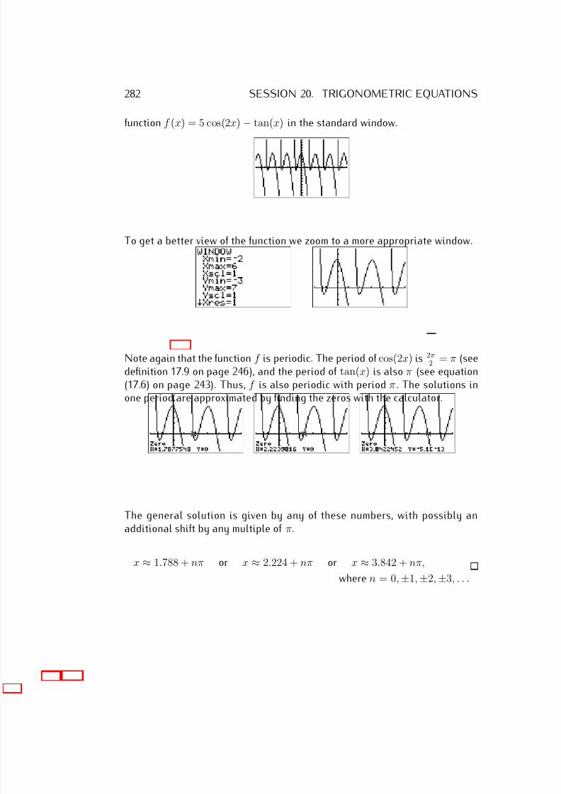
7/18/2019 Precalculus Tradler Carley
http://slidepdf.com/reader/full/precalculus-tradler-carley 292/424
282 SESSION 20. TRIGONOMETRIC EQUATIONS
function f (x) = 5 cos(2x) − tan(x) in the standard window.
To get a better view of the function we zoom to a more appropriate window.
Note again that the function f is periodic. The period of cos(2x) is 2π2 = π (see
definition 17.9 on page 246), and the period of tan(x) is also π (see equation(17.6) on page 243). Thus, f is also periodic with period π . The solutions inone period are approximated by finding the zeros with the calculator.
The general solution is given by any of these numbers, with possibly anadditional shift by any multiple of π.
x ≈ 1.788 + nπ or x ≈ 2.224 + nπ or x ≈ 3.842 + nπ,
where n = 0, ±1, ±2, ±3, . . .
7/18/2019 Precalculus Tradler Carley
http://slidepdf.com/reader/full/precalculus-tradler-carley 293/424
20.3. EXERCISES 283
20.3 Exercises
Exercise 20.1. Find all solutions of the equation, and simplify as much aspossible. Do not approximate the solution.
a) tan(x) =√
33 b) sin(x) =
√ 3
2 c) sin(x) = −√
22 d) cos(x) =
√ 3
2
e) cos(x) = 0 f ) cos(x) = −0.5 g) cos(x) = 1 h) sin(x) = 5
i) sin(x) = 0 j) sin(x) = −1 k) tan(x) = −√ 3 l) cos(x) = 0.2
Exercise 20.2. Find all solutions of the equation. Approximate your solutionwith the calculator.
a) tan(x) = 6.2 b) cos(x) = 0.45 c) sin(x) = 0.91d) cos(x) = −.772 e) tan(x) = −0.2 f ) sin(x) = −0.06
Exercise 20.3. Find at least 5 distinct solutions of the equation.
a) tan(x) = −1 b) cos(x) =√
22 c) sin(x) = −
√ 3
2 d) tan(x) = 0e) cos(x) = 0 f ) cos(x) = 0.3 g) sin(x) = 0.4 h) sin(x) = −1
Exercise 20.4. Solve for x. State the general solution without approximation.
a) tan(x) − 1 = 0 b) 2 sin(x) = 1c) 2 cos(x)
−
√ 3 = 0 d) sec(x) =
−2
e) cot(x) = √ 3 f ) tan2(x) − 3 = 0g) sin2(x) − 1 = 0 h) cos2(x) + 7 cos(x) + 6 = 0i) 4cos2(x) − 4 cos(x) + 1 = 0 j) 2 sin2(x) + 11 sin(x) = −5k) 2 sin2(x) + sin(x) − 1 = 0 l) 2 cos2(x) − 3cos(x) + 1 = 0m) 2cos2(x) + 9 cos(x) = 5 n) tan3(x) − tan(x) = 0
Exercise 20.5. Use the calculator to find all solutions of the given equation.Approximate the answer to the nearest thousandth.
a) 2 cos(x) = 2 sin(x) + 1 b) 7 tan(x) · cos(2x) = 1c) 4 cos2(3x) + cos(3x) = sin(3x) + 2 d) sin(x) + tan(x) = cos(x)
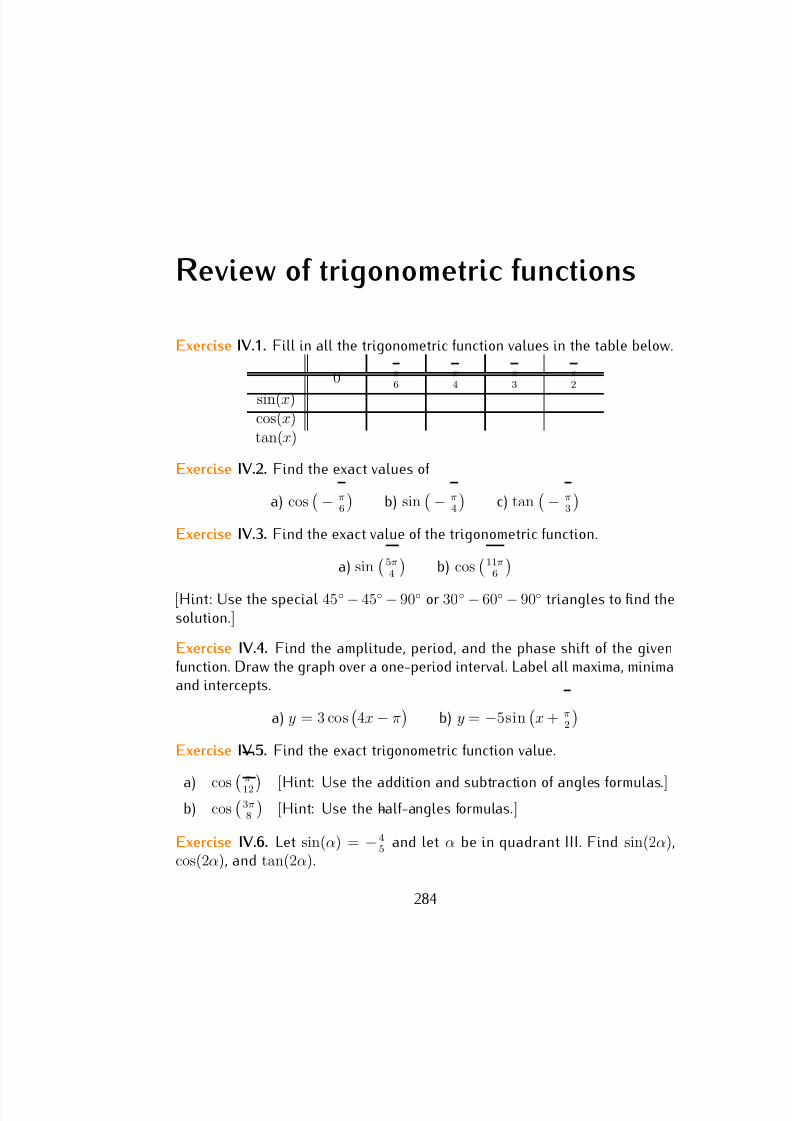
7/18/2019 Precalculus Tradler Carley
http://slidepdf.com/reader/full/precalculus-tradler-carley 294/424
Review of trigonometric functions
Exercise IV.1. Fill in all the trigonometric function values in the table below.
0 π6
π4
π3
π2
sin(x)cos(x)tan(x)
Exercise IV.2. Find the exact values of
a) cos− π
6
b) sin
− π4
c) tan
− π3
Exercise IV.3. Find the exact value of the trigonometric function.
a) sin 5π4 b) cos
11π6
[Hint: Use the special 45◦ − 45◦ − 90◦ or 30◦ − 60◦ − 90◦ triangles to find thesolution.]
Exercise IV.4. Find the amplitude, period, and the phase shift of the givenfunction. Draw the graph over a one-period interval. Label all maxima, minimaand intercepts.
a) y = 3 cos
4x − π
b) y = −5sin
x + π2
Exercise IV.5. Find the exact trigonometric function value.
a) cos π12 [Hint: Use the addition and subtraction of angles formulas.]
b) cos
3π8
[Hint: Use the half-angles formulas.]
Exercise IV.6. Let sin(α) = − 45 and let α be in quadrant III. Find sin(2α),
cos(2α), and tan(2α).
284
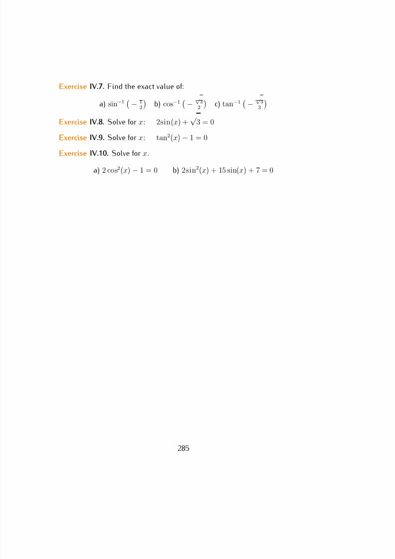
7/18/2019 Precalculus Tradler Carley
http://slidepdf.com/reader/full/precalculus-tradler-carley 295/424
Exercise IV.7. Find the exact value of:
a) sin−1− 1
2
b) cos−1
− √ 32
c) tan−1
− √ 33
Exercise IV.8. Solve for x: 2sin(x) +
√ 3 = 0
Exercise IV.9. Solve for x: tan2(x) − 1 = 0
Exercise IV.10. Solve for x.
a) 2 cos2(x) − 1 = 0 b) 2sin2(x) + 15 sin(x) + 7 = 0
285
7/18/2019 Precalculus Tradler Carley
http://slidepdf.com/reader/full/precalculus-tradler-carley 296/424
Part V
Complex numbers, sequences, and
the binomial theorem
286
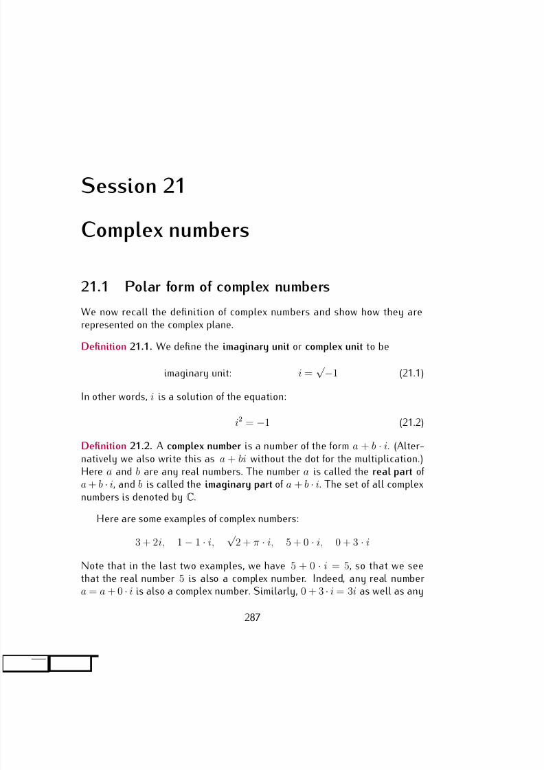
7/18/2019 Precalculus Tradler Carley
http://slidepdf.com/reader/full/precalculus-tradler-carley 297/424
Session 21
Complex numbers
21.1 Polar form of complex numbers
We now recall the definition of complex numbers and show how they arerepresented on the complex plane.
Definition 21.1. We define the imaginary unit or complex unit to be
imaginary unit: i =√ −1 (21.1)
In other words, i is a solution of the equation:
i2 = −1 (21.2)
Definition 21.2. A complex number is a number of the form a + b · i. (Alter-natively we also write this as a + bi without the dot for the multiplication.)Here a and b are any real numbers. The number a is called the real part of a + b · i, and b is called the imaginary part of a + b · i. The set of all complexnumbers is denoted by C.
Here are some examples of complex numbers:
3 + 2i, 1 − 1 · i, √ 2 + π · i, 5 + 0 · i, 0 + 3 · i
Note that in the last two examples, we have 5 + 0 · i = 5, so that we seethat the real number 5 is also a complex number. Indeed, any real numbera = a + 0 · i is also a complex number. Similarly, 0 + 3 · i = 3i as well as any
287
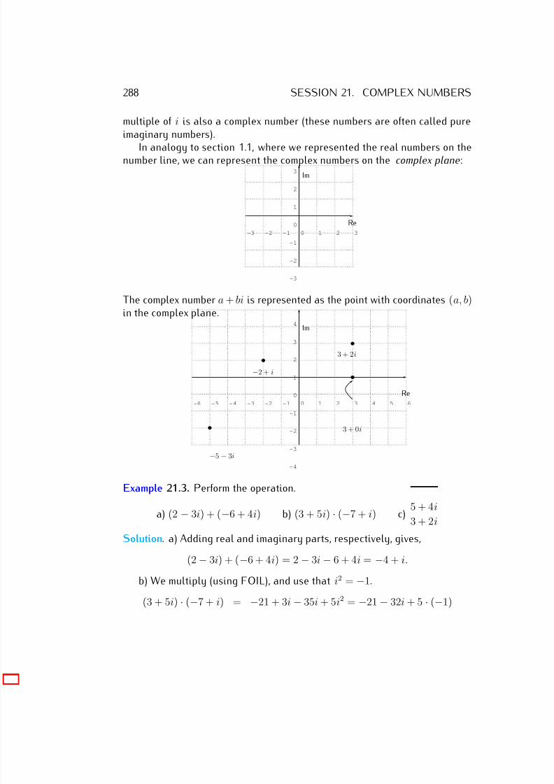
7/18/2019 Precalculus Tradler Carley
http://slidepdf.com/reader/full/precalculus-tradler-carley 298/424
288 SESSION 21. COMPLEX NUMBERS
multiple of i is also a complex number (these numbers are often called pure
imaginary numbers).In analogy to section 1.1, where we represented the real numbers on thenumber line, we can represent the complex numbers on the complex plane:
-3 -2 -1 0 1 2 3
-3
-2
-1
0
1
2
3
Re
Im
The complex number a + bi is represented as the point with coordinates (a, b)in the complex plane.
-6 -5 -4 -3 -2 -1 0 1 2 3 4 5 6
-4
-3
-2
-1
0
1
2
3
4
Re
Im
3 + 2i
−2 + i
−5 − 3i
3 + 0i
Example 21.3. Perform the operation.
a) (2 − 3i) + (−6 + 4i) b) (3 + 5i) · (−7 + i) c) 5 + 4i
3 + 2i
Solution. a) Adding real and imaginary parts, respectively, gives,
(2 − 3i) + (−6 + 4i) = 2 − 3i − 6 + 4i = −4 + i.
b) We multiply (using FOIL), and use that i2 = −1.
(3 + 5i) · (−7 + i) = −21 + 3i − 35i + 5i2 = −21 − 32i + 5 · (−1)
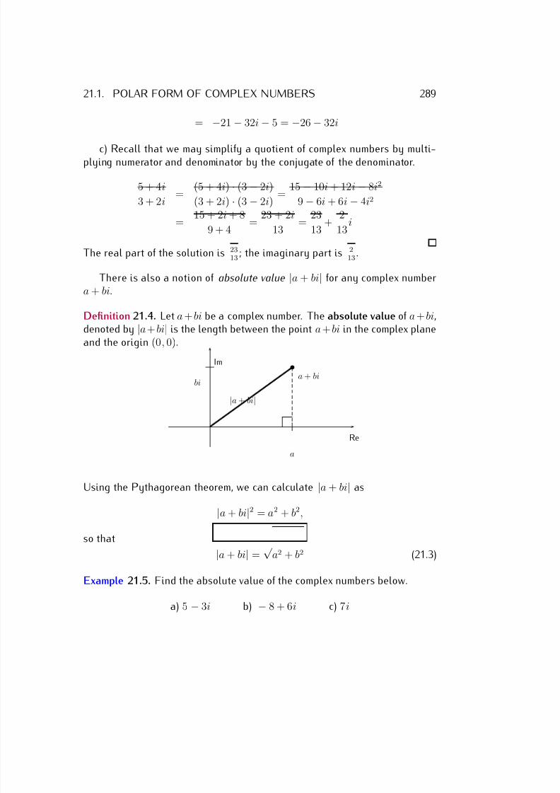
7/18/2019 Precalculus Tradler Carley
http://slidepdf.com/reader/full/precalculus-tradler-carley 299/424
21.1. POLAR FORM OF COMPLEX NUMBERS 289
= −21 − 32i − 5 = −26 − 32i
c) Recall that we may simplify a quotient of complex numbers by multi-plying numerator and denominator by the conjugate of the denominator.
5 + 4i
3 + 2i =
(5 + 4i) · (3 − 2i)
(3 + 2i) · (3 − 2i) =
15 − 10i + 12i − 8i2
9 − 6i + 6i − 4i2
= 15 + 2i + 8
9 + 4 =
23 + 2i
13 =
23
13 +
2
13i
The real part of the solution is 2313
; the imaginary part is 213
.
There is also a notion of absolute value |a + bi| for any complex numbera + bi.
Definition 21.4. Let a + bi be a complex number. The absolute value of a + bi,denoted by |a + bi| is the length between the point a + bi in the complex planeand the origin (0, 0).
Re
Im
a + bi
|a + bi|
a
bi
Using the Pythagorean theorem, we can calculate |a + bi| as
|a + bi|2 = a2 + b2,
so that
|a + bi| = √ a2 + b2 (21.3)
Example 21.5. Find the absolute value of the complex numbers below.
a) 5 − 3i b) − 8 + 6i c) 7i
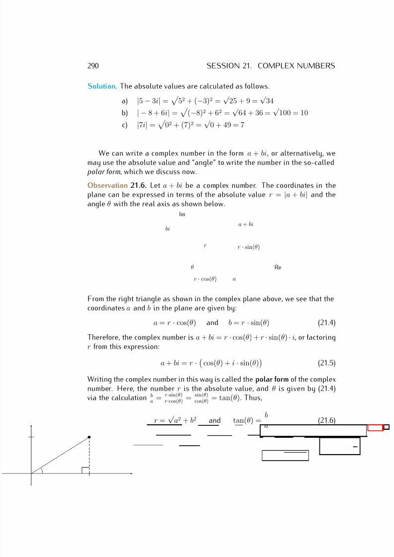
7/18/2019 Precalculus Tradler Carley
http://slidepdf.com/reader/full/precalculus-tradler-carley 300/424
290 SESSION 21. COMPLEX NUMBERS
Solution. The absolute values are calculated as follows.
a) |5 − 3i| = 52 + (−3)2 = √ 25 + 9 = √ 34
b) | − 8 + 6i| =
(−8)2 + 62 =√
64 + 36 =√
100 = 10
c) |7i| =
02 + (7)2 =√
0 + 49 = 7
We can write a complex number in the form a + bi, or alternatively, wemay use the absolute value and “angle” to write the number in the so-calledpolar form, which we discuss now.
Observation 21.6. Let a + bi be a complex number. The coordinates in the
plane can be expressed in terms of the absolute value r = |a + bi| and theangle θ with the real axis as shown below.
Re
Im
a + bi
θ
r
r · cos(θ)
r · sin(θ)
a
bi
From the right triangle as shown in the complex plane above, we see that thecoordinates a and b in the plane are given by:
a = r · cos(θ) and b = r · sin(θ) (21.4)
Therefore, the complex number is a + bi = r · cos(θ) + r · sin(θ) · i, or factoringr from this expression:
a + bi = r · cos(θ) + i · sin(θ)
(21.5)
Writing the complex number in this way is called the polar form of the complex
number. Here, the number r is the absolute value, and θ is given by (21.4)via the calculation b
a = r·sin(θ)r·cos(θ) = sin(θ)
cos(θ) = tan(θ). Thus,
r =√
a2 + b2 and tan(θ) = b
a (21.6)
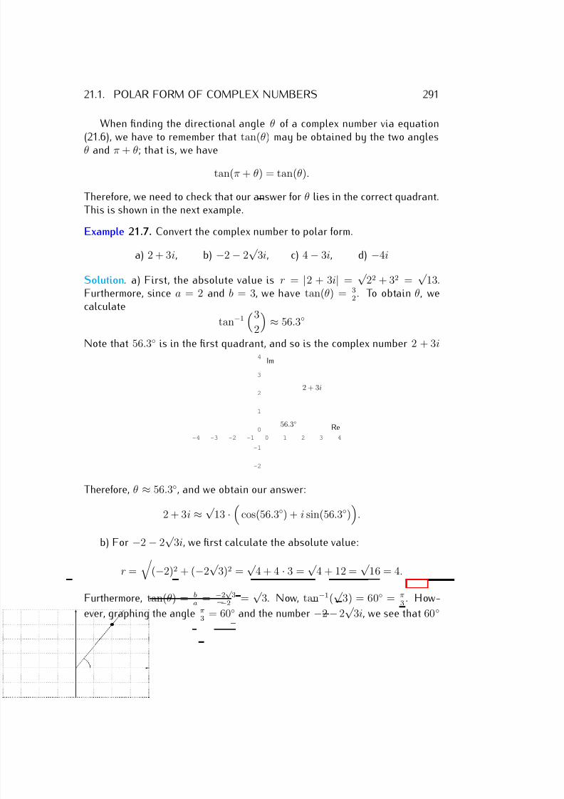
7/18/2019 Precalculus Tradler Carley
http://slidepdf.com/reader/full/precalculus-tradler-carley 301/424
21.1. POLAR FORM OF COMPLEX NUMBERS 291
When finding the directional angle θ of a complex number via equation
(21.6), we have to remember that tan(θ) may be obtained by the two anglesθ and π + θ; that is, we have
tan(π + θ) = tan(θ).
Therefore, we need to check that our answer for θ lies in the correct quadrant.This is shown in the next example.
Example 21.7. Convert the complex number to polar form.
a) 2 + 3i, b) −2 − 2√
3i, c) 4 − 3i, d) −4i
Solution. a) First, the absolute value is r = |2 + 3i| = √ 22 + 32 = √ 13.Furthermore, since a = 2 and b = 3, we have tan(θ) = 3
2 . To obtain θ, wecalculate
tan−13
2
≈ 56.3◦
Note that 56.3◦ is in the first quadrant, and so is the complex number 2 + 3i
-4 -3 -2 -1 0 1 2 3 4
-2
-1
0
1
2
3
4
Re
Im
2 + 3i
56.3◦
Therefore, θ ≈ 56.3◦, and we obtain our answer:
2 + 3i ≈√
13 ·
cos(56.3◦) + i sin(56.3◦)
.
b) For −2 − 2√
3i, we first calculate the absolute value:
r =
(−2)2 + (−2√
3)2 =√
4 + 4 · 3 =√
4 + 12 =√
16 = 4.
Furthermore, tan(θ) = ba
= −2√
3−2
=√
3. Now, tan−1(√
3) = 60◦ = π3
. How-
ever, graphing the angle π3
= 60◦ and the number −2 − 2√
3i, we see that 60◦
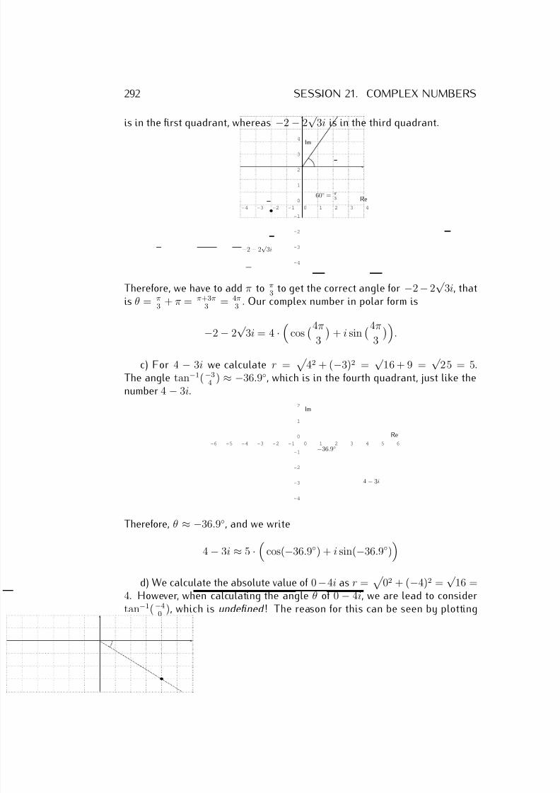
7/18/2019 Precalculus Tradler Carley
http://slidepdf.com/reader/full/precalculus-tradler-carley 302/424
292 SESSION 21. COMPLEX NUMBERS
is in the first quadrant, whereas −2 − 2√
3i is in the third quadrant.
-4 -3 -2 -1 0 1 2 3 4
-4
-3
-2
-1
0
1
2
3
4
Re
Im
−2 − 2√
3i
60◦ = π3
Therefore, we have to add π to π3 to get the correct angle for −2 − 2
√ 3i, that
is θ = π3
+ π = π+3π3
= 4π3
. Our complex number in polar form is
−2 − 2√
3i = 4 ·
cos4π
3
+ i sin
4π
3
.
c) For 4 − 3i we calculate r =
42 + (−3)2 =√
16 + 9 =√
25 = 5.The angle tan−1(−3
4 ) ≈ −36.9◦, which is in the fourth quadrant, just like thenumber 4 − 3i.
-6 -5 -4 -3 -2 -1 0 1 2 3 4 5 6
-4
-3
-2
-1
0
1
2
Re
Im
4 − 3i
−36.9◦
Therefore, θ ≈ −36.9◦, and we write
4 − 3i ≈ 5 · cos(−36.9◦) + i sin(−36.9◦)d) We calculate the absolute value of 0−4i as r =
02 + (−4)2 =
√ 16 =
4. However, when calculating the angle θ of 0 − 4i, we are lead to considertan−1(−4
0 ), which is undefined ! The reason for this can be seen by plotting
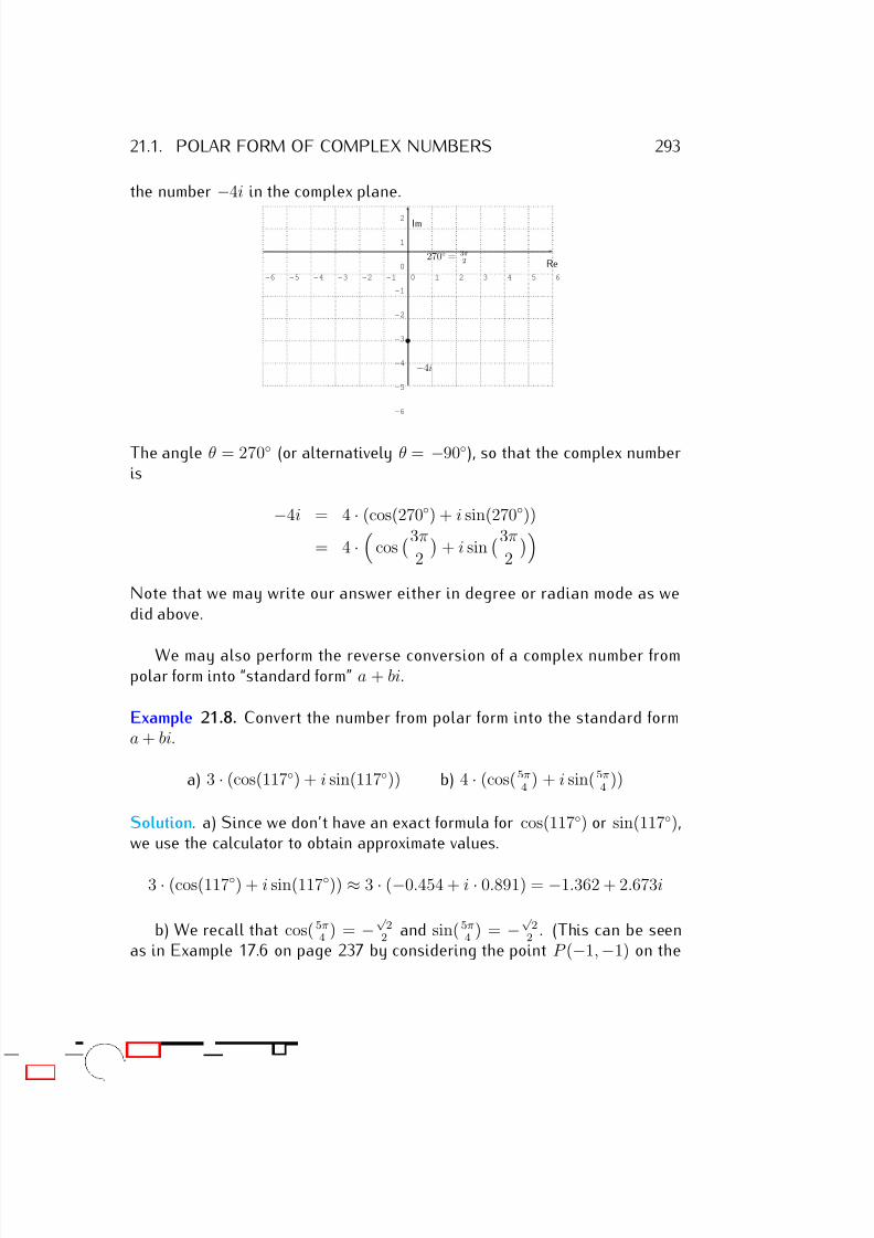
7/18/2019 Precalculus Tradler Carley
http://slidepdf.com/reader/full/precalculus-tradler-carley 303/424
21.1. POLAR FORM OF COMPLEX NUMBERS 293
the number −4i in the complex plane.
-6 -5 -4 -3 -2 -1 0 1 2 3 4 5 6
-6
-5
-4
-3
-2
-1
0
1
2
Re
Im
−4i
270◦ = 3π2
The angle θ = 270◦ (or alternatively θ = −90◦), so that the complex numberis
−4i = 4 · (cos(270◦) + i sin(270◦))
= 4 ·
cos3π
2
+ i sin
3π
2
Note that we may write our answer either in degree or radian mode as wedid above.
We may also perform the reverse conversion of a complex number frompolar form into “standard form” a + bi.
Example 21.8. Convert the number from polar form into the standard forma + bi.
a) 3 · (cos(117◦) + i sin(117◦)) b) 4 · (cos(5π4
) + i sin( 5π4
))
Solution. a) Since we don’t have an exact formula for cos(117◦) or sin(117◦),we use the calculator to obtain approximate values.
3 · (cos(117◦) + i sin(117◦)) ≈ 3 · (−0.454 + i · 0.891) = −1.362 + 2.673i
b) We recall that cos( 5π4 ) = −
√ 2
2 and sin( 5π4 ) = −
√ 2
2 . (This can be seenas in Example 17.6 on page 237 by considering the point P (−1, −1) on the
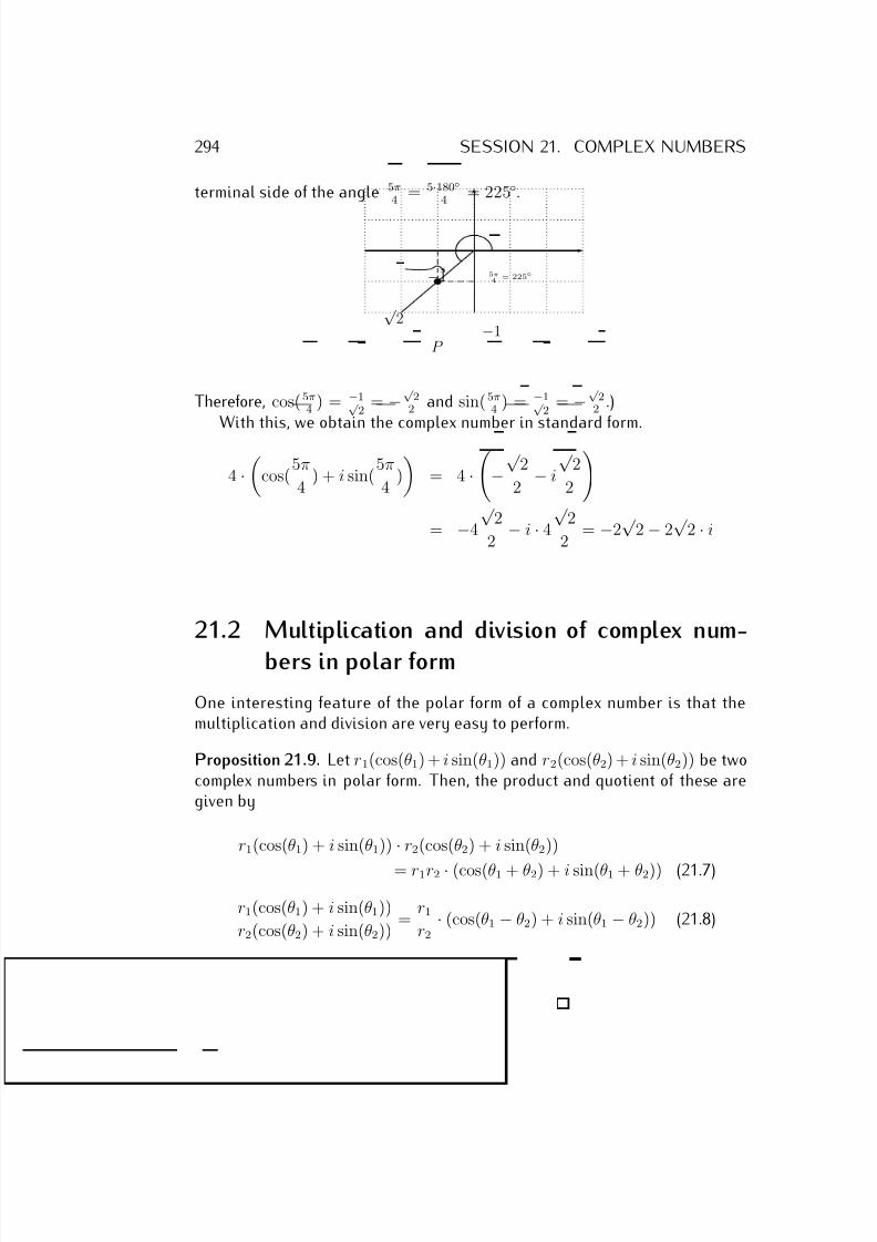
7/18/2019 Precalculus Tradler Carley
http://slidepdf.com/reader/full/precalculus-tradler-carley 304/424
294 SESSION 21. COMPLEX NUMBERS
terminal side of the angle 5π4
= 5·180◦4
= 225◦.
5π4
= 225◦−1
−1
√ 2
P
Therefore, cos( 5π4 ) = −1√
2 = −
√ 2
2 and sin( 5π4 ) = −1√
2 = −
√ 2
2 .)With this, we obtain the complex number in standard form.
4 ·
cos(5π
4 ) + i sin(
5π
4 )
= 4 ·
−
√ 2
2 − i
√ 2
2
= −4
√ 2
2 − i · 4
√ 2
2 = −2
√ 2 − 2
√ 2 · i
21.2 Multiplication and division of complex num-
bers in polar form
One interesting feature of the polar form of a complex number is that themultiplication and division are very easy to perform.
Proposition 21.9. Let r1(cos(θ1) + i sin(θ1)) and r2(cos(θ2) + i sin(θ2)) be twocomplex numbers in polar form. Then, the product and quotient of these aregiven by
r1(cos(θ1) + i sin(θ1)) · r2(cos(θ2) + i sin(θ2))
= r1r2 · (cos(θ1 + θ2) + i sin(θ1 + θ2)) (21.7)
r1(cos(θ1) + i sin(θ1))
r2(cos(θ2) + i sin(θ2)) =
r1
r2· (cos(θ1 − θ2) + i sin(θ1 − θ2)) (21.8)
7/18/2019 Precalculus Tradler Carley
http://slidepdf.com/reader/full/precalculus-tradler-carley 305/424
21.2. MULTIPLICATION AND DIVISION OF COMPLEX NUMBERS 295
Proof. The proof uses the addition formulas for trigonometric functions sin(α + β) and cos(α + β) fromproposition 18.1 on page 252.
r1(cos(θ1) + i sin(θ1)) · r2(cos(θ2) + i sin(θ2))
= r1r2 · (cos(θ1) cos(θ2) + i cos(θ1) sin(θ2) + i sin(θ1) cos(θ2) + i2 sin(θ1) sin(θ2))
= r1r2 · ((cos(θ1) cos(θ2) − sin(θ1)sin(θ2)) + i(cos(θ1)sin(θ2) + sin(θ1) cos(θ2)))
= r1r2 · (cos(θ1 + θ2) + i sin(θ1 + θ2))
For the division formula, note, that the multiplication formula (21.7) gives
r2(cos(θ2) + i sin(θ2)) · 1
r2(cos(−θ2) + i sin(−θ2)) = r2
1
r2(cos(θ2 − θ2) + i sin(θ2 − θ2))
= 1 · (cos 0 + i sin 0) = 1 · (1 + i · 0) = 1
=⇒ 1
r2(cos(θ2) + i sin(θ2)) =
1
r2(cos(−θ2) + i sin(−θ2)),
so that
r1(cos(θ1) + i sin(θ1))
r2(cos(θ2) + i sin(θ2))= r1(cos(θ1) + i sin(θ1)) · 1
r2(cos(θ2) + i sin(θ2))
= r1(cos(θ1) + i sin(θ1)) · 1
r2(cos(−θ2) + i sin(−θ2)) =
r1
r2· (cos(θ1 − θ2) + i sin(θ1 − θ2)).
Example 21.10. Multiply or divide the complex numbers, and write your an-swer in polar and standard form.
a) 5(cos(11◦) + i sin(11◦))
·8(cos(34◦) + i sin(34◦))
b) 3(cos( 5π8
) + i sin( 5π8
)) · 12(cos(7π8
) + i sin( 7π8
))
c) 32(cos( π
4 ) + i sin( π4 ))
8(cos( 7π12
) + i sin( 7π12
)) d)
4(cos(203◦) + i sin(203◦))
6(cos(74◦) + i sin(74◦))
Solution. We will multiply and divide the complex numbers using equations(21.7) and (21.8), respectively, and then convert them to standard notationa + bi.
a) 5(cos(11◦) + i sin(11◦)) · 8(cos(34◦) + i sin(34◦))
= 5·
8·
(cos(11◦ + 34◦) + i sin(11◦ + 34◦)) = 40(cos(45◦) + i sin(45◦))
= 40√ 2
2 + i
√ 22
= 40
√ 22
+ i · 40√ 2
2 = 20
√ 2 + 20
√ 2i
b) Similarly, we obtain the next product.
7/18/2019 Precalculus Tradler Carley
http://slidepdf.com/reader/full/precalculus-tradler-carley 306/424
7/18/2019 Precalculus Tradler Carley
http://slidepdf.com/reader/full/precalculus-tradler-carley 307/424
21.3. EXERCISES 297
21.3 Exercises
Exercise 21.1. Plot the complex numbers in the complex plane.
a) 4 + 2i b) −3 − 5i c) 6 − 2i d) −5 + i e) −2i
f )√
2 − √ 2i g) 7 h) i i) 0 j) 2i − √
3
Exercise 21.2. Add, subtract, multiply, and divide, as indicated.
a) (5 − 2i) + (−2 + 6i) b) (−9 − i) − (5 − 3i)c) (3 + 2i) · (4 + 3i) d) (−2 − i) · (−1 + 4i)e) 2+3i
2+i f ) (5 + 5i) ÷ (2 − 4i)
Exercise 21.3. Find the absolute value |
a + bi| of the given complex number,
and simplify your answer as much as possible.
a) |4 + 3i| b) |1 − 2i| c) | − 3i| d) | − 2 − 6i|e) |√
8 − i| f ) | − 2√
3 − 2i| g) | − 5| h) | − √ 17 + 4
√ 2i|
Exercise 21.4. Convert the complex number into polar form r(cos(θ)+i sin(θ)).
a) 2 + 2i b) 4√
3 + 4i c) 3 − 2i d) −5 + 5ie) 4 − 3i f) −4 + 3i g) −√
5 − √ 15i h)
√ 7 − √
21i
i) −5 − 12i j) 6i k) −10 l) −√ 3 + 3i
Exercise 21.5. Convert the complex number into the standard form a + bi.
a) 6(cos(134◦) + i sin(134◦)) b) 12
(cos( π17
) + i sin( π17
))
c) 2(cos(270◦) + i sin(270◦)) d) cos( π6 ) + i sin( π
6 )
e) 10(cos( 7π6 ) + i sin( 7π
6 )) f ) 6(cos(−5π12 ) + i sin(−5π
12 ))
Exercise 21.6. Multiply the complex numbers and write the answer in stan-dard form a + bi.
a) 4(cos(27◦) + i sin(27◦)) · 10(cos(33◦) + i sin(33◦))
b) 7(cos( 2π9 ) + i sin( 2π
9 )) · 6(cos( π9 ) + i sin( π
9 ))
c) (cos( 13π
12 ) + i sin( 13π
12 ))
·(cos(−11π
12 ) + i sin(−11π
12 ))
d) 8(cos( 3π7
) + i sin( 3π7
)) · 1.5(cos( 4π7
) + i sin( 4π7
))
e) 0.2(cos(196◦) + i sin(196◦)) · 0.5(cos(88◦) + i sin(88◦))
f ) 4(cos( 7π8
) + i sin( 7π8
)) · 0.25(cos(−5π24
) + i sin(−5π24
))
7/18/2019 Precalculus Tradler Carley
http://slidepdf.com/reader/full/precalculus-tradler-carley 308/424
298 SESSION 21. COMPLEX NUMBERS
Exercise 21.7. Divide the complex numbers and write the answer in standard
form a + bi.
a) 18(cos( π
2 ) + i sin( π2 ))
3(cos(π6
) + i sin( π6
)) b)
10(cos(254◦) + i sin(254◦))
15(cos(164◦) + i sin(164◦))
c)
√ 24(cos( 11π
14 ) + i sin( 11π
14 ))√
6(cos( 2π7 ) + i sin( 2π
7 ))d)
cos( 8π5
) + i sin(8π5
)
2(cos( π10 ) + i sin( π
10 ))
e) 42(cos( 7π
4 ) + i sin( 7π
4 ))
7(cos(5π12 ) + i sin( 5π
12 )) f )
30(cos(−175◦) + i sin(−175◦))
18(cos(144◦) + i sin(144◦))
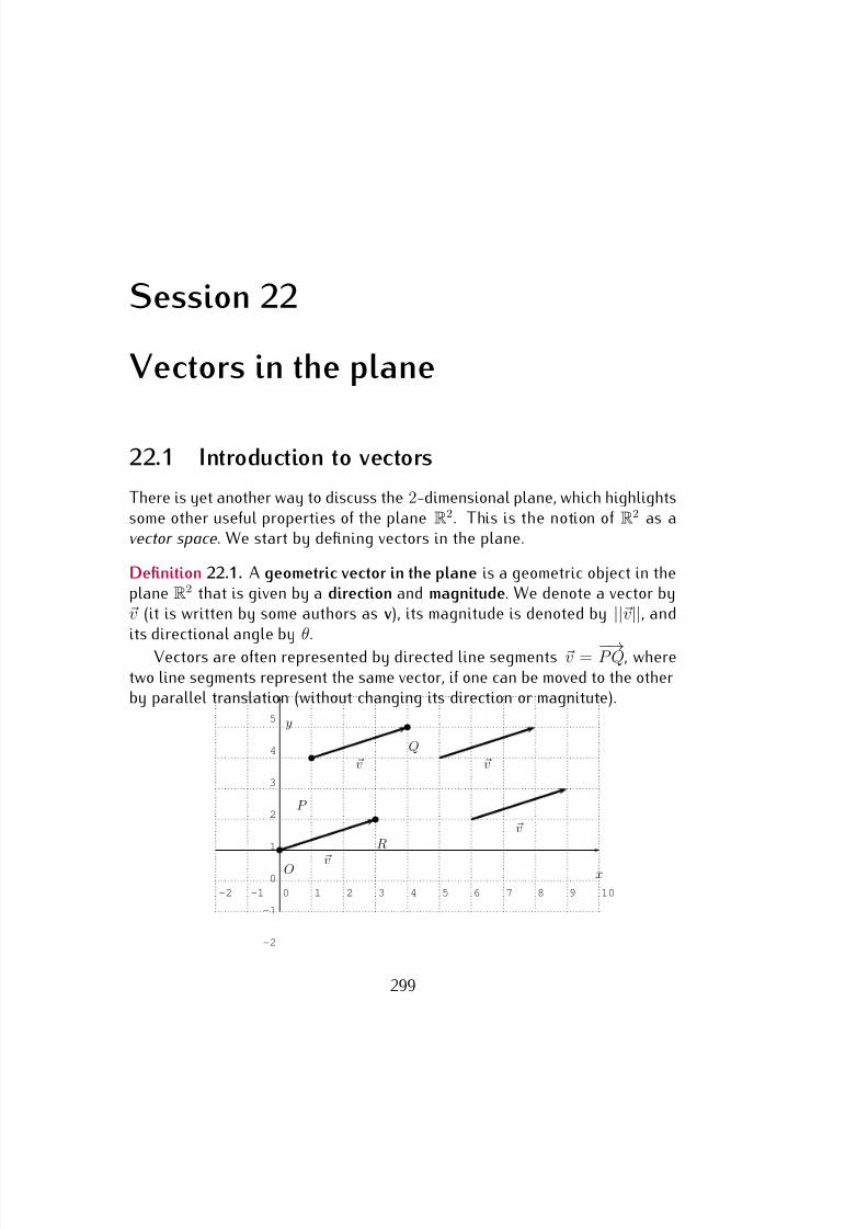
7/18/2019 Precalculus Tradler Carley
http://slidepdf.com/reader/full/precalculus-tradler-carley 309/424
Session 22
Vectors in the plane
22.1 Introduction to vectors
There is yet another way to discuss the 2-dimensional plane, which highlightssome other useful properties of the plane R2. This is the notion of R2 as avector space. We start by defining vectors in the plane.
Definition 22.1. A geometric vector in the plane is a geometric object in theplane R2 that is given by a direction and magnitude. We denote a vector byv (it is written by some authors as v), its magnitude is denoted by ||v||, andits directional angle by θ.
Vectors are often represented by directed line segments v = −→P Q, wheretwo line segments represent the same vector, if one can be moved to the otherby parallel translation (without changing its direction or magnitute).
-2 -1 0 1 2 3 4 5 6 7 8 9 10
-2
-1
0
1
2
3
4
5
x
y
v
P
Q
v
v
vO
R
299
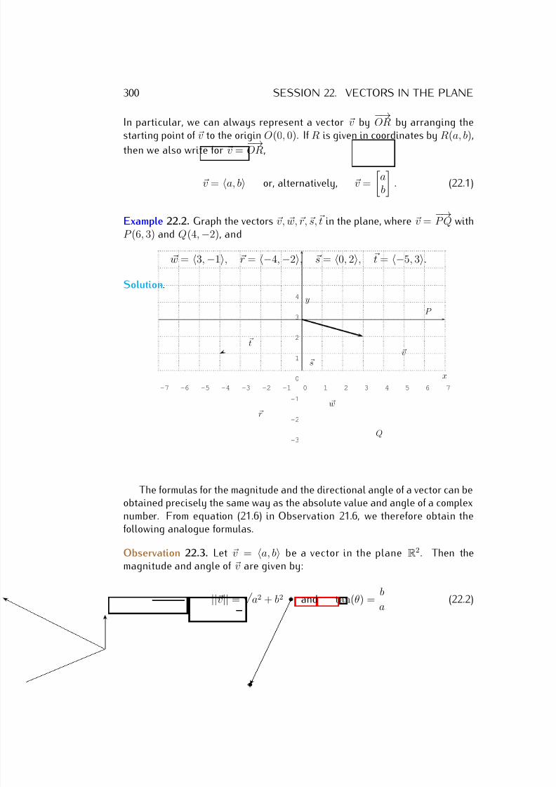
7/18/2019 Precalculus Tradler Carley
http://slidepdf.com/reader/full/precalculus-tradler-carley 310/424
300 SESSION 22. VECTORS IN THE PLANE
In particular, we can always represent a vector v by −→OR by arranging the
starting point of v to the origin O(0, 0). If R is given in coordinates by R(a, b),then we also write for v =
−→OR,
v = a, b or, alternatively, v =
ab
. (22.1)
Example 22.2. Graph the vectors v, w, r, s, t in the plane, where v =−→P Q with
P (6, 3) and Q(4, −2), and
w = 3, −1, r = −4, −2, s = 0, 2, t = −5, 3.
Solution.
-7 -6 -5 -4 -3 -2 -1 0 1 2 3 4 5 6 7
-3
-2
-1
0
1
2
3
4
x
y
w
r
s
tv
P
Q
The formulas for the magnitude and the directional angle of a vector can beobtained precisely the same way as the absolute value and angle of a complexnumber. From equation (21.6) in Observation 21.6, we therefore obtain thefollowing analogue formulas.
Observation 22.3. Let v = a, b be a vector in the plane R2. Then themagnitude and angle of v are given by:
||v|| =√
a2 + b2 and tan(θ) = b
a (22.2)
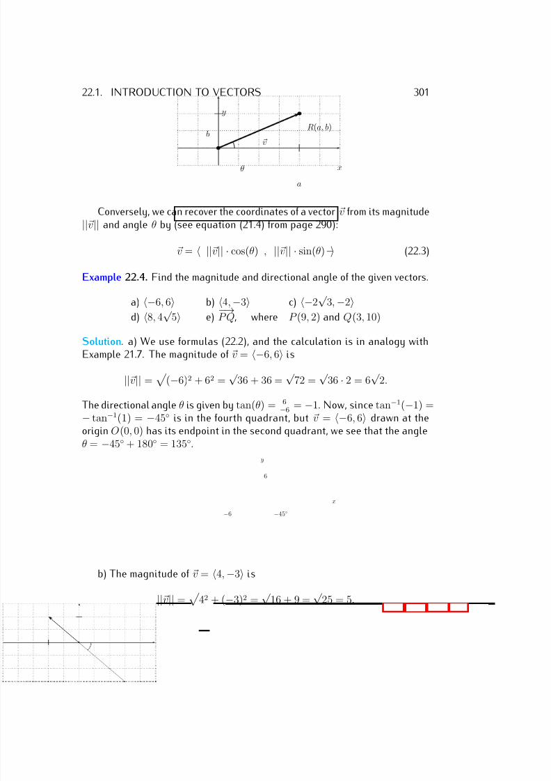
7/18/2019 Precalculus Tradler Carley
http://slidepdf.com/reader/full/precalculus-tradler-carley 311/424
22.1. INTRODUCTION TO VECTORS 301
x
y
v
R(a, b)
a
b
θ
Conversely, we can recover the coordinates of a vector v from its magnitude||v|| and angle θ by (see equation (21.4) from page 290):
v = ||v|| · cos(θ) , ||v|| · sin(θ) (22.3)
Example 22.4. Find the magnitude and directional angle of the given vectors.
a) −6, 6 b) 4, −3 c) −2√
3, −2d) 8, 4
√ 5 e)
−→P Q, where P (9, 2) and Q(3, 10)
Solution. a) We use formulas (22.2), and the calculation is in analogy withExample 21.7. The magnitude of v = −6, 6 is
||v|| =
(−6)2 + 62 =√
36 + 36 =√
72 =√
36 · 2 = 6√
2.
The directional angle θ is given by tan(θ) =
6
−6 = −1. Now, since tan−1
(−1) =− tan−1(1) = −45◦ is in the fourth quadrant, but v = −6, 6 drawn at theorigin O(0, 0) has its endpoint in the second quadrant, we see that the angleθ = −45◦ + 180◦ = 135◦.
x
y
6
−6 −45◦
b) The magnitude of v = 4, −3 is
||v|| =
42 + (−3)2 =√
16 + 9 =√
25 = 5.
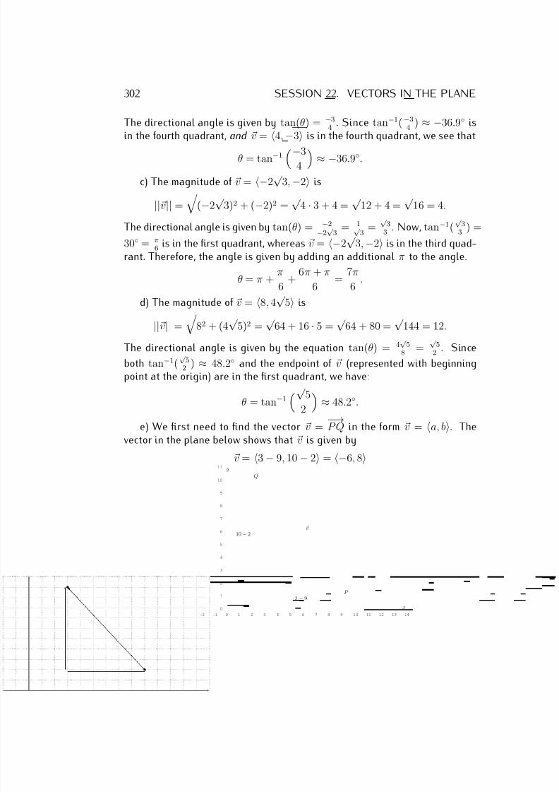
7/18/2019 Precalculus Tradler Carley
http://slidepdf.com/reader/full/precalculus-tradler-carley 312/424
302 SESSION 22. VECTORS IN THE PLANE
The directional angle is given by tan(θ) = −34
. Since tan−1(−34
) ≈ −36.9◦ is
in the fourth quadrant, and v = 4, −3 is in the fourth quadrant, we see that
θ = tan−1−3
4
≈ −36.9◦.
c) The magnitude of v = −2√
3, −2 is
||v|| =
(−2
√ 3)2 + (−2)2 =
√ 4 · 3 + 4 =
√ 12 + 4 =
√ 16 = 4.
The directional angle is given by tan(θ) = −2−2√
3 = 1√
3 =
√ 3
3 . Now, tan−1(
√ 3
3 ) =
30◦ = π6 is in the first quadrant, whereas v = −2
√ 3, −2 is in the third quad-
rant. Therefore, the angle is given by adding an additional π to the angle.
θ = π + π6 + 6π + π6 = 7π6 .
d) The magnitude of v = 8, 4√
5 is
||v|| =
82 + (4
√ 5)2 =
√ 64 + 16 · 5 =
√ 64 + 80 =
√ 144 = 12.
The directional angle is given by the equation tan(θ) = 4√
58 =
√ 5
2 . Since
both tan−1(√
52 ) ≈ 48.2◦ and the endpoint of v (represented with beginning
point at the origin) are in the first quadrant, we have:
θ = tan−1
√
5
2 ≈ 48.2◦.
e) We first need to find the vector v = −→P Q in the form v = a, b. The
vector in the plane below shows that v is given by
v = 3 − 9, 10 − 2 = −6, 8
-2 -1 0 1 2 3 4 5 6 7 8 9 10 11 12 13 14
0
1
2
3
4
5
6
7
8
9
10
11
x
y
P
Q
v
3 − 9
10 − 2
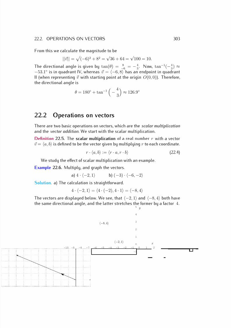
7/18/2019 Precalculus Tradler Carley
http://slidepdf.com/reader/full/precalculus-tradler-carley 313/424
22.2. OPERATIONS ON VECTORS 303
From this we calculate the magnitude to be
||v|| = (−6)2 + 82 = √ 36 + 64 = √ 100 = 10.
The directional angle is given by tan(θ) = 8−6
= − 43
. Now, tan−1(−43
) ≈−53.1◦ is in quadrant IV, whereas v = −6, 8 has an endpoint in quadrantII (when representing v with starting point at the origin O(0, 0)). Therefore,the directional angle is
θ = 180◦ + tan−1
− 4
3
≈ 126.9◦
22.2 Operations on vectorsThere are two basic operations on vectors, which are the scalar multiplication
and the vector addition. We start with the scalar multiplication.
Definition 22.5. The scalar multiplication of a real number r with a vectorv = a, b is defined to be the vector given by multiplying r to each coordinate.
r · a, b := r · a, r · b (22.4)
We study the effect of scalar multiplication with an example.
Example 22.6. Multiply, and graph the vectors.
a) 4 · −2, 1 b) (−3) · −6, −2Solution. a) The calculation is straightforward.
4 · −2, 1 = 4 · (−2), 4 · 1 = −8, 4The vectors are displayed below. We see, that −2, 1 and −8, 4 both havethe same directional angle, and the latter stretches the former by a factor 4.
-10 -9 -8 -7 -6 -5 -4 -3 -2 -1 0 1 2
-1
0
1
2
3
4
5
x
y
−8, 4
−2, 1
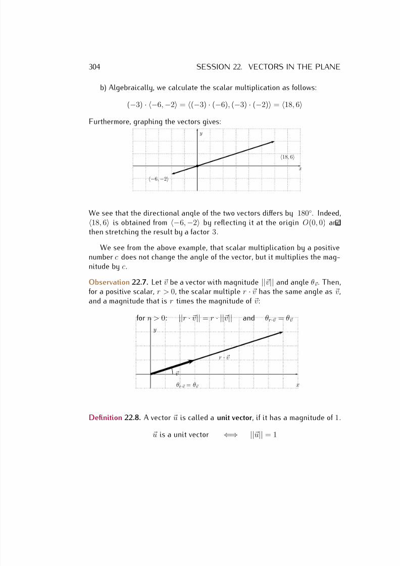
7/18/2019 Precalculus Tradler Carley
http://slidepdf.com/reader/full/precalculus-tradler-carley 314/424
304 SESSION 22. VECTORS IN THE PLANE
b) Algebraically, we calculate the scalar multiplication as follows:
(−3) · −6, −2 = (−3) · (−6), (−3) · (−2) = 18, 6
Furthermore, graphing the vectors gives:
x
y
−6, −2
18, 6
We see that the directional angle of the two vectors differs by 180◦. Indeed,18, 6 is obtained from −6, −2 by reflecting it at the origin O(0, 0) andthen stretching the result by a factor 3.
We see from the above example, that scalar multiplication by a positivenumber c does not change the angle of the vector, but it multiplies the mag-nitude by c.
Observation 22.7. Let v be a vector with magnitude ||v|| and angle θv. Then,for a positive scalar, r > 0, the scalar multiple r
·v has the same angle as v,
and a magnitude that is r times the magnitude of v:
for r > 0: ||r · v|| = r · ||v|| and θr·v = θv
x
y
θr·v = θv
v
r · v
Definition 22.8. A vector u is called a unit vector, if it has a magnitude of 1.
u is a unit vector ⇐⇒ ||u|| = 1
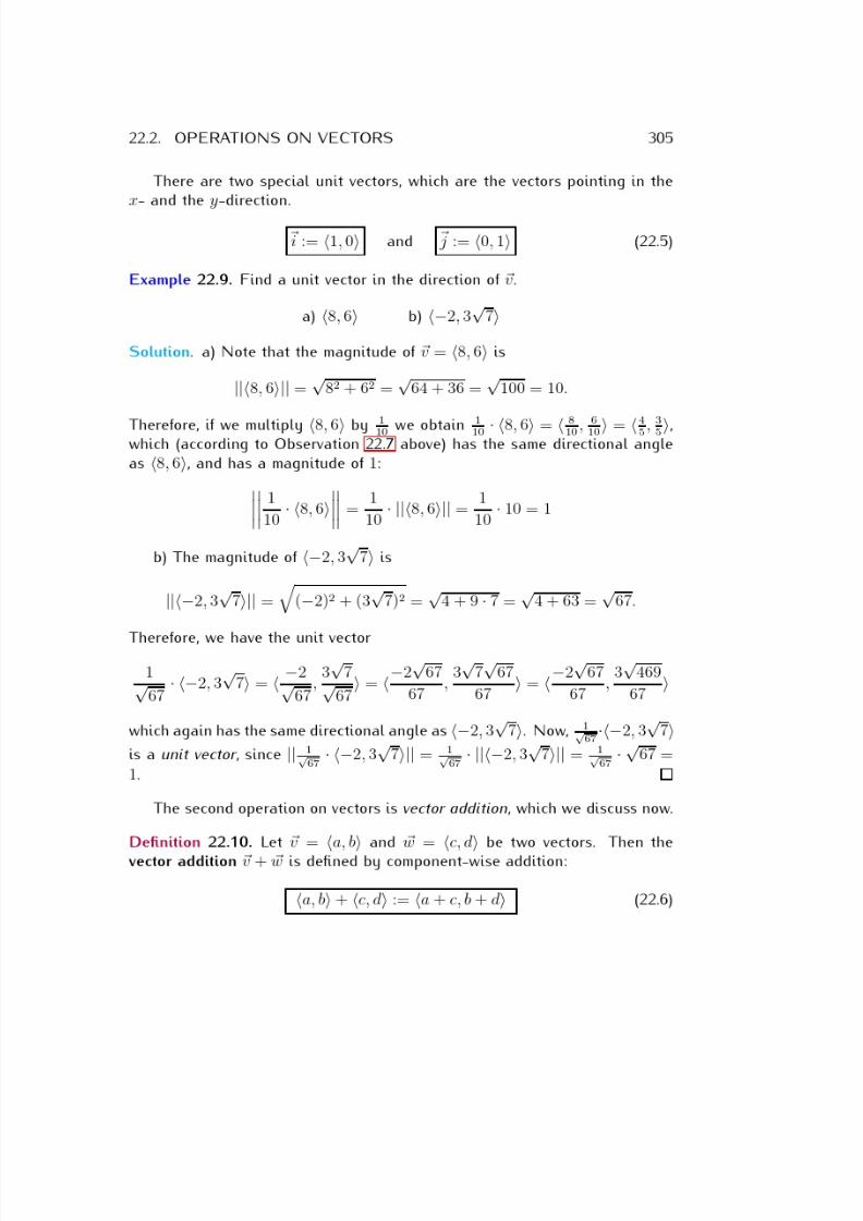
7/18/2019 Precalculus Tradler Carley
http://slidepdf.com/reader/full/precalculus-tradler-carley 315/424
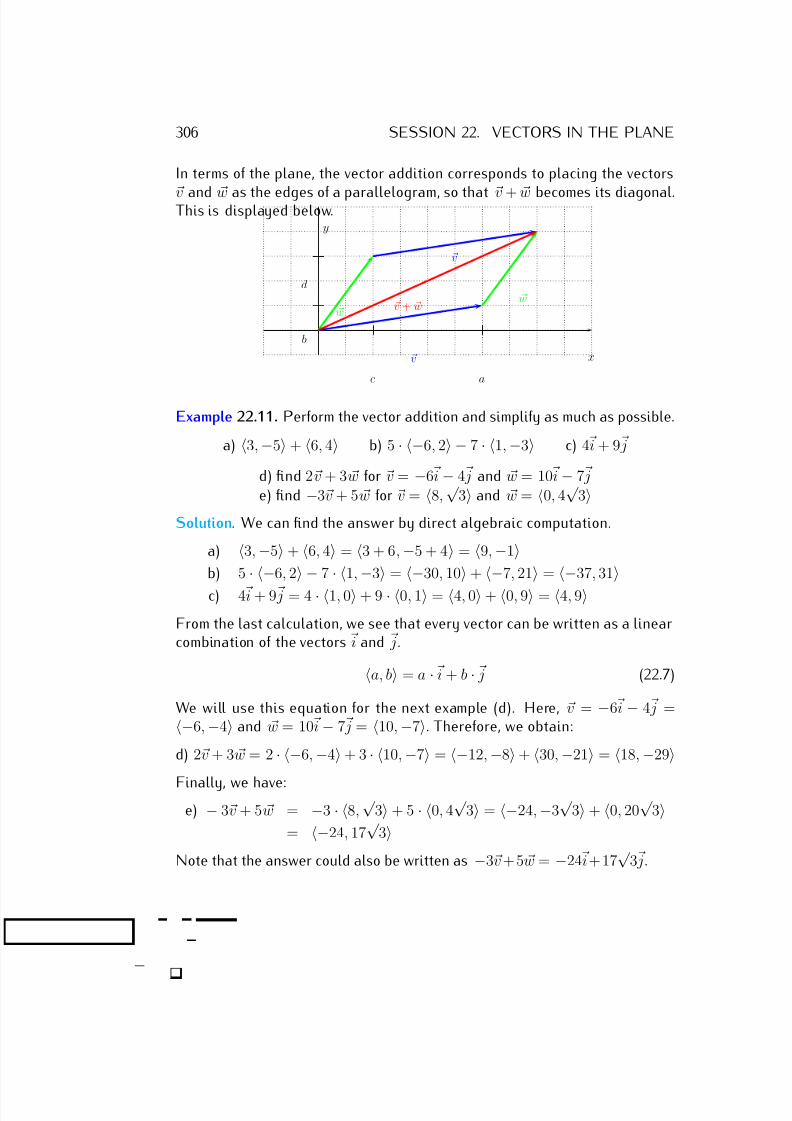
7/18/2019 Precalculus Tradler Carley
http://slidepdf.com/reader/full/precalculus-tradler-carley 316/424
306 SESSION 22. VECTORS IN THE PLANE
In terms of the plane, the vector addition corresponds to placing the vectors
v and w as the edges of a parallelogram, so that v + w becomes its diagonal.This is displayed below.
x
y
v
w w
v
v + w
a
b
c
d
Example 22.11. Perform the vector addition and simplify as much as possible.
a) 3, −5 + 6, 4 b) 5 · −6, 2 − 7 · 1, −3 c) 4 i + 9 j
d) find 2v + 3 w for v = −6 i − 4 j and w = 10 i − 7 je) find −3v + 5 w for v = 8,
√ 3 and w = 0, 4
√ 3
Solution. We can find the answer by direct algebraic computation.
a) 3, −5 + 6, 4 = 3 + 6, −5 + 4 = 9, −1b) 5
· −6, 2
−7
· 1,
−3
=
−30, 10
+
−7, 21
=
−37, 31
c) 4 i + 9 j = 4 · 1, 0 + 9 · 0, 1 = 4, 0 + 0, 9 = 4, 9From the last calculation, we see that every vector can be written as a linearcombination of the vectors i and j.
a, b = a · i + b · j (22.7)
We will use this equation for the next example (d). Here, v = −6 i − 4 j =−6, −4 and w = 10 i − 7 j = 10, −7. Therefore, we obtain:
d) 2v + 3 w = 2 · −6, −4 + 3 · 10, −7 = −12, −8 + 30, −21 = 18, −29
Finally, we have:e) − 3v + 5 w = −3 · 8,
√ 3 + 5 · 0, 4
√ 3 = −24, −3
√ 3 + 0, 20
√ 3
= −24, 17√
3Note that the answer could also be written as −3v +5 w = −24 i+17
√ 3 j.
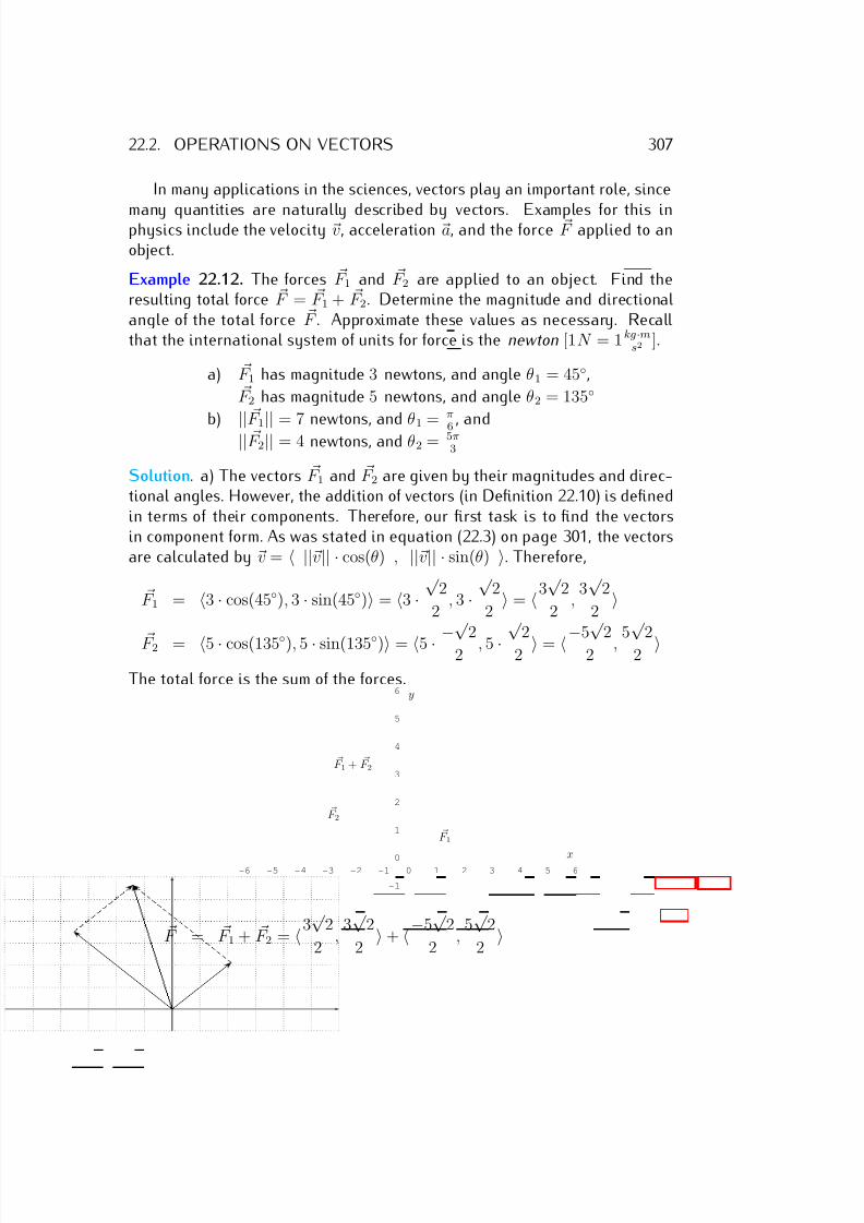
7/18/2019 Precalculus Tradler Carley
http://slidepdf.com/reader/full/precalculus-tradler-carley 317/424
22.2. OPERATIONS ON VECTORS 307
In many applications in the sciences, vectors play an important role, since
many quantities are naturally described by vectors. Examples for this inphysics include the velocity v, acceleration a, and the force F applied to anobject.
Example 22.12. The forces F 1 and F 2 are applied to an object. Find theresulting total force F = F 1 + F 2. Determine the magnitude and directionalangle of the total force F . Approximate these values as necessary. Recallthat the international system of units for force is the newton [1N = 1 kg·m
s2 ].
a) F 1 has magnitude 3 newtons, and angle θ1 = 45◦, F 2 has magnitude 5 newtons, and angle θ2 = 135◦
b) ||
F 1||
= 7 newtons, and θ1
= π
6, and
|| F 2|| = 4 newtons, and θ2 = 5π3
Solution. a) The vectors F 1 and F 2 are given by their magnitudes and direc-tional angles. However, the addition of vectors (in Definition 22.10) is definedin terms of their components. Therefore, our first task is to find the vectorsin component form. As was stated in equation (22.3) on page 301, the vectorsare calculated by v = ||v|| · cos(θ) , ||v|| · sin(θ) . Therefore,
F 1 = 3 · cos(45◦), 3 · sin(45◦) = 3 ·√
2
2 , 3 ·
√ 2
2 = 3
√ 2
2 ,
3√
2
2
F 2 = 5 · cos(135◦), 5 · sin(135◦) = 5 · −√
2
2 , 5 ·√
2
2 = −5√
2
2 , 5
√ 2
2 The total force is the sum of the forces.
-6 -5 -4 -3 -2 -1 0 1 2 3 4 5 6
-1
0
1
2
3
4
5
6
x
y
F 1
F 2
F 1 + F 2
F = F 1 + F 2 = 3√
2
2 ,
3√
2
2 + −5
√ 2
2 ,
5√
2
2
7/18/2019 Precalculus Tradler Carley
http://slidepdf.com/reader/full/precalculus-tradler-carley 318/424
7/18/2019 Precalculus Tradler Carley
http://slidepdf.com/reader/full/precalculus-tradler-carley 319/424
22.3. EXERCISES 309
and w there is a vector v + w, called the vector addition. For any real number r and vector v, there is avector r
·v called the scalar product. These operations have to satisfy the following properties.
Associativity: ( u + v) + w = u + (v + w)Commutativity: v + w = w + vZero eleme nt: there is a vector o such that o + v = v and v + o = v for every vector vNegative element: for every v there is a vector −v such that v + (−v) = o and (−v) + v = oDistributivity (1): r · (v + w) = r · v + r · wDistributivity (2): (r + s) · v = r · v + s · vScalar compatibility: (r · s) · v = r · (s · v)Identity: 1 · v = v
A very important example of a vector space is the 2-dimensional plane V = R2 as it was discussed in thischapter.
22.3 Exercises
Exercise 22.1. Graph the vectors in the plane.
a) −→P Q with P (2, 1) and Q(4, 7) b)
−→P Q with P (−3, 3) and Q(−5, −4)
c) −→P Q with P (0, −4) and Q(6, 0) d) −2, 4
e) −3, −3 f ) 5, 5√
2
Exercise 22.2. Find the magnitude and directional angle of the vector.
a) 6, 8 b) −2, 5 c) −4, −4d) 3, −3 e) 2, −2 f ) 4√ 3, 4g) −√
3, −1 h) −4, 4√
3 i) −2√
3, −2
j) −→P Q, where P (3, 1) and Q(7, 4)
k) −→P Q, where P (4, −2) and Q(−5, 7)
Exercise 22.3. Perform the operation on the vectors.
a) 5 · 3, 2 b) 2 · −1, 4c) (
−10)
· −32 ,
−75
d)
2, 3
+
6, 1
e) 5, −4−−8, −9 f ) 3 · 5, 3 + 4 · 2, 8g) (−2)−5, −4 − 6−1, −2 h) 2
3−3, 6 − 7
510, −15
i)√
2 · √
86 , −5
√ 2
12 − 22
3 , 53 j) 6 i − 4 j
k) −5 i + j + 3 i l) 3 · −4, 2 − 8 j + 12 i
7/18/2019 Precalculus Tradler Carley
http://slidepdf.com/reader/full/precalculus-tradler-carley 320/424
310 SESSION 22. VECTORS IN THE PLANE
m) find 4v + 7 w for v = 2, 3 and w = 5, 1√
3n) find v − 2 w for v = −11, −6 and w = −3, 2o) find 3v − w for v = −4 i + 7 j and w = 6 i + j
p) find −v − √ 5 w for v = 5 j and w = −8 i +
√ 5 j
Exercise 22.4. Find a unit vector in the direction of the given vector.
a) 8, −6 b) −3, −√ 7 c) 9, 2
d) −√ 5,
√ 31 e) 5
√ 2, 3
√ 10 f ) 0, −3
5
Exercise 22.5. The vectors v1 and v2 below are being added. Find the ap-proximate magnitude and directional angle of sum v = v1 + v2 (see Example
22.12). a) || v1|| = 6, and θ1 = 60◦, and|| v2|| = 2, and θ2 = 180◦
b) || v1|| = 3.7, and θ1 = 92◦, and|| v2|| = 2.2, and θ2 = 253◦
c) || v1|| = 8, and θ1 = 3π4
, and
|| v2|| = 8√
2, and θ2 = 3π2
7/18/2019 Precalculus Tradler Carley
http://slidepdf.com/reader/full/precalculus-tradler-carley 321/424
Session 23
Sequences and series
23.1 Introduction to sequences and series
Definition 23.1. A sequence is an ordered list of numbers. We write a se-quence in order as follows:
a1, a2, a3, a4, . . .
In short we write the above sequence as {an} or {an}n≥1.
You might wonder how this topic fits into the general theme of functions. We can alternatively define asequence a to be a function a : N
→ R , where the domain is all natural numbers, and the range R is a
subset of the real or complex numbers. We write the nth term of the sequence as an = a(n).
Example 23.2. Here are some examples of sequences.
a) 4, 6, 8, 10, 12, 14, 16, 18, . . .
b) 1, 3, 9, 27, 81, 243, . . .
c) +5, −5, +5, −5, +5, −5, . . .
d) 1, 1, 2, 3, 5, 8, 13, 21, 34, 55, . . .
e) 5, 8, −12, 4, 5.3, 7, −3, √ 2, 18, 23 , 9, . . .
For many of these sequences we can find rules that describe how to obtainthe individual terms. For example, in (a), we always add the fixed number 2to the previous number to obtain the next, starting from the first term 4. This
311
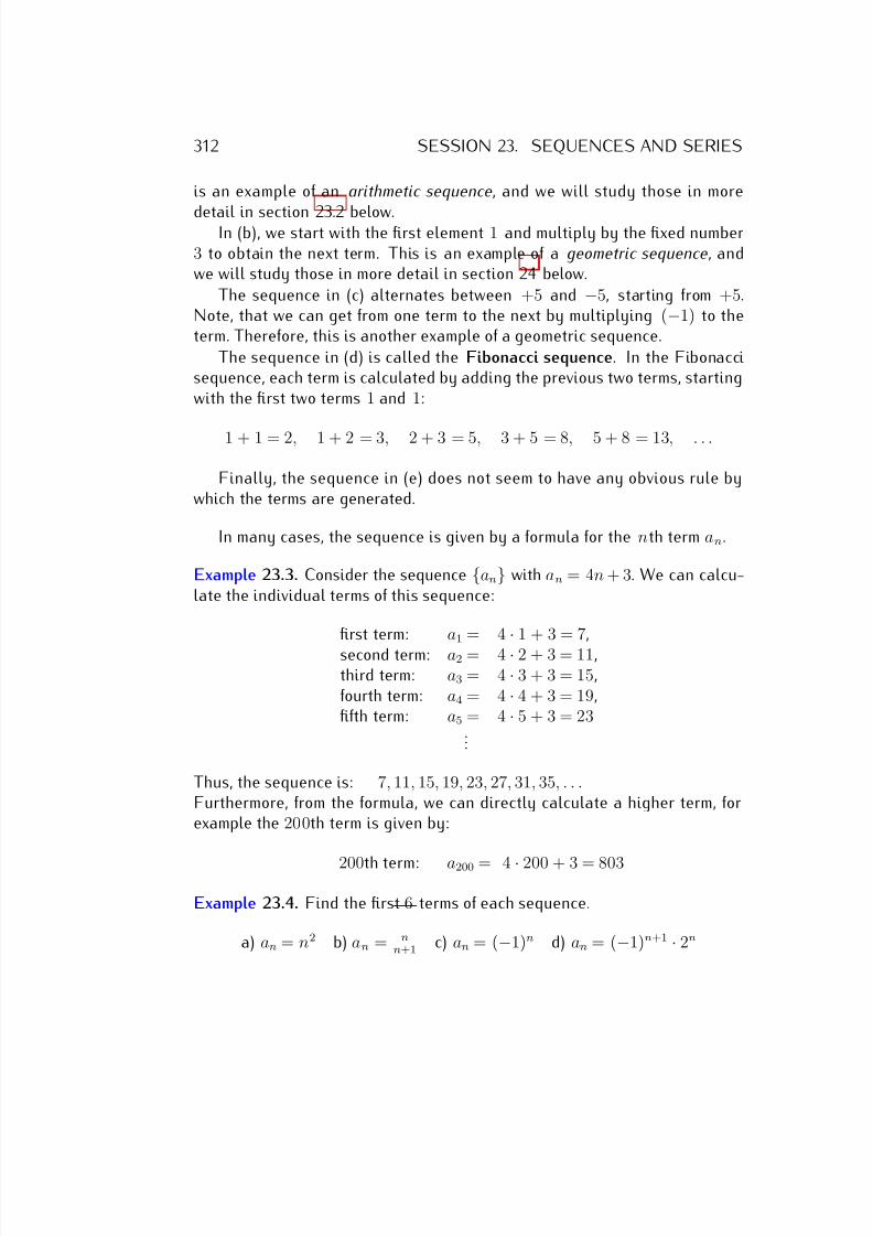
7/18/2019 Precalculus Tradler Carley
http://slidepdf.com/reader/full/precalculus-tradler-carley 322/424
312 SESSION 23. SEQUENCES AND SERIES
is an example of an arithmetic sequence, and we will study those in more
detail in section 23.2 below.In (b), we start with the first element 1 and multiply by the fixed number
3 to obtain the next term. This is an example of a geometric sequence, andwe will study those in more detail in section 24 below.
The sequence in (c) alternates between +5 and −5, starting from +5.Note, that we can get from one term to the next by multiplying (−1) to theterm. Therefore, this is another example of a geometric sequence.
The sequence in (d) is called the Fibonacci sequence. In the Fibonaccisequence, each term is calculated by adding the previous two terms, startingwith the first two terms 1 and 1:
1 + 1 = 2, 1 + 2 = 3, 2 + 3 = 5, 3 + 5 = 8, 5 + 8 = 13, . . .
Finally, the sequence in (e) does not seem to have any obvious rule bywhich the terms are generated.
In many cases, the sequence is given by a formula for the nth term an.
Example 23.3. Consider the sequence {an} with an = 4n + 3. We can calcu-late the individual terms of this sequence:
first term: a1 = 4
·1 + 3 = 7,
second term: a2 = 4 · 2 + 3 = 11,third term: a3 = 4 · 3 + 3 = 15,fourth term: a4 = 4 · 4 + 3 = 19,fifth term: a5 = 4 · 5 + 3 = 23
...
Thus, the sequence is: 7, 11, 15, 19, 23, 27, 31, 35, . . .Furthermore, from the formula, we can directly calculate a higher term, forexample the 200th term is given by:
200th term: a200 = 4 · 200 + 3 = 803
Example 23.4. Find the first 6 terms of each sequence.
a) an = n2 b) an = nn+1 c) an = (−1)n d) an = (−1)n+1 · 2n
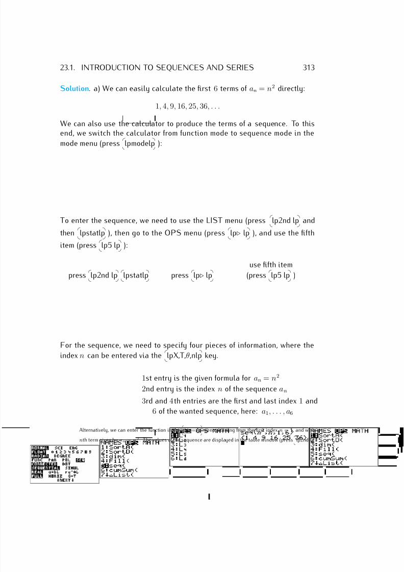
7/18/2019 Precalculus Tradler Carley
http://slidepdf.com/reader/full/precalculus-tradler-carley 323/424
23.1. INTRODUCTION TO SEQUENCES AND SERIES 313
Solution. a) We can easily calculate the first 6 terms of an = n2 directly:
1, 4, 9, 16, 25, 36, . . .
We can also use the calculator to produce the terms of a sequence. To thisend, we switch the calculator from function mode to sequence mode in the
mode menu (press
lpmodelp ):
To enter the sequence, we need to use the LIST menu (press
lp2nd lp and
then
lpstatlp ), then go to the OPS menu (press
lp⊲ lp ), and use the fifth
item (press
lp5 lp ):
use fifth item
press
lp2nd lp
lpstatlp press
lp⊲ lp (press
lp5 lp )
For the sequence, we need to specify four pieces of information, where the
index n can be entered via the
lpX,T,θ,nlp key.
1st entry is the given formula for an = n2
2nd entry is the index n of the sequence an
3rd and 4th entries are the first and last index 1 and6 of the wanted sequence, here: a1, . . . , a6
Alternatively, we can enter the function in the
lpy= lp menu, starting from the first index n = 1, and with
nth term given by an = n2. The values of the sequence are displayed in the table window (press
lp2nd lp
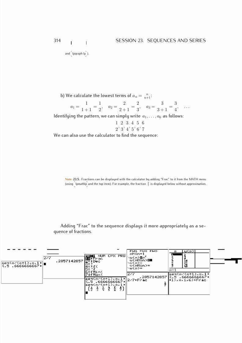
7/18/2019 Precalculus Tradler Carley
http://slidepdf.com/reader/full/precalculus-tradler-carley 324/424
314 SESSION 23. SEQUENCES AND SERIES
and
lpgraph lp ).
b) We calculate the lowest terms of an = nn+1
:
a1 = 1
1 + 1 =
1
2, a2 =
2
2 + 1 =
2
3, a3 =
3
3 + 1 =
3
4, . . .
Identifying the pattern, we can simply write a1, . . . , a6 as follows:
1
2, 2
3, 3
4, 4
5, 5
6, 6
7
We can also use the calculator to find the sequence:
Note 23.5. Fractions can be displayed with the calculator by adding “Frac” to it from the MATH menu(using
lpmathlp and the top item). For example, the fraction 2
7 is displayed below without approximation.
Adding “Frac” to the sequence displays it more appropriately as a se-quence of fractions.
7/18/2019 Precalculus Tradler Carley
http://slidepdf.com/reader/full/precalculus-tradler-carley 325/424
23.1. INTRODUCTION TO SEQUENCES AND SERIES 315
c) Since (−1)n is +1 for even n, but is −1 for odd n, the sequence an =
(−1)n
is: −1, +1, −1, +1, −1, +1
d) Similar to part (c), (−1)n+1 is −1 for even n, and is +1 for odd n. This,together with the calculation 21 = 2, 22 = 4, 23 = 8, 24 = 16, etc., we get thefirst six terms of the sequence:
+2, −4, +8, −16, +32, −64
Another way to describe a sequence is by giving a recursive formula for
the nth term an in terms of the lower terms. Here are some examples.
Example 23.6. Find the first 6 terms in the sequence described below.
a) a1 = 4, and an = an−1 + 5 for n > 1b) a1 = 3, and an = 2 · an−1 for n > 1c) a1 = 1, a2 = 1, and an = an−1 + an−2 for n > 2
Solution. a) The first term is explicitly given as a1 = 4. Then, we can calcu-late the following terms via an = an−1 + 5:
a2 = a1 + 5 = 4 + 5 = 9
a3 = a2 + 5 = 9 + 5 = 14
a4 = a3 + 5 = 14 + 5 = 19
a5 = a4 + 5 = 19 + 5 = 24...
b) We have a1 = 3, and calculate a2 = 2 · a1 = 2 · 3 = 6, a3 = 2 · a2 =2 · 6 = 12, a4 = 2 · a3 = 2 · 12 = 24, etc. We see that the effect of the recursiverelation an = 2 · an−1 is to double the previous number. The sequence is:
3, 6, 12, 24, 48, 96, 192, . . .
c) Starting from a1 = 1, and a2 = 1, we can calculate the higher terms:
a3 = a1 + a2 = 1 + 1 = 2
a4 = a2 + a3 = 1 + 2 = 3
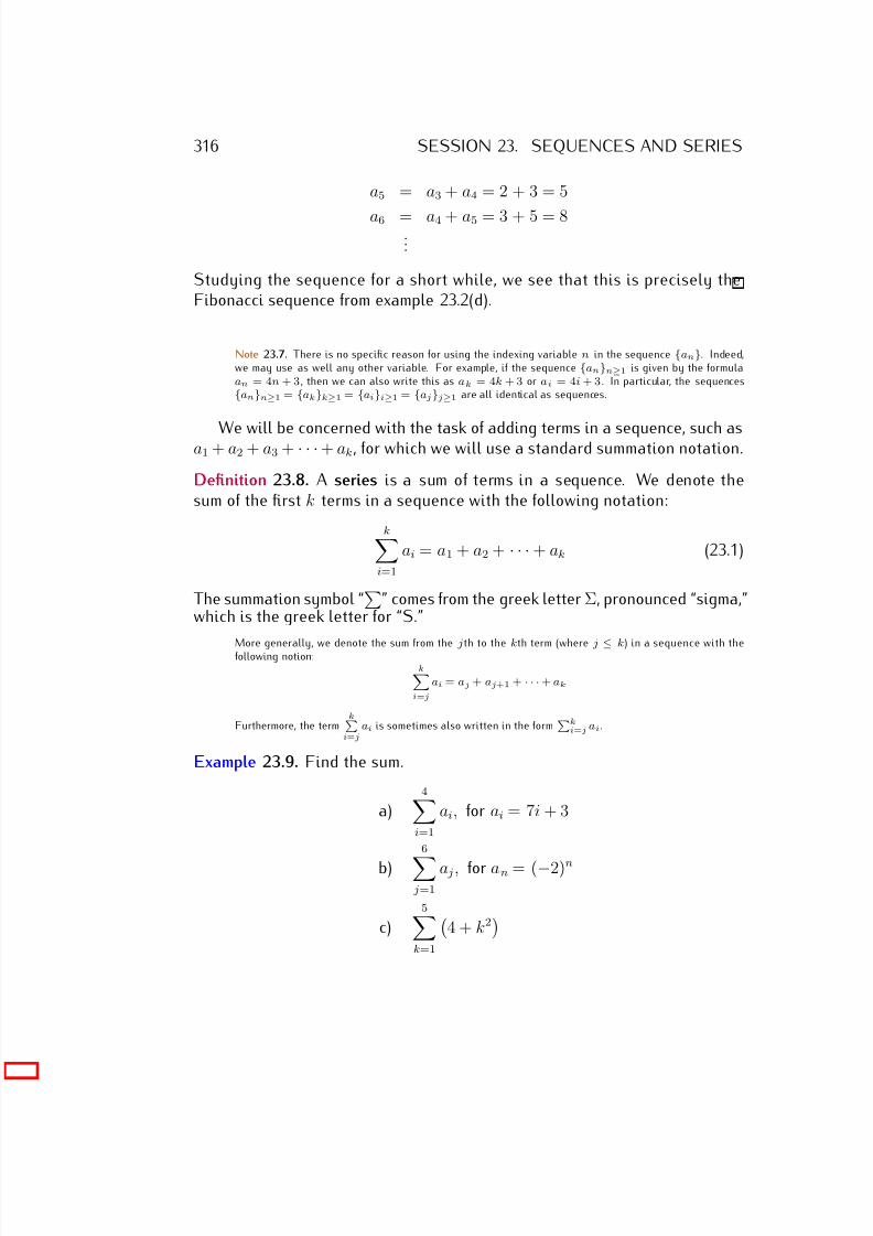
7/18/2019 Precalculus Tradler Carley
http://slidepdf.com/reader/full/precalculus-tradler-carley 326/424
316 SESSION 23. SEQUENCES AND SERIES
a5 = a3 + a4 = 2 + 3 = 5
a6 = a4 + a5 = 3 + 5 = 8...
Studying the sequence for a short while, we see that this is precisely theFibonacci sequence from example 23.2(d).
Note 23.7. There is no specific reason for using the indexing variable n in the sequence {an}. Indeed,we may use as well any other variable. For example, if the sequence {an}n≥1 is given by the formulaan = 4n + 3 , then we can also write this as ak = 4k + 3 or ai = 4i + 3 . In particular, the sequences{an}n≥1 = {ak}k≥1 = {ai}i≥1 = {aj}j≥1 are all identical as sequences.
We will be concerned with the task of adding terms in a sequence, such asa1 + a2 + a3 + · · · + ak, for which we will use a standard summation notation.
Definition 23.8. A series is a sum of terms in a sequence. We denote thesum of the first k terms in a sequence with the following notation:
ki=1
ai = a1 + a2 + · · · + ak (23.1)
The summation symbol “
” comes from the greek letter Σ, pronounced “sigma,”which is the greek letter for “S.”
More generally, we denote the sum from the jth to the kth term (where j ≤
k) in a sequence with thefollowing notion:
ki=j
ai = aj + aj+1 + · · · + ak
Furthermore, the termk
i=j
ai is sometimes also written in the formk
i=j ai .
Example 23.9. Find the sum.
a)4
i=1
ai, for ai = 7i + 3
b)
6 j=1
a j, for an = (−2)n
c)5
k=1
4 + k2
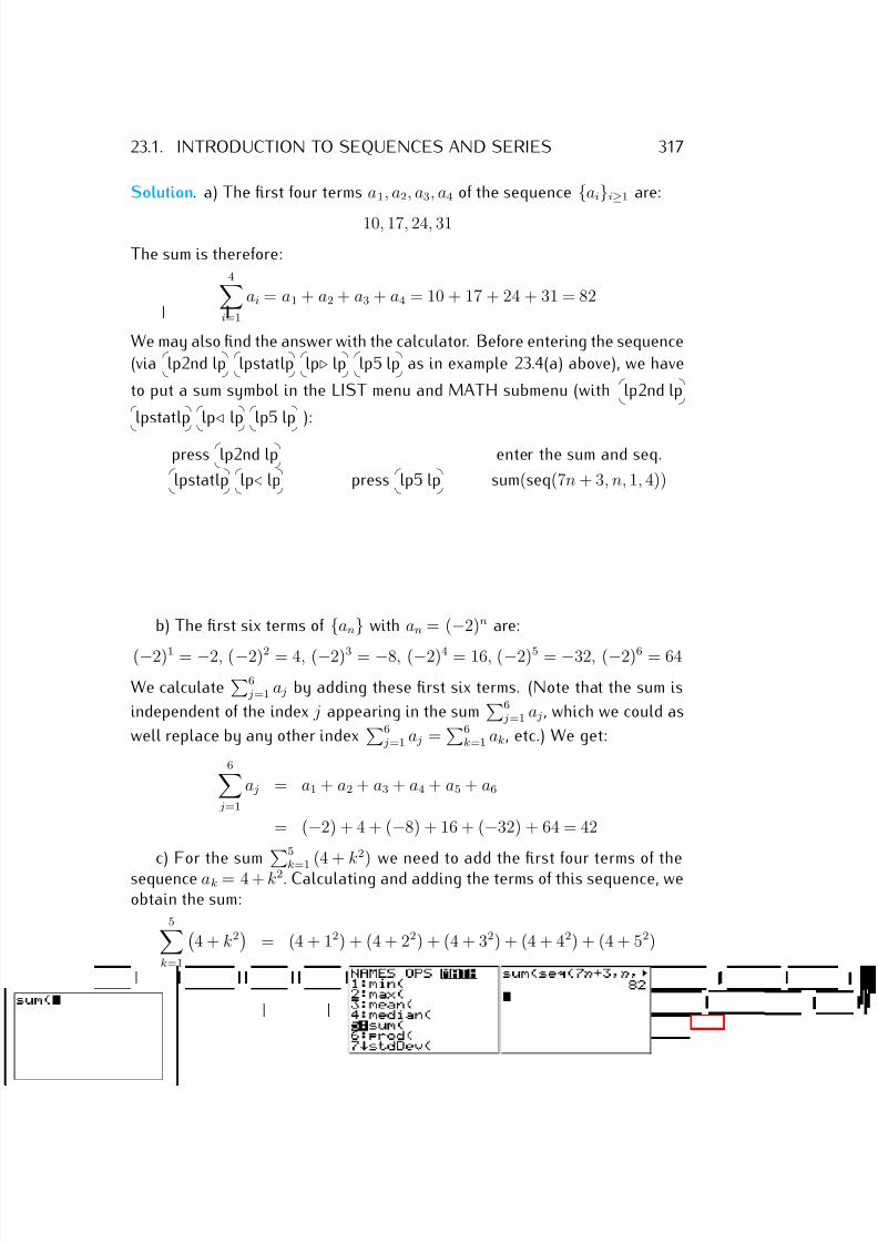
7/18/2019 Precalculus Tradler Carley
http://slidepdf.com/reader/full/precalculus-tradler-carley 327/424
23.1. INTRODUCTION TO SEQUENCES AND SERIES 317
Solution. a) The first four terms a1, a2, a3, a4 of the sequence {ai}i≥1 are:
10, 17, 24, 31
The sum is therefore:4
i=1
ai = a1 + a2 + a3 + a4 = 10 + 17 + 24 + 31 = 82
We may also find the answer with the calculator. Before entering the sequence
(via
lp2nd lp
lpstatlp
lp⊲ lp
lp5 lp as in example 23.4(a) above), we have
to put a sum symbol in the LIST menu and MATH submenu (with
lp2nd lp
lpstatlp
lp⊳ lp
lp5 lp ):
press
lp2nd lp enter the sum and seq.
lpstatlp
lp⊳ lp press
lp5 lp sum(seq(7n + 3, n, 1, 4))
b) The first six terms of {an} with an = (−2)n are:
(−2)1 = −2, (−2)2 = 4, (−2)3 = −8, (−2)4 = 16, (−2)5 = −32, (−2)6 = 64
We calculate6
j=1 a j by adding these first six terms. (Note that the sum is
independent of the index j appearing in the sum 6
j=1 a j , which we could as
well replace by any other index6
j=1 a j =6
k=1 ak, etc.) We get:
6 j=1
a j = a1 + a2 + a3 + a4 + a5 + a6
= (−2) + 4 + (−8) + 16 + (−32) + 64 = 42
c) For the sum 5k=1 (4 + k2) we need to add the first four terms of the
sequence ak = 4 + k2. Calculating and adding the terms of this sequence, weobtain the sum:
5k=1
4 + k2
= (4 + 12) + (4 + 22) + (4 + 32) + (4 + 42) + (4 + 52)
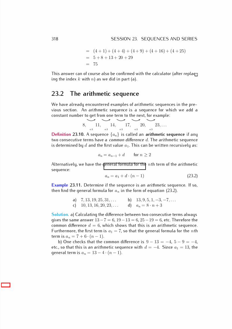
7/18/2019 Precalculus Tradler Carley
http://slidepdf.com/reader/full/precalculus-tradler-carley 328/424
318 SESSION 23. SEQUENCES AND SERIES
= (4 + 1) + (4 + 4) + (4 + 9) + (4 + 16) + (4 + 25)
= 5 + 8 + 13 + 20 + 29= 75
This answer can of course also be confirmed with the calculator (after replac-ing the index k with n) as we did in part (a).
23.2 The arithmetic sequence
We have already encountered examples of arithmetic sequences in the pre-vious section. An arithmetic sequence is a sequence for which we add a
constant number to get from one term to the next, for example:
8,+3
11,+3
14,+3
17,+3
20,+3
23, . . .
Definition 23.10. A sequence {an} is called an arithmetic sequence if anytwo consecutive terms have a common difference d. The arithmetic sequenceis determined by d and the first value a1. This can be written recursively as:
an = an−1 + d for n ≥ 2
Alternatively, we have the general formula for the nth term of the arithmeticsequence:
an = a1 + d · (n − 1) (23.2)
Example 23.11. Determine if the sequence is an arithmetic sequence. If so,then find the general formula for an in the form of equation (23.2).
a) 7, 13, 19, 25, 31, . . . b) 13, 9, 5, 1, −3, −7, . . .c) 10, 13, 16, 20, 23, . . . d) an = 8 · n + 3
Solution. a) Calculating the difference between two consecutive terms alwaysgives the same answer 13 −7 = 6, 19 −13 = 6, 25 −19 = 6, etc. Therefore thecommon difference d = 6, which shows that this is an arithmetic sequence.
Furthermore, the first term is a1 = 7, so that the general formula for the nthterm is an = 7 + 6 · (n − 1).
b) One checks that the common difference is 9 − 13 = −4, 5 − 9 = −4,etc., so that this is an arithmetic sequence with d = −4. Since a1 = 13, thegeneral term is an = 13 − 4 · (n − 1).
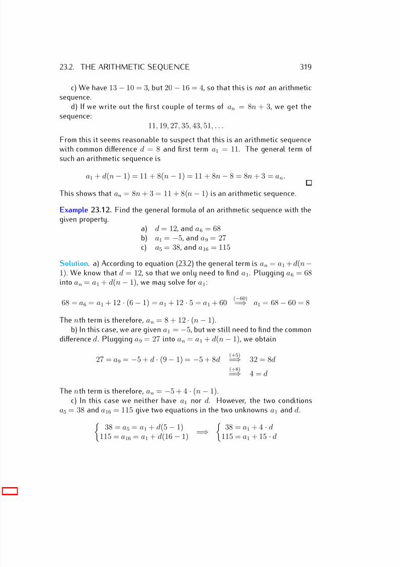
7/18/2019 Precalculus Tradler Carley
http://slidepdf.com/reader/full/precalculus-tradler-carley 329/424
23.2. THE ARITHMETIC SEQUENCE 319
c) We have 13 − 10 = 3, but 20 − 16 = 4, so that this is not an arithmetic
sequence.d) If we write out the first couple of terms of an = 8n + 3, we get thesequence:
11, 19, 27, 35, 43, 51, . . .
From this it seems reasonable to suspect that this is an arithmetic sequencewith common difference d = 8 and first term a1 = 11. The general term of such an arithmetic sequence is
a1 + d(n − 1) = 11 + 8(n − 1) = 11 + 8n − 8 = 8n + 3 = an.
This shows that an = 8n + 3 = 11 + 8(n−
1) is an arithmetic sequence.
Example 23.12. Find the general formula of an arithmetic sequence with thegiven property.
a) d = 12, and a6 = 68b) a1 = −5, and a9 = 27c) a5 = 38, and a16 = 115
Solution. a) According to equation (23.2) the general term is an = a1 + d(n −1). We know that d = 12, so that we only need to find a1. Plugging a6 = 68into an = a1 + d(n − 1), we may solve for a1:
68 = a6 = a1 + 12 · (6 − 1) = a1 + 12 · 5 = a1 + 60 (−60)=⇒ a1 = 68 − 60 = 8
The nth term is therefore, an = 8 + 12 · (n − 1).b) In this case, we are given a1 = −5, but we still need to find the common
difference d. Plugging a9 = 27 into an = a1 + d(n − 1), we obtain
27 = a9 = −5 + d · (9 − 1) = −5 + 8d (+5)
=⇒ 32 = 8d(÷8)=⇒ 4 = d
The nth term is therefore, an =−
5 + 4·
(n−
1).c) In this case we neither have a1 nor d. However, the two conditions
a5 = 38 and a16 = 115 give two equations in the two unknowns a1 and d. 38 = a5 = a1 + d(5 − 1)
115 = a16 = a1 + d(16 − 1) =⇒
38 = a1 + 4 · d115 = a1 + 15 · d
7/18/2019 Precalculus Tradler Carley
http://slidepdf.com/reader/full/precalculus-tradler-carley 330/424
320 SESSION 23. SEQUENCES AND SERIES
To solve this system of equations, we need to recall the methods for doing
so. One convenient method is the addition/subtraction method. For this, wesubtract the top from the bottom equation:
115 = a1 +15 · d−( 38 = a1 +4 · d )
77 = +11 · d (÷11)=⇒ 7 = d
Plugging d = 7 into either of the two equations gives a1. We plug it into thefirst equation 38 = a1 + 4d:
38 = a1 + 4
·7 =
⇒ 38 = a1 + 28
(−28)=
⇒ 10 = a1
Therefore, the nth term is given by an = 10 + 7 · (n − 1).
We can sum the first k terms of an arithmetic sequence using a trick, which,according to lore, was found by the German mathematician Carl FriedrichGauss when he was a child at school.
Example 23.13. Find the sum of the first 100 integers, starting from 1. Inother words, we want to find the sum of 1 + 2 + 3 + · · · + 99 + 100. First,note that he sequence 1, 2, 3, . . . is an arithmetic sequence. The main ideafor solving this problem is a trick, which will indeed work for any arithmetic
sequence:Let S = 1 + 2 + 3 + · · · +98+99+100 be what we want to find. Note that
2S = 1 + 2 + 3 · · · + 98 + 99 + 100
+ 100 + 99 + 98 · · · + 3 + 2 + 1 .
Note that the second line is also S but is added in the reverse order. Addingvertically we see then that
2S = 101 + 101 + 101 + · · · + 101 + 101 + 101,
where there are 100 terms on the right hand side. So
2S = 100 · 101 and therefore S = 100 · 101
2 = 5050.
The previous example generalizes to the more general setting starting withan arbitrary arithmetic sequence.
7/18/2019 Precalculus Tradler Carley
http://slidepdf.com/reader/full/precalculus-tradler-carley 331/424
23.2. THE ARITHMETIC SEQUENCE 321
Observation 23.14. Let {an} be an arithmetic sequence, whose nth term is
given by the formula an = a1 +d(n−1). Then, the sum a1 +a2 + · · ·+ak−1 +akis given by adding (a1 + ak) precisely k
2 times:
ki=1
ai = k
2 · (a1 + ak) (23.3)
In order to remember the formula above, it may be convenient to think of the right hand side as k · a1+ak
2 (this is, k times the average of the first andthe last term).
Proof. For the proof of equation (23.3), we write S = a1 + a2 + · · ·+ ak−1 + ak . We then add it to itself but in reverse order:
2S = a1 + a2 + a3 · · · + ak−2 + ak−1 + ak
+ ak + ak−1 + ak−2 · · · + a3 + a2 + a1.
Now note that in general al + am = 2a1 + d(l + m − 2). We see that adding vertically gives
2S = k(2a1 + d(k − 1)) = k(a1 + (a1 + d(k − 1)) = k(a1 + ak).
Dividing by 2 gives the desired result.
Example 23.15. Find the value of the arithmetic series.
a) Find the sum a1 + · · ·+ a60 for the arithmetic sequence an = 2+ 13(n−1).
b) Determine the value of the sum:1001 j=1
(5 − 6 j)
c) Find the sum of the first 35 terms of the sequence
4, 3.5, 3, 2.5, 2, 1.5, . . .
Solution. a) The sum is given by the formula (23.3): ki=1 ai = k
2
·(a1 + ak).
Here, k = 60, and a1 = 2 and a60 = 2+13·(60−1) = 2+13·59 = 2+767 = 769.We obtain a sum of
a1 + · · · + a60 =60
i=1
ai = 60
2 · (2 + 769) = 30 · 771 = 23130.
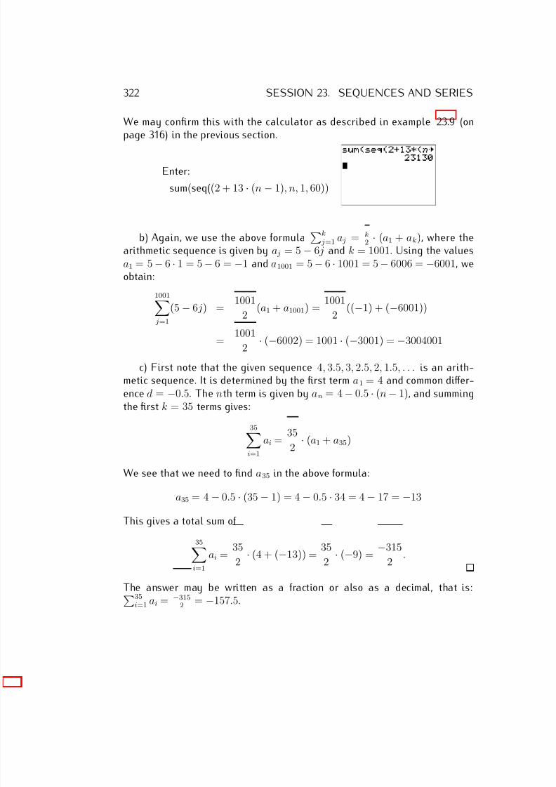
7/18/2019 Precalculus Tradler Carley
http://slidepdf.com/reader/full/precalculus-tradler-carley 332/424
322 SESSION 23. SEQUENCES AND SERIES
We may confirm this with the calculator as described in example 23.9 (on
page 316) in the previous section.
Enter:
sum(seq((2 + 13 · (n − 1), n, 1, 60))
b) Again, we use the above formulak
j=1 a j = k2 · (a1 + ak), where the
arithmetic sequence is given by a j = 5 − 6 j and k = 1001. Using the valuesa1 = 5
−6
·1 = 5
−6 =
−1 and a1001 = 5
−6
·1001 = 5
−6006 =
−6001, we
obtain:1001 j=1
(5 − 6 j) = 1001
2 (a1 + a1001) =
1001
2 ((−1) + (−6001))
= 1001
2 · (−6002) = 1001 · (−3001) = −3004001
c) First note that the given sequence 4, 3.5, 3, 2.5, 2, 1.5, . . . is an arith-metic sequence. It is determined by the first term a1 = 4 and common differ-ence d = −0.5. The nth term is given by an = 4 − 0.5 · (n − 1), and summingthe first k = 35 terms gives:
35i=1
ai = 35
2 · (a1 + a35)
We see that we need to find a35 in the above formula:
a35 = 4 − 0.5 · (35 − 1) = 4 − 0.5 · 34 = 4 − 17 = −13
This gives a total sum of
35i=1
ai = 352 · (4 + (−13)) = 35
2 · (−9) = −315
2 .
The answer may be written as a fraction or also as a decimal, that is:35i=1 ai = −315
2 = −157.5.
7/18/2019 Precalculus Tradler Carley
http://slidepdf.com/reader/full/precalculus-tradler-carley 333/424
23.3. EXERCISES 323
23.3 Exercises
Exercise 23.1. Find the first seven terms of the sequence.
a) an = 3n b) an = 5n + 3 c) an = n2 + 2 d) an = n
e) an = (−1)n+1 f ) an =√
n+1n g) ak = 10k h) ai = 5 + (−1)i
Exercise 23.2. Find the first six terms of the sequence.
a) a1 = 5, an = an−1 + 3 for n ≥ 2b) a1 = 7, an = 10 · an−1 for n ≥ 2c) a1 = 1, an = 2 · an−1 + 1 for n ≥ 2
d) a1 = 6, a2 = 4, an = an−1 − an−2 for n ≥ 3
Exercise 23.3. Find the value of the series.
a) 4
n=1 an, where an = 5n, b) 5
k=1 ak, where ak = k ,
c) 4
i=1 ai, where an = n2, d) 6
n=1(n − 4),
e)3
k=1(k2 + 4k − 4), f )4
j=11
j+1.
Exercise 23.4. Is the sequence below part of an arithmetic sequence? In thecase that it is part of an arithmetic sequence, find the formula for the nth
term an in the form an = a1 + d · (n − 1).
a) 5, 8, 11, 14, 17, . . . b) −10, −7, −4, −1, 2, . . .c) −1, 1, −1, 1, −1, 1, . . . d) 18, 164, 310, 474, . . .e) 73.4, 51.7, 30, . . . f ) 9, 3, −3, −8, −14, . . .g) 4, 4, 4, 4, 4, . . . h) −2.72, −2.82, −2.92, −3.02, −3.12, . . .i)
√ 2,
√ 5,
√ 8,
√ 11, . . . j) −3
5 , −110 , 2
5 , . . .k) an = 4 + 5 · n l) a j = 2 · j − 5m) an = n2 + 8n + 15 n) ak = 9 · (k + 5) + 7k − 1
Exercise 23.5. Determine the general nth term an of an arithmetic sequence
{an} with the data given below.
a) d = 4, and a8 = 57 b) d = −3, and a99 = −70c) a1 = 14, and a7 = −16 d) a1 = −80, and a5 = 224e) a3 = 10, and a14 = −23 f ) a20 = 2, and a60 = 32
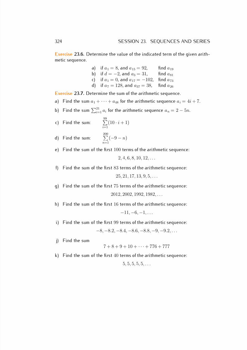
7/18/2019 Precalculus Tradler Carley
http://slidepdf.com/reader/full/precalculus-tradler-carley 334/424
324 SESSION 23. SEQUENCES AND SERIES
Exercise 23.6. Determine the value of the indicated term of the given arith-
metic sequence.a) if a1 = 8, and a15 = 92, find a19
b) if d = −2, and a3 = 31, find a81
c) if a1 = 0, and a17 = −102, find a73
d) if a7 = 128, and a37 = 38, find a26
Exercise 23.7. Determine the sum of the arithmetic sequence.
a) Find the sum a1 + · · · + a48 for the arithmetic sequence ai = 4i + 7.
b) Find the sum21
i=1 ai for the arithmetic sequence an = 2 − 5n.
c) Find the sum:
99i=1
(10 · i + 1)
d) Find the sum:200n=1
(−9 − n)
e) Find the sum of the first 100 terms of the arithmetic sequence:
2, 4, 6, 8, 10, 12, . . .
f) Find the sum of the first 83 terms of the arithmetic sequence:
25, 21, 17, 13, 9, 5, . . .
g) Find the sum of the first 75 terms of the arithmetic sequence:
2012, 2002, 1992, 1982, . . .
h) Find the sum of the first 16 terms of the arithmetic sequence:
−11, −6, −1, . . .
i) Find the sum of the first 99 terms of the arithmetic sequence:
−8, −8.2, −8.4, −8.6, −8.8, −9, −9.2, . . .
j) Find the sum
7 + 8 + 9 + 10 + · · · + 776 + 777
k) Find the sum of the first 40 terms of the arithmetic sequence:
5, 5, 5, 5, 5, . . .
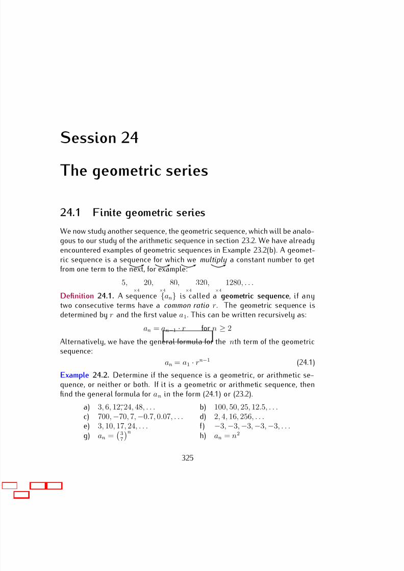
7/18/2019 Precalculus Tradler Carley
http://slidepdf.com/reader/full/precalculus-tradler-carley 335/424
Session 24
The geometric series
24.1 Finite geometric series
We now study another sequence, the geometric sequence, which will be analo-gous to our study of the arithmetic sequence in section 23.2. We have alreadyencountered examples of geometric sequences in Example 23.2(b). A geomet-ric sequence is a sequence for which we multiply a constant number to getfrom one term to the next, for example:
5,×4
20,×4
80,×4
320,×4
1280, . . .
Definition 24.1. A sequence {an} is called a geometric sequence, if anytwo consecutive terms have a common ratio r. The geometric sequence isdetermined by r and the first value a1. This can be written recursively as:
an = an−1 · r for n ≥ 2
Alternatively, we have the general formula for the nth term of the geometricsequence:
an = a1 · rn−1 (24.1)
Example 24.2. Determine if the sequence is a geometric, or arithmetic se-quence, or neither or both. If it is a geometric or arithmetic sequence, thenfind the general formula for an in the form (24.1) or (23.2).
a) 3, 6, 12, 24, 48, . . . b) 100, 50, 25, 12.5, . . .c) 700, −70, 7, −0.7, 0.07, . . . d) 2, 4, 16, 256, . . .e) 3, 10, 17, 24, . . . f ) −3, −3, −3, −3, −3, . . .g) an =
37
nh) an = n2
325
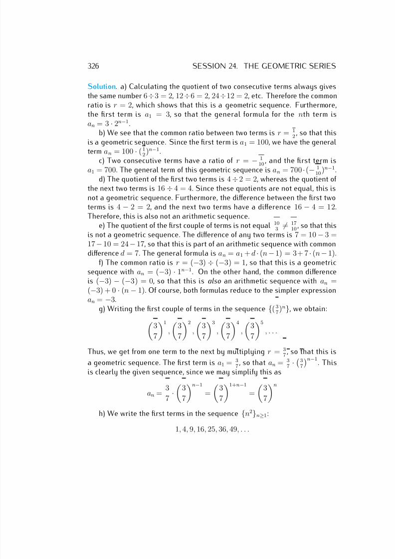
7/18/2019 Precalculus Tradler Carley
http://slidepdf.com/reader/full/precalculus-tradler-carley 336/424
326 SESSION 24. THE GEOMETRIC SERIES
Solution. a) Calculating the quotient of two consecutive terms always gives
the same number 6÷3 = 2, 12÷6 = 2, 24÷12 = 2, etc. Therefore the commonratio is r = 2, which shows that this is a geometric sequence. Furthermore,the first term is a1 = 3, so that the general formula for the nth term isan = 3 · 2n−1.
b) We see that the common ratio between two terms is r = 12
, so that thisis a geometric sequence. Since the first term is a1 = 100, we have the generalterm an = 100 · ( 1
2 )n−1.c) Two consecutive terms have a ratio of r = − 1
10, and the first term is
a1 = 700. The general term of this geometric sequence is an = 700 ·(− 110 )n−1.
d) The quotient of the first two terms is 4 ÷2 = 2, whereas the quotient of the next two terms is 16
÷4 = 4. Since these quotients are not equal, this is
not a geometric sequence. Furthermore, the difference between the first twoterms is 4 − 2 = 2, and the next two terms have a difference 16 − 4 = 12.Therefore, this is also not an arithmetic sequence.
e) The quotient of the first couple of terms is not equal 103 = 17
10 , so that thisis not a geometric sequence. The difference of any two terms is 7 = 10 − 3 =17 − 10 = 24 − 17, so that this is part of an arithmetic sequence with commondifference d = 7. The general formula is an = a1 + d · (n − 1) = 3+ 7 · (n − 1).
f) The common ratio is r = (−3) ÷ (−3) = 1, so that this is a geometricsequence with an = (−3) · 1n−1. On the other hand, the common differenceis (−3) − (−3) = 0, so that this is also an arithmetic sequence with an =
(−3) + 0 · (n − 1). Of course, both formulas reduce to the simpler expressionan = −3.g) Writing the first couple of terms in the sequence {( 3
7)n}, we obtain:
3
7
1
,
3
7
2
,
3
7
3
,
3
7
4
,
3
7
5
, . . .
Thus, we get from one term to the next by multiplying r = 37 , so that this is
a geometric sequence. The first term is a1 = 37
, so that an = 37 · 3
7
n−1. This
is clearly the given sequence, since we may simplify this as
an = 37 ·37n−1
= 371+n−1
= 37n
h) We write the first terms in the sequence {n2}n≥1:
1, 4, 9, 16, 25, 36, 49, . . .
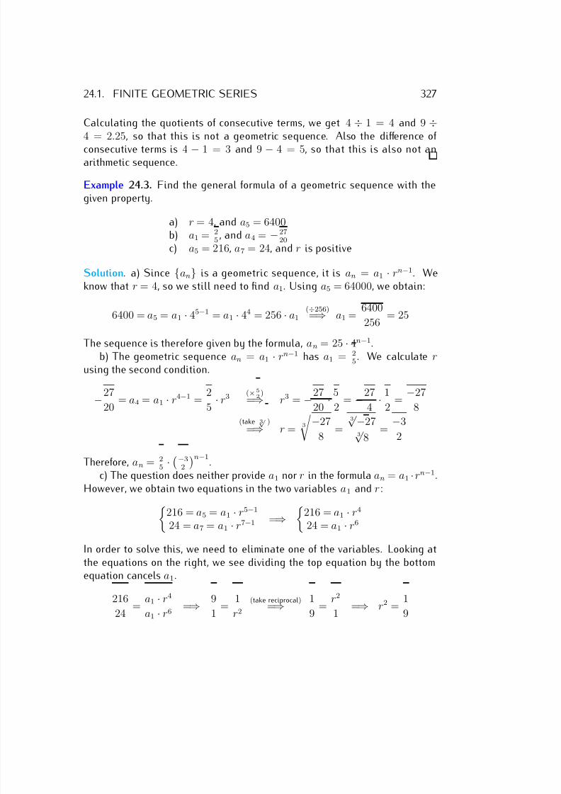
7/18/2019 Precalculus Tradler Carley
http://slidepdf.com/reader/full/precalculus-tradler-carley 337/424
24.1. FINITE GEOMETRIC SERIES 327
Calculating the quotients of consecutive terms, we get 4 ÷ 1 = 4 and 9 ÷4 = 2.25, so that this is not a geometric sequence. Also the difference of consecutive terms is 4 − 1 = 3 and 9 − 4 = 5, so that this is also not anarithmetic sequence.
Example 24.3. Find the general formula of a geometric sequence with thegiven property.
a) r = 4, and a5 = 6400b) a1 = 2
5, and a4 = −27
20
c) a5 = 216, a7 = 24, and r is positive
Solution. a) Since {an} is a geometric sequence, it is an = a1 · r
n
−1
. Weknow that r = 4, so we still need to find a1. Using a5 = 64000, we obtain:
6400 = a5 = a1 · 45−1 = a1 · 44 = 256 · a1(÷256)=⇒ a1 =
6400
256 = 25
The sequence is therefore given by the formula, an = 25 · 4n−1.b) The geometric sequence an = a1 · rn−1 has a1 = 2
5 . We calculate rusing the second condition.
−27
20 = a4 = a1 · r4−1 =
2
5 · r3 (×5
2)
=⇒ r3 = −27
20 · 5
2 = −27
4 · 1
2 =
−27
8(take 3√ )
=⇒ r = 3 −27
8 =
3√ −273√
8=
−3
2
Therefore, an = 25 · −3
2
n−1.
c) The question does neither provide a1 nor r in the formula an = a1 ·rn−1.However, we obtain two equations in the two variables a1 and r:
216 = a5 = a1 · r5−1
24 = a7 = a1 · r7−1 =⇒
216 = a1 · r4
24 = a1 · r6
In order to solve this, we need to eliminate one of the variables. Looking atthe equations on the right, we see dividing the top equation by the bottomequation cancels a1.
216
24 =
a1 · r4
a1 · r6 =⇒ 9
1 =
1
r2
(take reciprocal)=⇒ 1
9 =
r2
1 =⇒ r2 =
1
9
7/18/2019 Precalculus Tradler Carley
http://slidepdf.com/reader/full/precalculus-tradler-carley 338/424
328 SESSION 24. THE GEOMETRIC SERIES
To obtain r we have to solve this quadratic equation. In general, there are in
fact two solutions:r = ±
1
9 = ±1
3
Since the problem states that r is positive, we see that we need to take thepositive solution r = 1
3 . Plugging r = 13 back into either of the two equations,
we may solve for a1. For example, using the first equation a5 = 216, weobtain:
216 = a5 = a1 ·
1
3
5−1
= a1 ·
1
3
4
= a1 · 1
34 = a1 · 1
81(×
81)
=⇒ a1 = 81 · 216 = 17496
So, we finally arrive at the general formula for the nth term of the geometricsequence, an = 17496 · ( 1
3 )n−1.
We can find the sum of the first k terms of a geometric sequence usinganother trick, which is very different from the one we used for the arithmeticsequence.
Example 24.4. Consider the geometric sequence an = 8 · 5n−1, that is thesequence:
8, 40, 200, 1000, 5000, 25000, 125000, . . .
We want to add the first 6 terms of this sequence.
8 + 40 + 200 + 1000 + 5000 + 25000 = 31248
In general, it may be much more difficult to simply add the terms as we didabove, and we need to use a better general method. For this, we multiply(1 − 5) to the sum (8 + 40 + 200 + 1000 + 5000 + 25000) and simplify thisusing the distributive law:
(1 − 5) · (8 + 40 + 200 + 1000 + 5000 + 25000)
= 8 − 40 + 40 − 200 + 200 − 1000 + 1000 − 5000
+5000 − 25000 + 25000 − 125000
= 8 − 125000
7/18/2019 Precalculus Tradler Carley
http://slidepdf.com/reader/full/precalculus-tradler-carley 339/424
24.1. FINITE GEOMETRIC SERIES 329
In the second and third lines above, we have what is called a telescopic sum,
which can be canceled except for the very first and last terms. Dividing by(1 − 5), we obtain:
8 + 40 + 200 + 1000 + 5000 + 25000 = 8 − 125000
1 − 5 =
−124992
−4 = 31248
The previous example generalizes to the more general setting starting withan arbitrary geometric sequence.
Observation 24.5. Let {an} be a geometric sequence, whose nth term is givenby the formula an = a1 · rn−1. We furthermore assume that r = 1. Then, thesum a1 + a2 + · · · + ak−1 + ak is given by:
ki=1
ai = a1 · 1 − rk
1 − r (24.2)
Proof. We multiply (1 − r) to the sum (a1 + a2 + · · · + ak−1 + ak):
(1 − r) · (a1 + a2 + · · · + ak)
= (1 − r) · (a1 · r0 + a1 · r1 + · · · + a1 · rk−1)
= a1 · r0 − a1 · r1 + a1 · r1 − a1 · r2 + · · · + a1 · rk−1 − a1 · rk
= a1 · r0 − a1 · rk = a1 · (1 − rk)
Dividing by (1 − r), we obtain
a1 + a2 + · · · + ak = a1 · (1 − rk)
(1 − r) = a1 · 1 − rk
1 − r
This is the formula we wanted to prove.
Example 24.6. Find the value of the geometric series.
a) Find the sum6
n=1
an for the geometric sequence an = 10 · 3n−1.
b) Determine the value of the geometric series:5
k=1
−12k
c) Find the sum of the first 12 terms of the geometric sequence
−3, −6, −12, −24, . . .
7/18/2019 Precalculus Tradler Carley
http://slidepdf.com/reader/full/precalculus-tradler-carley 340/424
330 SESSION 24. THE GEOMETRIC SERIES
Solution. a) We need to find the sum a1 + a2 + a3 + a4 + a5 + a6, and we will
do so using the formula provided in equation (24.2). Since an = 10 · 3n
−1
, wehave a1 = 10 and r = 3, so that
6n=1
an = 10 · 1 − 36
1 − 3 = 10 · 1 − 729
1 − 3 = 10 · −728
−2 = 10 · 364 = 3640
b) Again, we use the formula for the geometric series n
k=1 ak = a1 · 1−rn
1−r ,
since ak = (−12
)k is a geometric series. We may calculate the first terma1 = −1
2 , and the common ratio is also r = −12 . With this, we obtain:
5k=1
−12
k=
−12
· 1 − (−12 )5
1 − (−12 )
=−1
2
· 1 − ((−1)5 15
25 )1 − (−1
2 ) =
=
−1
2
· 1 − (− 1
32)
1 − (−12 )
=
−1
2
· 1 + 1
32
1 + 12
=
−1
2
·
32+132
2+12
=
−1
2
·
333232
=
−1
2
· 33
32 · 2
3 = −1
2 · 11
16 = −11
32
c) Our first task is to find the formula for the provided geometric series−3, −6, −12, −24, . . . . The first term is a1 = −3 and the common ratio is
r = 2, so that an = (−3) · 2n
−1
. The sum of the first 12 terms of this sequenceis again given by equation (24.2):
12i=1
(−3) · 2i−1 = (−3) · 1 − 212
1 − 2 = (−3) · 1 − 4096
1 − 2 = (−3) · −4095
−1
= (−3) · 4095 = −12285
24.2 Infinite geometric series
In some cases, it makes sense to add not only finitely many terms of a geo-metric sequence, but all infinitely many terms of the sequence! An informaland very intuitive infinite geometric series is exhibited in the next example.
7/18/2019 Precalculus Tradler Carley
http://slidepdf.com/reader/full/precalculus-tradler-carley 341/424
24.2. INFINITE GEOMETRIC SERIES 331
Example 24.7. Consider the geometric sequence
1, 1
2, 1
4, 1
8,
1
16, . . .
Here, the common ratio is r = 12 , and the first term is a1 = 1, so that the
formula for an is an =
12
n−1. We are interested in summing all infinitely
many terms of this sequence:
1 + 1
2 +
1
4 +
1
8 +
1
16 + . . .
We add these terms one by one, and picture these sums on the number line:
0 1 1.5 1.75 2
1 = 1
1 + 1
2 = 1.5
1 + 1
2 +
1
4 = 1.75
1 + 12
+ 14
+ 18
= 1.875
1 + 1
2 +
1
4 +
1
8 +
1
16 = 1.9375
We see that adding each term takes the sum closer and closer to the number2. More precisely, adding a term an to the partial sum a1 + · · · + an−1 cutsthe distance between 2 and a1 + · · · + an−1 in half. For this reason we can,in fact, get arbitrarily close to 2, so that it is reasonable to expect that
1 + 1
2
+ 1
4
+ 1
8
+ 1
16
+
· · ·= 2
In the next definition and observation, this equation will be justified and mademore precise.
We start by providing the definition of an infinite series.
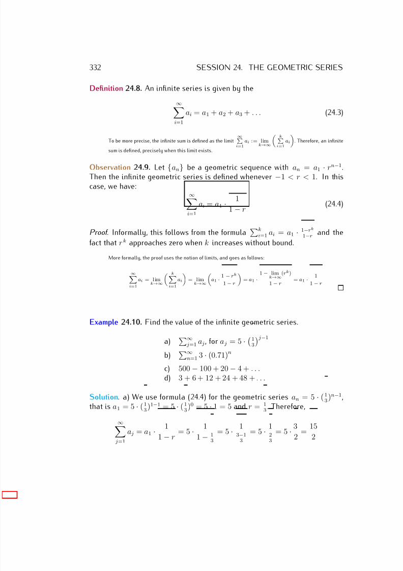
7/18/2019 Precalculus Tradler Carley
http://slidepdf.com/reader/full/precalculus-tradler-carley 342/424
332 SESSION 24. THE GEOMETRIC SERIES
Definition 24.8. An infinite series is given by the
∞i=1
ai = a1 + a2 + a3 + . . . (24.3)
To be more precise, the infinite sum is defined as the limit∞i=1
ai := limk→∞
ki=1
ai
. Therefore, an infinite
sum is defined, precisely when this limit exists.
Observation 24.9. Let {an} be a geometric sequence with an = a1 · rn−1.Then the infinite geometric series is defined whenever −1 < r < 1. In thiscase, we have:
∞i=1
ai = a1 · 11 − r
(24.4)
Proof. Informally, this follows from the formulak
i=1 ai = a1 · 1−rk
1−r and the
fact that r k approaches zero when k increases without bound.
More formally, the proof uses the notion of limits, and goes as follows:
∞i=1
ai = l imk→∞
ki=1
ai
= lim
k→∞
a1 · 1 − rk
1 − r
= a1 ·
1 − limk→∞
(rk)
1 − r = a1 · 1
1 − r
Example 24.10. Find the value of the infinite geometric series.
a) ∞
j=1 a j , for a j = 5 · 13
j−1
b)∞
n=1 3 · (0.71)n
c) 500 − 100 + 20 − 4 + . . .d) 3 + 6 + 12 + 24 + 48 + . . .
Solution. a) We use formula (24.4) for the geometric series an = 5 · (1
3 )n
−1
,that is a1 = 5 · ( 13
)1−1 = 5 · ( 13
)0 = 5 · 1 = 5 and r = 13
. Therefore,
∞ j=1
a j = a1 · 1
1 − r = 5 · 1
1 − 13
= 5 · 13−1
3
= 5 · 123
= 5 · 32
= 15
2
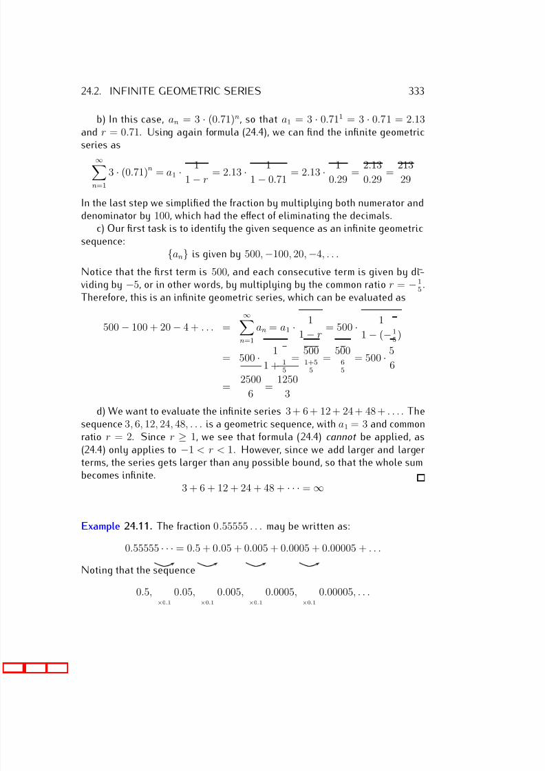
7/18/2019 Precalculus Tradler Carley
http://slidepdf.com/reader/full/precalculus-tradler-carley 343/424
24.2. INFINITE GEOMETRIC SERIES 333
b) In this case, an = 3 · (0.71)n, so that a1 = 3 · 0.711 = 3 · 0.71 = 2.13
and r = 0.71. Using again formula (24.4), we can find the infinite geometricseries as
∞n=1
3 · (0.71)n = a1 · 1
1 − r = 2.13 · 1
1 − 0.71 = 2.13 · 1
0.29 =
2.13
0.29 =
213
29
In the last step we simplified the fraction by multiplying both numerator anddenominator by 100, which had the effect of eliminating the decimals.
c) Our first task is to identify the given sequence as an infinite geometricsequence:
{an} is given by 500, −100, 20, −4, . . .
Notice that the first term is 500, and each consecutive term is given by di-viding by −5, or in other words, by multiplying by the common ratio r = −1
5.
Therefore, this is an infinite geometric series, which can be evaluated as
500 − 100 + 20 − 4 + . . . =∞
n=1
an = a1 · 1
1 − r = 500 · 1
1 − (−15
)
= 500 · 1
1 + 15
= 500
1+55
= 500
65
= 500 · 5
6
= 2500
6 =
1250
3
d) We want to evaluate the infinite series 3 + 6 + 12 + 24 + 48 + . . . . Thesequence 3, 6, 12, 24, 48, . . . is a geometric sequence, with a1 = 3 and commonratio r = 2. Since r ≥ 1, we see that formula (24.4) cannot be applied, as(24.4) only applies to −1 < r < 1. However, since we add larger and largerterms, the series gets larger than any possible bound, so that the whole sumbecomes infinite.
3 + 6 + 12 + 24 + 48 + · · · = ∞
Example 24.11. The fraction 0.55555 . . . may be written as:
0.55555 · · · = 0.5 + 0.05 + 0.005 + 0.0005 + 0.00005 + . . .
Noting that the sequence
0.5,×0.1
0.05,×0.1
0.005,×0.1
0.0005,×0.1
0.00005, . . .
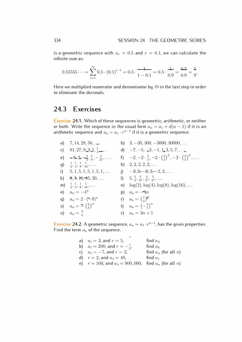
7/18/2019 Precalculus Tradler Carley
http://slidepdf.com/reader/full/precalculus-tradler-carley 344/424
334 SESSION 24. THE GEOMETRIC SERIES
is a geometric sequence with a1 = 0.5 and r = 0.1, we can calculate the
infinite sum as:
0.55555 · · · =∞
i=1
0.5 · (0.1)i−1 = 0.5 · 1
1 − 0.1 = 0.5 · 1
0.9 =
0.5
0.9 =
5
9,
Here we multiplied numerator and denominator by 10 in the last step in orderto eliminate the decimals.
24.3 Exercises
Exercise 24.1. Which of these sequences is geometric, arithmetic, or neitheror both. Write the sequence in the usual form an = a1 + d(n − 1) if it is anarithmetic sequence and an = a1 · rn−1 if it is a geometric sequence.
a) 7, 14, 28, 56, . . . b) 3, −30, 300, −3000, 30000, . . .
c) 81, 27, 9, 3, 1, 13 , . . . d) −7, −5, −3, −1, 1, 3, 5, 7, . . .
e) −6, 2, −23
, 29
, − 227
, . . . f ) −2, −2 · 23
, −2 · 23
2, −2 · 2
3
3, . . .
g) 12 , 1
4 , 18 , 1
16 , . . . h) 2, 2, 2, 2, 2, . . .
i) 5, 1, 5, 1, 5, 1, 5, 1, . . . j) −2, 2, −2, 2, −2, 2, . . .
k) 0, 5, 10, 15, 20, . . . l) 5, 5
3 , 5
32 , 5
33 , 5
34 , . . .m) 1
2, 1
4, 1
8, 1
16, . . . n) log(2), log(4), log(8), log(16), . . .
o) an = −4n p) an = −4n
q) an = 2 · (−9)n r) an =
13
n
s) an = − 57
nt) an =
−57
n
u) an = 2n v) an = 3n + 1
Exercise 24.2. A geometric sequence, an = a1 ·rn−1, has the given properties.Find the term an of the sequence.
a) a1 = 3, and r = 5, find a4
b) a1 = 200, and r = −12 , find a6
c) a1 = −7, and r = 2, find an (for all n)d) r = 2, and a4 = 48, find a1
e) r = 100, and a4 = 900, 000, find an (for all n)
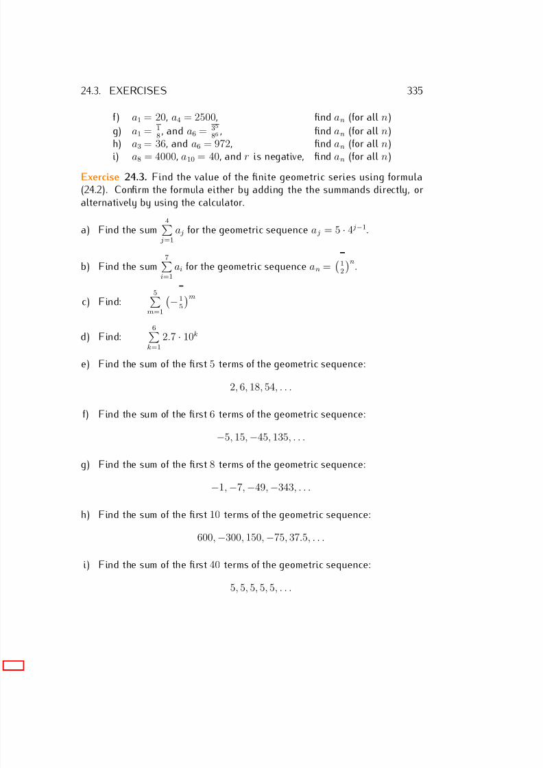
7/18/2019 Precalculus Tradler Carley
http://slidepdf.com/reader/full/precalculus-tradler-carley 345/424
24.3. EXERCISES 335
f) a1 = 20, a4 = 2500, find an (for all n)
g) a1 = 1
8 , and a6 = 35
86 , find an (for all n)h) a3 = 36, and a6 = 972, find an (for all n)i) a8 = 4000, a10 = 40, and r is negative, find an (for all n)
Exercise 24.3. Find the value of the finite geometric series using formula(24.2). Confirm the formula either by adding the the summands directly, oralternatively by using the calculator.
a) Find the sum4
j=1
a j for the geometric sequence a j = 5 · 4 j−1.
b) Find the sum
7i=1 ai for the geometric sequence an = 1
2n
.
c) Find:5
m=1
−15
m
d) Find:6
k=1
2.7 · 10k
e) Find the sum of the first 5 terms of the geometric sequence:
2, 6, 18, 54, . . .
f) Find the sum of the first 6 terms of the geometric sequence:
−5, 15, −45, 135, . . .
g) Find the sum of the first 8 terms of the geometric sequence:
−1, −7, −49, −343, . . .
h) Find the sum of the first 10 terms of the geometric sequence:
600, −300, 150, −75, 37.5, . . .
i) Find the sum of the first 40 terms of the geometric sequence:
5, 5, 5, 5, 5, . . .
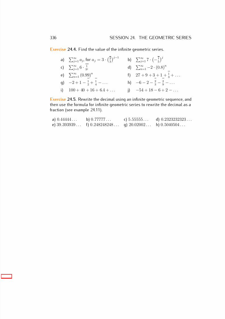
7/18/2019 Precalculus Tradler Carley
http://slidepdf.com/reader/full/precalculus-tradler-carley 346/424
336 SESSION 24. THE GEOMETRIC SERIES
Exercise 24.4. Find the value of the infinite geometric series.
a) ∞
j=1 a j , for a j = 3 · 23
j−1b) ∞
j=1 7 · −15
jc)
∞ j=1 6 · 1
3j d)
∞n=1 −2 · (0.8)n
e)∞
n=1 (0.99)n f ) 27 + 9 + 3 + 1 + 13 + . . .
g) −2 + 1 − 12 + 1
4 − . . . h) −6 − 2 − 23 − 2
9 − . . .
i) 100 + 40 + 16 + 6.4 + . . . j) −54 + 18 − 6 + 2 − . . .
Exercise 24.5. Rewrite the decimal using an infinite geometric sequence, andthen use the formula for infinite geometric series to rewrite the decimal as a
fraction (see example 24.11).
a) 0.44444 . . . b) 0.77777 . . . c) 5.55555 . . . d) 0.2323232323 . . .e) 39.393939 . . . f ) 0.248248248 . . . g) 20.02002 . . . h) 0.5040504 . . .
7/18/2019 Precalculus Tradler Carley
http://slidepdf.com/reader/full/precalculus-tradler-carley 347/424
Session 25
The binomial theorem
25.1 The binomial theorem
Recall the well-known binomial formula:
(a + b)2 = a2 + 2ab + b2
(since, using “FOIL,” we have: (a + b)2 = (a + b) · (a + b) = a2 + ab + ab + b2 = a2 + 2ab + b2 )
In this section we generalize this to find similar expressions for (a + b)n
for any natural number n. This is the content of the (generalized) binomialtheorem below. Before we can state the theorem, we need to define the notionof a factorial and combinations.
Definition 25.1. For a natural number n = 1, 2, 3, . . . , we define n! to be thenumber
n! = 1 · 2 · 3 · · · · · n
The number n! is called n factorial.To make the formulas below work nicely, we also define 0! to be 0! = 1.
It is easy to calculate some examples of factorials.
Example 25.2.
4! = 1 · 2 · 3 · 4 = 24
7! = 1 · 2 · 3 · 4 · 5 · 6 · 7 = 5040
337
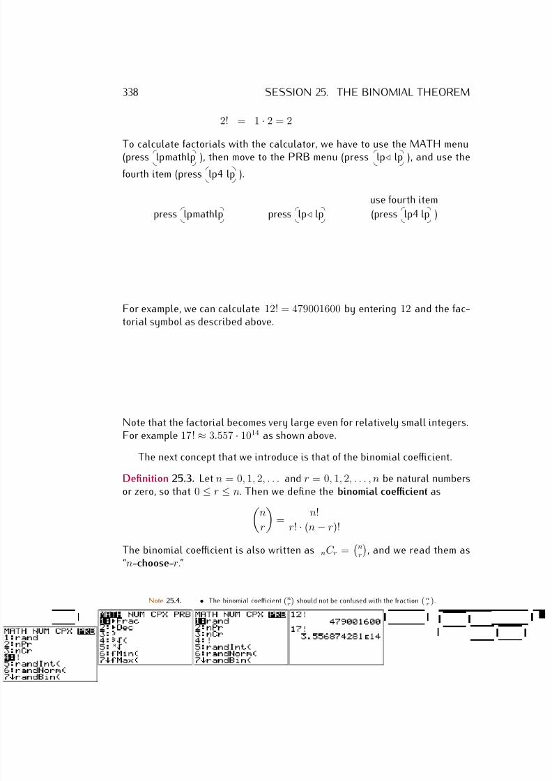
7/18/2019 Precalculus Tradler Carley
http://slidepdf.com/reader/full/precalculus-tradler-carley 348/424
338 SESSION 25. THE BINOMIAL THEOREM
2! = 1 · 2 = 2
To calculate factorials with the calculator, we have to use the MATH menu(press
lpmathlp ), then move to the PRB menu (press
lp⊳ lp ), and use the
fourth item (press
lp4 lp ).
use fourth item
press
lpmathlp press
lp⊳ lp (press
lp4 lp )
For example, we can calculate 12! = 479001600 by entering 12 and the fac-torial symbol as described above.
Note that the factorial becomes very large even for relatively small integers.For example 17! ≈ 3.557 · 1014 as shown above.
The next concept that we introduce is that of the binomial coefficient.
Definition 25.3. Let n = 0, 1, 2, . . . and r = 0, 1, 2, . . . , n be natural numbersor zero, so that 0 ≤ r ≤ n. Then we define the binomial coefficient as
n
r
=
n!
r! · (n − r)!
The binomial coefficient is also written as nC r = nr, and we read them as
“n-choose-r.”
Note 25.4. • The binomial coefficientnr
should not be confused with the fraction
nr
.
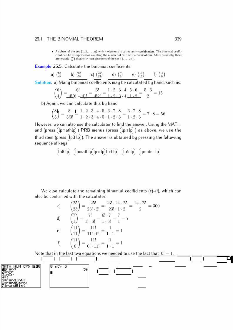
7/18/2019 Precalculus Tradler Carley
http://slidepdf.com/reader/full/precalculus-tradler-carley 349/424
25.1. THE BINOMIAL THEOREM 339
• A subset of the set {1, 2, . . . , n} with r elements is called an r-combination. The binomial coeffi-cient can be interpreted as counting the number of distinct r -combinations. More precisely, there
are exactlynr
distinct r -combinations of the set {1, . . . , n}.
Example 25.5. Calculate the binomial coefficients.
a)
64
b)
85
c)
2523
d)
71
e)
1111
f )
110
Solution. a) Many binomial coefficients may be calculated by hand, such as:
6
4
=
6!
4!(6 − 4)! =
6!
4!2! =
1 · 2 · 3 · 4 · 5 · 6
1 · 2 · 3 · 4 · 1 · 2 =
5 · 6
2 = 15
b) Again, we can calculate this by hand
8
5 =
8!
5!3! =
1
·2
·3
·4
·5
·6
·7
·8
1 · 2 · 3 · 4 · 5 · 1 · 2 · 3 =
6
·7
·8
1 · 2 · 3 = 7 · 8 = 56
However, we can also use the calculator to find the answer. Using the MATH
and (press
lpmathlp ) PRB menus (press
lp⊳ lp ) as above, we use the
third item (press
lp3 lp ). The answer is obtained by pressing the following
sequence of keys:
lp8 lp
lpmathlp
lp⊳ lp
lp3 lp
lp5 lp
lpenter lp
We also calculate the remaining binomial coefficients (c)-(f), which canalso be confirmed with the calculator.
c)
25
23
=
25!
23! · 2! =
23! · 24 · 25
23! · 1 · 2 =
24 · 25
2 = 300
d)
7
1
=
7!
1! · 6! =
6! · 7
1 · 6! =
7
1 = 7
e) 11
11 =
11!
11! · 0! =
1
1 · 1 = 1
f )
11
0
=
11!
0! · 11! =
1
1 · 1 = 1
Note that in the last two equations we needed to use the fact that 0! = 1.
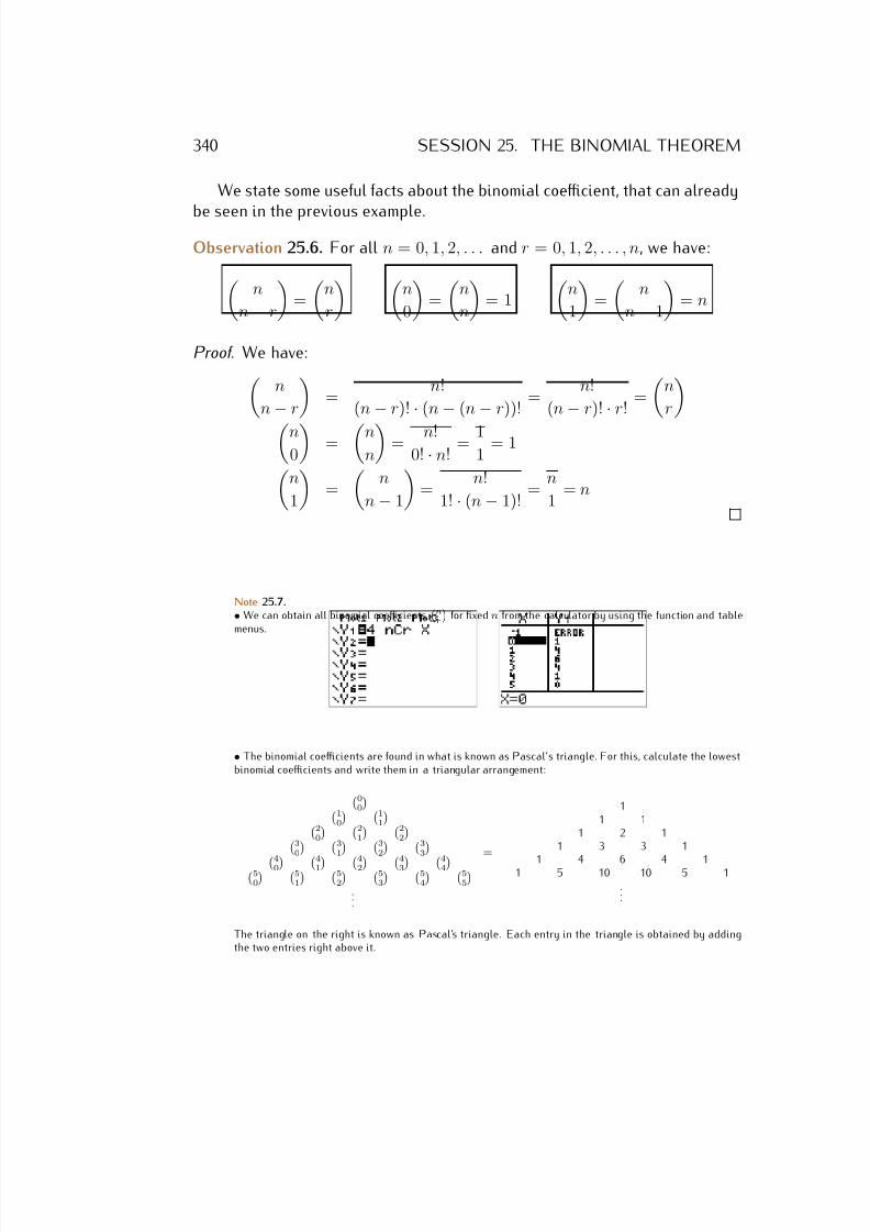
7/18/2019 Precalculus Tradler Carley
http://slidepdf.com/reader/full/precalculus-tradler-carley 350/424
340 SESSION 25. THE BINOMIAL THEOREM
We state some useful facts about the binomial coefficient, that can already
be seen in the previous example.
Observation 25.6. For all n = 0, 1, 2, . . . and r = 0, 1, 2, . . . , n, we have:
n
n − r
=
n
r
n
0
=
n
n
= 1
n
1
=
n
n − 1
= n
Proof. We have: n
n − r
=
n!
(n − r)! · (n − (n − r))! =
n!
(n − r)! · r! =
n
r
n
0
=
nn
= n!
0! · n! = 1
1 = 1
n
1
=
n
n − 1
=
n!
1! · (n − 1)! =
n
1 = n
Note 25.7.• We can obtain all binomial coefficients
nr
for fixed n from the calculator by using the function and table
menus.
• The binomial coefficients are found in what is known as Pascal’s triangle. For this, calculate the lowestbinomial coefficients and write them in a triangular arrangement:
00
1
0
11
2
0
21
22
30
31
32
334
0 4
1 4
2 4
3 4
45
0
51
52
53
54
55
...
=
11 1
1 2 11 3 3 1
1 4 6 4 11 5 10 10 5 1...
The triangle on the right is known as Pascal’s triangle. Each entry in the triangle is obtained by addingthe two entries right above it.
7/18/2019 Precalculus Tradler Carley
http://slidepdf.com/reader/full/precalculus-tradler-carley 351/424
25.1. THE BINOMIAL THEOREM 341
The binomial coefficients appear in the expressions for (a + b)n as we will
see in the next example.Example 25.8. We now calculate some simple examples.
(a + b)3 = (a + b) · (a + b) · (a + b)
= (a2 + 2ab + b2) · (a + b)
= a3 + 2a2b + ab2 + a2b + 2ab2 + b3
= a3 + 3a2b + 3ab2 + b3
Note that the coefficients 1, 3, 3, and 1 in front of a3, a2b,ab2, and b3, respec-tively, are precisely the binomial coefficients
30
,
31
,
32
, and
33
.
We also calculate the fourth power.
(a + b)4 = (a + b) · (a + b) · (a + b) · (a + b)
= (a3 + 3a2b + 3ab2 + b3) · (a + b)
= a4 + 3a3b + 3a2b2 + ab3 + a3b + 3a2b2 + 3ab3 + b4
= a4 + 4a3b + 6a2b2 + 4ab3 + b4
Again, the numbers 1, 4, 6, 4, and 1 are precisely the binomial coefficients40
,
41
,
42
,
43
, and
44
.
We are now ready to state the general binomial theorem:
Theorem 25.9 (Binomial theorem). The nth power (a + b)n can be expanded
as:
(a + b)n =
n
0
an +
n
1
an−1b1 +
n
2
an−2b2 + · · ·+
n
n − 1
a1bn−1 +
n
n
bn
Using the summation symbol, we may write this in short:
(a + b)n =n
r=0
n
r
· an−r · br (25.1)
Example 25.10. Expand (a + b)5.
Solution.
(a + b)5 =5
0
a5 +
51
a4b1 +
52
a3b2 +
53
a2b3 +
54
a1b4 +
55
b5
= a5 + 5a4b + 10a3b2 + 10a2b3 + 5ab4 + b5
7/18/2019 Precalculus Tradler Carley
http://slidepdf.com/reader/full/precalculus-tradler-carley 352/424
342 SESSION 25. THE BINOMIAL THEOREM
25.2 Binomial expansion
Using the binomial theorem, we can also expand more general powers of sumsor differences.
Example 25.11. Expand the expression.
a) (x2 + 2y3)5 b) (2xy2 − 4y2 )3 c) (
√ 2 + 1)6 d) (i − 3)4
Solution. a) We use the binomial theorem with a = x2 and b = 2y3:
(x2 + 2y3)5 = (x2)5 +5
1(x2)4(2y3) +
5
2(x2)3(2y3)2
+
5
3
(x2)2(2y3)3 +
5
4
(x2)(2y3)4 + (2y3)5
= x10 + 5x8 · 2y3 + 10x6 · 4y6 + 10x4 · 23y9 + 5x2 · 24y12 + 25y15
= x10 + 10x8y3 + 40x6y6 + 80x4y9 + 80x2y12 + 32y15
b) For part (b), it is a = 2xy2 and b = − 4y2 .
(2xy2 − 4
y2)3
= (2xy2)3 +31(2xy2)2(− 4
y2 ) + 32(2xy2)(− 4
y2 )2 + (− 4y2 )3
= 23x3y6 + 3 · 22x2y4(− 4
y2) + 3(2xy2)(−1)2 42
y4 + (−1)3 43
y6
= 8x3y6 − 48x2y2 + 96x · 1
y2 − 64 · 1
y6
c) Similarly, for part (c), we now have a =√
2 and b = 1:
(√
2 + 1)6 = (√
2)6 + 6
1(√
2)5 · 1 + 6
2(√
2)4 · 12 + 6
3(√
2)3 · 13
+6
4
(√
2)2 · 14 +6
5
(√
2) · 15 + 16
=√
64 + 6 ·√
32 + 15 ·√
16 + 20 ·√
8 + 15 ·√
4 + 6 ·√
2 + 1
= 8 + 6 ·√
16 · 2 + 15 · 4 + 20 ·√
4 · 2 + 15 · 2 + 6 ·√
2 + 1
7/18/2019 Precalculus Tradler Carley
http://slidepdf.com/reader/full/precalculus-tradler-carley 353/424
25.2. BINOMIAL EXPANSION 343
= 8 + 24√
2 + 60 + 40√
2 + 30 + 6√
2 + 1
= 99 + 70√ 2Note that the last expression cannot be simplified any further (due to theorder of operations).
d) Finally, we have a = i and b = −3, and we use the fact that i2 = −1,and therefore, i3 = −i and i4 = +1:
(i − 3)4 = i4 +
4
1
· i3 · (−3) +
4
2
· i2 · (−3)2 +
4
3
· i · (−3)3 + (−3)4
= 1 + 4 · (−i) · (−3) + 6 · (−1) · 9 + 4 · i · (−27) + 81
= 1 + 12i−
54−
108i + 81
= 28 − 96i
In some instances it is not necessary to write the full binomial expansion,but it is enough to find a particular term, say the kth term of the expansion.
Observation 25.12. Recall, for example, the binomial expansion of (a + b)6:
60
a6b0 +
61
a5b1 +
62
a4b2 +
63
a3b3 +
64
a2b4 +
65
a1b5 +
66
a0b6
first second third fourth fifth sixth seventhterm term term term term term term
Note that the exponents of the a’s and b’s for each term always add up to6, and that the exponents of a decrease from 6 to 0, and the exponents of bincrease from 0 to 6. Furthermore observe that in the above expansion thefifth term is
64
a2b4.
In general, we define the kth term by the following formula:
The kth term in the expansion of (a + b)n is: n
k − 1an−k+1bk−1 (25.2)
Note in particular, that the kth term has a power of b given by bk−1 (and not bk), it has a binomial coefficient
n
k−1
, and the exponents of a and b add up
to n.
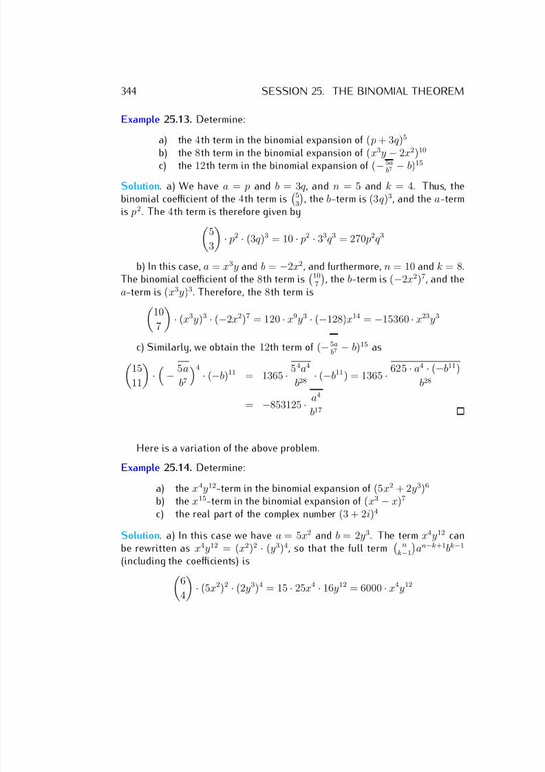
7/18/2019 Precalculus Tradler Carley
http://slidepdf.com/reader/full/precalculus-tradler-carley 354/424
344 SESSION 25. THE BINOMIAL THEOREM
Example 25.13. Determine:
a) the 4th term in the binomial expansion of ( p + 3q )5
b) the 8th term in the binomial expansion of (x3y − 2x2)10
c) the 12th term in the binomial expansion of (−5ab7 − b)15
Solution. a) We have a = p and b = 3q , and n = 5 and k = 4. Thus, thebinomial coefficient of the 4th term is
53
, the b-term is (3q )3, and the a-term
is p2. The 4th term is therefore given by5
3
· p2 · (3q )3 = 10 · p2 · 33q 3 = 270 p2q 3
b) In this case, a = x3
y and b = −2x2
, and furthermore, n = 10 and k = 8.The binomial coefficient of the 8th term is
107
, the b-term is (−2x2)7, and the
a-term is (x3y)3. Therefore, the 8th term is10
7
· (x3y)3 · (−2x2)7 = 120 · x9y3 · (−128)x14 = −15360 · x23y3
c) Similarly, we obtain the 12th term of (−5ab7 − b)15 as
15
11
·
− 5a
b7
4
· (−b)11 = 1365 · 54a4
b28 · (−b11) = 1365 · 625 · a4 · (−b11)
b28
= −853125 · a4
b17
Here is a variation of the above problem.
Example 25.14. Determine:
a) the x4y12-term in the binomial expansion of (5x2 + 2y3)6
b) the x15-term in the binomial expansion of (x3 − x)7
c) the real part of the complex number (3 + 2i)4
Solution. a) In this case we have a = 5x
2
and b = 2y
3
. The term x
4
y
12
canbe rewritten as x4y12 = (x2)2 · (y3)4, so that the full term n
k−1
an−k+1bk−1
(including the coefficients) is6
4
· (5x2)2 · (2y3)4 = 15 · 25x4 · 16y12 = 6000 · x4y12
7/18/2019 Precalculus Tradler Carley
http://slidepdf.com/reader/full/precalculus-tradler-carley 355/424
25.3. EXERCISES 345
b) The various powers of x in (x3 − x)7 (in the order in which they appear
in the binomial expansion) are:(x3)7 = x21, (x3)6 · x1 = x19, (x3)5 · x2 = x17, (x3)4 · x3 = x15, . . .
The last term is precisely the x15-term, that is we take the fourth term, k = 4.We obtain a total term (including the coefficients) of
7
3
· (x3)4 · (−x)3 = 35 · x12 · (−x)3 = −35 · x15
c) Recall that in is real when n is even, and imaginary when n is odd:
i1 = i
i2 = −1i3 = −ii4 = 1i5 = ii6 = −1
...
The real part of (3 + 2i)4 is therefore given by the first, third, and fifth termof the binomial expansion:
real part = 4
0 · 3
4
· (2i)
0
+ 4
2 · 3
2
· (2i)
2
+4
4 · 3
0
· (2i)
4
= 1 · 81 · 1 + 6 · 9 · 4i2 + 1 · 1 · 16i4 = 81 + 216 · (−1) + 16 · 1
= 81 − 216 + 16 = −119
The real part of (3 + 2i)4 is −119.
25.3 Exercises
Exercise 25.1. Find the value of the factorial or binomial coefficient.
a) 5! b) 3! c) 9! d) 2! e) 0! f ) 1! g) 19! h) 64!i)5
2
j)
96
k)
121
l)
120
m)
2322
n)
1912
o)
1311
p)
165
Exercise 25.2. Expand the expression via the binomial theorem.
a) (m + n)4 b) (x + 2)5 c) (x − y)6 d) (− p − q )5
7/18/2019 Precalculus Tradler Carley
http://slidepdf.com/reader/full/precalculus-tradler-carley 356/424
346 SESSION 25. THE BINOMIAL THEOREM
Exercise 25.3. Expand the expression.
a) (x − 2y)3 b) (x − 10)4 c) (x2y + y2)5 d) (2y2 − 5x4)4
e) (x +√
x )3 f) (−2 x2
y − y3
x )5 g) (√
2 − 2√
3)3 h) (1 − i)3
Exercise 25.4. Determine:
a) the first 3 terms in the binomial expansion of (xy − 4x)5
b) the first 2 terms in the binomial expansion of (2a2 + b3)9
c) the last 3 terms in the binomial expansion of (3y2 − x2)7
d) the first 3 terms in the binomial expansion of ( xy − y
x )10
e) the last 4 terms in the binomial expansion of (m3n + 12 n2)6
Exercise 25.5. Determine:
a) the 5th term in the binomial expansion of (x + y)7
b) the 3rd term in the binomial expansion of (x2 − y)9
c) the 10th term in the binomial expansion of (2 − w)11
d) the 5th term in the binomial expansion of (2x + xy)7
e) the 7th term in the binomial expansion of (2a + 5b)6
f ) the 6th term in the binomial expansion of (3 p2 − q 3 p)7
g) the 10th term in the binomial expansion of (4 + b2 )13
Exercise 25.6. Determine:
a) the x3y6-term in the binomial expansion of (x + y)9
b) the r 4s4-term in the binomial expansion of (r2 − s)6
c) the x4-term in the binomial expansion of (x − 1)11
d) the x3y6-term in the binomial expansion of (x3 + 5y2)4
e) the x7-term in the binomial expansion of (2x − x2)5
f) the imaginary part of the number (1 + i)3
7/18/2019 Precalculus Tradler Carley
http://slidepdf.com/reader/full/precalculus-tradler-carley 357/424
Review of complex numbers,
sequences, and the binomial
theorem
Exercise V.1. Multiply and write the answer in standard form:
(−4)(cos(207◦) + i sin(207◦)) · 2(cos(33◦) + i sin(33◦))
Exercise V.2. Divide and write the answer in standard form:
3(cos(π3
) + i sin( π3
))
15(cos( π2 ) + i sin( π
2 ))
Exercise V.3. Find the magnitude and directional angle of the vector
v = −7, −7√ 3.
Exercise V.4. Determine if the sequence is an arithmetic or geometric se-quence or neither. If it is one of these, then find the general formula for thenth term an of the sequence.
a) 54, −18, 6, −2, 23 , . . .
b) 2, 4, 8, 10, . . .c) 9, 5, 1, −3, −7, . . .
Exercise V.5. Find the sum of the first 75 terms of the arithmetic sequence:
−30, −22, −14, −6, 2, . . .
Exercise V.6. Find the sum of the first 8 terms of the geometric series:
−7, −14, −28, −56, −112, . . .
347
7/18/2019 Precalculus Tradler Carley
http://slidepdf.com/reader/full/precalculus-tradler-carley 358/424
Exercise V.7. Find the value of the infinite geometric series:
80 − 20 + 5 − 1.25 + . . .
Exercise V.8. Expand the expression via the binomial theorem.
(3x2 − 2xy)3
Exercise V.9. Write the first 3 terms of the binomial expansion:ab2 +
10
a
9
Exercise V.10. Find the 6th term of the binomial expansion:
(5 p − q 2)8
348
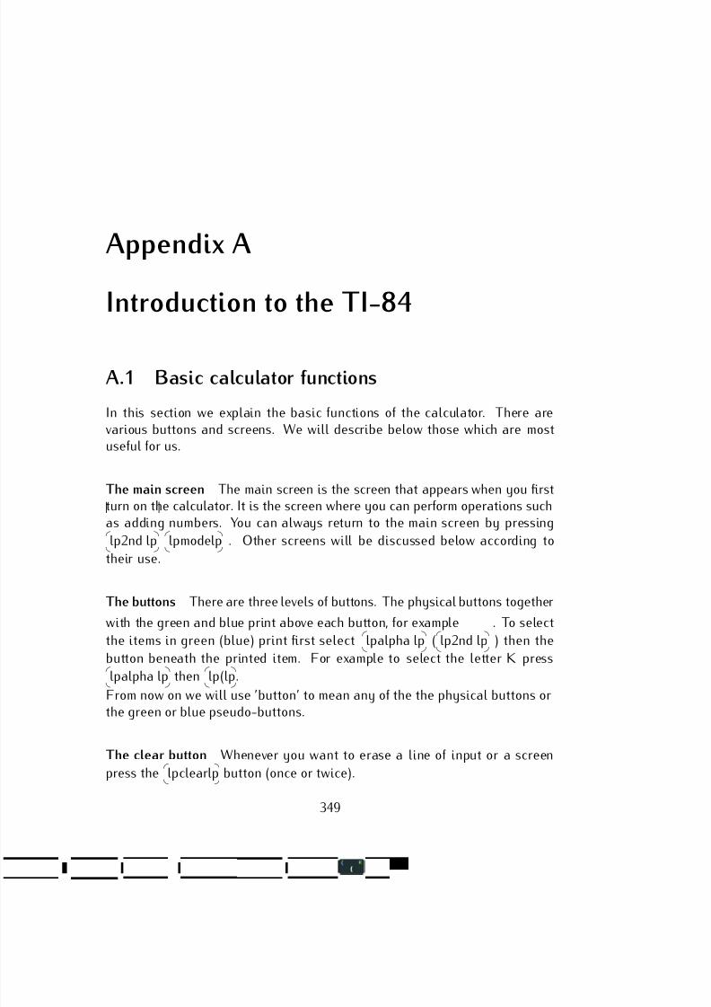
7/18/2019 Precalculus Tradler Carley
http://slidepdf.com/reader/full/precalculus-tradler-carley 359/424
Appendix A
Introduction to the TI-84
A.1 Basic calculator functions
In this section we explain the basic functions of the calculator. There arevarious buttons and screens. We will describe below those which are mostuseful for us.
The main screen The main screen is the screen that appears when you firstturn on the calculator. It is the screen where you can perform operations such
as adding numbers. You can always return to the main screen by pressing
lp2nd lp
lpmodelp . Other screens will be discussed below according to
their use.
The buttons There are three levels of buttons. The physical buttons together
with the green and blue print above each button, for example . To select
the items in green (blue) print first select
lpalpha lp (
lp2nd lp ) then the
button beneath the printed item. For example to select the letter K press
lpalpha lp then
lp(lp.
From now on we will use ’button’ to mean any of the the physical buttons orthe green or blue pseudo-buttons.
The clear button Whenever you want to erase a line of input or a screen
press the
lpclearlp button (once or twice).
349
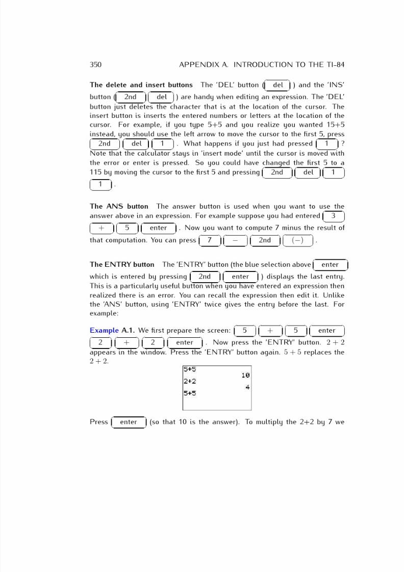
7/18/2019 Precalculus Tradler Carley
http://slidepdf.com/reader/full/precalculus-tradler-carley 360/424
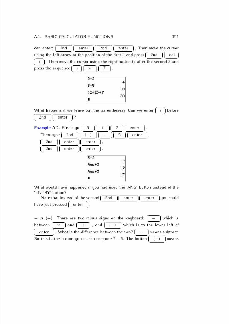
7/18/2019 Precalculus Tradler Carley
http://slidepdf.com/reader/full/precalculus-tradler-carley 361/424
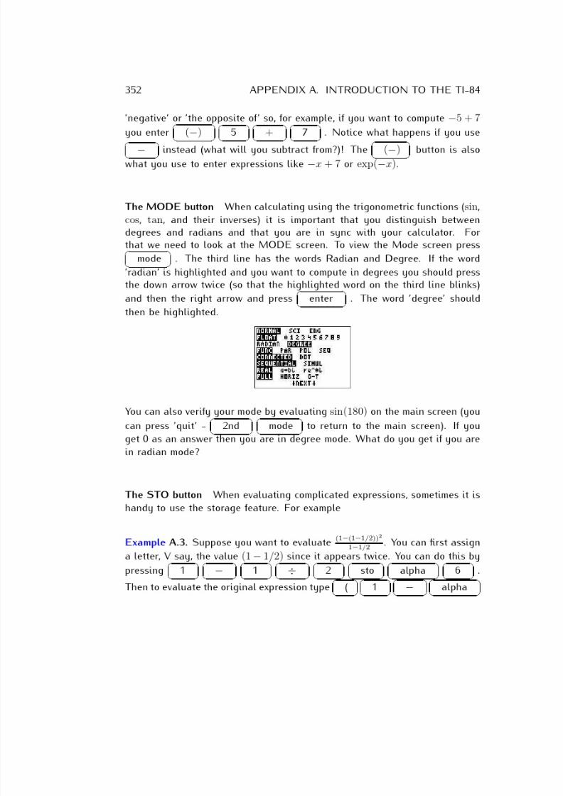
7/18/2019 Precalculus Tradler Carley
http://slidepdf.com/reader/full/precalculus-tradler-carley 362/424
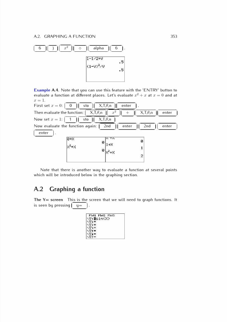
7/18/2019 Precalculus Tradler Carley
http://slidepdf.com/reader/full/precalculus-tradler-carley 363/424
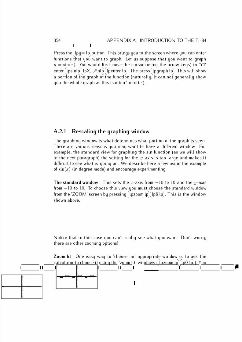
7/18/2019 Precalculus Tradler Carley
http://slidepdf.com/reader/full/precalculus-tradler-carley 364/424
354 APPENDIX A. INTRODUCTION TO THE TI-84
Press the
lpy= lp button. This brings you to the screen where you can enter
functions that you want to graph. Let us suppose that you want to graphy = sin(x). You would first move the cursor (using the arrow keys) to ’Y1’
enter
lpsinlp
lpX,T,θ,nlp
lpenter lp . The press
lpgraph lp . This will show
a portion of the graph of the function (naturally, it can not generally showyou the whole graph as this is often ’infinite’).
A.2.1 Rescaling the graphing window
The graphing window is what determines what portion of the graph is seen.There are various reasons you may want to have a different window. Forexample, the standard view for graphing the sin function (as we will showin the next paragraph) the setting for the y-axis is too large and makes itdifficult to see what is going on. We describe here a few using the exampleof sin(x) (in degree mode) and encourage experimenting.
The standard window This sets the x-axis from −10 to 10 and the y-axisfrom −10 to 10. To choose this view you must choose the standard window
from the ’ZOOM’ screen by pressing
lpzoom lp
lp6 lp . This is the window
shown above.
Notice that in this case you can’t really see what you want. Don’t worry,there are other zooming options!
Zoom fit One easy way to ’choose’ an appropriate window is to ask the
calculator to choose it using the ’zoom fit’ windows (
lpzoom lp
lp0 lp ). You
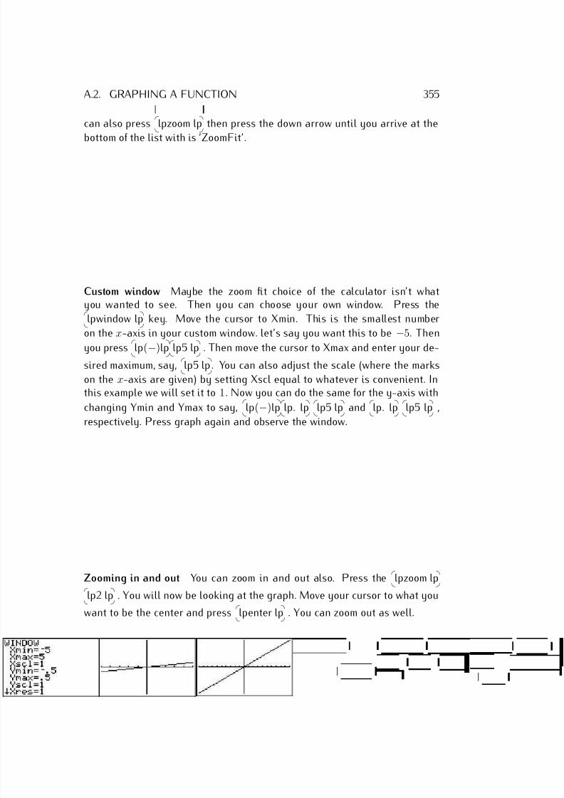
7/18/2019 Precalculus Tradler Carley
http://slidepdf.com/reader/full/precalculus-tradler-carley 365/424
A.2. GRAPHING A FUNCTION 355
can also press
lpzoom lp then press the down arrow until you arrive at the
bottom of the list with is ’ZoomFit’.
Custom window Maybe the zoom fit choice of the calculator isn’t whatyou wanted to see. Then you can choose your own window. Press the
lpwindow lp key. Move the cursor to Xmin. This is the smallest number
on the x-axis in your custom window. let’s say you want this to be −5. Then
you press
lp(−)lp
lp5 lp . Then move the cursor to Xmax and enter your de-
sired maximum, say,
lp5 lp. You can also adjust the scale (where the marks
on the x-axis are given) by setting Xscl equal to whatever is convenient. Inthis example we will set it to 1. Now you can do the same for the y-axis with
changing Ymin and Ymax to say,
lp(
−)lp
lp. lp
lp5 lp and
lp. lp
lp5 lp ,
respectively. Press graph again and observe the window.
Zooming in and out You can zoom in and out also. Press the
lpzoom lp
lp2 lp . You will now be looking at the graph. Move your cursor to what you
want to be the center and press
lpenter lp . You can zoom out as well.
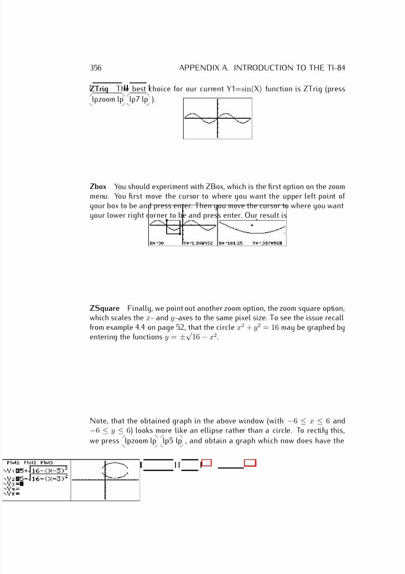
7/18/2019 Precalculus Tradler Carley
http://slidepdf.com/reader/full/precalculus-tradler-carley 366/424
356 APPENDIX A. INTRODUCTION TO THE TI-84
ZTrig The best choice for our current Y1=sin(X) function is ZTrig (press
lpzoom lp
lp7 lp ).
Zbox You should experiment with ZBox, which is the first option on the zoommenu. You first move the cursor to where you want the upper left point of your box to be and press enter. Then you move the cursor to where you wantyour lower right corner to be and press enter. Our result is
ZSquare Finally, we point out another zoom option, the zoom square option,which scales the x- and y-axes to the same pixel size. To see the issue recallfrom example 4.4 on page 52, that the circle x2 + y2 = 16 may be graphed byentering the functions y = ±√
16 − x2.
Note, that the obtained graph in the above window (with −6 ≤ x ≤ 6 and−6 ≤ y ≤ 6) looks more like an ellipse rather than a circle. To rectify this,
we press
lpzoom lp
lp5 lp , and obtain a graph which now does have the
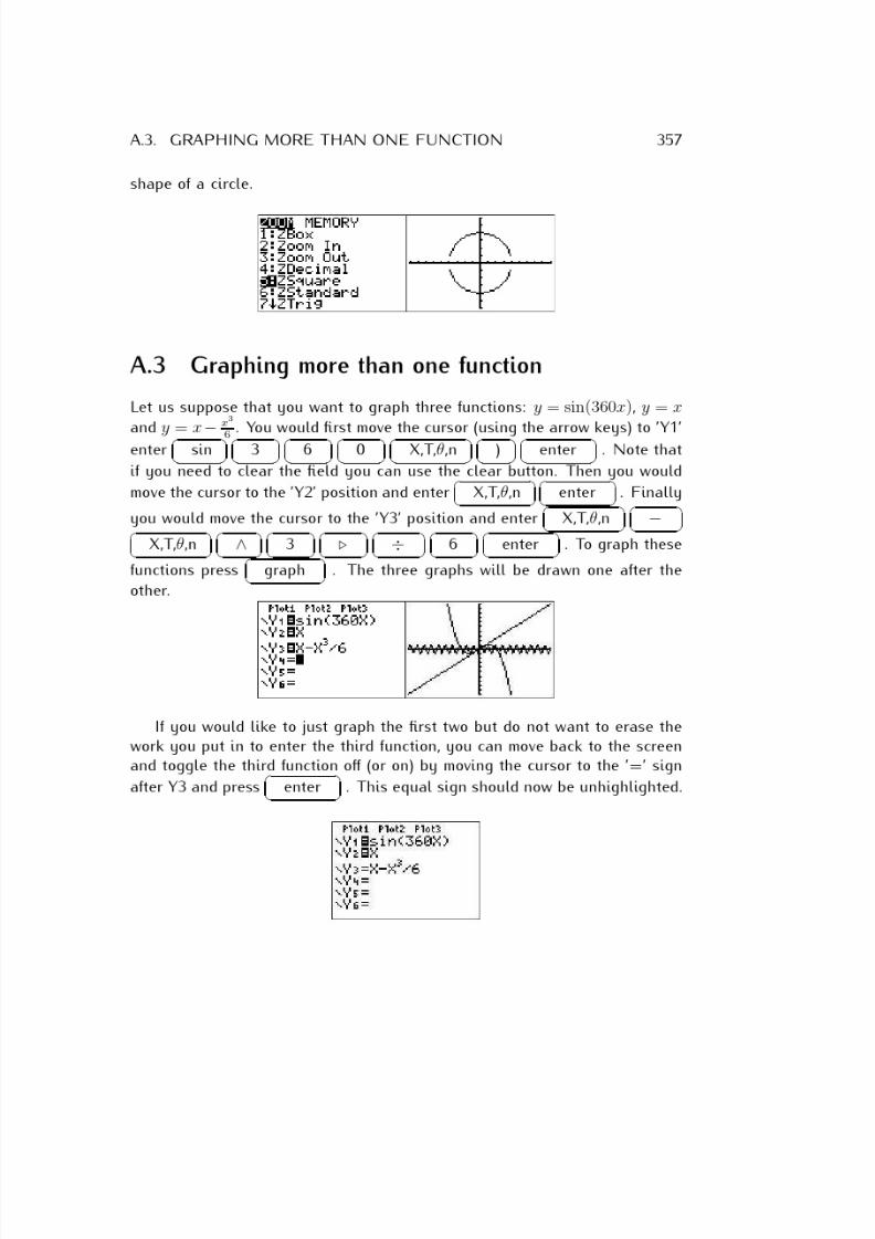
7/18/2019 Precalculus Tradler Carley
http://slidepdf.com/reader/full/precalculus-tradler-carley 367/424
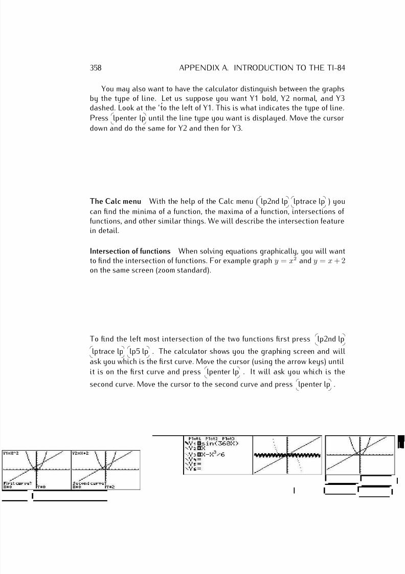
7/18/2019 Precalculus Tradler Carley
http://slidepdf.com/reader/full/precalculus-tradler-carley 368/424
358 APPENDIX A. INTRODUCTION TO THE TI-84
You may also want to have the calculator distinguish between the graphs
by the type of line. Let us suppose you want Y1 bold, Y2 normal, and Y3dashed. Look at the ’to the left of Y1. This is what indicates the type of line.
Press
lpenter lp until the line type you want is displayed. Move the cursor
down and do the same for Y2 and then for Y3.
The Calc menu With the help of the Calc menu (
lp2nd lp
lptrace lp ) youcan find the minima of a function, the maxima of a function, intersections of functions, and other similar things. We will describe the intersection featurein detail.
Intersection of functions When solving equations graphically, you will wantto find the intersection of functions. For example graph y = x2 and y = x + 2on the same screen (zoom standard).
To find the left most intersection of the two functions first press
lp2nd lp
lptrace lp
lp5 lp . The calculator shows you the graphing screen and will
ask you which is the first curve. Move the cursor (using the arrow keys) until
it is on the first curve and press
lpenter lp . It will ask you which is the
second curve. Move the cursor to the second curve and press
lpenter lp .
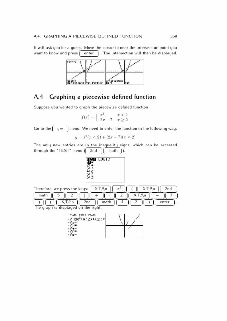
7/18/2019 Precalculus Tradler Carley
http://slidepdf.com/reader/full/precalculus-tradler-carley 369/424
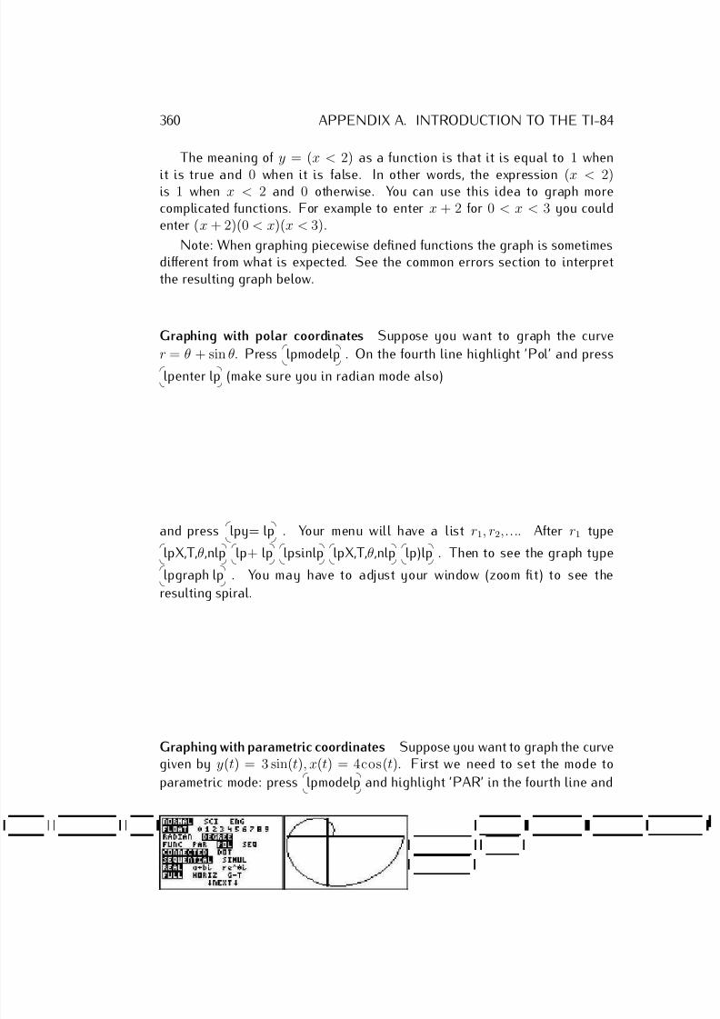
7/18/2019 Precalculus Tradler Carley
http://slidepdf.com/reader/full/precalculus-tradler-carley 370/424
360 APPENDIX A. INTRODUCTION TO THE TI-84
The meaning of y = (x < 2) as a function is that it is equal to 1 when
it is true and 0 when it is false. In other words, the expression (x < 2)is 1 when x < 2 and 0 otherwise. You can use this idea to graph morecomplicated functions. For example to enter x + 2 for 0 < x < 3 you couldenter (x + 2)(0 < x)(x < 3).
Note: When graphing piecewise defined functions the graph is sometimesdifferent from what is expected. See the common errors section to interpretthe resulting graph below.
Graphing with polar coordinates Suppose you want to graph the curve
r = θ + sin θ. Press
lpmodelp . On the fourth line highlight ’Pol’ and press
lpenter lp (make sure you in radian mode also)
and press
lpy= lp . Your menu will have a list r1, r2,.... After r1 type
lpX,T,θ,nlp
lp+ lp
lpsinlp
lpX,T,θ,nlp
lp)lp . Then to see the graph type
lpgraph lp . You may have to adjust your window (zoom fit) to see the
resulting spiral.
Graphing with parametric coordinates Suppose you want to graph the curvegiven by y(t) = 3 sin(t), x(t) = 4cos(t). First we need to set the mode to
parametric mode: press
lpmodelp and highlight ’PAR’ in the fourth line and
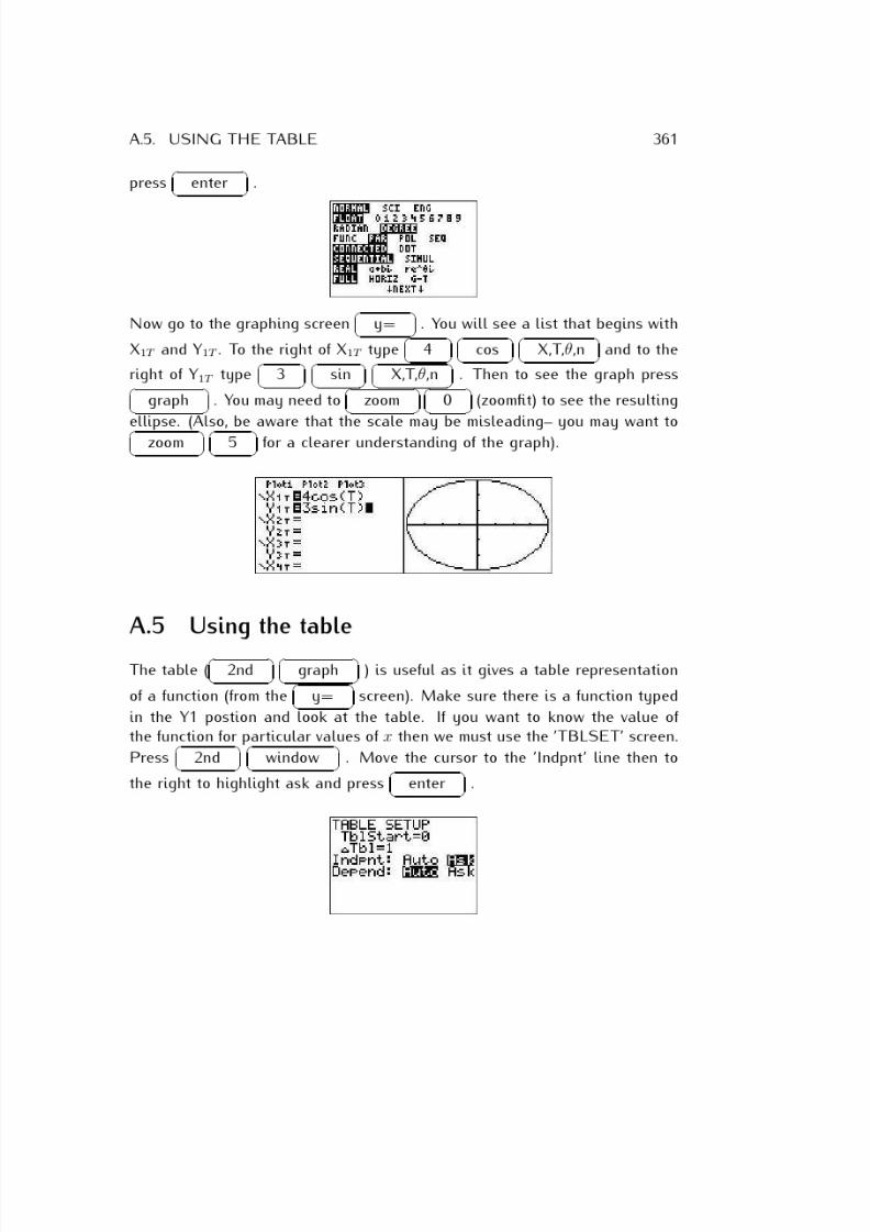
7/18/2019 Precalculus Tradler Carley
http://slidepdf.com/reader/full/precalculus-tradler-carley 371/424
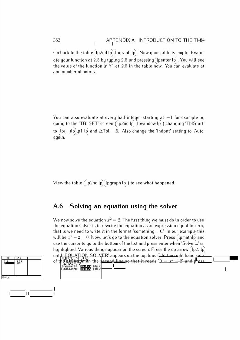
7/18/2019 Precalculus Tradler Carley
http://slidepdf.com/reader/full/precalculus-tradler-carley 372/424
362 APPENDIX A. INTRODUCTION TO THE TI-84
Go back to the table
lp2nd lp
lpgraph lp . Now your table is empty. Evalu-
ate your function at 2.5 by typing 2.5 and pressing
lpenter lp . You will seethe value of the function in Y1 at 2.5 in the table now. You can evaluate atany number of points.
You can also evaluate at every half integer starting at −1 for example bygoing to the ’TBLSET’ screen (
lp2nd lp
lpwindow lp ) changing ’TblStart’
to
lp(−)lp
lp1 lp and ∆Tbl= .5. Also change the ‘Indpnt’ setting to ‘Auto’
again.
View the table (
lp2nd lp
lpgraph lp ) to see what happened.
A.6 Solving an equation using the solver
We now solve the equation x2 = 2. The first thing we must do in order to usethe equation solver is to rewrite the equation as an expression equal to zero,that is we need to write it in the format ‘something= 0.’ In our example this
will be x2
− 2 = 0. Now, let’s go to the equation solver. Press
lpmathlp anduse the cursor to go to the bottom of the list and press enter when ’Solver...’ is
highlighted. Various things appear on the screen. Press the up arrow
lp△ lp
until ’EQUATION SOLVER’ appears on the top line. Edit the right hand sideof the equation on the second line so that it reads ’0 = x2 − 2’ and press
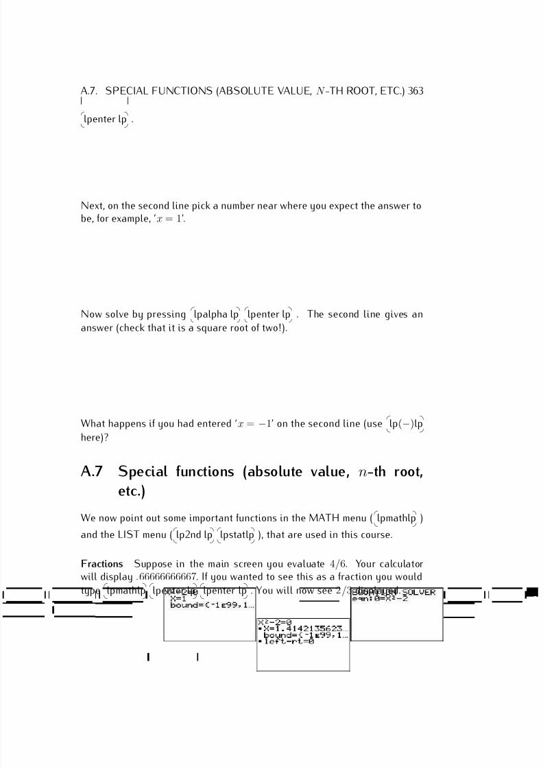
7/18/2019 Precalculus Tradler Carley
http://slidepdf.com/reader/full/precalculus-tradler-carley 373/424
A.7. SPECIAL FUNCTIONS (ABSOLUTE VALUE, N -TH ROOT, ETC.) 363
lpenter lp .
Next, on the second line pick a number near where you expect the answer tobe, for example, ’x = 1’.
Now solve by pressing
lpalpha lp
lpenter lp . The second line gives an
answer (check that it is a square root of two!).
What happens if you had entered ‘x = −1’ on the second line (use
lp(−)lp
here)?
A.7 Special functions (absolute value, n-th root,
etc.)
We now point out some important functions in the MATH menu (
lpmathlp )
and the LIST menu (
lp2nd lp
lpstatlp ), that are used in this course.
Fractions Suppose in the main screen you evaluate 4/6. Your calculatorwill display .66666666667. If you wanted to see this as a fraction you would
type
lpmathlp
lpenter lp
lpenter lp . You will now see 2/3 displayed.
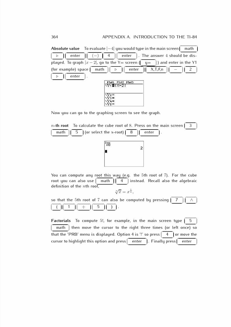
7/18/2019 Precalculus Tradler Carley
http://slidepdf.com/reader/full/precalculus-tradler-carley 374/424
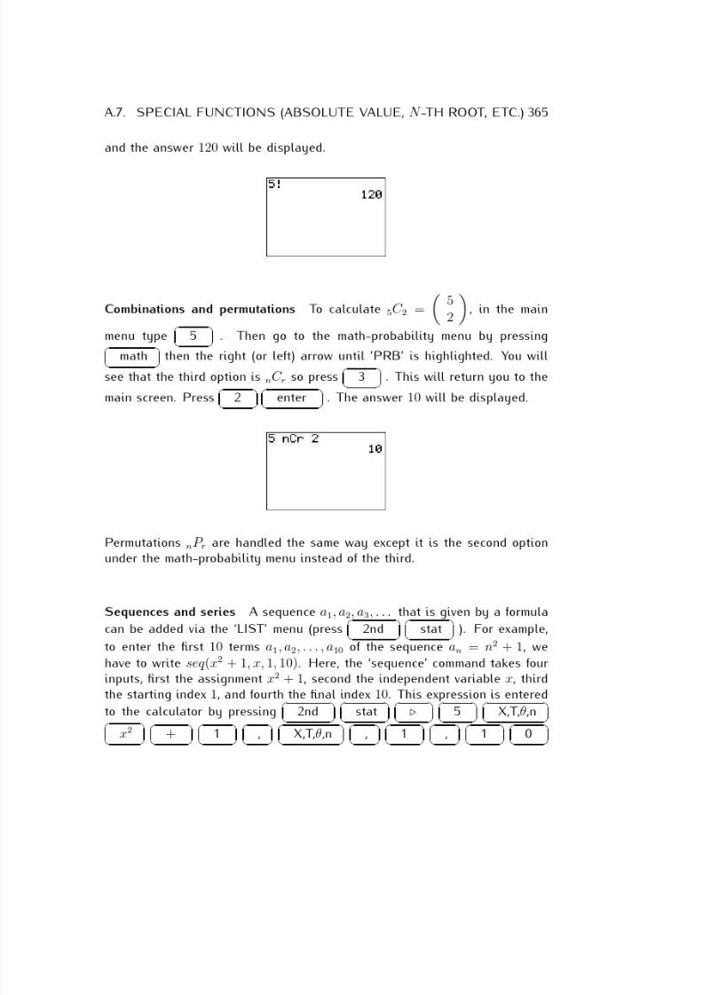
7/18/2019 Precalculus Tradler Carley
http://slidepdf.com/reader/full/precalculus-tradler-carley 375/424
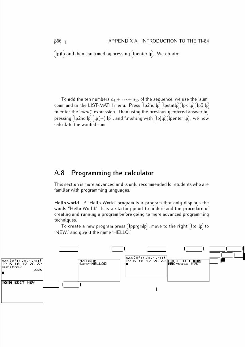
7/18/2019 Precalculus Tradler Carley
http://slidepdf.com/reader/full/precalculus-tradler-carley 376/424
366 APPENDIX A. INTRODUCTION TO THE TI-84
lp)lp and then confirmed by pressing
lpenter lp . We obtain:
To add the ten numbers a1 + · · · + a10 of the sequence, we use the ‘sum’
command in the LIST-MATH menu. Press
lp2nd lp
lpstatlp
lp⊳ lp
lp5 lp
to enter the ‘sum(’ expression. Then using the previously entered answer by
pressing
lp2nd lp
lp(
−) lp , and finishing with
lp)lp
lpenter lp , we now
calculate the wanted sum.
A.8 Programming the calculator
This section is more advanced and is only recommended for students who arefamiliar with programming languages.
Hello world A ‘Hello World’ program is a program that only displays thewords “Hello World.” It is a starting point to understand the procedure of creating and running a program before going to more advanced programmingtechniques.
To create a new program press
lpprgmlp , move to the right
lp⊲ lp to
‘NEW,’ and give it the name ‘HELLO.’
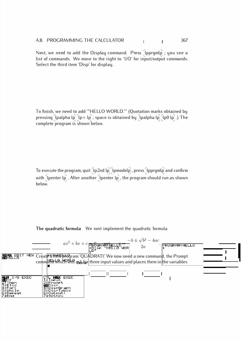
7/18/2019 Precalculus Tradler Carley
http://slidepdf.com/reader/full/precalculus-tradler-carley 377/424
A.8. PROGRAMMING THE CALCULATOR 367
Next, we need to add the Display command. Press
lpprgmlp ; you see a
list of commands. We move to the right to ‘I/O’ for input/output commands.Select the third item ‘Disp’ for display.
To finish, we need to add ‘”HELLO WORLD.”’ (Quotation marks obtained by
pressing
lpalpha lp
lp+ lp ; space is obtained by
lpalpha lp
lp0 lp .) Thecomplete program is shown below.
To execute the program, quit
lp2nd lp
lpmodelp , press
lpprgmlp and confirm
with
lpenter lp . After another
lpenter lp , the program should run as shownbelow.
The quadratic formula We next implement the quadratic formula
ax2 + bx + c = 0 =⇒ x = −b ± √ b2 − 4ac2a
.
Create a new program ‘QUADRATI.’ We now need a new command, the Promptcommand which will ask for three input values and places them in the variables
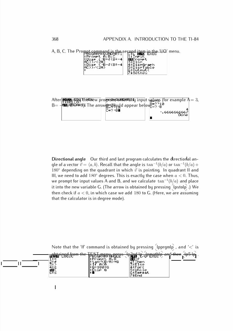
7/18/2019 Precalculus Tradler Carley
http://slidepdf.com/reader/full/precalculus-tradler-carley 378/424
368 APPENDIX A. INTRODUCTION TO THE TI-84
A, B, C. The Prompt command is the second item in the ‘I/O’ menu.
After executing the new program, enter any input values (for example A= 3,B= −10, C= −8). The answer should appear below.
Directional angle Our third and last program calculates the directional an-gle of a vector v = a, b. Recall that the angle is tan−1(b/a) or tan−1(b/a) +180◦ depending on the quadrant in which v is pointing. In quadrant II and
III, we need to add 180◦ degrees. This is exactly the case when a < 0. Thus,we prompt for input values A and B, and we calculate tan−1(b/a) and place
it into the new variable G. (The arrow is obtained by pressing
lpstolp .) We
then check if a < 0, in which case we add 180 to G. (Here, we are assumingthat the calculator is in degree mode).
Note that the ‘If’ command is obtained by pressing
lpprgmlp , and ‘<’ is
obtained from the TEST menu, press
lp2nd lp
lpmathlp and then
lp5 lp .
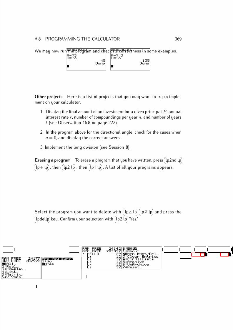
7/18/2019 Precalculus Tradler Carley
http://slidepdf.com/reader/full/precalculus-tradler-carley 379/424
A.8. PROGRAMMING THE CALCULATOR 369
We may now run the program and check its correctness in some examples.
Other projects Here is a list of projects that you may want to try to imple-ment on your calculator.
1. Display the final amount of an investment for a given principal P , annual
interest rate r, number of compoundings per year n, and number of yearst (see Observation 16.8 on page 222).
2. In the program above for the directional angle, check for the cases whena = 0, and display the correct answers.
3. Implement the long division (see Session 8).
Erasing a program To erase a program that you have written, press
lp2nd lp
lp+ lp , then
lp2 lp , then
lp1 lp . A list of all your programs appears.
Select the program you want to delete with
lp△ lp
lp▽ lp and press the
lpdellp key. Confirm your selection with
lp2 lp ‘Yes.’
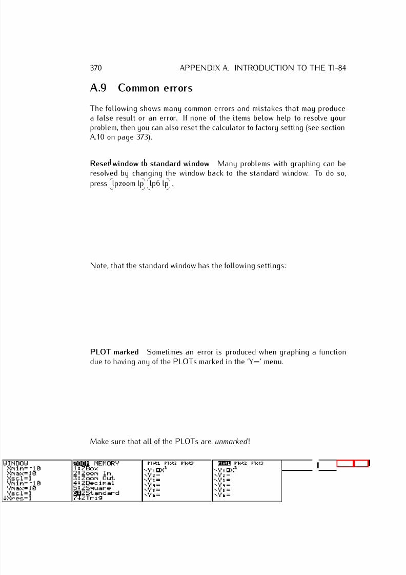
7/18/2019 Precalculus Tradler Carley
http://slidepdf.com/reader/full/precalculus-tradler-carley 380/424
370 APPENDIX A. INTRODUCTION TO THE TI-84
A.9 Common errors
The following shows many common errors and mistakes that may producea false result or an error. If none of the items below help to resolve yourproblem, then you can also reset the calculator to factory setting (see sectionA.10 on page 373).
Reset window to standard window Many problems with graphing can beresolved by changing the window back to the standard window. To do so,
press
lpzoom lp
lp6 lp .
Note, that the standard window has the following settings:
PLOT marked Sometimes an error is produced when graphing a functiondue to having any of the PLOTs marked in the ‘Y=’ menu.
Make sure that all of the PLOTs are unmarked !
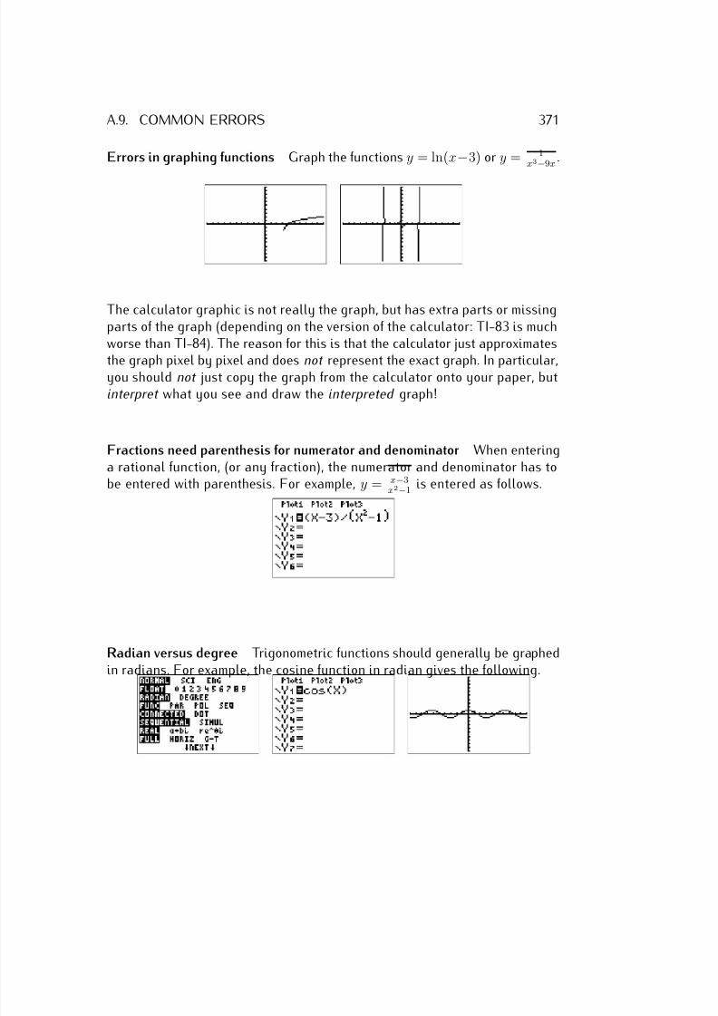
7/18/2019 Precalculus Tradler Carley
http://slidepdf.com/reader/full/precalculus-tradler-carley 381/424
A.9. COMMON ERRORS 371
Errors in graphing functions Graph the functions y = ln(x−3) or y = 1x3−9x
.
The calculator graphic is not really the graph, but has extra parts or missingparts of the graph (depending on the version of the calculator: TI-83 is muchworse than TI-84). The reason for this is that the calculator just approximates
the graph pixel by pixel and does not represent the exact graph. In particular,you should not just copy the graph from the calculator onto your paper, butinterpret what you see and draw the interpreted graph!
Fractions need parenthesis for numerator and denominator When enteringa rational function, (or any fraction), the numerator and denominator has tobe entered with parenthesis. For example, y = x−3
x2−1 is entered as follows.
Radian versus degree Trigonometric functions should generally be graphedin radians. For example, the cosine function in radian gives the following.
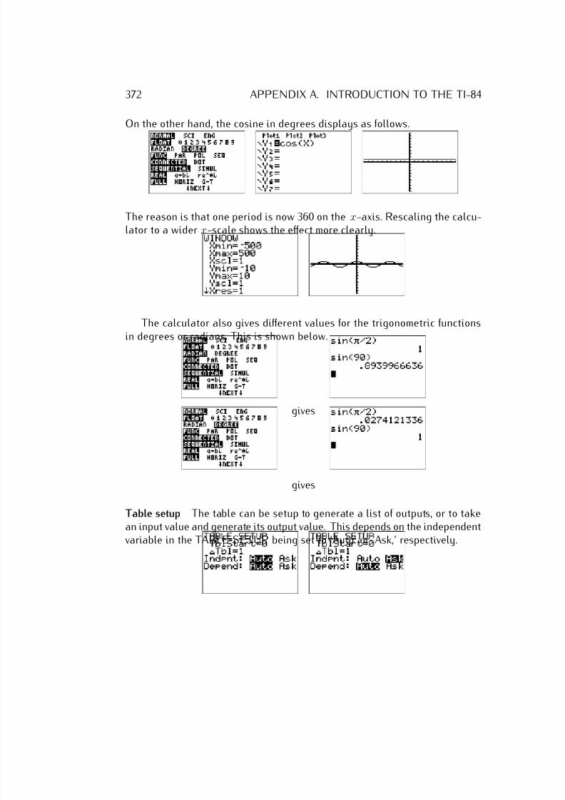
7/18/2019 Precalculus Tradler Carley
http://slidepdf.com/reader/full/precalculus-tradler-carley 382/424
372 APPENDIX A. INTRODUCTION TO THE TI-84
On the other hand, the cosine in degrees displays as follows.
The reason is that one period is now 360 on the x-axis. Rescaling the calcu-lator to a wider x-scale shows the effect more clearly.
The calculator also gives different values for the trigonometric functionsin degrees or radians. This is shown below.
gives
gives
Table setup The table can be setup to generate a list of outputs, or to takean input value and generate its output value. This depends on the independentvariable in the TABLE SETUP being set to ‘Auto’ or ‘Ask,’ respectively.
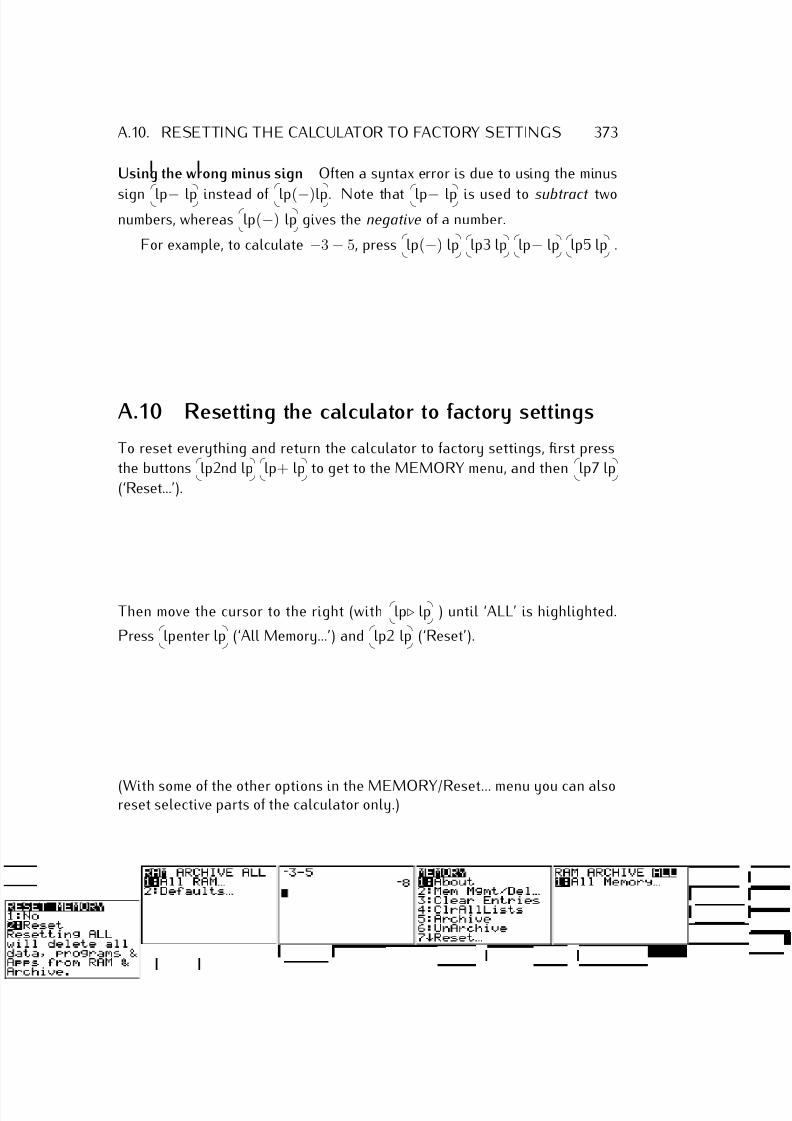
7/18/2019 Precalculus Tradler Carley
http://slidepdf.com/reader/full/precalculus-tradler-carley 383/424
A.10. RESETTING THE CALCULATOR TO FACTORY SETTINGS 373
Using the wrong minus sign Often a syntax error is due to using the minus
sign
lp− lp instead of
lp(−)lp. Note that
lp− lp is used to subtract twonumbers, whereas
lp(−) lp gives the negative of a number.
For example, to calculate −3 − 5, press
lp(−) lp
lp3 lp
lp− lp
lp5 lp .
A.10 Resetting the calculator to factory settings
To reset everything and return the calculator to factory settings, first press
the buttons
lp2nd lp
lp+ lp to get to the MEMORY menu, and then
lp7 lp
(‘Reset...’).
Then move the cursor to the right (with
lp⊲ lp ) until ‘ALL’ is highlighted.
Press
lpenter lp (‘All Memory...’) and
lp2 lp (‘Reset’).
(With some of the other options in the MEMORY/Reset... menu you can alsoreset selective parts of the calculator only.)
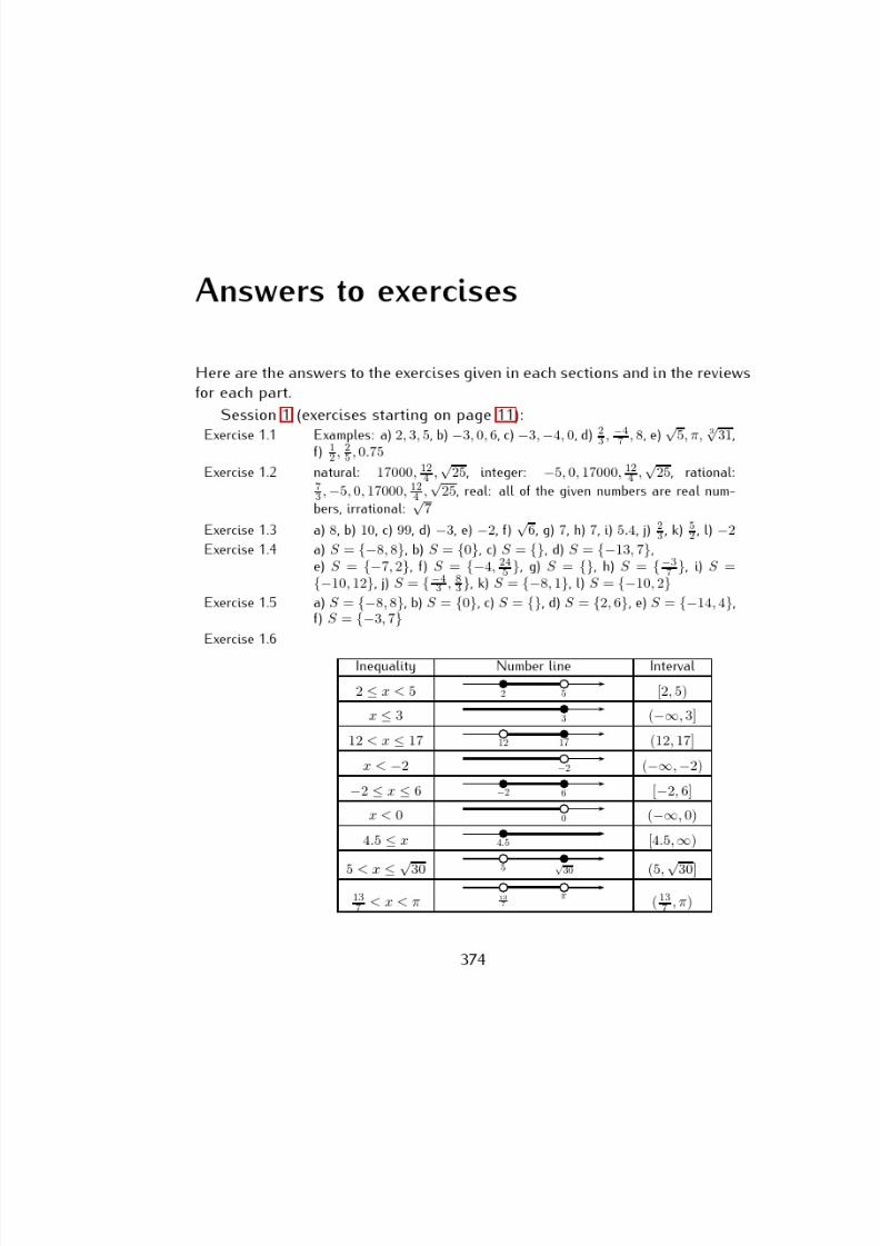
7/18/2019 Precalculus Tradler Carley
http://slidepdf.com/reader/full/precalculus-tradler-carley 384/424
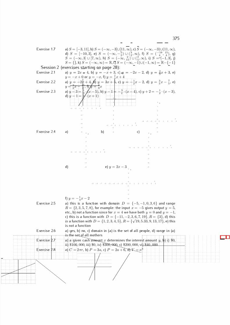
7/18/2019 Precalculus Tradler Carley
http://slidepdf.com/reader/full/precalculus-tradler-carley 385/424
375
Exercise 1.7 a) S = [−3, 11], b) S = (−∞, −3]∪[11, ∞), c) S = (−∞, −3)∪(11, ∞),d) S = [
−10, 3], e) S = (
−∞,
−52)
∪(32 ,
∞), f) S = (−19
4 , 154 ), g)
S = (−∞, 3] ∪ [7, ∞), h) S = (−∞, 215) ∪ (25 , ∞), i) S = [−1, 3], j)S = {}, k) S = (−∞, ∞) = R, l) S = (−∞, −1)∪(−1, ∞) = R−{−1}
Session 2 (exercises starting on page 28):Exercise 2.1 a) y = 2x − 4, b) y = −x + 3, c) y = −2x − 2, d) y = 2
5x + 3, e)
y = −x + 0 or y = −x, f) y = 23x + 4
Exercise 2.2 a) y = −2x + 4, b) y = 3x + 5, c) y = − 12x − 2, d) y = 3
5x − 75 , e)
y = 32
x − 152
, f) y = 89
x
Exercise 2.3 a) y − 3 = 13 · (x − 5), b) y − 1 = − 3
2 · (x − 4), c) y + 2 = − 12 · (x − 3),
d) y − 1 = 1 · (x + 1)
Exercise 2.4 a)
-3 -2 -1 0 1 2 3 4
-6
-5
-4
-3
-2
-1
0
1
2
x
y
b)
-2 -1 0 1 2 3 4 5
-2
-1
0
1
2
3
4
5
6
x
y
c)
-4 -3 -2 -1 0 1 2 3 4
-3
-2
-1
0
1
2
3
4
x
y
d)
-4 -3 -2 -1 0 1 2 3 4
-4
-3
-2
-1
0
1
2
3
4
x
y
e) y = 2x
−3
-5 -4 -3 -2 -1 0 1 2 3 4 5
-5
-4
-3
-2
-1
0
1
2
3
x
y
f) y = − 13x − 2
-9 - 8 - 7 - 6 - 5 - 4 - 3 - 2 - 1 0 1 2 3 4 5 6
-4
-3
-2
-1
0
1
2
3
x
y
Exercise 2.5 a) this is a function with domain D = {−5, −1, 0, 3, 6} and rangeR = {2, 3, 5, 7, 8}, for example: the input x = −5 gives output y = 5,etc., b) not a function since for x = 4 we have both y = 0 and y = −1,c) this is a function with D = {−11, −2, 3, 6, 7, 19}, R = {3}, d) thisis a function with D = {1, 2, 3, 4, 5}, R = {√
19, 5.33, 9, 13, 17}, e) thisis not a function
Exercise 2.6 a) yes, b) no, c) domain in (a) is the set of all people, d) range in (a)is the set of all mothers
Exercise 2.7 a) a given cash amount x determines the interest amount y, b) i) $0,ii) $100, 000, iii) $0 , iv) $300, 000, v) $200, 000, vi) $40, 000
Exercise 2.8 a) C = 2πr, b) P = 3a, c) P = 2a + 6, d) V = a3
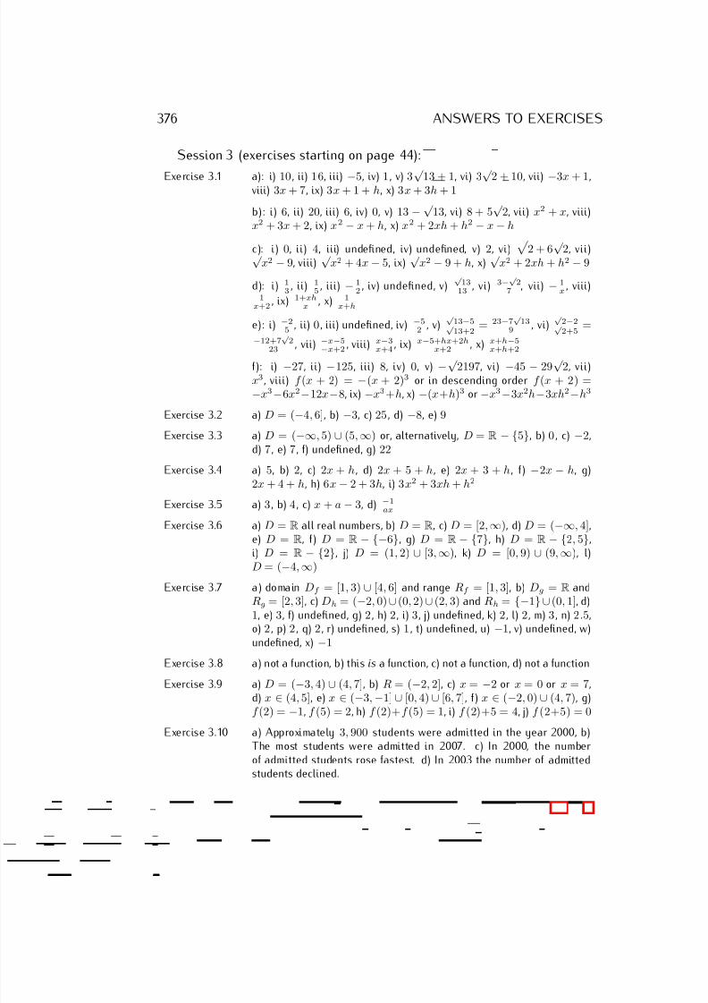
7/18/2019 Precalculus Tradler Carley
http://slidepdf.com/reader/full/precalculus-tradler-carley 386/424
376 ANSWERS TO EXERCISES
Session 3 (exercises starting on page 44):
Exercise 3.1 a): i) 10 , ii) 16, iii) −5, iv) 1 , v) 3√ 13 + 1, vi) 3√ 2 + 10, vii) −3x + 1,viii) 3x + 7, ix) 3x + 1 + h, x) 3x + 3h + 1
b): i) 6, ii) 20, iii) 6, iv) 0, v) 13 − √ 13, vi) 8 + 5
√ 2, vii) x2 + x, viii)
x2 + 3x + 2, ix) x2 − x + h, x) x2 + 2xh + h2 − x − h
c): i) 0, ii) 4, iii) undefined, iv) undefined, v) 2, vi)
2 + 6√
2, vii)√ x2 − 9, viii)
√ x2 + 4x − 5, ix)
√ x2 − 9 + h, x)
√ x2 + 2xh + h2 − 9
d): i) 13
, ii) 15
, iii) − 12
, iv) undefined, v)√ 1313
, vi) 3−√ 2
7 , vii) − 1
x, viii)
1x+2
, ix) 1+xhx
, x) 1x+h
e): i) −25
, ii) 0 , iii) undefined, iv) −52
, v)√ 13−5√ 13+2
= 23−7√ 13
9 , vi)
√ 2−2√ 2+5
=
−12+7√ 2
23 , vii) −x−5
−x+2, viii) x−3
x+4, ix) x−5+hx+2h
x+2 , x) x+h−5
x+h+2
f): i) −27, ii) −125, iii) 8, iv) 0, v) −√ 2197, vi) −45 − 29
√ 2, vii)
x3, viii) f (x + 2) = −(x + 2)3 or in descending order f (x + 2) =−x3−6x2−12x−8, ix) −x3+h, x) −(x+h)3 or −x3−3x2h−3xh2−h3
Exercise 3.2 a) D = (−4, 6], b) −3, c) 25 , d) −8, e) 9
Exercise 3.3 a) D = (−∞, 5) ∪ (5, ∞) or, alternatively, D = R − {5}, b) 0 , c) −2,d) 7 , e) 7 , f) undefined, g) 22
Exercise 3.4 a) 5, b) 2, c) 2x + h, d) 2x + 5 + h, e) 2x + 3 + h, f) −2x − h, g)2x + 4 + h, h) 6x − 2 + 3h, i) 3x2 + 3xh + h2
Exercise 3.5 a) 3 , b) 4 , c) x + a − 3, d) −1ax
Exercise 3.6 a) D = R all real numbers, b) D = R, c) D = [2, ∞), d) D = (−∞, 4],e) D = R, f) D = R − {−6}, g) D = R − {7}, h) D = R − {2, 5},i) D = R − {2}, j) D = (1, 2) ∪ [3, ∞), k) D = [0, 9) ∪ (9, ∞), l)D = (−4, ∞)
Exercise 3.7 a) domain Df = [1, 3) ∪ [4, 6] and range Rf = [1, 3], b) Dg = R andRg = [2, 3], c) Dh = (−2, 0) ∪ (0, 2) ∪ (2, 3) and Rh = {−1}∪ (0, 1], d)1, e) 3, f) undefined, g) 2 , h) 2, i) 3, j) undefined, k) 2, l) 2, m) 3 , n) 2.5,o) 2 , p) 2 , q) 2 , r) undefined, s) 1 , t) undefined, u) −1, v) undefined, w)undefined, x) −1
Exercise 3.8 a) not a function, b) this is a function, c) not a function, d) not a function
Exercise 3.9 a) D = (−3, 4) ∪ (4, 7], b) R = (−2, 2], c) x = −2 or x = 0 or x = 7,
d) x ∈ (4, 5], e) x ∈ (−3, −1] ∪ [0, 4) ∪ [6, 7], f) x ∈ (−2, 0) ∪ (4, 7), g)f (2) = −1, f (5) = 2, h) f (2)+f (5) = 1, i) f (2)+5 = 4, j) f (2+5) = 0
Exercise 3.10 a) Approximately 3, 900 students were admitted in the year 2000, b)The most students were admitted in 2007. c) In 2000, the numberof admitted students rose fastest. d) In 2003 the number of admittedstudents declined.
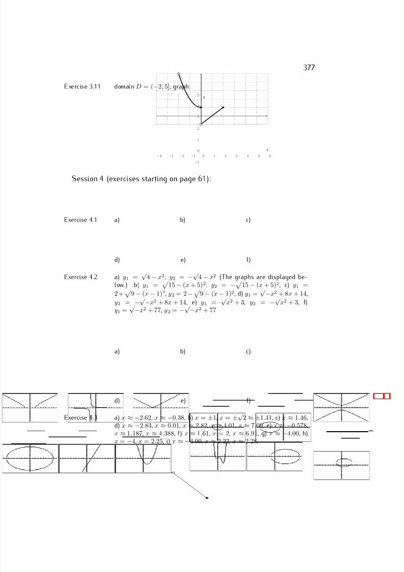
7/18/2019 Precalculus Tradler Carley
http://slidepdf.com/reader/full/precalculus-tradler-carley 387/424
377
Exercise 3.11 domain D = (−2, 5], graph:
-4 -3 -2 -1 0 1 2 3 4 5 6
-1
0
1
2
3
4
5
x
y
Session 4 (exercises starting on page 61):
Exercise 4.1 a) b) c)
d) e) f)
Exercise 4.2 a) y1 =√
4 − x2, y2 = −√ 4 − x2 (The graphs are displayed be-
low.) b) y1 =
15 − (x + 5)2, y2 = − 15 − (x + 5)2, c) y1 =
2 + 9 −(x
−1)2, y2 = 2
− 9 −(x
−1)2, d) y1 =
√
−x2 + 8x + 14,
y2 = −√ −x2 + 8x + 14, e) y1 = √ x2 + 3, y2 = −√ x2 + 3, f)y1 =
√ −x2 + 77, y2 = −√ −x2 + 77
a) b) c)
d) e) f)
Exercise 4.3 a) x ≈ −2.62, x ≈ −0.38, b) x = ±1, x = ±√ 2 ≈ ±1.41, c) x ≈ 1.46,
d) x ≈ −2.83, x ≈ 0.01, x ≈ 2.82, x ≈ 4.01, x ≈ 7.00, e) x ≈ −0.578,x ≈ 1.187, x ≈ 4.388, f) x ≈ 1.61, x = 2, x ≈ 6.91, g) x ≈ −4.00, h)x = −4, x = 2.25, i) x ≈ −4.00, x ≈ 2.22, x ≈ 2.28,
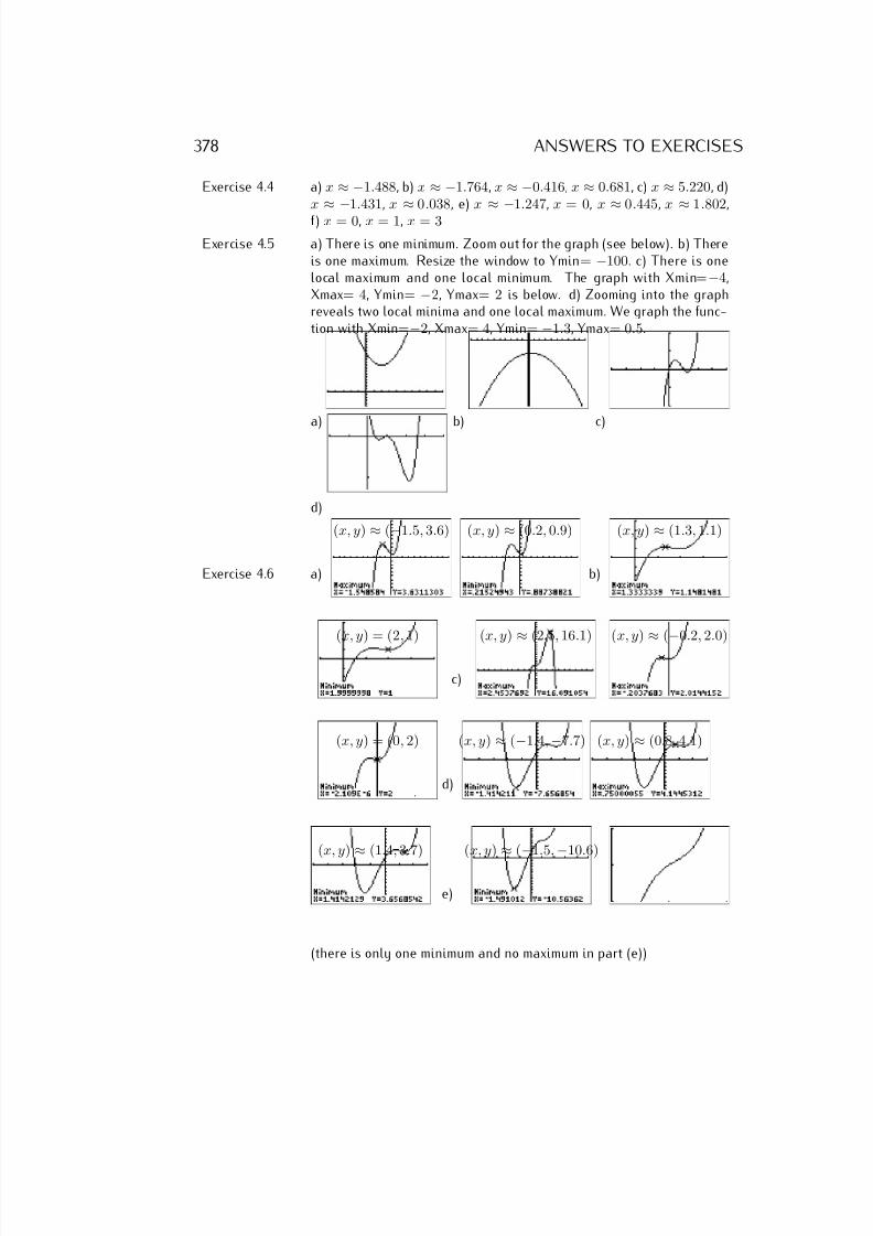
7/18/2019 Precalculus Tradler Carley
http://slidepdf.com/reader/full/precalculus-tradler-carley 388/424
378 ANSWERS TO EXERCISES
Exercise 4.4 a) x ≈ −1.488, b) x ≈ −1.764, x ≈ −0.416, x ≈ 0.681, c) x ≈ 5.220, d)x
≈ −1.431, x
≈ 0.038, e) x
≈ −1.247, x = 0, x
≈ 0.445, x
≈ 1.802,
f) x = 0, x = 1, x = 3
Exercise 4.5 a) There is one minimum. Zoom out for the graph (see below). b) Thereis one maximum. Resize the window to Ymin= −100. c) There is onelocal maximum and one local minimum. The graph with Xmin=−4,Xmax= 4, Ymin= −2, Ymax= 2 is below. d) Zooming into the graphreveals two local minima and one local maximum. We graph the func-tion with Xmin=−2, Xmax= 4, Ymin= −1.3, Ymax= 0.5.
a) b) c)
d)
Exercise 4.6 a)
(x, y) ≈ (−1.5, 3.6) (x, y) ≈ (0.2, 0.9)
b)
(x, y) ≈ (1.3, 1.1)
(x, y) = (2, 1)
c)
(x, y)
≈(2.5, 16.1) (x, y)
≈(
−0.2, 2.0)
(x, y) = (0, 2)
d)
(x, y) ≈ (−1.4, −7.7) (x, y) ≈ (0.8, 4.1)
(x, y)
≈(1.4, 3.7)
e)
(x, y)
≈(
−1.5,
−10.6)
(there is only one minimum and no maximum in part (e))
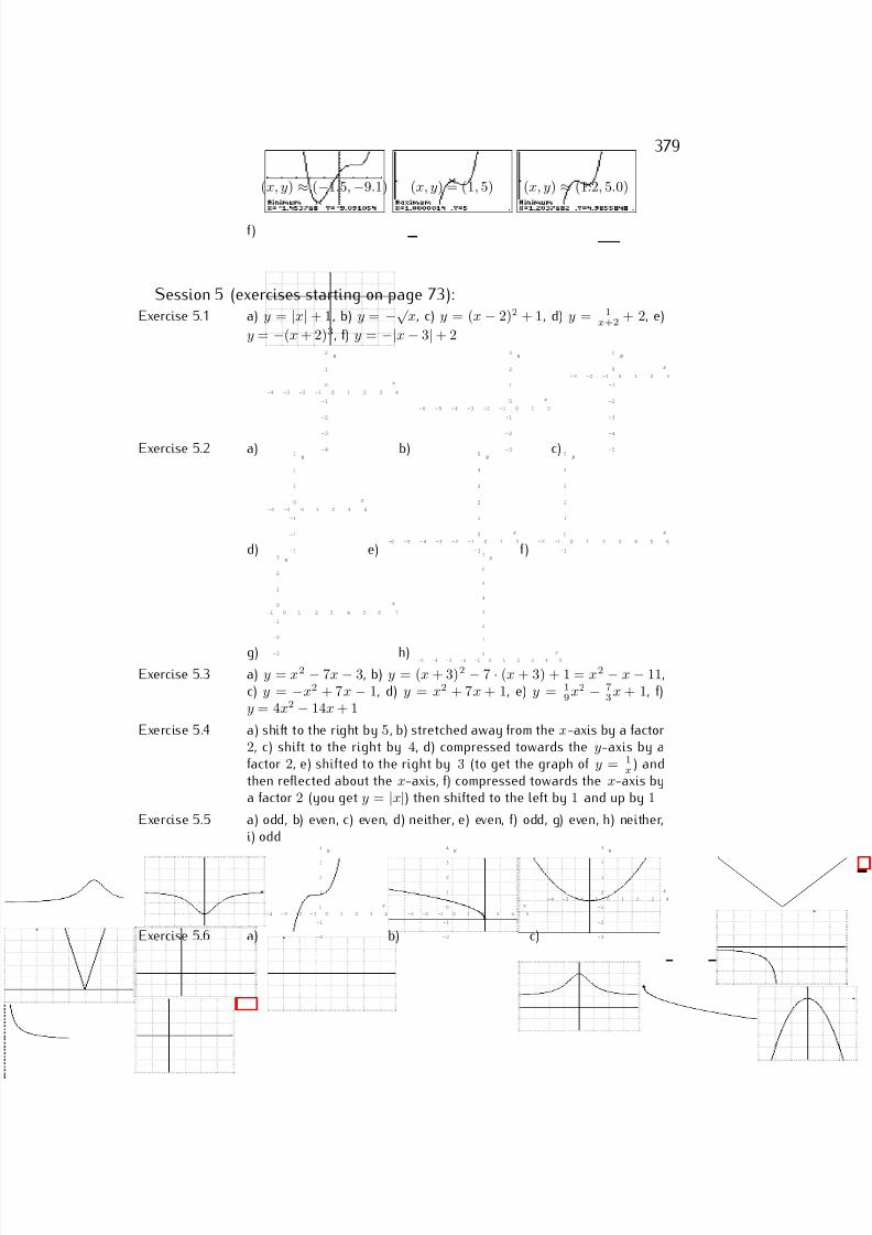
7/18/2019 Precalculus Tradler Carley
http://slidepdf.com/reader/full/precalculus-tradler-carley 389/424
379
f)
(x, y) ≈ (−1.5, −9.1) (x, y) = (1, 5) (x, y) ≈ (1.2, 5.0)
Session 5 (exercises starting on page 73):Exercise 5.1 a) y = |x| + 1, b) y = −√
x, c) y = (x − 2)2 + 1, d) y = 1x+2 + 2, e)
y = −(x + 2)3, f) y = −|x − 3| + 2
Exercise 5.2 a)
-4 -3 -2 -1 0 1 2 3 4
-4
-3
-2
-1
0
1
2
x
y
b)
-6 -5 -4 -3 -2 -1 0 1 2
-3
-2
-1
0
1
2
3
x
y
c)
-3 -2 -1 0 1 2 3
-5
-4
-3
-2
-1
0
1
x
y
d)
-2 -1 0 1 2 3 4
-3
-2
-1
0
1
2
3
x
y
e) -6 -5 -4 -3 -2 -1 0 1 2
-1
0
1
2
3
4
5
x
y
f) -2 -1 0 1 2 3 4 5 6
-1
0
1
2
3
4
5
x
y
g)
-1 0 1 2 3 4 5 6 7
-3
-2
-1
0
1
2
3
x
y
h)-5 -4 -3 -2 -1 0 1 2 3 4 5
0
1
2
3
4
5
6
7
x
y
Exercise 5.3 a) y = x2 − 7x − 3, b) y = (x + 3)2 − 7 · (x + 3) + 1 = x2 − x − 11,c) y = −x2 + 7x − 1, d) y = x2 + 7x + 1, e) y = 1
9x2 − 7
3x + 1, f)
y = 4x2 − 14x + 1
Exercise 5.4 a) shift to the right by 5, b) stretched away from the x-axis by a factor2, c) shift to the right by 4, d) compressed towards the y-axis by afactor 2, e) shifted to the right by 3 (to get the graph of y = 1
x) and
then reflected about the x-axis, f) compressed towards the x-axis bya factor 2 (you get y = |x|) then shifted to the left by 1 and up by 1
Exercise 5.5 a) odd, b) even, c) even, d) neither, e) even, f) odd, g) even, h) neither,i) odd
Exercise 5.6 a)
-4 -3 -2 -1 0 1 2 3 4
-2
-1
0
1
2
3
4
x
y
b)
-3 -2 -1 0 1 2 3 4 5
-2
-1
0
1
2
3
4
x
y
c)
-4 -3 -2 -1 0 1 2 3 4
-3
-2
-1
0
1
2
3
x
y
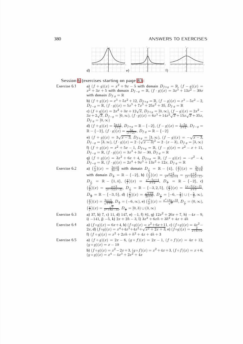
7/18/2019 Precalculus Tradler Carley
http://slidepdf.com/reader/full/precalculus-tradler-carley 390/424
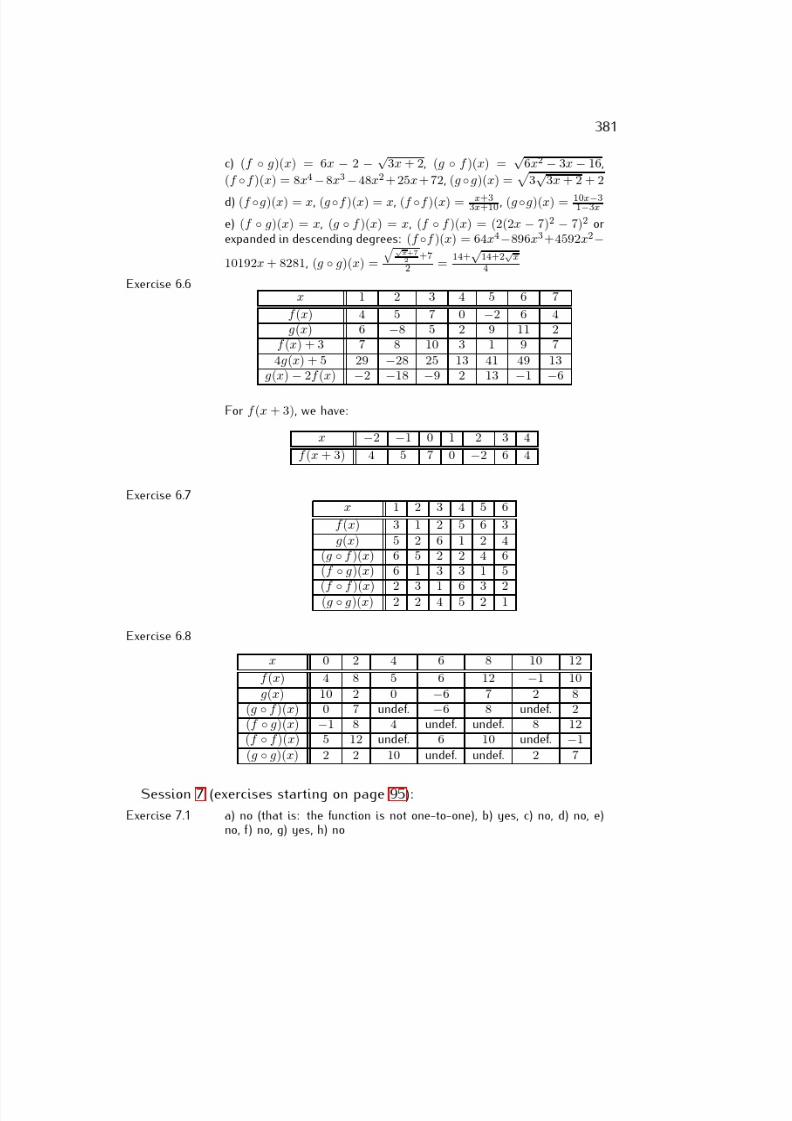
7/18/2019 Precalculus Tradler Carley
http://slidepdf.com/reader/full/precalculus-tradler-carley 391/424
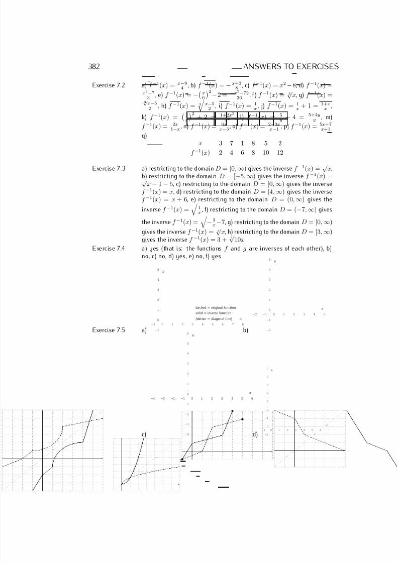
7/18/2019 Precalculus Tradler Carley
http://slidepdf.com/reader/full/precalculus-tradler-carley 392/424
382 ANSWERS TO EXERCISES
Exercise 7.2 a) f −1(x) = x−94 , b) f −1(x) = −x+3
8 , c) f −1(x) = x2−8, d) f −1(x) =x2
−7
3 , e) f
−1(x) =
−x6 2−2 = −
x2
−72
36 , f ) f
−1(x) = 3
√ x, g) f
−1(x) =
3√ x−52 , h) f −1(x) = 3
x−52 , i) f −1(x) = 1
x, j) f −1(x) = 1
x + 1 = 1+x
x ,
k) f −1(x) =1x
2+ 2 = 1+2x2
x2 , l) f −1(x) = 5
y + 4 = 5+4y
y , m)
f −1(x) = 2x1−x
, n) f −1(x) = 6xx−3
, o) f −1(x) = 2−3xx−1
, p) f −1(x) = 5x+7x+1
q)x 3 7 1 8 5 2
f −1(x) 2 4 6 8 10 12
Exercise 7.3 a) restricting to the domain D = [0, ∞) gives the inverse f −1(x) =√
x,b) restricting to the domain D = [−5, ∞) gives the inverse f −1(x) =√
x − 1 − 5, c) restricting to the domain D = [0, ∞) gives the inversef −1(x) = x, d) restricting to the domain D = [4,
∞) gives the inverse
f −1(x) = x + 6, e) restricting to the domain D = (0, ∞) gives the
inverse f −1(x) =
1x
, f) restricting to the domain D = (−7, ∞) gives
the inverse f −1(x) =
− 3x−7, g) restricting to the domain D = [0, ∞)
gives the inverse f −1(x) = 4√
x, h) restricting to the domain D = [3, ∞)gives the inverse f −1(x) = 3 + 4
√ 10x
Exercise 7.4 a) yes (that is: the functions f and g are inverses of each other), b)no, c) no, d) yes, e) no, f) yes
Exercise 7.5 a)-1 0 1 2 3 4 5 6 7 8
-1
0
1
2
3
4
5
x
y
dashed = original function
solid = inverse function
(dotten = diagonal line)
b)
-2 -1 0 1 2 3 4 5
-2
-1
0
1
2
3
4
5
x
y
c)
-4 -3 -2 -1 0 1 2 3 4 5 6
-4
-3
-2
-1
0
1
2
3
4
5
6
x
y
d)-1 0 1 2 3 4 5 6 7
-1
0
1
2
3
4
5
6
7
x
y
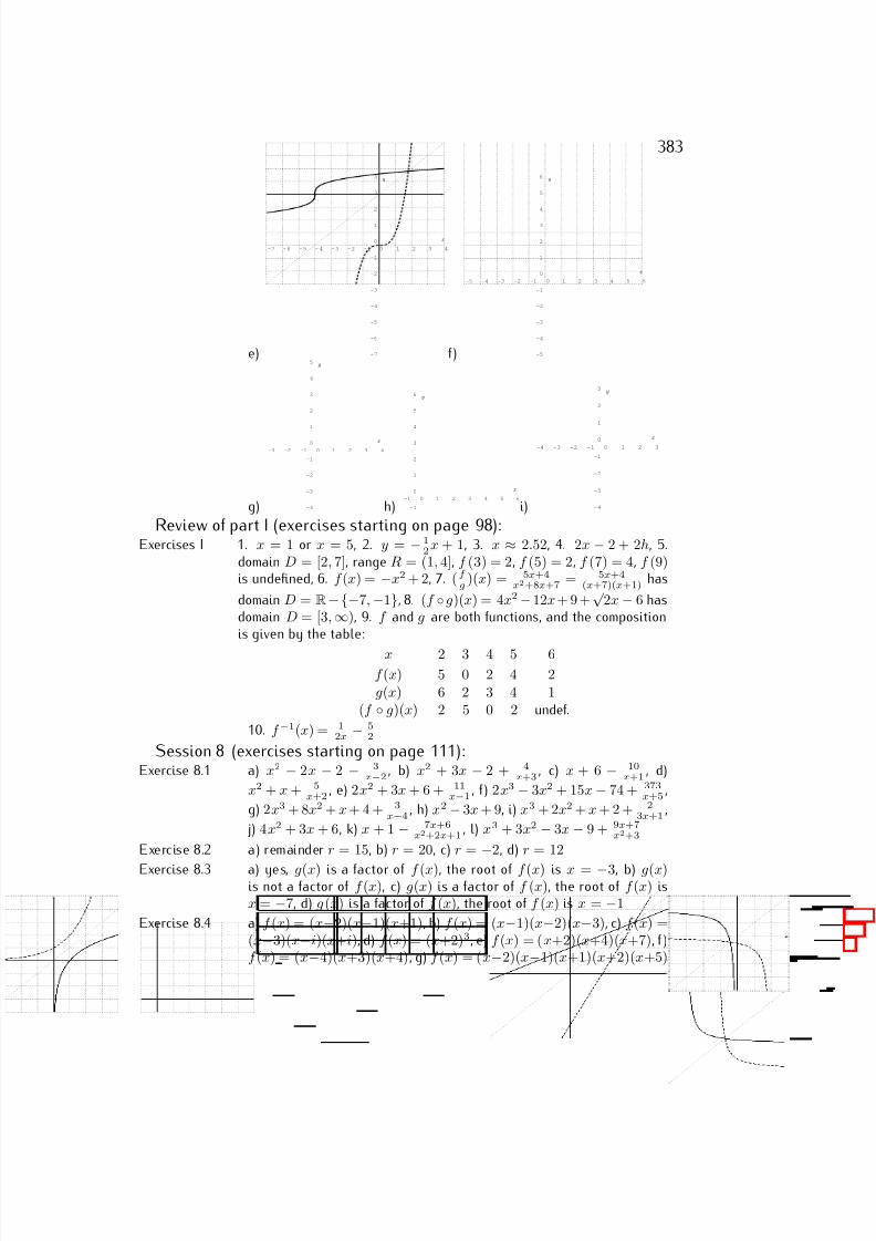
7/18/2019 Precalculus Tradler Carley
http://slidepdf.com/reader/full/precalculus-tradler-carley 393/424
383
e)
-7 - 6 - 5 - 4 - 3 - 2 - 1 0 1 2 3 4
-7
-6
-5
-4
-3
-2
-1
0
1
2
3
4
x
y
f)
-5 -4 -3 -2 -1 0 1 2 3 4 5 6
-5
-4
-3
-2
-1
0
1
2
3
4
5
6
x
y
g)
-3 -2 -1 0 1 2 3 4
-4
-3
-2
-1
0
1
2
3
4
5
x
y
h) -1 0 1 2 3 4 5 6
-1
0
1
2
3
4
5
6
x
y
i)
-4 -3 - 2 - 1 0 1 2 3
-4
-3
-2
-1
0
1
2
3
x
y
Review of part I (exercises starting on page 98):Exercises I 1. x = 1 or x = 5, 2. y = − 1
2x + 1, 3. x ≈ 2.52, 4. 2x − 2 + 2h, 5.
domain D = [2, 7], range R = (1, 4], f (3) = 2, f (5) = 2, f (7) = 4, f (9)is undefined, 6. f (x) = −x2 + 2, 7. (f
g)(x) = 5x+4
x2+8x+7 = 5x+4(x+7)(x+1)
has
domain D = R−{−7, −1}, 8. (f ◦ g)(x) = 4x2 −12x + 9 +√
2x − 6 hasdomain D = [3, ∞), 9. f and g are both functions, and the compositionis given by the table:
x 2 3 4 5 6f (x) 5 0 2 4 2g(x) 6 2 3 4 1
(f ◦ g)(x) 2 5 0 2 undef.
10. f −1(x) = 12x
− 52
Session 8 (exercises starting on page 111):Exercise 8.1 a) x2 − 2x − 2 − 3
x−2, b) x2 + 3x − 2 + 4
x+3, c) x + 6 − 10
x+1, d)
x2 + x + 5x+2
, e) 2x2 + 3x + 6 + 11x−1
, f) 2x3 − 3x2 + 15x − 74 + 373x+5
,
g) 2x3 + 8x2 + x + 4 + 3x−4
, h) x2 − 3x + 9, i) x3 + 2x2 + x + 2 + 23x+1
,
j) 4x2 + 3x + 6, k) x + 1 − 7x+6x2+2x+1
, l) x3 + 3x2 − 3x − 9 + 9x+7x2+3
Exercise 8.2 a) remainder r = 15, b) r = 20, c) r = −2, d) r = 12
Exercise 8.3 a) yes, g(x) is a factor of f (x), the root of f (x) is x = −3, b) g(x)is not a factor of f (x), c) g(x) is a factor of f (x), the root of f (x) isx = −7, d) g (x) is a factor of f (x), the root of f (x) is x = −1
Exercise 8.4 a) f (x) = (x−2)(x−1)(x+1), b) f (x) = (x−1)(x−2)(x−3), c) f (x) =(x−3)(x−i)(x+i), d) f (x) = (x+2)3, e) f (x) = (x+2)(x+4)(x+7), f )f (x) = (x−4)(x+3)(x+4), g) f (x) = (x−2)(x−1)(x+1)(x+2)(x+5)
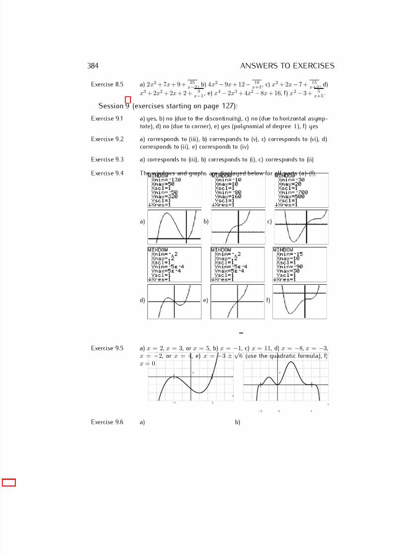
7/18/2019 Precalculus Tradler Carley
http://slidepdf.com/reader/full/precalculus-tradler-carley 394/424
384 ANSWERS TO EXERCISES
Exercise 8.5 a) 2x2 + 7x + 9 + 25x−2 , b) 4x2 − 9x + 12 − 18
x+3 , c) x2 + 2x− 7 + 15x+2 , d)
x3 + 2x2 + 2x + 2 + 3
x−1
, e) x4
−2x3 + 4x2
−8x + 16, f) x2
−3 + 5
x+5
.
Session 9 (exercises starting on page 127):
Exercise 9.1 a) yes, b) no (due to the discontinuity), c) no (due to horizontal asymp-tote), d) no (due to corner), e) yes (polynomial of degree 1), f) yes
Exercise 9.2 a) corresponds to (iii), b) corresponds to (v), c) corresponds to (vi), d)corresponds to (ii), e) corresponds to (iv)
Exercise 9.3 a) corresponds to (iii), b) corresponds to (i), c) corresponds to (ii)
Exercise 9.4 The windows and graphs are displayed below for all parts (a)-(f).
a) b) c)
d) e) f)
Exercise 9.5 a) x = 2, x = 3, or x = 5, b) x = −1, c) x = 11, d) x = −8, x = −3,x = −2, or x = 4, e) x = −3 ± √
6 (use the quadratic formula), f)x = 0
Exercise 9.6 a)
x
y
5−4
b)
x
y
−2 0 4
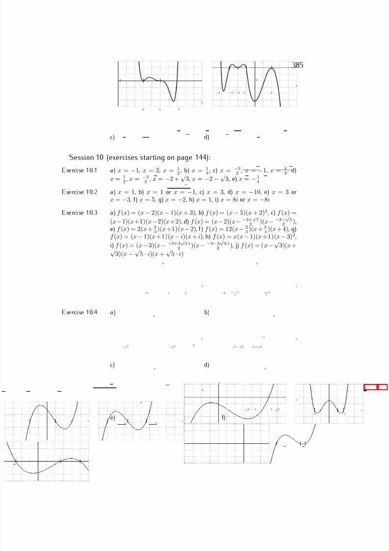
7/18/2019 Precalculus Tradler Carley
http://slidepdf.com/reader/full/precalculus-tradler-carley 395/424
385
c)
x
y
3 5 7
d)
x
y
−4 −3 −2 −1 2
Session 10 (exercises starting on page 144):
Exercise 10.1 a) x = −1, x = 2, x = 12
, b) x = 13
, c) x = −32
, x = −1, x = 43
, d)
x = 12 , x = −2
3 , x = −2 +√
3, x = −2 − √ 3, e) x = − 1
4
Exercise 10.2 a) x = 1, b) x = 1 or x = −1, c) x = 3, d) x = −10, e) x = 3 orx = −3, f) x = 5, g) x = −2, h) x = 1, i) x = 8i or x = −8i
Exercise 10.3 a) f (x) = (x − 2)(x − 1)(x + 3), b) f (x) = (x − 5)(x + 2)2, c) f (x) =
(x−1)(x+1)(x−2)(x+2), d) f (x) = (x−2)(x− −3+√ 5
2 )(x− −3−√ 5
2 ),e) f (x) = 2(x + 3
2)(x +1)(x−2), f ) f (x) = 12(x− 23)(x + 3
4)(x + 4), g)f (x) = (x − 1)(x +1)(x − i)(x + i), h) f (x) = x(x − 1)(x +1)(x − 3)2,
i) f (x) = (x−3)(x− −3+3√ 3·i
2 )(x− −3−3√ 3·i
2 ), j) f (x) = (x−√ 3)(x +√
3)(x − √ 5 · i)(x +
√ 5 · i)
Exercise 10.4 a)
x
y
3−2 1
b)
x
y
−4 −1−√ 5
2−1+
√ 5
2
c)
x
y
5−√ 7
√ 7
d)
x
y
−1
−3 − √ 2 −3 +
√ 2
e)
x
y
6
f)
x
y
−1 1√
3−√ 3
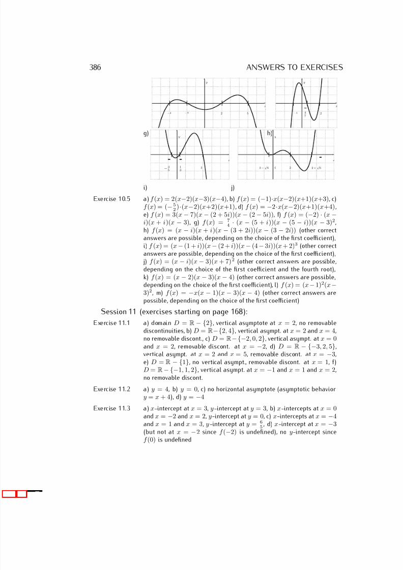
7/18/2019 Precalculus Tradler Carley
http://slidepdf.com/reader/full/precalculus-tradler-carley 396/424
386 ANSWERS TO EXERCISES
g)
x
y
5−2 2−4
h)
x
y
2−1 47
i)
x
y
13
3−35
j)
x
y
0 2 2 +√
62 − √ 6
Exercise 10.5 a) f (x) = 2(x−2)(x−3)(x−4), b) f (x) = (−1)·x(x−2)(x+1)(x+3), c)f (x) = (− 5
2)·(x−2)(x+2)(x+1), d) f (x) = −2·x(x−2)(x+1)(x+4),e) f (x) = 3(x − 7)(x − (2 + 5i))(x − (2 − 5i)), f) f (x) = (−2) · (x −i)(x + i)(x − 3), g) f (x) = 7
4 · (x − (5 + i))(x − (5 − i))(x − 3)2,h) f (x) = (x − i)(x + i)(x − (3 + 2i))(x − (3 − 2i)) (other correctanswers are possible, depending on the choice of the first coefficient),i) f (x) = (x − (1 + i))(x − (2 + i))(x − (4 − 3i))(x + 2)3 (other correctanswers are possible, depending on the choice of the first coefficient),
j) f (x) = (x − i)(x − 3)(x + 7)2 (other correct answers are possible,depending on the choice of the first coefficient and the fourth root),k) f (x) = (x − 2)(x − 3)(x − 4) (other correct answers are possible,depending on the choice of the first coefficient), l) f (x) = (x− 1)2(x−3)2, m) f (x) =
−x(x
−1)(x
−3)(x
−4) (other correct answers are
possible, depending on the choice of the first coefficient)
Session 11 (exercises starting on page 168):
Exercise 11.1 a) domain D = R − {2}, vertical asymptote at x = 2, no removablediscontinuities, b) D = R−{2, 4}, vertical asympt. at x = 2 and x = 4,no removable discont., c) D = R−{−2, 0, 2}, vertical asympt. at x = 0and x = 2, removable discont. at x = −2, d) D = R − {−3, 2, 5},vertical asympt. at x = 2 and x = 5, removable discont. at x = −3,e) D = R − {1}, no vertical asympt., removable discont. at x = 1, f)D = R− {−1, 1, 2}, vertical asympt. at x = −1 and x = 1 and x = 2,no removable discont.
Exercise 11.2 a) y = 4, b) y = 0, c) no horizontal asymptote (asymptotic behavior
y = x + 4), d) y = −4Exercise 11.3 a) x-intercept at x = 3, y-intercept at y = 3, b) x-intercepts at x = 0
and x = −2 and x = 2, y-intercept at y = 0, c) x-intercepts at x = −4and x = 1 and x = 3, y -intercept at y = 6
5, d) x-intercept at x = −3
(but not at x = −2 since f (−2) is undefined), no y-intercept sincef (0) is undefined
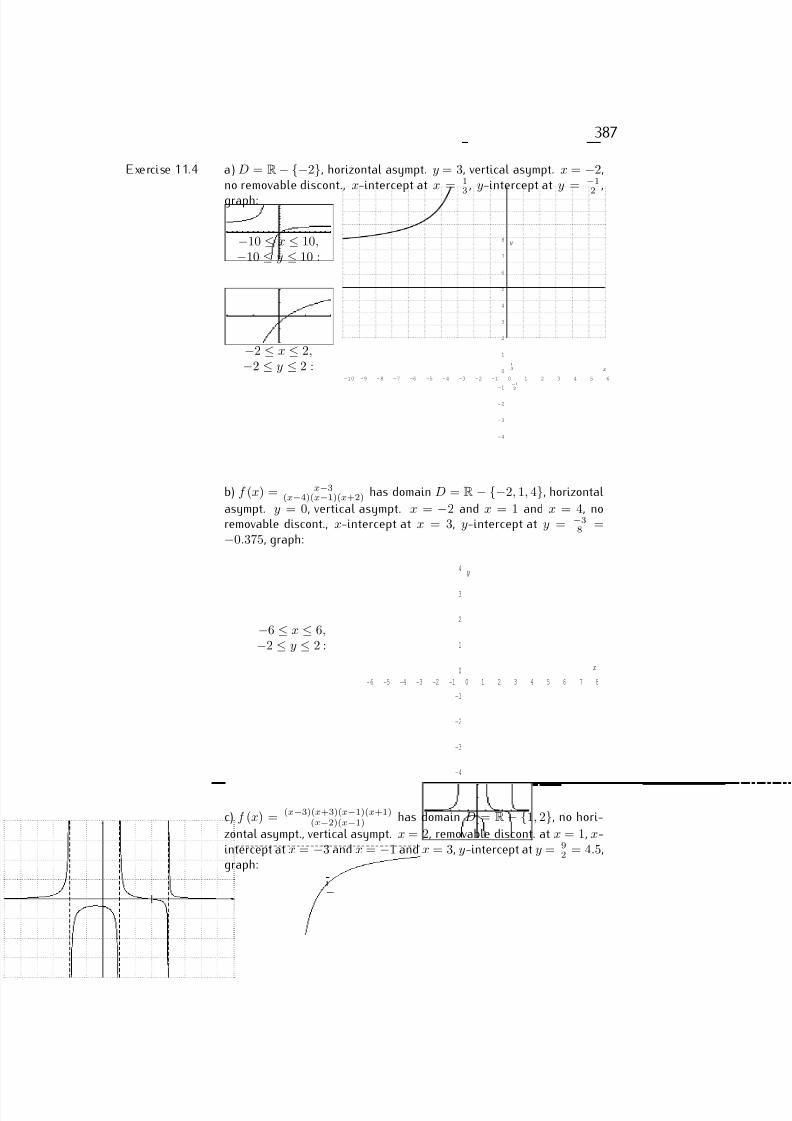
7/18/2019 Precalculus Tradler Carley
http://slidepdf.com/reader/full/precalculus-tradler-carley 397/424
387
Exercise 11.4 a) D = R− {−2}, horizontal asympt. y = 3, vertical asympt. x = −2,no removable discont., x-intercept at x = 1
3 , y-intercept at y = −12 ,
graph:
−10 ≤ x ≤ 10,−10 ≤ y ≤ 10 :
−2 ≤ x ≤ 2,−2 ≤ y ≤ 2 :
-10 -9 -8 -7 -6 -5 -4 -3 -2 -1 0 1 2 3 4 5 6
-4
-3
-2
-1
0
1
2
3
4
5
6
7
8
x
y
−12
13
b) f (x) = x−3(x−4)(x−1)(x+2) has domain D = R − {−2, 1, 4}, horizontal
asympt. y = 0, vertical asympt. x = −2 and x = 1 and x = 4, noremovable discont., x-intercept at x = 3, y-intercept at y = −3
8 =−0.375, graph:
−6 ≤ x ≤ 6,−2 ≤ y ≤ 2 :
-6 -5 -4 -3 -2 -1 0 1 2 3 4 5 6 7 8
-4
-3
-2
-1
0
1
2
3
4
x
y
c) f (x) = (x−3)(x+3)(x−1)(x+1)(x−2)(x−1)
has domain D = R − {1, 2}, no hori-
zontal asympt., vertical asympt. x = 2, removable discont. at x = 1, x-intercept at x = −3 and x = −1 and x = 3, y-intercept at y = 9
2 = 4.5,graph:
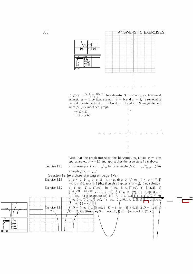
7/18/2019 Precalculus Tradler Carley
http://slidepdf.com/reader/full/precalculus-tradler-carley 398/424
388 ANSWERS TO EXERCISES
−10
≤x
≤10,
−10 ≤ y ≤ 10 :
-8 - 7 - 6 - 5 - 4 - 3 - 2 - 1 0 1 2 3 4 5 6
-2
-1
0
1
2
3
4
5
6
7
8
9
10
11
12
13
14
15
16
17
18
x
y
d) f (x) = (x
−3)(x
−1)(x+1)
x2(x−2) has domain D = R − {0, 2}, horizontalasympt. y = 1, vertical asympt. x = 0 and x = 2, no removablediscont., x-intercepts at x = −1 and x = 1 and x = 3, no y -interceptsince f (0) is undefined, graph:
−4 ≤ x ≤ 6,−5 ≤ y ≤ 5 :
-6 -5 -4 -3 -2 -1 0 1 2 3 4 5 6
-4
-3
-2
-1
0
1
2
3
4
x
y
Note that the graph intersects the horizontal asymptote y = 1 atapproximately x ≈ −2.3 and approaches the asymptote from above.
Exercise 11.5 a) for example f (x) = 1x−4
, b) for example f (x) = 5x2
x2−5x+6, c) for
example f (x) = x2−xx−1
Session 12 (exercises starting on page 179):Exercise 12.1 a) x ≤ 3, b) 1
2 > x, c) −4 ≥ x, d) x > 22
5 , e) −5 ≤ x ≤ 7, f)
−4 < x ≤ 3, g) x ≥ 2 (this then also implies x ≥ − 72 ), h) no solution
Exercise 12.2 a) (−∞, −2) ∪ (7, ∞), b) (−∞, −5] ∪ [7, ∞), c) [−2, 2], d)−3−√ 212 , −3+√ 212 , e) [−3, 2], f ) − 13 , 1, g) R−{2}, h) [−2, 1]∪[3, ∞),i) (−∞, −4), j) (0, 2) ∪ (2, ∞), k) [−3, −1] ∪ [1, 3], l) (−1, 1) ∪ (2, 3), m)(−∞, 0) ∪ (0, 2) ∪ (3, ∞), n) (−∞, −2] ∪ [0, 1] ∪ [2, 5], o) [1, 2] ∪ [3, 4] ∪[5, ∞), p) (−∞, 1]
Exercise 12.3 a) D = (−∞, 3] ∪ [5, ∞), b) D = (−∞, −3] ∪ [0, 3], c) D = [1, 4], d)D = [2, 5] ∪ [6, ∞), e) D = (−∞, 3), f) D = (−∞, −1) ∪ (7, ∞)
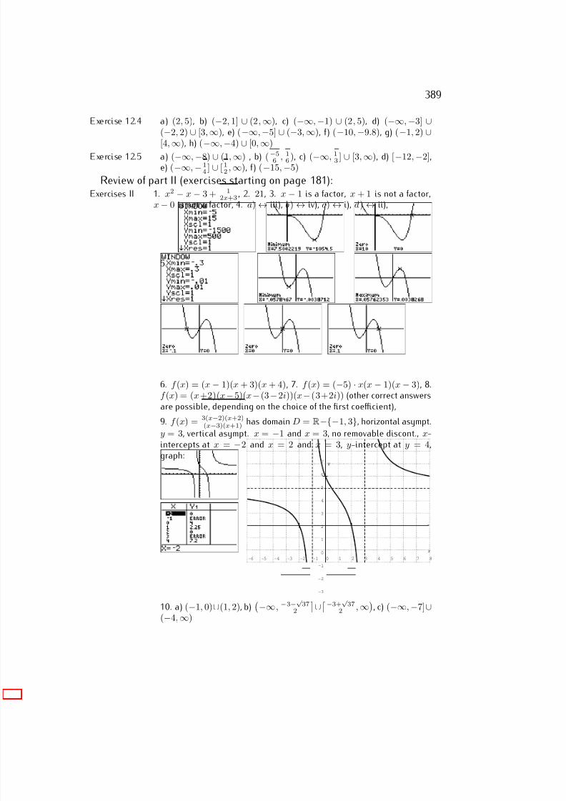
7/18/2019 Precalculus Tradler Carley
http://slidepdf.com/reader/full/precalculus-tradler-carley 399/424
389
Exercise 12.4 a) (2, 5), b) (−2, 1] ∪ (2, ∞), c) (−∞, −1) ∪ (2, 5), d) (−∞, −3] ∪(
−2, 2)
∪[3,
∞), e) (
−∞,
−5]
∪(
−3,
∞), f) (
−10,
−9.8), g) (
−1, 2)
∪[4, ∞), h) (−∞, −4) ∪ [0, ∞)
Exercise 12.5 a) (−∞, −8) ∪ (1, ∞) , b) (−56 , 16), c) (−∞, 13 ] ∪ [3, ∞), d) [−12, −2],
e) (−∞, − 14 ] ∪ [12 , ∞), f) (−15, −5)
Review of part II (exercises starting on page 181):Exercises II 1. x2 − x − 3 + 1
2x+3 , 2. 21, 3. x − 1 is a factor, x + 1 is not a factor,x − 0 is not a factor, 4. a) ↔ iii), b) ↔ iv), c) ↔ i), d) ↔ ii),
5.
6. f (x) = (x − 1)(x + 3)(x + 4), 7. f (x) = (−5) · x(x − 1)(x − 3), 8.f (x) = (x +2)(x−5)(x− (3−2i))(x− (3+2i)) (other correct answersare possible, depending on the choice of the first coefficient),
9. f (x) = 3(x−2)(x+2)(x−3)(x+1) has domain D = R−{−1, 3}, horizontal asympt.y = 3, vertical asympt. x = −1 and x = 3, no removable discont., x-intercepts at x = −2 and x = 2 and x = 3, y-intercept at y = 4,graph:
-6 -5 -4 -3 -2 -1 0 1 2 3 4 5 6 7 8
-3
-2
-1
0
1
2
3
4
5
6
7
x
y
10. a) (−1, 0)∪(1, 2), b)−∞, −3−
√ 37
2
∪−3+√ 37
2 , ∞, c) (−∞, −7]∪
(−4, ∞)
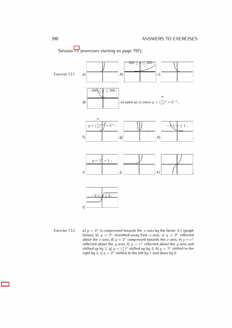
7/18/2019 Precalculus Tradler Carley
http://slidepdf.com/reader/full/precalculus-tradler-carley 400/424
390 ANSWERS TO EXERCISES
Session 13 (exercises starting on page 197):
Exercise 13.1 a) , b)
−200 ≤ x ≤ 200 :
, c) ,
d)
−200 ≤ x ≤ 200 :
, e) same as c) since y = (13)x = 3−x,
f)
y = (13)−x = 3x :
, g) , h)
−1 ≤ x ≤ 1 :
,
i)
y = 1x = 1 :
, j) , k) ,
l)
−2 ≤ y ≤ 2 :
Exercise 13.2 a) y = 4x is compressed towards the x-axis by the factor 0.1 (graphbelow), b) y = 2x stretched away from x-axis, c) y = 2x reflectedabout the x-axis, d) y = 2x compressed towards the x-axis, e) y = ex
reflected about the y-axis, f) y = ex reflected about the y-axis andshifted up by 1, g) y = (12)x shifted up by 3, h) y = 2x shifted to theright by 4, i) y = 2x shifted to the left by 1 and down by 6
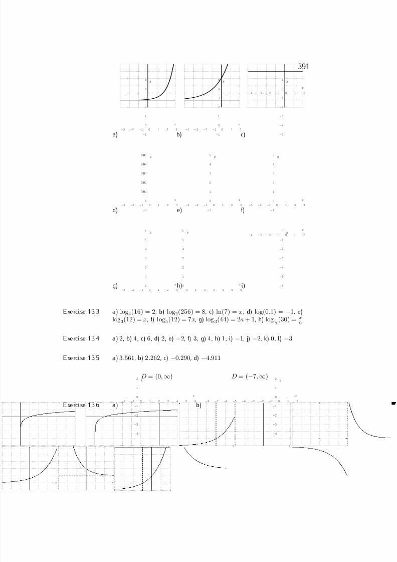
7/18/2019 Precalculus Tradler Carley
http://slidepdf.com/reader/full/precalculus-tradler-carley 401/424
391
a)-3 -2 -1 0 1 2 3
-1
0
1
2
3
4
5
x
y
b)-4 - 3 -2 - 1 0 1 2
-1
0
1
2
3
4
5
x
y
c)
-4 -3 - 2 - 1 0 1 2
-5
-4
-3
-2
-1
0
1
x
y
d)-3 -2 -1 0 1 2 3
-1
0
1
2
3
4
5
x
y
0.0
0.0
0.0
0.0
0.0
e)-3 -2 -1 0 1 2 3
-1
0
1
2
3
4
5
x
y
f)-3 -2 -1 0 1 2 3
-1
0
1
2
3
4
5
x
y
g)-3 -2 -1 0 1 2 3
0
1
2
3
4
5
6
x
y
h)0 1 2 3 4 5 6
0
1
2
3
4
5
6
x
y
i)
-4 -3 - 2 - 1 0 1 2
-6
-5
-4
-3
-2
-1
0 x
y
Exercise 13.3 a) log4(16) = 2, b) log2(256) = 8, c) ln(7) = x , d) log(0.1) = −1, e)log3(12) = x, f) log5(12) = 7x, g) log3(44) = 2a + 1, h) log 1
2(30) = x
h
Exercise 13.4 a) 2, b) 4 , c) 6, d) 2 , e) −2, f) 3 , g) 4 , h) 1 , i) −1, j) −2, k) 0 , l) −3
Exercise 13.5 a) 3.561, b) 2.262, c) −0.290, d) −4.911
Exercise 13.6 a)
D = (0, ∞)
-2 -1 0 1 2 3 4 5 6
-4
-3
-2
-1
0
1
2
x
y
b)
D = (−7, ∞)
-8 -7 -6 -5 -4 -3 -2 -1 0 1 2
-4
-3
-2
-1
0
1
2
x
y
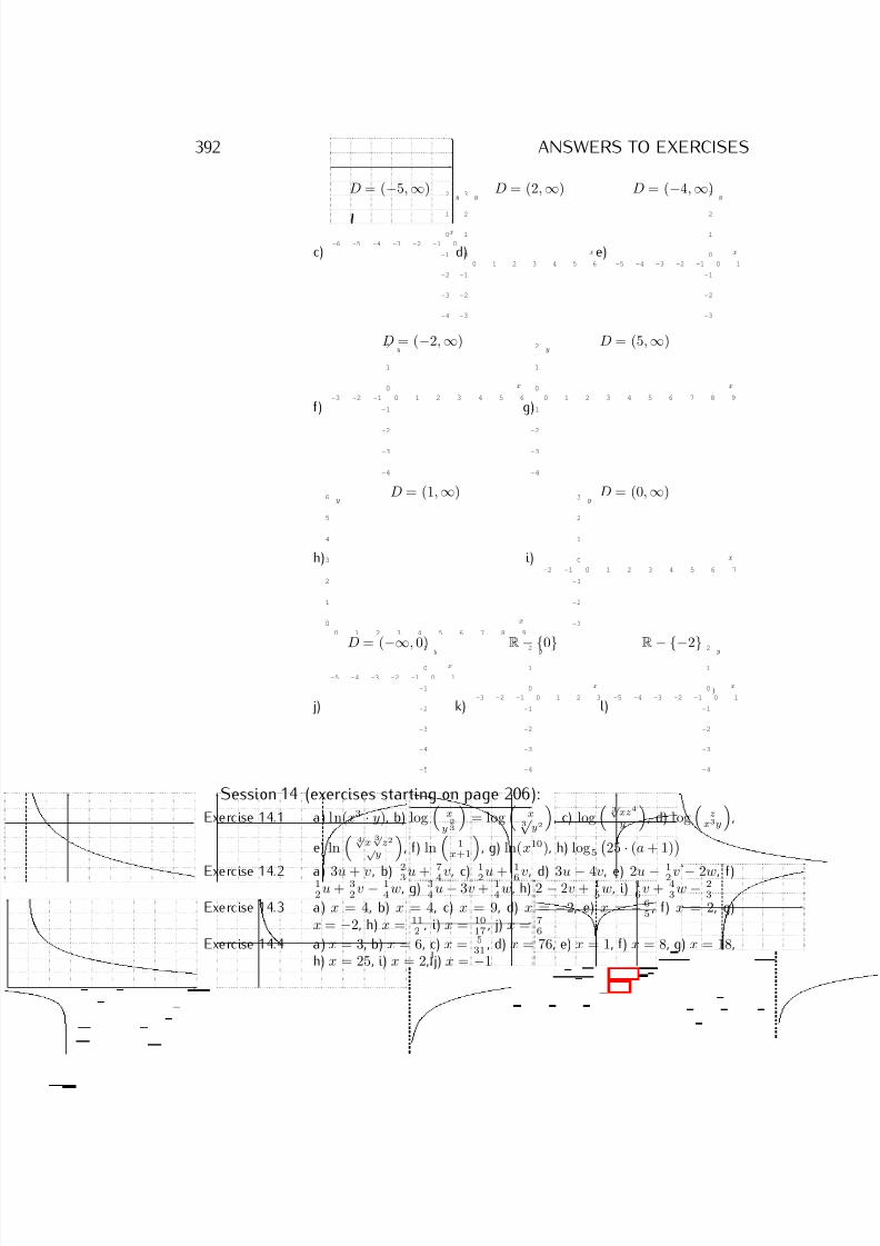
7/18/2019 Precalculus Tradler Carley
http://slidepdf.com/reader/full/precalculus-tradler-carley 402/424
392 ANSWERS TO EXERCISES
c)
D = (−5, ∞)
-6 -5 -4 -3 -2 -1 0
-4
-3
-2
-1
0
1
2
x
y
d)
D = (2, ∞)
0 1 2 3 4 5 6
-3
-2
-1
0
1
2
3
x
y
e)
D = (−4, ∞)
-5 -4 -3 -2 -1 0 1
-3
-2
-1
0
1
2
3
x
y
f)
D = (−2, ∞)
-3 -2 -1 0 1 2 3 4 5 6
-4
-3
-2
-1
0
1
2
x
y
g)
D = (5, ∞)
0 1 2 3 4 5 6 7 8 9
-4
-3
-2
-1
0
1
2
x
y
h)
D = (1, ∞)
0 1 2 3 4 5 6 7 8 9
0
1
2
3
4
5
6
x
y
i)
D = (0, ∞)
-2 -1 0 1 2 3 4 5 6 7
-3
-2
-1
0
1
2
3
x
y
j)
D = (
−∞, 0)
-5 -4 -3 -2 -1 0 1
-5
-4
-3
-2
-1
0
1
x
y
k)
R
− {0
}
-3 -2 -1 0 1 2 3
-4
-3
-2
-1
0
1
2
x
y
l)
R
− {−2
}
-5 -4 -3 -2 -1 0 1
-4
-3
-2
-1
0
1
2
x
y
)
Session 14 (exercises starting on page 206):
Exercise 14.1 a) ln(x3 · y), b) log
x
y23
= log
x3√
y2
, c) log
3√ xz4
y
, d) log
zx3y
,
e) ln
4√ x 3√ z2√
y , f) ln
1x+1
, g) ln(x10), h) log5 25 · (a + 1)
Exercise 14.2 a) 3u + v, b) 23u +
74v, c)
12u +
16v, d) 3u − 4v, e) 2u −
12v − 2w, f)1
2u + 3
2v − 1
4w, g) 3
4u − 3v + 1
4w, h) 2 − 2v + 1
5w, i) 1
6v + 4
3w − 2
3
Exercise 14.3 a) x = 4, b) x = 4, c) x = 9, d) x = −2, e) x = − 65
, f) x = 2, g)x = −2, h) x = 11
2 , i) x = 10
17, j) x = 7
6
Exercise 14.4 a) x = 3, b) x = 6, c) x = 531 , d) x = 76, e) x = 1, f) x = 8, g) x = 18,
h) x = 25, i) x = 2, j) x = −1
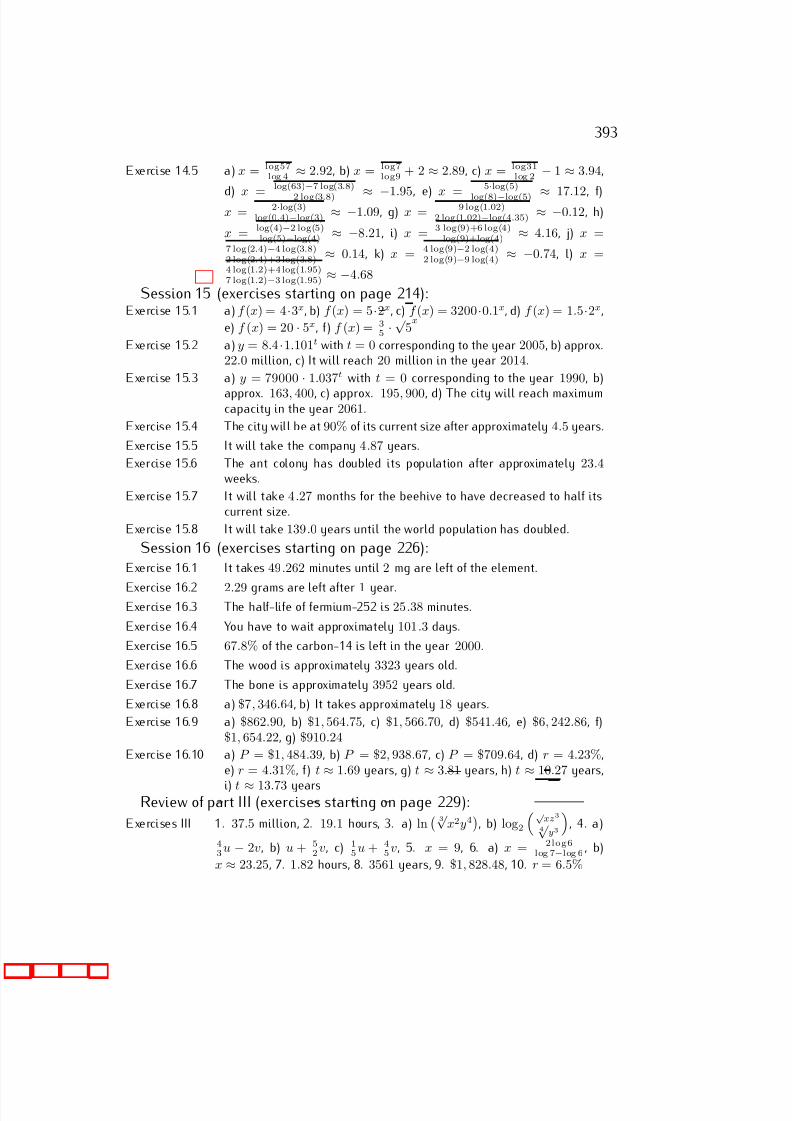
7/18/2019 Precalculus Tradler Carley
http://slidepdf.com/reader/full/precalculus-tradler-carley 403/424
393
Exercise 14.5 a) x = log57log 4 ≈ 2.92, b) x = log7
log9 + 2 ≈ 2.89, c) x = log31log 2 − 1 ≈ 3.94,
d) x =
log(63)
−7 log(3.8)
2 log(3.8) ≈ −1.95, e) x =
5
·log(5)
log(8)−log(5) ≈ 17.12, f)x = 2·log(3)
log(0.4)−log(3) ≈ −1.09, g) x = 9 log(1.02)2 log(1.02)−log(4.35) ≈ −0.12, h)
x = log(4)−2 log(5)log(5)−log(4) ≈ −8.21, i) x =
3 log(9)+6 log(4)log(9)+log(4) ≈ 4.16, j) x =
7 log(2.4)−4 log(3.8)2 log(2.4)+3log(3.8) ≈ 0.14, k) x = 4 log(9)−2 log(4)
2 log(9)−9 log(4) ≈ −0.74, l) x =4 log(1.2)+4log(1.95)7 log(1.2)−3 log(1.95) ≈ −4.68
Session 15 (exercises starting on page 214):Exercise 15.1 a) f (x) = 4·3x, b) f (x) = 5·2x, c) f (x) = 3200·0.1x, d) f (x) = 1.5·2x,
e) f (x) = 20 · 5x, f) f (x) = 35 ·
√ 5x
Exercise 15.2 a) y = 8.4 ·1.101t with t = 0 corresponding to the year 2005, b) approx.22.0 million, c) It will reach 20 million in the year 2014.
Exercise 15.3 a) y = 79000
·1.037t with t = 0 corresponding to the year 1990, b)
approx. 163, 400, c) approx. 195, 900, d) The city will reach maximumcapacity in the year 2061.
Exercise 15.4 The city will be at 90% of its current size after approximately 4.5 years.
Exercise 15.5 It will take the company 4.87 years.
Exercise 15.6 The ant colony has doubled its population after approximately 23.4weeks.
Exercise 15.7 It will take 4.27 months for the beehive to have decreased to half itscurrent size.
Exercise 15.8 It will take 139.0 years until the world population has doubled.
Session 16 (exercises starting on page 226):Exercise 16.1 It takes 49.262 minutes until 2 mg are left of the element.
Exercise 16.2 2.29 grams are left after 1 year.Exercise 16.3 The half-life of fermium-252 is 25.38 minutes.
Exercise 16.4 You have to wait approximately 101.3 days.
Exercise 16.5 67.8% of the carbon-14 is left in the year 2000.
Exercise 16.6 The wood is approximately 3323 years old.
Exercise 16.7 The bone is approximately 3952 years old.
Exercise 16.8 a) $7, 346.64, b) It takes approximately 18 years.
Exercise 16.9 a) $862.90, b) $1, 564.75, c) $1, 566.70, d) $541.46, e) $6, 242.86, f)$1, 654.22, g) $910.24
Exercise 16.10 a) P = $1, 484.39, b) P = $2, 938.67, c) P = $709.64, d) r = 4.23%,e) r = 4.31%, f) t
≈1.69 years, g) t
≈3.81 years, h) t
≈10.27 years,
i) t ≈ 13.73 yearsReview of part III (exercises starting on page 229):
Exercises III 1. 37.5 million, 2. 19.1 hours, 3. a) ln 3√
x2y4
, b) log2
√ xz3
4√
y3
, 4. a)
43u − 2v, b) u + 5
2v, c) 15u + 45v, 5. x = 9, 6. a) x = 2log6
log 7−log 6 , b)
x ≈ 23.25, 7. 1.82 hours, 8. 3561 years, 9. $1, 828.48, 10. r = 6.5%
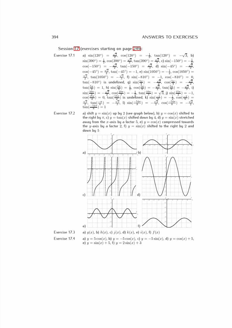
7/18/2019 Precalculus Tradler Carley
http://slidepdf.com/reader/full/precalculus-tradler-carley 404/424
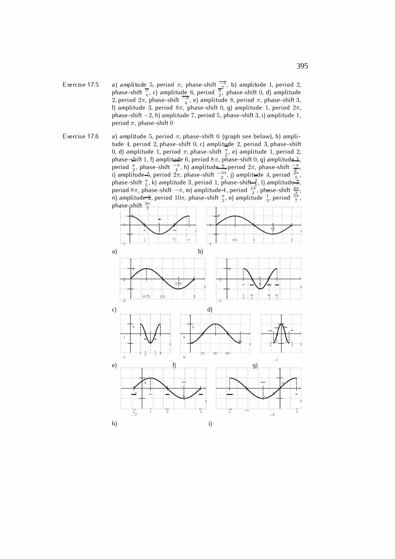
7/18/2019 Precalculus Tradler Carley
http://slidepdf.com/reader/full/precalculus-tradler-carley 405/424
395
Exercise 17.5 a) amplitude 5, period π, phase-shift −32 , b) amplitude 1, period 2,
phase-shift 5π
, c) amplitude 6, period π2 , phase-shift 0, d) amplitude
2, period 2π, phase-shift −π4 , e) amplitude 8, period π, phase-shift 3 ,
f) amplitude 3, period 8π, phase-shift 0, g) amplitude 1, period 2π,phase-shift −2, h) amplitude 7, period 5 , phase-shift 3, i) amplitude 1,period π , phase-shift 0
Exercise 17.6 a) amplitude 5, period π, phase-shift 0 (graph see below), b) ampli-tude 4, period 2, phase-shift 0, c) amplitude 2, period 3, phase-shift0, d) amplitude 1, period π, phase-shift π
2, e) amplitude 1, period 2,
phase-shift 1, f) amplitude 6 , period 8π, phase-shift 0, g) amplitude 1,period π
2 , phase-shift −π4 , h) amplitude 7, period 2π, phase-shift −π
4 ,i) amplitude 5, period 2π, phase-shift −3π
2 , j) amplitude 4, period 2π
5 ,
phase-shift π5
, k) amplitude 3 , period 1, phase-shift 2π
, l) amplitude 7 ,period 8π, phase-shift
−π, m) amplitude 1 , period 2π
3 , phase-shift 4π3 ,
n) amplitude 2 , period 10π, phase-shift π2 , o) amplitude 13 , period 5π
7 ,phase-shift 3π7
a)
x
y
5
−5
π4
π2
3π4
π
b)
x
y
4
−40.5 1
1.5
2
c)
x
y
2
−20.75 1.5
2.25
3
d)
x
y
1
−1
π2
3π4
π
5π4
3π2
e)
x
y
1
−11 3
2
2
52 3
f)
x
y
6
−62π 4π 6π
8π
g)
x
y
1
−1
−π4
−π8
π8 π
4
h)
x
y
7
−7
−π4
π4
3π4
5π4
7π4
i)
x
y
5
−5
−3π2 −π
−π2
π2
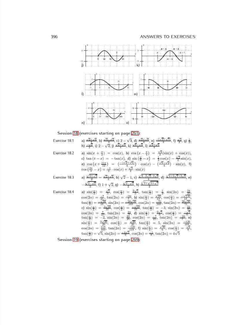
7/18/2019 Precalculus Tradler Carley
http://slidepdf.com/reader/full/precalculus-tradler-carley 406/424
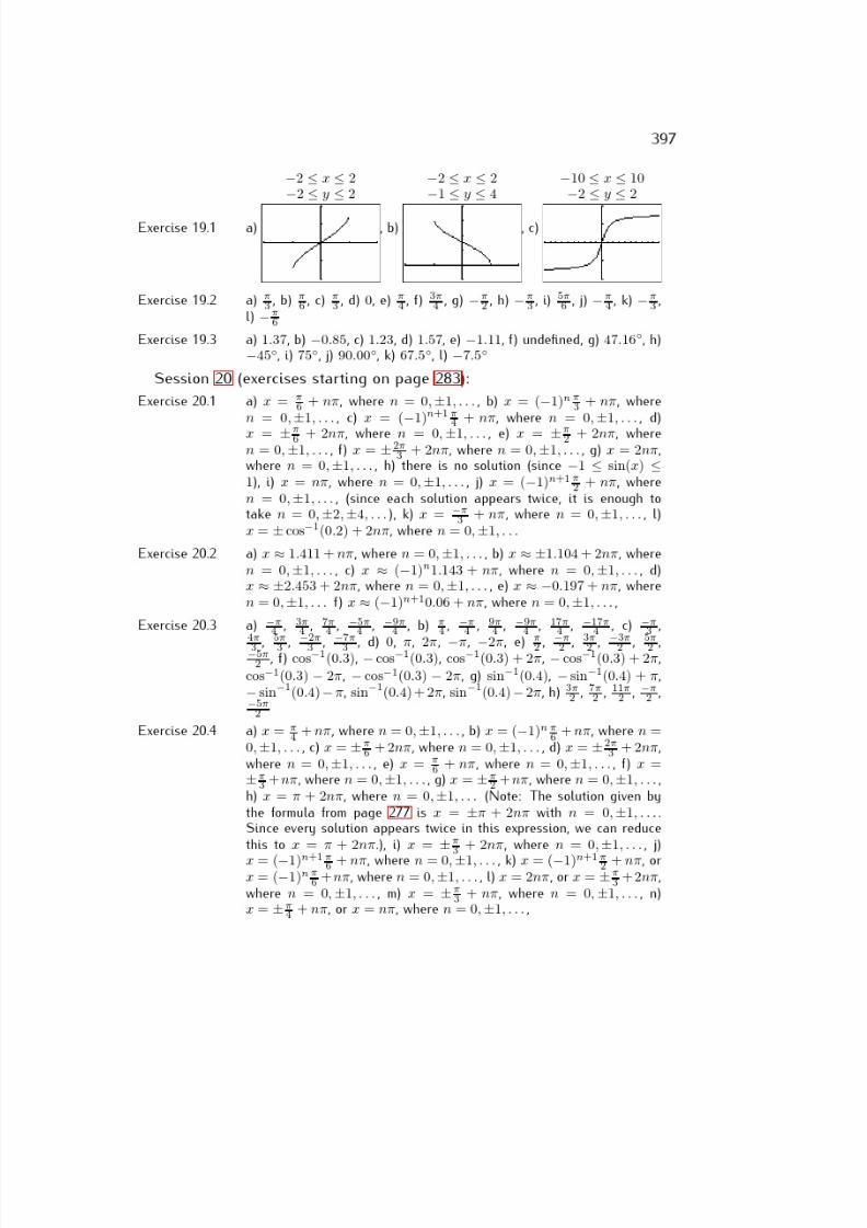
7/18/2019 Precalculus Tradler Carley
http://slidepdf.com/reader/full/precalculus-tradler-carley 407/424
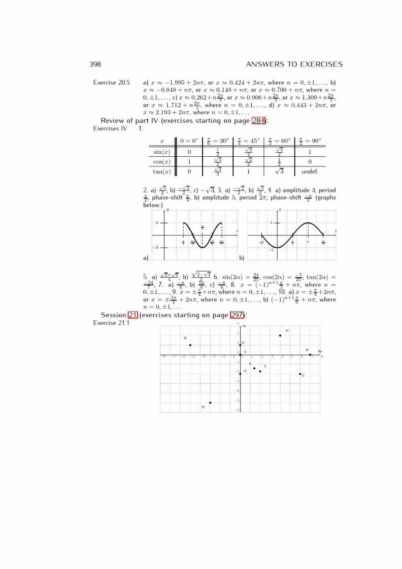
7/18/2019 Precalculus Tradler Carley
http://slidepdf.com/reader/full/precalculus-tradler-carley 408/424
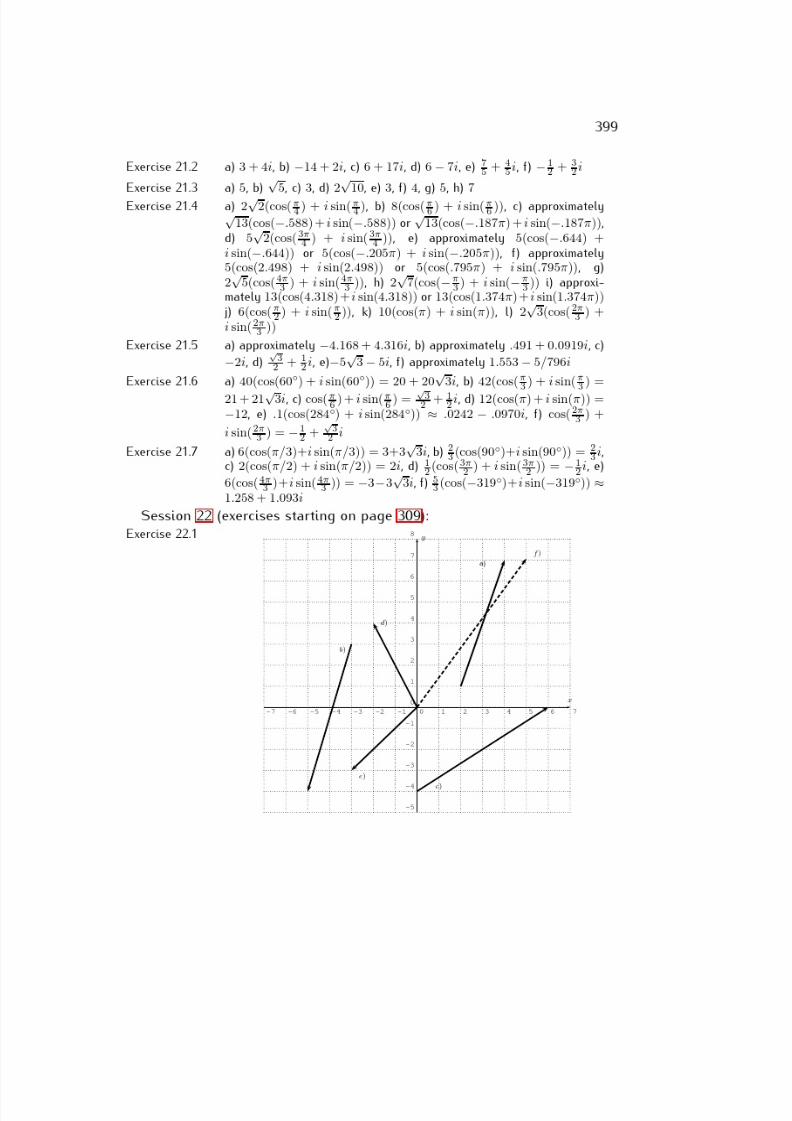
7/18/2019 Precalculus Tradler Carley
http://slidepdf.com/reader/full/precalculus-tradler-carley 409/424
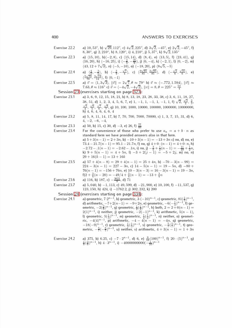
7/18/2019 Precalculus Tradler Carley
http://slidepdf.com/reader/full/precalculus-tradler-carley 410/424
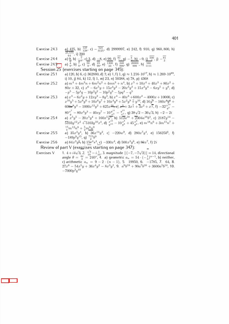
7/18/2019 Precalculus Tradler Carley
http://slidepdf.com/reader/full/precalculus-tradler-carley 411/424
401
Exercise 24.3 a) 425, b) 127128 , c) − 5213125 , d) 2999997, e) 242, f) 910, g) 960, 800, h)
25,575
64
, i) 200
Exercise 24.4 a) 9, b) − 76
, c) 3 , d) −8, e) 99 , f) 812
, g) −43
, h) −9, i) 5003
, j) − 812
Exercise 24.5 a) 49
, b) 79
, c) 509
, d) 2399
, e) 130033
, f) 248999
, g) 20000999
, h) 5601111
Session 25 (exercises starting on page 345):Exercise 25.1 a) 120, b) 6, c) 362880, d) 2, e) 1, f ) 1, g) ≈ 1.216·1017, h) ≈ 1.269·1089,
i) 10, j) 84 , k) 12 , l) 1 , m) 23, n) 50388, o) 78 , p) 4368
Exercise 25.2 a) m4 + 4m3n + 6m2n2 + 4mn3 + n4, b) x5 + 10x4 + 40x3 + 80x2 +80x + 32, c) x6 − 6x5y + 15x4y2 − 20x3y3 + 15x2y4 − 6xy5 + y6, d)− p5 − 5 p4q − 10 p3q 2 − 10 p2q 3 − 5 pq 4 − q 5
Exercise 25.3 a) x3 − 6x2y + 12xy2 − 8y3, b) x4 − 40x3 +600x2 − 4000x + 10000, c)x10y5 + 5x8y6 + 10x6y7 + 10x4y8 + 5x2y9 + y10, d) 16y8 − 160x4y6 +
600x8y4 − 1000x12y2 + 625x16, e) x3 + 3x52 + 3x2 + x
32 , f) −32x10
y5 −
80x7
y − 80x4
y3
− 40xy7
− 10y11
x2 − y15
x5 , g) 38√ 2 − 36√ 3, h) −2 − 2iExercise 25.4 a) x5y5 − 20x5y4 + 160x5y3, b) 512a18 + 2304a16b3, c) 2187y14 −
5103y12x2 + 5103y10x4, d) x10
y10 − 10x8
y8 + 45 x6
y6, e) m18n6 + 3m15n7 +
154
m12n8 + 52
m9n9
Exercise 25.5 a) 35x3y4, b) 36x14y2, c) −220w9, d) 280x7y4, e) 15625b6, f)−189 p9q 15, g) 715
2 b9
Exercise 25.6 a) 84x3y6, b) 15r4s4, c) −330x4, d) 500x3y6, e) 80x7, f) 2i
Review of part V (exercises starting on page 347):Exercises V 1. 4 + i4
√ 3, 2.
√ 3
10 − i 1
10, 3. magnitude ||−7, −7
√ 3|| = 14 , directional
angle θ = 4π3 = 240◦, 4. a) geometric an = 54 · (− 1
3)n−1, b) neither,c) arithmetic an = 9 − 2 · (n − 1), 5. 19950, 6. −1785, 7. 64, 8.27x6
−54x5y + 36x4y2
−8x3y3, 9. a9b18 + 90a7b16 + 3600a5b14, 10.
−7000 p3q 10
7/18/2019 Precalculus Tradler Carley
http://slidepdf.com/reader/full/precalculus-tradler-carley 412/424
References
The topics in this book are all standard and can be found in many precalculustextbooks. In particular, the precalculus textbooks below can be consulted forfurther reading.
1. Robert F. Blitzer, Precalculus, 4th edition, Prentice Hall
2. Thomas W. Hungerford, Douglas J. Shaw, Contemporary Precalculus: AGraphing Approach, 5th edition, Brooks Cole
3. Ron Larson, Precalculus, 8th edition, Brooks Cole
4. David Lippman, Melonie Rasmussen, Precalculus: An Investigation of
Functions, available on www.opentextbookstore.com/precalc
5. Revathi Narasimhan, Precalculus: Building Concepts and Connections,
Instructor’s edition, Houghton Mifflin6. Fred Safier, Schaum’s Outline of PreCalculus, 2nd edition, Schaum’s Out-
line Series, McGraw-Hill
7. Karl J. Smith, Precalculus: A Functional Approach To Graphing And Prob-
lem Solving, 6th edition, Jones & Bartlett Learning
8. James Stewart, Lothar Redlin, Saleem Watson, Precalculus: Mathematicsfor Calculus, 6th edition, Brooks Cole
Here are some books on calculus, which should be accessible to the readerafter finishing this book.
1. Ron Larson, Bruce H. Edwards, Calculus, 9th edition, Brooks Cole
2. Jon Rogawski, Calculus, 2nd edition, W. H. Freeman
3. James Stewart, Calculus, 6th edition, Brooks Cole
402
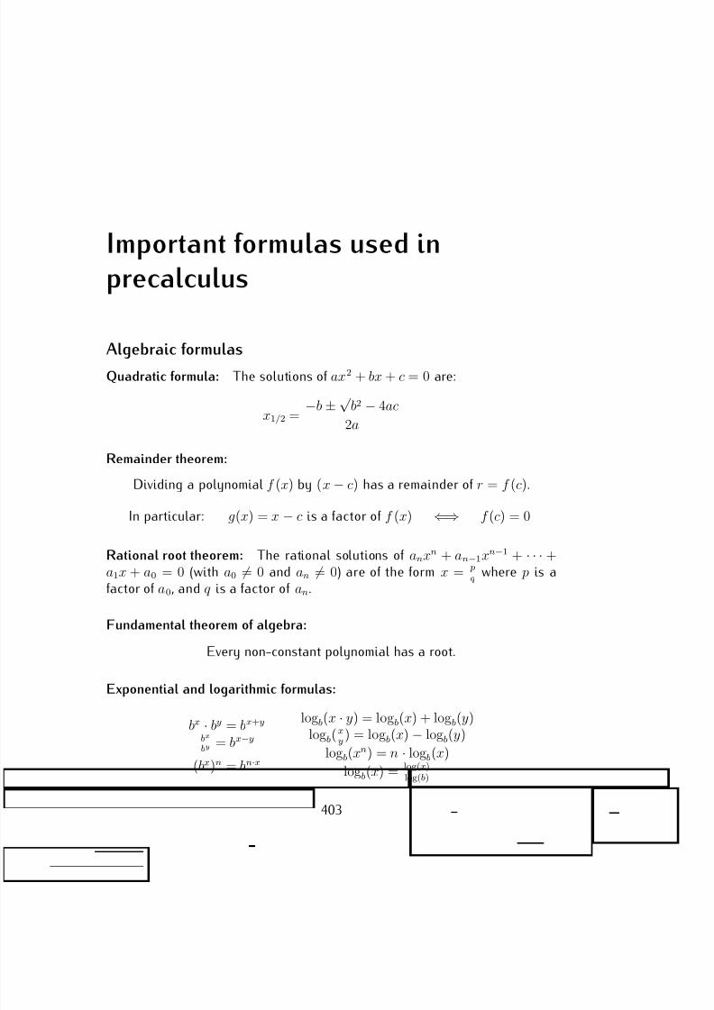
7/18/2019 Precalculus Tradler Carley
http://slidepdf.com/reader/full/precalculus-tradler-carley 413/424
Important formulas used in
precalculus
Algebraic formulasQuadratic formula: The solutions of ax2 + bx + c = 0 are:
x1/2 = −b ± √
b2 − 4ac
2a
Remainder theorem:
Dividing a polynomial f (x) by (x − c) has a remainder of r = f (c).
In particular: g(x) = x
−c is a factor of f (x)
⇐⇒ f (c) = 0
Rational root theorem: The rational solutions of anxn + an−1xn−1 + · · · +a1x + a0 = 0 (with a0 = 0 and an = 0) are of the form x = p
q where p is afactor of a0, and q is a factor of an.
Fundamental theorem of algebra:
Every non-constant polynomial has a root.
Exponential and logarithmic formulas:
bx · by = bx+y
bx
by = bx−y
(bx)n = bn·x
logb(x · y) = logb(x) + logb(y)logb( x
y) = logb(x) − logb(y)
logb(xn) = n · logb(x)
logb(x) = log(x)log(b)
403
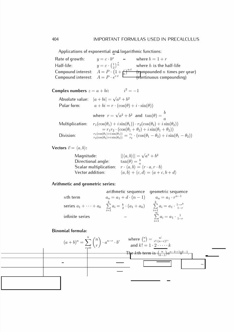
7/18/2019 Precalculus Tradler Carley
http://slidepdf.com/reader/full/precalculus-tradler-carley 414/424
404 IMPORTANT FORMULAS USED IN PRECALCULUS
Applications of exponential and logarithmic functions:
Rate of growth: y = c · bx where b = 1 + rHalf-life: y = c · 1
2
xh where h is the half-life
Compound interest: A = P · 1 + rn
n·t(compounded n times per year)
Compound interest: A = P · er·t (continuous compounding)
Complex numbers z = a + bi: i2 = −1
Absolute value: |a + bi| =√
a2 + b2
Polar form: a + bi = r · (cos(θ) + i · sin(θ))
where r = √ a2 + b2 and tan(θ) =
b
aMultiplication: r1(cos(θ1) + i sin(θ1)) · r2(cos(θ2) + i sin(θ2))
= r1r2 · (cos(θ1 + θ2) + i sin(θ1 + θ2))
Division: r1(cos(θ1)+i sin(θ1))r2(cos(θ2)+i sin(θ2)) = r1
r2· (cos(θ1 − θ2) + i sin(θ1 − θ2))
Vectors v = a, b:
Magnitude: ||a, b|| =√
a2 + b2
Directional angle: tan(θ) = ba
Scalar multiplication: r · a, b = r · a, r · bVector addition: a, b + c, d = a + c, b + d
Arithmetic and geometric series:
arithmetic sequence geometric sequencenth term an = a1 + d · (n − 1) an = a1 · rn−1
series a1 + · · · + ak
ki=1
ai = k2 · (a1 + ak)
ki=1
ai = a1 · 1−rk
1−r
infinite series –∞
i=1
ai = a1 · 11−r
Binomial formula:
(a + b)n =n
r=0
n
r
· an−r · br where
nr
= n!
r!·(n−r)!,
and k ! = 1 · 2 · · · · · k
The kth term is
nk−1
an−k+1bk−1.
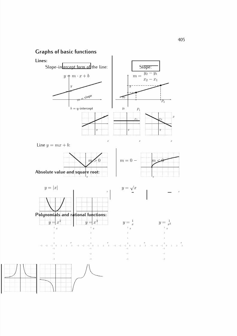
7/18/2019 Precalculus Tradler Carley
http://slidepdf.com/reader/full/precalculus-tradler-carley 415/424
405
Graphs of basic functions
Lines:
Slope-intercept form of the line: Slope:
y = m · x + b m = y2 − y1
x2 − x1
x
y
b = y-intercept
m = s l o p
e
x
y
P 2
P 1
x1 x2
y1
y2
Line y = mx + b:x
y
x
y
x
y
m > 0 m = 0 m < 0
Absolute value and square root:
y = |x| x
y
y =√
xx
y
Polynomials and rational functions:
y = x2 y = x3 y = 1x y = 1
x2
-3 -2 -1 0 1 2 3
-3
-2
-1
0
1
2
3
x
y
-3 -2 -1 0 1 2 3
-3
-2
-1
0
1
2
3
x
y
-3 -2 -1 0 1 2 3
-3
-2
-1
0
1
2
3
x
y
-3 -2 -1 0 1 2 3
-3
-2
-1
0
1
2
3
x
y
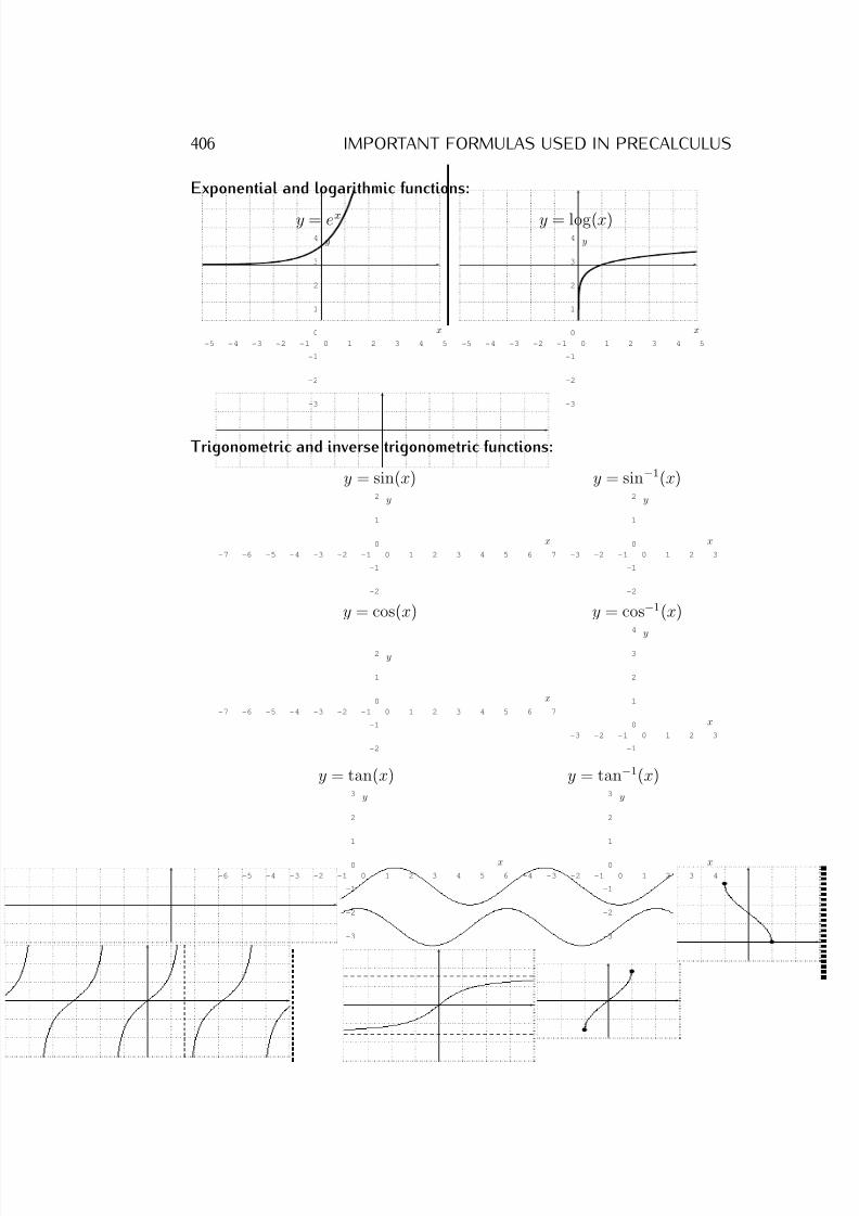
7/18/2019 Precalculus Tradler Carley
http://slidepdf.com/reader/full/precalculus-tradler-carley 416/424
406 IMPORTANT FORMULAS USED IN PRECALCULUS
Exponential and logarithmic functions:
y = ex y = log(x)
-5 -4 -3 -2 -1 0 1 2 3 4 5
-3
-2
-1
0
1
2
3
4
x
y
-5 -4 -3 -2 -1 0 1 2 3 4 5
-3
-2
-1
0
1
2
3
4
x
y
Trigonometric and inverse trigonometric functions:
y = sin(x) y = sin−1(x)
-7 -6 -5 -4 -3 -2 -1 0 1 2 3 4 5 6 7
-2
-1
0
1
2
x
y
-3 -2 -1 0 1 2 3
-2
-1
0
1
2
x
y
y = cos(x) y = cos−1(x)
-7 -6 -5 -4 -3 -2 -1 0 1 2 3 4 5 6 7
-2
-1
0
1
2
x
y
-3 -2 -1 0 1 2 3
-1
0
1
2
3
4
x
y
y = tan(x) y = tan−1(x)
-6 -5 -4 -3 -2 -1 0 1 2 3 4 5 6
-3
-2
-1
0
1
2
3
x
y
-4 -3 -2 -1 0 1 2 3 4
-3
-2
-1
0
1
2
3
x
y
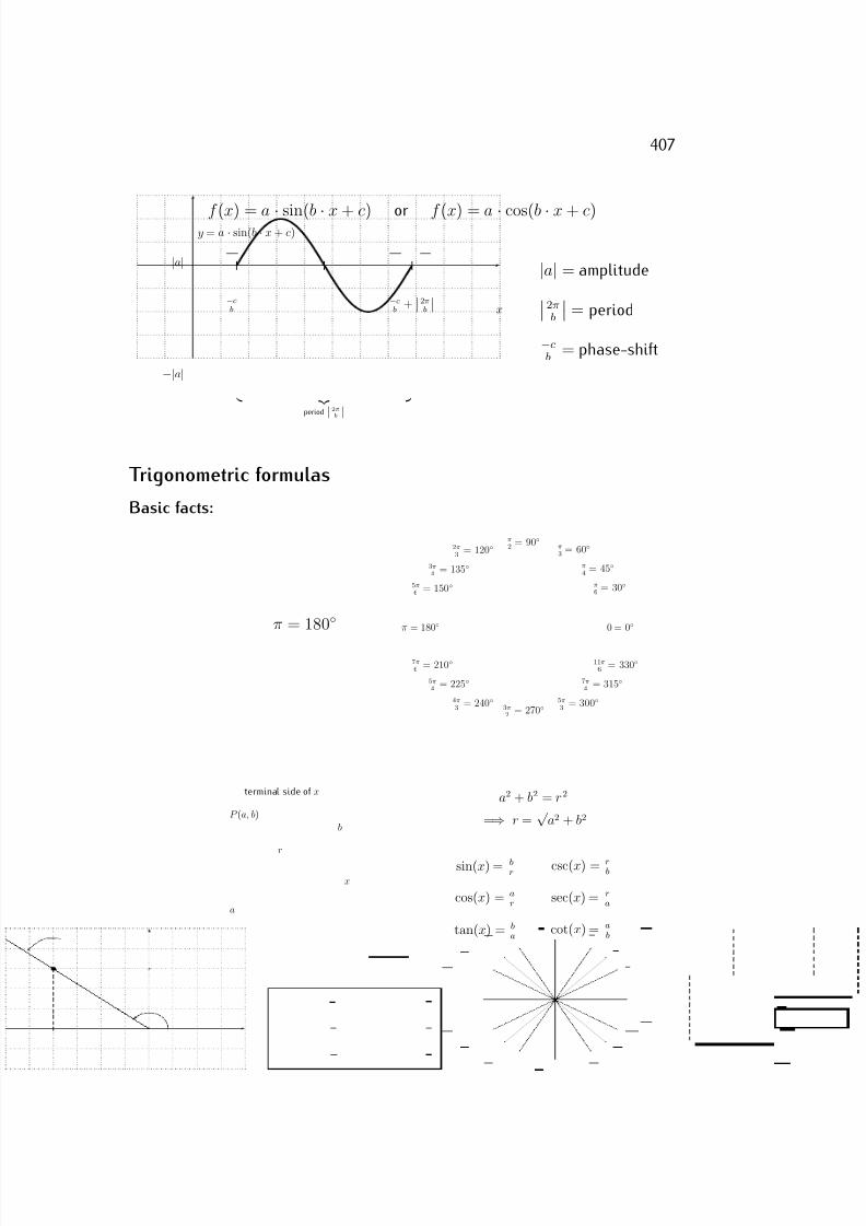
7/18/2019 Precalculus Tradler Carley
http://slidepdf.com/reader/full/precalculus-tradler-carley 417/424
407
f (x) = a · sin(b · x + c) or f (x) = a · cos(b · x + c)
x
y = a · sin(b · x + c)
−cb
−cb
+ 2π
b
period | 2πb |
|a|
−|a|
|a| = amplitude2πb
= period
−cb = phase-shift
Trigonometric formulas
Basic facts:
π = 180◦ 0 = 0◦π = 180◦
π2 = 90◦
3π2 = 270◦
π4 = 45◦
5π4
= 225◦
π3 = 60◦
4π3
= 240◦
π6 = 30◦
7π6 = 210◦
3π4 = 135◦
7π4
= 315◦
11π6 = 330◦
5π6 = 150◦
5π3
= 300◦
2π3
= 120◦
P (a, b)
x
a
b
r
terminal side of xa2 + b2 = r2
=⇒ r =√
a2 + b2
sin(x) = br
csc(x) = rb
cos(x) = ar sec(x) = r
a
tan(x) = ba
cot(x) = ab
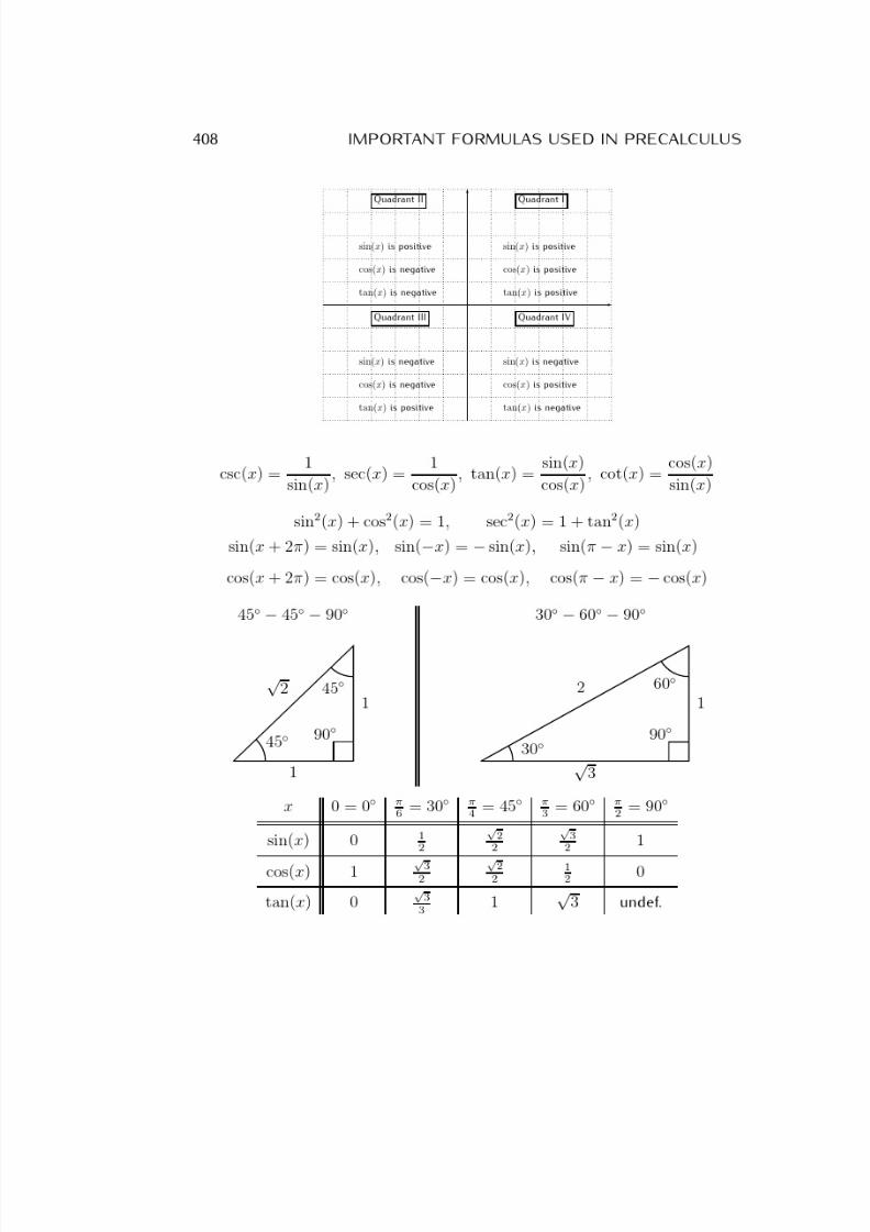
7/18/2019 Precalculus Tradler Carley
http://slidepdf.com/reader/full/precalculus-tradler-carley 418/424
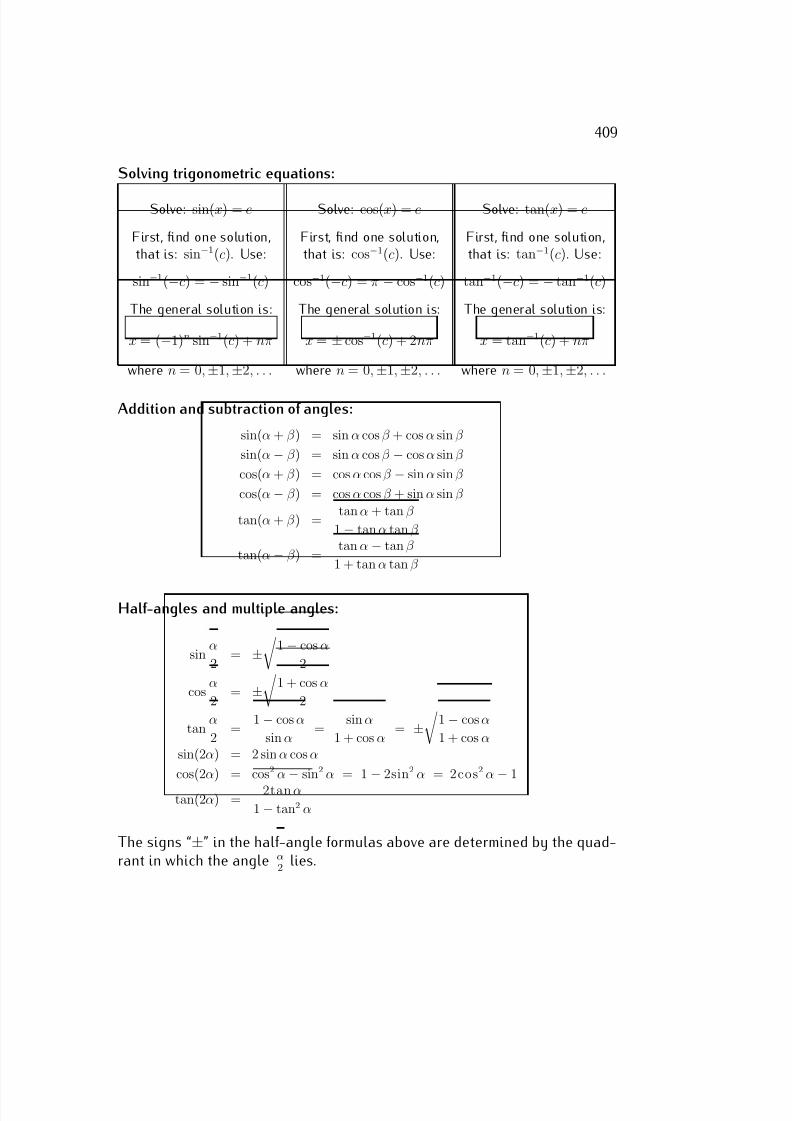
7/18/2019 Precalculus Tradler Carley
http://slidepdf.com/reader/full/precalculus-tradler-carley 419/424
409
Solving trigonometric equations:
Solve: sin(x) = c Solve: cos(x) = c Solve: tan(x) = c
First, find one solution, First, find one solution, First, find one solution,that is: sin−1(c). Use: that is: cos−1(c). Use: that is: tan−1(c). Use:
sin−1(−c) = − sin−1(c) cos−1(−c) = π − cos−1(c) tan−1(−c) = − tan−1(c)
The general solution is: The general solution is: The general solution is:
x = (−1)n sin−1(c) + nπ x = ± cos−1(c) + 2nπ x = tan−1(c) + nπ
where n = 0, ±1, ±2, . . . where n = 0, ±1, ±2, . . . where n = 0, ±1, ±2, . . .
Addition and subtraction of angles:
sin(α + β ) = sin α cos β + cos α sin β
sin(α − β ) = sin α cos β − cos α sin β
cos(α + β ) = cos α cos β − sin α sin β
cos(α − β ) = cos α cos β + sin α sin β
tan(α + β ) = tan α + tan β
1 − tan α tan β
tan(α − β ) = tan α − tan β
1 + tan α tan β
Half-angles and multiple angles:
sin α
2 = ±
1 − cos α
2
cos α
2 = ±
1 + cos α
2
tan α
2 =
1 − cos α
sin α =
sin α
1 + cos α = ±
1 − cos α
1 + cos αsin(2α) = 2 sin α cos α
cos(2α) = cos2 α
−sin2 α = 1
−2sin2 α = 2cos2 α
−1
tan(2α) = 2tan α
1 − tan2 α
The signs “±” in the half-angle formulas above are determined by the quad-rant in which the angle α
2 lies.
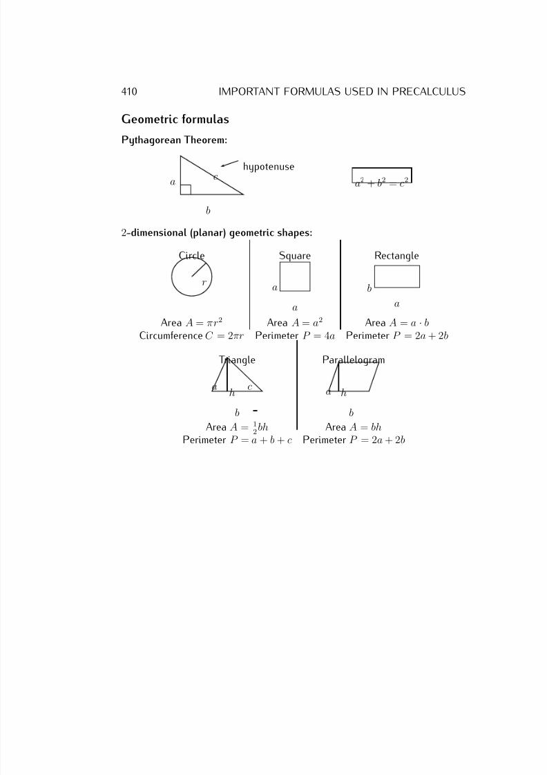
7/18/2019 Precalculus Tradler Carley
http://slidepdf.com/reader/full/precalculus-tradler-carley 420/424
410 IMPORTANT FORMULAS USED IN PRECALCULUS
Geometric formulas
Pythagorean Theorem:
b
a chypotenuse
a2 + b2 = c2
2-dimensional (planar) geometric shapes:
Circle Square Rectangle
r a
a
b
a
Area A = πr2 Area A = a2 Area A = a · bCircumference C = 2πr Perimeter P = 4a Perimeter P = 2a + 2b
Triangle Parallelogram
h
b
a c a
b
h
Area A = 12 bh Area A = bh
Perimeter P = a + b + c Perimeter P = 2a + 2b
7/18/2019 Precalculus Tradler Carley
http://slidepdf.com/reader/full/precalculus-tradler-carley 421/424
Index
10n, 20330◦ − 60◦ − 90◦ triangle, 23545◦ − 45◦ − 90◦ triangle, 235
nC r, 338
C, 287N, 2Q, 2R, 2R2, 299Z, 2arccos(x), 267arcsin(x), 265arctan(x), 263
nr
, 338
cos(x), 233
cos−1(x), 267cosh, 188cot(x), 233, 263csc(x), 233⌊x⌋, 27sec(x), 233sin(x), 233sin−1(x), 265sinh, 197
, 316
tan(x), 233tan−1(x), 263tanh, 197v, 299{an}, 311
{an}n≥1, 311e, 187n!, 337n factorial, 337
n-choose-r, 338nth root, 225
absolute value, 3, 62, 63, 289addition of angles formula for trigono-
metric functions, 252angle, 232arccosine, 267arcsine, 265arctangent, 263arithmetic sequence, 318
arithmetic series, 321asymptote, 118, 147, 148
base, 184, 191binomial coefficient, 338binomial theorem, 341
carbon dating method, 219carbon-14, 219codomain, 22coefficients, 101
combination, 339common difference, 318common ratio, 325complex conjugate, 140complex number, 287
411
7/18/2019 Precalculus Tradler Carley
http://slidepdf.com/reader/full/precalculus-tradler-carley 422/424
412 INDEX
absolute value, 289
imaginary part, 287polar form, 290real part, 287
complex numbers, 134complex plane, 288complex unit, 287compound interest, 216compounded n times per year, 222compounded quarterly, 221compounding, 222conjugate, 140
continuous compounding, 222cosecant csc(x), 233cosine cos(x), 233cotangent cot(x), 233, 263
degree, 101degree measure, 232dependent variable, 28difference quotient, 34directional angle, 299dividend, 104
divisor, 104domain, 22, 36double angle formula for trigonomet-
ric functions, 257
Euler number, 187even function, 71, 242exponential function, 184extrema, 114extremum, 53, 114
factor theorem, 107factorial, 337Fibonacci sequence, 312floor function, 27frequency, 246
function, 22
arccosine, 267arcsine, 265arctangent, 263composition, 78domain, 22, 36exponential, 184floor, 27graph, 37injective, 86inverse cosine, 267inverse function, 89
inverse sine, 265inverse tangent, 263logarithm, 191one-to-one, 86piecewise defined, 33range, 23, 36
fundamental theorem of algebra, 135
geometric sequence, 325geometric series, 329
infinite, 332geometric vector, 299graphs
y = arccos(x), 267y = arcsin(x), 265y = arctan(x), 263y = cos(x), 241y = cos−1(x), 267y = 1
x, 64
y = 1xn
, 148y = ln(x), 193, 197
y = log(x), 193, 197y = logb(x), 197y = sin(x), 241y = sin−1(x), 265y =
√ x, 64
7/18/2019 Precalculus Tradler Carley
http://slidepdf.com/reader/full/precalculus-tradler-carley 423/424
INDEX 413
y = tan(x), 243
y = tan−1
(x), 263y = bx, 186y = c · 2x, 189y = ex, 187y = x2, 64y = x3, 64y = xn, 114absolute value, 63arccosine, 267arcsine, 265arctangent, 263
hole, 151inverse cosine, 267inverse sine, 265inverse tangent, 263maximum, 53minimum, 53polynomial degree 2, 114polynomial degree 3, 115polynomial degree 4, 116polynomial degree 5, 116
rational function, 150reflect, 67shift, 65, 66stretch, compress, 66, 67
greater than, 4
half angle formula for trigonometricfunctions, 257
half-life, 217carbon-14, 219
horizontal asymptote, 147, 151
horizontal line test, 87hyperbolic cosine, 188hyperbolic sine, 197hyperbolic tangent, 197hypotenuse, 410
imaginary, 134
imaginary unit, 287independent variable, 28inequality, 10, 169infinite geometric series, 332infinite series, 332injective, 86input, 22integer, 2interest rate, 222interval, 5inverse function, 89
irrational number, 3
leading coefficient, 101less than, 4line, 13
x-intercept, 15y-intercept, 15graphing the line, 16point-slope form of the line, 15slope, 14
slope-intercept form of the line, 16logarithm, 191logarithm change of base, 200logarithm properties, 199long division, 102
magnitude, 299maximum, 53minimum, 53monomial, 101monthly, 223
multiplicity, 122, 140
natural logarithm, 191natural number, 2newton, 307
7/18/2019 Precalculus Tradler Carley
http://slidepdf.com/reader/full/precalculus-tradler-carley 424/424
414 INDEX
odd function, 71, 242, 243
one-to-one, 86output, 22
parabola, 114Pascal’s triangle, 340period, 246periodic function, 240phase shift, 246piecewise defined function, 33point-slope form of the line, 15polynomial, 101
degree, 101polynomial division, 102powers of 10, 203present value, 224principal, 221, 222programming the TI-84 calculator, 366Pythagorean theorem, 410
quadrant, 234quadratic formula, 124
quotient, 104
radian measure, 232range, 23, 36rate, 222rate of growth, 212rational function 102 147
resetting the calculator to factory set-
tings, 373root, 53, 101
scalar multiplication, 303secant sec(x), 233sequence, 311series, 316
arithmetic, 321geometric, 329infinite, 332infinite geometric, 332
Sigma Σ, 316sine sin(x), 233slant asymptote, 150slope-intercept form of the line, 16solving trigonometric equations, 277standard convention of domain, 36subtraction of angles formula for trigono-
metric functions, 252summation symbol, 316synthetic division, 109
tangent tan(x), 233telescopic sum, 329TI-84, 49
(−), 351e, 188nth root 225 364