COMPUTER AIDED ANALYSES OF SMOKE STACK DESIGNS

by

Joseph Charles Servaites

Thesis submitted to the Faculty of the

Virginia Polytechnic Institute and State University

in partial fulfillment of the requirement for the degree of

MASTER OF SCIENCE

in

MECHANICAL ENGINEERING

APPROVED:

___________________________

Dr. Larry D. Mitchell, Chairman

_______________________ ______________________

Dr. Clint L. Dancey Dr. Reginald G. Mitchiner

September, 1996

Blacksburg, Virginia

Keywords: Stack, Transfer Matrix, Vibration, Tapered Beam,

Vortex Shedding

ii

COMPUTER AIDED ANALYSES OF SMOKE STACK DESIGNS

by

Joseph Charles Servaites

Dr. Larry D. Mitchell, Chairman

Department of Mechanical Engineering

The purpose of this research is to analyze the statics and dynamics of steel smoke

stacks subject to excitation by aerodynamic forces. The wind loads experienced by smoke

stacks arise from various phenomenon, the most prominent of which are static drag load,

vortex shedding, and atmospheric turbulence. The nature of these loading sources around

a cylinder are studied in detail. Both static and dynamic loads are capable of producing

large tip deflections, and are of the most prominent design criteria for stack designers. A

computer program, STACK1, has been created by modifying an existing analysis code,

BEAM8, to be used specifically for stack analysis. This analysis code utilizes the

transfer matrix method to perform detailed bending and vibration analyses. This new

software has been developed to check stack designs for compliance with appropriate steel

stack standards, and provide the designer with information regarding the static and

dynamic response of the structure. A detailed analysis is performed to demonstrate the

validity of approximating a tapered Timoshenko beam with a series of continuous,

constant cross-section beams.

iii

Acknowledgment

The author would like to express sincere gratitude to his major advisor, Dr. Larry

D. Mitchell, for the immense amount of support, patience, and guidance provided for this

thesis and research. The author is also obliged to committee members Prof. Clint L.

Dancey and Prof. R. G. Mitchiner for providing advice and for reviewing the thesis.

The author would also like to thank the DuPont Company for its development

and sponsorship of this project. Specifically, the author thanks Dr. K. John Young and

Dr. Jimmy Y. Yeung without whose suggestions and support this research could not have

been completed.

iv

Table of Contents

Abstract ........................................................................................................ ii

Acknowledgment ......................................................................................... iv

Table of Contents ........................................................................................ v

Nomenclature .............................................................................................. vii

List of Illustrations ..................................................................................... xi

Introduction

1.1 Definition .......................................................................................... 1

1.2 Application of Research .................................................................... 1

1.3 Existing Suppression Mechanisms ................................................... 2

1.4 Aerodynamic Forces on Stacks ......................................................... 3

1.5 Analysis Methods ............................................................................. 4

Literature Survey

2.1 Smoke Stack Concerns ...................................................................... 7

2.2 Steel Smoke Stack Standards ............................................................. 7

v

2.3 Stack Analysis and Aerodynamic Interactions ................................. 8

2.4 Transfer Matrix Method .................................................................... 9

Aerodynamic Forces on Stacks

3.1 Introduction ....................................................................................... 11

3.2 Sources of Aerodynamic Loads ........................................................ 11

3.3 Static Response, Associated Stresses, Deflections ........................... 12

3.4 Dynamic Response and Harmonic Excitation .................................. 15

3.4.1 Atmospheric Turbulence .................................................................... 15

3.4.2 Vortex Shedding ................................................................................ 18

3.4.3 Motion Induced Forces ..................................................................... 23

3.5 Across Wind Response ..................................................................... 24

Transfer Matrix Method

4.1 Introduction ....................................................................................... 27

4.2 Coordinate System and Sign Convention ......................................... 27

4.3 State Vector and Transfer Matrix ...................................................... 29

4.4 Transfer Matrix Procedure ................................................................ 30

4.5 Transfer Matrices for Planar Vibrations of a Straight Beam ............. 35

vi

4.6 Complex Beams, Elimination of Intermediate State Vectors ............ 42

4.7 Steady-State Forced Vibrations and Statics ...................................... 46

BEAM8 Modifications and Implementation of ASME and ASCE

Standards to Generate STACK1

5.1 Introduction ....................................................................................... 53

5.2 Tapered Beam Subroutine ................................................................ 53

5.3 Static Considerations in Tapered Beam Approximation ................... 55

5.4 Dynamic Considerations in Tapered Beam Approximation .............. 61

5.5 Effects of Taper Angle on Beam Dynamics ..................................... 66

5.6 Dynamic Effects of Relative Tapered Section Length ...................... 68

5.7 Implementation of Tapered Beam Routine ....................................... 70

5.8 Implementation of ASME Steel Stack Standards Into

the STACK1 Code ............................................................................ 71

5.9 Static Loads and Deflection .............................................................. 73

5.10 Dynamic Loads and Vortex Shedding ...................................... ........ 77

Test Examples

6.1 ASME Example Stack ...................................................................... 79

6.2 DuPont Example Stack ..................................................................... 84

vii

Conclusion and Recommendations

7.1 Conclusion ........................................................................................ 90

7.2 Recommendations ............................................................................. 91

References ..................................................................................................... 92

Appendix I: Stack Example to Verify Code ................................................ 96

Appendix II: Derivation of Tapered Transfer Matrix .................................. 102

Vita ............................................................................................................... 111

viii

List of Illustrations

Figure 1-1. Add-on devices for suppression of vortex-induced vibration

of cylinders ........................................................................... 2

Figure 3-1 Example of Planetary Boundary Layer ................................. 13

Figure 3-2 Horizontal Wind-Speed Spectrum at Brookhaven National

Laboratory at about 100m (328 ft) height ............................. 16

Figure 3-3 Vortex shedding around a cylinder ........................................ 17

Figure 3-4 Vortex shedding regimes around a smooth cylinder .............. 19

Figure 3-5 A sequence of simultaneous surface pressure fields and

wake forms at Re = 112,000 for approximately one-third

of one cycle of vortex shedding ............................................. 20

Figure 3-7 Wind design speed contours within the United States ......... .

25

Figure 4-1 Transfer Matrix Coordinate System ..................................... 28

Figure 4-2 Spring-mass system .............................................................. 30

Figure 4-3 Free-body diagram of spring ................................................. 31

Figure 4-4 Free-body diagram of mass ................................................... 33

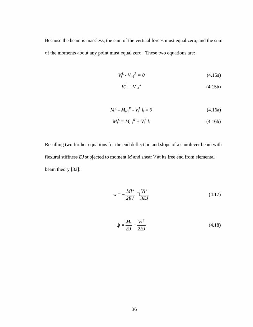
Figure 4-5 End forces and deflections for a massless beam ................... 35

Figure 4-6 Free body diagram of mass mi .............................................. 39

ix

Figure 4-7 Cantilever with concentrated end mass ................................ 40

Figure 4-8 Beam with discrete masses ................................................... 42

Figure 4-9 Fixed-free three section beam ............................................... 44

Figure 4-10 Beam section with uniformly distributed load q = Qcos(Ωt) .. 46

Figure 4-11 Example two section beam with uniform harmonic loading .. 48

Figure 5-1 Cylindrical beam cross section ............................................. 55

Figure 5-2 Area moment of inertia of a cylindrical beam for

different centroidal diameters, and constant wall

thickness of one inch (0.0254 m) ........................................... 56

Figure 5-3 Moment of cylindrical beam, three inch (0.0762 m)

variation in Dc ........................................................................ 57

Figure 5-4 Tapered beam section joining two constant sections ............ 58

Figure 5-5 Percent error in area moment calculations of a tapered

beam by replacing the tapered beam with a constant

beam with the midpoint diameter ......................................... 60

Figure 5-6 Stack design (a) used for convergence study ........................ 61

Figures 5-7a,b,c Convergence of eigenvalues for stack (a) ........................... 63

Figure 5-8 Stack design (b) used for convergence study ........................ 64

Figures 5-9a,b,c Convergence of eigenvalues for stack (b) ........................... 65

Figure 5-10 Stack model used in taper angle (α) study ........................... 67

x

Figure 5-11 Stack design used in Ls/Lt study ........................................... 69

Figure 5-12 Example of automatic mesh routine ...................................... 71

Figure 5-13 Velocity pressures for Blacksburg, Virginia ......................... 75

Figure 6-1 ASME Example stack geometry ............................................ 79

Figure 6-2 Model geometry within STACK1 for ASME

example smoke stack. ............................................................. 82

Figure 6-3 Static deflection, slope, moment and shear

graphs for example 1............................................................... 83

Figure 6-4 DuPont example smoke stack geometry ................................ 85

Figure 6-5 Model geometry within STACK1 for DUPONT example smoke

stack ................................................................................................... 88

Figure 6-6 Static deflection, slope, moment and shear

graphs for example 1............................................................... 89

References ...................................................................................................... 92

Figure A1-1 Example stack used for calculations ..................................... 96

Figure A.II-1 Section of beam acted upon by bending moment only............ 104

Figure A.II-2 Section of beam acted upon by bending and shear forces....... 104

Figure A.II-3 Forces acting on a beam element of length dx ........................ 105

Figure A.II-4 Tapered beam ......................................................................... 109

1

Chapter 1: Introduction

1.1 Definition

The purpose of this research is to analyze steel smoke stacks subject to excitation by

aerodynamic forces. The loads experienced by smoke stacks arise from various

phenomenon, the most prominent of which are static drag load, vortex shedding, and

atmospheric turbulence. These sources are capable of producing large tip deflections, and

are of the most prominent design criteria for stack designers. A computer program,

STACK1 has been created by modifying an existing analysis code, BEAM8, to be used

specifically for stack analysis. This new software has been developed to check stack

designs for compliance with appropriate steel stack standards and provide the designer

with information regarding the static and dynamic behavior of the structure.

1.2 Application of Research

The results of this research will help smoke-stack designers by providing insight into the

nature of wind and stack interactions. The designer will be able to expedite the design

process by using the computer program STACK1. This program is intended to be

completely self contained, that is, a complete analysis can be performed with a single

executable file. The STACK1 program is designed to perform an analysis of a smoke

stack design, then compare the static and dynamic behavior of the design with existing

2

standards. Any inconsistencies between the given design and the standards are brought to

the user's attention.

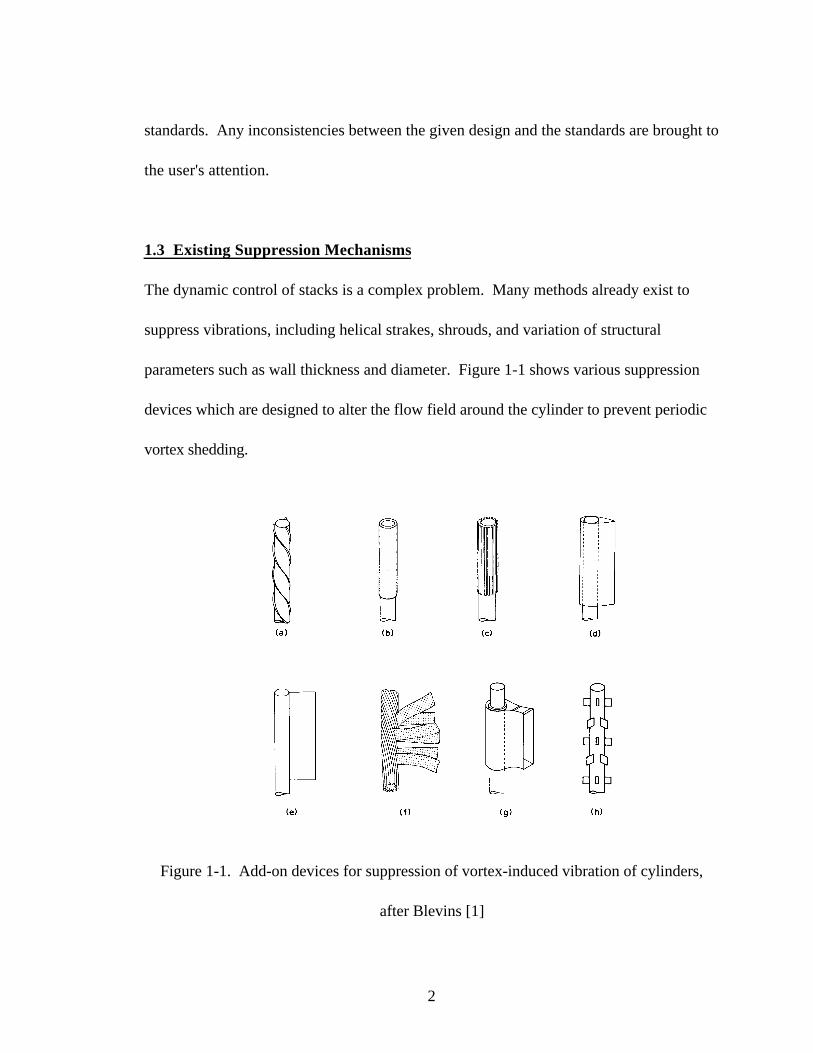
1.3 Existing Suppression Mechanisms

The dynamic control of stacks is a complex problem. Many methods already exist to

suppress vibrations, including helical strakes, shrouds, and variation of structural

parameters such as wall thickness and diameter. Figure 1-1 shows various suppression

devices which are designed to alter the flow field around the cylinder to prevent periodic

vortex shedding.

Figure 1-1. Add-on devices for suppression of vortex-induced vibration of cylinders,

after Blevins [1]

3

Because steel stacks have very little inherent structural damping, vibrations can be

further suppressed by increasing the stack damping. Methods for increasing the damping

include mass dampers, foundation fabric pads, hanging chains, and other devices [2].

It is of interest to design a stack with inherent dynamic stability. If a stack could be

designed to minimize deflections and avoid resonances, then fewer “add-on” suppressions

mechanisms would be necessary, and therefore reduce the cost, weight, and complexity of

the stack.

1.4 Aerodynamic Forces on Stacks

Two basic types of loads can be applied by wind: static pressure and harmonic excitation.

These loads are normally experienced simultaneously, although static drag can exist

without harmonic excitation under certain conditions [3]. Smoke-stack designers have

devised many methods to control the static and dynamic behavior of stacks. The static

deflection can be reduced increasing the stiffness of the stack or by modifying the air flow

field in the vicinity of the stack to reduce the drag load. The overall stiffness of the stack

can be enhanced by geometric modifications, such as increasing the wall thickness or

increasing the stack diameter. Guy wires can be added to enhance structural stiffness and

raise the resonance frequencies. Methods of modifying the air-flow field around a single

stack include changing the stack diameter, and attaching external devices to the stack, such

4

as plates, shrouds or helical strakes. If multiple stacks are present, certain spatial

arrangement patterns can help reduce the static wind loads.

1.5 Analysis Methods

In order to analyze stack designs, beam bending and vibration theory is used. Various

methods exist for analyzing beams, such as the so-called continuum method, the finite

element method, and the transfer matrix method. In the continuum method, the beam is

considered a continuous structure. Differential equations have been developed to

represent beams in the continuum, and these equations are solved by standard methods.

The arbitrary constants in the equations are determined by the boundary conditions of the

problem.

The finite element method, however, considers the beam to be broken up into a series of

small elements connected at adjacent nodes. The elastic behavior of the beam is then

found by calculating the relationship between force and displacement at each node.

Equilibrium and compatibility conditions at each node can be determined from the elastic

behavior, and an overall stiffness matrix is found in terms of unknown nodal

displacements. Nodal displacements are calculated by inverting the stiffness matrix, and

these displacements can be used to determine the stress in the beam.

5

The premise of the third method, the transfer matrix method, is that a complex structure

can be broken up into a series of simple structures. The properties of each section are

expressed in matrix form. Because the transfer matrix method uses continuum solutions

to describe each component of the structure, displacements and internal forces can be

found at any point along the structure. These displacements include deflection (w) and

angle (ψ), and the internal forces include moment (M) and shear (V). These are arranged in

a state vector, which describes the "state" of deflection and internal loading of the

structure. The state vectors on either side of a section are related by the transfer matrix of

the section. The matrix across the length of a section is called a field transfer matrix, and

the matrix across a point parameter such as a point mass, point load or point moment, is

called a point transfer matrix. A complex beam can be modeled as a series of field and

point transfer matrices. In order to relate the state vector at one end of the structure to

the other end, the intermediate transfer matrices are successively multiplied.

Each method described has inherent advantages and disadvantages. The classical

continuum method is useful for only very simple structures, and quickly becomes

cumbersome for more complex structures. The finite element method can provide very

accurate results if sufficient detail is included in the model, but the model building process

can be time consuming, the computational efforts are time consuming, and very large

computer resources are required to handle the size of the stiffness matrix. The size of

6

these matrix operations depend on the number of degrees of freedom used in the model.

The transfer matrix method, on the other hand, is very simple, and extremely useful for

structures that have a non-branching shape, that is, the structure can be modeled as a

series of elements linked together end-to-end in a linear topology. Various loading

configurations are easily modeled, including constant pressure or linearly varying

pressure. This method is not as useful for branched or coupled systems.

Smoke-stack geometry usually consists of various elements connected end-to-end. The

properties of stack sections are easily expressed in matrix form by using the differential

equation for a beam. Wind loads on a stack can be approximated as linearly varying

pressures along each section. It is for these reasons that the transfer matrix method is

very well suited for stack analysis.

7

Chapter 2: Literature Survey

2.1 Smoke-Stack Concerns

The purpose of a smoke stack is to vent exhaust gasses to the atmosphere [4]. The

mechanical design of smoke stacks is controlled in part by air pollution rules and

regulations. Stack heights and diameters are set by a considering both structural behavior

and function, while simultaneously meeting the requirements for air pollution control. In

years of late, the height requirements for stacks have increased to satisfy air pollution

regulations [4]. The design and analysis of smoke stacks are complex problems. Because

of the particular nature of stacks and their susceptibility to failures due to wind and

seismic-induced vibrations, along with corrosion and erosion, the design process is very

complex [5]. In addition to these structural concerns, recent regulations by the

Environmental Protection Agency (EPA) concerning emissions have placed a strong

emphasis on the mechanical design of stacks [5].

2.2 Steel Smoke-Stack Standards

In April of 1979 a group comprised of stack users, researchers, designers, fabricators, and

erectors all met to formulate a building code. The results of this meeting is a set of

comprehensive guidelines for mechanical design, material selection, the use of linings and

coatings, structural design, vibration considerations, access and safety, electrical

requirements, and fabrication and construction of steel stacks. These standards were

8

compiled and approved as an American National Standards Institute (ANSI) Standard in

August, 1986 and published as ASME/ANSI STS-1-1986 in May 1988 [2]. Much of the

procedures outlined within the ASME standards have been adapted by the American

Society of Civil Engineers (ASCE). The ASCE Steel Stack Standards [6], revised in 7-95,

provide essentially the same concepts as the ASME standards, with several

modifications.

2.3 Stack Analysis and Aerodynamic Interactions

In 1987 the ASCE compiled a text concerning wind loading and wind-induced structural

response [7]. This text supplements the ASCE standards by providing detailed

information on the wind environment, fundamentals of aeroelasticity, design concerns of

low buildings, tall buildings, and stacks. This text points out that the design of stacks

must take into consideration the effects of both along-wind and across-wind loads [8].

The text then proceeds to provide two methods to find the peak response of a stack.

In 1990 the Department of Civil Engineering at the University of Roorkee, India

published the Proceedings of the International Symposium of Experimental Determination

of Wind Loads on Civil Engineering Structures [9] [10]. This proceedings also included a

detailed analysis of the wind environment [9], as well as design considerations for

buildings and smoke stacks. In the paper dealing with wind loads on stacks, Vickery [10]

9

provides in-depth discussions of various excitation sources, including forces induced by

turbulence, wake effects, and motion-induced forces. Perhaps the most significant

information provided is that regarding aerodynamic damping. He describes how

aerodynamic damping can adversely affect structural vibrations. Aerodynamic damping is

almost always positive in the along-wind direction, but is very commonly negative in the

across-wind direction, thus leading to a severely underdamped structure. He shows that

negative aerodynamic damping in the across wind vibration may well be of the same order

as the positive structural damping. If the negative aerodynamic damping exceeds the

internal structural damping the net damping goes negative. The problem converts from a

vibration response problem to a dynamic stability problem.

A more detailed look at the fluid mechanics involved with flow over a cylinder is provided

by Blevins [11]. He provides a detailed description of the flow field around a cylinder, as

well an explanation of how the drag and lift forces originate. He also describes in detail

how the flow field changes with respect to a dimensionless parameter called the Reynolds

number (Re).

2.4 Transfer Matrix Method

As mentioned previously, the transfer matrix method is an ideal method of analysis for

smoke stacks. The necessary transfer matrix theory to perform detailed beam bending

and vibration analyses is provided by Pestel and Leckie [12]. The theory behind transfer

10

matrix analysis as it applies to static and dynamic analyses is developed in detail. A wide

variety of transfer matrices are presented in, including those for forced vibration. Various

examples are provided throughout the text to supplement the theory. Transfer matrices

for tapered beams including shear deformation and rotary inertia are not provided,

however.

In 1995 Shen [13] published a journal article dealing with the use of transfer matrices to

analyze tapered timoshenko beams. This article, however, does not derive a transfer

matrix for a continuously tapered beam, rather, it deals with approximating a tapered

beam with a series of continuous beam segments. The rate of convergence of a transfer

matrix model is compared to that of a finite element model, and it is shown that the

transfer matrix model converges much faster.

11

Chapter 3: Aerodynamic Forces on Stacks

3.1 Introduction

All buildings and stacks are subjected to various types of aerodynamic loading. Static

drag forces can cause a structure to deflect significantly, especially in intense storms. A

wind-bearing structure must be designed to withstand the stresses imposed by these

static loads. The presence of dynamic loading on structures does not require extremely

high wind velocities, only that one or more harmonic excitation sources be present. These

dynamic loads, if acting at or near a structural resonance, can cause large vibration

amplitudes. A structure subjected to dynamic loading must be able to withstand not only

the maximum stresses induced by large deflections, but must also be resistant to fatigue

failure. The first step in correctly designing a wind-bearing structure is to understand the

applied loading.

3.2 Sources of Aerodynamic Loads

The sources of stack excitation investigated in this study are limited to aerodynamic

loads. Wind across a structure gives rise to a variety of static and dynamic forces, in both

the along-wind and cross-wind direction. The aerodynamics associated with a smoke

stack is very similar to that of tall buildings from a general point of view. There are

several aspects, however, that allow various differences in stack analysis and design.

12

Buildings generally posses a much lower aspect ratio (height/width) than stacks.

Buildings are typically located in cities, where surrounding buildings of comparable height

are present. The airflow over buildings is, therefore, strongly three dimensional, and very

dependent on the surrounding structures [10]. However, most stacks are very tall,

slender structures, with very large aspect ratios. Stacks typically rise well above the

surrounding buildings and, therefore, are not subject to large amounts of interference

effects. The majority of the airflow over a stack is approximately two-dimensional, and

this assumption will be used to calculate the forces induced by wind. Another important

difference between buildings and stacks involves the design criteria. Tall buildings must

be designed so that accelerations (swaying) are kept to a minimum. The design of stacks,

however, is normally limited by material strength only.

In order to correctly design stacks one must consider both the static and dynamic

response.

3.3 Static Response, Associated Stresses, Deflections.

Perhaps the most obvious design concern in stacks is static deflection. Significant static

wind loads can develop in windy conditions, especially in coastal regions where wind

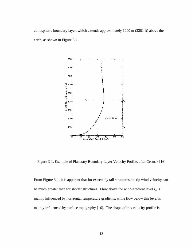
speeds can exceed 110 mph (49 m/s) [14]. One should bear in mind the substantial wind

velocity gradient near the earth’s surface. This gradient is due to what is called the

13

atmospheric boundary layer, which extends approximately 1000 m (3281 ft) above the

earth, as shown in Figure 3-1.

Figure 3-1. Example of Planetary Boundary Layer Velocity Profile, after Cermak [16]

From Figure 3-1, it is apparent that for extremely tall structures the tip wind velocity can

be much greater than for shorter structures. Flow above the wind-gradient level zg is

mainly influenced by horizontal temperature gradients, while flow below this level is

mainly influenced by surface topography [16]. The shape of this velocity profile is

14

dependent on a number of variables, including surface roughness, temperature gradients,

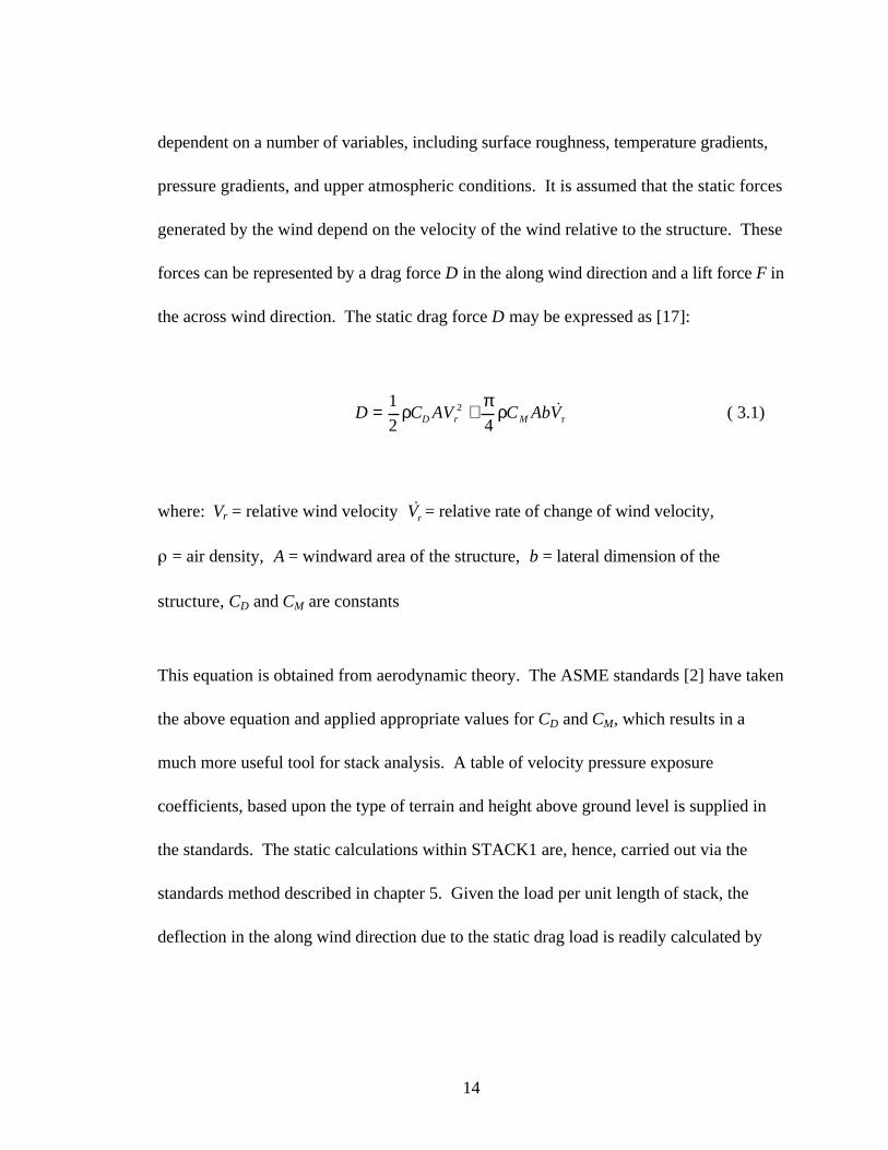
pressure gradients, and upper atmospheric conditions. It is assumed that the static forces

generated by the wind depend on the velocity of the wind relative to the structure. These

forces can be represented by a drag force D in the along wind direction and a lift force F in

the across wind direction. The static drag force D may be expressed as [17]:

D C AV C AbVD r M= +1

2 42ρ

πρ r ( 3.1)

where: Vr = relative wind velocity Vr = relative rate of change of wind velocity,

= air density, A = windward area of the structure, b = lateral dimension of the

structure, CD and CM are constants

This equation is obtained from aerodynamic theory. The ASME standards [2] have taken

the above equation and applied appropriate values for CD and CM, which results in a

much more useful tool for stack analysis. A table of velocity pressure exposure

coefficients, based upon the type of terrain and height above ground level is supplied in

the standards. The static calculations within STACK1 are, hence, carried out via the

standards method described in chapter 5. Given the load per unit length of stack, the

deflection in the along wind direction due to the static drag load is readily calculated by

15

transfer matrices. The detailed calculations are provided in appendix 1, and are included

in the newest version of the STACK1 software.

3.4 Dynamic Response and Harmonic Excitation

The vibrations of a stack are a concern of the designer if any of the number of dynamic

loads are applied at or near resonance conditions. The first and second bending modes are

generally all that are of interest [18], since very little energy is imparted at higher

frequencies, as will be shown. Because steel stacks are generally very long, slender

structures with relatively high flexibility and low structural damping, the frequency of the

first bending mode is usually extremely low, often less than 1 Hz. Various harmonic

excitation occurs at very low frequencies as well, so the first mode is generally produces

the largest deflections and stresses, although in certain instances the second mode must be

investigated as well.

Dynamic wind forces arise from various sources [10]:

• turbulent forces in the earth’s boundary layer,

• forces due to local turbulence within the stack's wake, particularly due

to vortex shedding, and

• forces induced by motion of the structure.

3.4.1 Atmospheric Turbulence

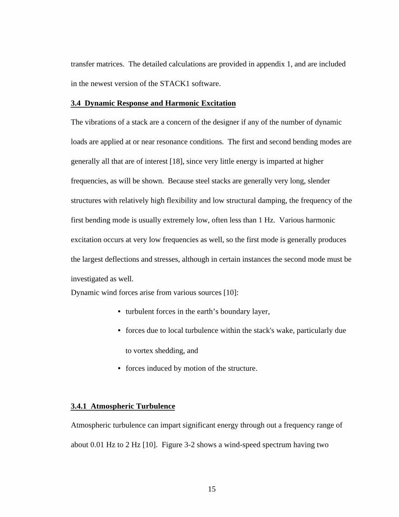
Atmospheric turbulence can impart significant energy through out a frequency range of

about 0.01 Hz to 2 Hz [10]. Figure 3-2 shows a wind-speed spectrum having two

16

distinct “humps” in the frequency domain. One area essentially represents static loads,

and a second region which represents dynamic loads that can cause vibration of the

structure.

Figure 3-2. Horizontal Wind-Speed Spectrum at Brookhaven National Laboratory at

about 100 m (328 ft) height, after Lin [19]

It should be noted that the higher frequency turbulence generally acts along the wind

direction, manifesting itself as wind gusts. However, due to the random nature of

turbulence, and due to the flow differences across the stack, cross-wind loading can also

be imparted. The magnitude of loading due to pure atmospheric turbulence is not

typically calculated, rather, the effect of combining the turbulence with the lift forces

resulting from vortex shedding is used [20].

17

3.4.2 Vortex Shedding

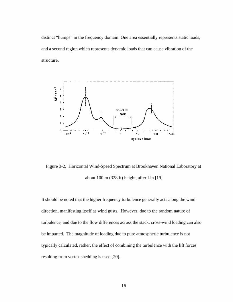
Stacks constitute what is known as a bluff structure. A bluff structure is one in which the

flow separates from large sections of the structure’s surface [21]. The area of turbulent

recirculation on the down-wind side of a bluff body is referred to as the wake. Under

most flow conditions, the wake of a long, slender structure will be unsteady and will shed

vortices. The nature of vortex shedding is a well studied phenomenon over a wide range

of flow conditions. A typical pattern of vortex shedding in the wake of a cylinder is

shown in Figure 3-3. This is the flow profile over a constant diameter cylinder with a

constant velocity flow profile.

Figure 3-3. Vortex shedding around a cylinder, after Blevins [22]

18

Vortex shedding around a cylinder has been studied extensively. Vortex shedding from a

smooth, circular cylinder at subsonic flows is a function of Reynolds number. The

Reynolds number is defined as:

ReUD

=ν

( 3.2)

where: U = free stream velocity, D = circular diameter, ν = kinematic viscosity (for air,

6.082 ft2/hr @ 68° F (15.7x10-6 m2/s @ 20° C) [23])

Experimental results have been tabulated for vortex shedding regimes around a smooth

circular cylinder of various Reynolds numbers as shown in Figure 3-4.

At very low Reynolds numbers (below Re = 5), the fluid follows a smooth, laminar

profile around the cylinder. In the range 5 < Re < 45, separation begins on the back of the

cylinder and a symmetric pair of vortices is formed close to the cylinder. The length of

the vortices in the along flow direction increases linearly with Reynolds number, reaching

a length of three cylinder diameters at Re = 45. Beyond this point, the wake becomes

unstable and one of the vortices breaks away. A laminar periodic wake of staggered

vortices with opposite rotation direction (vortex street) is formed. Between Re = 150 and

300, the vortices become turbulent, although the cylinder boundary layer remains laminar.

The subcritical range is defined as the range of 300 < Re < 1.5x105. In this range, the

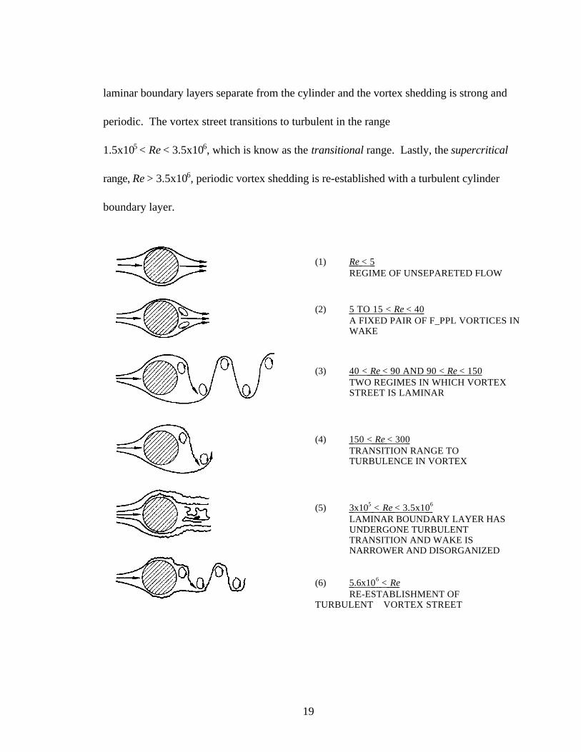
19

laminar boundary layers separate from the cylinder and the vortex shedding is strong and

periodic. The vortex street transitions to turbulent in the range

1.5x105 < Re < 3.5x106, which is know as the transitional range. Lastly, the supercritical

range, Re > 3.5x106, periodic vortex shedding is re-established with a turbulent cylinder

boundary layer.

(1) Re < 5 REGIME OF UNSEPARETED FLOW

(2) 5 TO 15 < Re < 40 A FIXED PAIR OF F_PPL VORTICES IN WAKE

(3) 40 < Re < 90 AND 90 < Re < 150TWO REGIMES IN WHICH VORTEX STREET IS LAMINAR

(4) 150 < Re < 300 TRANSITION RANGE TO TURBULENCE IN VORTEX

(5) 3x10 5 < Re < 3.5x10 6 LAMINAR BOUNDARY LAYER HAS UNDERGONE TURBULENT TRANSITION AND WAKE IS NARROWER AND DISORGANIZED

(6) 5.6x10 6 < Re RE-ESTABLISHMENT OF

TURBULENT VORTEX STREET

20

Figure 3-4. Vortex shedding regimes around a smooth cylinder, after Blevins [3]

Reynolds numbers associated with large stacks can exceed 107, so all of the above flow

regimes are possibilities. Wind speeds of above 20 mph (9 m/s) for stacks of cross

sectional diameter of 3 ft (0.9 m) or more will produce a turbulent vortex street similar to

item (3) and item (4) in Figure 3-4. Vortex shedding causes harmonic loading on a cylinder

in both the along wind and cross wind directions. These dynamic loads will cause stack

vibration under certain conditions. If a resonance frequency of the stack lies with in the

spectrum of vortex shedding frequencies, large across-wind vibration amplitudes could

arise if there is not sufficient damping.

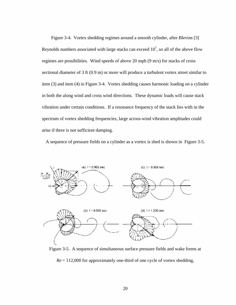
A sequence of pressure fields on a cylinder as a vortex is shed is shown in Figure 3-5.

Figure 3-5. A sequence of simultaneous surface pressure fields and wake forms at

Re = 112,000 for approximately one-third of one cycle of vortex shedding,

21

after Blevins [24]

In this diagram, it can be seen how the lift force, CL acts in a direction perpendicular to the

flow field, and the drag force, CD, acts in the along-wind direction.

The magnitude of lift force is given by [25]:

Fo(z) = CLρu2(zei)D(z) ( 3.3)

where: CL = lift coefficient; 0.45 for Re < 2x105; 0.14 for 2x105 < Re < 2x106;

0.2 for 2x106 < Re, ρ = density of air; 1.164 kg/m3 @ 68° F,

u(zei) = wind speed at height zei; where zei=(5/6)*height of stack, and

D(z) = stack diameter at height z

The variation of stack diameter and wind velocity make this lift force vary along the

length of the stack. In order to apply the lift forces in the STACK1 code, relationships

suggested by the ASME standards [26] should be used to apply the across-wind lift

forces. The standards exploit the near-uniform velocity profile on the upper one-third of

the stack to provide a lateral force ("lift" force) per unit length that is independent of

height. Moreover, the dynamic loads near the top of the stack are much more effective in

exciting the first and second modes of concern in this work.

22

The effect of atmospheric turbulence on the lift force due to the vortex street is much

more complicated. Assumptions must be made regarding the nature of the turbulent

interaction, and a modified lift force equation can be obtained [20]

Fo(z,t) = _ CL u2(zei)D(z)cos( st + ψ(t)) ( 3.4)

where ψ(t) is a slowly varying random process, and s is the frequency of vortex shedding

Since stacks are generally tall and rise above the greatest turbulent effects, the effect of

turbulence on the frequency of vortex shedding is, therefore, assumed to be small in this

analysis, as it is in the stack design standards [27].

3.4.3 Motion-Induced Forces

Motion-induced forces include those forces in-phase with displacement or acceleration

(aerodynamic stiffness or mass) and those forces in phase with velocity (negative

aerodynamic damping) or the forces 180° out-of-phase (positive aerodynamic damping)

[10]. The effects of negative aerodynamic damping can be quite substantial in the cross

wind direction only in the range just above U* > 1/S, where

23

U*=U/foB ( 3.5)

where: U = mean wind speed, fo = frequency of vibration, B = breadth of structure,

S = Strouhal number

Negative aerodynamic damping can cause excessive vibration amplitudes. Experiments

have shown that negative aerodynamic damping can exist on the same magnitude as

structural damping when regular vortex shedding is present [28]. If the frequency of

vortex shedding occurs at a structural resonance, the effects of negative aerodynamic

damping can cause extremely large tip oscillations. Under ‘ideal’ conditions unbounded

vibration amplitudes could occur, resulting in catastrophic failure. This is therefore an

extremely important consideration in stack design. The natural frequencies should be

designed into the structure at spectral points where periodic vortex shedding will not

occur.

3.5 Across-Wind Response

The aforementioned variables must be considered when calculating across-wind

responses. Along-wind responses requires only a knowledge of the drag coefficient [10].

The along-wind response is then predicted by a “gust-factor”, which is outlined in the

ASME Stack Standards [27] and ASCE standards [6] and is presented in detail in

appendix I.

24

In calculating the across-wind response due to vortex shedding, the main concern is

whether or not near-resonant conditions can occur. The frequency of vortex shedding is

given by the simple formula [29]

fs = SU/D Hz ( 3.6)

where: S = Strouhal number, typically used as 0.2 for single stacks, but can vary due to

Reynolds number and multiple stacks [27], U = free stream flow velocity, D = stack

diameter U and D must have consistent units.

The critical speed, Vc, is the speed at which wake-induced excitation reaches a maximum.

For long slender structures, Vc typically occurs below the design speed, VD, which is the

maximum wind speed the stack is designed to withstand [27].

Vc = f1d/S ( 3.7)

where f1 = the frequency of the first harmonic,

d = the mean diameter of the upper 1/3 of stack, ft.

To accurately predict the magnitude of across wind forces for a given stack design, the

range of wind speeds for a given geographical area must be know.

25

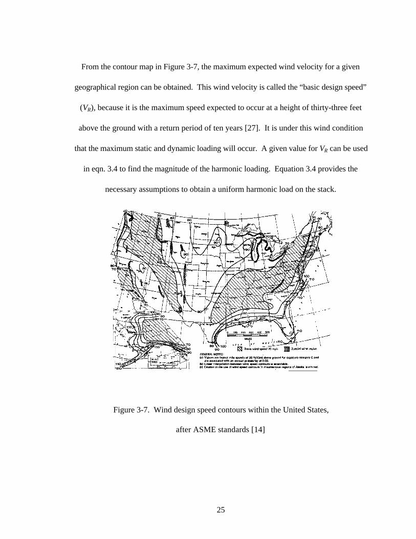
From the contour map in Figure 3-7, the maximum expected wind velocity for a given

geographical region can be obtained. This wind velocity is called the “basic design speed”

(VR), because it is the maximum speed expected to occur at a height of thirty-three feet

above the ground with a return period of ten years [27]. It is under this wind condition

that the maximum static and dynamic loading will occur. A given value for VR can be used

in eqn. 3.4 to find the magnitude of the harmonic loading. Equation 3.4 provides the

necessary assumptions to obtain a uniform harmonic load on the stack.

Figure 3-7. Wind design speed contours within the United States,

after ASME standards [14]

26

The ASME Standards [2] provide a set of comprehensive wind response calculations that

incorporates the harmonic response of the stack. This method of finding the stack

response is currently coded in STACK1. Based on these calculations, STACK1 advises

the user of the expected vibration amplitudes.

27

Chapter 4: Transfer Matrix Method

4.1 Introduction

The transfer matrix method is a method for finding the static and dynamic properties of

an elastic system. The basic principle behind this method is that of breaking up a

complicated system into individual parts with simple elastic and dynamic properties that

can be expressed in matrix form [29]. When these individual matrices are arranged in a

prescribed fashion and multiplied together, the static and dynamic behavior of the entire

system is readily calculated. Many structures encountered in practice consist of a

number of elements linked together end to end in a chain-like configuration. Examples of

this type of system include continuous beams, turbine rotors, crankshafts, pressure

vessels, etc. The transfer matrix method provides a quick and efficient analysis of such

systems simply by multiplying successive elemental transfer matrices together.

Therefore, this method is ideal for analyzing stacks with wind loading, which will be

treated as uniform continuous beams with external distributed loading.

4.2 Coordinate System and Sign Convention

The first step in developing transfer matrix theory is to establish a coordinate system. A

right-handed Cartesian coordinate system is used with the x-axis coinciding with the

centroidal axis of the beam. Looking at a small beam section, two faces will be exposed.

The face whose outward normal points in the positive x-direction is a positive face. The

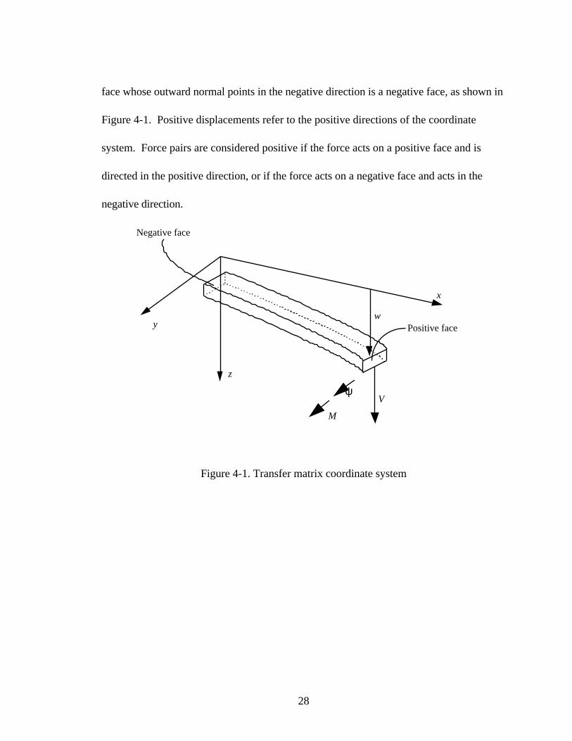
28

face whose outward normal points in the negative direction is a negative face, as shown in

Figure 4-1. Positive displacements refer to the positive directions of the coordinate

system. Force pairs are considered positive if the force acts on a positive face and is

directed in the positive direction, or if the force acts on a negative face and acts in the

negative direction.

Figure 4-1. Transfer matrix coordinate system

V

z

M

Positive face

x

yw

Negative face

ψ

29

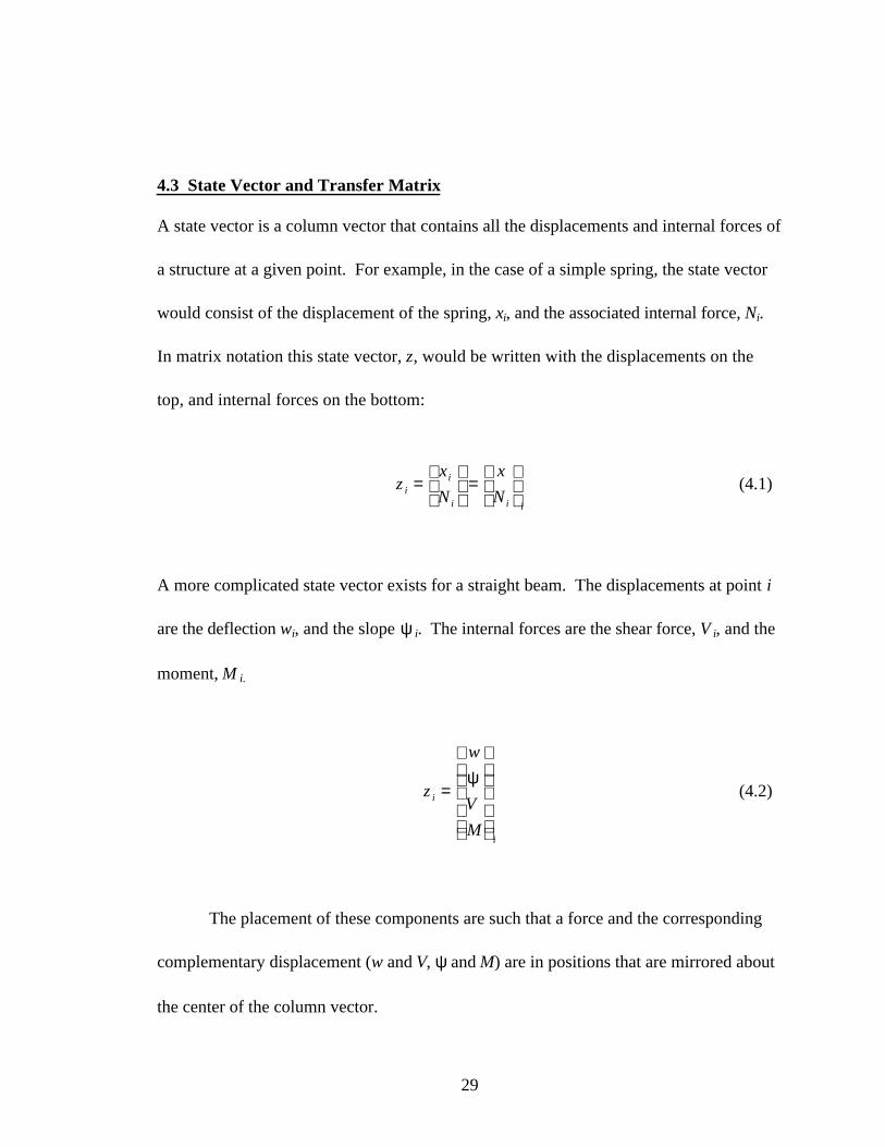
4.3 State Vector and Transfer Matrix

A state vector is a column vector that contains all the displacements and internal forces of

a structure at a given point. For example, in the case of a simple spring, the state vector

would consist of the displacement of the spring, xi, and the associated internal force, Ni.

In matrix notation this state vector, z, would be written with the displacements on the

top, and internal forces on the bottom:

zx

N

x

Nii

i i

=

=

i

(4.1)

A more complicated state vector exists for a straight beam. The displacements at point i

are the deflection wi, and the slope ψ i. The internal forces are the shear force, V i, and the

moment, M i.

z

w

V

M

i

i

=

ψ(4.2)

The placement of these components are such that a force and the corresponding

complementary displacement (w and V, ψ and M) are in positions that are mirrored about

the center of the column vector.

30

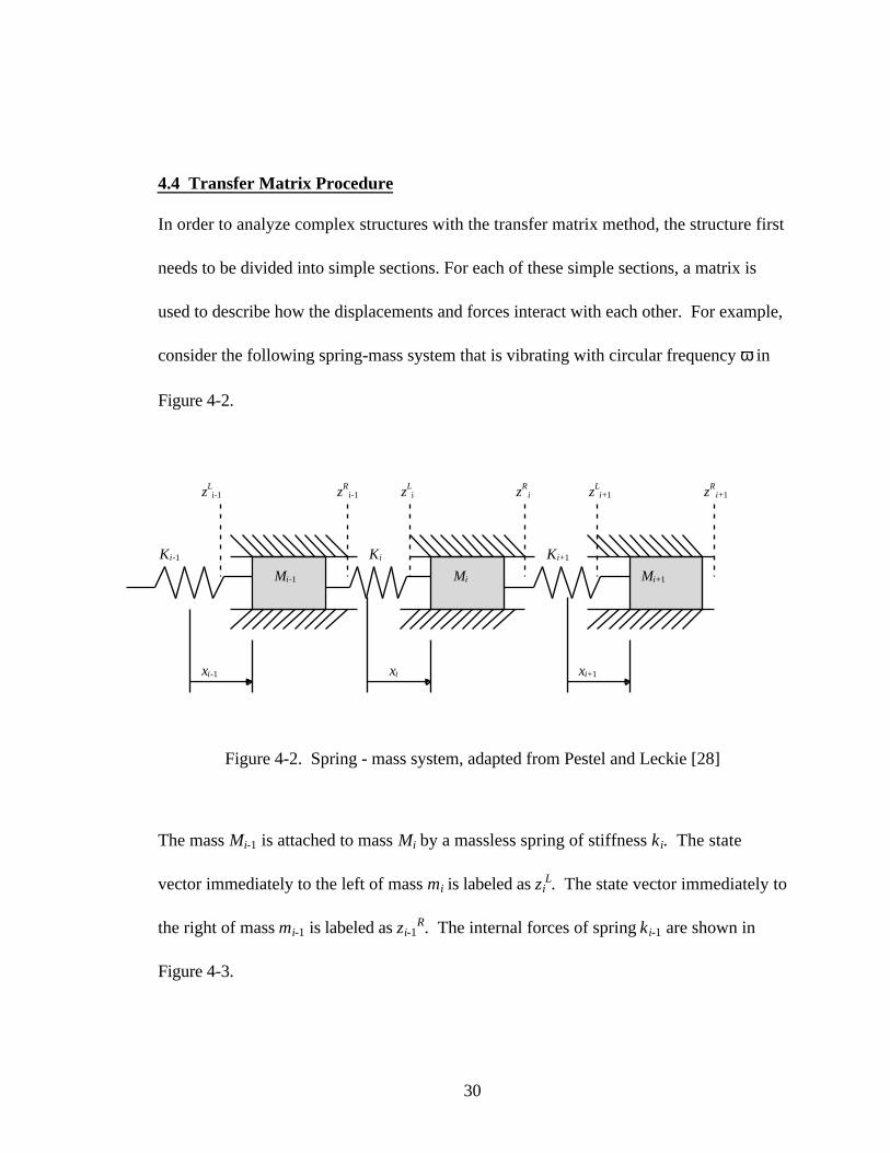
4.4 Transfer Matrix Procedure

In order to analyze complex structures with the transfer matrix method, the structure first

needs to be divided into simple sections. For each of these simple sections, a matrix is

used to describe how the displacements and forces interact with each other. For example,

consider the following spring-mass system that is vibrating with circular frequency ω in

Figure 4-2.

Figure 4-2. Spring - mass system, adapted from Pestel and Leckie [28]

The mass Mi-1 is attached to mass Mi by a massless spring of stiffness k i. The state

vector immediately to the left of mass mi is labeled as ziL. The state vector immediately to

the right of mass mi-1 is labeled as zi-1R. The internal forces of spring k i-1 are shown in

Figure 4-3.

Mi+1

Ki+1Ki-1 Ki

Mi-1 Mi

zLi-1 zR

i+1zLi+1zR

izLizR

i-1

xi-1 xi+1xi

31

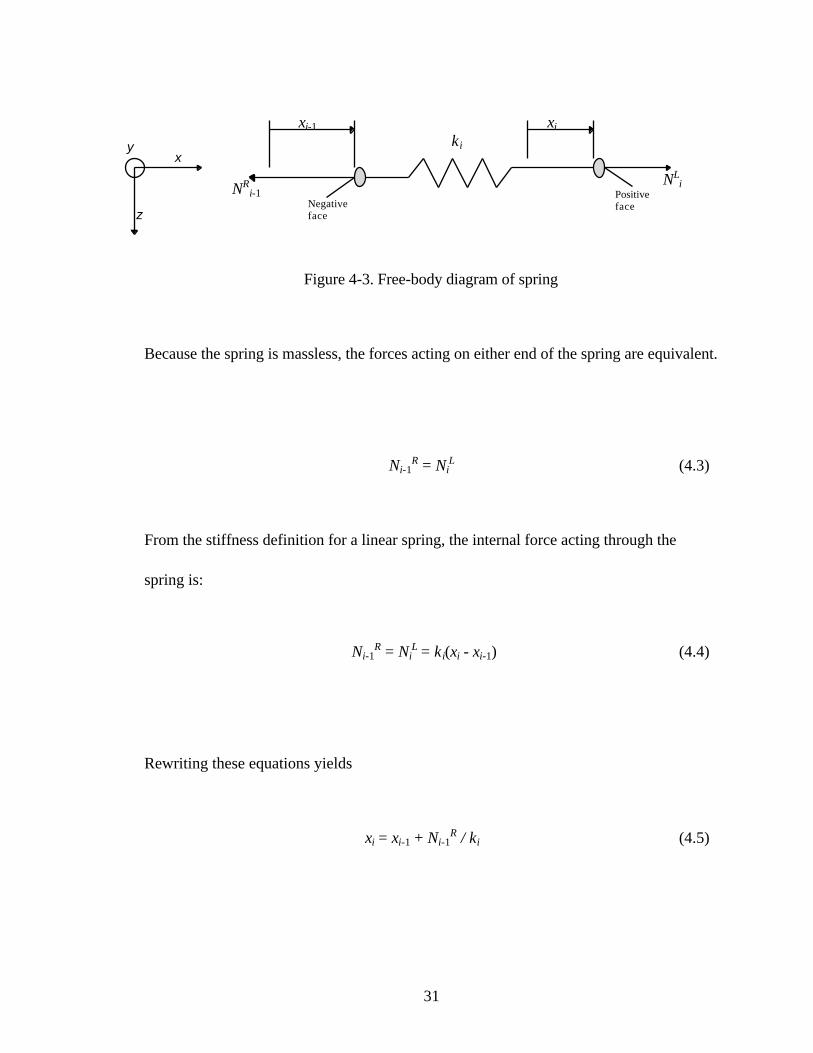
Figure 4-3. Free-body diagram of spring

Because the spring is massless, the forces acting on either end of the spring are equivalent.

Ni-1R = Ni

L (4.3)

From the stiffness definition for a linear spring, the internal force acting through the

spring is:

Ni-1R = Ni

L = k i(xi - xi-1) (4.4)

Rewriting these equations yields

xi = xi-1 + Ni-1R / ki (4.5)

NRi-1

NLi

xi-1 xi

k i

PositivefaceNegative

facez

xy

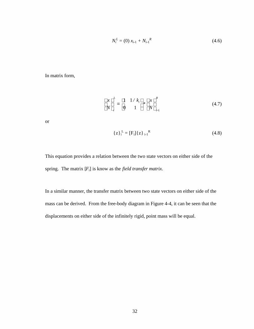
32

NiL = (0) xi-1 + Ni-1

R (4.6)

In matrix form,

x

N

/ k*

x

Ni

Li

i

R

=

−

1 1

0 11

(4.7)

or

ziL = [Fi]z i-1

R (4.8)

This equation provides a relation between the two state vectors on either side of the

spring. The matrix [Fi] is know as the field transfer matrix.

In a similar manner, the transfer matrix between two state vectors on either side of the

mass can be derived. From the free-body diagram in Figure 4-4, it can be seen that the

displacements on either side of the infinitely rigid, point mass will be equal.

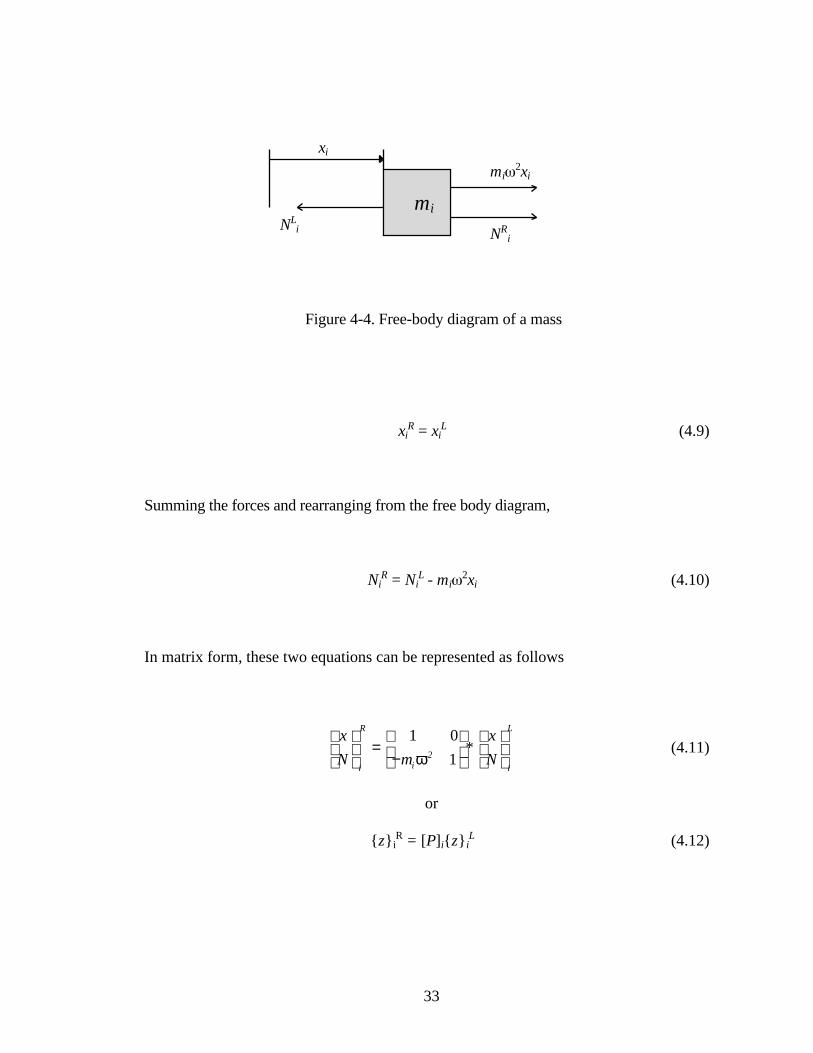
33

Figure 4-4. Free-body diagram of a mass

xiR = xi

L (4.9)

Summing the forces and rearranging from the free body diagram,

NiR = Ni

L - mi2xi (4.10)

In matrix form, these two equations can be represented as follows

x

N m*

x

Ni

R

i2

i

L

=−

1 0

1ω(4.11)

or

ziR = [P]izi

L (4.12)

mi2xi

NRi

NLi

xi

mi

34

Where [Pi] is referred to as the point transfer matrix.

From these two transfer matrices, a variety of spring - mass problems can easily be

analyzed. As mentioned before, [Pi] is the point transfer matrix for mass mi, and [Fi] is

the field transfer matrix for spring k i. To find the relation between the state vectors on

either side of the series of the structure shown in Figure 4.2, the internal transfer matrices

are multiplied together in the following fashion.

zi-1R = Pi-1zi-1

L

ziL = Fizi-1

R = Fi Pi-1zi-1L

ziR = Pizi

L = Pi Fi Pi-1zi-1L

zi+1L = Fi+1zi

R = Fi+1Pi Fi Pi-1zi-1L

zi+1R = Pi+1zi+1

L = Pi+1Fi+1Pi Fi Pi-1zi-1L (4.13)

The above transfer matrix multiplication can written as:

z i+1R = Uzi-1

L (4.14)

Where U is the global transfer matrix.

4.5 Transfer Matrices for Planar Vibrations of a Straight Beam

In order to analyze stacks, transfer matrices for beam sections must be used.

The above procedure can be extended to the analysis of beam vibrations. In order to

extract the eigenvalues for a continuum beam, the beam will first be modeled by replacing

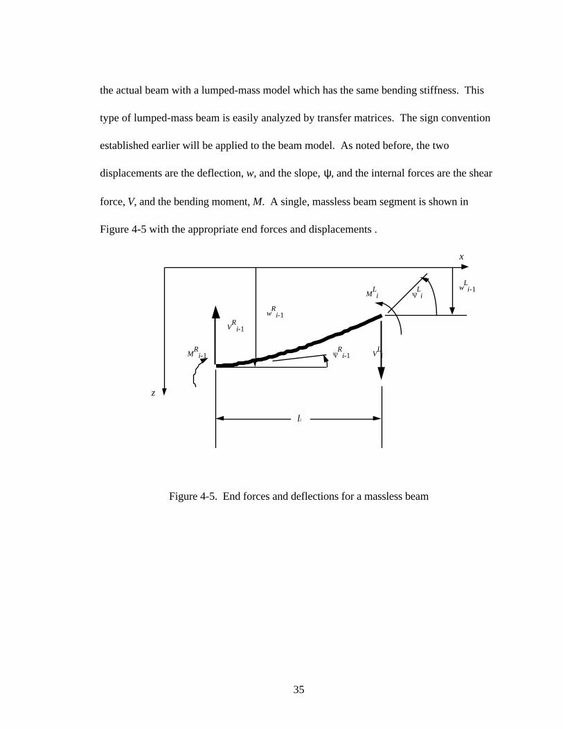
35

the actual beam with a lumped-mass model which has the same bending stiffness. This

type of lumped-mass beam is easily analyzed by transfer matrices. The sign convention

established earlier will be applied to the beam model. As noted before, the two

displacements are the deflection, w, and the slope, ψ, and the internal forces are the shear

force, V, and the bending moment, M. A single, massless beam segment is shown in

Figure 4-5 with the appropriate end forces and displacements .

Figure 4-5. End forces and deflections for a massless beam

li

x

z

Ri-1

Li

wR

i-1

MR

i-1

wLi-1

MLi

VLi

VR

i-1

36

Because the beam is massless, the sum of the vertical forces must equal zero, and the sum

of the moments about any point must equal zero. These two equations are:

ViL - Vi-1

R = 0 (4.15a)

ViL = Vi-1

R (4.15b)

MiL - Mi-1

R - ViL li = 0 (4.16a)

MiL = Mi-1

R + ViL li (4.16b)

Recalling two further equations for the end deflection and slope of a cantilever beam with

flexural stiffness EJ subjected to moment M and shear V at its free end from elemental

beam theory [33]:

wMl2EJ

Vl3EJ

2 3

= − + (4.17)

ψ = −MlEJ

Vl2EJ

2

(4.18)

37

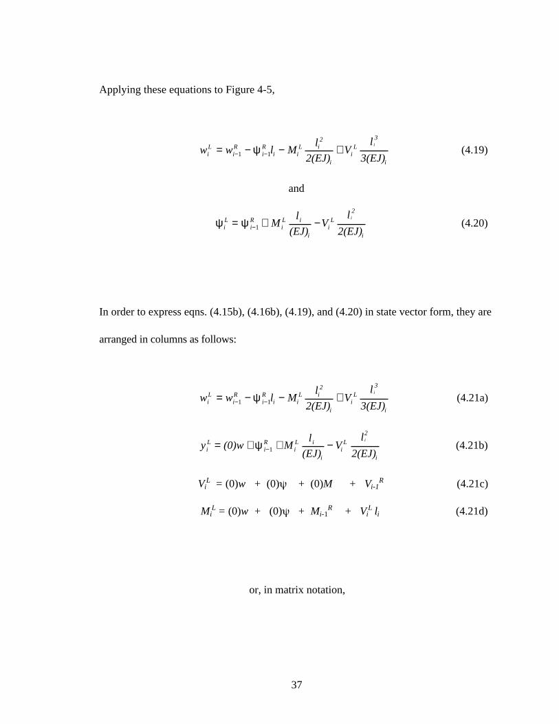
Applying these equations to Figure 4-5,

w w l Ml

2(EJ)V

l

3(EJ)iL

iR

iR

i iL i

2

iiL

3

i

i

= − − +− −1 1ψ (4.19)

and

ψ ψiL

iR

iL i

iiL

2

i

Ml

(EJ)V

l

2(EJ)i

= + −−1 (4.20)

In order to express eqns. (4.15b), (4.16b), (4.19), and (4.20) in state vector form, they are

arranged in columns as follows:

w w l Ml

2(EJ)V

l

3(EJ)iL

iR

iR

i iL i

2

iiL

3

i

i

= − − +− −1 1ψ (4.21a)

y (0)w Ml

(EJ)V

l

2(EJ)iL

iR

iL i

iiL

2

i

i

= + + −−ψ 1 (4.21b)

ViL = (0)w + (0) + (0)M + Vi-1

R (4.21c)

MiL = (0)w + (0) + Mi-1

R + ViL li (4.21d)

or, in matrix notation,

38

−

=

−

−

w

M

V

ll

2EJl

6EJ

0 lEJ

l2EJ

0 0 l

0 0 0

*

w

M

Vi

L2 3

2

i

i 1

R

ψ ψ

1

1

1

1

(4.22)

or ziL = [F]izi-1

L

where the matrix [Fi] is the field matrix for the massless beam.

In order to develop a transfer matrix for the lumped mass, relations are needed between

the left and right sides of the mass. It is noted that since the lumped mass is of zero

length, the deflection, slope, and moment are the same on either side of the mass.

wiR = wi

L iR = i

L MiR = Mi

L (4.23a)

The shear term, however is not the same across a vibrating mass. The inertia of the mass

introduces a discontinuity in shear. From the free body diagram of the mass, Figure 4-6,

equilibrium yields:

ViR = Vi

L - mi2wi (4.23b)

39

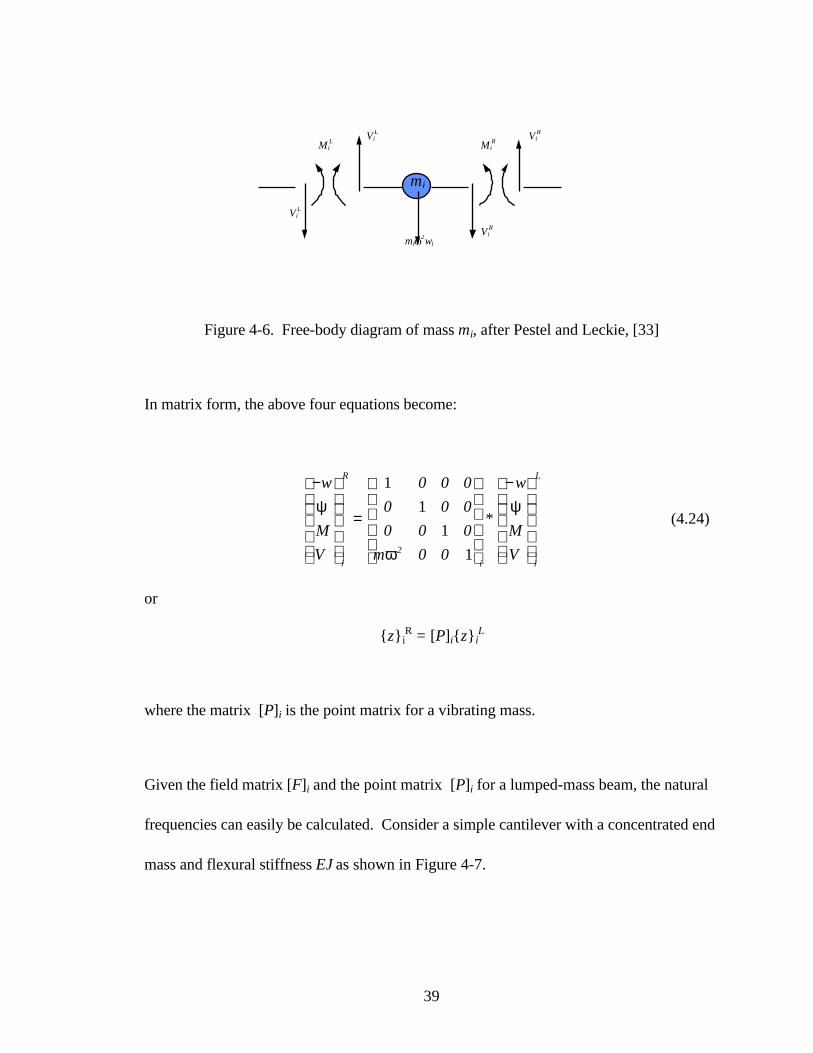
Figure 4-6. Free-body diagram of mass mi, after Pestel and Leckie, [33]

In matrix form, the above four equations become:

−

=

−

w

M

V

0 0 0

0 0 0

0 0 0

m 0 0

*

w

M

Vi

R

2i i

L

ψ

ω

ψ1

1

1

1

(4.24)

or

ziR = [P]izi

L

where the matrix [P]i is the point matrix for a vibrating mass.

Given the field matrix [F]i and the point matrix [P]i for a lumped-mass beam, the natural

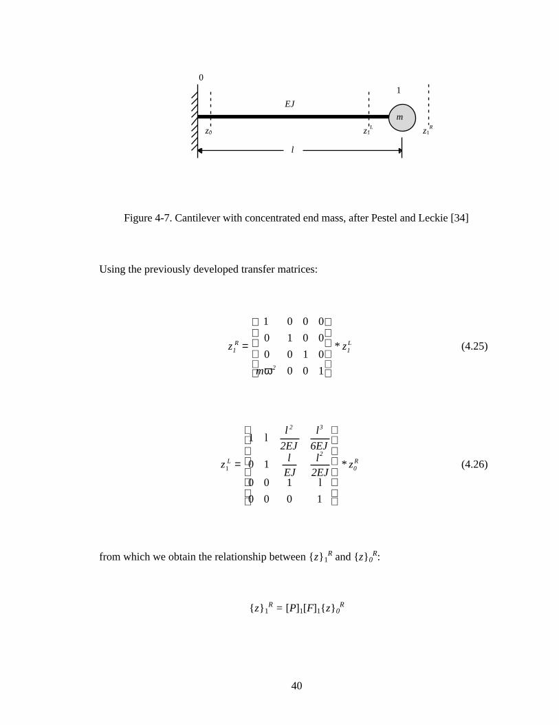
frequencies can easily be calculated. Consider a simple cantilever with a concentrated end

mass and flexural stiffness EJ as shown in Figure 4-7.

MiRMi

L

ViR

mi2wi

ViL Vi

R

ViL

mi

40

Figure 4-7. Cantilever with concentrated end mass, after Pestel and Leckie [34]

Using the previously developed transfer matrices:

z

m

* z1R

2

1L=

1 0 0 0

0 1 0 0

0 0 1 0

0 0 1ω

(4.25)

z

l2EJ

l6EJ

lEJ

l2EJ

zL

2 3

2

0R

1

1

0 1

0 0 1

0 0 0 1

=

l

l

* (4.26)

from which we obtain the relationship between z1R and z0

R:

z1R = [P]1[F]1z0

R

EJ

z0

l

m

1

0

z1L z1

R

41

or

−

=

+

−

w

M

V

ll

2EJl

6EJ

0l

EJl

2EJ0 0 l

m m l m l2EJ

m l6EJ

*

w

M

V1

L

2 3

2

2 22 2 2 3

0

R

ψ

ω ω ω ω

ψ

1

1

1

1

(4.27)

For this example, M1R =V1

R=w0= 0=0, which leads to the following:

-w1R = l2/(2EJ) * M0

R + l3/(6EJ) * V0R (4.28a)

ψ 1R = l/(EJ) * M0R + l2/(2EJ) * V0

R (4.28b)

0 = M0R + l * V0

R (4.28c)

0 = m 2l2/(2EJ) * M0R + (1 + m 2l2/(6EJ))V0

R (4.28d)

Rewriting the last two equations in matrix form,

1

10

0

lm l2EJ

m l6EJ

M

V2 2 2 3

o

R

ω ω+

=

(4.29)

For the last two equations to be satisfied, the non-trivial solution demands that the

determinant of the coefficient matrix be zero [35]:

1

10

lm l2EJ

m l6EJ

2 2 2 3ω ω+ = (4.30)

By expanding the determinant, the natural frequency is found to be:

42

ω23

3=

EJml

or

ω =3EJml 3 (4.31)

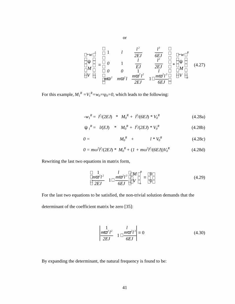
4.6 Complex Beams, Elimination of Intermediate State Vectors

The application of transfer matrices to more complex beams will now be discussed.

Consider a complex beam with multiple lumped masses and discrete massless beam

sections as shown in Figure 4-8.

Figure 4-8. Beam with discrete masses, after Pestel and Leckie [36]

Since the transfer matrices for the individual components of this beam are known, the

transfer matrix for the entire beam is easily found. Recalling the matrices [F]i and [P]i for

a beam section, the following relations exist between adjacent state vectors, as in the

spring mass system discussed earlier.

0 4321

m1

l1 l2

m2 m4m3

5

43

z1L = F1z0

R z1R = P1z1

L z2L = F2z1

R . . . z6L = F6z5

R z6R = P6z6

L z7L = F7z6

R

z7 = F7P6 F6P5 F5P4F4P3 F3P2F2P1F1z0

z7 = Uz0 (4.32)

Because the elements uik of the global transfer matrix [U] are know functions of the

natural frequency ω, this determinant serves as the characteristic equation for computing

the natural frequencies. Because there are four discrete masses in this system, the

expansion of the determinant will lead to an equation of fourth order in ω2.

In modeling stacks, only one type of boundary condition is considered, that of fixed base

with a free end. If the flexibility and damping of the stack foundation is of concern, this

can be modeled using a translational and rotational spring in an additional section

underneath the stack. The left side of the model will have a fixed boundary condition

regardless. Because of the prescribed boundary conditions, it is not necessary to carry

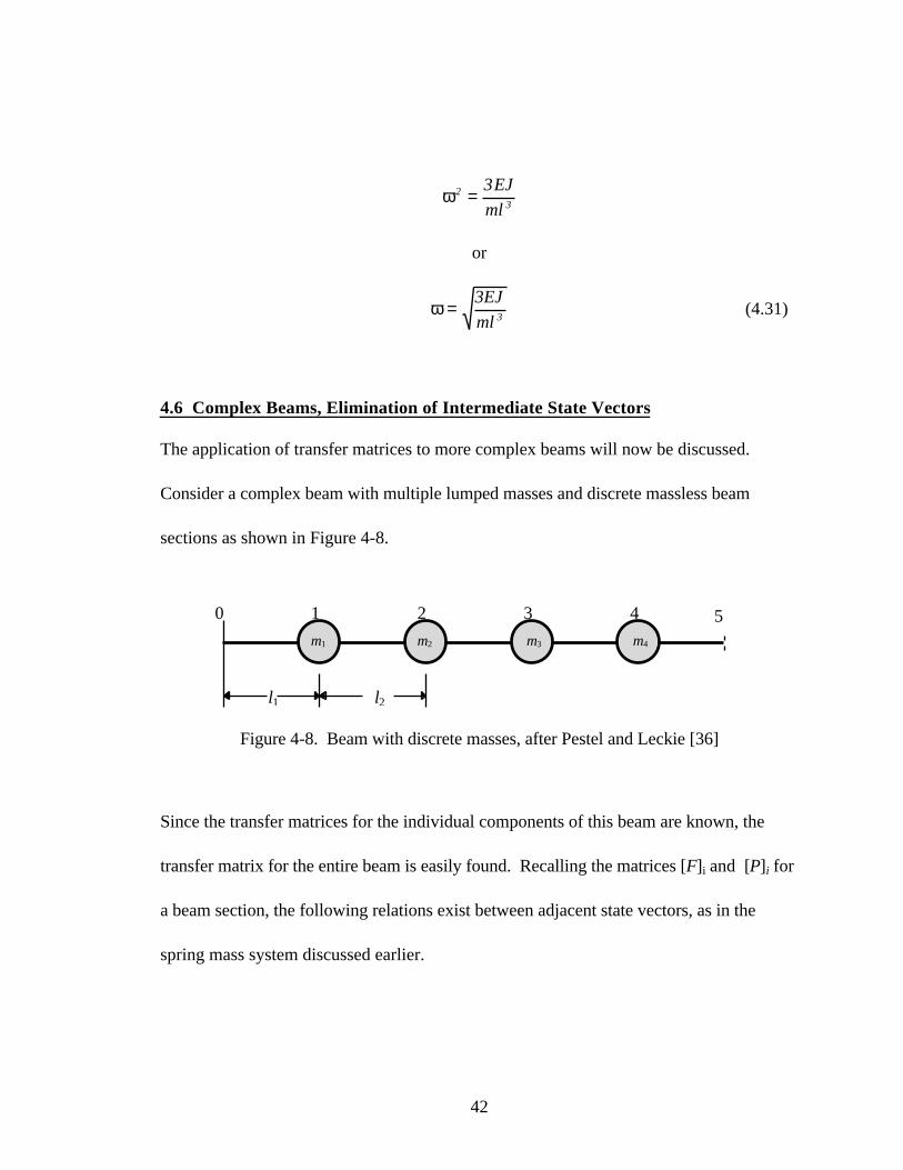
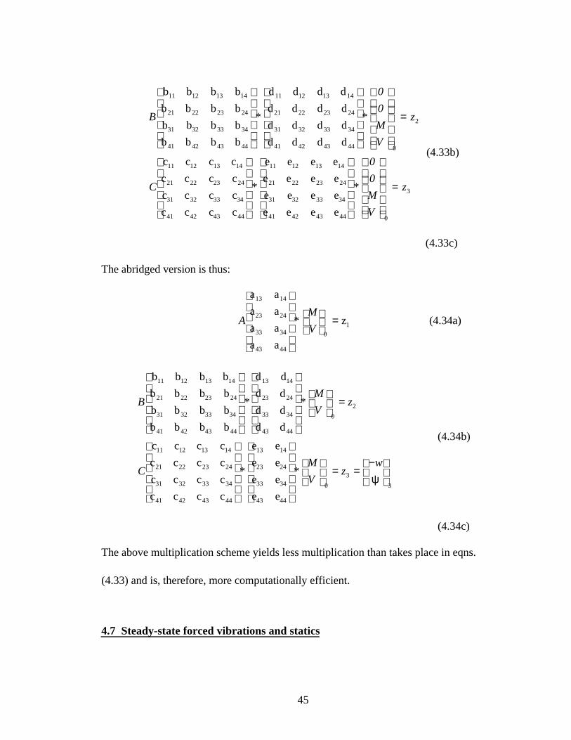
out the complete matrix multiplication. For example, consider the three section beam in

Figure 4-9 where the transfer matrices for section A, B, and C are known. The full matrix

multiplication would be set up as follows:

44

Figure 4-9. Fixed - free three section beam

Boundary conditions for fixed - free beam:

M1 = V1 = 0

w0 = 0 = 0

For this beam:

z1 = Az0 z2 = BAz0 z3 = CBAz0

When matrix multiplication is carried out, as shown below, the first and second columns

are multiplied by zero and thus play no part in the calculation. Therefore, elements of

matrices A, D, and E that are in the first and second columns can be omitted from the

multiplication.

A

0

0

M

V

z

a a a a

a a a a

a a a a

a a a a

11 12 13 14

21 22 23 24

31 32 33 34

41 42 43 44 0

1

=* (4.33a)

l1 l2

Section A Section CSection B

l3

320 1

45

B

0

0

M

V

z

C

b b b b

b b b b

b b b b

b b b b

d d d d

d d d d

d d d d

d d d d

c c c c

c c c c

c c c c

c c c c

e e e e

e e e e

e

11 12 13 14

21 22 23 24

31 32 33 34

41 42 43 44

11 12 13 14

21 22 23 24

31 32 33 34

41 42 43 44 0

2

11 12 13 14

21 22 23 24

31 32 33 34

41 42 43 44

11 12 13 14

21 22 23 24

=

* *

*31 32 33 34

41 42 43 44 0

3e e e

e e e e

=*

0

0

M

V

z

(4.33b)

(4.33c)

The abridged version is thus:

AM

V

a a

a a

a a

a a

z

13 14

23 24

33 34

43 44

0

1

=* (4.34a)

BM

Vz

CM

Vz

w

b b b b

b b b b

b b b b

b b b b

d d

d d

d d

d d

c c c c

c c c c

c c c c

c c c c

e e

e e

e e

e e

11 12 13 14

21 22 23 24

31 32 33 34

41 42 43 44

13 14

23 24

33 34

43 44

0

2

11 12 13 14

21 22 23 24

31 32 33 34

41 42 43 44

13 14

23 24

33 34

43 44

0

3

=

= =−

* *

* *ψ

3

(4.34b)

(4.34c)

The above multiplication scheme yields less multiplication than takes place in eqns.

(4.33) and is, therefore, more computationally efficient.

4.7 Steady-state forced vibrations and statics

46

In the previous sections it has been shown how transfer matrices can be used to find the

natural frequencies of an elastic system. Once the natural frequencies are known, it is

possible to solve general cases of forced undamped vibrations. Recalling from basic

vibrations that if a system is forced at a circular frequency, Ω, the system will vibrate in

steady state with the same circular frequency [37]. Because of this fact, transfer matrices

can be extended to the problem of steady-state forced vibrations and statics (Ω = 0).

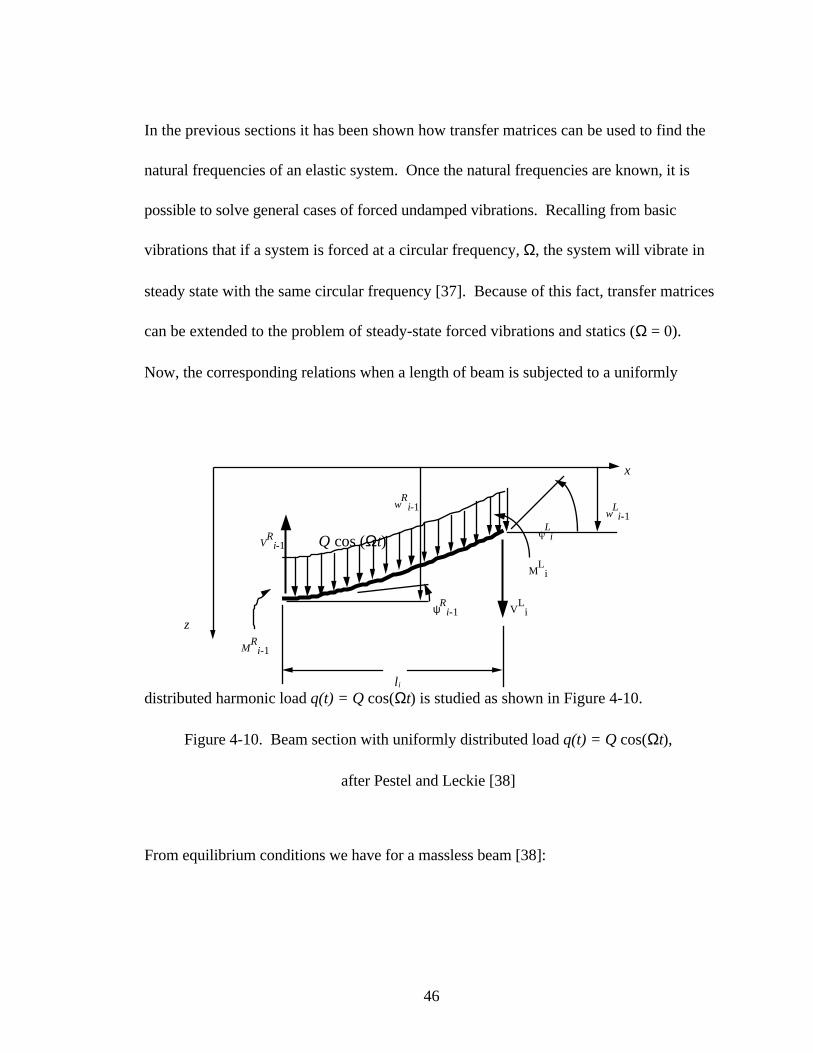
Now, the corresponding relations when a length of beam is subjected to a uniformly

distributed harmonic load q(t) = Q cos(Ωt) is studied as shown in Figure 4-10.

Figure 4-10. Beam section with uniformly distributed load q(t) = Q cos(Ωt),

after Pestel and Leckie [38]

From equilibrium conditions we have for a massless beam [38]:

ψRi-1

Li

wR

i-1

MR

i-1

wLi-1

ML

i

VL

i

VR

i-1 Q cos (Ωt)

li

z

x

47

ViL = Vi-1

R - qili MiL = Mi-1

R + ViL li - qili2 / 2 (4.35)

Also, from strength of materials, we obtain the following:

w w l Ml

2(EJ)V

l

3(EJ)q l8EJi

LiR

iR

i iL i

2

iiL

3

i

i i2

i

i

= − − + +− −1 1ψ (4.36)

ψ ψiL

iR

iL i

iiL

2

i

i i3

i

Ml

(EJ)V

l

2(EJ)q l6EJ

i

= + − +−1 (4.37)

The elimination of MiL and Vi

L from the right-hand side of the equations gives:

− = − + + + +− − − −w w y l Ml

2(EJ)V

l

6(EJ)q l

24EJiL

iR

iR

i iR i

2

ii 1R

3

i

i i4

i

i

1 1 1 (4.38)

ψ ψiL

iR

iR i

iiR

2

i

i i3

i

Ml

(EJ)V

l

2(EJ)q l6EJ

i

= + + +− − −1 1 1 (4.39)

Introducing the identity 1=1 into the lower row of the matrices to facilitate matrix

multiplication, the above equations can be written as:

48

w

M

V

i

L l l 2

2EJl3

6EJql 4

24EJ

0 lEJ

l 2

2EJql 3

6EJ

0 0 lql 2

20 0 0 ql

0 0 0 0 i

*

w

M

V

i

R

ψ ψ

1

1

1

1

1

1

1 1

=

− − − −

−

−

−

−

(4.40)

Or: ziL = [F]izR

i-1

where z is the extended state vector, and [F] is the extended field transfer matrix.

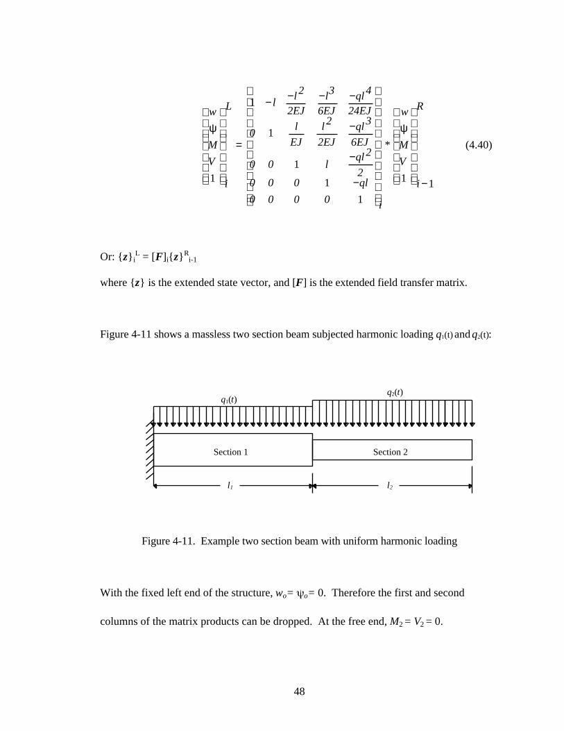
Figure 4-11 shows a massless two section beam subjected harmonic loading q1(t) and q2(t):

Figure 4-11. Example two section beam with uniform harmonic loading

With the fixed left end of the structure, wo= o= 0. Therefore the first and second

columns of the matrix products can be dropped. At the free end, M2 = V2 = 0.

l1 l2

q1(t)

Section 1

q2(t)

Section 2

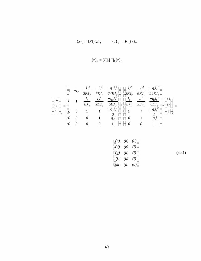
49

z2 = [F]2z1 z1 = [F]1z0

z2 = [F]2[F]1z0

−

=

−− − −

−

−

−

− − −

−

−

−

w

ll

2EJl

6EJq l

24EJ

0l

EJl

2EJq l

6EJ

0 0 l q l2

0 0 0 q l

0 0 0 0

*

l2EJ

l6EJ

q l24EJ

lEJ

l2EJ

q l6EJ

l q l2

0 q l

0 0

2

22

2

2

23

2

2 24

2

2

2

22

2

2 23

2

2 22

2 2

2

2

3 4

12 3

2ψ1

1

1

1

1

1

1

1

1

1 1

1

1 1

1

1

1

1

1 1

1

1 1

1 1

=*

M

V

01

(a) (b) (c)

(d) (e) (f)

(g) (h) (i)

(j) (k) (l)

(m) (n) (o)

(4.41)

50

With the matrix products as:

(a) = − −

−l 2l l

2EJl

2EJ

22 2

2

2

1 1

1

(b) = − −

−−l 3l l

6EJ3l l l

6EJ

3 22 2

22

3

2

1 1

1

1

(c) =

− ++

−q l 4q l l24EJ

2l (q l ) q l24EJ

4 32 2

3 22 2

4

2

1 1 1 1

1

1 1

(d) = l

EJl

EJ2

2

1

1

+

(e) = l

2EJ2l l l

2EJ

22 2

2

2

1

1

1−+

(f) = −

−− −q l

6EJ3q l l 3q l l q l

6EJ1

3 22 2

22 2

3

2

1

1

1 1 1 1

(g) = 1

(h) = l1 + l2

(i) = − −+

q L L(q l q l )

22

22 2

2

1 11 1

(j) = 0

(k) = 1

(l) = q1L1 - q2L2

(m) = 0

(n) = 0

(o) = 0

To find values for wo, ψo, M2 and V2, the equations will be simplified by substituting in

for the following constants, with the loads q1 and q2 as static loads for simplicity:

Section 1

Dc = 20 in.

Tk = 1 in.

L1 = 100 in.

J1 = (π/64)*(214 - 194) = 3149.5 in4

E = 3x107 psi

q1 = 8 lb/in

Section 2

Dc = 14 in.

Tk = 0.5 in.

L2 = 100 in.

J2 = (π/64)*(14.54 - 13.54) = 539.5 in4

E = 3x107 psi

q2 = 12 lb/in

51

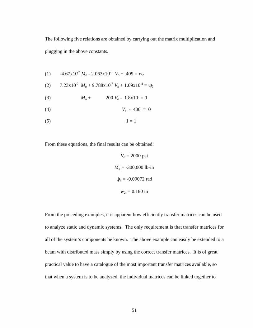
The following five relations are obtained by carrying out the matrix multiplication and

plugging in the above constants.

(1) -4.67x10-7 Mo - 2.063x10-5 Vo + .409 = w2

(2) 7.23x10-9 Mo + 9.788x10-7 Vo + 1.09x10-4 = ψ2

(3) Mo + 200 Vo - 1.8x105 = 0

(4) Vo - 400 = 0

(5) 1 = 1

From these equations, the final results can be obtained:

Vo = 2000 psi

Mo = -300,000 lb-in

ψ2 = -0.00072 rad

w2 = 0.180 in

From the preceding examples, it is apparent how efficiently transfer matrices can be used

to analyze static and dynamic systems. The only requirement is that transfer matrices for

all of the system’s components be known. The above example can easily be extended to a

beam with distributed mass simply by using the correct transfer matrices. It is of great

practical value to have a catalogue of the most important transfer matrices available, so

that when a system is to be analyzed, the individual matrices can be linked together to

52

form an appropriate solution (various transfer matrices are cataloged in Pestel and Leckie

[38]).

This type of analysis is ideal for implementation into a computer program. Various

transfer matrices were programmed into the STACK1 code so that the user would have an

extremely quick and easy tool to analyze many different types of systems. It is by this

program that all of the stack analyses were performed.

53

Chapter 5: BEAM8 Modifications and Implementation of ASME and

ASCE Standards to Generate STACK1

5.1 Introduction

In order to model stack geometry in the STACK1 program, various program changes were

made. Some modeling options that are irrelevant to stacks were removed in order to make

room for the added features. The user interface was modified to create an environment

that is more user friendly for designing stacks. One of the most extensively researched

aspects of stack design for this thesis was the behavior of tapered beams. A substantial

modeling change to the code was the addition of a tapered beam option. A new analysis

option was added for stacks. Within this module the stack design is subjected to an

extensive dynamic and static analysis to check for compliance with the standards.

5.2 Tapered-Beam Subroutine

It is straightforward to model stacks of continuous cross sections with transfer matrices.

However, many stacks are tapered or contain tapered sections, which presents a more

complicated modeling problem. Ideally, a new transfer matrix would be derived for

modeling continuously linear tapered beams, including rotary inertia and shear

deformation. After researching various sources for such a transfer matrix, it appeared that

this type of matrix was not available. Blevins [39] shows general expressions for the

54

natural frequencies and mode shapes of tapered beams. However, these expressions do

not give enough information to create a transfer matrix for the beam (relationships

between deflection, slope, moment, and shear are required). If the differential equation of

a tapered beam were used, a transfer matrix solution would be possible. Several transfer

matrices for constant cross section Euler-Bernoulli beams, which neglect rotary inertia and

shear deformation, are given in Pilkey [40]. This document has transfer matrices for

beams of various non-uniform cross sections, but shear deformation and rotary inertia are

not accounted for in any of the cases. A promising article was found that dealt with

modeling a tapered timoshenko beam by use of transfer matrices [13]. However, this

article did not address the problem of developing a single transfer matrix for a linear

tapered beam. This article instead focused on how stepped constant section continuum

mechanics transfer matrices could be used to model a tapered beam and how this

approach converged faster than a finite element approach.

In an attempt to derive the transfer matrix for a tapered beam, the method presented in

Pestel and Leckie [12] was applied to a beam where the moment, cross-sectional area, and

mass per unit length were treated as variables. However, while deriving this transfer

matrix for a tapered beam, several problems are encountered. This includes the fact that

complicated non-linear differential equations are obtained and a characteristic equation

55

that quickly becomes too large to be dealt with even when symbolic processors within

MATLAB® and MATHEMATICA® were utilized (see Appendix 2).

Therefore, instead of using a continuously tapered beam, it was decided to investigate the

possibility of using a series of stepped continuum beam segments as an approximation to

a tapered beam. The investigation would require that the static and dynamic behavior of

tapered sections be analyzed to find the density of stepped sections required to produce

acceptable results. In a stepped approximation to a tapered beam, a method of

determining the optimum outer diameter of the stepped sections is needed. The static and

dynamic behavior of the model will determine the criteria for how to create the model.

5.3 Static Considerations in Tapered-Beam Approximation

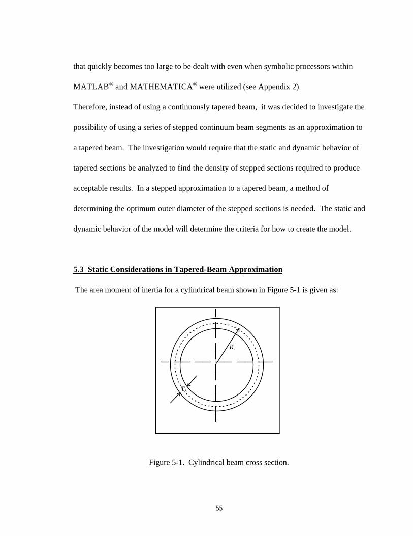
The area moment of inertia for a cylindrical beam shown in Figure 5-1 is given as:

Figure 5-1. Cylindrical beam cross section.

Rc

Tk

56

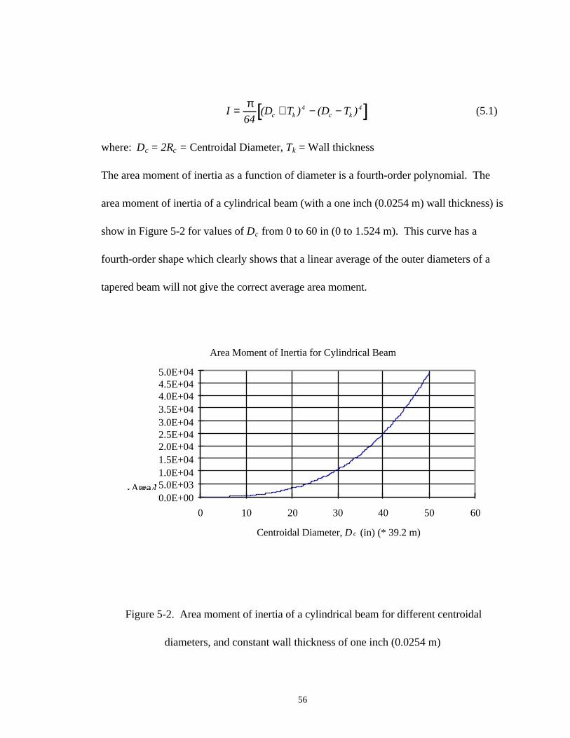
[ ]I64

(D T ) (D T )c k4

c k4= + − −

π(5.1)

where: Dc = 2Rc = Centroidal Diameter, Tk = Wall thickness

The area moment of inertia as a function of diameter is a fourth-order polynomial. The

area moment of inertia of a cylindrical beam (with a one inch (0.0254 m) wall thickness) is

show in Figure 5-2 for values of Dc from 0 to 60 in (0 to 1.524 m). This curve has a

fourth-order shape which clearly shows that a linear average of the outer diameters of a

tapered beam will not give the correct average area moment.

Figure 5-2. Area moment of inertia of a cylindrical beam for different centroidal

diameters, and constant wall thickness of one inch (0.0254 m)

Area Moment of Inertia for Cylindrical Beam

0.0E+005.0E+031.0E+041.5E+042.0E+042.5E+043.0E+043.5E+044.0E+044.5E+045.0E+04

0 10 20 30 40 50 60

Centroidal Diameter, D c (in) (* 39.2 m)

I, Area Moment of Inertia, (in^4), ( * 2.4x10^6 m^4)

57

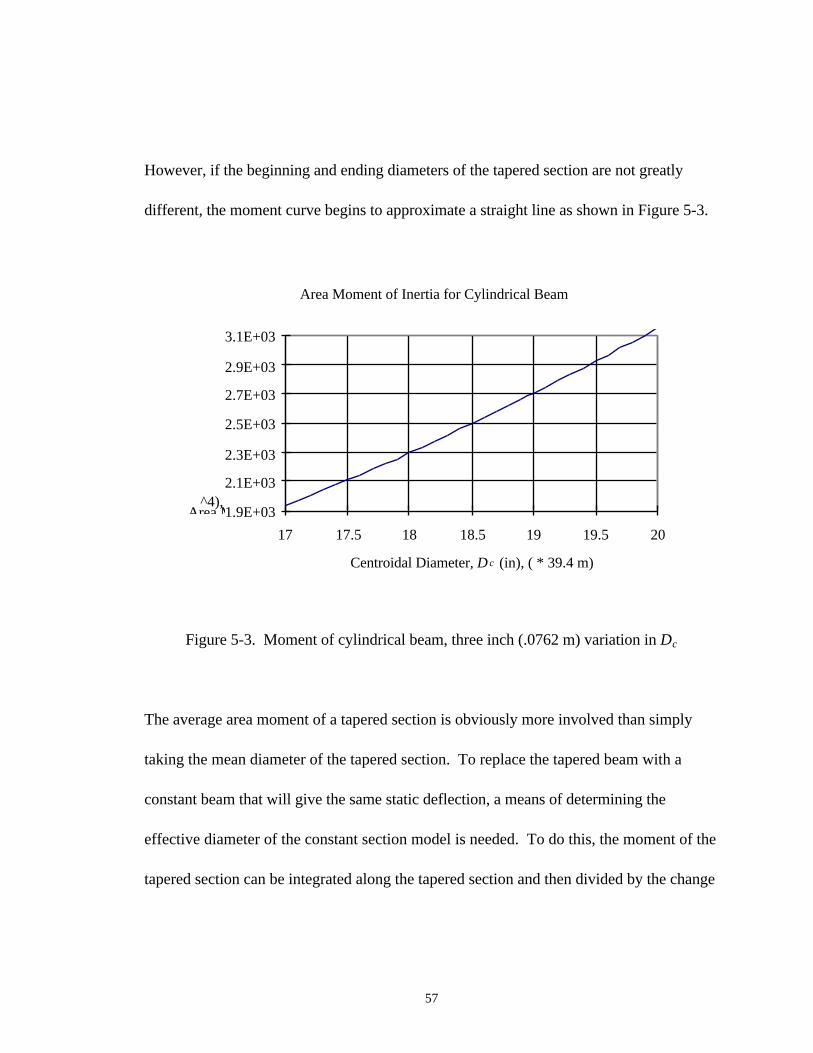
However, if the beginning and ending diameters of the tapered section are not greatly

different, the moment curve begins to approximate a straight line as shown in Figure 5-3.

Figure 5-3. Moment of cylindrical beam, three inch (.0762 m) variation in Dc

The average area moment of a tapered section is obviously more involved than simply

taking the mean diameter of the tapered section. To replace the tapered beam with a

constant beam that will give the same static deflection, a means of determining the

effective diameter of the constant section model is needed. To do this, the moment of the

tapered section can be integrated along the tapered section and then divided by the change

Area Moment of Inertia for Cylindrical Beam

1.9E+03

2.1E+03

2.3E+03

2.5E+03

2.7E+03

2.9E+03

3.1E+03

17 17.5 18 18.5 19 19.5 20

Centroidal Diameter, D c (in), ( * 39.4 m)

I, Area Moment of Inertia, (In ^4), ( * 2.4 x 10^6 m^4)

58

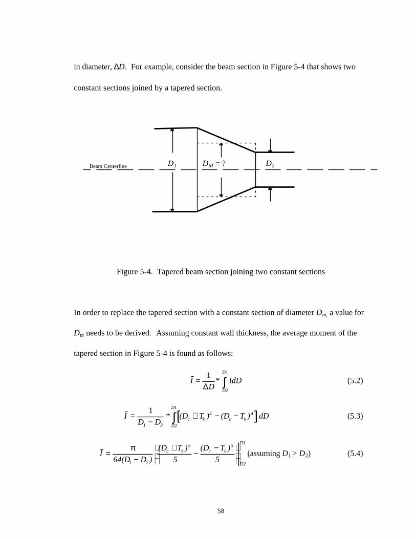
in diameter, ∆D. For example, consider the beam section in Figure 5-4 that shows two

constant sections joined by a tapered section.

Figure 5-4. Tapered beam section joining two constant sections

In order to replace the tapered section with a constant section of diameter Dm, a value for

Dm needs to be derived. Assuming constant wall thickness, the average moment of the

tapered section in Figure 5-4 is found as follows:

ID

* IdDD2

D

= ∫1 1

∆(5.2)

[ ]ID D

* (D T ) (D T ) dD2

c k4

c k4

D2

D

=−

+ − −∫1

1

1

(5.3)

I64(D D )

(D T )5

(D T )52

c k5

c k5

D2

D

=−

+−

−

π

1

1

(assuming D1 > D2) (5.4)

D2D1 DM = ?Beam Centerline

59

I64(D D )

(D T )5

(D T )5

(D T )5

(D T )52

2 k5

2 k5

k5

k5

=−

+−

−

−

+−

−

π

1

1 1 (5.5)

For example, consider a tapered beam for which D1 = 20 in (0.508 m), D2 = 17 in.

(0.432 m), Tk = 1 in. (0.00254 m), and L = 50 in (1.27 m). Using the above equation for

average area moment, I =150.6 in4 (6.27 x 10-5 m4). Equating this value to the moment for

a constant cross section cylindrical beam with the same wall thickness, it can be found

what outer diameter will give the same area moment as the tapered section:

[ ]I . 64L

D T D Tc k c k= = + − −2510 0 001054 4 4 4in m( ) ( ) ( )π

(5.6)

Equation (5.6) yields Dc = 18.54 in (0.471 m). This is very close to the (linear) mean

diameter of 18.5 in. (0.460 m), for which I = 2493.7 in4 (0.00104 m4), which is in error by

only 0.65% from the actual value of 2510 in4 (0.00105 m4). This shows that for this case

where the two diameters differ by 17%, using the mean diameter of the tapered beam

would produce very little error in moment calculations.

60

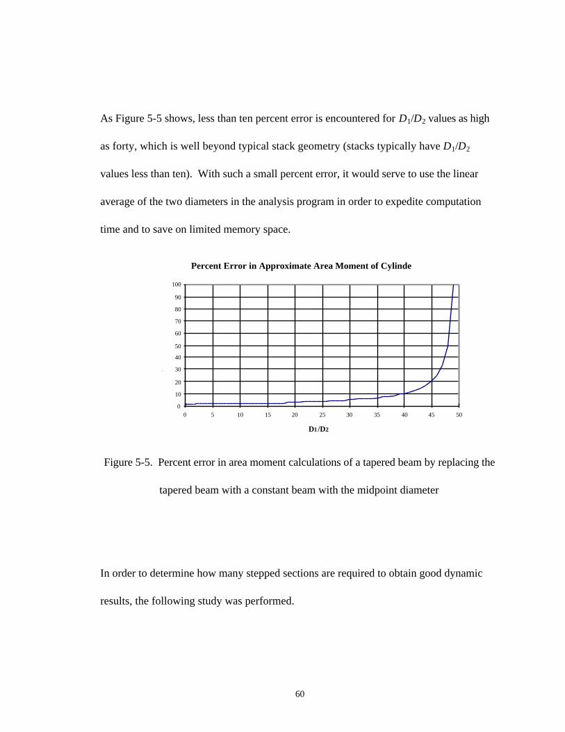
As Figure 5-5 shows, less than ten percent error is encountered for D1/D2 values as high

as forty, which is well beyond typical stack geometry (stacks typically have D1/D2

values less than ten). With such a small percent error, it would serve to use the linear

average of the two diameters in the analysis program in order to expedite computation

time and to save on limited memory space.

Percent Error in Approximate Area Moment of Cylinder

0

10

20

30

40

50

60

70

80

90

100

0 5 10 15 20 25 30 35 40 45 50

D1 /D2

Percent Error in M

Figure 5-5. Percent error in area moment calculations of a tapered beam by replacing the

tapered beam with a constant beam with the midpoint diameter

In order to determine how many stepped sections are required to obtain good dynamic

results, the following study was performed.

61

5.4 Dynamic Considerations in Tapered Beam Approximation

In any given stack model, there are several variables which will affect how fine a mesh is

required to obtain good estimates of the natural frequencies. For this study, “good”

results are determined by the number of stepped sections required to get within 5% of the

actual natural frequency. For computer memory limits as well as computational speed

considerations, the least amount of stepped sections that will allow accurate results

would be desirable. It is assumed that with an increasing number of sections to

approximate the tapered beam, the natural frequencies will converge to those for a smooth

tapered segment. The actual natural frequency of a tapered beam was determined by

doing a convergence study on two different stack designs, design (a) and design (b).

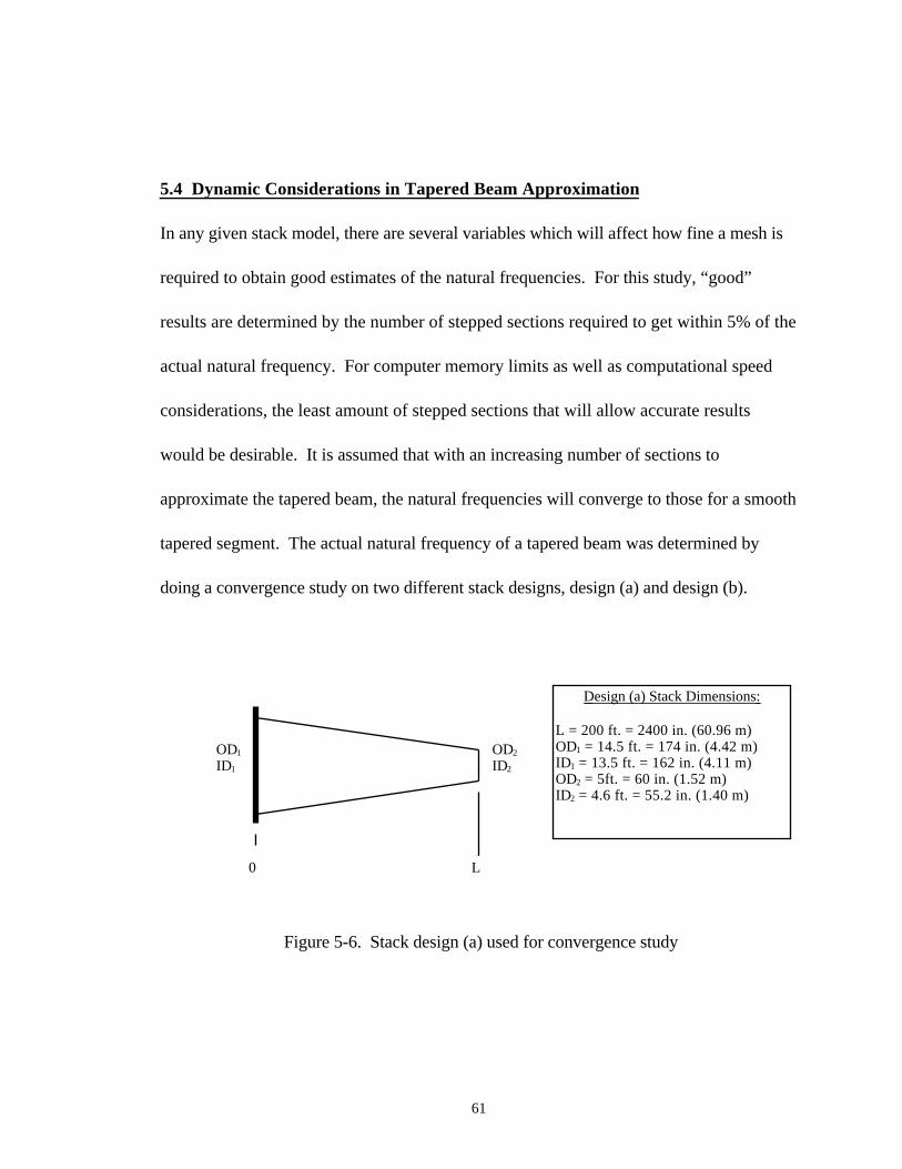
Figure 5-6. Stack design (a) used for convergence study

0 L

OD1

ID1

OD2

ID2

Design (a) Stack Dimensions:

L = 200 ft. = 2400 in. (60.96 m)OD1 = 14.5 ft. = 174 in. (4.42 m)ID1 = 13.5 ft. = 162 in. (4.11 m)OD2 = 5ft. = 60 in. (1.52 m)ID2 = 4.6 ft. = 55.2 in. (1.40 m)

62

Stack (a) consisted of one continuously tapered beam, with the dimensions taken from an

example in the ASME Steel Stack standards [42]. This model was analyzed and

eigenvalues were found using between two and thirty constant sections for the tapered

approximation.

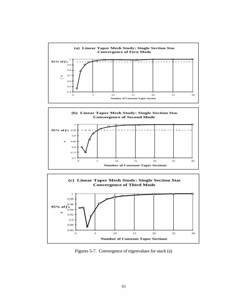
From Figures 5-7a, 5-7b, and 5-7c, it can be seen that convergence in the first three modes

occurred quite rapidly, the first mode converged to within 5% of its final value after six

segments were used. Only the first three modes were investigated, because this is where

the greatest deflection amplitudes will occur, and all aerodynamic excitation forces are

typically very low frequency.

63

(a) Linear Taper Mesh Study: Single Section Stack Convergence of First Mode

0.4

0.5

0.6

0.7

0.8

0.9

1

0 5 10 15 20 25 30

Number of Constant Taper Sections

f/fn

95% of f n

(b) Linear Taper Mesh Study: Single Section Stack

Convergence of Second Mode

0.7

0.75

0.8

0.85

0.9

0.95

1

0 5 10 15 20 25 30

Number of Constant Taper Sections

f/f

n

95% of f n

(c) Linear Taper Mesh Study: Single Section Stack Convergence of Third Mode

0.86

0.88

0.9

0.92

0.94

0.96

0.98

1

0 5 10 15 20 25 30

Number of Constant Taper Sections

f/fn

95% of f n

Figures 5-7. Convergence of eigenvalues for stack (a)

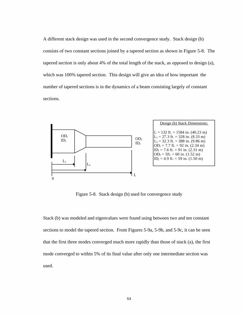
64

A different stack design was used in the second convergence study. Stack design (b)

consists of two constant sections joined by a tapered section as shown in Figure 5-8. The

tapered section is only about 4% of the total length of the stack, as opposed to design (a),

which was 100% tapered section. This design will give an idea of how important the

number of tapered sections is in the dynamics of a beam consisting largely of constant

sections.

Figure 5-8. Stack design (b) used for convergence study

Stack (b) was modeled and eigenvalues were found using between two and ten constant

sections to model the tapered section. From Figures 5-9a, 5-9b, and 5-9c, it can be seen

that the first three modes converged much more rapidly than those of stack (a), the first

mode converged to within 5% of its final value after only one intermediate section was

used.

0

L1L2

L

OD1

ID1OD2

ID2

Design (b) Stack Dimensions:

L = 132 ft. = 1584 in. (40.23 m)L1 = 27.3 ft. = 328 in. (8.33 m)L2 = 32.3 ft. = 388 in. (9.86 m)OD1 = 7.7 ft. = 92 in. (2.34 m)ID1 = 7.6 ft. = 91 in. (2.31 m)OD2 = 5ft. = 60 in. (1.52 m)ID2 = 4.9 ft. = 59 in. (1.50 m)

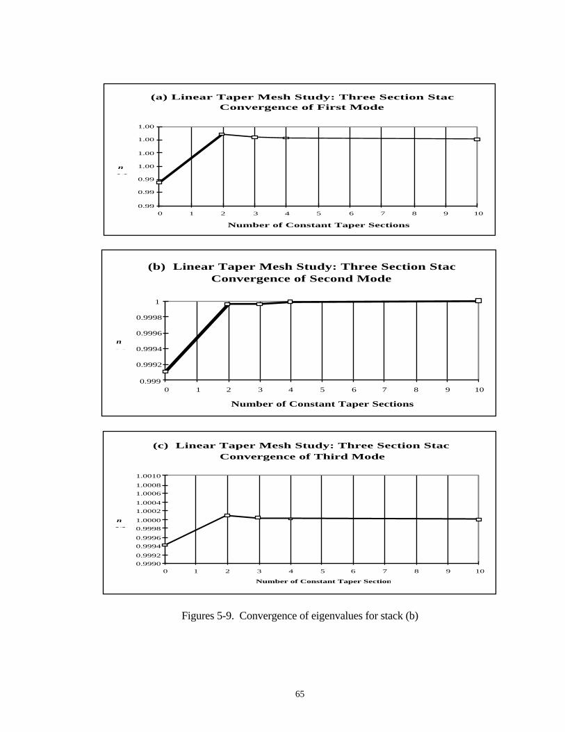
65

(a) Linear Taper Mesh Study: Three Section Stack Convergence of First Mode

0.99

0.99

0.99

1.00

1.00

1.00

1.00

0 1 2 3 4 5 6 7 8 9 10

Number of Constant Taper Sections

f/fn

(b) Linear Taper Mesh Study: Three Section Stack Convergence of Second Mode

0.999

0.9992

0.9994

0.9996

0.9998

1

0 1 2 3 4 5 6 7 8 9 10

Number of Constant Taper Sections

f/fn

(c) Linear Taper Mesh Study: Three Section Stack

Convergence of Third Mode

0.9990

0.9992

0.9994

0.9996

0.9998

1.0000

1.0002

1.0004

1.0006

1.0008

1.0010

0 1 2 3 4 5 6 7 8 9 10

Number of Constant Taper Sections

f/fn

Figures 5-9. Convergence of eigenvalues for stack (b)

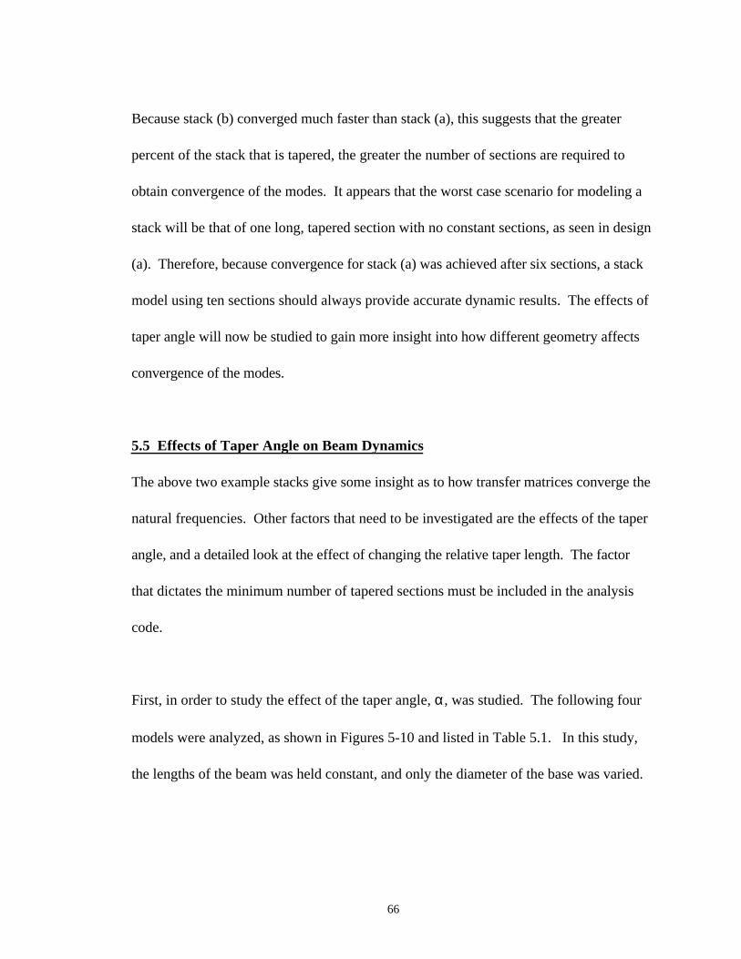
66

Because stack (b) converged much faster than stack (a), this suggests that the greater

percent of the stack that is tapered, the greater the number of sections are required to

obtain convergence of the modes. It appears that the worst case scenario for modeling a

stack will be that of one long, tapered section with no constant sections, as seen in design

(a). Therefore, because convergence for stack (a) was achieved after six sections, a stack

model using ten sections should always provide accurate dynamic results. The effects of

taper angle will now be studied to gain more insight into how different geometry affects

convergence of the modes.

5.5 Effects of Taper Angle on Beam Dynamics

The above two example stacks give some insight as to how transfer matrices converge the

natural frequencies. Other factors that need to be investigated are the effects of the taper

angle, and a detailed look at the effect of changing the relative taper length. The factor

that dictates the minimum number of tapered sections must be included in the analysis

code.

First, in order to study the effect of the taper angle, α, was studied. The following four

models were analyzed, as shown in Figures 5-10 and listed in Table 5.1. In this study,

the lengths of the beam was held constant, and only the diameter of the base was varied.

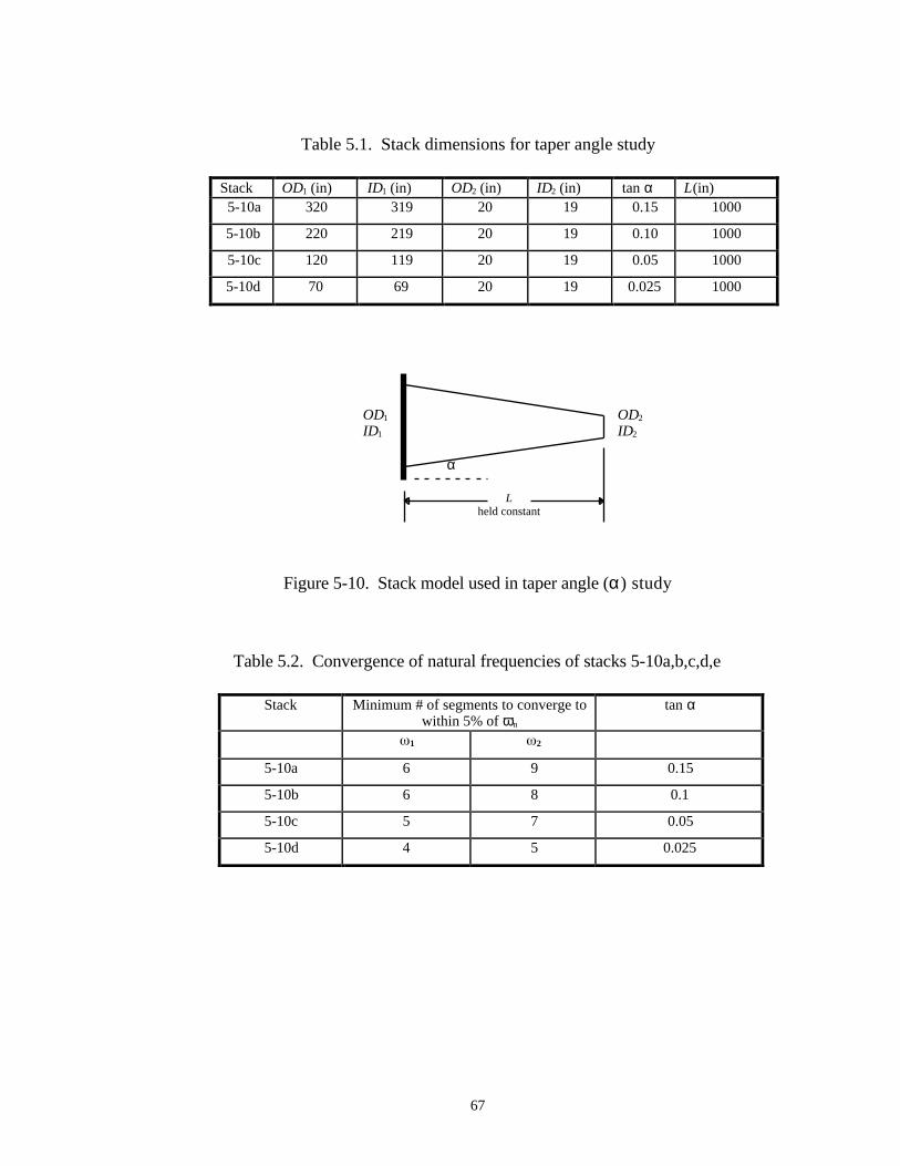
67

Table 5.1. Stack dimensions for taper angle study

Stack OD1 (in) ID1 (in) OD2 (in) ID2 (in) tan α L(in)5-10a 320 319 20 19 0.15 1000

5-10b 220 219 20 19 0.10 1000

5-10c 120 119 20 19 0.05 1000

5-10d 70 69 20 19 0.025 1000

Figure 5-10. Stack model used in taper angle (α) study

Table 5.2. Convergence of natural frequencies of stacks 5-10a,b,c,d,e

Stack Minimum # of segments to converge towithin 5% of ωn

tan α

1 2

5-10a 6 9 0.15

5-10b 6 8 0.1

5-10c 5 7 0.05

5-10d 4 5 0.025

α

OD1

ID1

L held constant

OD2

ID2

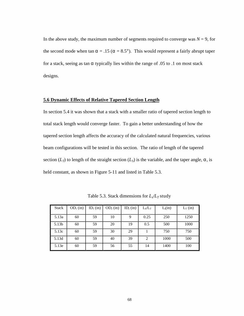
68

In the above study, the maximum number of segments required to converge was N = 9, for

the second mode when tan α = .15 (α = 8.5°). This would represent a fairly abrupt taper

for a stack, seeing as tan α typically lies within the range of .05 to .1 on most stack

designs.

5.6 Dynamic Effects of Relative Tapered Section Length

In section 5.4 it was shown that a stack with a smaller ratio of tapered section length to

total stack length would converge faster. To gain a better understanding of how the

tapered section length affects the accuracy of the calculated natural frequencies, various

beam configurations will be tested in this section. The ratio of length of the tapered

section (LT) to length of the straight section (LS) is the variable, and the taper angle, α, is

held constant, as shown in Figure 5-11 and listed in Table 5.3.

Table 5.3. Stack dimensions for Ls/LT study

Stack OD1 (in) ID1 (in) OD2 (in) ID2 (in) LS/LT Ls(in) LT (in)

5.13a 60 59 10 9 0.25 250 1250

5.13b 60 59 20 19 0.5 500 1000

5.13c 60 59 30 29 1 750 750

5.13d 60 59 40 39 2 1000 500

5.13e 60 59 56 55 14 1400 100

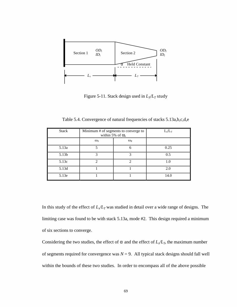
69

Figure 5-11. Stack design used in LS/LT study

Table 5.4. Convergence of natural frequencies of stacks 5.13a,b,c,d,e

Stack Minimum # of segments to converge towithin 5% of ωn

Ls/LT

1 2

5.13a 5 6 0.25

5.13b 3 3 0.5

5.13c 2 2 1.0

5.13d 1 1 2.0

5.13e 1 1 14.0

In this study of the effect of Ls/LT was studied in detail over a wide range of designs. The

limiting case was found to be with stack 5.13a, mode #2. This design required a minimum

of six sections to converge.

Considering the two studies, the effect of α and the effect of Ls/LT, the maximum number

of segments required for convergence was N = 9. All typical stack designs should fall well

within the bounds of these two studies. In order to encompass all of the above possible

OD1

ID1Section 1

α Held Constant

Section 2OD2

ID2

Ls LT

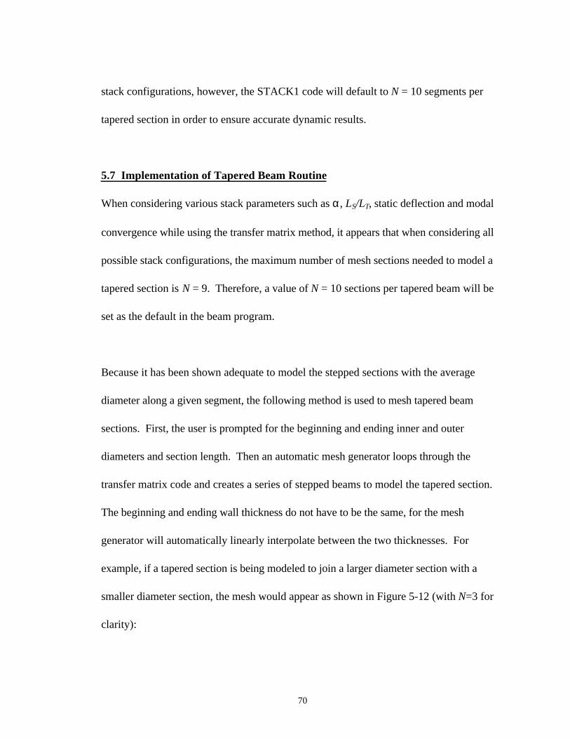
70

stack configurations, however, the STACK1 code will default to N = 10 segments per

tapered section in order to ensure accurate dynamic results.

5.7 Implementation of Tapered Beam Routine

When considering various stack parameters such as α, LS/LT, static deflection and modal

convergence while using the transfer matrix method, it appears that when considering all

possible stack configurations, the maximum number of mesh sections needed to model a

tapered section is N = 9. Therefore, a value of N = 10 sections per tapered beam will be

set as the default in the beam program.

Because it has been shown adequate to model the stepped sections with the average

diameter along a given segment, the following method is used to mesh tapered beam

sections. First, the user is prompted for the beginning and ending inner and outer

diameters and section length. Then an automatic mesh generator loops through the

transfer matrix code and creates a series of stepped beams to model the tapered section.

The beginning and ending wall thickness do not have to be the same, for the mesh

generator will automatically linearly interpolate between the two thicknesses. For

example, if a tapered section is being modeled to join a larger diameter section with a

smaller diameter section, the mesh would appear as shown in Figure 5-12 (with N=3 for

clarity):

71

Figure 5-12 shows only the half of the stack section. In this type of taper, the first taper

section is already reduced in diameter, in order for the real taper line (represented by the

dashed lines) to pass through the midpoint of the section. The same is true for the final

taper section, in that it is slightly larger in diameter than the following constant section in

order to maintain the correct average moment.

Figure 5-12. Example of automatic mesh routine

5.8 Implementation of ASME Steel Stack Standards Into STACK1 Code

Now that an efficient stack modeling procedure is available, the next step is to check the

stack design against the standards to obtain various static and dynamic information that

can be used to check and improve the stack designs. Various items, including stack

natural frequencies, geometry, wind exposure category (dependent on surrounding

structures), and geographic location (which determines maximum wind velocity) are

required to completely study the behavior of a given stack design. Care should be taken

Stack Centerline

R1

R2

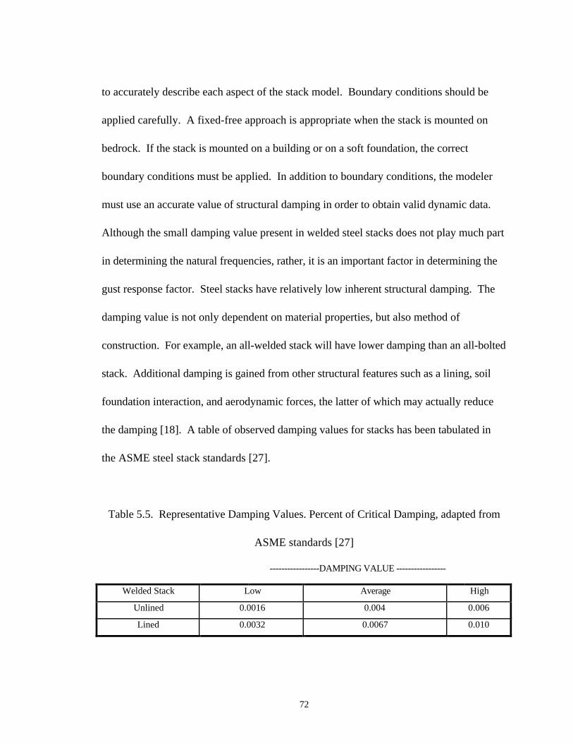
72

to accurately describe each aspect of the stack model. Boundary conditions should be

applied carefully. A fixed-free approach is appropriate when the stack is mounted on

bedrock. If the stack is mounted on a building or on a soft foundation, the correct

boundary conditions must be applied. In addition to boundary conditions, the modeler

must use an accurate value of structural damping in order to obtain valid dynamic data.

Although the small damping value present in welded steel stacks does not play much part

in determining the natural frequencies, rather, it is an important factor in determining the

gust response factor. Steel stacks have relatively low inherent structural damping. The

damping value is not only dependent on material properties, but also method of

construction. For example, an all-welded stack will have lower damping than an all-bolted

stack. Additional damping is gained from other structural features such as a lining, soil

foundation interaction, and aerodynamic forces, the latter of which may actually reduce

the damping [18]. A table of observed damping values for stacks has been tabulated in

the ASME steel stack standards [27].

Table 5.5. Representative Damping Values. Percent of Critical Damping, adapted from

ASME standards [27]

-----------------DAMPING VALUE -----------------

Welded Stack Low Average High

Unlined 0.0016 0.004 0.006

Lined 0.0032 0.0067 0.010

73

The damping values in the above table are given in terms of the fraction of critical

damping β which is related to the logarithmic decrement δ by the relationship δ = 2πβ

[27].

5.9 Static Loads and Deflection

Once the correct modeling procedures have been followed, the wind loads on the stack are

applied. The first step in doing this is realizing the geographic location of the stack. The

location dictates the corresponding basic design wind speed from the standards, as shown

in Chapter 3. The basic design speed (VR) is the “fastest mile” wind speed at a height of

33 ft (10.1 m). over open terrain having a return period of 50 years. VR is defined in miles

per hour [27].

After selecting a value for VR, the velocity pressure exposure coefficient, Kz is determined.

Kz is a function of exposure category and height above ground level. Exposure categories

are defined as in Table 5-6.

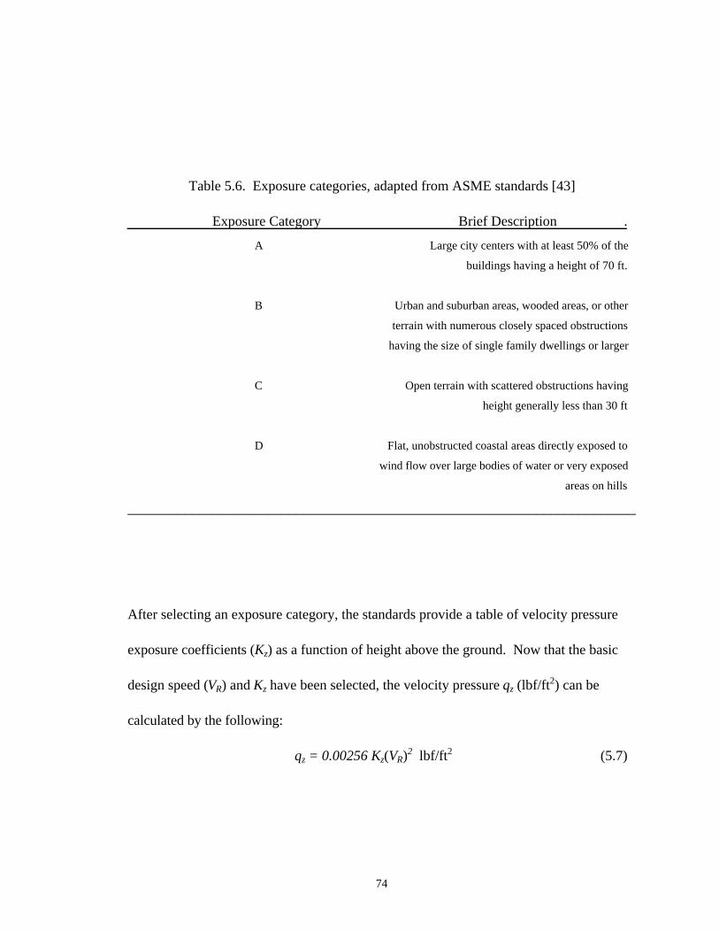
74

Table 5.6. Exposure categories, adapted from ASME standards [43]

Exposure Category Brief Description .

A Large city centers with at least 50% of the

buildings having a height of 70 ft.

B Urban and suburban areas, wooded areas, or other

terrain with numerous closely spaced obstructions

having the size of single family dwellings or larger

C Open terrain with scattered obstructions having

height generally less than 30 ft

D Flat, unobstructed coastal areas directly exposed to

wind flow over large bodies of water or very exposed

areas on hills

________________________________________________________________________

After selecting an exposure category, the standards provide a table of velocity pressure

exposure coefficients (Kz) as a function of height above the ground. Now that the basic

design speed (VR) and Kz have been selected, the velocity pressure qz (lbf/ft2) can be

calculated by the following:

qz = 0.00256 Kz(VR)2 lbf/ft2 (5.7)

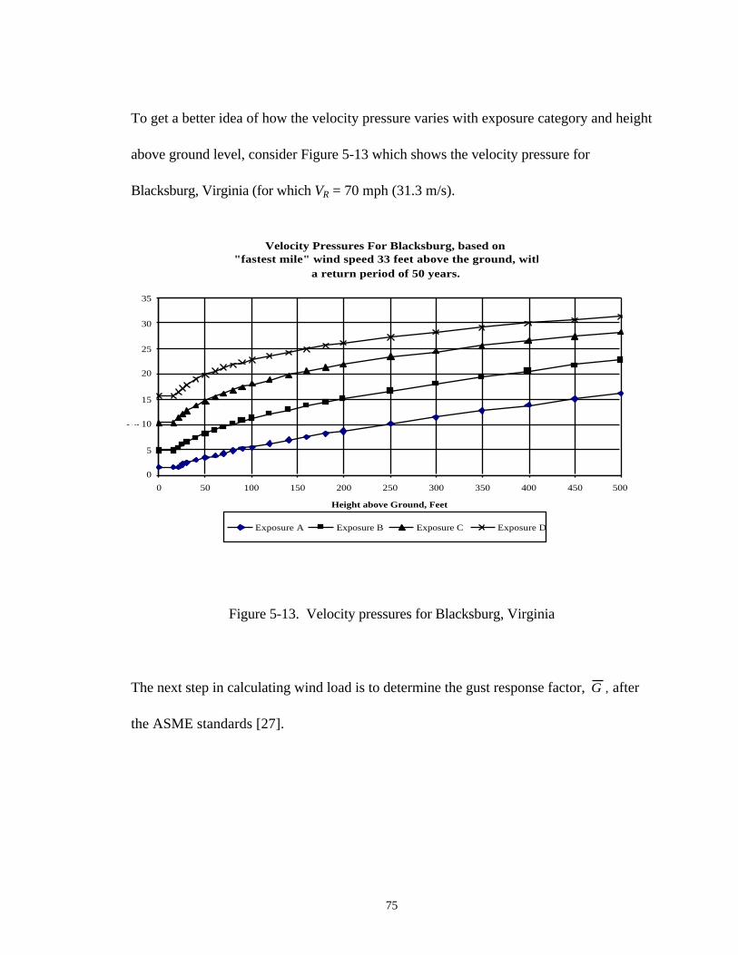
75

To get a better idea of how the velocity pressure varies with exposure category and height

above ground level, consider Figure 5-13 which shows the velocity pressure for

Blacksburg, Virginia (for which VR = 70 mph (31.3 m/s).

Figure 5-13. Velocity pressures for Blacksburg, Virginia

The next step in calculating wind load is to determine the gust response factor, G , after

the ASME standards [27].

Velocity Pressures For Blacksburg, based on"fastest mile" wind speed 33 feet above the ground, with

a return period of 50 years.

0

5

10

15

20

25

30

35

0 50 100 150 200 250 300 350 400 450 500

Height above Ground, Feet

Wind pressure, PSI

Exposure A Exposure B Exposure C Exposure D

76

GPb

TD

= ++

.

( . )

.

/

65332

1 0021

2 1 2

(5.8)

(see Appendix 1 for full discussion of all variables and calculations)

The above expression for G is taken from the 1992 ASME Steel Stack Standards [27]. A

more updated ASCE building code suggests that values of G can be approximated by a

simplified method which does not require many of the constants contained in the ASME

equations. The above ASME procedure is a valid analysis, but, for simplicity's sake

within the STACK1 code, the more recent ASCE code is used.

Finally, the load per unit height of the stack is given by:

Wz=CfqzDG (lb / ft) (5.9)

where: Cf = a force coefficient given in table 5.C-1 of the ASME standards [49],

qz = velocity pressure from eqn. 5.7, D = diameter of stack at 0.8H, and

G = gust response factor from eqn. 5.8.

(see appendix 1 for full discussion of all variables and calculations)

In the code, the value for Wz is determined at the beginning and end of each beam section.

STACK1 then determines static deflection based on this velocity pressure, as well as

internal shear, moment, and stresses.

77

5.10 Dynamic Loads and Vortex Shedding

Once the static load is known, the next step is to determine the dynamic behavior of the

stack. The mean hourly design speed, VD is defined as:

V z 1.18V KD R z( ) = ; where z = 5/6 H (5.10)

The critical wind speed, in feet per second, is given by:

Vc=f1d / St (5.11)

where: f1 = the first natural frequency, d = mean diameter of upper one-third of stack, ft.,

St = Strouhal number, usually used as .2 for single stacks, and may vary due to Reynolds

numbers and multiple

stacks [27]

If Vc > 1.3 VD, then no vortex shedding consideration is required. If this is not the case,

the following steps shall be used, after the ASME standards [27].

(A) Calculate m1, a constant used in the standards to calculate the dynamic response,

(see Appendix 1)

(B) If m1 < .4, large amplitude motions (tip deflections of .4d to 1.0d) are probable.

(C) If .4 < m1 < .8, large amplitude motions, up to .4d, are possible.

(D) If m1 > .8 and Vc > .4VD, then across wind motion in the fundamental mode is not

significant. If Vc < .4VD then across wind motion for the second mode should be

calculated and checked [27].

78

The STACK1 code will automatically advise the user as to what type of vortex induced

motion should be expected, as well as what types of tip deflections can be expected. The

following chapter shows how this process works on two example stacks.

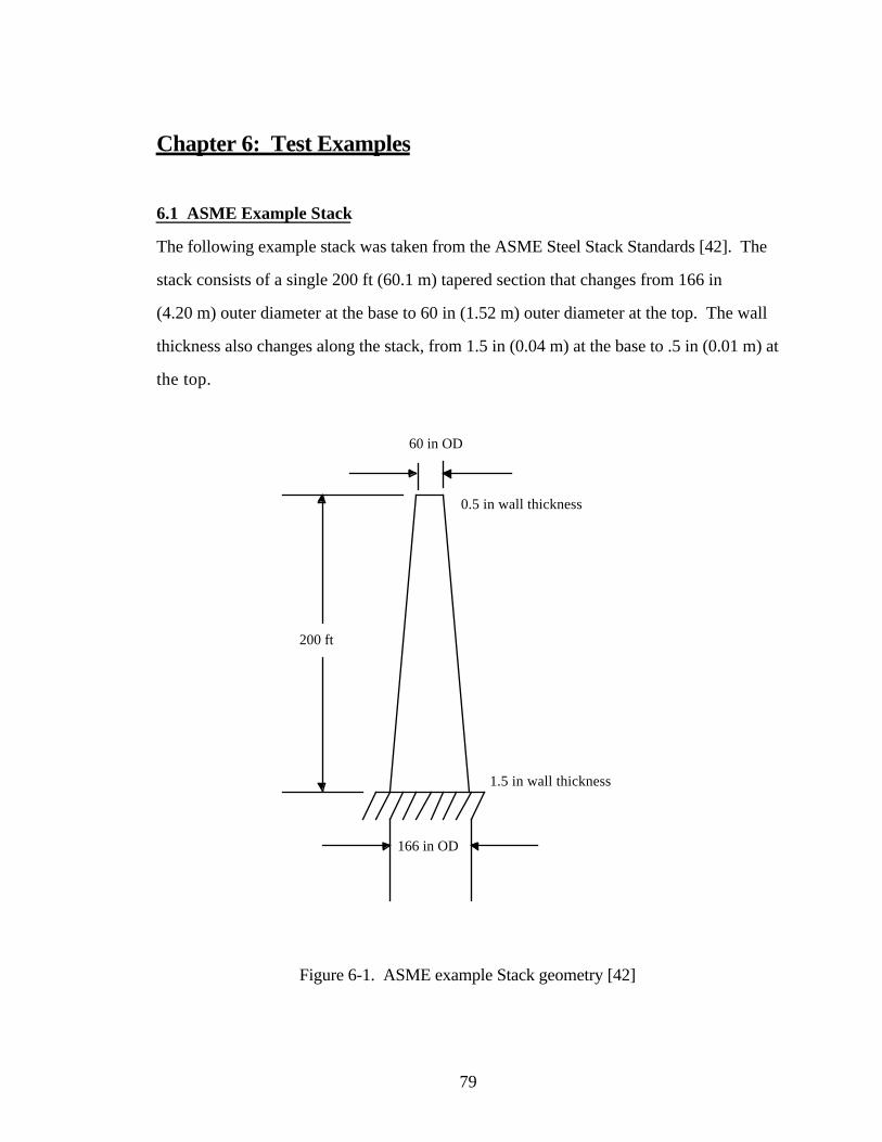
79

Chapter 6: Test Examples

6.1 ASME Example Stack

The following example stack was taken from the ASME Steel Stack Standards [42]. The

stack consists of a single 200 ft (60.1 m) tapered section that changes from 166 in

(4.20 m) outer diameter at the base to 60 in (1.52 m) outer diameter at the top. The wall

thickness also changes along the stack, from 1.5 in (0.04 m) at the base to .5 in (0.01 m) at

the top.

Figure 6-1. ASME example Stack geometry [42]

200 ft

166 in OD

60 in OD

0.5 in wall thickness

1.5 in wall thickness

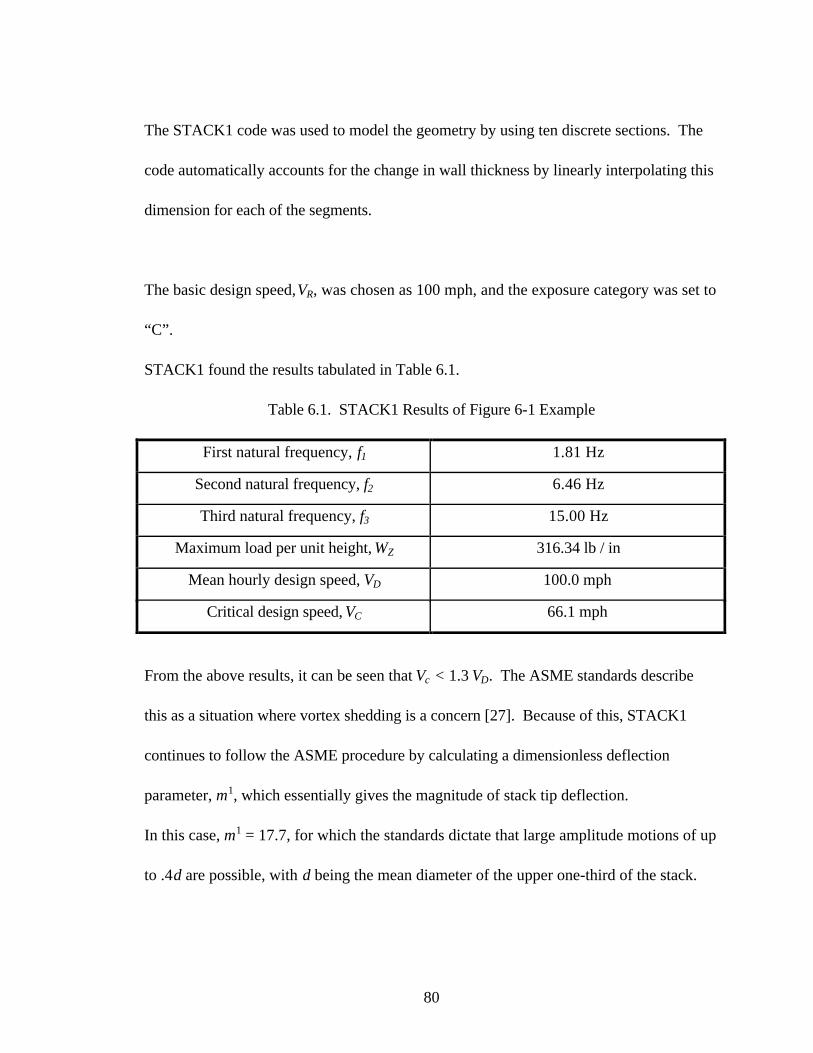
80

The STACK1 code was used to model the geometry by using ten discrete sections. The

code automatically accounts for the change in wall thickness by linearly interpolating this

dimension for each of the segments.

The basic design speed, VR, was chosen as 100 mph, and the exposure category was set to

“C”.

STACK1 found the results tabulated in Table 6.1.

Table 6.1. STACK1 Results of Figure 6-1 Example

First natural frequency, f1 1.81 Hz

Second natural frequency, f2 6.46 Hz

Third natural frequency, f3 15.00 Hz

Maximum load per unit height, WZ 316.34 lb / in

Mean hourly design speed, VD 100.0 mph

Critical design speed, VC 66.1 mph

From the above results, it can be seen that Vc < 1.3 VD. The ASME standards describe

this as a situation where vortex shedding is a concern [27]. Because of this, STACK1

continues to follow the ASME procedure by calculating a dimensionless deflection

parameter, m1, which essentially gives the magnitude of stack tip deflection.

In this case, m1 = 17.7, for which the standards dictate that large amplitude motions of up

to .4d are possible, with d being the mean diameter of the upper one-third of the stack.

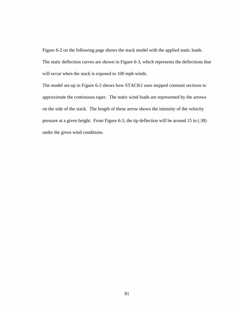
81

Figure 6-2 on the following page shows the stack model with the applied static loads.

The static deflection curves are shown in Figure 6-3, which represents the deflections that

will occur when the stack is exposed to 100 mph winds.

The model set-up in Figure 6-2 shows how STACK1 uses stepped constant sections to

approximate the continuous taper. The static wind loads are represented by the arrows

on the side of the stack. The length of these arrow shows the intensity of the velocity

pressure at a given height. From Figure 6-3, the tip deflection will be around 15 in (.38)

under the given wind conditions.

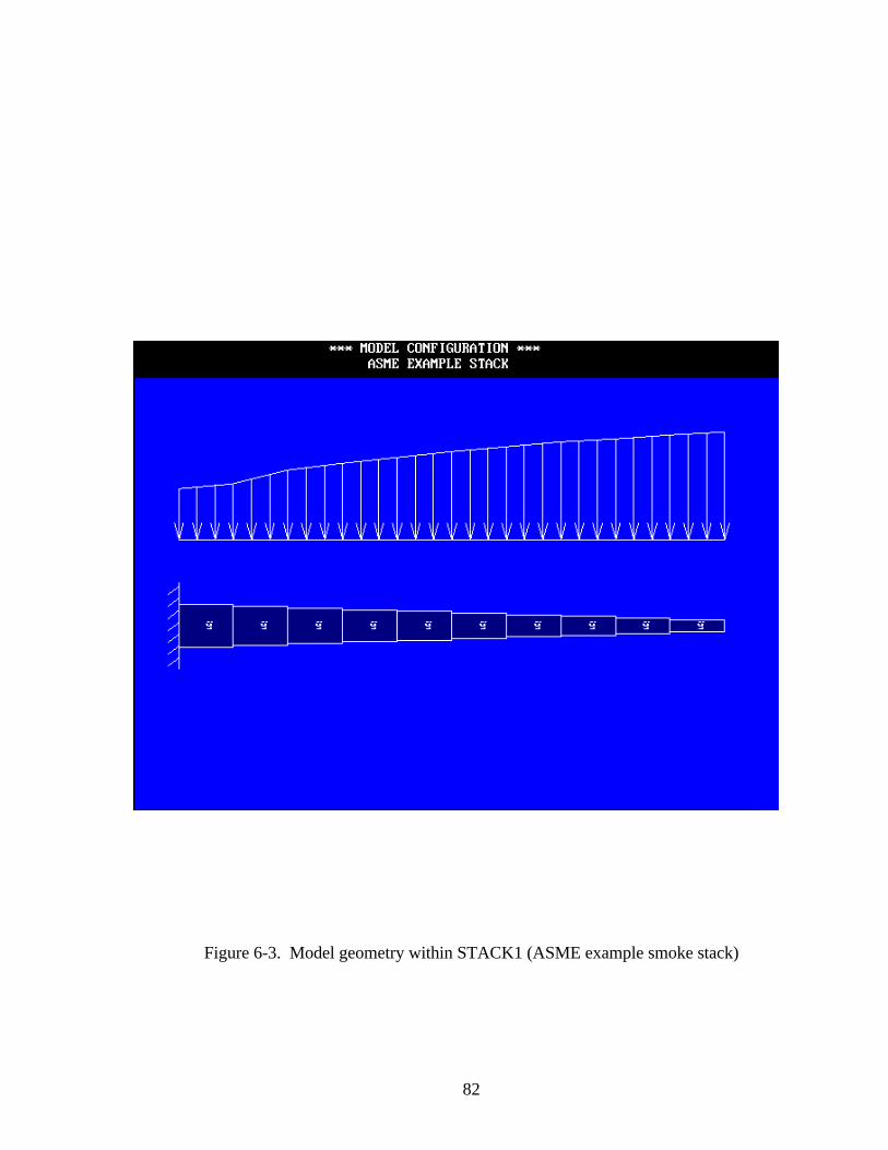
82

Figure 6-3. Model geometry within STACK1 (ASME example smoke stack)

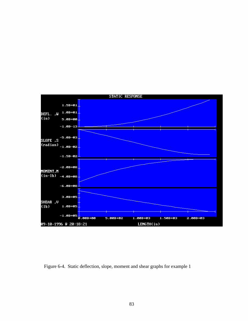
83

Figure 6-4. Static deflection, slope, moment and shear graphs for example 1

84

6.2 DUPONT Example Stack

The following example stack was taken from plans provided by DuPont. This design is

more complicated than the example demonstrated in section 6.1. This stack exploits the

tapered section option within STACK1, which provides the decreasing diameter taper and

the increasing diameter taper. The geometry of the four constant diameter sections and

three tapered sections are shown in Figure 6-4. The exposure category for this example is

"C", and the basic design wind speed is 100 mph.

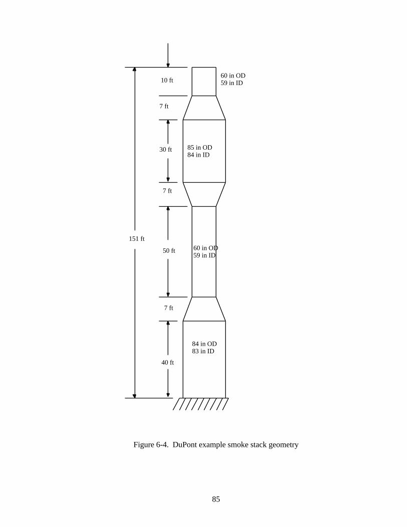
85

Figure 6-4. DuPont example smoke stack geometry

84 in OD83 in ID

151 ft

40 ft

7 ft

50 ft

7 ft

30 ft

7 ft

10 ft

60 in OD59 in ID

60 in OD59 in ID

85 in OD84 in ID

86

The STACK1 code was used to model the geometry by using various tapered and

constant sections. In this case, the tapered sections were modeled with five segments in

order to meet system memory requirements. The wall thickness of this stack is constant

throughout.

STACK1 found the results tabulated in Table 6.1.

Table 6.2. STACK1 Results of Figure 6-4 Example

First natural frequency, f1 1.03 Hz

Second natural frequency, f2 6.09 Hz

Third natural frequency, f3 17.23 Hz

Maximum load per unit height, WZ 66.56 lb / in

Mean hourly design speed, VD 100.0 mph

Critical design speed, VC 31.12 mph

From the above results, it can be seen that Vc < 1.3 VD. The ASME standards describe

this situation as similar to example 6-1, in that vortex shedding is a concern [27]. Because

of this, STACK1 continues to follow the ASME procedure by calculating a dimensionless

deflection parameter, m1, which essentially gives the magnitude of stack tip deflection.

In this case, m1 = 11.7, for which the standards dictate that large amplitude motions of up

to .4d are possible, with d being the mean diameter of the upper one-third of the stack.

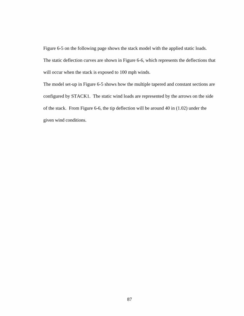
87

Figure 6-5 on the following page shows the stack model with the applied static loads.

The static deflection curves are shown in Figure 6-6, which represents the deflections that

will occur when the stack is exposed to 100 mph winds.

The model set-up in Figure 6-5 shows how the multiple tapered and constant sections are

configured by STACK1. The static wind loads are represented by the arrows on the side

of the stack. From Figure 6-6, the tip deflection will be around 40 in (1.02) under the

given wind conditions.

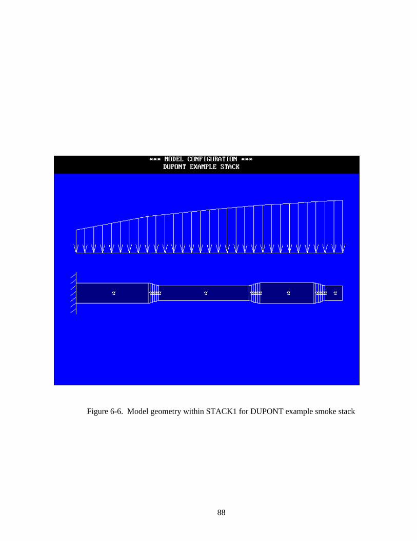
88

Figure 6-6. Model geometry within STACK1 for DUPONT example smoke stack

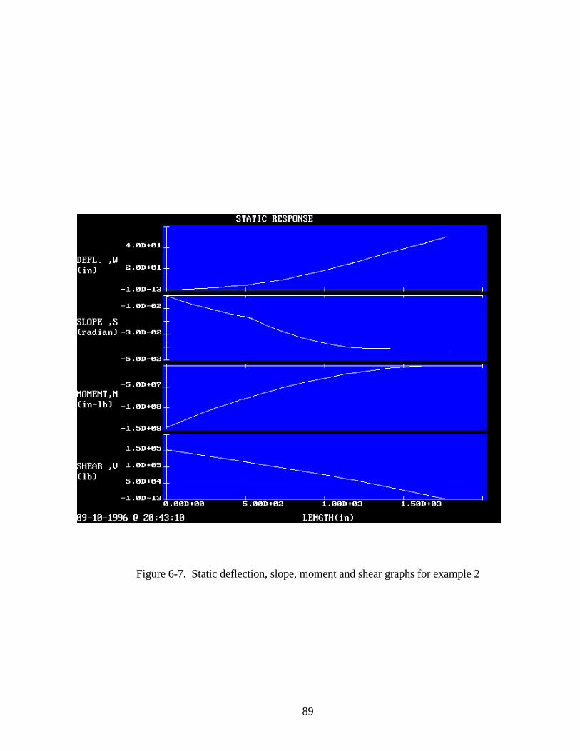
89

Figure 6-7. Static deflection, slope, moment and shear graphs for example 2

90

Chapter 7: Conclusions and Recommendations

7.1 Conclusions

In this research, the process of analyzing a steel smoke stack subject to wind loads was

studied in detail. The interaction of various aerodynamic forces such as static drag loads

and harmonic excitation by vortex shedding and atmospheric turbulence was studied in

detail. Vibrations in the along-wind direction as well as the across-wind direction were

studied, and the amplitudes of the vibration was predicted.

A computer program, STACK1, was developed which utilizes the transfer matrix method.

Many features to suit the stack analyst were incorporated in this code. First, a automatic

tapered beam generator was added to the code. Extensive studies were performed to

validate the method of modeling a tapered beam. Second, a complete static and dynamic

analysis was implemented to check the codes against the ASME Steel Stack Standards

[2]. Information regarding the static deflection and maximum vibration amplitudes are

provided to the user to expedite the design process.

91

7.2 Recommendations

To follow up on the research begun here, the following recommendations are suggested:

• Only bending vibration is treated in STACK1. Other modes of vibration, such as

axial and/or ovalling are typically concerns of stack designers as well. These

should be added to STACK1 to analyze stacks in more detail.

• The possibility of adding guy wires, stiffener rings, or other structural features

would facilitate a more accurate analysis of some stack designs.

• If possible, the operating platform of the STACK1 program should be upgraded

from DOS to WINDOWS 95, which would not only allow the program to grow

beyond the 640K memory barrier, but would also allow program debugging to

take place immensely faster than the current setup.

• A post processing module for analyzing the stresses could be implemented which

would include an option for fatigue analysis.

92

REFERENCES

1. Blevins, Robert D., Flow Induced Vibration,Van Nostrand Reinhold, New York,

1990, New York, New York, p. 78.

2. American Society of Mechanical Engineers, Steel Stacks ASME STS-1-1992,

American Society of Mechanical Engineers, 1993, p. 24.

3. Reference 2, p. 46.

4. Reference 2, p. 1.

5. Reference 2, p. iii.

6. American Society of Civil Engineers, Minimum Design Loads For Buildings and

Other Structures, American Society of Civil Engineers, New York, New York,

1995, p. 159.

7. American Society of Civil Engineers, Wind Loading and Wind-Induced Structural

Response, American Society of Civil Engineers, 1987.

8. Reference 7, p. 117.

9. Asawa, G. L.and Garde, R.J., “Atmospheric Boundary Layer and Its Simulation in

Wind Tunnels”, Wind Loads on Structures, 1991, pp. 21-37.

10. Vickery, B.J., “Wind Loads On Towers and Chimneys”, Wind Loads on Structures,

1991, pp. 87-100.

11. Reference 1, pp. 43-85.

12. Pestel, E. and Leckie, F., Matrix Methods in Elastomechanics, McGraw-Hill, New

93

York, 1963.

13. Shen, Ji Yao, “Continuous Dynamic Model for Tapered Beam-Like Structures,”

Journal of Aerospace Engineering, Vol. 7, October 1994, pp.435-445.

14. Reference 2, p. 87.

15. Cermak, Jack E, "Atmospheric Boundary Layer Modelling in Wind Tunnels," Wind

Loads on Structures, 1991, pp. 3-20.

16. Reference 15, p. 5.

17. Lin, Y. K., “Structural Response Under Turbulent Flow Excitations,” Random

Excitation of Structures by Earthquakes and Atmospheric Turbulence, CISM, Udine,

New York, 1977, p. 265.

18. Reference 2, p. 21.

19. Reference 17, p. 306.

20. Reference 17, p. 266.

21. Reference 1, p.1.

22. Reference 1, p. 36.

23. Kreith, Frank and Bohn, Mark S., Principles of Heat Transfer, West Publishing

Company, St. Paul, MN, 1993.

24. Reference 1, p. 44.

25. Reference 7, p. 118.

94

26. Reference 2, p. 79.

27. Reference 2, p. 22.

28. Reference 10, p. 89.

29. Reference 1, p. 47.

30. Reference 12, p. vii.

31. Reference 12, p. 53.

32. Reference 12, p. 51.

33. Reference 12, p. 57.

34. Reference 12, p. 58.

35. Reference 12, p. 59.

36. Reference 12, p. 60.

37. Reference 12, p. 82.

38. Reference 12, p.86.

39. Blevins, Robert D., Formulas for Natural Frequency and Mode Shape, Van

Nostrand Reinhold Company Inc., New York, 1979.

40. Pilkey, W. D., Manual for the Response of Structural Members Volume II,

Engineering Mechanics Division, IIT Research Institute, Chicago, p. III113.

41. Reference 12, pp. 132-137.

42. Reference 2, pp. 70-71.

43. Reference 2, p. 91.

95

44. Reference 2, p. 90.

45. Reference 2, p. 84.

46. Reference 2, p. 85.

47. Reference 2, p. 86.

48. Reference 2, p. 91.

49. Reference 2, p. 89.

50. Reference 12, p. 130.

51. Reference 12, p.133.

52. Reference 2, p. 78.

53. Reference 12, p. 134.

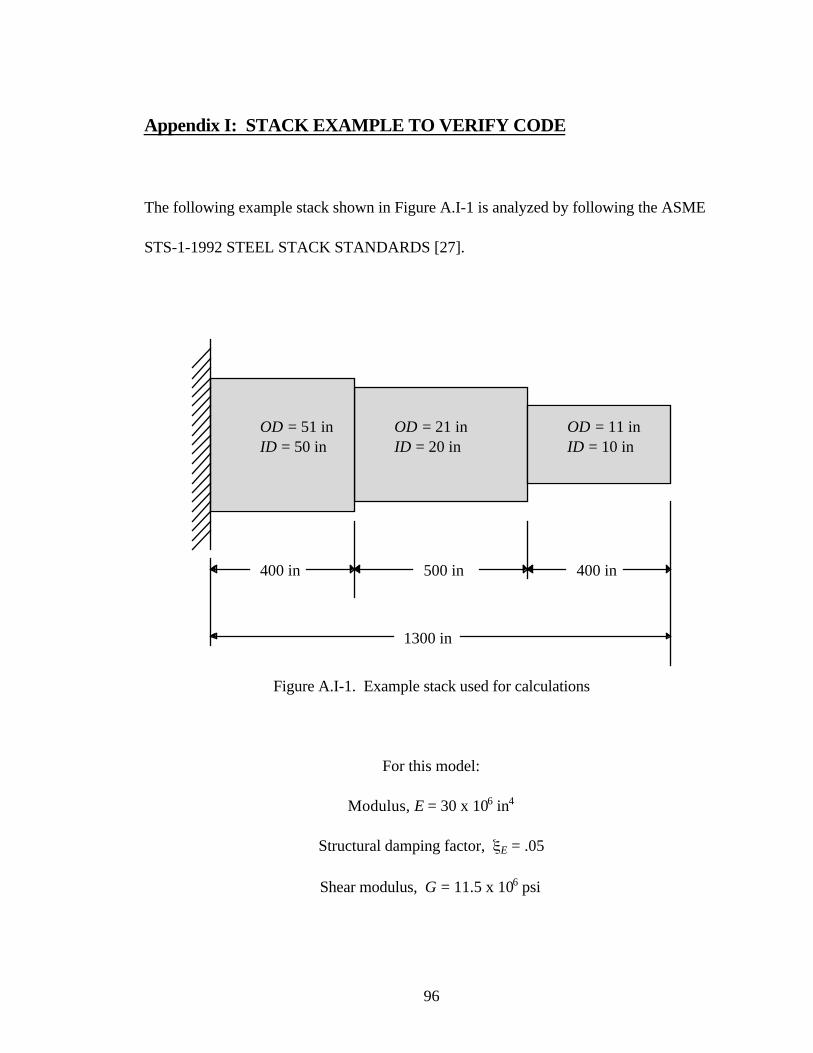
96

Appendix I: STACK EXAMPLE TO VERIFY CODE

The following example stack shown in Figure A.I-1 is analyzed by following the ASME

STS-1-1992 STEEL STACK STANDARDS [27].

Figure A.I-1. Example stack used for calculations

For this model:

Modulus, E = 30 x 106 in4

Structural damping factor, E = .05

Shear modulus, G = 11.5 x 106 psi

OD = 51 inID = 50 in

OD = 11 inID = 10 in

OD = 21 inID = 20 in

400 in500 in400 in

1300 in

97

Shear Damping factor, ξG = .05

Material density, ρ = 0.243 lb/in3

Exposure Category "C"

Basic Design Speed, Vr = 100 MPH

Equations used from ASME standards:

Velocity pressure, qz = 0.00256 Kz (VR)2 (A1.1)

where:

Kz is provided by the standards [44]

Gust response factor, GP T

D= +

+

0 65

332

1 0 0021

2 1 2

.( . )

.

/

β(A1.2)

Where:

P fJY= (A1.2a)

f = 10.5f1H/(sVR) (A1.2b)

J is provided by the standards [45]

Y is provided by the standards [46]

f1 = the first natural frequency of the stack

98

β = structural damping as a fraction of critical

S provided by the standards [47]

s provided by the standards [48]

H = total height of stack, ft.

D = diameter of stack at .8 H, ft.

VR = Basic Design Speed, mph

T1 = 2.35 (Do)1/2 / (z/30)1/α (A1.3)

where:

z = 2/3 H (A1.3a)

α is provided by the standards [48]

Do is provided by the standards [48]

Load per unit height, Wz = Cf qz D G (A1.4)

where:

Cf = a force coefficient provided by the standards [49]

Vortex shedding calculations:

Mean hourly design speed: VD(z) = 1.18 VR (Kz)1/2 (A1.5)

Where:

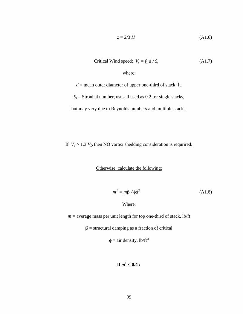
99

z = 2/3 H (A1.6)

Critical Wind speed: Vc = f1 d / St (A1.7)

where:

d = mean outer diameter of upper one-third of stack, ft.

St = Strouhal number, ususall used as 0.2 for single stacks,

but may very due to Reynolds numbers and multiple stacks.

If Vc > 1.3 VD then NO vortex shedding consideration is requrired.

Otherwise; calculate the following:

m1 = m / d2 (A1.8)

Where:

m = average mass per unit length for top one-third of stack, lb/ft

β = structural damping as a fraction of critical

= air density, lb/ft3

If m1 < 0.4 :

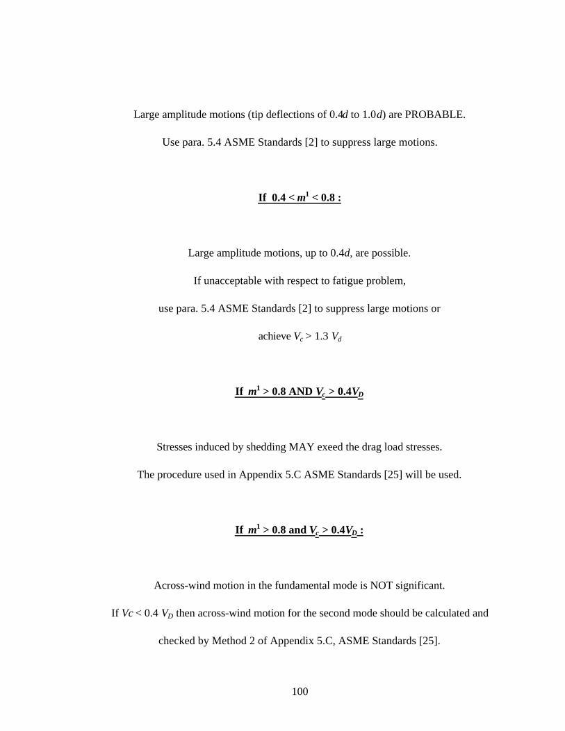
100

Large amplitude motions (tip deflections of 0.4d to 1.0d) are PROBABLE.

Use para. 5.4 ASME Standards [2] to suppress large motions.

If 0.4 < m1 < 0.8 :

Large amplitude motions, up to 0.4d, are possible.

If unacceptable with respect to fatigue problem,

use para. 5.4 ASME Standards [2] to suppress large motions or

achieve Vc > 1.3 Vd

If m1 > 0.8 AND Vc > 0.4VD

Stresses induced by shedding MAY exeed the drag load stresses.

The procedure used in Appendix 5.C ASME Standards [25] will be used.

If m1 > 0.8 and Vc > 0.4VD :

Across-wind motion in the fundamental mode is NOT significant.

If Vc < 0.4 VD then across-wind motion for the second mode should be calculated and

checked by Method 2 of Appendix 5.C, ASME Standards [25].

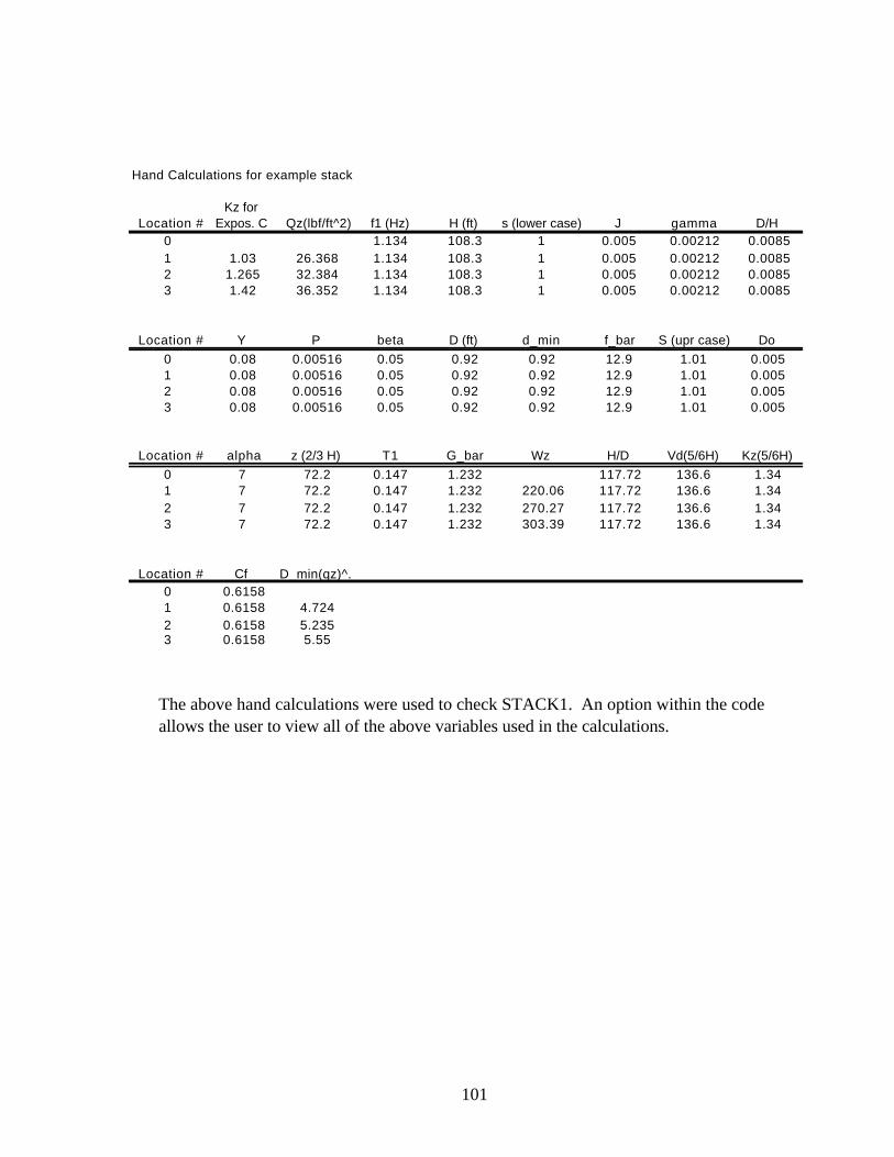
101

The above hand calculations were used to check STACK1. An option within the codeallows the user to view all of the above variables used in the calculations.

Hand Calculations for example stack

Kz forLocation # Expos. C Qz(lbf/ft^2) f1 (Hz) H (ft) s (lower case) J gamma D/H

0 1.134 108.3 1 0.005 0.00212 0.00851 1.03 26.368 1.134 108.3 1 0.005 0.00212 0.00852 1.265 32.384 1.134 108.3 1 0.005 0.00212 0.00853 1.42 36.352 1.134 108.3 1 0.005 0.00212 0.0085

Location # Y P beta D (ft) d_min f_bar S (upr case) Do

0 0.08 0.00516 0.05 0.92 0.92 12.9 1.01 0.0051 0.08 0.00516 0.05 0.92 0.92 12.9 1.01 0.0052 0.08 0.00516 0.05 0.92 0.92 12.9 1.01 0.0053 0.08 0.00516 0.05 0.92 0.92 12.9 1.01 0.005

Location # alpha z (2/3 H) T1 G_bar Wz H/D Vd(5/6H) Kz(5/6H)

0 7 72.2 0.147 1.232 117.72 136.6 1.341 7 72.2 0.147 1.232 220.06 117.72 136.6 1.342 7 72.2 0.147 1.232 270.27 117.72 136.6 1.343 7 72.2 0.147 1.232 303.39 117.72 136.6 1.34

Location # Cf D_min(qz)^.50 0.61581 0.6158 4.7242 0.6158 5.2353 0.6158 5.55

102

Appendix 2: Derivation of Tapered Transfer Matrix

A.2.1 Derivation of the transfer matrix from an nth-order differential equation

In order to obtain the transfer matrix for the flexural vibrations of a tapered beam, a

characteristic equation representing this beam needs be derived first. Drawing from the

methods described in Pestel and Leckie [50],

“The usual method of solving problems of one independent variable is to eliminate

n-1 of the dependent variables to give an nth-order ordinary differential equation in

the remaining dependent variable. If it is possible to find n closed solutions of this

equation, it is then a straightforward matter to develop the transfer matrix. The n

constants associated with the nth-order differential equation are determined by the

boundary conditions of the problem. We shall find these constants in terms of the

components of the state vector at an arbitrary point I-1 of the system.”

Therefore, it is necessary to first derive an nth order differential equation for the tapered

beam, and then find the n closed solutions to this equation.

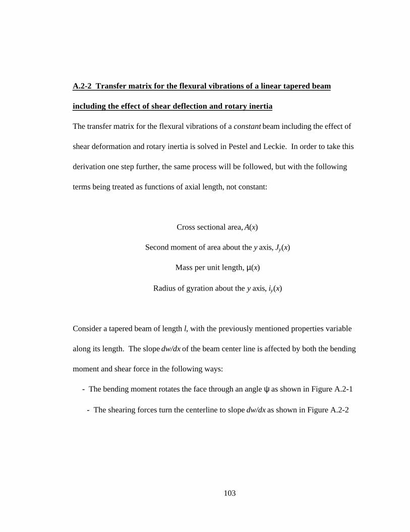
103

A.2-2 Transfer matrix for the flexural vibrations of a linear tapered beam

including the effect of shear deflection and rotary inertia

The transfer matrix for the flexural vibrations of a constant beam including the effect of

shear deformation and rotary inertia is solved in Pestel and Leckie. In order to take this

derivation one step further, the same process will be followed, but with the following

terms being treated as functions of axial length, not constant:

Cross sectional area, A(x)

Second moment of area about the y axis, Jy(x)

Mass per unit length, µ(x)

Radius of gyration about the y axis, iy(x)

Consider a tapered beam of length l, with the previously mentioned properties variable

along its length. The slope dw/dx of the beam center line is affected by both the bending

moment and shear force in the following ways:

- The bending moment rotates the face through an angle ψ as shown in Figure A.2-1

- The shearing forces turn the centerline to slope dw/dx as shown in Figure A.2-2

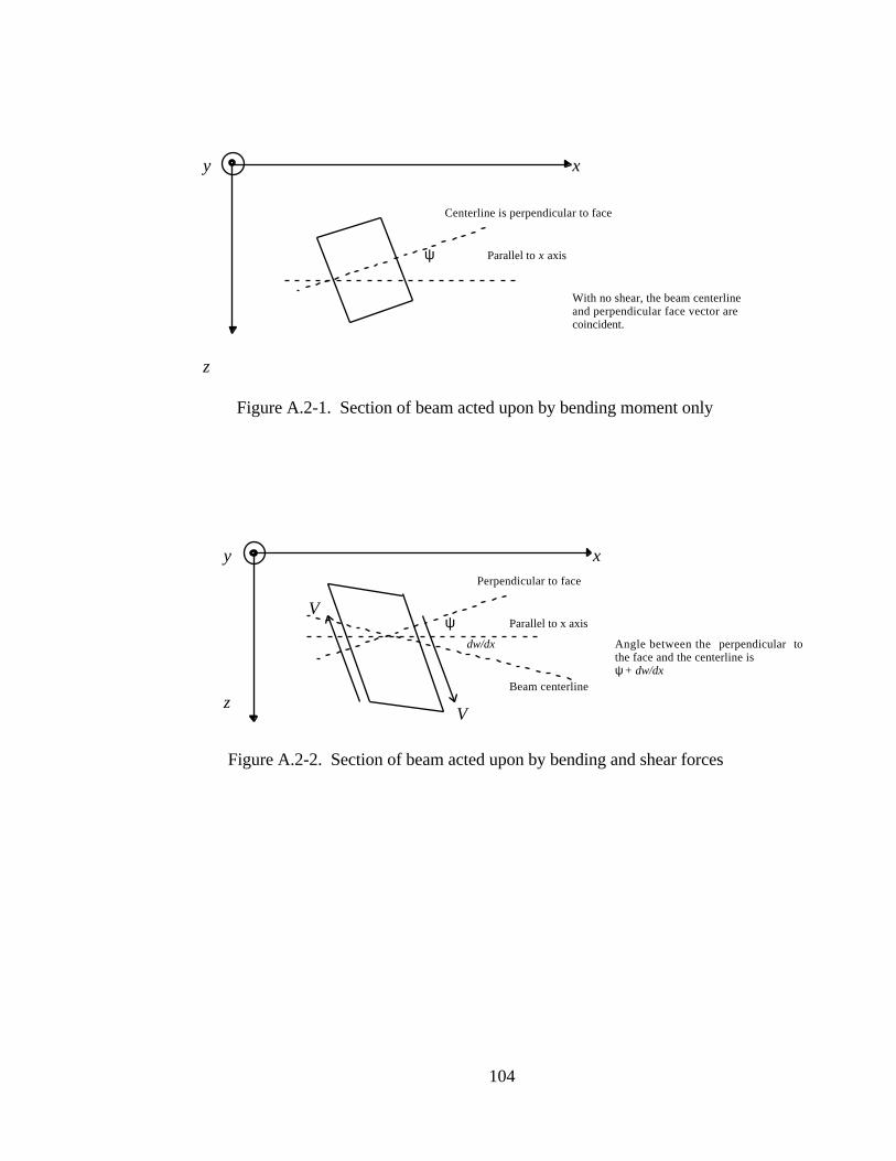
104

Figure A.2-1. Section of beam acted upon by bending moment only

Figure A.2-2. Section of beam acted upon by bending and shear forces

Perpendicular to face

Parallel to x axisψ

z

xy

Angle between the perpendicular tothe face and the centerline isψ + dw/dx

Beam centerline

V

V

dw/dx

Centerline is perpendicular to face

Parallel to x axisψ

z

With no shear, the beam centerlineand perpendicular face vector arecoincident.

xy

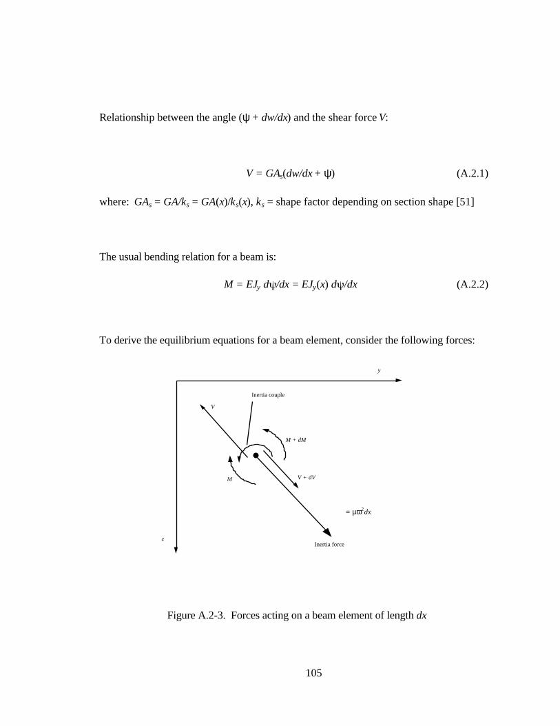
105

Relationship between the angle (ψ + dw/dx) and the shear force V:

V = GAs(dw/dx + ψ) (A.2.1)

where: GAs = GA/ks = GA(x)/ks(x), ks = shape factor depending on section shape [51]

The usual bending relation for a beam is:

M = EJy d /dx = EJy(x) d /dx (A.2.2)

To derive the equilibrium equations for a beam element, consider the following forces:

Figure A.2-3. Forces acting on a beam element of length dx

Inertia couple

Inertia force

M + dM

M

V

V + dV

z

y

= µω2dx

106

Summing the moments about the beam element:

(M+dM) - M + [ (x)iy(x)2 2 dx] - Vdx = 0

dM = Vdx - (x)iy(x)2 2 dx

dM/dx = V - (x)iy(x)2 2 (A.2.3)

Summing the forces on the beam element:

(V+dV) - V + (x) 2w(x)dx = 0

dV/dx = - (x) 2w(x) (A.2.4)

Taking the derivative of eqn(A.2.1):

dVdx

ddx

GA(x)K (x)

dwdxs

= +

ψ (A.2.5)

Substituting this expression for dV/dx into eqn(A.2.4)

ddx

GA(x)K (x)

dwdx

y x w xs

2+

= −µ ω( ) ( ) (A.2.6)

107

ddx

GA(x)K (x)

d wdx

dydx

x w xs

2

2

2

+

= −µ ω( ) ( ) (A.2.7)

Substituting in d /dx from eqn(A.2.4):

Gddx

A(x)K (x)

d w(x)dx

MEJ (x)

x w xs

2

2y

2

+

= −µ ω( ) ( ) (A.2.8)

Taking the derivative of eqn(A.2.3):

[ ]d Mdx

dVdx

ddx

x i (x) x2

2 y2 2= − µ ω ψ( ) ( )

Substitute in for d /dx from eqn(A.2.2) and dV/dx from eqn(A.2.4):

[ ]d Mdx

x w xM

EJ xddx

x i x2

22

yy

2 2= − −

µ ω µ ω( ) ( )( )

( ) ( ) (A.2.9)

Solving for M in eqn(A.2.5):

d w xdx

MEJ x

x w xG

ddx

k xA x

2

2y

2s( )

( )

( ) ( ) ( )

( )+ =

−µ ω

MEJ x

d w xdx

ddx

k xA x

x w xGy

2

2s

2

( )

( ) ( )

( )

( ) ( )= − −

µ ω

108

M EJ xd w x

dxddx

k xA x

EJ x x w x

Gy

2

2s y

2

= − −

( )

( ) ( )

( )

( ) ( ) ( )µ ω(A.2.10)

Substituting this equation for M into eqn(A.2.9):

[ ]d

dxEJ (x)

d w(x)

dx

ddx

k (x)A(x)

EJ (x) (x) w(x)

G(x) w(x)

ddx

(x)i (x)d w(x)

dx

ddx

k(x)A(x)

(x) w(x)G

2

2 y

2

2s y

22

y2 2

2

2s

2− −

=− −

−

µ ωµ ω µ ω

µ ω

Simplifying this derivative:

−

−

=E d

dxJ (x) d w(x)

dxddx

ddx

k (x)

A(x)

EJ (x) (x) w(x)

G

2

2 y

2

2

2

2s y

2µ ω

[ ]− −

−

m(x) w(x)ddx

(x)i (x)d w(x)

dxddx

k (x)

A(x)

EJ (x) (x) w(x)

G2

y2 2

2

2s y

2

ω µ ωµ ω

(A.2.11)

It is from this above equation that the transfer matrix is normally [53]. For a beam with

constant cross section, eqn(A.2.11) greatly simplifies to an ordinary differential equation

with constant coefficients. However, in order to solve this differential equation, the

expressions for Jy(x), Kx(x), A(x), (x), and iy(x) need to be derived in order to get the

equation in terms of only one variable, x. The bending moment for a cylindrical beam is

given as:

109

( )[ ]I64

D T D Tc k4

c k4= + − −

π( ) (A.2.12)

where: Dc = Centroidal Diameter, Tk = Wall thickness

For a tapered beam, the centroidal diameter is a function of the axial position, x. To

derive the bending moment for the following beam, an expression for the taper is needed.

The second moment of area of the beam shown in Figure A.2-4 (with taper angle θ and

starting radius Ro) can be shown to be:

[ ]I64

(2R 2xtan T ) (2R 2xtan T )o k4

o k4= − + − − −

πθ θ (A.2.12)

Now, the area as a function of x [A(x)] can be expressed as:

A(x) R xtan t R xtano2

o2= − + − −π θ π θ( ) ( )

Figure A.2-4. Tapered beam

R(x)

tk

x

Ro

L

θ

z

110

Mass per unit length, µ(x) is expressed as:

µ ρ ρπ θ π θ( ) ( ) ( ) ( )x A x R xtan t R xtano2

o2= = − + − − (A.2.13)

The radius of gyration as a function of length, iy(x) about the y axis is expressed as:

[ ]i

IA

64(2R 2xtan T ) (2R 2xtan T )

(R xtan t) (R xtan )y

2 xo k

4o k

4

o2

o2

= =− + − − −

− + − −

π θ θ

π θ π θ

Letting = Ro-xtan ,

[ ]i

IA

64(2 T ) (2 T )

( t) ( )y

2 xk

4k

4

2 2= =

+ − −

+ −

π α α

π α π α

When substituting the values for Jy(x), Kx(x), A(x), (x), and iy(x) back into the differential

equation of the beam, eqn(A.2.11), high orders of x are encountered, along with extremely

large amounts of differentiation and algebra. This task was attempted on the symbolic

processors, contained within the software packages MATHEMATICA® and

MATLAB®, but the size of the resulting equations grew beyond the capability of the

111

processor. Due to these difficulties, a closed-form solution of eqn(A.2.11) could not be

achieved by normal means.

It is for these reasons that the continuously tapered beam transfer matrix was not

implemented, and instead was approximated by a series of stepped beam segments. This

approach is shown in Chapter 5 to provide extremely accurate results.

Vita

Joseph Charles Servaites was born on May 22, 1972 in Dayton, Ohio, USA. After

graduating from high school in 1990, he enrolled in the University of Cincinnati, Ohio,

where he received a Bachelors of Science degree in Mechanical Engineering in 1995. While

obtaining this degree he was employed as a co-op at G. E. Aircraft Engines in Cincinnati,

Ohio. In Fall of 1995 he enrolled in Virginia Polytechnic and State University in

Blacksburg, Virginia where he completed his Masters of Science degree in September,

1996. He plans to start work with G. E. Aircraft Engines in October, 1996. His research

was sponsored by the DuPont company.