Buy-in Bulk Active Learning

Liu Yang Jaime Carbonell

December 2012 CMU-ML-12-110

Buy-in-Bulk Active Learning

Liu Yang Jaime CarbonellDecember 2012

CMU-ML-12-110

School of Computer ScienceCarnegie Mellon University

Pittsburgh, PA 15213

Abstract

In many practical applications of active learning, it is more cost-effective to request labels in largebatches, rather than one-at-a-time. This is because the cost of labeling a large batch of examplesat once is often sublinear in the number of examples in the batch. In this work, we study thelabel complexity of active learning algorithms that request labels in a given number of batches,as well as the tradeoff between the total number of queries and the number of rounds allowed.We additionally study the total cost sufficient for learning, for an abstract notion of the cost ofrequesting the labels of a given number of examples at once. In particular, we find that for sublinearcost functions, it is often desirable to request labels in large batches (i.e., buying in bulk); althoughthis may increase the total number of labels requested, it reduces the total cost required for learning.

This research is supported in part by NSF grant IIS-1065251 and a Google Core AI grant.

Keywords: Active Learning, Batch Queries, Sample Complexity

1 IntroductionIn many practical applications of active learning, the cost to acquire a large batch of labels at once issignificantly less than the cost of the same number of sequential rounds of individual label requests.This is true for both practical reasons (overhead time for start-up, reserving equipment in discretetime-blocks, multiple labelers working in parallel, etc.) and for computational reasons (e.g., timeto update the learner’s hypothesis and select the next examples may be large). Consider makingone vs multiple hematological diagnostic tests on an out-patient. There are fixed up-front costs:bringing the patient in for testing, drawing and storing the blood, entring the information in thehospital record system, etc. And there are variable costs, per specific test. Consider a microarrayassay for gene expression data. There is a fixed cost in setting up and running the microarray, butvirtually no incremental cost as to the number of samples, just a constraint on the max allowed.Either of the above conditions are often the case in scientific experiments (e.g., [Sheng & Ling,2006]), As a different example, consider calling a focused group of experts to address questionsw.r.t new product design or introduction. There is a fixed cost in forming the group (determinemembership, contract, travel, etc.), and a incremental per-question cost. The common abstractionin such real-world versions of “oracles” is that learning can buy-in-bulk to advantage becase oraclescharge either per batch (answering a batch of questions for the same cost the same as answering asingle question up to match maximum), or the cost per batch is axp + b, where b is the set-up cost,a is the number of queries (if normalized for unit cost), and p = 1 or p < 1 (for the case wherepractice yields efficiency).

Often we have other tradeoffs, such as delay vs testing cost. For instance in a medical diagnosiscase, the most cost-effective way to minimize diagnostic tests is purely sequential active learning,where each test may rule out a set of hypotheses (diagnoses) and informs the next test to perform.But a patient suffering from a serious disease may worsen while sequential tests are being con-ducted. Hence batch testing makes sense if the batch can be tested in parallel. In general one canconvert delay into a second cost factor and optimize for batch size that minimizes a combination oftotal delay and the sum of the costs for the individual tests. Parallelizing means more tests wouldbe needed, since we lack the benefit of earlier tests to rule out future ones. In order to perform thisbatch-size optimization we also need to estimate the number of redundant tests incurred by turninga sequence into a shorter sequence of batches.

For the reasons cited above, it can be very useful in practice to generalize active learning toactive-batch learning, with buy-in-bulk discounts. This paper developes a theoretical frameworkexploring the bounds and sample compelxity of active buy-in-bulk machine learning, and analyzingthe tradeoff that can be achieved between the number of batches and the total number of queriesrequired for accurate learning.

In another example, if we have many labelers (virtually unlimited) operating in parallel, butmust pay for each query, and the amount of time to get back the answer to each query is consideredindependent with some distribution, it may often be the case that the expected amount of timeneeded to get back the answers to m queries is sublinear in m, so that if the “cost” is a functionof both the payment amounts and the time, it might sometimes be less costly to submit multiplequeries to be labeled in parallel. In scenarios such as those mentioned above, a batch mode activelearning strategy is desirable, rather than a method that selects instances to be labeled one-at-a-

1

time.There have recently been several attempts to construct heuristic approaches to the batch mode

active learning problem (e.g., [Chakraborty et al., 2010]). However, theoretical analysis has beenlargely lacking. In contrast, there has recently been significant progress in understanding the ad-vantages of fully-sequential active learning (e.g., [Dasgupta et al., 2009, Dasgupta, 2005, Balcanet al., 2006, Hanneke, 2007, Hanneke, 2011]). In the present work, we are interested in extendingthe techniques used for the fully-sequential active learning model, studying natural analogues ofthem for the batch-model active learning model.

Formally, we are interested in two quantities: the sample complexity and the total cost. Thesample complexity refers to the number of label requests used by the algorithm. We expect batch-mode active learning methods to use more label requests than their fully-sequential cousins. Onthe other hand, if the cost to obtain a batch of labels is sublinear in the size of the batch, then wemay sometimes expect the total cost used by a batch-mode learning method to be significantly lessthan the analogous fully-sequential algorithms, which request labels individually.

2 Definitions and NotationAs in the usual statistical learning problem, there is a standard Borel space X , called the instancespace, and a set C of measurable classifiers h : X → {−1,+1}, called the concept space. Through-out, we suppose that the VC dimension of C, denoted d below, is finite.

In the learning problem, there is an unobservable distribution DXY over X ×{−1,+1}. Basedon this quantity, we let Z = {(Xt, Yt)}∞t=1 denote an infinite sequence of independent DXY -distributed random variables. We also denote by Zt = {(X1, Y1), (X2, Y2), . . . , (Xt, Yt)} the firstt such labeled examples. Additionally denote by DX the marginal distribution of DXY over X .For a classifier h : X → {−1,+1}, denote er(h) = P(X,Y )∼DXY (h(X) 6= Y ), the error rate ofh. Additionally, for m ∈ N and Q ∈ (X × {−1,+1})m, let er(h;Q) = 1

|Q|∑

(x,y)∈Q I[h(x) 6= y],the empirical error rate of h. In the special case that Q = Zm, abbreviate erm(h) = er(h;Q).For r > 0, define B(h, r) = {g ∈ C : DX(x : h(x) 6= g(x)) ≤ r}. For any H ⊆ C, defineDIS(H) = {x ∈ X : ∃h, g ∈ H s.t. h(x) 6= g(x)}. We also denote by η(x) = P (Y = +1|X = x),where (X, Y ) ∼ DXY , and let h∗(x) = sign(η(x)− 1/2) denote the Bayes optimal classifier.

In the active learning protocol, the algorithm has direct access to the Xt sequence, but mustrequest to observe each label Yt, sequentially. The algorithm asks up to a specified number of labelrequests n (the budget), and then halts and returns a classifier. We are particularly interested indetermining, for a given algorithm, how large this number of label requests needs to be in orderto guarantee small error rate with high probability, a value known as the label complexity. In thepresent work, we are also interested in the cost expended by the algorithm. Specifically, in thiscontext, there is a cost function c : N→ (0,∞), and to request the labels {Yi1 , Yi2 , . . . , Yim} of mexamples {Xi1 , Xi2 , . . . , Xim} at once requires the algorithm to pay c(m); we are then interestedin the sum of these costs, over all batches of label requests made by the algorithm. Depending onthe form of the cost function, minimizing the cost of learning may actually require the algorithmto request labels in batches, which we expect would actually increase the total number of labelrequests.

2

To help quantify the label complexity and cost complexity, we make use of the followingdefinition, due to [Hanneke, 2007, Hanneke, 2011].

Definition 2.1. [Hanneke, 2007, Hanneke, 2011] Define the disagreement coefficient of h∗ as

θ(ε) = supr>ε

DX (DIS(B(h∗, r)))

r.

3 Buy-in-Bulk Active Learning in the Realizable Case: k-batchCAL

We begin our anlaysis with the simplest case: namely, the realizable case, with a fixed prespecifiednumber of batches. We are then interested in quantifying the label complexity for such a scenario.

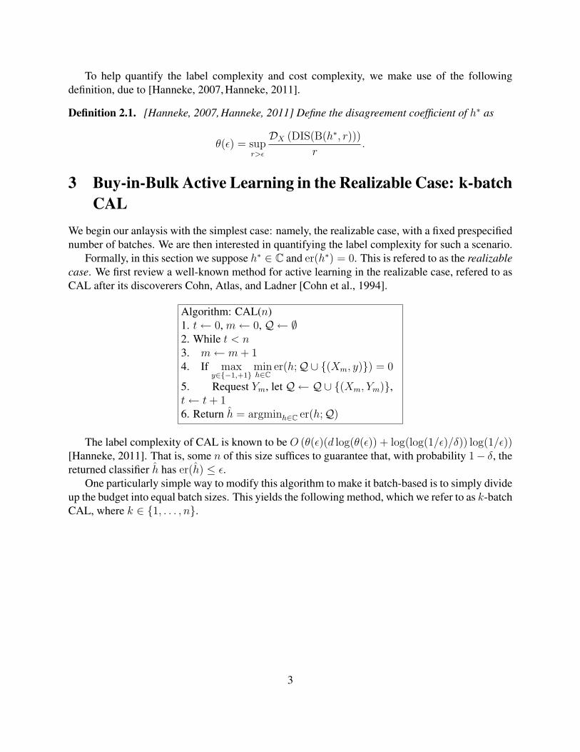
Formally, in this section we suppose h∗ ∈ C and er(h∗) = 0. This is refered to as the realizablecase. We first review a well-known method for active learning in the realizable case, refered to asCAL after its discoverers Cohn, Atlas, and Ladner [Cohn et al., 1994].

Algorithm: CAL(n)1. t← 0, m← 0, Q ← ∅2. While t < n3. m← m+ 14. If max

y∈{−1,+1}minh∈C

er(h;Q∪ {(Xm, y)}) = 0

5. Request Ym, let Q ← Q∪ {(Xm, Ym)},t← t+ 16. Return h = argminh∈C er(h;Q)

The label complexity of CAL is known to be O (θ(ε)(d log(θ(ε)) + log(log(1/ε)/δ)) log(1/ε))[Hanneke, 2011]. That is, some n of this size suffices to guarantee that, with probability 1− δ, thereturned classifier h has er(h) ≤ ε.

One particularly simple way to modify this algorithm to make it batch-based is to simply divideup the budget into equal batch sizes. This yields the following method, which we refer to as k-batchCAL, where k ∈ {1, . . . , n}.

3

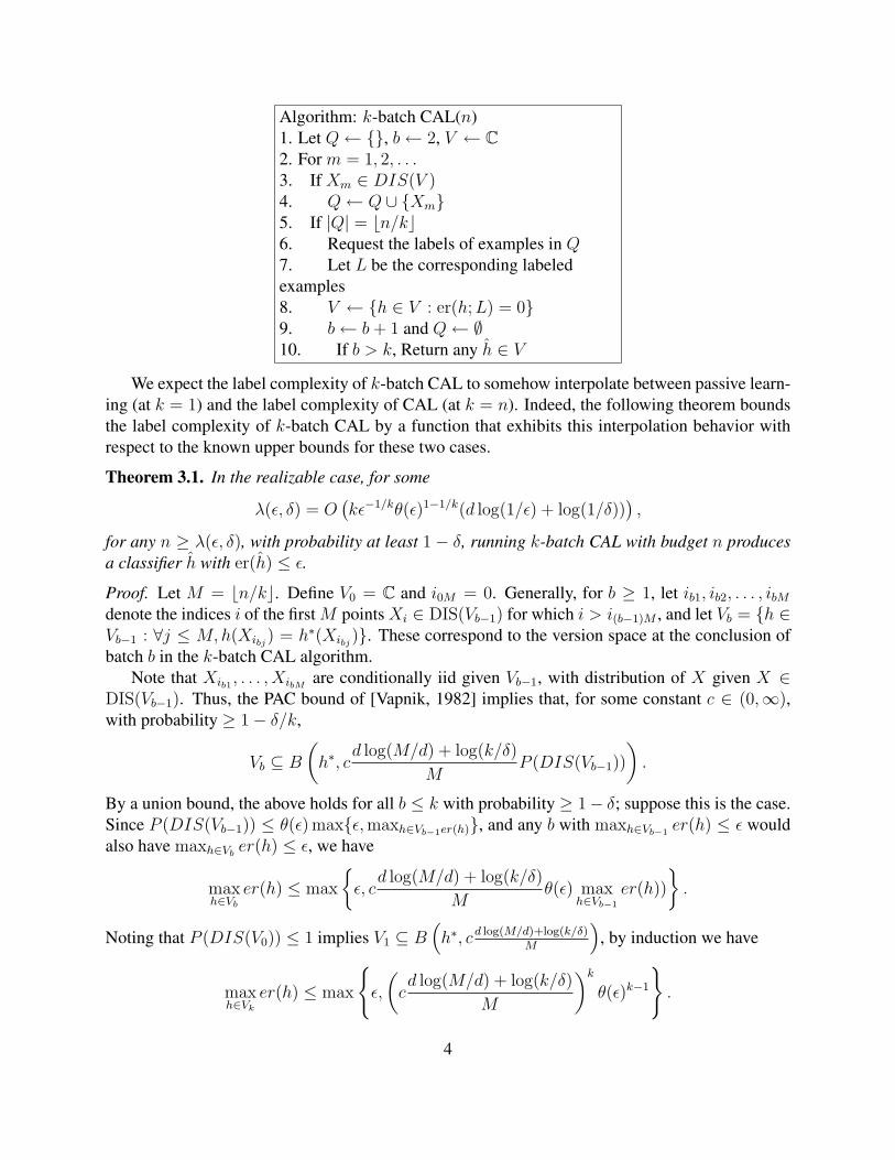
Algorithm: k-batch CAL(n)1. Let Q← {}, b← 2, V ← C2. For m = 1, 2, . . .3. If Xm ∈ DIS(V )4. Q← Q ∪ {Xm}5. If |Q| = bn/kc6. Request the labels of examples in Q7. Let L be the corresponding labeledexamples8. V ← {h ∈ V : er(h;L) = 0}9. b← b+ 1 and Q← ∅10. If b > k, Return any h ∈ V

We expect the label complexity of k-batch CAL to somehow interpolate between passive learn-ing (at k = 1) and the label complexity of CAL (at k = n). Indeed, the following theorem boundsthe label complexity of k-batch CAL by a function that exhibits this interpolation behavior withrespect to the known upper bounds for these two cases.

Theorem 3.1. In the realizable case, for some

λ(ε, δ) = O(kε−1/kθ(ε)1−1/k(d log(1/ε) + log(1/δ))

),

for any n ≥ λ(ε, δ), with probability at least 1 − δ, running k-batch CAL with budget n producesa classifier h with er(h) ≤ ε.

Proof. Let M = bn/kc. Define V0 = C and i0M = 0. Generally, for b ≥ 1, let ib1, ib2, . . . , ibMdenote the indices i of the first M points Xi ∈ DIS(Vb−1) for which i > i(b−1)M , and let Vb = {h ∈Vb−1 : ∀j ≤ M,h(Xibj) = h∗(Xibj)}. These correspond to the version space at the conclusion ofbatch b in the k-batch CAL algorithm.

Note that Xib1 , . . . , XibM are conditionally iid given Vb−1, with distribution of X given X ∈DIS(Vb−1). Thus, the PAC bound of [Vapnik, 1982] implies that, for some constant c ∈ (0,∞),with probability ≥ 1− δ/k,

Vb ⊆ B

(h∗, c

d log(M/d) + log(k/δ)

MP (DIS(Vb−1))

).

By a union bound, the above holds for all b ≤ k with probability ≥ 1− δ; suppose this is the case.Since P (DIS(Vb−1)) ≤ θ(ε) max{ε,maxh∈Vb−1er(h)}, and any b with maxh∈Vb−1

er(h) ≤ ε wouldalso have maxh∈Vb er(h) ≤ ε, we have

maxh∈Vb

er(h) ≤ max

{ε, c

d log(M/d) + log(k/δ)

Mθ(ε) max

h∈Vb−1

er(h))

}.

Noting that P (DIS(V0)) ≤ 1 implies V1 ⊆ B(h∗, cd log(M/d)+log(k/δ)

M

), by induction we have

maxh∈Vk

er(h) ≤ max

{ε,

(cd log(M/d) + log(k/δ)

M

)kθ(ε)k−1

}.

4

For some constant c′ > 0, any M ≥ c′ θ(ε)k−1k

ε1/k

(d log 1

ε+ log(k/δ)

)makes the right hand side ≤ ε.

Since M = bn/kc, it suffices to have n ≥ k

(1 + c′ θ(ε)

k−1k

ε1/k

(d log 1

ε+ log(k/δ)

)).

Theorem 3.1 has the property that, when the disagreement coefficient is small, the stated boundon the total number of label requests sufficient for learning is a decreasing function of k. Thismakes sense, since θ(ε) small would imply that fully-sequential active learning is much better thanpassive learning. Small values of k correspond to more passive-like behavior, while larger valuesof k take fuller advantage of the sequential nature of active learning. Note, however, that evenk = 2 can sometimes provide significant reductions in label complexity over passive learning: forinstance, by a factor proportional to 1/

√ε in the case that θ(ε) is bounded by a finite constant.

4 Batch Mode Active Learning with Tsybakov noiseThe above analysis was for the realizable case. While this provides a particularly clean and simpleanalysis, it is not sufficiently broad to cover many realistic learning applications. To move beyondthe realizable case, we need to allow the labels to be noisy, so that er(h∗) > 0. One popular noisemodel in the statistical learning theory literature is Tsybakov noise, which is defined as follows.

Definition 4.1. [Mammen & Tsybakov, 1999] The distribution DXY satisfies Tsybakov noise ifh∗ ∈ C, and for some c > 0 and α ∈ [0, 1],

∀t > 0,P(|η(x)− 1/2| < t) < c1tα

1−α ,

equivalently, ∀h, P (h(x) 6= h∗(x)) ≤ c2(er(h)− er(h∗))α, where c1 and c2 are constants.

Supposing DXY satisfies Tsybakov noise, we define a quantity

Em = c3

(d log(m/d) + log(km/δ)

m

) 12−α

.

based on a standard generalization bound for passive learning [Massart & Nedelec, 2006]. Specif-ically, [Massart & Nedelec, 2006] have shown that, for any V ⊆ C, with probability at least1− δ/(4km2),

suph,g∈V

|(er(h)− er(g))− (erm(h)− erm(g))| < Em. (1)

Consider the following modification of k-batch CAL, designed to be robust to Tsybakov noise.We refer to this method as k-batch Robust CAL, where k ∈ {1, . . . , n}.

5

Algorithm: k-batch Robust CAL(n)1. Let Q← {}, b← 1, V ← C, m1 ← 02. For m = 1, 2, . . .3. If Xm ∈ DIS(V )4. Q← Q ∪ {Xm}5. If |Q| = bn/kc6. Request the labels of examples in Q7. Let L be the corresponding labeledexamples8. V ← {h ∈ V :

(er(h;L)−ming∈V er(g;L)) bn/kcm−mb

≤ Em−mb}9. b← b+ 1 and Q← ∅10. mb ← m11. If b > k, Return any h ∈ V

We have the following result concerning this algorithm.

Theorem 4.2. Under the Tsybakov noise condition, letting β = α2−α , and β =

∑k−1i=0 β

i, for someλ(ε, δ) =

O

(k

(1

ε

) 2−αβ

(c2θ(c2εα))

1−βk−1

β ×(d log

(d

ε

)+ log

(kd

δε

)) 1+ββ−βkβ

),

for any n ≥ λ(ε, δ), with probability at least 1 − δ, running k-batch Robust CAL with budget nproduces a classifier h with er(h)− er(h∗) ≤ ε.

Proof. Let M = bn/kc. Define i0M = 0 and V0 = C. Generally, for b ≥ 1, let ib1, ib2, . . . , ibMdenote the indices i of the first M points Xi ∈ DIS(Vb−1) for which i > i(b−1)M , and let Qb ={(Xib1 , Yib1), . . . , (XibM , YibM )} and Vb = {h ∈ Vb−1 : (er(h;Qb)−ming∈Vb−1

er(g;Qb))M

ibM−i(b−1)M≤

EibM−i(b−1)M}. These correspond to the set V at the conclusion of batch b in the k-batch Robust

CAL algorithm.For b ∈ {1, . . . , k}, (1) (applied under the conditional distribution given Vb−1, combined with

the law of total probability) implies that ∀m > 0, letting

Zb,m = {(Xi(b−1)M+1, Yi(b−1)M+1), ..., (Xi(b−1)M+m, Yi(b−1)M+m)},

with probability at least 1− δ/(4km2), if h∗ ∈ Vb−1, then er(h∗;Zb,m)−ming∈Vb−1er(g;Zb,m) <

Em, and every h ∈ Vb−1 with er(h;Zb,m)−ming∈Vb−1er(g;Zb,m) ≤ Em has er(h)− er(h∗) < 2Em.

By a union bound, this holds for all m ∈ N, with probability at least 1 − δ/(2k). In particular,this means it holds for m = ibM − i(b−1)M . But note that for this value of m, any h, g ∈ Vb−1 haveer(h;Zb,m) − er(g;Zb,m) = (er(h;Qb) − er(g;Qb))

Mm

(since for every (x, y) ∈ Zb,m \ Qb, eitherboth h and g make a mistake, or neither do). Thus if h∗ ∈ Vb−1, we have h∗ ∈ Vb as well, andfurthermore suph∈Vb er(h) − er(h∗) < 2EibM−i(b−1)M

. By induction (over b) and a union bound,

6

these are satisfied for all b ∈ {1, . . . , k} with probability at least 1− δ/2. For the remainder of theproof, we suppose this 1− δ/2 probability event occurs.

Next, we focus on lower bounding ibM − i(b−1)M , again by induction. As a base case, weclearly have i1M − i0M ≥ M . Now suppose some b ∈ {2, . . . , k} has i(b−1)M − i(b−2)M ≥Tb−1 for some Tb−1. Then, by the above, we have suph∈Vb−1

er(h) − er(h∗) < 2ETb−1. By the

Tsybakov noise condition, this implies Vb−1 ⊆ B(h∗, c2

(2ETb−1

)α), so that if suph∈Vb−1er(h) −

er(h∗) > ε, P (DIS(Vb−1)) ≤ θ(c2εα)c2

(2ETb−1

)α. Now note that the conditional distributionof ibM − i(b−1)M given Vb−1 is a negative binomial random variable with parameters M and 1 −P (DIS(Vb−1)) (that is, a sum of M Geometric(P (DIS(Vb−1))) random variables). A Chernoffbound (applied under the conditional distribution given Vb−1) implies that P (ibM − i(b−1)M <M/(2P (DIS(Vb−1)))|Vb−1) < e−M/6. Thus, for Vb−1 as above, with probability at least 1− e−M/6,ibM − i(b−1)M ≥ M

2θ(c2εα)c2(2ETb−1)α

. Thus, we can define Tb as in the right hand side, which thereby

defines a recurrence. By induction, with probability at least 1− ke−M/6 > 1− δ/2,

ikM − i(k−1)M ≥M β

(1

4c2θ(c2εα)

)β−βk−1

×(

1

2(d log(M) + log(kM/δ))

)β(β−βk−1)

.

By a union bound, with probability 1−δ, this occurs simultaneously with the above suph∈Vk er(h)−er(h∗) < 2EikM−i(k−1)M

bound. Combining these two results yields

suph∈Vk

er(h)− er(h∗) = O

(((c2θ(c2ε

α))β−βk−1

M β

) 12−α

× (d log(M) + log(kM/δ))1+β(β−βk−1)

2−α

).

Setting this to ε and solving for n, we find that it suffices to have

M ≥ c4

(1

ε

) 2−αβ

(c2θ(c2εα))

1−βk−1

β ×(d log

(d

ε

)+ log

(kd

δε

)) 1+ββ−βkβ

,

for some constant c4 ∈ [1,∞), which then implies the stated result.

Note: the threshold Em in k-batch Robust CAL has a direct dependence on the parameters ofthe Tsybakov noise condition. In practice, such information is not often available. However, wecan replace Em with a data-dependent local Rademacher complexity bound Em, as in [Hanneke,2011], which also satisfies (1), and satisfies (with high probability) Em ≤ c′Em, for some constantc′ ∈ [1,∞) (see [Koltchinskii, 2006]).

When k = 1, Theorem 4.2 matches the best results for passive learning (up to log factors),which are known to be minimax optimal (again, up to log factors). If we let k become large (whilestill considered as a constant), our result converges to the known results for one-at-a-time activelearning with RobustCAL (again, up to log factors) [Hanneke, 2011, Hanneke, 2012]. Althoughthose results are not always minimax optimal, they do represent the state-of-the-art in the generalanalysis of active learning, and they are really the best we could hope for from basing our algorithmon RobustCAL.

7

5 Buy-in-Bulk Solutions to Cost-Adaptive Active LearningThe above sections discussed scenarios in which we have a fixed number k of batches, and wesimply bounded the label complexity achievable within that constraint by considering a variant ofCAL that uses k equal-sized batches. In this section, we take a slightly different approach to theproblem, by going back to one of the motivations for using batch-based active learning in the firstplace: namely, sublinear costs for answering batches of queries at a time. If the cost of answeringm queries at once is sublinear in m, then batch-based algorithms arise naturally from the problemof optimizing the total cost required for learning.

Formally, in this section, we suppose we are given a cost function c : (0,∞)→ (0,∞), whichis nondecreasing, satisfies c(αx) ≤ αc(x) (for x, α ∈ [1,∞)) , and further satisfies the conditionthat for every q ∈ N, ∃q′ ∈ N such that 2c(q) ≤ c(q′) ≤ 4c(q), which typically amounts to a kindof smoothness assumption.

To understand the total cost required for learning in this model, we consider the followingcost-adaptive modification of the CAL algorithm.

Algorithm: Cost-Adaptive CAL(C)1. Q ← ∅, R← DIS(C), V ← C, t← 02. Do3. q ← 14. Do until P (DIS(V )) ≤ P (R)/25. Let q′ > q be minimal such thatc(q′ − q) ≥ 2c(q)6. If c(q′ − q) + t > C, Return any h ∈ V7. Request the labels of the next q′ − q

examples in DIS(V )8. Update V by removing those classifiers

inconsistent with these labels9. Let t← t+ c(q′ − q)10. q ← q′

11. R← DIS(V )

Note that the total cost expended by this method never exceeds the budget argument C. Wehave the following result on how large of a budget C is sufficient for this method to succeed.

Theorem 5.1. In the realizable case, for some λ(ε, δ) =

O (c (θ(ε) (d log(θ(ε)) + log(log(1/ε)/δ))) log(1/ε)) ,

for any C ≥ λ(ε, δ), with probability at least 1 − δ, Cost-Adaptive CAL(C) returns a classifier hwith er(h) ≤ ε.

Proof. Supposing an unlimited budget (C = ∞), let us determine how much cost the algorithmincurs prior to having suph∈V er(h) ≤ ε; this cost would then be a sufficient size for C to guarantee

8

this occurs. First, note that h∗ ∈ V is maintained as an invariant throughout the algorithm. Also,note that if q is ever at least as large as O(θ(ε)(d log(θ(ε)) + log(1/δ′))), then as in the analysisfor CAL [Hanneke, 2011], we can conclude (via the PAC bound of [Vapnik, 1982]) that withprobability at least 1− δ′,

suph∈V

P (h(X) 6= h∗(X)|X ∈ R) ≤ 1/(2θ(ε)),

so thatsuph∈V

er(h) = suph∈V

P (h(X) 6= h∗(X)|X ∈ R)P (R) ≤ P (R)/(2θ(ε)).

We know R = DIS(V ′) for the set V ′ which was the value of the variable V at the time this R wasobtained. Supposing suph∈V ′ er(h) > ε, we know (by the definition of θ(ε)) that

P (R) ≤ P

(DIS

(B

(h∗, sup

h∈V ′er(h)

)))≤ θ(ε) sup

h∈V ′er(h).

Therefore,

suph∈V

er(h) ≤ 1

2suph∈V ′

er(h).

In particular, this implies the condition in Step 4 will be satisfied if this happens while suph∈V er(h) >ε. But this condition can be satisfied at most dlog2(1/ε)e times while suph∈V er(h) > ε (sincesuph∈V er(h) ≤ P (DIS(V ))). So with probability at least 1−δ′dlog2(1/ε)e, as long as suph∈V er(h) >ε, we always have c(q) ≤ 4c(O(θ(ε)(d log(θ(ε))+log(1/δ′)))) ≤ O(c(θ(ε)(d log(θ(ε))+log(1/δ′)))).Letting δ′ = δ/dlog2(1/ε)e, this is 1−δ. So for each round of the outer loop while suph∈V er(h) >ε, by summing the geometric series of cost values c(q′ − q) in the inner loop, we find the total costincurred is at mostO(c(θ(ε)(d log(θ(ε))+log(log(1/ε)/δ)))). Again, there are at most dlog2(1/ε)erounds of the outer loop while suph∈V er(h) > ε, so that the total cost incurred before we havesuph∈V er(h) ≤ ε is at most O(c(θ(ε)(d log(θ(ε)) + log(log(1/ε)/δ))) log(1/ε)).

Comparing this result to the known label complexity of CAL, which is (from [Hanneke, 2011])

O (θ(ε) (d log(θ(ε)) + log(log(1/ε)/δ)) log(1/ε)) ,

we see that the major factor, namely the O (θ(ε) (d log(θ(ε)) + log(log(1/ε)/δ))) factor, is nowinside the argument to the cost function c(·). In particular, when this cost function is sublinear, weexpect this bound to be significantly smaller than the cost required by the original fully-sequentialCAL algorithm, which uses batches of size 1, so that there is a significant advantage to using thisbatch-mode active learning algorithm.

Again, this result is formulated for the realizable case for simplicity, but can easily be extendedto the Tsybakov noise model as in the previous section. In particular, by reasoning quite similar tothat above, a cost-adaptive variant of the Robust CAL algorithm of [Hanneke, 2012] achieves errorrate er(h)− er(h∗) ≤ ε with probability at least 1− δ using a total cost

O(c(θ(c2ε

α)c22ε

2α−2dpolylog (1/(εδ)))

log (1/ε)).

9

We omit the technical details for brevity. However, the idea is similar to that above, exceptthat the update to the set V is now as in k-batch Robust CAL (with an appropriate modifica-tion to the δ-related logarithmic factor in Em), rather than simply those classifiers making nomistakes. The proof then follows analogous to that of Theorem 5.1, the only major change be-ing that now we bound the number of unlabeled examples processed in the inner loop beforesuph∈V P (h(X) 6= h∗(X)) ≤ P (R)/(2θ); letting V ′ be the previous version space (the one forwhich R = DIS(V ′)), we have P (R) ≤ θc2(suph∈V ′ er(h) − er(h∗))α, so that it suffices to havesuph∈V P (h(X) 6= h∗(X)) ≤ (c2/2)(suph∈V ′ er(h) − er(h∗))α, and for this it suffices to havesuph∈V er(h) − er(h∗) ≤ 2−1/α suph∈V ′ er(h) − er(h∗); by inverting Em, we find that it sufficesto have a number of samples O

((2−1/α suph∈V ′ er(h)− er(h∗))α−2d

). Since the number of label

requests among m samples in the inner loop is roughly O(mP (R)) ≤ O(mθc2(suph∈V ′ er(h) −er(h∗))α), the batch size needed to make suph∈V P (h(X) 6= h∗(X)) ≤ P (R)/(2θ) is at mostO(θc222/α(suph∈V ′ er(h)− er(h∗))2α−2d

). When suph∈V ′ er(h)−er(h∗) > ε, this is O

(θc222/αε2α−2d

).

If suph∈V P (h(X) 6= h∗(X)) ≤ P (R)/(2θ) is ever satisfied, then by the same reasoning as above,the update condition in Step 4 would be satisfied. Again, this update can be satisfied at mostlog(1/ε) times before achieving suph∈V er(h)− er(h∗) ≤ ε.

6 ConclusionsWe have seen that the analysis of active learning can be adapted to the setting in which labelsare requested in batches. We studied this in two related models of learning. In the first case,we supposed the number k of batches is specified, and we analyzed the number of label requestsused by an algorithm that requested labels in k equal-sized batches. As a function of k, this labelcomplexity became closer to that of the analogous results for fully-sequential active learning forlarger values of k, and closer to the label complexity of passive learning for smaller values of k,as one would expect. Our second model was based on a notion of the cost to request the labelsof a batch of a given size. We studied an active learning algorithm designed for this setting, andfound that the total cost used by this algorithm may often be significantly smaller than that usedby the analogous fully-sequential active learning methods, particularly when the cost function issublinear.

The tradeoff between the total number of queries and the number of rounds examined in thispaper is natural to study. Similar tradeoffs have been studied in other contexts. In any two-partycommunication task, there are three measures of complexity that are typically used: communica-tion complexity (the total number of bits exchanged), round complexity (the number of rounds ofcommunication), and time complexity. The classic work [Papadimitriou & Sipser, 1984] consid-ered the problem of the tradeoffs between communication complexity and rounds of communi-cation. [Harsha et al., 2004] studies the tradeoffs among all three of communication complexity,round complexity, and time complexity. Interested readers may wish to go beyond the present andto study the tradeoffs among all the three measures of complexity for batch mode active learning.

10

ReferencesBalcan, M. F., Beygelzimer, A., & Langford, J. (2006). Agnostic active learning. Proc. of the 23rd

International Conference on Machine Learning.

Chakraborty, S., Balasubramanian, V., & Panchanathan, S. (2010). An optimization based frame-work for dynamic batch mode active learning. Advances in Neural Information Processing.

Cohn, D., Atlas, L., & Ladner, R. (1994). Improving generalization with active learning. MachineLearning, 15, 201–221.

Dasgupta, S. (2005). Coarse sample complexity bounds for active learning. Advances in NeuralInformation Processing Systems 18.

Dasgupta, S., Kalai, A., & Monteleoni, C. (2009). Analysis of perceptron-based active learning.Journal of Machine Learning Research, 10, 281–299.

Hanneke, S. (2007). A bound on the label complexity of agnostic active learning. Proceedings ofthe 24th International Conference on Machine Learning.

Hanneke, S. (2011). Rates of convergence in active learning. The Annals of Statistics, 39, 333–361.

Hanneke, S. (2012). Activized learning: Transforming passive to active with improved label com-plexity. Journal of Machine Learning Research, 13, 1469–1587.

Harsha, P., Ishai, Y., Kilian, J., Nissim, K., & Venkatesh, S. (2004). Communication versus com-putation. The 31st International Colloquium on Automata, Languages and Programming (pp.745–756).

Koltchinskii, V. (2006). Local rademacher complexities and oracle inequalities in risk minimiza-tion. The Annals of Statistics, 34, 2593–2656.

Mammen, E., & Tsybakov, A. (1999). Smooth discrimination analysis. The Annals of Statistics,27, 1808–1829.

Massart, P., & Nedelec, E. (2006). Risk bounds for statistical learning. The Annals of Statistics,34, 2326–2366.

Papadimitriou, C. H., & Sipser, M. (1984). Communication complexity. Journal of Computer andSystem Sciences, 28, 260269.

Sheng, V. S., & Ling, C. X. (2006). Feature value acquisition in testing: a sequential batch testalgorithm. Proceedings of the 23rd international conference on Machine learning.

Vapnik, V. (1982). Estimation of dependencies based on empirical data. Springer-Verlag, NewYork.

11

Carnegie Mellon University does not discriminate in admission, employment, or administration of its programs or activities on the basis of race, color, national origin, sex, handicap or disability, age, sexual orientation, gender identity, religion, creed, ancestry, belief, veteran status, or genetic information. Futhermore, Carnegie Mellon University does not discriminate and if required not to discriminate in violation of federal, state, or local laws or executive orders.

Inquiries concerning the application of and compliance with this statement should be directed to the vice president for campus affairs, Carnegie Mellon University, 5000 Forbes Avenue, Pittsburgh, PA 15213,telephone, 412-268-2056

Carnegie Mellon University5000 Forbes AvenuePittsburgh, PA 15213