BUILDING MODEL RECONSTRUCTION FROM LIDAR DATA AND AERIAL PHOTOGRAPHS

DISSERTATION

Presented in Partial Fulfillment of the Requirements for

The Degree Doctor of Philosophy in the Graduate

School of the Ohio State University

By

Ruijin Ma *****

The Ohio State University

2004

Dissertation Committee:

Approved by Rongxing Li, Advisor Alan Saalfeld

_________________________________ Raul Ramirez Advisor

Graduate Program of Geodetic Science

© Copyright by

Ruijin Ma

2004

ABSTRACT

The objective of this research is to reconstruct 3D building models from imagery and

LIDAR data. The images used are stereo aerial photographs with known imaging

orientation parameters so that 3D ground coordinates can be calculated from conjugate

points; and 3D ground objects can be projected to image spaces. To achieve this

objective, a method of synthesizing both imagery data and LIDAR data is explored; thus,

the advantages of both data sets are utilized to derive 3D building models with a high

accuracy. In order to reconstruct complex building models, the polyhedral building model

is employed in this research. Correspondingly, the reconstruction method is a data-driven

oriented.

The general research procedure can be summarized as: a) building detection from

LIDAR data; b) 3D building model reconstruction; c) LIDAR data and imagery data co-

registration; and d) building model refinement. The main role of aerial image data in this

research is to improve the geometric accuracy of a building model.

The major contributions of this research lie in four aspects: 1) Two algorithms are

developed to perform LIDAR segmentation. Compared with the algorithms proposed by

other researchers, these two algorithms work well in urban and suburban areas. In

addition, they can keep fine features on the ground; 2) An algorithm of building boundary

ii

regularization is proposed in this study. Compared with the commonly used MDL

algorithm, it is simple to implement and fast in computation. Longer line segments have

larger weights in its adjustment process. This agrees with the fact that longer line

segments have more accurate azimuths provided that the accuracy of ending points are

the same for all segments; 3) A new method of 3D building model reconstruction from

LIDAR data is developed. It is comprised of constructing surface topology, calculating

corners from surface intersection, and ordering points of a roof surface in their correct

sequence; and 4) A new framework of building model refinement from aerial imagery

data is proposed. It refines building models in a consistent approach; and it utilized stereo

imagery information and roof constraints in deriving refined building models.

iii

Dedicated to my parents

iv

ACKNOWLEDGMENTS First of all, I would like to express my gratitude to my advisor, Dr. Ron Li, for his

support, patience, and encouragement throughout my graduate studies. Many

opportunities he gave me to practice have stimulated many of my interests and enabled

me to gain more experiences in my research field.

I am especially grateful to Dr. Raul Ramirez for his kind and all-aspect help. His

unreserved kindness has made the past years an ever-good memory in my life. His

supervision and continuous supports laid a smooth way for my studies and research work.

Special thanks also go to Dr. Alan Saalfeld. While serving on my dissertation

committee, he offered many constructive comments and suggestions. In addition, I

benefited enormously from taking his classes.

I am greatly thankful to Mr. Qian Xiao at Woolpert Inc. and Mr. Will Meyer in Harris

County, Texas, for their helps in providing experimental data for my research.

I wish to express my sincere appreciation to Dr. Kaichang Di. His comments and

suggestions to my dissertation are valuable. My gratitude should be extended to Dr. Tarig

Ali. Our friendship has led to many interesting and good-spirited discussions relating to

this research.

v

I also deeply appreciate my colleagues and friends both in GIS and Mapping Lab and

in Center for Mapping: Fengliang Xu, Xutong Niu, Dr. Mingjuan Huang, Dr. Lawrence

Spencer, Jue Wang, Leslie Smith, and many others.

Finally, I want to express my deep gratitude to my friend, Fang Ren, for her

emotional encouragement and support, and to my parents for their dedication and so

many years of support during my studies.

vi

VITA

April 27, 1974 . . . . . . . . . . . . . . . . . . . . . . . Born – Gaomi, Shandong Province, China

July 1996 . . . . . . . . . . . . . . . . . . . . . . . . . . . BS, Survey Engineering, Shandong

University of Science and Technology

June 1999. . . . . . . . . . . . . . . . . . . . . . . . . . . MS, Survey Engineering, Shandong

University of Science and Technology

August 2001. . . . . . . . . . . . . . . . . . . . . . . . . MS, Mapping and GIS The Ohio State

University

1999 – 2004. . . . . . . . . . . . . . . . . . . . . . . . . Research Assistant at The Ohio State

University

2004 – present. . . . . . . . . . . . . . . . . . . . . . . . Lecturer at SUNY Alfred

PUBLICATIONS

Research Publications

1. Di, K., R. Ma and R. Li, “Geometric Processing of IKONOS Stereo Imagery for

Coastal Mapping Application”, Journal of Photogrammetric Engineering & Remote

Sensing. Vol. 69 (8), pp. 873-879 (2003)

2. R. Li, K. Di and R. Ma, “3-D Shoreline Extraction from IKONOS Satellite

Imagery”, The 4th Special Issue on C&MGIS, Journal of Marine Geodesy. Vol. 26 (1/2),

pp.107-115 (2003) vii

3. Di, K., R. Ma and R. Li, “Rational Functions and Potential for Rigorous Sensor

Model Recovery”, Journal of Photogrammetric Engineering & Remote Sensing Vol. 69

(1), pp. 33-44 (2003)

4. Li, R., R. Ma and K. Di, “Digital Tide-Coordinated Shoreline”, Journal of

Marine Geodesy, Vol. 25, pp. 27-36 (2002)

FIELDS OF STUDY

Major Field: Geodetic Science Studies in:

GIS Mapping Photogrammetry and Remote Sensing

viii

TABLE OF CONTENTS

Abstract ...............................................................................................................................ii

Dedication ..........................................................................................................................iv

Acknowledgments...............................................................................................................v

Vita....................................................................................................................................vii

List of Figures ....................................................................................................................xi

List of Tables ...................................................................................................................xiv

Chapters:

1. Introduction and Problem Statement.............................................................................. 1

1.1 Motivation .........................................……………................................................ 1 1.2 Building Model and Model Reconstruction........................................................... 3 1.3 Peer research.......................................................................................................... 6

1.3.1 Reconstruction from LIDAR Data................................................................ 6 1.3.2 Reconstruction from Imagery Data............................................................. 10 1.3.3 Reconstruction from LIDAR, Imagery, and Other Auxiliary Data............. 16

1.4 Statement of Problem............................................................................................19 1.5 Research focus and Methodology.........................................................................22 1.6 Fundamental Concepts......................................................................................... 23

1.6.1 LIDAR vs. Photogrammetry....................................................................... 24 1.6.2 DTM vs. DSM............................................................................................. 28 1.6.3 Building Detection and Building Reconstruction........................................29

1.7 Dissertation Organization......................................................................................29

2. Building Detection From LIDAR Data......................................................................... 31

2.1 Conventional Terms............................................................................................. 33 2.2 DTM and DSM Generation.................................................................................. 34

2.2.1 Transformation from Point to Grid............................................................. 35

ix2.2.2 LIDAR Data Segmentation......................................................................... 37

2.2.2.1 Morphology Segmentation................................................................. 42 2.2.2.2 Planar-fitting Segmentation............................................................... 45 2.2.2.3 Height-jump Segmentation................................................................ 51

2.2.3 Comparison................................................................................................. 57 2.3 Building Detection from Normalized DSM......................................................... 59 2.4 Analysis and Conclusion...................................................................................... 65

3. Building Model Reconstruction.................................................................................... 67

3.1 Conventional Terms............................................................................................. 67 3.2 Boundary Extraction and Regularization.............................................................. 68

3.2.1 Line Simplification...................................................................................... 70 3.2.2 Boundary Regularization............................................................................. 75

3.3 Building Model Reconstruction............................................................................ 80 3.3.1 Roof Detection and Reconstruction............................................................ 84

3.3.1.1 Mean-shift Algorithm......................................................................... 86 3.3.1.2 Roof Reconstruction........................................................................... 93

3.3.2 Model Reconstruction................................................................................. 99

4. Building Model Refinement....................................................................................... 110

4.1 Co-registration of LIDAR and Aerial Photograph............................................. 112 4.1.1 3D Lines from LIDAR Data and 2D Edges from Photograph.................. 114 4.1.2 Image Resection from Linear Features...................................................... 115

4.2 Line Refinement in 2D Image Space.................................................................. 122 4.3 Reconstruct 3D Building Models with Refined Geometry................................. 128 4.4 Implementation................................................................................................... 133

5. Experiments and Results............................................................................................. 135

5.1 Data..................................................................................................................... 135 5.2 LIDAR Segmentation......................................................................................... 136 5.3 Building Reconstruction..................................................................................... 142 5.4 Building Model Refinement from Data Integration........................................... 147 5.5 Discussion........................................................................................................... 149

6. Conclusions and Future Research............................................................................... 152

6.1 Conclusions........................................................................................................ 152 6.2 Future Works...................................................................................................... 154

Bibliography................................................................................................................... 156

x

LIST OF FIGURES

Figure 1.1 Aerial photograph image geometry................................................................. 24

Figure 1.2 Stereo images and space intersection.............................................................. 25

Figure 1.3 Imaging geometry of a LIDAR system........................................................... 26

Figure 1.4 LIDAR height and reflectance data................................................................. 27

Figure 1.5 DTM and DSM................................................................................................ 28

Figure 2.1 Flowchart of DTM generation and building detection from LIDAR data...... 32

Figure 2.2 Conversion from points to grid........................................................................ 35

Figure 2.3 View of DSM from LIDAR data..................................................................... 37

Figure 2.4 A profile of LIDAR DSM............................................................................... 39

Figure 2.5 Morphology filter results................................................................................. 44

Figure 2.6 3D visualization of DTM and NDSM............................................................. 44

Figure 2.7 Flowchart of DTM generation from plane-fitting segmentation..................... 46

Figure 2.8 Planar surface conditions in classification...................................................... 48

Figure 2.9 Planar-fitting results........................................................................................ 49

Figure 2.10 3D visualization of planar-fitting DTM and NDSM..................................... 51

Figure 2.11 Flowchart of DTM generation from height-jump segmentation................... 52

Figure 2.12 Object height and topographical difference.................................................. 54

Figure 2.13 Height-jump segmentation results................................................................. 55

Figure 2.14 3D visualization of height-jump DTM and NDSM....................................... 56

Figure 2.15 Objects detected from height constraint........................................................ 60

Figure 2.16 Buildings detected from size constraint........................................................ 62

Figure 2.17 Separating buildings and trees from planar-fitting difference....................... 65

Figure 3.1 Extracted building boundaries......................................................................... 70

Figure 3.2 Line simplification using “sleeve” algorithm.................................................. 71

Figure 3.3 Line simplification using refined “sleeve” algorithm..................................... 74

Figure 3.4 An example of line simplification................................................................... 75

xi

Figure 3.5 Flowchart of boundary regularization............................................................. 76

Figure 3.6 An example of boundary regularization.......................................................... 79

Figure 3.7 Regularized building boundaries with DSM................................................... 79

Figure 3.8 Slope, aspect, and normal derived from DSM................................................ 85

Figure 3.9 Normal divergences in level surface............................................................... 85

Figure 3.10 Mean-shift in one dimension domain............................................................ 90

Figure 3.11 Feature space before applying mean-shift filtering....................................... 92

Figure 3.12 Feature space after applying mean-shift filtering.......................................... 92

Figure 3.13 Normal data calculated using different windows.......................................... 94

Figure 3.14 Normal data before and after applying mean-shift filtering.......................... 95

Figure 3.15 3D visualization of the X component from mean-shift filtering................... 96

Figure 3.16 Roof classification and extraction................................................................. 97

Figure 3.17 Point-in-polygon analysis.............................................................................. 98

Figure 3.18 Construct roofs and building boundary topology........................................ 100

Figure 3.19 Numbering roofs and vertical walls............................................................ 101

Figure 3.20 Reconstructed building corners................................................................... 105

Figure 3.21 Ordering roof polygon points...................................................................... 107

Figure 3.22 An example of reconstructed surface topology........................................... 109

Figure 3.23 An example of reconstructed 3D building model........................................ 109

Figure 4.1 Updating 2D lines in stereo images............................................................... 111

Figure 4.2 Co-registration of LIDAR and aerial images................................................ 113

Figure 4.3 Co-planarity of 2D and 3D line..................................................................... 115

Figure 4.4 A projected building model onto stereo images............................................ 123

Figure 4.5 Building image and detected edge pixels...................................................... 124

Figure 4.6 Detected pixels for line refinement............................................................... 126

Figure 4.7 Searching pixels and refined 2D line segments............................................. 128

Figure 5.1 Experimental data.......................................................................................... 136

Figure 5.2 The ground region detected from LIDAR segmentation............................... 138

Figure 5.3 Detected non-ground objects and buildings.................................................. 139

Figure 5.4 Regularized building boundaries with DSM................................................. 140

Figure 5.5 An example of boundary regularized............................................................ 141

Figure 5.6 Normal data after filtering and extracted roofs............................................. 143

xii

Figure 5.7 An example of 3D building models from LIDAR data................................. 145

Figure 5.8 A subset of reconstructed building................................................................ 146

Figure 5.9 3D visualization of reconstructed building models....................................... 146

Figure 5.10 Discrepancy among duplicated corners....................................................... 147

Figure 5.11 A refined model with consistency............................................................... 148

Figure 5.12 Deviations of reconstructed models from actual objects............................. 150

xiii

xiv

LIST OF TABLES

Table 3.1 Adjacency matrix of roofs and vertical walls................................................. 101

Table 3.2 An example of point-surface matrix............................................................... 105

CHAPTER 1

INTRODUCTION AND PROBLEM STATEMENT

1.1. Motivation

In the past few years, virtual city models have been used more and more in research

activities due to a great demand from a variety of users. A virtual city model can be

utilized in urban planning, cartography, architecture, environmental planning,

telecommunication, and tourism. One of the most challenging parts in building a virtual

city model is building model reconstruction. According to the survey conducted by The

European Organization for Experimental Photogrammetric Research (OEEPE), the most

interesting part within a virtual city model is 3D building data, which is superior to traffic

network data; the survey also showed that photogrammetry is the only economical

approach to acquire 3D city data (Förstner, 1999). Building extraction, especially in

urban areas, is one of the major problems in image understanding and photogrammetry

(Elaksher, et al., 2002).

Photogrammetry is the primary approach for cartographic and GIS production at

present. Experts from both computer science and photogrammetry are working together

for new applications. At the same time, new sensors are being developed and bring new

1

technologies into photogrammetry community, such as SAR (Synthetic Aperture Radar)

and LIDAR (LIght Detection And Ranging).

Introduced in the 1980s, LIDAR technology has continued to draw great attention

from researchers; and many commercial systems were already available by the mid-

1990s. LIDAR is now a mature technology, and it is widely used in flood control

applications, forestry applications, cartography, and other disciplines. Unlike traditional

photogrammetric sensors, a LIDAR system measures 3D coordinates of ground points

and makes it easy to automatically derive a digital surface model (DSM).

Photogrammetrists and computer scientists are demonstrating more and more interest

in building extraction and reconstruction. Much research has already been conducted

using imagery data captured from aerial platforms or ground platforms. People interested

in building extraction have begun using LIDAR technology due to its great degree of

automation for deriving a DSM from 3D ground coordinates. In reality, many building

reconstruction research studies based on imagery data began with the process of a DSM,

which was generated from stereo images. The major contribution of DSM in these studies

is to provide building candidates. In other words, the building detection usually is

achieved from a DSM. Many research works have been reported regarding LIDAR data

processing, among which building detection and reconstruction are two major issues

addressed by many experts. Despite the accomplishments achieved by researchers, there

are still many problems unsolved in this discipline. The objective of this research is to

find an approach, or methodology, to perform building model reconstruction from both

2

LIDAR data and aerial imagery. In this chapter, relevant research activities will be

reviewed and unsolved problems will be highlighted.

1.2. Building model and model reconstruction

Buildings in the real world have a great variety of forms. In the building research

community, a commonly accepted definition of building models is not available. People

are using their own models for research. Among those studies on building reconstruction,

there are roughly two kinds of building models defined (Förstner, 1999; Maas and

Vosselman, 1999). The first one is the parametric model and the second one is the

generic model. Because the generic model is too abstract, some sub models are proposed

such as the prismatic model, the polyhedral model and the CSG (Constructive Solid

Geometry) model (Förstner, 1999; Haala and Hahn, 1995; Wang, 1999). In reality, the

classification of building models is closely tied with the methods for model

reconstruction. Methods for building model reconstruction are generally classified as

model-driven, data-driven, and CSG methods. Generally speaking, a model-driven

approach deals with parametric building models and a data-driven approach deals with

generic models. A CSG approach is a hybrid of the other two approaches. In this section,

building reconstruction research will be reviewed according to these three major

reconstruction methods, namely, the model-driven approach, the data-driven approach,

and the CSG approach.

Model-driven method has a finite set of fixed building models. A building

reconstruction system using this method has a building model database. Each model in

3

the model base performs as a hypothesis in building reconstruction. Such a hypothesis

should be tested and verified from data. Several algorithms and strategies have been

developed to verify a building model hypothesis based on several kinds of information

derived from data. This approach is called the model-driven approach because it starts

from a model as a hypothesis, and it uses data to verify the model. This reconstruction

schema is easy to understand and to implement, but it can only handle simple building

models such as flat-roof and gable buildings. As mentioned above, actual buildings in the

world appear in a variety of forms and a model-driven system cannot model all kinds of

buildings in its model database. Some experimental systems have demonstrated very

good results in reconstructing simple buildings using this method.

The second approach of reconstruction is the data-driven method. This method deals

with generic building models, which are comprised of a series of building surfaces. The

data-driven approach usually follows three steps: 1) extraction of building primitives (the

surfaces of a building); 2) reconstruction of surface topology; and 3) construction of a

building model. This method doesn’t assume fixed building structures, thus it can handle

all kinds of buildings theoretically because buildings in the real world can be represented

as a set of primitives, regardless of whether they are planar facets or curved facets.

Compared with systems using parametric models, a system using generic models is more

difficult to implement.

Since the generic model is very complex and abstract, some sub models are proposed

based on specific distinctions (Förstner, 1999). They are prismatic models, polyhedral

models, and CSG models. Among these, the polyhedral model is the most important one.

4

It assumes a building is bounded by planar surfaces. This assumption is true for the

majority of actual buildings. In this research, a CSG model will be treated as a hybrid of a

parametric model and a generic model instead of being a sub model of the generic model.

A CSG model divides a complex building model into several simple primitives. Each

primitive is stored in a model base. The primitives play the same roles as the models in

the model-driven method. The critical procedure for a CSG reconstruction method is the

division of a complex building model into primitives. Sometimes it may generate

primitives not existing in the model base.

Building reconstruction systems can be distinguished as semi-automatic and

automatic systems depending on the degree to which a system user need to interact with

the system to guide it in finishing a project (Weidner and Főrstner, 1995; Forstner, 1999).

Automatic systems are still in the stage of proposal because there are many problems

unsolved yet. Semi-automatic systems have obtained great progress and generated

promising results because users can guide the systems to a reasonable direction and

discover results. User interaction can solve or avoid problems that cannot be solved by

computer itself.

The LIDAR research community is becoming very active in building reconstruction

(Maas and Vosselman, 1999; Maas, 1999a, 1999b, 1999c; Stamos and Allen, 2000;

Alharthy and Bethel, 2002; Haala and Hahn, 1995). One important reason is that

producing a DSM from LIDAR data is more easily automated than producing a DSM by

traditional photogrammetric techniques. Many research works on building reconstruction

begin with the process of a DSM, which is either obtained from LIDAR points or

5

imagery data. LIDAR data has the advantage in deriving a DSM over imagery data,

especially in a poor context situation. Generally, LIDAR data has a vertical accuracy of

25-30 centimeters and even as close as 15 centimeters; its horizontal accuracy varies

according to horizontal resolutions.

1.3. Peer Research

Building reconstruction involves two procedures. One is building detection, and the

other is 3D model reconstruction. Many studies have been carried out using different

types of data. The majority of this kind of research was conducted on aerial photographs.

In this section, the related research will be reviewed and analyzed.

1.3.1 Reconstruction from LIDAR data

Many researchers have reported their works on LIDAR data processing recently.

These works mainly include bald DTM generation, DSM generation, and building

reconstruction. Building reconstruction can be started from original LIDAR point data

(Maas and Vosselman, 1999) or from a grid DSM interpolated from LIDAR point data.

Generally, there are four steps involved to reconstruct building models from LIDAR data

(Alharthy, and Bethel, 2002; Axelsson, 1999; Elberink et al., 2000; Maas, 1999a, 1999b,

1999c):

• Data segmentation to distinguish LIDAR points falling onto a different object,

particularly points falling onto the ground, and points falling onto non-ground

6

objects such as buildings and trees. This work can be accomplished using

image filtering algorithms such as morphological filters;

• Building detection to differentiate building points from non-building points

(mainly points on trees) from the extracted non-ground points in LIDAR

segmentation. This task can be accomplished by computing and comparing

the region size, shape and elevation variance. Some LIDAR systems can

record the reflectance from objects together with the range recording. Thus,

reflectance data can also be used in this classification. Other auxiliary data

such as hyper-spectral data can also be used to help building detection

(Elberink and Maas, 2000; Alharthy and Bethel 2002; Mass, 1999a; Haala and

Brenner, 1999);

• Building reconstruction to generate 3D building models. In this procedure,

either a parametric model or a generic model can be used based on prior

knowledge of buildings. Some primitives are extracted here such as lines and

planes depending on how a building model is represented;

• Model refinement to improve model accuracy. For generic models, this task

involves plane combination, topology and geometry analysis. Due to poor

morphologic quality of LIDAR data, some algorithms or strategies are

employed to refine a building model. An important objective is to get sharp

and regular boundaries, typically rectangular boundaries for a building model.

Those algorithms usually use internal building characteristics like parallelism,

othogonality, symmetry and so on.

7

LIDAR segmentation is a major issue in LIDAR data processing. Several algorithms

have been developed to perform the classification of LIDAR points. To distinguish

ground points from LIDAR point data, morphology filters can be applied based on the

assumption that the ground point height is lower than its neighboring object points.

Another assumption is that the ground is smooth. In other words, there is no abrupt

elevation change on the ground. Some studies on this separation have been carried out

and promising results were produced (Weidner and Förstner, 1995; Morgan and Habib,

2002). However, morphology filters are sensitive to noise. Although a median filter can

be used to decrease the effects from a single error point, the effects from errors in a form

of a point patch cannot be eliminated or decreased. Kilian et al. (1996) used a “multi-

level opening” morphology operator in order to keep small ground features while

removing large non-ground objects. Because small windows have small weights in his

method, small features can still be removed.

“Linear prediction” is a statistical interpolation method. It is employed in LIDAR

data segmentation by researchers to generate digital surfaces (Lohmann and Koch, 1999;

Lohmann, et al., 2000; Kraus and Pfeifer, 1998; Lee and Younan, 2003). Vosselman

(2000) proposed a slope-based method to filter out non-ground points. It is a modification

of morphology erosion operator. Sithole (2001) modified this method to use different

maximal slope thresholds according to local terrain characteristics. Several other studies

have also been conducted to perform LIDAR segmentation (Matikainen, et al., 2003;

Rottensteiner and Briese, 2002; Lohmann, 2001; Brunn and Weidner, 1997; Axelsson,

1999; Haala and Brenner, 1999; Schiewe 2003).

8

After building regions are detected, a 3D building model can be reconstructed from

the LIDAR points falling within the detected building regions. Mass et al. (1999)

reported their works using raw LIDAR data. In one method they used, invariant moments

were applied to reconstruct parametric building models. They concluded that high order

invariant moment can be used to derive complex building models but these moments are

sensitive to noise. In their experiment, the 1st and 2nd order moments were used to derive

gable building models including dorms on building roofs. They also employed the

generic model (polyhedral model) to reconstruct buildings. The building planar facets of

a building were detected first using a clustering algorithm. To detect roof facets, a 3D

Hough transformation was performed on a Delauney Triangulation mesh generated from

building roof LIDAR points. The LIDAR data they used has a density of 5 points/m2.

They assumed that the point distribution is homogeneous in order to use invariant

moments. Inhomogeneous point distribution will introduce biases into the derived

building models.

Some recent LIDAR systems are capable of capturing multi-pulse information,

especially the first and the last pulses. Alharthy and Bethel (2002) reported their works

conducted on the first and the last pulse laser scanner data. They obtained sound results in

separating vegetation/trees from buildings using these two pulse reflection data because a

building has no or very low reflection in the last pulse while a tree area has a high

reflection due to laser penetration. Other objects like cars were eliminated based on

height and size thresholds. For computation convenience, they calculated the major-

minor directions for a building region using the cross-correlation between a building

9

region and a template; then the building region was rotated to have a horizontal/vertical

pose.

LIDAR data has special characteristics and it needs some particular methodologies to

process. For general LIDAR post-processing, Tao and Hu (2001) gave an overview of

commonly used algorithms. Point densities of LIDAR data used by researchers in the

building reconstruction community are very high; usually the studies were carried out

using LIDAR data of a density of approximate 4 points/m2 in order to get fine building

models. Thus, the cost of LIDAR data acquisition and data processing will be high.

Another disadvantage of LIDAR data is its poor morphological quality; it cannot capture

sharp linear features such as building boundaries. The consequence is that it is difficult to

get high accuracy building models only from LIDAR data if its point density is not high.

1.3.2 Reconstruction from imagery data

Plenty of studies on building reconstruction using imagery data have been reported.

Researchers have explored methods to reconstruct building models using different image

data sources. Basically, research methods using imagery data to reconstruct building

models can be differentiated as methods using monocular images, methods using stereo

images, and methods using multi-images.

Monocular imagery

Monocular imagery is usually used for building detection rather than building

reconstruction. Although some studies have been conducted to reconstruct 3D building

models from monocular imagery, the reconstructed building models are quite simple.

Generally, there are two commonly used clues in monocular imagery related research:

10

building shadows and vertical walls. These two clues are very useful in detecting

buildings and in verifying building hypotheses. In order to reconstruct 3D building

models, some auxiliary information is necessary such as the sun angle and the flight

height. Lin et al. (1995) used a perceptual grouping approach to generate, select, and

verify a building hypothesis. They processed oblique view images in order to use vertical

walls as detection clues and verification criteria in their experiments. They extracted

edges and grouped them to form parallel pairs as primitives for building detection. Their

further studies were focused on model verification and error correction (Nevatia et al.,

1997). They built a system through which system users can interact with it so that users

can guide the system to produce results qualitatively and quantitatively. A qualitative

interaction indicates a problem, whether it is a missing building or a falsely detected

building. A quantitative interaction performs spatial or geometric corrections. They

concluded that user interaction could dramatically improve the accuracy of system

outputs. Xu et al. (2002) reported their works using a Hopfield Neural Network reasoning

in building reconstruction. A Gabor filter was employed to eliminate noisy edges; and

then a Normalized Central Contour Sequence Moment (NCCSM) was used to pick up

regular contours, which are building boundary candidates. After the regular contours

were generalized using Hough Transformation, a Hopfield Neural Network was applied

to reconstruct building models. The algorithm was tested on flat-roof and gable buildings.

The sun angle and the approximate flight height related to the image under study are

needed in their experiments.

11

McGlone and Shufelt (1994) used a projective imaging geometry to extract

buildings and to estimate building parameters from monocular aerial images. They

calculated vanishing points using the Gaussian Sphere technique to detect horizontal

and vertical lines that are candidates for building edges. They detected corners from

perpendicular lines; then they used perpendicular line pairs to form boxes, which are

building hypothesizes to be confirmed using clues. By geometric consistency

checking, they eliminated some false hypotheses. For surviving hypotheses, they

estimated shadow intensity to verify building models. The height of a building model

was estimated from its roof points in object space.

These methods using monocular imagery usually assume that the surrounding

ground of a building is flat and level. This assumption is very strict. It cannot deal

with the occlusion problem either. In addition, it can only reconstruct simple building

models such as flat-roof and symmetric gable buildings.

Stereo and multiple images

For methods using stereo images, researchers usually follow a procedure of

building detection, and then model reconstruction. Weidner and Főrstner (1995) used

stereo images to construct high resolution DSMs. From this DSM, they performed

image segmentation using gray-scale morphology operators to detect building

boundaries. The geometric constraints in the form of a parametric building model

were applied in their experiments. They also developed a new MDL-based (Minimum

Description Length) approach to regularize the polygonal ground building footprint.

12

They used the parallelism and perpendicularity characteristics of a building boundary

to eliminate noises introduced by the conversion from raster to vector.

Haala and Hahn (1995) reported their studies using stereo images. A DHM

(Digital Height Model) was generated from stereo images; then buildings were

initialized from the DHM as the regions with a local height maximum. 3D line

segments were generated from matched 2D stereo image edges. They used parametric

building models in their research. Building models were compared with extracted 3D

line segments. They can estimate the parameters of a building model by minimizing

the distances between model lines and the calculated 3D lines from stereo images.

The problem of this method is the poor morphology quality of the stereo-image

derived DHM. It will introduce errors into building models.

Elaksher and Bethel (2002) used multiple images to extract 3D building wire-

frames with a robust multiple image line-matching algorithm. They intended to

overcome the occlusion problem existing in stereo image processing. The image

regions from segmentation were classified into regions based on region shape, size

and spectral information. Roof regions are then matched among multi images pair-

wise using the Scott and Longuet-Higgins algorithm (Scott and Longuet-Higgins,

1991; Pilu and Lorusso, 1997).

Elaksher (2002) elaborated his research on building reconstruction in his Ph.D.

dissertation. He used multiple images in reconstructing building models. The

primitives he used for building reconstruction are homogeneous regions because

region matching is more robust than point and line matching. He extracted

13

homogeneous regions using the split-and-merge methodology from each image; and

then he matched these homogeneous regions pair-wise among multiple images. One

major objective of his research is to solve the occlusion problem in object

reconstruction using the photogrammetry technology. A neural network algorithm

was employed to distinguish roof regions from these extracted image regions using

the indices he derived, which are height and linearity. The height information came

from a high accuracy DSM. He projected the DSM into the image space; then he used

the height information in roof region classification. Another criterion for roof region

classification is the linearity of region borders. The linearity indicates a percentage of

the points that can be represented by a linear segment. Finally, he used geometric

constraints to merge adjacent corners or points on roofs in order to obtain a correct

building model topology.

Nevatia et al. (1997) also used multiple images in their research. But they

reconstructed building models from a single aerial photograph. Reconstructed

building models were then projected to other aerial photographs so that they could

verify and refine these building models. They reconstructed building models from

each of the multiple images, and then verified and integrated the models using

information from other photographs.

There are several other research works using stereo or multiple images for

building reconstruction. Zimmermann (2001) used multiple clues to isolate, locate

and identify buildings. The clues include color, edge, textures and a DSM. Brunn

(2001) extracted buildings using statistical methods. He detected and reconstructed

14

building models using a Bayesian Network, then he refined the models using the

Markov-Random-Fields. Scholze et al. (2001) used high-resolution color stereo

images to reconstruct building models based on a polyhedral model. 3D lines were

grouped into plane patches and the Bayesian technique was used to generate and

verify building hypothesizes. They employed a bootstrap strategy to iteratively

generate, verify and improve hypothesis from those plane patches that passed the

Bayesian test, until a complete building model was found the hypothesis. Fuchs

(2001) proposed a structural approach for building reconstruction aiming at dealing

with mid-level 3D features in a unified framework. The roof shapes were represented

using an attributed relational graph. Frère et al. (1997) reconstructed polyhedral

building models from multiple images. The primitives they used for reconstruction

were homogeneous regions. Spreeuwers et al. (1997) used a model driven approach

for building reconstruction. Building models were compared and verified based on

the clues extracted from multiple images.

Basically, the methodology of building reconstruction based solely on imagery

data has a low degree of automation. Systems based on this methodology still need

many guides or interactions from users in order to get accurate and robust results. The

model-driven approach is better than the data-driven approach because the former has

more prior knowledge of a building model.

The research studies mentioned above usually assume some conditions such as

homogeneous point distribution, level and flat surrounding ground, and no abrupt

height changes on roofs. In addition, the reconstructed building models usually are

15

simple building types. In order to make a system handle more complex building

models, some auxiliary data should be used.

1.3.3 Reconstruction from LIDAR, imagery and other auxiliary data

It is believed that the synergy of data from different sources will give more

effective information than the sum of data (Csathó et al., 1999; Schenk, 2002). The

two technologies, LIDAR and photogrammetry, are treated by researchers as

complementary to each other (Baltsavias, 1999). The integration of both technologies

is believed to lead to more accurate and complete products (Baltsavias, 1999). But

currently, there is no hardware integration to simultaneously capture LIDAR data and

imagery data that have the same accuracy level as traditional aerial photographs.

Some research works tried to integrate LIDAR data, imagery data and GIS data from

different sources for building reconstruction. How to fuse or integrate the data is an

important and active research topic.

Haala and Brenner (1999) reported their works on building and tree extraction in

urban areas using both LIDAR data and imagery data. They used multi-spectral

imagery data and LIDAR data to classify buildings, trees and grass-covered areas;

then they used the LIDAR data and building ground plan data to reconstruct building

models. The ground plan data has the basic information of a building, especially the

boundary information. They assumed that the ground plans are correct and exactly

defines the boundary of building roofs. This assumption would not work in cases

where the ground plan data does not match the LIDAR data.

16

Stamos and Allen (2000) reconstructed building models using LIDAR data and

images. Both data sets were obtained from ground platforms. LIDAR data was

segmented to identify planar facets. Linear features were extracted from both range

data and images. These linear features were used to co-register images with LIDAR

data. Imagery data was projected to 3D building model. Using this approach, they

built a geometric and photogrammetric 3D scene. Because the LIDAR data they used

are very dense and highly accurate, fine linear features can be extracted directly from

it.

Mcintosh and Krupnik (2002) presented their research work on generating

accurate surface models. A laser-derived DSM has poor textural and structural

information. Thus, they tried to improve the DSM quality from image information.

They extracted 3D line segments from stereo image processing; and they registered

the 3D line segments with the DSM derived from laser data. Those 3D lines acted as

discontinuity lines and were used to improve the surface model. The DSM was

improved from a TIN model, which was generated from laser point data using the 3D

line segments as break lines. They provided a good example of data fusion for

LIDAR data and imagery data.

Vosselman and Suveg (2001) used ground plan data and LIDAR data to

reconstruct building models. They decomposed a building ground plan into polygon

segments. Each segment indicates a planar facet of a building roof. Different segment

composites were tested. Each segment was used to extract LIDAR points. The

parameters of a planar surface can be derived from the extracted points using the least

17

square method. The topology of these planes was analyzed and intersection lines were

derived, as were the corners. The planar surfaces from each segment were analyzed

and tied together using CSG operators such as the union operator and the intersection

operator. They also used ground plan data and aerial images to reconstruct building

models. The second approach is more model-driven oriented. For each segment, three

building hypothesizes were generated. 3D lines were extracted from stereo pairs with

the constraints from the ground plan data. The gradients of images were calculated.

The edges of building hypothesizes were projected onto images. Visible projected

edges on images were compared with the gradients to verify the hypothesis and to

compute building model parameters. They also pointed out that the fusion for LIDAR

data and image data will be very promising due to the fact that two data sets are very

complementary.

Csathó et al. (1999) proposed a theoretical framework of data fusion for aerial

images, LIDAR data, and other multi-sensor images in order to obtain more

information for object recognition, especially building reconstruction. The fusion can

be performed at different levels, namely the data level, the feature level and the object

level. Multi-spectral data can be classified and split into different class regions; and

region boundaries can be extracted. Surfaces will be constructed from LIDAR data

using a perceptual organization methodology. Edges extracted from stereo aerial

images can be used as discontinuity lines to match LIDAR surfaces. Thus, a LIDAR

surface can be improved. Objects will be extracted from the surfaces and multi-

spectral classes. They proposed that objects could also be analyzed and integrated,

18

which is a kind of fusion at the object level. Schenk and Csathó (2002) fused LIDAR,

aerial images, and hyper-spectral images for object recognition. Similar results were

also reported by Schenk (2002). The hyper-spectral data he used is AVIRIS (Airborne

Visible/Infrared Imaging Spectrometer). Seo (2002) used LIDAR data to extract

contours; and he classified these contours to distinguish building regions. He used

point, line and region as feature primitives and compared the features from different

data sets.

Data fusion for LIDAR data and aerial images is usually performed to take

advantages of both height information and context information. Actually, a great

percentage of stereo-image based studies in building reconstruction used a DSM,

which was generated from stereo images. LIDAR can provide much better quality

height information and it is easier to be processed automatically compared with the

photogrammetric approach. Comparably, photogrammetry can provide much better

surface discontinuities (or break lines). A fusion involving other GIS data like

building ground plans is also very helpful as demonstrated from reported

experiments. Generally, integration of data from different sources can provide an

effective or even more efficient approach for building reconstruction.

1.4. Problem statement

The ultimate objective of building reconstruction is to automatically reconstruct

building models. The data used can be LIDAR data, imagery data, and other auxiliary

data. Despite the achievement from the active research in the last two decades, there are

19

still many problems that should be solved before an automatic system can be

accomplished. The major problems can be summarized as followings:

1. Monocular image based approaches usually cannot deal with complex building

models. They cannot deal with a scene with high relief because shadow clues will

introduce great errors in building hypothesis verification. In addition, vertical

walls are not always available to be used as clues. Urban areas are not suitable for

applying the monocular approach. The accuracy of reconstructed building models

is very low because of little information is available in one single image than

stereo and multiple images.

2. In urban areas, the occlusion problem is not fully solved by researchers regardless

of whether a monocular image based or a stereo image based approach is used.

Multi-image based approaches could be an alternative to overcome the occlusion

problem as demonstrated in some experiments, but it will increase the expense of

data acquisition and processing. Still, complex building models are difficult to

reconstruct.

3. LIDAR data has high vertical accuracy at the level of 15-30cm or even better, but

its horizontal accuracy is at meter level depending on specific applications. The

majority of the works on building reconstruction addressed by researchers used

high-density LIDAR data, usually around 4 points per square meter. This

increases the expense for data acquisition. LIDAR data has poor structure or

texture information, thus it is difficult to extract accurate sharp boundaries of

objects solely from LIDAR data.

20

4. Aerial photographs generally provide higher horizontal accuracy than LIDAR

data (Ackermann, 1999). It can provide plenty of texture and structure

information about buildings and accurate edges can be extracted from imagery

data. But building boundaries are usually not complete due to poor contrast of

optical reflectance from adjacent but different objects. Furthermore, processing of

image data is difficult to be achieved automatically. A problem with imagery data

based approaches is that building detection is an expensive and low-accuracy task.

5. Complex building models are not fully investigated yet. Polyhedral or CSG

models have potentials in complex building reconstruction. A particular problem

is the vertical facets or height-jump line detection within a building complex. In

reality, this also applied to imagery based approaches.

6. Data fusion has been applied to some extent, but it is still not well explored yet.

Further research should be performed to investigate how to integrate data, features

and objects at different levels.

In general, there are three steps for building reconstruction, namely building

detection, building model reconstruction, and model refinement. Because a surface is

easy to generate and human made objects can be recognized on a surface, usually a

building reconstruction starts from the process of DSM when a DSM is available. LIDAR

technology has the advantage in providing a high vertical accuracy DSM and a great

degree of automation in data processing. Meanwhile, photogrammetry data can provide

plentiful structure and texture information. Both technologies also have their own

disadvantages. LIDAR data has poor structure information; it cannot capture sharp

21

features such as break lines (Ackerman, 1999); while photogrammetry has difficulties

with object recognition due to image interpretation complexity and data processing cost.

As addressed by several researchers, it is a trend in the photogrammetry community

that imagery data and LIDAR data be combined together for industrial application. As

Ackerman stated in 1999, it would be a revolution in photogrammetry if imagery data

could be directly combined with spatial position data, specifically LIDAR derived digital

surface model.

The research presented here will describe and analyze a new method to integrate

LIDAR data and aerial imagery data to take advantages of both kinds of data. The DSM

used in this study is derived from LIDAR data. The LIDAR data and the aerial

photographs were acquired separately.

1.5. Research Focus and Methodology

The objective of this research is to reconstruct 3D building models from imagery and

LIDAR data. The images to be used are stereo aerial photographs with known imaging

orientation parameters so that 3D ground coordinates can be calculated from conjugate

points and 3D ground objects can be projected to image spaces. To achieve this objective,

a method of synthesizing both imagery data and LIDAR data will be explored; thus, the

advantages of both data sets can be utilized to derive 3D building models with a high

accuracy. In order to reconstruct complex building models, the polyhedral building model

will be employed in this research. Correspondingly, the reconstruction method is data-

driven.

22

The general research procedure can be summarized as: a) building detection from

LIDAR data; b) 3D building model reconstruction; c) LIDAR data and imagery data co-

registration; and d) building model refinement. The main role of aerial image data in this

research will be to improve the geometric accuracy of a building model. With a point

density of approximate 1 point/m2, the building can be detected with LIDAR

segmentation. In this research, new algorithms will be developed to perform LIDAR

segmentation and to differentiate buildings from other non-ground objects such as trees.

The features of a reconstructed building model from LIDAR data have different

geometric accuracy. The edges generated from roof intersection will have a high

accuracy, for example, the ridge of a gable roof building. However, vertical walls will

have a low accuracy, and they need to be refined with the help from aerial image data.

One important challenge of this research is to derive a consistent and topology-correct

building model with sufficient details, though its geometry accuracy may not be very

high. The expected contributions of this research lie in three aspects: 1) an effective and

efficient approach to detecting building regions from LIDAR data; 2) a well-organized

methodology used to reconstruct 3D building models from LIDAR data; and 3) a well-

developed methodology for integrating LIDAR data with imagery data to improve the

accuracy of reconstructed building models from LIDAR data.

1.6. Fundamental Concepts

This section provides the basic terms, concepts, and technologies that will be used in

this research.

23

1.6.1. LIDAR vs. Photogrammetry

Photogrammetry is defined by ASPRS (American Society for Photogrammetry and

Remote Sensing) as “the art, science, and technology of obtaining reliable information

about physical objects and the environment through processing of recording, measuring,

and interpreting photographic images and patterns of recorded radiant electromagnetic

energy and other phenomena” (Wolf and Dewitt, 2000). The information can be collected

from terrestrial, aerial and space based platforms. The media for recording and storing

information can be films or electronic chips. The most commonly used photographs are

aerial photographs. According to the geometry of imaging, aerial photographs can be

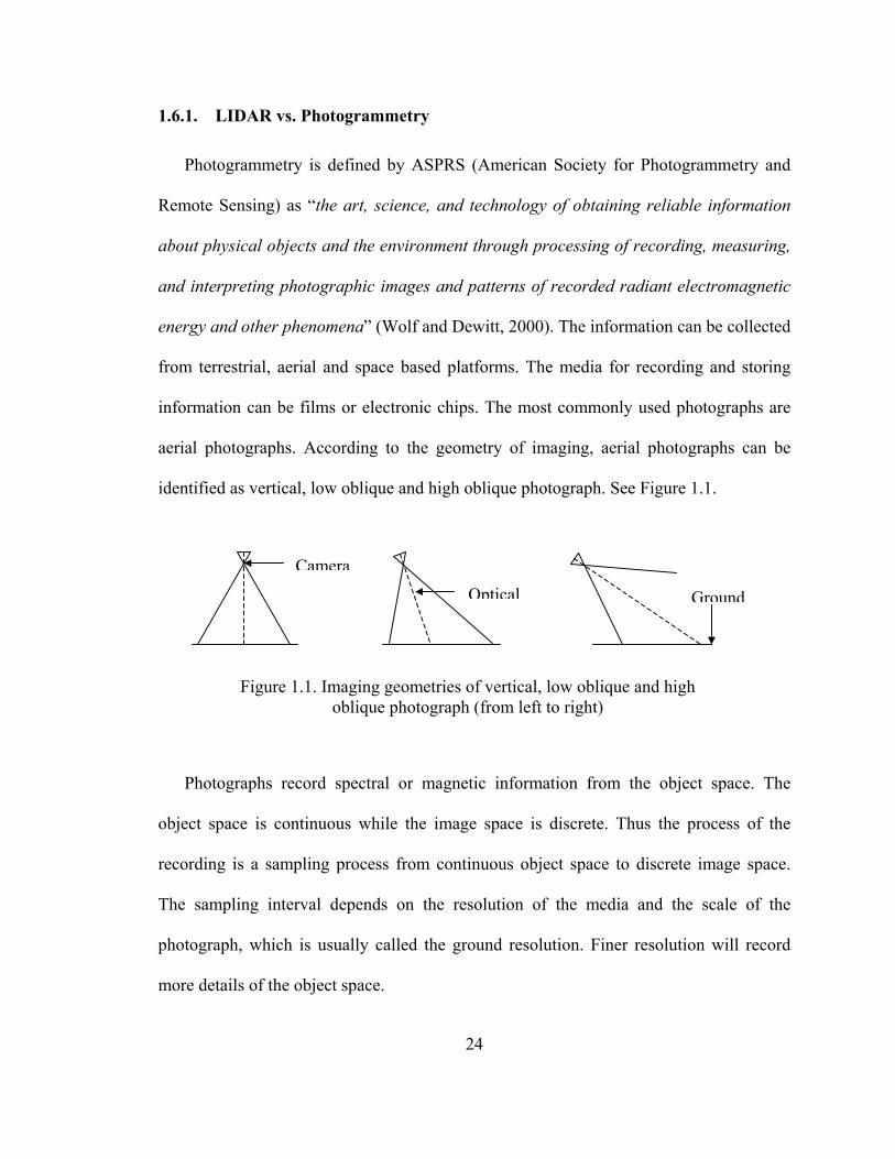
identified as vertical, low oblique and high oblique photograph. See Figure 1.1.

GroundOpticalCamera

Figure 1.1. Imaging geometries of vertical, low oblique and high oblique photograph (from left to right)

Photographs record spectral or magnetic information from the object space. The

object space is continuous while the image space is discrete. Thus the process of the

recording is a sampling process from continuous object space to discrete image space.

The sampling interval depends on the resolution of the media and the scale of the

photograph, which is usually called the ground resolution. Finer resolution will record

more details of the object space.

24

The objective of photogrammetry is to reconstruct object information in the object

space from image information. From the geometry of imaging, it is easy to understand

that the imaging is a process of information transformation from 3D space to 2D space.

The relationship from 3D space to 2D space is one-to-one; each object in 3D space

corresponds to one unique object in 2D space. However, the inverse transformation from

2D space to 3D space is one-to-many; each object in 2D space can find many

corresponding objects in 3D space. Thus, the reconstruction of 3D space cannot be

achieved from a single 2D image. In order to reconstruct the object space, stereo images

are utilized. See Figure 1.2. The fundamental principle used in photogrammetry is the

collinearity of the three points, i.e., the perspective center, image object (point) and the

object (point) in object space.

P2 P1

P

O1

Image 1 Image 2

Ground

O1 O2 O2

Figure 1.2. Stereo images (left) and space intersection for 3D space object reconstruction from stereo images (right)

According to the definition of photogrammetry, LIDAR (Light Detection And

Ranging) belongs to the scope of photogrammetry. However, due to its special

characteristics, LIDAR is usually treated as a separate technique different from

photogrammetry. The light used in a LIDAR system is laser. There are two kinds of laser

25

systems: the pulse laser system and the continuous-wave laser system. The commonly

used one is the pulse laser system.

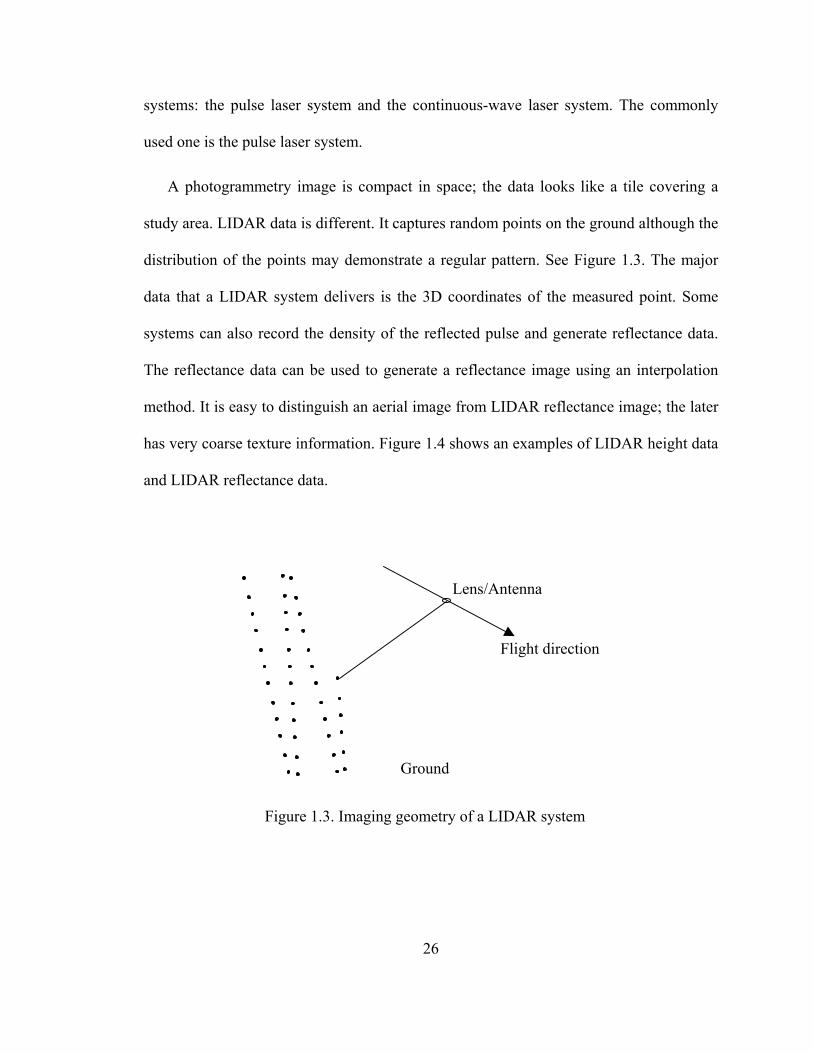
A photogrammetry image is compact in space; the data looks like a tile covering a

study area. LIDAR data is different. It captures random points on the ground although the

distribution of the points may demonstrate a regular pattern. See Figure 1.3. The major

data that a LIDAR system delivers is the 3D coordinates of the measured point. Some

systems can also record the density of the reflected pulse and generate reflectance data.

The reflectance data can be used to generate a reflectance image using an interpolation

method. It is easy to distinguish an aerial image from LIDAR reflectance image; the later

has very coarse texture information. Figure 1.4 shows an examples of LIDAR height data

and LIDAR reflectance data.

Flight direction

Ground

Lens/Antenna

Figure 1.3. Imaging geometry of a LIDAR system

26

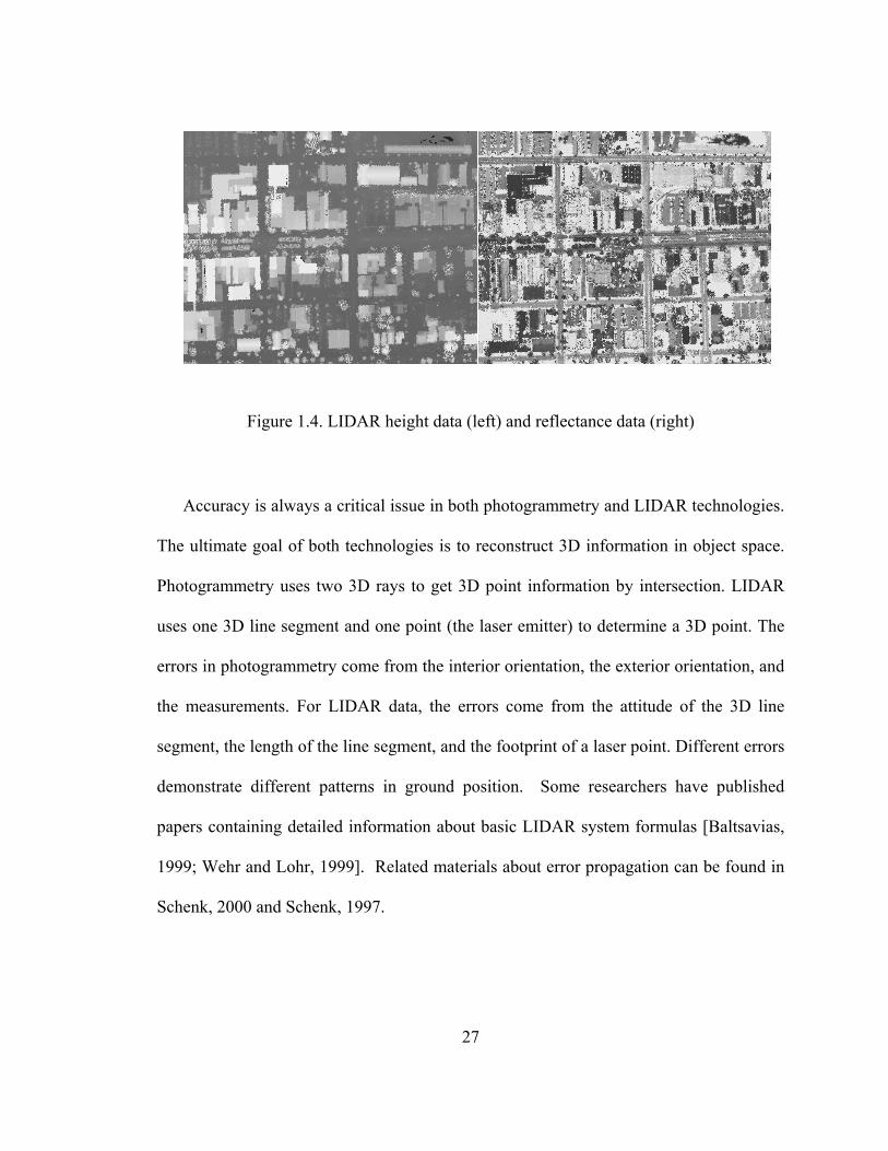
Figure 1.4. LIDAR height data (left) and reflectance data (right)

Accuracy is always a critical issue in both photogrammetry and LIDAR technologies.

The ultimate goal of both technologies is to reconstruct 3D information in object space.

Photogrammetry uses two 3D rays to get 3D point information by intersection. LIDAR

uses one 3D line segment and one point (the laser emitter) to determine a 3D point. The

errors in photogrammetry come from the interior orientation, the exterior orientation, and

the measurements. For LIDAR data, the errors come from the attitude of the 3D line

segment, the length of the line segment, and the footprint of a laser point. Different errors

demonstrate different patterns in ground position. Some researchers have published

papers containing detailed information about basic LIDAR system formulas [Baltsavias,

1999; Wehr and Lohr, 1999]. Related materials about error propagation can be found in

Schenk, 2000 and Schenk, 1997.

27

1.6.2. DTM vs. DSM

DTM refers to digital terrain model while DSM refers to digital surface model. DTM

depicts the topography of the bald earth. For DSM, both nature and man-made objects are

captured in the topography. See Figure 1.5.

Earth Earth

DSMDTM TreesTrees

Building Building

Figure 1.5. DTM (left) and DSM (right)

Both photogrammetry and LIDAR data can be used to generate DTM and DSM.

However, the direct product from these two techniques is DSM. In order to generate a

DTM, some filtering algorithms are employed to filter out the nature and man-made

objects from a DSM. The morphology filtering is one commonly used algorithm in

filtering out non-ground objects to generate a DTM. A DTM can be used for ground

planning applications such as flood control; while DSM can be used to detect objects on

the earth. The difference between DSM and DTM is usually called normalized DSM. It

keeps information about non-terrain objects such as buildings, trees, cars and so on. But

regardless of whether a DTM or a normalized DSM, they both come from DSM. Thus the

first data set to be processed for object reconstruction, especially building reconstruction,

is a DSM.

28

1.6.3. Building Detection and Building Reconstruction

Building detection refers to the process of differentiating buildings from other objects

measured within data. Taking an aerial image as an instance, which area or region on the

2D image is a building? This process is a qualitative process. An image can be segmented

into regions using algorithms; and each region can be analyzed and classified as an object

according to its spectral characteristics. Color image and multi-spectral images are used

in building detection because they capture more spectral information than Black/White

images. LIDAR can also be used for building detection. LIDAR data maps the

topography of the earth’s surface. Information about a building such as shape and

parallelism can be derived. These internal characteristics can also be calculated from

images.

Building reconstruction is the process of deriving building model parameters. The

commonly used building model is a CAD model, which has specific parameters such as

height, width, direction and other necessary information to reconstruct a building model.

These parameters cannot be captured by aerial images or LIDAR data directly. They need

complex spatial and topological analysis to be calculated. In this research, the building

detection and reconstruction are addressed in different parts.

1.7. Organization of this dissertation

This dissertation is organized into 6 chapters. Chapter 1 (the current chapter)

addresses the background related to the research.

29

30

Chapter 2 describes two new algorithms developed to perform LIDAR segmentation.

It illustrates how to extract building regions from LIDAR data. The so-called “height-

jump” and “planar-fitting” algorithms are developed and elaborated.

Chapter 3 presents a method for 3D building model reconstruction using a polyhedral

model. It describes a methodology for building model primitive construction, model

topology construction, and model reconstruction.

Chapter 4 elaborates an approach to building model refinement through the

integration of LIDAR data and imagery data. The focus of the refinement is the geometry

of a building model instead of its topology.

Chapter 5 demonstrates experimental results involved in this research to show how

the algorithms developed here work.

Chapter 6 concludes the dissertation research. It highlights the contributions and

analyzes the shortcomings of the research. It also projects further research in this topic.

CHAPTER 2

BUILDING DETECTION FROM LIDAR DATA

Building detection from LIDAR data is a part of LIDAR segmentation process. In

order to derive 3D building models, building regions will be detected and extracted from

LIDAR data first. In this study, two methods are developed to detect building regions in a

LIDAR segmentation process. These two methods are described in this chapter. The

comparison between these two methods and the morphology method is also presented.

The whole process of DTM generation and building detection can be illustrated in a

flowchart shown in Figure 2.1.

31

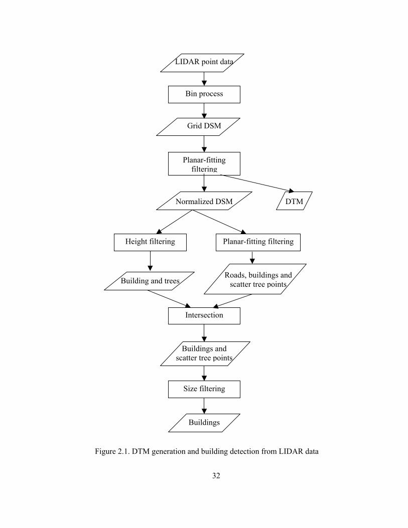
LIDAR point data

Buildings

Size filtering

Buildings and scatter tree points

Intersection

Building and treesRoads, buildings and

scatter tree points

Planar-fitting filtering Height filtering

Normalized DSM DTM

Planar-fitting filtering

Grid DSM

Bin process

Figure 2.1. DTM generation and building detection from LIDAR data

32

2.1. Conventional Terms

Morphology operators: Morphology operators include a group of filters. The

commonly used ones are open, close, dilation, and erosion. A basic character of

these operators is to order the pixel values within a neighbor defined using

structure elements, and assign a specific value to the pixel under test. Morphology

operators are commonly used in binary image data. When these operators are

applied to gray scale images, they are also called gray morphology operators.

Structure elements: Structure elements of a morphology operator define the

neighbor of a pixel under analysis. For example, a 3 by 3 square window defines

the pixels directly adjacent to the central pixel as the neighbor of the central pixel.

The structure elements of a morphology operator can be of other shapes such as a

circle and a cross.

Neighbor: A neighbor of a point is defined as points within a distance threshold to

the point under study. In different processes, different distance thresholds can be

applied. Points falling in a point’s neighbor are used in analysis.

Ground region: A ground region includes roads and open ground. Bridges are also

included in a ground region. In an urban or a suburban area, it is usually the

largest area.

Building boundary: In this study, a building boundary is referred as a building’s 2D

footprint on the ground.

33

2.2. DSM and DTM Generation

The original LIDAR range data are random points and it is not convenient to perform

building detection and DTM generation directly from these points. Two intermediate

products are commonly used by researchers to perform further process. One is grid

format image; and the other is Delaunay Triangulation. The later is also referred as

Irregular Triangulated Network (TIN). These are two forms representing a 2.5D surface.

LIDAR range data measures the surface exposing to a LIDAR antenna. For airborne

LIDAR data, it captures surfaces of objects on the ground and part of the earth’s surface

exposing to a LIDAR antenna. In GIS and remote sensing community, this surface is

called Digital Surface Model (DSM). Instead of DSM, the useful products for a GIS

system are Digital Terrain Model (DTM) and information about objects sitting on the

ground. Currently, how to separate DTM and objects from a DSM has become a popular

research topic, especially in the LIDAR research community. It is usually referred to as

LIDAR data segmentation.

In order to detect buildings, the DTM will be generated first, and then, a normalized

DSM (NDSM) will be generated for building detection in this research. A NDSM is a

surface relative to the DTM. Objects within a NDSM can be viewed as sitting on a level

plane. Building detection is then conducted on such a NDSM. In this research, the data

format used is grid format. Two criteria in choosing the grid format over the TIN model

are: 1) simple to process; and 2) available algorithms for preliminary process. The grid

format is simple; the spatial and topological relationships among pixels are easy to

34

calculate. In addition, there are many mature image processing algorithms that can be

applied to grid format LIDAR data.

2.2.1. Transformation of Points to Grid

To generate a grid DSM from random points, a transformation between the ground

horizontal coordinate system (X, Y) and the image coordinate system(i, j) is applied. For

transformation convenience, the X and i axes of these two systems are of the same

direction while the Y and j axis are of opposite directions. See Figure 2.2. The

transformation between these two systems is expressed in equation 2.1.

−=

stepXXIntegeri min

(2.1)

−=

stepYYIntegerj max

Y

X(Xmax, Ymin)

(Xmin, Ymax)

Figure 2.2. Conversion from points to grid

35

The step, or the resolution, of a grid is calculated as the inverse of the average density

of LIDAR points (see next paragraph for details). For each pixel (i, j) of a grid, its value

is assigned as the value of the LIDAR point that falls into the pixel calculated through

equation 2.1. However, due to uneven distribution of LIDAR points, some pixels have no

corresponding LIDAR points, while some pixels have more than one corresponding

LIDAR point. If a pixel has no corresponding point, an interpolation method will be

applied to derive its pixel value. If more than one point falls within a pixel, only the

minimum value is assigned to the pixel. The basic steps can be described as followings:

a. Calculate the maximum and minimum X and Y coordinates. Determine the spatial

resolution of the grid according to the range point density. Usually the resolution

is calculated as n1 , where n is the average number of points within an area;

b. Using equation 2.1, for each LIDAR point, the corresponding grid pixel location

is calculated and the Z value of the point is assigned to the grid pixel. During this

process, a test is performed. If a pixel is already assigned a value from another

point, this LIDAR point value is compared with the existing pixel value, and the

smaller value will be assigned to the pixel;

c. After each LIDAR point is processed, the value of a single vacant or an empty

pixel will be derived from its neighboring pixels using an interpolation algorithm.

In this research, the nearest neighbor method is applied to avoid introducing new

height values into the generated DSM. For a large empty patch like a pond, it will

36

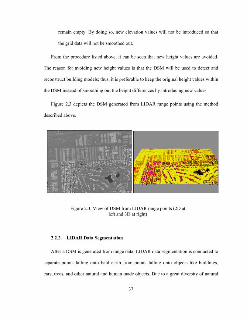
remain empty. By doing so, new elevation values will not be introduced so that

the grid data will not be smoothed out.

From the procedure listed above, it can be seen that new height values are avoided.

The reason for avoiding new height values is that the DSM will be used to detect and

reconstruct building models; thus, it is preferable to keep the original height values within

the DSM instead of smoothing out the height differences by introducing new values

Figure 2.3 depicts the DSM generated from LIDAR range points using the method

described above.

Figure 2.3. View of DSM from LIDAR range points (2D at left and 3D at right)

2.2.2. LIDAR Data Segmentation

After a DSM is generated from range data, LIDAR data segmentation is conducted to

separate points falling onto bald earth from points falling onto objects like buildings,

cars, trees, and other natural and human made objects. Due to a great diversity of natural

37

phenomena, there is no such single algorithm that can work in all situations. Algorithms

are usually application dependent. In other words, they are developed to solve specific

problems using specific data. Thus, the data used should be analyzed and an appropriate

algorithm should be employed for best performance. Several algorithms have been

developed by researchers for LIDAR data segmentation.

Based on an assumption that a ground point’s height is lower than its neighboring

object points, morphology filters can be applied to distinguish ground points in a LIDAR

data set. Figure 2.4 shows a profile demonstrating the difference between ground and

non-ground objects. Another assumption is that the ground is smooth. In other words,

there is no abrupt change on the ground. Some studies on this separation have been

carried out and good results were produced (Weidner and Förstner, 1995; Morgan and

Habib, 2002). However, morphology filters are sensitive to errors. Although a median

filter can be used to decrease effects from single error points, effects from errors in form

of a point patch cannot be eliminated or decreased. Kilian et al. (1996) used a “multi-

level opening” morphology operator in order to keep small ground features while

removing large non-ground objects. Because small windows they used have small

weights, fine features can still be removed.

38

Figure 2.4. A profile depicting the difference between ground and non-ground objects like building and trees

Axelsson (1999) presented an idea to separate ground and non-ground points from

LIDAR data. The idea is to move a surface from below to LIDAR point cloud to touch

the ground surface. Controlled by a few parameters, the moving surface can adjust itself

to include points on the ground.

“Linear prediction” is a statistical interpolation method. It is employed in LIDAR

data segmentation by researchers to generate digital surfaces (Lohmann and Koch, 1999;

Lohmann, et al., 2000; Kraus and Pfeifer, 1998; Lee and Younan, 2003). The

interpolation is founded on spatial correlations of neighboring points, which are

expressed in the form of covariance. A covariance is calculated using a covariance

function based on the distance between two points. By comparing the original digital

surface with the predicted one that is generated using the “linear prediction” method,

points’ weights are calculated according to their residuals. The weights are also used in

calculating a covariance matrix. A DTM is generated from the terrain points with their

weights. Iterative execution is necessary to obtain a high accuracy DTM using the “linear

39

prediction” method. An initial DTM surface is required in order to use this method,

which can be calculated using a moving plane.

Vosselman (2000) proposed a slope-based method to filter out non-ground points.

The method is a modification of the morphology erosion operator. A point is classified as

a ground point if the maximal slope of the vectors connecting this point under test to all

its defined neighbors does not exceed the maximal slope within the study area. Sithole

(2001) modified this method to use different maximal slope thresholds according to local

terrain characteristics. A rough slope map is required to calculate the local slope

threshold. Like morphology operators, the problem with these kinds of methods is how to

define the neighbor of a point.

Several studies have been conducted to investigate building detection from LIDAR

data. After performing a region growing segmentation, Matikainen, et al. (2003), used

height information to separate trees and buildings from the ground; then a fuzzy

classification method was applied to detect buildings based on three attributes: the Gray

Level Co-occurrence Matrix (GLCM) homogeneity of height; the GLCM homogeneity of

LIDAR intensity; and the average length of edges from a “shape polygon” derived from

the segment under test. Rottensteiner and Briese (2002) used the height difference

between a DSM and a DTM, a morphological opening operator, and a size measurement

to detect buildings and tree groups. A polymorphic feature extraction method was then

used to detect “point-like” pixels. Based on analysis of the number of “point-like” pixels

of each segment, tree groups were eliminated. This whole process was repeated before

final building regions were generated. Lohmann (2001) investigated the Gaussian

40

Laplace (GL) filter to detect break lines like dike edges. He proposed to use the mean

curvature to overcome the difficulty in determining thresholds for a GL filter result. This

method could be used to detect building outlines. Brunn and Weidner (1997) used a

Bayesian Network classification to detect buildings based on the height difference

between a DSM and a DTM, detected steep edges, and surface normal variation.

Axelsson (1999) used a classification method based on the minimum description length

criteria to separate buildings and trees. A cost function was calculated from the second

derivatives of the surface.

The measurement delivered directly in LIDAR data is the height information of the

earth’s surface. Other information such as texture can be derived based on neighboring

points, and this kind of information can be used to perform LIDAR data segmentation

(Elberink and Maas, 2000; Lohmann, 2001). Textures that can be derived from height

information are slope, variance, aspect, and so on.

From information delivered in a DSM, an important while simple characteristic is that

non-ground objects are higher than their neighboring ground region. Figure 2.4 shows a

profile demonstrating this characteristic. In this research, two algorithms were developed

based on this character to perform LIDAR data segmentation. The first algorithm is based

on the observation that objects are higher than the ground, and the ground and buildings

can be defined as planar surfaces locally. The second algorithm is based on the

observation that objects are separated, in other words, isolated from the ground by their

boundary points, which have high elevation differences within their neighborhood, such

41

as a 3 by 3 window. These two algorithms were tested and the results were compared

with the result from the morphology method.

2.2.2.1. Morphology Segmentation

The procedure using gray morphology operator to perform LIDAR segmentation can

be summarized as followings:

a. Based on a prior knowledge of the largest building size within a study area, the

window size of a morphology operator is determined to be larger than the largest

building. This window defines the neighbor of a pixel under analysis.

b. For each pixel of a DSM grid, the pixels within its neighbor are checked and their

height values are compared. The minimum value in its neighbor is assigned to it.

This operation is called erosion.

c. After the erosion is finished, each grid pixel is compared with the pixels within

it’s neighbor defined in step a. The maximum value in the neighbor is assigned to

it in this operation, which is called dilation.

This procedure is a morphology open filter on gray scale image. In order to apply this

method on segmentation, the neighborhood in the form of a window should be

determined in advance. Such a window is called structural element W. The size of W is

determined by prior knowledge of the maximum size of non-ground objects, and usually

it is the maximum building size in urban or suburban areas. The size of W is determined

in such a way that no object within the study area can totally cover the structural element.

Otherwise, points falling on objects other than the bald ground will not be filtered out;

42

and consequently, the generated DTM will be biased. The biases will also propagate to

NDSM and final building models. On the other hand, a large size window will remove

fine features on the ground, such as a cliff. Obviously, the critical step in morphology

operation is to correctly determine an optimal size of the structural element.

A filtered DSM is a version of the DTM. Due to the internal characteristic of the

morphology operator, some or many small ground features were eliminated. The quality

of the DTM can be improved by tracking back the removed ground points. To achieve

this objective, LIDAR points were compared with the DTM. Those points with small

height differences are tracked back as ground points. Then, a new version of DTM can be

generated with a better quality. This comparison can be repeated until no more or a small

number of new points can be tracked back. The height difference threshold is calculated

based on the vertical accuracy of LIDAR points.

Figure 2.5 depicts a DTM generated from original DSM using gray-based

morphology open filter. The ground points were detected by comparing the DTM with

LIDAR points. Those points have a elevation difference smaller than the difference

threshold. The final DTM and the normalized DSM are displayed in Figure 2.6.

43

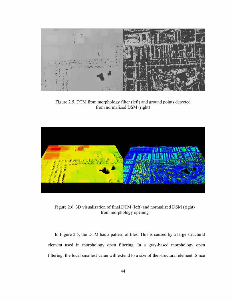
Figure 2.5. DTM from morphology filter (left) and ground points detected from normalized DSM (right)

Figure 2.6. 3D visualization of final DTM (left) and normalized DSM (right) from morphology opening

In Figure 2.5, the DTM has a pattern of tiles. This is caused by a large structural

element used in morphology open filtering. In a gray-based morphology open

filtering, the local smallest value will extend to a size of the structural element. Since

44

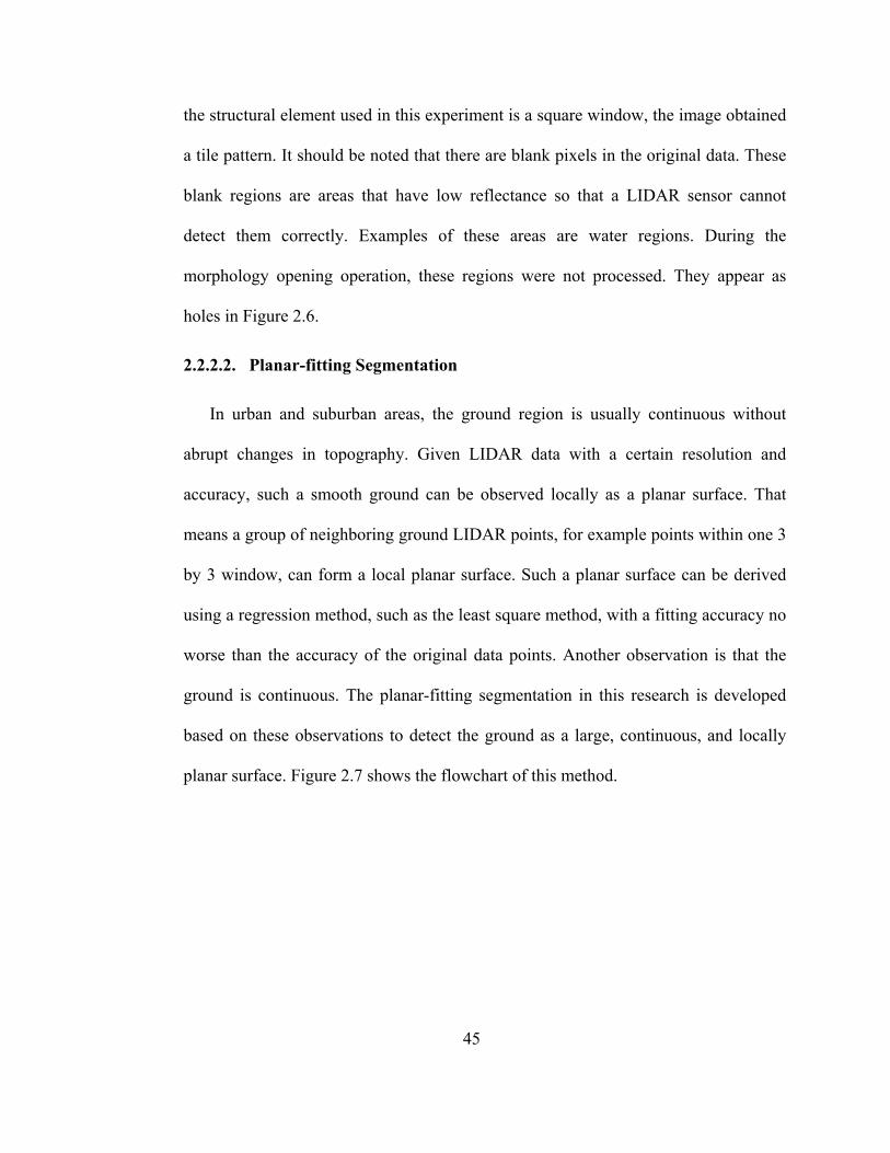
the structural element used in this experiment is a square window, the image obtained

a tile pattern. It should be noted that there are blank pixels in the original data. These

blank regions are areas that have low reflectance so that a LIDAR sensor cannot

detect them correctly. Examples of these areas are water regions. During the

morphology opening operation, these regions were not processed. They appear as

holes in Figure 2.6.

2.2.2.2. Planar-fitting Segmentation

In urban and suburban areas, the ground region is usually continuous without

abrupt changes in topography. Given LIDAR data with a certain resolution and

accuracy, such a smooth ground can be observed locally as a planar surface. That

means a group of neighboring ground LIDAR points, for example points within one 3

by 3 window, can form a local planar surface. Such a planar surface can be derived

using a regression method, such as the least square method, with a fitting accuracy no

worse than the accuracy of the original data points. Another observation is that the

ground is continuous. The planar-fitting segmentation in this research is developed

based on these observations to detect the ground as a large, continuous, and locally

planar surface. Figure 2.7 shows the flowchart of this method.

45

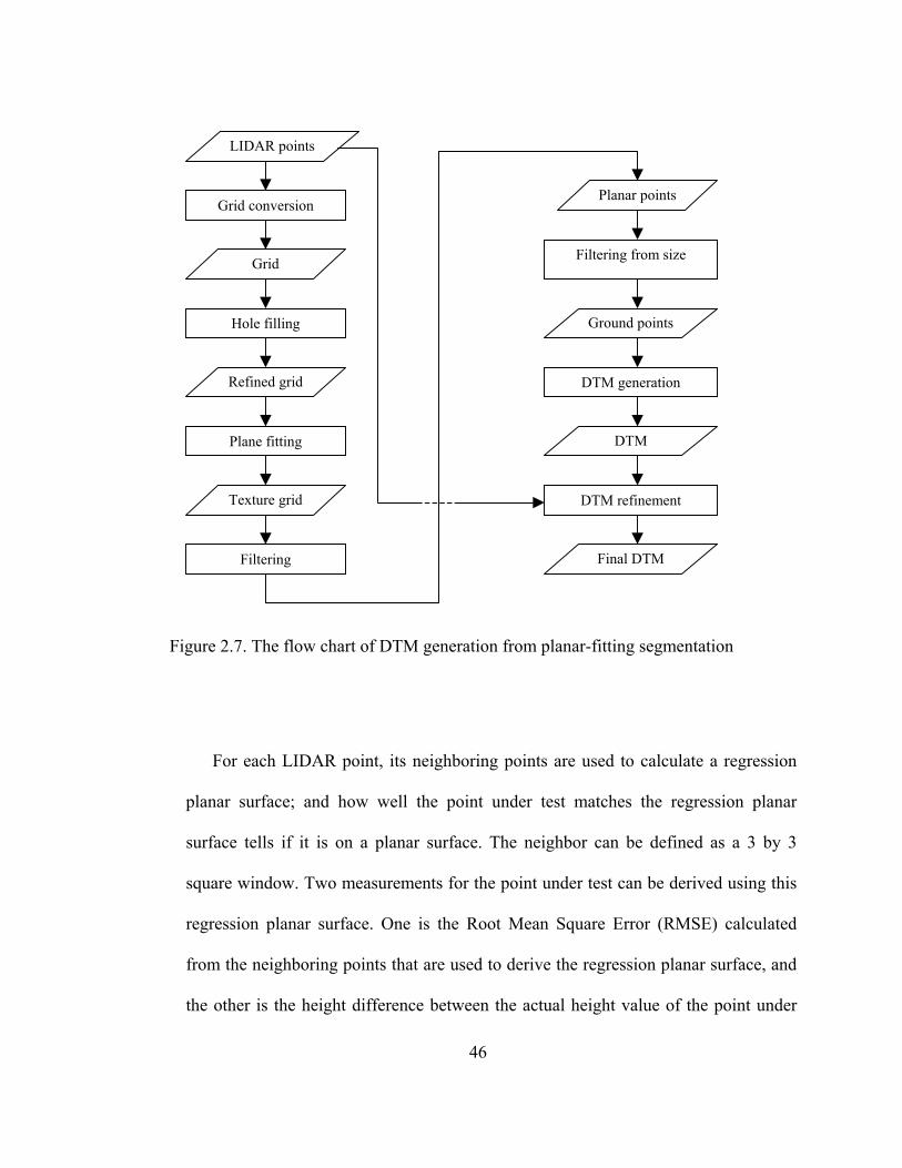
DTM generation

Ground points

Filtering from size

Planar points

Final DTM

DTM refinement

DTM

Filtering

Texture grid

Plane fitting

Refined grid

Hole filling

Grid

Grid conversion

LIDAR points

Figure 2.7. The flow chart of DTM generation from planar-fitting segmentation

For each LIDAR point, its neighboring points are used to calculate a regression

planar surface; and how well the point under test matches the regression planar

surface tells if it is on a planar surface. The neighbor can be defined as a 3 by 3

square window. Two measurements for the point under test can be derived using this

regression planar surface. One is the Root Mean Square Error (RMSE) calculated

from the neighboring points that are used to derive the regression planar surface, and

the other is the height difference between the actual height value of the point under

46

test and its height value calculated from the regression planar surface. Both

measurements indicate how well a point fits onto a planar surface formed by its

neighboring LIDAR points. These two measurements correlate with each other and

thus produce similar results. Points with a small RMSE or a small height difference

are classified as points on ground or building roofs, and points with a large RMSE or

height difference are classified as falling onto objects with non-planar surfaces like

trees and shrubs.

From its vertical accuracy of the original LIDAR data, a threshold of height

difference or RMS is determined to differentiate points falling onto planar planes

from points falling onto non-planar surfaces like trees. In this research, double stated

vertical accuracy of the original LIDAR data is used as the threshold. This threshold

can correctly classify most planar points, around 96 percent assuming a normal error

distribution. Further processing will be performed to test and classify more LIDAR

points as ground points. The classified planar points include points on the ground,

points on building roofs, and some scattered points on objects like trees and cars.

Another issue to deal with is what kind of ground surface this algorithm can

detect. The real terrain is not a perfect plane. The question is to what degree a rough

terrain can be classified as a local planar surface. This can be deduced from data

accuracy and data density, or the resolution of grid format data. Figure 2.8

demonstrates their relationship. The roughness of a terrain can be measured as

changes of terrain slopes.

47

2

α

β

)2

arctan(

2

Rh=

=

β

βα

βh

R

Figure 2.8. Conditions for a rough terrain to be classified as a planar surface using the planar-fitting algorithm

In Figure 2.8, α is the slope change caused by a terrain change. It is double β .

The symbol h is the fitting threshold used to test whether a point is falling onto a

planar surface or not. R is the resolution of the grid DSM. Since the window used for

plane fitting in this experiment is a 3 by 3 window, the maximal distance to the center

of the window is 2 R. As used in this experiment, R is 1 meter, and h is 0.3 meter.

Thus α is approximate 24 degrees. That means a ground surface with slope changes

smaller than 24 degrees can be classified as a planar surface. Thus, it can be correctly

extracted as a ground surface. In actual implementation, a rougher surface could be

classified as a planar surface because the central point is also used to define the

regression-fitting plane.

Points or pixels classified falling onto planar surfaces were extracted for further

process. First of all, connected regions were detected and labeled; and areas of these

connected regions were calculated by counting their pixel number. To differentiate

ground points from building roof points, it is assumed that the ground points form one

48

or more connected planar surfaces that have larger areas than the largest building

within a study area. In other words, the largest connected planar region is on the

ground. This assumption is true in urban and suburban areas where the ground region

is connected by a road system. Regions with areas larger than the largest building size

within a study area were extracted as ground regions. The ground region can also be

simply picked manually. LIDAR points falling within the ground regions were

extracted and used to generate an initial DTM. Figure 2.9 shows the calculated fitting

difference and an extracted ground region.

Figure 2.9. Calculated planar-fitting difference (left) and detected ground points (right) from planar-fitting segmentation method

After ground points were extracted, a DTM was generated using an interpolation

method. In this experiment, a TIN (Triangulated Irregular Network) model was

created first; then a DTM grid was generated from the TIN model. However, this

DTM is a rough one whose accuracy can be improved. A refinement was conducted

on the initial DTM to get a higher accuracy by tracking back more ground points

through a comparison of LIDAR point heights with the DTM elevation. In the planar-

49

surface fitting procedure, points falling on boundary regions of a planar surface also

had large fitting differences due to height jumps occurring in boundary regions. These

boundary points that are not initially classified as ground points should be included in

the final DTM. After the initial DTM was generated from initially classified ground

points, all LIDAR points classified as non-ground points were compared with the

DTM. Those points with differences smaller than the threshold were re-classified as

ground points, and these ground points were used to refine the DTM. Again, the

difference threshold in the comparison is twice the stated vertical accuracy of original

LIDAR point data.

Ground points were updated to include newly classified ground points from the

comparison of the previously generated DTM and actual point heights. The new

generated DTM had better accuracy since more ground points were included. This

procedure is repeated until no significant number of points are classified as on the

ground. This procedure can also be repeated for a fixed iteration number. For point

detection purpose during iteration, a simple interpolation method can be applied to

generate an intermediate DTM. The final DTM can be generated using a complicated

but accurate interpolation method, such as the Kriging method. A normalized DSM

can be obtained by subtracting the final DTM from the DSM. The final DTM and the

normalized DSM are displayed in Figure 2.10.

50

Figure 2.10. 3D visualization of final DTM (left) and normalized DSM (right) with2 times exaggeration in elevation from planar-fitting segmentation

In the normalized DSM, it can be seen that there are wall-like boundary regions.

These regions are caused by the different size of the DTM and the DSM. The size

difference exists as a consequence of point loss during LIDAR segmentation.

2.2.2.3. Height-jump Segmentation

An important kind of information delivered in LIDAR data is expressed in the

form of changes among data distribution. For example, a person can distinguish

roads, buildings, and trees from a photograph because he can differentiate spectral

changes of these objects. For a computer vision system, it is important to detect

changes among data under certain criteria. This rationale can also be applied to

LIDAR data segmentation. LIDAR data captures height information of the earth’s

surface. It can be observed that large changes within the elevation data indicate

changes of objects or structures. This observation is the basis of the height-jump

segmentation algorithm. The flow chart of this method is shown in Figure 2.11.

51

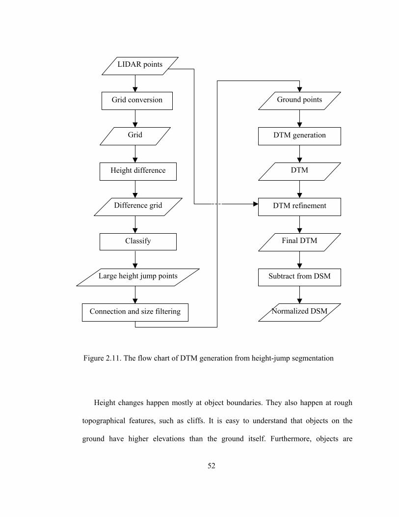
Normalized DSM

Grid

Grid conversion

LIDAR points

Subtract from DSM

DTM generation

Ground points

Connection and size filtering

Large height jump points

Final DTM

DTM refinement

DTM

Classify

Difference grid

Height difference

Figure 2.11. The flow chart of DTM generation from height-jump segmentation

Height changes happen mostly at object boundaries. They also happen at rough

topographical features, such as cliffs. It is easy to understand that objects on the

ground have higher elevations than the ground itself. Furthermore, objects are

52

isolated by large height-change points. This forms the major tasks of the height-jump

segmentation algorithm, to detect boundary points from height changes and to detect

connected regions separated by large height change points.

The question is, what is the height threshold to detect height-jump points? The

solution is determined by the vertical accuracy of LIDAR points, its point density or

the resolution of LIDAR grid data, topographical changes of the ground, and real

object heights. First of all, the height difference should be significantly larger than the

data vertical error. Otherwise, change information is at the same level as data error.

Signal-to-noise ratio is too small to correctly extract information. If the height

difference is larger than 3 times the vertical error, we have approximately 98 percent

confidence to conclude that the difference is caused by an actual physical elevation

change based on the assumption that the error follows a normal distribution.

How do data resolution and ground topography affect height difference? The

criterion is to differentiate the height difference caused by objects from the height

difference caused by topographic change. Figure 2.12 illustrates the relationship

among data resolution, topography, and objects. In Figure 2.12, h represents the

height change introduced by a terrain surface with a slope angle of α ; R is the

resolution of the grid DSM while H is the height of an object. H should be

significantly larger than h in order to distinguish H out of h’s. Thus, with an

estimation of the largest terrain slope within a study area, a height threshold of

minimal H can be calculated. For instance, a system can use double h as the minimum

53

H. Considering data vertical accuracy, the larger one of 2h and 3δ (δ is the vertical

error) will be used as height difference threshold.

α2

)tan(*2 αRh =

R

Hh

Figure 2.12. Object height vs. topographical difference

For each pixel of a grid DSM, its elevation is compared with the maximum

elevation within its neighborhood, such as a 3 by 3 square window. A new grid is

generated with each pixel representing the elevation difference as shown in Figure

2.13a. Compared with the difference threshold as described above, each pixel is

classified as either a pixel indicating existence of a shift from the terrain to an object

or a pixel without such a shift, see Figure 2.13b with white pixels representing large

difference points. From Figure 2.13b, it can be seen that the whole grid area is

divided into separate regions by such large height difference pixels. These isolated

regions are then labeled; and the ground region is detected and extracted using the

same method as in the planar-fitting segmentation. Figure 2.13 shows the process and

immediate results of the algorithm.

54

dc

b

dc

ba a

Figure 2.13. Process results of height-jump segmentation algorithm: a)

calculated height difference; b) classified large-difference points (white); c) isolated regions (white); and d) the detected ground region (white)

The ground region can be detected automatically. One straightforward way to

achieve this goal is to extract the ground as the region with the largest area. This

method is based on the observation that the largest connected ground region is usually

the largest object within an urban or a suburban area. Another approach is to compare

the elevation of each region with its adjacent regions. Across each sharing boundary

segment, the ground region should be lower than its adjacent regions. This is based on

the assumption that all objects are sitting on the ground and thus they are higher than

the ground. The first method is simple to implement. However, some small isolated

55

ground regions, such as a yard surrounded by buildings, cannot be detected. The

second approach can detect small ground regions, but it can also include some

isolated lower roof regions surrounded by higher roof regions. In addition, the second

method is complicated in comparing adjacent regions.

The extracted ground region is used to retrieve ground LIDAR points. Ground

points are then used to generate a DTM through a TIN model. As with the planar-

fitting algorithm, the generated DTM can be improved by including more ground

points. Using the same method as described in the planar-fitting segmentation

algorithm, new ground points are added to the DTM iteratively by comparing LIDAR

points’ elevations with the DTM. After a pre-set number of iteration is finished or

until no significant number of new points can be detected, the DTM refining is

stopped. Consequently, a finalized DTM is generated. Figure 2.14 shows two 3D

scenes displaying the DTM and the normalized DSM, which is generated by

subtracting the DTM from the DSM.

Figure 2.14. DTM and normalized DSM from height-jump segmentation

56

2.2.3. Comparison

LIDAR segmentation algorithms are all application-dependent. That means

algorithms are implemented based on an analysis of specific data sets. There is no such

algorithm that can be pre-set to apply to all kinds of LIDAR data under any conditions.

The characteristics of data should be analyzed before any segmentation algorithm can be

applied.

Morphology method needs prior knowledge about the maximal non-ground object

size in order to determine a moving window’s size. This is a disadvantage of morphology

operators. In addition, large non-ground objects are common in LIDAR sets so that a

large window size is required in order to correctly remove non-ground objects. At the

same time, a larger window will produce a smoother result. In many cases, this will

remove fine features and change the topography dramatically. This will make it very

complex and difficult, even impossible, to recover the topography. However, morphology

operators are easy to understand and simple to implement. In urban or suburban areas

without large topographic changes, this group of operators can work well in LIDAR

segmentation to obtain a good approximation of the terrain.

The planar-fitting algorithm is based on the assumption that the ground surface can be

observed as a planar surface considering the tolerance from data errors. It requires the

setup of the planar-fitting threshold, which is based on data errors, topography, data

resolution, and the roughness of a terrain. And sometimes it needs analysis of the

minimal height of the objects within a study area. However, these requirements are easy

to meet in applications especially for urban and suburban areas. The advantage is this

57

method can keep important ground linear features as long as a feature is continuous

across the data coverage. For example, a freeway intersection can be correctly classified

onto the ground. On the other hand, if an application doesn’t want the freeway

intersection in the ground, this becomes a disadvantage. A further process or new

algorithm should be developed to handle this. Compared with morphology operators, this

algorithm keeps the topography much better; thus, it is faster to recover the final DTM by

tracking back excluded ground points during the process at the beginning.

The height-jump algorithm is based on the observation that non-ground objects are

higher than their neighboring or surrounding ground, and their boundaries have

significant height difference from the ground. In practical applications, this method

should be applied with analysis of the topographic characteristics and data resolution. A

building object may be connected to a large-slope ground in a coarse resolution data.

Similar to the planar-fitting algorithm, this algorithm can keep fine ground linear features

as long as the features are not broken down. Compared with the planar-fitting algorithm,

the height-jump algorithm doesn’t have requirements for the roughness of a terrain while

it has requirements for terrain slopes. The planar-fitting algorithm doesn’t require the

terrain slope to meet certain condition, but it does have requirements for the terrain

roughness.

The differences among three algorithms of LIDAR data segmentation in this research

are reflected in the detection of the ground region, which is an initial DTM. The

following DTM refinement processes are the same. They all compare the original LIDAR

point data with the generated DTM to include more ground points so that the quality of

58

the DTM can be improved because more ground points provide more information about

the terrain. Different interpolation methods can be applied to the same ground data to

generate different quality DTM and normalized DSM. The method used in this research

is a TIN model, which is a linear interpolation. Based on analysis of terrain

characteristics, complex methods such as B-spline surface or the Kriging method can be

utilized to generate more accurate results. But the rationale or the philosophy related to

this research topic is the same.

2.3. Building Detection from Normalized DSM

After a normalized DSM is generated, non-ground objects such as buildings and trees

are observed as sitting in a level plane. In reality, errors are always inevitable. Even

though errors exist, the observation still makes sense from the data point of view. By

segmenting a normalized DSM using a height threshold, trees and building can be

distinguished out of the normalized DSM. A height threshold is determined from a prior

knowledge of the minimum height of objects the application wants to detect. For

example, a threshold of 3 meters can be used to detect buildings while eliminating other

objects like cars and bushes. In this research, the focus is to detect buildings from LIDAR

data, so a threshold of 3 meters is employed. Consequently, objects like cars and bushes

were eliminated while large trucks and some trees are kept from such a height threshold.

Other measurements or derived texture can be applied together with height information to

differentiate building from other objects. For example, shape measurements like

parallelism and size can be used to separate buildings and trees.

59

To reconstruct building models, buildings should be separated from other objects,

most likely trees, and be identified in order to derive parameters of building models. By

analyzing the characteristics of trees and buildings, we can find that they demonstrate

different spatial distributions and patterns as illustrated in Figure 2.15. It is true that

different objects can always be separated as long as sufficient information is available. In

the following discussion, the focus is how to separate buildings from trees.

Figure 2.15. Objects (buildings and trees) detected as objects higher than 3 meters

60

Buildings can be separated from trees because they have different characteristics.

With sufficient information, we can totally differentiate them. The questions are: what

kind of information do we need? And what kind of information can we obtain from a data

set? From elevation data, we can see that buildings and trees have different shapes, sizes

and elevation distribution patters. Usually buildings have regular shapes, such as

perpendicularity and parallelism. Their boundaries are straight line-segments or curves

that can be described as mathematic equations like one or half circle. Most buildings have

parallel boundaries, which means two consecutive boundary segments are perpendicular

to each other. Individual trees usually have random boundaries. Thus parallelism can be

utilized to differentiate some buildings from trees but not all of them. The reason is some

buildings have curved boundaries.

Before separating objects, objects themselves should be detected and labeled first.

After the height threshold was applied to a normalized DSM, building-like objects were

detected. See Figure 2.15. They are called “building-like” objects because they are

merged with buildings and buildings can only be detected through further processing.

First of all, all connected regions are extracted and assigned a unique label. The

connection is detected based on 8-neighbor connection relationship. At the same time, the

pixel number of each connected region is calculated. This produces the histogram in the

resulted image. Then, a prior knowledge of the minimal building size is used to eliminate

all objects with an area smaller than the minimum building size. After the elimination,

objects remaining are mostly buildings. Figure 2.16 shows the result after an elimination

using a minimum building size of 100 m2. Due to some noisy points adjacent to

61

buildings, detected building regions may have ragged boundaries. To smooth the

boundaries, a morphology close operator was applied to the resulted grid. This operator is

comprised of a dilation operator followed by an erosion operator.

Figure 2.16. Regions detected as buildings using the size threshold

The size threshold can dramatically reduce the number of objects remaining within

the resulted grid. However, size measurement alone cannot differentiate all buildings and

trees. Some trees have areas larger than the minimum building size, for example, large

trees and a group of trees. In addition, some trees are adjacent to buildings; and thus they

62

are connected to their adjacent buildings. If trees are connected with buildings, it will

introduce blunders in reconstructed building models. Thus, additional information or

measurements should be used to further classify buildings and trees.

In the real world, the elevation distribution of human made objects like buildings has

regular patterns. People can observe that most of buildings have roofs comprised of

planar facets. Such roofs can be represented as a planar facet. Thus the elevation of a

point on a planar roof can be predicted from the plane formed by its neighboring points.

On the other hand, trees usually have irregular elevation distribution patterns. This

distribution difference can be utilized to differentiate buildings from trees. One

measurement could be the distribution of slopes. Points on a building roof will form an

approximate homogeneous slope region except for its boundary, while points on top of a

tree will form a heterogeneous slope region due to random distribution of point

elevations. A second texture can be planar fitting difference as used in detecting ground

region in the previous section. The fitting difference or variation can be used to detect

planar-roof buildings.

The planar fitting measurements and the slope measurement are all based on point

elevation distribution. Internally, they will produce similar results. Since the planar fitting

difference image was already generated in DTM generation, this difference data will be

used to separate buildings from trees.

The size, slope, fitting difference, and height measurements are constraints applied to

differentiate buildings from trees. Each constraint can be used individually and the passed

results are the regions detected as building by that constraint. Each result can be treated

63

as a set. The intersection of the sets will be considered as building regions. Intersection

operator will eliminate those building regions not detected by one of the constraints. Thus

the constraints should be relaxed. It is preferable to get class I (commission) error instead

of class II (omission) error. That means buildings should be detected maximally at the

cost of trees surviving in one constraint test. Commission errors can be reduced by

applying other constraints later on, while omission error is difficult to reduce because

buildings that failed to pass a test are eliminated.

In detecting buildings with LIDAR data, a challenging problem is how to separate

large trees adjacent to buildings. After elevation and size constraint tests, these trees will

exist because they connect to building regions and are detected as a whole object. The

planar fitting algorithm demonstrates its advantage in differentiating between these two

different objects. The method produces more precise building objects by eliminating the

tree areas connected to buildings. Figure 2.17 shows an example.

In Figure 2.17, the image on the left shows a DSM generated from LIDAR points. It

can be seen that there are trees surrounded by one building and these trees are connected

to the building. The image in the middle shows the objects detected after a height

threshold was applied to the normalized DSM. It is obvious that these trees survived in

the height constraint. It is clear that a size constraint cannot remove these trees because

they are connected to the building and form a sufficiently large object to pass the test of

the size threshold. The image on the right presents the result after a planar-fitting

algorithm was applied to the DSM together with size constraint. It can be seen that trees

were removed because their heights cannot pass the planar-fitting constraint. The

64

structure of the building is correctly recovered. It can also be seen from the right image

that the skeleton of the building is thinner than the ones in the left and the middle images.

This is caused by the planar-fitting algorithm because boundary points of planar surfaces

cannot pass the test of the planar surface test. A further process is needed to compensate

for the loss. For example, a morphology dilation operator can be applied to widen the

building region.

Figure 2.17. Separation of buildings and trees using planar fitting difference

2.4. Analysis and Conclusion

DTM generation and building detection from LIDAR data are application-dependent

processes. The results and the accuracy depend on data quality and the characteristics of

an application area under study. Data resolution/density and data accuracy can

dramatically affect the results. The topography of a study area also plays an important

role. However, the algorithms presented in this chapter can be applied to most urban and

suburban areas. The height-jump algorithm can even be applied in forestry areas for

DTM generation and forest study.

65

66

The building detection algorithm proposed in this research is a new method. It should

be noted that this method is not supposed to detect every kind of buildings to every detail.

Actually, no building detection algorithm is capable of detecting all kinds of buildings. In

this research, buildings with arch roofs cannot be detected because they cannot meet the

planar surface requirement. In addition, some small structures like dormers on buildings

cannot be detected because they are too small given a data resolution of 1 meter.

CHAPTER 3

BUILDING MODEL RECONSTRUCTION

Building model reconstruction is a process to derive or calculate CAD building

models, which are of vector format. In this chapter, the primitives of a building model,

which are roof faces of a building, will be detected and their parameters will be

calculated. Topological relationship of primitives will be analyzed afterward to obtain

correct building model topology, followed by analysis of building model spatial or

geometric characteristics to reduce effects of errors propagating from the proposed

process sequence.

3.1. Conventional Terms

Building boundary: A building boundary in this part refers to the outline of a

building footprint on the ground. It is a series of line segments in a 2D space. It is

a close 2D polygon.

Boundary regularization: A building boundary is assumed to have a rectangular

shape in this study. Boundary regularization is the process to adjust a building’s

67

boundary into a 2D polygon with a rectangular shape. After regularization, two

consecutive line segments in a building boundary are perpendicular to each other.

3.2. Boundary Extraction and Regularization

Based on their imaging geometry, neither LIDAR data nor optical imagery can

capture or observe every structure of a building. The common missing information is the

vertical walls of a building. Some vertical walls cannot be observed by imaging sensors.

Thus, there are no measurements for these vertical walls. During the conversion from

LIDAR point data to grid DSM, available vertical measurements, if any, were lost. One

method could be going back to the original LIDAR data to recover the lost vertical wall

information. However, this method still cannot recover information about vertical walls

not captured in original point data.

In the real world, we can observe that almost every building is surrounded by vertical

walls. In other words, vertical walls form the boundary of a building. Thus, the boundary

of a building indicates existence of vertical walls. In this research, vertical walls will be

recovered from building boundaries. Another observation is that boundary segments of a

building, or vertical walls of a building, are perpendicular to each other. Two connected

vertical walls form a right angle. Thus an assumption is made in this research to

reconstruct building models. The assumption is that all boundary segments of a building

are perpendicular to each other. In other words, buildings have rectangular-shaped

boundaries. Buildings with arch boundaries will not be modeled in this research. Instead,

they are forced to have rectangular boundaries.

68

Before the roofs of a building are reconstructed, vertical walls will be recovered.

Thus, the boundary of a building will be extracted and then be regularized. Due to errors

within LIDAR data, also because of data resolution, detected building regions have noise

in their boundaries. One obvious distortion is that a straight line segment of a building

has ragged small line segments. In addition, consecutive segments are not perpendicular

to each other. So methods are needed to generalize line segments and to adjust them to

have right intersection angles. This is the purpose of building boundary regularization.

In this research, a refined version of the so-called “sleeve” method is first employed

to generalize boundary segments so that redundant points will be discarded. Then, a new-

developed regularization method is applied to adjust the generalized segments to be

perpendicular to each other.

The boundary of a building is first extracted and recorded as an ordered sequence of

points. Several commercial programs provide this function, such as ERDAS Imagine.

Figure 3.1 shows an example of extracted vector building boundaries.

69

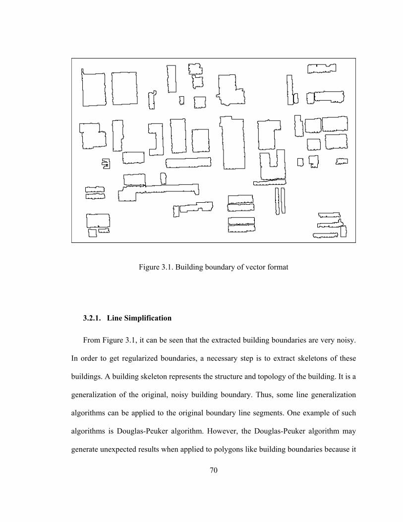
Figure 3.1. Building boundary of vector format

3.2.1. Line Simplification

From Figure 3.1, it can be seen that the extracted building boundaries are very noisy.

In order to get regularized boundaries, a necessary step is to extract skeletons of these

buildings. A building skeleton represents the structure and topology of the building. It is a

generalization of the original, noisy building boundary. Thus, some line generalization

algorithms can be applied to the original boundary line segments. One example of such

algorithms is Douglas-Peuker algorithm. However, the Douglas-Peuker algorithm may

generate unexpected results when applied to polygons like building boundaries because it

70

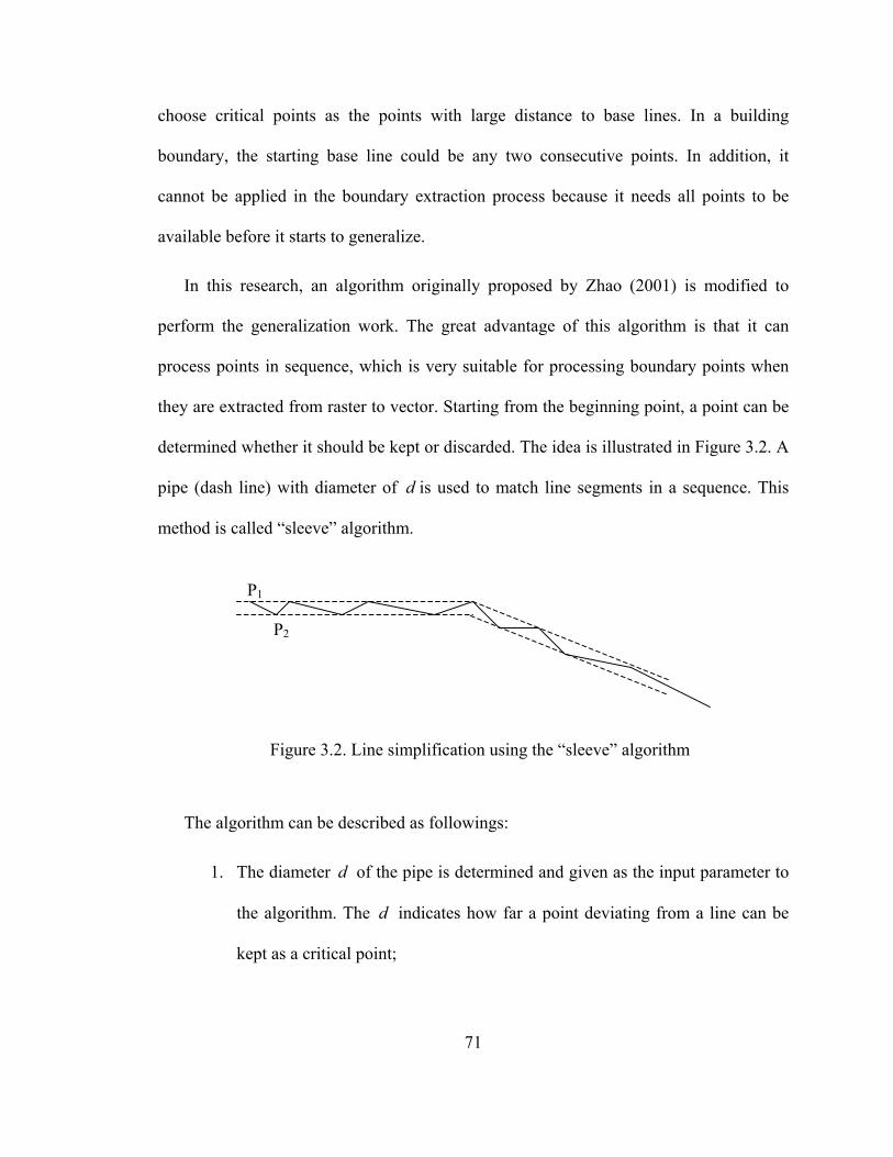
choose critical points as the points with large distance to base lines. In a building

boundary, the starting base line could be any two consecutive points. In addition, it

cannot be applied in the boundary extraction process because it needs all points to be

available before it starts to generalize.

In this research, an algorithm originally proposed by Zhao (2001) is modified to

perform the generalization work. The great advantage of this algorithm is that it can

process points in sequence, which is very suitable for processing boundary points when

they are extracted from raster to vector. Starting from the beginning point, a point can be

determined whether it should be kept or discarded. The idea is illustrated in Figure 3.2. A

pipe (dash line) with diameter of d is used to match line segments in a sequence. This

method is called “sleeve” algorithm.

P1

P2

Figure 3.2. Line simplification using the “sleeve” algorithm

The algorithm can be described as followings:

1. The diameter d of the pipe is determined and given as the input parameter to

the algorithm. The indicates how far a point deviating from a line can be

kept as a critical point;

d

71

2. Starting from the first two points P1 and P2, the direction 0β and length of

the line connecting these two points are calculated;

0l

3. Perpendicular to the current line segment (the line P1P2 at the beginning), the

direction range 0α at current point Pi (the second point P2 at the beginning) is

calculated according to the line segment length and d . The 0α is an angle

range 00 αβ ∆± and 0α∆ is calculated as )2arctan(0l

d ;

4. Next point Pi+1 is connected with the starting point P1 to form a new segment,

and its direction β and length l are calculated. In addition, a new direction

range α is calculated as αβ ∆± with )2arctan( ld=∆α ;

• If the direction β is within the calculated direction range 0α , the current

point Pi is discarded because it is not a critical point. Then a new direction

range at the point Pi+1 is generated as the intersection of the new direction

range α and the current direction range 0α . The new range 0α for

further testing is [max( 00 αβ ∆− , αβ ∆− ), min( 00 αβ ∆+ , αβ ∆+ )]. Go

back to step 3;

• If the new direction β is out of the direction range 0α , the current point Pi

is kept in the generalized line as a critical point. The current point Pi is

taken as the first point of a new line segment and the point Pi+1 is taken as

the second point for next generalization process. Repeat procedure 1 to 3

till the last point.

72

The advantage of the “sleeve” algorithm is that it can process points in a dynamic

manner. It is not necessary to wait until all points are available before processing. This

method is suitable for building boundary generalization because it can generalize the

boundary points when these points were traced. However, one special process should be

applied to building boundary generalization using the “sleeve” algorithm. A building

boundary is a close polygon. The starting point could be any point on a boundary

depending on the scanning process during the conversion from raster boundary to vector

boundary. In addition, the staring point is the ending point in a vector building boundary

polygon.

In order to apply the “sleeve” algorithm in generalizing building boundaries, two

refinements were applied to the original algorithm. The first one is to process the ending

point of a boundary. After the regular “sleeve” algorithm was performed, the starting and

the ending points in the original polygon were kept. These two points are actually the

same point. It is compared with the line formed by the second point and the second to the

last point. If the distance from the point to the line is larger than the distance tolerance d ,

the starting and the ending points are kept. Otherwise, if the point to line distance is

smaller than the distance tolerance, the original starting and ending points will be

discarded. In this case, either the second point is taken as the ending point, or the second

to the last point is taken as the starting point.

The second refinement is to improve the accuracy of generalized line segments. In the

original “sleeve” algorithm, all intermediate, non-critical points were discarded. In

reality, these discarded points also provide useful information. In this research, all

73

intermediate points of a line segment are used to derive parameters of the line using a

least square regression model. In this case, consecutive lines will intersect with each

other to generate critical points. Most likely, the generated critical points will not be in

the original data set. This intersection method will provide a more accurate result because

it takes much more information into account for calculating a line’s parameters. Figure

3.3 shows the refinement of the original algorithm. The bold line is the calculated one

from all intermediate points using a least-square regression model.

Figure 3.3. Line simplification using the refined “sleeve” algorithm

The parameter to be set up in this algorithm is the distance threshold, which can be

adjusted according to specific situations. Figure 3.4 depicts a simplification result using

this refined “sleeve” algorithm. The original boundary is the one extracted from a

building region in raster format.

74

Figure 3.4. Line simplification: The graph on the left shows the original line

segments. The squares are the remaining points after the simplification. The right one shows the simplified line segment

3.2.2. Boundary Regularization

The purpose of regularization is to adjust the boundary of a building to have a

rectangular shape. All line segments are either perpendicular to, or parallel to each other.

To eliminate noise effects and to get parallel or perpendicular boundary segments, some

researchers used the Minimum Description Length (MDL) method to regularize ragged

building boundaries (Weidner and Förstner, 1995). MDL is a statistical method, and it is

very expensive in computation due to iterative comparison. Mayer (2001) used a

constrained active contour method in optimizing building boundaries. However, the

constrained active contour needs a good initial approximation of a boundary. In addition,

it cannot merge or eliminate small line segments. Besides, the image used in the study

should provide sharp boundaries, which is difficult in LIDAR DSM. In this study, a new

regularization method was developed to get rectangular-shape building boundaries.

75

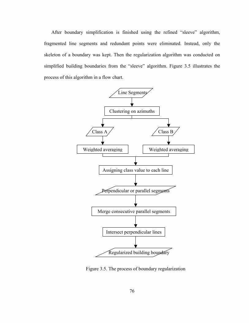
After boundary simplification is finished using the refined “sleeve” algorithm,

fragmented line segments and redundant points were eliminated. Instead, only the

skeleton of a boundary was kept. Then the regularization algorithm was conducted on

simplified building boundaries from the “sleeve” algorithm. Figure 3.5 illustrates the

process of this algorithm in a flow chart.

Regularized building boundary

Intersect perpendicular lines

Merge consecutive parallel segments

Perpendicular or parallel segments

Assigning class value to each line

Weighted averaging

Class B Class A

Weighted averaging

Clustering on azimuths

Line Segments

Figure 3.5. The process of boundary regularization

76

The proposed algorithm is comprised of a cluster process and an adjustment process.

The cluster method is similar to k-means method. It is described in the first item of the

following paragraph. The whole algorithm is described as followings:

• The azimuth of each line segment of a building boundary was calculated, and all

segments were clustered into two classes according to their azimuths. The

criterion used here was inter-class distances. A segment was classified into class

A if the difference between its azimuth and the averaged azimuth of class A was

smaller than the difference between its azimuth and the averaged azimuth of class

B. The result of this step is two groups of line segments, and they are supposed to

be perpendicular to each other;

• For each segment class, the weighted average of line azimuths was calculated.

The weight used for each line segment is its length:

∑∑=

i

ii

lazimuthlazimuth * , li is the length of ith segment in one class. This

matches the observation that a longer line segment has higher azimuth accuracy

than a shorter line segment provided that the position accuracy of end points is the

same. The output of this step is two azimuths that are supposed to be

perpendicular to each other;

• A weighted adjustment using the Gauss-Markov model was carried out to make

the azimuths of these two classes perpendicular. Again, the weight was calculated

as the total length of all segments in each class. After the adjustment, these two

azimuths assigned to two classes are perpendicular;

77

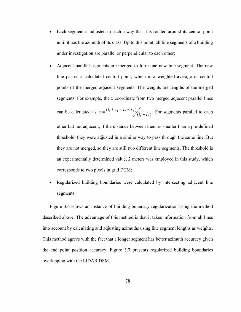
• Each segment is adjusted in such a way that it is rotated around its central point

until it has the azimuth of its class. Up to this point, all line segments of a building

under investigation are parallel or perpendicular to each other;

• Adjacent parallel segments are merged to form one new line segment. The new

line passes a calculated central point, which is a weighted average of central

points of the merged adjacent segments. The weights are lengths of the merged

segments. For example, the x coordinate from two merged adjacent parallel lines

can be calculated as )()(

21

2211ll

xlxlx +∗+∗= . For segments parallel to each

other but not adjacent, if the distance between them is smaller than a pre-defined

threshold, they were adjusted in a similar way to pass through the same line. But

they are not merged, so they are still two different line segments. The threshold is

an experimentally determined value, 2 meters was employed in this study, which

corresponds to two pixels in grid DTM;

• Regularized building boundaries were calculated by intersecting adjacent line

segments.

Figure 3.6 shows an instance of building boundary regularization using the method

described above. The advantage of this method is that it takes information from all lines

into account by calculating and adjusting azimuths using line segment lengths as weights.

This method agrees with the fact that a longer segment has better azimuth accuracy given

the end point position accuracy. Figure 3.7 presents regularized building boundaries

overlapping with the LIDAR DSM.

78

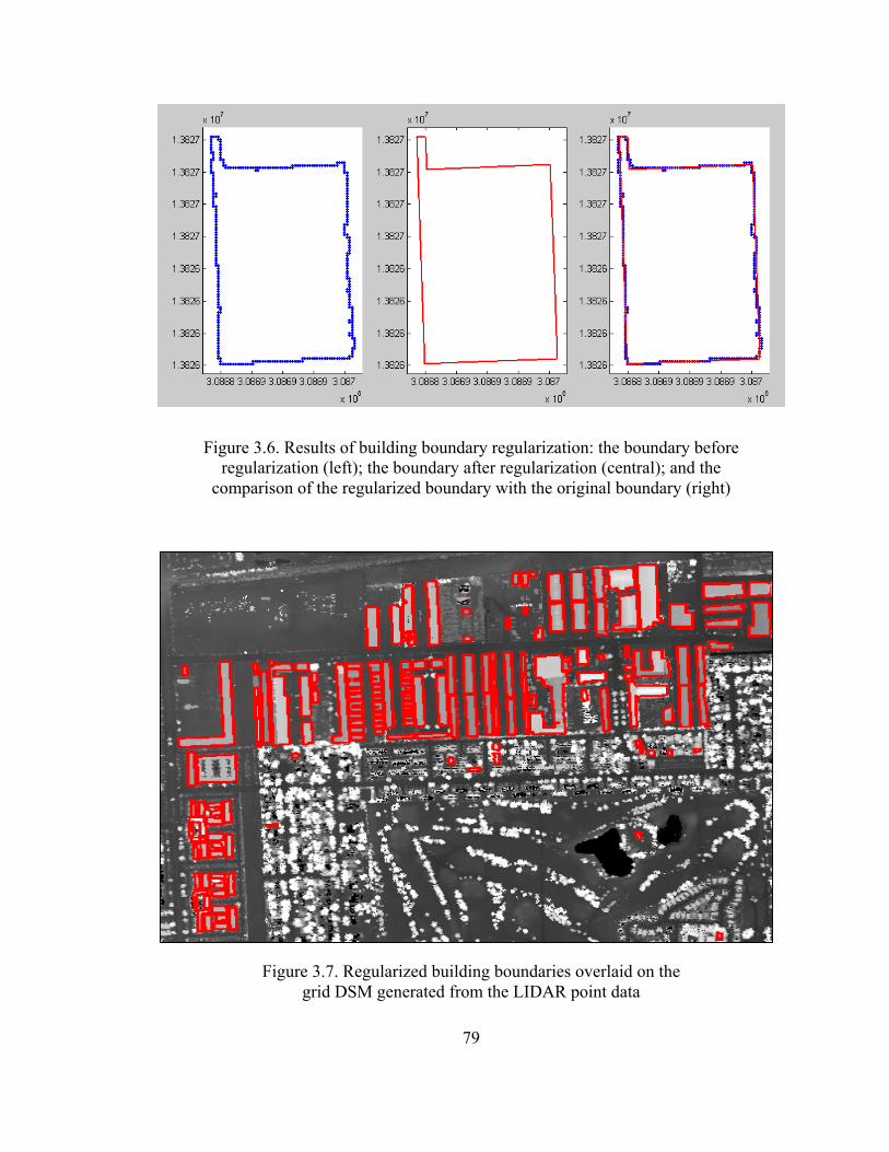
Figure 3.6. Results of building boundary regularization: the boundary before regularization (left); the boundary after regularization (central); and the

comparison of the regularized boundary with the original boundary (right)

Figure 3.7. Regularized building boundaries overlaid on the

grid DSM generated from the LIDAR point data

79

Compared with the MDL method, the proposed regularization method is efficient in

computation. It follows a schema from top to bottom. It finds out the general picture of a

building boundary; then it refines details of the boundary. In this way, it achieves a

globally optimized result.

3.3. Building Model Reconstruction

After the boundary of a building is extracted, a 3D model can be reconstructed from

LIDAR points falling within the building footprint. The process of 3D building model

reconstruction is to derive 3D building CAD models. Generally, there are two basic

approaches to building model reconstruction. One is model based, and the other is data

based. The former one has a database of known building models. A known building

model has available building structures with fixed topology. Thus, the parameter needed

to be calculated is its geometry. This type of method can only work with buildings that

match the models in the model database.

The data-driven approach usually assumes that a building is a polyhedral model,

which is comprised of a group of connected planar surfaces. The tasks are to derive the

topology and to intersect the planar roofs of a building to calculate model parameters.

This approach is flexible in working with different types of building models.

Theoretically, it can reconstruct all kinds of planar-roof buildings because it doesn’t

require prior knowledge about a building’s structure. Some researchers combined the

data-driven method and the model-driven method to take advantages of both approaches.

This combined method is referred as the CSG (Constructive Solid Geometry) method. In

80

the CSG method, a complex building model is decomposed into small building

primitives. These building primitives are stored in a primitive database. Each

decomposed component of a building model is matched with one primitive in the

database; and its geometric parameters are calculated. In the CSG approach, only a

limited number of building primitives are stored in the database, but a large number of

building models can be reconstructed by composing a group of such primitives. However,

the decomposition is usually very tricky.

The algorithm proposed in this research is a data-driven approach instead of a model-

driven approach, which means no a priori knowledge about a specific building model is

required. The assumption made here is that a building is a polyhedral model, which is

comprised of planar surfaces. This approach can theoretically handle most buildings

because most buildings are encompassed by planar surfaces in the real world. Each

surface in such a model is a model primitive. The mission for a building reconstruction

thus becomes detecting and reconstructing building roof primitives. Vertical walls can be

derived from building boundaries. Some researchers have presented their works on

building reconstruction using LIDAR data.

Maas and Vosselman (1999) proposed two algorithms to reconstruct 3D building

models using model-driven and data-driven approaches. They applied invariant moments

to reconstruct simple rectangular shaped buildings using model-driven approach. The

invariant moments cannot be applied to complex buildings. For generic data-driven

model reconstruction, they applied Hough-Transform to detect planar roof surfaces.

Points were organized into a TIN model. One triangle is a plane in 3D; and its plane

81

parameters were used to vote in the Hough parameter space. Vosselman (1999) also used

Hough-Transform to detect planar roofs. However, there are several drawbacks using

Hough-Transform in roof detection: 1) the computation is expensive; 2) the interval in

the parameter space is difficult to determine. A smaller interval will generate a higher

accuracy result but the computation is more expensive; a larger interval decreases the

computation but it generates a lower accuracy result; 3) the peak points in the parameter

space are difficult to detect; and further process is necessary for peak point detection. For

example, the entry with the second largest vote in the parameter space usually does not

represent a second roof of a building. It usually comes from the points contributing to the

first roof. Some algorithms can be applied to detect local peaks in order to correctly

detect roofs. However, this will increase computation load. Another option is to apply the

Hough-Transform algorithm iteratively. Each time only one roof will be detected. Points

contributing to the detected roof(s) will be masked out of the next iteration. Only

remaining points are used to perform Hough-Transform in a next iteration. However,

each of the alternatives will dramatically increase computation load. Even though high

dimensionality Hough-Transform can be implemented on the combination of one-

dimension Hough-Transforms, the right solution out of the combination is still

computation intensive if there are a great number of building LIDAR points, which is

usually the case.

A cluster algorithm, i.e., the k-means algorithm, can also be utilized to detect

buildings roofs based on surface normal data. However, a small horizontal space in high

density LIDAR data will cause its normal data to be very sensitive to noise (Maas and

82

Vosselman, 1999). Thus, a robust filter should be developed to decrease noise effects in

order to use normal data for roof detection.

Some studies were carried out using a region-growth method. Rottensteiner and

Briese (2002) detected seed regions for planar roofs by counting the percentage of “point-

like” points, which were classified using a polymorphic feature extraction based on the

Förstner operator. These seed regions were then compared with adjacent points to grow.

The topology of roofs was generated using a raster Voronoi Diagram. Adjacent co-planar

roof regions were then grouped together; and the roof topology was updated. From the

topology, a building model can be reconstructed by intersecting adjacent roofs.

To avoid direct detection of roofs from LIDAR data, building ground plans can be

utilized to decompose a building into simple building primitives. Such primitives can be

matched with LIDAR points; and their parameters can be calculated from a least square

regression. Finally, a CSG building model is constructed out of the primitives

(Vosselman and Dijkman, 2001; Haala, et al., 1998). Haala, et al. (1998) also used the

relationship between gradient direction and direction of ground plan segments to detect

roofs. This is based on the observation that the normal of a roof is perpendicular to the

bounding line segments of a building. However, the decomposition of the ground plan

could be very tricky sometimes. It may generate primitives that don’t match the models

in a primitive database. As a consequence, wrong models will be generated. In some

cases, the decomposition could generate too many small primitives although these small

primitives are in fact from the same roof.

83

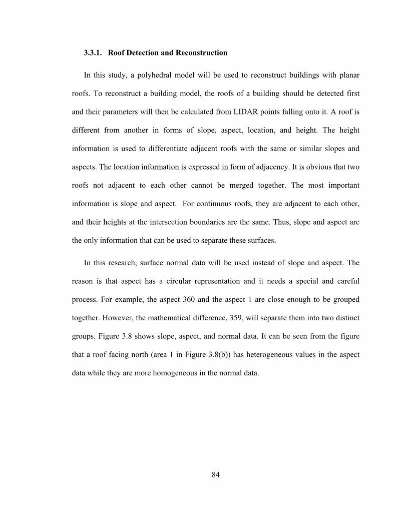
3.3.1. Roof Detection and Reconstruction

In this study, a polyhedral model will be used to reconstruct buildings with planar

roofs. To reconstruct a building model, the roofs of a building should be detected first

and their parameters will then be calculated from LIDAR points falling onto it. A roof is

different from another in forms of slope, aspect, location, and height. The height

information is used to differentiate adjacent roofs with the same or similar slopes and

aspects. The location information is expressed in form of adjacency. It is obvious that two

roofs not adjacent to each other cannot be merged together. The most important

information is slope and aspect. For continuous roofs, they are adjacent to each other,

and their heights at the intersection boundaries are the same. Thus, slope and aspect are

the only information that can be used to separate these surfaces.

In this research, surface normal data will be used instead of slope and aspect. The

reason is that aspect has a circular representation and it needs a special and careful

process. For example, the aspect 360 and the aspect 1 are close enough to be grouped

together. However, the mathematical difference, 359, will separate them into two distinct

groups. Figure 3.8 shows slope, aspect, and normal data. It can be seen from the figure

that a roof facing north (area 1 in Figure 3.8(b)) has heterogeneous values in the aspect

data while they are more homogeneous in the normal data.

84

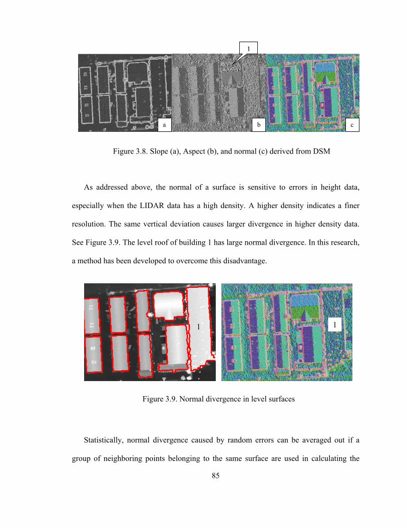
1

cba

Figure 3.8. Slope (a), Aspect (b), and normal (c) derived from DSM

As addressed above, the normal of a surface is sensitive to errors in height data,

especially when the LIDAR data has a high density. A higher density indicates a finer

resolution. The same vertical deviation causes larger divergence in higher density data.

See Figure 3.9. The level roof of building 1 has large normal divergence. In this research,

a method has been developed to overcome this disadvantage.

11

Figure 3.9. Normal divergence in level surfaces

Statistically, normal divergence caused by random errors can be averaged out if a

group of neighboring points belonging to the same surface are used in calculating the

85

normal. Generally, the more points used for calculating normal at each point, the more

consistent the calculated normal is. To calculate normal, a regression plane is used to fit

neighboring points of a point under study. The normal of the fitting plane is taken as the

normal at this point. Although regression calculation can decrease the divergence of

normal data, it is still necessary to be smoothed out for clustering. In this study, a mode

seeking algorithm will be used. This algorithm is the mean-shift algorithm.

3.3.1.1. Mean-shift

Mean-shift is an algorithm for nonparametric density gradient estimation using a

kernel. A mode means a local density maximum. It was first proposed by Fukunaga

and Hostetler (1975) to calculate density gradient. Cheng (1995) further investigated

this algorithm. He proved the convergence of the algorithm and applied it to

clustering. Comaniciu and Meer (2002) further proved its convergence and provided

the sufficient conditions for a mean-shift algorithm to converge. They proved that the

algorithm would converge as long as the kernel applied has a convex and

monotonically decreasing profile. In actual implementation, they argue that

convergence can be achieved if a uniform kernel is applied to estimating density.

They applied the mean-shift algorithm to filtering and segmenting gray scale and

color images.

Given a set of n data points xi (i=1, …., n) in a d-dimensional space Rd, the

multivariate kernel density with a kernel K(x) and a bandwidth matrix H (defined in

equation 3-3) is calculated as

86

∑=

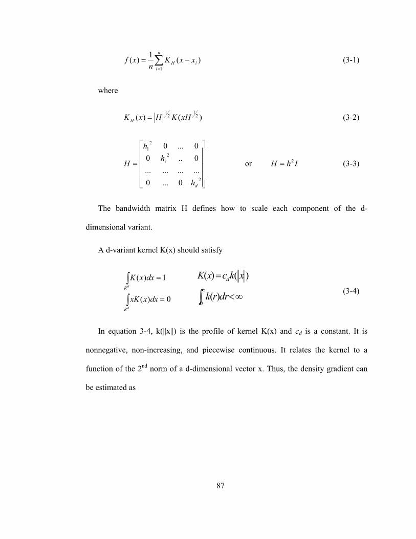
−=n

iiH xxK

nxf

1)(1)( (3-1)

where

)()( 21

21

xHKHxK H = (3-2)

=

2

2

21

0...0............0..00...0

d

i

h

hh

H or (3-3) IhH 2=

The bandwidth matrix H defines how to scale each component of the d-

dimensional variant.

A d-variant kernel K(x) should satisfy

∫

∫=

=

d

d

R

R

dxxxK

dxxK

0)(

1)(

∫

∞∞<

=

0)(

)()(

drrk

xkcxK d

(3-4)

In equation 3-4, k(||x||) is the profile of kernel K(x) and cd is a constant. It is

nonnegative, non-increasing, and piecewise continuous. It relates the kernel to a

function of the 2nd norm of a d-dimensional vector x. Thus, the density gradient can

be estimated as

87

}))((

))((}{))(({

}))((

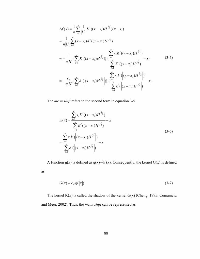
))((}{))(({1

))(()(1

)())((11)(

1

21'

1

21'

1

21'

1

21'

1

21'

1

21'

1

21'

1

21'

xHxxk

HxxkxHxxk

Hnc

xHxxK

HxxKxHxxK

Hn

HxxKxxHn

xxHxxKHn

xf

n

ii

n

iiin

ii

d

n

ii

n

iiin

ii

n

iii

i

n

ii

−−

−−−=

−−

−−−=

−−=

−−=∆

∑

∑∑

∑

∑∑

∑

∑

=

=

=

=

=

=

=

=

(3-5)

The mean shift refers to the second term in equation 3-5.

xHxxk

Hxxkx

xHxxK

HxxKxxm

n

ii

n

iii

n

ii

n

iii

−−

−=

−−

−=

∑

∑

∑

∑

=

=

=

=

1

21'

1

21'

1

21'

1

21'

))((

))((

))((

))(()(

(3-6)

A function g(x) is defined as g(x)=-k’(x). Consequently, the kernel G(x) is defined

as

)()( xgcxG d= (3-7)

The kernel K(x) is called the shadow of the kernel G(x) (Cheng, 1995; Comaniciu

and Meer, 2002). Thus, the mean shift can be represented as

88

xHxxg

Hxxgxxm n

ii

n

iii

−−

−=

∑

∑

=

=

1

21

1

21

))((

))(()( (3-8)

The shadow of a Gaussian Kernel is also a Gaussian Kernel. The Uniform Kernel

is the shadow of the Epanechnikov Kernel, which is defined as

>≤−

=101)1(

)(xifxifxC

xE d (3-9)

and the Uniform Kernel is defined as

>≤

=101

)(xifxifC

xF d (3-10)

In equation 3-9 and 3-10, the Cd is a constant to normalize the function so that the

integral of the function equals 1. In this study, the mean shift will be used to perform

filtering and clustering of DSM based on surface normal data. The Uniform Kernel

will be used.

In order to apply the mean-shift method to clustering, a feature space need to be

built up first. The advantage of the mean-shift method is that the feature space can be

built simultaneously from spatial information (x, y, and z) and attribute information

(gray values, color information, and texture measurements). Another filter that works

on both spatial domain and attribute domain simultaneously is the bilateral filtering

method (Tomasi and Manduchi, 1998). The difference between the mean-shift

method and the bilateral filtering method is that the former uses a dynamic searching

window while the later uses a static one. Another advantage of the mean-shift method

89

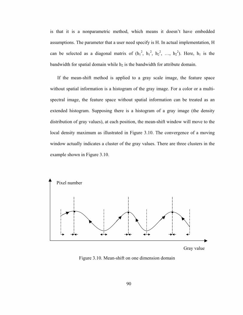
is that it is a nonparametric method, which means it doesn’t have embedded

assumptions. The parameter that a user need specify is H. In actual implementation, H

can be selected as a diagonal matrix of (h12, h1

2, h22, …, h2

2). Here, h1 is the

bandwidth for spatial domain while h2 is the bandwidth for attribute domain.

If the mean-shift method is applied to a gray scale image, the feature space

without spatial information is a histogram of the gray image. For a color or a multi-

spectral image, the feature space without spatial information can be treated as an

extended histogram. Supposing there is a histogram of a gray image (the density

distribution of gray values), at each position, the mean-shift window will move to the

local density maximum as illustrated in Figure 3.10. The convergence of a moving

window actually indicates a cluster of the gray values. There are three clusters in the

example shown in Figure 3.10.

Pixel number

Gray value

Figure 3.10. Mean-shift on one dimension domain

90

As addressed before, the mean-shift algorithm can be applied to spatial domain

and attribute domain jointly. In this case, the bandwidth of spatial domain and the

bandwidth of attribute domain should be selected individually. However, after

normalization, these two domains can be joined together to perform filtering. Figure

3.11 and Figure 3.12 illustrate a feature space before and after a filtering applied to a

gray value image using the mean-shift algorithm. X and Y axes are spatial

coordinates; and the gray axis is image pixel value. It can be seen that the feature

space has a plateau-like shape. After the filtering, the plateau shaped surface is

smoothed out (Figure 3.12).

The general procedure to perform the mean-shift filtering can be summarized as

the followings:

• User inputs of the bandwidths hs for spatial domain and ha for attribute

domain. Build up the feature space F(X|X=(x, y, a1, …, an));

• For each data in the data set (for each pixel in the image), initialize Y=Xi;

• Calculate the mean shift using equation 3-7. The kernel is a uniform kernel

(equation 3-10). Update Y=Y+m(x). Repeat until m(x) equals 0;

• Output the result Zi=(Xi(x, y), Y(a1, …, an)) . This assigns the spatial

information of the initial position and the attribute information of the

convergent position.

91

Figure 3.11. The feature space before applying the mean-shift filtering

Figure 3.12. Feature space after the mean-shift filtering is applied

92

Some methods can be employed to speed up the computation of the mean-shift

algorithm. The most expensive computation part is to search neighboring points,

which fall within bandwidths and are used to calculate the mean shift. Some

researchers proposed certain computation optimization methods in calculating the

mean shift (Georgescu, et al., 2003). In this research, the searching of neighboring

points is conducted in the spatial domain first, and then in the attribute domain. The

reason is that pixels’ coordinates provide the spatial topology of an image. Thus, the

points neighboring in spatial domain can be retrieved quickly.

3.3.1.2. Roof Reconstruction

The roofs of a building are detected based on the mean-shift algorithm as

described above. The data used is surface normal data derived from a LIDAR DSM.

As addressed before, the divergence in surface normal data introduced by errors is

largely due to small point spacing. Neighboring points are used to derive a fitting

plane; and the plane’s normal was assigned to the point under study. In this study, a 5

by 5 window is used to fit a DSM at each point as a plane. Figure 3.13 displays

calculated normal from a DSM. The one on the left is calculated from a 3 by 3 fitting

window, while the one on the right is calculated from a 5 by 5 window. It is obvious

that the normal calculated from a 5 by 5 window is much more consistent that the one

calculated form the 3 by 3 window (see region 1 in Figure 3.13).

93

11

Figure 3.13. Normals calculated from the DSM using different fitting windows: a 3 by 3 window (left) and a 5 by 5 window (right)

The calculated normal is clustered using the mean-shift algorithm. The normal is

filtered first by assigning the value of a density mode to pixels that converge to it.

One mode indicates one cluster in the data. All data points belonging to the same

mode are classified into one cluster. In actual implementation, points belonging to

the same mode do not have the exactly same value due to the round up in conversion

from float/double format data to integer format data. Thus, after filtering, all points

with a difference smaller than the bandwidths employed in the filtering process are

grouped together as one cluster and are labeled. The mean-shift algorithm was carried

out on the joint feature space, (x, y, nx, ny, nz). The (x, y) components are spatial

coordinates; the (nx, ny, nz) components are used to represent the red, green, and blue

channels. Figure 3.14 shows the normal data before and after the filtering. It can be

seen that the normal is smoothed out. Figure 3.15 illustrates the X component of the

normal before and after the filtering for building A outlined in Figure 3.14.

94

A

Figure 3.14. The normal data before (left) and after

(right) the filtering using the mean-shift method

95

Figure 3.15. 3D visualization of the X normal component before (left) and after (right) the filtering for the building A outlined in Figure 3.14

96

After filtering, the data can be classified into clusters by grouping similar points.

In this study, a supervised classification was performed on the normal data through a

commercial software. Small segments were merged to their adjacent large segments,

which share the longest boundary with them. This merge was achieved in vector

format. The segmented image was converted into Arc coverage using ERDAS

Imagine software. Polygons with a small area were then identified and merged to

their neighboring segments. The elimination of small polygons was conducted in

ArcGIS software. Figure 3.16 presents the classification result and roofs converted to

vector format. In a building reconstruction system, roofs can be extracted using the

detected building boundaries as described in the previous chapter.

Figure 3.16. Roof clustering and extraction

After the roofs of a building were extracted, their plane parameters can be

calculated from 3D LIDAR points. The boundary of a roof was used to extract

LIDAR points falling within its footprint using a point-in-polygon algorithm. The

algorithm applied here is the well-known Ray-Crossing method. Figure 3.17

97

illustrates its concept. The algorithm can be summarized as the following: 1) Given a

point and a polygon, a half horizontal line is draw from the point to the positive x-

axis direction; 2) This line is analyzed with the polygon’s boundary segments. The

number of segments that intersect with the half horizontal line is counted; 3) If the

number is an even number, then the point under analysis is outside the polygon; if the

intersection number is an odd number, that means the point under test is inside the

polygon. Points within a roof boundary are retrieved to calculate the roof’s plane

parameters using the Gauss-Markov model. The 3D plane is represented as

; and the parameters to be calculated are a, b, and c. 1** =++∗ zcYbXa

Figure 3.17. Point-in-polygon analysis

Due to roof detection and extraction biases, some points not belonging to a roof

could be extracted by the roof’s boundary. In order to improve the accuracy of a

derived roof plane, the plane fitting error δ , MSE (Mean Square Error), was

calculated; and those points with a residual larger than δ2 were detected and

rejected. Those remaining points were used to calculate a new set of parameters for a

roof plane. This refinement process can be repeated until no larger number of rejected

98

points can be detected. Usually, the repetition number is not large. In this research,

the refinement was performed twice.

3.3.2. Model Reconstruction

To reconstruct a 3D building model, the topology (the adjacency relationship) of its

roofs and vertical walls need to be built after 3D roof surfaces were calculated. This

produces an adjacency graph depicting the inter-relationship of those 3D surfaces. With

the adjacency graph, adjacent planes can be used to derive building corners.

Consequently, a 3D building model can be reconstructed.

The topology among those detected roofs can be derived immediately by checking if

they share a common boundary line segment. This can be done after roof polygons were

extracted or converted from a raster thematic image. To build an adjacency graph, some

researchers performed the raster Voronoi algorithm using the Chamfer mask (Ameri and

Fritsch, 2000). In their study, the detected roof planes are not complete. Roofs do not

touch each other due to the data and algorithm they employed. In this study, the detected

roof planes are complete. They share common boundaries. The topology of these detected

roofs was retrieved using a commercial software package, the ArcGIS software. After a

raster thematic image was generated, it was converted into Arc Polygon Coverage. The

topology was read out through an ArcView script. Obviously, the topology was built in a

2D space.

Vertical walls are represented as line segments in a 2D horizontal space, which forms

the boundary of a building. During roof detection, a roof’s bounding regions were lost

due to a large plane-fitting window. Thus, a building’s boundary (vertical walls) is

99

separated from its roof boundaries. Their adjacency cannot be constructed by directly

checking if they share common line segments. A new method is proposed in this study to

construct the topology between a building’s boundary (vertical walls) and its roofs.

The disconnection between a building’s boundary and its roof boundaries is mainly

caused by the plane fitting in normal calculation. Thus, the general distance of such a

disconnection is proportional to the size of a fitting window. If the building boundary is

shrunk or the roof boundaries are expanded, the building’s boundary will intersect or

touch its roof boundaries. In this research, a building’s boundary will be shrunk to

determine which roof polygon it is adjacent to. See Figure 3.18. A building boundary line

segment is expanded to its perpendicular direction to form a rectangle. If the rectangle

touches or intersects a boundary segment of a roof, the boundary is adjacent to the roof.

The width of such a rectangle is determined by the plane-fitting window size. It can be

double the size of the fitting window. In reality, the width can be controlled as a

parameter input by users. If the rectangle intersects or touches one roof polygon, the

adjacency is built between these two surfaces (the vertical wall and the roof).

2l

B

A

Figure 3.18. Topology of roofs and the building boundary

100

Based on the method described above, the topology of a building can be constructed.

Supposing the roofs (1-4) and the vertical walls (5-12) are numbered as shown in Figure

3.19, the topology can be represented in an adjacency graph or a correlation table, which

is represented as an adjacency matrix. Table 3.1 shows the adjacency matrix for the

building example in Figure 3.19.

1211

10

98

7

6

5

3 4

2

1

Figure 3.19. Numbering roofs and vertical walls

Table 3.1: Adjacency matrix for roofs and vertical walls

1111211111

1111101119

111811117

111611115

1111411113

1111111211111

121110987654321

101

Table 3.1 demonstrates an adjacency matrix. One entry of the matrix indicates the

relationship between two surfaces. The value of 1 indicates that the two surfaces are

adjacent to each other, while the value of 0 indicates that these two surfaces are not

connected. The matrix is symmetric. The diagonal elements are set to 0. Thus, adjacent

surfaces to a surface under study can be immediately retrieved by checking the row or

column entry values.

Each surface has an attribute indicating whether it is a roof surface or a bounding

vertical wall in an actual implementation. The bounding vertical walls of a building are

numbered in sequence. In this manner, the adjacency relationship among vertical walls

can be constructed from their numbers. Each vertical wall can only be adjacent to another

two vertical walls.

To reconstruct a 3D building model, building corners will be reconstructed first

because they are the primitives of a CAD model. In this research, a building’s corners are

divided into two groups; and they will be calculated using different approaches. The first

group is the corners formed by two vertical walls; the second group is formed by at least

two roof surfaces. This division is not an exclusive division. That means there is an

overlap between these two groups. After these two groups of corners were calculated

independently, all corners will be checked to eliminate any duplication. The method for

reconstructing corners formed by two vertical walls is described as followings:

1. Given two adjacent vertical walls a and b, retrieve their common adjacent roof

surface from the surface adjacency matrix. If they have common roof

surfaces, the common roof surfaces will generate a corner with these two

102

vertical walls. For example, in Figure 3.19, vertical walls 5 and 12 will find

the common roof 2. Record the belonging-to relationship between the

calculated corner and its calculating surfaces in a point-surface matrix;

2. If no common roof surfaces were found (see vertical walls 11 and 12 in

Figure 3.19), all roofs adjacent to either a or b are retrieved. If exactly two

roofs were retrieved, these four surfaces will be used to generate one corner

(see vertical walls 11, 12 and roofs 2, 3). Record the belonging-to relationship

between the calculated corner and its calculating surfaces in a point-surface

matrix;

3. If more than two roofs were found adjacent to a or to b, each of the retrieved

roofs generates a corner with these two vertical walls. The actual corner will

have at least two duplications among those corners. These duplications of the

actual corner will be close to each other while other corners will be far away

from the duplications. In this study, a threshold of 1 meter in distance was

used to test if two calculated corners are close to each other. If their distance is

smaller than the threshold, they will be taken as duplications of the actual

corner. The average of these two calculated corners will be taken as the actual

corner. Record the belonging-to relationship between the calculated corner

and its calculating surfaces in a point-surface matrix;

4. Repeat above calculations for all consecutive vertical walls.

The building corners in the second group are formed by at least two roof surfaces.

Similarly, the belonging-to relationship between the calculated corner and its calculating

103

surfaces is also recorded in the point-surface matrix when a corner is constructed. The

method can be summarized as:

1. Given a roof surface S, find out all its adjacent roof surfaces {S1, …, Sn};

2. For each T in {S1, …, Sn}, find out all the surfaces adjacent to both T and S

including roofs and vertical walls {T1, …, Tm}. For example, in Figure 3.19,

vertical walls 5 and 7 are adjacent to both roofs 1 and 2. They will be

retrieved as the set {T1, T2};

3. If {T1, …, Tm} is empty, go to step 5. Otherwise, for each I in {T1, …, Tm}, a

corner is calculated from {I, S, T}. Record the belonging-to relationship in the

point-surface matrix;

4. After all roofs S are processed using the steps from 1 to 3, corners in the

second group are compared. If two corners share at least three common roofs,

they are merged together. The point-surface matrix will be changed

accordingly. The reason to perform this operation is that the process is

redundant. For example, starting from roof 1 in Figure 3.19, roof 2 will be

retrieved and a corner will be generated with vertical wall 5. When starting

from roof 2, roof 1 will be retrieved to form a new corner with vertical wall 5.

In reality, these two corners are the same actual corner;

5. Repeat the process for each roof surface.

104

After all corners in the first group and the second group were generated, they are all

compared to check corner redundancy. If two corners are shorter than a threshold of 1

meter, they will be merged into one corner. The point-surface matrix will be changed

accordingly. Figure 3.20 shows an example of reconstructed building corners. The

Roman numerals represent corner number while the Arabic numerals represent surface

number. Correspondingly, Table 3.2 shows its point-surface matrix. The example matrix

has equal row and column numbers.

6

4

3 1 2 5

IIIIII

VI V IV

Figure 3.20. Reconstructed building corners

Table 3.2. Point-surface matrix for the example in Figure 3.20

I

1116115

1114113

1111211111

VIVIVIIIII

105

Up to this point, 3D corners of a building are constructed. A 3D building model can

be reconstructed through its 3D surfaces. A surface can be described by its bounding

corners, which are retrieved from the point-surface matrix. However, these bounding

points are not ordered to their sequence on surface boundary. A convex hull can be

calculated from corners as a surface for a convex roof polygon. But it does not work for a

concave polygon. For a vertical wall, the lower points can be derived by intersecting the

ground DTM. Before the lower points are derived, the upper points that are retrieved

from a point-surface matrix are ordered first. By doing so, points can be ordered in

consistency with the boundary. The method to order points on vertical walls can be

summarized as:

1. Giving a vertical wall surface, retrieve all its upper points from the point-

surface matrix, P{p1, …, pn}. These points are the upper points;

2. If n equals 2, take the order P {p1, p2}. Go to step 5;

3. If n is larger than 2, the horizontal coordinates will be used to order these

points. These points are projected to a horizontal plane and a 2D line is

formed. This line can be derived from the first two points, (x1, y1) and (x2, y2).

The line can be represented in the form shown in equation 3-11. Each point on

the line can be represented by a unique value t;

∆+=∆+=

ytyyxtxx

**

1

1 where

−=∆−=∆

12

12

yyyxxx

),( +∞−∞∈t (3-11)

4. Calculate t for every point and order the points based on t. This order applies

to the 3D points, P′{p1′, …, pn′};

106

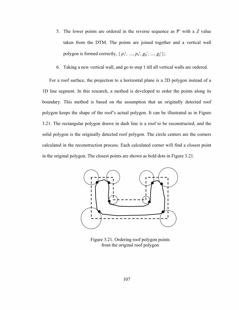
5. The lower points are ordered in the reverse sequence as P′ with a Z value

taken from the DTM. The points are joined together and a vertical wall

polygon is formed correctly, { p1′, …, pn′, pn′, …, p1′};

6. Taking a new vertical wall, and go to step 1 till all vertical walls are ordered.

For a roof surface, the projection to a horizontal plane is a 2D polygon instead of a

1D line segment. In this research, a method is developed to order the points along its

boundary. This method is based on the assumption that an originally detected roof

polygon keeps the shape of the roof’s actual polygon. It can be illustrated as in Figure

3.21. The rectangular polygon drawn in dash line is a roof to be reconstructed; and the

solid polygon is the originally detected roof polygon. The circle centers are the corners

calculated in the reconstruction process. Each calculated corner will find a closest point

in the original polygon. The closest points are shown as bold dots in Figure 3.21.

Figure 3.21. Ordering roof polygon points

from the original roof polygon

107

The method for ordering a roof polygon requires its original roof polygon detected

from normal data, which has its points ordered in the correct sequence. The method can

be described as followings:

1. Giving a roof polygon, retrieve all its points from the point-surface matrix,

P{p1, …, pn};

2. Retrieve the original roof polygon detected from normal data, which is

represented as a sequence of points in order. Number its points based on their

orders in the sequence, P′{p1′, …, pm′};

3. For each corner point pi in P, find the closest point pj′ in P′. Assign the

number j to the point pi as an attribute;

4. Order the corner points in P according to their attribute number js. This order

is the sequence for these calculated corners along a roof boundary. Thus, a

roof polygon is reconstructed.

Figure 3.22 presents an example of topology construction between vertical walls and

roof surfaces. The red segments are expanded segments parallel to vertical walls, which

are represented as blue segments. The green polygons are roof boundaries. After the

topology was built, coordinates of building corners were calculated and plotted as star

marks in Figure 3.22. The reconstructed 3D model of the same building from Figure 3.22

is shown in Figure 3.23.

108

109

Figure 3.22. The reconstruction of surface topology

Figure 3.23. An example of reconstructed 3D building models

CHAPTER 4

BUILDING MODEL REFINEMENT

LIDAR point data are random points with high vertical accuracy; however, these

points have lower horizontal accuracy mainly caused by large laser footprints on the

ground and navigation errors. LIDAR points are sample points of the earth’s surface.

This determines that LIDAR data cannot capture sharp linear features. Thus, a building

model reconstructed from LIDAR will have low geometrical accuracy, especially the

bounding boundary. This means that there is a great potential to improve a building’s

geometry, specifically its boundary, through data or information integration. A linear

feature derived from intersection of two roof surfaces will have a high accuracy because

the roofs derived from LIDAR points have high accuracy. Instead of being refined, these

features can be used as control features in data registration.

In this research, aerial photographs are employed to integrate with LIDAR data for

building model refinement. Aerial photographs are mainly used to extract linear features,

specifically building boundary edges. A method will be developed to integrate these

edges with reconstructed building models from LIDAR data to improve the accuracy of

the models. The method for data registration will be described first; then data integration

110

will be illustrated, followed by a description of building model refinement. Figure 4.1

shows the flowchart of the refinement process.

No

Keep the original linesKeep the updated lines

Yes

Both 2D lines are updated

NoNo

Yes

Calculate new line parameters

Found edge pixels for refinement

Yes

Calculate new line parameters

Found edge pixels for refinement

Edge pixel search for refinement

Edge pixel search for refinement

Edge detection Edge detection

2D polygon in image 2 2D polygon in image 1

Projection

3D building roof polygon

Figure 4.1. Simultaneously updating 2D lines in both stereo images

111

4.1. Co-Registration of LIDAR and Image Data

Integration of data from different sensors or platforms can be performed in different

levels: data level, feature level, and object level [Csathó, 1999]. In order to perform

integration, data from different sources should be registered under the same framework, a

common coordinate system. In order to integrate aerial photograph and LIDAR data for

refinement, these two data sets should be co-registered within one coordinate system.

Some research studies have been conducted to use linear features in image resection.

Habib (2002) used 2D ground linear features to estimate photograph exterior orientation

parameters (EOP) using a Modified Iterated Hough Transform methodology. Stamos

(2000) registered 3D and 2D linear features derived from LIDAR data and image data

respectively with known image EOP. Straight line-segments perform as control features

to derive EOP. Figure 4.2 shows the general procedure for co-registration of LIDAR data

and aerial photographs.

LIDAR data points are already in a 3D coordinate system. So it is convenient to take

the coordinate system of the LIDAR data as the common framework. Thus, a aerial

photograph will be registered to the LIDAR data system. The registration is the

calculation of interior and exterior orientation parameters for an aerial image. The interior

orientation is a transformation from a measuring system to the image system originated at

its calibrated principle point. The exterior orientation is to derive the EOP, which are the

position of the exposure center (X0, Y0, Z0) and camera pose (ω, φ, κ). The EOP of an

aerial photograph can be calculated from image resection using ground control points like

GPS control points or points from other sources with high accuracy.

112

Interior Orientation

ExteriorOrientationParameters

Least-Square to solve unknowns

Coplanarity Conditions

Conjugate LineSegmentsMatching

2D LineSegments

2D EdgeExtraction

Aerial Photo

3D LineSegments

AdjacentPlanar Surface

SurfaceIntersection

Planar surfacedetection

LIDAR Data

Figure 4.2. Co-registration of LIDAR and aerial images

For data integration, internal consistence of integrated data is very important. To have

a high consistence, it is a wise choice to select points or features from LIDAR data as

known control features for image resection. As mentioned before, LIDAR data cannot

capture either sharp linear or point features directly. Consequently, control features

113

cannot be measured directly from LIDAR data. However, accurate linear features can be

calculated from LIDAR data. Planar roofs have high accuracy parameters because a large

amount of points were applied to derive their parameters. Linear features derived from

intersection of adjacent planar roofs can be employed as control features. Compared with

linear features, corners formed by three intersecting roofs are less common in a LIDAR

data set. So linear features derived from roof intersection will be utilized to perform

image resection. After image resection, two data sets are registered in a common

coordinate system.

4.1.1. 3D Intersection Lines from LIDAR data and 2D Edges from Photograph

To perform image resection, conjugate line segments should be measured in 3D space

of LIDAR data and 2D space of aerial photographs. 3D line segments from LIDAR data

are calculated from adjacent intersecting planar roofs. This requires that 3D planar roofs

be calculated first.

To calculate 3D roof plane parameters for image resection, points belonging to a

plane are distinguished and extracted. After the points of a plane were extracted, the

plane’s parameters can be calculated using the least square regression method. A 3D line

is obtained by intersecting two adjacent 3D planes; and it will be represented using two

points on the line.

From a 2D image, the conjugate line segment of a 3D line segment in the 3D ground

space is interpreted manually, and its end points are measured. After applying the image

interior orientation transformation, the 2D edge will be ready for image resection

described in the following section.

114

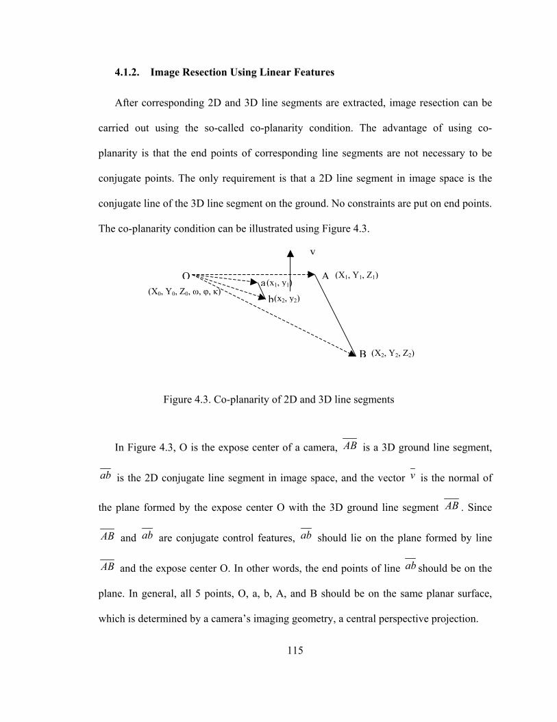
4.1.2. Image Resection Using Linear Features

After corresponding 2D and 3D line segments are extracted, image resection can be

carried out using the so-called co-planarity condition. The advantage of using co-

planarity is that the end points of corresponding line segments are not necessary to be

conjugate points. The only requirement is that a 2D line segment in image space is the

conjugate line of the 3D line segment on the ground. No constraints are put on end points.

The co-planarity condition can be illustrated using Figure 4.3.

v

(x2, y2)

(x1, y1)(X1, Y1, Z1)

(X0, Y0, Z0, ω, φ, κ) b

a

B

AO

(X2, Y2, Z2)

Figure 4.3. Co-planarity of 2D and 3D line segments

In Figure 4.3, O is the expose center of a camera, AB is a 3D ground line segment,

ab is the 2D conjugate line segment in image space, and the vector v is the normal of

the plane formed by the expose center O with the 3D ground line segment AB . Since

AB and ab are conjugate control features, ab should lie on the plane formed by line

AB and the expose center O. In other words, the end points of line ab should be on the

plane. In general, all 5 points, O, a, b, A, and B should be on the same planar surface,

which is determined by a camera’s imaging geometry, a central perspective projection.

115

In order to represent and to use co-planarity conditions in deriving EOP, two vectors

are drawn from the expose center O to points a and b respectively. Thus, the co-planarity

condition of the 5 points is equivalent to the condition that both vectors, Oa and Ob , are

perpendicular to the normal vector v . This guarantees that the line ab lies on the

common plane formed by O, A, and B. Vector v is also perpendicular to vectors OA and

OB . This condition can be written as equation 4-1.

×==•=•

ObOavOBvOAv

00

(4-1)

Each pair of control feature provides two equations, 0=• vOA and 0=• vOB .

Thus, for 6 unknowns of EOP, three pairs of linear control features can solve the

problem. For better accuracy, more than three pairs of control features are needed for

redundant checks. Then, the least-square method is used to minimize the discrepancy

among the conditions.

In order to use the co-planarity condition, all coordinates should be within one

common coordinate system. Here, the 3D coordinate system of the image space is used,

which is originated at the expose center O. Thus, a translation and a rotation will be

performed to transform ground coordinates into the image space system.

Suppose the rotation matrix from ground space to image space is R, the coordinates

of expose center O in the ground space is (X0, Y0, Z0), the coordinates of the end points

of a 2D line segment after interior orientation are (x1, y1) and (x2, y2) respectively, the

116

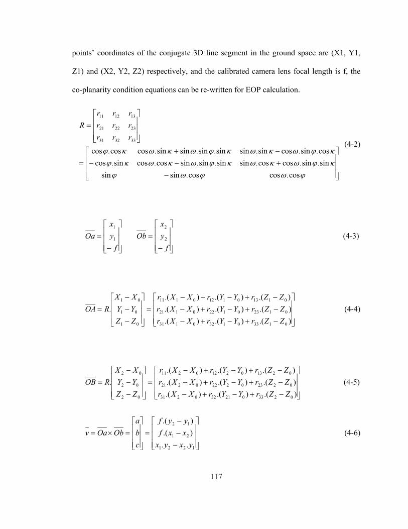
points’ coordinates of the conjugate 3D line segment in the ground space are (X1, Y1,

Z1) and (X2, Y2, Z2) respectively, and the calibrated camera lens focal length is f, the

co-planarity condition equations can be re-written for EOP calculation.

−+−−−+

=

=

ϕωϕωϕκϕωκωκϕωκωκϕκϕωκωκϕωκωκϕ

cos.coscos.sinsinsin.sin.coscos.sinsin.sin.sincos.cossin.coscos.sin.cossin.sinsin.sin.sinsin.coscos.cos

333231

232221

131211

rrrrrrrrr

R

(4-2)

−=

fyx

Oa 1

1

−=

fyx

Ob 2

2

(4-3)

−+−+−−+−+−−+−+−

=

−−−

=).().().().().().().().().(

.

013301320131

012301220121

011301120111

01

01

01

ZZrYYrXXrZZrYYrXXrZZrYYrXXr

ZZYYXX

ROA (4-4)

−+−+−−+−+−−+−+−

=

−−−

=).().().().().().().().().(

.

0233021320231

022302220221

021302120211

02

02

02

ZZrYYrXXrZZrYYrXXrZZrYYrXXr

ZZYYXX

ROB (4-5)

−−−

=

=×=

1221

21

12

..).().(

yxyxxxfyyf

cba

ObOav (4-6)

117

Thus, the co-planarity conditions can be written as

0)).().().(.()).().().(.(

)).().().(.(

013301320131

012301220121

0113011201111

=−+−+−+−+−+−+

−+−+−=•=

ZZrYYrXXrcZZrYYrXXrb

ZZrYYrXXravOAF

(4-7)

0)).().().(.()).().().(.(

)).().().(.(

023302320231

022302220221

0213021202112

=−+−+−+−+−+−+

−+−+−=•=

ZZrYYrXXrcZZrYYrXXrb

ZZrYYrXXravOBF

(4-8)

The six unknown exterior orientation parameters of a camera are included in

equations 4-7 and 4-8. These two equations can be used to solve the unknowns. However,

the equations are non-linear equations. So linear forms are derived using the Taylor

series, and an iterative approach is necessary to solve these parameters. The deduction is

presented in the following sections.

Suppose the variable in form of a vector is u , then

[ ]κϕω000 ZYXu T=

0).(!1

)()(

...).(!

)(...).(

!1)(

)()(

00

0

00

)(

00

0

≈−′

+≈

+−++−′

+=

uuuF

uF

uun

uFuu

uFuFuF n

n

(4-9)

118

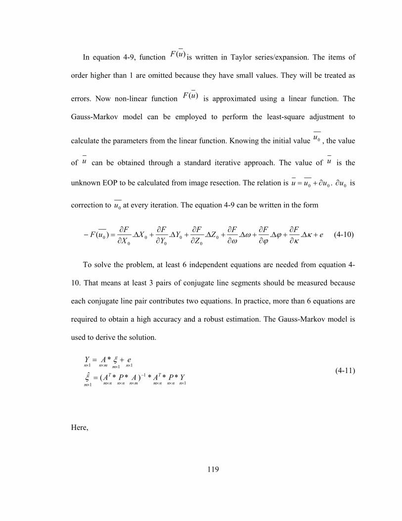
In equation 4-9, function )(uF is written in Taylor series/expansion. The items of

order higher than 1 are omitted because they have small values. They will be treated as

errors. Now non-linear function )(uF is approximated using a linear function. The

Gauss-Markov model can be employed to perform the least-square adjustment to

calculate the parameters from the linear function. Knowing the initial value 0u , the value

of u can be obtained through a standard iterative approach. The value of u is the

unknown EOP to be calculated from image resection. The relation is 00 uuu ∂+= . 0u∂ is

correction to 0u at every iteration. The equation 4-9 can be written in the form

eFFFZZFY

YFX

XFuF +∆

∂∂

+∆∂∂

+∆∂∂

+∆∂∂

+∆∂∂

+∆∂∂

=− κκ

ϕϕ

ωω

......)( 00

00

00

0 (4-10)

To solve the problem, at least 6 independent equations are needed from equation 4-

10. That means at least 3 pairs of conjugate line segments should be measured because

each conjugate line pair contributes two equations. In practice, more than 6 equations are

required to obtain a high accuracy and a robust estimation. The Gauss-Markov model is

used to derive the solution.

1

1

1

111

***)**(ˆ

*

×××

−

××××

××××

=

+=

nnnnm

T

mnnnnm

T

m

nmmnn

YPAAPA

eAY

ξ

ξ (4-11)

Here,

119

∂∂

∂∂

∂∂

∂∂

∂∂

∂∂

⋅⋅⋅⋅⋅⋅∂∂

∂∂

∂∂

∂∂

∂∂

∂∂

=

∂∂∂∂∂∂=

−−=

κϕω

κϕω

κϕωξ

nnnnnn

T

Tn

FFFZF

YF

XF

FFFZF

YF

XF

A

ZYX

uFuFY

000

111

0

1

0

1

0

1

000

010

],,,,,[

])(,...,)([

(4-12)

The coefficients of A can be calculated as in equation 4-13. In equation 4-13,

constants (a, b, c) are the coordinates of vector v . See equation 4-6. The Gauss-Markov

Model can be used to calculate the increments or the corrections

( κϕω ∂∂∂∂∂∂ ,,,,, 000 ZYX ). Then a camera’s EOP can be updated from its initial values.

After several iterations, the EOP can be calculated with required accuracy requirements.

The procedure can be summarized as following steps:

• Knowing the initial values of EOP 0u , matrix A and vector Y are calculated

using equations 4-12 and 4-13;

• Using the Gauss-Markov model to calculate the parameter increments

0u∂ (equation 4-11), and update 0u with 0u∂ by adding 0u∂ to 0u . The

weight matrix is determined by actual measurement accuracy. To simplify the

calculation, matrix P can be assigned as an identity matrix. This means

measurements are equally weighted;

• Check the increments 0u∂ , if 0u∂ is smaller than a pre-defined value, then

stops and 0u is the calculated EOP. Otherwise, go to step 1 and continue.

120

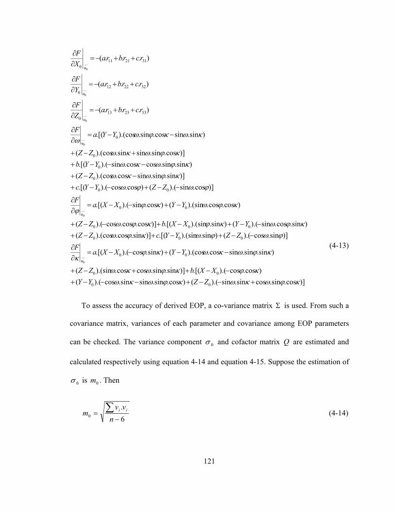
)]cos.sin.cossin.sin).(()cos.sin.sinsin.cos).(()cos.cos).(.[()]sin.sin.coscos.).(sin(

)sin.sin.sincos.).(cos()sin.cos).(.[(

)]sin.cos).(()sin.).(sin.[()]sin.cos.).(cos()sin.cos.sin).(()sin.).(sin.[()]cos.cos.cos).((

)cos.cos.).(sin()cos.sin).(.[(

)]cos.sin).(()cos.cos).(.[()]sin.sin.sincos.).(cos(

)sin.sin.coscos.sin).(.[()]cos.sin.sinsin.).(cos(

)sin.sincos.sin.).(cos.[(

)...(

)...(

)...(

00

00

00

000

000

00

00

0

0

0

0

3323130

3222120

3121110

0

0

0

0

0

0

κϕωκωκϕωκωκϕκϕωκω

κϕωκωκϕκ

ϕωϕωκϕωκϕωκϕκϕω

κϕωκϕϕ

ϕωϕωκϕωκω

κϕωκωκϕωκω

κωκϕωω

+−−+−−−+−−++−+

−−+−−=∂∂

−−+−+−+−−+−+−−+

−+−−=∂∂

−−+−−+−−+

−−−++−+

−−=∂∂

++−=∂∂

++−=∂∂

++−=∂∂

ZZYYXXbZZ

YYXXaFZZYYcZZ

YYXXbZZ

YYXXaF

ZZYYcZZ

YYbZZ

YYaF

rcrbraZF

rcrbraYF

rcrbraXF

u

u

u

u

u

u

(4-13)

To assess the accuracy of derived EOP, a co-variance matrix Σ is used. From such a

covariance matrix, variances of each parameter and covariance among EOP parameters

can be checked. The variance component 0σ and cofactor matrix Q are estimated and

calculated respectively using equation 4-14 and equation 4-15. Suppose the estimation of

0σ is m . Then 0

6.

0 −= ∑

nvv

m ii (4-14)

121

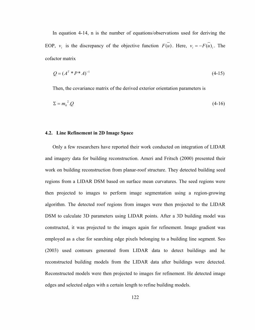
In equation 4-14, n is the number of equations/observations used for deriving the

EOP, is the discrepancy of the objective function iv )(uF . Here, ii uFv )(−= . The

cofactor matrix

1)**( −= APAQ T (4-15)

Then, the covariance matrix of the derived exterior orientation parameters is

Qm .20=Σ (4-16)

4.2. Line Refinement in 2D Image Space

Only a few researchers have reported their work conducted on integration of LIDAR

and imagery data for building reconstruction. Ameri and Fritsch (2000) presented their

work on building reconstruction from planar-roof structure. They detected building seed

regions from a LIDAR DSM based on surface mean curvatures. The seed regions were

then projected to images to perform image segmentation using a region-growing

algorithm. The detected roof regions from images were then projected to the LIDAR

DSM to calculate 3D parameters using LIDAR points. After a 3D building model was

constructed, it was projected to the images again for refinement. Image gradient was

employed as a clue for searching edge pixels belonging to a building line segment. Seo

(2003) used contours generated from LIDAR data to detect buildings and he

reconstructed building models from the LIDAR data after buildings were detected.

Reconstructed models were then projected to images for refinement. He detected image

edges and selected edges with a certain length to refine building models.

122

The direct information provided by images is in 2D image space. In order to improve

its geometry, a 3D building model will be projected to the image space in this study.

Then the projected model will be refined using extracted image information.

Consequently, the 3D model is refined. With known EOP, a 3D building model can be

projected to an image. Figure 4.4 shows an example of projected building roofs on a pair

of stereo aerial photographs. It is clear that there are discrepancies between the projected

model lines and their corresponding image lines. It should be noted that the discrepancies

at the upper right corners are caused by model assumption. In this research, building

models are assumed to have rectangular shapes. The refinement of model topology is not

the content of this study.

Figure 4.4. A building model from LIDAR data projected onto a pair of stereo images

The advantage of aerial photographs over LIDAR data is that they can capture sharp

linear features, i.e., edges. In order to use linear features to perform refinement, these

123

edges should be detected and extracted first. The Canny edge detector is employed to

detect edge pixels from aerial photograph data. Figure 4.5 presents an example of

detected edge pixels from a sub image covering a projected building model. The edge

detection was conducted on the red band of a color image.

Figure 4.5. Building image and the edge pixels detected from the Canny detector

In reality, a building under study is not the only foreground object in a study area.

There are also many other objects like cars and other constructions. Some of these objects

adjacent to a building have similar spectral characteristics to buildings. In this case, an

edge detector will be confused and will fail to detect edge pixels of the building under

study. Some of the unwanted objects have very different spectral characteristics. In this

case, they will introduce unwanted edge pixels. This can be seen from Figure 4.5. In

order to use the right edge pixels to refine a projected 2D building model, pixels

belonging to the building should be correctly separated from other edge pixels.

124

Although LIDAR data cannot capture sharp features, reconstructed building models

are still good approximations of actual buildings. Thus, a projected 2D building model is

close to the image of a real model; and provides valuable clues for further processing. To

pick the correct pixels of a building edge, a projected model provides two important

clues, orientation and position. An edge line of a projected model is parallel or almost

parallel to its corresponding image line. In addition, a pixel on a line has a gradient

azimuth perpendicular to the line it belongs to. The gradients of image pixels were

computed; and gradient azimuths were also calculated. Only those detected edge pixels

with a gradient azimuth perpendicular to a projected model line will be extracted for

further investigation. Here, the “perpendicular” is not exactly a 90-degree difference.

Instead, it is a confidential range. For example, a 5-degree deviation from 90-degree can

be treated as “perpendicular.”

Besides the azimuth, the position of a projected model line provides a second clue for

edge pixel searching. A reconstructed building model is a good approximation of a real

building. A projected 2D model on an image should be close to the actual image model.

To use this information, a buffer can be drawn to eliminate unwanted edge pixels far

away from a model line. The width of the buffer matches how well a model from LIDAR

data approximates its real building model.

In this study, the buffer sizes of the azimuth search and distance search are

determined by trying. In future research, they could be determined automatically. For

example, LIDAR data accuracy, image EOP accuracy, and comparison of building

boundaries before and after the regularization will provide some information for

125

calculating a buffer’s size. Figure 4.6 shows the detected edge pixels belonging to their

corresponding line of a projected model edge line.

Figure 4.6. Edge pixels detected from the azimuth constraint (left) and from both the azimuth and the position constraints (right)

After edge pixels were correctly detected, they can be used to refine projected model

edges. The refinement will be conducted line by line. In this study, the orthogonal least

square regression method will be employed to derive line parameters. Instead of

minimizing the vertical distance between observations and a fitting line as the traditional

least square method does, the orthogonal regression method minimizes the perpendicular

distance between the observations and a fitting line. For easier implementation, a line in a

2D image space will be represented using polar coordinates. The polar representation of a

line is (d, θ). Here, d is the perpendicular distance from the origin to this line while θ is

126

the normal direction of the line. This line is formed by all points whose projection on the

vector (cos(θ),sin(θ)) has a length of d. Such a line can be represented in equation (4-17).

)sin(*)cos(* θθ yxd += (4-17)

Equation (4-17) can be rewritten as constraint function in equation (4-18).

0)sin(*)cos(*),( =−−= θθ yxdyxF (4-18)

Given a random point (x’, y’), its perpendicular distance to the line is the absolute

value of F(x,y), |F(x’,y’)|. To derive the parameter of the fitting line using the orthogonal

regression, F(x,y) can be rewritten as

0)sin(*)cos(*),( =−−= θθθ yxddF (4-19)

Equation (4-19) has a nonlinear form. Thus, a linear form will be derived based on

the Taylor series. In order to get accurate line parameters, iterative calculations will be

performed.

0*),(*),(),(),( 00'

00'

00 ≈∆+∆+≈ θθθθθ θ dFddFdFdF d (4-20)

edFddFdF d +∆+∆=− θθθθ θ *),(*),(),( 00'

00'

00 (4-21)

Equation (4-20) is the form applied to derive the increments of line parameters. The

Gauss-Markov model will be used to minimize the error e. The projected 2D model lines

provide initial values for distance d and azimuth θ. At each iteration, increments of d and

θ are calculated; then d and θ are updated using the increments. Figure 4.7 shows the

searching for edge pixels and the refined edges using the orthogonal regression method.

127

Figure 4.7. Searching edge pixels (left) and refined edge lines (yellow line in right)

4.3. Reconstruct 3D Building Model with Refined Geometry

Based on imaging geometry, a 3D surface on the ground can be reconstructed through

stereo image processing. After 2D projected building lines were refined using image

information, specifically edge pixels detected from the Canny operator in this study, new

corners can be generated by intersecting the refined lines. In this way, the coordinates of

original corners can be updated from the refined lines. Due to different imaging

geometries, stereo images have different qualities. Some edges can be detected in one

image, but not in the other. In this case, the corners updated independently from each

image of a stereo pair are actually not conjugate points. They are not the same point on

the ground. So they cannot be used to perform space intersection for calculating 3D

ground coordinates.

128

To solve this problem, it is necessary to keep track of the updating of each corner.

Only corners updated from both stereo images from the same refined lines will be

updated. From the description of the previous section, it can be seen that the fundamental

refinement primitives are line segments. To simplify the processing, updating information

of a line segment was kept instead of a corner’s updating information. A boundary line is

updated if and only if it is updated in both stereo image spaces. Otherwise, the line will

remain unchanged. After all lines were processed, new corners were generated through

line intersection. Using this strategy, corners generated from stereo images are conjugate

points; and they can be processed using space intersection to derive 3D coordinates. It

should be noted that some of the new corners are actually not updated. However, it is not

necessary to differentiate updated corners from updated ones.

After the refinement of line segments was finished, coordinates of corners can be

calculated through intersecting adjacent line segments. Based on the line refinement

principle, conjugate corners are updated together in both stereo images. There will be no

case that a corner is updated in one image while its conjugate corner in the other image is

not updated correspondingly. 3D ground coordinates are calculated from conjugate points

using collinearity conditions of a ground point, its image point, and a camera’s exposure

center.

While the collinearity equations are the basic ones applied in space intersection, there

is other information that can be applied to derive a reliable and high accuracy for 3D

ground coordinates. From a 3D model reconstructed from LIDAR data, the relationship

among corners and surfaces is available. Due to high accuracy of LIDAR data in

129

mapping 3D surfaces, a planar roof’s parameters derived from a large number of points

have a high accuracy. This is the idea of quantity for quality, which means parameters

with high accuracy can be calculated from a large number of measurements with

relatively lower accuracy. In this study, a detected roof can have tens of or even hundreds

of LIDAR points. The points provide a great redundancy to derive a high accuracy planar

surface. Roof plane information can force constraints in space intersection.

Knowing the interior and exterior orientation parameters of an aerial image,

collinearity conditions can be written in equation 4-22. Collinearity means that the three

points (the ground point, the corresponding image point, and the camera exposure center)

are lying in the same 3D line. It is the nature of central perspective projection.

))(*)(*)(*)(*)(*)(*

(*

))(*)(*)(*)(*)(*)(*

(*

))(*)(*)(*)(*)(*)(*

(*

))(*)(*)(*)(*)(*)(*

(*

20332

20322

20312

20232

20222

20212

202

20332

20322

20312

20132

20122

20112

202

10331

10321

10311

10231

10221

10211

101

10331

10321

10311

10131

10121

10111

101

ZZrYYrXXrZZrYYrXXr

fyy

ZZrYYrXXrZZrYYrXXr

fxx

ZZrYYrXXrZZrYYrXXr

fyy

ZZrYYrXXrZZrYYrXXr

fxx

−+−+−−+−+−

−=

−+−+−−+−+−

−=

−+−+−−+−+−

−=

−+−+−−+−+−

−=

(4-22)

where,

(x1,y1) and (x2,y2) are the image coordinates of conjugate points after transformation;

(x10,y10) and (x20,y20) are the calibrated principle point coordinates respectively;

f is the calibrated camera focal length;

(X10,Y10,Z10) and (X20,Y20,Z20) are the exposure centers of the stereo images;

(X,Y,Z) is the ground coordinates to be solved from the equations;

r1ij and r2

ij are the (i,j) entry of the rotation matrix for each image respectively.

130

Equation 4-22 can be rewritten in a uniform formula to calculate ground coordinates.

See equation 4-23.

0))(*)(*)(*)(*)(*)(*

(*),,(

0))(*)(*)(*)(*)(*)(*

(*),,(

0))(*)(*)(*)(*)(*)(*

(*),,(

0))(*)(*)(*)(*)(*)(*

(*),,(

20332

20322

20312

20232

20222

20212

2024

20332

20322

20312

20132

20122

20112

2023

10331

10321

10311

10231

10221

10211

1012

10331

10321

10311

10131

10121

10111

1011

=−+−+−−+−+−

+−=

=−+−+−−+−+−

+−=

=−+−+−−+−+−

+−=

=−+−+−−+−+−

+−=

ZZrYYrXXrZZrYYrXXr

fyyZYXF

ZZrYYrXXrZZrYYrXXr

fxxZYXF

ZZrYYrXXrZZrYYrXXr

fyyZYXF

ZZrYYrXXrZZrYYrXXr

fxxZYXF

(4-23)

In order to calculate the unknowns from equation 4-23 in a computer, its linear form

should be used. The linear form can be written as

0***),,(),,( 000 =+∆∂∂

+∆∂∂

+∆∂∂

+= iiii

ii eZZF

YYF

XXF

ZYXFZYXF (4-24)

iiii

i eZZF

YYF

XXF

ZYXF +∆∂∂

+∆∂∂

+∆∂∂

=− ***),,( 000 (4-25)

In equations 4-24 and 4-25, ei is the error introduced by omitting items with high

order derivatives. The subscript “i” ranges from 1 to 4 representing the 4 equations in

equation 4-23. Using a vector form, the observation equations can be written as

eAL += ξ* (4-26)

where

−−−−

=

),,(),,(),,(),,(

0004

0003

0002

0001

ZYXFZYXFZYXFZYXF

L , , e ,

∆∆∆

=ZYX

ξ

=

4

3

2

1

eeee

131

and

∂∂

∂∂

∂∂

∂∂

∂∂

∂∂

∂∂

∂∂

∂∂

∂∂

∂∂

∂∂

=

ZF

YF

XF

ZF

YF

XF

ZF

YF

XF

ZF

YF

XF

A

444

333

222

111

The constraint that a ground corner is lying in a roof surface is applied together with

the observation equations to derive ground coordinates for a corner. A corner point can

belong to more than one roof surface. Generally, the constraint from the ith roof surface

can be written as

1*** =++ ZcYbXa iii (4-27)

To be integrated with the observation equations, 4-27 should use the increments

( ) as unknowns. It can be expressed in equation 4-28. ZYX ∆∆∆ ,,

000 ***1*** ZcYbXaZcYbXa iiii −−−=∆+∆+∆ (4-28)

Applying the same form as equation 4-26, equations 4-28 and 4-26 can be written in

combination as the equation 4-29.

WBeAL

=+=

ξξ

**

(4-29)

Applying the least square method together with the Lagrange approach, the unknowns

can be solved as in equations 4-30 and 4-31.

132

=

WLPA

BBAPA TTT **

*0

**λξ

(4-30)

=

−

WLPA

BBAPA TTT **

*0

**1

λξ

(4-31)

where,

P is the weight matrix;

λ is the unknowns introduced by the Lagrange method with a dimension of n by 1,

and n is the number of roof constraints applied to the current corner.

After ground coordinates were calculated for all corners of a building, a building

model was refined. The refined model from integration of LIDAR and imagery data has a

high geometric quality compared with the one reconstructed solely from LIDAR data. In

this study, corners belonging to building roofs were processed. Lower corners of vertical

walls were derived from their corresponding upper corners.

4.4. Implementation

The refinement can be implemented on roofs individually or on a whole building

model simultaneously. To use individual roofs, some 3D corners will be processed on

each roof respectively. Because these corners were processed independently from

different roofs, it is likely that coordinates of a corner calculated from different processes

don’t match each other. This is mainly caused by roof planar constraints applied to the

same corner from different roofs in different processes.

133

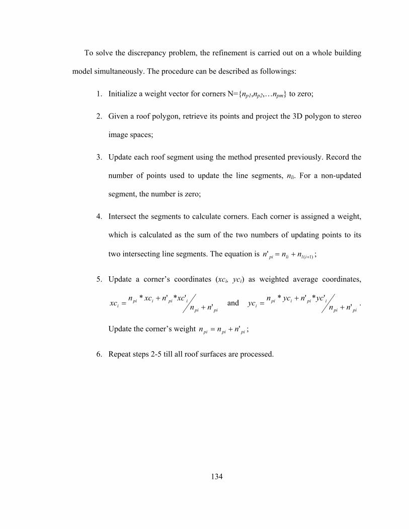
To solve the discrepancy problem, the refinement is carried out on a whole building

model simultaneously. The procedure can be described as followings:

1. Initialize a weight vector for corners N={np1,np2,…npm} to zero;

2. Given a roof polygon, retrieve its points and project the 3D polygon to stereo

image spaces;

3. Update each roof segment using the method presented previously. Record the

number of points used to update the line segments, nli. For a non-updated

segment, the number is zero;

4. Intersect the segments to calculate corners. Each corner is assigned a weight,

which is calculated as the sum of the two numbers of updating points to its

two intersecting line segments. The equation is )1(' ++= illipi nnn ;

5. Update a corner’s coordinates (xci, yci) as weighted average coordinates,

pipi

ipiipii nn

xcnxcnxc ''*'*

++

= and pipi

ipiipii nn

ycnycnyc ''*'*

++

= .

Update the corner’s weight pipipi nnn '+= ;

6. Repeat steps 2-5 till all roof surfaces are processed.

134

CHAPTER 5

EXPERIMENTS AND RESULTS

In previous chapters, the methodology of building model reconstruction from LIDAR

and imagery data is described in details. Some examples were also presented to illustrate

how the proposed method works. To substantially examine this methodology, a large data

set was employed to demonstrate how the method could be applied to reconstructing

building models from data integration. Instead of an autonomous system, the

implementation of this methodology was carried out as a sequence of user guided

operations, namely, building detection, 3D model reconstruction, and model refinement.

They will be demonstrated in the same sequence in this chapter.

5.1. Data

Two different types of data were used in this experiment, LIDAR data and aerial

photographs. The experimental site is located in a suburban area of Houston, Texas. The

LIDAR data has a point density of approximately 1 point per square meter, with a vertical

accuracy of approximate 15 centimeters and a horizontal accuracy of approximate 0.5

135

meter. The flying height is approximately 915 meters with a data swath of approximately

550 meters. The aerial photographs have a ground resolution of approximately 0.3 meter

with a scale of approximate 1 to 20000. The flying height is approximate 3350 meters.

Figure 5.1 shows a picture of the data used in this study. The one on the left is LIDAR

data converted into grid format; and the right one is an aerial image subset covering

approximately the same area. The area of this place is approximate 1.5 square kilometers.

Figure 5.1. Experimental data: the LIDAR data (left) and the aerial imagery data (right)

5.2. LIDAR Segmentation

LIDAR segmentation is the process to differentiate LIDAR points falling onto

different types of objects. One important process is to distinguish points falling on the

ground. Extracted ground points can be used to generate the DTM, a commonly used

product in geo-science. In this study, the focus is detection of building points. This is

achieved from LIDAR segmentation using the proposed methods. After a DTM was

generated from classified ground points, non-ground points were extracted by testing

136

their heights above the ground. These non-ground points were then analyzed to

differentiate buildings from other objects such as trees and cars. The information applied

at this process is surface texture and object size.

In order to separate ground points, two methods were proposed in this study, the

planar-fitting segmentation algorithm and the height-jump segmentation algorithm. In

fact, all LIDAR data segmentation algorithms are based on height difference among

different objects. The same principle applies to these two methods. LIDAR data was

converted to grid format for process. The ground region was extracted as the one with the

largest area after different objects were disconnected based on segmentation methods.

The classification of ground points is an iterative process. At the first iteration, the

majority of ground points were distinguished. However, points at boundaries and points

inside an inner court cannot be correctly classified at this time. Boundary points have

similar character as tree points in the planar-fitting segmentation. In the height-jump

method, some classified height-jump points are sitting on the boundary of the ground

region. For inner court points, they form an independent object different from the

detected ground region that is usually connected by a road network. These height-jump

points and inner-court points can be re-classified as ground points by checking their

heights with the DTM generated from ground points detected in the previous iteration.

Figure 5.2 presents a detected ground region after the first iteration and the 5th iteration

using the height-jump algorithm. From this figure, it is clear that the ground region after

the 5th iteration has much more details than the one detected in the first iteration.

137

Figure 5.2. The ground region detected from an iterative process: the 1st iteration (top) and the 5th iteration (bottom)

After a final DTM is generated from ground points, the so-called normalized DSM

can be generated by subtracting the DTM from the DSM, which is generated from

138

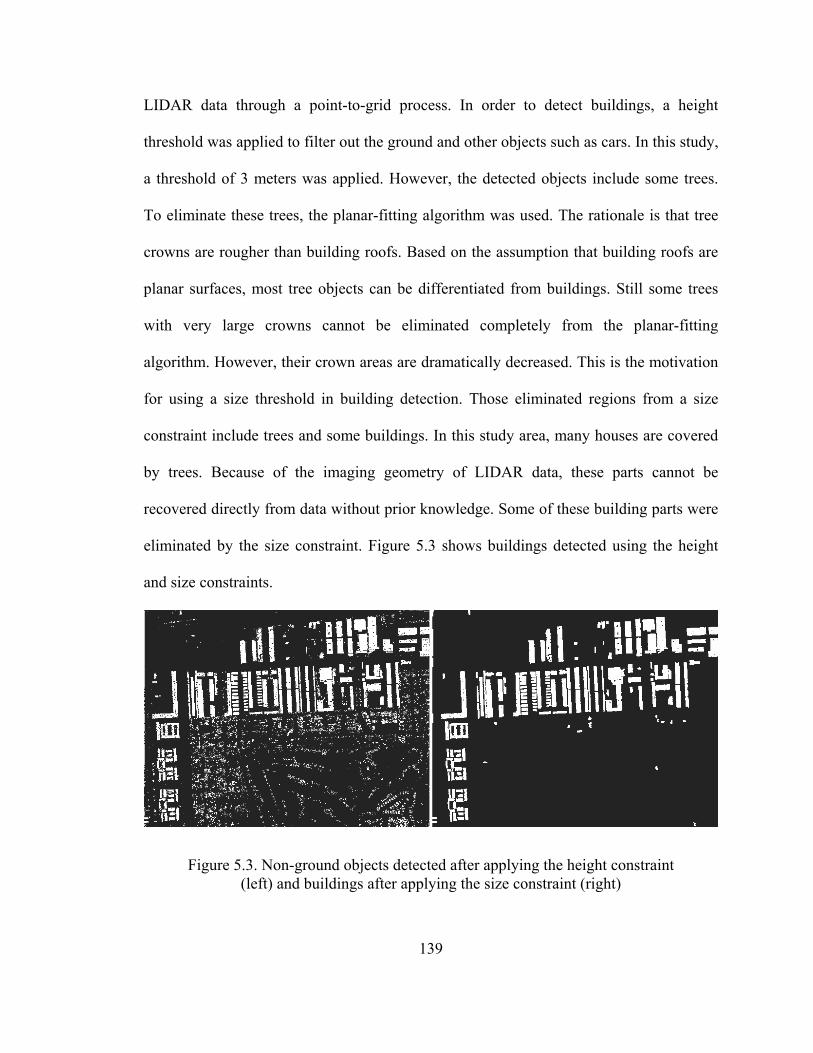
LIDAR data through a point-to-grid process. In order to detect buildings, a height

threshold was applied to filter out the ground and other objects such as cars. In this study,

a threshold of 3 meters was applied. However, the detected objects include some trees.

To eliminate these trees, the planar-fitting algorithm was used. The rationale is that tree

crowns are rougher than building roofs. Based on the assumption that building roofs are

planar surfaces, most tree objects can be differentiated from buildings. Still some trees

with very large crowns cannot be eliminated completely from the planar-fitting

algorithm. However, their crown areas are dramatically decreased. This is the motivation

for using a size threshold in building detection. Those eliminated regions from a size

constraint include trees and some buildings. In this study area, many houses are covered

by trees. Because of the imaging geometry of LIDAR data, these parts cannot be

recovered directly from data without prior knowledge. Some of these building parts were

eliminated by the size constraint. Figure 5.3 shows buildings detected using the height

and size constraints.

Figure 5.3. Non-ground objects detected after applying the height constraint

(left) and buildings after applying the size constraint (right)

139

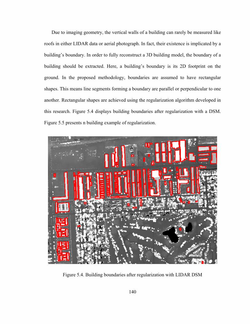
Due to imaging geometry, the vertical walls of a building can rarely be measured like

roofs in either LIDAR data or aerial photograph. In fact, their existence is implicated by a

building’s boundary. In order to fully reconstruct a 3D building model, the boundary of a

building should be extracted. Here, a building’s boundary is its 2D footprint on the

ground. In the proposed methodology, boundaries are assumed to have rectangular

shapes. This means line segments forming a boundary are parallel or perpendicular to one

another. Rectangular shapes are achieved using the regularization algorithm developed in

this research. Figure 5.4 displays building boundaries after regularization with a DSM.

Figure 5.5 presents n building example of regularization.

Figure 5.4. Building boundaries after regularization with LIDAR DSM

140

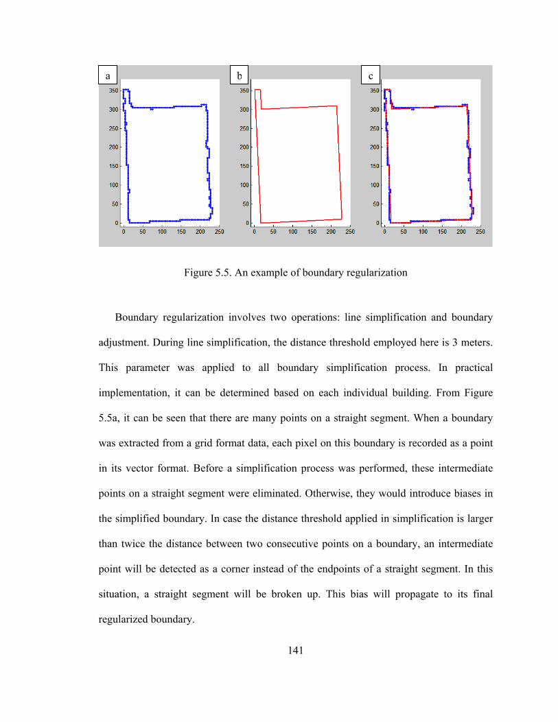
cba

Figure 5.5. An example of boundary regularization

Boundary regularization involves two operations: line simplification and boundary

adjustment. During line simplification, the distance threshold employed here is 3 meters.

This parameter was applied to all boundary simplification process. In practical

implementation, it can be determined based on each individual building. From Figure

5.5a, it can be seen that there are many points on a straight segment. When a boundary

was extracted from a grid format data, each pixel on this boundary is recorded as a point

in its vector format. Before a simplification process was performed, these intermediate

points on a straight segment were eliminated. Otherwise, they would introduce biases in

the simplified boundary. In case the distance threshold applied in simplification is larger

than twice the distance between two consecutive points on a boundary, an intermediate

point will be detected as a corner instead of the endpoints of a straight segment. In this

situation, a straight segment will be broken up. This bias will propagate to its final

regularized boundary.

141

By visually checking with the aerial photos, detected building objects are all from

ground buildings. However, some buildings on the ground were not classified as building

objects out of the detection. The major cause is the size constraint applied. These

undetected buildings are obscured by trees; and they cannot be mapped in the LIDAR

data. Totally, 144 buildings were detected in this experiment. Although some buildings

are covered by trees from top, they can still be detected because a large area they occupy.

Around 90 percent of the buildings are detected in this study area. But this number should

be refined through field check.

5.3. Building Reconstruction

After boundaries were regularized to rectangular shapes, they were included in the

building reconstruction process as vertical walls. To detect building roofs, the normal

data of a DSM was employed. The normal data was calculated from a plane fitting a 5 by

5 square window in this experiment. A small window will not be able to smooth out

noise, such as a 3 by 3 window; while a large window will decrease the difference

between different roof surfaces, such as a 9 by 9 window.

After the normal data was smoothed using the mean-shift filter, a supervised

classification was carried out to perform surface segmentation. The mean-shift algorithm

can also be applied to perform segmentation. The classification was employed because it

can be conducted in commercial software. The principles of the applied classification are

the same as the mean-shift algorithm.

142

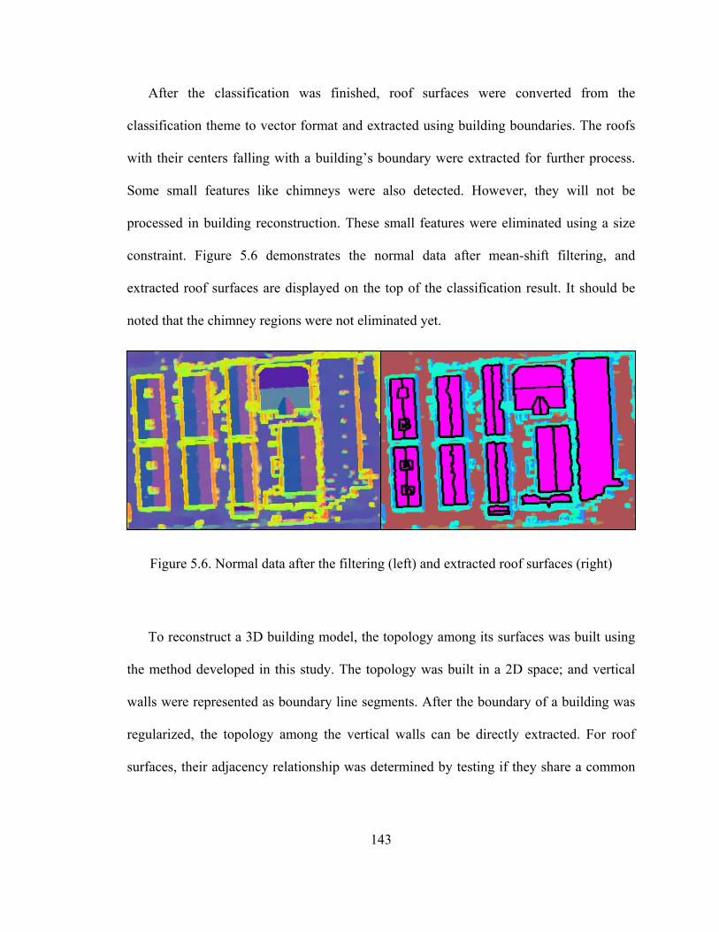
After the classification was finished, roof surfaces were converted from the

classification theme to vector format and extracted using building boundaries. The roofs

with their centers falling with a building’s boundary were extracted for further process.

Some small features like chimneys were also detected. However, they will not be

processed in building reconstruction. These small features were eliminated using a size

constraint. Figure 5.6 demonstrates the normal data after mean-shift filtering, and

extracted roof surfaces are displayed on the top of the classification result. It should be

noted that the chimney regions were not eliminated yet.

Figure 5.6. Normal data after the filtering (left) and extracted roof surfaces (right)

To reconstruct a 3D building model, the topology among its surfaces was built using

the method developed in this study. The topology was built in a 2D space; and vertical

walls were represented as boundary line segments. After the boundary of a building was

regularized, the topology among the vertical walls can be directly extracted. For roof

surfaces, their adjacency relationship was determined by testing if they share a common

143

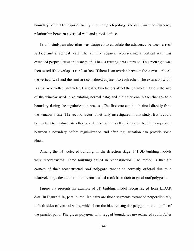
boundary point. The major difficulty in building a topology is to determine the adjacency

relationship between a vertical wall and a roof surface.

In this study, an algorithm was designed to calculate the adjacency between a roof

surface and a vertical wall. The 2D line segment representing a vertical wall was

extended perpendicular to its azimuth. Thus, a rectangle was formed. This rectangle was

then tested if it overlaps a roof surface. If there is an overlap between these two surfaces,

the vertical wall and the roof are considered adjacent to each other. The extension width

is a user-controlled parameter. Basically, two factors affect the parameter. One is the size

of the window used in calculating normal data; and the other one is the changes to a

boundary during the regularization process. The first one can be obtained directly from

the window’s size. The second factor is not fully investigated in this study. But it could

be tracked to evaluate its effect on the extension width. For example, the comparison

between a boundary before regularization and after regularization can provide some

clues.

Among the 144 detected buildings in the detection stage, 141 3D building models

were reconstructed. Three buildings failed in reconstruction. The reason is that the

corners of their reconstructed roof polygons cannot be correctly ordered due to a

relatively large deviation of their reconstructed roofs from their original roof polygons.

Figure 5.7 presents an example of 3D building model reconstructed from LIDAR

data. In Figure 5.7a, parallel red line pairs are those segments expanded perpendicularly

to both sides of vertical walls, which form the blue rectangular polygon in the middle of

the parallel pairs. The green polygons with ragged boundaries are extracted roofs. After

144

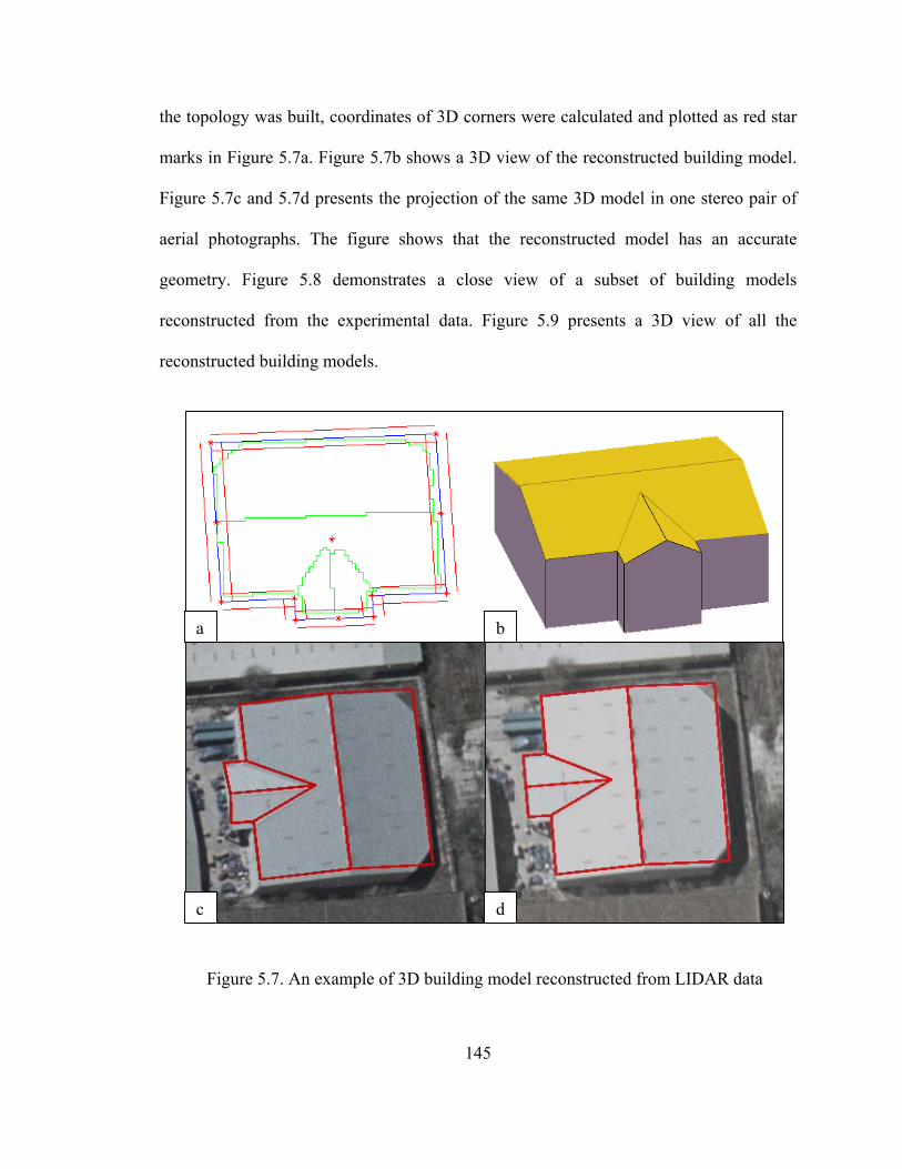
the topology was built, coordinates of 3D corners were calculated and plotted as red star

marks in Figure 5.7a. Figure 5.7b shows a 3D view of the reconstructed building model.

Figure 5.7c and 5.7d presents the projection of the same 3D model in one stereo pair of

aerial photographs. The figure shows that the reconstructed model has an accurate

geometry. Figure 5.8 demonstrates a close view of a subset of building models

reconstructed from the experimental data. Figure 5.9 presents a 3D view of all the

reconstructed building models.

dc

ba

Figure 5.7. An example of 3D building model reconstructed from LIDAR data

145

Figure 5.8. A close view of 3D building models

Figure 5.9. 3D view of all reconstructed building models

146

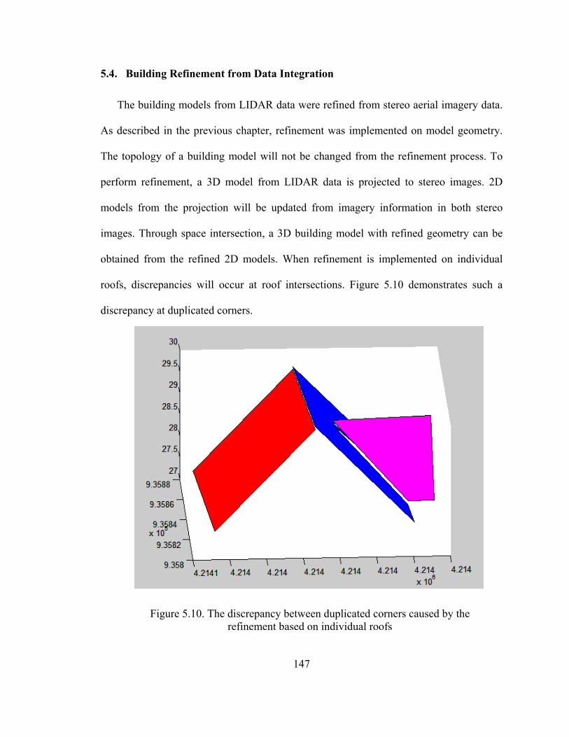
5.4. Building Refinement from Data Integration

The building models from LIDAR data were refined from stereo aerial imagery data.

As described in the previous chapter, refinement was implemented on model geometry.

The topology of a building model will not be changed from the refinement process. To

perform refinement, a 3D model from LIDAR data is projected to stereo images. 2D

models from the projection will be updated from imagery information in both stereo

images. Through space intersection, a 3D building model with refined geometry can be

obtained from the refined 2D models. When refinement is implemented on individual

roofs, discrepancies will occur at roof intersections. Figure 5.10 demonstrates such a

discrepancy at duplicated corners.

Figure 5.10. The discrepancy between duplicated corners caused by the refinement based on individual roofs

147

To solve the problems, a building model should be refined based on the whole model.

In this case, corners can be updated uniquely instead of multiple times. The algorithm is

described in Chapter 4. The refinement primitives are line segments. Whenever a line

segment is refined, it triggers the updating of its two end points.

After all roof surfaces of a building were processed for refinement, its corners were

updated consistently. From the surface-point relationship matrix built in the

reconstruction process, the surfaces containing a corner can be retrieved. Their planar

constraints will be applied to the space intersection for calculating 3D corner coordinates.

Compared with the corners’ original coordinates derived from LIDAR, the new

coordinates have a higher accuracy. In this way, a 3D building model was refined from

the imagery information. Figure 5.11 presents the same model as in Figure 5.10. It can be

seen that the discrepancy disappeared.

Figure 5.11. An example of model refinement with consistency

148

5.5. Discussion

Building models are important information applied in many disciplines. Building

reconstruction is the process used to calculate parameters of building models in a model

space, which is an abstract of the real world. “Abstract” means that the model space

cannot represent exactly the same details as the real world. Thus, it is normal that some

exceptions or errors will exist in reconstructed models due to limitations from both data

and algorithms applied.

Due to the limitation of LIDAR point data, small features cannot be detected or

reconstructed, such as chimneys. In addition, some buildings close to each other were

detected as one single building because of the lack of points between them. This will

introduce errors in detection results, and it may fail to provide a 3D model reconstruction.

As for imagery data, it is not possible to extract all the information needed for

refinement. The aerial photographs used are optical images. In some places, different

features have similar spectral characteristics. In this situation, the required information

for refinement cannot be extracted. Thus, the refinement in this study was applied to

those building features where required imagery information was available. For buildings

obscured by trees, they either cannot be detected or only a portion of such a building can

be detected. Imagery data cannot provide more information about the obscured parts of

buildings. This problem can be solved or partially solved by integrating other sources of

data into application. For example, hyper-spectral imagery data can be applied to

differentiate trees from buildings. Multi-return LIDAR data can also differentiate trees

from buildings effectively. Another possible solution is to deduce or guess the whole

149

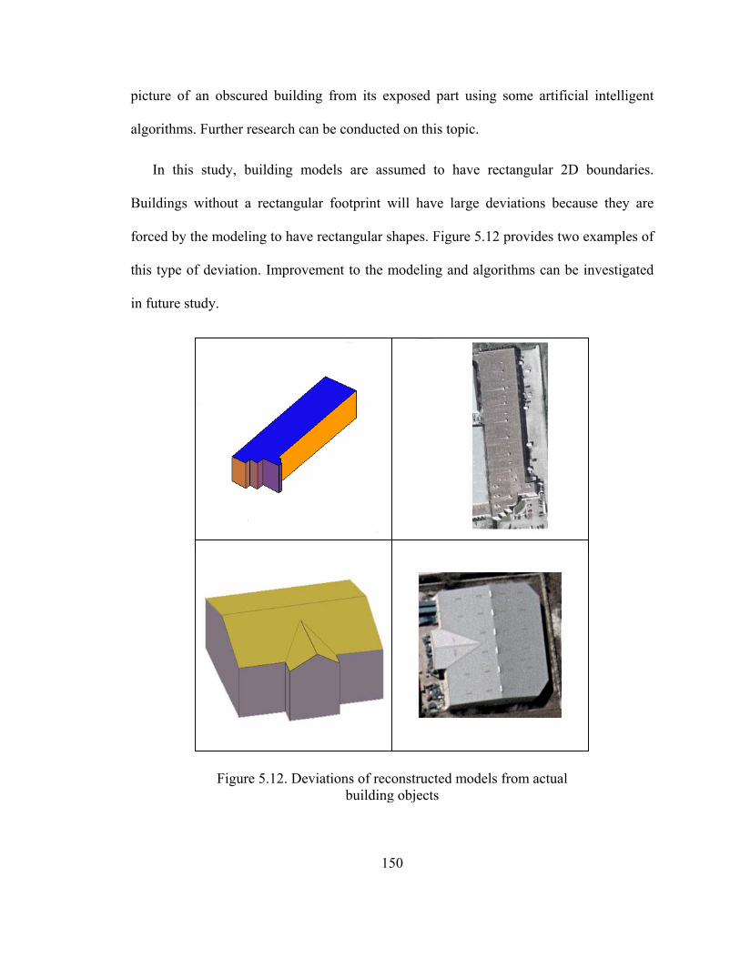
picture of an obscured building from its exposed part using some artificial intelligent

algorithms. Further research can be conducted on this topic.

In this study, building models are assumed to have rectangular 2D boundaries.

Buildings without a rectangular footprint will have large deviations because they are

forced by the modeling to have rectangular shapes. Figure 5.12 provides two examples of

this type of deviation. Improvement to the modeling and algorithms can be investigated

in future study.

Figure 5.12. Deviations of reconstructed models from actual building objects

150

151

In spite of the limitations mentioned above, the methodology developed in this

research can produce high accuracy building models from the integration of LIDAR data

and aerial photographs. The integration provides more information than either single data

type. From the experiments, the refinement from aerial photographs can improve the

accuracy of the models derived from LIDAR.

The co-registration of LIDAR and aerial photographs was not experimented in this

study because the exterior orientation parameters of the photographs were available from

the data provider. The method and related equations are described in chapter 4 for

completeness of the proposed building reconstruction methodology.

CHAPTER 6

CONCLUSIONS AND FUTURE RESEARCH

To reconstruct 3D building models from LIDAR and aerial photographs, a new

methodology is proposed in this research. The methodology is basically comprised of

three procedures: building detection, 3D model reconstruction, and 3D model refinement.

6.1. Conclusions

Under the proposed framework, a 3D building model can be reconstructed using

LIDAR and aerial imagery data. The methodology is implemented on polyhedral building

models. The major contributions of this research can be summarized as followings:

• Two algorithms are developed to perform LIDAR segmentation. Compared with

the algorithms proposed by other researchers, these two algorithms work well in

urban and suburban areas. In addition, they can keep fine features on the ground;

• An algorithm of building boundary regularization is proposed in this study.

Compared with the commonly used MDL algorithm, it is simple to implement

and fast in computation. Longer line segments have larger weights in its

152

adjustment process. This agrees with the fact that longer line segments have more

accurate azimuths provided that the accuracy of ending points are the same for all

segments;

• A new method of 3D building model reconstruction from LIDAR data is

developed. It is comprised of constructing surface topology, calculating corners

from surface intersection, and ordering points of a roof surface in their correct

sequence;

• A new framework of building model refinement from aerial imagery data is

proposed. It refines building models in a consistent approach; and it utilized

stereo imagery information and roof constraints in deriving refined building

models.

This approach doesn’t need much prior information about a building model to be

reconstructed. Thus, it can be used to reconstruct more types of buildings than methods

using a model-based approach. It can also avoid the decomposition of complex buildings

that CSG based methods have to do. Usually, such decomposition is a tricky task. The

experiments have shown that the methodology works successfully in building detection

and building model reconstruction. Besides the methodology of 3D model reconstruction

itself, there are also several methods developed to perform specific tasks in order to

achieve the ultimate goal of 3D building model reconstruction. These methods include

the algorithm for building footprint boundary regularization, the method for constructing

the topology of building surfaces, and the method for filtering surface normal data.

153

6.2. Future Works

It is a fact that no algorithm can work in every situation. The methodology proposed

in this study is not an exception. It also has some limitations. Some of the limitations are

caused by the data applied. For example, two different buildings might be detected as one

single building because they are very close to each other. They are so close that there are

only few points falling on the ground between them. These points are not sufficient to

separate two buildings. Another limitation is that the algorithm in ordering roof polygons

may fail to order a polygon in the correct sequence. This usually happens when a roof

polygon has a narrow part on it. When buildings are covered by trees, either they cannot

be detected or they can only be detected partially. Data from other sources can be applied

in the detection stage to help solve the problem. In addition, multi-return LIDAR data can

be applied to effectively differentiate trees from buildings.

A second type of limitation is from building modeling itself. In this study, buildings

are assumed to have rectangular footprints. Thus, non-rectangular footprints will be

forced to have rectangular shapes as the examples showed in experiments. Another

limitation is that 3D modeling assumes no height breakups within a building. In other

words, no vertical walls in a 3D building model are allowed. These issues can be further

investigated in future research. Major research topics in future work are the following:

• The reconstruction of small features using high-resolution data. For example, a

LIDAR data with a point density of approximately more than 4 points per square

meter can be used to detect dormers;

154

155

• The inclusion of vertical walls inside a building model. New data structure and

algorithm need to be developed to handle such inner vertical walls;

• The integration of LIDAR data and aerial imagery data in building detection. The

spectral information from imagery data could be integrated with LIDAR height

information to perform building detection;

• Model refinement from a single image. Currently, the information used in

refinement is an intersection of the information from both stereo images. For

example, a line segment is updated if and only if its corresponding segment in the

other image is updated. In future research, the union of the information from both

stereo images could be applied;

• Refinement of the topology of a building model from imagery data. New methods

should be developed to refine the topologies of building models derived from

LIDAR data. Fine features or structures not detected/reconstructed from LIDAR

data can be added to building models to be refined.

156

BIBLIOGRAPHY

Ackermann, F., 1999. Airborne laser scanning-present status and future expectations,

ISPRS Journal of Photogrammetry & Remote Sensing, Vol.54 pp64-67, 1999

Aelst, S., X. Wang, and R. H. Zamar, 2003. Linear grouping using orthogonal regression,

http://hajek.stat.ubc.ca/~ruben/website/ORCpaper.pdf, visited March 2004

Alharthy, A. and J. Bethel, 2002. Building extraction and reconstruction from LIDAR

data, Proceedings of ASPRS annual conference, 18-26, Washington

Ameri, B. and D. Fritsch, 2000. Automatic 3D building reconstruction using plane roof

structures, ASPRA Conference, Washington, DC, 2000

Ameri, B., 2000. Feature Based Model Verification (FBMV): A new concept for

hypothesis validation in building reconstruction, IAPRS Vol. XXXIII, Part B3/1,

Comm. III, pp. 24-35, ISPRS Congress, Amsterdam. 2000

Axelsson, P., 1999. Processing of laser scanner data – algorithm and applications, ISPRS

Journal of Photogrammetry & Remote Sensing, Vol.54 pp138 - 147, 1999

Axelsson, P., 2000. DEM generation from laser scanner data using adaptive TIN models,

IAPRA, 33, B4/1

Baltsavias, E. P., 1999. A comparision between photogrammetry and laser scanning,

ISPRS Journal of Photogrammetry & Remote Sensing, Vol.54 pp83-94, 1999

Bourke, Paul. 1987. http://astronomy.swin.edu.au/~pbourke/geometry/insidepoly/

Brenner, C., 2000. Towards fully automatic generation of city models, ISPRS,

Vol.XXXIII, Amsterdan, 2000

Brunn A. and U. Weidner, 1997. Extracting buildings from digital surface models,

IAPRS, 32, Stuttgart

Brunn, A., 2001. Statistical interpretation of DEM and image data for building extraction,

in Baltsavias et al. (edit), Automatic Extraction of Man-made Objects from Aerial and

Space Images (III), 2001.

Cawsey, Alison, 1998. Line Intersection.

http://www.cee.hw.ac.uk/~alison/ds98/node114.html, visited May 7, 2004

Cheng, Y., 1995. Mean shift, mode seeking, and clustering, IEEE Transaction on Pattern

Analysis and Machine Intelligence, Vol.17 (8), pp790-799, 1995

Comaniciu, D. and P. Meer, 2002. Mean shift: a robust approach toward feature space

analysis, IEEE Transaction on Pattern Analysis and Machine Intelligence, Vol.24 (5),

pp603-619, 2002

Csathó, B. and T. Schenk, 2002. Multisensor fusion to aid automatic image

understanding of urban scenes, http://dfc.jrc.it/doc/csatho%20020624.pdf

157

Csathó, B., T. Schenk, D.C. Lee, and S. Filin, 1999. Inclusion of multispectral data into

object recognition, International Archive of Photogrammetry and Remote Sensing,

Vol. 32, Part 7-4-3 W6, Valladolid, Spain, 3-4 June, 1999.

Dissanaike, G. and Sh. Wang, A Critical Examination of Orthogonal Regression and an

Application to tests of firm size interchangeability,

http://les1.man.ac.uk/sapcourses/Semstuff/Ort-wang.PDF, visited March 2004

Elaksher, A., 2002. Building extraction from multiple images, Ph.D. thesis, Purdue

University, 2002

Elaksher, A., J. Bethel, and E. Mikhail, 2002. Building extraction using multiple images,

Proceedings of ACSM-ASPRS 2002 Annual Conference, Washington, May 2002

Elberink, S.O. and H.G. Maas, 2000. The use of anisotropic height texture measurements

for the segmentation of airborne laser scanner data, IAPRS, 33, Amsterdam

Elberink, S.O. and H.G. Maas, 2000. The use of anisotropic height texture measurements

for the segmentation of airborne laser scanner data, IAPRS, 33, Amsterdam

Förstner, W., 1999. 3D-City Models: Automatic and semiautomatic acquisition methods.

http://www.ifp.uni-stuttgart.de/publications/phowo99/foerstner.pdf, visited in 2002.

Frère, D., M. Hendrickx, J. Vandekerckhove, T. Moons and L. Van Gool, 1997. On the

reconstruction of urban house roofs from aerial images, in Automatic Extraction of

Man-made Objects from Aerial and Space Images (II), edited by Gruen et al., 1997.

158

Fua, P. and C. Brechbüler, 1997. Imposing hard constraints on deformable models

through optimization in orthogonal subspaces, Computer Vision and Image

Understanding, 65(2):148-162

Fuchs, F., 2001. Building reconstruction in urban environment: a graph-based approach,

in Baltsavias et al. (edit), Automatic Extraction of Man-made Objects from Aerial and

Space Images (III), 2001.

Fukunaga, K. and L.D. Hostetler, 1975. The estimation of the gradient of a density

function, with applications in pattern recognition, IEEE Transaction on Pattern

Analysis and Machine Intelligence, Vol.IT21 (1), pp32-40, 1975

Gamba, P., 2000. Digital Surface Models and Building Extraction: A Comparision of

IFSAR and LIDAR Data, IEEE Transactions on Geoscience and Remote Sensing,

Vol.38, No.4, July 2000

Geogescu, B., I. Shimshoni, and P. Meer, 2003. Mean shift based clustering in high

dimensions: a texture classification example, Proceedings of the 9th IEEE

International Conference on Computer Vision, 2003

Haala, N. and C. Brenner, 1999. Extraction of buildings and trees in urban environments,

ISPRS Journal of Photogrammetry & Remote Sensing, Vol.54 pp130 - 137, 1999

Haala, N. and M. Hahn, 1995. Data fusion for the detection and reconstruction of

buildings. In Automatic Extraction of Man-Made Objexts from Aerial and Space

Images, edited by A. Gruen, O. Kuebler and P. Agouris, 1995.

159

Haala, N., C. Brenner, and K. Anders, 1998. 3D urban GIS from laser altimeter and 2D

map data, http://www.ifp.uni-stuttgart.de/publications/1998/ohio_laser.pdf, visited

July 2003

Habib, A.F., S.W. Shin, and M.F. Morgan, 2002. Automatic pose estimation of imagery

using free-form control linear features. ISPRS Commission III Symposium

“Photogrametric Computer Vision”, Graz, Austria, September 9-13, 2002

Hough, P.V.C., 1962. Method and means for recognizing Complex Patterns. U.S. Patent

3.069.654

Hu, Y. and C.V. Tao, 2002. Bald DEM generation and building extraction using range

and reflectance LIDAR data, Proceeding of ACSM-ASPRS 2002 Annual Conference,

Washington, D.C. (CD-ROM)

Hubeli, A., K. Meyer, and M. Gross, 2000. Mesh edge detection,

http://graphics.cs.ucdavis.edu/hvm00/abstracts/hubeli.pdf

Huising, E.J. and L.M. G. Pereira, 1998. Errors and accuracy estimates of laser data

acquired by various laser scanning systems for topographic applications, ISPRS

Journal of Photogrammetry & Remote Sensing, Vol.53 pp245-261, 1998

Iisaka, J. and T. S.A., 2000. Image analysis of remote sensing data integrating spectral

and spatial features of objects,

http://www.gisdevelopment.net/aars/acrs/2000/ts9/imgp0013.shtml, ACRS 2000

Kilian, J., N. Haala, and M. Englich, 1996. Capture and evaluation of airborne laser

scanner data, IAPRS, 31, B3

160

Kraus, K. and N. Pfeifer, 1998. Determination of terrain models in wooded areas with

airborne laser scanner data, ISPRS Journal of Photogrammetry & Remote Sensing, 53

(1998): 193-203

Lacroix, V. and M. Acheroy, 1998. Feature extraction using the constrained gradient,

ISPRS Journal of Photogrammetry & Remote Sensing, Vol.53 pp85 - 94, 1998

Lee, H. and N. H., Younan, 2003. DEM extraction of LIDAR returns via adaptive

processing, IEEE Transaction on Geoscience and Remote Sensing, 41(9): 2063-2069

Lin Ch., A. Huertas, and R. Nevatia, 1995. Detection of buildings from monocular

images. In Automatic Extraction of Man-Made Objexts from Aerial and Space

Images, edited by A. Gruen, O. Kuebler and P. Agouris, 1995.

Lohmann, P. and A. Koch, 1999. Quality assessment of laser-scanner-data,

http://www.ipi.uni-

hannover.de/html/publikationen/1999/koch/isprs99%20koch%20lohmann.pdf, visited

in September 2003

Lohmann, P., 2001. Segmentation and filtering of laser scanner digital surface models,

IAPRS, 34, 2

Lohmann, P., A. Kock, and M. Schaeffer, 2000. Approaches to the filtering of laser

scanner data, IAPRS, 33, Amsterdam

Ma, Y.W. and B.S. Manjunath, 1997. Edge flow: a framework of boundary detection and

image segmentation, Proceedings of the IEEE Conference on Computer Vision and

pattern recognition, Puerto Rico, 1997

161

Maas, H. and G. Vosselman, 1999. Two algorithms for extracting building models from

raw laser altimetry data, ISPRS Journal of Photogrammetry & Remote Sensing,

Vol.54 pp153 - 163, 1999

Maas, H.G., 1999a. Closed solution for the determination of parametric building models

from invariant moments of airborne laserscanner data, ISPRS conference ‘Automatic

Extraction of GIS Objects from Digital Imagery’, Munchen/Germany, 8-10. 9. 1999’.

(IAPRS Vol.32 pp193-199)

Maas, H.G., 1999b. Fast determination of parametric house models from dense airborne

laserscanner data, ISPRS workshop on mobile mapping technology, Bangkok,

Thailand, April 21-23, 1999.

Maas, H.G., 1999c. The potential of height texture measures for the segmentation of

airborne laserscanner data, 4th International Airborne Remote Sensing and Exhibition

/ 21st Canadian Symposium on Remote Sensing, Ottawa, Ontario, Canada, 21-24 June

1999

Matikainen, L., J. Hyyppä, and H. Hyyppä, 2003. Automatic detection of buildings from

laser scanner data for map updating, IAPRS, 34, Dresden

Mayer, Stefan, 2001. Constrained optimization of building contours from high-resolution

ortho-images, ICIP 2001, Thessaloniki, Greece

McGlone, J.Ch. and J. A. Shufelt, 1994. Projective and object space geometry for

monocular building extraction. Proceedings of IEEE Computer Society Conference

on Computer Vision and Pattern Recognition, 1994. Page(s): 54 -61

162

Mcintosh, K. and A. Krupnik, 2002. Integration of laser-derived DSMs and matched

image edges for generating an accurate surface model, ISPRS Journal of

photogrammetry & remote sensing, Vol. 56 pp167-176, 2002.

Morgan, M. and A. Habib, 2002. Interpolation of LIDAR data and automatic building

extraction, Proceeding of ACSM-ASPRS 2002 Annual Conference, Washington, D.C..

(CD-ROM)

Murakami, H., K. Nakagawa, H. Hasegawa, T. Shibata, and E. Iwanami, 1999. Change

detection of buildings using an airborne laser scanner, ISPRS Journal of

Photogrammetry & Remote Sensing, Vol.54 pp148 - 152, 1999.

Nevatia, R., Ch. Lin, and A. Huertas, 1997. A system for building detection from aerial

images. In Automatic Extraction of Man-Made Objects from Aerial and Space Images

(II), edited by A. Gruen, O. Kuebler and P. Agouris, 1997.

Pilu, M. and A. Lorusso, 1997. Uncalibrated stereo correspondence by singular value

decomposition, http://www.hpl.hp.co.uk/people/mp/docs/bmvc97/index.htm#content

Rottensteiner, DI. F., 2001. Semi-automatic extraction of buildings based on hybrid

adjustment using 3D surface models and management of building data in a TIS, PhD

thesis, http://www.ipf.tuwien.ac.at/fr/buildings/diss/dissertation.html

Rottensteiner, F. and Ch. Briese, 2002. A new method for building extraction in urban

areas from high-resolution LIDAR data, IAPRS, 34, Graz

Schenk, T., 1997. Towards automatic aerial triangulation, ISPRS Journal of

Photogrammetry & Remote Sensing, Vol.52 pp110-121, 1997

163

Schenk, T., 2002. Fusion of LIDAR and Imaging Data, in Mapping Geo-Surficial

Processing Using Laser Altimetry, The 3rd International LIDAR Workshop,

Columbus, Ohio, 2002.

Schiewe J., 2003. Integration of multi-sensor data for landscape modeling using a region

based approach, ISPRS Journal of Photogrammetry & Remote Sensing, 57 (2003):

371-379

Scholze, S., T. Moons and L. Van Gool, 2001. A probabilistic approach to roof patch

extraction and reconstruction, in Baltsavias et al. (edit), Automatic Extraction of Man-

made Objects from Aerial and Space Images (III), 2001.

Scott, G. and H. Longuet-Higgins, 1991. An algorithm for associating the features of two

patterns. In Proceedings of Royal Society London, vol. B244, pp. 21-26, 1991

Seo, S., 2002. Data fusion of aerial images and LIDAR data for automation of building

recognition, The 3rd International LIDAR Workshop, Columbus, Ohio, 2002.

Seo, S., 2003. Model Based Automatic Building Extraction from LIDAR and Aerial

Imagery, Ph.D. dissertation, The Ohio State University, 2003

Sithole, G., 2001. Filtering of laser altimetry data using a slope adaptive filter, IAPRS,

34, 3W4

Spreeuwers, L., K. Schutte, and Zweitze, 1997. A model driven approach to extract

buildings from multi-view aerial images, in Automatic Extraction of Man-made

Objects from Aerial and Space Images (II), edited by Gruen et al., 1997.

164

Stamos, I. and P. K. Allen, 2000. 3-D Model Construction Using Range and Image Data,

http://www.cs.columbia.edu/~allen/PAPERS/cvpr2000.pdf, 2000

Tao, V. and Y. Hu, 2001. A review of post-processing algorithms for airborne LIDAR

data. Proceedings of ASPRS Annual Conference (CD-ROM), 23-27 April, St. Louis,

2001.

Teh, Ch. and R. T. Chin, 1988. On image analysis by the methods of moments, IEEE

Transactions on pattern analysis and machine intelligence. Vol. 10, No. 4, July 1988.

Tomasi, C. and R. Manduchi, 1998. Bilateral filtering for gray and color images,

Proceedings of the 1998 IEEE International Conference on Computer Vision,

Bombay, India

Vosselman, G. and I. Suveg, 2001. Map based building reconstruction from laser data

and images, in Baltsavias et al. (edit), Automatic Extraction of Man-made Objects

from Aerial and Space Images (III), 2001.

Vosselman, G. and S. Dijkman, 2001. 3D building model reconstruction from point cloud

and ground plans, IAPRS, V.34/3-4W3, October, 2001, Annapolis, Maryland

Vosselman, G., 2000. Slope based filtering of laser altimetry data, IAPRS, 33,

Amsterdam

Vosselman, G., 1999. Building reconstruction using planar faces in very high density

height data, IAPRS, V.32/3-2W5

Wang, Zh., 1999. Surface reconstruction for object recognition, Ph.D. dissertation, The

Ohio State University, 1999

165

166

Wehr, A. and U. Lohr, 1999. Airborne laser scanning-an introduction and overview,

ISPRS Journal of Photogrammetry & Remote Sensing, Vol.54 pp68-82, 1999

Weidner, U. and W. Förstner, 1995. Towards automatic building extraction from high-

resolution digital elevation models, ISPRS Journal of Photogrammetry & Remote

Sensing, Vol.50 pp38 - 49, 1995

Wolf, P. R. and B. A. Dewitt, 2000. Elements of Photogrammetry with Applications in

GIS, 3rd edition. Published by Thomas Casson, 2000

Xu, F., X. Niu, and R. Li, 2002. Automatic recognition of civil infrastructure objects

using Hopfield Neural Networks, ASPRS annual conference, 18-26, Washington

Zhao, Zhiyuan, 2001. Line Simplification. http://www-cg-hci.informatik.uni-

oldenburg.de/~da/peters/Kalvin/Doku-CG.htm, visited November 12, 2002

Zimmermann, P., 2001. Automatic building detection analyzing multiple data, in

Baltsavias et al. (edit), Automatic Extraction of Man-made Objects from Aerial and

Space Images (III), 2001.