Building 3D subsurface models conforming to seismic structuraland stratigraphic features

Xinming Wu1

ABSTRACT

Subsurface modeling from seismic and borehole data isimportant for reservoir prediction, geophysical exploration, andproduction. A reasonable model should honor borehole rockproperties and conform to seismic structural and stratigraphicfeatures. Such a subsurface model can be difficult to build incases complicated by faults and unconformities. Automaticand semiautomatic methods have been proposed to build subsur-face models from seismic and borehole data; however, seismicstructural and stratigraphic features and borehole measurementsare not fully used in most methods. I have developed a workflowto fully use seismic and borehole data to build subsurface modelsthat honor borehole measurements and conform to seismichorizons, faults, unconformities, and stratigraphic features such

as channels. In this workflow, I first automatically removethe faulting and folding in seismic and borehole data and mapthem into an unfaulted and flattened space, in which seismicreflectors and borehole measurements corresponding to thesame geologic layers are horizontally aligned. I then build asubsurface model in this unfaulted and flattened space bycomputing a sequence of 2D horizontal interpolations of bore-hole data. Each horizontal interpolation is guided by the strati-graphic features apparent in the corresponding horizontal seismicslice, so that the interpolant conforms to the seismic stratigraphicfeatures. I finally map the interpolated model back into the inputspace and obtain a subsurface model that honors the seismicand borehole data. I demonstrate the proposed workflow usingsynthetic and real examples complicated by faults and uncon-formities.

INTRODUCTION

A subsurface model is often built using geophysical data such asseismic and borehole data. Lemon and Jones (2003) and Zhu et al.(2012) propose to build a subsurface model using only boreholedata. Well-log data provide a vertically high resolution of rock prop-erties that are difficult to obtain from the seismic image, but the welllogs are measured only at limited positions that may be far awayfrom each other. A model interpolated with only well-log measure-ments may have difficulty in following rapid structure variationsbetween the wells.Most methods build a structure model following seismic struc-

tures and integrate borehole measurements into the model. Tradi-tional structural modeling methods (e.g., Mallet, 2002; Caumonet al., 2009) use major horizon and fault surfaces, interpreted froma seismic image, as reference surfaces to build subsurface models.Hale (2010) fully uses seismic structure features to guide the inter-polation of well logs to obtain a model that conforms to well-log

measurements and seismic structures. However, this method mayfail to follow discontinuous structures across faults and to preservediscontinuities near unconformities. Naeini and Hale (2015) pro-vide a way to improve this method by using interpreted horizonsor unconformities as additional controls to guide the interpolation.Benefiting from recent progresses of high-resolution interpretationof seismic data, Jayr et al. (2008), Souche et al. (2013, 2014), Mallet(2014), and Labrunye and Carn (2015) propose volume-based tech-niques to compute subsurface models. In these methods, denselyinterpreted seismic horizons, faults, and unconformities are usedto build subsurface models conforming to the interpreted structuraland stratigraphic framework. However, seismic stratigraphic fea-tures such as channels are still not used in these methods to controlthe subsurface modeling.The subsurface modeling workflow discussed in this paper is also

based on full seismic interpretation. In this workflow, I first convertthe seismic and well-log data from the original time (or depth) do-main to the Wheeler domain (Wheeler, 1958), then I interpolate

Manuscript received by the Editor 15 May 2016; revised manuscript received 13 December 2016; published online 06 March 2017.1Bureau of Economic Geology, The University of Texas at Austin, Texas, USA. E-mail: xinming.wu@beg.utexas.edu.com.© 2017 Society of Exploration Geophysicists. All rights reserved.

IM21

GEOPHYSICS, VOL. 82, NO. 3 (MAY-JUNE 2017); P. IM21–IM30, 13 FIGS.10.1190/GEO2016-0255.1

Dow

nloa

ded

03/0

7/17

to 1

29.1

16.1

98.3

5. R

edis

trib

utio

n su

bjec

t to

SEG

lice

nse

or c

opyr

ight

; see

Ter

ms

of U

se a

t http

://lib

rary

.seg

.org

/

subsurface models following stratigraphic features in the Wheelerdomain, and finally I convert the interpolated models back to theoriginal domain. This workflow is similar to previous volume-basedmethods (Jayr et al., 2008; Souche et al., 2013, 2014; Mallet, 2014;Labrunye and Carn, 2015), but it is implemented in a simplerand more efficient way in this paper. Instead of using unstructuredmeshes to compute the domain transformation and specific grids tointerpolate subsurface rock properties, I compute the domain trans-formation directly on a seismic volume based on seismic structuralfeatures (folding and faulting). I also interpolate well-log propertiesfollowing stratigraphic features (channels) at the same scale as seis-mic data. By converting the seismic and well-log data into theWheeler domain, fault displacements are removed, folded structuresare flattened, and unconformities are represented as vertical gaps.Therefore, we can simply apply a sequence of 2D horizontal inter-polations of well logs to compute a model that conforms to hori-zons, faults, and unconformities. Moreover, stratigraphic featuressuch as channels are present on the horizontal slices of the unfaultedand flattened seismic data in the Wheeler domain, and we can usethe stratigraphic features as guidance to interpolate a subsurfacemodel that conforms to such features. In this workflow of buildingmodels in the Wheeler domain, the domain transformation is a keystep to compute geologically reasonable subsurface models.Numerous methods, such as stratal slicing, the uvt-transform,

phase unwrapping, and slope-based flattening, have been proposedto transform seismic data from the original time (depth) domain tothe Wheeler domain. The stratal-slicing method, proposed by Zeng

et al. (1998a, 1998b), uses interpreted major horizons to interpolatea “stratal time volume” and then uses it to build a “stratal slice vol-ume” in the Wheeler domain. Dorn (2011, 2013) and Dorn et al.(2011a, 2011b) improve the method by using interpreted majorunconformities and faulted horizons to generate vertical gaps andclose up spatial fault gaps in the stratal slice volume. With thesestratal-slicing methods, the resolution of domain transformation islimited to the number of horizons used in the domain transformation.To obtain a high-resolution transformation, de Groot et al. (2010) andQayyum et al. (2012) use “horizon cubes,” which are high-densitysets of interpreted horizons. The uvt-transform method, proposedby Mallet (2004, 2014), is a general space-time mathematical frame-work for the domain transform. This method has been applied to re-move folding and faulting (Labrunye et al., 2009; Mallet et al., 2010)and to handle manually interpreted unconformities (Mallet, 2014;Labrunye and Carn, 2015) in a seismic image. Stark (2004, 2005a,2005b, 2006) propose to use the phase-unwrapping method to con-struct an relative geologic time (RGT) volume and convert 3D seis-mic data to the Wheeler domain using the RGT volume. Stark’smethods can properly handle major and minor unconformities to gen-erate vertical gaps in the Wheeler domain, but it cannot close up thefault gaps. Wu and Zhong (2012) present a similar method to com-pute an RGT volume and a seismic Wheeler volume with constraintsfrom fault attributes and interpreted horizons and unconformities.The slope-based flattening method (Lomask et al., 2006; Fomel,2010; Parks, 2010) removes the folding in a seismic image with ver-tical shifts computed from seismic reflector slopes. All flatteningmethods that only use vertical shifts will not correctly flatten nonvert-ical deformations (e.g., faulting) in the seismic image. Therefore, Luoand Hale (2013) propose to use vector shifts to remove the faultingand folding in a seismic image. However, they cannot correctly dealwith unconformities to generate vertical gaps in the unfaulted andunfolded image. Wu and Hale (2015a, 2015b) introduce constraintsfrom unconformities and control points picked on horizons intoParks’s (2010) method to handle unconformities and faults in seismicflattening. These methods, however, still use vertical shifts for flat-tening and therefore produce distortions near faults, especially thosewith small dips.In this paper, I compute the mappings of domain transformations

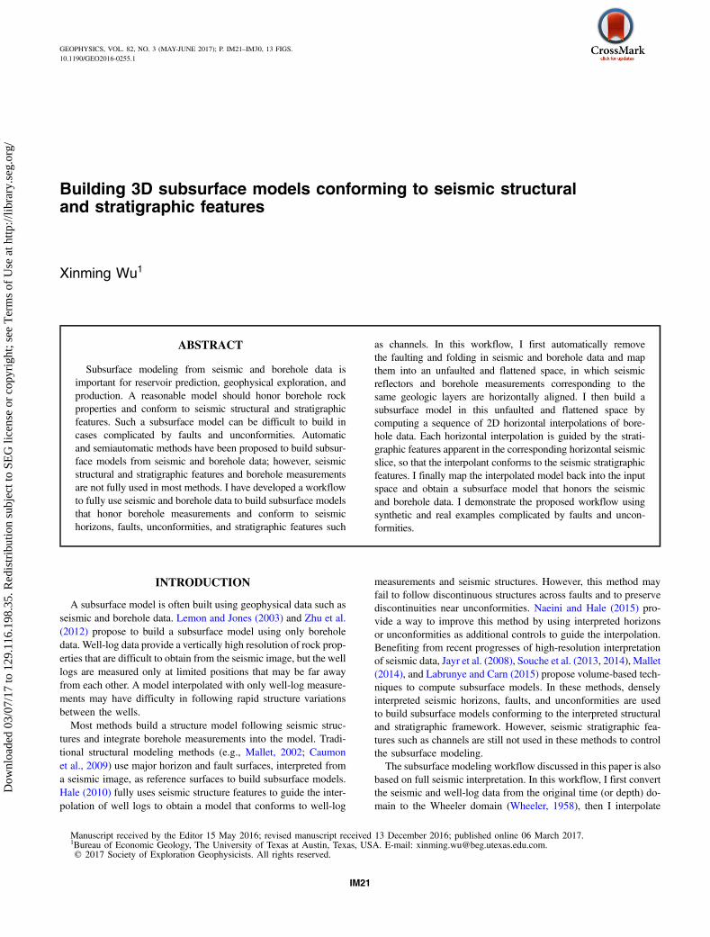
by combining the methods of computing fault surfaces and fault slipvectors from a 3D seismic image (Wu and Hale, 2016), removing thefaulting in the seismic image (Wu et al., 2016), extracting unconform-ity surfaces from the unfaulted image (Wu and Hale, 2015a), andflattening the unfaulted image with constraints from the unconform-ities (Wu and Hale, 2015b). Figure 1 shows the whole subsurfacemodeling workflow that includes three main steps: (1) forward-do-main transformation of 3D seismic and well-log data, (2) subsurfacemodeling in transformed domain, and (3) reverse transformation ofthe subsurface models. In the first step, I first extract fault surfacesand estimate fault slip vectors from a 3D seismic image (Figure 2a).I then use the estimated fault positions and slips to compute an un-faulting mapping to generate an unfaulted seismic image, in whichseismic reflectors are continuous across faults. I finally extract uncon-formities from the unfaulted image and use them as constraints tocompute a flattening mapping to generate a flattened image (Fig-ure 2b) in which seismic reflectors are flattened, stratigraphic featuressuch as channels are present on horizontal slices, and unconformitiesare represented as vertical gaps. Assuming that the well logs are tiedto the seismic image, I use the computed seismic unfaulting and flat-

Figure 1. The workflow of building 3D subsurface models that con-form to well-log properties and seismic structural and stratigraphicfeatures.

IM22 Wu

Dow

nloa

ded

03/0

7/17

to 1

29.1

16.1

98.3

5. R

edis

trib

utio

n su

bjec

t to

SEG

lice

nse

or c

opyr

ight

; see

Ter

ms

of U

se a

t http

://lib

rary

.seg

.org

/

tening mappings to also map the logs into the unfaulted and flattenedspace (Figure 2b), so that well-log measurements corresponding tothe same geologic layers are horizontally aligned.After mapping the seismic and well-log data into the unfaulted

and flattened space, the second step is to build a model (Figure 3a)in this space by simply computing a sequence of 2D horizontalinterpolations of the well-log measurements. Each horizontal inter-polation is computed using the image-guided interpolation method(Hale, 2009a), and the stratigraphic features are used to guide theinterpolation so that the interpolant conforms tothese features (Figure 3a). The third step is tomap this model (Figure 3a) from the unfaultedand flattened space back into the original spaceto obtain a subsurface model (Figure 3b) thatconforms to well-log properties, seismic hori-zons, faults, unconformities, and stratigraphicfeatures.

DOMAIN TRANSFORMATION

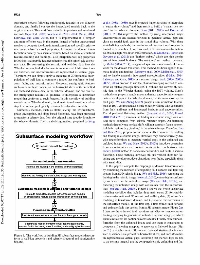
To illustrate the whole workflow of the subsur-face modeling, I created a 3D synthetic example(Figure 4a) with 121 (vertical) × 152 (inline) ×153 (crossline) samples. In creating this syntheticexample, I began with simple initial density,velocity, and reflectivity models with all flatlayers, in which a sinusoidal shape channel is de-fined with relatively high densities and veloc-ities. I then vertically sheared the flat models tocreate folding and dipping structures in the mod-els. Next, I added several flat layers on the top tocreate an unconformity between these flat layersabove and the dipping layers below. I finallyadded three planar faults sequentially by slidingmodel blocks on opposite of each fault with somespecific vector shifts. The seismic image shownin Figure 4a is computed by convolving thefolded and faulted reflectivity model with aRicker wavelet in directions perpendicular to thestructures and adding some random noise withrms ¼ 0.5. In this image, the unconformity isdislocated by all three faults, and the channelis cut by faults F1 and F2. To automatically ex-tract the unconformity and horizons from thisseismic image, we first need to remove the fault-ing in this image.

Unfaulting

To remove the faulting in the seismic image inFigure 4a, I first use the methods proposed byWu and Hale (2016) to automatically extractfault surfaces and to estimate fault slips on thefault surfaces. Note that I only compute dip slips,which are relative displacements of fault blocksin the dip directions of the fault. These dip slipsare estimated by correlating seismic reflectorsacross faults as discussed by Hale (2013) and Wuand Hale (2016). Fault strike slips are difficult tocompute by correlating these seismic reflectors

because the strike slips tend to be parallel to the seismic reflectors.The estimated fault dip slips are vectors with vertical, inline, and

crossline components in 3D. I only display the vertical componentswith colors on the fault surfaces in Figure 4b. To remove the faultingin the seismic image, I use all three components of the dip slips tocompute unfaulting vector shifts by applying the method proposedby Wu et al. (2016). With this method, I first compute unfaultingshifts skðxÞ in the original space (x ¼ ðx1; x2; x3Þ) by solving thefollowing two equations:

Figure 2. (a) A 3D seismic image and corresponding well logs in the original space aremapped into (b) the unfaulted and flattened space, by removing faulting and folding inthe seismic image and well logs.

Figure 3. (a) A 3D density model is first interpolated from the density logs in the un-faulted and flattened space, and then it is mapped back into (b) the original space. Thiscomputed density model (b) conforms to seismic horizons, faults, unconformities, andstratigraphic features (e.g., the channel).

Figure 4. From (a) a 3D seismic image, (b) fault surfaces are first extracted and fault slipsare then estimated on these surfaces. The estimated fault slips are vectors, but only faultthrows, the vertical components of slips, are displayed in color on the surfaces in (b).

Building 3D subsurface models IM23

Dow

nloa

ded

03/0

7/17

to 1

29.1

16.1

98.3

5. R

edis

trib

utio

n su

bjec

t to

SEG

lice

nse

or c

opyr

ight

; see

Ter

ms

of U

se a

t http

://lib

rary

.seg

.org

/

βcðxfÞðskðxhÞ − skðxfÞÞ ≈ βcðxfÞtkðxfÞωðxÞ∇skðxÞ ≈ 0; (1)

where tkðxÞðk ¼ 1; 2; 3Þ represent the three components of the faultslip vectors estimated on the faults, and skðxÞ; ðk ¼ 1; 2; 3Þ re-present the three components of the vector shifts to be computed;xf and xh represent the grid samples adjacent to the faults from thefootwall and hanging wall, respectively. Specifically, if a fault sam-ple is located on a seismic sampling grid point, xf represents thefault sample and xh represents the horizontally nearest grid pointfrom the hanging wall side in the fault normal direction. If a faultsample is not on a sampling grid point, xf and xh represent the hori-zontally nearest grid points from the footwall and hanging wall sides,respectively. This equation means that we expect the differences ofunfaulting shifts of samples xh and xf to be equal to the precomputedfault slip vectors; cðxÞ is a measure of the quality of the estimatedslips, and here, I use the fault likelihoods (Hale, 2013; Wu and Hale,2016) that are already computed on faults; β is a constant numberused to balance these two equations. For most examples, I useβ ¼ N∕L, where N represents the number of samples in the seismicimage and L is the number of samples on the faults. In the secondequation, ∇ represents the gradient operator and ωðxÞ are binaryweights, which are zeros at image samples (xf and xh) adjacent tofaults, and are ones elsewhere. This equation means that we expectunfaulting shifts to vary slowly and continuously everywhere exceptbetween two adjacent samples on opposite sides of a fault. Theapproximate signs in these two equations indicate that they are mini-mized by least squares. In solving these equations, zero-slope boun-dary conditions are considered in the finite-difference approximationof the gradient operator.By solving these equations independently for each component

(skðxÞ) of unfaulting shifts, I obtain vector shifts sðxÞ ¼ ðs1ðxÞ;s2ðxÞ; s3ðxÞÞ in the original space x ¼ ðx1; x2; x3Þ. Although I com-pute all the three components of the shifts sðxÞ, I display only thevertical shifts in Figure 5a. We observe that these shifts are discon-tinuous at faults and smoothly varying elsewhere, as expected.Using these computed vector shifts sðxÞ, I can then obtain the

mapping wðxÞ from input space x ¼ ðx1; x2; x3Þ to unfaulted spacew ¼ ðw1; w2; w3Þ as

wðxÞ ¼ x − sðxÞ: (2)

Assuming that the mapping wðxÞ is reversible, we must have a cor-responding mapping xðwÞ that converts points from the unfaultedspace into the input space, and we might define such a mapping as

xðwÞ ¼ wþ rðwÞ; (3)

where rðwÞ represent vector shifts in the unfaulted space.Because the mappings between the input and unfaulted spaces

are reversible, equations 2 and 3 imply the following relationshipbetween the vectors shifts rðwÞ and sðxÞ:

rðwðxÞÞ ¼ sðxÞ: (4)

This relationship indicates that we can compute the vector shiftsrðwÞ (unfaulted space) from the vector shifts sðxÞ calculated inthe original (input) space, by using an iterative method as discussedby Wu et al. (2016). This method begins with initial vector shiftsr0ðwÞ ¼ sðwÞ and iteratively updates the shifts by

r0ðwÞ ¼ sðwÞx0ðwÞ ¼ wþ r0ðwÞr1ðwÞ ¼ sðx0ðwÞÞx1ðwÞ ¼ wþ r1ðwÞ

· · ·

riðwÞ ¼ sðxi−1ðwÞÞxiðwÞ ¼ wþ riðwÞ

· · ·

rðwÞ ≈ rmðwÞ ¼ sðwþ rm−1ðwÞÞ: (5)

In this way, I keep updating the vector shifts riðwÞ until the updatesare insignificant in the mth iteration, to obtain the vector shiftsrðwÞ ≈ rmðwÞ in the unfaulted space.From the input seismic image fðxÞ (Figure 4a), I use the mapping

xðwÞ and a sinc interpolation of seismic amplitudes to compute anunfaulted image gðwÞ ¼ fðxðwÞÞ, as shown in Figure 5b. In thisunfaulted image (Figure 5b), seismic reflectors are more continuousacross faults compared with those in the input seismic image (Fig-ure 4a). This unfaulted image can also be mapped back into the

original space to obtain the input image fðxÞ ¼gðwðxÞÞ using the mapping wðxÞ and anothersinc interpolation. During the unfaulting, we ob-serve that nondata areas are generated in the un-faulted image, as shown in the lower left ofFigure 5b. These nondata areas will have no ef-fects in building a subsurface model with thesame size as the original seismic image becausethese nondata areas will not be used when map-ping the models back to the original space. Thesamples in the nondata areas in the unfaultedspace do not correspond to any samples in theoriginal seismic image.

Flattening with unconformities

The unfaulting processing facilitates imageflattening by removing the faulting in the seismic

Figure 5. The precomputed fault positions and fault slip vectors are used to compute(a) unfaulting shifts to remove the faulting in the seismic image and obtain (b) an un-faulted image. The unfaulting shifts are vectors, but only vertical components are dis-played in color in (a).

IM24 Wu

Dow

nloa

ded

03/0

7/17

to 1

29.1

16.1

98.3

5. R

edis

trib

utio

n su

bjec

t to

SEG

lice

nse

or c

opyr

ight

; see

Ter

ms

of U

se a

t http

://lib

rary

.seg

.org

/

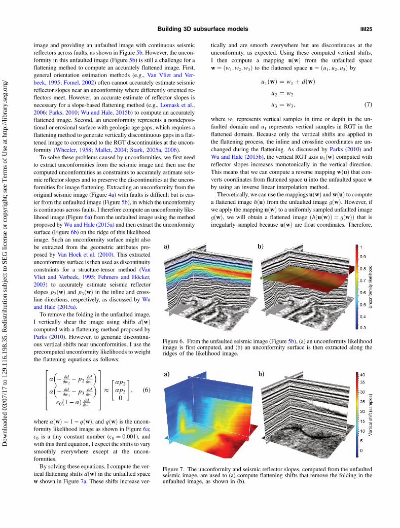
image and providing an unfaulted image with continuous seismicreflectors across faults, as shown in Figure 5b. However, the uncon-formity in this unfaulted image (Figure 5b) is still a challenge for aflattening method to compute an accurately flattened image. First,general orientation estimation methods (e.g., Van Vliet and Ver-beek, 1995; Fomel, 2002) often cannot accurately estimate seismicreflector slopes near an unconformity where differently oriented re-flectors meet. However, an accurate estimate of reflector slopes isnecessary for a slope-based flattening method (e.g., Lomask et al.,2006; Parks, 2010; Wu and Hale, 2015b) to compute an accuratelyflattened image. Second, an unconformity represents a nondeposi-tional or erosional surface with geologic age gaps, which requires aflattening method to generate vertically discontinuous gaps in a flat-tened image to correspond to the RGT discontinuities at the uncon-formity (Wheeler, 1958; Mallet, 2004; Stark, 2005a, 2006).To solve these problems caused by unconformities, we first need

to extract unconformities from the seismic image and then use thecomputed unconformities as constraints to accurately estimate seis-mic reflector slopes and to preserve the discontinuities at the uncon-formities for image flattening. Extracting an unconformity from theoriginal seismic image (Figure 4a) with faults is difficult but is eas-ier from the unfaulted image (Figure 5b), in which the unconformityis continuous across faults. I therefore compute an unconformity like-lihood image (Figure 6a) from the unfaulted image using the methodproposed by Wu and Hale (2015a) and then extract the unconformitysurface (Figure 6b) on the ridge of this likelihoodimage. Such an unconformity surface might alsobe extracted from the geometric attributes pro-posed by Van Hoek et al. (2010). This extractedunconformity surface is then used as discontinuityconstraints for a structure-tensor method (VanVliet and Verbeek, 1995; Fehmers and Höcker,2003) to accurately estimate seismic reflectorslopes p2ðwÞ and p3ðwÞ in the inline and cross-line directions, respectively, as discussed by Wuand Hale (2015a).To remove the folding in the unfaulted image,

I vertically shear the image using shifts dðwÞcomputed with a flattening method proposed byParks (2010). However, to generate discontinu-ous vertical shifts near unconformities, I use theprecomputed unconformity likelihoods to weightthe flattening equations as follows:2

66664α�− ∂d

∂w2− p2

∂d∂w1

�α�− ∂d

∂w3− p3

∂d∂w1

�ϵ0ð1 − αÞ ∂d

∂w1

377775 ≈

" αp2

αp3

0

#; (6)

where αðwÞ ¼ 1 − qðwÞ, and qðwÞ is the uncon-formity likelihood image as shown in Figure 6a;ϵ0 is a tiny constant number (ϵ0 ¼ 0.001), andwith this third equation, I expect the shifts to varysmoothly everywhere except at the uncon-formities.By solving these equations, I compute the ver-

tical flattening shifts dðwÞ in the unfaulted spacew shown in Figure 7a. These shifts increase ver-

tically and are smooth everywhere but are discontinuous at theunconformity, as expected. Using these computed vertical shifts,I then compute a mapping uðwÞ from the unfaulted spacew ¼ ðw1; w2; w3Þ to the flattened space u ¼ ðu1; u2; u3Þ by

u1ðwÞ ¼ w1 þ dðwÞu2 ¼ w2

u3 ¼ w3; (7)

where w1 represents vertical samples in time or depth in the un-faulted domain and u1 represents vertical samples in RGT in theflattened domain. Because only the vertical shifts are applied inthe flattening process, the inline and crossline coordinates are un-changed during the flattening. As discussed by Parks (2010) andWu and Hale (2015b), the vertical RGT axis u1ðwÞ computed withreflector slopes increases monotonically in the vertical direction.This means that we can compute a reverse mapping wðuÞ that con-verts coordinates from flattened space u into the unfaulted space wby using an inverse linear interpolation method.Theoretically, we can use the mappings uðwÞ andwðuÞ to compute

a flattened image hðuÞ from the unfaulted image gðwÞ. However, ifwe apply the mapping uðwÞ to a uniformly sampled unfaulted imagegðwÞ, we will obtain a flattened image ðhðuðwÞÞ ¼ gðwÞÞ that isirregularly sampled because uðwÞ are float coordinates. Therefore,

Figure 6. From the unfaulted seismic image (Figure 5b), (a) an unconformity likelihoodimage is first computed, and (b) an unconformity surface is then extracted along theridges of the likelihood image.

Figure 7. The unconformity and seismic reflector slopes, computed from the unfaultedseismic image, are used to (a) compute flattening shifts that remove the folding in theunfaulted image, as shown in (b).

Building 3D subsurface models IM25

Dow

nloa

ded

03/0

7/17

to 1

29.1

16.1

98.3

5. R

edis

trib

utio

n su

bjec

t to

SEG

lice

nse

or c

opyr

ight

; see

Ter

ms

of U

se a

t http

://lib

rary

.seg

.org

/

we instead use the inverse mappingwðuÞ and 3D sinc interpolation tocompute a uniformly sampled image hðuÞ ¼ gðwðuÞÞ in the flatteneddomain u. In this flattened image shown in Figure 7b, all seismicreflectors are flattened, the unconformity is represented as verticalgaps, and the channel is present on the horizontal slice. This flattenedimage hðuÞ can also be mapped back into the unfaulted space w toobtain the unfaulted image gðwÞ ¼ hðuðwÞÞ using the mapping uðwÞand another sinc interpolation.Using the unfaulting mapping xðwÞ and the flattening mapping

wðuÞ, we can also convert the well logs, like the 12 density logs inFigure 2, from the input space (Figure 2a) into the unfaulted andflattened space (Figure 2b). These 12 well logs are directly extractedfrom the corresponding density model. Before the conversion thewell logs using the mappings computed from the seismic image,we first need to tie these well logs to the seismic image usingmanual or automatic methods (e.g., Muñoz and Hale, 2015; Wuand Caumon, 2016). The seismic well ties help to correlate thewell-log values of some geologic layer with seismic reflectors thatcorrespond to the same geologic layer. Therefore, the mappingscomputed from the seismic image can also be used to remove fault-ing and folding in the well logs to obtain unfaulted and flattenedwell logs (Figure 2b). In these unfaulted and flattened well logs,well-log samples corresponding to the same geologic layer are hori-zontally aligned. The faults and the unconformity, which representgeologic layer discontinuities in the original space, generate dis-placements and gaps in the unfaulted and flattened well logs asshown in Figure 2a. After computing the unfaulted and flattenedseismic image and well logs, I address next how to efficiently builda subsurface model that honors well-log measurements and con-forms to seismic structures and stratigraphic features.

SUBSURFACE MODELING

Interpolating a subsurface model in the unfaulted and flattenedspace is straightforward because it requires only 2D horizontal in-terpolations to follow seismic structures such as horizons, faults,and unconformities. Stratigraphic features (such as channels) thatare present on horizontal slices of an unfaulted and flattened seismicimage can be used to guide the 2D interpolations. Therefore, I firstcompute a 3D model in the unfaulted and flattened space using a

sequence of 2D stratigraphic feature-guided interpolations and thenmap the model back into the input space to obtain a subsurface modelthat conforms to seismic horizons, faults, unconformities, and strati-graphic features.

Stratigraphic feature-guided interpolation

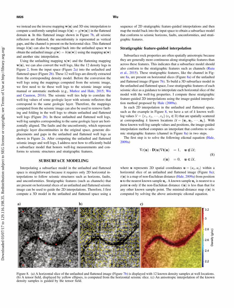
Subsurface rock properties are often spatially anisotropic becausethey are generally more continuous along stratigraphic features thanacross these features. This indicates that a subsurface model shouldalso conform to the stratigraphic features such as channels (Ruiuet al., 2015). These stratigraphic features, like the channel in Fig-ure 8a, are present on horizontal slices (Figure 8a) of the unfaultedand flattened image (Figure 7b). To build a 3D subsurface model inthe unfaulted and flattened space, I use stratigraphic features of eachseismic slice as a guidance to interpolate each horizontal slice of themodel with the well-log properties. I compute these stratigraphicfeature-guided 2D interpolations using the image-guided interpola-tion method proposed by Hale (2009a).In each 2D interpolation in the unfaulted and flattened space,

such as the example in Figure 8, we have a set of k known well-log values V ¼ fv1; v2; · · · ; vkg (vk ∈ R) that are spatially scatteredat corresponding k known locations U ¼ fu1; u2; · · · ; ukg. Withthese known well-log sample values and positions, the image-guidedinterpolation method computes an interpolant that conforms to seis-mic stratigraphic features (channel in Figure 8a) in two steps.The first step is to solve the following eikonal equation (Hale,

2009a)

∇tðuÞ · DðuÞ∇tðuÞ ¼ 1; u ∈= U;

tðuÞ ¼ 0; u ∈ U;(8)

where u represents 2D spatial coordinates u ¼ ðu2; u3Þ within ahorizontal slice of an unfaulted and flattened image (Figure 8a);tðuÞ is a map of non-Euclidean distance (Hale, 2009a) from positionu to the nearest known sample uk. A known sample uk is nearest to apoint u only if the non-Euclidean distance tðuÞ is less than that forany other known sample point. The minimal-distance map tðuÞ iscomputed by solving the above anisotropic eikonal equation.

Figure 8. (a) A horizontal slice of the unfaulted and flattened image (Figure 7b) is displayed with 12 known density samples at well locations.(b) A tensor field, displayed by yellow ellipses, is computed from the horizontal seismic slice. (c) An anisotropic interpolation of the knowndensity samples is guided by the tensor field.

IM26 Wu

Dow

nloa

ded

03/0

7/17

to 1

29.1

16.1

98.3

5. R

edis

trib

utio

n su

bjec

t to

SEG

lice

nse

or c

opyr

ight

; see

Ter

ms

of U

se a

t http

://lib

rary

.seg

.org

/

The metric tensor field DðuÞ (Figure 8b) represents the coherenceand orientation of the stratigraphic features in a seismic slice, andtherefore it often provides anisotropic and spatially variant coeffi-cients for the eikonal equation. As suggested by Hale (2010), Ichoose the tensor field such that the non-Euclidean distance t be-tween two points within the same stratigraphic feature is small,whereas the distance between two points in different stratigraphicfeatures is much larger. In the next section, I will discuss in detailhow to construct such a tensor field from a seismic amplitude slice(Figure 8a).In this first step, while computing the non-Euclidean distance

map tðuÞ from each point u to the nearest known sample uk, I alsocompute a nearest-neighbor interpolant pðuÞ by simply recordingthe known value pðuÞ ¼ vk of the nearest sample. This nearest-neighbor interpolant pðuÞ, together with the minimal distancemap tðuÞ, is used in the next step of computing a blended neighborinterpolation qðuÞ (Hale, 2009a)

qðuÞ − 1

2∇ · t2ðuÞDðuÞ∇qðuÞ ¼ pðuÞ: (9)

The partial differential equation above represents a smoothingprocessing of the input nearest-neighbor interpolant pðuÞ. Thesmoothing is oriented by the tensor field DðuÞ, and the extent ofsmoothing is controlled by the distance map tðuÞ. Therefore, theoutput blended neighbor interpolant qðuÞ is just a smoothed versionof the nearest-neighbor interpolant pðuÞ. At the known sample po-sitions uk, no smoothing is performed because the distance maptðukÞ ¼ 0, and the above equation 9 is qðukÞ ¼ pðukÞ ¼ vk. Thismeans that the interpolated values at the known sample positions areexactly equal to the known values at these points.

Computing the tensor field

As discussed above, the metric tensor field DðuÞ is important inboth steps to guide the interpolation. To compute a final interpola-tion qðuÞ that conforms to the seismic stratigraphic features, suchas the one in Figure 8c, the tensor field DðuÞ should represent thecoherence, orientation, and dimensionality of the stratigraphic fea-tures, as discussed by Hale (2009a).I construct such a tensor field DðuÞ from structure tensors SðuÞ

(Van Vliet and Verbeek, 1995; Fehmers and Höcker, 2003), whichare smoothed outer products of image gradients S ¼ hgg⊤is;, wherethe column vector g represents seismic image gradient vector com-puted for each image sample. I efficiently compute the image gra-dients using recursive Gaussian derivative filters (Deriche, 1993;Van Vliet et al., 1998; Hale, 2006) with radius σ ¼ 1 (sample);h·is denotes smoothing for each element of the outer product orstructure tensor. This smoothing, often implemented as a Gaussianfilter, helps to construct structure tensors with more stable estima-tions of orientations of image features.For a 2D seismic image (Figure 8a), a structure tensor, con-

structed for each image sample, is a symmetric positive-semidefin-ite 2 × 2 matrix with eigendecomposition

SðuÞ ¼ λaðuÞaðuÞa⊤ðuÞ þ λbðuÞbðuÞb⊤ðuÞ; (10)

where λaðuÞ and λbðuÞ are the eigenvalues corresponding to eigen-vectors aðuÞ and bðuÞ of SðuÞ. As discussed by Fehmers andHöcker (2003), the eigenvectors aðuÞ and bðuÞ provide estimations

of orientations of linear features in a 2D seismic image. If we labelthe eigenvalues λaðuÞ ≥ λbðuÞ ≥ 0, then the corresponding eigen-vectors aðuÞ are perpendicular to locally linear features in an image,and the eigenvectors bðuÞ are parallel to such features.As discussed by Hale (2009b), the eigenvalues λaðuÞ and λbðuÞ

provide measures of isotropy and linearity of structures apparent inthe seismic image. The linearity lðuÞ (1 ≥ lðuÞ ≥ 0) for each imagesample can be computed by the following ratio of the eigenvalues(Hale, 2009b):

lðuÞ ¼ λaðuÞ − λbðuÞλaðuÞ

: (11)

Linearities are close to one for samples in areas with continuous andcoherent stratigraphic features, but they are relatively smaller in theisotropic areas without linear features. Therefore, the linearity canbe used to highlight linear stratigraphic features such as the channelin Figure 8a.Because the eigenvectors aðuÞ and bðuÞ of the structure tensors

SðuÞ represent orientations of stratigraphic features, I construct themetric tensor fieldDðuÞ using the same eigenvectors but with differ-ent eigenvalues

DðuÞ ¼ μaðuÞaðuÞa⊤ðuÞ þ μbðuÞbðuÞb⊤ðuÞ: (12)

I choose the eigenvalues μaðuÞ and μbðuÞ to construct a tensor fieldDðuÞ so that the non-Euclidean distance tðuÞ in equation 8 increasesslowly in directions along the linear stratigraphic features, and itincreases rapidly in directions perpendicular to the features. In areaswith isotropic features, we should expect the distance tðuÞ to in-crease with the same speed in all directions.In Figure 8, I compute the eigenvalues μaðuÞ and μbðuÞ for the

tensor field DðuÞ by

μaðuÞ¼saðuÞλminþϵ0λaðuÞþϵ0

; and μbðuÞ¼λminþϵ0λbðuÞþϵ0

; (13)

where λmin ¼ minufλaðuÞ; λbðuÞg. The parameter ϵ0 is a small pos-itive number and is used to avoid dividing by zero in equation 13. Iuse the scales saðuÞ ¼ ð1 − lðuÞÞ4 in computing eigenvalues μaðuÞto increase the anisotropy of the tensor field DðuÞ. Specifically, inareas (e.g., channel) with relatively high linearity lðuÞ ≈ 1, smallscales saðuÞ yield small eigenvalues μaðuÞ, which make the non-Euclidean distances (computed by equation 8) increase rapidly alongdirections (eigenvectors a) perpendicular to the linear features.The yellow ellipses in Figure 8b show some examples of the met-

ric tensors DðuÞ that I compute for all image samples using equa-tion 12. The major axis of each ellipse represents the direction alonglinear stratigraphic features, whereas the minor axis denotes the di-rection perpendicular to the features. For samples in which the im-age features are isotropic, the major axes of the ellipses are nearlyequal to the minor axes, and the ellipses look like circles. Also, indirections along the longer radius of an ellipse, the non-Euclideandistance tðuÞ in equation 8 increases slowly, whereas it increasesrapidly in directions along the shorter radius. Near the channel inFigure 8b, the major radii of the ellipses are much longer than theminor radii, and the major radii are aligned along the channel. Thismeans that the non-Euclidean map tðuÞ computed using these met-ric tensors will increase slowly in directions along the channel butwill increase rapidly in directions perpendicular to the channel.

Building 3D subsurface models IM27

Dow

nloa

ded

03/0

7/17

to 1

29.1

16.1

98.3

5. R

edis

trib

utio

n su

bjec

t to

SEG

lice

nse

or c

opyr

ight

; see

Ter

ms

of U

se a

t http

://lib

rary

.seg

.org

/

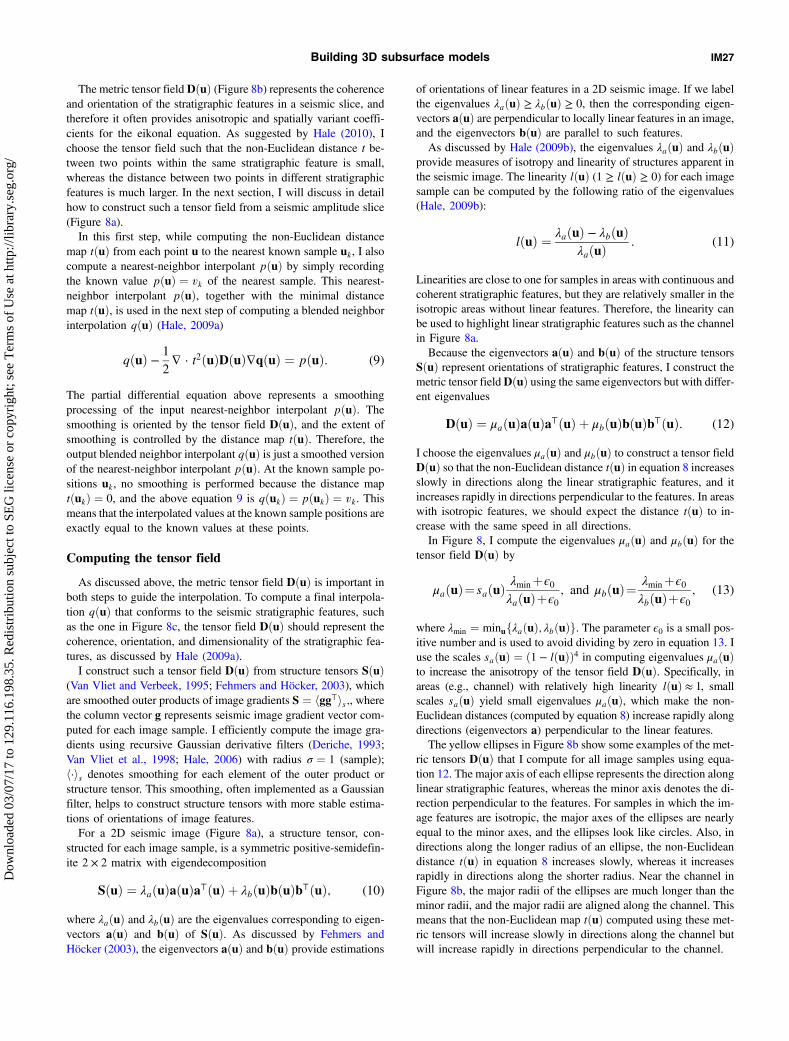
With the 12 known density-log values (Figure 8a) and the metrictensor field (Figure 8b), I computed a 2D interpolated density image(Figure 8c), which honors the known density values from well logsand also conforms to the stratigraphic features in the seismic slice.Similarly, I computed every horizontal slice (in vertical seismicscale) of the 3D density model in the unfaulted and flattened spacein Figure 3a. I then use the mappings uðwÞ and wðxÞ to convert thisdensity model (Figure 3a) back into the original space and obtain a3D subsurface model (Figures 3b and 9a) that conforms to seismicfaults, horizons, unconformities, and stratigraphic features. Thissubsurface model (Figure 9a), computed with only 12 density logs,is consistent with the true density model (Figure 9b).

APPLICATIONS

The first example I use to demonstrate the proposed methods isthe freely available Teapot Dome data set, which includes a time-migrated 3D seismic image and hundreds of well logs. Before atime-migrated seismic image can be used to guide interpolationof well logs measured in depth, the vertical axis of the image mustbe first converted from two-way time to depth, or the well logs mustbe first tied in time to the seismic image. The vertical axis of theseismic image shown in Figure 10a is already converted to depth byusing a time-to-depth conversion provided by Transform Softwareand Services (now a part of Drillinginfo).

Two groups of wells, called “shallow” and“deeper,” are provided in the Teapot Dome dataset, but I discarded all the shallow wells and onlyused the deeper ones in this paper because theshallow ones do not penetrate to the depths dis-played in Figure 10a. I also discarded some deeperwell logs containing obviously erroneous velocityvalues that are outside the range ½0.2; 20� km∕s.The velocity logs shown in Figure 10a have beenconverted to inline, crossline, and depth coordi-nates of the seismic image. The well-log samplesare downsampled to be consistent with the seismicsamples in depth by choosing the median well-logvalue within a depth window centered at each seis-mic depth sample.To build a 3D velocity model from the seismic

image and velocity logs shown in Figure 10a, Ifirst converted the image and logs from the inputspace (Figure 10a) into the unfaulted and flat-tened space (Figure 10b) by using the unfaultingand flattening mappings computed from the seis-mic image. I then built a 3D velocity model in theunfaulted and flattened space (Figure 11a) bycomputing a sequence of 2D stratigraphic fea-ture-guided interpolations of the velocity log val-ues within 2D seismic horizontal slices. Thestratigraphic features used in the interpolationare computed from the horizontal slices of theunfaulted and flattened seismic image. I finallyconverted the interpolated 3D velocity modelback into the input space and obtained a subsur-face velocity model that conforms to seismichorizons and faults as shown in Figure 11b.The second example (Figure 12) is a subset of

the Netherlands offshore F3 block acquired in theNorth Sea. This example is more complicatedthan the first one because of the multiple uncon-formities and faults including intersecting faultsin the seismic image (Figure 12). A subsurfacemodel computed with a limited number of hori-zons and faults may have difficulty followingsubsurface structures that are highly discontinu-ous near the unconformities and especially nearthe intensive faults. In this example, I first com-puted fault positions and fault slip vectors fromthe 3D seismic image (Figure 12a). The colorsdisplayed on the faults in Figure 12a representfault throws, which are the vertical components

Figure 9. (a) The density model, constructed from the seismic image and 12 densitylogs, is consistent with (b) the true density model. The white circles highlight the lo-cations of the channel with relatively higher density.

Figure 10. (a) A real 3D seismic image and velocity logs are mapped from input spaceinto unfaulted and (b) flattened space.

Figure 11. (a) A 3D velocity model is first interpolated in the unfaulted and flattenedspace and then mapped back into (b) the input space.

IM28 Wu

Dow

nloa

ded

03/0

7/17

to 1

29.1

16.1

98.3

5. R

edis

trib

utio

n su

bjec

t to

SEG

lice

nse

or c

opyr

ight

; see

Ter

ms

of U

se a

t http

://lib

rary

.seg

.org

/

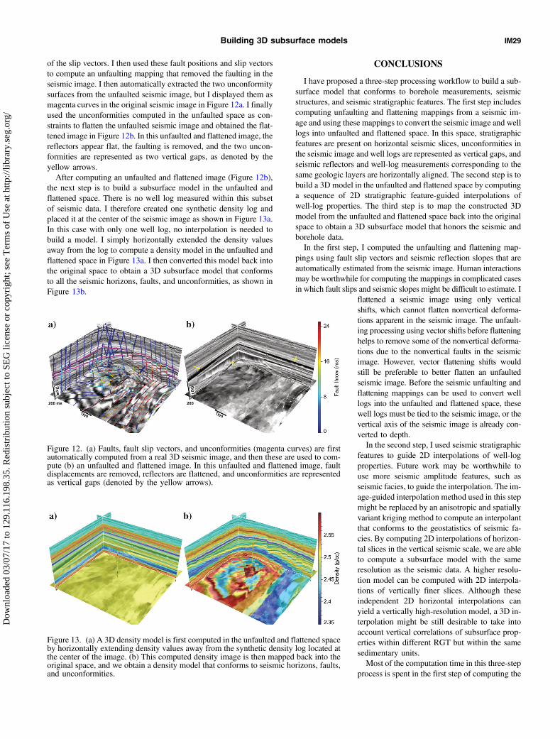
of the slip vectors. I then used these fault positions and slip vectorsto compute an unfaulting mapping that removed the faulting in theseismic image. I then automatically extracted the two unconformitysurfaces from the unfaulted seismic image, but I displayed them asmagenta curves in the original seismic image in Figure 12a. I finallyused the unconformities computed in the unfaulted space as con-straints to flatten the unfaulted seismic image and obtained the flat-tened image in Figure 12b. In this unfaulted and flattened image, thereflectors appear flat, the faulting is removed, and the two uncon-formities are represented as two vertical gaps, as denoted by theyellow arrows.After computing an unfaulted and flattened image (Figure 12b),

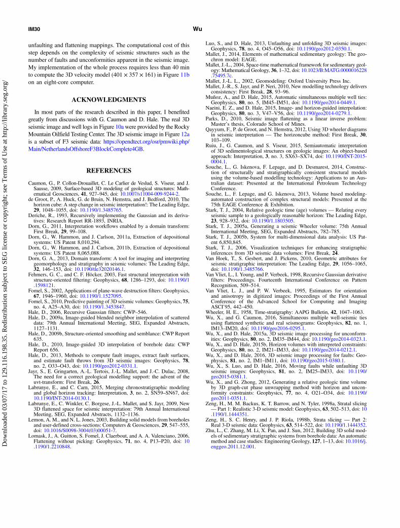
the next step is to build a subsurface model in the unfaulted andflattened space. There is no well log measured within this subsetof seismic data. I therefore created one synthetic density log andplaced it at the center of the seismic image as shown in Figure 13a.In this case with only one well log, no interpolation is needed tobuild a model. I simply horizontally extended the density valuesaway from the log to compute a density model in the unfaulted andflattened space in Figure 13a. I then converted this model back intothe original space to obtain a 3D subsurface model that conformsto all the seismic horizons, faults, and unconformities, as shown inFigure 13b.

CONCLUSIONS

I have proposed a three-step processing workflow to build a sub-surface model that conforms to borehole measurements, seismicstructures, and seismic stratigraphic features. The first step includescomputing unfaulting and flattening mappings from a seismic im-age and using these mappings to convert the seismic image and welllogs into unfaulted and flattened space. In this space, stratigraphicfeatures are present on horizontal seismic slices, unconformities inthe seismic image and well logs are represented as vertical gaps, andseismic reflectors and well-log measurements corresponding to thesame geologic layers are horizontally aligned. The second step is tobuild a 3D model in the unfaulted and flattened space by computinga sequence of 2D stratigraphic feature-guided interpolations ofwell-log properties. The third step is to map the constructed 3Dmodel from the unfaulted and flattened space back into the originalspace to obtain a 3D subsurface model that honors the seismic andborehole data.In the first step, I computed the unfaulting and flattening map-

pings using fault slip vectors and seismic reflection slopes that areautomatically estimated from the seismic image. Human interactionsmay be worthwhile for computing the mappings in complicated casesin which fault slips and seismic slopes might be difficult to estimate. I

flattened a seismic image using only verticalshifts, which cannot flatten nonvertical deforma-tions apparent in the seismic image. The unfault-ing processing using vector shifts before flatteninghelps to remove some of the nonvertical deforma-tions due to the nonvertical faults in the seismicimage. However, vector flattening shifts wouldstill be preferable to better flatten an unfaultedseismic image. Before the seismic unfaulting andflattening mappings can be used to convert welllogs into the unfaulted and flattened space, thesewell logs must be tied to the seismic image, or thevertical axis of the seismic image is already con-verted to depth.In the second step, I used seismic stratigraphic

features to guide 2D interpolations of well-logproperties. Future work may be worthwhile touse more seismic amplitude features, such asseismic facies, to guide the interpolation. The im-age-guided interpolation method used in this stepmight be replaced by an anisotropic and spatiallyvariant kriging method to compute an interpolantthat conforms to the geostatistics of seismic fa-cies. By computing 2D interpolations of horizon-tal slices in the vertical seismic scale, we are ableto compute a subsurface model with the sameresolution as the seismic data. A higher resolu-tion model can be computed with 2D interpola-tions of vertically finer slices. Although theseindependent 2D horizontal interpolations canyield a vertically high-resolution model, a 3D in-terpolation might be still desirable to take intoaccount vertical correlations of subsurface prop-erties within different RGT but within the samesedimentary units.Most of the computation time in this three-step

process is spent in the first step of computing the

Figure 12. (a) Faults, fault slip vectors, and unconformities (magenta curves) are firstautomatically computed from a real 3D seismic image, and then these are used to com-pute (b) an unfaulted and flattened image. In this unfaulted and flattened image, faultdisplacements are removed, reflectors are flattened, and unconformities are representedas vertical gaps (denoted by the yellow arrows).

Figure 13. (a) A 3D density model is first computed in the unfaulted and flattened spaceby horizontally extending density values away from the synthetic density log located atthe center of the image. (b) This computed density image is then mapped back into theoriginal space, and we obtain a density model that conforms to seismic horizons, faults,and unconformities.

Building 3D subsurface models IM29

Dow

nloa

ded

03/0

7/17

to 1

29.1

16.1

98.3

5. R

edis

trib

utio

n su

bjec

t to

SEG

lice

nse

or c

opyr

ight

; see

Ter

ms

of U

se a

t http

://lib

rary

.seg

.org

/

unfaulting and flattening mappings. The computational cost of thisstep depends on the complexity of seismic structures such as thenumber of faults and unconformities apparent in the seismic image.My implementation of the whole process requires less than 40 minto compute the 3D velocity model (401 × 357 × 161) in Figure 11bon an eight-core computer.

ACKNOWLEDGMENTS

In most parts of the research described in this paper, I benefitedgreatly from discussions with G. Caumon and D. Hale. The real 3Dseismic image and well logs in Figure 10a were provided by the RockyMountain Oilfield Testing Center. The 3D seismic image in Figure 12ais a subset of F3 seismic data: https://opendtect.org/osr/pmwiki.php/Main/NetherlandsOffshoreF3BlockComplete4GB.

REFERENCES

Caumon, G., P. Collon-Drouaillet, C. Le Carlier de Veslud, S. Viseur, and J.Sausse, 2009, Surface-based 3D modeling of geological structures: Math-ematical Geosciences, 41, 927–945, doi: 10.1007/s11004-009-9244-2.

de Groot, P., A. Huck, G. de Bruin, N. Hemstra, and J. Bedford, 2010, Thehorizon cube: A step change in seismic interpretation!: The Leading Edge,29, 1048–1055, doi: 10.1190/1.3485765.

Deriche, R., 1993, Recursively implementing the Gaussian and its deriva-tives: Research Report RR-1893, INRIA.

Dorn, G., 2011, Interpretation workflows enabled by a domain transform:First Break, 29, 99–108.

Dorn, G., W. Hammon, and J. Carlson, 2011a, Extraction of depositionalsystems: US Patent 8,010,294.

Dorn, G., W. Hammon, and J. Carlson, 2011b, Extraction of depositionalsystems: US Patent 8,065,088.

Dorn, G. A., 2013, Domain transform: A tool for imaging and interpretinggeomorphology and stratigraphy in seismic volumes: The Leading Edge,32, 146–153, doi: 10.1190/tle32020146.1.

Fehmers, G. C., and C. F. Höcker, 2003, Fast structural interpretation withstructure-oriented filtering: Geophysics, 68, 1286–1293, doi: 10.1190/1.1598121.

Fomel, S., 2002, Applications of plane-wave destruction filters: Geophysics,67, 1946–1960, doi: 10.1190/1.1527095.

Fomel, S., 2010, Predictive painting of 3D seismic volumes: Geophysics, 75,no. 4, A25–A30, doi: 10.1190/1.3453847.

Hale, D., 2006, Recursive Gaussian filters: CWP–546.Hale, D., 2009a, Image-guided blended neighbor interpolation of scattered

data: 79th Annual International Meeting, SEG, Expanded Abstracts,1127–1131.

Hale, D., 2009b, Structure-oriented smoothing and semblance: CWP Report635.

Hale, D., 2010, Image-guided 3D interpolation of borehole data: CWPReport 656.

Hale, D., 2013, Methods to compute fault images, extract fault surfaces,and estimate fault throws from 3D seismic images: Geophysics, 78,no. 2, O33–O43, doi: 10.1190/geo2012-0331.1.

Jayr, S., E. Gringarten, A.-L. Tertois, J.-L. Mallet, and J.-C. Dulac, 2008,The need for a correct geological modelling support: the advent of theuvt-transform: First Break, 26.

Labrunye, E., and C. Carn, 2015, Merging chronostratigraphic modelingand global horizon tracking: Interpretation, 3, no. 2, SN59–SN67, doi:10.1190/INT-2014-0130.1.

Labrunye, E., C. Winkler, C. Borgese, J.-L. Mallet, and S. Jayr, 2009, New3D flattened space for seismic interpretation: 79th Annual InternationalMeeting, SEG, Expanded Abstracts, 1132–1136.

Lemon, A. M., and N. L. Jones, 2003, Building solid models from boreholesand user-defined cross-sections: Computers & Geosciences, 29, 547–555,doi: 10.1016/S0098-3004(03)00051-7.

Lomask, J., A. Guitton, S. Fomel, J. Claerbout, and A. A. Valenciano, 2006,Flattening without picking: Geophysics, 71, no. 4, P13–P20, doi: 10.1190/1.2210848.

Luo, S., and D. Hale, 2013, Unfaulting and unfolding 3D seismic images:Geophysics, 78, no. 4, O45–O56, doi: 10.1190/geo2012-0350.1.

Mallet, J., 2014, Elements of mathematical sedimentary geology: The geo-chron model: EAGE.

Mallet, J.-L., 2004, Space-time mathematical framework for sedimentary geol-ogy: Mathematical Geology, 36, 1–32, doi: 10.1023/B:MATG.0000016228.75495.7c.

Mallet, J.-L. L., 2002, Geomodeling: Oxford University Press Inc.Mallet, J.-R., S. Jayr, and P. Neri, 2010, New modelling technology delivers

consistency: First Break, 28, 93–96.Muñoz, A., and D. Hale, 2015, Automatic simultaneous multiple well ties:

Geophysics, 80, no. 5, IM45–IM51, doi: 10.1190/geo2014-0449.1.Naeini, E. Z., and D. Hale, 2015, Image- and horizon-guided interpolation:

Geophysics, 80, no. 3, V47–V56, doi: 10.1190/geo2014-0279.1.Parks, D., 2010, Seismic image flattening as a linear inverse problem:

Master’s thesis, Colorado School of Mines.Qayyum, F., P. de Groot, and N. Hemstra, 2012, Using 3D wheeler diagrams

in seismic interpretation — The horizoncube method: First Break, 30,103–109.

Ruiu, J., G. Caumon, and S. Viseur, 2015, Semiautomatic interpretationof 3D sedimentological structures on geologic images: An object-basedapproach: Interpretation, 3, no. 3, SX63–SX74, doi: 10.1190/INT-2015-0004.1.

Souche, L., G. Iskenova, F. Lepage, and D. Desmarest, 2014, Construc-tion of structurally and stratigraphically consistent structural modelsusing the volume-based modelling technology: Applications to an Aus-tralian dataset: Presented at the International Petroleum TechnologyConference.

Souche, L., F. Lepage, and G. Iskenova, 2013, Volume based modeling-automated construction of complex structural models: Presented at the75th EAGE Conference & Exhibition.

Stark, T. J., 2004, Relative geologic time (age) volumes — Relating everyseismic sample to a geologically reasonable horizon: The Leading Edge,23, 928–932, doi: 10.1190/1.1803505.

Stark, T. J., 2005a, Generating a seismic Wheeler volume: 75th AnnualInternational Meeting, SEG, Expanded Abstracts, 782–785.

Stark, T. J., 2005b, System for multi-dimensional data analysis: US Pat-ent 6,850,845.

Stark, T. J., 2006, Visualization techniques for enhancing stratigraphicinferences from 3D seismic data volumes: First Break, 24.

Van Hoek, T., S. Gesbert, and J. Pickens, 2010, Geometric attributes forseismic stratigraphic interpretation: The Leading Edge, 29, 1056–1065,doi: 10.1190/1.3485766.

Van Vliet, L., I. Young, and P. Verbeek, 1998, Recursive Gaussian derivativefilters: Proceedings. Fourteenth International Conference on PatternRecognition, 509–514.

Van Vliet, L. J., and P. W. Verbeek, 1995, Estimators for orientationand anisotropy in digitized images: Proceedings of the First AnnualConference of the Advanced School for Computing and ImagingASCI’95, 442–450.

Wheeler, H. E., 1958, Time-stratigraphy: AAPG Bulletin, 42, 1047–1063.Wu, X., and G. Caumon, 2016, Simultaneous multiple well-seismic ties

using flattened synthetic and real seismograms: Geophysics, 82, no. 1,IM13–IM20, doi: 10.1190/geo2016-0295.1.

Wu, X., and D. Hale, 2015a, 3D seismic image processing for unconform-ities: Geophysics, 80, no. 2, IM35–IM44, doi: 10.1190/geo2014-0323.1.

Wu, X., and D. Hale, 2015b, Horizon volumes with interpreted constraints:Geophysics, 80, no. 2, IM21–IM33, doi: 10.1190/geo2014-0212.1.

Wu, X., and D. Hale, 2016, 3D seismic image processing for faults: Geo-physics, 81, no. 2, IM1–IM11, doi: 10.1190/geo2015-0380.1.

Wu, X., S. Luo, and D. Hale, 2016, Moving faults while unfaulting 3Dseismic images: Geophysics, 81, no. 2, IM25–IM33, doi: 10.1190/geo2015-0381.1.

Wu, X., and G. Zhong, 2012, Generating a relative geologic time volumeby 3D graph-cut phase unwrapping method with horizon and uncon-formity constraints: Geophysics, 77, no. 4, O21–O34, doi: 10.1190/geo2011-0351.1.

Zeng, H., M. M. Backus, K. T. Barrow, and N. Tyler, 1998a, Stratal slicing— Part 1: Realistic 3-D seismic model: Geophysics, 63, 502–513, doi: 10.1190/1.1444351.

Zeng, H., S. C. Henry, and J. P. Riola, 1998b, Strata slicing — Part 2:Real 3-D seismic data: Geophysics, 63, 514–522, doi: 10.1190/1.1444352.

Zhu, L., C. Zhang, M. Li, X. Pan, and J. Sun, 2012, Building 3D solid mod-els of sedimentary stratigraphic systems from borehole data: An automaticmethod and case studies: Engineering Geology, 127, 1–13, doi: 10.1016/j.enggeo.2011.12.001.

IM30 Wu

Dow

nloa

ded

03/0

7/17

to 1

29.1

16.1

98.3

5. R

edis

trib

utio

n su

bjec

t to

SEG

lice

nse

or c

opyr

ight

; see

Ter

ms

of U

se a

t http

://lib

rary

.seg

.org

/