Embed Size (px)
Citation preview

Lecture 2: Seismic Inversion and Imaging
Youzuo Lin1
Joint work with: Lianjie Huang1
Monica Maceira2
Ellen M. Syracuse1
Carene Larmat1
1: Los Alamos National Laboratory2: Oak Ridge National Laboratory
Graduate Student Workshop on Inverse Problem, 2016

Outline
1 Subsurface Applications
2 Schematic Description of Seismic imaging
3 Travel-Time Tomography and Full-Waveform InversionTravel-Time TomographyFull-Waveform InversionRegularization TechniquesA Modified Total-Variation Regularization Scheme
4 Computation Methods
5 Application to Global Seismology
6 Application to Enhanced Geothermal SystemsReservoir Monitoring with Time-Lapse DataBrady’s EGS SiteRobustness Tests
7 Conclusions
Youzuo Lin (LANL) Seismic Inversion Inverse Problems Workshop 1 / 77
Outline
1 Subsurface Applications
2 Schematic Description of Seismic imaging
3 Travel-Time Tomography and Full-Waveform InversionTravel-Time TomographyFull-Waveform InversionRegularization TechniquesA Modified Total-Variation Regularization Scheme
4 Computation Methods
5 Application to Global Seismology
6 Application to Enhanced Geothermal SystemsReservoir Monitoring with Time-Lapse DataBrady’s EGS SiteRobustness Tests
7 Conclusions
Youzuo Lin (LANL) Seismic Inversion Inverse Problems Workshop 2 / 77

Enhanced Geothermal System
• Geothermal is a sustainable energy because it is clean andreliable, however the exploration and drilling remain expensiveand risky.
• Quantitative monitoring for enhanced geothermal systems canhelp optimize the geothermal production and the placement ofnew wells.Youzuo Lin (LANL) Seismic Inversion Inverse Problems Workshop 2 / 77

Enhanced Geothermal System
• According to US Energy Information Administration (EIA), 9western states together have the geothermal potential to provideover 20% of electricity needs
• DOE aims a ten-fold increase of US electricity production fromgeothermal reservoirs within the next 10 years
Youzuo Lin (LANL) Seismic Inversion Inverse Problems Workshop 3 / 77

Enhanced Geothermal System
However, the reality is that• High Risk: Two to five out of every 10 geothermal wells
prospected end up dry
• Expensive to Drill: Wells cost between $2 million and $5 million,meaning geothermal investors risk losing millions on poor odds
An accurate characterization of the subsurface structure is thekey to a successful drilling schemes
Youzuo Lin (LANL) Seismic Inversion Inverse Problems Workshop 4 / 77

Quantitative Monitoring for CO2 Storage
• Quantifying changes in CO2 reservoirs is a key element forassessing the performance of geologic carbon sequestration.
• Reliably monitoring of potential CO2 leakage through fault zonesis crucial for ensuring safe CO2 storage.
Youzuo Lin (LANL) Seismic Inversion Inverse Problems Workshop 5 / 77

Global Seismology
• Seismic wave is currently the only effective tool that can penetratethe entire Earth
• Seismic inversion (tomography) is used to obtain the structuralinformation of the Earth
Youzuo Lin (LANL) Seismic Inversion Inverse Problems Workshop 6 / 77

Outline
1 Subsurface Applications
2 Schematic Description of Seismic imaging
3 Travel-Time Tomography and Full-Waveform InversionTravel-Time TomographyFull-Waveform InversionRegularization TechniquesA Modified Total-Variation Regularization Scheme
4 Computation Methods
5 Application to Global Seismology
6 Application to Enhanced Geothermal SystemsReservoir Monitoring with Time-Lapse DataBrady’s EGS SiteRobustness Tests
7 Conclusions
Youzuo Lin (LANL) Seismic Inversion Inverse Problems Workshop 7 / 77

Problem Description - Data Measurement
• Data Measurement
Source
Receiver
Media & Velocity 2Media & Velocity 1
���
���
����
Reflection Data
Source
Media & Velocity 1
Receiver
Media & Velocity 2
������
������
��
Transmission Data
Youzuo Lin (LANL) Seismic Inversion Inverse Problems Workshop 7 / 77

Problem Description - Data Usage
0 100 200 300 400 500 600 700 800−1
−0.5
0
0.5
1
1.5
2x 10
6
Time
Dis
pla
ce
me
nt
First Arrival Time
• First Arrival Time• Pros: Simplify the nonlinear problem to be linear; Efficient to solve.• Cons: Low-resolution imaging.
Youzuo Lin (LANL) Seismic Inversion Inverse Problems Workshop 8 / 77

Problem Description - Data Usage
0 100 200 300 400 500 600 700 800−1
−0.5
0
0.5
1
1.5
2x 10
6
Time
Dis
pla
ce
me
nt
Whole Waveform
• The Whole Waveform• Pros: High-resolution imaging.• Cons: Problem stays nonlinear; Computation load is expensive.
Youzuo Lin (LANL) Seismic Inversion Inverse Problems Workshop 8 / 77
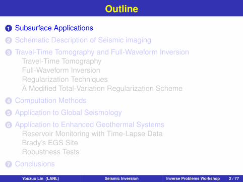
Problem Description - Inversion
• Data Inversion• A Model to Get Started (Initial Model)
• Generate The Simulated Data (Forward Modeling)• Match The Simulated Data to Measurement (Data Matching)• Use The Difference to Update The Initial Model (Model Update)
Initial ModelYouzuo Lin (LANL) Seismic Inversion Inverse Problems Workshop 9 / 77

Problem Description - Inversion
• Data Inversion• A Model to Get Started (Initial Model)• Generate The Simulated Data (Forward Modeling)
• Match The Simulated Data to Measurement (Data Matching)• Use The Difference to Update The Initial Model (Model Update)
Initial Model0 100 200 300 400 500 600 700 800
−1
−0.5
0
0.5
1
1.5
2x 10
6
Time
Dis
pla
ce
me
nt
Forward ModelingYouzuo Lin (LANL) Seismic Inversion Inverse Problems Workshop 9 / 77

Problem Description - Inversion
• Data Inversion• A Model to Get Started (Initial Model)• Generate The Simulated Data (Forward Modeling)• Match The Simulated Data to Measurement (Data Matching)
• Use The Difference to Update The Initial Model (Model Update)
Initial Model0 100 200 300 400 500 600 700 800
−1
−0.5
0
0.5
1
1.5
2x 10
6
Time
Dis
pla
ce
me
nt
Measurement
Simulating Data
Data MatchingYouzuo Lin (LANL) Seismic Inversion Inverse Problems Workshop 9 / 77

Problem Description - Inversion
• Data Inversion• A Model to Get Started (Initial Model)• Generate The Simulated Data (Forward Modeling)• Match The Simulated Data to Measurement (Data Matching)• Use The Difference to Update The Initial Model (Model Update)
Initial Model
?+
Model UpdateYouzuo Lin (LANL) Seismic Inversion Inverse Problems Workshop 9 / 77

Problem Description - Regularization & PriorInformation
• Inversion for ill-posed nonlinear problems can be much morechallenging to solve• Ill-posedness (cause of limited data coverage)• Local minima (cause of nonlinearity and non-convex optimization)
• Include prior information to constrain the inversion• To avoid the instability during the inversion of data.• To obtain more accurate reconstructions and a faster convergent
rate.• What can be prior information?
• Good initial guess (starting models)• Smoothness of the models• Locations of the regions of interests• Shapes of the reconstructions• etc.
• Regularization technique is a method to introduce priorinformation to the inversion.Youzuo Lin (LANL) Seismic Inversion Inverse Problems Workshop 10 / 77

Outline
1 Subsurface Applications
2 Schematic Description of Seismic imaging
3 Travel-Time Tomography and Full-Waveform InversionTravel-Time TomographyFull-Waveform InversionRegularization TechniquesA Modified Total-Variation Regularization Scheme
4 Computation Methods
5 Application to Global Seismology
6 Application to Enhanced Geothermal SystemsReservoir Monitoring with Time-Lapse DataBrady’s EGS SiteRobustness Tests
7 Conclusions
Youzuo Lin (LANL) Seismic Inversion Inverse Problems Workshop 11 / 77

Travel-Time Tomography
• The tomography is given as an over-determined linear systems:
w1GTph w1GTp
vp 0w2GTs
h 0 w2GTsvs
whLh 0 00 wpLvp 00 0 wsLvs
λhI 0 00 λpI 00 0 λsI
δhδmpδms
=
w1dTp
w2dTs
00000
,
where GTph , GTs
h , GTpvp , GTs
vs are the sensitivity matrices of the P- andS-arrivals, Lh, Lvp , and Lvs are the first-order smoothing matricesfor h, mp, and ms with weights of wh, wp, and ws; I is the identitymatrix weighted by λh, λp, and λs.
Youzuo Lin (LANL) Seismic Inversion Inverse Problems Workshop 11 / 77

Forward Waveform Modeling
• Forward Modeling
Acoustic-wave equation in the time-domain[1
K (r)∂2
∂t2 −∇ ·(
1ρ(r) ∇
)]p(r, t) = s(t),
where ρ(r) is density, K (r) is bulk modulus, s(t) is source, andp(r, t) is pressure field.
Youzuo Lin (LANL) Seismic Inversion Inverse Problems Workshop 12 / 77

Seismic Inversion
• Inverse Problem
Waveform Inversion
minm
{‖d− f (m)‖22
},
where ‖d− f (m)‖22 is the misfit function, d is recorded waveform data, and || · ||2 stands for the `2 norm.
• Difficulties and Solution• Ill-posedness, multiple minima, computational costly, slow
convergence• Regularization Techniques
Youzuo Lin (LANL) Seismic Inversion Inverse Problems Workshop 13 / 77

Inverse Problem & Regularization Techniques
• General Regularization Methodology
Full-waveform inversion (FWI) with regularization
minm
{‖d− f (m)‖22 + λR(m)
},
where ‖d− f (m)‖22 is data fidelity term, R(m) is the regularization term and λ is the regularization parameter.
• Specific Regularization and Its Characteristics• Total-Variation (TV): R(m) = ‖∇m‖1 =
∑i |(δm)i |, (1-D)
Best suited for reconstructing piecewise-constant functions, computationally expensive
• Tikhonov (TK): R(m) = ‖L m‖2 =∑
i(δm)2i , (1-D)
Best suited for reconstructing smooth functions, computationally cheap
5
2
1
2
• TVstep = 5;TVsmooth = 2 + 2 + 1 = 5.
• TKstep = 52 = 25;TKsmooth = 22+22+1 = 9←.
Youzuo Lin (LANL) Seismic Inversion Inverse Problems Workshop 14 / 77

A New Travel-Time Tomography
What does this application tell us?
• Sharp velocity contrast (total-variation might be a better choice)• Geologic data are available in the shallow layers (some kind of
a priori information)
Travel-Time Tomography with a Modified Total-Variation (MTV)Regularization (TomoMTV, Lin et. al., GJI (201) 2015):
E(m, u) = minm,u
{∥∥∥Gm− d∥∥∥2
2+ λ1 ‖m− u‖22 + λ2 ‖w ∇u‖1
}
•∥∥∥Gm− d
∥∥∥2
2is the data misfit term;
• ‖m− u‖22 and ‖w ∇u‖1 are the regularization terms;• λ1 and λ2 are the regularization parameters;• w incorporates the a priori information from geologic data.
Youzuo Lin (LANL) Seismic Inversion Inverse Problems Workshop 15 / 77

A Closer Look at the TomoMTV
• What does ‖w ∇u‖1 do to the inversion?• Avoid the smoothing of the inversion due to the TV term
• Further encourage the inversion at the sharp velocity contrastinferred from the geologic data
wi,j =
{0 if point (i, j) is on the interface1 if point (i, j) is off the interface .
• How to pick the two regularization parameters, λ1 and λ2?• We use L-curve method to pick λ1 due to its simplicity.
• We use UPRE method to pick the λ2.
Youzuo Lin (LANL) Seismic Inversion Inverse Problems Workshop 16 / 77

A Modified Total-Variation Regularization Scheme
FWI with Modified Total-Variation (MTV) Regularization (Lin &Huang, GJI (200) 2015):
E(m,u) = minm,u
{‖d − f (m)‖22 + λ1 ‖m− u‖22 + λ2 ‖u‖TV
},
where λ1 and λ2 are both positive regularization parameters.
• The MTV regularization term contains a new variable u and anadditional term ‖m− u‖22 compared to the conventional TVregularization term.
Youzuo Lin (LANL) Seismic Inversion Inverse Problems Workshop 17 / 77

FWI with Modified Total-Variation Regularization
FWI with Modified Total-Variation (MTV) Regularization (Lin &Huang, GJI (200) 2015):
E(m,u) = minu
{min
m
{‖d − f (m)‖22 + λ1 ‖m− u‖22
}+ λ2 ‖u‖TV
},
where λ1 and λ2 are both positive regularization parameters.
• The regularization parameter λ1 controls the trade-off between thedata misfit term and the Tikhonov regularization term, and λ2balances the amount of interface-preservation in FWI.
Youzuo Lin (LANL) Seismic Inversion Inverse Problems Workshop 18 / 77

FWI with MTV Regularization (A Closer Look)
FWI with Modified Total-Variation (MTV) Regularization (Lin &Huang, GJI (200) 2015):
E(m,u) = minu
{min
m
{‖d − f (m)‖22 + λ1 ‖m− u‖22
}+ λ2 ‖u‖TV
},
where λ1 and λ2 are both positive regularization parameters.
• The inner problem is to solve for m using a conventional FWI withthe Tikhonov regularization and prior model u.
• The outer subproblem is to solve for u using a standard L2-TVminimization method to preserve the sharpness of interfaces ininversion result m.
• The interleaving of solving these two subproblems leads to aninversion that not only improves the minimization of the data misfit,but also enhances the sharpness of interfaces.
Youzuo Lin (LANL) Seismic Inversion Inverse Problems Workshop 19 / 77

Outline
1 Subsurface Applications
2 Schematic Description of Seismic imaging
3 Travel-Time Tomography and Full-Waveform InversionTravel-Time TomographyFull-Waveform InversionRegularization TechniquesA Modified Total-Variation Regularization Scheme
4 Computation Methods
5 Application to Global Seismology
6 Application to Enhanced Geothermal SystemsReservoir Monitoring with Time-Lapse DataBrady’s EGS SiteRobustness Tests
7 Conclusions
Youzuo Lin (LANL) Seismic Inversion Inverse Problems Workshop 20 / 77

Computation Methods
We employ the Alternating Direction Method of Multipliers (ADMM) tosolve our new FWI with the modified total-variation regularization term
Alternating Direction Method of Multipliers (ADMM)
m(k) = argminm
{E1(m)}
= argminm
{‖d − f (m)‖22 + λ1
∥∥∥m− u(k−1)∥∥∥2
2
}u(k) = argmin
u{E2(u)}
= argminu
{∥∥∥m(k) − u∥∥∥2
2+ λ2 ‖u‖TV
}
Youzuo Lin (LANL) Seismic Inversion Inverse Problems Workshop 20 / 77

Selection of the Regularization Parameter: λ1
• The subproblem of m(k) is a classical FWI with Tikhonovregularization.
• Various parameter estimation method has been developed:L-Curve, GCV, etc.
• We employ the following formula:
Selection of λ1:
λ1 =‖d − f (m)‖22
k∥∥m− u(k−1)
∥∥22
,
where k is a dimensionless number, which is approximately 10.
Youzuo Lin (LANL) Seismic Inversion Inverse Problems Workshop 21 / 77
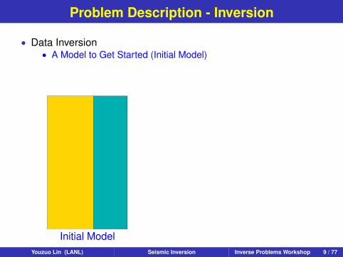
Selection of the Regularization Parameter: λ2
• The subproblem of u(k) is a classical L2-TV minimization.
• Surprisingly, not many effective methods in existing references.
• We employ the unbiased predictive risk estimator (UPRE):
Selection of λ2, (Lin et. al., SP (90) 2010):
λ2 = argminλ2
{1n‖rλ2‖
22 +
2σ2
ntrace(ATV,λ2)− σ
2}.
Youzuo Lin (LANL) Seismic Inversion Inverse Problems Workshop 22 / 77

Solving for m(k): Nonlinear Conjugate Gradients
• CG direction at each iteration is used as search direction of dk .* The search direction dk needs to be a descent direction
cos θ =∇ET
k dk
||∇Ek || ||dk ||< 0.
• Line search for βk , the Armijo condition is used{E(m(k) + β(k)d(k)) ≤ E(m(k)) + c1β
(k)(d(k))T∇E(m(k))
(d(k))T∇E(m(k) + β(k)d(k)) ≥ c2(d(k))T∇E(m(k)).
• Updating scheme
m(k+1) = m(k) + β(k)d(k).
Youzuo Lin (LANL) Seismic Inversion Inverse Problems Workshop 23 / 77

Gradients
• The gradient of the data misfit can be obtained by the adjoint-statemethod
∇m ‖d− f (m)‖22 =−2m3
∑shots
∑t
∂2−→f (k)
∂t2 ·←−r(k),
where−→f (k) is the forward propagated wavefield, and
←−r(k) is the
backward propagated residual at iteration k , which is furtherdefined as r(k) = d− f (m(k)).
• The gradient of L2-norm term can be simply derived as,
∇m
∥∥∥m− u(k−1)∥∥∥2
2= 2(m− u(i−1)).
Youzuo Lin (LANL) Seismic Inversion Inverse Problems Workshop 24 / 77

Solving for u(k)
• The subproblem of solving u(k) is a L2 − TV denoising problem.
• Any TV-solver can be used: Iteratively Reweighted NormAlgorithm, Lagged Diffusivity Fixed Point Iteration Algorithm,Split-Bregman Method, etc.
Youzuo Lin (LANL) Seismic Inversion Inverse Problems Workshop 25 / 77

Solving for u(k): Split-Bregman Method
• Reformulate the minimization of u(k) as an equivalent problembased on the Bregman distance:
E(u,dx ,dz) = minu,dx ,dz
∥∥∥u−m(k)∥∥∥2
2+ λ2 ‖u‖TV
+ µ∥∥∥dx −∇xu− b(k)
x
∥∥∥2
2+ µ
∥∥∥dz −∇zu− b(k)z
∥∥∥2
2.
• An alternating minimization algorithm can be employed, wheretwo subproblems need to be further minimized:
minu
∥∥∥u−m(k)∥∥∥2
2+µ∥∥∥d(k)
x −∇xu− b(k)x
∥∥∥2
2+µ∥∥∥d(k)
z −∇zu− b(k)z
∥∥∥2
2,
and
mindx ,dz
λ2 ‖u‖TV + µ∥∥∥dx −∇xu− b(k)
x
∥∥∥2
2+ µ
∥∥∥dz −∇zu− b(k)z
∥∥∥2
2.
Youzuo Lin (LANL) Seismic Inversion Inverse Problems Workshop 26 / 77

Computational Cost Analysis
• Suppose that the size of the model is m ∈ <m×n and the datap ∈ <q×n, where m is the depth, n is the offset, and q is the timesteps. We assume there are s shots and the finite-differencecalculation employs a scheme of o(δt2, δh4).
• The cost of solving for m(k):
COST1 ≈ k1 · (l + 3) · O(s · m · n · q) + (l + 5) · O(m · n),
where l is the number of trials in the line search for β(k) and k1 isthe total iteration steps.
• The cost of solving for u(k):
COST2 ≈ 18 · O(m · n).
• Therefore, the cost of solving for u(k) is trivial compared to thecost of solving for m(k).
Youzuo Lin (LANL) Seismic Inversion Inverse Problems Workshop 27 / 77

Outline
1 Subsurface Applications
2 Schematic Description of Seismic imaging
3 Travel-Time Tomography and Full-Waveform InversionTravel-Time TomographyFull-Waveform InversionRegularization TechniquesA Modified Total-Variation Regularization Scheme
4 Computation Methods
5 Application to Global Seismology
6 Application to Enhanced Geothermal SystemsReservoir Monitoring with Time-Lapse DataBrady’s EGS SiteRobustness Tests
7 Conclusions
Youzuo Lin (LANL) Seismic Inversion Inverse Problems Workshop 28 / 77

Results - True Model
19.2˚
19.4˚
1 km
19.2˚
19.4˚
3 km
-155.4˚ -155.2˚ -155˚ -154.8˚
19.2˚
19.4˚
5 km
7 km
9 km
-155.4˚ -155.2˚ -155˚ -154.8˚
11 km
4 5 6 7
Vp, km/sYouzuo Lin (LANL) Seismic Inversion Inverse Problems Workshop 28 / 77

Results - Tikhonov Inversion
19.2˚
19.4˚
1 km
19.2˚
19.4˚
3 km
-155.4˚ -155.2˚ -155˚ -154.8˚
19.2˚
19.4˚
5 km
7 km
9 km
-155.4˚ -155.2˚ -155˚ -154.8˚
11 km
4 5 6 7
Vp, km/sYouzuo Lin (LANL) Seismic Inversion Inverse Problems Workshop 29 / 77

Results - Total Variation Inversion
19.2˚
19.4˚
1 km
19.2˚
19.4˚
3 km
-155.4˚ -155.2˚ -155˚ -154.8˚
19.2˚
19.4˚
5 km
7 km
9 km
-155.4˚ -155.2˚ -155˚ -154.8˚
11 km
4 5 6 7
Vp, km/sYouzuo Lin (LANL) Seismic Inversion Inverse Problems Workshop 30 / 77
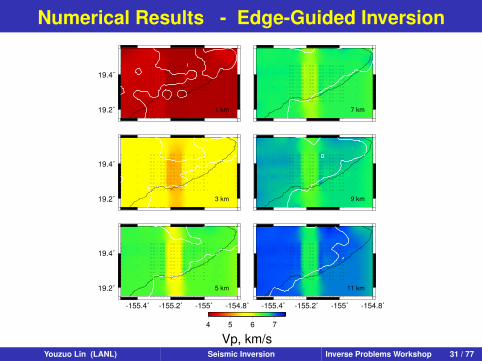
Numerical Results - Edge-Guided Inversion
19.2˚
19.4˚
1 km
19.2˚
19.4˚
3 km
-155.4˚ -155.2˚ -155˚ -154.8˚
19.2˚
19.4˚
5 km
7 km
9 km
-155.4˚ -155.2˚ -155˚ -154.8˚
11 km
4 5 6 7
Vp, km/sYouzuo Lin (LANL) Seismic Inversion Inverse Problems Workshop 31 / 77

Results - Tikhonov Inversion Difference
19.2˚
19.4˚
1 km
19.2˚
19.4˚
3 km
-155.4˚ -155.2˚ -155˚ -154.8˚
19.2˚
19.4˚
5 km
7 km
9 km
-155.4˚ -155.2˚ -155˚ -154.8˚
11 km
-0.2 -0.1 0.0 0.1 0.2
Vp, km/sYouzuo Lin (LANL) Seismic Inversion Inverse Problems Workshop 32 / 77

Results - Total Variation Inversion Difference
19.2˚
19.4˚
1 km
19.2˚
19.4˚
3 km
-155.4˚ -155.2˚ -155˚ -154.8˚
19.2˚
19.4˚
5 km
7 km
9 km
-155.4˚ -155.2˚ -155˚ -154.8˚
11 km
-0.2 -0.1 0.0 0.1 0.2
Vp, km/sYouzuo Lin (LANL) Seismic Inversion Inverse Problems Workshop 33 / 77

Results - Edge-Guided Inversion Difference
19.2˚
19.4˚
1 km
19.2˚
19.4˚
3 km
-155.4˚ -155.2˚ -155˚ -154.8˚
19.2˚
19.4˚
5 km
7 km
9 km
-155.4˚ -155.2˚ -155˚ -154.8˚
11 km
-0.2 -0.1 0.0 0.1 0.2
Vp, km/sYouzuo Lin (LANL) Seismic Inversion Inverse Problems Workshop 34 / 77

Results - Robustness Tests on the Sparse Data
• Randomly eliminate 50% of the earthquake events and stations(Left: Tikhonov, Middle: TV, Right: Edge-Guided TV)
19.2
˚
19.4
˚
1 k
m
19.2
˚
19.4
˚
3 k
m
19.2
˚
19.4
˚
5 k
m
19.2
˚
19.4
˚
7 k
m
19.2
˚
19.4
˚
9 k
m
-155.4
˚-1
55.2
˚-1
55˚
-154.8
˚
19.2
˚
19.4
˚
11 k
m
1 k
m
3 k
m
5 k
m
7 k
m
9 k
m
-155.4
˚-1
55.2
˚-1
55˚
-154.8
˚
11 k
m
19.2
˚
19.4
˚
1 k
m
19.2
˚
19.4
˚
3 k
m
19.2
˚
19.4
˚
5 k
m
19.2
˚
19.4
˚
7 k
m
19.2
˚
19.4
˚
9 k
m
-155.4
˚-1
55.2
˚-1
55˚
-154.8
˚19.2
˚
19.4
˚
11
km
45
67
Vp, km
/s
Youzuo Lin (LANL) Seismic Inversion Inverse Problems Workshop 35 / 77

Results - Robustness Tests on the Sparse Data
• Randomly eliminate 50% of the earthquake events and stations(Left: Tikhonov, Middle: TV, Right: Edge-Guided TV)
19.2
˚
19.4
˚
1 k
m
19.2
˚
19.4
˚
3 k
m
19.2
˚
19.4
˚
5 k
m
19.2
˚
19.4
˚
7 k
m
19.2
˚
19.4
˚
9 k
m
-155.4
˚-1
55.2
˚-1
55˚
-154.8
˚
19.2
˚
19.4
˚
11 k
m
1 k
m
3 k
m
5 k
m
7 k
m
9 k
m
-155.4
˚-1
55.2
˚-1
55˚
-154.8
˚
11 k
m
19.2
˚
19.4
˚
1 k
m
19.2
˚
19.4
˚
3 k
m
19.2
˚
19.4
˚
5 k
m
19.2
˚
19.4
˚
7 k
m
19.2
˚
19.4
˚
9 k
m
-155.4
˚-1
55.2
˚-1
55˚
-154.8
˚19.2
˚
19.4
˚
11
km
-0.2
-0.1
0.0
0.1
0.2
dV
p, km
/s
Youzuo Lin (LANL) Seismic Inversion Inverse Problems Workshop 36 / 77

Outline
1 Subsurface Applications
2 Schematic Description of Seismic imaging
3 Travel-Time Tomography and Full-Waveform InversionTravel-Time TomographyFull-Waveform InversionRegularization TechniquesA Modified Total-Variation Regularization Scheme
4 Computation Methods
5 Application to Global Seismology
6 Application to Enhanced Geothermal SystemsReservoir Monitoring with Time-Lapse DataBrady’s EGS SiteRobustness Tests
7 Conclusions
Youzuo Lin (LANL) Seismic Inversion Inverse Problems Workshop 37 / 77
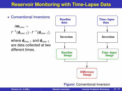
Reservoir Monitoring with Time-Lapse Data
• Conventional Inversions
δmconv =
f−1(dtime 2)−f−1(dtime 1),
where dtime 1 and dtime 2are data collected at twodifferent times.
Image
data
Inversion
Baseline
Image
Inversion
Image
dataTime−lapse
Time−lapse
Difference
Baseline
Figure: Conventional InversionYouzuo Lin (LANL) Seismic Inversion Inverse Problems Workshop 37 / 77

Reservoir Monitoring with Time-Lapse Data
• Double-Difference FWIThe method jointlyinverts time-lapse datafor reservoir changes.
δmDDFWI =
f−1(dsim time 2)−f−1(dsim time 1),
wheredsim time 1 = f (mbaseline)anddsim time 2 = dsim time 1 +(dtime 2 − dtime 1)
Modeling
Inversion
Baseline
Image
Inversion
DifferenceImage
Baseline Time−lapse
Data Data
Simulated
Time−lapse Data
ImageTime−lapse
SimulatedBaseline Data
Difference
Initial Model
Figure: Double-Difference FWI
Youzuo Lin (LANL) Seismic Inversion Inverse Problems Workshop 38 / 77
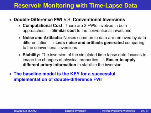
Reservoir Monitoring with Time-Lapse Data
• Double-Difference FWI V.S. Conventional Inversions• Computational Cost: There are 2 FWIs involved in both
approaches. → Similar cost to the conventional inversions
• Noise and Artifacts: Noises common to data are removed by datadifferentiation. → Less noise and artifacts generated comparingto the conventional inversions
• Stability: The inversion of the simulated time-lapse data focuses toimage the changes of physical properties. → Easier to applydifferent priory information to stabilize the inversion
• The baseline model is the KEY for a successfulimplementation of double-difference FWI
Youzuo Lin (LANL) Seismic Inversion Inverse Problems Workshop 39 / 77

Double-Difference FWI with MTV Regularization
Double-Difference FWI with MTV Regularization (Lin & Huang,GJI(203) 2015):
mbaseline = m1 = argminm1
{‖dtime1 − f (m1)‖22 + ‖m1‖MTV
},
mtime-lapse = m2 = argminm2
{‖dsim time2 − f (m2)‖22 + ‖δm‖MTV
},
where δm = m2 −m1 and ‖m‖MTV = λ1 ‖m− u‖22 + λ2‖u‖TV.
• Our FWI with the MTV regularization improves inversion of thebaseline dataset to obtain an accurate baseline model.
• we focus our inversion on the regions where time-lapse changesoccur using the regularization term ‖δm‖MTV to constrain thetime-lapse model differences.
Youzuo Lin (LANL) Seismic Inversion Inverse Problems Workshop 40 / 77

Reservoir Monitoring for EGS
0
0.5
1.0
1.5
De
pth
(km
)
0 0.5 1.0 1.5 2.0Horizontal Distance (km)
2000
2500
3000
3500
4000
4500
5000
Ve
locity
(m/s
)
Baseline Vp Model
0
0.5
1.0
1.5
De
pth
(km
)
0 0.5 1.0 1.5 2.0Horizontal Distance (km)
2000
2500
3000
3500
4000
4500
5000
Ve
locity
(m/s
)
Baseline Vs Model
• Models are built based on the Brady’s enhanced geothermalsystem (EGS) field (Lin & Huang, SGW 2012)
Youzuo Lin (LANL) Seismic Inversion Inverse Problems Workshop 41 / 77

Reservoir Monitoring for EGS
0
0.5
1.0
1.5
De
pth
(km
)
0 0.5 1.0 1.5 2.0Horizontal Distance (km)
2000
2500
3000
3500
4000
4500
5000
Ve
locity
(m/s
)
Vp Model After Stimulation
0
0.5
1.0
1.5
De
pth
(km
)
0 0.5 1.0 1.5 2.0Horizontal Distance (km)
2000
2500
3000
3500
4000
4500
5000
Ve
locity
(m/s
)
Vs Model After Stimulation
• Models are built based on the Brady’s enhanced geothermalsystem (EGS) field
• Stimulation leads to decreases in Vp and Vs
Youzuo Lin (LANL) Seismic Inversion Inverse Problems Workshop 42 / 77

Reservoir Monitoring for EGS
0
0.5
1.0
1.5
De
pth
(km
)
0 0.5 1.0 1.5 2.0Horizontal Distance (km)
-250
-200
-150
-100
-50
0
50
100
150
200
250
Ve
locity
Pe
rturb
atio
n (m
/s)
Time-lapse Difference of Vp
0
0.5
1.0
1.5
De
pth
(km
)
0 0.5 1.0 1.5 2.0Horizontal Distance (km)
-250
-200
-150
-100
-50
0
50
100
150
200
250
Ve
locity
Pe
rturb
atio
n (m
/s)
Time-lapse Difference of Vs
• Monitoring regions with time-lapse difference of Vp abd Vs
Youzuo Lin (LANL) Seismic Inversion Inverse Problems Workshop 43 / 77

Reservoir Monitoring for EGS
0
0.5
1.0
1.5
De
pth
(km
)
0 0.5 1.0 1.5 2.0Horizontal Distance (km)
2000
2500
3000
3500
4000
4500
5000
Ve
locity
(m/s
)
Vp Initial Model
0
0.5
1.0
1.5
De
pth
(km
)
0 0.5 1.0 1.5 2.0Horizontal Distance (km)
2000
2500
3000
3500
4000
4500
5000
Ve
locity
(m/s
)
Vs Initial Model
• The initial Vp and Vs models for inversion.• 96 sources and 500 receivers on the top surfaces of the models.• Ricker’s wavelet with a center frequency of 25 Hz is used as the
source function.
Youzuo Lin (LANL) Seismic Inversion Inverse Problems Workshop 44 / 77

Reservoir Monitoring for EGS
0
0.5
1.0
1.5
De
pth
(km
)
0 0.5 1.0 1.5 2.0Horizontal Distance (km)
2000
2500
3000
3500
4000
4500
5000
Ve
locity
(m/s
)
Vp Model
0
0.5
1.0
1.5
De
pth
(km
)
0 0.5 1.0 1.5 2.0Horizontal Distance (km)
2000
2500
3000
3500
4000
4500
5000
Ve
locity
(m/s
)
Vs Model
FWI without Regularization• Interfaces of the reconstruction are degraded.
Youzuo Lin (LANL) Seismic Inversion Inverse Problems Workshop 45 / 77

Reservoir Monitoring for EGS
0
0.5
1.0
1.5
De
pth
(km
)
0 0.5 1.0 1.5 2.0Horizontal Distance (km)
2000
2500
3000
3500
4000
4500
5000
Ve
locity
(m/s
)
Vp Model
0
0.5
1.0
1.5
De
pth
(km
)
0 0.5 1.0 1.5 2.0Horizontal Distance (km)
2000
2500
3000
3500
4000
4500
5000
Ve
locity
(m/s
)
Vs Model
FWI with TV Regularization• Lots of noise and artifacts are generated.
Youzuo Lin (LANL) Seismic Inversion Inverse Problems Workshop 46 / 77

Reservoir Monitoring for EGS
0
0.5
1.0
1.5
De
pth
(km
)
0 0.5 1.0 1.5 2.0Horizontal Distance (km)
2000
2500
3000
3500
4000
4500
5000
Ve
locity
(m/s
)
Vp Model
0
0.5
1.0
1.5
De
pth
(km
)
0 0.5 1.0 1.5 2.0Horizontal Distance (km)
2000
2500
3000
3500
4000
4500
5000
Ve
locity
(m/s
)
Vs Model
FWI with MTV Regularization• Interfaces of the reconstruction are well preserved.• Noise and artifacts are eliminated.
Youzuo Lin (LANL) Seismic Inversion Inverse Problems Workshop 47 / 77

Reservoir Monitoring for EGS
0
0.5
1.0
1.5
De
pth
(km
)
2000 3000 4000 5000Velocity (m/s)
Vp Model
0
0.5
1.0
1.5
De
pth
(km
)
2000 3000 4000 5000Velocity (m/s)
Vs Model
FWI without Regularization• Reconstructed values are still off the true values.
Youzuo Lin (LANL) Seismic Inversion Inverse Problems Workshop 48 / 77

Reservoir Monitoring for EGS
0
0.5
1.0
1.5
De
pth
(km
)
2000 3000 4000 5000Velocity (m/s)
Vp Model
0
0.5
1.0
1.5
De
pth
(km
)
2000 3000 4000 5000Velocity (m/s)
Vs Model
FWI with TV Regularization• Reconstructed values are highly oscillated.
Youzuo Lin (LANL) Seismic Inversion Inverse Problems Workshop 49 / 77

Reservoir Monitoring for EGS
0
0.5
1.0
1.5
De
pth
(km
)
2000 3000 4000 5000Velocity (m/s)
Vp Model
0
0.5
1.0
1.5
De
pth
(km
)
2000 3000 4000 5000Velocity (m/s)
Vs Model
FWI with MTV Regularization• Reconstructed values are very close to the true values.
Youzuo Lin (LANL) Seismic Inversion Inverse Problems Workshop 50 / 77

Reservoir Monitoring for EGS
0
0.5
1.0
1.5
De
pth
(km
)
0 0.5 1.0 1.5 2.0Horizontal Distance (km)
-250
-200
-150
-100
-50
0
50
100
150
200
250
Ve
locity
Pe
rturb
atio
n (m
/s)
Vp Model
0
0.5
1.0
1.5
De
pth
(km
)
0 0.5 1.0 1.5 2.0Horizontal Distance (km)
-250
-200
-150
-100
-50
0
50
100
150
200
250
Ve
locity
Pe
rturb
atio
n (m
/s)
Vs Model
Conventional Inversions
• Hard to identify the location of the reservoir.• Artifacts are significant.
Youzuo Lin (LANL) Seismic Inversion Inverse Problems Workshop 51 / 77

Reservoir Monitoring for EGS
0
0.5
1.0
1.5
De
pth
(km
)
0 0.5 1.0 1.5 2.0Horizontal Distance (km)
-250
-200
-150
-100
-50
0
50
100
150
200
250
Ve
locity
Pe
rturb
atio
n (m
/s)
Vp Model
0
0.5
1.0
1.5
De
pth
(km
)
0 0.5 1.0 1.5 2.0Horizontal Distance (km)
-250
-200
-150
-100
-50
0
50
100
150
200
250
Ve
locity
Pe
rturb
atio
n (m
/s)
Vs Model
Double-Difference FWI without Regularization
• Results are significantly improved.• The results still contain some artifacts.
Youzuo Lin (LANL) Seismic Inversion Inverse Problems Workshop 52 / 77

Reservoir Monitoring for EGS
0
0.5
1.0
1.5
De
pth
(km
)
0 0.5 1.0 1.5 2.0Horizontal Distance (km)
-250
-200
-150
-100
-50
0
50
100
150
200
250
Ve
locity
Pe
rturb
atio
n (m
/s)
Vp Model
0
0.5
1.0
1.5
De
pth
(km
)
0 0.5 1.0 1.5 2.0Horizontal Distance (km)
-250
-200
-150
-100
-50
0
50
100
150
200
250
Ve
locity
Pe
rturb
atio
n (m
/s)
Vs Model
Double-Difference FWI with MTV Regularization
• The monitoring regions are very easy to visualize.• Background noise and artifacts are significantly reduced.
Youzuo Lin (LANL) Seismic Inversion Inverse Problems Workshop 53 / 77

Reservoir Monitoring for EGS
0
0.5
1.0
1.5
De
pth
(km
)
-300 -200 -100 0 100Velocity Perturbation (m/s)
Vp Model
0
0.5
1.0
1.5
De
pth
(km
)
-300 -200 -100 0 100Velocity Perturbation (m/s)
Vs Model
Conventional Inversions
• The magnitudes of the inversion artifacts are almost the samelevel to those of the inversion results.
Youzuo Lin (LANL) Seismic Inversion Inverse Problems Workshop 54 / 77
Reservoir Monitoring for EGS
0
0.5
1.0
1.5
De
pth
(km
)
-300 -200 -100 0 100Velocity Perturbation (m/s)
Vp Model
0
0.5
1.0
1.5
De
pth
(km
)
-300 -200 -100 0 100Velocity Perturbation (m/s)
Vs Model
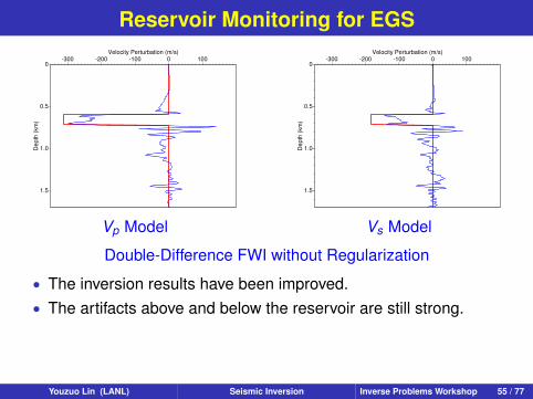
Double-Difference FWI without Regularization
• The inversion results have been improved.• The artifacts above and below the reservoir are still strong.
Youzuo Lin (LANL) Seismic Inversion Inverse Problems Workshop 55 / 77

Reservoir Monitoring for EGS
0
0.5
1.0
1.5
De
pth
(km
)
-300 -200 -100 0 100 200Velocity Perturbation (m/s)
Vp Model
0
0.5
1.0
1.5
De
pth
(km
)
-300 -200 -100 0 100 200Velocity Perturbation (m/s)
Vs Model
Double-Difference FWI with MTV Regularization
• Reconstructed values are very close to its true values.• The profiles are much less oscillated than all the other results.
Youzuo Lin (LANL) Seismic Inversion Inverse Problems Workshop 56 / 77

Reservoir Monitoring for EGS
1 2 3 4 5 6 7 8 9 10 11 120
0.1
0.2
0.3
0.4
0.5
0.6
0.7
0.8
0.9
1
Iterations
Da
ta M
isfi
t
Conventional DD AEWI
DD AEWI with Prior
DD AEWI with MTV
Data Misfit
1 2 3 4 5 6 7 8 9 10 11 120
0.1
0.2
0.3
0.4
0.5
0.6
0.7
0.8
0.9
1
Iterations
Mo
de
l M
isfi
t
Conventional DD AEWI
DD AEWI with Prior
DD AEWI with MTV
Model MisfitConvergence Plots
• Reference methods: conventional DD-FWI (in blue), the methoddeveloped in Zhang & Huang (2014) (in green)
• Our method converges fastest for both data misfit and model misfit
Youzuo Lin (LANL) Seismic Inversion Inverse Problems Workshop 57 / 77

Robustness Tests
• FWI can be very easily trapped in the local minima.• Using noisy measurements;
• Using inaccurate initial guess far away from the true model;
• Total-variation regularization can create those “stair-casing”artifacts• Smooth changes at the monitoring regions
Youzuo Lin (LANL) Seismic Inversion Inverse Problems Workshop 58 / 77

Robustness Test - Noisy MeasurementReceiver number
Tim
e (
s)
50 100 150 200 250 300 350 400 450 500
0.25
0.5
0.75
1
1.25
1.5
Common-Shot Gather
0.25 0.5 0.75 1 1.25 1.5 0.25−2
−1.5
−1
−0.5
0
0.5
1
1.5
2x 10
−5
Time (s)
Am
plit
ud
e
Clean
Noisy
Seismogram at Recv. Num. 250
Noisy Measurement (Baseline)
• Baseline measurement• 20 dB of white noise is added
Youzuo Lin (LANL) Seismic Inversion Inverse Problems Workshop 59 / 77

Robustness Test - Noisy MeasurementReceiver number
Tim
e (
s)
50 100 150 200 250 300 350 400 450 500
0.25
0.5
0.75
1
1.25
1.5
Common-Shot Gather
0.25 0.5 0.75 1 1.25 1.5 0.25−2
−1.5
−1
−0.5
0
0.5
1
1.5
2x 10
−5
Time (s)
Am
plit
ud
e
Clean
Noisy
Seismogram at Recv. Num. 250
Noisy Measurement (Repeat-survey)
• Repeat-survey measurement• 20 dB of different white noise is added
Youzuo Lin (LANL) Seismic Inversion Inverse Problems Workshop 60 / 77

Robustness Test - Noisy Measurement
0
0.5
1.0
1.5
De
pth
(km
)
0 0.5 1.0 1.5 2.0Horizontal Distance (km)
2000
2500
3000
3500
4000
4500
5000
Ve
locity
(m/s
)
Vp Model
0
0.5
1.0
1.5
De
pth
(km
)
0 0.5 1.0 1.5 2.0Horizontal Distance (km)
2000
2500
3000
3500
4000
4500
5000
Ve
locity
(m/s
)
Vs Model
Noisy Measurement
• Some additional artifacts in the deep layers of the velocityinversion results.
Youzuo Lin (LANL) Seismic Inversion Inverse Problems Workshop 61 / 77

Robustness Test - Noisy Measurement
0
0.5
1.0
1.5
De
pth
(km
)
0 0.5 1.0 1.5 2.0Horizontal Distance (km)
-250
-200
-150
-100
-50
0
50
100
150
200
250
Ve
locity
Pe
rturb
atio
n (m
/s)
Vp Model
0
0.5
1.0
1.5
De
pth
(km
)
0 0.5 1.0 1.5 2.0Horizontal Distance (km)
-250
-200
-150
-100
-50
0
50
100
150
200
250
Ve
locity
Pe
rturb
atio
n (m
/s)
Vs Model
Noisy Measurement
• Those artifacts do not effect the accuracy of the invertedtime-lapse changes in the monitoring region
Youzuo Lin (LANL) Seismic Inversion Inverse Problems Workshop 62 / 77
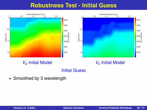
Robustness Test - Initial Guess
0
0.5
1.0
1.5
De
pth
(km
)
0 0.5 1.0 1.5 2.0Horizontal Distance (km)
2000
2500
3000
3500
4000
4500
5000
Ve
locity
(m/s
)
Vp Initial Model
0
0.5
1.0
1.5
De
pth
(km
)
0 0.5 1.0 1.5 2.0Horizontal Distance (km)
2000
2500
3000
3500
4000
4500
5000
Ve
locity
(m/s
)
Vs Initial Model
Initial Guess
• Smoothed by 3 wavelength
Youzuo Lin (LANL) Seismic Inversion Inverse Problems Workshop 63 / 77

Robustness Test - Initial Guess
0
0.5
1.0
1.5
De
pth
(km
)
0 0.5 1.0 1.5 2.0Horizontal Distance (km)
2000
2500
3000
3500
4000
4500
5000
Ve
locity
(m/s
)
Vp Initial Model
0
0.5
1.0
1.5
De
pth
(km
)
0 0.5 1.0 1.5 2.0Horizontal Distance (km)
2000
2500
3000
3500
4000
4500
5000
Ve
locity
(m/s
)
Vs Initial Model
Initial Guess
• Smoothed by 4 wavelength
Youzuo Lin (LANL) Seismic Inversion Inverse Problems Workshop 64 / 77

Robustness Test - Initial Guess
0
0.5
1.0
1.5
De
pth
(km
)
0 0.5 1.0 1.5 2.0Horizontal Distance (km)
2000
2500
3000
3500
4000
4500
5000
Ve
locity
(m/s
)
Vp Initial Model
0
0.5
1.0
1.5
De
pth
(km
)
0 0.5 1.0 1.5 2.0Horizontal Distance (km)
2000
2500
3000
3500
4000
4500
5000
Ve
locity
(m/s
)
Vs Initial Model
Initial Guess
• Smoothed by 5 wavelength
Youzuo Lin (LANL) Seismic Inversion Inverse Problems Workshop 65 / 77
Robustness Test - Initial Guess
0
0.5
1.0
1.5
De
pth
(km
)
0 0.5 1.0 1.5 2.0Horizontal Distance (km)
2000
2500
3000
3500
4000
4500
5000
Ve
locity
(m/s
)
Vp Model
0
0.5
1.0
1.5
De
pth
(km
)
0 0.5 1.0 1.5 2.0Horizontal Distance (km)
2000
2500
3000
3500
4000
4500
5000
Ve
locity
(m/s
)
Vs Model
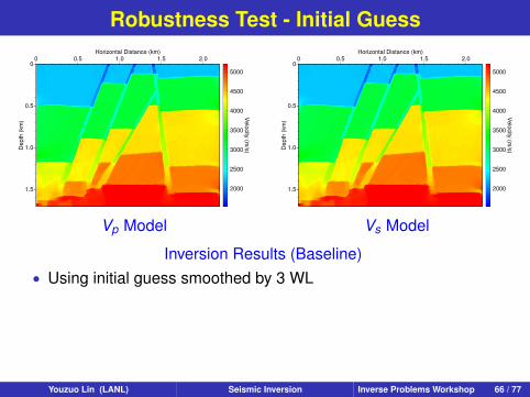
Inversion Results (Baseline)• Using initial guess smoothed by 3 WL
Youzuo Lin (LANL) Seismic Inversion Inverse Problems Workshop 66 / 77

Robustness Test - Initial Guess
0
0.5
1.0
1.5
De
pth
(km
)
0 0.5 1.0 1.5 2.0Horizontal Distance (km)
2000
2500
3000
3500
4000
4500
5000
Ve
locity
(m/s
)
Vp Model
0
0.5
1.0
1.5
De
pth
(km
)
0 0.5 1.0 1.5 2.0Horizontal Distance (km)
2000
2500
3000
3500
4000
4500
5000
Ve
locity
(m/s
)
Vs Model
Inversion Results (Baseline)• Using initial guess smoothed by 4 WL
Youzuo Lin (LANL) Seismic Inversion Inverse Problems Workshop 67 / 77

Robustness Test - Initial Guess
0
0.5
1.0
1.5
De
pth
(km
)
0 0.5 1.0 1.5 2.0Horizontal Distance (km)
2000
2500
3000
3500
4000
4500
5000
Ve
locity
(m/s
)
Vp Model
0
0.5
1.0
1.5
De
pth
(km
)
0 0.5 1.0 1.5 2.0Horizontal Distance (km)
2000
2500
3000
3500
4000
4500
5000
Ve
locity
(m/s
)
Vs Model
Inversion Results (Baseline)• Using initial guess smoothed by 5 WL
Youzuo Lin (LANL) Seismic Inversion Inverse Problems Workshop 68 / 77

Robustness Test - Initial Guess
0
0.5
1.0
1.5
De
pth
(km
)
0 0.5 1.0 1.5 2.0Horizontal Distance (km)
-250
-200
-150
-100
-50
0
50
100
150
200
250
Ve
locity
Pe
rturb
atio
n (m
/s)
Vp Model
0
0.5
1.0
1.5
De
pth
(km
)
0 0.5 1.0 1.5 2.0Horizontal Distance (km)
-250
-200
-150
-100
-50
0
50
100
150
200
250
Ve
locity
Pe
rturb
atio
n (m
/s)
Vs Model
Inversion Results (Time-Lapse)• Using initial guess smoothed by 3 WL
Youzuo Lin (LANL) Seismic Inversion Inverse Problems Workshop 69 / 77

Robustness Test - Initial Guess
0
0.5
1.0
1.5
De
pth
(km
)
0 0.5 1.0 1.5 2.0Horizontal Distance (km)
-250
-200
-150
-100
-50
0
50
100
150
200
250
Ve
locity
Pe
rturb
atio
n (m
/s)
Vp Model
0
0.5
1.0
1.5
De
pth
(km
)
0 0.5 1.0 1.5 2.0Horizontal Distance (km)
-250
-200
-150
-100
-50
0
50
100
150
200
250
Ve
locity
Pe
rturb
atio
n (m
/s)
Vs Model
Inversion Results (Time-Lapse)• Using initial guess smoothed by 4 WL
Youzuo Lin (LANL) Seismic Inversion Inverse Problems Workshop 70 / 77

Robustness Test - Initial Guess
0
0.5
1.0
1.5
De
pth
(km
)
0 0.5 1.0 1.5 2.0Horizontal Distance (km)
-250
-200
-150
-100
-50
0
50
100
150
200
250
Ve
locity
Pe
rturb
atio
n (m
/s)
Vp Model
0
0.5
1.0
1.5
De
pth
(km
)
0 0.5 1.0 1.5 2.0Horizontal Distance (km)
-250
-200
-150
-100
-50
0
50
100
150
200
250
Ve
locity
Pe
rturb
atio
n (m
/s)
Vs Model
Inversion Results (Time-Lapse)• Using initial guess smoothed by 5 WL
Youzuo Lin (LANL) Seismic Inversion Inverse Problems Workshop 71 / 77

Robustness Test - Smoothly Distributed Changes
0
0.5
1.0
1.5
De
pth
(km
)
0 0.5 1.0 1.5 2.0Horizontal Distance (km)
-250
-200
-150
-100
-50
0
50
100
150
200
250
Ve
locity
Pe
rturb
atio
n (m
/s)
Vp Model
0
0.5
1.0
1.5
De
pth
(km
)
0 0.5 1.0 1.5 2.0Horizontal Distance (km)
-250
-200
-150
-100
-50
0
50
100
150
200
250
Ve
locity
Pe
rturb
atio
n (m
/s)
Vs Model
Smoothly Distributed Changes
• For some practical applications, a spatial region with time-lapsechanges can be smoothly distributed other than piece-wiseconstant.
Youzuo Lin (LANL) Seismic Inversion Inverse Problems Workshop 72 / 77

Robustness Test - Smoothly Distributed Changes
0
0.5
1.0
1.5
De
pth
(km
)
0 0.5 1.0 1.5 2.0Horizontal Distance (km)
-250
-200
-150
-100
-50
0
50
100
150
200
250
Ve
locity
Pe
rturb
atio
n (m
/s)
Vp Model
0
0.5
1.0
1.5
De
pth
(km
)
0 0.5 1.0 1.5 2.0Horizontal Distance (km)
-250
-200
-150
-100
-50
0
50
100
150
200
250
Ve
locity
Pe
rturb
atio
n (m
/s)
Vs Model
Smoothly Distributed Changes
• Our inversion results preserve sharp edges and the smoothlydistributed changes.
Youzuo Lin (LANL) Seismic Inversion Inverse Problems Workshop 73 / 77

Robustness Test - Smoothly Distributed Changes
0
0.5
1.0
1.5
De
pth
(km
)
-300 -200 -100 0 100Velocity Perturbation (m/s)
Vp Model
0
0.5
1.0
1.5
De
pth
(km
)
-300 -200 -100 0 100Velocity Perturbation (m/s)
Vs Model
Smoothly Distributed Changes
• Our inversion results preserve sharp edges and the smoothlydistributed changes.
Youzuo Lin (LANL) Seismic Inversion Inverse Problems Workshop 74 / 77
Outline
1 Subsurface Applications
2 Schematic Description of Seismic imaging
3 Travel-Time Tomography and Full-Waveform InversionTravel-Time TomographyFull-Waveform InversionRegularization TechniquesA Modified Total-Variation Regularization Scheme
4 Computation Methods
5 Application to Global Seismology
6 Application to Enhanced Geothermal SystemsReservoir Monitoring with Time-Lapse DataBrady’s EGS SiteRobustness Tests
7 Conclusions
Youzuo Lin (LANL) Seismic Inversion Inverse Problems Workshop 75 / 77

Conclusions
• We have developed new travel-time tomography and full-waveforminversion method using a modified total-variation regularizationscheme.
• Our new seismic inversion methods not only preserve sharpinterfaces in inversion results, but also greatly reduce inversionartifacts.
• Our new methods employs the modified total-variationregularization to improve the inversion accuracy and enhance therobustness of our methods for noisy data to some extent.
Youzuo Lin (LANL) Seismic Inversion Inverse Problems Workshop 75 / 77

Related References
• “Lin et. al., GJI (201) 2015”: Youzuo Lin, Ellen M. Syracuse,Monica Maceira, Haijiang Zhang and Carene Larmat,“Double-difference traveltime tomography withedge-preserving regularization and a priori interfaces,”Geophysical Journal International, 201 (2): 574-594, 2015.
• “Lin & Huang,GJI (203) 2015”: Youzuo Lin and Lianjie Huang,“Quantifying Subsurface Geophysical Properties Changes UsingDouble-difference Seismic-Waveform Inversion with a ModifiedTotal-Variation Regularization Scheme,” Geophysical JournalInternational, 203 (3): 2125-2149, 2015.
• “Lin & Huang, GJI (200) 2015”: Youzuo Lin and Lianjie Huang,“Acoustic- and Elastic-Waveform Inversion Using a ModifiedTotal-Variation Regularization Scheme,” Geophysical JournalInternational, 200 (1): 489-502, 2015.
Youzuo Lin (LANL) Seismic Inversion Inverse Problems Workshop 76 / 77

Acknowledgement
• The research was supported by (1). the Geothermal TechnologiesProgram of the U.S. Department of Energy, and (2). LANL,Laboratory Directed Research and Development (LDRD) program.
• We thank Dr. John Queen of Hi-Q Geophysical Inc. for providingus with a velocity model of Brady’s EGS field.
Youzuo Lin (LANL) Seismic Inversion Inverse Problems Workshop 77 / 77
![Journal of Computational Physics - Purdue University · 2014. 10. 19. · In seismic inversion, full-waveform inversion (FWI) [28,41] is a promising technique to reconstruct subsurface](https://img.pdfslide.us/doc/110x75/60fe753ccd07a242cb1c7664/journal-of-computational-physics-purdue-university-2014-10-19-in-seismic.jpg)