Bresenham Noise

Masaki Kameya and John C. Hart

School of Electrical Engineering and Computer ScienceWashington State University

{mkameya,hart}@eecs.wsu.edu

ABSTRACTProcedural texture mapping is a powerful technique, and useof the Perlin noise function makes procedural textures ap-pear so realistic and interesting. It is also an expensive tech-nique, and executing a texturing procedure on a per-pixelbasis is costly, and usually prevents the method from beingused in real time applications. In this paper, we present amethod for computing the Perlin noise function for procedu-ral texturing using forward differencing. With this method,we can compute neighboring texture samples with a few ad-ditions instead of a number of multiplications thus reducingthe computation time to real-time performance.

1. INTRODUCTIONTexture mapping is one of the easiest ways to add realismand complexity to a rendered image. In conventional texturemapping, a two-dimensional image is required, which can betaken from a photograph or a drawing, and is stored in mem-ory. Coordinates of the texture image are associated withpoints on the object’s surface, and the image is then appliedto the surface of the object by the implied mapping. Themain disadvantage of 2D texture mapping is that it requireslarge amounts of memory to store images, especially whena large variety of textures are used. Another disadvantageis that if the surface of the object changes dramatically, thecorrespondences between the texture coordinates and theobject coordinates needs to be re-evaluated.

Procedural texturing typically uses solid texture coordinates.In solid texturing, three-dimensional texture coordinates areassociated with three dimensional world coordinates of pointson the surface. This correspondence is easier and moredirect than parameterizing a surface with two-dimensionalsurface coordinates. When the object is drawn, the textureon the point is computed from the texturing function basedon the corresponding texture coordinate. With proceduralsolid texturing, there is no need to store a texture image.Instead, texture is described by a mathematical function.

To add irregularity to the mathematically described texture,a random value is commonly added. This random value iscalled noise and it has some properties to make the textureappear more natural.

While procedural texturing is highly flexible, its disadvan-tage is its speed. Since the texture is computed pixel bypixel when the object is drawn, it requires significant com-putational power to compute the texture in real-time. Ourobjective for this research is to overcome this computationalcost to realize real-time procedural texture mapping.

We used the parametric procedural texturing described in[3] to generate texture and value noise for the noise function.For the texture to be computed pixel by pixel, we have toevaluate a quadratic function and several noise functions foreach pixel. In this paper, we utilize forward differencing tocompute the noise function to execute this texturing func-tion in real-time.

Our texturing model is described in Section 2. In Section 3the noise function we utilized is described. In Section 4 weexplain how to use forward differencing for our noise compu-tation and its algorithm is described. Results are presentedin Section 5.

2. TEXTURE MODELWe use the parameterized procedural solid texturing modelproposed in [3]. The texturing model maps solid texturecoordinate s = (s, t, r) into a color space c. Texture coordi-nates are associated with object coordinates by some func-tion (s, t, r) = S(x, y, z) where (x, y, z) is the object’s threedimensional coordinate. The simplest example of functionS is the identity mapping.

The texture model has the form p(s) = c (f(s)). Function fis a parameterized texturing function, which gives the indexto the color space and c is a mapping from this index into acolor space. Function f has two components represented as

f(s) = q(s) +Xi

ain(Ti(s)) (1)

where q is a quadric classification function and n is a noisefunction,

The quadric function controls the basic shape of the texture

q(s) = As2 + 2Bst+ 2Csr + 2Ds+ Et2 + 2Ftr+2Gt+Hr2 + 2Ir + J (2)

where s, t, r is a texture coordinate, A to J are parametersfor controlling textures. By changing the parameter of q, wecan make wide variety of textures including ramps, concen-tric cylinders and concentric spheres.

The noise function adds irregularity to the texture. Functionn is a noise function which implements value noise. Theparameter ai controls the amplitude of the noise function,Ti controls the frequency and the phase. In our model, fixednumber of noise function is used, typically four.

For example, a marble texture can be described as

f(s) = r +4Xi

2−in(2is, 2it, 2ir). (3)

Another example is wood texture and this is described as

f(s) = s2 + t2 + n(4s, 4t, r). (4)

More example are described in [3].

3. NOISE FUNCTIONThe noise function is used to add irregularity to a proceduraltexture. The properties of a noise function is important fac-tor to achieve realistic textures. The output of a noise func-tion should be random, but correlated. Noise functions arerepeatable pseudorandom functions with a known frequencybandwidth, do not exhibit obvious periodicities, stationaryand isotropic [1]. Several noise functions which satisfy theseproperties have been studied so far [4],[5],[6],[7]. Latticevalue noise is the one of the most popular implementationof noise for procedural texturing.

To generate lattice value noise, uniformly distributed ran-dom numbers are assigned to integer coordinates in texturespace. These points form an integer lattice in texture coor-dinates. The cube formed by eight adjacent integer latticepoints is called a cell. The noise value within the cell is com-puted from the random values at the eight corner points ofthe cell by interpolation. This interpolation is usually assmooth as possible. In our case we need to be as efficient aspossible, so we use tri-linear interpolation.

Given a point p whose texture coordinate is (s, t, r), noise iscomputed as follows. First, we find in which cell the pointresides. We then compute the random values assigned tothe eight vertices of the cell. We then interpolate these eightvalues to determine the noise value at the given point p.

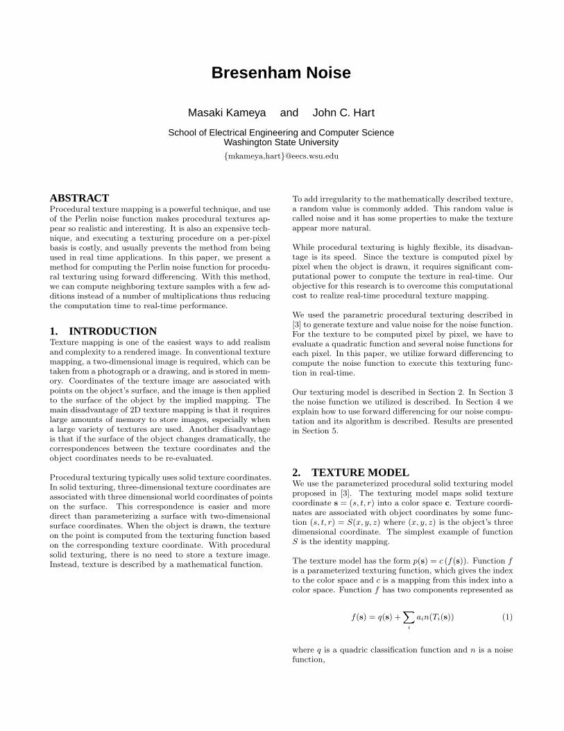
Let the coordinates s0, t0, r0 be the floor of s, t, r respec-tively, and likewise s1, t1, r1 be their respective ceiling. Letthe eight vertices of the cell be N0, N1, · · · , N7. Their coor-dinates areN0 : (s0, t0, r0), N1 : (s1, t0, r0), · · · , N6 : (s1, t1, r1), N7 :(s0, t1, r1), where {s/t/r}1 = {s/t/r}0 + 1. Let noise valueat the vertex Ni be ni, i = 0, · · · , 7. (Figure1)

After obtaining the random values on each of the eight ver-tices, noise is interpolated in terms of each coordinate. The

Figure 1: The cell in the texture coordinate.

noise value at point a is linearly interpolated from N0 andN1 in terms of s coordinate, i.e.

na = n0 + (n1 − n0)s− s0

s1 − s0(5)

The noise value is computed similarly at points b, c, d. Thenoise value is computed at point e and f by interpolating naand nb, nc and nd in terms of the t coordinate, respectively.

ne = na + (nb − na)t− t0t1 − t0

(6)

Finally, the noise value at point p is computed from noisevalue at e and f .

noise = ne + (nf − ne)r − r0

r1 − r0(7)

Since s1 = s0 + 1, t1 = t0 + 1andr1 = r0 + 1, equation(5),(6),(7) can be rewritten as

na = n0 + (n1 − n0)(s− s0)ne = na + (nb − na)(t− t0)

noise = ne + (nf − ne)(r − r0) (8)

s − s0 represents relative position from s0 and s satisfiess0 ≤ s ≤ s1 = s0 + 1. Therefore, (s − s0) can be replacedby sf which represents the fractional part of s and same ast and r. Then equation (8) can be rewritten as:

na = n0 + (n1 − n0)sf (9)ne = na + (nb − na)tf (10)

noise = ne + (nf − ne)rf (11)

where sf , tf and rf represents the fraction part of s, t and rrespectively. Incorporating equation (9) and (10) to (11),

noise = a+ bsf + ctf + drf + esf tf + ftfrf

+grfsf + hsf tfrf (12)

where coefficients a to h are the constants determined byni, i = 0, · · · , 7, i.e. the cells which point p resides. Thisequation shows that trilinear interpolation is a cubic func-tion of the coordinates.

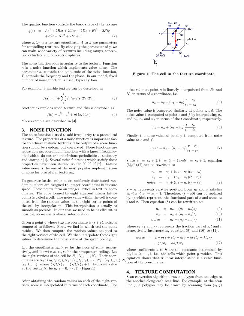
4. TEXTURE COMPUTATIONScan conversion algorithm draw a polygon from one edge tothe another along each scan line. For example, at the scanline j, a polygon may be drawn by scanning from (i0, j)

Figure 2: Texture coordinate and scan line

to (i1, j), as shown in Figure 2. Let the corresponding tex-ture coordinate of these points be (s0, t0, r0), and (s1, t1, r1).(Note these are not the same values as the corner latticepoints in the previous section.) The texture coordinates(s, t, r) of each pixel on this scanline of the polygon are lin-early interpolated between these two points are linearly in-terpolated from them.

The derivative of the texture coordinates along the scan lineare

(ds/di, dt/di, dr/di) =�s1 − s0

i1 − i0,t1 − t0i1 − i0

,r1 − r0

i1 − i0

�(13)

The texture coordinates of the point between the edges isnow computed as

(s, t, r) = (s0 + ∆ids/di, t0 + ∆idt/di, r0 + ∆idr/di) (14)

Given the texture coordinates at pixel (i, j), we can computethe color by evaluating the texturing function (1). Gener-ally, this texture is computed by pixel by pixel. That is, thetexture is computed every step of scan conversion by com-puting the texture coordinate and evaluating the texturingequation. If we compute the texture color only on at theenpoints of the scanline then linearly interpolate the result-ing color, we will miss the detail of the texture across largepolygons.

To make procedural texturing comutation in real-time, weapply the forward differencing technique to the noise func-tion.

4.1 Forward DifferenceThe computation of successive values of a polynomial can bedone efficiently with forward differencing [2]. In computergraphics, this has been used for drawing lines or curves.One of example is line drawing on the screen, such as Bre-senham’s line or circle drawing algorithms.

We utilize forward differencing to hasten the computationof successive noise values across the scanline, because com-putation of the noise function is expensive and can be rep-resented as a cubic function of the coordinates for linearlyinterpolated noise.

The texture coordinates on the scanline are linearly interpo-lated and the derivative of the texture coordinate along the

scan line, ds/di, dt/di, dr/di are computed for each scan line.Suppose the texture coordinate at (i0, j) is (s0, t0, r0). Thenthe texture coordinate at (i0 + ∆i, j) on the same scan lineis computed by (s0 + ∆ids/di, t0 + ∆idt/di, r0 + ∆idr/di).

Incorporating screen coordinate i and the derivatives of tex-ture coordinates ds/di, dt/di and dr/di to equation (12) ,noise can be represented as a function of ∆i. By replacing(s0, t0, r0) with (s, t, r) and regard i as the ∆i,

noise(∆i) = a+ b(s+ ∆ids/di)+ c(t+ ∆idt/di) + d(r + ∆idr/di)+ e(s+ ∆ids/di)(t+ ∆idt/di)+ f(t+ ∆idt/di)(r + ∆idr/di)+ g(r + ∆idr/di)(s+ ∆ids/di)+ h(s+ ∆ids/di)(t+ ∆idt/di)(r + ∆idr/di)= αi3 + βi2 + γi+ δ (15)

where α, β, γ and δ are constants determined by constantsa to h and s, t and r. Calculation of constans is describedin Appendix.

Therefore, the function noise is a cubic polynomial in termsof i. Instead of evaluating this function for each pixel posi-tion (i, j), we can use forward differencing to avoid a lot ofexpensive multiplication, which is replaced by small numberof setup multiplication and successive additions.

In scan conversion algorithms, the screen coordinate of iis incremented by one for each step. Thus noise can becomputed iteratively with forward difference as

noise(i+ 1) = noise(i) + ∆n(i) (16)

∆n(i) can be represented as

∆n(i) = noise(i+ 1)− noise(i)= α(i+ 1)3 + β(i+ 1)2 + γ(i+ 1) + δ

−(αi3 + βi2 + γi+ δ)= 3αi2 + i(3α+ 2β) + α+ β + γ (17)

Since equation (17) contains quadratic term of i, ∆n is afunction of i. Therefore, we apply forward difference to∆n(i).

∆n(i+ 1) = ∆n(i) + ∆(∆n(i))= ∆n(i)∆2n(i) (18)

Using similar computation in refeqn:deltan to ∆n(i), wehave

∆2n(i) = 6αi+ 6α+ 2β (19)

This still contains i, therefore we apply forward differenceonce more.

∆3n(i) = ∆2n(i+ 1)−∆2n(i)= 6α (20)

Initial values of the forward differences are obtained by plu-gin i = 0. Then we have

noise0 = δ

∆n0 = α+ β + γ

∆2n0 = 6α+ 2β∆3n0 = = 6α (21)

Then noise is iteratively computed as

noise + = ∆n∆n + = ∆2n

∆2n + = ∆3n (22)

4.2 Noise Computation AlgorithmIn this section, the algorithm to compute noise value withforward difference for scan conversion is described. Noise iscomputed by equation (22) in each step of scan conversion.We have to decide the constant a to h and α, β, γ and δ.

Constants a to h depend on the noise value at the lattice.We have to locate which cell the current point is in. Onceit is located and these constants are computed, same con-stants can be used as long as scan line proceed within thesame cell. If scan line reached another cell, these constantshave to be re-computed. Constants α, β, γ and δ depend onconstants a to h and derivatives of the texture coordinatealong the scan line dsdi, dtdi and drdi. These derivatives areconstants during one scan line and they are updated whenit has changed.

In summary, forward differences in equation (22) are re-computed when

• scan line reaches different cell or

• scan line has changed

Pseudo code of noise computation algorithm is shown below.

noise_compuation {

for j = min_edge to max_edge {Compute dsdi, dtdi, drdiCompute a, b, c, d, e, f, g, hCompute alpha, beta, gamma, deltaCompute n, dn, d2n, d3n

for i = edge_left to edge_right{

if ( (i,j) is in the same cell ){n += dndn += d2nd2n += d3n

} else {Compute a, b, c, d, e, f, g, hCompute alpha, beta, gamma, deltaCompute n, dn, d2n, d3n

}}

}}

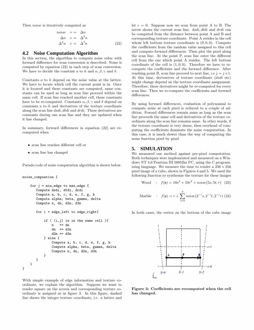
With simple example of edge information and texture co-ordinate, we explain the algorithm. Suppose we want torender square on the screen and corresponding texture co-ordinate is assigned as in figure 3. In this figure, dashedline shows the integer texture coordinate, i.e. a lattice and

let r = 0. Suppose now we scan from point A to B. Thearrow shows the current scan line. dsdi, dtdi and drdi canbe computed from the distance between point A and B andcorresponding texture coordinate. Point A resides in the cellwhose left bottom texture coordinate is (0, 0, 0). Computethe coefficients from the random value assigned to this celland compute forward differences. Then plot the pixel alongthe scan line. At the point P, scan line enter the differentcell from the one which point A resides. The left bottomcoordinate of the cell is (1, 0, 0). Therefore we have to re-compute the coefficients and the forward difference. Afterreaching point B, scan line proceed to next line, i.e j = j+1.At this time, derivatives of texture coordinate (dsdi etc)might change depend on the texture coordinate assignment.Therefore, these derivatives might be re-computed for everyscan line. Then we re-compute the coefficients and forwarddifferences.

By using forward differences, evaluation of polynomial tocompute noise at each pixel is reduced to a couple of ad-dition. Foward differences remain same as long as the scanline proceeds the same cell and derivatives of the texture co-ordinate along the scan line remains same. In other words, ifthe texture coordinate is very dense, then overhead of com-puting the coefficients dominate the noise computation. Inthis case, it is much slower than the way of computing thenoise function pixel by pixel.

5. SIMULATIONWe measured our method against per-pixel computation.Both techniques were implemented and measured on a Win-dows NT 4.0 Pentium III 500Mhz PC, using the C program-ming language. We measure the time to render a 256× 256pixel image of a cube, shown in Figures 4 and 5. We used thefollowing function to synthesize the texture for these images

Wood : f(s) = 10s2 + 10r2 + noise(5s, 5t, r) (23)

Marble : f(s) = r +3Xi=0

noise(2−is, 2−it, 2−ir) (24)

In both cases, the vertex on the bottom of the cube image

Figure 3: Coefficients are recomputed when the cellhas changed.

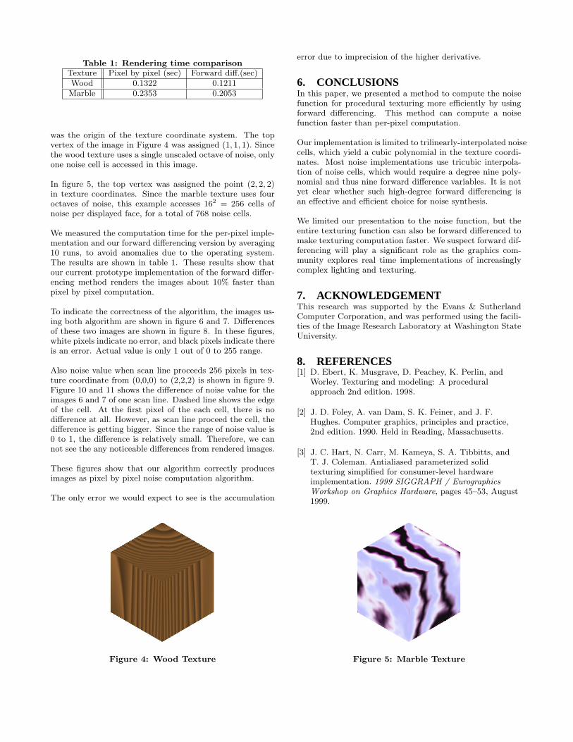
Table 1: Rendering time comparisonTexture Pixel by pixel (sec) Forward diff.(sec)Wood 0.1322 0.1211Marble 0.2353 0.2053

was the origin of the texture coordinate system. The topvertex of the image in Figure 4 was assigned (1, 1, 1). Sincethe wood texture uses a single unscaled octave of noise, onlyone noise cell is accessed in this image.

In figure 5, the top vertex was assigned the point (2, 2, 2)in texture coordinates. Since the marble texture uses fouroctaves of noise, this example accesses 162 = 256 cells ofnoise per displayed face, for a total of 768 noise cells.

We measured the computation time for the per-pixel imple-mentation and our forward differencing version by averaging10 runs, to avoid anomalies due to the operating system.The results are shown in table 1. These results show thatour current prototype implementation of the forward differ-encing method renders the images about 10% faster thanpixel by pixel computation.

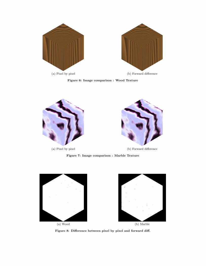
To indicate the correctness of the algorithm, the images us-ing both algorithm are shown in figure 6 and 7. Differencesof these two images are shown in figure 8. In these figures,white pixels indicate no error, and black pixels indicate thereis an error. Actual value is only 1 out of 0 to 255 range.

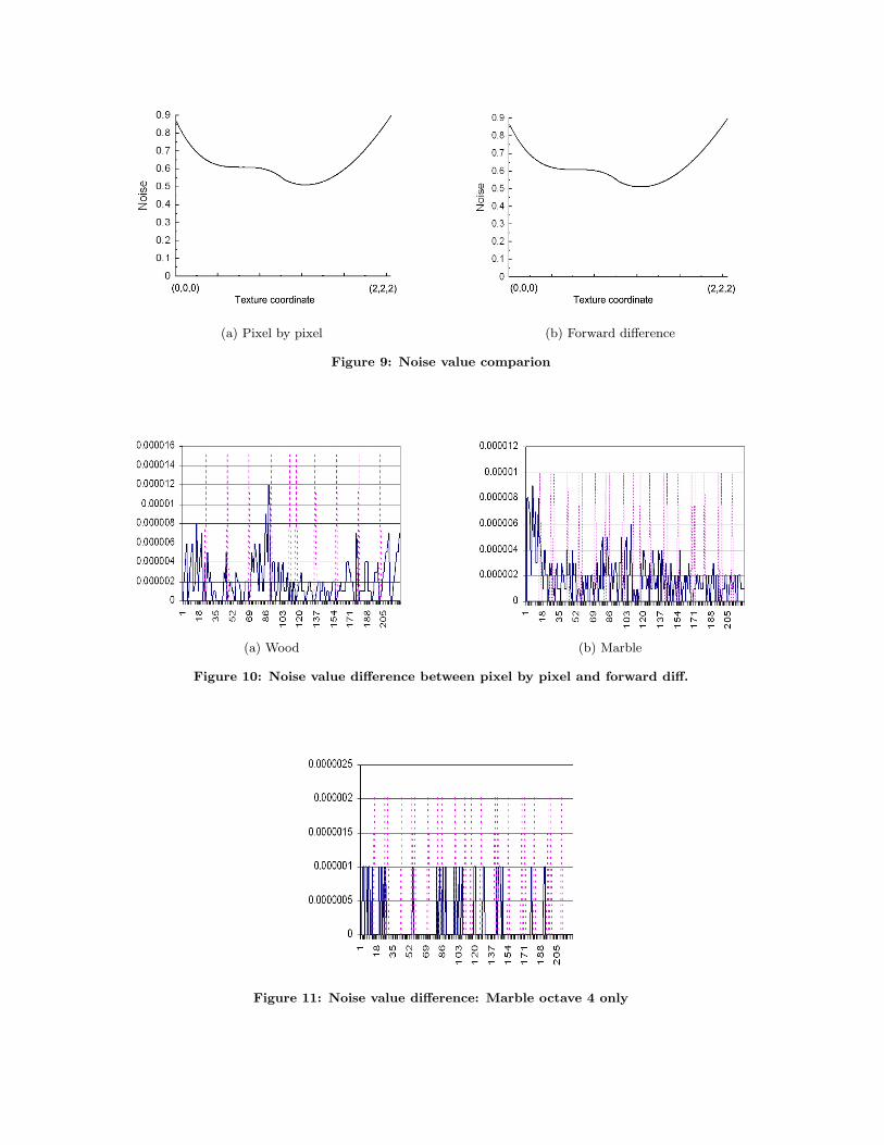
Also noise value when scan line proceeds 256 pixels in tex-ture coordinate from (0,0,0) to (2,2,2) is shown in figure 9.Figure 10 and 11 shows the difference of noise value for theimages 6 and 7 of one scan line. Dashed line shows the edgeof the cell. At the first pixel of the each cell, there is nodifference at all. However, as scan line proceed the cell, thedifference is getting bigger. Since the range of noise value is0 to 1, the difference is relatively small. Therefore, we cannot see the any noticeable differences from rendered images.

These figures show that our algorithm correctly producesimages as pixel by pixel noise computation algorithm.

The only error we would expect to see is the accumulation

Figure 4: Wood Texture

error due to imprecision of the higher derivative.

6. CONCLUSIONSIn this paper, we presented a method to compute the noisefunction for procedural texturing more efficiently by usingforward differencing. This method can compute a noisefunction faster than per-pixel computation.

Our implementation is limited to trilinearly-interpolated noisecells, which yield a cubic polynomial in the texture coordi-nates. Most noise implementations use tricubic interpola-tion of noise cells, which would require a degree nine poly-nomial and thus nine forward difference variables. It is notyet clear whether such high-degree forward differencing isan effective and efficient choice for noise synthesis.

We limited our presentation to the noise function, but theentire texturing function can also be forward differenced tomake texturing computation faster. We suspect forward dif-ferencing will play a significant role as the graphics com-munity explores real time implementations of increasinglycomplex lighting and texturing.

7. ACKNOWLEDGEMENTThis research was supported by the Evans & SutherlandComputer Corporation, and was performed using the facili-ties of the Image Research Laboratory at Washington StateUniversity.

8. REFERENCES[1] D. Ebert, K. Musgrave, D. Peachey, K. Perlin, and

Worley. Texturing and modeling: A proceduralapproach 2nd edition. 1998.

[2] J. D. Foley, A. van Dam, S. K. Feiner, and J. F.Hughes. Computer graphics, principles and practice,2nd edition. 1990. Held in Reading, Massachusetts.

[3] J. C. Hart, N. Carr, M. Kameya, S. A. Tibbitts, andT. J. Coleman. Antialiased parameterized solidtexturing simplified for consumer-level hardwareimplementation. 1999 SIGGRAPH / EurographicsWorkshop on Graphics Hardware, pages 45–53, August1999.

Figure 5: Marble Texture

(a) Pixel by pixel (b) Forward difference

Figure 6: Image comparison : Wood Texture

(a) Pixel by pixel (b) Forward difference

Figure 7: Image comparison : Marble Texture

(a) Wood (b) Marble

Figure 8: Difference between pixel by pixel and forward diff.

(a) Pixel by pixel (b) Forward difference

Figure 9: Noise value comparion

(a) Wood (b) Marble

Figure 10: Noise value difference between pixel by pixel and forward diff.

Figure 11: Noise value difference: Marble octave 4 only

[4] J.-P. Lewis. Algorithms for solid noise synthesis.Computer Graphics (Proceedings of SIGGRAPH 89),23(3):263–270, July 1989.

[5] K. Perlin. An image synthesizer. Computer Graphics(Proceedings of SIGGRAPH 85), 19(3):287–296, July1985.

[6] J. J. van Wijk. Spot noise-texture synthesis for datavisualization. Computer Graphics (Proceedings ofSIGGRAPH 91), 25(4):309–318, July 1991.

[7] S. P. Worley. A cellular texture basis function.Proceedings of SIGGRAPH 96, pages 291–294, August1996.

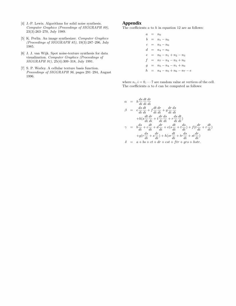
AppendixThe coefficients a to h in equation 12 are as follows:

a = n0

b = n1 − n0

c = n3 − n0

d = n4 − n0

e = n0 − n1 + n2 − n3

f = n7 − n4 − n3 + n0

g = n5 − n4 − n1 + n0

h = n4 − n5 + n6 − n7 − e

where ni, i = 0, · · · 7 are random value at vertices of the cell.The coefficients α to δ can be computed as follows:

α = hds

di

dt

di

dr

di

β = eds

di

dt

di+ f

dt

di

dr

di+ g

dr

di

ds

di

+h(sdt

di

dr

di+ t

dr

di

ds

di+ r

ds

di

dt

di)

γ = bds

di+ c

dt

di+ d

dr

di+ e(s

dt

di+ t

ds

di) + f(t

dr

di+ r

dt

di)

+g(rds

di+ s

dr

di) + h(sr

dt

di+ tr

ds

di+ st

dr

di)

δ = a+ bs+ ct+ dr + est+ ftr + grs+ hstr.