NEW MAP PROJECTION PARADIGMS: Bresenham Poly-Azimuthal Fly-Through Projections, Oblique Mercator Triptiks, and Dynamic Cartograms

Alan Saalfeld Department of Civil and Environmental Engineering and Geodetic Science

The Ohio State University Columbus, Ohio 43210-1275 USA

Abstract

We examine map projections and their distortions in a discretized, time-dependent computer mapping environment; and we propose some new map projection paradigms. The computer environment permits us to display animated projection evolution (realized as a movie of continuous deformation from a perspective view of the orig inal datum surface to the projection surface). An animated pro jection evolution technique may also be used to produce varivalent projections (cartograms) built by iterative discrete distortion tech niques. The discretized environment also allows us to quickly change the viewpoint and the projection orientation (by means of pixel shift operations) to produce a sequence of overlapping maps, each of which is distortion-free (up to sub-pixel resolution) with respect to a mov ing central point. We also examine methods for producing large scale route strip map sets such that each route segment is distortion-free throughout the strip map in which it is featured.

INTRODUCTIONWhat would the savvy map user ask for in a map projection these days if' he or she knew about the latest possibilities for computer generated maps? Probably the,same thing that a hopelessly naive user might request-a to tally distortion-free map! While a distortion-free map is and always will be a mathematical impossibility for any region containing 4 or more non- coplanar points, one may, nonetheless, (and for sufficiently large scales) hold displacement distortion to subpixel size and draw a map with no dis cernible distortion. The following are technology-inspired tactics to (1) min imize perceptible distortion at and around a rapidly moving viewpoint, to (2) minimize distortion along a particular route, and to (3) minimize distor tion under a magnifying glass that we baby-boomers are finding increasingly necessary to use to read our maps.

BRESENHAM-TYPE METHODSEvery computer graphics student learns early about J. E. Bresenham's el egantly simple algorithms for coloring pixels one by one to generate raster representations of straight lines [Bre65] and circles [Bre77]. The algorithms

347

employ elementary integer arithmetic operations of addition and subtrac tion (and nothing else!) They are fast, robust, and surprisingly easy to implement and to prove correct. This paper (and an associated computer demonstration) attempt to extend the flavor, if not the theory, of Bresen- ham's work to two and three dimensions by incrementally updating the pixels of the 2-D map of the ground below Dr. Bresenham as he moves along and above the surface of the earth in nice pixel-sized increments. What we accomplish with our incremental methods are real-time azimuthal projections continuously centered directly below a moving observer. There is never any linear or angular distortion at the current viewpoint (always the center of the map). Distortion is always radial (so directions from the current viewpoint are always correct); and concentric circles about the viewpoint delineate "contours of equal distortion." We discuss the different incremental procedures needed to update different azimuthal projections; and we define simple incremental procedures and analyze their resulting projection properties. The central symmetry of all of our adjustments per mits shortcut computations (similar to Bresenham's observation [Bre77] that for circles, one needs'only compute an arc that is 1/8 the circumfer ence, then reflect in various axes).

The speed of the incremental computations permits a discrete image to be generated at a much higher resolution than the display. The computed higher resolution grid may then be smoothed with a filter (in much the same way that anti-aliasing is often applied to remove the jaggies from Bresenham's line). Moreover, the incremental changes of the observer's movement may be everywhere realized as pixel shifts followed by smoothing or averaging (averaging is necessary when the finer grid pixels only move a fractional amount of the larger pixel size). The observer's movement may be decomposed into its X, Y, and Z components; and the effect on the image of each step in one of the three perpendicular directions may be computed once and stored in a lookup table. Since movements in the three independent directions "almost" commute with each other, we may sum the pixel shift effects of the X, Y, and Z components in any order to determine the net effect.

A Moving Pixel's Perspective

Motion of the viewer translates into apparent-motion of an image in the opposite direction. As a train passenger looks out the window; he sees the scenery moving past him in the opposite direction to the train's motion. Objects that are close to the train appear to move more rapidly than distant objects. The moon appears to be keeping up with the train because its relative motion is so slight that it seems to not move backwards at all! The geometry of this apparent motion with respect to the train window is straightforward—the rate that a stationary object appears to move past the window is inversely proportional to its distance from the viewer. One may

348

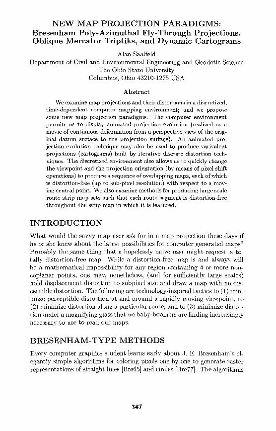
Figure 1: Linear point motion as captured in the digitized image plane.

discretize this apparent motion by imagining that the window is screened (a fine-grained rectangular grid), the viewer's eye is fixed with respect to its distance and position relative to the screen, and the viewed objects appear to move from one tiny rectangle of the screen to an adjacent rectangle as the train moves forward. For the train example, all actual motion and all apparent motion is horizontal! If the vehicle could move vertically as well, but continued in^a straight line, then the distant point object would appear to move from cell to cell in the gridded screen in exactly the same pattern as the incremental linear Bresenham algorithm generates successive grid cells, as is illustrated in Figure 1.

Pixel trajectories

Consider now the sequence of screen rectangles (pixels) in which a particular distant point light source appears over time. At any time the light point representation on the screen has a screen position and a screen velocity. If the screen contains a line parallel to the direction of motion of the train, then the lighted pixel's velocity will be constant and linear; hence, the individual pixel's trajectory over time will be correctly modeled by the Bresenham algorithm for painting successive pixels along a line at regularly spaced time intervals. If one knows all of the pixels' velocities (speed and direction) at each instant, then one may integrate the velocities to obtain tracks or trajectories for each individual pixel component of a map's images. The significant notions that we .can exploit here are (1) the pixel content (is it black or white or colored?) makes absolutely no difference to the trajectory determination; and (2) the pixel movements repeat their patterns (so that the full image of pixel shifts may be saved and re-used so that they may be applied repeatedly to generate successive images). The movement of objects in the foreground will appear to outpace the movement of more

349

distant objects; hence, foreground objects may overtake and temporarily obstruct the view of more distant objects, and then the foreground objects will again uncover or reveal distant objects as the foreground objects appear to move past the background objects. If all of the objects are in a single plane parallel to the screen (i.e., all the same distance from the plane of the screen), then the apparent pixel motion on the screen will be completely uniform (same direction and same pixel speed) everywhere. This model is a bit too simplified for our applications!

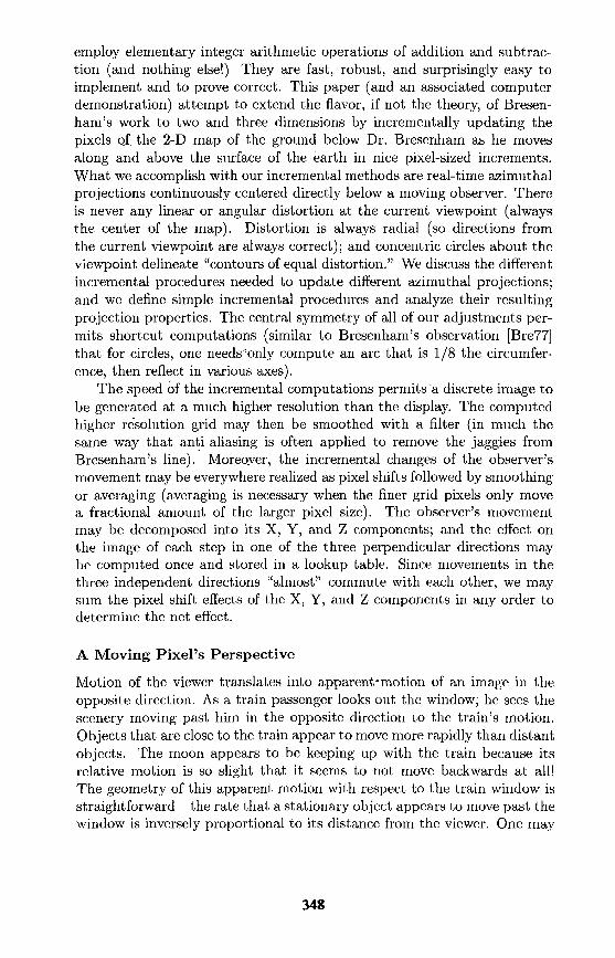
Figure 2: Pixels' displacement simulates rotational motion.

Let's look at some image updates for which pixel movement is not uni form. Consider the following simplified animation of the spinning earth icon or applet: shaded pixels are displayed in a circle in a way that produces the illusion of a spinning globe, as illustrated in Figure 2. The pixel shifts that accomplish this illusion produce trajectories along the perspective pro jection of parallel circles of latitude. The speed of the pixel movements is greater at the equator and diminishes near the poles. The speed near the edges of the circular disk also diminishes to produce the effect of less motion in the viewing screen plane (the greater component of the rotational motion is perpendicular to the viewing screen plane). Note that the persistence of the specular reflection (a lightening of pixels as they approach the center of the circle) reinforces the effect that the globe itself is rotating and the viewer and light source remain fixed. It is worthwhile to emphasize that the pixel shifts relative to their reference position in the circular display are identical from the first image to the second, from the second to the third, and from the third to the fourth. Each successive image represents a 20° rotation; and the pixel shifts are completely determined by that fact (and not by whatever happens to occupy a pixel location at any moment).

If the globe were transparent, and if we were far enough away from it (so that all rays that we perceive are effectively parallel), we would see each point on the earth trace out an ellipse. The pixel motion necessary to trace out an ellipse is easily described in terms of Bresenham's circle drawing routine: if we give our pixels an aspect ratio of b/a, then the figure that we draw with Bresenham's circle drawing routine is actually an ellipse; and the flattening of that ellipse is precisely (a — b)/a.

We may offer one final illustration based on the appearance of a rotating spherical globe as viewed from space: Suppose that we position ourselves one earth diameter from the earth's surface and we place a giant convex lens

350

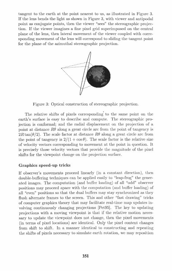
tangent to the earth at the point nearest to us, as illustrated in Figure 3. If the lens bends the light as shown in Figure 3, with viewer and antipodal point as conjugate points, then the viewer "sees" the stereographic projec tion. If the viewer imagines a fine pixel grid superimposed on the central plane of the lens, then lateral movement of the viewer coupled with corre sponding movement of the lens will correspond to sliding the tangent point for the plane of the azimuthal stereographic projection.

Figure 3: Optical construction of stereographic projection.

The relative shifts of pixels corresponding to the same point on the earth's surface is easy to describe and compute. The stereographic pro jection is conformal; and the radial displacement on the projection of a point at distance R9 along a great circle arc from the point of tangency is 2Rtan(6/2,). The scale factor at distance RO along a great circle arc from the point of tangency is 2/(l + cos 9). The scale factor is the relative size of velocity vectors corresponding to movement at the point in question. It is precisely those velocity vectors that provide the magnitude of the pixel shifts for the viewpoint change on the projection surface.

Graphics speed-up tricks

If observer's movements proceed linearly (in a constant direction), then double-buffering techniques can be applied easily to "leap-frog" the gener ated images. The computation (and buffer loading) of all "odd" observer positions may proceed apace with the computation (and buffer loading) of all "even" positions so that the dual buffers may stay synchronized as they flush alternate frames to the screen. This and other "fast drawing" tricks of computer graphics theory that may facilitate real-time map updates in volving continuously changing projections [Pet95]. The key to updating projections with a moving viewpoint is that if the relative motion neces sary to update the viewpoint does not change, then the pixel movements (in terms of pixel locations) are identical. Only the pixel content changes from shift to shift. In a manner identical to constructing and repeating the shifts of pixels necessary to simulate earth rotation, we may reposition

351

the tangent point of our azimuthal projection by shifting all pixels in the opposite direction. To move right, we take the pixel on the right and shift it left. A pixel that is far away will have to shift a greater distance. For example, a pixel that is 90° away from the tangent pixel will move twice as fast because the scale factor is exactly two in the projection at 90° from the point of tangency.

CONFORMAL TRIPTIKSIn this section we examine some opportunities to construct and use maps that are conformal along a route

Oblique Mercator Strip Maps

An oblique Mercator projection of the sphere, with its cylinder tangent to the great circle joining two points of interest, provides a distortion- free representation of all points along the shortest path between those two points [Sny94]. Such a representation provides a pilot or a navigator with a direct routing from start to destination. Any point along the great circle route corresponds to a point of no distortion on the map. For ground- following routes, one may approximate the multi-directional path by a se quence of great circle arcs on a sphere modeling the Earth; then one may compute oblique Mercator projections along each great circle arc. One might present each arc's projection separately; or one might even "blend" the projections using other available computer graphics techniques [Far93]. We will visit blending once again when we briefly touch upon homotopy and homotopic projections.

Minimizing distortion along and near a closed path

One may minimize distortion along a path by keeping the function confor mal in a neighborhood of the path and also maintaining a constant scale along the path. Since the length of a path on the map differs from the length on the datum surface by a factor of scale (which is constant), we must have that relative lengths along partial paths are preserved every where. Chebyschev had conjectured (and others later proved) [BS95] that a conformal scale-constant mapping of the closed boundary of a simply con nected region to the closed boundary of another simply connected region extends conformally to the interior of the regions in a way that minimizes scale variation within the region.

Cheng's Conformal Polyconics

Yang Cheng [Che92] showed how to attach a tangent developable surface to any smooth rectifiable curve on a datum surface (sphere or ellipsoid); and from that construction, he is able to extend the projection of that curve

352

conformally to a neighborhood of that curve with no distortion along the tangent curve itself. Cheng's methods have been applied in detail to specific important curves such as satellite ground tracks [Che96]. They may also be applied readily for any route on the sphere or ellipsoid for which we may compute geodesic curvature. We must merely construct a plane curve whose curvature matches the geodesic curvature of the curve on the sphere or ellipsoid; then we may widen, expand, or buffer the curve in the plane to produce a swath (or wiggly triptik!) on which we may construct a conformal mapping of a neighborhood of the curve. This conformal mapping will have no scale distortion along the curve itself.

DYNAMIC CARTOGRAMSMorphing technology in computer graphics has created a standard toolbox for animators, graphic artists, and image processors. We focus here on describing a subset of morphing tools that possess desirable map projection properties such as conformality and equivalence; and we show how those tools can be applied effectively to create an interesting collection of map products.

Homotopies

A homotopy may be regarded as a continuous deformation over time of one function to another. Formally, if / : X — *• Y and g : X — » Y are two functions on the same domain X and range Y, then we say that / and g are homotopic if there exists a continuous function 0 : X x [0, 1] — > Y such that for all x € X, f(x] = </>(#, 0) and g(x) — (/)(x, 1). One may regard the second parameter of the bivariate function 0 as a time parameter: at t — 0 the function </> behaves like /; at t = I the function 0 behaves like g] and for 0 < t < 1, the function 0 changes continuously with respect to t.

Because each cross-section (j> : X x {to} — * Y of a homotopy is only required to be continuous (and not necessarily bijective), the intermediate slices of two homotopic projections / and g may not be projections in the usual sense (because of collapsing). For example, if one rotates any projection through 180°:

If f(x) = (/t>,0), then g(x) = (p,0 + 180°),

then defines a straight line deformation from / to g:

then the function 0 collapses to the origin everywhere at t = 1/2.Often the function </> is called the convex combination of g and /. If g and

/ are analytic complex-valued functions of a complex variable, then every convex combination of g and / will also be an analytic function. Analytic is

353

the same as conformal or angle preserving provided the function does not collapse somewhere. There are many other possibilities for guaranteeing conformality of combined functions. All complex arithmetic operations return conformal functions.

Complex Variables and Conformal Functions

Conformal functions have some amazing properties related to the struc ture of the complex number field that mathematicians have discovered and studied. These properties are at the same time very constraining and yet very powerful in nature. One very important property is that the complex numbers are not simply two-vectors, they possess an algebraic interaction that manifests itself very nicely in the geometry. To multiply two complex numbers by adding their angles and multiplying their magnitudes is both incredible and liberating. Another defining property is differentiability in the complex variable sense. A derivative exists at each point; and it may be computed as a limit from any direction. A directional derivative is a scale factor in the particular direction. For conformal functions, all directional derivatives at a single point are the same (complex) value. In other words, at each individual point in the domain, the scale factor (magnitude change of any tangent vector) in every direction is the same; and so is the rotation component of each tangent vector. Here are some of the other amazing properties of conformal functions [Cur43]:

1. If a function is once (complex) differentiable in an open neighborhood of a point, then it is infinitely differentiable in the neighborhood of the point.

2. Each conformal mapping is fully determined in a maximum circular region about any point by the first, second, third, and higher order derivatives at the single point.

3. A conformal function is fully determined in a maximum circular region by its values on any open set, however small. (This is perhaps the most constraining property since we lose all freedom to assign our own set of values to a conformal function even far from the defining site.)

4. A conformal function has a power series expansion in a complex vari able. The radius of convergence extends exactly as far as the nearest singularity of the function.

5. We have some bad news, too: we want to stay away from singularities. In any neighborhood of a singularity, a conformal function assumes every possible sufficiently large value.

6. For any simply connected region, there exists a conformal function that sends the unit disk onto the region. (This says that we can

354

preserve local scale and shape and still distort the global picture as much as we want. This seems counter-intuitive!)

7. A conformal function is an open map. It sends open sets to open sets.

8. Any two conformal functions that agree on an infinite set of points agree everywhere.

9. The composition of two conformal functions remains conformal.

10. Boundary conditions may preclude the existence of any satisfying conformal functions.

11. Homotopy and conformality meet [ST83] in Cauchy's Theorem: If a closed path j(t) is homotopic to the null path in a region of differen tiability of /, then / / = 0. If two closed paths 7i(£) and 72(i) are homotopic in a region of differentiability of /, then j / = / /•

12. The homotopy properties guarantee the existence of anti-derivatives as well as infinitely many derivatives.

Quasiconformal Functions

Quasiconformal functions [Ahl87] are as close to conformal as one may get when boundary conditions are such that conformality is impossible. If we use the eccentricity of the ellipse of the Tissot indicatrix [Las89] to measure our failure to achieve conformality, then quasiconformal functions have the smallest eccentricity possible while still satisfying the defining boundary conditions. Some important quasiconformal functions correspond to con- formal transformations followed by affine transformations (which wind up flattening all Tissot ellipses in the same direction and by the same fractional amount).

Area Preservation and Area Distortion

Waldo Tobler [Tob86] and Lev Bugayevskiy [BS95] have studied the dif ferential equations of varivalent transformations; and Tobler has produced several programs to implement his methods [Tob74]. An opportunity to ex amine the discretized version of the transformations exists for us to apply the incremental methods described in this paper to the theory of Tobler and others.

FINAL REMARKSWe have only had time and space to present what appears to be a laundry list of possibilities for new map projection paradigms. We certainly do not claim to have exhausted the possibilities; and our limited perspective is just that—quite limited. Nevertheless, we believe that we have highlighted a

355

series of related opportunities; and we hope that our viewpoint stimulates new research into map projections and their uses.

References[Ahl87] Lars V. Ahlfors. Lectures in Quasiconformal Mappings. Wadsworth

and Brooks, Monterey, CA, 2nd edition, 1987.

[Bre65] J. E. Bresenham. Algorithm for computer control of digital plotter. IBM Systems Journal, 4:25-30, 1965.

[Bre77] J. E. Bresenham. A linear algorithm for incremental digital display of circular arcs. Communications of the ACM, 20:100-106, 1977.

[BS95] Lev M. Bugayevskiy and John P. Snyder. Map Projections: A Reference Manual. Taylor and Francis, London, 1995.

[Che92] Yang Cheng. On conformal projection maintaining a desired curve on the ellipsoid without distortion. In ACSM/ASPRS/RT '92 Technical Papers, volume 3, pages 294-303, Bethesda, MD, April 1992.

[Che96] Yang Cheng. The conformal space projection. Cartography and Geographic Information Systems, 23(1):37-50, January 1996.

[Cur43] David R. Curtiss. Analytic Functions of a Complex Variable. Mathematical Association of America, LaSalle, Illinois, 3rd edi tion, 1943.

[Far93] Gerald Farin. Differential Geometry and its Applications. Aca demic Press, San Diego, 3rd edition, 1993.

[Las89] Piotr H. Laskowski. The traditional and modern look at Tis- sot's Indicatrix. Cartography and Geographic Information Systems, 16(2): 123-133, April 1989.

[Pet95] Michael P. Peterson. Interactive and Animated Cartography. Pren tice Hall, New Jersey, 1995.

[Sny94] John P. Snyder. Map Projections: A Working Manual. USGS/US Government Printing Office, Washington, DC, 3rd edition, 1994.

[ST83] lan Stewart and David Tall. Complex Analysis. Cambridge Uni versity Press, London, 1983.

[Tob74] Waldo Tobler. Cartogram programs. Technical report, University of Michigan, Department of Geography, 1974.

[Tob86] Waldo Tobler. Pseudo-cartograms. American Cartographer, 13(1):43-50, 1986.

356