Branislav K. Nikoli ć - Delaware Physics · Branislav K. Nikoli ... predict exactly the situation of that same universe at a succeeding moment. but even if it ... Their surface area

1

Introduction to Deterministic Chaos

Branislav K. NikolićDepartment of Physics and Astronomy, University of Delaware, U.S.A.

PHYS 460/660: Computational Methods of Physics http://www.physics.udel.edu/~bnikolic/teaching/phys660/phys660.html

caoz

PHYS 460/660: Introduction to deterministic chaos2

Chaos vs. Randomness

Do not confuse chaotic with random temporal dynamics:

Random:

irreproducible and unpredictable

Chaotic (use characteristics below as definition):

irregular in time (it is not even the superposition of periodic motions – it is really aperiodic)

deterministic - same initial conditions lead to same final state -but the final state is very different for small changes to initial conditions

difficult or impossible to make long-term prediction! complex, but ordered, in phase space: it is associated with a fractal structure


Clockwork (Newton) vs. Chaotic (Poincaré) Universe

Suppose the Universe is made of particles of matter interacting according to Newton laws→ this is just a dynamical system governed by a (very large though) set of differential equations.

Given the starting positions and velocities of all particles, there is a unique outcome → P. Laplace’s Clockwork Universe (XVIII Century)!


Brief Chaotic History: Poincaré 1892 (Hamiltonian or Conservative Chaos)


Footnote: Did Poincaré get the money?

Jules Henri Poincaré was dubbed by E. T. Bell as the last universalist — a man who is at ease in all branches of mathematics, both pure and applied — Poincaré was one of these rare savants who was able to make many major contributions to such diverse fields as analysis, algebra, topology, astronomy, and theoretical physics.

While Poincaré did not succeed in giving a complete solution, his work was so impressive that he was awarded the prize anyway. The distinguished Weierstrass, who was one of the judges, said, “this work cannot indeed be considered as furnishing the complete solution of the question proposed, but that it is nevertheless of such importance that its publication will inaugurate a new era in the history of celestial mechanics.” (a lively account of this event is given in Newton's Clock: Chaos in Solar System)

To show how visionary Poincaré was, it is perhaps best to read his description of the hallmark of chaos - sensitive dependence on initial conditions:“If we knew exactly the laws of nature and the situation of the universe at the initial moment, we could predict exactly the situation of that same universe at a succeeding moment. but even if it were the case that the natural laws had no longer any secret for us, we could still only know the initial situation approximately. If that enabled us to predict the succeeding situation with the same approximation, that is all we require, and we should say that the phenomenon had been predicted, that it is governed by laws. But it is not always so; it may happen that small differences in the initial conditions produce very great ones in the final phenomena. A small error in the former will produce an enormous error in the latter. Prediction becomes impossible, and we have the fortuitous phenomenon. - in a 1903 essay "Science and Method"


Brief Chaotic History: Lorentz 1963 (Computers reveal dissipative chaos)


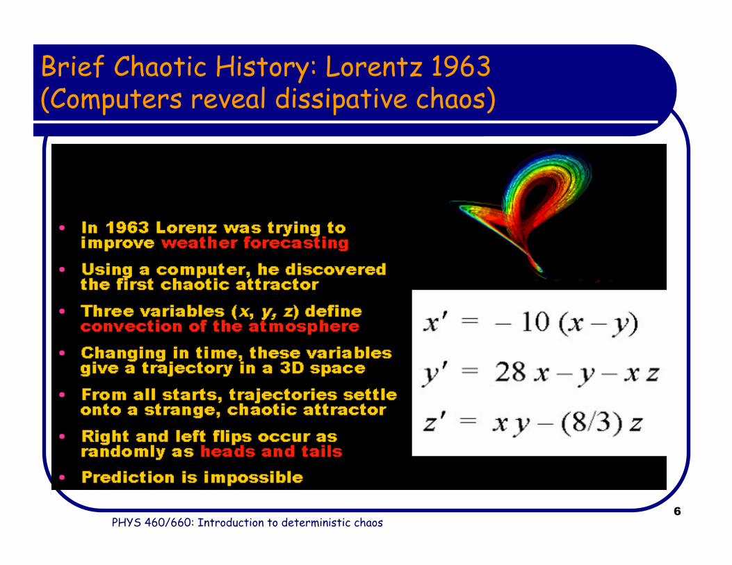
Chaos in the Brave New World of Computers

Poincaré created an original method to understand chaotic systems, and discovered their very complicated time evolution, but:"It is so complicated that I cannot even draw the figure."


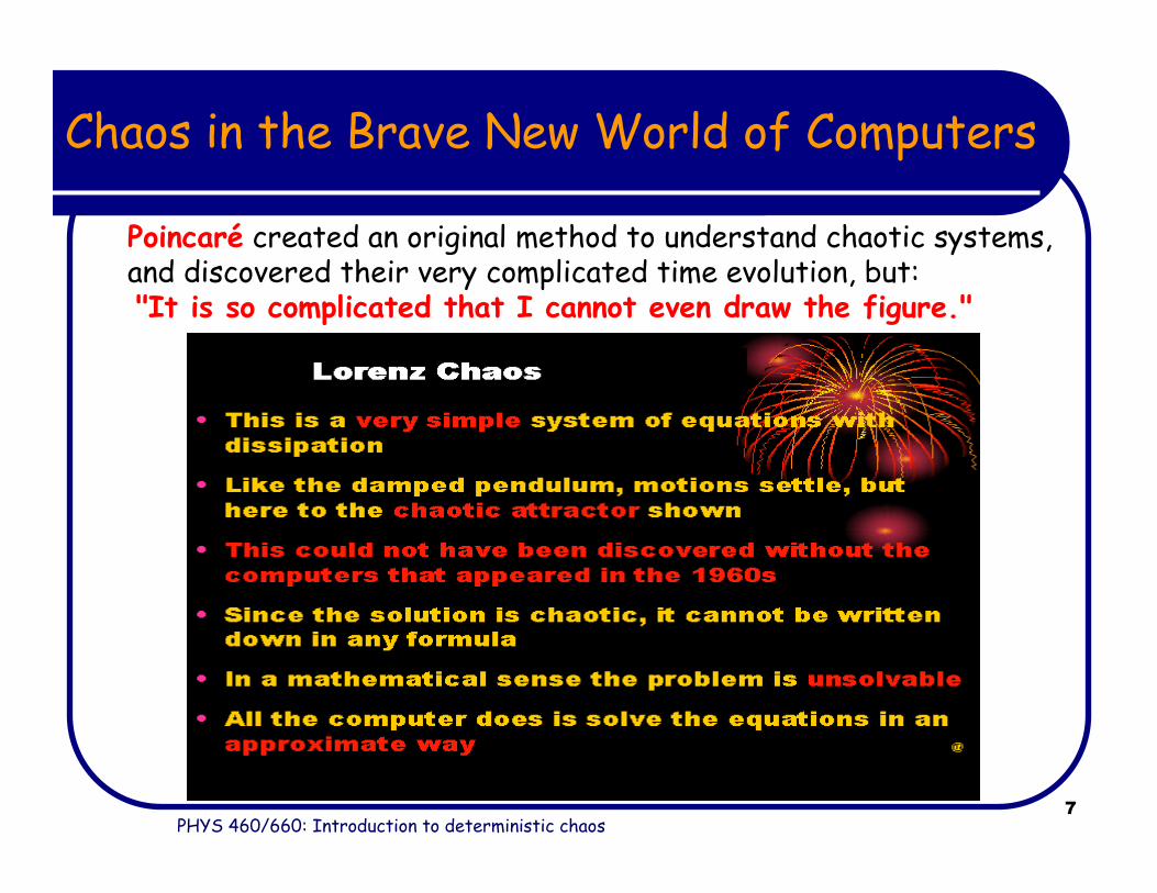
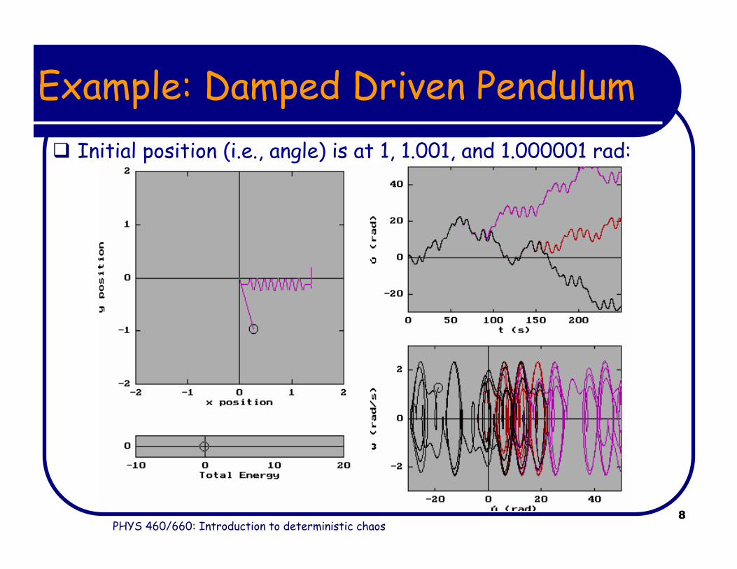
Example: Damped Driven Pendulum

Initial position (i.e., angle) is at 1, 1.001, and 1.000001 rad:


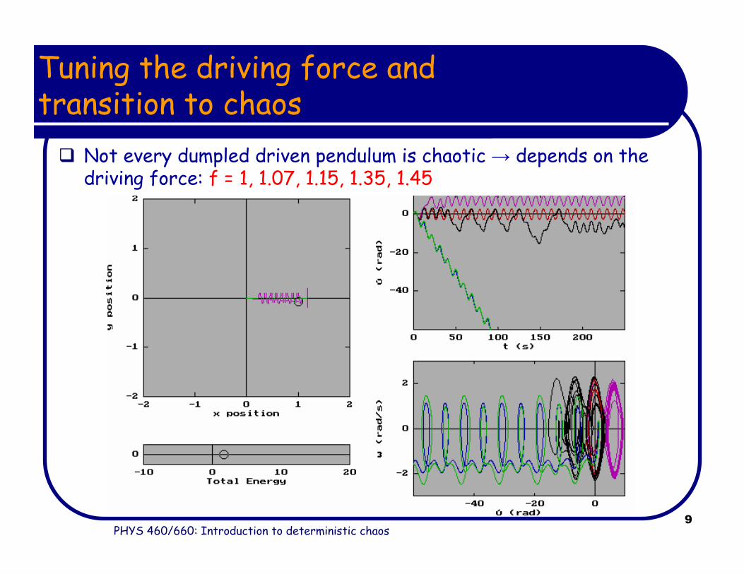
Tuning the driving force and transition to chaos

Not every dumpled driven pendulum is chaotic → depends on the driving force: f = 1, 1.07, 1.15, 1.35, 1.45


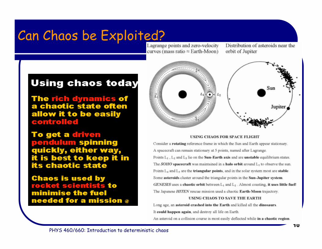
Can Chaos be Exploited?


Chaos in Physical Systems

Chaos is seen in many physical systems: fluid dynamics (weather patterns) and turbulence

some chemical reactions

Lasers

electronic circuits

particle accelerators

plasma (such as in fusion reactors and space)

Conditions necessary for chaos:system has 3 independent dynamical variables

the equations of motion are non-linear


Concepts in Dynamical System Theory

A dynamical system is defined as a deterministic mathematical prescription for evolving the state of a system forward in time.

Example: A system of N first-order and autonomous ODE

[ ]

11 2

21 21 2

1 2

1 2

( , , , )

set of points ( , , , ) is phase space( , , , )

( ), ( ), , ( ) is trajectory or flow

( , , , )

n

nn

n

Nn

dxF x x x

dt

dxx x xF x x x

dtx t x t x t

dxF x x x

dt

=

= ⇒

=

…

……

…⋮

…

3 nonlinearity CHAOS becomes possible!N ≥ + ⇒


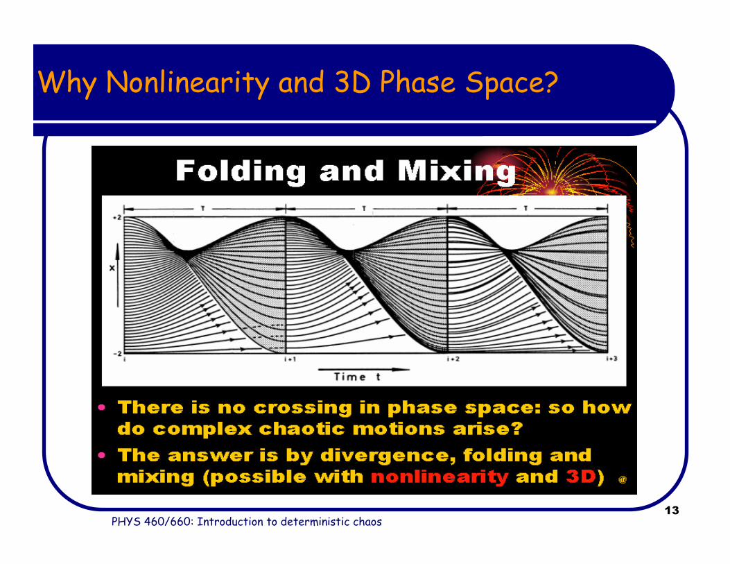
Why Nonlinearity and 3D Phase Space?


Differential Equation for damped Driven Pendulum

Nonlinear ODE of the second order:

First step for computational approach →convert ODE into a dimensionless form:

2

2sin cos( )

D

d dml c mg A t

dt dt

θ θθ ω φ+ + = +

0sin cos( )D

d dq f t

dt dt

ω θθ ω φ+ + = +


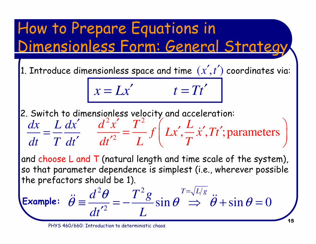
How to Prepare Equations in Dimensionless Form: General Strategy

x Lx′=

1. Introduce dimensionless space and time coordinates via:

t Tt′=

( , )x t′ ′

2. Switch to dimensionless velocity and acceleration:dx L dx

dt T dt

′=

′

2 2

2, , ;parameters

d x T Lf Lx x Tt

dt L T

′ ′ ′ ′= ′ ɺ

and choose L and T (natural length and time scale of the system), so that parameter dependence is simplest (i.e., wherever possible the prefactors should be 1).

Example:2 2

2sin sin 0

T L gd T g

dt L

θθ θ θ θ

=

≡ = − ⇒ + =′

ɺɺ ɺɺ


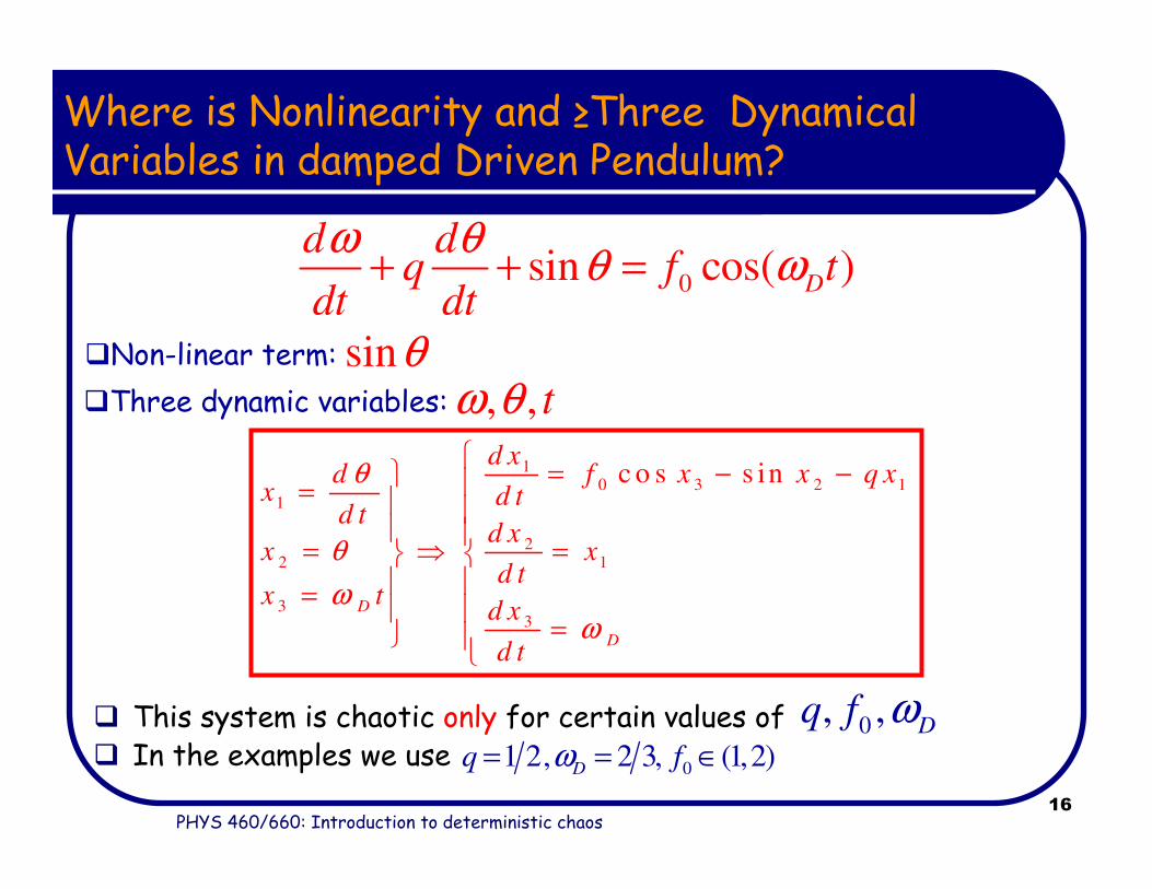
Where is Nonlinearity and ≥Three Dynamical Variables in damped Driven Pendulum?

This system is chaotic only for certain values of In the examples we use

10 3 2 1

1

22 1

33

c o s s in

D

D

d xf x x q xd

x d td t

d xx x

d tx t

d x

d t

θ

θ

ωω

= − − =

= ⇒ =

=

=

0sin cos( )D

d dq f t

dt dt

ω θθ ω+ + =

Non-linear term: sinθThree dynamic variables: , , tω θ

0, ,D

q f ω01 2, 2 3, (1,2)Dq fω= = ∈


07.10=f

15.10=f

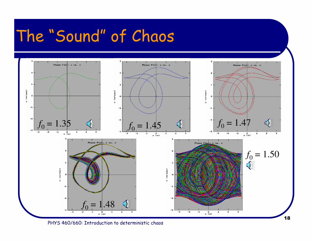
To watch the onset of chaos (as f0 is increased) we look at the motion of the system in phase space, once transients die away

Pay close attention to the period doubling that precedes the onset of chaos.

Routes to Chaos: Period Doubling


f0 = 1.35

f0 = 1.48

f0 = 1.45 f0 = 1.47

f0 = 1.50

The “Sound” of Chaos


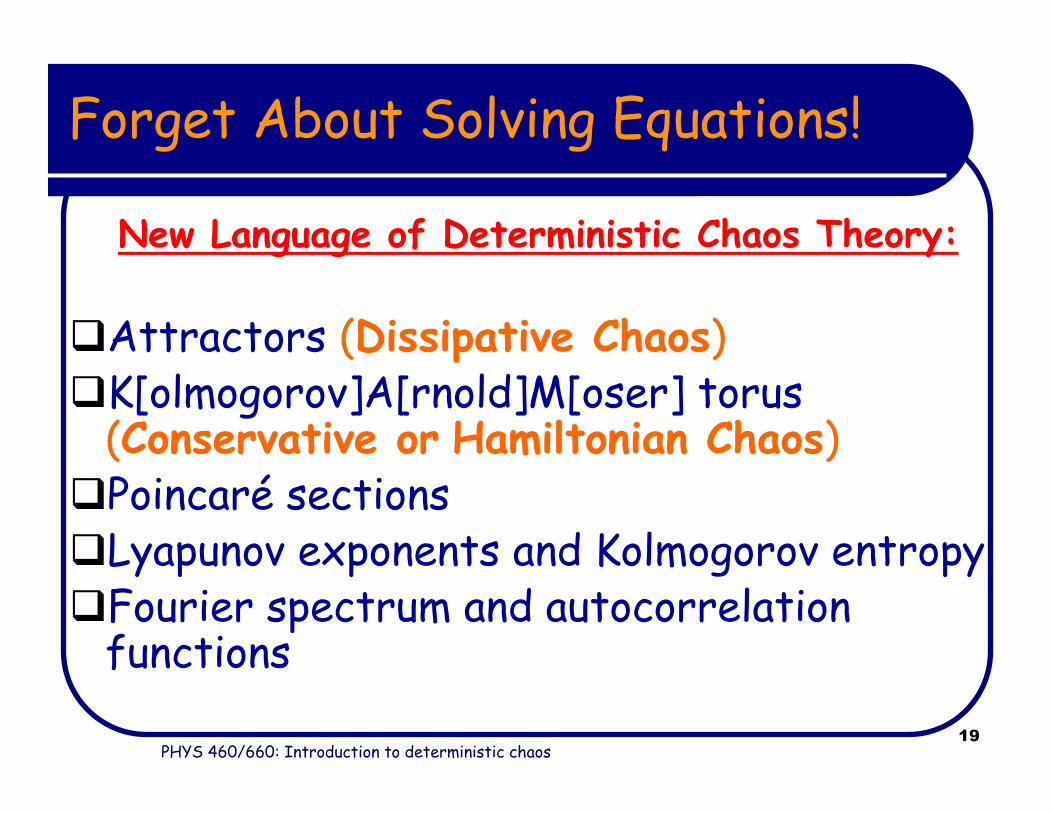
Forget About Solving Equations!

New Language of Deterministic Chaos Theory:

Attractors (Dissipative Chaos)K[olmogorov]A[rnold]M[oser] torus (Conservative or Hamiltonian Chaos)

Poincaré sectionsLyapunov exponents and Kolmogorov entropyFourier spectrum and autocorrelation functions


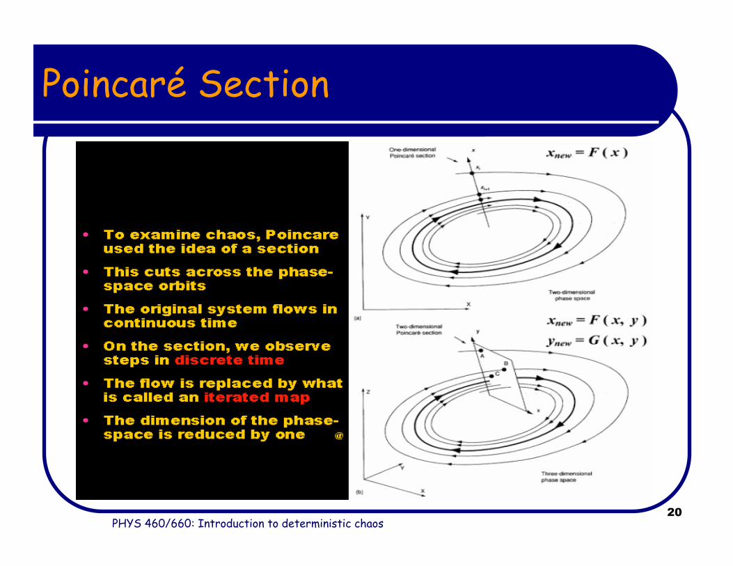
Poincaré Section


Poincaré Section: Examples

1 ( )n P nP f P+ =

Poincare Map: Continuous time evolution is replace by a discrete map


f0 = 1.07

f0 = 1.48

f0 = 1.50

f0 = 1.15

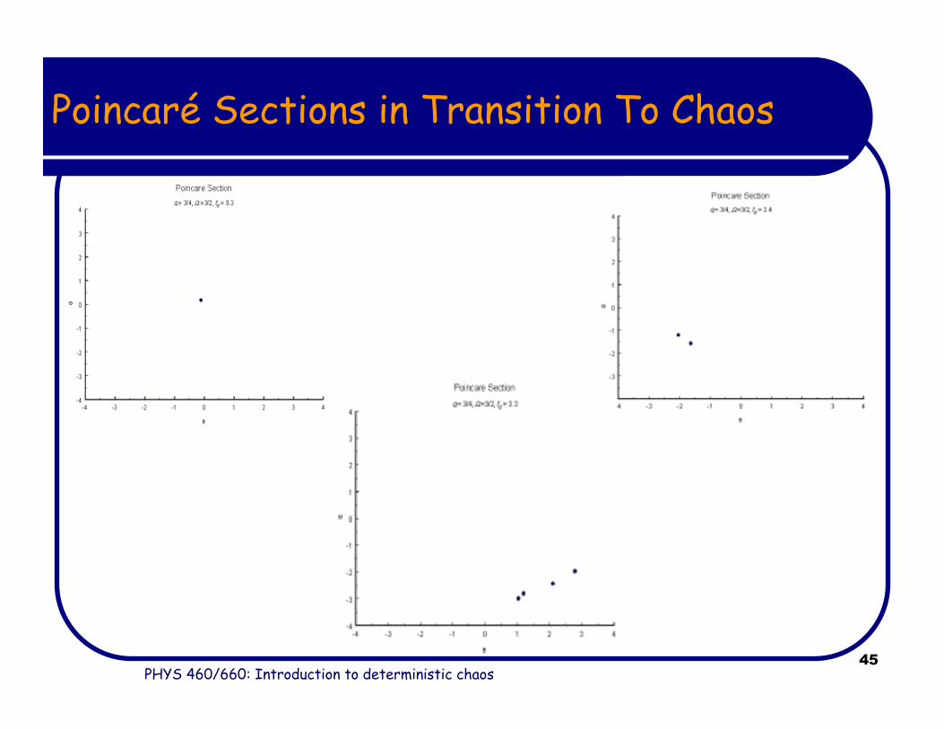
Poincaré Section of Pendulum: A slice of the 3D phase space at a fixed value of mod2Dtω π

q = 0.25


Attractors in Phase Space

The surfaces in phase space which the pendulum follows, after transient motion decays, are called attractors.

Non-Chaotic Attractor Examples:

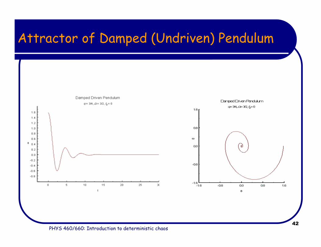
→for a damped undriven pendulum, attractor is just a point at θ=ω=0 (0D in 2D phase space).

→for an undamped pendulum, attractor is a curve (1D attractor).


Fractal Nature of Strange Attractors

Chaotic attractors of dissipative systems are strange → fractals with non-integer dimension (2<dim<3 for pendulum) and zero volume.The fine structure is quite complex and similar to the gross structure –fractals reveal self-similarity when viewed by a magnifying glass.


World of Fractals in PicturesA fractal is an object or quantity that displays self-similarity on all scales - the object need not exhibit exactly the same structure at all scales, but the same "type" of structures must appear on all scales

Their surface area is large and depends on the resolution (accuracy of measurement)

The prototypical example for a fractal in nature is the length of a coastline measured with different length rulers. The shorter the ruler, the longer the length measured, a paradox known as the coastline paradox.

Gosper:

Koch:

box:

Sierpinski:

Barnsley:

Mandelbrot:


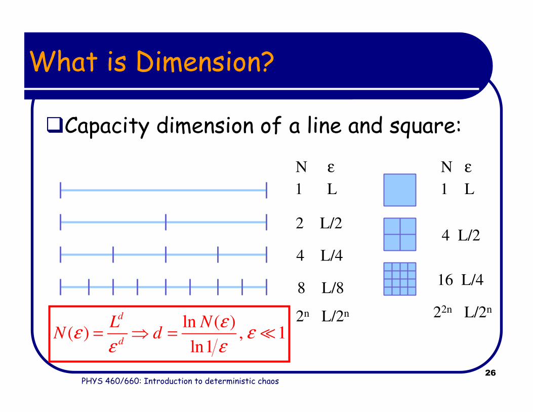
What is Dimension?

Capacity dimension of a line and square:

1 L

2 L/2

4 L/4

8 L/8

2n L/2n

N ε

1 L

4 L/2

16 L/4

22n L/2n

N ε

ln ( )( ) , 1

ln1

d

d

L NN d

εε ε

ε ε= ⇒ = ≪


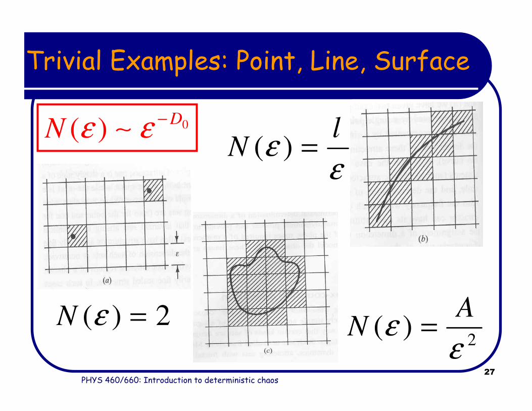
Trivial Examples: Point, Line, Surface

( ) 2N ε =2

( )A

N εε

=

( )l

N εε

=0( )

DN ε ε −

∼


Non-Trivial Examples: Cantor Set and Koch CurveThe Cantor set is produced as follows: N ε

1 1

2 1/3

4 1/9

8 1/271

ln 2 ln3

0

1 ln 22 boxes of size = ( ) 0.576 1

3 ln 3

n

nN Dε ε ε

− ⇒ = ⇒ = = <

0

ln 4

ln 3D =


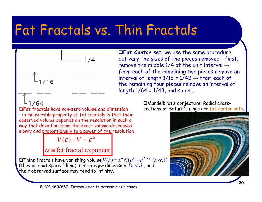
Mandelbrot’s conjecture: Radial cross-sections of Saturn's rings are fat Cantor sets.

Fat Fractals vs. Thin Fractals

Fat Cantor set: we use the same procedure but vary the sizes of the pieces removed - first, remove the middle 1/4 of the unit interval →from each of the remaining two pieces remove an interval of length 1/16 = 1/42 → from each of the remaining four pieces remove an interval of length 1/64 = 1/43, and so on …

( )

fat fractal exponent

V Vαε ε

α

−

≡

∼

Fat fractals have non-zero volume and dimension →a measurable property of fat fractals is that their observed volume depends on the resolution in such a way that deviation from the exact volume decreases slowly and proportionally to a power of the resolution

Thins fractals have vanishing volume (they are not space filling), non-integer dimension , and their observed surface may tend to infinity.

0( ) ( ) ( 1)d Dd

V Nε ε ε ε ε−= ∼ ≪

0D d<


Lyapunov Exponents

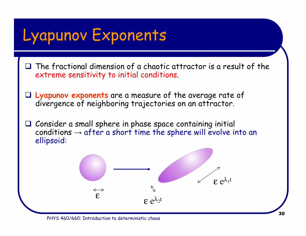
The fractional dimension of a chaotic attractor is a result of the extreme sensitivity to initial conditions.

Lyapunov exponents are a measure of the average rate of divergence of neighboring trajectories on an attractor.

Consider a small sphere in phase space containing initial conditions → after a short time the sphere will evolve into an ellipsoid:

εε eλ2t

ε eλ1t


Connection Between Lyapunov Exponents and Fractal Dimension

The average rate of expansion along the principle axes are the Lyapunov exponents

Chaos implies that at least one Lyapunovexponents is > 0!

For the pendulum: (damping coefficient)

→no contraction or expansion along t direction, so that exponent is zero

→can be shown that the dimension of the attractor is:

0 1 22D λ λ= −

i

i

qλ = −∑


Kolmogorov Entropy

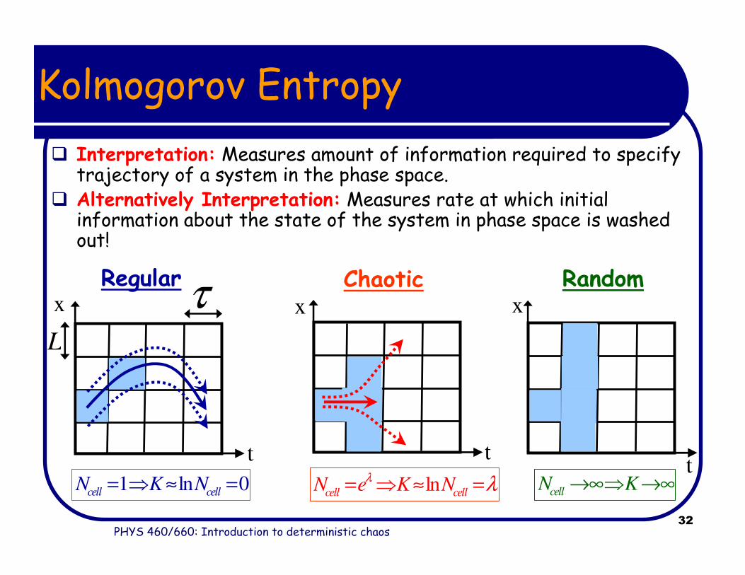
Interpretation: Measures amount of information required to specify trajectory of a system in the phase space.

Alternatively Interpretation: Measures rate at which initial information about the state of the system in phase space is washed out!

τL

1 ln 0cell cellN K N= ⇒ ≈ =

Regular Chaotic Random

lncell cellN e K Nλ λ= ⇒ ≈ = cellN K→∞⇒ →∞

x

tt

t

x x


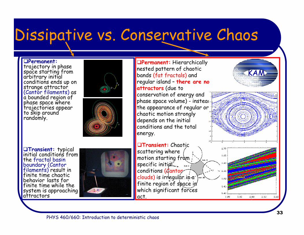
Dissipative vs. Conservative Chaos

Transient: typical initial conditions from the fractal basin boundary (Cantor filaments) result in finite time chaotic behavior lasts for finite time while the system is approaching attractors

Permanent: Hierarchically nested pattern of chaotic bands (fat fractals) and regular island – there are no attractors (due to conservation of energy and phase space volume) - instead the appearance of regular or chaotic motion strongly depends on the initial conditions and the total energy.

Transient: Chaotic scattering where motion starting from specific initial conditions (Cantor clouds) is irregular in a finite region of space in which significant forces act.

Permanent:trajectory in phase space starting from arbitrary initial conditions ends up on strange attractor (Cantor filaments) as a bounded region of phase space where trajectories appear to skip around randomly.

KAM


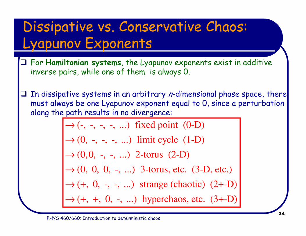
For Hamiltonian systems, the Lyapunov exponents exist in additive inverse pairs, while one of them is always 0.

In dissipative systems in an arbitrary n-dimensional phase space, there must always be one Lyapunov exponent equal to 0, since a perturbation along the path results in no divergence:

(-, -, -, -, ...) fixed point (0-D)

(0, -, -, -, ...) limit cycle (1-D)

(0,0, -, -, ...) 2-torus (2-D)

(0, 0, 0, -, ...) 3-torus, etc. (3-D, etc.)

( , 0, -, -, ...) strange (chaotic) (2+-D)

→

→

→

→

→ +

( , , 0, -, ...) hyperchaos, etc. (3+-D)→ + +

Dissipative vs. Conservative Chaos: Lyapunov Exponents


Logistic Map

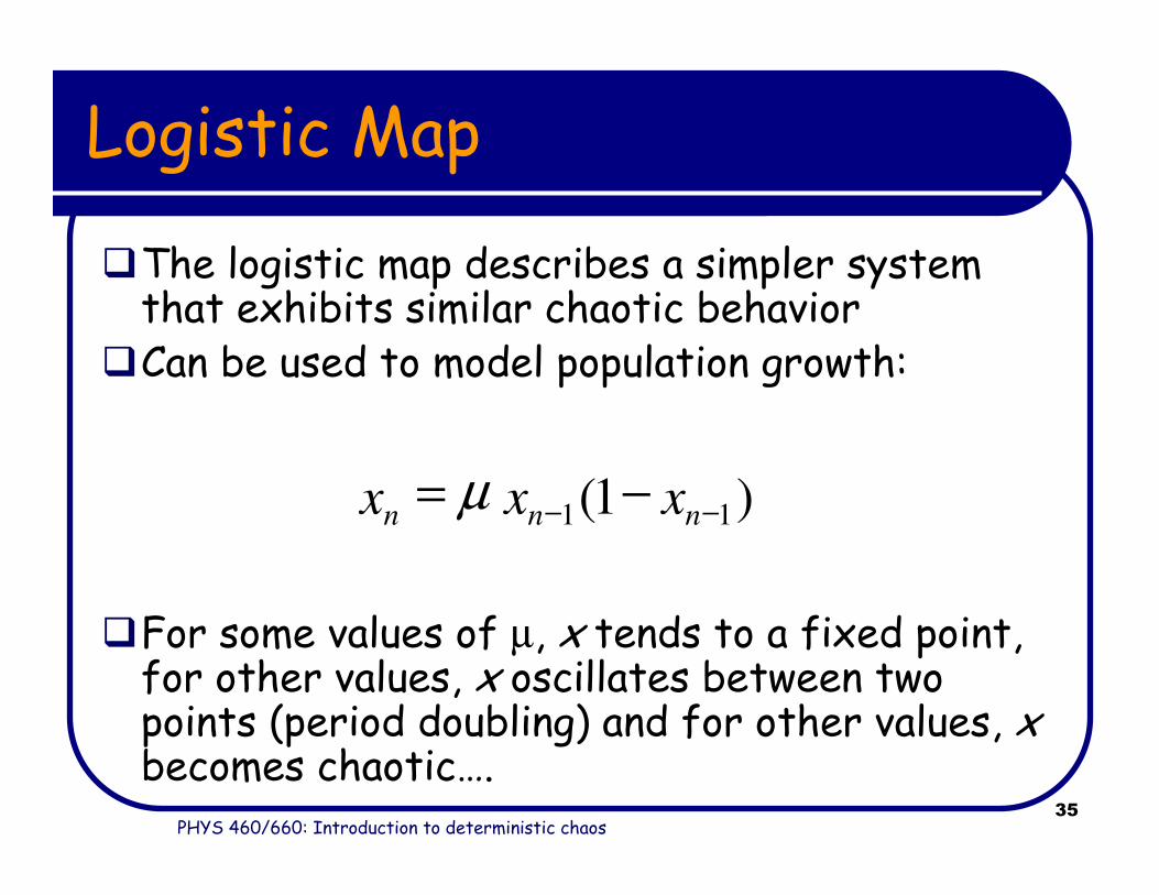
The logistic map describes a simpler system that exhibits similar chaotic behavior

Can be used to model population growth:

For some values of µ, x tends to a fixed point, for other values, x oscillates between two points (period doubling) and for other values, xbecomes chaotic….

)1( 11 −− −=nnn xxx µ


Logistic Map in Pictures

)1( 11 −− −=nnn xxx µ

xn-1

xn


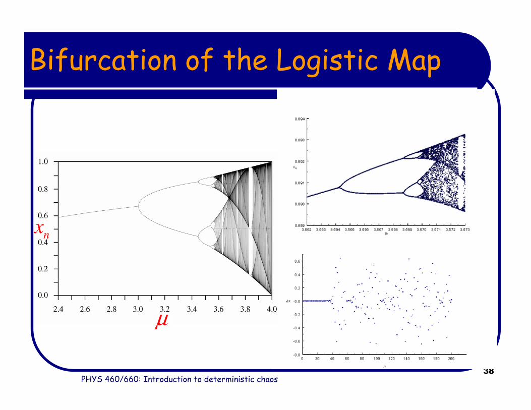
Bifurcation Diagrams

Bifurcation: a change in the number of solutions to a differential equation when a parameter is varied

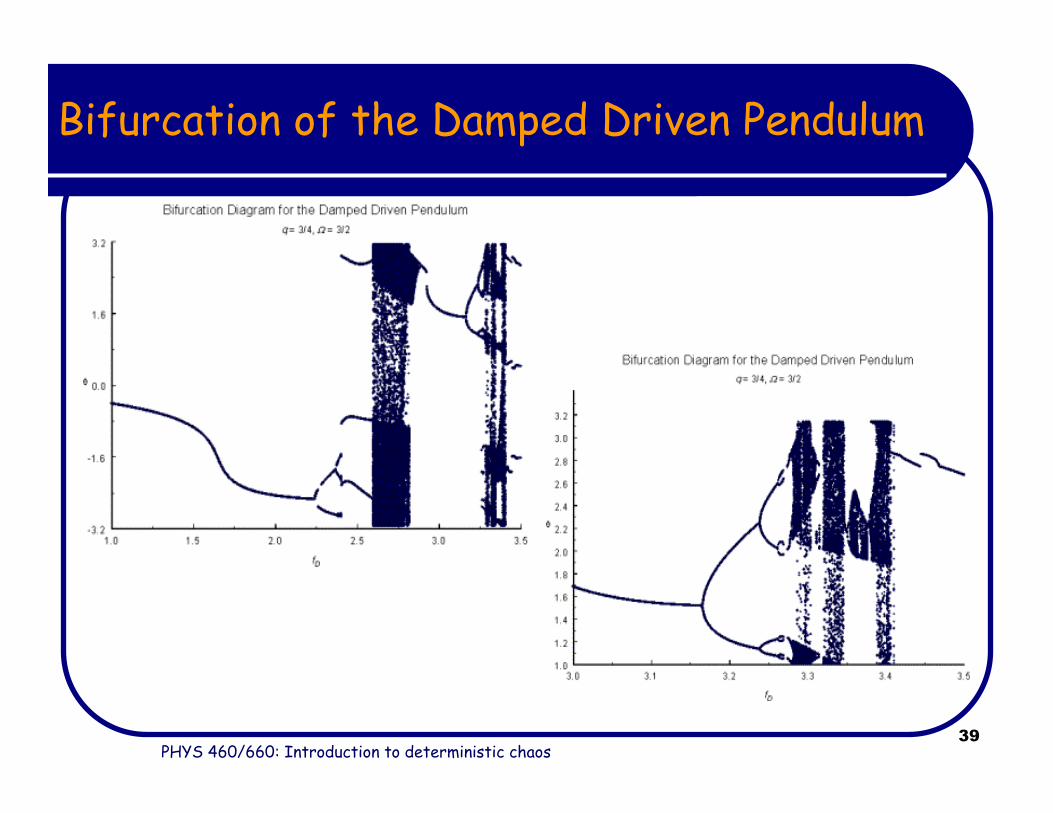
To observe bifurcation in damped driven pendulum, plot long term values of ω, at a fixed value of ωDt mod 2π as a function of the force term f0

If periodic → single value

Periodic with two solutions (left or right moving) →2 values

Period doubling → double the number

The onset of chaos is often seen as a result of successive period doublings...


Bifurcation of the Logistic Map

µ

nx


Bifurcation of the Damped Driven Pendulum


Feigenbaum Number

The ratio of spacings between consecutive values of µ at the bifurcations approaches a universal constant – the Feigenbaum number.

This is universal to all differential equations (within certain limits) and applies to the pendulum. By using the first few bifurcation points, one can predict the onset of chaos.

1

1

lim n n

nn n

µ µδ

µ µ−

→ ∞+

−=

−1

1

lim n n

nn n

F F

F F

−

→ ∞+

−=

−

n: value at which transition to period-2 takes placen nor Fµ

0 .4 6 6 9≈


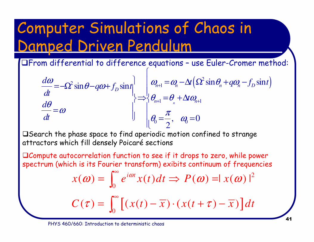
Computer Simulations of Chaos in Damped Driven Pendulum

( )22 1

1 1

0 0

sin sinsin sin

, 02

n

n n n n DD

n n

d t q f tq f t

dtt

d

dt

ω ω ω θ ωθ ω

θ θ ωθ

ω πθ ω

+

+ +

= −∆ Ω + −=−Ω − + ⇒ = +∆ = = =

Search the phase space to find aperiodic motion confined to strange attractors which fill densely Poicaré sections

Compute autocorrelation function to see if it drops to zero, while power spectrum (which is its Fourier transform) exibits continuum of frequencies

[ ]

2

0

0

( ) ( ) ( ) | ( ) |

( ) ( ( ) ) ( ( ) )

i tx e x t dt P x

C x t x x t x dt

ωω ω ω

τ τ

∞

∞

= ⇒ =

= − ⋅ + −

∫

∫

From differential to difference equations – use Euler-Cromer method:


Attractor of Damped (Undriven) Pendulum


Attractor of Damped Driven Pendulum in Non-Chaotic Regime


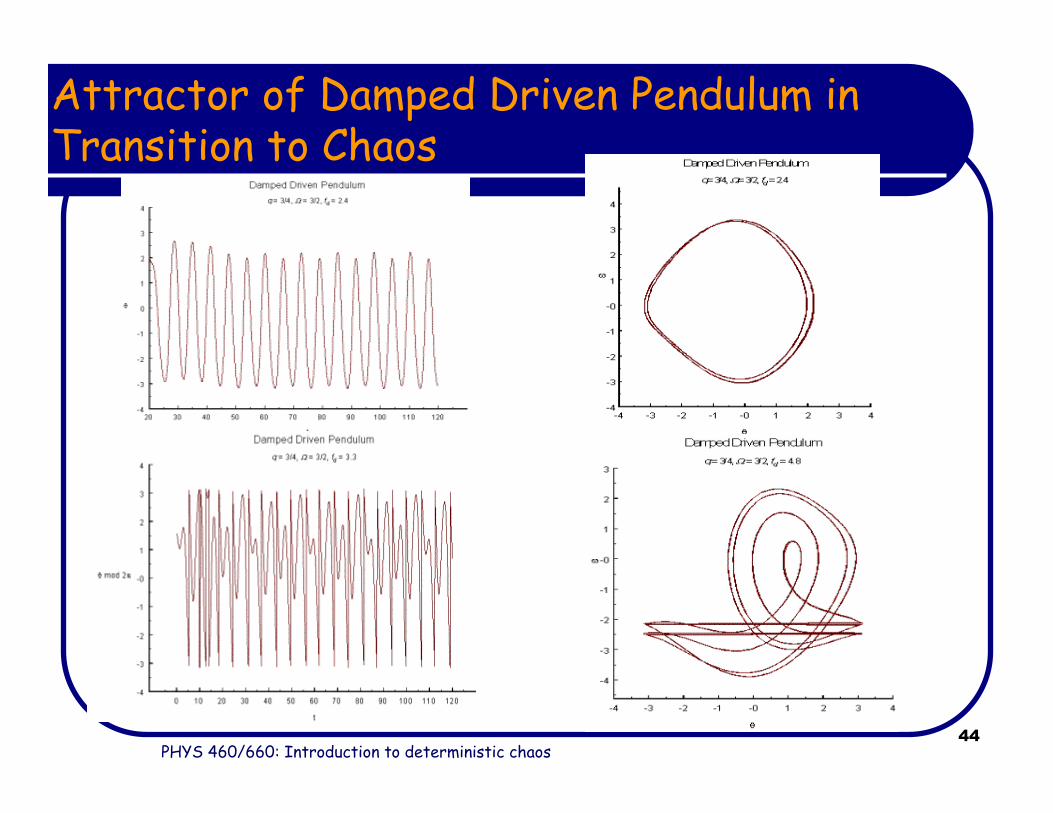
Attractor of Damped Driven Pendulum in Transition to Chaos


Poincaré Sections in Transition To Chaos


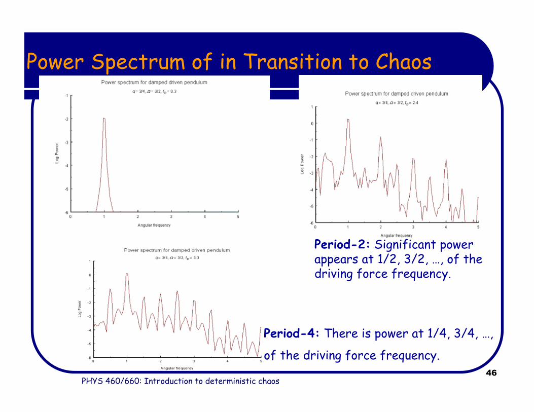
Power Spectrum of in Transition to Chaos

Period-2: Significant power appears at 1/2, 3/2, …, of the driving force frequency.

Period-4: There is power at 1/4, 3/4, …,

of the driving force frequency.


Power Spectrum in the Chaotic Regime

When the system is chaotic, there is still significant power at the drive frequency but there are no other sharp spikes in the spectrum.


Diagnostic Tools for Conservative Chaos in “Two balls in 1D with gravity” Problem

The dynamical system is chaotic if we find that:1. Poincare section contains areas which are densely filled with trajectory intersection points

3. Power spectrum displays wide continuum

2. Autocorrelation function decays fast to zero


Do Computers Simulations of Chaos Make Any Sense?

Shadowing Theorem: Numerically computed chaotic Although a trajectory diverges exponentially from the true trajectory with the same initial coordinates, there exists an errorless trajectory with a slightly different initial condition that stays near ("shadows") the numerically computed one. Therefore, the fractal structure of chaotic trajectories seen in computer maps is real.

14

14

28

10 a

ccur

acy

of in

itial

con

ditio

ns

210

1

45

twic

e as

long

pre

dict

ion

90

10

accu

racy

of i

nitia

l con

ditio

ns

n

n

n

−

−

−⇒

⇒

⇒

∼

∼

∼

Documents

Branislav K. Nikoli ć - Delaware Physics · Branislav K. Nikoli ... predict exactly the situation of that same universe at a succeeding moment. but even if it ... Their surface area