Embed Size (px)
Citation preview
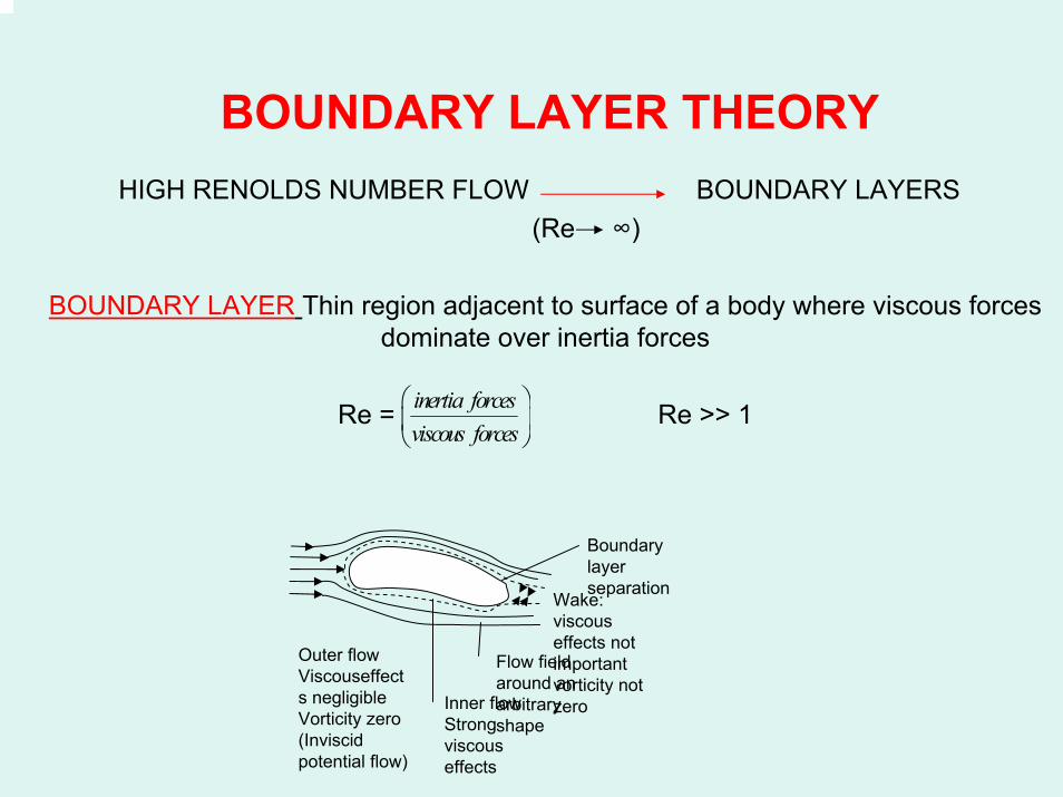
HIGH RENOLDS NUMBER FLOW BOUNDARY LAYERS(Re ∞)
BOUNDARY LAYER Thin region adjacent to surface of a body where viscous forces dominate over inertia forces
Re = Re >> 1
inertia forcesviscous forces⎛ ⎞⎜ ⎟⎝ ⎠
BoundarylayerseparationWake:
viscouseffects not importantvorticity not zero
Flow fieldaround an arbitraryshape
Inner flowStrongviscouseffects
Outer flowViscouseffects negligibleVorticity zero(Inviscidpotential flow)
BOUNDARY LAYER THEORY

Steady ,incompressible 2-D flow with no body
forces. Valid for laminar flow
O.D.E for To solve eq. we first ”assume” an approximate velocity profile inside the B.LRelate the wall shear stress to the velocity field
Typically the velocity profile is taken to be a polynomial in y, and the degree of fluid
this polynominal determines the number of boundary conditions which may be
satisfied
EXAMPLE: LAMINAR FLOW OVER A FLAT PLATE:
* 02
1( 2 )d dUdx dx U
τθ δ θθ ρ
+ + = 0 ( ) nud y
τ ∂∼
( )xθ
2 ( )u a b c fU
η η η= + + =
U∞
U ≈0,99U∞

Re ULν
=
High Reynolds Number Flow
• Laminar boundary layer predictable• Turbulent boundary layer poor predictability
• Controlling parameter
• To get two boundary layer flows identical match Re(dynamic similarity)
• Although boundary layer’s and prediction are complicated,simplify the N-S equations to make job easier
2-D , planar flow
u* = , x*, y*= * ,u vvU∞
= ,x yL
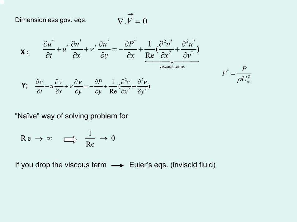
Dimensionless gov. eqs.
X ;
Y;
“Naïve” way of solving problem for
If you drop the viscous term Euler’s eqs. (inviscid fluid)
2 2
2 2
1 ( )Re
Put x y y x yν ν ν ν νν∂ ∂ ∂ ∂ ∂ ∂+ + = − + +
∂ ∂ ∂ ∂ ∂ ∂
. 0V→
∇ =
* * * * 2 * 2 ** *
2 2
viscous terms
1 ( )Re
u u u P u uut x y x x y
ν∂ ∂ ∂ ∂ ∂ ∂+ + = − + +
∂ ∂ ∂ ∂ ∂ ∂
*2
PPUρ ∞
=
1 0Re
→R e → ∞
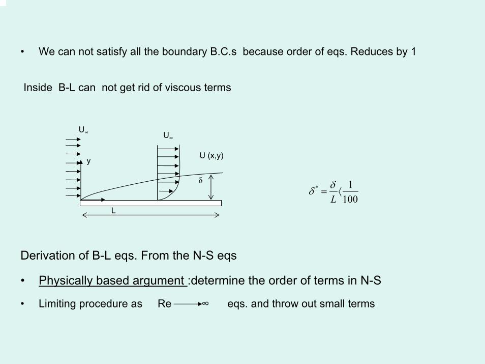
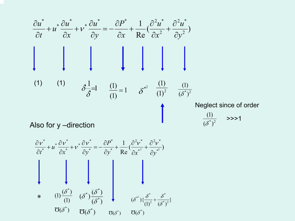
• We can not satisfy all the boundary B.C.s because order of eqs. Reduces by 1
Inside B-L can not get rid of viscous terms
Derivation of B-L eqs. From the N-S eqs
• Physically based argument :determine the order of terms in N-S
• Limiting procedure as Re ∞ eqs. and throw out small terms
U∞
U (x,y)y
L
U∞
δ* 1
100Lδδ = ⟨
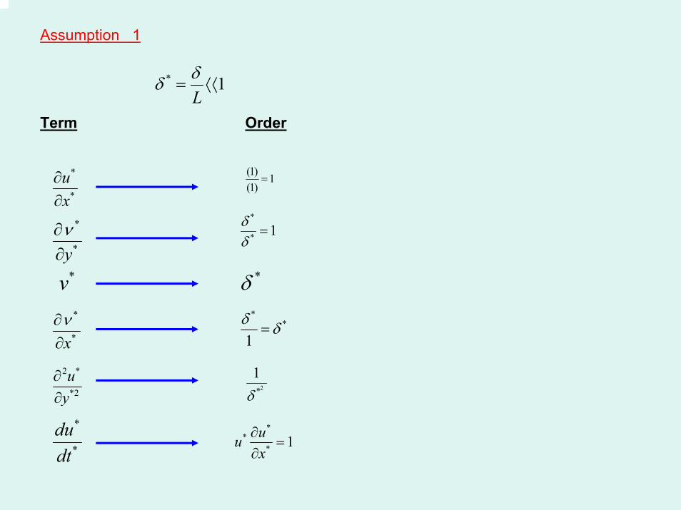
Assumption 1
Term Order
*v
* 1Lδδ = ⟨⟨
*
*
ux∂∂
*
*yν∂∂
*
*xν∂∂
2 *
*2
uy∂∂
*
*
dudt
(1) 1(1)
=
*
* 1δδ
=
**
1δ δ=
2*
1δ
**
* 1uux∂
=∂
*δ
(1) (1)
Neglect since of order
>>>1
2 2
* * * * 2 * 2 ** *
* * * * * *
1 ( )Re
Put x y y x yν ν ν ν νν∂ ∂ ∂ ∂ ∂ ∂
+ + = − + +∂ ∂ ∂ ∂ ∂ ∂
* * * * 2 * 2 ** *
2 2
1 ( )Re
u u u P u uut x y x x y
ν∂ ∂ ∂ ∂ ∂ ∂+ + = − + +
∂ ∂ ∂ ∂ ∂ ∂
**
1 1δδ= (1) 1
(1)=
2*δ 2
(1)(1) * 2
(1)( )δ
* 2
(1)( )δAlso for y –direction
*
*
( )(1)(1)
( )
δ
δ
**
*
*
( )( )( )
( )
δδδ
δ
* 2* *
*2 * 2
*
( ){ }(1) ( )
( )
δ δδδ
δ
+
*( )δ
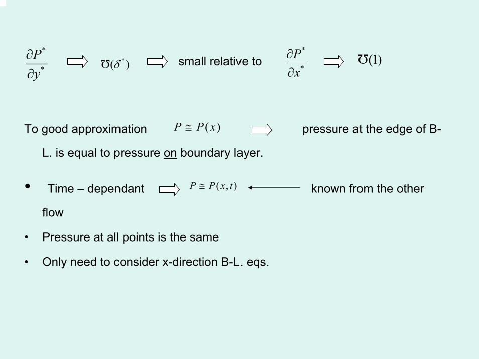
small relative to
To good approximation pressure at the edge of B-
L. is equal to pressure on boundary layer.
• Time – dependant known from the other
flow
• Pressure at all points is the same
• Only need to consider x-direction B-L. eqs.
*
*
Py
∂∂
*( )δ*
*
Px
∂∂
(1)
( )P P x≅
( , )P P x t≅
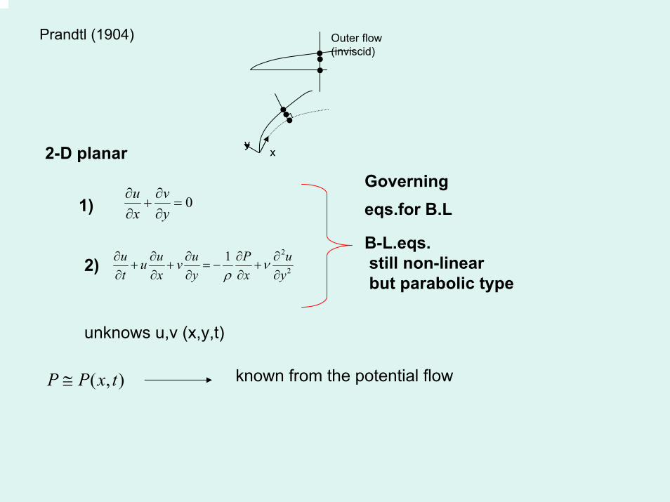
Prandtl (1904)
0u vx y∂ ∂
+ =∂ ∂
Outer flow(inviscid)
yx2-D planar
1)
2)2
2
1u u u P uu vt x y x y
νρ
∂ ∂ ∂ ∂ ∂+ + = − +
∂ ∂ ∂ ∂ ∂
Governingeqs.for B.L
B-L.eqs.still non-linearbut parabolic type
unknows u,v (x,y,t)
known from the potential flow( , )P P x t≅

Need B.C.s & I.C.(time dependant)
• 2-D, steady
BCs
• u= =0 at y=0
• u=u(y) at x=0
• u= (x) y (y ) marching condition
• B-L. eqs. can be solved exactly for several cases• Can approximate solution for other casesLimitation of B.L egs.: where they fail?(1) Abrupt chances
ν
U∞ ∞ δ
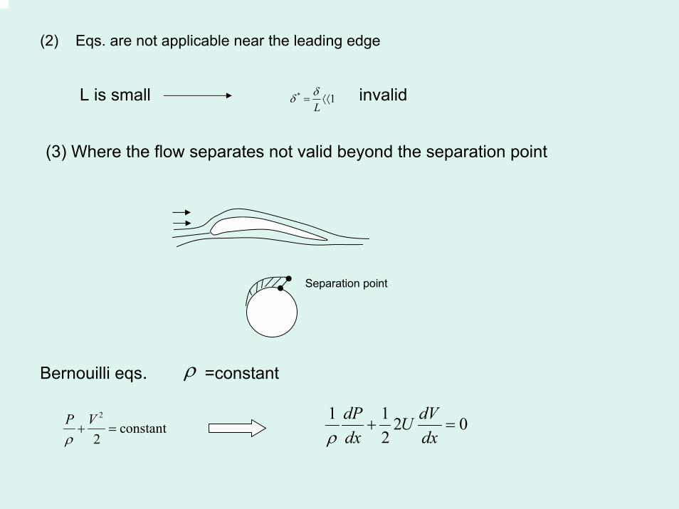
(2) Eqs. are not applicable near the leading edge
* 1Lδδ = ⟨⟨L is small invalid
(3) Where the flow separates not valid beyond the separation point
Separation point
Bernouilli eqs. =constantρ
1 1 2 02
dP dVUdx dxρ
+ =2
constant2
P Vρ+ =

Valid along the streamlines
substitute the B.L eqs u,v can be found
known
0dpdx
=
1 dP dUUdx dxρ
− =
SIMILARITY SOLUTION TO B.L. EQS
Example 1
Flow over a semi-infinite flat plate
Zero pressure gradient p = constant
Steady ,laminar & U=constant ( )0dpdx
=
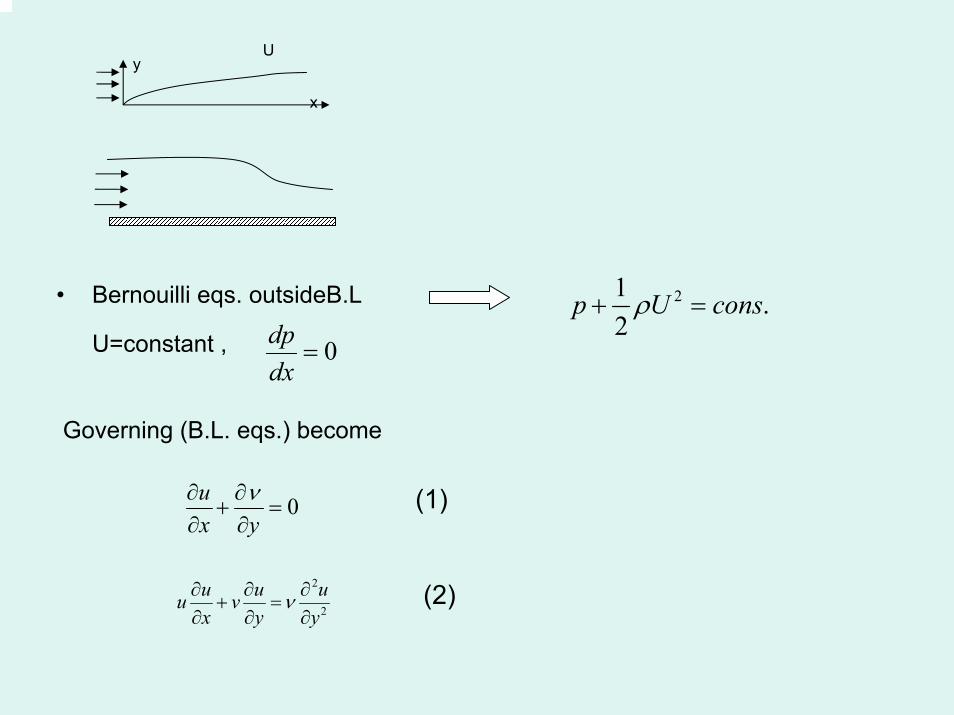
• Bernouilli eqs. outsideB.L
U=constant ,
Governing (B.L. eqs.) become
2
2
u u uu vx y y
ν∂ ∂ ∂+ =
∂ ∂ ∂
Uy
x
21 .2
p U consρ+ =
0dpdx
=
0ux y
ν∂ ∂+ =
∂ ∂(1)
(2)
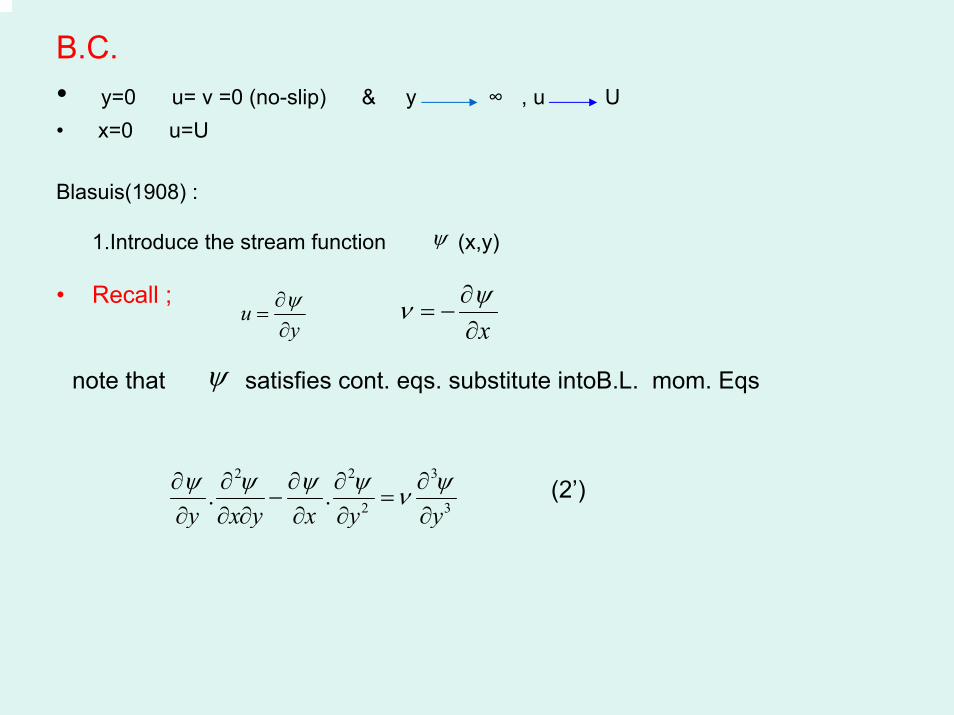
B.C.• y=0 u= v =0 (no-slip) & y ∞ , u U• x=0 u=U
Blasuis(1908) :
1.Introduce the stream function (x,y)
• Recall ;
ψ
uyψ∂
=∂ x
ψν ∂= −
∂
note that satisfies cont. eqs. substitute intoB.L. mom. Eqsψ
2 2 3
2 3. .y x y x y yψ ψ ψ ψ ψν∂ ∂ ∂ ∂ ∂
− =∂ ∂ ∂ ∂ ∂ ∂
(2’)

• Now, assume that we have a similarity “stretching” variable, which has all velocity
profiles on plate scaling on .i.e
( , , )g U xδ ν∞=
δ
( )u yfU δ∞
=y
δx
dimensional analysis
( ) (Re)U xg gxδ
ν∞= = 21 ( )
Reδ∼ δ ν∼
xUνδ
∞
∼ [ ]2
. .m m s ms m
= 1Rexx
δ ∼ both ( )δ
Viscous dif. Depth
yηδ
=
Re U xν∞= 5 x
Uνδ
∞
≈
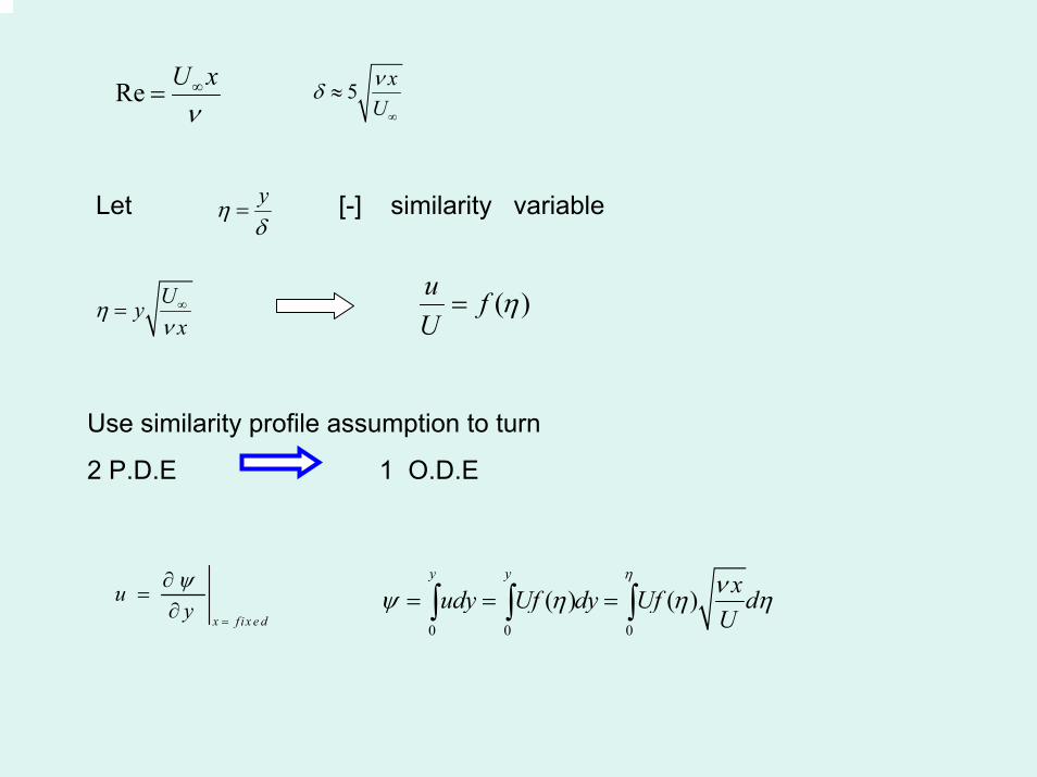
Let [-] similarity variable
Uyx
ην
∞= ( )u fU
η=
Use similarity profile assumption to turn
2 P.D.E 1 O.D.E
0 0 0
( ) ( )y y xudy Uf dy Uf d
U
η νψ η η η= = =∫ ∫ ∫x f ix e d
uyψ
=
∂=
∂
ψ
0
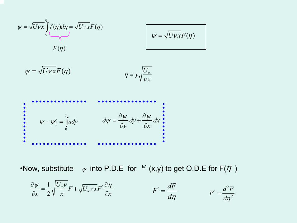
( ) ( )U x f d U xFη
ψ ν η η ν η= =∫
( )F η
( )U xFψ ν η=
( )U xFψ ν η= Uyx
ην
∞=
00
y
udyψ ψ− = ∫ d dy dxy xψ ψψ ∂ ∂
= +∂ ∂
•Now, substitute into P.D.E for (x,y) to get O.D.E for F( )ψ η
'12U F U xF
x x xνψ ην∞
∞∂ ∂
= +∂ ∂
' dFFdη
=2
''2
d FFdη
=

2''
2
UU Fy xψ
ν∞
∞∂
=∂
1 1 12 2
Uyx x x xη η
ν∞∂
= − = −∂
'1 ( )2U F F
x xνψ η∞∂
= −∂
' 'UU xF U Fy xψ ν
ν∞
∞ ∞∂
= =∂
2''
2U F
x y xψ η∞∂
= −∂ ∂
23'''
3
U Fy xψ
ν∞∂
=∂
Substituting into eq. (2’)
21 12 21'( ''') ( ) ( ') ( ) '' '''
2 2U U U UU F F F F U F Fx x x x
νη η νν ν
∞ ∞ ∞ ∞∞ ∞
⎡ ⎤ ⎡ ⎤− − − =⎢ ⎥ ⎢ ⎥⎣ ⎦ ⎣ ⎦ or
2
''2U Fxη∞−
21'2UFx∞−
21''2UF Fx∞+
2
'' ' UF Fx
η ∞= '''F
1''' '' 02
F FF+ = blasius eq. 3rd order , non linear ODE

00
0y
y
uyψ
==
∂= =∂
Note: for BVP''' '' 0F FF+ =2Uyx
ην∞=
BC’s are
At y=0 u=v=0 0η =
BC 1) 0' 0U Fη∞ =
= F’(0)=0
BC 2)0
0y
ν== 1 ( ') 0
2U F Fxν η∞− − =
F(0)=0
BC 3) (x,y ∞ ) U∞
y
Uyψ
∞→∞
∂→
∂'U F Uη∞ ∞→∞
= '( )F η →∞ 1 '( ) 1F ∞ =
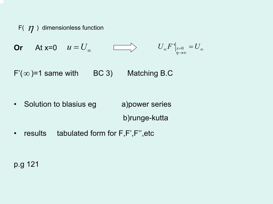
Or At x=0
F’( )=1 same with BC 3) Matching B.C
• Solution to blasius eg a)power series
b)runge-kutta
• results tabulated form for F,F’,F’’,etc
p.g 121
F( η ) dimensionless function
u U∞= 0' xU F Uη=∞ ∞→∞
=
∞
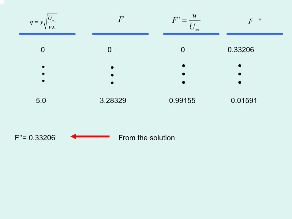
0 0 0 0.33206
F’’= 0.33206 From the solution
5.0 3.28329 0.99155 0.01591
Uyx
ην
∞= F ' uFU∞
= ''F
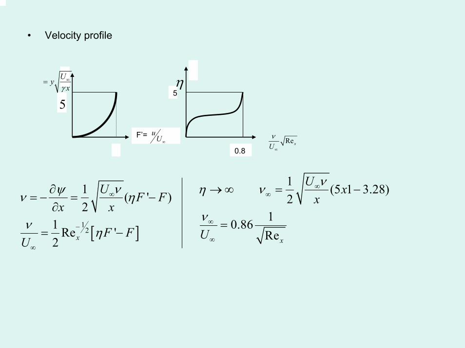
• Velocity profile
5
[ ]12
1 ( ' )2
1 Re '2 x
U F Fx x
F FU
νψν η
ν η
∞
−
∞
∂= − = −
∂
= −
1 (5 1 3.28)2
10.86Rex
U xx
U
νη ν
ν
∞∞
∞
∞
→ ∞ = −
=
RexUν
∞0.8
ηUyxγ∞=
5
F’= uU∞
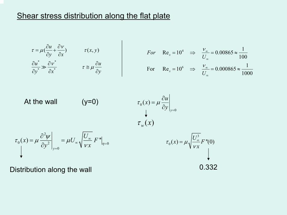
Shear stress distribution along the flat plate
* *
* *
( ) ( , )
u x yy x
u uy x y
ντ µ τ
ν τ µ
∂ ∂= +
∂ ∂
∂ ∂ ∂≅
∂ ∂ ∂
4
6
1 Re 10 0.00865100
1For Re 10 0.0008651000
x
x
ForU
U
ν
ν
∞
∞
∞
∞
= ⇒ = ≈
= ⇒ = ≈
At the wall (y=0) 00
( )y
uxy
τ µ=
∂=
∂
( )w xτ2
0 2 00
( ) ''y
Ux U Fy x η
ψτ µ µν
∞∞ =
=
∂= =
∂
3
0 ( ) ''(0)Ux Fx
τ µν
∞=
Distribution along the wall 0.332
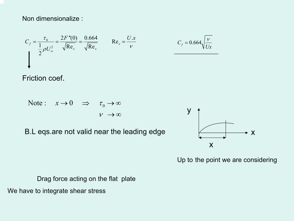
Non dimensionalize :
0
2
2 ''(0) 0.664 . Re1 Re Re2
f xx x
F U xCU
τνρ ∞
= = = = 0.664fC Uxν
=
Friction coef.
0Note : 0
x τν
→ ⇒ →∞
→∞ y
xB.L eqs.are not valid near the leading edge
x
Up to the point we are considering
Drag force acting on the flat plate
We have to integrate shear stress
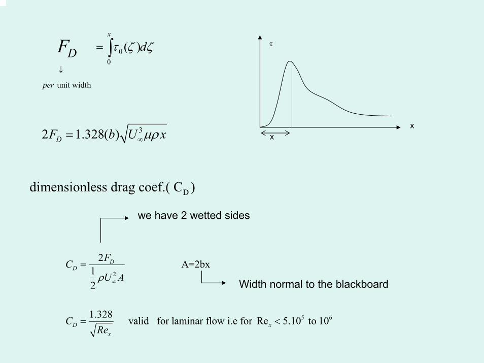
00
unit width
( )x
per
dDF τ ζ ζ
↓
= ∫
32 1.328( )DF b U xµρ∞=x
τ
x
Ddimensionless drag coef.( C )
we have 2 wetted sides
2
5 6
2 A=2bx12
1.328 valid for laminar flow i.e for Re 5.10 to 10
DD
D xx
FCU A
CRe
ρ ∞
=
= <
Width normal to the blackboard
6xfor Re >10 turbulent drag becomes considerably greater→
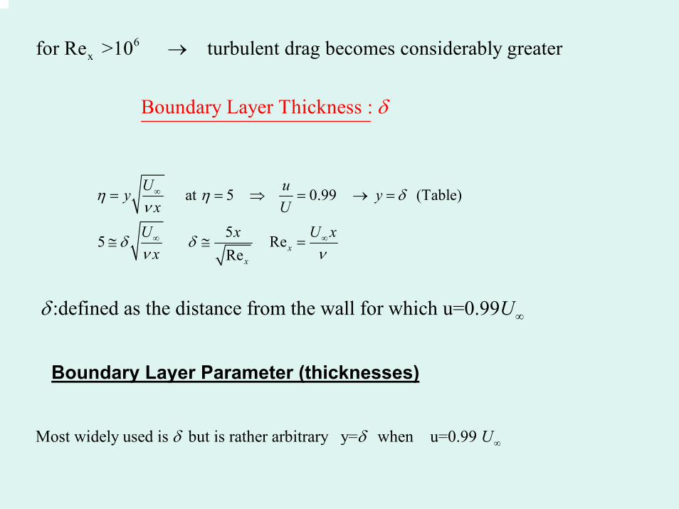
Boundary Layer Thickness : δ
at 5 0.99 (Table)
55 ReRe x
x
U uy yx U
U U xxx
η η δν
δ δν ν
∞
∞ ∞
= = ⇒ = → =
≅ ≅ =
:defined as the distance from the wall for which u=0.99Uδ ∞
Boundary Layer Parameter (thicknesses)
Most widely used is but is rather arbitrary y= when u=0.99 Uδ δ ∞
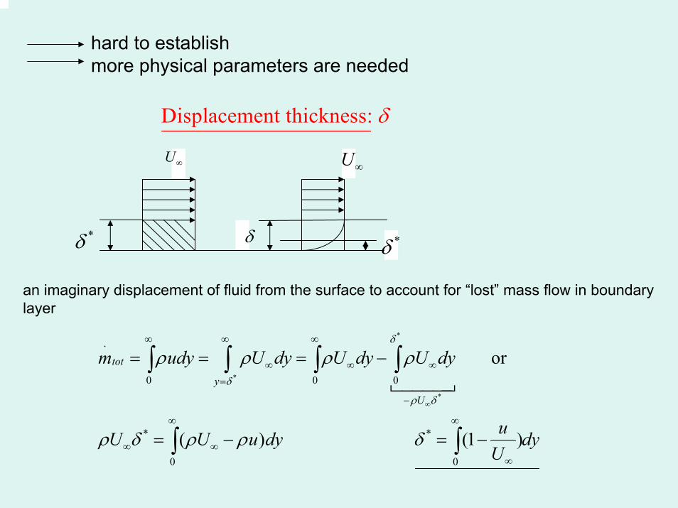
hard to establish more physical parameters are needed
Displacement thickness: δ
U∞ U∞
δ*δ *δ
an imaginary displacement of fluid from the surface to account for “lost” mass flow in boundary layer
*
*
*
.
0 0 0
* *
0 0
or
( ) (1 )
tot
y
U
m udy U dy U dy U dy
uU U u dy dyU
δ
δ
ρ δ
ρ ρ ρ ρ
ρ δ ρ ρ δ
∞
∞ ∞ ∞
∞ ∞ ∞=
−
∞ ∞
∞ ∞∞
= = = −
= − = −
∫ ∫ ∫ ∫
∫ ∫
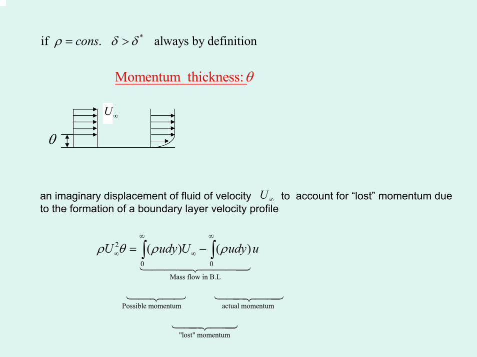
*if . always by definition consρ δ δ= >
Momentum thickness: θ
U∞
θ
an imaginary displacement of fluid of velocity to account for “lost” momentum due to the formation of a boundary layer velocity profile
U∞
2
0 0
Mass flow in B.L
Possible momentum actual momentum
( ) ( )
U udy U udy uρ θ ρ ρ∞ ∞
∞ ∞= −∫ ∫
"lost" momentum
0
(1 ) will occur in B.L eqs.u u dyU U
θ∞
∞ ∞
= −∫
*
*
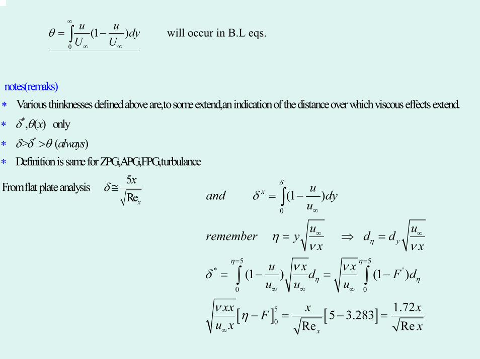
Various thinknesses defined above are,to some extend,an indication of the distance
noover which viscous effects extend.
, ( ) only> ( )
Definition is same
tes(remaks) f
xalways
δ θ
δ δ θ
∗
∗>
∗
∗or ZPG,APG,FPG,turbulance
5From flat plate analysis Rex
xδ ≅
[ ] [ ]
0
5 5* '
0 0
5
0
(1 )
(1 ) (1 )
1.725 3.283Re Re
x
y
x
uand dyu
u uremember y d dx x
u x xd F du u u
xx x xFu x x
δ
η
η η
η η
δ
ην ν
ν νδ
ν η
∞
∞ ∞
= =
∞ ∞ ∞
∞
= −
= ⇒ =
= − = −
− = − =
∫
∫ ∫
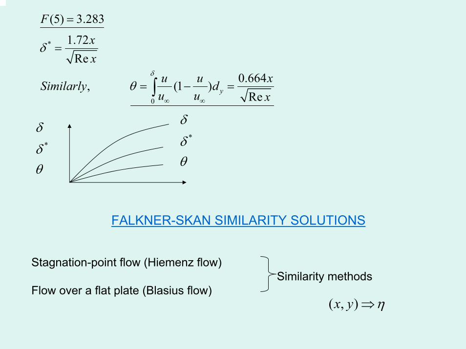
*
0
(5) 3.283
1.72Re
0.664, (1 )Rey
F
xx
u u xSimilarly du u x
δ
δ
θ∞ ∞
=
=
= − =∫
*
δ
δθ
*
δ
δθ
FALKNER-SKAN SIMILARITY SOLUTIONS
Stagnation-point flow (Hiemenz flow) Similarity methods
Flow over a flat plate (Blasius flow)( , )x y η⇒
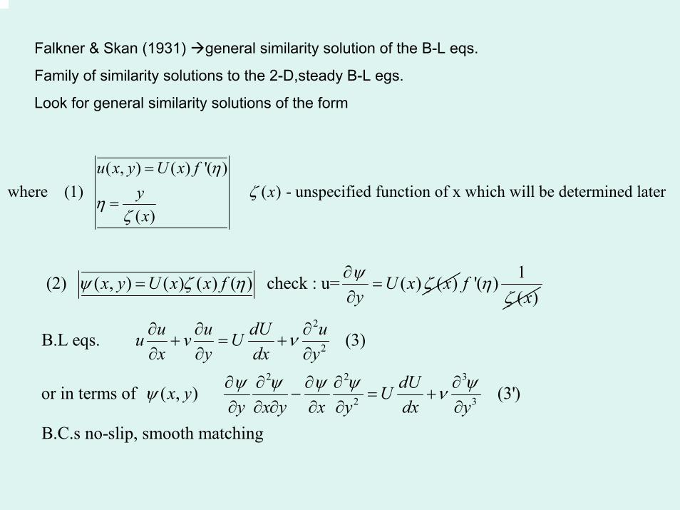
Falkner & Skan (1931) general similarity solution of the B-L eqs.
Family of similarity solutions to the 2-D,steady B-L egs.
Look for general similarity solutions of the form
( , ) ( ) '( ) where (1) ( ) - unspecified function of x which will be determined later
( )
u x y U x fxy
x
ηζ
ηζ
=
=
(2) ( , ) ( ) ( ) ( ) check : u= ( ) ( )x y U x x f U x xyψψ ζ η ζ∂
= =∂
1'( )( )
fx
ηζ
2
2
2 2 3
2 3
B.L eqs. (3)
or in terms of ( , ) (3')
B.C.s no-slip, smooth matching
u u dU uu v Ux y dx y
dUx y Uy x y x y dx y
ν
ψ ψ ψ ψ ψψ ν
∂ ∂ ∂+ = +
∂ ∂ ∂
∂ ∂ ∂ ∂ ∂− = +
∂ ∂ ∂ ∂ ∂ ∂
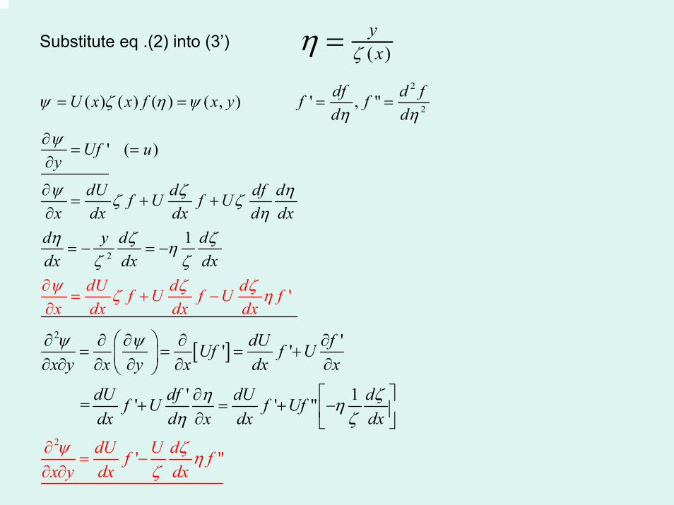
( )yxζη =Substitute eq .(2) into (3’)
2
2
2
( ) ( ) ( ) ( , ) ' , "
(
1
'
' )
df d fU x x f x y f fd d
Uf uy
dU d df df U f
dU d df U f U fx dx dx dx
Ux dx dx d dxd y d ddx dx dx
ψ ζ η ψη η
ψ
ψ ζ ηζ ζη
η
ψ ζ ζζ η
ζ ζηζ ζ
= = = =
∂= =
∂
∂= + +
∂
= −
∂= + −
∂
= −
[ ]
2
2 '' '
' 1 = ' '
' "
"
dU fUf f Ux y x y x dx x
dU df dU df U
dU U df
f Ufdx d
fx y d
x dx dx
x dx
ψ ψ
η ζηη ζ
ψ ζ ηζ
⎛ ⎞∂ ∂
∂=
∂ ∂ ∂= = = +⎜ ⎟∂ ∂ ∂ ∂ ∂ ∂⎝ ⎠
⎡ ⎤∂+ = +
−
−
∂ ∂
⎢ ⎥∂ ⎣ ⎦
[ ]2
2
3
3 2
2
2 22
2
"
"'
' "
Substitute above results into (3')
' ' " "'
1( ') " " "'
(
'
)
"
'
Uf Ufy y
dU dU
U fy
U fy
U d df U fdx
d U dU UUf f f U f f U fdx dx dc dx
dU dU d dU UU f U ff U ff U fdx dx dx dxdUu f
dx
dx
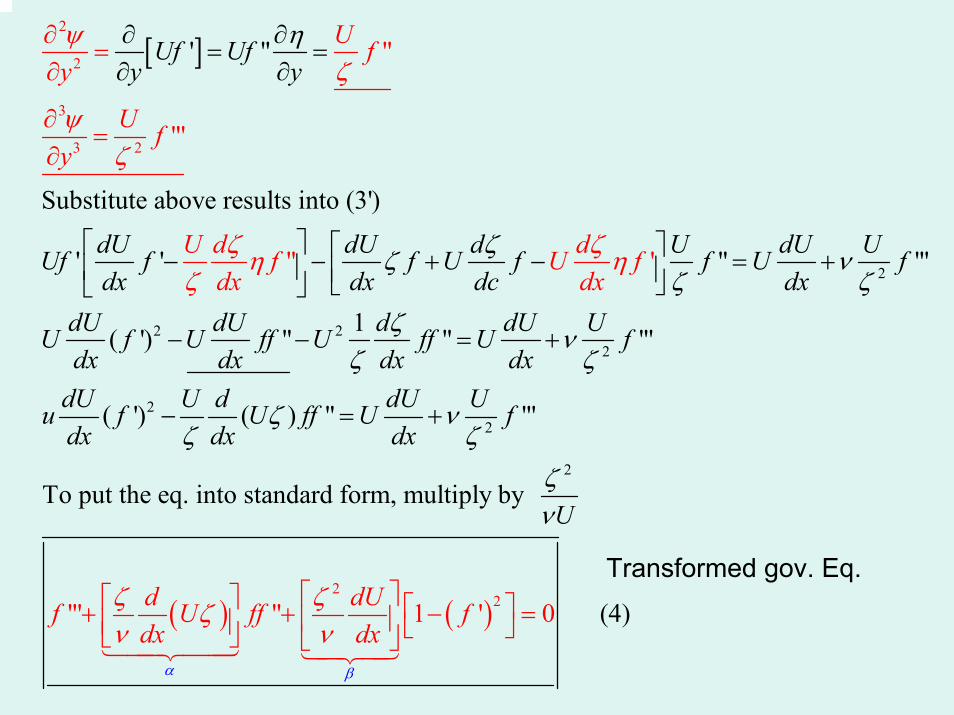
η
ζζ ν
ψζ
ψζ
ζ ζηζ ζ
ζ νζ ζ
ηζ
∂ ∂= =
∂ ∂
⎡ ⎤ ⎡ ⎤− − + − = +⎢ ⎥ ⎢ ⎥⎣ ⎦⎣ ⎦
∂=
= +
∂=
− −
∂
∂
( ) ( )
2
22
2
( ) " "'
To put the eq. into standard form, multiply by
"' " 1 ' 0 (4)d
U d dU UU ff U fdx dx
U
dUf U ff fdx dx
α β
ζ νζ ζ
ζν
ζ ζζν ν
⎡ ⎤⎡ ⎤ ⎡ ⎤+ + − =⎢ ⎥⎢ ⎥ ⎣ ⎦⎣ ⎦ ⎦
− =
⎣
+
Transformed gov. Eq.
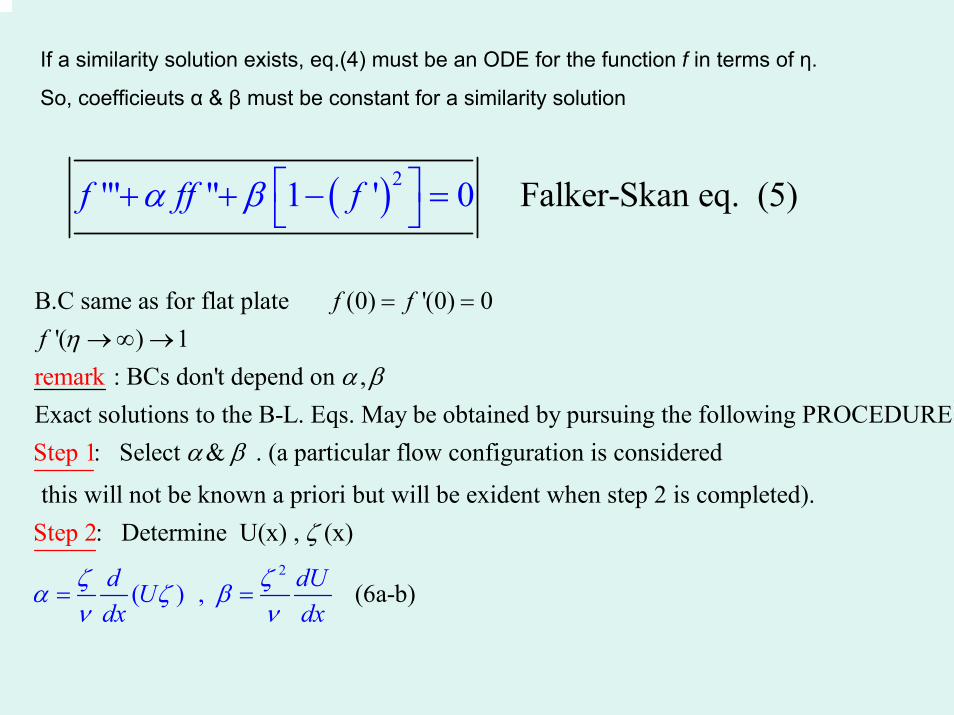
If a similarity solution exists, eq.(4) must be an ODE for the function f in terms of η.
So, coefficieuts α & β must be constant for a similarity solution
( )2 Falker-Skan "' " 1 ' eq. (0 5)f ff fα β ⎡ ⎤+ + − =⎣ ⎦
B.C same as for flat plate (0) '(0) 0'( ) 1
: BCs don't depend on ,Exact solutions to the B-L. Eqs. May be obtained by pursuing the following PROremark
StepCEDURE
: Select & . (a p ar1
f ff η
α β
α β
= =→∞ →
2
ticular flow configuration is considered
this will not be known a priori but will be exident when step 2 is completed).: Determine U
( ) ,
(x) , (x)
(6a-b)
Step 2
d dUUdx dx
ζ ζα ζν
ζ
βν
= =
'' ' 2
' '
: Determine the function f ( )which is the solution of the following problem
''' 1 ( ) 0
with BCs (0) (0) 0 , ( ) 1 as Calculate the stream fun
Step
ctionin
3
Step h4 p : y
f ff f
f f f
η
α β
η η
⎡ ⎤+ + − =⎣ ⎦= = → → ∞
( ) ( )2
2
sical coord.
( , ) ( ) ( )( )
in step #2 , instead of working with eqs. 6 a-b)
(6a)'
Remar
E
2 (6b)
k
'
Flate Pxample #1
step
la
te (ZPG)
#1
yx y U x x fx
dU d Udx dx
η
ψ ζζ
ζ β ζ ν α βν
⎛ ⎞⎜ ⎟
= ⎜ ⎟⎜ ⎟⎜ ⎟⎝ ⎠
= = −
( )2
'
means that flat plate at ZPG
1 = , =02
(6a)'
0 (6b)'
( ) 0 (6 ) leads to
step #2
U=con st0 .this
d UdxdUdx
dUx bdx
α β
ζ ν
ζν
ζ
=
=
≠ ⇒ = ⇒
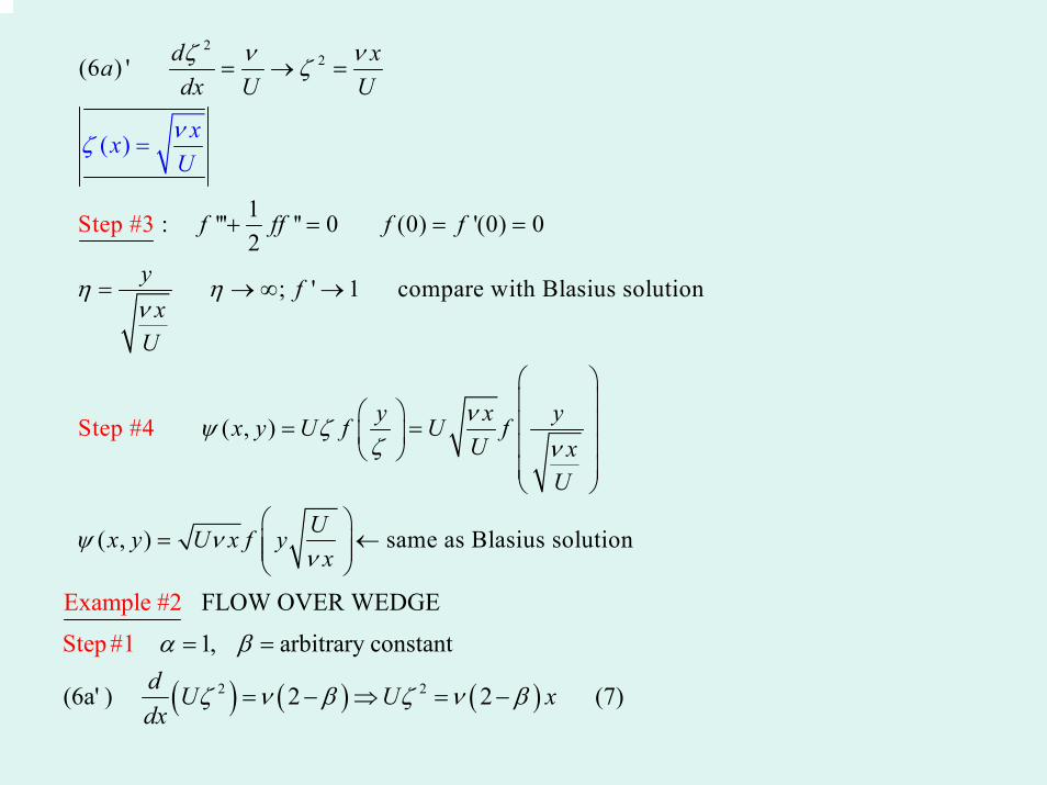
22(6 ) '
1 : ''' '' 0 (0) '(0) 02
; ' 1 compare with Blasius s
Step #3
Step #
olution
( , )
( )
,
4
( )
d xadx U U
f ff f f
y fxU
y x
xxU
yx y U f U fU x
U
x y U x f y
ζ ν νζ
η ην
νψ ζζ ν
ψ ν
νζ
= → =
+ = = =
= → ∞ →
⎛ ⎞⎜ ⎟⎛ ⎞ ⎜ ⎟= =⎜ ⎟ ⎜ ⎟⎝ ⎠⎜ ⎟⎝ ⎠
=
=
same as Blasius solution Uxν
⎛ ⎞←⎜ ⎟⎜ ⎟
⎝ ⎠
( ) ( ) ( )2 2
FLOW OVER WEDGE
1, arbitrary constant
(6a' )
Exampl
2 2
e #2
Step
(7)
#1d U U xdx
α β
ζ ν β ζ ν β
= =
= − ⇒ = −

2
2
(6 ')
Divide eq. (6b') by (7)
ln ln ln outer flow is that over a wedge of angle (Fig.)2
1 12
( )
dUU dx x
U x
dUbdx
U cxx cββ
ζ νβ
β πβ
β
β
β
−
=−
=
+ ⇒ ==−
2(1 )2 2
2
2
2
1
2
(9)
Solve the BVP
''' '' 1 ( ') 0
(0) '(0) 0 ' 1 Solve numerically to get ( ), '( ), '
(2 )( )
Step #3
'( )
dU c xdx
f ff f
f fas f f
c
f
x x
f
ββ
ββ
βζ νβ ζ νββ
β
η η η η
ν βζ
− −
−−
−= =−
⎡ ⎤+ + − =⎣ ⎦
= =→∞ →
−=
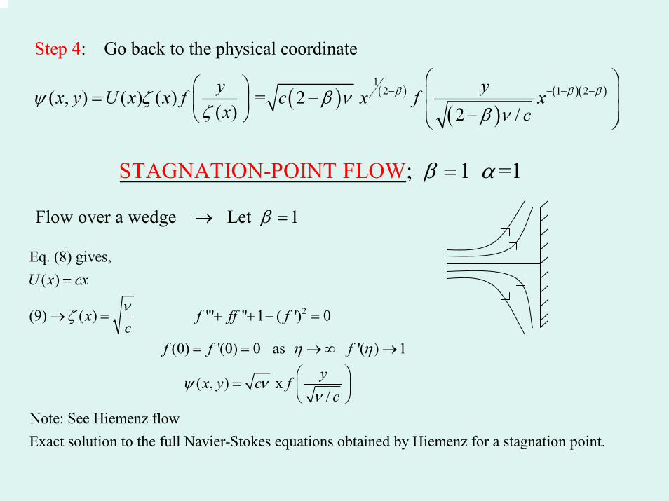
( ) ( )
( )( )( )
12 1 2
: Go back to the physical cStep oordinate
( , ) ( ) ( ) = 2 ( ) 2 /
4
y yx y U x x f c x f xx c
β β βψ ζ β νζ β ν
− − − −⎛ ⎞⎛ ⎞ ⎜ ⎟= −⎜ ⎟ ⎜ ⎟−⎝ ⎠ ⎝ ⎠
STAGNATION-POINT ; FLO =W 1 1β α=
Flow over a wedge Let 1β→ =
2
Eq. (8) gives, ( )
(9) ( ) "' " 1 ( ') 0
(0) '(0) 0 as '( ) 1
( , ) x /
Not
U x cx
x f ff fc
f f fyx y c fc
νζ
η η
ψ νν
=
→ = + + − =
= = →∞ →
⎛ ⎞= ⎜ ⎟⎝ ⎠
e: See Hiemenz flowExact solution to the full Navier-Stokes equations obtained by Hiemenz for a stagnation point.
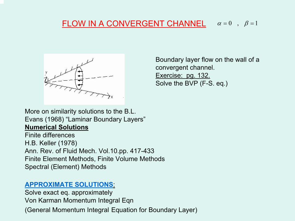
FLOW IN A CONVERGENT CHANNEL 0 , 1α β= =
Boundary layer flow on the wall of a convergent channel.Exercise: pg. 132.Solve the BVP (F-S. eq.)
More on similarity solutions to the B.L.Evans (1968) “Laminar Boundary Layers”Numerical SolutionsFinite differencesH.B. Keller (1978)Ann. Rev. of Fluid Mech. Vol.10.pp. 417-433Finite Element Methods, Finite Volume MethodsSpectral (Element) Methods
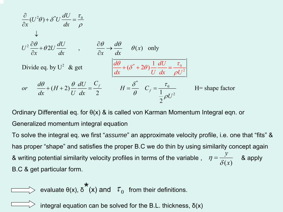
APPROXIMATE SOLUTIONS:Solve exact eq. approximatelyVon Karman Momentum Integral Eqn(General Momentum Integral Equation for Boundary Layer)
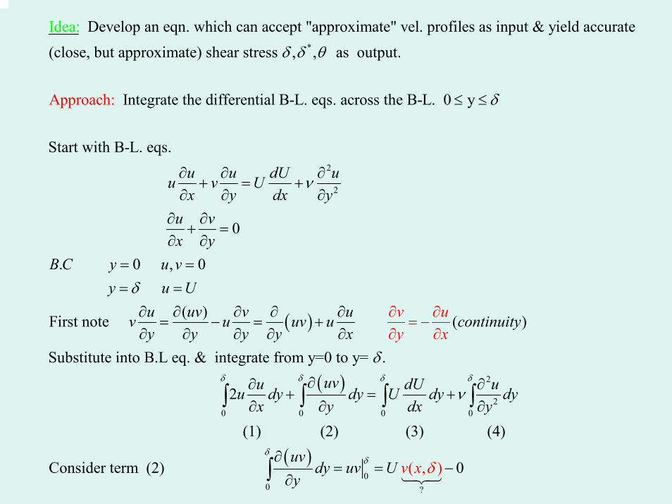
*
Develop an eqn. which can accept "approximate" vel. profiles as input & yield accurate (close, but approximate) shear stress , , as output.
Integrate the differen
I
tial B-L. eqs. Approac
ea:
h:
d
a
δ δ θ
2
2
cross the B-L. 0 y
Start with B-L. eqs.
0
. 0 , 0
First note
u u dU uu v Ux y dx y
u vx y
BC y u vy u U
δ
ν
δ
≤ ≤
∂ ∂ ∂+ = +
∂ ∂ ∂∂ ∂
+ =∂ ∂
= == =
( )
( ) 2
20 0 0
( ) ( )
Substitute into B.L eq. & integrate from y=0 to y= .
2
u uv v uv u uv u continuityy y y y
v uyx
uvu dU uu dy dy U dyx y dx
x
y
δ δ δ
δ
ν
∂ ∂= −
∂∂ ∂ ∂ ∂ ∂
= − = +∂ ∂ ∂ ∂ ∂
∂∂ ∂+ = +
∂
∂ ∂ ∂∫ ∫ ∫
( )
0
00 ?
(1) (2) (3) (4)
Consider term (2) 0( , )
dy
uvdy uv U v x
y
δ
δδ δ
∂= = −
∂
∫
∫
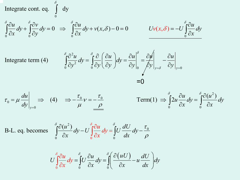
0
0 0 0 0
2
20 0 0 0
00
Integrate cont. eq. dy
0 ( , ) 0 0
Integrate term (4
( , )
)
y y
y
u v u udy dy dy v x U U dyx y x x
u u u u udy dyy y y y y y
d
x
y
v
ud
δ
δ δ δ δ
δδ δ
δ
δ
τ µ
δ
= =
=
∂ ∂ ∂ ∂+ = ⇒ + − = = −
∂ ∂ ∂ ∂
⎛ ⎞∂ ∂ ∂ ∂ ∂ ∂= = = −⎜ ⎟∂ ∂ ∂ ∂ ∂ ∂⎝ ⎠
= ⇒
∫
∫ ∫ ∫ ∫
∫ ∫
( )
20 0
0 0
0
20
0
00
0
( ) (4) Term(1) 2
( )B-L. eq. becomes
u uu dy dyx x
u dUdy U U dyx dx
uUu dUU
u dyx
u dyx
U dy ux x dx
δ
δ
δ δ
δ δ
δ
τ τνµ ρ
τρ
∂ ∂⇒ − = − ⇒ =
∂ ∂
∂− −
∂
⎛ ⎞∂∂= = −⎜ ⎟∂ ∂
∂
∂ ⎠
=
∂
⎝
∂
∫ ∫
∫ ∫
∫
∫
∫0
dyδ
∫
=0
( )
( ) ( )
20
0 0 0 0
2 0
0 0
2
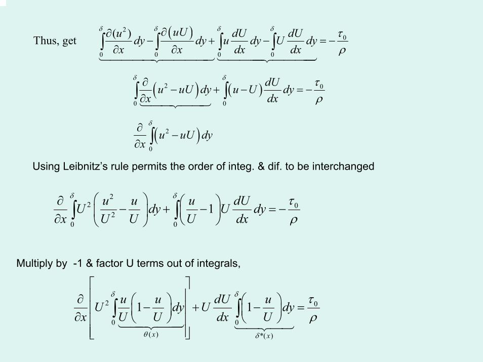
( )Thus, get
uUu dU dUdy dy u dy U dyx x dx dx
dUu uU dy u U dyx dx
ux
δ δ δ δ
δ δ
τρ
τρ
∂∂− + − = −
∂ ∂
∂− + − = −
∂
∂−
∂
∫ ∫ ∫ ∫
∫ ∫
( )0
uU dyδ
∫
Using Leibnitz’s rule permits the order of integ. & dif. to be interchanged
22 0
20 0
1u u u dUU dy U dyx U U U dx
δ δ τρ
⎛ ⎞∂ ⎛ ⎞− + − = −⎜ ⎟ ⎜ ⎟∂ ⎝ ⎠⎝ ⎠∫ ∫
Multiply by -1 & factor U terms out of integrals,
2 0
0 0( ) *( )
1 1
x x
u u dU uU dy U dyx U U dx U
δ δ
θ δ
τρ
⎡ ⎤⎢ ⎥∂ ⎛ ⎞ ⎛ ⎞− + − =⎢ ⎥⎜ ⎟ ⎜ ⎟∂ ⎝ ⎠ ⎝ ⎠⎢ ⎥⎢ ⎥⎣ ⎦
∫ ∫
2 * 0
2
2 *
*
02
( )
2 , ( ) only
Divide eq. by U & get
( 2)
(
2
12 )
ff
d dUd
dUU Ux dx
dU dU U xx dx x dx
Cd dUor H H Cdx U dx
x U dx Uτθ δ θ
τθ δρ
θ θ θθ θ
τθ θ δθ
ρ+ +
∂+ =
∂
↓∂ ∂
+ →∂
+
=
∂
+ = = = 0
2 H= shape factor1
2Uρ
Ordinary Differential eq. for θ(x) & is called von Karman Momentum Integral eqn. or
Generalized momentum integral equation
To solve the integral eq. we first “assume” an approximate velocity profile, i.e. one that “fits” &
has proper “shape” and satisfies the proper B.C we do thin by using similarity concept again
& writing potential similarity velocity profiles in terms of the variable , & apply
B.C & get particular form.
evaluate θ(x), δ*(x) and from their definitions.
integral equation can be solved for the B.L. thickness, δ(x)
( )yx
ηδ
=
0τ
η
0 ( )nudy
τ ∂∼U y δ=
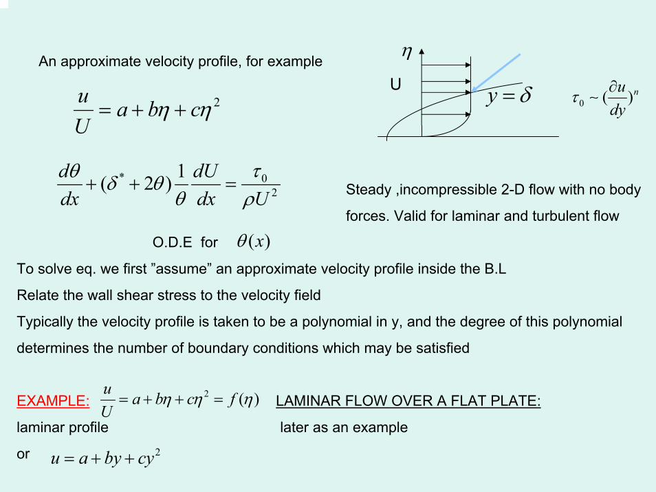
An approximate velocity profile, for example
2u a b cU
η η= + +
* 02
1( 2 )d dUdx dx U
τθ δ θθ ρ
+ + =
( )xθ
2 ( )u a b c fU
η η η= + + =
2u a by cy= + +
Steady ,incompressible 2-D flow with no body
forces. Valid for laminar and turbulent flow
O.D.E for
To solve eq. we first ”assume” an approximate velocity profile inside the B.L
Relate the wall shear stress to the velocity field
Typically the velocity profile is taken to be a polynomial in y, and the degree of this polynomial
determines the number of boundary conditions which may be satisfied
EXAMPLE: LAMINAR FLOW OVER A FLAT PLATE:
laminar profile later as an example
or
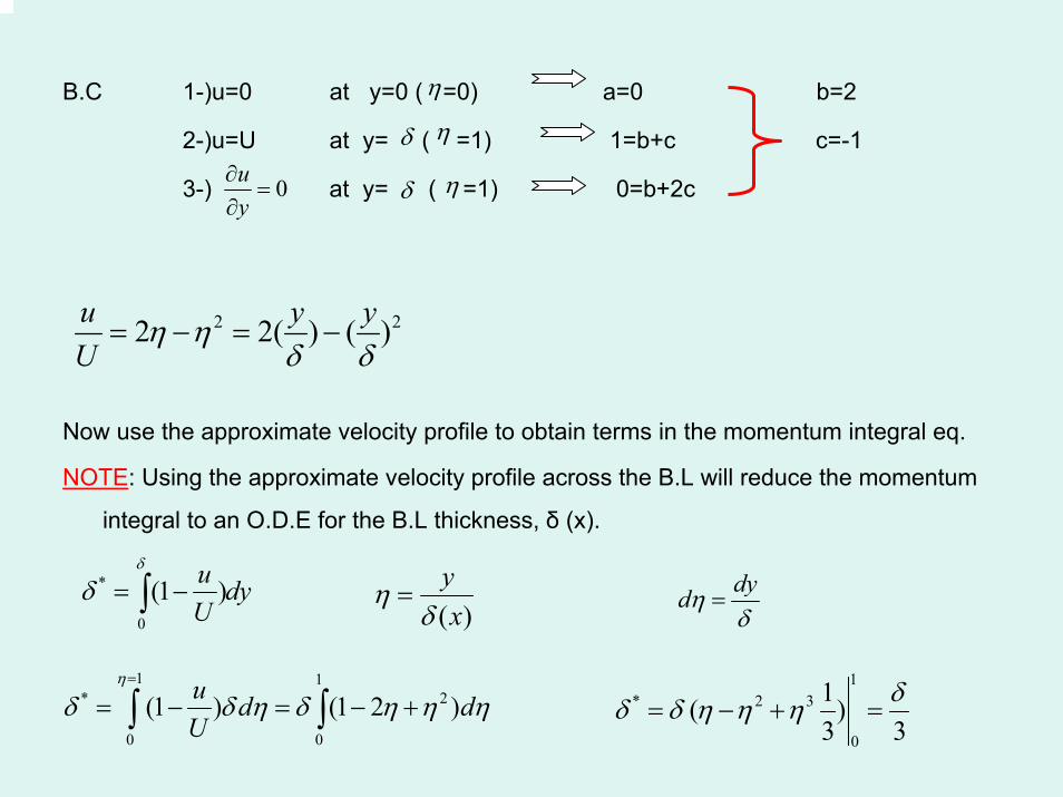
B.C 1-)u=0 at y=0 ( =0) a=0 b=2
2-)u=U at y= ( =1) 1=b+c c=-1
3-) at y= ( =1) 0=b+2c
Now use the approximate velocity profile to obtain terms in the momentum integral eq.
NOTE: Using the approximate velocity profile across the B.L will reduce the momentum
integral to an O.D.E for the B.L thickness, δ (x).
2 22 2( ) ( )u y yU
η ηδ δ
= − = −
*
0
(1 )u dyU
δ
δ = −∫ ( )yx
ηδ
= dydηδ
=
1 1* 2
0 0
(1 ) (1 2 )u d dU
η
δ δ η δ η η η=
= − = − +∫ ∫1
* 2 3
0
1( )3 3
δδ δ η η η= − + =
0uy∂
=∂
η
δ
δ
η
η
or
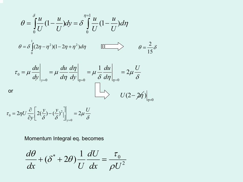
1
0 0
(1 ) (1 )u u u udy dU U U U
ηδ
θ δ η=
= − = −∫ ∫1
2 2
0
(2 )(1 2 )dθ δ η η η η η= − − +∫ 215
θ δ=
000 0
1 2y
du du d du Udy d dy d ηη
ητ µ µ µ µη δ η δ== =
= = = =
(2 2U η−0
)η=
20
0
2 2( ) ( ) 2y
y y UUy
τ η µδ δ δ=
∂ ⎡ ⎤= − =⎢ ⎥∂ ⎣ ⎦
* 02
1( 2 )d dUdx U dx U
τθ δ θρ
+ + =
Momentum Integral eq. becomes
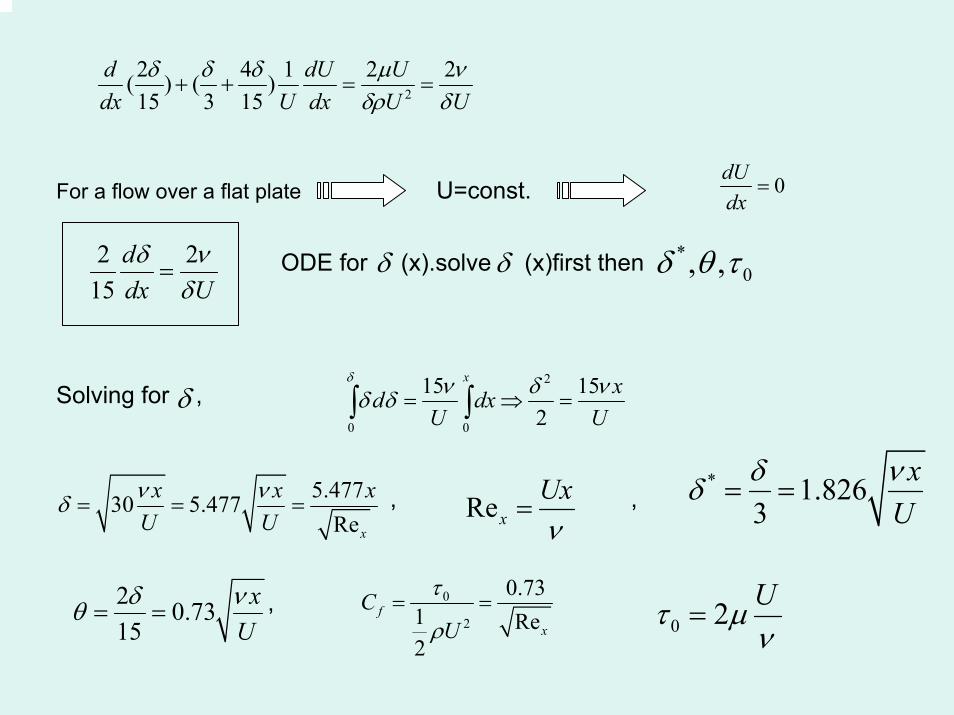
For a flow over a flat plate U=const.
ODE for (x).solve (x)first then
Solving for ,
, ,
,
2
2 4 1 2 2( ) ( )15 3 15
d dU Udx U dx U U
δ δ δ µ νδρ δ
+ + = =
0dUdx
=
δ δ2 215ddx Uδ ν
δ=
*0, ,δ θ τ
δ2
0 0
15 152
x xd dxU U
δ ν δ νδ δ = ⇒ =∫ ∫
5.47730 5.477Rex
x x xU Uν νδ = = = Rex
Uxν
=* 1.826
3xU
δ νδ = =
2 0.7315
xU
δ νθ = =0
2
0.731 Re2
fx
CU
τ
ρ= =
0 2 Uτ µν
=
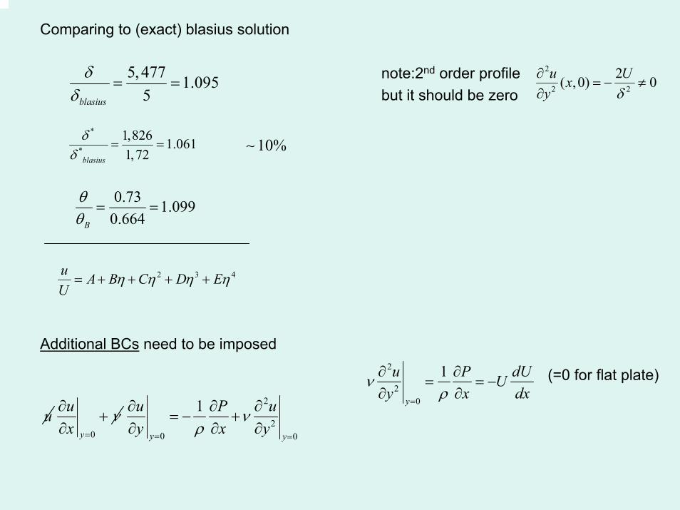
Comparing to (exact) blasius solution
note:2nd order profile but it should be zero
Additional BCs need to be imposed
(=0 for flat plate)
5,477 1.0955blasius
δδ
= =
*
*
1,826 1.0611,72blasius
δδ
= = 10%∼
2
2 2
2( ,0) 0u Uxy δ∂
= − ≠∂
0.73 1.0990.664B
θθ
= =
2 3 4u A B C D EU
η η η η= + + + +
u0y
ux
ν=
∂+
∂
2
20 0
1
y y
u P uy x y
νρ= =
∂ ∂ ∂= − +
∂ ∂ ∂
2
20
1
y
u P dUUy x dx
νρ
=
∂ ∂= = −
∂ ∂
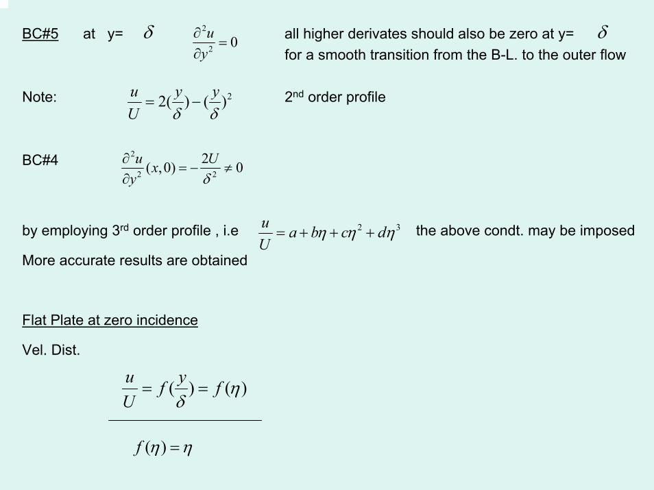
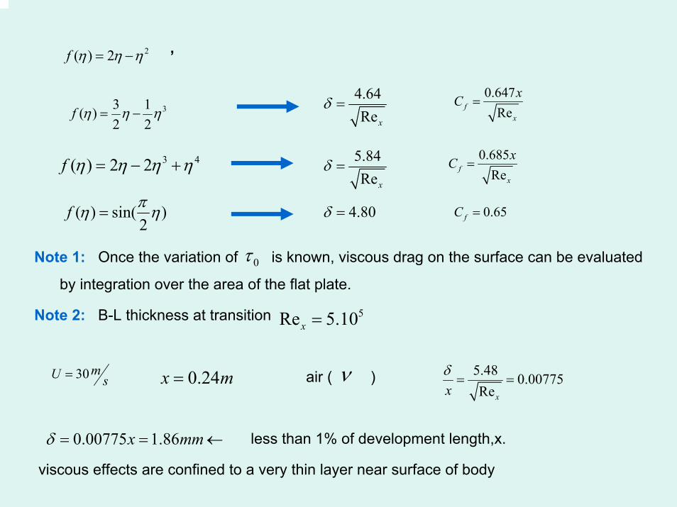
BC#5 at y= all higher derivates should also be zero at y= for a smooth transition from the B-L. to the outer flow
Note: 2nd order profile
BC#4
by employing 3rd order profile , i.e the above condt. may be imposed
More accurate results are obtained
Flat Plate at zero incidence
Vel. Dist.
δ 2
2 0uy∂
=∂
δ
22( ) ( )u y yU δ δ
= −
2
2 2
2( ,0) 0u Uxy δ∂
= − ≠∂
2 3u a b c dU
η η η= + + +
( ) ( )u yf fU
ηδ
= =
( )f η η=
,
Note 1: Once the variation of is known, viscous drag on the surface can be evaluated
by integration over the area of the flat plate.
Note 2: B-L thickness at transition
air ( )
less than 1% of development length,x.
viscous effects are confined to a very thin layer near surface of body
2( ) 2f η η η= −
33 1( )2 2
f η η η= −
3 4( ) 2 2f η η η η= − +
( ) sin( )2
f πη η=
4.64Rex
δ =
5.84Rex
δ =
4.80δ =
0.647Ref
x
xC =
0.685Ref
x
xC =
0.65fC =
0τ
5Re 5.10x =
30mU s= 0.24x m= ν 5.48 0.00775Rexx
δ= =
0.00775 1.86x mmδ = = ←
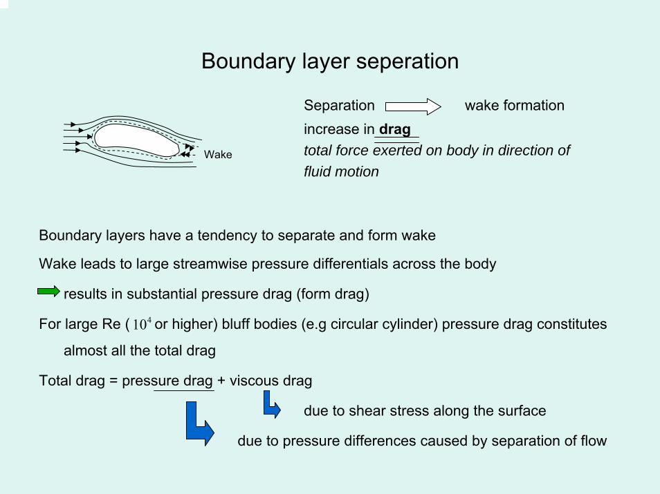
Boundary layer seperation
Separation wake formationincrease in dragtotal force exerted on body in direction offluid motion
Boundary layers have a tendency to separate and form wake
Wake leads to large streamwise pressure differentials across the body
results in substantial pressure drag (form drag)
For large Re ( or higher) bluff bodies (e.g circular cylinder) pressure drag constitutes
almost all the total drag
Total drag = pressure drag + viscous drag
due to shear stress along the surface
due to pressure differences caused by separation of flow
Wake
410

2) AIRFOILS-LIFT drops sharply “STALL” due to separation
force normal to flow directionShape of streamlines near point of separation
3) FLAT PLATE~ No separation
REMARK: After separation point ,external (decelerating) stream ceases to flow nearly parallel to the boundary surface
S
chord
tNo separation

Condition for separation
Pressure gradient ,
>0 adverse pressure gradient (decelerating external stream) increasing pressure in the flow direction
<0 favourable P.G and =0 (zero pressure gradient)
NOTE: pressure gradient along a B.L is determined by the outer flow
(Bern. Eq.)
Separation occurs only for APG condition
o Momentum contained in the fluid layers adjacent to surface will be insufficient
to overcome the force exerted by the pressure gradient , so that a region of
reverse flow occurs.
dPdx
dPdx
dPdx
dPdx
1dU dPUdx dxρ
= −
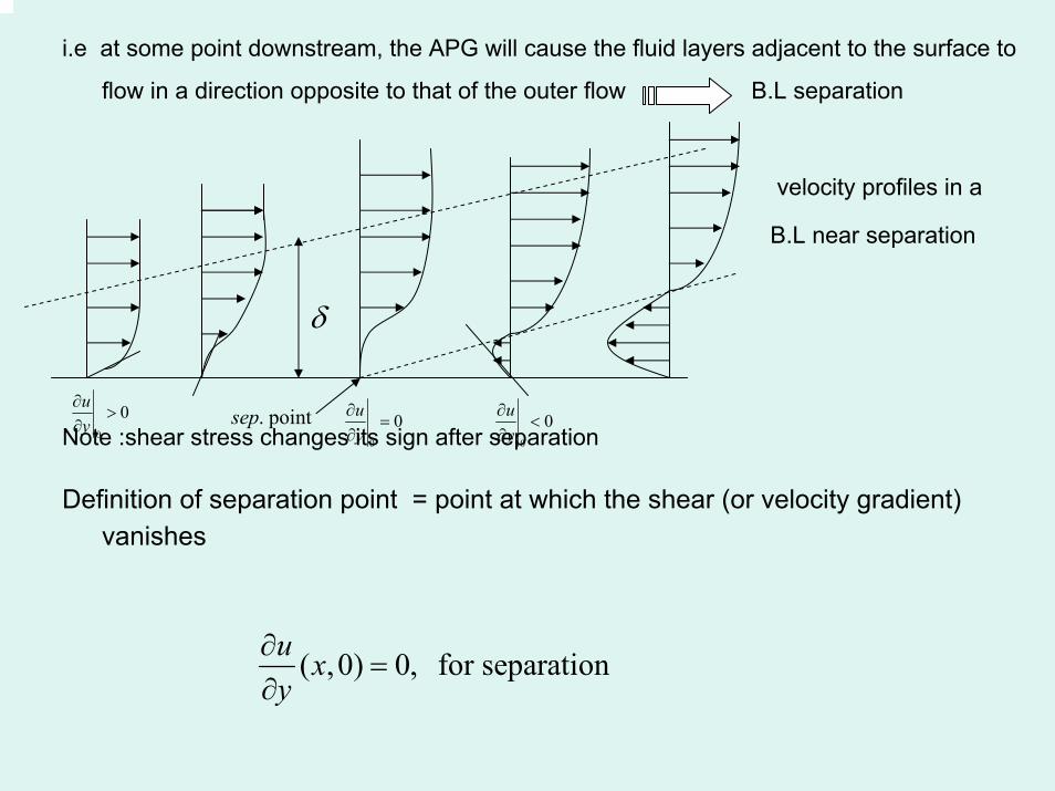
i.e at some point downstream, the APG will cause the fluid layers adjacent to the surface to
flow in a direction opposite to that of the outer flow B.L separation
velocity profiles in a
B.L near separation
Note :shear stress changes its sign after separation
Definition of separation point = point at which the shear (or velocity gradient)vanishes
( ,0) 0, for separationu xy∂
=∂
δ
0
0uy∂
>∂
0
0uy∂
=∂ 0
0uy∂
<∂
. pointsep

• Question show that separation can occur only in region of adverse pressure gradient !Steady state B.L eqs.
If <0
the same
u0y
u vx =
∂+
∂
2
20 0
1
y y
u P uy x y
νρ= =
∂ ∂ ∂= − +
∂ ∂ ∂2
20y
u dPy dx
µ=
∂=
∂
3
30
0y
uy
=
∂=
∂
dPdx
2
2
uy∂∂ 2
2u Py x∂ ∂
=∂ ∂0y =
y δ=2
2 0uy∂
=∂
0uy∂
>∂
0uy∂
=∂
0u =
u U=
uy∂∂
y
u
U
?
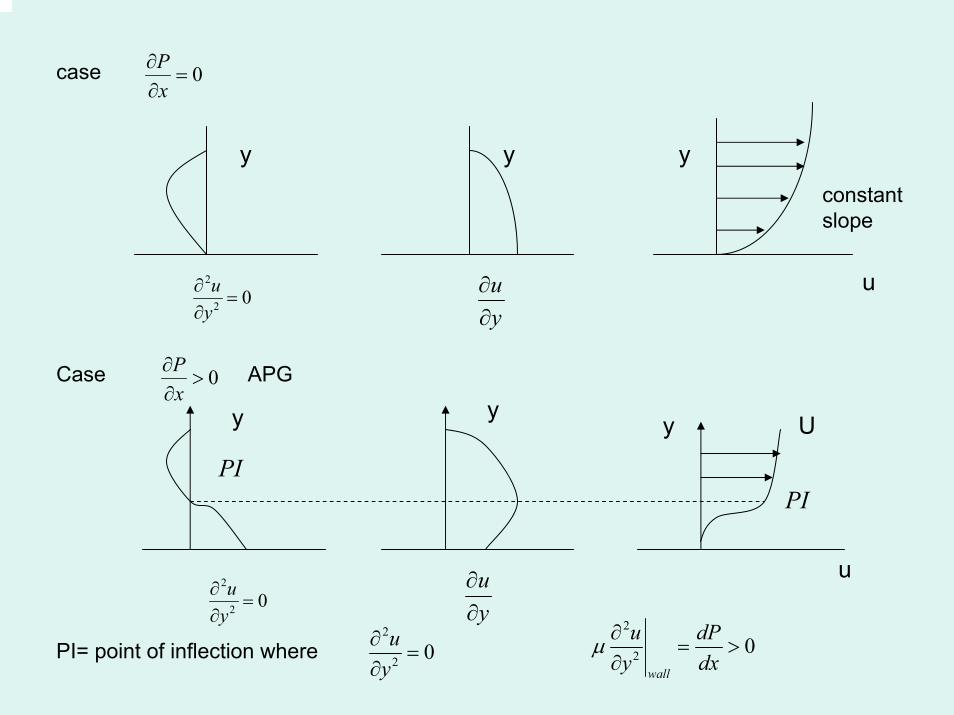
case
constant slope
Case APG
PI= point of inflection where
0Px
∂=
∂
yy y
2
2 0uy∂
=∂
uy∂∂
u
0Px
∂>
∂
uy∂∂
2
2 0uy∂
=∂
y
2
2 0uy∂
=∂
2
2 0wall
u dPy dx
µ ∂= >
∂
PI
y y
u
U
PI
Control of separation by suction
Control of separation by variable geometry and by blowing
How to calculate the separation point ?
Goldstein
Stewartson
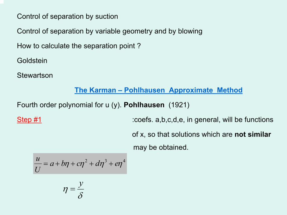
The Karman – Pohlhausen Approximate Method
Fourth order polynomial for u (y). Pohlhausen (1921)
Step #1 :coefs. a,b,c,d,e, in general, will be functions
of x, so that solutions which are not similar
may be obtained.
2 3 4u a b c d eU
η η η η= + + + +
yηδ
=
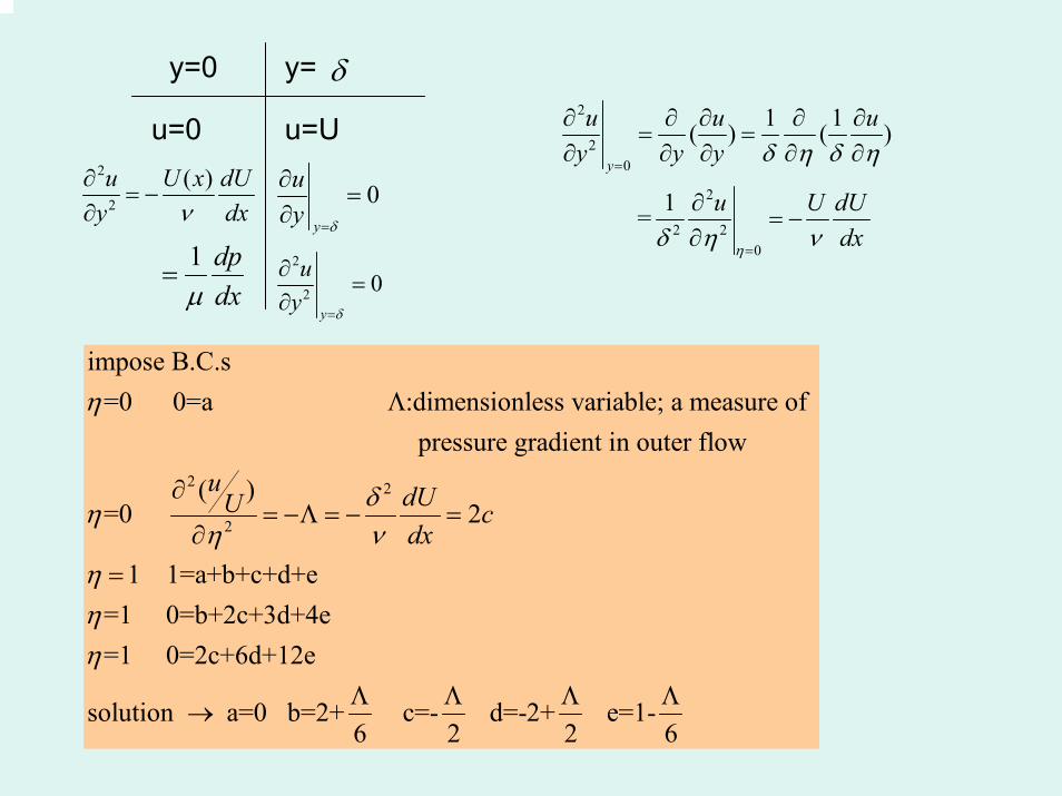
δ
2
2
( )u U x dUy dxν∂
= −∂
y=0 y=
u=0 u=U
0y
uy δ=
∂=
∂
1 dpdxµ
=2
2 0y
uy δ=
∂=
∂
2
20
2
2 20
1 1( ) ( )
1 =
y
u u uy y y
u U dUdxη
δ η δ η
δ η ν
=
=
∂ ∂ ∂ ∂ ∂= =
∂ ∂ ∂ ∂ ∂
∂= −
∂
2 2
2
impose B.C.s=0 0=a :dimensionless variable; a measure of
pressure gradient in outer flow
( )=0 2
u dUUdx
η
δηη ν
Λ
∂= −Λ = − =
∂1 1=a+b+c+d+e
=1 0=b+2c+3d+4e=1 0=2c+6d+12e
solution a=0 b=2+ c=- d=-2+ e=1-6 2 2 6
c
ηηη
=
Λ Λ Λ Λ→
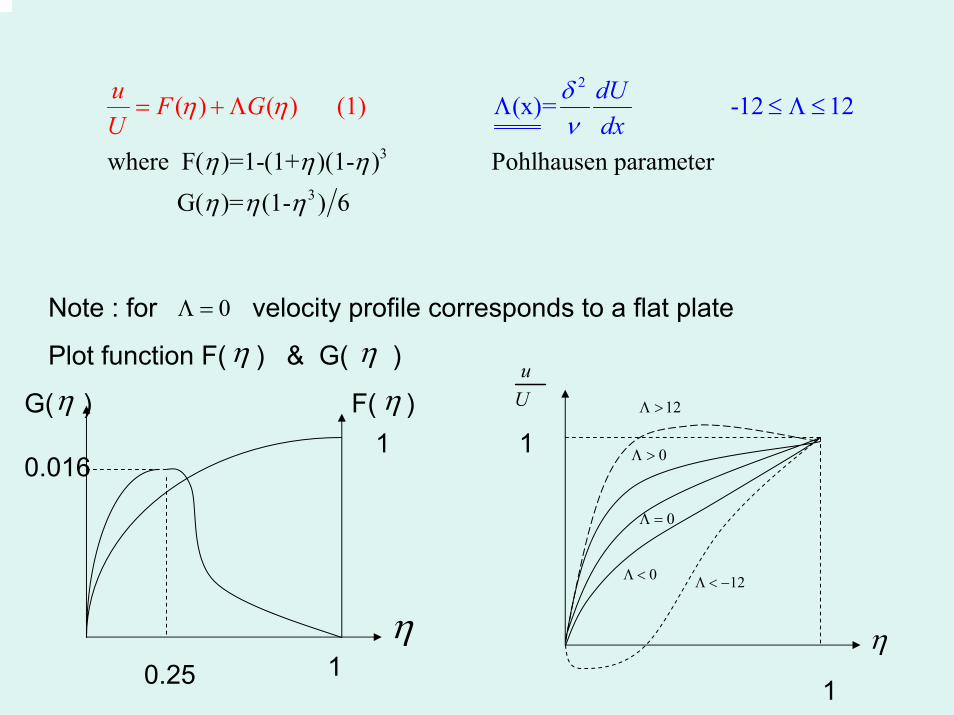
2
3
3
where F( )=1-(1+ )(1- ) Pohlhausen parameter G( )= (1-
(x)= -12 1( ) ( ) (1
)
) 2
6
u F G dUdxU
η
η η η
η η
ν
η
δη= ≤Λ Λ Λ ≤+
Note : for velocity profile corresponds to a flat plate
Plot function F( ) & G( )
0Λ =
ηη
1η
F( )ηG( )η
0.25
0.0161
1
1
12Λ < −0Λ <
0Λ =
0Λ >
12Λ >
uU
η
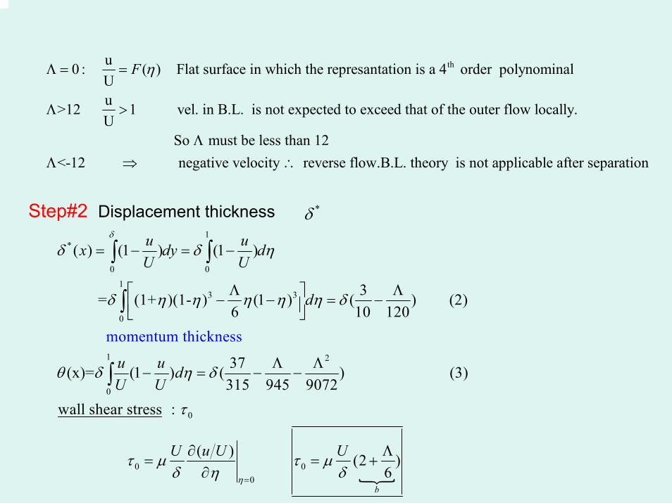
thu0 : ( ) Flat surface in which the represantation is a 4 order polynominalUu>12 1 vel. in B.L. is not expected to exceed that of the outer flow locally.U
F ηΛ = =
Λ >
So must be less than 12<-12 negative velocity reverse flow.B.L. theory is not applicable after separation
ΛΛ ⇒ ∴
*δ1
*
0 01
3 3
0
1 2
0
( ) (1 ) (1 )
3 = (1+ )(1- ) (1 ) ( ) (2)6 10 120
momentum thickness
37(x)= (1 ) ( ) (3)315 945 9072
wall
u ux dy dU U
d
u u dU U
δ
δ δ η
δ η η η η η δ
θ δ η δ
= − = −
Λ Λ⎡ ⎤− − = −⎢ ⎥⎣ ⎦
Λ Λ− = − −
∫ ∫
∫
∫0
0 00
shear stress :
( ) (2 )6
b
U u U U
η
τ
τ µ τ µδ η δ=
∂ Λ= = +
∂
Step#2 Displacement thickness

Uθν
Step #3 Plug into the general momentum eq. Multiply the mom. Eq. by
* 0
2 * 20
2
2 2 22
2
*
2
(2 ) or
1 ( ) (2 ) (5)2
(x)= evaluate each term in terms of (x)
37( ) ( ) 315 945 9072
3(10 120
( )
U d dUdx dx Ud dUUdx dx U
dUdx
dU dU KK xd dxx
x
τ θθ θ θθ δν ν µ
τ θθ δ θν θ ν µ
δν
θ θν
θ
θδ ν
δ
+ + =
+ + =
Λ Λ
Λ Λ= Λ = − − Λ =
Λ−
=
=
2
20
)( ) (6)
37( )315 945 9072
f( ) f(x) but K=K(x) f(K)
37( ) , g(K)=(2+ )( )6 315 945 9072
f K
g KU
τ θµ
=Λ Λ
− −
Λ → ⇒
Λ Λ Λ= − −

[ ]
[ ]{ }
0
2
2
2
(2 )6
1 ( ) 2 ( ) ( ) (7)2
where K= ( )
, let us take Z= as the new dependent variable so that K=Z and the mom,int. becomes
U 2 ( ) 2 ( ) ( U) or
U
dU f K K g Kdx
dU K xdx
d
dZ
UNowdx
dZ g K f K K H Kdx dx
τ µδθν
θν
θν
Λ= +
+ + =
=
= − + =
st
(8)
H(K) is known (1 order nonlinear , ODE for Z , solve numericallay , start x=0 stop =-12
)
(
H K=
→ Λ
[ ] separation )but complex H( )ODE for Z(x) - mom. int. reduces to above form IVP for ODfor any (x) K & H(K) may be evalu ted
Ea
Λ
Λ →
0.0783
0.47
H(K)
0.0783
0.47
H(K)
K
H(K)=0.47-6K (9)approximation
Linear in K over the range of interest
56
0
65
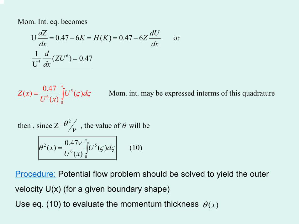
Mom. Int. eq. becomes
U 0.47 6 ( ) 0.47 6 or
1 ( ) 0.47U
0.47( ) ( ) ( )
Mom. int. may be expressed interms of this quadrax
dZ dUK H K Zdx dxd ZU
Z x U dU
dx
xς ς
= − = = −
=
= ∫
2
2 56
0
ture
then , since Z= , the value of will be
0.47 ( ) ( ) (10)( )
x
x U dU x
θ θν
νθ ς ς= ∫
Procedure: Potential flow problem should be solved to yield the outer
velocity U(x) (for a given boundary shape)
Use eq. (10) to evaluate the momentum thickness ( )xθ

2 22
Pr parameter (x) may be evaluated from the relation
(11) difficult to find (x)
found (x), (x) is evaluated from eq. (3)
3
37 (x)
7( ) ( )315 945
= (315
072
945
9
essure
havi
dU K xx
n
d
g δ
θ δ
θν
Λ Λ= = − −
Λ
Λ
Λ
Λ− −
2*
*
0
) and eq. (2)9072
3( ) 10 120
u ( ) ( ) vel. distribution eq (1)U
shear stress at the surface is given by eq. (4)
(2 )6
F G
Uu
δ
δ δ
η η
τ µ
Λ
Λ= −
= +Λ ←
Λ= +
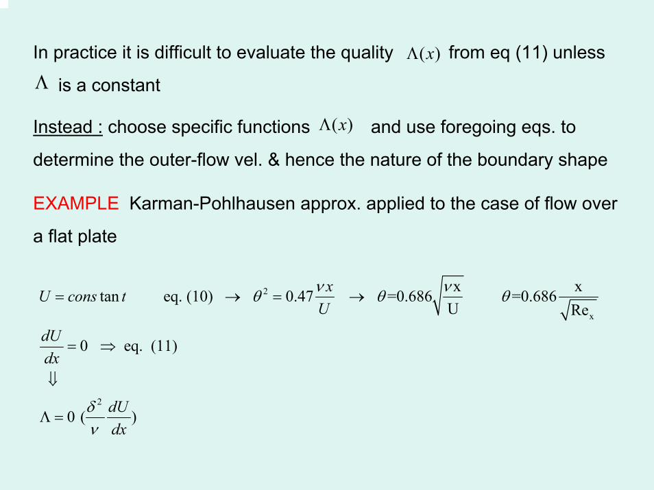
In practice it is difficult to evaluate the quality from eq (11) unless
is a constant
Instead : choose specific functions and use foregoing eqs. to
determine the outer-flow vel. & hence the nature of the boundary shape
EXAMPLE Karman-Pohlhausen approx. applied to the case of flow over
a flat plate
( )xΛ
Λ
( )xΛ
2
x
2
x xtan eq. (10) 0.47 =0.686 =0.686U Re
0 eq. (11)
0 ( )
xU cons tU
dUdx
dUdx
ν νθ θ θ
δν
= → = →
= ⇒
⇓
Λ =
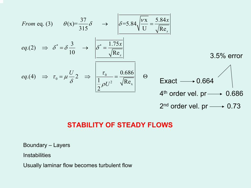
* *
00
2 x
37 x 5.84 eq. (3) (x)= =5.84315 U Re
3 1.75.(2) 10 Re
0.686.(4) 2 1 Re2
x
x
xFrom
xeq
UeqU
νθ δ δ
δ δ δ
ττ µδ ρ
→ =
⇒ = → =
⇒ = ⇒ = ΘExact 0.664
4th order vel. pr 0.686
2nd order vel. pr 0.73
3.5% error
STABILITY OF STEADY FLOWS
Boundary – Layers
Instabilities
Usually laminar flow becomes turbulent flow
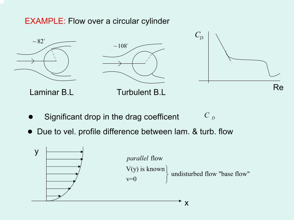
EXAMPLE: Flow over a circular cylinder
~ 82~ 108
Re
DC
Laminar B.L Turbulent B.L
• Due to vel. profile difference between lam. & turb. flow
Significant drop in the drag coefficent DC•
x
y flow
V(y) is knownundisturbed flow "base flow"
v=0
parallel
⎫⎬⎭
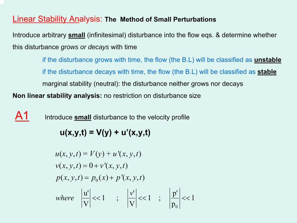
Linear Stability Analysis: The Method of Small Perturbations
Introduce arbitrary small (infinitesimal) disturbance into the flow eqs. & determine whether
this disturbance grows or decays with time
if the disturbance grows with time, the flow (the B.L) will be classified as unstable
if the disturbance decays with time, the flow (the B.L) will be classified as stable
marginal stability (neutral): the disturbance neither grows nor decays
Non linear stability analysis: no restriction on disturbance size
A1 Introduce small disturbance to the velocity profile
u(x,y,t) = V(y) + u’(x,y,t)
0
( , , ) = ( ) + '( , , )( , , ) 0 '( , , )( , , ) ( ) '( , , )
u x y t V y u x y tv x y t v x y tp x y t p x p x y t
= += +
0
u' ' p' 1 ; 1 ; 1V V p
vwhere << << <<
A2 Substitute A1 into the N-S eqs. & continuity
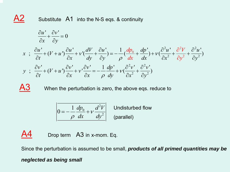
20
2
2 2
2 2
2 2
2 2
' ' 0
' ' ' 1 ' ' ' ; ( ') '( ) ( ) ( )
' ' ' 1 ' ' ' ; ( ') ' ( )
u vx y
u u dV u dp u ux V u vt x dy y dx x yv v v dp v vy
dp Vdx y
V u vt x x dy x y
νρ
νρ
∂ ∂+ =
∂ ∂
∂ ∂ ∂ ∂ ∂+ + + + = − + + + +
∂ ∂ ∂ ∂ ∂
∂ ∂ ∂ ∂ ∂+ + + = − + +
∂ ∂
∂
∂
∂
∂ ∂
A3 When the perturbation is zero, the above eqs. reduce to
20
2
10 dp d Vdx dy
νρ
= − +Undisturbed flow
(parallel)
A4 Drop term A3 in x-mom. Eq.
Since the perturbation is assumed to be small, products of all primed quantities may be
neglected as being small
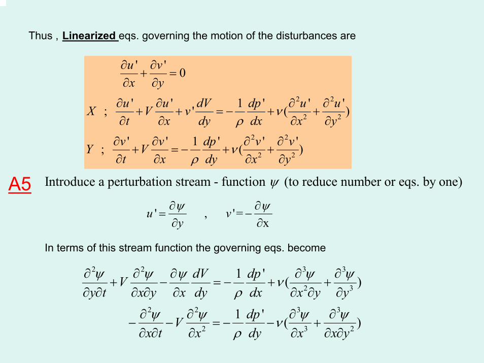
Thus , Linearized eqs. governing the motion of the disturbances are
2 2
2 2
2 2
2 2
' ' 0
' ' 1 ' ' ' ; ' ( )
' ' 1 ' ' ' ; ( )
u vx yu u dV dp u uX V vt x dy dx x yv v dp v vY Vt x dy x y
νρ
νρ
∂ ∂+ =
∂ ∂
∂ ∂ ∂ ∂+ + = − + +
∂ ∂ ∂ ∂
∂ ∂ ∂ ∂+ = − + +
∂ ∂ ∂ ∂
Introduce a perturbation stream - function (to reduce number or eqs. by one)ψA5' , '=
xu v
yψ ψ∂ ∂
= −∂ ∂
In terms of this stream function the governing eqs. become
2 2 3 3
2 3
2 2 3 3
2 3 2
1 ' ( )
1 ' ( )
dV dpVy t x y x dy dx x y y
dpVx t x dy x x y
ψ ψ ψ ψ ψνρ
ψ ψ ψ ψνρ
∂ ∂ ∂ ∂ ∂+ − = − + +
∂ ∂ ∂ ∂ ∂ ∂ ∂ ∂
∂ ∂ ∂ ∂− − = − − +∂ ∂ ∂ ∂ ∂ ∂
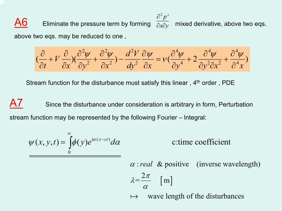
A6 Eliminate the pressure term by forming mixed derivative, above two eqs.
above two eqs. may be reduced to one ,
2 'px y∂∂ ∂
2 2 2 4 4 4
2 2 2 4 2 2 4( )( ) ( 2 )d VVt x y x dy x y y x x
ψ ψ ψ ψ ψ ψν∂ ∂ ∂ ∂ ∂ ∂ ∂ ∂+ + − = + +
∂ ∂ ∂ ∂ ∂ ∂ ∂ ∂ ∂
Stream function for the disturbance must satisfy this linear , 4th order , PDE
A7 Since the disturbance under consideration is arbitrary in form, Perturbation
stream function may be represented by the following Fourier – lntegral:
( )
0
( , , ) ( ) c:time coefficienti x ctx y t y e dαψ φ α∞
−= ∫
[ ]
: & positive (inverse wavelength)2= m
wave length of the disturbances
realαπλα

-i ct
-i cti
: time variation e if c > 0 e as t
disturbance will grow unstablein general co
r i
notec c c i
α
α= + → → → ∞ →∞
→-i ct
i
i
mplex number: if c < 0 e 0 as t
disturbance will decay stable c = 0 ne
α→ → →∞
→→ utrally stable
(c=0)
Plug in A6 yields the integro – differential equation:
( ) 2 i (x-ct)
0
2 2 4
2 4
2 4
4 i (x-ct)
0
( " ) " e
( ''' 2 " , i 1 i 1
" , ""= ,..
) e
.
i c i V i
d dd d
d
y
V d
y
α
α
α α φ α φ αφ α
ν φ α
φ φ
α
φ
φ φ
φ
α
∞
∞
⎡ ⎤− + − −⎣ ⎦
⎡ ⎤= − + −
=
⎣ ⎦ = =
∫
∫
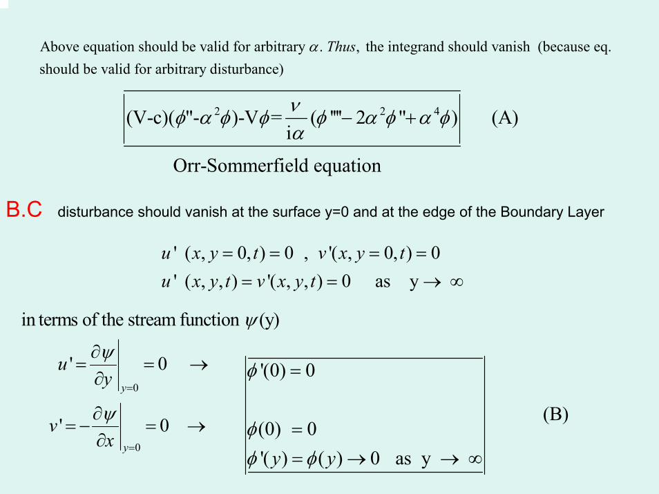
Above equation should be valid for arbitrary . , the integrand should vanish (because eq. should be valid for arbitrary disturbance)
Thusα
2 2 4(V-c)( "- )-V = ( '''' 2 " ) (A)i
Orr-Sommerfield equation
νφ α φ φ φ α φ α φα
− +
B.C disturbance should vanish at the surface y=0 and at the edge of the Boundary Layer
' ( , 0, ) 0 , '( , 0, ) 0' ( , , ) '( , , ) 0 as y u x y t v x y tu x y t v x y t
= = = == = → ∞
0
0
in terms of the stream function (y)
' 0
' 0
y
y
uy
vx
ψ
ψ
ψ=
=
∂= = →∂
∂= − = →
∂
'(0) 0
(B)(0) 0'( ) ( ) 0 as y y y
φ
φφ φ
=
== → → ∞

Solution of the Orr – Sommerfeld EquationUndisturbed vel. profile V(y) and disturbance wavelength is specifiedα
( ) & knownV y α
. (A) with BC.(B)represent an eigenvalue problem for the time coefficient , c , 0 flow stable 0 flow unstable ( ) , 0
r i i
i
i
Eqc c i c c
ci x ct cα
= + < ⇒> ⇒
− = neutral stablity⇒
i (x-ct) (y) e αψ φ=
unstable
stable
, 0istable c <
*
Re Uαν
=
Recritical
* α δ
Steady laminar flow can become another steady lam. flow
HTLT
. PrRa Gr=
Diagram:Stability
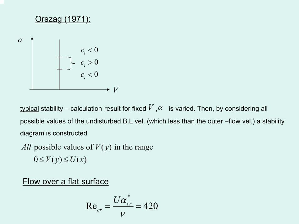
Orszag (1971):
000
i
i
i
ccc
<>
<
V
α
typical stability – calculation result for fixed , is varied. Then, by considering all
possible values of the undisturbed B.L vel. (which less than the outer –flow vel.) a stability
diagram is constructed
V α
possible values of ( ) in the range 0 ( ) ( )All V y
V y U x≤ ≤
Flow over a flat surface
*
Re 420crcr
Uαν
= =
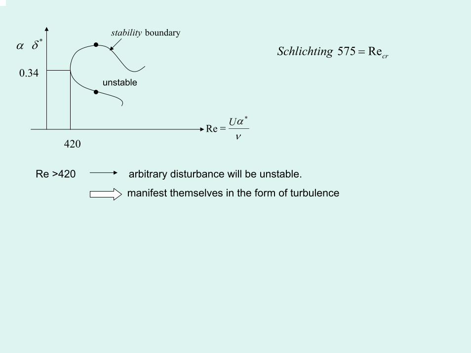
unstable
boundarystability
420
* α δ
*
Re Uαν
=
0.34
575 RecrSchlichting =
Re >420 arbitrary disturbance will be unstable.
manifest themselves in the form of turbulence
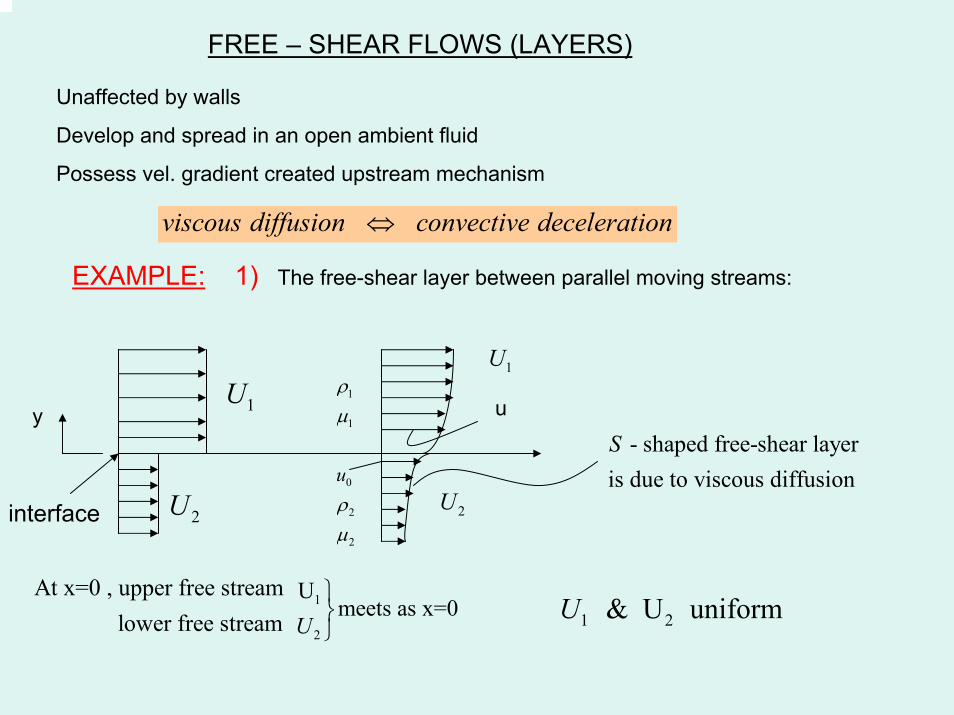
FREE – SHEAR FLOWS (LAYERS)
Unaffected by walls
Develop and spread in an open ambient fluid
Possess vel. gradient created upstream mechanism
viscous diffusion convective deceleration⇔
EXAMPLE: 1) The free-shear layer between parallel moving streams:
2U
1U1U
interface
y1
1
0
2
2
u
ρµ
ρµ
2U
u
- shaped free-shear layer is due to viscous diffusionS
At x=0 , upper free stream lower free stream
1
2
Umeets as x=0
U⎫⎬⎭ 1 2 & U uniformU

For each stream , can define a Blasius – type similarity variable
Lock(1951) – two different fluids with physical parameters
1 1 2 2( , ) & ( , )ρ µ ρ µ
1
1
j 1
, , j=1,22
2 ( )
jj j
j
j j j
uUy fx U
U x f
ην
ψ ν η
′= =
=
Following the same procedure as in derivation of Blasius equation, one can
obtain Blasius-type eq. for each layer
''' '' 0 j=1,2j j jf f f+ =
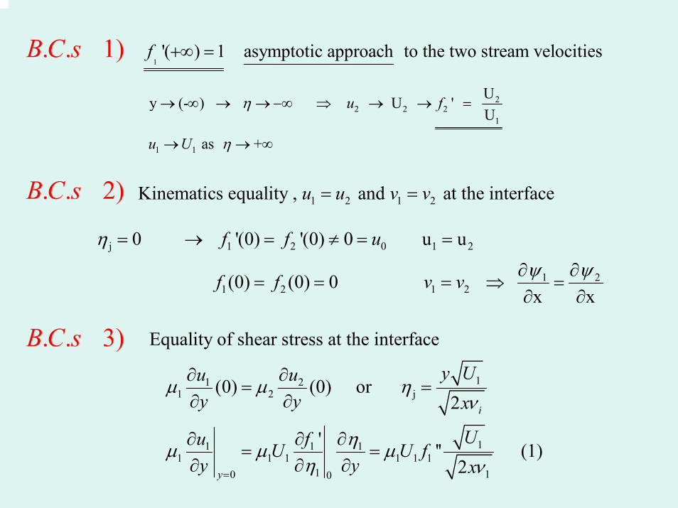
1'( ) 1 asymptotic approach to the two stream veloci i s t ef +∞ =. . 1) BC s
22 2 2
1
1 1
Uy (- ) U ' U
as +
u f
u U
η
η
→ ∞ → →−∞ ⇒ → → =
→ → ∞
. . 2) BC s 1 2 1 2Kinematics equality , and at the interfaceu u v v= =
j 1 2 0 1 2
1 21 2 1 2
0 '(0) '(0) 0 u u
(0) (0) 0 x x
f f u
f f v v
η
ψ ψ
= → = ≠ = =
∂ ∂= = = ⇒ =
∂ ∂
. . 3) BC s11 2
1 2 j
11 1 11 1 1 1 1 1
1 10 0
(0) (0) or 2
' '' (1)2
i
y
y Uu uy y x
Uu fU U fy y x
µ µ ην
ηµ µ µη ν=
∂ ∂= =
∂ ∂
∂ ∂ ∂= =
∂ ∂ ∂
Equality of shear stress at the interface

122 2 1 2
20
2 21 1 2 2 1 2
1 11 2
'' (2)2
1 1(1)=(2) ''(0) ''(0) ''(0) ''(0)
y
Uu U fy x
f f f f
µ µν
ρ µµ µρ µν ν
=
∂=
∂
⇒ = → =
2 21 2
1 1
''(0) ''(0) k=f k f ρ µρ µ
=
1 2 1 2 : k=1 (identical fluids) ; : a gas flowing over a liquid k>>1
ex
Case 1Case 2
. air-water
Most p
interf
ractic
ace k 60000 k 2
al cas s
45
e
ρ ρ µ µ= =
≈ ⇒ ≈

TURBULENCEINTRODUCTION
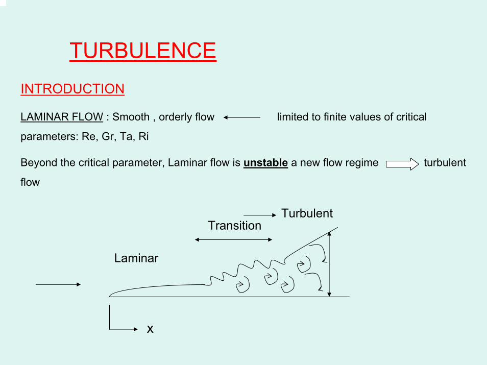
LAMINAR FLOW : Smooth , orderly flow limited to finite values of critical
parameters: Re, Gr, Ta, Ri
Beyond the critical parameter, Laminar flow is unstable a new flow regime turbulent
flow
Transition
Laminar
Turbulent
x
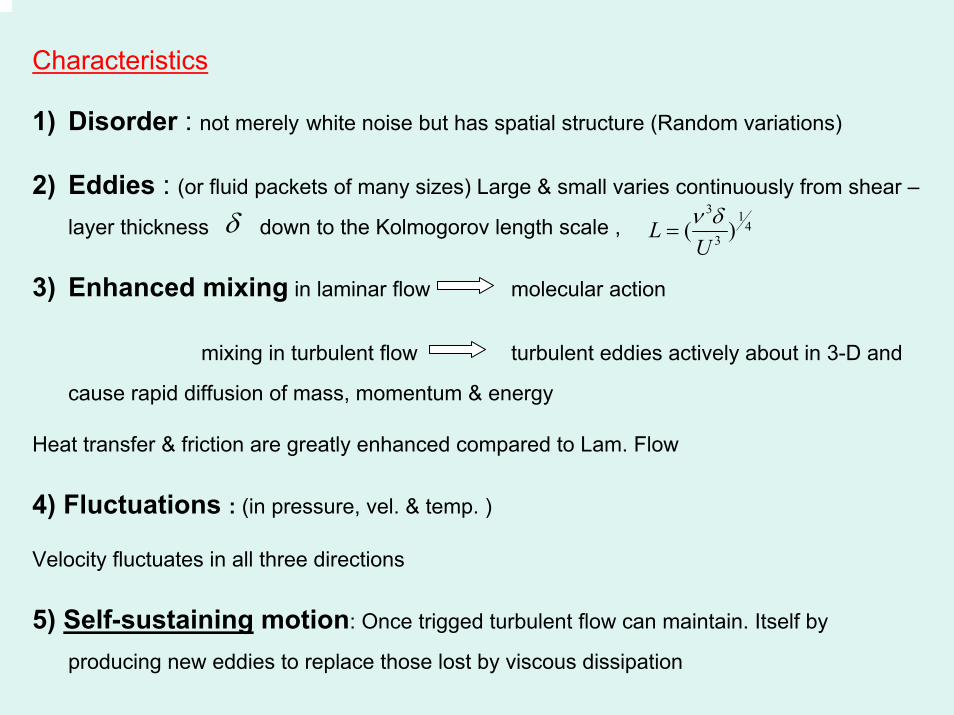
Characteristics
1) Disorder : not merely white noise but has spatial structure (Random variations)
2) Eddies : (or fluid packets of many sizes) Large & small varies continuously from shear –
layer thickness down to the Kolmogorov length scale ,
3) Enhanced mixing in laminar flow molecular action
mixing in turbulent flow turbulent eddies actively about in 3-D and
cause rapid diffusion of mass, momentum & energy
Heat transfer & friction are greatly enhanced compared to Lam. Flow
4) Fluctuations : (in pressure, vel. & temp. )
Velocity fluctuates in all three directions
5) Self-sustaining motion: Once trigged turbulent flow can maintain. Itself by
producing new eddies to replace those lost by viscous dissipation
δ3 1
43( )L
Uν δ
=
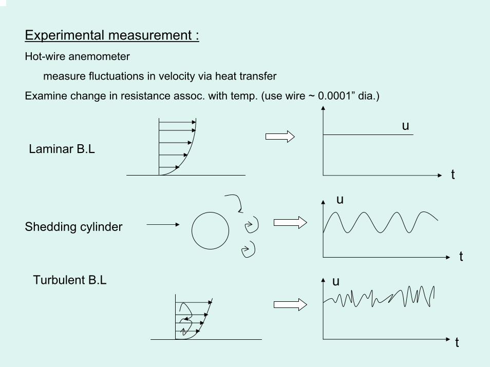
Experimental measurement :Hot-wire anemometer
measure fluctuations in velocity via heat transfer
Examine change in resistance assoc. with temp. (use wire ~ 0.0001” dia.)
u
t
u
t
u
t
Laminar B.L
Shedding cylinder
Turbulent B.L
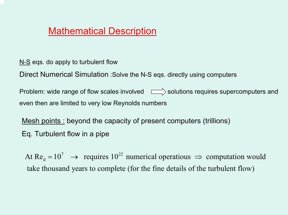
Mathematical Description
N-S eqs. do apply to turbulent flow
Direct Numerical Simulation :Solve the N-S eqs. directly using computers
Problem: wide range of flow scales involved solutions requires supercomputers and
even then are limited to very low Reynolds numbers
Mesh points : beyond the capacity of present computers (trillions)
Eq. Turbulent flow in a pipe
7 22dAt Re 10 requires 10 numerical operatious computation would
take thousand years to complete (for the fine details of the turbulent flow)= → ⇒
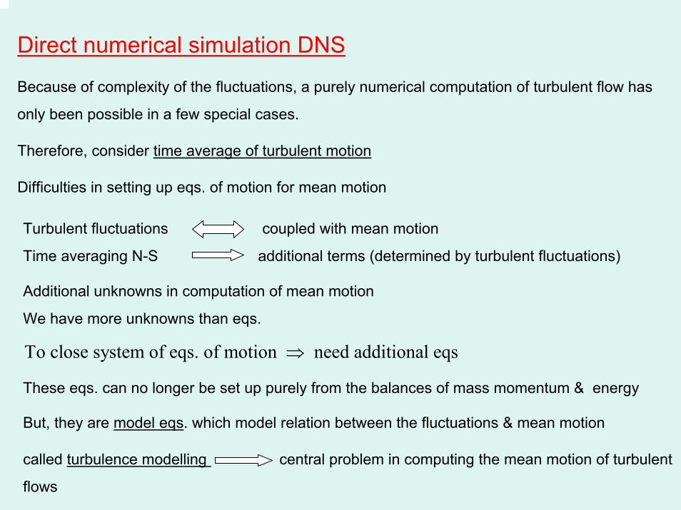
Direct numerical simulation DNS
Because of complexity of the fluctuations, a purely numerical computation of turbulent flow has
only been possible in a few special cases.
Therefore, consider time average of turbulent motion
Difficulties in setting up eqs. of motion for mean motion
Turbulent fluctuations coupled with mean motion
Time averaging N-S additional terms (determined by turbulent fluctuations)
Additional unknowns in computation of mean motion
We have more unknowns than eqs.
To close system of eqs. of motion need additional eqs ⇒
These eqs. can no longer be set up purely from the balances of mass momentum & energy
But, they are model eqs. which model relation between the fluctuations & mean motion
called turbulence modelling central problem in computing the mean motion of turbulent
flows

Mean Motion & Fluctuations
, time average valueu'u
Decompose the motion into a mean motion & a fluctuating motion
'
'
'
'
u u u
v v v
w w w
p p p
= +
= +
= +
= +
compressible turbulent flows
= ' ; '
In
T T Tρ ρ ρ+ = +
Average is formed as the time average at a fixed point in space
0
0
1 integral is to be taken over a sufficently large time interval T so that ( )t T
t
u u dt u f tT
+
= ← ≠∫

122
0
Characterization of fluctuation RMS
1 ( )T
u u u d tT
⇒
⎫⎧⎪ ⎪= −⎨ ⎬⎪ ⎪⎩ ⎭∫
' ( )
' ( )
u g t
u u u f t
=
= + =
definition time average of fluctuating quautities are zero i.e.
' 0 , ' 0 , ' 0 , ' 0 assume that mean motion indep. of time steady turbulent flow
By
u v w pFirst= = = =
⇒
u
t
steady unsteady
Turb. flow
u
u
t
steady unsteady
Lam . flow
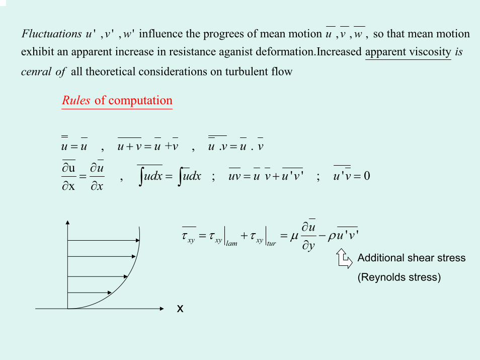
' , ' , ' influence the progrees of mean motion , , , so that mean motionexhibit an apparent increase in resistance aganist deformation.Increased apparent viscosity
all
Fluctuations u v w u v wis
cenral of theoretical considerations on turbulent flow
, + , . .
u , ; ' ' ; ' 0x
of computation
u u u v u v u v u v
u udx udx uv
Rul
u v u v u vx
es
= + = =
∂ ∂= = = + =
∂ ∂ ∫ ∫
x
' 'xy xy xylam tur
u u vy
τ τ τ µ ρ∂= + = −
∂Additional shear stress
(Reynolds stress)
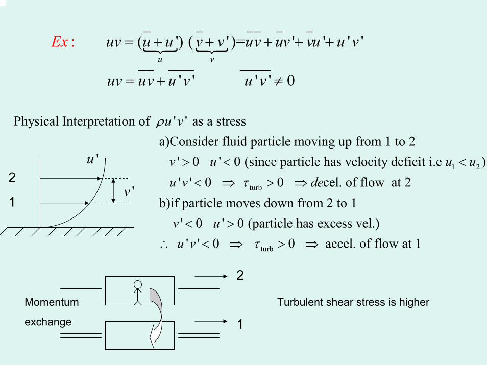
( ') ( ' )= ' ' ' '
' ' '
:
' 0u v
uv u u v v uv uv vu u v
uv
Ex
uv u v u v
= + + + + +
= + ≠
Physical Interpretation of ' ' as a stress a)Consider fluid particle moving up from 1 to 2 ' 0 ' 0 (since
u v
v u
ρ
> < 1 2
turb
particle has velocity deficit i.e ) ' ' 0 0 cel. of flow at 2 b)if particle moves down from
u uu v deτ
<< ⇒ > ⇒
turb
2 to 1 ' 0 ' 0 (particle has excess vel.) ' ' 0 0 accel. of flow at 1
v uu v τ< >
∴ < ⇒ > ⇒
2
1'v
'u
2
1
Momentum
exchange
Turbulent shear stress is higher

Basic Eqs. for Mean Motion of Turbulent Flows
Consider flows with constant properties
Continuity equation
(1) '
' of (1)
u v w u u ux y z
u u uTime averagingx x x
∂ ∂ ∂+ + = +
∂ ∂ ∂
∂ ∂ ∂− = +
∂ ∂ ∂
(2) =0
' ' '(3) Also , using (1) 0
time average values &fluctuations satisfy laminar flow continuity eq Momentum Eqs.(Re
y
u v wx y z
u v wx y z
Both
∂ ∂ ∂+ +
∂ ∂ ∂∂ ∂ ∂
+ + =∂ ∂ ∂
2Incomp. N-S eqs. ( ( . ) )
nolds eqs.)
- (4)V V V p Vt
ρ µ∂+ ∇ = ∇ + ∇
∂

Substitute ' ' ' ' into N-S s1) egu u u v v v w w w p p p= + = + = + = +
2) Time average the equations
3) Drop-out terms which `average` to zero . Use “Rules of Computation”
2
2
2
' '0 0 terms which are linear in fluctuating quantities 0
' 0 ' ' 0 terms which are quadratic in fluctuating quantities 0
u ut x
u u v
∂ ∂= = ← ⇒
∂ ∂
≠ ≠ ← ⇒
2
22
2
Resultant eqs. (called Reynolds eqs.)
( )
( )
' ' ' ' '( )
' ' ' ' '( )
u u u pu v w ux y z
u u v u wx y z
u v v v wx y
x
v v v pu v w vx y z zy
ρ
ρ
ρ µ
ρ µ
∂ ∂ ∂+ +
∂∂ ∂ ∂ ∂
+ + = − +∂ ∂
∂ ∂ ∂+
∇ −∂ ∂ ∂ ∂
∂ ∂ ∂ ∂+ + = − + ∇ −
∂ ∂+
∂∂ ∂ ∂∂
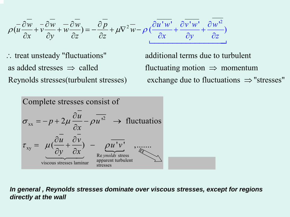
22
( )
treat unsteady "fluctuations" add
' ' ' ' '(
itional terms due to turbulentas added stresses call
)
ed
w w w pu v w wx
u w v w wx yy z z z
µ ρρ ∂ ∂ ∂+ +
∂ ∂ ∂∂ ∂ ∂ ∂
+ + = − + ∇ −∂ ∂ ∂ ∂
∴⇒ fluctuating motion momentum
Reynolds stresses(turbulent stresses) exchange due to fluctuations "stresses"⇒
⇒
2xx
xyRe stressapparent turbulentviscous stresses laminar stresses
Complete stresses consist of
2 ' fluctuatios
( ) ' ' ,.......ynolds
up ux
u v u vy x
σ µ ρ
τ µ ρ
∂= − + − →
∂∂ ∂
= + −∂ ∂
In general , Reynolds stresses dominate over viscous stresses, except for regions directly at the wall
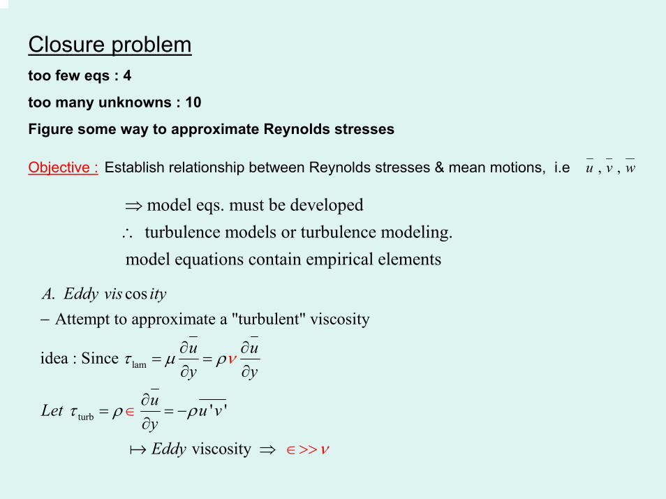
Closure problemtoo few eqs : 4
too many unknowns : 10
Figure some way to approximate Reynolds stresses
Objective : Establish relationship between Reynolds stresses & mean motions, i.e , , u v w
model eqs. must be developed turbulence models or turbulence modeling.
model equations contain empirical elements
⇒∴
lam
turb
. cos Attempt to approximate a "turbulent" viscosity
idea : Since
' '
viscosity
A Eddy vis ity
u uy y
uLet u vyEddy
τ µ νρ
τ ρ ρ
ν
−
∂ ∂= =
∂ ∂
∂= = −
∂⇒
∈
∈>>
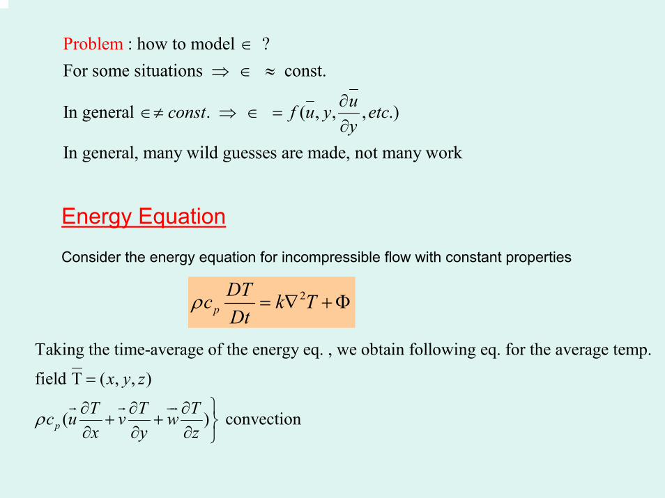
: how to model ?For some situations const.
In general . ( , , , .)
In general, many wild
Pr
guesses are made, not many work
oblem
uconst f u y etcy
∈⇒ ∈ ≈
∂∈≠ ⇒ ∈ =
∂
Energy Equation
Consider the energy equation for incompressible flow with constant properties
2pDTc k TDt
ρ = ∇ +Φ
Taking the time-average of the energy eq. , we obtain following eq. for the average temp.
field T ( , , )
( ) convectionp
x y z
T T Tc u v wx y z
ρ
=
⎫∂ ∂ ∂+ + ⎬∂ ∂ ∂ ⎭
2 2 2
2 2 2
p
2 2 2 2 2
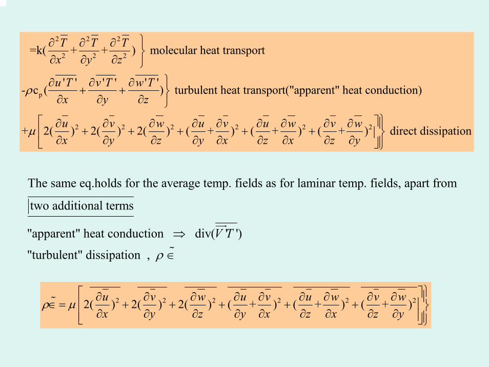
=k( + + ) molecular heat transport
' ' ' ' ' '- c ( ) turbulent heat transport("apparent" heat conduction)
+ 2( ) 2( ) 2( ) ( + ) ( + ) (
T T Tx y z
u T v T w Tx y z
u v w u v u w vx y z y x z x z
ρ
µ
⎫∂ ∂ ∂⎬∂ ∂ ∂ ⎭
⎫∂ ∂ ∂+ + ⎬∂ ∂ ∂ ⎭
∂ ∂ ∂ ∂ ∂ ∂ ∂ ∂+ + + + +
∂ ∂ ∂ ∂ ∂ ∂ ∂ ∂2+ ) direct dissipationw
y⎫⎡ ⎤∂ ⎪⎬⎢ ⎥∂ ⎪⎣ ⎦⎭
The same eq.holds for the average temp. fields as for laminar temp. fields, apart from
two additional terms
"apparent" heat conduction div( ' ')
"turbulent" dissipation ,
V T
ρ
⇒
∈
2 2 2 2 2 22( ) 2( ) 2( ) ( + ) ( + ) ( + )u v w u v u w v wx y z y x z x z y
ρ µ⎫⎡ ⎤∂ ∂ ∂ ∂ ∂ ∂ ∂ ∂ ∂ ⎪∈= + + + + +⎢ ⎥⎬∂ ∂ ∂ ∂ ∂ ∂ ∂ ∂ ∂⎢ ⎥⎪⎣ ⎦⎭

In turbulent flows mechanical energy is transformed into internal energy in two different ways:
a) Direct dissipation : transfer is due to the viscosity (as in laminar flow)
b) Turbulent dissipation : transfer is due to the turbulent fluctuations
The Turbulence Kinetic Energy Equation (K-equation)
Many attemps have been made to add “turbulence conservation” relationsto the time-averaged continuity, momentum and energy equations derived.
A relation for the turbulence kinetic energy K of fluctuations.
( )
1 2 3
1 12 2
Einstein summation notation,( , , ) ( , , )
i i
i
K u u v v w w u u
u u u u u v w
′ ′ ′ ′ ′ ′ ′ ′≡ + + =
= =
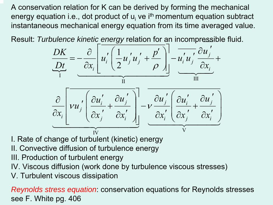
A conservation relation for K can be derived by forming the mechanicalenergy equation i.e., dot product of ui ve ith momentum equation subtractinstantaneous mechanical energy equation from its time averaged value.
Result: Turbulence kinetic energy relation for an incompressible fluid.
I IIIII
VIV
12
ji j j i j
i i
j j ji ij
i j i i j i
uDK pu u u u uDt x x
u u uu uux x x x x x
ρ
ν ν
′⎡ ⎤ ∂′⎛ ⎞∂ ′ ′ ′ ′ ′= − + − +⎢ ⎥⎜ ⎟∂ ∂⎝ ⎠⎢ ⎥⎣ ⎦
⎡ ⎤⎛ ⎞ ⎛ ⎞′ ′ ′′ ′∂ ∂ ∂∂ ∂∂ ⎢ ⎥′ ⎜ ⎟ ⎜ ⎟+ − +⎢ ⎥⎜ ⎟ ⎜ ⎟∂ ′ ′ ′ ′ ′∂ ∂ ∂ ∂ ∂⎝ ⎠ ⎝ ⎠⎢ ⎥⎣ ⎦
I. Rate of change of turbulent (kinetic) energyII. Convective diffusion of turbulence energyIII. Production of turbulent energyIV. Viscous diffusion (work done by turbulence viscous stresses)V. Turbulent viscous dissipation
Reynolds stress equation: conservation equations for Reynolds stressessee F. White pg. 406
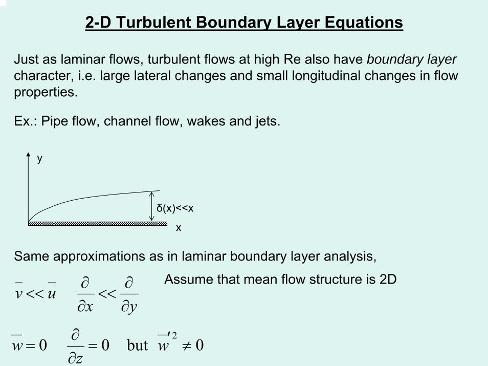
2-D Turbulent Boundary Layer Equations
Just as laminar flows, turbulent flows at high Re also have boundary layercharacter, i.e. large lateral changes and small longitudinal changes in flowproperties.
Ex.: Pipe flow, channel flow, wakes and jets.
δ(x)<<x
y
x
Same approximations as in laminar boundary layer analysis,
v ux y∂ ∂
<< <<∂ ∂
Assume that mean flow structure is 2D
20 0 but 0 w w
z∂ ′= = ≠∂
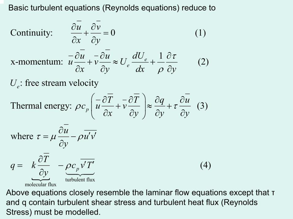
Basic turbulent equations (Reynolds equations) reduce to
Continuity: 0 (1)
1x-momentum: (2)
: free stream velocity
Thermal energy: (3)
where
ee
e
p
u vx y
dUu uu v Ux y dx y
U
T T q uc u vx y y y
τρ
ρ τ
τ
∂ ∂+ =
∂ ∂
∂ ∂ ∂+ ≈ +
∂ ∂ ∂
⎛ ⎞∂ ∂ ∂ ∂+ ≈ +⎜ ⎟∂ ∂ ∂ ∂⎝ ⎠
=
turbulent fluxmolecular flux
(4)p
u u vy
Tq k c v Ty
µ ρ
ρ
∂ ′ ′−∂
∂ ′ ′= −∂
Above equations closely resemble the laminar flow equations except that τand q contain turbulent shear stress and turbulent heat flux (ReynoldsStress) must be modelled.
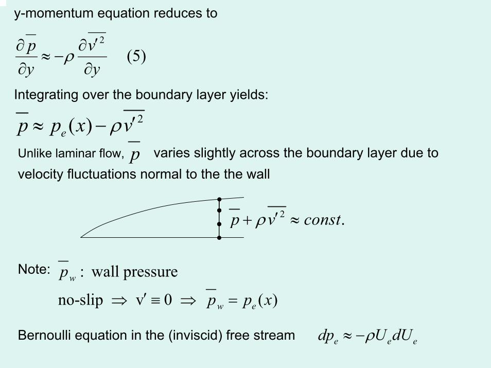
y-momentum equation reduces to
2
(5)p vy y
ρ′∂ ∂
≈ −∂ ∂
Integrating over the boundary layer yields:
2( )ep p x vρ ′≈ −Unlike laminar flow, p varies slightly across the boundary layer due tovelocity fluctuations normal to the the wall
2 .p v constρ ′+ ≈
Note: : wall pressure
no-slip v 0 ( )w
ew
p
p p x′⇒ ≡ ⇒ =
e e edp U dUρ≈ −Bernoulli equation in the (inviscid) free stream

Boundary Conditions:Free stream conditions Ue(x) and Te(x) are known.
No-slip, no jump: ( ,0) ( ,0) 0 , ( ,0) ( )
Free stream matching: ( , ) , ( , ) ( )w
e T e
u x v x T x T x
u x U T x T xδ δ
= = =
= =
The velocity and thermal boundary layer thicknesses (δ, δT) are not necessarily equal
u v if a suitable correlation for total shear τ is known.
but depend upon the Pr, as in laminar flow. Eqs. 1 and 2 can be solved for
Turbulent Boundary Layer Integral Relations:
The integral momentum equation has the identical form as laminar flow
( ) 2
*
0
*
22
1 , H= (momentum shape factor)
1
fe w
e e
e e
e
cdUd Hdx U dx U
u u dyU U
u dyU
τθ θρ
δθθ
δ
∞
+ + = =
⎛ ⎞= −⎜ ⎟
⎝ ⎠⎛ ⎞
= −⎜ ⎟⎝ ⎠
∫Turbulent velocity profile is more complicated in shape and many different correlations have been proposed.
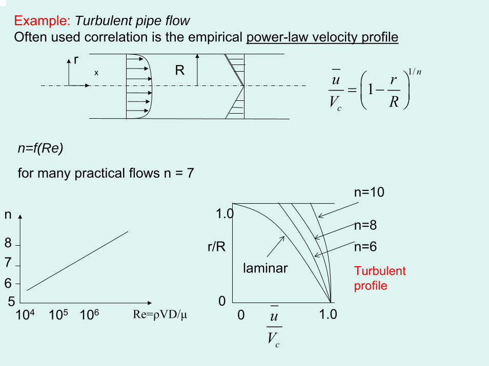
Example: Turbulent pipe flowOften used correlation is the empirical power-law velocity profile
Rxr
1/
1n
c
u rV R
⎛ ⎞= −⎜ ⎟⎝ ⎠
n=f(Re)
for many practical flows n = 7
10456
87
105 106
n
Re=ρVD/µ 00
1.0
1.0
r/Rlaminar
n=6n=8
n=10
Turbulentprofile
c
uV
Turbulent profiles are much “flatter” than laminar profileFlatness increases with Reynolds number (i.e., with n)
Turbulent velocity profile(s): The inner, outer, and overlap layers.Key profile shape consist of 3 layers
Inner layer: very narrow region near the wall (viscous sublayer) viscous (molecular) shear dominateslaminar shear stress is dominant, random eddying nature of flow is absentOuter layer: turbulent (eddy) shear (stress) dominatesOverlap layer: both types of shear important; profile smoothly connects inner and outer regions.
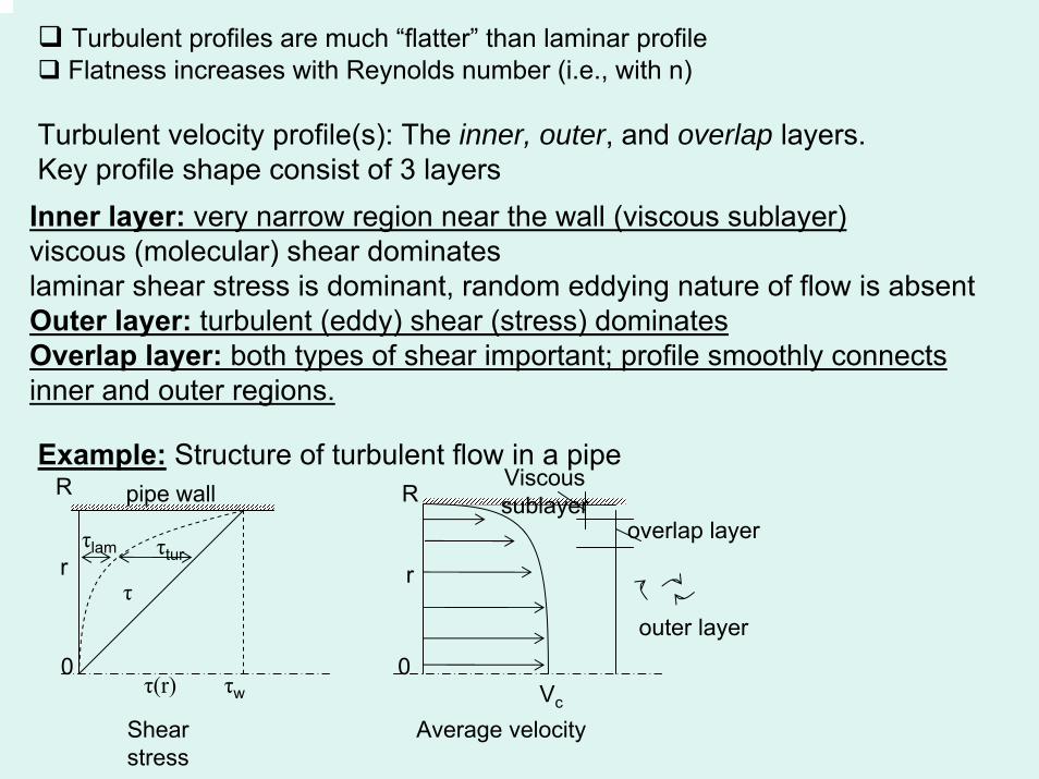
Example: Structure of turbulent flow in a pipeR
r
0
τlam τtur
τ
pipe wall
τwτ(r)
Shearstress
0
R
r
Vc
Viscoussublayer
overlap layer
outer layer
Average velocity

Inner law:
( , , , ) (1)wu f yτ ρ µ=
Velocity profile would not depend on free stream parameters.
Outer law:
( , , , , ) (2)ee w
dpU u g ydx
τ ρ δ− =
Wall acts as a source of retardation, independent of µ.
Overlap law:
(3)inner outeru u=We specify inner and outer functions merge together smoothly.
Dimensionless Profiles: The functional forms in Eqs.(1)-(3) are determined from experiment after use of dimensional analysis. Primary Dimensions: (mass, length, time) : 3Eq.(1) : 5 variablesΠ groups : 5-3 = 2 (dimensionless parameters)
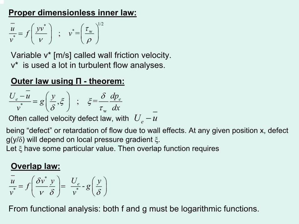
Proper dimensionless inner law:1/2*
* w* ; =u yvf vv
τν ρ
⎛ ⎞ ⎛ ⎞= ⎜ ⎟ ⎜ ⎟
⎝ ⎠⎝ ⎠
Variable v* [m/s] called wall friction velocity. v* is used a lot in turbulent flow analyses.
Outer law using Π - theorem:
*w
, ; =e eU u dpygv dx
δξ ξδ τ
− ⎛ ⎞= ⎜ ⎟⎝ ⎠
Often called velocity defect law, with eU u−being “defect” or retardation of flow due to wall effects. At any given position x, defectg(y/δ) will depend on local pressure gradient ξ. Let ξ have some particular value. Then overlap function requires
Overlap law:*
* * -eUu v y yf gv v
δν δ δ
⎛ ⎞ ⎛ ⎞= =⎜ ⎟ ⎜ ⎟⎝ ⎠⎝ ⎠
From functional analysis: both f and g must be logarithmic functions.
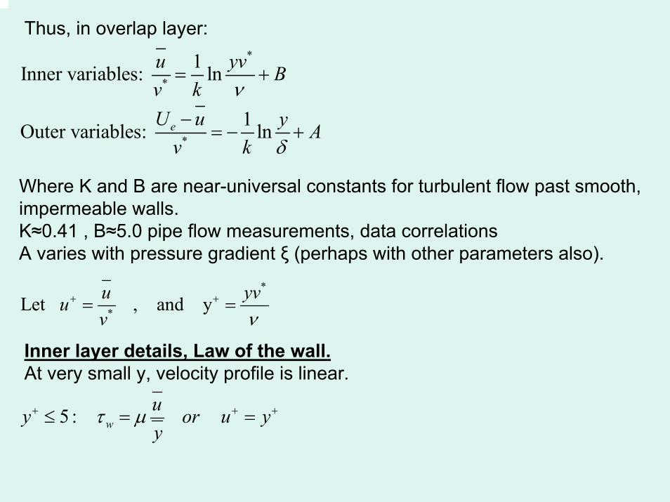
Thus, in overlap layer:*
*
*
1Inner variables: ln
1Outer variables: lne
u yv Bv kU u y Av k
ν
δ
= +
−= − +
Where K and B are near-universal constants for turbulent flow past smooth, impermeable walls. K≈0.41 , B≈5.0 pipe flow measurements, data correlationsA varies with pressure gradient ξ (perhaps with other parameters also).
*
*Let , and yu yvuv ν
+ += =
Inner layer details, Law of the wall.At very small y, velocity profile is linear.
5 : wuy or u yy
τ µ+ + +≤ = =
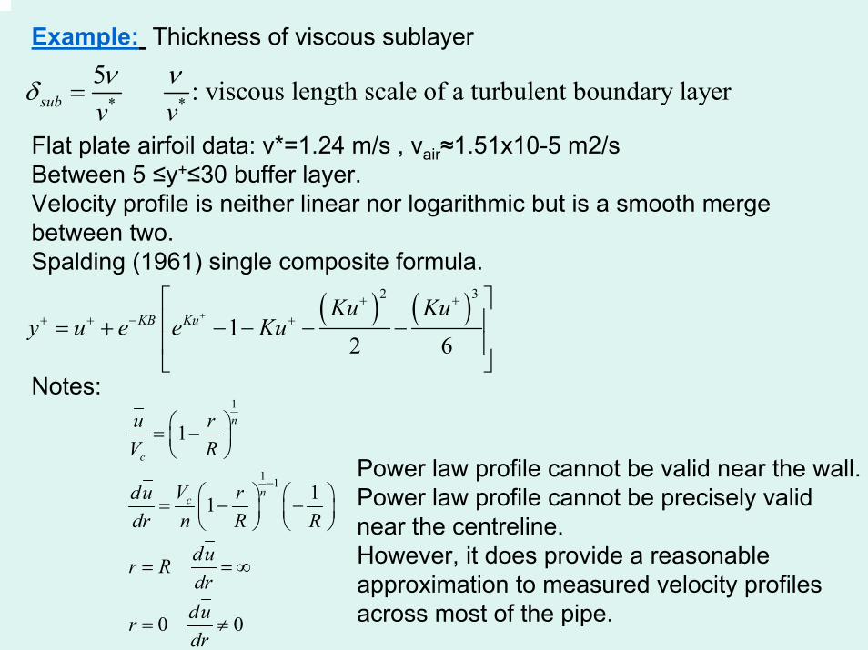
Example: Thickness of viscous sublayer
* *
5 : viscous length scale of a turbulent boundary layersub v vν νδ =
Flat plate airfoil data: v*=1.24 m/s , νair≈1.51x10⁻⁵ m2/sBetween 5 ≤y+≤30 buffer layer.Velocity profile is neither linear nor logarithmic but is a smooth merge between two. Spalding (1961) single composite formula.
( ) ( )2 3
12 6
KB KuKu Ku
y u e e Ku+
+ ++ + − +
⎡ ⎤⎢ ⎥= + − − − −⎢ ⎥⎣ ⎦
Notes:1
1 1
1
11
0 0
n
c
nc
u rV R
Vdu rdr n R R
dur Rdrdurdr
−
⎛ ⎞= −⎜ ⎟⎝ ⎠
⎛ ⎞ ⎛ ⎞= − −⎜ ⎟ ⎜ ⎟⎝ ⎠ ⎝ ⎠
= = ∞
= ≠
Power law profile cannot be valid near the wall.Power law profile cannot be precisely valid near the centreline. However, it does provide a reasonable approximation to measured velocity profiles across most of the pipe.
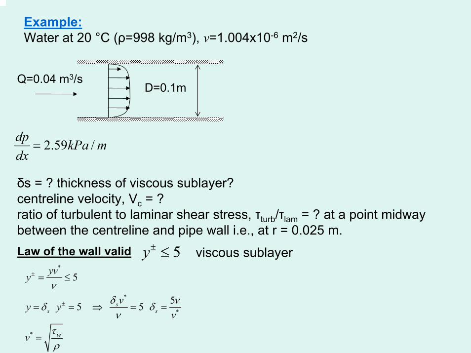
Example:Water at 20 °C (ρ=998 kg/m3), ν=1.004x10⁻⁶ m2/s
Q=0.04 m3/sD=0.1m
2.59 /dp kPa mdx
=
δs = ? thickness of viscous sublayer?centreline velocity, Vc = ?ratio of turbulent to laminar shear stress, τturb/τlam = ? at a point midway between the centreline and pipe wall i.e., at r = 0.025 m.Law of the wall valid 5y± ≤ viscous sublayer
*
*
*
*
5
5 5 5 ss s
w
yvy
vy yv
v
νδ νδ δν
τρ
±
±
= ≤
= = ⇒ = =
=
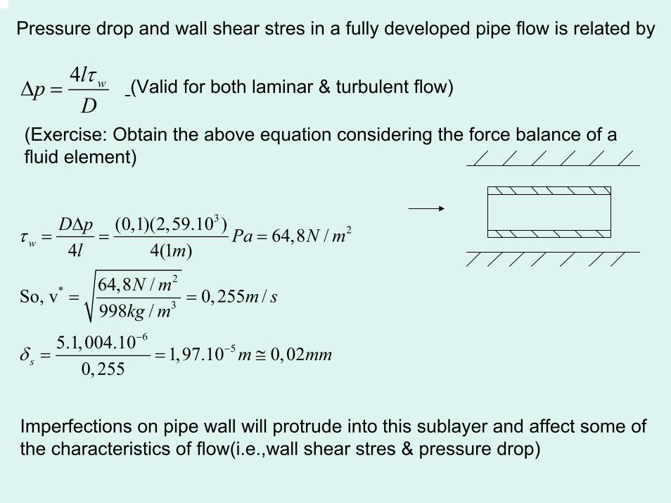
Pressure drop and wall shear stres in a fully developed pipe flow is related by
4 wlpDτ
∆ = (Valid for both laminar & turbulent flow)
(Exercise: Obtain the above equation considering the force balance of a fluid element)
32
2*
3
65
(0,1)(2,59.10 ) 64,8 /4 4(1 )
64,8 /So, v 0, 255 /998 /
5.1,004.10 1,97.10 0,020, 255
w
s
D p Pa N ml m
N m m skg m
m mm
τ
δ−
−
∆= = =
= =
= = ≅
Imperfections on pipe wall will protrude into this sublayer and affect some of the characteristics of flow(i.e.,wall shear stres & pressure drop)

3
2 2
56
5
0,04 / 5,09 /(0,1) / 45,09.(0,1)Re 5,07.101,004.10
Re 5,07.10 8, 4
Q m sV m sA mVD
n
π
ν −
= = =
= = =
= ⇒ =
Power-law profile
1/8,4
1/
02
2
22
c
(1 )
. (1 ) (2 )
2( 1)(2 1)
V 2 V ( 1)(2 1)
8,4 : V 1,186 1,186(5,09) 6,04 /
cR
nc
c
c
u rV R
rQ AV udA V r drR
nQ R Vn n
nQ R Vn n
n V m s
π
π
π
≅ −
= = = −
=+ +
= ∴ =+ +
= = = =
∫ ∫
Recall that Vc=2V for laminar pipe flow:

0,025
?turb
lam r m
ττ
=
= Shear stres distribution throughout the pipe
2 wrDττ = (Valid for laminar or turbulent flow)
rR=D/2 2
1/ (1 ) /
(1 8,4) /8,4
0,025
2(64,8).0,025( 0,025) 32, 4 /0,1
32, 4
; (1 ) (1 )
6,04 0,025(1 ) 26,58,4(0,05) 0,05
lam turb
n n nclam c
r
r N m
Vdu r du ru Vdr R dr nR R
dudr
τ
τ τ τ
τ µ −
−
=
= = =
= + =
= − = − ⇒ = − −
= − − = −
6 2
( )
(1,004.10 ).(998).( 26,5) 0,0266 /32, 4 0,0266 1220
0,0266
lam
turb
lam
du dudr dr
N m
τ µ νρ
ττ
−
= − = −
= − − =−
= =
As expected
turb lamτ τ>>Thus

Turbulent Boundary Layer on a Flat Plate
Problem of flow past a sharp flat plate at high Re has been studied extensively,numerous formulas have been proposed for friction factor.
-curve fits of data-use of Momentum Integral Equation and/or law of the wall-numerical computation using models of turbulent shear
Momentum Integral Analysis
20 ( .) 2f wCdp dU const
dx dx Uτθρ
= = = =
Momentum Interal Equation valid for either laminar or turbulent flow.
For turbulent flowa reasonable approximation to the velocity profile ( / )u f y
Uδ=
Functional relationship describing the wall shear stress
Need to use some empirical relationship
For laminar flow0
wy
uy
τ µ=
∂=
∂
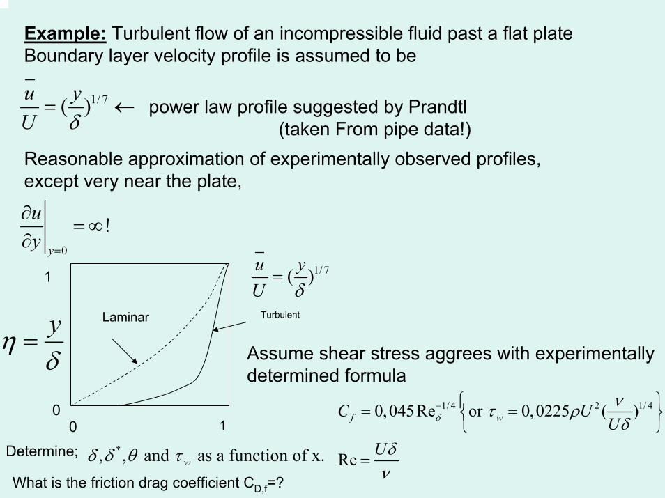
Example: Turbulent flow of an incompressible fluid past a flat plateBoundary layer velocity profile is assumed to be
1/ 7( )u yU δ
= ← power law profile suggested by Prandtl(taken From pipe data!)
Reasonable approximation of experimentally observed profiles,except very near the plate,
0
!y
uy =
∂= ∞
∂
Laminar Turbulent
100
1
yηδ
=
1/ 7( )u yU δ
=
Assume shear stress aggrees with experimentallydetermined formula
1/ 4 2 1/ 40,045Re or 0,0225 ( )
Re
f wC UU
U
δντ ρδ
δν
− ⎧ ⎫= =⎨ ⎬⎩ ⎭
=Determine; *, , and as a function of x.wδ δ θ τWhat is the friction drag coefficient CD,f=?

Momentum Integral Equation (with U=constant)1/ 7 1/ 7
2
1 11/ 7 1/ 7
0 0
1/ 4 1/ 4
1/ 4 1/ 4
0 0
1/5 4/5
; ( )2
7(1 ) (1 ) (1 )72
7 0,0225Re 0,0225( )72
0, 231( )
0,370( )
f w
o
x
Cd y u ydx U U
u u u udy d dU U U U
ddx U
d dxU
xU
δ
δ
τθ η ηρ δ δ
δθ δ η δ η η η
δ νδ
νδ δ
νδ
∞
−
= = = = =
= − = − = − =
= =
=
=
∫ ∫ ∫
∫ ∫
or in dimensionless form 1/5
0,370Rexx
δ=
Boundary layer at leading edge of plate is laminar but in practice,laminar boundary layeroften exists over a relatively short portion of plate.
error associated with starting turbulent boundary layer with =0 at x=0 can be negligible.δ∴1 1
* 1/ 7
0 0 0
*
1/5
(1 ) (1 ) (1 )8
0,0463Rex
u udy d dU U
x
δδ δ η δ η η
δ
∞
= − = − = − =
=
∫ ∫ ∫
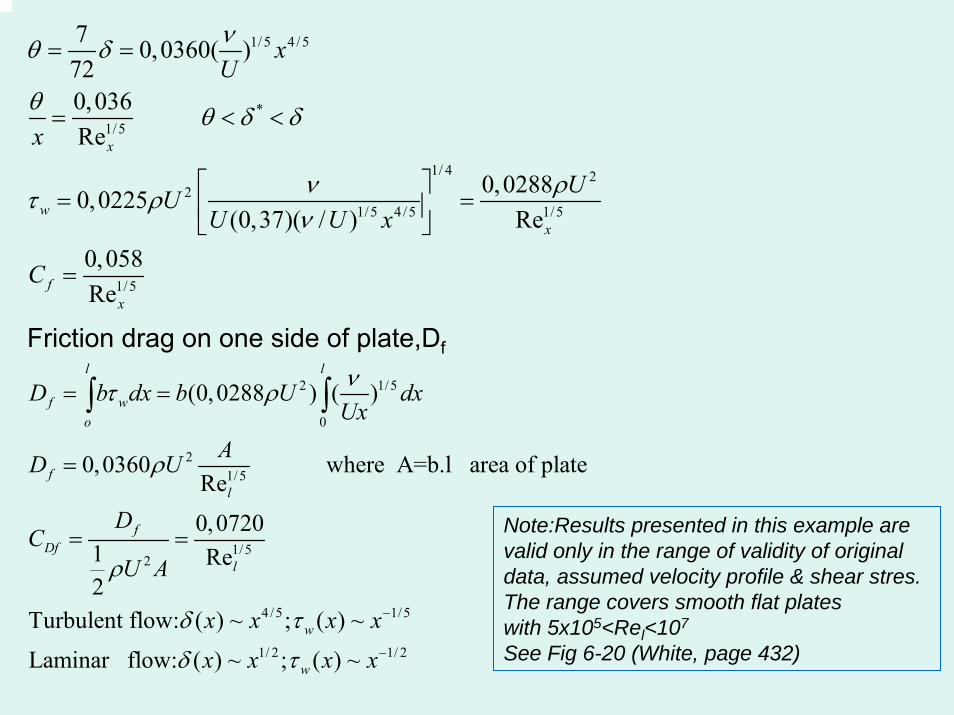
1/5 4 /5
*1/5
1/ 4 22
1/5 4 /5 1/5
1/5
7 0,0360( )720,036 Re
0,02880,0225(0,37)( / ) Re
0,058Re
x
wx
fx
xU
x
UUU U x
C
νθ δ
θ θ δ δ
ν ρτ ρν
= =
= < <
⎡ ⎤= =⎢ ⎥
⎣ ⎦
=
Friction drag on one side of plate,Df
2 1/5
0
21/5
1/52
4 /5 1/5
1/ 2 1/ 2
(0,0288 ) ( )
0,0360 where A=b.l area of plateRe
0,07201 Re2
Turbulent flow: ( ) ~ ; ( ) ~
Laminar flow: ( ) ~ ; ( ) ~
l l
f wo
fl
fDf
l
w
w
D b dx b U dxUx
AD U
DC
U A
x x x x
x x x x
ντ ρ
ρ
ρ
δ τ
δ τ
−
−
= =
=
= =
∫ ∫
Note:Results presented in this example arevalid only in the range of validity of originaldata, assumed velocity profile & shear stres.The range covers smooth flat plateswith 5x10⁵<Rel<107
See Fig 6-20 (White, page 432)
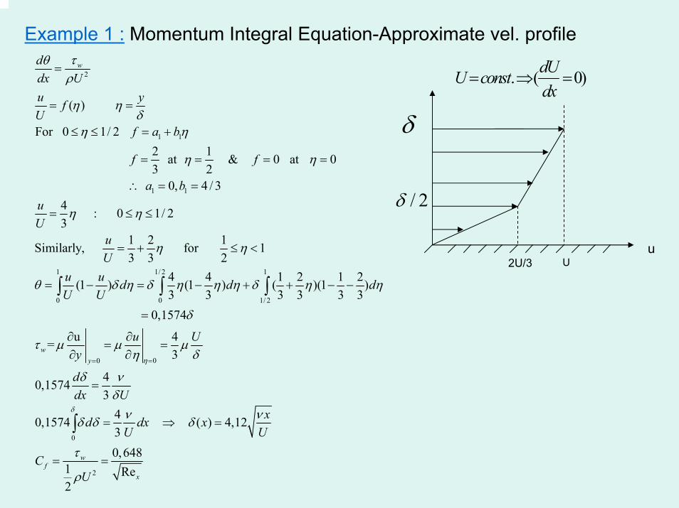
Example 1 : Momentum Integral Equation-Approximate vel. profile
. ( 0)dUU constdx
= ⇒ =2
1 1
1 1
( )
For 0 1/ 2 2 1 at & 0 at 03 2
0, 4 / 34 : 0 1/ 23
Similarly,
wddx Uu yfU
f a b
f f
a buU
τθρ
η ηδ
η η
η η
η η
=
= =
≤ ≤ = +
= = = =
∴ = =
= ≤ ≤
1 1/ 2 1
0 0 1/ 2
00
1 2 1 for 13 3 2
4 4 1 2 1 2(1 ) (1 ) ( )(1 )3 3 3 3 3 3
0,1574
u 4=3
40,15743
40,1574 3
wy
uU
u u d d dU U
u Uy
ddx U
d dxU
η
η η
θ δ η δ η η η δ η η
δ
τ µ µ µη δ
δ νδνδ δ
==
= + ≤ <
= − = − + + − −
=
∂ ∂= =
∂ ∂
=
= ⇒
∫ ∫ ∫
0
2
( ) 4,12
0,6481 Re2
wf
x
xxU
CU
δ νδ
τ
ρ
=
= =
∫
uU2U/3
/ 2δ
δ
U
l
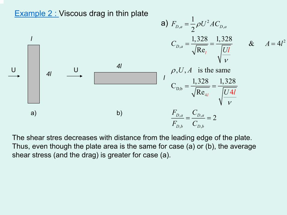
4l
a)
U 4l
l
b)
4
2, ,
2,
D,b
, ,
, ,
121,328 1,328 & 4
Re
, , is the same 1,328 1,328C
Re
2
4
l
l
D a D a
D a
D a D a
D b D b
F U AC
C A lU
U A
U
F C
l
l
F C
ρ
νρ
ν
=
= = =
= =
= =
a)
The shear stres decreases with distance from the leading edge of the plate. Thus, even though the plate area is the same for case (a) or (b), the averageshear stress (and the drag) is greater for case (a).
Example 2 : Viscous drag in thin plate
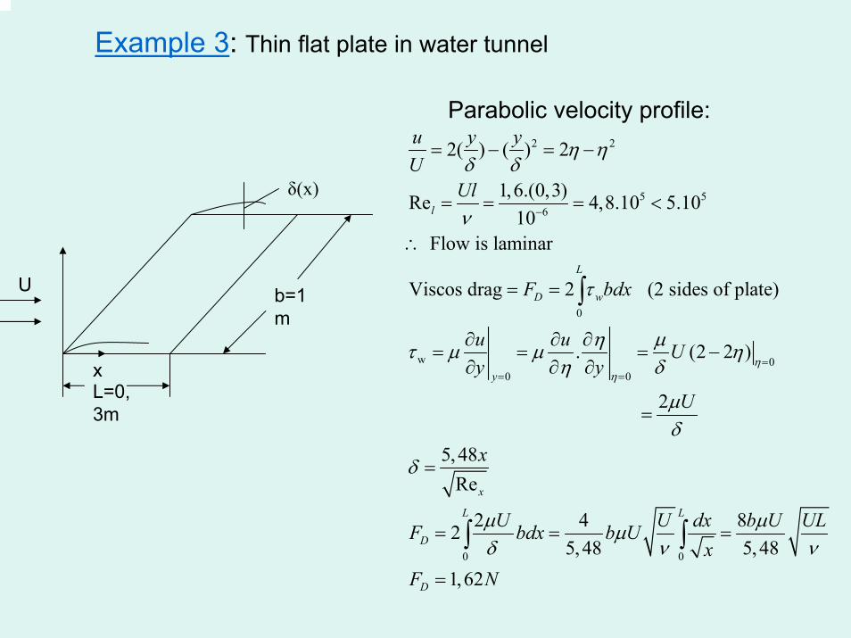
Example 3: Thin flat plate in water tunnel
Parabolic velocity profile:2 2
5 56
0
w 00 0
2( ) ( ) 2
1,6.(0,3)Re 4,8.10 5.1010
Flow is laminar
Viscos drag 2 (2 sides of plate)
. (2 2 )
l
L
D w
y
u y yU
Ul
F bdx
u u Uy y η
η
η ηδ δ
ν
τ
η µτ µ µ ηη δ
−
== =
= − = −
= = = <
∴
= =
∂ ∂ ∂= = = −
∂ ∂ ∂
∫
0 0
2
5, 48Re
2 4 825,48 5,48
1,62
x
L L
D
D
U
x
U U dx b U ULF bdx b Ux
F N
µδ
δ
µ µµδ ν ν
=
=
= = =
=
∫ ∫
b=1m
L=0,3m
U
x
δ(x)
2 30
* 2
2 * 20
. ,(0.3*0.3)*0.7 0.063 /
( ) ( 2 ) : effective area of the duct (allowing for the decreased flowrate in the b.l.)
Thus,( 2 ) 0.09
inlet
inlet
Continuity eq for incompressible flowQ d U m s
Q Q x UA U dA
d d
δ
δ
= = =
= = = −
= − = [ ]* *0 2 0.3 2 d d mδ δ⇒ = + = +
[ ]
[ ][ ]
5* 1.5*101.72 1.72 0.00796
0.3 0.0159
0.
m0.7
( 3 ) 328
d x
x x xU
m
d x m m
νδ−
= = =
=
=
+
≅