An Adaptive Finite Element Method for the Wave Scattering ...lipeijun/paper/2017/JLLZ_JSC_2017.pdf · Scattering with Transparent Boundary Condition ... Keywords Acoustic scattering

Noname manuscript No.(will be inserted by the editor)

An Adaptive Finite Element Method for the WaveScattering with Transparent Boundary Condition

Xue Jiang · Peijun Li · Junliang Lv ·Weiying Zheng

Received: date / Accepted: date

Abstract Consider the acoustic wave scattering by an impenetrable obstacle intwo dimensions. The model is formulated as a boundary value problem for theHelmholtz equation with a transparent boundary condition. Based on a dualityargument technique, an a posteriori error estimate is derived for the finite elementmethod with the truncated Dirichlet-to-Neumann boundary operator. The a pos-teriori error estimate consists of the finite element approximation error and thetruncation error of boundary operator which decays exponentially with respect tothe truncation parameter. A new adaptive finite element algorithm is proposedfor solving the acoustic obstacle scattering problem, where the truncation param-eter is determined through the truncation error and the mesh elements for localrefinements are marked through the finite element discretization error. Numericalexperiments are presented to illustrate the competitive behavior of the proposedadaptive method.

Keywords Acoustic scattering problem · Adaptive finite element method ·Transparent boundary condition · A posteriori error estimate

Mathematics Subject Classification (2000) 65M30 · 78A45 · 35Q60

X. JiangSchool of Science, Beijing University of Posts and Telecommunications, Beijing 100876, China.E-mail: [email protected]

P. LiDepartment of Mathematics, Purdue University, West Lafayette, Indiana 47907, USA.E-mail: [email protected]

J. LvSchool of Mathematics, Jilin University, Changchun 130012, China.E-mail: [email protected]

W. ZhengNCMIS, LSEC, ICMSEC, Academy of Mathematics and System Sciences, Chinese Academyof Sciences, Beijing, 100190, China.E-mail: [email protected]

2 X. Jiang, P. Li, J. Lv, W. Zheng

1 Introduction

The obstacle scattering problem is referred to as wave scattering by boundedimpenetrable obstacles. It usually leads to an exterior boundary value problemimposed in an open domain. Scattering theory in structures of bounded obstacleshas played a fundamental role in diverse scientific areas of applications such asradar and sonar, non-destructive testing, and geophysical exploration [12]. Due toits significant industrial, medical, and military applications, the obstacle scatteringproblem has received considerable attention in both the engineering and mathe-matical communities. It has been studied extensively in the past several decades.A large amount of information is available regarding its solutions. A variety ofnumerical methods are proposed to solve the scattering problem such as the finiteelement methods [20,21] and the boundary integral equation methods [11].

Since the problem is imposed in an open domain, the unbounded physical do-main needs to be truncated into a bounded computational domain in order toapply the finite element method. Therefore, an appropriate boundary conditionis needed on the boundary of the truncated domain so that no artificial wavereflection occurs. Such boundary conditions are called transparent boundary con-ditions or non-reflecting boundary conditions. They are still the subject matter ofmuch ongoing research [2,13,15–17]. The perfectly matched layer (PML) techniqueis one of the effective approaches to truncate unbounded domains into boundedones [7]. Various constructions of PML absorbing layers have been proposed andstudied for wave propagation problems [10,23,24]. Under the assumption that theexterior solution is composed of outgoing waves only, the basic idea of the PMLtechnique is to surround the physical domain by a layer of finite thickness withspecially designed model medium that would either slow down or attenuate all thewaves that propagate from the computational domain. Combined with the PMLtechnique, effective adaptive finite element methods were proposed to solve thediffraction grating problems [4,5,8], where the wave is scattered by periodic struc-tures. Due to their superior numerical performance, the methods were quicklyextended to solve the obstacle scattering problem for both the two-dimensionalHelmholtz equation and the three-dimensional Maxwell equations [6, 9].

Recently, an alternative adaptive finite element method was proposed for solv-ing the same acoustic obstacle scattering problem [19], where the transparentboundary condition was used to truncated the domain. In this approach, no ex-tra artificial domain needs to be imposed to surround the physical domain, whichmakes it different from the PML technique. The transparent boundary conditionis based on a nonlocal Dirichlet-to-Neumann (DtN) operator, which is definedby an infinite Fourier series. Since the transparent boundary condition is exact,the artificial boundary can be put as close as possible to surround the obstacle,which can reduce the size of the computational domain and the scale of the re-sulting linear system of algebraic equations. Numerically, the infinite series needsto be truncated into a sum of finite sequence by choosing some positive integer N .In [19], we derived an a posteriori error estimate, which accounted for the finiteelement discretization error but did not incorporate the truncation error of theDtN operator. Therefore, it was ad hoc to pick an appropriate truncation numberN and lacked of a rigorous analysis for the choice of this parameter.

The aim of this paper is to give a complete a posteriori error estimate andpresent an effective adaptive finite element algorithm. The new a posteriori error

Adaptive Finite Element for the Wave Scattering 3

estimate not only takes into account of the finite element discretization error butalso includes the truncation error of the boundary operator. It was shown in [18]that the convergence could be arbitrarily slow for the truncated DtN mapping tothe original DtN mapping in its operator norm. The a posteriori error analysisof the PML method cannot be applied to our DtN case since the DtN mappingof the truncated PML problem converges exponentially fast to the original DtNmapping. To overcome this difficulty, we adopt a duality argument and obtain ana posteriori error estimate between the solution of the scattering problem and thefinite element solution. The estimate is used to design the adaptive finite elementalgorithm to choose elements for refinements and to determine the truncation pa-rameter N . We show that the truncation error decays exponentially with respectto N . Therefore, the choice of the truncation parameter N is not sensitive to thegiven tolerance. The numerical experiments demonstrate a comparable behaviorto the adaptive PML method presented in [9]. They show much more competitiveefficiency by adaptively refining the mesh as compared with uniformly refining themesh. Thus, this work provides a viable alternative to the adaptive finite elementmethod with the PML technique for solving the acoustic scattering problem. Thealgorithm is expected to be applicable for solving many other wave propagationproblems in open domains and even more general model problems where trans-parent boundary conditions are available but the PML may not be applied. Werefer to [25] for a closely related adaptive finite element method with transparentboundary condition for solving the diffraction grating problem.

The outline of this paper is as follows. In section 2, we introduce the modelproblem of the acoustic wave scattering by an obstacle and its weak formulation byusing the transparent boundary condition. The finite element discretization withtruncated DtN operator is presented in section 3. Section 4 is devoted to the aposteriori error estimate by using a duality argument. In section 5, we discuss thenumerical implementation of our adaptive algorithm and present some numericalexperiments to demonstrate the competitive behavior of the proposed method. Thepaper is concluded with some general remarks and directions for future researchin section 6.

2 Model problem

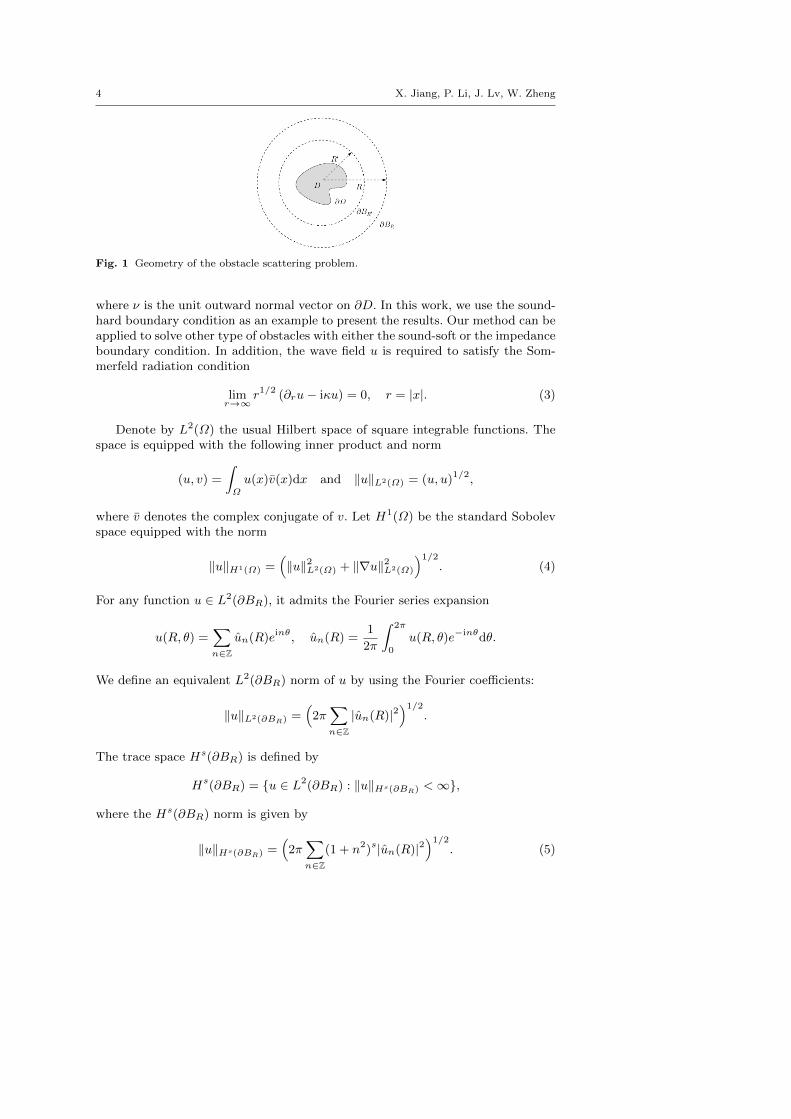
Consider the acoustic scattering by a sound-hard bounded obstacle D with Lips-chitz continuous boundary ∂D, as seen in Figure 1. Let BR = x ∈ R2 : |x| < Rand BR′ = x ∈ R2 : |x| < R′ be the balls with radii R and R′, respectively, whereR > R′ > 0. Denote by ∂BR and ∂BR′ the boundaries of BR and BR′ , respec-tively. Let R′ be large enough such that D ⊂ BR′ ⊂ BR. Denote by Ω = BR \ Dthe bounded domain, in which our boundary value problem will be formulated.

The acoustic wave propagation can be modeled by the two-dimensional Helmholtzequation

∆u+ κ2u = 0 in R2 \ D, (1)

where κ > 0 is a positive constant and is known as the wavenumber. Since theobstacle is sound-hard, the scattered wave field u satisfies the inhomogeneousNeumann boundary condition

∂νu = −g on ∂D, (2)


Fig. 1 Geometry of the obstacle scattering problem.

where ν is the unit outward normal vector on ∂D. In this work, we use the sound-hard boundary condition as an example to present the results. Our method can beapplied to solve other type of obstacles with either the sound-soft or the impedanceboundary condition. In addition, the wave field u is required to satisfy the Som-merfeld radiation condition

limr→∞

r1/2 (∂ru− iκu) = 0, r = |x|. (3)

Denote by L2(Ω) the usual Hilbert space of square integrable functions. Thespace is equipped with the following inner product and norm

(u, v) =

∫Ω

u(x)v(x)dx and ‖u‖L2(Ω) = (u, u)1/2,

where v denotes the complex conjugate of v. Let H1(Ω) be the standard Sobolevspace equipped with the norm

‖u‖H1(Ω) =(‖u‖2L2(Ω) + ‖∇u‖2L2(Ω)

)1/2. (4)

For any function u ∈ L2(∂BR), it admits the Fourier series expansion

u(R, θ) =∑n∈Z

un(R)einθ, un(R) =1

2π

∫ 2π

0

u(R, θ)e−inθdθ.

We define an equivalent L2(∂BR) norm of u by using the Fourier coefficients:

‖u‖L2(∂BR) =(

2π∑n∈Z|un(R)|2

)1/2.

The trace space Hs(∂BR) is defined by

Hs(∂BR) = u ∈ L2(∂BR) : ‖u‖Hs(∂BR) <∞,

where the Hs(∂BR) norm is given by

‖u‖Hs(∂BR) =(

2π∑n∈Z

(1 + n2)s|un(R)|2)1/2

. (5)


It is clear to note that the dual space of Hs(∂BR) is H−s(∂BR) with respect tothe scalar product in L2(∂BR) defined by

〈u, v〉∂BR=

∫∂BR

uvds.

In the exterior domain R2 \ BR, the solution of the Helmholtz equation (1) canbe written as a Fourier series in the polar coordinates:

u(r, θ) =∑n∈Z

H(1)n (κr)

H(1)n (κR)

uneinθ, un =

1

2π

∫ 2π

0

u(R, θ)e−inθdθ, r > R, (6)

where H(1)n (·) is the Hankel function of the first kind with order n.

Given u ∈ H1/2(∂BR), we introduce the DtN operator T : H1/2(∂BR) →H−1/2(∂BR):

(T u)(R, θ) =1

R

∑n∈Z

hn(κR)uneinθ, (7)

where

hn(z) = zH

(1)′

n (z)

H(1)n (z)

.

It follows from (6) and (7) that we have the transparent boundary condition

∂ru = T u on ∂BR. (8)

Multiplying (1) by the complex conjugate of a test function v ∈ H1(Ω), inte-grating over Ω, and using Green’s formula and the boundary conditions (2) and(8), we arrive at an equivalent variational formulation for the scattering problem(1)–(3): Find u ∈ H1(Ω) such that

a(u, v) = 〈g, v〉∂D for all v ∈ H1(Ω), (9)

where the sesquilinear form a: H1(Ω)×H1(Ω)→ C is defined by

a(u, v) = (∇u,∇v)− κ2(u, v)− 〈T u, v〉∂BR(10)

and the linear functional

〈g, v〉∂D =

∫∂D

gvds.

Following [18,19], we may show that the variational problem (9) has a uniqueweak solution u ∈ H1(Ω) for any wavenumber κ and the solution satisfies theestimate

‖u‖H1(Ω) ≤ C‖g‖H−1/2(∂D), (11)

where C is a positive constant depending on κ and R. Since H−1/2(∂D) is notcomputable in the a posteriori error estimate, we rewrite the estimate (11) as

‖u‖H1(Ω) ≤ C‖g‖L2(∂D). (12)


The general theory in Babuska and Aziz [1] implies that there exists a constantγ > 0 depending on κ and R such that it holds the following inf-sup condition:

sup0 6=v∈H1(Ω)

|a(u, v)|‖v‖H1(Ω)

≥ γ‖u‖H1(Ω) for all u ∈ H1(Ω).

We collect some results from [26] on the Bessel functions before proceeding tothe discrete approximation. Let Jn(t) and Yn(t) be the Bessel functions with ordern of the first and second kind, respectively. For any positive integer n, we have

J−n(t) = (−1)nJn(t), Y−n(t) = (−1)nYn(t).

The Hankel functions of the first and second kind with order n are

H(j)n (t) = Jn(t)± iYn(t), j = 1, 2.

For fixed t > 0, we have the asymptotic expressions

Jn(t) ∼ 1√2πn

(et

2n

)n, Yn(t) ∼ −

√2

πn

(et

2n

)−n, n→∞, (13)

which gives that

H(j)n (t) ∼ i(−1)j

√2

πn

(et

2n

)−n, n→∞. (14)

These asymptotic expressions will be used in subsequent analysis.

3 Finite element approximation

Let Mh be a regular triangulation of Ω, where h denotes the maximum diameterof all the elements in Mh. To avoid being distracted from the main focus ofthe a posteriori error estimate, we assume for simplicity that ∂D and ∂BR arepolygonal to keep from using the isoparametric finite element space and derivingthe approximation error of the boundaries ∂D and ∂BR. Thus any edge e ∈ Mh

is a subset of ∂Ω if it has two boundary vertices.Let Vh ⊂ H1(Ω) be a conforming finite element space, i.e.,

Vh := vh ∈ C(Ω) : vh|K ∈ Pm(K) for all K ∈Mh,

where m is a positive integer and Pm(K) denotes the set of all polynomials ofdegree no more than m. The finite element approximation to the problem (9)reads as follows: Find uh ∈ Vh such that

a(uh, vh) = 〈g, vh〉∂D for all vh ∈ Vh. (15)

In the above formulation, the DtN operator T defined in (7) is given by aninfinite series. Practically, it is necessary to truncate the nonlocal operator bytaking finitely many terms of the expansions so as to attain a feasible algorithm.Given a sufficiently large N , we define a truncated DtN operator

(TNu)(R, θ) =1

R

∑|n|≤N

hn(κR)uneinθ. (16)


Using the truncated DtN operator, we have the truncated finite element approxi-mation to the problem (9): Find uNh ∈ Vh such that

aN (uNh , vh) = 〈g, vh〉∂D for all vh ∈ Vh, (17)

where the sesquilinear form aN : Vh × Vh → C is defined as follows:

aN (u, v) = (∇u,∇v)− κ2(u, v)− 〈TNu, v〉∂BR. (18)

For sufficiently large N and sufficiently small h, the discrete inf-sup condition ofthe sesquilinear form aN may be established by a general argument of Schatz [22].It follows from the general theory in [1] that the truncated variational problem(17) admits a unique solution. We also refer to [18] for the well-posedness anderror analysis of the problem (18). In this work, our focus is the a posteriori errorestimate and the associated adaptive algorithm. Thus we assume that the discreteproblem (18) has a unique solution uNh ∈ Vh.

4 The a posteriori error analysis

For any T ∈Mh, denote by hT its diameter. Let Bh denote the set of all the edgesof T . For any e ∈ Bh, denote by he its length. For any interior edge e which is thecommon side of T1 and T2 ∈Mh, we define the jump residual across e as

Je = −(∇uNh |T1· ν1 +∇uNh |T2

· ν2),

where νj is the unit outward normal vector on the boundary of Tj , j = 1, 2. Forany boundary edge e ⊂ ∂BR, we define the jump residual

Je = 2(TNuNh −∇uNh · ν),

where ν is the unit outward normal on ∂BR. For any boundary edge e ⊂ Γ , wedefine the jump residual

Je = 2(∇uNh · ν + g).

Here ν is the unit outward normal on ∂D pointing toward Ω. For any T ∈ Mh,denote by ηT the local error estimator, which is defined by

ηT = hT ‖RuNh ‖L2(T ) +(1

2

∑e∈∂T

he‖Je‖2L2(e)

)1/2, (19)

where the residual operator R = ∆+ κ2.For brevity, we adopt the notation a . b to represent a ≤ Cb, where the positive

constant C may depend on κ,R,R′, but does not depend on the truncation of theDtN operator N or the mesh size of the triangulation h.

We now state the main result, which plays an important role for the numericalexperiments.

Theorem 1 Let u and uNh be the solutions of (9) and (17), respectively. Thereexists a positive integer N0 independent of h such that we have the following aposteriori error estimate for N > N0:

‖u− uNh ‖H1(Ω) .

( ∑T∈Mh

η2T

)1/2

+

(R′

R

)N‖g‖L2(∂D).


We remark that the first term on the right-hand side of the above estimatecomes from the finite element discretization error, while the second term accountsfor the truncation error of the DtN boundary operator. It is clear to note that theerror arising from the second term decays exponentially with respect to N sinceR′ < R.

In the rest of this section, we shall prove the a posteriori error estimator inTheorem 1 by adopting a duality argument, which is used in [3, 22] for a priorierror estimates of indefinite problems and in [25] for a posteriori error estimate forthe diffractive grating problem.

Denote the error ξ := u − uNh . Introduce a dual problem to the original scat-tering problem: Find w ∈ H1(Ω) such that

a(v, w) = (v, ξ) for all v ∈ H1(Ω). (20)

It can be verified that w is the weak solution to the following boundary valueproblem

∆w + κ2w = −ξ in Ω,

∂νw = 0 on ∂D,

∂rw − T ∗w = 0 on ∂BR,

(21)

where the adjoint operator T ∗ is defined as

(T ∗w)(R, θ) =1

R

∑n∈Z

hn(κR)wneinθ.

Following the same proof as that for the original scattering problem (9), we mayshow that the dual problem (20) has a unique weak solution, which satisfies theestimate

‖w‖H1(Ω) . ‖ξ‖L2(Ω). (22)

The following lemma gives some energy representations of the error ξ = u−uNhand is the basis for the a posteriori error analysis.

Lemma 1 Let u, uNh , and w be the solutions to the problems (9), (17), and (20),respectively. We have

‖ξ‖2H1(Ω) = Re (a(ξ, ξ) + 〈(T − TN )ξ, ξ〉∂BR)

+ Re〈TNξ, ξ〉∂BR+ (κ2 + 1)‖ξ‖2L2(Ω), (23)

‖ξ‖2L2(Ω) = a(ξ, w) + 〈(T − TN )ξ, w〉∂BR− 〈(T − TN )ξ, w〉∂BR

, (24)

a(ξ, ψ) + 〈(T − TN )ξ, ψ〉 = 〈g, ψ − ψh〉∂D − aN (uNh , ψ − ψh)

+ 〈(T − TN )u, ψ〉∂BRfor any ψ ∈ H1(Ω), ψh ∈ Vh. (25)

Proof It follows from the definition of the sesquilinear form of a in (10) that

a(ξ, ξ) = (∇ξ,∇ξ)− κ2(ξ, ξ)− 〈T ξ, ξ〉∂BR,

which gives

‖ξ‖2H1(Ω) = a(ξ, ξ) + 〈T ξ, ξ〉∂BR+ (κ2 + 1)‖ξ‖2L2(Ω).


Taking the real parts on both sides of the above equation yields (23). Taking v = ξin (20) gives (24). It remains to prove (25).

It follows from (9) and (17) that

a(ξ, ψ) =a(u− uNh , ψ − ψh) + a(u− uh, ψh)

=〈g, ψ − ψh〉∂D − a(uNh , ψ − ψh) + a(u− uNh , ψh)

=〈g, ψ − ψh〉∂D − aN (uNh , ψ − ψh)

+(aN (uNh , ψ − ψh)− a(uNh , ψ − ψh)

)+(a(u, ψh)− a(uNh , ψh)

).

Noting that a(u, ψh) = 〈g, ψh〉∂D = aN (uNh , ψh), we have

a(ξ, ψ) = 〈g, ψ − ψh〉∂D − aN (uNh , ψ − ψh) +(aN (uNh , ψ)− a(uNh , ψ)

)= 〈g, ψ − ψh〉∂D − aN (uNh , ψ − ψh) + 〈(T − TN )uNh , ψ〉∂BR

= 〈g, ψ − ψh〉∂D − aN (uNh , ψ − ψh)− 〈(T − TN )ξ, ψ〉∂BR

+ 〈(T − TN )u, ψ〉∂BR,

which implies (25).

It is necessary to estimate (25) and the last term in (24) in order to proveTheorem 1. We first show a trace regularity result.

Lemma 2 For any u ∈ H1(Ω), we have

‖u‖H1/2(∂BR) . ‖u‖H1(Ω), ‖u‖H1/2(∂BR′ ). ‖u‖H1(Ω).

Proof Consider the annulus

BR \ BR′ = (r, θ) : R′ < r < R, 0 < θ < 2π.

It is clear to note that BR \ BR′ ⊂ Ω. A simple calculation yields

(R−R′)|ζ(R)|2 =

∫ R

R′|ζ(r)|2dr +

∫ R

R′

∫ R

r

d

dt|ζ(t)|2dtdr

≤∫ R

R′|ζ(r)|2dr + (R−R′)

∫ R

R′2|ζ(r)||ζ′(r)|dr,

which implies by Young’s inequality that

|ζ(R)|2 ≤ (1 + (R−R′)−1)

∫ R

R′(1 + n2)1/2|ζ(r)|2dr +

∫ R

R′(1 + n2)−1/2|ζ′(r)|2dr.

Hence we have

(1 + n2)1/2|ζ(R)|2 ≤ (1 + (R−R′)−1)

∫ R

R′(1 + n2)|ζ(r)|2dr +

∫ R

R′|ζ′(r)|2dr

≤ (1 + (R−R′)−1)

∫ R

R′

((1 + n2)|ζ(r)|2 + |ζ′(r)|2

)dr


Given u ∈ H1(Ω), it follows from the definitions of the H1/2(∂BR) norm (5)and the H1(Ω) norm (4) that we have

‖u‖2H1/2(∂BR) = 2π∑n∈Z

(1 + n2)1/2|un(R)|2

and

‖u‖2H1(BR\BR′ )= 2π

∑n∈Z

∫ R

R′

((r +

n2

r)|un(r)|2 + r

∣∣u′n(r)∣∣2)dr.

Combining the above estimates gives

‖u‖2H1/2(∂BR) ≤ 2π(1 + (R−R′)−1)∑n∈Z

∫ R

R′

((1 + n2)|un(r)|2 + |u′n(r)|2

)dr

. 2π∑n∈Z

∫ R

R′

((r +

n2

r)|un(r)|2 + r

∣∣u′n(r)∣∣2)dr

= ‖u‖2H1(BR\BR′ )≤ ‖u‖2H1(Ω).

Similarly, the second estimate can be proved by observing that

(R−R′)|ζ(R′)|2 =

∫ R

R′|ζ(r)|2dr +

∫ R

R′

∫ R′

r

d

dt|ζ(t)|2dtdr,

which completes the proof.

Lemma 3 Let u be the solution to (9). We have

|un(R)| .(R′

R

)|n||un(R′)|.

Proof It is known that the solution of the scattering problem (1)–(3) admits theseries expansion

u(r, θ) =∑n∈Z

H(1)n (κr)

H(1)n (κR′)

un(R′)einθ, un(R′) =1

2π

∫ 2π

0

u(R′, θ)e−inθdθ. (26)

for all r > R′. Evaluating (26) at r = R yields

u(R, θ) =∑n∈Z

H(1)n (κR)

H(1)n (κR′)

un(R′)einθ,

which implies

un(R) =H

(1)n (kR)

H(1)n (kR′)

un(R′).

Using the asymptotic expression in (14), we obtain

|un(R)| =

∣∣∣∣∣ H(1)n (kR)

H(1)n (kR′)

∣∣∣∣∣|un(R′)| .(R′

R

)|n||un(R′)|,



Lemma 4 For any ψ ∈ H1(Ω), we have∣∣a(ξ, ψ) + 〈(T − TN )ξ, ψ〉∂BR

∣∣.

( ∑T∈Mh

η2T

)1/2

+

(R′

R

)N‖g‖L2(∂D)

‖ψ‖H1(Ω).

Proof Define

J1 = 〈g, ψ − ψh〉∂D − aN (uNh , ψ − ψh),

J2 = 〈(T − TN )u, ψ〉∂BR,

where ψh ∈ Vh. It follows from (25) that

a(ξ, ψ) + 〈(T − TN )ξ, ψ〉∂BR= J1 + J2.

By the definition of the sesquilinear form (18), J1 can be rewritten as

J1 =∑

T∈Mh

(∫T

(−∇uNh · ∇(ψ − ψh) + κ2uNh (ψ − ψh)

)dx

+∑

e∈∂T∩∂BR

∫e

TNuNh (ψ − ψh)ds+

∑e∈∂T∩Γ

∫e

g(ψ − ψh)ds

).

Using the integration by parts, we get

J1 =∑

T∈Mh

(∫T

(∆uNh + κ2uNh )(ψ − ψh)dx−∑e∈∂T

∫e

∇uNh · ν(ψ − ψh)ds

+∑

e∈∂T∩∂BR

∫e

TNuNh (ψ − ψh)ds+

∑e∈∂T∩Γ

∫e

g(ψ − ψh)ds

)

=∑

T∈Mh

(∫T

RuNh (ψ − ψh)dx+∑e∈∂T

1

2

∫e

Je(ψ − ψh)ds

)Now we take ψh = Πhψ ∈ Vh. Here Πh is the Scott–Zhang interpolation operator,which has the following interpolation estimates:

‖v −Πhv‖L2(T ) . hT ‖∇v‖L2(T ), ‖v −Πhv‖L2(e) . h1/2e ‖v‖H1(Te).

Here T and Te are the union of all the elements in Mh, which have nonemptyintersection with the element T and the side e, respectively. The trace theoremhas been used in the proof of the second estimate. In fact, assuming that the affinemapping (x1, x2) → (λ1, λ2) maps the element T onto the reference element Twith vertices P1(0, 0), P2(1, 0) and P3(0, 1), the side e onto the side e of T , andthe function v−Πhv on T into the function (v− Πhv)(λ1, λ2) = (v−Πhv)(x1, x2)on T , we have ∫

e

|v −Πhv|2ds . he

∫e

|v − Πhv|2ds.

It follows from the trace theorem that∫e

|v − Πhv|2ds . ‖v − Πhv‖2H1(T ).


Using the relationship between the Sobolev semi-norms of a function before andafter an affine mapping, we obtain

‖v − Πhv‖L2(T ) . h−1T ‖v −Πhv‖L2(T ), |v − Πhv|H1(T ) . |v −Πhv|H1(T ),

which give

‖v −Πhv‖L2(e) . h1/2e (h−1T ‖v −Πhv‖L2(T ) + |v −Πhv|H1(T )) . h1/2e ‖v‖H1(Te)

.

It follows from the Cauchy–Schwarz inequality and the interpolation estimatesthat

|J1| .∑

T∈Mh

(hT ‖RuNh ‖L2(T )‖∇ψ‖L2(T ) +

∑e∈∂T

1

2h1/2e ‖Je‖L2(e)‖ψ‖H1(Te)

)

.∑

T∈Mh

hT ‖RuNh ‖L2(T ) +

( ∑e∈∂T

1

2he‖Je‖2L2(e)

)1/2 ‖ψ‖H1(Ω).

Using (19), we immediately get

|J1| .

( ∑T∈Mh

η2T

)1/2

‖ψ‖H1(Ω).

It follows from the definitions of (7) and (16) that

|J2| = |〈(T − TN )u, ψ〉∂BR| =

∣∣∣2πR

∑|n|>N

hn(κR)un(R)¯ψn(R)

∣∣∣≤(

2π

R

) ∑|n|>N

|hn(κR)||un(R)||ψn(R)|.

Using Lemma 3, we obtain

|J2| .∑|n|>N

2π|hn(κR)|(R′

R

)|n||un(R′)||ψn(R)|

.

(R′

R

)N ∑|n|>N

2π|hn(κR)||un(R′)||ψn(R)|.

It is shown in [14] that

|hn(κR)| . (1 + n2)1/2 . |n|, (27)

which together with Lemma 3 yields

|J2| .(R′

R

)N ∑|n|>N

2π(1 + n2)1/2|un(R′)|21/2 ∑

|n|>N

2π(1 + n2)1/2|ψn(R)|21/2

.

(R′

R

)N‖u‖H1/2(∂BR′ )

‖ψ‖H1/2(∂BR) .

(R′

R

)N‖u‖H1(Ω)‖ψ‖H1(Ω).


Using the stability estimate (12), we get

|J2| .(R′

R

)N‖g‖L2(∂D)‖ψ‖H1(Ω).

Combining the above estimates yields

|J1 + J2| .

( ∑T∈Mh

η2T

)1/2

+

(R′

R

)N‖g‖L2(∂D)

‖ψ‖H1(Ω),


Lemma 5 Let w be the solution of the dual problem (20). We have

|〈(T − TN )ξ, w〉∂BR| . N−2‖ξ‖2H1(Ω).

Proof It follows from (27), the Cauchy–Schwarz inequality, and Lemma 2 that

|〈(T − TN )ξ, w〉∂BR| ≤ 2π

∑|n|>N

|hn(kR)||ξn(R)||wn(R)| . 2π∑|n|>N

|n||ξn(R)||wn(R)|

= 2π∑|n|>N

((1 + n2)1/2|n|3

)−1/2(1 + n2)1/4|ξn(R)||n|5/2|wn(R)|

. max|n|>N

((1 + n2)1/2|n|3

)−1/2

2π∑|n|>N

(1 + n2)1/2|ξn(R)|21/2

×

∑|n|>N

|n|5|wn(R)|21/2

. N−2‖ξ‖H1/2(∂BR)

∑|n|>N

|n|5|wn(R)|21/2

. N−2‖ξ‖H1(Ω)

∑|n|>N

|n|5|wn(R)|21/2

.

Next we consider the dual problem (21) in the annulus BR \ BR′ in order toestimate wn(R), i.e.,

∆w + κ2w = −ξ in BR \ BR′ ,w = w(R′, θ) on ∂BR′ ,

∂rw − T ∗w = 0 on ∂BR.

In the Fourier domain, we obtain a two-point boundary value problem for thecoefficient wn:

d2wn(r)

dr2+

1

r

dwn(r)

dr+

(κ2 − n2

r2

)wn(r) = −ξn(r), R′ < r < R,

dwn(R)

dr− 1

Rhn(κR)wn(R) = 0, r = R,

wn(R′) = wn(R′), r = R′.


It follows from the variation of parameters that the solution of the above secondorder equation is

wn(r) = Sn(r)wn(R′) +iπ

4

∫ r

R′tWn(r, t)ξn(t)dt

+iπ

4

∫ R

R′tSn(t)Wn(R′, r)ξn(t)dt, (28)

where

Sn(r) =H

(2)n (κr)

H(2)n (κR′)

, Wn(r, t) = det

[H

(1)n (κr) H

(2)n (κr)

H(1)n (κt) H

(2)n (κt)

].

Taking r = R in (28), we get

wn(R) = Sn(R)wn(R′) +iπ

4

∫ R

R′tSn(R)Wn(R′, t)ξn(t)dt,

which yields

|wn(R)| ≤ |Sn(R)||wn(R′)|+ π

4

∫ R

R′t|Sn(R)||Wn(R′, t)||ξn(t)|dt.

We may easily get from the asymptotic expressions (13) and (14) that

Sn(R) ∼(R′

R

)|n|as n→∞

and

Wn(R′, t) = 2iJn(κR′)Yn(κR′)

(Jn(κt)

Jn(κR′)− Yn(κt)

Yn(κR′)

)∼ − 2i

π|n|

((t

R′

)|n|−(R′

t

)|n|)as n→∞.

Thus, we obtain

|Sn(R)| .(R′

R

)|n|and |Wn(R′, t)| . |n|−1

(t

R′

)|n|.

Combining the above estimates yields

|wn(R)| .(R′

R

)|n||wn(R′)|+ |n|−1

(R′

R

)|n|‖ξn(t)‖L∞([R′,R])

∫ R

R′t

(t

R′

)|n|dt

.

(R′

R

)|n||wn(R′)|+ n−2‖ξn(t)‖L∞([R′,R]). (29)


For any t ∈ [R′, R], without loss of generality, we assume that t is closer to theleft endpoint R′ than the right endpoint R. Denote δ = R − R′. Then we haveR− t ≥ δ/2. Thus

|ξn(t)|2 =1

R− t

∫ t

R

((R− s)|ξn(s)|2

)′ds

=1

R− t

∫ t

R

(−|ξn(s)|2 + 2(R− s)Re(ξ′n(s)

¯ξn(s))

)ds

≤ 1

R− t

∫ R

t

|ξn(s)|2ds+ 2

∫ R

R′|ξn(s)||ξ′n(s)|ds,

which implies that

‖ξn(t)‖2L∞([R′,R]) ≤2

δ‖ξn(t)‖2L2([R′,R]) + 2‖ξn(t)‖L2([R′,R])‖ξ′n(t)‖L2([R′,R])

≤(

2

δ+ |n|

)‖ξn(t)‖2L2([R′,R]) + |n|−1‖ξ′n(t)‖2L2([R′,R]). (30)

Using (29) and (30) gives

∑|n|>N

|n|5|wn(R)|2 .∑|n|>N

|n|5((

R′

R

)|n||wn(R′)|+ n−2‖ξn(t)‖L∞([R′,R])

)2

.∑|n|>N

|n|5((

R′

R

)2|n||wn(R′)|2 + n−4‖ξn(t)‖2L∞([R′,R])

)= I1 + I2,

where

I1 =∑|n|>N

|n|5(R′

R

)2|n||wn(R′)|2 and I2 =

∑|n|>N

|n|‖ξn(t)‖2L∞([R′,R]).

Noting that the function t4e−t is bounded on (0,+∞), we have

I1 . max|n|>N

(|n|4

(R′

R

)2|n|) ∑|n|>N

|n||wn(R′)|2 . ‖w‖2H1/2(∂BR′ ). ‖ξ‖2H1(Ω)

and

I2 .∑|n|>N

(|n|(

2

δ+ |n|

)‖ξn‖2L2([R′,R]) + ‖ξ′n‖2L2([R′,R])

)

≤∑|n|>N

((2

δ|n|+ n2

)‖ξ(t)‖2L2([R′,R]) + ‖ξ′(t)‖2L2([R′,R])

). (31)

A simple calculation yields

‖ξ‖2H1(BR\BR′ )= 2π

∑n∈Z

∫ R

R′

((r +

n2

r)|ξn(r)|2 + r

∣∣ξ′n(r)∣∣2) dr

≥ 2π∑n∈Z

∫ R

R′

((R′ +

n2

R)|ξn(r)|2 +R′

∣∣ξ′n(r)∣∣2)dr. (32)


It is easy to note that

2

δ|n|+ n2 . R′ +

n2

R. (33)

It follows from (31)–(33) that

I2 . ‖ξ‖2H1(BR\BR′ )+

1

R′‖ξ‖2H1(BR\BR′ )

. ‖ξ‖2H1(BR\BR′ )≤ ‖ξ‖2H1(Ω).

Therefore, we have ∑|n|>N

|n|5|wn(R)|2 . ‖ξ‖2H1(Ω),


We now prove the main conclusion.

Proof It is easy to verify from (16) and (27) that

Re〈TNξ, ξ〉∂BR= 2π

∑|n|≤N

Re(hn(κR))|ξn|2 ≤ 0.

It follows from (23) and Lemma 4 that there exist two positive constants C1 andC2 independent of h and N such that

‖ξ‖2H1(Ω) ≤ C1

( ∑T∈Mh

η2T

)1/2

+

(R′

R

)N‖g‖L2(∂D)

‖ξ‖H1(Ω) + C2‖ξ‖2L2(Ω).

Using (24), Lemma 4, (22), and Lemma 5, we obtain

‖ξ‖2L2(Ω) ≤ C3

( ∑T∈Mh

η2T

)1/2

+

(R′

R

)N‖g‖L2(∂D)

‖ξ‖L2(Ω)+C4N−2‖ξ‖2H1(Ω),

where C3 > 0 and C4 > 0 are independent of h and N . Combining the above twoestimates, we have

‖ξ‖2H1(Ω) ≤ (C1 + C2C3)

( ∑T∈Mh

η2T

)1/2

+

(R′

R

)N‖g‖L2(∂D)

‖ξ‖H1(Ω)

+ C2C4N−2‖ξ‖2H1(Ω).

Choose a sufficiently large integer N0 such that C2C4N−20 ≤ 1/2, which completes

the proof by taking N > N0.

5 Implementation and numerical examples

In this section, we discuss the implementation of the adaptive finite element al-gorithm with the truncated DtN boundary condition and present two numericalexamples to demonstrate the competitive performance of the proposed method.


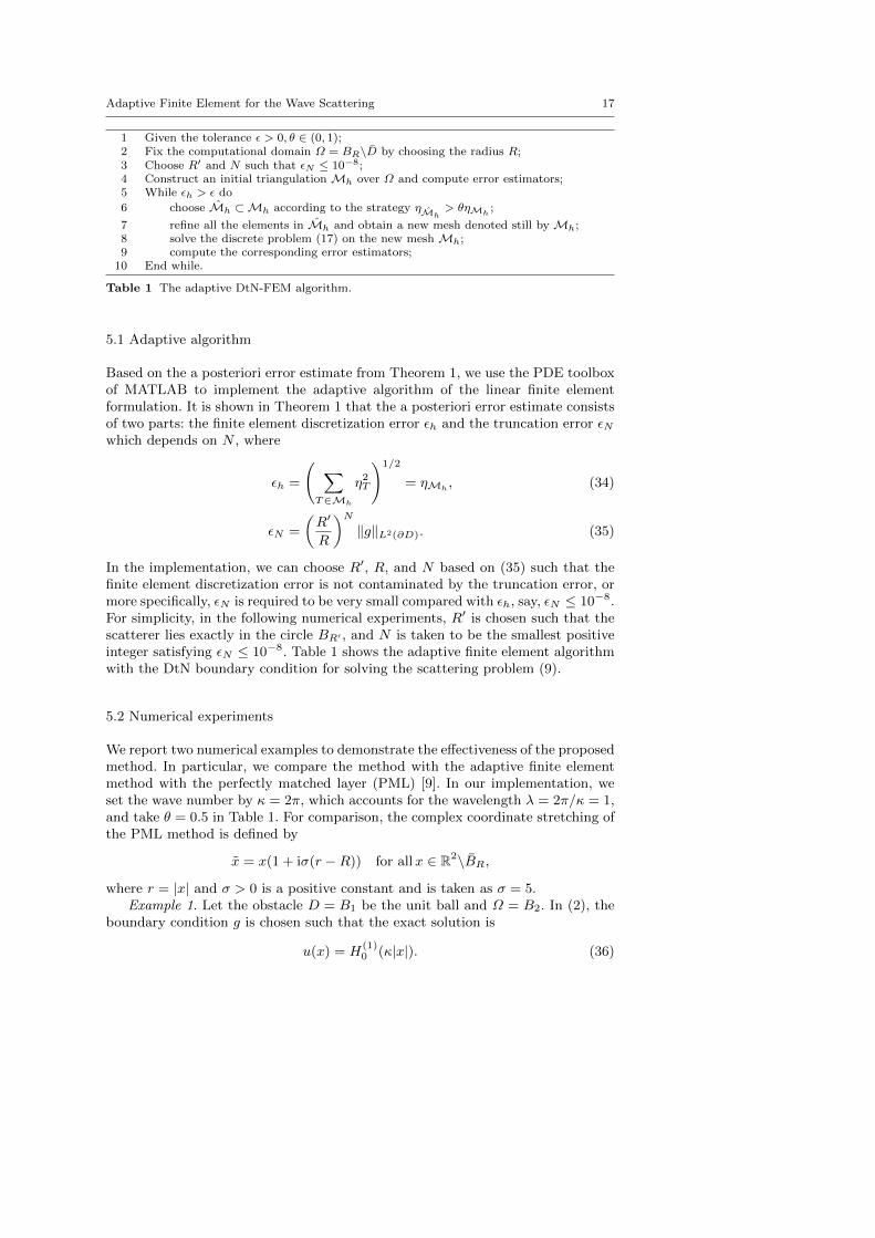
1 Given the tolerance ε > 0, θ ∈ (0, 1);2 Fix the computational domain Ω = BR\D by choosing the radius R;3 Choose R′ and N such that εN ≤ 10−8;4 Construct an initial triangulation Mh over Ω and compute error estimators;5 While εh > ε do

6 choose Mh ⊂Mh according to the strategy ηMh> θηMh

;

7 refine all the elements in Mh and obtain a new mesh denoted still by Mh;8 solve the discrete problem (17) on the new mesh Mh;9 compute the corresponding error estimators;

10 End while.

Table 1 The adaptive DtN-FEM algorithm.

5.1 Adaptive algorithm

Based on the a posteriori error estimate from Theorem 1, we use the PDE toolboxof MATLAB to implement the adaptive algorithm of the linear finite elementformulation. It is shown in Theorem 1 that the a posteriori error estimate consistsof two parts: the finite element discretization error εh and the truncation error εNwhich depends on N , where

εh =

( ∑T∈Mh

η2T

)1/2

= ηMh, (34)

εN =

(R′

R

)N‖g‖L2(∂D). (35)

In the implementation, we can choose R′, R, and N based on (35) such that thefinite element discretization error is not contaminated by the truncation error, ormore specifically, εN is required to be very small compared with εh, say, εN ≤ 10−8.For simplicity, in the following numerical experiments, R′ is chosen such that thescatterer lies exactly in the circle BR′ , and N is taken to be the smallest positiveinteger satisfying εN ≤ 10−8. Table 1 shows the adaptive finite element algorithmwith the DtN boundary condition for solving the scattering problem (9).

5.2 Numerical experiments

We report two numerical examples to demonstrate the effectiveness of the proposedmethod. In particular, we compare the method with the adaptive finite elementmethod with the perfectly matched layer (PML) [9]. In our implementation, weset the wave number by κ = 2π, which accounts for the wavelength λ = 2π/κ = 1,and take θ = 0.5 in Table 1. For comparison, the complex coordinate stretching ofthe PML method is defined by

x = x(1 + iσ(r −R)) for allx ∈ R2\BR,

where r = |x| and σ > 0 is a positive constant and is taken as σ = 5.Example 1. Let the obstacle D = B1 be the unit ball and Ω = B2. In (2), the

boundary condition g is chosen such that the exact solution is

u(x) = H(1)0 (κ|x|). (36)


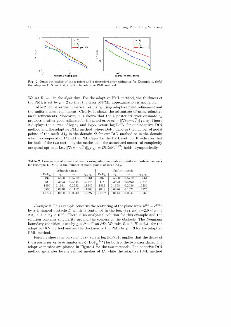
Fig. 2 Quasi-optimality of the a priori and a posteriori error estimates for Example 1. (left)the adaptive DtN method; (right) the adaptive PML method.

We set R′ = 1 in the algorithm. For the adaptive PML method, the thickness ofthe PML is set by ρ = 2 so that the error of PML approximation is negligible.

Table 2 compares the numerical results by using adaptive mesh refinement andthe uniform mesh refinement. Clearly, it shows the advantage of using adaptivemesh refinements. Moreover, it is shown that the a posteriori error estimate εhprovides a rather good estimate for the priori error eh = ‖∇(u−uNh )‖L2(Ω). Figure2 displays the curves of log eh and log εh versus log DoFh for our adaptive DtNmethod and the adaptive PML method, where DoFh denotes the number of nodalpoints of the mesh Mh in the domain Ω for our DtN method or in the domainwhich is composed of Ω and the PML layer for the PML method. It indicates thatfor both of the two methods, the meshes and the associated numerical complexity

are quasi-optimal, i.e., ‖∇(u− uNh )‖L2(Ω) = O(DoF−1/2h ) holds asymptotically.

Table 2 Comparison of numerical results using adaptive mesh and uniform mesh refinementsfor Example 1. DoFh is the number of nodal points of mesh Mh.

Adaptive mesh Uniform meshDoFh eh εh εh/eh DoFh eh εh εh/eh132 0.5358 0.5712 1.0661 132 0.5358 0.5712 1.0661529 0.3393 0.3645 1.0743 478 0.3592 0.3860 1.07451490 0.1911 0.2232 1.1646 1812 0.1698 0.2086 1.22806563 0.0870 0.1117 1.1680 7048 0.0826 0.1071 1.297517721 0.0428 0.0549 1.2827 27792 0.0414 0.0544 1.3163

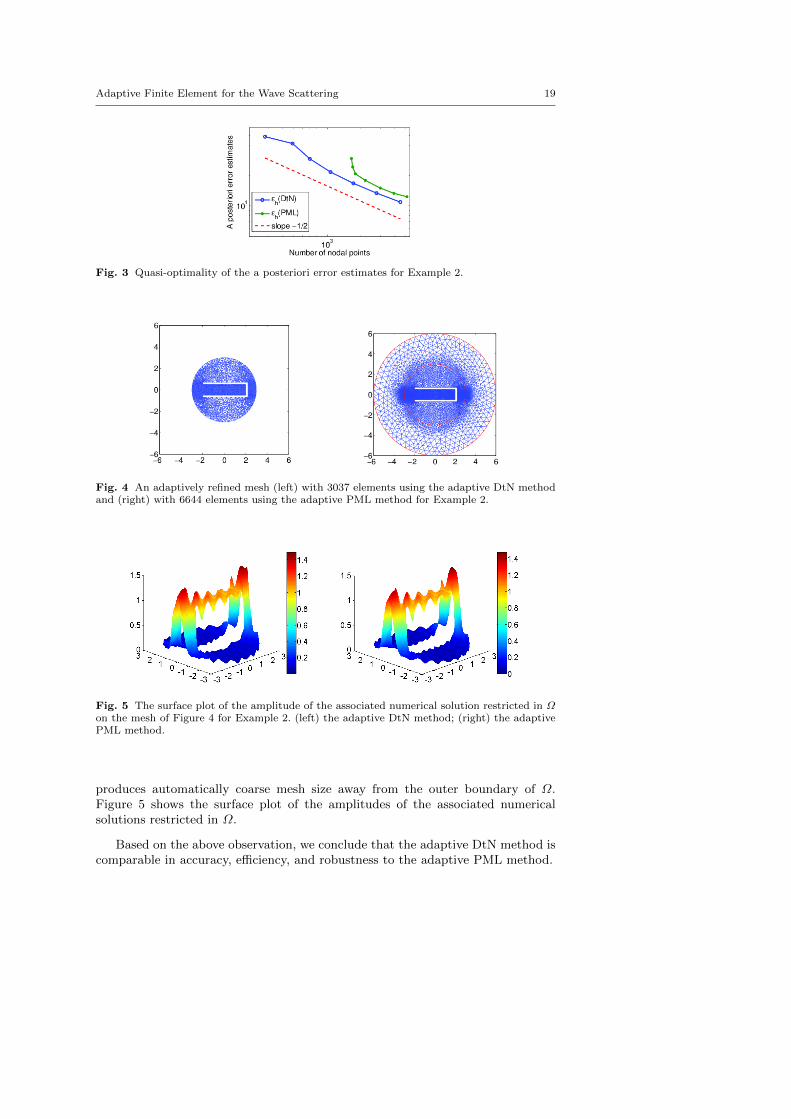
Example 2. This example concerns the scattering of the plane wave uinc = eiκx1

by a U-shaped obstacle D which is contained in the box (x1, x2) : −2.0 < x1 <2.2,−0.7 < x2 < 0.7. There is no analytical solution for this example and thesolution contains singularity around the corners of the obstacle. The Neumannboundary condition is set by g = ∂νu

inc on ∂D. We take R = 3, R′ = 2.31 for theadaptive DtN method and set the thickness of the PML by ρ = 3 for the adaptivePML method.

Figure 3 shows the curve of log εh versus log DoFh. It implies that the decay of

the a posteriori error estimates areO(DoF−1/2h ) for both of the two algorithms. The

adaptive meshes are plotted in Figure 4 for the two methods. The adaptive DtNmethod generates locally refined meshes of Ω, while the adaptive PML method


Fig. 3 Quasi-optimality of the a posteriori error estimates for Example 2.

Fig. 4 An adaptively refined mesh (left) with 3037 elements using the adaptive DtN methodand (right) with 6644 elements using the adaptive PML method for Example 2.

Fig. 5 The surface plot of the amplitude of the associated numerical solution restricted in Ωon the mesh of Figure 4 for Example 2. (left) the adaptive DtN method; (right) the adaptivePML method.

produces automatically coarse mesh size away from the outer boundary of Ω.Figure 5 shows the surface plot of the amplitudes of the associated numericalsolutions restricted in Ω.

Based on the above observation, we conclude that the adaptive DtN method iscomparable in accuracy, efficiency, and robustness to the adaptive PML method.


6 Conclusion

Based on the a posteriori error estimate, we presented an adaptive finite elementmethod with DtN boundary condition for the acoustic obstacle scattering problem.Numerical results show that the proposed method is competitive with the adap-tive PML method. This work provides a viable alternative to the adaptive finiteelement method with PML for solving the same problem and enriches the rangeof choices available for solving many other wave propagation problems. We hopethat the method can be applied to other scientific areas where the problems areproposed in unbounded domains, especially in the areas where the PML techniquemight not be applicable. Future work is to extend our analysis to the adaptiveDtN finite element method for solving the three-dimensional electromagnetic ob-stacle scattering problem, where the wave propagation is governed by Maxwell’sequations.

Acknowledgements The research of X.J. was supported in part by China NSF grant 11401040and by the Fundamental Research Funds for the Central Universities 24820152015RC17. Theresearch of P.L. was supported in part by the NSF grant DMS-1151308. The research of J.L.was partially supported by the China NSF grants 11126040 and 11301214. The author of W.Z.was supported in part by China NSF 91430215, by the Funds for Creative Research Groups ofChina (grant 11321061), and by the National Magnetic Confinement Fusion Science Program(2015GB110003).

References

1. Babuska, I., Aziz, A.: Survey Lectures on Mathematical Foundations of the Finite ElementMethod. in The Mathematical Foundations of the Finite Element Method with Applicationto the Partial Differential Equations. ed. by A. Aziz, Academic Press, New York, 5–359(1973).

2. Bayliss, A., Turkel, E.: Radiation boundary conditions for numerical simulation of waves.Comm. Pure Appl. Math. 33, 707–725 (1980).

3. Bao, G.: Finite element approximation of time harmonic waves in periodic structures.SIAM J. Numer. Anal. 32, 1155–1169 (1995).

4. Bao, G., Chen, Z., Wu, H.: Adaptive finite element method for diffraction gratings. J. Opt.Soc. Amer. A 22, 1106–1114 (2005).

5. Bao, G., Li, P., Wu, H.: An adaptive edge element method with perfectly matched ab-sorbing layers for wave scattering by periodic structures. Math. Comp. 79, 1–34 (2010).

6. Bao, G., Wu, H.: Convergence analysis of the perfectly matched layer problems for time-harmonic Maxwells equations. SIAM J. Numer. Anal. 43, 2121–2143 (2005).

7. Berenger, J.-P.: A perfectly matched layer for the absorption of electromagnetic waves. J.Comput. Phys. 114, 185–200 (1994).

8. Chen, Z., Wu, H.: An adaptive finite element method with perfectly matched absorbinglayers for the wave scattering by periodic structures. SIAM J. Numer. Anal. 41, 799–826(2003).

9. Chen, Z., Liu, X.: An adaptive perfectly matched layer technique for time-harmonic scat-tering problems. SIAM J. Numer. Anal. 43, 645–671 (2005).

10. Collino, F., Monk, P.: The perfectly matched layer in curvilinear coordinates. SIAM J.Sci. Comput. 19, 2061–2090 (1998).

11. Colton, D., Kress, R.: Integral Equation Methods in Scattering Theory. John Wiley &Sons, New York (1983).

12. Colton, D., Kress, R.: Inverse Acoustic and Electromagnetic Scattering Theory. SecondEdition, Springer, Berlin, New York (1998).

13. Engquist , B., Majda, A.: Absorbing boundary conditions for the numerical simulation ofwaves. Math. Comp. 31, 629–651 (1977).


14. O. G. Ernst, A finite-element capacitance matrix method for exterior Helmholtz problems,Numer. Math. 75 (1996) 175–204.

15. Grote, M., Keller, J.: On nonreflecting boundary conditions. J. Comput. Phys. 122, 231–243 (1995).

16. Grote, M., Kirsch, C.: Dirichlet-to-Neumann boundary conditions for multiple scatteringproblems. J. Comput. Phys. 201, 630–650 (2004).

17. Hagstrom, T.: Radiation boundary conditions for the numerical simulation of waves. ActaNumerica, 47–106 (1999).

18. Hsiao, G.C., Nigam, N., Pasciak, J.E., Xu, L.: Error analysis of the DtN-FEM for thescattering problem in acoustics via Fourier analysis. J. Comput. Appl. Math. 235, 4949–4965 (2011).

19. Jiang, X., Li, P., Zheng, W.: Numerical solution of acoustic scattering by an adaptive DtNfinite element method. Commun. Comput. Phys. 13, 1227–1244 (2013).

20. Jin, J.: The Finite Element Method in Electromagnetics. New York: Wiley (1993).21. Monk, P.: Finite Element Methods for Maxwell’s Equations. Clarendon Press, Oxford

(2003).22. Schatz, A.H.: An observation concerning Ritz–Galerkin methods with indefinite bilinear

forms. Math. Comp. 28, 959–962 (1974).23. Teixeira, F.L., Chew, W.C.: Advances in the theory of perfectly matched layers. in Fast

and Efficient Algorithms in Computational Electromagnetics, W. C. Chew et al., eds.,Artech House, Boston, 283–346 (2001).

24. Turkel, E., Yefet, A.: Absorbing PML boundary layers for wave-like equations. Appl.Numer. Math. 27, 533–557 (1998).

25. Wang, Z., Bao, G., Li, J., Li, P., Wu, H.: An adaptive finite element method for thediffraction grating problem with transparent boundary condition. SIAM J. Numer. Anal.53, 1585–1607 (2015).

26. Watson, G.N.: A Treatise on the Theory of Bessel Functions. Cambridge University Press,Cambridge, UK (1922).

Documents

An Adaptive Finite Element Method for the Wave Scattering ...lipeijun/paper/2017/JLLZ_JSC_2017.pdf · Scattering with Transparent Boundary Condition ... Keywords Acoustic scattering