'

&

$

%

MOTION FILTERING: FREQUENCY DOMAIN

APPROACH

Elena Zorn, Lokesh Ravindranathan

05-03-2010

Boston University

Department of Electrical and Computer Engineering

Technical Report No. ECE-2010-01

BOSTONUNIVERSITY

MOTION FILTERING: FREQUENCY DOMAINAPPROACH

Elena Zorn, Lokesh Ravindranathan

Boston University

Department of Electrical and Computer Engineering

8 Saint Mary’s Street

Boston, MA 02215

www.bu.edu/ece

05-03-2010

Technical Report No. ECE-2010-01

Summary

Motion filtering, is one of the less explored topics in video processing, but has a lot ofpotential with many applications. Taking advantage of our ability to isolate motionin the frequency domain is one of the basic motivations behind this project. Thisapproach to motion filtering is theorotically elegant but requires detailed understand-ing of the filters. We have developed a method to understand and test these filtersallowing for ease of implementation and analysis. We have designed and implementedgabor filters for the detection of motion in a particular direction (1 of 8) at a time.Two dimensional filters were designed for 2D simulated data followed by 3D filtersfor 3D simulated data. These filters were then used on natural images of BostonUniversity pedestrian traffic. Results show that motion could be filtered but therewere limitations.

i

Contents

1 Introduction 1

2 Literature Review 1

3 Problem Statement 2

4 Implementation 34.1 Ground Truthing in Two Dimensions . . . . . . . . . . . . . . . . . . 34.2 Ground Truthing in Three Dimensions . . . . . . . . . . . . . . . . . 5

5 Experimental Results 10

6 Conclusions 13

7 References 14

8 Appendix 158.1 Appendix A: Matlab Code . . . . . . . . . . . . . . . . . . . . . . . . 158.2 Appendix B: Parseval’s Theorem . . . . . . . . . . . . . . . . . . . . 16

iii

List of Figures

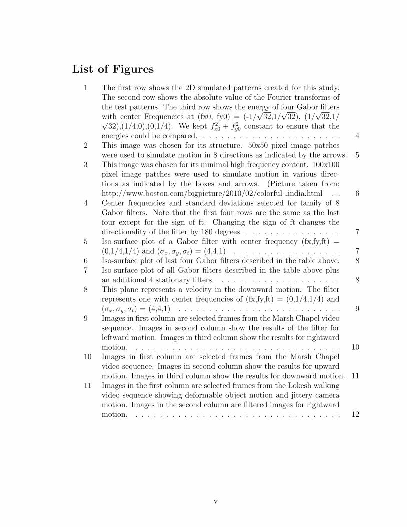
1 The first row shows the 2D simulated patterns created for this study.The second row shows the absolute value of the Fourier transforms ofthe test patterns. The third row shows the energy of four Gabor filterswith center Frequencies at (fx0, fy0) = (-1/

√32,1/

√32), (1/

√32,1/√

32),(1/4,0),(0,1/4). We kept f 2x0 + f 2

y0 constant to ensure that theenergies could be compared. . . . . . . . . . . . . . . . . . . . . . . . 4

2 This image was chosen for its structure. 50x50 pixel image patcheswere used to simulate motion in 8 directions as indicated by the arrows. 5

3 This image was chosen for its minimal high frequency content. 100x100pixel image patches were used to simulate motion in various direc-tions as indicated by the boxes and arrows. (Picture taken from:http://www.boston.com/bigpicture/2010/02/colorful india.html . . 6

4 Center frequencies and standard deviations selected for family of 8Gabor filters. Note that the first four rows are the same as the lastfour except for the sign of ft. Changing the sign of ft changes thedirectionality of the filter by 180 degrees. . . . . . . . . . . . . . . . . 7

5 Iso-surface plot of a Gabor filter with center frequency (fx,fy,ft) =(0,1/4,1/4) and (σx, σy, σt) = (4,4,1) . . . . . . . . . . . . . . . . . . 7

6 Iso-surface plot of last four Gabor filters described in the table above. 87 Iso-surface plot of all Gabor filters described in the table above plus

an additional 4 stationary filters. . . . . . . . . . . . . . . . . . . . . 88 This plane represents a velocity in the downward motion. The filter

represents one with center frequencies of (fx,fy,ft) = (0,1/4,1/4) and(σx, σy, σt) = (4,4,1) . . . . . . . . . . . . . . . . . . . . . . . . . . . 9

9 Images in first column are selected frames from the Marsh Chapel videosequence. Images in second column show the results of the filter forleftward motion. Images in third column show the results for rightwardmotion. . . . . . . . . . . . . . . . . . . . . . . . . . . . . . . . . . . 10

10 Images in first column are selected frames from the Marsh Chapelvideo sequence. Images in second column show the results for upwardmotion. Images in third column show the results for downward motion. 11

11 Images in the first column are selected frames from the Lokesh walkingvideo sequence showing deformable object motion and jittery cameramotion. Images in the second column are filtered images for rightwardmotion. . . . . . . . . . . . . . . . . . . . . . . . . . . . . . . . . . . 12

v

Motion Filtering 1

1 Introduction

As our society increases its consumption of video data, the required analysis is also be-coming more complex. Not only will motion detection in video sequences be required,but some form of motion analysis will be useful. Monitoring access to a store front inthe midst of high pedestrian activity, gesture recognition [3], anomaly detection androbotic visual scene interpretation are some of the applications of direction-specificmotion estimation. Motion filtering using frequency domain analysis is not a newtopic but it is not as well developed as time domain methods such as optical flow.There are many approaches to estimate motion using successive frames but filteringmotion in specific directions is difficult. The HornSchunck and Lucas-Kanade Opticalflow algorithms are common methods that use 2 frames for motion estimation. Theaccuracy of the estimates is not dependable because factors like changes in intensitybetween frames and the movement of highly textured objects [2]. We explored thecreation of a family of Gabor filters to which motion filtering in 8 directions was ap-plied. We approached the implementation in a careful manner by first understanding2 dimensional data and then moved to implementation with 3 dimensional simulateddata. Finally, the implementation with videos of pedestrian traffic around the BostonUniversity East Campus was analysed.

2 Literature Review

The application of motion filters using multiple frames is desirable. David Heeger’sthesis [1] is one of the earliest papers dealing with the filtering of movement usingmany frames. He uses twelve different Gabor filters to determine velocity on patchesof images over multiple frames. 8 of the filters are to determine velocities in theleft, right, up, down, and four other corners. The four additional filters are for sta-tionary responses. Several families of these filters could be built to describe variousspatiotemporal-frequency bands, but Heeger opted to use a Gaussian pyramid schemesimilar to the one described by Adelson Et Al [6][7]. Heeger[1][2] uses Parseval’s The-orem to determine motion energy in various directions. A more recent applicationof gabor filters for spatiotemporal motion estimation was used for interpretation ofdynamic hand gestures. Yeasin and Chaudhuri analyze a series of frames that en-compass a hand gesture like one that represents come here. Gabor filters are usedto determine various motions and a finite state machine developed by the authors isused to decide which hand gesture is being presented.[5]

2 Elena Zorn, Lokesh Ravindranathan

3 Problem Statement

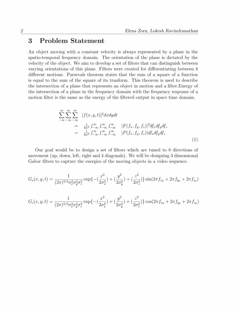
An object moving with a constant velocity is always represented by a plane in thespatio-temporal frequency domain. The orientation of the plane is dictated by thevelocity of the object. We aim to develop a set of filters that can distinguish betweenvarying orientations of this plane. Filters were created for differentiating between 8different motions. Parsevals theorem states that the sum of a square of a functionis equal to the sum of the square of its tranform. This theorem is used to describethe intersection of a plane that represents an object in motion and a filter.Energy ofthe intersection of a plane in the frequency domain with the frequency response of amotion filter is the same as the energy of the filtered output in space time domain.

∞∑−∞

∞∑−∞

∞∑−∞

|f(x, y, t)|2dxdydt

= 18π3

∫∞−∞

∫∞−∞

∫∞−∞ |F (fx, fy, fz)|2dfxdfydfz

= 18π3

∫∞−∞

∫∞−∞

∫∞−∞ |P (fx, fy, fz)|dfxdfydfz

(1)

Our goal would be to design a set of filters which are tuned to 8 directions ofmovement (up, down, left, right and 4 diagonals). We will be designing 3 dimensionalGabor filters to capture the energies of the moving objects in a video sequence.

Gs(x, y, t) =1

(2π)3/2σ2xσ

2yσ

2z

exp{−(x2

2σ2x

) + (y2

2σ2y

) + (z2

2σ2z

)} sin(2πfx0 + 2πfy0 + 2πfz0)

Gc(x, y, t) =1

(2π)3/2σ2xσ

2yσ

2z

exp{−(x2

2σ2x

) + (y2

2σ2y

) + (z2

2σ2z

)} cos(2πfx0 + 2πfy0 + 2πfz0)

Motion Filtering 3

4 Implementation

Our approach to defining a specific set of Gabor filters involved creating simulateddata to tune the Gabor filters. We first did this in two dimensions and then repeatedthe process for three dimensions. This is what we called ”Ground Truthing”. Finally,the Gabor filters were applied to real data.

4.1 Ground Truthing in Two Dimensions

We first created a two dimensional pattern out of a one dimensional signal. Froman image we selected a row of 50 pixels. This one dimensional signal was shiftedby one pixel (the end wrapping around to the beginning) and copied to the linebelow. This step was repeated until a two dimensional image of 50x50 pixels wascreated. The resulting image is a striped one like the one shown below. In a similarmanner, we created images to depict diagonal stripes that were orthogonal to theprevious image. In addition, horizontal and vertical striped images were created. Asa result, we obtained four images that had energy that closely resembled a line in thefrequency domain. For each of these images, the energy in the frequency domain isrepresented by a line. The energy of the Sine Gabor filters is shown. Since convolutionin the space-time domain is equivalent to multiplication in the frequency domain, theamount of energy captured by the filters is well represented with the center frequenciesprovided[8]. Similarly for the Cosine Gabor filters.

4 Elena Zorn, Lokesh Ravindranathan

Figure 1: The first row shows the 2D simulated patterns created for this study. Thesecond row shows the absolute value of the Fourier transforms of the test patterns.The third row shows the energy of four Gabor filters with center Frequencies at (fx0,fy0) = (-1/

√32,1/

√32), (1/

√32,1/

√32),(1/4,0),(0,1/4). We kept f 2

x0 + f 2y0 constant

to ensure that the energies could be compared.

Motion Filtering 5

4.2 Ground Truthing in Three Dimensions

Motion was simulated in a similar manner for ground truthing in three dimensions.From a highly textured image a small patch was extracted. For each frame the patchthat was captured was shifted in various directions by moving the area down, right,up, left or diagonally by a pixel. We created 50-frame simulations of 50x50 and100x100 pixel images. These frames were tested with a family of 8 Gabor filters thatrepresented the 4 cardinal directions and 4 diagonals. The center frequencies wereselected in a similar manner so that fx2 + fy2 remained constant. ft was selected tobe 1/4. This was a recommendation that came from Heeger’s paper on Optical Flow[4]. The images and filters that were tested are shown below.

Figure 2: This image was chosen for its structure. 50x50 pixel image patches wereused to simulate motion in 8 directions as indicated by the arrows. (Picture takenfrom: http://www.boston.com/bigpicture/2010/02/colorful india.html)

In order to understand the parameters of the filters and to ensure that they wereimplemented correctly, we visualized the magnitude of the filters in the frequencydomain. They were normalized to have a max of one and were displayed in an iso-surface plot where the surface displayed is at iso-surface = .5.

We could then see that any plane representing velocity of an object would pass

6 Elena Zorn, Lokesh Ravindranathan

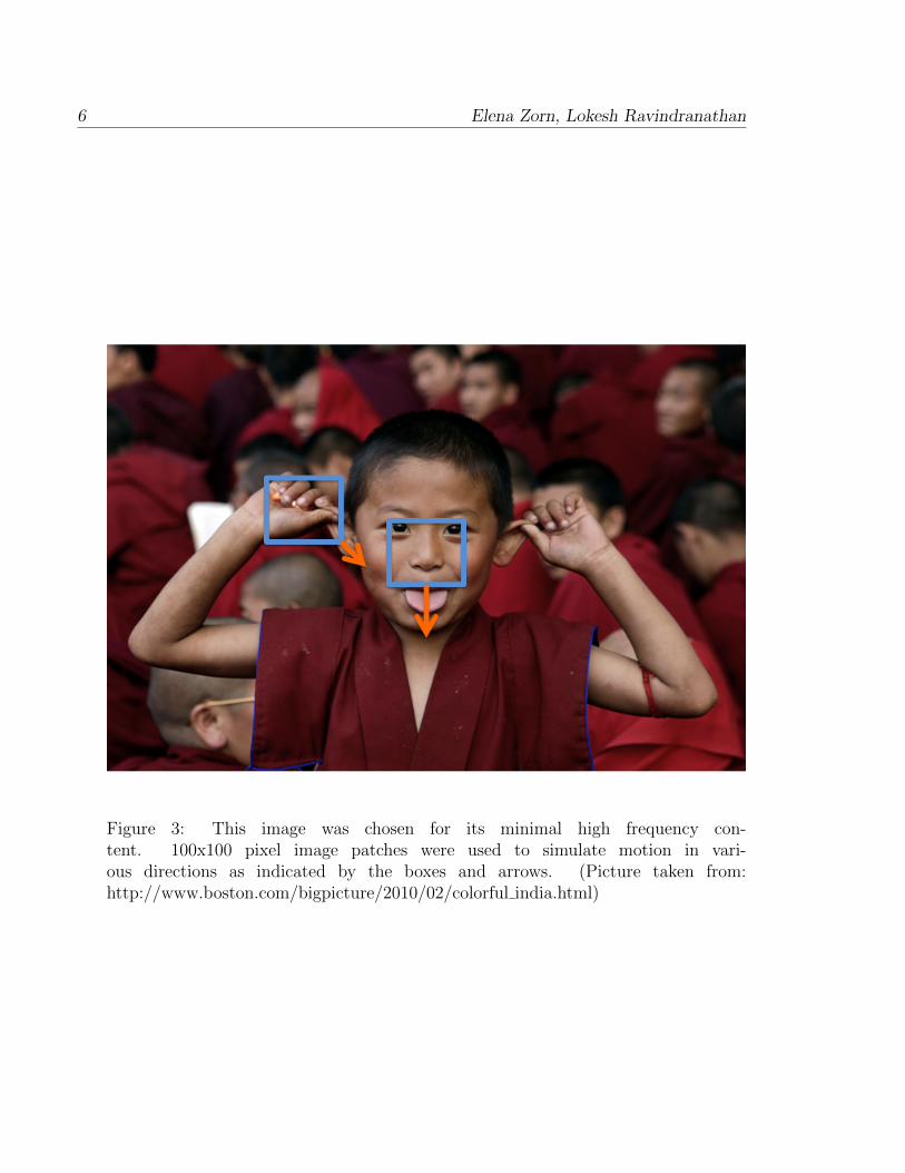
Figure 3: This image was chosen for its minimal high frequency con-tent. 100x100 pixel image patches were used to simulate motion in vari-ous directions as indicated by the boxes and arrows. (Picture taken from:http://www.boston.com/bigpicture/2010/02/colorful india.html)

Motion Filtering 7

Figure 4: Center frequencies and standard deviations selected for family of 8 Gaborfilters. Note that the first four rows are the same as the last four except for the signof ft. Changing the sign of ft changes the directionality of the filter by 180 degrees.

Figure 5: Iso-surface plot of a Gabor filter with center frequency (fx,fy,ft) =(0,1/4,1/4) and (σx, σy, σt) = (4,4,1)

8 Elena Zorn, Lokesh Ravindranathan

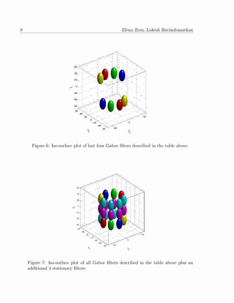
Figure 6: Iso-surface plot of last four Gabor filters described in the table above.

Figure 7: Iso-surface plot of all Gabor filters described in the table above plus anadditional 4 stationary filters.

Motion Filtering 9

Figure 8: This plane represents a velocity in the downward motion. The filter repre-sents one with center frequencies of (fx,fy,ft) = (0,1/4,1/4) and (σx, σy, σt) = (4,4,1)

through a combination of these filters. The goal would be to design these filters so thatthere is minimal ambiguity between the directional filters. The standard deviationsof the filters were selected to this effect.

10 Elena Zorn, Lokesh Ravindranathan

5 Experimental Results

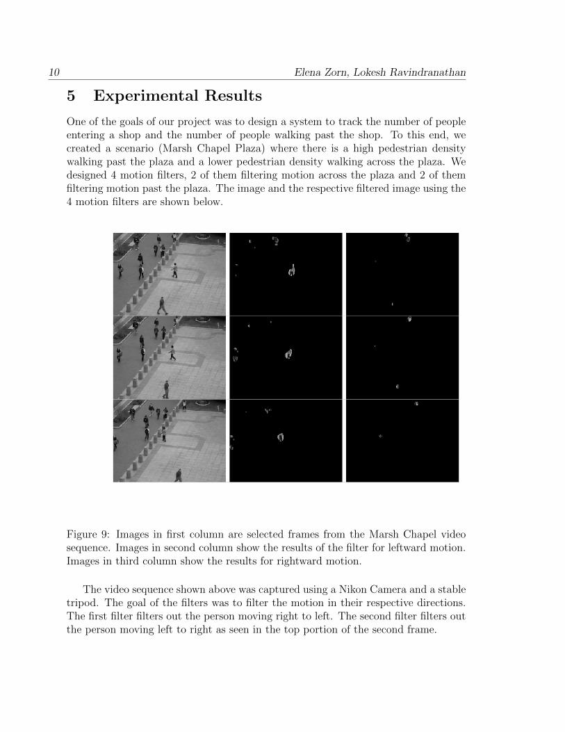
One of the goals of our project was to design a system to track the number of peopleentering a shop and the number of people walking past the shop. To this end, wecreated a scenario (Marsh Chapel Plaza) where there is a high pedestrian densitywalking past the plaza and a lower pedestrian density walking across the plaza. Wedesigned 4 motion filters, 2 of them filtering motion across the plaza and 2 of themfiltering motion past the plaza. The image and the respective filtered image using the4 motion filters are shown below.

Figure 9: Images in first column are selected frames from the Marsh Chapel videosequence. Images in second column show the results of the filter for leftward motion.Images in third column show the results for rightward motion.

The video sequence shown above was captured using a Nikon Camera and a stabletripod. The goal of the filters was to filter the motion in their respective directions.The first filter filters out the person moving right to left. The second filter filters outthe person moving left to right as seen in the top portion of the second frame.

Motion Filtering 11

Figure 10: Images in first column are selected frames from the Marsh Chapel videosequence. Images in second column show the results for upward motion. Images inthird column show the results for downward motion.

The video sequence shown above was captured using a Nikon Camera and a stabletripod. The goal of the filters was to filter the motion in their respective directions.The first filter filters out the pedestrian traffic moving from the bottom of the frameto the top. The highly textured area of the pedestrian’s shirt was detected easilyin the three frames shown. However, there is less texture in the pedestrian’s shirtmoving from the top of the frame to the bottom and has been detected only in thesecond frame of the filtered frames.

12 Elena Zorn, Lokesh Ravindranathan

Figure 11: Images in the first column are selected frames from the Lokesh walkingvideo sequence showing deformable object motion and jittery camera motion. Imagesin the second column are filtered images for rightward motion.

The video sequence shown above captured using a Nikon Camera. The filter filtersout the person moving right to left. Person’s head is cleary filtered out but the restof the body is not detected because of the non-linear motion. The camera is jitteryand hence the filtered image shows some portions of the background. Because of thesmall movements in the camera, objects at a distance were detected as moving.

Motion Filtering 13

6 Conclusions

Texture is important for performing motion filtering in the frequency domain.Analysis in the frequency domain is based on frequencies seen in x and y direc-tions of an image in an image sequence. An object with little texture will havelow frequencies and it would be tough to find the corresponding shift in thefrequency domain. An object with very high texture will have similar problemstoo.

Temporal Aliasing creates a huge hurdle in filtering motion. This kind of aliasingcauses the filter to detect wrong direction of motion.

Setting the right filter design parameters is challenging. Small spatio-temporalstandard deviations cause ambiguity in the frequency domain. Large spatio-temporal standard deviations can miss certain frequency planes.

Some of the difficulties we faced with the implementation were:(i) Brightness contrast between moving objects and background is required fordetecting motion.(ii) Diagonal movements are tougher to filter out since they are a combinationof two planes of motion.

Possible improvements using existing Gabor filters would be to:a. Estimate motion direction with a subset of Gabor Filters by taking advantageof the known ambiguities.b. Use a hierarchical approach by dividing the image into blocks and estimatedense vector field by using overlapping blocks.

14 Elena Zorn, Lokesh Ravindranathan

7 References

[1] David J. Heeger, Models for motion perception, Ph.D. Thesis, CIS Department,Univ. of Pennsylvania, 1987. (Technical report MS-CIS-87-91.)

[2] David J. Heeger, Optical Flow Using Spatiotemporal Filters International Journalof Computer vision, pp. 279-302, 1988.

[3] M. Yeasin, S. Chaudhuri, Visual understanding of dynamic hand gestures, PatternRecognition, Vol. 33, pp. 1805-1817, 2000.

[4] David J. Heeger, Model for the extraction of image flow, Journal of Optical SocietyAmerica, Vol. 4, No. 8, pp.1455-1471, August 1987.

[5] E. Bruno, D. Pellerin, Robust motion estimation using spatial Gabor-like filters,Signal Processing, Vol. 82, pp. 297-309, 2002.

[6] E.H. Adelson, C.H. Anderson, J.R. Bergen,P.J. Burt, J. M. Ogden, Pyramid meth-ods in image processing, RCA Engineer,Vol. 29-6, pp. 33-41, Nov/Dec 1984.

[7] E.P. Simoncelli, E.H. Adelson, Computing Optical Flow Distributions Using Spa-tiotemporal Filters, MIT Media Laboratory Vision and Modeling Technical report-165,1991.

[8] J.G. Daugman, Uncertainty relation for resolution in space, spatial frequency andorientation optimized by two dimensional visual cortical filters, J. Opt. Soc. Am. A2pp. 1160-1169, 1985.

[9] S.Schauland, J.Velten, A.Kummert, Detection of Moving object in Image Se-quences using 3D Velocity Fitlers,Int. J. Appl. Math. Comput. Sci., 2008, Vol.18, No. 1, 2131

Motion Filtering 15

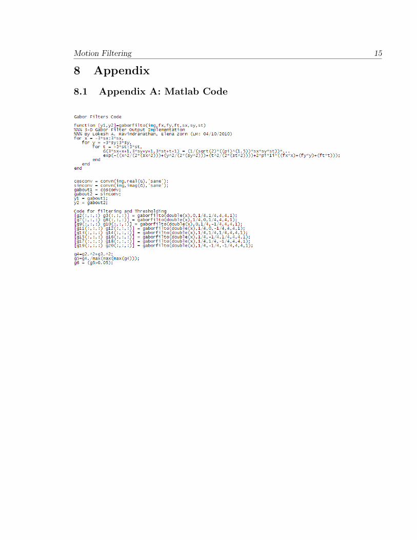
8 Appendix

8.1 Appendix A: Matlab Code

16 Elena Zorn, Lokesh Ravindranathan

8.2 Appendix B: Parseval’s Theorem

A 1-Dimensional Gabor odd phase(sine phase) filter is defined as a product of aGaussian signal and sine signal of a given frequency:

gs(t) = 1√2πσ

e−t22σ2 sin(2πf0t)

A 1-Dimensional Gabor even phase(cosine phase) filter is defined as a product ofa Gaussian signal and cosine signal of a given frequency:

gc(t) = 1√2πσ

e−t22σ2 cos(2πf0t)

Gabor function can also can be seen as: g(t) = Product [h1(t), h2(t)] where h1(t) =

1√2πσ

e−t22σ2 and h2(t) = sin(2πf0t)

Fourier Transform of Gabor Function is defined as F [g(t)] and can be re-writtenas follows: F [g(t)] = F [h1(t)] ∗ F [h2(t)] – Eqn(1)

Fourier transform of a Gaussian signal is: F [e−ax2(k)] =

√πae−

π2k2

a – Eqn(2)

Fourier transform of a sine signal of a given frequency is:F [sin(2πf0t)] = i

2(δ(f + f0)− δ(f − f0)) – Eqn(3)

Fourier transform of a cosine signal of a given frequency is:F [cos(2πf0t)] = 1

2(δ(f + f0) + δ(f − f0)) – Eqn(4)

Substituting Eqn(2), Eqn(3) in Eqn(1),Gs(f) = (e−π

2f22σ2) ∗ ( i

2(δ(f + f0)− δ(f − f0)))

Gs(f) = i2(e−π

2(f+f0)22σ2 − e−π2(f−f0)22σ2)

For odd phase filter, energy is calculated using Parseval’s theorem by convolvingthe filter with an arbitrary sine wave,∫∞

−∞ |Gs(f0) ∗ sin(2πf1)|2dx =∫∞−∞ |F [Gs(f0)]F [sin(2πf1)]|2df

= |(14)[g(f)− h(f)][δ(f + f1)− δ(f − f1)]|2

= ( 116

)[g(f)− h(f)]2[δ(f + f1) + δ(f − f1)− 2δ(f + f1)δ(f − f1)]= ( 1

16)[g(f1)− h(f1)]

2 + ( 116

)[g(−f1)− h(−f1)]2= (1

8)[g(f1)− h(f1)]

2

where g(f) = e−2π2σ2(f−f0)2 and h(f) = e−2π

2σ2(f+f0)2

For even phase filter, energy is given by,∫∞−∞ |F [Gc(f0)]F [sin(2πf1)]|2df = (1

8)[g(f1) + h(f1)]

2

Energy of a Gabor phase is the sum of the energies of odd phase and even phasefilters.

Etotal = (14)[g(f1)

2 + h(f1)2]

Motion Filtering 17

= [(14)e−4π

2σ2(f1−f0)2 ] + [(14)e−4π

2σ2(f1+f0)2 ]

Extending the concepts to a 3-D Gabor filter,

g(x, y, t) = 1(2π)3/2

e−( x

2

2σ2x+ y2

2σ2y+ t2

2σ2t

)sin(2πfx0x+ 2πfy0y + 2πft0t)

where fx0, fy0, ft0 are the set of spatial and temporal centre frequencies.

G(fx, fy, ft) = (14)e−4π

2[σ2x(fx−fx0)2+σ2

y(fy−fy0)2+σ2t (ft−ft0)2]

+(14)e−4π

2[σ2x(fx+fx0)

2+σ2y(fy+fy0)

2+σ2t (ft+ft0)

2]