Boson Sampling on a Photonic Chip

Justin B. Spring,1, ∗ Benjamin J. Metcalf,1 Peter C. Humphreys,1 W. Steven Kolthammer,1 Xian-Min

Jin,1, 2 Marco Barbieri,1 Animesh Datta,1 Nicholas Thomas-Peter,1 Nathan K. Langford,1, 3

Dmytro Kundys,4 James C. Gates,4 Brian J. Smith,1 Peter G.R. Smith,4 and Ian A. Walmsley1, †

1Clarendon Laboratory, Department of Physics, University of Oxford, OX1 3PU, UK2Department of Physics, Shanghai Jiao Tong University, Shanghai 200240, PR China

3Department of Physics, Royal Holloway, University of London, TW20 0EX, UK4Optoelectronics Research Centre, University of Southampton, Southampton, SO17 1BJ, UK

While universal quantum computers ideally solve problems such as factoring integers exponentiallymore efficiently than classical machines, the formidable challenges in building such devices motivatethe demonstration of simpler, problem-specific algorithms that still promise a quantum speedup. Weconstruct a quantum boson sampling machine (QBSM) to sample the output distribution resultingfrom the nonclassical interference of photons in an integrated photonic circuit, a problem thought tobe exponentially hard to solve classically. Unlike universal quantum computation, boson samplingmerely requires indistinguishable photons, linear state evolution, and detectors. We benchmark ourQBSM with three and four photons and analyze sources of sampling inaccuracy. Our studies pavethe way to larger devices that could offer the first definitive quantum-enhanced computation.

Universal quantum computers require physical systemsthat are well-isolated from the decohering effects of theirenvironment, while at the same time allowing precise ma-nipulation during computation. They also require qubit-specific state initialization, measurement, and the gen-eration of quantum correlations across the system [1–5].Although there has been substantial progress in proof-of-principle demonstrations of quantum computation [6–10], simultaneously meeting these demands has provendifficult. This motivates the search for schemes thatcan demonstrate quantum-enhanced computation undermore favorable experimental conditions. The power ofone qubit [11], permutational [12] and instantaneous [13]quantum computation, are examples that have allowedinvestigation of the space between classical and universalquantum machines.

Boson sampling has recently been proposed as a spe-cific quantum computation that is more efficient than itsclassical counterpart but only requires identical bosons,linear evolution, and measurement [14]. The distribu-tion of bosons that have passed through a linear systemrepresented by the transformation Λ is thought to beexponentially hard to sample from classically [14]. Theprobability amplitude of obtaining a certain output isdirectly proportional to the permanent of a correspond-ing submatrix of Λ. The permanent expresses the wave-function of identical bosons, which are symmetric underexchange [15, 16]; in contrast, the Slater determinant ex-presses the wavefunction of identical fermions, which areantisymmetric under exchange. While determinants canbe evaluated efficiently, permanents have long been be-lieved to be hard to compute [17]; the best known algo-rithm scales exponentially with the size of the matrix [18].One can envision a race between a classical and a quan-tum machine to sample the boson distribution given aninput state and Λ. The classical machine would evalu-ate at least part of the probability distribution, which

requires the computation of matrix permanents. TheQBSM instead creates indistinguishable bosons, directlyimplements Λ, and records the outputs. For a sufficientlylarge problem size, the quantum machine is expected towin [14].

FIG. 1. Model of quantum boson sampling. Givena specified initial number state |T〉 = |T1...TM 〉 and lineartransformation Λ, a quantum boson sampling machine effi-ciently samples from the distribution P (S|T) of possible out-comes |S〉 = |S1...SM 〉.

Photonics is a natural platform to implement bosonsampling since sources of indistinguishable photons arewell-developed [19], and integrated optics offers a scal-able route to large linear systems [20]. In addition,photons have extremely low decoherence rates. Impor-

arX

iv:1

212.

2622

v2 [

quan

t-ph

] 2

7 M

ay 2

013

2

tantly, boson sampling requires neither nonlinearities noron-demand entanglement, unlike photonic approaches touniversal quantum computation [21]. This clears theway for experimental boson sampling with existing pho-tonic technology, building on the extensively studied two-photon Hong-Ou-Mandel (HOM) interference effect [22].

A QBSM (Fig. 1) samples the output distribution ofa multi-particle bosonic quantum state |Ψout〉, preparedfrom a specified initial state |T〉 and linear transfor-mation Λ. A trial begins with the input state |T〉 =

|T1...TM 〉 ∝∏Mi=1(a†i )

Ti |0〉, which describes N =∑Mi=1 Ti

particles distributed inM input modes in the occupation-number representation. The output state |Ψout〉 is gen-erated according to the linear map from output to inputmode creation operators a†i =

∑Mj=1 Λij b

†j , where Λ is

an M×M matrix. Finally, the particles in each of theM output modes are counted. The probability of a par-ticular measurement outcome |S〉 = |S1...SM 〉 is givenby

P (S|T) = |〈S|Ψout〉|2 =

∣∣Per(Λ(S,T))∣∣2∏M

j=1 Sj !∏Mi=1 Ti!

(1)

where the N×N submatrix Λ(S,T) is obtained by keepingSj (Ti) copies of the jth column (ith row) of Λ[23].

The aim of boson sampling is to sample from the dis-tribution given by P (S|T). A QBSM achieves this ef-ficiently by directly sampling |〈S|Ψout〉|2. The classicalstrategy, on the other hand, requires evaluating the right-hand side of Eqn. (1), for which the calculation timescales exponentially in N [18].

Our QBSM consists of sources of indistinguishablesingle photons, a multiport linear optical circuit, andsingle-photon counting detectors. Two parametric down-conversion (PDC) pair sources [24] are used to inject upto four photons into a silica-on-silicon integrated pho-tonic circuit, fabricated by UV writing [25]. The cir-cuit is shown in Fig. 2a and consists of M=6 input andoutput spatial modes coupled by a network of ten beamsplitters [20]. The output state is measured with single-photon avalanche photodiodes on each mode. We onlyconsider outcomes in which the number of detectionsequals the intended number of input photons [23].

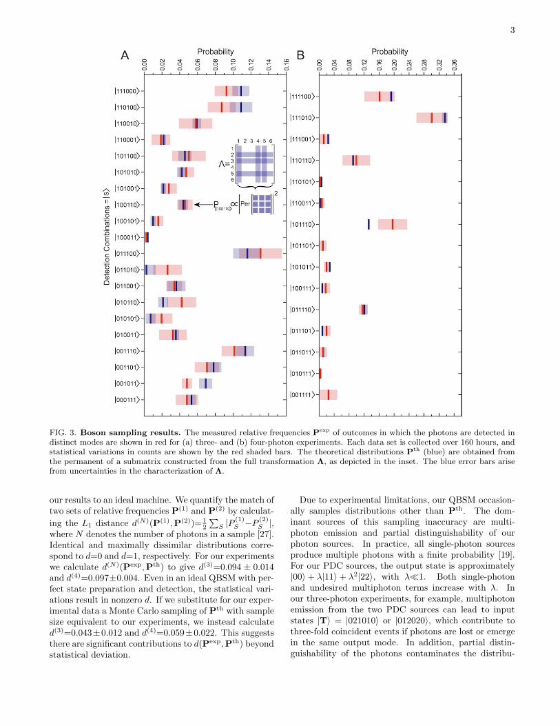
Our central result of three- and four-boson samplingis shown in Fig. 3. In the first case, we repeatedly in-ject three photons in the input state |T〉 = |011010〉,monitor all outputs, and collect all three-fold coincidentevents. In the four-photon experiment, we use the input|T〉 = |202000〉 and record all four-fold events. For eachexperiment, the measured relative frequencies P exp

S forevery allowed outcome |S〉 are shown along with their ob-served statistical variation. The corresponding theoreti-cal P th

S , calculated using the right-hand side of Eqn. (1),are shown along with their uncertainties arising from thecharacterization of Λ, described below.

FIG. 2. Schematic and characterization of the pho-tonic circuit. (a) The silica-on-silicon waveguide circuitsconsist of M = 6 accessible spatial modes (labeled 1−6). Forthe three-photon experiment, we launch single photons intoinputs i = 2, 3 and 5 from two parametric down-conversionsources and postselect outcomes in which three detections areregistered amongst the output modes j. For the four-photonexperiment, which is implemented on a different chip of iden-tical topology, we inject a double photon pair from a singlesource into the modes i = 1, 3 and postselect on four detectionevents. (b)-(c) Measured elements of the linear transforma-tion Λij = τije

iφij linking the input mode i to the outputmode j of our three-photon apparatus. The circuit topologydictates that several τij are zero, and our phase-insensitive in-put states and detection methods imply only six non-zero φij .Since only relative values are needed due to post-selection, werescale each row of τ so that its maximum value is unity.

We reconstruct Λ with a series of one- and two- pho-ton transmission measurements to determine its complex-valued elements Λij = τije

iφij [26]. The characteriza-tion results for the circuit used in the three-photon ex-periment are shown in Fig. 2b-c. To obtain the mag-nitude τij , single photons are injected in mode i. Theprobability of a subsequent detection in mode j is givenby P1(j, i) = |Λij |2 = τ2ij . The phases φij are deter-mined from two-photon quantum interference measure-ments. The probability that a photon is detected in eachof modes j1 and j2 when they are injected in modes i1 andi2 is given by P2(j1, j2, i1, i2) = |Λi1j1Λi2j2 + Λi2j1Λi1j2 |

2.

This expression is used to relate the relevant phases φijgiven the previously determined magnitudes τij . We usea least-squares fit to determine the phases φij from acomplete set of two-photon measurements [23].

To analyze the performance of our QBSM we compare

3

FIG. 3. Boson sampling results. The measured relative frequencies Pexp of outcomes in which the photons are detected indistinct modes are shown in red for (a) three- and (b) four-photon experiments. Each data set is collected over 160 hours, andstatistical variations in counts are shown by the red shaded bars. The theoretical distributions Pth (blue) are obtained fromthe permanent of a submatrix constructed from the full transformation Λ, as depicted in the inset. The blue error bars arisefrom uncertainties in the characterization of Λ.

our results to an ideal machine. We quantify the match oftwo sets of relative frequencies P(1) and P(2) by calculat-

ing the L1 distance d(N)(P(1),P(2))= 12

∑S |P

(1)S −P

(2)S |,

where N denotes the number of photons in a sample [27].Identical and maximally dissimilar distributions corre-spond to d=0 and d=1, respectively. For our experimentswe calculate d(N)(Pexp,Pth) to give d(3)=0.094 ± 0.014and d(4)=0.097±0.004. Even in an ideal QBSM with per-fect state preparation and detection, the statistical vari-ations result in nonzero d. If we substitute for our exper-imental data a Monte Carlo sampling of Pth with samplesize equivalent to our experiments, we instead calculated(3)=0.043±0.012 and d(4)=0.059±0.022. This suggeststhere are significant contributions to d(Pexp,Pth) beyondstatistical deviation.

Due to experimental limitations, our QBSM occasion-ally samples distributions other than Pth. The dom-inant sources of this sampling inaccuracy are multi-photon emission and partial distinguishability of ourphoton sources. In practice, all single-photon sourcesproduce multiple photons with a finite probability [19].For our PDC sources, the output state is approximately|00〉+ λ|11〉+ λ2|22〉, with λ�1. Both single-photonand undesired multiphoton terms increase with λ. Inour three-photon experiments, for example, multiphotonemission from the two PDC sources can lead to inputstates |T〉 = |021010〉 or |012020〉, which contribute tothree-fold coincident events if photons are lost or emergein the same output mode. In addition, partial distin-guishability of the photons contaminates the distribu-

4

FIG. 4. Sampling accuracy. We consider several boson outcome distributions: the experimental samples Pexp, the idealpredictions of Eqn. (1) Pth, and the predictions of the full model Pmod. (a) The L1 distance d between Pth and a Monte Carlosimulation of an ideal machine that samples Pth a finite number of times for our three and (b) four photon cases. The insethistograms show the variation in d expected for a sample size corresponding to the 1421 and 405 counts collected in our three-and four-photon experiments. The distance d(Pexp,Pth) (red) between our experimental sample and the ideal distributionsuggests an underlying systematic inaccuracy. A full model which includes multiphoton emission and photon distinguishabilityis validated by the distance d(Pexp,Pmod) (green) which is consistent with statistical variation. (c) The predicted variationin d(Pth,Pmod) is shown as a function of λ for the photon distinguishabilites V indicated for the three- and (d) four-photoncases. Our experimental conditions are marked (red dot).

tion sampled by the QBSM by mixing in one- and two-photon interference effects[28]. To characterize the pho-ton indistinguishability we performed two-photon Hong-Ou-Mandel experiments, in which interference visibilitieswere 90% of the expected values on average.

We form a new distribution Pmod that accounts forthe effects of multiphoton emission and photon distin-guishability [23]. The distance d(Pexp,Pmod), shown bythe green point in the insets of Fig. 4a-b, is found to beconsistent with the statistical variation due to a finitesample size, for both the three- and four-photon exper-iments. This suggests we have correctly identified andmodeled the significant sources of inaccuracy. Our vali-dated full model may be used to predict the performanceof realistic QBSMs and guide the design of future ma-chines with largerN . To investigate how the performanceof our QBSM depends on λ and photon distinguishabil-ity, we calculate d(Pmod,Pth) for a range of operatingparameters (Fig. 4c-d). In terms of λ, a clear tradeoffis presented between data rate and inaccuracy due tomultiphoton emission, which is an intrinsic consequenceof using PDC sources. Improvement in photon indistin-

guishability increases the fidelity to the ideal machine,and additionally is thought to enhance the computationalpower of a QBSM [28].

Our results demonstrate that boson sampling providesa model of quantum-enhanced computation that is exper-imentally feasible with existing photonic technology. Fu-ture generations of QBSMs will benefit from ongoing ad-vances in integrated photonics such as reduced transmis-sion loss, efficient number-resolving detectors [29], andmultiplexed [30, 31] or single-emitter [19] photon sources.Such improvements suggest a promising route to large-scale photonic QBSMs, which will provide clear evidencefor the computational power of quantum mechanics.

Acknowledgements: We thank Josh Nunn forvaluable insights. This work was supported by theEPSRC(EP/C51933/01 and EP/C013840/1), the ECproject Q-ESSENCE (248095), the Royal Society, andthe AFOSR EOARD. XMJ and NKL are supportedby EU Marie-Curie Fellowships (PIIF-GA-2011-300820and PIEF-GA-2010-275103). JBS acknowledges supportfrom the United States Air Force Institute of Technol-ogy. The views expressed in this article are those of the

5

authors and do not reflect the official policy or positionof the United States Air Force, Department of Defense,or the U.S. Government.

∗ j.spring1@physics.ox.ac.uk† i.walmsley1@physics.ox.ac.uk

[1] DiVincenzo, D. P. The physical implementation of quan-tum computation. Fortschritte der Physik 48, 771–783(2000).

[2] Raussendorf, R. & Briegel, H. J. A one-way quantumcomputer. Phys. Rev. Lett. 86, 5188–5191 (2001).

[3] Nielsen, M. A. Quantum computation by measurementand quantum memory. Phys. Lett. A 308, 96–100 (2003).

[4] Childs, A. M. Universal computation by quantum walk.Phys. Rev. Lett. 102, 180501 (2009).

[5] Lovett, N. B., Cooper, S., Everitt, M., Trevers, M. &Kendon, V. Universal quantum computation using thediscrete-time quantum walk. Phys. Rev. A 81 (2010).

[6] Walther, P. et al. Experimental one-way quantum com-puting. Nature 434, 169–176 (2005).

[7] Lu, C.-Y., Browne, D. E., Yang, T. & Pan, J.-W. Demon-stration of a compiled version of Shor’s quantum factor-ing algorithm using photonic qubits. Phys. Rev. Lett. 99,250504 (2007).

[8] Lanyon, B. P. et al. Experimental demonstration of acompiled version of Shor’s algorithm with quantum en-tanglement. Phys. Rev. Lett. 99, 250505 (2007).

[9] Lanyon, B. P. et al. Universal digital quantum simulationwith trapped ions. Science 334, 57–61 (2011).

[10] Lucero, E. et al. Computing prime factors with a Joseph-son phase qubit quantum processor. Nature Phys. 8, 719(2012).

[11] Knill, E. & Laflamme, R. Power of one bit of quantuminformation. Phys. Rev. Lett. 81, 5672–5675 (1998).

[12] Jordan, S. P. Permutational quantum computing. Quant.Inf. Comput. 10, 470–497 (2010).

[13] Shepherd, D. & Bremner, M. J. Temporally unstructuredquantum computation. Proc. R. Soc. A 465, 1413–1439(2009).

[14] Aaronson, S. & Arkhipov, A. The computational com-plexity of linear optics. In Proceedings of ACM Sympo-sium on the Theory of Computing, STOC (2011).

[15] Caianiello, E. On quantum field theory i: explicit solu-tion of Dyson’s equation in electrodynamics without useof Feynman graphs. Il Nuovo Cimento (1943-1954) 10,1634–1652 (1953).

[16] Troyansky, L. & Tishby, N. Permanent uncertainty : Onthe quantum evaluation of the determinant and the per-manent of a matrix. Proceedings of PhysComp (1996).

[17] Valiant, L. G. The complexity of computing the perma-nent. Theoretical Computer Science 8, 189–201 (1979).

[18] Ryser, H. Combinatorial mathematics (MathematicalAssociation of America, 1963).

[19] Eisaman, M. D., Fan, J., Migdall, A. & Polyakov, S. V.Single-photon sources and detectors. Rev. Sci. Instrum.82, 071101 (2011).

[20] Metcalf, B. J. et al. Multiphoton quantum interferencein a multiport integrated photonic device. Nature Com-munications 4, 1356 (2013).

[21] Knill, E., Laflamme, R. & Milburn, G. J. A scheme for

efficient quantum computation with linear optics. Nature409, 46–52 (2001).

[22] Hong, C. K., Ou, Z. Y. & Mandel, L. Measurementof subpicosecond time intervals between two photons byinterference. Phys. Rev. Lett. 59, 2044–2046 (1987).

[23] Materials and methods are available in supplementary in-formation .

[24] Mosley, P. J. et al. Heralded generation of ultrafast singlephotons in pure quantum states. Phys. Rev. Lett. 100,133601 (2008).

[25] Smith, B. J., Kundys, D., Thomas-Peter, N., Smith, P.G. R. & Walmsley, I. A. Phase-controlled integrated pho-tonic quantum circuits. Opt. Express 17, 264–267 (2009).

[26] Laing, A. & O’Brien, J. L. Super-stable tomography ofany linear optical device. arXiv:1208.2868v1 (2012).

[27] Gilchrist, A., Langford, N. K. & Nielsen, M. A. Distancemeasures to compare real and ideal quantum processes.Phys. Rev. A 71, 062310 (2005).

[28] Rohde, P. P. Optical quantum computing with photonsof arbitrarily low fidelity and purity. Phys. Rev. A 86,052321 (2012).

[29] Gerrits, T. et al. On-chip, photon-number-resolving,telecommunication-band detectors for scalable photonicinformation processing. Phys. Rev. A 84, 060301 (2011).

[30] Migdall, A. L., Branning, D. & Castelletto, S. Tailoringsingle-photon and multiphoton probabilities of a single-photon on-demand source. Phys. Rev. A 66, 053805(2002).

[31] Nunn, J. et al. Enhancing multiphoton rates with quan-tum memories. arXiv:1208.1534v1 (2012).

[32] Kundys, D. O., Gates, J. C., Dasgupta, S., Gawith, C.& Smith, P. G. R. Use of cross-couplers to decrease sizeof UV written photonic circuits. IEEE Photon. Technol.Lett. 21, 947 –949 (2009).

[33] Rahimi-Keshari, S. et al. Robust characterisation ofany linear photonic device. arXiv:1210.6463v1 (2012).arXiv:1210.6463v1.

[34] Scheel, S. Permanents in linear optical networks.arXiv:0406127v1 (2004).

[35] Thomas-Peter, N. et al. Integrated photonic sensing. NewJ. Phys. 13, 055024 (2011).

[36] Nielsen, M. A. & Chuang, I. L. Quantum Computationand Quantum Information (Cambridge Series on Infor-mation and the Natural Sciences) (Cambridge UniversityPress, 2004).

[37] Smith, B. J., Mahou, P., Cohen, O., Lundeen, J. S. &Walmsley, I. A. Photon pair generation in birefringentoptical fibers. Opt. Express 17, 23589 (2009).

6

SUPPLEMENTARY INFORMATION

MATERIALS AND METHODS

Multiphoton states generation. An 80 MHzTi-Sapphire oscillator outputs 100 fs pulses at 830 nm,which undergo type-I second harmonic generation in a700 µm β-BaB2O4 (BBO) crystal. This 415 nm lightis then used used to pump type-II collinear paramet-ric downconversion (PDC) in 8 mm-long AR-coatedPotassium Dihydrogen Phosphate (KDP) crystals [24].Both modes of the resulting squeezed state are passedthrough spectral filters (Semrock, ∆λ=3 nm), to max-imize photon indistinguishability. In the three-photonexperiment, two such PDC sources are coupled to fourpolarization-maintaining (PM) fibers [20]. One of thephotons is sent directly to a heralding detector, whilethe other three are coupled into the photonic circuitvia a PM v-groove array (VGA) on a 6-axis alignmentstage at the chip input. Programmable optical delayis provided by motor-controlled translation stages oneach single-photon mode preceding the circuit, allowingthe photons to arrive temporally coincident at theinterferometric network in Fig 2A. Another PM VGA atthe chip output couples the output modes into avalanchephotodiode (APD) single photon counting modules(PerkinElmer SPCM-AQ4C), which are monitored by ahome-built coincidence counting program loaded ontoa commercially available FPGA development board(Xilinx SP605) operating with a 5 ns coincidence win-dow. In the four-photon experiment, the higher orderemission (|22〉) from a single PDC crystal was launchedinto two spatial modes of a different chip, though ofidentical geometry, which had VGAs glued to input andoutput. This reduced the coupling efficiency uncertaintyfor the four-photon QBSM, which reduced the size ofthe error bars in Fig. 3B. In both cases, to minimizeundesired PDC emission terms the sources were pumpedas lightly as possible while maintaining reasonable countrates, yielding λ2=0.011 and 0.023 in the three- andfour-photon sampling experiments respectively.

Photonic circuit fabrication. The boson sampling isperformed on a UV-written silica-on-silicon integratedchip [20]. The chip was fabricated by focusing a continu-ous wave UV laser (244 nm) onto a photosensitive layerto create a local increase in the index of refraction. Thechip is then moved, via computer-controlled precisiontranslation stages, transversely to the incident UV beamto trace out the desired waveguide network geometry.One can fabricate cross-coupling beamsplitters of acertain reflectivity by crossing waveguides at a specificangle. Such beamsplitters take up less space thantraditional evanescent couplers in such circuits, allowingreduced chip size and lower loss [32]. While there are

eight spatial modes in the middle of the circuit (Fig.2A), the outer modes are not fabricated to the edge ofthe chip and are thus not accessible to the experimenter.They can then be accurately treated as losses on theneighboring modes, leaving a six (accessible) modeinterferometric network.

Boson sampling data collection. For the four-photon QBSM, the FPGA simultaneously counts allpossible combinations of coincidence detection events(one detection event, two coincident detections etc)amongst the six APDs monitoring the output modesof the integrated circuit. For the three-photon QBSM,a similar set of coincidences is taken, but conditionedon detection of the herald photon by a separate APD.There is a nonzero background count rate on eachdetector which contributes to erroneous N -fold detectionevents when N−1 APDs detect photons and anotherAPD erroneously fires. The N−1 coincidence rate isincluded in the above set of statistics collected by theFPGA and, by temporarily blocking all input modes tothe circuit, one can estimate the background rate oneach detector. The resulting background contributionto N -fold coincidences, comprising approximately 5% ofthe total counts, are then subtracted from the raw data,with the results plotted in Fig. 3.

Circuit characterization. Our photonic chip performsa non-unitary, complex-valued linear mapping of inputto output modes Λij=τije

iφij . We follow the methodoutlined in [26] to use a set of one- and two-photon datato reconstruct Λ.

We can find τi1,j1 by coupling light (single photons)into mode i1 and monitoring the probability of output inj1 yielding

∣∣∣〈0|bj1 a†i1 |0〉∣∣∣2 =

∣∣∣∣∣∣〈0|bj1M∑j=1

Λi1j b†j |0〉

∣∣∣∣∣∣2

= |Λi1j1 |2

= |τi1j1 |2

(2)

It is sufficient to measure the ratio of values betweenoutput ports, (τi1,j1/τi1,j2)

2, as this describes the trans-

formation induced by our circuit up to a constant fac-tor for each input, xi. If Λ is the true transformation,then this procedure gives us XΛ where X is a diago-nal matrix with entries Xii=xi. However, the propertiesof the matrix permanent give Per(X Λ)=(

∏i xi)Per(Λ).

Therefore, Eq. 1 of the main text shows, since we alwayslaunch the same input state, every portion of our bosondistribution is multiplied by a constant factor that can-cels in the normalization. This data is collected by peri-odically pausing boson sampling data collection, blockingtwo of the three photon inputs, and measuring the rela-tive power in each output mode. We thus obtain accurate

7

values for τ as well as a variance that is important forcalculating the error bars in Fig. 3.

One can then use two photon interference to find φi,j[26]. If one inputs two photons into modes i1, i2 and

detect in modes j1, j2, then we have |S〉=a†j1 a†j2|0〉 and

|T 〉=a†i1 a†i2|0〉. If single, indistinguishable photons are

used, then the probability of post-selecting this output is

Pindist =∣∣∣Per(Λ(S,T))

∣∣∣2=∣∣∣Λ(S,T)

11 Λ(S,T)22 + Λ

(S,T)12 Λ

(S,T)21

∣∣∣2= (τi1,j1τi2,j2)2 + (τi1,j2τi2,j1)2

+ 2τi1,j1τi1,j2τi2,j1τi2,j2

× cos(φi1,j1 − φi1,j2 − φi2,j1 + φi2,j2) (3)

If the photons launched into the individual modes aredistinguishable, then we get the incoherent sum of theirindividual statistics. We again take a matrix permanent,but as this is an incoherent process one finds

Pdist = (τi1,j1τi2,j2)2 + (τi1,j2τi2,j1)2 (4)

One can then perform a Hong-Ou-Mandel experimentand find that the resulting interference visibility is

V =Pdist − Pindist

Pdist

=2τi1,j1τi1,j2τi2,j1τi2,j2

(τi1,j1τi2,j2)2 + (τi1,j2τi2,j1)2

× cos(φi1,j1 + φi2,j2 − φi1,j2 − φi2,j1) (5)

We perform this two-photon interference experiment andfit a Gaussian to the resulting data to determine thevisibility. Using the known τi,j , one can then find|φi1,j1 + φi2,j2 − φi1,j2 − φi2,j1 |. Repeating this proce-dure for all accessible two photon dips, and applying ad-ditional constraints one can determine φi,j [26].

For our circuit geometry, we encounter an overcon-strained problem as we measure more interference visibil-ities than unknown φ. Therefore, we run a least squaresminimization to find the set of φ that best fits our twophoton interference data. To find the error bars in Fig.3, we use a Monte Carlo method where the elements of Λare selected from a normal distribution with an appropri-ate variance for each element. The one photon measure-ment was repeated periodically during the 160 hour longboson sampling data collection, thus yielding the vari-ance in the τij characterization, which was determinedto dominate the uncertainty in the predicted boson dis-tribution in Fig. 3. This explains why the four-photonQBSM, which had VGAs glued to the ends and thus wasmuch less susceptible to changes in the coupling, has sig-nificantly smaller error bars in the predicted distributionshown in Fig. 3B. The uncertainty in the Gaussian fit tothe two-photon interference patterns and in τij was thenused to determine the variance in φij .

This characterization process is efficient, as a generallinear transformation over M modes can be described byO(M2) parameters, requiringO(M2) measurements withthis technique. While photons from the PDC sourceswere used for the circuit characterization here, one canalso use classical coherent states [26, 33]. However, thesingle-photon based technique outlined here benefits fromnot requiring phase-stable path length matching and, be-cause we use the same sources for boson sampling andcharacterization, the photonic degrees of freedom (po-larization, spectrum etc) for the characterization matchthat used in the experiment.

With Λi,j experimentally determined over the accessi-ble modes, one can predict the post-selected boson dis-tribution for any input/output |S〉, |T 〉 by constructingΛ(S,T) from Λ and taking the permanent according toEq. (1) in the main text. Thus, we effectively use the oneand two photon boson distributions to characterize ournon-unitary operation over the accessible modes. Onecan then take various matrix permanents of this non-unitary matrix to predict the boson distribution for anyN .

SUPPLEMENTARY TEXT

In this section we first outline how the boson distri-bution is given by a set of matrix permanents. We thenshow how the boson distribution can be accurately pre-dicted by the permanents associated with a non-unitarymatrix describing a lossy channel, Λ, if one post-selectson trials where no photons are lost. Finally, the principalsources of error in this experiment, namely the photondistinguishability and higher order terms from our PDCphoton sources, are discussed.

The boson distribution is given by a set of matrixpermanents

We assume N bosons are injected into a network thatperforms a unitary transformation over M modes. Weconsider the special case, appropriate to our experiment,where the input (and output) states contain no more thanone boson per mode, though the general case is treatedelsewhere [34]. Without loss of generality, let modes 1 toN contain an input boson, while modes N+1 to M havevacuum inputs. The input state can then be describedby

|Ψin〉 = |T 〉 =

N∏i=1

a†i |0〉 (6)

8

The unitary transformation allows one to evolve the op-erators according to

a†i =

M∑j=1

Uij b†j (7)

where a†i and b†j are creation operators on the i-th inputand j-th output mode respectively. We then obtain theoutput state

|Ψout〉 =

N∏i=1

M∑j=1

Uij b†j

|0〉 (8)

To find the boson distribution, we project our outputonto a state |S〉 which, in the number state basis, wedescribe by an N element vector S, where Sj gives themode of the j-th boson. The probability of measuringthis state is then

PS = |〈S|ψout〉|2 (9)

=

∣∣∣∣∣∣〈0|N∏i=1

bSi

N∏j=1

(M∑k=1

Ujk b†k

) |0〉∣∣∣∣∣∣2

The term in square brackets can be expanded and in-cludes MN terms, as one is selecting N bosons from Mmodes where repetitions are allowed (> 1 boson in amode). One can rewrite this term in square brackets togive

PS =

∣∣∣∣∣∣〈0|N∏i=1

bSi

MN∑j=1

(N∏k=1

Uk,V jkb†V jk

) |0〉∣∣∣∣∣∣2

(10)

where V is the set of MN permutations of N photonsamongst M modes, repetitions allowed. The tilde no-tation will be used throughout this paper for a set ofpermutations. Then, V jk indicates the mode of the k-thboson in the j-th permutation. As an example, considerthe case with M = 3 modes and N = 2 input bosons,then

V 1 = [1, 1] V 2 = [1, 2] V 3 = [1, 3]

V 4 = [2, 1] V 5 = [2, 2] V 6 = [2, 3]

V 7 = [3, 1] V 8 = [3, 2] V 9 = [3, 3]

(11)

Let us denote all N ! permutations of S by S where Sjkindicates the mode of the k-th boson in the j-th permuta-tion. For example, if we project onto the state |S〉=|011〉then S=[2, 3] and

S1 = [2, 3] S2 = [3, 2] (12)

It is clear we only retain terms from the summation inEq. 10 where V j ∈ S, otherwise at least one annihilation

operator will act on vacuum and give PS=0. This thenleaves us with

PS =

∣∣∣∣∣∣N !∑j=1

N∏k=1

Uk,Sjk

∣∣∣∣∣∣2

(13)

The formula for the permanent of an n×n matrix A withelements aij is

Per(A) =

n!∑i=1

n∏j=1

aj,σij

(14)

where σij gives the j-th element of the i-th permutationof the numbers 1, 2, ...., n. The term inside the modulusof Eq. 13 has the same form as the matrix permanentin Eq. 14. Our original unitary, U , can be described byan M ×M matrix. However, it is obvious from Eq. 13that, in general, we take the permanent of a subsectionof U . Specifically, we only keep rows 1→ N , those rowscorresponding to modes with input photons. In addition,we only keep columns corresponding to the elements of S.Let us call this modified subsection of our original unitaryU (S,T). Then, using the definition of the permanent wecan rewrite Eq. 13

P (S|T) =∣∣∣Per(U (S,T))

∣∣∣2 (15)

If one allows the possibility of more than one photon perinput and output mode, then a similar analysis yields Eq.1 in the main text [34].

We also note that the above treatment assumes thebosonic commutation relation [b†i , b

†j ] = 0 ∀ i, j. If the

system consisted of indistinguishable fermions, then thecorresponding anticommutation relation {b†i , b

†j} = 0∀i, j

would be used, leading to alternating plus and minussigns introduced in the summation in Eq. 13, yieldingthe easily classically computable determinant.

Effects of loss

In any experimental implementation of boson samplingthere will be losses. These losses, regardless of wherethey occur, can be modeled as beam splitters that linkaccessible to inaccessible modes [35]. When these lossesare considered, it is important to ask whether the bosondistribution is still given by a set of matrix permanentsand, if so, what linear transformation does that matrixdescribe.

Let us adopt the convention that modes 1 to M areaccessible modes while inaccessible loss modes are giventhe labels M + 1 to L. There is an L × L unitary op-eration describing the evolution of our pure input state,though we must trace over these loss modes at the out-put, yielding a mixed state over the accessible modes.

9

Let us assume that photons are input into modes 1 to Nwhere N ≤M and we post-select on cases where N pho-tons are detected, by definition, in the accessible modes1 to M . Then Eq. 10 becomes

PS =

∣∣∣∣∣∣〈0|N∏i=1

bSi

LN∑j=1

(N∏k=1

Uk,V jkb†V jk

) |0〉∣∣∣∣∣∣2

(16)

but Si ≤M as we can only project on accessible modes.Therefore, even though U is an L × L matrix and theelements of V range from 1 → L, when we project ontoS (all the permutations of S) we are left with

PS =

∣∣∣∣∣∣N !∑j=1

N∏k=1

Uk,Sjk

∣∣∣∣∣∣2

=∣∣∣Per(U(S,T))

∣∣∣2 =∣∣∣Per(Λ(S,T))

∣∣∣2 (17)

where U (S,T) is again a modified version of the originalunitary but only keeping rows 1 → N and columns inS′i ≤M . Since these elements always describe the acces-sible modes, then we can equivalently work in terms of Λ,where Λi,j=Ui,j but i, j ≤ M . In summary, when post-selecting on no bosons being lost, one can work in termsof Λ, a non-unitary linear transformation that is sim-ply the subsection of U over the accessible modes. Thematrix permanents of such a non-unitary linear transfor-mation lead to the theoretical predictions in Fig. 3 of themain text.

Equivalently, we can describe our system as a noisy(lossy) quantum channel in the operator sum represen-tation [36]. This formalism will be useful later when wediscuss sources of error from higher order PDC terms. Inthis picture, the accessible modes are in the system Q,while all inaccessible loss modes form the environmentsystem E. We can describe the transformation inducedby our circuit over the full space Q⊗E by a unitary op-eration U . Let ρ and σ be the inputs to Q and E respec-tively, then the output in Q after a projective measure-ment Pm and tracing over the environment is describedby

ρout = trE(PmU(ρ⊗ σ)U†Pm) (18)

Let the basis for E be described by |ek〉 and the initialstate of the environment be σ =

∑j qj |j〉〈j|, then we can

express Eq. 18 as

ρout =∑jk

EjkρE†jk (19)

where Ejk =√qj〈ek|PmU |j〉 are the Kraus operators.

We do not directly characterize U , as it extends over theenvironment which is inaccessible to the experimenter.However, with photons we can assume σ = |0〉〈0|, and

all of our boson sampling results post-select on the casewhere no photons are lost to the environment. Therefore,the summation in Eq. 19 reduces to only one term withpostselection

ρout = E00ρE†00 (20)

Experimental boson sampling efforts will sample a non-unitary transformation that is equivalent, when post-selecting on no bosons being lost, to the E00 Kraus op-erator.

Sources of error

The computational difficulty for a classical machine tosample a boson distribution increases as the maximum er-ror threshold is lowered. Therefore, while a QBSM neednot sample the true boson distribution perfectly [14], itwill be easier to beat a classical machine if future QBSMsdesigns minimize their sampling errors. In this paper, wehave benchmarked the accuracy of our QBSMs by infer-ring the probability distribution from our data, labeledPexp, and comparing it to the distribution obtained fromEq. 1, labeled Pth. Throughout the text, we quantify thedistance between two probability distributions via the L1

distance, d(P(1),P(2))= 12

∑i |P

(1)i − P

(2)i |.

Our method of benchmarking QBSM accuracy will al-ways yield a nonzero d due to the finite number of col-lected samples. We perform a Monte Carlo simulation ofPexp from a QBSM that perfectly samples Pth as a func-tion of the number of counts collected (Fig. 4, A and B),to show the rate at which d asymptotically approacheszero as the number of samples collected increases. Inthe inset histograms, we show the range of outputs forthis ideal QBSM for the actual number of experimentalcounts collected in the three and four photon cases, whilethe red dots indicate d(Pth,Pexp). These two probabil-ity distributions show close agreement in Fig. 3, howevera comparison of the histogram and red dots in Fig. 4,A and B indicates there is an additional source of errorbeyond the finite number of samples.

Due to experimental limitations, occasionally we sam-ple distributions other than Pth. We model the effectof two such imperfections, photon distinguishability andhigher order terms from our PDC sources, and form anew distribution Pmod that accounts for these effects.We ignore the effects of photon impurity, as our post-selected data collection and use of nearly-spectrally fac-torable photon sources [24], minimizes this contribution.We find that the new d(Pexp,Pmod), indicated with thegreen dot in Fig. 4, A and B, comes well within the out-put variance of an ideal machine. This indicates we havecorrectly diagnosed and modeled the principal sources ofexperimental error, which will be important in guidingdesigns of future, larger N , QBSMs.

10

Effect of using heralded single photon sources

The parametric downconversion sources we use to gen-erate our photons actually generate a two-mode squeezedstate that is given by

|ΨPDC〉 =√

1− λ2∞∑n=0

λn|nn〉 (21)

where 0 ≤ λ < 1 is the squeezing parameter whose mag-nitude is determined, in part, by the type of crystal andpump power used. For our experiment we wish to mini-mize higher order terms (|22〉 and |33〉 for the three- andfour-photon QBSMs respectively) and so we deliberatelylower our pump power as much as possible while main-taining a feasible count rate. For the three-photon ex-periment, λ=

√0.011 and for the four-photon experiment

λ=√

0.023. However, even in this case we will sometimesinject more than N photons into our circuit which, dueto losses, could be observed as an N -fold detection at theoutput.

Due to the circuit characterization method employed,we have no information about what such terms will be.In the operator sum representation, our characterizationonly determines the E00 Kraus operator, which describesthe transformation of our input state when the environ-ment, which includes all loss modes, starts and ends withzero photons. For example, if we instead inject five pho-tons and lose two, then this process is described by theE20 operator, about which we have no information.

To model the effect of using such squeezed sources, westart with a circuit with the same geometry used in theexperiment. Non-uniform losses throughout the circuitcan then be modeled by adding beam splitters that linkthe depicted accessible modes shown in Fig. 2A to inac-cessible loss modes, where the beam splitter reflectivityindicates the loss in that channel [35]. Such ‘loss beam-splitters’ are added throughout the circuit. We cannotdirectly characterize these losses in our current circuit,however we can estimate them numerically. The char-acterized linear transformation Λ is a function of theselosses as well as the fabricated interferometers shown inFig. 2A. We have performed a loss-independent charac-terization of the interferometers [20], and then input thisdata into a genetic algorithm to find the relative lossesbetween modes that best reproduces the characterized Λ.We then apply three independent scaling factors to therelative losses at the sources, circuit and detectors. Thesource scaling factor is chosen to match the known sourceheralding efficiency, which is a measure of the loss in eachsource arm. The detector losses are scaled such that nodetector has an efficiency greater than 50%, which is ap-propriate for APDs detecting photons at 830 nm. Finally,we scale the relative losses in the circuit to reproduce theknown overall system transmission observed experimen-tally.

With knowledge of these losses, we reproduce an ac-tual unitary linear transformation U that extends overboth the N=6 modes as well as all loss modes and canbe used to accurately predict the effect of higher orderPDC terms. Taking the three-photon QBSM as an ex-ample, we use Eq. 1 of the main text to find the probabil-ity distributions when the input is |T〉=|011010〉 (desiredsingle-photon input), as well as |011020〉 or |022010〉 (thefirst higher-order terms from our two sources), which welabel P111, P112 and P221 respectively. The boson dis-tributions are then found by summing the terms wherethree photons appear in the desired accessible modes andzero, one, or two (respectively) photons appear in anycombination of loss modes. For example, the probabilityof obtaining |S〉=|111000〉 given input |T〉 = |022010〉 isthe summation of all terms where three photons appearin the first three accessible modes and two photons ap-pear in any combination of loss modes. The higher orderprobability distributions, P221 and P112, are weighted byλ2 which is obtained via a conditional second order corre-lation measurement, g(2)(0)[37]. As λ2 is small, we onlyconsider the first higher order terms from each source.

Photon Distinguishability

Boson sampling assumes indistinguishable bosons,while experimental implementations will always havesome distinguishability. Assuming pure inputs we followthe notation of [28] to write our input state as

|ψin〉 =

N∏i

(αA†ξ0,i +

√1− α2A†ξi,i

)|0〉 (22)

where N is again the number of photons, α is a distin-guishability parameter, and A†ξj ,i is the creation operatorfor photon i in mode ξj . Each photon is in a superpo-sition of a desired mode ξ0 and another mode ξi. Byanalyzing the reduction in HOM dip visibility at a beam-splitter inside our circuit we find α = 0.974 on averagein our experiment.

If one photon is distinguishable from the others, thenthe new probability distribution is given by the perma-nents of N−1 matrices which are incoherently summed.For example, assume an input state |T〉=|1〉τ |11000〉where τ labels a distinguishable photon, then for a uni-tary transformation U the probability of obtaining anoutput |S〉 is

P (S|T) =∣∣∣U (S,T)

11

∣∣∣2 |U (S,T)22 U

(S,T)33 + U

(S,T)23 U

(S,T)32 |2

+∣∣∣U (S,T)

12

∣∣∣2 ∣∣∣U (S,T)21 U

(S,T)33 + U

(S,T)23 U

(S,T)31

∣∣∣2+∣∣∣U (S,T)

13

∣∣∣2 ∣∣∣U (S,T)21 U

(S,T)32 + U

(S,T)22 U

(S,T)31

∣∣∣2(23)

11

where the terms in parentheses are permanents of 2 × 2matrices. We calculate these probability distributionswhen one photon is distinguishable and weight them by

|α2√

1− α2|2 and |α3√

1− α2|2, the probability that onephoton is distinguishable from the others for the three-and four-photon cases respectively. As α is large, weignore the case when two photons are distinguishable.