FEDERAL RESERVE BANK OF SAN FRANCISCO

WORKING PAPER SERIES

Bond Flows and Liquidity: Do Foreigners Matter?

Jens H. E. Christensen

Federal Reserve Bank of San Francisco

Eric Fischer Federal Reserve Bank of San Francisco

Patrick Shultz

Wharton School of the University of Pennsylvania

December 2019

Working Paper 2019-08

https://www.frbsf.org/economic-research/publications/working-papers/2019/08/

Suggested citation:

Christensen, Jens H. E., Eric Fischer, Patrick Shultz. 2019. “Bond Flows and Liquidity: Do Foreigners Matter?” Federal Reserve Bank of San Francisco Working Paper 2019-08. https://doi.org/10.24148/wp2019-08 The views in this paper are solely the responsibility of the authors and should not be interpreted as reflecting the views of the Federal Reserve Bank of San Francisco or the Board of Governors of the Federal Reserve System.

Bond Flows and Liquidity:

Do Foreigners Matter?

Jens H. E. Christensen†

Eric Fischer‡

Patrick Shultz∗

Abstract

In their search for yield in the current low interest rate environment, many investors

have turned to sovereign debt in emerging economies, which has raised concerns about

risks to financial stability from these capital flows. To assess this risk, we study the

effects of changes in the foreign-held share of Mexican sovereign bonds on their liquidity

premiums. We find that recent increases in foreign holdings of these securities have played

a significant role in driving up their liquidity premiums. Provided the higher compensation

for bearing liquidity risk is commensurate with the chance of a major foreign-led sell-off

in the Mexican government bond market, this development may not pose a material risk

to its financial stability.

JEL Classification: E43, E44, F36, G12

Keywords: term structure modeling, liquidity risk, financial market frictions, emerging mar-

kets, financial stability, foreign holdings

We thank participants at the 2019 IBEFA Summer Meeting, the IX FIMEF International Financial Re-search Conference, and the 89th Annual Meeting of the Southern Economics Association for helpful commentsand suggestions, including our discussants Yalin Gunduz, Polux Diaz Ruiz, and Jae Hoon Choi. We alsothank Dori Wilson for excellent research assistance. The views in this paper are solely the responsibility of theauthors and should not be interpreted as reflecting the views of the Federal Reserve Bank of San Francisco orthe Federal Reserve System.

†Corresponding author: Federal Reserve Bank of San Francisco, 101 Market Street MS 1130, San Francisco,CA 94105, USA; phone: 1-415-974-3115; e-mail: jens.christensen@sf.frb.org.

‡Federal Reserve Bank of San Francisco; e-mail: eric.fischer@sf.frb.org.∗Wharton School of the University of Pennsylvania; e-mail: patrickjshultz@gmail.com.This version: December 5, 2019.

1 Introduction

In their search for yield in the current low interest rate environment, many investors have

turned to sovereign debt in emerging markets. In light of the history of sovereign credit crises

in emerging markets, especially in Latin America, significant debt purchases from investors

outside the border could pose risks to financial stability. This is particularly true with mon-

etary policy normalization on the horizon in many advanced economies, which could provide

an impetus for foreign investments to move elsewhere. Hence, it seems warranted to study

the role of foreigners in these markets.

While previous research has explored the ties between debt flows and bond prices (see

Mitchell et al. 2007 and Beltran et al. 2013 for examples), the connection between debt flows

and market functioning and its potential implications for financial stability have received less

attention.1 To assess the potential financial stability implications of the increased foreign

participation in the sovereign debt markets in emerging economies, this paper analyzes the

influence of foreign investors on the liquidity premiums of domestic government bond securities

in a leading emerging market economy, namely Mexico.

Our focus on Mexican government bonds is motivated by several observations. First, little

is known about the magnitudes of liquidity premiums in regular sovereign bond markets.

Second, given that Mexico has one of the largest and most important sovereign bond markets

among emerging market economies, our analysis can serve as a benchmark for understanding

liquidity premiums and financial market frictions in other emerging economies. Finally, the

Bank of Mexico maintains a comprehensive database of foreign and domestic holdings for

all Mexican government securities that is instrumental to our analysis in order to establish

a connection between foreign holdings and bond risk premiums. In short, Mexico offers an

ideal setting for studying the question we are interested in.

To estimate the liquidity premiums of Mexican government bonds, we rely on recent re-

search by Andreasen et al. (2018, henceforth ACR), who show how a standard term structure

model can be augmented with a liquidity risk factor to accurately measure bond liquidity

premiums. Their approach identifies the liquidity risk factor from its unique loading, which

mimics the idea that, over time, an increasing fraction of the outstanding notional amount

of a given security tends to get locked up in buy-and-hold investors’ portfolios. This raises

its sensitivity to variation in the market-wide liquidity captured by the liquidity risk factor.

By observing a cross section of securities over time, the liquidity risk factor can be separately

identified and distinguished from the fundamental risk factors in the model. We model the

fundamental frictionless Mexican yields that would prevail in a world without any frictions

to trading using a standard Gaussian model, namely the arbitrage-free Nelson-Siegel (AFNS)

1One notable example is Christensen and Gillan (2019), who document that U.S. Treasury Inflation-Protected Securities (TIPS) purchases by the Federal Reserve during its second large-scale asset purchaseprogram lowered the priced frictions in the markets for TIPS and inflation swaps.

1

model introduced in Christensen et al. (2011), which we augment with a liquidity risk factor

structured as in ACR. We estimate both AFNS models and liquidity-augmented extensions

thereof, denoted AFNS-L models, using price information for individual Mexican bonds.2

Our results can be summarized as follows. First, we find that the liquidity-augmented

model improves model fit and delivers robust estimates of the risk factors that drive the

variation in the frictionless part of the Mexican government bond yield curve. Second, our

results show that liquidity premiums in the Mexican government bond market are of con-

siderable size with an average of 0.57 percent and a standard deviation of 0.19 percent. For

comparison, the liquidity premium advantage of newly issued ten-year U.S. Treasuries over

comparable seasoned securities has averaged less than 0.15 percent the past two decades, see

Christensen et al. (2017). Hence, liquidity risk is an important component in the pricing

of Mexican government bonds. Furthermore, we see significant variation around a general

upward trend during our sample period. The empirical question we are interested in is to

what extent this variation can be explained by changes in foreign investor holdings of Mexican

government securities. After running regressions with a large number of relevant controlling

variables, we find a strongly positive relationship whereby a one percentage point increase in

the foreign-held share of Mexican government bonds raises their liquidity premium by roughly

0.75 basis point. Given that the foreign market share has increased more than 40 percentage

points between 2010 and 2017, our results suggest that the large increase in foreign holdings

during this period could have raised the estimated bond liquidity premiums by as much as

0.3 percent.

What are the financial stability implications from these observations? Provided this in-

crease in the compensation demanded by investors for assuming the liquidity risk of Mexican

government bonds matches the risk and expected size of any future market sell-off driven

by foreigners leaving the Mexican market, there may not be any major threats to the finan-

cial stability of the Mexican government bond market at this point. However, if foreigners

turn out to represent a less stable and dedicated source of funding than domestic investors,

there does appear to be some risk that the Mexican government could face potentially severe

funding challenges down the road if foreigners were to decide to move their money elsewhere.

Furthermore, this tilt in the ownership composition of Mexican government bonds could have

implications for the monetary policy of the Bank of Mexico as it may be forced to put greater

emphasis on foreign developments, which could matter for both macroeconomic outcomes and

investors in these markets.

An important caveat to any conclusions, though, is that our sample only covers a period of

foreign capital inflows into the Mexican sovereign bond market. Thus, we have not been able

to model the dynamics of a potential sudden stop in the foreign supply of funds to the Mexican

bond market. More broadly, the analysis presented in this paper should be viewed as a first

2Only a limited number of papers have estimated dynamic term structure models using Mexican governmentbond yields; Espada and Ramos-Francia (2008b) and Espada et al. (2008) are examples.

2

step in connecting capital flows to liquidity premiums and financial stability assessments in

emerging markets.

The remainder of the paper is organized as follows. Section 2 reviews existing research

on the risks of foreign participation in local bond markets. Section 3 describes the bonos

data, while Section 4 details the no-arbitrage term structure models we use and presents

the empirical results. Section 5 analyzes the estimated Mexican government bond liquidity

premium and evaluates its connections to foreign holdings of Mexican government bonds.

Finally, Section 6 concludes. An online appendix contains various robustness checks of our

model results and regressions.

2 Risks to Local Bond Markets from Foreign Participation

In general, foreign participation in local currency sovereign bond markets can bring benefits

as well as costs, both of which may vary notably across time and complicate assessments of

the impact of increases in the share of foreign investors.

As for potential benefits, foreign investors help develop the domestic fixed-income markets

through improvements to technology, trading strategies, and related derivative markets and

by diversifying the set of financial market participants, all of which could improve market

liquidity.

Regarding downside risks, sudden stops in capital inflows are a major concern for emerg-

ing market economies integrated into global financial markets. Calvo et al. (2004) define

such events as large and unexpected drops in net capital inflows that exceed two standard

deviations below prevailing sample means. If aggregate bond spreads are elevated at the same

time, they refer to them as systemic sudden stops. As described in Calvo et al. (2004), many

emerging market countries have experienced sudden stops caused by a drying-up of capital

flows from spikes in global risk aversion or rises in global interest rates. Specifically, they

find that, for emerging market economies, systemic sudden stops tend to coincide with large,

real currency depreciations (exceeding 20 percent) and output collapses averaging about 10

percent from peak to trough. Furthermore, systemic sudden stops in net capital flows by

global investors are associated with greater slowdowns in economic activity and higher cur-

rency depreciations and are therefore more concerning than sudden flight events triggered by

local investors, which tend to merely cause temporary spikes in gross capital outflows with

much less negative impact on the domestic economy, as demonstrated by Rothenberg and

Warnock (2011). Thus, while systemic sudden stops may be rare, they are a risk that merits

careful monitoring by both policymakers and investors alike. In addition, large foreign inflows

may lead to domestic asset price and credit bubbles that would further expose local financial

markets and the economy to the risk of a sudden reversal in capital flows. Finally, even absent

sudden stops, increased foreign participation can make both the local bond markets and the

domestic economy more sensitive to shifts in global financial market sentiment.

3

In the current environment characterized by low global interest rates (see Holston et al.

2017) and an ongoing gradual normalization of U.S. monetary policy, a potential trigger

for a sudden-stop type of event could be deleveraging by international banks in response to

contractionary U.S. monetary policy shocks as described in Bruno and Shin (2015).3 Such

spillover effects are also known as the “risk-taking” transmission channel of monetary policy

first highlighted by Borio and Zhu (2012). However, in light of the overall deleveraging of

international banks since the global financial crisis, such effects may not be bank-led in the

future, but rather materialize directly in the markets for debt securities via asset managers

and other “buy side” investors as argued by Shin (2013). He therefore encourages careful

examination of the bond yields of emerging market debt securities, and our analysis can be

viewed as an attempt to meet that objective.

Specific to the concerns about the normalization of U.S. monetary policy, Iacoviello and

Navarro (2018) document that GDP in emerging economies tend to drop in response to U.S.

monetary policy tightening, particularly when economic and financial vulnerability is high,

see also Ammer et al. (2016). As for the international capital flows that are at the heart of

sudden stops, Avdjiev et al. (2017) provide evidence of time variation in the drivers of global

liquidity and suggest that they are likely to have changed since the global financial crisis.

More broadly, a number of papers have studied the drivers of foreign participation in

local currency sovereign bond markets in emerging market economies and their effects on

these assets. For example, Burger and Warnock (2006, 2007) examine bond markets in over

40 countries and find that greater foreign participation in local currency debt markets is

explained by countries that have stable inflation rates, strong creditor rights, and greater

macroeconomic stability. Other papers attribute some of this greater foreign participation in

local currency bond markets since the financial crisis to low U.S. Treasury yields (Miyajima

et al. 2015). To examine the effects of this increase in foreign participation, Peiris (2010)

uses pre-crisis data to show that foreign investors diversify the investor base and increase

liquidity of local currency bond markets. Ebeke and Lu (2015) use post-crisis data for 13

emerging market countries to show that increases in the foreign-held share of local currency

sovereign bonds tend to be associated with declines in general yield levels but increases in yield

volatility. Xiao (2015) and Zhou et al. (2014) analyze mutual fund portfolio flows in Mexico

and find that foreign investors are more responsive to global shocks than local investors.

The current paper complements this literature by looking directly at the connection between

foreign holdings and sovereign bond liquidity premiums.

3In the latest available annual financial system report released in November 2016 by the Bank of Mexico,a sharp increase in interest rates is listed as a major risk to the Mexican economy thanks to the significantshare of foreign holdings of Mexican public debt.

4

2007 2009 2011 2013 2015 2017

05

1015

2025

30

Tim

e to

mat

urity

in y

ears

(a) Distribution of bonos

2007 2009 2011 2013 2015 2017

05

1015

2025

Num

ber

of b

onds

(b) Number of bonos

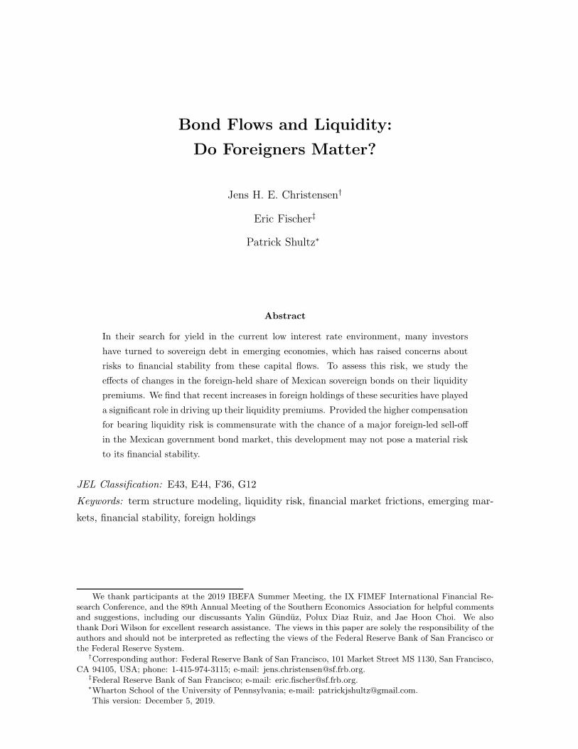
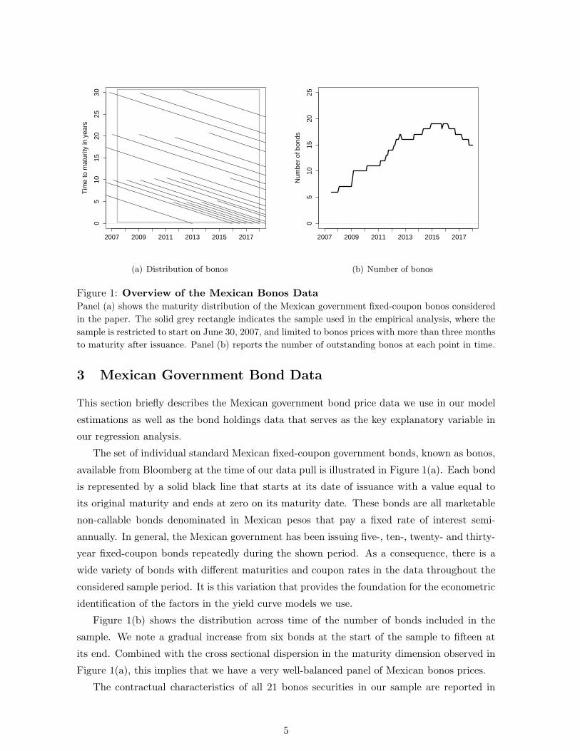
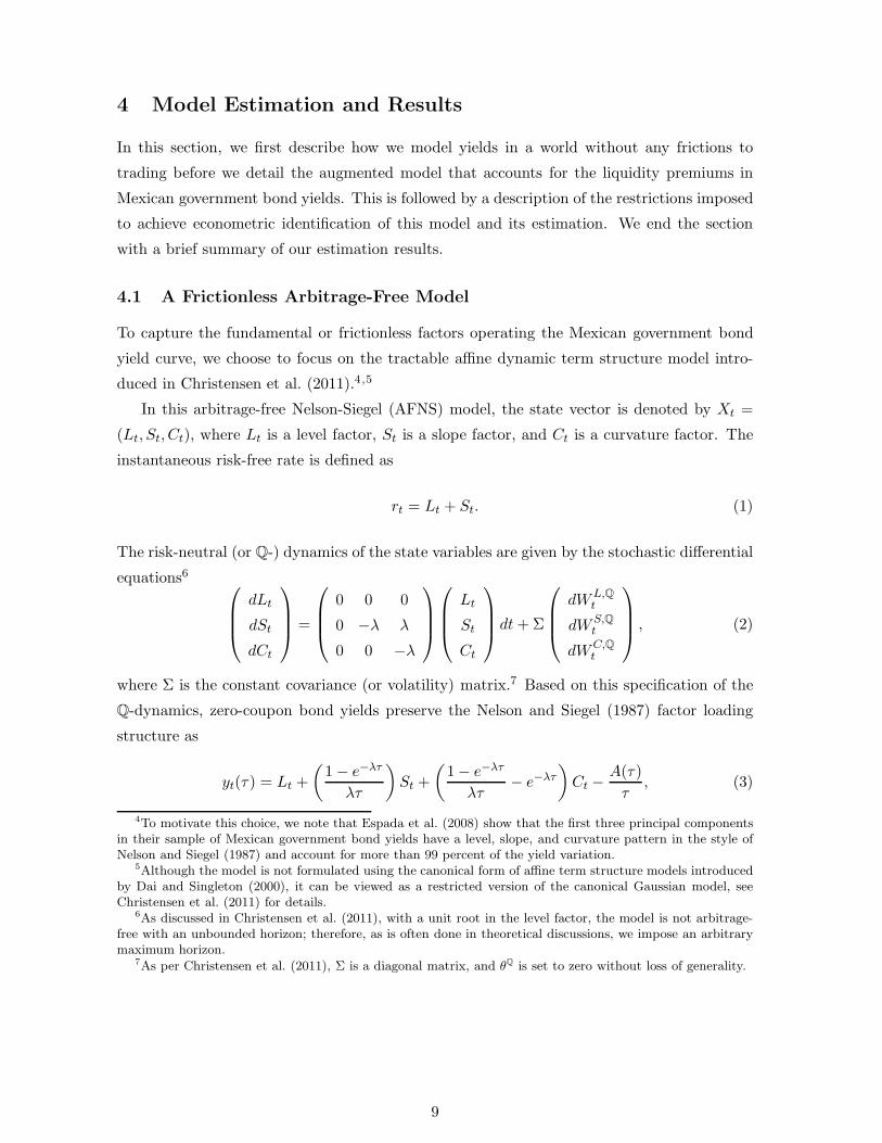
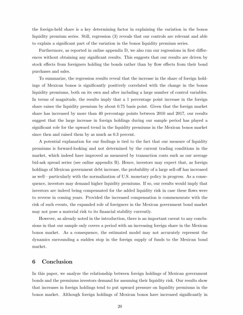
Figure 1: Overview of the Mexican Bonos Data

Panel (a) shows the maturity distribution of the Mexican government fixed-coupon bonos considered

in the paper. The solid grey rectangle indicates the sample used in the empirical analysis, where the

sample is restricted to start on June 30, 2007, and limited to bonos prices with more than three months

to maturity after issuance. Panel (b) reports the number of outstanding bonos at each point in time.

3 Mexican Government Bond Data

This section briefly describes the Mexican government bond price data we use in our model

estimations as well as the bond holdings data that serves as the key explanatory variable in

our regression analysis.

The set of individual standard Mexican fixed-coupon government bonds, known as bonos,

available from Bloomberg at the time of our data pull is illustrated in Figure 1(a). Each bond

is represented by a solid black line that starts at its date of issuance with a value equal to

its original maturity and ends at zero on its maturity date. These bonds are all marketable

non-callable bonds denominated in Mexican pesos that pay a fixed rate of interest semi-

annually. In general, the Mexican government has been issuing five-, ten-, twenty- and thirty-

year fixed-coupon bonds repeatedly during the shown period. As a consequence, there is a

wide variety of bonds with different maturities and coupon rates in the data throughout the

considered sample period. It is this variation that provides the foundation for the econometric

identification of the factors in the yield curve models we use.

Figure 1(b) shows the distribution across time of the number of bonds included in the

sample. We note a gradual increase from six bonds at the start of the sample to fifteen at

its end. Combined with the cross sectional dispersion in the maturity dimension observed in

Figure 1(a), this implies that we have a very well-balanced panel of Mexican bonos prices.

The contractual characteristics of all 21 bonos securities in our sample are reported in

5

Bonos No. Issuance Number of Total notionalBonos (coupon, maturity)

type obs. Date Amount auctions amount

(1) 9% 12/20/2012 10yr 63 1/9/2003 1,500 40 86,618(2) 8% 12/7/2023 20yr 127 10/30/2003 1,000 36 93,495(3) 8% 12/17/2015 10yr 99 1/5/2006 3,100 33 106,009(4) 10% 11/20/2036 30yr 127 10/26/2006 2,000 37 90,065(5) 7.5% 6/3/2027 20yr 127 1/18/2007 4,650 35 179,629(6) 7.25% 12/15/2016 10yr 111 2/1/2007 4,800 26 134,687(7) 7.75% 12/14/2017 10yr 116 1/31/2008 7,650 25 93,220(8) 8.5% 5/31/2029 20yr 108 1/15/2009 2,000 28 102,349(9) 8.5% 11/18/2038 30yr 108 1/29/2009 2,000 36 100,072(10) 8.5% 12/13/2018 10yr 107 2/12/2009 2,500 29 149,197(11) 8% 6/11/2020 10yr 95 2/25/2010 25,000 20 351,000(12) 6.5% 6/10/2021 10yr 83 2/3/2011 25,000 29 329,770(13) 6.25% 6/16/2016 5yr 56 7/22/2011 25,000 17 167,550(14) 7.75% 5/29/2031 20yr 76 9/9/2011 60,500 22 193,000(15) 6.5% 6/9/2022 10yr 71 2/15/2012 74,500 22 335,096(16) 7.75% 11/13/2042 30yr 69 4/20/2012 33,000 38 228,246(17) 5% 6/15/2017 5yr 56 7/19/2012 30,000 11 145,000(18) 4.75% 6/14/2018 5yr 53 8/30/2013 211,000 19 339,825(19) 7.75% 11/23/2034 20yr 45 4/11/2014 15,000 26 104,377(20) 5% 12/11/2019 5yr 38 11/7/2014 15,000 20 242,067(21) 5.75% 3/5/2026 10yr 27 10/16/2015 17,000 12 172,711

Table 1: Sample of Mexican Bonos

The table reports the bonos name, type, number of monthly observations in the sample period from

June 30, 2007, to December 29, 2017, first issuance date and amount, the total number of auctions,

and the total amount issued in millions of Mexican pesos for the considered set of Mexican government

fixed-coupon bonos based on the information available as of February 2018.

Table 1. The number of monthly observations for each bond using three-month censoring

before maturity is also reported in the table. Although each bond is issued at first with a

relatively small outstanding notional amount, they grow quickly thanks to a large number

of subsequent reopenings that can raise their outstanding amounts to as much as 350 billion

pesos, or close to 20 billion U.S. dollars. Thus, these are large bond series even by international

standards.

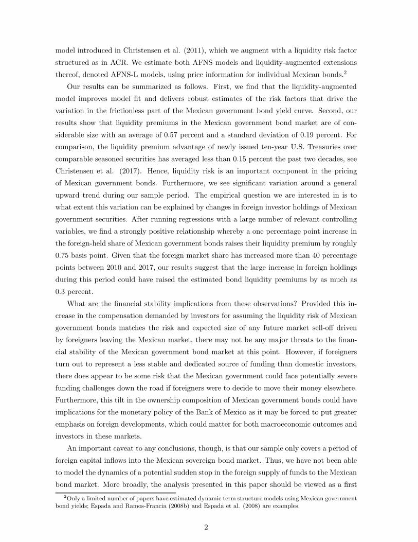
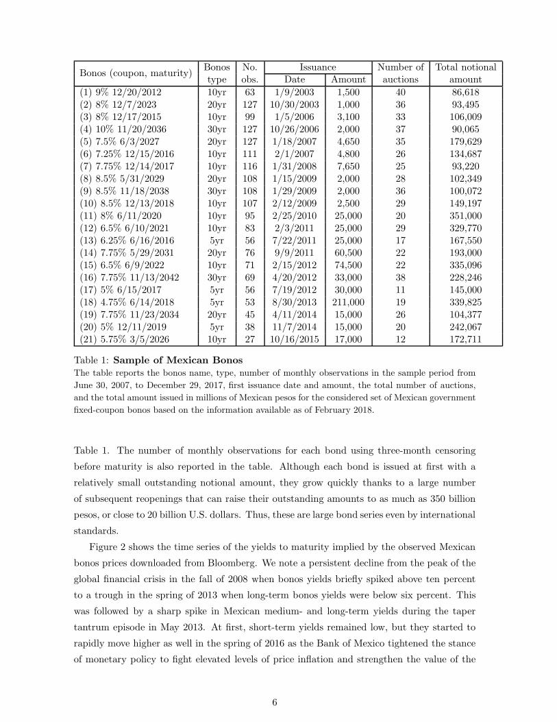
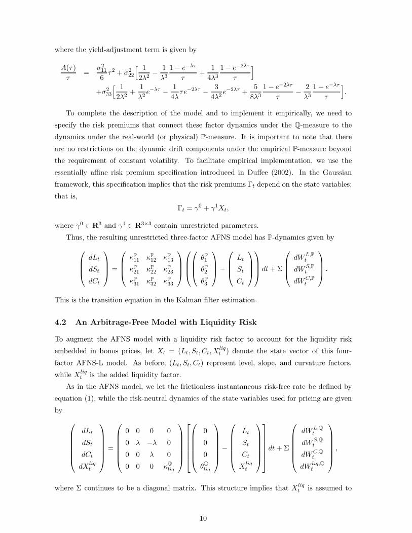
Figure 2 shows the time series of the yields to maturity implied by the observed Mexican

bonos prices downloaded from Bloomberg. We note a persistent decline from the peak of the

global financial crisis in the fall of 2008 when bonos yields briefly spiked above ten percent

to a trough in the spring of 2013 when long-term bonos yields were below six percent. This

was followed by a sharp spike in Mexican medium- and long-term yields during the taper

tantrum episode in May 2013. At first, short-term yields remained low, but they started to

rapidly move higher as well in the spring of 2016 as the Bank of Mexico tightened the stance

of monetary policy to fight elevated levels of price inflation and strengthen the value of the

6

2007 2009 2011 2013 2015 2017

02

46

810

12

Rat

e in

per

cent

Figure 2: Mexican Bonos Yields

Illustration of the yields to maturity implied by the Mexican government fixed-coupon bonos prices

downloaded from Bloomberg. The data are monthly covering the period from June 30, 2007, to

December 29, 2017, and censor the last three months for each maturing bond.

Mexican peso. Thus, there has been a fair amount of variation in the general yield level

in Mexico during our sample period. Furthermore, as in U.S. Treasury yield data, there is

notable variation in the shape of the yield curve. At times, like early in our sample, yields

across maturities are relatively compressed. At other times, the yield curve is steep, with long-

term bonos trading at yields that are 3 to 4 percent above those of shorter-term securities as

in 2015. It is these characteristics that underlie our choice of using a three-factor model for

the frictionless part of the Mexican yield curve similar to what is standard for U.S. and U.K.

data; see Christensen and Rudebusch (2012).

Finally, regarding the important question of a lower bound, the Bank of Mexico has never

been forced to lower its conventional policy rate even close to zero, and the bond yields in the

data have remained well above zero throughout the sample period. Thus, there is no need to

account for any lower bounds to model these fixed-coupon bond prices, which supports our

focus on standard Gaussian yield curve models.

7

2007 2008 2009 2010 2011 2012 2013 2014 2015 2016 2017 2018

050

010

0015

0020

00

Bill

ions

of p

esos

Domestic residents Foreigners

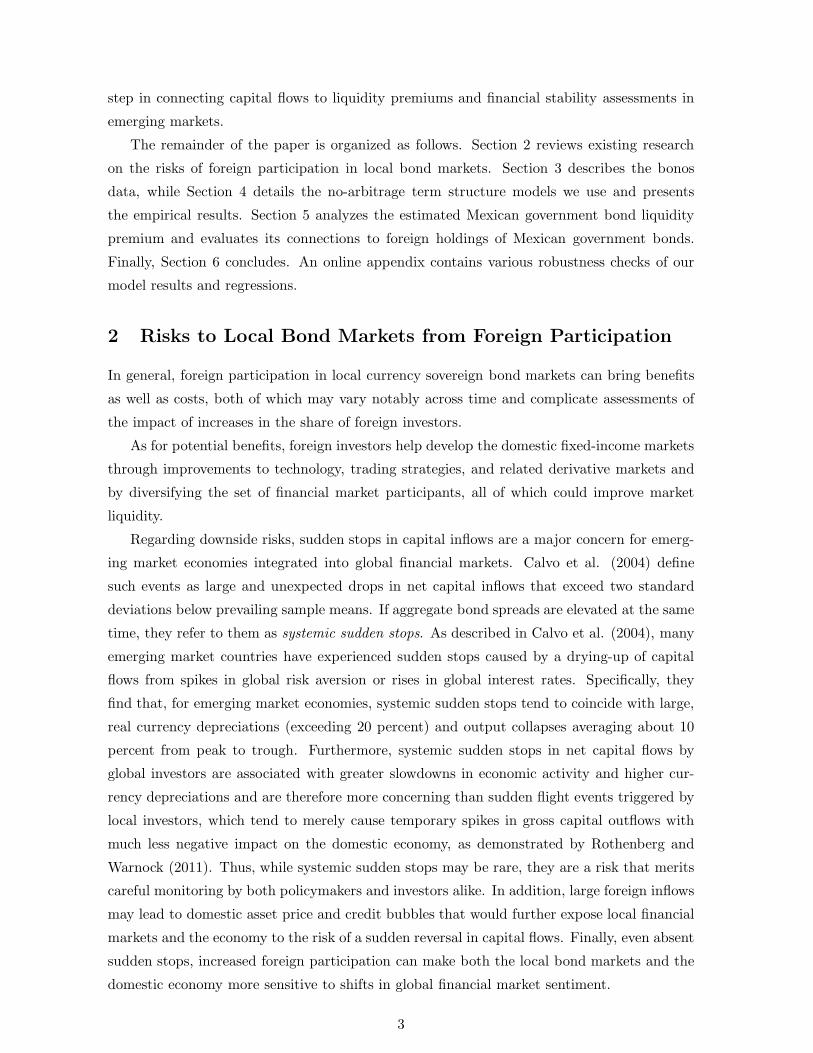
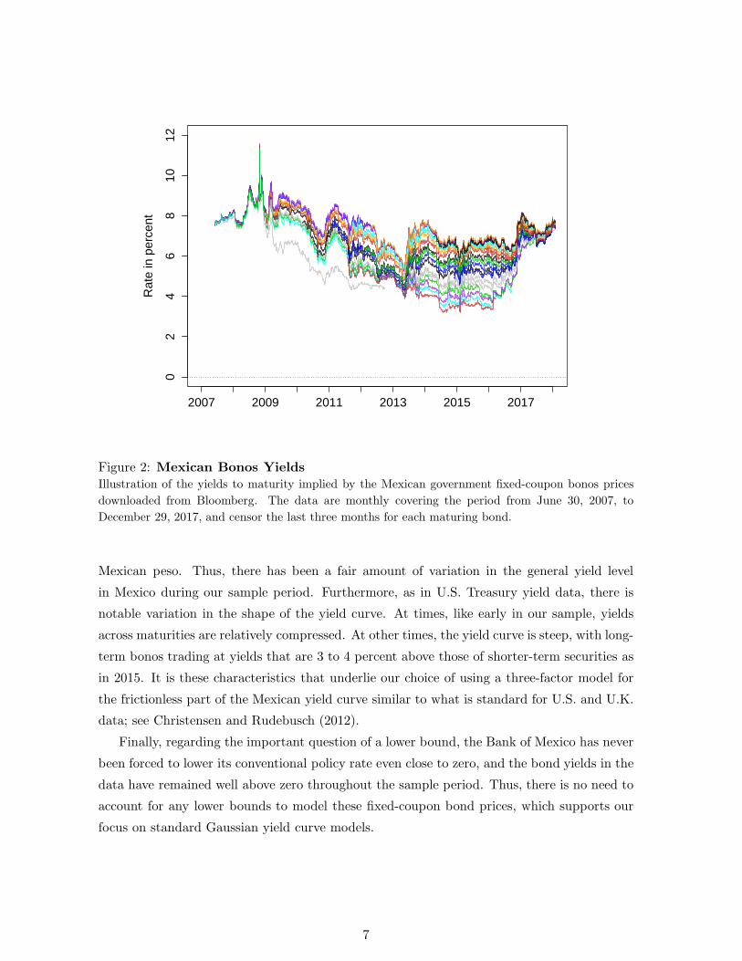
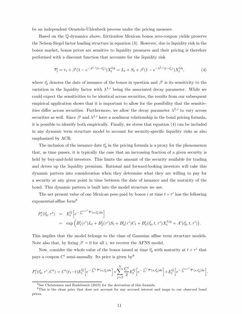
Figure 3: Net Holdings of Mexican Bonos

3.1 Mexican Government Debt Holdings

In addition to the bond price data described above, our analysis utilizes data on domestic

and foreign holdings of Mexican government debt securities that the Bank of Mexico requires

financial intermediaries to report as a way to track market activity in the Mexican sovereign

bond markets. These data have been collected since 1978 and are available at daily frequency

up to the present. A key strength of the data set is that it covers any change in Mexican

government debt holdings by either domestic or foreign investors. For each transaction, the

reporting forms also identify the type of Mexican government security. Therefore, we are able

to exploit the data reported for holdings of bonos alone and leave other Mexican government

securities for future research. Although the data are available at a daily frequency, we use

the observations at the end of each month to align them with our bond price data.

Figure 3 shows the monthly level of bonos holdings by domestic residents and foreigners

over the period from June 2007 through December 2017. We note that foreigners overtook

domestic residents in total holdings by late 2012 and have continued to increase their share

quite notably and now exceed those of domestic residents by a wide margin. The empirical

question we are interested in is whether this dramatic increase in foreign holdings of Mexican

government bonds has affected the liquidity risk in the market for these securities, but before

we can address that question we need to introduce and estimate our models.

8

4 Model Estimation and Results

In this section, we first describe how we model yields in a world without any frictions to

trading before we detail the augmented model that accounts for the liquidity premiums in

Mexican government bond yields. This is followed by a description of the restrictions imposed

to achieve econometric identification of this model and its estimation. We end the section

with a brief summary of our estimation results.

4.1 A Frictionless Arbitrage-Free Model

To capture the fundamental or frictionless factors operating the Mexican government bond

yield curve, we choose to focus on the tractable affine dynamic term structure model intro-

duced in Christensen et al. (2011).4 ,5

In this arbitrage-free Nelson-Siegel (AFNS) model, the state vector is denoted by Xt =

(Lt, St, Ct), where Lt is a level factor, St is a slope factor, and Ct is a curvature factor. The

instantaneous risk-free rate is defined as

rt = Lt + St. (1)

The risk-neutral (or Q-) dynamics of the state variables are given by the stochastic differential

equations6

dLt

dSt

dCt

=

0 0 0

0 −λ λ

0 0 −λ

Lt

St

Ct

dt+Σ

dWL,Qt

dWS,Qt

dWC,Qt

, (2)

where Σ is the constant covariance (or volatility) matrix.7 Based on this specification of the

Q-dynamics, zero-coupon bond yields preserve the Nelson and Siegel (1987) factor loading

structure as

yt(τ) = Lt +

(1− e−λτ

λτ

)St +

(1− e−λτ

λτ− e−λτ

)Ct −

A(τ)

τ, (3)

4To motivate this choice, we note that Espada et al. (2008) show that the first three principal componentsin their sample of Mexican government bond yields have a level, slope, and curvature pattern in the style ofNelson and Siegel (1987) and account for more than 99 percent of the yield variation.

5Although the model is not formulated using the canonical form of affine term structure models introducedby Dai and Singleton (2000), it can be viewed as a restricted version of the canonical Gaussian model, seeChristensen et al. (2011) for details.

6As discussed in Christensen et al. (2011), with a unit root in the level factor, the model is not arbitrage-free with an unbounded horizon; therefore, as is often done in theoretical discussions, we impose an arbitrarymaximum horizon.

7As per Christensen et al. (2011), Σ is a diagonal matrix, and θQ is set to zero without loss of generality.

9

where the yield-adjustment term is given by

A(τ)

τ=

σ211

6τ2 + σ2

22

[ 1

2λ2−

1

λ3

1− e−λτ

τ+

1

4λ3

1− e−2λτ

τ

]

+σ233

[ 1

2λ2+

1

λ2e−λτ −

1

4λτe−2λτ −

3

4λ2e−2λτ +

5

8λ3

1− e−2λτ

τ−

2

λ3

1− e−λτ

τ

].

To complete the description of the model and to implement it empirically, we need to

specify the risk premiums that connect these factor dynamics under the Q-measure to the

dynamics under the real-world (or physical) P-measure. It is important to note that there

are no restrictions on the dynamic drift components under the empirical P-measure beyond

the requirement of constant volatility. To facilitate empirical implementation, we use the

essentially affine risk premium specification introduced in Duffee (2002). In the Gaussian

framework, this specification implies that the risk premiums Γt depend on the state variables;

that is,

Γt = γ0 + γ1Xt,

where γ0 ∈ R3 and γ1 ∈ R3×3 contain unrestricted parameters.

Thus, the resulting unrestricted three-factor AFNS model has P-dynamics given by

dLt

dSt

dCt

=

κP11 κP12 κP13

κP21 κP22 κP23

κP31 κP32 κP33

θP1

θP2

θP3

−

Lt

St

Ct

dt+Σ

dWL,Pt

dWS,Pt

dWC,Pt

.

This is the transition equation in the Kalman filter estimation.

4.2 An Arbitrage-Free Model with Liquidity Risk

To augment the AFNS model with a liquidity risk factor to account for the liquidity risk

embedded in bonos prices, let Xt = (Lt, St, Ct,Xliqt ) denote the state vector of this four-

factor AFNS-L model. As before, (Lt, St, Ct) represent level, slope, and curvature factors,

while Xliqt is the added liquidity factor.

As in the AFNS model, we let the frictionless instantaneous risk-free rate be defined by

equation (1), while the risk-neutral dynamics of the state variables used for pricing are given

by

dLt

dSt

dCt

dXliqt

=

0 0 0 0

0 λ −λ 0

0 0 λ 0

0 0 0 κQliq

0

0

0

θQliq

−

Lt

St

Ct

Xliqt

dt+Σ

dWL,Qt

dWS,Qt

dWC,Qt

dWliq,Qt

,

where Σ continues to be a diagonal matrix. This structure implies that Xliqt is assumed to

10

be an independent Ornstein-Uhlenbeck process under the pricing measure.

Based on the Q-dynamics above, frictionless Mexican bonos zero-coupon yields preserve

the Nelson-Siegel factor loading structure in equation (3). However, due to liquidity risk in the

bonos market, bonos prices are sensitive to liquidity pressures and their pricing is therefore

performed with a discount function that accounts for the liquidity risk

rit = rt + βi(1− e−λL,i(t−ti0))X liq

t = Lt + St + βi(1 − e−λL,i(t−ti0))X liq

t , (4)

where ti0 denotes the date of issuance of the bonos in question and βi is its sensitivity to the

variation in the liquidity factor with λL,i being the associated decay parameter. While we

could expect the sensitivities to be identical across securities, the results from our subsequent

empirical application shows that it is important to allow for the possibility that the sensitiv-

ities differ across securities. Furthermore, we allow the decay parameter λL,i to vary across

securities as well. Since βi and λL,i have a nonlinear relationship in the bond pricing formula,

it is possible to identify both empirically. Finally, we stress that equation (4) can be included

in any dynamic term structure model to account for security-specific liquidity risks as also

emphasized by ACR.

The inclusion of the issuance date ti0 in the pricing formula is a proxy for the phenomenon

that, as time passes, it is typically the case that an increasing fraction of a given security is

held by buy-and-hold investors. This limits the amount of the security available for trading

and drives up the liquidity premium. Rational and forward-looking investors will take this

dynamic pattern into consideration when they determine what they are willing to pay for

a security at any given point in time between the date of issuance and the maturity of the

bond. This dynamic pattern is built into the model structure we use.

The net present value of one Mexican peso paid by bonos i at time t+τ i has the following

exponential-affine form8

P it (t

i0, τ

i) = EQt

[e−

∫ t+τi

tri(s,ti0)ds

]

= exp(Bi

1(τi)Lt +Bi

2(τi)St +Bi

3(τi)Ct +Bi

4(ti0, t, τ

i)XLiqt +Ai(ti0, t, τ

i)).

This implies that the model belongs to the class of Gaussian affine term structure models.

Note also that, by fixing βi = 0 for all i, we recover the AFNS model.

Now, consider the whole value of the bonos issued at time ti0 with maturity at t+ τ i that

pays a coupon Ci semi-annually. Its price is given by9

P it (t

i0, τ

i, Ci) = Ci(t1−t)EQt

[e−

∫ t1t ri(s,ti

0)ds

]+

N∑

j=2

Ci

2E

Qt

[e−

∫ tjt ri(s,ti

0)ds

]+E

Qt

[e−

∫ t+τi

tri(s,ti

0)ds

].

8See Christensen and Rudebusch (2019) for the derivation of this formula.9This is the clean price that does not account for any accrued interest and maps to our observed bond

prices.

11

Finally, to complete the description of the AFNS-L model, we again specify an essentially

affine risk premium structure, which implies that the risk premiums Γt take the form

Γt = γ0 + γ1Xt,

where γ0 ∈ R4 and γ1 ∈ R4×4 contain unrestricted parameters. Thus, the resulting unre-

stricted four-factor AFNS-L model has P-dynamics given by

dLt

dSt

dCt

dXliqt

=

κP11 κP12 κP13 κP14

κP21 κP22 κP23 κP24

κP31 κP32 κP33 κP34

κP41 κP42 κP43 κP44

θP1

θP2

θP3

θP4

−

Lt

St

Ct

Xliqt

dt+Σ

dWL,Pt

dWS,Pt

dWC,Pt

dWliq,Pt

.

This is the transition equation in the extended Kalman filter estimation.

4.3 Model Estimation and Econometric Identification

Due to the nonlinearity of the bond pricing formulas, the models cannot be estimated with

the standard Kalman filter. Instead, we use the extended Kalman filter as in Kim and

Singleton (2012), see Christensen and Rudebusch (2019) for details. To make the fitted errors

comparable across bonds of various maturities, we follow ACR and scale each bond price by

its duration. Thus, the measurement equation for the bond prices takes the following form:

P it (t

i0, τ

i, Ci)

Dit(t

i0, τ

i, Ci)=

P it (t

i0, τ

i, Ci)

Dit(t

i0, τ

i, Ci)+ εit,

where Pt(ti0, τ

i, Ci) is the model-implied price of bonos i and Dt(ti0, τ

i, Ci) is its duration,

which is fixed and calculated before estimation.10 In addition, we assume that all bond price

measurement equations have i.i.d. fitted errors with zero mean and standard deviation σε.

Since the liquidity factor is a latent factor that we do not observe, its level is not identified

without additional restrictions. As a consequence, when we include the liquidity factor X liqt ,

we let the first thirty-year bonos issued during our sample window have a unit loading on the

liquidity factor, that is, bonos number (9) in our sample issued on January 29, 2009, with

maturity on November 18, 2038, and a coupon rate of 8.5 percent has β9 = 1.

Furthermore, we note that the liquidity decay parameters λL,i can be hard to identify if

their values are too large or too small. As a consequence, we impose the restriction that they

fall within the range from 0.0001 to 10, which is without practical consequences based on the

evidence presented in ACR. Also, for numerical stability during the model optimization, we

impose the restrictions that the liquidity sensitivity parameters βi fall within the range from

0 to 250, which turns out not to be a binding constraint at the optimum.

10The robustness of this formulation of the measurement equation is documented in Andreasen et al. (2019).

12

Finally, we assume that the state variables are stationary and therefore start the Kalman

filter at the unconditional mean and covariance matrix. This assumption is supported by

the analysis in Chiquiar et al. (2010), who find that Mexican inflation seems to have become

stationary at some point in the early 2000s, while De Pooter et al. (2014) document that

measures of long-term inflation expectations from both surveys and the Mexican government

bond market have remained anchored close to the 3 percent inflation target of the Bank of

Mexico at least since 2003. Assuming real rates and bond risk premiums are stationary,11

this evidence would imply that Mexican government bond yields should be stationary as well,

as also suggested by visual inspection of the individual yield series depicted in Figure 2.

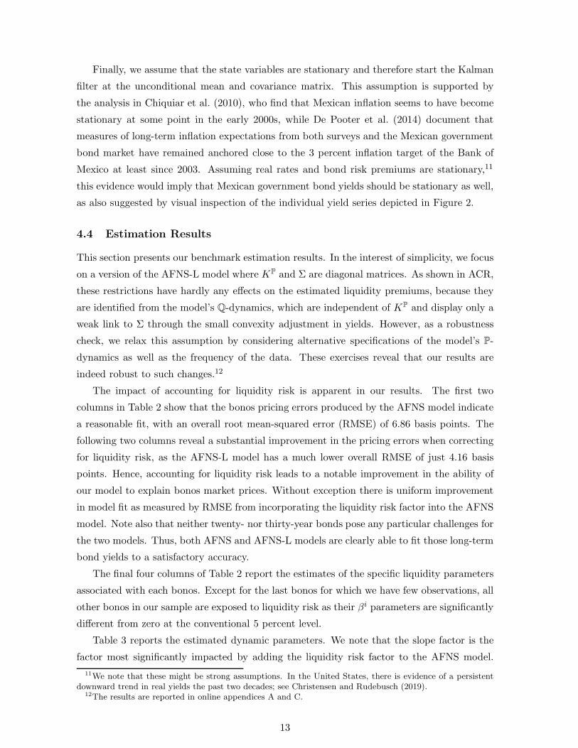
4.4 Estimation Results

This section presents our benchmark estimation results. In the interest of simplicity, we focus

on a version of the AFNS-L model where KP and Σ are diagonal matrices. As shown in ACR,

these restrictions have hardly any effects on the estimated liquidity premiums, because they

are identified from the model’s Q-dynamics, which are independent of KP and display only a

weak link to Σ through the small convexity adjustment in yields. However, as a robustness

check, we relax this assumption by considering alternative specifications of the model’s P-

dynamics as well as the frequency of the data. These exercises reveal that our results are

indeed robust to such changes.12

The impact of accounting for liquidity risk is apparent in our results. The first two

columns in Table 2 show that the bonos pricing errors produced by the AFNS model indicate

a reasonable fit, with an overall root mean-squared error (RMSE) of 6.86 basis points. The

following two columns reveal a substantial improvement in the pricing errors when correcting

for liquidity risk, as the AFNS-L model has a much lower overall RMSE of just 4.16 basis

points. Hence, accounting for liquidity risk leads to a notable improvement in the ability of

our model to explain bonos market prices. Without exception there is uniform improvement

in model fit as measured by RMSE from incorporating the liquidity risk factor into the AFNS

model. Note also that neither twenty- nor thirty-year bonds pose any particular challenges for

the two models. Thus, both AFNS and AFNS-L models are clearly able to fit those long-term

bond yields to a satisfactory accuracy.

The final four columns of Table 2 report the estimates of the specific liquidity parameters

associated with each bonos. Except for the last bonos for which we have few observations, all

other bonos in our sample are exposed to liquidity risk as their βi parameters are significantly

different from zero at the conventional 5 percent level.

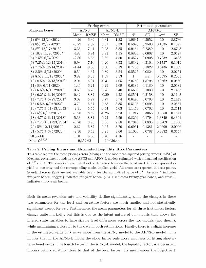
Table 3 reports the estimated dynamic parameters. We note that the slope factor is the

factor most significantly impacted by adding the liquidity risk factor to the AFNS model.

11We note that these might be strong assumptions. In the United States, there is evidence of a persistentdownward trend in real yields the past two decades; see Christensen and Rudebusch (2019).

12The results are reported in online appendices A and C.

13

Pricing errors Estimated parametersMexican bonos AFNS AFNS-L AFNS-L

Mean RMSE Mean RMSE βi SE λL,i SE

(1) 9% 12/20/2012† -0.26 6.39 0.34 1.33 1.9637 0.5052 10 8.8736(2) 8% 12/7/2023+ -3.72 7.02 0.51 5.33 0.5370 0.2500 0.1035 0.1097(3) 8% 12/17/2015† 3.35 7.44 0.08 3.85 0.9164 0.2389 10 2.6748(4) 10% 11/20/2036× 4.83 6.94 0.93 4.15 0.8830 0.0607 10 2.0527(5) 7.5% 6/3/2027+ -2.80 6.65 0.82 4.50 0.4527 0.0908 0.7032 1.3433(6) 7.25% 12/15/2016† 0.93 7.16 0.20 3.53 1.0332 0.3104 0.1757 0.1019(7) 7.75% 12/14/2017† -1.44 9.88 0.50 5.19 0.7783 0.1822 0.3435 0.1039(8) 8.5% 5/31/2029+ 0.59 4.37 0.89 3.54 0.5525 0.0824 10 2.0254(9) 8.5% 11/18/2038× 3.89 6.83 1.09 3.53 1 n.a. 0.3595 0.2033(10) 8.5% 12/13/2018† 2.04 5.04 -0.31 4.05 2.0760 1.5795 0.0562 0.0560(11) 8% 6/11/2020† 1.46 6.21 0.29 4.09 0.6184 0.1180 10 2.0681(12) 6.5% 6/10/2021† 3.63 6.78 0.78 3.40 0.5650 0.1030 10 2.1463(13) 6.25% 6/16/2016∗ 0.42 8.82 -0.29 4.28 0.8591 0.2158 10 2.1143(14) 7.75% 5/29/2031+ 3.02 5.27 0.77 3.74 0.6470 0.0708 10 2.1449(15) 6.5% 6/9/2022† 3.70 5.57 0.68 3.35 0.5195 0.0895 10 2.2551(16) 7.75% 11/13/2042× -2.31 5.55 0.44 5.03 1.1459 0.0702 10 2.2514(17) 5% 6/15/2017∗ -0.96 8.62 -0.25 5.23 1.1217 0.3066 0.3350 0.1541(18) 4.75% 6/14/2018∗ 5.33 8.84 0.22 5.59 0.8294 0.1794 1.3849 0.4361(19) 7.75% 11/23/2034+ -0.70 3.95 0.35 2.58 0.7843 0.0833 1.3709 1.1850(20) 5% 12/11/2019∗ 2.62 6.82 0.07 3.70 0.6961 0.1381 2.9699 2.0906(21) 5.75% 3/5/2026† -2.30 6.43 0.25 3.66 1.1060 3.0787 0.0932 0.3557

All yields 1.01 6.86 0.46 4.16 - - - -Max LEKF 9,352.62 10,036.44 - -

Table 2: Pricing Errors and Estimated Liquidity Risk Parameters

This table reports the mean pricing errors (Mean) and the root mean-squared pricing errors (RMSE) of

Mexican government bonds in the AFNS and AFNS-L models estimated with a diagonal specification

of KP and Σ. The errors are computed as the difference between the bond market price expressed as

yield to maturity and the corresponding model-implied yield. All errors are reported in basis points.

Standard errors (SE) are not available (n.a.) for the normalized value of β9. Asterisk * indicates

five-year bonds, dagger † indicates ten-year bonds, plus + indicates twenty-year bonds, and cross ×

indicates thirty-year bonds.

Both its mean-reversion rate and volatility decline significantly, while the changes in these

two parameters for the level and curvature factors are much smaller and not statistically

significant except for σ11. Furthermore, the mean parameters for all three frictionless factors

change quite markedly, but this is due to the latent nature of our models that allows the

filtered state variables to have sizable level differences across the two models (not shown),

while maintaining a close fit to the data in both estimations. Finally, there is a slight increase

in the estimated value of λ as we move from the AFNS model to the AFNS-L model. This

implies that in the AFNS-L model the slope factor puts more emphasis on fitting shorter-

term bond yields. The fourth factor in the AFNS-L model, the liquidity factor, is a persistent

process with a volatility close to that of the level factor. Its mean under the objective P

14

AFNS AFNS-LParameter

Est. SE Est. SE

κP11 0.2846 0.1246 0.4789 0.3286κP22 6.5806 1.2222 0.4156 0.5277κP33 0.3978 0.2915 0.1564 0.1986κP44 – – 0.2016 0.2883σ11 0.0077 0.0002 0.0120 0.0007σ22 0.0812 0.0020 0.0199 0.0024σ33 0.0282 0.0021 0.0226 0.0031σ44 – – 0.0175 0.0055θP1 0.2196 0.0095 0.0933 0.0130θP2 -0.1803 0.0068 -0.0456 0.0300θP3 -0.1200 0.0223 -0.0315 0.0609θP4 – – -0.0133 0.0422λ 0.1770 0.0036 0.2770 0.0097

κQliq – – 2.0004 0.3360

θQliq – – 0.0095 0.0020

σε 0.0008 1.02 × 10−5 0.0005 1.12× 10−5

Table 3: Estimated Dynamic Parameters

The table shows the estimated dynamic parameters for the AFNS and AFNS-L models estimated with

a diagonal specification of KP and Σ.

probability measure is -0.0133, which is close to the average of its filtered path. However, its

mean under the risk-neutral Q probability measure used for pricing is 0.0095, which explains

why the estimated bonos liquidity premiums described in the next section are strictly positive.

5 The Bonos Liquidity Premium

In this section, we analyze the bonos liquidity premium implied by the estimated AFNS-

L model described in the previous section. First, we formally define the bonos liquidity

premium, study its historical evolution, and assess its robustness before we end the section

by relating the estimated liquidity premium to foreign holdings of bonos, while controlling

for other relevant factors that could affect the liquidity risk of bonos.

5.1 The Estimated Bonos Liquidity Premium

We use the estimated AFNS-L model to extract the liquidity premium in the bonos market.

To compute this premium, we first use the estimated parameters and the filtered states{Xt|t

}T

t=1to calculate the fitted bonos prices

{P it

}T

t=1for all outstanding securities in our

sample. These bond prices are then converted into yields to maturity{yc,it

}T

t=1by solving

15

the fixed-point problem

P it = C(t1 − t) exp

{−(t1 − t)yc,it

}+

n∑

k=2

C

2exp

{−(tk − t)yc,it

}+ exp

{−(T − t)yc,it

}, (5)

for i = 1, 2, ..., N , meaning that{yc,it

}T

t=1is the rate of return on the ith bonos if held

until maturity. To obtain the corresponding yields corrected for liquidity risk, a new set of

model-implied bond prices are computed from the estimated AFNS-L model but using only

its frictionless part, i.e., using the constraints that Xliq

t|t = 0 for all t as well as σ44 = 0 and

θQliq = 0. These prices are denoted{P it

}T

t=1and converted into yields to maturity y

c,it using

(5). They represent estimates of the prices that would prevail in a world without any financial

frictions. The liquidity premium for the ith bonos is then defined as

Ψit ≡ y

c,it − y

c,it . (6)

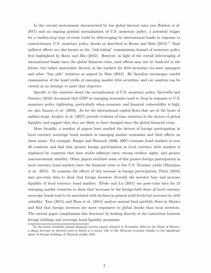
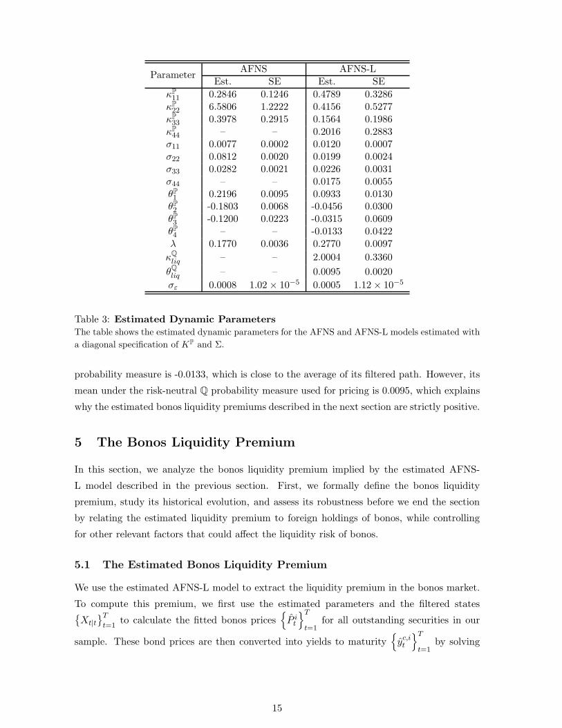
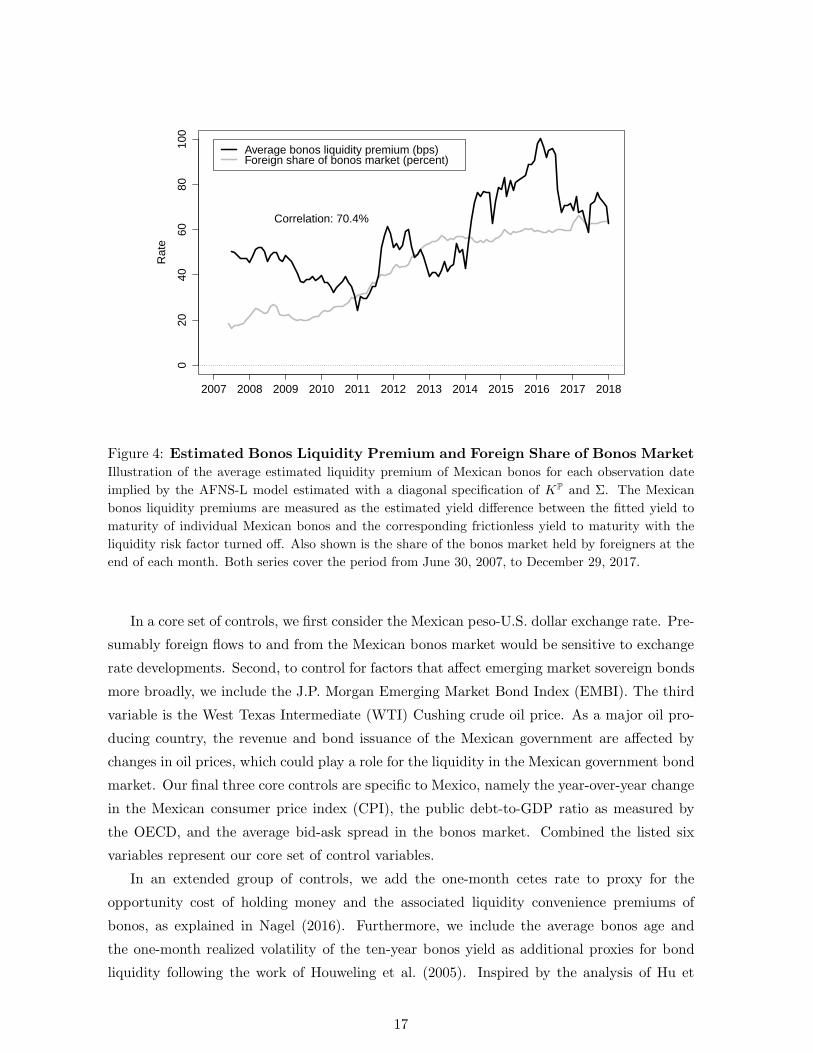
The average estimated liquidity premium of Mexican bonos implied by the AFNS-L model

is shown with a solid black line in Figure 4. We note that the estimated liquidity premium is

of considerable size, with an average of 0.57 percent and a standard deviation of 0.19 percent.

Hence, liquidity risk is an important component in the pricing of Mexican government bonds.

Furthermore, we see significant variation around a general upward trend during our sample

period, with notable spikes in the summer of 2011 and spring of 2014 and a persistent decline

in the fall of 2016.

Next, we are interested in understanding the determinants of the bonos liquidity premium

series and its ties to the increase in foreign holdings of Mexican government bonds described

in Section 3.1. Therefore, in Figure 4, we also show the market share of foreigners defined

as foreign net holdings divided by total public holdings (solid gray line) where we note a

high positive correlation (70 percent) between it and the average estimated bonos liquidity

premium. The key empirical question is to what extent variation in the estimated bonos

liquidity premium can be explained by the foreign-held share of the Mexican bonos market.

5.2 Regression Analysis

To explain the variation of the bonos liquidity premiums, we run standard regressions with the

liquidity premium series as the dependent variable and the share of foreign holdings of bonos

as the explanatory factor.13 In addition, we include a number of controls that are thought

to matter for bonos market liquidity specifically or bond market liquidity more broadly as

described in the following.14

13Our analysis is inspired by Hancock and Passmore (2015), who use the U.S. Federal Reserve’s holdingsas a share of the U.S. Treasury and mortgage backed securities (MBS) markets as explanatory variables todetermine their effect on MBS yields and mortgage rates.

14The full details of all control variables are provided in online appendix B.

16

2007 2008 2009 2010 2011 2012 2013 2014 2015 2016 2017 2018

020

4060

8010

0

Rat

e

Correlation: 70.4%

Average bonos liquidity premium (bps) Foreign share of bonos market (percent)

Figure 4: Estimated Bonos Liquidity Premium and Foreign Share of Bonos Market

Illustration of the average estimated liquidity premium of Mexican bonos for each observation date

implied by the AFNS-L model estimated with a diagonal specification of KP and Σ. The Mexican

bonos liquidity premiums are measured as the estimated yield difference between the fitted yield to

maturity of individual Mexican bonos and the corresponding frictionless yield to maturity with the

liquidity risk factor turned off. Also shown is the share of the bonos market held by foreigners at the

end of each month. Both series cover the period from June 30, 2007, to December 29, 2017.

In a core set of controls, we first consider the Mexican peso-U.S. dollar exchange rate. Pre-

sumably foreign flows to and from the Mexican bonos market would be sensitive to exchange

rate developments. Second, to control for factors that affect emerging market sovereign bonds

more broadly, we include the J.P. Morgan Emerging Market Bond Index (EMBI). The third

variable is the West Texas Intermediate (WTI) Cushing crude oil price. As a major oil pro-

ducing country, the revenue and bond issuance of the Mexican government are affected by

changes in oil prices, which could play a role for the liquidity in the Mexican government bond

market. Our final three core controls are specific to Mexico, namely the year-over-year change

in the Mexican consumer price index (CPI), the public debt-to-GDP ratio as measured by

the OECD, and the average bid-ask spread in the bonos market. Combined the listed six

variables represent our core set of control variables.

In an extended group of controls, we add the one-month cetes rate to proxy for the

opportunity cost of holding money and the associated liquidity convenience premiums of

bonos, as explained in Nagel (2016). Furthermore, we include the average bonos age and

the one-month realized volatility of the ten-year bonos yield as additional proxies for bond

liquidity following the work of Houweling et al. (2005). Inspired by the analysis of Hu et

17

al. (2013), we also include a noise measure of bonos prices to control for variation in the

amount of arbitrage capital available in this market. In addition, we use the five-year credit

default swap (CDS) rate for Mexico and the monthly return of the MSCI Mexico stock index

as two other measures of general developments in the Mexican economy of importance to

investors in the bonos market.15 We also add the VIX, which represents near-term uncertainty

about the general stock market as reflected in options on the Standard & Poor’s 500 stock

price index and is widely used as a gauge of investor fear and risk aversion. Furthermore,

we include the yield difference between seasoned (off-the-run) U.S. Treasury securities and

the most recently issued (on-the-run) U.S. Treasury security of the same ten-year maturity

mentioned earlier. This on-the-run (OTR) premium is a frequently used measure of financial

frictions in the U.S. Treasury market. The final variable is the U.S. TED spread, which is

calculated as the difference between the three-month U.S. LIBOR and the three-month U.S.

T-bill interest rate. This spread represents a measure of the perceived general credit risk in

global financial markets that could affect the pricing and trading of Mexican bonos.

To begin, we run regressions with each explanatory variable in isolation. The results are

reported in the last two columns of Table 4. The foreign-held share of the bonos market

and the average bonos age series have the largest individual explanatory power followed by

the debt-to-GDP ratio, the peso-U.S. dollar exchange rate, and the WTI oil price, while

the financial variables (the EMBI, the CDS rate, the return of the MSCI index, the VIX,

the on-the-run premium, and the TED spread) and CPI inflation only have a weak link

with the bonos liquidity premium as measured by the adjusted R2. The same holds for our

proxies of bonos market liquidity and frictions (bonos bid-ask spread, yield volatility, and

noise measure). Finally, the one-month cetes rate and the associated opportunity cost of

holding cash has a negative relationship with our estimated bonos liquidity premium series.

This is consistent with the findings of Nagel (2016) as increases in the convenience yield of

holding bonos, as measured by the cetes rate, should put downward pressure on the illiquidity

discount of bonos.

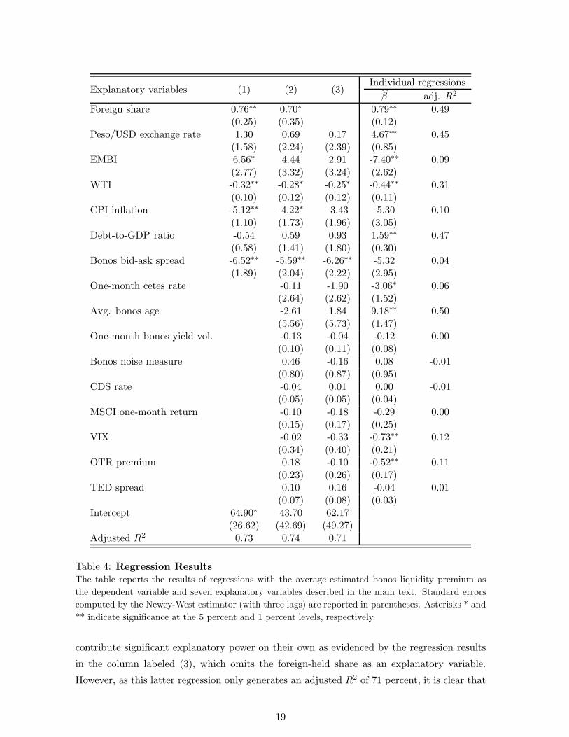
The columns labeled (1) and (2) in Table 4 show the results of our preferred joint regression

with our core set of variables and the full joint regression with all explanatory variables

included, respectively. Three things stand out. First, both regressions produce about the

same adjusted R2 (roughly 73 percent). Thus, the preferred regression yields about as much

explanatory power as possible given our fifteen control variables. Second, the foreign-held

share has an estimated coefficient that is close to 0.75 and statistically significant, that is, we

find a positive relationship whereby a 1 percentage point increase in the foreign-held share of

Mexican government bonds tends to raise their liquidity premium by about 0.75 basis point.

Third, the WTI, the Mexican CPI inflation, and the average bonos bid-ask spread all have

a stable relationship with the bonos liquidity premium series in these joint regressions and

15The MSCI index is a free-float weighted equity index designed to measure the performance of the largeand mid cap segments of the Mexican stock market. The index is reported in U.S. dollars.

18

Individual regressionsExplanatory variables (1) (2) (3)

β adj. R2

Foreign share 0.76∗∗ 0.70∗ 0.79∗∗ 0.49(0.25) (0.35) (0.12)

Peso/USD exchange rate 1.30 0.69 0.17 4.67∗∗ 0.45(1.58) (2.24) (2.39) (0.85)

EMBI 6.56∗ 4.44 2.91 -7.40∗∗ 0.09(2.77) (3.32) (3.24) (2.62)

WTI -0.32∗∗ -0.28∗ -0.25∗ -0.44∗∗ 0.31(0.10) (0.12) (0.12) (0.11)

CPI inflation -5.12∗∗ -4.22∗ -3.43 -5.30 0.10(1.10) (1.73) (1.96) (3.05)

Debt-to-GDP ratio -0.54 0.59 0.93 1.59∗∗ 0.47(0.58) (1.41) (1.80) (0.30)

Bonos bid-ask spread -6.52∗∗ -5.59∗∗ -6.26∗∗ -5.32 0.04(1.89) (2.04) (2.22) (2.95)

One-month cetes rate -0.11 -1.90 -3.06∗ 0.06(2.64) (2.62) (1.52)

Avg. bonos age -2.61 1.84 9.18∗∗ 0.50(5.56) (5.73) (1.47)

One-month bonos yield vol. -0.13 -0.04 -0.12 0.00(0.10) (0.11) (0.08)

Bonos noise measure 0.46 -0.16 0.08 -0.01(0.80) (0.87) (0.95)

CDS rate -0.04 0.01 0.00 -0.01(0.05) (0.05) (0.04)

MSCI one-month return -0.10 -0.18 -0.29 0.00(0.15) (0.17) (0.25)

VIX -0.02 -0.33 -0.73∗∗ 0.12(0.34) (0.40) (0.21)

OTR premium 0.18 -0.10 -0.52∗∗ 0.11(0.23) (0.26) (0.17)

TED spread 0.10 0.16 -0.04 0.01(0.07) (0.08) (0.03)

Intercept 64.90∗ 43.70 62.17(26.62) (42.69) (49.27)

Adjusted R2 0.73 0.74 0.71

Table 4: Regression Results

The table reports the results of regressions with the average estimated bonos liquidity premium as

the dependent variable and seven explanatory variables described in the main text. Standard errors

computed by the Newey-West estimator (with three lags) are reported in parentheses. Asterisks * and

** indicate significance at the 5 percent and 1 percent levels, respectively.

contribute significant explanatory power on their own as evidenced by the regression results

in the column labeled (3), which omits the foreign-held share as an explanatory variable.

However, as this latter regression only generates an adjusted R2 of 71 percent, it is clear that

19

the foreign-held share is a key determining factor in explaining the variation in the bonos

liquidity premium series. Still, regression (3) reveals that our controls are relevant and able

to explain a significant part of the variation in the bonos liquidity premium series.

Furthermore, as reported in online appendix D, we also run our regressions in first differ-

ences without obtaining any significant results. This suggests that our results are driven by

stock effects from foreigners holding the bonds rather than by flow effects from their bond

purchases and sales.

To summarize, the regression results reveal that the increase in the share of foreign hold-

ings of Mexican bonos is significantly positively correlated with the change in the bonos

liquidity premiums, both on its own and after including a large number of control variables.

In terms of magnitude, the results imply that a 1 percentage point increase in the foreign

share raises the liquidity premium by about 0.75 basis point. Given that the foreign market

share has increased by more than 40 percentage points between 2010 and 2017, our results

suggest that the large increase in foreign holdings during our sample period has played a

significant role for the upward trend in the liquidity premiums in the Mexican bonos market

since then and raised them by as much as 0.3 percent.

A potential explanation for our findings is tied to the fact that our measure of liquidity

premiums is forward-looking and not determined by the current trading conditions in the

market, which indeed have improved as measured by transaction costs such as our average

bid-ask spread series (see online appendix B). Hence, investors may expect that, as foreign

holdings of Mexican government debt increase, the probability of a large sell-off has increased

as well—particularly with the normalization of U.S. monetary policy in progress. As a conse-

quence, investors may demand higher liquidity premiums. If so, our results would imply that

investors are indeed being compensated for the added liquidity risk in case these flows were

to reverse in coming years. Provided the increased compensation is commensurate with the

risk of such events, the expanded role of foreigners in the Mexican government bond market

may not pose a material risk to its financial stability currently.

However, as already noted in the introduction, there is an important caveat to any conclu-

sions in that our sample only covers a period with an increasing foreign share in the Mexican

bonos market. As a consequence, the estimated model may not accurately represent the

dynamics surrounding a sudden stop in the foreign supply of funds to the Mexican bond

market.

6 Conclusion

In this paper, we analyze the relationship between foreign holdings of Mexican government

bonds and the premiums investors demand for assuming their liquidity risk. Our results show

that increases in foreign holdings tend to put upward pressure on liquidity premiums in the

bonos market. Although foreign holdings of Mexican bonos have increased significantly in

20

recent years and likely contributed to the upward trend in their liquidity premiums, this may

not pose a risk to financial stability provided the uptick in liquidity premium compensation is

adequate relative to the underlying risk of any major sell-off in coming years. More broadly,

this type of research may shed light on the important role that foreign investors play for the

stability of financial markets in emerging economies.

Finally, we feel compelled to stress the versatility of our empirical approach. For one, it

is straightforward to cast the considered model as a shadow-rate model that respects a lower

bound for bond yields using formulas provided in Christensen and Rudebusch (2015) in case

that is needed. Also, it is feasible to allow for stochastic volatility using the generalized AFNS

models developed in Christensen et al. (2014). Finally, the presented model can be expanded

with macroeconomic variables as in Espada and Ramos-Francia (2008a), with expectations

from surveys as in Kim and Orphanides (2012), or with real yields as in ACR. Thus, there are

many ways to enrich the analysis. However, we leave it for future research to explore those

avenues.

21

References

Ammer, John, Michiel De Pooter, Christopher J. Erceg, and Steven B. Kamin, 2016, “Inter-

national Spillovers of Monetary Policy,” IFDP Notes 2016-02-08-1, Board of Governors

of the Federal Reserve System.

Andreasen, Martin M., Jens H. E. Christensen, and Simon Riddell, 2018, “The TIPS Liq-

uidity Premium,” Working Paper 2017-11, Federal Reserve Bank of San Francisco.

Andreasen, Martin M., Jens H. E. Christensen, and Glenn D. Rudebusch, 2019, “Term

Structure Analysis with Big Data: One-Step Estimation Using Bond Prices,” Journal

of Econometrics, Vol. 212, 26-46.

Avdjiev, Stefan, Leonardo Gambacorta, Linda Goldberg, and Stefano Shiaffi, 2017, “The

Shifting Drivers of Global Liquidity,” Federal Reserve Bank of New York Staff Report

No. 819.

Beltran, Daniel O., Maxwell Kretchmer, Jaime Marquez, and Charles P. Thomas, 2013,

“Foreign Holdings of U.S. Treasuries and U.S. Treasury Yields,” Journal of International

Money and Finance, Vol. 32, 1120-1143.

Borio, C. and H. Zhu, 2012, “Capital Regulation, Risk-Taking and Monetary Policy: A

Missing Link in the Transmission Mechanism?,” Journal of Financial Stability, Vol. 8,

No. 4, 236-251.

Bruno, Valentina and Hyun Song Shin, 2015, “Capital Flows and the Risk-Taking Channel

of Monetary Policy,” Journal of Monetary Economics, Vol. 71, 119-132.

Burger, J.D. and Francis E. Warnock, 2006, “Local Currency Bond Markets,” IMF Staff

Papers No. 53, 115-132.

Burger, J.D. and Francis E. Warnock, 2007, “Foreign Participation in Local Currency Bond

Markets,” Review of Financial Economics, Vol. 16, 291-304.

Calvo, Guillermo A., Alejandro Izquierdo, and Ernesto Talvi, 2004, “Sudden Stops and

Phoenix Miracles in Emerging Markets,” American Economic Review, Vol. 96, No. 2,

405-410.

Chiquiar, Daniel, Antonio E. Noriega, and Manuel Ramos-Francia, 2010, “A Time-Series

Approach to Test a Change in Inflation Persistence: the Mexican Experience,” Applied

Economics, Vol. 42, 3067-3075.

Christensen, Jens H. E., Francis X. Diebold, and Glenn D. Rudebusch, 2011, “The Affine

Arbitrage-Free Class of Nelson-Siegel Term Structure Models,” Journal of Econometrics,

Vol. 164, No. 1, 4-20.

22

Christensen, Jens H. E. and James M. Gillan, 2019, “Does Quantitative Easing Affect Market

Liquidity?,” Working Paper 2013-26, Federal Reserve Bank of San Francisco.

Christensen, Jens H. E., Jose A. Lopez, and Glenn D. Rudebusch, 2014, “Can Spanned Term

Structure Factors Drive Stochastic Yield Volatility?,” Working Paper 2014-03, Federal

Reserve Bank of San Francisco.

Christensen, Jens H. E., Jose A. Lopez, and Patrick Shultz, 2017, “Is There an On-the-Run

Premium in TIPS?,” Working Paper 2017-10, Federal Reserve Bank of San Francisco.

Christensen, Jens H. E. and Glenn D. Rudebusch, 2012, “The Response of Interest Rates to

U.S. and U.K. Quantitative Easing,” Economic Journal, Vol. 122, F385-F414.

Christensen, Jens H. E. and Glenn D. Rudebusch, 2015, “Estimating Shadow-Rate Term

Structure Models with Near-Zero Yields,” Journal of Financial Econometrics, Vol. 13,

No. 2, 226-259.

Christensen, Jens H. E. and Glenn D. Rudebusch, 2019, “A New Normal for Interest Rates?

Evidence from Inflation-Indexed Debt,” forthcoming Review of Economics and Statis-

tics.

Dai, Qiang and Kenneth J. Singleton, 2000, “Specification Analysis of Affine Term Structure

Models,” Journal of Finance, Vol. 55, No. 5, 1943-1978.

De Pooter, Michiel, Patrice Robitaille, Ian Walker, and Michael Zdinak, 2014, “Are Long-

Term Inflation Expectations Well Anchored in Brazil, Chile, and Mexico?,” Interna-

tional Journal of Central Banking, Vol. 10, No. 2, 337-400.

Duffee, Gregory R., 2002, “Term Premia and Interest Rate Forecasts in Affine Models,”

Journal of Finance, Vol. 57, No. 1, 405-443.

Ebeke, Christian and Yinqiu Lu, 2015, “Emerging Market Local Currency Bond Yields

and Foreign Holdings—a Fortune or Misfortune?,” Journal of International Money and

Finance, Vol. 59, 203-219.

Espada, Josue Fernando Cortes and Manuel Ramos-Francia, 2008a, “A Macroeconomic

Model of the Term Structure of Interest Rates in Mexico,” Working paper 2008-10,

Bank of Mexico.

Espada, Josue Fernando Cortes and Manuel Ramos-Francia, 2008b, “An Affine Model of the

Term Structure of Interest Rates in Mexico,” Working paper 2008-09, Bank of Mexico.

Espada, Josue Fernando Cortes, Manuel Ramos-Francia, and Alberto Torres Garcıa, 2008,

“An Empirical Analysis of the Mexican Term Structure of Interest Rates,” Working

paper 2008-07, Bank of Mexico.

23

Hancock, Diana and Wayne Passmore, 2015, “How Does the Federal Reserve’s Large-Scale

Asset Purchases (LSAPs) Influence Mortgage-Backed Securities (MBS) Yields and U.S.

Mortgage Rates?,” Real Estate Economics, Vol. 43, No. 4, 855-890.

Holston, Kathryn, Thomas Laubach, and John C. Williams, 2017, “Measuring the Natural

Rate of Interest: International Trends and Determinants,” Journal of International

Economics, Vol. 108, 559-575.

Houweling, Patrick, Albert Mentink, and Ton Vorst, 2005, “Comparing Possible Proxies of

Corporate Bond Liquidity,” Journal of Banking and Finance, Vol. 29, 1331-1358.

Hu, Grace Xing, Jun Pan, and Jiang Wang, 2013, “Noise as Information for Illiquidity,”

Journal of Finance, Vol. 68, No. 6, 2341-2382.

Iacoviello, Matteo and Gaston Navarro, 2018, “Foreign Effects of Higher U.S. Interest Rates,”

International Finance Discussion Papers 1227, Board of Governors of the Federal Re-

serve System.

Kim, Don H. and Athanasios Orphanides, 2012, “Term Structure Estimation with Survey

Data on Interest Rate Forecasts,” Journal of Financial and Quantitative Analysis, Vol.

47, No. 1, 241-272.

Kim, Don H. and Kenneth J. Singleton, 2012, “Term Structure Models and the Zero Bound:

An Empirical Investigation of Japanese Yields,” Journal of Econometrics, Vol. 170, No.

1, 32-49.

Mitchell, M., Lasse Heje Pedersen, and T. Pulvino, 2007, “Slow Moving Capital,” American

Economic Review, Papers and Proceedings, Vol. 97, No. 2, 215-220.

Miyajima, Ken and M.S. Mohanty, Tracy Chan, 2015, “Emerging Market Local Currency

Bonds: Diversification and Stability,” Emerging Markets Review 22: 126-139.

Nagel, Stefan, 2016, “The Liquidity Premium of Near-Money Assets,” Quarterly Journal of

Economics, Vol. 131, No. 4, 1927-1971.

Nelson, Charles R. and Andrew F. Siegel, 1987, “Parsimonious Modeling of Yield Curves,”

Journal of Business, Vol. 60, No. 4, 473-489.

Peiris, Shanaka J., 2010, “Foreign Participation in Emerging Markets’ Local Currency Bond

Markets,” IMF Working Paper 10/88.

Rothenberg, Alexander D. and Francis Warnock, 2011, “Sudden flight and true sudden

stops,” Review of International Economics, Vol. 19, No. 3, 509-524.

24

Shin, Hyun Song, 2013, “The Second Phase of Global Liquidity and Its Impact on Emerging

Economies,” keynote address made at the 2013 Federal Reserve Bank of San Francisco

Asia Economic Policy Conference.

Xiao, Jasmine, 2015, “Domestic and Foreign Mutual Funds in Mexico: Do They Behave

Differently?,” IMF Working Paper 15/104.

Zhou, Jianping, Fei Han, and Jasmine Xiao, 2014, “Capital Flow Volatility and Investor

Behavior in Mexico: Selected Issues Paper,” IMF Country Report No. 14/320.

25

Online Appendix

Bond Flows and Liquidity:

Do Foreigners Matter?

Jens H. E. Christensen

Federal Reserve Bank of San Francisco

jens.christensen@sf.frb.org

Eric Fischer

Federal Reserve Bank of San Francisco

eric.fischer@sf.frb.org

Patrick Shultz

Wharton School of the University of Pennsylvania

patrickjshultz@gmail.com

The views in this paper are solely the responsibility of the authors and should not be interpreted asreflecting the views of the Federal Reserve Bank of San Francisco or the Board of Governors of the FederalReserve System.

This version: December 5, 2019.

Contents

A Sensitivity of Liquidity Premium to Data Frequency 2

B Description of Regression Variables 2

B.1 Core Control Variables . . . . . . . . . . . . . . . . . . . . . . . . . . . . . . . 3

B.2 Additional Control Variables . . . . . . . . . . . . . . . . . . . . . . . . . . . 5

C Bonos Term Premium Analysis 12

D Regressions in First Differences 18

1

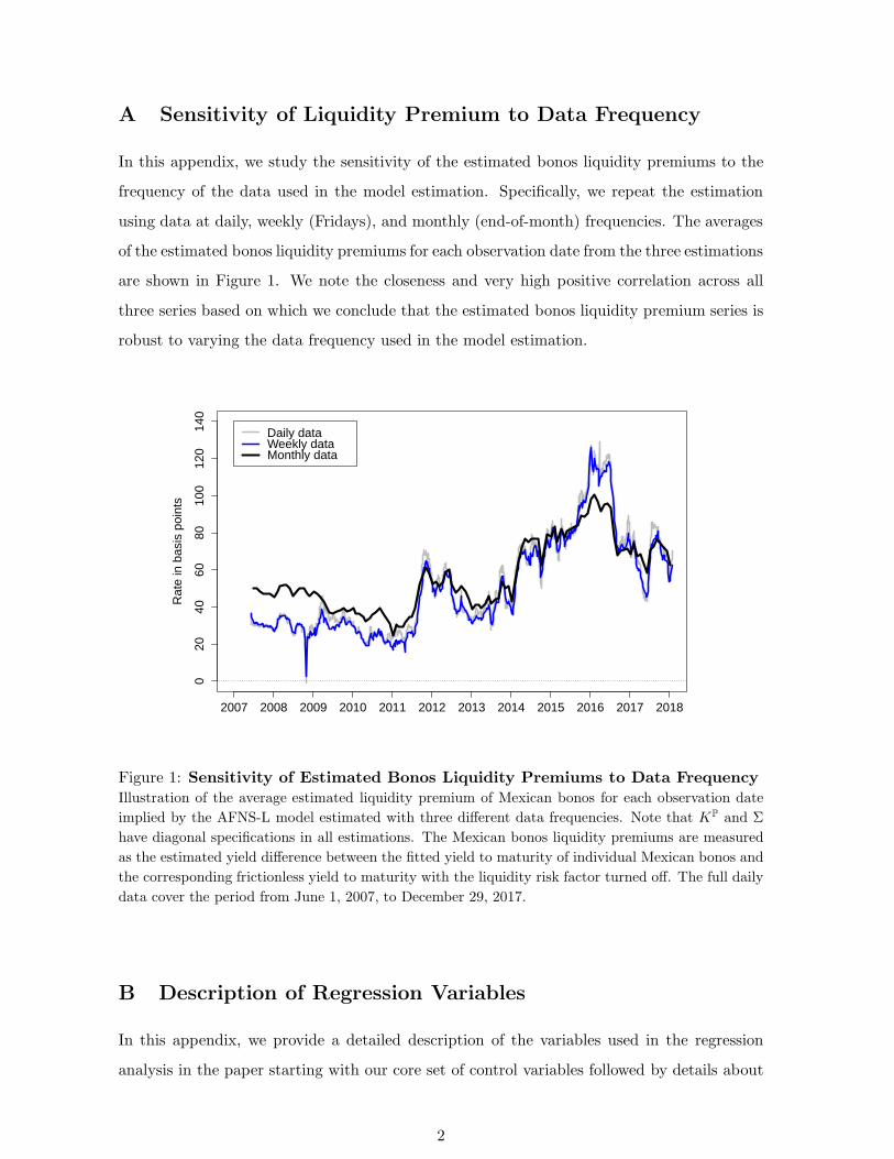
A Sensitivity of Liquidity Premium to Data Frequency

In this appendix, we study the sensitivity of the estimated bonos liquidity premiums to the

frequency of the data used in the model estimation. Specifically, we repeat the estimation

using data at daily, weekly (Fridays), and monthly (end-of-month) frequencies. The averages

of the estimated bonos liquidity premiums for each observation date from the three estimations

are shown in Figure 1. We note the closeness and very high positive correlation across all

three series based on which we conclude that the estimated bonos liquidity premium series is

robust to varying the data frequency used in the model estimation.

2007 2008 2009 2010 2011 2012 2013 2014 2015 2016 2017 2018

020

4060

8010

012

014

0

Rat

e in

bas

is p

oint

s

Daily data Weekly data Monthly data

Figure 1: Sensitivity of Estimated Bonos Liquidity Premiums to Data Frequency

Illustration of the average estimated liquidity premium of Mexican bonos for each observation date

implied by the AFNS-L model estimated with three different data frequencies. Note that KP and Σ

have diagonal specifications in all estimations. The Mexican bonos liquidity premiums are measured

as the estimated yield difference between the fitted yield to maturity of individual Mexican bonos and

the corresponding frictionless yield to maturity with the liquidity risk factor turned off. The full daily

data cover the period from June 1, 2007, to December 29, 2017.

B Description of Regression Variables

In this appendix, we provide a detailed description of the variables used in the regression

analysis in the paper starting with our core set of control variables followed by details about

2

the extended set of control variables also used in the analysis.

B.1 Core Control Variables

2007 2008 2009 2010 2011 2012 2013 2014 2015 2016 2017 2018

1012

1416

1820

22

Mex

ican

pes

os p

er U

.S. d

olla

r

Mexican peso − U.S. dollar exchange rate

Figure 2: Mexican Peso - U.S. Dollar Exchange Rate

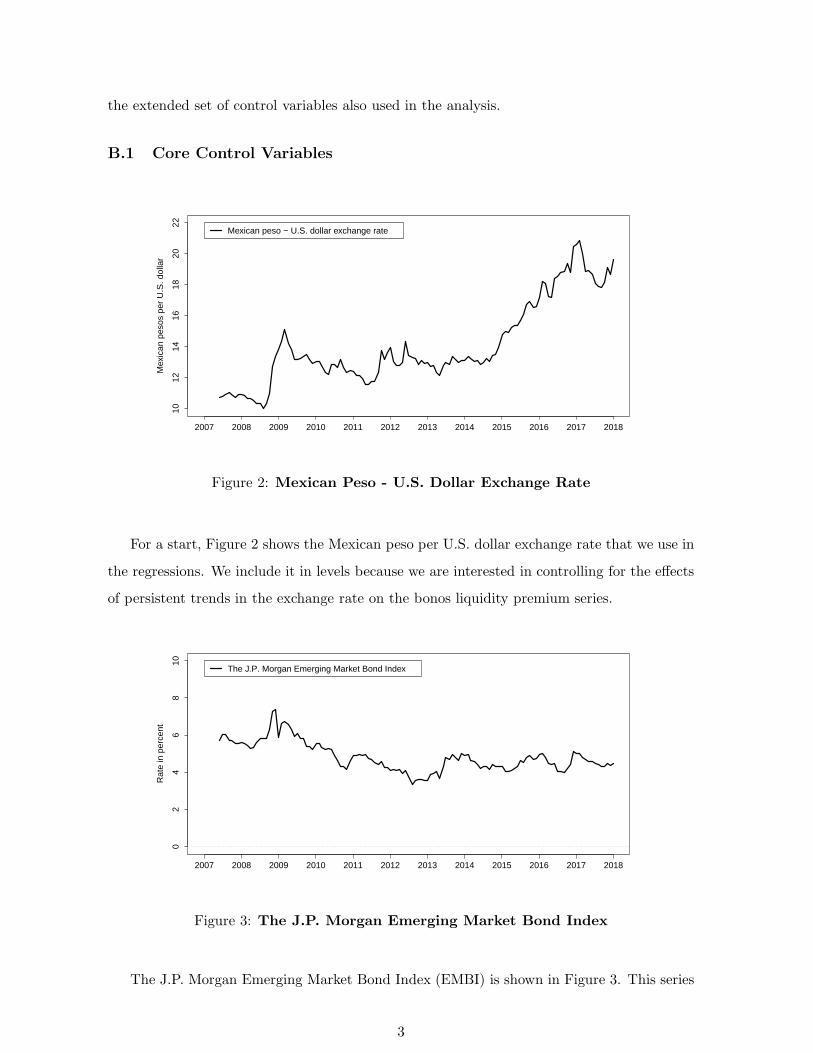
For a start, Figure 2 shows the Mexican peso per U.S. dollar exchange rate that we use in

the regressions. We include it in levels because we are interested in controlling for the effects

of persistent trends in the exchange rate on the bonos liquidity premium series.

2007 2008 2009 2010 2011 2012 2013 2014 2015 2016 2017 2018

02

46

810

Rat

e in

per

cent

The J.P. Morgan Emerging Market Bond Index

Figure 3: The J.P. Morgan Emerging Market Bond Index

The J.P. Morgan Emerging Market Bond Index (EMBI) is shown in Figure 3. This series

3

is used to control for factors that affect emerging market sovereign bonds more broadly.

2007 2008 2009 2010 2011 2012 2013 2014 2015 2016 2017 2018

050

100

150

U.S

. dol

lars

per

bar

rel

West Texas intermediate oil price

Figure 4: West Texas Intermediate Oil Price

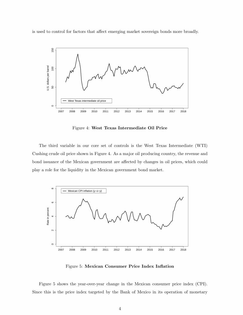
The third variable in our core set of controls is the West Texas Intermediate (WTI)

Cushing crude oil price shown in Figure 4. As a major oil producing country, the revenue and

bond issuance of the Mexican government are affected by changes in oil prices, which could

play a role for the liquidity in the Mexican government bond market.

2007 2008 2009 2010 2011 2012 2013 2014 2015 2016 2017 2018

02

46

8

Rat

e in

per

cent

Mexican CPI inflation (y−o−y)

Figure 5: Mexican Consumer Price Index Inflation

Figure 5 shows the year-over-year change in the Mexican consumer price index (CPI).

Since this is the price index targeted by the Bank of Mexico in its operation of monetary

4

policy, its variation is likely to matter for the pricing and market conditions of Mexican

bonos.

2007 2008 2009 2010 2011 2012 2013 2014 2015 2016 2017 2018

010

2030

4050

60

Rat

e in

per

cent

Mexican public debt−to−GDP ratio

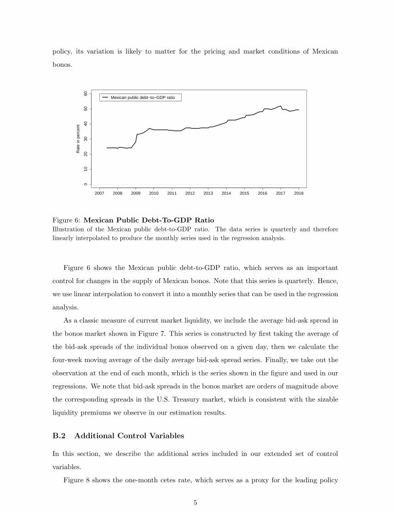
Figure 6: Mexican Public Debt-To-GDP Ratio

Illustration of the Mexican public debt-to-GDP ratio. The data series is quarterly and therefore

linearly interpolated to produce the monthly series used in the regression analysis.

Figure 6 shows the Mexican public debt-to-GDP ratio, which serves as an important

control for changes in the supply of Mexican bonos. Note that this series is quarterly. Hence,

we use linear interpolation to convert it into a monthly series that can be used in the regression

analysis.

As a classic measure of current market liquidity, we include the average bid-ask spread in

the bonos market shown in Figure 7. This series is constructed by first taking the average of

the bid-ask spreads of the individual bonos observed on a given day, then we calculate the

four-week moving average of the daily average bid-ask spread series. Finally, we take out the

observation at the end of each month, which is the series shown in the figure and used in our

regressions. We note that bid-ask spreads in the bonos market are orders of magnitude above

the corresponding spreads in the U.S. Treasury market, which is consistent with the sizable

liquidity premiums we observe in our estimation results.

B.2 Additional Control Variables

In this section, we describe the additional series included in our extended set of control

variables.

Figure 8 shows the one-month cetes rate, which serves as a proxy for the leading policy

5

2007 2008 2009 2010 2011 2012 2013 2014 2015 2016 2017 2018

01

23

45

6

Rat

e in

bas

is p

oint

s

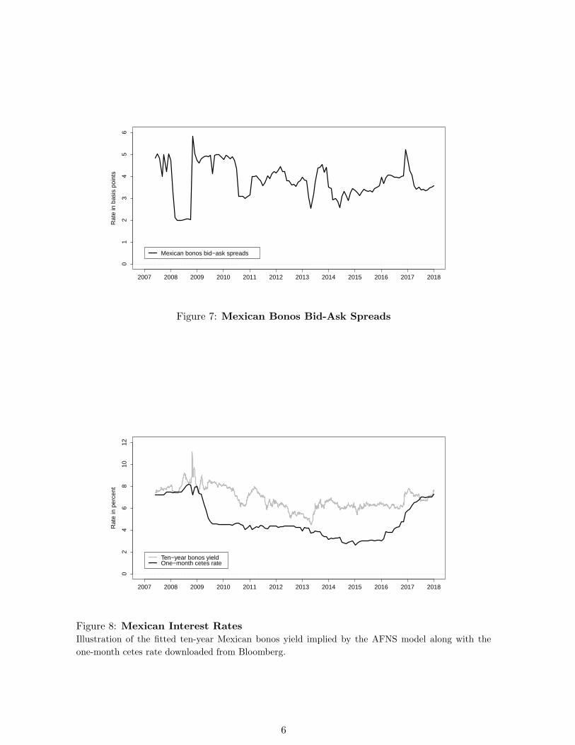
Mexican bonos bid−ask spreads

Figure 7: Mexican Bonos Bid-Ask Spreads

2007 2008 2009 2010 2011 2012 2013 2014 2015 2016 2017 2018

02

46

810

12

Rat

e in

per

cent

Ten−year bonos yield One−month cetes rate

Figure 8: Mexican Interest Rates

Illustration of the fitted ten-year Mexican bonos yield implied by the AFNS model along with the

one-month cetes rate downloaded from Bloomberg.

6

rate of the Bank of Mexico. We use this series as a measure of the opportunity costs of holding

money, which has been shown by Nagel (2016) to be a good proxy of the liquidity premiums

in U.S. Treasury bills, and we want to control for similar effects in the pricing of Mexican

bonos. The figure also shows the ten-year Mexican zero-coupon yield implied by the AFNS

model estimated with a one-step approach as recommended by Andreasen et al. (2019). This

series is used to construct the realized yield volatility series discussed later on.

2007 2008 2009 2010 2011 2012 2013 2014 2015 2016 2017 2018

02

46

810

1214

16

Ave

rage

in y

ears

Average bonos age Average bonos time to maturity

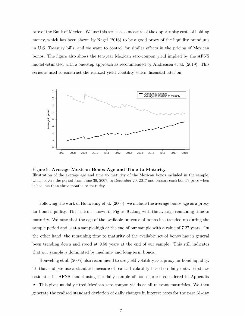
Figure 9: Average Mexican Bonos Age and Time to Maturity

Illustration of the average age and time to maturity of the Mexican bonos included in the sample,

which covers the period from June 30, 2007, to December 29, 2017 and censors each bond’s price when

it has less than three months to maturity.

Following the work of Houweling et al. (2005), we include the average bonos age as a proxy

for bond liquidity. This series is shown in Figure 9 along with the average remaining time to

maturity. We note that the age of the available universe of bonos has trended up during the

sample period and is at a sample-high at the end of our sample with a value of 7.27 years. On

the other hand, the remaining time to maturity of the available set of bonos has in general

been trending down and stood at 9.58 years at the end of our sample. This still indicates

that our sample is dominated by medium- and long-term bonos.

Houweling et al. (2005) also recommend to use yield volatility as a proxy for bond liquidity.

To that end, we use a standard measure of realized volatility based on daily data. First, we

estimate the AFNS model using the daily sample of bonos prices considered in Appendix

A. This gives us daily fitted Mexican zero-coupon yields at all relevant maturities. We then

generate the realized standard deviation of daily changes in interest rates for the past 31-day

7

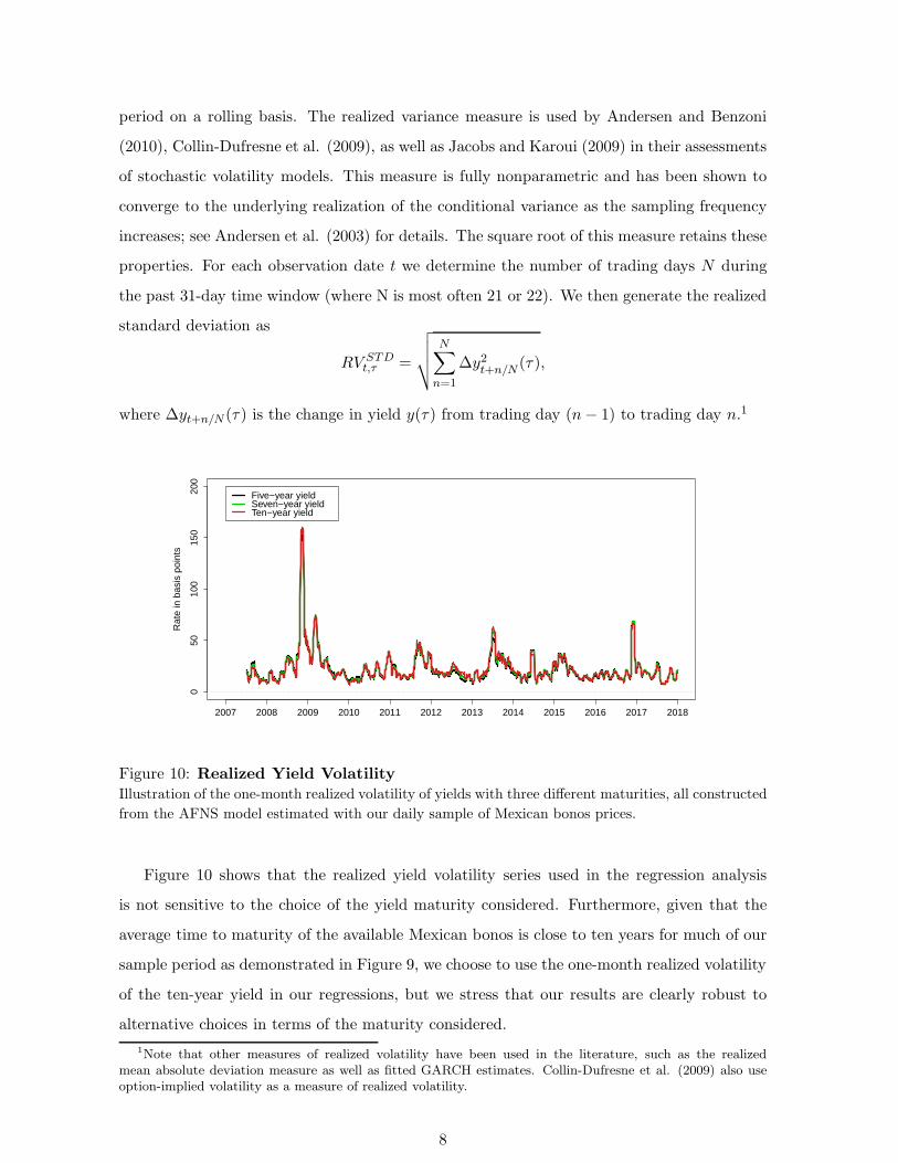
period on a rolling basis. The realized variance measure is used by Andersen and Benzoni

(2010), Collin-Dufresne et al. (2009), as well as Jacobs and Karoui (2009) in their assessments

of stochastic volatility models. This measure is fully nonparametric and has been shown to

converge to the underlying realization of the conditional variance as the sampling frequency

increases; see Andersen et al. (2003) for details. The square root of this measure retains these

properties. For each observation date t we determine the number of trading days N during

the past 31-day time window (where N is most often 21 or 22). We then generate the realized

standard deviation as

RV STDt,τ =

√√√√N∑

n=1

∆y2t+n/N (τ),

where ∆yt+n/N (τ) is the change in yield y(τ) from trading day (n− 1) to trading day n.1

2007 2008 2009 2010 2011 2012 2013 2014 2015 2016 2017 2018

050

100

150

200

Rat

e in

bas

is p

oint

s

Five−year yield Seven−year yield Ten−year yield

Figure 10: Realized Yield Volatility

Illustration of the one-month realized volatility of yields with three different maturities, all constructed

from the AFNS model estimated with our daily sample of Mexican bonos prices.

Figure 10 shows that the realized yield volatility series used in the regression analysis

is not sensitive to the choice of the yield maturity considered. Furthermore, given that the

average time to maturity of the available Mexican bonos is close to ten years for much of our

sample period as demonstrated in Figure 9, we choose to use the one-month realized volatility

of the ten-year yield in our regressions, but we stress that our results are clearly robust to

alternative choices in terms of the maturity considered.

1Note that other measures of realized volatility have been used in the literature, such as the realizedmean absolute deviation measure as well as fitted GARCH estimates. Collin-Dufresne et al. (2009) also useoption-implied volatility as a measure of realized volatility.

8

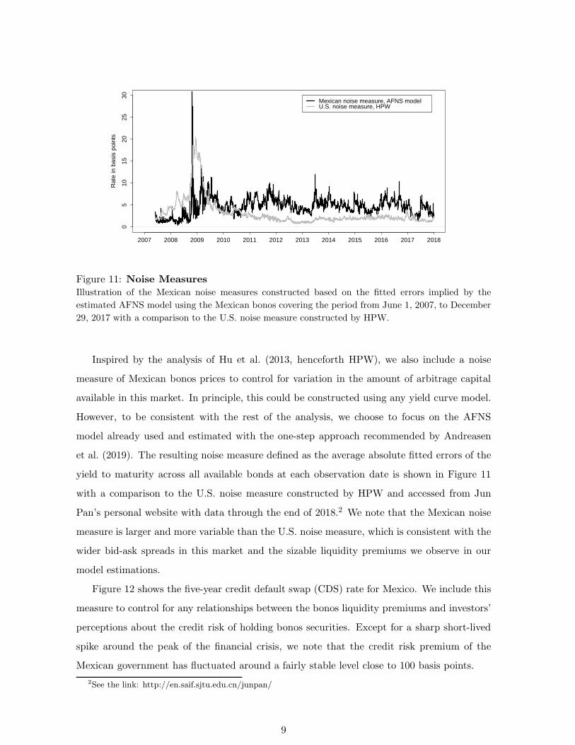
2007 2008 2009 2010 2011 2012 2013 2014 2015 2016 2017 2018

05

1015

2025

30

Rat

e in

bas

is p

oint

s

Mexican noise measure, AFNS model U.S. noise measure, HPW

Figure 11: Noise Measures

Illustration of the Mexican noise measures constructed based on the fitted errors implied by the

estimated AFNS model using the Mexican bonos covering the period from June 1, 2007, to December

29, 2017 with a comparison to the U.S. noise measure constructed by HPW.

Inspired by the analysis of Hu et al. (2013, henceforth HPW), we also include a noise

measure of Mexican bonos prices to control for variation in the amount of arbitrage capital

available in this market. In principle, this could be constructed using any yield curve model.

However, to be consistent with the rest of the analysis, we choose to focus on the AFNS

model already used and estimated with the one-step approach recommended by Andreasen

et al. (2019). The resulting noise measure defined as the average absolute fitted errors of the

yield to maturity across all available bonds at each observation date is shown in Figure 11

with a comparison to the U.S. noise measure constructed by HPW and accessed from Jun

Pan’s personal website with data through the end of 2018.2 We note that the Mexican noise

measure is larger and more variable than the U.S. noise measure, which is consistent with the

wider bid-ask spreads in this market and the sizable liquidity premiums we observe in our

model estimations.

Figure 12 shows the five-year credit default swap (CDS) rate for Mexico. We include this

measure to control for any relationships between the bonos liquidity premiums and investors’

perceptions about the credit risk of holding bonos securities. Except for a sharp short-lived

spike around the peak of the financial crisis, we note that the credit risk premium of the

Mexican government has fluctuated around a fairly stable level close to 100 basis points.

2See the link: http://en.saif.sjtu.edu.cn/junpan/

9

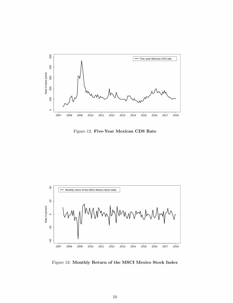
2007 2008 2009 2010 2011 2012 2013 2014 2015 2016 2017 2018

010

020

030

040

050

0

Rat

e in

bas

is p

oint

s

Five−year Mexican CDS rate

Figure 12: Five-Year Mexican CDS Rate

2007 2008 2009 2010 2011 2012 2013 2014 2015 2016 2017 2018

−40

−20

020

40

Rat

e in

per

cent

Monthly return of the MSCI Mexico stock index

Figure 13: Monthly Return of the MSCI Mexico Stock Index

10

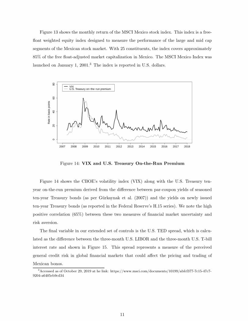
Figure 13 shows the monthly return of the MSCI Mexico stock index. This index is a free-

float weighted equity index designed to measure the performance of the large and mid cap

segments of the Mexican stock market. With 25 constituents, the index covers approximately

85% of the free float-adjusted market capitalization in Mexico. The MSCI Mexico Index was

launched on January 1, 2001.3 The index is reported in U.S. dollars.

2007 2008 2009 2010 2011 2012 2013 2014 2015 2016 2017 2018

020

4060

80

Rat

e in

bas

is p

oint

s

VIX U.S. Treasury on−the−run premium

Figure 14: VIX and U.S. Treasury On-the-Run Premium

Figure 14 shows the CBOE’s volatility index (VIX) along with the U.S. Treasury ten-

year on-the-run premium derived from the difference between par-coupon yields of seasoned

ten-year Treasury bonds (as per Gurkaynak et al. (2007)) and the yields on newly issued

ten-year Treasury bonds (as reported in the Federal Reserve’s H.15 series). We note the high

positive correlation (65%) between these two measures of financial market uncertainty and

risk aversion.

The final variable in our extended set of controls is the U.S. TED spread, which is calcu-

lated as the difference between the three-month U.S. LIBOR and the three-month U.S. T-bill

interest rate and shown in Figure 15. This spread represents a measure of the perceived

general credit risk in global financial markets that could affect the pricing and trading of

Mexican bonos.

3Accessed as of October 29, 2019 at he link: https://www.msci.com/documents/10199/abfcf377-7c15-47c7-9204-a6405eb9cd34

11

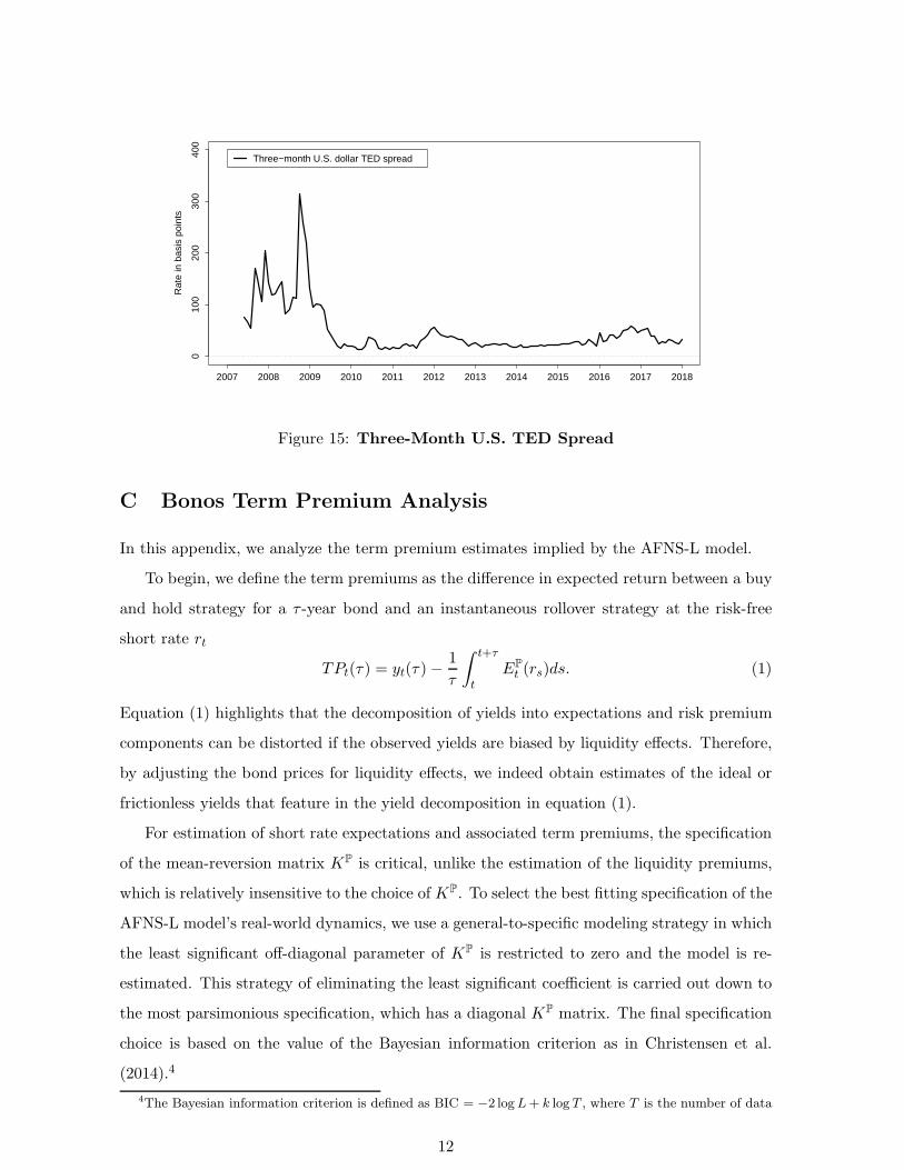
2007 2008 2009 2010 2011 2012 2013 2014 2015 2016 2017 2018

010

020

030

040

0

Rat

e in

bas

is p

oint

s

Three−month U.S. dollar TED spread

Figure 15: Three-Month U.S. TED Spread

C Bonos Term Premium Analysis

In this appendix, we analyze the term premium estimates implied by the AFNS-L model.

To begin, we define the term premiums as the difference in expected return between a buy

and hold strategy for a τ -year bond and an instantaneous rollover strategy at the risk-free

short rate rt

TPt(τ) = yt(τ)−1

τ

∫ t+τ

tEP

t (rs)ds. (1)

Equation (1) highlights that the decomposition of yields into expectations and risk premium

components can be distorted if the observed yields are biased by liquidity effects. Therefore,

by adjusting the bond prices for liquidity effects, we indeed obtain estimates of the ideal or

frictionless yields that feature in the yield decomposition in equation (1).

For estimation of short rate expectations and associated term premiums, the specification

of the mean-reversion matrix KP is critical, unlike the estimation of the liquidity premiums,

which is relatively insensitive to the choice of KP. To select the best fitting specification of the

AFNS-L model’s real-world dynamics, we use a general-to-specific modeling strategy in which

the least significant off-diagonal parameter of KP is restricted to zero and the model is re-

estimated. This strategy of eliminating the least significant coefficient is carried out down to

the most parsimonious specification, which has a diagonal KP matrix. The final specification

choice is based on the value of the Bayesian information criterion as in Christensen et al.

(2014).4

4The Bayesian information criterion is defined as BIC = −2 logL+ k log T , where T is the number of data

12

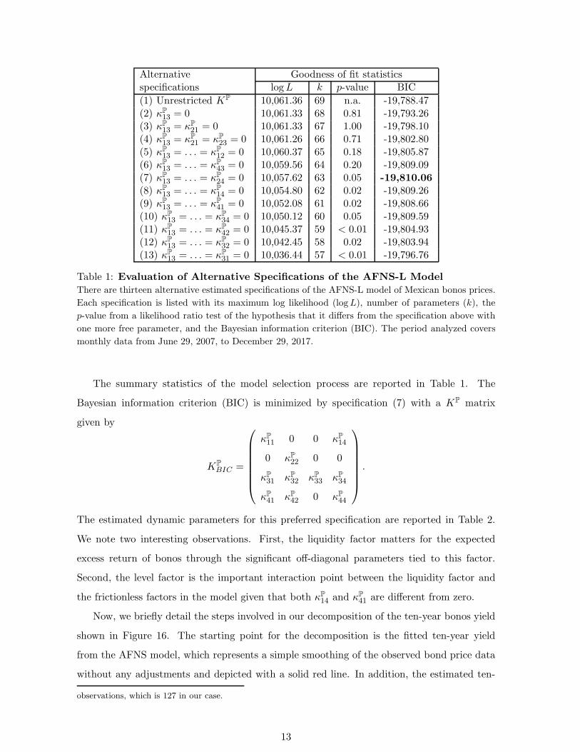
Alternative Goodness of fit statisticsspecifications logL k p-value BIC

(1) Unrestricted KP 10,061.36 69 n.a. -19,788.47(2) κP13 = 0 10,061.33 68 0.81 -19,793.26(3) κP13 = κP21 = 0 10,061.33 67 1.00 -19,798.10(4) κP13 = κP21 = κP23 = 0 10,061.26 66 0.71 -19,802.80(5) κP13 = . . . = κP12 = 0 10,060.37 65 0.18 -19,805.87(6) κP13 = . . . = κP43 = 0 10,059.56 64 0.20 -19,809.09(7) κP13 = . . . = κP24 = 0 10,057.62 63 0.05 -19,810.06

(8) κP13 = . . . = κP14 = 0 10,054.80 62 0.02 -19,809.26(9) κP13 = . . . = κP41 = 0 10,052.08 61 0.02 -19,808.66(10) κP13 = . . . = κP34 = 0 10,050.12 60 0.05 -19,809.59(11) κP13 = . . . = κP42 = 0 10,045.37 59 < 0.01 -19,804.93(12) κP13 = . . . = κP32 = 0 10,042.45 58 0.02 -19,803.94(13) κP13 = . . . = κP31 = 0 10,036.44 57 < 0.01 -19,796.76

Table 1: Evaluation of Alternative Specifications of the AFNS-L Model

There are thirteen alternative estimated specifications of the AFNS-L model of Mexican bonos prices.

Each specification is listed with its maximum log likelihood (logL), number of parameters (k), the

p-value from a likelihood ratio test of the hypothesis that it differs from the specification above with

one more free parameter, and the Bayesian information criterion (BIC). The period analyzed covers

monthly data from June 29, 2007, to December 29, 2017.

The summary statistics of the model selection process are reported in Table 1. The

Bayesian information criterion (BIC) is minimized by specification (7) with a KP matrix

given by

KPBIC =

κP11 0 0 κP14

0 κP22 0 0

κP31 κP32 κP33 κP34

κP41 κP42 0 κP44

.

The estimated dynamic parameters for this preferred specification are reported in Table 2.

We note two interesting observations. First, the liquidity factor matters for the expected

excess return of bonos through the significant off-diagonal parameters tied to this factor.

Second, the level factor is the important interaction point between the liquidity factor and

the frictionless factors in the model given that both κP14 and κP41 are different from zero.

Now, we briefly detail the steps involved in our decomposition of the ten-year bonos yield

shown in Figure 16. The starting point for the decomposition is the fitted ten-year yield

from the AFNS model, which represents a simple smoothing of the observed bond price data

without any adjustments and depicted with a solid red line. In addition, the estimated ten-

observations, which is 127 in our case.

13

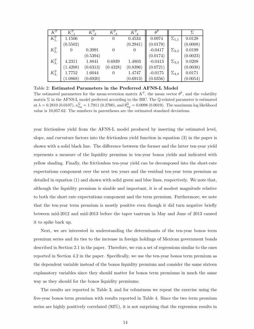
KP KP·,1 KP

·,2 KP·,3 KP

·,4 θP Σ

KP1,· 1.1506 0 0 0.4534 0.0974 Σ1,1 0.0128

(0.5502) (0.2941) (0.0179) (0.0008)KP

2,· 0 0.3991 0 0 -0.0417 Σ2,2 0.0199

(0.5394) (0.0174) (0.0023)KP

3,· 4.2311 1.8841 0.6939 1.4803 -0.0413 Σ3,3 0.0208

(1.4208) (0.6313) (0.4328) (0.8396) (0.0721) (0.0038)KP

4,· 1.7752 1.6044 0 1.4747 -0.0175 Σ4,4 0.0171

(1.0868) (0.6920) (0.6913) (0.0356) (0.0054)

Table 2: Estimated Parameters in the Preferred AFNS-L Model

The estimated parameters for the mean-reversion matrix KP, the mean vector θP, and the volatility

matrix Σ in the AFNS-L model preferred according to the BIC. The Q-related parameter is estimated

at λ = 0.2810 (0.0107), κQliq = 1.7911 (0.2700), and θQliq = 0.0098 (0.0019). The maximum log likelihood

value is 10,057.62. The numbers in parentheses are the estimated standard deviations.

year frictionless yield from the AFNS-L model produced by inserting the estimated level,

slope, and curvature factors into the frictionless yield function in equation (3) in the paper is

shown with a solid black line. The difference between the former and the latter ten-year yield

represents a measure of the liquidity premium in ten-year bonos yields and indicated with

yellow shading. Finally, the frictionless ten-year yield can be decomposed into the short-rate

expectations component over the next ten years and the residual ten-year term premium as

detailed in equation (1) and shown with solid green and blue lines, respectively. We note that,

although the liquidity premium is sizable and important, it is of modest magnitude relative

to both the short rate expectations component and the term premium. Furthermore, we note

that the ten-year term premium is mostly positive even though it did turn negative briefly

between mid-2012 and mid-2013 before the taper tantrum in May and June of 2013 caused

it to spike back up.

Next, we are interested in understanding the determinants of the ten-year bonos term

premium series and its ties to the increase in foreign holdings of Mexican government bonds

described in Section 2.1 in the paper. Therefore, we run a set of regressions similar to the ones

reported in Section 4.2 in the paper. Specifically, we use the ten-year bonos term premium as

the dependent variable instead of the bonos liquidity premium and consider the same sixteen

explanatory variables since they should matter for bonos term premiums in much the same

way as they should for the bonos liquidity premiums.

The results are reported in Table 3, and for robustness we repeat the exercise using the

five-year bonos term premium with results reported in Table 4. Since the two term premium

series are highly positively correlated (93%), it is not surprising that the regression results in

14

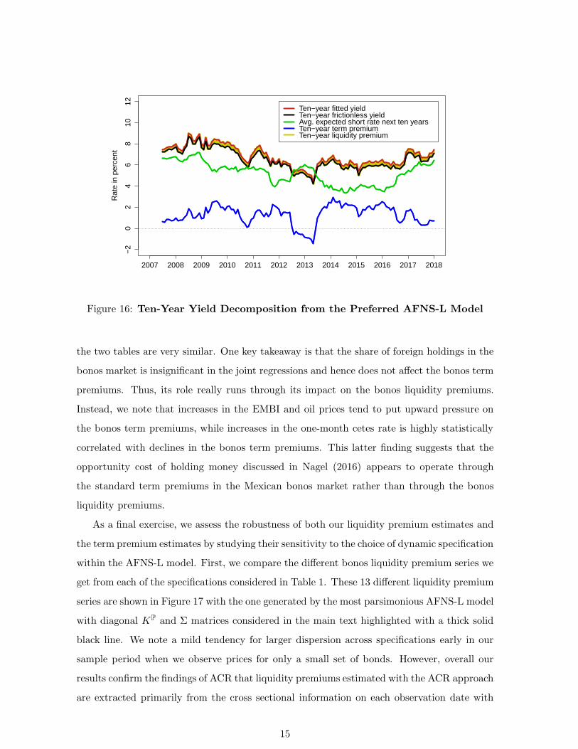
2007 2008 2009 2010 2011 2012 2013 2014 2015 2016 2017 2018

−2

02

46

810

12

Rat

e in

per

cent

Ten−year fitted yield Ten−year frictionless yield Avg. expected short rate next ten years Ten−year term premium Ten−year liquidity premium

Figure 16: Ten-Year Yield Decomposition from the Preferred AFNS-L Model

the two tables are very similar. One key takeaway is that the share of foreign holdings in the

bonos market is insignificant in the joint regressions and hence does not affect the bonos term

premiums. Thus, its role really runs through its impact on the bonos liquidity premiums.

Instead, we note that increases in the EMBI and oil prices tend to put upward pressure on

the bonos term premiums, while increases in the one-month cetes rate is highly statistically

correlated with declines in the bonos term premiums. This latter finding suggests that the

opportunity cost of holding money discussed in Nagel (2016) appears to operate through

the standard term premiums in the Mexican bonos market rather than through the bonos

liquidity premiums.

As a final exercise, we assess the robustness of both our liquidity premium estimates and

the term premium estimates by studying their sensitivity to the choice of dynamic specification

within the AFNS-L model. First, we compare the different bonos liquidity premium series we

get from each of the specifications considered in Table 1. These 13 different liquidity premium

series are shown in Figure 17 with the one generated by the most parsimonious AFNS-L model

with diagonal KP and Σ matrices considered in the main text highlighted with a thick solid

black line. We note a mild tendency for larger dispersion across specifications early in our

sample period when we observe prices for only a small set of bonds. However, overall our

results confirm the findings of ACR that liquidity premiums estimated with the ACR approach

are extracted primarily from the cross sectional information on each observation date with

15

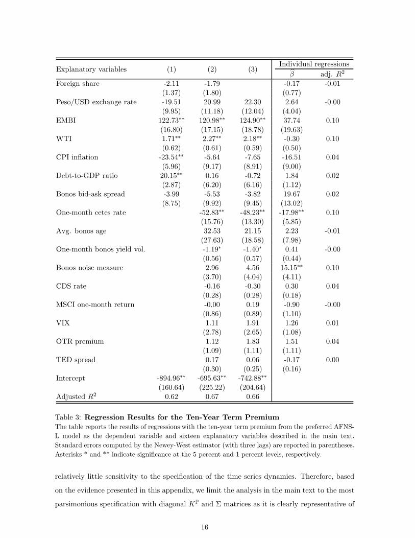
Individual regressionsExplanatory variables (1) (2) (3)

β adj. R2

Foreign share -2.11 -1.79 -0.17 -0.01(1.37) (1.80) (0.77)

Peso/USD exchange rate -19.51 20.99 22.30 2.64 -0.00(9.95) (11.18) (12.04) (4.04)

EMBI 122.73∗∗ 120.98∗∗ 124.90∗∗ 37.74 0.10(16.80) (17.15) (18.78) (19.63)

WTI 1.71∗∗ 2.27∗∗ 2.18∗∗ -0.30 0.10(0.62) (0.61) (0.59) (0.50)

CPI inflation -23.54∗∗ -5.64 -7.65 -16.51 0.04(5.96) (9.17) (8.91) (9.00)

Debt-to-GDP ratio 20.15∗∗ 0.16 -0.72 1.84 0.02(2.87) (6.20) (6.16) (1.12)

Bonos bid-ask spread -3.99 -5.53 -3.82 19.67 0.02(8.75) (9.92) (9.45) (13.02)

One-month cetes rate -52.83∗∗ -48.23∗∗ -17.98∗∗ 0.10(15.76) (13.30) (5.85)

Avg. bonos age 32.53 21.15 2.23 -0.01(27.63) (18.58) (7.98)

One-month bonos yield vol. -1.19∗ -1.40∗ 0.41 -0.00(0.56) (0.57) (0.44)

Bonos noise measure 2.96 4.56 15.15∗∗ 0.10(3.70) (4.04) (4.11)

CDS rate -0.16 -0.30 0.30 0.04(0.28) (0.28) (0.18)

MSCI one-month return -0.00 0.19 -0.90 -0.00(0.86) (0.89) (1.10)

VIX 1.11 1.91 1.26 0.01(2.78) (2.65) (1.08)

OTR premium 1.12 1.83 1.51 0.04(1.09) (1.11) (1.11)

TED spread 0.17 0.06 -0.17 0.00(0.30) (0.25) (0.16)

Intercept -894.96∗∗ -695.63∗∗ -742.88∗∗

(160.64) (225.22) (204.64)Adjusted R2 0.62 0.67 0.66

Table 3: Regression Results for the Ten-Year Term Premium

The table reports the results of regressions with the ten-year term premium from the preferred AFNS-

L model as the dependent variable and sixteen explanatory variables described in the main text.

Standard errors computed by the Newey-West estimator (with three lags) are reported in parentheses.

Asterisks * and ** indicate significance at the 5 percent and 1 percent levels, respectively.

relatively little sensitivity to the specification of the time series dynamics. Therefore, based

on the evidence presented in this appendix, we limit the analysis in the main text to the most

parsimonious specification with diagonal KP and Σ matrices as it is clearly representative of

16

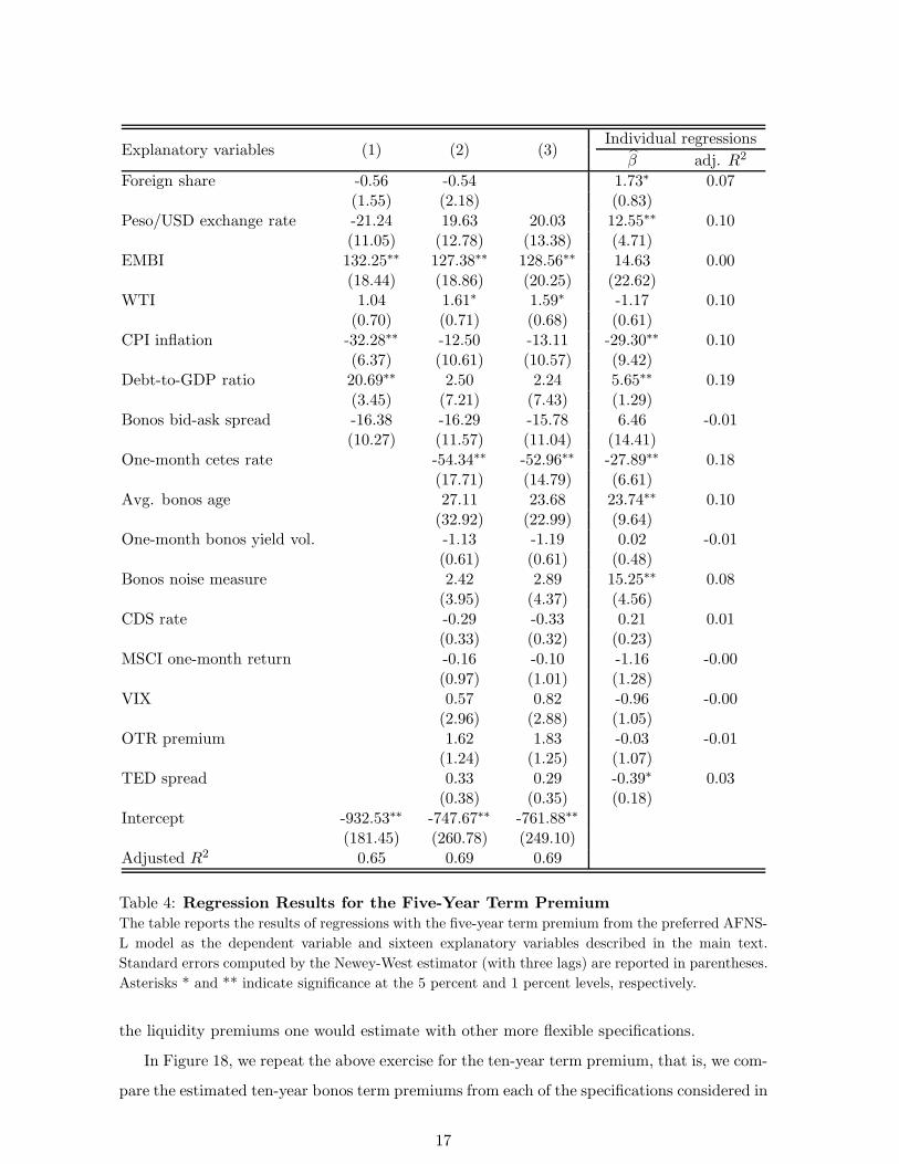
Individual regressionsExplanatory variables (1) (2) (3)

β adj. R2

Foreign share -0.56 -0.54 1.73∗ 0.07(1.55) (2.18) (0.83)

Peso/USD exchange rate -21.24 19.63 20.03 12.55∗∗ 0.10(11.05) (12.78) (13.38) (4.71)

EMBI 132.25∗∗ 127.38∗∗ 128.56∗∗ 14.63 0.00(18.44) (18.86) (20.25) (22.62)

WTI 1.04 1.61∗ 1.59∗ -1.17 0.10(0.70) (0.71) (0.68) (0.61)

CPI inflation -32.28∗∗ -12.50 -13.11 -29.30∗∗ 0.10(6.37) (10.61) (10.57) (9.42)

Debt-to-GDP ratio 20.69∗∗ 2.50 2.24 5.65∗∗ 0.19(3.45) (7.21) (7.43) (1.29)

Bonos bid-ask spread -16.38 -16.29 -15.78 6.46 -0.01(10.27) (11.57) (11.04) (14.41)

One-month cetes rate -54.34∗∗ -52.96∗∗ -27.89∗∗ 0.18(17.71) (14.79) (6.61)

Avg. bonos age 27.11 23.68 23.74∗∗ 0.10(32.92) (22.99) (9.64)

One-month bonos yield vol. -1.13 -1.19 0.02 -0.01(0.61) (0.61) (0.48)

Bonos noise measure 2.42 2.89 15.25∗∗ 0.08(3.95) (4.37) (4.56)

CDS rate -0.29 -0.33 0.21 0.01(0.33) (0.32) (0.23)

MSCI one-month return -0.16 -0.10 -1.16 -0.00(0.97) (1.01) (1.28)

VIX 0.57 0.82 -0.96 -0.00(2.96) (2.88) (1.05)

OTR premium 1.62 1.83 -0.03 -0.01(1.24) (1.25) (1.07)

TED spread 0.33 0.29 -0.39∗ 0.03(0.38) (0.35) (0.18)

Intercept -932.53∗∗ -747.67∗∗ -761.88∗∗

(181.45) (260.78) (249.10)Adjusted R2 0.65 0.69 0.69

Table 4: Regression Results for the Five-Year Term Premium

The table reports the results of regressions with the five-year term premium from the preferred AFNS-

L model as the dependent variable and sixteen explanatory variables described in the main text.

Standard errors computed by the Newey-West estimator (with three lags) are reported in parentheses.

Asterisks * and ** indicate significance at the 5 percent and 1 percent levels, respectively.

the liquidity premiums one would estimate with other more flexible specifications.

In Figure 18, we repeat the above exercise for the ten-year term premium, that is, we com-

pare the estimated ten-year bonos term premiums from each of the specifications considered in

17

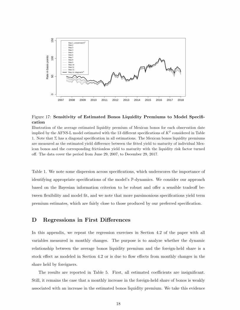
2007 2008 2009 2010 2011 2012 2013 2014 2015 2016 2017 2018

050

100

150

Rat

e in

bas

is p

oint

s

Step 1, unrestricted KP Step 2 Step 3 Step 4 Step 5 Step 6 Step 7 Step 8 Step 9 Step 10 Step 11 Step 12

Step 13, diagonal KP

Figure 17: Sensitivity of Estimated Bonos Liquidity Premiums to Model Specifi-

cation

Illustration of the average estimated liquidity premium of Mexican bonos for each observation date

implied by the AFNS-L model estimated with the 13 different specifications of KP considered in Table

1. Note that Σ has a diagonal specification in all estimations. The Mexican bonos liquidity premiums

are measured as the estimated yield difference between the fitted yield to maturity of individual Mex-

ican bonos and the corresponding frictionless yield to maturity with the liquidity risk factor turned

off. The data cover the period from June 29, 2007, to December 29, 2017.

Table 1. We note some dispersion across specifications, which underscores the importance of

identifying appropriate specifications of the model’s P-dynamics. We consider our approach

based on the Bayesian information criterion to be robust and offer a sensible tradeoff be-

tween flexibility and model fit, and we note that more parsimonious specifications yield term

premium estimates, which are fairly close to those produced by our preferred specification.

D Regressions in First Differences

In this appendix, we repeat the regression exercises in Section 4.2 of the paper with all

variables measured in monthly changes. The purpose is to analyze whether the dynamic

relationship between the average bonos liquidity premium and the foreign-held share is a

stock effect as modeled in Section 4.2 or is due to flow effects from monthly changes in the

share held by foreigners.

The results are reported in Table 5. First, all estimated coefficients are insignificant.

Still, it remains the case that a monthly increase in the foreign-held share of bonos is weakly

associated with an increase in the estimated bonos liquidity premium. We take this evidence

18

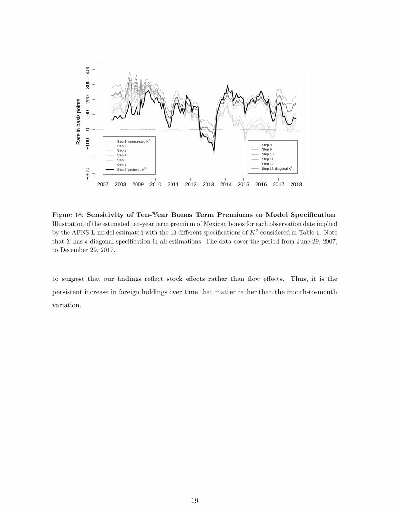
2007 2008 2009 2010 2011 2012 2013 2014 2015 2016 2017 2018

−30

0−

100

010

020

030

040

0

Rat

e in

bas

is p

oint

s

Step 1, unrestricted KP Step 2 Step 3 Step 4 Step 5 Step 6

Step 7, preferred KP

Step 8 Step 9 Step 10 Step 11 Step 12

Step 13, diagonal KP

Figure 18: Sensitivity of Ten-Year Bonos Term Premiums to Model Specification

Illustration of the estimated ten-year term premium of Mexican bonos for each observation date implied

by the AFNS-L model estimated with the 13 different specifications of KP considered in Table 1. Note

that Σ has a diagonal specification in all estimations. The data cover the period from June 29, 2007,

to December 29, 2017.

to suggest that our findings reflect stock effects rather than flow effects. Thus, it is the

persistent increase in foreign holdings over time that matter rather than the month-to-month

variation.

19

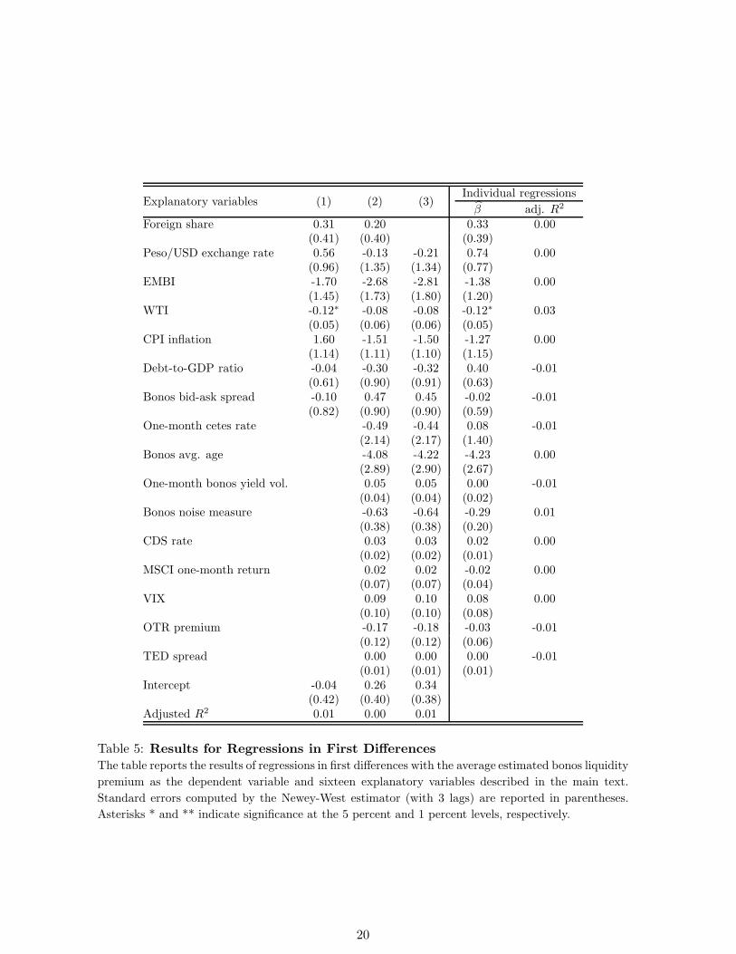
Individual regressionsExplanatory variables (1) (2) (3)

β adj. R2

Foreign share 0.31 0.20 0.33 0.00(0.41) (0.40) (0.39)

Peso/USD exchange rate 0.56 -0.13 -0.21 0.74 0.00(0.96) (1.35) (1.34) (0.77)

EMBI -1.70 -2.68 -2.81 -1.38 0.00(1.45) (1.73) (1.80) (1.20)

WTI -0.12∗ -0.08 -0.08 -0.12∗ 0.03(0.05) (0.06) (0.06) (0.05)

CPI inflation 1.60 -1.51 -1.50 -1.27 0.00(1.14) (1.11) (1.10) (1.15)

Debt-to-GDP ratio -0.04 -0.30 -0.32 0.40 -0.01(0.61) (0.90) (0.91) (0.63)

Bonos bid-ask spread -0.10 0.47 0.45 -0.02 -0.01(0.82) (0.90) (0.90) (0.59)

One-month cetes rate -0.49 -0.44 0.08 -0.01(2.14) (2.17) (1.40)

Bonos avg. age -4.08 -4.22 -4.23 0.00(2.89) (2.90) (2.67)

One-month bonos yield vol. 0.05 0.05 0.00 -0.01(0.04) (0.04) (0.02)

Bonos noise measure -0.63 -0.64 -0.29 0.01(0.38) (0.38) (0.20)

CDS rate 0.03 0.03 0.02 0.00(0.02) (0.02) (0.01)

MSCI one-month return 0.02 0.02 -0.02 0.00(0.07) (0.07) (0.04)

VIX 0.09 0.10 0.08 0.00(0.10) (0.10) (0.08)

OTR premium -0.17 -0.18 -0.03 -0.01(0.12) (0.12) (0.06)

TED spread 0.00 0.00 0.00 -0.01(0.01) (0.01) (0.01)

Intercept -0.04 0.26 0.34(0.42) (0.40) (0.38)

Adjusted R2 0.01 0.00 0.01

Table 5: Results for Regressions in First Differences

The table reports the results of regressions in first differences with the average estimated bonos liquidity

premium as the dependent variable and sixteen explanatory variables described in the main text.

Standard errors computed by the Newey-West estimator (with 3 lags) are reported in parentheses.

Asterisks * and ** indicate significance at the 5 percent and 1 percent levels, respectively.

20

References

Andersen, Torben, Tim Bollerslev, Francis X. Diebold, and P. Labys, 2003, “Modeling and

Forecasting Realized Volatility,” Econometrica, 71, 579-626.

Andersen, Torben G. and Luca Benzoni, 2010, “Do Bonds Span Volatility Risk in the U.S.

Treasury Market? A Specification Test for Affine Term Structure Models,” Journal of

Finance, Vol. 65, No. 2, 603-653.

Andreasen, Martin M., Jens H. E. Christensen, and Glenn D. Rudebusch, 2019, “Term

Structure Analysis with Big Data: One-Step Estimation Using Bond Prices,” Journal

of Econometrics, Vol. 212, 26-46.

Christensen, Jens H. E., Jose A. Lopez, and Glenn D. Rudebusch, 2014, “Do Central Bank

Liquidity Facilities Affect Interbank Lending Rates?,” Journal of Business and Eco-

nomic Statistics, Vol. 32, No. 1, 136-151.

Collin-Dufresne, P., Goldstein, R.S. and Jones, C.S., 2009, “Can Interest Rate Volatility Be

Extracted from the Cross-Section of Bond Yields?,” Journal of Financial Economics,

94, 47-66.

Gurkaynak, Refet S., Brian Sack, and Jonathan H. Wright, 2007, “The U.S. Treasury Yield

Curve: 1961 to the Present,” Journal of Monetary Economics, Vol. 54, No. 8, 2291-

2304.

Houweling, Patrick, Albert Mentink, and Ton Vorst, 2005, “Comparing Possible Proxies of

Corporate Bond Liquidity,” Journal of Banking and Finance, Vol. 29, 1331-1358.

Hu, Grace Xing, Jun Pan, and Jiang Wang, 2013, “Noise as Information for Illiquidity,”

Journal of Finance, Vol. 68, No. 6, 2341-2382.

Jacobs, Kris and Lofti Karoui, 2009, “Conditional Volatility in Affine Term Structure Mod-

els: Evidence from Treasury and Swap Markets,” Journal of Financial Economics, Vol.

91, 288-318.

Nagel, Stefan, 2016, “The Liquidity Premium of Near-Money Assets,” Quarterly Journal of

Economics, Vol. 131, No. 4, 1927-1971.

21