BMEGUI Tutorial 6 - University of North Carolina at Chapel ... · PDF fileBMEGUI Tutorial 6 Mean trend and ... Here we will only edit the temporal lags and their lag tolerances. To

BMEGUI Tutorial 6 Mean trend and covariance modeling

1. Objective

Spatial research analysts/modelers may want to remove a global offset (called mean trend

in BMEGUI manual and tutorials) from the space/time random field Z(s,t) at spatial

location s and time t, and use the detrended (residual) data X(s,t) for the subsequent

geostatistical analysis. Consider the following relationship:

Z(s,t) = µ(s,t) + X(s,t) (1)

where Z(s,t) represents the field of interest, µ(s,t) is a deterministic global offset and

X(s,t) is a spatially autocorrelated residual space/time random field. Removing the global

offset µ(s,t) from the field Z(s,t) is optional and depends on the choice of the modeler.

Once the global offset is removed, the geostatistical analysis is performed on the residual

field X(s,t)=Z(s,t)-µ(s,t), which results in estimates of the residual value X(sk,tk) at

unsampled point (sk,tk). Before making an actual prediction, the global offset µ(sk,tk) is

added back to the residual estimate to obtain the estimate Z(sk,tk)=µ(sk,tk)+X(sk,tk). If the

modeler can identify and quantify a meaningful global offset, this global offset explains a

portion of the variability of the raw data Z(s), and the residual data are expected to have a

lower residual variability, which can result in a more successful geostatistical analysis of

the residual field X(s,t). However, there is a real danger of over fitting data when deriving

the global offset, which could result in residual data with too little residual

autocorrelation to perform a successful geostatistical estimation of the residual field.

The global offset can be modeled as a space/time additive separable function of two

separate components, i.e. a temporal global offset and a spatial global offset. The degree

of smoothness in the space/time global offset can be controlled by applying an

exponential filter with user-defined search radius and smoothing range parameters. At

this stage the analyst/modeler has the flexibility of choosing a space/time global offset

from an infinite number of offsets that spans from an offset with long range variability

(i.e. very smooth, and thus pretty uninformative) to an offset with short range variability

(i.e. highly variable, and thus very informative). As explained above, a very informative

space/time global offset may leave too little autocorrelation in the residual data to

conduct a successful geostatistical estimation of the residual field. On the other hand, a

flat space/time global offset leaves a high variability in the residuals, which may produce

estimates with high posterior variance. Thus, there is a tradeoff between lowering the

variability of the residuals while keeping its autocorrelation structure, and hence the

modeler should explore a full assortment of global offsets ranging from

smooth/uninformative to highly variable/very informative in order to select an ideal

compromise that will explain some of the consistent space/time trends in the raw data,

while leaving reasonable autocorrelation in the residuals.

The primary objective of this tutorial is to perform a mean trend analysis (global mean

offset) and remove it from the data to obtain residual data, and then to see the effect of

the global offset on the covariance of the residual data. More specifically, this tutorial

considers five global offsets with varying degree of smoothness, and explores the effect

of each of these global offset on the covariance model parameters (i.e. sill and range) of

the corresponding residual data. This tutorial will help you understand the importance of

the global offset and its impact on the covariance model of the resulting residual data.

2. Install BMEGUI 3.0.1

See tutorial 1.

3. Data

To get the tutorial data, download the data file “data06.csv” from the Tutorial Data Files

and save it in a folder called “work06”. Open the data file using a spreadsheet editor or a

text editor to see the data available. The original data were downloaded from publicly

available online resources and compiled and prepared for this tutorial.

4. BMEGUI Operation

i.Start BMEGUI: double click on BMEGUI desktop icon. It will launch BMEGUI

window. (See the BMEGUI 3.0.1 user’s manual for more details).

ii.Workspace and data file selection: Click on the “Select Working Directory” button on

the “data and directory selection BMEGUI screen” and select the ‘work06’ folder.

Then click on the “Select Data File” button and select data file ‘data06.csv’

http://www.unc.edu/depts/case/BMEGUI/BMEGUI3.0.1/tutorialDataFiles/

http://www.unc.edu/depts/case/BMEGUI/BMEGUI3.0.1/BMEGUI3.0.1_DOCs/PDF/BMEGUI3.0.1_UserManual_v01.pdf

Figure 1: Data and directory selection BMGUI screen

iii.Click on the “OK” button. The “Data Field” screen appears after reading the data and

setting working directory

iv. In the “Data Field Setting” select the following column names from the dropdown

menu in each field.

X Field: Long

Y Field: Lat

Time Field: Time_sinceJan1_2007

ID: ID

Data Field: PM25

v.In the “Unit/Name” section, input the following units and name of data in each entry

box.

Space Unit: deg.

Time Unit: days

Data Unit: ug/m3

Name of Data: PM25

Figure 2: The “Data Field” screen

vi.Click on the “Next” button. The “Data Distribution” screen appears

vii.Check the basic statistics (mean, standard deviation, coefficient of skewness, and

coefficient of kurtosis) of the data and its log-transformed data in the “Statistics”

section.

viii.Check the histograms of raw data and log-transformed data. By clicking the “Raw

Data” and “Log Data” tab in the “Histogram” section, you can switch the

histograms

Figure 3: The “Data Distribution” screen showing the Histogram of “Raw Data” (upper) and “Log

Data” (lower)

ix. Since the log-transformed data looks normally distributed, click on the “Use Log-

transformed Data” select button at the bottom of the window

x.Click on the “Next” button. The “Exploratory Data Analysis” screen appears. At this

stage, BMEGUI allows you to perform a temporal and spatial exploratory data

analysis.

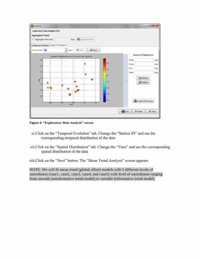
Figure 4: “Exploratory Data Analysis” screen

xi.Click on the “Temporal Evolution” tab. Change the “Station ID” and see the

corresponding temporal distribution of the data

xii.Click on the “Spatial Distribution” tab. Change the “Time” and see the corresponding

spatial distribution of the data

xiii.Click on the “Next” button. The “Mean Trend Analysis” screen appears

NOTE: We will fit mean trend (global offset) models with 5 different levels of

smoothness (case1, case2, case3, case4, and case5) with level of smoothness ranging

from smooth (uninformative trend model) to variable (informative trend model)

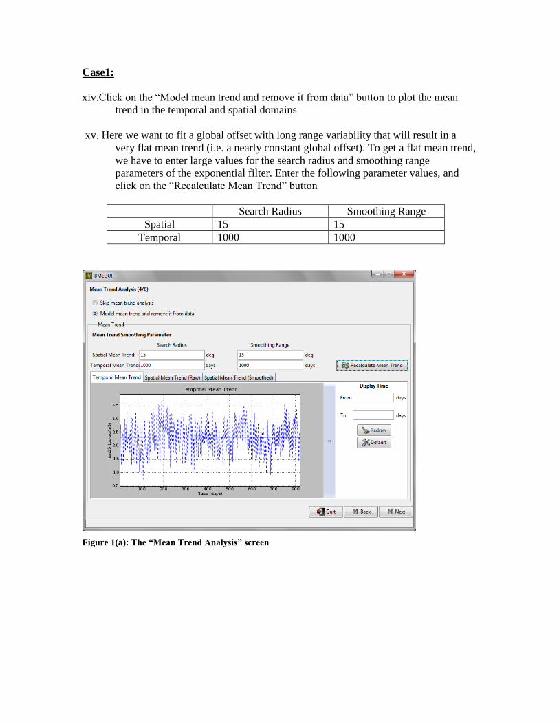
Case1:

xiv.Click on the “Model mean trend and remove it from data” button to plot the mean

trend in the temporal and spatial domains

xv. Here we want to fit a global offset with long range variability that will result in a

very flat mean trend (i.e. a nearly constant global offset). To get a flat mean trend,

we have to enter large values for the search radius and smoothing range

parameters of the exponential filter. Enter the following parameter values, and

click on the “Recalculate Mean Trend” button

Search Radius Smoothing Range

Spatial 15 15

Temporal 1000 1000

Figure 1(a): The “Mean Trend Analysis” screen

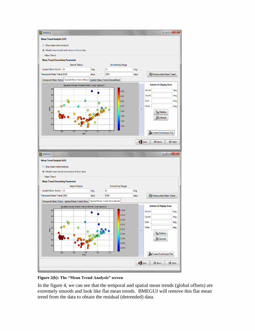
Figure 2(b): The “Mean Trend Analysis” screen

In the figure 4, we can see that the temporal and spatial mean trends (global offsets) are

extremely smooth and look like flat mean trends. BMEGUI will remove this flat mean

trend from the data to obtain the residual (detrended) data.

xvi.Click on the “Next” button. The “Space/Time Covariance Analysis” screen appears.

At this step BMEGUI calculates and plots experimental covariance valuesusing

the residual data.

xvii. We can manually edit temporal and spatial lags and their corresponding lag

tolerances to obtain more pairs of experimental covariance values (red dots) if

needed. Here we will only edit the temporal lags and their lag tolerances. To edit

the temporal lags, please click on the “Temporal Component” tab, and then click

on the “Edit Temporal Lags…” button. A dialog box with default lags appears.

Enter the following values in the “Temporal Lag” and “Temporal Lag Tolerance”

fields of the dialog box.

Temporal Lag:

0.0,20.0,40.0,68.3333333333,136.666666667,205.0,273.333333333,341.6666666

67,410.0,478.333333333,546.666666667,615.0,683.333333333

Temporal Lag Tolerance:

0.0,10,20.0,34.1666666667,34.1666666667,34.1666666667,34.1666666667,34.16

66666667,34.1666666667,34.1666666667,34.1666666667,34.1666666667,34.166

6666667

xviii.Click on the “OK” button. The experimental covariance plot (shown in red dots) is

automatically updated based on the entered temporal lags and corresponding

tolerances.

Figure 3: The “Space/Time Covariance Analysis” screen, showing Spatial and Temporal

Components of the covariance

xix.Now, we can model a covariance model that fits all experimental covariance values

(red dots) as best as possible. We will fit a two-structures covariance model to

ensure a good fit with the experimental covariance values. To fit a two-structures

covariance model, enter 2 in the “Number of covariance structure(1-4)”

xx. Now we have to enter covariance model parameters for each of the two covariance

structures. Input the following model parameters

Structure 1:

Sill: 0.2

Spatial Model: exponentialC

Spatial Range: 4

Temporal Model: exponentialC

Temporal Range: 7

Structure 2:

Sill: 0.19


Spatial Range: 100


Temporal Range: 75

xxi.Click on the “Plot Model” button. A plot of covariance model is superimposed on the

experimental covariance values.

Figure 4: The covariance model, shown on the Spatial Component (upper) and Temporal

Component (lower) plot

xxii.Click on the “Temporal Distribution” tab. To obtain the time series of BME estimates

at Station “43”, set the following estimation parameters in the “New Plot” section

BME Parameters: Use default settings

Estimation Parameters:

Station ID:43

Estimation Period: 1.0 days to 10.0

Display Parameter: Use default setting

xxiii.Click on the “Estimate” button. A new tab labeled “Plot ID: 0001” appears, and a

new entry appears on the list in the “Plot List” section.

Figure 5: The “BME Estimation” screen

xxiv.Click on the “Plot ID: 0001” tab and check the map of BME estimates.

Figure 6: Time series of BME estimates

xxv.Click on the “Quit” button to close the screen. A dialog box appears. Click on the

“OK” button of that dialog box to confirm that you want to quit BMEGUI.

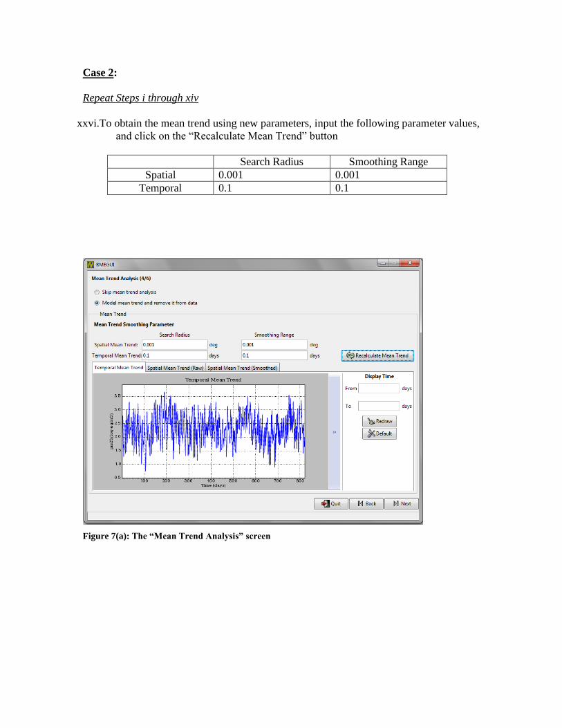
Case 2:

Repeat Steps i through xiv

xxvi.To obtain the mean trend using new parameters, input the following parameter values,

and click on the “Recalculate Mean Trend” button


Spatial 0.001 0.001

Temporal 0.1 0.1

Figure 7(a): The “Mean Trend Analysis” screen

Figure 8(b): The “Mean Trend Analysis” screen

xxvii.Click on the “Next” button. The “Space/Time Covariance Analysis” screen appears.

xxviii.Click on the “Temporal Component” tab, then on the “Edit Temporal Lags…” button.

A dialog box appears.

xxix.Input the following values in the “Temporal Lag” and “Temporal Lag Tolerance”

fields of the dialog box.

Temporal Lag:

0.0,20.0,40.0,68.3333333333,136.666666667,205.0,273.333333333,341.666666667,4

10.0,478.333333333,546.666666667,615.0,683.333333333

Temporal Lag Tolerance:

0.0,10,20.0,34.1666666667,34.1666666667,34.1666666667,34.1666666667,34.16666

66667,34.1666666667,34.1666666667,34.1666666667,34.1666666667,34.166666666

7

xxx.Click on the “OK” button. The experimental covariance plot (shown in red dots) is

automatically updated.

Figure 9: The “Space/Time Covariance Analysis” screen, showing Spatial and Temporal

Components of the covariance

xxxi.Enter 2 in “Number of covariance structure(1-4)”

xxxii.Input the following model parameters

Structure 1:

Sill: 0.05


Spatial Range: 1.5


Temporal Range: 5

Structure 2:

Sill: 0.0619


Spatial Range: 3


Temporal Range: 25

xxxiii.Click on the “Plot Model” button. A plot of covariance model is superimposed on the

experimental covariance values.

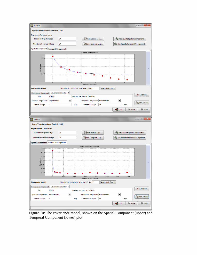
Figure 10: The covariance model, shown on the Spatial Component (upper) and

Temporal Component (lower) plot

Case 3:

Repeat all Steps in case 2 with following changes

xxvii. To obtain the mean trend using new parameters, input the following parameter values,



Spatial 1 1

Temporal 60 60

xxviii. Input the following model parameters

Structure 1:

Sill: 0.18


Spatial Range: 3.9


Temporal Range: 2

Structure 2:

Sill: 0.153


Spatial Range: 95


Temporal Range: 30

Case 4:


xxix. To obtain the mean trend using new parameters, input the following parameter values,



Spatial 0.2 0.2

Temporal 10 10

xxx. Input the following model parameters

Structure 1:

Sill: 0.157


Spatial Range: 3.7


Temporal Range: 2

Structure 2:

Sill: 0.13


Spatial Range: 85


Temporal Range: 20

Case 5:


xxxi. To obtain the mean trend using new parameters, input the following parameter values,



Spatial 0.1 0.1

Temporal 5 5

xxxii. Input the following model parameters

Structure 1:

Sill: 0.11


Spatial Range: 3


Temporal Range: 2

Structure 2:

Sill: 0.1312


Spatial Range: 30


Temporal Range: 15

The analysis carried out above in BMEGUI can be summarized using the tables shown

below

Table 1: Smoothing parameters used to obtain the 5 different global offset models. The

search radius is set to the same value as the smoothing range. Case 1 and case 2 are two

extremes of smoothness in the global offset and are tabulated in the first and last rows.

Spatial Component Temporal Component

case Search radius (deg.)

Smoothing range (deg.)

Search radius (days)

Smoothing range (days)

1 15 15 1000 1000

3 1 1 60 60

4 0.2 0.2 10 10

5 0.1 0.1 5 5

2 0.001 0.001 0.1 0.1

Table 2 Fitted covariance model parameters (sill and autocorrelation range) for each

global offset model.

case Structure 1 Structure 2

Sill

Spatial range (deg.)

Temporal range (days) Sill

Spatial range (deg.)

Temporal range (days)

1 0.2 4 7 0.19 100 75

3 0.18 3.9 2 0.153 95 30

4 0.157 3.7 2 0.13 85 20

5 0.11 3 2 0.132 30 15

2 0.05 1.5 5 0.0619 3 25

After careful analysis of table 1 and table 2 it can be observed that as we increase the

smoothness in the mean trend (the global offset) we observe changes in the experimental

covariance. An extremely smoothed (i.e. flat and uninformative) mean trend results in

higher residual variance and larger spatial and temporal autocorrelation ranges. On the

other hand, decreased smoothness in the mean trend results in smaller residual variance

but also shorter spatial and temporal autocorrelation ranges. Ideally, we seek large spatial

and temporal autocorrelation range but low variance for the residuals.

In order to see how the autocorrelation range and the residual variance change for each

mean trend model, we calculate for each mean trend model (case 1 to 5) the residual

variance as the sum of the two covariance sills, as well as the variance weighted spatial

range, and the variance weighted covariance range. Each mean trend model is then

represented as a circle in the following plot:

The mean trend model obtained in case 1 had the maximum smoothness (i.e. it is flat) and

it therefore had the largest residual variance. This mean trend model is therefore

represented by the circles with the highest residual variance. On the other hand the mean

trend obtained in case 2 had the smallest smoothness, and it therefore had the smallest

residual variance. This mean trend model is therefore represented by the circle with the

lowest residual variance. Cases 3-5 have residual variances that are in between the case 1

and 2 which are extremes of smoothness.

0.1 0.15 0.2 0.25 0.3 0.35 0.4 0.450

10

20

30

40

50

60

variance

variance w

eig

hte

d r

ange

spatial component

temporal component

mean spatial and tempooral components

As can be seen from the plot, each mean trend model represents a tradeoff between

residual variance and covariance range. As we start from the smoothest mean trend model

(with the highest residual variance) and we decrease the mean trend smoothest (i.e. we

are moving toward low residual variance), we see that the covariance range decreases.

This represents a tradeoff. The optimal level of smoothness in mean trend is the

breakpoint where further decrease in smoothness results a drastic decreases in

autocorrelation range. This point is shown in green in the plot.

Conclusion: The degree of smoothness in the space/time global offset can be controlled

by the search radius and smoothing range parameters. A very informative space/time

global offset leaves too little autocorrelation in the residuals to conduct a successful

geostatistical analysis of the residual field. On the other hand, a flat space/time global

offset leaves a large variability in the residuals which produces a covariance model with

high variance. Thus, there is a tradeoff between residual variability and autocorrelation

range, and hence one should choose a space/time global offset which capture some

variability in data and leaves reasonable autocorrelation in the residuals to conduct a

successful geostatistical analysis of the residual field.

Documents

BMEGUI Tutorial 6 - University of North Carolina at Chapel ... · PDF fileBMEGUI Tutorial 6 Mean trend and ... Here we will only edit the temporal lags and their lag tolerances. To