BLS WORKING PAPERS

U.S. DEPARTMENT OF LABORBureau of Labor Statistics

OFFICE OF PRICES AND LIVINGCONDITIONS

The Used Car Price Index: A Checkup and Suggested Repairs

B. Peter Pashigian, University of Chicago

Working Paper 338March 2001

The views expressed are those of the author and do not necessarily reflect the policies of the U.S. Bureau of LaborStatistics or the views of other staff members. This paper was part of the U.S. Bureau of Labor Statistics Conference onIssues in Measuring Price Change and Consumption in Washington, DC, June 2000.

The Used Car Price Index: A Checkup and Suggested Repairs

by

B. Peter PashigianGraduate School of Business

University of Chicago

Paper presented at Conference on “Issues in Measuring Price Change & Consumption,”sponsored by the Bureau of Labor Statistics, Department of Labor, June 5 - 8

NB. Professor Pashigian passed away on October 18, 2000. This was the lastversion of the paper received from him.

2

Introduction

The Bureau of Labor Statistics (BLS) has published the used car price index sinceDecember 1952 as part of the Consumer Price Index (CPI). As its 48th birthdayapproaches, the used car price index merits a timely review for at least two reasons. First,compared to the new car price index, the used car price index is akin to an ignoredstepchild, receiving less scrutiny but deserving of more attention. Second, there arenagging doubts and misgivings within the BLS about accuracy of the used car priceindex. These doubts arise from the suspect time series behavior of the used car index,related in part to the “higher” mean growth rate but especially to the “excess” volatility ofthe used car price index. Possible underlying causes of this questionable behavior arenumerous. Some candidates come to mine. The questionable behavior of the used carprice index could be an undesirable byproduct of the sampling procedures adopted by theBLS. Or, could the source of the price information that the BLS relies on be the culprit?What role has the treatment of quality improvements played in explaining the suspectbehavior of the used car price index? While any or all of these could be the underlyingcauses of the questionable behavior and should not be slighted, could the observed“excess” volatility of the used car price index be a real phenomenon? Used car marketsmight have less elastic supply curves and experience larger demand shocks compared tothose observed in the new car and other durable good markets. This alliance of a lesselastic supply curve and larger demand shocks could explain the observed “excess”volatility of used car prices.

The paper opens with a brief history of the used car price index. Section II establishessome basic facts about the used car price index. How fast has the used car price indexgrown over time and how volatile has the index been? Because there is no obvious way toassess volatility on an absolute scale, used car price volatility must be judged on acomparative basis. Since the used and new car markets are interrelated, a naturalcomparison is between the mean growth rate and volatility of the used car price indexwith that of the new car price index and also with price indices for other products knownfor their volatility. Section II presents some answers to these questions.

A comprehensive review of the used car price index inevitably involves an examinationof the procedures adopted by the BLS for selecting a sample of used cars and how thoseprocedures have changed over time. The sample selection methods adopted for used carscan be compared to the procedures followed for other durable goods for consistency ofpractice. How closely does the BLS sample of used cars mimic the new cars that weresold in recent years? If large discrepancies are discovered, what are the causes andconsequences of these discrepancies on the behavior of the used car price index? Theseissues are discussed in sections III and IV.

3

In Section V attention is directed at the feasibility of using other secondary sources ofused car price information. Several commercial guides publish used car priceinformation. The results of a previous study that used secondary source for priceinformation are reviewed. Instead of relying on auction price data, as collected andpublished by the National Automobile Dealers Association (NADA), the BLS could relyon other secondary sources of used car price information to construct its used car priceindex. If such a change was made, how would the mean growth rate and the volatility ofthe used car price index change? A preliminary but detailed exploration of comparativevolatility of different price sources is presented in the last section of this paper where thecurrently used National Automobile Dealers Association auction prices are comparedwith prices published in Kelley’s Blue Book. Hopefully, this preliminary pilot projectwill shed light on whether volatility of the used car prices would be lower if the BLSused a different secondary data source. Finally, in making adjustments to used car pricesbecause of quality change, the BLS assumes that its measure of the percentage qualityimprovement (obtained from auto manufacturers) affects used car prices and has the samepercentage effect on the price of a used car as the car ages. The paper ends with tests ofthese hypotheses.

I. A Brief History of the Used Car Price Index

A brief history of the used car price index is presented for the convenience of a curiousreader. The history will be mercifully brief because there is no paper trial that an outsideinvestigator such as myself can follow. The rationales for the numerous decisions thatwere made sporadically over the years are a part of an undocumented verbal tradition,known only to those who made the decisions but who have since moved on.

The used car price index was introduced into the Consumer Price Index in December of1952. The details of sample selection in the early years are fuzzy at best. At some point,the used car sample consisted of just 21 models that were from 2 to 6 years so that a totalof 105 used cars prices were gathered. The models were selected based on the productiontotals for the 1970-1974 models years (Kellar). This investigator could not findinformation that described the procedures used to select models or how prices of thosemodels were collected after the used car index was introduced. Apparently, no onethought it important to adjust used car prices for year to year quality improvements until1987. As is documented below, this glaring omission had significant repercussions on thebehavior of the used car price index from 1953 to 1987.

It was not until the major 1987 revisions were introduced that the BLS made a seriouseffort to adjust the used car prices for quality improvements. In contrast, the BLS beganto make adjustment for quality improvements of new cars in 1967, twenty years earlier.Numerous other changes were introduced to the index in 1987. The sample was expandedsignificantly. Second, the BLS restricted its attention to only used cars sold by business(rental car agencies, governments, etc.) to consumers. It obtained information about theage and types of cars sold by business to consumers via a report published by a privatecompany. These important decisions had a major impact on what cars were included intothe BLS sample and on the behavior of the index. Of the many changes introduced in

4

1987 one of the more significant is the treatment of quality improvements. For the firsttime the BLS confronted the quality improvement issue directly. It borrowed the methodthat it used to adjust new car prices for quality improvements and applied it to used carsas well. As will demonstrated below, some of the odd behavior of the index is due to thetardy introduction of a quality adjustment.

This brief review is neither comprehensive nor definitive. The reader is spared a moredetailed description of these changes until later in the paper.

II. Comparative Mean Growth and Volatility of Used Car Prices

A. Annual Percentage Price Change:

This section presents summary statistics on the mean growth rate and price volatility forselected products in the Consumer Price Index. Because this study focuses on used cars,the main objective is to establish some facts about the mean growth rate and volatility ofused car prices and then to compare used car price behavior to the price behavior ofselected components in the CPI. A natural comparison is between used and new cars sothroughout this paper the price volatility of used cars will often be compared to new cars.Other useful comparisons are between used cars and products that have been singled outby the BLS for their greater price volatility, such as energy and food, etc.

This examination of the used car price index begins by first looking at the mean growthand volatility of year-to-year price changes in the index and then moves on to examinemonthly price data. For most of the studied product groups, the sample of annualobservations covers a forty-three year period, beginning in 1955 and continuing through1998. Over this long period there have been several changes in methodology, datacollection methods, weighting procedures, etc. Sometimes, changes in methodology areadopted but a revision is not or cannot be made to previous years of the price series.Consequently, the existing price series are probably not entirely consistent over time. So,our summary measures of price volatility will reflect the effects of these changes as wellas the underlying price volatility of the product. The initial year of 1955 is selectedbecause the BLS began to collect transaction versus list prices for new cars in the middleof 1954. To analyze annual price volatility, the price ratio Pt / Pt-1 is the variable ofinterest where Pt is the price index in year t and Pt-1 is the price index in the previous year.The mean, standard deviation and the standard deviation/mean ratio of the Pt/Pt-1 ratio arecalculated for each product.

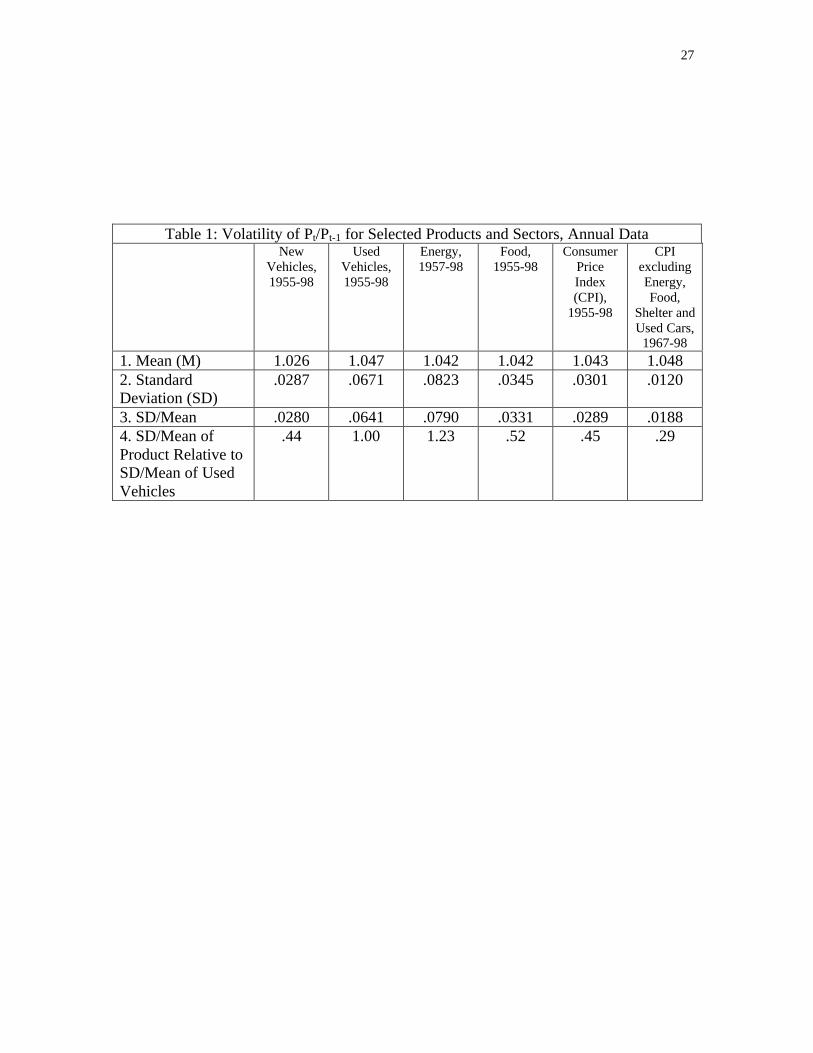
Table 1 shows the mean M (row 1), standard deviation SD (row 2), the ratio of thestandard deviation to the mean, SD/M, (row 3) and the ratio of SD/M for each productrelative to the SD/M for used cars (row 4) for 6 product categories: new vehicles, usedvehicles, energy, food, the Consumer Price Index (CPI), and CPI excluding energy, food,shelter and used cars. The BLS considers energy and food prices among the more volatilecomponents of the CPI, so much so that the BLS not only reports the CPI but the CPIwith the more volatile sectors excluded.

5

A puzzling, if not disturbing, feature of Table 1 is that from 1955 to 1998 the mean of theused car price ratio exceeds the mean of the new car price ratio by a full 2.1 percentagepoints per year. Another way of illustrating this odd behavior is to regress the used carprice ratio, R u

t , on the new car price ratio, R nt . The estimated equation is

R ut = .236 + 1.25 R n

t

(.311) (.302)where the standard errors are in the brackets below the line. The new and used car priceratios are equal when R n

t = .944. Since the new car price ratios have been invariably

greater than one, the regression results indicate that the used car price ratio has exceededthe new car price ratio in most years.

Just how could the used car price ratio consistently exceed the new car price ratio? Thehigher mean price ratio for used car prices displayed in row 1 is puzzling for both newand used car prices are suppose to be adjusted for quality change, or so I thought when Ibegan this project. As noted by Gordon (p. 322), a difference in the mean price ratioswould lead to the ridiculous conclusion that the used car price would ultimately exceedthe new car price. This puzzling difference occurred because the BLS has been moresuccessful and conscientious over time in adjusting new car prices for qualityimprovements than it has for used car prices. Much to my surprise, I learned that the BLSapparently made no quality adjustment to used cars until 1987. Consequently, the usedcar price index had an upward drift to it, in part because of the annual qualityimprovements built into new cars. As documented below, this excessive upward drift hasdisappeared since 1987 when the BLS faced the quality adjustment issue head-on andbegan to apply the new car price adjustment for quality change to used cars as well.i

A comparison of the first two columns shows that used car prices have been more volatilethan new car prices, both absolutely (SD: row 2) and relative to the mean growth rate(SD/M: row 3)) of the price index. Used car prices are less volatile than energy prices,but much of the apparent volatility of energy prices is concentrated in two episodes ofrapidly escalating and then contracting crude oil prices. Used car prices are much morevolatile than food prices, using either an absolute (SD) or a relative standard (SD/M).

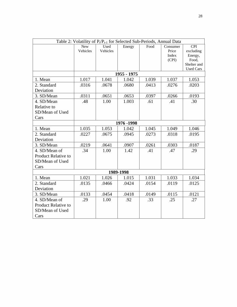
There is some evidence that price volatility has decreased over the forty-three yearperiod, at least for some product groups. Table 2 shows the same data for the 1955 –1975, (except where otherwise noted) sub-period, the 1976 – 1998 sub-period, and the1989 –1998 sub-period. Between 1976 and 1998 the volatility of energy prices increasedand this contributed to the increased price volatility for the CPI. When the more volatilesectors like energy, housing, food and used cars are excluded, the CPI was less volatile inthe second than the first half of the period. While the price volatility of new cars declinedin the second period, the decline for used cars was negligible. The decline was larger inboth an absolute and a relative sense for new than for used cars (row 4). Again, we findthat used car prices increased more rapidly than new car prices, although the differencebetween the mean growth rates decreased from 2.4 percentage points per year in the first

6

sub-period to 1.8 percentage points per year (row 1) in the second sub-period. Thisdecrease reflects the BLS effort to adjust used car prices for quality improvements inrecent years.

To validate this conclusion, an even shorter sub-period, from 1989 to 1998, wasexamined. The bottom panel of Table 2 shows a tiny difference of only .005 per yearbetween the mean of the price ratios for new and used cars. It appears that the qualityadjustment procedure introduced by the BLS after 1987 has effectively eliminated thegap. The difference in the mean price ratios for new and used cars over the 1955 – 1998span appears to be due in part to the omission of a quality adjustment for used cars in theearlier years of the sample. In passing it is worth emphasizing that between 1989 and1998 the relative volatility of used cars exceeded that of other products including energy.It is apparent from this brief survey that annual used car prices are relatively morevolatile.

This abbreviated history of used and new car price behavior can be instructive. The largedifference between the mean price ratio for new and used cars lasts for an extendedperiod of time – apparently between 1955 and 1987 after which an adjustment of qualityimprovements was adopted. Why it took so long to recognize and account for thisdifference remains a mystery from this vantagepoint. Used car price ratios cannot bepersistently larger than new car price ratios. If they were, lower quality items wouldultimately sell for more than higher quality items. The excess between the mean priceratio of used over that of new cars was allowed to persist much too long and should havetriggered an alarm that something was wrong with either the new or used or both priceindices. Perhaps, a reexamination of the new and used car price indices would have leadto a quicker adoption of a revised price adjustment for quality improvements in used cars.

B. Explanations for the Greater Volatility of Annual Used Car Prices

This review of the cross sectional and times series results has raised two questions. First,why did used car prices growing more rapidly than new car prices? Second, why isvolatility greater for used than new cars? As to the first question, a finger has beenpointed at an inadequate adjustment for the quality improvement of used relative to newcars up until 1987. The absence of a quality adjustment for used cars explains at least partof the gap.

There are several possible explanations for the greater volatility of used car prices. Onepossible explanation has to do with the different sources of the price data used tocalculate the used and new car price indices. Differences in the collection of used andnew car prices may have artificially raised used car price volatility. Later, we try to shedsome light on the effects of the sources of data on price volatility.

Another possible explanation is that the observed greater price volatility of usedcompared to new car prices is real and has little to do with the quality of the underlyingprice data. It is instructive to use a demand and supply model for new and used cars toexplain why used car prices could be more volatile than new car prices. Differences in (1)

7

the supply elasticity of new versus used cars and in (2) the demand variability of newversus used cars could explain the observed differences in price volatility. Over the wholeperiod the correlation between the annual price ratio for new cars and the price ratio ofused cars equals 0.3. This positive correlation in annual price changes suggests thatincreases in the demand for new cars are positively related with the increase in thedemand for used cars. However, the size of the correlation between percentage pricechanges is not large suggesting that there are times when an increase in demand for newcars occurs when the demand for used cars either does not increase or decreases.

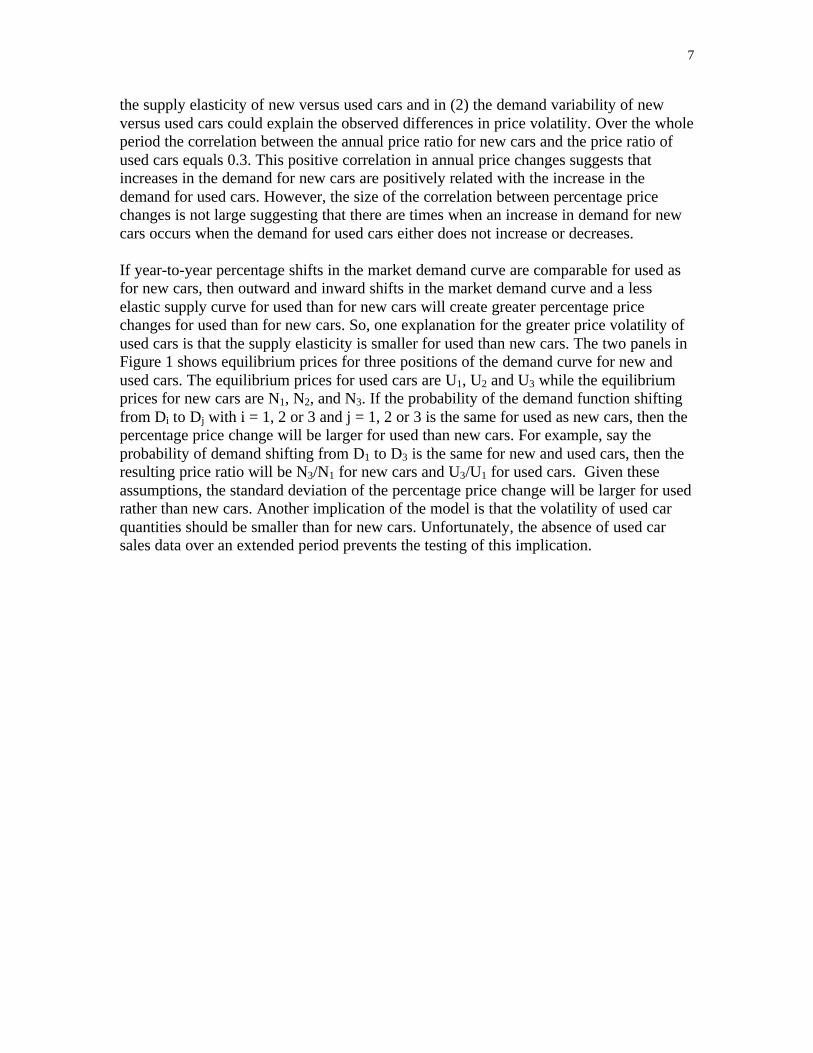
If year-to-year percentage shifts in the market demand curve are comparable for used asfor new cars, then outward and inward shifts in the market demand curve and a lesselastic supply curve for used than for new cars will create greater percentage pricechanges for used than for new cars. So, one explanation for the greater price volatility ofused cars is that the supply elasticity is smaller for used than new cars. The two panels inFigure 1 shows equilibrium prices for three positions of the demand curve for new andused cars. The equilibrium prices for used cars are U1, U2 and U3 while the equilibriumprices for new cars are N1, N2, and N3. If the probability of the demand function shiftingfrom Di to Dj with i = 1, 2 or 3 and j = 1, 2 or 3 is the same for used as new cars, then thepercentage price change will be larger for used than new cars. For example, say theprobability of demand shifting from D1 to D3 is the same for new and used cars, then theresulting price ratio will be N3/N1 for new cars and U3/U1 for used cars. Given theseassumptions, the standard deviation of the percentage price change will be larger for usedrather than new cars. Another implication of the model is that the volatility of used carquantities should be smaller than for new cars. Unfortunately, the absence of used carsales data over an extended period prevents the testing of this implication.

8

By a simple extension of this model, the volatility of new car prices would decline overtime if the supply elasticity of new cars became still more elastic over time. Anotherpossible explanation for the decline in new car price volatility over time is that the year toyear shifts in the position of new car demand curve has become smaller over time. Thismay have occurred as the relative importance of the annual model change has diminishedover time. Either or both changes could explain why new car price volatility hasdecreased more over time than has used car price volatility.

C. Monthly Price Volatility

Instead of measuring price volatility from year to year, it can be measured from month tomonth. Part of the within-year variability in prices is due to seasonal factors and part toreal factors that create greater monthly price variability. Below we show that used carprices have a larger seasonal swing in prices and, more surprisingly, they are morevolatile than the monthly prices of new cars even after adjusting for seasonal swings.

Two measures of monthly price volatility are considered. The first measure is the ratio ofthe non-seasonally adjusted price to the seasonally adjusted price, NSPt/SPt where NSPt

is the non-seasonally adjusted price in month t and SPt is the seasonally adjusted price inmonth t. This ratio is the seasonal factor for month t. By how much is the price in month tsystematically higher or lower than the average month. The larger the fluctuation of this

Sn

nD1

nD2

nD3

SuN3

N2N1

U3

U2

U1

New Car Market Used Car Market

Used CarPrice

New CarPrice

New Car Quantity Used Car Quantity

Figure 1: New and Used Car Price VolatilityCaused by Demand Shifts

uD1

uD2

uD3

9

ratio throughout the calendar year, the more important is the seasonal in prices. Thesecond measure is the monthly percentage change in the seasonally adjusted price index,SMPt/SMPt-1 where SMPt is the seasonally adjusted price index in month t and SMPt-1 isthe seasonally adjusted price index in the previous month. The second measure abstractsfrom the seasonal variation in prices and looks at the remaining monthly price variability.

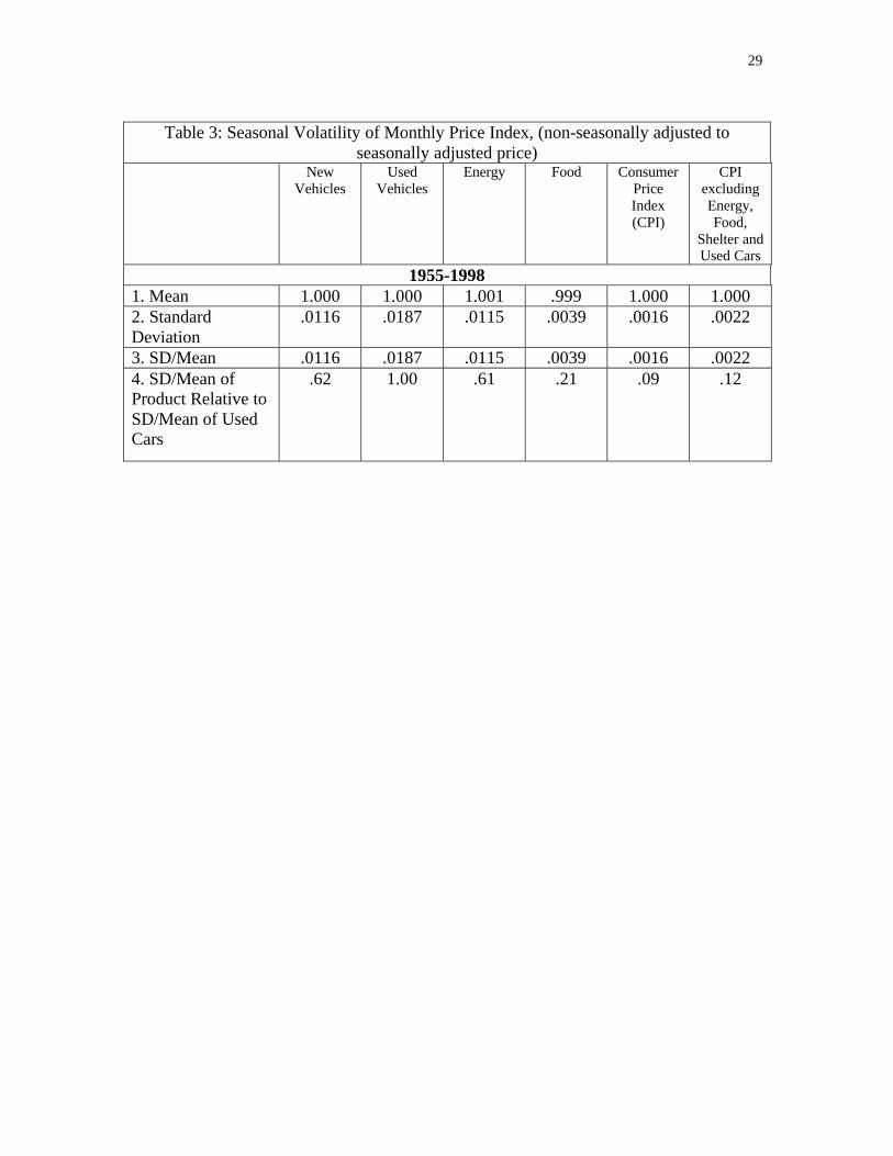
It is well known that new car prices follow a systematic seasonal pattern. New car pricesare typically higher at the beginning of a new model year and lower at the end of themodel year. However, this seasonal pattern has been diminishing in importance over time(Pashigian, Bowen and Gould 1995). The fluctuation of prices because of theintroduction of new models should play a less important role for used cars if consumerspurchase used cars for basic or reliable transportation and place less value on out-of-datefashion features. Nonetheless, Table 3 shows that monthly used car prices fluctuate evenmore than do new car prices or energy and food prices. As noted above, new car pricesfluctuate substantially over the model year. However, the seasonal price variability ofused car prices has not been look into before. Apparently, used car prices have an evenlarger seasonal factor. The new and used car price indexes fluctuate relative moreseasonally than do the price indexes for many of the products that make up the index.

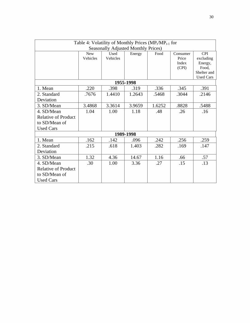
Now consider the second measure, monthly fluctuation in seasonally adjusted prices.From 1955 to 1998 ST/M is comparable for new and used cars. Once again, the energysector has the highest ST/Mean ratio. Caution should be exercised however since theresults are sample dependent. The bottom panel of Table 4 shows the monthly volatilityresults are different for the more recent 1989-1998 sub-period. In recent years monthlyused car prices are absolutely and relatively more volatile than new cars. Over the 1989to 1998 interval the annual or monthly data show that used car prices are more volatilethan new car prices. This occurs in spite of the fact that the monthly used car price indexis a three-month moving average.

III. A Search for Consistency in the BLS Price Collection Methodology

A. Comparing the Procedure for Housing with Used Cars

The purpose of the CPI is to measure the average price change over time for a givenmarket basket. With a perfect index, the quantity weights of the market basket of goodswill reflect the goods purchased by consumers. Ideally, the CPI should measure therequired percentage increase or decrease in the expenditure of a representative consumerwho bought the CPI market basket brought about by a myriad of individual price changesbetween any two dates.

The treatment of durable goods in the CPI raises a special and difficult problem. Whenthe price of a non-durable good rises, relative prices change and the consumer is worseoff. When the price of a durable good rises, a first time buyer of a used durable good isworse off than if the durable good price had not increased and would require an offsettingcost of living increase so that the consumer could purchase the market basket that wouldhave been purchased had the price not risen. An existing owner of a used durable could

10

be thought of hypothetically selling the used car in the market at a higher price and thenbuying it back. Because of the price increase, the consumer faces a change in relativeprices but receives a capital gain on the sale of the used car. If the consumer owns a two-year-old used car worth $16,000 and its price increases by $1,000, she couldhypothetically sell the car at $17,000 and then repurchase it at the higher price becauseshe received a capital gain of $1,000 when she sold the car. So she could continue topurchase the market basket that she had purchased before the price of the durable goodincreased even though she would not because of the change in relative prices.

If the sole objective of the price index is to measure the average price change of goodsover a given time period, then the used car transaction should be treated like a non-durable good transaction and included in the CPI. On the other hand, which prices shouldbe included in the index depends in large part on what the index is to be used for. If theprice index is used to derive an estimate of the required income change so that theconsumer could buy the same market basket after the price changes, the price change forused car should not be included in calculating the average price change for the indexsince it would involve double counting. The owner of the durable good has alreadyreceived a capital gain because of the price increase. So, a further income change isunwarranted to offset the price increase. This reasoning would imply that only thosetransactions where consumers are first time buyers of a durable should be used to createthe weight for the durable good in the CPI. I believe this is the philosophy behind the1987 adjustments.

The BLS has found it difficult to follow a consistent methodology when pricing theservice flows from durable goods in part because of the absence of relevant price data forsome durable goods. As a consequence, a consistent treatment of durable goods by theBLS has proven difficult to achieve. Each pricing group appears to develop anindependent methodology for collecting price data for each type of durable good. As aconsequence, consistency between the adopted methodologies has not had a high priorityand has not been achieved.

This is best illustrated by the different treatments the BLS gives to housing, which as ofDecember 1999 represents 39.6 percent of the CPI with shelter representing 30.2 percent,and used cars represents only 1.9 percent. When pricing the services of the housing stock,the BLS currently derives estimates of the owner’s rental equivalent of the existinghousing stock. Rental equivalence measures the change in the amount that a homeownerwould pay to rent, or would earn from renting, his or her home in a competitive marketplace. Since 1983, the rental equivalence index has been based on the implicit rent ofowner units. Until January 1999, these implicit rents were determined by changes in thepure rents of matched rental units. The weight for rental equivalence in the CPI is basedon the implicit rents reported by homeowners in a household survey. Changes in therental equivalence index are determined by changes in the rents of a sample of rentalunits, weighted to be representative of the owner-occupied housing stock.

If it could be easily implemented, the BLS would like to apply the rental equivalenceconcept to other durable goods as well. Unfortunately, this has not proved viable because

11

of the difficulty of obtaining appropriate lease data. Hence, the BLS applies a differentmethodology for other durable goods. For new and used cars, the BLS obtains prices forspecified qualities of cars. For new cars it has obtained “market prices” for the purchaseof specified new cars. A few years ago it investigated the possibility of using marketlease rates for new cars to develop a rental equivalent measure, as used for housing. It didnot pursue this avenue because, at the time, the lease market for new cars was justdeveloping and was still too thin. Since then, the leasing market for new cars hasexpanded rapidly and the BLS has begun experimenting with the rental equivalenceconcept for leased cars. Applying the rental equivalent concept to used cars, appears lesspromising at this time. The rental market for used cars is much less well developed so itdoes not appear as feasible at this time to derive a rental equivalent price index for usedcars.

The BLS treats the pricing of used cars differently. In 1987 a major change in themethodology was introduced and a larger sample of cars was selected. At that time theBLS reduced the weight that the used car category was assigned in the CPI from 2.507 to1.249 percent by limiting used car expenditures to the purchase of used cars byconsumers from business, government etc. The sale of a used car from one consumer toanother was considered a transfer and not an expenditure (except for dealer profit). TheBLS limited its sample of cars from the sales of used cars by non-consumers toconsumers, taking account car characteristic such as size of car, body style, engine size,front or rear wheel drive, etc. For most goods, the BLS collects data by returning to thesame outlet each month to price the item. The BLS uses a different procedure for usedcars. Because it could not assure that it would find the same used car of a given qualitymonth after month at outlets selling used cars, it obtains its used car price data from anational average price that is derived from auction prices at numerous weekly autoauctions. The National Automobile Dealers Association (NADA) reports these prices intheir Official Used Car Trade-In Guide. In each year each car included in the sample isbetween 2 and 6 years old and has a pre-specified set of options.

The decision to use auction prices was a critical one. Not only are auction prices morelike wholesale rather than retail prices but the sample of cars that are sold in auctions arehardly a random sample of the population of used cars from two to six years old. Asshown below, the sample of auction cars excludes the many popular foreign cars, sincefew foreign cars are sold as fleet sales. Fewer of the more popular domestic cars are soldas fleet sales as well.

If the same methodology used to derive used car price index was applied to housing, thenthe price of housing (or the rental equivalent) should be based only on sale prices (orrents paid) for new houses or used homes that were sold by firms and governments sincethese would business to consumer transactions. Sales of existing used houses by oneconsumer to another would be considered as transfers within the consumer sector, as arethe sales of used cars from one consumer to another. More importantly, this would implya change in the weight assigned to housing in the CPI. On the other hand, if themethodology adopted for the pricing used housing was followed for used cars, then the

12

sample of used cars should include a random sample of all used car transactions, not onlythose from business to consumers, as has been followed since 1987. It would seem that adesirable long-term goal is to strive for more consistency in the methodology acrossproducts.

IV. The Representativeness of the BLS Sample of Used Cars

A. The BLS Sample of Used Cars Under Samples the Best Selling Cars

Throughout the 1990s the BLS has relied on two different data sources to select a sampleof used cars. Between 1990 and 1997, BLS relied on a Rhunzheimer International Surveyto draw a sample of used cars sold by rental car agency, governmental units, creditcompanies etc. to consumers. The Rhunzheimer bi-annual reports showed the number ofcars sold by businesses to consumers by age and type of car (body style, options, enginesize, front or rear wheel drive, etc.). Because the report was recently terminated, the BLSturned to the Consumer Expenditure Survey (CES) beginning with 1998 to draw a sampleof used cars bought by consumers. These two data sources sample a different set of usedcars. The Rhunzheimer survey focuses only on the sales of used cars by firms toconsumers, and excludes sales from one consumer to another even when an intermediarylike a car dealer is used. So the resulting sample will depend on which cars are purchasedby businesses for their use. If businesses select cars based on the favorable price that theycan get from the car companies, then the more successful cars in the market which arediscounted less will not be purchased by rental agencies and governments. Or, businessesmight only buy the basic trim line of a model with fewer options. This means thatsuccessful cars have a lower probability of showing up in the BLS sample. Imported carsare less likely to show up in the BLS sample.

With the shift to the CES in 1998, the BLS abruptly shelved one of the requirementsimposed in the 1987 revisions -- only business to consumer transactions would be eligiblefor consideration. Beginning in 1998, all used car transactions were now eligible for thepurpose of selecting a sample of used cars even though this selection procedure seemsinconsistent with the philosophy advanced with the 1987 revisions.

The Consumer Expenditure Survey includes a sample of all used car purchases reportedby consumers. In principle it should give a more representative sample of the used carsbought by consumers whether those cars were bought from firms or other consumers. Myexpectation was to find the popular cars appearing more frequently in the 1998 samplethan in the earlier samples.

To determine how representative is the BLS sample of used cars, I compared thefrequency with which the cars in the BLS sample were among the top 10 best sellingmodels when new over the previous 6 years. How closely do the cars in the BLS samplemimic the new car sales of the most popular cars during the last six years? If the top tenbest selling new cars (ranked by units sold) accounted for (say) 40% of the new car

13

market in the last six years, were 40% of the used cars in the BLS sample among the topten best selling new cars?

Two cautions deserve mention. To compare the top 10 cars in the last six years againstthe BLS car sample implicitly assumes that the resale pattern of the top 10 best sellingcars is similar to that of used cars in the BLS sample. This is unlikely to be true. Themore successful selling cars when new are probably held by the original buyer for moreyears and traded-in less frequently. While true, this is unlikely to explain the largediscrepancy between the top 10 share of the new car market and the share of cars in theBLS sample that were in the top 10. Some preliminary evidence is presented below.Second, the BLS draws its used car sample based on consumer expenditures for used carsand not on units sold. My decision to rely on units sold as a standard was governed by theavailability of units sold data.

At the time this analysis was undertaken, the only data set available to me was the so-called “specification or characteristics” data set. This data set shows among other thingsthe auction location and the options on each car included in the sample. The specificationdata set includes an additional observation for each model that is used to calculatemonthly depreciation. In some cases a third observation for the same model will beincluded when another car must be substituted to calculate depreciation. The 1998specification data set has 1243 observations which was reduced to 1210 useableobservations while the number of observations that the BLS uses to calculate the priceindex is 563. Roughly speaking, each model is double counted in the “specification” dataset. The sensitivity of the results to the size of the sample is not known at this time but Isuspect the results will not change appreciably if the smaller sample had been used.

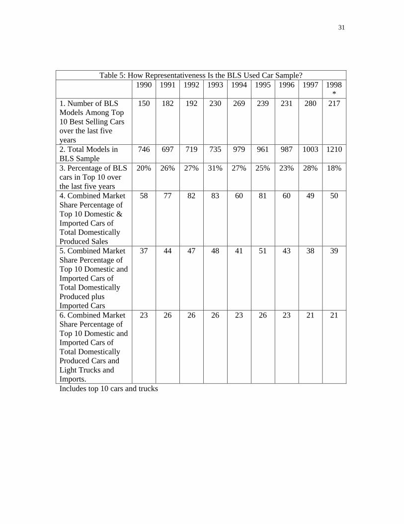
For each calendar year, the top 10 selling models were identified in each of the last 6years. For example, for 1990 we looked at the 10 best selling new cars in each year from1985 to 1990, i.e. cars that would be 1 to 6 years old at the end of 1990. For all the one-year old cars in the BLS sample, we determined what fraction of the BLS one-year-oldcars were among the top 10 best selling cars when they were new. We repeat thisprocedure for all used BLS cars for ages from 2 to 6 years old in 1990. Table 5 showsthat in 1990 150 of the 746 models in the BLS sample (or 20%) were ranked in the top 10new cars over the previous six years. In contrast row 5 shows that the top 10 best sellingnew cars (which includes domestically produced and imported cars) in years 1985 to1990 accounted for 37% of the total sales of domestic and imported cars. A comparisonof rows 3 and 5 shows that in each year the BLS sample of cars under counts the 10 bestselling domestically produced and imported cars in the U.S. new car market. The meanpercentage of BLS sample of cars that were in the top 10 is 25.9% between 1990 and1997 while the mean combined market share of the top 10 best selling cars ofdomestically produced and imported cars was 43.6%, a difference of 17.7 percentagepoints.

The procedure for calculating the market share of the top 10 best selling cars does notdistinguish between cars sold to consumers versus those sold to firms and governments.How the average discrepancy reported above would change if only cars that were sold to

14

consumers could be identified is unclear. However, it likely that the top 10 best sellingcars would have a lower probability of being sold to firms and governments. Hence, themarket share of the top 10 cars that are sold only to consumers would be still higher. Tothis extent, our procedure may underestimate the difference.

In general the best selling cars are under-reported in the BLS sample. The meandifference of 17.7 percentage points is a consequence of selecting used cars sold by rentalcar agencies governmental units and others. Those cars are unrepresentative of thepopulation of used cars held by consumers and may be unrepresentative of all used carsthat are sold. Honda Accord and the Toyota Camry were among the best selling new carsin the automobile market throughout the 1990s, as was the Ford Taurus. Yet, they areconsistently under represented in the BLS sample throughout the nineties. Makers ofthese and other best selling cars have less incentive to sell their cars to fleets. If thepurpose of the used car price index is to measure the average price change of used carsales, the procedures used to select the sample of cars between 1990 and 1998 should bereviewed both with regard to the criteria for inclusion and for the sample selectionmethods.

The Consumer Expenditure Survey (CES) reports information about consumer purchasesof used cars and (light) trucks. As noted above, the BLS turned to the CES to create the1998 BLS sample of used cars bought by consumers. Starting in 1998, the BLS expandedthe sample to reflect the increasing popularity of trucks. In principle this different sourceof information for selecting a sample of used cars and trucks should include all used carand truck purchases whether bought from other owners of used cars, dealers or rentalagencies, etc. If the BLS selected a random sample of all used vehicle purchases reportedby the CES, the percentage of vehicles selected from the CES sample that were amongthe top 10 best selling vehicles should be a close match for the share of sales accountedby the top 10 vehicles of all domestically produced and imported vehicles. This is what Iexpected but, much to my surprise, did not find.

The 1998 sample included 1210 observations (spanning the 1993 to 1998 model years) ofwhich 217 (18%) were among the top 10 new cars and trucks. As mentioned above, lighttrucks were included in the sample for the first time in 1998. The inclusion of trucks inthe sample causes an even larger distortion between the BLS sample of cars and trucks inthe top 10 and the share of sales of 10 best selling new cars and trucks over the last fiveyears. In 1998 the top 10 selling cars and trucks (from 1993 to 1998) accounted for 39%of the domestic car and truck production plus imports. Most surprising, the gap between18% and 39% remained large in spite of the use of the CES to create a new BLS sampleof cars and trucks.ii Some peculiarities appear when the 1998 sample of cars is scanned.For example, the 1998 sample contains more Corvettes than Camry observations.

Time and budget constraints prevented me from investigating the cause of the unexpecteddiscrepancy in 1998. I have been told that the CES is a sample of all used car transactionsand the BLS takes a very small sample of that sample. Perhaps, sampling variation isresponsible for the large discrepancies documented above. If this is the reason, then

15

serious thought should be given to increasing the size of the sample. I am not convincedthat this is the complete explanation so I remain perplexed by the 1998 results.

This investigator believes the procedures for drawing the sample of cars needs to bereexamined. Throughout the nineteen-nineties the BLS sample of cars has deviated fromthe population of used cars in the market. Possible reasons for the observed deviationsbetween 1990 and 1997 have been given above. However, the deviation observed in 1998when the CES sample was drawn remain a puzzle, a puzzle that needs to be solved.

Given the limited alternatives available and the large discrepancies found in this paper,feasible alternative procedures are not easy to recommend. Perhaps the easiest solution,though still imperfect, is for the BLS to select a sample of used cars based on the sales ofnew cars over the previous six years. While this procedure has some drawbacks, it iseasier to implement and appears to be an improvement over the results achieved to dateby using either the Runzheimer Report or the CES.

B. Differences Between the Retention Rates of the Top 10 Best Selling New Cars andLess Popular Cars

Could the share differences found throughout the nineties be due to the longer holdingperiods of buyers of the top ten selling new cars? There is fragmentary evidence thatbuyers of new imported cars hold them longer before trading them in. In a study ofownership changes for cars and trucks registered in Illinois, Porter and Sattler (1999)calculated the fraction of cars traded in as of December 1994 for owners who bought new1986 - 1988 model year cars. On average cars bought between 1986 and 1988 would be 7years old in December 1994. The authors report trade-in data by division of company.For example, the Ford car group represents all cars marketed by the Ford division of theFord Motor company while the Honda car group would represent all cars marketed by theHonda division, e.g. Accord, Civic, etc. If we select from the Porter-Sattler (P/Shereafter) study, the ten car groups with the lowest fractions traded in, the weightedaverage fraction of cars traded-in was .454. In other words, only 45% of these cars whenthey were bought new in the model years 1986-1998 had been traded by December 1994.It turns out all of the ten car groups represented imported cars, e.g. Volvo, VW, Saab,Subaru, Honda, Toyota etc. These ten car groups accounted for only .140 of the total carsin the sample throughout the 1986-1988 model years. Since the fraction of cars traded-infor the sample as a whole was .541, the fraction of cars traded-in for the remaining cargroups averaged .555. For 1986-1988 model years, original owners of imported carsretained their cars for longer periods than owners of cars produced by Americanmanufacturers.

While a larger fraction of imported cars were retained by their original owners, this wasnot true for the best selling cars during the 1986-1988 model years (mostly American carsduring this time period) where the difference between the percentage traded-in of the tenlargest selling car groups and the other car groups was negligible.

16

Since 1988, foreign cars have risen in the sales charts with Toyota, Honda, Civic andother imported cars regularly ranked among the top ten cars throughout the nineties. As aconsequence, the top ten best selling new cars in the nineties could very well have higherretention rates than other car models because more imported models were in the top tenbest selling cars. Could the difference between the market share of the top ten best sellingcars in the new car market and the lower fraction that BLS used cars were among the topten cars be due to the higher retention rates for imported cars?

What fraction of the used car market would the top 10 new cars command if they wereheld for longer period by their original owners? By making a few assumptions, anestimate of the share that the top selling cars would have of the used market can bederived. Assume that the top 10 best selling new cars in the nineties were traded in asinfrequently as the ten car groups with the lowest trade-in fractions during the 1986-1988model years. This is obviously a generous estimate since some of the top ten best sellingcars in the nineties were cars produced by domestic producers that typically have lowerretention rates. Between 1990-1997, the top ten best selling new cars accounted for anaverage of 43.6% of all domestically produced and imported cars. If the retention rates ofthese cars were the same as the retention rates of the 1986-1988 model year cars with theten lowest trade-in fractions, then the ratio of the fraction that the top 10 best selling newcars would account for in the used market to their fraction of the new car market is givenby

1

211

12111

11

1

1

)1(

11

)1(t

tssststs

ts

s

s

nnnnn

n

n

u

−+=

−+=

where n

u

s

s

1

1 is the ratio of share of the used car market that would be accounted for by the

top 10 best selling new cars to the share of the new car market accounted for by the top10 best selling cars and t2/t1 (> 1) is the ratio of the fraction traded-in of all cars otherthan the top 10 best selling cars (t2) to the fraction traded-in of the top 10 best selling cars(t1). This equation can be rewritten as

n

n

u

u

s

s

t

t

s

s

1

1

2

1

1

1

11 −=

−

Because 2

1

t

t is less than one, us1 will be less than s n

1 .

The top 10 best selling cars accounted for an average fraction of .436 of the new carmarket from 1990 – 1997.iii The share of non-Top 10 cars traded, t2, is estimated from therequirement that the share of top 10 cars times the fraction traded plus one minus theshare of top 10 cars times the unknown fraction of non-top 10 cars traded in must equal.541, the share of all cars traded in. The estimate value for t2 is .555 while t1 = .454assuming the top 10 best selling new cars matched the mean trade-in performance of the

17

imported cars. Inserting these numbers into the equation above yields an estimate for n

u

s

s

1

1

= .888.iv The market share of the used market held by the top 10 best selling cars in thenew market would be lower than their market share of the new market but only by aabout 12 % even under the generous assumption that the top 10 cars as a group couldmatch the retention rates of the imports for the model years 1986-1988. Given the top10’s average new car share is .436, the equation would predict their average used carshare would be.387. Consequently, the larger mean discrepancy that was found betweenthe mean share of BLS used cars that were among the top 10 best selling new cars and themean of the actual market share of the top 10 in the new car market cannot be explainedby the fact that the top 10 selling new cars are traded in less frequently than all other cars.Something else is causing the large observed discrepancy.

Two caution flags should be waved. The P/S study -- from which estimates of frequencyof trade-in data was obtained -- is from a single state, Illinois. How representative isIllinois of the nation is unknown. Second the estimates are based on the trade-inexperience in the 1986 to 1988 period. It is unknown whether the frequency with whichbuyers retain their new cars has changed over time.

V. The Effect of the Source of Used Car Price Data

The greater volatility of used car prices may be spurious in part and depend on the datasource used by the BLS. Could the reliance on auction price data contribute to the higherprice volatility of used car prices? This section reviews an earlier study that relied onused car price data published in car guides to develop separate new and used car priceindices. The study used hedonic techniques to account for price changes caused bychanges in the physical characteristics of cars. These hedonic adjusted price indices arecompared to the CPI price indices for new and used cars. In the second part of thissection, I compare price data taken from Kelley’s Blue Book with NADA auction pricedata to determine if used car price volatility depends on the source of the data.

A. Gordon’s New and Used Car Price Index Study

In his study of new and used car prices Gordon (1990) developed new and used car priceindices from 1947 to 1983 using prices reported in new and used car price guides.Gordon borrowed a methodology first implemented by Griliches and Ohta (1976). Inessence, Gordon estimates a hedonic for used (new) cars while controlling for the effectsof selected car physical characteristics and including a time dummy variable to measurean autonomous change in used car prices. In his hedonic regressions he includes weight,length, brake horsepower, age and type of engine. The time dummy measures changes ineither the used (new) car price after controlling for the effects of car characteristics listedabove. The estimated coefficient for the time dummy is obtained from regressions ofsuccessive two-year cross sectional observations. Gordon cautions the limitations of thehedonic approach especially for later years in his study where the more difficult tomeasure attributes like interior space, trim lines, environmental improvements becomemore prominent. He also questions the usefulness of car size in any hedonic regression

18

when cars were downsized during the second half of the 1970s, especially in 1977 and1979.

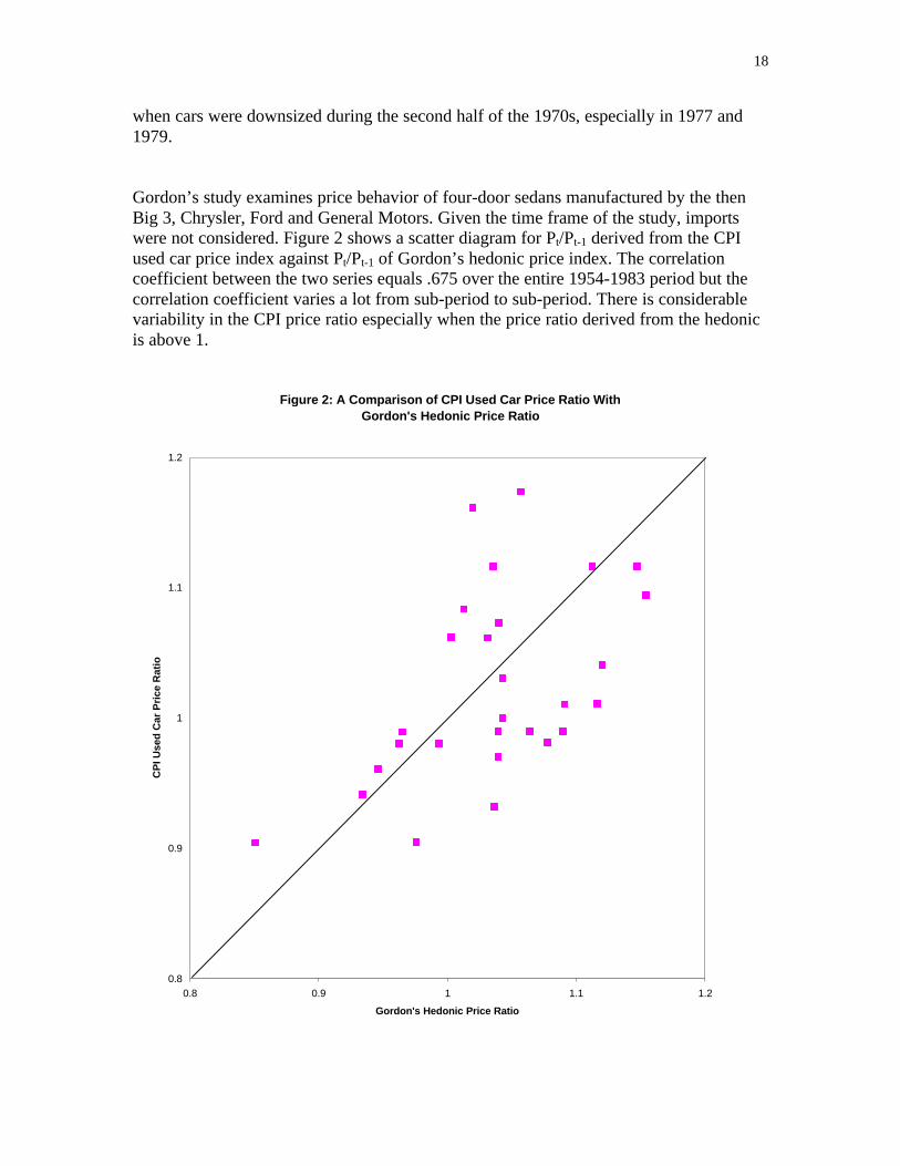
Gordon’s study examines price behavior of four-door sedans manufactured by the thenBig 3, Chrysler, Ford and General Motors. Given the time frame of the study, importswere not considered. Figure 2 shows a scatter diagram for Pt/Pt-1 derived from the CPIused car price index against Pt/Pt-1 of Gordon’s hedonic price index. The correlationcoefficient between the two series equals .675 over the entire 1954-1983 period but thecorrelation coefficient varies a lot from sub-period to sub-period. There is considerablevariability in the CPI price ratio especially when the price ratio derived from the hedonicis above 1.

Figure 2: A Comparison of CPI Used Car Price Ratio With Gordon's Hedonic Price Ratio

0.8

0.9

1

1.1

1.2

0.8 0.9 1 1.1 1.2

Gordon's Hedonic Price Ratio

CP

I Use

d C

ar P

rice

Rat

io

19

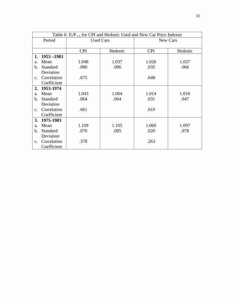
Table 6 shows the mean, standard deviation and the SD/M ratio of Pt/Pt-1 from 1953 to1983 and for two sub-periods from 1953 –1974 and from 1975-1983 for the CPI and forthe hedonic price indexes. Summary statistics are presented for both new and used cars.

The CPI used car price index grows on average by 1.1 percentage points faster per yearthan the hedonic index. Here again the failure to adjust the used car price index forquality improvements is the likely cause, especially in the earlier period from 1953 to1974, and gave an upward bias to the used car price index. As mentioned above, thecorrelation coefficient between the two price indexes was .675. In the more stable earlierperiod from 1953-1974 the difference in the mean growth rate was about 3.9 percentagepoints. In the more volatile period from 1975-1983 the mean growth rates of the twoindexes are about the same.

This comparison of the CPI with the hedonic price indices does not suggest that used carprice index would display less volatility if the BLS had used a different source for pricedata and adopted the hedonic methodology. The hedonic used car price index has a largerstandard deviation than the CPI in the more volatile period from 1975 to 1983. Evenmore disturbing is that the correlation coefficient between the two indexes from 1975-1983 drops to only .378. The two indexes move in the opposite directions in 1977 and1979, two years when American car producers introduced major downsizing programs.The lower correlation coefficient suggests that the regression coefficients for weight,engine size, etc., in the hedonic regression equations were not that stable in a period ofmajor downsizing of cars.v

Gordon’s pioneering study is a useful investigation. It represents a rare effort to use non-CPI price data to construct new and used car price indexes. Gordon’s derived priceindexes are different from the CPI price indices for new or used cars in two ways. First,the data source is different and second the methodology for correcting for quality changeis different. It is apparent that Gordon’s derived new and used car price indices leavemuch to be desired especially over the 1975–1983 period. Given currently available priceand car characteristics data, his results raise doubts that a hedonic approach willnecessarily reduce the volatility of used car prices compared to the methods currentlyused to calculate the used car component of the CPI, especially during periods of rapidchanges in product offerings.

B. Comparing the Mean Growth and Volatility of Kelley’s Prices with NADA Prices

When calculating the used car price index, the CPI starts with the raw auction prices asreported in the NADA Guide Book. These data are collected from numerous dealerauctions held throughout the country. The auction prices resemble wholesale prices sincethey are prices paid by dealers for cars that are subsequently resold to the final consumerafter any reconditioning. Other secondary sources of used car price information exist. Asmentioned above, a number of commercial used car price guides have published pricedata for many years. Some guides report the prices that dealers pay for used cars and

20

retail used car prices. One such guide is Kelley’s Blue Book. Kelley’s publishes trade-inprices, i.e., the price that a dealer would pay for a trade-in, and retail prices for used carsfour times a year. How much “smoothing” of the price data is done by Kelley’s or by theNADA prior to publication is unknown but is likely both sources smooth data byeliminating extreme price observations and, possibly, include their prior assessments ofmovements in car prices. As the 1999 Blue Book notes, “This guide book represents theopinion of the staff and management of Kelley Blue Book and is arrived at after carefulstudy of information we deem reliable.”(Blue Book)

For this paper, a pilot project was conducted whose purpose is to determine if the sourceof the price data affects the mean price change and price volatility. NADA price (auction)data were compared with Kelley’s trade-in (the price that dealers pay for a car) used carprice data. Kelley’s trade-in price was used because it, rather than the retail price, comesclosest to the NADA auction price. The initial step in this exercise takes NADA’s list ofoutlets (auctions) starting with the 1990 sample and selects only those outlets thatreported prices for the same car (model) in adjacent years. This procedure assures that theprice quotations in successive years are for the same model at the same auction location.While this matching procedure assures a degree of comparability between the priceobservations for successive years, the procedure cannot guarantee that the two cars areidentical, e.g., mileage might be different.

A 20 percent sample was selected of the cars that satisfy this requirement in each yearbeginning with the 1990 sample and continuing through to the 1997 sample. In yearswhen the sample was rotated (changed), it was not possible to match cars because priceswere not available in both years, e.g., 1993-1994. For each NADA car that was includedin the 20 percent sample, the published Kelley’s price for a base car was adjusted foroption package of the NADA car. Currently, Kelley’s assigns cars to one of 6 optionpackage categories. Each category has a different set of options. Cars assigned byKelley’s to class 1 are higher priced cars where most options are standard while carsassigned to category 6 are lower priced cars where few options are standard. A 20 percentsample of cars was selected because matching the Kelley’s car options with the BLS caroptions and then adjusting the Kelley’s prices for options is tedious and time consuming.A more comprehensive investigation would require more time and resources.

Whenever Kelley’s package of options differed from the package on the NADA car, e.g.,the NADA car had a larger or smaller engine, the Kelley’s price was adjusted based onKelley’s estimates of the retail prices for the more popular options. By following thisprocedure, the price that a dealer would pay for a trade-in was estimated based oninformation provided by Kelley’s for a car similarly equipped as the NADA car. Whilethe information supplied by Kelley’s can be used to adjust the Kelley’s prices, not alloptions are priced so some differences between the NADA and the Kelley’s price dataremain. Best effort was made to identify trim lines and to compare prices for the sametrim line of car. A more important difference between the NADA and the Kelley car isthat the mileage of the Kelley car is suppose to be for a car with a specified mileage rangethat depends on the age of car. On the other hand, the mileage of the NADA cars is

21

unknown but is likely to be higher since these are traded-ins by rental car companies, etc.While a dedicated effort was made to assure comparability between the NADA andKelley’s cars, some differences undoubtedly remain.

Once the prices have been derived for the similarly equipped cars, the mean growth andthe standard deviation of each cross section of cars can be calculated for each year andfor each price source. The percentage price changes between adjacent years can also becalculated first using NADA prices and then Kelley’s estimates of the prices that dealerspay. The mean and standard deviation of the percentage change in price between adjacentyears can be calculated.

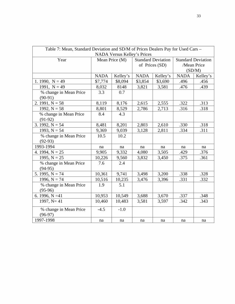
Table 7 shows the cross sectional mean, standard deviation, and the ratio of the standarddeviation to the mean of prices starting with the adjacent years 1990-91. In the 1990 and1991 comparison the mean 1990 NADA used car price is $7,774 while the mean of theKelley’s prices is $8,094 for the 49 used cars included in the 20% sample. In 1991 themean NADA price is $8,032 while the mean Kelley’s price is $8,148. I had expectedKelley’s mean price to be higher than NADA mean price in all years since I expected theaverage mileage of the NADA (rental) cars would be higher and/or that the NADA carsare in poorer condition. On the other hand, the cars traded in by rental car companies mayhave been better maintained than the cars traded in by individuals. Surprisingly, the meanNADA price exceeds the mean Kelly’s price in eight of the twelve years.

NADA mean price increased by 3.3% between 1990 and 1991 while Kelley’s mean priceincreased by only 0.7%. This pattern of a more rapid growth in NADA prices is observedin many of the adjacent year comparisons. Looking at the results for the six paired yearsindicates the percentage change (in absolute value) in the mean price is smaller forKelley’s prices in 5 of the 6 comparisons (the exception is 95-96). It appears that Kelley’smean prices have been more stable over time than NADA prices. The NADA pricesappear to catch up and then surpass Kelley’s prices between 1990 and 1995 after whichKelley’s prices are abruptly adjusted upward in 1996. By 1997 there is only a smalldifference between the mean prices.

The last two columns of Table 7 compare the cross-sectional variability of the two pricesources in adjacent years. In the 1990-1991 comparison, Kelley’s prices have smallerstandard deviations and lower SD/M ratios. Looking at all twelve cross sections, Kelley’sprices have smaller standard deviations in 10 of the 12 years and smaller SD/M ratios in 8of the 12 cases. So, Kelley’s prices display greater absolute and relative cross sectionalstability than NADA prices.

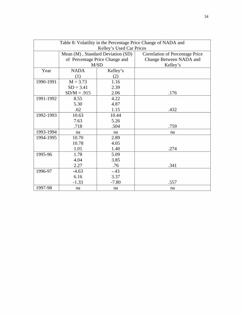
Table 8 compares the times-series variability in NADA and Kelley’s prices. The meanpercentage change, standard deviation and the standard deviation divided by the meanpercentage change are shown for both price sources for successive years. The lattermeasure has less meaning in the time series comparisons whenever the mean percentageprice change is close to zero. Between 1990 and 1991, the mean percentage price change(PPC) equals 3.73% for NADA prices and is 1.16% for Kelley’s prices. The standarddeviation is 3.41% for NADA prices and 2.39% for Kelley's prices. However, the

22

standard deviation relative to the mean percentage price change is higher for Kelley’sprices -- .915 versus 2.060 because the mean percentage price change for Kelley’s pricesis so low. The last column shows the simple correlation of the 1990-1991 percentageprice change between Kelley’s and NADA was only .176.

Looking at all six paired years, the standard deviation of the individual percentage pricechanges is smaller for Kelley’s prices in all 6 comparisons. These results suggest that thePPC’s of Kelley’s prices are less volatile. NADA prices are more variable betweenadjacent years. Turning to the simple correlation coefficients between the PPC’s ofKelley’s and NADA prices, they are quite variable ranging from a low of .176 for theprice changes between 1990-1991 to a high of .759 for price changes between 1992-1993. The average correlation coefficient is only .423. I had expected to observereasonably high coefficients between the percentage price changes from the two sources.Obviously, the two data sources often disagree with respect to the percentage pricechanges.

This pilot project was limited in scope because of time and data constraints.Consequently, it is perhaps wise not to make too much of the results. Clearly, more studyis needed before a final assessment can be reached. What does seem clear is that the crosssectional and time series volatility of Kelley’s prices appears smaller. So, there is someevidence that the source of the price information contributes to the observed “excess”volatility of used car prices. There is a clear hint in these results that price volatility mightbe lower if the BLS used a different price source.

An expanded project that included more years would have to be completed before adefinitive assessment can be reached. Such a project could determine if used car pricevolatility could be reduced by even more if the BLS used a weighted average of NADAand Kelley’s prices. The low correlation between NADA and Kelley’s price changessuggest that measured volatility would be lower if a weighted average of the pricechanges was adopted. In addition, such an expanded study should investigate quarterlyused car percentage price changes to determine if similar results are found when thequarterly Kelley’s prices are compared to the NADA prices. Another area to investigateis whether the inclusion of still other secondary sources might reduce volatility by evenmore.

VI. Testing the Quality Adjustment Assumption

The used car price index measures the mean price change of used cars after adjustingused car prices for any year to year quality change. Currently, the BLS adjusts used carprices for quality change by using the new car quality adjustment factor (percentage), asoriginally supplied to the BLS by manufacturers but modified by the BLS, to adjust usedcars prices for any quality change as manufacturers introduce improved cars. For usedcars, BLS applies this same new car quality adjustment factor as the car ages. Forexample, if quality improvements raise the cost of producing a new car by 1% from the

23

previous year’s model, the BLS assumes that the used car price of the model will also behigher by 1% from the previous year’s model because of the quality improvements as thecar ages. In other words, this quality adjustment procedure assumes that the qualityadjustment percentage is independent of the age of the car.

Two assumptions of the BLS quality change adjustment can be tested. First, pricesquoted in the used car market reflect the value consumers place on quality change. Usedcar prices for a given model in successive years can be used to determine if the measuredpercentage quality factor has a significant effect on used car prices. Second, the price of aused car of a given age that had a quality change of k% when new can be compared to theprice of the previous year’s model (of the same age) that does not have the k% addedquality improvements. For example, assume that a new car introduced at the end of yeart-2 had a k% quality improvement factor when new. At the end of year t this car is twoyears old and its used car price is P 2

t . This price can be expected to exceed the used car

price of two-year-old car of the same model in year t-1, P2

1−t , if the used car market

values the k% quality improvement either partially or fully. Similarly, in the next year theoriginal car will be three years old and its price P 3

1+t can be expected to exceed the price

of a three-year-old car in year t P 3t if the k% quality improvement is valued in the used

car market. By similar reasoning, the prices of similar aged cars in successive years canbe compared as the same two cars age through time.

A regression test of the independence hypothesis can be made by regressing the priceratio in successive years for a given age of car on the observed quality adjustment factorand dummy variables for the age of car and for year effects. Such a regression wouldinvolve a pooled cross sectional- time series analysis. Regression estimates are providedfor the following regression equation

(P it /P i

t 1− -1)100

..........)100)(( 955944933922911665544330 DbDbDbDbDbQAaAaAaAaa it ++++++++++=

where the subscript for model is suppressed. A is a dummy variable that equals one if thecar is two years old or three years old, etc. as the case may be and D is dummy variableequal to 1 if the year is 1991 etc., as the case may be. i

tQ denotes the quality adjustment

factor for the car when new. The dependent variable is the percentage price change of amodel of age i in year t compared to the price of the same model and same age car in yeart – 1. The percentage price change is assumed to be proportional to 100 + the percentagequality improvement factor. If the coefficient a 0 equals 1, the percentage price ratio

increases by the percentage quality improvement factor. If it is zero, the used car marketcompletely ignores the percentage quality improvement factor. Age of car is interactedwith the percentage quality improvement variable to determine how the percentage pricechange varies with the percentage quality improvement factor as the model ages. Theindependence hypothesis asserts that the coefficients a 3 ,…, a6 are equal to zero The

24

equation includes year effects that would account for stronger or weaker years for theused car market that would cause prices to rise or fall relative to the previous year.

Before looking at the regression results, it is instructive to look at some summarymeasures. A little less than eighty-four percent of the observations are for two and threeyear old cars. So, most of the observations are for younger used cars. The mean of thepercentage price change for NADA prices is 104.0 and the standard deviation is 8.20.The mean of the percentage quality improvement factor is 100.9 but the standarddeviation is only 1.40. These summary statistics show that there is considerably morevariability in the percentage price ratio than in the quality improvement factor. Hence, thepercentage improvement factor is not likely to be an important factor in explaining thepercentage price change. On the other hand, the results of the previous section suggestthat year effects will be important determinants of the percentage price change.

Columns 1 and 2 of Table 9 confirm these conjectures. Regression results for NADAprices are in column 1 while column 2 show results for Kelley’s prices. In both regressionequations the year effects dominate the effects of quality and age. After controlling foryear effects, the percentage quality factor is not even a significant determinant of thepercentage price ratio. Virtually all of the age interaction variables are insignificant aswell. Hence, the used car market appears to completely disregard the percentage qualityadjustment factor in establishing used car prices. These are interesting and in some wayssurprising results and cast some doubt on the BLS use of the quality improvement factorto adjust used car prices for quality change.

V. Summary and Conclusions

This paper has reexamined the used car price index to identify some of its strengths andweaknesses with the goal of suggesting some improvements. Among the findings are

• The failure to adjust used car prices for quality change between 1952 and 1987 helpsexplain why the used car price index rose more rapidly than the new car price index.Apparently, the quality improvement procedures adopted by the BLS in 1987effectively eliminated the discrepancy between the mean of new and used carpercentage price changes.

• Used car prices are among the more volatile in the CPI. The source of the price dataused by the BLS appears to contribute to the excess volatility of the used car priceindex. Preliminary evidence indicates that Kelley’s prices are less volatile thanNADA prices so that the used car price index would show less volatility if priceswere based on Kelley’s than NADA. Even if a better price data source is found, usedcar prices may still be more volatile. Another explanation for the volatility of used carprices is based on real factors, e.g., the supply curve is less elastic for used than newcars.

• The sample selection methods adopted by the BLS throughout the 1990s can beimproved. The sampling procedures of the BLS have underrepresented the morepopular domestic cars and the increasingly popular imports throughout the nineteennineties. Unless the BLS can improve the sampling techniques from the CES, it may

25

better to rely on the sales experience of new cars over the last six years to draw thesample.

• The under sampling of more popular cars is not due to buyers of the more popularcars being held longer by the original owners.

• The BLS adjustment of used car prices for quality improvement assumes that itsmeasure of quality improvements affects used car prices and has the same percentageeffect independent of the age of car. Regression results casts some doubt on theappropriateness of the quality adjustment since the percentage quality improvementvariable is not a significant determinant of the percentage price change betweenmodels one year apart.

26

Bibliography

Gordon, Robert, The Measurement of Durable Goods Prices, National Bureau ofEconomic Research, University of Chicago Press,1990.

Ohta,Makoto and Zvi Griliches, “Automobile Prices Revisited: Extensions on theHedonic Hypothesis,” Household Production and Consumption, ed. N. E.Terleckyj, NewYork, National Bureau of Economic Research, 1976, 325-90.

Kellar, Jeffrey, “New Methodology Reduces Importance of Used Cars in the RevisedCPI,” Monthly Labor Review, December 1988, 34-36.

Kelley Blue Book, Used Car Guide, January-June 2000, No. 1.

Pashigian, B. Peter, Brian Bowen and Eric Gould, “Fashion, Styling and the WithinSeason Decline in Automobile Prices,” Journal of Law and Economics, October 1995,281-310.

Porter, Robert H. and Peter Sattler, “Patterns of Trade In The Market For Used Durables:Theory and Evidence,” National Bureau of Economic Research, Inc., Working Paper7149, May 1999.

Stewart, Kenneth J. and Stephen B Reed, “Consumer Price Index Research Series UsingCurrent Methods, 1978-98” Monthly Labor Review, June 1999, 29-38.

27

Table 1: Volatility of Pt/Pt-1 for Selected Products and Sectors, Annual DataNew

Vehicles,1955-98

UsedVehicles,1955-98

Energy,1957-98

Food,1955-98

ConsumerPriceIndex(CPI),

1955-98

CPIexcludingEnergy,Food,

Shelter andUsed Cars,

1967-981. Mean (M) 1.026 1.047 1.042 1.042 1.043 1.0482. StandardDeviation (SD)

.0287 .0671 .0823 .0345 .0301 .0120

3. SD/Mean .0280 .0641 .0790 .0331 .0289 .01884. SD/Mean ofProduct Relative toSD/Mean of UsedVehicles

.44 1.00 1.23 .52 .45 .29

28

Table 2: Volatility of Pt/Pt-1 for Selected Sub-Periods, Annual DataNew

VehiclesUsed

VehiclesEnergy Food Consumer

PriceIndex(CPI)

CPIexcludingEnergy,Food,

Shelter andUsed Cars

1955 - 19751. Mean 1.017 1.041 1.042 1.039 1.037 1.0532. StandardDeviation

.0316 .0678 .0680 .0413 .0276 .0203

3. SD/Mean .0311 .0651 .0653 .0397 .0266 .01934. SD/MeanRelative toSD/Mean of UsedCars

.48 1.00 1.003 .61 .41 .30

1976 -19981. Mean 1.035 1.053 1.042 1.045 1.049 1.0462. StandardDeviation

.0227 .0675 .0945 .0273 .0318 .0195

3. SD/Mean .0219 .0641 .0907 .0261 .0303 .01874. SD/Mean ofProduct Relative toSD/Mean of UsedCars

.34 1.00 1.42 .41 .47 .29

1989-19981. Mean 1.021 1.026 1.015 1.031 1.033 1.0342. StandardDeviation

.0135 .0466 .0424 .0154 .0119 .0125

3. SD/Mean .0133 .0454 .0418 .0149 .0115 .01214. SD/Mean ofProduct Relative toSD/Mean of UsedCars

.29 1.00 .92 .33 .25 .27

29

Table 3: Seasonal Volatility of Monthly Price Index, (non-seasonally adjusted toseasonally adjusted price)

NewVehicles

UsedVehicles

Energy Food ConsumerPriceIndex(CPI)

CPIexcludingEnergy,Food,

Shelter andUsed Cars

1955-19981. Mean 1.000 1.000 1.001 .999 1.000 1.0002. StandardDeviation

.0116 .0187 .0115 .0039 .0016 .0022

3. SD/Mean .0116 .0187 .0115 .0039 .0016 .00224. SD/Mean ofProduct Relative toSD/Mean of UsedCars

.62 1.00 .61 .21 .09 .12

30

Table 4: Volatility of Monthly Prices (MPt/MPt-1 forSeasonally Adjusted Monthly Prices)

NewVehicles

UsedVehicles

Energy Food ConsumerPriceIndex(CPI)

CPIexcludingEnergy,Food,

Shelter andUsed Cars

1955-19981. Mean .220 .398 .319 .336 .345 .3912. StandardDeviation

.7676 1.4410 1.2643 .5468 .3044 .2146

3. SD/Mean 3.4868 3.3614 3.9659 1.6252 .8828 .54884. SD/MeanRelative of Productto SD/Mean ofUsed Cars

1.04 1.00 1.18 .48 .26 .16

1989-19981. Mean .162 .142 .096 .242 .256 .2592. StandardDeviation

.215 .618 1.403 .282 .169 .147

3. SD/Mean 1.32 4.36 14.67 1.16 .66 .574. SD/MeanRelative of Productto SD/Mean ofUsed Cars

.30 1.00 3.36 .27 .15 .13

31

Table 5: How Representativeness Is the BLS Used Car Sample?1990 1991 1992 1993 1994 1995 1996 1997 1998

*1. Number of BLSModels Among Top10 Best Selling Carsover the last fiveyears

150 182 192 230 269 239 231 280 217

2. Total Models inBLS Sample

746 697 719 735 979 961 987 1003 1210

3. Percentage of BLScars in Top 10 overthe last five years

20% 26% 27% 31% 27% 25% 23% 28% 18%

4. Combined MarketShare Percentage ofTop 10 Domestic &Imported Cars ofTotal DomesticallyProduced Sales

58 77 82 83 60 81 60 49 50

5. Combined MarketShare Percentage ofTop 10 Domestic andImported Cars ofTotal DomesticallyProduced plusImported Cars

37 44 47 48 41 51 43 38 39

6. Combined MarketShare Percentage ofTop 10 Domestic andImported Cars ofTotal DomesticallyProduced Cars andLight Trucks andImports.

23 26 26 26 23 26 23 21 21

Includes top 10 cars and trucks

32

Table 6: Pt/P t-1 for CPI and Hedonic Used and New Car Price IndexesPeriod Used Cars New Cars

CPI Hedonic CPI Hedonic1. 1953 –1983a. Meanb. Standard

Deviationc. Correlation

Coefficient

1.048.080

.675

1.037.086

1.026.035

.648

1.037.066

2. 1953-1974a. Meanb. Standard

Deviationc. Correlation

Coefficient

1.043.064

.661

1.004.064

1.014.031

.610

1.016.047

3. 1975-1983a. Meanb. Standard

Deviationc. Correlation

Coefficient

1.109.070

.378

1.105.085

1.060.020

.263

1.097.078

33

Table 7: Mean, Standard Deviation and SD/M of Prices Dealers Pay for Used Cars –NADA Versus Kelley’s Prices

Year Mean Price (M) Standard Deviationof Prices (SD)

Standard Deviation/Mean Price

(SD/M)NADA Kelley’s NADA Kelley’s NADA Kelley’s

1. 1990, N = 49 $7,774 $8,094 $3,854 $3,690 .496 .456 1991, N = 49 8,032 8148 3,821 3,581 .476 .439 % change in Mean Price

(90-91)3.3 0.7

2. 1991, N = 58 8,119 8,176 2,615 2,555 .322 .313 1992, N = 58 8,801 8,529 2,786 2,713 .316 .318 % change in Mean Price

(91-92)8.4 4.3

3. 1992, N = 54 8,481 8,201 2,803 2,610 .330 .318 1993, N = 54 9,369 9,039 3,128 2,811 .334 .311 % change in Mean Price

(92-93)10.5 10.2

1993-1994 na na na na na na4. 1994, N = 25 9,905 9,332 4,080 3,505 .429 .376 1995, N = 25 10,226 9,560 3,832 3,450 .375 .361

% change in Mean Price(94-95)

7.6 2.4

5. 1995, N = 74 10,361 9,741 3,498 3,200 .338 .328 1996, N = 74 10,516 10,235 3,476 3,396 .331 .332 % change in Mean Price

(95-96)1.9 5.1

6. 1996, N =41 10,953 10,549 3,688 3,670 .337 .348 1997, N= 41 10,460 10,483 3,581 3,597 .342 .343

% change in Mean Price(96-97)

-4.5 -1.0

1997-1998 na na na na na na

34

Table 8: Volatility in the Percentage Price Change of NADA andKelley’s Used Car Prices

Mean (M) , Standard Deviation (SD)of Percentage Price Change and

M/SD

Correlation of Percentage PriceChange Between NADA and

Kelley’sYear NADA

(1)Kelley’s

(2)1990-1991 M = 3.73

SD = 3.41SD/M = .915

1.162.392.06 .176

1991-1992 8.555.30.62

4.224.871.15 .432

1992-1993 10.637.63.718

10.445.26.504 .759

1993-1994 na na na1994-1995 10.70

10.781.01

2.894.051.40 .274

1995-96 1.784.042.27

5.093.85.76 .341

1996-97 -4.636.16-1.33

-.433.37-7.80 .557

1997-98 na na na

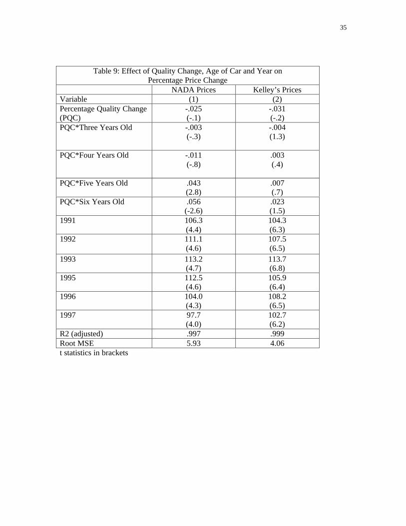
35

Table 9: Effect of Quality Change, Age of Car and Year onPercentage Price Change

NADA Prices Kelley’s PricesVariable (1) (2)Percentage Quality Change(PQC)

-.025(-.1)

-.031(-.2)

PQC*Three Years Old -.003(-.3)

-.004(1.3)

PQC*Four Years Old -.011(-.8)

.003(.4)

PQC*Five Years Old .043(2.8)

.007(.7)

PQC*Six Years Old .056(-2.6)

.023(1.5)

1991 106.3(4.4)

104.3(6.3)

1992 111.1(4.6)

107.5(6.5)

1993 113.2(4.7)

113.7(6.8)

1995 112.5(4.6)

105.9(6.4)

1996 104.0(4.3)

108.2(6.5)

1997 97.7(4.0)

102.7(6.2)

R2 (adjusted) .997 .999Root MSE 5.93 4.06t statistics in brackets

36

Footnotes

*Helpful comments and suggestions were received from John S. Greenlees, Tim Lafleurand Dennis Fixler. Bonifacius Pasaribu served ably as my research assistant. This studywas supported by the Bureau of Labor Statistics and by the Lynde and Harry Bradley,and the Sarah Scaife Foundations through grants to the George J. Stigler Center for theStudy of the Economy and the State, the University of Chicago.

i In personal correspondence John S. Greenlees notes that Stuart and Reed (MonthlyLabor Review) constructed a revised CPI-U series back to 1978 using current CPImethodology. In unpublished work the authors find their adjustments to the used car priceindex for quality improvements would have lowered the index by 0.6 percentage pointper year between 1978 and 1986.

ii If the 1998 sample is limited to just cars, 30% of the BLS cars account are in the top 10while the top 10 cars account for 39% of all domestically produced and imported cars. Ifthe sample is restricted to light trucks, 38% of the BLS trucks were in the top 10 sellinglight trucks while the top ten selling new light trucks represented 53% of all the lighttrucks sold.iii The formula can be modified to account for differences in the frequency of trades of thecar given that the original owner sells the car.iv The estimate of the fraction of non- Top10 cars that are traded in is derived from theequation

541.860.)454(.140. 2 =+ t

v For new cars, the hedonic price index exhibits more variability over the whole periodand grows faster by 1.1 percentage points with much of the difference occurring in the1975-1983 period. Unlike used cars, the difference between the mean growth rates fornew cars is modest from 1953-1974 suggesting the CPI adjustments for quality changesof new cars were more accurate than for used cars. As with used cars, the correlationbetween the CPI and hedonic indices falls drastically to only .263 in the 1975-1983period. As with used cars, the hedonic index has a larger standard deviation over thismore volatile interval.