Wo

rkin

g p

aper

sW

ork

ing

pap

ers

ng

pap

ers

M. Dolores Guilló, Chris Papageorgiou and Fidel Pérez-Sebastián

A unifi ed theory of structural changeadserie

WP-AD 2010-34

Los documentos de trabajo del Ivie ofrecen un avance de los resultados de las investigaciones económicas en curso, con objeto de generar un proceso de discusión previo a su remisión a las revistas científicas. Al publicar este documento de trabajo, el Ivie no asume responsabilidad sobre su contenido. Ivie working papers offer in advance the results of economic research under way in order to encourage a discussion process before sending them to scientific journals for their final publication. Ivie’s decision to publish this working paper does not imply any responsibility for its content. La Serie AD es continuadora de la labor iniciada por el Departamento de Fundamentos de Análisis Económico de la Universidad de Alicante en su colección “A DISCUSIÓN” y difunde trabajos de marcado contenido teórico. Esta serie es coordinada por Carmen Herrero. The AD series, coordinated by Carmen Herrero, is a continuation of the work initiated by the Department of Economic Analysis of the Universidad de Alicante in its collection “A DISCUSIÓN”, providing and distributing papers marked by their theoretical content. Todos los documentos de trabajo están disponibles de forma gratuita en la web del Ivie http://www.ivie.es, así como las instrucciones para los autores que desean publicar en nuestras series. Working papers can be downloaded free of charge from the Ivie website http://www.ivie.es, as well as the instructions for authors who are interested in publishing in our series. Edita / Published by: Instituto Valenciano de Investigaciones Económicas, S.A. Depósito Legal / Legal Deposit no.: V-41-2011 Impreso en España (enero 2011) / Printed in Spain (January 2011)

WP-AD 2010-34

A unified theory of structural change*

M. Dolores Guilló, Chris Papageorgiou and Fidel Pérez-Sebastián**

Abstract This paper uses dynamic general equilibrium and computational methods, inspired by the multi-sector growth model structure in Stephen Turnovsky’s previous and more recent work, to develop a theory that unifies two of the traditional explanations of structural change: sector-biased technical change and non-homothetic preferences. More specifically, we build a multisector overlapping generations growth model with endogenous technical-change and non-homothetic preferences based on an expanding-variety setup with two different R&D technologies; one for agriculture, and another for non-agriculture. Results give additional support to the biased technical-change hypothesis as an important determinant of the structural transformation. The paper also explores where this bias might come from. Our findings suggest that production-side specific factors, such as asymmetries in cross-sector knowledge spillovers could be behind it, and therefore be important to fully explain the process of structural change. Keywords: multi-sector growth model, structural change, agriculture and non-agriculture, R&D, directed innovation, hon-homothetic preferences. JEL Classification: O13, O14, O41. * We thank Santanu Chatterjee, Walt Fisher, Gerhard Sorger, Steven Turnovsky, and participants in the Workshop in Honor of Stephen J. Turnovsky May 2010, and the Society of Computational Economics session at the 2010 ASSA meeting in Atlanta for valuable comments. Financial support from Ministerio de Ciencia e Innovación and FEDER funds under project SEJ-2007-62656, and from Instituto Valenciano de Investigaciones Económicas is gratefully acknowledged. The views expressed in this study are the sole responsibility of the authors and should not be attributed to the International Monetary Fund, its Executive Board, or its management. ** M.D. Guilló & F. Pérez-Sebastian: University of Alicante. Contact author: fidel@merlin.fae.ua.es. C. Papageorgiou: International Monetary Fund 3

1 Introduction

Stephen Turnovsky’s graduate textbook Methods of Macroeconomic Dynamics made

a powerful mark on the field of macroeconomics by providing crucial building blocks

and useful applications of general equilibrium intertemporal dynamic macroeconomic

models. A notable offspring of such dynamics methods is a class of models employing

multi-sectoral dynamics in a long-run growth context, also developed by Turnovsky

(and coauthors; including, among may others, Fisher and Turnovsky, 1998; Eicher

and Turnovsky 1999a,b, 2001; Alvarez-Cuadrado, Monteiro and Turnovsky, 2004;

and Turnovsky, 2004), which has been the cornerstone of an entire research agenda

which to this date is vibrant and keeps branching out to new applications of macro-

economics.

This paper uses dynamic general equilibrium and computational methods that we

first discovered as junior assistant professors studying Turnovsky’s book and extends

our earlier work (Papageorgiou and Perez-Sebastian, 2004; 2006; 2007) inspired by

the multi-sector growth model structure in Turnovsky’s previous and more recent

work. More specifically, the goal of this paper is to construct a model that can unify

two of the traditional explanations of the structural transformation; namely sector-

biased technical change pioneered by Ngai and Pissarides (2007), and non-homothetic

preferences pioneered by Konsamut et al. (2001). The importance of integrating both

approaches is defended and left to future research by, for example, Acemoglu (2008).

A well-documented feature of modern growth commonly called structural change

or structural transformation is the decline of agriculture and the rise of services.1

Structural transformation has been studied extensively, resulting in two prominent

albeit divergent theories.2 The first one is based on consumer non-homothetic prefer-

ences pioneered by Konsamut, Rebelo and Xie (2001). The second builds on sector-

biased technical change and is represented by the influential contributions of Baumol

(1967) and Ngai and Pissarides (2007).

1This reallocation process has been documented by early pioneer contributions including Clark(1940), Kuznets (1957), and Chenery (1960).

2See e.g., Kuznets (1966) and Baumol (1967), Echevarria (1997), Parente et al. (2000), Caselliand Coleman (2001), and Strulik and Weisdorf (2008).

1

Konsamut, Rebelo and Xie (2001) were the first to present a model consistent with

both the Kaldor facts of constant growth rate, capital-output ratio, real rate of return

to capital, and input shares in national income, and the dynamics of sectoral labor

reallocation. These authors pioneered a model in which balanced growth is consistent

with structural change. These authors assumed a preference specification consistent

with the income elasticity of demand less than one for agricultural goods, equal to

one for manufacturing goods, and greater than one for services. Their additional

assumption of non-homothetic preferences was sufficient, for on otherwise standard

neoclassical model, to allow for structural change.

An alternative theory of structural change is based on the technological hypoth-

esis, proposed by Baumol (1967) and formalized by Ngai and Pissarides (2007) who

develop a formal framework that builds on the response of hours of work to the

uneven distribution of technological change across production sectors. They show

that if there are two sectors, one of them characterized by a larger total factor pro-

ductivity (TFP) growth, hours of work rises in the stagnant sector if the two goods

have a relatively large degree of complementarity; labor moves in the direction of the

progressive sector otherwise.

An important conclusion from the above literature is that biased technical change

has more weight on the explanation of the structural transformation than non-

homothetic preferences (see Ngai and Pissarides 2007, and Buera and Kaboski 2009).3

In this paper, we examine whether a more general approach with endogenous inno-

vation can encompass both of these influential theories of structural transformation,

and whether the conclusion holds in it.

In particular, we first ask whether the sector-biased technical change hypothesis

can follow from the non-homothetic preferences hypothesis. We examine the idea that

freeing labor from agriculture to feed other economic sectors might require a larger

total factor productivity (TFP) growth in agriculture; and that, as a consequence,

biased TFP growth could be an endogenous response to the non-homotheticity of the

3 Iscan (2010) presents quantitative results that suggest that non-homothetic preferences had alarger weight in the structural transformation in the early stages of the process, but that in the last70 years the main engine has been the technological biased. In Iscan’s model, technical change isexogenous.

2

utility function. Second, the paper searches for features of technological change that

can be responsible for the observed evolution of sectoral TFP.

In order to accomplish these goals, we build a multisector overlapping-generations

model of endogenous technical-change and economic growth. The production side of

the economy feeds from Romer (1990) and Jones (1995). The setup shows expanding-

varieties of intermediate goods that are designed using sector-specific R&D technolo-

gies. Production is disaggregated into two activities: agriculture, and non-agriculture.

Preferences are non-homothetic. We formalize the notion that inventors decide the

kind of technological improvements that they create. The paper is then also related

to the literature on directed technical change such as Acemoglu (2002, 2003). But

unlike these papers, we focus on ideas directed to different sectors instead of different

inputs.

A setup in which R&D technologies are symmetric across sectors is first consid-

ered. Results imply that the sector-biased technical change hypothesis can not follow

from non-homothetic preferences only, because the latter hypothesis generates both

larger TFP growth and labor inflows in the same sector, irrespective of the elasticity

of substitution between final goods. To generate reasonable dynamics, the long-run

value of TFP in agriculture needs to be larger than in other sectors. This is prevented

in our base model by the lower weight of agricultural-goods consumption in the utility

function. We then modify the R&D technologies to consider that agriculture benefits

from cross-sector knowledge spillovers. The resulting model predictions are now able

to reproduce the main patterns of TFP growth observed in the data.

The rest of the paper is organized as follows. Section 2 introduces the basic

model. Its predictions are analyzed in section 3. Section 4 presents results in the

case where the R&D technologies allow for cross-sector knowledge spillovers. Section

5 concludes.

3

2 The Model

2.1 Households

We consider an economy composed of overlapping generations of individuals. The size

of generation t is Lt, and grows exogenously at rate n. Individuals have preferences

over consumption of agricultural and non-agricultural goods. They are endowed with

one unit of labor when young that is inelastically supplied to the production activities.

For simplicity, we assume that consumption only occurs in the second period of

life, thus abstracting from consumption/saving decisions.4 At time t, a representative

consumer is solving the following problem:

max

⎧⎪⎨⎪⎩v(cat+1, cnt+1) =

⎡⎣Xi=a,n,

γi(cit+1 − c̄i)(ε−1)/ε

⎤⎦ε/(ε−1)⎫⎪⎬⎪⎭ ,

subject to

Pat+1cat+1 + cnt+1 = (1 + rt+1)wt;

where ε ∈ (0,∞); cat and cnt are consumption at date t of the agricultural and non-

agricultural products, respectively;5 r and w are the rental rates of capital and labor;

Pat is the price of agricultural goods; γa + γn = 1; finally, c̄i represents a minimum

subsistence-consumption level if positive, or a minimum endowment level if negative.

All prices in the model are expressed in units of the non-agricultural goods. The

right-hand side of the budget constrain reflects equality between interest rate and

the return to capital.

The first-order conditions to this problem provide the optimal weights in the

consumption bundle as follows:µPatγa

¶ε

(cat − c̄a) =

µ1

γn

¶ε

(cnt − c̄n).

4This should not have any impact on our results because saving only affects the total amount ofcapital, whereas our findings are driven by differences in the allocation of resources between the twosectors. Capital is not an important determinant of these differences given our assumption that theelasticity of capital is the same in the agriculture and non-agriculture production functions.

5Having three sectors such as agriculture, manufacturing, and services, instead of two, wouldcomplicate matters without adding a significant change to the basic message of the paper.

4

A larger weight in the utility function or a lower price contribute to increase demand

for that good.

2.2 Final-good production

A large number of firms produce goods using labor and capital, while each firm pro-

duces output Yit only in one sector i, with i ∈ {a, n}. At date t, capital employed is

composed of a mass Ait of differentiated producer durables. The production technol-

ogy is given by:

Yit = L1−αit

Z Ait

0[xit(z)]

α dz; (1)

where xit(z) and Lit are the amounts of equipment type z and labor employed by

sector i in period t.

Firms choose the amount of each type of capital good that they want to buy, and

the amount of labor that they want to hire so as to maximize profits. They solve the

following problem:

max{xit(z),Lit}

½PitL

1−αit

Z Ait

0[xit(z)]

α dz −Z Ait

0pit(z)xit(z) dz − wt Lit

¾;

where pit(z) is the price of durable good type z specific to sector i.

Solving this problem obtains the inverse demand functions:

xit(z) =

µαPitpit(z)

¶1/(1−α)Lit, (2)

Lit = (1− α)PitYitwt

. (3)

2.3 Intermediate-goods production

Technology (1) employs different types of capital goods. The manufacturing process of

these goods requires investing raw capital coming from saved manufacturing output.

We adopt the simplest technology to manufacture capital products: one unit of capital

can be converted at no cost into one unit of any variety of intermediate goods. Firms

that produce the varieties hold exclusive property rights on the designs, which allows

5

them to practice monopoly pricing. We assume that these property rights expire in

one generation.6 Capital also depreciates fully after one generation.

The problem of a firm that produces variety j for sector i is:

maxxit(j)

[pit(j)− (1 + rt)]xit(j);

where pit(j) is given by the inverse demand function of intermediate good xit(j),

that is, by equation (2). The monopolist charges a markup η equal to the inverse of

the elasticity of substitution between intermediate goods in final output production.

More specifically, the optimal decision, standard in the literature, is given by:

pit(j) = ηi(1 + rt) = pit, with ηi =1

α= η, ∀j. (4)

Since the price is the same for all varieties of intermediate goods, and they enter

symmetrically in final-good production, the amount demanded for each of them will

also be the same, xi(j) = xi ∀j. Profits then equal:

πit(j) = (η − 1) (1 + rt)xit = πit, also ∀j; (5)

2.4 R&D sector

Under the assumption of free entry into the R&D activity, there is a continuum of

firms that invest in deliberate R&D effort directed to create sector-specific varieties

of intermediate goods. These firms rent labor supplied by young individuals at the

beginning of period t. Researchers benefit from the existing knowledge base Ait

to prospect for new designs. The total number of ideas specific to sector i, with

i = {a, n}, that the R&D activity delivers by the end of the period is given by

Ait+1 = μAφitL

λ−1Ait

LAit ; (6)

where LAit is the number of workers employed in R&D directed to sector i.

There are several features of this R&D specification that are worth emphasizing.

First, the LHS is not written in increments, as most of the literature does, but in

levels. This is, however, consistent with the idea that technological levels can not6 If one generation is 30 years. This implies a depreciation rate of ideas of about 10%, figure

consistent with the evidence provided by Caballero and Jaffe (1993).

6

decrease. The reason is that, even though innovations can not depreciate, they can

become obsolete. This is what occurs every single period in our model. In particular,

as in Jones and Williams (2000), we assume that new generations of inventions come

in packages. A package is composed of both upgrades of old capital designs and

completely new ones. The key is that the whole new vintage or package of ideas

(Ait+1) has to be adopted together, which displaces the old one (Ait).

Under the above assumption, expression (6) is correct as long as Ait+1 ≥ Ait.

This always true in our simulations. In addition, the adoption of the new package,

besides bringing technological upgrades, needs to be profitable — notice that producers

could continue using old designs purchased in perfectly competitive markets because

patents last for one period. The appendix shows that the new vintage will be adopted

if and only if the markup ηi charged by monopolists is below (Ait/Ait−1)(1−α)/α. For

the shake of simplicity, we do not impose this condition. However, as will become

clear later, this should not have any effect on the main results of the paper. The

reason being that the markup and the rate of technical change reinforce each other in

the same direction when the condition is binding. As a result, the main consequence

of a markup that followed TFP growth would be an amplification of the cross-sector

differences in TFP growth.

Second, returns to labor at the individual and aggregate levels differ. On the one

hand, investment displays constant returns at the individual level. On the other, the

term Lλ−1Ait

implies that researchers generate negative externalities to each other. This

can be a consequence of patent races for example. The result is that the R&D tech-

nology at the aggregate level shows diminishing returns (0 < λ < 1) to R&D effort.

More specifically, in the symmetric equilibrium in which firms end up, expression (6)

becomes:

Ait+1 = μAφitL

λAit

.

Finally, the R&D specification allows for intertemporal knowledge spillovers (0 <

φ < 1).

After coming up with new innovations, inventors obtain patents that are imme-

7

diately sold.7 Those that purchase them invest capital at the end of date t to build

producer-durable units that will be available for final-goods manufacturing at t + 1

at monopoly prices. The outcome of this entire process is that the firm that sells the

intermediate goods obtains an amount of profits equal to πit, given by expression (5).

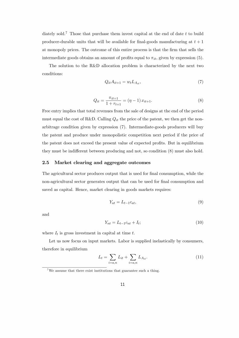
The solution to the R&D allocation problem is characterized by the next two

conditions:

QitAit+1 = wtLAit , (7)

Qit =πit+11 + rt+1

= (η − 1)xit+1. (8)

Free entry implies that total revenues from the sale of designs at the end of the period

must equal the cost of R&D. Calling Qit the price of the patent, we then get the non-

arbitrage condition given by expression (7). Intermediate-goods producers will buy

the patent and produce under monopolistic competition next period if the price of

the patent does not exceed the present value of expected profits. But in equilibrium

they must be indifferent between producing and not, so condition (8) must also hold.

2.5 Market clearing and aggregate outcomes

The agricultural sector produces output that is used for final consumption, while the

non-agricultural sector generates output that can be used for final consumption and

saved as capital. Hence, market clearing in goods markets requires:

Yat = Lt−1cat, (9)

and

Ynt = Lt−1cnt + It; (10)

where It is gross investment in capital at time t.

Let us now focus on input markets. Labor is supplied inelastically by consumers,

therefore in equilibrium

Lt =Xi=a,n

Lit +Xi=a,n

LAit . (11)

7We assume that there exist institutions that guarantee such a thing.

8

Saving in our model economy is entirely due to salary income, and is employed to

construct physical capital and finance the purchase of patents:

wtLt = Kt+1 +Xi=a,n

QitAit+1. (12)

In the last equality, Kt represents the aggregate capital stock in the economy at

time t. Since producer durables fully depreciate upon use, it follows that:

It−1 =Xi=a,n

∙Z Ait

0xit(z) dz

¸=Xi=a,n

Aitxit = Kt. (13)

In turn, the capital stock in sector i can be written as Kit =R Ait0 xit(z) dz = Aitxit.

Furthermore, given that prices and use of intermediate goods are the same within

both sectors, we can rewrite equation (1) at the aggregate level as:

Yit = (AitLit)1−αKα

it = Lit A1−αit kαit; (14)

where kit gives the capital labor ratio Kit/Lit in sector i at date t.

This expression, and optimality conditions (2)-(4) imply that:

1 + rt =α

ηPitA

1−αit kα−1it , (15)

wt = (1− α)PitA1−αit kαit. (16)

Then

kat = knt,

and

Pat =

µAnt

Aat

¶1−α.

Defining kt = Kt/Lt, it follows from (13) that:

(lat + lnt) kit = kt. (17)

From (7), (8) and (12), we get:

kt+1 (1 + n) (η − 1) = wt (lAat + lAnt) , (18)

9

In turn, equations (7), (8), (11), (12) and (18) deliver kit = ηkt. An implication of all

the above is that the ratio of the output shares equals the ratio of the labor shares:

Patyatlatyntlnt

=latlnt.

. (19)

2.6 The equation system

The following equations, along with (15) and (16), provide the system that charac-

terizes dynamics in this economy as a function of prices and predetermined stocks:µPatγa

¶ε

(cat − c̄a) =

µ1

γn

¶ε

(cnt − c̄n),

Ait+1 = μAφit [lAitLt]

λ ,

kt+1 (1 + n) + wt (lAat + lAnt) = wt,

Pat+1cat+1 + cnt+1 = (1 + rt+1)wt,

yatlat =cat1 + n

,

yntlnt =cnt1 + n

+ kt+1 (1 + n) ,

yit = A1−αit kαt lit,

lat + lnt + lAat + lAnt = 1,

lat+1lnt+1

lAnt

lAat

= 1,

kntkt= η;

where lit and lAit are the fractions of the labor force in the final goods and R&D of

sector i at date t, respectively.

The above system simplifies to:

Ait+1 = μAφit [lAntLt]

λ , (20)

Pat =

µAnt

Aat

¶1−α, (21)

(cnt − c̄n)Xi=a,n

P 1−εit

µγiγn

¶ε

+Xi=a,n

Pit c̄i = α2A1−αnt (ηkt)α (1 + n), (22)

10

kt+1 =α (1− α)wt

(1 + n), (23)

lat =P−εat

³γaγn

´ε £α2A1−αnt (kt/α)

α (1 + n)− c̄n¤+ c̄ah

1 + P 1−εat

³γaγn

´εiA1−αat (kt/α)

α (1 + n), (24)

lnt = α− lat, (25)

lAat =

µ1

α− 1¶lat+1, (26)

lAnt = (1− α)− lAat , (27)

Lt/Lt−1 = 1 + n; (28)

with kt, Ait, Lt being predetermined.

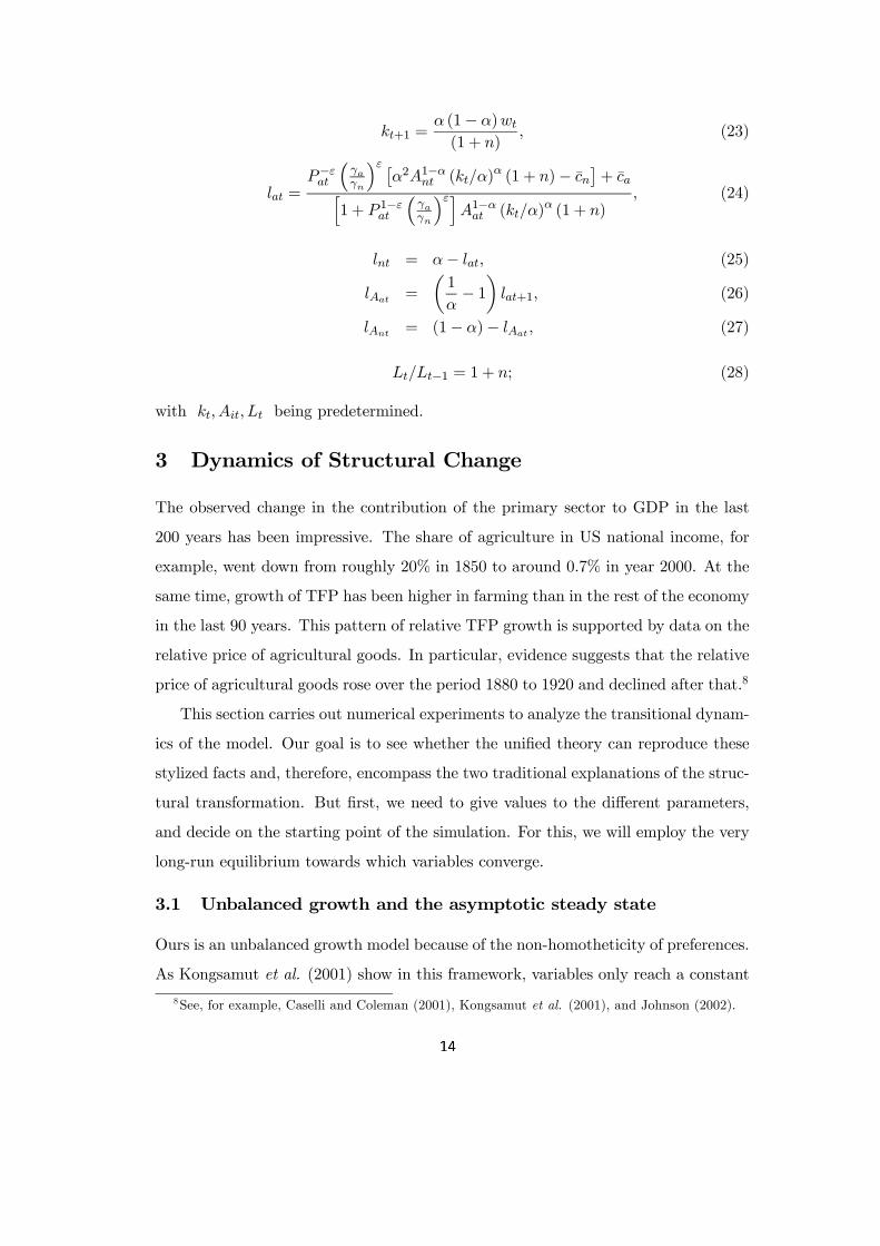
3 Dynamics of Structural Change

The observed change in the contribution of the primary sector to GDP in the last

200 years has been impressive. The share of agriculture in US national income, for

example, went down from roughly 20% in 1850 to around 0.7% in year 2000. At the

same time, growth of TFP has been higher in farming than in the rest of the economy

in the last 90 years. This pattern of relative TFP growth is supported by data on the

relative price of agricultural goods. In particular, evidence suggests that the relative

price of agricultural goods rose over the period 1880 to 1920 and declined after that.8

This section carries out numerical experiments to analyze the transitional dynam-

ics of the model. Our goal is to see whether the unified theory can reproduce these

stylized facts and, therefore, encompass the two traditional explanations of the struc-

tural transformation. But first, we need to give values to the different parameters,

and decide on the starting point of the simulation. For this, we will employ the very

long-run equilibrium towards which variables converge.

3.1 Unbalanced growth and the asymptotic steady state

Ours is an unbalanced growth model because of the non-homotheticity of preferences.

As Kongsamut et al. (2001) show in this framework, variables only reach a constant

8See, for example, Caselli and Coleman (2001), Kongsamut et al. (2001), and Johnson (2002).

11

growth rate in the particular case that c̄a(Pat/γa)ε = c̄n(1/γn)

ε. In all other scenarios,

variables approach and get infinitely close to the balanced-growth path associated

with the zero subsistence-consumption case.

When c̄a = c̄m = 0, per capita variables and wages grow at the same rate along

the balanced-growth path, and this rate equals the rate of technological change. The

rest of the variables, and in particular, the labor shares, the price of agricultural

goods, and the interest rate remain constant.

Specifically, let Gz be the gross growth rate of variable z, and eliminate the

time index to denote steady-state values. Clearing conditions (9)-(13) imply that

GYa = GcaGL, GYn = GcnGL = GK , and GLa = GLn = GLAa= GLAn = 1 + n.

Equations (20) and (21) imply that Pat remains constant at steady state because

GAa = GAn = (1 + n)λ/(1−φ).

Equation (14) then implies that GYi = GAi . Finally, given the output aggregate

Yt = PatYat + Ynt, we obtain that

Gy = (1 + n)λ/(1−φ); (29)

where y is per capita income.

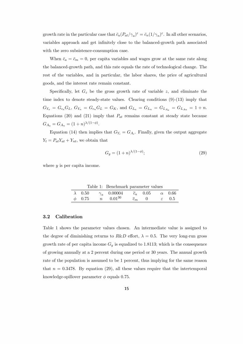
Table 1: Benchmark parameter values

λ 0.50 γa 0.00004 ca 0.05 α 0.66φ 0.75 n 0.0130 cm 0 ε 0.5

3.2 Calibration

Table 1 shows the parameter values chosen. An intermediate value is assigned to

the degree of diminishing returns to R&D effort, λ = 0.5. The very long-run gross

growth rate of per capita income Gy is equalized to 1.8113; which is the consequence

of growing annually at a 2 percent during one period or 30 years. The annual growth

rate of the population is assumed to be 1 percent, thus implying for the same reason

that n = 0.3478. By equation (29), all these values require that the intertemporal

knowledge-spillover parameter φ equals 0.75.

12

We think of capital broadly composed of physical as well as human capital com-

ponents, and therefore choose the capital share α = 0.66. The value of the elasticity

of substitution between consumption goods is taken from Buera and Kaboski (2009),

ε = 0.5. The minimum-consumption requirement c̄a is equalized to 0.05, and c̄n to

0. For the weights of the two types of consumption in the utility function, we use

the fact that agricultural GDP as a share of total GDP in 2002 was 0.7 percent, as

compiled by the Economic Research Service the USDA using data from the Bureau

of Economic Analysis. This share implies, in turn, by equations (9), (10), (19) and

(23) that γa = 0.00004.

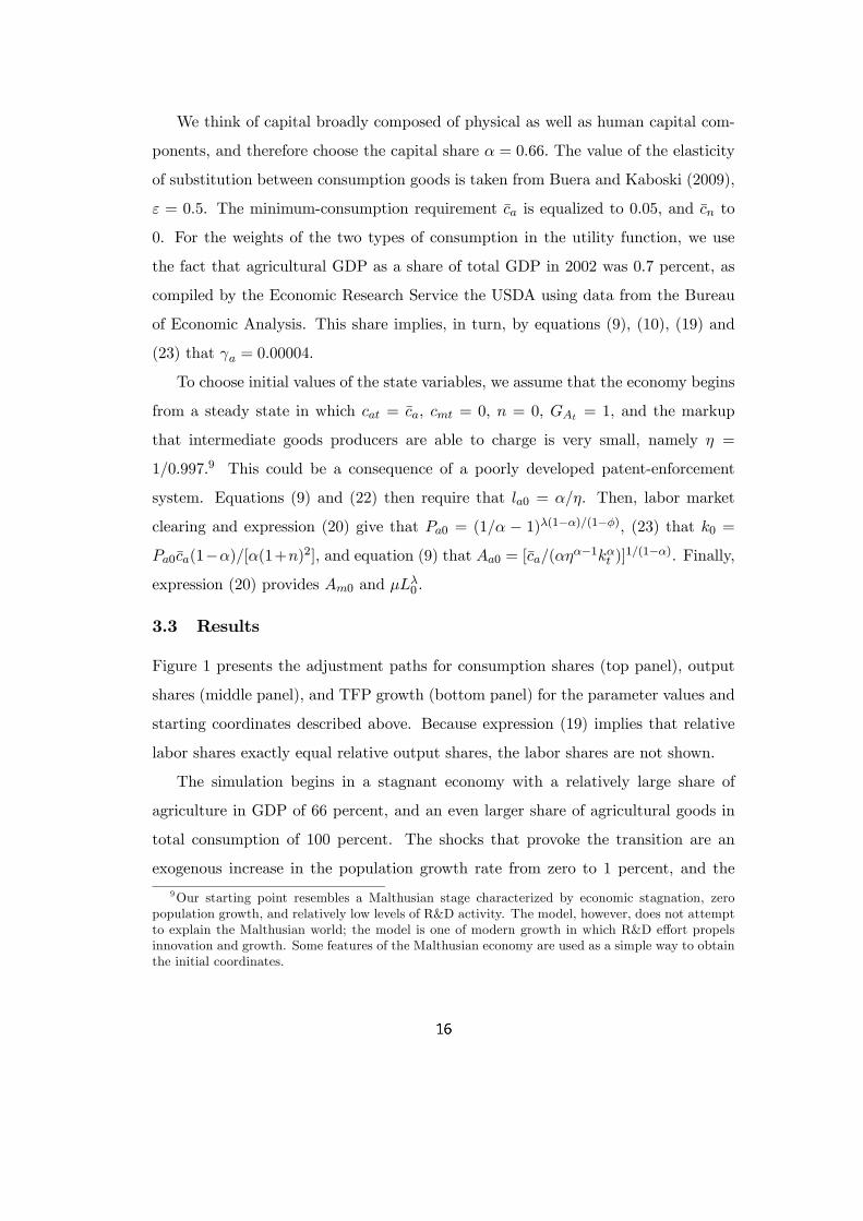
To choose initial values of the state variables, we assume that the economy begins

from a steady state in which cat = c̄a, cmt = 0, n = 0, GAt = 1, and the markup

that intermediate goods producers are able to charge is very small, namely η =

1/0.997.9 This could be a consequence of a poorly developed patent-enforcement

system. Equations (9) and (22) then require that la0 = α/η. Then, labor market

clearing and expression (20) give that Pa0 = (1/α − 1)λ(1−α)/(1−φ), (23) that k0 =

Pa0c̄a(1−α)/[α(1+n)2], and equation (9) that Aa0 = [c̄a/(αηα−1kαt )]

1/(1−α). Finally,

expression (20) provides Am0 and μLλ0 .

3.3 Results

Figure 1 presents the adjustment paths for consumption shares (top panel), output

shares (middle panel), and TFP growth (bottom panel) for the parameter values and

starting coordinates described above. Because expression (19) implies that relative

labor shares exactly equal relative output shares, the labor shares are not shown.

The simulation begins in a stagnant economy with a relatively large share of

agriculture in GDP of 66 percent, and an even larger share of agricultural goods in

total consumption of 100 percent. The shocks that provoke the transition are an

exogenous increase in the population growth rate from zero to 1 percent, and the

9Our starting point resembles a Malthusian stage characterized by economic stagnation, zeropopulation growth, and relatively low levels of R&D activity. The model, however, does not attemptto explain the Malthusian world; the model is one of modern growth in which R&D effort propelsinnovation and growth. Some features of the Malthusian economy are used as a simple way to obtainthe initial coordinates.

13

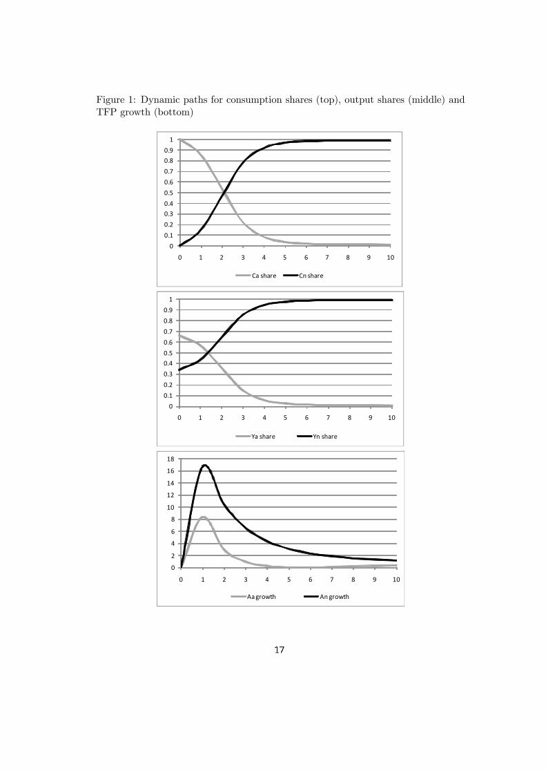
Figure 1: Dynamic paths for consumption shares (top), output shares (middle) andTFP growth (bottom)

00.10.20.30.40.50.60.70.80.91

0 1 2 3 4 5 6 7 8 9 10

Ca share Cn share

00.10.20.30.40.50.60.70.80.91

0 1 2 3 4 5 6 7 8 9 10

Ya share Yn share

0

2

4

6

8

10

12

14

16

18

0 1 2 3 4 5 6 7 8 9 10

Aa growth An growth

22

establishment of a strong paten system that allows firms charging their preferred

markup η = 1/α. This is what allows the growth of TFP.

At impact TFP growth achieves its largest values, and then progressively de-

creases. Higher population is able to generate more ideas, and output and consump-

tion shares start their transition towards an economy in which non-agriculture is the

most important activity. The transition is monotonic and relatively fast. The one

of output and consumption is almost finished after 7 generations, while that one of

TFP growth is still alive after 10.

The fact that the weight of the primary sector in total GDP declines and the

one of the non-agriculture rises as the economy develops is a consequence of the

non-homotheticity of preferences, and reproduces a main pattern of the structural

transformation. The evolution of TFP, however, is not consistent with the facts.

Non-agriculture TFP growth in the model economy is always the fastest, although

agriculture eventually converges to the productivity growth rates of the rest of the

economy. The predicted patterns do not depend on the value of c̄a nor on the value

of ε. In particular, changes in c̄a are fully neutral, whereas increases in the elasticity

of consumption-goods substitution only cause the convergence path to be slightly

smoother.

These findings suggest that non-homothetic preferences per se can not account

for the evolution of TFP. An alternative is that factors specific to the production

technology contribute to the structural transformation. Next we investigate whether

differences in the intensity of cross-sector knowledge spillovers can help reconcile our

theory with the facts.

4 Cross-Sector Knowledge Spillovers

Let us now consider that the agricultural sector benefits from spillovers coming from

the rest of the economy, in line with evidence provided, for example, by Johnson and

Evenson (1999). These authors argue that R&D spillovers are significant contributors

to agricultural productivity growth and that, in particular, sectors such as chemicals,

machinery, plastics, fabricated metals, and electric products contribute to it. The

14

agricultural R&D technology now takes the form:

Aat+1 = μAφatA

βntL

λAat; (30)

where β > 0 is the spillover parameter.

It is easy to show that the system of equations that characterize the model dynam-

ics remains the same with the exception of the new R&D technology that produces

ideas specific to the primary sector. In particular, the system is now composed of

conditions (20) with i = n, (21) to (28), and (30).

A difference compared to the previous scenario is that the price is no longer

approaching a constant value because it decreases with Aat. This feature of the

model implies that, with spillovers, variables approach a balanced growth path only

if ε = 1; but for ε = 0.5, no such reference exists. This lead us to maintaining the

calibrated parameters as in Table 1.

To determine the size of the spillover parameter, we look at Bernard and Jones

(1996, Table 1) who estimated TFP growth in the agricultural sector during the pe-

riod 1970-1987 to be double that of the industrial sector. To reproduce this difference

between agriculture and non-agriculture in our model after 10 periods, we assign a

value β = 0.214.

The computation of the initial values for the different state variables follows the

same logic as above. A steady-state equilibrium with cat = c̄a, cnt = 0, n = 0, and

η = 1/0.997 still exists, although showing that needs a bit more algebra. Equations

(9) and (22) again give la0 = α/η. In turn, combining expressions (10), (20), and

(23) obtains

k0 =

⎧⎨⎩"µ1− α

α

¶ λ1−φ ³ c̄a

α

´ 11−α

η

# 11+β/(1−φ)

(1− α)1

1−α

η

⎫⎬⎭1

1+ α1−α

11+β/(1−φ)

.

Knowing k0, we can easily recover An0, Aa0, and μLλ0 .

Results for consumption shares, output shares and TFP growth are presented in

the top, middle and bottom charts of Figure 2, respectively. Starting again from a

relatively large share of agriculture in GDP of 66 percent, an exogenous increase in

the population growth rate from zero to 1 percent, and in the markup from 1/0.997

15

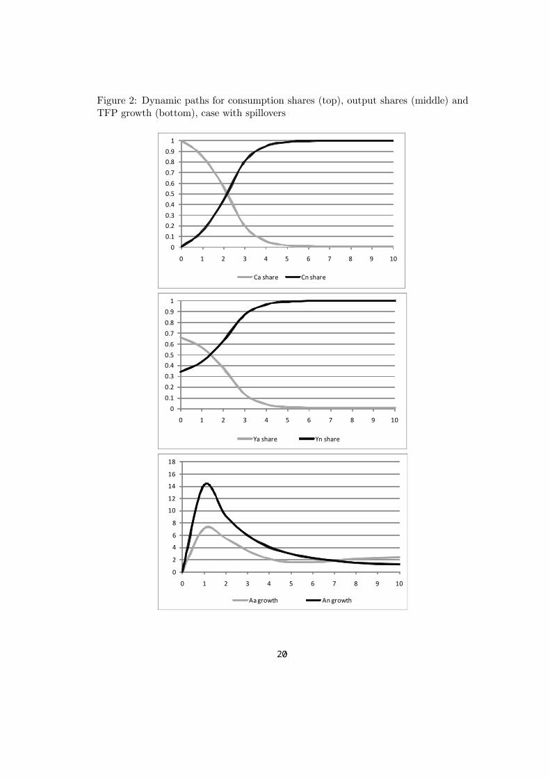
Figure 2: Dynamic paths for consumption shares (top), output shares (middle) andTFP growth (bottom), case with spillovers

00.10.20.30.40.50.60.70.80.91

0 1 2 3 4 5 6 7 8 9 10

Ca share Cn share

00.10.20.30.40.50.60.70.80.91

0 1 2 3 4 5 6 7 8 9 10

Ya share Yn share

0

2

4

6

8

10

12

14

16

18

0 1 2 3 4 5 6 7 8 9 10

Aa growth An growth

23

to 1/0.66 triggers structural transformation and the transition to positive economic

growth. The model shows again the highest TFP growth rates at impact, monoton-

ically decreasing after that point. As technology starts improving, the weight of

farming in total GDP declines, while the weight of non-agriculture rises. However

unlike in the case without spillovers, TFP growth in agriculture is below that for

non-agriculture only temporarily. After some periods, technological change in farm-

ing becomes the fastest. These trends are consistent with the main patterns observed

in the data.

Regarding comparative dynamics (not shown but available upon request), the

elasticity of substitution has an impact although relatively small. As ε rises, conver-

gence becomes a bit slower, and long-run differences in TFP growth between the two

sectors become larger. Subsistence consumption requirements, on the other hand,

have a significant effect when spillovers are present. In particular, the transition

becomes faster as c̄a rises, and differences in TFP growth between the activities get

larger.

5 Conclusion

Stephen Turnovsky’s work on multi-sector growth models has inspired a vibrant lit-

erature that is growing strong to this day. This paper extends this line of research

by using dynamic general equilibrium and computational methods, in an attempt to

develop a theory that unifies two of the traditional explanations of structural change:

sector-biased technical change, and non-homothetic preferences. More specifically,

we build a multisector overlapping-generations growth model that incorporates both

endogenous technical-change and non-homothetic preferences. Following a minimal-

ist approach, the model is based on an expanding-variety setup with only two types

of R&D technologies; one for agriculture, and the other for non-agriculture.

We first ask whether homothetic preferences can be the cause of the observed evo-

lution of sectoral TFP that represents the basic element of the sector-biased technical

change hypothesis. The analysis shows that this is not possible. Our baseline model,

in which cross-sector differences come from only consumer preferences, predicts that

16

agriculture is the most stagnant activity, a prediction not consistent with evidence.

We then ask a follow-up question: What kind of differences between sectors can

be responsible for TFP growth? When we consider knowledge spillovers from the

rest of the economy into agricultural R&D, the model is able to reproduce evolution

of consumption shares, output shares, and TFP growth in agriculture and in non-

agriculture consistent with evidence. We therefore conclude that production-side

specific factors, such as asymmetries in cross-sector knowledge spillovers, are needed

to reconcile the model with the main patterns observed in the data.

Although directed technical change can reconcile the two traditional theories of

structural transformation, our findings depart from the sector-biased technical change

hypothesis in one crucial way. The evolution of TFP does not need to be linked to

a relatively low elasticity of consumption-goods substitution to be consistent with

structural transformation. Endogenous technical change allows the agricultural sector

to shift from being the most stagnant to being the most vibrant sector, therefore

freeing labor to the rest of the economy, irrespective of the value of the elasticity of

substitution.

It is also interesting to note that our finding highlighting the need for cross-sector

variability and knowledge spillover effects is the main research topic in a related

literature that tries to explain cross-country growth variation by examining sectoral

resource (mis)allocations and their effects on aggregate TFP (see e.g. Restuccia and

Rogerson, 2008, and Hsieh and Klenow, 2009).

We conclude with a cautionary remark. Our analysis provides the simplest pos-

sible disaggregated setup to consider a unified theory of structural transformation.

More complicated multisector models are likely to be more successful in matching

the data. For example, we believe that further work could look at even more disag-

gregated setups, and search for sectoral asymmetries in manufacturing and services.

Recent emphasis on producing more and better quality data at the sectoral level

should provide further incentives to extend the analysis in this paper further.

17

A Restricted markup

All available designs become displaced by updates after one period. A final goodproducer at t can purchase the varieties Ait−1 at the marginal cost price or buy thenew cluster Ait of intermediate goods at markup price. The profits of a producer offinal goods in each case are, respectively,

Πoldit = xoldit

"(1 + rt)Ait−1

µ1

α− 1¶− wt

µ(1 + rt)

αPit

¶ 11−α#,

Πnewit = xnewit

"ηit (1 + rt)Ait

µ1

α− 1¶− wt

µηit (1 + rt)

αPit

¶ 11−α#.

It follows that the final good producer will adopt the new technology if and only if

ηit ≤µ

Ait

Ait−1

¶ 1−αα

.

18

References

[1] Acemoglu, D. (2002), “Directed Technical Change,” Review of Economic Studies69, 781-810.

[2] Acemoglu, D. (2003), “Labor- and Capital-Augmenting Technical Change,”Journal of European Economic Association 1, 1-37.

[3] Acemoglu, D. (2008), Introduction to Modern Economic Growth, Princeton Uni-versity Press.

[4] Alvarez-Cuadrado, F., G. Monteiro and S. Turnovsky. (2004), “Habit Formation,Catching up with the Joneses, and Economic Growth,” Journal of EconomicGrowth 9, 47-80.

[5] Baumol, W. (1967). “Macroeconomics of Unbalanced Growth: The Anatomy ofUrban Crisis,” American Economic Review 57, 415-426.

[6] Bernard B. and C.I. Jones. (1996), “Productivity Across Industries and Coun-tries: Time Series Theory and Evidence,” Review of Economics and Statistics78, 135-146.

[7] Buera, J.F. and J.P. Kaboski. (2009), “Can Traditional Theories of StructuralChange Fit the Data?” Journal of the European Economic Association 7, 469-477.

[8] Caballero, R.J. and A.B. Jaffe. (1993), “How High are the Giants’ Shoulders?,”in Olivier Blanchard and Stanley Fischer, eds., NBER Macroeconomics Annual,Cambridge, MA: MIT Press, 15-74.

[9] Caselli, F., and W.J. Coleman. (2001), “The U.S. Structural Transformation andRegional Convergence: A Reinterpretation” Journal of Political Economy 109,584-616.

[10] Chenery, H. (1960), “Patterns of Industrial Growth,” American Economic Re-view 50, 624-654.

[11] Chenery H. and T.N. Srinivasan. (1988), Handbook of Development Economics,Volume 1, Amsterdam: North Holland.

[12] Clark, C. (1940), The Conditions of Economic Progress (MacMillan: London).

[13] Echevarria, C. (1997), “Changes in Sectoral Composition Associated with Eco-nomic Growth,” International Economic Review 38, 431-452.

[14] Eicher, T. and S. Turnovsky. (1999a), “A Generalized Model of EconomicGrowth,” Economic Journal 109, 394-415.

19

[15] Eicher, T. and S. Turnovsky. (1999b), “Convergence in a Two-Sector Non-ScaleGrowth Model,” Journal of Economic Growth 4, 413-429.

[16] Eicher, T. and S. Turnovsky. (2001), “Transition Dynamics in Non-Scale Mod-els,” Journal of Economic Dynamics and Control 25, 85-113.

[17] Fisher, W.H. and S. Turnovsky. (1998), “Public Investment, Congestion, andPrivate Capital Accumulation,” Economic Journal 108, 399-413.

[18] Iscan, T. (2010), “How Much Can Engel’s Law and Baumol’s Disease Explainthe Rise of the Service Employment in the United States?” The B.E. Journal ofMacroeconomics 10, issue 1 (Contributions), article 26.

[19] Johnson, D.K.N. (2002), “Comment on ‘The U.S. Structural Transformation andRegional Convergence: A Reinterpretation’,” Journal of Political Economy 110,1414-1418.

[20] Johnson, D.K.N., and R.E. Evenson. (1999), “R&D Spillovers to Agriculture:Measurement and Application,” Contemporary Economic Policy 17, 432-456

[21] Jones, C.I. (1995), “R&D-Based Models of Economic Growth,” Journal of Po-litical Economy, 103:759-784.

[22] Jones, C.I, and J.C. Williams. (2000), “Too much of a good thing? The eco-nomics of investment in R&D,” Journal of Economic Growth, 65-85.

[23] Kongsamut, P., S. Rebelo and D. Xie. (2001), “Beyond Balanced Growth,” Re-view of Economic Studies 68, 869-882.

[24] Kuznets, S. (1957), “Quantitative Aspects of the Economic Growth of Nations;II,” Economic Development and Cultural Change 4, 3-11L.

[25] Kuznets, S. (1966). Modern Economic Growth: Rate, Structure, and Spread.New Haven, Conn.: Yale University Press.

[26] Ngai, L.R., and C.A. Pissarides. (2007), “Structural Change in a Multi-SectorModel of Growth,” American Economic Review 97, 429-443.

[27] Papageorgiou, C. and F. Perez-Sebastian. (2004), “Can Transition DynamicsExplain the International Output Data?” Macroeconomic Dynamics 8, 466-492.

[28] Papageorgiou, C. and F. Perez-Sebastian. (2006), “Dynamics in a Non-ScaleR&D Growth Model with Human Capital: Explaining the Japanese and SouthKorean Development Experiences,” Journal of Economic Dynamics and Control30, 901-930.

[29] Papageorgiou, C. and F. Perez-Sebastian. (2007), “Is the Asymptotic Speed ofConvergence a Good Proxy for the Transitional Growth Path?” Journal of MoneyCredit and Banking 39, 1-24.

20

[30] Parente, S., R. Rogerson, and R. Wright. (2000), “Homework In DevelopmentEconomics: Household Production and the Wealth of Nations,” Journal of Po-litical Economy 108, 680-688.

[31] Romer, P. (1990), “Endogenous Technological Change,” Journal of PoliticalEconomy, 98:S71-103.

[32] Strulik, H., and J. Weisdorf. (2008), “Population, food, and knowledge: a simpleunified growth theory,” Journal of Economic Growth 13(3), 195-216, September.

[33] Turnovsky, S. (2004), “The Transitional Dynamics of Fiscal Policy: Long-runCapital Accumulation and Growth,” Journal of Money, Credit, and Banking 36,883-910.

21

PUBLISHED ISSUES WP-AD 2009-01 “Does sex education influence sexual and reproductive behaviour of women? Evidence from

Mexico” P. Ortiz. February 2009. WP-AD 2009-02 “Expectations and forward risk premium in the Spanish power market” M.D. Furió, V. Meneu. February 2009. WP-AD 2009-03 “Solving the incomplete markets model with aggregate uncertainty using the Krusell-Smith

algorithm” L. Maliar, S. Maliar, F. Valli. February 2009. WP-AD 2009-04 “Employee types and endogenous organizational design: an experiment” A. Cunyat, R. Sloof. February 2009. WP-AD 2009-05 “Quality of life lost due to road crashes” P. Cubí. February 2009. WP-AD 2009-06 “The role of search frictions for output and inflation dynamics: a Bayesian assessment” M. Menner. March 2009. WP-AD 2009-07 “Factors affecting the schooling performance of secondary school pupils – the cost of high

unemployment and imperfect financial markets” L. Farré, C. Trentini. March 2009. WP-AD 2009-08 “Sexual orientation and household decision making. Same-sex couples’ balance of power and

labor supply choices” S. Oreffice. March 2009. WP-AD 2009-09 “Advertising and business cycle fluctuations”

B. Molinari, F. Turino. March 2009.

WP-AD 2009-10 “Education and selective vouchers” A. Piolatto. March 2009.

WP-AD 2009-11 “Does increasing parents’ schooling raise the schooling of the next generation? Evidence based on conditional second moments”

L. Farré, R. Klein, F. Vella. March 2009. WP-AD 2009-12 “Equality of opportunity and optimal effort decision under uncertainty” A. Calo-Blanco. April 2009. WP-AD 2009-13 “Policy announcements and welfare” V. Lepetyuk, C.A. Stoltenberg. May 2009. WP-AD 2009-14 “Plurality versus proportional electoral rule: study of voters’ representativeness” A. Piolatto. May 2009. WP-AD 2009-15 “Matching and network effects” M. Fafchamps, S. Goyal, M.J. van der Leij. May 2009. WP-AD 2009-16 “Generalizing the S-Gini family –some properties-” F.J. Goerlich, M.C. Lasso de la Vega, A.M. Urrutia. May 2009. WP-AD 2009-17 “Non-price competition, real rigidities and inflation dynamics” F. Turino. June 2009. WP-AD 2009-18 “Should we transfer resources from college to basic education?” M. Hidalgo-Hidalgo, I. Iturbe-Ormaetxe. July 2009.

* Please contact Ivie's Publications Department to obtain a list of publications previous to 2009.

WP-AD 2009-19 “Immigration, family responsibilities and the labor supply of skilled native women” L. Farré, L. González, F. Ortega. July 2009. WP-AD 2009-20 “Collusion, competition and piracy” F. Martínez-Sánchez. July 2009. WP-AD 2009-21 “Information and discrimination in the rental housing market: evidence from a field experiment” M. Bosch, M.A. Carnero, L. Farré. July 2009. WP-AD 2009-22 “Pricing executive stock options under employment shocks” J. Carmona, A. León, A. Vaello-Sebastiá. September 2009. WP-AD 2009-23 “Who moves up the career ladder? A model of gender differences in job promotions” L. Escriche, E. Pons. September 2009. WP-AD 2009-24 “Strategic truth and deception” P. Jindapon, C. Oyarzun. September 2009. WP-AD 2009-25 “Do social networks prevent bank runs? H.J. Kiss, I. Rodríguez-Lara, A. Rosa-García. October 2009. WP-AD 2009-26 “Mergers of retailers with limited selling capacity” R. Faulí-Oller. December 2009. WP-AD 2010-01 “Scaling methods for categorical self-assessed health measures” P. Cubí-Mollá. January 2010. WP-AD 2010-02 “Strong ties in a small world” M.J. van der Leij, S. Goyal. January 2010. WP-AD 2010-03 “Timing of protectionism”

A. Gómez-Galvarriato, C.L. Guerrero-Luchtenberg. January 2010. WP-AD 2010-04 “Some game-theoretic grounds for meeting people half-way” P.Gadea-Blanco, J.M. Jiménez-Gómez, M.C. Marco-Gil. February 2010. WP-AD 2010-05 “Sequential city growth: empirical evidence”

A. Cuberes. February 2010. WP-AD 2010-06 “Preferences, comparative advantage, and compensating wage differentials for job routinization” C. Quintana-Domeque. February 2010. WP-AD 2010-07 “The diffusion of Internet: a cross-country analysis” L. Andrés, D. Cuberes, M.A. Diouf, T. Serebrisky. February 2010. WP-AD 2010-08 “How endogenous is money? Evidence from a new microeconomic estimate” D. Cuberes, W.R. Dougan. February 2010. WP-AD 2010-09 “Trade liberalization in vertically related markets” R. Moner-Colonques, J.J. Sempere-Monerris, A. Urbano. February 2010. WP-AD 2010-10 “Tax evasion as a global game (TEGG) in the laboratory” M. Sánchez-Villalba. February 2010.

WP-AD 2010-11 “The effects of the tax system on education decisions and welfare” L.A. Viianto. March 2010. WP-AD 2010-12 “The pecuniary and non-pecuniary costs of job displacement. The risky job of getting

back to work” R. Leombruni, T. Razzolini, F. Serti. March 2010. WP-AD 2010-13 “Self-interest and justice principles”

I. Rodríguez-Lara, L. Moreno-Garrido. March 2010.

WP-AD 2010-14 “On spatial equilibria in a social interaction model” P. Mossay, P.M. Picard. March 2010. WP-AD 2010-15 “Noncooperative justifications for old bankruptcy rules” J.M. Jiménez-Gómez. March 2010. WP-AD 2010-16 “Anthropometry and socioeconomics in the couple: evidence from the PSID” S. Oreffice, C. Quintana-Domeque. April 2010. WP-AD 2010-17 “Differentiated social interactions in the US schooling race gap” L.J. Hall. April 2010. WP-AD 2010-18 “Things that make us different: analysis of variance in the use of time” J. González Chapela. April 2010. WP-AD 2010-19 “The role of program quality and publicly-owned platforms in the free to air broadcasting industry” M. González-Maestre, F. Martínez-Sánchez. June 2010. WP-AD 2010-20 “Direct pricing of retail payment methods: Norway vs. US” F. Callado, J. Hromcová, N. Utrero. June 2010. WP-AD 2010-21 “Sexual orientation and household savings. Do homosexual couples save more? B. Negrusa, S. Oreffice. June 2010. WP-AD 2010-22 “The interaction of minimum wage and severance payments in a frictional labor market: theory and estimation” C. Silva. June 2010. WP-AD 2010-23 “Fatter attraction: anthropometric and socioeconomic matching on the marriage market” P.A. Chiappori, S. Oreffice, C. Quintana-Domeque. June 2010. WP-AD 2010-24 “Consumption, liquidity and the cross-sectional variation of expected returns” E. Márquez, B. Nieto, G. Rubio. July 2010.

WP-AD 2010-25 “Limited memory can be beneficial for the evolution of cooperation” G. Horváth, J. Kovárík, F. Mengel. July 2010. WP-AD 2010-26 “Competition, product and process innovation: an empirical analysis” C.D. Santos. July 2010. WP-AD 2010-27 “A new prospect of additivity in bankruptcy problems” J. Alcalde, M.C. Marco-Gil, J.A. Silva. July 2010. WP-AD 2010-28 “Diseases, infection dynamics and development” S. Chakraborty, C. Papageorgiou, F. Pérez Sebastián. September 2010. WP-AD 2010-29 “Why people reach intermediate agreements? Axiomatic and strategic justification” J.M. Jiménez-Gómez. September 2010. WP-AD 2010-30 “Mobbing and workers’ health: an empirical analysis for Spain” M.A. Carnero, B. Martínez, R. Sánchez-Mangas. September 2010. WP-AD 2010-31 “Downstream mergers in a vertically differentiated unionized oligopoly”

B. Mesa-Sánchez. October 2010.

WP-AD 2010-32 “Endogenous quality choice under upstream market power” B. Mesa-Sánchez. November 2010. WP-AD 2010-33 “Itemised deductions: a device to reduce tax evasion” A. Piolatto. November 2010. WP-AD 2010-34 “A unified theory of structural change” M.D. Guilló, C. Papageorgiou, F. Pérez-Sebastián. December 2010.

IvieGuardia Civil, 22 - Esc. 2, 1º

46020 Valencia - SpainPhone: +34 963 190 050Fax: +34 963 190 055

Department of EconomicsUniversity of Alicante

Campus San Vicente del Raspeig03071 Alicante - Spain

Phone: +34 965 903 563Fax: +34 965 903 898

Website: www.ivie.esE-mail: publicaciones@ivie.es

adserie