Bloom Filter Performance on Graphics Engines Lin Ma Roger D. Chamberlain Jeremy D. Buhler Mark A. Franklin

Lin Ma, Roger D. Chamberlain, Jeremy D. Buhler, and Mark A. Franklin, “Bloom Filter Performance on Graphics Engines,” in Proc. of International Conference on Parallel Processing, September 2011, pp. 522-531. Dept. of Computer Science and Engineering Washington University in St. Louis

Bloom Filter Performance on Graphics Engines

Lin Ma1, Roger D. Chamberlain1,2, Jeremy D. Buhler1, Mark A. Franklin1,2

1Department of Computer Science and EngineeringWashington University in St. Louis

2BECS Technology, Inc., St. Louis, Missouri{lin.ma, roger, jbuhler, jbf}@wustl.edu

Abstract—Bloom filters are a probabilistic technique forlarge-scale set membership tests. They exhibit no false negativetest results but are susceptible to false positive results. They arewell-suited to both large sets and large numbers of membershiptests. We implement the Bloom filters present in an acceleratedversion of BLAST, a genome biosequence alignment applica-tion, on NVIDIA GPUs and develop an analytic performancemodel that helps potential users of Bloom filters to quantifythe inherent tradeoffs between throughput and false positiverates.

Keywords-NVIDIA GPU, Bloom Filter, BLAST

I. INTRODUCTION

A Bloom filter [2] is a probabilistic algorithm and data

structure for performing set membership tests. With a man-

ageable risk of producing false positives and no chance of

false negatives, Bloom filters are widely used for large-scale

data sets, including dictionaries [14], [16], databases [3],

[9], [23], networking applications [4], data speculation and

prefetching [18], and filtering of XML packets [8]. They

are an effective, space-efficient approach for testing mem-

bership.

In the field of computational bioinformatics, sequence

similarity search is a fundamental and crucial application

for comparing and revealing the possibly biologically mean-

ingful relationships between a given query sequence and

a database of known sequences. Sequences identified as

similar are hypothesized to be derived from the same ances-

tral sequence and therefore to share the same evolutionary

origin and function. A typical search is to systematically

compare a database of known sequences to an unknown

query sequence, identifying those members of the database

that exhibit a high degree of similarity to the query. Given

the rapid rate at which new genomic sequence data is being

produced, this search task has become progressively more

expensive, motivating the use of heuristics that reduce the

number of database sequences which must be compared in

detail to the query. These heuristics in turn have proved

amenable to acceleration on a variety of architectures.

The most widely used tool for similarity search is the

Basic Local Alignment Search Tool (BLAST) [1], a pro-

gram distributed by the National Center for Biological

Information (NCBI). This application has seen a number

of accelerated implementations, including TreeBLAST [10],

RC-BLAST [7], and Mercury BLAST [5], among others. All

of the above implementations use FPGAs as co-processors.

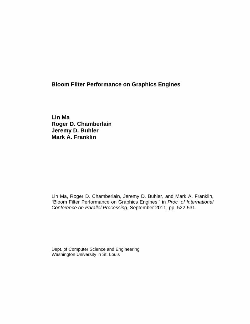
Figure 1 shows the computational pipeline for Mercury

BLAST. The original stage 1 of NCBI BLAST is here

further decomposed into two pipeline stages, stage 1a and

stage 1b. Stage 1, as a whole, is responsible for identifying

exact matches of substrings of length w (called w-mers)

between the pre-loaded query and the streaming database.

Mercury BLAST inserts a Bloom filter front end (stage 1a)

that discards a large fraction of the database prior to the

explicit table lookup used for match verification in stage 1b.

The remainder of the Mercury BLAST pipeline is described

in [5] and the implementation of the Bloom filters in stage 1a

on an FPGA is described in [11].

Figure 1. Mercury BLAST pipeline.

This work investigates the viability of using GPUs to

implement the Bloom filters used by stage 1a of Mercury

BLAST. We present an implementation of Bloom filters on

a GPU, specifically targeting the BLAST application. To

understand the performance achievable by such an imple-

mentation, we present an analytic performance model that

quantifies a multidimensional performance vector, including

sensitivity as well as throughput. We separate the param-

eters that inform this performance model into those that

are application-specific (set by the implementer/user of the

application) vs. architecture-specific (set by the manufac-

turer of the GPU, i.e. NVIDIA). This model is likely of

general use for predicting GPU Bloom filter performance in

applications other than BLAST (e.g., [22]).

Recently, several groups have implemented GPU-based

Bloom filters for applications including IP routing [15]

and error correction [13] [21]. These implementations have

distinct problem sizes that to a great extent determine

2011 International Conference on Parallel Processing

0190-3918/11 $26.00 © 2011 IEEE

DOI 10.1109/ICPP.2011.27

522

how to map the Bloom vector and computation onto dif-

ferent memory spaces, how to appropriately choose run-

time configurations, and how to program the kernel in an

application-specific efficient way. Some use texture memory

and/or constant memory for retaining the Bloom vector. Our

implementation relies on the on-chip shared memory, which

is significantly larger than the texture or constant caches.

Costa et al. designed and open-sourced a BloomGPU library

with flexiable APIs and automated tuning to offload Bloom

filter support to the GPU for targeted applications’ batch-

oriented usage pattern [6]. However, the paper only exploited

global memory rather than the much faster shared memory

which might potentially achieve a better performance. Liu et

al. [13] present DecGPU as the first parallel and distributed

error correction algorithm for high-throughput short reads

using a hybrid combination of CUDA and MPI. Extensive

comparison has been conducted between DecGPU and other

exsiting implementations. However, no detail about GPU

performance optimization is explicitly stated.

In addition to reporting on our Bloom filter implemen-

tation, we provide an analytic performance model that

quantifies the inherent tradeoffs that exist between two

performance indicators, sensitivity and throughput. There

exist several GPU performance models in the literature.

Liu et al. [12] present a general GPU performance model

classifying factors into three categories to establish the

relation between problem sizes and performance factors

and apply the model to a biosequence database scanning

application. However, that model does not look into the

fine-grained micro-architecture, including how choices of

numbers of threads and blocks influence the timing, and

how to map the computation onto a GPU architecture with

given specifications. Ryoo et al. [20] focus more on micro-

architecture and the kernel. They summarize five categories

of optimization mechanisms to prune the GPU program

optimization space by up to 98%. They do not, however,

consider multiple, conflicting performance indicators.

II. DESIGNING A BLOOM FILTER FOR MERCURY

BLAST USING A GPU

A. Parallel Bloom Filter Algorithm

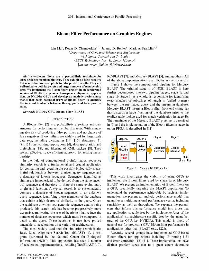
Bloom filters test set membership by performing multiple

hashes on a candidate element and checking a bit-vector,

called the Bloom vector, to see if the addresses resulting

from these hashes are all set to “true.” Figure 2 illustrates

this idea as applied to BLAST-style string matching. Fixed-

length candidate substrings of length w, or w-mers, from the

database are fed into k independent hash functions, and the

resulting addresses are checked against one or more Bloom

vectors loaded with portions of the query sequence.

Algorithm 1 gives pseudocode describing the Bloom

filter string-matching computation. With multiple candidate

elements, multiple sets, and multiple hash functions, this al-

gorithm provides many opportunities to exploit parallelism.

Figure 2. Parallel Bloom filters for detecting string matches of fixed lengthw between a query and a database.

In our design, long queries are split into multiple sub-queries of a given length n. Each sub-query is assigned an

individual Bloom vector of size m bits, and each w-mer

in the sub-query is considered to be an element of the set

for that vector. Each w-mer in the database is simultane-

ously checked for set membership in each sub-query. This

decomposition of a large set into multiple smaller sets (i.e.,

dividing a given query into a collection of sub-queries) is

common practice with Bloom filters, as the false positive

rate is a function of the number of elements in the set. A

larger number of sub-queries, each with fewer elements, can

lower the overall false positive rate.

Mercury BLAST, being FPGA-based, uses hash functions

hq from the H3 family [19], denoted as the set {hq|q ∈ Q},where Q represents the set of all possible i × j Boolean

matrices. q(k) is the bit string of the kth row of a given

matrix q ∈ Q. Correspondingly, x(k) is the kth bit of x,

the element that needs to be hashed. The hashing function

hq(x) is therefore defined as

hq(x) = x(1) · q(1)⊕ x(2) · q(2)⊕ · · · ⊕ x(i) · q(i) (1)

where · denotes the bit by bit AND operation and ⊕ the ex-

clusive OR operation. These bit-level linear transformations

are well-suited to hardware implementation. In this paper,

we do not investigate the use of alternative hash functions,

leaving this for future work.

B. GPU Implementation

The GPU used for this study is the NVIDIA GTX 480,

based on the Fermi architecture. It has 15 streaming multi-processors, each of which has 32 streaming processors or

processor cores (480 cores total) running at 1.4 GHz. The

GTX 480 has about 1.5 GB of off-chip global memory, while

each streaming multiprocessor has 48 KB of on-chip shared

memory.

Kernel computations on the GPU are organized around

thread blocks, which are independent from one another

and are distributed across the multiprocessors for execution.

523

Algorithm 1 Parallel Bloom Filters for BLAST

1: Input: query sequence

2: Input: database sequence

3: Output: stream of database w-mers

4: � Initialize Bloom vectors

5: for all sub-queries do6: initialize all-zero bitV ector of size m bits

7: for each w-mer in sub-query (denoted x) do8: for each hash function h do9: bitV ector[hashh(x)] = 1

10: end for11: end for12: end for13: � Perform membership tests

14: for all sub-queries do15: for each w-mer in database (denoted y) do16: for each hash function h do17: if bitV ector[hashh(y)] = 0 then18: discard this w-mer

19: break

20: end if21: end for22: if bitV ector[hashh(y)] = 1 for all h then23: output w-mer

24: end if25: end for26: end for

Each block consists of a number of threads, which are dis-

tributed across the processor cores within a multiprocessor.

Threads are scheduled in groups of 32, called warps. The

shared memory is shared across threads but is partitioned

across blocks. The registers within each core are not shared

but rather are partitioned across threads.

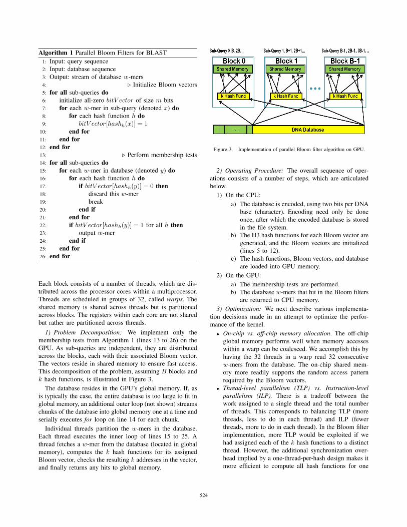
1) Problem Decomposition: We implement only the

membership tests from Algorithm 1 (lines 13 to 26) on the

GPU. As sub-queries are independent, they are distributed

across the blocks, each with their associated Bloom vector.

The vectors reside in shared memory to ensure fast access.

This decomposition of the problem, assuming B blocks and

k hash functions, is illustrated in Figure 3.

The database resides in the GPU’s global memory. If, as

is typically the case, the entire database is too large to fit in

global memory, an additional outer loop (not shown) streams

chunks of the database into global memory one at a time and

serially executes for loop on line 14 for each chunk.

Individual threads partition the w-mers in the database.

Each thread executes the inner loop of lines 15 to 25. A

thread fetches a w-mer from the database (located in global

memory), computes the k hash functions for its assigned

Bloom vector, checks the resulting k addresses in the vector,

and finally returns any hits to global memory.

Figure 3. Implementation of parallel Bloom filter algorithm on GPU.

2) Operating Procedure: The overall sequence of oper-

ations consists of a number of steps, which are articulated

below.

1) On the CPU:

a) The database is encoded, using two bits per DNA

base (character). Encoding need only be done

once, after which the encoded database is stored

in the file system.

b) The H3 hash functions for each Bloom vector are

generated, and the Bloom vectors are initialized

(lines 5 to 12).

c) The hash functions, Bloom vectors, and database

are loaded into GPU memory.

2) On the GPU:

a) The membership tests are performed.

b) The database w-mers that hit in the Bloom filters

are returned to CPU memory.

3) Optimization: We next describe various implementa-

tion decisions made in an attempt to optimize the perfor-

mance of the kernel.

• On-chip vs. off-chip memory allocation. The off-chip

global memory performs well when memory accesses

within a warp can be coalesced. We accomplish this by

having the 32 threads in a warp read 32 consecutive

w-mers from the database. The on-chip shared mem-

ory more readily supports the random access pattern

required by the Bloom vectors.

• Thread-level parallelism (TLP) vs. Instruction-levelparallelism (ILP). There is a tradeoff between the

work assigned to a single thread and the total number

of threads. This corresponds to balancing TLP (more

threads, less to do in each thread) and ILP (fewer

threads, more to do in each thread). In the Bloom filter

implementation, more TLP would be exploited if we

had assigned each of the k hash functions to a distinct

thread. However, the additional synchronization over-

head implied by a one-thread-per-hash design makes it

more efficient to compute all hash functions for one

524

w-mer in a single thread.

• Unrolling loops. As suggested in [20], we unrolled the

loop (lines 16 to 24) that iterates through the k hash

functions.

III. PERFORMANCE MODEL

It is common for the performance of an application to be

multidimensional. In the case of a Bloom filter, we have two

primary performance indicators of interest: throughput and

sensitivity. Throughput can be quantified for our BLAST

application as the number of database w-mers processed per

unit time, while sensitivity is quantified as the false positive

rate realized during set membership tests. These indicators

are influenced by a number of parameters, both application-

specific and architecture-specific. Those parameters that are

under control of the application developer are shown in

Table I, while those that are fixed by the particular choice

of GPU are shown in Table II. Additional variables used in

the model are shown in Table III.

Table IAPPLICATION-SPECIFIC PARAMETERS

Parameter Description

DB Database size (in w-mers)Q Query size (in w-mers)n Sub-query size (in w-mers)m Bloom vector size (in bits)k Number of hash functionsRT Number of registers per threadSB Shared memory used per block (in bytes)Br Requested number of blocks (total)Tr Requested number of threads per block

Table IIARCHITECTURE-SPECIFIC PARAMETERS

Parameter Description

MP Number of multiprocessorsS Shared memory per multiprocessor (in bytes)R Number of 32-bit registers per multiprocessorW Warp size (in number of threads)NW Min number of warpsBmax Max number of blocks (total)TmaxB Max number of threads per blockTmaxMP Max number of threads per multiprocessor

An analytic model that predicts throughput and sensitivity

can be used for a number of purposes. Such a model

can be used to tune the application so as to achieve

good performance in a predictive way without empirically

traversing a huge search space. In addition, multiobjective

optimization techniques can be employed to explore the

tradeoffs inherent in the performance vector. For example,

knowledge of the achievable downstream throughput in the

BLAST pipeline could be exploited to establish a throughput

Table IIIMODEL VARIABLES

Variable Description

SQ number of sub-queriesFP False positive countTP True positive count

FPR False positive rateBa Active number of blocks per multiprocessorA Peak performance indicator

Bopt Set of optimal numbers of blocks (total)Topt Set of optimal numbers of threads per blockTime Execution time (in seconds)Tput Throughput (in w-mers per second)

constraint and determine the best achievable sensitivity given

this constraint. Alternatively, one could optimize a weighted

combination of throughput and sensitivity. The analytic

model we present will support any of the above options.

A. Sensitivity

The sensitivity of a Bloom filter is quantified by the false

positive rate, FPR, or fraction of set membership tests that

return true when the element tested is not a member of

the set. Lower false positive rates reflect better Bloom filter

sensitivity.

Assuming element independence and good uniformity in

the hash functions, the false positive rate for a Bloom filter

is well modeled [4]. FPR is a function of the Bloom vector

size m, the number k of hash functions, and the number nof elements hashed into the vector:

FPR =

(1−

[1− 1

m

]kn)k

. (2)

According to the analytic model, FPR increases with nand decreases when m is increased. Increases in k can cause

FPR to move in either direction, depending upon the value

of the other two parameters.

In our usage of the Bloom filter within BLAST, both

k and m are design parameters under direct control of

the developer, while n is indirectly set by how the user

decomposes the complete query into sub-queries.

To investigate whether biosequence data sets are suffi-

ciently well-behaved so as to fit the theoretical expression for

FPR above, we tested our implementation using real DNA

sequences. Human chromosome 1 (250 Mbases) was used

as our query sequence, while human chromosome 22 (50

Mbases) was used as the database. During execution of our

GPU kernel, we counted false positives FP, false negatives

FN, and true positives TP. The empirical FPR for a database

of size DB is given by

FPR =FP

DB− TP. (3)

525

We confirmed empirically that FN = 0, as required by

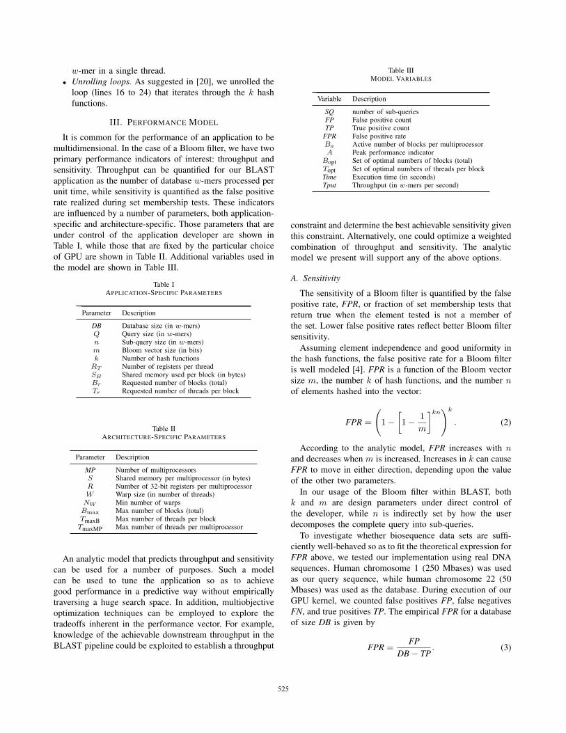
any correct implementation. Figures 4 and 5 compare the

theoretical and empirical FPR for a range of values of k,

m, and n. In both figures, lines indicate the theoretical FPR,

while mean measured FPR values over all sub-queries are

shown as points with associated 95% confidence intervals.

Figure 4 varies n for several values of m with a fixed k = 6,

while Figure 5 varies n for several values of k for a fixed

m = 256 Kbits. As expected, FPR grows with increasing nin all cases. For a given n, larger m leads to a smaller FPRand larger k can influence FPR either direction (depending

on the value of n).

Figure 4. Theoretical and empirical FPR (k = 6).

Figure 5. Theoretical and empirical FPR (m = 256 Kbits).

While the theoretical and empirical results are highly

similar, the theoretical quantities frequently lie outside the

confidence intervals of the empirical measurements. This is

due to the fact that DNA bases are, generally, not indepen-

dent of one another, but are in fact correlated. We explore

the magnitude of this discrepancy by plotting a histogram

of the relative error in Figure 6. While there are individual

measurements with relative error greater than 10%, they are

few, and the bulk of the errors are near zero.

Figure 6. Histogram of relative error between theoretical predictions andempirical measurements for FPR.

B. Throughput

We focus initially on the throughput of the kernel, defer-

ring the investigation of data movement to and from the GPU

until later. As there is significant interaction among the vari-

ous application-specific and architecture-specific parameters

that influence throughput, we will construct the model piece

by piece until all relevant parameters have been included.

The first two parameters to be investigated, the number of

hash functions k and the sub-query size n, influence both

sensitivity and throughput and so partly control the tradeoff

between them.1) Number of Hash Functions: Kernel execution time

should be linearly proportional to the number k of hash func-

tions used. This is because each thread computes the k hash

functions sequentially for each database w-mer assigned to

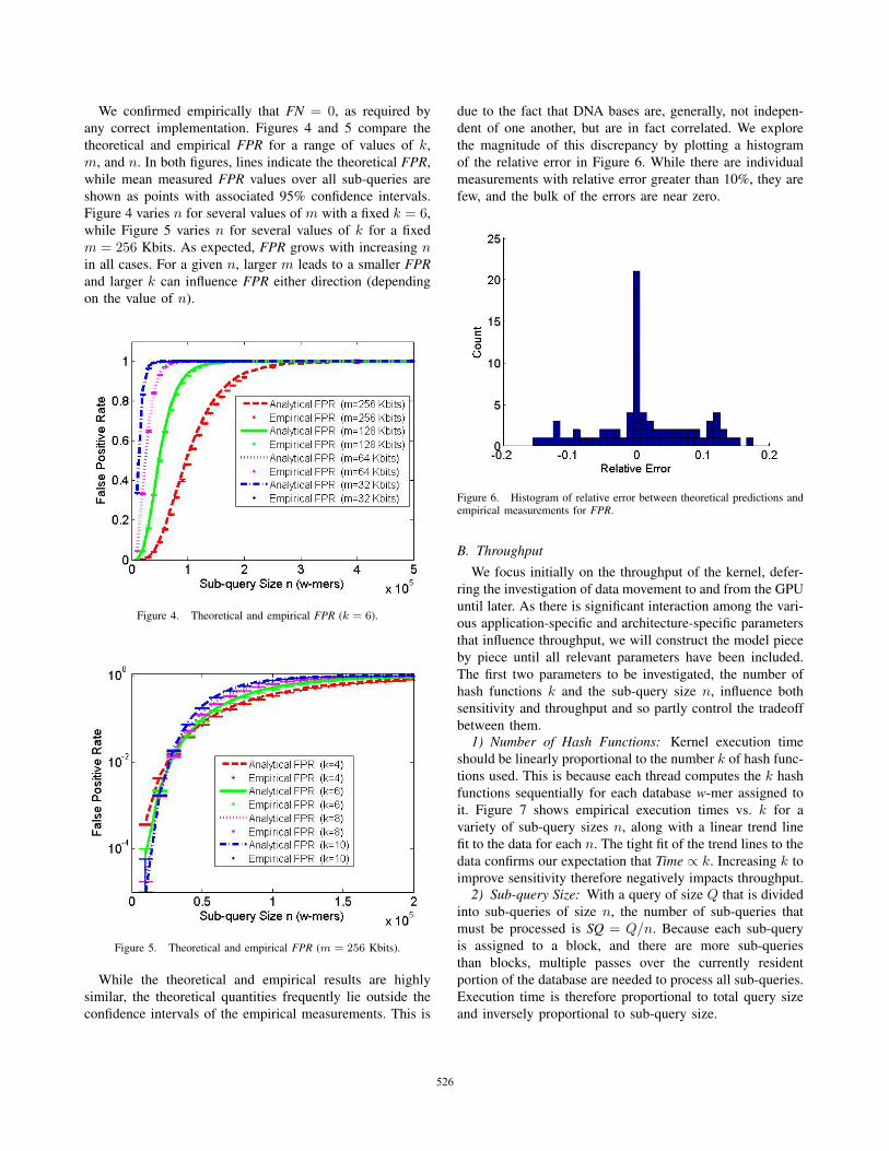
it. Figure 7 shows empirical execution times vs. k for a

variety of sub-query sizes n, along with a linear trend line

fit to the data for each n. The tight fit of the trend lines to the

data confirms our expectation that Time ∝ k. Increasing k to

improve sensitivity therefore negatively impacts throughput.2) Sub-query Size: With a query of size Q that is divided

into sub-queries of size n, the number of sub-queries that

must be processed is SQ = Q/n. Because each sub-query

is assigned to a block, and there are more sub-queries

than blocks, multiple passes over the currently resident

portion of the database are needed to process all sub-queries.

Execution time is therefore proportional to total query size

and inversely proportional to sub-query size.

526

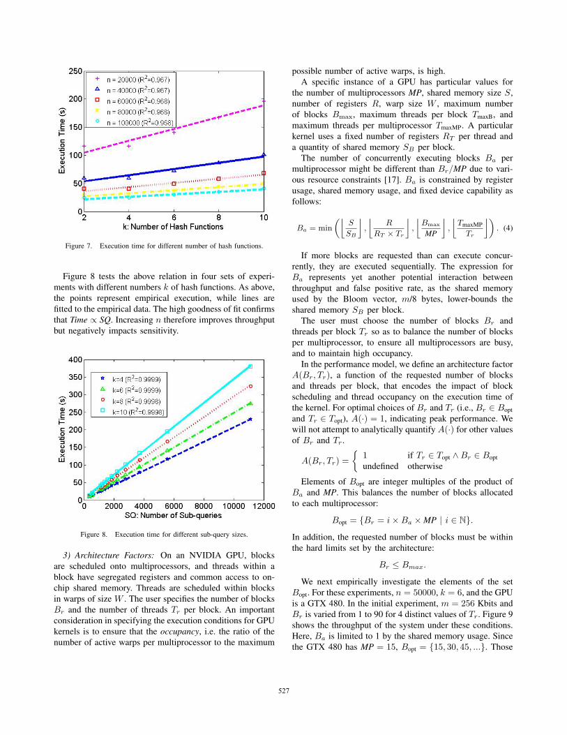
Figure 7. Execution time for different number of hash functions.

Figure 8 tests the above relation in four sets of experi-

ments with different numbers k of hash functions. As above,

the points represent empirical execution, while lines are

fitted to the empirical data. The high goodness of fit confirms

that Time ∝ SQ. Increasing n therefore improves throughput

but negatively impacts sensitivity.

Figure 8. Execution time for different sub-query sizes.

3) Architecture Factors: On an NVIDIA GPU, blocks

are scheduled onto multiprocessors, and threads within a

block have segregated registers and common access to on-

chip shared memory. Threads are scheduled within blocks

in warps of size W . The user specifies the number of blocks

Br and the number of threads Tr per block. An important

consideration in specifying the execution conditions for GPU

kernels is to ensure that the occupancy, i.e. the ratio of the

number of active warps per multiprocessor to the maximum

possible number of active warps, is high.

A specific instance of a GPU has particular values for

the number of multiprocessors MP, shared memory size S,

number of registers R, warp size W , maximum number

of blocks Bmax, maximum threads per block TmaxB, and

maximum threads per multiprocessor TmaxMP. A particular

kernel uses a fixed number of registers RT per thread and

a quantity of shared memory SB per block.

The number of concurrently executing blocks Ba per

multiprocessor might be different than Br/MP due to vari-

ous resource constraints [17]. Ba is constrained by register

usage, shared memory usage, and fixed device capability as

follows:

Ba = min

(⌊S

SB

⌋,

⌊R

RT × Tr

⌋,

⌊Bmax

MP

⌋,

⌊TmaxMP

Tr

⌋). (4)

If more blocks are requested than can execute concur-

rently, they are executed sequentially. The expression for

Ba represents yet another potential interaction between

throughput and false positive rate, as the shared memory

used by the Bloom vector, m/8 bytes, lower-bounds the

shared memory SB per block.

The user must choose the number of blocks Br and

threads per block Tr so as to balance the number of blocks

per multiprocessor, to ensure all multiprocessors are busy,

and to maintain high occupancy.

In the performance model, we define an architecture factor

A(Br, Tr), a function of the requested number of blocks

and threads per block, that encodes the impact of block

scheduling and thread occupancy on the execution time of

the kernel. For optimal choices of Br and Tr (i.e., Br ∈ Bopt

and Tr ∈ Topt), A(·) = 1, indicating peak performance. We

will not attempt to analytically quantify A(·) for other values

of Br and Tr.

A(Br, Tr) =

{1 if Tr ∈ Topt ∧Br ∈ Bopt

undefined otherwise

Elements of Bopt are integer multiples of the product of

Ba and MP. This balances the number of blocks allocated

to each multiprocessor:

Bopt = {Br = i×Ba ×MP | i ∈ N}.In addition, the requested number of blocks must be within

the hard limits set by the architecture:

Br ≤ Bmax.

We next empirically investigate the elements of the set

Bopt. For these experiments, n = 50000, k = 6, and the GPU

is a GTX 480. In the initial experiment, m = 256 Kbits and

Br is varied from 1 to 90 for 4 distinct values of Tr. Figure 9

shows the throughput of the system under these conditions.

Here, Ba is limited to 1 by the shared memory usage. Since

the GTX 480 has MP = 15, Bopt = {15, 30, 45, ...}. Those

527

values for Br are the peaks of the individual curves for

different Tr. On this plot and those that immediately follow,

we mark the peaks of the throughput curve with dark circles

so they can be readily identified. The throughput achieved

at these peaks is also shown with a horizontal dotted line.

Figure 9. Throughput vs. Br on GTX 480 (n = 50000, k = 6, m =256 Kbits).

Reducing shared memory usage per block from m =256 Kbits to 128 Kbits (see Figure 10), there may be up to

Ba = 2 active blocks on a single multiprocessor. However,

when Tr is large enough to deplete the register resources,

the limiting factor changes from shared memory to registers.

For example, in this case, when increasing Tr from 128 to

512, Ba stays at 2. As as result, throughput peaks every 30

blocks. However, when we further increase the threads per

block to 1024, local register resources only allow one active

block to launch per multiprocessor. Ba is reduced to 1, and

peaks now occur every 15 blocks.

The same behavior is observed when m = 64 Kbits and

m = 32 Kbits. In Figure 11, when using 128 threads, Ba =5; hence, Br reaches peak throughput at 75 and 150. 512

threads per block results in peaks being hit every 30 blocks.

Similarly, in Figure 12, the active block cycle for 128

threads per block is 120, given that Ba = 8. Hence, only

one peak is reached within the range of block counts tested.

Performance is consistent with our model even on a Tesla

C1060, which has more multiprocessors (MP = 30) than a

GTX 480. Our results are shown in Figure 13 and Figure 14.

We next turn our attention to Topt. [17] suggests that the

requested threads per block Tr should always be a multiple

of the warp size W , as the threads are scheduled in units of

a warp. It is recommended that at least NW warps should be

used to hide register read-after-write latencies and to ensure

that at least one warp is active while others are stalled on

blocking or long-latency operations such as memory loads.

Figure 10. Throughput vs. Br on GTX 480 (n = 50000, k = 6, m =128 Kbits).

Figure 11. Throughput vs. Br on GTX 480 (n = 50000, k = 6, m =64 Kbits).

The requested threads per block must stay within the hard

limits set by the architecture, and enough threads should

be requested to ensure that all multiprocessors are utilized.

These facts yield the following expression:

Topt = {Tr = j ×W | j ∈ N}subject to the additional constraints

Tr ≥ NW ×W,

Tr ≤ min

(TmaxB,

TmaxMP

Ba

),

Tr ≥RRt

Br

MP + 1.

528

Figure 12. Throughput vs. Br on GTX 480 (n = 50000, k = 6, m =32 Kbits).

Figure 13. Throughput vs. Br on Tesla C1060 (n = 50000, k = 6,m = 64 Kbits).

This model is illustrated in Figure 15, which shows empirical

throughput varying with Tr for n = 50000, k = 6,

m = 64 Kbits, and Br ∈ {15, 30, 45, 60} ⊆ Bopt, executing

on a GTX 480. For each of these curves, the performance

is relatively flat once a sufficient number of threads is

requested.

C. Data Movement

In Section III-B, our attention was limited to the execution

time of the kernel. We next consider the overhead of data

movement into and out of the GPU. Figure 16 stacks

measured data movement times below kernel execution time

for a range of values of the sub-query size n. The data

movement times include loading the initial Bloom vector

Figure 14. Throughput vs. Br on Tesla C1060 (n = 50000, k = 6,m = 32 Kbits).

Figure 15. Throughput vs. Tr on GTX 480 (n = 50000, k = 6, m =64 Kbits).

contents, loading the database, and returning the results. As

can can be seen in the graph, the kernel dominates the overall

time, and I/O is not a bottleneck for this application.

D. Overall Model

The overall performance model is therefore:

FPR =

(1−

[1− 1

m

]kn)k

(5)

and

Time ∝ k

n·Q · DB ·A(Br, Tr) (6)

or

Time = a1 · kn·Q · DB ·A(Br, Tr) + a0 (7)

529

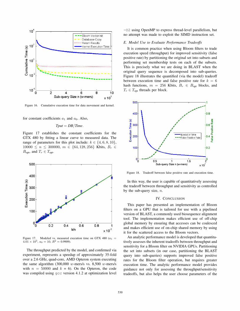
Figure 16. Cumulative execution time for data movement and kernel.

for constant coefficients a1 and a0. Also,

Tput = DB/Time.

Figure 17 establishes the constant coefficients for the

GTX 480 by fitting a linear curve to measured data. The

range of parameters for this plot include: k ∈ {4, 6, 8, 10},10000 ≤ n ≤ 300000, m ∈ {64, 128, 256} Kbits, Br ∈Bopt, and Tr ∈ Topt.

Figure 17. Modeled vs. measured execution time on GTX 480 (a1 =4.01× 105, a0 = 10, R2 = 0.9909).

The throughput predicted by the model, and confirmed via

experiment, represents a speedup of approximately 35-fold

over a 2.6 GHz, quad-core, AMD Opteron system executing

the same algorithm (300,000 w-mers/s vs. 8,500 w-mers/s

with n = 50000 and k = 6). On the Opteron, the code

was compiled using gcc version 4.1.2 at optimization level

-O2 using OpenMP to express thread-level parallelism, but

no attempt was made to exploit the SIMD instruction set.

E. Model Use to Evaluate Performance Tradeoffs

It is common practice when using Bloom filters to trade

execution speed (throughput) for improved sensitivity (false

positive rate) by partitioning the original set into subsets and

performing set membership tests on each of the subsets.

This is precisely what we are doing in BLAST when the

original query sequence is decomposed into sub-queries.

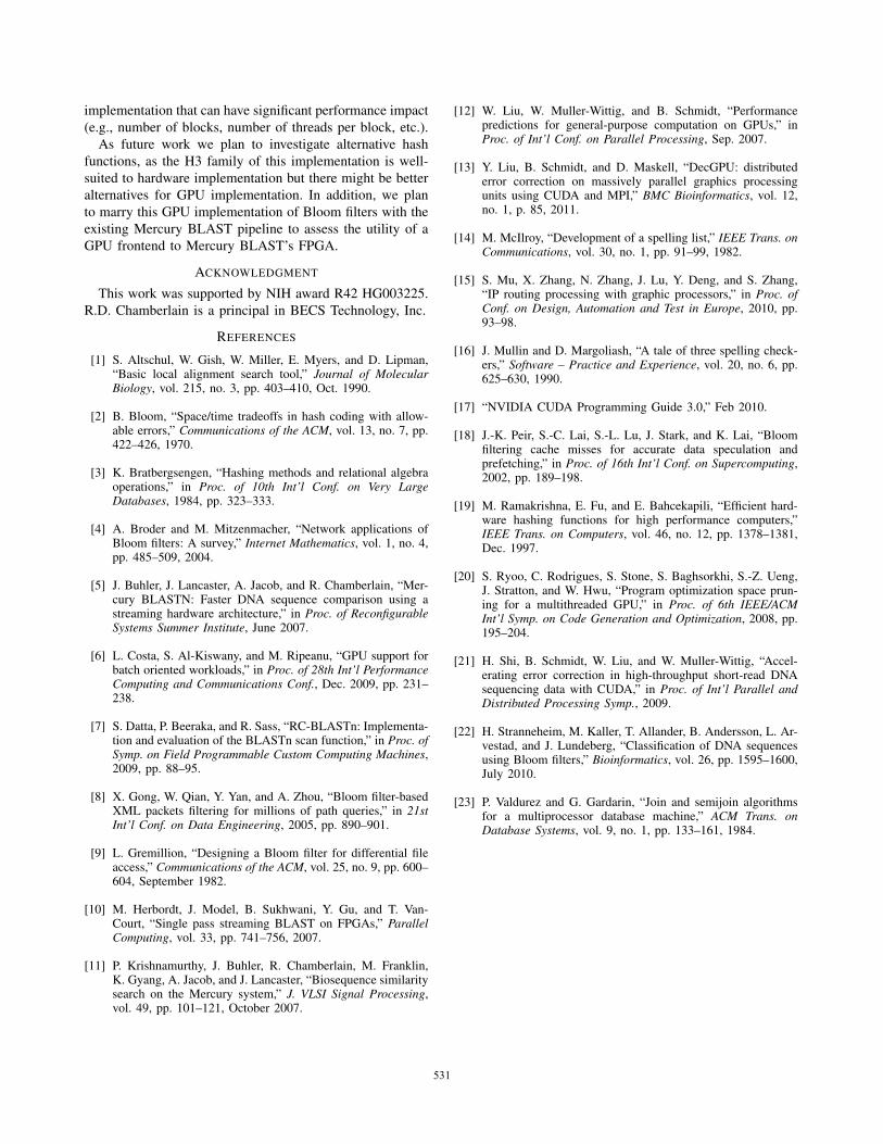
Figure 18 illustrates the quantified (via the model) tradeoff

between execution time and false positive rate for k = 6hash functions, m = 256 Kbits, Br ∈ Bopt blocks, and

Tr ∈ Topt threads per block.

Figure 18. Tradeoff between false positive rate and execution time.

In this way, the user is capable of quantitatively assessing

the tradeoff between throughput and sensitivity as controlled

by the sub-query size, n.

IV. CONCLUSION

This paper has presented an implementation of Bloom

filters on a GPU that is tailored for use with a pipelined

version of BLAST, a commonly used biosequence alignment

tool. The implementation makes efficient use of off-chip

global memory by ensuring that accesses can be coalesced

and makes efficient use of on-chip shared memory by using

it for the scattered access to the Bloom vectors.

An analytic performance model is developed that quantita-

tively assesses the inherent tradeoffs between throughput and

sensitivity for a Bloom filter on NVIDIA GPUs. Partitioning

the set into subsets (in our case, partitioning the BLAST

query into sub-queries) supports improved false positive

rates for the Bloom filter operation, but requires greater

execution time. The analytic performance model provides

guidance not only for assessing the throughput/sensitivity

tradeoffs, but also helps the user choose parameters of the

530

implementation that can have significant performance impact

(e.g., number of blocks, number of threads per block, etc.).

As future work we plan to investigate alternative hash

functions, as the H3 family of this implementation is well-

suited to hardware implementation but there might be better

alternatives for GPU implementation. In addition, we plan

to marry this GPU implementation of Bloom filters with the

existing Mercury BLAST pipeline to assess the utility of a

GPU frontend to Mercury BLAST’s FPGA.

ACKNOWLEDGMENT

This work was supported by NIH award R42 HG003225.

R.D. Chamberlain is a principal in BECS Technology, Inc.

REFERENCES

[1] S. Altschul, W. Gish, W. Miller, E. Myers, and D. Lipman,“Basic local alignment search tool,” Journal of MolecularBiology, vol. 215, no. 3, pp. 403–410, Oct. 1990.

[2] B. Bloom, “Space/time tradeoffs in hash coding with allow-able errors,” Communications of the ACM, vol. 13, no. 7, pp.422–426, 1970.

[3] K. Bratbergsengen, “Hashing methods and relational algebraoperations,” in Proc. of 10th Int’l Conf. on Very LargeDatabases, 1984, pp. 323–333.

[4] A. Broder and M. Mitzenmacher, “Network applications ofBloom filters: A survey,” Internet Mathematics, vol. 1, no. 4,pp. 485–509, 2004.

[5] J. Buhler, J. Lancaster, A. Jacob, and R. Chamberlain, “Mer-cury BLASTN: Faster DNA sequence comparison using astreaming hardware architecture,” in Proc. of ReconfigurableSystems Summer Institute, June 2007.

[6] L. Costa, S. Al-Kiswany, and M. Ripeanu, “GPU support forbatch oriented workloads,” in Proc. of 28th Int’l PerformanceComputing and Communications Conf., Dec. 2009, pp. 231–238.

[7] S. Datta, P. Beeraka, and R. Sass, “RC-BLASTn: Implementa-tion and evaluation of the BLASTn scan function,” in Proc. ofSymp. on Field Programmable Custom Computing Machines,2009, pp. 88–95.

[8] X. Gong, W. Qian, Y. Yan, and A. Zhou, “Bloom filter-basedXML packets filtering for millions of path queries,” in 21stInt’l Conf. on Data Engineering, 2005, pp. 890–901.

[9] L. Gremillion, “Designing a Bloom filter for differential fileaccess,” Communications of the ACM, vol. 25, no. 9, pp. 600–604, September 1982.

[10] M. Herbordt, J. Model, B. Sukhwani, Y. Gu, and T. Van-Court, “Single pass streaming BLAST on FPGAs,” ParallelComputing, vol. 33, pp. 741–756, 2007.

[11] P. Krishnamurthy, J. Buhler, R. Chamberlain, M. Franklin,K. Gyang, A. Jacob, and J. Lancaster, “Biosequence similaritysearch on the Mercury system,” J. VLSI Signal Processing,vol. 49, pp. 101–121, October 2007.

[12] W. Liu, W. Muller-Wittig, and B. Schmidt, “Performancepredictions for general-purpose computation on GPUs,” inProc. of Int’l Conf. on Parallel Processing, Sep. 2007.

[13] Y. Liu, B. Schmidt, and D. Maskell, “DecGPU: distributederror correction on massively parallel graphics processingunits using CUDA and MPI,” BMC Bioinformatics, vol. 12,no. 1, p. 85, 2011.

[14] M. McIlroy, “Development of a spelling list,” IEEE Trans. onCommunications, vol. 30, no. 1, pp. 91–99, 1982.

[15] S. Mu, X. Zhang, N. Zhang, J. Lu, Y. Deng, and S. Zhang,“IP routing processing with graphic processors,” in Proc. ofConf. on Design, Automation and Test in Europe, 2010, pp.93–98.

[16] J. Mullin and D. Margoliash, “A tale of three spelling check-ers,” Software – Practice and Experience, vol. 20, no. 6, pp.625–630, 1990.

[17] “NVIDIA CUDA Programming Guide 3.0,” Feb 2010.

[18] J.-K. Peir, S.-C. Lai, S.-L. Lu, J. Stark, and K. Lai, “Bloomfiltering cache misses for accurate data speculation andprefetching,” in Proc. of 16th Int’l Conf. on Supercomputing,2002, pp. 189–198.

[19] M. Ramakrishna, E. Fu, and E. Bahcekapili, “Efficient hard-ware hashing functions for high performance computers,”IEEE Trans. on Computers, vol. 46, no. 12, pp. 1378–1381,Dec. 1997.

[20] S. Ryoo, C. Rodrigues, S. Stone, S. Baghsorkhi, S.-Z. Ueng,J. Stratton, and W. Hwu, “Program optimization space prun-ing for a multithreaded GPU,” in Proc. of 6th IEEE/ACMInt’l Symp. on Code Generation and Optimization, 2008, pp.195–204.

[21] H. Shi, B. Schmidt, W. Liu, and W. Muller-Wittig, “Accel-erating error correction in high-throughput short-read DNAsequencing data with CUDA,” in Proc. of Int’l Parallel andDistributed Processing Symp., 2009.

[22] H. Stranneheim, M. Kaller, T. Allander, B. Andersson, L. Ar-vestad, and J. Lundeberg, “Classification of DNA sequencesusing Bloom filters,” Bioinformatics, vol. 26, pp. 1595–1600,July 2010.

[23] P. Valdurez and G. Gardarin, “Join and semijoin algorithmsfor a multiprocessor database machine,” ACM Trans. onDatabase Systems, vol. 9, no. 1, pp. 133–161, 1984.

531