Biomedical Image Processing in the Study of Living Cells

Biomedical Image Processing in the Study of Living Cells

Erlend Hodneland

Dissertation for the degree philosophiae doctor (PhD)

at the University of Bergen

25.07.2008

Acknowledgement

I wish to thank my three supervisors for their support and encouragement during the PhD

project. Their complementary background has been very useful in the process. My main super-

visor, Hans-Hermann Gerdes, has always encouraged me and believed in my skills and also shown

deep and honest fascination for the potential of image processing, which has been particularly

important for my own motivation. Arvid Lundervold has during the PhD project been a con-

stant source of encouragement by bridging the medical profession with image processing, and also

through his enthusiasm for mathematics. I wish to thank my external supervisor, Xue-Cheng

Tai, for numerous interesting discussions on mathematics and for keeping my mathematical

skills alive in my daily medical environment. He has been very supportive, understanding and

positive to my work at all stages. In the future I hope to continue the common work and further

strengthen the relation with all three supervisors. I deeply appreciate the work of Roland Kauf-

mann and his strong and painful efforts to keep my computer well functioning, and also Frode

Meland for reading the thesis and for giving constructive and precise feedback promoting further

development of the text. I also want to thank my collegues for a very positive collaboration

and hopefully mutual benefits in professional discussions. I have enjoyed the close collaboration

to Steffen Gurke and Nickolay Bukhoresthliev who have pushed the limits for applied image

processing. I am also grateful to Knut Teigen and the sofa he bought. It has been frequently

used. Furthermore, I want to thank the rest of my friends for changing my focus towards leisure

and enjoyable activities outside work.

Last but not least, I would like to thank my family, and in particular my parents, for their

everlasting and overwhelming support at all times.

Bergen, July 2008

i

Contents

Acknowledgement i

Chapter 1. List of publications 1

1.1. List of publications included in the PhD thesis 1

1.2. Related publications not included in the PhD thesis 3

Chapter 2. Introduction 5

2.1. Medical imaging and image processing 5

2.2. Fluorochromes and fluorescence microscopy 5

2.3. Fundamental steps in digital image processing 7

Chapter 3. Methodological projects 11

3.1. Preparation and acquisition of images 11

3.2. Segmentation of cells 13

3.3. A unified framework for segmentation of surface-stained cells 16

3.4. Segmentation evaluation of whole cell segmentation 31

3.5. Experimental results of whole cell segmentation 34

3.6. TNT detection 35

Chapter 4. Experimental projects 39

4.1. Quantification of transfer between cells 39

4.2. Segmentation and tracking of cytoplasmically stained NRK cells 41

4.3. Exocytosis of NPY-pHluorin superecliptic in PC12 cells 42

4.4. Partitioning and exocytosis of secretory granules during division of PC12 cells 42

Chapter 5. Summary and conclusions 45

Appendix A. Basic mathematical tools 49

A.1. Digital images 49

A.2. Morphology 49

A.3. Variational and PDE methods 53

Bibliography 55

iii

CHAPTER 1

List of publications

1.1. List of publications included in the PhD thesis

[I] Erlend Hodneland, Arvid Lundervold, Steffen Gurke, Xue-Cheng Tai, Amin Rustom and

Hans-Hermann Gerdes. Automated detection of Tunnelling Nanotubes in 3D images. Cytometry

Part A 69A:961-972 (2006).

[II] Xue-Cheng Tai, Erlend Hodneland, Joachim Weickert, Nickolay V. Bukoreshtliev, Arvid

Lundervold and Hans-Hermann Gerdes. Level set methods for watershed image segmentation.

Scale Space and Variational Methods in Computer Vision, Proceedings of the SSVM07:178-190

(2007).

[III] Erlend Hodneland, Xue-Cheng Tai and Hans-Hermann Gerdes. Four-Color Theorem and

Level Set Methods for Watershed Segmentation. Revised and resubmitted to International

Journal of Computer Vision.

[IV] Erlend Hodneland, Nickolay V. Bukoreshtliev, Tilo Eichler, Steffen D. Gurke, Xue-Cheng

Tai, Arvid Lundervold and Hans-Hermann Gerdes. A unified framework for automated 3D seg-

mentation of surface-stained living cells and a comprehensive segmentation evaluation. Revised

and resubmitted to IEEE Transactions of Medical Imaging.

[V] Nickolay V. Bukoreshtliev, Steffen Gurke, Erlend Hodneland and Hans-Hermann Gerdes.

Selective block of TNT formation inhibits intercellular organelle transfer between PC12 cells.

Manuscript in preparation.

[VI] Steffen Gurke, Joao F. Barroso, Erlend Hodneland, Nickolay V. Bukoreshtliev, Oliver

Schlicker and Hans-Hermann Gerdes. Tunneling nanotube (TNT)-like structures facilitate a

constitutive, ATP-dependent exchange of endocytic organelles between normal rat kidney cells.

Revised and resubmitted to Experimental Cell Research.

[VII] Nickolay V. Bukoreshtliev, Erlend Hodneland, Tilo Wolf Eichler, Patricia Eifart, Amin

Rustom and Hans-Hermann Gerdes. Partitioning and exocytosis of secretory granules during

division of PC12 cells. Manuscript in preparation.

1

2 1. LIST OF PUBLICATIONS

[VIII] Tanja Kogel, Rudiger Rudolf, Andrea Hellwig, Sergei A. Kuznetsov, Thomas Sllner, Flo-

rian Seiler, Erlend Hodneland, Joao Barroso and Hans-Hermann Gerdes. Distinct roles of myosin

Va in maturation and exocytosis of secretory granules in PC12 cells. Revised and resubmitted

to Traffic.

1.2. RELATED PUBLICATIONS NOT INCLUDED IN THE PHD THESIS 3

1.2. Related publications not included in the PhD thesis

[IX] Khanh Kim Dao, Knut Teigen, Reidun Kopperud, Erlend Hodneland, Frank Schwede, Anne

E. Christensen, Aurora Martinez and Stein Ove Døskeland. Epac1 and cAMP-dependent Pro-

tein Kinase Holoenzyme Have Similar cAMP Affinity, but Their cAMP Domains Have Distinct

Structural Features and Cyclic Nucleotide Recognition. The Journal of Biological Chemistry.

281 (30):21500-21511 (2006).

[X] Erlend Hodneland and Knut Teigen. A simple method to calculate the accessible volume of

protein-bound ligands: Application for ligand selectivity. J. Mol. Graph. Model. 26(2):429-433

(2007)

[XI] Ramadhan Oruch, Erlend Hodneland, Ian F. Pryme and Holm Holmsen. Interference by

psychotropic drugs of the tight coupling of polyphosphoinositide cycle metabolites in human

platelets: A result of receptor-independent drug intercalation in the plasma membrane? Ac-

cepted for Biochemical Journal.

CHAPTER 2

Introduction

2.1. Medical imaging and image processing

Medical imaging has become increasingly important in bio-medical research and clinical

practice, and it is the driving force in the development of modern volumetric imaging techniques

[1, 2, 3, 4, 5, 6]. In medical clinical research and practice, imaging has become an essential

part to diagnose and to study anatomy and function of the human body. MRI [7], X-Ray

and ultra-sound are imaging techniques that noninvasively can reveal tumors and fractures

with a minimal hazard to the living tissue. The data produced by the imaging techniques are

challenging to quantify both due to the complexity (3D, multichannel, multimodal) but also due

to the vast amount to be processed. Human resources are limited and are also impeded with

inter-observer variability. Computers can perform image analysis tasks on a large amount of

images with a higher degree of objectivity than humans. Especially segmentation, registration

and temporal analysis are image processing tasks suitable for computer algorithms. On the single

cell level, biologists generate 3D image stacks by fluorescence microscopy to better understand

the dynamics of living cells. Fluorescence microscopy enables the simultaneous recording of

different cellular structures down to the nanometer scale, and thus provides knowledge about

the dynamic interactions in terms of cell division, cell motility and cell-to-cell communication.

2.2. Fluorochromes and fluorescence microscopy

This work is entirely dealing with images from fluorescence microscopy, and a short intro-

duction to fluorochromes and image acquisition is therefore given in this section.

Fluorescence microscopy is based upon fluorescent reagents, fluorochromes, which upon exi-

tation by specific wavelengths emit light [8, 9]. The fluorochromes are used to selectively label

molecules like proteins, lipids, nucleic acids, ions and also cell populations and subcellular or-

ganelles. Normally, two types of fluorescent labeling are used in fluorescent microscopy. First,

the fluorescent dyes are popular due to their relatively straightforward process of use, which

involves immersing the sample in the dye or adding the dye to the specimen before imaging.

Second, the fluorescent proteins represent another type of labeling. The discovery of the green

fluorescent protein (GFP) enables fusing of the GFP to a wide range of protein targets by

cloning techniques. Thus, it became possible to study protein dynamics and function in living

cells and localize previously uncharacterized proteins. Combined with modern light sensitive

microscopy techniques, cells that express gene products tagged with GFP can be imaged over

several hours to provide information on protein distribution and cell function. Several other flu-

orescent proteins and mutants have been discovered, ranging over the whole imaging spectrum,

and fluorescent proteins can also be used in vivo to create fluorescently labeled organisms.

5

6 2. INTRODUCTION

xy plane

z

time

xy plane

z

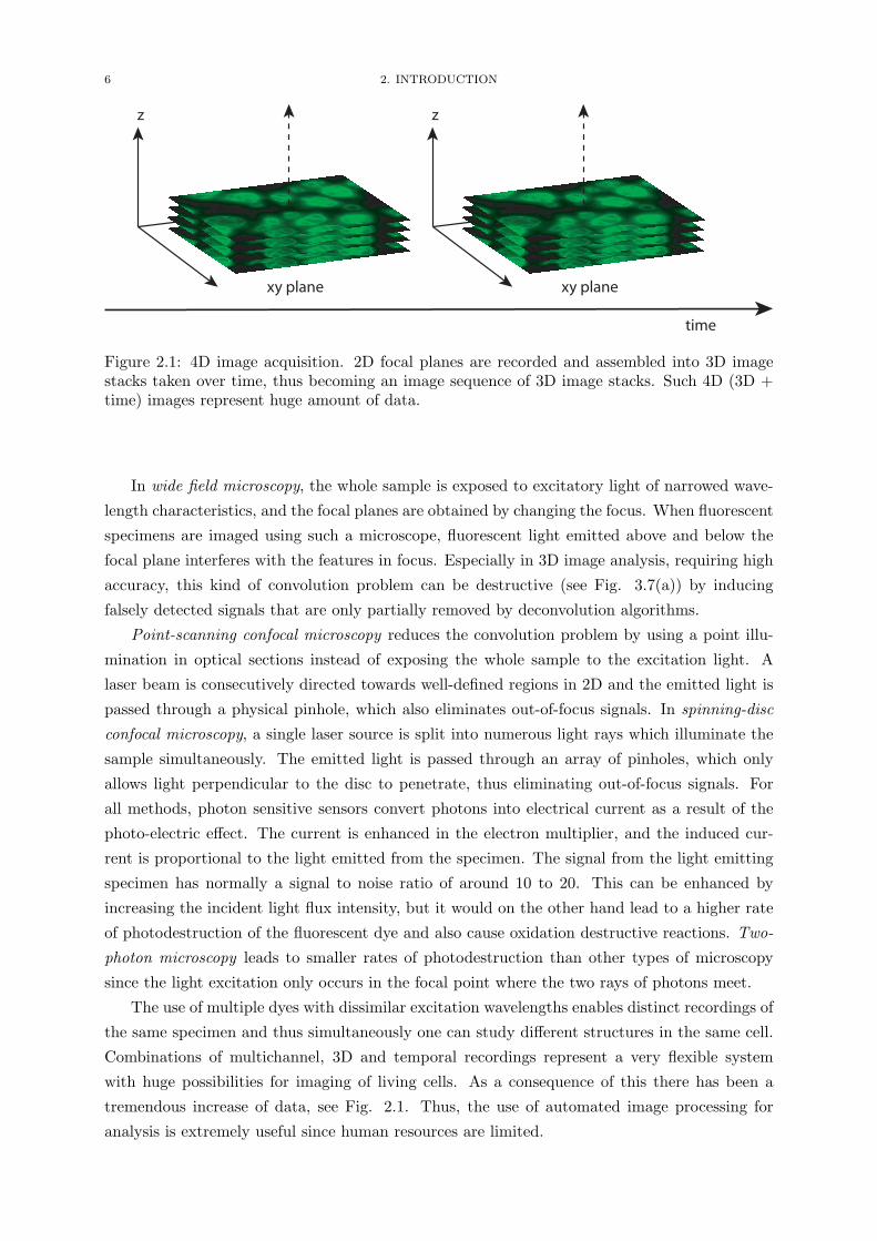
Figure 2.1: 4D image acquisition. 2D focal planes are recorded and assembled into 3D imagestacks taken over time, thus becoming an image sequence of 3D image stacks. Such 4D (3D +time) images represent huge amount of data.

In wide field microscopy, the whole sample is exposed to excitatory light of narrowed wave-

length characteristics, and the focal planes are obtained by changing the focus. When fluorescent

specimens are imaged using such a microscope, fluorescent light emitted above and below the

focal plane interferes with the features in focus. Especially in 3D image analysis, requiring high

accuracy, this kind of convolution problem can be destructive (see Fig. 3.7(a)) by inducing

falsely detected signals that are only partially removed by deconvolution algorithms.

Point-scanning confocal microscopy reduces the convolution problem by using a point illu-

mination in optical sections instead of exposing the whole sample to the excitation light. A

laser beam is consecutively directed towards well-defined regions in 2D and the emitted light is

passed through a physical pinhole, which also eliminates out-of-focus signals. In spinning-disc

confocal microscopy, a single laser source is split into numerous light rays which illuminate the

sample simultaneously. The emitted light is passed through an array of pinholes, which only

allows light perpendicular to the disc to penetrate, thus eliminating out-of-focus signals. For

all methods, photon sensitive sensors convert photons into electrical current as a result of the

photo-electric effect. The current is enhanced in the electron multiplier, and the induced cur-

rent is proportional to the light emitted from the specimen. The signal from the light emitting

specimen has normally a signal to noise ratio of around 10 to 20. This can be enhanced by

increasing the incident light flux intensity, but it would on the other hand lead to a higher rate

of photodestruction of the fluorescent dye and also cause oxidation destructive reactions. Two-

photon microscopy leads to smaller rates of photodestruction than other types of microscopy

since the light excitation only occurs in the focal point where the two rays of photons meet.

The use of multiple dyes with dissimilar excitation wavelengths enables distinct recordings of

the same specimen and thus simultaneously one can study different structures in the same cell.

Combinations of multichannel, 3D and temporal recordings represent a very flexible system

with huge possibilities for imaging of living cells. As a consequence of this there has been a

tremendous increase of data, see Fig. 2.1. Thus, the use of automated image processing for

analysis is extremely useful since human resources are limited.

2.3. FUNDAMENTAL STEPS IN DIGITAL IMAGE PROCESSING 7

2.3. Fundamental steps in digital image processing

Modern, high-speed imaging facilities produce huge amount of data. Image compression is

therefore used to reduce the quantity of data and at the same time preserve crucial information.

Image compression aims at removing information which is repetitive or irrelevant, and it should

not significantly reduce the quality of the images [1]. Image restoration is required to improve

the quality of the given image and thus restore the ”true” image as it would have appeared

free from noise and artifacts. Most real imaging applications produce images with a certain

amount of noise and artifacts. In fluorescence imaging, the artifacts may occur from endocytosed

dyes or inhomogeneous staining, the latter is responsible for large intensity variations between

the structures that are studied. Noise removal is an example of image restoration, as well as

inpainting which is the task of filling in missing parts of an image. Depending on the scientific

task, the aim is not restoration of the ”true” image, but rather image enhancement to obtain

an image with specific qualities enabling a quantification of structures of interest. For these

applications the human perception is frequently used as a gold standard since the needs are

driven by human perception of quality. Edge enhancing- and ridge enhancement filters belong

to this group, significantly enhancing edges or ridges compared to other structures.

Image restoration and enhancement techniques belong to low-level image processing [4].

These methods are crucial to obtain suitable images as input for high-level tasks like segmen-

tation, classification and tracking, often combined in real applications to create algorithms for

artificial intelligence and computer vision. High-level processing tries to mimic the excellent

human ability for shape detection and recognition, and simultaneously takes advantage of the

computers ability to process huge amount of data in an objective way. In particular, the advan-

tage of the computer compared to human perception becomes clear in the analysis of large 3D

data sets. On the other hand, the most challenging task for computerized image analysis is to

combine local and global image information, simultaneously including apriori information about

the system. The computer starts with an array of numbers, and lacks the vast source of experi-

ence that humans have. Especially in complex 2D recognition and tracking tasks the advantage

of humans becomes clear. Segmentation is the task of extracting regions or objects with common

features. It is strictly user-defined, since the desired output depends on the demands of the user.

As an example, consider the image in Fig 2.2(a). Detection of the face (b) of the woman clearly

returns another result than detection of the eyes (c). Segmentation is one of the most challenging

image analysis steps due to the ill-posedness, the large variability of images and the different

level of detail of the segmentation. Therefore, segmentation algorithms are often designed par-

ticularly to a special case or type of image, and the given segmentation protocol can be applied

to such set of images if they share important common features like shape, intensity, viewangle,

color-space, gradient and others. Segmentation can be done manually by humans, semiautomat-

ically by combining the human perception and the computers computational power, or it can

be performed fully automatically by computers. Commonly used segmentation algorithms are

statistical methods, thresholding, active contours, region growing and watershed segmentation.

A segmentation is often followed by a classification step. The segmentation divides the

image into disconnected regions, and the classification is required to assign the segmented regions

8 2. INTRODUCTION

(a) (b) (c)

Figure 2.2: Depending on the demands, a segmentation of the Lena picture (a) could be theextraction of any desired part, for instance the face (b) or the eyes (c).

into their respective classes. The classification normally relies on features extracted from the

segmentation step to label every segmented object based on its descriptors. In most cases the

classification requires a priori knowledge. The knowledge base can be a set of thresholds which

must be fulfilled for a given set of properties. Classification trees or neural networks represent

more advanced knowledge bases, which are produced from a ground truth.

The output from segmentation and classification can be utilized for tracking, a process for

identifying objects and following them in a sequence of images. Blind tracking with no directed

movement of the objects is obviously more challenging than tracking of directed movements

where the smoothness of the trajectory can be used as additional information. Also, tracking of

deformable objects represents a more challenging task than tracking of rigid objects. Tracking

is for instance used to follow the motion of clouds in meteorology, motion analysis for vehicles,

in astronomy and for military applications and in biology for tracking of vesicles [4, 10] and

drug delivery [11].

Tracing is a method which is associated to tracking. The tracing attempts to follow and

trace thin and elongated structures. Road detection in satellite images is an example, as well

as tracing of neurite extensions of neurons [12, 13]. Tracing represents a challenging task

if there are large intensity variations along the structure of interest, as well as crossing and

discontinuous segments. These challenges becomes clear in Fig 2.3 (left) and especially the

magnified selection A (right) which contains discontinuous segments, as well as crossing-overs,

bifurcation and merged neurite segments.

2.3. FUNDAMENTAL STEPS IN DIGITAL IMAGE PROCESSING 9

A

A

Figure 2.3: A neuron and its neurites. Tracing of neurites is a complex task due to discontinuoussegments, cross-overs, bifurcation and merging of neurite segments.

CHAPTER 3

Methodological projects

The primary focus in this work has been to accomplish whole cell segmentation of surface-

stained living cells in 3D, detection of organelle transfer betwen cells as well as detection of tun-

neling nanotubes (TNTs) connecting cells. Therefore, the image preparation has been directed

at creating high-quality images enabling these tasks. In this chapter, a protocol is described for

sample preparation, image acquisition, image reconstruction and enhancement, cell and TNT

detection and segmentation evaluation.

3.1. Preparation and acquisition of images

3.1.1. Sample preparation. Two cell types were used in the experiments for the projects

in Papers I-VIII, the spherical PC12 cells (rat pheochromocytoma cells, clone 251, Heumann

et al. [14]) and the more flat NRK cells (normal rat kidney cells, Mrs. M. Freshney, Glasgow,

UK). Three types of surface staining were applied to obtain images showing a strong and pro-

nounced plasma membrane, suitable for whole cell segmentation (Chapter 3.2.4). Wheat germ

agglutinin (WGA) conjugated to Alexa Fluor R© was most frequently used in our experiments

(Papers I-V and VII) due to the simple application and the strong labeling of the plasma mem-

brane which is obtained, see Fig. 3.2(a). WGA-Alexa Fluor R© is a dye, which is added to the

LabTekTMchambers (Nalge Nunc Int.,Wiesbaden, Germany) used for culturing of cells. The dye

is a lectin that binds to a distinct sugar moiety of plasma membrane proteins. Due to constitu-

tive internalization of small areas of the plasma membrane, a process termed endocytosis, the

dye is quickly internalized in living cells. The process of endocytosis creates increasing signals

from inside the cell, promoting the complexity of cell segmentation. To keep the endocytosed

material at a minimum, it is therefore important that imaging occurs within the first 45 minutes

after adding WGA-Alexa Fluor R©. The effect of endocytosed dye is shown in Fig. 3.1, where a

PC12 cell was imaged shortly after administration of WGA-Alexa Fluor R© (a) and 3 hours later

(b).

The second membrane marker which was used (Paper IV) is the PHD-YFP fusion protein

which is a F-actin binding protein enriched at actin assembly sites, both on the plasma membrane

and on endosomal vesicles. NRK cells were cultured in DMEM supplemented with 10% fetal calf

serum. To obtain a strong plasma membrane labeling of NRK cells, they were transfected with

the PHD-YFP cDNA construct as described in [15]. Transfection of NRK cells was accomplished

by electroporation as described in [16]. An example of the obtained images is shown in Fig.

3.2(b), where the plasma membrane labeling is clearly visible.

In the experiments estimating phagocytosis in the presence of cytochalasine B in Paper IV,

Bromphenol Blue was used to quench undesired signals from outside the cells (Chapter 4.1). The

Bromphenol Blue excitation channel itself was also suitable for segmentation due to the strong

11

12 3. METHODOLOGICAL PROJECTS

(a) A PC12 cell shortly af-ter administration ofWGA.

(b) The cell in (a) 3 hourslater.

Figure 3.1: Endocytosis of WGA-Alexa Fluor R©. The cell in (a) shows a pronounced plasmamembrane staining. After 3 hours the same cell (b) displays strong signals from inside the celldue to endocytosed dye. The images are single focal planes from a 3D image stack recorded byspinning-disc confocal microscopy.

(a) PC12 cells stained withWGA-Alexa Fluor R©.

(b) NRK cells trans-fected with PHD-YFP cDNA.

(c) PC12 cells stained withBromphenol Blue and DiI.

Figure 3.2: Different methods for plasma membrane labeling.

signal from the plasma membrane facing into the medium as well as facing towards adjacent

cells, see Fig. 3.2(c).

To obtain the 3D arrangement of cells resembling tissue (Chapter 3.5 and Paper IV), PC12

cells were embedded in agarose. Briefly, low melt agarose (Carl Roth GmbH) was prepared in a

2% (w/v) solution in DMEM 10% FCS and melted at 70 C. The solution was allowed to cool

down to 45 C for 15 min. Pellets of approximately 4 ·10+7 PC12 cells were loosesly resuspended

in 500µl of growth medium supplemented with WGA-Alexa Fluor R© and mixed with 500µl of

agarose stack solution, resulting in a 1% agarose end concentration. The latter mixture was

plated in LabTekTMchambers and allowed to cool at 4C for 5 min. 3D imaging was performed

immediately afterwards.

The NRK cells in Paper VI were stained with CellTrackerTMGreen CMFDA (10µM ) or

Vybrant R© DiD (2 − 6µM) (Molecular ProbesTM, Invitrogen detection technologies, Carlsbad,

CA, USA), performed as described in [17].

3.1.2. Image acquisition. For the image acquisition three different types of microscopy

were applied, wide-field, point-scanning confocal and spinning-disc confocal. For experiments in

3.2. SEGMENTATION OF CELLS 13

Figure 3.3: Wide-field Olympus microscope.

Papers I-V, a wide-field Zeiss microscope was used (Carl Zeiss MicroImaging GmbH, Jena, Ger-

many), equipped with a 63x Plan Apo /1.40 NA oilimmersion objective (Olympus Optical Co),

a monochromator-based imaging system (T.I.L.L. Photonics GmbH, Martinsried, Germany),

a tripleband filterset DAPI / FITC / TRITC F61-020 (AHF Analysetechnik AG, Tubingen,

Germany) and a piezo z-stepper (Physik Instrumente GmbH & Co., Karlsruhe, Germany).

Point-scanning confocal microscopy was used for experiments in Paper IV, performed with a

Leica TCS SP5 confocal microscope (Leica Microsystems, Mannheim, Germany). Spinning-disc

confocal microscopy was applied in Paper IV, specifically a PerkinElmer spinning-disc confo-

cal setup (PerkinElmer Ultra View TMRS Live Cell Imager, PerkinElmer Life and Analytical

Sciences, Boston, MA, USA).

For both the wide-field and confocal imaging setups, the cells were analyzed in 3D by nor-

mally acquiring single focal planes 300 to 500nm apart from each other in the z-direction,

spanning the whole cellular volume.

3.2. Segmentation of cells

Segmentation of cells is a major task in biological image processing. Proper cell segmentation

enables quantification of biological processes on a single cell level, which is the basis for additional

quantification tasks like estimation of cell volume and shape, sub-cellular distribution of signaling

molecules, detection of transfer between cells, colocalization of vesicles and tracking of cells.

There are at least four different approaches for cell segmentation: segmentation of unstained

cells, stained nuclei, cytoplasmically stained cells and segmentation of surface-stained cells. Each

method has unique properties that can be useful in particular experimental setups. At the same

time it is important to know their limiting factors in order to apply the optimal method for cell

segmentation in a given experiment. In this work we have gained experience with the use of

different stainings, types of microscopy and segmentation methods. In the following we describe

and discuss advantages and disadvantages associated with the various approaches.

3.2.1. Segmentation of unstained cells. It is possible to perform segmentation of un-

stained cells [18, 19, 20, 21]. The images are then obtained from transmitted light microscopy,

which has the advantage of being less harmful to the cells. However, transmitted light images

often suffer from poor contrast and from strong background signals. Also, the image quality


varies significantly at different focal planes, both due to variations in the contrast but also due

to the phenomenon that same cell structures can be reverted from bright to dark at different

focal levels. Differential interference contrast (DIC) transmitted light images additionally suffer

from a shadow effect since the exposed light is passed through a complex set of polarizers and

optical filters. Due to these limiting factors it is a challenging task to obtain satisfying success

rates from segmentation of transmitted light images.

3.2.2. Segmentation of stained nuclei. Segmentation of cell nuclei is well addressed

in the literature [22, 23, 24, 25, 26, 27, 28, 29]. The nucleus of the cell is stained with

a dye (Hoechst staining, see Chapter 3.2.5) accumulating in the nucleus, providing a strong

and well defined signal. Segmentation of stained nuclei is capable of detecting the volume

spanned by the nucleus, thus also the border around it. However, the nuclei segmentation is

not capable of detecting the outer border of the cell, and can therefore not be regarded as a

tool for cell segmentation. If the nuclei are densely packed, the segmentation often requires a

post-processing step which splits under-segmented objects. This can for instance be obtained

by a distance transform [27] or by controlled dilation [30]. Nucleus segmentation is particularly

useful to detect the number of cells since every cell has only one nucleus. Thus, it can for

instance be used to estimate the rate of cell division. Nucleus segmentation can also be used to

address gene amplification [30], for evaluation of in situ hybridization signals (FISH) [23] and

as initialization spots for whole cell segmentation.

3.2.3. Segmentation of cytoplasmically stained cells. The use of a fluorescent marker

accumulating in the cytoplasmic regions of the cell enables a segmentation of the cell volume.

This approach is particularly useful when the aim is to provide a binary representation of the

regions covered by cells. If this is achieved, it is possible to compare cell properties to those of

background or to other conditions. However, similar to nuclei segmentation, the segmentation

of cytoplasmically stained cells can not resolve the exact borders between adjacent cells in

densely packed arrangements since there is only a very small decrease in signal intensities on

the plasma membrane between attached cells with this kind of staining. This is demonstrated

in Fig. 3.4(a) which shows three attached PC12 cells stained with CellTrackerTM. Clearly, the

borders between the cells are not easily seen, and the segmentation in Fig. 3.4(b) was not able

to distinguish between the three cells and a cell cluster is therefore returned. If the cells are

only loosely connected with duplets and maybe triplets it is still possible to split the under-

segmented cells by similar methods as for the nuclei segmentation, for instance by applying

concavity requirements [31] or the distance transform [27]. However, if the cells are closely

packed and in particular when concavity assumptions are not valid for the cell type in use, the

splitting methods can not properly separate clustered cells. The borders facing outward towards

the medium are still easily resolved.

3.2.4. Segmentation of surface-stained cells. A high-quality surface staining offers

a wide range of opportunities for segmentation and analysis. The surface staining produces a

pronounced signal from the plasma membrane of every stained cell, thus creating a closed contour

with high intensities (Figs. 3.2(a) - 3.2(c)) which can be utilized for whole cell segmentation. A

3.2. SEGMENTATION OF CELLS 15

(a) Cytoplasmicstaining.

(b) Segmentation of(a).

(c) Surface staining. (d) Segmentation of(c).

Figure 3.4: Different types of stainings and cell segmentation.

whole cell segmentation implies that each cell is segmented separately, disconnected from the

other segmented cells. Figure 3.4(c) shows surface-stained cells with the corresponding whole

cell segmentation in Fig. 3.4(d). The cell area has been resolved similar to the segmentation for

the cytoplasmic staining in Fig. 3.4(b), and additionally, every cell in the triplet is detected and

represented individually. To the best of our knowledge only very few studies address the task

of segmentation of surface-stained cells. Notably, in these studies only fixed cells were used. In

one study antibodies against integrin receptor subunits were used as surface markers to label

the contour of fixed cells [24]. However, this method labels only the cell membrane attached

to the substrate, which restricts the analysis to 2D. Furthermore, the initialization seeds inside

cells had to be placed interactively for the commonly irregularly shaped cells. The study of

Baggett et al. [32] also reported on whole cell segmentation of surface-stained fixed cells. They

used Oregon Green 488 Phalloidin to label the peripheral F-actin cortex of cells and obtained

a high success rate for 2D images by initiating the algorithm interactively. Dow et al. [33]

performed a 2D segmentation of cell boundaries from cells of fixed biopsy material of melanoma

patients. They circumvented the problem of initiating markers for their snake algorithm by using

the information provided by Hoechst-stained nuclei. To extend the existing methods toward a

fully automated 3D segmentation of surface-stained living cells, we have developed a unified

framework for whole cell segmentation in 3D of surface-stained living cells which applies to

images showing fluorescently labeled cell borders (Paper IV). In particular, the use of living

cells instead of fixed cells enables the study of cell dynamics. The algorithms have been applied

to two distinct cell types, using different methods for cell surface labeling and various imaging

techniques to demonstrate the versatility of the method.

3.2.5. Combining staining techniques. The marker construction, the whole cell seg-

mentation and the classification step can all be performed on the surface-stained images. How-

ever, other available stainings can additionally be used to improve the segmentation. An optimal

solution can be a combination of a surface staining, a nucleus staining and a cytoplasmic stain-

ing. The nucleus staining labels the nuclei fluorescently with a one-to-one relationship to the

cells. Thus, it offers an approach to compute binarized representations of the nuclei, where each

binary region is inside one cell. This binarized representation can serve as a highly suitable

marker image for further segmentation of the cells shown in the surface-stained image, either

using watershed segmentation (Chapter 3.3.5) or active contours (Chapter 3.3.6). Background


Figure 3.5: Flow scheme for segmentation of surface-stained cells. The marker image can becreated either from the surface-stained image itself or from the nucleus staining. A backgroundmarker is advantageously constructed from the cytoplasmic staining. Based on the markers,a segmentation of the surface-stained cells is accomplished. Finally, the watershed regionscan be classified with a trained classifier using properties of the segmented regions from thesurface-stained image. To obtain further reliability of the cell classification, information fromthe nucleus image or a cytoplasmically stained image labeling the cell regions with strong signalscan additionally be used to improve the classification.

markers also need to be constructed, which for instance can be accomplished by thresholding

of the cytoplasmic image or the surface-stained image. Furthermore, the cytoplasmic staining

is especially useful in cell classification of the regions obtained from the segmentation since the

cells are labeled brighter than the background in the cytoplasmic image channel. Different com-

binations of stainings for segmentation are displayed in Fig. 3.5. Normally, there are less than

three available image channels for segmentation since the biological applications require at least

one channel, but also combinations of two channels can improve the segmentation compared to

only using the surface staining. Figure 3.6 demonstrates the use of three different combinations

of stainings, a surface, a nucleus and a cytoplasmic staining. The given examples show that it

is possible to only use the surface-stained image for whole cell segmentation, but the use of two

or even three image channels can improve the segmentation (Figs. 3.6(d) - 3.6(f)).

3.3. A unified framework for segmentation of surface-stained cells

Due to the restricted availability of image channels in fluorescent microscopy, the following

section contains a description of whole cell segmentation solely based on the surface-stained

images. A complementary description of the process is given in Paper IV.

3.3.1. Choosing the optimal fluorescent marker and microscopy technique. To

obtain a reliable and robust scheme of processing steps for segmentation of surface-stained

cells, it is important to plan the experiments carefully in close collaboration with the biologists

performing the imaging. As described in Chapter 3.1.1, we have used three different types of

fluorescent surface markers facilitating a segmentation of the plasma membrane, WGA-Alexa

Fluor R© (dye, see Fig. 3.2(a)), PHP-YFP cDNA (transfection, see Fig. 3.2(b)) and Bromphenol

Blue (dye, see Fig. 3.2(c)). WGA-Alexa Fluor R© is quickly endocytosed into the cells, creating

strong and undesired signals from inside the cell (Fig. 3.1). The imaging should therefore

be accomplished within 45min after adding the dye. PHD-YFP is a fusion protein which is

3.3. A UNIFIED FRAMEWORK FOR SEGMENTATION OF SURFACE-STAINED CELLS 17

(a) Surface staining. (b) Nucleus staining. (c) cytoplasmic staining.

(d) Segmentation only us-ing the surface-stainedimage in (a).

(e) Segmentation of (a),using (b) to createmarkers.

(f) Segmentation of (a),classification of cellsusing (c).

Figure 3.6: Combining staining techniques for segmentation. All segmentation was performedon the surface-stained image (a). In (d), the markers were constructed and cell classificationwas performed based on information from (a). Note the asterisk which denotes a region incor-rectly classified as a cell. In (e), the nucleus staining (b) was used to create markers for thesegmentation. For (f), the cytoplasmic staining (c) was used for cell classification. Both (e) and(f) are improved compared to (c) due to the additional information available from the nucleusand cytoplasmic staining.

expressed steadily over long time. Thus, the limited available recording time of WGA-Alexa

Fluor R© is therefore not a problem in the case of PHD-YFP. However, it is more preparatory

work to transfect the cells, not all cells are transfected and the expression of the PHD-YFP is

uneven and also stressful to the cells. The Bromphenol Blue is toxic to the cells, and the dye

is therefore not appropriate for experiments where the cells are required to survive for a longer

time during and after imaging.

Choosing the right microscopy technique is also important. The unlike properties of wide-

field and confocal microscopy can be used deliberately to improve the segmentation results of cells

with different morphology. The flat NRK cells are preferably recorded using confocal microscopy

due to its ability to achieve images from very thin optical sections. Imaging of NRK cells using

wide-field microscopy results in blurry and unsharp cell boundaries since the plasma membrane

of the NRK cells runs almost parallel to the optical plane. The phenomenon is displayed in Fig.

3.7(a) showing NRK cells imaged by wide-field microscopy. The plasma membrane is clearly

fuzzier than those obtained by confocal microscopy in Fig. 3.7(b). Therefore, the NRK cells

in Paper IV were imaged confocally. On the other hand, the spherical and higher PC12 cells

are easily imaged using a wide-field setup since the plasma membrane of the PC12 cells runs

perpendicular to the optical sections in large portions of the cell. In fact, imaging of PC12

cells using wide-field microscopy provides smoother images than those obtained from confocal

microscopy.


(a) NRK cells imaged by wide-fieldmicroscopy.

(b) NRK cells imaged byconfocal microscopy.

Figure 3.7: Comparison of wide-field and confocal microscopy for imaging of the flat NRKcells. Note that the plasma membrane is fuzzier for wide-field microscopy (a) than for confocalmicroscopy (b).

(a)

0 20 40 60 80 100 120 140 1600

0.2

0.4

0.6

0.8

1

(b)

Figure 3.8: The plasma membrane is expressed as ridges in surface-stained images (a). The lineprofile along the dashed line in (a) has been plotted in (b), where the ridges are indicated byarrows.

3.3.2. Filtering of the raw data. Prior to any further processing steps, it is advised to

conduct a filtering of the raw data as an image restoration. A suitable filtering will smooth

the images and reduce the impact of artifacts that occur as noise from the technical and optical

setup. More important than noise are undesired signals occuring from real biological phenomena

like endocytosis (see Fig. 3.1 and also white spots inside cells in Fig. 3.8(a)) and inhomogenious

staining. Normally, a qualified filtering method is designed to enhance edges and corners, thus

preserving the boundaries of desired objects [34]. However, the objects in the plasma membrane-

stained images of Paper IV have other target properties than sharp edges, rather strong ridges

or crests high-lighting the stained plasma membrane. Thus, the method of choice must aim at

preserving ridges more than edges. In 3D, the structures of interest are surfaces. Figure 3.8(a)

shows two PC12 cells where the plasma membrane is clearly visible as ridges. The intensity

profile along the dashed line has been plotted in Fig. 3.8(b) to emphasize the ridge property of

the plasma membrane, and the peaks of the ridges along the line profile are indicated by arrows.

A set of three direct spatial filters and three PDE based filter are presented and compared to

each other in Paper IV. In this thesis, these filter techniques are explained in more detail. The


image in Fig 3.8(a) was chosen as an example to demonstrate the effect of the filtering techniques

that we compare.

Gaussian smoothing. Gaussian smoothing is a fast and predictable method. Mathematically,

it is a convolution with the Gaussian convolution kernel

(3.3.1) gσ(x) =1

(2πσ2)m/2e−

|x|2

2σ2

where |x|2 = x2 + y2 + z2 is the squared blur radius in 3D, σ is the standard deviation of the

distribution and m is the number of variables. To obtain the Gaussian blurred image ug, the

convolution kernel gσ is embedded into an integral and applied to the image function u(x) in a

small neighborhood nγ(x),

(3.3.2) ug(x) = (u ∗ gσ)(x) =

∫

nγ(x)u(y)gσ(x − y)dy.

In the discrete image space, a discrete Gaussian filter mask must be computed to obtain an

approximation of the convolution integral. Define w(x) to be a square filter centered in x with

dimensions γ > 0 and let nγ(x) be the set of coordinates within the filter. An approximation of

the convolution integral can be obtained by computing [35]

(3.3.3) ug(x) ≈∑

y∈nγ(x)

u(y)wσ(x − y).

The discrete filter wσ(x) is computed from (3.3.1) and (3.3.2). However, more precise results

can be obtained using interpolation methods for the numerical approximation of the continuous

convolution integral [36]. Figure 3.9(a) demonstrates the Gaussian smoothing.

Median filtering. Median filtering is an order-statistic filter method preserving edges effi-

ciently [37]. In contrast with the Gaussian filtering, it is a non-linear operation not based on

convolution. Define the filter response R(x,y) = u(y)w(x−y). In the median filter, each output

pixel contains the median of the image values within the unity filter w(x− y) = 1 ∀ y ∈ nγ(x),

(3.3.4) um(x) = median y∈nγ(x)R(x,y).

The median filter has excellent noise-reduction capacities for salt-and-pepper noise [35]. Figure

3.9(b) shows the results from median filtering.

Directional coherence enhancement. Directional coherence enhancement [30] is a directional

filter performing a texture analysis to remove noise. The method has a high resistance against

noise due to a special averaging process called semi-Olympic averaging. In semi-Olympic aver-

aging, the largest element is removed before averaging, thus removing the outliers and reducing

the noise significantly. The semi-Olympic average operator sw applied to u(x) is defined as

(3.3.5) swu(x) =1

W

∑

y∈nγ(x),y 6=y∗

R(x,y)

where W is the sum of the elements in a directional filter wi, except from y∗ providing the

largest filter response, y∗ = y : R(x,y∗) ≥ R(x,y) ∀ y ∈ nγ(x). (3.3.5) is applied to u(x)

with four filters along different directions, i.e. horizontal, vertical and the two diagonals. For


(a) Gaussian filtering, γ =11 and σ = 3.

(b) Median filtering, γ =11.

(c) Directional coherenceenhancement filter,γ = 11.

(d) Edge enhancing diffu-sion, k = 0.01, ∆t =0.1 and 100 iterations.

(e) Coherence enhancingdiffusion, k = 0.0001,∆t = 0.2 and 100 iter-ations.

(f) Inverse diffusion, ∆t =0.2, λ2 = −0.5 and 5iterations.

Figure 3.9: Filtering of the image in 3.8(a) using three direct methods (a-c) and three iterativemethods (d-f). The ridges are better preserved using directional coherence enhancement filter(c), coherence enhancement filter(e) or inverse diffusion (f) than using the other methods.

γ = 3 the filters are given as

(3.3.6) w1 =

0 1 0

0 1 0

0 1 0

, w2 =

0 0 0

1 1 1

0 0 0

, w3 =

0 0 1

0 1 0

1 0 0

, w4 =

1 0 0

0 1 0

0 0 1

.

Every pixel in the smoothed image is computed as the maximum value of the semi-Olympic

average in the four directions, i.e. us(x) = maxi swiu(x) , i = 1, . . . , 4. Note, the directional

coherence enhancement operator can be applied to the gradient map when the aim is to enhance

edges. In our practical applications, γ ≈ 11. An example of directional coherence enhancement

is shown in Fig. 3.9(c).

Edge enhancement smoothing. Now, we turn to the iterative PDE based anisotropic diffusion

operators [38, 39]. In regions with steep gradients, they perform a stronger smoothing along

than across the edges. In flat parts, the system reduces to isotropic diffusion with nearly equal

diffusion in all directions. To obtain a local estimate of the edge direction, the gradient is

computed. Edge enhancing diffusion is described with the PDE

(3.3.7)∂u

∂t= ∇ · (D∇u)


whereD is a positive semi-definit and symmetric diffusion tensor. To obtain a more homogeneous

gradient map, the Gaussian smoothed ug is used to calculate D, which in 2D is constructed as

(3.3.8) D = RT

(

c1 0

0 c2

)

R

where R is the rotation matrix

(3.3.9) R =1

|∇ug|

(

(ug)x −(ug)y

(ug)y (ug)x

)

and |∇ug| =√

(ug)2x + (ug)2y. The columns of R are constructed from the gradient vector

[(ug)x (ug)y]T and an ortogonal component. Equations 3.3.8 and 3.3.9 lead to the diffusion

tensor D

(3.3.10) D =1

|∇u|2

(

c1(ug)2x + c2(ug)

2y (c2 − c1)(ug)x(ug)y

(c2 − c1)(ug)x(ug)y c1(ug)2y + c2(ug)

2x

)

The conductivity parameters c1 and c2 control the amount of smoothing along the gradient and

the orthogonal direction, respectively. Preferably, c2 > c1 which leads to higher diffusion along

the edges than across them. If c1 = c2 there will be isotropic diffusion with equal amount of

smoothing in all directions. One possible choice for c2 and c1 could be [40]

c2(|∇ug|) = e−|∇ug |2

k2 and c1(|∇ug|) = αc2(|∇ug|),(3.3.11)

where α ∈ [0, 1] and k is a tuneable diffusion parameter depending on the magnitude of the

gradient. Define

(3.3.12) D =

(

d11 d12

d12 d22

)

.

Then, the equation to solve becomes

(3.3.13) ∂tu = ∂x(d11∂xu) + ∂x(d12∂yu) + ∂y(d12∂xu) + ∂y(d22∂yu).

To stay within the 3 × 3 neighborhood, central differences should be used for the mixed terms,

and for the same reason a backward difference followed by a forward is advised to use in the

Laplacian terms. Figure 3.9(d) is an example of edge enhancing diffusion.

Coherence enhancing diffusion. The coherence enhancing diffusion has proved to be success-

ful on fingerprint images [41, 39]. The pictures presented in this work and fingerprint images

have the common property that important structures are thin lines or ridges. The aim for both

types of pictures is to smooth along the ridges and not across them. To estimate the local

orientation of the ridges, the structure tensor is used. In 2D, it is given as

(3.3.14) S =

(

s11 s12

s12 s22

)

=

(

g ∗ (u2x) g ∗ (uxuy)

g ∗ (uxuy) g ∗ (u2y)

)

.

It is important to choose a suitable scale of integration and standard deviation in the convolution

to preserve the desired structures. The integration scale in the Gaussian convolution should


reflect the size of the structures of interest. S is a symmetric positive semidefinite matrix,

and there exists an orthonormal set of eigenvectors v1 and v2 with eigenvalues µ1 > µ2 > 0.

The eigenvector v2 gives the local orientation perpendicular to the structures, and v1 gives the

orientation along the structures. The diffusion tensor D is designed as in (3.3.8), but here the

columns of R are given as the eigenvectors of S. They can be calculated analytically, leading to

the diffusion tensor

d11 =1

2

(

c1 + c2 +(c2 − c1)(s11 − s22)

α

)

d12 =(c2 − c1)s12

α

d22 =1

2

(

c1 + c2 +(c2 − c1)(s11 − s22)

α

)

where α =√

(s11 − s22)2 + 4s212. The eigenvalues are given as

(3.3.15) µ1,2 =1

2(s11 + s22 ± α) .

The diffusion coefficients c1 and c2 can be chosen as [40]

(3.3.16) c1 = max(

β, 1 − e−(µ1−µ2)2/k2)

and c2 = β

where β ∈ [0, 1]. The difference (µ1 − µ2)2 is a measure of the difference of gray-value changes

between the eigendirections, also called the local coherence. Figure 3.9(e) shows the image in

Fig 3.8(a) after coherence diffusion filtering.

Inverse diffusion. Inverse diffusion is a diffusion method where the diffusion across the edge

is reversed. This is an inherently unstable process since the diffusion equation has no backward

compatibility. However, if the diffusion is limited to only a few iterations, the method can

sharpen the ridges or edges of interest. The flow equations are similar to the scheme for the co-

herence enhancement diffusion and edge enhancing diffusion. A diffusion tensor D is constructed

as in (3.3.8), using the eigenvectors of (3.3.14) as column basis of R, similar to the approach in

coherence enhancement diffusion,

(3.3.17) D = RT

(

λ1 0

0 λ2

)

R.

However, the eigenvalues of D are chosen as λ1 = −α−1 and λ2 = α for some scalar α ∈ 〈0, 1〉.

The important difference to the coherence diffusion is the modification of the largest eigenvalue to

become negative. This inverts the diffusion across the principal edge direction and will enhance

the edges. Figure 3.9(f) displays the result after inverse diffusion of Fig. 3.8(a).

Comparison of the smoothing operators. The choice of filtering method depends on the data

available. If the images are of high quality, a traditional Gaussian filter is adequate for the

purpose. However, if there exists a considerable amount of noise and if the image structures are

characterized by discontinuities, the directional coherence enhancement, the coherence diffusion

filter or inverse diffusion are preferred methods. These filters are able to close minor gaps in

the structures along the principal flow direction. On the other hand, they can due to this useful

property also create artifacts and induce wrongly connected structures, which is the reason why


the Gaussian filter is preferred for images of high quality. However, in large data sets there will

always exist images with varying quality. In the long run the more advanced filters are therefore

to be preferred. The median filter and the edge enhancing filters are more edge preserving

than the already mentioned filters, and are not well suited for structures that manifest as ridges.

These filters enhance and even sharpen edges, thus edges that were hardly visible before filtering

will become sharper. Therefore, applied to images showing cells with cytoplasmic or nucleus

staining, the median filter or the edge enhancing filter are highly suitable since the aim then is

to enhance the edges in the transition zone between cells and background.

3.3.3. Ridge enhancement. As an image enhancement step, a ridge enhancement is rec-

ommended, especially for wide-field images since light from surrounding pixels will blur the

signal. The ridge enhancement increases the contrast of ridges compared to other structures,

and thus creates an image better suited for cell segmentation, and in particular better suited for

automated marker generation. In Paper IV we compare two methods for ridge enhancement,

the Hessian approach and our proposed method, ridge enhancement by curvature.

Hessian ridge enhancement. The Hessian method for ridge enhancement is the classical

approach. A convoluted Hessian matrix is given as

(3.3.18) Hg =

[

g ∗ (ug)xx g ∗ (ug)xy

g ∗ (ug)yx g ∗ (ug)yy

]

.

The eigenvalues are computed and every pixel is assigned a geometrical class according to the

sign of the eigenvalues [42]. Across the cell boundary there is a large intensity variation but the

variation is small along the tangent plane of the plasma membrane. Therefore, the 3D plasma

membrane has the characteristic geometrical property of λ1 < 0, λ2 ≈ 0, λ3 ≈ 0 where λ1, λ2

and λ3 are the eigenvalues of the Hessian matrix in decreasing absolute values. To highlight

the plasma membrane, a transfer function was defined as uH(x) = −λ1 − λ22 − λ2

3. Due to this

definition, the ridge enhanced image uH will take the largest values on the ridges compared to

other geometrical classes, see Fig. 3.10(a).

Ridge enhancement by curvature. As an extension to the Hessian ridge enhancement we

have introduced ridge enhancement by curvature. In ridge enhancement by curvature, the ridge

enhanced image is given as the curvature in the principal direction of variation of the second

derivative. Similar to the Hessian ridge enhancement, the eigenvalue decomposition of the

Hessian matrix is first computed. The purpose is to obtain the eigenvector with the largest

modulus of eigenvalues, pointing perpendicular to the ridge. Name this eigenvector v1. A twice

differentiable function can be expressed using the canonical parametrization r = xi + f(x)j.

Consider the vector formula for the curvature of a parameterized curve in 1D, [43]

(3.3.19) κ =|v × a|

|v|3=

|f ′′(x)|

(1 + f ′(x)2)3

2

where v is speed, a is acceleration and x is the argument along v1. The curvature for every pixel

in the image along v1 is computed. Thus, for any 2D or 3D image the problem is transformed

into finding the local curvature of the image intensities along a 1D line parallel to v1 passing


(a) Hessian ridge enhance-ment.

(b) Ridge enhancement bycurvature.

(c) Directional coherenceenhancement followedby ridge enhancementby curvature.

Figure 3.10: Comparing methods for ridge enhancement, the Hessian method (a) and ridgeenhancement by curvature (b), applied to the image in Fig. 3.8(a). In (c), coherence enhance-ment diffusion was first applied to the image, followed by a ridge enhancement by curvature.Obviously, (c) has the highest quality.

through x. A three-point derivative was used to compute f ′(x) and f ′′(x) along v1,

(3.3.20)

f ′(x) =ug(x + hv1) − ug(x − hv1)

2hand f ′′(x) =

ug(x + hv1) − 2ug(x) + ug(x − hv1)

h2.

for a stepsize h approximately equal to half the width of the ridge. For our data a value of h = 3

pixels was appropriate. A linear interpolation scheme was applied to extract the derivatives

from ug. The final ridge enhanced image by curvature is taken as uκ(x) = κ, an example is

shown in Fig. 3.10(b).

Clearly, both methods for ridge enhancement (Fig. 3.10(a) and Fig. 3.10(b)) produce strong

ridge patterns, but the ridge enhancement by curvature creates even more distinct ridges. The

filtering methods described in Chapter 3.3.2 produce smooth images with better properties

for segmentation than the raw images, but they can not substitute the ridge enhancement.

Preferably, the best results are obtained by combining the two steps, a filtering followed by a

ridge enhancement, see Fig. 3.10(c).

3.3.4. Automated marker generation. The marker-controlled watershed segmentation,

watershed by level set and the active contour model require a set of markers for initialization. For

the watershed segmentation, the markers are binary regions with a one-to-one correspondence

to the segmented regions. This is not the case for the active contours where the segmentation

around a marker can disappear. Region-markers are normally a better choice than point-markers

since region-markers are closer to the desired boundaries, which improves the segmentation.

Assigning the markers manually in high-throughput experiments is extensively time consuming.

Therefore, such experiments require automated methods for marker generation as well as cell

segmentation. Therefore, we have developed and applied methods for automated generation of

markers on a large number of images.

In Paper I we use morphological filling to detect markers. This method fills all holes in

a grayscale image, where a hole is defined as an area that cannot be reached by filling in the


background from the edge of the image. The sensitivity for filling can be increased by raising

the border values of the image. The values of the pixels belonging to a hole are replaced by the

mean of the respective holes (Fig. 3.11, D1). Thus, a set of constant valued regions are obtained

that can be easily detected from the zero gradient (Fig. 3.11, D2). Each connected marker is

closed and filled for small holes to obtain the final marker image, where each region is suitable

as markers since a majority of them have a one-to-one relationship to the cells (Fig. 3.11, D3).

In Papers II-VII we use another method to detect markers automatically. An adaptive

thresholding (Chapter 3.6.2) is applied to the surface-stained image, which creates a set of binary

regions labeling the high-intensity structures, mainly the cell borders (Fig. 3.11, C1). Small

objects are removed (Fig. 3.11, C2). Thereupon, an iterative closing is conducted to connect

interrupted binary structures originating from inhomogeneous staining in the raw image. After

each closing step, every hole in the binary image is detected and taken as a marker (Fig. 3.11,

C3) provided that it has no intersection with previously detected markers. This last requirement

improves the quality of the markers significantly by creating markers that are closer to the desired

boundaries. The process of this marker construction is described in more detail in Papers II,III

and IV.

3.3.5. Cell segmentation with watersheds. The watershed algorithm is briefly de-

scribed in Chapter A.2 and comprehensively documented in the literature. It is normally imple-

mented either as a flooding process [44, 45, 46, 47, 48] or by image integration [49, 50, 51, 52]

(Chapter A.2.9). We have in Paper V used the watershed algorithm for the segmentation of

surface-stained cells in our projects, where real biological questions have been resolved. This is

due to the high reliability of the watershed algorithm, its 3D implementation and the compu-

tational speed. The watershed segmentation has successfully been used in previous works for

segmentation of stained cytoplasm [53, 54, 31] or stained nuclei [23, 30, 25, 33]. An example

of watershed segmentation for whole cell segmentation of the image in Fig. 3.12(a) is given in

Fig. 3.12(c) where the segmentation is represented as a piecewise constant image up(x), uniquely

labeling every region.

The watershed algorithm has previously been combined with the snake model or active

models for segmentation of subcellular structures or whole cells [30, 23]. The watershed was

then often used to create an approximation of the solution, which was then refined with an

active contour. There are at least two reasons for this approach. First, the watershed is more

computational efficient than the active contours and is therefore suitable to create a rough

approximation to the solution. Second, the standard watershed has no smoothing term and

the solution is therefore often oscillating. The active contour model can easily be implemented

with a suitable smoothing operator and is therefore appropriate to fine-tune a smooth solution.

However, recent works on watershed approaches have included a smoothing term into their

models [50, 55].

3.3.6. Cell segmentation with active contours. For the active contours, there are at

lest two different types of models, parametrized and geometric active contours, the latter also

named implicit snakes. The first type synthesizes parameterized connected curves [28] and the

second type is implemented implicitly as a level curve of a higher dimensional function [24],


1

A B

C1 D1

C2 D2

C3 D3

Figure 3.11: Creating markers. The image in (A) was filtered by coherence enhancing filteringand further enhanced by ridge enhancement to obtain an image (B) well suited for automatedmarker generation. This image was used as input for either of the two methods for markergeneration, adaptive thresholding (C1-C3) or morphological filling (D1-D3).

often called the level set. The parameterized active contours have normally faster convergence

than the geometric, but the latter can better handle topology changes. In particular, they can

merge or disappear.

In Paper IV we have implemented the active contours described in Solorzano et. al [24].

They report segmentation of stained nuclei and whole lamin-stained cells using a geometric

snake. Consider the level set functions ψi, i = 1 . . . n where n is the number of markers. The

interface

(3.3.21) Γi = x : ψi(x) = 0

of the level set should overlap with the cell boundaries at convergence. Every marker is assigned

a level set function. Thus, a high number of markers require many level set functions, becoming

memory consuming and computationally costly to the computer. The governing equation for

the evolution is a parabolic PDE

(3.3.22) ψt − I(1 − εH) · |∇ψ| − β∇G · ∇ψ = 0


(a) Raw image. (b) Marker image.

(c) up(x) from water-shed.

(d) up(x) from activecontours.

(e) up(x) from ridge fol-lowing.

(f) up(x) from water-shed level set.

(g) After cell classifica-tion of (c).

(h) After cell classifica-tion of (d).

(i) After cell classifica-tion of (e).

(j) After cell classifica-tion of (f).

Figure 3.12: Algorithms for whole cell segmentation. The image in (a) was used to create aset of markers (b), which was used as initialization regions for the segmentation methods in(c), (d) and (f). In (e), initialization points (asterices) on the ridges were used to seed theridge following. The piecewise constant segmentation image and the classified cells are shownusing watershed (c,g), active contours (d,h), ridge following (e,i) and watershed level set (f,j),respectively.

which holds for every ψ = ψi. The second term is a variant of the mean curvature flow H|∇ψ|

where H is the curvature of the level curve (A.3.13).

The marker image normally contains more than one marker, and it is therefore necessary to

adapt the algorithm to handle the conflict when the interfaces of two or more level set functions

meet. If more than one level set function is larger than zero in a point, the solution is not

unique. This situation is undesireable, and to overcome the problem the conflict measure

(3.3.23) ψim+1 = min

ψim+1(trial),−ψjm

, 1 ≤ j ≤ n, i 6= j

was implemented where ψim+1(trial) is a trial version of ψim+1 before the conflict measure has

been applied. Thus, only one ψi will remain larger than zero in every point. Figure 3.13 shows

how the situation with no conflict (a) can develop into a situation where both level sets ψi and

ψj have regions where they are larger than zero (b, solid and dashed-dot lines). After the conflict

measure has been applied, the last updated level set function is modified to ensure there is no

overlap between ψi and ψj were both of them are larger than zero (b, solid lines). The final


(a) (b)

Figure 3.13: Conflict between level set functions. In (a) there is no conflict, but in (b) ψj isintersecting with ψi (solid and dashed-dot line). The conflict measure (3.3.23) ensures there isno overlap between ψi and ψj where they are both larger than zero. The dashed line is the zerolevel.

segmentation result is represented as a piecewise constant image up(x), constructed as

(3.3.24) up(x) = i for ψi(x) > 0, i = 1, . . . n.

Fig. 3.12(d) shows an example of up(x) where each region has a unique integer value in the

segmentation image.

3.3.7. Ridge following. Ridge following is a tracing technique, and it is used for tracing

of thin tubular structures like roads and neurites in neurons [12, 13, 56]. The cell boundaries

of plasma membrane stained cells are similar structures. Therefore, we implemented a ridge

following to examine whether it could be used for whole cell segmentation of plasma membrane

stained cells. In Paper IV we implemented the method described in [12, 13]. For this approach,

a set of initialization points on the ridges are used as starting points for the tracing. The

initialization points are detected from a 1D search for peaks along a rectangular grid. False

positive starting points are removed by excluding detected tracks below a certain length. The

tracking starts from one of the initialization points, and a set of left and right handed low pass

filter [1 2 0 − 1 − 1]T is rotated along orientations [0 → 2π] to find the ridge direction, see Fig.

3.14 where the left and right handed filters are shown along the direction ui⊥. The filter response

in pi along ui is given as

(3.3.25) R(pi,ui) =1

Kmedian[j=1...K]r(p

i + jui,ui⊥)

where r(pi,ui⊥) is the 1D filter response at pi along the direction ui⊥ perpendicular to ui at step

i, and K is the total length of the left- and right handed temples. The distance from pi until the

center of the filter can be adjusted and should be around half the ridge thickness. Also, the filter

size of the low pass filter can be adjusted. The local ridge orientation ui is given as the direction

where the filter response along ui⊥ is maximal. A step αui is then taken in this direction, α > 0.

However, the scheme can produce non-smooth traces, especially in high-curvature regions and

for large α. A fine-tuning step is therefore needed to optimize the position of the new tracing

point. The fine tuning step searches along a line perpendicular to the detected ridge orientation


+1~

Figure 3.14: Ridge following. The local ridge orientation is given as the orientation ui resultingin maximal filter response of ui

L and uiR. Note that (uiL,u

iR) ⊥ ui.

and adjusts the position by vi+1 such that the filter response is maximum. The updating scheme

is therefore expressed as

pi+1 = p + αui,(3.3.26)

pi+1 = pi+1 + vi+1.(3.3.27)

Fig. 3.12(e) demonstrates the segmentation image after ridge following. The initialization

points used for the algorithm were detected automatically and are given as asterices.

3.3.8. Watershed level set. The standard watershed approach has no term for smoothing

the obtained watershed lines, which is a drawback for noisy data. Recent progress has resulted

in methods for smoothing the watershed lines using an energy-based method, the so-called wa-

tersnakes [50]. Variational methods based on PDEs are very flexible with regard to additional

penalization terms, and therefore we aimed in Papers II [55] and III at constructing a method

for smoothing the watershed lines using variational methods. Our approach is based on level

sets [57] and the topographical distance function (Chapter A.2). Define Li(x) = L(x, y∗) where

y∗ = y | L(x, y∗) ≥ L(x, y) ∀ y ∈ mi and αi = u(y∗) for marker mi. The watershed lines be-

tween two adjacent minima mi,mj are defined as the points where αi+Li(x) = αj+Lj(x), i 6= j.

Normally, one level set function is needed for each region that is segmented. However, for a cell

image with hundreds of objects the computations become excessively time and memory con-

suming. Therefore, we have used the Four-Color theorem to be able to segment an arbitrary

number of objects with as few as four phases by labeling and grouping the markers into four

marker groups according to the Four-Color theorem. Let ψi = ψi(φ) ∈ 0, 1 be a characteristic

function for color i depending on one or more level set functions φ. The characteristic functions

ψi are constructed so there will be no non-zero overlap or vacuum between them. Based on this,

we get

(3.3.28)4∑

i=1

∫

Ωi

αi + Li(x)dx =

∫

Ω

4∑

i=1

αi + Li(x)ψidx.


where αi + Li(x) is computed around each marker group, i = 1, . . . , 4. In order to smooth

the watershed lines we add a penalization term controlling the smoothness of the characteristic

functions. We then try to solve the following minimization problem including a regularization

term,

(3.3.29) minφF (φ), F =

∫

Ω

4∑

i=1

αi + Li(x)ψidx + λ

∫

Ω

4∑

i=1

|∇ψi|dx.

The regularization is performed on ψi4i=1 which is different from [58] where the regularization

is performed directly on φ. As described in [59], a minimization of (3.3.29) with regard to φ

produces the following Euler-Lagrange equation

4∑

i=1

∂ψi∂φ

(

αi + Li(x) − λ∇ ·

(

∇ψi|∇ψi|

))

= 0(3.3.30)

if we have only one level set function. See [60, 61, 57] and Chapter A.3 for these calculations.

We have suggested four different level set methods that can be used in combination with (3.3.29).

First, we have proposed two piecewise constant level set methods which can be used to segment

an arbitrary number of phases with only one level set function. The characteristic functions ψi

for the method used in Paper III are given as

(3.3.31) ψi(φ) =1

2

(

φ− i+ 0.5√

(φ− i+ 0.5)2 + ε−

φ− i− 0.5√

(φ− i− 0.5)2 + ε

)

.

for a small ε. Also, the Binary level set formulation [62, 63, 64] with two level set functions

φ1, φ2 can be used, providing the characteristic functions

(3.3.32) ψi+1+2∗j =1

4

(

1 + (−1)iφ1

|φ1|

)(

1 + (−1)jφ2

|φ2|

)

, i, j = 1, 2

and the Euler-Lagrange equations

4∑

i=1

∂ψi∂φ1

(

αi + Li(x) − λ∇ ·

(

∇ψi|∇ψi|

))

+ 4σφ1(φ21 − 1) = 0(3.3.33)

4∑

i=1

∂ψi∂φ2

(

αi + Li(x) − λ∇ ·

(

∇ψi|∇ψi|

))

+ 4σφ2(φ22 − 1) = 0.(3.3.34)

Related to the Binary level set, is the Chan-Vese model where the four characteristic functions

are given by

ψ1(φ1, φ2) = H(φ1)H(φ2), ψ2(φ1, φ2) = (1 −H(φ1))H(φ2),

ψ3(φ1, φ2) = H(φ1)(1 −H(φ2)), ψ4(φ1, φ2) = (1 −H(φ1))(1 −H(φ2)).

with H(·) as the Heaviside function. For all three models, the derivatives ∂ψi

∂φ (piecewise constant

level set) or

∂ψi

∂φj

2

j=1(Chan-Vese or Binary) level set, i = 1, . . . , 4, are easily computed. More

details regarding the implementation are given in Papers II and III. An example of the segmen-

tation image using the binary watershed level set is shown in Fig. 3.12(f). Further experimental

results of cell segmentation using the three models are given in Papers II and III.

3.4. SEGMENTATION EVALUATION OF WHOLE CELL SEGMENTATION 31

3.3.9. Fragment merging of over-segmentation. Any segmentation method will pro-

duce some degree of over-segmentation, see Fig. 3.15(e). To reduce the impact of this problem,

a fragment merging can be used to merge regions that belong together. However, there is al-

ways a danger of merging regions incorrectly, so the fragment merging must be applied carefully

with relatively strong merging criteria. The parametrical settings of the fragment merging must

depend on the staining and the cell type. Typical merging criteria are estimated cell size, the

intensity of common borders and the change of convexity before and after merging. The latter

criteria is important since cells are often convex shaped, and over-segmentation creates highly

non-convex cavities inside larger regions (Fig. 3.15(e)). Thus, a merging can take place with a

neighbor if the cell size and the mean border intensity to the neighbor are smaller than given

thresholds, and if simultaneously the merging provides a steady or increased convexity. More

details regarding fragment merging are given in Paper IV.

3.3.10. Cell classification. After segmentation and fragment merging, a classification step

if often mandatory to classify every region into its respective class, either as a cell or background.

A marker image made from a nucleus staining has already implemented information about

classification since a nucleus marker is inherently inside a cell. However, in biological experiments

a nucleus staining is not always permitted since available image channels are required for other

purposes. In these situations, a classification procedure solely based on the properties of the

surface staining is required. To accomplish this, a set of classification rules are invoked and

applied to every detected region. From extensive experimental testing in Papers I-V we have

defined a set of classification criteria for the spherical PC12 cells labeled with WGA-Alexa

Fluor R©:

(1) minimum and maximum volume,

(2) minimum mean border intensity,

(3) minimum mean interior intensity and

(4) minimum shape convexity.

The Bromphenol Blue channel described in Chapter 3.1.1 produces a dark cell interior compared

to the WGA-Alexa Fluor R© staining. Therefore, entry (3) has to be modified when Bromphenol

Blue is used. The NRK cells have commonly irregular shapes and the convexity requirement

in entry (4) must be relaxed compared to the settings of the round-like PC12 cells. Thus, the

classification rules are depending on the fluorescent marker and the cell type. In early stages

of the PhD project we applied neural networks and decision trees for the classification of cells,

but due to the lack of flexibility this approach was abandoned since a neural network has to

be trained for 2D and 3D analysis, as well as for the cell type and fluorescent marker. Figs.

3.12(g), 3.12(h), 3.12(i) and 3.12(j) show examples of classified cells (gray) and background

(black), obtained from the segmentation images. For more details regarding cell classification,

see Section C4 in Paper IV.

3.4. Segmentation evaluation of whole cell segmentation

A proper comparison of different segmentation techniques requires a well defined framework

for segmentation evaluation. It is a commonly debated topic [65, 66], but in terms of cell


segmentation it is rarely applied. Only a few studies report on segmentation evaluation for cells

[18, 30, 67]. Segmentation evaluation can be divided into three groups, analytical, empirical

goodness and empirical discrepancy methods [66]. The analytical and the empirical goodness

methods analyze the effectiveness of segmentation methods based on analytical principles or a

priori information of desired objects. However, they tend to disagree with human perception

of a good segmentation. This is not the case for empirical discrepancy methods were humans

normally create a ground-truth. Therefore, to evaluate our segmentation approach, we have

proposed a variant of region differencing belonging to the empirical discrepancy methods.

Our evaluation scheme in Paper IV is based on a ground-truth segmented image, which

is delineated by a human expert. First, incorrectly positioned pixels must be penalized (Fig.

3.15(c)). Moreover, over-segmentation, where one region from the ground-truth is represented

by several automatically detected objects, must be taken care of (Fig. 3.15(e)). In this case, it

has to be decided via a selection procedure which one of the automatically segmented regions

should represent a given ground-truth region since there are obviously several candidates. Op-

posite to over-segmentation is under-segmentation, often referred to as degeneracy. Here, one

automatically segmented region covers several of those from the ground-truth (Fig. 3.15(g)).

All the given three types of mis-segmentation can occur in the same image. Our method for

segmentation evaluation takes into account all these three types of mis-segmentation and also

creates a one-to-one relationship between the automatically and manually segmented regions.

Given a manually segmented image with objects Smi , i = 1, . . . ,M and an automatically

segmented image with objects Saj , j = 1, . . . , N , we propose to create a similarity matrix A =

Aij : M ×N which reflects the amount of overlap between Smi and Saj . Here, let Aunion = A,

and define

(3.4.1) Aunionij ≡

∑

x∈Oij(1 − |fm(x) − fa(x)|)

∑

x∈Smi \Oij

fm(x) +∑

x∈Oij(1 − |fm(x) − fa(x)|) +

∑

x∈Saj \Oij

fa(x)

where fm(x) and fa(x) is the intensity function of the manually and automatically segmented

image, respectively, and Oij = Smi ∩Saj . This approach to measure overlap is scaled to the union

of Smi and Saj . A less strict requirement would be to scale it to the area of either Smi or Saj ,

giving

(3.4.2) Amanij ≡

∑

x∈Oij(1 − |fm(x) − fa(x)|)∑

x∈Smifm(x)

, Aautij ≡

∑

x∈Oij(1 − |fm(x) − fa(x)|)∑

x∈Sajfa(x)

.

Aunionij reflects the overall segmentation quality, and Amanij and Aautij are able to distinguish be-

tween under- and over-segmentation. In the case of over-segmentation, a situation that could

imply Sai ⊂ Smj , Aautij → 1 but Amanij will obtain a significantly lower value. The opposite ar-

gument holds for under-segmentation. Now, let Aij = Aunionij represent our choice of similarity

measure since it takes into account both under- and over-segmentation. Evidently, the matrix

A may consist of more than one non-zero entry per row and column, a problem which is re-

lated to degeneracy [68], the situation that each manually segmented region represents several

automatically segmented regions, and oppositely. Furthermore, empty columns and empty rows

represent over- and under-segmentation, respectively. Such situations must also be taken care

3.4. SEGMENTATION EVALUATION OF WHOLE CELL SEGMENTATION 33

(a) Manual delineation. (b) After classification of(a).

(c) Misplaced borders. (d) After classification of(c).

(e) Over-segmentation. (f) After classification of(e).

(g) Under-segmentation. (h) After classification of(g).

Figure 3.15: Different types of segmentation errors demonstrated on Fig. 3.8(a). Left columnshows from top to bottom the raw segmentation lines for a manual delineation (a), misplacedborders (c), over-segmentation (e) and under-segmentation (g). The right column is the finalsegmentation result after classification into cells (gray) and background (black). For segmen-tation evaluation, misplaced borders, over-segmentation and under-segmentation all need to bepenalized. This is reflected in the success rates from the segmentation evaluation comparedto the manual solution in (b), returning SMunion = 88% for (d), SMunion = 84% for (f) andSMunion = 31% for (h).


of properly. However, in the general case of a similarity matrix A, the choice of such elements

might not be unique. We propose a solution to this problem, which would be to establish a

one-to-one map between maximal subsets between Sm1 , . . . , SmM and Sa1 , . . . , S

aN by creating

a M ×N matrix B consisting of K = minM,N non-zero entries Aikjk , k = 1, . . . ,K, from A

providing the highest Frobenius norm,

(3.4.3) maxk=1,...,K

||B||F ≡

√

∑

ij

|Bij |2 =

√

∑

ik,jk

|Aikjk |2

.

The desired one-to-one map must conform to the requirements that B can have at most one

non-zero entry per row and per column, thus coping with the problem of degeneracy. The

optimization in (3.4.3) is accomplished by first letting B = A, and then iterate through all

elements in B in decreasing order. At each iteration the element is removed if there exists a

larger component in the same row or column. If not, the element remains unchanged. Then, by

construction, the largest possible Frobenius norm of B is obtained, satisfying the constraints.

The optimization may create empty rows or columns in B, corresponding to under-segmentation

and over-segmentation, respectively. The overall similarity measure for the image is obtained

by summing all elements in the derived matrix B, after each of them has been scaled to N =

max∑I

i=1 |Smi |,∑J

j=1 |Saj |, i.e. the maximum number of pixels of the automated or the manual

solution. This scaling is performed in order to ensure that each manual segmented region

influences the final similarity measure SM in a way which closely reflects its area or volume.

Such a scaling is also able to reflect and penalize an over- or under-segmentation. The final

similarity measure SM is therefore calculated as the sum of Bij , scaled by the relative number

of pixels Ni

N in each manually segmented region,

(3.4.4) SM =M∑

i=1

Bi·Ni

N,

By this definition, 0 ≤ SM ≤ 1 where SM → 0 indicates a poor segmentation and SM → 1

denotes an excellent segmentation. The differences between SMman, SMaut and SMunion can

help to distinguish between over- and under-segmentation, summarized in Table I of Paper IV.

Fig. 3.15 shows three examples of segmentation errors, misplaced borders (Fig. 3.15(d)), over-

segmentation (Fig. 3.15(f)) and under-segmentation (Fig. 3.15(h)). Using our segmentation

evaluation, these errors are all penalized by comparison to the manual solution in Fig. 3.15(b).

Note that Fig. 3.15(h) has a very low success rate although the segmentation covers both cells

in the manual delineation of Fig. 3.15(b). This is because degeneracy is penalized, which is

desired.

3.5. Experimental results of whole cell segmentation

Four different methods for cell segmentation were used for the study in Paper IV to inves-

tigate if these methods can be used for whole cell segmentation of surface-stained cells. The

watershed level set (Chapter 3.3.8) and ridge following (Chapter 3.3.7) are currently restricted

to 2D images and were therefore not tested in 3D. However, the application of these algorithms

on a set of sample images demonstrate their efficiency in 2D. The watershed algorithm (Chapter

3.6. TNT DETECTION 35

3.3.5) and the active contours (Chapter 3.3.6) can additionally handle 3D image segmenta-

tion. Therefore, to obtain a framework for segmentation of surface-stained living cells in 3D we

compared the watershed and active contours with manual cell segmentation. Both automated

methods were tested on 3D image stacks of NRK and PC12 cells, using image stacks from point-

scanning confocal, spinning-disc confocal, and wide-field microscopy, and by using two different

fluorescent markers, WGA-Alexa Fluor R© and PHD-YFP (Chapter 3.1.1). Six experiments were

conducted to compare the algorithms. In the first five, a ground-truth was created manually

from delineation by a human expert, and the segmentation evaluation was conducted as de-

scribed in Chapter 3.4. Table II in Paper IV shows the experimental settings with regard to cell

type, fluorescent marker and microscopy type.

The obtained results are given in Table III in Paper IV, and sample images are shown in

Figs. 11-15 in Paper IV. The success rate has a theoretical range of between 0% and 100%,

where 100% is a perfect overlap with the ground truth and 0% is no overlap. High success

rates were obtained for both the watershed algorithm and the active contours, although the

watershed had slightly better results. However, these differences were small and could also be

due to the sample choice. We therefore conclude that both methods are suitable and comparable

for 3D whole cell segmentation of surface-stained cells. However, it is of note that the watershed

has a significantly lower computational time than the active contours. Experiment F was a

high-throughput experiment with no ground truth. It was conducted to demonstrate the power

of automated cell segmentation. The aim was to quantify the change in cell volume of PC12

cells upon treatment with thymidine, which blocks the cell cycle. Three independent biological

experiments showed a statistically significant increase in cell volume between 14% and 23%

(pv < 0.0021, α = 0.05, two tailed t-test), see Table IV in Paper IV, which contains statistical

data from 548 thymidine treated and 691 non-thymidine treated cells. Clearly, it would require

a huge amount of human effort and resources to analyze such high number of cells manually.

3.6. TNT detection

3.6.1. Background. Rustom et al. [17] described thin, membranous tubes which repre-

sent an independent form of cell-to-cell communication, termed tunneling nanotubes (TNTs).

TNTs form in cultures of a variety of cells, have a diameter of 50-200 nm and connect cells,

resulting in complex networks. These fragile structures have been shown to transport organelles

of endocytic origin from one cell to another and to a limited amount also membrane components

[17]. Based on these data, Rustom and coworkers have proposed a novel biological principle of

cell-to-cell communication based on membrane continuity and intercellular transfer of organelles.

Subsequent studies have shown comparable membrane channels in variegated cellular systems

[69]. Thus, it emerges that TNTs fulfill important functions in intercellular communication.

Provided that TNTs are present in tissue, they may have numerous implications in cellular sig-

naling, including the spread of morphogens during developmental processes, intercellular spread

of immunogenic material [70] and spread of pathogens. Consequently, it is of great interest

for cell biology to increase the knowledge about these structures. One direction of research is

to monitor the formation of these networks in time and space in order to get first clues into

their function. It is possible to perform a 3D manual segmentation of TNTs. However, it is


time-consuming and to a higher degree subjected to varying inter-observer selection criteria than

automated detection. Moreover, the automated detection is more flexible and can easily accom-

modate to changing demands of quantification. A manual re-segmentation requires significantly

more human-resources than an automated re-segmentation, which is easily performed once the

system is established.

3.6.2. Methods for TNT detection. TNTs are thin and straight tubular structures

crossing from one cell to another. They can be fluorescently labeled by WGA-Alexa Fluor R©

and they have a stronger signal intensity than the background but still weaker than the plasma

membrane. Thus, global, intensity based methods are unsuitable to detect TNTs. We have

developed two different approaches for automated TNT detection, and both approaches rely on

a thrustable cell segmentation since a TNT must cross between two cells. The two different

approaches for TNT detection differ in the way they binarize the TNT candidates.

First, the watershed method described in Paper I [71] uses the edge map information from

Cannys edge detector to create a set of binarized TNT candidates outside the detected cells.

The obtained binary components are subtracted from a binary image showing the eroded cells

and eroded background as a unity. A morphological opening is applied to see if it is possible to

open up a channel from one cell to another. If this is achieved, the local neighborhood around

the TNT in the binary image is used as a marker image for a local watershed segmentation to

label the exact position of the TNT. Note that Cannys edge detector will label the gradient

of the structure and not the ridge itself. Therefore, the watershed segmentation is used to

locate the exact position of the ridge. The watershed segmentation is applied to a maximum

intensity projection in 2D of the raw image to capture 3D information from the TNTs frequently

crossing from one cell to another over several planes. The watershed lines intersecting with the

background are taken as TNT candidates, which undergo remaining exclusion criteria for TNTs.

Second, the adaptive thresholding method is not described elsewhere, it works in true 3D and

uses an adaptive thresholding, [72, 73]

ub(x, y) =

1 if u(x, y) > µmax(u) +Aδ(u, x, y)

0 else,

to compute a binary image ub of the high intensity structures of the raw image. µ is a user-

defined scalar threshold with typical values of [0.01 → 0.2] and δ is the filter dimension of the

average filter Aδ(u, x, y) of u in a δ-neighborhood around (x, y). The components in ub inside

cells and those below a certain length are removed.

The remaining steps of the TNT detection are similar for the two methods. First, a skele-

tonization is performed on every connected structure in order to remove the nodes from the

structure. The nodes are of special interest since the binarized, high-intensity regions of the

plasma membrane can create artifacts connected with the TNT candidates. Removal of the

nodes of the binary structures enables a separation of the TNT candidates from such sur-

rounding artifacts. Following this step, a Hough transformation [35] is applied to remove the

structures not fulfilling the straight line criteria. The threshold for removing a structure in the

Hough transformation needs to be dynamic and closely related to the length of the structure,

3.6. TNT DETECTION 37

(a) Raw image. (b) Detected cells andbinarized ridges.

(c) Cells and a TNTcandidate.

(d) After dilation.

Figure 3.16: TNT detection using adaptive thresholding. The image in (a) was used to detectcells (b, gray) by a watershed segmentation and ridges (b, white structures) by an adaptivethresholding. In (c), one of these structures is highlighted and this structure was subjected to adilation with itself as a structural element (d). Note that the resulting dilated structure has anintersection with two different cells, which is a crucial property to be a TNT.

since one can expect more bending and curves for longer structures than short ones. Also, the

very weak TNT candidates are removed. The algorithm at this stage is demonstrated in Fig.

3.16 for the adaptive thresholding method where the image in Fig. 3.16(a) was used to detect

the cells (gray) and TNT candidates (white) shown in Fig. 3.16(b).

A true TNT must connect two cells with each other, and this criterium is used to further

exclude false TNT candidates. The watershed method in [71] uses a morphological opening to

test whether a TNT candidate is crossing from one cell to another, but the adaptive thresholding

method described here uses a dilation. However, any of the two approaches can be used for the

two methods. The aim is to check whether every structure in its longitudinal direction is close

to any two cells. The dilation is performed using a structural element equal to the structure

itself. Extensive testing has revealed this to be a good choice, since it takes into account the size,

length and direction of the structure. If the structure after dilation has an overlap to exactly two

cells it fulfills the criteria for a TNT candidate. This process is shown in Figs. 3.16(c)-3.16(d)

for a TNT candidate.

3.6.3. Experimental results of TNT detection. For the project described in Paper I,

a total of 50 3D image stacks showing WGA-Alexa Fluor R© stained PC12 cells (see Chapter

3.1.1 for image preparation) were subjected to TNT detection in [71]. The automated method

for TNT detection was able to locate 183 out of 275 TNTs that were found by two independent

observers (agreed automated count), which corresponds to a success rate of 67%. The exper-

imental results from this work are summarized in Table 1 in [71]. Note that these results are

obtained using the watershed method described in Chapter 3.6.2. From empirical testing, the

adaptive thresholding method has turned out to represent an even more reliable method for

TNT detection (data not shown).

CHAPTER 4

Experimental projects

4.1. Quantification of transfer between cells

It was suggested in [17] that organelles can be transferred from one cell to another via TNTs.

In Paper IV, the cell segmentation and TNT detection were applied to a large number of image

stacks to analyze whether there is a direct correlation between TNT connections and transfer of

DiD stained organelles. A total of 16 experiments were conducted with 2h and a 24h time points

of cocultures of mixed cell populations. Approximately 30 image stacks were recorded for each

time point. Preliminary observations suggested that the drug cytochalasin B can selectively

block the formation of TNTs and thus reduce the number of TNTs significantly. Therefore, the

last 8 experiments also included 2h and 24h time points of cocultures containing cytochalasin

B. We used this drug to confirm whether the TNT number truly is decreasing in the presence

of cytochalasin B and also to analyze whether the transfer of organelles between PC12 cells is

reduced in the presence of the drug. If the latter is true, it would suggest that TNTs are involved

in transfer of organelles provided that cytochalasin B has no significant influence on fluid-phase

endocytosis and phagocytosis, which are known mechanisms for cellular uptake of components

from the extracellular space.

The cells were segmented in 3D using automated marker construction (Chapter 3.3.4) and the

watershed algorithm by immersion (Chapter 3.3.5). The TNTs were detected using the method

of adaptive thresholding (Chapter 3.6.2). Every detected cell was labeled as either CelltrackerTM

positive (acceptor cells), DiD positive (donor cells) or neutral, in the following referred to as CT

cells, DiD cells or unstained cells, respectively. The binary labeling of the cells was accomplished

by converting the CelltrackerTM and DiD channel into binary images by thresholding, the unity

value indicating the high intensity pixels in the image. For the CelltrackerTM channel, a global

thresholding was applicable since the signal was homogeneous, but the DiD channel required

an adaptive thresholding for the binarization due to the varying signal intensity. A cell was

labeled as CT or DiD positive if it had at least (4/3)πr3 connected unity pixels in the respective

channels, where r is the estimated radius of an organelle. A cell positive for both CT and DiD is

said to be double positive. Those cells are of special interest since DiD organelles have obviously

been transferred. Four groups of cell were defined, illustrated in Fig. 4.1:

• A: Double positive cells with a TNT to a DiD cell.

• B: CT cells with a TNT to a DiD cell.

• C: Double positive cells without a TNT to a DiD cell.

• D: CT cells without a TNT to a DiD cell.

From these definitions it follows that A ⊆ B and C ⊆ D since every double positive cell is also

CT positive. Furthermore, let A ∪B ∪ C ∪D ∩ G = ∅ where G is the set of CT cells with

39

40 4. EXPERIMENTAL PROJECTS

Group A

Group C

Group B

Group D

Figure 4.1: Defining groups in the transfer experiments. A blue circle indicates a CT cell, awhite circle with red dots inside represents a DiD cell. A blue cell with red dots inside describesa double positive cell, indicating organelle transfer. The straight lines connecting cells are TNTs.

at least one direct DiD neighbor. Thus, CT cells with at least one direct DiD neighbor were

excluded from the analysis to minimize influence from neighbor cells.

Three separate and statistically significant results were obtained from the analysis. First,

the TNT number was significantly reduced under the influence of cytochalasin B. For the 24h

time point, the TNT number per 100 cells dropped significantly (p = 10−6, two-tailed t-test)

from 28 until 3.9 in the presence of cytochalasin B compared to control, which represents a 7.2×

reduction, see Fig. 2, Paper V.

Second, the experiments revealed that the transfer rate of organelles between cells under

influence of cytochalasin B is significantly reduced. Let n(x, y) be the number of cells in group

x at time point y. Then, we define the transfer rate at time point y as tr(y) = (n(A, y) +

n(C, y))/(n(B, y)+n(D, y)) ≤ 1. Furthermore, the 2h time point was used as reference and was

subtracted from the 24h time point to obtain the normalized transfer rate TR between the time

points, TR = (tr(24h) − tr(2h)) × 100%. TR measured by microscopy was reduced from 7% to

2.4% (p = 0.02, two-tailed t-test) in the presence of cytochalasin B, which is in agreement with

results obtained by FACS sorting (Fig. 3, Paper V). The rate of endocytosis and phagocytosis

was also estimated in the presence of cytochalasin B to rule out the possibility that the reduction

of observed transfer is due to inhibition of endocytosis and phagocytosis by the drug. The

evaluation of the endocytosis and phagocytosis was conducted using microscopy and automated

cell segmentation (Chapter 3.3). For the experiments estimating the endocytosis in the presence

of cytochalasin B, the whole cell segmentation was applied to the WGA-Alexa Fluor R© channel.

The amount of endocytosis was detected by summing up the total intensities of endocytosed

WGA-Alexa Fluor R©-633 inside the cells. The statistical analysis reveals no significant change

in fluid-phase endocytocis between the two conditions (Fig. 4, Paper V). For the phagocytosis,

the cells were segmented using the Bromphenol Blue channel and phagocytosed cell debris was

detected using adaptive thresholding (Chapter 3.6.2) on the same image channel. The analysis

reveals no change in the rate of phagocytosis in the presence of cytochalasin B (Fig. 4, Paper

V). Due to the decreased number of TNTs and the maintained endocytosis and phagocytosis,

4.2. SEGMENTATION AND TRACKING OF CYTOPLASMICALLY STAINED NRK CELLS 41

we hypothesize that the reduced transfer in PC12 cells in the presence of cytochalasin B is due

to the reduced number of TNTs.

Third, the correlation between TNT connected cells and transfer was computed. The aim

was to find out whether there is a higher probability for a CT cell to become double posi-

tive, if it is connected with a TNT to a DiD cell than if it does not have such a connection.

The analysis was performed by comparing the number of objects in group A/B to C/D, after

subtracting the transfer rate of the current time point in order to normalize between the ex-

periments. Thus, the statistics was computed from comparing n(A, 24h)/n(B, 24h) − tr(24h)

with n(C, 24h)/n(D, 24h) − tr(24h) for all experiments. The statistics revealed a 1.64× higher

probability of transfer (p = 0.001, two-tailed t-test) for a CT cell with a TNT to a DiD cell than

for a CT cell without such a connection (Fig. 5, Paper V). A similar analysis was also applied to

the 2h time point, whereas no increased probability was observed (p = 0.08, two-tailed t-test).

This is to be expected since the TNTs have recently formed and the cells have had short time

to undergo transfer events.

4.2. Segmentation and tracking of cytoplasmically stained NRK cells

Tunneling nanotube (TNT)-like structures are connecting NRK cells as well as PC12 cells,

and they are shown to mediate the transfer of endocytic organelles between NRK cells (Paper

VI). During a block of endocytosis at low temperature a significant amount of transfer was

sustained, in agreement with a TNT-dependent transfer of organelles between NRK cells. In

some experiments, cells were embedded in agarose to exclude organelle transfer by diffusion

processes. Confocal microscopy and tracking [10] of the organelle movement by automated

image processing revealed that in the presence of agarose the maximum speed of the organelles

was reduced by up to 26× compared to control, thus, the diffusion of cell debris was almost

reduced to zero. The intracellular transfer between cells embedded in agarose was 9.1 ± 0.9%,

which was comparable to the transfer for cells where only a medium change was conducted.

These results indicate that one medium change after 1h of coculture is sufficient to measure true

organelle transfer which is not depending on diffusion through the culture medium. Moreover,

the NRK cells were cytoplasmically labeled with CellTrackerTMand segmented using k-means

clustering to evaluate the transfer in the different conditions with and without agarose and cell

debris. For the agarose condition, statistical evaluation of transfer was not possible by FACS,

and the transfer could only be evaluated by imaging of cells and quantitative image processing.

To deal with attached cells, we developed a method to define a border between them. NRK cells

are flat and are normally not connected to other cells in the upper sections, where the nucleus

is a dominating bulge. In this region, we constructed a set of Euclidean influence zones around

every cell. The borderlines between these zones were used to split the attached NRK cells in

lower planes, see a closer description in Paper VI. The transfer of DiD stained organelles was

detected using an adaptive thresholding (Chapter 3.6.2). The results of the detected transfer

by microscopy are shown in Fig. 2, Paper VI.

42 4. EXPERIMENTAL PROJECTS

4.3. Exocytosis of NPY-pHluorin superecliptic in PC12 cells

Exocytosis is the process where internal vesicles fuse with the plasma membrane and re-

lease their content into the extracellular space. The exocytosis of NPY-pHluorin superecliptic

containing vesicles creates a fluorescent response due to the change of pH during exocytosis.

The response signal appears as a sudden burst of bright light upon excitation, remaining for

one or more seconds before diminishing (Fig. 4.2). This phenomenon is here referred to as an

exocytosis event. To quantify exocytosis in PC12 cells, we detected exocytosis events automat-

ically using a segmentation and tracking algorithm. For this task, a segmentation was applied

to binarize all signals within the size of an exocytotis event. To label every event temporally,

a two-layer graph for tracking as described in [10] was applied to the segmented frames. A

three-layer graph was not used since the movements of the exocytosis events are highly random

and a directed movement is not expected. In the tracking, particles were allowed to appear and

disappear. Fusing was allowed, thus two fused particles where regarded as one. Every particle

had a maximum allowed distance of movement of 300nm during a time span of 1 second. Every

tracked particle had to undergo a selection procedure whether it fulfilled the criteria required

for true exocytosis events. This step was crucial to remove false exocytosis events, requiring:

(1) Lifetime longer than 10 seconds.

(2) Maximum intensity of the particle larger than a given threshold.

(3) Maximum gradient of the particle larger than a given threshold. This is important since

true exocytosis events occur promptly within a short time span, which corresponds to

a sharp gradient.

Requirements 2 and 3 were computed based on the mean value Mpi of particle p in frame i.

Provided that particle p exists in frames F = j, . . . , k, j ≤ k, the maximum gradient Gp

was computed as the maximum difference of mean intensity between the frames i + 1 and i,

Gp = max(Mpi −Mp

i−1)/δt ∀ i ∈ F where δt is the time step between two subsequent frames.

For i = j (first frame), Mpi−1 was computed using the coordinates of the particle in frame i, but

taking the mean values from the previous frame i− 1. Thus, Mpj−1 becomes an approximation

since the particle did not exist in the frame j−1. The exclusion criteria will exclude most wrong

exocytosis events and mainly the true ones remain. A set of tracked particles was thus obtained

from the tracking algorithm, with their corresponding coordinates and the frames in which they

appeared. From this information we could easily access statistical information about the events,

their mean intensity, duration, size and the number of events in a video sequence. Thus, positive

and negative regulations of exocytosis were identified.

4.4. Partitioning and exocytosis of secretory granules during division of PC12 cells

We have addressed the distribution, dynamics and exocytosis of secretory granules during

division of the neuroendocrine PC12 cells. Previously, it has been reported that in interphase

cells, the majority of secretory granules is restricted to the F-actin rich cortex. In metaphase

cells, secretory granules (SGs) are homogeneously distributed. To compare the rate of exocytosis

between interphase and metaphase cells, a semiautomated segmentation and evaluation algo-

rithm was written. Synchronized monolayers of PC12 cells were immuno-labeled for SgII and

4.4. PART. AND EXO. OF SECRETORY GRAN. DURING DIV. OF PC12 CELLS 43

Time

t = t0 t = t0+1s t = t0+2s t = t0+3s

Figure 4.2: Exocytosis event indicated by the arrowheads in the time sequence with 1 secondstime spacing from left to right. The scale bar indicates 3µm.

with Hoechst (Paper VII). In parallel, a WGA-Alexa Fluor R© surface staining was performed to

enable an identification of the plasma membrane of the cells. Metaphase cells, high-lighted by

the Hoechst stain, were chosen at random and the three channels for SgII, WGA and Hoechst

were recorded at the cell midzone. Interphase cells, visible in the same optical plane, were used

as internal control for each metaphase cell. The WGA-Alexa Fluor R© surface staining was used

for automated cell segmentation (Chapter 3.3). Cell borders located within cell clusters were

sometimes only partly recognized and were corrected manually by the use of a custom made

drawing tool. The identified cell borders at the outside of the cell clusters were extended by 3

pixels to each side to cover the plasma membrane, and the resulting binary region was superim-

posed on the SgII channel. The mean intensity of the SgII signal inside the binary region was

calculated. Due to the strong variability of the SgII signals at the cell borders located inside

the cell clusters facing adjacent cells, they were not considered for the quantification. From the

obtained average pixel value for SgII under stimulated conditions the identified average pixel

value of unstimulated cells was subtracted as a background. The segmentation process and the

plasma membrane detection are illustrated in Fig. SF1, A-F in Paper VII. The results indicate

that during cell division, exocytosis is reduced to around 50% but still functional.

CHAPTER 5

Summary and conclusions

During the last years, the development of modern imaging equipment has resulted in high-

resolution and high-speed imaging facilities. This allows us to monitor processes in cells on a

nanoscale and at high temporal resolution. However, as a consequence of this, the quantification

of the underlying biological processes has become a major challenge due to the time-consuming

and intriguing work of manual analysis. Certain image processing tasks are well performed man-

ually, for instance complicated segmentation and tracking problems. However, image processing

tasks like registration, 3D/4D segmentation, analysis of different modalities and high-throughput

experiments are rather processed automatically. In this respect, 3D automated cell segmentation

is useful for quantification of biological processes in cells [2].

In the past, segmentation of unstained cells [18, 19, 20, 21], of stained nuclei [22, 23,

24, 25, 26, 27, 28, 29] and cytoplasmically stained cells [23, 53, 54, 74, 56, 30] is well

documented. However, these methods fail to outline with high accuracy the plasma membrane

of the cells, especially for clustered cells. To accomplish this, a whole cell segmentation of plasma

membrane stained cells is required. Whole cell segmentation was reported in the past, but these

studies were restricted to 2D [24] or fixed cells [32, 33]. In Paper IV, we thoroughly describe

our experiences with successful combinations of fluorescent markers, microscopy type and cell

type, and we apply image processing methods to achieve an overall unified framework for whole

cell segmentation of surface-stained living cells in 3D. Wide-field microscopy is the choice for

imaging of the spherical PC12 cells, since it creates smoother signals than confocal microscopy.

However, imaging of the flat NRK cells requires the use of confocal microscopy to obtain sharp

images since the plasma membrane in the lower sections of the cells runs almost parallel to the

optical planes. The application of wide-field microscopy to the imaging of NRK cells results

in extensively blurry images. Also, we have shown that imaging of tissue-like arrangements of

both PC12 and NRK cells embedded in agarose requires the use of confocal microscopy since

the cells than are arranged in true 3D (Paper IV).

The first step in the unified framework for whole cell segmentation of plasma membrane

stained cells is a filtering to smooth the images. We found that coherence enhancing diffusion

[75, 76], inverse diffusion [77] or directional enhancement filter [30] are better suited than edge

enhancing filters [75, 78, 79] to preserve and enhance ridges in the images showing plasma

membrane stained cells. To control the amount of over-segmentation, we have used markers

or initialization regions. However, the automated generation of these markers requires high

contrast images of the cells. To obtain these, we have used a ridge enhancement after the

filtering. Note that a successful generation of automated markers requires the use of the ridge

enhanced images, which can not be replaced by the filtered images. In Papers I-IV we propose

methods to automatically generate 3D markers for high-throughput experiments (Chapter 3.3.4).

45

46 5. SUMMARY AND CONCLUSIONS

The methods have been extensively tested (Papers I and IV), also in real biological applications

(Paper V). For the cell segmentation we demonstrate the use of different methods; watershed,

active contours, ridge following and watershed level set. In 3D, we compare extensively the

watershed algorithm [80] and an active contour model [24] to manual segmentation by using

segmentation evaluation (Paper IV).

Segmentation evaluation in general is well documented in the literature [66, 65]. However,

evaluation of cell segmentation is poorly addressed. A very limited number of studies perform

evaluation of their cell segmentation algorithms [30, 18, 23], and they all use different crite-

ria. The results are therefore not comparable with each other. Thus, we aimed in Paper IV at

constructing a common framework for 3D segmentation evaluation by proposing an evaluation

scheme derived from region differencing [66]. Our evaluation scheme takes into account over-

and under-segmentation, as well as misplacement of borders. We applied this framework for

comparing watershed and active contours to manual segmentation of cells. The comprehensive

evaluation reveals high success rates for both the watershed algorithm and the active contours

when applied to two different cell lines, three types of microscopy and three fluorescent surface

markers (Paper IV). However, the watershed algorithm had even higher scores than the active

contours. Also, the segmentation of cells embedded in agarose in a tissue-like arrangement re-

sulted in high success rates. Moreover, by performing a quantification of change of cell size upon

treatment with thymidine, which blocks the cell cycle, we have demonstrated that the described

unified framework for whole cell segmentation can be used in high-throughput experiments in-

volving a large number of cells. These examples prove that our proposed framework can be very

useful for quantification of cell dynamics on a single cell level for a high number of cells.

The watershed algorithm was the preferred choice of method for segmentation in our real

biological experiments due to the high success rates and the fast convergence. However, the

standard watershed by immersion or by integration [81] has no smoothing term and is therefore

easily influenced by noise and artifacts, thus creating oscillating segmentation lines (surfaces)

not in accordance with the smooth plasma membrane of real cells. To overcome this type of

challenges, the energy-based watersnakes were proposed in [50]. On the other hand, PDE based

methods possess a huge degree of flexibility. Therefore, to establish a PDE based regularized

watershed segmentation, we proposed the watershed level set [82] (Papers II, III). The watershed

level set is based on image integration to obtain the topographical distance function, which is

used in the data term in a level set formulation for watershed segmentation. We use four

different level set methods for the segmentation; the Chan-Vese model, the Binary level set and

two types of piecewise constant level sets. The piecewise constant level set described in Paper III

is proposed by the authors. The regularization in all level set approaches is easily accomplished

by smoothing the level set functions or the characteristic functions. We also demonstrate in

Paper III how the PDE model can be extended by further requirements like a minimum size,

which facilitates segmentation and merging in one step. The high performance of the watershed

level set was demonstrated in a large number of examples, and the method was compared to the

watersnakes. The two methods behave similarly and can therefore be regarded as complementary

methods.

5. SUMMARY AND CONCLUSIONS 47

A segmentation of cells is often combined with an extraction of subcellular compartments

to obtain knowledge about cell dynamics and chemical processes in the cell. In Paper I, this is

performed by combining cell segmentation with reliable automated TNT detection, which is a

new application. In this thesis, in Chapter 3.6.2, we propose a slightly different method for TNT

detection depending upon adaptive thresholding and thinning. The crossing of TNTs between

cells is extensively used in our algorithms as an exclusion criteria for wrong TNT candidates, but

it requires the availability of a reliable cell segmentation. Thus, we demonstrate an application

with a close relation between a high-quality cell segmentation and the detection of a biological

structure, the TNTs. Our automated 3D TNT detection in Paper I also demonstrates the power

of automated analysis by counting and measuring the length of a high number of TNTs.

The automated setup in Paper V combines whole cell segmentation and TNT detection

with subcellular organelle detection to obtain statistically valid numbers for organelle transfer

between PC12 cells in microscopic data sets. We were able to show that the presence of the drug

cytochalasin B inhibited the formation of TNTs and thus led to a significant reduction in the

number of TNT structures. Furthermore, we found that the application of the drug resulted in a

reduced amount of transfer of organelles between cells, despite that endocytosis and phagocytosis

are unchanged in the presence of the drug. Moreover, we found a higher amount of organelle

transfer in CT cells with a TNT to a DiD cell than in cells with no such constellation. These

findings suggest that TNTs are important for the transfer of organelles between cells. A total

of approximately 25000 cells in 3D were detected in these experiments. Anlyzing these data

manually would represent a huge amount of work. To the best of our knowledge, a whole cell

segmentation of such high number of cells has not been reported before.

In Paper VI, the NRK cells were cytoplasmically stained and segmented using k-means

clustering and a morphological opening. The binarization of the cells using k-means clustering

is different from previously applied methods [26, 25, 30]. To divide attached cells, we used

a distance transform similar to [26]. The segmentation of cytoplasmically stained cells was

conducted to obtain information about transfer rates in NRK cells. The automated image

analysis obtained similar and comparable results to FACS sorting, and also provided information

about transfer rates of cells embedded in agarose. This information was not accessible by the

FACS method, which was compromised by the presence of agarose. Thus, the image processing

and FACS sorting showed complementary properties. Our findings indicate an energy-dependent

and continuous exchange of endocytic organelles between cells via TNTs.

In Paper VIII, the tracking method described in [10] was used to obtain biologically relevant

information about exocytosis in PC12 cells. The tracking was challenging since there was no

directed movement between the frames of the structures of interest. Moreover, the size of the

objects of interest varied between frames, which also increased the complexity of the analysis.

The flashing exocytosis events were detected and tracked over time. The number of exocytosis

events in different conditions was counted and statistically compared with each other. Every time

sequence contained several hundred time frames, and one experiment had many time sequences.

Thus, the automated analysis facilitated an efficient and objective analysis of the exocytosis

events in a huge data set, and positive and negative regulators of exocytosis were identified.

48 5. SUMMARY AND CONCLUSIONS

Taken together, in this project automated methods for 3D whole cell segmentation and

TNT and organelle detection have been developed and optimized, and they have been used in

real biological applications for the analysis of living cells. Modern fluorochromes and imaging

techniques enable the imaging of a vast amount of biological processes. These imaging data need

to be analysed for quantification. Certain complex analysis tasks require manual experience for

evaluation, but many applications both allow and require an automated analysis, the latter

due to the large amount of imaging data. Automated image processing provides a fast and

objective analysis with the use of a minimal amount of human resources. Satisfying results

from the automated analysis can only be obtained by choosing the right fluorescent marker and

the optimal microscopy technique, suitable for the cell type studied. To achieve this, a close

collaboration between mathematicians and biologists is demanded.

As a crucial processing step in the study of living cells, whole cell segmentation provides many

advantages compared to cytoplasmic segmentation or nucleus segmentation since it outlines the

periphery of every cell. Thus, when it is combined with a detection of fluorescent proteins or

subcelular structures in space and time it can be the basis for the analysis of numerous biological

phenomena inside the cell. Furthermore, the segmentation can be used as a geometrical model to

create simulations of metabolic and signaling networks in the cell. The whole cell segmentation

can certainly be applied to the plasma membrane stained image alone. However, it can with

high success be combined with information from a nucleus staining and a cytoplasmic staining.

This normally improves the segmentation even further, since a nucleus staining can be utilized to

produce reliable markers, and both the nucleus staining and the cytoplasmic staining are useful

for classification of cells. Unfortunately, the use of several image channels for segmentation

limits the potential of the initial experiment since there are fewer channels available for biological

applications. However, for some imaging setups there are up to four available channels, which

normally relieves more than one channel for segmentation.

For the study of genetically encoded animals, fluorescent dyes are not applicable due to the

restricted diffusion in tissue. We have shown that fluorescent proteins also can be used as surface

markers, and furthermore that it is possible to obtain a true automated 3D segmentation where

the cells are stacked on top of each other (agarose experiment in Paper IV). By combining these

findings, it should be possible to use fluorescent proteins to label the plasma membrane of cells

in tissue, which would enable an automated 3D segmentation of tissue. However, wide-field,

point-scanning confocal and spinning-disc confocal microscopy all have limited range in tissue.

For such applications, the two-photon microscopy is superior. Thus, from these suggestions, it

is possible to obtain a 3D segmentation of living cells in tissue, taken from living animals. This

would represent a great improvement compared to segmentation of cultured cells since it would

enable high-throughput studies of cell processes in a realistic environment for cells.

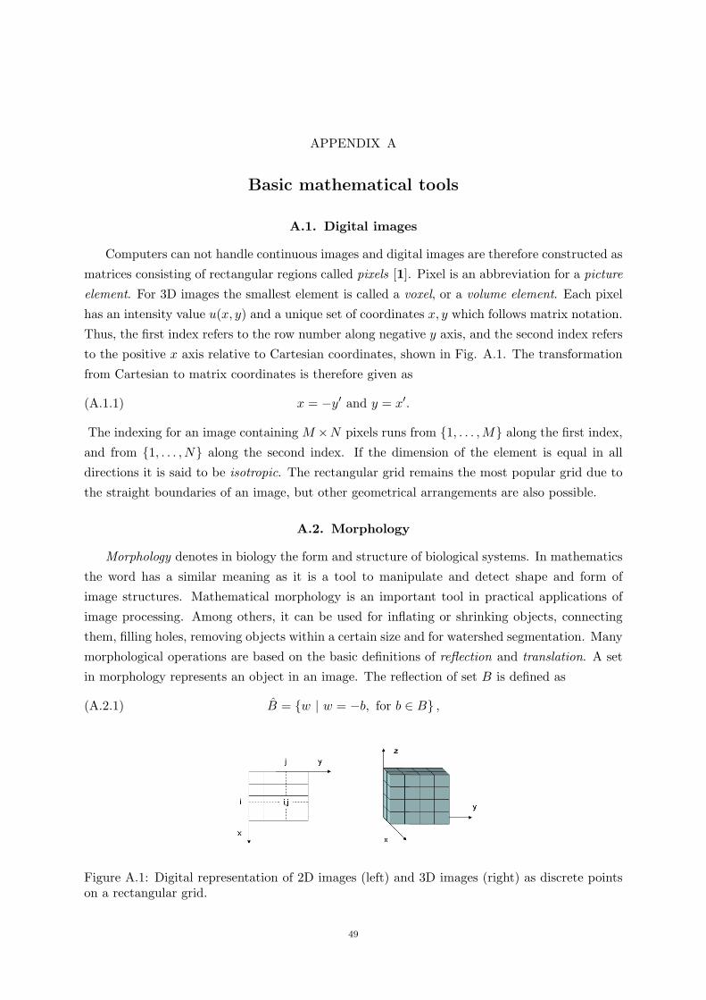
APPENDIX A

Basic mathematical tools

A.1. Digital images

Computers can not handle continuous images and digital images are therefore constructed as

matrices consisting of rectangular regions called pixels [1]. Pixel is an abbreviation for a picture

element. For 3D images the smallest element is called a voxel, or a volume element. Each pixel

has an intensity value u(x, y) and a unique set of coordinates x, y which follows matrix notation.

Thus, the first index refers to the row number along negative y axis, and the second index refers

to the positive x axis relative to Cartesian coordinates, shown in Fig. A.1. The transformation

from Cartesian to matrix coordinates is therefore given as

(A.1.1) x = −y′ and y = x′.

The indexing for an image containing M ×N pixels runs from 1, . . . ,M along the first index,

and from 1, . . . , N along the second index. If the dimension of the element is equal in all

directions it is said to be isotropic. The rectangular grid remains the most popular grid due to

the straight boundaries of an image, but other geometrical arrangements are also possible.

A.2. Morphology

Morphology denotes in biology the form and structure of biological systems. In mathematics

the word has a similar meaning as it is a tool to manipulate and detect shape and form of

image structures. Mathematical morphology is an important tool in practical applications of

image processing. Among others, it can be used for inflating or shrinking objects, connecting

them, filling holes, removing objects within a certain size and for watershed segmentation. Many

morphological operations are based on the basic definitions of reflection and translation. A set

in morphology represents an object in an image. The reflection of set B is defined as

(A.2.1) B = w | w = −b, for b ∈ B ,

Figure A.1: Digital representation of 2D images (left) and 3D images (right) as discrete pointson a rectangular grid.

49

50 A. BASIC MATHEMATICAL TOOLS

which is simply the set of all points in B where (x, y) has been replaced by (−x,−y). The

translation of B by point z = (z1, z2) is defined as

(A.2.2) Bz = c | c = b+ z, for b ∈ B .

Thus, Bz is all points where (x, y) have been replaced by (x + z1, y + z2), which represents a

translation. The two most basic morphological operations, erosion and dilation, are defined

from combining reflection and translation. An erosion shrinks the objects in an image according

to a structural element SE, which is a subimage or a set with specialized shape and size. A

typical structural element for inflation and shrinking is round-like and symmetrical,

(A.2.3) SE1 =

0 1 0

1 1 1

0 1 0

where the subscript indicates the radius of the structural element. The structural element

also defines the neighbourhood of the pixel. The structural element in (A.2.3) has a 4-connected

neigborhood since the central pixel has four neighours. In 2D, 4- and 8-connected neighborhoods

are the most common, and in 3D typical neighborhoods are 6, 18 and 26. Erosion of A by the

structural element SE is defined as

(A.2.4) A SE = z | Bz ⊆ A .

Consider the structural element B around origo and translate it by every point in A. Then, the

erosion is given as all points z such that B translated by z is entirely inside A. Note that a

useful property of erosion is detecting a one pixel wide outer perimeter P of a binary structure

A, accomplished by P = A − (A SE1). Erosion of Fig A.2(a) by a symmetrical, round-like

structural element SE6 is shown in Fig A.2(b) where the objects have shrinked according to the

structural element. The dilation is closely related to erosion, and will inflate an object when

applied. The dilation is defined as

(A.2.5) A⊕ SE =

z|Bz ∩A 6= ∅

,

which can be understood as all z, that after reflection and translation of SE by z, overlap A

with at least one element. A dilation of Fig A.2(a) by SE6 is shown in Fig A.2(c) where the

objects has been inflated according to SE.

In addition to erosion and dilation, opening and closing are useful morphological operators.

Opening of A by SE is defined as

(A.2.6) A SE = (A SE) ⊕ SE,

which is an erosion followed by a dilation using the same structural element. Opening has the

useful properties of smoothing the contour of objects, removing noise and at the same time

disconnecting objects without changing the overall shape of them. Compare the original image

in Fig A.2(a) to the opened image in Fig A.2(d) and take notice of the two noise grains that are

completely removed and the two right objects that are disconnected. Simultaneously, the objects

maintain their original shape except from the regions where the objects were disconnected.

A.2. MORPHOLOGY 51

(a) Original binaryimage.

(b) After erosion. (c) After dilation.

(d) After opening. (e) After closing.

Figure A.2: Morphological operations.

(a) Original binaryimage.

(b) Skeletonizationof (a).

(c) Pruning of (c)

(d) Filling holes in(a).

(e) Convex image of(a).

Figure A.3: Morphological operations.

Morphological closing is defined as

(A.2.7) A • SE = (A⊕ SE) SE,

which is a dilation followed by an erosion. Closing is particularly useful for bridging previously

disconnected objects without altering the overall shape of the objects. Fig A.2(e) shows a closing

of Fig A.2(a). In particular, note that the two objects to the left are connected after closing.

This property is useful in many practical applications to connect closely located objects. In

addition to the already described applications, morphology is applied for skeletonization (Fig.

A.3(b)), pruning ((Fig. A.3(c)), filling holes (Fig. A.3(d)), the convex hull (Fig. A.3(e)),

thinning, extraction of connected components, thickening and thinning.

Morphological operators can also be applied to gray-scale images, and in particular they

are used to perform image filtering. The top-hat filtering is an efficient method for filtering

that eliminates faint signals and preserves signals with a larger size than the structural element,

particularly useful in biology to preserve punctuated signals arising from organelles. The top-hat


filtering of the image u by the structural element SE is defined as

(A.2.8) T (u, SE) = u− (u SE).

The opening (u B) will eliminate objects larger than B, thus the objects smaller than SE

are subtracted from the image. Top-hat filtering can also be used for background correction,

removing slowly varying signals. Background correction is crucial in many applications, for

instance as preparation for threshold techniques in segmentation.

Watershed is the method of choice for segmentation in mathematical morphology. The un-

derlying idea comes from the visualization of a landscape. The rain falls in separate catchment

basins and are collected in reservoirs. All points that transport the water into the same catch-

ment basin are defined to be in the same watershed region. When the watershed segmentation is

applied directly to real images it often leads to severe over-segmenation due to the high number

of natural minima. The watershed algorithm does not distinguish between small and large min-

ima and will create a closed boundary around every minima. One solution to this problem is to

define a set of minima or initialisation regions also referred to as markers. Thus, the watershed

segmentation will be computed around each of those markers, in a one-to-one relationship, and

a strong over-segmentation is normally avoided. The watershed algorithm can be defined by

immersion or the topographical distance [81]. By immersion, it can be viewed as a landscape

immersed into water, and the watershed lines are defined as the point where the water from

different catchment basins meets. By topographical distance, the watershed transform is given

from image integration. The topographical distance between two points x and y in the image u

is given as

(A.2.9) Tu(x, y) = inf

∫

γ|∇u(γ(s))|ds,

which is the minimum variation of u along all possible paths from x to y. This definition leads

to the watershed transform. The catchment basin CB(mi) are defined as

(A.2.10) CB(mi) = x ∈ Ω | L(x,mi) < L(x,mj) ∀ i ∈ I, i 6= j

where I is the set of markers and mi a point marker within I and L(x,mi) = u(mi)+Tu(x,mi).

In the case of region markers, L(x,mi) is slightly differently defined. The watersheds or the

watershed lines are given as the points not belonging to any catchment basin,

(A.2.11) W (u) = x ∈ Ω | x /∈ ∪i∈ICB(mi) ,

which are the points where L(x,mi) = L(x,mj) for two adjacent markers mi and mj . The

topographical distance function and a 1D watershed point is demonstrated in Fig. A.4 where

L(x,m1) (dashed line) and L(x,m2) (dotted line) have been drawn around two markers m1 and

m2 (circles). Clearly, the watershed line W (u) (arrow) appears where L(x,m1) = L(x,m2).

Examples of watershed segmentation are given in Paper IV.

A.3. VARIATIONAL AND PDE METHODS 53

0 1 2 3 4 5

2

0

0.2

0.4

0.6

0.8

M1

M2

α1

+ L1

(x)

α2

+ L2

(x)

x

T(x

)

L(x,m1)

L(x,m2)

W(u)

u(x)

m1 m2

Figure A.4: Topographical distance function

A.3. Variational and PDE methods

Many image processing tasks can be formulated as a variational problem [83, 84, 85] where

the obtained solution u is given as

(A.3.1) u = argminuF [u]

where F [u] : Rn × . . . × R

n → R is a functional which is at least one time differentiable,

F ⊂ D1, and the variation is along the function(s) u. The minimazation requires a local

minimum (preferrably a global) of F for a satisfying solution of u. Let ∂F∂u be the Euler derivative

(first variation). Then, ∂F∂u = 0 is a necessary condition for u to be a minimizer. The variational

problem can be solved by resolving the Euler-Lagrange equations deduced in the first variation.

Consider functional F

(A.3.2) F [u] =

∫

ΩG(x, u,∇u)dx, u : R × R → R

2,

where u is a variable in 2D and F is the objective function. An incremental step is computed as

(A.3.3) F [u+ εv] =

∫

ΩG(x, u+ εv,∇(u+ εv))dx

as a function of a single variale ε in the direction of a randomly chosen test function v : R×R →

R2. In a minimum, (d/dε)F (u+ εv) = 0 for ε = 0. Using the chain rule,

0 =

∫

Ω

(

∂G

∂uv +

[

∂G

∂ux,∂G

∂uy

]

∇v

)

dx(A.3.4)

=

∫

Ω

(

∂G

∂u−∇ ·

[

∂G

∂ux,∂G

∂uy

]T)

vdx(A.3.5)


upon integration by parts. This relation is true for any test function v and any integration

domain Ω, and therefore the integrand has to be zero,

(A.3.6)∂G

∂u= ∇ ·

[

∂G

∂ux,∂G

∂uy

]T

,

which is the Euler-Lagrange equation to solve. The functional F can also be a function of more

variables, and this leads to a system of coupled equation. (A.3.6) is also named the Gateaux

derivative of F . The Euler-Lagrange equation can either be solved as an elliptic or parabolic

boundary value problem. A general elliptic equation has the form

Lu = f in Ω,(A.3.7)

∂u

∂ν= g on ∂Ω,(A.3.8)

using Neumann boundary requirements, and ν is the normal direction of the boundary. L is a

second order partial differential operator, depending on the spatial coordinates. n is the number

of orthogonal directions to span the solution space. The same problem can equavivalently be

solved with the parabolic boundary-value problem

ut + Lu = f in Ω × [0, T ],(A.3.9)

∂u

∂ν= g on ∂Ω × [0, T ],(A.3.10)

u = u0 on Ω × t = 0 ,(A.3.11)

where an artificial time evolution t = [0, T ] is introduced. The differential operator L depends

on the time t in addition to the spatial coordinates. In a steady-state solution it is required a

derivative equal to zero, and we therefore require

(A.3.12) ut = −∂F

∂u= 0.

A particularly important PDE in image processing is the mean curvature flow,

(A.3.13)∂φ

∂t= |∇φ|∇ ·

(

∇φ

|∇φ|

)

= κ|∇φ|, κ = −∇ ·

(

∇φ

|∇φ|

)

where κ is the curvature of the level curve of φ(x). Thus, (A.3.13) describes a movement of the

function φ which is proportional to the mean curvature of the level curve in any point. This

movement minimizes the length of the level curve and provides a smoother function φ, therefore

the equation is used for denoising. Note that the mean curvature flow has an element of isotropic

diffusion which is related to the Laplacian, ut = ∆u. The isotropic diffusion becomes clear if

|∇φ| is removed from the equation or is equal to unity everywhere. Then, the diffusion will

smooth the information homogeneously in all directions.

Bibliography

[1] Gonzalez RC, Woods RE. Digital Image Processing. Pearson Education, Inc. Upper Saddle River, New Jersey

07458; 2008.

[2] Bengtsson E. Computerized Cell Image Analysis: Past, Present, and Future. In: SCIA03; 2003. p. 395–407.

[3] Bhaskar H, Singh S. Live cell imaging: a computational perspective. 2007 Apr;1(3):195–212.

[4] Sonka M, Hlavac V, Boyle R. Image Processing, Analysis, and Machine Vision. Thomson-Engineering; 2007.

[5] Pratt WK. Digital Image Processing, Forth Edition. WILEY-INTERSCIENCE A John Wiley & Sons, Inc.,

Publication; 2007.

[6] Jahne B. Digital Image Processing, 6th revised and extended edition. Springer-Verlag Heidelberg; 2005.

[7] Hodneland E. Segmentation of Digital Images. University of Bergen, Norway; 2003.

[8] Goldman RD, Spector DL. Live Cell Imaging: A Laboratory Manual. CSHL Press; 2004.

[9] Abramowitz M. Fluorescence Microscopy: The Essentials. vol. 4. Olympus Corporation Publishing; 1993.

[10] Vallotton P, Ponti A, Waterman-Storer CM, E D Salmon z, Danuser G. Recovery, Visualization, and Analysis

of Actin and Tubulin Polymer Flow in Live Cells: A Fluorescent Speckle Microscopy Study. Biophysical

Journal. 2003;85:1289–1306.

[11] Suh J, Dawson M, Hanes J. Real-time multiple-particle tracking: applications to drug and gene delivery.

Advanced Drug Delivery Reviews. 2005;57(1):63–78.

[12] Al-Kofahi KA, Can A, Lasek S, Szarowski DH, Dowell-Mesfin N, Shain W, et al. Median-based robust

algorithms for tracing neurons from noisy confocal microscope images. IEEE Transactions on Information

Technology in Biomedicine. 2003;7(4):302–317.

[13] Can A, Shen H, Turner JN, Tanenbaum HL, Roysam B. Rapid automated tracing and feature extraction from

retinal fundus images using direct exploratory algorithms. IEEE Transactions on Information Technology in

Biomedicine. 1999;3(2):125–138.

[14] Block T, Kin C, Breckenridge BM. Mutants of PC12 cells with altered cyclic

AMP responses. Molecular and cellular biology. 1984;4(10):20912097. Available from:

http://www.pubmedcentral.nih.gov/picrender.fcgi?artid=369026\&blobtype=pdf.

[15] Rescher U, Ruhe D, Ludwig C, Zobiack N, Gerke V. Annexin 2 is a phosphatidylinositol (4,5)-

bisphosphate binding protein recruited to actin assembly sites at cellular membranes. Journal of Cell Science.

2004;117:3473–3480.

[16] Rudolf R, Salm T, Rustom A, Gerdes HH. Dynamics of immature secretory granules: role of cy-

toskeletal elements during transport, cortical restriction, and F-actin-dependent tethering. Mol Biol Cell.

2001;12:13531365.

[17] Rustom A, Saffrich R, Markovich I, Walther P, Gerdes HH. Nanotubular Highways for Intracellular Organelle

Transport. Science. 2004;303:1007–1010.

[18] Tscherepanow M, Zollner F, Kummert F. Automatic segmentation of unstained living cells in bright-field

microscope images. In: Perner P, editor. Workshop on Mass-Data Analysis of Images and Signals, MDA2006.

IBaI CD-Report; 2006. p. 86–95.

[19] Geusebroek J, Smeulders A, Geerts H. A Minimum Cost Approach for Segmenting Net-

works of Lines. International Journal of Computer Vision. 2001 Jul;43(2):99–111. Available from:

citeseer.ist.psu.edu/geusebroek01minimum.html.

[20] Wu K, Gauthier D, Levine M. Live Cell Image Segmentation. IEEE Transactions on Biomedical Engineering.

1995;42(1):1–12.

55

http://www.pubmedcentral.nih.gov/picrender.fcgi?artid=369026\&blobtype=pdf

citeseer.ist.psu.edu/geusebroek01minimum.html

56 BIBLIOGRAPHY

[21] Yu D, Pham TD, Yan H, Whang B, Crane DI. Segmentation of cultured neurons using logical analysis

of grey and distance differences. Journal of neuroscience methods. 2007;166(1):125–137. Available from:

citeseer.ist.psu.edu/wu95live.html.

[22] Adiga PSU, Chaudhuri BB. Efficient cell segmentation tool for confocal microscopy tissue images and quan-

titative evaluation of FISH signals. Microscopy Research and Technique. 1999;44(1):49–68.

[23] Adiga PSU. Integrated Approach for Segmentation of 3-D Confocal Images of a Tissue Specimen. Microscopy

Research and Technique. 2003;54(4):260–270.

[24] Solorzano COD, Malladi R, Lelievre SA, Lockett SJ. Segmentation of nuclei and cells using membrane related

protein markers. Journal of Microscopy. 2001;201:404–415.

[25] Malpica N, Ortiz de Solorzano C, Vaquero JJ, Santos A, Vallcorba I, Garcia-Sagredo JM, et al. Applying

watershed algorithms to the segmentation of clustered nuclei. Cytometry. 1997;28:289–297.

[26] Lin U G A, Olson K, Guzowski JF, Barnes CA, Roysam B. A Hybrid 3D Watershed Algorithm Incorpo-

rating Gradient Cues and Object Models for Automatic Segmentation of Nuclei in Confocal Image Stacks.

Cytometry, Part A. 2003;56A(1):23–26.

[27] Wahlby C, Sintorn IM, Erlandsson F, Borgefors G, Bengtsson E. Combining intensity, edge and shape

information for 2D and 3D segmentation of cell nuclei in tissue sections. Journal of Microscopy. 2004;215:67–

76.

[28] Zamani F, Safabakhsh R. An unsupervised GVF snake approach for white blood cell segmentation based on

nucleus. In: Signal Processing, The 8th International Conference on. vol. 2; 2006. .

[29] Dufour A, Shinin V, Tajbakhsh S, Guillen-Aghion N, Olivo-Marin JC, Zimmer C. Seg-

menting and Tracking Fluorescent Cells in Dynamic 3-D Microscopy With Coupled Ac-

tive Surfaces. Image Processing, IEEE Transactions on. 2005;14(9):1396–1410. Available from:

http://ieeexplore.ieee.org/xpls/abs_all.jsp?arnumber=1495511.

[30] Adiga U, Malladi R, Fernandez-Gonzalez R, Ortiz de Solorzano C. High-throughput analysis of multispectral

images of breast cancer tissue. IEEE Trans Image Process. 2006 August;15(8):2259–2268.

[31] Wahlby C, Lindblad J, Vondrus M, Bengtsson E, Bjorkesten L. Algorithms for cytoplasm segmentation of

fluorescence labelled cells. Analytical Cellular Pathology. 2002;24:101–111.

[32] Baggett D, Nakaya Ma, McAuliffe M, Yamaguchi TP, Lockett S. Whole cell segmentation in solid tissue

sections. Cytometry Part A. 2005;67A:137–143.

[33] Dow AI, Shafer SA, Kirkwood JM, Mascari RA, Waggoner AS. Automatic multiparameter fluorescence

imaging for determining lymphocyte phenotype and activation status in melanoma tissue sections. Cytometry.

1996;25:71–81.

[34] Chan TF, Osher S, Shen J. The digital TV filter and non-linear denoising. IEEE Transactions on Image

processing. 2001;10(2). Available from: http://ieeexplore.ieee.org/iel5/83/19508/00902288.pdf.

[35] Gonzalez RC, Woods RE. Digital Image Processing. Addison-Wesley Publishing Company; 1992.

[36] van den Boomgaard R, van der Weij R. Gaussian Convolutions. Numerical Approximations Based on In-

terpolation. In: Scale-Space ’01: Proceedings of the Third International Conference on Scale-Space and

Morphology in Computer Vision. London, UK: Springer-Verlag; 2001. p. 205–214.

[37] Baxes GA. Digital Image Processing: Principles and Applications. Wiley; 1994.

[38] Weickert J. Theoretical Foundations of Anisotropic Diffusion in Image Processing. In: Proceedings of the 7th

TFCV on Theoretical Foundations of Computer Vision. London, UK: Springer-Verlag; 1996. p. 221–236.

[39] Weichert J. A Review of Nonlinear Diffusion Filtering. Lecure Notes in Computer Science. 1997;.

[40] van den Boomgaard R. Algorithms for Non-Linear Diffusion. University of Amsterdam;. Available from:

http://staff.science.uva.nl/~rein/nldiffusionweb/nldiffusioncode.pdf.

[41] Weickert J. Multiscale Texture Enhancement. In: CAIP ’95: Proceedings of the 6th International Conference

on Computer Analysis of Images and Patterns. London, UK: Springer-Verlag; 1995. p. 230–237.

[42] Gautama S, Goeman W, D’Haeyer J. Robust detection of road junctions in VHR images using an improved

ridge detector. The International Archives of Photogrammetry, Remote sensing and Spatial Information

Sciences. 2004;34. Available from: http://www.isprs.org/istanbul2004/comm3/papers/381.pdf.

citeseer.ist.psu.edu/wu95live.html

http://ieeexplore.ieee.org/xpls/abs_all.jsp?arnumber=1495511

http://ieeexplore.ieee.org/iel5/83/19508/00902288.pdf

http://staff.science.uva.nl/~rein/nldiffusionweb/nldiffusioncode.pdf

http://www.isprs.org/istanbul2004/comm3/papers/381.pdf

BIBLIOGRAPHY 57

[43] Finney LR, Thomas Jr GB. Calculus. Addison-Wesley Publishing Company, Inc; 1994.

[44] Vincent L, Soille P. Watersheds in Digital Spaces: An Efficient Algorithm Based on Immersion Simulations.

IEEE Trans Pattern Anal Mach Intell. 1991;13(6):583–598.

[45] Rambabu C, Chakrabarti I. An efficient immersion-based watershed transform method and its prototype

architecture. J Syst Archit. 2007;53(4):210–226.

[46] Chien SY, Huang YW, Chen LG. Predictive watershed: a fast watershed algorithm for video segmentation.

CirSysVideo. 2003 May;13(5):453–461.

[47] Felkel P, Bruckschwaiger M, Wegenkittl R. Implementation and complexity of the watershed-from-markers

algorithm computed as a minimal cost forest. Computer Graphics Forum. 2002;20:2001. Available from:

http://www.citebase.org/abstract?id=oai:arXiv.org:cs/0206009.

[48] Najman L, Schmitt M. Watershed of a continuous function. Signal Process. 1994;38(1):99–112.

[49] Meyer F. Topographic distance and watershed lines. Signal Processing. 1994;38(1):113–125.

[50] Nguyen HT, Worring M, van den Boomgaard R. Watersnakes: Energy-Driven Wa-

tershed Segmentation. IEEE Trans on PAMI. 2003;25(3):330–342. Available from:

citeseer.ist.psu.edu/article/nguyen03watersnakes.html.

[51] Grau V, Mewes AJU, Raya MA, Kikinis R, Warfield SK. Improved watershed transform for medical im-

age segmentation using prior information. IEEE Trans Med Imaging. 2004;23(4):447–458. Available from:

http://dblp.uni-trier.de/db/journals/tmi/tmi23.html#GrauMRKW04.

[52] Osma-Ruiz V, Godino-Llorente JI, Saenz-Lechon N, Gomez-Vilda P. An improved watershed algorithm based

on efficient computation of shortest paths. Pattern Recogn. 2007;40(3):1078–1090.

[53] Bengtsson E, Wahlby C, Lindblad J. Robust cell image segmentation methods. Pattern Recognition and

Image Analysis. 2004;14:157–167.

[54] Lindblad L. Development of Algorithms for digital image cytometry, PhD thesis. Acta Universitatis Upsalien-

sis; 2002.

[55] Tai XC, Hodneland E, Weickert J, Bukoreshtliev NV, Lundervold A, Gerdes HH. Level Set Methods for

Watershed Image Segmentation. In: SSVM; 2007. p. 178–190.

[56] Dima A, Scholz M, Obermayer K. Automatic segmentation and skeletonization of neurons from confo-

cal microscopy images based on the 3-D wavelet transform. IEEE Transactions on Image Processing.

2002;11(7):790–801. Available from: http://dblp.uni-trier.de/db/journals/tip/tip11.html#DimaSO02.

[57] Tai XC, Chan TF. A survey on multiple set methods with applications for identifying piecewise constant

functions. International J Numerical Analysis and Modelling. 2004;1(1):25–48.

[58] Chan TF, Vese L. Active contours without edges. IEEE Trans on Image Processing. 2001;10:266–277.

[59] Tai XC, Chan TF. A survey on multiple level set methods with applications for identifying piecewise constant

functions. Int J Numer Anal Model. 2004;1(1):25–47.

[60] Vese LA, Chan TF. A Multiphase Level Set Framework for Image Segmentation Using the Mumford and

Shah Model. International Journal of Computer Vision. 2002;50(3):271–293.

[61] Chan TF, Moelich M, Sandberg B. Some recent developments in variational image segmentation. In: Tai

XC, Lie KA, Chan T, Osher S, editors. Image Processing based on partial differential equations. Springer,

Heidelberg; 2006. p. 175–201.

[62] Lie J, Lysaker M, Tai XC. A Binary Level Set Model and Some Applications to Mumford-Shah Image

Segmentation. IEEE Transactions on Image Processing. 2006;15(5):1171–1181.

[63] Song B, Chan TF. A Fast Algorithm for Level Set Based Optimization. CAM-UCLA. 2002;(68). Under

revision for publication in SIAM J. Sci. Comput.

[64] Lie J, Lysaker M, Tai XC. A piecewise constant level set framework. Int J Numer Anal Model. 2005;2(4):422–

438.

[65] Zhang YJ. Evaluation and comparison of different segmentation algorithms. Pattern Recognition Letters.

1997;18(10):963–974.

[66] Zhang YJ. A survey on evaluation methods for image segmentation. Pattern Recognition. 1996;29:1335–1346.

http://www.citebase.org/abstract?id=oai:arXiv.org:cs/0206009

citeseer.ist.psu.edu/article/nguyen03watersnakes.html

http://dblp.uni-trier.de/db/journals/tmi/tmi23.html#GrauMRKW04

http://dblp.uni-trier.de/db/journals/tip/tip11.html#DimaSO02

58 BIBLIOGRAPHY

[67] Goumeidane AB, Khamadja M, Belaroussi B, Benoit-Cattin H, Odet C. New discrepancy measures for

segmentation evaluation. Pattern Recognition Letters. 2003;2(10):411–414.

[68] Unnikrishnan R, Pantofaru C, Hebert M. A measure for objective evaluation of image segmentation algo-

rithms. In: Proceedings of the 2005 IEEE Conference on Computer Vision and Pattern Recognition (CVPR

’05), Workshop on Empirical Evaluation Methods in Computer Vision; 2005. .

[69] Baluska F, Volkmann D, Barlow PW. Cell-cell Channels, Ch. Tunneling Nanotubes: Cell-cell channels in

animal cells, Gerdes, H-H. and Rustom, A. Landes bioscience; 2005.

[70] Onfelt B, Nedvetzki S, Yanagi K, M Davis D. Cutting Edge: Membrane Nanotubes Connect Immuno Cells.

The Journal of Immunology. 2004;173:1511–1513.

[71] Hodneland E, Lundervold A, Gurke S, Tai XC, Rustom A, Gerdes HH. Automated detection of tunneling

nanotubes in 3D images. Cytometry Part A. 2006;69A:961–972.

[72] Chang SG, Yu B, Vetterli M. Spatially adaptive wavelet thresholding with context modeling for image

denoising. IEEE Transactions on Image Processing. 2000;9(9):1522–1531.

[73] Gonzalez RC, Woods RE. Digital Image Processing. Boston, MA, USA: Addison-Wesley Longman Publishing

Co., Inc.; 1992.

[74] Peng S, Urbanc B, Cruz L, Hyman BT, Stanley HE. Neuron recognition by parallel Potts seg-

mentation. Proceedings of the National Academy of Sciences. 2003;100(7):3847–3852. Available from:

http://www.pnas.org/cgi/content/abstract/100/7/3847.

[75] Weickert J, Romeny B, Viergever M. Efficient and Reliable Schemes for Nonlinear Diffu-

sion Filtering. IEEE Transactions on Image Processing. 1998 Mar;7(3):398–410. Available from:

citeseer.ist.psu.edu/weickert98efficient.html.

[76] Weickert J. Coherence-Enhancing Diffusion Filtering. Int J Comput Vision. 1999;31(2-3):111–127.

[77] Kimmel R, Malladi R, Sochen N. Images as Embedded Maps and Minimal Surfaces: Movies, Color, Texture,

and Volumetric Medical Images. Int J Comput Vision. 2000;39(2):111–129.

[78] Pollak I, Willsky AS, Krim H. Image Segmentation and Edge Enhancement with Stabilized Inverse Diffusion

Equations. IEEE transactions on image processing. 2000;9(2).

[79] Perona P, Malik J. Scale-Space and Edge Detection Using Anisotropic Diffusion. IEEE Transactions on

Pattern Analysis and Machine Intelligence. 1990;12(7):629–639.

[80] Vincent L, Soille P. Watersheds in Digital Spaces: An efficient Algorithm Based on Immersion Simulations.

IEEE Transactions on Pattern Analysis and Machine Intelligence. 1991;13, No. 6:583–598.

[81] Roerdink J, Meijster A. The Watershed Transform: Definitions, Algorithms and Parallelization Techniques.

Institute for Mathematics and Computer Science, University of Groningen, Groningen, The Netherlands,

IWI 99–9-06. 1999;Available from: citeseer.ist.psu.edu/roerdink01watershed.html.

[82] Tai XC, Hodneland E, Weickert J, Buroresthliev NV, Lundervold A, Gerdes HH. Level set methods for

watershed image segmentation. In: Scale Space and Variational Methods in Computer Vision, LNCS 4485.

Springer; 2007. p. 178–190.

[83] Chan TF, Shen J. Image Processing And Analysis: Variational, Pde, Wavelet, And Stochastic Methods.

Philadelphia, PA, USA: Society for Industrial and Applied Mathematics; 2005.

[84] Evans LC. Partial Differential Equations. American Mathematical Society; 1998.

[85] Sapiro G. Geometric Partial Differential Equations and Image Analysis. vol. 19. New York, NY, USA: Cam-

bridge University Press; 2001.

http://www.pnas.org/cgi/content/abstract/100/7/3847

citeseer.ist.psu.edu/weickert98efficient.html

citeseer.ist.psu.edu/roerdink01watershed.html

Documents

Biomedical Image Processing in the Study of Living Cells