Embed Size (px)
Citation preview
Revista Colombiana de EstadísticaJanuary 2017, Volume 40, Issue 1, pp. 65 to 83
DOI: http://dx.doi.org/10.15446/rce.v40n1.51738
Bimodal Regression Model
Modelo de regresión Bimodal
Guillermo Martínez-Flórez1,a, Hugo S. Salinas2,b,Heleno Bolfarine3,c
1Departamento de Matemáticas y Estadística, Facultad de Ciencias Básicas,Universidad de Córdoba, Córdoba, Colombia
2Departamento de Matemática, Facultad de Ingeniería, Universidad de Atacama,Copiapó, Chile
3Departamento de Estatística, IME, Universidad de Sao Paulo, Sao Paulo, Brasil
Abstract
Regression analysis is a technique widely used in different areas of hu-man knowledge, with distinct distributions for the error term. It is the case,however, that regression models with the error term following a bimodaldistribution are not common in the literature, perhaps due to the lack ofsimple to deal with bimodal error distributions. In this paper, we propose asimple to deal with bimodal regression model with a symmetric-asymmetricdistribution for the error term for which for some values of the shape pa-rameter it can be bimodal. This new distribution contains the normal andskew-normal as special cases. A real data application reveals that the newmodel can be extremely useful in such situations.
Key words: Bimodal Distribution, Generalized Gaussian Distribution, Lin-ear Regression, Power Regression Model.
Resumen
El análisis de regresión es una técnica muy utilizada en diferentes áreas deconocimiento humano, con diferentes distribuciones para el término de error,sin embargo los modelos de regresión con el termino de error siguiendo unadistribución bimodal no son comunes en la literatura, tal vez por la simplerazón de no tratar con errores con distribución bimodal. En este trabajoproponemos un camino sencillo para hacer frente a modelos de regresiónbimodal con una distribución simétrica - asimétrica para el término de errorpara la cual para algunos valores del parámetro de forma esta puede ser
aPhD. E-mail: [email protected]. E-mail: [email protected]. E-mail: [email protected]
65
66 Guillermo Martínez-Flórez, Hugo S. Salinas & Heleno Bolfarine
bimodal. Esta nueva distribución contiene a la distribución normal y ladistribución normal asimétrica como casos especiales. Una aplicación condatos reales muestra que el nuevo modelo puede ser extremadamente útil enalgunas situaciones.
Palabras clave: distribución bimodal, distribución gaussiana generalizada,regresión lineal, modelo de regresión exponenciado.
1. Introduction
To study the relationship between variables in different areas of human knowl-edge, linear and nonlinear regression models have been substantially used. It istypically considered that the error term follows a normal distribution althoughmore general symmetric error distributions have also been considered. One ofthose alternatives is to consider that the errors follow distributions with heaviertails than those of normal distribution, in order to reduce the influence of outly-ing observations. In this context, Lange, Little and Taylor (1989) proposed theStudent-t model with unknown degrees of freedom for parameter ν. Cordeiro, Fer-rari, Uribe-Opazo and Vasconcellos (2000), and Galea, Paula and Cysneiros (2005)present results from the study of inferential aspects of symmetrical nonlinear mod-els. For the asymmetric nonlinear model, we use the work of Cancho, Lachos andOrtega (2010). Symmetrical measurement error models have been investigated inArellano-Valle, Bolfarine and Vilca-Labra (1996).
One situation in which we encounter an anomaly in the error term of the modeloccurs when it is of interest to explain the fat percentage in the human body asa function of the individual weight. It is the case, however, that given inherentgender peculiarities, the exclusion of the gender variable can lead to a bimodalerror distribution model. That is, not taking into account the sex variable , leadsto a regression model for which the distribution of the error term is no longerunimodal.
A viable alternative to this situation is to use a mixture of normal distributionsfor the error term. According to this alternative, there are two models to estimate,one for each component of the normal mixture, namely (εj for j = 1, 2); they areboth normally distributed with mean zeros and variance σj for j = 1, 2. Accordingto De Veaux (1989), for the special case of two explanatory variables X1 and X2,the response variable can be written as
yi =
{β10 + β11x1i + β12x2i + ε1i, with probability p,β20 + β21x1i + β22x2i + ε2i, with probability 1− p
where the εji ∼ N(0, σ2j ) are independent, j = 1, 2, i = 1, 2, · · · , n. Consequently,
response yi has a pdf
f(yi) =p
σ1φ
(yi − β10 − β11x1i − β12x2i
σ1
)+
1− pσ2
φ
(yi − β20 − β21xi − β22x2i
σ2
),
Revista Colombiana de Estadística 40 (2017) 65–83
Bimodal Regression Model 67
for i = 1, 2, . . . , n. Although widely recommended, this alternative has some im-portant drawbacks. The first results from lack of identifiability of some modelparameters, more specifically, β10 and β20. Another difficulty is related to con-vergence problems with the algorithm for parameter estimation, including theproportion of data points for each model. Moreover, the model is not parsimo-nious at all, since by increasing the number of explanatory variables, the numberof parameters in the model jumps to nine. For instance, for one explanatory vari-able there are seven parameters to be estimated, making algorithm convergencedifficult. De Veaux (1989) presents an EM-algorithm for the mixture of regressionmodels. Further results can be found in Quandt (1958), Turner (2000), and Young& Hunter (2010), among others.
In this paper, we suggest using the symmetric-asymmetric bimodal alpha-powermodel, considered in Bolfarine, Martínez and Salinas (2012), to adjust data with alinear relation. Results from two real data applications are reported the illustratethe usefulness of the models developed. One alternative, clearly, is to undertakedata transformation or use mixtures of distributions, as mentioned above.
The paper is organized as follows. Section 2 is devoted to describing the bi-modal symmetric-asymmetric alpha-power distribution and some of its main prop-erties. The model considered generalizes both the skew-normal model (Azzalini1985) and the power-normal model (Pewsey, Gómez and Bolfarine 2012). Theextension of the normal multiple regression model to the case in which the errorterm follows the bimodal symmetric-asymmetric power-normal (ABPN) model isconsidered in Section 3. Maximum likelihood estimation is discussed in Section 4.In particular, it is shown that the Fisher information matrix is nonsingular andallows for normality to be tested using the likelihood ratio statistics. A real appli-cation considered in Section 5 illustrates the fact that the model considered canoutperform traditional symmetric models that have been previously considered inthe literature, in specifically the mixture of normals.
2. The Bimodal Symmetric-AsymmetricAlpha-Power Distribution
The alpha-power distribution was first considered in Durrans (1992), and itspdf is given by
g(z;α) = αφ(z){Φ(z)}α−1, z ∈ R, (1)
where α ∈ R+ is a shape parameter, and Φ and φ are the density and distributionfunctions of the standard normal, respectively. We use the notation Z ∼ PN(α).The location-scale extension of Z, Y = µ+ σZ, where ξ ∈ R and σ ∈ R+, have aprobability density function given by
ϕ(y;µ, σ, α) =α
σφ
(y − µσ
){Φ
(y − µσ
)}α−1
. (2)
We use the notation Y ∼ PN(µ, σ, α).
Revista Colombiana de Estadística 40 (2017) 65–83
68 Guillermo Martínez-Flórez, Hugo S. Salinas & Heleno Bolfarine
Several authors, for example, Gupta and Gupta (2008), Pewsey, Gómez &Bolfarine (2012), Rego, Cintra & Cordeiro (2012), studied properties of this model,but the fact that this model can be seen as an aditive generalized model seems to beunknown. This model can be further extended by considering µi = x′iβ replacingµ, where β is an unknown vector of regression coefficients and xi a vector of knownregressors, possibly correlated with the response vector.
Martínez-Flórez, Bolfarine & Gómez (2015) considered the multiple regressionmodel represented by
yi = x′iβ + εi, i = 1, 2, . . . , n, (3)
where β is a vector of unknown constants, xi are values of known explanatory vari-ables, and the error terms εi are independent random variables with power-normaldistribution, PN(0, σ, α). This model becomes a viable alternative to the ordinaryregression models under normality for the situation of asymmetrically distributederrors with kurtosis above 3 (normal distribution). These authors studied themain properties of this model, obtained equations to estimate model parametersvia maximum likelihood, and deduced its information matrices. They found thatthe Fisher information matrix is nonsingular. Although the new proposal is a vi-able alternative to model data with low and high asymmetry, this model can onlybe applied to unimodal situations.
As an extension of the PN model to bimodal data, Bolfarine, Martínez-Flórez& Salinas (2012) introduced the family of bimodal distributions, one symmetricand the other asymmetric. The corresponding density function of the bimodalpower-normal distribution is given by
ϕ(y;µ, σ, α) =α
σ
2α−1
2α − 1φ
(y − µσ
){Φ
(∣∣∣∣y − µσ∣∣∣∣)}α−1
, x ∈ R, (4)
where µ is the location parameter and σ is the scale parameter. We use thenotation BPN(µ, σ, α). Note that for α = 1 the normal distribution N(µ, σ2)follows.
The r-th moment of the random variable Y ∼ BPN(0, 1, α) is given by
E(Zr) =
{0, if r is odd,
2µr(0), if r is even.
where
µr(0) = αcα
∫ ∞0
zrφ(z) {Φ(z)}α−1dz, r = 0, 1, 2, . . . (5)
Hence, it follows that E(Z) = E(Z3) = 0. The authors show that the pdf issymmetric and, moreover, if α > 1, then its density function is bimodal. Fur-thermore, maximum likelihood estimation is considered for model parameters andthe Fisher information matrix is derived and shown to be nonsingular. Under
Revista Colombiana de Estadística 40 (2017) 65–83
Bimodal Regression Model 69
these conditions, and given that it is a regular continuous function, it also fol-lows the
√n-normal approximation for the maximum likelihood estimators for the
parameter vector.Bolfarine et al. (2012) also studied a distribution for fitting symmetric-asymmetric
data with bimodal behaviour and this distribution was termed the bimodal symmetric-asymmetric power-normal model.
The density function for the location-scale version of the model can be writtenas
ϕ(y;µ, σ, α, λ) =2αcασ
φ
(y − µσ
){Φ
(∣∣∣∣y − µσ∣∣∣∣)}α−1
Φ
(λy − µσ
),
where y ∈ R, µ ∈ R is a location parameter, σ > 0 is a scale parameter, α ∈ R+
is a shape parameter, λ ∈ R is an asymmetry parameter, and cα = 2α−1/(2α − 1)is the normalizing constant. We use the notation Y ∼ ABPN(µ, σ, α, λ).
The authors show that for α > 1 and λ satisfying[1− λ
zφ(λz)Φ(λz)
]> 0, this model
is bimodal asymmetric; whereas for α > 1 and λ = 0, it is bimodal symmetric.Conversely, for α ≤ 1 the resulting model is unimodal. We note that for α = 1the skew-normal model follows, for α = 1 and λ = 0 the normal case follows, andfor λ = 0 the bimodal power-normal model follows.
The r-th moment of a random variable Z ∼ ABPN(0, 1, α, λ) is given by
E(Zr) =
{2µr(0), if r is even,
2µr(0) + 2µr(β, α), if r is odd,
where
µr(λ, α) = 2αcα
∫ ∞0
zrφ(z) {Φ(z)}α−1Φ(λz)dz.
In addition to these results, these authors have shown that the informationmatrix is nonsingular at the vicinity of symmetry, that is, α = 1 and λ = 0. Thisleads to large sample normal distribution for the maximum likelihood estimatorsfor which the asymptotic covariance matrix is the inverse of the Fisher informationmatrix.
3. The Multiple Regression Model WithABPN Errors
We assume, under the ordinary multiple regression model, that the error termfollows a ABPN distribution with parameters µ = 0, σ, α and λ, that is, for i =1, 2, . . . , n, the εi are independent random variables with εi ∼ ABPN(0, σ, α, λ).Hence, it follows that the density function of εi is given by
ϕ(εi; 0, σ, α, λ) =2αcασ
φ(εiσ
){Φ(∣∣∣εiσ
∣∣∣)}α−1
Φ(λεiσ
),
Revista Colombiana de Estadística 40 (2017) 65–83
70 Guillermo Martínez-Flórez, Hugo S. Salinas & Heleno Bolfarine
for i = 1, . . . , n. Therefore, it follows that yi given xi (denoted yi | xi) also followsa ABPN distribution, that is, yi | xi ∼ ABPN(x′iβ, σ, α, λ), for i = 1, 2, . . . , n.In this model, x′iβ is a location parameter, σ is a scale parameter, α is a shapeparameter, and λ is an asymmetry parameter where β is a vector of unknownconstants and xi are values of known explanatory variables.
The interpretation of the systematic part of the model, namely (β0, β1, · · · , βp),is similar to that of the model under the ordinary normal assumption, and σ is ascale parameter related to the error terms.
Under the ABPN model, E(yi) 6= x′iβ, and we have to make the following cor-rection to obtain the regression line as the expected value of the response variableβ∗0 = β0 +µε, where µε = E(εi). Thus, E(yi) = x′iβ
∗ where β∗ = (β∗0 , β1, . . . , βp)′.
As special cases this model contains the model with normal errors, that is,λ = 0 and α = 1, as well as the model with skew-normal errors for α = 1 and thebimodal symmetric error model for λ = 0.
4. Inference for the Multiple Linear ABPN Model
4.1. Likelihood and Score Functions
Considering a matrix notation where Y denotes a (n × 1)-dimensional vectorwith entries yi and X the (n×(p+1))-matrix with rows x′i, the likelihood functionfor θ = (β′, σ, α, λ)′, given a random sample of size n, Y = (Y1, Y2, . . . , Yn)′, canbe written as
`(β;Y) = n[ln(2α) + ln(cα)− ln(σ)]
− 1
2σ2(Y −Xβ)′(Y −Xβ) + 1′ [(α− 1)U1 + U2] ,
where 1′ is a n-dimensional vector, U1 and U2 are n-dimensional vectors withelements ln
{Φ∣∣∣yi−x′
iβσ
∣∣∣} and ln{
Φ(λyi−x′
iβσ
)}, respectively, for i = 1, 2, . . . , n.
The score function, U = (U(β), U(σ), U(α), U(λ)), has elements that are given by
U(β) =∂`(β;Y)
∂β=
1
σX′ [Z− (α− 1)SΛ1α − λΛ1λ] ,
U(α) =∂`(β;Y)
∂α= n
(1
α+ U1
)+ n ln(2)(1− (1− 2−α)−1),
U(σ) =∂`(β;Y)
∂σ=
1
σ
[−n+ Z′Z− (α− 1) |Z|′ Λ1α − λZ′Λ1λ
],
U(λ) =∂`(β;Y)
∂λ= Z′Λ1λ,
where S = diag {sgn(z1), . . . , sgn(zn)},
Zk′ = (zk1 , . . . , zkn),
∣∣Zk∣∣′ =(∣∣zk1 ∣∣ , . . . , ∣∣zkn∣∣) ,
Revista Colombiana de Estadística 40 (2017) 65–83
Bimodal Regression Model 71
Λ1α =(φ(|z1|)Φ(|z1|) , . . . ,
φ(|zn|)Φ(|zn|)
)′, Λ1λ =
(φ(λz1)Φ(λz1) , . . . ,
φ(λzn)Φ(λzn)
)′and U1 = 1
n
∑ni=1 U1i
with zi =yi−x′
iβσ for i = 1, . . . , n.
After some algebraic manipulations, maximum likelihood estimating equationsare given by
β = βMQ + σ(X′X)−1X′ [(α− 1)SΛ1α + λΛ1λ] , α = − 1
U1
1
nZ′Z = 1 +
α− 1
n|Z|′ Λ1α +
λ
nZ′Λ1λ and Z′Λ1λ = 0
where βMQ = (X′X)−1X′Y. Hence the MLE of parameter vector β is equal to theleast squares estimator for β, plus the asymmetry and bimodal correcting terms.Non analytical solutions are available for the likelihood (score) equations, and,hence, they have to be solved numerically using iterative procedures such as theNewton-Raphson or quase-Newton type algorithms.
Hence, the maximum likelihood estimator for θ can be obtained by implement-ing the following iterative procedure:
θ(k+1) = θ(k) + [J(θ(k))]−1U(θ(k)), (6)
where J(θ) = − ∂2`(θ)
∂θ ∂θ>is the observed information matrix. There are however,
other numerical procedures based on the expected (Fisher) information matrix.These optimization algorithms can be found in the following packages: nlm,
optim, maxLik or optimx of the R software (R Development Core Team. (2015)).These are procedures that are based on the function score for parameter estima-tion.
To initialize the estimation process, the following algorithm is considered.Firstly, the ordinary normal linear regression model is fitted and model errorsare estimated. Using these estimates, the ABPN model is fitted, from which esti-mates for λ and α are computed. Then, µε can be estimated. For ε∗i = εi−µε, wehave E(ε∗) = 0 and V ar(ε∗) = σ2Φ2(α, λ), where Φ2 is the variance of the randomvariable ABPN(0, 1, α, λ).
Hence, the errors sum of squares are minimized, namely,
n∑i=1
ε∗2i =
n∑i=1
(yi − x′iβ∗)
2.
We the obtain the least squares estimators of β∗ and σ, which are given by:
β∗
= (X′X)−1X′Y and σ2 =Φ−1
2 (α, λ)
n− 2
n∑i=1
(yi − x′iβ
∗)2
.
Moreover, V ar(β∗) = σ2Φ2(α, λ)(X′X)−1.
Revista Colombiana de Estadística 40 (2017) 65–83
72 Guillermo Martínez-Flórez, Hugo S. Salinas & Heleno Bolfarine
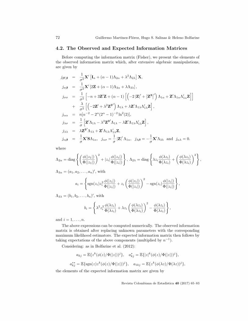
4.2. The Observed and Expected Information Matrices
Before computing the information matrix (Fisher), we present the elements ofthe observed information matrix which, after extensive algebraic manipulations,are given by
jβ′β =1
σ2X′[In + (α− 1)Λ2α + λ2Λ2λ
]X,
jσβ =1
σ2X′ [2Z + (α− 1)Λ3α + λΛ3λ] ,
jσσ =1
σ2
[−n+ 3Z′Z + (α− 1)
[(−2 |Z|′ +
∣∣Z3∣∣′)Λ1α + Z′Λ1αΛ′1αZ
]]+
λ
σ2
[(−2Z′ + λ2Z3′
)Λ1λ + λZ′Λ1λΛ′1λZ
],
jαα = n[α−2 − 2α(2α − 1)−2 ln2(2)],
jλσ =1
σ
[Z′Λ1λ − λ2Z3′Λ1λ − λZ′Λ1λΛ′1λZ
],
jλλ = λZ3′Λ1λ + Z′Λ1λΛ′1λZ,
jαβ =1
σX′SΛ1α, jασ =
1
σ|Z|′ Λ1α, jλβ = − 1
σX′Λ3λ and jαλ = 0.
where
Λ2α = diag
{(φ(|z1|)Φ(|z1|)
)2
+ |zi|φ(|zi|)Φ(|zi|)
}, Λ2λ = diag
{λzi
φ(λzi)
Φ(λzi)+
(φ(λzi)
Φ(λzi)
)2},
Λ3α = (a1, a2, . . . , an)′, with
ai =
{sgn(zi)z
2i
φ(|zi|)Φ(|zi|)
+ zi
(φ(|zi|)Φ(|zi|)
)2
− sgn(zi)φ(|zi|)Φ(|zi|)
},
Λ3λ = (b1, b2, . . . , bn)′, with
bi =
{λ2z2
i
φ(λzi)
Φ(λzi)+ λzi
(φ(λzi)
Φ(λzi)
)2
− φ(λzi)
Φ(λzi)
},
and i = 1, . . . , n.The above expressions can be computed numerically. The observed information
matrix is obtained after replacing unknown parameters with the correspondingmaximum likelihood estimators. The expected information matrix then follows bytaking expectations of the above components (multiplied by n−1).
Considering: as in Bolfarine et al. (2012):
akj = E{zk(φ(z)/Φ(|z|))j}, a∗kj = E{|z|k(φ(z)/Φ(|z|))j},
a∗∗kj = E{sgn(z)zk(φ(z)/Φ(|z|))j}, a1kj = E{zk(φ(λz)/Φ(λz))j},
the elements of the expected information matrix are given by
Revista Colombiana de Estadística 40 (2017) 65–83
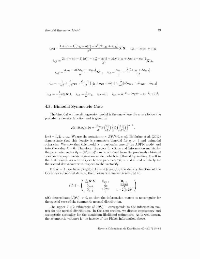
Bimodal Regression Model 73
iβ′β =1 + (α− 1)(a02 − a∗∗11) + λ2(βa111 + a102)
σ2X′X, iλλ = λa131 + a122
iσβ =2a10 + (α− 1) (a∗∗01 − a∗∗21 − a12) + λ(λ2a121 + λa112 − a101)
σ2X′1,
iλβ =a101 − λ(λa121 + a112)
σX′1, iλσ =
a111
σ− λ(λa131 + λa122)
σ2
iσσ = − 1
σ2+
3
σ2a20 +
α− 1
σ2[a∗31 + a22 − 2a∗11] +
λ
σ2[λ2a131 + λa122 − 2a111]
iαβ = − 1
σa∗∗01X
′1, iασ =1
σa∗11, iαλ = 0, iαα = α−2 − 2α(2α − 1)−2(ln 2)2.
4.3. Bimodal Symmetric Case
The bimodal symmetric regression model is the one where the errors follow theprobability density function and is given by
ϕ(εi; 0, σ, α, 0) =αcασφ(εiσ
){Φ(∣∣∣εiσ
∣∣∣)}α−1
,
for i = 1, 2, . . . , n. We use the notation εi ∼ BPN(0, σ, α). Bolfarine et al. (2012)demonstrate that this density is symmetric bimodal for α > 1 and unimodalotherwise. We note that this model is a particular case of the ABPN model andtake the value λ = 0. Therefore, the score functions and information matrix forthe parameter vector θ1 = (β′, σ, α)′ can be obtained from the previously obtainedones for the asymmetric regression model, which is followed by making λ = 0 inthe first derivatives with respect to the parameter β, σ and α and similarly forthe second derivatives with respect to the vector θ1.
For α = 1, we have ϕ(εi; 0, σ, 1) = φ (εi/σ) /σ, the density function of thelocation-scale normal density, the information matrix is reduced to
I(θ1) =
1σ2X
′X 0p+1 0p+1
0′p+12σ2
0.2063σ
0′p+10.2063σ 1− 2(ln 2)2
with determinant |I(θ1)| > 0, so that the information matrix is nonsingular forthe special case of the symmetric normal distribution.
The upper 2 × 2 submatrix of I(θ1)−1 corresponds to the information ma-trix for the normal distribution. In the next section, we discuss consistency andasymptotic normality for the maximum likelihood estimators. As is well-known,the asymptotic variance is the inverse of the Fisher information above.
Revista Colombiana de Estadística 40 (2017) 65–83
74 Guillermo Martínez-Flórez, Hugo S. Salinas & Heleno Bolfarine
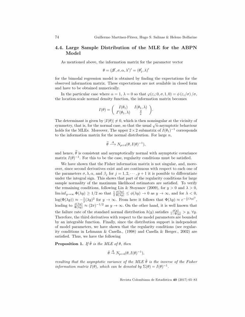
4.4. Large Sample Distribution of the MLE for the ABPNModel
As mentioned above, the information matrix for the parameter vector
θ = (β′, σ, α, λ′)′ = (θ′1, λ)′
for the bimodal regression model is obtained by finding the expectations for theobserved information matrix. These expectations are not available in closed formand have to be obtained numerically.
In the particular case where α = 1, λ = 0 so that ϕ(εi; 0, σ, 1, 0) = φ (εi/σ) /σ,the location-scale normal density function, the information matrix becomes
I(θ) =
(I(θ1) I(θ1, λ)
I ′(θ1, λ) 2π
).
The determinant is given by |I(θ)| 6= 0, which is then nonsingular at the vicinity ofsymmetry, that is, for the normal case, so that the usual
√n-asymptotic behaviour
holds for the MLEs. Moreover, The upper 2× 2 submatrix of I(θ1)−1 correspondsto the information matrix for the normal distribution. For large n,
θA−→ Np+4(θ, I(θ)−1),
and hence, θ is consistent and asymptotically normal with asymptotic covariancematrix I(θ)−1. For this to be the case, regularity conditions must be satisfied.
We have shown that the Fisher information matrix is not singular, and, more-over, since second derivatives exist and are continuous with respect to each one ofthe parameters σ, λ, α, and βj for j = 1, 2, · · · , p+ 1 it is possible to differentiateunder the integral sign. This shows that part of the regularity conditions for largesample normality of the maximum likelihood estimators are satisfied. To verifythe remaining conditions, following Lin & Stoyanov (2009), for y > 0 and λ > 0,lim infy→∞ Φ(λy) ≥ 1/2 so that 1
2φ(λy)Φ(λy) ≤ φ(λy) → 0 as y → ∞, and for λ < 0,
log(Φ(λy)) ≈ − 12 (λy)2 for y → ∞. From here it follows that Φ(λy) ≈ e−
12 (λy)2 ,
leading to φ(λy)Φ(λy) ≈ (2π)−1/2 as y → ∞. On the other hand, it is well known that
the failure rate of the standard normal distribution h(y) satisfies φ(y)1−Φ(y) > y, ∀y.
Therefore, the third derivatives with respect to the model parameters are boundedby an integrable function. Finally, since the distribution support is independentof model parameters, we have shown that the regularity conditions (see regular-ity conditions in Lehmann & Casella., (1998) and Casella & Berger., 2002) aresatisfied. Thus, we have the following
Proposition 1. If θ is the MLE of θ, then
θA→ Np+4(θ, I(θ)−1),
resulting that the asymptotic variance of the MLE θ is the inverse of the Fisherinformation matrix I(θ), which can be denoted by Σ(θ) = I(θ)−1.
Revista Colombiana de Estadística 40 (2017) 65–83
Bimodal Regression Model 75
5. Numerical Results
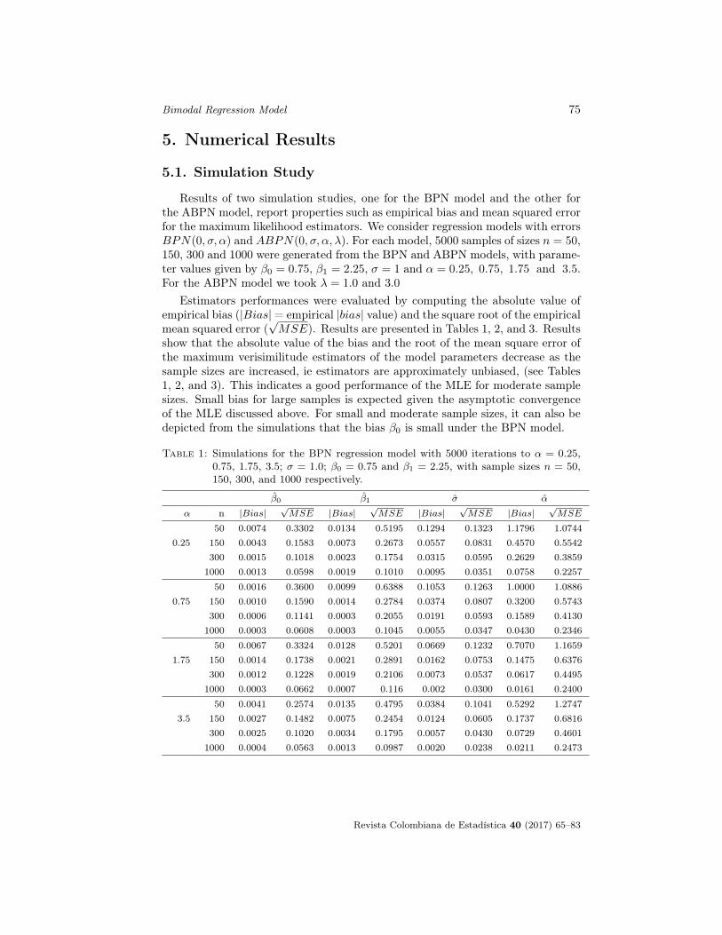
5.1. Simulation Study
Results of two simulation studies, one for the BPN model and the other forthe ABPN model, report properties such as empirical bias and mean squared errorfor the maximum likelihood estimators. We consider regression models with errorsBPN(0, σ, α) and ABPN(0, σ, α, λ). For each model, 5000 samples of sizes n = 50,150, 300 and 1000 were generated from the BPN and ABPN models, with parame-ter values given by β0 = 0.75, β1 = 2.25, σ = 1 and α = 0.25, 0.75, 1.75 and 3.5.For the ABPN model we took λ = 1.0 and 3.0
Estimators performances were evaluated by computing the absolute value ofempirical bias (|Bias| = empirical |bias| value) and the square root of the empiricalmean squared error (
√MSE). Results are presented in Tables 1, 2, and 3. Results
show that the absolute value of the bias and the root of the mean square error ofthe maximum verisimilitude estimators of the model parameters decrease as thesample sizes are increased, ie estimators are approximately unbiased, (see Tables1, 2, and 3). This indicates a good performance of the MLE for moderate samplesizes. Small bias for large samples is expected given the asymptotic convergenceof the MLE discussed above. For small and moderate sample sizes, it can also bedepicted from the simulations that the bias β0 is small under the BPN model.
Table 1: Simulations for the BPN regression model with 5000 iterations to α = 0.25,0.75, 1.75, 3.5; σ = 1.0; β0 = 0.75 and β1 = 2.25, with sample sizes n = 50,150, 300, and 1000 respectively.
β0 β1 σ α
α n |Bias|√MSE |Bias|
√MSE |Bias|
√MSE |Bias|
√MSE
50 0.0074 0.3302 0.0134 0.5195 0.1294 0.1323 1.1796 1.07440.25 150 0.0043 0.1583 0.0073 0.2673 0.0557 0.0831 0.4570 0.5542
300 0.0015 0.1018 0.0023 0.1754 0.0315 0.0595 0.2629 0.38591000 0.0013 0.0598 0.0019 0.1010 0.0095 0.0351 0.0758 0.2257
50 0.0016 0.3600 0.0099 0.6388 0.1053 0.1263 1.0000 1.08860.75 150 0.0010 0.1590 0.0014 0.2784 0.0374 0.0807 0.3200 0.5743
300 0.0006 0.1141 0.0003 0.2055 0.0191 0.0593 0.1589 0.41301000 0.0003 0.0608 0.0003 0.1045 0.0055 0.0347 0.0430 0.2346
50 0.0067 0.3324 0.0128 0.5201 0.0669 0.1232 0.7070 1.16591.75 150 0.0014 0.1738 0.0021 0.2891 0.0162 0.0753 0.1475 0.6376
300 0.0012 0.1228 0.0019 0.2106 0.0073 0.0537 0.0617 0.44951000 0.0003 0.0662 0.0007 0.116 0.002 0.0300 0.0161 0.2400
50 0.0041 0.2574 0.0135 0.4795 0.0384 0.1041 0.5292 1.27473.5 150 0.0027 0.1482 0.0075 0.2454 0.0124 0.0605 0.1737 0.6816
300 0.0025 0.1020 0.0034 0.1795 0.0057 0.0430 0.0729 0.46011000 0.0004 0.0563 0.0013 0.0987 0.0020 0.0238 0.0211 0.2473
Revista Colombiana de Estadística 40 (2017) 65–83
76 Guillermo Martínez-Flórez, Hugo S. Salinas & Heleno Bolfarine
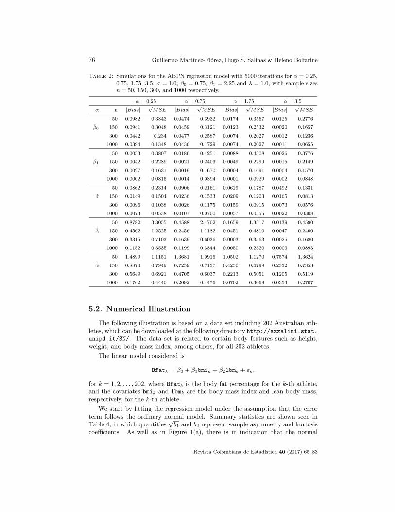
Table 2: Simulations for the ABPN regression model with 5000 iterations for α = 0.25,0.75, 1.75, 3.5; σ = 1.0; β0 = 0.75, β1 = 2.25 and λ = 1.0, with sample sizesn = 50, 150, 300, and 1000 respectively.
α = 0.25 α = 0.75 α = 1.75 α = 3.5
α n |Bias|√MSE |Bias|
√MSE |Bias|
√MSE |Bias|
√MSE
50 0.0982 0.3843 0.0474 0.3932 0.0174 0.3567 0.0125 0.2776
β0 150 0.0941 0.3048 0.0459 0.3121 0.0123 0.2532 0.0020 0.1657
300 0.0442 0.234 0.0477 0.2587 0.0074 0.2027 0.0012 0.1236
1000 0.0394 0.1348 0.0436 0.1729 0.0074 0.2027 0.0011 0.0655
50 0.0053 0.3807 0.0186 0.4251 0.0088 0.4308 0.0026 0.3776
β1 150 0.0042 0.2289 0.0021 0.2403 0.0049 0.2299 0.0015 0.2149
300 0.0027 0.1631 0.0019 0.1670 0.0004 0.1691 0.0004 0.1570
1000 0.0002 0.0815 0.0014 0.0894 0.0001 0.0929 0.0002 0.0848
50 0.0862 0.2314 0.0906 0.2161 0.0629 0.1787 0.0492 0.1331
σ 150 0.0149 0.1504 0.0236 0.1533 0.0209 0.1203 0.0165 0.0813
300 0.0096 0.1038 0.0026 0.1175 0.0159 0.0915 0.0073 0.0576
1000 0.0073 0.0538 0.0107 0.0700 0.0057 0.0555 0.0022 0.0308
50 0.8782 3.3055 0.4588 2.4702 0.1659 1.3517 0.0139 0.4590
λ 150 0.4562 1.2525 0.2456 1.1182 0.0451 0.4810 0.0047 0.2400
300 0.3315 0.7103 0.1639 0.6036 0.0003 0.3563 0.0025 0.1680
1000 0.1152 0.3535 0.1199 0.3844 0.0050 0.2320 0.0003 0.0893
50 1.4899 1.1151 1.3681 1.0916 1.0502 1.1270 0.7574 1.3624
α 150 0.8874 0.7949 0.7259 0.7137 0.4250 0.6799 0.2532 0.7353
300 0.5649 0.6921 0.4705 0.6037 0.2213 0.5051 0.1205 0.5119
1000 0.1762 0.4440 0.2092 0.4476 0.0702 0.3069 0.0353 0.2707
5.2. Numerical Illustration
The following illustration is based on a data set including 202 Australian ath-letes, which can be downloaded at the following directory http://azzalini.stat.unipd.it/SN/. The data set is related to certain body features such as height,weight, and body mass index, among others, for all 202 athletes.
The linear model considered is
Bfatk = β0 + β1bmik + β2lbmk + εk,
for k = 1, 2, . . . , 202, where Bfatk is the body fat percentage for the k-th athlete,and the covariates bmik and lbmk are the body mass index and lean body mass,respectively, for the k-th athlete.
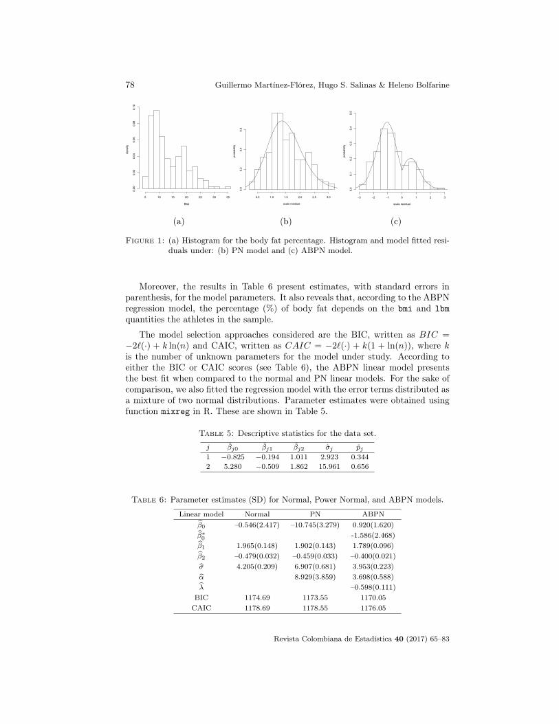
We start by fitting the regression model under the assumption that the errorterm follows the ordinary normal model. Summary statistics are shown seen inTable 4, in which quantities
√b1 and b2 represent sample asymmetry and kurtosis
coefficients. As well as in Figure 1(a), there is in indication that the normal
Revista Colombiana de Estadística 40 (2017) 65–83
Bimodal Regression Model 77
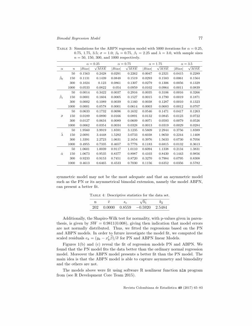
Table 3: Simulations for the ABPN regression model with 5000 iterations for α = 0.25,0.75, 1.75, 3.5; σ = 1.0; β0 = 0.75, β1 = 2.25 and λ = 3.0, with sample sizesn = 50, 150, 300, and 1000 respectively.
α = 0.25 α = 0.75 α = 1.75 α = 3.5
α n |Bias|√MSE |Bias|
√MSE |Bias|
√MSE |Bias|
√MSE
50 0.1563 0.2428 0.0291 0.2262 0.0047 0.2321 0.0415 0.2289β0 150 0.1131 0.1439 0.0848 0.1519 0.0293 0.1583 0.0061 0.1564
300 0.1024 0.123 0.0861 0.1307 0.0279 0.1306 0.0056 0.13291000 0.0533 0.0822 0.054 0.0959 0.0102 0.0964 0.0011 0.083950 0.0014 0.3422 0.0037 0.2916 0.0035 0.3106 0.0016 0.3266
β1 150 0.0001 0.1604 0.0005 0.1527 0.0015 0.1790 0.0019 0.1871300 0.0002 0.1089 0.0039 0.1160 0.0038 0.1287 0.0010 0.1323
1000 0.0001 0.0578 0.0001 0.0614 0.0003 0.0683 0.0012 0.070750 0.0633 0.1732 0.0696 0.1632 0.0546 0.1471 0.0417 0.1263
σ 150 0.0189 0.0890 0.0166 0.0891 0.0132 0.0845 0.0123 0.0722300 0.0127 0.0634 0.0089 0.0609 0.0071 0.0593 0.0079 0.0526
1000 0.0062 0.0354 0.0034 0.0328 0.0013 0.0319 0.0029 0.028450 1.9560 3.9919 1.8591 3.1235 0.5809 2.2944 0.3756 1.8389
λ 150 2.0091 3.4448 1.5292 3.0733 0.6038 1.9650 0.2244 1.1408300 1.3391 2.2723 1.0631 2.1654 0.3976 1.5633 0.0730 0.7056
1000 0.4955 0.7335 0.4657 0.7776 0.1183 0.6815 0.0132 0.361350 1.0601 1.0039 0.9117 1.0110 0.6094 1.1338 0.2134 1.3831
α 150 1.0673 0.9535 0.8377 0.8987 0.4103 0.8430 0.1443 0.9856300 0.9233 0.9153 0.7451 0.8720 0.3270 0.7984 0.0795 0.8308
1000 0.4613 0.6465 0.4533 0.7030 0.1156 0.6352 0.0356 0.5782
symmetric model may not be the most adequate and that an asymmetric modelsuch as the PN or its asymmetrical bimodal extension, namely the model ABPN,can present a better fit.
Table 4: Descriptive statistics for the data set.
n e se√b1 b2
202 0.0000 0.8559 −0.5920 2.5484
Additionally, the Shapiro-Wilk test for normality, with p-values given in paren-thesis, is given by SW = 0.9811(0.008), giving then indication that model errorsare not normally distributed. Thus, we fitted the regressions based on the PNand ABPN models. In order to future investigate the model fit, we computed thescaled residuals ek = (yk − x′kβ)/σ for PN and ABPN linear Models.
Figures 1(b) and (c) reveal the fit of regression models PN and ABPN. Wefound that the PN model fits the data better than the ordinary normal regressionmodel. Moreover the ABPN model presents a better fit than the PN model. Themain idea is that the ABPN model is able to capture asymmetry and bimodalityand the others are not.
The models above were fit using software R nonlinear function nlm programfrom (see R Development Core Team 2015).
Revista Colombiana de Estadística 40 (2017) 65–83
78 Guillermo Martínez-Flórez, Hugo S. Salinas & Heleno Bolfarine
Bfat
dens
ity
5 10 15 20 25 30 35
0.00
0.02
0.04
0.06
0.08
0.10
(a)
scale residual
prob
abili
ty
0.5 1.0 1.5 2.0 2.5 3.0
0.0
0.2
0.4
0.6
(b)
scale residual
prob
abili
ty
−3 −2 −1 0 1 2 3
0.0
0.1
0.2
0.3
0.4
0.5
(c)
Figure 1: (a) Histogram for the body fat percentage. Histogram and model fitted resi-duals under: (b) PN model and (c) ABPN model.
Moreover, the results in Table 6 present estimates, with standard errors inparenthesis, for the model parameters. It also reveals that, according to the ABPNregression model, the percentage (%) of body fat depends on the bmi and lbmquantities the athletes in the sample.
The model selection approaches considered are the BIC, written as BIC =−2`(·) + k ln(n) and CAIC, written as CAIC = −2`(·) + k(1 + ln(n)), where kis the number of unknown parameters for the model under study. According toeither the BIC or CAIC scores (see Table 6), the ABPN linear model presentsthe best fit when compared to the normal and PN linear models. For the sake ofcomparison, we also fitted the regression model with the error terms distributed asa mixture of two normal distributions. Parameter estimates were obtained usingfunction mixreg in R. These are shown in Table 5.
Table 5: Descriptive statistics for the data set.
j βj0 βj1 βj2 σj pj1 −0.825 −0.194 1.011 2.923 0.344
2 5.280 −0.509 1.862 15.961 0.656
Table 6: Parameter estimates (SD) for Normal, Power Normal, and ABPN models.
Linear model Normal PN ABPNβ0 –0.546(2.417) –10.745(3.279) 0.920(1.620)β∗0 -1.586(2.468)β1 1.965(0.148) 1.902(0.143) 1.789(0.096)β2 –0.479(0.032) –0.459(0.033) –0.400(0.021)σ 4.205(0.209) 6.907(0.681) 3.953(0.223)α 8.929(3.859) 3.698(0.588)λ –0.598(0.111)
BIC 1174.69 1173.55 1170.05CAIC 1178.69 1178.55 1176.05
Revista Colombiana de Estadística 40 (2017) 65–83
Bimodal Regression Model 79
We obtained BIC = 1170.17 and CAIC = 1179.17, meaning that, accordingto the BIC and CAIC criteria, the regression model ABPN fits the data betterthan the mixture of two normal distributions.
Following Therneau, Grambsch & Fleming (1990), we can adapt the deviancecomponent residual for the ABPN model with no censored data by considering
rMi= 1 + ln
(SABPN (y)
), i = 1, 2, . . . , n, (7)
where SABPN (y) is the ML estimate of the reliability function of the ABPN model.Therneau et al. (1990) proposed the deviance component residual as a trans-
formation of the martingale type residual so that the deviance component residualfor noncensored data can be taken as
rMTi= sgn(rMi
) {−2 [rMi+ ln(1− rMi
)]}1/2 , i = 1, 2, . . . , n. (8)
We use the residual rMTias a residual type martingale, given that they are sym-
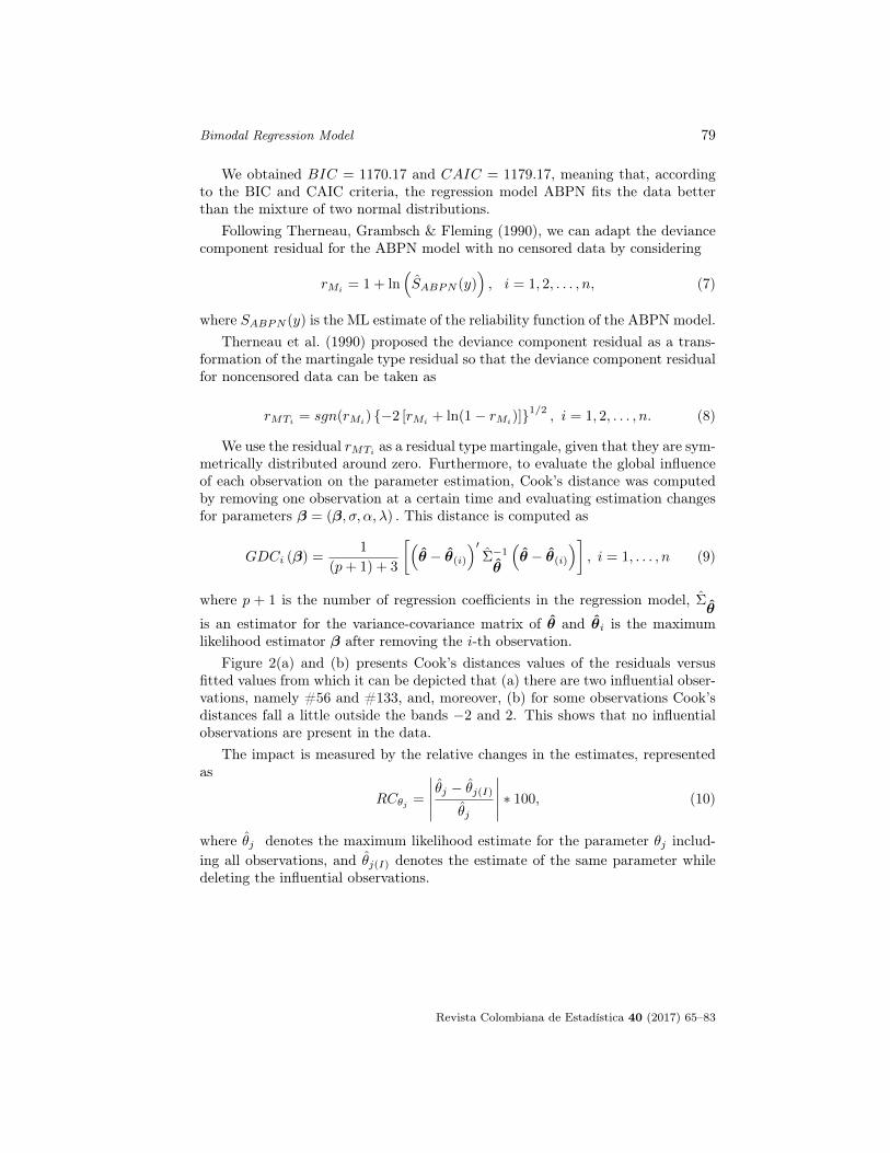
metrically distributed around zero. Furthermore, to evaluate the global influenceof each observation on the parameter estimation, Cook’s distance was computedby removing one observation at a certain time and evaluating estimation changesfor parameters β = (β, σ, α, λ) . This distance is computed as
GDCi (β) =1
(p+ 1) + 3
[(θ − θ(i)
)′Σ−1
θ
(θ − θ(i)
)], i = 1, . . . , n (9)
where p + 1 is the number of regression coefficients in the regression model, Σθ
is an estimator for the variance-covariance matrix of θ and θi is the maximumlikelihood estimator β after removing the i-th observation.
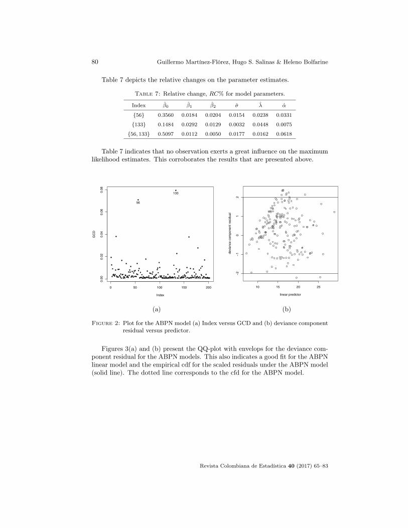
Figure 2(a) and (b) presents Cook’s distances values of the residuals versusfitted values from which it can be depicted that (a) there are two influential obser-vations, namely #56 and #133, and, moreover, (b) for some observations Cook’sdistances fall a little outside the bands −2 and 2. This shows that no influentialobservations are present in the data.
The impact is measured by the relative changes in the estimates, representedas
RCθj =
∣∣∣∣∣ θj − θj(I)θj
∣∣∣∣∣ ∗ 100, (10)
where θj denotes the maximum likelihood estimate for the parameter θj includ-ing all observations, and θj(I) denotes the estimate of the same parameter whiledeleting the influential observations.
Revista Colombiana de Estadística 40 (2017) 65–83
80 Guillermo Martínez-Flórez, Hugo S. Salinas & Heleno Bolfarine
Table 7 depicts the relative changes on the parameter estimates.
Table 7: Relative change, RC% for model parameters.
Index β0 β1 β2 σ λ α
{56} 0.3560 0.0184 0.0204 0.0154 0.0238 0.0331
{133} 0.1484 0.0292 0.0129 0.0032 0.0448 0.0075
{56, 133} 0.5097 0.0112 0.0050 0.0177 0.0162 0.0618
Table 7 indicates that no observation exerts a great influence on the maximumlikelihood estimates. This corroborates the results that are presented above.
0 50 100 150 200
0.00
0.02
0.04
0.06
0.08
Index
GC
D
56
133
(a)
10 15 20 25
−2
−1
01
2
linear predictor
dev
ianc
e co
mpo
nent
res
idua
l
(b)
Figure 2: Plot for the ABPN model (a) Index versus GCD and (b) deviance componentresidual versus predictor.
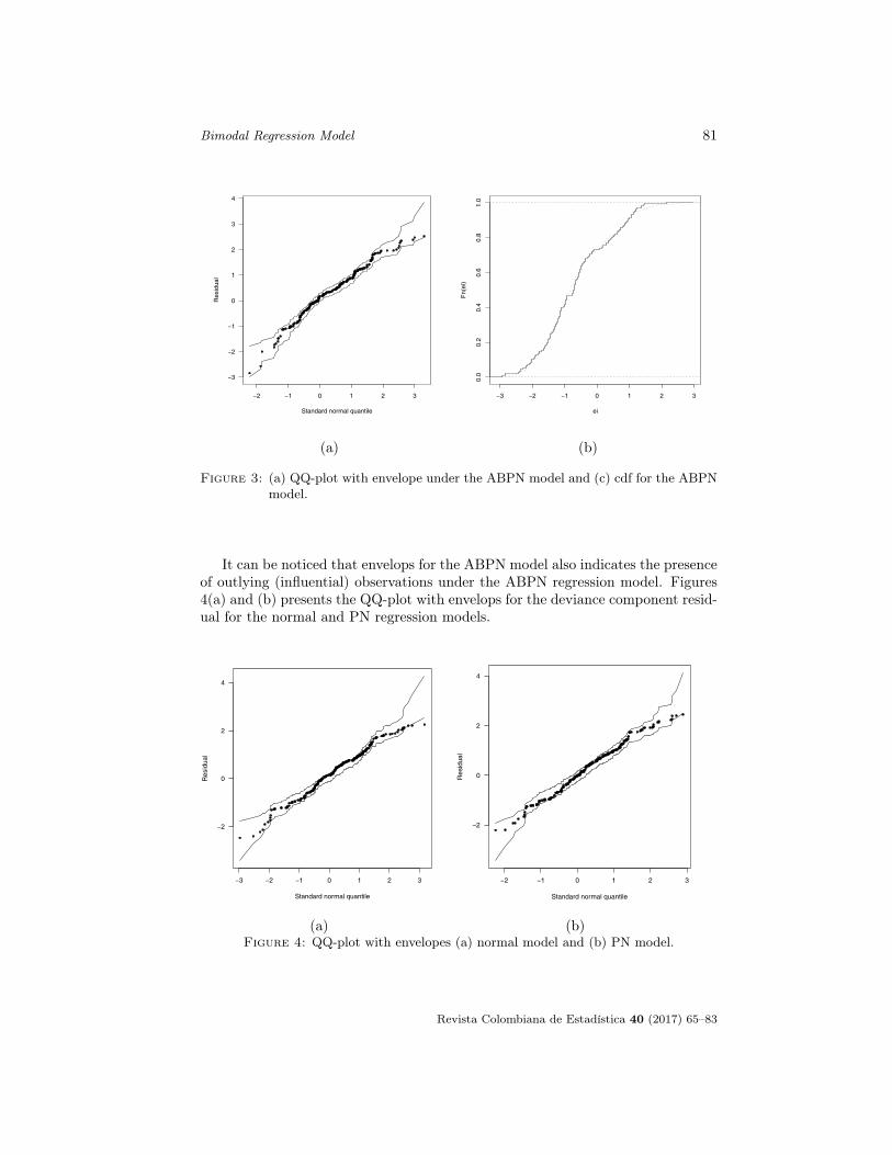
Figures 3(a) and (b) present the QQ-plot with envelops for the deviance com-ponent residual for the ABPN models. This also indicates a good fit for the ABPNlinear model and the empirical cdf for the scaled residuals under the ABPN model(solid line). The dotted line corresponds to the cfd for the ABPN model.
Revista Colombiana de Estadística 40 (2017) 65–83
Bimodal Regression Model 81
−2 −1 0 1 2 3
−3
−2
−1
0
1
2
3
4
Standard normal quantile
Res
idua
l
(a)
−3 −2 −1 0 1 2 3
0.0
0.2
0.4
0.6
0.8
1.0
ei
Fn(
ei)
(b)
Figure 3: (a) QQ-plot with envelope under the ABPN model and (c) cdf for the ABPNmodel.
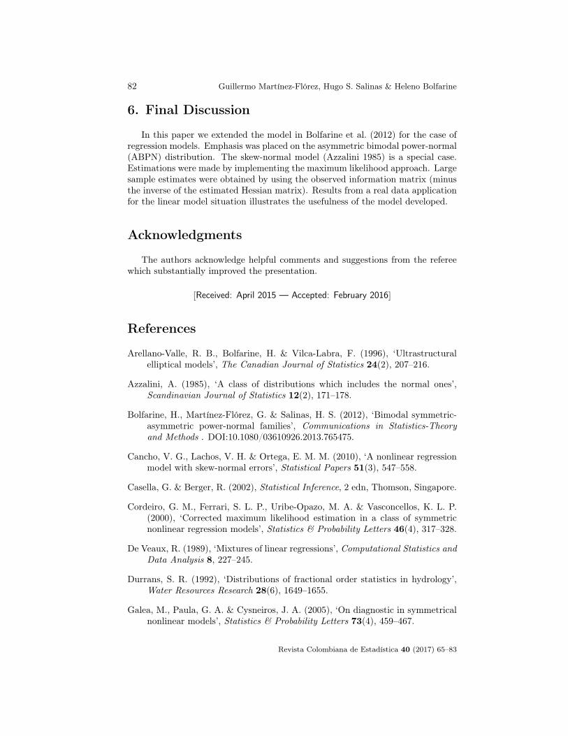
It can be noticed that envelops for the ABPN model also indicates the presenceof outlying (influential) observations under the ABPN regression model. Figures4(a) and (b) presents the QQ-plot with envelops for the deviance component resid-ual for the normal and PN regression models.
−3 −2 −1 0 1 2 3
−2
0
2
4
Standard normal quantile
Res
idua
l
(a)
−2 −1 0 1 2 3
−2
0
2
4
Standard normal quantile
Res
idua
l
(b)Figure 4: QQ-plot with envelopes (a) normal model and (b) PN model.
Revista Colombiana de Estadística 40 (2017) 65–83
82 Guillermo Martínez-Flórez, Hugo S. Salinas & Heleno Bolfarine
6. Final Discussion
In this paper we extended the model in Bolfarine et al. (2012) for the case ofregression models. Emphasis was placed on the asymmetric bimodal power-normal(ABPN) distribution. The skew-normal model (Azzalini 1985) is a special case.Estimations were made by implementing the maximum likelihood approach. Largesample estimates were obtained by using the observed information matrix (minusthe inverse of the estimated Hessian matrix). Results from a real data applicationfor the linear model situation illustrates the usefulness of the model developed.
Acknowledgments
The authors acknowledge helpful comments and suggestions from the refereewhich substantially improved the presentation.
[Received: April 2015 — Accepted: February 2016
]
References
Arellano-Valle, R. B., Bolfarine, H. & Vilca-Labra, F. (1996), ‘Ultrastructuralelliptical models’, The Canadian Journal of Statistics 24(2), 207–216.
Azzalini, A. (1985), ‘A class of distributions which includes the normal ones’,Scandinavian Journal of Statistics 12(2), 171–178.
Bolfarine, H., Martínez-Flórez, G. & Salinas, H. S. (2012), ‘Bimodal symmetric-asymmetric power-normal families’, Communications in Statistics-Theoryand Methods . DOI:10.1080/03610926.2013.765475.
Cancho, V. G., Lachos, V. H. & Ortega, E. M. M. (2010), ‘A nonlinear regressionmodel with skew-normal errors’, Statistical Papers 51(3), 547–558.
Casella, G. & Berger, R. (2002), Statistical Inference, 2 edn, Thomson, Singapore.
Cordeiro, G. M., Ferrari, S. L. P., Uribe-Opazo, M. A. & Vasconcellos, K. L. P.(2000), ‘Corrected maximum likelihood estimation in a class of symmetricnonlinear regression models’, Statistics & Probability Letters 46(4), 317–328.
De Veaux, R. (1989), ‘Mixtures of linear regressions’, Computational Statistics andData Analysis 8, 227–245.
Durrans, S. R. (1992), ‘Distributions of fractional order statistics in hydrology’,Water Resources Research 28(6), 1649–1655.
Galea, M., Paula, G. A. & Cysneiros, J. A. (2005), ‘On diagnostic in symmetricalnonlinear models’, Statistics & Probability Letters 73(4), 459–467.
Revista Colombiana de Estadística 40 (2017) 65–83
Bimodal Regression Model 83
Gupta, R. D. & Gupta, R. C. (2008), ‘Analyzing skewed data by power normalmodel’, TEST 17(1), 197–210.
Lange, K. L., Little, R. J. A. & Taylor, J. M. G. (1989), ‘Robust Statistical Model-ing Using the t Distribution’, Journal of the American Statistical Association84(408), 881–896.
Lehman, E. L. & Casella, G. (1998), Theory of Point Estimation, 2 edn, Springer,New York.
Lin, G. & Stoyanov, J. (2009), ‘The logarithmic Skew-Normal Distributions areMoment-Indeterminate’, Journal of Applied Probability Trust 46, 909–916.
Martínez-Flórez, G., Bolfarine, H. & Gómez, H. W. (2015), ‘Likelihood-basedinference for the power regression model’, SORT 39(2), 187–208.
Pewsey, A., Gómez, H. W. & Bolfarine, H. (2012), ‘Likelihood based inference fordistributions of fractional order statistics’, TEST 21(4), 775–789.
Quandt, R. (1958), ‘The estimation of the parameters of a linear regression systemobeying two separate regimes’, Journal of the American Statistical Associa-tion 53(284), 873–880.
R Core Team (2015), R: A Language and Environment for Statistical Computing,R Foundation for Statistical Computing, Vienna, Austria. ISBN 3-900051-07-0.*http://www.R-project.org/
Rego, L. C., Cintra, R. J. & Cordeiro, G. M. (2012), ‘On some properties of thebeta normal distribution’, Communications in Statistics-Theory and Methods41, 3722–3738.
Therneau, T., Grambsch, P. & Fleming, T. (1990), ‘Martingale-based residuals forsurvival models’, Biometrika 77, 147–160.
Turner, T. (2000), ‘Estimating the propagation rate of a viral infection of potatoplants via mixtures of regressions’, Applied Statistics 49(3), 371–384.
Young, D. S. & Hunter, D. R. (2010), ‘Mixtures of regressions with predictor-dependent mixing proportions’, Computational Statistics and Data Analysis54(10), 2253–2266.
Revista Colombiana de Estadística 40 (2017) 65–83