Nathaniel E. Helwig - Statisticsusers.stat.umn.edu/~helwig/notes/mvlr-Notes.pdf · The OLS solution has the form ^b = (X0X) ... Multivariate Linear Regression Updated 16-Jan-2017

Multivariate Linear Regression

Nathaniel E. Helwig

Assistant Professor of Psychology and StatisticsUniversity of Minnesota (Twin Cities)

Updated 16-Jan-2017

Nathaniel E. Helwig (U of Minnesota) Multivariate Linear Regression Updated 16-Jan-2017 : Slide 1

Copyright

Copyright c© 2017 by Nathaniel E. Helwig


Outline of Notes

1) Multiple Linear RegressionModel form and assumptionsParameter estimationInference and prediction

2) Multivariate Linear RegressionModel form and assumptionsParameter estimationInference and prediction


Multiple Linear Regression

Multiple Linear Regression


Multiple Linear Regression Model Form and Assumptions

MLR Model: Scalar Form

The multiple linear regression model has the form

yi = b0 +

p∑j=1

bjxij + ei

for i ∈ {1, . . . ,n} whereyi ∈ R is the real-valued response for the i-th observationb0 ∈ R is the regression interceptbj ∈ R is the j-th predictor’s regression slopexij ∈ R is the j-th predictor for the i-th observation

eiiid∼ N(0, σ2) is a Gaussian error term



MLR Model: Nomenclature

The model is multiple because we have p > 1 predictors.

If p = 1, we have a simple linear regression model

The model is linear because yi is a linear function of the parameters(b0, b1, . . . , bp are the parameters).

The model is a regression model because we are modeling a responsevariable (Y ) as a function of predictor variables (X1, . . . ,Xp).



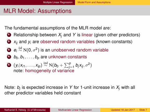
MLR Model: Assumptions

The fundamental assumptions of the MLR model are:1 Relationship between Xj and Y is linear (given other predictors)2 xij and yi are observed random variables (known constants)

3 eiiid∼ N(0, σ2) is an unobserved random variable

4 b0,b1, . . . ,bp are unknown constants

5 (yi |xi1, . . . , xip)ind∼ N(b0 +

∑pj=1 bjxij , σ

2)note: homogeneity of variance

Note: bj is expected increase in Y for 1-unit increase in Xj with allother predictor variables held constant



MLR Model: Matrix Form

The multiple linear regression model has the form

y = Xb + e

wherey = (y1, . . . , yn)′ ∈ Rn is the n × 1 response vectorX = [1n,x1, . . . ,xp] ∈ Rn×(p+1) is the n × (p + 1) design matrix• 1n is an n × 1 vector of ones• xj = (x1j , . . . , xnj )

′ ∈ Rn is j-th predictor vector (n × 1)

b = (b0,b1, . . . ,bp)′ ∈ Rp+1 is (p + 1)× 1 vector of coefficientse = (e1, . . . ,en)′ ∈ Rn is the n × 1 error vector



MLR Model: Matrix Form (another look)

Matrix form writes MLR model for all n points simultaneously

y = Xb + e

y1y2y3...

yn

=

1 x11 x12 · · · x1p1 x21 x22 · · · x2p1 x31 x32 · · · x3p...

......

. . ....

1 xn1 xn2 · · · xnp

b0b1b2...

bp

+

e1e2e3...

en



MLR Model: Assumptions (revisited)

In matrix terms, the error vector is multivariate normal:

e ∼ N(0n, σ2In)

In matrix terms, the response vector is multivariate normal given X:

(y|X) ∼ N(Xb, σ2In)


Multiple Linear Regression Parameter Estimation

Ordinary Least Squares

The ordinary least squares (OLS) problem is

minb∈Rp+1

‖y− Xb‖2 = minb∈Rp+1

n∑i=1

(yi − b0 −

∑pj=1 bjxij

)2

where ‖ · ‖ denotes the Frobenius norm.

The OLS solution has the form

b = (X′X)−1X′y



Fitted Values and Residuals

SCALAR FORM:

Fitted values are given by

yi = b0 +∑p

j=1 bjxij

and residuals are given by

ei = yi − yi

MATRIX FORM:


y = Xb


e = y− y



Hat Matrix

Note that we can write the fitted values as

y = Xb

= X(X′X)−1X′y= Hy

where H = X(X′X)−1X′ is the hat matrix.

H is a symmetric and idempotent matrix: HH = H

H projects y onto the column space of X.



Multiple Regression Example in R

> data(mtcars)> head(mtcars)

mpg cyl disp hp drat wt qsec vs am gear carbMazda RX4 21.0 6 160 110 3.90 2.620 16.46 0 1 4 4Mazda RX4 Wag 21.0 6 160 110 3.90 2.875 17.02 0 1 4 4Datsun 710 22.8 4 108 93 3.85 2.320 18.61 1 1 4 1Hornet 4 Drive 21.4 6 258 110 3.08 3.215 19.44 1 0 3 1Hornet Sportabout 18.7 8 360 175 3.15 3.440 17.02 0 0 3 2Valiant 18.1 6 225 105 2.76 3.460 20.22 1 0 3 1> mtcars$cyl <- factor(mtcars$cyl)> mod <- lm(mpg ~ cyl + am + carb, data=mtcars)> coef(mod)(Intercept) cyl6 cyl8 am carb25.320303 -3.549419 -6.904637 4.226774 -1.119855



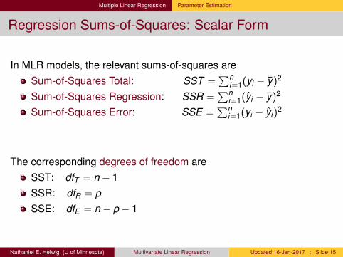
Regression Sums-of-Squares: Scalar Form

In MLR models, the relevant sums-of-squares areSum-of-Squares Total: SST =

∑ni=1(yi − y)2

Sum-of-Squares Regression: SSR =∑n

i=1(yi − y)2

Sum-of-Squares Error: SSE =∑n

i=1(yi − yi)2

The corresponding degrees of freedom areSST: dfT = n − 1SSR: dfR = pSSE: dfE = n − p − 1



Regression Sums-of-Squares: Matrix Form

In MLR models, the relevant sums-of-squares are

SST =n∑

i=1

(yi − y)2

= y′ [In − (1/n)J] y

SSR =n∑

i=1

(yi − y)2

= y′ [H− (1/n)J] y

SSE =n∑

i=1

(yi − yi)2

= y′ [In − H] y

Note: J is an n × n matrix of onesNathaniel E. Helwig (U of Minnesota) Multivariate Linear Regression Updated 16-Jan-2017 : Slide 16


Partitioning the Variance

We can partition the total variation in yi as

SST =n∑

i=1

(yi − y)2

=n∑

i=1

(yi − yi + yi − y)2

=n∑

i=1

(yi − y)2 +n∑

i=1

(yi − yi )2 + 2

n∑i=1

(yi − y)(yi − yi )

= SSR + SSE + 2n∑

i=1

(yi − y)ei

= SSR + SSE



Regression Sums-of-Squares in R

> anova(mod)Analysis of Variance Table

Response: mpgDf Sum Sq Mean Sq F value Pr(>F)

cyl 2 824.78 412.39 52.4138 5.05e-10 ***am 1 36.77 36.77 4.6730 0.03967 *carb 1 52.06 52.06 6.6166 0.01592 *Residuals 27 212.44 7.87---Signif. codes: 0 ‘***’ 0.001 ‘**’ 0.01 ‘*’ 0.05 ‘.’ 0.1 ‘ ’ 1

> Anova(mod, type=3)Anova Table (Type III tests)

Response: mpgSum Sq Df F value Pr(>F)

(Intercept) 3368.1 1 428.0789 < 2.2e-16 ***cyl 121.2 2 7.7048 0.002252 **am 77.1 1 9.8039 0.004156 **carb 52.1 1 6.6166 0.015923 *Residuals 212.4 27---Signif. codes: 0 ‘***’ 0.001 ‘**’ 0.01 ‘*’ 0.05 ‘.’ 0.1 ‘ ’ 1



Coefficient of Multiple Determination

The coefficient of multiple determination is defined as

R2 =SSRSST

= 1− SSESST

and gives the amount of variation in yi that is explained by the linearrelationships with xi1, . . . , xip.

When interpreting R2 values, note that. . .0 ≤ R2 ≤ 1Large R2 values do not necessarily imply a good model



Adjusted Coefficient of Multiple Determination (R2a )

Including more predictors in a MLR model can artificially inflate R2:Capitalizing on spurious effects present in noisy dataPhenomenon of over-fitting the data

The adjusted R2 is a relative measure of fit:

R2a = 1− SSE/dfE

SST/dfT

= 1− σ2

s2Y

where s2Y =

∑ni=1(yi−y)2

n−1 is the sample estimate of the variance of Y .

Note: R2 and R2a have different interpretations!



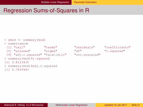
Regression Sums-of-Squares in R

> smod <- summary(mod)> names(smod)[1] "call" "terms" "residuals" "coefficients"[5] "aliased" "sigma" "df" "r.squared"[9] "adj.r.squared" "fstatistic" "cov.unscaled"> summary(mod)$r.squared[1] 0.8113434> summary(mod)$adj.r.squared[1] 0.7833943



Relation to ML Solution

Remember that (y|X) ∼ N(Xb, σ2In), which implies that y has pdf

f (y|X,b, σ2) = (2π)−n/2(σ2)−n/2e−1

2σ2 (y−Xb)′(y−Xb)

As a result, the log-likelihood of b given (y,X, σ2) is

ln{L(b|y,X, σ2)} = − 12σ2 (y− Xb)′(y− Xb) + c

where c is a constant that does not depend on b.



Relation to ML Solution (continued)

The maximum likelihood estimate (MLE) of b is the estimate satisfying

maxb∈Rp+1

− 12σ2 (y− Xb)′(y− Xb)

Now, note that. . .maxb∈Rp+1 − 1

2σ2 (y−Xb)′(y−Xb) = maxb∈Rp+1 −(y−Xb)′(y−Xb)

maxb∈Rp+1 −(y− Xb)′(y− Xb) = minb∈Rp+1(y− Xb)′(y− Xb)

Thus, the OLS and ML estimate of b is the same: b = (X′X)−1X′y



Estimated Error Variance (Mean Squared Error)

The estimated error variance is

σ2 = SSE/(n − p − 1)

=n∑

i=1

(yi − yi)2/(n − p − 1)

= ‖(In − H)y‖2/(n − p − 1)

which is an unbiased estimate of error variance σ2.

The estimate σ2 is the mean squared error (MSE) of the model.



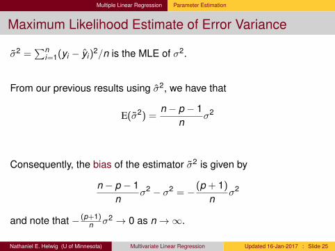
Maximum Likelihood Estimate of Error Variance

σ2 =∑n

i=1(yi − yi)2/n is the MLE of σ2.

From our previous results using σ2, we have that

E(σ2) =n − p − 1

nσ2

Consequently, the bias of the estimator σ2 is given by

n − p − 1n

σ2 − σ2 = −(p + 1)

nσ2

and note that − (p+1)n σ2 → 0 as n→∞.



Comparing σ2 and σ2

Reminder: the MSE and MLE of σ2 are given by

σ2 = ‖(In − H)y‖2/(n − p − 1)

σ2 = ‖(In − H)y‖2/n

From the definitions of σ2 and σ2 we have that

σ2 < σ2

so the MLE produces a smaller estimate of the error variance.



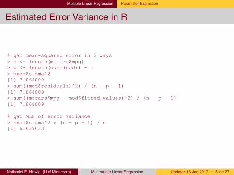
Estimated Error Variance in R

# get mean-squared error in 3 ways> n <- length(mtcars$mpg)> p <- length(coef(mod)) - 1> smod$sigma^2[1] 7.868009> sum((mod$residuals)^2) / (n - p - 1)[1] 7.868009> sum((mtcars$mpg - mod$fitted.values)^2) / (n - p - 1)[1] 7.868009

# get MLE of error variance> smod$sigma^2 * (n - p - 1) / n[1] 6.638633


Multiple Linear Regression Inference and Prediction

Summary of Results

Given the model assumptions, we have

b ∼ N(b, σ2(X′X)−1)

y ∼ N(Xb, σ2H)

e ∼ N(0, σ2(In − H))

Typically σ2 is unknown, so we use the MSE σ2 in practice.



ANOVA Table and Regression F Test

We typically organize the SS information into an ANOVA table:

Source SS df MS F p-valueSSR

∑ni=1(yi − y)2 p MSR F ∗ p∗

SSE∑n

i=1(yi − yi)2 n − p − 1 MSE

SST∑n

i=1(yi − y)2 n − 1MSR = SSR

p , MSE = SSEn−p−1 , F ∗ = MSR

MSE ∼ Fp,n−p−1,p∗ = P(Fp,n−p−1 > F ∗)

F ∗-statistic and p∗-value are testing H0 : b1 = · · · = bp = 0 versusH1 : bk 6= 0 for some k ∈ {1, . . . ,p}



Inferences about bj with σ2 Known

If σ2 is known, form 100(1− α)% CIs using

b0 ± Zα/2σb0 bj ± Zα/2σbj

whereZα/2 is normal quantile such that P(X > Zα/2) = α/2

σb0 and σbj are square-roots of diagonals of V(b) = σ2(X′X)−1

To test H0 : bj = b∗j vs. H1 : bj 6= b∗j (for some j ∈ {0,1, . . . ,p}) use

Z = (bj − b∗j )/σbj

which follows a standard normal distribution under H0.



Inferences about bj with σ2 Unknown

If σ2 is unknown, form 100(1− α)% CIs using

b0 ± t(α/2)n−p−1σb0 bj ± t(α/2)

n−p−1σbj

wheret(α/2)n−p−1 is tn−p−1 quantile with P(X > t(α/2)

n−p−1) = α/2

σb0 and σbj are square-roots of diagonals of V(b) = σ2(X′X)−1

To test H0 : bj = b∗j vs. H1 : bj 6= b∗j (for some j ∈ {0,1, . . . ,p}) use

T = (bj − b∗j )/σbj

which follows a tn−p−1 distribution under H0.



Coefficient Inference in R> summary(mod)

Call:lm(formula = mpg ~ cyl + am + carb, data = mtcars)

Residuals:Min 1Q Median 3Q Max

-5.9074 -1.1723 0.2538 1.4851 5.4728

Coefficients:Estimate Std. Error t value Pr(>|t|)

(Intercept) 25.3203 1.2238 20.690 < 2e-16 ***cyl6 -3.5494 1.7296 -2.052 0.049959 *cyl8 -6.9046 1.8078 -3.819 0.000712 ***am 4.2268 1.3499 3.131 0.004156 **carb -1.1199 0.4354 -2.572 0.015923 *---Signif. codes: 0 ‘***’ 0.001 ‘**’ 0.01 ‘*’ 0.05 ‘.’ 0.1 ‘ ’ 1

Residual standard error: 2.805 on 27 degrees of freedomMultiple R-squared: 0.8113, Adjusted R-squared: 0.7834F-statistic: 29.03 on 4 and 27 DF, p-value: 1.991e-09

> confint(mod)2.5 % 97.5 %

(Intercept) 22.809293 27.8313132711cyl6 -7.098164 -0.0006745487cyl8 -10.613981 -3.1952927942am 1.456957 6.9965913486carb -2.013131 -0.2265781401



Inferences about Multiple bj

Assume that q < p and want to test if a reduced model is sufficient:

H0 : bq+1 = bq+2 = · · · = bp = b∗

H1 : at least one bk 6= b∗

Compare the SSE for full and reduced (constrained) models:(a) Full Model: yi = b0 +

∑pj=1 bjxij + ei

(b) Reduced Model: yi = b0 +∑q

j=1 bjxij + b∗∑p

k=q+1 xik + ei

Note: set b∗ = 0 to remove Xq+1, . . . ,Xp from model.



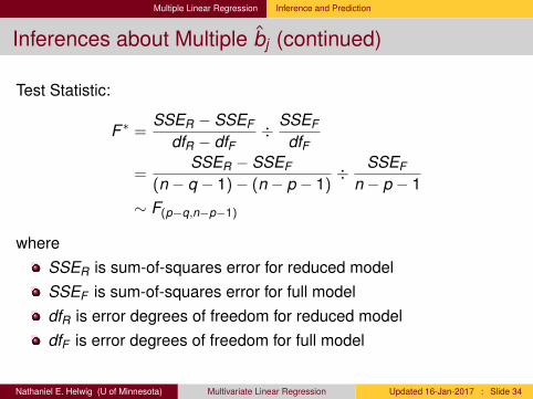
Inferences about Multiple bj (continued)

Test Statistic:

F ∗ =SSER − SSEF

dfR − dfF÷ SSEF

dfF

=SSER − SSEF

(n − q − 1)− (n − p − 1)÷ SSEF

n − p − 1∼ F(p−q,n−p−1)

whereSSER is sum-of-squares error for reduced modelSSEF is sum-of-squares error for full modeldfR is error degrees of freedom for reduced modeldfF is error degrees of freedom for full model



Inferences about Linear Combinations of bj

Assume that c = (c1, . . . , cp+1)′ and want to test:

H0 : c′b = b∗

H1 : c′b 6= b∗

Test statistic:

t∗ =c′b− b∗

σ√

c′(X′X)−1c∼ tn−p−1



Confidence Interval for σ2

Note that (n−p−1)σ2

σ2 = SSEσ2 =

∑ni=1 e2

iσ2 ∼ χ2

n−p−1

This implies that

χ2(n−p−1;1−α/2) <

(n − p − 1)σ2

σ2 < χ2(n−p−1;α/2)

where P(Q > χ2(n−p−1;α/2)) = α/2, so a 100(1− α)% CI is given by

(n − p − 1)σ2

χ2(n−p−1;α/2)

< σ2 <(n − p − 1)σ2

χ2(n−p−1;1−α/2)



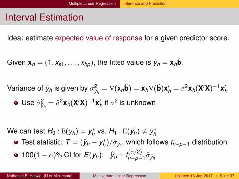
Interval Estimation

Idea: estimate expected value of response for a given predictor score.

Given xh = (1, xh1, . . . , xhp), the fitted value is yh = xhb.

Variance of yh is given by σ2yh

= V(xhb) = xhV(b)x′h = σ2xh(X′X)−1x′h

Use σ2yh

= σ2xh(X′X)−1x′h if σ2 is unknown

We can test H0 : E(yh) = y∗h vs. H1 : E(yh) 6= y∗hTest statistic: T = (yh − y∗h )/σyh , which follows tn−p−1 distribution

100(1− α)% CI for E(yh): yh ± t(α/2)n−p−1σyh



Predicting New Observations

Idea: estimate observed value of response for a given predictor score.

Note: interested in actual yh value instead of E(yh)

Given xh = (1, xh1, . . . , xhp), the fitted value is yh = xhb.

Note: same as interval estimation

When predicting a new observation, there are two uncertainties:location of the distribution of Y for X1, . . . ,Xp (captured by σ2

yh)

variability within the distribution of Y (captured by σ2)



Predicting New Observations (continued)

Two sources of variance are independent so σ2yh

= σ2yh

+ σ2

Use σ2yh

= σ2yh

+ σ2 if σ2 is unknown

We can test H0 : yh = y∗h vs. H1 : yh 6= y∗hTest statistic: T = (yh − y∗h )/σyh , which follows tn−p−1 distribution

100(1− α)% Prediction Interval (PI) for yh: yh ± t(α/2)n−p−1σyh



Confidence and Prediction Intervals in R

# confidence interval> newdata <- data.frame(cyl=factor(6, levels=c(4,6,8)), am=1, carb=4)> predict(mod, newdata, interval="confidence")

fit lwr upr1 21.51824 18.92554 24.11094

# prediction interval> newdata <- data.frame(cyl=factor(6, levels=c(4,6,8)), am=1, carb=4)> predict(mod, newdata, interval="prediction")

fit lwr upr1 21.51824 15.20583 27.83065



Simultaneous Confidence Regions

Given the distribution of b (and some probability theory), we have that

(b− b)′X′X(b− b)

σ2 ∼ χ2p+1 and

(n − p − 1)σ2

σ2 ∼ χ2n−p−1

which implies that

(b− b)′X′X(b− b)

(p + 1)σ2 ∼χ2

p+1/(p + 1)

χ2n−p−1/(n − p − 1)

≡ F(p+1,n−p−1)

To form a 100(1− α)% confidence region (CR) use limits such that

(b− b)′X′X(b− b) ≤ (p + 1)σ2F (α)(p+1,n−p−1)

where F (α)(p+1,n−p−1) is the critical value for significance level α.



Simultaneous Confidence Regions in R

−10 −6 −4 −2 0 2

−14

−10

−6

−2

0

α = 0.1

cyl6 coefficient

cyl8

coe

ffici

ent

●

−10 −6 −4 −2 0 2

−14

−10

−6

−2

0

α = 0.01

cyl6 coefficientcy

l8 c

oeffi

cien

t

●

dev.new(height=4,width=8,noRStudioGD=TRUE)par(mfrow=c(1,2))confidenceEllipse(mod,c(2,3),levels=.9,xlim=c(-11,3),ylim=c(-14,0),

main=expression(alpha*" = "*.1),cex.main=2)confidenceEllipse(mod,c(2,3),levels=.99,xlim=c(-11,3),ylim=c(-14,0),

main=expression(alpha*" = "*.01),cex.main=2)


Multivariate Linear Regression

Multivariate LinearRegression


Multivariate Linear Regression Model Form and Assumptions

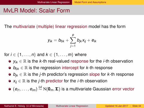
MvLR Model: Scalar Form

The multivariate (multiple) linear regression model has the form

yik = b0k +

p∑j=1

bjkxij + eik

for i ∈ {1, . . . ,n} and k ∈ {1, . . . ,m} whereyik ∈ R is the k -th real-valued response for the i-th observationb0k ∈ R is the regression intercept for k -th responsebjk ∈ R is the j-th predictor’s regression slope for k -th responsexij ∈ R is the j-th predictor for the i-th observation

(ei1, . . . ,eim)iid∼ N(0m,Σ) is a multivariate Gaussian error vector



MvLR Model: Nomenclature

The model is multivariate because we have m > 1 response variables.

The model is multiple because we have p > 1 predictors.

If p = 1, we have a multivariate simple linear regression model

The model is linear because yik is a linear function of the parameters(bjk are the parameters for j ∈ {1, . . . ,p + 1} and k ∈ {1, . . . ,m}).

The model is a regression model because we are modeling responsevariables (Y1, . . . ,Ym) as a function of predictor variables (X1, . . . ,Xp).



MvLR Model: Assumptions

The fundamental assumptions of the MLR model are:1 Relationship between Xj and Yk is linear (given other predictors)2 xij and yik are observed random variables (known constants)

3 (ei1, . . . ,eim)iid∼ N(0m,Σ) is an unobserved random vector

4 bk = (b0k ,b1k , . . . ,bpk )′ for k ∈ {1, . . . ,m} are unknown constants5 (yik |xi1, . . . , xip) ∼ N(b0k +

∑pj=1 bjkxij , σkk ) for each k ∈ {1, . . . ,m}

note: homogeneity of variance for each response

Note: bjk is expected increase in Yk for 1-unit increase in Xj with allother predictor variables held constant



MvLR Model: Matrix Form

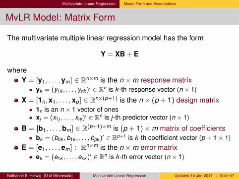
The multivariate multiple linear regression model has the form

Y = XB + E

whereY = [y1, . . . ,ym] ∈ Rn×m is the n ×m response matrix• yk = (y1k , . . . , ynk )′ ∈ Rn is k -th response vector (n × 1)

X = [1n,x1, . . . ,xp] ∈ Rn×(p+1) is the n × (p + 1) design matrix• 1n is an n × 1 vector of ones• xj = (x1j , . . . , xnj )

′ ∈ Rn is j-th predictor vector (n × 1)

B = [b1, . . . ,bm] ∈ R(p+1)×m is (p + 1)×m matrix of coefficients• bk = (b0k ,b1k , . . . ,bpk )′ ∈ Rp+1 is k -th coefficient vector (p + 1× 1)

E = [e1, . . . ,em] ∈ Rn×m is the n ×m error matrix• ek = (e1k , . . . ,enk )′ ∈ Rn is k -th error vector (n × 1)



MvLR Model: Matrix Form (another look)

Matrix form writes MLR model for all nm points simultaneously

Y = XB + E

y11 · · · y1my21 · · · y2my31 · · · y3m

.... . .

...yn1 · · · ynm

=

1 x11 x12 · · · x1p1 x21 x22 · · · x2p1 x31 x32 · · · x3p...

......

. . ....

1 xn1 xn2 · · · xnp

b01 · · · b0mb11 · · · b1mb21 · · · b2m

.... . .

...bp1 · · · bpm

+

e11 · · · e1me21 · · · e2me31 · · · e3m

.... . .

...en1 · · · enm



MvLR Model: Assumptions (revisited)

Assuming that the n subjects are independent, we have thatek ∼ N(0n, σkk In) where ek is k -th column of E

eiiid∼ N(0m,Σ) where ei is i-th row of E

vec(E) ∼ N(0nm,Σ⊗ In) where ⊗ denotes the Kronecker productvec(E′) ∼ N(0nm, In ⊗Σ) where ⊗ denotes the Kronecker product

The response matrix is multivariate normal given X

(vec(Y)|X) ∼ N([B′ ⊗ In]vec(X),Σ⊗ In)

(vec(Y′)|X) ∼ N([In ⊗ B′]vec(X′), In ⊗Σ)

where [B′ ⊗ In]vec(X) = vec(XB) and [In ⊗ B′]vec(X′) = vec(B′X′).



MvLR Model: Mean and Covariance

Note that the assumed mean vector for vec(Y′) is

[In ⊗ B′]vec(X′) = vec(B′X′) =

B′x1...

B′xn

where xi is the i-th row of X

The assumed covariance matrix for vec(Y′) is block diagonal

In ⊗Σ =

Σ 0m×m · · · 0m×m

0m×m Σ · · · 0m×m...

.... . .

...0m×m 0m×m · · · Σ


Multivariate Linear Regression Parameter Estimation

Ordinary Least Squares

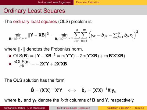
The ordinary least squares (OLS) problem is

minB∈R(p+1)×m

‖Y− XB‖2 = minB∈R(p+1)×m

n∑i=1

m∑k=1

(yik − b0k −

∑pj=1 bjkxij

)2

where ‖ · ‖ denotes the Frobenius norm.OLS(B) = ‖Y− XB‖2 = tr(Y′Y)− 2tr(Y′XB) + tr(B′X′XB)

∂OLS(B)∂B = −2X′Y + 2X′XB

The OLS solution has the form

B = (X′X)−1X′Y ⇐⇒ bk = (X′X)−1X′yk

where bk and yk denote the k -th columns of B and Y, respectively.



Fitted Values and Residuals

SCALAR FORM:


yik = b0k +∑p

j=1 bjkxij


eik = yik − yik

MATRIX FORM:


Y = XB


E = Y− Y



Hat Matrix

Note that we can write the fitted values as

Y = XB

= X(X′X)−1X′Y= HY

where H = X(X′X)−1X′ is the hat matrix.

H is a symmetric and idempotent matrix: HH = H

H projects yk onto the column space of X for k ∈ {1, . . . ,m}.



Multivariate Regression Example in R

> data(mtcars)> head(mtcars)

mpg cyl disp hp drat wt qsec vs am gear carbMazda RX4 21.0 6 160 110 3.90 2.620 16.46 0 1 4 4Mazda RX4 Wag 21.0 6 160 110 3.90 2.875 17.02 0 1 4 4Datsun 710 22.8 4 108 93 3.85 2.320 18.61 1 1 4 1Hornet 4 Drive 21.4 6 258 110 3.08 3.215 19.44 1 0 3 1Hornet Sportabout 18.7 8 360 175 3.15 3.440 17.02 0 0 3 2Valiant 18.1 6 225 105 2.76 3.460 20.22 1 0 3 1> mtcars$cyl <- factor(mtcars$cyl)> Y <- as.matrix(mtcars[,c("mpg","disp","hp","wt")])> mvmod <- lm(Y ~ cyl + am + carb, data=mtcars)> coef(mvmod)

mpg disp hp wt(Intercept) 25.320303 134.32487 46.5201421 2.7612069cyl6 -3.549419 61.84324 0.9116288 0.1957229cyl8 -6.904637 218.99063 87.5910956 0.7723077am 4.226774 -43.80256 4.4472569 -1.0254749carb -1.119855 1.72629 21.2764930 0.1749132



Sums-of-Squares and Crossproducts: Vector Form

In MvLR models, the relevant sums-of-squares and crossproducts areTotal: SSCPT =

∑ni=1(yi − y)(yi − y)′

Regression: SSCPR =∑n

i=1(yi − y)(yi − y)′

Error: SSCPE =∑n

i=1(yi − yi)(yi − yi)′

where yi and yi denote the i-th rows of Y and Y = XB, respectively.

The corresponding degrees of freedom areSSCPT : dfT = m(n − 1)

SSCPR: dfR = mpSSCPE : dfE = m(n − p − 1)



Sums-of-Squares and Crossproducts: Matrix Form

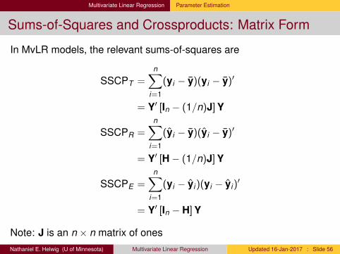
In MvLR models, the relevant sums-of-squares are

SSCPT =n∑

i=1

(yi − y)(yi − y)′

= Y′ [In − (1/n)J] Y

SSCPR =n∑

i=1

(yi − y)(yi − y)′

= Y′ [H− (1/n)J] Y

SSCPE =n∑

i=1

(yi − yi)(yi − yi)′

= Y′ [In − H] Y

Note: J is an n × n matrix of onesNathaniel E. Helwig (U of Minnesota) Multivariate Linear Regression Updated 16-Jan-2017 : Slide 56


Partitioning the SSCP Total Matrix

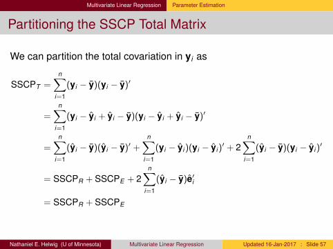
We can partition the total covariation in yi as

SSCPT =n∑

i=1

(yi − y)(yi − y)′

=n∑

i=1

(yi − yi + yi − y)(yi − yi + yi − y)′

=n∑

i=1

(yi − y)(yi − y)′ +n∑

i=1

(yi − yi )(yi − yi )′ + 2

n∑i=1

(yi − y)(yi − yi )′

= SSCPR + SSCPE + 2n∑

i=1

(yi − y)e′i

= SSCPR + SSCPE



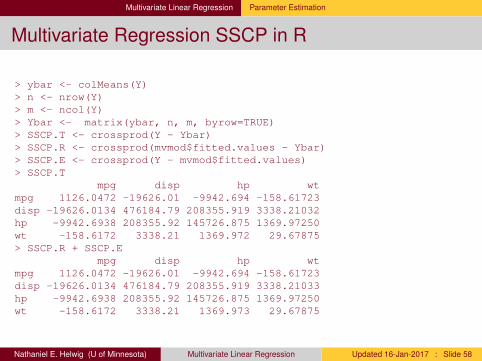
Multivariate Regression SSCP in R

> ybar <- colMeans(Y)> n <- nrow(Y)> m <- ncol(Y)> Ybar <- matrix(ybar, n, m, byrow=TRUE)> SSCP.T <- crossprod(Y - Ybar)> SSCP.R <- crossprod(mvmod$fitted.values - Ybar)> SSCP.E <- crossprod(Y - mvmod$fitted.values)> SSCP.T

mpg disp hp wtmpg 1126.0472 -19626.01 -9942.694 -158.61723disp -19626.0134 476184.79 208355.919 3338.21032hp -9942.6938 208355.92 145726.875 1369.97250wt -158.6172 3338.21 1369.972 29.67875> SSCP.R + SSCP.E

mpg disp hp wtmpg 1126.0472 -19626.01 -9942.694 -158.61723disp -19626.0134 476184.79 208355.919 3338.21033hp -9942.6938 208355.92 145726.875 1369.97250wt -158.6172 3338.21 1369.973 29.67875



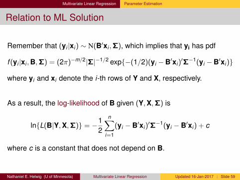
Relation to ML Solution

Remember that (yi |xi) ∼ N(B′xi ,Σ), which implies that yi has pdf

f (yi |xi ,B,Σ) = (2π)−m/2|Σ|−1/2 exp{−(1/2)(yi −B′xi)′Σ−1(yi −B′xi)}

where yi and xi denote the i-th rows of Y and X, respectively.

As a result, the log-likelihood of B given (Y,X,Σ) is

ln{L(B|Y,X,Σ)} = −12

n∑i=1

(yi − B′xi)′Σ−1(yi − B′xi) + c

where c is a constant that does not depend on B.



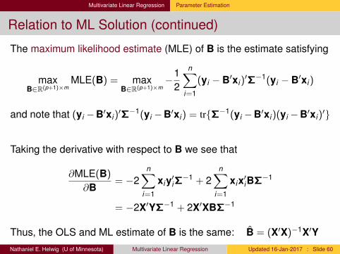
Relation to ML Solution (continued)

The maximum likelihood estimate (MLE) of B is the estimate satisfying

maxB∈R(p+1)×m

MLE(B) = maxB∈R(p+1)×m

−12

n∑i=1

(yi − B′xi)′Σ−1(yi − B′xi)

and note that (yi −B′xi)′Σ−1(yi −B′xi) = tr{Σ−1(yi −B′xi)(yi −B′xi)

′}

Taking the derivative with respect to B we see that

∂MLE(B)

∂B= −2

n∑i=1

xiy′iΣ−1 + 2

n∑i=1

xix′iBΣ−1

= −2X′YΣ−1 + 2X′XBΣ−1

Thus, the OLS and ML estimate of B is the same: B = (X′X)−1X′YNathaniel E. Helwig (U of Minnesota) Multivariate Linear Regression Updated 16-Jan-2017 : Slide 60


Estimated Error Covariance

The estimated error variance is

Σ =SSCPE

n − p − 1

=

∑ni=1(yi − yi)(yi − yi)

′

n − p − 1

=Y′ (In − H) Y

n − p − 1

which is an unbiased estimate of error covariance matrix Σ.

The estimate Σ is the mean SSCP error of the model.



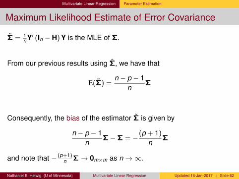
Maximum Likelihood Estimate of Error Covariance

Σ = 1n Y′ (In − H) Y is the MLE of Σ.

From our previous results using Σ, we have that

E(Σ) =n − p − 1

nΣ

Consequently, the bias of the estimator Σ is given by

n − p − 1n

Σ−Σ = −(p + 1)

nΣ

and note that − (p+1)n Σ→ 0m×m as n→∞.



Comparing Σ and Σ

Reminder: the MSSCPE and MLE of Σ are given by

Σ = Y′ (In − H) Y/(n − p − 1)

Σ = Y′ (In − H) Y/n

From the definitions of Σ and Σ we have that

σkk < σkk for all k

where σkk and σkk denote the k -th diagonals of Σ and Σ, respectively.MLE produces smaller estimates of the error variances



Estimated Error Covariance Matrix in R

> n <- nrow(Y)> p <- nrow(coef(mvmod)) - 1> SSCP.E <- crossprod(Y - mvmod$fitted.values)> SigmaHat <- SSCP.E / (n - p - 1)> SigmaTilde <- SSCP.E / n> SigmaHat

mpg disp hp wtmpg 7.8680094 -53.27166 -19.7015979 -0.6575443disp -53.2716607 2504.87095 425.1328988 18.1065416hp -19.7015979 425.13290 577.2703337 0.4662491wt -0.6575443 18.10654 0.4662491 0.2573503> SigmaTilde

mpg disp hp wtmpg 6.638633 -44.94796 -16.6232233 -0.5548030disp -44.947964 2113.48487 358.7058833 15.2773945hp -16.623223 358.70588 487.0718440 0.3933977wt -0.554803 15.27739 0.3933977 0.2171394


Multivariate Linear Regression Inference and Prediction

Expected Value of Least Squares Coefficients

The expected value of the estimated coefficients is given by

E(B) = E [(X′X)−1X′Y]

= (X′X)−1X′E(Y)

= (X′X)−1X′XB= B

so B is an unbiased estimator of B.



Covariance Matrix of Least Squares Coefficients

The covariance matrix of the estimated coefficients is given by

V{vec(B′)} = V{vec(Y′X(X′X)−1)}= V{[(X′X)−1X′ ⊗ Im]vec(Y′)}= [(X′X)−1X′ ⊗ Im]V{vec(Y′)}[(X′X)−1X′ ⊗ Im]′

= [(X′X)−1X′ ⊗ Im][In ⊗Σ][X(X′X)−1 ⊗ Im]

= [(X′X)−1X′ ⊗ Im][X(X′X)−1 ⊗Σ]

= (X′X)−1 ⊗Σ

Note: we could also write V{vec(B)} = Σ⊗ (X′X)−1



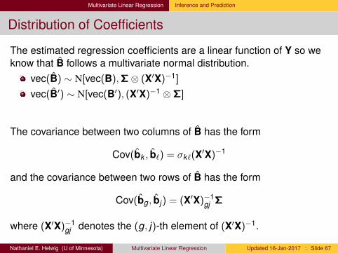
Distribution of Coefficients

The estimated regression coefficients are a linear function of Y so weknow that B follows a multivariate normal distribution.

vec(B) ∼ N[vec(B),Σ⊗ (X′X)−1]

vec(B′) ∼ N[vec(B′), (X′X)−1 ⊗Σ]

The covariance between two columns of B has the form

Cov(bk , b`) = σk`(X′X)−1

and the covariance between two rows of B has the form

Cov(bg , bj) = (X′X)−1gj Σ

where (X′X)−1gj denotes the (g, j)-th element of (X′X)−1.



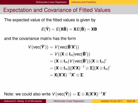
Expectation and Covariance of Fitted Values

The expected value of the fitted values is given by

E(Y) = E(XB) = XE(B) = XB

and the covariance matrix has the form

V{vec(Y′)} = V{vec(B′X′)}= V{(X⊗ Im)vec(B′)}= (X⊗ Im)V{vec(B′)}(X⊗ Im)′

= (X⊗ Im)[(X′X)−1 ⊗Σ](X⊗ Im)′

= X(X′X)−1X′ ⊗Σ

Note: we could also write V{vec(Y)} = Σ⊗ X(X′X)−1X′



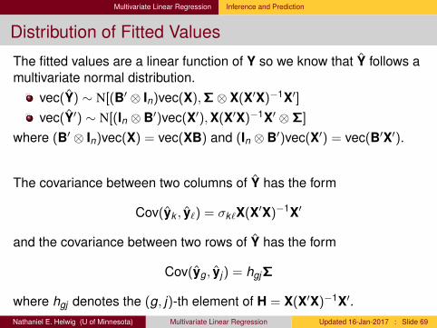
Distribution of Fitted Values

The fitted values are a linear function of Y so we know that Y follows amultivariate normal distribution.

vec(Y) ∼ N[(B′ ⊗ In)vec(X),Σ⊗ X(X′X)−1X′]vec(Y′) ∼ N[(In ⊗ B′)vec(X′),X(X′X)−1X′ ⊗Σ]

where (B′ ⊗ In)vec(X) = vec(XB) and (In ⊗ B′)vec(X′) = vec(B′X′).

The covariance between two columns of Y has the form

Cov(yk , y`) = σk`X(X′X)−1X′

and the covariance between two rows of Y has the form

Cov(yg , yj) = hgjΣ

where hgj denotes the (g, j)-th element of H = X(X′X)−1X′.Nathaniel E. Helwig (U of Minnesota) Multivariate Linear Regression Updated 16-Jan-2017 : Slide 69


Expectation and Covariance of Residuals

The expected value of the residuals is given by

E(Y− Y) = E([In − H]Y) = (In − H)E(Y) = (In − H)XB = 0n×m

and the covariance matrix has the form

V{vec(E′)} = V{vec(Y′[In − H])}= V{([In − H]⊗ Im)vec(Y′)}= ([In − H]⊗ Im)V{vec(Y′)}([In − H]⊗ Im)

= ([In − H]⊗ Im)[In ⊗Σ]([In − H]⊗ Im)

= (In − H)⊗Σ

Note: we could also write V{vec(E)} = Σ⊗ (In − H)



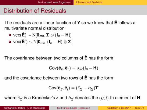
Distribution of Residuals

The residuals are a linear function of Y so we know that E follows amultivariate normal distribution.

vec(E) ∼ N[0mn,Σ⊗ (In − H)]

vec(E′) ∼ N[0mn, (In − H)⊗Σ]

The covariance between two columns of E has the form

Cov(ek , e`) = σk`(In − H)

and the covariance between two rows of E has the form

Cov(eg , ej) = (δgj − hgj)Σ

where δgj is a Kronecker’s δ and hgj denotes the (g, j)-th element of H.



Summary of Results

Given the model assumptions, we have

vec(B) ∼ N[vec(B),Σ⊗ (X′X)−1]

vec(Y) ∼ N[vec(XB),Σ⊗ H]

vec(E) ∼ N[0mn,Σ⊗ (In − H)]

where vec(XB) = (B′ ⊗ In)vec(X).

Typically Σ is unknown, so we use the mean SSCP error matrix Σ.



Coefficient Inference in R> mvsum <- summary(mvmod)> mvsum[[1]]

Call:lm(formula = mpg ~ cyl + am + carb, data = mtcars)


-5.9074 -1.1723 0.2538 1.4851 5.4728


(Intercept) 25.3203 1.2238 20.690 < 2e-16 ***cyl6 -3.5494 1.7296 -2.052 0.049959 *cyl8 -6.9046 1.8078 -3.819 0.000712 ***am 4.2268 1.3499 3.131 0.004156 **carb -1.1199 0.4354 -2.572 0.015923 *---Signif. codes: 0 ‘***’ 0.001 ‘**’ 0.01 ‘*’ 0.05 ‘.’ 0.1 ‘ ’ 1

Residual standard error: 2.805 on 27 degrees of freedomMultiple R-squared: 0.8113, Adjusted R-squared: 0.7834F-statistic: 29.03 on 4 and 27 DF, p-value: 1.991e-09Nathaniel E. Helwig (U of Minnesota) Multivariate Linear Regression Updated 16-Jan-2017 : Slide 73


Coefficient Inference in R (continued)> mvsum <- summary(mvmod)> mvsum[[3]]

Call:lm(formula = hp ~ cyl + am + carb, data = mtcars)


-41.520 -17.941 -4.378 19.799 41.292


(Intercept) 46.5201 10.4825 4.438 0.000138 ***cyl6 0.9116 14.8146 0.062 0.951386cyl8 87.5911 15.4851 5.656 5.25e-06 ***am 4.4473 11.5629 0.385 0.703536carb 21.2765 3.7291 5.706 4.61e-06 ***---Signif. codes: 0 ‘***’ 0.001 ‘**’ 0.01 ‘*’ 0.05 ‘.’ 0.1 ‘ ’ 1

Residual standard error: 24.03 on 27 degrees of freedomMultiple R-squared: 0.893, Adjusted R-squared: 0.8772F-statistic: 56.36 on 4 and 27 DF, p-value: 1.023e-12Nathaniel E. Helwig (U of Minnesota) Multivariate Linear Regression Updated 16-Jan-2017 : Slide 74


Inferences about Multiple bjk

Assume that q < p and want to test if a reduced model is sufficient:

H0 : B2 = 0(p−q)×m

H1 : B2 6= 0(p−q)×m

where

B =

(B1B2

)is the partitioned coefficient vector.

Compare the SSCP-Error for full and reduced (constrained) models:(a) Full Model: yik = b0k +

∑pj=1 bjkxij + eik

(b) Reduced Model: yik = b0k +∑q

j=1 bjkxij + eik



Inferences about Multiple bjk (continued)

Likelihood Ratio Test Statistic:

Λ =maxB1,Σ L(B1,Σ)

maxB,Σ L(B,Σ)

=(|Σ||Σ1|

)n/2

whereΣ is the MLE of Σ with B unconstrainedΣ1 is the MLE of Σ with B2 = 0(p−1)×m

For large n, we can use the modified test statistic

−ν log(Λ) ∼ χ2m(p−q)

where ν = n − p − 1− (1/2)(m − p + q + 1)Nathaniel E. Helwig (U of Minnesota) Multivariate Linear Regression Updated 16-Jan-2017 : Slide 76


Some Other Test Statistics

Let E = nΣ denote the SSCP error matrix from the full model, and letH = n(Σ1 − Σ) denote the hypothesis (or extra) SSCP error matrix.

Test statistics for H0 : B2 = 0(p−1)×m versus H1 : B2 6= 0(p−1)×m

Wilks’ lambda =∏s

i=11

1+ηi= |E||E+H|

Pillai’s trace =∑s

i=1ηi

1+ηi= tr[H(E + H)−1]

Hotelling-Lawley trace =∑s

i=1 ηs = tr(HE−1)

Roy’s greatest root = η11+η1

where η1 ≥ η2 ≥ · · · ≥ ηs denote the nonzero eigenvalues of HE−1



Testing a Reduced Multivariate Linear Model in R> mvmod0 <- lm(Y ~ am + carb, data=mtcars)> anova(mvmod, mvmod0, test="Wilks")Analysis of Variance Table

Model 1: Y ~ cyl + am + carbModel 2: Y ~ am + carbRes.Df Df Gen.var. Wilks approx F num Df den Df Pr(>F)

1 27 29.8622 29 2 43.692 0.16395 8.8181 8 48 2.525e-07 ***---Signif. codes: 0 ‘***’ 0.001 ‘**’ 0.01 ‘*’ 0.05 ‘.’ 0.1 ‘ ’ 1

> anova(mvmod, mvmod0, test="Pillai")Analysis of Variance Table

Model 1: Y ~ cyl + am + carbModel 2: Y ~ am + carb

Res.Df Df Gen.var. Pillai approx F num Df den Df Pr(>F)1 27 29.8622 29 2 43.692 1.0323 6.6672 8 50 6.593e-06 ***---Signif. codes: 0 ‘***’ 0.001 ‘**’ 0.01 ‘*’ 0.05 ‘.’ 0.1 ‘ ’ 1

> Etilde <- n * SigmaTilde> SigmaTilde1 <- crossprod(Y - mvmod0$fitted.values) / n> Htilde <- n * (SigmaTilde1 - SigmaTilde)> HEi <- Htilde %*% solve(Etilde)> HEi.values <- eigen(HEi)$values> c(Wilks = prod(1 / (1 + HEi.values)), Pillai = sum(HEi.values / (1 + HEi.values)))

Wilks Pillai0.1639527 1.0322975



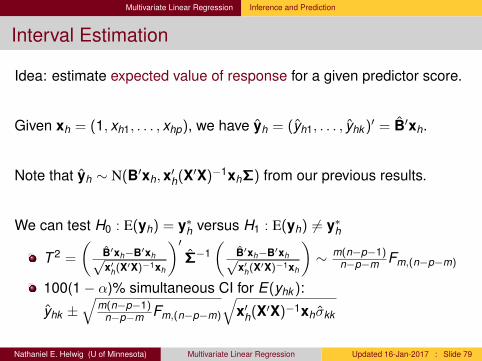
Interval Estimation

Idea: estimate expected value of response for a given predictor score.

Given xh = (1, xh1, . . . , xhp), we have yh = (yh1, . . . , yhk )′ = B′xh.

Note that yh ∼ N(B′xh,x′h(X′X)−1xhΣ) from our previous results.

We can test H0 : E(yh) = y∗h versus H1 : E(yh) 6= y∗h

T 2 =

(B′xh−B′xh√x′h(X′X)−1xh

)′Σ−1

(B′xh−B′xh√x′h(X′X)−1xh

)∼ m(n−p−1)

n−p−m Fm,(n−p−m)

100(1− α)% simultaneous CI for E(yhk ):

yhk ±√

m(n−p−1)n−p−m Fm,(n−p−m)

√x′h(X′X)−1xhσkk



Predicting New Observations

Idea: estimate observed value of response for a given predictor score.Note: interested in actual yh value instead of E(yh)Given xh = (1, xh1, . . . , xhp), the fitted value is still yh = B′xh.

When predicting a new observation, there are two uncertainties:location of distribution of Y1, . . . ,Ym for X1, . . . ,Xp, i.e., V (yh)variability within the distribution of Y1, . . . ,Ym, i.e., Σ

We can test H0 : yh = y∗h versus H1 : yh 6= y∗h

T 2 =

(B′xh−B′xh√

1+x′h(X′X)−1xh

)′Σ−1

(B′xh−B′xh√

1+x′h(X′X)−1xh

)∼

m(n−p−1)n−p−m Fm,(n−p−m)

100(1− α)% simultaneous PI for E(yhk ):

yhk ±√

m(n−p−1)n−p−m Fm,(n−p−m)(α)

√(1 + x′h(X′X)−1xh)σkk



Confidence and Prediction Intervals in R

Note: R does not yet have this capability!> # confidence interval> newdata <- data.frame(cyl=factor(6, levels=c(4,6,8)), am=1, carb=4)> predict(mvmod, newdata, interval="confidence")

mpg disp hp wt1 21.51824 159.2707 136.985 2.631108

> # prediction interval> newdata <- data.frame(cyl=factor(6, levels=c(4,6,8)), am=1, carb=4)> predict(mvmod, newdata, interval="prediction")

mpg disp hp wt1 21.51824 159.2707 136.985 2.631108



R Function for Multivariate Regression CIs and PIs

pred.mlm <- function(object, newdata, level=0.95,interval = c("confidence", "prediction")){

form <- as.formula(paste("~",as.character(formula(object))[3]))xnew <- model.matrix(form, newdata)fit <- predict(object, newdata)Y <- model.frame(object)[,1]X <- model.matrix(object)n <- nrow(Y)m <- ncol(Y)p <- ncol(X) - 1sigmas <- colSums((Y - object$fitted.values)^2) / (n - p - 1)fit.var <- diag(xnew %*% tcrossprod(solve(crossprod(X)), xnew))if(interval[1]=="prediction") fit.var <- fit.var + 1const <- qf(level, df1=m, df2=n-p-m) * m * (n - p - 1) / (n - p - m)vmat <- (n/(n-p-1)) * outer(fit.var, sigmas)lwr <- fit - sqrt(const) * sqrt(vmat)upr <- fit + sqrt(const) * sqrt(vmat)if(nrow(xnew)==1L){

ci <- rbind(fit, lwr, upr)rownames(ci) <- c("fit", "lwr", "upr")

} else {ci <- array(0, dim=c(nrow(xnew), m, 3))dimnames(ci) <- list(1:nrow(xnew), colnames(Y), c("fit", "lwr", "upr") )ci[,,1] <- fitci[,,2] <- lwrci[,,3] <- upr

}ci

}



Confidence and Prediction Intervals in R (revisited)

# confidence interval> newdata <- data.frame(cyl=factor(6, levels=c(4,6,8)), am=1, carb=4)> pred.mlm(mvmod, newdata)

mpg disp hp wtfit 21.51824 159.2707 136.98500 2.631108lwr 16.65593 72.5141 95.33649 1.751736upr 26.38055 246.0273 178.63351 3.510479

# prediction interval> newdata <- data.frame(cyl=factor(6, levels=c(4,6,8)), am=1, carb=4)> pred.mlm(mvmod, newdata, interval="prediction")

mpg disp hp wtfit 21.518240 159.27070 136.98500 2.6311076lwr 9.680053 -51.95435 35.58397 0.4901152upr 33.356426 370.49576 238.38603 4.7720999



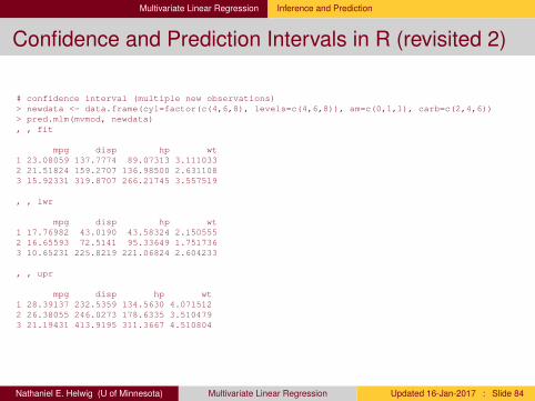
Confidence and Prediction Intervals in R (revisited 2)

# confidence interval (multiple new observations)> newdata <- data.frame(cyl=factor(c(4,6,8), levels=c(4,6,8)), am=c(0,1,1), carb=c(2,4,6))> pred.mlm(mvmod, newdata), , fit

mpg disp hp wt1 23.08059 137.7774 89.07313 3.1110332 21.51824 159.2707 136.98500 2.6311083 15.92331 319.8707 266.21745 3.557519

, , lwr

mpg disp hp wt1 17.76982 43.0190 43.58324 2.1505552 16.65593 72.5141 95.33649 1.7517363 10.65231 225.8219 221.06824 2.604233

, , upr

mpg disp hp wt1 28.39137 232.5359 134.5630 4.0715122 26.38055 246.0273 178.6335 3.5104793 21.19431 413.9195 311.3667 4.510804


Documents

Nathaniel E. Helwig - Statisticsusers.stat.umn.edu/~helwig/notes/mvlr-Notes.pdf · The OLS solution has the form ^b = (X0X) ... Multivariate Linear Regression Updated 16-Jan-2017