Big Bang and Loop Quantum Cosmologyrelativity.phys.lsu.edu/ilqgs/singh060606.pdf · Some age-old questions Does the theory provides a non-singular evolution through the big bang ?

Big Bang and Loop Quantum Cosmology

Parampreet SinghInstitute for Gravitational Physics and Geometry, Penn State

Loop Quantum Gravity World Seminar

LQG Seminar – p.1

Standard model of cosmology provides an excellent agreementwith the observational data. Age of precision cosmology.

Though we have a ‘working model’ (= hot big bang + inflation+ dark energy + dark matter + ...) in cosmology, importantquestions remain unanswered:

The backward evolution of our Universe leads to a BigBang singularity (result of powerful singularity theorems).General Relativity inadequate to provide correct physics athigh curvature scales. Occurrence of singularity � � limitof validity of the theoryJustification of various assumptions in models of very earlyUniverse ? Primordial perturbations ? Dark energy ?

Need for inputs from quantum gravity.

What does Quantum Gravity tell us about the physics near the Big Bang ?

(BASED ON WORK WITH ABHAY ASHTEKAR AND TOMASZ PAWLOWSKI)

LQG Seminar – p.2

Some age-old questions

Does the theory provides a non-singular evolution through thebig bang ?

What is on the other side of the big bang ? Quantum foam or aclassical spacetime ?

What is the scale at which the spacetime ceases to be classical ?Does the spacetime continuum exists at all scales, especiallywhen primordial fluctuations were generated ?

What are the modifications to the Friedmann dynamics atscales of high curvature and at what scales these becomeimportant ?

Does the theory make testable predictions ?(complex set of questions � difficult to answer without detailed analytical,

phenomenological and numerical investigations)

LQG Seminar – p.3

Various Innovative Ideas

Pre big bang scenarios: Based on the scale factor duality of thestring dilaton action. Big bang not the beginning. The post bigbang phase with

��

preceded by a pre bigbang phase with

� � � � � � �

.Major Problem: No non-singular evolution between the prebig bang and the post big bang phase.

?

Pre−Big Bang Post−Big Bang

Curvature

time

Similar problems with Ekpyrotic/Cyclic modelsLQG Seminar – p.4

Various models propose modifications to Friedmann dynamicsat high energies. Classical general relativity is envisioned as alow energy effective theory. It is modified at high energies.

Popular Ideas: Modifications may arise due to higher orderterms in the gravity action, large extra dimensions, ...

Example: Randall-Sundrum model. Our Universe exists on a3-brane embedded in 5 dimensional anti-de Sitter bulk.

� � � ��

��

�

�� , � � � � . As � � �

,

� � � �.Singular evolution. Problems related to big bang as in

standard cosmology.

Extensions yield limited success (unnatural conditions to get a bounce).LQG Seminar – p.5

Hope has been that higher order perturbative corrections onthe continuum spacetime might be enough to capture thedetails of singularity resolution – limited success

Ideas assume the existence of a spacetime continuum at allscalesNon-perturbative quantum gravitational modifications notincluded

Quantum nature of dynamical spacetime not captured in theseapproaches

Do non-perturbative quantum gravitational effects resolve the big bangsingularity ?

LQG Seminar – p.6

Background independent non-perturbative quantum gravity –LQG is leading approach.Our Strategy: Construct a quantum cosmological model based onLQG � � LQC

Caveats:Homogeneous and Isotropic setting

Relationship with full theory unclearHopes:

Glimpses of singularity resolution and physics of very earlyUniverseLearning/Testing ground for model building,phenomenological applications, making testable predictions

Valuable insights/lessons to complete the program in LQGand other non-perturbative approaches

LQG Seminar – p.7

LQC: Homogeneous and Isotropic setting

Spatial homogeneity and isotropy: fix a fiducial triad� � �� and

co-triad

� � �� . Symmetries �

� �� Basic variables: � and satisfying

� � � � ��

.Relation to scale factor:� � � � �

(two possible orientations for the triad)�� (on the space of physical solutions of GR).

Elementary variables – Holonomies:�� ! � � "$# �� &% � , � ' � � � �

Elements of form �( ) * � � � ��– generate algebra of almost

periodic functions

Hilbert space:+-,. / � 0 � 1 2 3� 2 �

Orthonormal basis:

4 �� ( ) * � � � ��

;

5 4 �� 4 �� 6 �7 � 8:9<; 9 =

Hilbert Space different from the Wheeler-DeWitt theory.

LQG Seminar – p.8

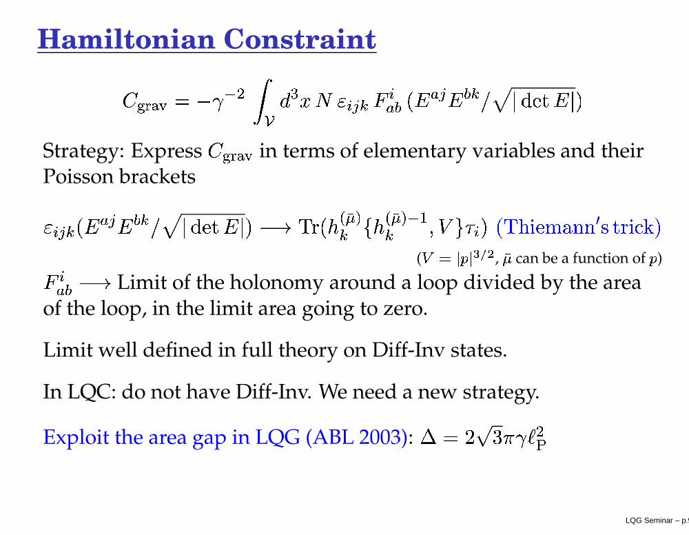
Hamiltonian Constraint

��

3 �� 4� ��

Strategy: Express

� � � � � in terms of elementary variables and theirPoisson brackets

�� 9 �� 9 � �� % � � � � " �� # # 6 � " � � �

(�� ! � " #$

, � 9 can be a function of ) �� Limit of the holonomy around a loop divided by the areaof the loop, in the limit area going to zero.

Limit well defined in full theory on Diff-Inv states.

In LQC: do not have Diff-Inv. We need a new strategy.

Exploit the area gap in LQG (ABL 2003):

% � � �� & �('

LQG Seminar – p.9

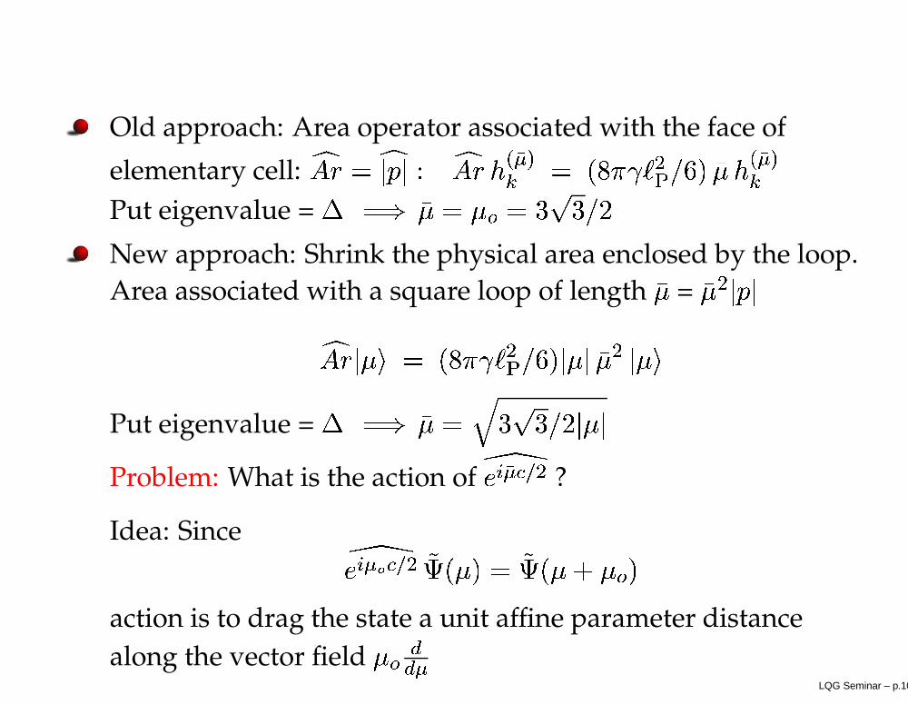
Old approach: Area operator associated with the face ofelementary cell:

�� 9 �� & �(' �� 9 ��

Put eigenvalue =

% � � � � � � � � � � � �New approach: Shrink the physical area enclosed by the loop.Area associated with a square loop of length� � =� � � � �

�� 7 � �� & �(' �� 7

Put eigenvalue =

% � � � � � � � � ��

Problem: What is the action of

� �� 9 � �

?

Idea: Since � �9 � � � ��

action is to drag the state a unit affine parameter distancealong the vector field � � �� 9

LQG Seminar – p.10

Set

� �� 9 � � ��

as Lie drag of the state by a unit affine parameterdistance along the vector field� � �� 9 .Affine parameter of this vector field:

� � � �# � � � � � � � � � � � � � ��

� are proportional to the eigenvalues of the Volume operator. � ��

is invertible,

� �

function of � .

� � � �7 �

� � ��

�& �' � �7

Orthonormal basis in+ ,. / : 5 � � � � �7 � 8�� ; ��

Consider

� � � � �� : � �� 9 � � � � � � � � � � �


Quantum Constraint

Quantization of the constraint leads to difference equation:

� ��

� � � � � � � � � ��

where

� � � � �

� ��

� �� & '

� � � � � � � ��

� � � � � �

�

� � � ��

� �

� �� is self-adjoint and negative definite.

Evolution in steps which are constant in eigenvalues of thevolume operator. Earlier constraint based on � � had stepswhich are constant (

�� ) in eigenvalues of the triad operator.

Evolution non-singular across � � �

for all states.

� �� with natural factor ordering for

� � � � � .


What is the physics of singularity resolution ?What are the physical predictions in LQC ?

Algorithm to extract Physics in LQC

Seek a dynamical variable that can play the role of internaltime (physical interpretations more transparent).

Introduce Inner Product, find Physical Hilbert Space.

Construct Dirac Observables, raise them to operators.

Construct physical semi-classical states representing a largeclassical Universe.Evolve these states backward towards Big Bang usingquantum constraint. Analyze the behavior of expectationvalues and fluctuations of Dirac observables.Compare with classical dynamics, extract predictions.


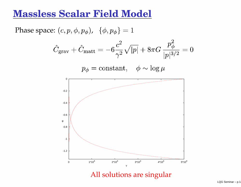
Massless Scalar Field ModelPhase space:

� � � �

,

� � � � � �

� ��

� � � ��

� � � � # �# � � ��

-1.2

-1

-0.8

-0.6

-0.4

-0.2

0

0 1*104 2*104 3*104 4*104 5*104

v

φ

All solutions are singularLQG Seminar – p.14

�

is a monotonic function – can play the role of internal time.Evolution refers to relational dynamics – the way geometrychanges with ‘time’ (or as

�

evolves).

Dirac Observables: � ,

� � � � �

For

� �� , use Thiemann’s trick and get:

�# ��

� �7 �

�� & �'

� � �� 7

� � � � � � � ��

� � � � � � � � � � � � � � � � � � ��

� � � � � � � � �

For

� � � � � , eigenvalue � �# � � � � .� � � � � � � � � � ��


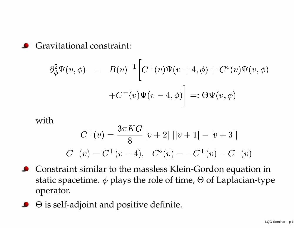
Gravitational constraint:

� ��

� � � � � � � � � � � � � � � � � � � �

� � � � � � � � � � ��

with

� � � � ��

� � � � ��

� � � � � �

� � � � � � � � � � � � � � � � � � � � � � � �

Constraint similar to the massless Klein-Gordon equation instatic spacetime.

�plays the role of time,

�

of Laplacian-typeoperator.

�

is self-adjoint and positive definite.


For

� � � � � ,

� � � � B

� �� .Wheeler-DeWitt limit for the constraint:

� ��

� ��

� � � � �

In geometrodynamics classical constraint:

� ��

In quantum theory natural choice of factor ordering �

Laplacian for

� ��

.LQC Hamiltonian constraint automatically yields the naturalfactor ordering for Wheeler-DeWitt.

Action of parity operator:��

� � � �

� � � large gauge transformation on the space of solutions. Noobservable which can detect the change in orientation of thetriad. Physical considerations require symmetric states.


Inner Product:Demand that action of operators corresponding to Diracobservables is self-adjointGroup averaging

Result:

� � � �

are positive frequency: � * ��

5 � � � � �7 ��

� � ��

Dirac observables act as:

� � � � � * � ��

Physical Hilbert space divided into sectors:

+�� + ,

' � ��

.States have support on � � � � � �� . Predictions insensitive tothe choice of sectors.


Numerics

Evolution in

�

:

Initial value problem in

�

. Solve

� ��

� � � � � � countablenumber of coupled ODE’s.

Initial data at

�� consists of

� � � � � and

�� . Initialdata specified in three different ways using classical equations.

For semi-classical states choose a large value of � � �� . Fix a

point

� � � � � on the classical trajectory for � � � � (largeclassical Universe). Using quantum constraint follow itsevolution backward.Example of initial state:

� � � � � �

� �

3� � 6 � � ��


Quantum Bounce

0

0.2

0.4

0.6

0.8

1

1.2

1.4

1.6

-1.2

-1

-0.8

-0.6

-0.4

-0.2

5*103

1.0*104

1.5*104

2.0*104

2.5*104

3.0*104

3.5*104

4.0*104

0

0.5

1

1.5

|Ψ(v,φ)|

v

φ

|Ψ(v,φ)|


Results of Loop Quantum Evolution

States remain sharply peaked through out evolution.

Expectation values of

� � � � and � are in good agreement withclassical trajectories until energy density becomes of the orderof a critical density (of the order Planck).

The state bounces at critical density from expanding branch tothe contracting branch with same value of

5 � � 7 . Thisphenomena is generic. Big bang replaced by a big bounce atPlanck scale.Norm and expectation value of

� � remain constant.

Fluctuations of observables remain small. Some differencesarise near the bounce point depending on the methodspecification.


Comparison of Evolution

-1.2

-1

-0.8

-0.6

-0.4

-0.2

0

0 1*104 2*104 3*104 4*104 5*104

v

φ

quantumclassical


Effective Theory

An effective Hamiltonian description can be obtained by usingthe geometric methods.

Results in the effective Friedmann equation:

� � � ��

�� . � �� . � �

�

� � � � � � � � �

Features:

Similar to the Friedmann equation in Randall-Sundrumbraneworlds, except for the (-) sign.

Small difference in Friedmann equation � Profoundimplications for Physics.

For � � � � � . � , classical Friedmann dynamics recovered.


Answers to some long pending questionsDoes the theory provides non-singular evolution through thebig bang ? Yes, for all solutions.

What is on the other side of the big bang ? Quantum foam or aclassical spacetime ? Universe escapes big bang and bounces atPlanck scale to a pre-big bang classical contracting branch.

What is the scale at which the spacetime ceases to be classical ?Does the spacetime continuum exists at all scales ? When theenergy density becomes of the order of a critical density ( �

0.82 � ' � � / � , ), deviations from classical dynamics are significantand spacetime ceases to be classical. Picture of a continuumspacetime breaks down in the deep Planck regime.

What about the modifications to Friedmann equation ? � �

modifications at high energy scales with a negative sign.


Summary and Open Issues

Loop quantum cosmology provides a new picture of theUniverse near and at the big bang and beyond. Big bang notthe beginning, big crunch not the end. Two classical regions ofspacetime joined by a quantum geometric bridge.

Quantum gravitational effects play important role at Planckscales to yield non-singular evolution for generic initial data.No need to introduce exotic matter or ad-hoc assumptions.

Long standing problem of singularity resolution inhomogeneous and isotropic spacetimes resolved. Newavenues to test non-perturbative techniques opened.

Important lessons learned in quantization of simple modelsabout ambiguities. Example: In � � evolution, critical densitynot constant

� � � � �, bounce could occur at small curvatures !

Physical ramifications can narrow down the ambiguities �

lead to the choice of � evolution.LQG Seminar – p.25

Results obtained in flat homogeneous and isotropic model,devoid of perturbations.

Does the picture of bounce survive with addition ofperturbations ?

Relax symmetries: Work in progress. Early indications frommore general situations suggest singularity resolution but adetailed picture yet to be worked out.

What happens in case of closed models, anisotropies andpotentials ?For closed model a similar picture appears. Effective theorygives useful insights on picture of bounce in presence ofpotentials and anisotropies.

Connection with full theory ?

Testable predictions ? Confirmation with observations ??


Documents

Big Bang and Loop Quantum Cosmologyrelativity.phys.lsu.edu/ilqgs/singh060606.pdf · Some age-old questions Does the theory provides a non-singular evolution through the big bang ?