Bid-Ask Spreads, Volume, and Volatility:

Evidence from Livestock Markets

Julieta Frank Assistant Professor

Agribusiness and Agricultural Economics University of Manitoba

376 Agriculture Building, Winnipeg, Manitoba R3T 2N2 julieta_frank@umanitoba.ca

Philip Garcia Professor, T. A. Hieronymus Distinguished Chair in Futures Markets

Agricultural and Consumer Economics, University of Illinois 341 Mumford Hall, Urbana, IL 61801

p-garcia@illinois.edu Selected Paper prepared for presentation at the Agricultural & Applied Economics Association 2009

AAEA & ACCI Joint Annual Meeting, Milwaukee, Wisconsin, July 26‐29, 2009 Copyright 2009 by Julieta Frank and Philip Garcia. All rights reserved. Readers may make verbatim copies of this document for non‐commercial purposes by any means, provided that this copyright notice appears on all such copies.

2

Abstract

Understanding the determinants of liquidity costs in agricultural futures markets is

hampered by a need to use proxies for the bid-ask spread which are often biased, and by a

failure to account for a jointly determined micro-market structure. We estimate liquidity

costs and its determinants for the live cattle and hog futures markets using alternative

liquidity cost estimators, intraday prices and micro-market information. Volume and

volatility are simultaneously determined and significantly related to the bid-ask spread.

Daily volume is negatively related to the spread while volatility and volume per

transaction display positive relationships. Electronic trading has a significant competitive

effect on liquidity costs, particularly in the live cattle market. Results are sensitive to the

bid-ask spread measure, with a modified Bayesian method providing estimates most

consistent with expectations and the competitive structure found in these markets.

Key words: Bayesian estimation, bid-ask spread determinants, liquidity cost

3

Bid-Ask Spreads, Volume, and Volatility: Evidence from Livestock Markets

In agricultural futures markets, traders face a variety of transaction costs including

brokerage fees, exchange fees, and liquidity costs which influence the effectiveness of

marketing decisions. The first two costs are available, but estimation of liquidity costs is

challenging, and is often performed using a measure of the bid-ask spread (BAS).

Regardless the measure, there is evidence that the liquidity costs change over time and

with market conditions. Identifying the factors that influence liquidity costs is of

substantial value for participants and decision makers operating in the market. For

instance, the cost of placing an order on a lightly traded day may be higher than the same

order a few days later if trading activity increases. Hence, understanding the determinants

of liquidity costs can help identify cost-reducing opportunities in marketing decisions.

Our understanding of the factors that influence liquidity costs in agricultural

futures markets is limited for several reasons. In most agricultural markets, liquidity costs

are not directly observed and proxies must be used. Also, previous research in

agricultural markets generally has been performed for short periods of time, mainly due

to data availability and computational complications associated with high frequency

intraday data (e.g. Thompson and Waller 1988, Brorsen 1989). These short-term

investigations make it difficult to identify the presence of contract and time-to-maturity

effects. Further, in light of the increase in electronic trading in agricultural markets,

relationships may have changed and its effect on pit-trading liquidity costs is not clear.

For instance, Bryant and Haigh (2004) provide evidence in cocoa and coffee markets that

4

bid-ask spreads widened with electronic trading, a result that contrasts with Pirrong's

(1996) findings for financial futures. Cocoa and coffee markets are thinly traded, and it is

not clear whether more actively traded agricultural markets follow a similar pattern. In

addition, both studies examined the effect of electronic trading on a combined bid-ask

spread, and did not identify the effect of electronic trading on pit trading. While

electronic trading has increased markedly, in many agricultural markets pit trading is still

a viable alternative, and the effect of electronic trading on the cost of liquidity is of

interest to decision makers. Finally, previous work has not accounted for the potential

simultaneity between the factors influencing liquidity costs and bid-ask spread measures.

Reported determinants of liquidity costs may not totally reflect causal relationships, but

rather be a result of a common dependence on latent information flows which influence

volume, price variability, and BAS measures. Modeling agricultural futures markets in a

simultaneous framework may permit a better understanding of their structure and

dynamics (Wang and Yau 2000).

The paper estimates liquidity costs and its determinants in lean hogs and live

cattle markets using several bid-ask spread measures, taking into account the

simultaneous relationship between market information and BAS. To our knowledge, no

research on the determinants of BAS in these livestock markets exists. We use the volume

by tick database from the CME group which provides prices and volume of all trades

executed during the day in the open outcry. We estimate liquidity costs for the period

2005-2008 using different estimators including recently developed Bayesian methods.

The period of analysis covers almost all contracts traded in 2005 to 2008. We use a

5

generalized-method-of-moments instrumental variable (GMM IV) estimator which

permits consistent and efficient estimation in the presence of simultaneity,

autocorrelation, and heteroscedasticity. In the analysis we examine the effects of days to

maturity, day of the week, volume per transaction, and the relative proportion of

electronic trading as well as volume and volatility variables identified in the literature.

Our findings suggest that volume and volatility are endogenous variables and

significantly related to the bid-ask spread. Consistent with expectations, volume and

volatility are simultaneously determined and significantly related to the bid-ask spread.

Daily volume is negatively related to the spread while volatility and volume per

transaction generally display positive relationships. In live cattle we also find electronic

trading and day of the week effects to have a significant effect. Results are sensitive to

the measure of the bid-ask spread, with Bayesian methods providing estimates of

liquidity costs and its determinants consistent with a competitive structure found in these

markets. These findings should be of interest to decision makers seeking to implement

cost-reducing marketing strategies and to manage their liquidity risk.

Background

Few studies have investigated the relationship between the bid-ask spreads and its

determinants in agricultural futures markets. Most of this research has analyzed the effect

of trading volume, volatility, and time to contract maturity of grains on a measure of

BAS, often using the Roll (RM) or Thompson-Waller (TW) measures. Recent studies

6

have incorporated structural changes in trading mechanisms such as the opening of

electronic markets.

An impediment to studying the relationship between BAS and its determinants is

the measurement of the BAS. A lack of bid-ask quotes in U.S. exchanges makes it

difficult to estimate these relationships directly. Even when estimators exist, their

differences may distort the BAS-determinant relationship (Bryant and Haigh 2004). For

instance, analyzing liquidity costs for corn and oats contracts traded in the Chicago Board

of Trade (CBOT), Thompson and Waller (1988) find a positive relationship between

trading volume and BAS when Roll’s measure is used, but a negative relationship when

the TW estimator is used.

Nevertheless, several studies provide insights into the determinants of liquidity

costs in agricultural markets. Thompson and Waller (1988) find that price volatility

explained bid-ask spread movements. Using the first difference of the variance of prices,

price volatility consistently has a positive effect on the BAS, indicating that an increase

in market uncertainty translates into higher cost of holding risky positions for scalpers.

Brorsen (1989) identified factors affecting liquidity costs in corn for six contract

months between 1983 and 1984. Liquidity costs are measured as the standard deviation of

log price changes and scalpers’ returns using naïve trading rules. Maturity (number of

months prior to expiration), volume and seasonality are the factors examined. Volume

and seasonality are significant in explaining liquidity costs; however volume is

negatively related to the standard deviation whereas it is positively related to scalpers’

returns.

7

Further evidence of the negative relationship between volume and liquidity costs

is provided by Thompson, Eales, and Seibold (1993) who compare liquidity costs of

wheat futures contracts from two exchanges with different trading activity, Chicago and

Kansas City. Liquidity costs estimated using RM and TW measures in Kansas City (the

exchange with the lowest volume) were found to be higher than in Chicago. In addition,

liquidity costs at both exchanges also increased during the expiration month. Other

corroborative evidence on the importance of volume was identified by Thompson and

Waller (1987) who examined the level of trading activity in coffee and cocoa contracts on

the New York Board of Trade (NYBOT) and found lower execution costs in actively

traded nearby contracts relative to thinly traded more distant contracts. It is important to

note that none of the above studies use volume per transaction to explain BAS.

Thompson and Waller (1988), and Brorsen (1989) recognize that the volume per

transaction should be included as a determinant of the BAS, however these data were not

available.

In a more recent study, Bryant and Haigh (2004) find a negative and significant

relationship between volume and BAS and a positive relationship between volatility and

BAS for LIFFE coffee. In cocoa these same relationships appear only after moving to

electronic trading. Bryant and Haigh (2004) also find the spread widened after the

introduction of electronic trading which they attribute to an adverse selection problem.

An important difference in this study for agricultural markets is that Bryant and Haigh

use actual bids and asks for which these relationships are expected to be reliable.

8

Findings financial futures markets are more extensive. Here, we discuss several

salient studies that focus on issues related to our research. Ding and Chong (1997) study

the determinants of the BAS of the Nikkei stock index futures trading in the Singapore

Monetary Exchange (SIMEX) using tick bid and ask quotes. The BAS is found to be

positively correlated with volatility and negatively correlated with trading activity.

Volatility is measured as the standard deviation of transaction prices and the positive

relationship is explained by the risk that market makers face. Trading activity is measured

by the number of transactions and its negative relationship is explained by the existence

of scale economies which result in a lower BAS as trading activity increases. Daily

percentage BAS is found to be at a minimum and flat from 13 days to 3 days prior to

maturity which coincides with active trading in the nearby contract, but increases slightly

in the last two days. In another study, Ding (1999), investigating the foreign exchange

(FXF) futures market, also finds a negative relationship for number of transactions and a

positive relationship for volatility. The findings show that there are differences in BASs

by delivery months, suggesting the presence of a seasonal effect in BASs, and reveal that

it may be less costly to transact in specific contracts.

Wang and Yau (2000) find that trading volume, BAS, and price volatility are

jointly determined in two financial (S&P500 and deutsche mark) and two metal (silver

and gold) futures contracts, and that failure to account for simultaneity leads to

downward biased parameter estimates. Using a GMM estimation procedure, their results

indicate trading volume and BAS are negatively related, and price volatility and BAS are

positively related. While their findings are intuitive, the strength of the results may be

9

compromised because their procedures do not account for the autocorrelation and

heteroscedasticity often found in these markets.

Pirrong (1996) argues that the cost of liquidity in the open outcry and the

electronic systems are different. Scalpers in the open outcry are less vulnerable to adverse

selection because they observe information on the floor and they know which brokers are

bidding and offering so they can anticipate incoming orders. In contrast to liquidity

suppliers in the computerized system, scalpers in the pit do not have real time access to

fundamental information. Using RM and TW measures and computerized DTB and

LIFFE Bund contracts, he finds that the computerized system is more liquid than the

open outcry, a finding that contrasts with Bryant and Haigh’s (2004) results in cocoa and

coffee markets where the spread has widened after the trading was automated.

Bid-Ask Spread Measures

To develop an improved understanding of the relationship between liquidity costs and

their determinants, we use four bid-ask spread estimators, Roll’s (RM) serial covariance

(Roll 1984), Thompson-Waller’s (TW) mean absolute price change (Thompson and

Waller 1987), Hasbrouck’s (HAS) Bayesian (Hasbrouck 2004), and a modified Bayesian

estimator (ABS) using absolute price changes. Previous research has identified rather

large differences in bid-ask costs using various measures (e.g. Bryant and Haigh 2004),

but none has examined systematic differences using Bayesian methods and their effect in

identifying the determinants of liquidity.

10

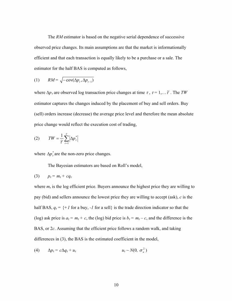
The RM estimator is based on the negative serial dependence of successive

observed price changes. Its main assumptions are that the market is informationally

efficient and that each transaction is equally likely to be a purchase or a sale. The

estimator for the half BAS is computed as follows,

(1) RM = 1cov( , )p pτ τ −− Δ Δ

where Δpτ are observed log transaction price changes at time τ , τ = 1,…τ~ . The TW

estimator captures the changes induced by the placement of buy and sell orders. Buy

(sell) orders increase (decrease) the average price level and therefore the mean absolute

price change would reflect the execution cost of trading,

(2) ∑=

Δ=τ

τττ

~

1

*~1 pTW

where *τpΔ are the non-zero price changes.

The Bayesian estimators are based on Roll’s model,

(3) pτ = mτ + cqτ

where mτ is the log efficient price. Buyers announce the highest price they are willing to

pay (bid) and sellers announce the lowest price they are willing to accept (ask), c is the

half BAS, qτ = +1 for a buy, -1 for a sell is the trade direction indicator so that the

(log) ask price is aτ = mτ + c, the (log) bid price is bτ = mτ – c, and the difference is the

BAS, or 2c. Assuming that the efficient price follows a random walk, and taking

differences in (3), the BAS is the estimated coefficient in the model,

(4) Δpτ = cΔqτ + uτ uτ ~ N(0, 2uσ )

11

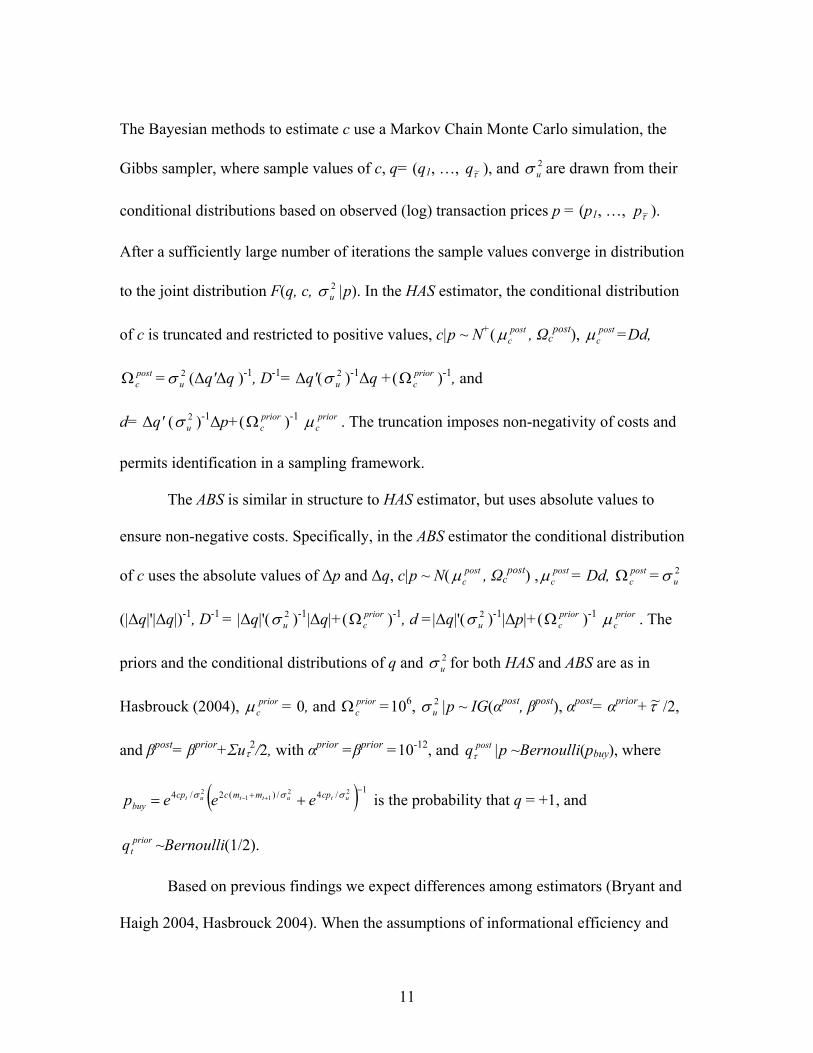
The Bayesian methods to estimate c use a Markov Chain Monte Carlo simulation, the

Gibbs sampler, where sample values of c, q= (q1, …, τ~q ), and 2uσ are drawn from their

conditional distributions based on observed (log) transaction prices p = (p1, …, τ~p ).

After a sufficiently large number of iterations the sample values converge in distribution

to the joint distribution F(q, c, 2uσ |p). In the HAS estimator, the conditional distribution

of c is truncated and restricted to positive values, c|p ~ N+( postcμ , Ωc

post), postcμ =Dd,

postcΩ = 2

uσ (Δq'Δq )-1, D-1= Δq'( 2uσ )-1Δq +( prior

cΩ )-1, and

d= Δq' ( 2uσ )-1Δp+( prior

cΩ )-1 priorcμ . The truncation imposes non-negativity of costs and

permits identification in a sampling framework.

The ABS is similar in structure to HAS estimator, but uses absolute values to

ensure non-negative costs. Specifically, in the ABS estimator the conditional distribution

of c uses the absolute values of Δp and Δq, c|p ~ N( postcμ , Ωc

post) , postcμ = Dd, post

cΩ = 2uσ

(|Δq|'|Δq|)-1, D-1 = |Δq|'( 2uσ )-1|Δq|+( prior

cΩ )-1, d =|Δq|'( 2uσ )-1|Δp|+( prior

cΩ )-1 priorcμ . The

priors and the conditional distributions of q and 2uσ for both HAS and ABS are as in

Hasbrouck (2004), priorcμ = 0, and prior

cΩ =106, 2uσ |p ~ IG(αpost, βpost), αpost= αprior+τ~ /2,

and βpost= βprior+Σuτ2/2, with αprior =βprior =10-12, and postqτ |p ~Bernoulli(pbuy), where

( ) 1/4/)(2/4 2211

2 −+ += +− ututtut cpmmccpbuy eeep σσσ is the probability that q = +1, and

priortq ~Bernoulli(1/2).

Based on previous findings we expect differences among estimators (Bryant and

Haigh 2004, Hasbrouck 2004). When the assumptions of informational efficiency and

12

equal probability of buy and sell incoming orders do not hold the RM estimator will be

biased. Hasbrouck (2004) demonstrates that RM is upward biased for several futures

markets including pork bellies. Also, when the covariance between successive price

changes is positive the RM estimator cannot be computed. The TW measure has been

criticized because it does not distinguish true price change from bid-ask spread, and

therefore may provide an upward estimate of the BAS (Smith and Whaley 1994). The

Bayesian estimators do not have these limitations since they do not assume efficient

incorporation of information, and the probability of buy and sells are computed

conditional on the transaction prices. In addition, since the Bayesian methods are

estimated using a Markov Chain Monte Carlo simulation, they permit a more precise

identification of liquidity costs. Findings suggest that the HAS estimator tends to generate

unexpectedly small measures of liquidity cost. Hasbrouck argues that the procedure more

accurately reflects market dynamics because it does not impose efficiency in equation

(4), which is assumed in the RM, but rather estimates the autocorrelation and incorporates

it into the liquidity cost measure. However, it is uncertain whether the autocorrelation

incorporated into the liquidity is due to market dynamics or a function of the truncation

imposed. It is clear that truncation influences the mean and variance of a distribution and

the degree to which observations are autocorrelated, and in a sampling framework the

direction of the effects and their magnitude are not evident. Here, we circumvent these

issues by using absolute values in the ABS measure that also ensures non-negativity and

may allow the observations to reflect more accurately the distribution of liquidity costs.

13

Determinants of the Bid-Ask Spread

Scalpers supply liquidity to the market by providing quotes and standing ready to buy

contracts at a bid price and to sell them at an ask price. Holding an outstanding long or

short position for a period of time means the scalper is subject to risk. If bad news enters

the market after a large buy, the scalper may have to sell the contracts at a much lower

price than the purchase price. For bearing this risk a scalper earns the spread, the

difference between bid and ask prices.

With low trading activity, the time between trades is longer, and the risk that the

scalper faces is higher (Brorsen 1989). Similarly, high trading activity is associated with

lower risk, lower liquidity costs and lower spreads. Consequently, volume is negatively

related to the bid-ask spread. In contrast, large individual orders may have an opposite

effect on spreads. For instance, a scalper buying a large order may have trouble

liquidating the position quickly, thus increasing risk. Volume per transaction is therefore

a dimension of volume that we expect to positively influence bid-ask spreads. This notion

of market depth identifies price movements due to an increase in the order flow (Kyle

1985). The cost of transacting of larger orders will be higher as they increase the risk

incurred by the scalper.

The volatility of prices represents another dimension of risk. Volatility reflects

new information in the market. With new information, prices are more variable and the

risk associated with scalper’s inventories increases, resulting wider spread. Information

entering the market may also induce changes in the volume of contracts transacted which

in turn influence the scalpers’ exposure to risk. Hence, volatility is jointly determined

14

with volume and spreads, and information shocks cause a reaction in all three variables

jointly.

The effect of electronic trading on liquidity costs and the bid-ask spread is

uncertain. Electronic trading can be a source of competition to pit trading, reducing the

pit spread to a more competitive level. However in the presence of adverse selection

identified by Bryant and Haigh (2004), a competitive effect of electronic trading on pit

spreads is less likely to exist.

Finally, research shown that liquidity costs can change as a function of contract

months, days of the week, and time to maturity. Contract months may have a significant

effect in the presence of seasonality not captured in daily volume, and days of the week

may reflect the characteristics of cash markets and their interaction with volume traded.

A time-to-maturity effect may exist if daily volume does not adequately identify the

changing nature of market activity.

Based on our discussion, we model liquidity costs using (5),

(5) BASiht = β0 + β1 EXPht + β2 SDht +β3 VOLht +β4 VOL/TRANht +β5 ETt + β6 D1ht

+β7 D2ht + β8 MONt + β9 TUEt + β10 WEDt + β11 THUt + uiht

where BASiht is the half bid-ask spread for day t, for contract h, using BAS estimator i =

RM, TW, HAS, ABS, EXPht is the number of days to expiration for contract h, SDht is the

log standard deviation of transaction prices for contract h, VOLht is the log of volume of

contract h, VOL/TRANht is the log volume per transaction for contract h, ETt is the

proportion of electronic trading volume (e-volume/(pit-volume + e-volume)), D1ht and

D2ht are dummies for contract months, MON – THU are dummy variables that take the

15

value of 1 for the particular day of the week and 0 otherwise, β are parameter estimates,

and uiht is a random error.

We first estimate (5) using OLS and perform diagnostic tests, including error

misspecification (autocorrelation and heteroscedasticity) and endogeneity tests for the

variables that may be jointly determined with the BAS. For autocorrelation we use the

Breusch-Godfrey test and the autocorrelation and partial autocorrelation functions of the

error term. For heteroscedasticity we use the Breusch-Pagan test. Endogeneity tests are

performed on total volume, average volume per transaction, and volatility to assess their

common dependence on latent information flows.

The endogeneity test is based on an instrumental variables (IV) approach. The

standard test Durbin-Wu-Hausman compares the resulting coefficient vectors β = (β0…

βk) of both the OLS and IV models. The test statistic is the difference between the two

coefficient vectors scaled by a precision matrix D = Var[βIV] – Var[βOLS] and is

distributed as χ2 with degrees of freedom equal to the number of regressors being tested

for endogeneity (Hausman 1978). However, identifying endogeneity becomes more

complicated in the presence of heteroscedastic and autocorrelated errors which are

commonly found in time series data. Below we present the specification of the IV model,

error specification tests, and the modification of the endogeneity test accounting for

misspecified errors.

For the specification of the IV model we need at least one instrument for each

endogenous variable satisfying two conditions: i) the instrument is highly correlated with

the endogenous variable, and ii) the instrument is uncorrelated with uit. For instruments,

16

we select lag values of the endogenous variables except for volatility where we use the

first difference of the log standard deviation of prices as suggested by Thompson, Eales,

and Seibold (1993) and our own preliminary results. We examine the first condition with

a simple OLS regression where the dependent variable is the endogenous variable and the

independent variable is its instrument, and check the significance of the parameter

estimate. We also perform tests for relevance of instruments by computing the F-test of

the joint significance of the excluded instruments in the first-stage regression. In order to

avoid misleading conclusions about the F-statistic when one instrument is highly

correlated with more than one instrumented variable, we compute Shea’s (1997) partial

R2 that takes into account intercorrelations among instruments. For instance, if the system

has two endogenous variables and two instruments, and one instrument is highly

correlated with both endogenous variables, then the joint F-statistic will be highly

significant but the Shea partial R2 will be low, indicating that the model may be

unidentified, biasing the IV model coefficients.

The IV model is estimated using the two stage least square (2SLS) estimator. In

matrix form, (5) can be written as,

(6) y = X β + u

where β is the vector of coefficients (β0… βk)' and X is T x k. Defining a matrix Z of the

same dimension as X in which the endogenous regressors (VOLt, VOL/TRANSt and SDt)

are replaced by the instruments (VOLt-1, VOL/TRANSt-1, and ΔSD), the IV estimator and

its variance under iid disturbances are,

(7) SLSβ2ˆ = (X'PZX)-1X'PZy

17

(8) Var[ SLSβ2ˆ ] = 2σ (X'PZX)-1

where PZ is the projection matrix Z(Z'Z)-1Z', and 2σ = T/ˆ'ˆ uu . If the disturbances in (6)

are not iid, then the 2SLS estimates will be consistent but inefficient, and the model

variance should be estimated using a robust method. Here we use a generalized-method-

of-moments (GMM) estimator that will give consistent and efficient estimates in the

presence of non-iid errors (Hayashi 2000).

When we define the covariance matrix of u in (6) as E[uu'|X] = Ω where Ω is a

TxT matrix with heteroscedastic and/or autocorrelated errors, the (feasible) efficient

GMM estimator is,1

(9) FEGMMβ = (X'ZS -1Z'X)-1X'ZS -1Z'y

where S-1 is the optimal weighting matrix that produces the most efficient estimate, and

S is the estimator of S = E[Z'ΩZ] which will take different forms depending on the

specification of u in (6). When the disturbance in (6) is iid, and Ω = σ2IT, then (9) reduces

to (7), and the 2SLS estimator is the efficient GMM estimator (Hayashi 2000). When the

disturbance in (6) cannot be assumed to be homoscedastic, a heteroscedastic-consistent

estimator of S is given by the standard “sandwich” Huber-White robust covariance

estimator (Huber 1967, White 1980),

(10) ∑=

==T

ttttu

TT 1

'2ˆ1)ˆ'(1ˆ ZZZΩZS

where Ω is the diagonal matrix of squared residuals 2ˆtu from the first-stage estimation.

18

When the disturbance in (6) exhibits both heteroscedasticity and autocorrelation,

S can be estimated using the Newey-West (1987) heteroscedasticity and autocorrelation

consistent covariance matrix as implemented by Baum, Schaffer, and Stillman (2007),

(11) ( )∑=

++=q

jjj

1

'0

ˆˆ ˆˆ ΓΓΓS κ

where ∑=

=T

ttttu

T 1

'20 ˆ1ˆ ZZΓ , ∑

−

=−−=

jt

tjtjtttj ZuuZ

T 1

' ˆˆ1Γ is the sample autocovariance matrix

for lag j, jtt uu −ˆ and ˆ are consistent residuals from the first-stage estimation, and κ = (1 -

j/qT) if j ≤ qT - 1 and 0 otherwise is the Bartlett kernel function with bandwidth qT which

weights each term of the summation with decreasing weights as j increases. We select the

bandwidth using Newey and West’s (1994) procedure.

In the IV model we perform error specification tests for heteroscedasticity and

autocorrelation using extensions of OLS tests. For heteroscedasticity we use the Pagan

and Hall (1983) test which relaxes the assumption of homoscedasticity in the system

equations that are not explicitly estimated (i.e., regressions of endogenous variables with

the instruments) and which is required by most of other standard tests for OLS

regression. In the test we use p variables, the instruments, their squares, and cross-

products to compute the test statistic that under the null of homoscedasticity is distributed

as 2pχ . In the presence of heteroscedasticity we estimate the IV model using (9) and (10).

For autocorrelation we use the Cumby-Huizinga (1992) test which is a generalization of

the Breusch and Godfrey test used above for OLS regressions because this and other

standard tests for OLS such as Box-Pierce and Durbin’s h test are invalid in the presence

19

of endogenous regressors. In the presence of heteroscedasticity and autocorrelation we

estimate the GMM IV model using (9) and (11).

When the GMM IV model is estimated in the presence of heteroscedasticity

and/or autocorrelation, the Durbin-Wu-Hausman test for endogeneity needs to be

modified. We use the C statistic or GMM distance test implemented by Baum, Schaffer

and Stillman (2007). The test uses the GMM objective function J )ˆ(β = T )'ˆ(βg

1ˆ −S )ˆ(βg where )ˆ(βg = 1/T Z'u are the orthogonality conditions and S is the weighting

matrix defined in (10) and (11). The test statistic is defined as (J - JA) and is distributed as

χ2 with degrees of freedom equal to the number of regressors being tested, where J is the

value of the GMM objective function for the efficient GMM that uses the full set of

orthogonality conditions, and JA is the value of the efficient GMM that uses only the

number of orthogonality conditions for the variables known to be exogenous.

Data

The analysis is performed for lean hogs and live cattle futures contracts trading in the

CME group. The open-outcry prices and volume of all trades executed during the day are

taken from the volume by tick database. For both commodities we use February, April,

June, August, October, and December contracts trading between January 2005 and

October 2008. We compute liquidity costs on a daily basis to more carefully identify

factors influencing its behavior.

We use a period of 80 trading days prior to maturity to study expiration effects, as

suggested by Cunningham (1979), and Brorsen (1989). To account for expiration, EXP

20

has a value of zero on the expiration day, a value of 1 the day before, a value of 2 two

days before, and so forth to the 80th day. As we switch to another contract, the first day

takes a value of 80, and the variable declines to expiration. Depending on holidays and

weekends in different months, some contracts may have as many as 85 days prior to

maturity.

To construct a daily dataset with approximately 80 trading days for each contract

and no overlapping observations we use three contracts per year. We built two datasets of

three contracts each which include most of the contracts trading for each commodity. For

both commodities, a first dataset uses prices from the April, August, and December

contracts (AAD), and the second uses prices from the February, June, and October

contracts (FJO).

Our determinants are measured on a daily basis. Volatility is computed as the

standard deviation of transaction prices for a specific contract each day. Volume is the

total number of contracts for a specific contract, and volume per transaction is the total

volume divided by the number of transactions on that day. Daily data on the proportion of

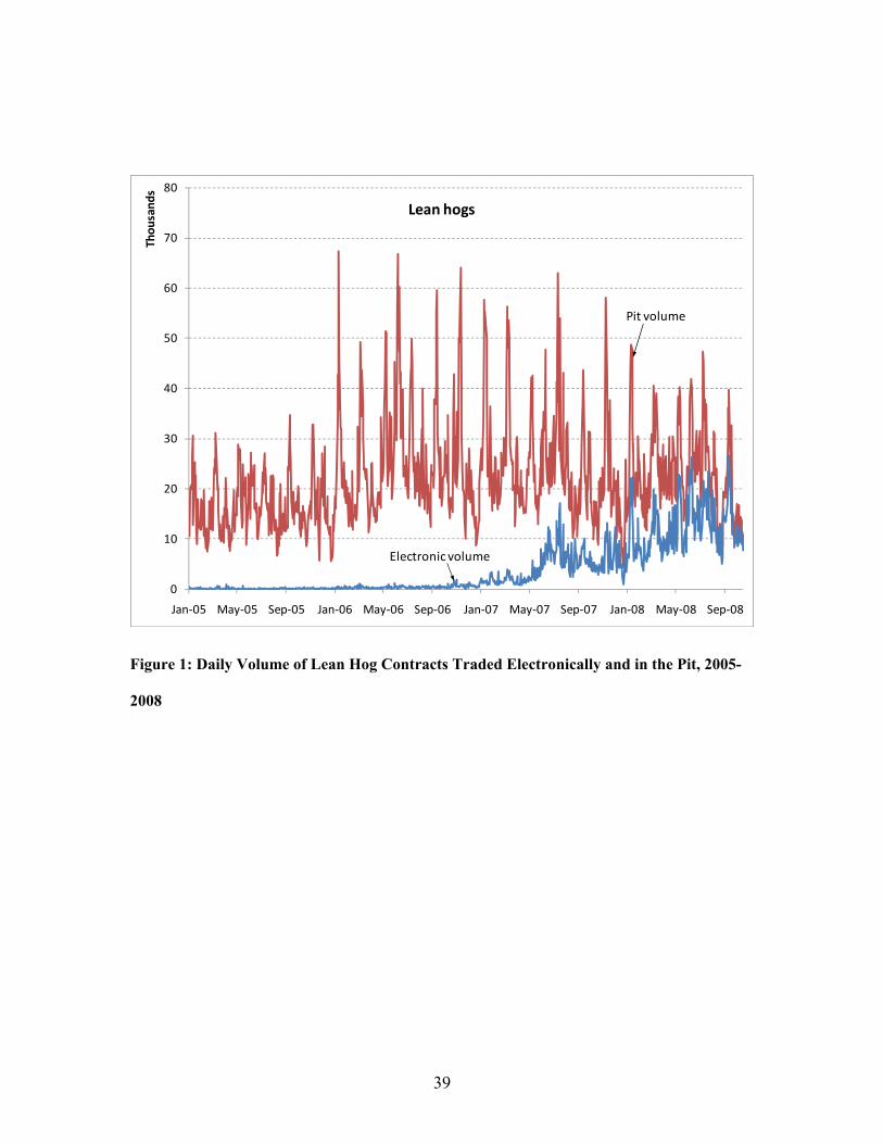
electronic trading (ET) comes from the CME group. In hogs and cattle markets the open

outcry regular trading hours are 9:05am to 1:00pm. The CME GLOBEX electronic

platform operates side-by-side with extended hours, opening at 9:05 am on Mondays and

closing at 1:30 pm on Fridays.2 The relative volume of electronic trading (ET) is

computed as a proportion of the volume of transactions traded electronically (for all

contracts) over the total volume (for all contracts) in both the pit and electronic markets.

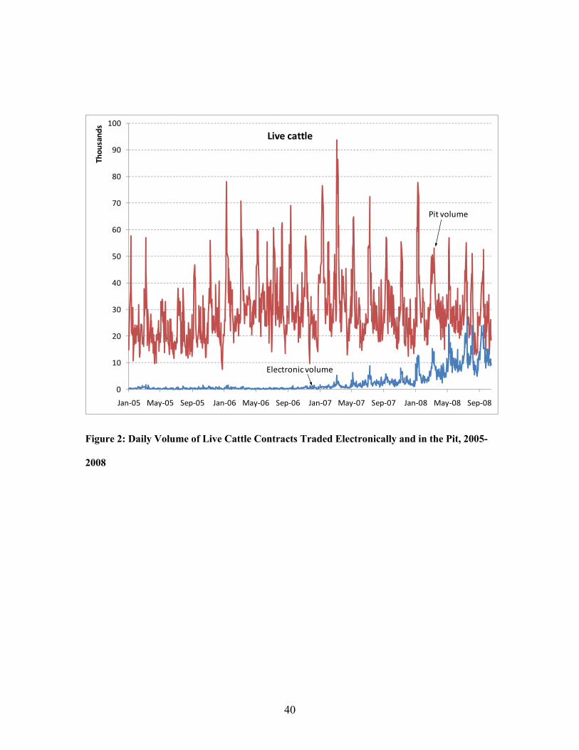
Figures 1 and 2 show the total daily volume for hogs and cattle, respectively, traded in

21

the pit and in the electronic platform. As can be seen, electronic trading in these markets

was negligible during the early part of the period, but has increased recently.3

Results

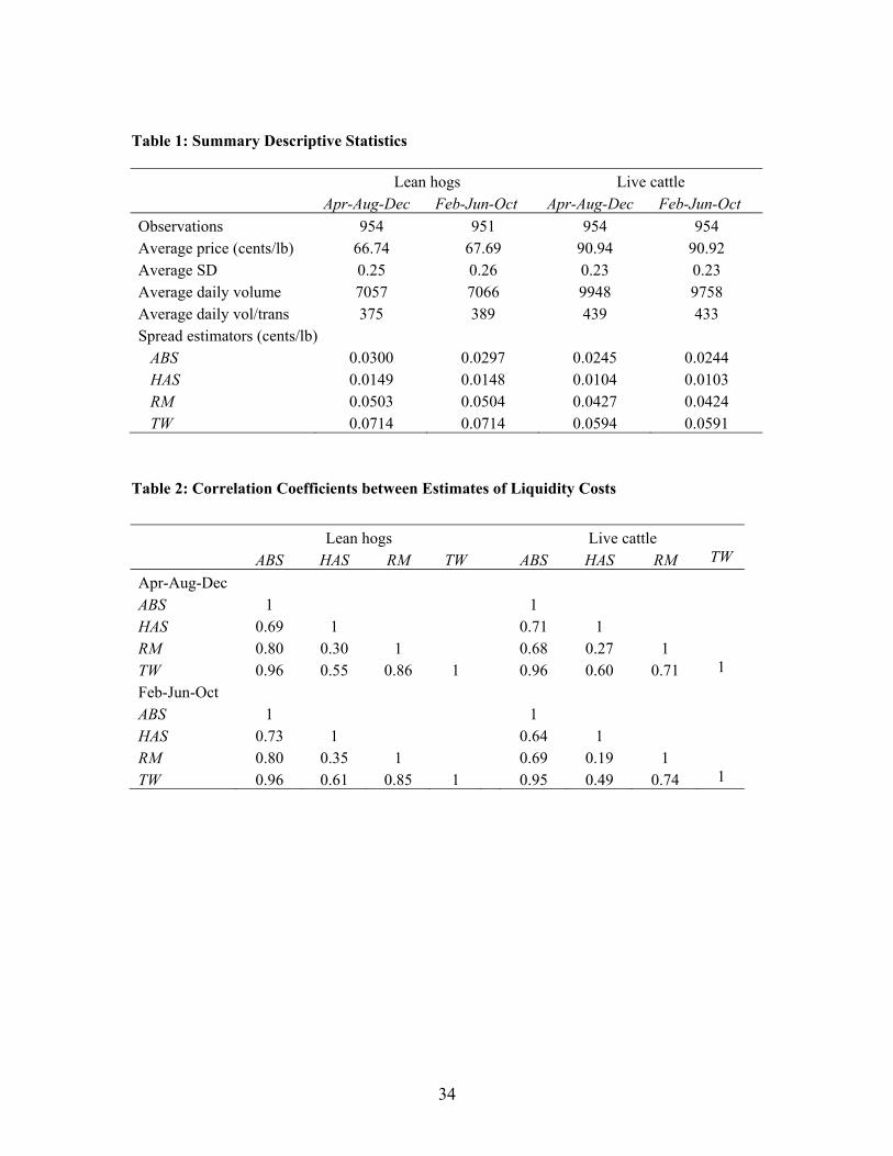
Table 1 shows the average values of the spread estimators identified, Roll serial

covariance (RM), Thompson-Waller (TW), Hasbrouck’s Bayesian (HAS), and modified

Bayesian (ABS) for each commodity and set of expiration months. TW yields the highest

estimates, followed by RM and ABS, and then by HAS. In the presence of negative

correlation and noise, the efficiency assumption in RM’s measure does not hold and the

RM measure overestimates the liquidity cost (Hasbrouck 2004).4 The TW, based on all

price changes, also seems to be upwardly biased, a finding consistent with Bryant and

Haigh (2004) and others. The ABS estimates are the closest to the tick level—the

minimum price changed allowed by the exchange—of 0.025 cents/lb. The HAS’

estimates are always the smallest, and consistently below tick changes. Table 2 presents

the correlation between the different measures. ABS and TW appear to be the most

correlated while HAS seems to be the least correlated with other measures. These results

are consistent across contract months and commodities. Across commodities, liquidity

costs are always lower in cattle with consistent higher volume traded. No differences in

liquidity costs and the other summary statistics appear to exist.

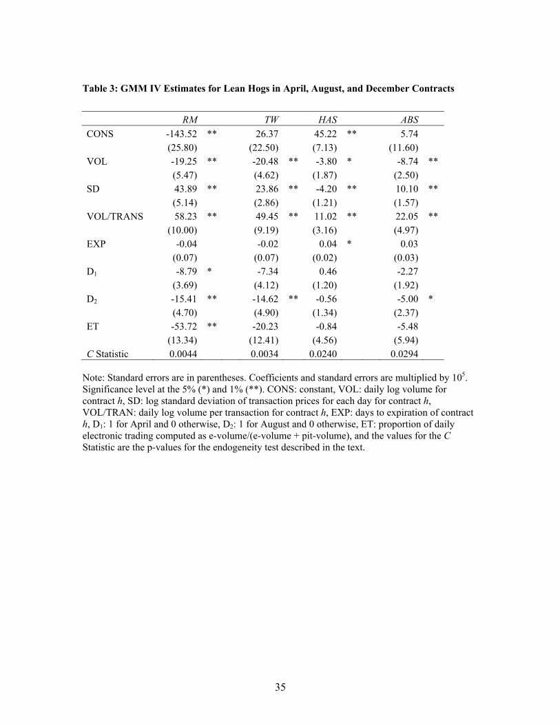
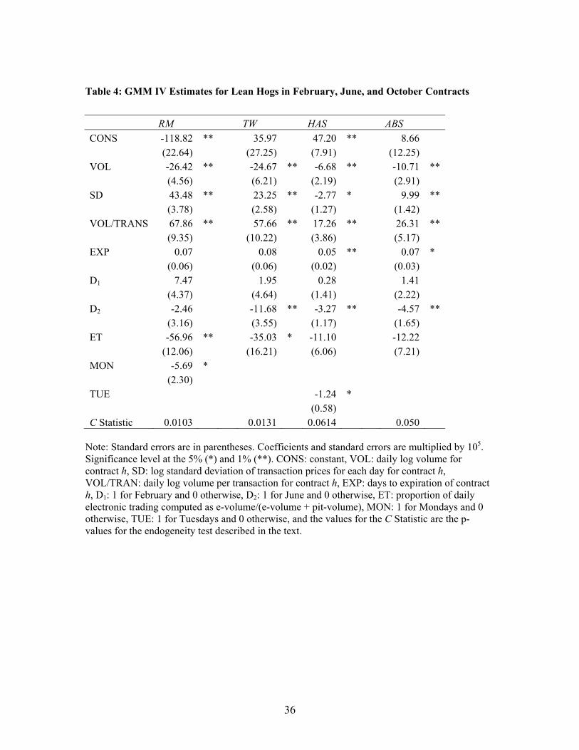
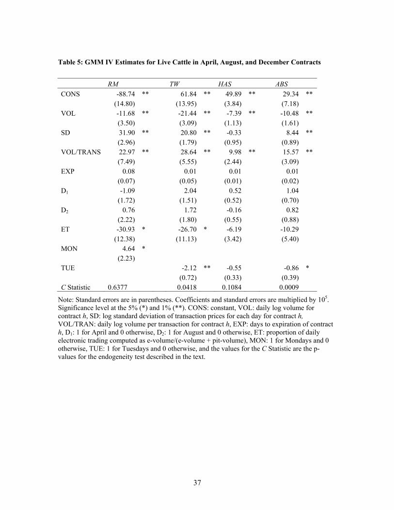
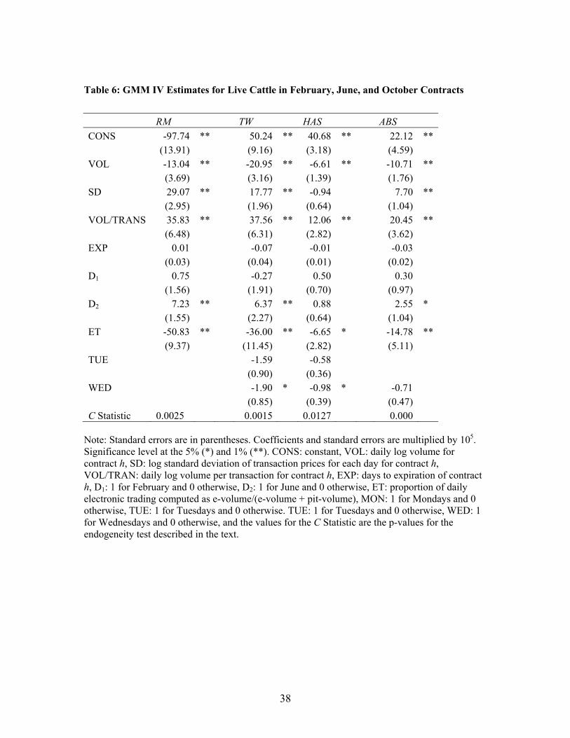
Tables 3 and 4 present the estimation results for lean hogs, and tables 5 and 6 for

live cattle. Each table contains the results of the estimation for the four measures of bid-

ask spread, RM, TW, HAS, and ABS. All four measures were computed in log differences

22

and thus represent percentage price changes. In almost all cases the endogeneity test for

total volume, volume per transaction, and volatility was significant, indicating these

variables should be treated as endogenous. Only for the AAD live cattle when we use the

RM and HAS measures do we fail to reject the null hypothesis of no endogeneity. In light

of the evidence of endogeneity we perform IV estimation for all cases. Error specification

tests also indicate the presence of heteroscedasticity and autocorrelation in all cases

analyzed. Therefore, the estimation for all models in tables 3 through 6 was performed

using the GMM IV model with heteroscedastic and autocorrelated standard errors.

Results for lean hogs demonstrate that volume, volatility, and volume per

transaction consistently stand out as determinants of the BAS. As expected and consistent

with Thompson and Waller (1987), Thompson, Eales, and Seibold (1993), and Bryant

and Haigh (2004), the volume has negative sign in all cases, showing that higher volumes

imply less risk of holding contracts for scalpers which results in lower liquidity costs.

When volume decreases buyers (sellers) have difficulty filling their orders and scalpers

provide the necessary liquidity at a higher cost c. While the direction of the volume effect

is consistent for all measures, the magnitude of the effect varies considerably across

measures. The coefficients for volume range from -26.42 for RM (table 4) to -3.80 for

HAS (table 3), which means that when volume increases by 1%, the cost of liquidity

decreases by 0.02642% and 0.0038% respectively.5 For an average price of 65 cents/lb,

this translates into a decrease of $6.90 and $1.00 per contract.

For all bid-ask spread measures, the log volume per transaction (VOL/TRANS)

has a positive sign, with the magnitudes following a similar pattern as the results for

23

volume. The highest coefficient is for RM and the lowest for HAS. The coefficient which

can be viewed as a measure of market depth supports the notion that a larger volume per

transaction means that traders must pay a price for immediacy. For the ABS estimate, an

average price of 65 cents/lb and an average volume of 380 contracts per transaction (table

1), an increase of 10 contracts (approximately a 2.6% increase) would lead to an increase

of $5.88 per contract, or roughly half a tick.

The volatility of transactions prices has the expected positive sign when we use

RM, TW, and ABS. The findings are in line with Thompson and Waller (1988) and Bryant

and Haigh (2004). However, with HAS a negative and significant coefficient emerges

which is hard to explain. The higher the volatility in prices, the more uncertainty scalpers

face and the higher increase the cost of their service, raising c.6

Days to maturity has a positive and significant sign only when HAS and ABS are

used, however the coefficients are small. A positive sign implies that the further from

expiration the higher the liquidity cost. Here, using the ABS measure and for the FJO

months increases 0.00007% the liquidity cost each day further away from expiration day.

Using the RM and TW measures the estimated coefficients are negative for AAD months

and positive for FJO months, but they are never significant at the 5% level.

In table 3, liquidity costs for the June contract are lower than for other contracts

and this is consistent across spread measures. In most cases the coefficient is significant,

although the magnitude of the effect varies between -11.68 for TW to -3.27 for HAS. In

our analysis we use trading periods of about four months for each contract and so the

June contract effect refers to trading from March to June. This finding suggests longer-

24

term patterns may exist in liquidity costs perhaps associated with seasonality in volume

which are not captured by the daily volume variables.

Day-of-the-week and electronic trading displayed little effect on liquidity costs.

There is no effect in AAD months (table 3) and only two measures, RM and HAS,

identified a Monday and a Tuesday negative effect on FJO months in table 4.7 The effect

of electronic trading on the pit liquidity cost also is weak. While not significant in most

cases, the sign is negative. The recent increase in electronic activity (figure 1) may have

increased competitive pressure on trading in the pit. This contrasts with Bryant and

Haigh’s (2004) findings in the coffee and cocoa markets in which adverse selection

problems lead to larger spreads with the introduction of electronic trading. However, they

seem to be consistent with Pirrong’s (1996) findings in the more liquid Bund market,

indicating that electronic trading resulted in lower liquidity costs. Here again, the

coefficients of electronic trading display high variability between the different spread

measures, ranging from -53.72 for RM to -0.84 for HAS.

Live cattle liquidity costs follow a similar structure to those described for hogs.

Volume is negatively related to liquidity costs, and volatility and volume per transaction

increase liquidity costs. Here again the signs of the volatility when using HAS are also

negative but not significant. Days to maturity has mixed signs but is not significant in

either liquidity cost measure and sets of contract months. Here longer-term volume

patterns also emerge in the June contract. The day-of-the week effect is stronger in cattle,

where the results suggest that liquidity costs are lower during the early part of the week.

Notice that cash cattle markets primarily are “early in the week” markets which means

25

more trading activity in futures during this period as market participants offset and

establish new positions. The effect of electronic trading is also stronger in cattle than in

hogs as all its coefficients are significant. The negative direction of the effect is similar to

hogs.

Along with volatility, volume in its two dimensions appears to be the main

determinants of liquidity costs. For both hogs and cattle, all three variables are

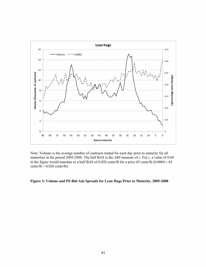
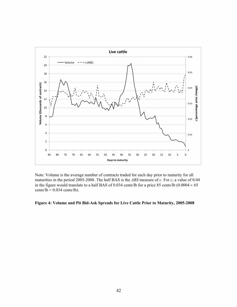
consistently significant across measures and set of contract months. To investigate the

relationship between volume and liquidity costs in more depth consider figures 3 and 4

which provide the behavior of volume as a contract approaches maturity and the ABS

measure.8 The figures are constructed averaging the volume across contracts for the same

number of days to maturity. For hogs there are two peaks occurring approximately 25 and

65 days before expiration. For cattle we also observe two peaks, the main one

approximately 35 days before expiration and the second one around 75 trading days prior

to maturity. The observed peaks in volume are consistent with the large influx of index

fund trading activity—long positions that were rolled on well-defined days—during this

period (Sanders, Irwin, and Merrin 2008).9 Consistent with the estimated relationships,

the figures identify a clear pattern of higher liquidity costs during periods of low volume,

particularly as expiration approaches. They also are indicative of slightly higher liquidity

costs during peak market activity, reflecting market depth and the higher volume per

transaction prevalent during these periods.

26

Concluding Remarks

Estimation of the determinants of liquidity costs in agricultural futures markets is not

straightforward. Measurement problems, changes in market conditions, and statistical

problems complicate our understanding of the determinants of liquidity costs. We

estimate a model for lean hogs and live cattle using commonly used spread estimators,

Hasbrouck’s Bayesian estimator, and the modified Bayesian estimator using absolute

values. We perform the estimation for almost all contracts trading during 2005 and 2008,

and estimate coefficients for total volume per day, volume per transaction, price risk, the

proportion of electronic trading, days to maturity, day-of-the-week effects, and other

explanatory factors.

Our results show that the price, volume, and volatility are jointly determined and

the estimation of a GMM IV model for heteroscedastic and autocorrelated errors is

needed. Liquidity costs are lower in cattle with consistent higher volume traded. Volume

and volatility appear to be the most important determinants of the BAS. For both

commodities the direction of the effects of total volume and volatility are consistent with

findings by Thompson and Waller (1987), Thompson, Eales, and Seibold (1993), and

Bryant and Haigh (2004). The cost of liquidity depends on scalpers’ risk of holding

positions. Higher traded volume implies lower time between trades and therefore lower

risk for the scalper. In contrast, higher price volatility is associated with a higher risk of

holding a position. Volume per transaction which is viewed as a measure of market depth

has the expected positive sign and is a significant factor explaining liquidity cost

movements in both hogs and cattle. Visual inspection of volume and liquidity costs

27

generated by the ABS estimator reveals a clear pattern of higher liquidity costs during

periods of low volume, particularly as expiration approaches. Slightly higher liquidity

costs emerge during observed peaks in volume, reflecting higher volume per transaction

prevalent during these periods and the price of immediacy in a competitive environment.

Identification of these patterns may help decision makers target low-cost trading days.

Other factors explaining liquidity costs movements are days-of-the week effects,

the introduction of electronic trading, and seasonality. Day-of-the-week effects are

stronger in cattle, implying lower liquidity costs for transactions performed during the

first days of the week. The negative coefficient for the proportion of electronic trading

suggests the presence of competitive pressure from electronic to pit markets that

decreases liquidity costs in the pit. Here the effect is also stronger for live cattle. The

results are more in line with Pirrong (1996) for Bund contracts and contrast with Bryant

and Haigh’s (2004) findings for coffee and cocoa thin markets. For both commodities

seasonality in the June contract also emerges.

Finally, while the determinants of liquidity costs generally seem to emerge

regardless of the procedure used, large differences in their magnitudes and, to a lesser

extent, differences in their signs exist. When we use the traditional RM and the TW

measures which have shown to provide biased estimates of the spread, estimated liquidity

costs and the effects of its determinants are always larger. Bayesian measures which do

not impose efficient incorporation of information and allow for more flexibility and

efficient estimation, identify appreciably smaller liquidity costs and determinant effects.

Consistent with previous findings, the HAS estimator generates the smallest liquidity

28

costs—on average below the minimum tick size set by the exchange—and the smallest

estimated coefficients. Within the context of the market relationships, the HAS estimator

provides counterintuitive estimates of the expected positive relationship between price

volatility and liquidity costs. In contrast, the ABS estimator generates average liquidity

costs more compatible with minimum tick size, provides estimated coefficients that

correspond to market relationships, and identifies the relationship between the aspects of

volume and liquidity costs that would be expected in competitive markets faced with

large peaks in market activity. Further research on liquidity costs using Bayesian

procedures seems warranted to identify more explicitly the source of the differences

between HAS and ABS estimators, under what conditions they can provide meaningful

measures of cost, and their usefulness in different markets which are experiencing a

movement to electronic trading.

29

Endnotes

1 The term “feasible” arises because the matrix S is not known and must be estimated.

The estimation of S involves making some assumptions about Ω (iid, heteroscedastic, or

heteroscedastic-autocorrelated disturbances) and is a two-step procedure. In the first step,

we estimate SLS2β , obtain the residuals and construct Ω . Then we estimate FEGMMβ using

Ω to compute S . The efficient GMM estimator is EGMMβ = (X'ZS-1Z'X)-1X'ZS-1Z'y, and

the feasible efficient two-step GMM is the EGMM using S (Baum, Schaffer, and

Stillman 2007).

2 CME GLOBEX trading is closed from 4:00 to 5:00 pm Monday through Thursday for

regularly scheduled maintenance. All times refer to Central Time.

3 Spikes observed in the total volume figures coincide with roll-overs and options

expirations.

4 In four cases a RM measure could not be computed due to positive covariance between

price changes.

5 In general, the determinant effects are larger with the traditional TM and RM than for

the Bayesian measures, in part reflecting their higher liquidity cost estimates.

6 To assess the effect of endogeneity, the basic model was estimated using OLS and the

ABS measure of liquidity costs. As expected, OLS coefficient estimates are smaller and

consistent with Wang and Yau ‘s (2000) findings for the S&P500, deutsche mark, silver,

and gold futures contracts.

30

7 In preliminary estimations we included a full set days of the week. In the final

estimation we only include only days with significant coefficients. We also included

dummy variables for USDA announcement effects (Hogs and Pigs Reports and Cattle on

Feed) in early estimations, but find no significant effects.

8 Volatility patterns are less well defined.

9Index fund activity has increased markedly, reaching over 20 percent of open interest in

live cattle and hogs for 2006-2008. The roll period is identified as the “Goldman roll”

and refers to the days index funds shift positions from nearby to more distant contracts. In

both commodities the main peak coincides with the “Goldman roll” which occurs on the

5th through 9th business day of the month proceeding the expiration month. Note lean

hogs expire on the 10th business day of the contract month, and live cattle expires on the

last day of the contract month. For details see (www2.goldmansachs.com).

31

References

Baum, C., M. Schaffer, and S. Stillman. 2007. “Enhanced Routines for Instrumental

Variables/GMM Estimation and Testing.” Boston College Working Paper No. 667.

Bryant, H. and M. Haigh. 2004. “Bid-ask Spreads in Commodity Futures Markets.”

Applied Financial Economics 14:923-936.

Cumby, R. and J. Huizinga. 1992. “Testing the Autocorrelation Structure of Disturbances

in Ordinary Least Squares and Instrumental Variables Regressions.” Econometrica

60(1):185-195.

Ding, D. 1999. “The Determinants of the Bid-Ask Spreads in the Foreign Exchange

Futures Market: A Microstrure Analysis.” Journal of Futures Markets 19(3):307-

324.

Ding, D. and B. Chong. 1997. “Simex Nikkei Futures Spreads and their Determinants.”

Advances in Pacific Basin Financial Markets 3:39-53.

Hasbrouck, J. 2004. “Liquidity in the Futures Pits: Inferring Market Dynamics from

Incomplete Data.” Journal of Financial and Quantitative Analysis 39(2):305-326.

Hausman, J. 1978. “Specification Tests in Econometrics.” Econometrica 46:1251-1271.

Hayashi, F. 2000. “Econometrics.” 1st ed. Princeton, NJ: Princeton University Press.

Huber, P. 1967. “The Behavior of Maximum Likelihood Estimates under Non-standard

Conditions.” In Proceedings of the Fifth Berkeley Symposioum in Mathematical

Statistics and Probability 1:221-233. Berkely, CA: University of California Press.

Kyle, A.S. 1985. “Continuous Auctions and Insider Trading.” Econometrica 53:1315-

1365.

32

Newey, W.K. and K.D. West, 1994. “Automatic Lag Selection in Covariance Matrix

Estimation.” Review of Economic Studies, 61(4):631-653.

Pagan, A. and D. Hall. 1983. “Diagnostic Tests as Residual Analysis.” Econometric

Reviews 2(2):159-218.

Pirrong, C. 1996. “Market Liquidity and Depth on Computerized and Open Outcry

Trading Systems: A Comparison of the DTB and LIFFE Bund Contracts.” Journal

of Futures Markets 16(5):519-543.

Roll, R. 1984. “A Simple Implicit Measure of the Effective Bid-Ask Spread in an

Efficient Market.” Journal of Finance 23:1127-1139.

Sanders, D., S.H. Irwin, and R. Merrin. 2008. “The Adequacy of Speculation in

Agricultural Futures Markets: Too Much of a Good Thing?” Proceedings of the

NCCC-134 Conference on Applied Commodity Price Analysis, Forecasting, and

Market Risk Management. St. Louis, MO. (http://www.farmdoc.uiuc.edu/nccc134)

Shea, J. 1997. “Instrument Relevance in Multivariate Linear Models: A Simple

Measure.” Review of Economics & Statistics 79(2):349-352.

Smith, T., and R. Whaley. 1994. “Estimating the Effective Bid-Ask Spread from Time

and Sales Data.” Journal of Futures Markets 14:437-456.

Thompson, S., and M. Waller. 1987. “The Execution Cost of Trading in Commodity

Futures Markets.” Food Research Institute Studies 20(2):141-163.

Thompson, S., J. Eales, and D. Seibold. 1993. “Comparison of Liquidity Costs Between

the Kansas City and Chicago Wheat Futures Contracts.” Journal of Agricultural

and Resource Economics 18(2):185-197.

33

Thompson, S., and M. Waller. 1988. “Determinants of Liquidity Costs in Commodity

Futures Markets.” Review of Futures Markets 7:110-126.

Wang, G.H.K., and J. Yau. 2000. “Trading Volume, Bid-Ask Spread, and Price Volatility

in Futures Markets.” Journal of Futures Markets. 20(10):943-970.

White, H. 1980. “A Heteroskedasticity-consistent Covariance Matrix Estimator and a

Direct Test for Heteroskedasticity.” Econometrica 48:817-838.

34

Table 1: Summary Descriptive Statistics

Lean hogs Live cattle Apr-Aug-Dec Feb-Jun-Oct Apr-Aug-Dec Feb-Jun-Oct

Observations 954 951 954 954 Average price (cents/lb) 66.74 67.69 90.94 90.92 Average SD 0.25 0.26 0.23 0.23 Average daily volume 7057 7066 9948 9758 Average daily vol/trans 375 389 439 433 Spread estimators (cents/lb) ABS 0.0300 0.0297 0.0245 0.0244 HAS 0.0149 0.0148 0.0104 0.0103 RM 0.0503 0.0504 0.0427 0.0424 TW 0.0714 0.0714 0.0594 0.0591

Table 2: Correlation Coefficients between Estimates of Liquidity Costs

Lean hogs Live cattle ABS HAS RM TW ABS HAS RM TW

Apr-Aug-Dec ABS 1 1 HAS 0.69 1 0.71 1 RM 0.80 0.30 1 0.68 0.27 1 TW 0.96 0.55 0.86 1 0.96 0.60 0.71 1 Feb-Jun-Oct ABS 1 1 HAS 0.73 1 0.64 1 RM 0.80 0.35 1 0.69 0.19 1 TW 0.96 0.61 0.85 1 0.95 0.49 0.74 1

35

Table 3: GMM IV Estimates for Lean Hogs in April, August, and December Contracts

RM TW HAS ABS CONS -143.52 ** 26.37 45.22 ** 5.74

(25.80) (22.50) (7.13) (11.60) VOL -19.25 ** -20.48 ** -3.80 * -8.74 **

(5.47) (4.62) (1.87) (2.50) SD 43.89 ** 23.86 ** -4.20 ** 10.10 **

(5.14) (2.86) (1.21) (1.57) VOL/TRANS 58.23 ** 49.45 ** 11.02 ** 22.05 **

(10.00) (9.19) (3.16) (4.97) EXP -0.04 -0.02 0.04 * 0.03

(0.07) (0.07) (0.02) (0.03) D1 -8.79 * -7.34 0.46 -2.27

(3.69) (4.12) (1.20) (1.92) D2 -15.41 ** -14.62 ** -0.56 -5.00 *

(4.70) (4.90) (1.34) (2.37) ET -53.72 ** -20.23 -0.84 -5.48

(13.34) (12.41) (4.56) (5.94) C Statistic 0.0044 0.0034 0.0240 0.0294

Note: Standard errors are in parentheses. Coefficients and standard errors are multiplied by 105. Significance level at the 5% (*) and 1% (**). CONS: constant, VOL: daily log volume for contract h, SD: log standard deviation of transaction prices for each day for contract h, VOL/TRAN: daily log volume per transaction for contract h, EXP: days to expiration of contract h, D1: 1 for April and 0 otherwise, D2: 1 for August and 0 otherwise, ET: proportion of daily electronic trading computed as e-volume/(e-volume + pit-volume), and the values for the C Statistic are the p-values for the endogeneity test described in the text.

36

Table 4: GMM IV Estimates for Lean Hogs in February, June, and October Contracts

RM TW HAS ABS CONS -118.82 ** 35.97 47.20 ** 8.66

(22.64) (27.25) (7.91) (12.25) VOL -26.42 ** -24.67 ** -6.68 ** -10.71 **

(4.56) (6.21) (2.19) (2.91) SD 43.48 ** 23.25 ** -2.77 * 9.99 **

(3.78) (2.58) (1.27) (1.42) VOL/TRANS 67.86 ** 57.66 ** 17.26 ** 26.31 **

(9.35) (10.22) (3.86) (5.17) EXP 0.07 0.08 0.05 ** 0.07 *

(0.06) (0.06) (0.02) (0.03) D1 7.47 1.95 0.28 1.41

(4.37) (4.64) (1.41) (2.22) D2 -2.46 -11.68 ** -3.27 ** -4.57 **

(3.16) (3.55) (1.17) (1.65) ET -56.96 ** -35.03 * -11.10 -12.22

(12.06) (16.21) (6.06) (7.21) MON -5.69 *

(2.30) TUE -1.24 *

(0.58)C Statistic 0.0103 0.0131 0.0614 0.050

Note: Standard errors are in parentheses. Coefficients and standard errors are multiplied by 105. Significance level at the 5% (*) and 1% (**). CONS: constant, VOL: daily log volume for contract h, SD: log standard deviation of transaction prices for each day for contract h, VOL/TRAN: daily log volume per transaction for contract h, EXP: days to expiration of contract h, D1: 1 for February and 0 otherwise, D2: 1 for June and 0 otherwise, ET: proportion of daily electronic trading computed as e-volume/(e-volume + pit-volume), MON: 1 for Mondays and 0 otherwise, TUE: 1 for Tuesdays and 0 otherwise, and the values for the C Statistic are the p-values for the endogeneity test described in the text.

37

Table 5: GMM IV Estimates for Live Cattle in April, August, and December Contracts

RM TW HAS ABS CONS -88.74 ** 61.84 ** 49.89 ** 29.34 **

(14.80) (13.95) (3.84) (7.18) VOL -11.68 ** -21.44 ** -7.39 ** -10.48 **

(3.50) (3.09) (1.13) (1.61) SD 31.90 ** 20.80 ** -0.33 8.44 **

(2.96) (1.79) (0.95) (0.89) VOL/TRANS 22.97 ** 28.64 ** 9.98 ** 15.57 **

(7.49) (5.55) (2.44) (3.09) EXP 0.08 0.01 0.01 0.01

(0.07) (0.05) (0.01) (0.02) D1 -1.09 2.04 0.52 1.04

(1.72) (1.51) (0.52) (0.70) D2 0.76 1.72 -0.16 0.82

(2.22) (1.80) (0.55) (0.88) ET -30.93 * -26.70 * -6.19 -10.29

(12.38) (11.13) (3.42) (5.40) MON 4.64 *

(2.23) TUE -2.12 ** -0.55 -0.86 *

(0.72) (0.33) (0.39) C Statistic 0.6377 0.0418 0.1084 0.0009

Note: Standard errors are in parentheses. Coefficients and standard errors are multiplied by 105. Significance level at the 5% (*) and 1% (**). CONS: constant, VOL: daily log volume for contract h, SD: log standard deviation of transaction prices for each day for contract h, VOL/TRAN: daily log volume per transaction for contract h, EXP: days to expiration of contract h, D1: 1 for April and 0 otherwise, D2: 1 for August and 0 otherwise, ET: proportion of daily electronic trading computed as e-volume/(e-volume + pit-volume), MON: 1 for Mondays and 0 otherwise, TUE: 1 for Tuesdays and 0 otherwise, and the values for the C Statistic are the p-values for the endogeneity test described in the text.

38

Table 6: GMM IV Estimates for Live Cattle in February, June, and October Contracts

RM TW HAS ABS CONS -97.74 ** 50.24 ** 40.68 ** 22.12 **

(13.91) (9.16) (3.18) (4.59) VOL -13.04 ** -20.95 ** -6.61 ** -10.71 **

(3.69) (3.16) (1.39) (1.76) SD 29.07 ** 17.77 ** -0.94 7.70 **

(2.95) (1.96) (0.64) (1.04) VOL/TRANS 35.83 ** 37.56 ** 12.06 ** 20.45 **

(6.48) (6.31) (2.82) (3.62) EXP 0.01 -0.07 -0.01 -0.03

(0.03) (0.04) (0.01) (0.02) D1 0.75 -0.27 0.50 0.30

(1.56) (1.91) (0.70) (0.97) D2 7.23 ** 6.37 ** 0.88 2.55 *

(1.55) (2.27) (0.64) (1.04) ET -50.83 ** -36.00 ** -6.65 * -14.78 **

(9.37) (11.45) (2.82) (5.11) TUE -1.59 -0.58

(0.90) (0.36)WED -1.90 * -0.98 * -0.71

(0.85) (0.39) (0.47) C Statistic 0.0025 0.0015 0.0127 0.000

Note: Standard errors are in parentheses. Coefficients and standard errors are multiplied by 105. Significance level at the 5% (*) and 1% (**). CONS: constant, VOL: daily log volume for contract h, SD: log standard deviation of transaction prices for each day for contract h, VOL/TRAN: daily log volume per transaction for contract h, EXP: days to expiration of contract h, D1: 1 for February and 0 otherwise, D2: 1 for June and 0 otherwise, ET: proportion of daily electronic trading computed as e-volume/(e-volume + pit-volume), MON: 1 for Mondays and 0 otherwise, TUE: 1 for Tuesdays and 0 otherwise. TUE: 1 for Tuesdays and 0 otherwise, WED: 1 for Wednesdays and 0 otherwise, and the values for the C Statistic are the p-values for the endogeneity test described in the text.

39

0

10

20

30

40

50

60

70

80

Jan‐05 May‐05 Sep‐05 Jan‐06 May‐06 Sep‐06 Jan‐07 May‐07 Sep‐07 Jan‐08 May‐08 Sep‐08

Thou

sand

s

Lean hogs

Electronic volume

Pit volume

Figure 1: Daily Volume of Lean Hog Contracts Traded Electronically and in the Pit, 2005-

2008

40

0

10

20

30

40

50

60

70

80

90

100

Jan‐05 May‐05 Sep‐05 Jan‐06 May‐06 Sep‐06 Jan‐07 May‐07 Sep‐07 Jan‐08 May‐08 Sep‐08

Thou

sand

s

Live cattle

Pit volume

Electronic volume

Figure 2: Daily Volume of Live Cattle Contracts Traded Electronically and in the Pit, 2005-

2008

41

0

0.01

0.02

0.03

0.04

0.05

0.06

0.07

0

2

4

6

8

10

12

14

16

0510152025303540455055606570758085

c (percentage price change)

Volume (tho

usands of contracts)

Days to maturity

Lean hogs

Volume c (ABS)

Note: Volume is the average number of contracts traded for each day prior to maturity for all maturities in the period 2005-2008. The half BAS is the ABS measure of c. For c, a value of 0.04 in the figure would translate to a half BAS of 0.026 cents/lb for a price 65 cents/lb (0.0004 × 65 cents/lb = 0.026 cents/lb).

Figure 3: Volume and Pit Bid-Ask Spreads for Lean Hogs Prior to Maturity, 2005-2008

42

0

0.01

0.02

0.03

0.04

0.05

0.06

0

2

4

6

8

10

12

14

16

18

20

22

0510152025303540455055606570758085

c(percentage price change)

Volume (tho

usands of contracts)

Days to maturity

Live cattle

Volume c (ABS)

Note: Volume is the average number of contracts traded for each day prior to maturity for all maturities in the period 2005-2008. The half BAS is the ABS measure of c. For c, a value of 0.04 in the figure would translate to a half BAS of 0.034 cents/lb for a price 85 cents/lb (0.0004 × 65 cents/lb = 0.034 cents/lb).

Figure 4: Volume and Pit Bid-Ask Spreads for Live Cattle Prior to Maturity, 2005-2008