ERASMUS UNIVERSITY ROTTERDAM

ERASMUS SCHOOL OF ECONOMICS

Master Thesis

Econometrics & Management Science – Quantitative Finance

Beyond the visibleSearching for two latent clusters in the corporate bond market

Author

Maksim Anisimov (527144)

Supervisors

Maria Grith, PhD (Erasmus School of Economics)

Patrick Houweling, PhD (Robeco)

Frederik Muskens (Robeco)

Second assessor

Dick van Dijk, PhD (Erasmus School of Economics)

Date: October 1, 2020

The content of this thesis is the sole responsibility of the author and does not reflect the view of the

supervisors, second assessor, Erasmus School of Economics, Erasmus University Rotterdam or Robeco.

– Page intentionally left blank –

Abstract

When investors talk about two asset groups in the corporate debt market, they of-

ten refer to high- (investment-grade) and low-rated (high-yield) bonds. Researchers

use this split to test risk factors, while practitioners employ it to manage funds. For

technical reasons, bond separation in terms of exposure to risk factors is usually ig-

nored, and our study fills this gap. We argue that Instrumented Principal Component

Analysis (IPCA) proposed by Kelly et al. (2019) resolves issues with the estimation

of factor loadings and develop a new methodology to use it for clustering. Under

the assumption that bonds are generated by two cluster-specific models, we show

that bond market segmentation according to exposures to a common latent factor is

superior to the split into investment-grade and high-yield groups in terms of out-of-

sample predictions. Bonds from the statistical cluster related to a high-yield group

exhibit higher maturity and tend to be undervalued as opposed to “real” high-yield

bonds. Since the exposure to the latent factor is associated with a market beta, we

reestablish the importance of market exposure in the context of corporate bonds.

JEL Classification: C23, C38, G12

Keywords: asset pricing; clustering; financial econometrics; fixed income

CONTENTS

Contents

1 Introduction 1

2 Literature review 2

3 Data 6

4 Methodology 10

4.1 Preliminaries . . . . . . . . . . . . . . . . . . . . . . . . . . . . . . . . . . . . . . 10

4.2 IPCA . . . . . . . . . . . . . . . . . . . . . . . . . . . . . . . . . . . . . . . . . . . 11

4.3 New intuition behind IPCA . . . . . . . . . . . . . . . . . . . . . . . . . . . . . . . 13

4.3.1 Γβ representation via OLS slope estimates . . . . . . . . . . . . . . . . . . 13

4.3.2 When characteristic-managed portfolios are related to prominent anomalies 16

4.4 Holy grail model . . . . . . . . . . . . . . . . . . . . . . . . . . . . . . . . . . . . 17

4.5 Gaussian mixture . . . . . . . . . . . . . . . . . . . . . . . . . . . . . . . . . . . . 19

4.6 On why and how to cluster IPCA factor loadings . . . . . . . . . . . . . . . . . . . 22

4.7 Weighting schemes implied by IPCA . . . . . . . . . . . . . . . . . . . . . . . . . . 24

4.8 Measuring quality of results . . . . . . . . . . . . . . . . . . . . . . . . . . . . . . 26

5 In-sample results 28

5.1 IPCA without cluster structure . . . . . . . . . . . . . . . . . . . . . . . . . . . . . 28

5.2 IPCA with IG/HY split . . . . . . . . . . . . . . . . . . . . . . . . . . . . . . . . . 29

5.3 Holy grail model . . . . . . . . . . . . . . . . . . . . . . . . . . . . . . . . . . . . 31

5.4 Model-free clustering . . . . . . . . . . . . . . . . . . . . . . . . . . . . . . . . . . 33

5.5 Clustering IPCA factor loadings . . . . . . . . . . . . . . . . . . . . . . . . . . . . 34

6 Out-of-sample results 41

7 Conclusion 42

References 44

Appendix 48

CONTENTS

A Data 48

A.1 Definitions of characteristics . . . . . . . . . . . . . . . . . . . . . . . . . . . . . . 48

A.2 Description of characteristics and nominal classes . . . . . . . . . . . . . . . . . . 50

B Methodology 54

B.1 New intuition behind IPCA . . . . . . . . . . . . . . . . . . . . . . . . . . . . . . . 54

B.2 Further research: clusters with similar within-cluster betas . . . . . . . . . . . . . 59

B.3 Interpretation of weighting schemes through latent returns . . . . . . . . . . . . . 60

B.4 Relation between Gaussian mixture and k-means . . . . . . . . . . . . . . . . . . 62

C In-sample results 64

C.1 Additional analysis of common IPCA . . . . . . . . . . . . . . . . . . . . . . . . . 64

C.2 Evidence of IG/HY split relevance . . . . . . . . . . . . . . . . . . . . . . . . . . . 65

C.3 Robustness check . . . . . . . . . . . . . . . . . . . . . . . . . . . . . . . . . . . . 65

C.4 Description of in-sample model-free GM split of default risk characteristics . . . . 67

C.5 Structure of Γβ in IPCA with a latent and market factor . . . . . . . . . . . . . . . 68

C.6 Description of in-sample IPCA-based GM split of loadings on one latent factor . . 69

C.7 Description of clusters formed by IPCA-based split of loadings on one latent factor 70

C.8 Clustering IPCA loadings on multiple factors (with a weighting scheme) . . . . . 70

C.9 Three clusters . . . . . . . . . . . . . . . . . . . . . . . . . . . . . . . . . . . . . . 71

C.10 Description of in-sample IPCA-based GM split of two types of latent returns . . . . 71

D Python programming files description 73

D.1 Utils . . . . . . . . . . . . . . . . . . . . . . . . . . . . . . . . . . . . . . . . . . . 73

D.2 Notebooks . . . . . . . . . . . . . . . . . . . . . . . . . . . . . . . . . . . . . . . . 74

1. Introduction

The corporate bond market attracts billions of dollars every year and increased in value

during the last two decades (Celik et al., 2020). The diversity of companies provides investors

with a wide range of risk-return investment opportunities. To improve the quality of decisions,

traders and asset managers differentiate bonds in terms of risk. One of the popular two-group

separations is a split into investment-grade (BBB- or better rating) and high-yield (BB+ or worse

rating) bonds (Chen et al., 2014). Some say that they constitute different asset classes, however,

is this segmentation optimal and can we improve upon it using statistical techniques?

One of the statistical methods to separate objects into groups is clustering, which is popu-

lar to partition stocks, funds and companies. Researchers usually cluster either characteristics or

time series of returns. While the former (relatively naive) approach is applicable to bonds, the

latter is infeasible because series of bond returns often have different lengths, that is, panel data

of returns is imbalanced. The time-series approach may also require a factor model which usu-

ally needs long series of returns to estimate factor loadings. Furthermore, bonds often mature

and are time-varying, so assuming that one bond return series is generated by a single cluster

may be unrealistic. Hence, this is not surprising that the only academic bond clustering study

is the work done by Bagde and Tripathi (2018) who cluster trading prices. In contrast, our

goal is to find latent bond clusters that are better candidates to constitute two asset classes than

investment-grade (IG) and high-yield (HY) groups.

In this work, we develop a novel methodology to cluster bonds into an arbitrary number

of groups. First, we assume that each cluster is related to a cluster-specific model. To estimate

bond models we employ Instrumented Principal Component Analysis (IPCA) proposed by Kelly

et al. (2019). We use IPCA since it allows for time-varying factor loadings (betas) and does not

require long series of individual bond returns. To measure the goodness of clustering we propose

using total R-squared (Kelly et al., 2019) of cluster-specific models. Secondly, we present a

new intuition about how IPCA factor loadings are estimated and show that they can also be

interpreted as latent characteristics. Thirdly, we adapt the clustering method proposed by Ando

and Bai (2017) to the bond market and develop the holy grail model which provides the best

possible split of bonds. As opposed to Ando and Bai (2017), we allow bonds to change clusters

over time and estimate time-varying factor loadings. The holy grail is descriptive and serves as

1

an upper threshold for predictive clustering methods. Since this model cannot be used in an out-

of-sample framework, we present a practical method to partition bonds in terms of exposures to

common latent factors.

The empirical part demonstrates how to use our methodology in the case of two clusters.

Our results indicate that the IG/HY split is superior to other two-group nominal classifications

and to clusters created by comparing asset characteristics. However, we improve upon the

IG/HY benchmark by clustering bonds using common-risk IPCA betas via a Gaussian mixture

and a unit-level split. This implies that clusters with different exposures to the common latent

factor are more likely to form two bond classes than investment-grade and high-yield groups.

The superiority of our statistical clusters is robust and predominantly significant. Moreover,

we show that the common latent factor is related to a market factor. Hence, we reaffirm the

prominent equity market evidence that assets can be well-separated in terms of low- and high

market exposure. Finally, we emphasize that the estimation of the common-risk factor through

IPCA is essential to create outperforming clusters.

The remainder of the paper is organized as follows. Section 2 presents a literature review

of financial data clustering and bond risk characteristics. Section 3 describes the data we use in

our research. Section 4 demonstrates our methodological contribution. Section 5 and Section 6

provide in-sample and out-of-sample clustering results, and Section 7 concludes.

2. Literature review

Models of asset risk-return relations are massively influenced by the no-arbitrage asset

pricing theory. This theory implies that expected returns are linear functions of factor prices and

corresponding exposures. There are two main methods to estimate factors and loadings. The

first one utilizes empirical knowledge about average returns and defines factors as long-short

portfolios (Fama and French, 1993). This definition of factors is the main disadvantage of this

approach since insights from past experience can be subjective and unstable over time. On the

other hand, this method avoids potentially cumbersome factor estimation by using predefined

factor-mimicking portfolios. The second approach entails that factors are latent and does not

rely on personal views about risk-return relations. Factors and loadings are estimated simultane-

ously, which can be done using PCA (Chamberlain and Rothschild, 1983, Connor and Korajczyk,

1986). The latent factor approach seems less popular, while useful improvements have been

2

presented in this field recently. Namely, Kelly et al. (2019) address the issue of extracting latent

factors and loadings when panel data of returns is imbalanced, which is especially relevant for

bonds. This problem arises when researchers estimate factor loadings as ordinary least squares

(OLS) estimates in the regression of bond excess returns on factor realizations and thus ignore

bonds issued recently (Bai et al., 2019). Fortunately, Instrumented Principal Component Anal-

ysis (IPCA) proposed by Kelly et al. (2019) maps asset characteristics into factor loadings and

circumvents this complication. Also, IPCA estimates time-varying factor loadings that are specif-

ically realistic for bonds. This and other return models usually imply a common risk structure,

whereas some researchers argue that cluster-specific factors are important as well (Ando and

Bai, 2017, Alonso et al., 2020). Cluster effects can be found by studying nominal classes such

as credit rating groups or by detecting latent clusters through estimation methods.

Searching for latent clusters often requires the use of machine learning (ML) techniques.

They are mostly justified by the compactness hypothesis (Arkedev and Braverman, 1966) which

states that objects with similar characteristics can be perceived as groups. There are three main

types of ML clustering techniques: partitioning, density-based and hierarchical methods. Parti-

tioning methods form clusters using group centroids which serve as their representative objects.

One such technique is k-means which is designed by MacQueen et al. (1967) and uses the Eu-

clidean distance between multidimensional points as a measure of dissimilarity. The estimation

algorithm (Lloyd, 1982) requires a prespecified number of clusters and outputs cluster centers

(centroids), and every point is assigned to a cluster which corresponds to the closest centroid in

the Euclidean space. Another method, the Gaussian mixture (GM) model, is a generalization of

k-means. The GM model accounts not only for means but also for variances within clusters and

outputs probabilities of cluster assignments. Besides, it has a statistical rationale since it implies

that data is generated by a mix of normal distributions. The Gaussian mixture requires an iter-

ative estimation and is often run with the expectation-maximization (EM) algorithm (Dempster

et al., 1977). Additionally, there are density-based methods such as the Density-based spatial

clustering of applications with noise (DBSCAN) proposed by Ester et al. (1996) and hierarchical

methods such as agglomerative clustering. Partitioning and hierarchical methods require a pre-

specified number of clusters which can be selected according to some prior knowledge or a Gap

statistic (Tibshirani et al., 2001).

In the scope of financial clustering, we highlight model-free and model-search approaches.

3

The model-free approach implies that one applies clustering techniques to observed character-

istics or time series of asset returns. The review about how this approach is used for financial

data is presented by Cai et al. (2016), who show that stocks, companies and funds attract major

attention. Anguelov et al. (2000) apply various distance measures to cluster US stock prices

to mimic the S&P 500 stock classification and report that data dimension reduction via PCA

improves clustering results. Another example is the work done by Wittman (2002) who tries

to recover industry classification using historical stock prices. Clustering time series of stock

returns seems to remain one of the most widely used methods (Kakushadze and Yu, 2016, Ando

and Bai, 2016, 2017, Alonso et al., 2020). To illustrate, Kakushadze and Yu (2016) use hi-

erarchical methods to cluster series of returns scaled by their variances trying to find hidden

industries of stocks. Asset characteristics can also be used for clustering. Marvin (2015) argues

that correlations between asset returns change considerably during financial stresses, so their

time series relations cannot be used for robust clustering. Instead, the author clusters stocks in

terms of the weighted average of RevenuesAssets and Net Income

Assets using k-means.

Model-search clustering is an explicit search for cluster-specific pricing models by means

of an iterative estimation procedure. It joins the effects of risk factors, loadings and returns

but can usually be only a descriptive tool. Econometricians often consider three cases: when

factor loadings differ per cluster, when risk factors differ per cluster or both (common factors

can be also allowed). Sun (2005) assumes that each cluster is defined by the same linear

model coefficients and finds probabilities of group assignments via logistic regression. Lin and

Ng (2012) design a method where “pseudo” threshold variables are estimated to separate assets

into groups. Ando and Bai (2016) study clusters of US mutual funds and Chinese stocks allowing

OLS model parameters to be group-specific or individual. Su et al. (2016) propose the classifier-

Lasso (C-Lasso) where model coefficients are assumed different per group but homogeneous

inside a cluster. Finally, Ando and Bai (2017) develop a model-search method allowing for

observed common factors, latent common factors and latent group-specific factors. To derive

unobserved factors they apply PCA to time series of equity returns. Although the authors’ model

is flexible, they assume that cluster memberships are constant over time, which seems irrelevant

for bonds.

We also distinguish miscellaneous clustering approaches. First of all, nominal classifica-

tions are the most straightforward splits of the universe (Diebold et al., 2008, Houweling and

4

Van Zundert, 2017). Secondly, there is a prominent separation of stocks in terms of market

beta. Similar splits can be created if one clusters exposures to other risk factors. Thirdly, some

researchers perform a combination of model-free and model-search clustering. To illustrate,

Alonso et al. (2020) apply hierarchical clustering to generalized cross-sectional correlations of

returns (model-free approach) and estimate cluster-specific factor models (model-search idea).

Finally, one could consider a combination of clustering factor exposures and the model-search

approach, which we have not found in the literature.

Clustering is originally an unsupervised problem, so researchers must be creative to mea-

sure the quality of results. Marvin (2015) tests a statistical grouping by tracking a portfolio

composed of stocks with the highest Sharpe ratio within each cluster. Ando and Bai (2017)

use modifications of R-squared to identify how well cluster splits explain variation in stock re-

turns. Besides, they apply Fisher’s exact test to discover whether their clusters are independent

of industry and listing exchange classifications. One can also consider simulating data from

cluster-specific models and testing whether a proposed method recovers cluster memberships

accurately (Alonso et al., 2020).

Statistical bond clustering is a rare research topic. Most of the related works split bond

universe using a nominal classification or a user-defined split. Diebold et al. (2008) separate

bonds into country groups and derive global and country-specific factors that drive sovereign

yield curves. Ben Dor et al. (2007) perform a user-defined partition in a hierarchical fashion.

They separate bonds by sector, then by duration and, finally, by credit spread level. The only

paper related to statistical bond clustering seems to be Bagde and Tripathi (2018). The authors

consider how prices group in the Portuguese market and do not cluster bonds in terms of risk.

Several works show which risk characteristics and factors seem to drive expected bond

returns. The prominent paper by Fama and French (1993) emphasizes maturity and default risk

to explain cross-sectional differences in expected returns. Portfolio managers often measure an

interest rate risk with Macaulay’s duration (Macaulay, 1938) which is closely related to maturity.

Ben Dor et al. (2007) present that spread duration multiplied by spread (Duration Times Spread,

DTS) is a decent volatility predictor and a strong driver of expected returns. Houweling and

Van Zundert (2017) show that factors related to size, value, momentum and low risk explain

differences in returns and are weakly correlated with each other. Bai et al. (2018) demonstrate

that credit, liquidity and downside risks have economically and statistically significant effects on

5

future bond returns. Some works, e.g. Mahanti et al. (2008), demonstrate that a bond’s age is

closely related to its liquidity. With regards to credit risk, one may measure it with rating, credit

spread or the distance-to-default (Merton, 1974, Bystrom et al., 2003). Jostova et al. (2013)

present that momentum is significant in US high-yield corporate bonds. In contrast, Khang and

King (2004), Gebhardt et al. (2005) report no momentum in bonds and argue that there is a

significant reversal effect in the investment-grade class.

Bai et al. (2018) state that stock factors can explain variation in bond returns since these

markets are somewhat linked. For example, an equity value, which is often measured with

the market value (Fama and French, 1993), can affect a default risk by changing an expected

default loss. Other strong equity factors are related to book-to-market ratio (Fama and French,

1993), momentum (Carhart, 1997), liquidity (Pastor and Stambaugh, 2003), profitability and

investments (Fama and French, 2015). Novy-Marx (2013) proposes measuring profitability with

gross profits-to-assets and shows that it has as strong ability to forecast average stock returns as

the book-to-market ratio.

Researchers highlight that some risk-return relations are robust only within high-yield or

investment-grade class. Fama and French (1993) mention that factors related to maturity and

default risks do not explain variation in low-grade bond returns. Jostova et al. (2013) reveal

no profits in momentum strategies for investment-grade bonds. Khang and King (2004), Geb-

hardt et al. (2005) report a significant reversal effect only in the investment-grade bond market.

These findings reflect that high-yield and investment-grade bonds may constitute individual

asset classes (Chen et al., 2014, Houweling and Van Zundert, 2017). However, it is unclear

whether this separation is optimal since rating agencies may be biased (Dilly and Mahlmann,

2016) and lag behind when assigning credit ratings to bonds. Thus, detecting statistical clusters

that improve upon IG/HY split may reveal a new market structure and improve bond return

models.

3. Data

We use monthly data on callable and non-callable corporate bonds of public companies

between August 2001 and December 2019. This data includes next-month excess returns and

information about bonds and issuers. Information on corporate bonds was retrieved from

Bloomberg Barclays Indices, while data about US and non-US companies was obtained from

6

Compustat and Worldscope respectively. We study bonds that:

1. belong to US or EU investment-grade or high-yield bond index;

2. have available data about spread, maturity, Duration Times Spread, major rating, next-

period excess and total return;

3. have a price between $5 and $1000 (Bai et al., 2018);

4. have a maturity of 1 year or greater [this is to disregard downside price distortion of

short-term bonds created by passive investors (Bai et al., 2018)];

5. have positive duration.

Doing so we narrow our scope to relatively liquid assets and ignore bonds with unreliable

data. Then, we create characteristics which are believed to be strong drivers of corporate bond

returns according to previous research (see the full justification in Appendix A). Following Bai

et al. (2018) we represent a bond rating as a numeric feature ranging from 1 (AAA) to 21 (C).

We apply the same transformation to a less granular issuer major rating that varies from 1 (AAA)

to 8 (CC-C). As a final step, we drop bonds that have any missing characteristic values.

Our final data sample consists of approximately 1.15 million month-bond observations.

Figure 3.1 depicts that both the number of issues and issuing mother companies per month in-

creased between 2001 and 2019. The data period starts with approximately 900 issuing mother

companies and 4000 issues in 2001. In 2019 there were around 1300 issuers and 7500 issues

per month. There was a drop in the number of issuing companies between 2008 and 2010 due

to the bankruptcy of multiple firms during the financial crisis.

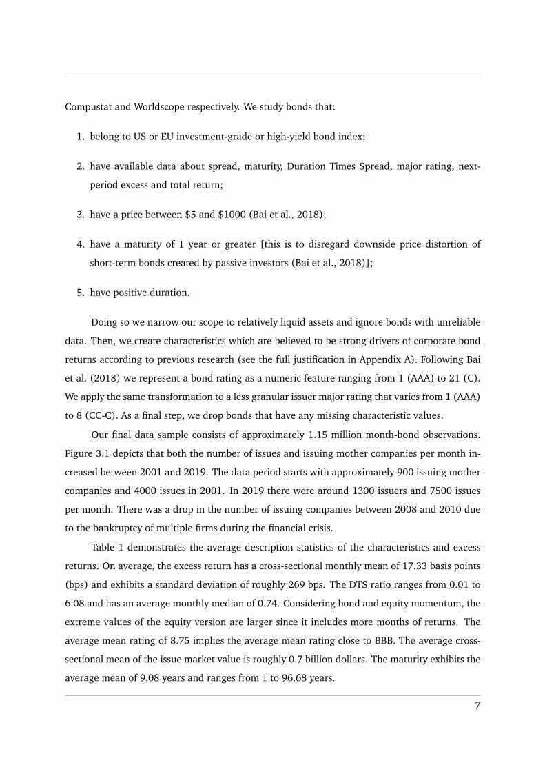
Table 1 demonstrates the average description statistics of the characteristics and excess

returns. On average, the excess return has a cross-sectional monthly mean of 17.33 basis points

(bps) and exhibits a standard deviation of roughly 269 bps. The DTS ratio ranges from 0.01 to

6.08 and has an average monthly median of 0.74. Considering bond and equity momentum, the

extreme values of the equity version are larger since it includes more months of returns. The

average mean rating of 8.75 implies the average mean rating close to BBB. The average cross-

sectional mean of the issue market value is roughly 0.7 billion dollars. The maturity exhibits the

average mean of 9.08 years and ranges from 1 to 96.68 years.

7

Figure 3.1: Monthly numbers of bonds and issuers over the sample from August 2001 to December2019.

According to Figure A.1, average maturity and DTS declined over time, while the average

age and issue market value were mostly increasing. Spikes in equity book-to-market ratio and

equity momentum and a dip in a distance-to-default correspond to the time of the Global Fi-

nancial Crisis. Among all characteristics, only pairs of bond rating and issuer major rating and

issue market value and size exhibit an average cross-sectional Pearson’s correlation larger than

0.8 (Figure A.4).

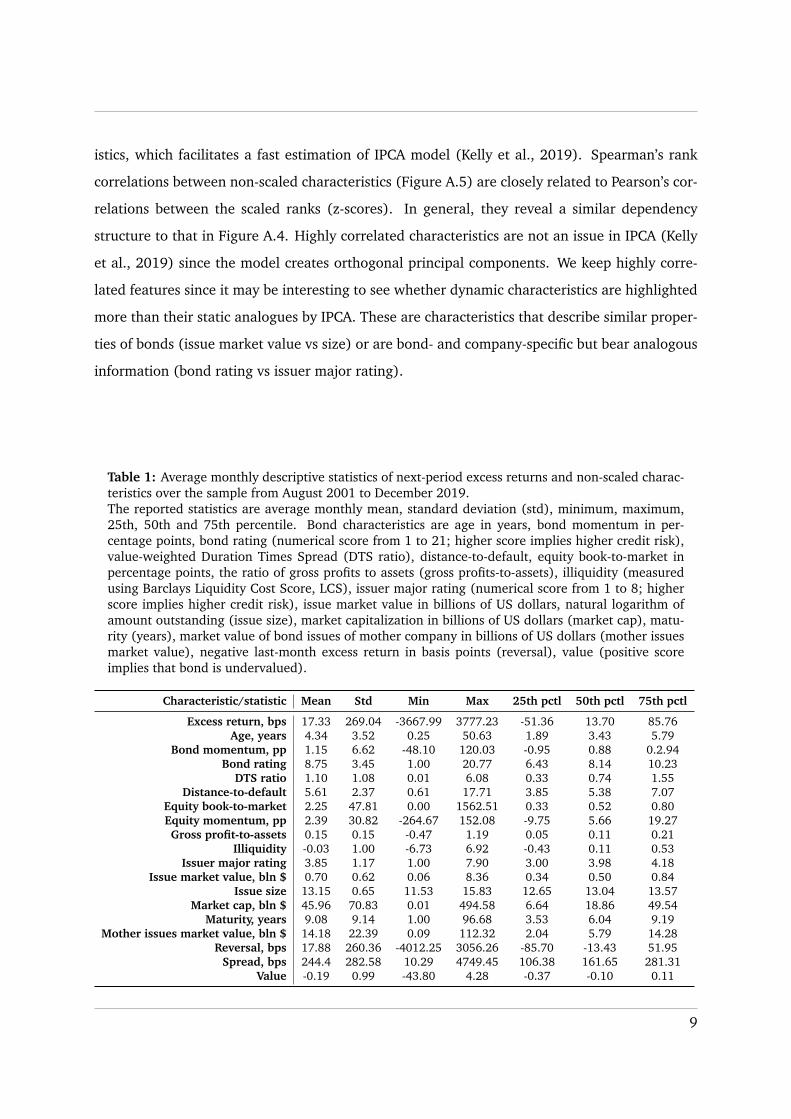
Figure 3.2 shows that the sample is dominated by US-index and investment-grade bonds.

The majority of bonds were senior and issued by industrial companies. Around 80% of bonds

were issued in North America and denominated in US dollars, while the European Monetary

Union (EMU) and Euro took second place accordingly. There were few bonds issued in pound

sterling, Swiss franc and Swedish krona as well. Finally, the distribution of nominal classes was

fairly stable over time (Figure A.2).

To remove the effects of remaining outliers and obtain a cross-sectional distribution of

each characteristic with zero mean and unit variance, we follow the procedure described by

Kozak et al. (2020). For every month and every characteristic we rank feature’s values and

divide them by the number of available monthly observations plus one. Then, we standard-

ize these rank ratios and call obtained values cross-sectional z-scores1. The last step is helpful

since some characteristics have multiple instances of the same values which distorts the uniform

distribution of ranks. By scaling the rank ratios we obtain a stable distribution of character-

1One can also call them stable z-scores since the ranking step already reduces effects of outliers.

8

istics, which facilitates a fast estimation of IPCA model (Kelly et al., 2019). Spearman’s rank

correlations between non-scaled characteristics (Figure A.5) are closely related to Pearson’s cor-

relations between the scaled ranks (z-scores). In general, they reveal a similar dependency

structure to that in Figure A.4. Highly correlated characteristics are not an issue in IPCA (Kelly

et al., 2019) since the model creates orthogonal principal components. We keep highly corre-

lated features since it may be interesting to see whether dynamic characteristics are highlighted

more than their static analogues by IPCA. These are characteristics that describe similar proper-

ties of bonds (issue market value vs size) or are bond- and company-specific but bear analogous

information (bond rating vs issuer major rating).

Table 1: Average monthly descriptive statistics of next-period excess returns and non-scaled charac-teristics over the sample from August 2001 to December 2019.The reported statistics are average monthly mean, standard deviation (std), minimum, maximum,25th, 50th and 75th percentile. Bond characteristics are age in years, bond momentum in per-centage points, bond rating (numerical score from 1 to 21; higher score implies higher credit risk),value-weighted Duration Times Spread (DTS ratio), distance-to-default, equity book-to-market inpercentage points, the ratio of gross profits to assets (gross profits-to-assets), illiquidity (measuredusing Barclays Liquidity Cost Score, LCS), issuer major rating (numerical score from 1 to 8; higherscore implies higher credit risk), issue market value in billions of US dollars, natural logarithm ofamount outstanding (issue size), market capitalization in billions of US dollars (market cap), matu-rity (years), market value of bond issues of mother company in billions of US dollars (mother issuesmarket value), negative last-month excess return in basis points (reversal), value (positive scoreimplies that bond is undervalued).

Characteristic/statistic Mean Std Min Max 25th pctl 50th pctl 75th pctl

Excess return, bps 17.33 269.04 -3667.99 3777.23 -51.36 13.70 85.76Age, years 4.34 3.52 0.25 50.63 1.89 3.43 5.79

Bond momentum, pp 1.15 6.62 -48.10 120.03 -0.95 0.88 0.2.94Bond rating 8.75 3.45 1.00 20.77 6.43 8.14 10.23

DTS ratio 1.10 1.08 0.01 6.08 0.33 0.74 1.55Distance-to-default 5.61 2.37 0.61 17.71 3.85 5.38 7.07

Equity book-to-market 2.25 47.81 0.00 1562.51 0.33 0.52 0.80Equity momentum, pp 2.39 30.82 -264.67 152.08 -9.75 5.66 19.27Gross profit-to-assets 0.15 0.15 -0.47 1.19 0.05 0.11 0.21

Illiquidity -0.03 1.00 -6.73 6.92 -0.43 0.11 0.53Issuer major rating 3.85 1.17 1.00 7.90 3.00 3.98 4.18

Issue market value, bln $ 0.70 0.62 0.06 8.36 0.34 0.50 0.84Issue size 13.15 0.65 11.53 15.83 12.65 13.04 13.57

Market cap, bln $ 45.96 70.83 0.01 494.58 6.64 18.86 49.54Maturity, years 9.08 9.14 1.00 96.68 3.53 6.04 9.19

Mother issues market value, bln $ 14.18 22.39 0.09 112.32 2.04 5.79 14.28Reversal, bps 17.88 260.36 -4012.25 3056.26 -85.70 -13.43 51.95

Spread, bps 244.4 282.58 10.29 4749.45 106.38 161.65 281.31Value -0.19 0.99 -43.80 4.28 -0.37 -0.10 0.11

9

Figure 3.2: Distribution of nominal classes in the over the sample from August 2001 to December2019.Rating groups: investment grade (IG) and high yield (HY). Seniority groups: senior and subordi-nated. Index groups: United States (US) and European Union (EU) bond index. Sectors: industrial,financial and utility. Regions: North America, EMU (European Monetary Union), other Europe, otherdeveloped countries, emerging markets. Currency groups: US dollar (USD), euro (EUR), pound ster-ling (GBP), Swiss franc (CHF) and Swedish krona (SEK).

4. Methodology

4.1. Preliminaries

In our study, we explore whether cluster effects are important to explain cross-sectional differ-

ences in expected returns. Consider a general cross-sectional bond return model

ri,t+1 = at+1 +L∑l=1

b(l)t+1z

(l)i,t + ei,t+1,

where is ri,t+1 is the excess return of bond i at time t+ 1, z(l)i,t is the characteristic l of bond

i at time t, at+1 is the intercept in this cross-sectional regression and b(l)t+1 is the slope coefficient

corresponding to the characteristic l. We can rewrite this in a vector form:

ri,t+1 = at+1 + zi,tbt+1 + ei,t+1. (1)

10

4.2 IPCA

The usual question in asset pricing is what should play the role of characteristics zi,t. One

may consider asset characteristics or factor loadings to factor-mimicking portfolios (Bai et al.,

2018). When time-varying loadings (betas) are used as zi,t, Equation (1) becomes

ri,t+1 = at+1 + βi,tbt+1 + ei,t+1. (2)

We argue that estimating dynamic bond factor loadings is especially convenient using IPCA

(Kelly et al., 2019). Besides, later we show how clustering common-risk IPCA factor loadings

incorporates cluster structure into the bond market.

4.2. IPCA

We select IPCA to price bonds due to its multiple advantages. First, it solves the issue of imbal-

anced panel data. Secondly, it estimates time-varying factor-loadings by means of asset charac-

teristics. Thirdly, it reduces the dimension of the potential “zoo” of factors and characteristics

that drive expected returns. Finally, it outputs betas that have a dual interpretation of factor

loadings and latent characteristics. Following Kelly et al. (2019), consider IPCA model in which

the excess return ri,t+1 is driven by the following system of equations:

ri,t+1 = αi,t + βi,tft+1 + εi,t+1

αi,t = z′i,tΓα + να,i,t

βi,t = z′i,tΓβ + νβ,i,t ,

(3)

where zi,t is the L × 1 vector of characteristics of bond i at t, ft+1 is the K × 1 vector of

common latent factors realized at t + 1, βi,t is the K × 1 vector of corresponding factor loadings

and αi,t is the scalar anomaly term. The factor loadings and the anomaly term are mapped from

L observed characteristics through the L×K matrix Γβ and the L×1 vector Γα accordingly. Besides,

there are the K ×1 residual νβ,i,t corresponding to βi,t, the scalar residual να,i,t that corresponds

to the anomaly term and the error εi,t+1 in the excess return equation. Kelly et al. (2019) develop

an asset pricing test to verify whether Γα is statistically indistinguishable from a zero vector.

They use a bootstrap procedure to simulate a distribution of Γα under null hypothesis and test

an observed Γα using a Wald-type test statistic Wα = Γ ′α Γα. Intuitively, this test identifies whether

characteristics explain variation in expected returns that is not related to factor exposures. The

11

4.2 IPCA

drawback of IPCA is that it ignores cluster-specific factors, which, among others, may lead to

wrong conclusions about mispricing according to the anomaly term. Besides, this may lead to

suboptimal estimation of latent factors (Alonso et al., 2020).

Assume that Γα = 0. Then IPCA model can be written as ε

ri,t+1 = αi,t + βi,tft+1 + εi,t+1

αi,t = να,i,t

βi,t = z′i,tΓβ + νβ,i,t ,

or equivalently

ri,t+1 = βi,tft+1 + εi,t+1

βi,t = z′i,tΓβ + νβ,i,t ,(4)

where εi,t+1 = να,i,t + εi,t+1. Plugging in the formula for time-varying loadings, we obtain:

ri,t+1 = (z′i,tΓβ)ft+1 + ε∗i,t+1,

where ε∗i,t+1 = νβ,i,tft+1 + εi,t+1. The beta term, z′i,tΓβ , stands for new (latent) characteristics of

bonds, which are linear combinations of observed characteristics. For a fixed cross section the

model equation is

rt+1 = (ZtΓβ)ft+1 + ε∗i,t+1. (5)

To draw an analogy between IPCA and OLS models, define Bt := ZtΓβ and assume Γβ is

known. Then the model

rt+1 = Btft+1 + ε∗i,t+1 (6)

is estimated via OLS ∀t where ft+1 is a slope vector, while Bt plays a role of regressors.

Thus,

ft+1 = (B′tBt)−1B′trt+1∀t.

12

4.3 New intuition behind IPCA

Substituting back Bt and using Γβ instead of Γβ , since we do not know the “true” Γβ , we

obtain the estimation formula proposed by Kelly et al. (2019):

ft+1 = (Γ ′βZ′tZt Γβ)−1Γ ′βZ

′trt+1∀t. (7)

That is, the estimate of latent factors ft+1 is the vector of OLS coefficient estimates in the

cross-sectional regression of next-period excess returns on current factor loadings (latent char-

acteristics). Therefore, ft+1 captures the cross-sectional dependency of expected excess returns

on IPCA betas. If this relation differs per cluster, factor estimates may deviate considerably for

each group when IPCA is estimated separately.

Above we assumed that we know Γβ or its estimate, which is not necessarily true. One of

the main contributions made by Kelly et al. (2019) is the formula to estimate this matrix that

maps observed characteristics into betas (given the latent factor estimates):

vec(Γ ′β) =

T−1∑t=1

Z ′tZt ⊗ ft+1f′t+1

−1 T−1∑

t=1

[Z ′t ⊗ f ′t+1

]′rt+1

. (8)

This formula generalizes principal component estimates by additionally taking into ac-

count time variation in cross-sectional relations between characteristics through the second mo-

ment matrix Z ′tZt. If we replaced every Z ′tZt by (T − 1)−1 ∑tZ′tZt, then Equation (8) would

output the PCA estimate (Kelly et al., 2019). The IPCA solution may look cumbersome for

some readers, so we derive a new intuition behind it in the following subsection. In essence,

IPCA model is estimated by alternating least square (ALS) method where alternations are made

between Equation (7) and Equation (8)2.

4.3. New intuition behind IPCA

4.3.1. Γβ representation via OLS slope estimates

Kelly et al. (2019) interpret the matrix Γβ as the matrix driven by characteristic-managed port-

folios, where the portfolio managed by a characteristic z(l) at time t + 1 is defined as

xl,t+1 :=1

Nt+1

Nt+1∑i=1

z(l)it ri,t+1. (9)

2See Kelly et al. (2019) for the solution when Γα , 0, which is analogous to that for the constrained IPCA.

13

4.3 New intuition behind IPCA

One might be interested in how exactly weights of characteristics in Γβ are estimated.

Equation (8) may seem involved for those who are not mathematically inclined, so a relatively

simple intuition behind Γβ may be demanded to understand which effects define weights of

characteristics. Therefore, we consider a special but realistic situation to develop further under-

standing of how IPCA works. Consider the case when:

1. There are two observed characteristics: L = 2;

2. There is one latent factor: K = 1;

3. Characteristics (instruments) are cross-sectionally scaled: z(l)t = 0, Var

(z

(l)it

)= 1 ∀l, t, where

Var (.) is the population cross-sectional variance.

4. The number of assets on each date is constant over time: Nt+1 =N ∀t.

Recall the formula for the matrix that maps observed characteristics into factor loadings:

vec(Γ ′β) =

T−1∑t=1

Z ′tZt ⊗ ft+1f′t+1

−1 T−1∑

t=1

[Z ′t ⊗ f ′t+1

]′rt+1

.After some rearrangements (see Appendix B.1 for the full derivation), we obtain a solution

for vec(Γ ′β) which is interpretable via OLS slope estimates related to the characteristic-managed

portfolios under the mild assumptions 1− 4. For this representation define additionally:

• βOLSxl as an OLS estimate of a slope coefficient in a pairwise time-series linear regression

without intercept xl,t+1 = βxl ft+1 + et+1;

• v :=∑T−1t=1 ρ12,t f

2t+1∑T−1

t=1 f2t+1

, (10)

where ρ12,t is the sample cross-sectional correlation between z(1)i and z(2)

i at time t.

v ∈ [−1;1] since∣∣∣∣∑T−1

t=1 ρ12,t f2t+1

∣∣∣∣ ≤ ∑T−1t=1

∣∣∣∣ρ12,t f2t+1

∣∣∣∣ ≤ ∑T−1t=1 f

2t+1 =⇒

∣∣∣∣∣∣∣∑T−1t=1 ρ12,t f

2t+1∑T−1

t=1 f2t+1

∣∣∣∣∣∣∣ ∈ [0;1].

|v| = 1 in a rare case when characteristics are perfectly positively or negatively correlated

in every cross section:∣∣∣ρ12,t

∣∣∣ = 1 ∀t;

• u :=1

1− v2 , (11)

where u > 0 ∀|v| , 1.

14

4.3 New intuition behind IPCA

The term v is related to the sample cross-sectional correlations of characteristics which are

weighted by squared next-period factor realizations (divided by the sum of all squared factors):

v =T−1∑t=1

f 2t+1∑T−1

t=1 f2t+1

ρ12,t .

This implies that if the squared factor estimate at t + 1 is considerably far from its time-

series average, the value of v is massively affected by the sample correlation between character-

istics at t. The sign of v is defined solely by the series of ρ12,t, so if the sample cross-correlation

of characteristics is often positive, especially when a next-period squared factor is large, v is

positive.

Using the definitions of xl,t+1, βOLSxl , v and u, we show in Appendix B.1 that the solution

for the mapping matrix Γβ can be represented as

vec(Γ ′β) = u

βOLSx1− vβOLSx2

βOLSx2− vβOLSx1

. (12)

Now, we can interpret the elements in Γβ through the OLS coefficient estimates. Recall that

u > 0, |v| ∈ [0;1] and ignore the case when characteristics are perfectly (negatively or positively)

correlated in each cross section. Then, for a characteristic l it holds that (ceteris paribus)

• ∀v s.t. |v| , 1: ↑ βOLSxl =⇒↑ vec(Γ ′β)l;

• ∀v > 0: ↑ βOLSxm =⇒↓ vec(Γ ′β)l , where m , l;

• ∀v < 0: ↑ βOLSxm =⇒↑ vec(Γ ′β)l , where m , l.

Note that u only defines magnitude of weights and does not affect relative weights of

characteristics (ceteris paribus). Kelly et al. (2019) notice that finding a unique estimate of Γβ

requires an identification restriction when factors are latent. They follow the regular constraint

of PCA that principal components must be orthogonal and orthonormal imposing that Γ ′βΓβ = IK

(which is used in our work as well). Using this restriction, we obtain

vec(Γ ′β) =1√(

βOLSx1 − vβOLSx2

)2+(βOLSx2 − vβOLSx1

)2

βOLSx1− vβOLSx2

βOLSx2− vβOLSx1

. (13)

15

4.3 New intuition behind IPCA

Now, we have a representation of vec(Γ ′β) solely through the term v and the OLS estimates

of slope coefficients in a linear regression of characteristic-managed portfolios on a contempora-

neous factor estimate. An assumption of linearly independent characteristics (in a cross section)

simplifies Equation (12) even more. Assuming ρ12,t = 0 ∀t, we obtain that∑T−1t=1 ρ12,t f

2t+1 = 0

and v = 0. The non-identified solution becomes

vec(Γ ′β) = u

βOLSx1

βOLSx2

. (14)

Since characteristics are linearly independent, the slope estimates related to their corre-

sponding portfolios do not affect each other’s weights (ceteris paribus). Now, elements in Γβ

depend only on the individual time-series relation of the factor and a characteristic-managed

portfolio. The stronger it is, the higher the weight of the corresponding characteristic. After

imposing the identification restriction we obtain

vec(Γ ′β) =1√(

βOLSx1

)2+(βOLSx2

)2

βOLSx1

βOLSx2

, (15)

which is simply a normalized vector of the OLS slope estimates. Essentially, this special

case shows that IPCA betas capture complex relations between characteristics, factor realizations

and returns. Hence, it may be useful to use them instead of observed characteristics to cluster

bonds. The presented intuition also holds approximately if the sample variances equal one in

sufficiently large cross sections or if the number of assets on each date is fairly stable over time.

4.3.2. When characteristic-managed portfolios are related to prominent anomalies

In IPCA characteristic-managed portfolios play a key role in defining the structure of Γβ . Recall

the definition of a characteristic-managed portfolio [Equation (9)] and consider the following

cases:

1. z(l)i,t = 1 ∀i, t (unit characteristic). Then the characteristic-managed portfolio l is the “one-

over-N” portfolio (DeMiguel et al., 2009):

xl,t+1 =1

Nt+1

Nt+1∑i=1

ri,t+1.

16

4.4 Holy grail model

If the factor has a loading which heavily relies on a unit (constant) characteristic, it is

related to the risk of the “one-over-N” portfolio, although this risk does not seem inter-

pretable.

2. z(l)i,t is the market value (MV) of bond i at time t divided by the value of the whole market

and multiplied by Nt+1. Then the characteristic-managed portfolio l is the market portfolio

xl,t+1 =1

MVt

Nt+1∑i=1

MVi,tri,t+1,

where MVt is the value of the entire market at t and MVi,t is the market value of bond

i at time t. Therefore, the factor which has a large impact of the market value in its

corresponding loading (that is, a corresponding column in Γβ has a high weight of market

value) is closely related to the market factor.

3. z(l)i,t is the momentum characteristic (MOM) of bond i at time t [as defined by Jostova et al.

(2013)] multiplied by Nt+1. Then, the characteristic-managed portfolio l is closely related

to the momentum portfolio

xl,t+1 =Nt+1∑i=1

MOMi,tri,t+1

which has long positions in past winners and short positions in previous losers (adjusted

for the magnitude of past performance). The factor that has a corresponding loading with

a high positive weight of the momentum characteristic is closely related to the momentum

portfolio.

This is not an exhaustive list of anomaly-related managed portfolios and one can use the

logic presented above to think about other cases. Note that these exact links to anomalies are

valid when non-scaled characteristics are used in IPCA, which is not the case in our study.

4.4. Holy grail model

To incorporate cluster structure into IPCA, we assume that the observed bond returns are gen-

erated from cluster-specific IPCA models. We call the model-search clustering method that ex-

plicitly finds these clusters the “holy grail” model. Essentially, the holy grail is the model by

17

4.4 Holy grail model

Ando and Bai (2017) adapted to the bond market. The authors assume that the following asset

pricing model holds:

ri,t+1 = βo,ifo,t+1 + βs,ifs,t+1 + βi |ci × ft+1|ci + εi,t+1|ci , (16)

where fo,t+1 is the vector of observed common factors realized at t + 1, fs,t+1 is the vector

of latent common (shared) factors at t+ 1, ft+1|ci is the vector of latent cluster-specific factors at

t + 1, βo,i , βs,i and βi |ci are the loadings to corresponding factor vectors and are assumed to be

constant over time. Finally, ci denotes the cluster membership of asset i which is constant over

time as well. We find some assumptions imposed by Ando and Bai (2017) too restrictive for the

bond market. Namely, constant factor loadings and cluster memberships seem unrealistic since

bonds change as time passes. To illustrate, if true clusters are investment grade and high yield

groups, bonds can be up- and downgraded over time. Thus, for bond analysis we propose three

adjustments to build our holy grail model:

1. Cluster memberships of each bond can vary over time within one model estimation;

2. IPCA is used instead of PCA to estimate time-varying loadings and latent factors;

3. There is only a cluster-specific part3, so common-risk parts βo,ifo,t+1 and βs,ifs,t+1 are set to

zero.

Thus, our holy grail model is:

ri,t+1 = βi,t |cit × ft+1|cit + εi,t+1|cit

βi,t |cit = z′i,t × Γβ |cit + νβ,i,t |cit ,(17)

where conditioning on the cluster membership cit implies that the parameter is generated

by the IPCA model of the cluster cit. This is a holy grail in the sense that it provides a perfect fit

for each month-bond observation and theoretically finds two data-generating IPCA models. Our

estimation procedure is the following:

3This assumption is not too restrictive since IPCA generally allows for prespecified factors, while cluster-specificfactors of distinct clusters can coincide theoretically. Hence, it is straightforward to extend our model to the formwith common parts if needed.

18

4.5 Gaussian mixture

1. Initialization. Initialize cluster memberships of bonds using some nominal classification

(e.g. IG/HY split) or random assignment.

2. IPCA step. Estimate cluster-specific IPCA models.

3. Clustering step. Calculate return returns implied by cluster-specific IPCA models. Update

cluster memberships according to the smallest squared model prediction error:

cit = argminct=1,...,C

(ri,t+1 − ri,t+1|ct

)2.

4. Iterate between 2 and 3 until convergence4.

This algorithm is a special case of the method proposed by Ando and Bai (2017) since

we use IPCA instead of PCA, cluster month-bond observations instead of asset time series and

ignore the common-risk part. Hence, our estimation procedure inherits convergence properties

derived by the authors. We identify IPCA cluster-specific factors using identification restriction

proposed by Kelly et al. (2019). To estimate factors Ando and Bai (2017) assume that common

and cluster-specific factors are orthogonal, whereas we ignore the common part. The holy grail

model is a useful descriptive method but cannot be employed for out-of-sample analysis. This is

because our clustering step always uses a next-period asset return, as well as that in the model

by Ando and Bai (2017)5, so the model inevitably possesses a look-ahead bias. Hence, we also

propose clustering methods that can avoid this practical issue.

4.5. Gaussian mixture

To develop a clustering model that can be predictive, we need to employ a method that accounts

only for differences in current features of objects. Unfortunately, many popular machine learn-

ing clustering techniques do not have a solid statistical rationale. For example, the density-based

method DBSCAN aims to reproduce a human’s ability to recognize parts of data with low and

high density. This is only a computational technique (although powerful for specific problems)

which does not imply any assumption about how data is generated. Spectral clustering relies on

the assumption that data can be represented as a weighted graph, which does not seem plausible

4We define convergence as a situation when changes in cluster memberships are smaller than 1e-6 and the averagechange in IPCA parameters is smaller than 1e-6.

5Ando and Bai (2017) propose their method to describe influence of the Global Financial Crisis on stock dataheterogeneity and not to predict cluster memberships for future dates.

19

4.5 Gaussian mixture

for corporate bonds. Besides, it utilizes the connectivity matrix with dimension of the number

of observations. Since we study more than a million of month-bond observations, spectral clus-

tering is simply infeasible. Hierarchical clustering is sometimes used to cluster companies since

it can output a structure similar to industries and countries. However, it is a computational, not

statistical procedure. In contrast, partitioning methods appear to be more statistically-based.

They implicitly search for several data-generating processes that output observed data points,

and the methods differ in terms of how these processes are defined.

In order to rely on statistical rationale, we use Gaussian mixture as an ML clustering

technique in our study. Mixture models are based on the assumption that observed data is

generated from several distributions. These models find these distributions and assign proba-

bilities of memberships to each observation. The Gaussian mixture, in particular, implies that

data is drawn from C normal distributions with mean vectors µ1, ...,µC and covariance matrices

Σ1, ...,ΣC . The Gaussian mixture cumulative distribution function can be represented as

F(yi) =C∑c=1

pcFc(yi),

where Fc(y) is the cumulative distribution function of normal distribution c and pc is the

unconditional probability that a data point yi is drawn from the distribution c. Notice that a

mixture of normal distributions is generally not normal, although it is their linear combination.

Suppose there are data points y1, ..., yN that we want to group into C clusters. In Gaussian

mixture we need to estimate C vectors of means µ, C covariance matrices Σ and unconditional

probabilities of each distribution p1, ...,pC . If we knew which distribution each observation be-

longs to, we would only need to find these parameters via the maximum likelihood estimation

(MLE). However, we generally do not know cluster memberships and thus rely on their expec-

tations through conditional probability vectors of cluster memberships P (y1), ..., P (yN ), which

need to be estimated too. Therefore, we use EM algorithm Dempster et al. (1977) to perform

Gaussian mixture clustering:

1. Initialization step. Initialize vectors of means µ1, ...,µC , covariance matrices Σ1, ...,ΣC and

unconditional probabilities p1, ...,pC .

2. Expectation step. Under known parameters of normal distributions, calculate conditional

20

4.5 Gaussian mixture

probabilities as

pc∗(yi) =pc∗f (yi |µc∗ ,Σc∗)∑Cc=1pcf (yi |µc,Σc)

.

Assign cluster memberships according to a mode probability:

ci = argmaxc=1,...,C

pc(yi).

3. Maximization step. Under known conditional probabilities, maximize the expected log-

likelihoodN∑i=1

pc(yi)C∑c=1

(logpc + logfc(yi |µc,Σc)

)over µ1, ...,µC , Σ1, ...,ΣC and p1, ...,pC .

4. Iterate between 2 and 3 until convergence6 of the log-likelihood function:

N∑i=1

log

C∑c=1

pc(yi)fc(yi |µc,Σc)

.Hamilton (1990) shows that the likelihood function never decreases during EM itera-

tions and the model estimates asymptotically converge to model parameters (under specific

conditions). The EM algorithm is relatively simple since it implies iterating between two sets

of closed-form solutions. However, since the procedure is iterative, fast convergence is by no

means guaranteed. One may also argue that EM may converge to a local optimum. This can be

resolved by running EM algorithms with different initalizations and selecting a result with the

highest value of the log-likelihood function.

We cluster the entire cross section at once to avoid matching clusters estimated on dif-

ferent dates. We treat observations related to the same bond on different dates as separate

data points to relax an unrealistic assumption of constant cluster memberships. In this case the

computation of the expected and “true” likelihood requires us to assume local independence of

clustered data points (Dias et al., 2009). That is, we suppose that all clustered observations are

independent conditionally on cluster-specific Gaussian distribution, which may be mitigated in

further studies. The most straightforward example of clustered data points is asset character-

6We define convergence as a situation when a change in the log-likelihood function is smaller than 1e-6.

21

4.6 On why and how to cluster IPCA factor loadings

istics (Marvin, 2015, Cai et al., 2016). If they are decent risk proxies, clustering results will

imply a sensible risk differentiation. However, this might seem naive and the use of more smart

features, e.g. factor loadings, may lead to improvements.

4.6. On why and how to cluster IPCA factor loadings

One of the most meaningful equity market splits is the segmentation into high and low market

beta stocks. The typical unit-level threshold separates stocks into high-beta stocks (beta larger

than one) and low-beta stocks (otherwise). The split in terms of exposure to the market is used

by investors to select stocks and manage equity portfolios, whereas it seems overlooked in the

bond market. This is probably due to technical issues with bond factor loadings estimation. A

traditional approach is to run time series regression of asset excess returns on market excess

returns. However, this implies ignorance of all bonds with short series of returns. Moreover,

bonds are time-varying, so previous returns may be much less relevant for bond loadings than

for stock betas. Fortunately, IPCA (Kelly et al., 2019) solves these technical issues by handling

imbalanced panel of bond returns and mapping bond characteristics into factor loadings. Thus,

it allows to separate the entire bond universe in terms of time-varying exposures to risk factors.

By assuming that this method may output clusters generated by cluster-specific pricing models,

we incorporate the idea of model-search methods. The proposed type of clustering can be

performed not only for a market beta but also for multiple IPCA betas simultaneously.

Another useful property of IPCA factor loadings is that they have an alternative inter-

pretation of latent characteristics. Recall that IPCA constructs betas as βi,t = z′i,tΓβ + νβ,i,t, that

is, every loading is modelled as a linear combination of observed characteristics. To estimate

risk exposures, IPCA uses information from characteristics, returns and factor realizations by

means of the mapping matrix Γβ [Equation (8)]. Section 4.3 shows how this is explicitly done

in a low-dimensional case. Besides, IPCA betas help to reduce a potentially high dimension of

characteristics. If this is done, they also emphasize differences in certain characteristics. To illus-

trate, suppose that we reduce dimension from eighteen observed characteristics to three latent

characteristics and these latent characteristics turn out to be market value, DTS ratio and rating

accordingly. Therefore, clustering these latent characteristics implies accounting for differences

only in market value, DTS and rating and ignoring differences in other observed features. Im-

portantly, this weighting scheme is justified by how IPCA selects characteristics which are most

related to risk factors. To summarize, clustering IPCA betas implies looking for clusters of bonds

22

4.6 On why and how to cluster IPCA factor loadings

that

• possess factor loadings of similar magnitude;

• have similar values of latent characteristics, while differences in observed characteristics

are weighted by IPCA.

To detect clusters with distinct common-risk IPCA betas we propose the following one-pass

algorithm:

1. Common IPCA step. Estimate a common IPCA model and save common-risk betas βi,t.

2. Clustering step. Cluster assets in terms of common-risk betas.

3. Cluster-specific IPCA step. Estimate cluster-specific IPCA models and study their good-

ness of fit.

The risk is common in the sense that factors are estimated using the whole bond universe.

We mainly use Gaussian mixture to cluster common-risk loadings, but in general any algorithm

can be chosen. This clustering approach is suitable if one believes that bonds with similar betas

from the common pricing model (common-risk betas) constitute asset clusters. Our question

is whether clusters estimated by means of the proposed algorithm outperform IG/HY separa-

tion for modelling bond returns. An idea for further bond clustering research can be found in

Appendix B.2.

Clustering IPCA betas is practical as opposed to the holy grail model and the method

suggested by Ando and Bai (2017) since it can be extended for out-of-sample (OOS) analysis. In

this case Γβ is time-varying, while cluster memberships and cluster-specific factor loadings are

predicted to explain cross-sectional variation in expected returns out-of-sample:

ri,tOOS+1= βi,tOOS

|ci,tOOS× fi,tOOS+1

|ci,tOOS+ ei,tOOS+1

|ci,tOOS, (18)

where fi,tOOS+1|ctOOS

is estimated as the vector of cluster-specific cross-sectional OLS coeffi-

cients. The out-of-sample estimation procedure is the following:

1. In-sample common IPCA step. Fix the data period from tstart to tend7. Estimate a common

IPCA model using data from tstart to tend and retrieve common-risk IPCA beta(s).

7Note that this data set also includes next-period excess returns realized at tend + 1.

23

4.7 Weighting schemes implied by IPCA

2. In-sample clustering step. Cluster assets in terms of common-risk IPCA betas from tstart

to tend as the full sample.

3. Out-of-sample prediction step.

(a) Prediction of common-risk IPCA betas. Predict common-risk IPCA betas out-of-

sample as

βi,tOOS= zi,tOOS

× Γβ , (19)

where tOOS = tend + 1 and Γβ is estimated in the common IPCA from the step 1.

(b) Prediction of clusters. Forecast cluster assignments ci,tOOSby applying the clustering

model fitted on the step 2 to predicted common-risk IPCA betas βi,tOOS.

4. Cluster-specific IPCA step.

(a) Run cluster-specific IPCA models using data from tstart to tend.

(b) Predict cluster-specific IPCA betas as

βi,tOOS|ci,tOOS

= zi,tOOS× Γβ |ci,tOOS

, (20)

where ci,tOOSis obtained on the step 3.

(c) Run cluster-specific cross-sectional regressions of next-period excess returns on cluster-

specific IPCA betas

ri,tOOS+1= βi,tOOS

|ci,tOOS× fi,tOOS+1

|ci,tOOS+ ei,tOOS+1

|ci,tOOS

and save model errors.

5. Shift data range by one date and repeat steps 1-4. Terminate the procedure if there is no

data left.

4.7. Weighting schemes implied by IPCA

Recall that clustering IPCA betas with dimension reduction implies emphasizing differences in

some observed characteristics. We can go further and also overweight differences in factor

loadings explicitly. Consider clustering IPCA betas using a simple partitioning method, e.g. k-

means or Gaussian mixture when covariance matrix is irrelevant for clustering (Appendix B.4).

24

4.7 Weighting schemes implied by IPCA

Then, this implies that we measure dissimilarity between bond betas and a centroid of cluster c

by means of the Euclidean distance

√√√K∑k=1

(β

(k)i,t − β

(k)c,t

)2.

As a generalization, consider the weighted distance

√√√K∑k=1

w(k)t

(β

(k)i,t − β

(k)c,t

)2, (21)

where the distance between β(k)i,t and the centroid β(k)

c,t is over- or underweighted by means

of w(k)t . Note that these weights do not necessarily add up to one. These weights can be subjec-

tive, but IPCA can help to choose them. Recall that each beta corresponds to some latent risk.

In addition, define a price of risk associated with the factor k as the average factor realization

(Kelly et al., 2019):

λ(k) :=1

T − 1

T−1∑t=1

f(k)t+1. (22)

Additionally, denote the average absolute value of the factor realization k as λ(k)∗ (robust

risk price)8:

λ(k)∗ :=

1T − 1

T−1∑t=1

∣∣∣∣f (k)t+1

∣∣∣∣ . (23)

Then we can consider the following weighting schemes implied by IPCA model (though

the list is not exhaustive):

1. w(k)t =

(f

(k)t+1

)2. The use of squared next-period factor estimates highlights betas related to

the largest realized risk.

2. w(k)t =

(λ(k)

)2. This weighting scheme is more stable since weights become time-invariant.

It emphasizes betas that are related to the most “expensive” risk.

3. w(k)t =

(λ

(k)∗

)2. This scheme circumvents time effects of factor realizations and the issue of

flipping sign of the factors.

8This definition solves a potential problem of flipping sign of f (k)t+1, which leads to underestimated risk price λ(k).

25

4.8 Measuring quality of results

The proposed weighting schemes are interesting since they possess an additional interpre-

tation through IPCA “latent” returns. Define the following variables:

1. The latent return k of bond i at t + 1: r(k)i,t+1 := β(k)

it × f(k)t+1. (24)

2. The predictive latent return k of bond i at t + 1: r(k)i,t+1 := β(k)

it ×λ(k). (25)

3. The robust latent return k of bond i at t + 1: r∗(k)i,t+1 := β(k)

it ×λ(k)∗ . (26)

All these latent returns are associated with a risk implied by the factor k. In Appendix

B.3 we derive that for clustering methods that use the Euclidean distance (e.g. k-means and

Gaussian mixture) and when only means (centroids) are relevant:

1. Clustering IPCA betas with the weighting scheme w(k)t =

(f

(k)t+1

)2is equivalent to clustering

latent returns r(k)i,t+1;

2. Clustering IPCA betas with the weighting scheme w(k)t =

(λ(k)

)2is equivalent to clustering

predictive latent returns r(k)i,t+1;

3. Clustering IPCA betas with the weighting scheme w(k)t =

(λ

(k)∗

)2is equivalent to clustering

robust latent returns r∗(k)i,t+1.

This interpretation builds a bridge between our methodology and partitioning methods

such as k-means used for cross sections of factor loadings or characteristics. It also presents

how to efficiently save betas to employ a desired weighting scheme in partitioning clustering

methods that use the Euclidean distance and take into account means. For instance, if you want

to apply squared risk prices as weights to betas, cluster predictive latent returns. This simplifies

generalization of well-known clustering techniques, especially when computer software does

not allow for a weighting scheme explicitly.

4.8. Measuring quality of results

To measure IPCA model performance we follow Kelly et al. (2019) and use total R2:

Total R2 := 1−∑T−1t=1

∑Nt+1i=1 (ri,t+1 − ri,t+1)2∑T−1t=1

∑Nt+1i=1 r

2i,t+1

. (27)

This metric indicates the quality of how IPCA models asset riskiness in cross-sections of corporate

bonds. By assuming that data is generated by two cluster-specific IPCA models we convert the

26

4.8 Measuring quality of results

unsupervised clustering problem into the supervised, which allows us to use total R2 to measure

clustering quality.

We also test whether a statistical split outperforms the IG/HY split in terms of the cross-

sectional residual sum of squares (RSS) using the Model Confidence Set (MCS) procedure pro-

posed by Hansen et al. (2011)9. We employ this method since it can be applied to any general

set of alternatives and does not impose restrictions on a distribution of model errors. We use the

MCS procedure only for the models that outperform the benchmark separation in terms of total

R2. The method is also used in other works related to bonds (De Pooter et al., 2010).

The MCS procedure considers a set of competing models, M0, and reduces it by testing

differences in loss functions to output the model confidence set M∗1−ααα, where ααα is a significance

level10. Hence, M∗1−ααα contains the “best” models at a confidence level 1−ααα. The first step to run

the MCS algorithm is to initializeM asM0. Then, the following hypothesis is tested at level ααα:

H0,M : E(djk,t) = 0 ∀j,k ∈M,

where djk,t = Lj,t − Lk,t is the difference between losses implied by models j and k at

time t and L is the loss function. If the null hypothesis is not rejected, M∗1−ααα is defined as M.

Otherwise, an elimination rule is used to drop one object from M and the null hypothesis is

tested again. To test H0,M we employ the “relative” test statistic (Hansen et al., 2011)

TR,M = maxj,k∈M

∣∣∣tjk∣∣∣ ,where tjk =

djk√Var(djk)

for j,k ∈ M and djk = 1n

∑nt=1djk,t. Note that Hansen et al. (2011)

assume that the time series of losses are used to compare models. Since we have the panel of

model errors, we define the loss of model j at t + 1 as cross-sectional RSS:

Lj,t+1 =Nt+1∑i=1

(ri,t+1 − r(j)i,t+1)2,

which is closely related to total R2. Thus, the MCS procedure finds models that explain

variation in cross sections of expected returns “best”. Because we perform pairwise comparisons,

9We thank Michael Gong for Python implementation of the MCS procedure.10We use bold font for the significance level to avoid confusion with α in IPCA.

27

the model confidence set contains no more than two models. This may increase the chance

that this set consists of one model. If it is singleton and mild assumptions hold, M∗1−ααα is an

asymptotically unbiased estimate of the “true” set of superior modelsM∗ (Hansen et al., 2011):

limn→∞

P(M∗ = M∗1−ααα

)= 1.

We run the MCS procedure with a bootstrap size of 1000, block size of 12 months and

significance levels of 5% and 10%. We test model performances independently for different

numbers of latent factors K and constraints regarding Γα. Finally, we also follow Ando and Bai

(2017) and use Fisher’s exact test to discover whether two clustering results are not related to

each other.

5. In-sample results

To present how our methodology can be used for empirical analysis, we apply it to find

two clusters and improve upon the prominent IG/HY separation. In general, our methods may

be employed for larger numbers of groups to enhance splits such as sectors and regions. In this

section we present our two-group clustering results with one estimation for the full sample.

5.1. IPCA without cluster structure

To begin with, we present the first evidence, to the best of our knowledge, of how IPCA prices

the entire panel of corporate bonds11. To illustrate this, we use IPCA models with characteristics

from the paper by Houweling and Van Zundert (2017), with all bond characteristics and, finally,

with all bond and company characteristics (“blender”). Additionally, each set of characteristics

is complemented with a constant. The characteristics proposed by Houweling and Van Zundert

(2017) are value, bond momentum, mother issues market value and low risk. Instead of low

risk we input maturity and bond rating to let IPCA define the low-risk characteristic statistically.

Table 2 demonstrates considerable differences in in-sample total R2 between the model with

characteristics from the paper by Houweling and Van Zundert (2017) and the blender model.

This may imply usefulness of the entire set of characteristics which is reduced to lower dimen-

sions by IPCA (e.g. to six factor loadings). Table 2 also shows that differences between restricted

(Γα = 0) and unrestricted (Γα , 0) models are pretty small. In Table 7 the asset pricing test that

11We thank S. Pruitt for Python code to run IPCA (https://sethpruitt.net/research/downloads).

28

5.2 IPCA with IG/HY split

Γα = 0 (Kelly et al., 2019) tends to confirm that Γα is statistically not different from zero for

various model settings. Note that the p-values do not necessarily decrease as K increases. This

is because characteristics may explain larger portion of variation in expected returns not related

to factor exposures even if the number of factors grows.

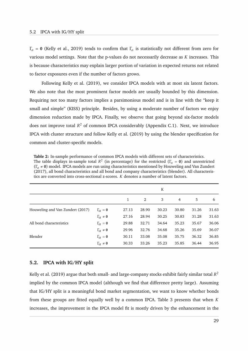
Following Kelly et al. (2019), we consider IPCA models with at most six latent factors.

We also note that the most prominent factor models are usually bounded by this dimension.

Requiring not too many factors implies a parsimonious model and is in line with the “keep it

small and simple” (KISS) principle. Besides, by using a moderate number of factors we enjoy

dimension reduction made by IPCA. Finally, we observe that going beyond six-factor models

does not improve total R2 of common IPCA considerably (Appendix C.1). Next, we introduce

IPCA with cluster structure and follow Kelly et al. (2019) by using the blender specification for

common and cluster-specific models.

Table 2: In-sample performance of common IPCA models with different sets of characteristics.The table displays in-sample total R2 (in percentage) for the restricted (Γα = 0) and unrestricted(Γα , 0) model. IPCA models are run using characteristics mentioned by Houweling and Van Zundert(2017), all bond characteristics and all bond and company characteristics (blender). All characteris-tics are converted into cross-sectional z-scores. K denotes a number of latent factors.

K

1 2 3 4 5 6

Houweling and Van Zundert (2017) Γα = 0 27.13 28.90 30.23 30.80 31.26 31.63

Γα , 0 27.16 28.94 30.25 30.83 31.28 31.63

All bond characteristics Γα = 0 29.88 32.71 34.64 35.23 35.67 36.06

Γα , 0 29.96 32.76 34.68 35.26 35.69 36.07

Blender Γα = 0 30.11 33.08 35.08 35.75 36.32 36.85

Γα , 0 30.33 33.26 35.23 35.85 36.44 36.95

5.2. IPCA with IG/HY split

Kelly et al. (2019) argue that both small- and large-company stocks exhibit fairly similar total R2

implied by the common IPCA model (although we find that difference pretty large). Assuming

that IG/HY split is a meaningful bond market segmentation, we want to know whether bonds

from these groups are fitted equally well by a common IPCA. Table 3 presents that when K

increases, the improvement in the IPCA model fit is mostly driven by the enhancement in the

29

5.2 IPCA with IG/HY split

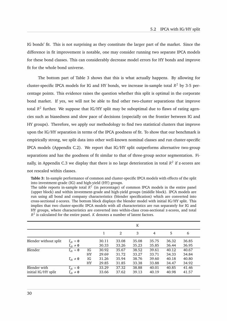
IG bonds’ fit. This is not surprising as they constitute the larger part of the market. Since the

difference in fit improvement is notable, one may consider running two separate IPCA models

for these bond classes. This can considerably decrease model errors for HY bonds and improve

fit for the whole bond universe.

The bottom part of Table 3 shows that this is what actually happens. By allowing for

cluster-specific IPCA models for IG and HY bonds, we increase in-sample total R2 by 3-5 per-

centage points. This evidence raises the question whether this split is optimal in the corporate

bond market. If yes, we will not be able to find other two-cluster separations that improve

total R2 further. We suppose that IG/HY split may be suboptimal due to flaws of rating agen-

cies such as biasedness and slow pace of decisions (especially on the frontier between IG and

HY groups). Therefore, we apply our methodology to find two statistical clusters that improve

upon the IG/HY separation in terms of the IPCA goodness of fit. To show that our benchmark is

empirically strong, we split data into other well-known nominal classes and run cluster-specific

IPCA models (Appendix C.2). We report that IG/HY split outperforms alternative two-group

separations and has the goodness of fit similar to that of three-group sector segmentation. Fi-

nally, in Appendix C.3 we display that there is no large deterioration in total R2 if z-scores are

not rescaled within classes.

Table 3: In-sample performance of common and cluster-specific IPCA models with effects of the splitinto investment-grade (IG) and high-yield (HY) groups.The table reports in-sample total R2 (in percentage) of common IPCA models in the entire panel(upper block) and within investment-grade and high-yield groups (middle block). IPCA models arerun using all bond and company characteristics (blender specification) which are converted intocross-sectional z-scores. The bottom block displays the blender model with initial IG/HY split. Thisimplies that two cluster-specific IPCA models with all characteristics are run separately for IG andHY groups, where characteristics are converted into within-class cross-sectional z-scores, and totalR2 is calculated for the entire panel. K denotes a number of latent factors.

K

1 2 3 4 5 6

Blender without split Γα = 0 30.11 33.08 35.08 35.75 36.32 36.85Γα , 0 30.33 33.26 35.23 35.85 36.44 36.95

Blender Γα = 0 IG 30.92 35.67 38.52 39.61 40.12 40.67HY 29.69 31.72 33.27 33.71 34.33 34.84

Γα , 0 IG 31.26 35.94 38.76 39.60 40.18 40.80HY 29.85 31.85 33.38 33.88 34.47 34.92

Blender with Γα = 0 33.29 37.32 38.88 40.01 40.85 41.46initial IG/HY split Γα , 0 33.66 37.62 39.13 40.19 40.98 41.57

30

5.3 Holy grail model

5.3. Holy grail model

Following our proposed model-search clustering procedure, we find bond clusters generated by

two IPCA models. We initialize cluster 0 and cluster 1 as HY and IG group accordingly. Note that

the holy grail estimation does not include estimation of common IPCA model. For simplicity we

present descriptions of the results for the three-factor holy grail model without anomaly term.

Figure 5.1 depicts that the holy grail clusters sometimes depart from IG/HY separation

significantly. This may be the evidence that although IG/HY separation is useful, it is suboptimal

theoretically. Fisher’s test p-values tend to be either close to zero or to one. Nonetheless, the

distribution of p-values implies that in general the holy grail clusters tend to be related to IG/HY

split. The time-series dynamics of holy grail cluster probabilities looks much more noisy than

that of IG/HY split (Figure 5.2). Bonds from the cluster 1 tend to dominate the bond universe,

although during the financial crisis bonds from the cluster 0 prevail. This makes sense since

the cluster 0 is related to HY group and multiple bonds become perceived riskier due to the

economic situation in the US and EU. Figure 5.2 reports that the cluster 1 seems to be related

to IG group since it often includes more IG bonds. Relation to bond seniority is rather mixed,

although senior bonds tend to be represented in the cluster 1 a bit more often. Finally, Figure 5.2

depicts that many financial companies migrate to the cluster 0 during the financial crisis. These

pieces of evidence show that the holy grail clusters are similar to IG/HY segmentation, but do

not mimic it completely. In support of this, we note that the holy grail HY-like group (cluster 0)

tends to be undervalued and exhibits higher average maturity in cross sections then the “real”

HY bonds (Table 4). According to Table 5, splitting the bond universe according to the holy

grail model provides massive gains in terms of the goodness of fit as opposed to the “no split”

setting and IG/HY separation. Note that for the holy grail it is possible that total R2 decreases

when K increases or Γα is introduced. This is because the overall goodness of fit depends on the

segmentation as well.

We could use the holy grail in the out-of-sample framework as well if we we were able

to forecast its cluster memberships. To check this we use the entire set of characteristics as

explanatory variables. We employ logistic regression and random forest to rely on statistical

background and allow for non-linear relations accordingly. The logistic regression provides poor

classification even in the in-sample estimation, which leads to negative total R2. In contrast,

the random forest split achieves the goodness of fit similar to that of the true holy grail model.

31

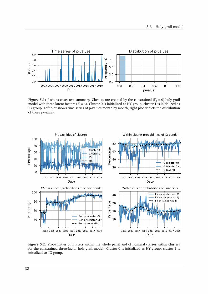
5.3 Holy grail model

Figure 5.1: Fisher’s exact test summary. Clusters are created by the constrained (Γα = 0) holy grailmodel with three latent factors (K = 3). Cluster 0 is initialized as HY group, cluster 1 is initialized asIG group. Left plot shows time series of p-values month by month, right plot depicts the distributionof these p-values.

Figure 5.2: Probabilities of clusters within the whole panel and of nominal classes within clustersfor the constrained three-factor holy grail model. Cluster 0 is initialized as HY group, cluster 1 isinitialized as IG group.

32

5.4 Model-free clustering

However, when we separate data into training and test set, the random forest’s prediction ability

deteriorates. Although its classification precision is around 95% and recall is roughly 75%,

classification errors turn out to be costly and deliver negative total R2 in the test data. Therefore,

we conclude that the holy grail clusters are not predictable and the model is not applicable out-

of-sample.

To summarize, we find that IG/HY split is notably far from the theoretically best market

segmentation in terms of total R2. Hence, we proceed with searching for a cluster separation

that would come closer to the holy grail.

5.4. Model-free clustering

Our model-free approach implies using the Gaussian mixture to cluster bond and company char-

acteristics. It is model-free in the sense that most characteristics that we cluster are not obtained

from involved models. Although this method may seem naive, it can serve as a sanity check for

clustering IPCA factor loadings that we perform later. In all Gaussian mixtures we use IG/HY

split as initialization. After finding two clusters of bonds, we price them using cluster-specific

IPCA models and calculate total R2 for the entire panel. We use the following sets of character-

istics to cluster bonds:

1. Non-scaled bond rating;

2. Cross-sectional z-scores of default risk characteristics: issue rating, spread and distance-

to-default.

3. Large set of cross-sectional z-scores: all characteristics except for size and issuer major

rating.

The use of non-scaled rating implies that we discover whether the Gaussian mixture de-

fines a better threshold for bond rating than the IG/HY split, which employs BBB- rating as a

borderline. By using default risk characteristics we try to create a more dynamic and complex

measure of credit quality than solely rating. Lastly, we use a large set of characteristics as an

extreme version of model-free clustering. We exclude size and issuer major rating since they

are highly correlated with market value and issue rating (Figures A.4-A.5) and less dynamic.

We perform clustering for the full sample at once since non-scaled rating and cross-sectional

z-scores are time-invariant. This also removes the problem of matching clusters when clustering

is performed date by date.

33

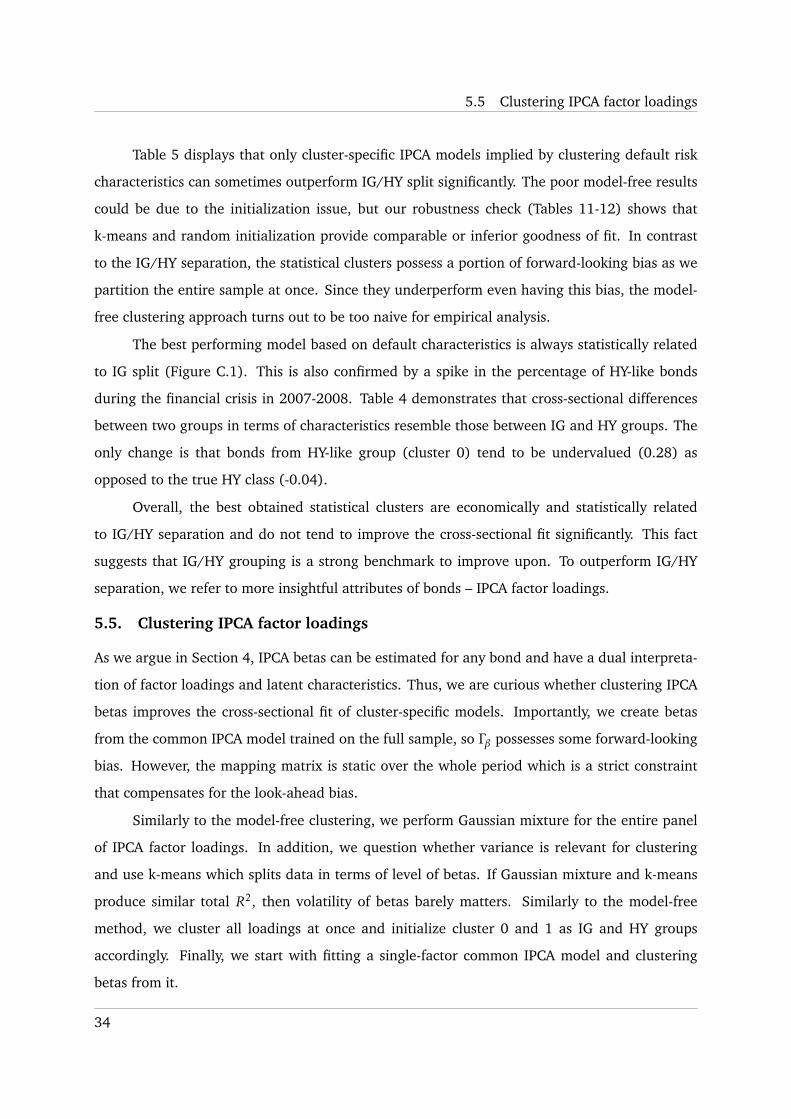
5.5 Clustering IPCA factor loadings

Table 5 displays that only cluster-specific IPCA models implied by clustering default risk

characteristics can sometimes outperform IG/HY split significantly. The poor model-free results

could be due to the initialization issue, but our robustness check (Tables 11-12) shows that

k-means and random initialization provide comparable or inferior goodness of fit. In contrast

to the IG/HY separation, the statistical clusters possess a portion of forward-looking bias as we

partition the entire sample at once. Since they underperform even having this bias, the model-

free clustering approach turns out to be too naive for empirical analysis.

The best performing model based on default characteristics is always statistically related

to IG split (Figure C.1). This is also confirmed by a spike in the percentage of HY-like bonds

during the financial crisis in 2007-2008. Table 4 demonstrates that cross-sectional differences

between two groups in terms of characteristics resemble those between IG and HY groups. The

only change is that bonds from HY-like group (cluster 0) tend to be undervalued (0.28) as

opposed to the true HY class (-0.04).

Overall, the best obtained statistical clusters are economically and statistically related

to IG/HY separation and do not tend to improve the cross-sectional fit significantly. This fact

suggests that IG/HY grouping is a strong benchmark to improve upon. To outperform IG/HY

separation, we refer to more insightful attributes of bonds – IPCA factor loadings.

5.5. Clustering IPCA factor loadings

As we argue in Section 4, IPCA betas can be estimated for any bond and have a dual interpreta-

tion of factor loadings and latent characteristics. Thus, we are curious whether clustering IPCA

betas improves the cross-sectional fit of cluster-specific models. Importantly, we create betas

from the common IPCA model trained on the full sample, so Γβ possesses some forward-looking

bias. However, the mapping matrix is static over the whole period which is a strict constraint

that compensates for the look-ahead bias.

Similarly to the model-free clustering, we perform Gaussian mixture for the entire panel

of IPCA factor loadings. In addition, we question whether variance is relevant for clustering

and use k-means which splits data in terms of level of betas. If Gaussian mixture and k-means

produce similar total R2, then volatility of betas barely matters. Similarly to the model-free

method, we cluster all loadings at once and initialize cluster 0 and 1 as IG and HY groups

accordingly. Finally, we start with fitting a single-factor common IPCA model and clustering

betas from it.

34

5.5 Clustering IPCA factor loadings

Table 5 presents that k-means clustering is usually inferior to the IG/HY split when we

cluster exposures to one IPCA latent factor. In contrast, separation of bonds through the Gaus-

sian mixture often outperforms the benchmark, although gains are not always significant. Figure

5.3 displays that the Gaussian mixture clusters differ from k-means clusters in two ways. First,

the Gaussian mixture implies a higher maximum value of IPCA beta for the cluster 1. Secondly,

the Gaussian mixture accounts not for level but for magnitude of betas. As a result, cluster 0

contains bonds not only with high but also with very low loadings. However, the number of

bonds with betas from the left tail is relatively small, so we suppose that the largest effect comes

from a better choice of upper threshold for the cluster 1.

The best Gaussian mixture split reminds of the prominent separation in the stock market

– low- and high- market beta segmentation. Hence, we also construct Γβ by specifying a single

IPCA factor as a market factor. As usual, we construct the market factor as the value-weighted

portfolio of bonds. Then, we fit Γβ according to Equation (8)12, retrieve market betas and cluster

them all at once. First, we notice that the exposure to one latent factor and the market beta are

generated by similar Γβ relative coefficients (Figure C.3). Secondly, we observe that a sample

time-series correlation between the latent factor and the market factor is 96.13% (Figure C.4).

Hence, we conclude that the latent-factor IPCA beta is closely related to the market beta. This

also shows that low/high market beta separation seems relevant in the corporate bond market.

However, Table 5 reports that statistical estimation of a common single factor is superior to the

use of market factor for clustering.

Finally, we can test a simpler rule to split the bond universe according to IPCA betas.

Recall that in the equity market low- and high-beta stocks are usually separated by the unit

threshold, so we employ it as well. Table 5 indicates that this split outperforms all alternatives

when clustering latent-factor betas. This seems to confirm that Gaussian mixture outperforms

k-means mainly due to the better threshold selection (Figure 5.3). The unit-level split of latent-

factor betas tends to be significantly superior to the IG/HY segmentation. In contrast, the same

scheme applied to market exposures does not improve upon the benchmark.

12There is no need to impose an identification restriction on Γβ since the factor is identified.

35

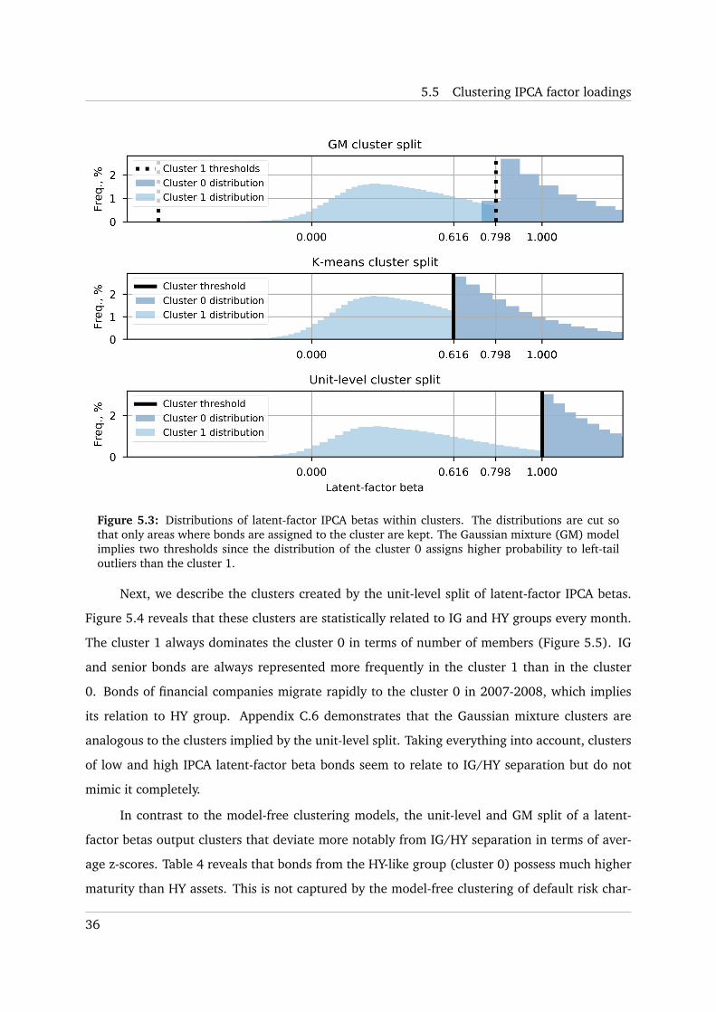
5.5 Clustering IPCA factor loadings

Figure 5.3: Distributions of latent-factor IPCA betas within clusters. The distributions are cut sothat only areas where bonds are assigned to the cluster are kept. The Gaussian mixture (GM) modelimplies two thresholds since the distribution of the cluster 0 assigns higher probability to left-tailoutliers than the cluster 1.

Next, we describe the clusters created by the unit-level split of latent-factor IPCA betas.

Figure 5.4 reveals that these clusters are statistically related to IG and HY groups every month.

The cluster 1 always dominates the cluster 0 in terms of number of members (Figure 5.5). IG

and senior bonds are always represented more frequently in the cluster 1 than in the cluster

0. Bonds of financial companies migrate rapidly to the cluster 0 in 2007-2008, which implies

its relation to HY group. Appendix C.6 demonstrates that the Gaussian mixture clusters are

analogous to the clusters implied by the unit-level split. Taking everything into account, clusters

of low and high IPCA latent-factor beta bonds seem to relate to IG/HY separation but do not

mimic it completely.

In contrast to the model-free clustering models, the unit-level and GM split of a latent-

factor betas output clusters that deviate more notably from IG/HY separation in terms of aver-

age z-scores. Table 4 reveals that bonds from the HY-like group (cluster 0) possess much higher

maturity than HY assets. This is not captured by the model-free clustering of default risk char-

36

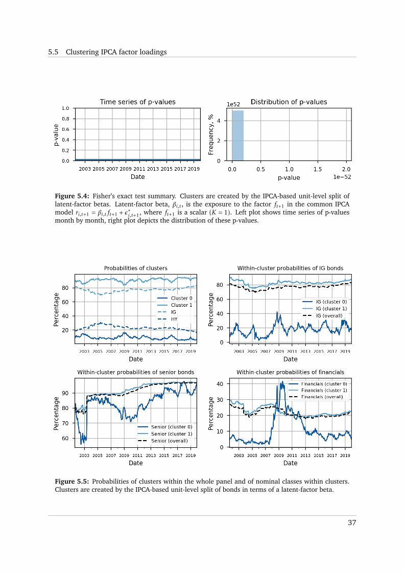
5.5 Clustering IPCA factor loadings

Figure 5.4: Fisher’s exact test summary. Clusters are created by the IPCA-based unit-level split oflatent-factor betas. Latent-factor beta, βi,t, is the exposure to the factor ft+1 in the common IPCAmodel ri,t+1 = βi,tft+1 + ε∗i,t+1, where ft+1 is a scalar (K = 1). Left plot shows time series of p-valuesmonth by month, right plot depicts the distribution of these p-values.

Figure 5.5: Probabilities of clusters within the whole panel and of nominal classes within clusters.Clusters are created by the IPCA-based unit-level split of bonds in terms of a latent-factor beta.

37

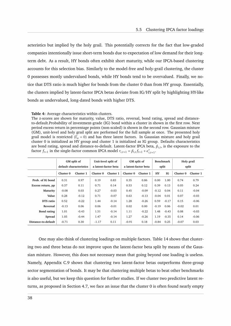
5.5 Clustering IPCA factor loadings

acteristics but implied by the holy grail. This potentially corrects for the fact that low-graded

companies intentionally issue short-term bonds due to expectation of low demand for their long-

term debt. As a result, HY bonds often exhibit short maturity, while our IPCA-based clustering

accounts for this selection bias. Similarly to the model-free and holy-grail clustering, the cluster

0 possesses mostly undervalued bonds, while HY bonds tend to be overvalued. Finally, we no-

tice that DTS ratio is much higher for bonds from the cluster 0 than from HY group. Essentially,

the clusters implied by latent-factor IPCA betas deviate from IG/HY split by highlighting HY-like

bonds as undervalued, long-dated bonds with higher DTS.

Table 4: Average characteristics within clusters.The z-scores are shown for maturity, value, DTS ratio, reversal, bond rating, spread and distance-to-default.Probability of investment-grade (IG) bond within a cluster in shown in the first row. Nextperiod excess return in percentage points (non-scaled) is shown in the second row. Gaussian mixture(GM), unit-level and holy grail split are performed for the full sample at once. The presented holygrail model is restricted (Γα = 0) and has three latent factors. In Gaussian mixture and holy grailcluster 0 is initialized as HY group and cluster 1 is initialized as IG group. Defaults characteristicsare bond rating, spread and distance-to-default. Latent-factor IPCA beta, βi,t, is the exposure to thefactor ft+1 in the single-factor common IPCA model ri,t+1 = βi,tft+1 + ε∗i,t+1.

GM split of Unit-level split of GM split of Benchmark Holy grail

default characteristics a latent-factor beta a latent-factor beta split split

Cluster 0 Cluster 1 Cluster 0 Cluster 1 Cluster 0 Cluster 1 HY IG Cluster 0 Cluster 1

Prob. of IG bond 0.31 0.97 0.19 0.83 0.35 0.86 0.00 1.00 0.74 0.79

Excess return, pp 0.37 0.11 0.71 0.14 0.53 0.12 0.39 0.13 0.05 0.24

Maturity -0.08 0.03 0.27 -0.03 0.45 -0.09 -0.12 0.04 0.11 -0.04

Value 0.28 -0.12 0.71 -0.07 0.63 -0.13 -0.04 0.01 0.07 -0.03

DTS ratio 0.52 -0.22 1.44 -0.14 1.28 -0.26 0.59 -0.17 0.15 -0.06

Reversal -0.13 0.06 0.06 -0.01 0.02 0.00 -0.19 0.06 -0.02 0.01

Bond rating 1.01 -0.43 1.51 -0.14 1.11 -0.22 1.48 -0.43 0.08 -0.03

Spread 1.05 -0.44 1.47 -0.14 1.27 -0.26 1.19 -0.35 0.14 -0.06

Distance-to-default -0.71 0.30 -1.17 0.11 -0.91 0.18 -0.84 0.25 -0.07 0.03

One may also think of clustering loadings on multiple factors. Table 14 shows that cluster-

ing two and three betas do not improve upon the latent-factor beta split by means of the Gaus-

sian mixture. However, this does not necessary mean that going beyond one loading is useless.

Namely, Appendix C.9 shows that clustering two latent-factor betas outperforms three-group

sector segmentation of bonds. It may be that clustering multiple betas to beat other benchmarks

is also useful, but we keep this question for further studies. If we cluster two predictive latent re-

turns, as proposed in Section 4.7, we face an issue that the cluster 0 is often found nearly empty

38

5.5 Clustering IPCA factor loadings

(Figure C.7), so running cluster-specific IPCA is not possible. In contrast, clustering two robust

latent returns (Section 4.7) outputs well-defined clusters (Figure C.8), probably by solving the

problem of a flipping sign of IPCA factors. Furthermore, this weighting scheme provides stable

gains over the IG/HY split (Table 14), which are comparable to those of the unit-level split of ex-

posures to one latent factor. Besides, Figure C.8 displays that the obtained cluster 1 is somewhat

linked to the investment-grade and senior bond groups. Many financial companies migrate to

the cluster 0 during the financial crisis, which reaffirms its relation to high-yield bonds. Overall,

we see gains from applying squared robust prices as a weighting scheme to IPCA betas.

Our in-sample results imply that clustering the corporate bond universe in terms of latent-

factor betas with Gaussian mixture or a unit-level threshold tends to be superior to IG/HY split.

Besides, we conclude that using solely observed characteristics does not produce large gains, no

matter how many we choose and how smart our choice is. This highlights the importance of

creating fewer but smarter bond attributes that incorporate rich asset information. We argue

that it can be a latent-factor IPCA beta, while the clustering method matters and a weighting

scheme can be helpful. The IPCA beta accounts for the whole variety of information about

bonds – characteristics, returns and risk factors. By clustering these betas with the Gaussian

mixture and a unit threshold we tend to significantly outperform the investment-grade/high-

yield segmentation and move a little bit towards the quality of the holy grail. Furthermore, the

outperforming unit-level split implies that IG-like bonds have a lower maturity than the true IG

bonds. Similarly, investors that manage investment-grade bond funds sometimes exclude long-

dated bonds to create enhanced investment-grade definition.13 As we noticed, our in-sample

statistical clustering suffers from a forward-looking bias – IPCA betas are constructed using the

entire data sample, although constant Γβ may compensate for that. To find whether splitting the

bond universe in terms of exposures to one latent factor is a practical method, we do this in the

out-of-sample framework.

13For example, in Robeco Global Multi-Factor Credits fund.

39

5.5 Clustering IPCA factor loadings

Table 5: In-sample performance of cluster-specific IPCA models in the whole panel.The table reports in-sample total R2 (in percentage). Each cluster-specific IPCA model has theblender specification (includes all characteristics). Data is split according to nominal or clusterclassifications and characteristics are converted into within-class cross-sectional z-scores. IG/HYseparation is used as initialization in Gaussian mixture (GM), k-means and the holy grail and clus-tering is performed for the full sample at once. Total R2 value is bold if it exceeds that value ofcluster-specific IPCA models implied by IG/HY split with the same model settings (the holy grail isignored). One asterisk marks models that outperform the IG/HY classification according to the MCSprocedure applied to RSS at a significance level of 5%, whereas two asterisks indicate outperfor-mance at a significance level of 10%. K denotes a number of latent factors in cluster-specific IPCAmodels.

K

Clustering method 1 2 3 4 5 6

Nominal classification IG vs HY Γα = 0 33.29 37.32 38.88 40.01 40.85 41.46

Γα , 0 33.66 37.62 39.13 40.19 40.98 41.57

Model-free GM cluster split based of

rating Γα = 0 32.91 37.05 38.74 39.88 40.76 41.47

Γα , 0 33.30 37.35 38.97 40.04 40.90 41.59

default risk characteristics Γα = 0 33.45 36.95 39.00 40.42 41.42 42.11**

Γα , 0 33.94 37.34 39.32 40.59 41.55 42.23**

large set of characteristics Γα = 0 32.28 35.38 37.42 38.48 39.33 39.85

Γα , 0 32.66 35.68 37.68 38.67 39.45 39.96

IPCA-based k-means cluster split of

market beta Γα = 0 32.60 36.21 38.49 39.64 40.55 41.14

Γα , 0 33.04 36.55 38.80 39.87 40.67 41.26

latent-factor beta Γα = 0 32.86 36.55 38.79 40.00 40.93 41.55

Γα , 0 33.33 36.91 39.13 40.24 41.05 41.66

IPCA-based GM cluster split of

market beta Γα = 0 33.24 37.05 39.17 40.46** 41.46* 42.14*

Γα , 0 33.74 37.43 39.54 40.70* 41.58** 42.26*

latent-factor beta Γα = 0 33.64 37.52 39.52* 40.92* 41.98* 42.71*

Γα , 0 34.18 37.94 39.93* 41.17* 42.12* 42.83*

IPCA-based unit-level split of

market beta Γα = 0 31.91 35.26 37.63 38.61 39.44 39.97

Γα , 0 32.27 35.54 37.87 38.80 39.56 40.08

latent-factor beta Γα = 0 33.97 38.22** 40.22* 41.76* 43.02* 43.96*

Γα , 0 34.57 38.69* 40.65* 41.98* 43.18* 44.10*

Holy grail Γα = 0 66.31 69.38 71.01 71.85 72.42 73.04

Γα , 0 66.73 68.96 71.33 71.87 72.46 73.00

40

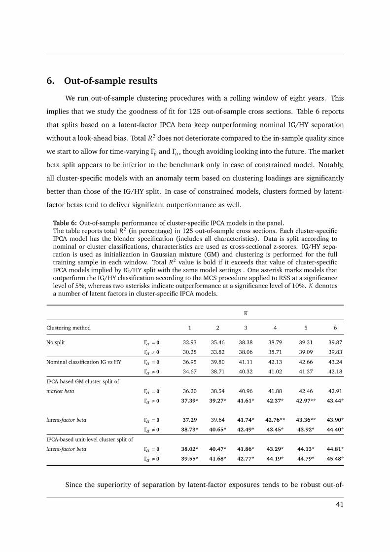
6. Out-of-sample results

We run out-of-sample clustering procedures with a rolling window of eight years. This

implies that we study the goodness of fit for 125 out-of-sample cross sections. Table 6 reports

that splits based on a latent-factor IPCA beta keep outperforming nominal IG/HY separation

without a look-ahead bias. Total R2 does not deteriorate compared to the in-sample quality since

we start to allow for time-varying Γβ and Γα, though avoiding looking into the future. The market

beta split appears to be inferior to the benchmark only in case of constrained model. Notably,

all cluster-specific models with an anomaly term based on clustering loadings are significantly

better than those of the IG/HY split. In case of constrained models, clusters formed by latent-

factor betas tend to deliver significant outperformance as well.

Table 6: Out-of-sample performance of cluster-specific IPCA models in the panel.The table reports total R2 (in percentage) in 125 out-of-sample cross sections. Each cluster-specificIPCA model has the blender specification (includes all characteristics). Data is split according tonominal or cluster classifications, characteristics are used as cross-sectional z-scores. IG/HY sepa-ration is used as initialization in Gaussian mixture (GM) and clustering is performed for the fulltraining sample in each window. Total R2 value is bold if it exceeds that value of cluster-specificIPCA models implied by IG/HY split with the same model settings . One asterisk marks models thatoutperform the IG/HY classification according to the MCS procedure applied to RSS at a significancelevel of 5%, whereas two asterisks indicate outperformance at a significance level of 10%. K denotesa number of latent factors in cluster-specific IPCA models.

K

Clustering method 1 2 3 4 5 6

No split Γα = 0 32.93 35.46 38.38 38.79 39.31 39.87

Γα , 0 30.28 33.82 38.06 38.71 39.09 39.83

Nominal classification IG vs HY Γα = 0 36.95 39.80 41.11 42.13 42.66 43.24

Γα , 0 34.67 38.71 40.32 41.02 41.37 42.18

IPCA-based GM cluster split of

market beta Γα = 0 36.20 38.54 40.96 41.88 42.46 42.91

Γα , 0 37.39* 39.27* 41.61* 42.37* 42.97** 43.44*

latent-factor beta Γα = 0 37.29 39.64 41.74* 42.76** 43.36** 43.90*

Γα , 0 38.73* 40.65* 42.49* 43.45* 43.92* 44.40*

IPCA-based unit-level cluster split of

latent-factor beta Γα = 0 38.02* 40.47* 41.86* 43.29* 44.13* 44.81*

Γα , 0 39.55* 41.68* 42.77* 44.19* 44.79* 45.48*

Since the superiority of separation by latent-factor exposures tends to be robust out-of-

41

sample, scholars and practitioners may think of using this split for their research and invest-

ments. Namely, creating separate funds of bonds with high and low exposure to the latent

factor can meet needs of clients with different risk profiles. Furthermore, one should not miss

these clusters when debating over two asset classes in the bond market. This is because the

popular segmentation into investment-grade and high-yield bonds tends to be inferior to the

statistical clusters that we present.

7. Conclusion

Investors often differentiate stocks as low and high market beta assets. However, they

tend to overlook this split in the corporate bond market and usually use investment-grade/high-

yield separation. This is probably due to technical issues with the estimation of bond factor

loadings. Bonds change over time and mostly have limited time series of returns. Hence, this

makes it impossible to estimate bond betas in a traditional time-series framework. Luckily, new

improvements in econometrics are here to resolve this problem.

In our study, we demonstrated that IPCA (Kelly et al., 2019) is a convenient pricing model

for bonds. We developed a new intuition about how it works and presented a dual interpretation

of IPCA betas, which incorporate rich information from characteristics, returns and factors. By

means of IPCA we showed that separation based on exposures to a latent factor provides gains

in terms of cross-sectional fit as opposed to the prominent IG/HY split. These improvements

are mostly significant for different settings of cluster-specific models and in in-sample and out-

of-sample framework. We emphasized the importance of defining a threshold to separate the

common-risk betas and revealed that the Gaussian mixture and a unit-level split work well. We

conclude that our statistical clusters are at least as important as IG and HY groups and seem a

more accurate estimate of two clusters in the bond market. Finally, we found that the common

latent factor is closely related to a market factor but remains preferred for clustering. Thus, we

reaffirmed the well-known equity market notion of low and high market beta split but in the

context of corporate bonds.

Lack of bond clustering studies creates a large room for further research. First, one may

consider more than two clusters or develop a test to establish the number of groups. Secondly,

clustering techniques other than the Gaussian mixture and k-means could be used, but with

careful reasoning. Thirdly, one could build a model that introduces a time-series dependency

42

of bond cluster assignments. Lastly, we showcased the usefulness of IPCA to estimate bond

loadings, so this model can be widely used in later studies.

43

REFERENCES

References

Alonso, A. M., Galeano, P., and Pena, D. (2020). A robust procedure to build dynamic factor

models with cluster structure. Journal of Econometrics, 216(1):35–52.

Ando, T. and Bai, J. (2016). Panel data models with grouped factor structure under unknown

group membership. Journal of Applied Econometrics, 31(1):163–191.

Ando, T. and Bai, J. (2017). Clustering huge number of financial time series: A panel data

approach with high-dimensional predictors and factor structures. Journal of the American

Statistical Association, 112(519):1182–1198.

Anguelov, D., Gavrilov, M., Indyk, P., and Motwani, R. (2000). Mining the stock market: which

measure is best. In 6th American International Conference on Knowledge Discovery & Data

Mining, pages 487–496.

Arkedev, A. and Braverman, E. (1966). Computers and Pattern Recognition. Thompson.

Bagde, U. and Tripathi, P. (2018). A comprehensive analysis of traditional clustering algorithms

on corporate bond data. In 2018 Second International Conference on Computing Methodologies

and Communication (ICCMC), pages 281–286. IEEE.

Bai, J., Bali, T. G., and Wen, Q. (2018). Common risk factors in the cross-section of corporate

bond returns. Journal of Financial Economics, 131:619–642.

Bai, J., Bali, T. G., and Wen, Q. (2019). Common risk factors in the cross-section of corporate

bond returns. Journal of Financial Economics, 131(3):619–642.

Ben Dor, A., Dynkin, L., Hyman, J., Houweling, P., van Leeuwen, E., and Penninga, O. (2007).

DTSSM (duration times spread). The Journal of Portfolio Management, 33(2):77–100.

Bystrom, H. et al. (2003). Merton for dummies: a flexible way of modelling default risk. Tech-

nical report.

Cai, F., Le-Khac, N.-A., and Kechadi, T. (2016). Clustering approaches for financial data analysis:

a survey. ArXiv preprint arXiv:1609.08520.

Carhart, M. (1997). On persistence in mutual fund performance. Journal of Finance, 52(1):57–

82.

44

REFERENCES

Celik, S., Demirtas, G., and Isaksson, M. (2020). Corporate bond market trends, emerging risks

and monetary policy.

Chamberlain, G. and Rothschild, M. (1983). Arbitrage, factor structure, and mean-variance

analysis on large asset markets. Econometrica, 51(5):1281–304.

Chen, Z., Lookman, A. A., Schurhoff, N., and Seppi, D. J. (2014). Rating-based investment

practices and bond market segmentation. The Review of Asset Pricing Studies, 4(2):162–205.

Connor, G. and Korajczyk, R. (1986). Performance measurement with the arbitrage pricing

theory: A new framework for analysis. Journal of Financial Economics, 15(3):373–394.

De Pooter, M., Ravazzolo, F., and Van Dijk, D. J. (2010). Term structure forecasting using macro

factors and forecast combination. FRB International Finance Discussion Paper, (993).

DeMiguel, V., Garlappi, L., and Uppal, R. (2009). Optimal versus naive diversification: How

inefficient is the 1/N portfolio strategy? The review of Financial studies, 22(5):1915–1953.

Dempster, A. P., Laird, N. M., and Rubin, D. B. (1977). Maximum likelihood from incomplete

data via the em algorithm. Journal of the Royal Statistical Society: Series B (Methodological),

39(1):1–22.

Dias, J. G., Vermunt, J. K., and Ramos, S. (2009). Mixture hidden markov models in finance

research. In Advances in data analysis, data handling and business intelligence, pages 451–459.

Springer.

Diebold, F. X., Li, C., and Yue, V. Z. (2008). Global yield curve dynamics and interactions: A

dynamic Nelson-Siegel approach. Journal of Econometrics, 146(2):351–363.

Dilly, M. and Mahlmann, T. (2016). Is there a “boom bias” in agency ratings? Review of Finance,

20(3):979–1011.

Ester, M., Kriegel, H.-P., Sander, J., Xu, X., et al. (1996). A density-based algorithm for discov-

ering clusters in large spatial databases with noise. In Kdd, volume 96, pages 226–231.

Fama, E. and French, K. (1993). Common risk factors in the returns on stocks and bonds. Journal

of Financial Economics, 33:3–56.

45

REFERENCES

Fama, E. F. and French, K. R. (2015). A five-factor asset pricing model. Journal of financial

economics, 116(1):1–22.

Gebhardt, W. R., Hvidkjaer, S., and Swaminathan, B. (2005). Stock and bond market interac-

tion: Does momentum spill over? Journal of Financial Economics, 75(3):651–690.

Hamilton, J. D. (1990). Analysis of time series subject to changes in regime. Journal of Econo-

metrics, 45(1-2):39–70.

Hansen, P. R., Lunde, A., and Nason, J. M. (2011). The model confidence set. Econometrica,

79(2):453–497.

Houweling, P. and Van Zundert, J. (2017). Factor investing in the corporate bond market.

Financial Analysts Journal, 73(2):100–115.

Jostova, G., Nikolova, S., Philipov, A., and Stahel, C. W. (2013). Momentum in corporate bond

returns. The Review of Financial Studies, 26(7):1649–1693.

Kakushadze, Z. and Yu, W. (2016). Statistical industry classification. Journal of Risk & Control,

3(1):17–65.

Kelly, B. T., Pruitt, S., and Su, Y. (2019). Characteristics are covariances: A unified model of risk

and return. Journal of Financial Economics, 134(3):501–524.

Khang, K. and King, T.-H. D. (2004). Return reversals in the bond market: evidence and causes.

Journal of banking & finance, 28(3):569–593.

Kozak, S., Nagel, S., and Santosh, S. (2020). Shrinking the cross-section. Journal of Financial

Economics, 135(2):271–292.

Lin, C.-C. and Ng, S. (2012). Estimation of panel data models with parameter heterogeneity

when group membership is unknown. Journal of Econometric Methods, 1(1):42–55.

Lloyd, S. (1982). Least squares quantization in PCM. IEEE transactions on information theory,

28(2):129–137.

Macaulay, F. R. (1938). Some Theoretical Problems Suggested by the Movements of Interest Rates,

Bond Yields and Stock Prices in the United States since 1856. National Bureau of Economic

Research, New York.

46

REFERENCES

MacQueen, J. et al. (1967). Some methods for classification and analysis of multivariate obser-

vations. In Proceedings of the fifth Berkeley symposium on mathematical statistics and probabil-

ity, volume 1, pages 281–297. Oakland, CA, USA.

Mahanti, S., Nashikkar, A., Subrahmanyam, M., Chacko, G., and Mallik, G. (2008). Latent

liquidity: A new measure of liquidity, with an application to corporate bonds. Journal of

Financial Economics, 88:272–298.

Marvin, K. (2015). Creating diversified portfolios using cluster analysis. Princeton University.

Merton, R. C. (1974). On the pricing of corporate debt: The risk structure of interest rates. The

Journal of Finance, 29(2):449–470.

Novy-Marx, R. (2013). The other side of value: The gross profitability premium. Journal of

Financial Economics, 108(1):1–28.

Pastor, L. and Stambaugh, R. F. (2003). Liquidity risk and expected stock returns. Journal of

Political economy, 111(3):642–685.

Su, L., Shi, Z., and Phillips, P. C. (2016). Identifying latent structures in panel data. Economet-

rica, 84(6):2215–2264.

Sun, Y. (2005). Estimation and inference in panel structure models. Available at SSRN 794884.

Tibshirani, R., Walther, G., and Hastie, T. (2001). Estimating the number of clusters in a data set

via the gap statistic. Journal of the Royal Statistical Society: Series B (Statistical Methodology),

63(2):411–423.

Wittman, T. (2002). Time-series clustering and association analysis of financial data. University

of Texas, Austin.

47

Appendix

A. Data

A.1. Definitions of characteristics

We create and use the following characteristics which are believed to be strong drivers of corpo-

rate bond returns according to past papers:

1. Age (Mahanti et al., 2008): the number of years since an issue date, which is closely

related to liquidity (but exhibits a moderate correlation with our measure of illiquidity).

2. Bond momentum (Jostova et al., 2013): the cumulative excess return during last six

months with an implementation lag of one month. The last month is skipped to elimi-

nate the reversal effect.

3. Bond rating (Bai et al., 2018): the bond default risk measure.

4. DTS ratio (Ben Dor et al., 2007): the weighted product of spread duration and spread

level. We weight DTS by the bond market value relative to the whole market:

DTSratio,it :=Market Valueit∑Nt+1n=1 Market Valuent

DTSit ,

where Nt+1 is the number of bonds with returns realized at t + 1 and characteristics avail-

able at t.

5. Distance-to-default (Bystrom et al., 2003):

1/LtLt − 1

1σE,t

,

where Lt is the ratio of the firm’s debt to assets (leverage) at t and σE,t is the volatility of

the firm’s equity return measured at t. The distance-to-default (DtD) proxies default risk

of the entire company.

6. Equity book-to-market (Fama and French, 1993): the characteristics that shows whether

the company’s equity is over- or undervalued.

48

A.1 Definitions of characteristics

7. Equity momentum (Carhart, 1997): the cumulative equity return over last 12 months with

a one-month implementation lag which shows past winners and losers in the stock market.

8. Gross profit-to-assets (Novy-Marx, 2013): the measure of company’s profitability.

9. Illiquidity [LCSproxy orthogonal]. In contrast to Bai et al. (2018), we analyze monthly data

and cannot borrow their liquidity characteristic which requires daily limit order book data.

Therefore, we use Barclays Liquidity Cost Score (LCS) which focuses on cost of trading.

Since for some bonds this measure is unavailable, we use Robeco’s LCS proxy which fills

missing values based on a linear model prediction. Finally, we orthogonalize LCS to DTS

by means of the cross-sectional regression

LCSproxy,i = α + βDTSi,t + ei

and define ei as the illiquidity measure of the bond i called “LCSproxy orthogonal”.

10. Issuer major rating: the rating of an issuer which is less granular than bond rating.

11. Issue market value: the market value of bond issue.

12. Issue size (Bai et al., 2018): the natural logarithm of bond amount outstanding.

13. Market cap (Fama and French, 1993): the market measure of company’s size.

14. Maturity (Fama and French, 1993): the proxy for an interest rate risk.

15. Mother issues market value (Houweling and Van Zundert, 2017): the market value of all

outstanding bonds of mother company.

16. Reversal (Khang and King, 2004, Gebhardt et al., 2005): the last-month excess return with

a reverse sign.

17. Spread: the market-implied measure of default risk which is more dynamic than rating

but may be more noisy.

18. Value (Houweling and Van Zundert, 2017). To create the value characteristic, we follow

Houweling and Van Zundert (2017) and perform the following procedure:

49

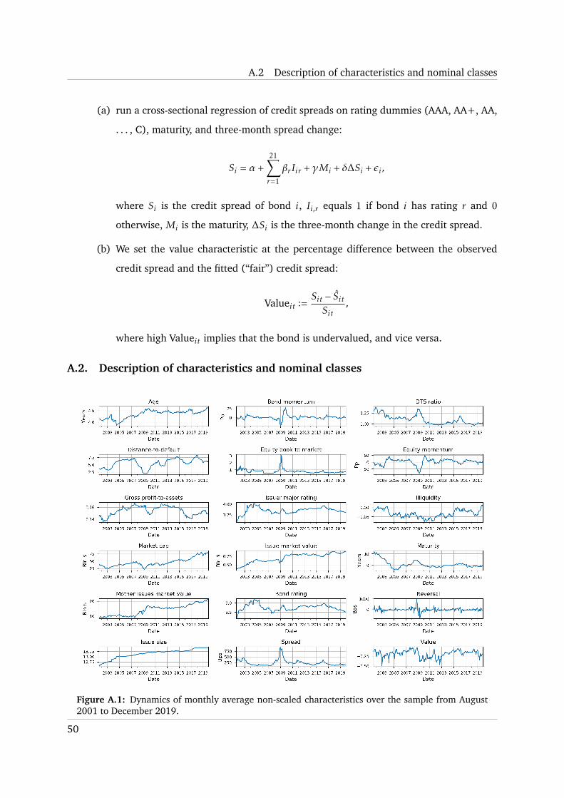
A.2 Description of characteristics and nominal classes

(a) run a cross-sectional regression of credit spreads on rating dummies (AAA, AA+, AA,

. . . , C), maturity, and three-month spread change:

Si = α +21∑r=1

βrIir +γMi + δ∆Si + εi ,

where Si is the credit spread of bond i, Ii,r equals 1 if bond i has rating r and 0

otherwise, Mi is the maturity, ∆Si is the three-month change in the credit spread.

(b) We set the value characteristic at the percentage difference between the observed

credit spread and the fitted (“fair”) credit spread:

Valueit :=Sit − SitSit

,

where high Valueit implies that the bond is undervalued, and vice versa.

A.2. Description of characteristics and nominal classes

Figure A.1: Dynamics of monthly average non-scaled characteristics over the sample from August2001 to December 2019.

50

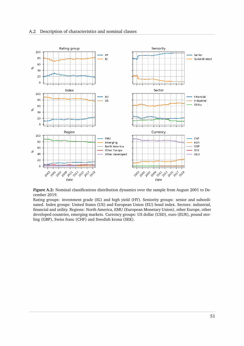
A.2 Description of characteristics and nominal classes

Figure A.2: Nominal classifications distribution dynamics over the sample from August 2001 to De-cember 2019.Rating groups: investment grade (IG) and high yield (HY). Seniority groups: senior and subordi-nated. Index groups: United States (US) and European Union (EU) bond index. Sectors: industrial,financial and utility. Regions: North America, EMU (European Monetary Union), other Europe, otherdeveloped countries, emerging markets. Currency groups: US dollar (USD), euro (EUR), pound ster-ling (GBP), Swiss franc (CHF) and Swedish krona (SEK).

51

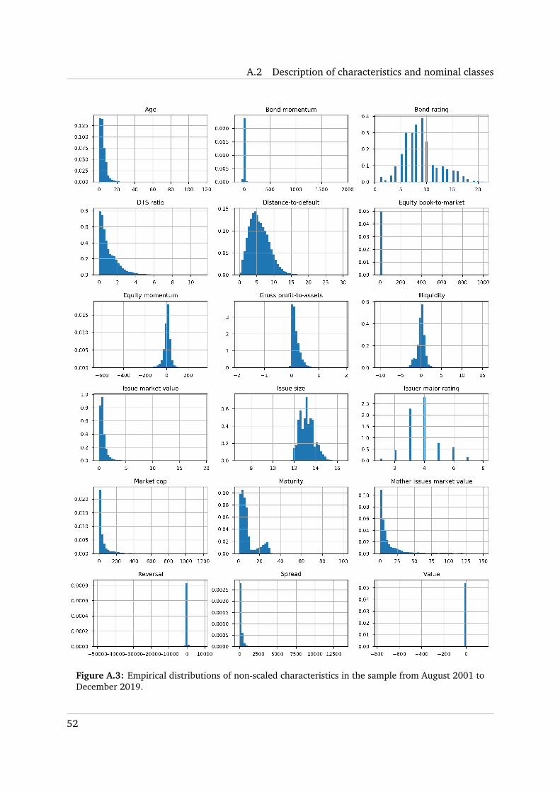
A.2 Description of characteristics and nominal classes

Figure A.3: Empirical distributions of non-scaled characteristics in the sample from August 2001 toDecember 2019.

52

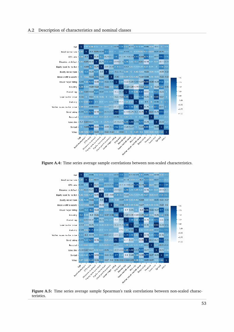
A.2 Description of characteristics and nominal classes

Figure A.4: Time series average sample correlations between non-scaled characteristics.

Figure A.5: Time series average sample Spearman’s rank correlations between non-scaled charac-teristics.

53

B. Methodology

B.1. New intuition behind IPCA

Consider a special case when:

1. There are two observed characteristics: L = 2;

2. There is one latent factor: K = 1;

3. Characteristics (instruments) are cross-sectionally scaled: z(l)t = 0, Var

(z

(l)it

)= 1 ∀l, t, where

Var (.) is the population cross-sectional variance.

4. The number of assets on each date is constant over time: Nt+1 =N ∀t.

Recall the formula for the matrix that maps observed characteristics into factor loadings:

vec(Γ ′β) =

T−1∑t=1

Z ′tZt ⊗ ft+1f′t+1

−1 T−1∑

t=1

[Z ′t ⊗ f ′t+1

]′rt+1

. (28)

Consider the second moment matrix of characteristics Z ′tZt:

Z ′tZt =

∑Nt+1i=1

[z

(1)it

]2 ∑Nt+1i=1 z

(1)it z

(2)it∑Nt+1

i=1 z(1)it z

(2)it

∑Nt+1i=1

[z

(2)it

]2

.Since z(l)

t = 0 ∀l, t, for the population variance it holds that

Var(z

(l)it

)=

1Nt+1

Nt+1∑i=1

[z

(l)it

]2.

Since we assume unit cross-sectional population variances and Nt+1 = N ∀t, it holds that∑Ni=1

[z

(l)it

]2=N ∀l. Thus,

Z ′tZt =

N∑Ni=1 z

(1)it z

(2)it∑N

i=1 z(1)it z

(2)it N

.54

B.1 New intuition behind IPCA

Note that

N∑i=1

z(1)it z

(2)it =N ×

∑Ni=1 z

(1)it z

(2)it

N=N ×

∑Ni=1 z

(1)it z

(2)it√

N ×N=N ×

∑Ni=1 z

(1)it z

(2)it√∑N

i=1

[z

(1)it

]2×∑Ni=1

[z

(2)it

]2,

where the sample correlation coefficient between characteristics with zero cross-sectional

sample means at time t is

ρ12,t =

∑Ni=1 z

(1)it z

(2)it√∑N

i=1

[z

(1)it

]2×∑Ni=1

[z

(2)it

]2

by definition, which implies∑Ni=1 z

(1)it z

(2)it =N × ρ12,t. Hence,

Z ′tZt =

N Nρ12,t

Nρ12,t N

.Denote:

M :=T−1∑t=1

Z ′tZt ⊗ ft+1f′t+1,

which is the inverse of the first multiplier in the Equation (28).

M =T−1∑t=1

Z ′tZt ⊗ ft+1f′t+1 =

∑T−1t=1 Nf

2t+1

∑T−1t=1 Nρ12,t f

2t+1∑T−1

t=1 Nρ12,t f2t+1

∑T−1t=1 Nf

2t+1

.

D = det(M) =

T−1∑t=1

Nf 2t+1

2

−

T−1∑t=1

Nρ12,t f2t+1

2

=N2

T−1∑t=1

f 2t+1

2

−

T−1∑t=1

ρ12,t f2t+1

2 .

M−1 =

T−1∑t=1

Z ′tZt ⊗ ft+1f′t+1

−1

=1D

N∑T−1t=1 f

2t+1 −N

∑T−1t=1 ρ12,t f

2t+1

−N∑T−1t=1 ρ12,t f

2t+1 N

∑T−1t=1 f

2t+1

.Consider the second multiplier in the Equation (28):

[Z ′t ⊗ f ′t+1

]′=

z

(1)1t ft+1 z

(2)1t ft+1

... ...

z(1)Nt+1,t

ft+1 z(2)Nt+1,t

ft+1

′

55

B.1 New intuition behind IPCA

[Z ′t ⊗ f ′t+1

]′rt+1 =

∑Nt+1i=1 z

(1)it ft+1ri,t+1∑Nt+1

i=1 z(2)it ft+1ri,t+1

T−1∑t=1

[Z ′t ⊗ f ′t+1

]′rt+1 =

∑T−1t=1

∑Nt+1i=1 z

(1)it ft+1ri,t+1∑T−1

t=1∑Nt+1i=1 z

(2)it ft+1ri,t+1

=

∑T−1t=1 ft+1

(∑Nt+1i=1 z

(1)it ri,t+1

)∑T−1t=1 ft+1

(∑Nt+1i=1 z

(2)it ri,t+1

)

Recall that xl,t+1 :=1

Nt+1

∑Nt+1i=1 z

(l)it ri,t+1 and that we assume Nt+1 =N ∀t. Thus

T−1∑t=1

[Z ′t ⊗ f ′t+1

]′rt+1 =

∑T−1t=1 ft+1Nx1,t+1∑T−1t=1 ft+1Nx2,t+1

=

N∑T−1t=1 ft+1x1,t+1

N∑T−1t=1 ft+1x2,t+1

.

Finally, transforming the two multipliers we obtain:

vec(Γ ′β) =1D

N∑T−1t=1 f

2t+1 −N

∑T−1t=1 ρ12,t f

2t+1

−N∑T−1t=1 ρ12,t f

2t+1 N

∑T−1t=1 f

2t+1

N

∑T−1t=1 ft+1x1,t+1

N∑T−1t=1 ft+1x2,t+1

=N2

D

∑T−1t=1 f

2t+1 −

∑T−1t=1 ρ12,t f

2t+1

−∑T−1t=1 ρ12,t f

2t+1

∑T−1t=1 f

2t+1

∑T−1t=1 ft+1x1,t+1∑T−1t=1 ft+1x2,t+1

=N2

D

[∑T−1

t=1 f2t+1

] [∑T−1t=1 ft+1x1,t+1

]−[∑T−1

t=1 ρ12,t f2t+1

] [∑T−1t=1 ft+1x2,t+1

][∑T−1

t=1 f2t+1

] [∑T−1t=1 ft+1x2,t+1

]−[∑T−1

t=1 ρ12,t f2t+1

] [∑T−1t=1 ft+1x1,t+1

] .

Denoting D∗ =[∑T−1

t=1 f2t+1

]2−[∑T−1

t=1 ρ12,t f2t+1

]2we receive N 2

D = 1D∗ . Divide and multiply

56

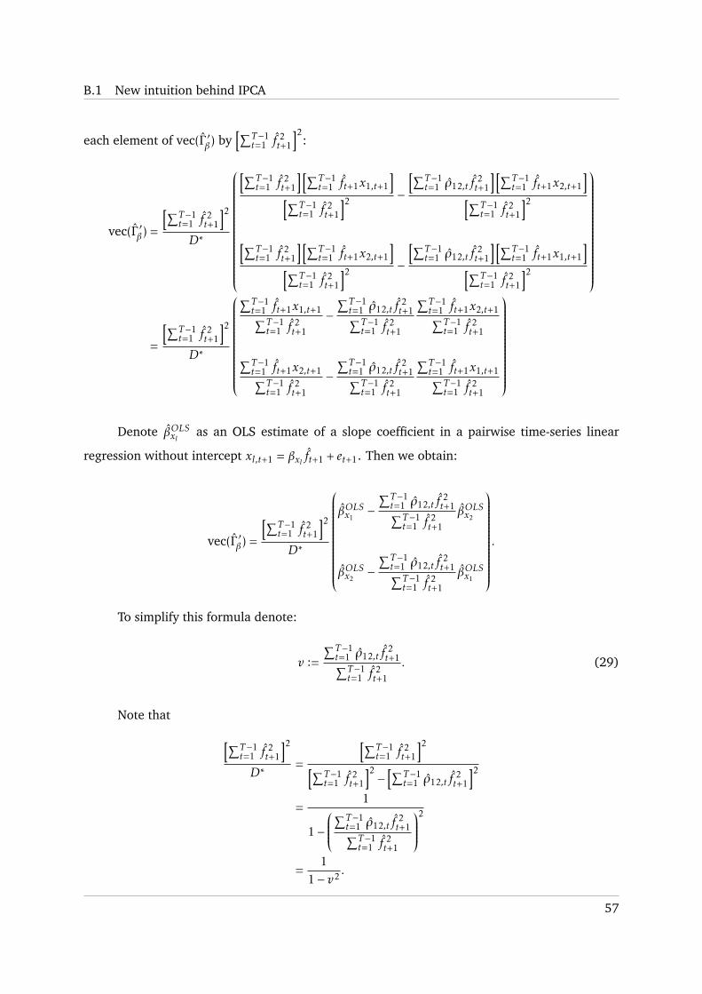
B.1 New intuition behind IPCA

each element of vec(Γ ′β) by[∑T−1

t=1 f2t+1

]2:

vec(Γ ′β) =

[∑T−1t=1 f

2t+1

]2D∗

[∑T−1t=1 f

2t+1

] [∑T−1t=1 ft+1x1,t+1

][∑T−1

t=1 f2t+1

]2 −

[∑T−1t=1 ρ12,t f

2t+1

] [∑T−1t=1 ft+1x2,t+1

][∑T−1

t=1 f2t+1

]2[∑T−1

t=1 f2t+1

] [∑T−1t=1 ft+1x2,t+1

][∑T−1

t=1 f2t+1

]2 −

[∑T−1t=1 ρ12,t f

2t+1

] [∑T−1t=1 ft+1x1,t+1

][∑T−1

t=1 f2t+1

]2

=

[∑T−1t=1 f

2t+1

]2D∗

∑T−1t=1 ft+1x1,t+1∑T−1

t=1 f2t+1

−∑T−1t=1 ρ12,t f

2t+1∑T−1

t=1 f2t+1

∑T−1t=1 ft+1x2,t+1∑T−1

t=1 f2t+1

∑T−1t=1 ft+1x2,t+1∑T−1

t=1 f2t+1

−∑T−1t=1 ρ12,t f

2t+1∑T−1

t=1 f2t+1

∑T−1t=1 ft+1x1,t+1∑T−1

t=1 f2t+1

Denote βOLSxl as an OLS estimate of a slope coefficient in a pairwise time-series linear

regression without intercept xl,t+1 = βxl ft+1 + et+1. Then we obtain:

vec(Γ ′β) =

[∑T−1t=1 f

2t+1

]2D∗

βOLSx1−

∑T−1t=1 ρ12,t f

2t+1∑T−1

t=1 f2t+1

βOLSx2

βOLSx2−

∑T−1t=1 ρ12,t f

2t+1∑T−1

t=1 f2t+1

βOLSx1

.

To simplify this formula denote:

v :=∑T−1t=1 ρ12,t f

2t+1∑T−1

t=1 f2t+1

. (29)

Note that [∑T−1t=1 f

2t+1

]2D∗

=

[∑T−1t=1 f

2t+1

]2[∑T−1t=1 f

2t+1

]2−[∑T−1

t=1 ρ12,t f2t+1

]2=

1

1−

∑T−1t=1 ρ12,t f

2t+1∑T−1

t=1 f2t+1

2

=1

1− v2 .

57

B.1 New intuition behind IPCA

Define

u :=1

1− v2 =

[∑T−1t=1 f

2t+1

]2D∗

. (30)

Hence, we arrive at

vec(Γ ′β) = u

βOLSx1− vβOLSx2

βOLSx2− vβOLSx1

. (31)

Note that v ∈ [−1;1]. This is guaranteed since∣∣∣∣∑T−1

t=1 ρ12,t f2t+1

∣∣∣∣ ≤∑T−1t=1

∣∣∣∣ρ12,t f2t+1

∣∣∣∣ ≤∑T−1t=1 f

2t+1,

and thus

∣∣∣∣∣∣∣∑T−1t=1 ρ12,t f

2t+1∑T−1

t=1 f2t+1

∣∣∣∣∣∣∣ ∈ [0;1]. This also implies that u > 0 ∀|v| , 1.

Besides, we can interpret v using OLS estimate of a slope coefficient as well. We can write

this term as follows:

v =∑T−1t=1 ρ12,t f

2t+1∑T−1

t=1 f4t+1

∑T−1t=1 f

4t+1∑T−1

t=1 f2t+1

.

Denote βOLSρ,f 2 as an OLS estimate of a slope coefficient in the following pairwise linear

regression without intercept:

ρ12,t = βρ,f 2 f 2t+1 + et .

Therefore, we can write

v = βOLSρ,f 2

∑T−1t=1 f

4t+1∑T−1

t=1 f2t+1

,

where the second term is the ratio of the fourth moment of a latent factor estimate to its

second moment.

Using Equation (31) it becomes possible to interpret Γβ using OLS coefficient estimates.

Recall that u > 0 ∀|v| , 1, |v| ∈ [0;1] and ignore a rare case when |v| = 1. Then, for a characteristic

l it holds that (ceteris paribus)

• ∀v s.t. |v| , 1: ↑ βOLSxl =⇒↑ vec(Γ ′β)l;

• ∀v > 0(βOLSρ,f 2 > 0

): ↑ βOLSxm =⇒↓ vec(Γ ′β)l , where m , l;

• ∀v < 0(βOLSρ,f 2 < 0

): ↑ βOLSxm =⇒↑ vec(Γ ′β)l , where m , l.

Using the identification restriction for Γβ (Kelly et al., 2019) we obtain

58

B.2 Further research: clusters with similar within-cluster betas

vec(Γ ′β) =1√(

βOLSx1 − vβOLSx2

)2+(βOLSx2 − vβOLSx1

)2

βOLSx1− vβOLSx2

βOLSx2− vβOLSx1

. (32)

Assume ρ12,t = 0 ∀t. Therefore,∑T−1t=1 ρ12,t f

2t+1 = 0 and βOLS

ρ,f 2 = 0. The non-identified

solution becomes

vec(Γ ′β) = u

βOLSx1

βOLSx2

. (33)

After imposing the identification restriction (Kelly et al., 2019) we obtain

vec(Γ ′β) =1√(

βOLSx1

)2+(βOLSx2

)2

βOLSx1

βOLSx2

. (34)

These results also hold approximately if

1. the sample variances equal one when cross sections are sufficiently large (N ≈N − 1) or

2. Nt+1 is fairly stable over time (Nt+1 ≈N ∀t).

B.2. Further research: clusters with similar within-cluster betas

This can be achieved by the following iterative algorithm:

1. Initialization. Initialize cluster memberships of bonds using some nominal classification

(e.g. IG/HY split) or random assignment.

2. IPCA step. Estimate cluster-specific IPCA models.

3. Clustering step. Calculate average betas inside each cluster and group bonds according

to the smallest distance to these average betas:

ci,t = argminct∈{c1,t ,...,cC,t}

√√√K∑k=1

(β

(k)i,t |ct − β

(k)c,t |ct

)2.

4. Iterate between 2 and 3 until convergence.

This is a useful algorithm for those who believe that betas of bonds should not deviate

much from each other within each cluster-specific IPCA model. To illustrate, if some cluster

59

B.3 Interpretation of weighting schemes through latent returns

has a risk factor related to momentum, all bonds of this cluster should be similarly exposed

to this risk. Otherwise, bonds with a different magnitude of this beta should be assigned to a

different cluster. The clustering step borrows the idea of testing under null hypothesis - if the

bond belongs to a cluster, it should lie close to the center of mass of the betas’ distribution.

Unfortunately, in our empirical analysis the proposed estimation procedure does not con-

verge, but we think the general idea could be useful. Further studies may develop a converging

method that detects clusters with similar within-cluster IPCA betas.

B.3. Interpretation of weighting schemes through latent returns

Define the IPCA-implied latent return k of the bond i at time t + 1 as

r(k)i,t+1 := β(k)

it × f(k)t+1. (35)

Note that in IPCA the fitted return can be decomposed into the sum of the latent returns:

ri,t+1 =K∑k=1

r(k)i,t+1.

Define the mean latent return k in the cluster c at time t + 1 as

¯r(k)c,t+1 =

1Nct

Nct∑i=1

r(k)i,t+1, (36)

where Nct is the number of bonds from the cluster c with excess return available at t + 1.

We call the vector of means ¯rc,t+1 the centroid of the cluster c at time t. To define whether

latent returns of some bond are close to the centroid of the cluster c at time t, we may use the

Euclidean distance:

D(ri,t+1; ¯rc,t+1) =

√√√K∑k=1

(r

(k)i,t+1 − ¯r(k)

c,t+1

)2.

Using the definition of latent returns [Equation (35)], we can rewrite this distance as

60

B.3 Interpretation of weighting schemes through latent returns

D(ri,t+1; ¯rc,t+1) =

√√√K∑k=1

[f

(k)t+1 × β

(k)it − f

(k)t+1 × β

(k)ct

]2

=

√√√K∑k=1

[f

(k)t+1 ×

(β

(k)it − β

(k)ct

)]2

.

As a result, we obtain the Euclidean distance between IPCA betas, where pointwise dis-

tances are weighted by squared realizations of next-period risk factors:

D(ri,t+1; ¯rt+1) =

√√√K∑k=1

(f

(k)t+1

)2×(β

(k)it − β

(k)ct

)2. (37)

We can present a similar interpretation for the weighting scheme with squared risk prices.

Define a predictive latent return k as

r(k)i,t+1 := β(k)

it ×λ(k). (38)

Then

D(ri,t+1; ¯rt+1) =

√√√K∑k=1

[λ(k) × β(k)

it −λ(k) × β(k)ct

]2

=

√√√K∑k=1

(λ(k)

)2×(β

(k)it − β

(k)ct

)2.

(39)

Finally, if we define robust latent returns as

r∗i,t+1 := β(k)it ×λ

(k)∗ , (40)

61

B.4 Relation between Gaussian mixture and k-means

and cluster them, we apply the weighting scheme with squared robust risk prices:

D(r∗i,t+1; r∗t+1) =

√√√K∑k=1

[λ

(k)∗ × β

(k)it −λ

(k)∗ × β

(k)ct

]2

=

√√√K∑k=1

(λ

(k)∗

)2×(β

(k)it − β

(k)ct

)2.

(41)

B.4. Relation between Gaussian mixture and k-means

Consider clustering one-dimensional points using k-means and Gaussian mixture. In k-means

each data points y1, ..., yN are assigned to a cluster according to a smallest distance to a cluster

centroid µc in the Euclidean space:

ci = argminc=1,...,C

√(yi −µc

)2.

In Gaussian mixture the clustering step is the maximization of likelihood that a data point is

generated from a cluster-specific distribution c:

ci = argmaxc=1,...,C

1√2πσ2

c

exp{− 1

2σ2c

(yi −µc

)2}.

We can apply a natural logarithm to this likelihood, multiply the result by -1 and transform the

problem into minimization:

ci = argminc=1,...,C

[12

log(2π) +12

log(2σ2c ) +

12σ2c

(yi −µc

)2].

We can further ignore the first constant term. Assume that cluster-specific variance σ2c is irrel-

evant for optimization. Then, we can drop the second term and divide the third one by12σ2c .

Thus

ci = argminc=1,...,C

(yi −µc

)2,

which implies minimization of the squared Euclidean distance between data point yi and cen-

troid µc. We can apply a monotonous positive transformation by taking the square root and

62

B.4 Relation between Gaussian mixture and k-means

obtain

ci = argminc=1,...,C

√(yi −µc

)2,

which is equivalent to the clustering step in k-means. The similar derivation can be obtained

considering multidimensional points. Hence, if variance (covariance matrix) of clusters does not

affect cluster assignments, the solutions of Gaussian mixture and k-means coincide.

63

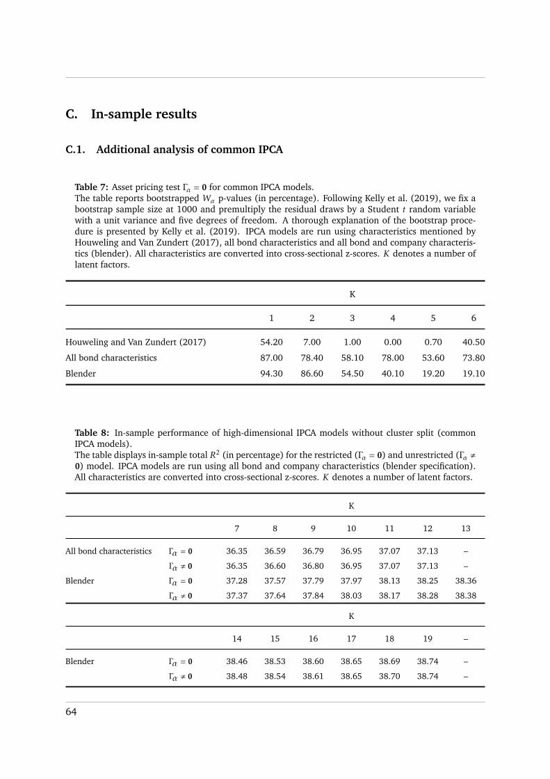
C. In-sample results

C.1. Additional analysis of common IPCA

Table 7: Asset pricing test Γα = 0 for common IPCA models.The table reports bootstrapped Wα p-values (in percentage). Following Kelly et al. (2019), we fix abootstrap sample size at 1000 and premultiply the residual draws by a Student t random variablewith a unit variance and five degrees of freedom. A thorough explanation of the bootstrap proce-dure is presented by Kelly et al. (2019). IPCA models are run using characteristics mentioned byHouweling and Van Zundert (2017), all bond characteristics and all bond and company characteris-tics (blender). All characteristics are converted into cross-sectional z-scores. K denotes a number oflatent factors.

K

1 2 3 4 5 6

Houweling and Van Zundert (2017) 54.20 7.00 1.00 0.00 0.70 40.50

All bond characteristics 87.00 78.40 58.10 78.00 53.60 73.80

Blender 94.30 86.60 54.50 40.10 19.20 19.10

Table 8: In-sample performance of high-dimensional IPCA models without cluster split (commonIPCA models).The table displays in-sample total R2 (in percentage) for the restricted (Γα = 0) and unrestricted (Γα ,0) model. IPCA models are run using all bond and company characteristics (blender specification).All characteristics are converted into cross-sectional z-scores. K denotes a number of latent factors.

K

7 8 9 10 11 12 13

All bond characteristics Γα = 0 36.35 36.59 36.79 36.95 37.07 37.13 –

Γα , 0 36.35 36.60 36.80 36.95 37.07 37.13 –

Blender Γα = 0 37.28 37.57 37.79 37.97 38.13 38.25 38.36

Γα , 0 37.37 37.64 37.84 38.03 38.17 38.28 38.38

K

14 15 16 17 18 19 –

Blender Γα = 0 38.46 38.53 38.60 38.65 38.69 38.74 –

Γα , 0 38.48 38.54 38.61 38.65 38.70 38.74 –

64

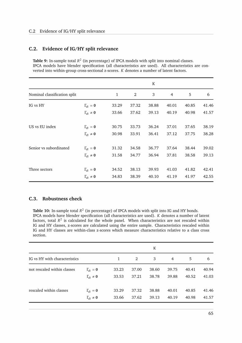
C.2 Evidence of IG/HY split relevance

C.2. Evidence of IG/HY split relevance

Table 9: In-sample total R2 (in percentage) of IPCA models with split into nominal classes.IPCA models have blender specification (all characteristics are used). All characteristics are con-verted into within-group cross-sectional z-scores. K denotes a number of latent factors.

K

Nominal classification split 1 2 3 4 5 6

IG vs HY Γα = 0 33.29 37.32 38.88 40.01 40.85 41.46

Γα , 0 33.66 37.62 39.13 40.19 40.98 41.57

US vs EU index Γα = 0 30.75 33.73 36.24 37.01 37.65 38.19

Γα , 0 30.98 33.91 36.41 37.12 37.75 38.28

Senior vs subordinated Γα = 0 31.32 34.58 36.77 37.64 38.44 39.02

Γα , 0 31.58 34.77 36.94 37.81 38.58 39.13

Three sectors Γα = 0 34.52 38.13 39.93 41.03 41.82 42.41

Γα , 0 34.83 38.39 40.10 41.19 41.97 42.55

C.3. Robustness check

Table 10: In-sample total R2 (in percentage) of IPCA models with split into IG and HY bonds.IPCA models have blender specification (all characteristics are used). K denotes a number of latentfactors, total R2 is calculated for the whole panel. When characteristics are not rescaled withinIG and HY classes, z-scores are calculated using the entire sample. Characteristics rescaled withinIG and HY classes are within-class z-scores which measure characteristics relative to a class crosssection.

K

IG vs HY with characteristics 1 2 3 4 5 6

not rescaled within classes Γα = 0 33.23 37.00 38.60 39.75 40.41 40.94

Γα , 0 33.53 37.21 38.78 39.88 40.52 41.03

rescaled within classes Γα = 0 33.29 37.32 38.88 40.01 40.85 41.46

Γα , 0 33.66 37.62 39.13 40.19 40.98 41.57

65

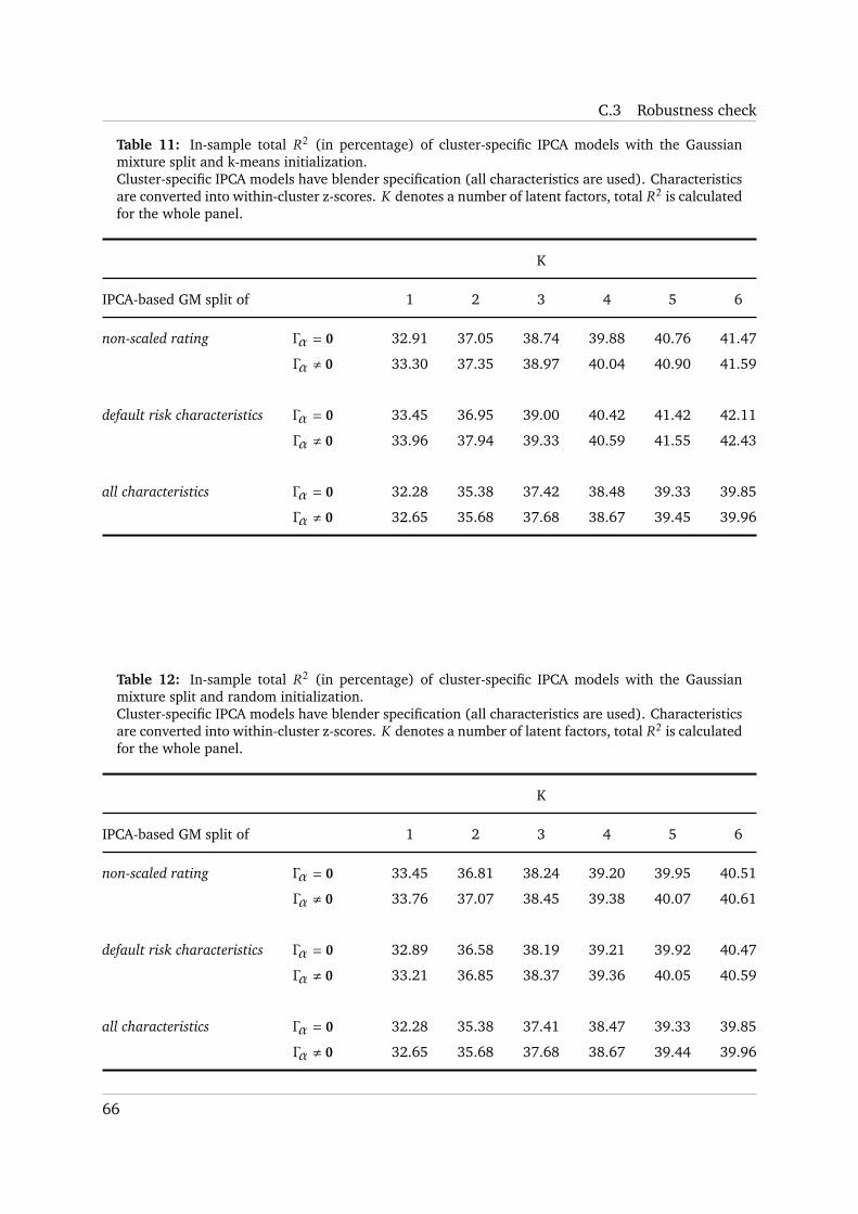
C.3 Robustness check

Table 11: In-sample total R2 (in percentage) of cluster-specific IPCA models with the Gaussianmixture split and k-means initialization.Cluster-specific IPCA models have blender specification (all characteristics are used). Characteristicsare converted into within-cluster z-scores. K denotes a number of latent factors, total R2 is calculatedfor the whole panel.

K

IPCA-based GM split of 1 2 3 4 5 6

non-scaled rating Γα = 0 32.91 37.05 38.74 39.88 40.76 41.47

Γα , 0 33.30 37.35 38.97 40.04 40.90 41.59

default risk characteristics Γα = 0 33.45 36.95 39.00 40.42 41.42 42.11

Γα , 0 33.96 37.94 39.33 40.59 41.55 42.43

all characteristics Γα = 0 32.28 35.38 37.42 38.48 39.33 39.85

Γα , 0 32.65 35.68 37.68 38.67 39.45 39.96

Table 12: In-sample total R2 (in percentage) of cluster-specific IPCA models with the Gaussianmixture split and random initialization.Cluster-specific IPCA models have blender specification (all characteristics are used). Characteristicsare converted into within-cluster z-scores. K denotes a number of latent factors, total R2 is calculatedfor the whole panel.

K

IPCA-based GM split of 1 2 3 4 5 6

non-scaled rating Γα = 0 33.45 36.81 38.24 39.20 39.95 40.51

Γα , 0 33.76 37.07 38.45 39.38 40.07 40.61

default risk characteristics Γα = 0 32.89 36.58 38.19 39.21 39.92 40.47

Γα , 0 33.21 36.85 38.37 39.36 40.05 40.59

all characteristics Γα = 0 32.28 35.38 37.41 38.47 39.33 39.85

Γα , 0 32.65 35.68 37.68 38.67 39.44 39.96

66

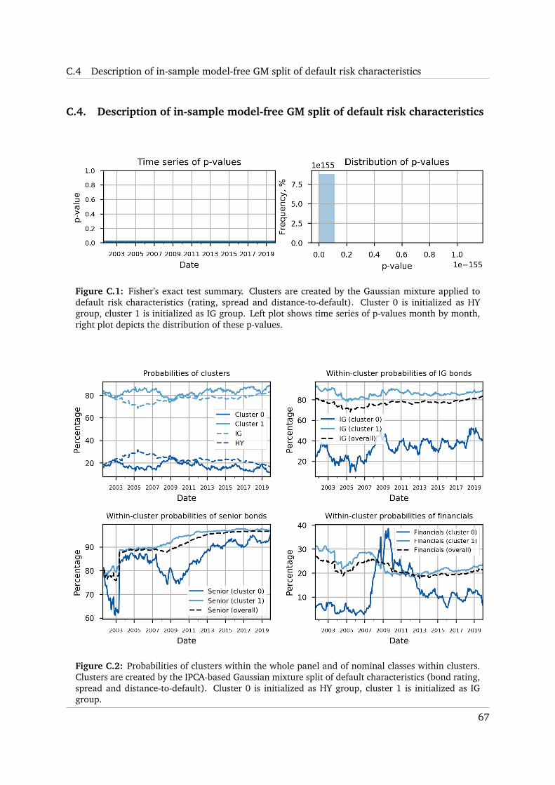
C.4 Description of in-sample model-free GM split of default risk characteristics

C.4. Description of in-sample model-free GM split of default risk characteristics

Figure C.1: Fisher’s exact test summary. Clusters are created by the Gaussian mixture applied todefault risk characteristics (rating, spread and distance-to-default). Cluster 0 is initialized as HYgroup, cluster 1 is initialized as IG group. Left plot shows time series of p-values month by month,right plot depicts the distribution of these p-values.

Figure C.2: Probabilities of clusters within the whole panel and of nominal classes within clusters.Clusters are created by the IPCA-based Gaussian mixture split of default characteristics (bond rating,spread and distance-to-default). Cluster 0 is initialized as HY group, cluster 1 is initialized as IGgroup.

67

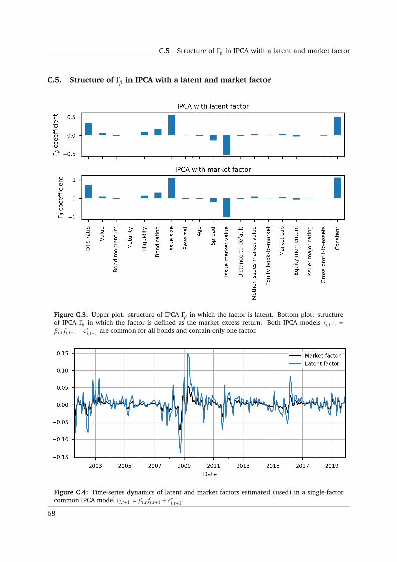
C.5 Structure of Γβ in IPCA with a latent and market factor

C.5. Structure of Γβ in IPCA with a latent and market factor

Figure C.3: Upper plot: structure of IPCA Γβ in which the factor is latent. Bottom plot: structureof IPCA Γβ in which the factor is defined as the market excess return. Both IPCA models ri,t+1 =βi,tfi,t+1 + ε∗i,t+1 are common for all bonds and contain only one factor.

Figure C.4: Time-series dynamics of latent and market factors estimated (used) in a single-factorcommon IPCA model ri,t+1 = βi,tfi,t+1 + ε∗i,t+1.

68

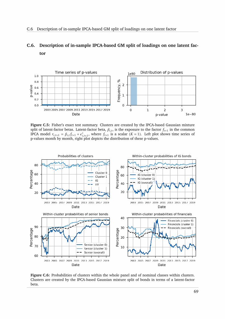
C.6 Description of in-sample IPCA-based GM split of loadings on one latent factor

C.6. Description of in-sample IPCA-based GM split of loadings on one latent fac-

tor

Figure C.5: Fisher’s exact test summary. Clusters are created by the IPCA-based Gaussian mixturesplit of latent-factor betas. Latent-factor beta, βi,t, is the exposure to the factor ft+1 in the commonIPCA model ri,t+1 = βi,tft+1 + ε∗i,t+1, where ft+1 is a scalar (K = 1). Left plot shows time series ofp-values month by month, right plot depicts the distribution of these p-values.

Figure C.6: Probabilities of clusters within the whole panel and of nominal classes within clusters.Clusters are created by the IPCA-based Gaussian mixture split of bonds in terms of a latent-factorbeta.

69

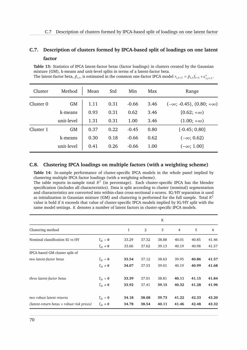
C.7 Description of clusters formed by IPCA-based split of loadings on one latent factor

C.7. Description of clusters formed by IPCA-based split of loadings on one latent

factor

Table 13: Statistics of IPCA latent-factor betas (factor loadings) in clusters created by the Gaussianmixture (GM), k-means and unit-level splits in terms of a latent-factor beta.The latent-factor beta, βi,t, is estimated in the common one-factor IPCA model ri,t+1 = βi,tft+1 +ε∗i,t+1.

Cluster Method Mean Std Min Max Range

Cluster 0 GM 1.11 0.31 -0.66 3.46 (−∞; -0.45), (0.80; +∞)

k-means 0.93 0.31 0.62 3.46 [0.62; +∞)

unit-level 1.31 0.31 1.00 3.46 (1.00; +∞)

Cluster 1 GM 0.37 0.22 -0.45 0.80 [-0.45; 0.80]

k-means 0.30 0.18 -0.66 0.62 (−∞; 0.62)

unit-level 0.41 0.26 -0.66 1.00 (−∞; 1.00]

C.8. Clustering IPCA loadings on multiple factors (with a weighting scheme)

Table 14: In-sample performance of cluster-specific IPCA models in the whole panel implied byclustering multiple IPCA factor loadings (with a weighting scheme).The table reports in-sample total R2 (in percentage). Each cluster-specific IPCA has the blenderspecification (includes all characteristics). Data is split according to cluster (nominal) segmentationand characteristics are converted into within-class cross-sectional z-scores. IG/HY separation is usedas initialization in Gaussian mixture (GM) and clustering is performed for the full sample. Total R2

value is bold if it exceeds that value of cluster-specific IPCA models implied by IG/HY split with thesame model settings. K denotes a number of latent factors in cluster-specific IPCA models.

K

Clustering method 1 2 3 4 5 6

Nominal classification IG vs HY Γα = 0 33.29 37.32 38.88 40.01 40.85 41.46

Γα , 0 33.66 37.62 39.13 40.19 40.98 41.57

IPCA-based GM cluster split of

two latent-factor betas Γα = 0 33.54 37.12 38.63 39.95 40.86 41.57

Γα , 0 34.07 37.53 39.01 40.19 40.99 41.68

three latent-factor betas Γα = 0 33.39 37.01 38.81 40.11 41.15 41.84

Γα , 0 33.92 37.41 39.15 40.32 41.28 41.96

two robust latent returns Γα = 0 34.18 38.08 39.73 41.22 42.33 43.20

(latent-return betas × robust risk prices) Γα , 0 34.78 38.54 40.11 41.46 42.48 43.32

70

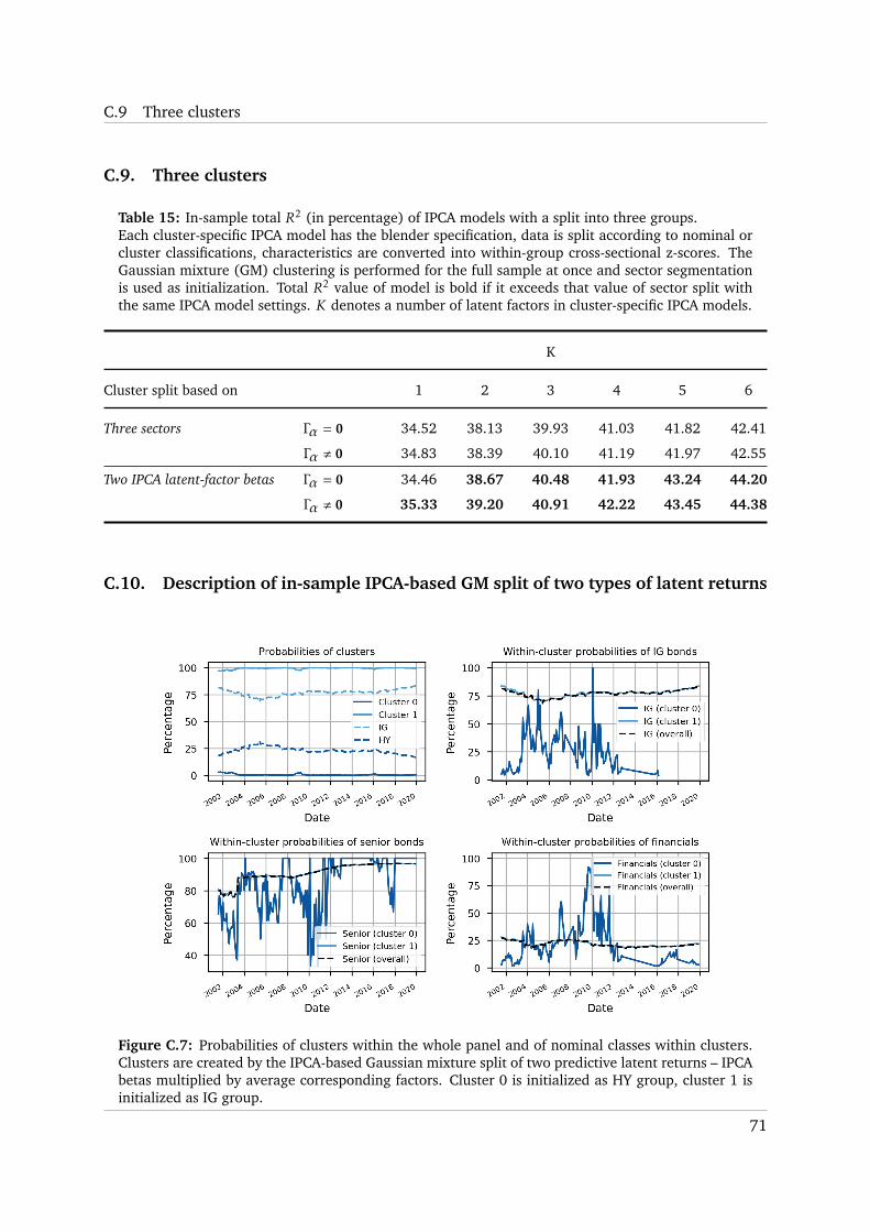
C.9 Three clusters

C.9. Three clusters

Table 15: In-sample total R2 (in percentage) of IPCA models with a split into three groups.Each cluster-specific IPCA model has the blender specification, data is split according to nominal orcluster classifications, characteristics are converted into within-group cross-sectional z-scores. TheGaussian mixture (GM) clustering is performed for the full sample at once and sector segmentationis used as initialization. Total R2 value of model is bold if it exceeds that value of sector split withthe same IPCA model settings. K denotes a number of latent factors in cluster-specific IPCA models.

K

Cluster split based on 1 2 3 4 5 6

Three sectors Γα = 0 34.52 38.13 39.93 41.03 41.82 42.41

Γα , 0 34.83 38.39 40.10 41.19 41.97 42.55

Two IPCA latent-factor betas Γα = 0 34.46 38.67 40.48 41.93 43.24 44.20

Γα , 0 35.33 39.20 40.91 42.22 43.45 44.38

C.10. Description of in-sample IPCA-based GM split of two types of latent returns

Figure C.7: Probabilities of clusters within the whole panel and of nominal classes within clusters.Clusters are created by the IPCA-based Gaussian mixture split of two predictive latent returns – IPCAbetas multiplied by average corresponding factors. Cluster 0 is initialized as HY group, cluster 1 isinitialized as IG group.

71

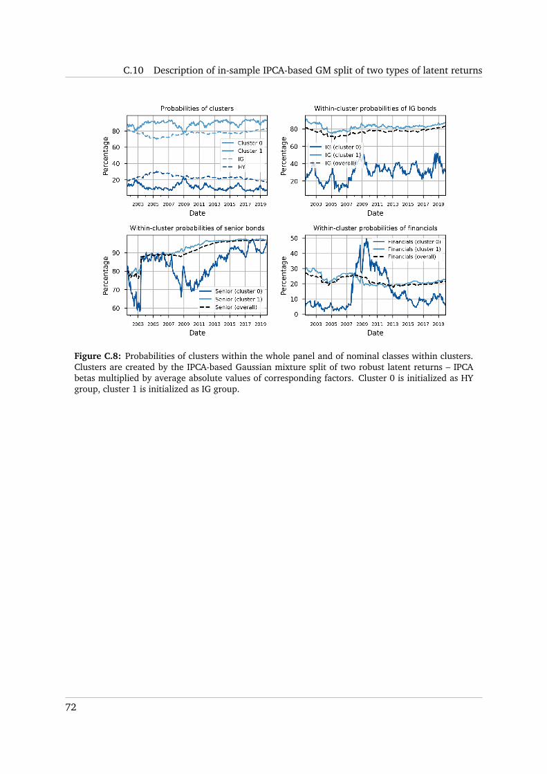
C.10 Description of in-sample IPCA-based GM split of two types of latent returns

Figure C.8: Probabilities of clusters within the whole panel and of nominal classes within clusters.Clusters are created by the IPCA-based Gaussian mixture split of two robust latent returns – IPCAbetas multiplied by average absolute values of corresponding factors. Cluster 0 is initialized as HYgroup, cluster 1 is initialized as IG group.

72

D. Python programming files description

D.1. Utils

These are modules (libraries) mostly created by the author for the research. They are pre-

uploaded in the notebooks where they are needed.

1. clustering.py

The module contains functions to run clustering models.

2. correlation analytics.py

The module contains functions to run some correlation analysis.

3. feature filtering.py

The module contains functions to create some features (characteristics).

4. fill NaNs.py

The module contains a general function to fill missing values.

5. finalize data.py

The module contains general functions to drop missing values and rank and scale charac-

teristics cross-sectionally.

6. MCS.py

The module contains code created by Michael Gong

(https://michael-gong.com/blogs/model-confidence-set/) to run the Model Confidence

Set procedure (Hansen et al., 2011).

7. merge many.py

The module contains a function to merge multiple data frames into one data frame fast.

8. myIPCA.py

The module contains some code created by the author to run IPCA (Kelly et al., 2019)

from scratch.

9. PruittIPCA.py

The module contains the code to run IPCA (Kelly et al., 2019) provided by S. Pruitt

(https://sethpruitt.net/research/downloads/) and enhanced by the author.

73

D.2 Notebooks

10. quality metrics.py

The module contains functions to calculate some quality metrics.

11. regressions.py

The module contains a function to run OLS regressions.

D.2. Notebooks

This is a folder with Jupyter notebooks used for the research. By running the code in the order

of numbered folders one must be able to reproduce research results.

1. Data Preprocessing

(a) Gather data.ipynb

The notebook gathers original data files, selects data from 1994 onwards, drops some

useless columns and columns with perfect multicollinearity and creates data with

bonds from the bond universe only.

(b) Feature filtering.ipynb

The notebook removes, preprocesses and creates characteristics, removes observa-

tions having unrealistic values (e.g. negative duration) and detects highly correlated

characteristics.

(c) Finalize data dropna.ipynb

The notebook selects data from August 2001 onwards, applies some final filtering,

drops non-public companies and missing values.

(d) Finalize data scale.ipynb

The notebook creates cross-sectional ranks from characteristics and converts them

into cross-sectional z-scores according to Kozak et al. (2020).

2. Data Description

(a) Dropna data description.ipynb

The notebook outputs data description.

3. IPCA without cluster structure

74

D.2 Notebooks

(a) Arbitrary IPCA.ipynb

The notebook allows to run arbitrary IPCA and can be used by an interested reader

to try their own ideas.

(b) AllBondCharacteristics IPCA.ipynb

The notebook runs in-sample common IPCA with all bond characteristics.

(c) Blender IPCA.ipynb

The notebook runs in-sample common IPCA with all bond and company characteris-

tics (blender specification).

(d) HouwelingVanZundert IPCA.ipynb

The notebook runs in-sample common IPCA with characteristics mentioned by Houwel-

ing and Van Zundert (2017).

4. IPCA with nomclass split

(a) NominalClassifications IPCA.ipynb

The notebook runs in-sample IPCA with splits according to IG/HY, bond index, senior-

ity and sector segmentation and out-of-sample IPCA according to IG/HY grouping.

5. Holy grail

(a) HolyGrail INSAMPLE.ipynb

The notebook runs the holy grail models in the in-sample framework.

(b) HolyGrail ROLLING WINDOW.ipynb

The notebook runs the holy grail models in the out-of-sample framework which are

presented in the main text of the thesis. Its results are not presented in the thesis, but

the notebook can be used for further research.

6. IPCA with statistical cluster structure (in-sample)

Perform in-sample clustering and then run in-sample cluster-specific IPCA models.

(a) IPCA INSAMPLE clustering characteristics.ipynb

The notebook runs in-sample model-free clustering.

(b) IPCA INSAMPLE clustering market betas.ipynb

The notebook runs in-sample clustering of market betas.

75

D.2 Notebooks

(c) IPCA INSAMPLE clustering stat loadings.ipynb

The notebook runs in-sample clustering of IPCA loadings on one latent factor.

(d) IPCA INSAMPLE clustering stat loadings more betas.ipynb

The notebook runs in-sample clustering of IPCA loadings on multiple latent factors.

(e) IPCA INSAMPLE clustering stat loadings three clusters.ipynb

The notebook runs in-sample clustering of IPCA factor loadings to find three clusters.

(f) IPCA INSAMPLE clustering stat loadings weighting schemes.ipynb

The notebook runs in-sample clustering of IPCA loadings on multiple latent factors

with weighting schemes.

7. IPCA with statistical cluster structure (out-of-sample)

Perform out-of-sample clustering and then run out-of-sample cluster-specific IPCA models.

(a) IPCA OOS GM clustering market betas.ipynb

The notebook runs out-of-sample clustering of market betas using the Gaussian mix-

ture.

(b) IPCA OOS GM clustering stat betas.ipynb

The notebook runs out-of-sample clustering of IPCA loadings on one latent factor

using the Gaussian mixture.

(c) IPCA OOS unit level split stat betas.ipynb

The notebook runs out-of-sample unit-level split of IPCA loadings on one latent factor.

8. Model analysis

(a) Cluster analysis.ipynb

The notebook outputs Fisher’s exact test summary and relation to nominal classes of

statistical clusters.

(b) Common IPCA analysis.ipynb

The notebook outputs analysis of common IPCA with one market factor and one

latent factor.

9. Statistical testing

76

D.2 Notebooks

(a) MCS.ipynb

The notebook runs the Model Confidence Set procedure (Hansen et al., 2011) to com-

pare time series of RSS of in-sample and out-of-sample IPCA models with statistical

cluster structure to IPCA models with IG/HY structure.

77