Embed Size (px)
Citation preview

Thermal radiation interpreted by a three-year old
Learning to Analyze what is Beyond the Visible Spectrum
Linköping Studies in Science and TechnologyDissertation No. 2024
Amanda Berg
Amanda Berg Learning to Analyze w
hat is Beyond the Visible Spectrum
2019
FACULTY OF SCIENCE AND ENGINEERING
Linköping Studies in Science and Technology, Dissertation No. 2024, 2019 Department of Electrical Engineering
Linköping UniversitySE-581 83 Linköping, Sweden
www.liu.se

Linköping Studies in Science and TechnologyDisserta ons, No. 2024
Learning to Analyze what is Beyond the Visible Spectrum
Amanda Berg
Linköping UniversityDepartment of Electrical Engineering
Computer Vision LaboratorySE-581 83 Linköping, Sweden
Linköping 2019

Edition 1:1
© Amanda Berg, 2019ISBN 978-91-7929-981-1ISSN 0345-7524URL http://urn.kb.se/resolve?urn=urn:nbn:se:liu:diva-161077
Published articles have been reprinted with permission from the respectivecopyright holder.Typeset using XƎTEX
Printed by LiU-Tryck, Linköping 2019
ii

For Olov and Alfons
iii


POPULÄRVETENSKAPLIG SAMMANFATTNING
Sensorer som kan mäta termisk infraröd strålning över ett större område och produceraen visuell bild, så kallade värmekameror, har länge använts för militärt bruk. Däremot harvärmekameror inte varit lika vanliga inom civila tillämpningar, främst på grund av att de harvarit dyra och utrymmeskrävande. På senare år har utvecklingen gått framåt och samtidigtsom kamerorna blivit mindre och billigare har även bildkvalitén förbättrats avsevärt. Nufinns det till och med små värmekameror att fästa på eller bygga in i mobiltelefoner. I taktmed att värmekamerorna har blivit mindre och billigare så har fler civila tillämpningarvuxit fram. Till exempel har det blivit vanligt att använda värmekameror i industrin, föreftersökning av försvunna personer, i säkerhetssystem i bilar, för att upptäcka bränder ochi medicinska sammanhang, för att nämna några. Jämfört med kameror känsliga för synligtljus är de fördelaktiga i många situationer eftersom de kan producera en bild i totalt mörker.Värmekameror gör inte heller lika mycket intrång på personlig integritet.
Denna avhandling behandlar området automatisk bildanalys i termiskt infraröda bilder ochvideo. Fokus ligger på maskininlärning, en undergrupp till området artificiell intelligens.En vanlig missuppfattning är att bildanalys i termiskt infraröda bilder är identiskt medbildanalys i visuella gråskalebilder. Avhandlingen visar att föregående påstående inte alltidstämmer. Så länge en metod designad för visuella bilder inte är beroende av färgattributkan den appliceras på termiskt infrarött, men resultaten för olika metoder har visat sigvariera beroende på om de används på visuella eller termiska sekvenser. Det vill säga, olikaangreppssätt fungerar olika bra i de två olika modaliteterna.
Tre olika typer av bildanalysproblem studeras i avhandlingen: visuell objektsföljning, ano-malidetektion, och övergångar mellan två olika modaliteter. Det bedrivs mycket forskninginom alla tre områdena och de är också är relevanta för många civila tillämpningar.
För det första problemet, visuell objektsföljning, innehåller avhandlingen tre bidrag sombehandlar utvärdering av metoder för så kallad korttidsföljning, d.v.s, följning av enstakaobjekt i korta sekvenser givet objektets initiala position och utbredning. Det första bidragetär ett dataset som bland annat använts i den första tävlingen i korttidsföljning i termiskinfraröd video. Det andra bidraget är en metod för semi-automatisk annotering av multi-modala videosekvenser. Slutligen föreslås också en metod för automatisk korttidsföljning avett objekt i termisk infraröd video.
Det andra problemet, anomalidetektion, avser detektion av sällsynta objekt eller händelser,så kallade anomalier. Det första bidraget inom detta område är en metod för anomalide-tektion där det inte finns några exempel på hur anomalierna ser ut. Metoden bygger på såkallade generativa adversiella nätverk, en form av neurala nätverk. Det andra bidraget är enmetod för hinderdetektion framför tåg, ett tidigare obehandlat problem. Metoden uppdate-rar kontinuerligt en modell av bakgrunden och detektioner av hinder definieras som missadedetektioner av bakgrund. Det tredje och sista bidraget inom området anomalidetektion ären metod för karaktärisering och klassificering av automatiskt detekterade fjärrvärmeläckormed syfte att minimera antalet falsklarm.
Slutligen, så innehåller avhandlingen också ett bidrag inom området för övergång mellantvå olika modaliteter. Övergången från termiskt infrarött till perceptuellt realistiska visuellabilder är också det ett tidigare obehandlat problem, relevant för till exempel säkerhetssystemi bilar. Metoden som föreslås använder sig av neurala nätverk och drar nytta av den skillnadi skärpa som finns hos det mänskliga ögat för skillnader i färg jämfört med skillnader iluminans.
v

ABSTRACT
Thermal cameras have historically been of interest mainly for military applications. Increas-ing image quality and resolution combined with decreasing camera price and size duringrecent years have, however, opened up new application areas. They are now widely usedfor civilian applications, e.g., within industry, to search for missing persons, in automotivesafety, as well as for medical applications. Thermal cameras are useful as soon as thereexists a measurable temperature difference. Compared to cameras operating in the visualspectrum, they are advantageous due to their ability to see in total darkness, robustness toillumination variations, and less intrusion on privacy.
This thesis addresses the problem of automatic image analysis in thermal infrared imageswith a focus on machine learning methods. The main purpose of this thesis is to study thevariations of processing required due to the thermal infrared data modality. In particular,three different problems are addressed: visual object tracking, anomaly detection, andmodality transfer. All these are research areas that have been and currently are subjectto extensive research. Furthermore, they are all highly relevant for a number of differentreal-world applications.
The first addressed problem is visual object tracking, a problem for which no prior in-formation other than the initial location of the object is given. The main contributionconcerns benchmarking of short-term single-object (STSO) visual object tracking methodsin thermal infrared images. The proposed dataset, LTIR (Linköping Thermal Infrared),was integrated in the VOT-TIR2015 challenge, introducing the first ever organized chal-lenge on STSO tracking in thermal infrared video. Another contribution also related tobenchmarking is a novel, recursive, method for semi-automatic annotation of multi-modalvideo sequences. Based on only a few initial annotations, a video object segmentation(VOS) method proposes segmentations for all remaining frames and difficult parts in needfor additional manual annotation are automatically detected. The third contribution to theproblem of visual object tracking is a template tracking method based on a non-parametricprobability density model of the object’s thermal radiation using channel representations.
The second addressed problem is anomaly detection, i.e., detection of rare objects or events.The main contribution is a method for truly unsupervised anomaly detection based on Gen-erative Adversarial Networks (GANs). The method employs joint training of the generatorand an observation to latent space encoder, enabling stratification of the latent space and,thus, also separation of normal and anomalous samples. The second contribution is thepreviously unaddressed problem of obstacle detection in front of moving trains using atrain-mounted thermal camera. Adaptive correlation filters are updated continuously andmissed detections of background are treated as detections of anomalies, or obstacles. Thethird contribution to the problem of anomaly detection is a method for characterizationand classification of automatically detected district heat leakages for the purpose of falsealarm reduction.
Finally, the thesis addresses the problem of modality transfer between thermal infrared andvisual spectrum images, a previously unaddressed problem. The contribution is a methodbased on Convolutional Neural Networks (CNNs), enabling perceptually realistic trans-formations of thermal infrared to visual images. By careful design of the loss function themethod becomes robust to image pair misalignments. The method exploits the lower acuityfor color differences than for luminance possessed by the human visual system, separatingthe loss into a luminance and a chrominance part.
vi

Acknowledgments
As my masters degree was approaching in 2013, I was thinking about what todo with my future. I had at that time spent many years within the educationalsystem and felt a desire to try something different. I was not quite sure aboutprecisely what I wanted to do, but I was completely certain that I did notwant to enrol as a PhD student, and yet, here I am. The opportunity tocombine industry and academia as an industrial PhD student was an offer Icould not refuse, a decision I have (almost) never regretted.
There have been many emotions related to this journey. I have been deter-mined to succeed, while at the same time scared to fail. I have been nervousprior to presentations, happy and proud of fellow PhD students, and grate-ful for being given this opportunity. At the same time, I have been angryat unfair reviews and confusing code, tired and fed-up with late nights, an-noyed and irritated as deadlines have approached, relieved as they were over,dejected after rejects and hopeful after accepts. I have felt lost among codelines, while at the same time focused on the goal, divided between academiaand industry, while at the same time strengthened by the combination. Tobe honest, I have not loved every part of the journey, but being a part of theacademic society is a wonderful thing. I have met numerous inspiring, bright,persons of which I would like to mention a few in particular.
First and foremost, I would like to thank my main supervisor MichaelFelsberg for always being positive but still realistic and objective, I have re-ally appreciated that. Thank you for all the interesting discussions, guidance,and support. For my co-supervisor Jörgen Ahlberg, I am not sure where tobegin. Without you, I would never have started this journey in the first place.I am grateful that you encouraged me and, all this time, you have believed inme at times when I have not done so myself. Thank you for always answeringmy questions in a very sensible way, not matter how stupid they might be.
As an industrial PhD student, I have been fortunate enough to experi-ence the best of both academia and industry. I would like to thank all of mycolleagues at the company Termisk Systemteknik AB. Even though thecompany is unusually academic in its nature it has given me a well-needed con-nection to the real world. Thank you Stefan Sjökvist and Jörgen Ahlbergfor accepting me for the district heating master thesis project what feels like
vii

ages ago, Claes Nelsson for bringing order during periods of confusion, Mag-nus Uppsäll for the bad jokes, Staffan Cederkrantz, Göran Carlsson,Patrik Stensbo, and Patrik Svensson for helping me with practical stuff,such as operating a thermal camera, and finally, David Rexander and Per-Magnus Olsson for advices regarding programming issues. I would also liketo give additional thanks to Patrik Stensbo who helped me with the permitnecessary for the cover aerial thermal image.
While being on a journey of this kind, it helps to have others persons inyour vicinity who actually understand what you are complaining about. Iwould like to thank all of my colleagues at the Computer Vision Labo-ratory at Linköping University for the support and interesting discussions.In particular, past and present fellow PhD students for the support in pe-riods of doubt, and my roommates Gustav Häger and Kristoffer Öfjällfor mutual whining sessions. I am also very grateful to Joakim Johnander,Abdelrahman Eldesokey, Felix Järemo-Lawin, Mikael Persson, andGustav Häger who has proof-read parts of this thesis. I would also like tothank Bertil Grelsson for kindly sharing the thesis template.
Believe it or not, there is a life outside work as well. Thank you Familyand Friends for your love, support, and the much appreciated distractionswhenever needed. In particular, my husband Olov Johansson Berg whohas been passively exposed to the life of a PhD student. You are my rock inlife. Thank you for supporting me through all of the ups and downs, alwayscheering.
Finally, Alfons Berg, we are fortunate to have you in our lives. Yourarrival forced me to take a well-needed break where I could focus on whatis important in life. In the last couple of years, your unconditional love hashelped me through tough periods. Nothing beats a hug from you.
The research leading to this thesis has been funded by the Swedish Re-search Council through the project Learning Systems for Remote Ther-mography, grant no. D0570301, the European Community FrameworkProgramme 7, through the projects Privacy Preserving Perimeter Protec-tion Project (P5), grant agreement no. 312784, and Intelligent Piracy Avoid-ance using Threat detection and Countermeasure Heuristics (IPATCH), grantagreement no. 607567, as well as the ECSEL Joint Undertaking undergrant agreement no. 783221, Aggregate FARming in the CLOUD (AFar-Cloud).
Linköping, October 2019Amanda Berg
viii

About the cover(Front) A mosaic of aerial thermal infrared images and a set of connected,artificial, neurons organized in the shape of a brain to symbolize artificiallearning for the purpose of automatic image analysis.(Back) Thermal radiation interpreted by a three-year old.
ix
Contents
Abstract v
Acknowledgments ix
Contents x
I Background 1
1 Introduction 31.1 Motivation . . . . . . . . . . . . . . . . . . . . . . . . . . . . . . . . 31.2 Goals of this thesis . . . . . . . . . . . . . . . . . . . . . . . . . . . 51.3 Contributions . . . . . . . . . . . . . . . . . . . . . . . . . . . . . . 61.4 Outline . . . . . . . . . . . . . . . . . . . . . . . . . . . . . . . . . . 81.5 Included publications . . . . . . . . . . . . . . . . . . . . . . . . . 101.6 Additional publications . . . . . . . . . . . . . . . . . . . . . . . . 18
2 Thermal Infrared Imaging 212.1 Infrared and thermal radiation . . . . . . . . . . . . . . . . . . . . 212.2 Thermal imaging . . . . . . . . . . . . . . . . . . . . . . . . . . . . 232.3 Advantages and limitations of thermal imaging . . . . . . . . . . 262.4 Image analysis in thermal infrared images . . . . . . . . . . . . . 27
3 Representation 293.1 Representations of visual information . . . . . . . . . . . . . . . . 293.2 Sparse representations . . . . . . . . . . . . . . . . . . . . . . . . . 303.3 Grid-based representations . . . . . . . . . . . . . . . . . . . . . . 303.4 Channel representations . . . . . . . . . . . . . . . . . . . . . . . . 31
4 Learning Methods 354.1 Intelligence and learning . . . . . . . . . . . . . . . . . . . . . . . 354.2 Introduction to machine learning . . . . . . . . . . . . . . . . . . 354.3 Online learning . . . . . . . . . . . . . . . . . . . . . . . . . . . . . 374.4 Ensemble learning . . . . . . . . . . . . . . . . . . . . . . . . . . . 384.5 Neural networks and deep learning . . . . . . . . . . . . . . . . . 41
x

5 Addressed Problems within Thermal Infrared Image Analysis 515.1 Visual object tracking . . . . . . . . . . . . . . . . . . . . . . . . . 515.2 Anomaly detection . . . . . . . . . . . . . . . . . . . . . . . . . . . 605.3 Cross-spectral transfer learning . . . . . . . . . . . . . . . . . . . 655.4 Relevance to real-world applications . . . . . . . . . . . . . . . . 69
6 Concluding Remarks 716.1 Conclusions and discussion . . . . . . . . . . . . . . . . . . . . . . 716.2 Future work . . . . . . . . . . . . . . . . . . . . . . . . . . . . . . . 726.3 Impact on society . . . . . . . . . . . . . . . . . . . . . . . . . . . 73
Bibliography 75
II Publications 95
Paper A A Thermal Object Tracking Benchmark 97
Paper B Semi-automatic Annotation of Objects in Visual-Thermal Video
107
Paper C Channel Coded Distribution Field Tracking for Ther-mal Infrared Imagery 121
Paper D Detecting Rails and Obstacles using a Train-Mounted Thermal Camera
133
Paper E Enhanced Analysis of Thermographic Images forMonitoring of District Heat Pipe Networks 149
Paper F Unsupervised Adversarial Learning of Anomaly De-tection in the Wild
163
Paper G Generating Visible Spectrum Images from ThermalInfrared
175
xi


Part I
Background
1


1
Introduction
Automatic image analysis in thermal infrared images has historically been ofinterest mainly for military purposes. Increasing image quality and resolutioncombined with decreasing camera price and size during recent years have,however, opened up new application areas. Thermal cameras are advanta-geous in many applications due to their ability to see in total darkness, theirrobustness to illumination changes, and less intrusion on privacy. Thermalinfrared images are visual displays of the measured thermal infrared radiationwithin an area and they can reveal additional information beyond the visiblespectrum, a few examples are provided in Fig. 1.1.
This thesis addresses automatic analysis in thermal infrared images witha focus on machine learning methods. The main purpose is to study the vari-ations of processing required due to the thermal infrared data modality. Thethesis addresses three problems highly relevant for a number of different real-world applications: visual object tracking, anomaly detection, and modalitytransfer.
1.1 Motivation
The electromagnetic spectrum is broad and divided into smaller bands basedon their different properties. Close to the visual part lies the near infraredwavelength band. Visual and near infrared cameras measure mostly reflectedradiation. Radiation within the thermal infrared wavelength band have longerwavelength. In contrast to visual and near infrared cameras, thermal cam-eras measure mostly emitted radiation. The observed phenomena related toreflected and emitted radiation differ in several aspects, indicating that imageanalysis in thermal infrared images is slightly different than that of visualimages.
There are two common misconceptions regarding image analysis in ther-mal infrared images. The first misconception is related to the temperature
3

1. Introduction
(a) (b) (c)
Figure 1.1: Thermal infrared images can provide additional information be-yond what can be seen in the visible spectrum. (a) Someone has been walkingon the floor, (b) someone has touched the plant, (c) a thermal infrared imagereveals which bricks have been touched recently.
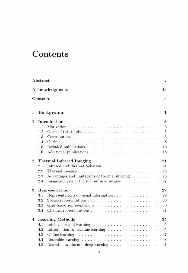
of interesting objects in the scene. It is often assumed to be significantlydifferent than the temperature of the background, requiring only a straight-forward threshold in order to separate an interesting object from background.This assumption is valid in some special cases, but for most applications thesituation is more complex, some examples are provided in Fig. 1.2. Objecttemperatures may vary over the object and some parts may be of the sametemperature as the background. The second misconception is that thermal in-frared image analysis is identical to image analysis of grayscale visual images.Hence, image analysis methods suitable for visual images would also be suit-able for thermal infrared images. There are, however, significant differencesbetween the two types of imagery. For example, in the noise characteris-tics, the amount of discernible spatial patterns, the data format, and how theemitted radiation behave in comparison to reflected radiation.
Machine learning, as a part of the broader field of artificial intelligence, isan area of intense research. A machine learning method is an algorithm that isable to learn from data. As one of the keys to understanding intelligence itself,learning methods provide a highly effective approach to solving problems toocomplex for hand-crafted programs designed by humans. Machine learningmethods can solve many different types of tasks. In this thesis, they areapplied to the problems of: visual object tracking, anomaly detection, andmodality transfer.
Many applications connected to thermal cameras can be related to a sus-tainable society, for example, prevention and localisation of energy losses, as
4
1.2. Goals of this thesis
(a) (b) (c)
Figure 1.2: A few examples of situations where thresholding based on tem-perature in order to separate an interesting object from the background willnot work.
well as environmental friendly transportation. Two of the included publica-tions address these areas. Paper E addresses reduction of false alarms amongautomatically detected district heating leakages. Detection is performed inthermographic images captured with an airborne thermal camera. In addi-tion, a method for temporal analysis of energy losses of a district heatingnetwork given two or more acquisitions of thermal imagery is presented. InPaper D, an automatic method for rail and obstacle detection using a train-mounted thermal camera is proposed. The system aims at providing an earlywarning to train drivers under impaired view. An early warning enables thedriver to break before collision, significantly reducing repair costs.
1.2 Goals of this thesis
The aim of the work leading to this thesis has been to study the variationsof processing required due to the thermal infrared data modality. The topicis broad, and an investigation of all possible aspects is out of scope for thisthesis. The goal has, therefore, been to approach the subject from a fewdifferent directions, more specifically, the problems of visual object tracking,anomaly detection, and modality transfer, or the methodology of benchmark-ing, method design, and real-world applications. Not all of the proposedmethods are limited to thermal infrared images. The idea behind each one ofthe included publications has, however, stemmed from a problem or an appli-cation related to the thermal infrared modality. The problem formulations ofeach one of the included publications are quite narrow, but they are all partof the overall aim of the thesis.
Paper A, B, and C address the problem of visual object tracking. Paper Aand B address benchmarking of short-term tracking methods in thermal in-frared images. Paper B proposes a multi-modal semi-automatic annotationmethod that is not limited to thermal infrared images, but the idea arose fromthe desire to create a multi-modal dataset for the VOT-RGBT 2019 challenge
5

1. Introduction
[106]. Paper C proposes a template-based tracking method. The employedrepresentation is particularly beneficial for the thermal infrared modality.
Paper D, E, and F address the problem of anomaly detection. The pro-posed approach in Paper D, adaptive correlation filters, is suitable for ther-mal infrared images since there are no shadows or rapid illumination changespresent. The proposed method in Paper E for false alarm reduction is applied,but not limited to, thermal infrared images. Paper F proposes a methodfor unsupervised anomaly detection. The idea arose from the desire to per-form unsupervised anomaly detection in thermal infrared images, but due tothe lack of available annotated datasets, the evaluation was performed ongrayscale visual images. The method is not limited to any specific modality.
Finally, Paper G addresses the problem of modality transfer between ther-mal infrared and perceptually realistic visual RGB images. The problems thatarise due to the thermal modality are addressed and the proposed method isdesigned based on these. For example, since it is very difficult to obtain per-fect pixel to pixel correspondence between a thermal infrared and visual RGBimage due to the physical properties of the different materials of the lenses,the method had to be robust to image pair misalignment.
1.3 Contributions
This thesis contains contributions within the field of image analysis in thermalinfrared images. The included publications address the problems of visualobject tracking (Paper A, B, and C), anomaly detection (Paper D, E, and F),and modality transfer (Paper G). The common feature of Paper C-G is thatthey all apply learning methods to the different problems to various degrees.
Common performance metrics and datasets are necessary for comparisonof tracking results between different tracking methods. Without the existenceof a common dataset that is sufficiently challenging, publications presentingnew tracking methods tend to use proprietary datasets for evaluation. Con-sequently making it difficult to get an overview of the current status andadvances within the field. Paper A argued that existing datasets at that timefor benchmarking of tracking methods in thermal infrared video had becomeoutdated. A new, publicly available, more challenging, thermal infraredbenchmark for short-term single-object tracking methods was presented.The proposed dataset LTIR (Linköping Thermal Infrared) was integrated inthe VOT2015 challenge, introducing the VOT-TIR2015 challenge [62] as thefirst ever organized challenge on short-term single-object tracking in thermalinfrared images. LTIR was also used in a revised form in the VOT-TIR2016challenge [65].
Apart from images, a tracking benchmark also requires ground-truth an-notations. Manual ground-truth annotation of video sequences is a labour-intensive process, inevitable in many computer vision applications. In Pa-
6

1.3. Contributions
per B, a novel, recursive, semi-automatic annotation method was pro-posed. Based on only a few initial manual annotations, a video object seg-mentation (VOS) method proposes segmentations for all remaining frames ina multi-modal video sequence. Difficult parts that require additional manualannotations are automatically detected. The proposed method was estimatedto reduce the workload for a human annotator with about 78% compared tofull manual annotation. Sequences annotated with the proposed method wasused in the VOT-RGBT 2019 tracking challenge [106].
Paper C addresses the problem of short-term, single-object tracking for thecase of thermal infrared video. The publication introduces a template-basedtracking method (ABCD) designed specifically for thermal infrared, withan online template update. Template-based tracking methods for visual videowas seeing fast progress at that time, while not being previously explored forthermal infrared video. The proposed method was not restricted by someof the usual constraints for thermal infrared tracking methods, e.g., warmobjects, low spatial resolution, and static camera. When participating in theVOT-TIR2015 tracking challenge [62], ABCD ended up in sixth place out of24 competing trackers.
Detection of previously unseen rare objects or events, so called anomalies,in high dimensional data such as images is a challenging problem. Three ofthe included publications address this problem. Paper D proposes a methodfor obstacle detection in front of moving trains based on adaptivecorrelation filters. TIR images were captured from a camera mounted in thefront end of a train. Despite its similarity to road and lane detection, theproblem was previously unaddressed.
Paper E applies learning methods to the problem of false alarm reductionamong automatically detected district heating leakages. Pixel intensity valuesof district heating leakages are treated as anomalies compared to the distribu-tion of normal intensity values. A method for characterization and clas-sification of automatically detected district heat leakages for falsealarm reduction is proposed. In addition, a method for temporal analysisof the status of a district heating network in the case of multiple acquisitionsis also presented.
In Paper F, it is noted that previously published anomaly detection meth-ods based on Generative Adversarial Networks (GANs) often claim to beunsupervised while using anomaly free, i.e., weakly labelled, data for train-ing. In the paper, performance of several state-of-the-art methods is evaluatedon contaminated data. An additional encoder network, trained jointly withthe generator is proposed. The joint training leads to a separation in la-tent space between normal and anomalous samples. The proposed methodfor unsupervised adversarial learning of anomaly detection achievedstate-of-the-art performance.
Machine learning methods typically require large amounts of labelled data.Large datasets and/or networks pre-traind on thermal infrared images are
7

1. Introduction
rare and cross-spectral transfer learning from visual RGB to thermal infraredis, therefore, highly relevant. There are two main approaches for knowledgetransfer from a model pre-trained on visual images to thermal infrared images.First, the model itself can be adapted using, e.g., transfer learning techniquesthat modify the coefficients of trained parameters. Another alternative is tofind a mapping between the two modalities. The first ever published methodon perceptually realistic thermal infrared to visual spectrum imagetransformation is presented in Paper G. Two fully automatic versions of thesame approach based on Convolutional Neural Networks robust to image pairmisalignments are proposed.
In summary, the contributions of this thesis concern applications of au-tomatic image analysis methods onto thermal infrared images. The methodsproposed in Paper B and F are, however, not limited to thermal infrared andcan be applied to any image modality. The proposed benchmark (Paper A)raised the standard for publicly available thermal infrared tracking datasetsand increased the visibility for thermal infrared tracking through its role inthe VOT-TIR 2015 challenge. The included publications have concerned pre-viously unadressed problems (Paper D and G), have achieved state-of-the-artperformance (Paper F), and have adapted methods common for visual imagesto thermal infrared (Paper C, D, and E).
1.4 Outline
This thesis is organized into two main parts. Part I provides background the-ory for the publications included in Part II. Parts of the material presented inPart I has already been published by the author in technical reports and con-ference articles. There are also parts that appeared in the author’s licentiatethesis [25].
1.4.1 Outline Part I: BackgroundChapter 2 gives an overview of the physical principles related to thermalinfrared imaging as well as explains its advantages and limitations. It alsopresents the main differences between image analysis in visual and thermalimages. The contents of Chapter 2 are relevant for most of the included papersin this thesis.
Chapters 3 and 4 describe the background theory for Paper C, D, E, F, andG related to representation and learning methods. In the subsequent chapter,Chapter 5, the three addressed problems: visual object tracking, anomalydetection, and modality transfer are introduced. The chapter also describestheir relevance to real-world applications. Finally, concluding remarks andfuture work are given in Chapter 6.
8

1.4. Outline
1.4.2 Outline Part II: Included PublicationsPreprint versions of seven publications are included in Part II. The abstractstogether with a description of the background and author’s contributions aresummarized in the next section.
9

1. Introduction
1.5 Included publications
Paper A: “A Thermal Object Tracking Benchmark”
A. Berg, J. Ahlberg, and M. Felsberg. “A Thermal Object Track-ing Benchmark”. In: 2015 12th IEEE International Conferenceon Advanced Video and Signal Based Surveillance (AVSS). Aug.2015, pp. 1–6. doi: 10.1109/AVSS.2015.7301772
Abstract: Short-term single-object (STSO) tracking in thermal images is achallenging problem relevant in a growing number of applications. In orderto evaluate STSO tracking algorithms on visual imagery, there are de factostandard benchmarks. However, we argue that tracking in thermal imageryis different than in visual imagery, and that a separate benchmark is needed.The available thermal infrared datasets are few and the existing ones are notchallenging for modern tracking algorithms. Therefore, we hereby propose athermal infrared benchmark according to the Visual Visual Object Tracking(VOT) protocol for evaluation of STSO tracking methods. The benchmarkincludes the new LTIR dataset containing 20 thermal image sequences whichhave been collected from multiple sources and annotated in the format usedin the VOT Challenge. In addition, we show that the ranking of differenttracking principles differ between the visual and thermal benchmarks, con-firming the need for the new benchmark.
Background and author’s contributions: This publication describesa new thermal infrared dataset (LTIR) for evaluation of short term, singleobject (STSO) trackers. Compared to previously available datasets, theLTIR dataset contained both 8- and 16-bit data, had higher resolution, morechallenging sequences, as well as sequences captured with both moving andstationary sensors. The LTIR dataset was also used in the first thermalinfrared tracking challenge for STSO trackers, VOT-TIR2015 [62]. Theauthor was part of developing the ideas for this publication, did the datacollection and annotations, conducted experiments, and did the main part ofthe writing.
10

1.5. Included publications
Paper B: “Semi-automatic Annotation of Objects in Visual-ThermalVideo”
A. Berg, J. Johnander, F. Durand De Gevigney, J. Ahlberg,and M. Felsberg. “Semi-automatic Annotation of Objects inVisual-Thermal Video”. In: IEEE International Conference onComputer Vision Workshops (ICCVW). Oct. 2019
First frame Last frameSegmentation
Fusion
Segmentation
TIR
RGB
Abstract: Deep learning requires large amounts of annotated data. Manualannotation of objects in video is, regardless of annotation type, a tedious andtime-consuming process. In particular, for scarcely used image modalitieshuman annotation is hard to justify. In such cases, semi-automatic annotationprovides an acceptable option.
In this work, a recursive, semi-automatic annotation method for videois presented. The proposed method utilizes a state-of-the-art video objectsegmentation method to propose initial annotations for all frames in a videobased on only a few manual object segmentations. In the case of a multi-modaldataset, the multi-modality is exploited to refine the proposed annotationseven further. The final tentative annotations are presented to the user formanual correction.
The method is evaluated on a subset of the RGBT-234 visual-thermaldataset reducing the workload for a human annotator with approximately78% compared to full manual annotation. Utilizing the proposed pipeline,sequences are annotated for the VOT-RGBT 2019 challenge.
Background and author’s contributions: In this publication, a novel,semi-automatic annotation method for, but not limited to, multi-modal videowas proposed. The method was used to generate rotated bounding boxesfor the VOT-RGBT 2019 tracking challenge [106]. Compared to previoussemi-automatic methods, the failure detection is automatic and the methodrecursively recommends where additional manual annotations are needed.The author was part of developing the ideas for this publication, implementedthe failure detection and segmentation fusion, and did the main part of thewriting. Experiments were conducted by the author in collaboration withJoakim Johnander and Flavie Durand De Gevigney.
11

1. Introduction
Paper C: “Channel Coded Distribution Field Tracking for ThermalInfrared Imagery”
A. Berg, J. Ahlberg, and M. Felsberg. “Channel Coded Dis-tribution Field Tracking for Thermal Infrared Imagery”. In:2016 IEEE Conference on Computer Vision and Pattern Recog-nition Workshops (CVPRW). June 2016, pp. 1248–1256. doi:10.1109/CVPRW.2016.158
Abstract: We address short-term, single-object tracking, a topic that is cur-rently seeing fast progress for visual video, for the case of thermal infrared(TIR) imagery. The fast progress has been possible thanks to the develop-ment of new template-based tracking methods with online template updates,methods which have not been explored for TIR tracking. Instead, trackingmethods used for TIR are often subject to a number of constraints, e.g., warmobjects, low spatial resolution, and static camera. As TIR cameras becomeless noisy and get higher resolution these constraints are less relevant, and foremerging civilian applications, e.g., surveillance and automotive safety, newtracking methods are needed.
Due to the special characteristics of TIR imagery, we argue that template-based trackers based on distribution fields should have an advantage overtrackers based on spatial structure features. In this paper, we propose atemplate-based tracking method (ABCD) designed specifically for TIR andnot being restricted by any of the constraints above. In order to avoidbackground contamination of the object template, we propose to exploitbackground information for the online template update and to adaptivelyselect the object region used for tracking. Moreover, we propose a novelmethod for estimating object scale change. The proposed tracker is evaluatedon the VOT-TIR2015 and VOT2015 datasets using the VOT evaluationtoolkit and a comparison of relative ranking of all common participatingtrackers in the challenges is provided. Further, the proposed tracker, ABCD,and the VOT-TIR2015 winner SRDCFir are evaluated on maritime data.Experimental results show that the ABCD tracker performs particularly wellon thermal infrared sequences.
12
1.5. Included publications
Background and author’s contributions: In this publication, a template-based tracking method designed for thermal infrared images is presented.The method extends the EDFT [60] tracker to adaptively select the objectregion for tracking and to incorporate background information in the modelupdate. The author developed the ideas for this publication, implementedthe proposed method, conducted the experiments and evaluation, and didthe main part of the writing.
13

1. Introduction
Paper D: “Detecting Rails and Obstacles Using a Train-MountedThermal Camera”
A. Berg, K. Öfjäll, J. Ahlberg, and M. Felsberg. “Detecting Railsand Obstacles Using a Train-Mounted Thermal Camera”. In:Scandinavian Conference on Image Analysis (SCIA). SpringerInternational Publishing, 2015, pp. 492–503. isbn: 978-3-319-19665-7. doi: https://doi.org/10.1007/978-3-319-19665-7_42
Abstract: We propose a method for detecting obstacles on the railway infront of a moving train using a monocular thermal camera. The problemis motivated by the large number of collisions between trains and variousobstacles, resulting in reduced safety and high costs. The proposed methodincludes a novel way of detecting the rails in the imagery, as well as a wayto detect anomalies on the railway. While the problem at a first glance lookssimilar to road and lane detection, which in the past has been a popularresearch topic, a closer look reveals that the problem at hand is previouslyunaddressed. As a consequence, relevant datasets are missing as well, andthus our contribution is two-fold: We propose an approach to the novelproblem of obstacle detection on railways and we describe the acquisition ofa novel data set.
Background and author’s contributions: This publication describesnew methods for rail detection and correction in thermal infrared imagesas well as detection of obstacles on the railway. The author was part ofdeveloping the ideas for this publication, implemented the anomaly detectorand rail corrector, conducted experiments on the same, wrote Section 3 and4 and was the main author.
14
1.5. Included publications
Paper E: “Enhanced Analysis of Thermographic Images for Moni-toring of District Heat Pipe Networks”
A. Berg, J. Ahlberg, and M. Felsberg. “Enhanced Analysis ofThermographic Images for Monitoring of District Heat Pipe Net-works”. In: Pattern Recognition Letters 83 (2016). Advances inPattern Recognition in Remote Sensing, pp. 215–223. issn: 0167-8655. doi: https://doi.org/10.1016/j.patrec.2016.07.002
Thermal images
OpenStreetMap
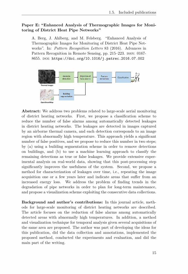
Abstract: We address two problems related to large-scale aerial monitoringof district heating networks. First, we propose a classification scheme toreduce the number of false alarms among automatically detected leakagesin district heating networks. The leakages are detected in images capturedby an airborne thermal camera, and each detection corresponds to an imageregion with abnormally high temperature. This approach yields a significantnumber of false positives, and we propose to reduce this number in two steps;by (a) using a building segmentation scheme in order to remove detectionson buildings, and (b) to use a machine learning approach to classify theremaining detections as true or false leakages. We provide extensive exper-imental analysis on real-world data, showing that this post-processing stepsignificantly improves the usefulness of the system. Second, we propose amethod for characterization of leakages over time, i.e., repeating the imageacquisition one or a few years later and indicate areas that suffer from anincreased energy loss. We address the problem of finding trends in thedegradation of pipe networks in order to plan for long-term maintenance,and propose a visualization scheme exploiting the consecutive data collections.
Background and author’s contributions: In this journal article, meth-ods for large-scale monitoring of district heating networks are described.The article focuses on the reduction of false alarms among automaticallydetected areas with abnormally high temperatures. In addition, a methodand visualization technique for temporal analysis given several acquisitions ofthe same area are proposed. The author was part of developing the ideas forthis publication, did the data collection and annotations, implemented theproposed method, conducted the experiments and evaluation, and did themain part of the writing.
15

1. Introduction
Paper F: “Unsupervised Adversarial Learning of Anomaly Detec-tion in the Wild”
A. Berg, J. Ahlberg, and M. Felsberg. “Unsupervised AdversarialLearning of Anomaly Detection in the Wild”. In: Submitted to the24th European Conference on Artificial Intelligence (ECAI 2020).2019
𝑧𝑋𝑔 = 𝐺(𝑧)𝐺
𝐸
𝐷
𝑋𝑟
Ƹ𝑧
𝑌
Abstract: Unsupervised learning of anomaly detection in high-dimensionaldata, such as images, is a challenging problem recently subject to intense re-search. Through careful modelling of the data distribution of normal samples,it is possible to detect deviant samples, so called anomalies. Generative Ad-versarial Networks (GANs) can model the highly complex, high-dimensionaldata distribution of normal image samples, and have shown to be a suitableapproach to the problem. Previously published GAN-based anomaly detec-tion methods often assume that anomaly-free data is available for training.However, this assumption is not valid in most real-life scenarios, a.k.a. in thewild. In this work, we evaluate the effects of anomaly contaminations in thetraining data on state-of-the-art GAN-based anomaly detection methods. Asexpected, detection performance deteriorates. To address this performancedrop, we propose to add an additional encoder network already at trainingtime and show that joint generator-encoder training stratifies the latent space,mitigating the problem with contaminated data. We show experimentallythat the norm of a query image in this stratified latent space becomes a highlysignificant cue to discriminate anomalies from normal data. The proposedmethod achieves state-of-the-art performance on CIFAR-10 as well as on alarge, previously untested dataset with cell images.
Background and author’s contributions: This paper employs a Gen-erative Adversarial Network (GAN) for the purpose of anomaly detection.In contrast to previous GAN-based anomaly detection methods, an encoderis trained together with the generator and the latent space of the trainedencoder is examined. It is concluded that the technique used for encodertraining affects the structure of the latent space. Further, the norm of latentvectors can serve as an important cue when discriminating normal samplesfrom anomalous. The author developed the ideas for this publication, imple-mented the proposed method, conducted the experiments and the evaluation,and did the main part of the writing.
16

1.5. Included publications
Paper G: “Generating Visible Spectrum Images from Thermal In-frared”
A. Berg, J. Ahlberg, and M. Felsberg. “Generating VisibleSpectrum Images from Thermal Infrared”. In: 2018 IEEE Con-ference on Computer Vision and Pattern Recognition Workshops(CVPRW). June 2018. doi: 10.1109/CVPRW.2018.00159
H
W
TIR input
32
64 128128
𝑊
2
Visual output
256 192
96
32
𝐻
2
𝐻
2
𝑊
2𝑊
4
𝑊
4
𝑊
4
𝑊
4
𝑊
4
𝐻
4
𝐻
4
𝐻
4
𝐻
4
𝐻
4
W
H
1/3
H
W
1
Abstract: Transformation of thermal infrared (TIR) images into visual, i.e.perceptually realistic color (RGB) images, is a challenging problem. TIRcameras have the ability to see in scenarios where vision is severely impaired,for example in total darkness or fog, and they are commonly used, e.g., forsurveillance and automotive applications. However, interpretation of TIRimages is difficult, especially for untrained operators. Enhancing the TIRimage display by transforming it into a plausible, visual, perceptually realisticRGB image presumably facilitates interpretation. Existing grayscale to RGB,so called, colorization methods cannot be applied to TIR images directly sincethose methods only estimate the chrominance and not the luminance.
In the absence of conventional colorization methods, we propose two fullyautomatic TIR to visual color image transformation methods, a two-step andan integrated approach, based on Convolutional Neural Networks. The meth-ods require neither pre- nor postprocessing, do not require any user input,and are robust to image pair misalignments. We show that the methods doindeed produce perceptually realistic results on publicly available data, whichis assessed both qualitatively and quantitatively.
Background and author’s contributions: This publication proposesan approach for automatic transformation from thermal infrared to percep-tually realistic color (RGB) images, a previously unaddressed problem. Theproposed approach was based on an autoencoder architecture due to theability of Convolutional Neural Networks to model semantic representations.The author developed the ideas for this publication, implemented the pro-posed method, conducted the experiments and evaluation, and did the mainpart of the writing.
17
1. Introduction
1.6 Additional publications
Parts of the material presented in this thesis also appeared in the author’slicentiate thesis:
A. Berg. Detection and Tracking in Thermal Infrared Imagery.Licentiate thesis No. 1744. Linköping University Electronic Press,2016. isbn: 978-91-7685-789-2. doi: 10.3384/lic.diva-126955
1.6.1 Preliminary versions of included publicationsPaper E is a journal extension of the following three publications. The firstone [18] is an early version that was rewritten to form [14]. In [13], a temporalanalysis of the district heating pipes was added. This extension together withthe classification in [14] was rewritten and extended in Paper E.
A. Berg, J. Ahlberg, and M. Felsberg. “Classifying District Heat-ing Network Leakages in Aerial Thermal Imagery”. In: SwedishSymposium on Image Analysis (SSBA). 2014(Also [18])
A. Berg and J. Ahlberg. “Classification of Leakage Detections Ac-quired by Airborne Thermography of District Heating Networks”.In: Pattern Recognition in Remote Sensing (PRRS), IAPR Work-shop on. 2014. doi: 10.1109/PRRS.2014.6914288(Also [14])
A. Berg and J. Ahlberg. “Classification and Temporal Analysisof District Heating Leakages in Thermal Images”. In: The 14thInternational Symposium on District Heating and Cooling (DHC).2014(Also [13])
The publication below, describing the LTIR dataset, is an early version ofPaper A. The manuscript was rewritten for Paper A and extended with abenchmark based on the VOT-protocol. Results from seven state-of-the-artvisual object tracking methods was reported.
A. Berg, J. Ahlberg, and M. Felsberg. “A Thermal InfraredDataset for Evaluation of Short-term Tracking Methods”. In:Swedish Symposium on Image Analysis (SSBA). 2015
18

1.6. Additional publications
1.6.2 Publications related to included papersA. Berg, J. Ahlberg, and M. Felsberg. “Object Tracking inThermal Infrared Imagery based on Channel Coded DistributionFields”. In: Swedish Symposium on Image Analysis (SSBA). 2017(Revised version of Paper C.)
A. Berg, J. Ahlberg, and M. Felsberg. “Visual Spectrum ImageGeneration from Thermal Infrared”. In: Swedish Symposium onImage Analysis (SSBA). 2019(Revised version of Paper G.)
1.6.3 Other publicationsJ. Ahlberg and A. Berg. “Evaluating Template Rescaling in Short-term Single-object Tracking”. In: IEEE International Conferenceon Advanced Video- and Signal-based Surveillance Workshops.Aug. 2015, pp. 1–4. doi: 10.1109/AVSS.2015.7301745
M. Felsberg, A. Berg, G. Häger, J. Ahlberg, M. Kristan, J. Matas,A. Leonardis, L. Cehovin, G. Fernandez, et al. “The ThermalInfrared Visual Object Tracking VOT-TIR2015 Challenge Re-sults”. In: IEEE International Conference on Computer VisionWorkshops (ICCVW). Institute of Electrical and Electronics En-gineers (IEEE), 2015, pp. 639–651. doi: 10.1109/ICCVW.2015.86
A. Berg, M. Felsberg, G. Häger, and J. Ahlberg. “An Overviewof the Thermal Infrared Visual Object Tracking VOT-TIR2015Challenge”. In: Swedish Symposium on Image Analysis (SSBA).2016(Overview of the previous paper.)
M. Felsberg, M. Kristan, J. Matas, A. Leonardis, R. Pflugfelder,G. Häger, A. Berg, A. Eldesokey, J. Ahlberg, et al. “The Ther-mal Infrared Visual Object Tracking VOT-TIR2016 ChallengeResults”. In: Proceedings on the European Conference on Com-puter Vision Workshops (ECCVW). vol. 9914. Lecture Notesin Computer Science. Springer, Cham, 2016, pp. 824–849. doi:https://doi.org/10.1007/978-3-319-48881-3_55
M. Kristan, J. Matas, A. Leonardis, M. Felsberg, R. Pflugfelder,J.-K. Kamarainen, L. Cehovin, O. Drbohlav, A. Lukezic, A.
19

1. Introduction
Berg, A. Eldesokey, et al. “The Seventh Visual Object TrackingVOT2019 Challenge Results”. In: 2019 IEEE International Con-ference on Computer Vision Workshops (ICCVW). 2019
T. Nawaz, A. Berg, J. Ferryman, J. Ahlberg, and M. Felsberg.“Effective Evaluation of Privacy Protection Techniques in Visibleand Thermal Imagery”. In: Journal of Electronic Imaging (JEI)26.5 (2017), pp. 1–16. doi: 10.1117/1.JEI.26.5.051408
J. Heggenes, A. Odland, T. Chevalier, J. Ahlberg, A. Berg, andD. Bjerketvedt. “Herbivore Grazing–or Trampling? TramplingEffects by a Large Ungulate in Cold High-latitude Ecosystems”.In: Ecology and Evolution 7.16 (2017), pp. 6423–6431. doi:10.1002/ece3.3130
20

2
Thermal Infrared Imaging
Thermal infrared radiation is emitted, reflected, and transmitted around usevery day. While rarely considered on a daily basis, the temperature differ-ence of different objects can provide valuable information. Visual displaysof the measured thermal infrared radiation, thermal infrared images, formthe basis of this thesis. The following chapter gives a brief overview of theunderlying physics as well as automatic image analysis in thermal infraredimages. The chapter also explains the relation between infrared light andthe planet Uranus, shows examples of the properties of different materials inthermal infrared, and explains why it is not possible to see through windowswith thermal cameras. This chapter is a revised version of Chapter 2 in theauthor’s licentiate thesis [25].
2.1 Infrared and thermal radiation
The discovery of infrared radiation is credited to the astronomer and composerWilliam Herschel (1738-1822). In the year 1800, he conducted a series ofexperiments [87, 88, 89] where he postulated and tried to prove that visiblelight and radiant heat was of the same quantity. The postulation was basedon one of his first experiments [87], where he used a prism to split sunlightinto different colors and then measured the radiant heat of each color. Tohis surprise, his control thermometer placed outside the visible sunlight washeated as well. Finally, the following conclusion was made:
“To conclude, if we call light, those rays which illuminate objects,and radiant heat, those which heat bodies, it may be inquired,whether light be essentially different from radiant heat? In answerto which I would suggest, that we are not allowed, by the rulesof philosophizing, to admit two different causes to explain certaineffects, if they may be accounted for by one.”[87]
21

2. Thermal Infrared Imaging
Thermal infrared
X-rayMicrowaveand radio
Ult
ra V
iole
t
Vis
ible
Nea
r in
frar
ed
Sho
rtw
ave
infr
ared
Mid
wav
ein
frar
ed
Lo
ngw
ave
infr
ared
Far
infr
ared
0.01 0.4 0.7 1 3 5 8 12 1000
Wavelength [μm]
Figure 2.1: Infrared radiation is a part of the electromagnetic spectrum. Long-wave, and sometimes midwave, infrared is commonly referred to as thermalinfrared. Between 5–8 µm, the atmosphere attenuates most of the radiation.
Apart from these experiments, William Herschel is famous for writing 24symphonies and, together with his sister Caroline, building telescopes anddiscovering four moons, eight comets, and one planet (Uranus) [166]. WilliamHerschel draw these conclusions without neither the knowledge of electro-magnetic radiation, nor the concept of wavelength. It is now known that thevisible and infrared wavelength bands only span a small part of the electro-magnetic spectrum, as illustrated in Fig. 2.1. The name, infrared, originatesfrom the Latin word infra, which means below. That is, the infrared band liesbelow the visual red light band, since it has lower frequency.
The infrared wavelength band is in turn usually divided into smaller partsbased on their different properties. The near infrared (NIR, wavelengths 0.7–1µm) and shortwave infrared (SWIR, 1–3 µm) bands are dominated by reflectedradiation and are dependent on illumination. Essentially, they behave simi-larly to visual light, except that we cannot see it. In contrast, the midwaveinfrared (MWIR, 3–5 µm), longwave infrared (LWIR, 8–12 µm), and far in-frared (FIR, 12–1000 µm) bands are dominated by emitted radiation. Otherdefinitions of the infrared bands exist as well. LWIR, and sometimes MWIR,is commonly referred to as thermal infrared (TIR).
All objects with temperatures above absolute zero emit thermal radiationto a different extent depending on temperature and material. Emitted ther-mal radiation originates from the conversion of an object’s thermal energyinto electromagnetic energy. Objects at normal everyday temperatures emitmostly in the LWIR band, while a hot object like the sun emits most in thevisual band, thus making the LWIR band the most suitable for night vision.
When interacting with matter, electromagnetic radiation is absorbed (α),transmitted (τ) and/or reflected (ρ). The total radiation law states that1 = α+ρ+τ where α, τ, ρ ∈ [0,1]. An object defined as a black body is an opaqueand non-reflective object that absorbs all incident radiation (α = 1). Blackbodies do not exist in nature, but are commonly used as an approximation.
22

2.2. Thermal imaging
1 2 3 4 5 6 7 8 9 10 11 12 13Wavelength [ m]
0
0.2
0.4
0.6
0.8
1T
rans
mis
sion
UVVIS
NIRSWIR
MWIRLWIR
Figure 2.2: Atmospheric attenuation depends on radiation wavelength. Imagecourtesy of Jörgen Ahlberg.
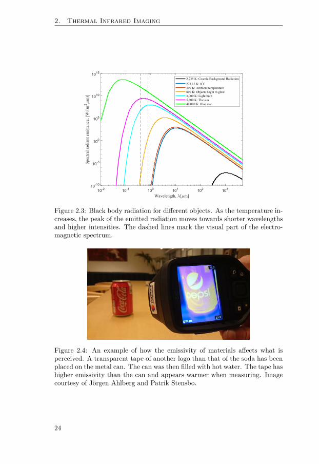
Examples of black body radiation curves for some known objects can be seenin Fig. 2.3. Note that the peak of the sun lies in the reflective part of theelectromagnetic spectrum. The blackbody radiation curves were described byMax Planck almost exactly 100 years after Herschel’s discovery of infraredradiation [158].
Emissivity (ϵ) is the ratio of the actual emittance of an object to theemittance of a black body at the same temperature. Further, Kirchhoff’s lawstates that α = ϵ, i.e., ϵ = 1 for a black body. Since emissivity is materialdependent, it is an important property when measuring temperatures with athermal camera. An example of how the emissivity of an object can affectwhat is perceived is given in Fig. 2.4.
Due to scattering by particles and absorption by gases, the atmospherewill attenuate radiation, making the measured apparent temperature decreasewith increased distance. The level of attenuation depends on radiation wave-length, Fig. 2.2. As can be seen in the figure, there are some sections in whichthe atmosphere transmits a major part of the radiation. These are calledthe atmospheric windows; there is one VNIR (Visual and NIR) window, twowindows in SWIR, two windows in MWIR, and a large window in LWIR [165].
This section only provides a brief overview of the topic, for more infor-mation on thermal infrared detectors and physical principles, see for example[165, 166].
2.2 Thermal imaging
Thermal images are visual displays of the measured thermal radiation withinan area. Again, it should be emphasized that thermal cameras are sensitiveto emitted radiation in everyday temperatures and that they should not beconfused with NIR and SWIR cameras that mostly measure the reflected radi-ation. They are dependent on illumination and behave in general in a similarway as visual cameras.
23
2. Thermal Infrared Imaging
10-2 10-1 100 101 102 103
Wavelength, [ m]
10-10
10-5
100
105
1010
1015
Spe
ctra
l rad
iant
em
itta
nce,
[W
/(m
2m
)]
2.735 K: Cosmic Background Radiation
273.15 K: 0°C300 K: Ambient temperature800 K: Objects begin to glow3,000 K: Light bulb5,800 K: The sun40,000 K: Blue star
Figure 2.3: Black body radiation for different objects. As the temperature in-creases, the peak of the emitted radiation moves towards shorter wavelengthsand higher intensities. The dashed lines mark the visual part of the electro-magnetic spectrum.
Figure 2.4: An example of how the emissivity of materials affects what isperceived. A transparent tape of another logo than that of the soda has beenplaced on the metal can. The can was then filled with hot water. The tape hashigher emissivity than the can and appears warmer when measuring. Imagecourtesy of Jörgen Ahlberg and Patrik Stensbo.
24

2.2. Thermal imaging
Incident radiation from object surroundings
Path(atmosphere)
Reflected radiation from object surroundings
Emitted radiationfrom object
Emitted radiation from path
Transmitted radiation from object
Transmitted radiation from object surroundings
Internal cameraradiation
Figure 2.5: The radiation measured by a thermal camera when observing anobject is a combination of multiple sources, not only the amount of radiationemitted by the object, which is typically what is desired.
Thermal cameras are either cooled or uncooled. High-end cooled camerascan deliver hundreds of High Definition (HD) resolution frames per secondand have a temperature sensitivity of 20 mK. Images are typically stored as16 bits per pixel to allow a large dynamic range, for example 0–382.2K with aprecision of 10 mK. Uncooled cameras usually have bolometer detectors andoperate in LWIR. They yield noisier images at a lower framerate, but aresmaller, silent, and less expensive.
A thermal camera is said to be thermographic if it is calibrated in orderto measure temperatures. Some uncooled cameras provide access to the raw16-bit intensity values, so called radiometric cameras, while others convertthe images to 8-bits and compress them, e.g., using MPEG. In the lattercase, the dynamic range is adaptively changed in order provide an image thatlooks good to the eye, but the temperature information is lost. For automaticanalysis, such as target detection, classification, and tracking, it is in mostcases preferable to use the original signal, i.e., the raw 16-bit intensity valuesfrom a radiometric camera.
In order to produce accurate thermographic measurements, all differentsources of thermal radiation need to be considered, an illustration is providedin Fig. 2.5. The amount of radiation emitted by the object depends on itsemissivity as explained in the previous section. In addition, thermal radiationfrom other objects are reflected on the surface of the object. Therefore, it isalso important to know the reflectivity of the object. The amount of radiationthat reaches the detector is affected by the atmosphere. Some is transmittedthrough the atmosphere, some is absorbed by the atmosphere, and some iseven emitted from the atmosphere itself, in contrast to the visual band. More-over, the camera itself emits thermal radiation during operation. In order tomeasure thermal radiation and, thus, temperatures as accurately as possible,all these effects need to be considered. At short distances, atmospheric effectscan be disregarded. But for greater distances, e.g., from aircrafts as in Pa-per E, it is crucial to consider atmospheric effects if temperatures are to bemeasured correctly. However, if you are only interested in an image that looksgood to the eye and not temperatures, these effects do not have to be taken
25

2. Thermal Infrared Imaging
(a) Gray (b) Iron (c) Rainbow
Figure 2.6: A thermal infrared image visualized using different color maps.
into account. In that case, thermal images can be used as visual displays ofreceived thermal radiation on a sensor. When presented to an operator, colormaps are often used to map pixel intensity values in order to visualize detailsmore clearly. Examples of a thermal image with three widely used color mapscan be seen in Fig. 2.6.
2.3 Advantages and limitations of thermal imaging
From the aspect of measuring temperatures, thermal imaging is not consideredto be as accurate as contact methods. It is, however, advantageous comparedto point-based methods when it comes to measuring the temperature distribu-tion over a large area. In addition, thermal imaging, as well as pyrometry ingeneral, provides the possibility of remote temperature measurement, whichcan be favourable in some applications.
Compared to visual cameras, thermal cameras are favourable as soon asthere is a temperature difference connected to the object or phenomenon youwant to detect. For example, emerging fires, humans, animals, increased bodytemperatures, or differences in heat transfer ability in materials. When itcomes to applications, thermal cameras are especially advantageous to visualcameras in outdoor applications. Thermal cameras can produce an imagewith no or few distortions during darkness and/or difficult weather conditions(e.g. fog/rain/snow). This is again due to the fact that a thermal camera issensitive for emitted radiation, even from relatively cold objects, in contrastto a visual or NIR camera that measures reflected radiation and thus dependson illumination.
Thermal cameras are expensive and have low resolution compared to vi-sual cameras. State of the art is currently 1280x1024 pixels, and increasedresolution comes with a higher price tag, up to €200 000. Prices depend onthe choice of detector (cooled/uncooled, MWIR/LWIR), optics etc.
In comparison to a visual camera, a thermal camera typically requiresmore training for correct usage. In order to provide accurate measurements,the operator needs to be aware of the physical principles and phenomena com-
26

2.4. Image analysis in thermal infrared images
(a) Glass (b) Water (c) Plastic bag
Figure 2.7: Examples of a few different materials in RGB images (first row)versus thermal infrared images (second row).
monly viewed in thermal imagery. That is, the emissivity and reflectivity ofdifferent materials as well as the impact of the atmosphere and other objects.
From thermal images, it is not considered possible to perform person iden-tification, a fact that is both an advantage as well as a limitation. Conse-quently, a thermal camera can be used in applications where preservation ofprivacy is crucial. If person identification is requested, the thermal camerahas to be combined with a visual camera.
2.4 Image analysis in thermal infrared images
In this section, differences between thermal and visual images when perform-ing automatic image analysis are described. Some descriptions are intention-ally left brief since they are further described in Section 5.1 in relation tovisual object tracking in thermal infrared.
Materials have different properties in the thermal and visual spectrum re-spectively, a few examples are provided in Fig. 2.7. Some materials that arereflective and/or transparent in the visual spectrum are not in the thermalspectrum and vice versa. For example, water and glass are opaque and highlyreflective in the thermal spectrum while mostly transparent in the visual spec-trum. Therefore, the lens of a thermal camera is not manufactured in glassbut in another material, typically germanium, a material that is opaque andreflective in the visual spectrum but transparent in the thermal spectrum, seeexample in Fig. 2.9. Glass, water puddles and wet soil can cause reflectionssimilar to shadows.
27

2. Thermal Infrared Imaging
(a) RGB (b) Thermal infrared
Figure 2.8: Four pieces of jersey fabric that have different visual color patterns.In the (a) visual spectrum, they are easily separated, while having identicalappearance in the (b) thermal infrared spectrum.
Figure 2.9: Example of a germanium lens. Germanium is opaque and reflectivein the visual spectrum while transparent in the thermal spectrum.
In the thermal infrared spectrum, there are no shadows since mostly emit-ted radiation is measured. In most applications, the emitted radiation changesmuch slower than the reflected radiation. That is, an object moving from adark room into the sunlight will not immediately change its appearance (asit would in visual imagery).
Regarding noise, thermal imagery has different characteristics than visualimagery. Compared to a visual camera, a thermal infrared camera typicallyhas more blooming, lower resolution and a larger percentage of dead pixels.Visual color patterns are discernible in thermal infrared images only if theycorrespond to variations in material or temperature, as illustrated in Fig. 2.8.
Finally, a thermal infrared camera is itself a source of thermal radiation.During operation, especially during start-up, it heats itself. The radiationreaching the sensor can to a large part originate from the camera itself. Tocompensate for this, thermal infrared cameras typically have internal ther-mometers and they also perform radiometric calibration at regular time in-tervals. During calibration, a plate with known temperature is inserted infront of the sensor, and frames are lost.
28

3
Representation
As visible light enters our eyes through the cornea and spreads across theretina, the light intensity measured by the photosensitive cells is mapped toa different representation prior to interpretation [194]. Similarly, the grid ofintensity values measured by a visual or thermal camera must, in computervision, be mapped to a representation suitable for the problem at hand. Theaim of a representation method is to extract the information relevant to thesolution of the addressed problem in order to facilitate data processing [104].The following chapter introduces representation methods and, in particular,provides background information on the channel representation, employed inPaper C.
3.1 Representations of visual information
The mapping of an image to another representation where the discriminativeinformation for the specific task is maximized can significantly improve theperformance and reduce the computational effort. The best choice of repre-sentation method is task dependant, which has led to the development of aplethora of different feature extraction and description techniques, e.g., thelocal descriptors SIFT [130], and BRIEF [37], and object template descriptorssuch as the HOG descriptor [46]. Representations can be hand-crafted basedon a-priori knowledge about the problem (Paper E) or learned from data, forexample in the layers of a Deep Neural Network [77].
Processing of high-dimensional data, such as images, is a difficult, com-putationally demanding problem. The so called manifold hypothesis justi-fies the use of representations for the purpose of automatic image analysis.The hypothesis states that real-world, natural, images lie on low-dimensionalmanifolds embedded in the high-dimensional space. Constraints arising fromphysical laws entail this low-dimensional structure [58]. Generative Adversar-
29

3. Representation
ial Networks [78] are examples of methods that exploit this fact in order tosample in this lower-dimensional space.
In some applications, parts of the image may be irrelevant to the solutionof the problem. For example, the part above the horizon in the case of boatdetection at sea (Paper C) and railway detection (Paper D). Images can alsobe represented in different color spaces, such as YUV or CIELAB (Paper G).
The purpose of the following sections is to introduce the reader to thechannel representation, a biologically inspired, sparse, grid-based approachthat fuses the concepts of histograms and wavelets. The channel representa-tion provides a good compromise between hand-crafted descriptors and thea-priori structureless feature spaces that can be seen in the layers of deepnetworks [61].
3.2 Sparse representations
A sparse representation describes an input signal using only a few active, i.e.,non-zero, units. Hence, most of the units of the representation are zero. Incontrast, a compact representation method maximizes the information con-tent in a minimum number of units, where all units are active. Examplesof compact representations are dimensionality reduction techniques such asPrincipal Component Analysis (PCA) [156]. PCA is an orthogonal transfor-mation of a set of samples into a smaller set of linearly uncorrelated principalcomponents that maximize the variance of the data.
Sparse representations are often dictionary-based, i.e., each unit of therepresentation correspond to the coefficient of some basis function or elementand a sample can be reconstructed by a linear combination of these. TheFourier-transform of a sinusoid is an example of a sparse representation. Forother types of signals, the Fourier transform can be used to create sparserepresentations by setting all but a few of the coefficients to zero assumingthat the original signal still can be represented sufficiently well [134]. Thisapproach is, for example, employed by the JPEG image compression format[178].
3.3 Grid-based representations
A representation of a signal is grid-based if it maps the original signal on aregular (or irregular [79]) grid. Thus, a histogram, where the range of val-ues is binned on a grid, would be considered as a grid-based representation.However, histogram-based representations often suffer from the lack of spatialinformation, an unfavourable property for some applications [61]. Other ex-amples of grid-based representations are Gaussian Mixture Models (GMMs)and Kernel Density Estimators (KDEs) [152].
30

3.4. Channel representations
(a) TIR image (b) n = 1 (c) n = 2 (d) n = 3 (e) n = 4
(f) n = 5 (g) n = 6 (h) n = 7 (i) n = 8 (j) n = 9
Figure 3.1: Example of a (a) thermal infrared image, exploded into a distribu-tion field using Nb = 9 bins. Images (b)-(j) display each one of the dimensionsn = 1, ...,Nb. The distribution field has been convolved with a Gaussian kernelwith σ = 1 in the spatial and feature direction.
The idea behind the grid-based representation Distribution Fields [184] isto compute density estimates of the feature distribution on a regular grid. ADistribution Field (DF) is an NDF-dimensional array. A 2D grayscale inputimage is exploded into a DF by increasing the dimension of the input arrayfrom 2 to NDF = 2 +DF where the DF dimensions index the chosen featurespace. The ranges of the values of the feature space are binned using a his-togram representation. In other words, in the case of intensity values (DF = 1)as features, the DF is a three-dimensional array. Each pixel is extended to ahistogram where each bin represents a range of intensity values from the orig-inal image, an example is provided in Fig. 3.1. In order to make the modelrobust to small changes, the DF is smoothed in the spatial and/or featuredirection by a Gaussian kernel.
Distribution fields have been applied to the problems of image alignment[137] and visual object tracking [185]. The Distribution Field Tracker (DFT)[185] was later improved by Felsberg who proposed the Enhanced Distribu-tion Field tracker (EDFT) [60]. The main aspect being the exchange froma histogram representation to channel vectors. Paper C extended the EDFTtracker to mitigate the problems of background contamination of the objectmodel and object scale change.
3.4 Channel representations
The channel representation was proposed by Nordberg et al. [147], stemmingfrom a biologically inspired information representation [79]. It is a sparse,grid-based, nonparametric approach that fuses the concepts of histograms andwavelets [61]. The channel representation share many similarities with popu-
31

3. Representation
(a) TIR image (b) n = 1 (c) n = 2 (d) n = 3 (e) n = 4
(f) n = 5 (g) n = 6 (h) n = 7 (i) n = 8 (j) n = 9
Figure 3.2: (a) A thermal infrared image, channel encoded using N = 9 chan-nels. Images (b)-(j) display the channel coefficients at each channel n.
lation codes in computational neuroscience [131, 160, 161], the relationship isfurther explained in [66].
The core idea of the channel representation is to represent values by theiractivations of overlapping shifted basis functions, so called channels, that areevenly placed along the range of the values. The channel representation canbe seen as a soft histogram, sharing some similarities with the Average ShiftedHistogram [183], that approximates a Kernel Density Estimator (KDE) [152]in a regular grid [59]. If Gaussian basis functions are used, the channel repre-sentation corresponds to the Radial Basis Functions [35] in machine learning[149]. Compared to a DF, channel representations apply a soft assignment,i.e., pre-smoothing, instead of post-smoothing of the bin assignments whichhas been shown to be more efficient [60].
The channel representation has been successfully used in many applica-tions, e.g., point-set registration [49], object recognition [64], object segmen-tation [199], image denoising [63], and visual object tracking (Paper C) [47,60, 150].
3.4.1 Channel encodingA set of scalar samples xm, where m ∈ {1, . . . ,M} is the sample index, can bechannel encoded into a set of channel vectors cm using a basis of N channels.In the case of images, xm is a function of spatial coordinates and the channelencoding is performed at each spatial location, i.e., pixel-wise, as illustratedin Fig. 3.2. Multi-dimensional channel encoding is also possible [100, 149],but out of scope for this thesis.
The channel encoding of a set of scalar samples xm is a set of channelvectors cm = [cm1 , . . . , cmN ] of channel coefficients cmn , where n ∈ {1, . . . ,N} isthe index of the channels, ξn are the channel centers, and K() is the encoding
32
3.4. Channel representations
-2 0 2 4 6 8 10 12 14 160
0.2
0.4
0.6
0.8
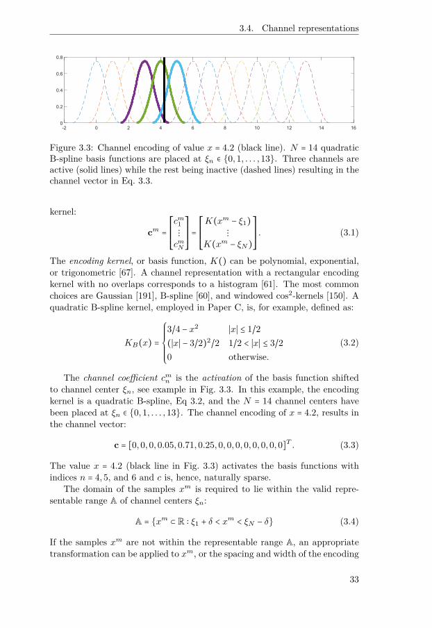
Figure 3.3: Channel encoding of value x = 4.2 (black line). N = 14 quadraticB-spline basis functions are placed at ξn ∈ {0,1, . . . ,13}. Three channels areactive (solid lines) while the rest being inactive (dashed lines) resulting in thechannel vector in Eq. 3.3.
kernel:
cm =⎡⎢⎢⎢⎢⎢⎣
cm1⋮cmN
⎤⎥⎥⎥⎥⎥⎦=⎡⎢⎢⎢⎢⎢⎣
K(xm − ξ1)⋮
K(xm − ξN)
⎤⎥⎥⎥⎥⎥⎦. (3.1)
The encoding kernel, or basis function, K() can be polynomial, exponential,or trigonometric [67]. A channel representation with a rectangular encodingkernel with no overlaps corresponds to a histogram [61]. The most commonchoices are Gaussian [191], B-spline [60], and windowed cos2-kernels [150]. Aquadratic B-spline kernel, employed in Paper C, is, for example, defined as:
KB(x) =
⎧⎪⎪⎪⎪⎪⎨⎪⎪⎪⎪⎪⎩
3/4 − x2 ∣x∣ ≤ 1/2(∣x∣ − 3/2)2/2 1/2 < ∣x∣ ≤ 3/20 otherwise.
(3.2)
The channel coefficient cmn is the activation of the basis function shiftedto channel center ξn, see example in Fig. 3.3. In this example, the encodingkernel is a quadratic B-spline, Eq 3.2, and the N = 14 channel centers havebeen placed at ξn ∈ {0,1, . . . ,13}. The channel encoding of x = 4.2, results inthe channel vector:
c = [0,0,0,0.05,0.71,0.25,0,0,0,0,0,0,0,0]T . (3.3)
The value x = 4.2 (black line in Fig. 3.3) activates the basis functions withindices n = 4,5, and 6 and c is, hence, naturally sparse.
The domain of the samples xm is required to lie within the valid repre-sentable range A of channel centers ξn:
A = {xm ⊂ R ∶ ξ1 + δ < xm < ξN − δ} (3.4)
If the samples xm are not within the representable range A, an appropriatetransformation can be applied to xm, or the spacing and width of the encoding
33

3. Representation
kernels adapted in order to fulfil this criteria. The offset δ depends on thewidth of the chosen basis function as well as the distance between channelcenters and it ensures that each possible value of xm activates an equal numberof channels, δ = 0.5 in the example in Fig. 3.3. The number of activatedchannels w for each value xm can be chosen arbitrarily for the purpose ofencoding. Motivated by the decoding [67], the standard choice has, however,been w = 3 [100]. A proof regarding minimal channel overlap is given in [149].
For the purpose of, e.g., visualization, the channel vectors need to bedecoded. Channel decoding is, however, out of scope for this thesis. Theinterested reader is referred to [61, 149]. Decoding do infer some additionalrequirements on the shape of the basis function and the minimal channeloverlap, as mentioned above. The necessary and sufficient conditions on thebasis function for the purpose of decoding and representing distributions hasbeen identified by Öfjäll [149].
In the case of limited ranges of discrete input samples xm, for examplepixel intensity values ∈ [0,255], the channel encodings for all possible val-ues of xm can be pre-computed and placed in a look-up table, enabling acomputationally efficient representation.
3.4.2 Properties of channel vectorsThe channel representation possess many useful properties, a few of them arementioned here. First, since it is a sparse representation, multiple values canbe represented in the same channel vector as:
c =⎡⎢⎢⎢⎢⎢⎣
c1⋮cN
⎤⎥⎥⎥⎥⎥⎦= 1
M
⎡⎢⎢⎢⎢⎢⎣
∑Mm=1 c
m1
⋮∑M
m=1 cmN
⎤⎥⎥⎥⎥⎥⎦. (3.5)
Two encoded values located in opposite ends of the representable range can beseparated when decoding the channel vector. If they are too close, decodingwill provide an average of the two. The smallest distance between samples,the metameric distance, that the channel representation can handle is furtherinvestigated in [61, 67].
The basis functions of the channel representation are required to be non-negative, implying that also the channel coefficients of c are non-negative.This in turn, implies that the sum of a channel vector is equal to the ℓ1 norm:
∣∣c∣∣1 =N
∑n=1∣cn∣ =
N
∑n=1
cn. (3.6)
The sum of a channel vector for the cos2 and B-spline basis functions is con-stant as long as the encoded value lies within the representable range A. Fora quadratic B-spline, the sum of a channel vector equals to one, a propertyexploited in Paper C. Proofs of these properties are given in [67].
34

4
Learning Methods
Learning is considered to be a major part of what is defined as human intelli-gence. Learning demonstrated by artificial systems, so called machine learn-ing, is a subject of intense research frequently applied to problems within thefield of computer vision. Machine learning methods enable us to define whata system should do, instead of how they should do it. The aim of this sectionis to provide background for the learning methods employed in Papers C, D,E, F, and G.
4.1 Intelligence and learning
Over the years, the definition of human intelligence has been focused on dif-ferent aspects of the same. Psychologists have, however, agreed that the keyto understanding intelligence is adaptation. A number of cognitive processesare required for effective adaptation, such as perception, memory, reasoning,problem solving, and learning [193]. Learning, as a part of intelligence, is aprocess that leads to change. As a consequence, concepts, ideas, and/or theworld will be seen differently. Learning occurs as a result of experience andincreases the potential for improved performance [7].
Artificial Intelligence (AI), is defined as human intelligence demonstratedby machines. The part of AI connected to learning is known as machinelearning. Machine learning is introduced in Section 4.2, followed by someexamples of machine learning properties and methods: online learning, Section4.3, ensemble learning, Section 4.4, and neural networks, Section 4.5. Themethods have been put into context in Fig. 4.1.
4.2 Introduction to machine learning
The history of machine learning dates back as early as the mid 18th centurywith the introduction of classical techniques such as Bayes’ theorem (1763)
35

4. Learning Methods
Artificial Intelligence
Machinelearning
ANNs
Ensemble methods
Deep learning
Figure 4.1: Deep learning techniques are a specific type of Artificial NeuralNetworks (ANNs). Together with ensemble methods, ANNs are a part ofthe more general topic of machine learning, and machine learning is in turn apart of the more general topic of artificial intelligence. Other types of machinelearning methods exist as well, the purpose of this figure is to provide contextfor the methods described in this chapter.
[11] and the Least Squares method for data fitting (1805) [119], techniquesthat are fundamental for machine learning today. Machine learning, defined asthe scientific study of systems that can learn from sample data, is a broad areathat spans from linear curve fitting methods to complex non-linear algorithmssuch as deep neural networks. This section provides a short introduction tomachine learning concepts utilized in the remainder of this chapter. The booksby Bishop [29] and Hastie [82] provide a broader overview of the machinelearning field.
The key to the success of any machine learning method is its ability togeneralize. That is, its ability to make correct decisions when exposed topreviously unseen data. Given a set of training samples represented in somefeature space the task of a machine learning method is to find a mappingfunction g ∶ x ↦ y from the space of inputs x to the space of outputs y. Ifthis mapping is overly adapted to the training data, the algorithm will notgeneralize well.
4.2.1 Categorization of machine learning methodsMachine learning methods are categorized according to their properties andpurpose. Some examples of common categorizations are presented below.Note that a machine learning method can possess more than one of theseproperties.
36

4.3. Online learning
𝑥1
𝑥2
(a) Classification
𝑥1
𝑥2
(b) Regression
𝑥1
𝑥2
(c) Clustering
Figure 4.2: Illustrations of (a) classification, (b) regression, and (c) clustering.
Categorization based on input
Supervised learning methods have access to labelled training samples(x1,y1), ..., (xT ,yT ) in contrast to unsupervised learning methods that onlyhave unlabelled samples x1, ...,xT . Unsupervised methods learn the inherentstructure of the input data. In the case of reinforcement learning, theinput is accompanied with additional information, e.g., positive or negativefeedback depending on the outcome of the method. If only a subset of thetraining samples are labelled, the method is semi-supervised. Finally, inself-supervised learning, training data is autonomously (or automatically)labelled. Methods such as autoencoders, Section 4.5.3, where the input isequal to the output are also categorized as self-supervised.
Categorization based on output
Classification methods find one or many decision boundaries and outputdiscrete class labels. Conversely, regression methods have a continuous out-put. The aim of clustering methods is to discover structure in unlabelleddata and, hence, they are typically unsupervised. Illustrations of these cate-gorizations can be seen in Fig. 4.2.
Discriminative vs. generative methods
There are discriminative methods, such as classification algorithms, thatmodel the decision boundary between classes. In contrast, generative modelsexplicitly model the distribution of each class, i.e., for the purpose of clusteringor image generation.
4.3 Online learning
Online learning is a property of machine learning methods rather than amethod itself. In contrast to offline (or batch) learning methods, new training
37

4. Learning Methods
data can be incorporated without retraining the full model [174]. In offlinelearning methods, the model is trained using the full set of training samplesand, once completed, the parameters of the model are kept static and no fur-ther learning is permitted. In order for an offline method to incorporate newinformation, it has to be retrained using the new data samples together withall previous ones [99]. In the case of online machine learning, data becomesavailable in sequential order and the parameters of the model are updated con-tinuously. The requirements for the computational demand and the memoryusage do, however, vary between definitions [149].
In its simplest form, online machine learning can be the weighted averageof the model mt−1 at time t−1 and a new observation of the object ot, weightedby update factor α ∈ [0,1]:
mt = (1 − α)mt−1 + αot. (4.1)
This convex combination update is employed in the methods presented inPapers C and D. The two methods are designed for different applications anduse different representations. Paper C use a channel vector field while PaperD performs the update in the fourier domain. The simplicity of Eq. 4.1 is alsoits strength which makes it preferable in many applications.
While being particularly attractive solutions for large-scale, dynamicallychanging environments, online machine learning methods are prone to driftsince they can be sensitive to sudden changes in the input. Their main ad-vantage is, however, their ability to adapt to previously unseen data sampleswithout retraining the whole model with the full set of training samples [99].
4.4 Ensemble learning
The term ensemble learning, refers to the combination of several weaker learn-ing methods in order to increase the predictive performance compared to eachconstituent learning method alone. The weak learning method can be of anytype, e.g., linear regression model, decision tree, neural network, etc. [175].Two types of ensemble methods are evaluated in Paper E, AdaBoost andRandom Forests.
The well-known Condorcet’s jury theorem [42] states that for a jury ofindependent votes, the probability pjury of the jury making the correct votewill be larger than the probability p of each individual voter to be correct,requiring p > 0.5. That is, p > 0.5 implies pjury > p. Furthermore, pjury → 1
as the number of voters approaches infinity [167]. Hence, if the conditionsare met, it is safe to assume that the combination of a sufficiently large setof weak learning methods with a performance slightly better than random,will increase the predictive performance compared to each one of the weakmethods alone.
Different techniques can be used to increase the stability and accuracy ofensemble learning methods. One example is bootstrap aggregation, or bagging
38

4.4. Ensemble learning
…ℎ1(𝐱)
𝒟𝑚: { 𝐱𝑡 , 𝑦𝑡 , 𝑑𝑚(𝑡)}𝑡=1𝑇 , 𝑑1 𝑡 = Τ1 𝑇
𝐻 𝐱
𝛼1 𝛼2 𝛼3 𝛼𝑀
ො𝐲
ℎ2(𝐱) ℎ3(𝐱) ℎ𝑀(𝐱)𝒟2 𝒟3
Figure 4.3: An illustration of the AdaBoost algorithm. The weak classifiershm(x) are trained sequentially using the training dataset Dm with sampleweights dm(t) ∈ [0,1]. The weights are updated before being fed to the nextclassifier. The strong classifier H(x) weights the outputs of the weak classifiersusing classifier weights αm.
for short. Given a training set D and M number of weak learning methods,bagging generates M new training subsets Dm each one of the same size bysampling from D uniformly with replacement [32, 82]. The sampling can alsobe done based on prior information about the training samples. Each weaklearning method is trained using a different subset Dm. Bagging has beenshown to reduce the variance of the result and also the risk for overfitting[32]. The idea behind a different technique, known as boosting, is to train theweak learning methods in sequential order using the full training set D, butwith weights indicating the importance of each sample. The first practicalexample of a boosting algorithm was the AdaBoost method, described below.
4.4.1 AdaBoostAdaptive Boosting, or AdaBoost, is an ensemble boosting classificationmethod proposed by Freund and Schapire [68]. The method combines M
weak classifiers hm(x) into one strong classifier H(x). The weak classifiersare often decision stumps, i.e., decision trees with a single split. The weakclassifiers are trained sequentially and after each iteration the training sampleweights dm(t) are updated. When combining all of the weak classifiers intoa strong classifier, the weak classifiers are weighted using weights αm. Thetraining of the standard discrete AdaBoost algorithm is summarized in Algo-rithm 1 and illustrated in Fig. 4.3. There exists many other different types ofboosting algorithms as well, a comprehensive summary is given by Schapireand Freund in [179].
39

4. Learning Methods
Algorithm 1 Discrete AdaBoost training.1: Given: Dm ∶ {(xt, yt), dm(t)}Tt=1, where (xt, yt) are the labelled training
samples, yt ∈ {−1,+1}, and dm(t) ∈ [0,1] are the sample weights.2: Initialize: d1(t) = 1
T
3: Iterate over the weak classifiers hm(x) and update sample weights dm(t):4: for m = 1, ...,M do5: Find weak classifier: hm(x) = {−1,+1}6: that minimizes: ϵm = ∑T
t=1 dm(t)I(yt ≠ hm(xt))
7: where I(yt ≠ hm(xt)) =⎧⎪⎪⎨⎪⎪⎩
1, if yt ≠ hm(xt)0, otherwise.
8: Set: αm = 12ln 1−ϵm
ϵm
9: Update weights: dm+1(t) = dm(t)e−αmythm(xt)
10: Renormalize: dm+1(t) = dm+1(t)∑T
t=1 dm+1(t)
11: Output final hypothesis: H(x) = sign (∑Mm=1 αmhm(x))
4.4.2 Decision treeA decision tree is a branching structure that partitions the feature space intoa set of decision regions [82]. It is constituted by a root node, internal nodes,and leaf nodes. The internal nodes are the weak learners of this ensemblelearning method. Each internal node applies an operation to a subset of theinput dimensions and a threshold is then applied to the output in order tosplit the feature space [82]. The leaf nodes correspond to regions in the featurespace to which some information or conclusion based on the input data hasbeen assigned, e.g., classification labels. An example of a binary decision treewith a 2D-input can be seen in Fig. 4.4.
In theory, a decision tree of sufficient depth can describe any decisionboundary, but an increased depth also increases the risk for overfitting. There-fore, the depth of a decision tree is in practice usually regulated by somestopping criterion while training. Decision trees can also be pruned in orderto remove redundant sections for the purpose of complexity reduction and,hence, also reduction of the risk for overfitting [82].
4.4.3 Decision forestA decision forest is an ensemble of decision trees. The most well-known de-cision forest is the random forest [33]. A random forest combines baggingwith a random selection of features in each split. It has been shown that thegeneralization error for a random forest converges as the number of trees in
40

4.5. Neural networks and deep learning
𝐱 = [𝒙𝟏, 𝒙𝟐]
𝒙𝟐 ≥ 𝝉𝟏𝒙𝟐 < 𝝉𝟏
𝒙𝟏 < 𝝉𝟐 𝒙𝟏 ≥ 𝝉𝟐 𝒙𝟏 < 𝝉𝟑 𝒙𝟏 ≥ 𝝉𝟑
𝒙𝟐 < 𝝉𝟒 𝒙𝟐 ≥ 𝝉𝟒
1
2 3
4
𝑅1 𝑅2
𝑅3 𝑅4 𝑅5
(a) Decision tree
𝑥1
𝑥2
𝜏1
𝜏2𝜏3
𝜏4
𝑅1
𝑅2𝑅3
𝑅4 𝑅5
(b) Feature space
Figure 4.4: (a) A shallow decision tree with a 2D-input x. (b) Each internalnode partitions the feature space into a set of decision regions R1, ...,R5.
… Σ 𝑦
𝑥1
𝑥2
𝑥𝑁 𝑤𝑁
𝑤1
𝑤2𝑓
𝑏
Figure 4.5: An artificial neuron is designed to mimic the features of a biologicalneuron. The activation function f is applied to the weighted sum of the inputsand the bias b, producing the output y = f(∑N
n=1wnxn + b).
the forest becomes large [33]. All of the trees in a decision forest are generatedindependently, which makes it suitable for parallelization.
Decision forests are mainly used for the purpose of classification and re-gression, but can also be used for, e.g., clustering [187] and visual objectdetection [135].
4.5 Neural networks and deep learning
An Artificial Neural Network (ANN) is a biologically inspired machine learn-ing method intended to replicate human intelligence. An ANN consists of anetwork of nodes, arranged in layers. The nodes are constituted by so calledartificial neurons, designed to mimic the properties of a biological neuron, anexample is provided in Fig. 4.5. The artificial neuron is a generalization ofthe perceptron architecture proposed by Rosenblatt in 1958 [169].
An artificial neuron is by itself a linear classifier, thus, suffering from theincapacity of correct classification of non-linearly separable data, e.g., theXOR-problem, as pointed out by Minsky and Papert in 1969 [139]. When
41

4. Learning Methods
𝒚𝟏
𝑥1
𝑥2
𝑥3
𝑤111 𝑓
𝑥4
Σ
Σ
Σ
Σ
𝑓
𝑓
𝑓
Σ
Σ
Σ 𝑓
𝑓
𝑓
𝒚𝟐
𝑤144𝑤234
𝑤211
𝑤323
𝑤311
Figure 4.6: An example of a small, fully-connected, multi-layer, artificial neu-ral network with two hidden layers. Each connection has a weight wijk, wherethe indices i, j, and k denote layer, node, and incoming connection.
combined into multi-layer networks, they do, however, become able to modelnon-linearities, provided a non-linear activation function. A multi-layer net-work with linear activations can be represented by a single layer, since a linearcombination of linear functions is a linear function itself. Hence, a non-linearactivation function is required. One of the early works of multi-layered ar-chitectures was the Neocognitron architecture proposed by Fukushima in the1980’s [70, 71]. An example of a shallow fully-connected1 ANN is provided inFig. 4.6.
ANNs are trained, i.e., the weights and biases for each node are updatedbased on the training samples, using the error back-propagation method [203].The back-propagation method is a gradient-based optimization algorithm thatexploits the chain rule of derivatives, thus, requiring the activation functionsof the network to be differentiable2 and non-linear.
The following sections introduce the reader to two specific types of neuralnetworks, the autoencoder and the Generative Adversarial Network, employedin Papers F and G. The prerequisites for understanding these architecturesare the concepts of deep learning and Convolutional Neural Networks ex-plained below. For a more comprehensive summary of the history of NeuralNetworks, see, for example, the overview by Schmidhuber [182], and for thearchitectures, different types of layers and components etc., the deep learningbook by Goodfellow et al. [77].
1Each node is connected to all of the outputs of the previous layer.2In practice, some non-differentiable functions can be used as well. For example, the
popular ReLU function f(x) =max{0, x} which is not differentiable at x = 0.
42

4.5. Neural networks and deep learning
4.5.1 Deep learningMulti-layered neural networks with a large number of hidden layers camesoon to be known as Deep Neural Networks (DNNs), and the specific type ofmachine learning as deep learning [77]. Despite the success of multi-layeredneural networks, the progress was limited by computational speed and theamount of labelled data required for training. Motivated by this fact, Rus-sakovsky et al. launched ImageNet [172], a free database of more than 14million labelled images. The availability of large amounts of training data to-gether with the significant speed-up of parallell processing hardware (GPUs),soon led to a rapid increase in both depth and complexity of published meth-ods. Krizhevsky et al. proposed AlexNet [112], a Deep Convolutional (seeSection 4.5.2) Neural Network with Rectified Linear Units (ReLUs) as activa-tion functions. AlexNet won several classification challenges in 2011 and 2012outperforming its competitors. Shortly after, it was accompanied by VGG-16[189], VGG-19 [189], ResNet [83], and GoogLeNet [195] just to mention a few.
Deep Neural Networks dominate many areas of signal processing and ma-chine learning today. They have successfully been applied to many differentapplications, for example, early detection of skin cancer [57], restoration ofcolors in black and white photos [95], and semantic segmentation for the pur-pose of autonomous driving [186].
4.5.2 Convolutional Neural NetworksA Convolutional Neural Network (CNN), is defined as a Deep Neural Networkthat uses convolutions instead of matrix multiplications in at least one of itslayers [77]. Convolution layers in deep neural networks were proposed alreadyby Fukushima in 1980 [71]. Ten years later, LeCun et al. successfully traineda CNN using back-propagation for the first time, the network was applied tohandwritten zip code and digit recognition [116, 117]. CNNs are suitable fordata with a grid-like topology, e.g., images, time-series, medical data etc.
Similarly to a fully-connected ANN, each node in each layer of a CNNreceives as input every output from the previous layer, see example in Fig 4.7.The difference lies in the design of the node. Instead of a set of single neuronsas nodes, each layer of a standard CNN consists of nodes that contain threeparts, inspired by the early findings about the mammal visual system by Hubeland Wiesel [93]. First, the input is convolved (or correlated [77]) using a filter,or convolution kernel, producing a set of linear activations. Each node of thelayer has a different kernel. The convolution is followed by a non-linearity, anactivation function and, finally, a pooling operation is applied to the outputfeature map. A pooling operation replaces the feature map at certain locationswith a summary of the statistic of the nearby locations. A common poolingoperation is, for example, max pooling [215] that extracts the maximum valuewithin a rectangular neighbourhood. Max pooling reduces the dimensionality
43

4. Learning Methods
∗
∗
∗
𝑓
𝑓
𝑓
∗ 𝑓
∗ 𝑓
Figure 4.7: An example of a small Convolutional Neural Network with twoconvolution layers and a 2D-array input X and output Y. Each node of aconvolution layer consists of a convolution ∗, a non-linear activation f , and apooling operation P.
of the feature map, provides invariance to small translations, while at the sametime reducing the risk for overfitting [77]. Additional techniques that can beused for increased stability and faster training are, e.g., batch normalization[97, 177] and regularization by dropout [192].
Each node of a CNN is constituted by a spatial grid of neurons and eachneuron receives as input the values from a local neighbourhood, the receptivefield. The local neighbourhood has the same size as the convolution kernel.The weights, or kernel coefficients, are shared among the neurons in the samenode, enabling efficient training. As layers are stacked, the receptive field ofa neuron is enlarged. Neurons in the final layer of a CNN may be indirectlyconnected to all of the neurons in the first layer. An example is provided inFig. 4.8.
As mentioned above, the architecture of a CNN was inspired by the visualprocessing found in the primary visual cortex of the mammal brain. Hubeland Wiesel [92, 93] examined the neurons in the primary visual cortex ofa cat and discovered two different kinds of cells, simple and complex. Theconvolutions in a CNN correspond to the simple cells and the pooling to thecomplex cells [71]. In later years, CNN visualization techniques have been ableto confirm that the convolution layers indeed represent increasingly complexvisual features as we move up in the visual hierarchy, similar to the mammalvisual system [36, 56, 188, 209].
4.5.3 AutoencodersThe idea of using neural networks for representation learning and, more specif-ically, designing a network in such a way that a compressed representationof the original input is imposed, may have emerged as early as 1987 [182].These networks, known as autoencoders, enable efficient learning of compact
44

4.5. Neural networks and deep learning
𝑛11 𝑛12 𝑛13 𝑛15𝑛14
𝑛21 𝑛22 𝑛23 𝑛25𝑛24
𝑛31 𝑛32 𝑛33 𝑛35𝑛34
00
0 0
Figure 4.8: The receptive field (highlighted) of a neuron in the final layer ofa Convolutional Neural Network is enlarged as the total number of layers isincreased. In this example, the convolution kernel has width 3 and the neuronn33 is indirectly connected to all of the neurons in the input layer. Paddingtechniques, dashed neurons, can be added at the borders in order to maintainthe size of the feature map. The figure was inspired by Fig. 9.4 in [77].
representations. The general architecture of an autoencoder is presented inFig. 4.9a. An autoencoder can be seen as a nonlinear generalization of Prin-cipal Component Analysis (PCA) [77].
While training, input samples x are propagated through an encoderE(x ∶ θE), E ∶ x ↦ z with parameters θE . The output of the encoder is thelatent vector z. Subsequently, z is propagated through a decoder C(z ∶ θC),C ∶ z↦ x. The aim is to minimize the reconstruction error L(x, x), usually de-fined as a distance function between x and x. The architecture of the encoderE may vary and have an arbitrary number of layers that decrease the dimen-sionality of the input signal. The architecture of the decoder C is typicallyinverted compared to E and instead increases resolution while reconstructingthe signal.
In order for z to become a compact representation of the input data, theoutput signal x should be identical to the input signal x, and the dimensionof z should be less than the dimension of x. If the dimensions are equal, thenetwork could just learn to copy the values along the network. The challengewith autoencoders lies in finding meaningful compact representations thatgeneralize well to unseen data. There are several regularization techniquesfor this purpose. For example, sparse autoencoders [133] in which activationsare penalized during training, and denoising autoencoders [198] where noiseis added to the input signal in the training phase.
Since the input signal x should be identical to the output signal x, theproblem at hand is neither supervised nor unsupervised. Therefore, autoen-coder training is often referred to as self-supervised representation learning.The learnt encoder can, e.g., be used as a feature descriptor, or, in combina-tion with the decoder, for signal compression and decompression.
45

4. Learning Methods
…𝐱 ො𝐱
𝐳
ℰ 𝒞
(a) Autoencoder
…𝐱
𝐳
ℰ 𝒞 𝐲
(b) U-Net
Figure 4.9: (a) The general structure of an autoencoder architecture. Anautoencoder consists of an encoder E and a decoder C network. The output ofE is the latent vector z, a compressed representation of the input signal x. (b)The general structure of a U-Net architecture. So called skip connections havebeen added to the traditional autoencoder structure and the output signal yis not required to be identical to the input signal x.
While minimizing the reconstruction error, comparing inputs to outputs,autoencoders learn the density of a data distribution rather than the distri-bution itself, i.e., they do not have a probabilistic interpretation. Therefore,autoencoders are not considered to be generative models. The latent spacein which the encoded vectors lie may not be continuous and a random z maylie in a discontinuity, generating unrealistic outputs. In contrast, so calledvariational autoencoders (VAEs) [103] estimate the parameters of a data dis-tribution and can, thus, generate unseen samples from the same distribution.
Architectures similar to autoencoders, where the encoder-decoder struc-ture remains, but the output signal x is not identical to the input signal x,are common as well. One example is the U-Net architecture [168], an exampleis provided in Fig. 4.9b. In contrast to the standard autoencoder structure,the output y is not identical to the input x and there are so called skip con-nections between the encoder and the decoder. A skip connection appends allchannels at layer i with those at layer I − i (where I is the total number oflayers). These connections ensure that the features learnt while contractingthe signal are also considered when reconstructing it. U-Net type architec-tures have been used, e.g., for grayscale colorization [98], image segmentation[10], and modality transfer (Paper G).
This section has only provided a brief overview of autoencoders. Autoen-coders can, and have been, used in numerous different configurations andapplications. For more information on autoencoders and VAEs, see, for ex-ample, the overviews by Bengio and Courville [12], and Tschannen et al. [197].
46

4.5. Neural networks and deep learning
𝐱g𝒟𝒢𝐳
𝐱data𝐲OR 𝐱
Figure 4.10: The general structure of a Generative Adversarial Network(GAN). A GAN consists of a generator G and a discriminator D.
4.5.4 Generative Adversarial NetworksAt first sight, a Generative Adversarial Network (GAN) somewhat resemblesan autoencoder turned inside out, Fig. 4.10. Taking a closer look, there are,however, significant objective and implementation differences. In its originalformulation [78], a GAN consists of two fully-connected networks; a generatorG and a discriminator D.
A GAN can model complex, high-dimensional data distributions [44]. Be-hind the theory of GANs lies the assumption that there exist a lower di-mensional subspace in which the training samples xdata ∼ pdata(x) can berepresented, the so called latent space. The aim of a GAN is to find a map-ping G ∶ z↦ xg from the latent space, a prior z ∼ pz(z), to generated samplesxg ∼ pg(x) for which the two distributions pg and pdata overlap. pdata(x)denotes the probability density function over a random vector x that lies inR∣x∣.
This mapping G(z ∶ θG) with parameters θG is found by training the gen-erator G and the discriminator D alternately. The objective of D(x ∶ θD),D ∶ x ↦ y is to correctly classify input samples x as samples coming frompg(x) or pdata(x), while the objective of G is to fool D. As training proceeds,D will improve its classification skills while, at the same time, G will becomebetter at generating samples similar to the original data. In other words, theaim is to find the Nash equilibrium of this non-convex minmax two-playergame [176].
Hence, the objective, or loss function, of a standard GAN is defined as:
minθG
maxθD
Ex∼pdata(x)
q(D(x)) + Ez∼pz(z)
q(1 −D(G(z))) (4.2)
where q(x) = log(x) in the original formulation [78]. In practice, G and Dare trained and updated alternately. GAN training has proven to be cumber-some, and improved techniques have been proposed. Radford et al. [162] usedconvolutional instead of fully-connected layers (Deep Convolutional GAN,DCGAN), and Salimans et al. [176] suggested some tips and tricks that couldbe used to further improve stability. Among other things, DCGANs are, how-ever, known to suffer from mode collapse [8]. In order to mitigate these prob-lems, Arjovsky et al. [8] proposed to use a Wasserstein loss (WGAN) instead
47

4. Learning Methods
of Eq. 4.2. Improved training techniques for WGANs were later proposed byGulrajani et al. [81] (WGAN-GP). Progressive Growing GANs (progGAN)[102] progressively add layers that increase resolution while training. Someexamples of thermal infrared images generated using a progGAN can be seenin Fig. 4.11. This summary is only a brief review, for more information, see,e.g., [76, 113, 200, 201].
Several alterations to the original GAN architecture have been proposedfor different applications. For example, conditional GANs [140] (cGAN) thatuse extra label information while training, and InfoGANs [39] that can learndisentangled representations. There are GANs suitable for clustering [142],image-to-image translation [217], image super resolution [118], image inpaint-ing [128], anomaly detection (Paper F), and many more.
Inverting the generator
In contrast to autoencoders, standard GANs do not possess the ability of map-ping back from an observation x to a latent, compressed, representation z. InGAN terminology, this mapping is sometimes known as an inference mech-anism. A GAN inference mechanism can be useful, e.g., for discriminativetasks such as classification, manipulation of images [157, 216], or providinginteresting insights to what a trained GAN has learned [43]. There are twomain approaches to GAN inference; introducing an additional neural network,an encoder, or formulating the inversion as an optimization problem. Eachone is described in further detail below.
When introducing an additional neural network, an encoder E(x ∶ θE),E ∶ x ↦ ze, there are two options. The encoder can either be trained in hind-sight as in, e.g., [180] or trained simultaneously (Paper F) [54, 55]. Simultane-ous training, although not applicable to pre-trained models, was advocated byDonahue, Dumoulin et al. [54, 55]. Donahue et al. [54] (BiGAN) and concur-rent work by Dumoulin et al. [55] (ALI) proposed similar architectures, Fig.4.12a. Tuples of observations and encoded samples (xdata,ze) or generatedsamples and prior (xg,z) are fed to the discriminator D during training. Theobjective of the discriminator D is to determine if the joint pairs originatesfrom the original or generated distribution. The generator G and encoder Eare trained jointly. Various training strategies to learn an encoder was ex-plored by Dumoulin et al. [55], although on a very specific set of problems,and they emphasized the importance of learning G and E jointly.
These networks, BiGAN and ALI, are trained for the purpose of accuraterecovery of latent vectors. Depending on the purpose and application, thedesign and implementation of both architecture and objective function maychange. For example, Mukherjee et al. [142] added an encoder trained jointlywith the generator in order to improve the clustering performance of theirnetwork (ClusterGAN), the architecture can be seen in Fig. 4.12b. The em-ployed objective function compared distances in the latent space rather than
48

4.5. Neural networks and deep learning
(a) Real images
(b) Generated images
Figure 4.11: Examples of a) real and b) generated aerial thermal infraredimage patches using a Progressive Growing GAN.
49

4. Learning Methods
𝐱g
𝒟
𝒢𝐳
𝐱data
𝐲OR (𝐱, 𝐳)
ℰ𝐳e
(𝐱g, 𝐳)
(𝐱data, 𝐳e)
(a) BiGAN/ALI
𝐱g𝒟𝒢𝐳
𝐱data𝐲OR 𝐱
ℰ𝐳e
(b) ClusterGAN/Paper F
Figure 4.12: Examples of two different GAN inference mechanisms. EncodersE map from an observation x to latent vector z. a) BiGAN [54] and ALI [55]inputs tuples of observations and encoded samples (xdata,ze) or generatedsamples and prior (xg,z) to the discriminator D. b) ClusterGAN [142] (nodashed line) and Paper F (dashed line) instead trains the encoder E jointlywith G, employing an encirclement loss.
the image space. For anomaly detection, Schlegl et al. [180] instead showedthat an objective function where distances in image space are compared waspreferable. This was also confirmed in Paper F.
There are some disadvantages associated with an additional encoder net-work. First, additional parameters have to be trained, leading to an increasedrisk for the network to overfit [195] or to memorize samples [96]. Second, en-coder networks trained jointly with the generator and discriminator can notbe applied to pre-trained GANs and are, thus, not useful for GAN evaluation.Lipton et al. [127] instead suggest to use Stochastic Gradient Descent in com-bination with gradient clipping to search for the closest match for observationx in latent space, yielding the following optimization problem:
minz′∣∣x − G(z′)∣∣22 (4.3)
where z′ is a random latent variable over which Eq. 4.3 is optimized. Gra-dient descent then performs the update z′ ← z′ − η∇z′ ∣∣x − G(z′)∣∣22. A similarapproach is proposed by Creswell et al. [43]. Formulating the inversion asan optimization problem provides accurate results but suffers from computa-tional inefficiency [180, 181].
One might ask how these GAN inference networks differ from variationalautoencoders (VAEs). Why not use a VAE instead since it already includesan inference mechanism? Depending on the application, a VAE may indeedbe a better choice of generative model. VAEs are, however, known to pro-duce samples of lower quality than those generated by GAN-based approaches[115, 162]. Image samples from VAE-trained models tend to be blurry sinceVAEs suffer from a well- recognized issue of the maximum likelihood trainingparadigm [55]. A VAE learns the probability distribution explicitly while aGAN learns an implicit distribution.
50

5
Addressed Problems withinThermal Infrared Image
Analysis
As thermal cameras become more widely used in civilian applications, theneed for effective methods for automatic image analysis in thermal infraredimages increases. In this chapter, three different problems are addressed: vi-sual object tracking, anomaly detection, and modality transfer. The problemof modality transfer is described in the context of cross-spectral transfer learn-ing. The following chapter introduces the reader to these three problems anddescribes their relevance to real-world applications. The chapter also explainsthe difference between different types of tracking, describes how correlationfilters can be used for obstacle detection, and shows examples of large piles ofbiofuel being classified as beds.
5.1 Visual object tracking
The general problem of tracking can be defined as the identification of anobject trajectory over time. The trajectory can be represented either by theobject’s positions at each time step or its shape. An object is defined as any-thing that might be of interest for further analysis, e.g., humans, vehicles,or chocolate. The choice of representation of the trajectory depends on theapplication. The object shape is, for example, typically required for objectclassification while virtual fences (intrusion alarms) only require object posi-tions. Parts of this section are revised versions of parts of Section 3.3 in theauthor’s licentiate thesis [25].
51

5. Addressed Problems within Thermal Infrared Image Analysis
(a) Target tracking (b) Ext. target tracking (c) Visual object tracking
Figure 5.1: An illustration of the differences between a) target tracking, b) ex-tended target tracking, and c) visual object tracking. The first row showsmeasurements (red points and squares) at time t and the second row mea-surements at time t + 1. The figure was inspired by Fig. 1. in [80].
5.1.1 Difference between tracking and trackingIt is important not to confuse visual object tracking with target tracking. Tar-get tracking is defined as the prediction of future locations of a dynamicalsystem based on its estimates and measurements. A target is defined as any-thing whose state is of interest, similar to the definition of an object withinthe computer vision field. Within the field of target tracking, there are twomain assumptions on the target: the target can be modelled as a point and itgives rise to at most one single measurement per time step [80]. Hence, targettracking is applied to point measurements in one or many different sensors.The sensors can be of any type, microphone, LiDAR, GPS, etc. The problemthen lies in the association of the measurements. A highly complex problemdue to sensor noise, missed detections, clutter detections, and measurementorigin uncertainty.
There are, however, a variety of scenarios for which the two point assump-tions are not valid. Tracking of targets that occupy more than one sensor cellis known as extended target tracking. In extended target tracking, the targetgives rise to a varying number of potentially noisy measurements from differ-ent spatially distributed measurement sources. In contrast to regular targettracking, the aim is not only to estimate the target’s state but also its shape[80].
Visual object tracking, as opposed to extended target tracking, refers totracking of extended objects in the image domain. In addition, the number
52

5.1. Visual object tracking
of measurements (pixels) per object per time-step is usually high in contrastto extended target tracking where the measurements are few and sparse. Theaim of visual object tracking is to locate a certain object in all frames ofa video, given only its location in the first frame. A visual object trackingmethod typically stores a model of the object appearance which is updatedcontinuously. Illustrations of the differences between target tracking, extendedtarget tracking, and visual object tracking can be seen in Fig. 5.1.
Within the field of visual object tracking, there are subdivisions dependingon the type of problem. For example, there are short/long-term, single/multi-target, and single/multi-sensor tracking methods. This thesis focuses onthe problem of short-term, single-object, single-sensor visual object tracking.Short-term means that only short periods of time, a couple of minutes maxi-mum, are considered, and also that there is no requirement of re-identificationof objects.
5.1.2 Challenges of visual object trackingThere are a number of different challenges associated with visual object track-ing [110, 204, 208]. First of all, there is a loss of information caused by theprojection of the 3D world on a 2D image. This loss makes, for example, thehandling of occlusions more difficult. Partial or full object occlusions mayappear due to other objects in the scene or self-occlusion by the object itself.The effects can be mitigated by using multi-camera or multi-sensor systemsto help with depth information.
Complex and unpredictable object and/or camera motion might lead tomotion blur and difficulties in modelling of object motion. Properties of thescene affect the degree of difficulty as well. There can be scene illuminationchanges and background clutter, that is, background in the vicinity of theobject that has similar appearance. Complex object shapes, scale variations,and aspect ratio changes due to the non-rigid nature of some objects mayaggravate accurate tracking of objects even further. In addition, there mightbe image noise and real-time processing requirements.
Common ways to reduce the complexity of the tracking problem at handis to use motion and/or appearance constraints (when applicable) as well asto utilize prior knowledge about the object appearance to pre-train an objectmodel.
5.1.3 Template-based trackingTemplate-based tracking is a visual object tracking technique where an exam-ple image patch of the object, a template, is extracted in the first frame. Thetemplate constitutes an initial object model. In each new frame, the trackerfinds the region that best matches the object and updates the object model.
53

5. Addressed Problems within Thermal Infrared Image Analysis
Initialize objectmodel, 𝐦0
Predict position in next frame
Extract and encode search
area
Search for best match
Update objectmodel, 𝐦𝑡𝑡 = 0
𝑡 = 𝑡 + 1
Figure 5.2: An overview of a typical template-based tracking technique wherea model mt of the object is updated in each time-step. Variations of theflowchart exist as well.
A template-based tracking method designed specifically for thermal infraredimages is presented in Paper C.
The principle of template-based tracking techniques is illustrated inFig. 5.2. When designing a template-based tracking method, several deci-sions have to be made, such as the choice of a object region, a representationof appearance, a representation of motion and position, as well as a methodfor measuring similarity, optimization and template update. Each one ofthese areas are described more thoroughly below.
Object region: The most common choice for representation of the objectregion is the bounding box. The bounding box is advantageous due to itssimple representation (position, width, and height), but in most cases, it doesnot represent the object well. A majority of the area inside the boundingbox can even be background and not object depending on the object shape.However, to a certain extent, including background in the object model canbe beneficial since the background/object contrast can provide valuable in-formation. Approaches where object and non-object areas inside a boundingbox are identified and the information incorporated in the tracking have beenproposed, for example, in Paper C and by Ning et al. [146]. Other commonlyused object regions are: ellipses, contours, blobs, patches, salient features,parts, and multiple bounding boxes [190].
Representation of appearance: Representation of object appearancebasically boils down to the question of how to represent the object pixelintensity values in order to preserve spatial and temporal information. Therepresentation can be N -dimensional and correspond to a 2D-array of imagedata, a 1D-histogram of ordered properties, or an N -dimensional featurevector. The simplest approach is to use the raw pixel intensity values them-selves, as in, e.g., the Normalized Cross-Correlation tracker [34]. Examples ofother representations are histograms, discriminative correlation filters, kerneldensity estimators [183], channel representations [79, 147], and deep features.Combinations of different features and representations are also possible.
54

5.1. Visual object tracking
Some trackers also consider scale variations and, in that case, informationabout object appearance at a larger scale should preferably be kept sincecrucial information might be lost during downsampling.
Representation of motion and position: A common choice of motionrepresentation is to use linear or non-linear dynamic models in the form ofstate space models like the Kalman or Particle filters. The motion predictionis typically used to provide an initial estimate of the position in order to limitthe search space. In many cases, the constant position/velocity motion modelhas proven to be sufficient.
Search method/similarity measurement: An initial guess for the searchmethod is typically provided by the motion prediction. Search methods caneither be exhaustive or heuristic, and are usually limited by real-time process-ing requirements. Heuristic methods risk being stuck in local minima.
The choice of similarity measure depends on the choice of appearancerepresentation. Generative tracking methods, for example, use a distancemeasurement that measures the distance from a tentative patch to the targetdistribution in feature space. Another example are methods based on corre-lation filters that search for the best matching patch and measures similarityvia convolution.
Template update: A naïve assumption is that the object appearance re-mains the same throughout the entire sequence. This assumption can bevalid for short periods of time, but eventually, due to changes in viewpointand lightning as well as non-rigid object motion, the initial object model willgenerally not be an accurate representation of the object appearance. Howto correctly update the object model is one of the greatest challenges withintemplate-based tracking. The so called template update problem has been de-scribed by, e.g., Matthews et al. [136]. It implies that small errors that aremerged into the object model during update accumulates over time, causingthe tracker to drift.
The choice of update strategy typically depends on the choice of objectregion as well as the representation of appearance. A common approach is touse a simple linear adaptive update scheme where the object model at timet, mt, is updated by weighting together the object model at time t − 1, mt−1
and the best matching object patch zt as
mt = (1 − α)mt−1 + αzt, (5.1)
using a weight α ∈ [0,1]. The model m and patch z are all in the chosenrepresentation. Non-linear weighting approaches exist as well. The problemwith adaptive update strategies is that they have a quite short memory span.Other update strategies that use learning methods, i.e. discriminative trackingtechniques, can have longer memory spans.
55

5. Addressed Problems within Thermal Infrared Image Analysis
5.1.4 Tracking benchmarks and datasetsVisual object tracking is a challenging problem [74, 125, 141] that has at-tracted significant attention in the past two decades. Established methodolo-gies for performance evaluation are necessary to assess the advances withinthe field. Several initiatives have been made to establish a common groundin tracking performance evaluation, such as PETS [210], the Visual ObjectTracking (VOT) challenges [105, 106, 107, 108, 109, 110, 111] and the ObjectTracking Benchmark [204, 205]. Within the area of thermal infrared tracking,far fewer benchmarks and datasets exist. Those that do are described below.
Benchmarks
There are, to the best of the authors knowledge, only two initiatives thatinclude challenges on tracking in thermal infrared images. The series of work-shops on Performance Evaluation of Tracking and Surveillance (PETS) in-cluded TIR tracking in the challenges organized in 2005 [210], 2015 [124],2016 [153], and 2017 [154]. The challenge was detection, multi-camera/long-term tracking and behavior (threat) analysis in contrast to the other initiativeorganized in conjunction with the Visual Object Tracking challenge (VOT).The VOT-TIR 2015 [62], VOT-TIR 2016 [65], and VOT-RGBT 2019 [106]challenges instead focused on the problem of short-term tracking. The au-thor was part of the data collection of thermal infrared sequences for PETS2015, 2016, and 2017, as well as VOT-TIR 2015, and 2016. The multi-modalsemi-automatic annotation process that was utilized to create the dataset forVOT-RGBT 2019 is presented in Paper B.
VOT-TIR, introduced in 2015, was the first thermal infrared, short-termtracking challenge. Like the VOT challenge, the VOT-TIR challenge con-sidered single-camera, single-target, model-free, causal trackers, applied toshort-term tracking. That is, pre-built object models and incorporation ofinformation from future frames were prohibited. VOT-TIR was featured asa sub-challenge to VOT2015, organized in conjunction with ICCV2015. Thechallenge enabled participants not only to evaluate their results on visual data,but also to benchmark their trackers on thermal infrared sequences. TheVOT-TIR2015 challenge was based on the LTIR-dataset introduced in Pa-per A. The main idea of VOT-TIR was to carry the idea of an established eval-uation methodology to the area of thermal infrared data. In VOT-TIR 2016[65], the LTIR dataset was updated with new, more challenging sequences. ForVOT-RGBT 2019, the VOT committee decided to make a community-drivenmove towards the combination of RGB and thermal sequences (RGBT) and anew dataset was needed. A multi-modal semi-automatic annotation method(Paper B) was developed for this purpose.
56

5.1. Visual object tracking
Tabl
e5.
1:Pr
oper
ties
ofth
ecu
rren
tlyav
aila
ble
civi
lian
data
sets
for
benc
hmar
king
ofT
IR-
and
RG
B-T
-tra
ckin
gm
etho
ds.λ
deno
tes
the
wave
leng
thba
nd(L
WIR
/MW
IR),
Bpp
isth
enu
mbe
rof
bits
per
pixe
l,an
dSt
at/M
ovin
dica
tes
ifth
ese
quen
ces
inth
eda
tase
twer
ere
cord
edus
ing
ast
atic
and/
orm
ovin
gca
mer
a.T
his
tabl
eis
anup
date
dve
rsio
nof
the
tabl
eap
pear
ing
inth
eau
thor
’slic
entia
teth
esis
[25]
.
Typ
eN
ame
#Se
qTo
t#
fram
esR
esol
utio
nλ
Bpp
Stat
/Mov
Pub
lishe
d
TIR
OSU
-TP
[50]
100.
2k36
0×24
0L
8Y
/N20
05Te
rrav
icM
otio
n[1
38]
2023
.3k
320×24
0L
8Y
/N20
06A
SL-T
ID[1
59]
94.
3k32
4×25
6L
8/16
N/Y
2014
BU
-TIV
[206
]16
64k
Up
to10
24×1024
M16
Y/N
2014
LTIR
(Pap
erA
)20
11.2
kU
pto
1920×48
0L
8/16
Y/Y
2015
PT
B-T
IR[1
29]
6030
.1k
Up
to12
80×72
0?
8Y
/Y20
18
RG
B-T
OSU
-CT
[51]
617
k36
0×24
0L
8Y
/N20
07LI
TIV
[196
]9
6.3k
320×24
0L
8Y
/N20
12K
AIS
T-M
S[9
4]41
95k
640×51
2(320×25
6)L
8N
/Y20
15G
TO
T[1
21]
5015
.8k
400×29
6L
8Y
/N20
16R
GB
T21
0[1
23]
210
210k
630×46
0L
8Y
/Y20
17C
AM
EL
[75]
3044
.5k
336×25
6L
8Y
/Y20
18R
GB
T23
4[1
22]
234
233.
8k63
0×46
0L
8Y
/Y20
18
57

5. Addressed Problems within Thermal Infrared Image Analysis
Datasets
Compared to the amount of available datasets for evaluation of tracking meth-ods in the visual domain, the number of available datasets for tracking evalu-ation in thermal infrared images is small. In the absence of relevant datasets,researchers will start evaluating their methods on proprietary datasets, mak-ing it difficult to get an overview of advancements made in the field. Asummary of currently available civilian thermal infrared datasets for bench-marking of tracking methods is provided in Table 5.1. Snapshots from eachdataset are presented in Fig. 5.3.
In summary, the number of sequences per dataset, the total number offrames, and the resolution of thermal infrared tracking datasets have in-creased in the last couple of years. The included sequences have also becomemore challenging, with an increasing number of sequences featuring, e.g., oc-clusions, distractors, and objects with apparent temperatures similar to thebackground. There are, however, still only a few datasets available in 16-bitsper pixel: LTIR (Paper A) and ASL-TID [159].
5.1.5 Tracking in thermal infrared imagesThere are two common beliefs regarding visual object tracking in thermal in-frared images. The first is that it is all about tracking warm objects againstcold backgrounds, so called hotspot tracking. This assumption is valid for cer-tain applications only, e.g., tracking aircrafts against a cold sky, but for mostother applications the situation is more complex. For example, in a surveil-lance application, the object can be warmer than the background initially,but as the day progresses and the sun rises and heats the surroundings, theobject will soon be colder than the background. At some point, the objectand the background will even have the same apparent temperature.
The second common belief is that tracking in thermal infrared is identicalto tracking in grayscale visual images. Consequently, a good tracker designedfor visual images should also be a good tracker for thermal infrared. In Pa-per A and VOT-TIR 2015 [62] it was shown that hotspot tracking is applicableto specific applications only and benchmarks were performed where the rela-tive ranking of the participating trackers were different on visual (RGB) andthermal infrared sequences.
Tracking in thermal infrared vs. visual images
The characteristics of thermal infrared (TIR) imagery and how they differfrom those of visual imagery were described in Section 2.4. The describeddifferences indicate that tracking in TIR images is not identical to trackingin grayscale visual images. Listed below are the differences between the twotypes of imagery that affect the design of a TIR tracking method.
58

5.1. Visual object tracking
(a) OSU-TP (b) Terravic Motion (c) ASL-TID
(d) BU-TIV (e) LTIR (f) PTB-TIR
(g) OSU-CT (h) LITIV (i) KAIST-MS (j) GTOT
(k) RGBT210 (l) CAMEL (m) RGBT234
Figure 5.3: Snapshots from all datasets listed in Table 5.1 cropped to haveequal height/width ratio. (a)-(f) are TIR datasets and (g)-(m) are RGB-Tdatasets.
59

5. Addressed Problems within Thermal Infrared Image Analysis
• Noise characteristics: A tracker that depends heavily on (high reso-lution) spatial structure is presumably suboptimal for TIR images sincesuch images have different noise characteristics, e.g., lower resolutionand more blooming.
• Shadows: The absence of shadows might make a tracker designed tohandle shadows in the visual domain suboptimal for TIR images.
• Spatial patterns: Visual colour patterns are discernible in the ther-mal infrared spectrum only if they correspond to variations in materialor temperature. Thus, re-identification and resolving occlusions mighthave to be done differently. For example, two persons with differentlypatterned or coloured clothes might look similar in TIR images.
• Emitted vs. reflected radiation: Trackers that exploit the absolutelevels should have an advantage in TIR images due to the fact thatthe emitted radiation change much slower than the reflected radiationin most applications. Examples of such trackers are trackers based ondistribution fields and the tracker described in Paper C.
• 16-bit data: Trackers that are able to exploit 16-bit data from ra-diometric cameras should have an advantage since they have a dynamicrange large enough to accommodate relevant temperature intervals with-out adapting the dynamic range to each frame.
• Colour features: There is no colour in TIR images and trackers relyingon colour features are, therefore, not suitable. Video-rate multispectralthermal cameras exist but they are rare and out of scope of this thesis.
5.2 Anomaly detection
Anomaly, or outlier, detection is the identification of rare samples, objects, orevents that can be regarded as anomalous compared to what is considered tobe normal [90]. In the context of machine learning, anomaly detection can besupervised, semi-supervised, or unsupervised. By definition, the percentage ofanomalies in a dataset is small, usually less than 1%. Therefore, unsupervisedmethods are commonly used to address the problem.
The objective of unsupervised anomaly detection is to detect unseen, rare,objects or events without any prior knowledge about these. Since anomaliesare rare and unknown to the user at training time, anomaly detection in mostcases boils down to the problem of modelling the normal data distribution anddefining a measurement in this space in order to classify samples as anomalousor normal, this is illustrated in Fig. 5.4. Classical methods model the datadistribution, e.g., by using a non-parametric Kernel Density Estimator (KDE)[152] as in [207] where it is applied to intrusion detection. Samples in low
60

5.2. Anomaly detection
Normal samples
Anomaly
Figure 5.4: Anomaly detection in most cases boils down to the problem ofmodelling the distribution of normal samples. A distance measurement isthen defined in this space and all samples outside a certain decision boundary(dashed line) are classified as anomalies.
density areas are treated as anomalies. In high-dimensional data such asimages, distances in the original space quickly lose descriptive power due to thecurse of dimensionality and a mapping to a more suitable, lower dimensional,space is required.
The problem of anomaly detection, as such, is quite general and, there-fore, it can be found in a wide range of different fields, e.g., agriculture [40],medicine [180, 181], and finance [1, 4]. Three of the included papers (PaperD, E, and F) employ different types of unsupervised anomaly detection, allof which are introduced in the following sections. Section 5.2.2 previouslyappeared in the author’s licentiate thesis [25].
5.2.1 Background subtractionBackground subtraction, also known as change detection, is an example ofan anomaly detection problem. A model of the background is automaticallylearnt and all samples not belonging to what is defined as background areclassified as foreground, or anomalies. Background subtraction is a broadresearch topic and a complete review of techniques is out of scope for thisthesis.
In Paper E, the detection of district heating leakages is treated as ananomaly detection, or background subtraction problem. Thermal images areacquired from an aircraft, Fig. 5.5a and 5.5b, during the night or dawn. Datacollection during the day would complicate the detection task due to sunheating effects. The media (water or steam) inside district heating pipesis warm, implying that a damaged pipe leaking media would also heat itssurroundings. The temperature difference between the background and adistrict heating media leakage can be visualized by a high-end, cooled, thermal
61

5. Addressed Problems within Thermal Infrared Image Analysis
(a) (b)
(c) (d)
Figure 5.5: Detection of potential district heating leakages in thermal infraredimages. (a) A high-end thermal infrared camera mounted in an aircraft ac-quires (b) a set of thermal infrared images covering an area. Pixel intensityvalues of all pixels inside a binary heat pipe image mask forms (c) a histogram,estimating the distribution of normal intensity variations pT (x). Intensitiesin the upper tail are treated as anomalies (red area), possibly due to media(water or steam) leakages. (d) Example of visualization of a media leakage.
camera. The flight height and speed put certain requirements on the employedsensor, hence, a high-end cooled sensor is used.
The background of each acquisition flight is modelled by the pixel intensitydistribution pT (x), a model of the normal variations of pixel intensity values.Since real leakages are rare, pT (x) is estimated, without significant bias, bythe histogram of all intensity values under a binary image mask of the districtheating pipe network, Fig. 5.5c. The pipe mask is found by projecting theGIS-layer of pipe locations onto the corresponding registered thermal images[69].
Media leakages are expected to cause higher surface temperatures thanwhat is normal. They are, thus, outliers with respect to pT (x) and are as-sumed to be found in the upper tail of pT (x). Intensity values above a certainthreshold corresponding to a certain percentage of the pixels with the high-est intensity values, are classified as anomalies or potential media leakages,in this case. Some morphological operations are applied to areas with pixels
62

5.2. Anomaly detection
classified as potential leakages and the areas are visualized to the end user,Fig. 5.5d. Additional details can be found in [69].
Another example of a background modelling technique is to use chan-nel representations, previously described in Section 3.4. The technique wasemployed in Paper C in order to mitigate the problem of background con-tamination of the object model. Each pixel of the object region is representedby a channel vector and in each frame, the background model is updated ac-cording to Eq. 5.1. In Paper C, the background model is only updated in aregion around the tracked object in order to reduce the computational cost.The channel representation is favourable for TIR images since it models thedistribution of intensity values rather than spatial features, this was also con-cluded in Paper A. Trackers based on spatial structure were ranked higher onthe RGB dataset than the TIR dataset. For the EDFT tracker that is basedon channel representations, it was the other way around.
5.2.2 Correlation filtersAdaptive/discriminative correlation filters (DCF’s) can be used for a numberof different applications. Examples within the field of computer vision are,visual tracking [31, 48, 86], object detection [72, 85], and object alignment[30].
The object detection methods referenced above [72, 85] address detectionof specific objects, e.g., pedestrians. DCF’s can, however, also be used forunsupervised anomaly detection if the background is repetitive. That is, ananomaly is defined as a failure to detect background. A DCF based approachto unsupervised anomaly detection models the appearance of the backgroundby adaptive, discriminative correlation filters and detection is performed viaconvolution.
The Convolution Theorem states that correlation becomes an element-wise multiplication in the Fourier domain. Therefore, all filter operations areperformed in the Fourier domain using the Fast Fourier Transform in order toreduce computation time. Correlation in the Fourier domain between a filterH and an image patch F takes the form:
G = F ⊙H. (5.2)
The bar denotes complex conjugation and ⊙ represents element-wise multi-plication.
DCF based approaches find a filter H that minimizes the sum of squarederrors of the difference between the desired output Gj and the convolutionFj ⊙H for a number of training samples j ∈ {1, . . . , J}, i.e.,
minH∑j
∣∣Fj ⊙H −Gj ∣∣2. (5.3)
63

5. Addressed Problems within Thermal Infrared Image Analysis
The desired output Gj is the Fourier transform of the ideal filter response,typically a Gaussian with its peak centred at the target. The solution to (5.3)is:
H =∑j Gj ⊙ Fj
∑j Fj ⊙ Fj
, (5.4)
where division is performed element-wise. A complete derivation is given in[31].
The predicted position of the detected object at time t is found at themaximum value of the filter response yt:
yt = F−1{HtZ}, (5.5)
where Z is an image patch of a search area. If new examples of the object areprovided and added to the set of training samples, an optimal filter can beobtained by minimizing the output error over the complete set. This approachis, however, not feasible for online learning applications. Instead, the filter isadaptively updated using a weighted average with update factor α ∈ [0,1] as
Ht =At
Bt, (5.6)
whereAt = (1 − α)At−1 + α (Gt−1 ⊙ Ft−1) , (5.7)
Bt = (1 − α)Bt−1 + α (F t−1 ⊙ Ft−1) . (5.8)
In order to reduce the problem of zero-frequency components in F leadingto division by zero, a regularization parameter λ can be added to Eq. 5.3, see[31].
Paper D utilizes a one-dimensional DCF for anomaly detection. The pa-per addresses the problem of obstacle detection in front of a train when usingthermal imagery from a train-mounted camera. Here, due to the known ge-ometry and repetitive nature of the area between rails, a one-dimensional,horizontal filter is employed. The filter is applied row-wise within a rail maskprovided by a preceding rail detection step.
5.2.3 Generative adversarial networksUnsupervised anomaly detection in high-dimensional data such as images isa challenging problem addressed in recent works [5, 6, 53, 145, 180, 181, 212,213] (and Paper F). As previously mentioned, distances in high-dimensionaldata quickly lose discriminative power due to the curse of dimensionality.Through their latent space, Generative Adversarial Networks (GANs) [78] canmodel complex, high-dimensional data distributions [44] and are, therefore,suitable for anomaly detection in images.
64

5.3. Cross-spectral transfer learning
In their original formulation, GANs do not possess the ability of map-ping an observation back to the latent space. GAN-based anomaly detectionmethods are, therefore, often extended with an addition called an inferencemechanism. The inference mechanism enables backprojection of image sam-ples onto the latent space. Examples of a few different inference mechanismshave been described in Section 4.5.4.
GAN-based methods learn an implicit distribution of the normal data incontrast to probabilistic methods that learn the distribution explicitly. There-fore, anomaly detection can typically not be performed in the latent space,since this would require backprojection of an unreasonable high number of nor-mal samples (assuming relatively high dimensionality of the latent space). Thetypical approach of a GAN-based method is, therefore, instead to search forthe closest match z of a query image Q in latent space. An anomaly score canthen be formulated as the difference between the reconstructed (by the genera-tor) image G(z) and Q by some image similarity measurement. This approachassumes that the generator can generate normal samples but not anomalies,and that the reconstructed closest match G(z) will be an image similar to thequery image Q without the anomaly present. Hence, GAN-based methodsalso provide the ability to detect anomalous regions, i.e., localize anomalieswithin images, in contrast to many classical anomaly detection methods byapplying some threshold to the residual image xR = ∣Q − G(z)∣.
In Paper F, a method for unsupervised anomaly detection based on a Gen-erative Adversarial Network is presented. In contrast to previous methods,the proposed method trains an encoder jointly with the generator employingan encirclement loss, a more detailed description was given in Section 4.5.4.The encirclement loss enforces similar images to lie close to each other alsoin the latent space. In this stratified latent space, norms of backprojectedanomalies are smaller than the norms of backprojected normal samples. Thenorm can, thus, be used as an additional cue to discriminate anomalous fromnormal samples.
5.3 Cross-spectral transfer learning
Deep learning techniques, Convolutional Neural Networks (CNNs) in partic-ular, have had great success in a number of different research areas recently.CNNs do, however, often require large amounts of training data in order tobe successful. By using transfer learning techniques, it is possible to benefitfrom the recent advances also when only small amounts of training data isavailable. Large datasets and/or networks pre-trained on thermal infrared(TIR) images are rare and cross-spectral transfer learning from visual RGBto TIR is, therefore, highly relevant.
Pan et al. [151] define the aims of transfer learning to be the ”extractionof knowledge from one or more source tasks followed by application of this
65
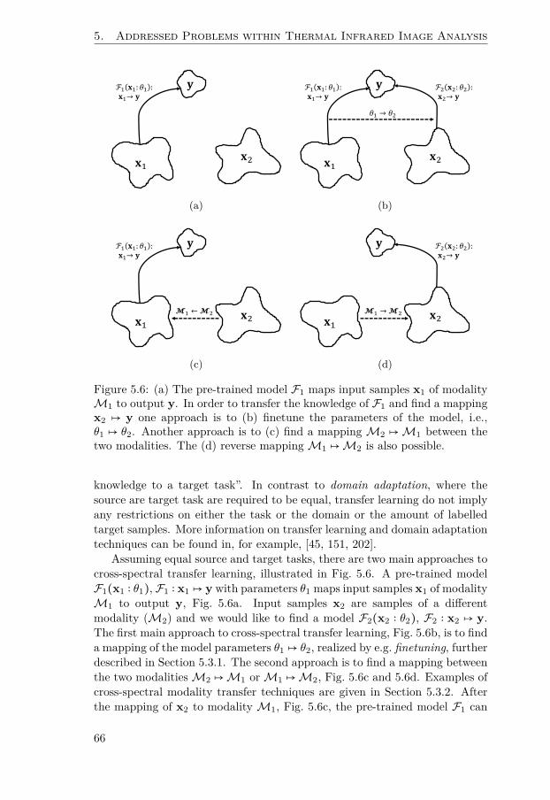
5. Addressed Problems within Thermal Infrared Image Analysis
𝐱1𝐱2
𝐲ℱ1 𝐱1: 𝜃1 :𝐱1→ 𝐲
(a)
𝐱1𝐱2
𝐲
𝜃1 → 𝜃2
ℱ2 𝐱2: 𝜃2 :𝐱2→ 𝐲
ℱ1 𝐱1: 𝜃1 :𝐱1→ 𝐲
(b)
𝐱1𝐱2
𝐲
𝓜1 ←𝓜2
ℱ1 𝐱1: 𝜃1 :𝐱1→ 𝐲
(c)
𝐱1𝐱2
𝐲
𝓜1 →𝓜2
ℱ2 𝐱2: 𝜃2 :𝐱2→ 𝐲
(d)
Figure 5.6: (a) The pre-trained model F1 maps input samples x1 of modalityM1 to output y. In order to transfer the knowledge of F1 and find a mappingx2 ↦ y one approach is to (b) finetune the parameters of the model, i.e.,θ1 ↦ θ2. Another approach is to (c) find a mapping M2 ↦M1 between thetwo modalities. The (d) reverse mapping M1 ↦M2 is also possible.
knowledge to a target task”. In contrast to domain adaptation, where thesource are target task are required to be equal, transfer learning do not implyany restrictions on either the task or the domain or the amount of labelledtarget samples. More information on transfer learning and domain adaptationtechniques can be found in, for example, [45, 151, 202].
Assuming equal source and target tasks, there are two main approaches tocross-spectral transfer learning, illustrated in Fig. 5.6. A pre-trained modelF1(x1 ∶ θ1), F1 ∶ x1 ↦ y with parameters θ1 maps input samples x1 of modalityM1 to output y, Fig. 5.6a. Input samples x2 are samples of a differentmodality (M2) and we would like to find a model F2(x2 ∶ θ2), F2 ∶ x2 ↦ y.The first main approach to cross-spectral transfer learning, Fig. 5.6b, is to finda mapping of the model parameters θ1 ↦ θ2, realized by e.g. finetuning, furtherdescribed in Section 5.3.1. The second approach is to find a mapping betweenthe two modalitiesM2 ↦M1 orM1 ↦M2, Fig. 5.6c and 5.6d. Examples ofcross-spectral modality transfer techniques are given in Section 5.3.2. Afterthe mapping of x2 to modality M1, Fig. 5.6c, the pre-trained model F1 can
66

5.3. Cross-spectral transfer learning
(a) (b) (c)
(d) (e) (f)
Figure 5.7: A YOLO9000 object detector applied to thermal infrared imagesfeaturing an outdoor biofuel storage. In (a)-(c) there has been no finetun-ing of the detector. Pink (bed), orange (car), and green (train) boxes areYOLO9000 detections of different classes. In (d)-(f), the YOLO9000 detectorwas finetuned for the purpose of vehicle detection. The images show successfulexamples. Pink boxes are YOLO9000 detections of class truck and red boxesare ground truth annotations.
be applied. Another option would be the reverse mapping, M1 ↦ M2, inorder to generate more training data inM2. The model F2 ∶ x2 ↦ y can thenbe trained from scratch, as illustrated in Fig. 5.6d.
5.3.1 FinetuningThe most common approach to deep transfer learning is to simply freeze allbut one or a few of the final layers in a pre-trained network and then retrain itusing the target dataset [9]. This approach, known as finetuning, is based onthe well-known fact that the upper layers of a network are more task specificwhile the lower layers are more modal specific [120]. Therefore, in the case ofcross-spectral transfer learning, this approach might not be the optimal oneand different techniques should be examined further.
67

5. Addressed Problems within Thermal Infrared Image Analysis
Some examples of detection results from a default and finetunedYOLO9000 object detector [164] applied to thermal infrared images can beseen in Fig. 5.7. The network was pre-trained on the COCO object detectiondataset [126] and default parameters were used. Without finetuning, Fig. 5.7a-5.7c, the detector failed to detect any of the vehicles in the validation dataset.It did, however, provide some interesting results. For example, it could suc-cessfully detect a train in the thermal infrared modality, Fig. 5.7c, large pilesof biofuel apparently had certain similarities to beds, Fig. 5.7a, and a cara-van was labelled as a car, Fig. 5.7b, while the two cars next to it remainedundetected. After finetuning the last layer of the detector for the purpose ofvehicle detection, detection performance improves. A few successful examplesare shown in Fig. 5.7d-5.7f.
These examples provide some insight in the difficulties related to transferlearning from visual RGB to TIR. Deep neural networks, despite their suc-cesses, do not by default possess the highly complex modality generalizationabilities possessed by the human brain.
5.3.2 Cross-spectral modality transferModality transfer is the process of altering a source domain as an attempt tobring the distribution of the source closer to that of the target. There aremultiple objectives for modality transfer, the purpose can, e.g., be transferlearning, as described above, or visualization in order to facilitate interpreta-tion, as in Paper G. In the case of thermal to visual spectrum image transfer,there is no correspondence between the measured thermal radiation of anobject and its color, which makes it a challenging problem. It is assumed,however, that there is an underlying semantic representation common to thetwo modalities and the aim is to find these latent representations.
In Paper G, a dataset with corresponding TIR and visual RGB imagepairs enabled semi-supervised learning in the form of an autoencoder net-work. The acquisition of TIR and visual RGB image pairs with perfect pixelto pixel correspondence is, however, a difficult task. Since glass is opaque inTIR wavelengths, optics for thermal cameras are typically made of materialslike germanium. Hence, it is difficult, but not impossible, to acquire thermaland visual images with the same optical axis. A modality transfer method is,therefore, required to be robust to image pair misalignments. In Paper G, theproblem is mitigated by separating the loss into a luminance and a chromi-nance part, exploiting the lower acuity for color differences possessed by thehuman visual system.
The method proposed in Paper G was the first published approach to TIRto perceptually realistic RGB transfer. The work was later extended by Ny-berg et al. [148] who proposed an unsupervised method based on generativeadversarial networks for unpaired thermal to visible spectrum transfer. Com-pared to the method in Paper G, the proposed method does not require image
68

5.4. Relevance to real-world applications
(a) Detection of mastitis† (b) Obstacle detection‡ (c) Fire monitoring⋆
(d) Spot weld inspection⋆ (e) Fever screening◇ (f) Intrusion detection⋆
Figure 5.8: Examples of real-world applications related to the addressedproblems. Image courtesy of ⋆Termisk Systemteknik AB, †Agricam AB, and◇Imafor AB. ‡Reproduced with the permission of Springer.
pairs with pixel to pixel correspondence and the resulting visual spectrum im-ages were sharper.
5.4 Relevance to real-world applications
In this chapter, three different problems have been described in the contextof image analysis in thermal infrared (TIR) images. There are many real-world applications related to automatic image analysis in TIR images and tothe addressed problems in particular. As TIR image resolution and qualityincrease and prices decrease there will be even more, not even thought of yet.
5.4.1 Visual object trackingVisual object tracking is a general problem relevant to a number of different ar-eas, for example, surveillance, robotics, autonomous driving, automation, andmedicine. Examples include tracking of objects in various research projects,e.g., tracking and counting bats emerging from a cave [91]. Other examplesare tracking of pedestrians in systems for automotive safety, using a smallthermal camera mounted in the front of a car (or train) (Paper D) [28, 214],Fig. 5.8b, and search and rescue, searching for persons independently ofdaylight using cameras carried by UAVs, helicopters or rescue robots [170].
69

5. Addressed Problems within Thermal Infrared Image Analysis
Tracking methods can also be used within agriculture for monitoring ofwild and domestic animals in order to e.g. perform behaviour analysis, orto estimate population sizes [73, 91]. For security applications, detection,tracking, and behaviour analysis of persons and vehicles can be applied forthe purpose of detection of intrusions and suspicious behaviour (Paper C) [52,101], Fig. 5.8f.
5.4.2 Anomaly detectionThe general nature of the formulation of the anomaly detection problem makesit applicable to a range of different fields. For example, problems within thefield of agriculture such as detection of diseases in plants [163] or detection ofinflammations in dairy cows [41], Fig. 5.8a. Other examples include problemswithin industry, e.g., detection of different materials, positioning, and non-destructive testing (Paper E) [144, 171], Fig. 5.8d.
Thermal (radiometric) cameras can also be useful for fire detection sincethey can see through smoke, Fig. 5.8c. They are commonly used by fire fightersto find persons and to localise the base of the fire [155, 173]. For medicalapplications, thermal infrared cameras can be used for detection of tumoursin early stages, inflammations, fever screening, etc. [3, 38, 114], Fig. 5.8e.
5.4.3 Cross-spectral modality transferLearning methods such as deep neural networks usually require large amountsof training data. As described in Section 5.3.2, cross-spectral modality transferis highly relevant for scarcely used image modalities such as thermal infrared.These methods, thus, enable application of pre-trained models on visual im-ages onto, e.g., thermal infrared images. In summary, real-world applicationsthat benefit from the TIR modality due to, e.g., operation during night canmake use of methods pre-trained for the visual modality without requiringannotation of large amounts of training data.
70

6
Concluding Remarks
This thesis has addressed the problem of automatic image analysis in thermalinfrared images with a focus on machine learning methods. The main purposehas been to study the variations of processing required due to the thermalinfrared modality. In particular, three different problems have been addressed:visual object tracking, anomaly detection, and modality transfer. This chapterconcludes the thesis by discussing the results, suggesting directions for futurework, and describing its impact on society.
6.1 Conclusions and discussion
In this thesis, the variations of processing required due to the thermal in-frared (TIR) modality have been studied from a few different directions. Eventhough each one of the included publications has a quite narrow problem for-mulation, they are all part of the overall aim of the thesis. Common to mostof the included papers is the usage of machine learning methods. It can beconcluded that the specification to thermal infrared images often lies in therepresentation, or design of the loss function, rather than the machine learn-ing method itself. Some exceptions presumably exist, one example could, forexample, be in the design of a CNN, see future work.
A thermal infrared camera measures the thermal infrared radiation, i.e.,radiation beyond the visible spectrum, within an area. The differences betweenthermal infrared and visible imagery have been explained in this thesis. Forexample, in the noise characteristics, the amount of discernible spatial pat-terns, the data format, and how the emitted radiation behave in comparisonto reflected radiation.
Some of the common challenges to image analysis methods when appliedto visual images, e.g., rapid illumination changes and shadows, do not exist inthermal infrared (TIR) images. On the other hand, it is usually, for example,more difficult to discriminate between different objects in TIR since visual
71

6. Concluding Remarks
color patterns are discernible in TIR only if they correspond to variations inmaterial or temperature. In conclusion, image analysis in TIR compared tovisual images is more simple in some aspects and more complicated in others.
Within the last couple of years, there has been many published workswithin the computer vision field where standard methods designed for visualimages have been applied directly to thermal infrared images. The methodsare often applied without considering the differences between the two modal-ities. As has been shown in this thesis, methods designed for visual imagesmight be suboptimal for TIR for several reasons. For example, these methodsare often designed to be invariant to illumination changes, a phenomenon thatdoes not exist in thermal infrared images.
Finally, it is of the author’s belief that the included publications have raisedawareness of the problems related to image analysis in thermal infrared imagescompared to visual images. Especially through the published benchmark,leading to the challenges VOT-TIR 2015 and 2016, raising the standard forpublicly available thermal infrared tracking benchmarks.
6.2 Future work
This thesis have focused on three problems within the field of computer visionfor thermal infrared images: visual object tracking, anomaly detection, andmodality transfer. There are many other aspects of the overall goal to studythe variations of processing required that have not been addressed here. Inaddition, there are aspects and parts of the addressed problems that couldbe examined further. In the remainder of this section, a few of these arediscussed.
The VOT-TIR 2015 benchmark compared trackers participating both inthe visual tracking challenge VOT and the thermal infrared challenge VOT-TIR. Since the visual and thermal datasets were completely unrelated, thecomparison could only be made by an examination of the relative ratings ofthe different trackers. Future work could be to construct a large, fully syn-chronized RGB and TIR dataset for tracking evaluation. Comparing trackingresult on RGB and TIR could provide insight on what features of a trackerthat are important for RGB and TIR respectively. In particular, frame-wiselabels of visual attributes, e.g., camera motion, occlusion etc. could providefurther insight. The VOT-RGBT 2019 benchmark had a multi-modal RGB-Tdataset, the synchronization was, however, not perfect and the challenge wasjoint RGB and TIR tracking.
The semi-automatic annotation method proposed in Paper B could be im-proved. One suggestion is to incorporate frame-wise labels of visual attributesin order to prevent the failure detection method to get stuck in occlusion areas.
Concerning Convolutional Neural Networks (CNNs) trained on TIR im-ages it should be examined further what features are learnt by the filters in
72

6.3. Impact on society
comparison to CNNs trained on visual images. There are many publications[56, 120, 132, 209, 211] that visualizes and examines what happens at thedifferent nodes and layers, what filters that are learnt etc. for visual images,but not for the thermal infrared modality.
There are several special cases not addressed in Paper D that could beaddressed in future work, e.g., heated railroad switches and connecting rail-roads. Furthermore, the railroad detection could possibly be aided by theincorporation of a GPS and access to a railroad map.
Regarding anomaly detection by Generative Adversarial Networks(GANs), a more extensive examination of the structure of the latent space,especially in the case when an encirclement loss and encoder is introduced, isneeded. Other ways to structure the latent space for the purpose of anomalydetection should be further examined as well. It has been shown that GANsindeed do not copy training samples but rather learns the distribution, e.g., byKarras et al. [102]. The percentage of anomalies in the training data that canbe included before the GAN includes them in the learnt distribution should beinvestigated. Further work is also to apply the method proposed in Paper Fto thermal infrared, or multi-spectral images. For example, the method couldbe applied to the problem of district heating leakage detection discussed inPaper E.
Finally, this thesis barely scratches upon the topic of transfer learningtechniques between different modalities. An area that should be investigatedfurther since it is highly relevant. For scarcely used modalities such as ther-mal infrared, manual annotation is difficult to justify and only a few fullyannotated large-scale datasets exist.
6.3 Impact on society
The popularity of thermal cameras have increased in recent years as imageresolution and quality have increased in combination with a decrease in cameraprice and size. Thermal cameras are advantageous to visual cameras in manyapplications due to their ability to see in total darkness, their robustness toillumination changes, and less intrusion on privacy. In the future, they willbe even more common in civilian applications than they are today.
Many applications connected to thermal cameras can be related to a sus-tainable society, for example, prevention and localisation of energy losses, aswell as environmental friendly transportation. Areas that are highly relevantin today’s society.
Privacy-preserving techniques will become more important as cameras be-come increasingly common in our every day lives. Thermal infrared imagingis considered to be a technique that preserves the privacy of humans and will,thus, play an important role.
73

6. Concluding Remarks
As technology evolves, the human-machine interface will become moreimportant. Modality transfer techniques for the purpose of visualization willfacilitate the interpretation for those that are not an expert on the specificmodality.
Finally, some of the methods covered in this thesis are already used in real-world applications today, making an impact on society by detecting intrusions,preventing fires, and detecting district heating leakages.
74

Bibliography
[1] A. Abdallah, M. A. Maarof, and A. Zainal. “Fraud Detection System:A Survey”. In: Journal of Network and Computer Applications 68 (June2016), pp. 90–113. issn: 1084-8045.
[2] J. Ahlberg and A. Berg. “Evaluating Template Rescaling in Short-term Single-object Tracking”. In: IEEE International Conference onAdvanced Video- and Signal-based Surveillance Workshops. Aug. 2015,pp. 1–4. doi: 10.1109/AVSS.2015.7301745.
[3] J. Ahlberg, A. Berg, and N. Markuš. “Multi-person Fever Screeningusing a Thermal and a Visual Camera”. In: Swedish Symposium onImage Analysis (SSBA). 2015.
[4] M. Ahmed, A. N. Mahmood, and M. R. Islam. “A Survey of AnomalyDetection Techniques in Financial Domain”. In: Future GenerationComputer Systems 55 (Feb. 2016), pp. 278–288.
[5] S. Akçay, A. Atapour-Abarghouei, and T. P. Breckon. “GANomaly:Semi-supervised Anomaly Detection via Adversarial Training”. In: 2018Asian Conference on Computer Vision (ACCV). Springer InternationalPublishing, Dec. 2019, pp. 622–637.
[6] S. Akçay, A. Atapour-Abarghouei, and T. P. Breckon. “Skip-GANomaly: Skip Connected and Adversarially Trained Encoder-Decoder Anomaly Detection”. In: 2019 International Joint Conferenceon Neural Networks (IJCNN). IEEE, Jan. 2019, pp. 1–8.
[7] S. A. Ambrose, M. C. Lovett, M. W. Bridges, M. K. Norman, and M.DiPietro. How Learning Works: Seven Research-Based Principles forSmart Teaching. 2010.
[8] M. Arjovsky, S. Chintala, and L. Bottou. “Wasserstein GAN”. In: arXive-prints (Jan. 2017). arXiv: 1701.07875 [stat.ML].
75
Bibliography
[9] H. Azizpour, A. S. Razavian, J. Sullivan, A. Maki, and S. Carlsson.“Factors of Transferability for a Generic ConvNet Representation”. In:IEEE Transactions on Pattern Analysis and Machine Intelligence 38.9(Sept. 2016), pp. 1790–1802.
[10] V. Badrinarayanan, A. Kendall, and R. Cipolla. “SegNet: A Deep Con-volutional Encoder-Decoder Architecture for Image Segmentation”. In:IEEE Transactions on Pattern Analysis and Machine Intelligence 39.12(Dec. 2017), pp. 2481–2495.
[11] T. Bayes and R. Price. “An Essay Towards Solving a Problem in theDoctrine of Chance”. In: Philosophical Transactions of the Royal Soci-ety of London 53.0 (1763), pp. 370–418.
[12] Y. Bengio, A. Courville, and P. Vincent. “Representation Learning:A Review and New Perspectives”. In: IEEE Transactions on PatternAnalysis and Machine Intelligence 35.8 (Aug. 2013), pp. 1798–1828.
[13] A. Berg and J. Ahlberg. “Classification and Temporal Analysis of Dis-trict Heating Leakages in Thermal Images”. In: The 14th InternationalSymposium on District Heating and Cooling (DHC). 2014.
[14] A. Berg and J. Ahlberg. “Classification of Leakage Detections Acquiredby Airborne Thermography of District Heating Networks”. In: PatternRecognition in Remote Sensing (PRRS), IAPR Workshop on. 2014.doi: 10.1109/PRRS.2014.6914288.
[15] A. Berg, J. Ahlberg, and M. Felsberg. “A Thermal Infrared Dataset forEvaluation of Short-term Tracking Methods”. In: Swedish Symposiumon Image Analysis (SSBA). 2015.
[16] A. Berg, J. Ahlberg, and M. Felsberg. “A Thermal Object TrackingBenchmark”. In: 2015 12th IEEE International Conference on Ad-vanced Video and Signal Based Surveillance (AVSS). Aug. 2015, pp. 1–6. doi: 10.1109/AVSS.2015.7301772.
[17] A. Berg, J. Ahlberg, and M. Felsberg. “Channel Coded Distribu-tion Field Tracking for Thermal Infrared Imagery”. In: 2016 IEEEConference on Computer Vision and Pattern Recognition Workshops(CVPRW). June 2016, pp. 1248–1256. doi: 10.1109/CVPRW.2016.158.
[18] A. Berg, J. Ahlberg, and M. Felsberg. “Classifying District HeatingNetwork Leakages in Aerial Thermal Imagery”. In: Swedish Symposiumon Image Analysis (SSBA). 2014.
[19] A. Berg, J. Ahlberg, and M. Felsberg. “Generating Visible SpectrumImages from Thermal Infrared”. In: 2018 IEEE Conference on Com-puter Vision and Pattern Recognition Workshops (CVPRW). June2018. doi: 10.1109/CVPRW.2018.00159.
76
Bibliography
[20] A. Berg, J. Ahlberg, and M. Felsberg. “Object Tracking in ThermalInfrared Imagery based on Channel Coded Distribution Fields”. In:Swedish Symposium on Image Analysis (SSBA). 2017.
[21] A. Berg, J. Ahlberg, and M. Felsberg. “Unsupervised AdversarialLearning of Anomaly Detection in the Wild”. In: Submitted to the 24thEuropean Conference on Artificial Intelligence (ECAI 2020). 2019.
[22] A. Berg, J. Ahlberg, and M. Felsberg. “Visual Spectrum Image Genera-tion from Thermal Infrared”. In: Swedish Symposium on Image Analysis(SSBA). 2019.
[23] A. Berg, M. Felsberg, G. Häger, and J. Ahlberg. “An Overview of theThermal Infrared Visual Object Tracking VOT-TIR2015 Challenge”.In: Swedish Symposium on Image Analysis (SSBA). 2016.
[24] A. Berg, J. Johnander, F. Durand De Gevigney, J. Ahlberg, and M.Felsberg. “Semi-automatic Annotation of Objects in Visual-ThermalVideo”. In: IEEE International Conference on Computer Vision Work-shops (ICCVW). Oct. 2019.
[25] A. Berg. Detection and Tracking in Thermal Infrared Imagery. Licenti-ate thesis No. 1744. Linköping University Electronic Press, 2016. isbn:978-91-7685-789-2. doi: 10.3384/lic.diva-126955.
[26] A. Berg, J. Ahlberg, and M. Felsberg. “Enhanced Analysis of Ther-mographic Images for Monitoring of District Heat Pipe Networks”. In:Pattern Recognition Letters 83 (2016). Advances in Pattern Recogni-tion in Remote Sensing, pp. 215–223. issn: 0167-8655. doi: https://doi.org/10.1016/j.patrec.2016.07.002.
[27] A. Berg, K. Öfjäll, J. Ahlberg, and M. Felsberg. “Detecting Rails andObstacles Using a Train-Mounted Thermal Camera”. In: ScandinavianConference on Image Analysis (SCIA). Springer International Publish-ing, 2015, pp. 492–503. isbn: 978-3-319-19665-7. doi: https://doi.org/10.1007/978-3-319-19665-7_42.
[28] M. Bertozzi, A. Broggi, A. Fascioli, T. Graf, and M. Meinecke. “Pedes-trian Detection for Driver Assistance using Multiresolution InfraredVision”. In: Vehicular Technology, IEEE Transactions on 53.6 (2004),pp. 1666–1678.
[29] C. M. Bishop. Pattern Recognition and Machine Learning (InformationScience and Statistics). Berlin, Heidelberg: Springer-Verlag, 2006. isbn:0387310738.
[30] V. N. Boddeti, T. Kanade, and B. V. Kumar. “Correlation Filters forObject Alignment”. In: 2013 IEEE Conference on Computer Visionand Pattern Recognition (CVPR). IEEE, June 2013, pp. 2291–2298.
77

Bibliography
[31] D. S. Bolme, J. R. Beveridge, B. A. Draper, and Y. M. Lui. “VisualObject Tracking Using Adaptive Correlation Filters.” In: 2010 IEEEConference on Computer Vision and Pattern Recognition (CVPR).IEEE Computer Society, 2010, pp. 2544–2550.
[32] L. Breiman. “Bagging Predictors”. In: Machine Learning 24.2 (1996),pp. 123–140.
[33] L. Breiman. “Random Forests”. In: Machine Learning 45.1 (2001),pp. 5–32.
[34] K. Briechle and U. Hanebeck. “Template Matching Using Fast Normal-ized Cross Correlation”. In: Proceedings of SPIE - The InternationalSociety for Optical Engineering 4387 (2001).
[35] D. S. Broomhead and D. Lowe. “Multivariable Functional Interpolationand Adaptive Networks”. In: Complex Systems 2 (1988), pp. 321–355.
[36] S. A. Cadena, G. H. Denfield, E. Y. Walker, L. A. Gatys, A. S. Tolias,M. Bethge, and A. S. Ecker. “Deep Convolutional Models ImprovePredictions of Macaque V1 Responses to Natural Images”. In: PLOSComputational Biology 15.4 (Apr. 2019). Ed. by W. Einhäuser.
[37] M. Calonder, V. Lepetit, C. Strecha, and P. Fua. “BRIEF: BinaryRobust Independent Elementary Features”. In: The European Confer-ence on Computer Vision (ECCV). Springer, Berlin, Heidelberg, 2010,pp. 778–792.
[38] S. Y. Chekmenev, A. A. Farag, and E. A. Essock. “Thermal Imag-ing of the Superficial Temporal Artery: An Arterial Pulse RecoveryModel”. In: 2007 IEEE Conference on Computer Vision and PatternRecognition (CVPR). IEEE, June 2007, pp. 1–6.
[39] X. Chen, Y. Duan, R. Houthooft, J. Schulman, I. Sutskever, and P.Abbeel. “InfoGAN: Interpretable Representation Learning by Informa-tion Maximizing Generative Adversarial Nets”. In: Advances in Neu-ral Information Processing Systems 29. Curran Associates, Inc., 2016,pp. 2172–2180.
[40] P. Christiansen, L. N. Nielsen, K. A. Steen, R. N. Jørgensen, andH. Karstoft. “DeepAnomaly: Combining Background Subtraction andDeep Learning for Detecting Obstacles and Anomalies in an Agricul-tural Field.” In: Sensors 16.11 (Nov. 2016).
[41] A. Colak, B. Polat, Z. Okumus, M. Kaya, L. E. Yanmaz, and A. Hayirli.“Early Detection of Mastitis Using Infrared Thermography in DairyCows”. In: Journal of Dairy Science 91.11 (2008), pp. 4244–4248.
[42] J.-A.-N. d. C. Condorcet. Essai sur l’Application de l’Analyse à laProbabilité des Décisions Rendues à la Pluralité des Voix. 1785.
78

Bibliography
[43] A. Creswell and A. A. Bharath. “Inverting the Generator of a Genera-tive Adversarial Network”. In: IEEE Transactions on Neural Networksand Learning Systems 30.7 (July 2019), pp. 1967–1974.
[44] A. Creswell, T. White, V. Dumoulin, K. Arulkumaran, B. Sengupta,and A. A. Bharath. “Generative Adversarial Networks: An Overview”.In: IEEE Signal Processing Magazine 35.1 (Jan. 2018), pp. 53–65.
[45] G. Csurka. “Domain Adaptation for Visual Applications: A Compre-hensive Survey”. In: Domain Adaptation in Computer Vision Appli-cations. Springer Series: Advances in Computer Vision and PatternRecognition, Feb. 2017.
[46] N. Dalal and B. Triggs. “Histograms of Oriented Gradients for HumanDetection”. In: 2005 IEEE Conference on Computer Vision and PatternRecognition (CVPR). IEEE, 2005.
[47] M. Danelljan, G. Häger, F. S. Khan, and M. Felsberg. “Coloring Chan-nel Representations for Visual Tracking”. In: Scandinavian Conferenceon Image Analysis (SCIA). Springer, Cham, 2015, pp. 117–129.
[48] M. Danelljan, G. Häger, F. Shahbaz Khan, and M. Felsberg. “AccurateScale Estimation for Robust Visual Tracking”. In: Proceedings of theBritish Machine Vision Conference (BMVC). British Machine VisionAssociation, 2014, pp. 65.1–65.11.
[49] M. Danelljan, G. Meneghetti, S. Khan, and M. Felsberg. “A Probabilis-tic Framework for Color-Based Point Set Registration”. In: 2016 IEEEConference on Computer Vision and Pattern Recognition (CVPR).2016.
[50] J. W. Davis and M. A. Keck. “A Two-stage Template Approach toPerson Detection in Thermal Imagery”. In: Applications of ComputerVision and the IEEE Workshop on Motion and Video Computing, IEEEWorkshop on 1 (2005), pp. 364–369.
[51] J. W. Davis and V. Sharma. “Background-subtraction Using Contour-based Fusion of Thermal and Visible Imagery”. In: Computer Visionand Image Understanding 106.2 (2007), pp. 162–182.
[52] J. Davis and V. Sharma. “Robust Detection of People in Thermal Im-agery”. In: Proceedings of the 17th International Conference on PatternRecognition (ICPR). IEEE, 2004, pp. 713–716.
[53] L. Deecke, R. Vandermeulen, L. Ruff, S. Mandt, and M. Kloft. “Im-age Anomaly Detection with Generative Adversarial Networks”. In:Machine Learning and Knowledge Discovery in Databases. SpringerInternational Publishing, 2018, pp. 3–17.
[54] J. Donahue, P. Krähenbühl, and T. Darrell. “Adversarial FeatureLearning”. In: 5th International Conference on Learning Representa-tions (ICLR). May 2017.
79

Bibliography
[55] V. Dumoulin, I. Belghazi, B. Poole, O. Mastropietro, A. Lamb, M.Arjovsky, and A. Courville. “Adversarially Learned Inference”. In: 5thInternational Conference on Learning Representations (ICLR). June2017.
[56] D. Erhan, Y. Bengio, A. Courville, and P. Vincent. “Visualizing Higher-Layer Features of a Deep Network”. In: Technical Report, Univeristyde Montreal (2009).
[57] A. Esteva, B. Kuprel, R. A. Novoa, J. Ko, S. M. Swetter, H. M. Blau,and S. Thrun. “Dermatologist-level Classification of Skin Cancer withDeep Neural Networks”. In: Nature 542.7639 (Feb. 2017), pp. 115–118.
[58] C. Fefferman, S. Mitter, and H. Narayanan. “Testing the ManifoldHypothesis”. In: Journal of the American Mathematical Society 29.4(2016), pp. 983–1049.
[59] M. Felsberg and G. Granlund. “P-Channels: Robust Multivariate M-Estimation of Large Datasets”. In: 18th International Conference onPattern Recognition (ICPR). IEEE, 2006, pp. 262–267.
[60] M. Felsberg. “Enhanced Distribution Field Tracking Using ChannelRepresentations”. In: 2013 IEEE International Conference on Com-puter Vision Workshops (ICCVW). IEEE, Dec. 2013, pp. 121–128.
[61] M. Felsberg. “Probabilistic and Biologically Inspired Feature Represen-tations”. In: Synthesis Lectures on Computer Vision 8.2 (May 2018),pp. 1–103.
[62] M. Felsberg, A. Berg, G. Häger, J. Ahlberg, M. Kristan, J. Matas,A. Leonardis, L. Cehovin, G. Fernandez, et al. “The Thermal InfraredVisual Object Tracking VOT-TIR2015 Challenge Results”. In: IEEEInternational Conference on Computer Vision Workshops (ICCVW).Institute of Electrical and Electronics Engineers (IEEE), 2015, pp. 639–651. doi: 10.1109/ICCVW.2015.86.
[63] M. Felsberg, P.-E. Forssén, and H. Scharr. “Channel Smoothing: Ef-ficient Robust Smoothing of Low-level Signal Features”. In: IEEETransactions on Pattern Analysis and Machine Intelligence 28 (2004),pp. 209–222.
[64] M. Felsberg and J. Hedborg. “Real-Time Visual Recognition of Objectsand Scenes Using P-Channel Matching”. In: Scandinavian Conferenceon Image Analysis (SCIA). Berlin, Heidelberg: Springer Berlin Heidel-berg, 2007, pp. 908–917.
80

Bibliography
[65] M. Felsberg, M. Kristan, J. Matas, A. Leonardis, R. Pflugfelder, G.Häger, A. Berg, A. Eldesokey, J. Ahlberg, et al. “The Thermal InfraredVisual Object Tracking VOT-TIR2016 Challenge Results”. In: Pro-ceedings on the European Conference on Computer Vision Workshops(ECCVW). Vol. 9914. Lecture Notes in Computer Science. Springer,Cham, 2016, pp. 824–849. doi: https://doi.org/10.1007/978-3-319-48881-3_55.
[66] M. Felsberg, K. Öfjäll, and R. Lenz. “Unbiased Decoding of BiologicallyMotivated Visual Feature Descriptors”. In: Frontiers in Robotics andAI 2 (Aug. 2015), p. 20.
[67] P.-E. Forssén. “Low and Medium Level Vision Using Channel Repre-sentations”. PhD thesis. Linköping University, The Institute of Tech-nology, 2004. isbn: 91-7373-876-X.
[68] Y. Freund and R. E. Schapire. “A Decision-theoretic Generalizationof On-line Learning and an Application to Boosting”. In: Journal ofComputer and System Sciences 55.1 (Aug. 1997), pp. 119–139.
[69] O. Friman, P. Follo, J. Ahlberg, and S. Sjökvist. “Methods for Large-Scale Monitoring of District Heating Systems Using Airborne Ther-mography”. In: IEEE Transactions on Geoscience and Remote Sensing52.8 (Aug. 2014), pp. 5175–5182.
[70] K. Fukushima. “Neocognitron: A Hierarchical Neural Network Capa-ble of Visual Pattern Recognition”. In: Neural Networks 1.2 (1988),pp. 119–130.
[71] K. Fukushima. “Neocognitron: A Self-organizing Neural NetworkModel for a Mechanism of Pattern Recognition Unaffected by Shiftin Position”. In: Biological Cybernetics 36.4 (Apr. 1980), pp. 193–202.
[72] H. K. Galoogahi, T. Sim, and S. Lucey. “Multi-channel CorrelationFilters”. In: 2013 IEEE International Conference on Computer Vision(ICCV). IEEE, Dec. 2013, pp. 3072–3079.
[73] V. Gan, P. Carr, and J. Soltis. “Monitoring Giraffe Behavior in Ther-mal Video”. In: IEEE Winter Conference on Applications and Com-puter Vision Workshops (WACVW) (2015), pp. 36–43.
[74] D. M. Gavrila. “The Visual Analysis of Human Movement”. In: Com-puter Vision and Image Understanding 73.1 (1999), pp. 82–98.
[75] E. Gebhardt and M. Wolf. “CAMEL Dataset for Visual and Ther-mal Infrared Multiple Object Detection and Tracking”. In: 2018 15thIEEE International Conference on Advanced Video and Signal BasedSurveillance (AVSS). IEEE, Nov. 2018, pp. 1–6.
[76] I. Goodfellow. “NIPS 2016 Tutorial: Generative Adversarial Networks”.In: arXiv e-prints (Dec. 2016). arXiv: 1701.00160 [cs.LG].
81

Bibliography
[77] I. Goodfellow, Y. Bengio, and A. Courville. Deep Learning. MIT Press,2016.
[78] I. Goodfellow, J. Pouget-Abadie, M. Mirza, B. Xu, D. Warde-Farley,S. Ozair, A. Courville, and Y. Bengio. “Generative Adversarial Nets”.In: Advances in Neural Information Processing Systems 27. CurranAssociates, Inc., 2014, pp. 2672–2680.
[79] G. H. Granlund. “An Associative Perception-action Structure using aLocalized Space Variant Information Representation”. In: Proceedingsof the Second International Workshop on Algebraic Frames for thePerception-Action Cycle. Springer-Verlag, 2000, pp. 48–68.
[80] K. Granström, M. Baum, and S. Reuter. “Extended Object Tracking:Introduction, Overview and Applications”. In: arXiv e-prints (2016).arXiv: 1604.00970 [cs.CV].
[81] I. Gulrajani, F. Ahmed, M. Arjovsky, V. Dumoulin, and A. Courville.“Improved Training of Wasserstein GANs”. In: Proceedings of the 31stInternational Conference on Neural Information Processing Systems.2017, pp. 5769–5779.
[82] T. Hastie, R. Tibshirani, and J. Friedman. The Elements of StatisticalLearning. Springer Series in Statistics. New York, NY, USA: SpringerNew York Inc., 2001.
[83] K. He, X. Zhang, S. Ren, and J. Sun. “Deep Residual Learning forImage Recognition”. In: 2016 IEEE Conference on Computer Visionand Pattern Recognition (CVPR). IEEE, 2016, pp. 770–778.
[84] J. Heggenes, A. Odland, T. Chevalier, J. Ahlberg, A. Berg, and D.Bjerketvedt. “Herbivore Grazing–or Trampling? Trampling Effects bya Large Ungulate in Cold High-latitude Ecosystems”. In: Ecology andEvolution 7.16 (2017), pp. 6423–6431. doi: 10.1002/ece3.3130.
[85] J. F. Henriques, J. Carreira, R. Caseiro, and J. Batista. “Beyond HardNegative Mining: Efficient Detector Learning via Block-Circulant De-composition”. In: 2013 IEEE International Conference on ComputerVision (ICCV). IEEE, Dec. 2013, pp. 2760–2767.
[86] J. F. Henriques, R. Caseiro, P. Martins, and J. Batista. “High-SpeedTracking with Kernelized Correlation Filters”. In: IEEE Transac-tions on Pattern Analysis and Machine Intelligence 37.3 (Mar. 2015),pp. 583–596.
[87] W. Herschel. “Experiments on the Refrangibility of the Invisible Raysof the Sun”. In: Philosophical Transactions of the Royal Society 90(1800), pp. 284–292.
82

Bibliography
[88] W. Herschel. “Experiments on the Solar, and on the Terrestrial Raysthat Occasion Heat; With a Comparative View of the Laws WhichOccasion Them, are Subject, in Order to Determine Whether Theyare the Same, or Different.” In: Philosophical Transactions of the RoyalSociety 90 (1800), Part I: 293–326 Part II: 437–538.
[89] W. Herschel. “Investigation of the Powers of the Prismatic Colours toHeat and Illuminate Objects; With Remarks, That Prove the DifferentRefrangibility of Radiant Heat. To Which is Added, an Inquiry intothe Method of Viewing the Sun Advantageously, with Telescopes of”.In: Philosophical Transactions of the Royal Society 90 (1800), pp. 255–283.
[90] V. J. Hodge and J. Austin. “A Survey of Outlier Detection Method-ologies”. In: Artificial Intelligence Review 22.2 (Oct. 2004), pp. 85–126.
[91] N. Hristov, M. Betke, D. Theriault, A. Bagchi, and T. Kunz. “Sea-sonal Variation in Colony Size of Brazilian Free-tailed Bats at CarlsbadCavern Based on Thermal Imaging”. In: Journal of Mammalogy 91.1(2010), pp. 183–192.
[92] D. H. Hubel and T. N. Wiesel. “Receptive Fields of Single Neuronesin the Cat’s Striate Cortex”. In: The Journal of physiology 148.3 (Oct.1959), pp. 574–91.
[93] D. H. Hubel and T. N. Wiesel. “Receptive Fields, Binocular Interac-tion and Functional Architecture in the Cat’s Visual Cortex”. In: TheJournal of Physiology 160.1 (Jan. 1962), pp. 106–154.
[94] S. Hwang, J. Park, N. Kim, Y. Choi, and I. S. Kweon. “Multi-spectral Pedestrian Detection: Benchmark Dataset and Baseline”. In:2015 IEEE Conference on Computer Vision and Pattern Recognition(CVPR). IEEE, June 2015, pp. 1037–1045.
[95] S. Iizuka, E. Simo-Serra, and H. Ishikawa. “Let there be Color!: JointEnd-to-end Learning of Global and Local Image Priors for AutomaticImage Colorization with Simultaneous Classification”. In: ACM Trans-actions on Graphics (Proc. of SIGGRAPH 2016) 35.4 (2016).
[96] D. J. Im, C. D. Kim, H. Jiang, and R. Memisevic. “Generating Imageswith Recurrent Adversarial Networks”. In: arXiv e-prints (Feb. 2016).arXiv: 1602.05110 [cs.LG].
[97] S. Ioffe and C. Szegedy. “Batch Normalization: Accelerating Deep Net-work Training by Reducing Internal Covariate Shift”. In: Proceedings ofthe 32nd International Conference on Machine Learning (ICML-15).2015, pp. 448–456.
83

Bibliography
[98] P. Isola, J.-Y. Zhu, T. Zhou, and A. A. Efros. “Image-to-Image Trans-lation with Conditional Adversarial Networks”. In: 2017 IEEE Con-ference on Computer Vision and Pattern Recognition (CVPR). Nov.2017. arXiv: 1611.07004. url: http://arxiv.org/abs/1611.07004.
[99] L. C. Jain, M. Seera, C. P. Lim, and P. Balasubramaniam. “A Review ofOnline Learning in Supervised Neural Networks”. In: Neural Computingand Applications 25.3-4 (Sept. 2014), pp. 491–509.
[100] E. Jonsson. “Channel-Coded Feature Maps for Computer Vision andMachine Learning”. PhD thesis. Linköping University, The Institute ofTechnology, 2008. isbn: 978-91-7393-988-1.
[101] H. Ju and B. Bhanu. “Human Activity Recognition in Thermal InfraredImagery”. In: 2005 IEEE Conference on Computer Vision and PatternRecognition Workshops (CVPRW). IEEE, 2005.
[102] T. Karras, T. Aila, S. Laine, and J. Lehtinen. “Progressive Growing ofGANs for Improved Quality, Stability, and Variation”. In: 6th Inter-national Conference on Learning Representations (ICLR). 2018.
[103] D. P. Kingma and M. Welling. “Auto-Encoding Variational Bayes”.In: 2nd International Conference on Learning Representations (ICLR)(2014).
[104] J. Koenderink. “What is a ”Feature”?” In: Journal of Intelligent Sys-tems 3.1 (Jan. 1993).
[105] M. Kristan, J. Matas, A. Leonardis, M. Felsberg, L. Cehovin, et al.“The Visual Object Tracking VOT2015 Challenge Results”. In: 2015IEEE International Conference on Computer Vision Workshop (IC-CVW). IEEE, Dec. 2015, pp. 564–586.
[106] M. Kristan, J. Matas, A. Leonardis, M. Felsberg, R. Pflugfelder, J.-K.Kamarainen, L. Cehovin, O. Drbohlav, A. Lukezic, A. Berg, A. Eldes-okey, et al. “The Seventh Visual Object Tracking VOT2019 ChallengeResults”. In: 2019 IEEE International Conference on Computer VisionWorkshops (ICCVW). 2019.
[107] M. Kristan, A. Leonardis, J. Matas, et al. “The Visual Object TrackingVOT2017 Challenge Results”. In: 2017 IEEE International Conferenceon Computer Vision Workshops (ICCVW). IEEE, Oct. 2017, pp. 1949–1972.
[108] M. Kristan, A. Leonardis, J. Matas, et al. “The Visual Object TrackingVOT2016 Challenge Results”. In: The 2016 European Conference onComputer Vision Workshops (ECCVW). Vol. 9914. Springer, Cham,2016, pp. 777–823.
84

Bibliography
[109] M. Kristan, A. Leonardis, J. Matas, et al. “The Sixth Visual ObjectTracking VOT2018 Challenge Results”. In: The 2018 European Con-ference on Computer Vision Workshops (ECCVW). Springer, Cham,Jan. 2019, pp. 3–53.
[110] M. Kristan, R. Pflugfelder, A. Leonardis, J. Matas, et al. “The VisualObject Tracking VOT2013 Challenge Results”. In: 2013 IEEE Interna-tional Conference on Computer Vision Workshops (ICCVW). IEEE,Dec. 2013, pp. 98–111.
[111] M. Kristan, R. Pflugfelder, A. Leonardis, J. Matas, et al. “The Vi-sual Object Tracking VOT2014 Challenge Results”. In: The 2014 Euro-pean Conference on Computer Vision Workshops (ECCVW). Springer,Cham, 2015, pp. 191–217.
[112] A. Krizhevsky, I. Sutskever, and G. E. Hinton. “ImageNet Classifi-cation with Deep Convolutional Neural Networks”. In: Advances inNeural Information Processing Systems 25. Curran Associates, Inc.,2012, pp. 1097–1105.
[113] K. Kurach, M. Lucic, X. Zhai, M. Michalski, and S. Gelly. “A Large-Scale Study on Regularization and Normalization in GANs”. In: Pro-ceedings of the 36th International Conference on Machine Learning.PMLR, 2019, pp. 3581–3590.
[114] B. Lahiri, S. Bagavathiappan, T. Jayakumar, and J. Philip. “Medi-cal Applications of Infrared Thermography: A Review”. In: InfraredPhysics & Technology 55.4 (July 2012), pp. 221–235.
[115] A. B. L. Larsen, S. K. Sønderby, H. Larochelle, and O. Winther. “Au-toencoding Beyond Pixels using a Learned Similarity Metric”. In: Pro-ceedings of The 33rd International Conference on Machine Learning.PMLR, 2016, pp. 1558–1566.
[116] Y. LeCun, B. Boser, J. S. Denker, D. Henderson, R. E. Howard, W.Hubbard, and L. D. Jackel. “Backpropagation Applied to Handwrit-ten Zip Code Recognition”. In: Neural Computation 1.4 (Dec. 1989),pp. 541–551.
[117] Y. LeCun, B. Boser, J. S. Denker, R. E. Howard, W. Habbard, L. D.Jackel, and D. Henderson. “Handwritten Digit Recognition with aBack-propagation Network”. In: Advances in Neural Information Pro-cessing Systems 2. San Francisco, CA, USA: Morgan Kaufmann Pub-lishers Inc., 1990, pp. 396–404.
[118] C. Ledig, L. Theis, F. Huszar, J. Caballero, A. Cunningham, A. Acosta,A. Aitken, A. Tejani, J. Totz, Z. Wang, and W. Shi. “Photo-RealisticSingle Image Super-Resolution Using a Generative Adversarial Net-work”. In: 2017 IEEE Conference on Computer Vision and PatternRecognition (CVPR). 2017, pp. 105–114.
85

Bibliography
[119] A. M. Legendre. Nouvelles Methodes pour la Determination des Orbitesdes Cometes. F. Didot Paris, 1805.
[120] K. Lenc and A. Vedaldi. “Understanding Image Representations byMeasuring Their Equivariance and Equivalence”. In: InternationalJournal of Computer Vision 127.5 (May 2019), pp. 456–476.
[121] C. Li, H. Cheng, S. Hu, X. Liu, J. Tang, and L. Lin. “Learning Col-laborative Sparse Representation for Grayscale-thermal Tracking”. In:IEEE Transactions on Image Processing 25.12 (Dec. 2016), pp. 5743–5756.
[122] C. Li, X. Liang, Y. Lu, N. Zhao, and J. Tang. “RGB-T Object Tracking:Benchmark and Baseline”. In: arXiv e-prints (May 2018). arXiv: 1805.08982 [cs.CV].
[123] C. Li, N. Zhao, Y. Lu, C. Zhu, and J. Tang. “Weighted Sparse Rep-resentation Regularized Graph Learning for RGB-T Object Tracking”.In: ACM International Conference on Multimedia (ACM MM). 2017,pp. 1856–1864.
[124] L. Li, T. Nawaz, and J. Ferryman. “PETS 2015: Datasets and Chal-lenge”. In: 2015 12th IEEE International Conference on AdvancedVideo and Signal Based Surveillance (AVSS). 2015.
[125] X. Li, W. Hu, C. Shen, Z. Zhang, A. Dick, and A. van den Hengel.“A Survey of Appearance Models in Visual Object Tracking”. In: ACMTransactions on Intelligent Systems and Technology 4.4 (2013), 58:1–58:48.
[126] T.-Y. Lin, M. Maire, S. Belongie, J. Hays, P. Perona, D. Ramanan,P. Dollár, and C. L. Zitnick. “Microsoft COCO: Common Objects inContext”. In: The European Conference on Computer Vision (ECCV).Springer, Cham, 2014, pp. 740–755.
[127] Z. C. Lipton and S. Tripathi. “Precise Recovery of Latent Vectors fromGenerative Adversarial Networks”. In: arXiv e-prints (2017). arXiv:1702.04782v2 [cs.LG].
[128] G. Liu, F. A. Reda, K. J. Shih, T.-C. Wang, A. Tao, and B. Catan-zaro. “Image Inpainting for Irregular Holes Using Partial Convolu-tions”. In: The European Conference on Computer Vision (ECCV).Springer, Cham, 2018.
[129] Q. Liu and Z. He. “PTB-TIR: A Thermal Infrared Pedestrian TrackingBenchmark”. In: IEEE Transactions on Multimedia (2019).
[130] D. G. Lowe. “Distinctive Image Features from Scale-Invariant Key-points”. In: International Journal of Computer Vision 60.2 (Nov. 2004),pp. 91–110.
86

Bibliography
[131] N. Ludtke, R. Wilson, and E. Hancock. “Probabilistic Population Cod-ing of Multiple Edge Orientation”. In: Proceedings. International Con-ference on Image Processing. Vol. 2. IEEE, 2002, pp. II–865–II–868.
[132] A. Mahendran and A. Vedaldi. “Understanding Deep Image Represen-tations by Inverting them”. In: IEEE Conference on Computer Visionand Pattern Recognition (CVPR). IEEE Computer Society, Oct. 2015,pp. 5188–5196.
[133] A. Makhzani and B. Frey. “k-Sparse Autoencoders”. In: arXiv e-prints(Dec. 2013). arXiv: 1312.5663 [cs.LG].
[134] S. Mallat. A Wavelet Tour of Signal Processing: The Sparse Way. 3rd.Elsevier, 2009. isbn: 978-0-12-374370-1.
[135] N. Markuš, M. Frljak, I. S. Pandžić, J. Ahlberg, and R. Forchheimer.“Object Detection with Pixel Intensity Comparisons Organized inDecision Trees”. In: arXiv e-prints (May 2013). arXiv: 1305 . 4537[cs.CV].
[136] L. Matthews, T. Ishikawa, and S. Baker. “The Template Update Prob-lem”. In: IEEE Transactions on Pattern Analysis and Machine Intelli-gence 26.6 (June 2004), pp. 810–815.
[137] B. Mears, L. Sevilla-Lara, and E. Learned-Miller. “Distribution Fieldswith Adaptive Kernels for Large Displacement Image Alignment”. In:Proceedings of the British Machine Vision Conference (BMVC). 2013,pp. 17.1–17.11.
[138] R. Miezianko. IEEE OTCBVS WS Series Bench; Terravic ResearchInfrared Database. url: http://vcipl-okstate.org/pbvs/bench/Data/05/download.html.
[139] M. Minsky and S. Papert. Perceptrons: An Introduction to Computa-tional Geometry. The MIT Press, 1969.
[140] M. Mirza and S. Osindero. “Conditional Generative Adversarial Nets”.In: arXiv e-prints (2014). arXiv: 1411.1784 [cs.LG].
[141] T. B. Moeslund, A. Hilton, and V. Krüger. “A Survey of Advancesin Vision-based Human Motion Capture and Analysis”. In: ComputerVision and Image Understanding 104.2 (Nov. 2006), pp. 90–126.
[142] S. Mukherjee, H. Asnani, E. Lin, and S. Kannan. “ClusterGAN : LatentSpace Clustering in Generative Adversarial Networks”. In: The 33rdConference on Artificial Intelligence (AAAI). 2019.
[143] T. Nawaz, A. Berg, J. Ferryman, J. Ahlberg, and M. Felsberg. “Effec-tive Evaluation of Privacy Protection Techniques in Visible and Ther-mal Imagery”. In: Journal of Electronic Imaging (JEI) 26.5 (2017),pp. 1–16. doi: 10.1117/1.JEI.26.5.051408.
87

Bibliography
[144] Y.-M. H. Ng, M. Yu, Y. Huang, and R. Du. “Diagnosis of Sheet MetalStamping Processes Based on 3-D Thermal Energy Distribution”. In:IEEE Transactions on Automation Science and Engineering 4.1 (Jan.2007), pp. 22–30.
[145] C. P. Ngo, A. A. Winarto, C. K. K. Li, S. Park, F. Akram, and H. K.Lee. “Fence GAN: Towards Better Anomaly Detection”. In: arXiv e-prints (Apr. 2019). arXiv: 1904.01209 [cs.LG].
[146] J. Ning, L. Zhang, D. Zhang, and C. Wu. “Robust Mean-shift Trackingwith Corrected Background-weighted Histogram”. In: IET ComputerVision 6.1 (2012), p. 62.
[147] K. Nordberg, G. Granlund, and H. Knutsson. “Representation andLearning of Invariance”. In: Proceedings of 1st International Conferenceon Image Processing. Vol. 2. IEEE Comput. Soc. Press, 1994, pp. 585–589.
[148] A. Nyberg, A. Eldesokey, D. Bergström, and D. Gustafsson. “UnpairedThermal to Visible Spectrum Transfer Using Adversarial Training”. In:2018 European Conference on Computer Vision Workshops (ECCVW).Springer, Cham, Sept. 2018, pp. 657–669.
[149] K. Öfjäll. “Adaptive Supervision Online Learning for Vision BasedAutonomous Systems”. PhD thesis. Linköping University, Faculty ofScience & Engineering, 2016. isbn: 978-91-7685-815-8.
[150] K. Öfjäll and M. Felsberg. “Weighted Update and Comparison forChannel-Based Distribution Field Tracking”. In: The European Con-ference on Computer Vision (ECCV). Springer, Cham, 2014, pp. 218–231.
[151] S. J. Pan and Q. Yang. “A Survey on Transfer Learning”. In: IEEETransactions on Knowledge and Data Engineering 22.10 (Oct. 2010),pp. 1345–1359.
[152] E. Parzen. “On Estimation of a Probability Density Function andMode”. In: The Annals of Mathematical Statistics 33.3 (1962), pp.1065–1076.
[153] L. Patino, T. Cane, A. Vallee, and J. Ferryman. “PETS 2016: Datasetand Challenge”. In: 2016 IEEE Conference on Computer Visionand Pattern Recognition Workshops (CVPRW). IEEE, June 2016,pp. 1240–1247.
[154] L. Patino, T. Nawaz, T. Cane, and J. Ferryman. “PETS 2017: Datasetand Challenge”. In: 2017 IEEE Conference on Computer Vision andPattern Recognition Workshops (CVPRW). IEEE, July 2017, pp. 2126–2132.
88

Bibliography
[155] R. Paugam, M. J. Wooster, and G. Roberts. “Use of Handheld ThermalImager Data for Airborne Mapping of Fire Radiative Power and Energyand Flame Front Rate of Spread”. In: IEEE Transactions on Geoscienceand Remote Sensing 51.6 (June 2013), pp. 3385–3399.
[156] K. Pearson. “On Lines and Planes of Closest Fit to Systems of Points inSpace”. In: The London, Edinburgh, and Dublin Philosophical Magazineand Journal of Science 2.11 (Nov. 1901), pp. 559–572.
[157] G. Perarnau, J. van de Weijer, B. Raducanu, and J. M. Álvarez. “In-vertible Conditional GANs for Image Editing”. In: NIPS Workshop onAdversarial Training. Nov. 2016.
[158] M. Planck. “Zur Theorie des Gesetzes der Energieverteilung imNormalspektrum”. In: Verhandlungen der Deutschen PhysikalischenGesellschaft 2.17 (1900), pp. 237–245.
[159] J. Portmann, S. Lynen, M. Chli, and R. Siegwart. “People Detectionand Tracking from Aerial Thermal Views”. In: Proceedings of the IEEEInternational Conference on Robotics and Automation (ICRA). 2014.
[160] A. Pouget, P. Dayan, and R. Zemel. “Information Processing withPopulation Codes”. In: Nature Reviews Neuroscience 1.2 (Nov. 2000),pp. 125–132.
[161] A. Pouget, P. Dayan, and R. S. Zemel. “Inference and Computationwith Population Codes”. In: Annual Review of Neuroscience 26.1 (Mar.2003), pp. 381–410.
[162] A. Radford, L. Metz, and S. Chintala. “Unsupervised RepresentationLearning with Deep Convolutional Generative Adversarial Networks”.In: arXiv e-prints (Nov. 2015). arXiv: 1511.06434 [cs.LG].
[163] S.-e.-A. Raza, G. Prince, J. P. Clarkson, and N. M. Rajpoot. “Auto-matic Detection of Diseased Tomato Plants Using Thermal and StereoVisible Light Images”. In: PLOS ONE 10.4 (Apr. 2015).
[164] J. Redmon and A. Farhadi. “YOLO9000: Better, Faster, Stronger”. In:2017 IEEE Conference on Computer Vision and Pattern Recognition(CVPR). 2016, pp. 6517–6525.
[165] W. Rees. Physical Principles of Remote Sensing. 2nd ed. CambridgeUniversity Press, 2001.
[166] A. Rogalski. “History of Infrared Detectors”. In: Opto-Electronics Re-view 20.3 (2012), pp. 279–308.
[167] L. Rokach. “Ensemble-based Classifiers”. In: Artificial Intelligence Re-view 33 (2010), pp. 1–39.
89

Bibliography
[168] O. Ronneberger, P. Fischer, and T. Brox. “U-Net: Convolutional Net-works for Biomedical Image Segmentation”. In: International Confer-ence on Medical Image Computing and Computer-Assisted Intervention(MICCAI). Springer, Cham, May 2015, pp. 234–241.
[169] F. Rosenblatt. “The Perceptron: A Probabilistic Model for InformationStorage and Organization in the Brain”. In: Psychological Review 65.6(1958), pp. 386–408.
[170] P. Rudol and P. Doherty. “Human Body Detection and Geolocaliza-tion for UAV Search and Rescue Missions Using Color and ThermalImagery”. In: IEEE Aerospace Conference. IEEE, Mar. 2008, pp. 1–8.
[171] A. Runnemalm, J. Ahlberg, A. Appelgren, and S. Sjökvist. “AutomaticInspection of Spot Welds by Thermography”. In: Journal of Nonde-structive Evaluation 33.3 (Sept. 2014), pp. 398–406.
[172] O. Russakovsky, J. Deng, H. Su, J. Krause, S. Satheesh, S. Ma, Z.Huang, A. Karpathy, A. Khosla, M. Bernstein, A. C. Berg, and L.Fei-Fei. “ImageNet Large Scale Visual Recognition Challenge”. In: In-ternational Journal of Computer Vision 115.3 (Dec. 2015), pp. 211–252.
[173] J. Rydell and E. Bilock. “Real-time Positioning and Mapping Withthe Panther Chameleon”. In: Swedish Symposium on Image Analysis(SSBA). 2015.
[174] D. Saad. On-Line Learning in Neural Networks. Publications of theNewton Institute. Cambridge University Press, 1999.
[175] O. Sagi and L. Rokach. “Ensemble Learning: A Survey”. In: WileyInterdisciplinary Reviews: Data Mining and Knowledge Discovery 8.4(July 2018).
[176] T. Salimans, I. Goodfellow, W. Zaremba, V. Cheung, A. Radford, andX. Chen. “Improved Techniques for Training GANs”. In: Advances inNeural Information Processing Systems 29. Curran Associates, Inc.,2016, pp. 2234–2242.
[177] S. Santurkar, D. Tsipras, A. Ilyas, and A. Madry. “How Does BatchNormalization Help Optimization?” In: Advances in Neural Informa-tion Processing Systems 31. Curran Associates, Inc., 2018, pp. 2483–2493.
[178] K. Sayood. Introduction to Data Compression. 3rd. Morgan KaufmannPublishers Inc, 2006. isbn: 978-0-12-620862-7.
[179] R. E. Schapire and Y. Freund. Boosting: Foundations and Algorithms.MIT Press, 2012.
90

Bibliography
[180] T. Schlegl, P. Seeböck, S. M. Waldstein, G. Langs, and U. Schmidt-Erfurth. “f-AnoGAN: Fast Unsupervised Anomaly Detection with Gen-erative Adversarial Networks”. In: Medical Image Analysis (2019),pp. 1–24.
[181] T. Schlegl, P. Seeböck, S. M. Waldstein, U. Schmidt-Erfurth, and G.Langs. “Unsupervised Anomaly Detection with Generative AdversarialNetworks to Guide Marker Discovery”. In: Information Processing inMedical Imaging. Mar. 2017, pp. 146–157.
[182] J. Schmidhuber. “Deep Learning in Neural Networks: An Overview”.In: Neural Networks 61 (2015), pp. 85–117.
[183] D. Scott. “Averaged Shifted Histograms: Effective Nonparametric Den-sity Estimators in Several Dimensions”. In: The Annals of Statistics 13(1985).
[184] L. Sevilla-Lara and E. Learned-Miller. Distribution Fields. Tech. rep.University of Massachusetts Amherst, 2011, Technical Report UM–CS–2011–027.
[185] L. Sevilla-Lara and E. Learned-Miller. “Distribution Fields for Track-ing”. In: 2012 IEEE Conference on Computer Vision and PatternRecognition (CVPR). 2012, pp. 1910–1917.
[186] E. Shelhamer, J. Long, and T. Darrell. “Fully Convolutional Networksfor Semantic Segmentation”. In: IEEE Transactions on Pattern Anal-ysis and Machine Intelligence 39.4 (Apr. 2017), pp. 640–651.
[187] T. Shi, D. Seligson, A. S. Belldegrun, A. Palotie, and S. Horvath.“Tumor Classification by Tissue Microarray Profiling: Random ForestClustering Applied to Renal Cell Carcinoma”. In: Modern Pathology18.4 (Apr. 2005), pp. 547–557.
[188] K. Simonyan, A. Vedaldi, and A. Zisserman. “Deep Inside Convolu-tional Networks: Visualising Image Classification Models and SaliencyMaps”. In: International Conference on Learning Representations. Dec.2013.
[189] K. Simonyan and A. Zisserman. “Very Deep Convolutional Networksfor Large-Scale Image Recognition”. In: International Conference onLearning Representations (Sept. 2014).
[190] A. W. M. Smeulders, D. M. Chu, R. Cucchiara, S. Calderara, A. De-hghan, and M. Shah. “Visual Tracking: An Experimental Survey”. In:IEEE Transactions on Pattern Analysis and Machine Intelligence 36.7(July 2014), pp. 1442–1468.
[191] H. P. Snippe and J. J. Koenderink. “Discrimination Thresholds forChannel-coded Systems”. In: Biological Cybernetics 66.6 (Apr. 1992),pp. 543–551.
91

Bibliography
[192] N. Srivastava and R. Salakhutdinov. “Multimodal Learning with DeepBoltzmann Machines”. In: Journal of Machine Learning Research 15(2014), pp. 2949–2980.
[193] R. J. Sternberg. Human Intelligence. 2017. url: https : / / www .britannica.com/science/human-intelligence-psychology.
[194] J. V. Stone. Vision an Brain: How we Perceive the World. MIT Press,2012.
[195] C. Szegedy, W. Liu, Y. Jia, P. Sermanet, S. Reed, D. Anguelov, D.Erhan, V. Vanhoucke, and A. Rabinovich. “Going Deeper with Con-volutions”. In: 2015 IEEE Computer Vision and Pattern Recognition(CVPR). 2015.
[196] A. Torabi, G. Massé, and G. A. Bilodeau. “An Iterative IntegratedFramework for Thermal-visible Image Registration, Sensor Fusion, andPeople Tracking for Video Surveillance Applications”. In: ComputerVision and Image Understanding 116.2 (2012), pp. 210–221.
[197] M. Tschannen, O. Bachem, and M. Lucic. “Recent Advances inAutoencoder-Based Representation Learning”. In: arXiv e-prints (Dec.2018). arXiv: 1812.05069 [cs.LG].
[198] P. Vincent, H. Larochelle, Y. Bengio, and P.-A. Manzagol. “Extractingand Composing Robust Features with Denoising Autoencoders”. In:Proceedings of the 25th International Conference on Machine Learning(ICML). New York, New York, USA: ACM Press, 2008, pp. 1096–1103.
[199] M. Wallenberg, M. Felsberg, P.-E. Forssén, and B. Dellen. “ChannelCoding for Joint Colour and Depth Segmentation”. In: Joint PatternRecognition Symposium (DAGM). Springer, Berlin, Heidelberg, 2011,pp. 306–315.
[200] K. Wang, C. Gou, Y. Duan, Y. Lin, X. Zheng, and F.-Y. Wang.“Generative Adversarial Networks: Introduction and Outlook”. In:IEEE/CAA Journal of Automatica Sinica 4.4 (2017), pp. 588–598.
[201] Z. Wang, Q. She, and T. E. Ward. “Generative Adversarial Networks:A Survey and Taxonomy”. In: arXiv e-prints (June 2019). arXiv: 1906.01529 [cs.LG].
[202] K. Weiss, T. M. Khoshgoftaar, and D. Wang. “A Survey of TransferLearning”. In: Journal of Big Data 3.1 (2016), p. 9.
[203] P. Werbos and P. John. “Beyond Regression : New Tools for Predictionand Analysis in the Behavioral Sciences”. PhD thesis. 1974.
[204] Y. Wu, J. Lim, and M.-H. Yang. “Object Tracking Benchmark”. In:IEEE Transactions on Pattern Analysis and Machine Intelligence 37(2015), p. 1.
92

Bibliography
[205] Y. Wu, J. Lim, and M.-H. Yang. “Online Object Tracking: A Bench-mark”. In: 2013 IEEE Conference on Computer Vision and PatternRecognition (CVPR). IEEE, June 2013, pp. 2411–2418.
[206] Z. Wu, N. Fuller, D. Theriault, and M. Betke. “A Thermal InfraredVideo Benchmark for Visual Analysis”. In: 2014 IEEE Conference onComputer Vision and Pattern Recognition Workshops (CVPRW). 2014.
[207] D.-Y. Yeung and C. Chow. “Parzen-window Network Intrusion Detec-tors”. In: Object Recognition Supported by User Interaction for ServiceRobots. Vol. 4. IEEE Comput. Soc, 2002, pp. 385–388.
[208] A. Yilmaz, O. Javed, and M. Shah. “Object Tracking: A Survey”. In:ACM Computing Surveys 38 (2006), pp. 1–45.
[209] J. Yosinski, J. Clune, A. Nguyen, T. Fuchs, and H. Lipson. “Un-derstanding Neural Networks Through Deep Visualization”. In: DeepLearning Workshop, International Conference on Machine Learning(ICML). 2015.
[210] D. Young and J. Ferryman. “PETS Metrics: On-Line PerformanceEvaluation Service”. In: 2005 IEEE International Workshop on VisualSurveillance and Performance Evaluation of Tracking and Surveillance.IEEE, 2005, pp. 317–324.
[211] M. D. Zeiler and R. Fergus. “Visualizing and Understanding Convolu-tional Networks”. In: The European Conference on Computer Vision(ECCV). Vol. 8689. Springer Verlag, 2014, pp. 818–833.
[212] H. Zenati, C. S. Foo, B. Lecouat, G. Manek, and V. R. Chandrasekhar.“Efficient GAN-Based Anomaly Detection”. In: arXiv e-prints (Feb.2018). arXiv: 1802.06222 [cs.LG].
[213] H. Zenati, M. Romain, C. S. Foo, B. Lecouat, and V. R. Chan-drasekhar. “Adversarially Learned Anomaly Detection”. In: 2018 IEEEInternational Conference on Data Mining (ICDM). Dec. 2018, pp. 727–736.
[214] L. Zhang, B. Wu, and R. Nevatia. “Pedestrian Detection in InfraredImages based on Local Shape Features”. In: IEEE Conference on Com-puter Vision and Pattern Recognition (CVPR). 2007.
[215] Y. T. Zhou and R. Chellappa. “Computation of Optical Flow using aNeural Network”. In: IEEE International Conference on Neural Net-works. IEEE, 1988, 71–78 vol.2.
[216] J.-Y. Zhu, P. Krähenbühl, E. Shechtman, and A. A. Efros. “Genera-tive Visual Manipulation on the Natural Image Manifold”. In: Euro-pean Conference on Computer Vision (ECCV). Springer InternationalPublishing, 2016, pp. 597–613.
93

Bibliography
[217] J.-Y. Zhu, T. Park, P. Isola, and A. A. Efros. “Unpaired Image-to-Image Translation using Cycle-Consistent Adversarial Networks”. In:2017 IEEE International Conference on Computer Vision (ICCV).Mar. 2017, pp. 2242–2251.
94

Part II
Publications
95

Publications
The publications associated with this thesis have been removed for copyright reasons. For more details about these see:
http://urn.kb.se/resolve?urn=urn:nbn:se:liu:diva-161077


Thermal radiation interpreted by a three-year old
Learning to Analyze what is Beyond the Visible Spectrum
Linköping Studies in Science and TechnologyDissertation No. 2024
Amanda Berg
Amanda Berg Learning to Analyze w
hat is Beyond the Visible Spectrum
2019
FACULTY OF SCIENCE AND ENGINEERING
Linköping Studies in Science and Technology, Dissertation No. 2024, 2019 Department of Electrical Engineering
Linköping UniversitySE-581 83 Linköping, Sweden
www.liu.se