Embed Size (px)
Citation preview

Political Analysis (2011) 19:245–268doi:10.1093/pan/mpr014
Benford’s Law and the Detection of Election Fraud
Joseph Deckert, Mikhail Myagkov, and Peter C. Ordeshook
University of Oregon 97403 and California Institute of Technology 91124
e-mail: [email protected] (corresponding author)
The proliferation of elections in even those states that are arguably anything but democratic has given rise to
a focused interest on developing methods for detecting fraud in the official statistics of a state’s election
returns. Among these efforts are those that employ Benford’s Law, with the most common application being
an attempt to proclaim some election or another fraud free or replete with fraud. This essay, however, argues
that, despite its apparent utility in looking at other phenomena, Benford’s Law is problematical at best as
a forensic tool when applied to elections. Looking at simulations designed to model both fair and fraudulent
contests as well as data drawn from elections we know, on the basis of other investigations, were either
permeated by fraud or unlikely to have experienced any measurable malfeasance, we find that conformity with
and deviations from Benford’s Law follow no pattern. It is not simply that the Law occasionally judges
a fraudulent election fair or a fair election fraudulent. Its ‘‘success rate’’ either way is essentially equivalent to
a toss of a coin, thereby rendering it problematical at best as a forensic tool and wholly misleading at worst.
1 Introduction
Accusations of fraud and electoral skullduggery seem an ever-present component of democraticprocess. Although things may have not changed much historically, today at least regardless ofwhether voting concerns Florida or Tehran, Ohio or Kyiv, South Carolina or Moscow, the winnersrejoice, whereas the losers claim foul. And with even the most corrupt and autocratic regimes seeking themantra of democratic legitimacy, it seems as if election observer is now a full-time job. The difficulty,though, with achieving a conclusive assessment of an election on the basis of direct observation is thatregimes can, as Russia’s did in 2008, erect formidable administrative barriers that render any objectiveand viable oversight an impossibility; or, as occurred in Ukraine in 2004, both sides of a conflict can fieldtheir own cadre of observers asserting or denying fraud, whereas the rest of us are left to debate who tobelieve. Indeed, with observers subject to the accusation that they operate with political agendas beyondencouraging free and fair elections, we can appreciate the necessity for developing statistical tools andindicators that when applied to official returns, both augment the findings and conclusions of first-handobservation and guide further investigations into an election’s legitimacy.
The search for objective methods using the data provided by a state’s election commission began,perhaps, with the late Sobyanin and Suchovolsky’s (1993) analysis of Russia’s 1993 parliamentaryelections and constitutional referendum. But although several of the indicators of fraud he proposed havesubsequently been refined and extended as valuable tools, one indicator in particular reveals the dangersof this enterprise. Here Sobyanin took note of an empirical relationship that pertains to an interestinglywide range of phenomena. Specifically, suppose we take the variable X, where Xi measures the populationof city i, the sales of corporation i, the energy of subatomic particle i, or even the population of insectspecies i, suppose X1 > X2 > . . . > Xn, and suppose we graph log(Xi) against the rank i. Then for thevariables cited, the necessarily negatively sloped relationship is nearly perfectly approximated bya straight line. Applying this idea to the absolute votes won by the several parties in Russia’s 1993proportional representation parliamentary elections held alongside its constitutional referendum,Sobyanin interpreted the deviations from a linear relationship as an indicator of fraud’s magnitude.
The problems here should be obvious. If voters are sophisticated and strategic and if parties mustmeet some threshold of representation, then we can anticipate a nonlinear drop in the vote shares ofparties that are not expected to win seats. Similarly, if Duverger’s law holds in single mandate contests,then an even more pronounced discontinuity in shares will appear among all parties that rank third or
� The Author 2011. Published by Oxford University Press on behalf of the Society for Political Methodology.All rights reserved. For Permissions, please email: [email protected]
245
at California Institute of T
echnology on Novem
ber 7, 2011http://pan.oxfordjournals.org/
Dow
nloaded from

lower. Indeed, it is precisely relationships of this type that Cox (1997) formally generalizes for a rangeof electoral systems, which is to say that there are good theoretical reasons for supposing that a log-linearrelationship will not hold in a free and fair election. The search for a readily applied indicator of fraud didnot, of course, end with Sobyanin, and the quest for an easily applied forensic tool with the attendantstatistical and mathematical rigor is part of the attraction of recent applications of Benford’s Law toelections. However, here we argue that this ‘‘law’’ is no less suspect as a means for detecting electoralfraud than is Sobyanin’s adaptation of the log-rank model.
We emphasize the importance of not only finding appropriate statistical tools for detecting andmeasuring fraud but also, from the perspective of the discipline as a whole, the importance of gettingit right wherein our research is set on a sound theoretical foundation. Again, if we judge things by theproliferation of Web sites and Internet blogs, the application of Benford’s Law to elections is now animportant part of political science’s public face. Unfortunately, the ‘‘research’’ offered is anything butpeer reviewed. This essay, then, can be interpreted as an assessment of the conclusions that might applywere peer review a part of this component of the discipline’s public persona. We begin in the next section,then, with a brief review of Benford’s Law and a discussion of the need for theory linking it to elections andelectoral fraud. In Section 3, we turn to some simulations wherein we evaluate the Law’s performancewhen applied to artificial data generated in accordance with the standard spatial model of partycompetition in which fraud is wholly absent followed by an assessment of the Law’s value when votesare transferred fraudulently from one candidate to the other in this artificial data. This section, then, can beinterpreted as an assessment of the Law’s propensity, in the abstract, to commit Type 1 and Type 2 errors,respectively—to signal fraud when there is none and to signal a free and fair vote when there is fraud.However, rather than rely exclusively on artificial data, in Sections 4 and 5, we apply the Law to data fromUkraine’s 2004 presidential vote and its 2007 parliamentary contest. We emphasize that the choice ofUkraine and of these two elections is not a mere convenience. For reasons we elaborate later, bothelections constitute a virtually perfect controlled social science experiment for assessing indicators ofelectoral malfeasance. This analysis of Ukraine is then followed, in Section 6, with an assessment ofRussia’s most recent presidential contest in 2008. The utility of using this data for assessing Benford’sLaw is that we have good priors as towhere fraud is most likely to have occurred and where it is likely to beabsent of at least muted.
2 Benford’s Law
Briefly, Benford’s Law states (or, rather, observes) that a number of processes or measurements give rise tonumbers (e.g., returns on investment, population of cities, street addresses, sales of corporations, heights ofbuildings) that establish patterns in the digits that might otherwise seem counterintuitive wherein lowerdigits are more common than larger ones. Although we might expect digits to be uniformly (randomly)distributed when there is no hidden nefarious hand generating the numbers that contain them, suppose, forthe simplest example, that we invest $100 and that our investment doubles every year. If we now record thevalue of that investment everymonth, our first 12 observations will begin with the digit ‘‘1,’’ our next sevenwith the digit ‘‘2,’’ our next four with the digit ‘‘3,’’ and so on. Thus, a graph of the distribution of firstdigits will look like a log-normal density. Alternatively, if we collect home street numbers at random froma telephone book because nearly all streets begin with the number ‘‘1’’ (or 10 or 100) and sincerenumbering will occur when a street crosses a municipal boundary or simply ends before numbersbeginning with higher digits appear, addresses will more often begin with a ‘‘1’’ than a ‘‘2,’’ more oftenwith a ‘‘2’’ than a ‘‘3’’ and so on.
The processes in these examples that give rise to sequences of first digits that approximate Benford’sLaw are self-evident and statistically significant deviations from it can be taken as evidence that someonehas ‘‘cooked the books’’ or employed an unusual algorithm for numbering residences. Not a little efforthas been devoted, then, to formalizing that law mathematically and uncovering less obvious and moregeneral mechanisms of number generation that would yield conformity to it in other contexts (Janvresseand la Rue 2004). Formally, Benford’s Law can be expressed thus: The probability that the digit d (d 5 0,
1, . . ., 9) arises in the nth (n > 1) position isP10n21
k5 10n22
log10�11 1
10k1d
�:
246 Joseph Deckert et al.
at California Institute of T
echnology on Novem
ber 7, 2011http://pan.oxfordjournals.org/
Dow
nloaded from

Thus, for processes thought to match Benford’s Law, Table 1 gives the predicted frequencies for boththe first and second digits (referred to as the 1BL and 2BL models):
In the realm of election forensics, it is these predictions that we see widely applied on a variety of Websites when the author wishes to argue the some election was free or fraudulent. Of course, the Web ishardly the place to judge an indicator’s veracity since the authors of those sites often have politicalagendas that render any conclusion suspect. On the other hand, we can assume that those analyses taketheir inspiration from a more academic literature that attempts to rest the application of Benford’s Law toelections on a more scientific footing (see especially Mebane 2006, 2007, 2008, Mebane and Kalinin2009, Buttorf 2008). It is this literature that we address here.
First, though, we should note that for wholly plausible reasons, Mebane (2009) argues forabandoning any focus on the first digit of election data. The argument, in its simplest form, is perhapsbest illustrated by Brady’s (2005) observation that if a competitive two candidate race occurs in districtswhose magnitude varies between 100 and 1000, the modal first digit for each candidate’s vote will not be 1or 2 but rather 4, 5, or 6. This example, though, also points to a general problem with applications of 2BLto elections, namely there does not yet exist any model—any theory—that compels us to believe thatmanipulated vote tallies lead us away from the predictions of the Law and that a free and fair vote yieldsdata consistent with a 2BL distribution. Correspondingly, there is little in the way of analysis and theory totell what parameters we need to assess in determining the Law’s relevance or irrelevance.
Two examples illustrate what we mean here. The first, which we can discuss only briefly owing toits technical nature, is the analysis by Ijiri and Simon (1977) of the linear log-rank relationship applied tofirm size—the same relationship Sobyanin sought to adapt to elections. Observing that a linearrelationship appears to hold empirically in this specific context, Ijiri and Simon propose a formal modelof investment and acquisition that predicts a relationship that approximately conforms to the log-rankhypothesis. Their model, though, does more than that. First, rather than a strictly linear relationship,it predicts a modestly concave one and the fact that the data precisely matches that deviation from a strictlylinear fit gives credence to their assumptions. But second and more importantly, the precise nature of thoseassumptions in combination with their substantive interpretations, the things (e.g., governmentintervention and regulation) that would occasion deviations from the predicted concave relationship.
A second example illustrates a less formal type of theory we deem essential for evaluating anyproposed forensic indicator of fraud. We refer here to the argument of Berber and Scacco (2008) for therelevance of looking at the last and next to last digits of vote tallies. They begin by noting that if there islittle chance that the perpetrators of fraud fear prosecution even if detected (as is the case in contemporaryRussia), it is not unreasonable to be suspicious of precinct or regional tallies that report a proportion ofzeros and fives as the last digit in excess of what we expect by chance. Their ‘‘theory’’ here is simply thesupposition that absent any legal disincentives for committing fraud, precinct and local election officialscan meet their ‘‘quotas’’ and save effort by employing the simple heuristic of rounding off the numbersthey report, presumably without regard to actual ballots cast. Indeed, it is precisely rounding of this sortthat one finds in abundance in the turnout numbers of Russia’s 2004 and 2008 presidential elections(Buzin and Lubarev 2008). And here we are reminded of the unintentionally humorous remark ofVladimir Shevchuk of Tatarstan’s central election commission when commenting on Russia’s 2000presidential election that elevated Putin to prominence: ‘‘there has been fraud of course, but some ofit may be due to the inefficient mechanism used to count ballots . . . To do it the right way they wouldhave needed more than one night. They were already dead tired so they did it in an expedient way’’(Moscow Times, September 9, 2000). Berber and Scacco, though, also confront the possibility that fraud’sperpetrators will seek to disguise their actions, and here they note that if perpetrators attempt to do so byentering what they regard as random (but nevertheless, manipulated) numbers in official tallies, there isa considerable body of experimental evidence in behavioral economics to suggest (as a parallel to the
Table 1 Benford Law frequencies
0 1 2 3 4 5 6 7 8 9 Mean
First digit — 0.301 0.176 0.125 0.097 0.079 0.067 0.058 0.051 0.046 3.441Second digit 0.120 0.114 0.109 0.104 0.100 0.097 0.093 0.090 0.088 0.085 4.187
247Benford’s Law and the Detection of Election Fraud
at California Institute of T
echnology on Novem
ber 7, 2011http://pan.oxfordjournals.org/
Dow
nloaded from

gambler’s fallacy) they will write repeated digits less frequently than what we expect by chance (Camerer2003). That is, protocol entries ending with the digits ‘‘00,’’ ‘‘11,’’ ‘‘22,’’ and so on should, in a fraud freeelection, occur a tenth of the time, and it is reasonable to be suspicious of protocols if observedfrequencies are significantly less than this fraction (for the application of this test to a suspect electionsee Levin et al. 2009).
There are, of course, reasons for not relying exclusively on Berber and Scacco’s proposed indicators.Among other things, we do not knowwhether we ought to look at vote totals for individual candidates orturnout figures.Also,we have nohypotheses to guide us if an analysis of digits yields one inferencewhenlooking at say candidate totals and the opposite inferencewhenwe examine turnout. Nevertheless, theiridea does point the way toward a fuller theoretical explication of an analysis of digits grounded inalternative models of the heuristics people might follow when committing fraud in various contextsand forms. Ijiri and Simon’s analysis, in turn, illustrates a more fully developed theory of a potentialindicator wherein specific hypotheses can be tested to explain deviations from some formally predictedregularity.
In contrast, the relevance of Benford’s Law to elections and its connection to specific forms of fraudawait explication. The principle justification offered for its relevance rests on the finding that aggregatesof numbers generated from different and uncorrelated random processes will, in the limit, fit the Law(Hill 1998; Janvresse and la Rue 2004). Mebane (2006), in turn, argues for its relevance by asserting thatvotingderives fromasequenceofstochasticchoices—forwhomtovote,whether tovote,errors invoting,andso on. Such verbal arguments, though, are a weak reed upon which to rest a test for democratic legitimacy.Amongother things, it ignores the fact that fraud itself is often implemented in ahighly decentralizedwaybylocal and regional officials, each using their own schemes, heuristics, and procedures—thereby adding yetanother stochastic element to the mix and, arguably, encouraging an even closer fit to the Law. The fact is,unlikeBerberandScacco’sanalysisof lastandnext-to-lastdigitsor Ijiri andSimon’smodelofinvestmentandacquisitions, there isnocorrespondingbehavioralor theoretical reason for supposing that the seconddigitsoffraud free datawill look anydifferent fromdata drawn froman election permeatedwith instances of falsifiedvotes and protocols (a potential exception here is Diekmann’s (2010) experimental study of fraudulentlygenerated statistical data). It may be that simulations of data that fit 2BL can be perturbed by falsificationsofa specificsort (Mebane2006),but that isno reason forbelieving that fraud freedata itselfwill correspond to2BL.Nor does it tell uswhen fraudmightmove official data closer in linewithBenford’s Law. Indeed, asweshow shortly with both real and simulated data, that is precisely what can occur.
Some proponents of Benford’s Law might argue that it should be employed only as one of severalforensic tools. But in addition to noting those innumerable internet blogs that consider ONLYdeviations from 1BL or 2BL (which is more a comment on the ‘‘scholarship’’ of those blogs thanthe legitimacy of the Law), we also see the Law’s strongest proponents offering arguments that hintat viewing it as a virtual magic black box: Witness the assertion that ‘‘. . . it does not require that wehave covariates to which we may reasonably assume the votes are related across political jurisdictions.The method is based on tests of the distribution of the digits in reported vote counts, so all that is neededare the vote counts themselves’’ (Mebane 2006, 1). The statement is technically correct in terms of howthe Law is applied andMebane does qualifies things by stating that analyses employing 2BLmight merelybe used to flag suspicious data and augment on the ground observation and vote recounts. Nevertheless,any inference that the analysis of official returns can begin and end with Benford’s Law or that we candispense with measuring other variables such as the socioeconomic correlates of voting is unwarranted:Detecting and measuring fraud is much like any criminal investigation and requires a careful gathering ofall available data and evidence in conjunction with a ‘‘theory of the crime’’ that takes into accountsubstantive knowledge of the election being considered, including the geographic correlates of voting,the motives for committing fraud (which themselves might correlate with other observable variables), andthe instruments at the disposal of those intent of falsifying the vote. In an ideal world, a ‘‘theory of thecrime’’ in combination with this additional data would then be used, in combination with a theory relatingthe Law to free and fair elections, to ascertain its relevance and the deviations from it that might arise forwholly innocuous reasons. However, absent a clearly specified theory of how Benford’s Law applies toelection data—formal or otherwise—it is unclear how to make it a part of any ‘‘criminal investigation.’’Indeed, the argument that follows is that as presently developed, the Law is suspect at best if not irrelevantas a forensic indicator: Deviations from it are as likely to signal fraud when there is none as it is to fail to
248 Joseph Deckert et al.
at California Institute of T
echnology on Novem
ber 7, 2011http://pan.oxfordjournals.org/
Dow
nloaded from

signal fraud when it in fact exists. Our argument here, then, is that Benford’s Law gives an unacceptablyhigh chance of committing both Type 1 and Type 2 errors.
3 Simulations
Absent a theory that links Benford’s Law to elections and specific models of fraud, there areessentially two ways to assess its value as an indicator: Simulations and its application to electionsin which we are confident, a priori, that there was or was not significant fraud. Turning first, then, tosimulation, the difficulty here is that unless the simulations are themselves grounded in some well-definedparadigm or conceptualization of elections, we cannot preclude the possibility of inadvertently selectinga structure that is somehow biased for or against a positive evaluation of things. This is all the moreproblematic here since, to repeat ourselves, the assumptions justifying the relevance of Benford’sLaw to elections remain unspecified—there is no proscribed model of an election with which to beginthe generation of artificial data. Our approach then is to begin with what is perhaps the most widely usedformal conceptualization of an election—the spatial model wherein voters are identified by ideal points inan Euclidean ‘‘issue’’ space, candidates take positions in that space, and voters vote (or abstain) for thecandidate closest to their idea.
To simulate the data of a fraud-free election, we appreciate that there are a great many ways to proceed.We wish here, though, to proceed with as few assumptions as possible in order to insure a homogeneouselectorate that yields a final vote count favoring one candidate or the other only because of the candidate’srelative electoral strategies—in our case, their spatial positions relative to the electorate. We begin thenwith the usual Downsian model of an electorate in which eligible voters occupy positions in a two-dimensional space, where, if they vote, they do so for the candidate closest to their ideal position.The positions of the candidates—point in that policy space—are then exogenously set to induce simulatedelections of different degrees of competitiveness. Keep in mind, now, that aside from district size and theexpected division of the vote between the candidates, the absolute values of several parameters (i.e.,sseveral means and variances) hold no substantive meaning since spatial dimensions have no natural met-ric associated with them. Thus, to induce random and homogeneous preferences and turnout distributions,we formalize the spatial structure of our simulations by letting, for each voter i,
Xi 5 bXVi1uxi
Yi 5 bYVi1uYi
Ti 5 bTVi1uTi
where Vi � N(g, 2) and g � N(G, 0.15), where G 5 2 for Xi and Yi, where Xi is the voter i’s X position, Yi isi’s Y position, Ti is i’s ‘‘voting coefficient’’ (i.e., if Ti > some fixed T*, i votes, otherwise i abstains), andwhere bX and bY vary between districts such that bX � N(2, 0.15) and bY � N(21, 0.15). The parameters bT
and G are fixed exogenously at 4 for turnout and T* 5 15 so that turnout varies between 40% and 60%across districts. Finally, the variable u is a noise term, such that u � N(0, 2.0).1
The motivation for this structure is as follows: Suppose G denotes the mean personal incomes of thevoting age population nationally. Thus, although we fix the national average, the mean income of eachdistrict, g, is drawn randomly from the distribution N(G, 0.15). Voter i’s income, then, is a draw from thedistribution N(g, 2.0). However, to accommodate the possibility that income impacts policy preferencesdifferentially across districts owing to unobserved variables, we let bx be its ‘‘impact’’ in i’s district. Therandomly selected voter in question, i, will have the income Vi drawn from a distribution that correspondsto his or her district, N(g, 0.15). The impact of that income on his or her position on issue X is then taken to
1We note again that the various mean and variance parameter values of 2, 0.15, and –1 merely dictate the spread of ideal points andthus dictate the positions of the candidates we must choose to achieve specific splits in the candidates’ vote shares. They do not, ofthemselves, determine second-digit frequencies. Moreover, in this model, turnout is not a function of candidate positions, second-digit frequencies are also invariant with the specifics of those positions except insofar as they determine vote shares.
249Benford’s Law and the Detection of Election Fraud
at California Institute of T
echnology on Novem
ber 7, 2011http://pan.oxfordjournals.org/
Dow
nloaded from
be Vi times bX, to which we add an additional random component so as to, in effect, spread voters out onissue X (note that the means of bX and bYare different, set at 2 and –1, respectively, to allow for differentialsalience of the underlying social determinants of policy preferences on the two issues . . . which, in effect,ensures that our two-dimensional distribution of ideal points will not be radially symmetric).2
The parameters of interest now are district size and the winning candidate’s margin of victory.3 Oursimulations, though, consist of two types. In the first type, we simulate an election by creating 1000districts wherein each contains the same fixed number of eligible voters. Here we run several sequencesof elections where every district contains 1000 eligible voters, elections where every district contains10,000 voters, and elections where every district contains 20,000 voters. With respect to these numbers,we note that in the real world, we are generally at the mercy of election commissions and the level ofaggregation with which they report data. For example, for data from places such as Russia and Ukraine, ifit is available at the precinct level, we can access data in which the average number of eligible voters perobservation equals 1000 (and, if we delete special districts, will typically vary between 200 and 2500eligible voters). A similar variation is observed in most American states, whereas in Taiwan, precinctsrarely exceed 500 eligible voters. On the other hand, the data available to us are often more highlyaggregated and can range in size from 10,000 eligible voters on up to the adult population of entireprovinces. Naturally, ‘‘too great’’ a level of aggregation undermines any hope of statistical reliability(e.g., if, in Ukraine, we are compelled to rely on formally defined election district data, we have at most255 observations with virtually no opportunity to control for those things we can reasonably assumecorrelate with the likelihood of fraud such as percent urban (for a discussion of this issue in the Russiancase, which applies to Ukraine as well, see Berezkin et al. 1999, 2003). And ‘‘too low’’ a level ofaggregation, wherein the number of eligible voters per observation vary between, say, 1 and 500,confounds even 2BL since the second digit can be the last or next to last. In this case, if Berber andScacco’s (2008) hypothesis as to how fraud can impact last and next to last digits, we must assume thatfraud will impact the fit with 2BL in unknown ways. Given these considerations, then, we let the size of‘‘precincts’’ in our simulations take one of three values—1000, 10,000, or 20,000—with the assumptionthat if we are compelled to rely on observations that average more than 20,000 eligible voters, the level ofaggregation is likely to be too great for a confident assessment of things using any methodology.
Our second series of simulations takes cognizance of the fact that precincts are rarely if ever of the samesize and rarely is the distribution of sizes uniform or even normal. For example, for the two empiricalcases, we examine in detail later—Ukraine and Russia—precincts vary generally between 100 and 2500eligible voters, where precincts between, say, 100 and 500 eligible voters far outnumber those withbetween 500 and 1000 and precincts with between 500 and 1000 eligible voters are more common thatthose with between 1000 and 2500. In this second series of simulations, then, we allow the size of districtsto be randomly distributed around means of 1000, 10,000, or 20,000, where each district is similar in thecharacteristics of the population, but where smaller districts are more common than larger ones.Specifically, we let the size of each district, Sd, be generated by the function,
Pd 5 0:75m1ed;
where Sd is the number of eligible voters in the district, m is the mean district size, and ed is anexponentially distributed random variable with mean 0.25 m.
Our second parameter, now, is the vote share of the winning candidate in a two-candidate contest. Herewe let that share assume one of three values: 52%, 57%, and 66%. Both sets of simulations are then dividedinto two halves. The first half calculates the mean value of the second digit for both candidates using thedata generated by the process just described. Data of this sort, though, allow us only to assess the
2The software employed in these simulations along with instructions for their implementation are available upon request.3We report here on a total of 136 simulated elections with each set of parameter values simulated several times. Because of the highnumber of voters and districts, each simulation run takes a significant amount of computing time and running more simulations thanalready included would require a significant cost in terms of computer time at a negligible benefit in terms of increased confidencelevels. However, the degrees of freedom when testing the second-digit mean in these simulations is derived from the number ofdistricts in each election, which is 1000 in every case. Thus, we can achieve high levels of confidence about the second-digit mean ineach scenario without running more simulations. So although N 5 136 may seem small for simulated data, we are actually workingwith N 5 1000 for each of the statistical tests performed.
250 Joseph Deckert et al.
at California Institute of T
echnology on Novem
ber 7, 2011http://pan.oxfordjournals.org/
Dow
nloaded from

hypothesis that 2BL can be used to identify a free and fair vote. To assess the opposite—the likelihoodthat Benford’s Law will fail to signal detect fraud when it in fact exists requires that we introduce fraud ofsome sort into the analysis. Manipulations of the vote can, of course, take a variety of forms, includingstuffed ballot boxes and stolen votes. To simplify things with a form that magnifies its effects, the secondhalf of our simulations takes our fraud-free data and transfers a percentage of the second (losing)candidate’s vote in each district to the first (winning) candidate. In our simulations, the percentagetransferred varies across districts according to a uniform distribution between 0% and 30%. Thus,the winning candidate on average gains 15% of the minority candidate’s vote.
The article’s Appendix offers a complete set of the second-digit means generated by our simulations,including an accounting of statistical significance. Here we summarize that data from severalperspectives, concluding that 2BL gains no support as an indicator of fraud. Table 2 begins this summaryfor the first half of our simulations—districts of fixed and uniform size—with an assessment of the extentto which observed second digits differ significantly from the 2BL value of 4.187. Our data here areorganized by a three-way partition: size of districts (1k, 10k, and 20k), the candidates’ vote shares(52–48, 55–45, and 66–34), and the majority versus minority candidate. Each cell of this table, in turn,offers two numbers—the number of elections in which the mean value of the second digit is significantlydifferent from 4.187 at the .01 level of significance (p values < .01) and the number that are not significantat this level. For example, then, with a 52/48 split in the vote and a district size of 10,000 eligible voters,two simulations yield mean second digits significantly different from 4.187 and three do not.
There are hints here that 2BL performs better when districts are small and when the election iscompetitive, but clearly 2BL is anything but a reliable indicator of a fraud free contest. Nearly 75%of all observed second-digit means are significantly different than 4.187 at the .01 level of confidence.And Table 3, which matches the format of Table 1, but now considers the corresponding simulations withfraud, provides little or no reason to alter this conclusion. Indeed, the overall number of average seconddigits significantly different from 4.187 drops from 80 to 72 despite the induced fraud. This is not to saythat there are no patterns in Table 3 that proponents of Benford’s Law might take in a positive light. Forexample, when election districts are ‘‘small’’ (i.e., 1k or 10k), the number of observed means significantlydifferent than 4.187 for the majority candidate rises when moving from fair to fraudulent elections from 23
Table 2 Number of fraud–free elections with mean second–digit significantly different versus number notsignificantly different than 4.187, constant district size
District size 52–48 55–45 66–34 Row summary
Majority candidate 1k 5/0 4/2 4/2 13/410k 2/3 3/3 5/1 10/720k 4/1 6/0 6/0 16/1
Minority candidate 1k 3/2 4/2 5/1 12/510k 3/2 5/1 6/0 14/320k 4/1 6/0 5/1 15/2
Column summary 21/9 28/8 31/5 80/22
Table 3 Number of fraudulent elections with mean second–digit significantly different versus number notsignificantly different than 4.187, constant district size
District size 52–48 55–45 66–34 Row summary
Majority candidate 1k 5/0 6/0 6/0 17/010k 4/1 5/1 6/0 15/220k 3/2 4/2 1/5 8/9
Minority candidate 1k 5/0 6/0 0/6 11/610k 5/0 6/0 0/6 11/620k 4/1 3/3 3/3 10/7
Column summary 26/4 30/6 16/20 72/30
251Benford’s Law and the Detection of Election Fraud
at California Institute of T
echnology on Novem
ber 7, 2011http://pan.oxfordjournals.org/
Dow
nloaded from

to 32 (of 34 elections). It is when we turn to larger districts (20k) that 2BL becomes wholly unsatisfactory:although 31 of 34 means (summing across both candidates) are significantly different from 4.187 in ourfraud-free simulations, only 18 are thus different in our fraudulent simulations. In fact, if we limit ourfocus to relatively close contests (52–48 and 55–45), 2BL hardly distinguishes between fraud free andfraudulent: 49 of 66means are significantly different from 4.187 in the fraud-free simulations, wherein thisnumber increases to only 56 in the fraud simulations.
Of course, one can also ask if fraud at least moves the calculation of second-digit means in the‘‘right’’ direction—ignoring tests of statistical significance (and in fact, as our Appendix shows, mostchanges are not significant) what share of means move further from 4.187 when fraud is introduced intoour simulations? Table 4 answers this question where the first number in each cell corresponds to thenumber of means that move further from 4.187 and the second corresponds to the number that more closerto 4.187 with the introduction of fraud. For example, then, with a 52/48 split in the vote and districts eachwith 10,000 eligible voters, one simulation moves the calculated second-digit mean away from 4.187 inabsolute terms, whereas 4 simulations move it closer.
Table 4 reveals that 2BL’s performance is appreciably better by this measure in close elections thanin landslide victories. When the majority candidate wins but 52% of the vote, fraud moves thecalculation of mean second digits closer to 4.187 in only 7 of 30 cases, whereas when the election isa 66%–34% landslide, fraud has the opposite effect on mean second digits. Nevertheless, the introductionof fraud across all our simulations here actually moves the mean value of second digits closer to 4.187 ina majority of cases (57 vs. 45). Of course, one might object to this assessment with the argument thatrequiring districts of equal size biases our numbers away from 2BL’s value—that our simulations contain‘‘too much normality’’ for Benford’s Law to apply. Table 5, then, reproduces Table 2, except than now weconsider those simulations with variable district sizes—elections in which the sizes of districts aredistributed exponentially. And, in fact, 2BL does less poorly here than with constant district sizes.Generally, although 80 of 102 (slightly less than 80%) calculated means are significantly different than4.187 with constant district sizes, that number drops to 57 of 170 calculated means (or approximately35%).
Labeling 35% of fraud-free elections as fraudulent is hardly the sought after characteristic we seek ina forensic indicator and is not one likely to carry much weight in the world of public opinion. Nevertheless,continuing with our assessment of things and examining the consequences of the introduction of fraud intoour simulations here, Table 6 parallels Table 3 in its construction. For various cells here, 2BL appears toperform well. For example, with a 55 to 45 split in the vote and an average district size of 10k, 12 of 15calculated means are significantly different from 4.187. But as good as this number might seem to pro-ponents of Benford’s Law, notice that if we turn to the losing candidate, ALL calculated second-digitmeans fail to differ significantly from 4.187. And overall, only 68 of 180 means depart significantly from4.187. Thus, 102 of 170 simulated results give thewrong inference—the inference of a free and fair contestdespite the fact that fully 15% of the losing candidate’s vote has been transferred to the winning opponent.With exponentially distributed districts, then, Benford’s Law can be said to commit the Type 1 error ofincorrectly labeling a free and fair vote as fraudulent 34% of the time and the Type 2 error of labelinga fraudulent election as free and fair 60% of the time.
Table 4 Number of elections with mean second–digit moving away from versus number moving toward 4.187, withthe introduction of fraud, constant district size
District size 52–48 55–45 66–34 Row summary
Majority candidate 1k 0/5 1/5 4/2 5/1210k 1/4 2/4 5/1 8/920k 1/4 5/1 6/0 12/5
Minority candidate 1k 2/3 2/4 6/0 10/710k 1/4 3/3 6/0 10/720k 2/3 5/1 5/1 12/5
Column summary 7/23 18/18 32/4 57/45
252 Joseph Deckert et al.
at California Institute of T
echnology on Novem
ber 7, 2011http://pan.oxfordjournals.org/
Dow
nloaded from

None of this is to say that there might not be another simulated model of elections that would yielda better fit to 2BL nor can we preclude the possibility that there are forms of fraud other than the one weimplement here wherein 2BL might perform better. Unfortunately, it is here that the absence of any well-defined theory connecting Benford’s Law to elections undermines its relevance. With such a theory, wewould know, as Ijiri and Simon illustrate with and explicit model linking firm size to a log-rankrelationship, the magnitude of deviations from 4.187 that should concern us, the forms of fraud ifany 2BL is likely to detect, and how its performance is impacted by such things as the election law,the presence or absence of strategic voting, and the number of competing parties or candidates. But absenta theoretical derivation of the law in an electoral context and absent an exploration of a potential infinityof alternative simulations and formalizations of fraud within them, proponents of Benford’s Law oughtminimally to be concerned that it does not appear to give reliable information when applied to datagenerated by a quite standard two-candidate spatial model and a rather straightforward formalizationof fraud.
4 Ukraine 2004
Simulations provide but one basis for evaluating a quasi-theoretical idea; real-world data are a secondvenue that needs to be explored. And here there is perhaps no better source of data with which to evaluatean indicator of fraud than Ukraine’s 2004 presidential election. Pitting two candidates, a Western-leaningViktor Yushchenko against the pro-Russian Putin-backed Viktor Yanukovich (along with a variety ofuncompetitive candidates), that election is as close to a controlled experiment as we are likely to findin the social sciences. Briefly, few plans were implemented for electoral skullduggery in the election’sfirst (October) round since it was universally understood that no candidate would pass the 50% thresholdand that the two Viktors would compete against each other in a (November) runoff for a politically andgeographically divided electorate. And in conformity with public opinion polls, Yushchenko wasofficially credited with 39.90% of the vote, Yanukovich garnered 39.26%, and no other candidatewon more than 6%. The November runoff was an altogether different story. Ukraine’s Central ElectionCommission proclaimed Yanukovich the winner, awarding him 49.46% of the vote as compared to
Table 5 Number of fraud–free elections with mean second–digit significantly different versus number notsignificantly different than 4.187, exponentially distributed district sizes
District size 52–48 55–45 66–34 Row summary
Majority candidate 1k 4/6 9/6 8/2 21/1410k 6/4 9/6 7/3 22/1320k 1/4 1/4 0/5 2/13
Minority candidate 1k 2/8 0/15 3/7 5/3010k 2/8 1/14 1/9 4/3120k 1/4 1/4 1/4 3/12
Column summary 16/34 21/49 20/30 57/113
Table 6 Number of fraudulent elections with mean second–digit significantly different versus number notsignificantly different than 4.187, exponentially distributed district sizes
District size 52–48 55–45 66–34 Row summary
Majority candidate 1k 5/5 11/4 8/2 24/1110k 8/2 12/3 7/3 27/820k 1/4 2/3 0/5 3/12
Minority candidate 1k 0/10 1/14 6/4 7/2810k 1/9 0/15 4/6 5/3020k 1/4 0/5 1/4 2/13
Column summary 26/4 30/6 16/20 68/102
253Benford’s Law and the Detection of Election Fraud
at California Institute of T
echnology on Novem
ber 7, 2011http://pan.oxfordjournals.org/
Dow
nloaded from

Yushchenko’s 46.61% (a 1.2 million vote plurality), but the balloting was marred by any number of ir-regularities, including turnout rates in excess of 100% in Yanukovich’s strongholds, university studentsclaiming they were not allowed to mark their ballots except for Yanukovich, and precinct administratorswho testified to their own stratagems for manipulating the vote on Yanukovich’s behalf. Nearlyimmediately, upwards of a half million people took to the streets of Kyiv in a protest termed the OrangeRevolution, demanding that Ukraine’s Supreme Court invalidate the vote and require a second runoff.And here the critical piece of evidence the court could not ignore when it ruled the November vote invalidcame, interestingly, from the offices of Yanukovich’s primary sponsor, then incumbent President LeonidKuchma. To allow the presidential administration to monitor the vote as the returns came in, a dualcomputer system was established whereby returns were sent simultaneously to the President’s officeas well as to Ukraine’s Central Election Commission. However, as the person in charge of the President’shalf of that system, Chief Consultant to the Administration of the President Lyudmyla Hrebenyuk,testified, in mid-afternoon when trends indicated a victory for Yushchenko, 1.1 million votes mysteriouslyappeared for Yanukovich in the CEC’s public accounting that did not register on the President’scomputers. Put simply, in addition to the countless instances of fraud in the form of coercion andmanipulations at the local and precinct levels, the CEC simply manufactured over a million votesout of thin air in favor of Yanukovich with the documentary evidence of their actions in the files andcomputer hard drives of the President’s office.4
Following Ms Hrebenyuk’s testimony, with the Orange Revolution in full swing and with virtually allWestern governments refusing to recognize the November result, the Supreme Court required a rerun ofthe runoff in December. At that point, a greatly embarrassed Putin withdrew his spin doctors from Kyiv,the composition of the CEC was reconstituted and countless members of Ukraine’s diaspora poured intothe country to monitor the second runoff—this time stationing themselves in those districts that hadearlier produced the most evidently suspicious numbers. At the same time President Kuchma, no longercertain that he was in control of his country’s varied security forces, signaled his neutrality and therebyfreed regional political bosses and administrators from any obligation to manipulate the vote. The neteffect of all this was to present students of election fraud with a nearly perfect social science experiment:A November vote that in an unambiguous way saw something between 5 and 10% of the vote falsified infavor of one specific candidate, followed by a second vote with the same two candidates, the same issuesand the same voters but with the opportunities and incentives to engage in fraud greatly reduced if notwholly eliminated. Unsurprisingly, turnout in districts that had reported rates in excess of 100% inNovember saw their numbers drop to a more reasonable 70%–80%, both official and unofficial observersreported few if any irregularities and, in conformity with pre-election and exit polls, Yushchenko won therunoff 51.99% versus 44.20%.
It is these two votes that we and others use to assess the performance of a variety of indicators offraud other than 2BL—distributions of turnout, the relationship between turnout and each candidate’sshare of the eligible electorate, econometric estimates of the flow of votes between elections, and theanalysis of last and next-to-last digits. Here we note simply that all such indicators, in addition to havinga formally well-defined link to detecting election fraud in the form of the non-homogeneities in the dataoccasioned by stolen votes, fictitious vote counts, and outright ballot box stuffing, are consistent with thehypothesis that the November balloting saw between 1.5 and 3 million suspect or explicitly fraudulentvotes whereas there is essentially no evidence of fraud in the December runoff (Myagkov et al. 2009). Thequestion, then, is: What does 2BL tell us?
Taking official returns from Ukraine’s 755 rayons (counties), if we look first at the numbersreported for the candidates, we find a mean value of 4.21 for both the first and second rounds inYushchenko’s votes, whereas the means for Yanukovich are 4.37 in the first (November) runoff and4.28 in the December re-vote. Thus, one might be tempted to conclude that none of the November fraudimpacted Yushchenko’s vote and that the difference of 0.09 signals a less fraudulent second runoff onYanukovich’s behalf. However, we should keep in mind that Benford’s Law does not tell us what numbersshould be analyzed and that half or more of the fraud in November took the form of artificially inflated
4This evidence merely confirms what two of this essay’s authors were told before the October vote by a Putin advisors sent to Kyiv tofacilitate Yanukovich’s campaign, namely that ‘‘if necessary we can fudge 3% of the vote; 10% would be more difficult.’’
254 Joseph Deckert et al.
at California Institute of T
echnology on Novem
ber 7, 2011http://pan.oxfordjournals.org/
Dow
nloaded from

turnout—literally stuffed ballot boxes and falsified protocols—wherein no less than 1.5 millionnonexistent voters were added to the count. A second-digit analysis of official turnout figures, though,would seem to contest this fact: The mean second-digit in the first runoff is 4.22 and increases to 4.39 inthe December vote. In other words, if we draw any inferences at all from 2BL it is, contrary to all that weknow about the election and despite all documented evidence to the contrary, the December re-runoff wasmore likely to be fraudulent than the November vote.
One might be tempted, of course, in defense of Benford’s Law, to argue that the mean values justreported are sufficiently close to the 4.187 value dictated by 2BL so as to be, at worst, inconclusiveand requiring additional analysis. As we well know, however, mean values near 4.187 can arise fromany number of distributions, and thus, a graph of second-digit frequencies is perhaps more telling thana simple summary statistic. And, in fact, these frequencies reveal very little in the way of meaningfulpatterns or patterns that suggest any relevance of Benford’s Law one way or the other. Figure 1a graphsYushchenko’s second and third-round second-digit distributions, Fig. 1b does the same for Yanukovich,and Fig. 1c does so for turnout across all election districts. Although it is true that ‘‘0’’ is the mostfrequently observed second digit for Yushchenko in the second round (and nearly so in the third),the next two most frequently observed digits are ‘‘4’’ and ‘‘5.’’ Yanukovich’s third-round pattern doesfit 2BL. But for turnout, despite the well-documented fraud that occurred, it is the second round and notthe third that seems to fit 2BL best wherein the numbers ‘‘0,’’ ‘‘1,’’ and ‘‘2’’ are most common in the
Fig. 1 (a) Yushchenko second-digit distribution, Ukraine 2004. (b) Yanukovich second-digit distribution, Ukraine2004. (c) Turnout second-digit distribution, Ukraine 2004.
255Benford’s Law and the Detection of Election Fraud
at California Institute of T
echnology on Novem
ber 7, 2011http://pan.oxfordjournals.org/
Dow
nloaded from

second round, but ‘‘4’’, ‘‘5,’’ and ‘‘6’’ capture that honor in the third. In fact, detecting meaningful patternsin any of these distributions seems akin to seeing cats, dogs, and cows in clouds.
5 Ukraine 2007
If Ukraine’s 2004, presidential election was the near-perfect social science experiment, the country’s2007 parliamentary vote is perhaps an even better basis for evaluating a forensic tool. Here we not onlyknow of the existence of fraud, we also know its approximate magnitude and precise form. Although theelection received high marks from international observers for meeting the standards of free and fair, oneregion nevertheless fell under suspicion—Donetsk, which is Yanukovich’s home region and the center ofsupport of his party, The Party of Regions. By way of understanding the motives for fraud, we note thatfollowing the 2006 parliamentary vote, Yanukovich resurrected himself as head of Regions to becomePrime Minister by forming a coalition government with the Communists and Oskar Moroz’s Socialists.And although the Communists were Yanukovich’s natural allies, the participation of the Socialists in hiscoalition came as a rude shock to Yanukovich’s opponents since Moroz had thrown in his lot with theOrange Coalition in 2004. However, opposed to Yushchenko’s goal of securing NATO membership anddenied the lucrative post of Speaker of the Parliament, Moroz performed an about face and, accepting thelabel ‘traitor’ in Western Ukraine, sided with Yanukovich.
Moroz’s switch in allegiance and Yanukovich’s subsequent ability to thwart Yushchenko’s agendaled the President to dissolve parliament and call for new elections in 2007 with well-defined strategiesfor the competing sides. For Yushchenko is was to maintain one’s support in the West, pick up thosevoters who had previously supported Moroz, and pursue incremental gains in the East. Yanukovich’sstrategy was equally clear: Hold onto one’s traditional support, do nothing to undermine the Com-munists, and facilitate Moroz’s campaign in the East. Most critically, Yanukovich’s ability to remainPrime Minister hinged on whether Moroz’s Socialists would exceed the 3% threshold for represen-tation which at a minimum was worth 15 of 450 parliamentary seats. The chances of sustaining hiscoalition, then, depended on whether the Socialists could make up in the East the losses they werecertain to incur in Western Ukraine. However, as the votes were counted it became evident that theSocialists would fall short of the mark—that voters who might have approved of the Socialist’s switch toYanukovich preferred nevertheless to cast their ballots for either the Communists or Regions. Put simply,voters were rational: A vote for the Socialists was an uncertain option. Although a vote for them signaledsupport for Yanukovich, if the party failed to pass the threshold for representation, the votewas wasted. Forthosewho supported Yanukovich and his coalition, then, it was better to cast one’s ballot for Regions or theCommunists, both of which were certain to pass the threshold. It was at this point, in late afternoon, thatthe flow of precinct vote counts from Donetsk suspiciously stopped and when they resumed they reportedan improbably high level of support for Moroz’s Socialists—in many instances, support that exceededRegions by factors of 5 and 10.
Subsequent analysis of the returns leave little doubt that, in the attempt to push the Socialists past the3% threshold, rather than simply manufacture votes for the Socialists (and be caught red-handed, as in2004, with reported turnout rates in excess of 100%), something between 100,000 and 160,000 votes weresimply subtracted in a subset of precincts in Donetsk from the totals reported for Regions and awarded tothe Socialists (Myagkov et al. 2009, 210–20). Put simply, in approximately 350 of Donetsk’s 2455 pre-cincts, ballots marked for Regions were put in the Socialist pile. This tactic has a clear logic under PR:Although the loss of even 160,000 votes might cost Regions a seat or two, the coalition would gain the 15seats of the Socialists if the party inched past the threshold. This effort failed, of course, because Yanu-kovich’s minions realized too late that voters in Eastern Ukraine were not offsetting the Socialist’s lossesin the West.5
For our purposes, we note that Regions officially won upwards of 1,718,600 votes in Donetsk,whereas the Socialists were credited with a bit more than 190,000. Thus, the transferred votes constituted
5Although the media noted these discrepancies and even anticipated them, little was made officially of things by either side. Ya-nukovich was hardly going to admit to fraud in his home region. Yushchenko’s coalition, on the other hand, actually gained a net oftwo or three seats from the fraud—enough to form a new governing coalition that deposed Yanukovich as Prime Minister in favor ofYulia Tymoshenko. Neither side, then, had any incentive to challenge the vote count in Donetsk.
256 Joseph Deckert et al.
at California Institute of T
echnology on Novem
ber 7, 2011http://pan.oxfordjournals.org/
Dow
nloaded from

approximately 5%–10% of the support for Regions, but upwards of 80% of that for the Socialists. Thequestion, then, is whether Benford’s Law detects this fraud. More to the point, although we might expectthe returns for Regions in Donetsk to continue to match the predictions of 2BL since fraud impacted itsnumbers only slightly and then only in a subset of precincts, we can hardly expect the same of theSocialists. Interestingly, though, we find precisely the opposite. After eliminating precincts in whicha party wins fewer than 100 votes, the mean second digit for Regions is 3.66, whereas for the Socialistsit is 4.08. That is, the data for the Socialists better fit 2BL than does that for Regions.6 Thus, althoughBenford’s Law suggests substantial fraud on behalf of Regions in Donetsk, it gives essentially a clean billof health to the Socialists, which we know it not the case. If we deem fraud on the order of 10% asinsignificant when compared to 80%, we might even say that in Donetsk, Benford’s Law commits bothType 1 and Type 2 errors simultaneously—offering the incorrect inference of a free and fair vote in thecase of the Socialist tally and the inference of a fraudulent vote for the less perturbed tally of Regions.
6 Russia
A focus on data from Ukraine is valuable not only because it provides a nearly perfectly controlledlaboratory for the study of election fraud but also because fraud in 2004 and 2007 took two distinctiveand well-documented forms: Artificially inflated turnout in 2004 and, as in our simulations, the transfer ofvotes from one party to another in 2007. But of the countries that provide definitive data with which toassess Benford’s Law as a forensic tool, Russia ranks a close second to Ukraine. That fraud in variousforms permeated its 2004 and 2008 national elections is undisputed except by Putin apologists. Forexample, despite the ongoing war in Chechnya, official turnout never fell below 90% since Putin’sascension to power (94.0% in 2004 and 91.0% in 2008) with nearly equivalent percentages of the voteostensibly cast in support of his regime (92.3% for Putin in 2004 and 88.7% for his anointed successor,Medvedev in 2008). Such numbers would have us believe that the mujahideen descended from theirmountain hideaways disguised as babushkas to cast votes for a regime committed to killing them.Alternatively, one can look to the republics of Tatarstan and Bashkortostan who report levels of supportnearly as extreme as Chechnya7 and where we can readily find election districts (rayons) in which nearlyall precincts report turnout rates of 100% with 100% of the vote supporting Putin or Medvedev. Finally,we have the Islamic Republic of Ingushetia (Chechnya’s neighbor), which in 2004, reported a turnout of96.2% with Putin credited with an amazing 98.2% of the ballots cast. However, shortly after the election,the Web site of dissident Magomed Yevloyev conducted a survey of the electorate (where respondentswere required to confirmed their answers by giving their internal passport numbers) in which roughly halfof those interviewed (n ffi 50,000) confirmed that they had not voted. Although such methodology canhardly be taken as decisive evidence of fraud, we note that shortly thereafter, Yevloyev had the misfortuneof returning to Ingushetia on the same plane as the republic’s Kremlin-appointed president, whereupon hewas arrested and placed in handcuffs at the airport. Mysteriously (or rather, miraculously), the officialpolice report states that he freed himself on the drive to the capitol and, while wrestling for a gun,succeeded in shooting himself several times in the head, only to then have his body fall from the caras it proceeded on (http://news.bbc.co.uk/2/hi/europe/7590719.stm).
The advantages of looking at Russia as a test of any election forensic tool, though, does not derivesimply from knowing that fraud occurred. Rather, it lies in the fact that fraud is not uniformlydistributed across the country and we know where it is most prevalent on the basis of prior analyses,first-hand testimony, and the logic of political opportunities and incentives. Insofar as those incentives areconcerned, with both political and economic control of the regions now centered in the Kremlin and withPutin having dispensed with regional executive elections in favor of direct Kremlin appointment, regional
6One might conjecture that the lowmean for Regions derives from peculiarities in the size of precincts. That is true in a complex way.If we isolate those 1841 smaller districts in which Regions’ vote lies between 100 and 1000, the mean second digit shoots up to 4.43whereas for the remaining 530 larger precincts, its second-digit score drops to 1.00 (a comparable reanalysis for the Socialistschanges nothing since it secured 1000 or more votes in only 11 of the 353 districts in which it won more than 100 votes).
7In 2004, Tatarstan and Bashkortostan reported turnout of 83.0% and 89%, respectively, whereas in 2008 those numbers were littlechanged at 83.0% and 90%. In 2004, Putin was awarded 86.55% and 91.8% of the vote in these two republics, respectively, whereasMedvedev’s reported totals declined slightly to 79.2% and 88.0%.
257Benford’s Law and the Detection of Election Fraud
at California Institute of T
echnology on Novem
ber 7, 2011http://pan.oxfordjournals.org/
Dow
nloaded from

bosses are, in effect, caught in a game much like a Prisoners’ Dilemma with its dominant strategy:Regardless of the actions of anyone else, each must not merely show fealty to the center but must,as best they can, show no less support than the next boss. To act otherwise is to endanger one’s positionand even opens the door to criminal prosecution. Thus, for the same motives that the NKVD exceeded theKremlin’s targets by a factor of five for the killing of ‘‘kulaks’’ in 1937 (Snyder 2010), with everyoneknowing that no one is prosecuted for encouraging, facilitating or engaging in fraud, provided only that itbenefits the powers that be in Moscow, regional bosses have little incentive to ensure a free and fair voteand every incentive to act otherwise.
Of course, regional bosses do not all enjoy the same authority in their domains: Some control all media,whereas others do not; some control the industrial enterprises that dominate a region’s economy, whereasothers do not; some have held political control of their regions since before the fall of the Soviet Union,whereas others are recent appointments, and some have an ideological predisposition to supporting Putin,whereas others do not. The 2008 election also added an additional wrinkle that mediated the degree ofelectoral support expected by the Kremlin. Although the Kremlin sought a landslide victory for Medvedev,Putin arguably did not want his protege to exceed the vote share he was awarded in 2004.8 Thus, Putin’snumbers in 2004 set an upper bound for each region and to fall short of that target in any significant way in2008 was likely to endanger a one’s position, whereas to exceed it would doubtlessly earn a reprimand.
We also have good ideas as to which bosses are best positioned to control the vote count, namely thosewho control Russia’s ethnic republics—the ‘‘usual suspects’’ from the 1990’s on have consistently beenthe republics of Tatarstan, Bashkortostan, Chechnya, Ingushetia, Dagestan, and Mordovia.9 This is not tosay that fraud does not occur elsewhere, but its magnitude in the form of official tallies that bear little or norelationship to actual ballots cast is unlikely to be exceeded in other regions.10 Put simply, any forensicindicator that suggests that the above mentioned regions are not the prime suspects in fabricated votecounts or that gives them a clean bill of health with respect to electoral fraud runs afoul of what we knowsubstantively about contemporary Russian politics. This, however, is precisely what 2BL would lead us tobelieve.
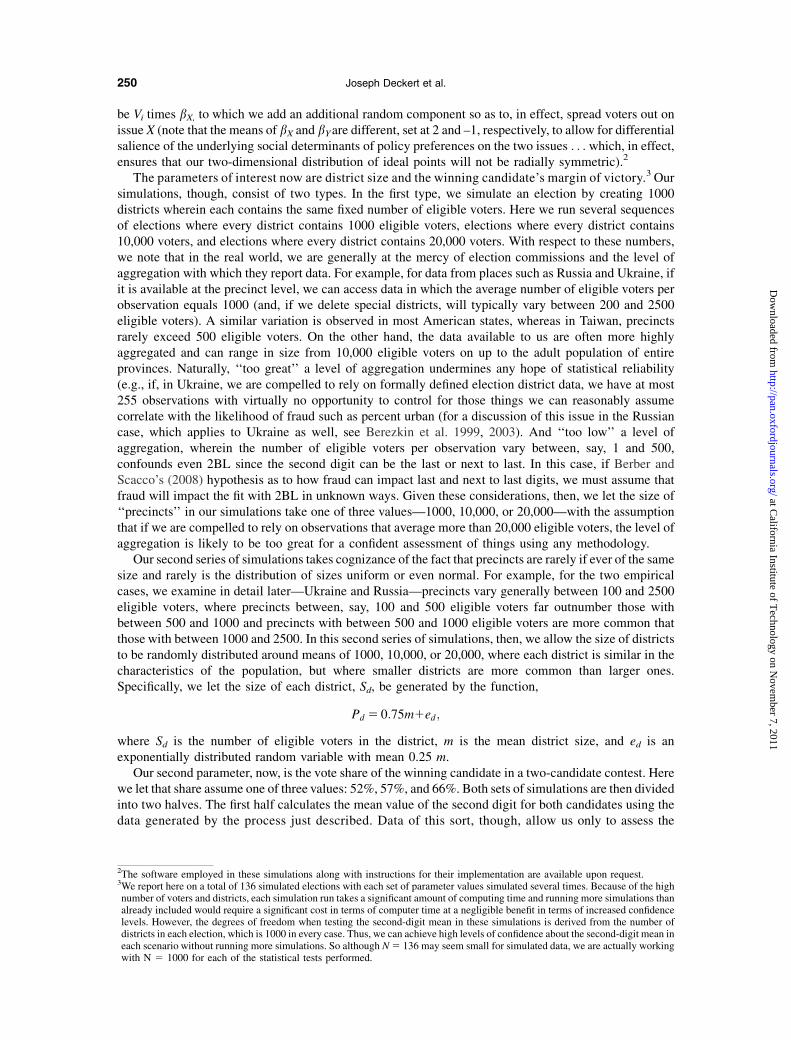
Looking first at the precinct level returns for Medvedev in 2008 (since the vote counts for other can-didates yield numbers that too infrequently entail more than two digits), and calculating the average of thesecond digit by region, Figure 2 gives the overall distribution of second-digit averages across all of Rus-sia’s regions (as before, we eliminate all precincts in which Medvedev receives fewer than 100 votes).What we see here is a distribution that, despite variations in district sizes and the number of precincts ineach (varying between 53 to 3301, with an average of 1020), largely corresponds to the national second-digit average of 4.081—or slightly lower than the 2BL prediction of 4.187. Although such a difference,given the large number of precincts (n 5 85,526), might be cause for suspicion, it is unlikely to convinceanyone that much was amiss in Russia’s 008 vote. Indeed, were we to have no other information aboutRussia and no other forensic evidence, we would most likely be unwilling to reject the hypothesis that its2008 vote was wholly free, fair, and absent significant fraud.
However, looking at things more closely, notice that Fig. 2 revels the great variety of numbers thata second-digit calculation generates, which is consistent with the supposition that a national average dis-guises considerable variation in the quality and legitimacy of vote counts. Thus, we must ask whether thecomponents of this distribution match what we know about the country’s political geography. And it ishere that Benford’s second-digit ‘‘law’’ falls woefully short with both Type 1 and Type 2 errors. Specif-ically, supposewe rank order the regions by the extent to which they depart from the 2BL number of 4.187.In this case, the ranks of the ‘‘usual suspects’’ are as follows:
8th Ingueshetia (mean 5 3.795)
8Putin was credited with 71.31% of the vote in 2004 versus Medvedev’s 71.25% in 2008.9Although turnover characterizes governments in Chechnya and Ingushetia owing to assassinations and the Kremlin’s search forleaders loyal to Moscow, M. Shaymiyev has led Tatarstan since 1991, M. Rakhimov has held the position of president of Bashkorto-stan since 1993, M. Merkushkin has held the same post in Moldovia since 1995, and recent Putin appointee M. Aliyev heads Dage-stan after replacing M. Magomedov, who ruled from 1982 to 2006.
10Despite its attempt at diplomatic language, the OSCE’s official report on the 2004 election (ODIHR June 2, 2004), singled outDagestan, Mordovia, Bashkortostan, Ingushetia, Tatarstan, and Chechnya in an Appendix titled ‘‘Sample of Implausible Turnoutand Result Figures.’’
258 Joseph Deckert et al.
at California Institute of T
echnology on Novem
ber 7, 2011http://pan.oxfordjournals.org/
Dow
nloaded from

17th Tatarstan (mean 5 3.890)
20th Chechnya (mean 5 3.920)
39th Karachaevo-Cherkassia (mean 5 4.021)
40th Mordova (mean 5 4.346)
47th Dagestan (mean 5 4.044)
71st Bashkortostan (mean 5 4.219).
Although Ingushetia, Chechnya, and Tatarstan’s means fall significantly below 4.187, to find thatBashkortostan is afforded a clean bill of health substantiates 2BL as an unreliable forensic tool. Moreimpressive still from the perspective of undermining 2BL’s value is the list of regions that rank highestin the magnitude of their departure from 4.187. Those regions are from 1st to 6th:
Khanti–Mansi (mean 5 3.135)
St. Petersburg (mean 5 3.635)
Archangel oblast (mean 5 3.684)
Yamalo-Nenetz oblast (mean 5 4.683)
Kemerovskaya oblast (mean 5 3.754)
Omsk oblast (mean 5 3.765).
One might argue that the inclusion of St Petersburg on this list should not be deemed incredible since it isPutin’s home district (although we can argue that St. Petersburg is an unlikely locus of significant fraud).But consider the fact that for the seven ‘‘usual suspects,’’ Medvedev’s average vote was 89.4% (with anaverage turnout of 90.9%) whereas for the six regions that yield the greatest deviation from 2BL, Med-vedvev’s vote averaged slightly less than 70% (with an average turnout of approximately 77%). Thus,were we to take the calculation of second-digit means at face value, we might conclude that therewas fraud, but in the form of millions of ballots for Medvedev that were wholly discarded or givento opposing candidates. If there is a hypothesis in political science to which we can assign a zero prior,it is that one.
7 Conclusions
Our earlier critique of Sobyanin’s application of the log-rank model to elections is not based on itsperformance in Russia’s 1993 Constitutional referendum. Indeed, we might say that this applicationillustrates a ‘‘Type 3’’ error—corroborating the correct hypothesis for the wrong reasons. Although theresurely was some fraud in the 1993 vote (Yeltsin’s tailor-made constitution could not be ratified unlessturnout exceeded 50% and there is evidence to suggest that votes were manufactured in various regionsto satisfy that requirement), the log-rank model was rejected as a forensic tool for theoretical reasons.Conversely, the model gained acceptance in a different context because Ijiri and Simon (1977) offereda theoretical rational for it that fit that context. Both manifestations of the log-rank model, then, illustrate
Distribution of 2nd digit means by region, Russia 2008
02468
101214
3.6
3.65 3.
7
3.75 3.
8
3.85 3.
9
3.95 4
4.05 4.
1
4.15 4.
2
4.25 4.
3
4.35 4.
4
4.45 4.
5
4.55 4.
6
4.65
2nd digit mean
# re
gion
s
Fig. 2 Distribution of second-digit means by region, Russia 2008.
259Benford’s Law and the Detection of Election Fraud
at California Institute of T
echnology on Novem
ber 7, 2011http://pan.oxfordjournals.org/
Dow
nloaded from

that absent a theoretical basis for assuming otherwise, generalized statements of empirical relationshipsthat apply in one context cannot be transported to other contexts willy-nilly. With respect to Benford’sLaw, we know some of the conditions that, if satisfied, yield numbers in accordancewith it, but just as thereis no basis for supposing that the Ijiri-Simon model of firm size or an empirical relationship that holds forinsects and city sizes applies to parties, candidates or anything else political, there is no reason to supposea priori that the conditions sufficient to occasion digits matching 2BL necessarily hold any meaning forelections. Indeed, if Ijiri and Simon’s model provides any guidance—and we note again that they focus ona specific process with specific assumptions and that their model does not predict a strictly linear relation-ship between log and rank, but rather a slightly convex one—it, in combination with what we know aboutthe stochastic processes sufficient to yield digits in conformity with Benford’s Law, is that the Law isnot universally applicable magic box into which we plug election statistics and out of which comes anassessment of an election’s legitimacy. This is not to say it is fruitless to search for special electoralcontexts in which 2BL has some relevance, but our analysis suggests that the data required to validatethat relevance must be richer than simple election returns.
We can illustrate what we mean here with another indicator proposed by Sobyanin that, unlike thelog-rank model, has been refined to become a valuable forensic tool. Briefly, Sobyanin noted that,absent fraud in the form of artificially inflated turnout, the relationship in otherwise homogeneous databetween turnout, T, and a candidate’s share of the eligible electorate, V/E, should match the candidate’soverall share of the vote. Thus, if we estimate V/E 5 a 1bT, then absent fraud and unobserved variablesthat correlate with both T and V, a should approximately equal 0 and b should approximate the candidate’spercentage of the counted vote. If, though, a candidate’s vote share is padded by adding ballots inotherwise low turnout districts, estimates of a will turn negative and estimates of b increase until, inextreme cases, it exceeds 1.0 (e.g., upwards of 1.6 in places like Russia’s Tatarstan). The operant clausehere, though, is ‘‘in otherwise homogeneous data’’ since this indicator is intended to detect theheterogeneity introduced by fraud. Any preexisting heterogeneity can only distort our conclusionsand it is essential that we control for those other parameters that might intervene between turnoutand candidate preference. Knowing what these things might be—regional loyalties, ethnic identities,or differences in voting patterns between urban and rural voters—is where substantive expertise entersand belies a blind application of this indicator.
To illustrate things further, we note that if, after separating Republican from Democratic precincts(since these subsets are on average demographically distinct), we apply Sobyanin’s second indicatorto data from Cuyahoga (Cleveland) or Franklin (Columbus) counties Ohio, nothing hinting at fraudappears. But if we do the same for Hamilton County (Cincinnati), it would seem that significant fraudhas occurred in every presidential election beginning with 1992 (Myagkov et al. 2009, see especially257–65). It is unreasonable to suppose, though, that fraud of the magnitude suggested by a blind appli-cation of this indicator has gone unnoticed through five presidential elections. But there is an innocuousexplanation—the Republican precincts in Cincinnati itself that are demographically distinct from those inthe suburbs—districts that vote Republican by slim margins and with considerably lower rates of turnoutthan other districts. Thus, merely separating precincts by party preference is a poor control for demo-graphic heterogeneity in the country and results in a false signal of fraud (for a similar example in Taiwanowing to military districts and districts with heavy concentrations of ‘‘aboriginal populations’’ see Chaingand Ordeshook 2009).
To suppose that Benford’s Law or any proposed indicator can avoid these methodologicalcomplexities is unwarranted. A valid analysis, regardless of the forensic tool proposed, must includea model that either specifies the generalized impact of parameters such as district magnitude,competitiveness, and regional clustering of support or it must give us sound theoretical argumentsfor supposing that those parameters will not impact our conclusions. Thus, even if there are thosewho reject the inference drawn from our analysis—that Benford’s Law is irrelevant to assessing anelection’s conformity with good democratic practice and that effort should be directed elsewhere inthe search for forensic indicators—we cannot escape the conclusion that any future development of thatLaw’s application to elections must necessarily identify likely intervening variables with their impact ondigit distributions adjusted in a theoretically proscribed way.
260 Joseph Deckert et al.
at California Institute of T
echnology on Novem
ber 7, 2011http://pan.oxfordjournals.org/
Dow
nloaded from
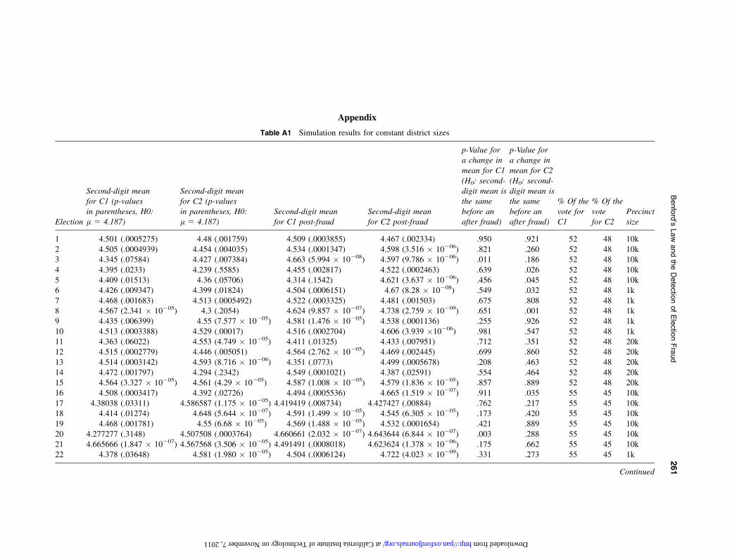
Table A1 Simulation results for constant district sizes
Election
Second-digit meanfor C1 (p-valuesin parentheses, H0:l 5 4.187)
Second-digit meanfor C2 (p-valuesin parentheses, H0:l 5 4.187)
Second-digit meanfor C1 post-fraud
Second-digit meanfor C2 post-fraud
p-Value fora change inmean for C1(H0: second-digit mean isthe samebefore anafter fraud)
p-Value fora change inmean for C2(H0: second-digit mean isthe samebefore anafter fraud)
% Of thevote forC1
% Of thevotefor C2
Precinctsize
1 4.501 (.0005275) 4.48 (.001759) 4.509 (.0003855) 4.467 (.002334) .950 .921 52 48 10k2 4.505 (.0004939) 4.454 (.004035) 4.534 (.0001347) 4.598 (3.516 � 10206) .821 .260 52 48 10k3 4.345 (.07584) 4.427 (.007384) 4.663 (5.994 � 10208) 4.597 (9.786 � 10206) .011 .186 52 48 10k4 4.395 (.0233) 4.239 (.5585) 4.455 (.002817) 4.522 (.0002463) .639 .026 52 48 10k5 4.409 (.01513) 4.36 (.05706) 4.314 (.1542) 4.621 (3.637 � 10206) .456 .045 52 48 10k6 4.426 (.009347) 4.399 (.01824) 4.504 (.0006151) 4.67 (8.28 � 10208) .549 .032 52 48 1k7 4.468 (.001683) 4.513 (.0005492) 4.522 (.0003325) 4.481 (.001503) .675 .808 52 48 1k8 4.567 (2.341 � 10205) 4.3 (.2054) 4.624 (9.857 � 10207) 4.738 (2.759 � 10209) .651 .001 52 48 1k9 4.435 (.006399) 4.55 (7.577 � 10205) 4.581 (1.476 � 10205) 4.538 (.0001136) .255 .926 52 48 1k10 4.513 (.0003388) 4.529 (.00017) 4.516 (.0002704) 4.606 (3.939 �10206) .981 .547 52 48 1k11 4.363 (.06022) 4.553 (4.749 � 10205) 4.411 (.01325) 4.433 (.007951) .712 .351 52 48 20k12 4.515 (.0002779) 4.446 (.005051) 4.564 (2.762 � 10205) 4.469 (.002445) .699 .860 52 48 20k13 4.514 (.0003142) 4.593 (8.716 � 10206) 4.351 (.0773) 4.499 (.0005678) .208 .463 52 48 20k14 4.472 (.001797) 4.294 (.2342) 4.549 (.0001021) 4.387 (.02591) .554 .464 52 48 20k15 4.564 (3.327 � 10205) 4.561 (4.29 � 10205) 4.587 (1.008 � 10205) 4.579 (1.836 � 10205) .857 .889 52 48 20k16 4.508 (.0003417) 4.392 (.02726) 4.494 (.0005536) 4.665 (1.519 � 10207) .911 .035 55 45 10k17 4.38038 (.03311) 4.586587 (1.175 � 10205) 4.419419 (.008734) 4.427427 (.00884) .762 .217 55 45 10k18 4.414 (.01274) 4.648 (5.644 � 10207) 4.591 (1.499 � 10205) 4.545 (6.305 � 10205) .173 .420 55 45 10k19 4.468 (.001781) 4.55 (6.68 � 10205) 4.569 (1.488 � 10205) 4.532 (.0001654) .421 .889 55 45 10k20 4.277277 (.3148) 4.507508 (.0003764) 4.660661 (2.032 � 10207) 4.643644 (6.844 � 10207) .003 .288 55 45 10k21 4.665666 (1.847 � 10207) 4.567568 (3.506 � 10205) 4.491491 (.0008018) 4.623624 (1.378 � 10206) .175 .662 55 45 10k22 4.378 (.03648) 4.581 (1.980 � 10205) 4.504 (.0006124) 4.722 (4.023 � 10209) .331 .273 55 45 1k
Continued
Appendix
261
Benford’s
Law
andtheDetectio
nofElectio
nFraud
at California Institute of Technology on November 7, 2011 http://pan.oxfordjournals.org/ Downloaded from

Table A1 (continued)
Election
Second-digit meanfor C1 (p-valuesin parentheses, H0:l 5 4.187)
Second-digit meanfor C2 (p-valuesin parentheses, H0:l 5 4.187)
Second-digit meanfor C1 post-fraud
Second-digit meanfor C2 post-fraud
p-Value fora change inmean for C1(H0: second-digit mean isthe samebefore anafter fraud)
p-Value fora change inmean for C2(H0: second-digit mean isthe samebefore anafter fraud)
% Of thevote forC1
% Of thevotefor C2
Precinctsize
23 4.655656 (1.42 � 10207) 4.515516 (.0003743) 4.798799 (4.37 � 10211) 4.634635 (1.001 � 10206) .259 .353 55 45 1k24 4.617 (2.234 � 10206) 4.387 (.02699) 4.468 (.002137) 4.558 (5.05 � 10205) .246 .183 55 45 1k25 4.407 (.01897) 4.557 (4.847 � 10205) 4.539 (.0001007) 4.544 (7.182 � 10205) .310 .919 55 45 1k26 4.541542 (9.315 � 10205) 4.573574 (3.161 � 10205) 4.647648 (2.663 � 10207) 4.514515 (.0002764) .403 .647 55 45 1k27 4.428428 (.008399) 4.414414 (.01163) 4.583584 (1.753 � 10205) 4.617618 (2.035 � 10206) .231 .111 55 45 1k28 4.633 (8.14 � 10207) 4.579 (1.412 � 10205) 4.482 (.000954) 4.327 (.1272) .233 .050 55 45 20k29 4.620621 (2.712 � 10206) 4.592593 (7.71 � 10206) 4.48048 (.001549) 4.381381 (.03417) .286 .101 55 45 20k30 4.603 (5.952 � 10206) 4.617 (1.614 � 10206) 4.488 (.0009504) 4.321 (.1338) .372 .019 55 45 20k31 4.563 (3.897 � 10205) 4.433 (.005638) 4.382 (.02903) 4.512 (.0003035) .156 .531 55 45 20k32 4.738739 (2.632 � 10209) 4.557558 (4.978 � 10205) 4.421421 (.01077) 4.540541 (8.29 � 10205) .015 .894 55 45 20k33 4.456456 (.003211) 4.598599 (9.859 � 10206) 4.495495 (.0005469) 4.516517 (.0002988) .759 .527 55 45 20k34 4.574 (4.458 � 10205) 4.63 (2.348 � 10207) 4.457 (.00348) 4.122 (.4462) .007 .000 66 34 10k35 4.364 (.05588) 4.579 (7.138 � 10206) 4.431 (.007285) 4.191 (.9628) .781 .016 66 34 10k36 4.629 (1.252 � 10206) 4.64 (2.509 � 10207) 4.617 (3.921 � 10206) 4.151 (.6736) .252 .000 66 34 10k37 4.836837 (1.029 � 10212) 4.781782 (9.35 � 10212) 4.558559 (6.631 � 10205) 4.011011 (.03234) .031 .000 66 34 10k38 4.575576 (2.582 � 10205) 4.702703 (5.587 � 10209) 4.465465 (.002793) 4.144144 (.6091) .400 .000 66 34 10k39 4.652653 (1.239 � 10207) 4.703704 (6.548 � 10209) 4.494494 (.0007267) 4.062062 (.1382) .209 .000 66 34 10k40 4.659 (8.397 � 10208) 4.632 (6.96 � 10207) 4.638 (1.183 � 10206) 4.144 (.6069) .225 .000 66 34 1k41 4.457 (.003266) 4.591 (3.329 � 10206) 4.45 (.004156) 4.053 (.1168) .519 .000 66 34 1k42 4.546 (.0001129) 4.696 (5.164 � 10209) 4.478 (.002178) 4.118 (.3996) .561 .000 66 34 1k43 4.402402 (.0206) 4.60961 (2.407 � 10206) 4.439439 (.00522) 4.153153 (.6892) .775 .000 66 34 1k44 4.378378 (.0334) 4.478478 (.0009649) 4.408408 (.01654) 4.07007 (.1654) .816 .001 66 34 1k45 4.715716 (3.159 � 10209) 4.578579 (1.133 � 10205) 4.543544 (9.907 � 10205) 4.054054 (.1189) .176 .000 66 34 1k46 4.437 (.005334) 4.408 (.01554) 4.242 (.5394) 4.35 (.07605) .741 .098 66 34 20k47 4.553 (4.77 � 10205) 4.625 (1.424 � 10206) 4.468 (.001930) 4.491 (.0006196) .673 .349 66 34 20k48 4.545 (.0001375) 4.502 (.0005964) 4.276 (.3304) 4.373 (.04544) .783 .802 66 34 20k
Continued
262
JosephDeckertetal.
at California Institute of Technology on November 7, 2011 http://pan.oxfordjournals.org/ Downloaded from

Table A1 (continued)
Election
Second-digit meanfor C1 (p-valuesin parentheses, H0:l 5 4.187)
Second-digit meanfor C2 (p-valuesin parentheses, H0:l 5 4.187)
Second-digit meanfor C1 post-fraud
Second-digit meanfor C2 post-fraud
p-Value fora change inmean for C1(H0: second-digit mean isthe samebefore anafter fraud)
p-Value fora change inmean for C2(H0: second-digit mean isthe samebefore anafter fraud)
% Of thevote forC1
% Of thevotefor C2
Precinctsize
49 4.477477 (.001300) 4.550551 (5.063 � 10205) 4.37037 (.05199) 4.57958 (1.554 � 10205) .411 .819 66 34 20k50 4.631632 (9.491 � 10207) 4.484484 (.0007496) 4.234234 (.6293) 4.484484 (.001128) .003 .000 66 34 20k51 4.495495 (.0007575) 4.498498 (.0007485) 4.277277 (.329) 4.375375 (.03263) .093 .334 66 34 20k
263
Benford’s
Law
andtheDetectio
nofElectio
nFraud
at California Institute of Technology on November 7, 2011 http://pan.oxfordjournals.org/ Downloaded from

Table A2 Simulation results for exponentially distributed district sizes
ElectionSimulation
Second-digit meanfor C1 (p-values in
parentheses,H0: l 5 4.187)
Second-digitmean for C2(p-values inparentheses,H0: l 5 4.187)
Second-digitmean for C1post-fraud
Second-digitmean for C2post-fraud
p-Value fora change inmean for C1(H0: second-digit mean isthe samebefore anafter fraud)
p-Value fora change inmean for C1(H0: second-digit mean isthe samebefore anafter fraud)
% Of the votefor C1
% Of the votefor C2
Meanprecinct size
1 4.375 (.03723) 4.494 (.0007654) 4.315 (.1624) 4.265 (.3766) .641 .071 52 48 10k2 4.597 (4.914 � 10206) 4.421 (.0096) 4.499 (.0006681) 4.099 (.3190) .443 .011 52 48 10k3 4.463 (.002034) 4.245 (.5148) 4.562 (5.46 � 10205) 4.224 (.6817) .441 .868 52 48 10k4 4.585 (1.251 � 10205) 4.397 (.01931) 4.475 (.001429) 4.269 (.3651) .389 .315 52 48 10k5 4.436 (.005637) 4.308 (.1861) 4.319 (.1428) 4.331 (.1054) .357 .857 52 48 10k6 4.501 (.0005242) 4.236 (.5849) 4.579 (1.971 � 10205) 4.155 (.7204) .544 .522 52 48 10k7 4.415 (.01245) 4.238 (.5732) 4.436 (.006641) 4.456 (.002677) .871 .087 52 48 10k8 4.438 (.005221) 4.417 (.01064) 4.559 (5.909 � 10205) 4.074 (.2037) .347 .007 52 48 10k9 4.328 (.1196) 4.312 (.1693) 4.523 (.0002332) 4.151 (.6845) .129 .205 52 48 10k10 4.302 (.1982) 4.264 (.383) 4.507 (.000254) 4.073 (.2028) .101 .129 52 48 10k11 4.451 (.003308) 4.061 (.1574) 4.496 (.000615) 4.186 (.991) .723 .320 52 48 1k12 4.238 (.5682) 4.302 (.1917) 4.429 (.006254) 4.102 (.3475) .129 .113 52 48 1k13 4.3 (.202) 4.425 (.009896) 4.468 (.001753) 4.173 (.8743) .182 .049 52 48 1k14 4.243 (.5294) 4.424 (.007323) 4.399 (.01635) 4.221 (.7061) .213 .108 52 48 1k15 4.458 (.002585) 4.331 (.1051) 4.491 (.000796) 4.062 (.1631) .796 .033 52 48 1k16 4.185 (.9822) 4.325 (.1291) 4.481 (.001105) 4.063 (.1706) .020 .041 52 48 1k17 4.44 (.006702) 4.347 (.07146) 4.319 (.1587) 4.087 (.2491) .359 .036 52 48 1k18 4.276 (.3230) 4.321 (.1363) 4.405 (.01566) 4.159 (.754) .311 .201 52 48 1k19 4.462 (.002603) 4.215 (.7561) 4.394 (.02297) 4.287 (.2729) .597 .574 52 48 1k20 4.333 (.1057) 4.365 (.04856) 4.402 (.01725) 4.207 (.8205) .588 .210 52 48 1k21 4206 (.835) 4.416 (.01250) 4.306 (.1962) 4.399 (.01963) .440 .895 52 48 20k22 4.348 (.07895) 4.528 (.0001858) 4.422 (.009263) 4.544 (8.018 � 10205) .565 .901 52 48 20k23 4.444 (.004794) 4.321 (.1436) 4.313 (.1686) 4.282 (.3047) .310 .764 52 48 20k24 4.369 (.04315) 4.413 (.01175) 4.287 (.2799) 4.256 (.4331) .525 .211 52 48 20k25 4.287 (.2827) 4.41 (.01646) 4.343 (.08714) 4.288 (.2668) .667 .348 52 48 20k26 4.533 (.0001920) 4.322 (.1333) 4.5 (.0007578) 4.099 (.3305) .801 .080 55 45 10k
Continued
264
JosephDeckertetal.
at California Institute of Technology on November 7, 2011 http://pan.oxfordjournals.org/ Downloaded from

Table A2 (continued)
ElectionSimulation
Second-digit meanfor C1 (p-values in
parentheses,H0: l 5 4.187)
Second-digitmean for C2(p-values inparentheses,H0: l 5 4.187)
Second-digitmean for C1post-fraud
Second-digitmean for C2post-fraud
p-Value fora change inmean for C1(H0: second-digit mean isthe samebefore anafter fraud)
p-Value fora change inmean for C1(H0: second-digit mean isthe samebefore anafter fraud)
% Of the votefor C1
% Of the votefor C2
Meanprecinct size
27 4.5 (.0006922) 4.31 (.1744) 4.557 (4.726 � 10205) 4.134 (.5558) .659 .168 55 45 10k28 4.418 (.00888) 4.444 (.003754) 4.597 (7.534 � 10206) 4.108 (.3726) .158 .007 55 45 10k29 4.292 (.2421) 4.397 (.01780) 4.6 (4.319 � 10206) 4.162 (.7761) .015 .060 55 45 10k30 4.355 (.06605) 4.277 (.3167) 4.18 (.9398) 4.355 (.06699) .179 .543 55 45 20k31 4.261 (.4044) 4.28 (.3071) 4.407 (.01452) 4.25 (.4804) .248 .814 55 45 20k32 4.528 (.0002149) 4.546 (7.524 � 10205) 4.446 (.004772) 4.396 (.02109) .527 .241 55 45 20k33 4.268 (.3762) 4.347 (.07731) 4.446 (.004732) 4.4 (.02097) .169 .682 55 45 20k34 4.224 (.6914) 4.348 (.07841) 4.294 (.2396) 4.422 (.01036) .591 .567 55 45 20k35 4.347 (.07858) 4.178 (.9216) 4.288 (.2654) 4.174 (.8863) .646 .975 56 44 10k36 4.546 (7.449 � 10205) 4.367 (.04757) 4.593 (1.117 � 10205) 4.16 (.7591) .715 .102 56 44 10k37 4.568 (3.246 � 10205) 4.258 (.4284) 4.353 (.06979) 4.076 (.2036) .096 .146 56 44 10k38 4.324 (.1342) 4.266 (.3751) 4.542 (7.24 � 10205) 4.025 (.07301) .088 .057 57 42 10k39 4.571 (2.237 � 10205) 4.33 (.1237) 4.402 (.01936) 4.265 (.375) .189 .611 57 42 10k40 4.366 (.04677) 4.347 (.07172) 4.719 (3.390 � 10209) 4.214 (.756) .005 .284 57 42 10k41 4.454 (.003739) 4.288 (.2683) 4.474 (.001390) 4.2 (.8845) .876 .491 57 42 10k42 4.366 (.04909) 4.329 (.1111) 4.448 (.003855) 4.089 (.2616) .522 .054 57 42 10k43 4.609 (5.349 � 10206) 4.345 (.07207) 4.478 (.001054) 3.965 (.01241) .306 .002 57 42 10k44 4.458 (.002898) 4.165 (.8045) 4.579 (1.562 � 10205) 4.187 (1.00) .345 .861 57 42 10k45 4.423 (.01027) 4.304 (.1975) 4.595 (7.079 � 10206) 4.306 (.1846) .182 .987 57 43 10k46 4.446 (.004842) 4.211 (.786) 4.447 (.004746) 3.969 (.01261) .994 .051 57 42 1k47 4.336 (.1049) 4.078 (.2195) 4.255 (.4474) 4.012 (.05682) .528 .605 57 42 1k48 4.377 (.03293) 4.316 (.1474) 4.527 (.0001435) 4.144 (.6239) .234 .169 57 42 1k49 4.357 (.06095) 4.344 (.08281) 4.33 (.1199) 4.068 (.1790) .834 .029 57 42 1k50 4.548 (6.399 � 10205) 4.248 (.4991) 4.531 (.0001395) 4.009 (.03756) .894 .055 57 42 1k51 4.624 (1.651 � 10206) 4.338 (.08835) 4.437 (.005437) 4.213 (.7717) .143 .321 57 42 1k52 4.428 (.007625) 4.221 (.7091) 4.488 (.001098) 4.2 (.8825) .641 .868 57 42 1k
Continued
265
Benford’s
Law
andtheDetectio
nofElectio
nFraud
at California Institute of Technology on November 7, 2011 http://pan.oxfordjournals.org/ Downloaded from

Table A2 (continued)
ElectionSimulation
Second-digit meanfor C1 (p-values in
parentheses,H0: l 5 4.187)
Second-digitmean for C2(p-values inparentheses,H0: l 5 4.187)
Second-digitmean for C1post-fraud
Second-digitmean for C2post-fraud
p-Value fora change inmean for C1(H0: second-digit mean isthe samebefore anafter fraud)
p-Value fora change inmean for C1(H0: second-digit mean isthe samebefore anafter fraud)
% Of the votefor C1
% Of the votefor C2
Meanprecinct size
53 4.341 (.08887) 4.162 (.7805) 4.532 (.0001005) 4.145 (.638) .131 .893 57 42 1k54 4.457 (.002744) 4.172 (.8656) 4.549 (6.757 � 10205) 4.187 (1.00) .471 .906 57 42 1k55 4.337 (.1011) 4.357 (.05251) 4.555 (4.540 � 10205) 4.149 (.6798) .089 .102 57 42 1k56 4.475 (.00145) 4.144 (.6288) 4.552 (7.545 � 10205) 4.066 (.1774) .550 .537 57 42 1k57 4.444 (.003567) 4.394 (.02015) 4.514 (.0003058) 3.968 (.01367) .579 .001 57 42 1k58 4.523 (.0003052) 4.282 (.2786) 4.477 (.001416) 3.917 (.002229) .723 .003 57 42 1k59 4.386 (.02808) 4.245 (.5188) 4.363 (.0551) 3.994 (.03192) .858 .048 57 42 1k60 4.479 (.001822) 4.12 (.4518) 4.347 (.07485) 4.039 (.09256) .308 .517 57 42 1k61 4.414 (.01213) 4.044 (.1114) 4.558 (7.675 � 10205) 3.946 (.006403) .268 .436 67 33 10k62 4.56 (3.133 � 10205) 4.049 (.1196) 4.527 (.0002456) 4.105 (.3717) .797 .661 67 33 10k63 4.558 (5.019 � 10205) 4.125 (.5021) 4.745 (1.445 � 10209) 4.051 (.1357) .147 .568 67 33 10k64 4.585 (1.529 � 10205) 3.979 (.01998) 4.464 (.002669) 3.906 (.001334) .351 .559 67 33 10k65 4.385 (.03358) 3.893 (.001100) 4.384 (.02601) 3.985 (.0229) .994 .466 67 33 10k66 4.452 (.004241) 4.121 (.466) 4.435 (.007164) 3.976 (.01704) .896 .252 67 33 10k67 4.471 (.002035) 4.109 (.3856) 4.398 (.02090) 3.996 (.03156) .573 .371 67 33 10k68 4.582 (9.777 � 10206) 4.062 (.1726) 4.627 (1.874 � 10206) 3.921 (.002590) .725 .267 67 33 10k69 4.441 (.00409) 4.021 (.06735) 4.405 (.01680) 3.968 (.01495) .776 .678 67 33 10k70 4.383 (.02998) 4.066 (.1561) 4.577 (2.137 � 10205) 3.856 (.0001946) .131 .088 67 33 10k71 4.531 (.0001346) 3.938 (.005614) 4.724 (3.6 � 10209) 3.973 (.01645) .129 .782 67 33 1k72 4.288 (.2774) 4.02 (.06748) 4.312 (.1625) 3.985 (.024) .852 .784 67 33 1k73 4.374 (.04327) 4.002 (.04144) 4.417 (.01071) 3.845 (.0001319) .739 .217 67 33 1k74 4.519 (.0003204) 3.811 (2.245 � 10205) 4.45 (.004604) 3.951 (.008805) .597 .267 67 33 1k75 4.632 (1.4 � 10206) 4.072 (.2013) 4.426 (.009122) 3.754 (1.098 � 10206) .112 .012 67 33 1k76 4.517 (.0003017) 3.903 (.001606) 4.459 (.002817) 3.9 (.001564) .652 .981 67 33 1k77 4.602 (9.836 � 10206) 4.039 (.1016) 4.462 (.002454) 4.014 (.05669) .282 .845 67 33 1k78 4.463 (.002138) 4.067 (.1774) 4.569 (2.616 � 10205) 4.067 (.1836) .405 1.000 67 33 1k
Continued
266
JosephDeckertetal.
at California Institute of Technology on November 7, 2011 http://pan.oxfordjournals.org/ Downloaded from
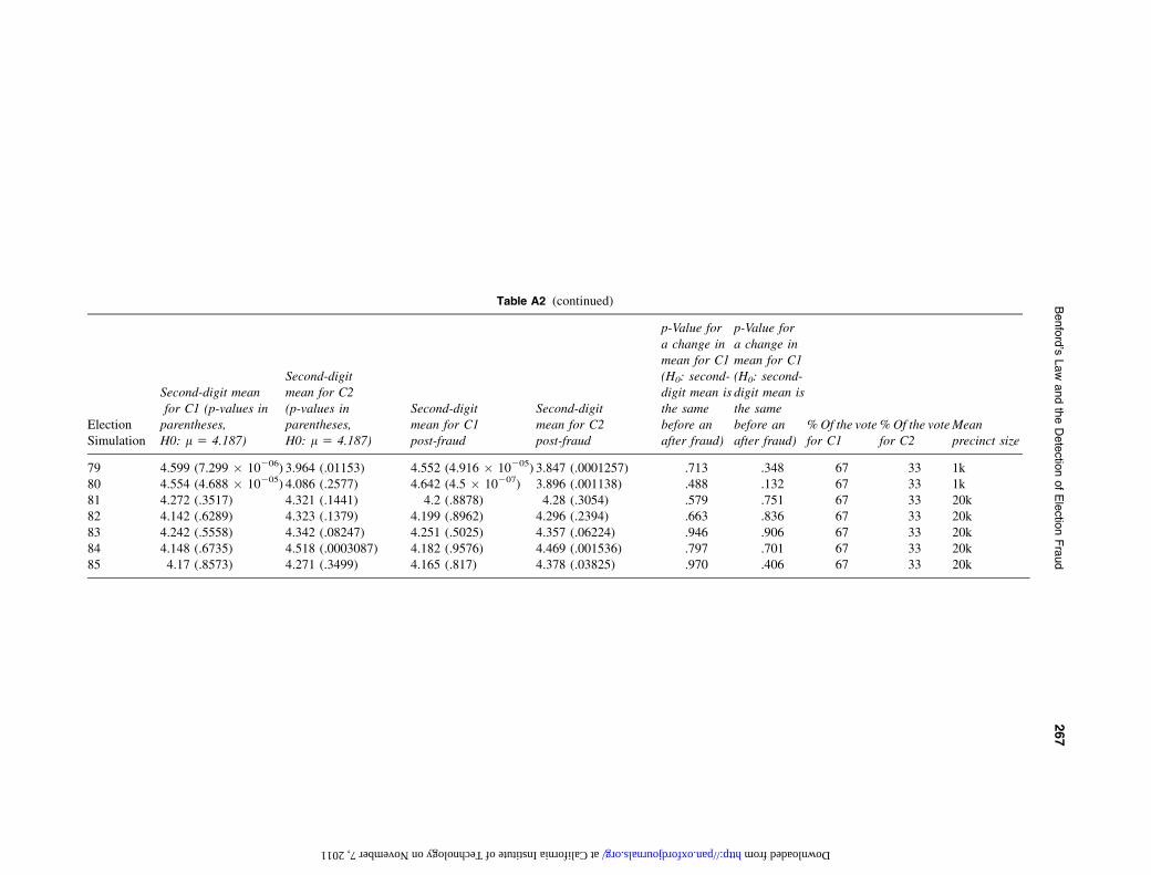
Table A2 (continued)
ElectionSimulation
Second-digit meanfor C1 (p-values in
parentheses,H0: l 5 4.187)
Second-digitmean for C2(p-values inparentheses,H0: l 5 4.187)
Second-digitmean for C1post-fraud
Second-digitmean for C2post-fraud
p-Value fora change inmean for C1(H0: second-digit mean isthe samebefore anafter fraud)
p-Value fora change inmean for C1(H0: second-digit mean isthe samebefore anafter fraud)
% Of the votefor C1
% Of the votefor C2
Meanprecinct size
79 4.599 (7.299 � 10206) 3.964 (.01153) 4.552 (4.916 � 10205) 3.847 (.0001257) .713 .348 67 33 1k80 4.554 (4.688 � 10205) 4.086 (.2577) 4.642 (4.5 � 10207) 3.896 (.001138) .488 .132 67 33 1k81 4.272 (.3517) 4.321 (.1441) 4.2 (.8878) 4.28 (.3054) .579 .751 67 33 20k82 4.142 (.6289) 4.323 (.1379) 4.199 (.8962) 4.296 (.2394) .663 .836 67 33 20k83 4.242 (.5558) 4.342 (.08247) 4.251 (.5025) 4.357 (.06224) .946 .906 67 33 20k84 4.148 (.6735) 4.518 (.0003087) 4.182 (.9576) 4.469 (.001536) .797 .701 67 33 20k85 4.17 (.8573) 4.271 (.3499) 4.165 (.817) 4.378 (.03825) .970 .406 67 33 20k
267
Benford’s
Law
andtheDetectio
nofElectio
nFraud
at California Institute of Technology on November 7, 2011 http://pan.oxfordjournals.org/ Downloaded from
Funding
The California Institute of Technology by the National Council for Eurasian and East European Research.
ReferencesBerber, Bernd, and Alexandra Scacco. 2008. What the numbers say: A digit based test for election fraud using new data from Nigeria.
Paper presented at the Annual Meeting of the Am. Political Science Association, Boston, MA, August 28–31.
Berezkin, Andrei V., Mikhail Myagkov, and Peter C. Ordeshook. 1999. The urban rural divide in the Russian electorate and the effects
of distance from urban centers. Post-Soviet Geography and Economics 40:395–406.
———. 2003. Location and political influence: A further elaboration of their effects on voting in recent Russian elections. Post-Soviet
Geography and Economics 44:169–83.
Brady, Henry E. 2005. Comments on Benfords Law and the Venezuelan election Unpublished manuscript, Stanford University, Jan-
uary 19, 2005.
Buttorf, Gail. 2008. Detecting fraud in America’s gilded age. Unpublished manuscript, University of Iowa.
Buzin, Andrei, and Arkadii Lubarev. 2008. Crime without punishment. Moscow, Russia: Nikkolo M.
Camerer, Colin. 2003. Behavioral game theory: Experiments in strategic interaction. Princeton, NJ: Princeton University Press.
Chaing, Lichun, and Peter C. Ordeshook. 2009. Fraud, elections and the American gene in Taiwan’s democracy. Unpublished man-
uscript, California Institute of Technology.
Cox, Gary. 1997. Making votes count: Strategic coordination in the World’s electoral systems. Cambridge, UK: Cambridge Uni-
versity Press.
Diekmann, Andreas. 2010. Not the first digit: Using Benford’s Law to detect fraudlent data. Unpublished paper, Swiss Federal In-
stitute of Technology, Zurich. Paper Presented at the 2010 Conference on Plagiarism, 21–23 June, Newcastle, UK.
Ijiri, Yuri, and Herbert Simon. 1977. Skew distributions and the sizes of business firms. New York, NY: North Holland Publishing Co.
Janvresse, Elise, and Thierry de la Rue. 2004. From uniform distributions to Benford’s Law. Journal of Applied Probability
41:1203–10.
Levin, Ines, Gabe A. Cohn, R. Michael Alvarez, and Peter C. Ordeshook. 2009. Detecting voter fraud in an electronic voting context:
An analysis of the unlimited reelection vote in Venezuela. Electronic Voting Technology Workshop/Workshop on Trustworthy
Elections. Online Proceedings.
Mebane, Walter. 2006. Election forensics: Vote counts and Benford’s Law. Paper prepared for the 2006 Summer Meeting of the
Political Methodology Society, University of California, Davis, July 20–22.
——— . 2007.Election forensics: Statistics, recounts and fraud Paper presented at the 2007 AnnualMeeting of theMidwest Political
Science Association. Chicago, IL, April 12–16.
———. 2008. Election forensics: The Second Digit Benford’s Law Test and recent American presidential elections. In Election
fraud, ed. R. M. Alvarez, T. E. Hall, and S. D. Hyde. Washington, DC: Brookings.
Mebane, Walter, and Kirill Kalinin. 2009. Electoral falsifications in Russia: Complex diagnostics selections 2003–2004, 2007–8.
Electoral Policy REO, 57–70 (in Russian).
Myagkov, Mikhail, Peter C. Ordeshook, and Dimitri Shakin. 2009. The forensics of election fraud. Cambridge: Cambridge University
Press.
Snyder, Timothy. 2010. Bloodlands: Europe between Hitler and Stalin. New York, NY: Basic Books.
Sobyanin, Alexandar, and V. Suchovolsky. 1993. Elections and the referendum December 11, 1993, in Russia. Unpublished report to
the Administration of the President of the RF, Moscow.
268 Joseph Deckert et al.
at California Institute of T
echnology on Novem
ber 7, 2011http://pan.oxfordjournals.org/
Dow
nloaded from