Benefits of Advanced Traffic Management Solutions: Before

BENEFITS OF ADVANCED TRAFFIC MANAGEMENT SOLUTIONS: BEFORE

AND AFTER CRASH ANALYSIS FOR DEPLOYMENT OF A VARIABLE

ADVISORY SPEED LIMIT SYSTEM

A Thesis

presented to

the Faculty of California Polytechnic State University,

San Luis Obispo

In Partial Fulfillment

of the Requirements for the Degree

Master of Science in Civil and Environmental Engineering

by

Alexander Lindsay Chambers

June 2016

ii

© 2016


ALL RIGHTS RESERVED

iii

COMMITTEE MEMBERSHIP

TITLE:

AUTHOR:

DATE SUBMITTED:

COMMITTEE CHAIR:

COMMITTEE MEMBER:

COMMITTEE MEMBER:

Benefits of Advanced Traffic Management Solutions: Before and After Crash Analysis for Deployment of a Variable Advisory Speed Limit System Alexander Lindsay Chambers June 2016 Robert L. Bertini, Ph.D. Associate Professor of Civil and Environmental Engineering Anurag Pande, Ph.D. Associate Professor of Civil and Environmental Engineering Kimberley Mastako, Ph.D. Lecturer of Civil and Environmental Engineering

iv

ABSTRACT

Benefits of Advanced Traffic Management Solutions: Before and After Crash

Analysis for Deployment of a Variable Advisory Speed Limit System


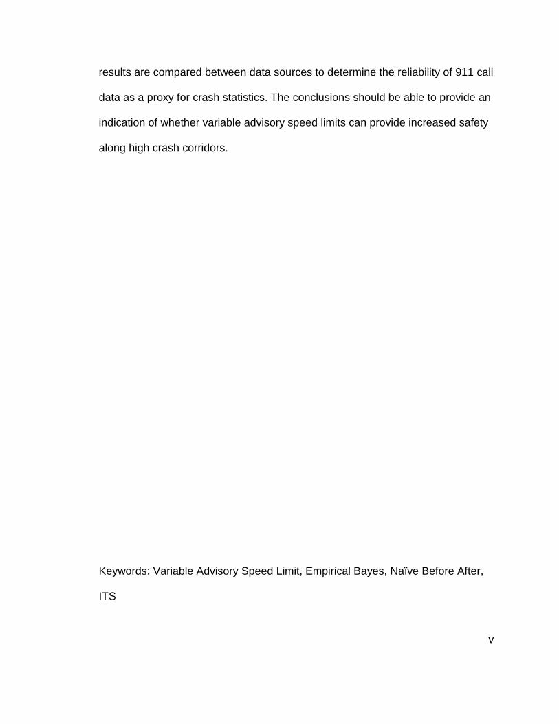
Variable speed limit (VSL) systems are important active traffic management tools

that are being deployed across the U.S. and indeed around the world for relieving

congestion and improving safety. Oregon’s first variable advisory speed limit

signs were activated along Oregon Highway 217 in the summer of 2014. The

variable advisory speed system is responsive to both congestion and weather

conditions. This seven-mile corridor stretches around Western Portland and has

suffered from high crash rates and peak period congestion in the past. VSL

systems are often deployed to address safety, mobility and sustainability related

performance. This research seeks to determine whether the newly implemented

variable advisory speed limit system has had measurable impacts on traffic

safety and what the scale of the impact has been. The research utilizes a before-

after crash analysis with three years of data prior to implementation and around

16 months after. Statistical analysis using an Empirical Bayes (EB) approach will

aim to separate the direct impacts of the variable advisory speed limit signs from

the long term trends on the highway. In addition, the analysis corrects for the

changes in traffic volumes over the study period. Three data sources will be

utilized including Washington County 911 call data, Oregon incident reports, and

official Oregon Department of Transportation crash data reports. The analysis

v

results are compared between data sources to determine the reliability of 911 call

data as a proxy for crash statistics. The conclusions should be able to provide an

indication of whether variable advisory speed limits can provide increased safety

along high crash corridors.

Keywords: Variable Advisory Speed Limit, Empirical Bayes, Naïve Before After,

ITS

vi

ACKNOWLEDGMENTS

Thanks to Oregon Department of Transportation for the information and

data, without which this project would not have been possible. I would like to

thank to my excellent thesis advisor Dr. Robert Bertini, whose support and

experience has been invaluable throughout my graduate schooling. As well I’d

like to thank my committee members Dr. Anurag Pande, for his support and

encouragement to pursue a Master’s degree, and Dr. Kimberely Mastako, for

speaking on my behalf in becoming a graduate student and supporting my thesis.

All of my committee members have been invaluable in supporting my research

by taking time from their busy days to assist and guide me. I’d also like to thank

all of my fellow Cal Poly transportation graduate students with special note of,

Bobby Sidhu, Krista Purser, Kevin Carstens, Travis Low, and Edward Tang. The

friendship and camaraderie they exhibited has helped make this research an

enjoyable experience. And of course I would like to thank my wonderful parents

Brian and Jean Chambers. Without their support and investment in my education

I would have never been able to make it to this point.

vii

TABLE OF CONTENTS

Page

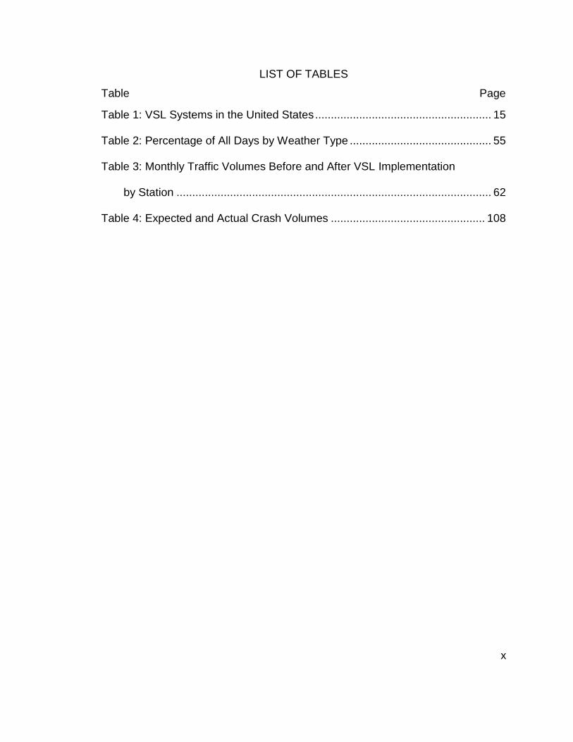
LIST OF TABLES ................................................................................................. x

LIST OF FIGURES ...............................................................................................xi

1.0 Introduction ..................................................................................................... 1

1.1 Variable Speed Limits ................................................................................. 2

1.2 OR 217 VSL System Background ............................................................... 6

1.3 Motivation & Objectives............................................................................. 10

1.4 Organization .............................................................................................. 10

2.0 Literature Review .......................................................................................... 12

2.1 History ....................................................................................................... 12

2.2 System Types & Purposes ........................................................................ 16

2.2.1 Weather-Responsive .......................................................................... 16

2.2.2 Congestion-Responsive ..................................................................... 17

2.2.3 Work Zone Systems ........................................................................... 18

2.3 Evaluation Methods & Results .................................................................. 19

2.3.1 Naïve Before and After Evaluation Methods ....................................... 20

2.3.2 Empirical Bayes Analysis ................................................................... 22

2.4 OR 217 Evaluations .................................................................................. 23

2.5 Summary ................................................................................................... 24

3.0 Motivations for VSL on OR 217 .................................................................... 26

3.1 Corridor Almanac ...................................................................................... 27

3.2 Crash Trends ............................................................................................ 31

3.3 Effects of Adverse Weather ...................................................................... 33

3.4 Summary ................................................................................................... 34

4.0 Data Sources ................................................................................................ 36

4.1 Corridor Instrumentation ........................................................................... 36

4.2 Data Description ....................................................................................... 44

4.2.1 Traffic Flow Data ................................................................................ 44

4.2.2 Washington County 911 Call Data ..................................................... 46

viii

4.2.3 Transportation Operation Center Data ............................................... 50

4.2.4 Transportation Data Section Data ...................................................... 50

4.2.5 Summary of Crash Databases ........................................................... 51

4.2.6 Weather Data ..................................................................................... 54

4.3 Evaluation Framework .............................................................................. 55

5.0 Naïve Before-After Study .............................................................................. 56

5.1 Methodology ............................................................................................. 56

5.1.1 Traffic Volumes .................................................................................. 57

5.1.2 Crash Data ......................................................................................... 66

5.2 WCCCA Data ............................................................................................ 66

5.2.1 Crash Frequency ................................................................................ 68

5.2.2 By Crash Category ............................................................................. 71

5.2.3 By Milepost ......................................................................................... 73

5.2.4 By Direction by Crash Category ......................................................... 75

5.2.5 By Direction by Milepost ..................................................................... 77

5.2.6 Analysis by Weather ........................................................................... 80

5.2.7 Summary ............................................................................................ 81

5.3 TOCS Data ............................................................................................... 82

5.3.1 Crashes Over Time ............................................................................ 85

5.3.2 Summary ............................................................................................ 85

5.4 TDS Data .................................................................................................. 86

5.4.1 Crashes Over Time ............................................................................ 86

5.4.2 By Weather Condition ......................................................................... 88

5.4.3 By Lighting Condition .......................................................................... 90

5.4.4 By Crash Type .................................................................................... 92

5.4.5 By Injury Class ................................................................................... 93

5.4.6 Summary ............................................................................................ 95

5.4.7 Updated Incomplete Data ................................................................... 95

5.5 Statistical Analysis .................................................................................... 98

5.6 Summary ................................................................................................... 99

6.0 Empirical Bayesian Analysis ....................................................................... 102

ix

6.1 Methodology ........................................................................................... 102

6.2 WCCCA .................................................................................................. 107

6.3 TOCS ...................................................................................................... 110

6.4 TDS ......................................................................................................... 112

7.0 Conclusions ................................................................................................ 114

7.1 Contributions ........................................................................................... 115

7.2 Limitations ............................................................................................... 115

7.3 Future Research ..................................................................................... 115

References ....................................................................................................... 117

x

LIST OF TABLES

Table Page

Table 1: VSL Systems in the United States ........................................................ 15

Table 2: Percentage of All Days by Weather Type ............................................. 55

Table 3: Monthly Traffic Volumes Before and After VSL Implementation

by Station .................................................................................................... 62

Table 4: Expected and Actual Crash Volumes ................................................. 108

xi

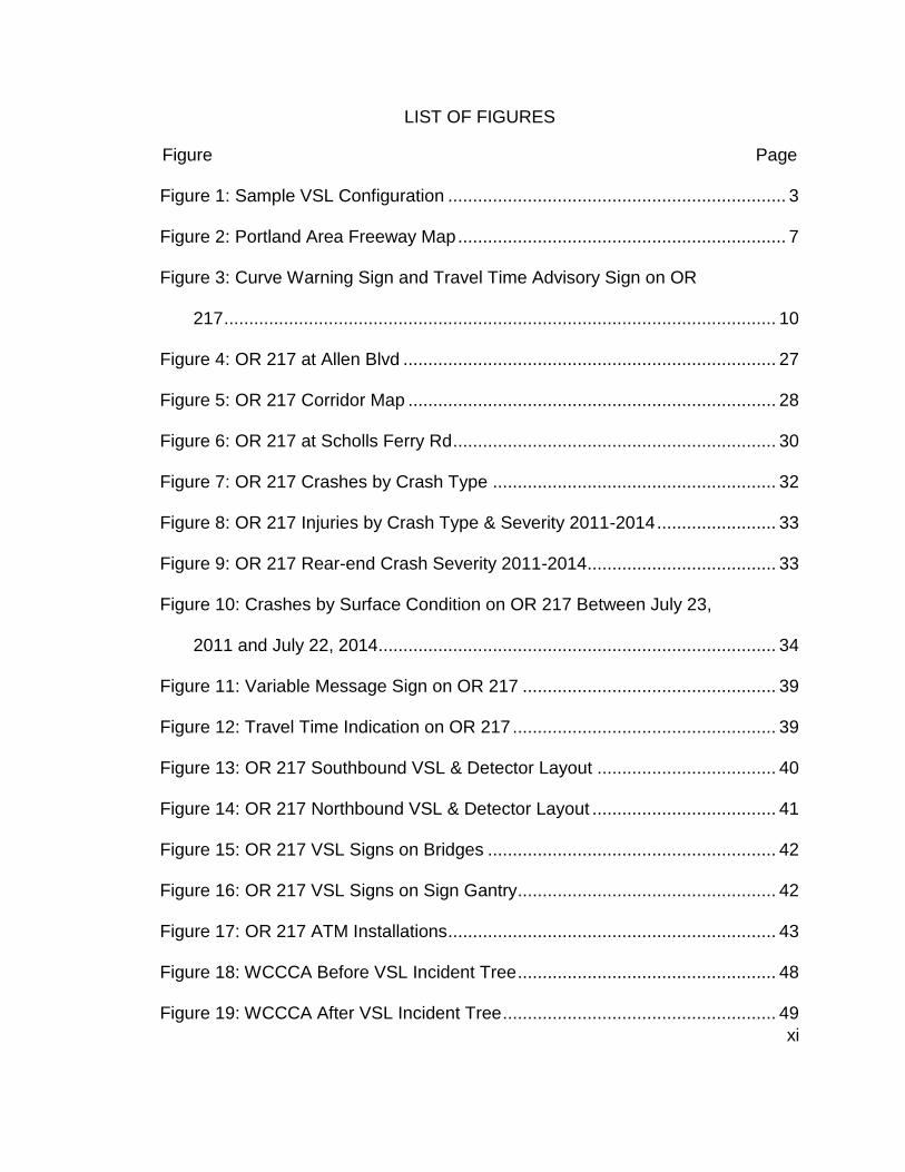
LIST OF FIGURES

Figure Page

Figure 1: Sample VSL Configuration .................................................................... 3

Figure 2: Portland Area Freeway Map .................................................................. 7

Figure 3: Curve Warning Sign and Travel Time Advisory Sign on OR

217 ............................................................................................................... 10

Figure 4: OR 217 at Allen Blvd ........................................................................... 27

Figure 5: OR 217 Corridor Map .......................................................................... 28

Figure 6: OR 217 at Scholls Ferry Rd ................................................................. 30

Figure 7: OR 217 Crashes by Crash Type ......................................................... 32

Figure 8: OR 217 Injuries by Crash Type & Severity 2011-2014 ........................ 33

Figure 9: OR 217 Rear-end Crash Severity 2011-2014 ...................................... 33

Figure 10: Crashes by Surface Condition on OR 217 Between July 23,

2011 and July 22, 2014................................................................................ 34

Figure 11: Variable Message Sign on OR 217 ................................................... 39

Figure 12: Travel Time Indication on OR 217 ..................................................... 39

Figure 13: OR 217 Southbound VSL & Detector Layout .................................... 40

Figure 14: OR 217 Northbound VSL & Detector Layout ..................................... 41

Figure 15: OR 217 VSL Signs on Bridges .......................................................... 42

Figure 16: OR 217 VSL Signs on Sign Gantry.................................................... 42

Figure 17: OR 217 ATM Installations .................................................................. 43

Figure 18: WCCCA Before VSL Incident Tree .................................................... 48

Figure 19: WCCCA After VSL Incident Tree ....................................................... 49

xii

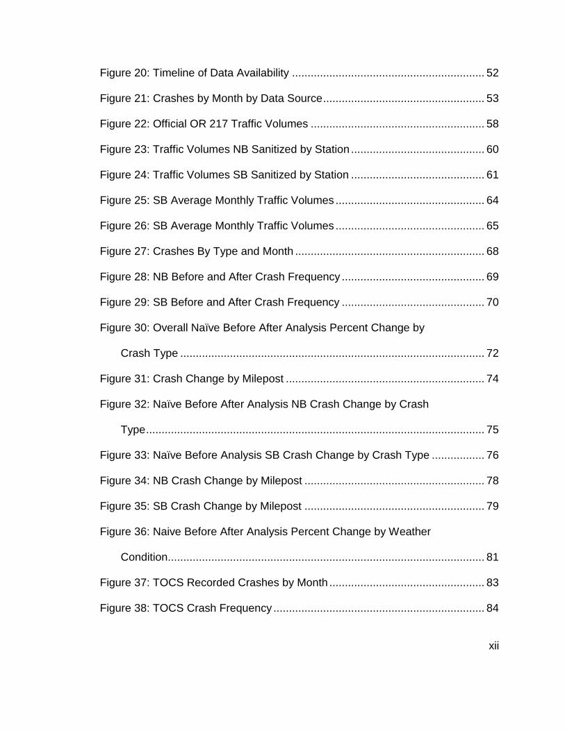
Figure 20: Timeline of Data Availability .............................................................. 52

Figure 21: Crashes by Month by Data Source .................................................... 53

Figure 22: Official OR 217 Traffic Volumes ........................................................ 58

Figure 23: Traffic Volumes NB Sanitized by Station ........................................... 60

Figure 24: Traffic Volumes SB Sanitized by Station ........................................... 61

Figure 25: SB Average Monthly Traffic Volumes ................................................ 64

Figure 26: SB Average Monthly Traffic Volumes ................................................ 65

Figure 27: Crashes By Type and Month ............................................................. 68

Figure 28: NB Before and After Crash Frequency .............................................. 69

Figure 29: SB Before and After Crash Frequency .............................................. 70

Figure 30: Overall Naïve Before After Analysis Percent Change by

Crash Type .................................................................................................. 72

Figure 31: Crash Change by Milepost ................................................................ 74

Figure 32: Naïve Before After Analysis NB Crash Change by Crash

Type ............................................................................................................. 75

Figure 33: Naïve Before Analysis SB Crash Change by Crash Type ................. 76

Figure 34: NB Crash Change by Milepost .......................................................... 78

Figure 35: SB Crash Change by Milepost .......................................................... 79

Figure 36: Naive Before After Analysis Percent Change by Weather

Condition ...................................................................................................... 81

Figure 37: TOCS Recorded Crashes by Month .................................................. 83

Figure 38: TOCS Crash Frequency .................................................................... 84

xiii

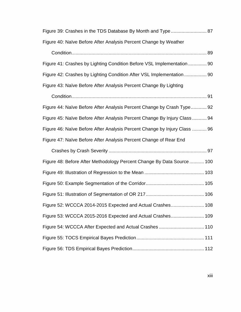
Figure 39: Crashes in the TDS Database By Month and Type ........................... 87

Figure 40: Naïve Before After Analysis Percent Change by Weather

Condition ...................................................................................................... 89

Figure 41: Crashes by Lighting Condition Before VSL Implementation .............. 90

Figure 42: Crashes by Lighting Condition After VSL Implementation ................. 90

Figure 43: Naïve Before After Analysis Percent Change By Lighting

Condition ...................................................................................................... 91

Figure 44: Naïve Before After Analysis Percent Change by Crash Type ............ 92

Figure 45: Naïve Before After Analysis Percent Change By Injury Class ........... 94

Figure 46: Naïve Before After Analysis Percent Change by Injury Class ........... 96

Figure 47: Naïve Before After Analysis Percent Change of Rear End

Crashes by Crash Severity .......................................................................... 97

Figure 48: Before After Methodology Percent Change By Data Source ........... 100

Figure 49: Illustration of Regression to the Mean ............................................. 103

Figure 50: Example Segmentation of the Corridor ............................................ 105

Figure 51: Illustration of Segmentation of OR 217 ............................................ 106

Figure 52: WCCCA 2014-2015 Expected and Actual Crashes ......................... 108

Figure 53: WCCCA 2015-2016 Expected and Actual Crashes ......................... 109

Figure 54: WCCCA After Expected and Actual Crashes .................................. 110

Figure 55: TOCS Empirical Bayes Prediction ................................................... 111

Figure 56: TDS Empirical Bayes Prediction ...................................................... 112

1

1.0 Introduction

Roadway safety is an ever present and increasingly visible problem in the

United States. Despite significant declines in fatalities over the past few decades,

in 2014 traffic crashes caused a total of 32,675 fatalities and over 2.3 million

injuries (NHTSA). Recent initiatives such as Vision Zero address the fact that

these deaths are far too high a cost as “life and health can never be exchanged

for other benefits within the society,” eschewing traditional cost benefit models.

(Monash 1999). The goal of reducing traffic deaths to zero has been adopted by

many US cities in the past few years including Portland, Oregon, which aims for

no fatalities in the city in 10 years.

A complementary issue to roadway safety in urban environments is

congestion. Congestion compounds safety issues as crash “frequency on both

freeways and arterials tends to increase with an increase in the congestion level”

(Chang 2003). This is in addition to other issues congestion brings such as the

cost of excess travel time, fuel consumption and emissions. The Texas A&M

Transportation Institute (TTI) estimates that congestion costs Americans $121

billion per year, equating to a rate of $818 per commuter (Schrank et al., 2012).

As urbanization increases in the US the congestion problems, and associated

safety issues, are expected to increase significantly.

To support the lofty safety goals of Vision Zero new strategies for

managing traffic are needed. In congested urban areas, building out of the

problem with more lanes or freeways is not possible from a right of way

2

standpoint and cost prohibitive. The goal now is to achieve more with existing

assets through proactive management strategies. One of the most promising

recent strategies is Active Traffic Management (ATM) systems. Transportation

Research Board’s (TRB) Glossary of Regional Transportation Systems

Management and Operations (RTSMO) terms defines ATM as “the ability to

dynamically manage recurrent and non-recurrent congestion on the mainline

based on prevailing traffic congestion” through the use of new technologies

(Neudorff, Mason, & Bauer, 2012). ATM systems come in many forms, including

(either individually or in combination) surveillance, incident management, ramp

metering, queue warning, traveler information, lane management and variable

speed limits, with the latter serving as the focus of this study. They have been

implemented in both congestion and weather-responsive applications and have

produced some promising results to be discussed later.

1.1 Variable Speed Limits

Variable speed limit (VSL) systems are a form of ATM that assign an

appropriate speed limit to the roadway depending on information from traffic

detectors, weather sensors, and other road surface condition data. Through

driver compliance, the speed limits are intended to improve safety or the

operation of the roadway through speed and flow harmonization across lanes,

and longitudinal speed dampening upstream of a queue/bottleneck. The systems

can be used for several different purposes, with speed management in

congested conditions, adverse roadways conditions, or work zones the most

3

Figure 1: Sample VSL Configuration Source: The Oregonian

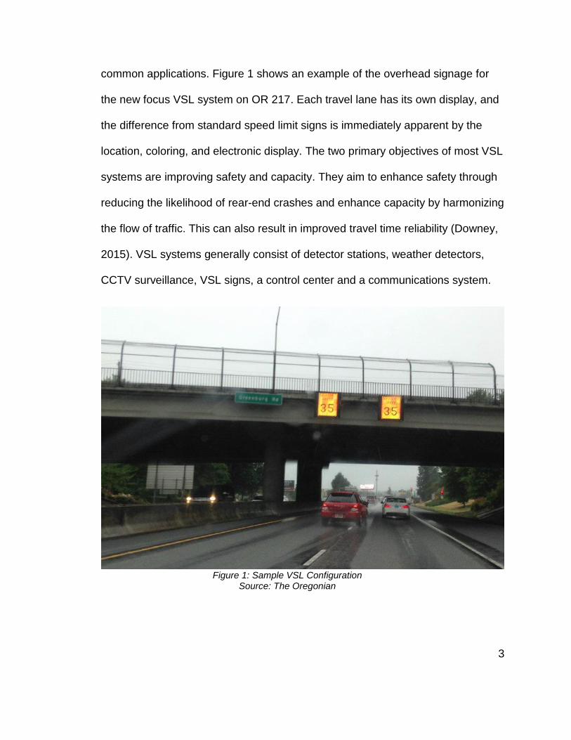
common applications. Figure 1 shows an example of the overhead signage for

the new focus VSL system on OR 217. Each travel lane has its own display, and

the difference from standard speed limit signs is immediately apparent by the

location, coloring, and electronic display. The two primary objectives of most VSL

systems are improving safety and capacity. They aim to enhance safety through

reducing the likelihood of rear-end crashes and enhance capacity by harmonizing

the flow of traffic. This can also result in improved travel time reliability (Downey,

2015). VSL systems generally consist of detector stations, weather detectors,

CCTV surveillance, VSL signs, a control center and a communications system.

4

A VSL system is typically controlled manually by traffic management

personnel and patrol officers or automatically using predetermined algorithms

(Vukanovic, 2007). In both cases, the jurisdiction in charge typically has

threshold values set for measures such as rainfall intensity or lane occupancy,

and activates the system when these values are surpassed. Therefore, the signs

may be blank and off for large periods of time before activating, showing reduced

speeds when conditions dictate. They will then adjust to the conditions until

deactivating when conditions improve and no longer exceed any thresholds. VSL

systems can gradually step down speeds upstream of congestion, to help drivers

avoid being caught off guard when they come upon more congested conditions.

A key distinguishing feature of any VSL system is whether the speeds

displayed are regulatory or advisory. Regulatory systems are subject to local

enforcement, while variable advisory speed (VAS) systems are generally not but

speeds may be enforced under the principle of Oregon’s basic speed rule (ORS

811.100). In this study the term VSL will be used for both systems with the terms

regulatory or advisory attached as needed. The Federal Highway Administration

(FHWA) recommends that VSL systems be regulatory rather than advisory

because they generally result in higher levels of compliance. Most international

applications include automated enforcement (spot or section) as part of each

VSL implementation. However, the OR 217 system was installed as an advisory

system at the behest of the Oregon State Police, the enforcement agency for this

freeway. The Oregon Statewide Variable Speed System Concept of Operations,

5

created before installation of the OR 217 system, determined that the benefits of

greater flexibility in setting speeds and greater public acceptance, as well as the

basic speed rule enforcement, made an advisory system workable for OR 217

(DKS Associates, 2013).

Several general guidelines regarding the display and placement of VSL

signs have been established when setting up any VSL system, despite the

unique characteristics of each VSL installation. The FHWA summarized such

guidelines in a 2012 report (Katz et al., 2012) as follows:

Using speed limits in five mph increments

Displaying speed limit changes for at least one minute

Not allowing speed differentials of more than 15 mph between

consecutive signs without advance warning

Using variable message signs to explain reason for speed

reductions

Additionally, the state of Oregon has a number of rules dictating the

establishment of VSL systems. OAR 734-020-0018 is the most important of

these, mandating a comprehensive engineering study with crash patterns, traffic

characteristics, and the adverse road conditions, including the type and

frequency, prior to the establishment of VSL (ODOT, 2012). Furthermore, the

engineering study shall provide specific recommendations regarding system

6

boundaries, algorithms, sign placement, and the procedures for changing posted

speeds.

1.2 OR 217 VSL System Background

The VSL system on OR 217 was under construction during early 2014 and

activated on July 22, 2014. This study seeks to evaluate the effectiveness of this

advisory VSL system on the safety of drivers in the corridor. OR 217 is shown in

the middle of Figure 2, and is a 7.5 mile highway southwest of downtown

Portland travelling between two large suburban communities of Beaverton and

Tigard. It has developed a well established reputation for heavy congestion with

traffic dynamics being quite sudden. In 2010, the Oregon Department of

Transportation published the OR 217 Interchange Management Study in an

attempt to identify strategies to enhance the safety and operations of this

corridor. Initially geometric improvements of widening to six lanes with braided on

and off ramps was considered, however, the cost of $1 billion was too high and

an advisory VSL system was ultimately chosen as the most promising and cost-

effective solution.

7

The justification for choosing VSL revolved around the speed harmonizing

effects of VSL, which had the potential to address all of the crash and congestion

issues experienced on OR 217. Bottlenecks and stop-and-go traffic often arise

from un-expecting drivers coming upon heavy traffic and suddenly hitting the

brakes to decelerate creating a shockwave that propagates upstream as other

drivers also use their brakes. By gradually dampening the speed of all drivers in

a harmonious fashion, preventing them from slamming on their brakes and

scaring following drivers into doing the same, such situations could be eliminated

Figure 2: Portland Area Freeway Map Source: AARoads

8

or minimized. Travel times would also become more reliable, as vehicles travel at

a uniform predictable rate. Harmonizing traffic speeds and flows can also be

linked with heightened safety, particularly on OR 217 where a substantial

proportion of crashes are typically rear-ends. These crashes are closely linked to

stop and go traffic and a reduction in this traffic would lead to a corresponding

decline in crashes. In giving their final endorsement of the VSL system, ODOT

estimated it would bring about a 20% reduction in rear-end crashes and a 5%

reduction in delay, with a total benefit of $6.6 million in improved mobility and

safety (DKS Associates, 2010).

Portland area freeway on-ramps all include ramp meters. Although not

considered in this study, the System-Wide Adaptive Ramp Metering (SWARM)

system which was present both before and after the deployment of the VSL, was

reprogrammed in the entire Portland region (including on OR 217) in an attempt

to improve operations. Implementation of this system began in May 2005 and a

similar “before and after” evaluation of the SWARM system was carried out in

2008. That study found that with SWARM implemented along OR 217, average

delay increased and reliability decreased, contrary to the system’s intent

(Monsere, Eshel, & Bertini, 2009). The fact that OR 217 is relatively short and

bounded by freeway interchanges on both ends along with, the corridor’s

relatively short ramp spacing and high mainline flows were highlighted as

possible reasons for why the results did not align with expectations and changes

to SWARM parameters were recommended. Many of the demand and geometric

9

issues that limited the SWARM system’s effectiveness will likely apply to the VSL

system and limit its impact. In addition, the SWARM system occasionally

switches back and forth between fixed-rate and optimized metering, making it

difficult to definitively separate any operational benefits associated with the VSL

system from the variable SWARM system conditions. Notably the SWARM

system was offline and functioning as a fixed-time system for several months

(September – December 2014) immediately following the VSL system activation.

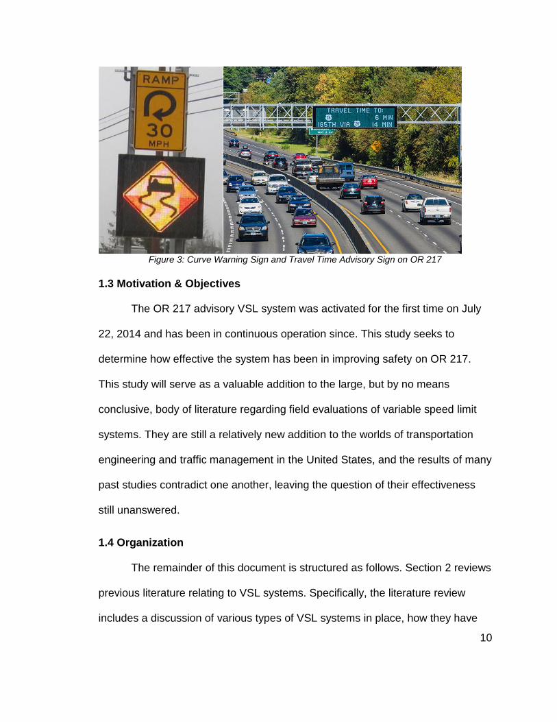
Another aspect of the ATM system implemented on OR 217 in July 2014

was the curve warning detectors and traveler information system that provides

travel time information on variable message signs. An example of each is shown

in Figure 3. These were activated at the same time as the VSL signs and are

placed at four ramps along OR 217. Three are active curve warning displays on

loop ramps at the northern terminus with US 26 and one at the southern

interchange with I-5. These activate when poor weather is detected and road

conditions as measured by the “grip factor” decline. As a caveat, the difficulty in

attributing crashes to specific locations on OR 217 could cause any impacts from

these curve warning detectors to be mixed in with the VSL results.

10

Figure 3: Curve Warning Sign and Travel Time Advisory Sign on OR 217

1.3 Motivation & Objectives

The OR 217 advisory VSL system was activated for the first time on July

22, 2014 and has been in continuous operation since. This study seeks to

determine how effective the system has been in improving safety on OR 217.

This study will serve as a valuable addition to the large, but by no means

conclusive, body of literature regarding field evaluations of variable speed limit

systems. They are still a relatively new addition to the worlds of transportation

engineering and traffic management in the United States, and the results of many

past studies contradict one another, leaving the question of their effectiveness

still unanswered.

1.4 Organization

The remainder of this document is structured as follows. Section 2 reviews

previous literature relating to VSL systems. Specifically, the literature review

includes a discussion of various types of VSL systems in place, how they have

11

been evaluated, and what the results of past studies have indicated. Section 3

details the corridor and the motivations for installing a VSL system on OR 217.

The following section discusses the sources of data for this study and their

merits. Section 5 analyzes the corridor using a Naïve Before After study with the

methodology and results discussed. Section 6 completes the same safety

analysis using the more powerful Empirical Bayes analysis, complete with

methodology and results. The following section discusses the results from both

analysis methods, develops conclusions, and provides future research

recommendations.

12

2.0 Literature Review

VSL systems are perhaps the most visible and novel aspects of ATM

systems, consequently becoming a well-studied component. As ATM has

become a more common solution to congestion and other roadway performance

issues, interest in the performance of such systems has grown. This section

reviews and discusses previous research related to VSL systems. Their history,

adoption, wide variety of system types, various evaluation methods, and the

evaluation results are all reviewed.

2.1 History

In the past decade, interest in VSL systems has increased significantly but

the systems have a much longer history with some of the first dating to the

1950’s. New Jersey police officer occasionally put up temporary wooden signs

during adverse weather to try to reduce vehicle speeds (Goodwin, 2003). These

changes were not based on algorithms but rather the police officers’ feel for the

appropriate speeds. Following this early experimental tradition New Jersey was

one of the first two domestic location to try VSL systems, along with Michigan

(Robinson, 2000). On the John C. Lodge Freeway near Detroit and the New

Jersey Turnpike, systems utilized traffic officials to manually change posted

speed limits based on personal observations of traffic conditions. Both of these

precursor systems aimed to improve safety and operation during congestion.

However officials in Michigan did not feel results were apparent or significant

enough and elected to dismantle and remove the system around 1967 after 5

13

years of running (Robinson, 2000). The New Jersey Turnpike system still

operates, however it has had substantial upgrades to make it an automated and

weather responsive system (Robinson, 2000). Internationally, Germany installed

its first VSL system with automated enforcement in the 1970s to stabilize traffic

flow during congestion, and the Netherlands first implemented a system in the

early 1980s, also an automated enforcement system (Han, Luk, Pyta, & Cairney,

2009).

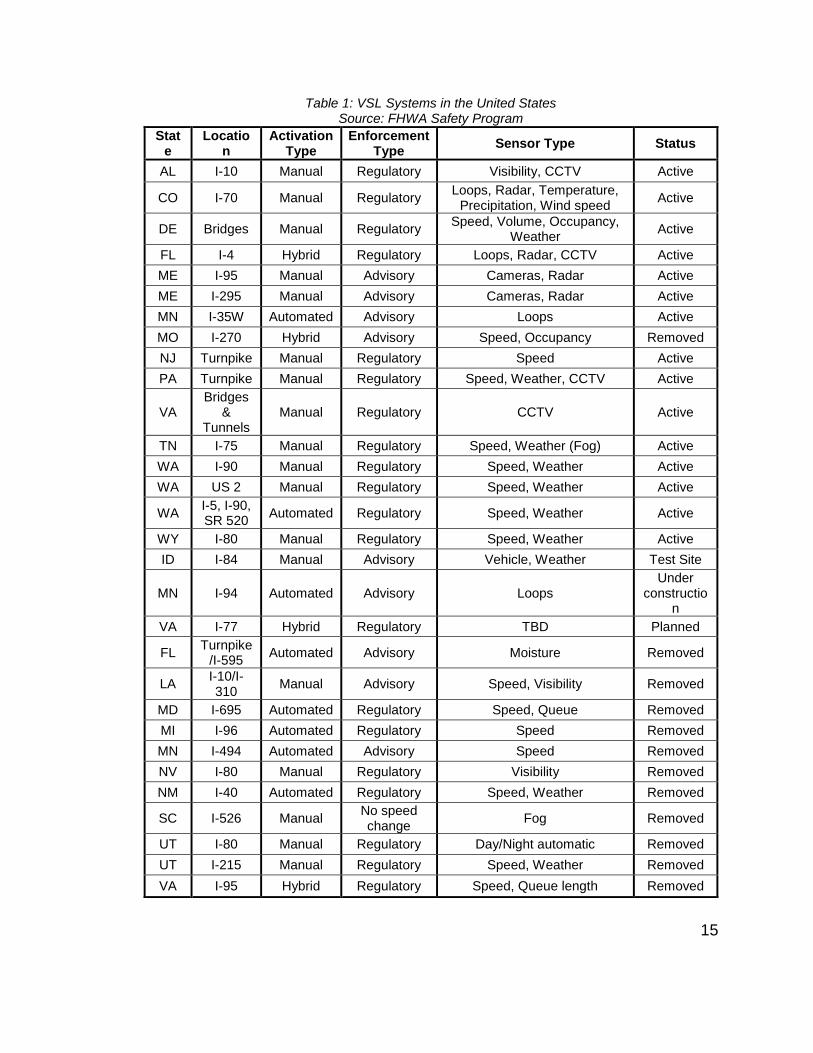
Since the first experimental systems, the number of VSL systems has

grown tremendously, especially since 1990. As of 2012, 20 U.S. states had either

implemented VSL systems or were planning future installations (Katz et al.,

2012). Table 1, created with information from a 2012 report by the FHWA’s

Safety Program (Katz et al., 2012), summarizes the VSL systems that, as of

2012, have been built or planned in the United States. Most systems are

regulatory and require manual activation, with speed and weather being the

typical targets. In the United States many systems have been taken down after

failing to meet expectations. Abroad, installations have also been implemented in

Australia, France, Finland, Sweden and the United Kingdom, with the early

systems in Germany and the Netherlands updated and expanded (Al-Kaisy,

Ewan, & Veneziano, 2012). The sizes, purposes and characteristics of these

systems vary widely, and the results match this with large variations in

effectiveness. Each system can be distinguished with manual or automatic

activation, congestion or weather-responsive, urban or rural, and regulatory or

14

advisory. Details on the performance of a few of these systems will help to

illustrate the variation among their performance and how no one system is

perfect for every application.

15

Table 1: VSL Systems in the United States Source: FHWA Safety Program

State

Location

Activation Type

Enforcement Type

Sensor Type Status

AL I-10 Manual Regulatory Visibility, CCTV Active

CO I-70 Manual Regulatory Loops, Radar, Temperature,

Precipitation, Wind speed Active

DE Bridges Manual Regulatory Speed, Volume, Occupancy,

Weather Active

FL I-4 Hybrid Regulatory Loops, Radar, CCTV Active

ME I-95 Manual Advisory Cameras, Radar Active

ME I-295 Manual Advisory Cameras, Radar Active

MN I-35W Automated Advisory Loops Active

MO I-270 Hybrid Advisory Speed, Occupancy Removed

NJ Turnpike Manual Regulatory Speed Active

PA Turnpike Manual Regulatory Speed, Weather, CCTV Active

VA Bridges

& Tunnels

Manual Regulatory CCTV Active

TN I-75 Manual Regulatory Speed, Weather (Fog) Active

WA I-90 Manual Regulatory Speed, Weather Active

WA US 2 Manual Regulatory Speed, Weather Active

WA I-5, I-90, SR 520

Automated Regulatory Speed, Weather Active

WY I-80 Manual Regulatory Speed, Weather Active

ID I-84 Manual Advisory Vehicle, Weather Test Site

MN I-94 Automated Advisory Loops Under

construction

VA I-77 Hybrid Regulatory TBD Planned

FL Turnpike

/I-595 Automated Advisory Moisture Removed

LA I-10/I-310

Manual Advisory Speed, Visibility Removed

MD I-695 Automated Regulatory Speed, Queue Removed

MI I-96 Automated Regulatory Speed Removed

MN I-494 Automated Advisory Speed Removed

NV I-80 Manual Regulatory Visibility Removed

NM I-40 Automated Regulatory Speed, Weather Removed

SC I-526 Manual No speed change

Fog Removed

UT I-80 Manual Regulatory Day/Night automatic Removed

UT I-215 Manual Regulatory Speed, Weather Removed

VA I-95 Hybrid Regulatory Speed, Queue length Removed

16

2.2 System Types & Purposes

2.2.1 Weather-Responsive

The first VSL systems primarily focused on coping with inclement weather,

so the majority of systems worldwide are still weather-oriented. In 1994, Finland

built its first experimental VSL system on a 15 mile rural segment of E18 in the

southeastern portion of the country (Al-Kaisy et al., 2012; Robinson, 2000). This

regulatory system is purely weather-responsive. A series of 67 VSL signs are

connected to 2 automated weather stations capable of measuring precipitation,

temperature, and road surface conditions, and posted speeds range from 49 to

74 miles per hour (mph) depending on measured conditions. Both drivers and

officials support the system with an astounding 95% of drivers in favor.

In the United States, the state of Wyoming installed its first variable speed

limit corridor along a remote section of Interstate 80 in 2009, adding four other

sections in the following years. The remoteness of the system encourages the

use of overhead boards to inform drivers of conditions during Wyoming’s

notoriously difficult winters faster than they might be informed otherwise. Each

VSL corridor has LED VSL signs, road weather information systems (RWIS)

capable of monitoring temperature, humidity, and wind speed, and Wavetronix

radar based speed sensors capable of monitoring volume, individual vehicle

speed, occupancy, and vehicle classification. These systems are currently

manually operated by highway patrol officers and the Traffic Management

Center. They observe the recorded weather data and adjust speed limits

17

accordingly. Perhaps unsurprisingly for such a remote area, the manual

activation was shown to be inefficient by a University of Wyoming research

project, so an automated protocol based on real-time speed and weather data

was developed, and simulations showed it would be more effective and efficient

(Buddemeyer, Young, Sabawat, & Layton, 2010; Young, Sabawat, Saha, & Sui,

2012).

2.2.2 Congestion-Responsive

In urban scenarios heavy congestion and high incident frequency is often

a focus of VSL implementations. One example is the advisory VSL system

activated in Minnesota in 2010. This system was deployed in a heavily urbanized

corridor of I-35W near downtown Minneapolis. This particular system is not

regulatory but rather an advisory system and primarily responds to the

congestion, however it is capable of weather warnings as Minnesota can

experience heavy winter weather. It is one of the few active VSL deployments in

the United States that focuses improving highway operations during congestion,

however this is an area of increasing interest (Edara, Sun, & Hou, 2013). A total

of 174 VSL signs are linked with the highway’s system of single loop detectors

(Katz et al., 2012). Detector readings of speed and density are collected every 30

seconds, as an algorithm determines if using a reduced speed limit is appropriate

according to several set thresholds. The algorithm utilized is designed to mitigate

shockwave formation on the highway (Kwon, Park, Lau, & Kary, 2011).

18

In 2008, the Missouri Department of Transportation installed a VSL

system along parts of Interstate 270 and Interstate 255 near St. Louis. Like the

Minneapolis system, the St. Louis system is primarily aimed at dealing with

recurring congestion in an urban area. During the first three years the system

used regulatory speed limits however on I-270 this was changed to advisory

speed limits in 2011. The corridor is split into zones composed of a few loop

detector stations, and 30-second average speed, flow and occupancy readings

for each zone are fed into a VSL algorithm. If average occupancy is found to be

greater than 7%, flow greater than 10 vehicles in 30 seconds (equivalent to 1200

vehicles per hour), and average speed less than 55 mph, an enforceable

reduced speed limit equal to the average speed rounded up to the nearest

multiple of 5 will be recommended by the system. A degree of manual control is

built in as well, as TMC operators verify conditions through camera feeds before

posting reduced speed limits (Kianfar, Edara, & Sun, 2013). However, this

system was unsuccessful and was ultimately removed in 2013. Operators cited

that it did not produce the results that they aimed for (Lippmann 2013).

2.2.3 Work Zone Systems

In addition to permanent corridor-wide applications VSL systems have

been used around temporary work zones in the past few years to improve both

operations and safety during construction. Before implementation, simulation

studies by Lin et al. and others demonstrated the potential benefits of VSL

control around work zones (Lin, Kang, & Chang, 2004), and the results of those

19

studies have since led to real applications. In 2006, a two-state VAS system was

developed and implemented for a work zone on I-494 near Minneapolis in order

to bring upstream speeds down to the level of downstream traffic (Kwon,

Brannan, Shouman, Isackson, & Arseneau, 2007). Both regulatory and advisory

VSL systems have also been utilized around work zones in Washington,

Missouri, Ohio, Virginia and New Hampshire (Edara et al., 2013).

2.3 Evaluation Methods & Results

Given the unique characteristics of each VSL/VAS system, it is difficult to

single out a specific set of evaluation methods and performance measures that

can be applied to each of them. In an FHWA report documenting lessons learned

from ATM installations throughout the United States, travel time, travel speeds,

travel time reliability and variability, spatial and temporal extent of congestion,

throughput, and user perceptions are identified as key measures of effectiveness

for ATM evaluations (Kuhn, Gopalakrishna, & Schreffler, 2013). Another

potentially important performance measure is compliance with the VSL systems.

Using a Paramics simulation model, Hellinga and Mandelzys found that a very

high compliance scenario resulted in a 39% improvement in safety relative to no

VSL, while a low compliance scenario resulted in only a 10% improvement

(Hellinga & Mandelzys, 2011). With loop detector data, compliance rates are

fairly straightforward to calculate. The University of Wyoming summarized speed

compliance for Wyoming’s VSL system by computing the percentage of vehicles

traveling above and below the posted speed limit. Speed variance was also

20

captured by computing the percentage of vehicles traveling three and five mph

above and below the posted speed limit (Young et al., 2012).

Given the nature of this study and its emphasis on safety, crash records

from before and after are the primary performance measure, using analysis

methodologies that have been utilized in prior studies, the Naïve Before After

Study and an Empirical Bayes study. A work zone safety VSL system in place on

I-495 in Virginia was also removed two years after installation. This project was

studied by Fudala and Fontaine, finding that simulations produced a reduction in

safety surrogates such as lane changes and speed harmonization. The authors

recommend continued study of VSL systems as a potential solution but that

scenarios be carefully screened for potential effectiveness. (Fudula & Fontaine,

2010)

2.3.1 Naïve Before and After Evaluation Methods

Naïve Before and after studies of VSL systems similar to the one studied

here have been conducted several times before. In Missouri a hybrid automated

system installed in 2008 was shown by Bham et al. to result in a reduction in

crashes of around 6.5% with a Naïve Before After study and 8.4% with an

Empirical Bayes study (Bham et al., 2010). This system changed from a

regulatory to advisory system after three years of use. Despite these reductions,

other factors caused the system to be removed a few years later in 2013. The

agency chose to focus on changeable message signs as the main method of

communicating slowdowns to drivers.

21

Rama and Schirokoff found that a weather-responsive VSL system in

Finland reduced crashes by 13% during the winter and 2% during the summer

and reduced the overall injury crash risk by 10% (Rama & Schirokoff, 2004).

Model estimation using field data showed that Wyoming’s VSL system was

expected to reduce crash frequency by 0.67 crashes per week per 100 miles of

corridor length, or about 50 crashes per year. In monetary terms, this was

equated to an annual safety benefit of about $4.7 million (Young et al., 2012). In

a summary of VSL applications throughout the world, Robinson noted that VSL

on several rural Autobahn stretches in Germany has reduced crash rates by 20

to 30% and a system on the M-25 highway near London contributed to a 10 to

15% reduction in crashes (Robinson, 2000).

Related to the reduction in crashes associated with VSL systems, they

have also been effective at reducing speeds and speed variability during poor

weather in several locations. A system on A16 in the Netherlands aimed at

creating safer driving conditions during fog led to an 8 to 10 kilometer per hour

(kph) drop in mean speeds during foggy conditions (Robinson, 2000). Another

VSL system primarily aimed at addressing foggy conditions in Utah led to a

reduction in the average standard deviation of vehicle speeds by 22% (Perrin,

Martin, & Coleman, 2002). The previously mentioned Wyoming system also

helped to reduce speed variation during winter storms because it provided

drivers guidance as to an appropriate reduced speed (Young et al., 2012).

22

2.3.2 Empirical Bayes Analysis

The Empirical Bayes methodology has been applied less often in safety

studies but is often noted as producing more accurate results. An 18% reduction

in crashes was observed in Belgium on freeways with a regulatory, automated

VSL system. This analysis by De Pauw et al., found that the decrease was

largely due to a significant reduction in rear end crashes of 20%. The authors

conducted an Empirical Bayes analysis with up to 12 years of crash data for 5

separate freeway segments (De Pauw at al., 2015). The Missouri study by Bham

et al. was shown to have a higher 8.4% reduction when an Empirical Bayes study

was conducted (Bham et al., 2010).

Despite the numerous studies linking VSL systems to lower crash rates, in

an evaluation of the same VSL system near Antwerp, Belgium, Corthout et al.

claimed that the homogenizing effects of VSL actually have little to do with

observed reductions in crashes. Rather, they argued that crashes dropped

mostly because of accompanying warning signs that heighten driver awareness,

since secondary crashes tend to be reduced more than crashes as a whole

(Corthout, Tampere, & Deknudt, 2010). Their conclusions suggest that even the

safety benefits of VSL, which have been studied in much more depth than the

operational benefits, are still a matter of contention and lacking overarching

consensus.

The Empirical Bayes methodology is noted for combating regression to

the mean bias and creating more accurate estimates of the actual treatment

23

effect. Ezra Hauer is a key figure in the development of this methodology and his

book “Observational Before-After Studies in Road Safety” forms the backbone of

both the Naïve Before After Study and the Empirical Bayes Analysis utilized in

this work (Hauer 1997). Similarly, the Highway Safety Manual (HSM) makes

extensive use of Empirical Bayes studies in the methodology and the draft

freeway section helped to guide the Empirical Bayes portion of this study (HSM

2012).

2.4 OR 217 Evaluations

OR 217 has been studied multiple times before after the implementation of

the VSL system. One study by Riggins, et al. focused on the compliance of

drivers along OR 217 as compared to those on German Autobahns. The results

showed that compliance was fairly poor with speeds typically 5 to 15 mph above

the displayed speed limit (Riggins et al. 2015). Compliance was also lower on

OR 217 than the one the German roadways. Another study by Downey, et al.

studied safety, travel time reliability, lane flows, and bottleneck flow

characteristics. This crash analysis in that report used one data source and found

that the crash distribution had shifted away from the VSL sign locations.

However, the analysis did not show any significant safety benefits with crash

increases, based on a small sample of data from a 5 month period after VSL

activation (Downey, et al. 2015). A more recent study summary of safety on the

corridor was conducted by ODOT using multiple data sources in a simple

comparison of crash numbers before and after the VSL implementation showing

24

a 13% decline with 911 call data and 20% decline with official crash data (ODOT,

2016).

2.5 Summary

A large body of previous research into various aspects of VSL systems

exists. This section has shown that there is a substantial amount of diversity

among VSL applications, evaluation methods, and results. Regarding the actual

effects of VSL systems, studies seem to indicate that crashes decrease however

the effect is quite varied and the reasoning disputed.

Several potential reasons exist for why so many VSL studies seem to

contradict one another, but a major one is the inherent differences in the

characteristics of each system. A system designed to address winter weather in

Finland is going to be very different in purpose and have a different impact than a

system aimed at mitigating congestion problems near downtown Seattle.

Similarly, a system in rural Wyoming and systems in urban Germany have little in

common. Even similar congestion-responsive systems in St. Louis, Minneapolis,

and Portland will vary quite a bit from one another because the cities have

unique highway alignments, driver characteristics, and traffic flows.

Studies should be carried out before the implementation of a system to

ensure that the corridor being looked at has potential for a benefit rather than

applying past results haphazardly. Goals for the corridor must be firmly set and

used as part of the analysis of any intended system.

25

The system in place on OR 217 is unique from many of those reviewed as

since it is both congestion and weather-responsive with safety as the primarily

goal. In addition, it has not been installed for a long period of time requiring more

careful analysis to determine the results. Because of this, the study will be

conducted with multiple data sources and both standard crash analysis methods.

OR 217 has been studied before and this research intends to build upon and

clarify results for this particular corridor using more detailed safety analysis

methods. Furthermore, the analysis will add to the body of research for VSL

systems in general and develop a better understanding of them.

26

3.0 Motivations for VSL on OR 217

The issues associated with OR 217 pre-VSL are numerous and wide-

ranging, relating to both safety and operations. In this section, a brief almanac of

the corridor and its general performance trends is presented and the major

problems with the corridor that prompted to ODOT to explore and ultimately

implement VSL are discussed.

27

3.1 Corridor Almanac

OR 217 is a 7.52-mile highway stretching between Interstate 5 at the

southern terminus and US Highway 26 at the northern terminus (refer to Figure

2). It primarily serves as a connector between downtown Portland and

southwestern suburbs including Beaverton and Tigard. The highway has a

Figure 4: OR 217 at Allen Blvd Source: DKS Associates

28

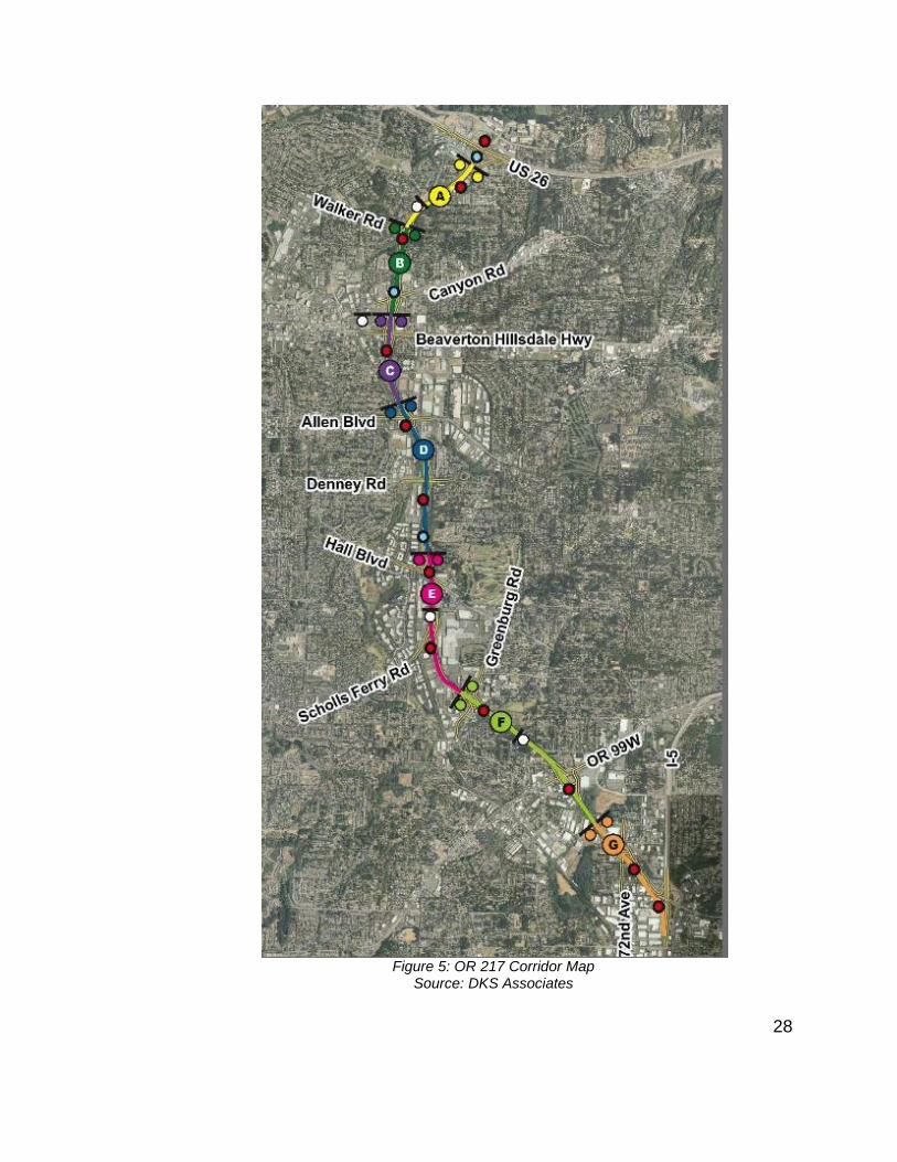
Figure 5: OR 217 Corridor Map Source: DKS Associates

29

posted speed limit of 55 miles per hour and fully divided with typically 2 lanes of

traffic in each direction. The corridor developed from an older highway with at-

grade intersections and as it developed formed a large number of connections

with local streets. After full grade separation it has eleven sets of on- and off-

ramps in each direction. Most interchanges are typical diamonds but several

have loop or hook ramps. The close spacing of the ramps has led to most being

connected by short auxiliary lanes, creating many weaving zones along the

highway. Its location relative to downtown Portland makes OR 217 a popular

route for commuters. All on-ramps include ramp meters. Figure 5 provided,

courtesy of DKS, presents a map of the study area, with the labels indicating the

locations of interchanges, and Figure 4 and Figure 6 are current aerial

photographs of two of these interchanges.

According to official Oregon Department of Transportation’s officially

published traffic volumes, in the most recent year before the VSL system was

deployed, OR 217 had an average annual daily traffic (AADT) of approximately

110,000 vehicles across both directions, equivalent to an average daily vehicle-

miles traveled (VMT) value of about 830,000 vehicle-miles. In the immediate full

year before the system activation, 2013, there were 322 crashes reported along

the corridor in 2013, a rate of 1.06 crashes per million VMT (2013 Crash Book).

30

Figure 6: OR 217 at Scholls Ferry Rd Source: DKS Associates

31

3.2 Crash Trends

In addition to the capacity and mobility challenges facing OR 217, it also

exhibits safety issues. In 2013 (the last full calendar year prior to the VSL system

deployment) OR 217 had 322 reported crashes according to the ODOT 2013

State Highway Crash Rate Tables (these are the official statewide crash data,

later referred to as TDS). This equates to a crash rate of 1.06 crashes per million

vehicle miles, higher than the statewide average of 0.92 for urban non-interstate

freeways. All but one of the eight segments into which the corridor is split in the

report experienced increased from the previous year crash rates.

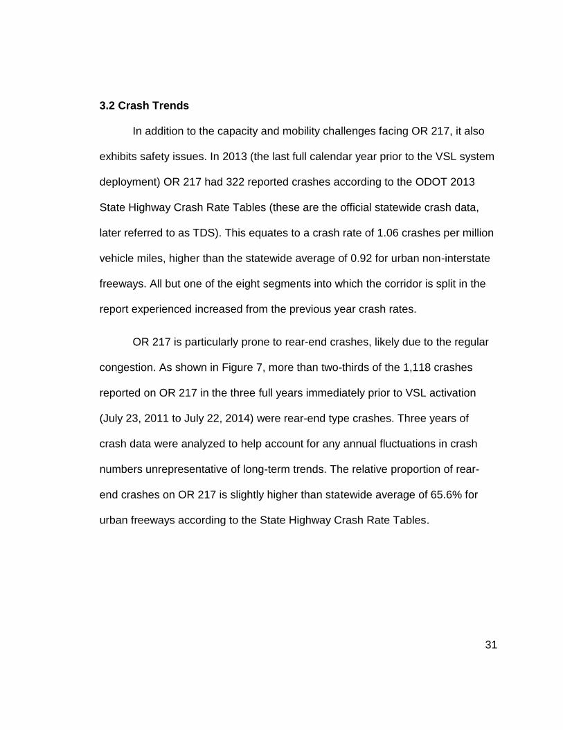
OR 217 is particularly prone to rear-end crashes, likely due to the regular

congestion. As shown in Figure 7, more than two-thirds of the 1,118 crashes

reported on OR 217 in the three full years immediately prior to VSL activation

(July 23, 2011 to July 22, 2014) were rear-end type crashes. Three years of

crash data were analyzed to help account for any annual fluctuations in crash

numbers unrepresentative of long-term trends. The relative proportion of rear-

end crashes on OR 217 is slightly higher than statewide average of 65.6% for

urban freeways according to the State Highway Crash Rate Tables.

32

Just under half of the 1,118 total crashes on OR 217 between 2011 and

2014 involved at least one injury. As shown in Figure 8, the majority of these

injuries were Class C and came from rear-end crashes. In Oregon, Class C injury

crashes are those resulting in “possible injuries”, which are generally complaints

of pain or relatively minor visible injuries. Figure 8 and Figure 9 demonstrates

that the common notion that rear-end crashes tend to be minor “fender benders”

is a misconception, as more than near half of the rear-end crashes on OR 217

between July 23, 2011 and July 22, 2014 resulted in at least one injury. In

addition to the safety-related consequences, each one of these frequent rear-end

Fixed Object 9%

Other 4%

Rear End 71%

Sideswipe -Overtaking

10%

Turning 6%

Crashes By Type

Fixed Object

Other

Rear End

Sideswipe - Overtaking

Turning

Figure 7: OR 217 Crashes by Crash Type 2011 - 2014

n=1118

33

crashes typically leads to the formation of a new bottleneck, restricting flow

through the entire corridor for an extended period of time.

Figure 8: OR 217 Injuries by Crash Type &

Severity 2011-2014 Figure 9: OR 217 Rear-end Crash Severity

2011-2014

3.3 Effects of Adverse Weather

OR 217 has a weather-responsive component in addition to the

congestion-responsive component because the corridor has a history of

diminished safety and efficiency during adverse weather. With adverse weather,

particularly precipitation, present, OR 217 has a tendency to experience more

crashes and significantly higher and even less reliable travel times.

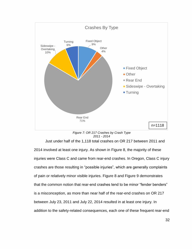
Figure 10 shows the percentage of the 1,118 crashes on OR 217 from

2011 through 2014 that occurred in various road surface conditions. Forms of

winter precipitation such as snow were factors in a very small portion of crashes,

which can be attributed to the relatively rare occurrence of frozen precipitation in

0

100

200

300

400

500

600

700

FATAL INJ A INJ B INJ C PDO

Crash Type by Injury Class

Angle

Fixed

Sideswipe -OvertakeRear End

0

50

100

150

200

250

300

350

400

450

Injury PDO

Rear-end Crash Severity

n=1118

n=797

34

Portland. Rain, however, was falling during more than one quarter of the reported

crashes and roads were wet during more than one third. Precipitation was only

reported by the National Weather Service during about 10% of all the hours

during these three years, indicating that wet weather conditions are significantly

overrepresented in the crash data and that crashes become much more likely on

OR 217 during precipitation events.

Figure 10: Crashes by Surface Condition on OR 217 Between July 23, 2011 and July 22, 2014

3.4 Summary

Analysis of the conditions on OR 217 prior to the VSL system’s

implementation clearly demonstrates that the corridor has some significant

problems and has the potential to benefit from an effective VSL system. OR 217

is prone to severe congestion and recurrent bottlenecks on a regular basis during

DRY 67%

WET 29%

ICE 1%

SNO 0%

UNK 3%

Crashes by Surface Condition

DRY

WET

ICE

SNO

UNK

n=1118

35

weekdays, with average speed declines of 50% not uncommon during peak

demand hours. Recurrent bottlenecks in both directions create queues several

miles long that last for several hours. Additionally, the corridor’s performance

varies a great deal between different hours and days, contributing to highly

unreliable travel times. OR 217 is particularly prone to rear-end crashes, with an

average of more than one every day, and these crashes can have major

consequences in terms of both safety and throughput. Finally, during adverse

weather, OR 217 is even more susceptible to crashes and travel times are higher

and more unreliable.

Historical trends suggest OR 217’s problems are not going to solve

themselves. Between 1985 and 2005, traffic volumes doubled, and they are

expected to grow another 30% by 2025. The growth in demand is expected to

increase the extent of daily congestion from 3 hours to 8 hours by 2025. The

crash rate has increased 89% just since 2009. These trends, combined with the

previously discussed mobility and safety issues, clearly indicate that something

needed to be done to improve OR 217, and ODOT ultimately settled on an

advisory VSL system.

36

4.0 Data Sources

The previous section demonstrated that prior the VSL system, OR 217

was suffering from a number of issues. In order to assess the effectiveness of the

VSL system in addressing these issues, data from several different sources was

obtained and analyzed using an array of analysis techniques. Each of these

analyses was carried out in the form of a “before and after” comparison in order

to gain an understanding of how safety on OR 217 has changed since the VSL

system’s implementation. In this chapter, available instrumentation along OR 217

and the various types of data used are detailed as well as any addendums made.

4.1 Corridor Instrumentation

The primary means of traffic data collection along OR 217 is a series of

dual-loop detector stations placed upstream of each entrance ramp. These

stations record and store vehicle count, occupancy, and speed measurements

every 20 seconds. At each detector station, there are one set of dual-loop

detectors in each traffic lane. Single loops are also located on each

accompanying ramp, but these loops only capable of recording vehicle counts.

Since 2014 OR 217 is also instrumented with a series of radar traffic sensors,

manufactured by Wavetronix, which collect the same data as the loop detectors.

As with the loop detectors, the radar detectors are grouped into stations, with one

sensor for each traffic lane. The Wavetronix sensors were strategically located

along OR 217 to minimize any large gaps between loop detector stations, thus

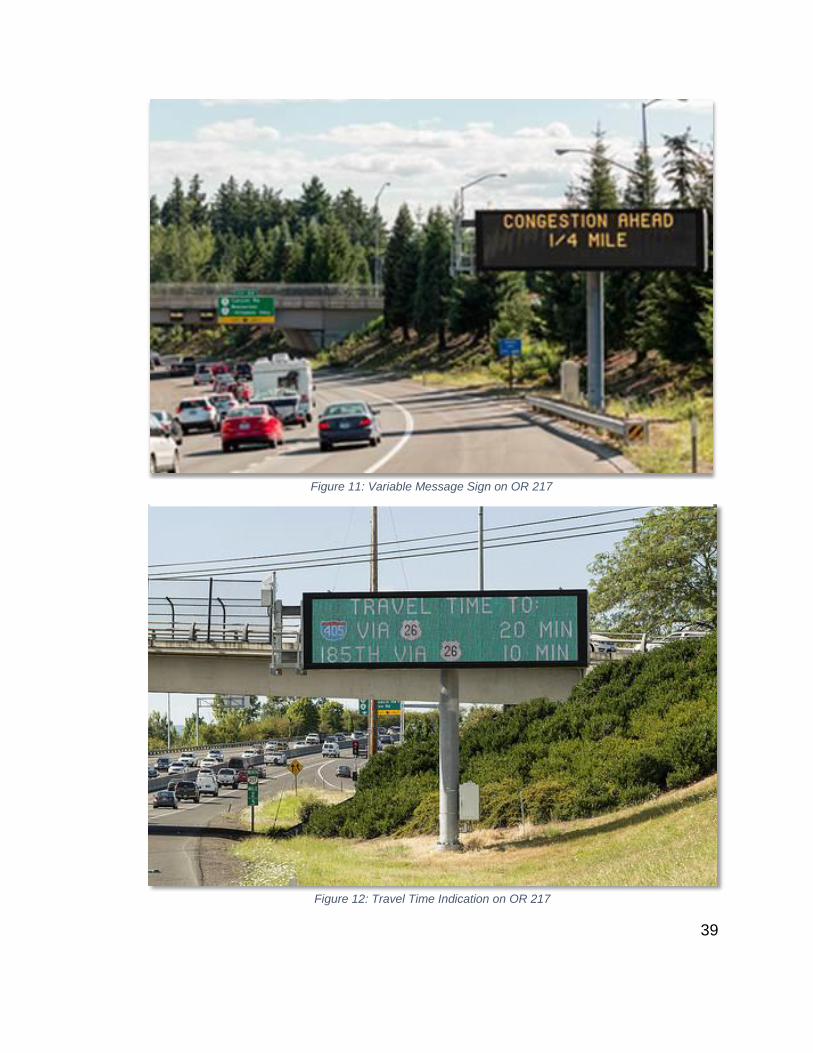
improving the resolution of traffic measurements. Figure 13 and Figure 14 show

37

the lane configurations and layout of available instrumentation on OR 217

southbound and northbound, respectively.

The VAS system being evaluated in this study was constructed on OR 217

over the past several years as one component of the OR 217 Active Traffic

Management project and consists of a series of large electronic message signs.

There are ten locations along OR 217 with these variable speed signs for both

the northbound and southbound directions. Figure 15 and Figure16 show the two

primary configurations of these signs, either on bridges or metal structures. As

shown, each travel lane has its own sign, and adjacent signs do not necessarily

display the same speed.

The congestion-responsive component of the system works by collecting

data from the corridor’s traffic detectors. Each VAS sign is assigned a segment

reaching to the next sign downstream, and any sensor data within that segment

is relayed to that sign. Each detector station is assigned a certain volume and

occupancy threshold, one of which must be met for its speed readings to

influence the VAS sign. If one of these thresholds is met, the 85th percentile

speed at that station is computed and rounded to the nearest 5 mph. Finally,

these 85th percentile station speeds for each station within a VAS sign’s

segments meeting either the volume or occupancy threshold are compiled, and

the lowest one is displayed on the sign until the controlling station’s 85th

percentile speed has risen to the next highest 5 mph increment. If the lowest 85th

percentile station speed is below 25 mph, the sign display will read “SLOW”

38

instead of an actual speed. Speeds displayed at VAS signs upstream of the most

congested segments are stepped down based on how far upstream they are to

encourage drivers to gradually decelerate before they reach the heaviest

congestion.

The weather-responsive component of OR 217’s VAS sign continuously

collects real-time data from new RWIS sensors installed along the corridor,

represented as diamonds in Figure 17. The VAS systems then uses a lookup

table to determine an appropriate reduced speed to display based on the sensor

measurements of visibility and grip factor, which indicates the level of grip of the

roadway surface. If both congestion and adverse weather are occurring, the

component which computes the lowest appropriate speed for each sign takes

priority. The Oregon Statewide Variable Speed System Concept of Operations

explains the two different components in greater detail (DKS Associates, 2013).

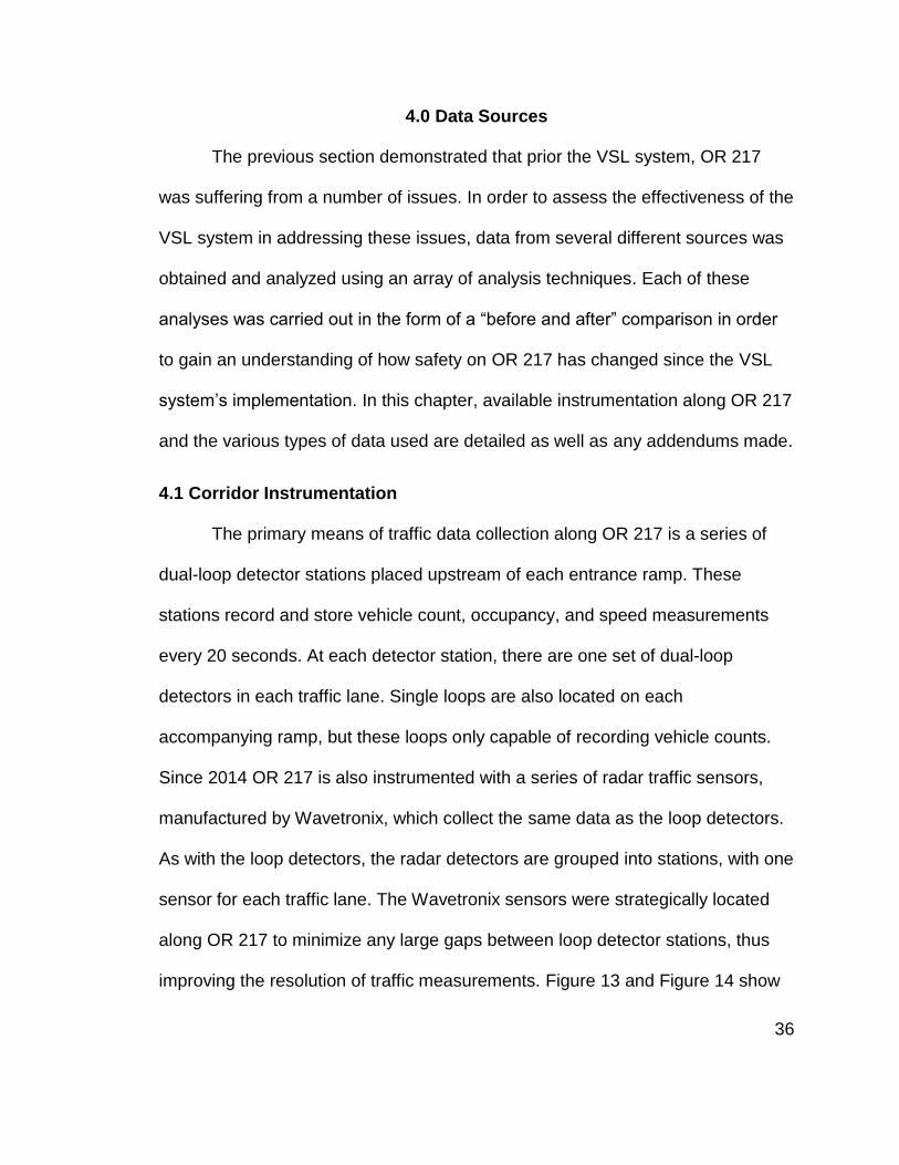
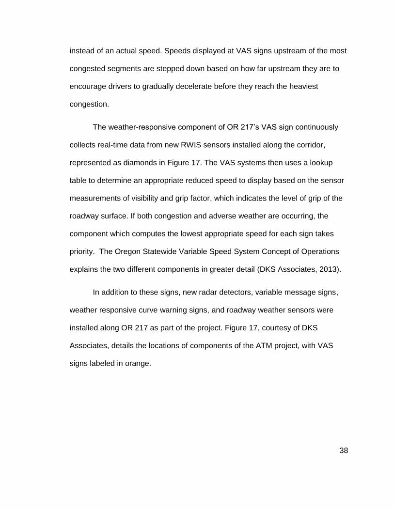
In addition to these signs, new radar detectors, variable message signs,

weather responsive curve warning signs, and roadway weather sensors were

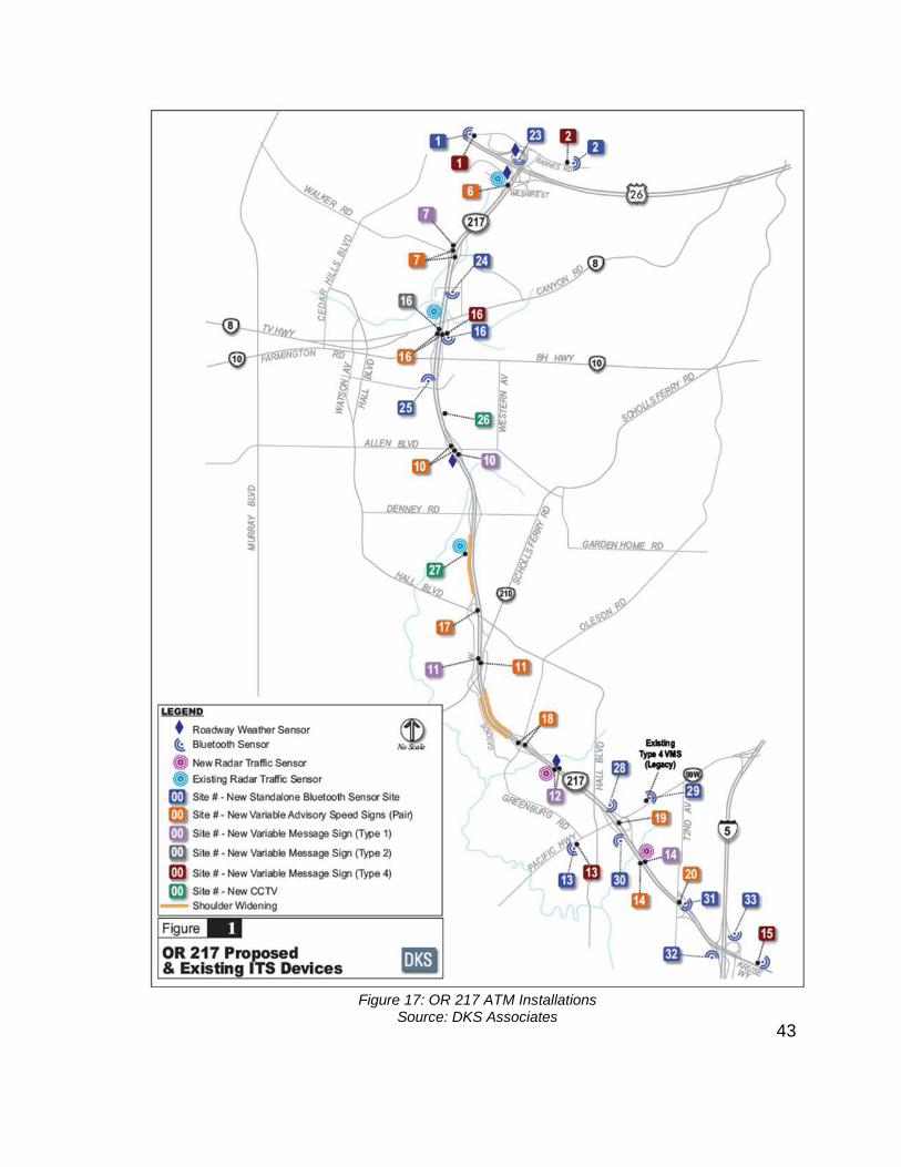
installed along OR 217 as part of the project. Figure 17, courtesy of DKS

Associates, details the locations of components of the ATM project, with VAS

signs labeled in orange.

39

Figure 11: Variable Message Sign on OR 217

Figure 12: Travel Time Indication on OR 217

http://www.google.com/url?sa=i&rct=j&q=&esrc=s&frm=1&source=images&cd=&cad=rja&uact=8&ved=0CAcQjRxqFQoTCMKeu8qZ68gCFQvuYwodSdQPAA&url=http://www.flickriver.com/photos/tags/or217/interesting/&psig=AFQjCNGRtTPJokeRqiZEpQ3xlrW6qZz-Fw&ust=1446328961536924

https://www.google.com/url?sa=i&rct=j&q=&esrc=s&frm=1&source=images&cd=&cad=rja&uact=8&ved=0CAcQjRxqFQoTCMT677qn0sgCFQMxiAod1hoG-A&url=https://www.tripcheck.com/realtime/see-the-signs.asp&psig=AFQjCNEvXZNTxSWZleXa4o1kc1FiVTAP9g&ust=1445473685180610

40

Station Influence Length

MP .10 - Barnes

MP .45 - Wilshire

MP .76 - Walker

MP 1.92 – B-H Hwy

MP 2.55 - Allen

MP 3.12 - Denney

MP 3.5 - Hall

MP 4.35 – Scholls Ferry

MP 5.11 - Greenburg

MP 5.95 – 99W West

MP 6.77 – 72nd

MP 7.0 – OR 217 WB to SB

U.S. 26 West

U.S. 26 East

I-5 SB

MP .25 - Wavetronix

MP 1.5 - Wavetronix

MP 3.4 - Wavetronix

7

6

5

4

3

2

1

0

Milepost

MP .25 – VAS Sign

MP .91 – VAS Sign

MP 1.58 – VAS Sign





= Loop Detector

= Radar Detector

= VAS Sign

Figure 13: OR 217 Southbound VSL & Detector Layout

41

Figure 14: OR 217 Northbound VSL & Detector Layout

MP .66 - Walker

MP 1.34 – TV Hwy

MP 2.16 – Allen

MP 2.68 - Denney

MP 3.85 – Scholls Ferry

MP 4.65 - Greenburg

MP 5.85 – 99W West

MP 5.9 – 99W East

MP 6.61 – 72nd

.54

.42

.41

.59

.62

.59

.62

1.00

U.S. 26 East

MP .25 - Wavetronix

MP 3.4 - Wavetronix

MP 1.5 - Wavetronix

.46

.63

1.01

Station Influence Length

0.38

7

6

5

4

3

2

1

0

Milepost

MP .91 – VAS Sign







= Loop Detector

= Radar Detector

= VAS Sign

42

Figure 15: OR 217 VSL Signs on Bridges Source: The Oregonian

Figure 16: OR 217 VSL Signs on Sign Gantry

https://www.google.com/url?sa=i&rct=j&q=&esrc=s&frm=1&source=images&cd=&cad=rja&uact=8&ved=0CAcQjRxqFQoTCP6DxKKn0sgCFUgviAodTbMP3Q&url=https://commons.wikimedia.org/wiki/File:RealTime_signs_on_OR_217_(15035883625).jpg&psig=AFQjCNEvXZNTxSWZleXa4o1kc1FiVTAP9g&ust=1445473685180610

43

Figure 17: OR 217 ATM Installations Source: DKS Associates

44

4.2 Data Description

4.2.1 Traffic Flow Data

This study uses multiple sources of traffic data for the differing analysis

methods. ODOT provides official traffic volumes for the corridor at several

different mileposts. However due to construction occurring on OR 217 and the

deactivation of most traffic detectors, the officially published statewide traffic

volumes for the year 2014 are understandably problematic, indicating a decrease

of 50% in a single year. These values are not used in this study. In addition, no

official volume data for the corridor has been published yet for 2015. The ODOT

report on the OR 217 VSL systems (ODOT, 2016) provided traffic data for both

before and after the VSL system by determining peak hour vehicle per hour per

lane volumes from functioning in road loop detectors before and after

implementation. This traffic information was not utilized as the crash databases

do not provide enough resolution to attribute crashes by time of day.

The main traffic flow data utilized comes from Portal (portal.its.pdx.edu), a

comprehensive transportation data archive for Portland’s transportation network,

collecting and storing data relating to a number of different performance

measures. The Portal user interface offers a number of useful and interesting

features in addition to raw data, such as various charts and plots, but all Portal

data used in this evaluation was raw counts downloaded directly from the

database.

45

Of particular interest was Portal’s historical traffic data for OR 217. The

previously mentioned loop detectors and radar detectors installed on OR 217 are

connected to this archive, so that all 20-second volume, occupancy and speed

readings from the corridor’s detector stations are easily obtainable. The tables of

detector readings contain five columns for time, volume, speed, occupancy, and

detector ID, and were merged with a separate table containing more detailed

information for each detector, such as lane number and milepost. Data from

detectors placed in the mainline lanes in each directions was considered for this

study. Ramp detector data was omitted because the ramp detectors often

experienced system errors making ramp data unavailable for a large portions of

time. Ramp detectors are also only present on on-ramps making it unsuitable for

portions of the analysis.

Ramp data was instead obtained from another official ODOT resource, the

published ramp volumes for OR 217. These are published annually and were

available online through 2014. Correspondence with ODOT officials provided the

preliminary volumes for 2015 as well. These volumes were utilized as they

included volumes for off-ramps as well.

Since this was a “before and after” evaluation, it was necessary to select

appropriate time periods to act as sources for the “before” and “after” data sets.

The OR 217 VSL system was activated on July 22, 2014, so the chosen “after”

period for most data types was July 22, 2014 through April 30, 2016. This time

period matches the most up to date crash resources available and maximizes the

46

length of the after period, increasing statistical reliability. For the “before” traffic

data, a standard 3 years of information, July 22, 2011 through July 21, 2014 was

used to match the crash information. Using data from before the study period

was considered to develop a more complete three years of traffic volume

information but decides against due to the rapid growth in traffic volumes making

older data less relevant. Some of the loop detectors were installed as part of the

project, and so some detectors lacked information from before the VSL system

and were eliminated from the analysis. In addition, this data does have flaws, as

detectors go down and come back up sporadically. The period immediately prior

to activation of the VSL system is notably problematic with no detectors

functioning for several months due to construction operations that deactivated

the detectors. Others will generate erroneous values requiring data clean up as

will be explained in Section 5.1.1. Once the data has been cleaned up to remove

any erroneous volumes, the most consistent detectors can be used to determine

a representative before and after traffic volumes, forming a key basis of the study

analysis.

4.2.2 Washington County 911 Call Data

Washington County retains detailed dispatch records of all 911 calls

received by jurisdiction, location, and type of emergency in database referred to

as WCCCA in this study. It serves as the primary database for the study to

determine its usefulness in transportation safety studies. The 911 call records for

any reported crashes occurring on OR 217 that led to an emergency response

47

for 3 years prior to the implementation of the VSL system in July 2014 and since

have been utilized for this study. The database is extremely up to date with

records becoming available almost immediately. This makes it especially

valuable for studying the OR 217 VSL system due to the limited time frame of

after data. Information contained within the database for each record includes the

record number, date, responding agency, crash classification acronym, crash

description (typically the crash acronym written out), and a description of the

location. Newer additions to the database may include GPS coordinates for the

approximate location of the crash. The data used for this study has been

screened to ensure that only crashes on Highway 217 have been utilized and

that duplicate records, resulting when multiple citizens contact emergency

services about the same crash, are resolved. With the crash location description,

the direction of travel can be ascertained. Also using the location text description

and OR 217 inventory documents, the milepost for each crash can be found.

Weather information obtained from another data source detailed below can be

combined to determine approximate weather conditions for the dates on which

crashes occur. Some of the crashes logged in this database do not directly

pertain to traffic crashes and have been removed from the analysis in this study.

The incident trees below show the relative frequency of each reported crash type

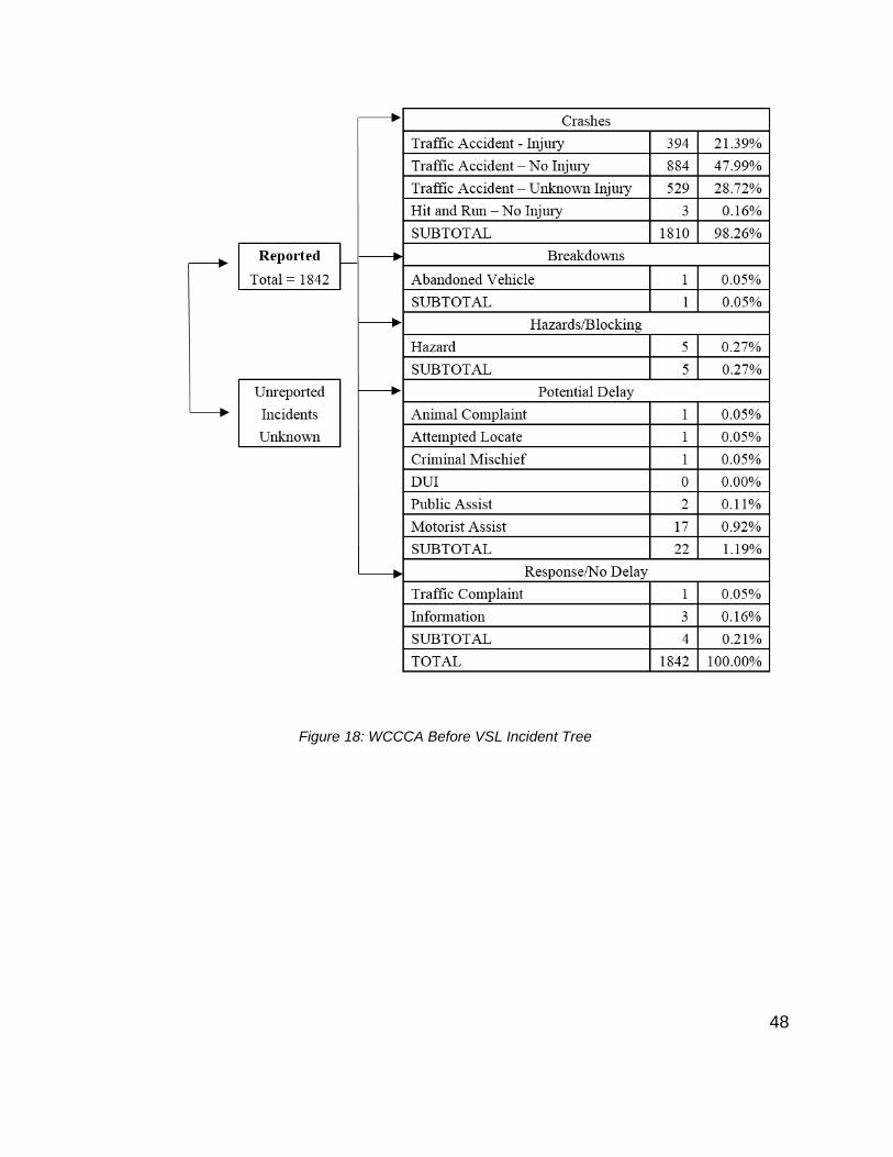
before and after the system’s activation.

48

Figure 18: WCCCA Before VSL Incident Tree

49

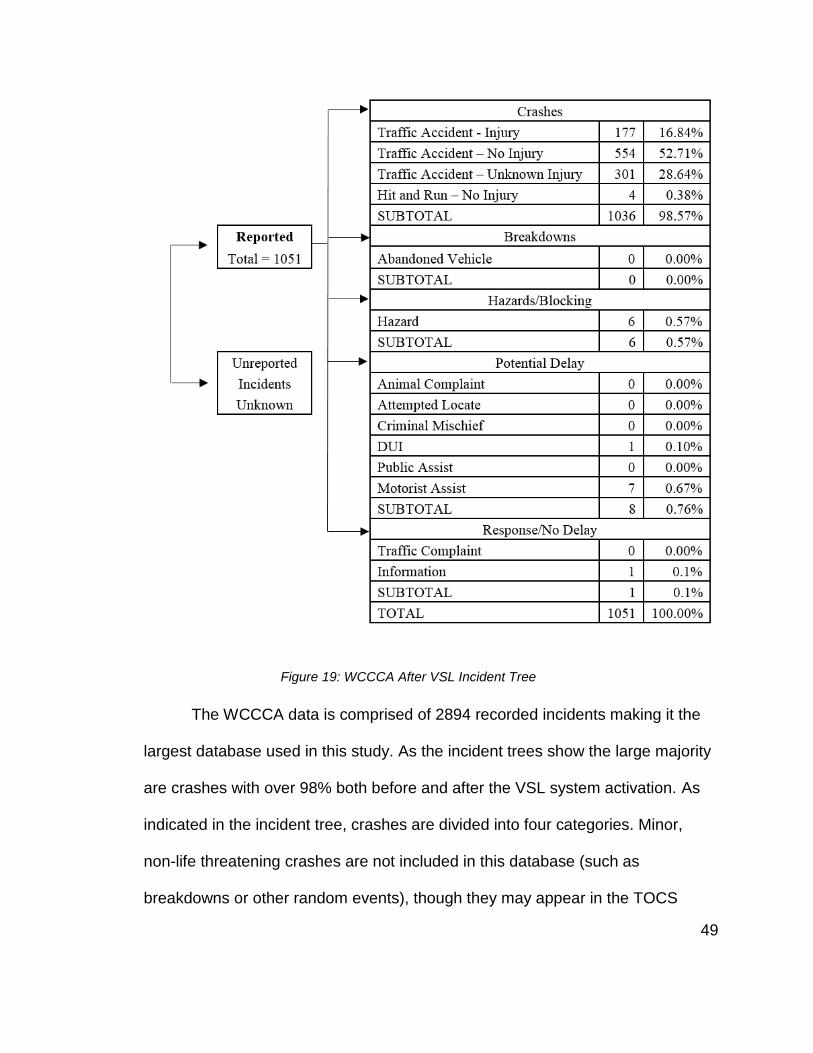
The WCCCA data is comprised of 2894 recorded incidents making it the

largest database used in this study. As the incident trees show the large majority

are crashes with over 98% both before and after the VSL system activation. As

indicated in the incident tree, crashes are divided into four categories. Minor,

non-life threatening crashes are not included in this database (such as

breakdowns or other random events), though they may appear in the TOCS

Figure 19: WCCCA After VSL Incident Tree

50

database described in section 4.2.3. For the purposes of this study all of the data

not in the crash category was eliminated.

4.2.3 Transportation Operation Center Data

Data from all reported incidents along OR 217 that initiate a response from

ODOT are available from the agency’s Transportation Operation Center System

(TOCS) database. These incidents include, but are not limited to, crashes,

breakdowns, stalls, maintenance, and construction. This database contains data

regarding the type, time, duration and location of each incident. It should be

noted that the TOCS database does not include all OR 217 incidents, as some

are responded to by other agencies, some are not reported, and some occur

while the traffic management center is not staffed. The data provided for this

study was limited to only include crashes and portions of the data do not include

all of the associated information, such as time of day. With only 829 crashes in

the database, 510 from before, the data is limited and statistical conclusions

harder to extract. However, this data source is also extremely up to date allowing

for a longer after period in the analysis.

4.2.4 Transportation Data Section Data

The Transportation Data Section (TDS) database is the official statewide

crash reporting system. ODOT’s statewide reported crash database stores

information pertaining to any reported crash involving a fatality, injury and/or

damages in excess of $1,500. This database contains extensive amounts of data

for each crash, including time, location, type and severity. ODOT’s annual state

51

highway crash rate tables combine this reported crash data with vehicle miles

traveled (VMT) data to compute crash rates for each highway covered by the

agency. Because the database is so extensive and detailed it has a long lag time

while details of each crash are reported, evaluated, and compiled. For this study,

the complete database with finalized data is available from July 2011 to

December 2014. This provides a full three years of before data but only 5 months

of after VSL implementation data. This data contains a total of 1301 crashes with

over 1100 being from before the VSL system was implemented.

Preliminary data for the year of 2015 is available but cannot be fully

utilized due to incompleteness, as more crashes could be reported to the DOT,

and it does not contain Property Damage Only (PDO) crashes. Nevertheless the

additional 149 crashes in the preliminary 2015 data can still be used, provided

analysis does not include PDO crashes and understands the likelihood of the

newer data underreporting crashes. This data source provides the best

information regarding the overall crash rate of rear end crashes, a particular

focus of the OR 217 VSL system. Future research should be done in the future

that can incorporate TDS crash data through July 2017 for the full three year

after period.

4.2.5 Summary of Crash Databases

The WCCCA and TOCS databases both provide up to date crash

information and potentially offer the ability to more quickly determine safety

impacts from the system. However, the low data resolution does not allow for

52

detailed analysis of crash types, time of day, or even fine-tuned locations. The

TDS data by contrast offers extremely high resolution but does a long lag time

making a thorough determination of the VSL impacts difficult at present. The

incomplete analysis for 2015 increases the TDS value significantly but limits its

application to only injury crashes. WCCCA is treated as the principal data source

in this study, with TOCS as a supplementary source, and TDS serving to

illuminate more targeted information such as rear end crashes.

All three data sources offer different data period lengths, through WCCCA

and TOCS are virtually identical. All of the data sources have full and complete

before data for three years. TDS only provides complete data for 5 months after

the installation, with another twelve available in a more limited function. WCCCA

and TOCS both have around twenty-one months of after data, over half of the

traditional thirty six months. The relative timelines are indicated in Figure 20. The

raw crashes are shown by month and datasource for both before and after the

VSL implementation in Figure 21.

Figure 20: Timeline of Data Availability

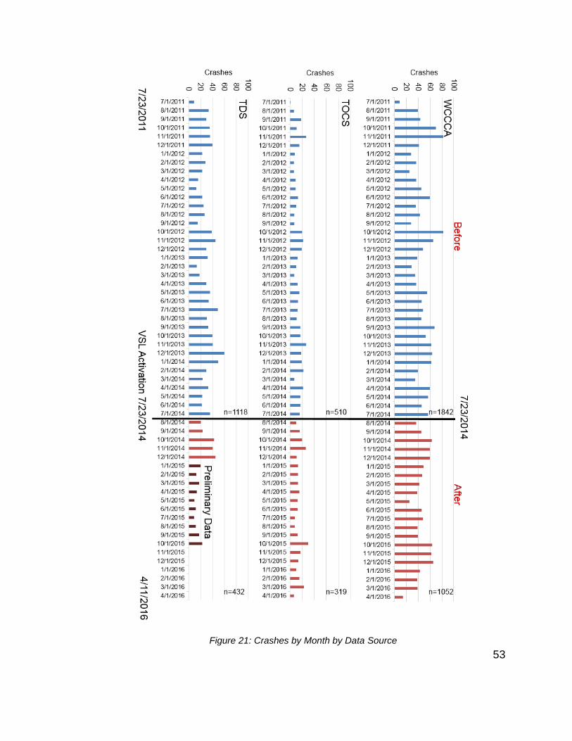
53

Figure 21: Crashes by Month by Data Source

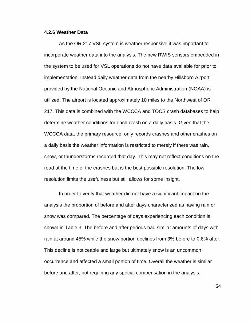
54

4.2.6 Weather Data

As the OR 217 VSL system is weather responsive it was important to

incorporate weather data into the analysis. The new RWIS sensors embedded in

the system to be used for VSL operations do not have data available for prior to

implementation. Instead daily weather data from the nearby Hillsboro Airport

provided by the National Oceanic and Atmospheric Administration (NOAA) is

utilized. The airport is located approximately 10 miles to the Northwest of OR

217. This data is combined with the WCCCA and TOCS crash databases to help

determine weather conditions for each crash on a daily basis. Given that the

WCCCA data, the primary resource, only records crashes and other crashes on

a daily basis the weather information is restricted to merely if there was rain,

snow, or thunderstorms recorded that day. This may not reflect conditions on the

road at the time of the crashes but is the best possible resolution. The low

resolution limits the usefulness but still allows for some insight.

In order to verify that weather did not have a significant impact on the

analysis the proportion of before and after days characterized as having rain or

snow was compared. The percentage of days experiencing each condition is

shown in Table 3. The before and after periods had similar amounts of days with

rain at around 45% while the snow portion declines from 3% before to 0.6% after.

This decline is noticeable and large but ultimately snow is an uncommon

occurrence and affected a small portion of time. Overall the weather is similar

before and after, not requiring any special compensation in the analysis.

55

Table 2: Percentage of All Days by Weather Type

Conditions Before After

No. of Days Percent No. of Days Percent

Clear 575 52.4% 345 54.9%

Rain 489 44.5% 280 44.5%

Snow 34 3.1% 4 0.6%

Total 1098 100% 629 100%

4.3 Evaluation Framework

The data sources outlined above are all utilized as inputs to the two

studies made. This information regarding crashes, traffic volumes, and weather is

used in evaluating OR 217 in both a Naïve Before-After study and Empirical

Bayes study. The specific use of each data source in Naïve Before-After and

Empirical Bayes Analysis is explained in methodology sections.

56

5.0 Naïve Before-After Study

The first portion of analysis for OR 217 used in this study is a Naïve

Before-After analysis. This utilizes crash data for prior to and after the installation

of the system. It uses simple statistical procedures to make predict crash rates

for comparison with recorded ones. Because of its ease of use it is a good

measure for quick updates, suiting some of the data sources. The methodology

behind the analysis is explained in Section 5.1.

5.1 Methodology

The Naïve Before After analysis relies on using crash data prior to the

system implementation to predict the number of crashes expected in the after

period should the VSL system have not been activated. The ideal situation is to

use the same amount of data for both before and after, with three years being the

established typical value. Because of the recent installation of the system a full

three years of data is not available for the after period. The methodology can

accommodate this time disparity through use of a correction factor, correlating

the length of before and after time and their respective crash counts.

A known issue with this methodology is that it holds all other factors as

constant, notably traffic volumes. The correction factor for the traffic functions

similarly to the study time period function by relating the number of crashes prior

to the crash with the traffic volumes prior and essentially creating a crash rate.

The correction does the same with after crashes and forms a ratio between the

rates to be applied to the before crash counts to create the after crash

57

predictions. This single traffic rate has an outsize impact on the overall after

crash prediction, and thus overall reduction, making it essential that traffic

volumes for both before and after are as accurate and representative of the

corridor as possible. Traffic volumes for the before and after periods do not

require a standard format, only that they be the same measurement for a fair

comparison.

As this method requires prediction of how many crashes would have

occurred the estimate is only the center part of a possible range of values. The

data also requires a large amount of before data to make accurate predictions

that are able to observe small impacts. All of the predictions made are shown

with error bars representing the possible range of prediction, though changes are

estimated from the center. The statistical viability of predictions is addressed in

Section 5.5.

5.1.1 Traffic Volumes

Multiple sources of traffic data provide competing information about

number of vehicles utilizing OR 217 before and after implementation. ODOT

produces an annual report with traffic volumes for all highways in the state, and

this document is considered to be the official traffic information. Because the

traffic data is produced in an annual January to December format it doesn’t allow

for easy comparison given the July system activation. In addition, the data

collectors along OR 217 were not recording data during the construction phase of

the project. The official figures are shown below in Figure 22. The official data is

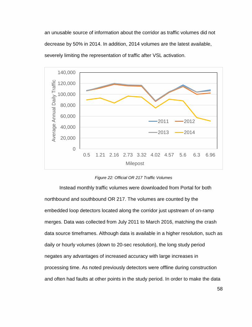
58

an unusable source of information about the corridor as traffic volumes did not

decrease by 50% in 2014. In addition, 2014 volumes are the latest available,

severely limiting the representation of traffic after VSL activation.

Figure 22: Official OR 217 Traffic Volumes

Instead monthly traffic volumes were downloaded from Portal for both

northbound and southbound OR 217. The volumes are counted by the

embedded loop detectors located along the corridor just upstream of on-ramp

merges. Data was collected from July 2011 to March 2016, matching the crash

data source timeframes. Although data is available in a higher resolution, such as

daily or hourly volumes (down to 20-sec resolution), the long study period

negates any advantages of increased accuracy with large increases in

processing time. As noted previously detectors were offline during construction

and often had faults at other points in the study period. In order to make the data

0

20,000

40,000

60,000

80,000

100,000

120,000

140,000

0.5 1.21 2.16 2.73 3.32 4.02 4.57 5.6 6.3 6.96

Ave

rage

An

nu

al D

aily

Tra

ffic

Milepost

2011 2012

2013 2014

59

acceptable it is sanitized, removing any extraneous data points. Values that vary

significantly from the long term trends, typically by a factor of 2 or more, are

eliminated from the data. To ensure that traffic volumes were consistent in

capturing the same traffic before and after installation, detectors that existed only

before or after the systems implementation were eliminated. The northbound and

southbound mainline traffic volumes are shown in Figure 23 and 24.

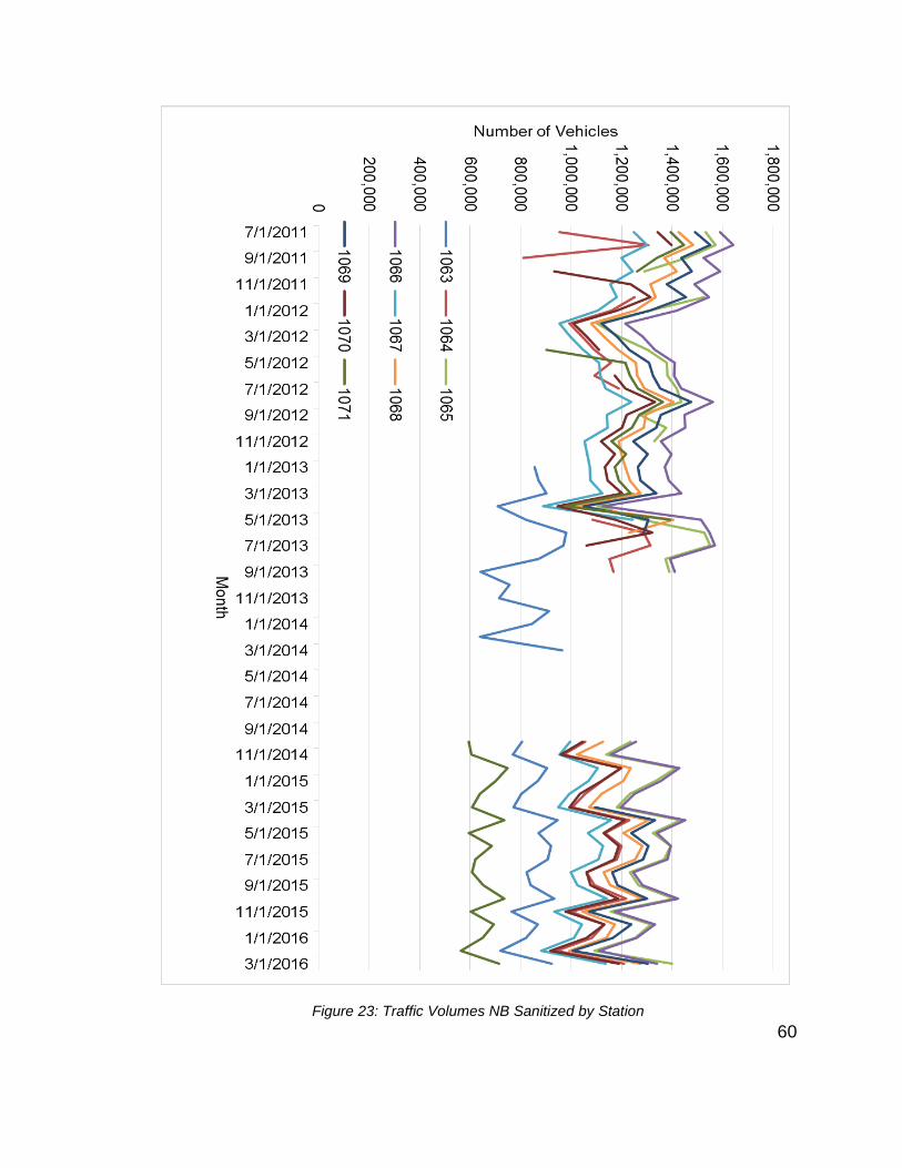
60

Figure 23: Traffic Volumes NB Sanitized by Station

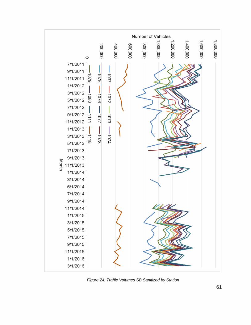
61

Figure 24: Traffic Volumes SB Sanitized by Station

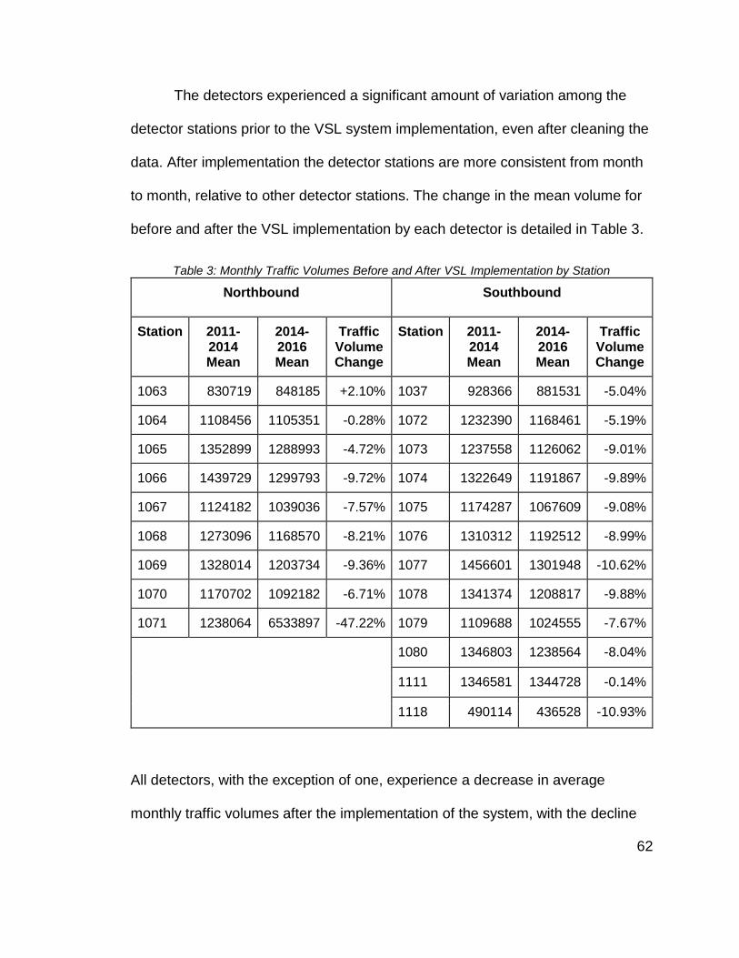
62

The detectors experienced a significant amount of variation among the

detector stations prior to the VSL system implementation, even after cleaning the

data. After implementation the detector stations are more consistent from month

to month, relative to other detector stations. The change in the mean volume for

before and after the VSL implementation by each detector is detailed in Table 3.

Table 3: Monthly Traffic Volumes Before and After VSL Implementation by Station

Northbound Southbound

Station 2011-2014 Mean

2014-2016 Mean

Traffic Volume Change

Station 2011-2014 Mean

2014-2016 Mean

Traffic Volume Change

1063 830719 848185 +2.10% 1037 928366 881531 -5.04%

1064 1108456 1105351 -0.28% 1072 1232390 1168461 -5.19%

1065 1352899 1288993 -4.72% 1073 1237558 1126062 -9.01%

1066 1439729 1299793 -9.72% 1074 1322649 1191867 -9.89%

1067 1124182 1039036 -7.57% 1075 1174287 1067609 -9.08%

1068 1273096 1168570 -8.21% 1076 1310312 1192512 -8.99%

1069 1328014 1203734 -9.36% 1077 1456601 1301948 -10.62%

1070 1170702 1092182 -6.71% 1078 1341374 1208817 -9.88%

1071 1238064 6533897 -47.22% 1079 1109688 1024555 -7.67%

1080 1346803 1238564 -8.04%

1111 1346581 1344728 -0.14%

1118 490114 436528 -10.93%

All detectors, with the exception of one, experience a decrease in average

monthly traffic volumes after the implementation of the system, with the decline

63

typically 8-10% from the prior to implementation volumes. This seems

counterintuitive with the previous growth rate shown by traffic on the corridor,

however the data shows the trend clearly. For the purposes of this portion of the

study, the data is used and analysis results are compared to if traffic volumes

had no changed.

To develop reliable before and after traffic volumes several of the detector

stations are excluded from the analysis. The northbound end detectors both are

missing data for one of the lanes, giving a heavily reduced volume. The

southbound data includes two sets of detectors at the northern end of the

corridor that only capture on ramp volumes but do not include the traffic coming

from eastbound OR 26. After exclusion, the monthly traffic volumes for all of the

detectors is averaged for northbound and southbound. The average northbound

and southbound values are shown in Figure 25 and Figure 26.

64

Figure 25: SB Average Monthly Traffic Volumes

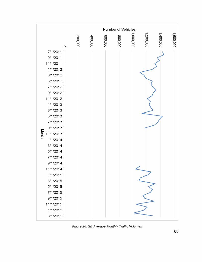
65

Figure 26: SB Average Monthly Traffic Volumes

66

Both sets of data follow similar trends from month to month and exhibit

consistent seasonal variations. The southbound direction experiences a small

amount more traffic with volumes typically 1-2% higher. Using this information,

the average monthly traffic volumes for before and after VSL implementation

were determined for each direction, as well as the corridor in total. Both

directions showed traffic volume declines consistent with those measured by

individual loop detector stations. Verification that the monthly traffic volumes are

reliable was done by dividing the volume by 30 and comparing against the official

ODOT Average Annual Daily Traffic (AADT) volumes.

5.1.2 Crash Data

All of the crash databases required being divided into before and after

periods. The raw data was filtered into crashes by years starting on July 22, and

ending on July 21 in line with the VSL activation date. This data was further

processed into a variety of categories such as by type of crash, crash milepost,

or weather conditions. This allows for analysis of the VSL impact on more

specific elements of crashes. For example, filtering the TDS data allows for

understanding the VSL impacts on rear end crashes, a target of the VSL system.

Naïve Before-After analysis was then conducted on each data sources and the

subsets of data within them.

5.2 WCCCA Data

The WCCCA data serves as the primary database for this project and the

main analysis target. As the data contains a limited amount of information,

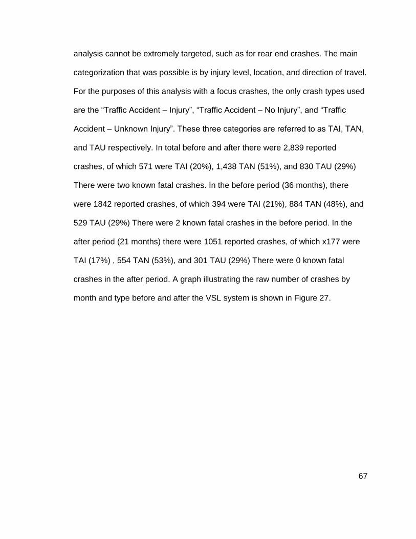
67

analysis cannot be extremely targeted, such as for rear end crashes. The main

categorization that was possible is by injury level, location, and direction of travel.

For the purposes of this analysis with a focus crashes, the only crash types used

are the “Traffic Accident – Injury”, “Traffic Accident – No Injury”, and “Traffic

Accident – Unknown Injury”. These three categories are referred to as TAI, TAN,

and TAU respectively. In total before and after there were 2,839 reported

crashes, of which 571 were TAI (20%), 1,438 TAN (51%), and 830 TAU (29%)

There were two known fatal crashes. In the before period (36 months), there

were 1842 reported crashes, of which 394 were TAI (21%), 884 TAN (48%), and

529 TAU (29%) There were 2 known fatal crashes in the before period. In the

after period (21 months) there were 1051 reported crashes, of which x177 were

TAI (17%) , 554 TAN (53%), and 301 TAU (29%) There were 0 known fatal

crashes in the after period. A graph illustrating the raw number of crashes by

month and type before and after the VSL system is shown in Figure 27.

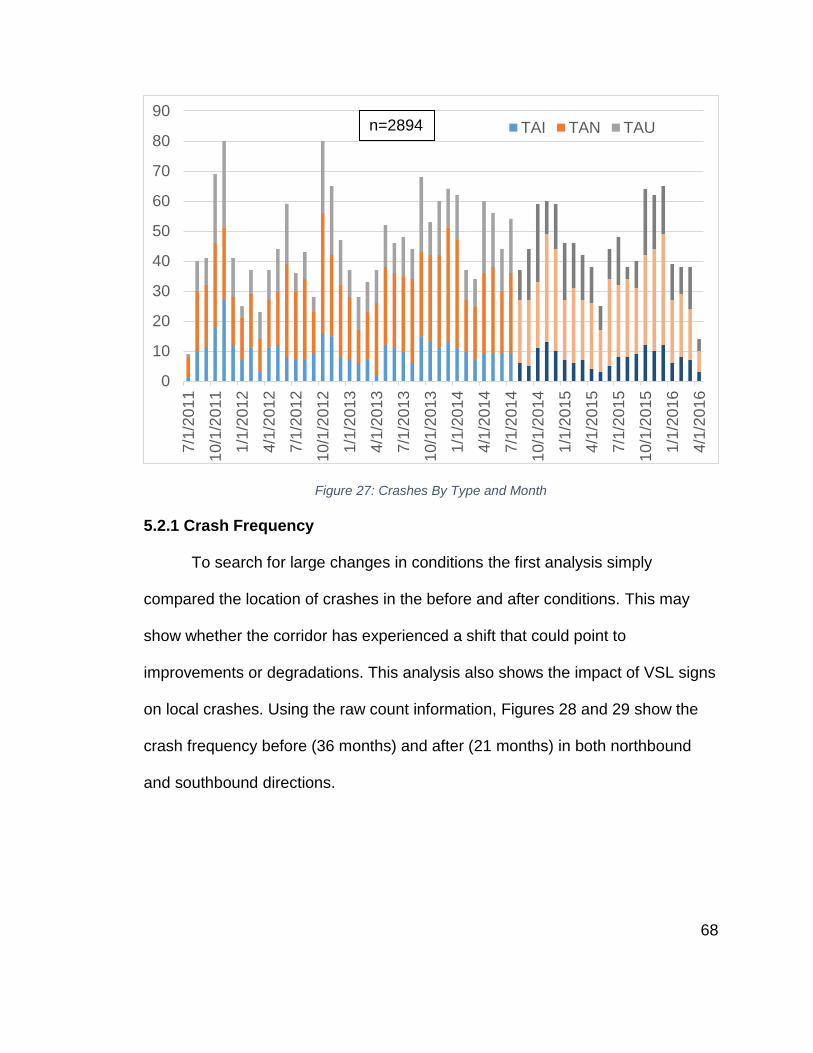
68

Figure 27: Crashes By Type and Month

5.2.1 Crash Frequency

To search for large changes in conditions the first analysis simply

compared the location of crashes in the before and after conditions. This may

show whether the corridor has experienced a shift that could point to

improvements or degradations. This analysis also shows the impact of VSL signs

on local crashes. Using the raw count information, Figures 28 and 29 show the

crash frequency before (36 months) and after (21 months) in both northbound

and southbound directions.

0

10

20

30

40

50

60

70

80

90

7/1

/20

11

10/1

/20

11

1/1

/20

12

4/1

/20

12

7/1

/20

12

10/1

/20

12

1/1

/20

13

4/1

/20

13

7/1

/20

13

10/1

/20

13

1/1

/20

14

4/1

/20

14

7/1

/20

14

10/1

/20

14

1/1

/20

15

4/1

/20

15

7/1

/20

15

10/1

/20

15

1/1

/20

16

4/1

/20

16

TAI TAN TAUn=2894

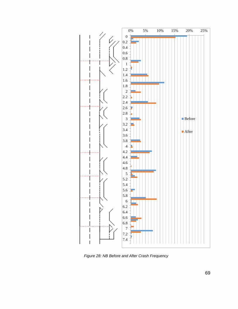
69

Figure 28: NB Before and After Crash Frequency

0% 5% 10% 15% 20% 25%

0

0.2

0.4

0.6

0.8

1

1.2

1.4

1.6

1.8

2

2.2

2.4

2.6

2.8

3

3.2

3.4

3.6

3.8

4

4.2

4.4

4.6

4.8

5

5.2

5.4

5.6

5.8

6

6.2

6.4

6.6

6.8

7

7.2

7.4

Before

After

70

Figure 29: SB Before and After Crash Frequency

0% 5% 10% 15% 20% 25%

0

0.2

0.4

0.6

0.8

1

1.2

1.4

1.6

1.8

2

2.2

2.4

2.6

2.8

3

3.2

3.4

3.6

3.8

4

4.2

4.4

4.6

4.8

5

5.2

5.4

5.6

5.8

6

6.2

6.4

6.6

6.8

7

7.2

7.4

Before

After

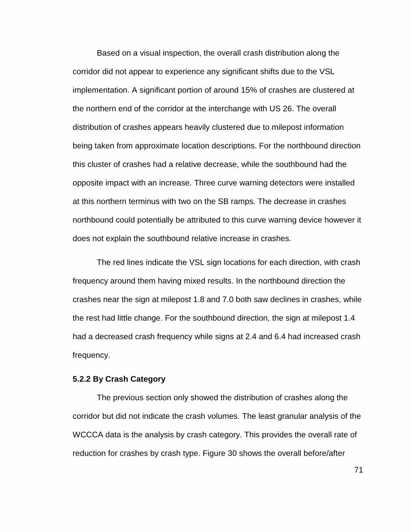
71

Based on a visual inspection, the overall crash distribution along the

corridor did not appear to experience any significant shifts due to the VSL

implementation. A significant portion of around 15% of crashes are clustered at

the northern end of the corridor at the interchange with US 26. The overall

distribution of crashes appears heavily clustered due to milepost information

being taken from approximate location descriptions. For the northbound direction

this cluster of crashes had a relative decrease, while the southbound had the

opposite impact with an increase. Three curve warning detectors were installed

at this northern terminus with two on the SB ramps. The decrease in crashes

northbound could potentially be attributed to this curve warning device however it

does not explain the southbound relative increase in crashes.

The red lines indicate the VSL sign locations for each direction, with crash

frequency around them having mixed results. In the northbound direction the

crashes near the sign at milepost 1.8 and 7.0 both saw declines in crashes, while

the rest had little change. For the southbound direction, the sign at milepost 1.4

had a decreased crash frequency while signs at 2.4 and 6.4 had increased crash

frequency.

5.2.2 By Crash Category

The previous section only showed the distribution of crashes along the

corridor but did not indicate the crash volumes. The least granular analysis of the

WCCCA data is the analysis by crash category. This provides the overall rate of

reduction for crashes by crash type. Figure 30 shows the overall before/after

72

crash percent change by crash type as well as for the corridor overall (left hand

y-axis). The whisker bars show plus/minus one standard deviation in each

direction. The values indicate the difference between the recorded number of

crashes and what would be expected given the before conditions. Adjustments to

the length of study period and the traffic volumes were made, as explained in the

Methodology Section 5.1. The numbers of before and after crashes are also

shown (right hand y-axis).

Figure 30: Overall Naïve Before After Analysis Percent Change by Crash Type

According to the Naïve Before After analysis, the Injury crashes showed a

decrease of 8% after the VSL implementation. The overall corridor saw an

increase of 4% in crashes after the VSL system was activated. As the figure

-2000

-1500

-1000

-500

0

500

1000

1500

2000

- 20 %

- 15 %

- 10 %

- 05 %

+ 0 %

+ 05 %

+ 10 %

+ 15 %

+ 20 %

TAI TAN TAU Overall

Nu

mb

er

of C

rashe

s

Ch

an

ge

in

Cra

she

s

Change in Crashes

Number of Before Crashes

Number of After Crashes

n=2894

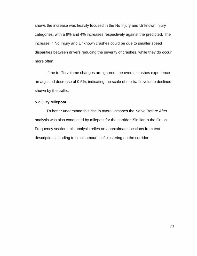
73

shows the increase was heavily focused in the No Injury and Unknown Injury

categories, with a 9% and 4% increases respectively against the predicted. The

increase in No Injury and Unknown crashes could be due to smaller speed

disparities between drivers reducing the severity of crashes, while they do occur

more often.

If the traffic volume changes are ignored, the overall crashes experience

an adjusted decrease of 0.5%, indicating the scale of the traffic volume declines

shown by the traffic.

5.2.3 By Milepost

To better understand this rise in overall crashes the Naïve Before After

analysis was also conducted by milepost for the corridor. Similar to the Crash

Frequency section, this analysis relies on approximate locations from text

descriptions, leading to small amounts of clustering on the corridor.

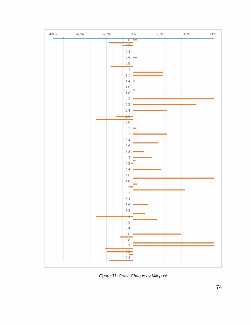
74

Figure 31: Crash Change by Milepost

-60% -40% -20% 0% 20% 40% 60%

0

0.2

0.4

0.6

0.8

1

1.2

1.4

1.6

1.8

2

2.2

2.4

2.6

2.8

3

3.2

3.4

3.6

3.8

4

4.2

4.4

4.6

4.8

5

5.2

5.4

5.6

5.8

6

6.2

6.4

6.6

6.8

7

7.2

7.4

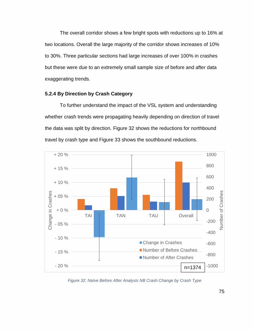
75

The overall corridor shows a few bright spots with reductions up to 16% at

two locations. Overall the large majority of the corridor shows increases of 10%

to 30%. Three particular sections had large increases of over 100% in crashes

but these were due to an extremely small sample size of before and after data

exaggerating trends.

5.2.4 By Direction by Crash Category

To further understand the impact of the VSL system and understanding

whether crash trends were propagating heavily depending on direction of travel

the data was split by direction. Figure 32 shows the reductions for northbound

travel by crash type and Figure 33 shows the southbound reductions.

Figure 32: Naïve Before After Analysis NB Crash Change by Crash Type

-1000

-800

-600

-400

-200

0

200

400

600

800

1000

- 20 %

- 15 %

- 10 %

- 05 %

+ 0 %

+ 05 %

+ 10 %

+ 15 %

+ 20 %

TAI TAN TAU Overall

Nu

mb

er

of C

rashe

s

Ch

an

ge

in

Cra

she

s

Change in Crashes



n=1374

76

Figure 33: Naïve Before Analysis SB Crash Change by Crash Type

The by direction information shows that the increase in Injury crashes has

been almost entirely due to the southbound traffic. The northbound direction has

experienced an increase of only 1% for injury crashes. However the other crash

type’s crashes increase more notably in the northbound direction, rising by 22%

for No Injury and 14% for Unknown Injury crashes. This disparity could be due to

better harmonization in traffic volumes resulting in lower speed differentials

reducing the number of crashes. It could also be related to the larger number of

VSL signs in the southbound direction causing distractions.

-1000

-800

-600

-400

-200

0

200

400

600

800

1000

- 20 %

- 15 %

- 10 %

- 05 %

+ 0 %

+ 05 %

+ 10 %

+ 15 %

+ 20 %

TAI TAN TAU Overall

Nu

mb

er

of C

rashe

s

Ch

an

ge

in

Cra

she

s

Change in Crashes



n=1465

77

5.2.5 By Direction by Milepost

To identify the problem spots in each direction the crashes were also

divided by mile post and direction of travel. Figure 34 shows the change in

crashes for northbound traffic and Figure 35 shows the same for southbound.

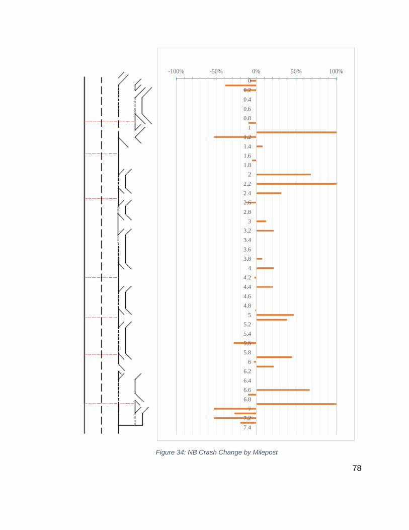
78

Figure 34: NB Crash Change by Milepost

-100% -50% 0% 50% 100%

0

0.2

0.4

0.6

0.8

1

1.2

1.4

1.6

1.8

2

2.2

2.4

2.6

2.8

3

3.2

3.4

3.6

3.8

4

4.2

4.4

4.6

4.8

5

5.2

5.4

5.6

5.8

6

6.2

6.4

6.6

6.8

7

7.2

7.4

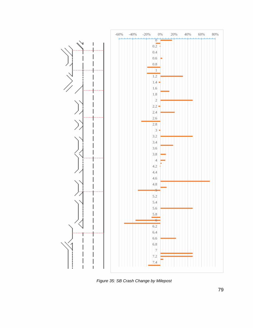
79

Figure 35: SB Crash Change by Milepost

-60% -40% -20% 0% 20% 40% 60% 80%

0

0.2

0.4

0.6

0.8

1

1.2

1.4

1.6

1.8

2

2.2

2.4

2.6

2.8

3

3.2

3.4

3.6

3.8

4

4.2

4.4

4.6

4.8

5

5.2

5.4

5.6

5.8

6

6.2

6.4

6.6

6.8

7

7.2

7.4

80

The by milepost analysis shows that the large increases in crashes at a

few locations shown in Section 5.2.3 are due to the northbound traffic. The

southbound traffic has a more consistent amount of smaller crash increases

along the corridor, typically around 15%.

5.2.6 Analysis by Weather

To determine the impact that weather conditions have had on the corridor,

the Naïve Before After analysis was completed using the recorded weather for

each day on which a crash occurred and was logged in the WCCCA database.

The weather information is simplistic and only notes if a weather event did occur

that day as crashes cannot be attributed to certain times of day to determine

more accurate roadway conditions. The relative frequencies of the weather for

the before and after periods are shown in Section 4.2.6.

81

Figure 36: Naive Before After Analysis Percent Change by Weather Condition

The results indicate that the crashes occurring on days with wet weather

experienced a decline of 8%. The snow conditions in the after period were less

often but more crashes occurring creating the appearance of a large increase.

The extremely large variability is indicative of the low frequency of this type of

crash both before and after the VSL system. Clear days showed a 4% increase

in crashes with the Naïve Before After analysis, showing that the system may be

performing best during adverse weather conditions.

5.2.7 Summary

The WCCCA data shows a large increase in crashes occurring around the

VSL installation. The overall Naïve Before After adjusted crash rate increased by

-600

-400

-200

0

200

400

600

800

1000

1200

- 60 %

- 40 %

- 20 %

+ 0 %

+ 20 %

+ 40 %

+ 60 %

+ 80 %

+ 100 %

+ 120 %

Clear Rain Snow

Nu

mb

er

of C

rashe

s

Ch

an

ge

in

Cra

she

s

Change in Crashes


Number of After Crashesn=2894

82

roughly 4% with No Injury crashes having a dramatic increase of 20%. The

smaller increase of only 2.7% for crashes resulting in an injury shows that the

more severe crashes are increasing a lower rate. The northbound traffic

experiences higher increases in crashes at peak places and a larger increase in

No Injury crashes but has almost no increase in Injury crashes. These results

contrast with the reported 13% decrease that the ODOT determined from the

WCCCA data. The ODOT research used the numbers for just one year before

and after, whereas this study used a much larger study period. In addition the

ODOT report utilized a simple comparison of the raw numbers not accounting for

the changes in traffic volumes, as this analysis does. If this Naïve Before After

Analysis ignores the traffic volume changes, the WCCCA data shows a .5%

decrease in crashes using the full study period data.

5.3 TOCS Data

The TOCS data provides an account of traffic crashes from a different

perspective. Whereas the WCCCA data is crowdsourced through public 911 calls

and subsequently verified by emergency responders, the TOCS data comes from

the highway operating agency’s traffic management center responding in real

time and notifying incident responders and the public of possible issues. This

database is also used in real time to manage incident response. The crash data

logged in this database is then more focused on incidents that the agency

believes impacts operations. As a result it likely does not capture the same

crashes as the 911 call data, but rather the more operationally important crashes.

83

In the TOCS database there were 510 crashes before, and 319 crashes after.

Figure 37 shows the change in crashes by month for before and after the VSL

system was activated. The overall crash distribution for the corridor from the raw

TOCS data is shown in Figure 38.

Figure 37: TOCS Recorded Crashes by Month

0 5 10 15 20 25 30

7/1/2011

10/1/2011

1/1/2012

4/1/2012

7/1/2012

10/1/2012

1/1/2013

4/1/2013

7/1/2013

10/1/2013

1/1/2014

4/1/2014

7/1/2014

10/1/2014

1/1/2015

4/1/2015

7/1/2015

10/1/2015

1/1/2016

4/1/2016

Crashes

Mo

nth

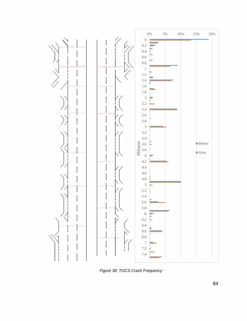
84

Figure 38: TOCS Crash Frequency

0% 5% 10% 15% 20%

0

0.2

0.4

0.6

0.8

1

1.2

1.4

1.6

1.8

2

2.2

2.4

2.6

2.8

3

3.2

3.4

3.6

3.8

4

4.2

4.4

4.6

4.8

5

5.2

5.4

5.6

5.8

6

6.2

6.4

6.6

6.8

7

7.2

7.4

Mil

epo

st Before

After

85

The corridor shows similar clustering to that of the WCCCA data indicating

similar underlying crash trends. The crash frequency declined at the northern

terminus of the corridor at the interchange with US 26. This may be attributable

to the curve warning detectors installed at the large loop ramps. A similar marked

decline in frequency occurs at the 1 mile post, between two VSL signs. Another

location at milepost 5.6 saw a significant increase in crashes as a percent of the

total. This location is not near a VSL sign and the increase is likely unassociated

with the system.

5.3.1 Crashes Over Time

Figure 37 showed the raw crash distribution by month over the before and

after period. The crashes showed a higher frequency in the year before the VSL

implementation with almost all months showing high crash counts. These

crashes could potentially be due to the construction associated with the VSL

system. After the system activation the crashes regained the more seasonal

nature of the previous years, but with higher counts per month. Immediately after

the system activations crashes spiked, however these month coincided with the

historically more crash prone fall months. This seasonal increase was repeated

the following year October of 2015 the most crash heavy month in the database.

5.3.2 Summary

When the Naïve Before After Analysis is applied to the TOCS data the end

results is an overall increase in crashes of 10%. This is higher than the WCCCA

data indicates. The data in the TOCS records is not for all hours of the day and

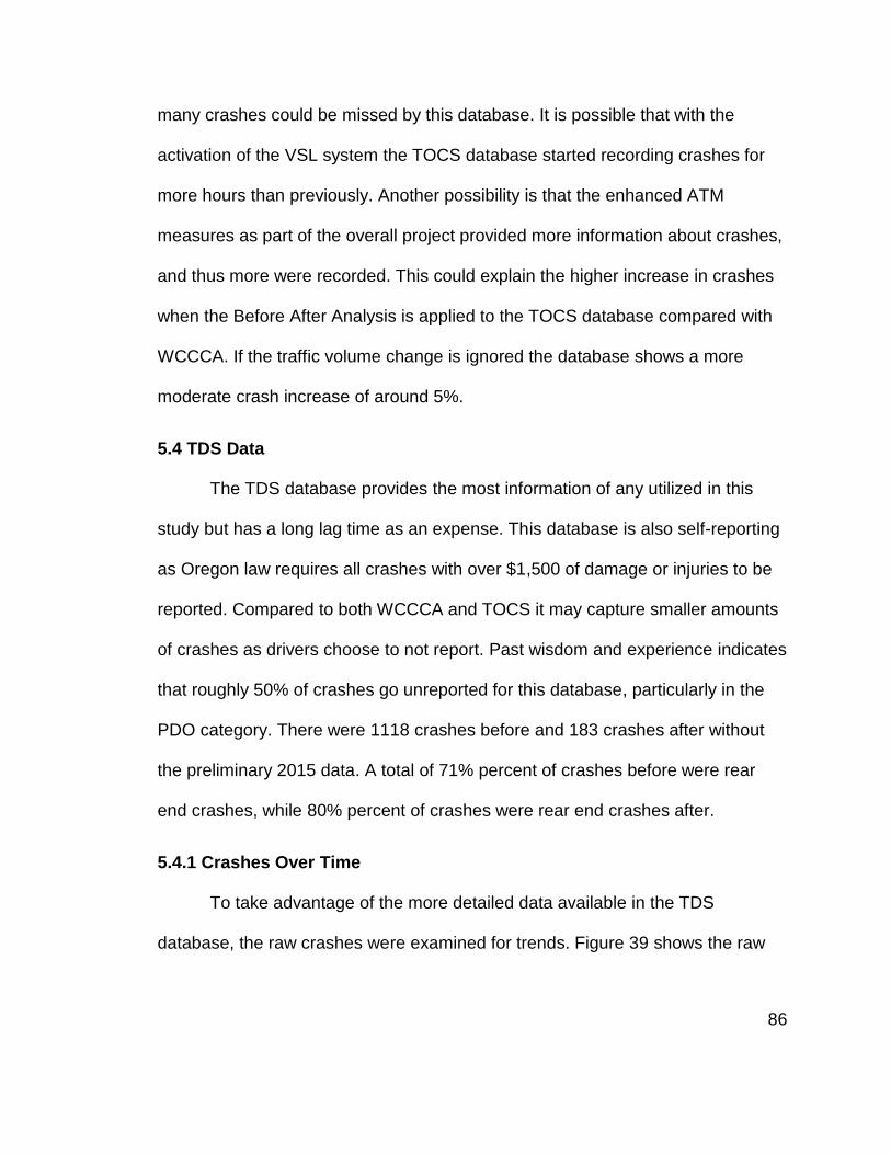
86

many crashes could be missed by this database. It is possible that with the

activation of the VSL system the TOCS database started recording crashes for

more hours than previously. Another possibility is that the enhanced ATM

measures as part of the overall project provided more information about crashes,

and thus more were recorded. This could explain the higher increase in crashes

when the Before After Analysis is applied to the TOCS database compared with

WCCCA. If the traffic volume change is ignored the database shows a more

moderate crash increase of around 5%.

5.4 TDS Data

The TDS database provides the most information of any utilized in this

study but has a long lag time as an expense. This database is also self-reporting

as Oregon law requires all crashes with over $1,500 of damage or injuries to be

reported. Compared to both WCCCA and TOCS it may capture smaller amounts

of crashes as drivers choose to not report. Past wisdom and experience indicates

that roughly 50% of crashes go unreported for this database, particularly in the

PDO category. There were 1118 crashes before and 183 crashes after without

the preliminary 2015 data. A total of 71% percent of crashes before were rear

end crashes, while 80% percent of crashes were rear end crashes after.

5.4.1 Crashes Over Time

To take advantage of the more detailed data available in the TDS

database, the raw crashes were examined for trends. Figure 39 shows the raw

87

crash volumes on a monthly basis by crash category. Other factors such as the

weather and lighting will be examined individually in subsequent sections.

Figure 39: Crashes in the TDS Database By Month and Type

0 20 40 60

7/1/2011

10/1/2011

1/1/2012

4/1/2012

7/1/2012

10/1/2012

1/1/2013

4/1/2013

7/1/2013

10/1/2013

1/1/2014

4/1/2014

7/1/2014

10/1/2014

1/1/2015

4/1/2015

7/1/2015

10/1/2015

Crashes

Mo

nth

FIX OTHER REAR SS-O TURN

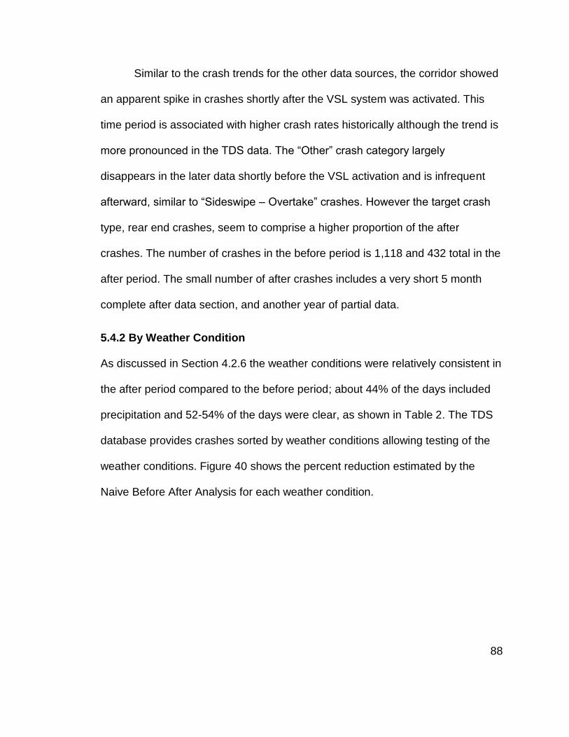
88

Similar to the crash trends for the other data sources, the corridor showed

an apparent spike in crashes shortly after the VSL system was activated. This

time period is associated with higher crash rates historically although the trend is

more pronounced in the TDS data. The “Other” crash category largely

disappears in the later data shortly before the VSL activation and is infrequent

afterward, similar to “Sideswipe – Overtake” crashes. However the target crash

type, rear end crashes, seem to comprise a higher proportion of the after

crashes. The number of crashes in the before period is 1,118 and 432 total in the

after period. The small number of after crashes includes a very short 5 month

complete after data section, and another year of partial data.

5.4.2 By Weather Condition

As discussed in Section 4.2.6 the weather conditions were relatively consistent in

the after period compared to the before period; about 44% of the days included

precipitation and 52-54% of the days were clear, as shown in Table 2. The TDS

database provides crashes sorted by weather conditions allowing testing of the

weather conditions. Figure 40 shows the percent reduction estimated by the

Naive Before After Analysis for each weather condition.

89

Figure 40: Naïve Before After Analysis Percent Change by Weather Condition

During wet surface conditions crashes were noted as increasing by

approximately 5%. Other surface conditions improved, through dry surface

conditions only improved by 0.54%. Less snow was recorded in the after

condition potentially explaining the reduction in crashes. The “Unknown”

condition also declined, however this could be due to better records of weather or

crashes. Given that Section 3.3 showed dry and wet surface conditions are

associated with over 95% of all crashes, the increase for wet conditions and

small reduction in dry conditions is concerning.

-1000

-800

-600

-400

-200

0

200

400

600

800

1000

- 30 %

- 20 %

- 10 %

+ 0 %

+ 10 %

+ 20 %

+ 30 %

DRY WET ICE SNO UNK

Nu

mb

er

of C

rashe

s

Ch

an

ge

in

Cra

she

s

Change in Crashes


Number of After Crashes n=1301

90

5.4.3 By Lighting Condition

The other data sources provide limited information about time of day that

crashes occur making the TDS lighting condition information valuable. To

illustrate the lighting conditions commonly occurring with the crashes see Figure

41 and Figure 42. The figure shows that the percentage of crashes occurring

during dusk increased while the percentage during the day decreased markedly.

Figure 41: Crashes by Lighting Condition Before VSL Implementation

Figure 42: Crashes by Lighting Condition After VSL Implementation

To test the casual observations the Naïve Before After methodology was applied

by lighting condition and results are shown below in Figure 43. Note that the

DLIT category means Dark, Lighted and that most of OR 217 is well lit.

53, 5%20, 2%

807, 72%

195, 17%

3, 0%

40, 4%

DARK DAWN DAY

DLIT UNK DUSK

16, 9%

4, 2%

113, 62%

28, 15%

0, 0%

22, 12%

DARK DAWN DAY

DLIT UNK DUSK

n=1118 n=332

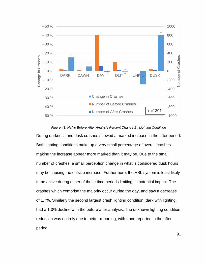
91

Figure 43: Naïve Before After Analysis Percent Change By Lighting Condition

During darkness and dusk crashes showed a marked increase in the after period.

Both lighting conditions make up a very small percentage of overall crashes

making the increase appear more marked than it may be. Due to the small

number of crashes, a small perception change in what is considered dusk hours

may be causing the outsize increase. Furthermore, the VSL system is least likely

to be active during either of these time periods limiting its potential impact. The

crashes which comprise the majority occur during the day, and saw a decrease

of 1.7%. Similarly the second largest crash lighting condition, dark with lighting,

had a 1.3% decline with the before after analysis. The unknown lighting condition

reduction was entirely due to better reporting, with none reported in the after

period.

-1000

-800

-600

-400

-200

0

200

400

600

800

1000

- 50 %

- 40 %

- 30 %

- 20 %

- 10 %

+ 0 %

+ 10 %

+ 20 %

+ 30 %

+ 40 %

+ 50 %

DARK DAWN DAY DLIT UNK DUSK

Nu

mb

er

of C

rashe

s

Ch

an

ge

in

Cra

she

s

Change in Crashes


Number of After Crashes n=1301

92

5.4.4 By Crash Type

A focus of the VSL system was to reduce the number of rear end

crashes occurring on OR 217. The TDS database categorizes each crash by its

type allowing for comparison using the Naïve Before After methodology. In both

before and after conditions, rear end is the largest category with fixed object,

sideswipe – overtake, and turning crashes contributing the bulk of the remainder.

The reduction in crashes can be seen in Figure 44.

Figure 44: Naïve Before After Analysis Percent Change by Crash Type

The target crashes, rear end, have increased in the after condition

according to the Naïve Before After analysis. The other main crash type

categories all experience reductions with the new VSL system. The “Other” crash

-300

-100

100

300

500

700

- 30 %

- 10 %

+ 10 %

+ 30 %

+ 50 %

+ 70 %

Nu

mb

er

of C

rashe

s

Ch

an

ge

in

Cra

she

s

Change in Crashes



n=1301

93

type experiences a dramatic increase however this is due to an extremely small

sample size. Similarly, the crash types showing a 15% reduction are all due to

having no recorded crashes of that type in the after condition making the Naïve

Before After Analysis not applicable.

5.4.5 By Injury Class

The TDS data provides information on the class of injury recorded. Oregon

follows a standard five class system with Fatal, Injury A (incapacitating injury),

Injury B (visible injury), Injury C (complaint of pain or minor), or Property Damage

Only. The most severe category, fatal, has a small sample size and is combined

with Injury A to increase the statistical reliability. Figure 45 shows the percent

reduction by injury class.

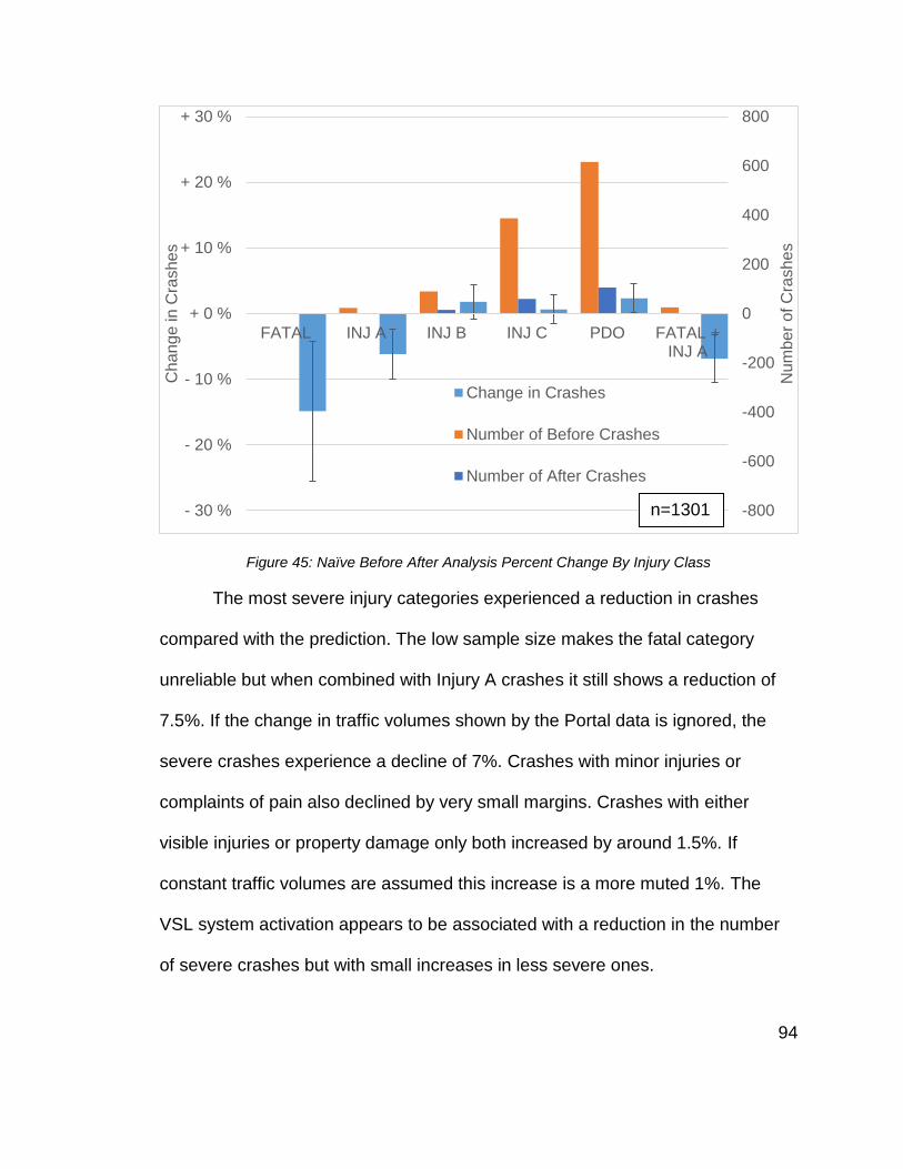
94

Figure 45: Naïve Before After Analysis Percent Change By Injury Class

The most severe injury categories experienced a reduction in crashes

compared with the prediction. The low sample size makes the fatal category

unreliable but when combined with Injury A crashes it still shows a reduction of

7.5%. If the change in traffic volumes shown by the Portal data is ignored, the

severe crashes experience a decline of 7%. Crashes with minor injuries or

complaints of pain also declined by very small margins. Crashes with either

visible injuries or property damage only both increased by around 1.5%. If

constant traffic volumes are assumed this increase is a more muted 1%. The

VSL system activation appears to be associated with a reduction in the number

of severe crashes but with small increases in less severe ones.

-800

-600

-400

-200

0

200

400

600

800

- 30 %

- 20 %

- 10 %

+ 0 %

+ 10 %

+ 20 %

+ 30 %

FATAL INJ A INJ B INJ C PDO FATAL +INJ A

Nu

mb

er

of C

rashe

s

Ch

an

ge

in

Cra

she

s

Change in Crashes



n=1301

95

5.4.6 Summary

The Naïve Before After Analysis of the TDS data shows an overall 3%

increase in crashes on the corridor. When conditions of the crashes are looked at

in more detail, analysis shows that crashes are reduced during daylight hours,

and when it is dry. However, an increase in crashes occurs during wet

conditions, already a significant contributor to the crashes on OR 217. One of the

targets of the VSL system, rear end crashes, increased by 2% during the after

condition. Severe crashes decline significantly while less severe crashes

increase by a more modest amount. The results show a mixture of good and bad

for the corridor. The short after period for this analysis of only 5 months causes

some reliability problems. The after data does not capture all seasons but covers

the notably tricky fall conditions, potentially skewing the results. If the traffic

volumes are not adjusted and assumed identical, the crash rate increases by a

more modest 1.5% according to the Naïve Before After methodology.

5.4.7 Updated Incomplete Data

To try to compensate for the small quantity of after data from the TDS data

source, additional analysis was conducted on some preliminary, incomplete data

from the year 2015. This new data does not include any property damage only

crashes, and may not include all of the other crashes as well. The state of

Oregon has a long reporting period and some crashes may have not yet been

processed into the database at the time it was received. Analysis was then

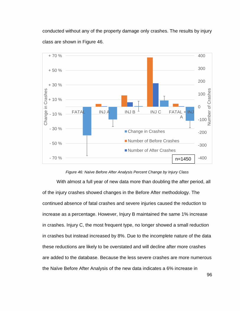
96

conducted without any of the property damage only crashes. The results by injury

class are shown in Figure 46.

Figure 46: Naïve Before After Analysis Percent Change by Injury Class

With almost a full year of new data more than doubling the after period, all

of the injury crashes showed changes in the Before After methodology. The

continued absence of fatal crashes and severe injuries caused the reduction to

increase as a percentage. However, Injury B maintained the same 1% increase

in crashes. Injury C, the most frequent type, no longer showed a small reduction

in crashes but instead increased by 8%. Due to the incomplete nature of the data

these reductions are likely to be overstated and will decline after more crashes

are added to the database. Because the less severe crashes are more numerous

the Naïve Before After Analysis of the new data indicates a 6% increase in

-400

-300

-200

-100

0

100

200

300

400

- 70 %

- 50 %

- 30 %

- 10 %

+ 10 %

+ 30 %

+ 50 %

+ 70 %

FATAL INJ A INJ B INJ C FATAL + INJA

Nu

mb

er

of C

rashe

s

Ch

an

ge

in

Cra

she

s

Change in Crashes



n=1450

97

crashes overall. Regardless the declines in the most severe crashes may

indicate a positive impact from the VSL system.

With the new data including only injury crashes, further analysis of rear

end crashes was needed. Rear end crashes are the highest contributor to injury

crashes and are a target of the VSL system. Figure 47 shows the change in rear

end crashes by crash severity.

Figure 47: Naïve Before After Analysis Percent Change of Rear End Crashes by Crash Severity

The more severe crashes saw sharp declines for rear end crashes,

dropping by around 15%. However, the less severe crashes of visible injuries

and minor injuries, both had increases in the number of crashes according to the

Before After methodology. This suggests that rear end crashes are becoming

-400

-300

-200

-100

0

100

200

300

400

- 80 %

- 60 %

- 40 %

- 20 %

+ 0 %

+ 20 %

+ 40 %

+ 60 %

+ 80 %

FATAL INJ A INJ B INJ C FATAL + INJA

Nu

mb

er

of C

rashe

s

Ch

an

ge

in

Cra

she

s

Change in Crashes


Number of After Crashesn=1450

98

less severe but may be occurring more often. Conducting this analysis again at

the end of 2018 would yield more reliable results and capture the longer term

trends.

5.5 Statistical Analysis

To test whether results are statistically significant the methodology

established by Hauer provides a method of determining how many data points

are needed to reliably detect changes of specified percentages. Given that in this

case the data was all complete and could not be added to, the process was

reversed in this analysis, determining the change that could be detected from

each data source. The number of crashes in the before period is compared with

the index of effectiveness and ratio of before and after study time periods to

determine the change observable by a formula. The index of effectiveness is a

measure of the predicted crashes and the actual crashes to determine the

reduction or increase that occurred. For example, an index of effectiveness of 0.9

represents 9 crashes occurring for every 10 predicted.

For the overall WCCCA data source with 1842 crashes before the VSL

activation, the change that can be reliably detected is around 8%. The TOCS

data source only has 510 crashes in the before data set and cannot reliably

detect changes of 15%. The TDS data source had 1,118 crashes in the before

data set and can detect changes of around 10%. Any division of the data into

smaller categories prior to analysis makes the detectable change larger and the

estimates more statistically unreliable. All of the data sources are unable to

99

reliable detect changes as small as those determined from the naïve analysis

making the results potentially unreliable. However, they do provide an idea of the

change that may be occurring.

The simplest way to decrease the number of before crashes required is to

lengthen the after study period, making the Rd factor larger. In this particular

study the Rd factor is 0.6 as the after period is shorter than the before period,

requiring more before crashes to detect changes. A study in the future when the

Rd factor is 1.0 or greater would be far better for analyzing the corridor and

developing reliable estimates for the safety capable of determining smaller

impacts.

5.6 Summary

With all three data sources analyzed using the Naïve Before After

Analysis, the results generally show an increase in crashes after the VSL system

was activated. Figure 48 summarizes the key results from all three data sources.

100

Figure 48: Before After Methodology Percent Change By Data Source

The complete databases range from estimating a 3% to 10% increase in

crashes. The 10% value from the TOCS analysis is out of line with the other data

sources. It may be due to enhanced ATM capabilities on the corridor making it

easier to identify and track crashes during the after period. WCCCA and TDS

both show similar crash increases of around 4%. Splitting the crashes by

direction of travel did not indicate that either experienced a major change. The

TDS database was studied to determine the impact to the targeted crash type,

rear end crashes, which experienced a 3% increase as well. All of the crash data

0% 2% 4% 6% 8% 10% 12%

WCCCA

WCCCA - NB

WCCCA - SB

TOCS

TDS

TDS - Rear End

TDS - New Data

101

sources do not have enough data to reliably detect the change that the Before

After analysis is showing.

102

6.0 Empirical Bayesian Analysis

The Naïve Before After Study forms a solid base understanding of the

impact the VSL system has had but has some flaws. This research aims to

address those flaws by using Empirical Bayes analysis, a more complex method

that accounts for regression to the mean. The Empirical Bayes Analysis is well

established as the best analysis method for roadway safety studies. It seeks to

use the crash records for the study site as well as comparative sites to determine

the impact of a treatment. Section 6.1 explains the methodology behind the

analysis.

6.1 Methodology

The flaw with Naive Before After studies is assuming that crashes before

the implementation of the system are representative of conditions occurring

afterward. Adjusting for the study period length and the traffic volumes helps to

correct this but better estimates are possible through the Empirical Bayes

method. The methodology allows for adapting expected crash counts from similar

sites to the study site. This method reduces the likelihood of regression to the

mean as a cause for an apparent decline in crashes. Sites selected for treatment,

such as OR 217, are often outliers with higher than typical crash rates. These

higher rates could merely reflect the roadway experiencing a time period of

above the mean crashes, or could reflect a fundamental issue with the roadway

causing the increased crashes. Treatments showing a decrease in crashes could

be the roadway reverting closer the mean, something that would have happened

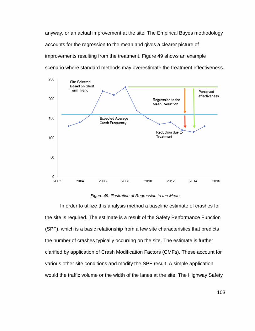
103

anyway, or an actual improvement at the site. The Empirical Bayes methodology

accounts for the regression to the mean and gives a clearer picture of

improvements resulting from the treatment. Figure 49 shows an example

scenario where standard methods may overestimate the treatment effectiveness.

Figure 49: Illustration of Regression to the Mean

In order to utilize this analysis method a baseline estimate of crashes for

the site is required. The estimate is a result of the Safety Performance Function

(SPF), which is a basic relationship from a few site characteristics that predicts

the number of crashes typically occurring on the site. The estimate is further

clarified by application of Crash Modification Factors (CMFs). These account for

various other site conditions and modify the SPF result. A simple application

would the traffic volume or the width of the lanes at the site. The Highway Safety

104

Manual (HSM) provides a method for creating SPFs for three main site types and

the associated CMFs (Bonneson 2010). Currently the First Edition does not

contain any methodology on urban freeway segments, however a draft chapter

for freeways is available online (Bonneson 2012). This methodology was applied

to OR 217 to develop the crash estimates.

The first step in applying the SPF is dividing the facility, OR 217, into

smaller “sites” which are either homogeneous freeway segments or speed

change lanes. Figure 50 shows a simplified version of the segmentation process

for speed change lanes and freeway segments.

105

Figure 50: Example Segmentation of the Corridor Source: Highway Safety Manual

Figure 51 shows an example of how one portion of OR 217 was

segmented into sites. The green section represents a speed change lane next to

a freeway segment in red. These segments begin and end at every ramp gore

point. OR 217 was divided into a total of 23 segments for this analysis with the

ends of the corridor excluded. These ends were excluded as the VSL signs are

not located at the very ends of the corridor and the geometry of the freeway

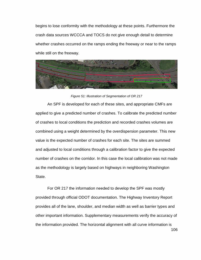
106

begins to lose conformity with the methodology at these points. Furthermore the

crash data sources WCCCA and TOCS do not give enough detail to determine

whether crashes occurred on the ramps ending the freeway or near to the ramps

while still on the freeway.

Figure 51: Illustration of Segmentation of OR 217

An SPF is developed for each of these sites, and appropriate CMFs are

applied to give a predicted number of crashes. To calibrate the predicted number

of crashes to local conditions the prediction and recorded crashes volumes are

combined using a weight determined by the overdispersion parameter. This new

value is the expected number of crashes for each site. The sites are summed

and adjusted to local conditions through a calibration factor to give the expected

number of crashes on the corridor. In this case the local calibration was not made

as the methodology is largely based on highways in neighboring Washington

State.

For OR 217 the information needed to develop the SPF was mostly

provided through official ODOT documentation. The Highway Inventory Report

provides all of the lane, shoulder, and median width as well as barrier types and

other important information. Supplementary measurements verify the accuracy of

the information provided. The horizontal alignment with all curve information is

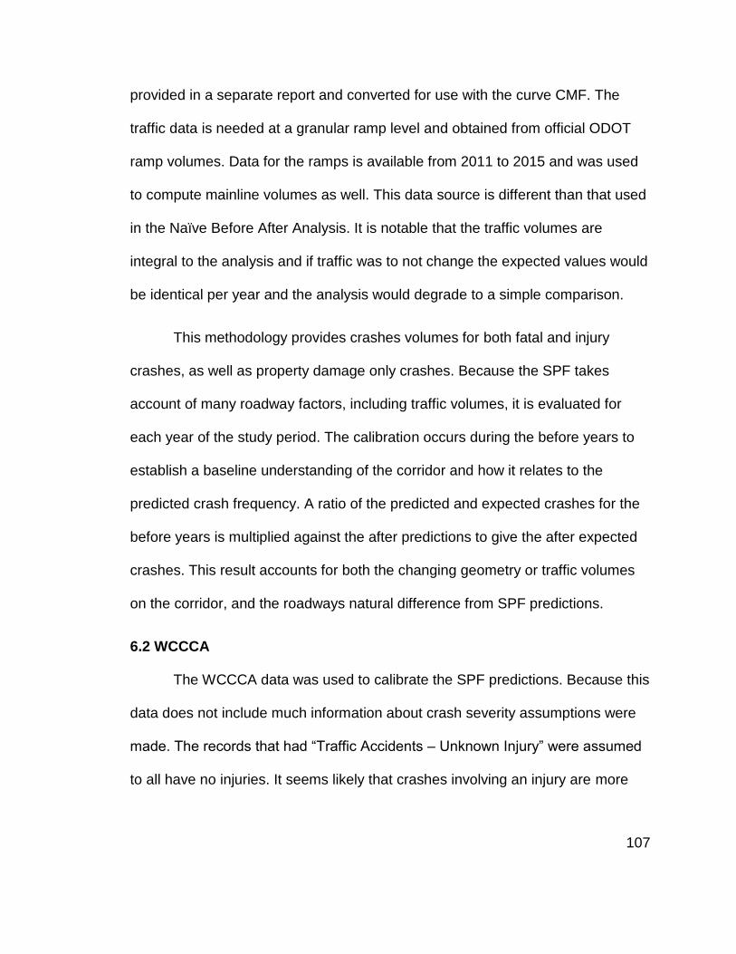
107

provided in a separate report and converted for use with the curve CMF. The

traffic data is needed at a granular ramp level and obtained from official ODOT

ramp volumes. Data for the ramps is available from 2011 to 2015 and was used

to compute mainline volumes as well. This data source is different than that used

in the Naïve Before After Analysis. It is notable that the traffic volumes are

integral to the analysis and if traffic was to not change the expected values would

be identical per year and the analysis would degrade to a simple comparison.

This methodology provides crashes volumes for both fatal and injury

crashes, as well as property damage only crashes. Because the SPF takes

account of many roadway factors, including traffic volumes, it is evaluated for

each year of the study period. The calibration occurs during the before years to

establish a baseline understanding of the corridor and how it relates to the

predicted crash frequency. A ratio of the predicted and expected crashes for the

before years is multiplied against the after predictions to give the after expected

crashes. This result accounts for both the changing geometry or traffic volumes

on the corridor, and the roadways natural difference from SPF predictions.

6.2 WCCCA

The WCCCA data was used to calibrate the SPF predictions. Because this

data does not include much information about crash severity assumptions were

made. The records that had “Traffic Accidents – Unknown Injury” were assumed

to all have no injuries. It seems likely that crashes involving an injury are more

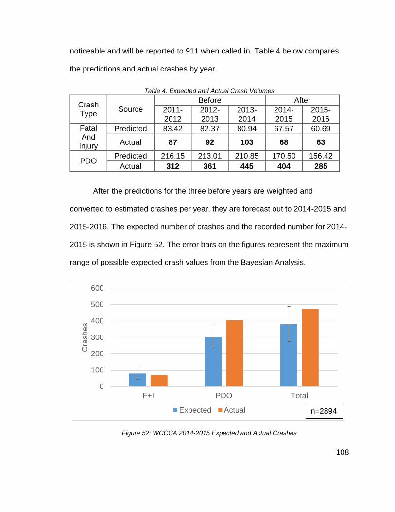
108

noticeable and will be reported to 911 when called in. Table 4 below compares

the predictions and actual crashes by year.

Table 4: Expected and Actual Crash Volumes

Crash Type

Source Before After

2011-2012

2012-2013

2013-2014

2014-2015

2015-2016

Fatal And

Injury

Predicted 83.42 82.37 80.94 67.57 60.69

Actual 87 92 103 68 63

PDO Predicted 216.15 213.01 210.85 170.50 156.42

Actual 312 361 445 404 285

After the predictions for the three before years are weighted and

converted to estimated crashes per year, they are forecast out to 2014-2015 and

2015-2016. The expected number of crashes and the recorded number for 2014-

2015 is shown in Figure 52. The error bars on the figures represent the maximum

range of possible expected crash values from the Bayesian Analysis.

Figure 52: WCCCA 2014-2015 Expected and Actual Crashes

0

100

200

300

400

500

600

F+I PDO Total

Cra

sh

es

Expected Actual n=2894

109

Figure 53 shows that fatal and injury crashes are lower in the year

immediately following the system activation. However, as the figure also shows,

these crashes are much fewer in number than non-injury crashes and the overall

freeway saw a large increase in overall crashes. If the trend is carried out to the

most recent data from 2015-2016 the same pattern emerges as Figure 54 shows.

Figure 53: WCCCA 2015-2016 Expected and Actual Crashes

The newer data shows an even larger decline in the small numbers of

crashes with injuries, while also have a reduced increase in the number of

property damage only crashes. This may indicate that the system is performing

and improving but needs more time for drivers to become accustomed to it. The

overall after period estimate and actual crash counts are in Figure 54.

0

50

100

150

200

250

300

350

400

450

500

F+I PDO Total

Cra

she

s


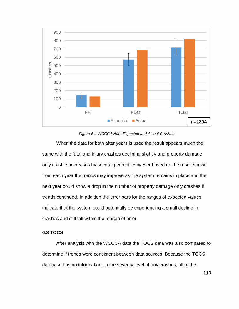
110

Figure 54: WCCCA After Expected and Actual Crashes

When the data for both after years is used the result appears much the

same with the fatal and injury crashes declining slightly and property damage

only crashes increases by several percent. However based on the result shown

from each year the trends may improve as the system remains in place and the

next year could show a drop in the number of property damage only crashes if

trends continued. In addition the error bars for the ranges of expected values

indicate that the system could potentially be experiencing a small decline in

crashes and still fall within the margin of error.

6.3 TOCS

After analysis with the WCCCA data the TOCS data was also compared to

determine if trends were consistent between data sources. Because the TOCS

database has no information on the severity level of any crashes, all of the

0

100

200

300

400

500

600

700

800

900

F+I PDO Total

Cra

she

s


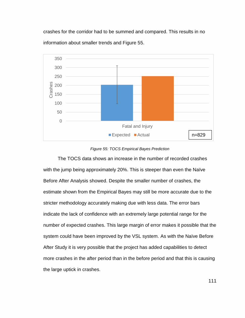
111

crashes for the corridor had to be summed and compared. This results in no

information about smaller trends and Figure 55.

Figure 55: TOCS Empirical Bayes Prediction

The TOCS data shows an increase in the number of recorded crashes

with the jump being approximately 20%. This is steeper than even the Naïve

Before After Analysis showed. Despite the smaller number of crashes, the

estimate shown from the Empirical Bayes may still be more accurate due to the

stricter methodology accurately making due with less data. The error bars

indicate the lack of confidence with an extremely large potential range for the

number of expected crashes. This large margin of error makes it possible that the

system could have been improved by the VSL system. As with the Naïve Before

After Study it is very possible that the project has added capabilities to detect

more crashes in the after period than in the before period and that this is causing

the large uptick in crashes.

0

50

100

150

200

250

300

350

Fatal and Injury

Cra

she

s


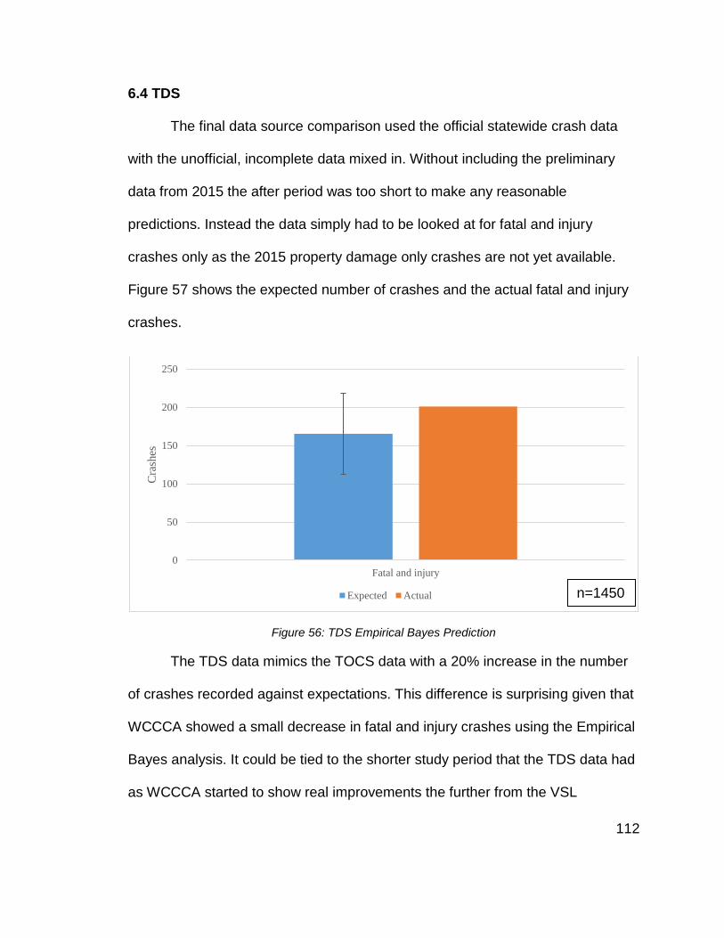
112

6.4 TDS

The final data source comparison used the official statewide crash data

with the unofficial, incomplete data mixed in. Without including the preliminary

data from 2015 the after period was too short to make any reasonable

predictions. Instead the data simply had to be looked at for fatal and injury

crashes only as the 2015 property damage only crashes are not yet available.

Figure 57 shows the expected number of crashes and the actual fatal and injury

crashes.

Figure 56: TDS Empirical Bayes Prediction

The TDS data mimics the TOCS data with a 20% increase in the number

of crashes recorded against expectations. This difference is surprising given that

WCCCA showed a small decrease in fatal and injury crashes using the Empirical

Bayes analysis. It could be tied to the shorter study period that the TDS data had

as WCCCA started to show real improvements the further from the VSL

0

50

100

150

200

250

Fatal and injury

Cra

shes


113

activation date. The error bars show that the range of expected crashes is quite

large and the system could be potentially experiencing a small decline at one

extreme.

114

7.0 Conclusions

When the analysis methods of both a Naïve Before After study and

Empirical Bayes study are considered, the results for OR 217 are not clear

regarding safety. Most measures show the corridor as have a marked decline in

safety with crashes going up by between 4% and 20%. However, the same

sample sizes render some of these estimates null while others may be inflated by

unequal data reporting in the before and after period. The Naïve study results

generally conform, despite having statistical difficulty proving their validity, while

the Bayesian results vary more substantially.

The main data source for this study, WCCCA, shows a decrease in more

severe crashes through the Bayesian Analysis while the other data sources show

large jumps. This could be due to better data collection for TOCS and the limited

time period for the TDS data as the results generally appear to improve as time

goes on, shown even in the WCCCA data for 2014-2015 and 2015-2016.

The increase in crashes generally appears to be more noticeable for the

lower severity crashes, a potential positive. This could be due to drivers having

closer speed matches after the system was activated and thus reducing the

crash severity. The past research on OR 217 showed that speed lane

differentials changed little before and after with different sites experiencing either

an increase or decrease of less than 5%. The possible rise is crashes may

similarly be due to the lower compliance of drivers on the roadway as recent

research found (Riggins, 2015).

115

The increase in crashes could also be the result of information overload as

drivers are suddenly faced with additional information on an already busy

corridor. Drivers have new VSL signs, variable message signs, curve warning

signs, and all of the other signage associated with 11 sets of ramps in one 7-mile

freeway. In the literature review about the removed system in Missouri, too much

information for drivers was cited as a common complaint and heavily influenced

the decision to remove those boards.

7.1 Contributions

This study shed more light on the complex subject of roadway safety and

how it is impacted by VSL systems. Its results add to the knowledge of systems

evaluated using both a Naïve Before After Analysis and Empirical Bayes

Analysis.

7.2 Limitations

This analysis does have limitations about the implications of its results.

The limited data available in all of the data sources prevented small changes in

crash volumes from being reliably detected. In addition, the short after period

made seeing trends more difficult and may not be capturing the full impact after

drivers have settled into the new system and gotten used to all of the information

available.

7.3 Future Research

Conducting this study again in two years when the full three years of after

data is available would allow for better determinations of the actual impact. The

116

safety effects are currently generally negative and to follow up with additional

data could show an improvement that starts slowly as the WCCCA data may

indicate. In addition, this research would likely be more accurate due to the

reduced volume of before crashes required.

Research into drivers’ perceptions of the system would also help to

answer a crucial part of the analysis, how safe drivers feel. Improvements in

safety may occur but if drivers do not feel safer then it may not have been worth

it. Determining this would go a long way towards deciding if the OR 217 VSL

system is a success in the eyes of its most important people, the users.

117

References

Al-Kaisy, A., Ewan, L., & Veneziano, D. (2012). Evaluation of a Variable Speed Limit System for Wet and Extreme Weather Conditions: Phase 1 Report. Bozeman, MT.

Bham, G., Long, S., Baik, H., Ryan, T., & Gentry, L. (2010). Evaluation of Variable Speed Limits on I-270/I-255 in St. Louis. Jefferson City, MO.

Bonneson, J. A. (2010). Highway Safety Manual. Washington, D.C.: American Association of State Highway and Transportation Officials.

Bonneson, J. A. (2012). Safety Prediction methodology and Analysis Tool for Freeways and Interchanges. College Station, Texas.

Buddemeyer, J., Young, R., Sabawat, V., & Layton, E. (2010). Variable Speed Limits System for Elk Mountain Corridor. Laramie, WY.

Corthout, R., Tampere, C. M. J., & Deknudt, P. (2010). Assessment of Variable Speed Limits from the Drivers’ Perspective. In 13th International IEEE Annual Conference on Intelligent Transportation Systems. Madeira Island, Portugal: IEEE.

De Pauw, E., Daniels, S., Franckx, L., & Mayeres, I. (2015). Dynamic speed limits on Flemish motorways. Hasselt, Belgium.

DKS Associates. (2010). OR 217 Interchange Management Study. Salem, OR.

DKS Associates. (2013). Oregon Statewide Variable Speed System Concept of Operations. Salem, OR.

Downey, M. B., (2015) Evaluating the Effects of a Congestion and Weather Responsive Advisory Variable Speed Limit System in Portland, Oregon. Dissertations and Theses. Paper 2397.

Edara, P., Sun, C., & Hou, Y. (2013). Evaluation of Variable Advisory Speed Limits in Work Zones. Columbia, MO.

Fedala, N. J., & Fontaine, M. D. (2010). Work Zone Variable Speed Limit Systems: Effectiveness and System Design Issues. Richmond, VA

FHWA. (2014). How Do Weather Events Impact Roads? Retrieved January 23, 2015, from http://www.ops.fhwa.dot.gov/weather/q1_roadimpact.htm

118

Goodwin, L. C. (2003). Best Practices for Road Weather Management. Washington, D.C.

Han, C., Luk, J., Pyta, V., & Cairney, P. (2009). Best Practice for Variable Speed Limits: Literature Review. Sydney, Australia.

Hauer, E. (1997). Observational before--after studies in road safety: Estimating the effect of highway and traffic engineering measures on road safety. Oxford, OX, U.K.: Pergamon.

Hellinga, B., & Mandelzys, M. (2011). Impact of Driver Compliance on the Safety and Operational Impacts of Freeway Variable Speed Limit Systems. Journal of Transportation Engineering, 137, 260–268. http://doi.org/10.1061/(ASCE)TE.1943-5436.0000214

Katz, B., O-Donnell, C., Donoughe, K., Atkinson, J., Finley, M., Balke, K., … Warren, D. (2012). Guidelines for the Use of Variable Speed Limit Systems in Wet Weather. McLean, VA.

Kianfar, J., Edara, P., & Sun, C. (2013). Operational Analysis of a Freeway Variable Speed Limit System - Case Study of Deployment in Missouri. In TRB 92nd Annual Meeting Compendium of Papers. Washington, D.C.: Transportation Research Board.

Kuhn, B., Gopalakrishna, D., & Schreffler, E. (2013). The Active Transportation and Demand Management Program (ATDM): Lessons Learned. College Station, TX.

Kwon, E., Brannan, D., Shouman, K., Isackson, C., & Arseneau, B. (2007). Field Evaluation of a Variable Advisory Speed Limit System for Reducing Traffic Conflicts at Work Zones. In TRB 86th Annual Meeting Compendium of Papers. Washington, D.C.: Transportation Research Board.

Kwon, E., Park, C., Lau, D., & Kary, B. (2011). Minnesota Variable Speed Limit System: Adaptive Mitigation of Shock Waves for Safety and Efficiency of Traffic Flows. In TRB 90th Annual Meeting Compendium of Papers. Washington, D.C.: Transportation Research Board.

Lin, P.-W., Kang, K.-P., & Chang, G.-L. (2004). Exploring the Effectiveness of Variable Speed Limit Controls on Highway Work-Zone Operations. Journal of Intelligent Transportation Systems, 8, 155–168. http://doi.org/10.1080/15472450490492851

119

Monsere, C. M., Eshel, O., & Bertini, R. L. (2009). Empirical Evaluation of Freeway Corridor Performance Before and After System-Wide Adaptive Ramp Metering System Implementation. In TRB 88th Annual Meeting Compendium of Papers. Washington, D.C.: Transportation Research Board.

Neudorff, L. G., Mason, J., & Bauer, J. (2012). Glossary of Regional Transportation Systems Management and Operations Terms. Washington, D.C.

ODOT. (2012) Establishment of Variable Speed Zones, Pub. L. No. 734-020-0018. Oregon, United States of America.

ODOT. (2016). OR 217: Active Traffic Management. Portland, OR.

Perrin, J., Martin, P. T., & Coleman, B. (2002). Testing the Adverse Visibility Information System Evaluation (ADVISE) - Safer Driving in Fog. In TRB 81st Annual Meeting Compendium of Papers. Washington, D.C.: Transportation Research Board.

Rama, P., & Schirokoff, A. (2004). Effects of Weather-Controlled Variable Speed Limits on Injury Accidents. In Paper presented at the 4th European Congress on ITS. Budapest, Hungary: ERTICO - ITS Europe.

Riggins, G., Bertini, R. L., Ackaah, W., & Bogenberger, K. (2015). Measurement and Assessment of Driver Compliance with Variable Speed Limit Systems: Comparision of U.S. and Germany. In TRB 95th Annual Meeting Compendium of Papers. Washington, D.C.: Transportation Research Board.

Robinson, M. (2000). Examples of Variable Speed Limit Applications. Washington, D.C.

Schrank, D., Eisele, B., & Lomax, T. (2012). TTI’s 2012 Urban Mobility Report. College Station, TX.

SWOV Fact sheet: The influence of weather on road safety. (2012). Leidschendam, the Netherlands.

Vukanovic, S. (2007) Intelligent link control framework with empirical objective function:INCA. Dissertation. Munich, 2007

Young, R., Sabawat, V., Saha, P., & Sui, Y. (2012). Rural Variable Speed Limits: Phase II. Laramie, WY.

Documents

Benefits of Advanced Traffic Management Solutions: Before