Embed Size (px)
Citation preview
Bayesian Time Series Learning
with Gaussian Processes
Roger Frigola-AlcaldeDepartment of Engineering
St Edmund’s CollegeUniversity of Cambridge
August 2015
This dissertation is submitted for the degree ofDoctor of Philosophy

SUMMARY
The analysis of time series data is important in fields as disparateas the social sciences, biology, engineering or econometrics. In thisdissertation, we present a number of algorithms designed to learnBayesian nonparametric models of time series. The goal of thesekinds of models is twofold. First, they aim at making predictionswhich quantify the uncertainty due to limitations in the quantityand the quality of the data. Second, they are flexible enough tomodel highly complex data whilst preventing overfitting when thedata does not warrant complex models.
We begin with a unifying literature review on time series mod-els based on Gaussian processes. Then, we centre our attentionon the Gaussian Process State-Space Model (GP-SSM): a Bayesiannonparametric generalisation of discrete-time nonlinear state-spacemodels. We present a novel formulation of the GP-SSM that offersnew insights into its properties. We then proceed to exploit thoseinsights by developing new learning algorithms for the GP-SSMbased on particle Markov chain Monte Carlo and variational infer-ence.
Finally, we present a filtered nonlinear auto-regressive model witha simple, robust and fast learning algorithm that makes it well suitedto its application by non-experts on large datasets. Its main advan-tage is that it avoids the computationally expensive (and potentiallydifficult to tune) smoothing step that is a key part of learning non-linear state-space models.

ACKNOWLEDGEMENTS
I would like to thank Carl Rasmussen who took the gamble of ac-cepting a candidate for a PhD in statistical machine learning whobarely knew what a probability distribution was. I am also gratefulto Zoubin Ghahramani, Rich Turner and Daniel Wolpert for creat-ing such a wonderful academic environment at the Computationaland Biological Learning Lab in Cambridge; it has been incredibleto interact with so many talented people. I would also like to thankThomas Schon for hosting my fruitful academic visit at LinkopingUniversity (Sweden).
I am indebted to my talented collaborators Fredrik Lindsten andYutian Chen. Their technical skills have been instrumental to de-velop ideas that were only fuzzy in my head.
I would also like to thank my thesis examiners, Rich Turner andJames Hensman, and Thang Bui for their helpful feedback that hascertainly improved the thesis. Of course, any remaining inaccura-cies and errors are entirely my fault!
Finally, I can not thank enough all the colleagues, friends and fam-ily with whom I have spent so many joyful times throughout mylife.
DECLARATION
This dissertation is the result of my own work and includes noth-ing which is the outcome of work done in collaboration except asspecified in the text.
This dissertation is not substantially the same as any that I havesubmitted, or, is being concurrently submitted for a degree or diplo-ma or other qualification at the University of Cambridge or anyother University or similar institution. I further state that no sub-stantial part of my dissertation has already been submitted, or, isbeing concurrently submitted for any such degree, diploma or otherqualification at the University of Cambridge or any other Univer-sity of similar institution.
This dissertation does not exceed 65,000 words, including appen-dices, bibliography, footnotes, tables and equations. This disserta-tion does not contain more than 150 figures.


“Would you tell me, please, which way I ought to go from here?”
“That depends a good deal on where you want to get to,” said theCat.
“I don’t much care where —” said Alice.
“Then it doesn’t matter which way you go,” said the Cat.
“— so long as I get somewhere,” Alice added as an explanation.
“Oh, you’re sure to do that,” said the Cat, “if you only walk longenough.”
Lewis Carroll, Alice’s Adventures in Wonderland

Contents
1 Introduction 11.1 Time Series Models . . . . . . . . . . . . . . . . . . . . . . . . . . 11.2 Bayesian Nonparametric Time Series Models . . . . . . . . . . . 2
1.2.1 Bayesian Methods . . . . . . . . . . . . . . . . . . . . . . 21.2.2 Bayesian Methods in System Identification . . . . . . . . 41.2.3 Nonparametric Models . . . . . . . . . . . . . . . . . . . 4
1.3 Contributions . . . . . . . . . . . . . . . . . . . . . . . . . . . . . 5
2 Time Series Modelling with Gaussian Processes 72.1 Introduction . . . . . . . . . . . . . . . . . . . . . . . . . . . . . . 72.2 Gaussian Processes . . . . . . . . . . . . . . . . . . . . . . . . . . 8
2.2.1 Gaussian Processes for Regression . . . . . . . . . . . . . 92.2.2 Graphical Models of Gaussian Processes . . . . . . . . . 11
2.3 A Zoo of GP-Based Dynamical System Models . . . . . . . . . . 122.3.1 Linear-Gaussian Time Series Model . . . . . . . . . . . . 132.3.2 Nonlinear Auto-Regressive Model with GP . . . . . . . . 142.3.3 State-Space Model with Transition GP . . . . . . . . . . . 162.3.4 State-Space Model with Emission GP . . . . . . . . . . . 182.3.5 State-Space Model with Transition and Emission GPs . . 192.3.6 Non-Markovian-State Model with Transition GP . . . . . 212.3.7 GP-LVM with GP on the Latent Variables . . . . . . . . . 22
2.4 Why Gaussian Process State-Space Models? . . . . . . . . . . . . 23
3 Gaussian Process State-Space Models – Description 253.1 GP-SSM with State Transition GP . . . . . . . . . . . . . . . . . . 25
3.1.1 An Important Remark . . . . . . . . . . . . . . . . . . . . 283.1.2 Marginalisation of f1:T . . . . . . . . . . . . . . . . . . . . 293.1.3 Marginalisation of f(x) . . . . . . . . . . . . . . . . . . . 30
3.2 GP-SSM with Transition and Emission GPs . . . . . . . . . . . . 313.2.1 Equivalence between GP-SSMs . . . . . . . . . . . . . . . 32
3.3 Sparse GP-SSMs . . . . . . . . . . . . . . . . . . . . . . . . . . . . 333.4 Summary of GP-SSM Densities . . . . . . . . . . . . . . . . . . . 34
4 Gaussian Process State-Space Models – Monte Carlo Learning 374.1 Introduction . . . . . . . . . . . . . . . . . . . . . . . . . . . . . . 374.2 Fully Bayesian Learning . . . . . . . . . . . . . . . . . . . . . . . 38
4.2.1 Sampling State Trajectories with PMCMC . . . . . . . . . 384.2.2 Sampling the Hyper-Parameters . . . . . . . . . . . . . . 404.2.3 Making Predictions . . . . . . . . . . . . . . . . . . . . . . 41
ix
x CONTENTS
4.2.4 Experiments . . . . . . . . . . . . . . . . . . . . . . . . . . 414.3 Empirical Bayes . . . . . . . . . . . . . . . . . . . . . . . . . . . . 44
4.3.1 Particle Stochastic Approximation EM . . . . . . . . . . . 454.3.2 Making Predictions . . . . . . . . . . . . . . . . . . . . . . 474.3.3 Experiments . . . . . . . . . . . . . . . . . . . . . . . . . . 48
4.4 Reducing the Computational Complexity . . . . . . . . . . . . . 514.4.1 FIC Covariance Function . . . . . . . . . . . . . . . . . . 514.4.2 Sequential Construction of Cholesky Factorisations . . . 52
4.5 Conclusions . . . . . . . . . . . . . . . . . . . . . . . . . . . . . . 53
5 Gaussian Process State-Space Models – Variational Learning 555.1 Introduction . . . . . . . . . . . . . . . . . . . . . . . . . . . . . . 555.2 Evidence Lower Bound of a GP-SSM . . . . . . . . . . . . . . . . 56
5.2.1 Interpretation of the Lower Bound . . . . . . . . . . . . . 585.2.2 Properties of the Lower Bound . . . . . . . . . . . . . . . 595.2.3 Are the Inducing Inputs Variational Parameters? . . . . . 60
5.3 Optimal Variational Distributions . . . . . . . . . . . . . . . . . . 605.3.1 Optimal Variational Distribution for u . . . . . . . . . . . 605.3.2 Optimal Variational Distribution for x . . . . . . . . . . . 61
5.4 Optimising the Evidence Lower Bound . . . . . . . . . . . . . . 635.4.1 Alternative Optimisation Strategy . . . . . . . . . . . . . 63
5.5 Making Predictions . . . . . . . . . . . . . . . . . . . . . . . . . . 645.6 Extensions . . . . . . . . . . . . . . . . . . . . . . . . . . . . . . . 65
5.6.1 Stochastic Variational Inference . . . . . . . . . . . . . . . 655.6.2 Online Learning . . . . . . . . . . . . . . . . . . . . . . . 66
5.7 Additional Topics . . . . . . . . . . . . . . . . . . . . . . . . . . . 675.7.1 Relationship to Regularised Recurrent Neural Networks 675.7.2 Variational Learning in Related Models . . . . . . . . . . 685.7.3 Arbitrary Mean Function Case . . . . . . . . . . . . . . . 71
5.8 Experiments . . . . . . . . . . . . . . . . . . . . . . . . . . . . . . 725.8.1 1D Nonlinear System . . . . . . . . . . . . . . . . . . . . . 725.8.2 Neural Spike Train Recordings . . . . . . . . . . . . . . . 72
6 Filtered Auto-Regressive Gaussian Process Models 756.1 Introduction . . . . . . . . . . . . . . . . . . . . . . . . . . . . . . 75
6.1.1 End-to-End Machine Learning . . . . . . . . . . . . . . . 766.1.2 Algorithmic Weakening . . . . . . . . . . . . . . . . . . . 76
6.2 The GP-FNARX Model . . . . . . . . . . . . . . . . . . . . . . . . 776.2.1 Choice of Preprocessing and Covariance Functions . . . 78
6.3 Optimisation of the Marginal Likelihood . . . . . . . . . . . . . 796.4 Sparse GPs for Computational Speed . . . . . . . . . . . . . . . . 806.5 Algorithm . . . . . . . . . . . . . . . . . . . . . . . . . . . . . . . 806.6 Experiments . . . . . . . . . . . . . . . . . . . . . . . . . . . . . . 81
7 Conclusions 857.1 Contributions . . . . . . . . . . . . . . . . . . . . . . . . . . . . . 857.2 Future work . . . . . . . . . . . . . . . . . . . . . . . . . . . . . . 86

CONTENTS xi
A Approximate Bayesian Inference 87A.1 Particle Markov Chain Monte Carlo . . . . . . . . . . . . . . . . 87
A.1.1 Particle Gibbs with Ancestor Sampling . . . . . . . . . . 87A.2 Variational Bayes . . . . . . . . . . . . . . . . . . . . . . . . . . . 89

xii CONTENTS
Chapter 1
Introduction
”The purpose of computing is insight, not numbers.”
Richard W. Hamming
”The purpose of computing is numbers — specifically, correct numbers.”
Leslie F. Greengard
1.1 TIME SERIES MODELS
Time series data consists of a number of measurements taken over time. Forexample, a time series dataset could be created by recording power generatedby a solar panel, by storing measurements made by sensors on an aircraft, or bymonitoring the vital signs of a patient in a hospital. The ubiquity of time seriesdata makes its analysis important for fields as disparate as the social sciences,biology, engineering or econometrics.
Time series tend to exhibit high correlations induced by the temporal struc-ture in the data. It is therefore not surprising that specialised methods for timeseries analysis have been developed over time. In this thesis we will focuson a model-based approach to time series analysis. Models are mathematicalconstructions that often correspond to an idealised view about how the datais generated. Models are useful to make predictions about the future and tobetter understand what was happening while the data was being recorded.
The process of tuning models of time series using data is called system iden-tification in the field of control theory (Ljung, 1999). In the fields of statisticsand machine learning it is often referred to as estimation, fitting, inference orlearning of time series (Hamilton, 1994; Shumway and Stoffer, 2011; Barberet al., 2011; Tsay, 2013). Creating faithful models given the data at our disposalis of great practical importance. Otherwise any reasoning, prediction or designbased on the data could be fatally flawed.
Models are usually not perfect and the data available to us is often limitedin quantity and quality. It is therefore normal to ask ourselves: are we limited
1
2 1. INTRODUCTION
to creating just one model or could we make a collection of models that wereall plausible given the available data? If we embrace uncertainty, we can movefrom the notion of having a single model to that of keeping a potentially infinitecollection of models and combining them to make decisions of any sort. Thisis one of the fundamental ideas behind Bayesian inference.
In this thesis, we develop methods for Bayesian inference applied to dy-namical systems using models based on Gaussian processes. Although we willwork with very general models that can be applied in a variety of situations, ourmindset is that of the field of system identification. In other words, we focuson learning models typically found in engineering problems where a relativelylimited amount of noisy sensors give a glimpse at the complex dynamics of asystem.
1.2 BAYESIAN NONPARAMETRIC TIME SERIES MOD-
ELS
1.2.1 BAYESIAN METHODS
When learning a model from a time series, we never have the luxury of aninfinite amount of noiseless data and unlimited computational power. In prac-tice, we deal with finite noisy datasets which lead to uncertainty about whatthe most appropriate model is given the available data. In Bayesian inference,probabilities are treated as a way to represent the subjective uncertainty of therational agent performing inference (Jaynes, 2003). This uncertainty is repre-sented as a probability distribution over the model given the data
p(M | D), (1.1)
where the model is understood here in the sense of the functional form andthe value of any parameter that the model might have. This contrasts with themost common approaches to time series analysis where a single model of thesystem is found, usually by optimising a cost function such as the likelihood(Ljung, 1999; Shumway and Stoffer, 2011). After optimisation, the resultingmodel is considered the best available representation of the system and usedfor any further application.
In a Bayesian approach, however, it is acknowledged that several models(or values of a parameter) can be consistent with the data (Peterka, 1981). Inthe case of a parametric model, rather than obtaining a single estimate of the“best” value of the parameters θ∗, Bayesian inference will produce a posteriorprobability distribution over this parameter p(θ|D). This distribution allowsfor the fact that several values of the parameter might also be plausible giventhe observed data D. The posterior p(θ|D) can then interpreted as our degreeof belief about the value of the parameter θ. Predictions or decisions based onthe posterior are made by computing expectations over the posterior. Infor-mally, one can think of predictions as being an average using different values
1.2. BAYESIAN NONPARAMETRIC TIME SERIES MODELS 3
of the parameters weighted by how much the parameter is consistent with thedata. Predictions can be made with error bars that represent both the system’sinherent stochasticity and our own degree of ignorance about what the correctmodel is.
For the sake of example, let’s consider a parametric model of a discrete-timestochastic dynamical system with a continuous state defined by xt. The statetransition density is
p(xt+1|xt, θ). (1.2)
Bayesian learning provides a posterior over the unknown parameter θ giventhe data p(θ|D). To make predictions about the state transition we can integrateover the posterior in order to average over all plausible values of the parameterafter having seen the data
p(xt+1|xt,D) =
∫p(xt+1|xt, θ) p(θ|D) dθ. (1.3)
Here, predictions are made by considering all plausible values of θ, not only a“best guess”.
Bayesian inference needs a prior: p(θ) for our example above. The prior isa probability distribution representing our uncertainty about the object to beinferred before seeing the data. This requirement of a subjective distributionis often criticised. However, the prior is an opportunity to formalise manyof the assumptions that in other methods may be less explicit. MacKay (2003)points out that “you cannot do inference without making assumptions”. In Bayesianinference those assumptions are very clearly specified.
In the context of learning dynamical systems, Isermann and Munchhof (2011)derive maximum likelihood and least squares methods from Bayesian infer-ence. Although maximum likelihood and Bayesian inference are related intheir use of probability, there is a fundamental philosophical difference. Spiegel-halter and Rice (2009) summarise it eloquently:
At a simple level, ‘classical’ likelihood-based inference closely resemblesBayesian inference using a flat prior, making the posterior and likelihoodproportional. However, this underestimates the deep philosophical differ-ences between Bayesian and frequentist inference; Bayesian [sic] makestatements about the relative evidence for parameter values given a dataset,while frequentists compare the relative chance of datasets given a parame-ter value.
Bayesian methods are also relevant in “big data” settings when the com-plexity of the system that generated the data is large relative to the amount ofdata. Large datasets can contain many nuances of the behaviour of a complexsystem. Models of large capacity are then required if those nuances are to becaptured properly. Moreover, there will still be uncertainty about the systemthat generated the data. For example, even if a season’s worth of time seriesdata recorded from a Formula 1 car is in the order of a petabyte, there will be,hopefully, very little data of the car sliding sideways out of control. Therefore,
4 1. INTRODUCTION
models about the behaviour of the car at extremely large slip angles would behighly uncertain.
1.2.2 BAYESIAN METHODS IN SYSTEM IDENTIFICATION
Despite Peterka (1981) having set the basis for Bayesian system identification,Bayesian system identification has not had a significant impact within the con-trol community. For instance, consider this quote from a recent book by wellknown authors in the field (Isermann and Munchhof, 2011):
Bayes estimation has little relevance for practical applications in the area ofsystem identification. [...] Bayes estimation is mainly of theoretical value.It can be regarded as the most general and most comprehensive estimationmethod. Other fundamental estimation methods can be derived from thisstarting point by making certain assumptions or specializations.
It is apparent that the authors recognise Bayesian inference as a sound frame-work for estimation but later dismiss it on the grounds of its mathematical andcomputational burden and its need for prior information.
However, since Peterka’s article in 1981, there have been radical improve-ments in both computational power and algorithms for Bayesian learning. Someinfluential recent developments such as the regularised kernel methods of Chenet al. (2012) can be interpreted from a Bayesian perspective. Their use of a priorfor regularised learning has shown great promise and moving from this to thecreation of a posterior over dynamical systems is straightforward.
1.2.3 NONPARAMETRIC MODELS
In Equation (1.3) we have made use of the fact that
p(xt+1|xt, θ,D) = p(xt+1|xt, θ), (1.4)
which is true for parametric models: predictions are conditionally indepen-dent of the observed data D given the parameters. In other words, the datais distilled into the parameter θ and any subsequent prediction does not makeuse of the original dataset. This is very convenient but it is not without itsdrawbacks. Choosing a model from a particular parametric class constrains itsflexibility. An alternative is to use nonparametric models. In those models, thedata is not reduced to a finite set of parameters. In fact, nonparametric modelscan be shown to have an infinite-dimensional parameter space (Orbanz, 2014).This allows the model to represent more complexity as the size of the datasetD grows; defying in this way the bound in model complexity existing in para-metric models.
Models can be thought of as an information channel from past data to futurepredictions (Ghahramani, 2012). In this context, a parametric model constitutesa bottleneck in the information channel: predictions are made based only onthe learnt parameters. However, nonparametric models are memory-based since
1.3. CONTRIBUTIONS 5
they need to “remember” the full dataset in order to make predictions. Thiscan be interpreted as nonparametric models having a number of parametersthat progressively grows with the size of the dataset.
Bayesian nonparametric models combine the two aspects presented up tothis point: they allow Bayesian inference to be performed on objects of infinitedimensionality. Next chapter introduces how Gaussian processes (Rasmussenand Williams, 2006) can be used to infer a function given data. The result of in-ference will not be a single function but a posterior distribution over functions.
1.3 CONTRIBUTIONS
The main contributions in this dissertation have been published before in
• Roger Frigola and Carl E. Rasmussen, (2013). Integrated preprocessingfor Bayesian nonlinear system identification with Gaussian processes. InIEEE 52nd Annual Conference on Decision and Control (CDC), pp. 5371-5376.
• Roger Frigola, Fredrik Lindsten, Thomas B. Schon, and Carl E. Rasmussen.(2013). Bayesian inference and learning in Gaussian process state-spacemodels with particle MCMC. In Advances in Neural Information ProcessingSystems 26 (NIPS), pp. 3156-3164.
• Roger Frigola, Fredrik Lindsten, Thomas B. Schon, and Carl E. Rasmussen.(2014). Identification of Gaussian process state-space models with parti-cle stochastic approximation EM. In 19th World Congress of the Interna-tional Federation of Automatic Control (IFAC), pp. 4097-4102.
• Roger Frigola, Yutian Chen, and Carl E. Rasmussen. (2014). VariationalGaussian process state-space models. In Advances in Neural InformationProcessing Systems 27 (NIPS), pp. 3680-3688.
However, I take the opportunity that the thesis format offers to build on thepublications and extend the presentation of the material. In particular, the lackof asphyxiating page count constraints will allow for the presentation of subtledetails of Gaussian Process State-Space Models that could not fit in the papers.Also, there is now space for a comprehensive review highlighting prior workusing Gaussian processes for time series modelling. Models that were origi-nally presented in different contexts and with differing notations are now putunder the same light for ease of comparison. Hopefully, this review will beuseful to researchers entering the field of time series modelling with Gaussianprocesses.
A summary of technical contributions of this thesis can be found in Sec-tion 7.1.

6 1. INTRODUCTION
Chapter 2
Time Series Modelling withGaussian Processes
This chapter aims at providing a self-contained review of previous work ontime series modelling with Gaussian processes. A particular effort has beenmade to present models with a unified notation and separate the models them-selves from the algorithms used to learn them.
2.1 INTRODUCTION
Learning dynamical systems, also known as system identification or time seriesmodelling, aims at the creation of a model based on measured signals. Thismodel can be used, amongst other things, to predict future behaviour of thesystem, to explain interesting structure in the data or to denoise the originaltime series.
Systems displaying temporal dynamics are ubiquitous in nature, engineer-ing and the social sciences. For instance, we could obtain data about how thenumber of individuals of several species in an ecosystem changes with time;we could record data from sensors in an aircraft; or we could log the evolutionof share price in a stock market. In all those cases, learning from time seriescan provide both insight and the ability to make predictions.
We consider that there will potentially be two kinds of measured signals.In the system identification jargon those signals are named inputs and out-puts. Inputs are external influences to the system (e.g. rain in an ecosystemor turbulence affecting an aircraft) and outputs are signals that depend on thecurrent properties of the system (e.g. the number of lions in a savannah or thespeed of an aircraft). We will denote the input vector at time t by ut ∈ Rnu andthe output vector by yt ∈ Rny .
In this review we are mainly concerned with two important families of dy-namical system models (Ljung, 1999). First, auto-regressive (AR) models di-rectly model the next output of a system as a function of a number of previous
7
8 2. TIME SERIES MODELLING WITH GAUSSIAN PROCESSES
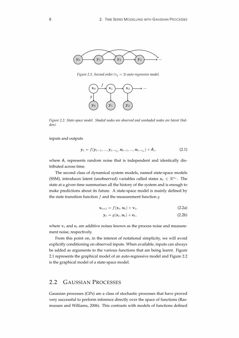
y0 y1 y2 y3 ...
Figure 2.1: Second order (τy = 2) auto-regressive model.
x0 x1 x2
y0 y1 y2
...f
g
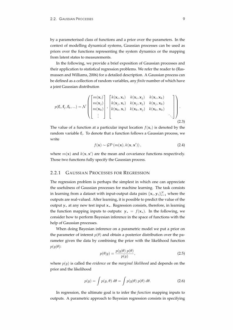
Figure 2.2: State-space model. Shaded nodes are observed and unshaded nodes are latent (hid-den).
inputs and outputs
yt = f(yt−1, ...,yt−τy ,ut−1, ...,ut−τu) + δt, (2.1)
where δt represents random noise that is independent and identically dis-tributed across time.
The second class of dynamical system models, named state-space models(SSM), introduces latent (unobserved) variables called states xt ∈ Rnx . Thestate at a given time summarises all the history of the system and is enough tomake predictions about its future. A state-space model is mainly defined bythe state transition function f and the measurement function g
xt+1 = f(xt,ut) + vt, (2.2a)
yt = g(xt,ut) + et, (2.2b)
where vt and et are additive noises known as the process noise and measure-ment noise, respectively.
From this point on, in the interest of notational simplicity, we will avoidexplicitly conditioning on observed inputs. When available, inputs can alwaysbe added as arguments to the various functions that are being learnt. Figure2.1 represents the graphical model of an auto-regressive model and Figure 2.2is the graphical model of a state-space model.
2.2 GAUSSIAN PROCESSES
Gaussian processes (GPs) are a class of stochastic processes that have provedvery successful to perform inference directly over the space of functions (Ras-mussen and Williams, 2006). This contrasts with models of functions defined
2.2. GAUSSIAN PROCESSES 9
by a parameterised class of functions and a prior over the parameters. In thecontext of modelling dynamical systems, Gaussian processes can be used aspriors over the functions representing the system dynamics or the mappingfrom latent states to measurements.
In the following, we provide a brief exposition of Gaussian processes andtheir application to statistical regression problems. We refer the reader to (Ras-mussen and Williams, 2006) for a detailed description. A Gaussian process canbe defined as a collection of random variables, any finite number of which havea joint Gaussian distribution
p(fi, fj , fk, ...) = N
m(xi)
m(xj)
m(xk)...
,k(xi,xi) k(xi,xj) k(xi,xk)
k(xj ,xi) k(xj ,xj) k(xj ,xk)
k(xk,xi) k(xk,xj) k(xk,xk)
. . .
.
(2.3)The value of a function at a particular input location f(xi) is denoted by therandom variable fi. To denote that a function follows a Gaussian process, wewrite
f(x) ∼ GP (m(x), k(x,x′)) , (2.4)
where m(x) and k(x,x′) are the mean and covariance functions respectively.Those two functions fully specify the Gaussian process.
2.2.1 GAUSSIAN PROCESSES FOR REGRESSION
The regression problem is perhaps the simplest in which one can appreciatethe usefulness of Gaussian processes for machine learning. The task consistsin learning from a dataset with input-output data pairs {xi,yi}Ni=1 where theoutputs are real-valued. After learning, it is possible to predict the value of theoutput y∗ at any new test input x∗. Regression consists, therefore, in learningthe function mapping inputs to outputs: y∗ = f(x∗). In the following, weconsider how to perform Bayesian inference in the space of functions with thehelp of Gaussian processes.
When doing Bayesian inference on a parametric model we put a prior onthe parameter of interest p(θ) and obtain a posterior distribution over the pa-rameter given the data by combining the prior with the likelihood functionp(y|θ):
p(θ|y) =p(y|θ) p(θ)
p(y), (2.5)
where p(y) is called the evidence or the marginal likelihood and depends on theprior and the likelihood
p(y) =
∫p(y, θ) dθ =
∫p(y|θ) p(θ) dθ. (2.6)
In regression, the ultimate goal is to infer the function mapping inputs tooutputs. A parametric approach to Bayesian regression consists in specifying
10 2. TIME SERIES MODELLING WITH GAUSSIAN PROCESSES
a family of functions parameterised by a finite set of parameters, putting aprior on those parameters and performing inference. However, we can finda less restrictive and very powerful approach to inference on functions by di-rectly specifying a prior over an infinite-dimensional space of functions. Thiscontrasts with putting a prior over a finite set of parameters which implicitlyspecify a distribution over functions.
A very useful prior over functions is the Gaussian process. In a Gaussianprocess, once we have selected a finite collection of points x , {x1, ...,xN}at which to evaluate a function, the prior distribution over the values of thefunction at those locations, f ,
(f(x1), ..., f(xN )
), is a Gaussian distribution
p(f |x) = N (m(x),K(x)), (2.7)
where m(x) and K(x) are the mean vector and covariance matrix defined in thesame way as in Equation (2.3). This is due to the marginal of a Gaussian processbeing a Gaussian distribution. Therefore, when we only deal with the Gaussianprocess at a finite set of inputs, computations involving the prior are basedon Gaussian distributions. Bayes’ theorem can be applied in the conventionalmanner to obtain a posterior over the latent function at all locations x whereobservations y , {y1, ...,yN} are available
p(f |y,x) =p(y|f) p(f |x)
p(y|x)=p(y|f) N (f |m(x),K(x))
p(y|x). (2.8)
And since the denominator is a constant for any given dataset1, we note theproportionality
p(f |y,x) ∝ p(y|f) N (f |m(x),K(x)). (2.9)
In the particular case where the likelihood has the form p(y|f) = N (y|f ,Σn),this posterior can be computed analytically and is Gaussian
p(f |y,x) = N (f |K(x)(K(x) + Σn
)−1(y −m(x)
),
K(x)−K(x)(K(x) + Σn
)−1K(x)). (2.10)
This is the case in Gaussian process regression when additive Gaussian noise isconsidered. However, for arbitrary likelihood functions the posterior will notnecessarily be Gaussian.
The distribution p(f |y,x) represents the posterior over the latent functionf(x) at all locations in the set x. This can be useful in itself, but we may alsobe interested in the value of f(x) at other locations in the input space. In otherwords, we may be interested in the predictive distribution of f∗ = f(x∗) at anew location x∗
p(f∗|x∗,y,x). (2.11)
1Note that we are currently considering mean and covariance functions that do not have hyper-parameters to be tuned.
2.2. GAUSSIAN PROCESSES 11
This can be achieved by marginalising f
p(f∗|x∗,y,x) =
∫p(f∗, f |x∗,y,x) df =
∫p(f∗|x∗, f ,x) p(f |y,x) df , (2.12)
where the first term in the second integral is always a Gaussian that resultsfrom the Gaussian process prior linking all possible values of f and f∗ with ajoint normal distribution (Rasmussen and Williams, 2006). The second term,p(f |y,x), is simply the posterior of f from Equation (2.8). When the likeli-hood is p(y|f) = N (y|f ,Σn), both the posterior and predictive distributionsare Gaussian. For other likelihoods one may need to resort to approximationmethods (e.g. (Murray et al., 2010; Nguyen and Bonilla, 2014)).
For Gaussian likelihoods it is also straightforward to marginalise the un-known values of the function and obtain a tractable marginal likelihood of themodel
p(y|x) = N (y|m(x),K(x) + Σn). (2.13)
Maximising the marginal likelihood with respect to the mean and covariancefunctions provides a practical way to perform Bayesian model selection (MacKay,2003; Rasmussen and Williams, 2006).
2.2.2 GRAPHICAL MODELS OF GAUSSIAN PROCESSES
A possible way to represent Gaussian processes in a graphical model consistsin drawing a thick solid bar between the jointly normally-distributed variables(Rasmussen and Williams, 2006). All the variables that touch the solid bar be-long to the same Gaussian process and are fully interconnected, i.e. in principleno conditional independence statements between those variables can be madeuntil one examines the covariance function. There are an infinite amount ofvariables in the Gaussian process but we only draw a finite set. Periods ofellipsis can be drawn at the extremities of the solid bar to reinforce this idea.
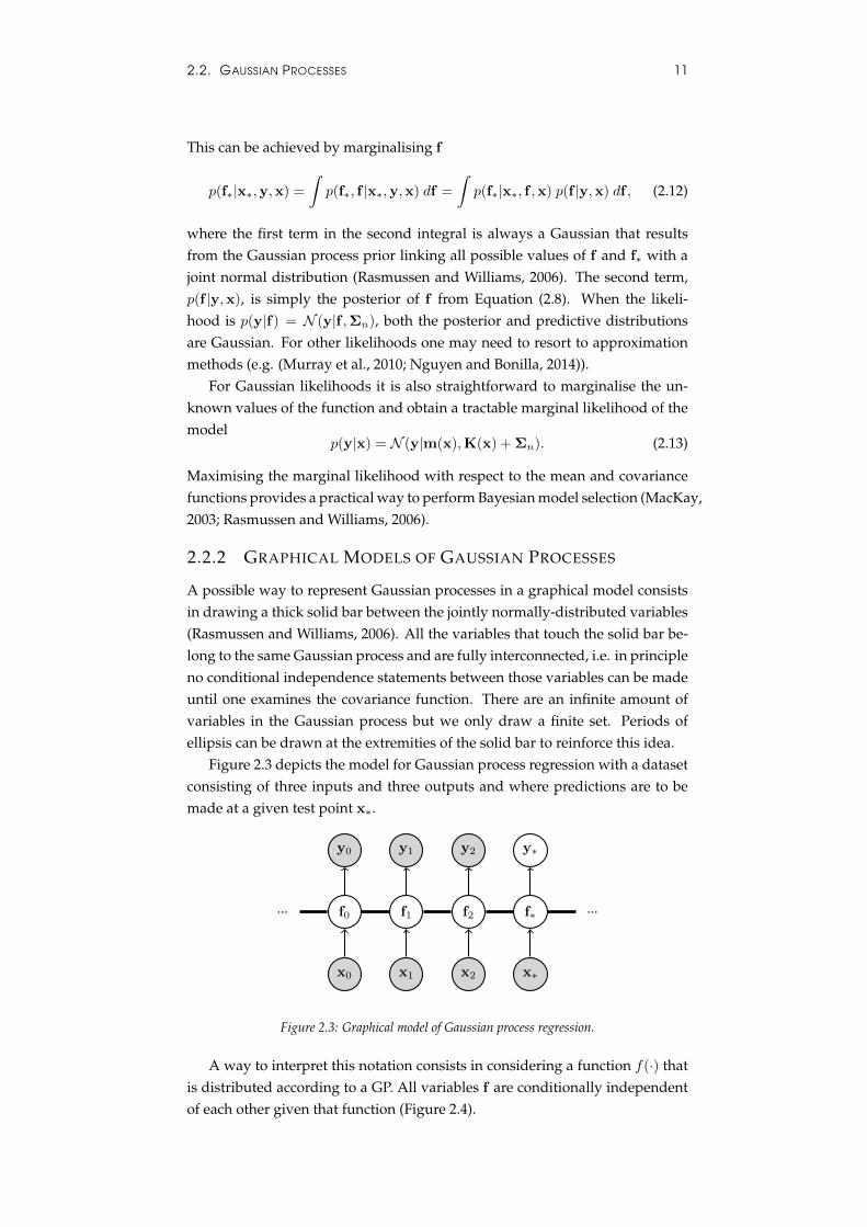
Figure 2.3 depicts the model for Gaussian process regression with a datasetconsisting of three inputs and three outputs and where predictions are to bemade at a given test point x∗.
x0 x1 x2 x∗
f0 f1 f2 f∗
y0 y1 y2 y∗
... ...
Figure 2.3: Graphical model of Gaussian process regression.
A way to interpret this notation consists in considering a function f(·) thatis distributed according to a GP. All variables f are conditionally independentof each other given that function (Figure 2.4).
12 2. TIME SERIES MODELLING WITH GAUSSIAN PROCESSES
x0 x1 x2 x∗
f0 f1 f2 f∗
y0 y1 y2 y∗
f(·)
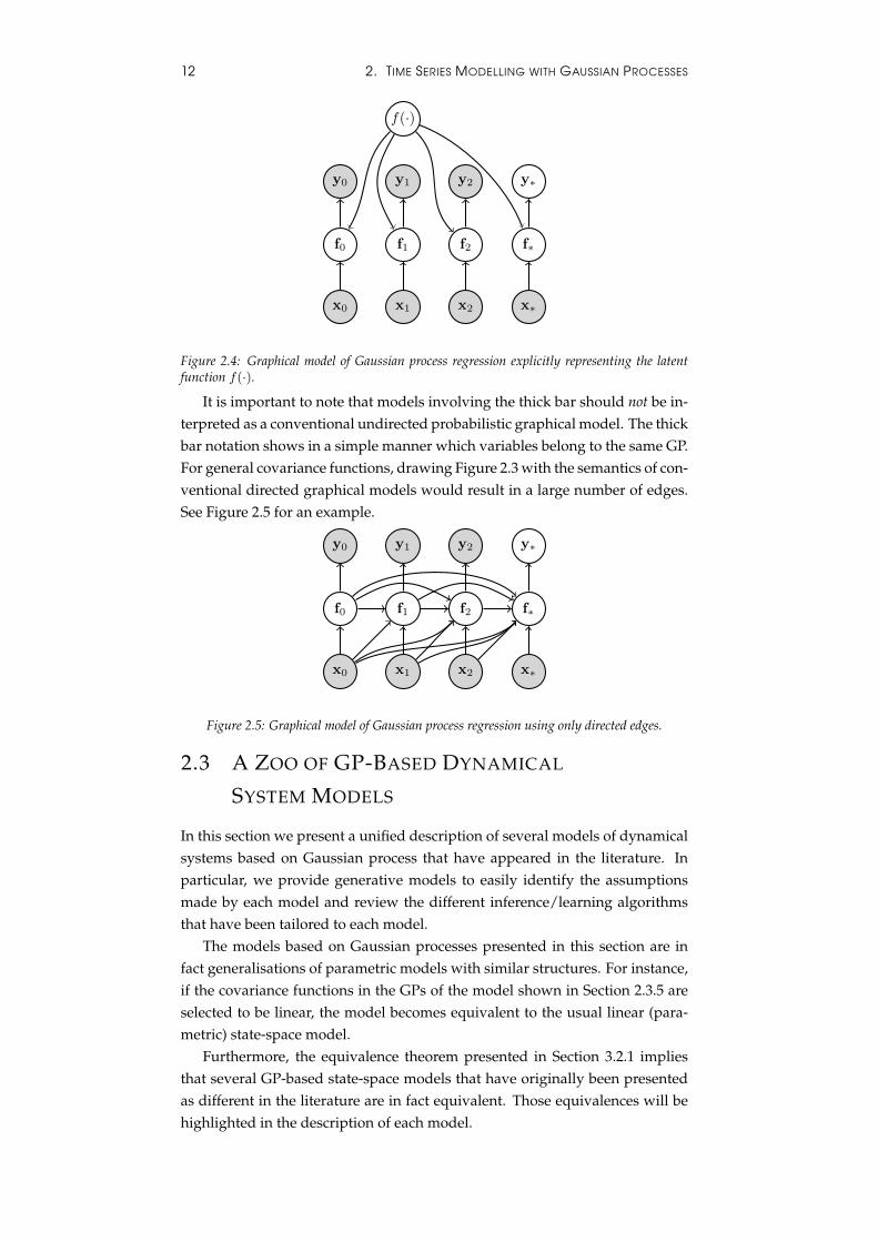
Figure 2.4: Graphical model of Gaussian process regression explicitly representing the latentfunction f(·).
It is important to note that models involving the thick bar should not be in-terpreted as a conventional undirected probabilistic graphical model. The thickbar notation shows in a simple manner which variables belong to the same GP.For general covariance functions, drawing Figure 2.3 with the semantics of con-ventional directed graphical models would result in a large number of edges.See Figure 2.5 for an example.
x0 x1 x2 x∗
f0 f1 f2 f∗
y0 y1 y2 y∗
Figure 2.5: Graphical model of Gaussian process regression using only directed edges.
2.3 A ZOO OF GP-BASED DYNAMICAL
SYSTEM MODELS
In this section we present a unified description of several models of dynamicalsystems based on Gaussian process that have appeared in the literature. Inparticular, we provide generative models to easily identify the assumptionsmade by each model and review the different inference/learning algorithmsthat have been tailored to each model.
The models based on Gaussian processes presented in this section are infact generalisations of parametric models with similar structures. For instance,if the covariance functions in the GPs of the model shown in Section 2.3.5 areselected to be linear, the model becomes equivalent to the usual linear (para-metric) state-space model.
Furthermore, the equivalence theorem presented in Section 3.2.1 impliesthat several GP-based state-space models that have originally been presentedas different in the literature are in fact equivalent. Those equivalences will behighlighted in the description of each model.
2.3. A ZOO OF GP-BASED DYNAMICAL SYSTEM MODELS 13
2.3.1 LINEAR-GAUSSIAN TIME SERIES MODEL
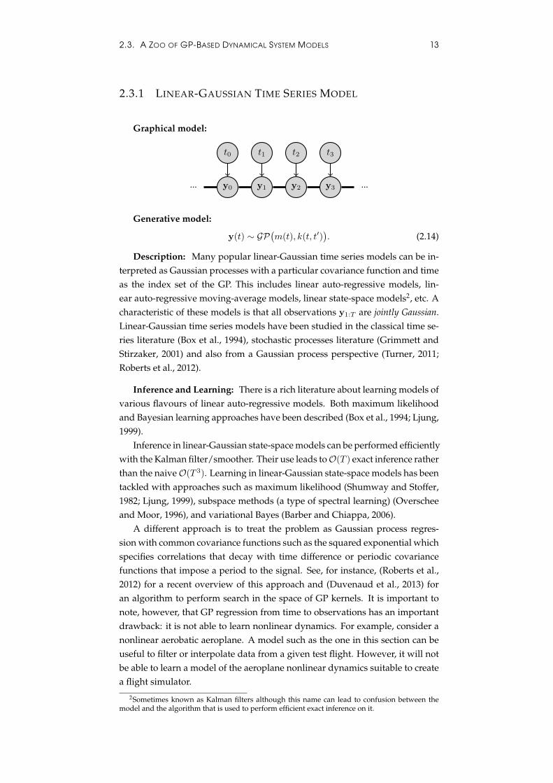
Graphical model:
t0 t1 t2 t3
y0 y1 y2 y3... ...
Generative model:
y(t) ∼ GP(m(t), k(t, t′)
). (2.14)
Description: Many popular linear-Gaussian time series models can be in-terpreted as Gaussian processes with a particular covariance function and timeas the index set of the GP. This includes linear auto-regressive models, lin-ear auto-regressive moving-average models, linear state-space models2, etc. Acharacteristic of these models is that all observations y1:T are jointly Gaussian.Linear-Gaussian time series models have been studied in the classical time se-ries literature (Box et al., 1994), stochastic processes literature (Grimmett andStirzaker, 2001) and also from a Gaussian process perspective (Turner, 2011;Roberts et al., 2012).
Inference and Learning: There is a rich literature about learning models ofvarious flavours of linear auto-regressive models. Both maximum likelihoodand Bayesian learning approaches have been described (Box et al., 1994; Ljung,1999).
Inference in linear-Gaussian state-space models can be performed efficientlywith the Kalman filter/smoother. Their use leads toO(T ) exact inference ratherthan the naiveO(T 3). Learning in linear-Gaussian state-space models has beentackled with approaches such as maximum likelihood (Shumway and Stoffer,1982; Ljung, 1999), subspace methods (a type of spectral learning) (Overscheeand Moor, 1996), and variational Bayes (Barber and Chiappa, 2006).
A different approach is to treat the problem as Gaussian process regres-sion with common covariance functions such as the squared exponential whichspecifies correlations that decay with time difference or periodic covariancefunctions that impose a period to the signal. See, for instance, (Roberts et al.,2012) for a recent overview of this approach and (Duvenaud et al., 2013) foran algorithm to perform search in the space of GP kernels. It is important tonote, however, that GP regression from time to observations has an importantdrawback: it is not able to learn nonlinear dynamics. For example, consider anonlinear aerobatic aeroplane. A model such as the one in this section can beuseful to filter or interpolate data from a given test flight. However, it will notbe able to learn a model of the aeroplane nonlinear dynamics suitable to createa flight simulator.
2Sometimes known as Kalman filters although this name can lead to confusion between themodel and the algorithm that is used to perform efficient exact inference on it.
14 2. TIME SERIES MODELLING WITH GAUSSIAN PROCESSES
2.3.2 NONLINEAR AUTO-REGRESSIVE MODEL WITH GP
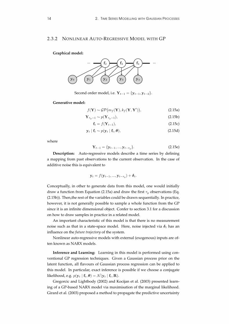
Graphical model:
y0 y1 y2 y3 y4
f2 f3 f4... ...
Second order model, i.e. Yt−1 = {yt−1,yt−2}.
Generative model:
f(Y) ∼ GP(mf (Y), kf (Y,Y′)
), (2.15a)
Yτy−1 ∼ p(Yτy−1), (2.15b)
ft = f(Yt−1), (2.15c)
yt | ft ∼ p(yt | ft,θ), (2.15d)
whereYt−1 = {yt−1, ...,yt−τy}. (2.15e)
Description: Auto-regressive models describe a time series by defininga mapping from past observations to the current observation. In the case ofadditive noise this is equivalent to
yt = f(yt−1, ...,yt−τy ) + δt.
Conceptually, in other to generate data from this model, one would initiallydraw a function from Equation (2.15a) and draw the first τy observations (Eq.(2.15b)). Then,the rest of the variables could be drawn sequentially. In practice,however, it is not generally possible to sample a whole function from the GPsince it is an infinite dimensional object. Confer to section 3.1 for a discussionon how to draw samples in practice in a related model.
An important characteristic of this model is that there is no measurementnoise such as that in a state-space model. Here, noise injected via δt has aninfluence on the future trajectory of the system.
Nonlinear auto-regressive models with external (exogenous) inputs are of-ten known as NARX models.
Inference and Learning: Learning in this model is performed using con-ventional GP regression techniques. Given a Gaussian process prior on thelatent function, all flavours of Gaussian process regression can be applied tothis model. In particular, exact inference is possible if we choose a conjugatelikelihood, e.g. p(yt | ft,θ) = N (yt | ft,R).
Gregorcic and Lightbody (2002) and Kocijan et al. (2003) presented learn-ing of a GP-based NARX model via maximisation of the marginal likelihood.Girard et al. (2003) proposed a method to propagate the predictive uncertainty

2.3. A ZOO OF GP-BASED DYNAMICAL SYSTEM MODELS 15
in GP-based NARX models for multiple-step ahead forecasting. More recently,Gutjahr et al. (2012) have proposed the use of sparse Gaussian processes inorder to reduce computational complexity and to scale to time series with mil-lions of data points.
16 2. TIME SERIES MODELLING WITH GAUSSIAN PROCESSES
2.3.3 STATE-SPACE MODEL WITH TRANSITION GP
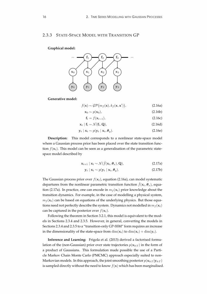
Graphical model:
x0 x1 x2 x3
f1 f2 f3... ...
y0 y1 y2 y3
Generative model:
f(x) ∼ GP(mf (x), kf (x,x′)
), (2.16a)
x0 ∼ p(x0), (2.16b)
ft = f(xt−1), (2.16c)
xt | ft ∼ N (ft,Q), (2.16d)
yt | xt ∼ p(yt | xt,θy). (2.16e)
Description: This model corresponds to a nonlinear state-space modelwhere a Gaussian process prior has been placed over the state transition func-tion f(xt). This model can be seen as a generalisation of the parametric state-space model described by
xt+1 | xt ∼ N (f(xt,θx),Q), (2.17a)
yt | xt ∼ p(yt | xt,θy). (2.17b)
The Gaussian process prior over f(xt), equation (2.16a), can model systematicdepartures from the nonlinear parametric transition function f(xt,θx), equa-tion (2.17a). In practice, one can encode in mf (xt) prior knowledge about thetransition dynamics. For example, in the case of modelling a physical system,mf (xt) can be based on equations of the underlying physics. But those equa-tions need not perfectly describe the system. Dynamics not modelled inmf (xt)
can be captured in the posterior over f(xt).Following the theorem in Section 3.2.1, this model is equivalent to the mod-
els in Sections 2.3.4 and 2.3.5. However, in general, converting the models inSections 2.3.4 and 2.3.5 to a “transition-only GP-SSM” form requires an increasein the dimensionality of the state-space from dim(xt) to dim(xt) + dim(yt).
Inference and Learning: Frigola et al. (2013) derived a factorised formu-lation of the (non-Gaussian) prior over state trajectories p(x0:T ) in the form ofa product of Gaussians. This formulation made possible the use of a Parti-cle Markov Chain Monte Carlo (PMCMC) approach especially suited to non-Markovian models. In this approach, the joint smoothing posterior p(x0:T |y0:T )
is sampled directly without the need to know f(x) which has been marginalised.
2.3. A ZOO OF GP-BASED DYNAMICAL SYSTEM MODELS 17
Note that this is markedly different to the conventional approach in parametricmodels where the smoothing distribution is obtained conditioned on a modelof the dynamics. A related approach seeking a maximum (marginal) likelihoodestimate of the hyper-parameters via Stochastic Approximation EM was pre-sented in (Frigola et al., 2014b). Finding point estimates of the hyper-parameterscan be particularly useful when it is not obvious how to specify a prior overthose parameters, e.g. for the inducing input locations in sparse GPs. Chap-ter 4 provides an expanded exposition of those learning methods based onPMCMC.
McHutchon and Rasmussen (2014) and McHutchon (2014) used a paramet-ric model for the state transition function inspired by the form of a GP regres-sion posterior akin to that presented in (Turner et al., 2010). They comparedseveral inference and learning schemes based on analytic approximations andsampling. Learning was performed by finding maximum likelihood estimatesof the parameters of the state transition function and the hyper-parameters.
Wu et al. (2014) used a state-space model with transition GP to model volatil-ities in a financial time-series setting. They presented an online inference andlearning algorithm based on particle filtering.
18 2. TIME SERIES MODELLING WITH GAUSSIAN PROCESSES
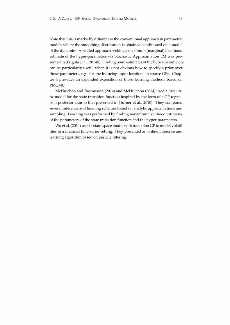
2.3.4 STATE-SPACE MODEL WITH EMISSION GP
Graphical model:
x0 x1 x2 x3
g0 g1 g2 g3... ...
y0 y1 y2 y3
Generative model:
g(x) ∼ GP(mg(x), kg(x,x
′)), (2.18a)
x0 ∼ p(x0), (2.18b)
xt+1 | xt ∼ p(xt+1 | xt,θx), (2.18c)
gt = g(xt), (2.18d)
yt | gt ∼ p(yt | gt,θy). (2.18e)
Description: As opposed to the state-space model with transition GP, inthis model the state transition has a parametric form whereas a GP prior isplaced over the emission function g(x).
If p(yt | gt,θy) = N (yt | gt,R) it is possible to analytically marginalise g(x)
to obtain a Gaussian likelihood p(y0:T | x0:T ) with a potentially non-diagonalcovariance matrix.
Following the theorem in Section 3.2.1, this model is equivalent to the tran-sition GP model (Section 2.3.3). Moreover, if the parametric state transition inthis model is linear-Gaussian, it can be considered a special case of the GP-LVMwith GP on the latent variables (Section 2.3.7).
Inference and Learning: Ferris et al. (2007) introduced this model as a GP-LVM with a Markovian parametric density on the latent variables. The modelwas learnt by finding maximum a posteriori (MAP) estimates of the states.
2.3. A ZOO OF GP-BASED DYNAMICAL SYSTEM MODELS 19
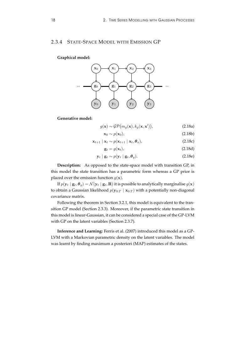
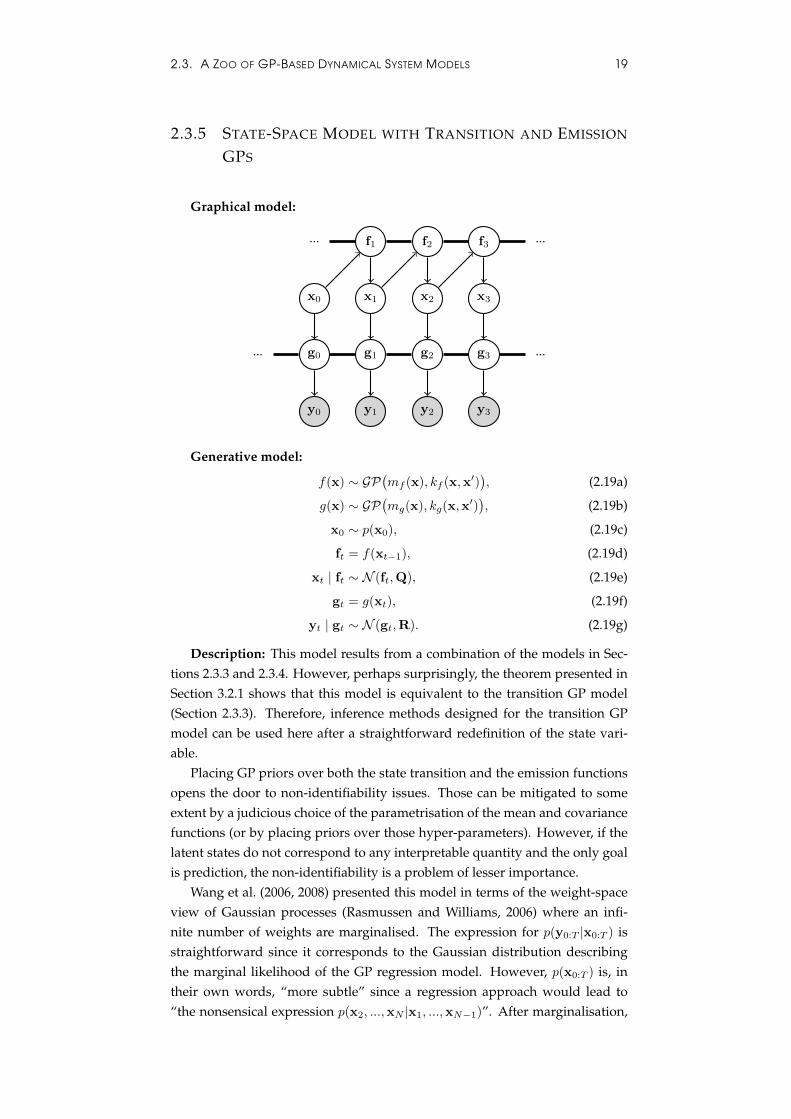
2.3.5 STATE-SPACE MODEL WITH TRANSITION AND EMISSION
GPS
Graphical model:
x0 x1 x2 x3
f1 f2 f3... ...
g0 g1 g2 g3... ...
y0 y1 y2 y3
Generative model:
f(x) ∼ GP(mf (x), kf (x,x′)
), (2.19a)
g(x) ∼ GP(mg(x), kg(x,x
′)), (2.19b)
x0 ∼ p(x0), (2.19c)
ft = f(xt−1), (2.19d)
xt | ft ∼ N (ft,Q), (2.19e)
gt = g(xt), (2.19f)
yt | gt ∼ N (gt,R). (2.19g)
Description: This model results from a combination of the models in Sec-tions 2.3.3 and 2.3.4. However, perhaps surprisingly, the theorem presented inSection 3.2.1 shows that this model is equivalent to the transition GP model(Section 2.3.3). Therefore, inference methods designed for the transition GPmodel can be used here after a straightforward redefinition of the state vari-able.
Placing GP priors over both the state transition and the emission functionsopens the door to non-identifiability issues. Those can be mitigated to someextent by a judicious choice of the parametrisation of the mean and covariancefunctions (or by placing priors over those hyper-parameters). However, if thelatent states do not correspond to any interpretable quantity and the only goalis prediction, the non-identifiability is a problem of lesser importance.
Wang et al. (2006, 2008) presented this model in terms of the weight-spaceview of Gaussian processes (Rasmussen and Williams, 2006) where an infi-nite number of weights are marginalised. The expression for p(y0:T |x0:T ) isstraightforward since it corresponds to the Gaussian distribution describingthe marginal likelihood of the GP regression model. However, p(x0:T ) is, intheir own words, “more subtle” since a regression approach would lead to“the nonsensical expression p(x2, ...,xN |x1, ...,xN−1)”. After marginalisation,
20 2. TIME SERIES MODELLING WITH GAUSSIAN PROCESSES
Wang et al. obtain an analytic expression for the non-Gaussian p(x0:T ). InChapter 3 of this dissertation, we provide an alternative derivation of p(x0:T )
which leads to a number of insights on the model that we use to derive newlearning algorithms.
Inference and Learning: Wang et al. (2006) obtained a MAP estimate ofthe latent state trajectory. Later, in (Wang et al., 2008), they report that MAPlearning is prone to overfitting for high-dimensional states and suggest twosolutions: 1) a non-probabilistic regularisation of the latent variables, and 2)maximising the marginal likelihood with Monte Carlo Expectation Maximi-sation where the joint smoothing distribution is sampled using HamiltonianMonte Carlo.
Ko and Fox (2011) use weak labels of the state to obtain a MAP estimateof the state trajectory and hyper-parameters. The weak labels of the state areactually direct observations of the state contaminated with Gaussian noise.Somehow, this is not the spirit of the model which should “discover” whatthe state representation is given any sort of observations. In other words,weak labels are nothing else than a particular type of observation that givesa glimpse into what the state actually is. (Note that Ko and Fox (2011) hasa crucial technical problem in its Equation 14 which leads to the expressionp(x2, ...,xN−1,xN |x1,x2, ...,xN−1) that Wang et al. (2006) had successfully sidestepped.In Chapter 3 of this thesis we provide a novel formulation of the model thatsheds light on this issue.)
Turner et al. (2010) presented an approach to learn a model based on thestate-space model with transition an emission GPs. They propose a parametricmodel for the latent functions f(x) and g(x) that takes the form of a posteriorfrom Gaussian process regression whose input and output “datasets” are pa-rameters to be tuned. A point estimate of the parameters for f(x) and g(x)
is learnt via maximum likelihood with Expectation Maximisation while treat-ing the state trajectory as latent variables. Several approaches for filtering andsmoothing in this kind of models have been developed (Deisenroth et al., 2012;Deisenroth and Mohamed, 2012; McHutchon, 2014). A related model was pre-sented in (Ghahramani and Roweis, 1999) where the nonlinear latent functionstake the shape of Gaussian radial basis functions (RBFs) and learning is per-formed with the EM algorithm using an Extended Kalman Smoother for theE-step.
2.3. A ZOO OF GP-BASED DYNAMICAL SYSTEM MODELS 21
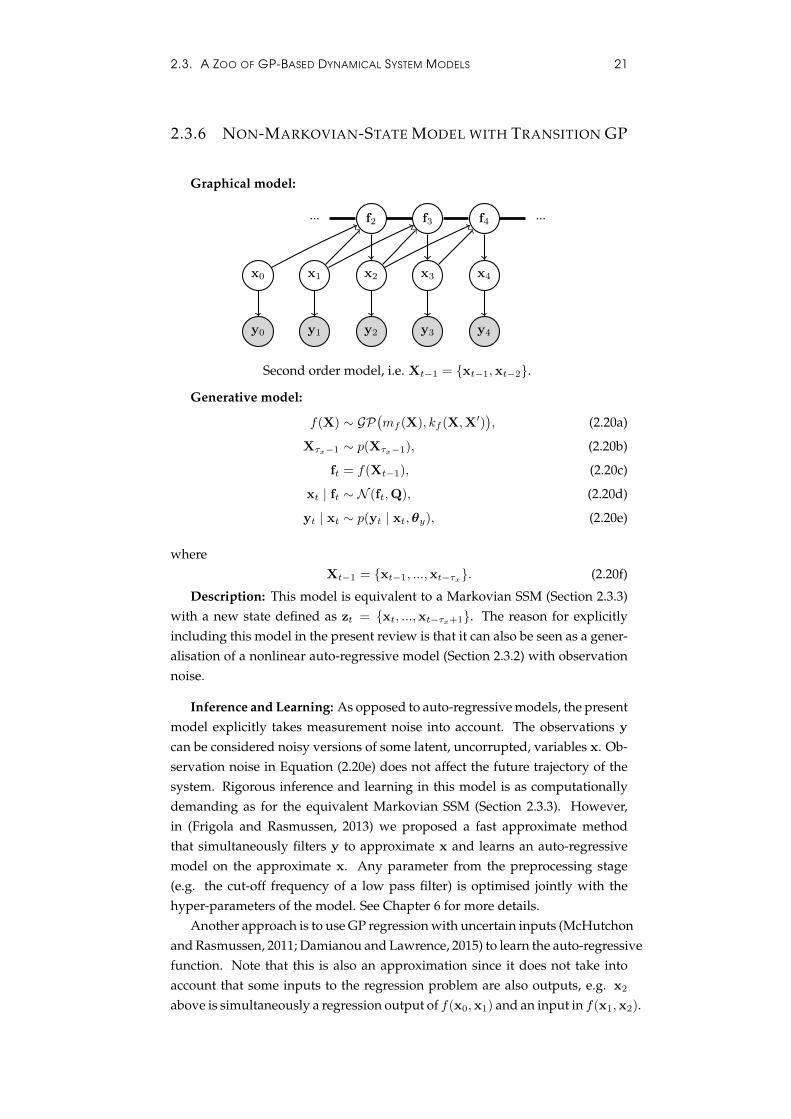
2.3.6 NON-MARKOVIAN-STATE MODEL WITH TRANSITION GP
Graphical model:
x0 x1 x2 x3 x4
y0 y1 y2 y3 y4
f2 f3 f4... ...
Second order model, i.e. Xt−1 = {xt−1,xt−2}.
Generative model:
f(X) ∼ GP(mf (X), kf (X,X′)
), (2.20a)
Xτx−1 ∼ p(Xτx−1), (2.20b)
ft = f(Xt−1), (2.20c)
xt | ft ∼ N (ft,Q), (2.20d)
yt | xt ∼ p(yt | xt,θy), (2.20e)
whereXt−1 = {xt−1, ...,xt−τx}. (2.20f)
Description: This model is equivalent to a Markovian SSM (Section 2.3.3)with a new state defined as zt = {xt, ...,xt−τx+1}. The reason for explicitlyincluding this model in the present review is that it can also be seen as a gener-alisation of a nonlinear auto-regressive model (Section 2.3.2) with observationnoise.
Inference and Learning: As opposed to auto-regressive models, the presentmodel explicitly takes measurement noise into account. The observations y
can be considered noisy versions of some latent, uncorrupted, variables x. Ob-servation noise in Equation (2.20e) does not affect the future trajectory of thesystem. Rigorous inference and learning in this model is as computationallydemanding as for the equivalent Markovian SSM (Section 2.3.3). However,in (Frigola and Rasmussen, 2013) we proposed a fast approximate methodthat simultaneously filters y to approximate x and learns an auto-regressivemodel on the approximate x. Any parameter from the preprocessing stage(e.g. the cut-off frequency of a low pass filter) is optimised jointly with thehyper-parameters of the model. See Chapter 6 for more details.
Another approach is to use GP regression with uncertain inputs (McHutchonand Rasmussen, 2011; Damianou and Lawrence, 2015) to learn the auto-regressivefunction. Note that this is also an approximation since it does not take intoaccount that some inputs to the regression problem are also outputs, e.g. x2
above is simultaneously a regression output of f(x0,x1) and an input in f(x1,x2).
22 2. TIME SERIES MODELLING WITH GAUSSIAN PROCESSES
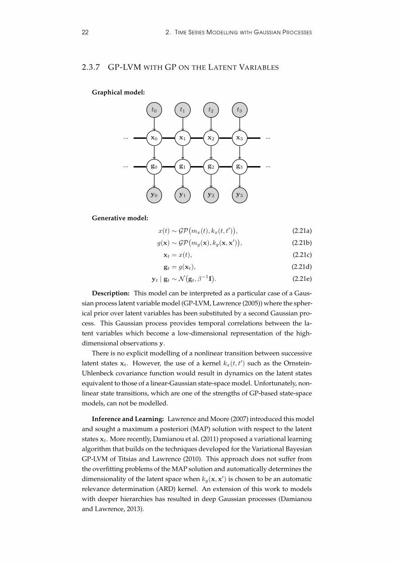
2.3.7 GP-LVM WITH GP ON THE LATENT VARIABLES
Graphical model:
t0 t1 t2 t3
x0 x1 x2 x3... ...
g0 g1 g2 g3... ...
y0 y1 y2 y3
Generative model:
x(t) ∼ GP(mx(t), kx(t, t′)
), (2.21a)
g(x) ∼ GP(mg(x), kg(x,x
′)), (2.21b)
xt = x(t), (2.21c)
gt = g(xt), (2.21d)
yt | gt ∼ N(gt, β
−1I). (2.21e)
Description: This model can be interpreted as a particular case of a Gaus-sian process latent variable model (GP-LVM, Lawrence (2005)) where the spher-ical prior over latent variables has been substituted by a second Gaussian pro-cess. This Gaussian process provides temporal correlations between the la-tent variables which become a low-dimensional representation of the high-dimensional observations y.
There is no explicit modelling of a nonlinear transition between successivelatent states xt. However, the use of a kernel kx(t, t′) such as the Ornstein-Uhlenbeck covariance function would result in dynamics on the latent statesequivalent to those of a linear-Gaussian state-space model. Unfortunately, non-linear state transitions, which are one of the strengths of GP-based state-spacemodels, can not be modelled.
Inference and Learning: Lawrence and Moore (2007) introduced this modeland sought a maximum a posteriori (MAP) solution with respect to the latentstates xt. More recently, Damianou et al. (2011) proposed a variational learningalgorithm that builds on the techniques developed for the Variational BayesianGP-LVM of Titsias and Lawrence (2010). This approach does not suffer fromthe overfitting problems of the MAP solution and automatically determines thedimensionality of the latent space when kg(x,x′) is chosen to be an automaticrelevance determination (ARD) kernel. An extension of this work to modelswith deeper hierarchies has resulted in deep Gaussian processes (Damianouand Lawrence, 2013).
2.4. WHY GAUSSIAN PROCESS STATE-SPACE MODELS? 23
Latent force models (Alvarez et al., 2009, 2013) can also be interpreted asa particular case of GP-LVM with a GP on the latent variables. The variablesx in the top layer are the latent forces whereas the g layer encodes the linear-Gaussian stochastic differential equation of the latent force model.
2.4 WHY GAUSSIAN PROCESS STATE-SPACE MOD-
ELS?
Gaussian Process State-Space Models are particularly appealing because theyenjoy the generality of nonlinear state-space models together with the flexi-ble prior over the transition function provided by the Gaussian process. Asopposed to auto-regressive models, the presence of a latent state allows for asuccinct representation of the dynamics in the form of a Markov chain. Thestate needs to contain only the information about the system that is essential todetermine its future trajectory. As a consequence, discovering a state represen-tation for a system provides useful insights about its nature since it decouplesthe observations that happen to be available from the dynamics.
A related advantage of state-space models over auto-regressive ones is thatobservation noise can be explicitly taken into account. To train an auto-regressivemodel, a time series is broken down into a set of input/output pairs and thefunction mapping inputs to outputs is learnt with regression techniques. Onecould use noise-in-the-inputs regression (also known as errors-in-variables) todeal with observation noise. However, this would fail to exploit the fact thatthe particular noise realisation affecting the observation yt is the same whenusing yt as an input or as an output. When learning a state-space model,the time series is not broken down into input/output pairs and inference andlearning are performed in a way that coherently takes into account observationnoise. This will be clearer in the learning algorithms of the following chapters.

24 2. TIME SERIES MODELLING WITH GAUSSIAN PROCESSES
Chapter 3
Gaussian Process State-SpaceModels – Description
”Trying to understand a hidden Markov model from its observed time se-ries is like trying to figure out the workings of a noisy machine from look-ing at the shadows its moving parts cast on a wall, with the proviso thatthe shadows are cast by a randomly-flickering candle.”
Shalizi (2008)
This chapter presents a novel formalisation of Gaussian Process State-SpaceModels (GP-SSMs). In particular, we go beyond describing the joint probabil-ity of the model and provide a practical approach to generate samples from itsprior. The insights provided by the new description of GP-SSMs will be ex-ploited in the next chapters to derive learning and inference methods adaptedto the characteristics of the model. In addition, we present an equivalence re-sult stating that GP-SSMs with GP priors on the transition and emission func-tions can be reformulated into GP-SSMs with a GP only on the state transitionfunction.
3.1 GP-SSM WITH STATE TRANSITION GP
As presented in Section 2.3, there exist many flavours of GP-SSMs. For clarity,in this section we shall restrict ourselves to a GP-SSM which has a Gaussianprocess prior on the transition function but a parametric density to describe thelikelihood (i.e. the model introduced in Section 2.3.3). This particular modelcontains the main feature that has made GP-SSMs hard to describe rigorously:the states are simultaneously inputs and outputs of the state transition func-tion. In other words, we want to learn a function whose inputs and outputs arenot only latent but also connected in a chain-like manner.
Given an observed time series {y1, ...,yT }, we construct a stochastic model
25
26 3. GAUSSIAN PROCESS STATE-SPACE MODELS – DESCRIPTION
that attempts to explain it by defining a chain of latent states {x0, ...,xT }
xt | xt−1 ∼ N (xt | f(xt−1),Q), (3.1a)
yt | xt ∼ p(yt | xt,θy), (3.1b)
where f(·) in an unknown nonlinear state transition function and Q and θy areparameters of the state transition density and likelihood respectively. A com-mon way to learn the unknown state transition function is to define a para-metric form for it and proceed to learn its parameters. Common choices forparametric state transition functions are linear functions (Shumway and Stof-fer, 1982), radial basis functions (RBFs) (Ghahramani and Roweis, 1999) andother types of neural networks.
GP-SSMs do not restrict the state transition function to a particular parame-terised class of functions. Instead, they place a Gaussian process prior over theinfinite-dimensional space of functions. This prior can encode assumptionssuch as continuity or smoothness. In fact, with an appropriate choice of thecovariance function, the GP prior puts probability mass over all continuousfunctions (Micchelli et al., 2006). In other words, as opposed to parameterisedfunctions, GPs do not restrict a priori the class of continuous functions that canbe learnt provided that one uses covariance functions that are universal kernels(Micchelli et al., 2006). The squared exponential is an example of such a kernel.
The generative model for a GP-SSM with a GP prior over the state transitionfunction and an arbitrary parametric likelihood is
f(x) ∼ GP(m(x), k(x,x′)
), (3.2a)
x0 ∼ p(x0), (3.2b)
ft = f(xt−1), (3.2c)
xt | ft ∼ N (xt | ft,Q), (3.2d)
yt | xt ∼ p(yt | xt,θy). (3.2e)
In order to get an intuitive understanding of this model, it can be useful todevise a method to generate synthetic data from it. An idealised approach togenerate data from a GP-SSM could consist in first sampling a state transitionfunction (i.e. an infinite-dimensional object) from the GP. This only needs tohappen once. Then the full sequence of states can be generated by first sam-pling the initial state x0 and then sequentially sampling the rest of the chain{f1,x1, ..., fT ,xT }. Each observation yt can be sampled conditioned on its cor-responding state xt.
However, this idealised sampling procedure can not be implemented inpractice. The reason for this is that it is not possible to sample an infinite-dimensional function and store it in memory. Instead, we will go back to thedefinition of a Gaussian process and define a practical sampling procedure forthe GP-SSM.
A Gaussian process is defined as a collection of random variables, any finite
3.1. GP-SSM WITH STATE TRANSITION GP 27
number of which have a joint Gaussian distribution (Rasmussen and Williams,2006). However, in a GP-SSM, there is additional structure linking the vari-ables. A sequential sampling procedure provides insight into what this struc-ture is. To sample ft, instead of conditioning on an infinite-dimensional func-tion, we condition only on the transitions {xi−1, fi}t−1
i=1 seen up to that point.For a zero-mean GP
x0 ∼ p(x0), (3.3a)
f1 | x0 ∼ N (f1 | 0, k(x0,x0)) , (3.3b)
x1 | f1 ∼ N (x1 | f1,Q), (3.3c)
f2 | f1,x0:1 ∼ N (f2 | k(x1,x0)k(x0,x0)−1f1,
k(x1,x1)− k(x1,x0)k(x0,x0)−1k(x0,x1)), (3.3d)
x2 | f2 ∼ N (x2 | f2,Q), (3.3e)
f3 | f1:2,x0:2 ∼ N (f3 | [k(x2,x0) k(x2,x1)]
[k(x0,x0) k(x0,x1)
k(x1,x0) k(x1,x1)
]−1 [f1
f2
],
k(x2,x2)− [k(x2,x0) k(x2,x1)]
[k(x0,x0) k(x0,x1)
k(x1,x0) k(x1,x1)
]−1 [k(x0,x2)
k(x1,x2)
]),
(3.3f)
...
Since this notation is very cumbersome, we will use the shorthand notationfor kernel matrices
Ki:j,k:l ,
k(xi,xk) . . . k(xi,xl)
......
k(xj ,xk) . . . k(xj ,xl)
, (3.4)
and Ki:j , Ki:j,i:j . Note that the covariance function k(·, ·) returns a matrixof the same size as the state in an analogous manner to multi-output Gaussianprocesses (Rasmussen and Williams, 2006). With this notation, equations (3.3)become
x0 ∼ p(x0), (3.5a)
f1 | x0 ∼ N (f1 | 0,K0) , (3.5b)
x1 | f1 ∼ N (x1 | f1,Q), (3.5c)
f2 | f1,x0:1 ∼ N (f2 | K1,0K−10 f1, K1,1 −K1,0K
−10 K0,1), (3.5d)
x2 | f2 ∼ N (x2 | f2,Q), (3.5e)
f3 | f1:2,x0:2 ∼ N (f3 | K2,0:1K−10:1f1:2, K2,2 −K2,0:1K
−10:1K0:1,2), (3.5f)
...
28 3. GAUSSIAN PROCESS STATE-SPACE MODELS – DESCRIPTION
0
time
stat
es0
time
0
time
0
time
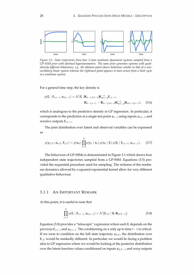
Figure 3.1: State trajectories from four 2-state nonlinear dynamical systems sampled from aGP-SSM prior with identical hyperparameters. The same prior generates systems with quali-tatively different behaviours, e.g. the leftmost panel shows behaviour similar to that of a non-oscillatory linear system whereas the rightmost panel appears to have arisen from a limit cyclein a nonlinear system.
For a general time step, the key density is
p(ft | f1:t−1,x0:t−1) = N (ft |Kt−1,0:t−2K−10:t−2f1:t−1,
Kt−1,t−1 −Kt−1,0:t−2K−10:t−2K0:t−2,t−1), (3.6)
which is analogous to the predictive density in GP regression. In particular, itcorresponds to the prediction at a single test point xt−1 using inputs x0:t−2 andnoiseless outputs f1:t−1.
The joint distribution over latent and observed variables can be expressedas
p(y1:T ,x0:T , f1:T ) = p(x0)
T∏t=1
p(yt | xt) p(xt | ft) p(ft | f1:t−1,x0:t−1). (3.7)
The behaviour of GP-SSMs is demonstrated in Figure 3.1 which shows fourindependent state trajectories sampled from a GP-SSM. Equations (3.5) pro-vided the sequential procedure used for sampling. The richness of the nonlin-ear dynamics allowed by a squared exponential kernel allow for very differentqualitative behaviour.
3.1.1 AN IMPORTANT REMARK
At this point, it is useful to note that
T∏t=1
p(ft | f1:t−1,x0:t−1) = N(f1:T | 0,K0:T−1
). (3.8)
Equation (3.8) provides a “telescopic” expression where each ft depends on theprevious f1:t−1 and x0:t−1. The conditioning on x only up to time t−1 is critical.If we were to condition on the full state trajectory x0:T , the distribution overf1:T would be markedly different. In particular, we would be facing a problemakin to GP regression where we would be looking at the posterior distributionover the latent function values conditioned on inputs x0:T−1 and noisy outputs
3.1. GP-SSM WITH STATE TRANSITION GP 29
x1:T
p(f1:T | x0:T ) = N(f1:T |K0:T−1K
−10:T−1x1:T ,
K0:T−1 −K0:T−1K−10:T−1K
>0:T−1
), (3.9)
with K0:T−1 , K0:T−1 + IT ⊗Q. As one could expect, this expression reducesto f1:T = x1:T if Q = 0.
We can summarise the previous argument by stating that
T∏t=1
p(ft | f1:t−1,x0:t−1) = N(f1:T | 0,K0:T−1
)6= p(f1:T | x0:T ). (3.10)
For completeness, we provide the expressions for an arbitrary mean func-tion where we use m0:t , [m(x0)>, ...,m(xt)
>]>:
T∏t=1
p(ft | f1:t−1,x0:t−1) = N(f1:T |m0:T−1,K0:T−1
), (3.11)
and
p(f1:T | x0:T ) = N(f1:T |m0:T−1 + K0:T−1K
−10:T−1(x1:T −m0:T−1),
K0:T−1 −K0:T−1K−10:T−1K
>0:T−1
). (3.12)
3.1.2 MARGINALISATION OF f1:T
By marginalising out the variables f1:T we will obtain a prior distribution overstate trajectories that will be particularly useful for learning GP-SSMs withsample-based approaches (Chapter 4). The density over latent variables in aGP-SSM is
p(x0:T , f1:T ) = p(x0)
T∏t=1
p(xt | ft) p(ft | f1:t−1,x0:t−1) (3.13a)
= p(x0) N (x1:T | f1:T , IT ⊗Q) N (f1:T |m0:T−1,K0:T−1). (3.13b)
Marginalising with respect to f1:T we obtain the prior distribution over thelatent state trajectory
p(x0:T ) =
∫p(x0:T , f1:T ) df1:T (3.14a)
= p(x0)
∫N (x1:T | f1:T , IT ⊗Q) N (f1:T |m0:T−1,K0:T−1) df1:T
(3.14b)
= p(x0)|(2π)nxT K0:T−1|−12 exp(−1
2(x1:T −m0:T−1)>K−1
0:T−1(x1:T −m0:T−1)),
(3.14c)
which is the density provided in (Wang et al., 2006) albeit in a slightly differentform.
30 3. GAUSSIAN PROCESS STATE-SPACE MODELS – DESCRIPTION
0.0920.0940.0960.0980.1
0.0920.094
0.0960.098
0.10.102
0.104
2000
4000
6000
8000
x1
x2
p(x 1,x
2|x0,x
3)
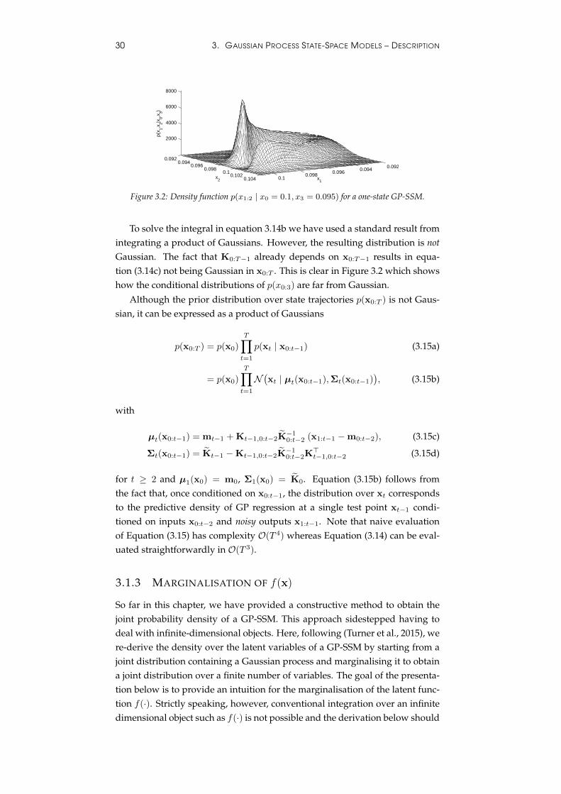
Figure 3.2: Density function p(x1:2 | x0 = 0.1, x3 = 0.095) for a one-state GP-SSM.
To solve the integral in equation 3.14b we have used a standard result fromintegrating a product of Gaussians. However, the resulting distribution is notGaussian. The fact that K0:T−1 already depends on x0:T−1 results in equa-tion (3.14c) not being Gaussian in x0:T . This is clear in Figure 3.2 which showshow the conditional distributions of p(x0:3) are far from Gaussian.
Although the prior distribution over state trajectories p(x0:T ) is not Gaus-sian, it can be expressed as a product of Gaussians
p(x0:T ) = p(x0)
T∏t=1
p(xt | x0:t−1) (3.15a)
= p(x0)
T∏t=1
N(xt | µt(x0:t−1),Σt(x0:t−1)
), (3.15b)
with
µt(x0:t−1) = mt−1 + Kt−1,0:t−2K−10:t−2 (x1:t−1 −m0:t−2), (3.15c)
Σt(x0:t−1) = Kt−1 −Kt−1,0:t−2K−10:t−2K
>t−1,0:t−2 (3.15d)
for t ≥ 2 and µ1(x0) = m0, Σ1(x0) = K0. Equation (3.15b) follows fromthe fact that, once conditioned on x0:t−1, the distribution over xt correspondsto the predictive density of GP regression at a single test point xt−1 condi-tioned on inputs x0:t−2 and noisy outputs x1:t−1. Note that naive evaluationof Equation (3.15) has complexity O(T 4) whereas Equation (3.14) can be eval-uated straightforwardly in O(T 3).
3.1.3 MARGINALISATION OF f(x)
So far in this chapter, we have provided a constructive method to obtain thejoint probability density of a GP-SSM. This approach sidestepped having todeal with infinite-dimensional objects. Here, following (Turner et al., 2015), were-derive the density over the latent variables of a GP-SSM by starting from ajoint distribution containing a Gaussian process and marginalising it to obtaina joint distribution over a finite number of variables. The goal of the presenta-tion below is to provide an intuition for the marginalisation of the latent func-tion f(·). Strictly speaking, however, conventional integration over an infinitedimensional object such as f(·) is not possible and the derivation below should
3.2. GP-SSM WITH TRANSITION AND EMISSION GPS 31
be considered just a sketch. We refer the reader to (Matthews et al., 2015) fora much more technical exposition of integration of infinite dimensional objectsin the context of sparse Gaussian processes.
We start with a joint distribution of the state trajectory and the randomfunction f(·)
p(x0:T , f(·)) = p(f(·)) p(x0)
T∏t=1
p(xt|xt−1, f(·),Q), (3.16)
and introduce new variables ft = f(xt−1) which, in probabilistic terms can bedefined as a Dirac delta p(ft | f(·),xt−1) = δ(ft − f(xt−1)).
p(x0:T , f1:T , f(·)) = p(f(·)) p(x0)
T∏t=1
p(xt|ft,Q)p(ft | f(·),xt−1), (3.17)
By integrating the latent function at every point other than x0:T−1 we obtain
p(x0:T , f1:T ) =
∫p(x0:T , f1:T , f(·)) df\x0:T−1
(3.18a)
= p(x0)
(T∏t=1
N (xt|ft,Q)
)∫p(f(·))
T∏t=1
δ(ft − f(xt−1)) df\x0:T−1
(3.18b)
= p(x0) N (x1:T | f1:T , IT ⊗Q) N (f1:T |m0:T−1,K0:T−1), (3.18c)
which recovers the joint density from equation (3.13b)
3.2 GP-SSM WITH TRANSITION AND EMISSION GPS
GP-SSMs containing a nonlinear emission function with a GP prior have alsobeen studied in the literature (see Section 2.3.5). In such a model, the nonlinearfunction g(xt) in the state-space model
xt | xt−1 ∼ N (xt | f(xt−1),Q), (3.19a)
yt | xt ∼ N (yt | g(xt),R), (3.19b)
also has a GP prior which results in a generative model described by
f(x) ∼ GP(mf (x), kf (x,x′)
), (3.20a)
g(x) ∼ GP(mg(x), kg(x,x
′)), (3.20b)
x0 ∼ p(x0), (3.20c)
ft = f(xt−1), (3.20d)
xt | ft ∼ N (xt | ft,Q), (3.20e)
gt = g(xt), (3.20f)
yt | gt ∼ N (yt | gt,R). (3.20g)
32 3. GAUSSIAN PROCESS STATE-SPACE MODELS – DESCRIPTION
This variant of GP-SSM is a straightforward extension to the one with aparametric observation model. The distribution over latent states and tran-sition function values is the same. However, an observation at time t is notconditionally independent of the rest of the observations given xt. The jointprobability distribution of this model is
p(y1:T ,g1:T ,x0:T , f1:T ) = p(x0:T , f1:T ) p(g1:T |x1:T )
T∏t=1
p(yt|gt) (3.21a)
= p(x0:T , f1:T ) N (g1:T |m(g)1:T ,K
(g)1:T )
T∏t=1
N (yt | gt,R).
(3.21b)
Where p(x0:T , f1:T ) is the same as in Equation (3.7) and m(g) and K(g) denotethe mean function vector and kernel matrix using the mean and covariancefunctions in Equation (3.20b).
3.2.1 EQUIVALENCE BETWEEN GP-SSMS
In the following, we present an equivalence result between the two GP-SSMvariants introduced in this chapter. We show how the model with nonlineari-ties for both the transition and emission functions (Sec. 2.3.5 and 3.2) is equiv-alent to a model with a redefined state-space but which only has a nonlinearfunction in the state transition (Sec. 2.3.3 and 3.1).
We consider state-space models with independent and identically distributedadditive noise
xt+1 = f(xt) + vt, (3.22a)
yt = g(xt) + et. (3.22b)
In GP-SSMs, Gaussian process priors are placed over f and g in order toperform inference on those functions.
THEOREM: The model in (3.22) is a particular case of the following model
zt+1 = h(zt) + wt, (3.23a)
yt = γγγt + et, (3.23b)
where zt , (ξξξt, γγγt) is the augmented state.
PROOF: Consider the case where
zt+1 = (ξξξt+1, γγγt+1) =(f(ξξξt), g(ξξξt)
)+ (νννt, 0). (3.24)
3.3. SPARSE GP-SSMS 33
Then, the model in (3.23) can be written as
ξξξt+1 = f(ξξξt) + νννt, (3.25a)
γγγt+1 = g(ξξξt), (3.25b)
yt = γγγt + et. (3.25c)
If we now take ξξξt = xt+1 and νννt = vt+1 and substitute them in (3.25) we obtain
xt+1 = f(xt) + vt, (3.26a)
yt = g(xt) + et. (3.26b)
COROLLARY: A learning procedure that is able to learn an unknown state tran-sition function can also be used to simultaneously learn both f(xt) and g(xt).
3.3 SPARSE GP-SSMS
Gaussian processes are very useful priors over functions that, in comparisonwith parametric models, place very few assumptions on the shapes of the un-known functions. However, this richness comes at a price: computational re-quirements for training and prediction scale unfavourably with the size of thetraining set. To alleviate this problem, methods relying on sparse Gaussian pro-cesses have been developed that retain many of the advantages of vanilla Gaus-sian processes while reducing the computational cost (Quinonero-Candela andRasmussen, 2005; Titsias, 2009; Hensman et al., 2013, 2015).
Sparse Gaussian processes often rely on a number of inducing points. Thoseinducing points, denoted by ui, are values of the unknown function at arbitrarylocations named inducing inputs
ui = f(zi). (3.27)
For conciseness of notation, we define the set with all inducing points u ,
{ui}Mi=1 and the set of their respective inducing inputs z , {zi}Mi=1. If weplace a Gaussian process prior over a function f , the inducing points are jointlyGaussian with values of the latent function at any other location
p(f ,u) = N
([f
u
] ∣∣ [mx
mz
],
[Kx Kx,z
Kz,x Kz
]). (3.28)
This method of explicitly representing the values of the function at an ad-ditional finite number of input locations z is sometimes called augmentation.However, one could argue that the model has not been augmented since the in-ducing points were “already there”; we are simply assigning a variable nameto the value of the function at input locations z.
For regression, a variety of sparse GP methods have been developed by
34 3. GAUSSIAN PROCESS STATE-SPACE MODELS – DESCRIPTION
making additional assumptions on the relationships between function valuesat the training, test and inducing inputs (Quinonero-Candela and Rasmussen,2005). More recently, a variational approach to sparse GPs (Titsias, 2009) hasresulted in sparse GP methods for a number of models (Titsias and Lawrence,2010; Damianou et al., 2011; Hensman et al., 2013, 2015).
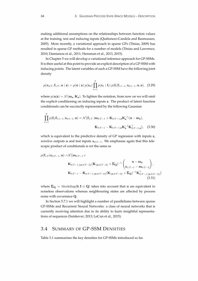
In Chapter 5 we will develop a variational inference approach for GP-SSMs.It is then useful at this point to provide an explicit description of a GP-SSM withinducing points. The latent variables of such a GP-SSM have the following jointdensity
p(x0:T , f1:T ,u | z) = p(u | z) p(x0)
T∏t=1
p(xt | ft) p(ft|f1:t−1,x0:t−1,u, z), (3.29)
where p(u|z) = N (mz,Kz). To lighten the notation, from now on we will omitthe explicit conditioning on inducing inputs z. The product of latent functionconditionals can be succinctly represented by the following Gaussian
T∏t=1
p(ft|f1:t−1,x0:t−1,u) = N(f1:T |m0:T−1 + K0:T−1,zK
−1z (u−mz),
K0:T−1 −K0:T−1,zK−1z K>0:T−1,z
), (3.30)
which is equivalent to the predictive density of GP regression with inputs z,noiseless outputs u and test inputs x0:T−1. We emphasise again that this tele-scopic product of conditionals is not the same as
p(f1:T |x0:T−1,u) =N(m0:T−1+
K0:T−1,{z,0:T−2}(K{z,0:T−2} + ΣΣΣQ)−1
(u−mz
x1:T−1 −m0:T−2
),
K0:T−1 −K0:T−1,{z,0:T−2}(K{z,0:T−2} + ΣΣΣQ)−1K>0:T−1,{z,0:T−2})
(3.31)
where ΣΣΣQ = blockdiag(0, I ⊗ Q) takes into account that u are equivalent tonoiseless observations whereas neighbouring states are affected by processnoise with covariance Q.
In Section 5.7.1 we will highlight a number of parallelisms between sparseGP-SSMs and Recurrent Neural Networks: a class of neural networks that iscurrently receiving attention due to its ability to learn insightful representa-tions of sequences (Sutskever, 2013; LeCun et al., 2015).
3.4 SUMMARY OF GP-SSM DENSITIES
Table 3.1 summarises the key densities for GP-SSMs introduced so far.
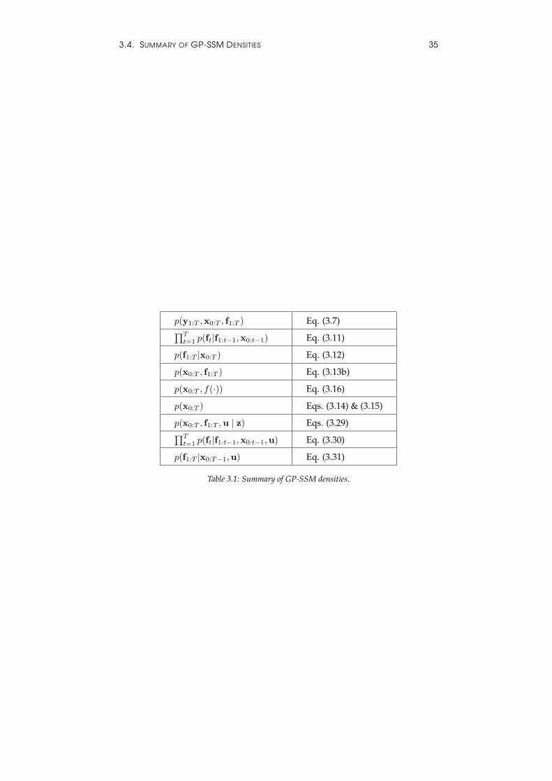
3.4. SUMMARY OF GP-SSM DENSITIES 35
p(y1:T ,x0:T , f1:T ) Eq. (3.7)∏Tt=1 p(ft|f1:t−1,x0:t−1) Eq. (3.11)
p(f1:T |x0:T ) Eq. (3.12)
p(x0:T , f1:T ) Eq. (3.13b)
p(x0:T , f(·)) Eq. (3.16)
p(x0:T ) Eqs. (3.14) & (3.15)
p(x0:T , f1:T ,u | z) Eqs. (3.29)∏Tt=1 p(ft|f1:t−1,x0:t−1,u) Eq. (3.30)
p(f1:T |x0:T−1,u) Eq. (3.31)
Table 3.1: Summary of GP-SSM densities.

36 3. GAUSSIAN PROCESS STATE-SPACE MODELS – DESCRIPTION
Chapter 4
Gaussian Process State-SpaceModels – Monte CarloLearning
This chapter exploits insights from the novel description of Gaussian ProcessState-Space Models presented so far to derive Bayesian learning methods basedon Monte Carlo sampling. In particular, we present a fully Bayesian approachto jointly sample from all variables and a related Empirical Bayes method thatfinds maximum likelihood estimates of the hyper-parameters while approxi-mately marginalising the latent state trajectories.
This chapter introduces new learning methods for GP-SSMs originally pub-lished in (Frigola et al., 2013) and (Frigola et al., 2014b) that rely on the newexpression for the prior density over the state trajectory expressed as a productof Gaussians (Equation 3.15b).
4.1 INTRODUCTION
The sampling methods presented in this chapter make heavy use of recent ad-vances in Particle Markov Chain Monte Carlo (PMCMC). In contrast to priorwork on learning GP-SSMs, we do not restrict ourselves to the case where thedimensionality of the state-space is much lower than that of the observationspace.
The key feature of our approach is that we sample from the smoothingdistribution while the nonlinear dynamics are marginalised out. In other words,samples from the posterior over state trajectories are obtained without hav-ing to specify the dynamics of the system. This contrasts with conventionalapproaches to smoothing where the smoothing distribution is conditioned onfixed dynamics (Barber et al., 2011; Murphy, 2012).
The main advantage of Monte Carlo methods over approaches such as vari-ational inference (Chapter 5) is that they do not rely on assumptions about the
37
38 4. GAUSSIAN PROCESS STATE-SPACE MODELS – MONTE CARLO LEARNING
shape of the posterior. Therefore, they are useful as a gold standard againstwhich to compare other learning algorithms. In terms of practical application,however, they tend to suffer from longer computation time, in particular whendoing predictions.
4.2 FULLY BAYESIAN LEARNING
This section introduces a fully Bayesian approach to learning GP-SSMs. Learn-ing the state transition function in a GP-SSM is particularly challenging be-cause the states are not observed. The goal is to learn a function where bothits inputs and outputs are latent variables. Most previous approaches, see(McHutchon, 2014) for an overview, hinge on learning a parametric approx-imation to a GP-SSM. We address this problem in a fundamentally differentway that keeps alive all the nonparametric richness of the model.
Our approach is based on the key observation that learning the transitionfunction in a GP-SSM is equivalent to finding the smoothing distribution in thatmodel. In other words, once the smoothing distribution p(x0:T | y1:T ,θ) hasbeen found, the posterior over the state transition function can be straightfor-wardly computed. The predictive distribution over f∗ = f(x∗), evaluated at anarbitrary test point x∗, is
p(f∗ | x∗,y1:T ,θ) =
∫p(f∗ | x∗,x0:T ,θ) p(x0:T | y1:T ,θ) dx0:T , (4.1)
where the distribution p(f∗ | x∗,x0:T ,θ) is equivalent to the predictive distri-bution in Gaussian process regression using x0:T−1 as inputs and x1:T as noisyoutputs.
In practice, there are a number of parameters in a GP-SSM that we wouldlike to learn from data: hyper-parameters of the GP, covariance matrix Q,etc. We employ a blocked Gibbs sampling approach which alternates betweensampling from the smoothing distribution p(x0:T |y1:T ,θ) and from the hyper-parameters p(θ|y1:T ,x0:T ). This results in a joint posterior distribution overstate trajectories and parameters p(x0:T ,θ|y1:T ) that can be used to make pre-dictions (Section 4.2.3).
4.2.1 SAMPLING STATE TRAJECTORIES WITH PMCMC
To obtain samples from p(x0:T | y1:T ,θ) we propose the use of Particle MarkovChain Monte Carlo (PMCMC, Andrieu et al. (2010) and Appendix A.1). PM-CMC is an influential recent technique that is particularly suited to samplingfrom high-dimensional and highly correlated distributions.
One of the challenges of applying Monte Carlo methods to high dimen-sional distributions with complex patterns of dependence is the design of ap-propriate proposal distributions. The essence of PMCMC is the use of Sequen-tial Monte Carlo to generate proposals of the highly correlated variables, in ourcase, the state trajectory. Samples obtained with PMCMC can be interpreted as
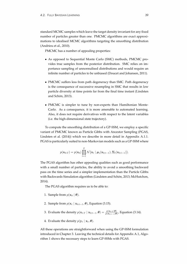
4.2. FULLY BAYESIAN LEARNING 39
standard MCMC samples which leave the target density invariant for any fixednumber of particles greater than one. PMCMC algorithms are exact approxi-mations to idealised MCMC algorithms targeting the smoothing distribution(Andrieu et al., 2010).
PMCMC has a number of appealing properties:
• As opposed to Sequential Monte Carlo (SMC) methods, PMCMC pro-vides true samples from the posterior distribution. SMC relies on im-portance sampling of unnormalised distributions and would require aninfinite number of particles to be unbiased (Doucet and Johansen, 2011).
• PMCMC suffers less from path degeneracy than SMC. Path degeneracyis the consequence of successive resampling in SMC that results in lowparticle diversity at time points far from the final time instant (Lindstenand Schon, 2013).
• PMCMC is simpler to tune by non-experts than Hamiltonian Monte-Carlo. As a consequence, it is more amenable to automated learning.Also, it does not require derivatives with respect to the latent variables(i.e. the high-dimensional state trajectory).
To compute the smoothing distribution of a GP-SSM, we employ a specificvariant of PMCMC known as Particle Gibbs with Ancestor Sampling (PGAS,Lindsten et al. (2014)) which we describe in more detail in Appendix A.1.1.PGAS is particularly suited to non-Markovian models such as a GP-SSM where
p(x0:T ) = p(x0)
T∏t=1
N(xt | µt(x0:t−1),Σt(x0:t−1)
).
The PGAS algorithm has other appealing qualities such as good performancewith a small number of particles, the ability to avoid a smoothing backwardpass on the time series and a simpler implementation than the Particle Gibbswith Backwards Simulation algorithm (Lindsten and Schon, 2013; McHutchon,2014).
The PGAS algorithm requires us to be able to:
1. Sample from p(x0 | θ).
2. Sample from p(xt | x0:t−1,θ), Equation (3.15).
3. Evaluate the density p(xt:T | x0:t−1,θ) = p(x0:T |θ)p(x0:t−1|θ) , Equation (3.14).
4. Evaluate the density p(yt | xt,θ).
All these operations are straightforward when using the GP-SSM formulationintroduced in Chapter 3. Leaving the technical details for Appendix A.1, Algo-rithm 1 shows the necessary steps to learn GP-SSMs with PGAS.
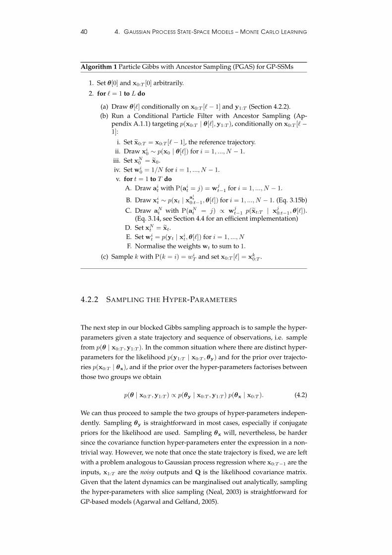
40 4. GAUSSIAN PROCESS STATE-SPACE MODELS – MONTE CARLO LEARNING
Algorithm 1 Particle Gibbs with Ancestor Sampling (PGAS) for GP-SSMs
1. Set θ[0] and x0:T [0] arbitrarily.
2. for ` = 1 to L do
(a) Draw θ[`] conditionally on x0:T [`− 1] and y1:T (Section 4.2.2).(b) Run a Conditional Particle Filter with Ancestor Sampling (Ap-
pendix A.1.1) targeting p(x0:T | θ[`],y1:T ), conditionally on x0:T [`−1]:
i. Set x0:T = x0:T [`− 1], the reference trajectory.ii. Draw xi0 ∼ p(x0 | θ[`]) for i = 1, ..., N − 1.
iii. Set xN0 = x0.iv. Set wi
0 = 1/N for i = 1, ..., N − 1.v. for t = 1 to T do
A. Draw ait with P(ait = j) = wjt−1 for i = 1, ..., N − 1.
B. Draw xit ∼ p(xt | xait
0:t−1,θ[`]) for i = 1, ..., N − 1. (Eq. 3.15b)
C. Draw aNt with P(aNt = j) ∝ wjt−1 p(xt:T | xj0:t−1,θ[`]).
(Eq. 3.14, see Section 4.4 for an efficient implementation)D. Set xNt = xt.E. Set wi
t = p(yt | xit,θ[`]) for i = 1, ..., N
F. Normalise the weights wt to sum to 1.
(c) Sample k with P(k = i) = wiT and set x0:T [`] = xk0:T .
4.2.2 SAMPLING THE HYPER-PARAMETERS
The next step in our blocked Gibbs sampling approach is to sample the hyper-parameters given a state trajectory and sequence of observations, i.e. samplefrom p(θ | x0:T ,y1:T ). In the common situation where there are distinct hyper-parameters for the likelihood p(y1:T | x0:T ,θy) and for the prior over trajecto-ries p(x0:T | θx), and if the prior over the hyper-parameters factorises betweenthose two groups we obtain
p(θ | x0:T ,y1:T ) ∝ p(θy | x0:T ,y1:T ) p(θx | x0:T ). (4.2)
We can thus proceed to sample the two groups of hyper-parameters indepen-dently. Sampling θy is straightforward in most cases, especially if conjugatepriors for the likelihood are used. Sampling θx will, nevertheless, be hardersince the covariance function hyper-parameters enter the expression in a non-trivial way. However, we note that once the state trajectory is fixed, we are leftwith a problem analogous to Gaussian process regression where x0:T−1 are theinputs, x1:T are the noisy outputs and Q is the likelihood covariance matrix.Given that the latent dynamics can be marginalised out analytically, samplingthe hyper-parameters with slice sampling (Neal, 2003) is straightforward forGP-based models (Agarwal and Gelfand, 2005).
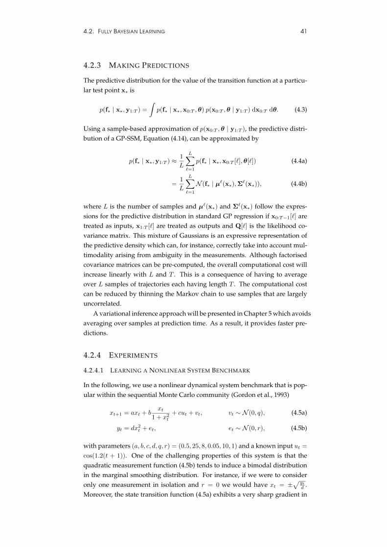
4.2. FULLY BAYESIAN LEARNING 41
4.2.3 MAKING PREDICTIONS
The predictive distribution for the value of the transition function at a particu-lar test point x∗ is
p(f∗ | x∗,y1:T ) =
∫p(f∗ | x∗,x0:T ,θ) p(x0:T ,θ | y1:T ) dx0:T dθ. (4.3)
Using a sample-based approximation of p(x0:T ,θ | y1:T ), the predictive distri-bution of a GP-SSM, Equation (4.14), can be approximated by
p(f∗ | x∗,y1:T ) ≈ 1
L
L∑`=1
p(f∗ | x∗,x0:T [`],θ[`]) (4.4a)
=1
L
L∑`=1
N (f∗ | µ`(x∗),Σ`(x∗)), (4.4b)
where L is the number of samples and µ`(x∗) and Σ`(x∗) follow the expres-sions for the predictive distribution in standard GP regression if x0:T−1[`] aretreated as inputs, x1:T [`] are treated as outputs and Q[`] is the likelihood co-variance matrix. This mixture of Gaussians is an expressive representation ofthe predictive density which can, for instance, correctly take into account mul-timodality arising from ambiguity in the measurements. Although factorisedcovariance matrices can be pre-computed, the overall computational cost willincrease linearly with L and T . This is a consequence of having to averageover L samples of trajectories each having length T . The computational costcan be reduced by thinning the Markov chain to use samples that are largelyuncorrelated.
A variational inference approach will be presented in Chapter 5 which avoidsaveraging over samples at prediction time. As a result, it provides faster pre-dictions.
4.2.4 EXPERIMENTS
4.2.4.1 LEARNING A NONLINEAR SYSTEM BENCHMARK
In the following, we use a nonlinear dynamical system benchmark that is pop-ular within the sequential Monte Carlo community (Gordon et al., 1993)
xt+1 = axt + bxt
1 + x2t
+ cut + vt, vt ∼ N (0, q), (4.5a)
yt = dx2t + et, et ∼ N (0, r), (4.5b)
with parameters (a, b, c, d, q, r) = (0.5, 25, 8, 0.05, 10, 1) and a known input ut =
cos(1.2(t + 1)). One of the challenging properties of this system is that thequadratic measurement function (4.5b) tends to induce a bimodal distributionin the marginal smoothing distribution. For instance, if we were to consideronly one measurement in isolation and r = 0 we would have xt = ±
√ytd .
Moreover, the state transition function (4.5a) exhibits a very sharp gradient in
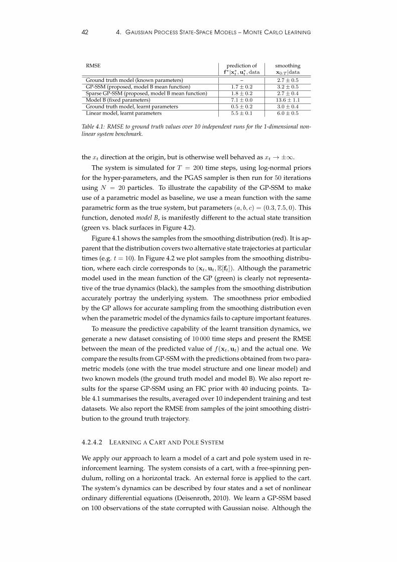
42 4. GAUSSIAN PROCESS STATE-SPACE MODELS – MONTE CARLO LEARNING
RMSE prediction off∗|x∗
t ,u∗t , data
smoothingx0:T |data
Ground truth model (known parameters) – 2.7± 0.5GP-SSM (proposed, model B mean function) 1.7± 0.2 3.2± 0.5Sparse GP-SSM (proposed, model B mean function) 1.8± 0.2 2.7± 0.4Model B (fixed parameters) 7.1± 0.0 13.6± 1.1Ground truth model, learnt parameters 0.5± 0.2 3.0± 0.4Linear model, learnt parameters 5.5± 0.1 6.0± 0.5
Table 4.1: RMSE to ground truth values over 10 independent runs for the 1-dimensional non-linear system benchmark.
the xt direction at the origin, but is otherwise well behaved as xt → ±∞.
The system is simulated for T = 200 time steps, using log-normal priorsfor the hyper-parameters, and the PGAS sampler is then run for 50 iterationsusing N = 20 particles. To illustrate the capability of the GP-SSM to makeuse of a parametric model as baseline, we use a mean function with the sameparametric form as the true system, but parameters (a, b, c) = (0.3, 7.5, 0). Thisfunction, denoted model B, is manifestly different to the actual state transition(green vs. black surfaces in Figure 4.2).
Figure 4.1 shows the samples from the smoothing distribution (red). It is ap-parent that the distribution covers two alternative state trajectories at particulartimes (e.g. t = 10). In Figure 4.2 we plot samples from the smoothing distribu-tion, where each circle corresponds to (xt,ut,E[ft]). Although the parametricmodel used in the mean function of the GP (green) is clearly not representa-tive of the true dynamics (black), the samples from the smoothing distributionaccurately portray the underlying system. The smoothness prior embodiedby the GP allows for accurate sampling from the smoothing distribution evenwhen the parametric model of the dynamics fails to capture important features.
To measure the predictive capability of the learnt transition dynamics, wegenerate a new dataset consisting of 10 000 time steps and present the RMSEbetween the mean of the predicted value of f(xt,ut) and the actual one. Wecompare the results from GP-SSM with the predictions obtained from two para-metric models (one with the true model structure and one linear model) andtwo known models (the ground truth model and model B). We also report re-sults for the sparse GP-SSM using an FIC prior with 40 inducing points. Ta-ble 4.1 summarises the results, averaged over 10 independent training and testdatasets. We also report the RMSE from samples of the joint smoothing distri-bution to the ground truth trajectory.
4.2.4.2 LEARNING A CART AND POLE SYSTEM
We apply our approach to learn a model of a cart and pole system used in re-inforcement learning. The system consists of a cart, with a free-spinning pen-dulum, rolling on a horizontal track. An external force is applied to the cart.The system’s dynamics can be described by four states and a set of nonlinearordinary differential equations (Deisenroth, 2010). We learn a GP-SSM basedon 100 observations of the state corrupted with Gaussian noise. Although the
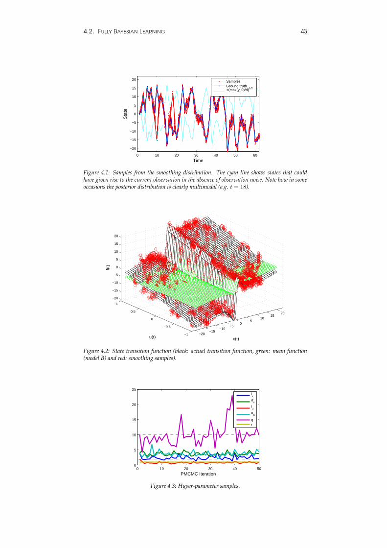
4.2. FULLY BAYESIAN LEARNING 43
0 10 20 30 40 50 60
−20
−15
−10
−5
0
5
10
15
20
Time
Sta
te
SamplesGround truth±(max(y
t,0)/d)1/2
Figure 4.1: Samples from the smoothing distribution. The cyan line shows states that couldhave given rise to the current observation in the absence of observation noise. Note how in someoccasions the posterior distribution is clearly multimodal (e.g. t = 18).
−20−15
−10−5
05
1015
20
−1
−0.5
0
0.5
1
−20
−15
−10
−5
0
5
10
15
20
x(t)u(t)
f(t)
Figure 4.2: State transition function (black: actual transition function, green: mean function(model B) and red: smoothing samples).
0 10 20 30 40 500
5
10
15
20
25
PMCMC Iteration
lx
σx
lu
σu
qr
Figure 4.3: Hyper-parameter samples.
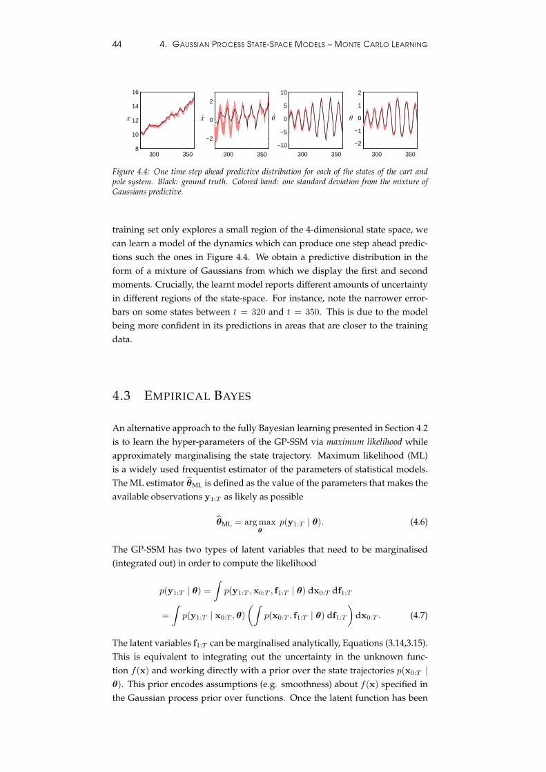
44 4. GAUSSIAN PROCESS STATE-SPACE MODELS – MONTE CARLO LEARNING
300 3508
10
12
14
16
x
300 350
−2
0
2
x
300 350
−10
−5
0
5
10
θ
300 350
−2
−1
0
1
2
θ
Figure 4.4: One time step ahead predictive distribution for each of the states of the cart andpole system. Black: ground truth. Colored band: one standard deviation from the mixture ofGaussians predictive.
training set only explores a small region of the 4-dimensional state space, wecan learn a model of the dynamics which can produce one step ahead predic-tions such the ones in Figure 4.4. We obtain a predictive distribution in theform of a mixture of Gaussians from which we display the first and secondmoments. Crucially, the learnt model reports different amounts of uncertaintyin different regions of the state-space. For instance, note the narrower error-bars on some states between t = 320 and t = 350. This is due to the modelbeing more confident in its predictions in areas that are closer to the trainingdata.
4.3 EMPIRICAL BAYES
An alternative approach to the fully Bayesian learning presented in Section 4.2is to learn the hyper-parameters of the GP-SSM via maximum likelihood whileapproximately marginalising the state trajectory. Maximum likelihood (ML)is a widely used frequentist estimator of the parameters of statistical models.The ML estimator θML is defined as the value of the parameters that makes theavailable observations y1:T as likely as possible
θML = arg maxθ
p(y1:T | θ). (4.6)
The GP-SSM has two types of latent variables that need to be marginalised(integrated out) in order to compute the likelihood
p(y1:T | θ) =
∫p(y1:T ,x0:T , f1:T | θ) dx0:T df1:T
=
∫p(y1:T | x0:T ,θ)
(∫p(x0:T , f1:T | θ) df1:T
)dx0:T . (4.7)
The latent variables f1:T can be marginalised analytically, Equations (3.14,3.15).This is equivalent to integrating out the uncertainty in the unknown func-tion f(x) and working directly with a prior over the state trajectories p(x0:T |θ). This prior encodes assumptions (e.g. smoothness) about f(x) specified inthe Gaussian process prior over functions. Once the latent function has been
4.3. EMPIRICAL BAYES 45
marginalised, the likelihood becomes
p(y1:T | θ) =
∫p(y1:T | x0:T ,θ) p(x0:T | θ) dx0:T . (4.8)
The integration with respect to x0:T , however, is not analytically tractable. Thisdifficulty will be addressed in the following section.
Direct application of maximum likelihood on p(y1:T |x0:T ,θy) to obtain es-timates of the state trajectory and likelihood parameters would result in over-fitting due to the large dimensionality of the state trajectory. However, by intro-ducing a prior on the state trajectories and marginalising them as in (4.8), weobtain the so-called marginal likelihood. Maximisation of the marginal like-lihood with respect to the parameters results in a procedure known as type IImaximum likelihood or empirical Bayes (Bishop, 2006). Empirical Bayes reducesthe risk of over-fitting since it automatically incorporates a trade-off betweenmodel fit and model complexity, a property often known as Bayesian Occam’srazor (MacKay, 2003; Ghahramani, 2012).
In the context of GP-SSMs, an Empirical Bayes approach can be useful if onehas no meaningful prior over some of the hyper-parameters. For instance, thiscould be the case for pseudo-inputs parameterising a FIC covariance function(Section 4.4.1). If meaningful priors are available, we recommend using thefully Bayesian approach from Section 4.2 since it has the same prediction costbut handles uncertainty in the hyper-parameters.
4.3.1 PARTICLE STOCHASTIC APPROXIMATION EM
As pointed out above, direct evaluation of the marginal likelihood (4.8) is notpossible for a GP-SSM. However, by viewing the latent states x0:T as missingdata, we are able to evaluate the complete data log-likelihood
log p(y1:T ,x0:T | θ) = log p(y1:T | x0:T ,θ) + log p(x0:T | θ). (4.9)
We therefore turn to the Expectation-Maximisation (EM) algorithm (Dempsteret al., 1977). The EM algorithm uses Equation (4.9) to construct a surrogate costfunction for the maximum likelihood problem, defined as
Q(θ,θ′) =
∫p(x0:T | y1:T ,θ
′) log p(y1:T ,x0:T | θ) dx0:T . (4.10)
Expectation-maximisation is an iterative procedure that maximises (4.8) by it-erating two steps, expectation (E) and maximisation (M),
E: Find Q(θ,θk−1).
M: Find θk = arg maxθ Q(θ,θk−1).
The resulting sequence {θk}k≥0 will, under weak assumptions, converge to alocal maximum of the marginal likelihood p(y1:T | θ).
46 4. GAUSSIAN PROCESS STATE-SPACE MODELS – MONTE CARLO LEARNING
To implement the above procedure it is necessary to compute the integralin (4.10), which, in general, is not tractable for a GP-SSM. To deal with this dif-ficulty, we employ a Monte-Carlo-based implementation of the EM algorithm,referred to as Particle Stochastic Approximation EM (PSAEM) (Lindsten, 2013).This procedure is a combination of stochastic approximation EM (SAEM) (De-lyon et al., 1999) and Particle MCMC (Andrieu et al., 2010). PSAEM is a com-petitive alternative to particle-smoothing-based EM algorithms as it enjoys bet-ter convergence properties and has a much lower computational cost (Lind-sten, 2013). The method maintains a stochastic approximation of the auxiliaryquantity (4.10), Qk(θ) ≈ Q(θ,θk−1). This approximation is updated accordingto
Qk(θ) = (1− γk)Qk−1(θ) + γk log p(y1:T ,x0:T [k] | θ). (4.11)
Here, {γk}k≥0 is a sequence of step sizes, satisfying the usual stochastic ap-proximation conditions:
∑k γk = ∞ and
∑k γ
2k < ∞ (Robbins and Monro,
1951). A typical choice is to take γk = k−p with p ∈ ]0.5, 1], where a smallervalue of p gives a more rapid convergence at the cost of higher variance. Inthe vanilla SAEM algorithm, x0:T [k] is a draw from the smoothing distributionp(x0:T | y1:T ,θk−1). In this setting, (Delyon et al., 1999) show that using thestochastic approximation (4.11) instead of (4.10) in the EM algorithm results ina valid method, i.e. {θk}k≥0 will still converge to a maximiser of the marginallikelihood p(y0:T | θ).
The PSAEM algorithm is an extension of SAEM which is useful when itis not possible to easily sample from the joint smoothing distribution. This isindeed the case in our setting. Instead of sampling from the smoothing dis-tribution, the sample state trajectory x0:T [k] in Equation (4.11) may be drawnfrom an ergodic Markov kernel, leaving the smoothing distribution invariant.Under suitable conditions on the kernel, this will not violate the validity ofSAEM, see (Andrieu et al., 2005; Andrieu and Vihola, 2011).
In PSAEM, the Markov kernel on the space of trajectories, denoted asPNθ (x?0:T | x0:T ),is constructed using PMCMC theory. In particular, we use the Particle Gibbswith Ancestor Sampling algorithm (PGAS, Lindsten et al. (2014)) that we de-scribed in Section 4.2. PGAS is a sequential Monte Carlo method, akin to astandard particle filter, but with the difference that one particle at each timepoint is specified a priori. This reference state trajectory, denoted as x0:T , can bethought of as guiding the particles of the particle filter to the “correct” regionsof the state-space. More formally PGAS defines a Markov kernel which leavesthe joint smoothing distribution invariant, i.e. for any θ∫
PNθ (x?0:T | x0:T )p(x0:T | y1:T ,θ) dx0:T = p(x?0:T | y1:T ,θ). (4.12)
The PGAS kernel is indexed by N , which is the number of particles used inthe underlying particle filter. Note that the desired property (4.12) holds forany number of particles, i.e. the number of particles only affects the mixing
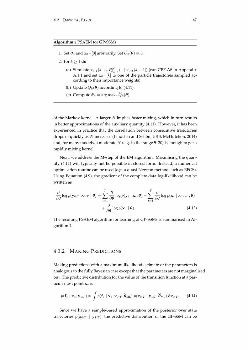
4.3. EMPIRICAL BAYES 47
Algorithm 2 PSAEM for GP-SSMs
1. Set θ0 and x0:T [0] arbitrarily. Set Q0(θ) ≡ 0.
2. for k ≥ 1 do
(a) Simulate x0:T [k] ∼ PNθk−1( · | x0:T [k − 1]) (run CPF-AS in Appendix
A.1.1 and set x0:T [k] to one of the particle trajectories sampled ac-cording to their importance weights).
(b) Update Qk(θ) according to (4.11).
(c) Compute θk = arg maxθ Qk(θ).
of the Markov kernel. A larger N implies faster mixing, which in turn resultsin better approximations of the auxiliary quantity (4.11). However, it has beenexperienced in practice that the correlation between consecutive trajectoriesdrops of quickly as N increases (Lindsten and Schon, 2013; McHutchon, 2014)and, for many models, a moderate N (e.g. in the range 5–20) is enough to get arapidly mixing kernel.
Next, we address the M-step of the EM algorithm. Maximising the quan-tity (4.11) will typically not be possible in closed form. Instead, a numericaloptimisation routine can be used (e.g. a quasi-Newton method such as BFGS).Using Equation (4.9), the gradient of the complete data log-likelihood can bewritten as
∂
∂θlog p(y0:T ,x0:T | θ) =
T∑t=1
∂
∂θlog p(yt | xt,θ) +
T∑t=1
∂
∂θlog p(xt | x0:t−1,θ)
+∂
∂θlog p(x0 | θ), (4.13)
The resulting PSAEM algorithm for learning of GP-SSMs is summarised in Al-gorithm 2.
4.3.2 MAKING PREDICTIONS
Making predictions with a maximum likelihood estimate of the parameters isanalogous to the fully Bayesian case except that the parameters are not marginalisedout. The predictive distribution for the value of the transition function at a par-ticular test point x∗ is
p(f∗ | x∗,y1:T ) ≈∫p(f∗ | x∗,x0:T , θML) p(x0:T | y1:T , θML) dx0:T . (4.14)
Since we have a sample-based approximation of the posterior over statetrajectories p(x0:T | y1:T ), the predictive distribution of the GP-SSM can be
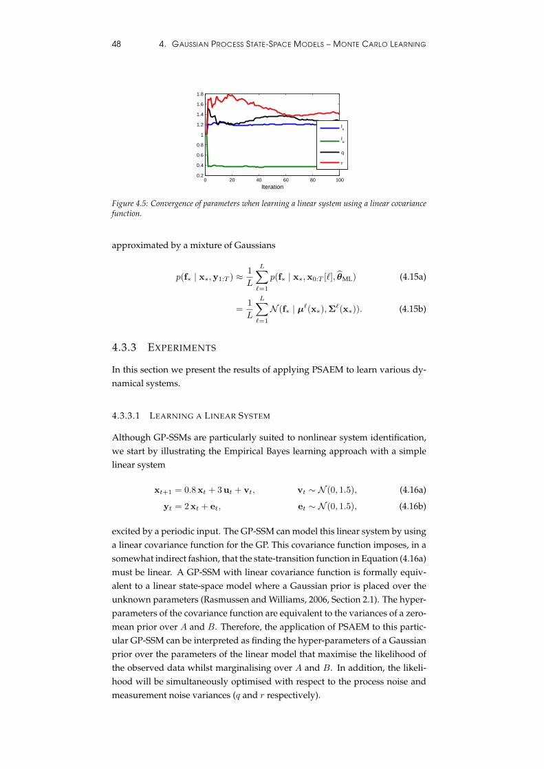
48 4. GAUSSIAN PROCESS STATE-SPACE MODELS – MONTE CARLO LEARNING
0 20 40 60 80 1000.2
0.4
0.6
0.8
1
1.2
1.4
1.6
1.8
Iteration
lx
lu
q
r
Figure 4.5: Convergence of parameters when learning a linear system using a linear covariancefunction.
approximated by a mixture of Gaussians
p(f∗ | x∗,y1:T ) ≈ 1
L
L∑`=1
p(f∗ | x∗,x0:T [`], θML) (4.15a)
=1
L
L∑`=1
N (f∗ | µ`(x∗),Σ`(x∗)). (4.15b)
4.3.3 EXPERIMENTS
In this section we present the results of applying PSAEM to learn various dy-namical systems.
4.3.3.1 LEARNING A LINEAR SYSTEM
Although GP-SSMs are particularly suited to nonlinear system identification,we start by illustrating the Empirical Bayes learning approach with a simplelinear system
xt+1 = 0.8 xt + 3 ut + vt, vt ∼ N (0, 1.5), (4.16a)
yt = 2 xt + et, et ∼ N (0, 1.5), (4.16b)
excited by a periodic input. The GP-SSM can model this linear system by usinga linear covariance function for the GP. This covariance function imposes, in asomewhat indirect fashion, that the state-transition function in Equation (4.16a)must be linear. A GP-SSM with linear covariance function is formally equiv-alent to a linear state-space model where a Gaussian prior is placed over theunknown parameters (Rasmussen and Williams, 2006, Section 2.1). The hyper-parameters of the covariance function are equivalent to the variances of a zero-mean prior over A and B. Therefore, the application of PSAEM to this partic-ular GP-SSM can be interpreted as finding the hyper-parameters of a Gaussianprior over the parameters of the linear model that maximise the likelihood ofthe observed data whilst marginalising over A and B. In addition, the likeli-hood will be simultaneously optimised with respect to the process noise andmeasurement noise variances (q and r respectively).
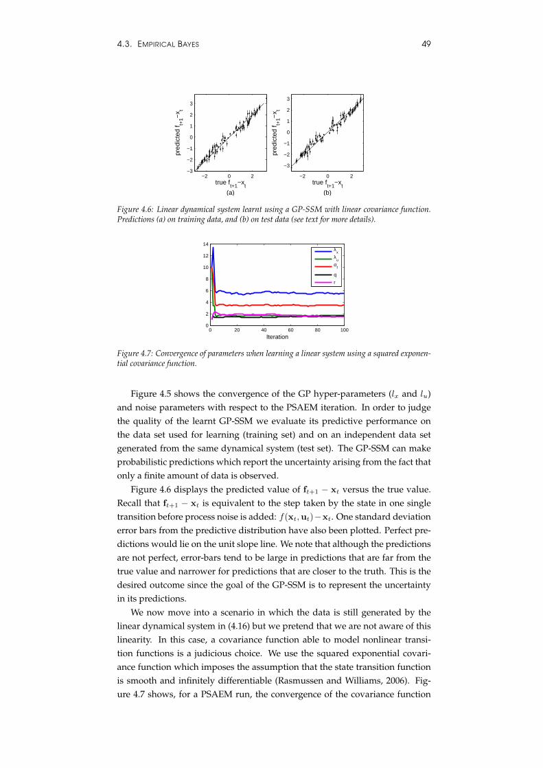
4.3. EMPIRICAL BAYES 49
−2 0 2−3
−2
−1
0
1
2
3
true ft+1
−xt
(a)
pred
icte
d f t+
1−x t
−2 0 2
−3
−2
−1
0
1
2
3
true ft+1
−xt
(b)
pred
icte
d f t+
1−x t
Figure 4.6: Linear dynamical system learnt using a GP-SSM with linear covariance function.Predictions (a) on training data, and (b) on test data (see text for more details).
0 20 40 60 80 1000
2
4
6
8
10
12
14
Iteration
λ
xλ
uσ
f
q
r
Figure 4.7: Convergence of parameters when learning a linear system using a squared exponen-tial covariance function.
Figure 4.5 shows the convergence of the GP hyper-parameters (lx and lu)and noise parameters with respect to the PSAEM iteration. In order to judgethe quality of the learnt GP-SSM we evaluate its predictive performance onthe data set used for learning (training set) and on an independent data setgenerated from the same dynamical system (test set). The GP-SSM can makeprobabilistic predictions which report the uncertainty arising from the fact thatonly a finite amount of data is observed.
Figure 4.6 displays the predicted value of ft+1 − xt versus the true value.Recall that ft+1 − xt is equivalent to the step taken by the state in one singletransition before process noise is added: f(xt,ut)−xt. One standard deviationerror bars from the predictive distribution have also been plotted. Perfect pre-dictions would lie on the unit slope line. We note that although the predictionsare not perfect, error-bars tend to be large in predictions that are far from thetrue value and narrower for predictions that are closer to the truth. This is thedesired outcome since the goal of the GP-SSM is to represent the uncertaintyin its predictions.
We now move into a scenario in which the data is still generated by thelinear dynamical system in (4.16) but we pretend that we are not aware of thislinearity. In this case, a covariance function able to model nonlinear transi-tion functions is a judicious choice. We use the squared exponential covari-ance function which imposes the assumption that the state transition functionis smooth and infinitely differentiable (Rasmussen and Williams, 2006). Fig-ure 4.7 shows, for a PSAEM run, the convergence of the covariance function
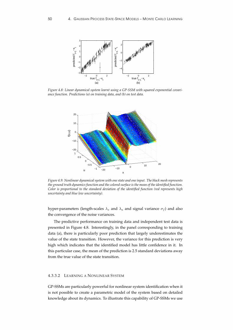
50 4. GAUSSIAN PROCESS STATE-SPACE MODELS – MONTE CARLO LEARNING
−2 0 2−3
−2
−1
0
1
2
3
true ft+1
−xt
(a)
pred
icte
d f t+
1−x t
−2 0 2
−4
−2
0
2
true ft+1
−xt
(b)
pred
icte
d f t+
1−x t
Figure 4.8: Linear dynamical system learnt using a GP-SSM with squared exponential covari-ance function. Predictions (a) on training data, and (b) on test data.
−20−10
010
20
−1
−0.5
0
0.5
1
−20
−10
0
10
20
xu
f(x,
u)
Figure 4.9: Nonlinear dynamical system with one state and one input. The black mesh representsthe ground truth dynamics function and the colored surface is the mean of the identified function.Color is proportional to the standard deviation of the identified function (red represents highuncertainty and blue low uncertainty).
hyper-parameters (length-scales λx and λu and signal variance σf ) and alsothe convergence of the noise variances.
The predictive performance on training data and independent test data ispresented in Figure 4.8. Interestingly, in the panel corresponding to trainingdata (a), there is particularly poor prediction that largely underestimates thevalue of the state transition. However, the variance for this prediction is veryhigh which indicates that the identified model has little confidence in it. Inthis particular case, the mean of the prediction is 2.5 standard deviations awayfrom the true value of the state transition.
4.3.3.2 LEARNING A NONLINEAR SYSTEM
GP-SSMs are particularly powerful for nonlinear system identification when itis not possible to create a parametric model of the system based on detailedknowledge about its dynamics. To illustrate this capability of GP-SSMs we use
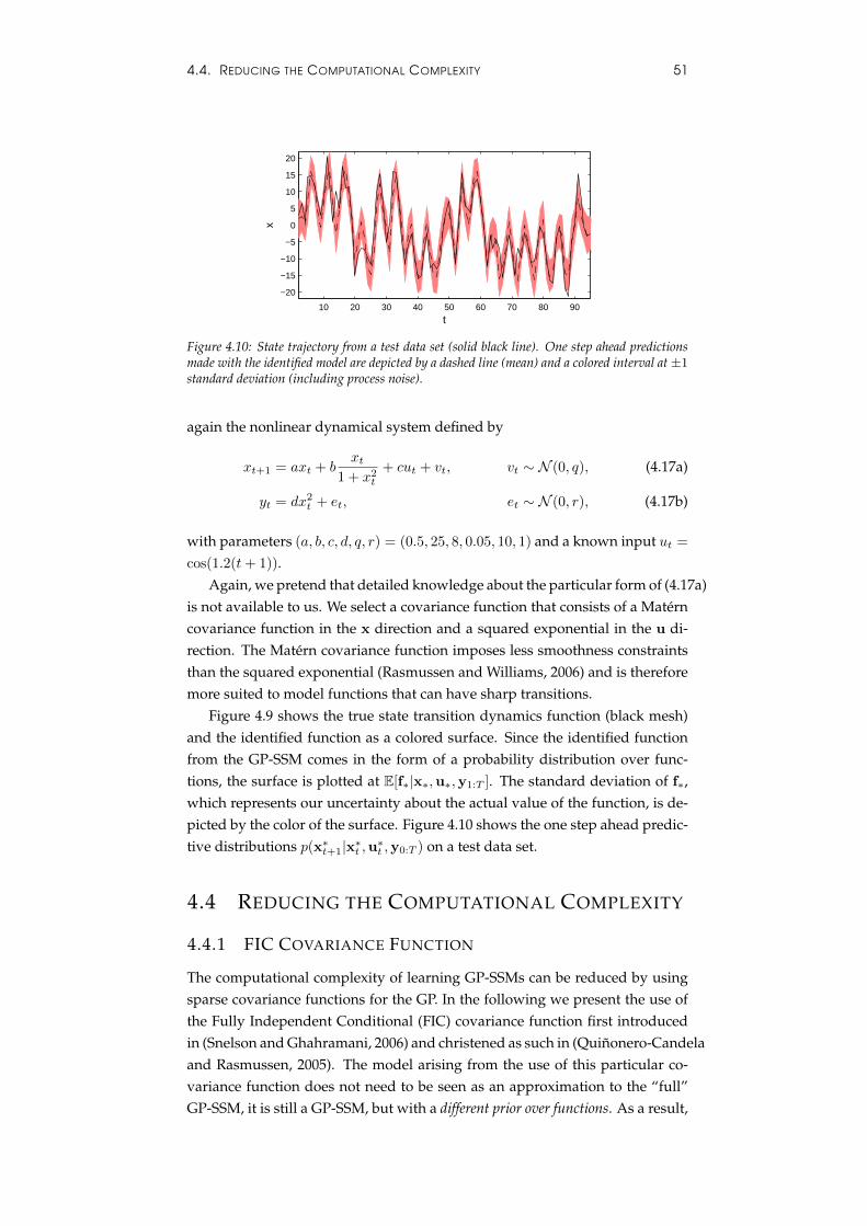
4.4. REDUCING THE COMPUTATIONAL COMPLEXITY 51
10 20 30 40 50 60 70 80 90
−20
−15
−10
−5
0
5
10
15
20
t
x
Figure 4.10: State trajectory from a test data set (solid black line). One step ahead predictionsmade with the identified model are depicted by a dashed line (mean) and a colored interval at±1standard deviation (including process noise).
again the nonlinear dynamical system defined by
xt+1 = axt + bxt
1 + x2t
+ cut + vt, vt ∼ N (0, q), (4.17a)
yt = dx2t + et, et ∼ N (0, r), (4.17b)
with parameters (a, b, c, d, q, r) = (0.5, 25, 8, 0.05, 10, 1) and a known input ut =
cos(1.2(t+ 1)).Again, we pretend that detailed knowledge about the particular form of (4.17a)
is not available to us. We select a covariance function that consists of a Materncovariance function in the x direction and a squared exponential in the u di-rection. The Matern covariance function imposes less smoothness constraintsthan the squared exponential (Rasmussen and Williams, 2006) and is thereforemore suited to model functions that can have sharp transitions.
Figure 4.9 shows the true state transition dynamics function (black mesh)and the identified function as a colored surface. Since the identified functionfrom the GP-SSM comes in the form of a probability distribution over func-tions, the surface is plotted at E[f∗|x∗,u∗,y1:T ]. The standard deviation of f∗,which represents our uncertainty about the actual value of the function, is de-picted by the color of the surface. Figure 4.10 shows the one step ahead predic-tive distributions p(x∗t+1|x∗t ,u∗t ,y0:T ) on a test data set.
4.4 REDUCING THE COMPUTATIONAL COMPLEXITY
4.4.1 FIC COVARIANCE FUNCTION
The computational complexity of learning GP-SSMs can be reduced by usingsparse covariance functions for the GP. In the following we present the use ofthe Fully Independent Conditional (FIC) covariance function first introducedin (Snelson and Ghahramani, 2006) and christened as such in (Quinonero-Candelaand Rasmussen, 2005). The model arising from the use of this particular co-variance function does not need to be seen as an approximation to the “full”GP-SSM, it is still a GP-SSM, but with a different prior over functions. As a result,
52 4. GAUSSIAN PROCESS STATE-SPACE MODELS – MONTE CARLO LEARNING
it could even outperform its non-sparse version in the same way as it happensin some regression problems (Snelson and Ghahramani, 2006).
Most sparse GP methods can be formulated in terms of a set of inducingvariables (Quinonero-Candela and Rasmussen, 2005; Titsias, 2009). These vari-ables live in the space of the latent function and have a set z , {zi}Mi=1 ofcorresponding inducing inputs. The assumption is that, conditionally on theinducing variables, the latent function values are mutually independent. Al-though the inducing variables are marginalised analytically, the inducing in-puts have to be chosen in such a way that they, informally speaking, coverthe same region of the input space covered by the data. Crucially, in order toachieve computational gains, the number M of inducing variables is selectedto be smaller than the original number of data points.
As shown in (Quinonero-Candela and Rasmussen, 2005), the FIC prior isobtained by replacing the covariance function k(·, ·) with
kFIC(xi,xj) = s(xi,xj) + δij(k(xi,xj)− s(xi,xj)
), (4.18)
where s(xi,xj) , k(xi, z)k(z, z)−1k(z,xj), δij is Kronecker’s delta and we usethe convention whereby when k(·, ·) takes a set as one of its arguments it gen-erates a matrix of covariances. Using the Woodbury matrix identity, we canexpress the one-step density p(xt|x0:t−1) of a GP-SSM, Equation (3.15b), as aGaussian with the following mean and covariance matrix
µFICt (x0:t−1) = mt−1 + Kt−1,zPKz,0:t−2Λ
−10:t−2 (x1:t−1 −m0:t−2), (4.19a)
ΣFICt (x0:t−1) = Kt−1 − St−1 + Kt−1,zPKz,t−1, (4.19b)
where
P , (Kz + Kz,0:t−2Λ−10:t−2K0:t−2,z)−1, (4.20a)
Λ0:t−2 , diag[K0:t−2 − S0:t−2], (4.20b)
SA,B , KA,zK−1z Kz,B. (4.20c)
Despite its apparent cumbersomeness, the computational complexity involvedin computing the above mean and covariance is O(M2t). This contrasts withthe O(t3) complexity for general covariance functions when evaluating Equa-tion (3.15b).
4.4.2 SEQUENTIAL CONSTRUCTION OF CHOLESKY FACTORISA-TIONS
A naive implementation of the CPF-AS algorithm gives rise to O(T 4) compu-tational complexity, since at each time step t = 1, ..., T , a matrix of size T × Tneeds to be factorised. However, it is possible to update and reuse the fac-tors from the previous time step, bringing the total computational complexitydown to the familiar O(T 3). Furthermore, by introducing a sparse GP model,
4.5. CONCLUSIONS 53
we can reduce the complexity from O(M2T 2) to O(M2T ) where M � T .There are two costly operations of the CPF-AS algorithm: (i) sampling from
the prior, requiring the computation of Equations (3.15c) and (3.15d) and (ii)evaluating the ancestor sampling probabilities which requires to evaluate thejoint density p(y1:T ,x0:T ). Both of these operations can be carried out effi-ciently by keeping track of a Cholesky factorisation of the matrix
K({xi0:t−1, xt:T−1}) = LitLi>t ,
for each particle i = 1, ..., N (see Section A.1.1 for the full PGAS algorithm).Here, K({xi0:t−1, xt:T−1}) is a matrix defined analogously to K0:T−1, but wherethe covariance function is evaluated for the concatenated state trajectory{xi0:t−1, xt:T−1}. From Lit, it is possible to identify sub-matrices correspondingto the Cholesky factors for the covariance matrix Σt(x
i0:t−1) as well as for the
matrices needed to efficiently evaluate the ancestor sampling probabilities.It remains to find an efficient update of the Cholesky factor to obtain Lit+1.
As we move from time t to t+1 in the algorithm, xt will be replaced by xit in theconcatenated trajectory. Hence, the matrix K({xi0:t, xt+1:T−1}) can be obtainedfrom K({xi0:t−1, xt:T−1}) by replacing nx rows and columns, corresponding toa rank 2nx update. (Recall that nx is the dimensionality of the state-space.)It follows that we can compute Lit+1 by making nx successive rank one up-dates and downdates on Lit. Refer to (Gill et al., 1974) for a comprehensivereview of methods for rank-one update/downdate of Cholesky factors and tothe supplementary material of (Frigola et al., 2013) for a derivation tailored tothe current problem.
In summary, for an arbitrary covariance function, all the operations at aspecific time step can be done in O(T 2) computations, leading to a total com-putational complexity ofO(T 3). For the GP-SSM with FIC covariance function,a naive implementation gives rise toO(M2T 2) computational complexity. Thiscan be reduced toO(M2T ) by keeping track of a factorisation for the matrix P.However, to reach the O(M2T ) cost, all intermediate operations scaling withT have to be avoided, requiring the reuse of not only the matrix factorisations,but also the intermediate matrix-vector multiplications.
4.5 CONCLUSIONS
We have shown how to directly sample from the smoothing distribution of aGP-SSM without needing to know the nonlinear state transition function. Oncesamples from the smoothing distribution have been obtained, it is straightfor-ward to describe the posterior over the state transition function.
We have also shown how samples from the smoothing distribution can beobtained using the Particle Gibbs with Ancestor Sampling algorithm (Lindstenet al., 2014). This algorithm has proven to achieve very good mixing while be-ing extremely easy to use. Although the PGAS algorithm is able to effectivelysample from very high-dimensional distributions for long time series (large T ),

54 4. GAUSSIAN PROCESS STATE-SPACE MODELS – MONTE CARLO LEARNING
its reliance on a particle filter limits their effectiveness when the state dimen-sion (nx) is large.
The fully Bayesian learning approach presented in this chapter obtains jointsamples from the smoothing distribution and the posterior distribution overthe (hyper-)parameters. Therefore, uncertainty about all unknown variables isquantified. We have also presented an alternative empirical Bayes approachwhich can find maximum likelihood point estimate over all, or some, (hyper-)parameters. This can be useful for parameters over which it is hard to find ameaningful prior, e.g. the inducing inputs of a FIC covariance function.
Chapter 5
Gaussian Process State-SpaceModels – Variational Learning
In this chapter we introduce a Variational Inference approach to Bayesian learn-ing of sparse Gaussian Process State-Space Models. The result of learning isa tractable approximate posterior over nonlinear dynamical systems that canprovide very fast predictions at test time. In comparison to conventional para-metric models this approach offers the possibility to straightforwardly tradeoff model capacity and computational cost whilst preventing overfitting.
As opposed to the learning algorithms presented in Chapter 4, the varia-tional approach does not exactly marginalise out the nonlinear dynamics. In-stead, it learns an explicit posterior of the dynamical system by computing anapproximate posterior over the inducing variables of a sparse GP-SSM.
The presentation in this chapter expands the results previously publishedin (Frigola et al., 2014a).
5.1 INTRODUCTION
A GP-SSM has, in principle, the ability to model nonlinear state transition func-tions belonging to an infinite-dimensional space of functions. This contrastswith parametric nonlinear functions in which the model capacity is restricted apriori by the choice of the parametric form.
The sampling approaches introduced in Chapter 4 are able to learn the statetransition function of a GP-SSM without the need of parametric approxima-tions. However, they do so at a cost: each prediction of a state transition needsto average over samples of the latent state trajectory and hence has an O(TL)
computational cost where T is the length of the time series and L is the numberof samples.
The variational methods presented in this chapter will take a fundamentallydifferent approach: they will attempt to represent the posterior over the statetransition function with a finite number of parameters, the inducing points.The methodology shares many elements with the seminal work of Titsias (2009)
55
56 5. GAUSSIAN PROCESS STATE-SPACE MODELS – VARIATIONAL LEARNING
for Gaussian process regression but is adapted to the challenging setting oftime series data. In a GP-SSM, the goal is to learn a function whose inputs andoutputs are both unobserved.
Variational methods for GP-SSMs have two fundamental advantages overthe Monte Carlo approaches presented in Chapter 4. First, they offer fast prob-abilistic predictions at test time with a computational complexity that is inde-pendent of the length of the time series. Second, mini-batch training is possi-ble and leads to significant speed improvements when using large datasets. Amore detailed discussion about advantages and disadvantages of variationalinference is provided in Section 5.2.2.
5.2 EVIDENCE LOWER BOUND OF A GP-SSM
Variational inference is a popular method for approximate Bayesian inferencebased on making assumptions about the posterior over parameters and latentvariables. These assumptions lead to a tractable lower bound on the marginallikelihood of the model. The marginal likelihood is also known as the evidenceand its lower bound is sometimes referred to as the ELBO (Evidence LowerBOund). An approximation of the evidence is the objective function that wemaximised for learning GP-SSMs in Section 4.3. In the variational inferencesetting, maximising the evidence lower bound is equivalent to minimising theKullback-Leibler divergence between the approximate posterior and the exactone. (See Appendix A.2 for a very brief presentation and (Jordan et al., 1999) foran authoritative exposition.) Following standard variational inference method-ology, we obtain the evidence lower bound of a GP-SSM augmented with in-ducing points u (Section 3.3)
log p(y|θ) ≥ 〈logp(x, f ,u,y)
q(x, f ,u)〉q(x,f ,u)
= 〈logp(u)p(x0)
∏Tt=1 p(ft|f1:t−1,x0:t−1,u)p(yt|xt)p(xt|ft)
q(x, f ,u)〉q(x,f ,u).
(5.1)
In order to make the formulas slightly less cumbersome, we are using the short-hand notation x , x0:T , y , y1:T , f , f1:T , u , u1:M , and 〈f(x)〉p(x) ,∫f(x)p(x) dx.
At this point, it is critical to chose a variational distribution q(x, f ,u) thatpresents a favourable trade-off between tractability and expressivity. Inspiredby a strand of work started by Titsias (2009), we chose a distribution for thelatent variables in the GP-SSM that leads to cancellation of difficult terms in-volving the latent function. In particular, we use
q(x, f ,u) = q(u)q(x)
T∏t=1
p(ft|f1:t−1,x0:t−1,u), (5.2)
where q(u) and q(x) can take any form at this stage and will be variationally
5.2. EVIDENCE LOWER BOUND OF A GP-SSM 57
optimised later. However, the terms relating to f are taken to match those ofthe prior. As a consequence, the difficult p(ft|...) terms inside the log cancel outand lead to the following lower bound
log p(y|θ) ≥ 〈logp(u)p(x0)
∏Tt=1(((((((((
p(ft|f1:t−1,x0:t−1,u)p(yt|xt)p(xt|ft)q(u)q(x)
∏Tt=1(((((((((
p(ft|f1:t−1,x0:t−1,u)〉q(x,f ,u),
(5.3a)
= 〈logp(u)p(x0)
∏Tt=1 p(yt|xt)p(xt|ft)q(u)q(x)
〉q(x,f ,u), (5.3b)
, L(q(u), q(x),θ). (5.3c)
Equation (5.3c) makes it explicit that the evidence lower bound is a function ofthe functions q(u) and q(x) and of the hyper-parameters θ. In the next section,we will use the calculus of variations to optimise the ELBO with respect tothe functions q(u) and q(x). Now, we break down the ELBO into a sum ofinterpretable terms
L(q(u), q(x),θ) =〈logp(u)
q(u)〉q(u) + 〈log
1
q(x)〉q(x) + 〈log p(x0)〉q(x0)
+ 〈log
T∏t=1
p(xt|ft)〉q(x,f ,u) + 〈log
T∏t=1
p(yt|xt)〉q(x)
=− KL(q(u)‖p(u)) +H(q(x)) + 〈log p(x0)〉q(x0)
+
T∑t=1
{〈〈log p(xt|ft)〉p(ft|xt−1,u)︸ ︷︷ ︸
Φ(xt−1:t,u)
〉q(x)q(u) + 〈log p(yt|xt)〉q(x)
},
(5.4)
where KL denotes the Kullback-Leibler divergence
KL(q(u)‖p(u)) ,∫q(u) log
q(u)
p(u)du, (5.5)
H denotes the entropy
H(q(x)) , −∫q(x) log q(x) dx. (5.6)
The integral with respect to ft in the lower bound can be solved analytically1:
Φ(xt−1:t,u) = 〈log p(xt|ft)〉p(ft|xt−1,u) (5.7a)
= 〈logN (xt|ft,Q)〉N (ft|At−1u,Bt−1) (5.7b)
= −1
2tr(Q−1Bt−1) + logN (xt|At−1u,Q), (5.7c)
1for simplicity of interpretation, the derivation that follows in the rest of the chapter is for thezero-mean GP case, see Section 5.7.3 for expressions for an arbitrary mean function
58 5. GAUSSIAN PROCESS STATE-SPACE MODELS – VARIATIONAL LEARNING
where
At−1 , Kt−1,zK−1z , (5.8a)
Bt−1 , Kt−1,t−1 −Kt−1,zK−1z Kz,t−1. (5.8b)
As we will see in Section 5.3.1, the distribution q(u) that maximises theELBO is a Gaussian distribution: N (u|µ,Σ). Therefore, the following expecta-tion in the ELBO has a closed form expression
〈Φ(xt−1:t,u)〉q(u) =
∫Φ(xt−1:t,u)N (u|µ,Σ) du (5.9a)
= −1
2tr(Q−1(Bt−1 + At−1ΣA>t−1)) + logN (xt|At−1µ,Q).
(5.9b)
Therefore, the ELBO becomes
L(q(u), q(x),θ) =− KL(q(u)‖p(u)) +H(q(x)) + 〈log p(x0)〉q(x0)
+
T∑t=1
{− 1
2〈tr(Q−1(Bt−1 + At−1ΣA>t−1))〉q(xt−1)
+ 〈logN (xt|At−1µ,Q)〉q(xt−1:t)
+ 〈log p(yt|xt)〉q(xt)
}. (5.10)
5.2.1 INTERPRETATION OF THE LOWER BOUND
We can provide an interpretation of the influence that each term in Equation (5.10)has when maximising the evidence lower bound
• −KL(q(u)‖p(u)) : regularisation term encouraging the approximate pos-terior q(u) to remain close to the prior p(u) which encodes assumptions(e.g. smoothness) about the state transition function.
• H(q(x)) : entropy term discouraging overly tight smoothing distribu-tions over the state trajectories.
• 〈log p(x0)〉q(x0) : encourages the state trajectory to start in a region of thestate space where the prior is high. This term can be neglected if the prioron the initial state is sufficiently broad.
• − 12 〈tr(Q
−1Bt−1)〉q(xt−1) : penalises states that are far from the inducinginputs. This is apparent when interpreting Bt−1 as the predictive covari-ance of GP regression at a test point xt−1 with z as the regression inputs(5.8b). States close to the inducing inputs have little predictive varianceand result in a small penalty.
• − 12 〈tr(Q
−1At−1ΣA>t−1)〉q(xt−1) : penalises variance in the approximateposterior q(u). It opposes the KL term between prior and posterior over
5.2. EVIDENCE LOWER BOUND OF A GP-SSM 59
u. The expression At−1ΣA>t−1 can be interpreted as the extra covari-ance in a prediction of ft due to variance in the posterior of u, see Equa-tion (5.27d).
• 〈logN (xt|At−1µ,Q)〉q(xt−1:t) : crucial term that quantifies the agreementbetween neighbouring states (xt,xt−1) and the mean of the (approxi-mate) posterior over the inducing points of the state transition function.
• 〈log p(yt|xt)〉q(xt) : data fit term encouraging state trajectories that givehigh probability to the observed data.
5.2.2 PROPERTIES OF THE LOWER BOUND
As in other sparse GP models, variational inference gives the ability to obtainan approximate posterior of the state transition function of a GP-SSM at thelocations of the inducing inputs. Away from those locations, the posterior takesthe form of the prior conditioned on the inducing variables. By increasing thenumber of inducing variables, the ELBO can only become tighter (as in (Titsias,2009)). This offers a straightforward trade-off between model capacity andcomputation cost without increasing the risk of overfitting.
The evidence lower bound provided by variational inference is very usefulto obtain point estimates of hyper-parameters that approximate the maximumlikelihood solution. Also, in many applications it has been found that maximis-ing the ELBO results in shorter training times compared to Monte Carlo-basedmethods.
However, variational inference is based on making assumptions about theshape of the approximate posterior such as factorisation assumptions or speci-fying a particular parametric form for the approximate posterior. This contrastswith Monte Carlo methods where no such assumptions are made.
As useful as variational inference is, it is important to keep in mind thecharacteristics of the approximation. Perhaps the most important characteristicis that approximations from variational inference tend to be more compact thanthe true distribution (MacKay, 2003) although this is not strictly always thecase (Turner and Sahani, 2011). Underestimating uncertainty is an undesirableproperty because it gives an illusion of certainty. However, as MacKay (2003)argues, it is often better to underestimate uncertainty rather than to ignore italtogether.
Another issue with variational inference is due to the fact that maximisingthe evidence lower bound biases the solution towards areas where the boundis tighter (Turner and Sahani, 2011). As a consequence, the optimal setting ofthe parameters on the lower bound is not necessarily the maximum of the evi-dence. The bias in the parameters will depend on the particular characteristicsof the lower bound that we chose to maximise.
60 5. GAUSSIAN PROCESS STATE-SPACE MODELS – VARIATIONAL LEARNING
5.2.3 ARE THE INDUCING INPUTS VARIATIONAL PARAMETERS?
The inducing inputs z appear both in the generative model of a sparse GP-SSM, Equation (3.29), and in the variational distribution, Equation. (5.2). Itcould appear that they are parameters of the model that are being reused inthe variational distribution much in the same way as the covariance functionhyper-parameters. However, on close observation it is apparent that the in-ducing inputs in a sparse GP-SSM behave in a very particular manner: if theinducing variables are integrated out, the marginal distribution over the rest ofvariables (i.e. the non-sparse GP-SSM) does not depend on the inducing inputs∫
p(y,x, f ,u | z) du = p(y,x, f | z) = p(y,x, f). (5.11)
Since the location of the inducing inputs does not affect the distribution overobserved data, state trajectories or latent function, the inducing inputs becomeparameters that can be tuned at our will. Adjusting the inducing inputs doesnot change our assumptions about how the data was generated. But, crucially,adjusting the inducing inputs changes the variational distribution q(x, f ,u)
and can lead to a tighter lower bound on the model evidence.
5.3 OPTIMAL VARIATIONAL DISTRIBUTIONS
5.3.1 OPTIMAL VARIATIONAL DISTRIBUTION FOR u
The optimal distribution for q(u) is a stationary point of the functionalL(q(u), q(x),θ).The evidence lower bound has a stationary point with respect to the functionq(u) if and only if this function satisfies the Euler-Lagrange equation (Ap-pendix A.2)
∂
∂q(u)
{q(u) log
p(u)
q(u)+ q(u)
T∑t=1
〈Φ(xt−1:t,u)〉q(xt−1:t)
}= 0, (5.12)
which results in an optimal distribution q∗(u)
0 = logp(u)
q∗(u)− 1 +
T∑t=1
〈Φ(xt−1:t,u)〉q(xt−1:t), (5.13a)
log q∗(u) = log p(u)− 1 +
T∑t=1
〈Φ(xt−1:t,u)〉q(xt−1:t), (5.13b)
which, after exponentiation, becomes
q∗(u) ∝ p(u)
T∏t=1
exp〈logN (xt|At−1u,Q)〉q(xt−1:t). (5.14)
In the following, we show that the optimal variational distribution q∗(u)
is, conveniently, a multivariate Gaussian distribution. This is not an extra as-
5.3. OPTIMAL VARIATIONAL DISTRIBUTIONS 61
sumption that we have added to the variational inference but a natural conse-quence of the evidence lower bound that is being maximised.
q∗(u) ∝ N (u | 0,Kz)
T∏t=1
exp〈logN (xt|At−1u,Q)〉q(xt−1:t),
∝ N (u | 0,Kz)
T∏t=1
exp〈xTt Q−1At−1u−1
2uTAT
t−1Q−1At−1u〉q(xt−1:t),
∝ exp{T∑t=1
〈xTt Q−1At−1〉q(xt−1:t)u
− 1
2uT
(K−1
z +
T∑t=1
〈ATt−1Q
−1At−1〉q(xt−1)
)u}. (5.15a)
From this expression we confirm that q∗(u) is indeed a Gaussian distributionwith natural parameters
ηηη1 =
T∑t=1
〈ATt−1Q
−1xt〉q(xt−1:t), (5.16a)
ηηη2 = −1
2
(K−1
z +
T∑t=1
〈ATt−1Q
−1At−1〉q(xt−1)
). (5.16b)
Therefore, the optimal distribution q∗(u) depends on the sufficient statistics
Ψ1 ,T∑t=1
〈KTt−1,zQ
−1xt〉q(xt−1:t), (5.17a)
Ψ2 ,T∑t=1
〈KTt−1,zQ
−1Kt−1,z〉q(xt−1). (5.17b)
The mean and covariance matrix of q∗(u), denoted as µ and Σ respectively, canbe computed as µ = Σηηη1 and Σ = (−2ηηη2)−1
µ = ΣK−1z Ψ1 =
(I + K−1
z Ψ2
)−1Ψ1, (5.18a)
Σ =(K−1
z + K−1z Ψ2K
−1z
)−1. (5.18b)
5.3.2 OPTIMAL VARIATIONAL DISTRIBUTION FOR x
We follow an analogous procedure to find the optimal distribution over thestate trajectory that maximises the evidence lower bound for a fixed q(u). TheEuler-Lagrange equation with respect to the distribution q(x) is
∂
∂q(x)
{−q(x) log q(x) + q(x0) log p(x0) +
T∑t=1
q(x)〈Φ(xt−1:t,u)〉q(u)
+
T∑t=1
q(x) log p(yt|xt)}
= 0, (5.19)
62 5. GAUSSIAN PROCESS STATE-SPACE MODELS – VARIATIONAL LEARNING
which results in an optimal distribution q∗(x)
0 = − log q∗(x)− 1 + log p(x0) +
T∑t=1
{〈Φ(xt−1:t,u)〉q(u) + log p(yt|xt)
}, (5.20)
which, after exponentiation and using q(u) = N (u|µ,Σ), becomes
q∗(x) ∝ p(x0)
T∏t=1
p(yt|xt) exp{−1
2tr(Q−1(Bt−1+At−1ΣAT
t−1))}N (xt|At−1µ,Q).
(5.21)Examining the optimal distribution q∗(x), we can see that it can be interpretedas the smoothing distribution of an auxiliary parametric state-space model.This auxiliary model is simpler than a GP-SSM since the latent states factorisewith a Markovian structure. Equation (5.21) can be interpreted as a the jointdistribution of a nonlinear state-space model with a Gaussian state transitiondensity
p(xt | xt−1) = N (xt|At−1µ,Q), (5.22)
and a likelihood augmented with an additional term
p(y | x) ∝T∏t=1
p(yt|xt) exp{−1
2tr(Q−1(Bt−1 + At−1ΣAT
t−1))}. (5.23)
Recall that At−1 and Bt−1 depend on xt−1.
To gain an intuition about the additional term exp{...}, it is useful to con-sider the case where there is no uncertainty about u and, therefore, the ad-ditional term becomes exp{− 1
2 tr(Q−1Bt−1
)}. Bt−1 is the predictive variance
of Gaussian process regression at a test point xt−1 when using the inducingpoints and inducing inputs as noiseless training data. Therefore, the predictivevariance is zero if xt−1 has the same value as one of the inducing inputs. Theadditional likelihood term in Equation (5.23) becomes larger when the statesare closer to the inducing inputs.
Smoothing in a nonlinear Markovian state-space model such as this aux-iliary model is a standard problem in the context of time series. There existmany strategies to find the smoothing distribution (Sarkka, 2013). However,their performance varies depending on the characteristics of the peculiaritiesof the problem. For instance, in a mildly nonlinear system with Gaussian noise,an extended Kalman smoother can have good performance by making a Gaus-sian approximation to the smoothing distribution. On the other hand, prob-lems with severe nonlinearities and/or non-Gaussian likelihoods can lead toheavily multimodal smoothing distributions that are better represented usingparticle methods such as sequential Monte Carlo (SMC) or Particle MarkovChain Monte Carlo (PMCMC) (Andrieu et al., 2010).
5.4. OPTIMISING THE EVIDENCE LOWER BOUND 63
Algorithm 3 Variational learning of GP-SSMs with particle smoothing andvanilla gradient descent. Batch mode (i.e. non-SVI) is the particular case wherethe mini-batch is the whole dataset.Require: Observations y1:T . Initial values for θ, ηηη1 and ηηη2. Schedules for ρ andλ. i = 1.repeat
yτ :τ ′ ← SAMPLEMINIBATCH(y1:T ){xτ :τ ′}Ll=1 ← GETSAMPLESOPTIMALQX(yτ :τ ′ ,θ, ηηη1, ηηη2) sample eq. (5.21)∇θL ← GETTHETAGRADIENT({xτ :τ ′}Ll=1,θ) supp. materialηηη∗1, ηηη
∗2 ← GETOPTIMALQU({xτ :τ ′}Ll=1,θ) eq. (5.16) or (5.28)
ηηη1 ← ηηη1 + ρi(ηηη∗1 − ηηη1)
ηηη2 ← ηηη2 + ρi(ηηη∗2 − ηηη2)
θ ← θ + λi∇θLi← i+ 1
until ELBO convergence.
5.4 OPTIMISING THE EVIDENCE LOWER BOUND
To learn the model, we maximise the evidence lower bound with respect to thevariational distributions and the hyper-parameters. We employ a procedurethat alternates between sampling from the optimal distribution q∗(x), updatingthe natural parameters of q∗(u) and applying gradient ascent in θ.
Algorithm 3 presents a simple gradient ascent strategy with only two learn-ing rates. The optimisation could also be carried out using more advancedstochastic optimisation techniques with additional learning rates and strate-gies to set them, e.g. AdaGrad (Duchi et al., 2011), RMSProp (Hinton, 2012),Adam (Kingma and Ba, 2015), etc.
As discussed in Section 5.2.3, the inducing inputs z can be considered vari-ational parameters. Therefore, as far as the optimisation of the lower boundis concerned, we can bundle the inducing inputs together with the rest of themodel hyper-parameters θ and optimise them jointly.
5.4.1 ALTERNATIVE OPTIMISATION STRATEGY
In an analogous way to (Titsias, 2009), it is possible to plug the optimal q∗(u)
into the lower bound to obtain a version of the lower bound that depends ex-clusively on q(x) and θ
L(q(x),θ) =− KL(q∗(u)‖p(u)) +H(q(x)) + 〈log p(x0)〉q(x0)
+
T∑t=1
{〈Φ(xt−1:t,u)〉q∗(u)q(x) + 〈log p(yt|xt)〉q(x)
}, (5.24)
where q∗(u) = N (u | µ(q(x)),Σ(q(x))) uses the means and covariances inEquation (5.18) which are a function of q(x).
Finding an explicit expression for the distribution q∗(x) that maximises Lwould be extremely useful. It would avoid the need to take steps in the naturalparameters of q∗(u) as proposed in Algorithm 3. In an analogous way as inSection 5.3.2, we proceed to find a stationary point of L with respect to q(x)
64 5. GAUSSIAN PROCESS STATE-SPACE MODELS – VARIATIONAL LEARNING
using the Euler-Lagrange equation. However, now there is an added difficultysince the term 〈Φ(xt−1:t,u)〉q∗(u) depends on q(x)
0 =∂
∂q(x)
{−q(x) log q(x) + q(x0) log p(x0)
+
T∑t=1
q(x)〈Φ(xt−1:t,u, q(x))〉q∗(u)
+
T∑t=1
q(x) log p(yt|xt)}. (5.25)
Which results in
0 =− log q∗(x)− 1 + log p(x0)
+
T∑t=1
{〈Φ(xt−1:t,u, q
∗(x))〉q∗(u)
+ q∗(x)∂
∂q(x)〈Φ(xt−1:t,u, q(x))〉q∗(u)
∣∣q(x)=q∗(x)
+ log p(yt|xt)}. (5.26)
Developing this equation further leads to expectations over products of kernelmatrices that may be analytically tractable for some choices of the covariancefunction. However, I have so far been unable to solve them.
5.5 MAKING PREDICTIONS
One of the most appealing properties of the variational approach to learningGP-SSMs is that the approximate predictive distribution of the state transitionfunction at a test point x∗ can be cheaply computed
p(f∗|x∗,y) =
∫p(f∗|x∗,x,u) p(x|u,y) p(u|y) dxdu (5.27a)
≈∫p(f∗|x∗,u) p(x|u,y) q(u) dxdu (5.27b)
=
∫p(f∗|x∗,u) q(u) du (5.27c)
= N (f∗|A∗µ,B∗ + A∗ΣA>∗ ). (5.27d)
This derivation contains two approximations: 1) predictions at new test pointsare considered to depend only on the inducing variables, and 2) the posteriordistribution over u is approximated by a variational distribution (Section 5.3.1).
The predictive covariance can be decomposed in two terms. The term B∗
can be interpreted as the variance due to the fact that there are only a finitenumber of inducing points. An infinite amount of inducing inputs spread overthe state space would result in B∗ = 0 for any x∗. On the other hand, the termA∗ΣA>∗ is a consequence of variance in the posterior over the inducing points.Perfect knowledge of u would result in A∗ΣA>∗ = 0.
5.6. EXTENSIONS 65
After pre-computations, the cost of each prediction is O(M) for the meanand O(M2) for the variance. This contrasts with the O(TL) and O(T 2L) com-plexity of approaches based on sampling from the smoothing distribution wherethe predictive distribution is approximated with L samples from p(x|y) (Chap-ter 4). Instead, the variational approach condenses the learning of the latentfunction on the inducing points u and does not explicitly need the smoothingdistribution p(x|y) to make predictions.
5.6 EXTENSIONS
5.6.1 STOCHASTIC VARIATIONAL INFERENCE
When applying conventional variational inference to long time series, it is nec-essary to draw samples of state trajectories from q∗(x) which have the samelength as the time series. This computationally costly operation needs to bere-run every time that the parameters are updated. Such a strategy is partic-ularly inefficient at the start of the optimisation process, when the parametersare far from optimal. In this situation, samples are drawn from q∗(x) usingparameters that misrepresent the system’s dynamics and, as a consequence,produce poor state trajectories. Stochastic variational inference (SVI) techniqueshave been developed to mitigate this problem by using approximate gradi-ents/updates which can be computed much faster than the conventional ones.This is achieved by using only a subset of data at each step instead of the fulldataset (Neal and Hinton, 1998; Hoffman et al., 2013). As a result, many stepsin parameter space can be taken in the time that would be required to makea single step using the full dataset. This enables swift progress in parameterspace by reducing wasted computation in areas that are clearly not optimal.
Stochastic variational inference techniques usually make the assumptionthat all data points are independent. This allows for the computation of unbi-ased estimates of expectations using only subsets of the data selected at ran-dom from the full data set. Those subsets of data are often known as mini-batches. In a time series context, data points are not independent and their or-der is of crucial importance. Therefore, it is necessary to develop a customisedversion of SVI.
In our formulation, both q∗(u) and ∂L∂θ depend on q(x) via sufficient statis-
tics that contain a summation over all elements in the state trajectory. In par-ticular, these sufficient statistics depend only on marginals involving states ata single time step q(xt) or at two neighbouring time steps q(xt−1:t). We canobtain unbiased estimates of the sufficient statistics by using segments of thesequence that are sampled uniformly at random. Estimates of the optimal pa-rameters of q∗(u) can be computed using only a segment of the time series of
66 5. GAUSSIAN PROCESS STATE-SPACE MODELS – VARIATIONAL LEARNING
length S spanning from time τ to τ ′
ηηη1 ≈T
S
τ ′∑t=τ
〈ATt−1Q
−1xt〉q(xt−1:t), (5.28a)
ηηη2 ≈ −1
2
K−1z +
T
S
τ ′∑t=τ
〈ATt−1Q
−1At−1〉q(xt−1)
. (5.28b)
In order to obtain unbiased estimates, the only requirement is that segmentsare sampled in such a way that all terms in the sum from t = 1 to T have thesame probability to appear in the sample.
Although we can obtain unbiased estimates that only involve sums overa part of the time series, it is still necessary to compute q∗(xτ−1:τ ′). Such anoperation has complexity O(T ) because the full observed time series is nec-essary to obtain the smoothing distribution. That would negate most of thecomputational benefit offered by SVI. However, in practice, q∗(xτ−1:τ ′) canbe well approximated by running the smoothing algorithm locally around thesegment τ − 1 : τ . This can be justified by the fact that the smoothing distribu-tion at a particular time is less affected by measurements that are far into thepast or into the future (Sarkka, 2013). In parallel with our work (Frigola et al.,2014a), Foti et al. (2014) presented the use of stochastic variational inferencefor Hidden Markov Models (HMM). Foti et al. (2014) compute an approxima-tion to q∗(xτ−1:τ ′) by using observations beyond the edges of the sequence:yτ−1−l:τ ′+l. They also provide an algorithm to adaptively change l althoughthey report experimental results showing that l << S is sufficient unless S isvery small.
Finally, we note that our stochastic variational inference algorithm is aninstance of doubly stochastic variational inference (Titsias and Lazaro-Gredilla,2014). One source of stochasticity originates from the use of mini-batches ofdata at each time step. The second source originates from the computation ofexpectations with respect to q∗(x) that are approximated using samples fromthat distribution.
5.6.2 ONLINE LEARNING
Our variational approach to learn GP-SSMs also leads naturally to an onlinelearning implementation. This is of particular interest in the context of dynam-ical systems as it is often the case that data arrives in a sequential manner, e.g. arobot learning the dynamics of different objects by interacting with them. On-line learning in a Bayesian setting consists in sequential application of Bayesrule whereby the posterior after observing data up to time t becomes the priorat time t + 1 (Opper, 1998; Broderick et al., 2013). In our case, this involves re-placing the prior p(u) = N (u|0,Kz) by the approximate posterior N (u|µ,Σ)
obtained in the previous step. The expressions for the update of the natural
5.7. ADDITIONAL TOPICS 67
parameters of q∗(u) with a new mini batch yτ :τ ′ are
ηηη′1 = ηηη1 +
τ ′∑t=τ
〈ATt−1Q
−1xt〉q(xt−1:t), (5.29a)
ηηη′2 = ηηη2 −1
2
τ ′∑t=τ
〈ATt−1Q
−1At−1〉q(xt−1). (5.29b)
5.7 ADDITIONAL TOPICS
5.7.1 RELATIONSHIP TO REGULARISED RECURRENT NEURAL
NETWORKS
Recurrent Neural Networks (RNNs) are a class of neural networks particularlysuited to modelling sequences that have seen a resurgence in recent years (see(Sutskever, 2013; LeCun et al., 2015) for recent overviews.) RNNs are dynam-ical systems that take a sequence as an input and produce another sequenceas the output. There exist many architectures for RNNs. However, recenttrends (see references above) focus on architectures that correspond to para-metric state-space models such as those presented in Section 2.1. AlthoughRNNs are not probabilistic models, they are attractive since they are computa-tionally very efficient and have proved to learn insightful representations fromsequence data.
GP-SSMs are nonparametric models which can model complex state tran-sition functions. However, as it happens in GP regression and classification,it is often convenient to resort to approximations and limit the model capac-ity when dealing with large datasets. Our variational approach to learn sparseGP-SSMs is a possible approximation. By obtaining a posterior over the finitedimensional vector of inducing points u, we implicitly define a posterior overthe state transition function. The result is a posterior distribution over transi-tion functions. Following a result from Section 5.7.2.1, the particular choice ofvariational distribution used in this chapter results in an evidence lower boundthat is equivalent to having used the following state transition density
p(ft | xt−1,u) = N (ft | At−1u,Bt−1), (5.30)
with a prior over the inducing points
p(u) = N (u | 0,Kz). (5.31)
The mean of the predictive distribution can be expressed as
At−1u = Kxt−1,zK−1z u =
M∑i=1
k(xt−1, zi) wi, (5.32)
where, for simplicity, we use a vector of weights w , K−1z u.2 From the equa-
2Translating the prior over inducing inputs to the weights we obtain a prior p(w) =
68 5. GAUSSIAN PROCESS STATE-SPACE MODELS – VARIATIONAL LEARNING
tions above, we can view the mean of the transition density as a neural network(e.g. a Radial Basis Function) mapping xt−1 to ft withM hidden units, where w
is the vector of hidden to output weights and the kernel function is the hiddenunit transfer function.
5.7.2 VARIATIONAL LEARNING IN RELATED MODELS
In the following, we examine the application of a similar variational evidencelower bound on models related to the GP-SSM.
5.7.2.1 MARKOVIAN MODEL WITH HETEROSCEDASTIC NOISE
Although not strictly a GP-SSM, it is also interesting to consider a model wherethe state transitions are independent of each other given the inducing variables
p(f1:T ,x0:T |u) = p(x0)
T∏t=1
N(ft|A(xt−1)u,B(xt−1)
)p(xt|ft). (5.33)
This model can be interpreted as a parametric model where A(xt−1)u is a de-terministic transition function and B(xt−1) is the covariance matrix of an het-eroscedastic process noise. The model is parameterised by the inducing inputsz and inducing points u. Note that this process noise is independent betweenany two time steps. Maximum likelihood learning and inference in such aparametric model has been studied in detail in (Turner et al., 2010; McHutchon,2014).
If we derive an evidence lower bound with using an analogous procedureto that presented in Section 5.2 using the variational distribution
q(x, f ,u) = q(u)q(x)
T∏t=1
N(ft|A(xt−1)u,B(xt−1)
), (5.34)
the lower bound becomes the same as the one obtained in Equation (5.4) for aGP-SSM.
5.7.2.2 BASIS FUNCTION MODEL
Another interesting nonlinear model can be created using a parametric statetransition function of the form f(x) = φ(x)>w. Where w is a vector of weightsand φ(x) is vector of basis functions evaluated at x. The state transition densityis
p(xt | xt−1,w) = N(xt|φ(xt−1)>w,Q
). (5.35)
Note that, as opposed to the model in Section 5.7.2.1, these transition dynamicsare not heteroscedastic. Here, the transition from one state to the next is theconsequence of a deterministic nonlinear mapping plus a Gaussian noise ofconstant covariance.
N (0,K−1z ).
5.7. ADDITIONAL TOPICS 69
Ghahramani and Roweis (1999) used EM to find maximum likelihood so-lutions for this nonlinear state-model where φ(x) were Gaussian radial basisfunctions.
It is possible to represent a GP-SSM in the form of a basis function modelby approximating the Gaussian process with a truncated basis expansion, e.g.(Lazaro-Gredilla et al., 2010; Solin and Sarkka, 2014; Svensson et al., 2015).Those approximations put a Gaussian prior on the weights p(w) = N (0,S).
The joint distribution of a state-space model with such a prior over the tran-sition dynamics is
p(y,x,w) = p(w)p(x0)
T∏t=1
p(yt | xt)p(xt | xt−1,w)
= N (w | 0,S) p(x0)
T∏t=1
p(yt | xt)N(xt|φ(xt−1)>w,Q
). (5.36)
Using the variational distribution
q(x,w) = q(x)q(w), (5.37)
we can obtain the following lower bound on the evidence
L(q(w), q(x),θ) =〈logp(w)
q(w)〉q(w) + 〈log
1
q(x)〉q(x) + 〈log p(x0)〉q(x0)
+ 〈log
T∏t=1
p(xt|xt−1,w)〉q(x,w) + 〈log
T∏t=1
p(yt|xt)〉q(x)
=− KL(q(w)‖p(w)) +H(q(x)) + 〈log p(x0)〉q(x0)
+
T∑t=1
{〈N(xt|φ(xt−1)>w,Q
)〉q(x)q(w) + 〈log p(yt|xt)〉q(x)
},
(5.38)
which results in the optimal distributions
q∗(w) ∝ p(w)
T∏t=1
exp〈logN (xt|φ(xt−1)>w,Q)〉q(xt−1:t), (5.39a)
q∗(x) ∝ p(x0)
T∏t=1
p(yt|xt) exp{−1
2tr(Q−1φ(xt−1)>Σφ(xt−1)>
)}N (xt|φ(xt−1)>µ,Q),
(5.39b)
where q∗(w) is, conveniently, a Gaussian distribution which we parameterisewith mean µ and covariance matrix Σ. Note how in these expressions thematrix φ(xt−1)> takes the role of At−1 in the sparse GP-SSM and there is nocontribution equivalent to that of Bt−1.
70 5. GAUSSIAN PROCESS STATE-SPACE MODELS – VARIATIONAL LEARNING
5.7.2.3 GP-SSM WITH TRANSITION AND EMISSION GPS
A state space model having a Gaussian process prior over the state transitionfunction and the emission/observation function can be represented by
f(x) ∼ GP(mf (x), kf (x,x′)
), (5.40a)
g(x) ∼ GP(mg(x), kg(x,x
′)), (5.40b)
x0 ∼ p(x0) (5.40c)
xt | ft ∼ N (xt | ft,Q), (5.40d)
yt | gt ∼ N (yt | gt,R), (5.40e)
where we have used ft , f(xt−1) and gt , g(xt). If the transition GP is aug-mented with inducing variables u and the emission GP is augmented with v,we obtain the following joint distribution of the model
p(y,x, f ,u,g,v) = p(g|x,v) p(x, f |u) p(u) p(v)
T∏t=1
p(yt|gt), (5.41)
where p(x, f |u) is the same as in the model presented in the paper and p(g|x,v)
is straightforward since it is conditioned on all the states.
We use the following variational distribution over latent variables
q(x, f ,u,g,v) = q(u)q(v)q(x)p(g|x,v)
T∏t=1
p(ft|f1:t−1,x0:t−1,u). (5.42)
Terms with latent variables inside kernel matrices cancel inside the log
log p(y|θ) ≥ 〈logp(u)p(v)p(x0)
∏Tt=1 p(yt|gt)p(xt|ft)
q(u)q(v)q(x)〉q(x,f ,u,g,v)
= −KL(q(u)‖p(u))− KL(q(v)‖p(v)) +H(q(x)) + 〈log p(x0)〉q(x)
+
T∑t=1
{〈〈log p(xt|ft)〉p(ft|xt−1,u)〉q(x)q(u)
+ 〈〈log p(yt|gt)〉p(gt|xt,v)〉q(x)q(v)
}.
The optimal distribution q∗(u) is the same as in Equation (5.14) and the op-timal variational distribution of the emission inducing variables is a Gaussiandistribution
q∗(v) ∝ p(v)
T∏t=1
exp{〈logN (yt|Ct v,R)〉q(xt)} (5.43)
where
Ct = Kt,vK−1v ,
Dt = Kt,t −Kt,vK−1v Kv,t.
5.7. ADDITIONAL TOPICS 71
The optimal variational distribution of the state trajectory is
q∗(x) ∝ p(x0)
T∏t=1
exp{−1
2tr(Q−1(Bt−1 + At−1ΣAt−1
T ))− 1
2tr(R−1(Dt + CtΛCt
T ))}
N (xt|At−1µ,Q)N (yt|Ctν,R), (5.44)
where we have used q(v) = N (ν,Λ).
5.7.3 ARBITRARY MEAN FUNCTION CASE
To simplify the interpretation of the equations, the rest of the chapter has beenwritten for GP priors with a zero mean function. This section presents the ex-pressions for the arbitrary mean function case. When a rough model of the dy-namics is available it can be used as a mean function of the GP prior. This helpsin obtaining meaningful distributions over the state trajectories from the firstlearning iterations. Recall that we use the shorthand notation mx , mf (x).
EVIDENCE LOWER BOUND The evidence lower bound has the same expres-sion as for the zero-mean case except for the terms:
p(u) = N (u |mz,Kz), (5.45a)
Φ(xt−1:t,u) = −1
2tr(Q−1Bt−1) + logN (xt |mxt−1 + At−1u,Q), (5.45b)
The ELBO becomes
L(q(u), q(x),θ) =− KL(q(u)‖p(u)) +H(q(x)) + 〈log p(x0)〉q(x0)
+
T∑t=1
{− 1
2〈tr(Q−1(Bt−1 + At−1ΣA>t−1))〉q(xt−1)
+ 〈logN (xt |mxt−1 + At−1µ,Q)〉q(xt−1:t)
+ 〈log p(yt | xt)〉q(xt)
}. (5.46)
OPTIMAL VARIATIONAL DISTRIBUTION FOR u The natural parameters forthe (Gaussian) optimal distribution q∗(u) are
ηηη1 =
T∑t=1
〈(xt −mxt−1)TQ−1At−1〉q(xt−1:t) + m>z K−1
z , (5.47a)
ηηη2 = −1
2
(K−1
z +
T∑t=1
〈ATt−1Q
−1At−1〉q(xt−1)
). (5.47b)
OPTIMAL VARIATIONAL DISTRIBUTION FOR x
q∗(x) ∝ p(x0)
T∏t=1
p(yt|xt) exp{−1
2tr(Q−1(Bt−1+At−1ΣAT
t−1))}N (xt|mxt−1
+At−1µ,Q).
(5.48)
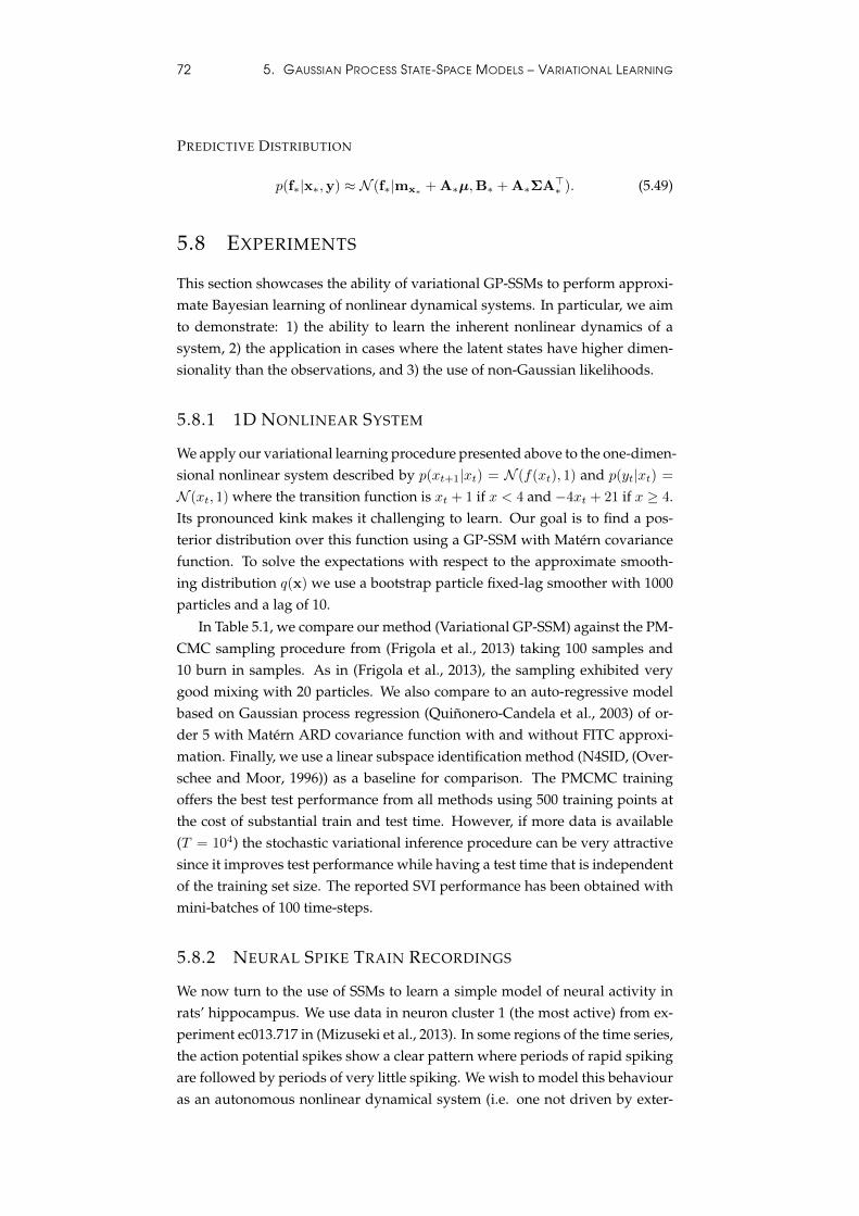
72 5. GAUSSIAN PROCESS STATE-SPACE MODELS – VARIATIONAL LEARNING
PREDICTIVE DISTRIBUTION
p(f∗|x∗,y) ≈ N (f∗|mx∗ + A∗µ,B∗ + A∗ΣA>∗ ). (5.49)
5.8 EXPERIMENTS
This section showcases the ability of variational GP-SSMs to perform approxi-mate Bayesian learning of nonlinear dynamical systems. In particular, we aimto demonstrate: 1) the ability to learn the inherent nonlinear dynamics of asystem, 2) the application in cases where the latent states have higher dimen-sionality than the observations, and 3) the use of non-Gaussian likelihoods.
5.8.1 1D NONLINEAR SYSTEM
We apply our variational learning procedure presented above to the one-dimen-sional nonlinear system described by p(xt+1|xt) = N (f(xt), 1) and p(yt|xt) =
N (xt, 1) where the transition function is xt + 1 if x < 4 and −4xt + 21 if x ≥ 4.Its pronounced kink makes it challenging to learn. Our goal is to find a pos-terior distribution over this function using a GP-SSM with Matern covariancefunction. To solve the expectations with respect to the approximate smooth-ing distribution q(x) we use a bootstrap particle fixed-lag smoother with 1000particles and a lag of 10.
In Table 5.1, we compare our method (Variational GP-SSM) against the PM-CMC sampling procedure from (Frigola et al., 2013) taking 100 samples and10 burn in samples. As in (Frigola et al., 2013), the sampling exhibited verygood mixing with 20 particles. We also compare to an auto-regressive modelbased on Gaussian process regression (Quinonero-Candela et al., 2003) of or-der 5 with Matern ARD covariance function with and without FITC approxi-mation. Finally, we use a linear subspace identification method (N4SID, (Over-schee and Moor, 1996)) as a baseline for comparison. The PMCMC trainingoffers the best test performance from all methods using 500 training points atthe cost of substantial train and test time. However, if more data is available(T = 104) the stochastic variational inference procedure can be very attractivesince it improves test performance while having a test time that is independentof the training set size. The reported SVI performance has been obtained withmini-batches of 100 time-steps.
5.8.2 NEURAL SPIKE TRAIN RECORDINGS
We now turn to the use of SSMs to learn a simple model of neural activity inrats’ hippocampus. We use data in neuron cluster 1 (the most active) from ex-periment ec013.717 in (Mizuseki et al., 2013). In some regions of the time series,the action potential spikes show a clear pattern where periods of rapid spikingare followed by periods of very little spiking. We wish to model this behaviouras an autonomous nonlinear dynamical system (i.e. one not driven by exter-
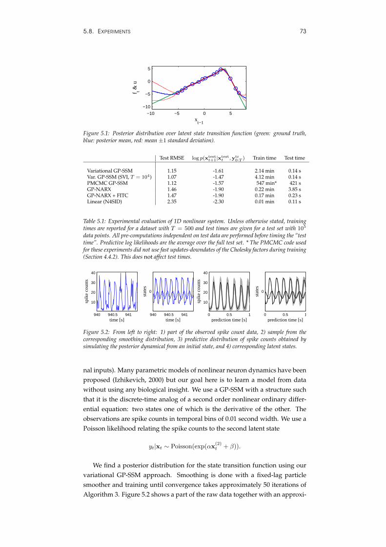
5.8. EXPERIMENTS 73
−10 −5 0 5
−10
−5
0
5
xt−1
f t & u
Figure 5.1: Posterior distribution over latent state transition function (green: ground truth,blue: posterior mean, red: mean ±1 standard deviation).
Test RMSE log p(xtestt+1|xtest
t ,ytr0:T ) Train time Test time
Variational GP-SSM 1.15 -1.61 2.14 min 0.14 sVar. GP-SSM (SVI, T = 104) 1.07 -1.47 4.12 min 0.14 sPMCMC GP-SSM 1.12 -1.57 547 min* 421 sGP-NARX 1.46 -1.90 0.22 min 3.85 sGP-NARX + FITC 1.47 -1.90 0.17 min 0.23 sLinear (N4SID) 2.35 -2.30 0.01 min 0.11 s
Table 5.1: Experimental evaluation of 1D nonlinear system. Unless otherwise stated, trainingtimes are reported for a dataset with T = 500 and test times are given for a test set with 105
data points. All pre-computations independent on test data are performed before timing the “testtime”. Predictive log likelihoods are the average over the full test set. * The PMCMC code usedfor these experiments did not use fast updates-downdates of the Cholesky factors during training(Section 4.4.2). This does not affect test times.
940 940.5 941
10
20
30
40
time [s]
spik
e co
unts
940 940.5 941
0
time [s]
stat
es
0 0.5 1
10
20
30
40
prediction time [s]
spik
e co
unts
0 0.5 1
0
prediction time [s]
stat
es
Figure 5.2: From left to right: 1) part of the observed spike count data, 2) sample from thecorresponding smoothing distribution, 3) predictive distribution of spike counts obtained bysimulating the posterior dynamical from an initial state, and 4) corresponding latent states.
nal inputs). Many parametric models of nonlinear neuron dynamics have beenproposed (Izhikevich, 2000) but our goal here is to learn a model from datawithout using any biological insight. We use a GP-SSM with a structure suchthat it is the discrete-time analog of a second order nonlinear ordinary differ-ential equation: two states one of which is the derivative of the other. Theobservations are spike counts in temporal bins of 0.01 second width. We use aPoisson likelihood relating the spike counts to the second latent state
yt|xt ∼ Poisson(exp(αx(2)t + β)).
We find a posterior distribution for the state transition function using ourvariational GP-SSM approach. Smoothing is done with a fixed-lag particlesmoother and training until convergence takes approximately 50 iterations ofAlgorithm 3. Figure 5.2 shows a part of the raw data together with an approxi-
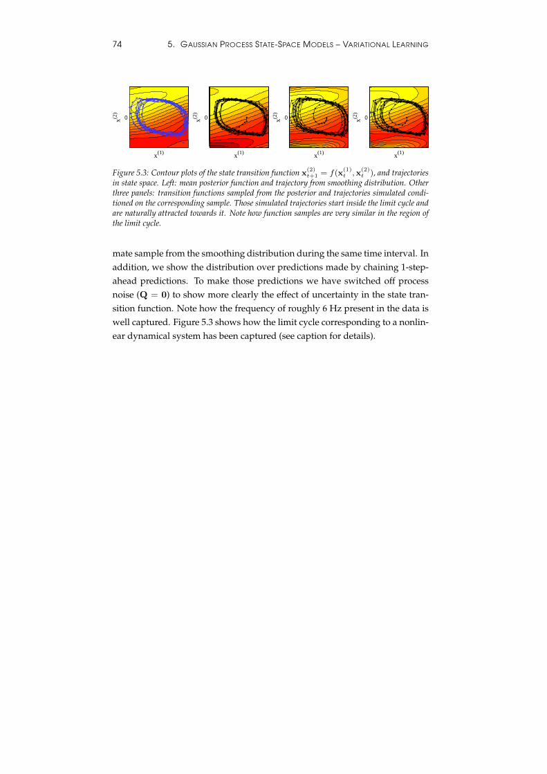
74 5. GAUSSIAN PROCESS STATE-SPACE MODELS – VARIATIONAL LEARNING
0
x(1)
x(2)
x(1)
x(2)
0
x(1)
x(2)
0
x(1)
x(2)
0
Figure 5.3: Contour plots of the state transition function x(2)t+1 = f(x
(1)t ,x
(2)t ), and trajectories
in state space. Left: mean posterior function and trajectory from smoothing distribution. Otherthree panels: transition functions sampled from the posterior and trajectories simulated condi-tioned on the corresponding sample. Those simulated trajectories start inside the limit cycle andare naturally attracted towards it. Note how function samples are very similar in the region ofthe limit cycle.
mate sample from the smoothing distribution during the same time interval. Inaddition, we show the distribution over predictions made by chaining 1-step-ahead predictions. To make those predictions we have switched off processnoise (Q = 0) to show more clearly the effect of uncertainty in the state tran-sition function. Note how the frequency of roughly 6 Hz present in the data iswell captured. Figure 5.3 shows how the limit cycle corresponding to a nonlin-ear dynamical system has been captured (see caption for details).
Chapter 6
Filtered Auto-RegressiveGaussian Process Models
This chapter presents a novel approach to learning nonlinear models of timeseries which integrates an automatic data preprocessing step with the train-ing of a nonlinear auto-regressive model (Frigola and Rasmussen, 2013). Theresulting algorithm is extremely simple to implement and can quickly learn aposterior over nonlinear dynamical systems from long time series data. Thisposterior can be used for prediction, extrapolation and other related tasks. Forinstance, one could learn a model of a nonlinear dynamical system from in-put/output data and use this model to design a feedback controller to stabilisethe system.
6.1 INTRODUCTION
Gaussian Process State-Space Models are very general and flexible models ofnonlinear dynamical systems. One of their main strengths is their ability tomodel dynamics in an abstract state space that is different to the observationspace. However, this poses the challenge of needing to infer the posteriordistribution over the state trajectories given the observed time series, i.e. thesmoothing distribution. This operation can be performed very efficiently witha Kalman smoother when the state-space model is linear and Gaussian. How-ever, for general nonlinear and/or non-Gaussian models, one needs to resort toapproximations such as the Extended Kalman Smoother, the Particle Smootheror Particle MCMC. Depending on the particular characteristics of the problemat hand, a given method can perform brilliantly or fail miserably.
In this section we present a method based on an auto-regressive nonlinearmodel (Section 2.3.6) where the difficult task of state smoothing is sidestepped.This leads to learning with a simple algorithm, less computational cost andmore robustness due to avoiding the use of a state smoother.
However, auto-regressive models are less general than state-space models.They are not able to separate between process noise (e.g. turbulence changing
75
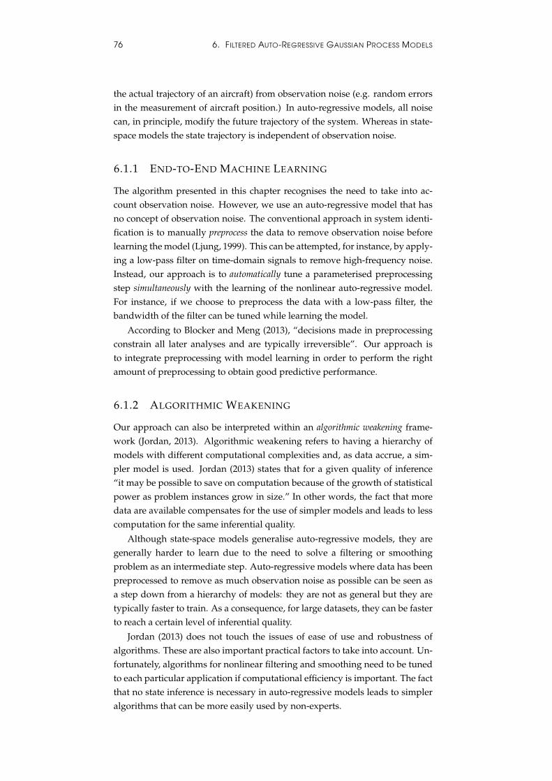
76 6. FILTERED AUTO-REGRESSIVE GAUSSIAN PROCESS MODELS
the actual trajectory of an aircraft) from observation noise (e.g. random errorsin the measurement of aircraft position.) In auto-regressive models, all noisecan, in principle, modify the future trajectory of the system. Whereas in state-space models the state trajectory is independent of observation noise.
6.1.1 END-TO-END MACHINE LEARNING
The algorithm presented in this chapter recognises the need to take into ac-count observation noise. However, we use an auto-regressive model that hasno concept of observation noise. The conventional approach in system identi-fication is to manually preprocess the data to remove observation noise beforelearning the model (Ljung, 1999). This can be attempted, for instance, by apply-ing a low-pass filter on time-domain signals to remove high-frequency noise.Instead, our approach is to automatically tune a parameterised preprocessingstep simultaneously with the learning of the nonlinear auto-regressive model.For instance, if we choose to preprocess the data with a low-pass filter, thebandwidth of the filter can be tuned while learning the model.
According to Blocker and Meng (2013), “decisions made in preprocessingconstrain all later analyses and are typically irreversible”. Our approach isto integrate preprocessing with model learning in order to perform the rightamount of preprocessing to obtain good predictive performance.
6.1.2 ALGORITHMIC WEAKENING
Our approach can also be interpreted within an algorithmic weakening frame-work (Jordan, 2013). Algorithmic weakening refers to having a hierarchy ofmodels with different computational complexities and, as data accrue, a sim-pler model is used. Jordan (2013) states that for a given quality of inference“it may be possible to save on computation because of the growth of statisticalpower as problem instances grow in size.” In other words, the fact that moredata are available compensates for the use of simpler models and leads to lesscomputation for the same inferential quality.
Although state-space models generalise auto-regressive models, they aregenerally harder to learn due to the need to solve a filtering or smoothingproblem as an intermediate step. Auto-regressive models where data has beenpreprocessed to remove as much observation noise as possible can be seen asa step down from a hierarchy of models: they are not as general but they aretypically faster to train. As a consequence, for large datasets, they can be fasterto reach a certain level of inferential quality.
Jordan (2013) does not touch the issues of ease of use and robustness ofalgorithms. These are also important practical factors to take into account. Un-fortunately, algorithms for nonlinear filtering and smoothing need to be tunedto each particular application if computational efficiency is important. The factthat no state inference is necessary in auto-regressive models leads to simpleralgorithms that can be more easily used by non-experts.
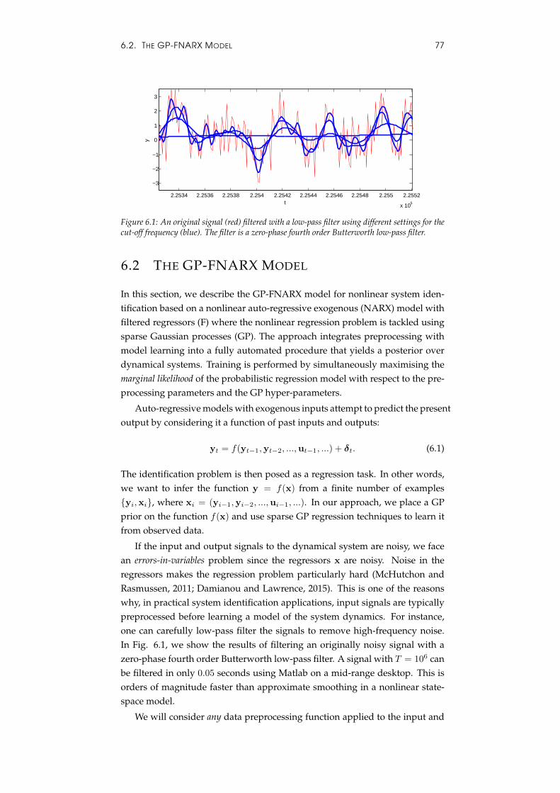
6.2. THE GP-FNARX MODEL 77
2.2534 2.2536 2.2538 2.254 2.2542 2.2544 2.2546 2.2548 2.255 2.2552
x 105
−3
−2
−1
0
1
2
3
t
y
Figure 6.1: An original signal (red) filtered with a low-pass filter using different settings for thecut-off frequency (blue). The filter is a zero-phase fourth order Butterworth low-pass filter.
6.2 THE GP-FNARX MODEL
In this section, we describe the GP-FNARX model for nonlinear system iden-tification based on a nonlinear auto-regressive exogenous (NARX) model withfiltered regressors (F) where the nonlinear regression problem is tackled usingsparse Gaussian processes (GP). The approach integrates preprocessing withmodel learning into a fully automated procedure that yields a posterior overdynamical systems. Training is performed by simultaneously maximising themarginal likelihood of the probabilistic regression model with respect to the pre-processing parameters and the GP hyper-parameters.
Auto-regressive models with exogenous inputs attempt to predict the presentoutput by considering it a function of past inputs and outputs:
yt = f(yt−1,yt−2, ...,ut−1, ...) + δt. (6.1)
The identification problem is then posed as a regression task. In other words,we want to infer the function y = f(x) from a finite number of examples{yi,xi}, where xi = (yi−1,yi−2, ...,ui−1, ...). In our approach, we place a GPprior on the function f(x) and use sparse GP regression techniques to learn itfrom observed data.
If the input and output signals to the dynamical system are noisy, we facean errors-in-variables problem since the regressors x are noisy. Noise in theregressors makes the regression problem particularly hard (McHutchon andRasmussen, 2011; Damianou and Lawrence, 2015). This is one of the reasonswhy, in practical system identification applications, input signals are typicallypreprocessed before learning a model of the system dynamics. For instance,one can carefully low-pass filter the signals to remove high-frequency noise.In Fig. 6.1, we show the results of filtering an originally noisy signal with azero-phase fourth order Butterworth low-pass filter. A signal with T = 106 canbe filtered in only 0.05 seconds using Matlab on a mid-range desktop. This isorders of magnitude faster than approximate smoothing in a nonlinear state-space model.
We will consider any data preprocessing function applied to the input and
78 6. FILTERED AUTO-REGRESSIVE GAUSSIAN PROCESS MODELS
output signals(y, u) = h(y,u,ωωω) (6.2)
where the preprocessed signals vary smoothly with respect to a vector of pre-processing parameters ωωω. This smoothness condition is imposed in order toobtain a probabilistic model with a differentiable marginal likelihood with re-spect to ωωω.
We can rephrase the auto-regressive model in terms of the preprocessedregressors:
yt = f(yt−1, yt−2, ..., ut−1, ...). (6.3)
Note that the left hand side term is not preprocessed.
6.2.1 CHOICE OF PREPROCESSING AND COVARIANCE FUNCTIONS
6.2.1.1 CAUSAL PREPROCESSING
If trained GP-FNARX models are intended to make online predictions, it isconvenient to use causal preprocessing. Causal preprocessing consists in theuse of a preprocessing algorithm whose output depends on past and currentinputs but not on future inputs. For example, a conventional moving averagefilter is a causal filter but the zero-phase filter in Figure 6.1 is non-causal.
Using a causal preprocessing stage mimics the kind of filtering that can berealistically performed online. Therefore, the preprocessing parameters tunedduring training can be used on exactly the same filtering algorithm when themodel is deployed.
6.2.1.2 COVARIANCE FUNCTION
An alternative to causal preprocessing on the full input and output signals is toembed a filter in the covariance function of the Gaussian process. For example,a kernel could incorporate a moving average filter
k(ya:b,y′a:b) = k(
b∑i=a
yi,
b∑i=a
y′i) (6.4)
or more sophisticated parameterised preprocessing
k(ya:b,y′a:b) = k
(h(ya:b,ωωω), h(y′a:b,ωωω)
). (6.5)
In such kernels, preprocessing can be interpreted as an explicit intermediatefeaturisation of the GP index set. In fact, h(ya:b,ωωω) does not need to have thesame dimensionality as ya:b. For example, it could be a filtered version of ya:b
sub-sampled at a few locations.
This formalisation of preprocessing converts the problem of tuning prepro-cessing parameters into a kernel search problem. (See (Duvenaud, 2014) foran excellent tutorial on expressing structure with kernels and an overview of
6.3. OPTIMISATION OF THE MARGINAL LIKELIHOOD 79
kernel search.) In our Gaussian process framework, kernel search can be per-formed via maximisation of the marginal likelihood.
Note that, within a kernel, it is feasible to relax the requirement for a causalfilter even when predictions will be made online. For instance, consider a lineardigital filter
k(ya:b,y′a:b) = k
(Hya:b,Hy′a:b
), (6.6)
where H is the linear digital filter matrix. A filtering and subsampling strat-egy could be implemented using a wide and short matrix. There is no needfor this filter to be causal within the a : b range, therefore H does not requirea triangular structure. H could be relatively large, e.g. 4 × 100, but param-eterised very lightly, e.g. with only a scalar bandwidth parameter. It wouldalso be possible to start training with such a light parameterisation and oncea rough bandwidth has been found switch to optimisation of all the elementsin H. This would let the algorithm “discover” the best combination of filtertype, subsampling strategy and hyper-parameters for the base kernel k(·, ·). Asimilar filtering strategy could be implemented for the mean function of theGP.
6.3 OPTIMISATION OF THE MARGINAL LIKELIHOOD
In Section 2.2.1 we described how the marginal likelihood provides a verypowerful metric to perform model selection due to its ability to automaticallytrade off model fit and model complexity in a principled manner. Our goal herewill be to maximise the marginal likelihood of the Gaussian process regressionmodel with respect to the signal preprocessing parameters and also, simulta-neously, with respect to the hyper-parameters of the GP. For convenience, weintroduce ψψψ , {ωωω,θθθ} grouping the two kinds of parameters.
We will employ hill-climbing optimisation to maximise the marginal like-lihood (or, equivalently, its logarithm). For notational simplicity, we group allthe preprocessed regressors into a matrix X = X(y,u,ωωω). The log marginallikelihood becomes
log p(y|X(ωωω), θθθ). (6.7)
Its derivatives with respect to the GP hyper-parameters
∂
∂θθθjlog p(y|X(ωωω), θθθ), (6.8)
are straightforward since we typically choose differentiable covariance func-tions. However, the derivatives with respect to any of the preprocessing pa-rameters
∂
∂ωωωklog p(y|X(ωωω), θθθ) (6.9)
can be more difficult to compute since derivatives with respect to the kernelmatrix also need to be computed. We can write the derivative of a single ele-
80 6. FILTERED AUTO-REGRESSIVE GAUSSIAN PROCESS MODELS
Algorithm 4 High-level pseudo-code for the GP-FNARX algorithm.Inputs: I = {output signals y1:T , input signals u1:T , model order η}
1. ψψψ0 ← INITIALGUESS(I)
2. ψψψOpt ←MAXIMISEMARGLIKELIHOOD(ψψψ0, I)
3. Predictive model← PRECOMPUTEPREDICTOR(ψOpt, I)
ment of the covariance matrix as
∂Kij
∂ωωωk=∂k(xi, xj)
∂ωωωk=
∂k
∂xi
∂xi∂ωωωk
+∂k
∂xj
∂xj∂ωωωk
(6.10)
where the derivatives with respect to the regressors are straightforward to com-pute when using smooth covariance functions. However, the derivatives of theregressors with respect to the preprocessing parameters may be hard to com-pute. In any case, if the preprocessing function is smooth, the derivatives ∂x
∂ωωωk
can be approximated numerically by finite differences at the cost of one extraevaluation of the preprocessing function per dimension of ωωω.
6.4 SPARSE GPS FOR COMPUTATIONAL SPEED
Computing the marginal likelihood for datasets with more than a few thou-sand points becomes computationally expensive. In such settings we can usesparse Gaussian processes for regression such as FITC (Snelson and Ghahra-mani, 2006) or variational sparse GPs (Titsias, 2009). Their computational com-plexity during training is O(M2T ) instead of the O(T 3) of the full GP. Afterall possible pre-computations, the computational complexity of making pre-dictions with sparse GPs is O(M) for the mean of the predictive distributionand O(M2) for its variance. The computational efficiency comes from havingcondensed the original dataset with roughly T points into a smaller set of Minducing points.
6.5 ALGORITHM
In Algorithm 4 we present a high-level overview of the GP-FNARX algorithm.The first step consists in providing an initial guess for the unknown hyper-parameters. We have found that, in the absence of any problem-specific knowl-edge that could guide the initial guess, a successful data-based heuristic is torun a few steps of optimisation of the marginal likelihood with respect to theGP hyper-parameters followed by a few steps of optimisation with respect tothe preprocessing parameters. By running these two steps, the algorithm canrapidly hone in the right order of magnitude for the unknown parameters.
The second step consists in a straightforward joint optimisation of the GPhyper-parameters and the preprocessing parameters. This step can be per-
6.6. EXPERIMENTS 81
formed by either using a subset of the data with a conventional GP or, prefer-ably, on the full dataset using a sparse GP (Quinonero-Candela and Rasmussen,2005; Titsias, 2009).
In the third and final step, any O(T ) operation in the sparse GP predictorcan be pre-computed in order to obtain a model that is able to provide predic-tive means in O(M) and predictive variances in O(M2).
The choice of the order of the auto-regressive model is not critical for theperformance of the algorithm provided that two conditions are met: i) the or-der is chosen to be higher than the optimal order and ii) the automatic rele-vance determination (ARD) covariance function is chosen for the GP. This isdue to the fact that the Bayesian Occam’s razor embodied by the marginal like-lihood is able to automatically disable regressors that are irrelevant to the taskat hand. In our experiments we verified that adding hundreds of regressors ona problem of low order did not cause any overfitting and only represented acomputation time penalty.
6.6 EXPERIMENTS
In this section we present an experimental evaluation of the proposed systemidentification method. We have used data from two nonlinear system identifi-cation benchmarks based on electric circuits: i) the Silverbox benchmark orig-inating from the 2004 IFAC Symposium on Nonlinear Control Systems (NOL-COS) and ii) the SYSID09 Wiener-Hammerstein system identification bench-mark (Schoukens et al., 2009) which has been the object of a special section inthe November 2012 issue of the “Control Engineering Practice” journal (Hjal-marsson et al., 2012).
Both datasets have >105 data points and are corrupted by a very smallamount of noise. For instance, the authors of the Wiener-Hammerstein datasetestimate its signal to noise ratio to be of 70 dB. Since we are attempting todemonstrate the ability of our method to cope with measurement noise, wewill inject different amounts of synthetic i.i.d. Gaussian noise to the outputsignals to make the identification task more challenging. Being able to haveoriginal signals with little noise will be convenient to test the quality of theresulting models.
We have compared GP-FNARX against other off-the-shelf alternatives. Inparticular, we use several NARX models available in the Matlab System Iden-tification toolbox (Ljung, 2012).
Following this spirit, we have avoided any tuning of our method to the par-ticular benchmarks presented in this section. For instance, using knowledgeabout the underlying system of the Silverbox benchmark, we obtained betterperformance by adding cubic regressors into our NARX model. However, wehave not used those custom regressors when reporting the performance of ourmodel.
Regarding the preprocessing step, we have chosen a simple zero-phase sec-
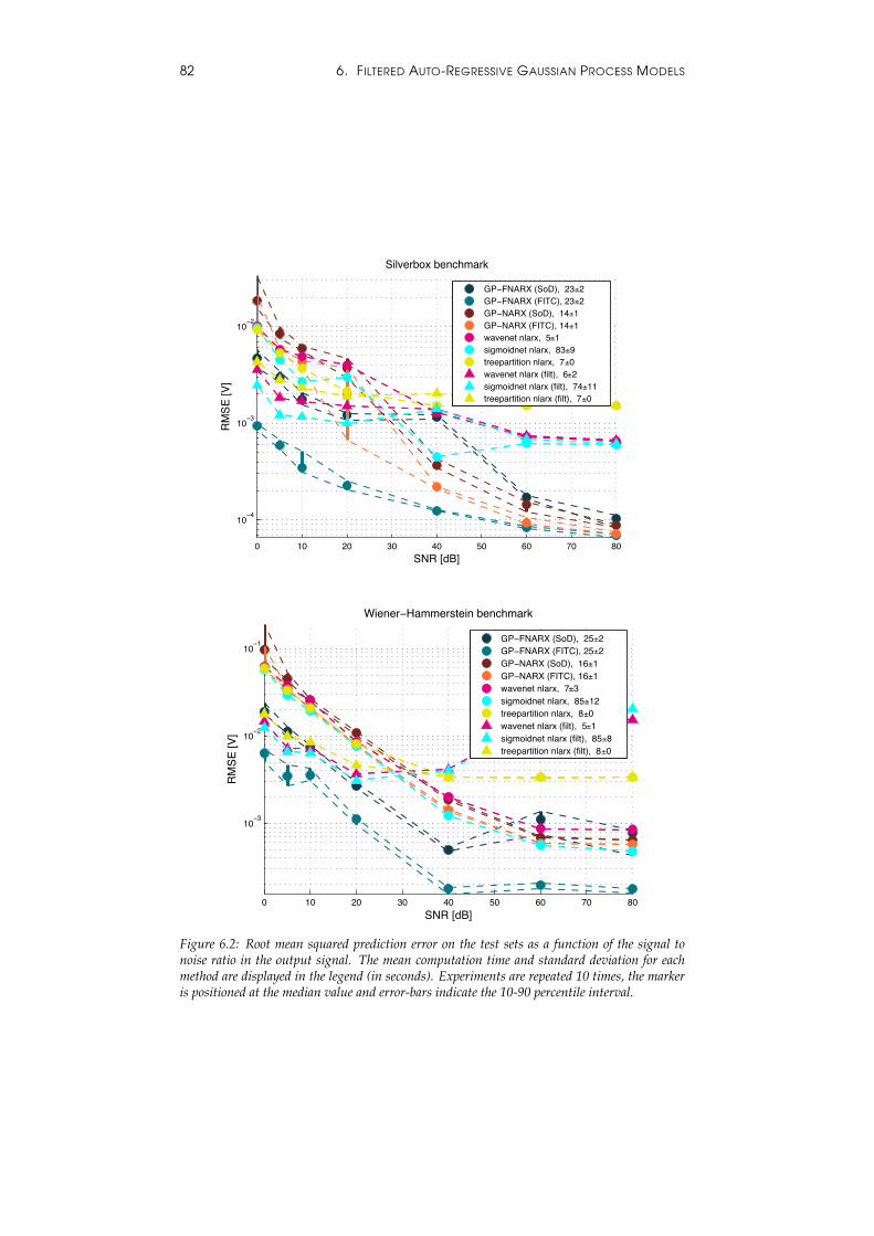
82 6. FILTERED AUTO-REGRESSIVE GAUSSIAN PROCESS MODELS
0 10 20 30 40 50 60 70 80
10−4
10−3
10−2
SNR [dB]
RM
SE [V
]
Silverbox benchmark
GP−FNARX (SoD), 23±2GP−FNARX (FITC), 23±2GP−NARX (SoD), 14±1GP−NARX (FITC), 14±1wavenet nlarx, 5±1sigmoidnet nlarx, 83±9treepartition nlarx, 7±0wavenet nlarx (filt), 6±2sigmoidnet nlarx (filt), 74±11treepartition nlarx (filt), 7±0
0 10 20 30 40 50 60 70 80
10−3
10−2
10−1
SNR [dB]
RM
SE [V
]
Wiener−Hammerstein benchmark
GP−FNARX (SoD), 25±2GP−FNARX (FITC), 25±2GP−NARX (SoD), 16±1GP−NARX (FITC), 16±1wavenet nlarx, 7±3sigmoidnet nlarx, 85±12treepartition nlarx, 8±0wavenet nlarx (filt), 5±1sigmoidnet nlarx (filt), 85±8treepartition nlarx (filt), 8±0
0 10 20 30 40 50 60 70 80
10−4
10−3
10−2
SNR [dB]
RM
SE [V
]
Silverbox benchmark
GP−FNARX (SoD), 23±2GP−FNARX (FITC), 23±2GP−NARX (SoD), 14±1GP−NARX (FITC), 14±1wavenet nlarx, 5±1sigmoidnet nlarx, 83±9treepartition nlarx, 7±0wavenet nlarx (filt), 6±2sigmoidnet nlarx (filt), 74±11treepartition nlarx (filt), 7±0
0 10 20 30 40 50 60 70 80
10−3
10−2
10−1
SNR [dB]
RM
SE [V
]
Wiener−Hammerstein benchmark
GP−FNARX (SoD), 25±2GP−FNARX (FITC), 25±2GP−NARX (SoD), 16±1GP−NARX (FITC), 16±1wavenet nlarx, 7±3sigmoidnet nlarx, 85±12treepartition nlarx, 8±0wavenet nlarx (filt), 5±1sigmoidnet nlarx (filt), 85±8treepartition nlarx (filt), 8±0
Figure 6.2: Root mean squared prediction error on the test sets as a function of the signal tonoise ratio in the output signal. The mean computation time and standard deviation for eachmethod are displayed in the legend (in seconds). Experiments are repeated 10 times, the markeris positioned at the median value and error-bars indicate the 10-90 percentile interval.
6.6. EXPERIMENTS 83
ond order Butterworth low-pass filter. In this case, the filter parameter ωωω rep-resents the cut-off frequency of the filter.
In Figure 6.2 we have plotted the prediction errors on both benchmarks fora number of different models and signal-to-(synthetic)-noise ratios. We havetested the following models:
• GP-FNARX (SoD): the model presented in this paper using a subset of 512randomly chosen points (subset of data approximation, SoD (Rasmussenand Williams, 2006)).
• GP-FNARX (FITC): the model presented in this paper using a FITC sparseGP (Quinonero-Candela and Rasmussen, 2005) with M = 512 inducingpoints chosen at random.
• GP-NARX (SoD): same as GP-FNARX (SoD) but with no pre-filtering of thesignals.
• GP-NARX (FITC): same as GP-FNARX (FITC) but with no pre-filtering of thesignals.
• * nlarx: 3 different NARX models implemented in the Matlab SystemIdentification toolbox (Ljung, 2012). Default options. No pre-filteringof the signals.
• * nlarx (filt): same as * nlarx but using the pre-filtering parameters takenfrom GP-FNARX (FITC) (the computation time for computing those param-eters is not taken included in the reported figure).
All models have order 10 for the inputs and the outputs.We observe that the GP-FNARX method with a FITC sparse GP provides
the lowest error for all noise levels in both benchmarks. Overall, these re-sults allow us to be optimistic with regards to the prediction capabilities ofGP-FNARX models and validate the use of the marginal likelihood as a crite-rion for model selection in the context of automated preprocessing of the data.
The legend of Figure 6.2 reports the computation times of the experimentswhen performed on a machine with a 2008 Intel Core i7-920 processor at 2.67GHz. Although the training time of the GP-FNARX model is higher than thewavenet and treepartition models, it is significantly faster than sigmoidnet yet itprovides a lower prediction error.
GP models have a one degree of freedom knob which can be used to tradeoff accuracy with speed: the number of data points used for SoD or the numberof inducing points in a sparse GP method such as FITC.

84 6. FILTERED AUTO-REGRESSIVE GAUSSIAN PROCESS MODELS
Chapter 7
Conclusions
7.1 CONTRIBUTIONS
In this thesis, we have presented a number of contributions towards practicalBayesian learning of nonlinear time series models. Solutions have been offeredto attempt to achieve a number of often conflicting goals:
Bayesian learning: All the work presented in this thesis has aimed at obtain-ing posteriors over nonlinear dynamical systems. These posteriors modelthe uncertainty about what the actual dynamical systems are given theparticular time series used for training. In some settings, quantifying pre-dictive uncertainty is useful to improve decisions made with the model.For example, our methods can be used as one of the building blockswithin Bayesian reinforcement learning or for the design of adaptive-robust feedback controllers.
Nonparametric modelling: We presented learning algorithms for models oftime series based on Gaussian processes. The sampling methods intro-duced in Chapter 4 and the GP-FNARX auto-regressive model in Chap-ter 6 are able to learn fully nonparametric models of time series whichcombine very large model capacity while avoiding the risk of overfitting.
Fast training: Throughout the thesis we have provided sparse versions for allmodels. Models based on sparse Gaussian processes inherit most of theproperties of their fully nonparametric counterparts whilst reducing thecomputational complexity. In particular, they offer a convenient knob totrade off model capacity and computation time. We also presented anorthogonal approach to reduce training time for large datasets based onmini-batches (Chapter 5). Learning from mini-batches avoids having toprocess the full dataset at each iteration which can result in much fasteroptimisation when the time series are long.
Fast prediction: Monte Carlo methods from Chapter 4 can capture the fullnonparametric expressivity of GP-SSMs but are slow at test time. Thevariational learning approach in Chapter 5 was designed to avoid thisproblem by approximating the posterior over nonlinear dynamical sys-
85
86 7. CONCLUSIONS
tems with a representation whose size is independent on the length ofthe time series.
Ease of use: The filtered nonlinear auto-regressive algorithm introduced in Chap-ter 6 provides a simple, robust and fast learning method that makes itwell suited to application by non-experts. Its main advantage is that itavoids the expensive (and potentially difficult to tune) smoothing stepthat is a key part of learning nonlinear state-space models.
Most of the work in this thesis has revolved around Gaussian Process State-Space Models. We started by providing a literature review that unifies previouswork related to the model. We then derived a new formulation for the modelthat enables straightforward sampling from the prior. The insights offered bythe new formulation have led us to the creation of new Bayesian learning algo-rithms for the GP-SSM based on Particle MCMC and variational inference.
7.2 FUTURE WORK
The models presented in this dissertation are probabilistic in nature. They rep-resent an idealisation of the complex system that generated the data. By usinginverse probability it is possible to go from observed data to a posterior overthe unobserved variables of interest. This posterior captures uncertainty whichcan be propagated to future predictions in a principled manner.
However, many recent successes in sequence modelling have stemmed frommodels that are essentially non-probabilistic1 (Graves et al., 2013; Sutskever,2013; LeCun et al., 2015). Although we have advocated for the use of gener-ative probabilistic models, we should ask ourselves: what are the characteris-tics of non-probabilistic models such as Recurrent Neural Networks that allowthem to learn such insightful representations of sequences? A tentative answercould be that their success is based on the combination of large datasets andvery well engineered training algorithms.
Modelling uncertainty in probabilistic learning algorithms imposes an extracomputational burden that their non-probabilistic counterparts do not have tobear. An interesting avenue of future work consists in taking the insights andtechniques that have led to successful non-probabilistic methods and to applythem in the context of learning probabilistic generative models. A relativelystraightforward way to achieve this is by first training computationally effi-cient but non-probabilistic models of time series and subsequently use themas an initialisation for probabilistic learning algorithms such as the variationalGP-SSM in Chapter 5. An interesting alternative to this approach consists inreinterpreting successful algorithms for non-probabilistic models in ways thatallow them to capture model uncertainty, see for instance (Gal and Ghahra-mani, 2015). This would capitalise on the heavy engineering already done forsome non-probabilistic models and allow us to move towards the ultimate goalof providing uncertainty estimates for any prediction.
1In the sense that they do not model uncertainty in the parameters and states of the model.
Appendix A
Approximate BayesianInference
In this appendix we provide an overview of the two main learning algorithmsthat are used in this thesis to learn Gaussian Process State-Space Models.
A.1 PARTICLE MARKOV CHAIN MONTE CARLO
Markov Chain Monte Carlo (MCMC) methods are popular in Bayesian learn-ing because they allow approximate learning in intractable models. They op-erate by simulating a Markov chain which admits the target distribution as itsstationary distribution. If the target distribution is the posterior, samples ob-tained via MCMC can be treated as samples from the posterior distribution(with some caveats, see for example (Bishop, 2006)).
Particle MCMC (Andrieu et al., 2010) is a recent variant of MCMC thathas proven to be particularly suited to sample from high-dimensional distri-butions with high correlations. From the various Particle MCMC algorithmsintroduced in (Andrieu et al., 2010), we use the Particle Gibbs algorithm. Parti-cle Gibbs can be considered a Gibbs sampler that relies on a modified particlefilter which is conditioned on a reference trajectory.
A.1.1 PARTICLE GIBBS WITH ANCESTOR SAMPLING
We now introduce the detailed algorithm for Particle Gibbs with Ancestor Sam-pling (PGAS, Algorithm 5, Lindsten et al. (2014)). PGAS builds on ParticleGibbs by adding an additional sampling step that mitigates the effects of pathdegeneracy. This improves mixing and allows the use of a small number ofparticles (Lindsten et al., 2014).
To sample the state trajectory, PGAS makes use of a Sequential Monte Carlo-like procedure referred to as the Conditional Particle Filter with Ancestor Sam-pling (CPF-AS, Algorithm 6). This approach is particularly well suited to non-Markovian latent variable models, as it relies only on a forward recursion
87
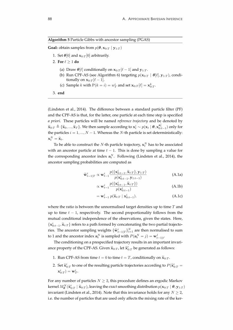
88 A. APPROXIMATE BAYESIAN INFERENCE
Algorithm 5 Particle Gibbs with ancestor sampling (PGAS)
Goal: obtain samples from p(θ,x0:T | y1:T )
1. Set θ[0] and x0:T [0] arbitrarily.
2. For ` ≥ 1 do
(a) Draw θ[`] conditionally on x0:T [`− 1] and y1:T .(b) Run CPF-AS (see Algorithm 6) targeting p(x0:T | θ[`],y1:T ), condi-
tionally on x0:T [`− 1].(c) Sample k with P(k = i) = wiT and set x0:T [`] = xk0:T .
3. end
(Lindsten et al., 2014). The difference between a standard particle filter (PF)and the CPF-AS is that, for the latter, one particle at each time step is specifieda priori. These particles will be named reference trajectory and be denoted byx0:T , {x0, ..., xT }. We then sample according to xit ∼ p(xt | θ,x
ait
0:t−1) only forthe particles i = 1, ..., N − 1. Whereas the N -th particle is set deterministically:xNt = xt.
To be able to construct the N -th particle trajectory, xNt has to be associatedwith an ancestor particle at time t − 1. This is done by sampling a value forthe corresponding ancestor index aNt . Following (Lindsten et al., 2014), theancestor sampling probabilities are computed as
wit−1|T ∝ wi
t−1
p({xi0:t−1, xt:T },y1:T )
p(xi0:t−1,y1:t−1)(A.1a)
∝ wit−1
p({xi0:t−1, xt:T })p(xi0:t−1)
(A.1b)
= wit−1 p(xt:T | xi0:t−1). (A.1c)
where the ratio is between the unnormalised target densities up to time T andup to time t − 1, respectively. The second proportionality follows from themutual conditional independence of the observations, given the states. Here,{xi0:t−1, xt:T } refers to a path formed by concatenating the two partial trajecto-ries. The ancestor sampling weights {wi
t−1|T }Ni=1 are then normalised to sum
to 1 and the ancestor index aNt is sampled with P (aNt = j) = wjt−1|t.
The conditioning on a prespecified trajectory results in an important invari-ance property of the CPF-AS. Given x0:T , let x′0:T be generated as follows:
1. Run CPF-AS from time t = 0 to time t = T , conditionally on x0:T .
2. Set x′0:T to one of the resulting particle trajectories according to P (x′0:T =
xi0:T ) = wiT .
For any number of particles N ≥ 2, this procedure defines an ergodic MarkovkernelMN
θ (x′0:T | x0:T ), leaving the exact smoothing distribution p(x0:T | θ,y1:T )
invariant (Lindsten et al., 2014). Note that this invariance holds for any N ≥ 2,i.e. the number of particles that are used only affects the mixing rate of the ker-
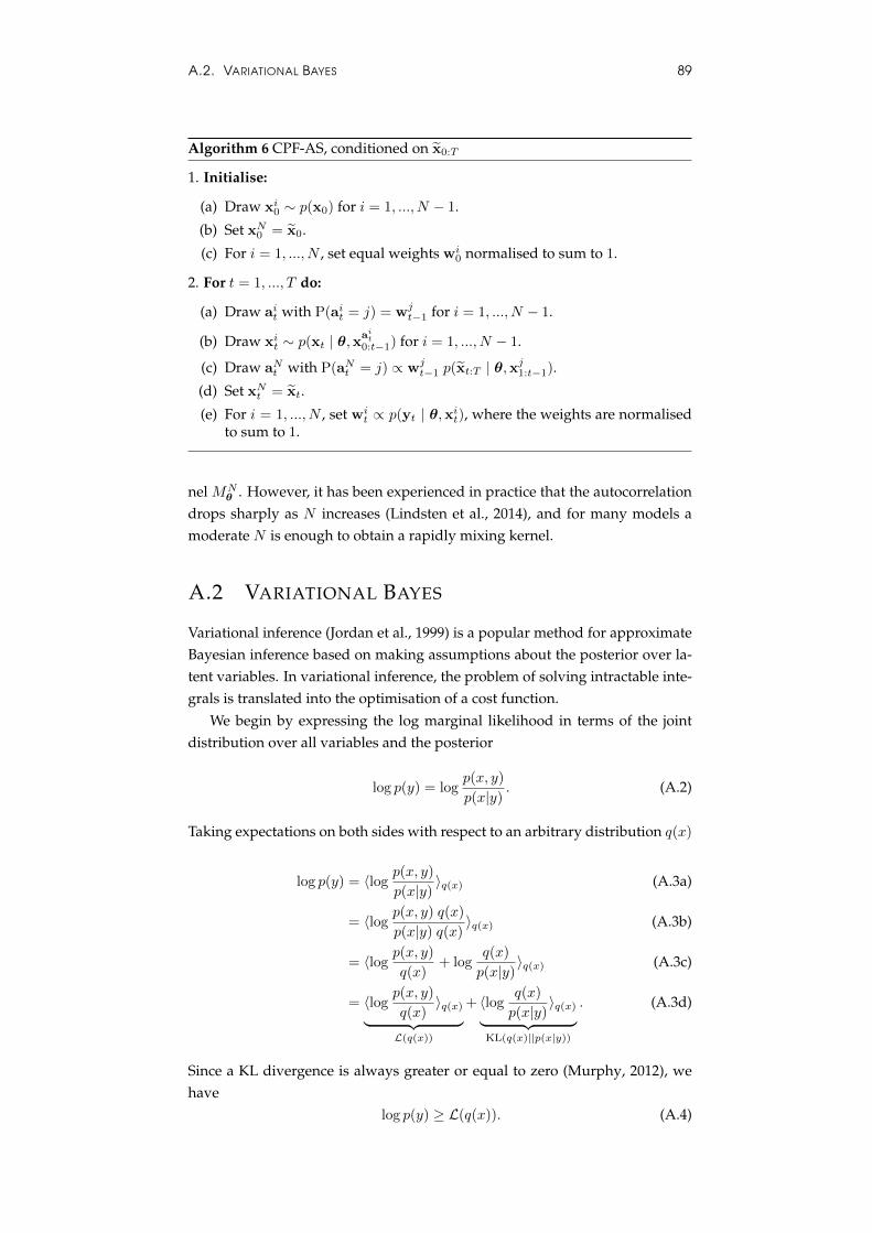
A.2. VARIATIONAL BAYES 89
Algorithm 6 CPF-AS, conditioned on x0:T
1. Initialise:
(a) Draw xi0 ∼ p(x0) for i = 1, ..., N − 1.
(b) Set xN0 = x0.
(c) For i = 1, ..., N , set equal weights wi0 normalised to sum to 1.
2. For t = 1, ..., T do:
(a) Draw ait with P(ait = j) = wjt−1 for i = 1, ..., N − 1.
(b) Draw xit ∼ p(xt | θ,xait
0:t−1) for i = 1, ..., N − 1.
(c) Draw aNt with P(aNt = j) ∝ wjt−1 p(xt:T | θ,x
j1:t−1).
(d) Set xNt = xt.
(e) For i = 1, ..., N , set wit ∝ p(yt | θ,xit), where the weights are normalised
to sum to 1.
nel MNθ . However, it has been experienced in practice that the autocorrelation
drops sharply as N increases (Lindsten et al., 2014), and for many models amoderate N is enough to obtain a rapidly mixing kernel.
A.2 VARIATIONAL BAYES
Variational inference (Jordan et al., 1999) is a popular method for approximateBayesian inference based on making assumptions about the posterior over la-tent variables. In variational inference, the problem of solving intractable inte-grals is translated into the optimisation of a cost function.
We begin by expressing the log marginal likelihood in terms of the jointdistribution over all variables and the posterior
log p(y) = logp(x, y)
p(x|y). (A.2)
Taking expectations on both sides with respect to an arbitrary distribution q(x)
log p(y) = 〈logp(x, y)
p(x|y)〉q(x) (A.3a)
= 〈logp(x, y) q(x)
p(x|y) q(x)〉q(x) (A.3b)
= 〈logp(x, y)
q(x)+ log
q(x)
p(x|y)〉q(x) (A.3c)
= 〈logp(x, y)
q(x)〉q(x)︸ ︷︷ ︸
L(q(x))
+ 〈logq(x)
p(x|y)〉q(x)︸ ︷︷ ︸
KL(q(x)||p(x|y))
. (A.3d)
Since a KL divergence is always greater or equal to zero (Murphy, 2012), wehave
log p(y) ≥ L(q(x)). (A.4)
90 A. APPROXIMATE BAYESIAN INFERENCE
The bound is tight if and only if q(x) = p(x|y). In other words, if the vari-ational distribution q(x) perfectly matches the posterior. Minimisation of theKL divergence between the variational distribution and the true posterior canbe achieved by maximising the lower bound L(q(x)). There are two main ap-proaches to maximise the lower bound when the posterior is not analyticallytractable:
1. Choose a parametric form for the variational distribution, parameteriseit with θ and maximise the evidence lower bound with respect to thoseparameters
θ∗ = arg maxθ
L(qθ(x)). (A.5)
2. Choose a particular form for the approximate posterior (e.g. q(x1, x2) =
q(x1)q(x2)) and use the calculus of variations to find the optimal distri-butions that maximise the lower bound. In the calculus of variations op-timisation is done with respect to functions rather than parameters. Inour case, the functions are probability distributions and need to satisfythe constraint that they integrate to one. Finding a stationary point of theevidence lower bound with respect to a variational distribution can betranslated to the problem of finding the distribution that is a solution tothe Euler-Lagrange differential equation. For
L(q(x)) = 〈logp(x, y)
q(x)〉q(x) =
∫I (x, q(x)) dx, (A.6)
the Euler-Lagrange equation is
∂
∂q(x)I (x, q(x)) = 0, (A.7)
∂
∂q(x)q(x) log
p(x, y)
q(x)= 0, (A.8)
logp(x, y)
q∗(x)− 1 = 0. (A.9)
Which results in the optimal variational distribution q∗(x) ∝ p(x, y) andsince p(x, y) ∝ p(x|y) we obtain the result that was expected: the ev-idence lower bound is maximised when the variational distribution isequal to the true posterior. In such a case the bound is tight: log p(y) =
L(q∗(x)). However, this is not particularly useful since the posterior is thevery distribution that we are trying to find. It is by making assumptionsabout the variational distribution, such as q(x1, x2) = q(x1)q(x2), thatone can obtain useful results. This can be achieved by using the Euler-Lagrange equation to find stationary points of L with respect to partsof the variational distribution such as q(x1). The evidence lower boundis then maximised by executing a “coordinate”-wise optimisation in thespace of variational distributions. Bishop (2006) and Murphy (2012) pro-vide a much more thorough exposition of the calculus of variations andvariational inference.
Bibliography
Agarwal, D. K. and Gelfand, A. E. (2005). Slice sampling for simulation based fitting ofspatial data models. Statistics and Computing, 15(1):61–69. (cited in p. 40)
Alvarez, M., Luengo, D., and Lawrence, N. (2009). Latent force models. Proceedings ofthe Twelfth International Conference on Artificial Intelligence and Statistics, 5:9–16. (citedin p. 23)
Alvarez, M., Luengo, D., and Lawrence, N. (2013). Linear latent force models usingGaussian processes. Pattern Analysis and Machine Intelligence, IEEE Transactions on,35(11):2693–2705. (cited in p. 23)
Andrieu, C., Doucet, A., and Holenstein, R. (2010). Particle Markov chain MonteCarlo methods. Journal of the Royal Statistical Society: Series B (Statistical Methodology),72(3):269–342. (cited in pp. 38, 39, 46, 62, and 87)
Andrieu, C., Moulines, E., and Priouret, P. (2005). Stability of stochastic approximationunder verifiable conditions. SIAM Journal on Control and Optimization, 44(1):283–312.(cited in p. 46)
Andrieu, C. and Vihola, M. (2011). Markovian stochastic approximation with expand-ing projections. arXiv.org, arXiv:1111.5421. (cited in p. 46)
Barber, D., Cemgil, A. T., and Chiappa, S. (2011). Bayesian Time Series Models. CambridgeUniversity Press. (cited in pp. 1 and 37)
Barber, D. and Chiappa, S. (2006). Unified inference for variational Bayesian linearGaussian state-space models. In Advances in Neural Information Processing Systems(NIPS), volume 20. (cited in p. 13)
Bishop, C. M. (2006). Pattern Recognition and Machine Learning. Springer. (cited in pp. 45,87, and 90)
Blocker, A. W. and Meng, X.-L. (2013). The potential and perils of preprocessing: Build-ing new foundations. Bernoulli, 19(4):1176–1211. (cited in p. 76)
Box, G. E. P., Jenkins, G. M., and Reinsel, G. C. (1994). Time Series Analysis: Forecastingand Control. Prentice-Hall. (cited in p. 13)
Broderick, T., Boyd, N., Wibisono, A., Wilson, A. C., and Jordan, M. I. (2013). Stream-ing variational Bayes. In Burges, C., Bottou, L., Welling, M., Ghahramani, Z., andWeinberger, K., editors, Advances in Neural Information Processing Systems 26, pages1727–1735. Curran Associates, Inc. (cited in p. 66)
Chen, T., Ohlsson, H., and Ljung, L. (2012). On the estimation of transfer functions,regularizations and Gaussian processesrevisited. Automatica, 48(8):1525–1535. (citedin p. 4)
91
92 BIBLIOGRAPHY
Damianou, A. and Lawrence, N. (2013). Deep Gaussian processes. In Carvalho, C. andRavikumar, P., editors, Proceedings of the Sixteenth International Workshop on ArtificialIntelligence and Statistics (AISTATS-13), AISTATS ’13, pages 207–215. JMLR W&CP 31.(cited in p. 22)
Damianou, A. and Lawrence, N. (2015). Semi-described and semi-supervised learningwith Gaussian processes. Uncertainty in Artificial Intelligence (UAI). (cited in pp. 21and 77)
Damianou, A. C., Titsias, M., and Lawrence, N. D. (2011). Variational Gaussian pro-cess dynamical systems. In Shawe-Taylor, J., Zemel, R., Bartlett, P., Pereira, F., andWeinberger, K., editors, Advances in Neural Information Processing Systems 24, pages2510–2518. (cited in pp. 22 and 34)
Deisenroth, M. (2010). Efficient Reinforcement Learning using Gaussian Processes. PhDthesis, Karlsruher Institut fur Technologie. (cited in p. 42)
Deisenroth, M. and Mohamed, S. (2012). Expectation Propagation in Gaussian processdynamical systems. In Bartlett, P., Pereira, F., Burges, C., Bottou, L., and Weinberger,K., editors, Advances in Neural Information Processing Systems 25, pages 2618–2626.(cited in p. 20)
Deisenroth, M., Turner, R., Huber, M., Hanebeck, U., and Rasmussen, C. (2012). Robustfiltering and smoothing with Gaussian processes. Automatic Control, IEEE Transactionson, 57(7):1865 –1871. (cited in p. 20)
Delyon, B., Lavielle, M., and Moulines, E. (1999). Convergence of a stochastic approxi-mation version of the EM algorithm. The Annals of Statistics, 27(1):pp. 94–128. (citedin p. 46)
Dempster, A. P., Laird, N. M., and Rubin, D. B. (1977). Maximum likelihood from in-complete data via the EM algorithm. Journal of the Royal Statistical Society. Series B(Methodological), 39(1):pp. 1–38. (cited in p. 45)
Doucet, A. and Johansen, A. (2011). A tutorial on particle filtering and smoothing: Fif-teen years later. In Crisan, D. and Rozovsky, B., editors, Oxford Hand-book of NonlinearFiltering. Oxford University Press. (cited in p. 39)
Duchi, J., Hazan, E., and Singer, Y. (2011). Stochastic variational inference. Journal ofMachine Learning Research, 12:2121–2159. (cited in p. 63)
Duvenaud, D. (2014). Automatic Model Construction with Gaussian Processes. PhD thesis,Computational and Biological Learning Laboratory, University of Cambridge. (citedin p. 78)
Duvenaud, D., Lloyd, J., Grosse, R., Tenenbaum, J., and Zoubin, G. (2013). Structure dis-covery in nonparametric regression through compositional kernel search. In Proceed-ings of The 30th International Conference on Machine Learning (ICML), pages 1166–1174.(cited in p. 13)
Ferris, B., Fox, D., and Lawerence, N. (2007). WiFi-SLAM using Gaussian process la-tent variable models. In Proceedings of the International Joint Conference on ArtificialIntelligence (IJCAI). (cited in p. 18)
Foti, N., Xu, J., Laird, D., and Fox, E. (2014). Stochastic variational inference for hid-den markov models. In Ghahramani, Z., Welling, M., Cortes, C., Lawrence, N., andWeinberger, K., editors, Advances in Neural Information Processing Systems 27, pages3599–3607. Curran Associates, Inc. (cited in p. 66)
BIBLIOGRAPHY 93
Frigola, R., Chen, Y., and Rasmussen, C. E. (2014a). Variational Gaussian process state-space models. In Advances in Neural Information Processing Systems 27 (NIPS), pages3680–3688. (cited in pp. 55 and 66)
Frigola, R., Lindsten, F., Schon, T. B., and Rasmussen, C. E. (2013). Bayesian inferenceand learning in Gaussian process state-space models with particle MCMC. In Bottou,L., Burges, C., Ghahramani, Z., Welling, M., and Weinberger, K., editors, Advances inNeural Information Processing Systems 26 (NIPS), pages 3156–3164. (cited in pp. 16, 37,53, and 72)
Frigola, R., Lindsten, F., Schon, T. B., and Rasmussen, C. E. (2014b). Identification ofGaussian process state-space models with particle stochastic approximation EM. In19th World Congress of the International Federation of Automatic Control (IFAC), pages4097–4102. (cited in pp. 17 and 37)
Frigola, R. and Rasmussen, C. E. (2013). Integrated pre-processing for Bayesian non-linear system identification with Gaussian processes. In Decision and Control (CDC),2013 IEEE 52nd Annual Conference on, pages 5371–5376. (cited in pp. 21 and 75)
Gal, Y. and Ghahramani, Z. (2015). Dropout as a Bayesian approximation: Representingmodel uncertainty in deep learning. In Deep Learning Workshop, ICML. (cited in p. 86)
Ghahramani, Z. (2012). Bayesian nonparametrics and the probabilistic approach tomodelling. Philosophical Transactions of the Royal Society A. (cited in pp. 4 and 45)
Ghahramani, Z. and Roweis, S. (1999). Learning nonlinear dynamical systems using anEM algorithm. In M. J. Kearns, S. A. S. and Cohn, D. A., editors, Advances in NeuralInformation Processing Systems 11. MIT Press. (cited in pp. 20, 26, and 68)
Gill, P., Golub, G., Murray, W., and Saunders, M. (1974). Methods for modifying matrixfactorizations. Mathematics of Computation, 126(28):505–535. (cited in p. 53)
Girard, A., Rasmussen, C. E., Quinonero-Candela, J., and Murray-Smith, R. (2003).Gaussian process priors with uncertain inputs — application to multiple-step aheadtime series forecasting. In Becker, S., Thrun, S., and Obermayer, K., editors, Advancesin Neural Information Processing Systems 15, pages 529–536, Cambridge, MA, USA. TheMIT Press. (cited in p. 14)
Gordon, N., Salmond, D., and Smith, A. (1993). Novel approach to nonlinear/non-gaussian Bayesian state estimation. Radar and Signal Processing, IEE Proceedings F,140(2):107–113. (cited in p. 41)
Graves, A., Mohamed, A.-R., and Hinton, G. (2013). Speech recognition with deeprecurrent neural networks. In Acoustics, Speech and Signal Processing (ICASSP), 2013IEEE International Conference on, pages 6645–6649. (cited in p. 86)
Gregorcic, G. and Lightbody, G. (2002). Gaussian processes for modelling of dynamicnon-linear systems. In Proceedings of the Irish Signals and Systems Conference, pages141–147. (cited in p. 14)
Grimmett, G. and Stirzaker, D. (2001). Probability and Random Processes. Oxford Univer-sity Press. (cited in p. 13)
Gutjahr, T., Ulmer, H., and Ament, C. (2012). Sparse Gaussian processes with uncertaininputs for multi-step ahead prediction. In Proceedings of the 16th IFAC Symposium onSystem Identification (SYSID), volume 16, pages 107–112. (cited in p. 15)
Hamilton, J. D. (1994). Time Series Analysis. Princeton University Press. (cited in p. 1)
Hensman, J., Fusi, N., and Lawrence, N. D. (2013). Gaussian processes for big data.Conference on Uncertainty in Artificial Intelligence, (UAI). (cited in pp. 33 and 34)
94 BIBLIOGRAPHY
Hensman, J., Matthews, A., and Ghahramani, Z. (2015). Scalable variational Gaussianprocess classification. 18th International Conference on Artificial Intelligence and Statis-tics, (AISTATS). (cited in pp. 33 and 34)
Hinton, G. (2012). Lecture 6: Stochastic optimisation. Coursera: Neural Networks forMachine Learning. (cited in p. 63)
Hjalmarsson, H., Rojas, C. R., and Rivera, D. E. (2012). System identification: A Wiener-Hammerstein benchmark. Control Engineering Practice, 20(11):1095 – 1096. (cited inp. 81)
Hoffman, M. D., Blei, D. M., Wang, C., and Paisley, J. (2013). Stochastic variationalinference. Journal of Machine Learning Research, 14:1303–1347. (cited in p. 65)
Isermann, R. and Munchhof, M. (2011). Identification of Dynamic Systems, An Introductionwith Applications. Springer. (cited in pp. 3 and 4)
Izhikevich, E. M. (2000). Neural excitability, spiking and bursting. International Journalof Bifurcation and Chaos, 10(06):1171–1266. (cited in p. 73)
Jaynes, E. T. (2003). Probability Theory, The Logic of Science. Cambridge University Press.(cited in p. 2)
Jordan, M. I. (2013). On statistics, computation and scalability. Bernoulli, 19:1378–1390.(cited in p. 76)
Jordan, M. I., Ghahramani, Z., Jaakkola, T. S., and Saul, L. K. (1999). An introduction tovariational methods for graphical models. Machine Learning, 37(2):183–233. (cited inpp. 56 and 89)
Kingma, D. P. and Ba, J. L. (2015). Adam: A method for stochastic optimization. Inter-national Conference on Learning Representations (ICLR 2015). (cited in p. 63)
Ko, J. and Fox, D. (2011). Learning GP-BayesFilters via Gaussian process latent variablemodels. Autonomous Robots. (cited in p. 20)
Kocijan, J., Girard, A., Banko, B., and Murray-Smith, R. (2003). Dynamic systems identi-fication with Gaussian processes. IEEE Region 8 EUROCON: computer as a tool, A:352–356. (cited in p. 14)
Lawrence, N. D. (2005). Probabilistic non-linear principal component analysis withgaussian process latent variable models. Journal of Machine Learning Research, 6:1783–1816. (cited in p. 22)
Lawrence, N. D. and Moore, A. J. (2007). Hierarchical Gaussian process latent variablemodels. In Proceedings of the 24th International Conference on Machine learning, pages481–488. (cited in p. 22)
Lazaro-Gredilla, M., Quinonero-Candela, J., Rasmussen, C. E., and Figueiras-Vidal,A. R. (2010). Sparse spectrum Gaussian process regression. Journal of Machine Learn-ing Research, 11:1865–1881. (cited in p. 69)
LeCun, Y., Bengio, Y., and Hinton, G. (2015). Deep learning. Nature, 521:436–444. (citedin pp. 34, 67, and 86)
Lindsten, F. (2013). An efficient stochastic approximation EM algorithm using condi-tional particle filters. In Proceedings of the 38th IEEE International Conference on Acous-tics, Speech, and Signal Processing (ICASSP), pages 6274–6278. (cited in p. 46)
Lindsten, F., Jordan, M. I., and Schon, T. B. (2014). Particle Gibbs with ancestor sampling.Journal of Machine Learning Research, 15:2145–2184. (cited in pp. 39, 46, 53, 87, 88,and 89)
BIBLIOGRAPHY 95
Lindsten, F. and Schon, T. B. (2013). Backward simulation methods for Monte Carlostatistical inference. Foundations and Trends in Machine Learning, 6(1):1–143. (cited inpp. 39 and 47)
Ljung, L. (1999). System Identification: Theory for the User. Prentice Hall, second edition.(cited in pp. 1, 2, 7, 13, and 76)
Ljung, L. (2012). System Identification ToolboxTMUser’s Guide (R2012b). The MathWorks.(cited in pp. 81 and 83)
MacKay, D. J. C. (2003). Information Theory, Inference, and Learning Algorithms. CambridgeUniversity Press. (cited in pp. 3, 11, 45, and 59)
Matthews, A. G. d. G., Hensman, J., Turner, R. E., and Ghahramani, Z. (2015). Onsparse variational methods and the Kullback-Leibler divergence between stochasticprocesses. arXiv:1504.07027. (cited in p. 31)
McHutchon, A. (2014). Nonlinear Modelling and Control using Gaussian Processes. PhDthesis, University of Cambridge. (cited in pp. 17, 20, 38, 39, 47, and 68)
McHutchon, A. and Rasmussen, C. E. (2011). Gaussian process training with inputnoise. In Advances in Neural Information Processing Systems 25, Granada, Spain. (citedin pp. 21 and 77)
McHutchon, A. and Rasmussen, C. E. (2014). Comparing learning in Gaussian processstate space models. submitted. (cited in p. 17)
Micchelli, C. A., Xu, Y., and Zhang, H. (2006). Universal kernels. Journal of MachineLearning Research, 7:2651–2667. (cited in p. 26)
Mizuseki, K., Sirota, A., Pastalkova, E., Diba, K., and Buzski, G. (2013). Multiple singleunit recordings from different rat hippocampal and entorhinal regions while the ani-mals were performing multiple behavioral tasks. CRCNS.org. http://dx.doi.org/10.6080/K09G5JRZ. (cited in p. 72)
Murphy, K. P. (2012). Machine Learning, a Probabilistic Perspective. MIT Press. (cited inpp. 37, 89, and 90)
Murray, I., Adams, R. P., and MacKay, D. J. (2010). Elliptical slice sampling. JMLR:W&CP, 9:541–548. (cited in p. 11)
Neal, R. M. (2003). Slice sampling. Ann. Statist., 31(3):705–767. (cited in p. 40)
Neal, R. M. and Hinton, G. E. (1998). A view of the EM algorithm that justifies incremen-tal, sparse, and other variants. In Jordan, M. I., editor, Learning in Graphical Models,volume 89 of NATO ASI Series, pages 355–368. Springer. (cited in p. 65)
Nguyen, T. V. and Bonilla, E. V. (2014). Automated variational inference for Gaussianprocess models. In Ghahramani, Z., Welling, M., Cortes, C., Lawrence, N., and Wein-berger, K., editors, Advances in Neural Information Processing Systems 27, pages 1404–1412. (cited in p. 11)
Opper, M. (1998). A Bayesian approach to on-line learning. In Saad, D., editor, On-LineLearning in Neural Networks. Cambridge University Press. (cited in p. 66)
Orbanz, P. (2014). Lecture notes on Bayesian nonparametrics. Columbia University. (citedin p. 4)
Overschee, P. V. and Moor, B. D. (1996). Subspace Identification for Linear Systems: TheoryImplementation Applications. Kluwer. (cited in pp. 13 and 72)
96 BIBLIOGRAPHY
Peterka, V. (1981). Bayesian system identification. Automatica, 17(1):41 – 53. (cited inpp. 2 and 4)
Quinonero-Candela, J., Girard, A., Larsen, J., and Rasmussen, C. E. (2003). Propaga-tion of uncertainty in Bayesian kernel models - application to multiple-step aheadforecasting. In ICASSP 2003, volume 2, pages 701–704. (cited in p. 72)
Quinonero-Candela, J. and Rasmussen, C. E. (2005). A unifying view of sparse approx-imate Gaussian process regression. Journal of Machine Learning Research, 6:1939–1959.(cited in pp. 33, 34, 51, 52, 81, and 83)
Rasmussen, C. E. and Williams, C. K. I. (2006). Gaussian Processes for Machine Learning.The MIT Press. (cited in pp. 5, 8, 9, 11, 19, 27, 48, 49, 51, and 83)
Robbins, H. and Monro, S. (1951). A stochastic approximation method. Ann. Math.Statist., 22(3):400–407. (cited in p. 46)
Roberts, S., Osborne, M., Ebden, M., Reece, S., Gibson, N., and Aigrain, S. (2012). Gaus-sian processes for time-series modelling. Philosophical Transactions of the Royal Societyof London A: Mathematical, Physical and Engineering Sciences, 371(1984). (cited in p. 13)
Sarkka, S. (2013). Bayesian Filtering and Smoothing. Cambridge University Press. (citedin pp. 62 and 66)
Schoukens, J., Suykens, J., and Ljung, L. (2009). Wiener-Hammerstein benchmark. InSymposium on System Identification (SYSID) Special Session, volume 15. (cited in p. 81)
Shalizi, C. (2008). Book review: “Hidden Markov models and dynamical sys-tems” by Andrew M. Fraser. The Bactra Review, http: // bactra. org/ reviews/fraser-on-HMMs/ , (139). (cited in p. 25)
Shumway, R. H. and Stoffer, D. S. (1982). An approach to time series smoothing andforecasting using the EM algorithm. Journal of Time Series Analysis, 3(4):253–264. (citedin pp. 13 and 26)
Shumway, R. H. and Stoffer, D. S. (2011). Time Series Analysis and Its Applications.Springer. (cited in pp. 1 and 2)
Snelson, E. and Ghahramani, Z. (2006). Sparse Gaussian processes using pseudo-inputs.In Weiss, Y., Scholkopf, B., and Platt, J., editors, Advances in Neural Information Process-ing Systems 18, pages 1257–1264. The MIT Press, Cambridge, MA. (cited in pp. 51, 52,and 80)
Solin, A. and Sarkka, S. (2014). Hilbert space methods for reduced-rank Gaussian pro-cess regression. arXiv preprint arXiv:1401.5508. (cited in p. 69)
Spiegelhalter, D. and Rice, K. (2009). Bayesian statistics. Scholarpedia, 4(3):5230. (citedin p. 3)
Sutskever, I. (2013). Training Recurrent Neural Networks. PhD thesis, University ofToronto. (cited in pp. 34, 67, and 86)
Svensson, A., Solin, A., Sarkka, S., and Schon, T. B. (2015). Computationally efficientBayesian learning of Gaussian process state space models. arXiv:1506.02267. (cited inp. 69)
Titsias, M. and Lawrence, N. (2010). Bayesian Gaussian process latent variable model. InProceedings of the Thirteenth International Conference on Artificial Intelligence and Statis-tics (AISTATS), volume 9, pages 844–851. (cited in pp. 22 and 34)
BIBLIOGRAPHY 97
Titsias, M. K. (2009). Variational learning of inducing variables in sparse Gaussian pro-cesses. Twelfth International Conference on Artificial Intelligence and Statistics, (AISTATS),pages 567–574. (cited in pp. 33, 34, 52, 55, 56, 59, 63, 80, and 81)
Titsias, M. K. and Lazaro-Gredilla, M. (2014). Doubly stochastic variational Bayes fornon-conjugate inference. 31st International Conference on Machine Learning (ICML).(cited in p. 66)
Tsay, R. S. (2013). Multivariate Time Series Analysis. Wiley. (cited in p. 1)
Turner, R. D. (2011). Gaussian Processes for State Space Models and Change Point Detection.PhD thesis, University of Cambridge. (cited in p. 13)
Turner, R. D., Deisenroth, M. P., and Rasmussen, C. E. (2010). State-space inferenceand learning with Gaussian processes. In Teh, Y. W. and Titterington, M., editors,13th International Conference on Artificial Intelligence and Statistics, volume 9 of W&CP,pages 868–875, Chia Laguna, Sardinia, Italy. Journal of Machine Learning Research.(cited in pp. 17, 20, and 68)
Turner, R. E., Rasmussen, C. E., van der Wilk, M., Bui, T. D., and Frigola, R. (2015).Gaussian process state space models. Unpublished Note, January 2015. (cited inp. 30)
Turner, R. E. and Sahani, M. (2011). Two problems with variational expectation max-imisation for time-series models. In Barber, D., Cemgil, T., and Chiappa, S., editors,Bayesian Time Series Models, chapter 5, pages 109–130. Cambridge University Press.(cited in p. 59)
Wang, J., Fleet, D., and Hertzmann, A. (2006). Gaussian process dynamical models. InWeiss, Y., Scholkopf, B., and Platt, J., editors, Advances in Neural Information ProcessingSystems 18, pages 1441–1448. MIT Press, Cambridge, MA. (cited in pp. 19, 20, and 29)
Wang, J., Fleet, D., and Hertzmann, A. (2008). Gaussian process dynamical modelsfor human motion. Pattern Analysis and Machine Intelligence, IEEE Transactions on,30(2):283–298. (cited in pp. 19 and 20)
Wu, Y., Hernandez-Lobato, J. M., and Ghahramani, Z. (2014). Gaussian process volatil-ity model. arXiv:1402.3085v1 [stat.ME]. (cited in p. 17)