BAYESIAN CLASSIFICATION USING GAUSSIAN MIXTURE … · BAYESIAN CLASSIFICATION USING GAUSSIAN MIXTURE MODEL AND ... Bayesian Classiﬁcation Using Gaussian Mixture Model and EM Estimation:

LAPPEENRANTA UNIVERSITY OF TECHNOLOGY

DEPARTMENT OF INFORMATION TECHNOLOGY

BAYESIAN CLASSIFICATION USING GAUSSIAN

MIXTURE MODEL AND EM ESTIMATION:

IMPLEMENTATIONS AND COMPARISONS

Information Technology Project

Examiner: Professor Pekka Toivanen

Supervisors: Researcher, Dr.Tech. Joni Kämäräinen, Professor Heikki Kälviäinen

Lappeenranta, June 23, 2004

Pekka Paalanen

Leirikatu 2 G 10

53600 Lappeenranta

Tel. 050 321 0527

[email protected]

http://www.iki.fi/pq/

ABSTRACT

Lappeenranta University of Technology

Department of Information Technology

Pekka Paalanen

Bayesian Classification Using Gaussian Mixture Model and EM Estimation:

Implementations and Comparisons

Information Technology Project

2004

35 pages, 10 figures, 1 table and 2 appendices.

Supervisors: Researcher, Dr.Tech. Joni Kämäräinen, Professor Heikki Kälviäinen

Keywords: Bayesian classification, Gaussian mixture, overfitting, expectation maximiza-

tion, maximum likelihood, gmmbayes toolbox

The main purpose of this project was to develop a Bayesian classification toolbox with

Gaussian mixture probability densities for Matlab. The toolbox has two parts: the training

part estimates Gaussian mixture parameters from training samples and the classifier part

classifies new samples according to the estimated parameters. Three different expectation

maximization algorithms for Gaussian mixture estimation were implemented: the basic

expectation maximization algorithm, an algorithm proposed by Figueiredo and Jain, and

the greedy expectation maximization algorithm by Verbeek, Vlassis and Kröse.

The toolbox was tested with neighbor-bank transformed forest spectral color data, wave-

forms and noise data, and letter image recognition data. The basic expectation maximiza-

tion algorithm produces the best classification accuracy, but requires tuning parameters

by hand and is failure prone. Figueiredo-Jain algorithm produces better accuracy than the

greedy algorithm, but requires a certain number of training data before it works at all. The

greedy algorithm has much lower requirement for the amount of training data.

ii

Contents

1 INTRODUCTION 3

1.1 Background . . . . . . . . . . . . . . . . . . . . . . . . . . . . . . . . . 3

1.2 Objectives and Restrictions . . . . . . . . . . . . . . . . . . . . . . . . . 4

1.3 Structure of the Report . . . . . . . . . . . . . . . . . . . . . . . . . . . 4

2 FUNDAMENTALS 6

2.1 Classifier . . . . . . . . . . . . . . . . . . . . . . . . . . . . . . . . . . 6

2.2 Bayesian Classification . . . . . . . . . . . . . . . . . . . . . . . . . . . 6

2.3 Gaussian Mixture Probability Density Function . . . . . . . . . . . . . . 8

2.4 Complex Valued Features . . . . . . . . . . . . . . . . . . . . . . . . . . 10

3 GAUSSIAN MIXTURE DENSITY ESTIMATION 12

3.1 Maximum Likelihood Estimation . . . . . . . . . . . . . . . . . . . . . . 12

3.2 Basic EM Estimation . . . . . . . . . . . . . . . . . . . . . . . . . . . . 13

3.3 Figueiredo-Jain Algorithm . . . . . . . . . . . . . . . . . . . . . . . . . 16

3.4 Greedy EM Algorithm . . . . . . . . . . . . . . . . . . . . . . . . . . . 17

4 GMMBAYES TOOLBOX 20

4.1 GMMBayes Matlab Toolbox Interface . . . . . . . . . . . . . . . . . . . 20

4.2 Avoiding Covariance Matrix Singularities . . . . . . . . . . . . . . . . . 21

4.3 Algorithm Implementation Details . . . . . . . . . . . . . . . . . . . . . 21

5 EXPERIMENTS 23

5.1 Forest Spectral Colors . . . . . . . . . . . . . . . . . . . . . . . . . . . . 24

5.2 Waveforms and Noise . . . . . . . . . . . . . . . . . . . . . . . . . . . . 28

5.3 Letter Image Recognition Data . . . . . . . . . . . . . . . . . . . . . . . 30

6 CONCLUSIONS 32

REFERENCES 34

APPENDIX 1. Derivation of the FJ Cost Function

APPENDIX 2. Experiment Save File Format

1

ABBREVIATIONS AND SYMBOLS

CEM Component-wise EM algorithm

EM Expectation Maximization

FJ Figueiredo-Jain algorithm

GEM Greedy Expectation Maximization algorithm

GMM Gaussian Mixture Model

ML Maximum Likelihood

PDF Probability Density Function

SCC Sub-Cluster Classifier

c (algorithmic) component index in a mixture

C number of components in a mixture

Cnz number of non-zero component weights in a mixture

D number of data dimensions

EY[·] expectation of a function with Y as the random variable

k (algorithmic) index of a class

K number of classes

n (algorithmic) index of a sample

N number of samples

p(·) probability density function

P (·) probability (mass) function

V number of parameters of a mixture distribution component

x a sample, data vector

X a set of vectors

A∗ Adjoint matrix, complex conjugate matrix: A = (aij)⇔ A

∗ = (aji)

ℵ(·) the size of a set (cardinal number)

αc weight of the cth component in a mixture

µ mean vector of a Gaussian distribution

ωk kth class

Σ (variance-)covariance matrix of a Gaussian distribution

|Σ| determinant of a covariance matrix

θ full set of mixture distribution parameters

2

1 INTRODUCTION

1.1 Background

When something is measured a piece of data is acquired. Naturally measurements are

never exact, and at least some kind of noise is always present in the data. Getting the

data itself is not in the focus but the problem is to understand what does the data mean.

That is, we need to classify the data. For example, if the vibration of an electric motor

is measured, how can one tell from the results if the bearings have gone bad? The data

is usually so vague or complex that we cannot just say ”If it is like this, then the case is

that.” We need to develop a classifier that takes the data, examines it and gives a meaning

to it according to experience and knowledge of the phenomena.

Classification is a very common task in information processing, and it is not generally

easy. Some of the application areas are industrial quality control, object recognition from

a visual image, and separating different voices from hum of voices. While these tasks

might be easy for human beings they are very hard for machines. Even with the simplest

cases there are noise and distortions affecting the measurement results and making the

classification task nontrivial.

Classifier algorithms do not usually work well with raw data, such as a huge array of

numbers representing a digital image. Data have to be preprocessed to extract few pieces

of valuable information, called features. Features are represented as a feature vector where

the dimension of a vector is the number of scalar components of different features. Feature

extraction is very important for achieving good classification results and it is typically

application specific. Usually each known sample, i.e., feature vector, is labeled to belong

to a known class.

Feature vectors with class labels can be used to estimate a model describing a class, pro-

vided that there are enough good samples available. Some assumptions have to be made

about the structure of the estimating model because totally arbitrary models are difficult

to handle. For example in the Bayesian classification it can be assumed that a class can

be represented in feature space with a Gaussian probability density function (PDF). The

classification of unknown samples is based on estimated class representations in a feature

space. [1]

3

1.2 Objectives and Restrictions

The purpose of this study is to familiarize with Bayesian classifier, Gaussian mixture

probability density function models, and several maximum likelihood parameter estima-

tion methods. Gaussian mixture model is a weighted sum of Gaussian probability density

functions which are referred to as Gaussian components of the mixture model describing a

class. The goal is to implement a Bayesian classifier that can handle any feasible number

of variables (data dimensions), classes and Gaussian components of a mixture model.

Feature extraction is a crucial part of recognition systems, but it is not considered here.

Data used in classification are assumed to come from a proper feature extraction, to be

real valued, and not to have any missing values in samples. Data used in a classifier

construction are assumed to contain class labels. Now training of a classifier is actually

supervised learning.

The project was supposed to be started by an implemention of a simple classifier system

of two classes for one-dimensional data and a single Gaussian component. The classifier

system should have contained two main components: a training function and a classi-

fication function, both implemented in Matlab. Additionally it may have been made to

work with complex valued data. Purpose was to implement more than one expectation

maximization (EM) algorithms in the training functionality.

The training methods should be evaluated by testing how well they learn artificially gen-

erated and real world data. Purpose was to integrate the classification system into the

facial evidence detection system [2, 3] developed by Kämäräinen et al. where it should

challenge the Mahalanobis-distance-based sub-cluster classifier (SCC) method.

The director of the project is professor Heikki Kälviäinen and the project was supervised

by researcher Joni Kämäräinen. The work supports research areas of Laboratory of Infor-

mation Processing, Department of Information Technology, Lappeenranta University of

Technology.

1.3 Structure of the Report

This report is organized as follows: In Section 2 the classifier overfitting scenario and the

Bayesian classification are presented. Also Gaussian mixture models are introduced and

4

complex valued data are discussed with respect to Gaussian mixtures. Section 3 presents

the maximum likelihood principle and the basic EM algorithm, and describes the other

two variations of the EM algorithm. In Section 4 some implementation details concerning

the GMMBayes Matlab toolbox are revealed. Experiments and results are presented in

Section 5, and the report is concluded in Section 6.

5

2 FUNDAMENTALS

2.1 Classifier

Classifier is an algorithm with features as input and concludes what it means based on

information that is encoded into the classifier algorithm and its parameters. The output is

usually a label, but it can contain also confidence values.

Knowledge of a classification task can be incorporated into a classifier by selecting an

appropriate classifier type, for example a neural network, a distance transform or the

Bayesian classifier. Knowledge is also required to determine a suitable inner structure for

the classifier, for example the number of neurons and layers in a neural network classi-

fier. For the Bayesian classifier the probability density models, or functions, need to be

selected. The complexity of a classifier is determined mostly by these choices.

Classifier complexity is a tradeoff between representational power and generality for a

task. A simple classifier may not be able to learn or represent classes well which yields

poor accuracy. An overly complex classifier can lead to a situation shown in Figure 1: an

overfitted classifier can classify the training data 100% correct, but when a different data

set from the same task is presented, the accuracy can be poor. Therefore the training data

is usually divided into two disjoint sets: an actual training set and a test set, so that the

classifier performance can be estimated objectively.

A classifier can have numerous parameters that have to be adjusted according to the task.

This is called training or learning. In supervised learning the training samples are labeled,

and the training algorithm tries to minimize the classification error of the training set. In

unsupervised learning or clustering the training samples are not labeled but the training

algorithm tries to find clusters and form classes. In reinforcement learning the training

samples are also not labeled, but the training algorithm uses feedback saying if it classifies

a sample correctly or not. [1]

2.2 Bayesian Classification

Bayesian classification and decision making is based on probability theory and the prin-

ciple of choosing the most probable or the lowest risk (expected cost) option [4].

6

−4 −3 −2 −1 0 1 2−2

−1

0

1

2

3

4

x1

x 2

Training set and boundaries

Class AClass B

(a) Training data plot.

−4 −3 −2 −1 0 1 2−2

−1

0

1

2

3

4

x1

x 2

Test set and boundaries

Class AClass B

(b) Test data plot.

Figure 1: Too complex decision boundary (solid line) can separate the training set withoutany errors (Fig. (a)), but it can make many mistakes with another data set (Fig. (b)).Dashed line is a more general boundary that leads to lower average classification error.

Assume that there is a classification task to classify feature vectors (samples) to K dif-

ferent classes. A feature vector is denoted as x = [x1, x2, . . . , xD]T where D is the

dimension of a vector. The probability that a feature vector x belongs to class ωk is

P (ωk|x), and it is often referred to as a posteriori probability. The classification of the

vector is done according to posterior probabilities or decision risks calculated from the

probabilities.

The posterior probabilities can be computed with the Bayes formula

P (ωk|x) =p(x|ωk)P (ωk)

p(x)(1)

where p(x|ωk) is the probability density function of class ωk in the feature space and

P (ωk) is the a priori probability, which tells the probability of the class before measuring

any features. If prior probabilities are not actually known, they can be estimated by the

class proportions in the training set. The divisor

p(x) =K

∑

i=1

p(x|ωi)P (ωi) (2)

is merely a scaling factor to assure that posterior probabilities are really probabilities, i.e.,

their sum is one.

It can be shown that choosing the class of the highest posterior probability produces the

7

minimum error probability [1, 4]. However, if the cost of making different kinds of errors

is not uniform, the decision can be made with a risk function that computes the expected

cost using the posterior probabilities, and choose the class with minimum risk.

The major problem in the Bayesian classifier is the class-conditional probability density

function p(x|ωk). The function tells the distribution of feature vectors in the feature space

inside a particular class, i.e., it describes the class model. In practice it is always unknown,

except in some artificial classification tasks. The distribution can be estimated from the

training set with a range of methods.

2.3 Gaussian Mixture Probability Density Function

The Gaussian probability density function in one dimension is a bell shaped curve defined

by two parameters, mean µ and variance σ2. In the D-dimensional space it is defined in a

matrix form as

N (x; µ, Σ) =1

(2π)D/2|Σ|1/2exp

[

−1

2(x− µ)T Σ−1(x− µ)

]

(3)

where µ is the mean vector and Σ the covariance matrix. In Figure 2 is shown an example

of 2-dimensional Gaussian PDF. Equiprobability surfaces of a Gaussian are µ-centered

hyperellipsoids.

−5 −4 −3 −2 −1 0 1 2 3 4 5−5

0

5

−0.15

−0.1

−0.05

0

0.05

0.1

x2

x1

p

Figure 2: An example surface of two-dimensional Gaussian PDF with µ = [0; 0] andΣ = [1.56,−0.97;−0.97, 2.68] and contour plots (equiprobability surfaces) to emphasizethe shape.

The Gaussian distribution is usually quite good approximation for a class model shape

in a suitably selected feature space. It is a mathematically sound function and extends

8

easily to multiple dimensions. In the Gaussian distribution lies an assumption that the

class model is truly a model of one basic class. If the actual model, the actual probability

density function, is multimodal, it fails. For example, if we are searching for different

face parts from a picture and there are several basic types of eyes, because of people from

different races perhaps, the single Gaussian approximation would describe a wide mixture

of all eye types, including patterns that might not look like an eye at all.

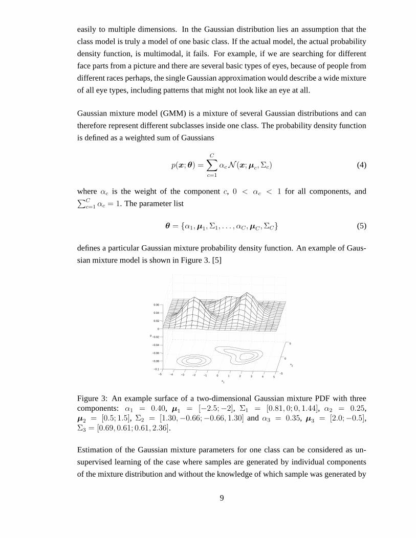
Gaussian mixture model (GMM) is a mixture of several Gaussian distributions and can

therefore represent different subclasses inside one class. The probability density function

is defined as a weighted sum of Gaussians

p(x; θ) =C

∑

c=1

αcN (x; µc, Σc) (4)

where αc is the weight of the component c, 0 < αc < 1 for all components, and∑C

c=1αc = 1. The parameter list

θ = {α1, µ1, Σ1, . . . , αC , µC , ΣC} (5)

defines a particular Gaussian mixture probability density function. An example of Gaus-

sian mixture model is shown in Figure 3. [5]

−5 −4 −3 −2 −1 0 1 2 3 4 5−5

0

5

−0.1

−0.08

−0.06

−0.04

−0.02

0

0.02

0.04

0.06

x2

x1

p

Figure 3: An example surface of a two-dimensional Gaussian mixture PDF with threecomponents: α1 = 0.40, µ1 = [−2.5;−2], Σ1 = [0.81, 0; 0, 1.44], α2 = 0.25,µ2 = [0.5; 1.5], Σ2 = [1.30,−0.66;−0.66, 1.30] and α3 = 0.35, µ3 = [2.0;−0.5],Σ3 = [0.69, 0.61; 0.61, 2.36].

Estimation of the Gaussian mixture parameters for one class can be considered as un-

supervised learning of the case where samples are generated by individual components

of the mixture distribution and without the knowledge of which sample was generated by

9

which component. Clustering usually tries to identify the exact components, but Gaussian

mixtures can also be used as an approximation of an arbitrary distribution.

2.4 Complex Valued Features

Some applications utilize complex valued features, for example describing the amplitude

and phase of a sinusoidal signal. These features can be handled in three different ways.

First, a single real value can be calculated from each complex attribute, by probably losing

some information. Second, the complex value can be divided to two real values, which

means that the length of feature vectors is doubled. Third, it might be possible to use the

complex arithmetics directly.

The first approach is good in the sense that it reduces the dimensionality of a problem,

which can lead to better performance even with small number of training data. If this is

the case, it should have been done already in the feature extraction phase. On the other

hand, combining two values into one can cause a loss of valuable information and the

performance may degrade.

Dividing complex values into two parts, real and imaginary or modulus and argument,

preserves all information, but increases the dimensionality of the problem. This can be

a real problem with high dimensional complex valued data since the amount of training

data may become insufficient or computation time increases too much.

Using the complex values directly is something between the two previous cases. It intro-

duces a constraint to the Gaussian distribution model and requires little modifications in

classifier training algorithms and the Gaussian PDF. If the transpose operation in Eq. 3 is

changed to conjugate transpose, the resulting formula

N (x; µ, Σ) =1

(2π)D/2|Σ|1/2exp

[

−1

2(x− µ)∗Σ−1(x− µ)

]

(6)

works also with complex valued µ and Σ, assuming the covariance matrix is still positive

definite. Changes in the training algorithms are explained later.

The constraint affects the shape of the distribution. It forces the shape of the density

function to be spherical on each complex plane, eliminating the covariance between the

real and imaginary part of a variable and making the variances equal.

10

The differences between approaches for using complex valued data in the Gaussian PDF

are presented in Table 1. The degree of freedom here refers to an unknown value and

the number of such values in the D-dimensional case are shown in the table. With the

covariance matrix Σ the symmetry and real valued diagonal constraints are taken into

account.

Table 1: Comparison of degrees of freedom in a single multivariate Gaussian densityfunction with different approaches for using complex data.

Degrees of FreedomApproach µ Σ

Convert to single real value D 1

2D2 + 1

2D

Divide to two real values 2D 2D2 + D

Use complex value 2D D2

11

3 GAUSSIAN MIXTURE DENSITY ESTIMATION

3.1 Maximum Likelihood Estimation

In construction of a Bayesian classifier the class-conditional probability density functions

need to be determined. The initial model selection can be done for example by visualizing

the training data, but the adjustment of the model parameters requires some measure of

goodness, i.e., how well the distribution fits the observed data. Data likelihood is a such

goodness value.

Assume that there is a set of independent samples X = {x1, . . . , xN} drawn from a

single distribution described by a probability density function p(x; θ) where θ is the PDF

parameter list. The likelihood function

L(X; θ) =N∏

n=1

p(xn; θ) (7)

tells the likelihood of the data X given the distribution or, more specifically, given the

distribution parameters θ. The goal is to find θ̂ that maximizes the likelihood:

θ̂ = arg maxθL(X; θ). (8)

Usually this function is not maximized directly but the logarithm

L(X; θ) = lnL(X; θ) =

N∑

n=1

ln p(xn; θ), (9)

called the log-likelihood function which is analytically easier to handle. Because of the

monotonicity of the logarithm function the solution to Eq. 8 is the same using L(X; θ) or

L(X; θ). [4]

Depending on p(x; θ) it might be possible to find the maximum analytically by setting

the derivatives of the log-likelihood function to zero and solving θ. It can be done for

a Gaussian PDF, which leads to the intuitive estimates for a mean and variance [1], but

usually the analytical approach is intractable. In practice an iterative method such as the

expectation maximization (EM) algorithm is used. Maximizing the likelihood may in

some cases lead to singular estimates, which is the fundamental problem of maximum

likelihood methods with Gaussian mixture models [5].

12

Recall the task of classifying vectors into K classes. If different classes can be seen as

independent, i.e., training samples belonging to one class tell nothing about other classes,

the estimation problem of K class-conditional PDFs can be divided into K separate esti-

mation problems.

3.2 Basic EM Estimation

The expectation maximization (EM) algorithm is an iterative method for calculating max-

imum likelihood distribution parameter estimates from incomplete data (some elements

missing in some feature vectors). It can also be used to handle cases where an analyti-

cal approach for maximum likelihood estimation is infeasible, such as Gaussian mixtures

with unknown and unrestricted covariance matrices and means.

Assume that each training sample contains known features and missing or unknown fea-

tures. Mark all good features of all samples with X and all unknown features of all samples

with Y. The expectation step (E-step) for the EM algorithm is to form the function

Q(θ; θi) ≡ EY[ lnL(X, Y; θ) |X; θi ] (10)

where θi is the previous estimate for the distribution parameters and θ is the variable for

a new estimate describing the (full) distribution. L is the likelihood function (Eq. 7). The

function calculates the likelihood of the data, including the unknown feature Y marginal-

ized with respect to the current estimate of the distribution described by θi. The maxi-

mization step (M-step) is to maximize Q(θ; θi) with respect to θ and set

θi+1 ← arg maxθ

Q(θ; θi). (11)

The steps are repeated until a convergence criterion is met. [1]

For the convergence criterion it is suggested in [1] that

Q(θi+1; θi)−Q(θi; θi−1) ≤ T (12)

with a suitably selected T and in [4] that

||θi+1 − θi|| ≤ ε (13)

13

for an appropriately chosen vector norm and ε. Common for both of these criteria is that

iterations are stopped when the change in the values falls below a threshold. A more

sophisticated criterion can be derived from Eq. 12 by using a relative rather than absolute

rate of change.

The EM algorithm starts from an initial guess θ0 for the distribution parameters and the

log-likelihood is guaranteed to increase on each iteration until it converges. The conver-

gence leads to a local or global maximum, but it can also lead to singular estimates, which

is true particularly for Gaussian mixture distributions with arbitrary covariance matrices.

The description of the general EM algorithm and also its application for the Gaussian

mixture model can be found in [6, 1, 4].

The initialization is one of the problems of the EM algorithm. The selection of θ0 (partly)

determines where the algorithm converges or hits the boundary of the parameter space

producing singular, meaningless results. Some solutions use multiple random starts or a

clustering algorithm for initialization. [7]

The application of the EM algorithm to Gaussian mixtures according to [7] goes as fol-

lows. The known data X is interpreted as incomplete data. The missing part Y is the

knowledge of which component produced each sample xn. For each xn there is a bi-

nary vector yn = {yn,1, . . . , yn,C}, where yn,c = 1, if the sample was produced by the

component c, or zero otherwise. The complete data log-likelihood is

lnL(X, Y; θ) =N

∑

n=1

C∑

c=1

yn,c ln (αc p(xn|c; θ)) . (14)

The E-step is to compute the conditional expectation of the complete data log-likelihood,

the Q-function, given X and the current estimate θi of the parameters. Since the complete

data log-likelihood lnL(X, Y; θ) is linear with respect to the missing Y, the conditional

expectation W ≡ E[Y |X, θ] has simply to be computed and put it into lnL(X, Y; θ).

Therefore

Q(θ, θi) ≡ E[

lnL(X, Y; θ) |X, θi]

= lnL(X, W; θ) (15)

where the elements of W are defined as

wn,c ≡ E[

yn,c |X, θi]

= Pr[

yn,c = 1 |xn, θi]

. (16)

14

The probability can be calculated with the Bayes law

wn,c =αi

c p(xn|c; θi)

∑Cj=1

αij p(xn|j; θ

i)(17)

where αic is the a priori probability (of estimate θi) and wn,c is the a posteriori probability

that yn,c = 1 after observing xn. In other words, wn,c is the probability that xn was

produced by component c. [7]

Applying the M-step to the problem of estimating the distribution parameters for C-

component Gaussian mixture with arbitrary covariance matrices, the resulting iteration

formulas are as follows:

αi+1c =

1

N

N∑

n=1

wn,c (18)

µi+1c =

∑Nn=1

xnwn,c∑N

n=1wn,c

(19)

Σi+1c =

∑Nn=1

wn,c(xn − µi+1c )(xn − µi+1

c )T

∑Nn=1

wn,c

. (20)

The new estimates are gathered to θi+1 (Eq. 5). If the convergence criterion (Eqs. 12 or 13)

is not satisfied, i← i + 1 and Eqs. 17–20 are evaluated again with new estimates. [1]

The interpretation of the Eqs. 18–20 is actually quite intuitive. The weight αc of a com-

ponent is the portion of samples belonging to that component. It is computed by approxi-

mating the component-conditional PDF with the previous parameter estimates and taking

the posterior probability of each sample point belonging to the component c (Eq. 17).

The component mean µc and covariance matrix Σc are estimated in the same way. The

samples are weighted with their probabilities of belonging to the component, and then the

sample mean and sample covariance matrix are computed.

It is worthwhile to note that so far the number of components C was assumed to be

known. Clustering techniques try to find the true clusters and components from a training

set, but our task of training a classifier only needs a good enough approximation of the

distribution of each class. Therefore, C does not need to be guessed accurately, it is

just a parameter defining the complexity of the approximating distribution. Too small C

prevents the classifier from learning the sample distributions well enough and too large C

may lead to an overfitted classifier. More importantly, too large C will definitely lead to

singularities when the amount of training data becomes insufficient.

15

3.3 Figueiredo-Jain Algorithm

The Figueiredo-Jain (FJ) algorithm tries to overcome three major weaknesses of the ba-

sic EM algorithm. The EM algorithm presented in Section 3.2 requires the user to set

the number of components and the number will be fixed during the estimation process.

The FJ algorithm adjusts the number of components during estimation by annihilating

components that are not supported by the data. This leads to the other EM failure point,

the boundary of the parameter space. FJ avoids the boundary when it annihilates compo-

nents that are becoming singular. FJ also allows to start with an arbitrarily large number

of components, which tackles the initialization issue with the EM algorithm. The initial

guesses for component means can be distributed into the whole space occupied by training

samples, even setting one component for every single training sample. [7]

The classical way to select the number of mixture components is to adopt the ”model-

class/model” hierarchy, where some candidate models (mixture PDFs) are computed for

each model-class (number of components), and then select the ”best” model. The idea

behind the FJ algorithm is to abandon such hierarchy and to find the ”best” overall model

directly. Using the minimum message length criterion and applying it to mixture models

leads to the objective function

Λ(θ, X) =V

2

∑

c:αc>0

ln(Nαc

12) +

Cnz

2ln

N

12+

Cnz(V + 1)

2− lnL(X, θ) (21)

where N is the number of training points, V is the number of free parameters specifying

a component, and Cnz is the number of components with nonzero weight in the mixture

(αc > 0). θ in the case of Gaussian mixture is the same as in Eq. 5. The last term

lnL(X, θ) is the log-likelihood of the training data given the distribution parameters θ

(Eq. 9). [7]

The EM algorithm can be used to minimize Eq. 21 with a fixed Cnz [7]. It leads to the

M-step with component weight updating formula

αi+1c =

max

{

0,

(

N∑

n=1

wn,c

)

− V2

}

C∑

j=1

max

{

0,

(

N∑

n=1

wn,j

)

− V2

} . (22)

This formula contains an explicit rule of annihilating components by setting their weights

to zero. Other distribution parameters are updated as in Eqs. 19 and 20. [7]

16

The above M-steps are not suitable for the basic EM algorithm though. When initial

C is high, it can happen that all weights become zero because none of the components

have enough support from the data. Therefore a component-wise EM algorithm (CEM) is

adopted. CEM updates the components one by one, computing the E-step (updating W)

after each component update, where the basic EM updates all components ”simultane-

ously”. When a component is annihilated its probability mass is immediately redistributed

strengthening the remaining components. [7]

When CEM converges, it is not guaranteed that the minimum of Λ(θ, X) is found, because

the annihilation rule (Eq. 22) does not take into account the decrease caused by decreasing

Cnz. After convergence the component with the smallest weight is removed and the CEM

is run again, repeating until Cnz = 1. Then the estimate with the smallest Λ(θ, X) is

chosen. [7]

The implementation of the FJ algorithm uses a modified cost function instead of Λ(θ, X).

The derivation of the modified cost function is presented in Appendix 1.

Hitherto the only things assumed for the mixture distribution are that an EM algorithm

can be written for it and all components are parameterized the same way (number of

parameters V for a component). With Gaussian mixture model the number of parameters

per component V = D+ 1

2D2+ 1

2D in the case of real valued data and arbitrary covariance

matrices. With complex valued data the number of real free parameters V = 2D + D2

where D is the dimensionality of the (complex) data. It would seem logical to choose

this value for V instead of the previous one defined with real valued data. As seen in

Eq. 22 this amplifies the annihilation which makes sense because there are more degrees

of freedom in a component. On the other hand there are more training data with the same

number of training points, because the data is complex (two values in one variable as

opposed to one value). The nature of complex data with Gaussian PDF has been discussed

in Section 2.4.

3.4 Greedy EM Algorithm

The greedy algorithm starts with a single component and then adds components into the

mixture one by one. The optimal starting component for a Gaussian mixture is trivially

computed, optimal meaning the highest training data likelihood. The algorithm repeats

two steps: insert a component into the mixture, and run EM until convergence. Inserting

17

a component that increases the likelihood the most is thought to be an easier problem than

initializing a whole near-optimal distribution. Component insertion involves searching

for the parameters for only one component at a time. Recall that EM finds a local opti-

mum for the distribution parameters, not necessarily the global optimum which makes it

initialization dependent method.

Let pC denote a C-component mixture with parameters θC . The general greedy algorithm

for Gaussian mixture is as follows [8]:

1. Compute the optimal (in the ML sense) one-component mixture p1 and set C ← 1.

2. Find a new component N (x; µ′, Σ′) and corresponding mixing weight α′ that in-

crease the likelihood the most:

{µ′, Σ′, α′} = arg max{µ,Σ,α}

N∑

n=1

ln[(1− α)pC(xn) + αN (xn; µ, Σ)] (23)

while keeping pC fixed.

3. Set pC+1(x)← (1− α′)pC(x) + α′N (x; µ′, Σ′) and then C ← C + 1.

4. Update pC using EM (or some other method) until convergence. [optional]

5. Evaluate some stopping criterion; go to Step 2 or quit.

The stopping criterion in Step 5 can be for example any kind of model selection criterion,

wanted number of components, or a minimum message length criterion.

The crucial point is of course Step 2. Finding the optimal new component requires a

global search, which is performed by creating CNcand candidate components. The num-

ber of candidates will increase linearly with the number of components C, having Ncand

candidates per each existing component. The candidate resulting in the highest likelihood

when inserted into the (previous) mixture is selected. The parameters and weight of the

best candidate are then used in Step 3 instead of the truly optimal values. [8].

The candidates for executing Step 2 are initialized as follows: the training data set X is

partitioned into C disjoint data sets {Ac}, c = 1 . . . C, according to the posterior proba-

bilities of individual components; the data set is Bayesian classified by the mixture com-

ponents. From each Ac number of Ncand candidates are initialized by picking uniformly

randomly two data points xl and xr in Ac. The set Ac is then partitioned into two using the

18

smallest distance selection with respect to xl and xr. The mean and covariance of these

two new subsets are the parameters for two new candidates. The candidate weights are

set to half of the weight of the component that produced the set Ac. Then new xl and xr

are drawn until Ncand candidates are initialized with Ac. The partial EM algorithm is then

used on each of the fresh set of candidates. The partial EM differs from the EM and CEM

algorithms by optimizing (updating) only one component of a mixture, it does not change

any other components. In order to reduce the time complexity of the algorithm a lower

bound on the log-likelihood is used instead of the true log-likelihood. The lower-bound

log-likelihood is calculated with only the points in the respective set Ac. The partial EM

update equations are as follows:

wn,C+1 =αN (xn; µ, Σ)

(1− α)pC(x) + αN (x; µ, Σ)(24)

α =1

ℵ(Ac)

∑

n∈Ac

wn,C+1 (25)

µ =

∑

n∈Ac

wn,C+1xn∑

n∈Ac

wn,C+1

(26)

Σ =

∑

n∈Ac

wn,C+1(xn − µ)(xn − µ)T

∑

n∈Ac

wn,C+1

(27)

where ℵ(Ac) is the number of training samples in the set Ac. These equations are much

like the basic EM update Eqs. 18–20. The partial EM iterations are stopped when the

relative change in log-likelihood of the resulting C + 1 -component mixture drops be-

low threshold or maximum number of iterations is reached. When the partial EM has

converged the candidate is ready to be evaluated. [8]

19

4 GMMBAYES TOOLBOX

4.1 GMMBayes Matlab Toolbox Interface

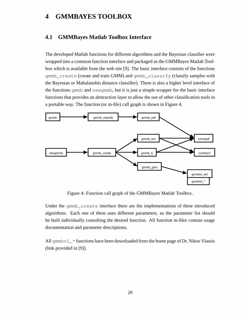
The developed Matlab functions for different algorithms and the Bayesian classifier were

wrapped into a common function interface and packaged as the GMMBayes Matlab Tool-

box which is available from the web site [9]. The basic interface consists of the functions

gmmb_create (create and train GMM) and gmmb_classify (classify samples with

the Bayesian or Mahalanobis distance classifier). There is also a higher level interface of

the functions gmmb and newgmmb, but it is just a simple wrapper for the basic interface

functions that provides an abstraction layer to allow the use of other classification tools in

a portable way. The function (or m-file) call graph is shown in Figure 4.

newgmmb

gmmb

gmmb_create

gmmb_classify

gmmb_em

gmmb_fj

gmmb_gem

cmvnpdf

covfixer2

gmmbvl_*

gmmbvl_em

gmmb_pdf

Figure 4: Function call graph of the GMMBayes Matlab Toolbox.

Under the gmmb_create interface there are the implementations of three introduced

algorithms. Each one of them uses different parameters, so the parameter list should

be built individually consulting the desired function. All function m-files contain usage

documentation and parameter descriptions.

All gmmbvl_* functions have been downloaded from the home page of Dr. Nikos Vlassis

(link provided in [9]).

20

4.2 Avoiding Covariance Matrix Singularities

The EM algorithm tends to converge to a singular solution, especially when training data

is (nearly) insufficient. The FJ algorithm does not suffer from this, but still the training

data may sometimes lead to an invalid covariance matrix.

Function covfixer2 takes a candidate covariance matrix and returns a slightly modified

matrix that fulfills the requirements for a valid covariance matrix (semipositive definite,

complex conjugate symmetric). If the input matrix is already valid, it is returned as is.

In the function the matrix is forced to complex conjugate symmetric as follows:

Σ← Σ−Σ− Σ∗

2. (28)

Possible imaginary components are removed from the diagonal, which results in a Her-

mitian matrix. Then it is tested for positive definiteness (Cholesky factorization), and

while the test fails one of two things is done: i) If there is a negative element in the diag-

onal, then one percent of the maximum element in the diagonal is added to all diagonal

elements; ii) Otherwise all the diagonal elements are increased by one percent.

By growing the covariance matrix diagonal we try to get rid of singular matrices. The

iterative algorithm, which called the covfixer2 function, is supposed to fix the possible

ill effects of the matrix modifications on next iterations, but it may also lead again to a

singular covariance matrix; algorithm starts to oscillate and may jam.

4.3 Algorithm Implementation Details

The Gaussian probability density function is evaluated in cmvnpdf function, which is a

modified version of the Matlab R13 mvnpdf function, since it does not handle complex

valued data correctly.

The gmmb_classify function can additionally classify samples according to Maha-

lanobis distance, where the distance is computed to each component of each trained class.

This method ignores all a priori and component weight information. When using the

function to classify using the Bayesian rule, the function can output either only a class

label or all posterior probabilities for each sample.

21

The EM implementation uses fuzzy c-means clustering for initializing the component

means. Component covariance matrices are initialized to diagonal part of the whole data

covariance matrix. Weights are set to equal. The covfixer2 function is used on every

iteration. The algorithms stops when relative change1 of the log-likelihood of the data

falls below a threshold. The implementation can compute with complex data directly.

In the Figueiredo-Jain algorithm implementation component mean vectors are initialized

to random data points. Covariance matrices are initialized to σ2I , where I is the unitary

matrix and σ2 is one tenth of the maximum of the diagonal of the whole data covariance

matrix. Initial component weights are equal. The covfixer2 function is used on every

iteration of the component-wise EM algorithm. The stopping criteria for the component-

wise EM is a threshold in the relative change of the data log-likelihood, and the whole

algorithm stops when the minimum number of components is reached and CEM has con-

verged. The FJ implementation also computes with complex data.

The greedy EM implementation contains a trivial initialization step, because it starts from

a single Gaussian component; the standard mean and covariance of the data. The stopping

condition for the partial EM when creating candidates is the relative change in data log-

likelihood falling below 0.01 or number of iterations reaching 20. After all candidates

are created one of the candidate components is selected and then it is updated again with

partial EM with relative log-likelihood change threshold 10−5. The change in the log-

likelihood when inserting the new component is checked and the component is inserted if

the log-likelihood increases. Otherwise the algorithm stops. The whole mixture updating

EM is stopped when the relative change in log-likelihood falls below 10−5.

1Originally it was the absolute change, but it was changed in gmmb_em.m revision 1.7.

22

5 EXPERIMENTS

Three different data sets were used in the experiments: forest spectral colors, artificial

waveforms and noise, and letter image recognition data. The tests were run with the

following parameters:

EM

relative log-likelihood change threshold: 10−5

number of mixture components: 1 to 8

Figueiredo-Jain

relative log-likelihood change threshold: 10−5

maximum number of mixture components: 4, 8, 16, 32, 64

Greedy EM

maximum number of mixture components: 4, 8, 16, 32, 64

number of candidates per existing component: 8

For each algorithm the number of components was varied.

In a test round a data set was randomly divided into three: the test data, the training data

and unused data. The test data was always 30% of the data set and the training data was

varied from 20% to 70% with ten percent unit steps. The division algorithm assures that

the training and test data sets are non-overlapping and the class proportions remain the

same in the three subsets and the data set.

A test round produced an accuracy ratio (correctly classified samples in the test data set),

the estimated Gaussian mixture model and miscellaneous data about the used algorithm.

One test round was repeated three times with the same parameters and data sets. For each

set of parameters the training and test sets were randomly created five times. This method

totals to 15 test rounds per a test run with each fixed parameters, algorithm and data set.

Description of the result file format is in Appendix 2.

Because the FJ and GEM can produce different number of components for different

classes within a single test round, the maximum number of components of class mod-

els is used to describe the result of a round. The crashed runs are taken into account as

zero accuracy.

23

An algorithm crash is a situation where the algorithm did not produce a final mixture

estimate and cannot continue. For example in the EM algorithm a covariance matrix

becomes undefined, or in the FJ algorithm all mixture components get annihilated.

Test runs were executed for every combination of data set, parameter and algorithm men-

tioned in this section.

5.1 Forest Spectral Colors

The forest colors set contains samples of reflectance spectra of pine, spruce and birch.

The spectra is recorded in wavelength interval 390 nm – 850 nm with 5 nm resolution

which leads to 93-element sample vectors. There are 349 samples from spruce, 337 from

birch and 370 from pine. [10]

The data is too high-dimensional to be used directly, and it was thus transformed with

neighbor-bank projection [11] to 23, 15 and 10-dimensional data sets with cos2 bank

shape. The 23-dimensional case was near the classification accuracy optimum in [11],

and 15 and 10-dimensional cases were created in case 23 dimensions would be too much

for the algorithms considering the amount of training data.

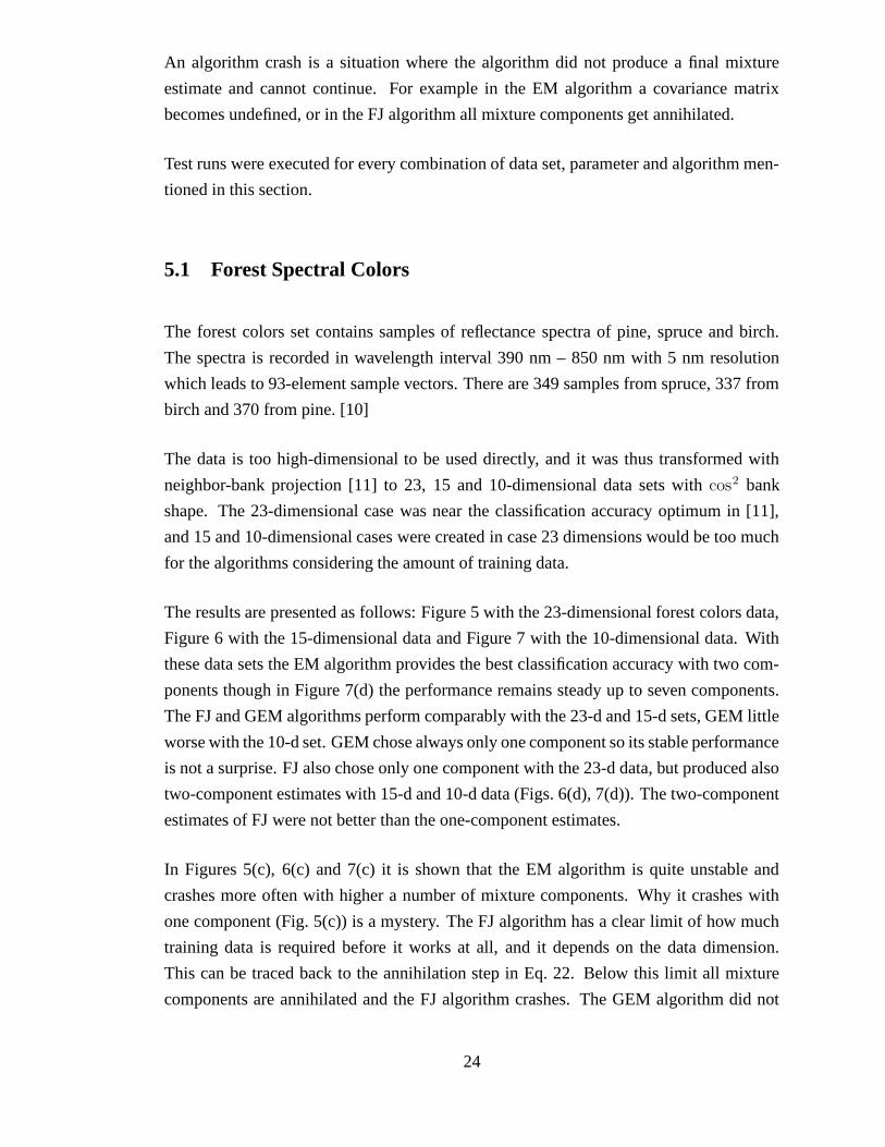
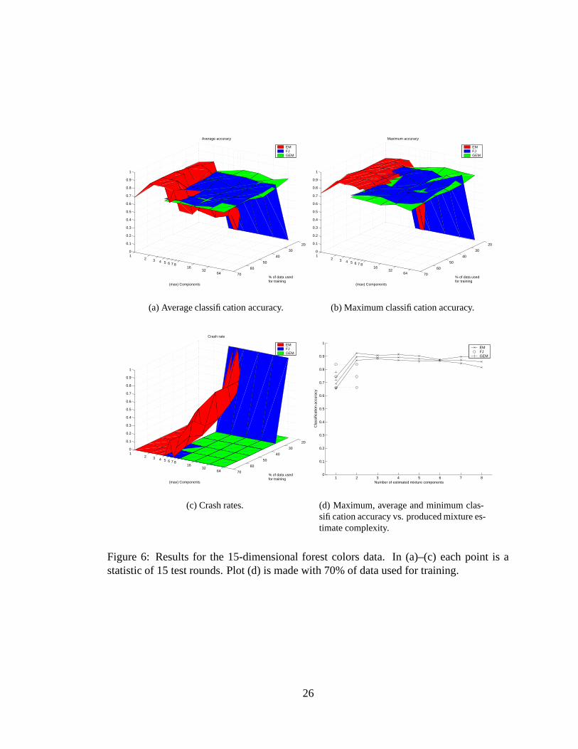
The results are presented as follows: Figure 5 with the 23-dimensional forest colors data,

Figure 6 with the 15-dimensional data and Figure 7 with the 10-dimensional data. With

these data sets the EM algorithm provides the best classification accuracy with two com-

ponents though in Figure 7(d) the performance remains steady up to seven components.

The FJ and GEM algorithms perform comparably with the 23-d and 15-d sets, GEM little

worse with the 10-d set. GEM chose always only one component so its stable performance

is not a surprise. FJ also chose only one component with the 23-d data, but produced also

two-component estimates with 15-d and 10-d data (Figs. 6(d), 7(d)). The two-component

estimates of FJ were not better than the one-component estimates.

In Figures 5(c), 6(c) and 7(c) it is shown that the EM algorithm is quite unstable and

crashes more often with higher a number of mixture components. Why it crashes with

one component (Fig. 5(c)) is a mystery. The FJ algorithm has a clear limit of how much

training data is required before it works at all, and it depends on the data dimension.

This can be traced back to the annihilation step in Eq. 22. Below this limit all mixture

components are annihilated and the FJ algorithm crashes. The GEM algorithm did not

24

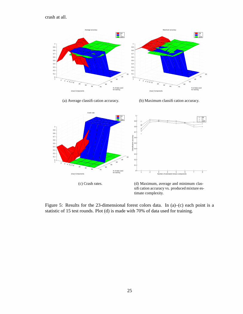
crash at all.

20

30

40

50

60

70

12 3 4 5 6 7 8

1632

64

0

0.1

0.2

0.3

0.4

0.5

0.6

0.7

0.8

0.9

1

% of data usedfor training

Average accuracy

(max) Components

EMFJGEM

(a) Average classification accuracy.

20

30

40

50

60

70

12 3 4 5 6 7 8

1632

64

0

0.1

0.2

0.3

0.4

0.5

0.6

0.7

0.8

0.9

1


Maximum accuracy

(max) Components

EMFJGEM

(b) Maximum classification accuracy.

20

30

40

50

60

70

12 3 4 5 6 7 8

1632

64

0

0.1

0.2

0.3

0.4

0.5

0.6

0.7

0.8

0.9

1


Crash rate

(max) Components

EMFJGEM

(c) Crash rates.

1 2 3 4 5 6 7 80

0.1

0.2

0.3

0.4

0.5

0.6

0.7

0.8

0.9

1

Number of estimated mixture components

Cla

ssifi

catio

n ac

cura

cy

EMFJGEM

(d) Maximum, average and minimum clas-sification accuracy vs. produced mixture es-timate complexity.

Figure 5: Results for the 23-dimensional forest colors data. In (a)–(c) each point is astatistic of 15 test rounds. Plot (d) is made with 70% of data used for training.

25

20

30

40

50

60

70

12 3 4 5 6 7 8

1632

64

0

0.1

0.2

0.3

0.4

0.5

0.6

0.7

0.8

0.9

1


Average accuracy

(max) Components

EMFJGEM


20

30

40

50

60

70

12 3 4 5 6 7 8

1632

64

0

0.1

0.2

0.3

0.4

0.5

0.6

0.7

0.8

0.9

1


Maximum accuracy

(max) Components

EMFJGEM


20

30

40

50

60

70

12 3 4 5 6 7 8

1632

64

0

0.1

0.2

0.3

0.4

0.5

0.6

0.7

0.8

0.9

1


Crash rate

(max) Components

EMFJGEM

(c) Crash rates.

1 2 3 4 5 6 7 80

0.1

0.2

0.3

0.4

0.5

0.6

0.7

0.8

0.9

1


Cla

ssifi

catio

n ac

cura

cy

EMFJGEM



26

20

30

40

50

60

70

12 3 4 5 6 7 8

1632

64

0

0.1

0.2

0.3

0.4

0.5

0.6

0.7

0.8

0.9

1


Average accuracy

(max) Components

EMFJGEM


20

30

40

50

60

70

12 3 4 5 6 7 8

1632

64

0

0.1

0.2

0.3

0.4

0.5

0.6

0.7

0.8

0.9

1


Maximum accuracy

(max) Components

EMFJGEM


20

30

40

50

60

70

12 3 4 5 6 7 8

1632

64

0

0.1

0.2

0.3

0.4

0.5

0.6

0.7

0.8

0.9

1


Crash rate

(max) Components

EMFJGEM

(c) Crash rates.

1 2 3 4 5 6 7 80

0.1

0.2

0.3

0.4

0.5

0.6

0.7

0.8

0.9

1


Cla

ssifi

catio

n ac

cura

cy

EMFJGEM



27

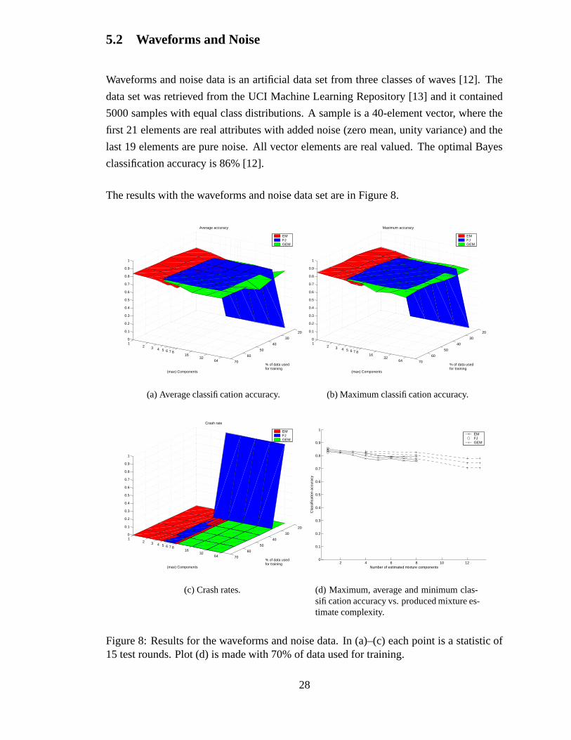
5.2 Waveforms and Noise

Waveforms and noise data is an artificial data set from three classes of waves [12]. The

data set was retrieved from the UCI Machine Learning Repository [13] and it contained

5000 samples with equal class distributions. A sample is a 40-element vector, where the

first 21 elements are real attributes with added noise (zero mean, unity variance) and the

last 19 elements are pure noise. All vector elements are real valued. The optimal Bayes

classification accuracy is 86% [12].

The results with the waveforms and noise data set are in Figure 8.

20

30

40

50

60

70

12 3 4 5 6 7 8

1632

64

0

0.1

0.2

0.3

0.4

0.5

0.6

0.7

0.8

0.9

1


Average accuracy

(max) Components

EMFJGEM


20

30

40

50

60

70

12 3 4 5 6 7 8

1632

64

0

0.1

0.2

0.3

0.4

0.5

0.6

0.7

0.8

0.9

1


Maximum accuracy

(max) Components

EMFJGEM


20

30

40

50

60

70

12 3 4 5 6 7 8

1632

64

0

0.1

0.2

0.3

0.4

0.5

0.6

0.7

0.8

0.9

1


Crash rate

(max) Components

EMFJGEM

(c) Crash rates.

2 4 6 8 10 120

0.1

0.2

0.3

0.4

0.5

0.6

0.7

0.8

0.9

1


Cla

ssifi

catio

n ac

cura

cy

EMFJGEM


Figure 8: Results for the waveforms and noise data. In (a)–(c) each point is a statistic of15 test rounds. Plot (d) is made with 70% of data used for training.

28

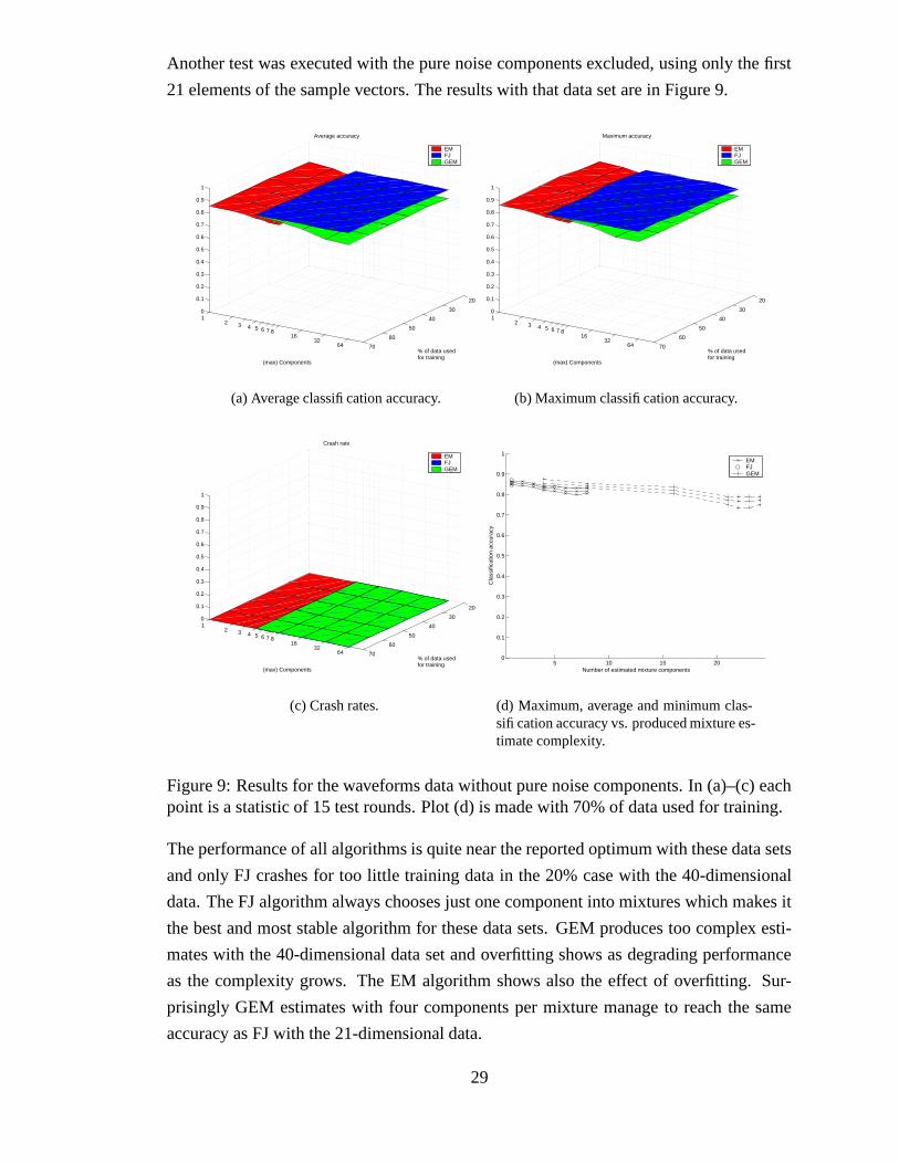
Another test was executed with the pure noise components excluded, using only the first

21 elements of the sample vectors. The results with that data set are in Figure 9.

20

30

40

50

60

70

12 3 4 5 6 7 8

1632

64

0

0.1

0.2

0.3

0.4

0.5

0.6

0.7

0.8

0.9

1


Average accuracy

(max) Components

EMFJGEM


20

30

40

50

60

70

12 3 4 5 6 7 8

1632

64

0

0.1

0.2

0.3

0.4

0.5

0.6

0.7

0.8

0.9

1


Maximum accuracy

(max) Components

EMFJGEM


20

30

40

50

60

70

12 3 4 5 6 7 8

1632

64

0

0.1

0.2

0.3

0.4

0.5

0.6

0.7

0.8

0.9

1

(max) Components


Crash rate

EMFJGEM

(c) Crash rates.

5 10 15 200

0.1

0.2

0.3

0.4

0.5

0.6

0.7

0.8

0.9

1


Cla

ssifi

catio

n ac

cura

cy

EMFJGEM


Figure 9: Results for the waveforms data without pure noise components. In (a)–(c) eachpoint is a statistic of 15 test rounds. Plot (d) is made with 70% of data used for training.

The performance of all algorithms is quite near the reported optimum with these data sets

and only FJ crashes for too little training data in the 20% case with the 40-dimensional

data. The FJ algorithm always chooses just one component into mixtures which makes it

the best and most stable algorithm for these data sets. GEM produces too complex esti-

mates with the 40-dimensional data set and overfitting shows as degrading performance

as the complexity grows. The EM algorithm shows also the effect of overfitting. Sur-

prisingly GEM estimates with four components per mixture manage to reach the same

accuracy as FJ with the 21-dimensional data.

29

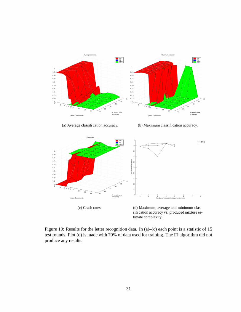
5.3 Letter Image Recognition Data

The letter image recognition data is an artificial data set containing 20,000 16-element

sample vectors. The black-and-white letter images were generated from 20 different fonts

using 26 different uppercase letters and adding random distortions. The sample vectors

were calculated from those images, and include attributes such as mean x and y variance

of pixels. [14]

The data set was retrieved from the UCI Machine Learning Repository [13]. All attributes

were already transformed to integers in the range [0, 15] which makes this data set diffi-

cult, because the algorithms were coded for real valued, not integer, data. The class

distribution of the 26 classes (letters) ranged from 734 to 813 samples per class. The best

classification accuracy obtained in [14] was a little over 80%.

The results with the letter image recognition data set are shown in Figure 10.

The data set proved to be very difficult indeed, only the EM implementation produced

results. FJ did not finish a single test round within reasonable time and thus there are no

results from FJ, and only in few test rounds GEM did not crash (Fig. 10(c)). The EM

implementation is quite reliable with one, two and even three components for mixtures

and produces classification accuracies near 90% (Fig. 10(d)).

30

20

30

40

50

60

70

12 3 4 5 6 7 8

1632

64

0

0.1

0.2

0.3

0.4

0.5

0.6

0.7

0.8

0.9

1


Average accuracy

(max) Components

EMFJGEM


20

30

40

50

60

70

12 3 4 5 6 7 8

1632

64

0

0.1

0.2

0.3

0.4

0.5

0.6

0.7

0.8

0.9

1


Maximum accuracy

(max) Components

EMFJGEM


20

30

40

50

60

70

12 3 4 5 6 7 8

1632

64

0

0.1

0.2

0.3

0.4

0.5

0.6

0.7

0.8

0.9

1


Crash rate

(max) Components

EMFJGEM

(c) Crash rates.

1 2 3 4 5 6 7 80

0.1

0.2

0.3

0.4

0.5

0.6

0.7

0.8

0.9

1


Cla

ssifi

catio

n ac

cura

cy

EM


Figure 10: Results for the letter recognition data. In (a)–(c) each point is a statistic of 15test rounds. Plot (d) is made with 70% of data used for training. The FJ algorithm did notproduce any results.

31

6 CONCLUSIONS

The goal for this project is well achieved, although it took over a year to complete. The

Bayesian classifier using Gaussian mixtures is functional and the three different Gaussian

mixture estimation algorithms are available in the developed GMMBayes Matlab Tool-

box. The experiments show that the toolbox is working well and that there are differences

in the behavior of the three implemented estimation algorithms.

There are some projection errors in the 3-dimensional graphs due to the way Matlab and

PostScript handle the vector graphics, but they should not obscure the results. Corretly

projected bitmap images can found at [9].

The EM implementation requires the user to set the number of components a priori for

each mixture, but seems to outperform the other algorithms if a good number is found.

Another downside of EM is its crash rate, but as the letter image recognition data experi-

ments proved, it can work in situations where the other algorithms fail.

The FJ implementation determines the number of components by itself, going down from

the user defined maximum. FJ also produced better classification accuracies than the

GEM implementation, but FJ has a failure mode too: its minimum requirement for the

number of training samples is higher than with the other algorithms. For some reason

FJ could not produce a single mixture estimate with the letter image recognition data,

although in preliminary tests during the development FJ did produce results.

The GEM implementation also determines the number of components by itself, inserting

components one by one. GEM was the most stable implementation on average, looking

at the crash rates, but produced generally a little worse classification accuracies than FJ.

GEM produced results where the FJ implementation failed, except with the letter image

recognition data, where they both failed.

The EM and FJ implementations work also with complex valued data, using complex

arithmetics. The effects of the different approaches to using complex valued data de-

scribed in Section 2.4 were not tested, but it would be an interesting topic, though the

behavior might be application dependent.

The GMMBayes Toolbox was incorporated in the facial evidence detection system [2, 3]

developed by Kämäräinen et al. where it outperformed the SCC method. The results can

32

be found in [15].

The GMMBayes Matlab Toolbox is already in use or to be used in several other projects

at the Laboratory of Information Processing in Lappeenranta university of Technology.

33

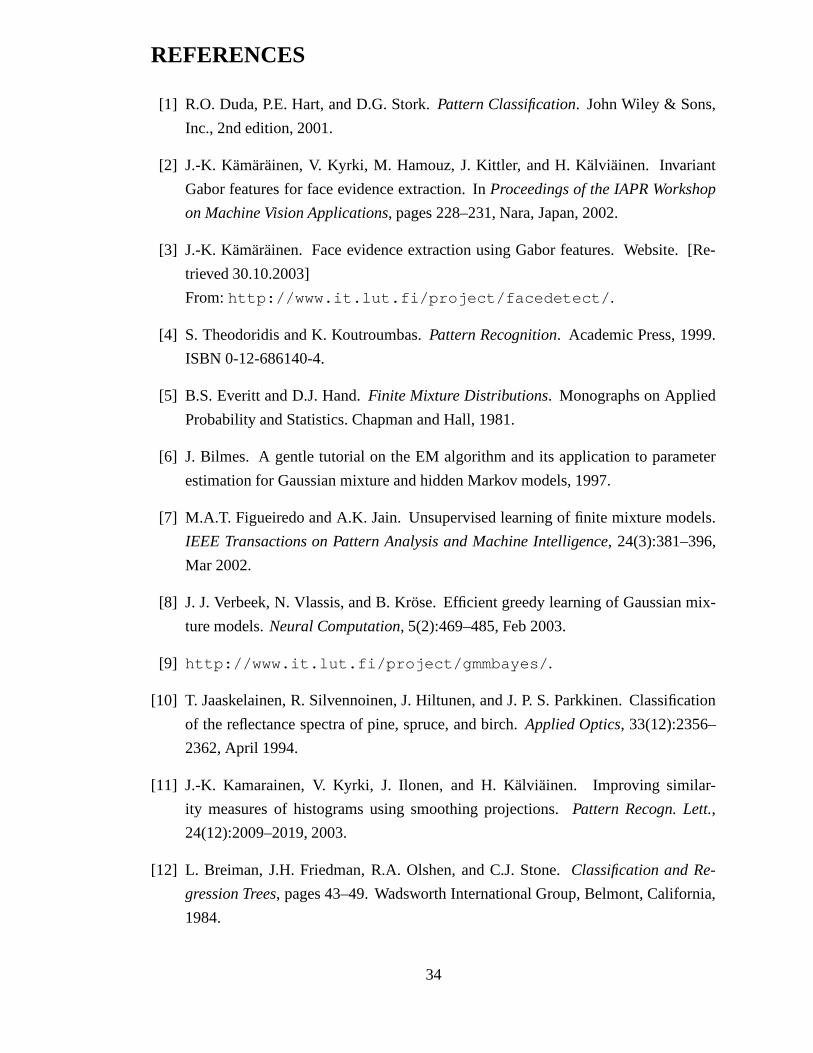
REFERENCES

[1] R.O. Duda, P.E. Hart, and D.G. Stork. Pattern Classification. John Wiley & Sons,

Inc., 2nd edition, 2001.

[2] J.-K. Kämäräinen, V. Kyrki, M. Hamouz, J. Kittler, and H. Kälviäinen. Invariant

Gabor features for face evidence extraction. In Proceedings of the IAPR Workshop

on Machine Vision Applications, pages 228–231, Nara, Japan, 2002.

[3] J.-K. Kämäräinen. Face evidence extraction using Gabor features. Website. [Re-

trieved 30.10.2003]

From: http://www.it.lut.fi/project/facedetect/.

[4] S. Theodoridis and K. Koutroumbas. Pattern Recognition. Academic Press, 1999.

ISBN 0-12-686140-4.

[5] B.S. Everitt and D.J. Hand. Finite Mixture Distributions. Monographs on Applied

Probability and Statistics. Chapman and Hall, 1981.

[6] J. Bilmes. A gentle tutorial on the EM algorithm and its application to parameter

estimation for Gaussian mixture and hidden Markov models, 1997.

[7] M.A.T. Figueiredo and A.K. Jain. Unsupervised learning of finite mixture models.

IEEE Transactions on Pattern Analysis and Machine Intelligence, 24(3):381–396,

Mar 2002.

[8] J. J. Verbeek, N. Vlassis, and B. Kröse. Efficient greedy learning of Gaussian mix-

ture models. Neural Computation, 5(2):469–485, Feb 2003.

[9] http://www.it.lut.fi/project/gmmbayes/.

[10] T. Jaaskelainen, R. Silvennoinen, J. Hiltunen, and J. P. S. Parkkinen. Classification

of the reflectance spectra of pine, spruce, and birch. Applied Optics, 33(12):2356–

2362, April 1994.

[11] J.-K. Kamarainen, V. Kyrki, J. Ilonen, and H. Kälviäinen. Improving similar-

ity measures of histograms using smoothing projections. Pattern Recogn. Lett.,

24(12):2009–2019, 2003.

[12] L. Breiman, J.H. Friedman, R.A. Olshen, and C.J. Stone. Classification and Re-

gression Trees, pages 43–49. Wadsworth International Group, Belmont, California,

1984.

34

[13] C.L. Blake and C.J. Merz. UCI repository of machine learning databases, 1998.

[14] P.W. Frey and D.J. Slate. Letter recognition using Holland-style adaptive classifiers.

Machine Learning, 6(2):161–182, March 1991.

[15] M. Hamouz, J. Kittler, J.-K. Kamarainen, P. Paalanen, and H. Kälviäinen. Affine-

invariant face detection and localization using GMM-based feature detector and en-

hanced appearance model. In Proceedings of the Sixth IEEE International Confer-

ence on Automatic Face and Gesture Recognition, pages 67–72, 2004.

35

APPENDIX 1. Derivation of the FJ Cost Function

The objective function was defined in Eq. 21 as

Λ(θ, X) =V

2

∑

c:αc>0

ln

(

Nαc

12

)

+Cnz

2ln

N

12+

Cnz(V + 1)

2− lnL(X, θ).

The log-likelihood is not of interest here and it is discarded during the deriving. By

decomposing the logarithms of products into sums of logarithms we get

V

2

∑

c:αc>0

(ln N + lnαc − ln 12) +Cnz

2(ln N − ln 12) +

Cnz(V + 1)

2.

The only thing dependent on c inside the sum is ln αc so the other terms can be taken out.

Cnz is defined as the number of summables.

V

2

∑

c:αc>0

ln αc +V Cnz

2(ln N − ln 12) +

Cnz

2(ln N − ln 12) +

Cnz(V + 1)

2

Rearranging the terms and adding the log-likelihood back we get

V

2

∑

c:αc>0

ln αc +Cnz(V + 1)

2ln N + (V + 1)(1− ln 12)− lnL(X, θ).

Recalling the message length interpretation of Eq. 21 the term (V + 1)(1 − ln 12) can

be discarded because it is an irrelevant additive constant which does not depend on the

data or component weights of the mixture (V is the parameter count for one component).

Therefore the final cost function to be minimized is

Λ′(θ, X) =V

2

∑

c:αc>0

ln αc +Cnz(V + 1)

2ln N − lnL(X, θ).

APPENDIX 2. Experiment Save File Format

The result save file is a MAT-file with two variables: desc and results. It is produced

by the testrun function which takes the desc as argument.

The desc is a structure with fields:

datafile the input data file name

method EM, FJ or GEM

params cell array of algorithm specific parameters

trainsizes vector of relative training set sizes

redivs number of division repetitions

iters number of test run repetitions

savefile the result save file name

The results variable is a length(trainsizes) long cell array of structures:

sets{redivs} cell array of data division label vectors

rounds{redivs} cell array of arrays of the round structures

trainsize the training set size used

The round[iters] array of structures:

bayesS structure describing the estimated Gaussian mixture model

stats miscellaneous information about the test run

accuracy the test set classification accuracy

The stats field is a number of classes long cell array of structures with fields depending

on the used algorithm and logging level:

iterations algorithm iterations, all algorithms

covfixer2 covariance fixer running counts, EM and FJ

loglikes history of the log-likelihood, all algorithms

initialmix the initial guess, EM and FJ, extra logging

mixtures history of the mixture model, EM and FJ, extra logging

costs development of the FJ cost function

annihilations FJ component annihilation history

Documents

BAYESIAN CLASSIFICATION USING GAUSSIAN MIXTURE … · BAYESIAN CLASSIFICATION USING GAUSSIAN MIXTURE MODEL AND ... Bayesian Classiﬁcation Using Gaussian Mixture Model and EM Estimation: