Paper 7200-2016

Bayesian Inference for Gaussian Semiparametric Multilevel Models Jason Bentley, The University of Sydney, New South Wales, Australia

Cathy Yuen Yi Lee, University of Technology Sydney, New South Wales, Australia

ABSTRACT Bayesian inference for complex hierarchical models with smoothing splines is typically intractable, requiring approximate inference methods for use in practice. Markov Chain Monte Carlo (MCMC) is the standard method for generating samples from the posterior distribution. However, for large or complex models, MCMC can be computationally intensive, or even infeasible. Mean Field Variational Bayes (MFVB) is a fast deterministic alternative to MCMC. It provides an approximating distribution that has minimum Kullback-Leibler distance to the posterior. Unlike MCMC, MFVB efficiently scales to arbitrarily large and complex models. We derive MFVB algorithms for Gaussian semiparametric multilevel models and implement them in SAS/IML® software. To improve speed and memory efficiency, we use block decomposition to streamline the estimation of the large sparse covariance matrix. Through a series of simulations and real data examples, we demonstrate that the inference obtained from MFVB is comparable to that of PROC MCMC. We also provide practical demonstrations of how to estimate additional posterior quantities of interest from MFVB either directly or via Monte Carlo simulation.

INTRODUCTION The growing emergence of machine learning and data mining tools has helped researchers capture and understand patterns from large and complex datasets that are typically of grouped or hierarchical structure. The most common data types are longitudinal and multilevel data, which are frequently seen in many applied areas such as education, epidemiology, medicine, population health and social science. These data structures give rise to correlations among observations within groups/clusters and therefore require sophisticated statistical models that take into account such correlations during data analysis.

Linear mixed models extend standard linear models by adding normal random effects on the linear predictor scale to account for correlated observations within groups. However, this flexibility is traded with analytical tractability and may suffer from computational complexity and decreased efficiency. In the Bayesian paradigm, estimation of mixed models via Markov chain Monte Carlo (MCMC) techniques is challenging since the integral over the random effects is intractable. In this paper we use the SAS® Interactive Matrix Language (IML) environment to implement Mean Field Variational Bayes for Bayesian Gaussian semiparametric multilevel models.

The IML environment while different in behavior to standard SAS procedures and the SAS Data Step, is well suited to coding new computational procedures in SAS from start to finish. This is because the IML environment operates in terms of vectors and matrices, and while this will be familiar to many users of other analytical software such as R or Matlab, the IML language is intuitive to use. Results of computation in IML can be easily output to SAS Datasets for use in existing analytic or graphics procedures, and so can be seamlessly integrated into analyses in SAS.

This paper will introduce SAS users to a fast deterministic alternative to MCMC which provides an approximating distribution that has minimum Kullback-Leibler distance to the posterior of a Bayesian Gaussian semiparametric multilevel model, using the IML environment. Simulation comparisons will focus mainly on random intercept models with a single covariate that requires smoothing using penalized splines and a few typical covariates (continuous and binary). Some knowledge of using splines for smoothing non-linear associations between an outcome and a continuous covariate, particularly the random-effects formulation (penalized splines) is advantageous. Further, an understanding of the covariance structures that arise in multilevel models, Bayesian inference using MCMC, creating expanded design matrices when using categorical covariates, and the role of centering and standardizing data prior to an analysis will assist readers in getting the most out of this paper.

1

THE BAYESIAN GAUSSIAN SEMIPARAMETRIC MULTILEVEL MODEL The Bayesian Gaussian semiparametric multilevel model belongs to the class of linear mixed models of the form

𝒚|𝜷,𝒖,𝜎𝜎𝜀𝜀2~𝑁(𝑿𝜷 + 𝒁𝒖, 𝜎𝜎𝜀𝜀2𝑰𝑁), 𝒖|𝑮 ~ 𝑵(𝟎,𝑮). (1)

The matrices 𝑿 and 𝒁 are the respective ∑ 𝑛𝑖 × 𝑝𝑚𝑖=1 fixed effects design matrix and ∑ 𝑛𝑖 × 𝑞𝑚

𝑖=1 random effects design matrix, 𝜷 and 𝒖 are the so-called 𝑝 × 1 fixed effects vector and 𝑞 × 1 random effects vector, and 𝑚 is the number of groups. The random effects vectors are given a multivariate normal prior with zero mean and covariance matrix 𝑮, and 𝜎𝜎𝜀𝜀2𝑰𝑁 is the residuals covariance matrix. A wide range of models can be accommodated through various choices of 𝒁 and 𝑮 within the branches of longitudinal data analysis and multilevel modeling. Here we focus on those corresponding to a two-level nested hierarchical structure where lower-level units are nested in one and only one higher-level unit with a semiparametric extension (smoothing with splines).

This model is a direct extension of the random intercept and slope model since the random effects 𝒖 have two components: random group effects (superscript R) and general semiparametric components (superscript G). For the random group effects, we treat the random intercepts and random slopes as a random sample from a bivariate normal distribution with an unstructured 2 × 2 covariance matrix 𝚺𝑅𝑅. This accounts for possible variability in the group intercepts, group slopes and allows for an intercept-slope correlation. For the semiparametric extension, the approach is to include penalized regression splines through a random effects formulation that have the same form as those used traditionally in longitudinal and multilevel data analysis (e.g. Ruppert et al. 2003). For example, given a continuous predictor 𝑠, we can model its non-linear association with the response 𝑦𝑦 by simply adding a smooth, unspecified function

𝑓(𝑠) = 𝛽𝛽𝑠𝑠 + ∑ 𝑢𝑘𝐺𝑞𝐺𝑘=1 𝑧𝑘(𝑠), 𝑢𝑘𝐺~ 𝑁(0,𝜎𝜎𝑢2), (2)

where 𝑧1 … 𝑧𝑞𝐺 is a set of spline basis functions that can be considered as covariates and the coefficients 𝑢1𝐺 … 𝑢𝑞𝐺

𝐺 can be considered as a measure of the basis amplitude since they regulate the smoothness of the curve. In order to avoid over-fitting the data, we impose a penalty on the basis coefficients by treating them as a random sample from a normal distribution with mean zero and variance 𝜎𝜎𝑢2. Hence, the covariance matrix 𝑮 for the multi-predictor semiparametric regression model is

𝑮 = �

blockdiag1≤ℓ≤𝐿(𝜎𝜎𝑢ℓ2 𝑰𝑞ℓ𝐺) 𝟎

𝟎 𝑰𝑚 ⊗ 𝚺𝑅𝑅�. (3)

Throughout this article we assign the prior distribution of the fixed effects vector to be of the form 𝜷~𝑁(𝟎,𝜎𝜎𝛽2𝑰𝐾), where 𝜎𝜎𝛽

2 is a hyperparamater to be chosen by the analyst. Further, we use proper but “diffuse” conditionally conjugate priors for the random effects; this corresponds to a Half-Cauchy distribution for a single variance component (Result 5 of Wand et al. 2011), such as

𝜎𝜎𝜀𝜀2|𝑎𝜀𝜀~InverseGamma(0.5, 𝑎𝜀𝜀−1), 𝑎𝜀𝜀~InverseGamma(0.5, 𝐴𝜀𝜀−2),

𝜎𝜎𝑢ℓ2 |𝑎𝑢ℓ~InverseGamma(0.5, 𝑎𝑢ℓ−1), 𝑎𝑢ℓ~InverseGamma(0.5, 𝐴𝑢ℓ−2). (4)

The multivariate extension of the Half-Cauchy distribution is a Scaled Inverse-Wishart distribution for the 𝑞𝑅𝑅 × 𝑞𝑅𝑅 random group effects covariance matrix (Huang et al. 2013)

𝚺𝑅𝑅|𝑎1𝑅𝑅 , … , 𝑎𝑞𝑅𝑅𝑅 ~InverseWishart(𝑣 + 𝑞𝑅𝑅 − 1, 2𝑣 diag(1/𝑎1𝑅𝑅 , … ,1/𝑎𝑞𝑅

𝑅𝑅 )),

𝑎𝑟𝑅𝑅~InverseGamma(0.5, 𝐴𝑅𝑅𝑟−2), 1 ≤ 𝑟 ≤ 𝑞𝑅𝑅, (5)

2

where 𝑣,𝐴𝜀𝜀,𝐴𝑢ℓ,𝐴𝑅𝑅𝑟 are all positively constrained hyperparameters. We recommend setting 𝑣 to be 2 since this corresponds to having uniform distributions over (-1, 1) for the correlation parameters and Half-t distributions with 2 degrees of freedom for the standard deviation parameters. Note that in the case of a random intercepts only model, (5) reduces to an Inverse Gamma distribution.

REGRESSION SPLINES IN SAS

Penalized regression splines provide a convenient method for the smoothing of non-linear associations for continuous variables in regression models. The spline function provides a decomposition of the original variable and each has an associated penalized coefficient which when combined provides a smoothed estimate of the association. To provide sufficient flexibility to model a range of functional associations for a continuous covariate, 20 to 30 individual spline terms are typically used, which is a sufficient choice for most applications (Li Y et al. 2008). The number of spline terms is determined by the order of the splines and the number of internal knots with the addition of two boundary splines at the minimum and maximum values of the covariate. In this paper we used the BSPLINE function available in both IML and PROC TRASNREG to generate the required splines. We note there are a number of other options for obtaining or fitting splines in SAS, either through different functions (e.g. SPLINE) or other SAS procedures.

FITTING THE MODEL IN PROC MCMC

The SAS code below provides an outline of the set-up for PROC MCMC to obtain inference for the Bayesian model in (1), with the exception of the hyper-priors for the scale parameters of the Inverse-Wishart prior for the covariance of the random effects. proc mcmc data=dataset /*options*/; /* set-up arrays for Z and U for (e.g. 29) B-splines generated from the original variable to be smoothed, s_var */ array Z[29] spl_1-spl_29; array U[29]; /* set-up arrays for (e.g. 20) regression coefficients, X and beta */ array X[20] var_1-var_20; array beta[20]; /* theta contains the random intercepts (alpha) and slopes (gamma) */ array theta[2] alpha gamma; /* the prior for the mean of random intercept and slopes is a normal prior with mean 0 and large variance (e.g. 1000) */ array theta_re[2]; array mu_theta_re[2] (0 0); array sig_theta_re[2,2] (1000 0 0 1000); /* prior for the covariance of the random intercepts and slopes is Inverse Wishart with v=2 and scale matrix s_sig_re */ array sig_re[2,2]; array s_sig_re[2,2] (1 0 0 1); /* mean and covariance for random intercepts and slopes */ parms theta_re sig_re; /* standard regression coefficients */ parms beta: ; /* variance parameters for residuals and penalized spline smoothing */ parms var_y var_z;

3

/* coefficients for the average and penalized spline smoothing */ parms delta U: ; /* hyperprior parameters */ parms a_e a_u; /* priors for the random intercepts and slopes */ prior theta_re ~ mvn(mu_theta_re,sig_theta_re); prior sig_re ~ iwish(2,s_sig_re); /* prior for standard regression coefficients */ prior beta: ~ normal(0,var=1000); /* priors for the residual and penalized spline smoothing variances */ prior var_y ~ igamma(shape=0.5,scale=1/a_e); hyperprior a_e ~ igamma(shape=0.5,scale=1/1000); prior var_z ~ igamma(shape=0.5,scale=1/a_u); hyperprior a_u ~ igamma(shape=0.5,scale=1/1000); /* priors for delta and U */ prior delta ~ normal(0,var=1000); prior U: ~ normal(delta,var=var_z); /* create the product of the Z and U */ call mult(Z,U,ZU); /* create the product of the X and beta */ call mult(X,beta,XB); /* random effects ~ normal with mean theta_re and covariance sig_re */ random theta ~ mvn(theta_re,sig_re) subject=group_id; /* model for y: contributions from random effects, standard covariates and the penalized spline smoothing of s_var */ mu = (alpha + gamma*slope_var) + XB + (delta*s_var + ZU); model y ~ normal(mu,var=var_y); run;

APPROXIMATE BAYESIAN INFERENCE VIA MEAN FIELD VARIATIONAL BAYES Mean field Variational Bayes (MFVB) approximations are a family of approximate inference techniques that recast the problem of computing posterior probabilities as a functional optimization problem. The essence of such approximations is to find a simpler, factorized distribution that best matches the posterior through minimization of some measure of dissimilarity. The aforementioned Bayesian model (1-5) has the following joint posterior

𝑝(𝜷,𝒖,𝒂𝑅𝑅,𝒂𝑢, 𝑎𝜀𝜀 ,𝚺𝑅𝑅 ,𝝈𝑢2 ,𝜎𝜎𝜀𝜀2|𝒚). (6)

We then approximate the joint posterior (6) with a so-called approximating density function, which we refer to as a q-density, which is subject to the following product density restricted form (Lee et al. 2015)

4

𝑝(𝜷,𝒖,𝒂𝑅𝑅,𝒂𝑢 , 𝑎𝜀𝜀 ,𝚺𝑅𝑅,𝝈𝑢2 ,𝜎𝜎𝜀𝜀2|𝒚) ≈ 𝑞(𝜷,𝒖,𝒂𝑅𝑅 ,𝒂𝑢, 𝑎𝜀𝜀 ,𝚺𝑅𝑅,𝝈𝑢2 ,𝜎𝜎𝜀𝜀2)

= 𝑞(𝜷,𝒖)𝑞(𝚺𝑅𝑅)𝑞(𝜎𝜎𝜀𝜀2)𝑞(𝑎𝜀𝜀)��𝑞(𝑎𝑟𝑅𝑅)𝑞𝑅

𝑟=1

� ��𝑞(𝑎𝑢ℓ)𝐿

ℓ=1

� ��𝑞(𝜎𝜎𝑢ℓ2 )𝐿

ℓ=1

�. (7)

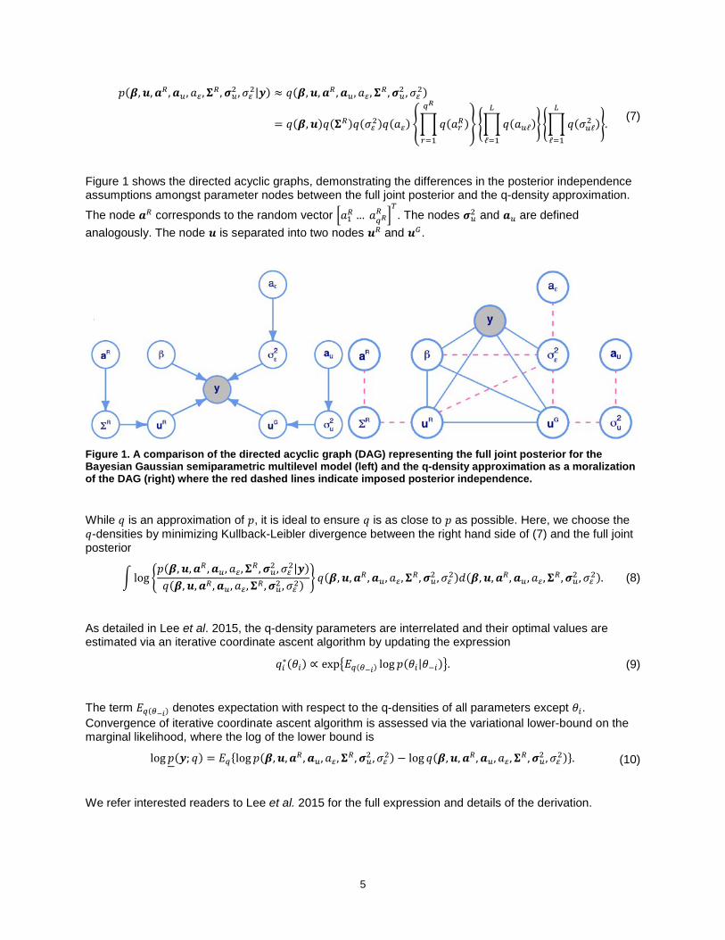
Figure 1 shows the directed acyclic graphs, demonstrating the differences in the posterior independence assumptions amongst parameter nodes between the full joint posterior and the q-density approximation.

The node 𝒂𝑅𝑅 corresponds to the random vector �𝑎1𝑅𝑅 … 𝑎𝑞𝑅𝑅𝑅 �

𝑇. The nodes 𝝈𝑢2 and 𝒂𝑢 are defined

analogously. The node 𝒖 is separated into two nodes 𝒖𝑅𝑅 and 𝒖𝐺.

Figure 1. A comparison of the directed acyclic graph (DAG) representing the full joint posterior for the Bayesian Gaussian semiparametric multilevel model (left) and the q-density approximation as a moralization of the DAG (right) where the red dashed lines indicate imposed posterior independence.

While 𝑞 is an approximation of 𝑝, it is ideal to ensure 𝑞 is as close to 𝑝 as possible. Here, we choose the 𝑞-densities by minimizing Kullback-Leibler divergence between the right hand side of (7) and the full joint posterior

� log �

𝑝(𝜷,𝒖,𝒂𝑅𝑅 ,𝒂𝑢, 𝑎𝜀𝜀 ,𝚺𝑅𝑅,𝝈𝑢2 ,𝜎𝜎𝜀𝜀2|𝒚)𝑞(𝜷,𝒖,𝒂𝑅𝑅 ,𝒂𝑢, 𝑎𝜀𝜀 ,𝚺𝑅𝑅,𝝈𝑢2 ,𝜎𝜎𝜀𝜀2) � 𝑞(𝜷,𝒖,𝒂𝑅𝑅 ,𝒂𝑢, 𝑎𝜀𝜀 ,𝚺𝑅𝑅,𝝈𝑢2 ,𝜎𝜎𝜀𝜀2)𝑑(𝜷,𝒖,𝒂𝑅𝑅,𝒂𝑢 , 𝑎𝜀𝜀 ,𝚺𝑅𝑅,𝝈𝑢2 ,𝜎𝜎𝜀𝜀2). (8)

As detailed in Lee et al. 2015, the q-density parameters are interrelated and their optimal values are estimated via an iterative coordinate ascent algorithm by updating the expression

𝑞𝑖∗(𝜃𝑖) ∝ exp�𝐸𝑞(𝜃−𝑖) log 𝑝(𝜃𝑖|𝜃−𝑖)�. (9)

The term 𝐸𝑞(𝜃−𝑖) denotes expectation with respect to the q-densities of all parameters except 𝜃𝑖. Convergence of iterative coordinate ascent algorithm is assessed via the variational lower-bound on the marginal likelihood, where the log of the lower bound is

log 𝑝(𝒚; 𝑞) = 𝐸𝑞{log 𝑝(𝜷,𝒖,𝒂𝑅𝑅 ,𝒂𝑢, 𝑎𝜀𝜀 ,𝚺𝑅𝑅,𝝈𝑢2 ,𝜎𝜎𝜀𝜀2) − log 𝑞(𝜷,𝒖,𝒂𝑅𝑅,𝒂𝑢, 𝑎𝜀𝜀 ,𝚺𝑅𝑅 ,𝝈𝑢2 ,𝜎𝜎𝜀𝜀2)}. (10)

We refer interested readers to Lee et al. 2015 for the full expression and details of the derivation.

5

MEAN FIELD VARIATIONAL BAYES ALGORITHM

The naïve MFVB algorithm is provided below as Algorithm 1 where 𝑪 ≡ [𝑿 𝒁], and provides the following q-density posterior distributions

𝑞∗(𝜷,𝒖) = N�𝝁𝑞(𝜷,𝒖),𝚺𝑞(𝜷,𝒖)�,

𝑞∗(𝜎𝜎𝜀𝜀2) = InverseGamma �0.5 �� 𝑛𝑖 + 1𝑚

𝑖=1� ,𝐵𝑞�𝜎𝜀2��,

𝑞∗(𝑎𝜀𝜀) = InverseGamma�1,𝐵𝑞(𝑎𝜀)�,

𝑞∗(𝜎𝜎𝑢ℓ2 ) = InverseGamma �0.5�𝑞ℓ𝐺 + 1�,𝐵𝑞�𝜎𝑢ℓ2 ��,

𝑞∗(𝑎𝑢ℓ) = InverseGamma�1,𝐵𝑞(𝑎𝑢ℓ)�,

𝑞∗(𝚺𝑅𝑅) = InverseWishart �𝑣 + 𝑚 + 𝑞𝑅𝑅 − 1,𝑩𝑞�𝚺𝑅��,

𝑞∗(𝑎𝜀𝜀) = InverseGamma �0.5(𝑣 + 𝑞𝑅𝑅),𝐵𝑞�𝑎𝑟𝑅��.

(12)

Initialize the following: 𝜇𝑞�1/𝜎𝜀2� > 0, 𝜇𝑞(1/𝑎𝜀) > 0, 𝜇𝑞(1/𝑎𝑢ℓ) > 0, 𝜇𝑞�1/𝜎𝑢ℓ

2 � > 0, 𝜇𝑞�1/𝑎𝑟𝑅� > 0, 1 ≤ ℓ ≤ 𝐿, 1 ≤ 𝑟 ≤ 𝑞𝑅𝑅,𝑴𝑞�(𝚺𝑅)−1� pos. def.

While increase in log 𝑝(𝒚; 𝑞) > tolerance, cycle through the updates:

𝚺𝑞(𝜷,𝒖) ← �𝜇𝑞 �1𝜎𝜎𝜀𝜀2� 𝑪𝑇𝑪 + �

𝜎𝜎𝛽−2𝑰𝑝 𝟎 𝟎

𝟎 blockdiag1≤ℓ≤𝐿 �𝜎𝜎𝑢ℓ2 𝑰𝑞ℓ𝐺� 𝟎

𝟎 𝟎 𝑰𝑚 ⊗ 𝚺𝑅𝑅��

−1

𝝁𝑞(𝜷,𝒖) ← 𝜇𝑞�1/𝜎𝜀2�𝚺𝑞(𝜷,𝒖)𝑪𝑇𝒚

𝐵𝑞�𝜎𝜀2� ← 𝜇𝑞(1/𝑎𝜀) + 0.5 ��𝒚 − 𝑪𝝁𝑞(𝜷,𝒖)�2 + tr(𝑪𝑇𝑪𝚺𝑞(𝜷,𝒖))�

𝜇𝑞�1/𝜎𝜀2� ← 0.5 �� 𝑛𝑖 + 1𝑚

𝑖=1� /𝐵𝑞�𝜎𝜀2�

𝜇𝑞(1/𝑎𝜀) ← 1/{𝜇𝑞�1/𝜎𝜀2� + 𝐴𝜀𝜀−2}

For 𝑟 = 1, … , 𝑞𝑅𝑅

𝐵𝑞�𝑎𝑟𝑅� ← 𝑣 �𝑴𝑞�(𝚺𝑅)−1��𝑟𝑟+ 𝐴𝑅𝑅𝑟−2

𝜇𝑞�1/𝑎𝑟𝑅� ← 0.5(𝑣 + 𝑞𝑅𝑅)/𝐵𝑞�𝑎𝑟𝑅�

𝑩𝑞�𝚺𝑅� ←� �𝝁𝑞�𝒖𝑖𝑅�𝝁𝑞�𝒖𝑖𝑅�𝑇 + 𝚺𝑞�𝒖𝑖𝑅��

𝑚

𝑖=1+ 2𝑣 diag�𝜇𝑞�1/𝑎1

𝑅�, … , 𝜇𝑞�1/𝑎

𝑞𝑅𝑅 �

�

𝑴𝑞((𝚺𝑅)−1) ← (𝑣 + 𝑚 + 𝑞𝑅𝑅 − 1)𝑩𝑞(𝚺𝑅)−1

Forℓ = 1, … , 𝐿 𝜇𝑞(1/𝑎𝑢ℓ) ← 1/{𝜇𝑞�1/𝜎𝑢ℓ

2 � + 𝐴𝑢ℓ−2}

𝜇𝑞�1/𝜎𝑢ℓ2 � ←

𝑞ℓ𝐺 + 1

2𝜇𝑞(1/𝑎𝑢ℓ) + �𝝁𝑞�𝒖ℓ𝐺��2

+ tr �𝚺𝑞�𝒖ℓ𝐺��

Algorithm 1: Naïve mean field variational Bayes algorithm for the Bayesian Gaussian semiparametric multilevel model.

6

The benefit of this approximation is that we have a closed form algebraic expression for the model parameters and their posterior distributions. The most computational burden comes from the inversion of the large yet sparse covariance matrix to obtain 𝚺𝑞(𝜷,𝒖). However, the naïve algorithm has already been shown to be much faster than MCMC (Lee et al. 2015), and streamlining the inversion of the large sparse covariance matrix by using a block decomposition can provide further gains in efficiency. The streamlined version of the MFVB algorithm is provided in the Appendix, and interested readers should consult Lee et al. 2015 for further details and the derivation.

IMPLEMENTATION IN SAS/IML

The following code implements the naïve MFVB algorithm (Algorithm 1) for the Bayesian Gaussian semiparametric multilevel model in the SAS IML environment. start Gauss_Naive_MFVB(y,idnum,XR,XG,ZG,ZR,A_eps=1000,A_R=1000,A_U=1000, nuVal=2,sigsq_beta=1000); /* number of observations */ numObs = countn(y); /* specification of constant matrices */ X = XR||XG; CG = X||ZG; C = CG||ZR; CTC = t(C)*C; CTy = t(C)*y; /* number of columns of... */ ncC = ncol(C); ncX = ncol(X); ncXR = ncol(XR); ncCG = ncol(CG); ncZG = ncol(ZG); /* number of covariates with splines expansions */ L = 1; /* number of groups and observations per group */ m = countunique(idnum); call tabulate(nVecID,nVec,idnum); /* set initial values for q-densities */ mu_q_recip_sigsqeps = 1; mu_q_recip_aeps = 1; M_q_inv_SigmaR = I(ncXR); mu_q_recip_sigsqu = J(L,1,1); A_q_sigsq_u = J(1,L,0); B_q_sigsq_u = J(1,L,0); mu_q_recip_a_R = J(ncXR,1,1); /* controls for update cycles and assessing convergence */ cycle = 0; prev_LB_value = -1e20; relErr = 1; tolerance = 0.0000001; /* cycle until convergence */ do while(relErr > tolerance); cycle = cycle + 1; print(cycle); /* create M_q_sigma */ if ncXR = 1 then M_q_Sigma = block(diag(J(ncX,1,1/sigsq_beta)), diag(J(1,ncZG,mu_q_recip_sigsqu)),I(m)@M_q_inv_SigmaR); if ncXR > 1 then M_q_Sigma = block(diag(J(ncX,1,1/sigsq_beta)), I(ncZG)@mu_q_recip_sigsqu,I(m)@M_q_inv_SigmaR);

7

/* Update q*(beta,u) parameters */ Sigma_q_betau = solve(mu_q_recip_sigsqeps*(CTC)+M_q_Sigma,I(ncC)); mu_q_betau = mu_q_recip_sigsqeps*Sigma_q_betau*CTy; /* Compute the determinant of Sigma.q.betau */ det_Sigma_q_betau = log(abs(det(Sigma_q_betau))); /* Update q*(1/sigsq_eps) parameters */ A_q_sigsqeps = 0.5*(sum(nVec)+1); B_q_sigsqeps = mu_q_recip_aeps + 0.5*(ssq(y-C*mu_q_betau) +sum(diag(CTC*Sigma_q_betau))); mu_q_recip_sigsqeps = A_q_sigsqeps/B_q_sigsqeps; /* Update q*(a_eps) parameter */ B_q_aeps = mu_q_recip_sigsqeps+(1/(A_eps*A_eps)); mu_q_recip_aeps = 1/B_q_aeps; /* Update q*(a_R) parameters */ B_q_a_R = nuVal*vecdiag(M_q_inv_SigmaR)+(1/(A_R*A_R)); mu_q_recip_a_R =(0.5*(nuVal + ncXR))/B_q_a_R; /* Update q*(SigmaR^{-1}) parameters */ if ncXR = 1 then B_q_SigmaR = 2*nuVal*mu_q_recip_a_R; if ncXR > 1 then B_q_SigmaR = 2*nuVal*diag(mu_q_recip_a_R); indsStt = ncCG + 1; do i = 1 to m;

indsEnd = indsStt + ncXR - 1; inds = indsStt:indsEnd; B_q_SigmaR = B_q_SigmaR + Sigma_q_betau[inds,inds] + (mu_q_betau[inds]*t(mu_q_betau[inds]));

indsStt = indsStt + ncXR; end; M_q_inv_SigmaR = (nuVal+m+ncXR-1)*solve(B_q_SigmaR,I(ncol(M_q_inv_SigmaR))); /* Update q*(a.u) parameters */ B_q_a_u = mu_q_recip_sigsqu + (1/(A_u*A_u)); mu_q_recip_a_u = 1/B_q_a_u; /* Update q*(sigsq.u) parameters */ indsStt = ncX+1; do j = 1 to L;

mu_q_betauG = mu_q_betau[1:ncCG]; Sigma_q_betauG = Sigma_q_betau[1:ncCG,1:ncCG]; indsEnd = indsStt + ncZG[j] - 1;

inds = indsStt:indsEnd; A_q_sigsq_u[j] = ncZG[j] + 1; B_q_sigsq_u[j] = (2*mu_q_recip_a_u[j]+ssq(mu_q_betauG[inds])+ sum(diag(Sigma_q_betauG[inds,inds]))); indsStt = indsEnd + 1;

end; mu_q_recip_sigsqu = A_q_sigsq_u/B_q_sigsq_u; /* calculate the lower bound to assess convergence */ Curr_LB_value = Gauss_Naive_MFVB_logML(nuVal,ncXR,ncX,ncZG,m,numObs,L,C, sigsq_beta,mu_q_betauG,Sigma_q_betauG,det_Sigma_q_betau,Sigma_q_betau,B_q_SigmaR,B_q_sigsq_u,A_R,M_q_inv_SigmaR,mu_q_recip_a_R,B_q_a_R,A_U,B_q_a_u,mu_q_re

8

cip_a_u,mu_q_betau,mu_q_recip_sigsqu,A_eps,B_q_sigsqeps,B_q_aeps,mu_q_recip_aeps,mu_q_recip_sigsqeps); /* calculate change in log lower bound on marginal likelihood */ relErr = abs((Curr_LB_value/prev_LB_value)-1); prev_LB_value = Curr_LB_value; end;

The implementation of the naïve MFVB algorithm in SAS IML along with the corresponding lower bound function has been provided as a supplementary file. With the functions in place, a user can import the required data into the SAS IML environment, create the input matrices, and then use CALL to run the function GAUSS_NAIVE_MFVB.

MFVB VERSUS MCMC VIA NUMERICAL SIMULATION In this section we first step through the analysis of a simulated dataset and compare the inference obtained from MCMC and MFVB for a number of parameters typically of interest in a regression analysis. These include; regression coefficients, variance parameters, smoothed non-linear associations, linear combinations of regression coefficients, the intra-class correlation coefficient and posterior predictive checks. This section finishes with a summary of a brief simulation study comparing MFVB and MCMC.

SIMULATING A BAYESIAN GAUSSIAN SEMIPARAMETRIC RANDOM INTERCEPT MODEL

We now describe the set-up used for simulating data for the purpose of comparing MFVB and MCMC. Data was simulated according to (1) with the exception of using a random intercept only, such that Σ𝑅𝑅 reduces to a single variance parameter which we denote 𝜎𝜎𝑅𝑅2. The simulation parameters were as follows

𝑦𝑦𝑖𝑗|𝜷,𝑢0𝑖𝑅𝑅 ,𝜎𝜎𝜀𝜀2~𝑁�𝛽𝛽0 + 𝛽𝛽1𝑥1𝑖𝑗 + 𝛽𝛽2𝑥2𝑖𝑗 + 𝛽𝛽3𝑥3𝑖𝑗 + 𝑢0𝑖𝑅𝑅 + 𝑓�𝑠𝑖𝑗�,𝜎𝜎𝜀𝜀2� for 1 ≤ 𝑖 ≤ 𝑚, 1 ≤ 𝑗 ≤ 𝑛𝑖, (13)

where

𝑓(𝑠)~1 −13

5√2𝜋exp �−

(𝑠 − 0.15)2

0.2� − (2.3𝑠 − 0.07𝑠2) + 0.5�1 −𝚽(𝑠; 0.8,0.07)�,

𝑥1𝑖𝑗~Uniform(0,1),

𝑥2𝑖𝑗~Bernoulli(0.4),

𝑥3𝑖𝑗~Bernoulli(0.2),

𝑠𝑖𝑗~Uniform(0,1),

𝑢0𝑖𝑅𝑅 |𝜎𝜎𝑅𝑅2~𝑁(0,𝜎𝜎𝑅𝑅2),

and where 𝚽 is the normal cumulative distribution function. The model parameters selected for the simulation were

𝜷 = {0.5,1.1,1.4,1.6}, 𝜎𝜎𝜀𝜀2 = 0.8, 𝜎𝜎𝑅𝑅2 = 2.0, 𝑚 = 50, 𝑛𝑖 ∈ {40,50}.

In addition, the BSPLINE function available within the SAS IML environment was used to generate B-splines of degree 3 with 25 internal knots resulting in 29 covariates for modeling of 𝑓(𝑠).

To provide a useful summary measure of how well an MFVB approximated posterior agrees with the estimate according to MCMC, we calculated the accuracy, which for a generic parameter 𝜃 is

Accuracy�𝑞∗(𝜃)� ≡ 100�1 − 0.5� |𝑞∗(𝜃) − 𝑝𝑀𝐶𝑀𝐶(𝜃|𝒚)|

∞

−∞𝑑𝜃�%, (14)

9

where 𝑞∗(𝜃) the MFVB q-density and 𝑝𝑀𝐶𝑀𝐶(𝜃|𝒚) is the best approximation to posterior 𝑝(𝜃|𝒚) estimated from a kernel approximation based on the obtained MCMC samples using PROC KDE. The accuracy is calculated using numerical integration based on a common set of points. Note that for the instances where Monte Carlo simulation is required to obtain a posterior distribution from MFVB, 𝑞∗(𝜃) is replaced with a kernel approximation.

To provide a good basis for comparison with MFVB, it is important to obtain good Bayesian inference using PROC MCMC. This requires ensuring well mixing chains which can be sensitive to the choice of blocking (grouping of parameters to update simultaneously), proposal distributions and initial values. Further, multilevel models are often challenging due to a degree of co-linearity between random effects and the increase in the number of parameters. This makes centering and standardizing data important as well as hierarchical centering where the random effects are centered on an overall intercept as opposed to zero. To obtain reasonable inference while allowing for simulation studies, we set values for initializing parameters to the true simulation value where applicable and used a moderate number of blocks in attempt to prevent poor mixing from either high acceptance rates in a localized region of the posterior (narrow conditional proposal distributions) or low acceptance rates for global moves (sparse joint proposal distributions). We retained the tuning phase, used 10,000 iterations for burn-in and then generated 1,000 posterior sample points for the parameters of interest based on a run of 10,000 with a thinning of 10.

While MFVB provides approximations to the posterior distributions of parameters in the model, inference for combinations of these quantities may be of interest. For example linear combinations of regression coefficients such as the smoothed spline function or the combined effect of two binary covariates may be of interest. Both examples amount to linear combinations of normal distributions which can be further obtained in closed-form as another normal distribution. Other combinations of parameters may require the posterior to be obtained via Monte Carlo simulation. For example the per cent of variance explained at the group level can be estimated from the intra-class correlation coefficient (ICC). The ICC is the random intercept variance divided by the sum of this variance and the residual variance, which involves dividing one inverse gamma distribution by the sum of two inverse gamma distributions. Thus, Monte Carlo simulation from the two relevant inverse gamma distributions provides the quickest means of obtaining the posterior distribution for the ICC when using the MFVB algorithm.

Finally, in Bayesian inference the posterior predictive distribution (PPD) plays an important role in assessing model fit and prediction. For assessing model fit, the PPD is

𝑝(𝑦𝑦rep|𝑦𝑦) = �𝑝(𝑦𝑦rep|𝜃, 𝑦𝑦)𝑝(𝜃|𝑦𝑦)𝑑𝜃, (15)

where 𝑝(𝜃|𝑦𝑦) is the joint posterior distribution for the parameters in 𝜃 and 𝑝(𝑦𝑦rep|𝜃,𝑦𝑦) is the sampling distribution for 𝑦𝑦, which in this case is given by (1). Without a closed form solution for 𝑝(𝑦𝑦rep|𝑦𝑦), Monte Carlo simulation was used to obtain samples by firstly sampling from 𝑝(𝜃|𝑦𝑦) and then using the sampled values in 𝑝(𝑦𝑦rep|𝜃,𝑦𝑦) to provide replicated samples of 𝑦𝑦, 𝑦𝑦rep. With PROC MCMC draws from the PPD can be obtained by using the PREDDIST option, while for MFVB draws can be obtained via Monte Carlo simulation. For assessing model fit, 𝑦𝑦rep can then be used to assess the compatibility between any individual observed value of 𝑦𝑦 and its corresponding PPD, or more usefully any statistic for 𝑦𝑦, 𝑇(𝑦𝑦). For individual observations, one common PPD check is to see how well the observed value agrees with the associated PPD, as follows

Pr[(𝑦𝑦rep)𝑖 > 𝑦𝑦𝑖]. (16)

For a statistic of 𝑦𝑦, 𝑇(𝑦𝑦), a similar calculation can be performed

Pr[𝑇(𝑦𝑦rep) > 𝑇(𝑦𝑦)], (17)

where common choices of 𝑇 include the minimum or maximum of 𝑦𝑦.

10

We performed the following comparisons between MFVB and MCMC, where for each instance the accuracy was calculated.

1. The posterior distributions for comparable parameters, namely: 𝛽𝛽1,𝛽𝛽2,𝛽𝛽3,𝜎𝜎𝜀𝜀2,𝜎𝜎𝑅𝑅2.

2. The posterior distributions for parameters that are combination of those estimated directly in the model, using the following examples:

a. The estimation of the 𝑓(𝑠) using penalized B-splines,

b. 𝛽𝛽2 + 𝛽𝛽3 (combined association for 𝑥2 and 𝑥3) which is available in closed form as if 𝛽𝛽0~N(𝜇0,𝜎𝜎02) and 𝛽𝛽1~N(𝜇1,𝜎𝜎12) then 𝛽𝛽0 + 𝛽𝛽1~N(𝜇0 + 𝜇1,𝜎𝜎02 + 𝜎𝜎12),

c. 𝜎𝜎𝑅𝑅2/(𝜎𝜎𝑅𝑅2 + 𝜎𝜎𝜀𝜀2) which is the ICC (variance explained by the group level), obtained via Monte Carlo simulation (1,000 sample points).

3. The PPD obtained via Monte Carlo simulation (1,000 sample points), where in addition to the accuracy, the PPD probabilities (16) and (17) were also calculated for the following examples:

a. The PPDs for two selected observations 𝑦𝑦400 and 𝑦𝑦500,

b. The PPDs for two summary statistics of 𝑦𝑦, which were chosen as the minimum of 𝑦𝑦, 𝑇𝑚𝑖𝑛(𝑦𝑦) = minimum(𝑦𝑦), and the maximum of 𝑦𝑦, 𝑇𝑚𝑎𝑥(𝑦𝑦) = maximum(𝑦𝑦).

RESULTS

The first panel in Figure 2 demonstrates the quick convergence of the MFVB algorithm, which required only 7 iterations. From Figure 2, it is clear that the posterior distributions for 𝛽𝛽1,𝛽𝛽2,𝛽𝛽3,𝜎𝜎𝜀𝜀2,𝜎𝜎𝑅𝑅2 from MCMC and the MFVB q-density approximations agree very well, with the accuracy values ranging from 96% to 98%. From Figure 3, the inference obtained for 𝑓(𝑠) is almost identical between MCMC and MFVB, with good agreement for both the mean estimate of the smoothed function as well as the 95% pointwise credible interval. Both of these findings are consistent with those reported comparing MCMC and MFVB using R and RStan in (Lee et al. 2015).

The left-hand panel of Figure 4 demonstrates that the posterior distribution for the linear combination of the regression coefficients for the two binary covariates (𝑥2 and 𝑥3) agreed well between MFVB and MCMC. This suggests that the posterior distributions of linear combinations of normal regression coefficients will provide inference comparable to that of MCMC. In the case of the ICC (Figure 4, right panel) there was also good agreement between MCMC and MFVB. These findings are particularly useful given in many real world applications analysts are likely to be interested in a combination of risk factors or the variation observed in an outcome attributable to a group level effect, especially in health and medicine.

Figure 5 compares the PPDs obtained from MCMC with those from MFVB obtained via Monte Carlo simulation. There was good agreement between MCMC and MFVB with accuracies ranging from 97% to 98%. The posterior probabilities assessing how well the PPD agrees with the observed values or statistics are also very similar, with differences at worst being 0.01 in absolute terms. This suggests that for these models basic PPD checking of model adequacy is comparable between MCMC and MFVB.

11

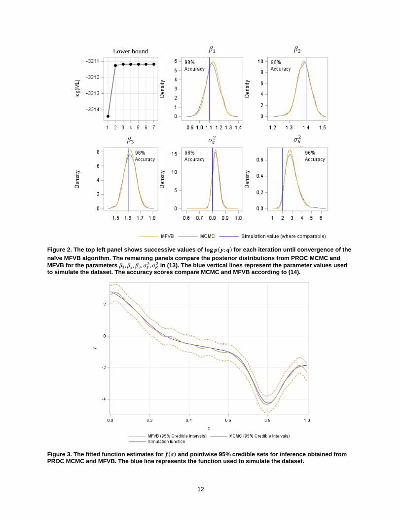
Figure 2. The top left panel shows successive values of 𝐥𝐨𝐠𝒑(𝒚;𝒒) for each iteration until convergence of the naïve MFVB algorithm. The remaining panels compare the posterior distributions from PROC MCMC and MFVB for the parameters 𝛽𝛽1,𝛽𝛽2,𝛽𝛽3,𝜎𝜎𝜀𝜀2,𝜎𝜎𝑅𝑅2 in (13). The blue vertical lines represent the parameter values used to simulate the dataset. The accuracy scores compare MCMC and MFVB according to (14).

Figure 3. The fitted function estimates for 𝒇(𝒔) and pointwise 95% credible sets for inference obtained from PROC MCMC and MFVB. The blue line represents the function used to simulate the dataset.

𝛽𝛽1

𝛽𝛽3

𝛽𝛽2

𝜎𝜎𝜀𝜀2 𝜎𝜎𝑅𝑅2

Lower bound

12

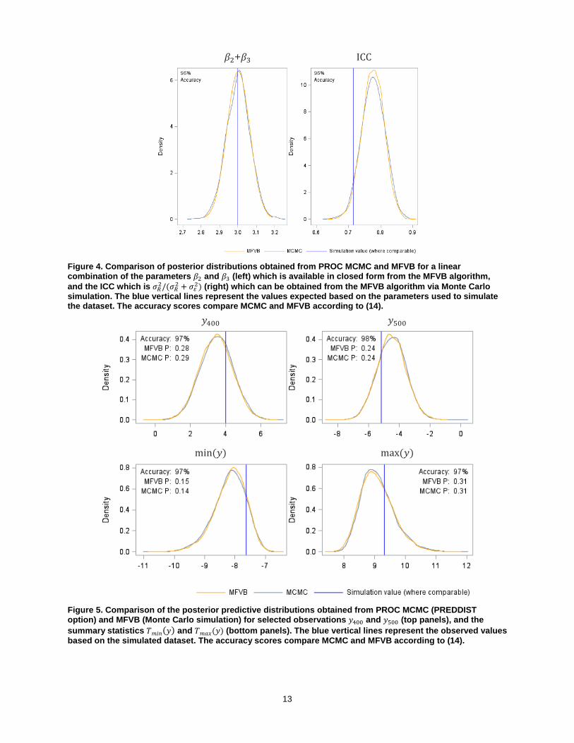
Figure 4. Comparison of posterior distributions obtained from PROC MCMC and MFVB for a linear combination of the parameters 𝛽𝛽2 and 𝛽𝛽3 (left) which is available in closed form from the MFVB algorithm, and the ICC which is 𝜎𝜎𝑅𝑅2/(𝜎𝜎𝑅𝑅2 + 𝜎𝜎𝜀𝜀2) (right) which can be obtained from the MFVB algorithm via Monte Carlo simulation. The blue vertical lines represent the values expected based on the parameters used to simulate the dataset. The accuracy scores compare MCMC and MFVB according to (14).

Figure 5. Comparison of the posterior predictive distributions obtained from PROC MCMC (PREDDIST option) and MFVB (Monte Carlo simulation) for selected observations 𝑦𝑦400 and 𝑦𝑦500 (top panels), and the summary statistics 𝑇𝑚𝑖𝑛(𝑦𝑦) and 𝑇𝑚𝑎𝑥(𝑦𝑦) (bottom panels). The blue vertical lines represent the observed values based on the simulated dataset. The accuracy scores compare MCMC and MFVB according to (14).

𝑦𝑦400 𝑦𝑦500

max(𝑦𝑦) min(𝑦𝑦)

ICC 𝛽𝛽2+𝛽𝛽3

13

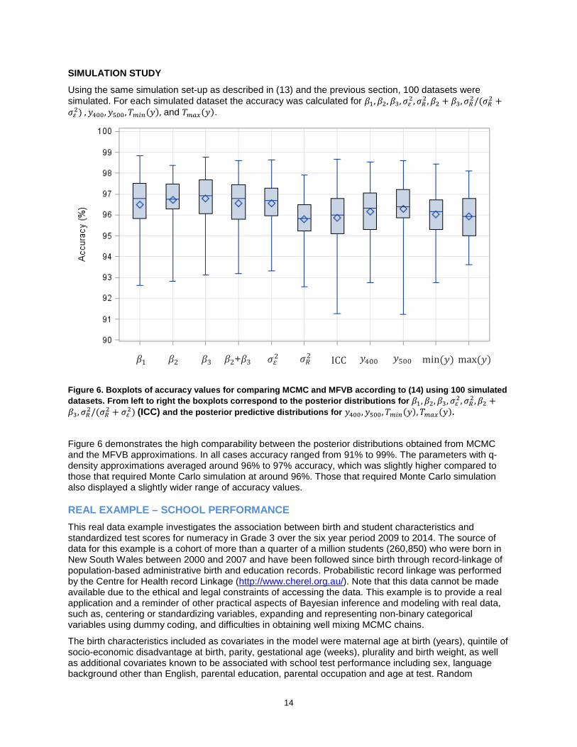
SIMULATION STUDY

Using the same simulation set-up as described in (13) and the previous section, 100 datasets were simulated. For each simulated dataset the accuracy was calculated for 𝛽𝛽1,𝛽𝛽2,𝛽𝛽3,𝜎𝜎𝜀𝜀2,𝜎𝜎𝑅𝑅2,𝛽𝛽2 + 𝛽𝛽3,𝜎𝜎𝑅𝑅2/(𝜎𝜎𝑅𝑅2 +𝜎𝜎𝜀𝜀2) ,𝑦𝑦400,𝑦𝑦500,𝑇𝑚𝑖𝑛(𝑦𝑦), and 𝑇𝑚𝑎𝑥(𝑦𝑦).

Figure 6. Boxplots of accuracy values for comparing MCMC and MFVB according to (14) using 100 simulated datasets. From left to right the boxplots correspond to the posterior distributions for 𝛽𝛽1,𝛽𝛽2,𝛽𝛽3,𝜎𝜎𝜀𝜀2,𝜎𝜎𝑅𝑅2,𝛽𝛽2 +𝛽𝛽3,𝜎𝜎𝑅𝑅2/(𝜎𝜎𝑅𝑅2 + 𝜎𝜎𝜀𝜀2) (ICC) and the posterior predictive distributions for 𝑦𝑦400,𝑦𝑦500,𝑇𝑚𝑖𝑛(𝑦𝑦),𝑇𝑚𝑎𝑥(𝑦𝑦).

Figure 6 demonstrates the high comparability between the posterior distributions obtained from MCMC and the MFVB approximations. In all cases accuracy ranged from 91% to 99%. The parameters with q-density approximations averaged around 96% to 97% accuracy, which was slightly higher compared to those that required Monte Carlo simulation at around 96%. Those that required Monte Carlo simulation also displayed a slightly wider range of accuracy values.

REAL EXAMPLE – SCHOOL PERFORMANCE This real data example investigates the association between birth and student characteristics and standardized test scores for numeracy in Grade 3 over the six year period 2009 to 2014. The source of data for this example is a cohort of more than a quarter of a million students (260,850) who were born in New South Wales between 2000 and 2007 and have been followed since birth through record-linkage of population-based administrative birth and education records. Probabilistic record linkage was performed by the Centre for Health record Linkage (http://www.cherel.org.au/). Note that this data cannot be made available due to the ethical and legal constraints of accessing the data. This example is to provide a real application and a reminder of other practical aspects of Bayesian inference and modeling with real data, such as, centering or standardizing variables, expanding and representing non-binary categorical variables using dummy coding, and difficulties in obtaining well mixing MCMC chains.

The birth characteristics included as covariates in the model were maternal age at birth (years), quintile of socio-economic disadvantage at birth, parity, gestational age (weeks), plurality and birth weight, as well as additional covariates known to be associated with school test performance including sex, language background other than English, parental education, parental occupation and age at test. Random

𝛽𝛽1 𝜎𝜎𝜀𝜀2 𝛽𝛽3 𝛽𝛽2 𝜎𝜎𝑅𝑅2 ICC 𝛽𝛽2+𝛽𝛽3 𝑦𝑦400 𝑦𝑦500 min(𝑦𝑦) max(𝑦𝑦)

14

intercepts and slopes were included to account for differences in the average result for each school over time. B-splines (order 3 with 25 internal knots) were used to model a non-linear association between birth weight and test results. The variables socio-economic disadvantage at birth, gestational age, parental education and parental occupation were categorical variables with more than two categories and so were expanded into sets of dummy variables using PROC TRANSREG. Year of test and age at test were both mean-centered and birth weight was transformed into a z-score standardized by gestational age and sex before creating the B-spline expansion using the BSPLINE functionality in PROC TRANSREG. Note that the numeracy score was not further standardized as it had already been nationally equated. The equivalent model was also fit using PROC MCMC.

In order to allow PROC MCMC to run within a reasonable time frame and to avoid PROC MCMC or the naïve MFVB algorithm in IML running into memory allocation problems, we used a sub-sample of 350 schools from the original cohort data. This provided a sample of 87,954 students and posterior means with 95% equal-tail credible intervals for the birth characteristics and test related covariates were calculated using the naïve MFVB algorithm and posterior samples obtained from PROC MCMC.

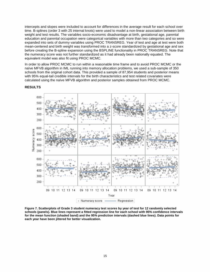
RESULTS

Figure 7. Scatterplots of Grade 3 student numeracy test scores by year of test for 12 randomly selected schools (panels). Blue lines represent a fitted regression line for each school with 95% confidence intervals for the mean function (shaded band) and the 95% prediction intervals (dashed blue lines). Data points for each year have been jittered for better visualization.

15

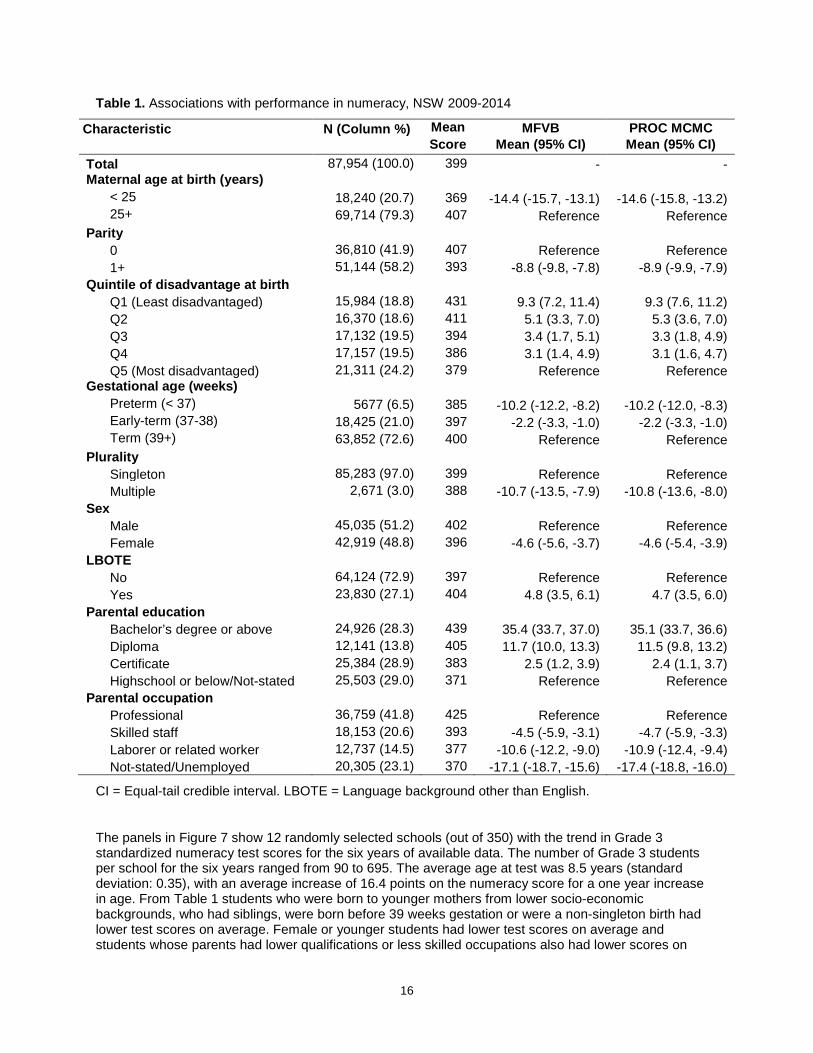
Table 1. Associations with performance in numeracy, NSW 2009-2014

Characteristic N (Column %) Mean MFVB PROC MCMC Score Mean (95% CI) Mean (95% CI) Total 87,954 (100.0) 399 - - Maternal age at birth (years)

< 25 18,240 (20.7) 369 -14.4 (-15.7, -13.1) -14.6 (-15.8, -13.2) 25+ 69,714 (79.3) 407 Reference Reference

Parity 0 36,810 (41.9) 407 Reference Reference 1+ 51,144 (58.2) 393 -8.8 (-9.8, -7.8) -8.9 (-9.9, -7.9)

Quintile of disadvantage at birth Q1 (Least disadvantaged) 15,984 (18.8) 431 9.3 (7.2, 11.4) 9.3 (7.6, 11.2) Q2 16,370 (18.6) 411 5.1 (3.3, 7.0) 5.3 (3.6, 7.0) Q3 17,132 (19.5) 394 3.4 (1.7, 5.1) 3.3 (1.8, 4.9) Q4 17,157 (19.5) 386 3.1 (1.4, 4.9) 3.1 (1.6, 4.7) Q5 (Most disadvantaged) 21,311 (24.2) 379 Reference Reference

Gestational age (weeks) Preterm (< 37) 5677 (6.5) 385 -10.2 (-12.2, -8.2) -10.2 (-12.0, -8.3) Early-term (37-38) 18,425 (21.0) 397 -2.2 (-3.3, -1.0) -2.2 (-3.3, -1.0) Term (39+) 63,852 (72.6) 400 Reference Reference

Plurality Singleton 85,283 (97.0) 399 Reference Reference Multiple 2,671 (3.0) 388 -10.7 (-13.5, -7.9) -10.8 (-13.6, -8.0)

Sex Male 45,035 (51.2) 402 Reference Reference Female 42,919 (48.8) 396 -4.6 (-5.6, -3.7) -4.6 (-5.4, -3.9)

LBOTE No 64,124 (72.9) 397 Reference Reference Yes 23,830 (27.1) 404 4.8 (3.5, 6.1) 4.7 (3.5, 6.0)

Parental education Bachelor’s degree or above 24,926 (28.3) 439 35.4 (33.7, 37.0) 35.1 (33.7, 36.6) Diploma 12,141 (13.8) 405 11.7 (10.0, 13.3) 11.5 (9.8, 13.2) Certificate 25,384 (28.9) 383 2.5 (1.2, 3.9) 2.4 (1.1, 3.7) Highschool or below/Not-stated 25,503 (29.0) 371 Reference Reference

Parental occupation Professional 36,759 (41.8) 425 Reference Reference Skilled staff 18,153 (20.6) 393 -4.5 (-5.9, -3.1) -4.7 (-5.9, -3.3) Laborer or related worker 12,737 (14.5) 377 -10.6 (-12.2, -9.0) -10.9 (-12.4, -9.4) Not-stated/Unemployed 20,305 (23.1) 370 -17.1 (-18.7, -15.6) -17.4 (-18.8, -16.0)

CI = Equal-tail credible interval. LBOTE = Language background other than English.

The panels in Figure 7 show 12 randomly selected schools (out of 350) with the trend in Grade 3 standardized numeracy test scores for the six years of available data. The number of Grade 3 students per school for the six years ranged from 90 to 695. The average age at test was 8.5 years (standard deviation: 0.35), with an average increase of 16.4 points on the numeracy score for a one year increase in age. From Table 1 students who were born to younger mothers from lower socio-economic backgrounds, who had siblings, were born before 39 weeks gestation or were a non-singleton birth had lower test scores on average. Female or younger students had lower test scores on average and students whose parents had lower qualifications or less skilled occupations also had lower scores on

16

average. The naïve MFVB algorithm took 22 seconds to run on a Dell Windows 7 desktop with a 3.2GHz Intel Core i7 processor and 16 GB of random access memory, taking 9 iterations to converge. For PROC MCMC it proved very challenging to obtain well mixing chains.

Table 1 demonstrates the reasonable agreement between the posterior means and 95% credible intervals obtained for the covariates from PROC MCMC and the MFVB q-density approximations. However, as mentioned ensuring good mixing for MCMC was challenging and some of the minor differences will most likely be due to this fact. Overall, a handful of posterior means agreed exactly, with the remainder differing by no more than 0.3, with many of those being only 0.1. The credible intervals were in similar agreement with the difference in limits between MFVB and MCMC never exceeding 0.4. Importantly though, the inference obtained from both MFVB and MCMC is the same; while all coefficients remained significant, the socio-demographic variables (prenatal occupation, parental education, socio-economic disadvantage at birth) attenuated the most after adjustment and accounting for differences between schools over time.

CONCLUSION This paper summarizes a fast efficient implementation of inference for Bayesian Gaussian semiparametric multilevel models in SAS IML. It is hoped that by providing an overview of the MFVB approach to Bayesian inference, researchers, analysts and academics using SAS will be able to apply the method to their own problems and explore the approach in an applied setting and through simulation.

There are a number of points about this methodology and future research that warrant consideration:

1. The naïve MFVB algorithm was implementable in the SAS IML environment and was quite efficient, and with streamlining the calculation of 𝚺𝑞(𝜷,𝒖) a possibility, further gains in efficiency are possible.

2. MFVB provides comparable inference for regression coefficients, variance parameters and posterior predictive distributions for Bayesian Gaussian semiparametric multilevel models.

3. The MFVB algorithm is purely algebraic and so scales efficiently to arbitrarily large and complex models.

4. MFVB can be extended to the broader class of generalized linear mixed models (e.g. Binomial or Poisson responses).

5. The MFVB approach can also be adapted to include additional model complexity such as multiple smoothed covariates using penalized splines, curve by factor interactions, missing data, measurement error or real-time updating.

6. When using MFVB the product-restriction (independence) assumptions underlying the q-density approximation of the joint posterior distribution need to be both reasonable for the data and reflective of the inferential goals.

7. MFVB algorithms provide a useful set of tools that could be incorporated into PROC MCMC for preliminary model exploration before implementing a full MCMC approach, as well as providing fast computation of initial values and potentially proposal distributions.

REFERENCES Huang, A. and Wand, M. P. 2013. “Simple marginally noninformative prior distributions for covariance matrices.” Bayesian Analysis, 8:439–452

Li, Y. and Ruppert, D. 2008. “On the asymptotics of penalized splines.” Biometrika, 95:415–436.

Lee, C. Y. Y. and Wand, M. P. 2015. “Streamlined mean field variational Bayes for longitudinal and multilevel data analysis.” Biometrical Journal, in press.

Ruppert, D., Wand, M. P., and Carroll, R. J. 2003. Semiparametric regression. Volume 12. New York: Cambridge university press.

Wand, M. P., Ormerod, J. T., Padoan, S. A., and Fruhwirth, R. 2011. “Mean field variational Bayes for elaborate distributions.” Bayesian Analysis, 7:847–900.

17

ACKNOWLEDGMENTS We would like to acknowledge the NSW Ministry of Health and the Department of Education for providing access to population health and education data, and the NSW Centre for Health Record Linkage for linking the datasets. The linkage was funded by a National Health and Medical Research Council (NHMRC) Project Grant (APP1085775). Jason Bentley was supported by an Australian Postgraduate Award Scholarship, Sydney University Merit Award and a Northern Clinical School Scholarship Award, and Cathy Lee was supported by an Australian Postgraduate Award, a University of Technology Sydney Chancellor’s Research Award.

RECOMMENDED READING • SAS/IML® 9.3 User’s Guide

• SAS/STAT® 9.3 User’s Guide, The MCMC Procedure

CONTACT INFORMATION Your comments and questions are valued and encouraged. Contact the author at:

Jason Bentley The University of Sydney jason.bentley@sydney.edu.au

SAS and all other SAS Institute Inc. product or service names are registered trademarks or trademarks of SAS Institute Inc. in the USA and other countries. ® indicates USA registration.

Other brand and product names are trademarks of their respective companies.

18

APPENDIX: MEAN FIELD VARIATIONAL BAYES ALGORITHM FOR THE BAYESIAN GAUSSIAN SEMIPARAMETRIC MULTILEVEL MODEL WITH STREAMLINED UPDATE EXPRESSIONS FOR 𝚺𝒒(𝜷,𝒖)

Initialize the following: 𝜇𝑞�1/𝜎𝜀2� > 0, 𝜇𝑞(1/𝑎𝜀) > 0,𝜇𝑞(1/𝑎𝑢ℓ) > 0, 𝜇𝑞�1/𝜎𝑢ℓ

2 � > 0, 𝜇𝑞�1/𝑎𝑟𝑅� > 0, 1 ≤ ℓ ≤ 𝐿, 1 ≤ 𝑟 ≤ 𝑞𝑅𝑅,𝑀𝑞�(Σ𝑅)−1� pos. def.

While increase in log 𝑝(𝒚; 𝑞) > tolerance, cycle through the updates:

𝑺 ← 𝟎 𝒔 ← 𝟎 For 𝑖 = 1, … ,𝑚

𝑮𝑖 ← 𝜇𝑞�1/𝜎𝜀2�(𝑪𝑖𝐺)𝑇𝑿𝑖𝑅𝑅

𝑯𝑖 ← �𝜇𝑞�1/𝜎𝜀2�(𝑿𝑖𝑅𝑅)𝑇𝑿𝑖𝑅𝑅 + 𝑴𝑞�(𝚺𝑅)−1��

−1

𝑺 ← 𝑺 + 𝑮𝑖𝑯𝑖𝑮𝑖𝑇 𝒔 ← 𝒔 + 𝑮𝑖𝑯𝑖(𝑿𝑖𝑅𝑅)𝑇𝒚𝑖

𝚺𝑞(𝜷,𝒖𝐺) ← �𝜇𝑞�1/𝜎𝜀2�(𝑪𝐺)𝑇𝑪𝐺 + �

𝜎𝜎𝛽−2𝑰𝑝 𝟎

𝟎 blockdiag1≤ℓ≤𝐿 �𝜇𝑞�1/𝜎𝑢ℓ2 �𝑰𝑞ℓ𝐺�

� − 𝑺�

−1

𝝁𝑞(𝜷,𝒖𝐺) ← 𝜇𝑞�1/𝜎𝜀2�𝚺𝑞(𝜷,𝒖𝐺){(𝑪𝐺)𝑇𝒚 − 𝒔} For 𝑖 = 1, … ,𝑚

𝚺𝑞(𝒖𝑖𝑅) ← 𝑯𝑖 + 𝑯𝑖𝑮𝑖𝑇𝚺𝑞(𝜷,𝒖𝐺)𝑮𝑖𝑯𝑖

𝝁𝑞(𝒖𝑖𝑅) ← 𝑯𝑖{𝜇𝑞�1/𝜎𝜀2�(𝑿𝑖

𝑅𝑅)𝑇𝒚𝑖 − 𝑮𝑖𝑇𝝁𝑞(𝜷,𝒖𝐺) }

𝐵𝑞�𝜎𝜀2� ← 𝜇𝑞(1/𝑎𝜀) + 0.5��𝒚 − 𝑪𝐺𝝁𝑞�𝜷,𝒖𝐺� − �𝑿1𝑅𝑅𝝁𝑞�𝒖1𝑅�

⋮𝑿𝑚𝑅𝑅 𝝁𝑞�𝒖𝑚𝑅 �

��

2

+ tr �(𝑪𝐺)𝑇𝑪𝐺𝚺𝑞�𝜷,𝒖𝐺��

+� tr �(𝑿𝑖𝑅𝑅)𝑇𝑿𝑖𝑅𝑅𝚺𝑞(𝒖𝑖𝑅)�

𝑚

𝑖=1− 2𝜇𝑞�1/𝜎𝜀2�

−1 � tr �𝑮𝑖𝑯𝑖𝑮𝑖𝑇𝚺𝑞�𝜷,𝒖𝐺��𝑚

𝑖=1�

𝜇𝑞�1/𝜎𝜀2� ← 0.5 �� 𝑛𝑖 + 1𝑚

𝑖=1� /𝐵𝑞�𝜎𝜀2�

𝜇𝑞(1/𝑎𝜀) ← 1/{𝜇𝑞�1/𝜎𝜀2� + 𝐴𝜀𝜀−2}

For 𝑟 = 1, … , 𝑞𝑅𝑅

𝐵𝑞�𝑎𝑟𝑅� ← 𝑣 �𝑴𝑞�(𝚺𝑅)−1��𝑟𝑟+ 𝐴𝑅𝑅𝑟−2

𝜇𝑞�1/𝑎𝑟𝑅� ← 0.5(𝑣 + 𝑞𝑅𝑅)/𝐵𝑞�𝑎𝑟𝑅�

𝑩𝑞�𝚺𝑅� ←� �𝝁𝑞�𝒖𝑖𝑅�𝝁𝑞�𝒖𝑖𝑅�𝑇 + 𝚺𝑞�𝒖𝑖𝑅��

𝑚

𝑖=1+ 2𝑣 diag�𝜇𝑞�1/𝑎1

𝑅�, … , 𝜇𝑞�1/𝑎

𝑞𝑅𝑅 �

�

𝑴𝑞((𝚺𝑅)−1) ← (𝑣 + 𝑚 + 𝑞𝑅𝑅 − 1)𝑩𝑞(𝚺𝑅)−1

Forℓ = 1, … , 𝐿 𝜇𝑞(1/𝑎𝑢ℓ) ← 1/{𝜇𝑞�1/𝜎𝑢ℓ

2 � + 𝐴𝑢ℓ−2}

𝜇𝑞�1/𝜎𝑢ℓ2 � ←

𝑞ℓ𝐺 + 1

2𝜇𝑞(1/𝑎𝑢ℓ) + �𝝁𝑞�𝒖ℓ𝐺��2

+ tr �𝚺𝑞�𝒖ℓ𝐺��

19